by Alan Huang - JScholarship - Johns Hopkins University

DEVELOPMENT AND APPLICATION OF NOVEL PHYSIOLOGICAL MRI METHODS TO IMAGE

CHANGES IN OXYGENATION

by

Alan Huang

A dissertation submitted to Johns Hopkins University in conformity with the requirements for the degree of Doctor of Philosophy

Baltimore, Maryland January 2014

© 2014 Alan Huang All Rights Reserved

ii

Abstract

Acute ischemic stroke is the third leading cause of death and leading cause of disability

in developed countries. An ischemic stroke results when there is an obstruction of the blood

supply to the brain. When a patient presents with acute ischemic stroke in the emergency room,

the first decision that needs to be made is whether or not the patient is a suitable candidate for

thrombolytic treatment, which can be risky and lead to death. Currently, doctors use a

combination of multiple magnetic resonance imaging (MRI) scans to determine whether or not a

patient is suitable for thrombolytic treatment. The combination of diffusion and perfusion scans

allow doctors to see regions of the brain that have already infarcted and regions at risk of

infarction. However, perfusion scans frequently overestimate the tissue at risk of infarction,

which results in stroke patients being taken in for aggressive therapies that they may not benefit

from. In this dissertation, I explored three ways to improve the current state of diagnostic stroke

imaging by allowing for better visualization of regions at risk of infarction and by doing this

non-invasively.

Upon lack of oxygen delivery to the brain, autoregulatory mechanisms lead to

vasodilatation of cerebral blood vessels. After blood vessels vasodilatate for an extended time,

cerebral blood vessels eventually collapse, and the region of tissue supplied by these vessels

progress to infarction. I hypothesized that regions of the brain with increased cerebral blood

volume (as a result of vasodilatation) could be salvageable with thrombolytic therapy. To image

these regions, I scanned eighteen patients using Vascular Space Occupancy (VASO) MRI, a new

method sensitive to changes in cerebral blood volume. While VASO MRI can provide a different

type of contrast and potentially offers information that is not available through diffusion and

iii

perfusion scans, it is cumbersome to process VASO images, and VASO MRI can be confounded

by changes in T1 especially if tissue has already progressed to infarction.

Recent research has shown that pH is a better indicator of regions of the brain at risk of

irreversible damage. Chemical exchange saturation transfer (CEST) MRI is a novel MRI method

that is sensitive changes in the exchange rate between bulk water and exchangeable protons on

proteins. Amide proton transfer (APT) MRI is a subset of CEST-based techniques that is

sensitive to changes in pH. I scanned healthy volunteers and acute stroke patients with APT MRI.

I showed that APT MRI has the potential to accurately determine whether or not a region of

tissue is at risk of infarction.

It has also been shown that changes in the oxygen extraction fraction, the percentage of

available oxygen extracted by the brain from the blood, is also a useful indicator when making

decisions about unique treatment plans for each patient. Hemoglobin, the protein responsible for

transporting oxygen to all parts of the body, exists in two different states (oxyhemoglobin and

deoxyhemoglobin), each with exchangeable protons in different parts of the spectrum. By

applying CEST and frequency label exchange (FLEX) transfer MRI in bovine blood, I detected

differences in the oxygenation of hemoglobin.

The work completed in this dissertation has the potential to aid physicians in treatment

planning for acute ischemic stroke patients.

iv

Thesis Committee

Dr. Peter van Zijl (thesis advisor, reader)

F.M. Kirby Center for Functional Brain Imaging,

The Russell H. Morgan Department of Radiology and Radiological Science,

Johns Hopkins University

Dr. Susumu Mori (reader)

Department of Biomedical Engineering,




Dr. Peter Barker




Dr. Argye Hillis-Trupe

Department of Neurology,

Department of Physical Medicine and Rehabilitation,

Department of Cognitive Science,


v

Acknowledgements

This work would not have been possible without the constant and amazing support of my

PhD advisor, Dr. Peter van Zijl. I have not only learned how to actively pursue a problem in

science from Peter, but also how to negotiate, how to enjoy life (World Cup in front of MR1),

how to make simple presentations that get the point across, and how to present. Thank you for

your guidance, your wisdom, and the many lessons that I have learned from you about magnetic

resonance, science, and life.

Next, I would like to thank my family. I thank my wife, Chun-Ting Chao 趙君婷, for the

constant support she offered me even when it meant spending our first Christmas and first New

Year’s as a married couple in the lab. I thank my mother, my father, and my brother, Bernard for

giving me constant support during my PhD program and being understanding when final exams,

abstract deadlines, and conference deadlines prevented me from going home to Texas. I would

also like to thank my cousin, Dr. Ching-Hui Huang, and cousin-in-law, Dr. Kido Nwe, for

insightful discussions about CEST.

I would also like to thank my committee members, Dr. Peter Barker Dr. Susumu Mori,

and Dr. Argye Hillis for their suggestions to my dissertation. Thank you Dr. Barker and Dr. Mori

for insights regarding CEST imaging, and thank you Dr. Hillis for advice about developing new

sequences for acute stroke imaging.

I would also like to thank all of the members of the F.M. Kirby Center for their friendship

and interesting (and quite often amusing) lunch discussions. I would like to thank Dr. Jun Hua

for always being able to stimulate my nose with his lunches and with his help and his guidance

with MT-VASO MRI. I would like to thank Dr. Craig Jones for his advice about life (about

vi

dealing with parents and in-laws about wedding plans) and for his help with python, with

MATLAB, and with CEST. I would like to thank Dr. Nirbhay Yadav for his help with python

and with FLEX. I would like to thank Dr. Ksenija Grgac for all of her help related to learning

how to operate the perfusion phantom, operating the perfusion phantom, and learning how to fix

any problem that derives out of perfusion phantom-based experiments. I would like to thank Dr.

Jiadi Xu for his help in the animal facility on the 500 MHz and 700 MHz spectrometers. Thank

you Dr. Jonathan Farrell and Dr. Bennett Landman for your help with modeling code. I would

like to thank Dr. Manus Donahue for introducing me into the lab and to arterial spin labeling.

Thank you Dr. Qin Qin for your thought-provoking discussions with ASL. And thank you Ying

Cheng, Dr. Jim Pekar, Dr. Ann Choe, Dr. Xu Li, Dr. Juan Wei, Dr. Haifeng Zeng, Dr. Suresh

Joel, Dr. Samson Jarso, and Dr. Issel Lim for being great friends. I would also like to thank

Joseph Gillen for all of his help with issues related to the MR scanner and to issues related to

Godzilla/House/Sumatra. My deepest gratitude goes to the MRI techs Ms. Terri Brawner, Ms.

Kathleen Kahl, and Ms. Ivana Kusevic for all of their help related to operating the MR machine

and the many times that they scanned me with my sequences while I went into the machine. And

last but not least, I would like to thank Ms. Candace Herbster for either knowing the answer to

all most questions related to KKI or if not the answer, then knowing who to find to give me the

proper answer, and Mrs. Heather Mackey for ordering any materials I need the second that I

request them.

I would like to thank my collaborator Dr. Richard Leigh for his effort in selecting suitable

patients for my APT in acute stroke project. I would like to thank my collaborators at the NIH

for the VASO in acute stroke project, Dr. Steven Warach and Dr. Li An.

vii

I would also like to thank Hong Lan, the go-to person for any problems related to

procedures in the BME department and in life. Thank you for all of your advice, and I would like

to thank the Biomedical Engineering department for giving me the opportunity to train here and

to lead you from 2009-2010.

Finally, I would like to thank all of my friends and roommates in Baltimore who have

made my time in the PhD program pass quickly. Thank you Dr. Ji-Liang Shiu, Wan-Ting Chen,

Kate Huang, and Janice Lu. Thank you “222ers” Yunching Chen, Pailing Lo, Yunke Song, Ariel

Yung, Bryce Chiang, Pauline Che, Xindong Song, Henan Xu, Dr. Cheng-Ran Huang, Yu-Ja

Huang, Brook Sung, Angela Chen, April Zhao, Engine Chen, Dan Jiang, Lin Guo, and Nan Zhou.

And thank you to everyone else who participated in 222 activities Dr. Nan Li, Wei-Chiang Chen,

Cecilia Ng, Dr. Alice Ho, and Derrick Lum. Thank you Dr. Suneil Hosmane for insightful

discussions on post-PhD career options such as management consulting and investment banking.

Finally, I thank all of my volunteers who went into the scanner for me so I could collect

all of the data needed to graduate!

viii

Table of Contents

Abstract …………………………………………………………………………..……………ii

Acknowledgements ……………………………………………………………………………v

Table of Contents ……………………………………………………………………………viii

List of Tables ………………………………………………..…..……………………………xii

List of Figures ……………………………………………………………….………………xiii

Chapter 1. Introduction and Overview …………………………...……………………………1

1.1 . Introduction ……………………………………...…………………………………..1

1.2 . Overview …………….……………………………...……………………………….2

Chapter 2. Basic Principles of Magnetic Resonance Imaging ………………………………..4

2.1. Chapter Goal …………………………………………………………………………4

2.2. Quantum Mechanical Description of Nuclear Magnetic Resonance (NMR) ………..4

2.3. Relaxation (Spin-Lattice (T1), Spin-Spin (T2), and T2∗ Relaxation Mechanisms) …...6

2.4. The Classical Description of NMR: Bloch Equations …………………………….…8

2.5. Chemical Exchange: Bloch-McConnell Equations ……………………………….…9

2.6. Spatial Encoding, Signal Detection, and Imaging Pulse Sequences .…………….…11

2.6.1. Spatial Encoding ………………………………………………………….11

2.6.2. Detection of Signal ………………………………………………….……13

2.6.3. Gradient Echo Imaging Pulse Sequence ………………………………….13

2.6.4. Spin Echo Imaging Pulse Sequence …………………………………..…..15

2.6.5. Gradient Spin Echo (GraSE) Imaging Pulse Sequence …………………..16

2.7. Conclusion ………………………………………………………………………….17

ix

2.8. References ………………………………………………………………………….18

Chapter 3. Hemoglobin, Blood, and Tissue Oxygenation …………………………………19

3.1. Hemoglobin …………………………………………...….…………………….…19

3.2. Blood, Vasculature, and Tissue Oxygenation ……………………….…………..….25

3.3. Conclusion ….....……………………………………………………………………27

3.4. References ……..……………………………………………………………………28

Chapter 4. Cerebral Ischemia: Mechanism, Diagnostic Tools, and Clinical Management .30

4.1. Chapter Goal ……...………….………..………………………………………….30

4.2. Pathophysiology of Ischemia .…………………………………………………….30

4.3. Imaging Diagnosis of Ischemic Stroke ………………………………………….35

4.3.1. Positron Emission Tomography (PET)……………..……………………..36

4.3.2. Computed Tomography (CT)…………………….……………………….38

4.3.3. Magnetic Resonance Imaging (MRI)……………...………………………41

4.4. Clinical Management of Cerebral Ischemia ………………………………………45

4.4.1. Intravenous Tissue Plasminogen Activator (iv-tPA)……………………..45

4.4.2. Intra-arterial Tissue Plasminogen Activator (ia-tPA)……………………46

4.4.3. Mechanical Thrombectomy……………………………………………….46

4.5. Clinical Trials……………………………………………………………………….47

4.6. Conclusion ………………………………………………………………….………50

4.7. References ……………………………………………………………..……………51

x

Chapter 5. Assessing Cerebral Blood Volume Changes in Acute Ischemic Stroke Patients

Using Magnetization Transfer-Enhanced Vascular Space Occupancy (MT-

VASO) ………………………………………………..…………………………………………55

5.1. Abstract …………………………………………………………………………...55

5.2. Introduction ……………….………………………………………………………56

5.3. Materials and Methods ……...…………………………………………………….59

5.3.1. Simulations ………………………………….……………………………59

5.3.2. Derivation of VASO Model to Estimate Ipsilateral CBV in Acute Stroke 61

5.3.3. Imaging Parameters ………………………………………………………63

5.4. Data Processing .…………………………………………………………………..65

5.4.1. MT-VASO Data Processing ……………………………………………65

5.4.2. Determination of DWI/PWI/FLAIR Lesions …………………………..67

5.4.3. Analysis of Infarction Percentage …………………………..………….67

5.5. Results and Discussion ………….…………………………………………………68

5.5.1. Patients …………………………………………………………………....68

5.5.2. Simulations ……………………………………………………………….71

5.5.3. Patient 1 ………………………………………………………………….72

5.5.4. Patient 2 ………………………………………………………………..74

5.5.5. Patient 3 ………………………………………………………….…….75

5.5.6. Group Analysis ……………………………………………….………….77

5.6. Conclusion ………………………………………………………………………….78

5.7. References .…………………………………………………………………………79

xi

Chapter 6. Application of Steady State Pulsed CEST to Image Acute Ischemic Stroke

Patients ………………………………………………………………………………………….84

6.1. Abstract ……………………………………………………………………………..84

6.2. Introduction …………………………………………………………………………84

6.3. Materials and Methods ……………………………………………………………...87

6.3.1. Simulations ……………………………………………………..………..88

6.3.2. Phantom Creation ………………………………………………………95

6.3.3. Phantom Scan …………………………………………………………..97

6.3.4. CEST Baseline Correction …………………………..…………………98

6.3.5. Healthy Volunteers ………………………………………………...….99

6.3.6. Patients …………………………………………………………………99

6.3.7. Imaging Parameters ……………………….…………………………..101

6.4. Data Processing …………………………………………………………………102

6.4.1. Pulsed CEST Data Processing …………………………….……………102

6.4.2. Determination of DWI Lesions………………………………………….102

6.4.3. Perfusion Weighted Imaging Data Processing ………………………102

6.4.4. Estimation of Infarct Percentage…………………………………….104

6.5. Results and Discussion ………………………………………………………….105

6.5.1. CEST Baseline Correction ….……………………………………..……105

6.5.2. Phantom Study……………….………………………………………….107

6.5.3. Controls …………..……………………………………………………..109

6.5.4. Patient 1 …………………………………………………………...…..111

6.5.6. Patient 2 ….....………………..…………………………………………114

xii

6.5.7. Patient 3 …………………………………...…………………………….117

6.6. Conclusion ….…………………………………..………………………………122

6.7. References ……………………………………..…………………………………123

Chapter 7. Using CEST and Frequency-Labeled Exchange Transfer (FLEX) MRI to Image

B l o o d O x y g e n a t i o n D e p e n d e n t E x c h a n g e a b l e P r o t o n s i n B l o o d

(boldCEST/boldFLEX) …….………………………………………………………………128

7.1. Abstract ……………………………………………………………………….…128

7.2. Introduction .………………………………………………………………………129

7.3. Materials …………..…………………………………….………………………132

7.3.1. Sample: Why Bovine Blood? ……………………………………………132

7.3.2. Carbonmonoxy Hemoglobin …………………………………………….133

7.3.3. Whole Blood ……………………………………………………………133

7.3.4. Washed Erythrocytes ……………………………………………...……134

7.3.5. Experimental Set-up ……………………………………………………136

7.3.6. Flow Analysis …………………………………………………………137

7.4. Methods – Part 1 .………………………………………..……………………….138

7.4.1. Optimizing Spin Echo ………………………………………….……….138

7.4.2. FLEX Imaging Parameters ………………………………………….….139

7.4.3. CEST Imaging Parameters ……………………………………………..144

7.4.4. Optimizing CEST Saturation Pulse Duration …………………………..145

7.4.5. 1-H WATERGATE Imaging Parameters ……………………………….149

7.5. Data Processing ..…………………………………………………………………151

7.5.1. FLEX Processing ……………………………………………………..152

xiii

7.5.2. CEST Processing ……………………………………………………..153

7.6. Results and Discussion – Part 1 ………………………………………………….154

7.6.1. Carbonmonoxy Hemoglobin ………………………………….……….154

7.6.2. 30 µs FLEX of 44% Hematocrit Whole Blood ………………..……..156

7.6.3. 30 µs FLEX of Washed Erythrocytes …………………………………..158

7.6.4. CEST of Whole Blood ………………………………………………….159

7.6.5. Varying Offset (and Pulse Duration) for FLEX Imaging on 44% Hematocrit

Whole Blood at 66% Oxygenation ……………………………………………160

7.7. Methods – Part 2 .………………..………………………………………………162

7.7.1. Checking the Profile Acquisition ………………………………………164

7.7.2. Baseline CEST Spectrum Drift ………………………………………..164

7.7.3. Testing Stop & Go with FLEX Acquisition ………………………….165

7.7.4. Testing Stop & Go with CEST Acquisition …………………………..166

7.7.5. CEST Acquisitions Using Stop & Go …………………………………166

7.8. Results and Discussion – Part 2 ..…………………………………………………167

7.9. Conclusion ………………………………………………………….……………169

7.10. References …..……………………………………………………………………170

Chapter 8. Conclusion and Future Work……………………………………………………175

8.1. Conclusion ………………………………………………………………………175

8.2. Future Work ……………………………………………………………………..177

Appendix A. License Agreements to Reproduce Published Figures….……………………179

Curriculum Vitae…………………………………………………………………………….180

xiv

List of Tables

Table 4.1. Components of a Multimodal CT Acute Stroke Examination ...……………………..39

Table 4.2. Multimodal MRI Acute Stroke Examination Used at Johns Hopkins Hospital ……..42

Table 5.1. Simulation Parameters and Values ……..……………………………………………61

Table 5.2. Sequence parameters for sequences acquired on acute ischemic stroke patients ...….64

Table 5.3. Background information about each patient ….......……………...…………………..69

Table 6.1. Simulation Parameters ……………………………………………………………….91

Table 6.2. Table of APT values at Different pHs and the Difference from Normal ..….……….95

Table 6.3. Relevant Patient Information ………………………………...……………………100

Table 7.1. Data from Flow Speed Tests ………………………………………………………..137

Table 7.2. Percentage of Label Flown at for Different Flow Speeds ………………….………138

Table 7.3. Checking the Efficiency FLEX 90° Pulse versus Slice Thickness …..……………..163

xv

List of Figures

Figure 2.1. A hydrogen nuclei precesses at Larmor frequency, proportional to the large external

magnetic field it is placed in ……………………………………………………………………5

Figure 2.2. Distribution of spins aligning with and against B0 ……………………………...….5

Figure 2.3. Buildup and decay of longitudinal spin magnetization ……………………….……7

Figure 2.4. Dephasing of the magnetization vector when tipped onto transverse plane using a 90°

radiofrequency pulse ..…………………………………………………………………………….7

Figure 2.5. Spatial selection in MRI using slice select (z-direction), frequency encode (x-

direction), and phase encode (y-direction) gradients ………………………………………….13

Figure 2.6. Gradient Echo Pulse Sequence Diagram …..………………………………………..14

Figure 2.7. Spin Echo Pulse Sequence Diagram ………...………………..……………………..15

Figure 2.8. Gradient Spin Echo (GraSE) Pulse Sequence Diagram …..………………………17

Figure 3.1. Structure of Oxyhemoglobin and Deoxyhemoglobin ……………………………..22

Figure 3.2. Human Oxygen Dissociation Curve ………………………………………………..24

Figure 3.3. Blood Circulation in the Human Body ……………………………………………25

Figure 4.1. Timeline of Cellular and Molecular Events that Occur During Ischemia ……...31

Figure 4.2. How Cellular and Molecular Events Following Ischemia Relate to the Ischemic

Penumbra ……………………………………………………………………………………….35

Figure 4.3. PET Imaging of Ischemic Penumbra ……………………………..……………….37

Figure 4.4. State-of-the-art Multimodal CT images of an acute stroke patient …………….…41

Figure 4.5. Multimodal Magnetic Resonance Images of an Acute Stroke Patient ………..…..44

Figure 5.1. VASO MRI Pulse Sequence ………………………………………………………58

xvi

Figure 5.2. Flow-chart of data processing of MT-VASO Scan ……………………………….67

Figure 5.3. Simulated decrease in MT-VASO signal intensity due to different increases in

microvascular cerebral blood volume (CBV) ...…………………………………………………71

Figure 5.4. Images from patient 1, scanned 1 hour 36 minutes after last seen normal ………..73

Figure 5.5. Images from patient 2, who was scanned 2 hours and 11 minutes after last seen

normal ………...………………………………………………………………………………....75

Figure 5.6. Images from patient 3, scanned 19 hours and 7 minutes after last seen normal ….76

Figure 5.7. Percentage of Penumbral Voxels in White Matter that Progress to Infarction ..….77

Figure 6.1. Analysis of Optimal CEST Saturation Pulse Parameters Based on 3-pool Bloch-

McConnell Simulation for Gray Matter and White Matter ……………………………………92

Figure 6.2. Simulation of 3-pool Bloch-McConnell Equation for Changes in pH (A) in a voxel

with 100% Gray Matter and (B) in a voxel with 100% White Matter ………………………..94

Figure 6.3. Images of pH phantoms ……………………………………………………………..96

Figure 6.4. Steady-state pulsed CEST Pulse Sequence with navigator .………………….….102

Figure 6.5. Scanner Drift (A) XMR (B) MR1 …………………………………..……………..105

Figure 6.6. CEST Baseline Correction: Comparison of Corrected and Uncorrected for pH 6.3

10% BSA phantom …………………………………………………………………………….106

Figure 6.7. Lorentzian Difference Analysis (LDA) of the different pH phantoms ……………108

Figure 6.8. Correlation Graph of pH versus Lorentzian Difference (A) at Δω=±2.9 ppm; and (B)

at Δω=±3.5 ppm ………………………………………………………………………………..109

Figure 6.9. Data acquired on a healthy control subject ………………………………………110

Figure 6.10. Data acquired on another healthy control subject ...……………………………...111

Figure 6.11. (A) Diffusion weighted scan (mean diffusion weighted image) and

xvii

(B) Perfusion weighted scan of ischemic stroke patient (time to peak image) ………………112

Figure 6.12. MTRasymmetry (+3.5 ppm) image of (A) heal thy volunteer and

(B) ischemic stroke patient …………………………………………………….…………….113

Figure 6.13. Images of diffusion lesion (red), possible pH penumbra (blue), and perfusion

penumbra (green) overlaid on CEST M0 image ……………………………………………..114

Figure 6.14. Slices 18 to 23 for Patient 2 ………………………………………………….....115

Figure 6.15. Slices 24 to 29 for Patient 2 …………………………………………………….116

Figure 6.16. Example of patient motion on DTI scan ………………………………………..118

Figure 6.17. Processed data for carotid artery stenosis patient (Slices 16-20) (displayed in

radiologic convention) ……………………………………………………………………….119





Figure 7.1. Washed Cells Under a Microscope at 40x Magnification …………………………135

Figure 7.2. 1D Profile Read-out of Spin Echo. Slice thickness = 3 cm ….………………….139

Figure 7.3. FLEX Sequence ……………….………………………………………………….141

Figure 7.4. (A) FLEX, texch = 10 ms, without phase cycle (B) FLEX, texch = 10 ms, with phase

cycle (C) FLEX, texch = 20 ms, with phase cycle (D) FLEX, texch = 20 ms, without phase

cycle ……………………………………………………………………………….................143

Figure 7.5. FLEX Excitation Profiles for (A) 30 µs block pulse applied at +46.10 ppm

(B) 40 µs block pulse applied at +34.57 ppm ………………………………………………….144

Figure 7.6. CEST Sequence ……………………………………………………………………145

xviii

Figure 7.7. Data Over Multiple Saturation Pulse Durations …………………………………...147

Figure 7.8. Excitation Profile of 1H-WATERGATE sequence on 700 MHz scanner ………...150

Figure 7.9. Explanation of why WATERGATE at 700 MHz using our hardware does not

work ……………………………………………………………………………………………151

Figure 7.10. FLEX results for 2.4 mM and 4.9 mM HbCO ……………………………………154

Figure 7.11. CEST (top) and MTRasymmetry (bottom) spectra for 4.9 mM concentration of

HbCO …………………………………………………………………………………….…….155

Figure 7.12. FLEX Results of Multi-oxygenation Scan ……………………………………….157

Figure 7.13. FLEX data and spectra of 44% hematocrit washed erythrocytes with

(A) 100% oxygenation; and (B) 65% oxygenation …………………………………………….159

Figure 7.14. CEST spectra (top) and MTRasymmetry (bottom) for 44% hematocrit Whole Blood at

Multiple Oxygenations …………………………………………………………………………160

Figure 7.15. FLEX Spectra for (A) FLEX Excitation Pulse Applied at 46.10 ppm (B) FLEX

Excitation Pulse Applied at -46.10 ppm (C) FLEX Excitation Pulse Applied at 34.57 ppm ….162

Figure 7.16. Drift of S0 Images at 700 MHz …………………………………………………...165

Figure 7.17. Testing Stop & Go Acquisition Using FLEX …………………………………….166

Figure 7.18. Testing Stop & Go Acquisition Using CEST …………………………………….167

Figure 7.19. CEST spectra (top) and MTRasymmetry (bottom) of 44% hematocrit whole blood at

100% oxygenation (red) and 60% oxygenation (blue) ………………………………………169

Figure 7.20. Follow-up Results CEST Spectra (top) and MTRasymmetry (bottom) for

(A) B1=1.4 µT (B) B1=2.5 µT ……………………………………………………………….…170

1

Chapter 1. Introduction and Overview

1.1 Introduction

Management of acute ischemic cerebrovascular syndrome (AICS), more commonly

known as acute ischemic stroke, is complicated by the heterogeneity of the disease, by the

need to make fast individualized decisions on a per patient basis, and by deleterious side

effects of aggressive treatments. Magnetic resonance imaging (MRI) is an emerging form of

diagnostic imaging with the potential of deriving many new contrast mechanisms by

manipulating the timing of radiofrequency and magnetic field gradient pulses. Three-

dimensional images can be acquired quickly, non-invasively, with high spatial resolution,

and without delivering ionizing radiation to the patient.

In acute ischemic stroke, an embolus or thrombus obstructs blood flow to certain

regions of the brain and reduces cerebral perfusion, needed for delivery of oxygen to the

brain. This results in a “core” region of the brain (where neurons cannot survive due to the

lack of oxygen) that progresses to infarction (in other words, dies) and is unsalvageable with

any treatment. However, a few decades ago it was found using Positron Emission

Tomography (an imaging modality that measures cerebral metabolism and perfusion using

radiotracers injected into the bloodstream) that regions of the brain surrounding the core that

have low perfusion and are electrically inactive but are not yet irreversibly damaged can be

salvaged with thrombolytic therapy. This salvageable region of the brain has been termed the

“ischemic penumbra”. More recently, the original definition of penumbra has been somewhat

modified in that the complete region of reduced perfusion surrounding the core has been

included, which generally is larger than just electrically dysfunctional tissue, Depending on

2

the type of imaging used, multiple penumbra (perfusion-based, pH-based, oxygen extraction

based) have been defined in an attempt to guide therapy of ischemic stroke patients. There

are currently three main therapeutic options available to restore blood flow to the brain: 1)

intravenous tissue plasminogen activator (IV-tPA); 2) intra-arterial tPA (IA-tPA); and 3)

mechanical thrombectomy (clot retraction). Each therapeutic option carries its own benefits

and risks, while neurologists frequently have to use incomplete diagnostic information to

make a decision to treat or not, and which therapy to use. Current MR methodologies focus

on perfusion deficits and frequently overestimate the ischemic penumbra, which results in

patients being taken for aggressive therapy and being exposed to unnecessary risks. This

dissertation is written with the long-term goal of advancing the field of diagnostic stroke

imaging with the development and application of novel MRI contrast mechanisms to image

the ischemic penumbra in AICS patients.

1.2. Overview

This dissertation is organized in the following way. First, the reader is given an

introduction into the physical mechanisms of nuclear magnetic resonance (Chapter 2). Next,

the reader is introduced to blood (and its components) and how blood delivers oxygen to the

rest of the body to maintain aerobic metabolism (Chapter 3). Following this, the reader is

introduced to acute ischemic stroke, a particular pathology where oxygen delivery is

disrupted due to vessel blockage and, depending on the level of disruption, causes a cascade

of changes in the human brain (Chapter 4). Next, Chapter 5 presents the work done on

optimizing Vascular Space Occupancy (VASO) MRI, a cerebral blood volume sensitive

method, to image the ischemic penumbra based on changes in cerebral blood volume during

3

ischemia. After seeing interesting results using VASO, we decided to image tissue pH, a

parameter that should be a better indicator of tissue at risk, as it is only changed when

anaerobic metabolism starts to occur. Results of optimizing the pulse sequence, testing on

healthy volunteers, and applying the pulse sequence to image intracellular pH in acute

ischemic stroke patients are presented in Chapter 6. Then, preliminary data from a novel

idea to use signals of exchangeable protons on hemoglobin proteins in blood to measure

oxygenation are presented in Chapter 7. Finally, Chapter 8 summarizes the work and

identifies some potential future research directions.

4

Chapter 2. Basic Principles of Magnetic Resonance Imaging

2.1. Chapter Goal

This chapter introduces the reader to fundamental concepts of magnetic resonance

imaging (MRI). Because this dissertation is focused on the optimization and development of

novel magnetic resonance imaging techniques, it is important to have a fundamental

understanding of how the MRI machine generates images.

“Magnetic resonance imaging is actually nuclear magnetic resonance imaging, but

scientists in the field removed the term “nuclear” from the name because at the time, the

general public had a fear of the term nuclear.”

- Peter van Zijl, from multiple introductory lectures on MRI methods

2.2. Quantum Mechanical Description of Nuclear Magnetic Resonance (NMR)

Nuclei have four unique properties: mass, electric charge, magnetism, and

spin. Spin is a form of angular momentum that is intrinsic to the nucleus. Due to the

broad scope of this topic, we will limit discussion to hydrogen nuclei, the most

commonly studied nuclei in NMR. It is a spin-1/2 particle. When it is placed in a

large external magnetic field, it becomes quantized to two states (mz = +1/2 and mz =

-1/2) only due to the interaction between the magnetic moment and the field. The

energy difference between these two states is described by equation 2.1.

∆𝐸 = 𝛾𝐻ℏ𝐵0 (Equation 2.1)

Where γH is 267.522x106 rad/(T∙s) and represents the gyromagnetic ratio (the

ratio of magnetic moment of the nucleus and its angular momentum) of hydrogen; ħ

5

is Plank’s constant (6.626068 × 10-34 m2 kg / s) divided by 2π; and B0 represents the

large external magnetic field and has units of Tesla (T). The energy difference is

related to the frequency of precession through the following relationship: ΔE=ħω.

𝜔0 = 𝛾𝐻𝐵0 (Equation 2.2)

This frequency, ω0 (rad/s), is known as the Larmor frequency.

Figure 2.1. A hydrogen nuclei precesses at the Larmor frequency, proportional to the

large external magnetic field it is placed in.

When a group of spin-1/2 is placed in a magnetic field, every spin aligns in

one of two directions: with the magnetic field (lower energy) or against the magnetic

field (higher energy). This is known as the Zeeman effect (figure 2.2).

Figure 2.2. Distribution of spins aligning with and against B0.

The Boltzmann distribution (equation 2.2) relates the ratio of spins in the two

energy levels to the difference in energy between the two levels.

𝑁𝛼𝑁𝛽

= 𝑒−ΔE kbT⁄ (Equation 2.2)

6

Nα and Nβ represent the number of spins in the lower and higher energy states,

respectively. ΔE is the energy difference between the two energy states (equation 2.1),

kb is the Boltzmann constant, 1.381x10-23 𝑚2𝑘𝑔𝑠2𝐾

, and T is the absolute temperature in

Kelvin (K).

When a sample is placed in a large magnetic field (B0), the difference between

the two energy states (with and against the magnetic field) forms the longitudinal

magnetization vector with which we can use the classical description of NMR to

continue our discussion.

2.3. Relaxation (Spin-Lattice (T1), Spin-Spin (T2), and 𝐓𝟐∗ Relaxation Mechanisms)

Before continuing with the classical description of NMR, we offer an

introduction to relaxation mechanisms which is necessary before we continue. When

a sample is rapidly brought into the presence of a large magnetic field, the rate at

which the longitudinal magnetization vector forms is in the form of an exponential

function:

𝑀𝑧(𝑡) = 𝑀0(1 − 𝑒−(𝑡−𝑡𝑜𝑛)

𝑇1� ) (Equation 2.3)

Similarly, if the sample is rapidly brought out of the presence of a large magnetic

field, the decay is also an exponential function of the form:

𝑀𝑧(𝑡) = 𝑀0𝑒

−�𝑡−𝑡𝑜𝑓𝑓�𝑇1�

(Equation 2.4)

This longitudinal relaxation rate is known as T1.

7

Figure 2.3. Buildup and decay of longitudinal spin magnetization. Reproduced with

permission from (1).

Another relaxation mechanism that is important when studying NMR is the

transverse relaxation rate, or T2. When a spin ensemble is placed onto the transverse

plane (x-y plane) using a radiofrequency pulse, the magnetization vector begins to

dephase as shown in figure 2.5. The rate at which this dephasing occurs is the

transverse relaxation time. This decay is governed by equation 2.5.

𝑀𝑥𝑦(𝑡) = 𝑀𝑥𝑦(0)𝑒−𝑡𝑇2� (Equation 2.5)

Figure 2.4. Dephasing of the magnetization vector when tipped onto

transverse plane using a 90° radiofrequency pulse.

However, pure transverse (T2) decay is only from the completely random

interactions between spins, which requires a completely homogeneous main magnetic

field. In reality, there are inhomogeneities in the main magnetic field and

8

susceptibility differences in the sample that cause transverse magnetization to decay

at a faster rate, known as 𝑇2∗.

1𝑇2∗

= 1𝑇2

+ 𝛾∆𝐵𝑖𝑛ℎ𝑜𝑚𝑜𝑔𝑒𝑛𝑒𝑖𝑡𝑖𝑒𝑠 (Equation 2.6)

2.4. The Classical Description of NMR: Bloch Equations

2.4.1. Basic Bloch Equations

Being able to treat the combined behavior of all of the spins in the system as a

magnetization vector allows the use of a classical description to give a simpler picture

of an NMR experiment via the Bloch Equation (2):

�̇�(𝑡) = 𝛾𝑴(𝑡) × 𝑩(𝑡) (Equation 2.7)

When analyzing the Bloch equation in the orthogonal components, the Bloch

equation can be broken down into its components including the relaxation terms:

𝑑𝑀𝑧𝑑𝑡

= 𝑀0−𝑀𝑧𝑇1

(Equation 2.8)

𝑑𝑀𝑥𝑑𝑡

= 𝜔0𝑀𝑦 −𝑀𝑥𝑇2

(Equation 2.9)

𝑑𝑀𝑦

𝑑𝑡= −𝜔0𝑀𝑥 −

𝑀𝑦

𝑇2 (Equation 2.10)

These Bloch equations can be solved for the magnetization evolution and

relaxation to yield:

𝑀𝑥(𝑡) = 𝑒−𝑡

𝑇2� (𝑀𝑥(0) cos𝜔0𝑡 + 𝑀𝑦(0) sin𝜔0𝑡) (Equation 2.11)

𝑀𝑦(𝑡) = 𝑒−𝑡

𝑇2� (𝑀𝑦(0) cos𝜔0𝑡 − 𝑀𝑥(0) sin𝜔0𝑡) (Equation 2.12)

𝑀𝑧(𝑡) = 𝑀𝑧(0)𝑒−𝑡

𝑇1� + 𝑀0(1 − 𝑒−𝑡

𝑇1� ) (Equation 2.13)

9

In order to detect any signal from an NMR experiment, a radiofrequency (RF)

field must be used to tip the magnetization onto the transverse plane. We can model

this in the rotating frame (rotation speed omega) as:

𝐵�⃗ 𝑒𝑓𝑓 = �𝐵0 −𝜔𝛾� �̂� + 𝐵1𝑥�′ (Equation 2.14)

Then, the Bloch equations in the rotating frame become:

𝑑𝑀𝑧𝑑𝑡

= −𝜔1𝑀𝑦 + 𝑀0−𝑀𝑧𝑇1

(Equation 2.15)

𝑑𝑀𝑥𝑑𝑡

= ∆𝜔𝑀𝑦 −𝑀𝑥𝑇2

(Equation 2.16)

𝑑𝑀𝑦

𝑑𝑡= −∆𝜔𝑀𝑥 + 𝜔1𝑀𝑧 −

𝑀𝑦

𝑇2 (Equation 2.17)

Where Δω = ω0 – ω, and the solution to this set of differential equations is:

𝑀𝑥(𝑡) = 𝑒−𝑡 𝑇2⁄ (𝑀𝑥(0) cos∆𝜔𝑡 + 𝑀𝑦 sin∆𝜔𝑡) (Equation 2.18)

𝑀𝑦(𝑡) = 𝑒−𝑡 𝑇2⁄ (𝑀𝑦(0) cos∆𝜔𝑡 − 𝑀𝑥 sin∆𝜔𝑡) (Equation 2.19)

𝑀𝑧(𝑡) = 𝑀𝑧(0)𝑒−𝑡 𝑇1⁄ + 𝑀0(1 − 𝑒−𝑡 𝑇1⁄ ) (Equation 2.20)

2.5. Chemical Exchange: Bloch-McConnell Equations

A unique feature of NMR is its ability to measure chemical exchange, for instance

such as it is occurring between -OH, -NH, and -SH groups and the solvent water. For two

exchange sites (otherwise known as a two-pool model), we begin with the simple system

with two pools: pool S and pool W.

10

Where kSW is the rate constant for exchange from pool S to pool W and kWS is the rate

constant for exchange from pool W to pool S. The concentrations of S and W can be related

to the rate constants through the following equations:

𝑑[𝑆]𝑑𝑡

= −𝑘𝑠𝑤[𝑆] + 𝑘𝑤𝑠[𝑊] (Equation 2.21)

𝑑[𝑊]𝑑𝑡

= 𝑘𝑠𝑤[𝑆] − 𝑘𝑤𝑠[𝑊] (Equation 2.22)

This is intuitive in that the differential concentration of pool S will be increased by

the amount of molecules from pool W exchanged to pool S (given by the product of rate of

exchange from pool W to pool S times the concentration of pool W) and decreased by the

amount of molecules from pool S exchanged to W, and similarly for the differential

concentration of pool W.

To describe chemical exchange in a spin system, we need to convert these

concentration-based equations to reflect the magnetization of these two pools in order to add

them to the Bloch equations. The equilibrium magnetization of pools S and W are directly

proportional to the concentrations of pools S and W, therefore, equations 2.21 and 2.22 can

be written to describe the effect of exchange on the magnetization of pool s and pool W. The

chemical exchange modified Bloch equations are known as Bloch-McConnell equations

named after Harden McConnell who derived them in 1958 and are given in equations 2.23-

2.28 (3):

𝑑𝑀𝑥𝑠𝑑𝑡

= −∆𝜔𝑠𝑀𝑦𝑠 − 𝑅2𝑠𝑀𝑥𝑠 − 𝑘𝑠𝑤𝑀𝑥𝑠 + 𝑘𝑤𝑠𝑀𝑥𝑤 (Equation 2.23)

𝑑𝑀𝑦𝑠

𝑑𝑡= ∆𝜔𝑠𝑀𝑥𝑠 + 𝜔1𝑀𝑧𝑠 − 𝑅2𝑠𝑀𝑦𝑠 − 𝑘𝑠𝑤𝑀𝑦𝑠 + 𝑘𝑤𝑠𝑀𝑦𝑤 (Equation 2.24)

𝑑𝑀𝑧𝑠𝑑𝑡

= −𝜔1𝑀𝑦𝑠 − 𝑅1𝑠(𝑀𝑧𝑠 − 𝑀0𝑠) − 𝑘𝑠𝑤𝑀𝑧𝑠 + 𝑘𝑤𝑠𝑀𝑧𝑤 (Equation 2.25)

𝑑𝑀𝑥𝑤𝑑𝑡

= −∆𝜔𝑤𝑀𝑦𝑤 − 𝑅2𝑤𝑀𝑥𝑤 + 𝑘𝑠𝑤𝑀𝑥𝑠 − 𝑘𝑤𝑠𝑀𝑥𝑤 (Equation 2.26)

11

𝑑𝑀𝑦𝑤

𝑑𝑡= ∆𝜔𝑤𝑀𝑥𝑤 + 𝜔1𝑀𝑧𝑤 − 𝑅2𝑤𝑀𝑦𝑤 + 𝑘𝑠𝑤𝑀𝑦𝑠 − 𝑘𝑤𝑠𝑀𝑦𝑤 (Equation 2.27)

𝑑𝑀𝑧𝑤𝑑𝑡

= −𝜔1𝑀𝑦𝑤 − 𝑅1𝑤(𝑀𝑧𝑤 −𝑀0𝑤) + 𝑘𝑠𝑤𝑀𝑧𝑠 − 𝑘𝑠𝑤𝑀𝑧𝑤 (Equation 2.28)

Where R1 and R2 are the longitudinal and transverse relaxation rates, M0 is the

equilibrium magnetization, and ksw and kws are the exchange rates of protons from pool s to w

and vice versa. Under equilibrium, the system obeys the relationship:

𝑘𝑠𝑤𝑀0𝑠 = 𝑘𝑤𝑠𝑀0𝑤 (Equation 2.29)

2.6. Spatial Encoding, Signal Detection, and Imaging Pulse Sequences

2.6.1. Spatial Encoding

The measurement of the precessional frequency of the longitudinal

magnetization gives information about the magnetic field experienced by any

ensemble of spins. If the magnetic field is varied in a controlled manner, the

frequency information can yield spatial information. To demonstrate this principle,

let’s take the main magnetic field and add a gradient in the z-direction (Gz). Then in

the z-direction, the field becomes:

𝐵𝑧(𝑧, 𝑡) = 𝐵0 + 𝑧𝐺(𝑡) (Equation 2.30)

The deviation from the Larmor frequency becomes linear in both z and G and

can be quantified using the following equation:

𝜔𝐺(𝑧, 𝑡) = 𝛾𝑧𝐺(𝑡) (Equation 2.31)

This relationship allows us to perform frequency encoding of spatial

information using gradients along the z-axis and leads us to the commonly known 1D

imaging equation that defines the signal s as a function of frequency.

𝑠(𝑘) = ∫𝑑𝑧𝜌(𝑧)𝑒−𝑖2𝜋𝑘𝑧 (Equation 2.32)

12

Where ρ(z) is the spin density as a function of position along the z-axis and is

being integrated over that dimension. However, for imaging in vivo systems, we need

to encode a 3D volume. For a sample being excited with a set of three orthogonal

gradients, we can extend the 1D imaging equation to the following (2):

𝑠�𝑘�⃗ � = ∭𝑑𝑥 𝑑𝑦 𝑑𝑧 𝜌(𝑥, 𝑦, 𝑧)𝑒−𝑖2𝜋�𝑘𝑥𝑥+𝑘𝑦𝑦+𝑘𝑧𝑧�

= ∫𝑑3𝑟𝜌(𝑟)𝑒−𝑖2𝜋𝑘�⃗ ∙𝑟 (Equation 2.33)

Another way to think about slice selection and spatial encoding is to consider

a sample in a large magnetic field, B0. This sample has a Larmor frequency of γB0.

When a small linear gradient is added in the z-direction, there is spatial variation of

frequencies in the z-direction. Spins on one end will precess at a faster frequency than

spins on the other end. A radiofrequency pulse can be used to selectively excite a

region of spins (i.e. where the precessing frequency is equal to γB0), determined by

the Fourier transform of the radiofrequency pulse. The thickness of the slice is then

determined by the strength of the gradient (figure 2.5). A thicker slice can be selected

with a smaller gradient (this way a larger region will have spins precessing with

frequency γB0), and a thinner slice can be selected with a larger gradient (the spatial

variation of frequencies is larger so a smaller region will have spins precessing with

frequency γB0). Now that a slice has been selected (z-direction), encoding needs to be

performed in the x-y plane to resolve in-plane features. Gradients can be turned on in

the x-direction to perform frequency encoding, which is used to resolve features in

the left right direction. This is known as frequency encoding because similar to slice

selection where a gradient is turned on to modulate frequency with respect to position

along the z-axis, the x-direction gradient is also used to modulate frequency in the x

13

direction. Y-direction encoding is done by modulating the phase of the signal (known

as phase encoding). The phase encoding gradient is “stepped” during the acquisition

of a slice. Combined together, slice select, frequency encoding, and phase encoding

gradients allow MRI to resolve samples in three dimensions.

Figure 2.5. Spatial selection in MRI using slice select (z-direction), frequency encode

(x-direction), and phase encode (y-direction) gradients.

2.6.2. Detection of Signal

To detect the NMR signal, an RF coil must be placed in the transverse plane,

perpendicular to the main magnetic field (B0), where an electric magnetic force (emf)

is induced that is proportional to the magnetization. The signal from the coil is

measured using phase sensitive detection, which records the signal on two axes,

providing real and imaginary components.

2.6.3. Gradient Echo Imaging Pulse Sequence

A gradient echo sequence is one of the most common MR sequences used to

acquire an image. In gradient echo imaging (see figure 2.7), a single RF pulse with

14

flip angle α (where α ≤ 90°) is applied to tip the magnetization onto t he transverse

plane then a readout gradient reversal scheme with a net zero gradient integral at the

echo time is used to refocus the echo. In gradient echo imaging, magnetic field

inhomogeneities and susceptibility differences are not refocused and affect the

imaging contrast. Therefore, it is important to have a homogeneous magnetic field

when using GRE imaging. The flip angle (α) can be set to give optimized SNR using

the Ernst flip angle equation:

𝛼 = 𝑐𝑜𝑠−1(𝑒−𝑇𝑅 𝑇1⁄ ) (Equation 2.34)

Where TR is the given repetition time, T1 is the longitudinal relaxation time of

the tissue being imaged, and α is the optimal flip angle. One way to accelerate GRE

imaging is with an echo planar imaging (EPI) readout. An EPI read-out can be done

by acquiring all of the lines of k-space after the excitation pulse, known as “single-

shot,” or by using multiple lower flip-angle excitation pulses and acquiring a few

lines of k-space each time, known as “multi-shot.”

Figure 2.6. Gradient Echo Pulse Sequence Diagram (4). Reproduced with permission

by the Journal of Magnetic Resonance Imaging.

In Chapter 6, I will use a multi-shot gradient-echo acquisition scheme to

acquire pH-weighted images to aid physicians to make individualized treatment

15

decisions for each patient. Furthermore, in Chapter 5, I will use a single-shot gradient

echo EPI acquisition scheme to quickly acquire cerebellar blood flow-weighted

images.

2.6.4. Spin Echo Imaging Pulse Sequence

One issue with the gradient echo imaging method is its sensitivity to magnetic

field inhomogeneities as well as microscopic fields in the sample. One way to address

these concerns is with a spin echo acquisition. A spin echo acquisition uses a 90°

pulse to tilt the magnetization onto the transverse plane. When that happens, the

magnetization begins to dephase due to T2, T2* and T2

’ mechanisms. A certain time

later, a 180° pulse is applied to invert the direction of evolution of the magnetization.

After waiting another duration of similar length, the spin echo is formed and acquired.

The time from applying the 90° pulse to acquiring the spin echo is known as the echo

time (TE). In order for an echo to form at that time, the 180° pulse is applied at TE/2.

Figure 2.7 shows the pulse sequence diagram of a spin echo sequence.

Figure 2.7. Spin Echo Pulse Sequence Diagram (4). Reproduced with permission by

the Journal of Magnetic Resonance Imaging.

16

Equation 2.35 governs the contrast given a specific repetition time (TR) or

echo time (TE) in a spin echo experiment.

𝑀𝑧 = 𝑀0(1 − 𝑒−𝑇𝑅 𝑇1⁄ )𝑒−𝑇𝐸 𝑇2⁄ (Equation 2.35)

In chapter 8, I will use the spin echo acquisition method to study

exchangeable proton signals in bovine blood because of its high signal-to-noise and

because it is not susceptible to local magnetic field inhomogeneities caused by

deoxyhemoglobin.

2.6.5. Gradient Spin Echo (GraSE) Imaging Pulse Sequence

In gradient echo imaging, the static magnetic field must be highly

homogenous, and high gradients and fast gradient switching times are also needed.

Disadvantages of spin echo imaging includes a longer duration due to the presence of

many 180° pulses plus high RF power deposition for the 180° pulses. One way to

minimize the issues of gradient echo and spin echo imaging is by alternating the two

techniques to form a gradient spin echo (or GraSE) acquisition. Figure 2.9 shows a

diagram of the GraSE sequence.

17

Figure 2.8. Gradient Spin Echo (GraSE) Pulse Sequence (5). Reproduced with

permission from Magnetic Resonance in Medicine.

Using a GraSE acquisition scheme, multiple 180° pulses are used to refocus

the magnetization to create multiple spin echoes. After each 180° pulse (each spin

echo), multiple gradient recalled echoes are formed using the method described in

section 2.4.2. Different speed-up factors can be achieved depending on the number of

spin echoes and gradient echoes formed. The GraSE acquisition offers a unique way

of acquiring true 3D images in a short amount of time. In chapter 6, we will utilize a

3D GraSE sequence to detect changes in cerebral blood volume in acute ischemic

stroke patients.

2.7. Conclusion

In conclusion, magnetic resonance is a versatile tool with many ways of generating

images with different contrast mechanisms in the human body. Throughout this dissertation,

we will apply these basic concepts of NMR to develop novel imaging methods to study acute

ischemic stroke in the human brain.

18

2.8. References

1. Levitt MH. Spin dynamics : basics of nuclear magnetic resonance. Chichester ; New

York: John Wiley & Sons; 2001. xxiv, 686 p. p.

2. Haacke EM. Magnetic resonance imaging : physical principles and sequence design.

New York: Wiley; 1999. xxvii, 914 p. p.

3. Zhou J, Wilson DA, Sun PZ, Klaus JA, Van Zijl PC. Quantitative description of

proton exchange processes between water and endogenous and exogenous agents for

WEX, CEST, and APT experiments. Magn Reson Med. 2004;51(5):945-52.

4. Markl M, Leupold J. Gradient echo imaging. J Magn Reson Imaging.

2012;35(6):1274-89.

5. Oshio K, Feinberg DA. GRASE (Gradient- and spin-echo) imaging: a novel fast MRI

technique. Magn Reson Med. 1991;20(2):344-9.

19

Chapter 3. Hemoglobin, Blood, and Tissue Oxygenation

3.1. Hemoglobin

Hemoglobin is a protein responsible for the transport of oxygen in many different

organisms. In humans, unique chemical and structural features of hemoglobin allow it to bind

oxygen in the lungs, carry it to other parts of the body, and release it. Hemoglobin is

contained inside of erythrocytes, one of the four major components (erythrocytes, leukocytes,

platelets, and plasma) of blood, at a 5 mM concentration. Hemoglobin contains a four heme

groups composed of an iron molecule (Fe2+) in a porphyrin (a heterocyclic ring). The iron is

the part of hemoglobin that binds oxygen. However, iron can only bind oxygen if it is in the

reduced state (Fe2+). If iron is in the oxidized state (Fe3+), it is unable to bind oxygen. When

this happens, methemoglobin reductase, an enzyme commonly found inside erythrocytes,

will reduce the iron core to Fe2+ to allow it to bind oxygen again. When erythrocytes are

lysed, the forward rate constant of methemoglobin reductase reduces by several fold.

3.1.1. Synthesis of Hemoglobin

The synthesis of hemoglobin requires the coordinated synthesis of heme and

globin. Heme is synthesized in the mitochondria and begins with the condensation of

glycine and succinyl-CoA to form 5-aminolevulinic acid (ALA), which is then

transported to the cytosol where a set of reactions will produce coprophorynogen III.

Then this molecule is transported back into the mitochondria to produce

protoporphyrin IX, which the enzyme ferrochetalase then inserts iron to form the

heme. Alpha and beta globin is synthesized from DNA on chromosomes 16 and 11,

20

respectively, in the ribosome. After the heme is formed in the mitochondria, it exits

the mitochondria to be combined with the synthesized alpha and beta globins in the

cytosol.

3.1.2. Structure of Hemoglobin

When studying proteins, there are four levels of protein structure that are

analyzed: the primary, secondary, tertiary, and quaternary structures. The primary

structure refers to the sequence of amino acids that the protein is composed of. In the

case of human hemoglobin, there are four subunits: 2 α subunits and 2 β subunits. In

the alpha subunit, there are 144 amino acids, and in the beta subunit there are 146

amino acids. The secondary structure of protein refers to the alpha helices and beta

pleated sheets that it has. In hemoglobin, most of the alpha subunit (75%) is

hydrogen-bonded to form several alpha helices. In the beta subunit, there are eight

distinct alpha helices. The tertiary structure of protein is how a single subunit of a

protein folds and is usually defined by disulfide bonds. The tertiary structure of

hemoglobin is such that it forms a box around the heme group, which gives the Fe2+ a

hydrophobic environment and makes it more difficult for it to be oxidized. When

hemoglobin binds oxygen, changes in the tertiary structure occur. These changes have

been studied with X-ray crystallography and have been detailed extensively in his

1977 PNAS publication (1).

The quaternary structure of protein refers to how different subunits of a

protein interact with each other. Hemoglobin is a tetramer because it has four subunits

that interact with one another to form the entire protein. Hemoglobin is generally

21

thought to have two main quaternary structures or states: T or tense/taut state

(deoxyhemoglobin) and R or relaxed state (oxyhemoglobin) (shown in figure 1.1). In

the tense state, hemoglobin has less of an affinity for oxygen than in the relaxed state.

Interestingly, many people have done research on this and have identified certain

structural and chemical properties that can be used to identify hemoglobin in its tense

or relaxed state (2-6). Many tools have been used to elucidate physical and chemical

differences between the two quaternary structures. Using ultraviolet (UV) spectra,

difference spectra between T state and R state contains peaks in the aromatic region at

279, 287, 294, and 302 nm. Using UV circular dichroism, T state hemoglobin exhibits

a band of negative ellipticity with a single maximum at 287 nm, and derivatives of the

R structure show weak positive ellipticity in this region with slight dips at 285 nm

and 290 nm. Using nuclear magnetic resonance, a characteristic of the R state is an

exchangeable proton resonance 5.8 ppm downfield from water, whereas the T state

has a characteristic exchangeable proton resonance 10.0 ppm downfield from water.

And using SH reactivity, the rates of reaction of Cys F9 with p-mercuribenzoate are

slowed by the R→T transition from the salt bridge formed between His HC3β and

Asp FG1β of the T structure that shields the SH group from the reagent.

22

(A)

(B)

Figure 3.1. Structure of (A) Oxyhemoglobin and (B) Deoxyhemoglobin. (Source:

http://en.wikipedia.org/wiki/Hemoglobin). Reproduced under the Wikimedia Commons free

license.

Here we will also introduce the primary structure of bovine hemoglobin because the

experiments mentioned in Chapter 7 will use bovine blood. In bovine blood, there are also

four subunits: 2 α subunits and 2 β subunits. However, the bovine hemoglobin alpha subunit

has 142 amino acids, and the beta subunit has 145 subunits. Secondary, tertiary, and

quaternary structures of human and bovine blood are very similar. Another major difference

between bovine blood and human blood is in the regulation of binding oxygen. In human

blood, 2,3-bisphosphoglyceric acid (2,3-BPG) is used to regulate hemoglobin’s affinity for

oxygen. However, in bovine blood, this is done with chloride ions. In general, bovine blood

and human blood are closely related (7) so many scientific studies substitute bovine blood for

human blood (8-10).

Other than oxygen, hemoglobin is also able to bind to other molecules such as carbon

monoxide (C=O). However, hemoglobin binds carbon monoxide with a binding constant of

250 times that of the binding constant to oxygen (11). Therefore, when hemoglobin binds to

http://en.wikipedia.org/wiki/Hemoglobin�

23

carbon monoxide, it causes grave toxicity because it inhibits the ability of hemoglobin to

bind oxygen. Typically carbon monoxide poisoning is treated with hyperbaric oxygen

therapy, which involves using putting a patient suffering from carbon monoxide poisoning in

a chamber with oxygen higher than that of atmospheric pressure. It has been shown that

delivery of oxygen at three times that of atmospheric pressure reduces the half life of carbon

monoxide in hemoglobin to 23 minutes compared to 80 minutes at normal atmospheric

pressure as well as provides delivery of oxygen through blood plasma.

When carbon monoxide binds to hemoglobin, the combined protein is known as

carbonmonoxyhemoglobin (or HbCO). Although this protein is unlikely to exist in the

human body at high amounts, the high binding constant of carbon monoxide relative to

oxygen makes this molecule very stable and easy to study.

3.1.3. Oxygen Dissociation Curve

The oxygen dissociation curve (ODC) helps us understand how hemoglobin carries

oxygen throughout our body. It relates the partial pressure of oxygen in the environment (for

humans, the environment is the blood) to the oxygen saturation of hemoglobin and is defined

by hemoglobin’s affinity for oxygen. The ODC has a sigmoidal shape (figure 3.2A) governed

by the Hill equation (Equation 1.1) that is evident for the cooperative binding of oxygen (12)

(11):

𝑌 = (𝑝𝑂2)𝑛

(𝑝𝑂2)𝑛+(𝑝50)𝑛,𝑛 = 1 − 4 (Equation 3.1)

Where Y is the oxygen saturation fraction, p50 is the partial pressure of oxygen at 50%

saturation, and n is the Hill’s coefficient representing the number of oxygen molecules that

can bind to hemoglobin. The oxygen dissociation curve can be shifted left or right depending

24

on various factors such as pH, temperature, the partial pressure of CO2, and 2,3-BPG (figure

3.2B).

Figure 3.2. Human oxygen dissociation curve. Reproduced with permission from (12).

The average lifetime of a red blood cell is 100-120 days. After four months of push

(by arteries), pull (by veins), and being squeezed through small capillaries, erythrocytes

experience eryptosis, or erythrocyte programmed cell death. During this process,

erythrocytes undergo changes in their plasma membranes so they can be recognized by

macrophages and phagocytosed. Hemoglobin, the major constituent of a red blood cell, is

broken down into heme and globin. The globin can either be recycled or broken down into its

respective amino acides, which are either recycled or metabolized. Because the iron portion

25

of the heme is valuable, it is recycled back to the bone marrow to make new heme and

subsequently hemoglobin. The heme is then converted to bilirubin and bound to plasma

proteins, which carries it to the liver where it is secreted as bile.

3.2. Blood, Vasculature, and Tissue Oxygenation

Blood is responsible for delivering nutrients and oxygen to the entire body.

Hemoglobin, previously mentioned, is responsible for binding oxygen. Figure 3.3 shows a

cartoon diagram of the circulatory system of the human body. Oxygen is breathed in at the

lungs where there is a high partial pressure of oxygen enabling four oxygen molecules to

bind to hemoglobin. Blood carries this oxygen to the heart where it is then pumped to the rest

of the body.

Figure 3.3. Blood Circulation in the Human Body. Taken from the patient

information website of Cancer Research UK: http://www.cancerresearchuk.org/cancerhelp.

Blood leaves the heart through the aorta, a large artery, and travels through

progressively smaller arteries until it reaches the arterioles, which feeds directly into the

http://www.cancerresearchuk.org/cancerhelp�

26

capillary network where the walls of the blood vessels are permeable for oxygen to diffuse

outside and oxygenate limbs and organs. Carbon dioxide and other wastes are removed from

the tissue in these capillaries and then carried through the blood stream to be disposed of by

other organs. The blood flow is fastest in the aorta (~50 cm/s) after leaving the heart, but

because there is only one aorta in the human body, it is only a small portion of the entire

vasculature.

Blood vessels have different structural characteristics depending on the function they

serve in transporting blood. The arteries, which carry blood away from the heart,

accommodate flow speeds of around twice as fast as in the veins. In order to accommodate

flow under pressures of 100 mmHg, arteries close to the heart such as the aorta and

pulmonary arteries have thick walls containing large quantities of elastic tissue with large

radii. Beyond the aorta, arteries have less elastic tissue and more muscular tissue. Following

arteries, blood flows eventually flows through thinner arterioles with smooth muscle that

regulates blood flow through vasodilatation or vasoconstriction. The flow of blood is slowest

in capillaries where the combined surface area is largest and endothelial cell lining is thinnest

(5-10 μm), which is optimal for nutrients to diffuse out to tissue and for waste products such

as carbon dioxide to diffuse into the bloodstream. Capillaries then come together to form

venules and eventually veins that carry deoxygenated blood back to heart and eventually the

lungs to be re-oxygenated. In most people with an average heart rate of 70 times/minute and

an average of 70 mL of blood pumped per beat (13), it will take one minute to pump blood

around the body once (70 times/minute * 70 mL/time = 4900 mL/minute, which corresponds

roughly to the 5 L of blood that each person has in their body).

27

3.3. Conclusion

Each person has five liters of blood in their body, and there are five million red blood

cells in a milliliter. This corresponds to 25 trillion red blood cells in the human body. Also,

the human brain is only 2% of the weight in a human body, yet it utilizes 20% of the

resources in its metabolism. In this dissertation, we will focus on developing imaging

techniques which directly or indirectly (through other parameters related to oxygenation)

measure oxygenation in the brain. Therefore, this introduction is given to have a general

understanding of how tissue and blood oxygenation are controlled in the human body.

28

3.4. References

1. Gelin BR, Karplus M. Mechanism of tertiary structural change in hemoglobin. Proc

Natl Acad Sci U S A. 1977;74(3):801-5.

2. Fung LW, Ho C. A proton nuclear magnetic resonance study of the quaternary

structure of human homoglobins in water. Biochemistry. 1975;14(11):2526-35.

3. Kanaori K, Tajiri Y, Tsuneshige A, Ishigami I, Ogura T, Tajima K, Neya S, Yonetani

T. T-quaternary structure of oxy human adult hemoglobin in the presence of two

allosteric effectors, L35 and IHP. Biochim Biophys Acta. 2011;1807(10):1253-61.

4. Ogawa S, Shulman RG. High resolution nuclear magnetic resonance spectra of

hemoglobin. 3. The half-ligated state and allosteric interactions. Journal of molecular

biology. 1972;70(2):315-36.

5. Mihailescu MR, Russu IM. A signature of the T ---> R transition in human

hemoglobin. Proc Natl Acad Sci U S A. 2001;98(7):3773-7.

6. Lukin JA, Kontaxis G, Simplaceanu V, Yuan Y, Bax A, Ho C. Quaternary structure

of hemoglobin in solution. Proc Natl Acad Sci U S A. 2003;100(2):517-20.

7. Zhao JM, Clingman CS, Narvainen MJ, Kauppinen RA, van Zijl PC. Oxygenation

and hematocrit dependence of transverse relaxation rates of blood at 3T. Magn Reson

Med. 2007;58(3):592-7.

8. Lu H, Xu F, Grgac K, Liu P, Qin Q, van Zijl P. Calibration and validation of TRUST

MRI for the estimation of cerebral blood oxygenation. Magn Reson Med.

2012;67(1):42-9.

29

9. Grgac K, van Zijl PC, Qin Q. Hematocrit and oxygenation dependence of blood (1)

H(2) O T(1) at 7 tesla. Magn Reson Med. 2012.

10. Hall JE, Guyton AC, ScienceDirect (Online service). Guyton and Hall textbook of

medical physiology. Philadelphia, PA: Saunders/Elsevier,; 2011.

11. PROCEEDINGS OF THE PHYSIOLOGICAL SOCIETY: January 22, 1910. The

Journal of Physiology. 1910;40(Suppl):i-vii.

12. Hay WW, Jr. Physiology of oxygenation and its relation to pulse oximetry in

neonates. J Perinatol. 1987;7(4):309-19.

13. Curtis, Helena. Biology: 5th Edition. New York: Worth, 1989: 756.

30

Chapter 4. Cerebral Ischemia: Mechanism, Diagnostic Tools, and Clinical

Management

4.1. Chapter Goal

The work presented throughout this dissertation relates to optimizing recently

developed MRI methods and developing new MRI methods with the purpose of improving

and augmenting information so physicians can make fast and accurate decisions regarding

individualized patient therapy for cerebral ischemia. The goal of this chapter is three-fold:

1) Introduce ischemia, defined by Merriam-Webster dictionary as the “deficient supply

of blood to a body part that is due to obstruction of the inflow of arterial blood,” and

describe the cascade of cellular and molecular events that unfold when ischemia

occurs;

2) Introduce diagnostic imaging modalities that are currently being used by physicians

to guide treatment decisions;

3) Introduce the options for treatment of ischemia.

4.2. Pathophysiology of Ischemia

4.2.1. Cellular and Molecular Response to Ischemia

Ischemia happens when a thrombus or embolus partially or totally obstructs

blood flow, and subsequently oxygen delivery, to a certain part of the body. When a

thrombus or embolus blocks the delivery of oxygen and glucose to the brain, multiple

events occur on a cellular and molecular level. It is important to understand the

effects of this process to design therapies that can protect against harmful effects and

31

to design effective diagnostic tools using non-invasive imaging techniques to have a

window into what is happening. Another reason why this is important is because

research has shown that ischemia is a heterogeneous disease. Patients frequently

present with different symptoms and at different time points and require different or

even no treatment. Molecular pathways and mechanisms that mediate neuronal injury

include glutamate-mediated excitotoxicity, increase of intracellular calcium, acidosis,

secondary messenger systems, inflammatory mechanisms, free radicals, cellular

apoptosis, and nitric oxide (1).

Figure 4.1. Timeline of Cellular and Molecular Events that Occur During Ischemia.

SEP = somatically evoked potentials, EEG = electroencephalogram, hsp72 = heat

shock protein-72. Adapted and reproduced from (2).

During early ischemia, protein synthesis is one of the first cellular functions

that is affected. Furthermore, when cerebral blood flow continues to decrease, heat

32

shock proteins (hsp) are activated. Heat shock proteins is one of the molecular

hallmarks of tissue at risk of infarction because they are activated when cells are

exposed to various types of stresses including abnormal temperatures, infection,

inflammation, toxins, and hypoxia. In ischemia, upregulation of hsp occurs when

neurons are exposed to hypoxic stresses and binds to proteins to maintain protein

their structure and functionality (3).

As blood flow continues to decrease, nitric oxide (NO), another

neurotransmitter and neuromodulator, is activated to help and repair the brain under

ischemic conditions. NO has been identified to be produced in from three different

types of protein in the brain: neuronal nitric oxide synthase (nNOS), endothelial cell-

induced NOS (eNOS), and induced NOS (iNOS). As part of the autoregulatory

response when cerebral perfusion is reduced, eNOS serves as a neurotransmitter to

signal blood vessels to vasodilatate to increase blood flow, and subsequently the

delivery of oxygen, to the brain. This temporarily increases cerebral microvascular

blood volume. Contrary to the neuroprotective effects of eNOS, nNOS and iNOS

have both been shown to be unfavorable to tissue outcome (3). Clinical trials have

been started to investigate how the mechanisms of NO can be translated to clinical

therapies (4).

Eventually, cerebral blood flow reaches a critical threshold when tissue

acidosis occurs. When there is an insufficient supply of oxygen being delivered to the

brain (i.e. cerebral perfusion is between 22 mL/100 g parenchyma/minute and 35

mL/100 g parenchyma/minute) (2), neurons change from aerobic respiration to

anaerobic respiration. When this happens, glucose is metabolized to lactate to

33

produce 2 adenosine triphosphate (ATP) (instead of pyruvate to produce 36 ATP

under circumstances of normal cerebral perfusion), the source of molecular energy.

During ischemia with normal serum glucose levels, pH may drop from its normal

physiological value of 7.3-7.4 to 6.4 to 6.6. However, if cerebral perfusion is not

quickly restored, then eventually plasma hyperglycemia occurs from the continual

delivery of glucose, which will cause the intracellular pH to drop to 6.0.

Finally, when ATP is completely depleted, neurons do not have the means to

maintain ionic gradients and anoxic depolarization occurs. This is triggered by the

nonsynaptic release of glutamate that increases concentrations of extracellular

glutamate. Furthermore, glutamate uptake is impaired by compromised adenosine

triphosphate (ATP) production, because when the delivery of oxygen is reduced in

ischemia, neurons switch from aerobic respiration to anaerobic respiration. A

combination of increased extracellular glutamate and reduced glutamate uptake leads

to prolonged glutamate receptor activation, which causes increased cytosolic levels of

Ca2+. Increased levels of Ca2+ can trigger lipase and protease production and other

processes that lead to neuronal death.

Additionally, free radicals (reactive oxygen species (ROS) and reactive

nitrogen species (RNS)), constantly being generated in cells (mostly in the

mitochondria), are removed by various defense mechanisms in the body. However, it

has been shown that nicotinamide adenine dinucleotidue phosphate (NADPH)

oxidase generates a majority of superoxide anions during ischemia and activates N-

methyl-D-aspartate (NMDA) receptors (caused by increased concentrations of

glutamate) (5, 6). Furthermore, it has been validated that glutamate-activated NMDA

34

receptors increases ROS both in neurons and vascular cells, suggesting damage by

vascular ROS during ischemia. Additionally, RNS significantly impacts cellular

functions by inhibiting mitochondrial enzymes, damaging DNA, and activating Poly

ADP ribose polymerase (PARP), which is another one of the mechanisms that leads

to cellular apoptosis.

4.2.2. Ischemic Penumbra

In acute stroke, when the brain has been deprived of oxygen for an extended

of period of time, membrane ion channels fail to maintain an ionic gradient, apoptotic

mechanisms initiate, water rushes into the cell, and cytotoxic edema occurs in a core

region. However, it was noticed that in areas surrounding this “core” key neurological

functions (e.g. protein synthesis, aerobic metabolism) are suppressed to conserve

energy. In 1977, the concept known as the ischemic penumbra was proposed by

Astrup as a region of tissue that was functionally silent but anatomically intact (7).

However, this region of “misery perfusion” was not visualized for the first until 1981

by Baron et al using positron emission tomography (PET) imaging (8). Figure 4.2

augments figure 4.1 to approximate the flow values where the ischemic penumbra is

believed to represent.

35

Figure 4.2. How Cellular and Molecular Events Following Ischemia Relate to the

Ischemic Penumbra. Reproduced with permission from (2).

Imaging the ischemic penumbra has been a primary focus of acute stroke

imaging research. In the next few sections, we will outline how imaging the ischemic

penumbra has evolved over the past 30 years. Following the imaging techniques, we

will introduce current treatments for ischemic stroke and explain what imaging

techniques need to be developed and validated for more patients to be exposed to

these treatments.

4.3. Imaging Diagnosis of Ischemic Stroke

The utility of imaging as applied to ischemic stroke arises from the necessity to

determine what course of therapy is most suitable for each particular patient. Because

ischemic strokes are of a heterogeneous nature, stroke therapy evolves quickly tailoring

unique treatments to each unique case.

36

Here, we introduce the different imaging modalities that have been used to image the

ischemic penumbra and guide therapeutic options for patients. We begin with positron

emission tomography, the first imaging modality applied to imaging ischemic stroke, and

then we move to the more popular computed tomography, where a stroke exam can be

finished in 10 minutes. Finally, we introduce magnetic resonance imaging and the different

contrasts it offers and how they help construct a comprehensive stroke examination.

4.3.1. Positron Emission Tomography (PET)

Positron Emission Tomography (PET), developed in 1951 and applied to

humans in 1953, was the first imaging modality applied to image acute stroke to view

the ischemic penumbra. It relies on the injection of a radiotracer on a biologically

active molecule to measure different metabolic functions of the body (depending on

which radiotracer is being injected). H2O15, more commonly known as O-15 water, is

a commonly used radiotracer for measuring cerebral blood flow (CBF) with PET.

Figure 4.3 shows PET images from a patient who presented with right hemiparesis (8).

Here, CBF was measured using a 15O-water intravenous bolus method with 20 mCi,

then the patient inhaled 50 mCi 15O2 gas in a single breath. Arterial blood sampling

from a radial artery catheter yielded regional values for CBF (Figure 4.3A), cerebral

metabolic rate of oxygen (CMRO2) (Figure 4.3B), and oxygen extraction fraction

(OEF) (Figure 4.3C).

37

(A) (B) (C)

Figure 4.3. PET Imaging of Ischemic Penumbra. (A) Cerebral Blood Flow

(B) Cerebral Metabolic Rate of Oxygen (C) Oxygen Extraction Fraction. Reproduced

with permission from (9).

This patient has a region of the brain that has no delivery of oxygen of the

brain indicated by the hypointensity in the cerebral blood flow image of figure 4.4A.

A subset of the hypointensity in the cerebral blood flow image is shown to not be

metabolizing oxygen in the CMRO2 image of figure 4.4B. And in figure 4.4C, we see

that the oxygen extraction fraction is significantly increased (red area) in the

difference between the hypointensities of figure 4.4A and 4.4B and increased in other

areas characterized in green. This would point out that the region that is not

metabolizing oxygen has most likely irreversibly progressed to infarction (the core of

the infarct). If therapy is provided to restore blood flow, then the regions in figure

4.3C denoted by red and green could possibly be salvaged (ischemic penumbra).

However, PET has a few disadvantages. First, it requires the injection of a

radioactive tracer into the human body. And second, the radiotracer is not widely

available and requires sophisticated equipment (15O needs cyclotron) to produce.

38

4.3.2. Computed Tomography (CT)

Computed tomography is currently used in many emergency departments to

quickly evaluate whether or not a patient is suitable for thrombolytic therapy. A

typical multi-modal computed tomographic (CT) scan for an acute stroke patient

takes 10 minutes and is comprised of three scans: 1) Noncontrast Head CT; 2) CT

Angiography; 3) CT Perfusion. Table 4.1 summarizes each CT modality and how it is

used in acute stroke diagnosis.

39

Table 4.1. Components of a Multimodal CT Acute Stroke Examination. (9)

Imaging Modality Clinical Use

Noncontrast Head CT

- Excludes or diagnoses intracranial hemorrhage.

- May identify certain stroke mimics (e.g. tumor,

infection), arterial occlusion, or early signs of

infarction.

- Diagnoses subarachnoid hemorrhage (SAH).

- Detects large ischemic strokes and infarcts.

CT Angiography

- Evaluates the intracranial and extracranial arterial

circulation for occlusion or stenosis.

- Evaluates for some secondary causes of intracerebral

hemorrhage and vascular abnormalities in SAH (e.g.

aneurysms, arteriovenous malformations).

CT Perfusion

- Quantifies cerebral blood volume, cerebral blood flow,

and mean transit time for blood flow through brain

tissue.

A noncontrast head CT (NCCT) is acquired on a CT scanner, which creates

images using an x-ray tube mounted on one side of a rotating frame with an arc-

detector on the other side. One slice is acquired when the rotating frame creates a fan

beam of x-ray around the patient and detects it. This process can be repeated multiple

times to acquire a volume of slices over the whole brain. CT Angiography (CTA)

images are acquired by injecting an iodine-based contrast agent intravenously

(typically through the arm) into the patient. This non-invasive procedure yields

40

similar information to an angiogram, which requires a catheter to be inserted into the

patient from the femoral artery to deliver contrast agent at the site of interest. CTAs

reduce the risk of infection and perforation of an artery during an angiogram. CT

Perfusion (CTP) images are derived by acquiring CT images also while an iodine-

based contrast agent is injected intravenously into the patient. Deconvolution and

other mathematical models (such as the central volume principle) can be employed to

calculate maps of cerebral blood flow (CBF), cerebral blood volume (CBV), and

mean transit time (MTT) based on the central volume principle. Cerebral blood

volume is defined as the microvascular blood volume (introduced in section 4.2.1),

the amount of blood that is in the arterioles, capillaries, and venules. As previously

mentioned under conditions of reduced cerebral perfusion, cerebral autoregulatory

mechanisms will release NO leading to vasodilatation of cerebral microvessels and

increased cerebral blood volume. Additionally, mean transit time can be calculated as

the ratio of cerebral blood volume to cerebral blood flow. Thus, MTT is a quantity

with units of time and gives information about the average time it takes for blood to

traverse the cerebral microvasculature. In normally perfused tissue, average mean

transit times measured by CTP are around four seconds, but in ischemic regions, this

can increase up to twelve seconds (11). However, the accuracy of these mathematical

models and the reproducibility of CTP is currently still being debated (12).

Figure 4.4 shows state-of-the-art multimodal CT images of an acute stroke

patient (13). Figure 4.4A, the noncontrast head CT image for this patient is

unremarkable and shows no evidence of infarction or tissue at risk of infarction.

Figure 4.4B-D show results of the perfusion CT scan, which shows reduced cerebral

41

blood flow (CBF) (Figure 4.4B, white arrows), asymmetric cerebral blood volume

(CBV) (Figure 4.4C, white arrows), and mean transit time (MTT) (Figure 4.4D)

shows a region of potentially salvageable tissue (region in red surrounded by white

arrows).

(A)

(B)

(C)

(D)

Figure 4.4. State-of-the-art Multimodal CT Images of an Acute Stroke Patient.

(A) Noncontrast Head CT (B) Cerebral Blood Flow (CBF) (C) Cerebral Blood

Volume (CBV) (D) Mean Transit Time (MTT). Reproduced with permission from

(12).

4.3.3. Magnetic Resonance Imaging (MRI)

Although it has not yet reached a mainstream diagnostic tool for ischemic

stroke, magnetic resonance imaging (MRI) has a lot of information to offer to doctors

who are deciding what course of treatment to give a patient and how that treatment is

progressing. Two major benefits MRI offers to the acute stroke field are: 1) non-

ionizing radiation and 2) a myriad of contrast mechanisms. Unlike CT and PET, MRI

scans do not leave patients with traces of harmful ionizing radiation. Additionally,

MRI offers a plethora of different contrast mechanisms by varying how

radiofrequency (rf) pulses are played out (or pulse sequence). A few examples of

MRI contrasts that are currently used in the diagnosis of acute ischemia include

42

FLuid Attenuated Inversion Recovery (FLAIR), GRadient Echo (GRE), Magnetic

Resonance Angiography (MRA), Diffusion Weighted Imaging (DWI), and Perfusion

Weighted Imaging (PWI). Table 4.2 outlines a few of the modalities that are

commonly used to image acute stroke patients and the clinical relevance of those

scans.

Table 4.2. Multimodal MRI Acute Stroke Protocol Used at Johns Hopkins Hospital.

Imaging Modality Clinical Use

Diffusion-Weighted

Imaging (DWI)

- Assess for dense cerebral ischemia and likely cerebral

infarction.

Gradient Recalled

Echo (GRE)

- Assess for cerebral microbleeds.

- Rule out intracerebral hemorrhage.

Perfusion-Weighted

Imaging (PWI)

- Assess for cerebral ischemia and extent of tissue at risk

of infarction.

Magnetic Resonance

Angiography (MRA)

- Assess for intracranial vessel occlusion.

Fluid Attenuated

Inversion Recovery

(FLAIR) or T2-

Weighted Imaging

- Assess for extent of infarcted tissue, small vessel disease,

and prior territorial infarction.

- Rule out subarachnoid hemorrhage.

Diffusion-weighted imaging (DWI) uses the addition of field gradients to an

MRI acquisition to sensitize it to water diffusion (14). This is mostly done using spin

echo acquisition, but other approaches are also possible. In acute stroke, DWI is

particularly useful to visualize regions of the brain in which there is insufficient

43

energy (ATP) to maintain cellular ion channel patency and cytotoxic edema has

occurred. Because of DWI’s sensitivity to imaging water diffusion, regions where

cytotoxic edema have occurred have more restricted water diffusion on average, and

these regions appear hyperintense in diffusion-weighted images where the strength of

the gradient is high. An example of this can be seen in figure 4.5A. Recent research

has shown that hyperintense regions on diffusion-weighted images in acute stroke

patients progress to infarction. This has led to the use of DWI to visualize the “core”

of the stroke.

Dynamic susceptibility contrast perfusion-weighted imaging (DSC-PWI)

tracks the injection of a gadolinium-based contrast agent that changes the relaxation

properties of the tissue it passes through. As the contrast agent passes through the

tissue of interest (in stroke, it is the brain), images are rapidly acquired (15, 16).

Through equations that relate signal intensity to relaxation (T2*) and using the central

volume principle, the data then can be reconstructed to yield maps of cerebral blood

volume (CBV), cerebral blood flow (CBF), mean transit time (MTT), and time-to-

peak (TTP). These images can then be used to map regions of reduced perfusion. The

combination of hyperintensities in diffusion-weighted and perfusion-weighted images

(known as the diffusion-perfusion mismatch (DPMM)) can yield information on the

ischemic penumbra (figure 4.5A and figure 4.5B). Unfortunately, studies have

analyzed the effectiveness of using the DPMM to evaluate treatment options for

stroke patients and found that DSC-PWI frequently overestimates the tissue at risk of

infarction (17).

44

(A)

(B)

(C)

(D)

Figure 4.5. Multimodal MRI of an Acute Stroke Patient illustrating ischemic

penumbra with diffusion-perfusion mismatch. (A) Diffusion-weighted Image shows a

small lesion (hyperintensity) in the deep middle cerebral artery vascular territory. (B)

Hyperintensity in Time-to-Peak weighted Image (calculated from Perfusion-

Weighted Imaging) and (C) Magnetic Resonance Angiography show complete

occlusion of the left middle cerebral artery territory. (D) Fluid-Attenuated Inversion

Recovery showing final infarct. Reproduced with permission from (18).

In addition to not being effective at estimating tissue at risk of infarction, it

has recently been observed that a small group patients with compromised kidney

function who had received one or more exposures to gadolinium-based contrast

agents (GBCA) from DSC-PWI develop nephrogenic systemic fibrosis (NSF), a

fibrosing disease that mainly affects the skin and subcutaneous tissues but can also

affect other organs too. Currently, there is no effective treatment for this disease,

which has been fatal to some patients. Thus a set of recommendations have been

developed that advises doctors not to administer gadolinium-based contrast agents to

patients with a glomerular filtration rate (GFR) of less than 30 ml/min/1.73m2 (19).

Therefore, it is important to develop non-invasive techniques with higher sensitivity

to detect tissue at risk of infarction. This will be done in Chapter 5, where we will use

a non-invasive method to measure cerebral blood volume and apply this method to

45

acute ischemic stroke patients to study whether relative increases in cerebral blood

volume is a good indicator of tissue that may progress to infarction. We will also

introduce another non-invasive method in Chapter 6 where we will use pH-weighted

imaging to study pH changes in acute ischemia.

4.4. Clinical Management of Cerebral Ischemia

Before imaging technologies were available, acute stroke was deemed an untreatable

disease where physicians could only make patients as comfortable as possible while they

waited for patients to stabilize. Now, doctors, equipped with multiple imaging modalities and

with blood thinners and clot busting agents at their side, can manage the disease as it

progresses. Currently, the three most commonly used therapies include intravenous tissue

plasminogen activator (IV-tPA), intra-arterial tPA (IA-tPA), and mechanical thrombectomy

where devices are used to mechanically retrieve the clot.

4.4.1. Intravenous Tissue Plasminogen Activator (IV-tPA)

Tissue plasminogen activator (or tPA) is a protein involved in breaking down

blood clots. It catalyzes the conversion of plasminogen to plasmin, the main enzyme

responsible for the breakdown of clots to fibrin degradation products (FDPs).

Currently, tPA is the only approved drug by the United States Food and Drug

Administration (USFDA) for thrombolysis of the blood clot, and it is only approved

for usage within a three hour window. This means that patients must present within

three hours of onset of ischemic stroke symptoms and have the contraindications of

tPA ruled out in order to be eligible to receive tPA. In reality, less than 5% of patients

that present with acute ischemic stroke receive tPA although many more patients

46

could benefit from it. One disadvantage of tPA is that it causes hemorrhage in 5% of

the patients that it is used in. Therefore, it is extremely important to have diagnostic

tools that accurately identify patients who can benefit from tPA.

4.4.2. Intra-arterial tPA (IA-tPA)

Intra-arterial administration of thrombolytic agents offer a higher

concentration of drug delivery to the therapeutic site and open the treatment window

from three (treatment by IV-tPA) to six hours. IA-tPA is also used for patients who

have recently had surgery or are on blood thinners. The procedure for IA-tPA begins

by inserting a catheter in the groin area and threads it up to the brain. Then tPA is

administered locally to break up the clot, and pieces of the clot are then physically

removed from the brain using a device integrated with the catheter. Because IA-tPA

requires the insertion of a catheter, IA-tPA is more invasive than IV-tPA.

4.4.3. Mechanical Thrombectomy

Beyond the tPA therapeutic windows (> 6 hours) for thrombolytic therapy,

many stroke physicians have turned to mechanical thrombectomy. Currently, there

are two FDA-approved devices in the United States. One of them is known as the

Merci retriever device that is composed of a wire in a spring device that is positioned

distal to the thrombus, then it is mechanically used to extract the thrombus from the

vessel. The other device is called the penumbra system, which is used to break up the

clot and aspirate the pieces through a reperfusion catheter connected to a vacuum

system. Mechanical thrombectomy is the most invasive treatment.

47

4.5. Clinical Trials

A clinical trial, Echoplanar Imaging Thrombolysis Evaluation Trial (EPITHET), has

been performed to evaluate the benefit of giving intravenous tissue plasminogen activator

beyond the currently FDA-approved three hour window (19). Diffusion and Perfusion

Imaging Evaluation for Understanding Stroke Evolution (DEFUSE) (20) and Diffusion and

Perfusion Imaging Evaluation for Understanding Stroke Evolution-2 (DEFUSE-2) (21), are

two clinical trials that have evaluated whether patients with diffusion-perfusion mismatch

selectively treated with iv-TPA would have a favorable clinical outcome.

EPITHET was a double-blind clinical trial that studied whether iv-TPA was effective

for patients with a DPMM beyond three hours of stroke onset. To test this hypothesis, a one

hundred and one patients were enrolled and stratified into two groups: fifty-two patients

received the thrombolytic agent, and forty-nine patients received a placebo three to six hours

after onset of ischemic stroke. Patients were scanned on a 1.5T MRI machine with standard

DWI, PWI, and MRA sequences. Imaging mismatch was defined as a perfusion to diffusion

lesion ratio of 1.2 and at least a 10 mL PWI and DWI lesion volume. Reperfusion was

defined as a greater than 90% attenuation of the PWI lesion between baseline and day three.

A good neurological outcome was defined as a National Institutes of Health Stroke Scale of 0

or 1 at day 90 or improvement of eight or more points from baseline. A good functional

outcome was defined as a modified Rankin Score at day 90 of zero to two. The primary

hypothesis was patients with imaging mismatch who received iv-TPA would have larger

attenuation of infarct growth. The primary method of analysis was the ratio of the geometric

mean (defined as the exponential of mean log relative growth). Secondary methods of

analyses included relative growth, absolute growth, and difference in cube root lesion

48

volumes. A secondary hypothesis was that patients with imaging mismatch who received iv-

TPA were more likely to reperfuse and achieve good neurological and functional outcome.

Data were analyzed before revealing treatment allocation. When analyzing the data using the

primary method of analysis, the authors negatively concluded (primary hypothesis) lower

infarct growth in mismatch patients with iv-TPA. However, secondary methods of analyses

support the primary hypothesis that iv-TPA can reduce infarct growth beyond three hours.

With regards to the second hypothesis, the authors concluded that occurrence of reperfusion

was significantly higher in the patients with mismatch who received iv-TPA than in those

who received the placebo. However, the occurrence of good neurological and functional

outcome did not differ between treatment groups. In conclusion, intravenous tissue

plasminogen activator increased reperfusion in patients who presented three to six hours after

symptom onset and was strongly associated with a reduction of infarct growth and good

neurological and functional outcome.

The authors of the DEFUSE clinical trial hypothesized and confirmed that patients

with a DPMM profile who received iv-TPA had a more favorable clinical outcome (20). In

this trial, seventy-five patients were enrolled between April 2001 and April 2005. Patients

were divided into four different categories based on the presentation of their DPMM: 1) A

“Mismatch” profile was defined by a presentation of the PWI lesion that was 120% or greater

and 10 mL or more of the DWI lesion. A subset of this group who did not have a PWI lesion

of 100 mL or more with a Tmax delay of eight seconds or longer was known as the “Target

Mismatch” profile; 2) Patients with a DPMM who did have a PWI lesion of 100 mL or more

with a Tmax of eight seconds or longer were categorized as the “Malignant” profile; 3) A

“Small Lesion” profile was established by DWI and PWI lesions of less than 10 mL; and 4)

49

A “No Mismatch” profile was defined by a PWI lesion volume of less than 120% of the DWI

lesion volume. Of the fifty-four percent of patients with a “Mismatch” profile, fifty-six

percent had a favorable clinical response with early reperfusion (defined as a 30% or greater

and 10 mL or more reduction in the PWI lesion volume on the three to six hour follow-up

scan) versus nineteen percent who did not have a favorable clinical response. It was also

observed that patients with a “Small Lesion” profile typically had favorable clinical

outcomes. Of the patients with a “No Mismatch” profile, none of the four patients with early

reperfusion had a favorable clinical response compared to five out of seven patients who did

not have early reperfusion. Furthermore, early reperfusion in “Target Mismatch” patients

were associated with a favorable clinical outcome in sixty-seven percent of patients

compared to nineteen percent who did not have early reperfusion. The three patients with a

“Malignant” profile that received early reperfusion all had symptomatic intracranial

hemorrhages and died. The authors concluded that acute MRI scans are able to identify

patients that could potentially benefit from early reperfusion therapies from patients who are

unlikely to benefit or may even be harmed.

In DEFUSE-2, investigators studied whether MRI can aid in identifying patients who

could potentially benefit from endovascular stroke treatment (21). A hundred and four

patients were studied from eight centers in the United States and one in Austria between July

2008 and September 2011. MRI scans were taken before treatment, within twelve hours of

revascularization, and five days after treatment. The target DPMM was defined as a ratio of

1.8 or more between the volume of the perfusion lesion (defined as Tmax > 6 s) and the

volume of the diffusion lesion (defined as an apparent diffusion coefficient of less than

600x10-6 mm2/s) and. A patient was considered to have early reperfusion if they had more

50

than 50% reduction in the volume of the perfusion-weighted MRI lesion between baseline

and follow-up. A favorable clinical response was defined as an improvement in the NIHSS

score of eight points or more between the baseline and day thirty score. Similar to the

DEFUSE trial, the authors concluded that pre-treatment (or baseline) MRI data with

automated imaging analysis software can be used to stratify ischemic stroke patients into two

groups: 1) patients with the target DPMM who received reperfusion had significantly better

clinical outcomes than those who did not receive reperfusion; and 2) patients with no target

mismatch who show no correlation between those who did or did not receive reperfusion.

4.6. Conclusion

In conclusion, because of the current availability of several treatment options for

acute stroke, one has the need for imaging methods that can accurately determine the optimal

course of treatment on a per patient basis. Issues that complicate this include the

heterogeneity of how acute ischemic stroke presents, the time limitation of treatment options

available, and the invasiveness of treatment options. Newer imaging techniques are being

developed to yield more specific information so physicians can make informed decisions on

how patients can be treated. In this dissertation, we will investigate how we can apply

advanced imaging techniques to non-invasively image the ischemic penumbra via cerebral

blood volume information (Chapter 6), tissue acidosis information (Chapter 7) and how we

can possibly develop new techniques sensitive to tissue oxygenation (Chapter 8).

51

4.7. References

1. Barnett HJM. Stroke : pathophysiology, diagnosis, and management. 3rd ed. New

York: Churchill Livingstone; 1998. xxiv, 1459 p., 12 p. of plates p.

2. Hossmann KA. Pathophysiology and therapy of experimental stroke. Cellular and

molecular neurobiology. 2006;26(7-8):1057-83.

3. Hata R, Mies G, Wiessner C, Hossmann KA. Differential expression of c-fos and

hsp72 mRNA in focal cerebral ischemia of mice. Neuroreport. 1998;9(1):27-32.

4. Glyceryl trinitrate vs. control, and continuing vs. stopping temporarily prior

antihypertensive therapy, in acute stroke: rationale and design of the Efficacy of

Nitric Oxide in Stroke (ENOS) trial (ISRCTN99414122). International journal of

stroke : official journal of the International Stroke Society. 2006;1(4):245-9.

5. Girouard H, Wang G, Gallo EF, Anrather J, Zhou P, Pickel VM, Iadecola C. NMDA

receptor activation increases free radical production through nitric oxide and NOX2. J

Neurosci. 2009;29(8):2545-52.

6. Brennan AM, Suh SW, Won SJ, Narasimhan P, Kauppinen TM, Lee H, Edling Y,

Chan PH, Swanson RA. NADPH oxidase is the primary source of superoxide induced

by NMDA receptor activation. Nature neuroscience. 2009;12(7):857-63.

7. Astrup J, Symon L, Branston NM, Lassen NA. Cortical evoked potential and

extracellular K+ and H+ at critical levels of brain ischemia. Stroke. 1977;8(1):51-7.

8. Baron JC, Bousser MG, Rey A, Guillard A, Comar D, Castaigne P. Reversal of focal

"misery-perfusion syndrome" by extra-intracranial arterial bypass in hemodynamic

52

cerebral ischemia. A case study with 15O positron emission tomography. Stroke.

1981;12(4):454-9.

9. Sobesky J, Zaro Weber O, Lehnhardt FG, Hesselmann V, Neveling M, Jacobs A,

Heiss WD. Does the mismatch match the penumbra? Magnetic resonance imaging

and positron emission tomography in early ischemic stroke. Stroke. 2005;36(5):980-5.

10. Nentwich LM, Veloz W. Neuroimaging in acute stroke. Emergency medicine clinics

of North America. 2012;30(3):659-80.

11. Kamena A, Streitparth F, Grieser C, Lehmkuhl L, Jamil B, Wojtal K, Ricke J, Pech M.

Dynamic perfusion CT: optimizing the temporal resolution for the calculation of

perfusion CT parameters in stroke patients. European journal of radiology.

2007;64(1):111-8.

12. Zussman BM, Boghosian G, Gorniak RJ, Olszewski ME, Read KM, Siddiqui KM,

Flanders AE. The relative effect of vendor variability in CT perfusion results: a

method comparison study. AJR Am J Roentgenol. 2011;197(2):468-73.

13. Lui YW, Tang ER, Allmendinger AM, Spektor V. Evaluation of CT perfusion in the

setting of cerebral ischemia: patterns and pitfalls. AJNR Am J Neuroradiol.

2010;31(9):1552-63.

14. Le Bihan D, van Zijl P. From the diffusion coefficient to the diffusion tensor. NMR

Biomed. 2002;15(7-8):431-4.

15. Ostergaard L, Weisskoff RM, Chesler DA, Gyldensted C, Rosen BR. High resolution

measurement of cerebral blood flow using intravascular tracer bolus passages. Part I:

Mathematical approach and statistical analysis. Magn Reson Med. 1996;36(5):715-25.

53

16. Ostergaard L, Sorensen AG, Kwong KK, Weisskoff RM, Gyldensted C, Rosen BR.

High resolution measurement of cerebral blood flow using intravascular tracer bolus

passages. Part II: Experimental comparison and preliminary results. Magn Reson Med.

1996;36(5):726-36.

17. Kucinski T, Naumann D, Knab R, Schoder V, Wegener S, Fiehler J, Majumder A,

Rother J, Zeumer H. Tissue at risk is overestimated in perfusion-weighted imaging:

MR imaging in acute stroke patients without vessel recanalization. AJNR Am J

Neuroradiol. 2005;26(4):815-9.

18. Muir KW, Buchan A, von Kummer R, Rother J, Baron JC. Imaging of acute stroke.

Lancet Neurol. 2006;5(9):755-68.

19. Leiner T, Kucharczyk W. NSF prevention in clinical practice: summary of

recommendations and guidelines in the United States, Canada, and Europe. J Magn

Reson Imaging. 2009;30(6):1357-63.

20. Davis SM, Donnan GA, Parsons MW, Levi C, Butcher KS, Peeters A, Barber PA,

Bladin C, De Silva DA, Byrnes G, Chalk JB, Fink JN, Kimber TE, Schultz D, Hand

PJ, Frayne J, Hankey G, Muir K, Gerraty R, Tress BM, Desmond PM. Effects of

alteplase beyond 3 h after stroke in the Echoplanar Imaging Thrombolytic Evaluation

Trial (EPITHET): a placebo-controlled randomised trial. Lancet Neurol.

2008;7(4):299-309.

21. Albers GW, Thijs VN, Wechsler L, Kemp S, Schlaug G, Skalabrin E, Bammer R,

Kakuda W, Lansberg MG, Shuaib A, Coplin W, Hamilton S, Moseley M, Marks MP.

Magnetic resonance imaging profiles predict clinical response to early reperfusion: the

54

diffusion and perfusion imaging evaluation for understanding stroke evolution

(DEFUSE) study. Ann Neurol. 2006;60(5):508-17.

22. Lansberg MG, Straka M, Kemp S, Mlynash M, Wechsler LR, Jovin TG, Wilder MJ,

Lutsep HL, Czartoski TJ, Bernstein RA, Chang CW, Warach S, Fazekas F, Inoue M,

Tipirneni A, Hamilton SA, Zaharchuk G, Marks MP, Bammer R, Albers GW. MRI

profile and response to endovascular reperfusion after stroke (DEFUSE 2): a

prospective cohort study. Lancet Neurol. 2012;11(10):860-7.

55

Chapter 5: Assessing Cerebral Blood Volume Changes in Acute Ischemic

Stroke Patients Using Magnetization Transfer-Enhanced Vascular Space

Occupancy (MT-VASO)

5.1. Abstract

It is widely known that thrombolytic therapy (intravenous tissue plasminogen

activator, tPA) if given quickly after the occurrence of an ischemic stroke can significantly

improve clinical outcome. To evaluate whether a candidate should receive thrombolytic

therapy, the diffusion-perfusion mismatch based on magnetic resonance imaging can be used.

However, the region of reduced perfusion that is at risk of infarction is frequently

overestimated with current gadolinium-based perfusion weighted imaging. Recent literature

has shown that increased cerebral blood volume (CBV) may be a marker for salvageable

tissue in acute ischemia patients. The hypothesis is that, following an occlusion, the body’s

autoregulatory mechanism will allow blood vessels in the affected region to vasodilatate to

accommodate for more blood to be transported to the area. However, over time these blood

vessels will exhaust their capacity and collapse.

Vascular Space Occupancy (VASO) MRI uses blood nulling to asses changes in CBV.

In this study, we explore the feasibility of using magnetization transfer-enhanced VASO

MRI as a diagnostic tool for evaluating the ischemic penumbra, or salvageable region, in

acute stroke patients. Data for this technique is presented for three patients. Initial analysis

shows that this technique is able to capture a larger region of tissue that eventually progresses

to infarction, but is not as well localized as gadolinium-based mean transit time and time to

56

peak maps. Other drawbacks of the technique include that analysis is currently limited to

white matter and can be confounded by changes in longitudinal relaxation times.

5.2. Introduction

Stroke, the third leading cause of death and leading cause of disability, affects

approximately fifteen million people each year in the world (1). Acute ischemic stroke,

caused by the occlusion of cerebral blood vessels by an arterial embolus or thrombus,

accounts for approximately 85% of cases (2). A number of studies have shown that

thrombolytic treatment with intravenous tPA to restore blood flow can be useful for reducing

tissue infarction when given within the first 3-6 hours post-onset (3). However, the benefit of

tPA must be weighed against the risk of intracranial hemorrhage (4-6), which occurs in

approximately 6% (7) of cases in which patients are treated with tPA and frequently leads to

irreversible damage. The ability to quickly and accurately assess whether patients have

salvageable ischemic tissue is critical to improving functional outcome and minimizing long-

term disability.

tPA has a number of contraindications for its usage (8). The most important one is

evidence of hemorrhage, which can be assessed by CT or MRI. Of these, CT is faster, but

MRI is more versatile in that it offers other contrasts. Diffusion-weighted imaging (DWI) and

dynamic susceptibility contrast-based perfusion-weighted imaging (PWI) are MRI-based

scans that are frequently used to evaluate whether a patient would be a good candidate for

tPA. Specifically, DWI is able to portray regions where disruption of the cellular membrane

potential has occurred. This corresponds to tissue that is likely to progress to infarction, even

though exceptions are known to occur. DSC PWI employs the use of an exogenous

57

gadolinium-based tracer; following the tracer as a function of time allows for qualitative

assessment of mean transit time (MTT), time to peak (TTP), cerebral blood flow (CBF), and

cerebral blood volume (CBV) (9, 10). All of the parametric maps derived from the PWI scan

can be used to determine regions of the brain that are functionally intact but potentially at

risk of infarction if the ischemia is not reversed. These regions are indicators of the suitability

for thrombolytic treatment with tPA. Thus, the DWI/PWI mismatch, or “perfusion penumbra,”

can be used in principle to assess the extent of tissue that is ischemic but has not yet

proceeded to infarction. However, the actual ischemic penumbra, or region at true risk of

infarction, is not always easy to identify from the DWI/PWI mismatch. There have been

numerous reports that the penumbra defined by PWI frequently overestimates the actual

region at risk (11). This is because reductions in perfusion imaged with PWI span over two

regions: (1) an oligemic region that contains benign reductions in blood flow that will

eventually revert to normal perfusion, and (2) a region that, if left untreated, will progress to

infarction. Recent evidence has shown that microvascular CBV (12-15) changes in the early

stages of ischemia. During ischemia, microvascular CBV adjusts as a consequence of blood

pH reduction (16, 17), which lead to relaxation of smooth muscle cells and vasodilatation

(increased CBV).

Vascular Space Occupany (VASO) MRI is an inversion recovery-based sequence

where the inversion time (TI) is equal to the nulling time of blood, and at that time while

blood magnetization is zero, the magnetization of parenchyma is slightly positive (18).

Figure 5.1 shows an image of the VASO pulse sequence and a graph that shows how much

each spin ensemble has recovered when blood is nulled.

58

Figure 5.1. VASO MRI Pulse Sequence. Reproduced with permission from (19).

VASO has been used to assess CBV changes in fMRI, Alzheimer’s disease, carotid

artery stenosis patients, and leukoaraiosis (18, 20-22). One major disadvantage of VASO is

its low signal-to-noise ratio (SNR). Magnetization Transfer-Enhanced VASO (MT-VASO)

uses a magnetization transfer pulse at an offset far away from the center frequency of water

to reduce the tissue magnetization before the inversion pulse to increase SNR by 40-50%

(23). In this study, we used MT-VASO to acquire images weighted by CBV.

Our hypothesis is that patients with regions of increased CBV have not yet exhausted

autoregulatory mechanisms and could benefit from thrombolysis. Here we explore the

feasibility of using Magnetization Transfer (MT-VASO) to visualize tissue at risk of

infarction in acute cerebral ischemia patients in a clinically feasible time frame. MT-VASO

may provide a two-prong benefit to current methods for looking at the ischemic penumbra: (1)

MT-VASO is a non-invasive MRI technique, while numerous studies have linked

occurrences of nephrogenic systemic fibrosis (NSF) to use of gadolinium-based contrast

agents in kidney patients (24). (2) MT-VASO will not highlight regions of benign oligemia.

59

5.3. Materials and Methods

5.3.1. Simulations

Simulations were performed using the VASO model described in Donahue et

al (19) to determine how the VASO signal intensity would change for various

increases in microvascular CBV. Modifications for the MT pulse from Hua et al (23)

were added to account for the effects of the magnetization transfer (MT) pulse.

Parameters for the simulation are listed in Table 5.1. The total MRI signal (𝑆𝑡𝑜𝑡𝑎𝑙) in

Equation 5.1 can be described using a three-compartment (gray matter parenchyma

(𝑆𝐺𝑀 ), white matter parenchyma (𝑆𝑊𝑀 ), CSF (𝑆𝐶𝑆𝐹 )) slow-exchange biophysical

model.

𝑆𝑡𝑜𝑡𝑎𝑙 = (1 − 𝑋𝑊𝑀 − 𝑋𝐶𝑆𝐹) ∙ 𝑆𝐺𝑀 + 𝑋𝑊𝑀 ∙ 𝑆𝑊𝑀 + 𝑋𝐶𝑆𝐹 ∙ 𝑆𝐶𝑆𝐹 (Equation 5.1)

𝑆𝑖~(𝐶𝑖 − 𝐶𝐵𝑉𝑖 ∙ 𝐶𝑏) ∙ 𝑀𝑖𝑁𝑆(𝑇𝑅,𝑇𝐼) ∙ 𝑒

− 𝑇𝐸𝑇2,𝑖 + 𝐶𝐵𝑉𝑖 ∙ 𝐶𝑏 ∙ 𝑀𝑏

𝑁𝑆(𝑇𝑅,𝑇𝐼) ∙ 𝑒− 𝑇𝑅𝑇2,𝑏,

𝑖 = 𝐺𝑀,𝑊𝑀 (Equation 5.2)

where b is blood, MNS(TR,TI) is the longitudinal magnetization after non-selective

(NS) inversion, T2 is the transverse relaxation time, and CBV is the CBV fraction in

units of ml blood/ml parenchyma (VASO units). The units for MR signal are

magnetization/ml tissue for a given voxel, based on the units of M (magnetization/ml

water), X (dimensionless), and the water density C (ml water/ml tissue).

The Bloch equations can be simulated to account for the effect of reducing the

tissue magnetization with the MT pulse (𝑀𝑇𝑝𝑢𝑙𝑠𝑒,𝐺𝑀/𝑊𝑀) before the non-selective

inversion.

𝑑𝑀𝑧𝑖

𝑑𝑡= 𝑀0

𝑖−𝑀𝑧𝑖

𝑇1𝑖 − 𝑅𝑖𝑗 ∙ 𝑀𝑧

𝑖 + 𝑅𝑗𝑖 ∙ 𝑀𝑧𝑗 + 𝜔1 ∙ 𝑀𝑦

𝑖 (Equation 5.3)

60

𝑑𝑀𝑥𝑖

𝑑𝑡= −𝑀𝑥

𝑖

𝑇2𝑖 +2𝜋 ∙ ∆ ∙ 𝑀𝑦

𝑖 (Equation 5.4)

𝑑𝑀𝑦𝑖

𝑑𝑡= −𝑀𝑦

𝑖

𝑇2𝑖 − 2𝜋 ∙ ∆ ∙ 𝑀𝑥

𝑖 + 𝜔1 ∙ 𝑀𝑧𝑖 (Equation 5.5)

Where 𝑀𝑖 is the proton magnetization of the bulk water (w) or macromolecule (m)

pools, respectively, that is exchange with the other pool (j), 𝑇1𝑖 is the T1 in pool i, 𝑇2𝑖 is

the T2 in pool i, Rij is the exchange rate constant, and Δ is the chemical shift offset for

the particular pool.

However, this has been derived elsewhere so we will not review it detail here (23).

After accounting for the effect of the MT pulse (𝑀𝑇𝑝𝑢𝑙𝑠𝑒,𝑗), we get to equation 5.6.

𝑀𝑗𝑁𝑆(𝑇𝑅,𝑇𝐼) = 𝑀0 �1 − 2 ∗ 𝑀𝑇𝑝𝑢𝑙𝑠𝑒,𝑗 ∗ 𝑒− 𝑇𝐼𝑇1,𝑗 + 𝑒

− 𝑇𝑅𝑇1,𝑗�

𝑗 = 𝐶𝑆𝐹,𝐺𝑀,𝑊𝑀, 𝑏 (Equation 5.6)

Notice that MTpulse is listed for CSF, GM, WM, and blood. However, previous

work has shown that the MT pulse does not affect blood (23). The contributions to

MR water signal from CSF and the parenchymal compartments (extravascular tissue

signal + microvascular blood signal) are given by Equation 5.1. Under steady-state

conditions, the effect of the non-selective (NS) inversion is described by Equation 5.2.

Simulations were performed based on information from Derdeyn et al that

microvascular CBV changes up to 150% can occur under the autoregulatory range

(25). The inversion time (TI) for blood was calculated to be 1081 ms given a

repetition time (TR) of 6000 ms using Equation 5.2. All simulations were written in

MATLAB® R2008a (The Mathworks, Natick, MA).

61

Table 5.1. Simulation Parameters and Values.

5.3.2. Derivation of VASO Model to Estimate Ipsilateral CBV in Acute Stroke

We begin with the VASO model equations (Equations 5.2 and 5.3).

𝑆𝑖~(𝐶𝑖 − 𝐶𝐵𝑉𝑖 ∙ 𝐶𝑏) ∙ 𝑀𝑖𝑁𝑆(𝑇𝑅,𝑇𝐼) ∙ 𝑒

− 𝑇𝐸𝑇2,𝑖 + 𝐶𝐵𝑉𝑖 ∙ 𝐶𝑏 ∙ 𝑀𝑏

𝑁𝑆(𝑇𝑅,𝑇𝐼) ∙ 𝑒− 𝑇𝐸𝑇2,𝑏,

𝑖 = 𝐺𝑀,𝑊𝑀

𝑀𝑗 = 𝑀0�1 − 2 ∙ 𝑀𝑇𝑝𝑢𝑙𝑠𝑒,𝑗 ∙ 𝑒−𝑇𝐼/𝑇1,𝑗 + 𝑒−𝑇𝑅/𝑇1,𝑗�, 𝑗 = 𝐺𝑀,𝑊𝑀,𝐶𝑆𝐹, 𝑏𝑙𝑜𝑜𝑑

Simulation Parameters Value Units Source Echo time 12.25 ms Sequence parameter T1 Gray matter 1209 ms (26) White matter 758 ms (26) Blood 1627 ms (26) Cerebrospinal Fluid 4300 ms (26) T2 Gray matter 70.8 ms (19) White matter 81 ms (26)

Arterial Blood 123 ms (19)

Venular Blood 34 ms (19)

Cerebrospinal Fluid 1442 ms (19)

C Gray matter 0.89 mL H20/mL compartment (27)

White matter 0.73 mL H20/mL compartment (28)

Blood 0.87 mL H20/mL compartment (28)

Cerebrospinal Fluid 1 mL H20/mL compartment (28)

CBV Gray matter 0.053 mL/100 g parenchyma (19)

White matter 0.02 mL/100 g parenchyma (19)

MT pulse Duration 240 ms Sequence Parameter

Strength (B1) 2 µT Sequence Parameter

Offset -40 ppm Sequence Parameter

62

In a VASO experiment, data is acquired when blood is nulled so we can set

this equation to 0.

𝑪𝑩𝑽𝒊 ∙ 𝑪𝒃 ∙ 𝑴𝒃𝑵𝑺(𝑻𝑹,𝑻𝑰) ∙ 𝒆−𝑻𝑬/𝑻𝟐,𝒃 = 𝟎 (Equation 5.7)

𝑆𝑊𝑀~(𝐶𝑊𝑀 − 𝐶𝐵𝑉𝑊𝑀 ∙ 𝐶𝑏) ∙ 𝑀0 ∙ �1 − 2 ∙ 𝑒− 𝑇𝐼𝑇1,𝑊𝑀 + 𝑒

− 𝑇𝑅𝑇1,𝑊𝑀� ∙ 𝑒

− 𝑇𝐸𝑇2,𝑊𝑀 + 𝟎

(Eq. 5.8)

This equation is problematic because we do not have a way of quantifying M0

from our data. If we assume that the signal on the ipsilateral side of the brain will be

different from the signal on the contralateral side of the brain due to hypothesized

increased microvascular cerebral blood volume, then we can further write down these

next two equations.

𝑆𝑊𝑀,𝑖𝑝𝑠𝑖 = �𝐶𝑊𝑀,𝑖𝑝𝑠𝑖 − 𝐶𝐵𝑉𝑊𝑀,𝑖𝑝𝑠𝑖 ∙ 𝐶𝑏� ∙ 𝑀0 ∙

(1 − 2 ∙ 𝑒− 𝑇𝐼𝑇1,𝑊𝑀,𝑖𝑝𝑠𝑖 + 𝑒

− 𝑇𝑅𝑇1,𝑊𝑀,𝑖𝑝𝑠𝑖) ∙ 𝑒

− 𝑇𝐸𝑇2,𝑊𝑀,𝑖𝑝𝑠𝑖 (Eq. 5.9)

𝑆𝑊𝑀,𝑐𝑜𝑛𝑡𝑟𝑎 = �𝐶𝑊𝑀,𝑐𝑜𝑛𝑡𝑟𝑎 − 𝐶𝐵𝑉𝑊𝑀,𝑐𝑜𝑛𝑡𝑟𝑎 ∙ 𝐶𝑏� ∙ 𝑀0 ∙

(1 − 2 ∙ 𝑒− 𝑇𝐼𝑇1,𝑊𝑀,𝑐𝑜𝑛𝑡𝑟𝑎 + 𝑒

− 𝑇𝑅𝑇1,𝑊𝑀,𝑐𝑜𝑛𝑡𝑟𝑎) ∙ 𝑒

− 𝑇𝐸𝑇2,𝑊𝑀,𝑐𝑜𝑛𝑡𝑟𝑎 (Eq. 5.10)

If we assume that the T1 and T2 of the white matter on both sides of the brain

is the same (i.e. tissue relaxation has not begun to change in the ipsilateral side so

𝑇1,𝑊𝑀,𝑐𝑜𝑛𝑡𝑟𝑎 = 𝑇1,𝑊𝑀,𝑖𝑝𝑠𝑖 and 𝑇2,𝑊𝑀,𝑐𝑜𝑛𝑡𝑟𝑎 = 𝑇2,𝑊𝑀,𝑖𝑝𝑠𝑖 , then 𝑀0(1 − 2𝑒−𝑇𝐼/𝑇1,𝑊𝑀 +

𝑒−𝑇𝑅/𝑇1,𝑊𝑀) ∙ 𝑒−𝑇𝐸/𝑇2,𝑊𝑀 will cancel out on the numerator and the denominator. If we

assume a normal value for WM CBV (2 mL/100 g parenchyma) on the contralateral

side, then we can solve for CBV on the ipsilateral side (29).

𝑆𝑊𝑀,𝑐𝑜𝑛𝑡𝑟𝑎𝑆𝑊𝑀,𝑖𝑝𝑠𝑖

= (𝐶𝑊𝑀,𝑐𝑜𝑛𝑡𝑟𝑎−𝐶𝐵𝑉𝑊𝑀,𝑐𝑜𝑛𝑡𝑟𝑎∙𝐶𝑏)(𝐶𝑊𝑀,𝑖𝑝𝑠𝑖−𝐶𝐵𝑉𝑊𝑀,𝑖𝑝𝑠𝑖∙𝐶𝑏)

(Eq. 5.11)

63

�𝐶𝑊𝑀,𝑖𝑝𝑠𝑖 − 𝐶𝐵𝑉𝑊𝑀,𝑖𝑝𝑠𝑖 ∙ 𝐶𝑏� = 𝑆𝑊𝑀,𝑖𝑝𝑠𝑖

𝑆𝑊𝑀,𝑐𝑜𝑛𝑡𝑟𝑎(𝐶𝑊𝑀,𝑐𝑜𝑛𝑡𝑟𝑎 − 𝐶𝐵𝑉𝑊𝑀,𝑐𝑜𝑛𝑡𝑟𝑎 ∙ 𝐶𝑏)

(Eq. 5.12)

𝐶𝐵𝑉𝑊𝑀,𝑖𝑝𝑠𝑖 ∙ 𝐶𝑏 = 𝐶𝑊𝑀,𝑖𝑝𝑠𝑖 −𝑆𝑊𝑀,𝑖𝑝𝑠𝑖

𝑆𝑊𝑀,𝑐𝑜𝑛𝑡𝑟𝑎(𝐶𝑊𝑀,𝑐𝑜𝑛𝑡𝑟𝑎 − 𝐶𝐵𝑉𝑊𝑀,𝑐𝑜𝑛𝑡𝑟𝑎 ∙ 𝐶𝑏)

(Eq. 5.13)

𝐶𝐵𝑉𝑊𝑀,𝑖𝑝𝑠𝑖 =𝐶𝑊𝑀,𝑖𝑝𝑠𝑖−

𝑆𝑊𝑀,𝑖𝑝𝑠𝑖𝑆𝑊𝑀,𝑐𝑜𝑛𝑡𝑟𝑎

(𝐶𝑊𝑀,𝑐𝑜𝑛𝑡𝑟𝑎−𝐶𝐵𝑉𝑊𝑀,𝑐𝑜𝑛𝑡𝑟𝑎∙𝐶𝑏)

𝐶𝑏 (Eq. 5.14)

5.3.3. Imaging Parameters

Eighteen acute ischemic stroke patients were consented under an Institutional

Review Board (IRB) and scanned on a 3T MRI scanner (Achieva, Philips Medical

Systems, Best, The Netherlands) at the Washington Hospital Center (Washington DC,

USA) with body coil transmit and 8-channel head coil with sensitivity encoding

(SENSE). Diffusion tensor images (DTI), fluid attenuated inversion recovery

(FLAIR), and dynamic susceptibility contrast-based (DSC) perfusion weighted

images (PWI) were also acquired. Individual scan parameters can be found in Table

5.2.

64

Table 5.2. Sequence parameters for sequences acquired on acute ischemic stroke patients.

The MT-VASO scan was acquired using a field-of-view of 240x240x140 mm3

with an imaging matrix of 80x80x40. The data was reconstructed to 256x256 to allow

for co-registration with other imaging modalities. A 240 ms MT pulse (B1 = 2 μT,

offset frequency = -40 ppm) was applied before the 1800 inversion pulse to attenuate

the tissue magnetization at inversion and increase tissue SNR after TI. Other

parameters include TI/TR/TE = 1081/6000/14 ms, which resulted in a total scan time

of two minutes and forty-five seconds. The MT-VASO scan is described in detail

elsewhere (23).

Scan Duration (mins)

Resolution (mm3)

TR (ms)

TE (ms) Other parameters

Diffusion Tensor Imaging (DTI) 2:15 2x2x3.5 4418 62

max b-value = 1000, 16 directions

Gradient Echo (GRE) 2:13 0.7x0.7x3.5 800 12 Fluid Attenuated Inversion Recovery (FLAIR) 1:48 1x1x3.5 9000 120 TI = 2600 ms Magnetic Resonance Angiography (MRA) 2:09 0.7x0.7x0.7 23 3.5 FH = 60 mm Transverse Relaxation Time (T2) 1:12 1x1x7 3000 90

Magnetization Transfer Enhanced VASO (MT-VASO) 2:45 2x2x3.5 6000 14

TI = 1081 ms, MT pulse offset = -40 ppm, MT pulse B1 = 2 µT, MT pulse duration = 240 ms

DSC Perfusion Weighted Imaging (PWI) 1:24 3x3x7 1000 25

80 acquisitions, 20 mL of Magnevist (Bayer HealthCare)

T1 Post-contrast 1:25 0.7x0.7x7 450 8

65

A follow-up FLAIR scan was acquired between 20 and 26 hours after the

acute scan to verify tissue that progressed to infarction and to determine the size of

the final infarct. The scan parameters of the follow-up FLAIR were identical to that

of the acute FLAIR scan.

5.4. Data Processing

All data was processed using in-house written MATLAB® R2008a (The Mathworks,

Natick, MA) routines. The different MRI modalities, DTI, FLAIR, DSC PWI, and MT-

VASO, were coregistered using CATNAP (Coregistration, Adjustment, and Tensor-

Solving – a Nicely Automated Program, https://masi.vuse.vanderbilt.edu/index.php/,

developed at Johns Hopkins University, Baltimore, Maryland, USA, maintained by

Vanderbilt University) (30). After co-registration, mean diffusion weighted (MDW),

apparent diffusion coefficient (ADC), and fractional anisotropy (FA) parametric maps were

generated automatically by CATNAP.

5.4.1. MT-VASO data processing

To allow for comparison between imaging modalities, we interpolated all

scans to the same resolution (0.94 x 0.94 x 3.5 mm3). Since small reductions in

VASO signal intensity may be difficult to see with the naked eye, we automated the

data analysis as follows. First, an in-house written region-growing algorithm was

generated to create a white matter (WM) mask. Then, a region in contralateral normal

appearing white matter (CNAWM) was selected. A t-statistic map of the ipsilateral

https://masi.vuse.vanderbilt.edu/index.php/�

66

side was calculated to assess difference with respect to CNAWM. The t-statistic was

calculated on a voxel-by-voxel basis using the following equation:

𝑡𝑣𝑜𝑥𝑒𝑙 = 𝑥𝑣𝑜𝑥𝑒𝑙−𝜇𝐶𝑁𝐴𝑊𝑀𝜎𝐶𝑁𝐴𝑊𝑀/𝑛

(Equation 5.15)

Where 𝑥𝑣𝑜𝑥𝑒𝑙 is defined as each voxel’s VASO signal intensity, 𝜇𝐶𝑁𝐴𝑊𝑀 is

defined as the mean VASO signal intensity over the CNAWM region, 𝜎𝐶𝑁𝐴𝑊𝑀 is

defined as standard deviation of the VASO signal intensity over the CNAWM region,

and 𝑛 is defined as the number of voxels in the CNAWM region. In essence, what

this equation mean is, every voxel was compared to the mean and standard deviation

of the CNAWM. If the signal intensity of a particular voxel is comparable to

CNAWM region, then its t-statistic will be close to zero. However, if a voxel contains

increased microvascular CBV, then its signal intensity will be lower than that of the

mean of the CNAWM region, which will lead to an increased t-statistic.

One issue with this method is deep gray matter. Because MT-VASO is an

inversion recovery sequence, it is highly sensitive to differences in T1. Since deep

gray matter has a longer T1 than white matter and less MT effect, it results in lower

signal intensity than white matter for the MT-VASO sequence. This can lead to the

misunderstanding that deep gray matter has higher CBV changes. To fix this problem,

we compared the contralateral deep gray matter region with the ipsilateral gray matter

region. This led to a more reasonable t-statistic value in the deep gray matter. Thus,

we can use equation 4.6 to identify tissue with increased CBV that may be

salvageable. Finally, one standard deviation above the mean of the CNAWM of the t-

statistic map was used to threshold the entire t-statistic map, and this was overlaid on

the original MT-VASO image. Figure 4.2 outlines this process in a flow chart. To

67

interpret these images, one should look for asymmetries between the ipsilateral and

contralateral side.

Figure 5.2. Flow-chart of data processing of MT-VASO Scan.

5.4.2. Determination of DWI/PWI/FLAIR lesions

Hyperintensities on the mean diffusion weighted images, time to peak

weighted images, and 24-hour follow-up FLAIR images were manually delineated

and chosen to represent the diffusion cores, perfusion penumbra, and final infarct in

MIPAV (Medical Image Processing, Analysis, and Visualization, NIH).

5.4.3. Analysis of Infarct Percentage

Further data analysis was performed by analyzing the percentage of voxels

that progressed to infarction. To determine this, the region of final infarct (determined

68

by the hyperintensity in the FLAIR image) was subtracted from the region of

hyperintensity on the mean diffusion weighted image to get the region of voxels that

progressed to infarction. In this region, the number of voxels defined by the time to

peak (DSC PWI) and MT-VASO scans were divided by the total number of voxels in

this region to analyze the predictive power of the two techniques.

5.5. Results and Discussion

5.5.1. Patients

In total, six females (Age: 66±15 years old) and twelve males (Age: 60±12

years old) were scanned. Demographics for these patients include twelve African-

Americans and five Caucasians.

Fifteen patients were scanned within fifteen hours of the ischemic event and

before thrombolytic treatment (either with tPA or surgery). The other three patients

were scanned 15 hours, 17 hours, and 21 hours after the ischemic event. One patient

had severe leukoaraiosis (LA), which interfered with our ability to properly process

the data because LA changes the T1 relaxation time so this patient was excluded from

the analysis. Background information on each patient can be found in Table 5.3.

69

Table 5.3. Background information about each patient.

Patient Age Gender

Time of MRI Scan

with respect to 'Last Seen Normal'

NIH Stroke Scale

(Admit/Dischar

ge)

Stroke Location

Vascular Territory Treatment

1 50 F 1 hour 37 minutes 26/10 frontal lobe,

parietal lobe left MCA IV tPA

2 62 M 2 hours 11 minutes 15/14

frontal lobe, parietal

lobe, centrum

semiovale

right MCA Stenting,

mechanical thrombectomy

3 57 F 19 hours 7 minutes 18/13 frontal lobe,

parietal lobe right MCA



lobe, temporal

lobe, occipital

lobe, caudate, putamen, internal capsule, globus

pallidus, centrum

semiovale, thalamus

right MCA,

right PCA IV tPA

5 66 M 3 hours 56 minutes 16/13† frontal lobe left MCA IV tPA


midbrain, pons,

cerebellum basilar

Stenting, angioplasty,

ReoPro

7 76 M 7 hours 10 minutes 10/1 pariental

lobe right MCA IV tPA



lobe, temporal

lobe

right ACA, right MCA IV tPA

9* 76 F 6 hours 12 minutes 22/4 frontal lobe left MCA IV tPA

70

* This dataset was discarded because this patient had leukoaraiosis, which changed tissue

T1 and interfered with the MT-VASO analysis.

† These datasets did not have discharge NIHSS information so 30-day NIHSS information

was used.


frontal lobe, temporal

lobe right MCA

11 62 F 0 hours 57 minutes 12/42


lobe, caudate, putamen, centrum

semiovale, cerebellum

right MCA Stent

12 63 M 5 hours 30 minutes 22/9†


lobe, temporal

lobe, caudate, putamen, internal capsule, globus

pallidus, centrum

semiovale, thalamus

right MCA IV tPA

13 85 F 2 hours 2 minutes 21/28†

frontal lobe, temporal

lobe left MCA

14 49 M 1 hour 33 minutes 15/0 frontal lobe left MCA IV tPA


internal capsule, thalamus

right lenticulostr

iate IV tPA

16 84 M 3 hours 35 minutes 21/5 frontal lobe,

parietal lobe right MCA IV tPA

17 78 F 6 hours 31 minutes 17/2


lobe, temporal

lobe, caudate

left MCA IV tPA

18 44 M 0 hour 48 minutes 7/7


lobe, temporal

lobe

left MCA IV tPA

71

5.5.2. Simulations

Figure 5.3 shows the results for expected changes in the VASO signal based

on 30% incremented increases of white matter microvascular blood volume. In

Donahue et al, assumptions were made on the size of the different compartments

(white matter, gray matter, and CSF) (19). However, in our particular application of

this technique, because of the partial voluming issue with gray matter and CSF and

given the limits of our resolution, we limit our analysis to white matter. Thus, our

simulations assumed that voxels contain 100% white matter. The simulations showed

that for white matter, microvascular CBV increases of 30%, 60%, 90%, 120%, and

150%, respectively, will manifest in reductions of the VASO signal intensity from

baseline CBV conditions by 1%, 2%, 3%, 4%, and 5%, respectively.

Figure 5.3. Simulated decrease in MT-VASO signal intensity due to different

increases in microvascular cerebral blood volume (CBV).

Because of the time-sensitive nature of acute ischemia patients, I was only

able to scan for 2 minutes and 45 seconds, which gave me a resolution of 2x2x3.5

mm3. However, at this resolution, partial voluming effects (PVE) do not allow

72

adequate resolution of gray matter so we restrict our analysis to white matter for

patients.

5.5.3. Patient 1

Figure 5.4 shows data from a patient who was scanned one hour and thirty-

seven minutes after last seen normal. The acute FLAIR scan shows no visible signs of

infarct. The diffusion weighted scan shows a hyperintensity in the left hemisphere

(radiological convention used in display) that spans across multiple slices indicating

an area that may eventually progress to infarction. Time-to-peak weighted images

show a region below the diffusion lesion that may progress to infarction if left

untreated. The processed VASO images highlight a region similar to the

hyperintensity on the time to peak weighted map. The follow-up FLAIR scan

acquired 24 hours after the acute scans show evidence of infarction where the

diffusion lesion was as well as where there were some perfusion abnormalities.

73

Figure 5.4. Images from patient 1, scanned 1 hour 36 minutes after last seen normal.

In this particular case, the processed VASO image is highly useful in showing

asymmetries in multiple slices that could be due to increases in microvascular CBV

caused by the occlusion in this patient. Additionally, it is interesting to notice

asymmetries in the processed VASO map in the region where there are

hyperintensities on the TTP-weighted images. Furthermore, the region of elevated

time to peak and increased microvascular CBV do not appear to have progressed to

infarction based on the follow-up FLAIR acquired one day later. Because this patient

was treated with IV-tPA, one hypothesis would be that blood flow was restored to the

regions of elevated microvascular CBV before blood vessels in that region collapsed

allowing cerebral perfusion to be restored before cytotoxic edema occurred. Also, the

74

hypothesis is that the regions are still viable when CBV is increased, which would be

confirmed by this result.

5.5.4. Patient 2

Figure 5.5 shows data from a patient who was scanned two hours and eleven

minutes after they were last seen normal. The acute FLAIR scan shows no evidence

of changes in T2 yet. However, a hyperintensity can be seen in the acute DWI. The

DSC time-to-peak weighted image shows large regions of perfusion abnormalities.

The DSC CBV weighted image shows elevated microvascular CBV in the ipsilateral

region of the patient. The processed VASO image shows abnormalities in the same

location of increased CBV. The follow-up FLAIR scan shows a lesion where the

asymmetry in the processed VASO image was.

75

Figure 5.5. Images from patient 2, who was scanned 2 hours and 11 minutes after last

seen normal.

In this second patient, the VASO image correlates well with the gadolinium-

based dynamic susceptibility contrast weighted cerebral blood volume and time to

peak parametric maps. Asymmetries in the VASO image are noted in regions with

increased TTP and hyperintensities in the CBV parametric maps.

5.5.5. Patient 3

Figure 5.6 shows data from a patient who was scanned nineteen hours and

seven minutes after she was last seen normal. In this patient, the acute FLAIR scan

shows a hyperintensity, which is indicative of T2 relaxation time increases. The acute

mean diffusion weighted scan shows larger region of hyperintensity than the acute

76

FLAIR scan, which may imply that the ischemic region is larger than the infarct and

more infarction may occur. The acute time to peak weighted scan shows two distinct

regions: a core region that is in the same location as the diffusion lesion, as well as a

penumbral region larger than the region of restricted diffusion. The DSC CBV image

shows a region of reduced CBV where the blood vessels may have already collapsed

and is not being perfused anymore. Our processed VASO map shows a distinct

asymmetry. The 24-hour follow-up FLAIR scan shows a region of infarction as large

as the region of perfusion deficit.

Figure 5.6. Images from patient 3, scanned 19 hours and 7 minutes after last seen

normal.

The data from this particular patient shows that our technique may only be

useful during the hyperacute phase of ischemia. After changes in the relaxation times

77

(T1 and T2) have begun to occur, it is difficult to distinguish these changes from CBV

changes. Additionally, changes of T1 and T2 lead to the collapse of assumptions

surrounding the model derived in section 5.3.2.

5.5.6. Group Analysis

Figure 5.6 shows the percentage of voxels that progressed to infarction.

Patients 5 and 14 show no voxels that progressed to infarction based on the penumbra

determined by the PWI.

Figure 5.7. Percentage of Penumbral Voxels in White Matter that Progress to

Infarction.

Except for patient 15, the results show that the area at risk of infarction judged

from the VASO analysis is more predictive than that from the PWI/DWI mismatch.

However, the VASO method is more tedious than the PWI approach.

78

There are a number of limitations with this study. First, we only investigated

18 patients. To determine if this technique is useful clinically, a study on a much

larger scale would need to be conducted. Second, a limitation of this technique is its

dependence on T1. This causes problems if T1 changes in stroke patients occur, which

typically occurs if the blood clot is not treated in time. Additionally, because many

stroke patients are older, other pathologies such as leukoaraiosis that causes T1

changes may mask our ability to use this technique to analyze relative cerebral blood

volume.

5.6. Conclusion

We developed a new method to image possible increases in microvascular cerebral

blood volume and T1 in white matter. MT-VASO can add information about regions of

increased CBV, which may imply regions at-risk-of infarction in the perfusion penumbra.

Drawbacks of this technique include (1) sensitivity to T1 changes, which when past a certain

time window could lead to a false interpretation of the data, and (2) limited analysis to white

matter and deep gray matter because of insufficient signal-to-noise and resolution (in a

clinically acceptable time frame) in the gray matter.

79

5.7. References

1. Mathers CD, Loncar D. Projections of global mortality and burden of disease from

2002 to 2030. PLoS Med. 2006;3(11):e442.

2. Rymer MM, Thrutchley DE. Organizing regional networks to increase acute stroke

intervention. Neurol Res. 2005;27 Suppl 1:S9-16.

3. Furlan A, Higashida R, Wechsler L, Gent M, Rowley H, Kase C, Pessin M, Ahuja A,

Callahan F, Clark WM, Silver F, Rivera F. Intra-arterial prourokinase for acute

ischemic stroke. The PROACT II study: a randomized controlled trial. Prolyse in

Acute Cerebral Thromboembolism. JAMA. 1999;282(21):2003-11.

4. Knight RA, Barker PB, Fagan SC, Li Y, Jacobs MA, Welch KM. Prediction of

impending hemorrhagic transformation in ischemic stroke using magnetic resonance

imaging in rats. Stroke. 1998;29(1):144-51.

5. Brinker G, Pillekamp F, Hossmann KA. Brain hemorrhages after rt-PA treatment of

embolic stroke in spontaneously hypertensive rats. Neuroreport. 1999;10(9):1943-6.

6. Busch E, Kruger K, Allegrini PR, Kerskens CM, Gyngell ML, Hoehn-Berlage M,

Hossmann KA. Reperfusion after thrombolytic therapy of embolic stroke in the rat:

magnetic resonance and biochemical imaging. J Cereb Blood Flow Metab.

1998;18(4):407-18.

7. Hacke W, Donnan G, Fieschi C, Kaste M, von Kummer R, Broderick JP, Brott T,

Frankel M, Grotta JC, Haley EC, Jr., Kwiatkowski T, Levine SR, Lewandowski C,

Lu M, Lyden P, Marler JR, Patel S, Tilley BC, Albers G, Bluhmki E, Wilhelm M,

80

Hamilton S. Association of outcome with early stroke treatment: pooled analysis of

ATLANTIS, ECASS, and NINDS rt-PA stroke trials. Lancet. 2004;363(9411):768-74.

8. Blakeley JO, Llinas RH. Thrombolytic therapy for acute ischemic stroke. J Neurol

Sci. 2007;261(1-2):55-62.







1996;36(5):726-36.




Neuroradiol. 2005;26(4):815-9.

12. Sorensen AG, Copen WA, Ostergaard L, Buonanno FS, Gonzalez RG, Rordorf G,

Rosen BR, Schwamm LH, Weisskoff RM, Koroshetz WJ. Hyperacute stroke:

simultaneous measurement of relative cerebral blood volume, relative cerebral blood

flow, and mean tissue transit time. Radiology. 1999;210(2):519-27.

13. Hatazawa J, Shimosegawa E, Toyoshima H, Ardekani BA, Suzuki A, Okudera T,

Miura Y. Cerebral blood volume in acute brain infarction: A combined study with

dynamic susceptibility contrast MRI and 99mTc-HMPAO-SPECT. Stroke.

1999;30(4):800-6.

81

14. Iadecola C. Bright and dark sides of nitric oxide in ischemic brain injury. Trends

Neurosci. 1997;20(3):132-9.

15. Gally JA, Montague PR, Reeke GN, Jr., Edelman GM. The NO hypothesis: possible

effects of a short-lived, rapidly diffusible signal in the development and function of

the nervous system. Proc Natl Acad Sci U S A. 1990;87(9):3547-51.

16. Moro MA, Cardenas A, Hurtado O, Leza JC, Lizasoain I. Role of nitric oxide after

brain ischaemia. Cell Calcium. 2004;36(3-4):265-75.

17. Back T, Hoehn M, Mies G, Busch E, Schmitz B, Kohno K, Hossmann KA.

Penumbral tissue alkalosis in focal cerebral ischemia: relationship to energy

metabolism, blood flow, and steady potential. Ann Neurol. 2000;47(4):485-92.

18. Lu H, Golay X, Pekar JJ, Van Zijl PC. Functional magnetic resonance imaging based

on changes in vascular space occupancy. Magn Reson Med. 2003;50(2):263-74.

19. Donahue MJ, Lu H, Jones CK, Edden RA, Pekar JJ, van Zijl PC. Theoretical and

experimental investigation of the VASO contrast mechanism. Magn Reson Med.

2006;56(6):1261-73.

20. Uh J, Lewis-Amezcua K, Martin-Cook K, Cheng Y, Weiner M, Diaz-Arrastia R,

Devous M, Sr., Shen D, Lu H. Cerebral blood volume in Alzheimer's disease and

correlation with tissue structural integrity. Neurobiol Aging. 2010;31(12):2038-46.

21. Donahue MJ, van Laar PJ, van Zijl PC, Stevens RD, Hendrikse J. Vascular space

occupancy (VASO) cerebral blood volume-weighted MRI identifies hemodynamic

impairment in patients with carotid artery disease. J Magn Reson Imaging.

2009;29(3):718-24.

82

22. Uh J, Yezhuvath U, Cheng Y, Lu H. In vivo vascular hallmarks of diffuse

leukoaraiosis. J Magn Reson Imaging. 2010;32(1):184-90.

23. Hua J, Donahue MJ, Zhao JM, Grgac K, Huang AJ, Zhou J, van Zijl PC.

Magnetization transfer enhanced vascular-space-occupancy (MT-VASO) functional

MRI. Magn Reson Med. 2009;61(4):944-51.

24. Agarwal R, Brunelli SM, Williams K, Mitchell MD, Feldman HI, Umscheid CA.

Gadolinium-based contrast agents and nephrogenic systemic fibrosis: a systematic

review and meta-analysis. Nephrol Dial Transplant. 2009;24(3):856-63.

25. Derdeyn CP, Videen TO, Yundt KD, Fritsch SM, Carpenter DA, Grubb RL, Powers

WJ. Variability of cerebral blood volume and oxygen extraction: stages of cerebral

haemodynamic impairment revisited. Brain. 2002;125(Pt 3):595-607.

26. Lu H, Nagae-Poetscher LM, Golay X, Lin D, Pomper M, van Zijl PC. Routine

clinical brain MRI sequences for use at 3.0 Tesla. J Magn Reson Imaging.

2005;22(1):13-22.

27. Lu H, Golay X, van Zijl PC. Intervoxel heterogeneity of event-related functional

magnetic resonance imaging responses as a function of T(1) weighting. Neuroimage.

2002;17(2):943-55.

28. Herscovitch P, Raichle ME. What is the correct value for the brain--blood partition

coefficient for water? J Cereb Blood Flow Metab. 1985;5(1):65-9.

29. Leenders KL, Perani D, Lammertsma AA, Heather JD, Buckingham P, Healy MJ,

Gibbs JM, Wise RJ, Hatazawa J, Herold S, et al. Cerebral blood flow, blood volume

and oxygen utilization. Normal values and effect of age. Brain. 1990;113 ( Pt 1):27-

47.

83

30. Farrell JA, Landman BA, Jones CK, Smith SA, Prince JL, van Zijl PC, Mori S.

Effects of signal-to-noise ratio on the accuracy and reproducibility of diffusion tensor

imaging-derived fractional anisotropy, mean diffusivity, and principal eigenvector

measurements at 1.5 T. J Magn Reson Imaging. 2007;26(3):756-67.

84

Chapter 6: Application of Steady State Pulsed CEST to Image Acute

Ischemic Stroke Patients

6.1. Abstract

It is widely known that thrombolytic therapy (intravenous tissue plasminogen

activator), if given quickly after the occurrence of ischemia, can significantly improve

clinical outcome. Currently, to evaluate whether a patient is a candidate for receiving

thrombolytic therapy, the diffusion-perfusion mismatch based on magnetic resonance

imaging can be used. However, the region of reduced perfusion that is at risk of infarction is

frequently overestimated with current gadolinium-based perfusion weighted imaging, due to

part of the area being due to benign oligemia. This can result in patients being taken for

aggressive therapy when it may not actually be needed. Tissue pH reductions are expected to

be a better marker for at risk tissue in acute ischemia patients that is still salvageable because

they reflect impaired aerobic metabolism. In this chapter, we explore using a modified

steady-state pulsed chemical exchange saturation transfer imaging sequence to analyze pH

changes in acute ischemic stroke patients.

6.2. Introduction

Stroke, the third leading cause of death and leading cause of disability, affects

approximately fifteen million people each year in the world (1). Acute ischemic stroke,

caused by the occlusion of cerebral blood vessels by an arterial embolus or thrombus,

accounts for approximately 85% of cases (2). A number of studies have shown that

thrombolytic treatment with intravenous tissue plasminogen activator (tPA) to restore blood

85

flow can be useful for reducing tissue infarction when given within the first 3-6 hours post-

onset (3). However, the benefit of tPA must be weighed against the risk of intracranial

hemorrhage (4-6), which occurs in approximately 6% (7) of cases in which patients are

treated with tPA and frequently leads to irreversible damage. The ability to quickly and

accurately assess whether patients have salvageable ischemic tissue is critical to improving

functional outcome and minimizing long-term disability.

tPA has a number of contraindications for its usage (8). One of the most important

contraindications before giving tPA is evidence of hemorrhage, which can be assessed by CT

or MRI. Of these, CT is faster and more convenient, but MRI is much more versatile and can

offer other contrasts. Diffusion-weighted imaging (DWI) and dynamic susceptibility

contrast-based perfusion-weighted imaging (PWI) are MRI-based scans that are frequently

used to evaluate whether a patient would be a good candidate for tPA. Specifically, DWI is

able to portray regions where disruption of cellular membrane potential has occurred. This

corresponds to tissue that is likely to progress to infarction. DSC PWI employs the use of an

exogenous gadolinium-based tracer; following the tracer as a function of time allows for

qualitative assessment of mean transit time (MTT), time to peak (TTP), cerebral blood flow

(CBF), and cerebral blood volume (CBV) (9, 10). The parametric maps derived from the

PWI scan can be used to determine regions of the brain that are functionally intact but at risk

of infarction if the ischemia is not reversed. Patients with these regions are ideal candidates

for thrombolytic treatment with tPA. Thus, the DWI/PWI mismatch, or “perfusion penumbra,”

can be used in principle to assess the extent of tissue that is ischemic but has not yet

proceeded to infarction. However, the actual ischemic penumbra, i.e. region at risk of

infarction, is not straightforward to identify from the DWI/PWI mismatch. There have been

86

numerous reports that the penumbra defined by PWI frequently overestimates the true region

at risk (11). This is because reductions in perfusion imaged with PWI actually cover two

regions: (1) an oligemic region that contains benign reductions in blood flow that will

eventually revert on its own to normal perfusion, and (2) a region that, if left untreated, will

progress to infarction. Recent evidence has shown that intracellular pH is reduced in regions

of the brain with cerebral blood flow low enough such that functional integrity is maintained,

but cellular respiration changes from aerobic respiration (with oxygen) to anaerobic

respiration, which leads to a build up of lactic acid and reduced pH.

Chemical exchange saturation transfer (CEST) MRI has recently been shown to be

sensitive to changes in pH (12-15), especially the use of so-called amide proton transfer

(APT) MRI, in which the combined signals of amide protons in brain tissue are detected via

their exchange with the water signal detected by MRI. Preclinical ischemia models have

confirmed that APT may predict areas that go to infarction better than PWI or DWI (15).

Our hypothesis is that patients with regions of reduced blood flow and reduced pH

and no diffusion impairment have tissue that is at risk of infarction if not properly reperfused.

Here we explore the feasibility of using a Steady State Pulsed Chemical Exchange Saturation

Transfer (SSP-CEST) to visualize tissue at risk of infarction in acute cerebral ischemia

patients in a clinically feasible time frame. CEST offers several benefits to current methods

for looking at the ischemic penumbra: (1) CEST is a non-invasive technique. Numerous

studies have linked occurrences of nephrogenic systemic fibrosis (NSF) to use of

gadolinium-based contrast agents; (2) CEST will not highlight regions of benign oligemia

because pH contrast is derived from cellular anaerobic respiration caused by reduced cerebral

blood flow making it potentially more accurate than the currently used DSC-PWI.

87

6.3. Materials and Methods

CEST MRI generally involves the acquisition of a so-called saturation spectrum or Z-

spectrum (16) in which the ratio of the saturated (Ssat) and unsaturated (S0) water signals is

plotted as a function of saturation frequency difference (Δω) with water. Because the

exchangeable protons tend to resonate downfield (at higher frequency) from water and in an

effort to remove the symmetric effects from direct water saturation (DS), CEST data are

commonly analyzed using asymmetry analysis with respect to the water frequency set at

Δω=0 and normalized to unsaturated signal (S0). Defining the MT ratio (MTR) as 1 – Ssat/S0,

this gives:

𝑀𝑇𝑅𝑎𝑠𝑦𝑚𝑚𝑒𝑡𝑟𝑦(∆𝜔) = 𝑀𝑇𝑅(∆𝜔) + 𝑀𝑇𝑅(−∆𝜔) = 𝑆𝑠𝑎𝑡(−∆𝜔)−𝑆𝑠𝑎𝑡(∆𝜔)𝑆0

(Equation

6.1)

Obviously such an analysis will not be completely correct if any MT effects occur

upfield from water. This unfortunately is the case in vivo where MT effects of semi-solid

tissue components (conventional MT contrast or MTC) cause a strong, broad (tens of ppm)

and asymmetric component to the Z-spectrum (17, 18). To complicate matters, a recent study

of glycosaminoglycans (19) indicated the presence of an additional upfield MT effect. This

was attributed to nuclear Overhauser enhancements (NOE) in the NMR spectral range for

aliphatic and olefinic protons, ranging from 0-5 ppm in the proton spectrum or -5 to 0 ppm in

the Z-spectrum (20-22). This was later confirmed by others (23, 24). Assuming removal of

the DS, the asymmetry thus needs to be described by:

𝑀𝑇𝑅𝑎𝑠𝑦𝑚𝑚𝑒𝑡𝑟𝑦(∆𝜔) = 𝑀𝑇𝑅𝑎𝑠𝑦𝑚𝑚𝑒𝑡𝑟𝑦𝐶𝐸𝑆𝑇 (∆𝜔) + 𝑀𝑇𝑅𝑎𝑠𝑦𝑚𝑚𝑒𝑡𝑟𝑦𝑀𝑇𝐶 (∆𝜔) + 𝑀𝑇𝑅𝑎𝑠𝑦𝑚𝑚𝑒𝑡𝑟𝑦𝑁𝑂𝐸 (∆𝜔)

(Equation 6.2)

88

Notice that the MTC effects in (semi)-solid tissue components originate from fast

dipolar transfer of NOEs through spin diffusion followed by transfer to water and are hidden

in a broad solid-state spectrum. The sharper NOE-based signals measured in the aliphatic and

olefinic spectral range, on the other hand, are from mobile macromolecular components with

finite linewidth (20, 21). The fact that signals originating from non-exchangeable protons

appear in the Z-spectrum indicates the presence of a transfer mechanism to water, which has

been attributed to either direct through-space dipolar transfer (19, 24) or a relay mechanism

via exchangeable protons (22). Irrespective of this, the opportunity to detect NOE-relayed

signals based in mobile macromolecules offers an opportunity to study such compounds non-

invasively with high sensitivity in vivo.

One problem to address is how these NOEs can be detected without too much MTC

interference. Fortunately, the relative contributions of MTC and CEST effects can be tuned

(25, 26) by varying saturation pulse length (tsat) and field strength (B1). We recently showed

that this approach can be optimized to detect slower transfer processes, such as due to

exchanging amide protons and NOE-relayed effects, with minimal MTC interference (23).

This can be accomplished by performing a low-power steady state pulsed CEST experiment

and removing the DS contribution using a Lorentzian difference analysis (LD).

6.3.1. Simulations

Simulations were performed using the 3-pool model (a = bulk water pool, b =

bound water pool, and c = amide proton pool) of the chemical exchange modified

Bloch equations (Equations 6.1-6.9) (27). Analysis was performed of how much

amide proton exchange rate and proton transfer ratio (PTR) drops when tissue

89

acidosis occurs. Recent research from positron emission tomography (PET) and as

well as other research techniques have shown that during ischemia, pH can drop to

6.4 to 6.6 if serum glucose is still in the normal range (28). However, with plasma

hyperglycemia, tissue pH can drop down to 6.0 or 6.1 because of continued delivery

of glucose and production of lactate during anaerobic glycolysis (28). Furthermore,

when pH drops to 5.9, tissue infarction occurs (29). Both gray matter and white

matter values were simulated. Table 6.1 summarizes a list of parameters that were

used for this simulation.

𝑑𝑀𝑥𝑎

𝑑𝑡= −(𝜔𝑎 − 𝜔)𝑀𝑦

𝑎 − 𝑘2𝑎𝑀𝑥𝑎 + 𝐶𝑏𝑀𝑥

𝑏 + 𝐶𝑐𝑀𝑥𝑐 (Equation 6.3)

𝑑𝑀𝑥𝑏

𝑑𝑡= −(𝜔𝑏 − 𝜔)𝑀𝑦

𝑏 − 𝑘2𝑏𝑀𝑥𝑏 + 𝐶𝑎𝑏𝑀𝑥

𝑎 (Equation 6.4)

𝑑𝑀𝑥𝑐

𝑑𝑡= −(𝜔𝑐 − 𝜔)𝑀𝑦

𝑐 − 𝑘2𝑐𝑀𝑥𝑐 + 𝐶𝑎𝑐𝑀𝑥

𝑎 (Equation 6.5)

𝑑𝑀𝑦𝑎

𝑑𝑡= (𝜔𝑎 − 𝜔)𝑀𝑥

𝑎 − 𝑘2𝑎𝑀𝑦𝑎 + 𝐶𝑏𝑀𝑦

𝑏 + 𝐶𝑐𝑀𝑦𝑐 − 𝜔1𝑀𝑧

𝑎 (Equation 6.6)

𝑑𝑀𝑦𝑏

𝑑𝑡= (𝜔𝑏 − 𝜔)𝑀𝑥

𝑏 − 𝑘2𝑏𝑀𝑦𝑏 + 𝐶𝑎𝑏𝑀𝑦

𝑎 − 𝜔1𝑀𝑧𝑏 (Equation 6.7)

𝑑𝑀𝑦𝑐

𝑑𝑡= (𝜔𝑐 − 𝜔)𝑀𝑥

𝑐 − 𝑘2𝑐𝑀𝑦𝑐 + 𝐶𝑎𝑐𝑀𝑦

𝑎 − 𝜔1𝑀𝑧𝑐 (Equation 6.8)

𝑑𝑀𝑧𝑎

𝑑𝑡= 𝑀0

𝑎

𝑇1𝑎 − 𝑘1𝑎𝑀𝑧

𝑎 + 𝐶𝑏𝑀𝑧𝑏 + 𝐶𝑐𝑀𝑧

𝑐 + 𝜔1𝑀𝑦𝑎 (Equation 6.9)

𝑑𝑀𝑧𝑏

𝑑𝑡= 𝑀0

𝑏

𝑇1𝑏 − 𝑘1𝑏𝑀𝑧

𝑏 + 𝐶𝑎𝑏𝑀𝑧𝑎 + 𝜔1𝑀𝑦

𝑏 (Equation 6.10)

𝑑𝑀𝑧𝑐

𝑑𝑡= 𝑀0

𝑐

𝑇1𝑐 − 𝑘1𝑐𝑀𝑧

𝑐 + 𝐶𝑎𝑐𝑀𝑧𝑎 + 𝜔1𝑀𝑦

𝑐 (Equation 6.11)

Where 𝑀𝑥𝑖 ,𝑀𝑦

𝑖 , and 𝑀𝑧𝑖 (i = a, b, c) represents the magnetization in the x, y, and z

directions for pool i , T1i and T2i (i = a, b, c) is the longitudinal and transverse relaxation

times in the absence of exchange for pool i, ω is the RF irradiation frequency, ωi (i = a, b, c)

90

is the Larmor frequency of pool i, ω1 is the nutation rate of the RF irradiation, Cab is the

transition rate of pool A protons leaving pool A and entering pool B, and Cac is the transition

rate of pool A protons leaving pool A and entering pool C. Due to mass conservation, the

following equalities also hold true:

𝐶𝑎𝑏 = (𝑀0𝑏

𝑀0𝑎)𝐶𝑏 (Equation 6.12)

𝐶𝑎𝑐 = (𝑀0𝑐

𝑀0𝑎)𝐶𝑐 (Equation 6.13)

𝐶𝑎 = 𝐶𝑎𝑏 + 𝐶𝑎𝑐 (Equation 6.14)

Where 𝑀0𝑖 is the equilibrium magnetization for pool i (i = a, b, c) that are proportional

to the concentrations of the three pools, and equations for k1i (i = a, b, c) and k2i (i = a, b, c)

are the following:

𝑘1𝑖 = 1𝑇1𝑖

+ 𝐶𝑖 (Equation 6.15)

𝑘2𝑖 = 1𝑇2𝑖

+ 𝐶𝑖 (Equation 6.16)

91

Table 6.1 shows parameters used in the simulations.

Table 6.1. Simulation Parameters

Free Water

Pool (GM)

Free Water

Pool (WM)

Bound Water

Pool (pool b)

Amide Proton

Pool (pool c)

T1 (ms) 1209(30) 758(30) 1200 590ǂ

T2 (ms) 70.8(30) 81(30) 0.011(18) 33

Exchange Rate,

Cab and Cac (1/s) 0 0 14 28(12)

Chemical Shift

(ppm) 0 0 0 3.5(12)

ǂ This value could not be found in literature for the 3T field strength; thus, it was

estimated using published values at 4.7T. At 4.7T, R1,amide = 1.3 s (T1,amide = 0.77 s)

(31)

A simulation (figure 6.1) of the steady state pulsed CEST sequence over a

variety of CEST saturation pulse parameters (using a sinc-gauss saturation pulse)

shows that the pulse duration and pulse B1 that maximize the CEST effect 17 ms and

1.2 µT, respectively.

92

(A)

(B)

Figure 6.1. Analysis of Optimal CEST Saturation Pulse Parameters Based on 3-pool

Bloch-McConnell Simulation for (A) Gray Matter and; (B) White Matter

However, when using this combination to simulate a z-spectra, it was found

that a 17.5 ms pulse is not selective enough and leads to a significant amount of direct

saturation, particularly around the irradiation offset frequency of interest (ω = +3.5

ppm). This makes using the Lorentzian Difference Analysis (LDA) to process z-

spectra quite difficult because the resulting z-spectrum is not in the form of a

Lorentzian (23). Therefore, further investigation was performed to find a more

selective saturation pulse and a saturation pulse B1 that would yield a z-spectrum with

a lineshape that could be fit with a Lorentzian and could maximize the CEST effect.

Further analysis showed that a sinc-gauss saturation pulse duration of 25 ms and a

saturation pulse B1 of 1 µT fulfills this criteria.

Using this optimal saturation pulse duration (25 ms) and optimal saturation

pulse B1 (1 µT), it was explored how pH changes the exchange rate of amide protons

93

and how this affects the APT effect. Using the base-catalyzed equation (Equation

6.15) determined by Zhou et al using phosphorus spectroscopy, we substituted several

relevant pHs (6.0 to 7.4, increment 0.1) for ischemia and calculated the exchange rate

for those respective pHs (12). These exchange rates were evaluated in the context of

the 3-pool model to see how the APT effect changes for reductions in pH.

𝐶𝑎𝑐 = 5.57 ∗ 10𝑝𝐻−6.4 (Equation 6.17)

94

The resulting CEST z-spectra for those simulations are shown in figure 6.2.

(A)

(B)

Figure 6.2. Simulation of 3-pool Bloch-McConnell Equation for Changes in pH (A) in a

voxel with 100% Gray Matter and (B) in a voxel with 100% White Matter.

Futhermore when using MRI to acquire images of the brain, one of the issues that we

frequently run into is partial volume effects. Because the signals that we are trying to detect

are very small (based on simulations, on the order of 0.2-1.3%), it is important to acquire

larger voxels to increase the signal-to-noise ratio (SNR). However, when larger voxels are

acquired, one voxel has multiple compartments including gray matter, white matter,

cerebrospinal fluid (CSF), and blood. When a voxel has multiple compartments, we have

partial volume effects and need to account for this in our model. In order to simulate the APT

signal in cases where partial volume effects leads to multiple compartments in each voxel,

we simulated a voxel with 20% gray matter and 80% white matter. Results from this

simulation are displayed in table 6.2.

95

Table 6.2. Table of APT values at Different pHs and the Difference from Normal.

pH ksw

(1/s)

APT in

100%

GM

Change

from

Normal pH

APT in

100%

WM

Change

from

Normal pH

APT in

20% GM,

80% WM

Change

from

Normal pH

7.4 55.7 1.60 0% 1.11 0% 1.21 0%

7.3 44.2 1.50 -5.92% 1.05 -6.05% 1.14 -6.02%

7.2 35.1 1.38 -14.00% 0.96 -14.23% 1.04 -14.16%

7.1 27.9 1.22 -23.60% 0.85 -23.91% 0.92 -23.83%

7.0 22.1 1.06 -33.88% 0.73 -34.23% 0.80 -34.14%

6.9 17.6 0.90 -44.00% 0.62 -44.37% 0.68 -44.27%

6.8 14.0 0.75 -53.36% 0.52 -53.73% 0.56 -53.63%

6.7 11.1 0.61 -61.64% 0.42 -62.00% 0.46 -61.90%

6.6 8.8 0.50 -68.72% 0.35 -69.06% 0.38 -68.97%

6.5 7.0 0.41 -74.66% 0.28 -74.97% 0.30 -74.89%

6.4 5.6 0.33 -79.56% 0.23 -79.84% 0.25 -79.77%

6.3 4.4 0.26 -83.56% 0.18 -83.81% 0.20 -83.75%

6.2 3.5 0.21 -86.80% 0.14 -87.03% 0.16 -86.97%

6.1 2.8 0.17 -89.41% 0.12 -89.62% 0.13 -89.57%

6.0 2.1 0.14 -91.52% 0.09 -91.70% 0.10 -91.65%

6.3.2. Phantom Creation

A 10% BSA phantom was created by dissolving 42 g of BSA (66.5 kD;

Sigma–Aldrich, St Louis, MO) in 420 mL of phosphate-buffered solution, giving a

96

1.5 mM solution. The resulting mixture was poured into eight 50-mL Falcon tubes

and the pH was titrated (Seven Compact, Mettler Toledo) to 5.70, 6.01, 6.33, 6.61,

7.01, 7.29, 7.60, and 8.00. A ninth tube was filled with PBS as a control. A solution

of 0.2% sodium azide (Sigma-Alderich, St. Louis, MO) was added to each of the nine

tubes to preserve the phantoms. All tubes were capped and sealed with Parafilm (Lab

Depot, Dawsonville, GA, USA). The phantoms were then placed in a larger container

(The Container Store, Plano, TX, USA), and the large container containing the eight

pH phantoms and PBS were placed in the 32 channel head coil on the 3T Philips

system.

(A)

(B)

Figure 6.3. Images of pH phantoms (A) Arrangement of phantoms asymmetrically in large

container, and (B) Corresponding MRI image of phantoms.

97

6.3.3. Phantom Scan

The phantoms were scanned on a 3T Philips Achieva scanner using a 32-

channel receive only SENSitivity-Encoded (SENSE) head coil to detect the signal.

For the phantom scan, a steady state pulsed CEST sequence was run with the

following parameters: saturation pulse duration = 25 ms, saturation pulse B1 = 1 µT.

The spatial resolution was 4.4x4.4x4.4 mm3. A random number generator was used to

generate the order of frequencies that the scan was run. The randomly ordered

saturation frequency offsets (in ppm, relative to the water frequency set to 0) were

unsaturated (unsat), unsat, -5.6, -10, -0.5, 7, 14.4, unsat, 10.4, -0.4, -2.7, -11.4, -0.9,

unsat, -11.6, -3.3, -6, 1.1, -7.4, unsat, -5.2, 6.4, -1.4, 11.2, -5.8, unsat, 12.4, 4.9, -1.9,

5.7, -3.1, unsat, -10.6, -1.3, -4.3, 12, -32, unsat, -3.9, -4.4, -28, -6.8, -9.6, unsat, -8.8, -

0.3, 3.9, -4.6, 36, unsat, 0.7, -3, 4.5, 0.5, 3.7, unsat, -14.4, 14.2, 3.2, 5.6, 3.8, unsat, 4,

-7.2, 3.5, 9, -0.8, unsat, 8, -3.2, 40, -2.9, -1.6, unsat, -15, -14.2, -18, -24, 5, unsat, -5,

11.4, 5.3, 6.6, -8.4, unsat, -4.5, -12.6, 0.3, 5.8, 3.3, unsat, 1.7, 4.2, -9.2, 5.9, 13.8,

unsat, 11.6, -9.8, -2.2, -14.6, 2.6, unsat, -3.6, -13.6, -0.7, 10, 0.8, unsat, -2, 2.3, -12, -

1.7, 9.8, unsat, -5.1, -3.4, -1.5, 5.1, -2.8, unsat, 6, 4.4, -4.8, 4.1, 1.5, unsat, 4.8, -5.9,

1.6, -7.6, 0.1, unsat, 8.2, -10.2, 3.4, -13.8, 15, unsat, 1.4, 7.6, 9.2, -2.3, -2.4, unsat,

12.8, 14.8, 6.2, 1.8, 1.9, unsat, -3.5, 8.8, -9, -11.2, 2.5, unsat, -6.4, 8.6, 0.2, -36, -13,

unsat, -4, 2.9, -11.8, -10.4, -1, unsat, 32, 7.8, -4.1, -13.2, 3.1, unsat, 5.2, -8.6, 5.4, 18, -

14, unsat, 20, -3.7, 3, 9.4, 0.9, unsat, 2.2, 0, -0.2, 12.6, -8.2, unsat, 9.6, 11.8, 0.6, -8,

14, unsat, 5.5, 13.2, 12.2, 7.4, -0.1, unsat, 14.6, 0.4, -7.8, -12.2, -12.4, unsat, -5.5, 1.3,

13, -11, 1, unsat, -1.8, -9.4, 2.1, 11, -4.9, unsat, 6.8, 28, 2.4, -16, -5.4, unsat, 2, -0.6, -

6.6, -13.4, -20, unsat, 3.6, -3.8, 24, -5.3, -4.2, unsat, 2.8, 10.6, 13.6, -2.1, -2.6, unsat,

98

13.4, 16, 4.6, -4.7, 10.8, unsat, -7, -12.8, 4.3, 7.2, -14.8, unsat, 1.2, -10.8, 2.7, -1.2, -

2.5, unsat, -1.1, -40, -5.7, 8.4, 4.7, unsat, 10.2, -6.2, unsat, unsat. Total acquisition

time was 97 minutes 59 seconds. The unsaturated references were acquired using the

same sequence as the saturated volume (including the TR) except with the RF

saturation pulse turned off.

6.3.4. CEST Baseline Correction

It was observed that the intensive gradient switching in this sequence led to a

baseline signal intensity drift that affected the measured CEST effects. To measure

such scanner drift, a multishot gradient echo scan (7 lines of k-space acquired each

shot) was run continuously for 65 minutes on a standard issue Philips “blue head”

phantom, which was subsequently used to verify drift on two of our 3T Philips

scanners (XMR and MR1). To quantify this drift, signal intensities were normalized

to the first point and multiplied by 100 to convert it into a percentage.

In order to correct for this drift in the pH phantoms, we acquired S0 volumes

every five frequencies (see frequency list in section 5.3.3). To perform baseline

correction, we fitted a smoothed spline to the S0 points as a function of scan time

elapsed on a voxel-wise basis. Then between each pair of S0 points, the spline fit was

linearly interpolated, and this information was used to correct the data acquired. This

method was applied to the pH phantoms to verify that it removed biases caused by

scanner drift.

99

6.3.5. Healthy Volunteers

Three healthy volunteers (Age: 45 ± 18) were consented and scanned on a

Philips Achieva 3T MRI scanner using a 32-channel SENSE receive only head coil

for signal reception. Demographics of healthy volunteers include two females and one

male, one Asian and two Caucasians. Healthy volunteers received a FLuid Attenuated

Inversion Recovery (FLAIR) scan, a Gradient Recalled Echo (GRE) scan, a steady-

state pulsed CEST, a Magnetic Resonance Angiography (MRA) scan, and a Diffusion

Tensor Imaging (DTI) scan.

6.3.6. Patients

Five acute stroke patients (Age: 55 ± 23) were consented and scanned on a

Philips Achieva 3T MRI scanner using a 32-channel SENSE receive only head coil.

One dataset had to be repeated due to excessive motion. Patients received the

following scans: 1) Acute FLAIR, to confirm evidence infarction; 2) DTI, to see if

there are regions that will progress to infarction; 3) SSP-CEST, to study pH changes;

and 4) PWI, to study the perfusion diffusion mismatch. A follow-up FLAIR was

acquired at least 24 hours after the initial scan. Two patients did not receive a follow-

up FLAIR scans because they were discharged from the hospital before a follow-up

could be acquired and could not be reached. Other relevant patient information can be

found in Table 5.

Upon admission, patients were evaluated with the National Institutes of

Health Stroke Scale (NIHSS), a tool used by physicians to quantify the degree of

impairment of stroke patients. The NIHSS rates patients over eleven categories

100

including level of consciousness, horizontal eye movement, visual field test, facial

palsy, motor arm, motor leg, limb ataxia, sensory, language, dysarthria, extinction and

inattention. Most categories are rated from zero to four (some are zero to two, some

zero to three), where zero represents normal function and four represents severe

impairment. Scores from each category are summed together to arrive at the

comprehensive NIHSS score. The maximum score is 42, and the minimum score is 0.

Table 6.3. Relevant Patient Information.

Patient Age Gender NIHSS

(Admit)

‘Last Seen

Normal’

(with

respect to

imaging)

Stroke

Location Treatment

1* 86 F 10 62 hours Right MCA hypertension

2 40 F 4 36 hours

Occlusion of

MCA above

bifurcation

Heparin

3* 57 M Not

performed

24 hours†

7 days

Multiple

ACA/MCA and

MCA/PCA

strokes, left

ICA stenosis

Anticoagulant,

hypertension

* Patients that did not receive follow-up FLAIR scans.

101

† This patient was scanned twice due to excessive motion. This is the time of the first

scan.

6.3.7. Imaging Parameters

Individual scan parameters were: FLAIR: 1.1 mm in-plane resolution, 4.4 mm

slice thickness, TE/TR/TI = 100/7000/2500 ms; DTI: 2.2 mm isotropic voxels, b-

value = 700 mT/m, 32 directions, TE/TR = 71/7043 ms, 70 slices acquired; PWI:

2.2x2.2x4.4 mm3 voxels, TE/TR = 40/1500 ms, 80 dynamics acquired, 22 slices

acquired. SSP-CEST was used to acquire images weighted by pH (16). SSP-CEST

parameters include: 4.4 mm3 isotropic voxels, saturation pulse duration = 25 ms,

saturation pulse B1 = 1 µT, TR/TE = 65/7 ms, 35 slices acquired. A binomial

excitation pulse (1-2-1) with flip angle 12° was used for fat suppression by exciting

only water spins while leaving fat spins unperturbed. One patient (patient 1) received

a SSP-CEST scan that had a resolution of 2.2 mm2 in plane, but 4.4 mm slice

thickness. Pulsed CEST images were acquired at 61 frequencies: ±9 , ±7 , ±5 , ±4.5 ,

±4.3 , ±4.1, ±3.9 , ±3.7, ±3.5, ±3.3, ±3.1, ±2.9, ±2.7, ±2.5, ±2.0, ±1.5, ±1.4, ±1.3, ±1.2,

±1.1, ±1.0, ±0.9, ±0.8, ±0.7, ±0.6, ±0.5, ±0.4, ±0.3, ±0.2, ±0.1, and 0 ppm (relative to

the water frequency). Four unsaturated volumes were acquired with the same

sequence with the RF saturation pulse turned off and averaged together to get S0.

Additionally, a navigator was acquired to correct for physiological noise (32). Total

scan time for pulsed CEST was 10 minutes 34 seconds. The steady state pulsed CEST

sequence is shown in figure 5.4.

102

Figure 6.4. Steady-state pulsed CEST Pulse Sequence with navigator.



Natick, MA) routines. The different MRI modalities, DTI, FLAIR, DSC PWI, and MT-

VASO, were coregistered using CATNAP (Coregistration, Adjustment, and Tensor-

Solving – a Nicely Automated Program, https://masi.vuse.vanderbilt.edu/index.php/,

developed at Johns Hopkins University, Baltimore, Maryland, USA, maintained by

Vanderbilt University) (33). After coregistration, mean diffusion weighted (MDW), apparent

diffusion coefficient (ADC), and fractional anisotropy (FA) parametric maps were generated

automatically by CATNAP. Additionally, the images were skull-stripped using the brain

extraction algorithm from FSL (34).

6.4.1. Pulsed CEST data processing

The pulsed CEST data were processed on a voxel-wise basis as follows: 1)

The center frequency shift map was determined by fitting a Lorentzian lineshape to a

https://masi.vuse.vanderbilt.edu/index.php/�

103

sub-spectrum of the following frequencies: ±9 , ±7 , ±5, ±1.0, ±0.9, ±0.8, ±0.7, ±0.6,

±0.5, ±0.4, ±0.3, ±0.2, ±0.1, and 0 ppm (known as the Lorentzian Difference Analysis

(LDA)) (23). 2) Using the center frequency shift map, the z-spectra were shifted so

that the center frequency of each voxel was at 0 ppm. 3) Next, magnetization transfer

ratios, (MTR) at +3.5 ppm and -3.5 ppm were calculated by averaging signal

intensities at ±3.7, ±3.5, and ±3.3 ppm. 4) MTR asymmetry (MTRasymmetry(+3.5 ppm))

maps were calculated by subtracting MTR(-3.5 ppm) from MTR(+3.5 ppm) (12). 5)

Finally, APT and NOE maps were calculated by averaging the LDA(+3.3, +3.5, +3.7)

and LDA(-2, -2.5, -2.7, -2.9, -3.1, -3.3, -3.5, -3.7, -3.9, -4.1, -4.5, -5), respectively.

6.4.2. Determination of DWI lesions

Voxels exhibiting signal intensity greater than one and a half standard

deviations above the mean of the mean diffusion image were designated as diffusion

lesions.

6.4.3. Perfusion Weighted Imaging Data Processing

PWI data were computed on a voxel-wise basis to generate a time to peak

(TTP) map for each patient. For one stroke patient, the TTP map was further

processed by generating a TTP delay map using the contralateral normally perfused

tissue as reference (35). Furthermore, cutoffs of the TTP delay map were applied at

≥2, ≥3, ≥4, ≥5, and ≥6 seconds. These cutoffs were chosen because recent

publications comparing PET and MR methods for identifying penumbral blood flow

104

have confirmed that a TTP delay of four seconds corresponds closely to the PWI

penumbra (35-37). The other stroke patient did not have a pH-weighted lesion so we

did not perform this analysis for that patient.

6.4.4. Estimation of Infarct Percentage

To study how the pH penumbra estimates tissue at risk of infarction

differently than the PWI penumbra, we applied two thresholds (MTRasymmetry(+3.5

ppm) ≤ -2 and MTRasymmetry(+3.5 ppm) ≤ -3) to determine the pH penumbra for the

stroke patient that had a pH lesion and overlapped the pH penumbra mask with maps

at the different TTP delay cutoffs.

105

6.5. Results and Discussion

6.5.1. CEST Baseline Correction

Results of the 65 minute scan to analyze scanner drift can be seen in figure 6.5.

Figure 6.5. Scanner Drift (A) XMR (B) MR1

It can be seen that scanner drift can potentially shift relative signal intensities

by ±1%. However, this is problematic because small changes in pH are reflected in

changes of a fraction of a percent in the APT signal (refer to figure 6.2).

106

Figure 6.6. CEST Baseline Correction: Comparison of Corrected and Uncorrected for

pH 6.3 10% BSA phantom. (A) S0 points and Fitted Spline (B) Corrected and

Uncorrected Acquired Data (C) Uncorrected and Baseline Corrected CEST spectra

(D) Uncorrected and Corrected LDA

The proposed method for CEST baseline correction was applied to pH

phantoms and worked well to correct baseline inconsistencies. In figure 6.6A, the S0

points are displayed as blue points and a smooth spline (red line) is fitted through

those points as a function of time. In figure 6.6B, the uncorrected and corrected data

are displayed in blue and red, respectively. Notice how the blue line drifts down

approximately 5%. The baseline CEST correction method corrects this to ensure that

normalized S0 intensities remain at 100%. Figure 6.6C shows the CEST spectra

107

before and after baseline correction. The uncorrected data (blue line) is noticeably

noisier towards the ends (points greater than 10 ppm and less than -10 ppm) of the

spectrum. The Lorentzian Difference Analysis (LDA) can be performed to analyze

CEST effects. The LDA for uncorrected and baseline corrected CEST spectra is

shown in figure 6.6D. After subtracting the raw data from the fitted Lorentzian, the

baseline corrected CEST spectra yields a clean baseline.

6.5.2. Phantom Study

Figure 6.7 shows the results of the phantom study.

108

Figure 6.7. Lorentzian Difference Analysis (LDA) of the different pH phantoms. In

this figure, APEX is defined as amine proton exchange, which is the average of the

LDA at (ω=+2.5, +2.6, +2.7, +2.8, and +2.9 ppm), and NOE is defined as the Nuclear

Overhauser Effects, which is the average of the LDA at (ω=-2.9, -2.8, -2.7, -2.6, and -

2.5 ppm).

The Lorentzian Difference Analysis gives us a clear distinction of

exchangeable protons in BSA. Two main peaks are seen: one from amines and

amides (downfield from water) and one from Nuclear Overhauser Effects (NOE)

(upfield from water). Additionally, a correlation plot was made to verify that the

steady state pulsed CEST sequence was indeed sensitive to differences in pH. Figure

6.8 shows the correlation of pH versus Lorentzian Difference Analysis.

109

(A)

(B)

Figure 6.8. Correlation Graph of pH versus Lorentzian Difference (A) at Δω=±2.9

ppm; and (B) at Δω=±3.5 ppm.

Figure 6.8A shows that amine protons, which resonate 2.9 ppm downfield

from water, show a strong negative pH dependence, which is expected based on

current literature (24) yet NOEs show a strong positive pH dependence. In figure

6.8B, amide protons show a weaker positive pH dependence yet NOEs still show a

strong positive pH dependence. This is important because traditionally analysis of

CEST spectra was performed using MTRasymmetry. However, if there is pH dependence

in both the 𝑆𝑠𝑎𝑡(−∆𝜔) and 𝑆𝑠𝑎𝑡(∆𝜔) terms, then care should be taken when

interpreting the combination of these images.

6.5.3. Controls

Data from all controls did not have hyperintensities in mean diffusion

weighted images and FLAIR images (in other words, control data was diffusion and

110

FLAIR negative). Figures 6.9 and 6.10 present results from two of the controls over

six slices that cover the whole brain. pH-weighted images (MTRasymmetry(3.5 ppm),

APT, and NOE) also show symmetry between the right and left hemispheres and in

both datasets.

Figure 6.9. Data acquired on a healthy control subject. Select slices from the (A)

FLAIR scan, (B) Mean Diffusion Weighted Image, (C) MTRasymmetry(3.5 ppm)

processed from the Steady State Pulsed CEST (pH-weighted), (D) APT processed

from the Steady State Pulsed CEST scan, and (E) NOE processed from the Steady

State Pulsed CEST scan.

111

Figure 6.10. Data acquired on another healthy control subject. Select slices from the

(A) FLAIR scan, (B) Mean Diffusion Weighted Image, (C) MTRasymmetry(3.5 ppm)

processed from the Steady State Pulsed CEST (pH-weighted), (D) APT processed

from the Steady State Pulsed CEST scan, and (E) NOE processed from the Steady

State Pulsed CEST scan.

6.5.4. Patient 1

Figure 6.11 shows data for an 84 year old female imaged 62 hours after

symptoms onset, presented with several diffusion positive regions (Figure 6.11A) and

a perfusion deficit covering the entire vascular territory of the right anterior cerebral

artery (Figure 6.11B) in the acute scan. This can be seen by an increase in the time to

peak of the patient’s right hemisphere (left in image; radiological convention). In

112

figure 6.12, a healthy control’s MTRasymmetry(+3.5 ppm) image (Figure 6.12A) is

compared to the patient’s MTRasymmetry(+3.5 ppm) image (Figure 6.12B) over a

similar region of interest. Notice that the healthy control’s MTRasymmetry(+3.5 ppm)

image is symmetric between the two hemispheres whereas the ischemic patient’s

MTRasymmetry(+3.5 ppm) image is asymmetric because of possible tissue acidosis in

the right hemisphere.

Figure 6.11. (A) Diffusion weighted scan (mean diffusion weighted image) and

(B) Perfusion weighted scan of ischemic stroke patient (time to peak image).

113

Figure 6.12. MTRasymmetry (+3.5 ppm) image of (A) healthy volunteer and

(B) ischemic stroke patient.

In figure 6.13, two different thresholds for the pH weighted images from

patient 1 are used (Figure 6.13A: MTRasymmetry (+3.5 ppm) ≤ -3 and figure 6.13B:

MTRasymmetry (+3.5 ppm) ≤ -2) to determine the pH penumbra. Notice that the pH

penumbra is contained around the diffusion lesions. Additionally, the PWI penumbra

appears to overestimate the tissue at risk of infarction.

114

Figure 6.13. Images of diffusion lesion (red), possible pH penumbra (blue), and

perfusion penumbra (green) overlaid on CEST M0 image. Top row: pH penumbra

was determined with MTRasymmetry(+3.5 ppm) ≤ -3. Bottom row: pH penumbra was

determined with MTRasymmetry (+3.5 ppm) ≤ -2.

Unfortunately, this patient did not receive a follow-up FLAIR scan so we

could not correlate whether or not the region found to have reduced pH progressed to

infarction.

6.5.5. Patient 2

This patient presented with right middle cerebral artery (MCA) infarct and

right carotid artery occlusion. Figures 6.14 and 6.15 display this patient’s acute

FLAIR scan (figure 6.14A&6.15A), acute mean diffusion weighted scan (figure

6.14B&6.15B), time to peak image (figure 6.14C&6.15C), MTRasymmetry(3.5 ppm)

(figure 6.14D&6.15D), APT (figure 6.14E&6.15E), NOE (figure 6.14F&6.15F) and

follow-up FLAIR scan (figure 6.14G&6.15G).

115

Figure 6.14. Slices 18 to 23 for Patient 1. (A) Acute FLAIR scan. (B) Acute mean

diffusion weighted image. (C) Time-to-peak image. (D) MTRasymmetry(3.5 ppm). (E)

APT. (F) NOE (G) Follow-up FLAIR.

116

Figure 6.15. Slices 24 to 29 for Patient 2. (A) Acute FLAIR scan. (B) Acute mean

diffusion weighted image. (C) Time-to-peak image. (D) MTRasymmetry(3.5 ppm). (E)

APT. (F) NOE (G) Follow-up FLAIR.

Notice in the acute FLAIR scan, the hyperintensity is evidence that tissue T2

has already begun to change in the hyperintense region of the mean diffusion

weighted image. However, the time to peak image shows an asymmetry in cerebral

117

perfusion between the two hemispheres. Furthermore, the hyperintense region in the

time to peak image is significantly larger than the diffusion lesion (a diffusion-

perfusion mismatch), which would imply that there is a large region of tissue at risk

of infarction. However, when analyzing the pH-weighted images (MTRasymmetry(3.5

ppm), APT, and NOE), the two hemispheres appear symmetric implying that the

hyperintense region in the time to peak is benign oligemia. This is confirmed in the

follow-up FLAIR images where final infarct region is limited to the original lesion on

the diffusion–weighted image.

6.5.6. Patient 3

This patient (57 year old male) presented with aphasia and right side weakness.

Acute MRI confirmed a previous stroke in the right hemisphere and acute infarcts in

the left watershed distribution region followed with a much larger region of reduced

perfusion at risk of infarction. We were interested in understanding whether or not

this patient’s perfusion deficit would progress to infarction so the patient was scanned

using the acute stroke MRI protocol with pH-weighted imaging. This patient received

a scan 24 hours after being admitted. However, this patient was uncooperative and

moved around a lot during the initial scan. He was taken out of the scanner and

scanned seven days later. An example of the motion is shown in figure 6.16 on the

DTI scan. Figures 6.17-6.19 detail the results of the scans performed seven days after

the initial scan.

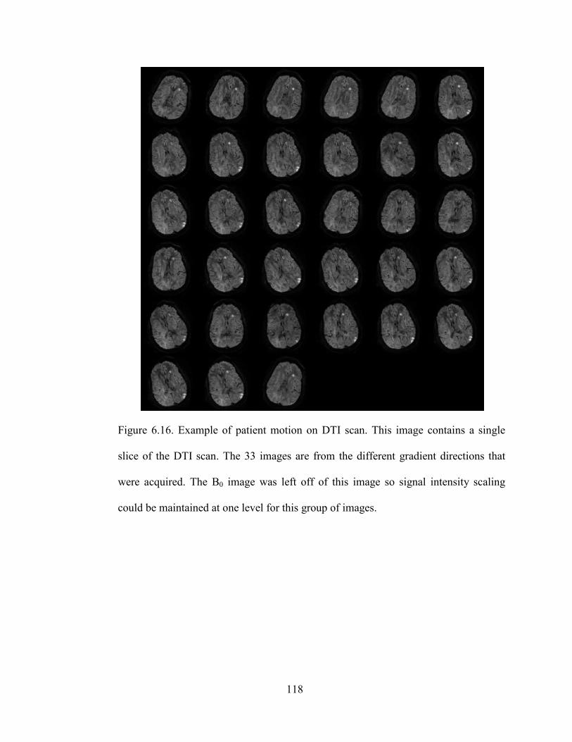
118

Figure 6.16. Example of patient motion on DTI scan. This image contains a single

slice of the DTI scan. The 33 images are from the different gradient directions that

were acquired. The B0 image was left off of this image so signal intensity scaling

could be maintained at one level for this group of images.

119

Figure 6.17. Processed data for carotid artery stenosis patient (Slices 16-20)

(displayed in radiologic convention). (A) Acute FLAIR scan (B) Acute Mean

Diffusion Weighted scan (C) Acute Time to Peak scan (D) MTRasymmetry(3.5 ppm)

(pH-weighted) (E) APT (F) NOE

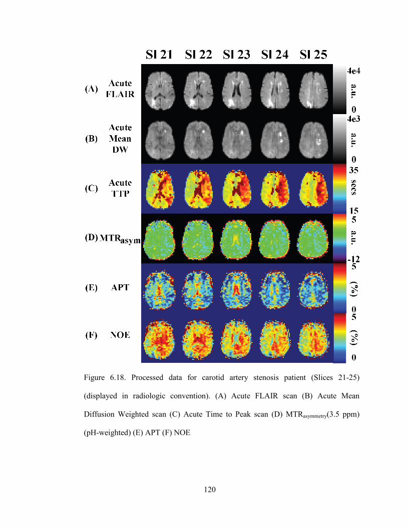
120





121





122

The patient’s old stroke in the right parietal-occipital region can be seen in the

FLAIR scan between slices 18-28. Mean diffusion weighted images show

hyperintensities between slices 18-29 in the left hemisphere, and time to peak images

show a large region at risk of infarction covering the entire MCA distribution on the

left hemisphere. MTRasymmetry(3.5 ppm) images shows regions of possible reductions

in pH. These regions appear to be smaller in size than the perfusion deficit, which

may indicate that not all tissue that is indicated to be hypoperfused by the time to

peak image is at risk of infarction.

6.6. Conclusion

We present an initial application of using pulsed CEST to image different pHs in 10%

BSA pH phantoms and translated this to healthy volunteers and eventually to acute ischemic

stroke patients. Comparison of MTRasymmetry(+3.5 ppm) images between a healthy volunteer

and an ischemic stroke patient showed a reduction in the MTRasymmetry(+3.5 ppm) in the

region of delayed perfusion that was attributed to tissue acidosis, and comparison of the pH

penumbra to the PWI penumbra (by using different TTP delay thresholds) shows that the pH

penumbra localizes a region smaller than the PWI penumbra. Therefore, APT MRI shows

sensitivity to pH changes that are not visible using diffusion or perfusion imaging. A patient

with a large perfusion penumbra that was believed to be benign oligemia was also imaged.

pH-weighted imaging (MTRasymmetry(+3.5 ppm)) showed symmetric hemispheres similar to

what was seen for normal volunteers. Follow-up FLAIR imaging confirmed that the large

perfusion penumbra was indeed benign oligemia as infarction was confined to regions of

diffusion hyperintensities. And finally, pulsed CEST was applied to a patient with a stenosed

left internal carotid artery that appeared to localize pH changes around diffusion lesions.

123

6.7. References

1. Mathers CD, Loncar D. Projections of global mortality and burden of disease from

2002 to 2030. PLoS Med. 2006;3(11):e442.

2. Rymer MM, Thrutchley DE. Organizing regional networks to increase acute stroke

intervention. Neurol Res. 2005;27 Suppl 1:S9-16.

3. Furlan A, Higashida R, Wechsler L, Gent M, Rowley H, Kase C, Pessin M, Ahuja A,

Callahan F, Clark WM, Silver F, Rivera F. Intra-arterial prourokinase for acute

ischemic stroke. The PROACT II study: a randomized controlled trial. Prolyse in

Acute Cerebral Thromboembolism. JAMA. 1999;282(21):2003-11.

4. Knight RA, Barker PB, Fagan SC, Li Y, Jacobs MA, Welch KM. Prediction of

impending hemorrhagic transformation in ischemic stroke using magnetic resonance

imaging in rats. Stroke. 1998;29(1):144-51.

5. Brinker G, Pillekamp F, Hossmann KA. Brain hemorrhages after rt-PA treatment of

embolic stroke in spontaneously hypertensive rats. Neuroreport. 1999;10(9):1943-6.

6. Busch E, Kruger K, Allegrini PR, Kerskens CM, Gyngell ML, Hoehn-Berlage M,

Hossmann KA. Reperfusion after thrombolytic therapy of embolic stroke in the rat:

magnetic resonance and biochemical imaging. J Cereb Blood Flow Metab.

1998;18(4):407-18.

7. Hacke W, Donnan G, Fieschi C, Kaste M, von Kummer R, Broderick JP, Brott T,

Frankel M, Grotta JC, Haley EC, Jr., Kwiatkowski T, Levine SR, Lewandowski C,

Lu M, Lyden P, Marler JR, Patel S, Tilley BC, Albers G, Bluhmki E, Wilhelm M,

124

Hamilton S. Association of outcome with early stroke treatment: pooled analysis of

ATLANTIS, ECASS, and NINDS rt-PA stroke trials. Lancet. 2004;363(9411):768-74.

8. Blakeley JO, Llinas RH. Thrombolytic therapy for acute ischemic stroke. J Neurol

Sci. 2007;261(1-2):55-62.







1996;36(5):726-36.




Neuroradiol. 2005;26(4):815-9.

12. Zhou J, Payen JF, Wilson DA, Traystman RJ, van Zijl PC. Using the amide proton

signals of intracellular proteins and peptides to detect pH effects in MRI. Nature

medicine. 2003;9(8):1085-90.

13. Ward KM, Balaban RS. Determination of pH using water protons and chemical

exchange dependent saturation transfer (CEST). Magn Reson Med. 2000;44(5):799-

802.

14. Zhou J, van Zijl PC. Defining an Acidosis-Based Ischemic Penumbra from pH-

Weighted MRI. Translational stroke research. 2011;3(1):76-83.

125

15. Sun PZ, Zhou J, Sun W, Huang J, van Zijl PC. Detection of the ischemic penumbra

using pH-weighted MRI. J Cereb Blood Flow Metab. 2007;27(6):1129-36.

16. Bryant RG. The dynamics of water-protein interactions. Annual review of biophysics

and biomolecular structure. 1996;25:29-53.

17. Pekar J, Jezzard P, Roberts DA, Leigh JS, Jr., Frank JA, McLaughlin AC. Perfusion

imaging with compensation for asymmetric magnetization transfer effects. Magn

Reson Med. 1996;35(1):70-9.

18. Hua J, Jones CK, Blakeley J, Smith SA, van Zijl PC, Zhou J. Quantitative description

of the asymmetry in magnetization transfer effects around the water resonance in the

human brain. Magn Reson Med. 2007;58(4):786-93.

19. Ling W, Regatte RR, Navon G, Jerschow A. Assessment of glycosaminoglycan

concentration in vivo by chemical exchange-dependent saturation transfer (gagCEST).

Proc Natl Acad Sci U S A. 2008;105(7):2266-70.

20. Mori S, Eleff SM, Pilatus U, Mori N, van Zijl PC. Proton NMR spectroscopy of

solvent-saturable resonances: a new approach to study pH effects in situ. Magn Reson

Med. 1998;40(1):36-42.

21. van Zijl PC, Zhou J, Mori N, Payen JF, Wilson D, Mori S. Mechanism of

magnetization transfer during on-resonance water saturation. A new approach to

detect mobile proteins, peptides, and lipids. Magn Reson Med. 2003;49(3):440-9.

22. van Zijl PC, Yadav NN. Chemical exchange saturation transfer (CEST): what is in a

name and what isn't? Magn Reson Med. 2011;65(4):927-48.

126

23. Jones CK, Polders D, Hua J, Zhu H, Hoogduin HJ, Zhou J, Luijten P, van Zijl PC. In

vivo three-dimensional whole-brain pulsed steady-state chemical exchange saturation

transfer at 7 T. Magn Reson Med. 2012;67(6):1579-89.

24. Jin T, Wang P, Zong X, Kim SG. Magnetic resonance imaging of the Amine-Proton

EXchange (APEX) dependent contrast. Neuroimage. 2012;59(2):1218-27.

25. Desmond KL, Stanisz GJ. Understanding quantitative pulsed CEST in the presence of

MT. Magn Reson Med. 2012;67(4):979-90.

26. Song X, Gilad AA, Joel S, Liu G, Bar-Shir A, Liang Y, Gorelik M, Pekar JJ, van Zijl

PC, Bulte JW, McMahon MT. CEST phase mapping using a length and offset varied

saturation (LOVARS) scheme. Magn Reson Med. 2012;68(4):1074-86.

27. Woessner DE, Zhang S, Merritt ME, Sherry AD. Numerical solution of the Bloch

equations provides insights into the optimum design of PARACEST agents for MRI.

Magn Reson Med. 2005;53(4):790-9.

28. Barnett HJM. Stroke : pathophysiology, diagnosis, and management. 3rd ed. New

York: Churchill Livingstone; 1998. xxiv, 1459 p., 12 p. of plates p.

29. Kraig RP, Pulsinelli WA, Plum F. Hydrogen ion buffering during complete brain

ischemia. Brain Res. 1985;342(2):281-90.

30. Donahue MJ, Lu H, Jones CK, Edden RA, Pekar JJ, van Zijl PC. Theoretical and

experimental investigation of the VASO contrast mechanism. Magn Reson Med.

2006;56(6):1261-73.

31. Zhou J, Wilson DA, Sun PZ, Klaus JA, Van Zijl PC. Quantitative description of

proton exchange processes between water and endogenous and exogenous agents for

WEX, CEST, and APT experiments. Magn Reson Med. 2004;51(5):945-52.

127

32. Versluis MJ, Peeters JM, van Rooden S, van der Grond J, van Buchem MA, Webb

AG, van Osch MJ. Origin and reduction of motion and f0 artifacts in high resolution

T2*-weighted magnetic resonance imaging: application in Alzheimer's disease

patients. Neuroimage. 2010;51(3):1082-8.

33. Farrell JA, Landman BA, Jones CK, Smith SA, Prince JL, van Zijl PC, Mori S.

Effects of signal-to-noise ratio on the accuracy and reproducibility of diffusion tensor

imaging-derived fractional anisotropy, mean diffusivity, and principal eigenvector

measurements at 1.5 T. J Magn Reson Imaging. 2007;26(3):756-67.

34. Smith SM. Fast robust automated brain extraction. Hum Brain Mapp.

2002;17(3):143-55.

35. Neumann-Haefelin T, Wittsack HJ, Wenserski F, Siebler M, Seitz RJ, Modder U,

Freund HJ. Diffusion- and perfusion-weighted MRI. The DWI/PWI mismatch region

in acute stroke. Stroke. 1999;30(8):1591-7.

36. Sobesky J, Zaro Weber O, Lehnhardt FG, Hesselmann V, Thiel A, Dohmen C, Jacobs

A, Neveling M, Heiss WD. Which time-to-peak threshold best identifies penumbral

flow? A comparison of perfusion-weighted magnetic resonance imaging and positron

emission tomography in acute ischemic stroke. Stroke. 2004;35(12):2843-7.

37. Zaro-Weber O, Moeller-Hartmann W, Heiss WD, Sobesky J. Maps of time to

maximum and time to peak for mismatch definition in clinical stroke studies validated

with positron emission tomography. Stroke. 2010;41(12):2817-21.

128

Chapter 7: Using CEST and Frequency-Labeled Exchange Transfer

(FLEX) MRI to Image Blood Oxygenation Dependent Exchangeable

Protons in Blood (boldCEST/boldFLEX)

7.1. Abstract

Blood oxygenation is an important pathophysiological parameter that changes in

numerous pathological states including ischemia. Previously mentioned in Chapter 1,

hemoglobin is the protein responsible for binding oxygen in the lungs where there is a high

partial pressure of oxygen (it becomes oxyhemoglobin here) and for transporting oxygen to

various parts of the body where oxygen diffuses out of the blood stream (because of a low

partial pressure of oxygen in tissue) to engage in metabolic processes. Over the past decades,

high resolution NMR has been used to identify a number of exchangeable proton resonances

on hemoglobin, some of which have a frequency dependence on oxygenation. Until recently,

the only way to measure these exchangeable protons was through spectroscopy, which

offered good specificity, but poor sensitivity. Recently, chemical exchange saturation transfer

MRI has been proposed as a novel way of increasing sensitivity of MR to exchangeable

protons. And even more recently, a more powerful technique, frequency labeled exchange

transfer (dubbed FLEX) MRI, not only increases sensitivity to exchangeable protons but can

also measure multiple protons simultaneously and quantify exchange rates. In this chapter,

we aim to use chemical exchange saturation transfer and frequency-labeled exchange transfer

to image these signals.

129

7.2. Introduction

Oxygenation is an important pathophysiological parameter that changes in many

pathological states such as ischemia and chronic obstructive pulmonary disease. Oxygenation

can be imaged using positron emission tomography (PET) and magnetic resonance imaging

(MRI). PET imaging of oxygenation involves injecting a radiotracer into the body and

tracking the tracer as it decays. On the other hand, MRI is capable of imaging oxygenation

non-invasively with non-ionizing radiation, which makes it the ideal modality of imaging

when tracking the course of a heterogeneous disease such as acute ischemic stroke.

Currently, magnetic resonance techniques that are sensitive to blood oxygenation

include blood oxygenation level dependent (BOLD) functional magnetic resonance imaging

(BOLD fMRI), T2 relaxation under spin tagging (TRUST), global oxygen extraction fraction

(OEF) measurement at internal jugular vein, Gradient Echo Sampling of Spin Echo (GESSE),

and quantitative imaging of extraction of oxygen and tissue consumption (QUIXOTIC) (1-5).

BOLD fMRI uses a gradient echo sampling scheme with an echo time of approximately 25

ms at 3 Tesla to be sensitive to decreases in paramagnetic deoxyhemoglobin between a

resting state and activated state (where a subject is asked to perform a certain task). Theory

has been developed to show that these decreases in paramagnetic deoxyhemoglobin arises

from increased cerebral blood flow (CBF), cerebral blood volume (CBV), and oxygen

extraction fraction (6). TRUST MRI and the global OEF measurement at the internal jugular

vein measures the transverse relaxation time (T2) of venous blood and uses a calibration

curve to map the T2 to the oxygen extraction fraction (OEF). Issues with these methods are

that they are not spatially resolved and only give whole brain oxygenation values. GESSE

(otherwise known as quantitative BOLD) uses a gradient echo sampling scheme to sample

130

magnetization around a spin echo and uses susceptibility theory to data to parameters OEF,

deoxygenated blood volume, ratio of interstitial fluid and cerebrospinal fluid, R2 (inverse of

transverse relaxation time, T2) of brain tissue, frequency shift, and brain concentration of

deoxyhemoglobin. One issue with the GESSE technique is its high number of fitting

variables, which can lead to high degrees of freedom where multiple solutions are possible.

And finally, QUIXOTIC uses velocity selective modules (RF pulses and associated gradients)

to define a bolus of blood leaving the capillaries and then label this bolus in a similar manner

as arterial spin labeling described earlier in Chapter 4. The labeled bolus is then subtracted

from a control bolus defined similarly. Because velocity selective modules can be spatially

resolved, QUIXOTIC offers spatially resolved information about oxygenation in the brain.

However, it suffers from low signal-to-noise ratios.

One method that has not been exploited to image oxygenation in the body is by using

exchangeable proton signals in blood, which is responsible for delivering oxygen throughout

the body so organs can produce energy and function and transporting waste products to be

disposed of. Blood has four main constituents: erythryocytes, plasma, leukocytes, and

thrombocytes. Hemoglobin, found in erythrocytes, is the protein in the body responsible for

the transport of oxygen. It is a large molecule (65 kiloDalton) composed of two α strands

(each with 144 amino acids) and two β strands (each with 146 amino acids) and has many

exchangeable protons on it that have been studied in detail by many groups using nuclear

magnetic resonance (NMR) (7-14). A good review that summarizes much of the work that

has been done on exchangeable protons in oxyhemoglobin, deoxyhemoglobin, and

carbonmonoxy-hemoglobin using NMR between the 1970s and 1980s was written by Drs.

Chien Ho and Dr. Janice Perussi in 1994 published in Methods in Enzymology (15).

131

Recently, chemical exchange saturation transfer (CEST) MRI has been introduced to

provide amplification of micromolar concentrations of exchangeable protons (16, 17). CEST

MRI does this by capitalizing on the chemical exchange trait of certain protons (OH, NH) in

molecules. CEST uses a saturation pulse to irradiate protons resonating at a particular

frequency, which makes them “invisible” to MR detection. If enough of the irradiated

protons exchange with bulk water, then the ultimate effect will be a reduction in the detected

water signal. By utilizing the exchange with bulk water, CEST is a powerful technique with

the capability of amplifying millimolar concentrations of compounds to be detected with the

molar water signal of MRI. CEST has been demonstrated to be sensitive to changes in pH,

protein content, and temperature and has been applied in the clinic to study brain tumors and

acute stroke (18-21). CEST MRI has also been used to study exchangeable protons in the

serine protease system (22). However, CEST MRI has not yet been used to study

exchangeable protons on hemoglobin, which has a high intracellular concentration (~5 mM)

in erythrocytes and a sufficiently large number of exchangeable protons to make it a suitable

target for applying CEST MR imaging to.

Frequency-labeled exchange (FLEX) transfer MRI is a novel imaging technique that

has recently been shown to be sensitive to slowly and quickly exchanging protons (23-25).

FLEX MRI modulates the water intensity by encoding the chemical shift of exchangeable

proton groups through label transfer modules (LTMs), which consist of four parts: 1) a

selective 90𝑥° pulse that excites protons over a large range of frequencies and minimizes

excitation of water; 2) a delay during which excited protons undergo chemical shift evolution;

3) a selective 90−𝑥° pulse that flips the magnetization back to the longitudinal axis; and 4)

another delay for labeled protons to exchange into the bulk water pool. Sensitivity

132

enhancement for low concentrations of exchangeable protons can be achieved by increasing

the number of LTMs. Because of the flexibility of the FLEX sequence (can be tuned to detect

slowly or quickly exchanging protons, RF pulse placed closer to water can detect

exchangeable resonances close to water or further away can detect exchangeable proton

resonances over a larger range), we applied FLEX MRI to image blood to look for

exchangeable proton resonances in blood.

In this chapter, we aim to use CEST and FLEX MRI to try to detect blood

oxygenation dependent exchangeable protons in bovine blood.

7.3. Materials

In this chapter, two types of hemoglobin were investigated: adult human hemoglobin

bound to carbon monoxide and bovine hemoglobin. In the next section (Section 7.4.1), we

will describe why the use of bovine blood is more advantageous than human blood for this

particular project.

7.3.1. Sample: Why Bovine Blood?

Bovine blood was used as the main model system for this study. Bovine blood

has similar characteristics as human blood (14). One advantage for using bovine

blood over human blood in this is that human blood contains 2,3-diphosphoglycerate

(2,3-DPG), which is used for control of oxygenation. However, when human blood is

removed from the body, the concentration of 2,3-DPG becomes depleted very quickly,

which makes it more difficult to externally control the binding of oxygen.

133

7.3.2. Carbonmonoxy Hemoglobin

Because of carbon monoxide’s high binding constant to hemoglobin (250x

that of oxygen), carbonmonoxy hemoglobin is an ideal sample to use when

developing and optimizing pulse sequences. Hemoglobin can be purified, dissolved in

PBS, ligated to carbon monoxide, and stored away in a sealed glass tube for an

extended period of time. Additionally, it serves as a good control for exchangeable

protons of oxyhemoglobin and deoxyhemoglobin because of conformational

differences between these three structures (15). This results in different chemical

shifts for each of exchangeable protons on each protein.

Human adult blood samples were obtained from a local blood bank. Human

adult hemoglobin (Hb A) was isolated and purified by established methods in Dr.

Chien Ho’s laboratory (15). All Hb A samples used were in the CO-ligated form in

0.1 M sodium phosphate buffer at pH 7.4, and the Hb A concentrations (in terms of

tetramer) used in this study were about 2.4 mM and 4.9 mM.

7.3.3. Whole Blood

Fresh bovine blood was provided by a local slaughterhouse. The blood was

collected into a container filled with a distilled de-ionized water solution of the

anticoagulant sodium citrate to give a final concentration of 25 mM. Blood was

filtered to remove clots and impurities accumulated during the procedure of blood

collection.

Whole blood samples of 44% hematocrit were prepared by spinning down

whole blood using a centrifuge (Beckman Coulter Avanti Centrifuge J-25I, Rotor

134

Number: JA-10) at 10,000 G for 15 minutes. Plasma and packed erythrocytes were

combined and mixed to create a sample with 44% hematocrit. Oxygenation of the

44% hematocrit sample was manipulated by using a gas tank (Airgas) filled with 94%

nitrogen, 5% oxygen, and 1% carbon dioxide. pH of the sample was manipulated by

using a gas tank (Airgas) filled with 100% carbon dioxide. Hematocrit, pH and

methemoglobin (MetHb) values, together with the blood oximetry parameters sO2,

pO2 and pCO2 were measured with a blood gas analyzer (Radiometer ABL 700 series,

Radiometer, Copenhagen, Denmark). All blood samples were stored at 4°C and used

within a week after preparation. During that time, none of the samples exhibited any

formation of blood clots or increase in MetHb levels.

7.3.4. Washed Erythrocytes

Because whole blood is largely constituted of plasma and erythrocytes, it is

possible that detected signals using whole blood could come from proteins in plasma.

Therefore, it is important to verify that detected exchangeable proton signals are

indeed coming from hemoglobin. One way of doing this is to wash whole blood using

phosphate buffer solution. The resulting sample would have no plasma with

erythrocytes suspended in buffer solution.

Washed erythrocytes were prepared by centrifuging (Beckman Coulter Avanti

Centrifuge J-25I, Rotor Number: JA-10) whole blood at 10,000 G for 15 minutes,

extracting plasma, and replacing immediately with phosphate buffer solution (PBS).

The solution was hand mixed for 10 minutes to ensure adequate mixing between

packed erythrocytes and PBS and centrifuged again at 10,000 G for 15 minutes. PBS

135

was extracted and replaced immediately with new PBS. This solution was mixed for

30 minutes to ensure adequate mixing between packed erythrocytes and PBS. This

mixture was centrifuged at 10,000 G for 15 minutes, and PBS was extracted and

replaced with new PBS to give a solution of 44% hematocrit washed erythrocytes.

The first time we performed the procedure, we put a smear of cells under a

microscope (Olympus, IX71) at 40x magnification to verify that erythrocytes

maintained their shape after washing (figure 8.1).

Figure 7.1. Washed Cells Under a Microscope at 40x Magnification.

It can be seen that the washing process did not perturb the isotonicity of

erythrocytes. This is important as we want to study erythrocytes in their normal

environment, and the washing process is just to remove plasma from the sample.

136

7.3.5. Experimental Set-up

Blood was circulated in a gas exchange perfusion system at a controlled

physiological temperature (37 °C) within the 700 MHz spectrometer. Details of the

perfusion system setup were described previously (15). Blood was sampled right

before and after the MR measurements and oxygenation determined using a blood gas

analyzer (Radiometer, ABL700) to ensure less than 2% difference of oxygenation.

Additionally, blood pO2 was monitored during the MR measurement with a needle-

encased sensor (Oxford Optronix, Oxford, UK) placed close to the spectrometer.

7.3.6. Flow Analysis

There are two reasons why we flowed blood through a perfusion system for

these measurements: (1) CEST experiments require sweeping over a wide range of

frequencies and can take up to an hour and sometimes more (more details on this

later). Erythrocyte sedimentation rates (as a measure of how quickly erythrocytes

settle in a test tube in 1 hour) of normal blood are in the range of 10-30 mm/hr (26).

Without flow, erythrocytes would quickly settle to the bottom of a sample tube and

the distribution of erythrocytes and plasma would be uneven (erythrocytes as the

bottom and plasma on top). (2) Blood is constantly flowing through the body. Any

technique developed for the measurement of oxygenation should take this into

account. However, both CEST and FLEX MRI have several seconds of “labeling”

where radiofrequency pulses are used to “label” exchangeable spins in the blood. If

flow is turned on during labeling periods, we need to be sure that the sample that is

being “labeled” does not flow out of the detection coil before it is being imaged.

137

Therefore, we performed a quick analysis to determine the optimal flow speeds for

this experiment.

To experimentally determine the flow speed of the motor (which has 3

settings: 1-3), we pumped phosphate buffer throughout the tubing, dripped it into a 14

mL Falcon tube, and timed how long it took (at three different flow settings) for the

14 mL Falcon tube to be immersed with buffer. Table 7.1 displays the results of the

flow speed tests.

Table 7.1. Data from Flow Speed Tests

Flow

Setting

Try 1 (s) Try 2 (s) Try 3 (s) Summary (s) Calculated

Flow Speed

1 82 86 85 84±2 0.17 mL/s

2 45 45 45 45±0 0.31 mL/s

3 28 30 29 29±1 0.48 mL/s

In order to calculate how long we should label, we need to calculate the

volume of blood that is labeled with the RF coil. To derive this number, we can use

the volume of a cylinder equation:

𝑉 = 𝜋 ∗ 𝑟𝑎𝑑𝑖𝑢𝑠2 ∗ 𝐿𝑒𝑛𝑔𝑡ℎ = 3.14 ∗ (0.5 𝑐𝑚)2 ∗ 3 𝑐𝑚 = 2.36 𝑐𝑚3 (Equation 7.1)

Then the percentage of label flown out can be calculated by multiplying the

flow speed by the flow rate divided by the volume of the coil. The data is presented in

table 7.2.

138

Table 7.2. Percentage of Label Flown at for Different Flow Speeds

Flow Setting

and (Speed)

1 s label 2 s label 3 s label 4 s label 5 s label

1 (0.17 mL/s) 7.1% 14% 21% 28% 35%

2 (0.31 mL/s) 13% 26 % 40% 53% 66%

3 (0.48 mL/s) 20% 41% 61% 82% 102%

It can be seen that with a five second label duration at a flow speed of 3 (0.48

mL/s), all of the label will have flowed out. Therefore, a five second CEST labeling

duration at a flow speed of 3 would only waste time. Thus, we decided to try CEST

labeling durations of one, two, and three seconds. More details about this will be

described later.

7.4. Methods – Part 1

All MR experiments were carried out on a 700 MHz (16.4 T) Bruker Avance

Spectrometer (Billerica, MA) equipped with a 1000 W amplifier and a 30 mm

imaging transceiver coil connected through a 300 W combiner for dual channel

quadrature detection.

7.4.1. Optimizing Spin Echo

When choosing an acquisition method for a sequence, it is important to

consider speed (gradient echo is a faster sequence that will allow shorter echo times

to be used, resulting in higher signal to noise if samples have a short T2) and signal-

139

to-noise (spin echo has a higher signal to noise because of ability to refocus

inhomogeneities caused by paramagnetic species, such as the deoxyhemoglobin we

plan on imaging). In CEST imaging, exchangeable protons yield signals that depend

on a number of different factors such as concentration, exchange rate, saturation pulse

B1, and saturation pulse duration. However, because these signals are typically on the

order of a few percent, imaging sequences with high signal-to-noise are especially

important and we therefore chose to use a spin echo acquisition scheme.

When imaging, it is important to excite a homogeneous slab of signal to image.

To do this, we can use slice selection gradients with the 90° and 180° pulse and use a

read-out gradient to create a 1-dimensional profile of the sample (shown in figure 7.2).

Figure 7.2. 1D Profile Read-out of Spin Echo. Slice thickness = 3 cm.

7.4.2. FLEX Imaging Parameters

In our initial proof-of-principle scan, we wanted to sweep a wide range of

frequencies and detect all possible exchangeable protons in the whole blood. To do

this, we wanted to place the FLEX pulse as far away from the water frequency as

possible. The calculation of the FLEX pulse offset is derived from the off-resonance

field generated by hard pulses (Δωeff):

140

∆𝜔𝑒𝑓𝑓 = �𝜔12 + ∆𝜔𝑠012 (Equation 7.2)

Where is the ω1 is the B1 field strength, and Δωo1 is the offset frequency. An

offset ∆𝜔𝑠01 can be chosen such that the product 𝜔𝑒𝑓𝑓 ∙ 𝜏90 is 2π radians on water and

π/2 for exchangeable protons to minimize water excitation thereby functioning as a

water suppression pulse. This relationship is then governed by equation 7.3.

∆𝜔𝑠𝑜1 = 𝜔1 ∙ √15 (Equation 7.3)

Using the highest power we could (limited only by hardware), we determined

that we could use a 30 µs pulse placed at 32266.67 Hz (or +46.10 ppm at 700 MHz).

However, this offset is actually a little bit unfortunate because we were originally also

interested in imaging the histidine proton (known as the distal histidine) next to the

iron on deoxyhemoglobin. Previous research has shown that the chemical shift of the

distal histidines of the alpha and beta globin chains in this deoxygenated molecule are

at 58.5 ppm and 71.0 ppm, respectively (27).

Other FLEX parameters that need to be defined include: 1) the evolution time

and number of tevolution times needed to encode the chemical shift evolution of

exchangeable proton peaks; 2) the exchange time, which is the delay after labeling

used for labeled peaks to exchange to bulk water (this exchange time parameter can

also be tuned for the FLEX sequence to be sensitized to slowly or quickly exchanging

protons); and 3) the number of LTMs, which is the number of repetitions of the label

transfer module. The FLEX sequence is displayed in figure 7.3 for the user’s

reference.

141

Figure 7.3. FLEX Sequence. RF pulses are represented using blue blocks: The FLEX

90° and -90° pulses were block pulses; and the 90° and 180° pulses for spin echo

were Gaussian pulses. Gradients are represented in yellow. A gradient was used

during the texch period to dephase any residual transverse magnetization. The next two

gradients are for slice selection for the 90° pulse. This is followed by a dephase

gradient, slice selection gradient for the 180° pulse, and readout gradient.

In our initial efforts, we chose to vary the evolution times between 0 and 1 ms

in increments of 5 µs (also known as the dwell time). The duration of the dwell time

is important in fulfilling the Nyquist sampling theorem, which defines the minimum

sampling rate to be twice the frequency of the signal of interest. Using a 5 µs dwell

time applied at a reference frequency of 32,266.67 Hz, we would be able to

adequately measure signals oscillating at 100,000 Hz away from our reference

frequency. We decided to initially go with 400 LTMs with a single LTM duration of

5 ms (yielding a texch of 4.94 ms), which gives us a total FLEX preparation time of

two seconds (400*5 ms = 2000 ms). Using a short exchange time sensitizes the FLEX

sequence to fast exchanging protons because after the protons are frequency labeled,

they are only given a short period of time to exchange with bulk water. Therefore, the

label on fast exchanging protons is transferred effectively whereas the label on the

more slowly exchanging protons does not have enough time to exchange yet. The

142

reason why our initial efforts focused on fast exchanging protons is because the

protons that we were interested in detecting are histidine protons, and past research

has shown that histidine protons can exchange between 500-10,000 times per second

(28).

Multi-pulse sequences such as the FLEX may have contamination from many

signal components, for instance stimulated echoes. An important way to improve the

signal quality of FLEX experiments is through phase cycling, which can be used to

eliminate unwanted signals from NMR experiments on the basis of their phase. In

order to get phase-sensitive spectra, we acquired a cosine and sine component for the

FLEX signal. Phase cycling for the cosine component employed 0°, 90°, 180°, 360°

with the flip-back pulse set to 180°, 270°, 0°, 90°. Phase cycling for the sine

component was implemented with 0°, 90°, 180°, 270° with the flip-back pulse set to

90°, 180°, 270°, 0°. To make sure phase cycling does not adversely affect our spectra,

we ran FLEX experiments with the following parameters on the 4.9 mM HbCO

sample:

Experiment 1) tevol = 0 to 1 ms (increment 5 µs), texch = 10 ms, LTMs = 400, without

phase cycling.

Experiment 2) tevol = 0 to 1 ms (increment 5 µs), texch = 10 ms, LTMs = 400, with

phase cycling.

Experiment 3) tevol = 0 to 1 ms (increment 5 µs), texch = 20 ms, LTMs = 400, without

phase cycling.

Experiment 4) tevol = 0 to 1 ms (increment 5 µs), texch = 20 ms, LTMs = 400, with

phase cycling.

143

Results of these four experiments are presented below in figure 7.4.

Figure 7.4. (A) FLEX, texch = 10 ms, without phase cycle (B) FLEX, texch = 10 ms,

with phase cycle (C) FLEX, texch = 20 ms, with phase cycle (D) FLEX, texch = 20 ms,

without phase cycle

Based on the data presented in figure 7.4, phase cycling appears to help clean-

up unwanted signals in our FLEX acquisition and does not appear to introduce any

unwanted artifacts.

144

Additionally, it is important to check FLEX excitation profiles to verify that 1)

water excitation is minimized; and 2) the range of exchangeable protons that we are

interested is properly excited. FLEX excitation profiles were acquired experimentally

on a sample of 44% hematocrit 100% oxygenated whole blood by applying a 90°

pulse across a wide range of offset frequencies. Excitation profiles for FLEX pulse

durations of 30 µs and 40 µs are presented in figure 7.5.

(A)

(B)

Figure 7.5. FLEX Excitation Profiles for (A) 30 µs block pulse applied at +46.10 ppm

(B) 40 µs block pulse applied at +34.57 ppm

It appears that there may be some overtipping of the FLEX excitation pulses

near the frequency offset where the pulse is applied, but the excitation profiles follow

what we would expect for these pulses.

7.4.3. CEST Imaging Parameters

The CEST sequence is composed of three main parts: 1) Pre-scan delay, to

allow for enough time for the magnetization to recover after saturation; 2) Saturation

Pulse, to saturate over a range of frequencies so saturated exchangeable protons can

145

exchange into bulk water and replaced by non-saturated protons; and 3) Acquisition.

The optimized CEST sequence is displayed in figure 7.6.

Figure 7.6. CEST Sequence. RF pulses are represented in blue: the saturation pulse is

represented by a blue box because a block pulse was used for it; and Gaussian pulses

were used for spin echo 90° and 180°. Gradients are represented in yellow. The

gradient after the CEST pulse is to dephase any transverse magnetization left after the

CEST pulse. The next two gradients are for slice selection for the 90° pulse. This is

followed by a dephase gradient, slice selection gradient for the 180° pulse, and

readout gradient.

An unsaturated CEST scan (S0) was collected after all of the saturated

volumes were collected and was composed of exactly the same sequence but with the

B1 of the saturation pulse set to zero.

7.4.4. Optimizing CEST Saturation Pulse Duration

One important parameter to optimize in CEST experiments is the saturation

pulse duration. A quick glance at how the saturation efficiency of the CEST pulse is

determined (equations 7.3-7.5) would tell us that a saturation pulse of infinite

duration would yield the highest CEST effect (29):

146

𝛼 = 𝜔12

𝜔12+𝑝𝑞

(Equation 7.3)

𝑝 = 𝑟2𝑐 −𝐶𝑎𝑐𝐶𝑐𝑎𝑟2𝑎

(Equation 7.4)

𝑞 = 𝑟1𝑐 −𝐶𝑎𝑐𝐶𝑐𝑎𝑟1𝑎

(Equation 8.5)

Where r1c is the sum of R1c, the longitudinal relaxivity of the amide proton

and Cac, the exchange rate between bulk water and the amide proton and r2c is the sum

of R2c, the transverse relaxivity (inverse of T2c) of the amide proton and Cac, the

exchange rate between bulk water and the amide proton. Additionally, it can be

simulated that exchangeable proton pools with a short T2 do not undergo complete

saturation with short saturation pulses.

At 37°C bovine blood is only fresh for a certain period of time (~12 hours), so

we want a short enough saturation pulse to minimize scan time yet a long enough

saturation pulse to increase the CEST effect (PTR) and minimize artifacts from the

possibly short T2 of exchangeable protons on hemoglobin. At low oxygenation (60%)

and high field (700 MHz), T2 of deoxygenated blood is very short (~13 ms for 44%

hematocrit and τcpmg = 0.5 ms (unpublished data)). We put in a sample of 44%

hematocrit whole blood at 65% oxygenation and ran three CEST experiments with B1

= 14.1 µT but with different saturation times (1 seconds, 2 seconds, 3 seconds) with

the pre-scan delay set to 8 seconds over the frequency range -5 ppm to 5 ppm in

increments of 0.2 ppm. Here, flow was set to 0.48 mL/second.

147

Figure 7.7. Data Over Multiple Saturation Pulse Durations.

“Wiggles” (green boxes) in the CEST spectra show that a saturation pulse

duration of less than three seconds may not be long enough for the exchangeable

protons in blood to be in steady state saturation. Based on this data, we chose a

saturation pulse duration of three seconds for our CEST experiments. Now that we

have determined the saturation pulse duration, we can estimate a pre-scan delay

needed to allow magnetization to return back to normal. It is well-known that five

times the longitudinal magnetization relaxation time is enough time for magnetization

to recover. We ran a quick inversion recovery experiment and quantified the T1 of

44% hematocrit, 100% oxygenated blood to be 2,462 ms. Five times of that would be

12.31 seconds. Interestingly, because the blood is constantly flowing, another way to

calculate a pre-scan delay would be to figure out how long it takes for the current

bolus to flow out. To do this, we could divide the volume of blood that the coil

148

excites (2.356 mL) by the flow speed (0.49 mL/second) and arrive at 4.8 seconds. We

could even add one second for a margin of error. After six seconds, the bolus of blood

that was previously saturated has already flowed out. Therefore, we selected a pre-

scan delay of six seconds.

Another parameter that needs to be chosen for CEST experiments is the

saturation pulse B1. The simplified solution for saturation efficiency (α) under slow

exchange conditions on the NMR time scale tells us that the B1 we choose for our

experiments will depend on the exchange rate of the proton we are interested in.

𝛼 = (𝛾𝐵1)2

(𝛾𝐵1)2+𝑘𝑠𝑤2 (Equation 7.6)

Where γ is the gyromagnetic ratio of hydrogen (267.53x106 𝑟𝑎𝑑𝑠∙𝑇

), B1 is the

power of the saturation pulse, and ksw is the exchange rate of the exchangeable proton.

Because the histidine protons that we were trying to detect has a fast exchange rate,

we chose to use a 14.1 µT pulse.

And finally, the last CEST parameter that needs to be set is the frequency

range over which the saturation pulse will be swept. Previously, we mentioned in the

FLEX section that it may also be interesting to detect the distal histidine of

deoxyhemoglobin. However, in order to detect that far away from water, it would be

necessary to sweep from +80 ppm to -10 ppm in order to capture the water offset to

determine whether or not there was a B0 shift over the period of our experiment.

However, in order to have enough spectral resolution to differentiate narrow peaks,

we would have to acquire a point every 0.2 ppm, which would make the total scan

time 67 minutes and 48 seconds long for a single oxygenation and a single B1. To be

practical, we decided we would use the FLEX scan to “screen” the blood to see if

149

there were any exchangeable proton resonances on deoxyhemoglobin. If so, then we

would run a CEST scan with frequency offsets from +80 ppm to -10 ppm in

increments of 0.2 ppm. Otherwise, we would restrict ourselves between +15 ppm to -

15 ppm in increments of 0.2 ppm.

7.4.5. 1-H WATERGATE Imaging Parameters

Traditionally, exchangeable protons have been detected using spectroscopic

sequences with water suppression that does not saturate the water signal until just

before acquisition of the spectra, such as the well-known WATERGATE (3-9-19)

sequence (30). Because spectroscopy has been previously used to study exchangeable

protons on hemoglobin, we believed that it would be an independent check for any

exchangeable protons detected with CEST or FLEX. However, after optimizing the

1H-WATERGATE sequence, we checked the excitation profile and realized we could

only acquire between -10 ppm and 11 ppm if we wanted at least 1% excitation

efficiency (figure 7.8).

150

Figure 7.8. Excitation Profile of 1H-WATERGATE sequence on 700 MHz scanner.

We realized that the reason why this happened was because of hardware

limitations. Using the highest power we could achieve on the 30 mm imaging probe,

the shortest duration of the longest rectangular pulse in the 3-9-19 pulse train was

59.50 µs. In the frequency domain, this would be equal to 16,807 Hz, which at 700

MHz, corresponds to 24 ppm. This means that the excitation profile of a

WATERGATE sequence will be a convolution of the WATERGATE excitation

profile with infinitely short pulses with the frequency response of a 59.5 µs pulse

(figure 7.9). Because of hardware limitations, we decided not to continue with this

sequence.

151

Figure 7.9. Explanation of why WATERGATE at 700 MHz using our hardware does

not work.



Natick, MA) and in-house written Python routines.

152

7.5.1. FLEX Processing

The FLEX FID was generated by integrating the spin echo projection of the

sample at each evolution time for both cosine and sine components. Next, the FID

was normalized by the integral of S0 and multiplied by 100 to yield a percentage.

Then, we fit the S/S0 cosine and sine FIDs to the five component exponential FLEX

equation (equation 7.7).

𝐹𝐿𝐸𝑋𝐹𝐼𝐷 = ∑ 𝑃𝑇𝑅𝑠 ∙ 𝑒−(𝑘𝑠𝑤+𝑅2∗)∙𝑡𝑒𝑣𝑜𝑙 ∙ cos(∆𝜔𝑠𝑜1 ∙ 𝑡𝑒𝑣𝑜𝑙 + 𝜑)𝑠 (Equation 7.7)

Where PTRs is the amplitude of the exchangeable proton resonance, 𝑅2∗ is

inverse of the time constant of the loss of phase coherence of the exchangeable

protons, Δωs01 is the frequency difference between the resonance offset of the

exchangeable proton and the frequency offset of the FLEX excitation pulse. A five

compartment model was chosen because the first component was fitted for low

frequency drift, the second component was fitted for the amide proton component, the

third component was fitted for NOEs, the fourth component was fitted for bulk water,

and the last component was allowed to vary to fit for the oxygenation dependent peak.

Fitting bounds for the frequency of the last component were used to prevent other

peaks from being fitted. After determining the baseline and low frequency drift using

the fitted values, we subtracted these from the data to derive the baseline-corrected

FLEX FID. Then, we combined the real (cosine FLEX) and imaginary (sine FLEX)

components using the Hilbert transform theory to arrive at the combined FID. To

prevent truncation artifacts that frequently arise from not sampling the FID until the

signal has completely decayed, we applied a cosine filter over the time domain.

Finally, we took the Fourier transform of the combined FID to get the phase-sensitive

153

frequency spectrum. To calculate the frequency offsets for the spectrum, we

calculated the sweep width to be the inverse of the dwell time, defined as the

increment in FLEX evolution times. Zeroth order and first order phase corrections

were performed the same way as Friedman et al (23).

Additional data processing to study what we believed to be an oxygenation

dependent peak in the FLEX spectrum included time domain fitting using the

exponential FLEX equation to fit out the amide proton, water, and Nuclear

Overhauser Effects from the FID. After subtracting out the amide proton, bulk water,

and NOEs from the fid, we were left with a spectrum with only a peak at 10 ppm.

7.5.2. CEST Processing

At each irradiation offset frequency, the raw CEST data were processed by

applying a Fourier Transform to the spin echo to get the 1D projection of the sample.

Then, the spin echo was integrated over the frequency spectrum to get a single

intensity value. This value was then normalized using the first unsaturated (S0) scan

acquired and multiplied by 100 to yield a percentage value.

Because of scanner drift, S0 scans were interspersed throughout the data

acquisition after every ten frequencies. CEST baseline correction was performed on

the z-spectra similarly to the method described in Chapter 6.

Furthermore, asymmetry curves were calculated based on the following

equation:

𝑀𝑇𝑅𝑎𝑠𝑦𝑚𝑚𝑒𝑡𝑟𝑦(∆𝜔) = 𝑆𝑠𝑎𝑡(−∆𝜔)−𝑆𝑠𝑎𝑡(∆𝜔)𝑆0

(Equation 7.6)

154

Where Ssat(-Δω) is the saturated volume acquired Δω ppm upfield of water,

Ssat(Δω) is the saturated volume acquired Δω ppm downfield of water, and S0 is the

unsaturated image.

7.6. Results & Discussion – Part 1

7.6.1. Carbonmonoxy Hemoglobin

The FLEX results for carbonmonoxy hemoglobin are displayed in figure 7.10.

The results are in line with what is expected for the two concentrations of HbCO. A

higher concentration of HbCO would yield peaks with higher protein effects (amide

protons and NOEs). The difference in the water peak arises from the difference

between the T1 of the two samples. It is also clear that there are no other peaks from

exchangeable protons in this spectrum, which is also in line with what is understood

about carbon monoxy hemoglobin.

Figure 7.10. FLEX results for 2.4 mM and 4.9 mM HbCO.

155

The FLEX spectrum for carbonmonoxy hemoglobin at two different

concentrations both shows three main peaks. The peak downfield of water (to the left

of water) around +3.5 ppm are amide protons on the carbonmonoxy hemoglobin

protein. The peak at 0 ppm is the bulk water signal. Notice between the two different

concentrations of HbCO that the bulk water peak is slightly different. This is because

the bulk water peak is proportional to T1 and T2, which is probably different between

these two concentrations. And finally, the peak on the right around -4 ppm is due to

NOEs.

The CEST results for 4.9 mM HbCO are shown in figure 7.11 for a saturation

pulse duration of five seconds with B1 = 1.4 uT.

Figure 7.11. CEST (top) and MTRasymmetry (bottom) spectra for 4.9 mM concentration

of HbCO.

156

The CEST spectra of the 4.9 mM HbCO is in line with the results of the

FLEX data. There is a clear peak from amide protons around 3.5 ppm, and a peak

between -5 and -2 ppm from NOEs. There do not appear to be any other

exchangeable protons detectable with CEST or FLEX at this concentration of HbCO.

7.6.2. 30 µs FLEX of 44% Hematocrit Whole Blood

The initial results of the multi-oxygenation scan were quite interesting and

have been summarized in figure 8.12A-D.

157

Figure 7.12. FLEX Results of Multi-oxygenation Scan (A) FLEX results for 5

different oxygenations. (B) Amide Proton, Bulk Water, and NOE-filtered FLEX

spectrum

(C) Zoomed-in 10 ppm peaks for 5 different oxygenations (D) Linear correlation of

Oxygenation vs Peak Amplitude, r2 = 0.86

FLEX scans run on a sample of 44% hematocrit whole blood over a range of

oxygenations show a possible oxygenation dependent peak around 10 ppm (figure

7.12A). To further study the peak, bulk water, amide protons, and NOEs were filtered

out using time domain analysis only to leave the peak around 10 ppm (figure

7.12B&figure 7.12C). After independently phase correcting each peak, there appears

to be an oxygenation dependent at 10 ppm. When plotting the peak amplitude against

158

oxygenation (figure 7.12D), there is a strong correlation (r2 = 0.86) with the equation

relating the two being:

Peak Amplitude = -0.001*O2+0.236 (Equation 7.7)

I thought that I imaged the so-called “T-marker” that uniquely identifies

deoxyhemoglobin, resonating at 9.4 ppm with respect to water (8). It was previously

identified by Fung et al (8) to be a hydrogen bond between α42 tyrosine and β99

aspartic acid at the α1β2 interface and follows a similar behavior as what we have

uncovered. It can be argued that the exchangeable proton that our data points to is

sitting at 10.3 ppm from water so this is not necessarily the T-marker. However, it is

widely known that chemical shift is very sensitive to environment and protein

conformation. In Fung et al’s studies, they isolated human hemoglobin A and

dissolved it in a phosphate buffer of pH 7.4 whereas we were imaging bovine whole

blood, which means hemoglobin is inside of red blood cells, at pH 7.2.

159

7.6.3. 30 µs FLEX of Washed Erythrocytes

After seeing the previous results, we were worried that the peak may have

been from proteins (albumin) in plasma. To test our hypothesis that the peak is due to

an oxygenation dependent exchangeable proton on hemoglobin, we washed the

erythrocytes to remove plasma and ran the FLEX scan on a sample of 100%

oxygenated washed erythrocytes and a sample of 65% oxygenated washed

erythrocytes. Data is presented in figure 7.13.

(A)

(B)

Figure 7.13. FLEX data and spectra of 44% hematocrit washed erythrocytes with

(A) 100% oxygenation; and (B) 65% oxygenation.

Interestingly, we still saw a peak in the sample with lower oxygenation, and

the peak appeared inverted in the higher oxygenated sample. Thus, FLEX spectra

acquired on washed cells confirm the existence of an oxygenation dependent peak

around 10 ppm and show that this peak is not due to proteins in plasma. In figure

7.13A, the peak around 10 ppm appeared to be inverted, but at the time, we thought

160

this was something that could be corrected with data processing. More details on this

later.

7.6.4. CEST of Whole Blood

After showing that the peak at 10 ppm could be due to an exchangeable proton

on deoxyhemoglobin, we decided to move to CEST imaging. Using the results of the

FLEX spectra, we thought we were imaging a histidine proton and used a higher

saturation pulse B1 for CEST imaging because of faster exchange rates of histidine

protons. The results of imaging 44% hematocrit whole blood at multiple oxygenations

using CEST is presented in Figure 7.14.

Figure 7.14. CEST spectra (top) and MTRasymmetry (bottom) for 44% hematocrit

Whole Blood at Multiple Oxygenations.

Oddly, we did not see the exchangeable proton we thought we were able to

image from the FLEX data. However, we do believe that this data makes sense. When

161

looking at the CEST spectra, the direct saturation region becomes wider for lower

oxygenations. This is due to a shorter T2 in lower oxygenations and is in line with

what is published in literature.

7.6.5. Varying Offset (and Pulse Duration) for FLEX Imaging on 44% Hematocrit

Whole Blood at 66% Oxygenation

Therefore, we decided to go back to FLEX imaging to understand why this

was happening. Using a 30 µs pulse, one simple modification we can make to the

pulse sequence is to apply the pulse at -46.10 ppm (instead of +46.10 ppm). If an

exchangeable proton were to resonate around 10 ppm, then changing the excitation

pulse offset to the negative side would lower the sensitivity of detecting that proton

because the FLEX excitation efficiency would be much lower for the peak around 10

ppm. The result for the FLEX sequence with pulse offset applied at -46.10 ppm on

44% hematocrit, 57% oxygenated whole blood is displayed in figure 7.15B. A dataset

acquired with the same parameters but with the pulse offset at +46.10 ppm is

displayed in figure 7.15A for comparison. Additionally, another scan with the FLEX

excitation pulse set to +34.57 ppm was run with all other parameters (durLTM, number

of LTMs, tevol) equal.

162

(A)

(B)

(C)

Figure 7.15. FLEX Spectra for (A) FLEX Excitation Pulse Applied at 46.10 ppm (B)

FLEX Excitation Pulse Applied at -46.10 ppm (C) FLEX Excitation Pulse Applied at

34.57 ppm.

As expected, a peak around 10 ppm is seen in figure 7.15A, but a couple of

aspects of figure 7.15B stand out. First, the NOE peak appears to be “larger” than the

amide proton peak relative to figure 7.15A. This makes sense because application of

the pulse at a negative offset frequency would give the NOE peak higher sensitivity

because of a higher excitation efficiency (see FLEX excitation efficiency plots in

figure 7.5). What is odd is that the peak that we originally detected around +10 ppm is

now around -10 ppm. Furthermore, if we look to figure 7.15C where we moved the

frequency offset at which the FLEX excitation pulse was applied closer to water, we

would expect the peak around 10 ppm to have an even higher excitation efficiency

than when the FLEX excitation pulse was at +46.10 ppm. However, that peak is not

visible.

Our conclusion was that the peak around 10 ppm that we imaged using FLEX

MRI was actually a flow artifact that manifested in a phase change. If we refer to the

exponential FLEX equation (equation 7.5), we see that φ is an important component

163

of the equation and represents the phase of the exchangeable proton that is being

imaged. When blood (or any other sample that is imaged) is flowing, there is a phase

change, and the phase change was being modulated in the FLEX spectrum. However,

this explanation alone is not enough to explain the oxygenation dependence of the

peak amplitude. Our conclusion is that the flow artifact resulted in a fold over of the

bulk water peak. Because the T1 and T2 of blood are different for different

oxygenations, we believe we were imaging these T1 and/or T2 differences in a fold

over artifact.

Therefore, we concluded that we should stop the flow during RF preparation

and data acquisition. We also took a closer look at the slice thickness and wondered

whether or not RF inhomogeneities at the edge of the RF coil would cause any issues

too. And finally, we believed that there may be baseline drift in our CEST images and

needed a method to correct for this. Additionally, we thought that the high power of

the saturation pulse (high B1) was saturating much of the bound proton pool (from

erythrocyte cell membranes), and we were worried that this generated an MT effect

that could also mask the 1-2% effect that we were interested in.

7.7. Methods – Part 2

After realizing the issues that we faced may be hiding the signal we were interested in,

we decided to modify our experiments. To do this, we reanalyzed our profile to reduce the

RF inhomogeneities at the edges of the coil, and we flowed the blood in the phantom except

during RF preparation and data acquisition. To flow blood in the phantom except during RF

preparation and data acquisition, code was written to run in the background of the NMR

164

console synchronized with the data acquisition to instruct me when to flow the blood and

when to stop it.

7.7.1. Checking the Profile Acquisition

After realizing that RF inhomogeneities at the edges of the coil may be

causing “un-clean” FLEX labeling that are flowed into the region where we were

detecting the signal, we decided to run the following test. Before the spin echo

acquisition, we added a single 30 µs 90° FLEX pulse to test the efficiency of the

FLEX 90° pulse and varied the slice thickness (by varying the strength of the readout

gradient).

Table 7.3. Checking the Efficiency FLEX 90° Pulse versus Slice Thickness.

Slice Thickness (cm) Percentage of Signal Left after 90° Pulse (%)

3 15.37%

2.5 8.25%

2 8.01%

1 6.59%

It appeared that RF inhomogeneities at the edges of the coil significantly

reduced the efficiency of the FLEX 90° labeling pulse when a 3 cm slice was used.

Although it appears that the labeling efficiency is optimal for a 1 cm slice, we

considered the loss in signal-to-noise ratio (SNR) with a 1 cm slice. SNR in MRI is

directly proportional to slice thickness so a 1 cm slice would have three times less

165

SNR than a 3 cm slice. Ultimately, we decided a 2.5 cm slice maximized the signal-

to-noise ratio and sufficiently reduced inhomogeneities from the edges of the RF coil.

7.7.2. Baseline CEST Spectrum Drift

Because the signals we detect using CEST are of the order of 1-2%, it is

important to verify that the baseline of the z-spectra has no interference from other

sources of noise. However, similar to the human data in Chapter 6, we noticed

instabilities in the baseline of the CEST spectra so we ran unsaturated scans

repeatedly for 47 minutes.

Figure 7.16. Drift of S0 Images at 700 MHz.

Because of the baseline drift of unsaturated images, S0 scans need to be

interspersed throughout the CEST acquisition to correct for this drift. Baseline drift

can be corrected in a similar manner as described in Chapter 6.

166

7.7.3. Testing Stop & Go with FLEX Acquisition

It is important to verify that stopping and flowing the blood does not cause

any unwanted artifacts in the FLEX spectrum so we put 44% hematocrit whole blood,

100% oxygenation into the perfusion system and ran FLEX scans using a flow speed

of 0.17 mL/second and while using the Stop & Go program. Furthermore, we

increased the exchange time (texch) to 10 ms and reduced the number of LTMs to 200

so the total RF preparation time for FLEX remained the same (2 seconds).

Figure 7.17. Testing Stop & Go Acquisition Using FLEX

It does not appear that the Stop&Go acquisition introduces any artifacts into

the FLEX spectrum.

167

7.7.4. Testing Stop and Go with CEST Acquisition

Additional testing with the stop and go was also performed with CEST

acquisitions where we flowed the blood during the pre-scan delay and stopped it three

second before the saturation pulse was applied. We wanted to generate

Figure 7.18. Testing Stop & Go Acquisition Using CEST.

Our data shows that the Stop & Go acquisition does not introduce any

abnormal artifacts into the CEST spectra either.

7.7.5. CEST Acquisitions Using Stop & Go

After verifying that flowing the blood except during RF preparation and data

acquisition did not induce any artifacts in the CEST and FLEX spectra, we proceeded

with acquiring data this new way. This allowed us to maximize signal-to-noise by

imaging all of the exchangeable protons that we labeled (previously a portion of the

protons that were labeled were flowing out). We proceeded to acquire CEST data

with the following sequence parameters: saturation pulse duration = 5 seconds,

saturation pulse B1 = 1.4 µT, offset frequencies acquired: -15 ppm to +15 ppm

168

(increments of 0.2 ppm), pre-scan delay = 11 seconds. Unsaturated scans (S0) were

interspersed throughout the acquisition after every 10 frequencies acquired so

baseline correction can be applied. This resulted in a total scan time of 44 minutes

and 39 seconds. We also tried increasing the range at which our offset frequencies

were acquired to -20 ppm to +20 ppm. This increased the total scan time to 59

minutes and 37 seconds. We acquired the CEST data using a saturation pulse B1 = 1.4

µT and 2.5 µT.

7.8. Results and Discussion – Part 2

CEST – with flowing blood EXCEPT during RF preparation and data acquisition

After re-thinking the experiments and optimizing the necessary parameters,

we ran the CEST scans again and saw some interesting results (figure 7.19).

169

Figure 7.19. CEST spectra (top) and MTRasymmetry (bottom) of 44% hematocrit whole

blood at 100% oxygenation (red) and 60% oxygenation (blue).

Saturation pulse duration = 5 seconds, saturation pulse B1 = 1.4 µT.

The CEST data in figure 7.19 shows two distinct peaks in the CEST spectra of

the 44% hematocrit whole blood at 60% oxygenation. The peak at +13.4 ppm shows

an effect of 3-4% with a linewidth of 0.4 ppm, and the peak at +7.6 ppm shows an

effect of 2-3% with a linewidth of 0.3 ppm. At a chemical shift of +7.6 ppm and

+13.4 ppm in the 100% oxygenation CEST spectra, there do not appear to be any

peaks. Unfortunately, after running a few scans, the oxygenation of the blood could

not be held constant and the sample had to be discarded.

We tried to repeat that experiment at more oxygenations, however, we did not

see the peaks that we previously saw. Results of follow-up CEST scans done with

44% hematocrit whole blood at 58%, 70%, 90%, and 100% oxygenations with

170

saturation pulse duration of five seconds and saturation pulse B1 of 1.4 and 2.5 µT are

presented in figure 7.20.

(A)

(B)

Figure 7.20. Follow-up Results CEST Spectra (top) and MTRasymmetry (bottom) for

(A) B1=1.4 µT (B) B1=2.5 µT

There appear to be some small differences in the MTRasymmetry graphs between

different oxygenations, but these effects are likely due to differences in T1 and T2,

which are known to affect the direct saturation region of the CEST spectra.

7.9. Conclusion

In conclusion, while our initial efforts have taught us many new concepts and shown

some interesting results for this topic, we have been unable to reproduce consistent results.

Possible ways for improving stability includes using a motor with automatic control for

stopping and starting flow that can be synchronized to the spectrometer or using a different

experimental set-up with the capability of mixing blood while imaging occurs. We believe it

should be possible to detect exchangeable protons in blood using CEST and FLEX, and a

technique capable of doing so would be beneficial to stroke imaging.

171

7.10. References

1. Ogawa S, Lee TM, Kay AR, Tank DW. Brain magnetic resonance imaging with

contrast dependent on blood oxygenation. Proc Natl Acad Sci U S A.

1990;87(24):9868-72.

2. Lu H, Ge Y. Quantitative evaluation of oxygenation in venous vessels using T2-

Relaxation-Under-Spin-Tagging MRI. Magn Reson Med. 2008;60(2):357-63.

3. Qin Q, Grgac K, van Zijl PC. Determination of whole-brain oxygen extraction

fractions by fast measurement of blood T(2) in the jugular vein. Magn Reson Med.

2011;65(2):471-9.

4. Bolar DS, Rosen BR, Sorensen AG, Adalsteinsson E. QUantitative Imaging of

eXtraction of oxygen and TIssue consumption (QUIXOTIC) using venular-targeted

velocity-selective spin labeling. Magn Reson Med. 2011;66(6):1550-62.

5. He X, Yablonskiy DA. Quantitative BOLD: mapping of human cerebral

deoxygenated blood volume and oxygen extraction fraction: default state. Magn

Reson Med. 2007;57(1):115-26.

6. van Zijl PC, Eleff SM, Ulatowski JA, Oja JM, Ulug AM, Traystman RJ, Kauppinen

RA. Quantitative assessment of blood flow, blood volume and blood oxygenation

effects in functional magnetic resonance imaging. Nature medicine. 1998;4(2):159-67.

7. Mihailescu MR, Russu IM. A signature of the T ---> R transition in human

hemoglobin. Proc Natl Acad Sci U S A. 2001;98(7):3773-7.

8. Fung LW, Ho C. A proton nuclear magnetic resonance study of the quaternary

structure of human homoglobins in water. Biochemistry. 1975;14(11):2526-35.

172

9. Greenfield NJ, Williams MN. Proton magnetic resonance studies of human

hemoglobin. Histidine titrations. Biochim Biophys Acta. 1972;257(2):187-97.

10. Yuan Y, Simplaceanu V, Ho NT, Ho C. An investigation of the distal histidyl

hydrogen bonds in oxyhemoglobin: effects of temperature, pH, and inositol

hexaphosphate. Biochemistry. 2010;49(50):10606-15.

11. Russu IM, Ho NT, Ho C. A proton nuclear Overhauser effect investigation of the

subunit interfaces in human normal adult hemoglobin. Biochim Biophys Acta.

1987;914(1):40-8.

12. Chang CK, Simplaceanu V, Ho C. Effects of amino acid substitutions at beta 131 on

the structure and properties of hemoglobin: evidence for communication between

alpha 1 beta 1- and alpha 1 beta 2-subunit interfaces. Biochemistry.

2002;41(17):5644-55.

13. Song XJ, Yuan Y, Simplaceanu V, Sahu SC, Ho NT, Ho C. A comparative NMR

study of the polypeptide backbone dynamics of hemoglobin in the deoxy and

carbonmonoxy forms. Biochemistry. 2007;46(23):6795-803.

14. Song XJ, Simplaceanu V, Ho NT, Ho C. Effector-induced structural fluctuation

regulates the ligand affinity of an allosteric protein: binding of inositol hexaphosphate

has distinct dynamic consequences for the T and R states of hemoglobin.

Biochemistry. 2008;47(17):4907-15.

15. Ho C, Perussi JR. Proton nuclear magnetic resonance studies of hemoglobin. Methods

in enzymology. 1994;232:97-139.

173

16. Ward KM, Balaban RS. Determination of pH using water protons and chemical

exchange dependent saturation transfer (CEST). Magn Reson Med. 2000;44(5):799-

802.

17. Ward KM, Aletras AH, Balaban RS. A new class of contrast agents for MRI based on

proton chemical exchange dependent saturation transfer (CEST). J Magn Reson.

2000;143(1):79-87.

18. Zhou J, Payen JF, Wilson DA, Traystman RJ, van Zijl PC. Using the amide proton

signals of intracellular proteins and peptides to detect pH effects in MRI. Nature

medicine. 2003;9(8):1085-90.

19. McVicar N, Li AX, Suchy M, Hudson RH, Menon RS, Bartha R. Simultaneous in

vivo pH and temperature mapping using a PARACEST-MRI contrast agent. Magn

Reson Med. 2012.

20. Zhou J, Lal B, Wilson DA, Laterra J, van Zijl PC. Amide proton transfer (APT)

contrast for imaging of brain tumors. Magn Reson Med. 2003;50(6):1120-6.

21. Jones CK, Schlosser MJ, van Zijl PC, Pomper MG, Golay X, Zhou J. Amide proton

transfer imaging of human brain tumors at 3T. Magn Reson Med. 2006;56(3):585-92.

22. Lauzon CB, van Zijl P, Stivers JT. Using the water signal to detect invisible

exchanging protons in the catalytic triad of a serine protease. Journal of biomolecular

NMR. 2011;50(4):299-314.

23. Friedman JI, McMahon MT, Stivers JT, Van Zijl PC. Indirect detection of labile

solute proton spectra via the water signal using frequency-labeled exchange (FLEX)

transfer. Journal of the American Chemical Society. 2010;132(6):1813-5.

174

24. Lin CY, Yadav NN, Friedman JI, Ratnakar J, Sherry AD, van Zijl PC. Using

frequency-labeled exchange transfer to separate out conventional magnetization

transfer effects from exchange transfer effects when detecting ParaCEST agents.

Magn Reson Med. 2012;67(4):906-11.

25. Yadav NN, Jones CK, Xu J, Bar-Shir A, Gilad AA, McMahon MT, van Zijl PC.

Detection of rapidly exchanging compounds using on-resonance frequency-labeled

exchange (FLEX) transfer. Magn Reson Med. 2012;68(4):1048-55.

26. Chanarin I. Blood and its diseases. 3rd ed. Edinburgh ; New York: Churchill

Livingstone; 1984. viii, 333 p. p.

27. Takahashi S, Lin AK, Ho C. Proton nuclear magnetic resonance studies of

hemoglobins M Boston (alpha 58E7 His leads to Tyr) and M Milwaukee (beta 67E11

Val leads to Glu): spectral assignments of hyperfine-shifted proton resonances and of

proximal histidine (E7) NH resonances to the alpha and beta chains of normal human

adult hemoglobin. Biochemistry. 1980;19(23):5196-202.

28. Liepinsh E, Otting G. Proton exchange rates from amino acid side chains--

implications for image contrast. Magn Reson Med. 1996;35(1):30-42.

29. McMahon MT, Gilad AA, Zhou J, Sun PZ, Bulte JW, van Zijl PC. Quantifying

exchange rates in chemical exchange saturation transfer agents using the saturation

time and saturation power dependencies of the magnetization transfer effect on the

magnetic resonance imaging signal (QUEST and QUESP): Ph calibration for poly-L-

lysine and a starburst dendrimer. Magn Reson Med. 2006;55(4):836-47.

175

30. Liu ML, Mao XA, Ye CH, Huang H, Nicholson JK, Lindon JC. Improved

WATERGATE pulse sequences for solvent suppression in NMR spectroscopy.

Journal of Magnetic Resonance. 1998;132(1):125-9.

176

Chapter 8. Conclusion and Future Directions

8.1. Conclusion

The research described in this dissertation developed, optimized, and applied novel

pulse sequences for imaging the ischemic penumbra in acute stroke patients. All of the work

in this dissertation focused on magnetic resonance imaging modalities that are non-invasive

owing to recent research showing the dangers (nephrogenic systemic fibrosis, an untreatable

disease that at its severest stage leads to death) of using gadolinium-based contrast agents.

In this work, we quantitatively measured blood flow in the cerebellum using

pseudocontinuous arterial spin labeling. It was demonstrated that a shorter labeling duration

(600 ms) coupled with shorter post labeling delays could be used to quantify blood flow in

the cerebellum. Acquired perfusion-weighted images correspond well to co-registered

anatomical images, and cerebellar blood flow values and transit times fitted from data

acquired over five volunteers are in good agreement with values published in literature from

positron emission tomography and magnetic resonance imaging.

Next, we optimized magnetization transfer vascular space occupancy (MT-VASO), a

cerebral blood volume weighted technique, for imaging acute ischemic stroke patients. Work

done on this topic included modeling MT-VASO signal changes over the range of cerebral

blood volume changes for ischemic stroke patients, testing the sequence on normal

volunteers, and applying the sequence to elucidate changes in cerebral blood volume in

patients. Results in three patients showed that MT-VASO localized increases in the cerebral

blood volume of patients (due to autoregulation) with blood vessels that may not have

collapsed yet. However, processing of this data is tedious and can be complicated by changes

177

in the longitudinal and transverse relaxation times of tissue that change in later stages of

ischemia.

Furthermore, recent research showing that reductions in cerebral blood flow beyond a

certain threshold (30% of normal cerebral blood flow) causes neurons to switch from aerobic

respiration (with oxygen) to anaerobic respiration (without oxygen) and leads to the build-up

of lactic acid, which eventually causes tissue acidosis. We proceeded to apply pH-weighted

imaging with CEST MRI to image the tissue acidosis, but noticed that scanner drift interfered

with our measurements. We developed a baseline correction method for pH-weighted

imaging based on acquiring unsaturated images interspersed within the saturated images. The

unsaturated scans were fit with a smooth spline and the saturated images were corrected

accordingly. This helped to reduce the noise within the CEST spectra leading to better fits

using the Lorentzian difference method of analysis. Results from two ischemic stroke

patients show that pH-weighted imaging could possibly predict tissue at risk of infarction

more accurately than perfusion weighted imaging. An additional result from a third stroke

patient (who also had stenosis in the left carotid artery) suggests that pH-weighted imaging

may have some useful applications in carotid artery stenosis patients.

Finally, when thinking about how to develop image methods that are sensitive to

other parameters that change for ischemia, we began work on developing a technique that

could show changes in oxygenation based on using CEST MRI and frequency label exchange

transfer MRI to study exchangeable protons on hemoglobin proteins in the blood. Although

this study has not yet been completed yet, we have performed a number of experiments and

learned a tremendous amount of information. Preliminary data shows the possibility of

178

oxygenation dependent exchangeable protons at +13.4 ppm and +7.6 ppm downfield from

the water peak.

8.2. Future Directions

Much of the work in this dissertation can be continued further. We will summarize

how some of the work mentioned in this dissertation can be carried further in the following

bullet points:

• For pH-weighted imaging in ischemic stroke patients, we have shown some

promising initial results of pH-weighted imaging being a better predictor of tissue at

risk of infarction. However, this is just the beginning. Further studies should

systematically compare the predictive value (of tissue progressing to infarction) of

pH-weighted imaging to perfusion weighted imaging using a receiver operating

characteristic (ROC) curve, a plot based on correctly and falsely identifying tissue

that will progress to infarction.

Improvements can also be made from a sequence development perspective.

Patient motion is always an issue especially with stroke patients given the level of

discomfort that they feel. Recently, data acquisition methods have been developed

and accounts for patient motion during acquisition. Tailoring such a sequence towards

pH-weighted imaging for stroke patients would not be trivial but could be immensely

useful in the clinic.

• For using chemical exchange saturation transfer and frequency label exchange

transfer to image exchangeable protons on hemoglobin, our results show that it

should be possible to image oxygenation dependent exchangeable protons on

179

hemoglobin and use this as a way to spatially image oxygen extraction fractions in the

brain and other areas of the body.

In conclusion, we believe the work presented in this dissertation has made

contributions to the area of diagnostic stroke imaging. However, exciting future work is not

limited to the contents of this dissertation. It will also depend on the funding opportunities

and future students/researchers’ interest. We hope more excellent research work could be

carried out based on the contribution of the work from this dissertation.

180

ALAN HUANG CURRICULUM VITAE

CONTACT INFORMATION Office Address Home Address F.M Kirby Functional MRI Research Center 222 East University Parkway 707 North Broadway Street Baltimore, MD 21218 Baltimore, MD 21205 Tel: 443-834-0202 E-mail: [email protected] Fax: 443-923-9505 EDUCATION Ph.D. 2006 – 2014 Biomedical Engineering Specialization: Imaging Physics (MRI Pulse Sequence Development) Johns Hopkins University School of Medicine, Baltimore, MD B.S. 2006 Honors Electrical and Computer Engineering

Specialization: Biomedical Electronics, Digital Signal Processing University of Texas at Austin, Austin, TX

B.S. 2006 Biology

Specialization: Neurobiology University of Texas at Austin, Austin, TX

WORK EXPERIENCE FM Kirby Research Center Functional Brain Imaging – Thesis 02/07-present

• Developed a chemical exchange saturation transfer-based neuroimaging technique to image oxygenation in the brain.

• Optimizing a chemical exchange saturation transfer-based imaging technique to image exchange-relayed Nuclear Overhauser Effects (NOEs).

• Co-developed a technique to improve stability of amide proton transfer (APT) imaging.

• Measured T2 of bovine blood at 700 MHz to model chemical exchange and diffusion inside of red blood cells.

• Developed neuroimaging technique to image changes in cerebral blood volume to estimate tissue infarction in acute ischemic stroke patients.

• Imaged cerebellar blood flow quantitatively using pseudo-continuous arterial spin labeling.

• Optimized a cerebral blood volume technique to quantify changes in cerebral blood volume in acute ischemic stroke patients.

181

Wireless Networking and Communications Group - Dell Research Project 01/05-06/06 • Undergraduate student investigator in performance characterization of the new ultra

wideband (UWB) IEEE 802.15 standard. • Ran tests to determine whether coexistence issues existed between the ultra wideband

(UWB) network and other wireless network standards.

Applied Research Laboratories – UT Austin – Honors Scholars Program 06/04 – 08/04 • Developed a prototype for electromagnetic vehicle detection sensor using giant

magnetoresistors (GMR). • Designed hardware interface and analog signal processing circuitry to improve signal

quality from the GMRs. • Programmed computer software and algorithms to accurately and efficiently process

the electromagnetic signature of multiple vehicles. Electro-Thermal Bioinstrumentation Lab 01/04 – 06/05

• Research description: Design of a thermistor-based data acquisition system using basic signal processing to measure atherosclerotic plaques.

• Ran comparative analysis of various biomedical amplifier designs. • Built hardware circuits to confirm analysis and verify simulations of circuit

parameters. AWARDS

• Third Place in JHU Business Case Competition (2012) • ISMRM Magna Cum Laude Abstract Merit Award (2012) • Finalist for JHU Outstanding Teaching Assistant Award (2009)

o Nominated by students for ability to breakdown complex concepts in a difficult undergraduate class.

• Recipient of ISMRM (International Society of Magnetic Resonance in Medicine) Travel Award (2008, 2011, 2012)

o Amount Received: $400, $120, $140 respectively • Recipient of Neuroengineering Training Grant Initiative (2007-2008)

o Amount Received: ~$30,000 • Membership to Eta Kappa Nu, Electrical Engineering Honors Society (2004) • Recipient of Ernest Cockrell Excellence in Engineering Scholarship (2002)

o Amount received: $800 JOURNAL PUBLICATIONS 1. Qin Qin, Alan J. Huang, Jun Hua, John E. Desmond, Robert Stevens, Peter van Zijl.

Three-dimensional whole-brain perfusion quantification using pseudo-continuous arterial spin labeling MRI at multiple post-labeling delays: accounting for both arterial transit time and impulse response function. NMR Biomed. 2013.

182

2. Craig Jones, Alan J. Huang, Jiadi Xu, Richard A. Edden, Michael Schär, Jun Hua, Nikita Oskolov, Domenca Zaca, Michael T. McMahon, Jay Pillai, Peter van Zijl. Nuclear Overhauser enhancement (NOE) Imaging in the human brain at 7T. Neuroimage. 2013 Aug; 77:114-24.

3. Jun Hua, Robert Stevens, Alan Huang, James Pekar, Peter van Zijl. “Physiological

origin for the BOLD post-stimulus undershoot in human brain: vascular compliance versus oxygen metabolism.” Journal of Cerebral Blood Flow and Metabolism. 2011 Jul;31(7):1599-611.

4. Bennett A. Landman, Alan J. Huang, Aliya Gifford, Deepti S. Vikram, Issel Anne L.

Lim, Jonathan A.D. Farrell, John A. Bogovic, Jun Hua, Min Chen, Samson Jarso, Seth A. Smith, Suresh Joel, Susumu Mori, James J. Pekar, Peter B. Barker, Jerry L. Prince, Peter C.M. van Zijl. “MULTI-PARAMETRIC NEUROIMAGING REPRODUCIBILITY: A 3T RESOURCE STUDY.” NEUROIMAGE. 2011;54(4):2854-66.

5. J. Hua, M.J. Donahue, Jason N. Zhao, Ksenija Grgac, A.J. Huang, J.Y. Zhou, and P.CM. van Zijl. “Magnetization Transfer Enhanced Vascular-Space-Occupancy (MT-VASO) Functional MRI”. Magnetic Resonance in Medicine. 61:944-51. April 2009.

PUBLISHED CONFERENCE ABSTRACTS 1. CK Jones, A.J. Huang, J Xu, RAE Edden, M Schär, J Hua, N Oskolkov, MT

McMahon, PCM van Zijl. “NOE Imaging in the Human Brain at 7T.” International Workshop on Chemical Exchange Saturation Transfer, Annapolis, United States. October 2012.

2. Qin Qin, Alan J. Huang, Jun Hua, Robert Stevens, John E. Desmond, Peter van Zijl. “3D High-Resolution CBF Quantification with Consideration of Both Arterial Arrival Time and Impulse Residue Function.” International Society for Magnetic Resonance in Medicine Perfusion Workshop, Amsterdam, Netherlands. October 2012.

3. Alan J. Huang, Craig Jones, Richard Leigh, Samson Jarso, Peter van Zijl. “Initial

Application of pH-weighted Imaging with Pulsed CEST to Image an Acute Ischemic Stroke Patient,” International Society for Magnetic Resonance in Medicine, Melbourne, Australia. May 2012. Page 1007.

4. Qin Qin, Alan J. Huang, Jun Hua, Robert Stevens, John E. Desmond, Peter van Zijl.

“3D High-Resolution Whole-Brain Perfusion Measurement Using Pseudocontinuous ASL at Multiple Post-Labeling Delays.” International Society for Magnetic Resonance in Medicine, Melbourne, Australia. May 2012. Page 3513.

5. Alan J. Huang, J. Hua, J. Farrell, Q. Qin, J. Pekar, Matthias van Osch, P.C.M. van

Zijl. “Quantification of Cerebellar Blood Flow using Pseudocontinuous Arterial Spin Labeling”, International Society for Magnetic Resonance in Medicine, Montreal, Canada. May 2011. Page 301.

183

6. Alan J. Huang, Li An, Jun Hua, Manus Donahue, Steven Warach, Peter C.M. van

Zijl. “Non-invasive method to image changes in cerebral blood volume in acute ischemic stroke patients.”, International Society for Magnetic Resonance in Medicine, Montreal, Canada. May 2011. Page 2134.

7. Craig Jones, Alan J. Huang, P.C.M. van Zijl. “Nuclear Overhauser Effects from a

pulsed CEST Approach”, International Society for Magnetic Resonance in Medicine, Montreal, Canada. May 2011. Page 2735.

8. Qin Qin, Alan J. Huang, Jun Hua, Matthias van Osch, P.C.M. van Zijl. “Acquisition

Strategy of 3D GraSE with a Sharp Point Spread Function for Whole Brain ASL Perfusion Mapping at 3T”, International Society for Magnetic Resonance in Medicine, Montreal, Canada. May 2011. Page 3983.

9. Jun Hua, Robert Stevens, Alan J. Huang, James J. Pekar, Peter C.M. van Zijl.

“Hemodynamic responses following brief breath-holding and visual stimulation reconcile the vascular compliance and sustained oxygen metabolism origins for the BOLD post-stimulus undershoot in human brain”, International Society for Magnetic Resonance in Medicine, Stockholm, Sweden, May 2010. Page 183.

10. Jun Hua, Robert Stevens, Manus J. Donahue, Alan J. Huang, James J. Pekar, Peter

C.M. van Zijl. “Cerebral blood volume changes in arterial and post-arterial compartments and their relationship with cerebral blood flow alteration during brief breath-holding and visual stimulation in human brain”, International Society for Magnetic Resonance in Medicine, Stockholm, Sweden, May 2010. Page 1127.

11. Manus J. Donahue, Robert D. Stevens, Jun Hua, Alan Huang, James J. Pekar, Peter

C.M. van Zijl. “Cerebral Blood Flow (CBF) and Cerebral Blood Volume (CBV) Coupling Differs During Neuronal and Vascular Tasks”, International Society for Magnetic Resonance in Medicine, Honolulu, Hawaii, May 2009. Page 513.

12. Jun Hua, Manus J. Donahue, Jason M. Zhao, Ksenija Grgac, Alan J. Huang, Jinyuan

Zhou, Peter C. M. van Zijl. “Using Magnetization Transfer (MT) to Enhance SNR and CNR for VASO MRI”, International Society for Magnetic Resonance in Medicine, Toronto, Canada, May 2008. Page 3582.

PRESENTATIONS AND INVITED TALKS 1. Quantification of Cerebellar Blood Flow with Arterial Spin Labeling.

International Society for Magnetic Resonance in Medicine. Montreal, Quebec, Canada. May 10, 2011. Arterial Spin Labeling Section.

2. Non-invasive method to image cerebral blood volume changes in acute ischemic

stroke patients. National Institute of Neurological Disorders and Stroke. Bethesda, MD. March 28, 2011. Invited by Dr. Steven Warach.

184

3. Imaging Changes in Cerebral Blood Volume of Acute Stroke Patients.

Neuroradiology MR Physics Seminar Series. Johns Hopkins School of Medicine. October 19, 2010. Invited by Dr. Richard Edden.

4. Non-invasive Method to Image Cerebral Blood Volume Changes in Acute Ischemic Stroke Patients. Radiology MR Division Retreat, Johns Hopkins School of Medicine. October 8, 2010. Invited by Dr. Peter van Zijl.

5. Towards Quantitative Cerebellar Blood Flow Imaging. Radiology MR Division

Retreat, Johns Hopkins School of Medicine. October 23, 2009. Invited by Dr. Peter van Zijl.

TEACHING EXPERIENCE Signals and Controls Teaching Assistant (01/08-05/08 and 01/09-05/09)

• Involved in teaching approximately 120 sophomore undergraduate students the fundamentals of signals and systems properties and analysis.

• Guest lectured for professor several times throughout the semester. • Taught three recitation sections (20-30 students each section) each week.

Digital Logic Design Teaching Assistant (01/04-05/04)

• Assisted in teaching course material to students. • Graded tests, homework assignments, and lab assignments for students taking the

course. LEADERSHIP POSITIONS President of JHU Biomedical Engineering PhD Council 08/09-08/10

• Worked with professors and PhD students to develop and implement policies fair to both parties to accelerate the time to graduation in our department.

• Budgeted and planned symposia, leadership training, and social events for PhD students in the biomedical engineering department.

• Co-procured $10k activity budget per anum. President of JHU Taiwanese Students Association 05/07-05/08

• Worked with the JHU International Students Office and the Taipei Economic and Cultural Representative Office to implement guidelines to facilitate the smooth transition of over 100 recently arrived Taiwanese graduate students to life in the United States.

• Recognized by Taiwan’s Department of Education for outstanding leadership.

185

PROFESSIONAL SOCIETIES International Society for Magnetic Resonance in Medicine (ISMRM) (2008 – present) Order of the Engineer (2006 – present) Eta Kappa Nu (Electrical Engineering Honors Society) (2004 – present) SPECIAL SKILLS AND INTERESTS 1. Fluent in English and Mandarin Chinese; reading knowledge of Spanish. 2. Four years of programming experience with Philips MR machines. 3. Six years of experience with developing MATLAB software for image processing. 4. Five years clinical scanning experience (sickle cell patients, acute ischemic stroke,

alcoholics, stroke recovery patients). 5. One year of experience using and programming high resolution NMR spectrometers

(Bruker 500 MHz horizontal and vertical bore, Bruker 700 MHz). 6. Proficient in fMRI data analysis tools (FSL, FAST segmentation, FLIRT image

registration, BET brain extraction tool). 7. Proficient in Microsoft Word, Excel, PowerPoint.

Vita

Alan Huang was born on June 29, 1984 in Redbank, New Jersey. He was raised by Dr. Nian Huang and Mrs. Piching Huang and grew up with his younger brother Bernard Huang. He received a Bachelors of Science in Electrical Engineering and a Bachelors in Science in Neurobiology in 2006 from the University of Texas at Austin in 2006. From there, he enrolled in the PhD program in the Department of Biomedical Engineering at Johns Hopkins University School of Medicine. His research interests lies in the development of novel contrast mechanisms with MRI.

After obtaining his PhD in Biomedical Engineering in Professor Peter van Zijl’s lab, Alan will pursue a career in industry by joining Philips Healthcare in Best, Netherlands as a Clinical MRI Expert performing Research and Development functions within the MRI business unit.

He can be reached at [email protected].

by Alan Huang - JScholarship - Johns Hopkins University

Documents

Transcript of by Alan Huang - JScholarship - Johns Hopkins University