Chapter 10

Plant Entry in a More Liberalised

Industrialisation Process: An Experience of

Indonesian Manufacturing during the 1990s

Dionisius A. Narjoko

Centre for Strategic and International Studies

March 2009

This chapter should be cited as

Narjoko, D. A. (2009), ‘Plant Entry in a More Liberalised Industrialisation Process: AN

Experience of Indonesian Manufacturing during the 1990s’, in Corbett, J. and S.

Umezaki (eds.), Deepening East Asian Economic Integration. ERIA Research Project

Report 2008-1, pp.356-406. Jakarta: ERIA.

356

CHAPTER 10

Plant Entry in a More Liberalised Industrialisation Process: An Experience of Indonesian Manufacturing during the 1990s1

DIONISIUS A. NARJOKO2

Centre for Strategic and International Studies

Some major policy changes towards a more open trade and investment regime occurred in Indonesia during the 1980s and 1990s. The impact of these policy changes on the country’s industrialisation has been generally favourable. However, little is known about the impact on the dynamics of plant in the country’s manufacturing. This study addresses this subject, examining the extent and determinants of plant entry in Indonesian manufacturing over the period 1993-96, and asking how the policy reforms affected plant entry. The key finding suggests that the policy reforms increased the extent of competition within industry. This, however, does not seem to be very strong, and the study puts forward some possible explanations. The discussion reaches a consensus that maybe, during the period under this study, the process of the reform had not really been completed and, at the same time, the (predicted) positive impact of the liberalisation had not been fully realised.

1 This report revises an earlier version of the final draft report, based on the comments made by the participants in a workshop on the research project, held in the ERIA office Jakarta, February 9, 2009. The author thanks, and is grateful for the comments provided by the participants in the workshop. 2 The author is a researcher at the Department of Economics, CSIS, Indonesia. Email: dion_ardiyanto@csis.or.id.

357

1. Introduction

Some major policy changes towards a more open trade and investment regime

occurred in Indonesia for about a decade over the late 1980s and early 1990s, in

response to various events experienced by the Indonesian economy. After about 15

years of an import substitution policy, sheltered by large oil revenues, the policy

direction shifted dramatically towards outward orientation. The policy changes took

place in a series of bold and comprehensive reforms aimed at liberalising the economy,

increasing investment and promoting exports.

The impact of the policy changes on industrialisation is apparent. The Indonesian

manufacturing sector transformed rapidly during this time and had become an important

source of growth by the mid 1990s. The share of the sector in GDP increased from 12

per cent in 1975 to 24 per cent in 1995, manufacturing exports increased substantially in

the 1990s, and there was also an increase in foreign participation over the reform

period.3

Notwithstanding the favourable industry performance, little is known about the

impact of the policy reforms on the dynamics of plant in Indonesian manufacturing.

This study addresses this subject, by examining the extent and determinants of plant

entry in the Indonesian manufacturing sector over the period 1993-96. It addresses the

question of how the reforms affected the entry of plants, the importance of the reforms

in determining the extent of the entry, and the role of other industry-level factors – if

any – in explaining the level of entry over the period.

The rest of this paper is organised as follows. Section 2 briefly reviews the policy

reforms in that occurred in the decade of 1980s and 1990s. Section 3 describes the

impact of the policy reforms on the extent of plant entry over the period 1993-96.

Section 4 briefly reviews some theoretical consideration on the determinants of

plant/firm entry, which provides some basis for the econometric component of the

study. Section 5 presents the hypotheses. Section 6 describes the statistical framework

and variable measurements used in the econometric exercise, and section 7 present the

results of the exercise. Section 8 summarises and concludes the findings of the study. 3 See Hill (1996) for a presentation of the favourable Indonesian manufacturing performance during the 1990s.

358

2. Policy Changes Affecting the Manufacturing Sector during the

1980s and 1990s

The key policy direction governing the Indonesian manufacturing since early 1970s

to mid of 1980s had been an import substitution strategy. Within this period, the

government implemented tariff and non-tariff barriers (NTB) to support the strategy.

According to Thee (1994), tariffs were implemented to support the earlier stage of

import substitution which focused on the downstream industries (i.e. final consumer

goods) and NTB were used to support the second stage of import substitution, which

focused on upstream industries (i.e. intermediate and capital goods). As in other

developing countries, this policy had a ‘cascading effect’, which sets higher tariff rates

for consumer goods compared to intermediate and capital goods (Ariff and Hill 1985).

The government implemented a wide range of measures. The most significant were

the restrictions on foreign investment and imports. In 1973 the government established

the Investment Coordinating Board (Badan Koordinasi Penanaman Modal, BKPM).

The board was given discretionary authority to approve both foreign and domestic

investment. BKPM published an annual Priority Investment List that detailed the

economic sectors in which investment was allowed, for both domestic and foreign

investors. The number of industries that were closed to foreign investors continuously

increased during this import-substitution period.

Despite the inward orientation of the industrial strategy, some reforms were

introduced in the early 1980s in response to falling oil and commodity prices.

Exchange rate devaluation and banking sector deregulation were undertaken. The latter

included removal of the interest rate ceiling, the credit ceiling and a reduction in

liquidity credits. Apart from the macroeconomic and financial sector reforms, the

government also introduced tax and trade reforms during this period.

Two other major trade reforms were undertaken in 1985. The first was the

rationalisation of tariffs, in the form of an across-the-board reduction in the range and

level of nominal tariffs. The range of tariffs was reduced from an initial 0-225 % to 0-

60 %, with most tariffs ranging from 5-35 %. The second reform was the improvement

359

of customs and port procedures. All operations relating to import and export goods by

the customs department were handed over to private companies.

The continuing threat of falling oil prices between 1982 and 1986 forced the

government to initiate an export promotion policy objective. The government reacted

quickly by devaluating the Rupiah by a massive 45 per cent in 1983, while at the same

time controlling inflation using monetary and fiscal policies. In addition, a series of

deregulation packages aiming to liberalise trade and investment regimes, and the

financial sector, were introduced.

For trade liberalisation, bold measures were taken to reduce the export bias.

Included in these were measures to reduce the costs of exports and to increase the flow

of investment. In May 1986, a new and improved duty drawback scheme was

introduced. Unlike the old system, this scheme allowed exporters to source imported

input at international prices and exempted them from all duties and regulation on

imported inputs. Moreover, the scheme also allowed exporters to import directly

without having to deal with import licensing.

The measures to reduce protection included the reduction of the general level of

tariffs and the removal of many NTBs. These were undertaken in a series of

deregulation packages from 1987 to 1997 before the 1997/98 crisis. The NTB removal

was done by transforming them to equivalent tariffs and export taxes. One example was

the removal of the import monopoly on plastics. Before the reform, the right to import

plastic raw materials had been awarded to a single government trading company, which

then appointed a sole agent from a well-connected group. All of the imports had to be

undertaken by the agent, who charged a fee and took a longer time to deliver the goods

than would have happened if they had been imported directly.

Concerning the liberalisation in the investment regime, equity restriction and

divestment rules were gradually removed in a series of deregulations between 1986 and

1995.

As noted by some (e.g. Hill 1996; Pangestu 1996), policy governing foreign direct

investment (FDI) before mid 1980s was very restricted, reflecting the conflict between

establishing foreign links to accelerate industrialisation and some possible ‘foreign

domination’ resulting from such links. Essentially, the perception at that time was

foreign investment supplements domestic investment. All these were translated into

360

some restrictive provisions in laws and/or regulations governing direct investment

before mid 1980s, and these are reflected in the following characteristics of

multinational operation during that time (Pangestu 1996):

i. Multinationals operation are restricted in only some sectors of the economy;

ii. Multinationals are subject to many operating licences and strictly controlled in

accessing domestic capital market;

iii. Multinationals are not entitled to benefit of the government incentive programs;

iv. Multinationals are subject to some specific regulations in regard to minimum

capital requirement, minimum share of domestic ownership, and eventual

transfer of the foreign share of the investment to domestic investors (i.e., the

‘phasing-out provision’).4

As results of the restrictive policy approach, Indonesia had become substantially less

competitive than its neighbouring countries for hosting multinationals.

Significant reforms were undertaken between 1992 and 1994 to respond to the

perceived decline in the investment climate in Indonesia (Pangestu 1996). Several

policy changes were important during this period. Firstly, the obligation for foreign

firms to establish joint ventures with Indonesian partners was relaxed. In particular,

joint venture with a maximum of 95 percent of foreign ownership was allowed, which

had not been the case earlier. In addition, and more importantly, the government also

allowed 100 percent of foreign ownership albeit this is only applied to only nine public

sectors which are now opened for foreign investment. Secondly, the minimum capital

for foreign investment was reduced from about $1 million to $250,000 in 1992 and

finally removed in 1994. Thirdly, the government finally opened up nine sectors which

had previously been closed for foreign investment, which are ports, electricity

generation, telecommunications, shipping, air transport, drinking water, railway,

automatic generation plants, and mass media.

4 As stated in Pangestu (1996), the minimum capital requirement for FDI was set to be $1 million based on the 1967 Investment Law. Meanwhile, the phasing-out provision, as defined in the Law, requires that foreign investors must transfer their shares to Indonesian investors in a certain period of time after a (generally 30 years), otherwise the company is subject to mandatory liquidation.

361

Fourthly, the obligation to divest the majority of capital over a certain period of

time was substantially relaxed. The divestment rule for a joint-venture with at least 5

percent domestic ownership is not longer mandatory, and the divestment decision is left

to shareholders. Meanwhile, for companies with 100 percent of foreign ownership,

there is still phasing-out provision, but it is relaxed significantly, and that is, the amount

of the divested investment is not officially ruled and left to the investors’ decision.

Lastly, the provision governing the foreign investment license was made greatly less

restrictive. The 30-years of license is now automatically be renewed as long as the

Investment Board acknowledges that the investment brings positive benefit for the

economic development in general. Earlier, under the 1967 Investment Law, the 30-

years license is non-renewable, and at the end of 30-years limit, foreign ownership must

all be transferred to domestic investors, or else the company will be mandatory

liquidated.

The government introduced a major financial sector reform in 1988, which

principally removed entry restrictions for new banks. Foreign banks could enter

Indonesia as joint ventures, with equity up to 85 % and without any product or

geographical restrictions. As a result of this reform, the banking sector boomed and

funds available to firms were greatly increased.

Although economic reforms supporting export orientation were the dominant

feature of policy changes between 1985 and 1995, there were remaining regulations that

preserved the protectionist industrial policy. Some sectors remained closed to foreign

investors and untouched by the reforms. In terms of NTBs, some industries continued

to be assisted by restrictive licensing, administratively determined local-content

requirements, restrictive marketing arrangements and export taxes (WTO 1998).

3. Plant Entry over the Period 1993-96

3.1. Key Hypothesis

This section attempts to gauge the impact of the policy reforms described in the

previous section on the extent of plant entry over the 1993-96 period. Before presenting

362

the description, it is useful to seek some guidance from theory on the likely impact of

the policy reforms.

Theory, unfortunately, does not give a clear-cut prediction of this impact. On the

one hand, the change towards a more open trade and investment regime could increase

plant/firm entry, and this is for the reason of the profit expected by potential entrants.

The classical firm entry model of Orr (1974) postulates that entry occurs as long as

there is a positive difference between the expected – or short-run – profits and the long-

run – or competitive-level – profits.

On the other hand, a more open trade and investment regime could deter entry.

This prediction comes, however, as a potential ‘second-round’ effect of the increased

extent of entry due to an exposure of the expected profits of the potential entrants. The

rationale for this entry-deterrence effect comes from theories on the relationship

between collusive behaviour and business cycles. These are, in particular, the models

put forwards Rotemberg and Saloner (1986) and Rotemberg and Woodford (1992),

which hypothesise that the likelihood of collusion break-down is small when demand is

low. The firm that lowers its price relative to another is not likely to capture a large

portion of the market since the market price has already been lowered. Meanwhile,

“punishment” from the deviation could be large if the demand resumes to its normal

state. The benefit from deviating may be exceeded by its costs. Thus, based on these

models, because expected profits would be likely to attract entry, the incumbents should

predict a fall in demand – since the entry increases the number of firms in the industry –

and when this happens, incumbents could increase the extent of their collusive

behaviour, hence deterring entry.

3.2. Data and Measurement of Entry

The main data are drawn from the annual manufacturing surveys of medium- and

large-scale establishments (Statistik Industry, or SI) from 1992 to 1996. The surveys

are undertaken by the Indonesian Statistics Agency (Badan Pusat Statistik, or BPS) and

the establishments are defined as those with 20 or more employees. The data cover a

wide range of information on the establishments, including some basic information

(ISIC classification, year of starting production, location), ownership (share of foreign,

domestic and government), production (gross output, stocks, capacity utilisation, share

363

of output exported), material costs and various type of expenses, labour (head-count and

salary and wages), capital stock and investment, and sources of investment funds.

The sample consists of 72 manufacturing industries at the four-digit level. The

number of industries is smaller than the number of industries available in the data base.

Oil and gas industries (ISIC 353 and 354) were dropped because they are largely

monopoly state-owned companies. Some other industries were also dropped because of

the difficulty in matching the ISIC code with SITC (the classification used in trade

statistics) and because of the unavailability of average tariff rates. Despite these

eliminations, the sample still represents a large variety of industries in Indonesian

manufacturing.

It is worth mentioning here that in its first draft, this study considered the other

period of data, namely the period post the 1997/98 economic crisis. The inclusion of

this period should have been very useful in the context of this study, owing to the

accelerated trade and investment reforms during the crisis period (1997-2000). A close

examination of the data for this period, as well as many econometric experiments using

the period’s data, however, revealed a major weakness of the data, which results in

unreliable results. The examination indicates that the number of observations (i.e.,

plants) for the period is significantly under-enumerated, resulting in a continuously

declining plant entry rate over the period 2001-05. While the declining entry could

reflect the real-world situation (i.e., plant entry does not seem to recover post the crisis),

it could also be the result of statistical error, in the form of under numerated

observations. The latter seems to have some support based on the most recent data

published by BPS, the SI data of 2006, whereby the number of plants enumerated in this

data set jump by about 30 per cent of the average number of the plants over the 2001-05

period. Because the 2006 data were only very recently available to the author, the

assessment of the data, and, therefore, the assessment of the entry for the post crisis

period are not covered in this study.

As commonly adopted in other research (e.g. Davis et al. 1996), this study defines

entry rate in terms of the number of plants and employment. The entry rate in terms of

number of plants is labelled as 1EN , while the entry rate in terms of employment is

labelled as 2EN . 1EN for industry j between t and 1t is defined as

364

1,

,,1

tj

tjtj NTP

NEPEN ,

where: tjNEP , = total number of plants that enter industry j between t and 1t ,

1, tjNTP = total number of plants in industry j in year 1t .

EN2 for industry j between t and t-1 is defined as

,,

, 1

_2

_j t

j tj t

EMPL ENEN

EMPL T

,

where: ,_ j tEMPL EN = total employment of plants that enter industry j between t

and 1t ,

, 1_ j tEMPL T = total employment of plants in industry j in 1t .

As applied in some other studies, this study also includes the measurement of entry

in terms of output, as another alternative measure of entry in addition to measurement in

terms of employment. Entry rate in terms of output is labelled as EN3, for industry j

between t and 1t , it is defined as

1,

,, _

_3

tj

tjtj TVA

ENVAEN ,

where: tjENVA ,_ = total value added of plants that enter industry j between t and

1t

1,_ tjTVA = total value added of plants in industry j in year 1t

Here, plants’ value added is adopted as the basis for computing the entrants’ output,

instead of plants’ output. This approach is adopted to avoid the ‘double-counting’ issue

in computing output at aggregated industry level.

There are different types of entry. Within the entry category, entry can occur

through acquisition of the established production units or creation of new ones

365

(greenfield entry). There is a substantial difference in the effect of these types of entry.

A greenfield entry affects industry's supply directly and immediately, while it is not

clear whether or not the effects of acquisition entry are immediate (Baldwin 1998).

This difference would, ideally, lead to separation of the analysis according to each type

of entry. The separation, however, cannot be done, because the information needed (i.e.

the reasons for firms entry and exit) is unavailable. Consequently, this study assumes

that the entry is greenfield entry.

3.3. The Impact of the Trade and Investment Reforms on Plant Entry over the

Period 1993-96

Figures 1 shows the extent of plant entry in terms of number of plants and

employment, respectively. It seems to suggest a positive impact on the extent of plant

entry resulting from the trade and investment policy reforms undertaken by the

government during the 1980s and early 1990s. The entry rate (EN1) increased

substantially over the four years from 1993; as described in Section 2, the early 1990s

was the period when the government implemented bold liberalisation measures on the

trade and investment policy front. The entry rate peaked in 1995, and it was very high,

reaching almost about 20 %, which was about twice the rate in 1993.

Figure 1. Entry Rate in the Indonesian Manufacturing (%), 1993-96

0

5

10

15

20

1993 1994 1995 1996

Ent

ry ra

te (%

)

Entry rate (%, in terms of number of plants) Entry rate (%, in terms of number of employment)

366

A quite different picture, however, is shown when the entry rate is measured in

terms of employment, and that is, that the extent of entry had moved up and down over

the period. It declined in 1994, increased in 1995, but declined again in 1996.

Therefore, the indication from Figure 1 of a positive impact does not seem to have been

quite robust.

It is worth mentioning here that the difference between EN1 and EN2 is quite high.

This indicates that many of the entries over this period were of relatively small plants.

While this indication might not be favourable in terms of industrialisation – because

large plants tend to perform better than smaller ones, due to the advantage arising from

economies of scale – it is consistent with the general characteristics of entry drawn from

empirical studies of entry in other countries.

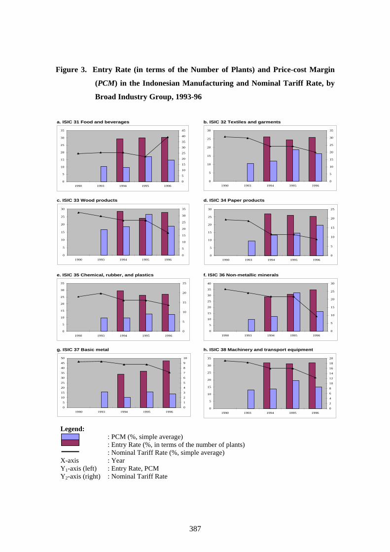
Figure 2 (a) to (h), which show the entry rate (in terms of number of plants) for the

period by broad industry group, and the trend in the nominal tariff rate over the 1990-96

period, provide a more detailed picture of the effect of the reforms on the extent of plant

entry. Here, as the key observation, however, the comparison of the rate of entry and

the tariff rate over the period, and across the groups, , does not seem to show a

consistent picture of the impact, i.e., whether it is positive or negative. Looking at the

comparison for the industry group of ISIC 32, 33, 34, and 35 (i.e., textile-garments,

wood products, paper products, and chemical products, respectively), the policy reforms

are suggested to have increased plant entry, and hence indicate a positive impact. The

declining trend in the tariff rate is accompanied by a pattern of increasing entry for these

industries.

367

Figure 2. Entry Rate (in terms of Number of Plants) in the Indonesian

Manufacturing and Nominal Tariff Rate by Broad Industry Group,

1993-96 a. ISIC 31 Food and beverages b. ISIC 32 Textiles and garments

c. ISIC 33 Wood products d. ISIC 34 Paper products

e. ISIC 35 Chemical, rubber, and plastics f. ISIC 36 Non-metallic minerals

g. ISIC 37 Basic metal h. ISIC 38 Machinery and transport equipment

0

2

4

6

8

10

12

14

16

18

20

1990 1993 1994 1995 1996

0

5

10

15

20

25

30

35

40

45

0

2

4

6

8

10

12

14

16

18

20

1990 1993 1994 1995 1996

0

5

10

15

20

25

30

35

0

5

10

15

20

25

30

1990 1993 1994 1995 1996

0

5

10

15

20

25

30

35

0

5

10

15

20

25

1990 1993 1994 1995 1996

0

5

10

15

20

25

0

2

4

6

8

10

12

14

1990 1993 1994 1995 1996

0

5

10

15

20

25

0

5

10

15

20

25

30

35

1990 1993 1994 1995 1996

0

5

10

15

20

25

30

0

2

4

6

8

10

12

14

16

18

1990 1993 1994 1995 1996

0

1

2

3

4

5

6

7

8

9

10

0

5

10

15

20

25

1990 1993 1994 1995 1996

0

2

4

6

8

10

12

14

16

18

20

Legend: : Entry rate (%, in terms of number of plants) : Nominal tariff rate (%, simple average) X-axis (left) : Entry rate X-axis (right) : Nominal tariff rate Y-axis : Year

368

In contrast, the comparison for the industry group of ISIC 36, 37, and 38 (i.e., non-

metallic minerals, basic metal, and machinery-and-transport equipment, respectively)

suggests that the reforms deterred entry, and hence indicate a negative impact. For

these industries, the declining trend in the tariff rate is matched by either declining or

relatively low entry rate.

All in all, the description above indicates that indeed the reforms create some

impact on the extent of plant entry, and this is recorded in the period covered by this

study. The description, however, clearly shows a varying impact, particularly in terms

of the direction of the impact (i.e., whether it is a positive or negative impact). Another

variable impact is in terms of the magnitude. In other words, there is no robust answer

on how the reforms affected plant entry.

Given the varying impact, few immediate questions can be asked. These include,

for example, did the reform really have some impact on the entry? If indeed the reforms

played some role in shaping plant entry in the period, in which direction were these

reforms really affecting the entry rate? Were they increasing, or decreasing the entry

rate? Equally important is the question of what other factors shaped the dynamics and

variation of entry across industries in the period. This question assumes the importance

of the other factors in determining entry, as suggested by the literature.

In an attempt to find some answer to these questions, this study proceeds with an

econometric exercise that gauges the determinants of entry over the period 1993-96. To

facilitate the search for answers, some variables that can be associated with the policy

reform variables are included in the exercise.

4. Some Theoretical Considerations

To facilitate the rest of the empirical analysis, this subsection briefly reviews the

theoretical framework that explains firm entry.

369

4.1. Prevailing Views about Firm Entry

There are two major approaches to the analysis of the determinants of entry. These

are the limit-price model and the stochastic-replacement process.

4.1.1. Limit Price Model

This approach assumes entry is an equilibrating process which is attracted by, and

serves to bid away, the excess profit. Entry is hypothesised to occur whenever the

expected post-entry profit exceeds the level of profit in the long run. The approach

adopts the concept of a limit-price model (Bain 1949), which posits that there exists a

limit price which is low enough for incumbents to be able to deter entry.

The extent to which the limit price deters entry is determined by two factors,

namely the size of the market and the entrant's average costs curve. The latter gives rise

to a cost advantage for incumbents over new entrants who may have to pay a substantial

fixed entry cost. This implies the average cost curves of entrants and incumbents are

not the same. According to Bain (1956), the cost advantages of incumbents over

entrants are determined mainly by economies of scale, product differentiation and some

absolute cost advantages

.

4.1.2. Stochastic Replacement View

This approach considers entry as a stochastic process which does not necessarily

respond to profit and may occur even if price equals marginal cost (Baldwin and

Gorecki 1987). Baldwin and Gorecki argue two situations in which profit is irrelevant

to the entry process. The first is related to how easily entrants can enter and capture a

market share. This is governed by market demand growth. In a growing market,

additional firms entering the market are unlikely to depress the market price. Hence

incumbents are less threatened by entrants and are therefore less likely to act

aggressively. The second is a situation where entrants simply replace some existing

firms, even when long run profits are zero.

370

4.2. Interdependence between Entry and Exit5

As in the limit price approach, entry takes place when profit is positive.

Accordingly, exit should occur when profit is negative and entry andexit are expected to

be negatively correlated. In contrast, several studies found the correlation to be positive

(e.g. Dunne et al. 1988; Dunne and Roberts 1991; Austin and Rosenbaum 1991; Lay

2003). For example, Dunne and Roberts found that entry and exit are positively

correlated with the price-cost margin for US manufacturing, implying that higher profit

encourages both entry and exit. Lay documented that the correlation coefficient of

instantaneous entry and exit for Taiwan manufacturing was positive and relatively high

(about 0.5).

The literature records several explanations for the positive correlation, often termed

as “interdependence”. Geroski (1995) argues that entry and exit seem to be part of an

evolutionary process in which a large number of new firms displace a large number of

existing firms without much changing the total number of firms in an industry. This

argument is similar to the ‘stochastic-replacement’ view of entry (Baldwin and Gorecki

1987) which posits that entry can still be expected even when industry’s profitability is

zero. Entry in this view simply replaces some existing firms.

Shapiro and Khemani (1987) offer two reasons for the interdependence. First, to

the extent that cost heterogeneity exists, there might be some high-cost incumbents who

can be displaced by low-cost entrants. Second, to the extent that barriers to entry are

also barriers to exit (Caves and Porter 1976; Eaton and Lipsey 1980), potential

displacement is limited and incumbents are deterred from exiting. The symmetrical

relationship between entry and exit barriers arises from investments with sunk cost

characteristics (i.e. investment in durable and specific assets). Sunk cost creates barriers

to entry because it represents a higher opportunity cost that has to be met by entrants,

and higher risk owing to the large losses associated with unsuccessful entry. At the

same time, sunk cost also creates barriers to exit because incumbents are limited by

inability to divest, owing to the non-recoverable nature of the assets (Shapiro and

Khemani 1987, p.16).

5 A useful review of the interdependence is provided by Fotopoulus and Spence (1998).

371

Shapiro and Khemani’s displacement effect implies that entry is responsible for

exit. Fotopoulus and Spence (1998) consider that the process could be the other way

around. That is, exit creates room for new entry. If the two directions hold, entry and

exit are causally related and the interdependence may be due to some ‘displacement-

replacement’ effect.

5. Model Specification and Hypotheses

5.1. Model Specification

This study follows a specification of entry model similar to those in the literature.

An exit model is also specified for the reason that entry and exit might be causally

related, as discussed in the previous section. Ignoring industry and time subscripts, these

are

),,,( 1111 REPLZYXfEN (1)

),,,( 2222 DISPZYXfEX (2)

where EN ( EX ) is entry (exit) rate, 1X ( 2X ) is a vector of incentives for entry (exit),

1Y ( 2Y ) is a vector of entry (exit) barriers, 1Z ( 2Z ) is a vector of other relevant

variables, REPL is replacement entry and DISP is displacement entry. DISP and

REPL are included to represent displacement and replacement behaviour, respectively.

As is commonly done in the literature, REPL and DISP are assumed to be a

function of exit and entry, respectively. Thus, equations (1) and (2) can be expressed as

),,,( 1111 EXZYXfEN (3)

),,,( 2222 ENZYXfEX (4)

Having specified displacement and replacement behaviour, the discussion now turns to

the specification of other vectors. Consider, first, 1X . The specification of 1X is

derived from Orr’s (1974) model, which posits that entry ( E ) is expected to occur

whenever expected post entry profits ( e ) are above the entry-precluding level ( * ).

372

The entry-precluding level refers to profits which would be earned by incumbents in the

long-run after all entry has ceased. Orr’s model is

*)( efE (5)

Adopting the concept of a limit-price model (Bain 1949 and 1956), Orr assumes *

depends on a vector of entry barriers ( ENB ) and market risk ( R ), that is

),(* RENBf (6)

Substituting (6) into (5), Orr’s model becomes

),,( RENBfE e (7)

To incorporate the stochastic replacement view of entry, industry growth (GR ) is added

to equation (7).6 So that it becomes

),,,( RENBGRfE e (8)

This study uses pre-entry profitability to proxy e and price-cost margin to proxy

profitability ( 1tPCM ). Market risk is proxied by the variability in industry

profitability, defined as the standard deviation of PCM ( SDPCM ). Following Shapiro

and Khemani (1987), GR is deflated by the minimum efficient scale ( MES ) to reflect a

situation that there must be sufficient growth to justify additional capacity in an

industry. The deflation is defined as ROOM variable.

The use of pre-entry profitability as a proxy for e has been the usual procedure in

empirical studies. However, the procedure is unlikely to proxy e properly. The

(naïve) entrants neglect the effect their entry may have on profits because profitability

between post- and pre-entry is assumed to be the same (Geroski 1991). Moreover,

employing the naïve expectation may open up the possibility for incumbents to

manipulate pre-entry profit and hence could discourage entry. An alternative approach

is to assume that entrants form rational expectations to make the entry decision. The

6 Baldwin and Gorecki (1987) introduced market size to capture replacement entry. This study does not follow this approach since replacement entry has been assumed to depend on exit.

373

rational expectation assumption leads to the procedure of forecasting profit based on an

autoregressive model of profit. Several studies, e.g. Highfield and Smiley (1987) and

Jeong and Masson (1991), provide evidence that using forecasted profits performed

better than pre-entry profits. Although the alternative approach is more reasonable, it is

not possible in this study because there are not enough time-series observations in the

data base.

Two variables are included to represent barriers to entry: economies of scale ( ES )

and capital requirement ( KR ). Economies of scale acts as an entry barrier if industry

output accounted for by minimum efficient scale ( MES ) constitutes a significant part of

the quantity demanded at a competitive price. Potential entrants could enter on a large

scale but would trigger retaliation by incumbents. Capital requirement is included to

capture the extent of cost disadvantages faced by entrants. According to Bain (1956),

borrowers’ lack of information about potential entrants provides incumbents with an

absolute cost advantage over entrants, which results in difficulties for entrants in raising

investment funds.

Seller concentration is included in 1Y to capture the strategic deterrence actions by

incumbents. These are likely to occur in the post-entry period. Examples of these

actions include predatory pricing, aggressive advertising campaigns and credible threats

to compete hard against new rivals (Evans and Siegfried 1992). However, seller

concentration may also attract entry. It facilitates collusion that in turn provides a

higher survival chance given that entry has occurred. Chamberlin’s (1933) model

predicts that once concentration levels reach a certain point, oligopolies recognise their

interdependence and that together they produce a monopoly output for the market.

The specification of vector 2X in equation (4) follows earlier empirical work on the

determinants of exit (e.g Deutsch 1984; MacDonald 1986; Shapiro and Khemani 1987;

Flynn 1990; Doi 1999) and is similar to that of vector 1X and 1Y in the entry equation.

According to models of firm bankruptcy (e.g. Schary 1991), a firm decision to shut

down depends on a short-term cash flow problem and assessment of long term

prospects. Therefore, profitability ( PCM ) and industry growth (GR ) are included in

X2.

As noted earlier, exit barriers arise from sunk costs. The relationship between sunk

costs and the probability of exit relates to the ‘duration’ view of sunk costs (Rosenbaum

374

and Lamort 1992, p.299). That is, a longer production time is needed to recover

sufficient returns from investment as the resale value of the non-recoverable assets

cannot be added to the stream of income generated by these assets. The implication is

that firms with high sunk-capital costs are forced to stay in an industry longer than firms

with low sunk-capital costs.

Therefore, the ideal proxies for exit barriers are those that can represent the extent

of sunk costs. The strategy commonly applied in empirical studies is to create some

proxies based on characteristic sunk costs, which are durability and specificity in assets.

The only problem here is that it is often difficult to obtain such proxies as a result of the

specificity characteristics. Despite this, Caves and Porter (1976, p.44) argue that each

source of entry barrier identified by Bain can also be erected as a barrier to exit. In this

argument, the durability and specificity of assets can to some extent be captured by

Bain’s entry barriers. For example, it is often argued that incumbents must have some

resources which are at least temporarily specific to allow them to create some cost

advantages over potential entrants. Otherwise, potential entrants could easily duplicate

the resources and enter. Following Caves and Porter, 2Y is specified to be identical to

barriers to entry.

4CR is also included in 2Y . Seller concentration facilitates collusion, which could

increase the probability of survival and hence may discourage exit. Despite this, low

exit rates in highly concentrated industries may also be possible simply because firms

are likely to be the established firms (Flynn 1990).

Vectors 1Z and 2Z are specified to include variables related to trade and

international competition. The first is foreign ownership ( FOR ). The impact of

concentration of foreign ownership on entry is ambiguous. On the one hand, it could

discourage entry, for the reason that foreign firms are usually large, and therefore, they

tend to have economies of scale in their production, which raises some barriers to entry

into the industry. Moreover, a strong chance of survival for foreign firms in the

presence of economic shocks, vis-à-vis domestic firms, implies a greater likelihood that

foreign firms will stay in the industry in the event of an economic shock. This, in turn,

suggests a negative relationship to entry. On the other hand, high concentration of

foreign ownership in an industry could also encourage entry, and this could simply be

375

due to the signalling effect activities “must” be highly profitable in an industry with

such a high foreign ownership concentration.

The second variable is export orientation ( EXP ). The greater profit opportunities

provided by the export market are likely to attract entry and hinder exit. In contrast, a

higher degree of export orientation could also discourage entry and encourage exit,

because it signals a greater intensity of competition in the industry. Nevertheless, the

pressure for higher exit is likely to be weak since established firms must have paid

substantial costs for participating in export markets.

This study includes import penetration ( IMP ) and trade protection (TARIFF ) to

represent the effect of international competition on entry. At the same time, these

variables also represent the variables that are related to, or can be associated with, the

reforms which are the focus of this study. It is often argued that greater trade protection

tends to facilitate non-competitive behaviour, such as collusion, and protects less

efficient firms. Therefore, incumbents in a protected industry could collude and deter

entry. However, entry could also be encouraged because the trade protection which

allows incumbents to behave non-competitively could also be a more important

incentive than the profit incentive.

Meanwhile, the effect of import competition on entry and exit is ambiguous.

Higher import competition could be expected to reduce entry unless it widens the

domestic market. However, it could also encourage exit as more firms increase

competition and reduce the survivability of incumbents.

The other variables considered in the model aim at capturing the industry factor-

intensity ( FI ) effect. It could be predicted that the extent of entry should be higher in

the industries where the country has some comparative advantage . In this study, a set

of dummy variables representing industry factor intensity is considered, and these are

the dummy for labour-intensive industries, resource-based but labour-intensive

industries, resource-based but capital-intensive industries, and footloose capital-

intensive industries.

To sum up, the entry and exit equations can be specified as follows

( , , , , , 4, , , , , , )EN f PCM ROOM SDPCM ES KR CR FOR EXP IMP TARIFF FI EX (9)

( , , , , 4, , , , , , )EX f PCM GR ES KR CR FOR EXP IMP TARIFF FI EN (10)

376

The definition of the variables in these equations is given in the next section.

5.2. Hypotheses

The following paragraphs present the hypotheses to be tested in the econometric

exercise, based on the theoretical discussion of the previous sections.

5.2.1. Trade Protection and Import Competition

This is the key hypotheses to be tested. Based on the brief theoretical discussion in

Section 3.1, the effect of trade protection (TARIFF ) in attracting entry might not have

been clear. It could have increased entry, for the reason that lowered tariff and other

international trade barriers reveal the positive expected profits for potential entrants.

Lowered tariff protection, however, could have also deterred entry. As discussed, the

threat from potential entrants could increase the extent of collusive behaviour, which in

turn could increase the strength of entry barriers. This reasoning also suggests that

higher import competition ( IMP ) could have been negatively related to entry – higher

competition from imports could trigger or increase the extent of collusive behaviour,

hence raising the entry barriers.

5.2.2. Symmetrical Relationship between Entry and Exit

The symmetrical relationship between entry and exit might hold. This is because,

for any potential entrant, the opportunity cost for any new investment is likely to have

been relatively low during the period. As noted, there was a bold banking sector

deregulation that increased the role of financial intermediaries in the sector. In

addition, the period covered by the study was a rapidly growing period in the

Indonesian economy, and, therefore, there should be a favourable profitability for doing

business in this period. Meanwhile, for the established firms, the role of sunk costs as

exit barriers may not have been very important, since many firms were unlikely to find

themselves in depressing situations during this period.

5.2.3. Displacement and Replacement Entry

Displacement entry should not have been more important. This is because

favourable economic conditions tend to shelter the inefficient firms, helping them to

377

survive. This situation therefore reduces the opportunity for low-cost potential entrants

to enter and successfully compete with the incumbents.

5.2.4. Demand Situation

In theory, profitability ( PCM ) and market growth ( ROOM ) are expected to have

been important in attracting entry. Even so, they may not have been vitally important.

In a developing country like Indonesia, a situation that creates the expectation of a

stable profit – instead of the expected profit itself – could have been the determining

factor. It is often argued in the literature that the existence of imperfect markets, low

levels of competition, and trade protection are the major source of this situation. Given

these contrasting arguments, there could have also been the conflicting effect of market

risk ( SDPCM ) in determining entry.

5.2.5. Entry Barriers

According to the limit-price model, economies of scale ( ES ) and capital

requirements ( KR ) should be negatively related to entry.

Meanwhile, the effect of strategic entry deterrence behaviour, proxied by 4CR , is

difficult to predict a priori. Strategic behaviour might have been positively related to

entry (i.e. it encouraged entry), for the reason that retaliatory behaviour is unlikely to

occur when demand is growing, which was the situation for the period covered by this

study.

However, as discussed earlier, there are models that predict that the probability of

collusion is lower in a high demand situation (e.g. Rotemberg and Saloner 1986;

Rotemberg and Woodford 1992). This implies that the effect of industry concentration

can be expected to have been negative.

5.2.6. Foreign Ownership

The effect of foreign ownership ( FOR ) is also difficult to predict a priori. As

noted, the economies of scale effect raised by high concentrations of foreign ownership

suggests a negative relationship, but the signal of a profitable industry that the high

concentration provides could also result in a positive relationship.

378

5.2.7. Export Orientation7

Export orientation ( EXP ) is expected to have strongly attracted entry. The

reasoning is clear, and that is that higher export orientation provides higher expected

profitability. Export orientation, however, could also imply a higher competitive threat

from firms in the global economy, and this could in contrast lower the expected

profitability. The effect of export orientation, therefore, could have also been negative.

5.2.8. Factor Intensity

Given the comparative advantage that Indonesia has, labour-intensive industries are

predicted to encourage more entry than any other industry, particularly the capital-

intensive industries.

6. Methodology

6.1. Statistical Framework

Equations (9) and (10) form the basic equations to be estimated. Before outlining

the estimating equations, it is important to discuss several relevant issues.

First, the literature does not clearly indicate whether EX in the entry equation or

EN in the exit equation should enter as current or lagged variables. Several studies,

e.g. Austin and Rosenbaum (1991), Evans and Siegfried (1992) and Fotopoulus and

Spence (1998), specified EX and EN as their current variables. In other words,

EX and EN are assumed to be endogenous in entry and exit equations, respectively.

Other studies, such as Sluewagen and Dehandschutter (1991) and Lay (2003), specified

EX and EN as their lagged variables, treating them as weakly exogenous variables.8

Because the literature is silent on which approach is more appropriate, this study

experimented with both.

7 The inclusion of foreign ownership and factor intensity as two determinants of entry were motivated and suggested by a participant in the workshop of this research project. 8 In one of their specifications Shapiro and Khemani (1987) include the lagged exit in the entry equation but include the current entry in the exit equation, rendering equations (3) and (4) a recursive system model.

379

Secondly, it might not be reasonable to assume the effect of profitability and growth

in the entry equation is exactly mirrored in the exit equation. Following previous

studies, ROOM is assumed to have one lag structure in the entry equation while PCM

and GR are assumed to have no lags in the exit equation.9 This approach follows

Shapiro and Khemani (1987), who assume that exit responds more quickly to profit and

growth than entry. However, the approach does not mean the exit process is

instantaneous. Shapiro and Khemani were aware that there are lags between the time

when exit is considered and when it actually occurs. The assumption simply tries to

capture the idea that entry is likely to be a better-prepared action than exit.

The third issue relates to the specification of entry and exit barriers. Certain types

of barriers are likely to be omitted from the regression based on equations (9) and (10).

For example, Geroski (1991) noted it is difficult to measure the control of incumbents

over some strategic resources. Further, and as noted, specificity implied by sunk cost

suggests many exit barriers are unlikely to be captured in the structural variables in the

equations. To solve this problem, fixed effects – in the form of industry dummy

variables – are introduced into equations (9) and (10) to capture the unobserved entry

and exit barriers. This introduction is justified because entry and exit barriers tend to be

constant over time, at least in the short and medium term.

This study assumes all structural variables are exogenous. To secure this

assumption, lagged values are used instead of current ones.

Finally, as entry and exit are measured in relative terms (i.e. proportion), the

dependent variables in theory and practice are bounded between zero and one.

Therefore, it is reasonable to assume that the sample is not drawn from a normal

distribution and this may lead to bias and inconsistent least square estimates. To solve

this problem, logistic transformation on the dependent variables was carried out. With

EN and EX (entry and exit rates) as the observed variables, the transformations are

)1/ln(' ENENEN and

)1/ln(' EXEXEX ,

9 Rosenbaum and Lamort (1992) also adopt a similar approach.

380

where 'EN and 'EX are the logistic transformation of EN and EX , respectively.

These transformations allow the dependent variables in the regression to be drawn from

a normal distribution and the estimations by a least squares approach.

While useful, this transformation approach has two limitations (Wooldridge 2002,

p.662). First, it cannot be used when EN and EX take the boundary values of either

zero or one. As is commonly done in other cases, this study manipulated the boundary

values by substituting the value zero with 0.1111 and value one with 0.9999. The data

manipulation is a common approach adopted both in general empirical studies

(Wooldridge, 2002) and studies on firm entry (e.g. Khemani and Shapiro 1986; Mata

1993).

The second limitation is that the parameters are difficult to interpret. According to

Papke and Wooldridge (1996), further assumptions on the distribution of errors are

needed to obtain the expected value of dependent variable conditional on the

explanatory variables and, even with these assumptions, it is still non-trivial to obtain

the expected value. Notwithstanding this limitation, this study proceeds with the

transformation approach, because the focus here is on the change in the effect of the

explanatory variables between two periods of time rather than on the magnitude of the

effect.

The discussion has established two pairs of estimating entry and exit equations,

specified as follows:

Model I:

1,51,41,31,21,1,' tjtjtjtjtjtj KRESSDPCMROOMPCMEN

6 , 1 7 , 1 8 , 1 9 , 14 j t j t j t j tCR EXP IMP TARIFF

10 , 1 ,j t j j tEX (11)

, 1 , 2 , 3 , 1 4 , 1 5 , 1 6 , 1' 4j t j t j t j t j t j t j tEX PCM GR ES KR CR EXP

7 , 1 8 , 1 9 , 1 ,j t j t j t j j tIMP TARIFF EN (12)

Model II:

1,51,41,31,21,1,' tjtjtjtjtjtj KRESSDPCMROOMPCMEN

6 , 1 7 , 1 8 , 1 9 , 14 j t j t j t j tCR EXP IMP TARIFF

10 , ,j t j j tEX (13)

381

, 1 , 2 , 3 , 1 4 , 1 5 , 1 6 , 1' 4j t j t j t j t j t j t j tEX PCM GR ES KR CR EXP

7 , 1 8 , 1 9 , ,j t j t j t j j tIMP TARIFF EN (14)

where, t = 1994, 1995, 1996 j = industry j

'EN = logistic transformation of the entry rate 'EX = logistic transformation of the exit rate EN = the entry rate EX = the exit rate PCM = price-cost margin ROOM = industry room GR = annual industry growth SDPCM = standard deviation of PCM EOS = economies of scale KR = capital requirement 4CR = seller concentration EXP = export intensity IMP = import penetration TARIFF = trade protection

j , j = industry fixed effect of industry j

Model I and II are different in the way right-hand-side EX and EN are specified.

The equations in Model I were first considered as independent, assuming no

interdependence between entry and exit, and estimated by OLS. Next, the equations

were estimated by the SURE method to account for the interdependence. The SURE

method is considered because it is able to take into account the non-zero

contemporaneous correlation in the error terms between the two equations. The

equations in Model II were estimated by the 2SLS method. This is because tjEN , and

tjEX , can be thought to be determined simultaneously.

382

6.2. Measurement of Variables

6.2.1. Dependent Variables (Entry and Exit Rates)

The entry rates have been presented earlier. As for the exit rates, this study adopts

two exit rate measures, in terms of number of plants, employment and value added,

labelled as 1EX , 2EX , and 3EX , respectively.

1EX for industry j between t and 1t is defined as

1,

,,1

tj

tjtj NTP

NXPEX ,

where: tjNXP , = total number of plants that exit industry j between t and 1t

1, tjNTP = total number of plants in industry j in year 1t

EX2 for industry j between t and t-1 is defined as

,,

, 1

_2

_j t

j tj t

EMPL EXEX

EMPL T

,

where: ,_ j tEMPL EX = total employment of plants that exit industry between

t and 1t

, 1_ j tEMPL T = total employment of plants in industry j in 1t

EX3 for industry j between t and t-1 is defined as

1,

,, _

_3

tj

tjtj TVA

EXVAEX ,

where: tjEXVA ,_ = total value added of plants that exit industry j between t and

1t

1,_ tjTVA = total value added of plants in industry j in year 1t

6.2.2. Independent Variables

383

All of the variables are defined for industry j , which is defined at the four digit

level.

Price-cost margin ( PCM )

PCM is defined as the ratio of gross profit to sales, and for industry j, it is defined

as:

j j jj

j

output inputs wagesPCM

output

Gross profit is computed as the value of output minus inputs and wages and salary.

Included in inputs are raw material, fuel and electricity.

Seller concentration ( 4CR ) and Herfindahl Index ( HHI ) to proxy the extent of

competition

CR4 for industry j is defined as

4

1

1

4i

ij n

ii

VACR

VA

While HHI for industry j is defined as

2

ij

i i

VAHHI

VA

where iVA is the value added of plant i in industry j .

Import penetration ( IMP )

IMP for industry j is defined as

jj

j

MIMP

Q

384

where jQ and jM are the domestic production and imports in industry j , respectively.

Industry growth (GR )

GR is measured as the percentage change in real value added of industry j between

t and 1t

, , 1

, 1

j t j t

j t

RVA RVAGR

RVA

where VA is the value added of industry j . The industry value added is deflated by the

wholesale price index (WPI) at the three digit ISIC level.

Industry room ( ROOM )

ROOM is measured as GR divided by .MES MES is defined as the average plant

size accounting for 50 percent of industry output (Caves et al. 1975). Plant size is

measured by total number of workers.

Standard deviation of profitability ( SDPCM )

SDPCM is measured by the standard deviation of PCM , defined at the three digit

level of ISIC.

Economies of scale ( ES )

ES is defined following (Caves et al. 1975) as a compound variable using MES and

cost-disadvantages ratio (CDR), that is

MESCDRES *)1(

CDR is defined as

largest

smallest

)/(

)/(

LVA

LVACDR

385

where smallest)/( LVA is the value added per labour for the smallest plants accounting for

50% of industry output and largest)/( LVA is the value added per labour for the largest

plants accounting for the largest 50% of industry output.

Capital requirement ( KR )

KR is measured following Caves et al. (1980) as

MESQ

KKR *

where QK / is the ratio of capital to labour. In the absence of reliable capital stock

estimates, QK / is proxied by the ratio of energy expenditure to production labour.

This proxy follows the approach taken by Globerman et al. (1994), which was

motivated by some previous studies which show that capital and energy are

complementary inputs in production. Thus,

MESKR *Lprod

eexpenditurenergy

where prodL is the number of production workers.

Export intensity ( EXP )

EXP is measured as the ratio of export to industry output.

output

exportsEXP

Trade protection (TARIFF )

This study uses the average nominal tariff rate to proxy .TARIFF The data for the

tariff rate are derived from WITS database for the period of 1994-96.

386

7. Some Descriptive Analysis and Estimation Results

Before presenting and analysing the estimation results, it is useful to briefly present

some descriptive analysis of the impact of tariff on some of the entry determinants.10

Here, based on the discussion in the theoretical background, we selected some of the

determinant variables for the description, namely price-cost margin (PCM), industry

concentration variables (HHI), and industry export share (EXP).

Consider, first, the impact of the declining tariff rate on price-cost margin, of which

the picture is presented in Figure 3 for the entry rate in terms of number of plants.

While the Figure does not seem to show any obvious pattern, the decline of tariff rate

over the period 1990-96 seems to have increased price-cost margin in the non-metallic

and basic metal industry (i.e., ISIC 36 and 37, respectively) and decreased the price-cost

margin in textile-and-garments, paper products, chemical products, and transport-and-

machinery equipments (i.e., ISIC 32, 34, 35, and 38, respectively).

The decline in price-cost margin, along with the declining trend in the tariff rate,

indicates an increase in the extent of competition from a more open economy. As for

the increase in the price-cost margin, however, it suggests two scenarios. Either there is

still a substantial market opportunity that had not been explored until the industry

experienced the decline in the tariff rate, or some firms in the industries engaged in

some collusive behaviour which could be triggered by more open industries. The

pictures based on entry rate in terms of employment and output, which are not shown

here, also deliver the same message, and in fact show very similar pictures across the

industry groups.

10 The description is provided in the light of a comment made during the workshop of this research project.

387

Figure 3. Entry Rate (in terms of the Number of Plants) and Price-cost Margin

(PCM) in the Indonesian Manufacturing and Nominal Tariff Rate, by

Broad Industry Group, 1993-96

a. ISIC 31 Food and beverages b. ISIC 32 Textiles and garments

c. ISIC 33 Wood products d. ISIC 34 Paper products

e. ISIC 35 Chemical, rubber, and plastics f. ISIC 36 Non-metallic minerals

g. ISIC 37 Basic metal h. ISIC 38 Machinery and transport equipment

0

5

10

15

20

25

30

35

1990 1993 1994 1995 1996

0

5

10

15

20

25

30

35

40

45

0

5

10

15

20

25

30

1990 1993 1994 1995 1996

0

5

10

15

20

25

30

35

0

5

10

15

20

25

30

1990 1993 1994 1995 1996

0

5

10

15

20

25

30

35

0

5

10

15

20

25

30

1990 1993 1994 1995 1996

0

5

10

15

20

25

0

5

10

15

20

25

30

35

1990 1993 1994 1995 1996

0

5

10

15

20

25

0

5

10

15

20

25

30

35

40

1990 1993 1994 1995 1996

0

5

10

15

20

25

30

0

5

10

15

20

25

30

35

40

45

50

1990 1993 1994 1995 1996

0

1

2

3

4

5

6

7

8

9

10

0

5

10

15

20

25

30

35

1990 1993 1994 1995 1996

0

2

4

6

8

10

12

14

16

18

20

Legend: : PCM (%, simple average) : Entry Rate (%, in terms of the number of plants)

: Nominal Tariff Rate (%, simple average) X-axis : Year Y1-axis (left) : Entry Rate, PCM Y2-axis (right) : Nominal Tariff Rate

388

Turning to the impact of the declining tariff rate on the seller concentration, as

noted in Figure 4 for the HHI measure of the concentration and entry rate in terms of

number of plants, again there is a mixed picture and no clear pattern for the impact. The

Herfindahl Indexes for the food-and-beverage, basic metals, and transport-and-

machinery equipment industries (i.e., ISIC 31, 37, and 38) show an increase in the Index

over the period 1994-96. This is in contrast to the decline in the Index for the textile-

and-garments, paper products, non-metallic minerals, and transport-and-machinery

equipment industries. At the experimental stage, some graphs for CR4 were also

derived and show similar results, although they were not as robust as those produced by

the Herfindahl Index.

Figure 4 gives the message that for industries experiencing an increase in seller

concentration over the period – and at the same time looking at the trend in the tariff

rate – there is a possibility that the extent of collusive behaviour, or the motivation for

it, in these industries could have been wiped out by the more open industries, indicated

by the declining trend of the tariff rate. Using the same rationale, it is suggested that the

extent of or motivation for collusive behaviour could have strengthened in some

industries that experienced an increasing trend in seller concentration. The two

contrasting possibilities are consistent with the previous graph on the impact of the

declining tariff rate on price-cost margin. Although they are not shown here, the

inference drawn from the picture of the impact when using entry rate in terms of

employment and output is the same.

389

Figure 4. Entry Rate (in Terms of the Number of Plants) and Herfindahl Index

(HHI) in the Indonesian Manufacturing and Nominal Tariff Rate, by

Broad Industry Group, 1993-96

a. ISIC 31 Food and beverages b. ISIC 32 Textiles and garments

c. ISIC 33 Wood products d. ISIC 34 Paper products

e. ISIC 35 Chemical, rubber, and plastics f. ISIC 36 Non-metallic minerals

g. ISIC 37 Basic metal h. ISIC 38 Machinery and transport equipment

0

2

4

6

8

10

12

14

16

18

20

1990 1993 1994 1995 1996

0

5

10

15

20

25

30

35

40

45

0

2

4

6

8

10

12

14

16

18

20

1990 1993 1994 1995 1996

0

5

10

15

20

25

30

35

0

5

10

15

20

25

30

1990 1993 1994 1995 1996

0

5

10

15

20

25

30

35

0

5

10

15

20

25

1990 1993 1994 1995 1996

0

5

10

15

20

25

0

2

4

6

8

10

12

14

1990 1993 1994 1995 1996

0

5

10

15

20

25

0

5

10

15

20

25

30

35

1990 1993 1994 1995 1996

0

5

10

15

20

25

30

0

5

10

15

20

25

1990 1993 1994 1995 1996

0

1

2

3

4

5

6

7

8

9

10

0

5

10

15

20

25

30

1990 1993 1994 1995 1996

0

2

4

6

8

10

12

14

16

18

20

Legend: : HHI (simple average) : Entry Rate (%, in terms of the number of plants) : Nominal Tariff Rate (%, simple average) X-axis : Year Y1-axis (left) : Entry Rate, HHI Y2-axis (right) : Nominal Tariff Rate

390

Figure 5 provides a picture of the impact of the declining tariff rate on industries’

export share. Unlike the previous two tables, there is a clearer picture of the impact. In

particular, the declining tariff rate is suggested to have increased the export share of

some industries, namely textile-and-garments, wood products, chemical products, non-

metallic mineral products, and transport-and-machinery equipment. The impact is not

so clear in the case of the paper and basic metal industries.

This rather solid finding suggests that trade liberalisation benefited some sectors

substantially. While encouraging, in terms of entry, this does not necessarily mean that

increased exports could immediately result in an increase of the entry rate, although it is

worth noting that the pattern in the entry rate over this short time period seems to follow

the trend in industry export share. In short, here the key point is that the positive impact

of the declining tariff rate on an industry’s export share is not suggested to have fully

‘transferred’ to an equally higher entry rate. Thus, the increase in the export share

should partly come from some firms that have already established themselves in the

industry (i.e., the incumbents).

391

Figure 5. Entry Rate (in Terms of the Number of Plants) and Industry Export

Share (EXP) in the Indonesian Manufacturing and Nominal Tariff Rate,

by Broad Industry Group, 1993-96

a. ISIC 31 Food and beverages b. ISIC 32 Textiles and garments

c. ISIC 33 Wood products d. ISIC 34 Paper products

e. ISIC 35 Chemical, rubber, and plastics f. ISIC 36 Non-metallic minerals

g. ISIC 37 Basic metal h. ISIC 38 Machinery and transport equipment

0

2

4

6

8

10

12

14

16

18

20

1990 1993 1994 1995 1996

0

5

10

15

20

25

30

35

40

45

0

5

10

15

20

25

30

35

40

45

50

1990 1993 1994 1995 1996

0

5

10

15

20

25

30

35

0

5

10

15

20

25

30

35

40

45

50

1990 1993 1994 1995 1996

0

5

10

15

20

25

30

35

0

5

10

15

20

25

1990 1993 1994 1995 1996

0

5

10

15

20

25

0

5

10

15

20

25

1990 1993 1994 1995 1996

0

5

10

15

20

25

0

5

10

15

20

25

30

35

1990 1993 1994 1995 1996

0

5

10

15

20

25

30

0

5

10

15

20

25

30

35

40

45

50

1990 1993 1994 1995 1996

0

1

2

3

4

5

6

7

8

9

10

0

5

10

15

20

25

1990 1993 1994 1995 1996

0

2

4

6

8

10

12

14

16

18

20

Legend: : EXP (%, simple average) : Entry Rate (%, in terms of number of plants) : Nominal Tariff Rate (%, simple average) X-axis : Year Y1-axis (left) : Entry Rate, EXP Y2-axis (right) : Nominal Tariff Rate

392

7.1. The Estimation Results

Equations in Models I and II are estimated using entry and exit rates in terms of

number of plants and employment (EN1, EX1, 2EN , 2EX , EN3, and EX3). Model II

was dropped from the analysis because the estimation results of model II using the

2SLS method rendered almost all the variables in the equations insignificant. Although

this is obviously not a good result, several studies have obtained similar results (e.g.

Shapiro and Khemani 1987; Austin and Rosenbaum 1991; Fotopoulus and Spence

1998).

Several industries were identified as outliers using the Hadi (1992) method. This

study controls the outliers by removing them from the sample. The usual approach of

introducing dummy variables that identifies them was not adopted because it results in a

perfect collinearity with the fixed industry effects (the industry dummy variables).

Table 1 presents the estimation results for Model I using the SURE method, with

'1EN and '1EX as the dependent variable.11 Breusch-Pagan Lagrange Multiplier (LM)

statistics are employed to test whether the error terms of the entry and exit equation in

Model I are contemporaneously correlated. The null hypothesis of equal error terms in

the entry and exit equation is rejected at the 1 per cent significance level.12 Therefore, it

can be concluded that entry and exit in the period were correlated. Accordingly, the

results obtained by the SURE method provide the basis for the analysis (Table 7.4), and

the OLS results are not reported here. The coefficients produced by the SURE method

are similar to those obtained by OLS and have the same signs. However, the t-statistics

improve in some estimated coefficients, which indicates the improvement in efficiency

and justifies the reference to the SURE results.

11 Three alternative specifications of entry were experimented with. The first was as in equations (11) or (13), the second was where ROOM was replaced by GR and the third was where ROOM was retained but ES was dropped. The specifications are motivated by the way ROOM is generated, which raises possible colinearity with ES. As presented, ES is measured as ES=(1-CDR)*MES, where CDR is the cost disadvantage ratio. The experiment shows that the results did not differ greatly from one specification to the other. But because the first specification performed better in terms of F-statistics, it was chosen as the basis for the analysis. 12 The degree of freedom for the LM tests is one.

393

Table 1. The Determinants of Entry and Exit, 1994-96: Regression Results of

Model I

Method: SURE Dependent variable EN1'j,t EX1'j,t

(1) (2)

PCMj,t-1 0.638 (1.13) SDPCMj,t-1 0.002 (0.00) PCMj,t -0.581 (1.21)ROOMj,t-1 -0.139 (0.38) GRj,t 0.055 (0.75)

ESj,t-1a) -0.005 -0.036

(0.18) (1.36)

KRj,t-1a) 0.0185 2.811

(0.09) (1.50)CR4j,t-1 0.251 0.656 (0.94) (2.81)**FORj,t-1 -0.560 -0.283 (1.73)+ (0.96)EXPj,t-1 0.502 0.666 (1.95)+ (2.76)**IMPj,t-1 -0.018 -0.012 (1.88)+ (1.44)TARIFFj,t-1 0.014 0.002 (1.90)+ (0.21)EN1j,t-1 1.058 (2.42)*EX1j,t-1 2.888 (2.66)** DUMMY LABOUR INTENSIVE INDUSTRIES 0.099 0.064 (1.53) (0.77)DUMMY RESOURCE-BASED, LABOUR INTENSIVE INDUSTRIES 0.002 0.163 (0.01) (0.92)DUMMY FOOTLOOSE, CAPITAL INTENSIVE INDUSTRIES 0.061 0.004 (1.86)+ (0.08)YEAR DUMMY 1995 -2.499 0.000 (9.64)** (.)YEAR DUMMY 1996 -2.654 0.336 (10.90)** (3.49)**Constant 0.000 -3.394 (.) (10.28)**Observations 165 165R-squared 0.26 0.30

Note: 1) t-statistics in parentheses 2) Significance level: ** significant at 1%; * significant at 5%; + significant at 10% a) The coefficients were multiplied by 103 to improve presentation.

394

This study employs an analysis based on the fixed-effect panel estimation

approach.13 This approach assures that a large portion of the unobserved variables is

taken into account and hence we are more confident that the results are unbiased,

although it perhaps does not give satisfactory results in terms of statistical significance.

Adopting this approach is particularly important because large variables representing

entry and exit barriers can be unobserved or industry specific (Geroski 1991).

The results presented in Table 1 include all entry-barrier variables in one regression

model. At the experiment stage, there were three other sets of estimations which were

done by including the entry-barrier variables one-by-one. 14 The results of these

experiments did not give substantially different results compared to those presented in

Table 1, and because the F statistics of the estimations in Table 1 are substantially

higher than those drawn from the experimental estimations, the experimental

estimations were not used for the discussion. Partial correlations between the dependent

and all independent variables are presented in Appendix 1.

7.2. The Structural Determinants of Entry

7.2.1. Entry

Of the trade-related variables, 1tTARIFF is positively related to entry and is

statistically significant. Therefore, trade protection seems to have attracted entry in this

period. However, this impact cannot confidently be applied across all industries,

because the estimated coefficient is only marginally statistically significant (i.e., at the

10 per cent level). This marginal importance is emphasised by a rather low correlation

between the dependent variable and 1tTARIFF , which is 0.29 (see Appendix 1).

Meanwhile, the coefficient of 1tIMP shows a negative sign but is only moderately

significant (i.e. significant at the 10 per cent level). Thus, a higher extent of

competition from imports seems to have discouraged entry during the period under the

13 This is different from other studies (e.g. Fotopoulus and Spence 1998) who based their analysis on results without inclusion of fixed industry effects. 14 These experiments respond to the comment made by a participant of the workshop of this research project.

395

study. This result is also consistent with an earlier finding by Anagnostaki and Louri

(1995) that import penetration is negatively related to entry and exit.

None of the entry barrier variables appears to explain entry. The coefficient of all

of these variables is statistically insignificant. Moreover, while not significant, the

coefficients are all positive, which contradicts the theoretical prediction.

While it does not seem statistically to explain entry, it is worth discussing the result

of 14 tCR as an entry barrier variable. Its positive coefficient implies that seller

concentration induced, rather than impeded, entry. A possible explanation is that this

finding supports the argument that concentrated industries provide a higher survival

chance once entry has occurred. This comment is further supported by the coefficient

of 1tKR which also shows a positive correlation, although, again, it is not statistically

significant.

The coefficient of 1tFOR is negative, and statistically significant at the 10 per cent

level. Therefore, a high concentration of foreign ownership in an industry is expected to

reduce the extent of entry. This finding thus provides some support for the argument of

the superiority of foreign firms in terms of economies of scale, which provides some

insulation of these firms from potential entrants, through the ability of the firms to

charge a competitive level of industry price by exercising their economies of scale.

The result of 1tEXP is encouraging in terms of entry. The coefficient of 1tEXP is

positive and statistically significantly, although only at the 10 per cent level. This

finding reflects the descriptive analysis presented earlier on the rather clear positive

impact of the declining tariff rate on industry export share, and to some extent on the

trend of firm entry. Supporting this even further, the partial correlation of this variable

to the dependent variable is small, that is, 0.23 (see Appendix 1).

The results on the dummy variables for industry groups, by their factor intensity, do

not give satisfactory results. The extent of entry in the labour-intensive industry group

does not seem to have been high, compared to that in the resource-based capital-

intensive industry group which acts as the base-dummy variable.

396

7.2.2. The Determinants of the Interdependence between Entry and Exit

This section seeks evidence concerning the validity of the displacement-

replacement effect and the symmetry hypothesis implied by entry and exit determinants.

The results provide some support for the symmetry hypothesis. All entry barrier

variables ( 1tES , 1tKR and 14 tCR ) show the same sign in both the entry and exit

equations. The estimated coefficients are similar across equations, indicating a similar

effect from these variables in inducing or deterring entry and exit.

It is worth noting that the process involved with the symmetry hypothesis is

unlikely to be the same as the one originally hypothesised by Caves and Porter (1976).

Instead of a discouraging effect, entry barriers seem to encourage both entry and exit at

the same time. Two of the entry barriers variables, 14 tCR and 1tKR , show positive

signs in both the entry and exit equations.

It is worth mentioning here the large impact of seller concentration on exit,

indicated by the strong estimate of the 14 tCR estimate. This suggests an existence of

collusive behaviour that warrants some profitable profit margin, based on the theory

postulated by limit price model.

Some support for the symmetry hypothesis is also displayed by the other variables.

1tIMP appears to moderately prevent both entry and exit. As argued by Fotopoulus and

Spence (1997), one reason might be that expansion in markets with high import

penetration is not enough to ensure new plant creation or capacity expansion at the

minimum efficient scale while, at the same time, lack of expansion in the domestic

market tends to sustain collusive behaviour among incumbents. 1tEXP is positively

related to entry and exit. This confirms earlier findings (e.g. Anagnostaki and Louri

1995; Sleuwagen and Dehandschutter 1991) that the extent of the external market

encourages both entry and exit in domestic industries. While it seems to contradict a

stylised fact from the micro exporting literature, which suggests that exit should have

been lower in exporting industries – because firms in these industries tend to be more

efficient than those in other industries –, the positive relationship on exit might occur if

there was a co-existence of efficient and inefficient firms in the exporting industries

(Anagnostaki and Louri, 1995). According to Anagnostaki and Louri, inefficient firms

397

are likely to be displaced by more efficient firms entering the industries, which are most

likely be attracted by the profit opportunity provided by export markets.

Despite these findings, the results do not strongly validate the symmetry hypothesis.

1tEXP is only statistically significant in the exit equation.

The results provide some indications on displacement and replacement entry. Both

11 tEN and 11 tEX in the exit and entry equation respectively, are positive. Moreover,

the displacement effect is suggested to have been strong, indicated by a very high level

of statistical significance of the 11 tEN and 11 tEX coefficient. This inference is also

supported by a strong correlation of these variables to their relevant dependent

variables, as written in Appendix 1 (i.e., 0.35 and 0.36 for 11 tEN and 11 tEX ,

respectively). The estimated coefficient of 11 tEX , which is about 2, suggests a rather

large effect of replacement under a one year adjustment structure.

7.2.3. Estimation Results using the Alternative Entry and Exit Measure

In the preceding analysis, entry and exit rates are measured in terms of the number

of plants. The equations in Model I are now re-estimated using entry and exit rates

measured in terms of employment ( '2EN and '2EX ) and output ( '3EN and '3EX ) to

provide robustness for the earlier findings. The results are presented in Table 2 and 3,

for the entry-exit rate in terms of employment and output, respectively. The equations

are estimated using the SURE method, as the LM tests conclude that the error terms in

the entry and exit equations are correlated. In terms of model fit, the results are

generally satisfactory. In the equations presented, the 2 'R s do not deviate much from

the ones in '1EN and '1EX equations and the F tests are significant at the 1 per cent or

better level.

398

Table 2. The Determinants of Entry and Exit, 1993-96: Regression Results of

Model I with EN2' and EX2' as the Dependent Variable

Method: SURE Dependent variable EN2''j,t EX2''j,t

(1) (2)

PCMj,t-1 -0.473 (0.56) SDPCMj,t-1 -0.571 (1.27) PCMj,t -1.004 (1.19) ROOMj,t-1 0.139 (0.26) GRj,t 0.116 (0.90)

ESj,t-1 a) 0.032 -0.041

(0.73) (0.87)

KRj,t-1 a) -0.624 -0.023

(2.03)* (0.07) CR4j,t-1 -0.216 0.271 (0.54) (0.65) FORj,t-1 -0.278 0.097 (0.57) (0.18) EXPj,t-1 -0.354 0.782 (0.92) (1.83)+ IMPj,t-1 -0.028 -0.025 (2.04)* (1.65)+ TARIFFj,t-1 0.011 0.002 (0.95) (0.12) EN2j,t-1 1.525 (2.00)* EX2j,t-1 5.681 (3.56)** DUMMY LABOUR INTENSIVE INDUSTRIES 0.004 0.150 (0.04) (1.02) DUMMY RESOURCE-BASED, LABOUR INTENSIVE INDUSTRIES 0.103 0.208 (0.57) (0.67) DUMMY FOOTLOOSE, CAPITAL INTENSIVE INDUSTRIES 0.039 0.069 (0.79) (0.88) YEAR DUMMY 1995 -2.787 -4.153 (7.20)** (7.17)** YEAR DUMMY 1996 -2.914 -3.964 (8.01)** (7.12)** Constant 0.000 0.000 (.) (.)

Observations 165 165 R-squared 0.22 0.19 Note: 1) t-statistics in parentheses 2) Significance level: ** significant at 1%; * significant at 5%; + significant at 10% a) The coefficients were multiplied by 103 to improve presentation.

399

Table 3. The Determinants of Entry and Exit, 1993-96: Regression Results of

Model I with EN3' and EX3' as the Dependent Variable

Method: SURE Dependent Variable EN3'j,t EX3'j,t

(1) (2)

PCMj,t-1 -2.926 (2.19)* SDPCMj,t-1 -0.007 (0.01) PCMj,t -2.915 (2.28)* ROOMj,t-1 -1.65 (1.92)+ GRj,t 0.328 (1.38) ESj,t-1

a) -0.034 -0.041 (0.48) (0.57)

KRj,t-1 a) 0.202 0.091

(0.41) (0.18) CR4j,t-1 -1.938 -0.393 (3.04)** (0.63) FORj,t-1 0.339 -0.739 (0.44) (0.93) EXPj,t-1 -0.243 0.946 (0.40) (1.45) IMPj,t-1 -0.036 -0.033 (1.63) (1.44) TARIFFj,t-1 -0.006 0.018 (0.35) (0.83) EN3j,t-1 2.411 (2.09)* EX3j,t-1 4.125 (1.63) DUMMY LABOUR INTENSIVE INDUSTRIES 0.055 0.075 (0.36) (0.34) DUMMY RESOURCE-BASED, LABOUR INTENSIVE INDUSTRIES 0.481 -0.160 (1.66)+ (0.34) DUMMY FOOTLOOSE, CAPITAL INTENSIVE INDUSTRIES 0.124 0.079 (1.60) (0.66) YEAR DUMMY 1995 -1.761 0.000 (2.86)** (.) YEAR DUMMY 1996 -1.960 0.141 (3.39)** (0.55) Constant 0.000 -4.183 (.) (4.78)**

Observations 164 164 R-squared 0.18 0.23 Note: 1) t-statistics in parentheses 2) Significance level: ** significant at 1%; * significant at 5%; + significant at 10% a) The coefficients were multiplied by 103 to improve presentation.

400

In general, some results from the estimations using the alternative entry-exit

measures are different from the previous results, and hence one could claim that the

earlier results are not really robust. However, and as noted earlier, the results using

entry rate in terms of number of plants (i.e., EN1 and EX1) should be given more weight

for the basis of analysis. This is theoretically justified since measures of market

structure, which is one of the key determinants of entry, often stress the significance of

the number of firms (Baldwin 1998, p.12).

Nonetheless, it is useful to mention the key differences between the previous results

and the results presented in Tables 2 and 3.

Consider, first, the results of using the entry-exit rate in terms of employment. The

coefficient of 1tKR is negative and very statistically significant (i.e., at the 1 % level).

This suggests that the initially required capital, which determines other aspects of firm

size at entry, seems to have been material in determining entry in terms of employment.

The other difference is that the coefficient of 1tEXP is very disappointing, as is 1tFOR .

In particular, the coefficient of 1tEXP is negative, which contradicts the earlier finding.

But, more importantly, the coefficient of these two variables is statistically insignificant,

which suggest that foreign ownership and export share does not seem to have attracted

entry at all in terms of employment.

However, there are at least a few similar findings. First, the coefficients of

1tTARIFF and 1tFOR are in accordance with the results of using the entry-exit variable

measured by the number of plants. But these coefficients are statistically insignificant.

Secondly, the same finding is also shown for the displacement and replacement effect.

Moreover, the results based on employment entry-exit suggest that the replacement

effect is very strong and large, since the coefficient of 12 tEX in the entry equation is

very large, as well as highly statistically significant.

Turning to the estimation results based on entry-exit in terms of output, the first

difference is that there seems to have been a strong displacement effect, but very weak

replacement effect, since the latter is not statistically significant. 14 tCR in the entry

equation now has a negative coefficient and is highly statistically significant. This

indicates that much of the entry comprises many small firms in terms of output.

401

Meanwhile, 1tEXP and 1tFOR do not seem to have attracted entry when the entry is

measured in terms of output. The t-statistics are very low, implying very low statistical

confidence for the relationship. A disappointing result also applies to the key variables

of the econometric exercise, which are the 1tTARIFF and 1tIMP . The most

unsatisfactory result is for the coefficient of 1tTARIFF , which is statistically

insignificant.

8. Summary and Discussion

This study examines the impact of major trade and investment reforms that took

place in the 1980s and 1990s on the extent of plant entry in Indonesian manufacturing.

The descriptive picture does not give a clear indication of the impact. Specifically,

while for some industry groups the generally declining pattern of trade protection seems

to have been followed by some increase in the extent of plant entry over the period

covered by this study, which is 1993-96, this does not seem to have been the case for

other industry groups. Industries that produce textile and garments, wood products, and

paper products, for example, are those which recorded some increase in the plant entry

rates, while the industries that produce machinery and transport equipment are those

which evidently experienced lower plant entry rate over the time.

An attempt to further assess the importance of the reforms with an econometric

exercise somewhat helps the study to provide a general hypothesis on the impact of

trade and investment liberalisation. In particular, recalling the estimated coefficient of

TARIFF, there is stronger guidance on the impact of the trade and investment

liberalisation on the extent of firm entry in Indonesian manufacturing. As noted, the

descriptive analysis earlier in this study was not able to clearly define the direction of

the impact (i.e., either positive or negative). The results suggest that the trade and

investment liberalisation occurring between the mid 1980s and the mid 1990s tended to

deter entry. Based on the theory, this further indicates that the industry became more

competitive, in terms of lower motivation to collude, although this comes with a lower

profit margin. This message is consistent with the results that come from the import-

402

penetration ratio which suggests a negative relationship between increased competition

from import, and firm entry.

Why was it that a more liberalised trade and investment regime did not lead to

higher plant entry? As noted, this tends to conflict a conventional belief that the impact

of such a regime would be positive. While clearly more research needs to be done,

there are at least possible explanations for this, which may have been specific only to

the case of Indonesia, at least during the period covered by this study. It could be the

case that there was still a quite high level of trade protection during the period. The

source of this high protection level is likely to have come from NTBs, owing to the fact

that the nominal tariff rate declined substantially during the early 1990s. In fact, as

reviewed, there were still some NTBs that were implemented during the period, despite

the major trade reforms occurring at the same time. Moreover, as also reviewed, there

were also some regulations that preserved a protective industrial policy.

This explanation thus implies that the Indonesian experience does not necessary

conflict with the common prediction of the positive impact of trade and investment

liberalisation; that is, some protectionist policies and measures that still existed at that

time caused the (predicted) positive impact of the liberalisation not to be fully realised.

The explanation is also consistent with the finding from the estimation in regards to

the interdependence between entry and exit. As presented above, displacement entry

does not seem to have been as large as the extent of replacement entry. This implies

that some inefficient plants were still able operate. At the same time, it also suggests

that the decline in tariff protection at that time was perhaps not able to induce the level

of competitive pressure that brings about strong competition between firms. Indeed, the

revealed positive relationship between industry concentration and the entry level

support this argument. This itself suggests that non-competitive behaviour, such as

collusive action, tended to exist.

403

Appendix 1. Correlation Matrix

EN

1'j,t

EX

1'j,t

EN

2''j,

t

EX

2''j,

t

EN

3'j,t

EX

3'j,t

PC

Mj,t

-1

RO

OM

j,t-1

SD

PC

Mj,t

-1

ES j

,t-1

KR

j,t-1

CR

4 j,t-

1

FO

Rj,t

-1

EX

Pj,t

-1

IMP

j,t-1

TA

RIF

F j,t-

1

EX

1 j,t-

1

EN

1 j,t-

1

EX

2 j,t-

1

EN

2 j,t-

1

EX

3 j,t-

1

EN

3 j,t-

1

DU

MM

Y L

AB

OU

RIN

TE

NS

IVE

IN

D.

DU

MM

Y R

ES

OU

RC

E-

BA

SE

D, L

AB

. IN

T. I

ND

.

DU

MM

Y F

OO

TL

OO

SE

,

CA

PIT

AL

IN

T. I

ND

.

EN1'j,t 1.00

EX1'j,t 0.26 1.00

EN2''j,t 0.68 0.18 1.00

EX2''j,t 0.33 0.73 0.40 1.00

EN3'j,t 0.39 0.11 0.75 0.33 1.00

EX3'j,t 0.28 0.55 0.36 0.81 0.36 1.00

PCMj,t-1 0.11 -0.07 -0.03 -0.07 -0.19 -0.22 1.00

ROOMj,t-1 -0.06 0.00 0.01 0.02 -0.15 0.10 -0.03 1.00

SDPCMj,t-1 0.02 0.08 -0.11 -0.02 -0.05 -0.03 0.13 0.10 1.00

ESj,t-1 -0.04 -0.05 -0.04 -0.09 0.01 -0.02 -0.19 -0.04 0.01 1.00

KRj,t-1 0.00 0.10 -0.16 -0.08 -0.03 -0.06 -0.04 -0.09 0.00 0.53 1.00

CR4j,t-1 0.12 0.21 0.02 0.09 -0.22 -0.04 0.19 0.14 -0.05 -0.06 0.15 1.00

FORj,t-1 0.04 0.04 -0.02 0.11 -0.12 -0.04 0.30 0.00 0.00 -0.13 -0.15 0.40 1.00

EXPj,t-1 0.23 0.26 -0.01 0.23 0.03 0.25 -0.13 -0.10 0.07 -0.04 -0.01 -0.14 0.20 1.00

IMPj,t-1 -0.22 -0.10 -0.20 -0.13 -0.10 -0.12 -0.07 0.06 -0.02 0.01 0.06 -0.11 -0.09 -0.10 1.00

TARIFFj,t-1 0.29 0.09 0.11 0.11 -0.01 0.19 0.02 0.01 -0.02 -0.03 -0.02 -0.04 0.10 0.44 -0.19 1.00

EX1j,t-1 0.36 0.27 0.34 0.30 0.09 0.27 0.08 0.08 -0.02 -0.11 0.02 0.32 0.07 0.16 -0.12 0.20 1.00

EN1j,t-1 0.41 0.35 0.22 0.29 0.01 0.22 0.05 0.25 -0.03 -0.06 -0.07 0.13 0.07 0.23 0.05 0.05 0.20 1.00

EX2j,t-1 0.15 0.11 0.25 0.18 0.04 0.19 -0.02 0.22 -0.09 -0.10 -0.05 0.21 0.01 0.06 -0.05 0.16 0.75 0.10 1.00

EN2j,t-1 0.29 0.21 0.39 0.32 0.20 0.29 -0.07 0.43 0.02 0.03 -0.10 0.02 -0.04 0.01 0.02 0.00 0.14 0.67 0.13 1.00

EX3j,t-1 0.03 0.09 0.23 0.18 0.14 0.21 -0.05 0.24 -0.08 -0.07 -0.08 0.12 0.02 0.03 0.05 0.07 0.54 0.19 0.77 0.21 1.00

EN3j,t-1 0.06 0.01 0.17 0.16 0.14 0.19 -0.09 0.43 0.04 -0.02 -0.13 -0.06 -0.05 0.01 -0.02 -0.09 -0.01 0.29 0.07 0.58 0.10 1.00DUMMY LABOUR INTENSIVEIND.

0.12 0.11 -0.03 0.16 -0.06 0.12 -0.01 -0.01 0.04 0.00 -0.10 0.08 0.31 0.24 -0.02 0.17 0.06 0.11 0.07 0.00 0.02 -0.06 1.00

DUMMY RESOURCE-BASED,

LAB. INT. IND.-0.08 0.06 0.03 -0.01 0.13 0.01 -0.12 0.05 -0.07 -0.04 0.07 -0.20 -0.36 -0.08 0.00 -0.02 -0.08 -0.10 -0.07 0.04 -0.12 0.12 -0.34 1.00

DUMMY FOOTLOOSE,

CAPITAL INT. IND.0.08 -0.07 0.11 0.05 0.03 0.06 0.19 0.03 -0.02 0.06 -0.09 0.23 0.15 -0.23 0.02 -0.21 0.10 0.06 0.07 0.03 0.10 0.04 -0.21 -0.28 1.00

404

References

Anagnostaki, V. and H, Louri (1995), ‘Entry and Exit from Greek Manufacturing Industry: a Test of the Symmetry Hypothesis, International Review of Applied Economics, 9(1), p.86-95.

Ariff, M. and H. Hill (1985), Export-Oriented Industrialisation: The ASEAN Experience. Sydney: Allen and Unwin.

Austin, J.S. and D.I. Rosenbaum (1991), ‘The Determinants of Entry and Exit Rates into US Manufacturing Industries, Review of Industrial Organisation, 5(2), pp.119-28.

Bain, J.S. (1949), ‘A Note on Pricing Monopoly and Oligopoly’, American Economic Review, 39(1), pp.448-69.

Bain, J.S. (1956), Barriers to New Competition. Cambridge, MA: Harvard University Press.

Baldwin, J. R. (1998), The Dynamics of Industrial Competition: a North American Perspective. Cambridge: Cambridge University Press.

Baldwin, J.R. and P. Gorecki (1987), ‘Plant Creation versus Plant Acquisition: the Entry Process in Canadian Manufacturing’, International Journal of Industrial Organization, 5(1), pp.27-41.

Caves, R.E., J. Khalilzadeh-Shirazi and M.E. Porter (1975), ‘Scale Economies in Statistical Analysis of Market Power’, Review of Economics and Statistics, 57(2), pp.133-40.

Caves, R.E. and M.E. Porter (1976), ‘Barries to Exit’, in R.T. Masson and P.D. Qualls (eds.), Essays on Industrial Organization in Honorof Joe. S. Bain, Cambridge, MA: Ballinger, pp.36-39.

Caves, Richard E., M.E. Porter and A.M. Spence (1980), Competition in the Open Economy: a Model Applied to Canada. Cambridge, MA: Harvard University Press.

Chamberlin, Edward H. (1933), The Theory of Monopolistic Competition. Cambridge, MA: Harvard University Press.

Davis, S.L., J.C. Haltiwanger and S. Schuh (1996), Job Creation and Destruction. Cambridge, MA: MIT Press.

Deutsch, L. (1984), ‘An Examination of Industry Exit Patterns’, Review of Industrial Organization, 1, pp.60-69.

Doi, N (1999), ‘The Determinants of Firm Exit in Japanese Manufacturing Industries’, Small Business Economics, 13(4), pp.331-37.

Dunne, T., M. and M. Roberts (1991), ‘Variation in Producer Turnover across US Manufacturing’, in P. Geroski and J. Schwalbach (eds.), Entry and Market Contestability: an International Comparison, Oxford: Basil Blackwell, pp.187-203.

405

Dunne, T., M. Roberts and L. Samuelson (1988), ‘Patterns of Firm Entry and Exit in US Manufacturing’, Rand Journal of Economics, 19(4), pp.495-515.

Eaton, B.C and R.G Lipsey (1980), ‘Exit Barriers are Entry Barriers: the Durability of Capital as a Barrier to Entry’, Bell Journal of Economics, 11(2), pp.721-29.

Evans, L.B. and J.J Siegfried (1992), ‘Entry and Exit in United States Manufacturing industries from 1977 to 1982’, in D.B. Audretsch and J.J. Siegfried (eds.), Empirical Studies in Industrial Organization: Essays in Honor of Leonard W. Weiss, The Netherlands: Kluwer Academic Publishers, pp.253-73.

Flynn, J.E. (1990), ‘The Determinants of Exit in an Open Economy’, Small Business Economics, 3(3), pp.225-32.

Fotopoulus, G. and N. Spence (1997), ‘Net Entry of Firms into Greek Manufacturing: The Effect of Business Condition’, Small Business Economics, 9(3), pp.239-53.

Fotopoulus, G. and N. Spence (1998), ‘Entry and Exit from Manufacturing Industries: Symmetry, Turbulence and Simultaneity – Some Empirical Evidence from Greek Manufacturing, 1982-1988’, Applied Economics, 30(2), pp.245-262.

Geroski, P. (1991), ‘Domestic and Foreign Entry in the United Kingdom’, in P. Geroski and J. Schwalbach (eds.), Entry and Market Contestability: An International Comparison, Oxford: Basil Blackwell, pp.63-88.

Geroski, P.A. (1995), ‘What do We Know about Entry?’, International Journal of Industrial Organization, 13(4), pp.421-40.

Globerman, S., C.R John and I. Vertinsky (1994), ‘The Economic Performance of Foreign Affiliates in Canada’, Canadian Journal of Economics, 27(1), pp.143-156.

Hadi, Ali S. (1992), ‘A New measure of Overall Potential Influence in Linear Regression’, Computational Statistics & Data Analysis, 14(1), p.1-27.

Highfield, R. and R. Smiley (1987), ‘New Business Starts and Economic Activity: an Empirical Investigation’, International Journal of Industrial Organization, 5(1), pp.51-56.

Hill, H. (1996), Southeast Asia’s Emerging Giant: Indonesian Economic Policy and Development since 1966. Cambridge: Cambridge University Press.

Jeong K.Y. and R.T. Masson (1991), ‘Entry during Explosive Growth: Korea during Take-off’, in P. Geroski and J. Schwalbach (eds.), Entry and Market Contestability: An International Comparison. Oxford: Basil Blackwell, pp.143-67.

Khemani, R.S. and D.M. Shapiro (1986), ’The Determinants of New Plant Entry in Canada’, Applied Economics, 18, pp.1243-57.

Lay, T. (2003), ‘The Determinants of and Interaction between Entry and Exit in Taiwan’s Manufacturing’, Small Business Economics, 20(4), pp.319-34.

MacDonald, J. (1986), ‘Entry and Exit on the Competitive Fringe’, Southern Economic Journal, 52(3), pp.640-52.

406

Mata, J. (1993), ‘Entry and Type of Entrant: Evidence from Portugal’, International Journal of Industrial Organization, 11(1), pp. 101-22.

Orr, D. (1974), ‘The Determinants of Entry: A study of the Canadian manufacturing Industries’, Review of Economics and Statistics, 56(1), pp.58-66.

Pangestu, M. (1996), Economic Reform, Deregulation, and Privatization: the Indonesian Experience. Jakarta: CSIS.

Papke, Leslie E. and Jeffrey M. Wooldridge (1996), ‘Econometric Methods for Fractional Response Variables with an Application to 401 (K) Plan Participation Rates’, Journal of Applied Econometrics, 6(11), pp.619-32.

Rosenbaum, D.I. and F. Lamort (1992), ‘Entry, Barriers, Exit, and Sunk Cost: an Analysis’, Applied Economics, 24, pp.297-304.

Rotemberg, J.J. and G. Saloner (1986), ‘A Supergame-theoritic Model of Price Wars during Booms’, American Economic Review, 76(3), pp.390-407.

Rotemberg, J.J. and Woodford, M. (1992) ‘Oligopolistic Pricing and the Effects of Aggregate Demand on Economic Activity’, Journal of Political Economy, 100(6), p.1153-207.

Schary, M.A. (1991), ‘Probability of Exit’, RAND Journal of Economics, 22(3), pp. 339-53.

Shapiro, D. and R.S. Khemani (1987), ’The Determinants of Entry and Exit Reconsidered’, International Journal of Industrial Organization, 5(1), pp.15-26.

Sleuwagen, L. and W. Dehandschutter (1991), ‘Entry and Exit in Belgian Manufacturing’, in P. Geroski and J. Schwalbach (eds.), Entry and Market Contestability: An International Comparison, Oxford: Basil Blackwell, pp. 111-20.

Thee, K.W. (1994), Industrialisasi di Indonesia: Beberapa Kajian. Jakarta: LP3ES.

Wooldridge, Jeffrey M. (2002), Econometric Analysis of Cross Section and Panel Data. Cambridge, MA: MIT Press.

World Trade Organization (WTO) (1998), Trade Policy Review: Indonesia 1998. Geneva: World Trade Organization.