Changes in atmospheric CO 2 concentrations and climate from the Late Eocene to Early Miocene:...

www.elsevier.com/locate/palaeo

Palaeogeography, Palaeoclimatology, Palaeoecology 205 (2004) 43–67

Changes in atmospheric CO2 concentrations and climate from the

Late Eocene to Early Miocene: palaeobotanical reconstruction

based on fossil floras from Saxony, Germany

A. Roth-Nebelsicka,*, T. Utescherb,1, V. Mosbruggerc,2,L. Diester-Haassd,3, H. Walthere,4

a Institute for Geosciences, University of Tubingen, Germanyb Institute for Geology, University of Bonn, Germany

c Institute for Geosciences, University of Tubingen, GermanydZentrum fur Umweltforschung, Saarland University, Germany

eStaatliches Museum fur Mineralogie und Geologie, Landesmuseum des Freistaates Sachsen, Germany

Received 15 January 2003; received in revised form 27 October 2003; accepted 28 November 2003

Abstract

In the present study, proxy data concerning changes in atmospheric CO2 and climatic conditions from the Late Eocene to the

Early Miocene were acquired by applying palaeobotanical methods. Fossil floras from 10 well-documented locations in Saxony,

Germany, were investigated with respect to (1) stomatal density/index of fossil leaves from three different taxa

(Eotrigonobalanus furcinervis, Laurophyllum pseudoprinceps and Laurophyllum acutimontanum), (2) the coexistence

approach (CA) based on nearest living relatives (NLR) and (3) leaf margin analysis (LMA). Whereas the results of approach

(1) indicate changes in atmospheric CO2 concentration, approaches (2) and (3) provide climate data. The results of the analysis

of stomatal parameters indicate that the atmospheric CO2 concentration was higher during the Late Eocene than during the Early

Oligocene and increased towards the Late Oligocene. A lower atmospheric pCO2 level after the Late Eocene is also suggested

by an increase in marine palaeoproductivity at this time. From the Late Oligocene onwards, no changes in atmospheric CO2

concentration can be detected with the present data. For the considered sites, the results of the coexistence approach and of the

leaf margin analysis document a significant cooling event from the Late Eocene to the Early Oligocene. The pCO2 decrease

from the Late Eocene to the Early Oligocene indicated by the stomatal data raised in this study was thus coupled to a

temperature decrease which is reflected by the present datasets. From the Early Oligocene onwards, however, no further

fundamental climate change can be inferred for the considered locations. The pCO2 increase from the Early Oligocene to the

Late Oligocene, which is indicated by the present data, is thus not accompanied by a climate change at the considered sites. A

warming event during the Late Oligocene is, however, recorded by marine climate archives. According to the present data, no

0031-0182/$ - see front matter D 2004 Elsevier B.V. All rights reserved.

doi:10.1016/j.palaeo.2003.11.014

* Corresponding author. Institut und Museum fur Geologie und Palaontologie, Universitat Tubingen, Sigwartstrasse 10, Tubingen D-72076,

Germany. Tel.: +49-7071-2973561; fax: +49-7071-295217.

E-mail addresses: [email protected] (A. Roth-Nebelsick), [email protected] (T. Utescher),

[email protected] (V. Mosbrugger), [email protected] (L. Diester-Haass), [email protected] (H. Walther).1 Tel.: +49-228-739773; fax: +49-228-739037.2 Tel.: +49-7071-2972489; fax: +49-7071-295727.3 Tel.: +49-681-30264145; fax: +49-6841-171774.4 Tel.: +49-351-8926403.

A. Roth-Nebelsick et al. / Palaeogeography, Palaeoclimatology, Palaeoecology 205 (2004) 43–6744

change in pCO2 occurred during the cooling event at the Oligocene/Miocene boundary, which is also indicated by marine data.

The quality and validity of stomatal parameters as sensors for atmospheric CO2 concentration are discussed.

D 2004 Elsevier B.V. All rights reserved.

Keywords: Palaeoclimatology; Carbon dioxide; Stomatal density/index; Leaves; Palaeogene; Neogene

1. Introduction mination of isotope ratios of marine carbonates (Popp

It has long been stated that CO2 plays a key role in

the Earth’s climate changes because it represents a

greenhouse gas leading to back radiation of infrared

radiation (Arrhenius, 1896; Chamberlin, 1898). Inter-

vals of high temperature are thus expected to represent

intervals of high atmospheric CO2 concentration or

CO2 partial pressure ( pCO2) (Crowley and Berner,

2001). The relationship between pCO2 and global

temperature is of high general interest particularly

due to the recent anthropogenically induced rise of

atmospheric CO2 as monitored by direct atmospheric

measurements such as at Mauna Loa since 1958 or ice

core data (Neftel et al., 1985; Keeling, 1993). These

data sources provide a direct access to atmospheric

CO2 content during time. The recent limit for direct

determination of past atmospheric CO2 concentration

is approximately 420,000 years with data supplied by

the Vostoc ice core (Petit et al., 1999). There is thus no

direct means to determine atmospheric CO2 concen-

tration for time periods older than approximately

400,000 years.

There is general agreement about a global green-

house condition across the Palaeocene/Eocene bound-

ary with a climatic optimum during the Early Eocene

(for example, Miller et al., 1987; Zachos et al., 1994).

The global temperature then decreased continuously

during the Eocene towards a glaciation event at the

early Early Oligocene (Prothero and Berggren, 1992).

Periods of warming and cooling then followed until a

local climatic optimum was reached in the Middle

Miocene (Zachos et al., 2001). Because these geolog-

ical time periods date further back than 400,000 years

before present (BP), pCO2 during these time intervals

has to be reconstructed by indirect evidence. This can

be achieved by (1) modelling of the global CO2

budget (Berner and Kothavala, 2001; Wallmann,

2001) or (2) by using palaeoatmospheric pCO2 prox-

ies. Biogeochemical proxy data comprise the deter-

et al., 1989; Freeman and Hayes, 1992) or soil

carbonates (Cerling, 1991, 1999; Mora et al., 1996)

and boron isotope ratios of shells (Pearson and Palm-

er, 1999, 2000). These different methods are summa-

rized and discussed in, for example, Royer et al.

(2001) and Boucot and Gray (2001). A palaeobotan-

ical approach for determining past CO2 concentration,

which is utilized in this study, is based on the fact that,

in many plant species, the density of the stomata

(pores on the plant surface, usually on the leaves if

present) per surface area decreases with increasing

pCO2 (Woodward, 1987; Beerling et al., 1993; van

der Burgh et al., 1993; Kurschner, 1996). The general

trend of increasing stomatal density with decreasing

pCO2 appears to be a stable phenomenon, especially

on the long-term scale (however, not all species are

sensitive to pCO2 with respect to stomatal parameters;

Royer, 2001). An increase or decrease of stomatal

parameters is therefore expected to indicate a decrease

or increase in pCO2.

Based on these proxy data, several authors have

suggested that the pCO2 during the greenhouse period

in the Eocene was higher than today (e.g., Berner,

1991; Arthur et al., 1991; Freeman and Hayes, 1992;

McElwain, 1998; Kurschner et al., 2001). Recent

results based on different methods mentioned above

indicate, however, that, at least during parts of the

Early, Middle and Late Eocene, pCO2 was similar to

recent values (boron isotope ratios of ancient plank-

tonic foraminifera—Pearson and Palmer, 1999, 2000;

stomatal parameters—Royer et al., 2001). By using

boron isotope ratios of ancient planktonic foraminif-

era, Pearson and Palmer (2000) recorded a pCO2 peak

during the early Mid-Eocene cooling event. Addition-

ally, their data do not reflect a long-term drop of pCO2

during the Middle Miocene when global temperature

decreased (Pearson and Palmer, 2000). Pagani et al.

(1999) used carbon isotope analysis for CO2 recon-

struction during the Late Oligocene and the Miocene.

Fig. 1. Lower picture: a map showing the position of the different

sites (marked by E). Shaded area marked by WB: Weisselster

basin. Shaded area marked by LB: Lausitz basin. Upper picture:

typical remains of E. furcinervis (A), location of Knau, L.

pseudoprinceps (B), location of Witznitz, and L. acutimontanum

(C), location of Witznitz (after Kriegel, 2001).

A. Roth-Nebelsick et al. / Palaeogeography, Palaeoclimatology, Palaeoecology 205 (2004) 43–67 45

They found no evidence for a high atmospheric CO2

concentration during the climatic optimum of the late

Early Miocene. The results of Pagani et al. (1999,

2000) and of Royer et al. (2001) concerning the

Miocene confirm each other by using different proxy

data. Furthermore, the results of Pagani et al. (1999)

suggest an increase in pCO2 following the strong

expansion of the East Antarctic ice shield. Results

of Ekart et al. (1999) based on isotope data from

palaeosols indicate that pCO2 was not constant

throughout the Palaeogene/Neogene with higher lev-

els during the Eocene and Oligocene. The biogeo-

chemical model GEOCARB (Berner and Kothavala,

2001) indicates a general decline in CO2 and a pCO2

level slightly higher than today during the Palaeogene

and Neogene. It shows, however, both a considerable

error range as well as a low temporal resolution.

The recent studies concerning climate change

and pCO2 during the Palaeogene/Neogene based

on proxy data summarized so far thus cast doubt

on an inevitable ‘‘cause-and-effect’’ coupling be-

tween global temperature and pCO2 and suggest an

at least partial decoupling between the two. The

discrepancies between the results based on isotopic

studies and those based on stomatal proxy data, as

well as discrepancies between different stomatal

data themselves, may also be due to the following

methodological reasons: (1) low stratigraphic reso-

lution (essential for events of short duration such

as the Initial Eocene Thermal Maximum); (2)

possible uncertainties and broad error ranges of

isotopic data; (3) sampling size, variance and

therefore statistical background noise for stomatal

data (Beerling and Royer, 2002a). A special prob-

lem of stomatal parameters exists with high pCO2.

The response of stomatal density and index

becomes nonlinear with pCO2 levels higher than

present, and many species react insensitively in this

case (Woodward and Bazzaz, 1988; Royer et al.,

2001; Beerling and Royer, 2002b). It has been

argued that genetic adaptation is probably the

reason for the so-called ‘‘CO2 ceiling’’, which is

observed in short-time experiments (Kurschner et

al., 1997). Low pCO2 levels prevailed during the

Neogene, and it can therefore be assumed that the

extant flora is genetically adapted to this condition

(Kurschner et al., 1998; Beerling and Royer,

2002b).

Many sets of different proxy data dealing with

climate and pCO2 during the Palaeogene/Neogene

show temporal gaps and/or provide only data for

temperature or pCO2 (e.g., Pearson and Palmer,


1999, 2000; Retallack, 2001; Royer et al., 2001;

Zachos et al., 2001; Beerling and Royer, 2002a).

Moreover, the single types of proxy data are prone

to several sources of uncertainty (see above; Boucot

and Gray, 2001). More data about climate and

pCO2 during the Palaeogene/Neogene are thus de-

sirable. In this contribution, a combined palaeobo-

tanical approach is applied which (1) allows for

simultaneous reconstruction of terrestrial climate

data and changes in pCO2, (2) provides data from

the Late Eocene, Early and Late Oligocene, the

Oligocene/Miocene boundary and the Early Mio-

cene and (3) uses plant remains of taxa which

existed in geographically adjacent regions through

these time slices. It comprises (1) stomatal density

and stomatal index for atmospheric CO2 concentra-

tion, (2) the coexistence approach [CA; derived

from the nearest living relative (NLR) method] for

various climatic data and (3) leaf margin analysis

(LMA) for temperature. The intentions of this study

are to (1) provide a more or less continuous record

of changes in pCO2 during an interval of the

Palaeogene/Neogene and (2) reconstruct the climate

parameters of the considered location during this

time interval. Three fossil dicotyledonous species

commonly found in fossil beds of Saxony, Germany

were utilized: Laurophyllum acutimontanum (Laur-

Table 1

List of leaf materials available for this study

Species

E. furcinervis

Location—age n.l. n.c.

Haselbach—Late Eocene 4 31

Profen—Late Eocene 7 71

Knau—Late Eocene 4 52

Beucha—early Early Oligocene – –

Haselbach—late Early Oligocene – –

Regis III—Early Oligocene – –

Borna—Late Oligocene – –

Kleinsaubernitz—Late Oligocene 8 96

Espenhain—Late Oligocene – –

Bitterfeld—Late Oligocene – –

Witznitz—Oligocene/Miocene boundary 7 55

Espenhain—Early Miocene 1 16

Grobern—Early Miocene – –

S 31 321

n.l.: number of leaves. n.c.: total number of counts.

aceae), Laurophyllum pseudoprinceps (Lauraceae)

and Eotrigonobalanus furcinervis (Fagaceae).

2. Material and methods

2.1. The fossil material

Fossil material from 10 localities in Saxony, Ger-

many was used. The various locations provide rich

and well-documented fossil floras spanning a time

interval from the Late Eocene to the Early Miocene:

Haselbach, Profen, Knau, Grobern, Bitterfeld, Klein-

saubernitz, Witznitz, Beucha, Borna, Regis III and

Espenhain (see Fig. 1 and Table 1). All cuticle

preparations and the material for coexistence approach

and leaf margin analysis originate from systematically

well-determined and excellently preserved material

from these 10 fossil-rich localities. In most cases,

the sites represent brown coal formations of the

Weisselster basin which were exploited by open-cast

mining, with the exception of Kleinsaubernitz, which

is of volcanic origin. This locality represents a sedi-

ment-filled maar and preserved a parauthochtonous

floral complex. The Late Palaeogene/Neogene sedi-

ments of the Weisselster basin represent marine influ-

enced fluviatile–lacustrine sediments of a complex

L. pseudoprinceps L. acutimontanum

n.l. n.c. n.l. n.c.

– – – –

– – – –

– – – –

– – 6 28

2 17 3 24

1 8 – –

– – 8 52

1 20 4 30

4 54 1 10

– – 11 66

31 134 5 21

– – – –

– – 21 142

39 233 59 373


river system composed of various amounts of

swamps, riparian forests, laurel peat forests and

aquatic sites. The fossil floras of the Weisselster basin

clearly document the vegetation change during the

Palaeogen/Neogene. The Middle and Upper Eocene

flora represents a palaeotropical laurophyllous ‘‘Mas-

tixioid Flora’’ (Mai and Walther, 2000). A change to

Arcto-Tertiary elements occurred at the Eocene/Oli-

gocene boundary with the formation of Mixed Meso-

phytic forests (Mai and Walther, 2000). The fossil

floras and the locations are described in detail in a

series of publications by Mai and Walther (1978,

1985, 1991, 2000) and Walther (1999).

The three species that were selected for this

study follow two criteria: (1) excellent preservation

allowing for cuticle preparation and determination

of stomatal density/index; and (2) wide stratigraphic

range. The selected species are: L. acutimontanum

MAI (Lauraceae; 373 cuticle preparations), L. pseu-

doprinceps WEYLAND and KILPPER (Lauraceae;

233 cuticle preparations) and E. furcinervis (ROSS-

MAESSLER) WALTHER and KVACEK (Fagaceae;

321 cuticle preparations; see Fig. 1). The latter

species represents a geographically widely distribut-

ed species (Mediterranean area, central Europe to

Russia), occurring from the Middle Eocene to the

Oligocene/Miocene boundary (Mai and Walther,

1978, 1985, 1991, 2000; Walther, 1999). It was

therefore an important element of the palaeoflora of

these locations with broad ecological amplitude. The

utilized material (numbers of leaves and fragment

counts) is summarized in Table 1. In the case of the

material from the Early Oligocene, it is possible to

resolve the age into early Early and late Early

Oligocene. This differentiation was, however, only

useful for the climate reconstruction [coexistence

approach (CA), see Section 2.3; and leaf margin

analysis (LMA), see Section 2.4]. For the stomatal

density and index analysis, the data were pooled

into an ‘‘Early Oligocene’’ group. The cuticles were

prepared and are stored at the Museum for Miner-

alogy and Geology, Dresden, Germany.

2.2. Stomatal density and stomatal index as pCO2

sensors

Stomatal data can show considerable scattering

between individual plants, between leaves and even

over a single leaf (Poole et al., 1996 and citations

therein). This is due to numerous environmental

parameters, especially humidity and light intensity,

which influence stomatal density (Stahl, 1883; Max-

imov, 1929). In the case of, for example, Quercus

petraea, it has been shown by greenhouse experi-

ments that humidity and temperature significantly

influence stomatal density (Kurschner, 1996; Kursch-

ner et al., 1998). It is thus necessary to account for

these variances if stomatal data are to be measured.

Furthermore, the ratio between epidermal cells and

stomata, expressed as the stomatal index, is less

influenced by these parameters (Salisbury, 1927) and

is thus expected to supply a clearer CO2 signal (Poole

and Kurschner, 1999). Stomatal density and index

were determined after Poole and Kurschner (1999).

An exact replication of the procedure described by

Poole and Kurschner (1999) was, however, not pos-

sible due to the nature of the fossil material. The fossil

leaves were often fragmented, and stomata counting in

fields of a standard grid, which divides the leaf area

into squares, could not be accomplished. Furthermore,

it was often not possible to reconstruct the exact

location of a fragment within the original leaf. Mar-

ginal regions, which tend to show a different stomatal

density than more central regions, could also not be

excluded (Poole and Kurschner, 1999). The area of a

single count amounted at least to 0.03 mm2 and, in

most cases, to about 0.09 mm2. Usually, a cuticle

preparation of a leaf fragment was sufficiently large to

allow for at least 3–4 counts.

The determination of stomatal density and sto-

matal index was completed by transferring the

microscopic image into a digital image. The im-

age-processing package (OPTIMAS, BioScan) was

used for supporting the identification and counting

of stomata and epidermis cells (for stomatal index).

Identification of stomata and epidermis cells was

performed by visual inspection of the computer-

enhanced picture. The stomata and epidermis cells

were marked in the image after counting. Finally,

the considered area was measured by the program,

and the image was stored as a file in a database.

The number of leaves and counts are summarized in

Table 1. Stomatal density was determined for all

three species, and stomatal index was determined

only for L. acutimontanum and L. pseudoprinceps

because it is usually not possible to recognize


epidermal cells of the lower epidermis of E. furci-

nervis leaves. Statistical analyses were carried out

by using SPSS for Windows, Release 10.0.7.

The stomatal data are used to recognize a qualita-

tive change in pCO2. No attempt was made to

reconstruct pCO2 quantitatively, i.e., the calculation

of pCO2 with transfer functions, due to the following

considerations. The reconstruction of palaeoatmo-

spheric CO2 concentration requires the calibration of

the stomatal density or index of a plant species against

pCO2. This is usually achieved by conducting green-

house experiments with extant plants or by calibration

of herbarium material with actual atmospheric CO2

measurements or ice core data (e.g., Kurschner, 1996;

Rundgren and Beerling, 1999; Wagner et al., 1999;

McElwain et al., 2002). In every case, extant plants

are used for producing calibration curves. The quan-

titative reaction of stomatal density to pCO2 is ex-

tremely species-specific, and efforts are thus made to

use ‘‘living fossils’’ or to identify fossil leaves which

probably represent a still extant species (Kurschner et

al., 1996; Royer et al., 2001; Beerling and Royer,

2002b). Because all three taxa in the present study are

fossil taxa with no certain extant representative, a

calibration is not possible. E. furcinervis, for example,

belongs to the Fagaceae and is ‘‘in between’’ the

Castanoideae and the Quercoideae (Kvacek and

Walther, 1989). An extant species that is phylogenet-

ically so close to E. furcinervis that it can be consid-

ered as conspecific can therefore not be identified.

An alternative approach is the identification of a

nearest living equivalent (NLE) (McElwain and Chal-

oner, 1995; McElwain, 1998). The central idea is that

an ecologically equivalent species of the fossil taxon

is identified which is expected to react to pCO2 in the

same way as the fossil species with respect to stomatal

parameters. This approach is currently under debate

(Boucot and Gray, 2001). However, we attempted to

perform this method for the present dataset (see

Section 4).

2.3. The coexistence approach

The coexistence approach (CA) is described in

detail in Mosbrugger and Utescher (1997) and Mos-

brugger (1999). Only a brief explanation will thus be

provided. The distribution of plant species is—besides

other factors—dependent on various climatic param-

eters such as mean annual temperature (MAT) or

precipitation. The fossil flora of a location thus

provides evidence about the climatic conditions under

which the different plant taxa coexisted, provided that

the climatic demands of the fossil taxa are known.

This is achieved using the concept of ‘‘nearest living

relatives’’ (NLR), which presupposes that the fossil

taxon and its extant counterpart have very similar

environmental demands (Hickey, 1977; Kershaw and

Nix, 1988; Wing and Greenwood, 1993; Greenwood

and Wing, 1995; Greenwood et al., 2003b). This key

assumption dates back as far as the 19th century, and

has since been extensively used (Heer, 1855–1859;

Schwarzbach, 1968; van der Burgh, 1973).

The CA follows the nearest living relative concept.

It is based on parameter ranges that are typical for the

considered taxa, which are identified as representa-

tives of the fossil taxa. This is accomplished by listing

the climatic conditions of the areas in which these

extant representatives exist today. By using this data-

base of extant taxa and their climatic requirements, a

‘‘coexistence interval’’ of different climatic parame-

ters can be calculated which allowed the majority of

considered plant taxa to exist at that location. Numer-

ous taxa have to be included and overlapping of the

‘‘taxa ranges’’ defines the coexistence interval which

represents the range of the palaeoclimate. The interval

size of the different parameters decreases in general

with the increasing numbers of species. The CA was

tested extensively with respect to reliability and res-

olution, and its advantages and disadvantages are

discussed thoroughly in Mosbrugger and Utescher

(1997). For example, it can be demonstrated that

evolutionary shifts of the climate ranges of taxa can

be detected by statistical methods and by the occur-

rence of ‘‘outliers’’ which do not fit into the coexis-

tence interval (Mosbrugger and Utescher, 1997).

The core of the coexistence approach (CA) is

represented by the database CLIMBOT which con-

tains the climatic requirements of numerous plant taxa

from the Palaeogen/Neogene based on the climatic

requirements of their nearest living relatives. The first

step requires that the taxa of a given fossil flora

represented by fruits, seeds or leaves have to be

determined to the genus or species level. The database

CLIMBOT is then accessed by an analysis algorithm,

which calculates the intervals of coexistence for the

climate parameters of the nearest living relatives (see

A. Roth-Nebelsick et al. / Palaeogeography, Palaeoc

Fig. 2). The coexistence intervals of the single param-

eters are expressed as ‘‘left’’ (lower) and ‘‘right’’

(upper) boundaries. For example, the coexistence

interval concerning the mean annual temperature

(MAT) is expressed as lowest possible MAT (MAT_L)

and highest possible MAT (MAT_R). Both values

represent the lower and upper temperature limits in

which the considered taxa are able to coexist. In the

present study, the CA is applied to the fossil taxa of

the different locations shown in Fig. 1. Taxa numbers

are summarized in Section 3.2 together with the

results. The taxa lists are documented in Mai and

Walther (1978, 1985, 1991, 2000) and Walther

(1999).

Fig. 2. Flowchart of the coexistence approach (CA). The core of the

program is represented by the database CLIMBOT which contains

the climatic requirements of the nearest living relatives.

2.4. Leaf margin analysis

Leaf margin analysis (LMA) represents a second

proxy approach used for reconstructing palaeotemper-

ature. It is well known that the character of the leaf

margins of the different taxa composing a local flora

correlates with the mean annual temperature (MAT) of

that region (Bailey and Sinnott, 1915, 1916; Wolfe,

1979). This phenomenon is utilized in the LMA and

represents a widespread tool in determining palae-

otemperatures (Wolfe, 1979, 1993; Wilf, 1997; Wie-

mann et al., 1998). The leaf margin is scored as

‘‘entire’’ or ‘‘toothed’’. The percent proportion of

entire-margined species is used in linear equations

which return the MAT. The equations are the results of

leaf margin analyses carried out on extant floras in

which the varying proportions of entire-margined

leaves is mathematically related to local climates.

LMA therefore requires the calibration with extant

vegetation. In the present paper, three formulas are

used which were found for different geographic

regions (summarized by Wiemann et al., 1998):

Wolfe (1979) for forests in Eastern Asia:

MAT ¼ 1:14þ 0:306�%entire ð1Þ

Greenwood (1992) for species of Australian wet

forest sites (provided by Wiemann et al., 1998, who

converted the original plot into the following linear

equation):


Wilf (1997) for temperate and tropical America:


This approach represents thus a simple binomial

score (Wilf, 1997). The LMA approach was expanded

by including numerous other leaf characteristics, such

as form of the leaf base or presence/absence of drip

tips, in order to form a multiple character approach

which is termed as CLAMP (Wolfe, 1993). In the

present study, the simple LMA, considering only leaf

margin type, was applied because it was demonstrated

that multiple character models may not necessarily be

superior to the LMA (Wilf, 1997; Wiemann et al.,

1998). The LMA is carried out with the leaf floras

which are documented for the various locations (see

limatology, Palaeoecology 205 (2004) 43–67 49


Mai and Walther, 1978, 1985, 1991, 2000; Walther,

1999). Recent systematic revisions for single taxa

were considered also in the case of the LMA.

According to Wilf (1997), (1) only vascularized

leaf teeth were scored as teeth; (2) irregular serrations

were not scored as teeth; and (3) only leaf extensions

with an incision less than one quarter the distance

from margin to midrib were considered as teeth. If no

teeth were identified, then the leaf was scored as

‘‘entire’’. In the case of Eotrigonobalanus, toothed

and untoothed specimens occur. In this case, a score

of 0.5 was chosen according to standard practice

(Wolfe, 1993; Wilf, 1997). Inspection of the data

revealed, however, that this single species does not

significantly influence the results. It is to be expected

that the LMA result approaches the true MAT with

increasing number of considered taxa (for example,

see Burnham et al., 2001). Two kinds of error have to

be considered for the LMA results: (1) the binomial

Fig. 3. (A) The results of all counts of stomatal density per leaf for E. furc

age, the specimens are arranged randomly. The results per leaf are represe

lowest value, and the boxes span the 50% interquartile. The median is indic

as o. LE: Late Eocene. LO: Late Oligocene. OM-B: Oligocene–Miocene

the fossil material of Profen. (C) Cumulative mean of successive counts c

sampling error that results from the selection of a

limited number of species from a much larger species

pool and (2) the standard error. In the case of fossil

floras, the binomial sampling error is generally higher

than the standard error (Wilf, 1997). In the present

study, only the binomial sampling error was thus

considered. The binomial standard error increases

with decreasing species number, and was calculated

according to Wilf (1997).

3. Results

3.1. Stomatal density and index

3.1.1. E. furcinervis

Statistical tests (Kolmogoroff–Smirnoff test and

Q–Q diagrams of SPSS) reveal that a normal distri-

bution cannot be assumed for all data groups of E.

inervis plotted against the stratigraphic age of the leaves. Within one

nted as box–whisker plots. The vertical lines mark the highest and

ated by the horizontal line within the boxes. Single outliers are drawn

boundary. (B) Cumulative mean of successive counts calculated for

alculated for the fossil material of Kleinsaubernitz.

Fig. 4. Median values of stomatal density (SD) for each leaf plotted

against stratigraphic age for E. furcinervis. LE: Late Eocene. LO:

Late Oligocene. OM-B: Oligocene–Miocene boundary.

Table 2

Statistical results for significance of differences in stomatal density

between leaves of different age for E. furcinervis

Dataset 1 Significance

of testaDataset 2 MWU sdb

Late Eocene 0.03 Late Oligocene 27, n1 = 8,

n2 = 15

Late Oligocene ND, 0.67 Oligocene/Miocene

boundary

28, n1 = 8,

n2 = 8

Late Eocene 0.05 Oligocene/Miocene

boundary

30, n1 = 8,

n2 = 15

The significance was tested between Dataset 1 and Dataset 2,

respectively, by using the nonparametric Mann–Whitney U-test.a ND: no statistically significant difference between datasets.b Mann–Whitney U-value for stomatal density.


furcinervis. Therefore, median and variance are cal-

culated for the leaf counts instead of mean values and

standard deviation. This was also observed by Poole

et al. (1996) studying stomatal parameters of Alnus

glutinosa. Fig. 3A shows the counts for each leaf

which are grouped according to stratigraphic age of

the leaves (Late Eocene, Late Oligocene, Oligocene/

Miocene boundary). The data of each single epoch

show considerable scattering for both plots. High

data-scatter in the case of stomatal parameters of

dicotyledonous leaves is common due to the numer-

ous factors which influence the stomatal density

(Poole et al., 1996; Beerling and Royer, 2002a,b). It

is especially high for fossil material. An example is

the study of McElwain (1998) in which stomatal

indices of fossil Litsea and Lindera genera were

investigated. Another factor is the difficulty of apply-

ing standardized methods to measure stomatal param-

eters in fossil leaves (see Section 2). A more detailed

discussion of the present data scatter is provided in

Section 4.1.

An appropriate way to account for the variance of

the stomatal parameters is calculating the cumulative

mean of successive counts of different leaves of one

data group as suggested by Beerling and Royer

(2002a). The resulting plots demonstrate the minimum

number of leaves necessary for assessing the variance.

This was accomplished for the leaves of each site.

Two characteristic results of this method applied to E.

furcinervis are included in Fig. 3B and C. The plots

demonstrate that a minimum sample size of about 4–5

leaves for each site is necessary for E. furcinervis. For

Ginkgo adiantoides, Beerling and Royer (2002b)

found a minimum sample size of about 5 whereas

for Neolitsea dealbata, a minimum sample size of

about 3 was found (Greenwood et al., 2003a). A

number of 4–5 leaves appear thus to be in the range

of a typical minimum sample size.

Fig. 4 shows only the median values of each leaf,

again grouped according to stratigraphic age. In order

to detect statistically significant differences between

the stratigraphic data groups, statistical tests were

applied to the median data (Fig. 4). Because the data

show neither normal distribution nor homogeneous

variances (according to the Levene test), possible

differences between the data groups from Late Eo-

cene, Late Oligocene and Oligocene/Miocene bound-

ary were tested with the nonparametric Kruskal–

Wallis test. The calculated v2 = 6.29 (2 degrees of

freedom) indicates that differences exist between the

three datasets (with a significance of 0.043). In the

next step, the nonparametric Mann–Whitney U-test

was applied which yields the significance of differ-

ences between two groups (see Table 2). The differ-

ence between the datasets of the Late Eocene and Late

Oligocene and between Late Eocene and Oligocene/

Miocene boundary is significant (see Table 2). The

Late Eocene group shows therefore significantly low-

er stomatal densities than the two other groups.

However, there is no statistically significant difference

between the datasets of Late Oligocene and Oligo-

cene/Miocene boundary (see Table 2).

Fig. 6. Median values of stomatal density (SD) per leaf plotted

against stratigraphic age for L. pseudoprinceps. EO: Early

Oligocene. LO: Late Oligocene. OM-B: Oligocene–Miocene

boundary.

alaeoclimatology, Palaeoecology 205 (2004) 43–67

3.1.2. L. pseudoprinceps

The results for stomatal density are presented in

Figs. 5 and 6 in the same way as for E. furcinervis,

because the data also did not prove to be normally

distributed. Fig. 5 shows the single counts for each

leaf and Fig. 6 shows the median data for the

leaves, plotted against stratigraphic age. In the case

of the stomatal index, Fig. 7A presents the single

counts for each leaf, whereas Fig. 8 depicts the

median data for the leaves. Fig. 7B and Fig. 7C

show two examples of plots of the cumulative

mean for successive counts of SI and indicate that

a sampling size of about 3 leaves per site is

sufficient in order to assess the variance within

the data.

No differences appear to be visible for the diffe-

rent datasets of L. pseudoprinceps, neither for the

stomatal density nor for the stomatal index data. A

statistical test confirms that no significant differ-

ences can be inferred from the dataset of L.

pseudoprinceps: the Kruskal–Wallis test yields

v2 = 0.7 (2 degrees of freedom, significance: 0.7).

The data thus provide no evidence of statistically

significant changes of stomatal parameters in L.

pseudoprinceps. It is possible that this species

belongs to the group of insensitive species or that

a very weak signal exists in L. pseudoprinceps, and

that more data would be necessary to detect it.

A. Roth-Nebelsick et al. / Palaeogeography, P52

Fig. 5. The results of all counts of stomatal density for each leaf of L. pseu

one age, the specimens are arranged randomly. The results per leaf are rep

and lowest value, and the boxes span the 50% interquartile. The median is

drawn as o. EO: Early Oligocene. LO: Late Oligocene. OM-B: Oligocen

Stomatal index and stomatal density are positive-

ly correlated. The single-leaf counts of stomatal

density and stomatal index show a coefficient cor-

relation of 0.73 (significance\0.01, Spearman rho;

Fig. 9), and the leaf median data of stomatal density

and stomatal index show a degree of correlation of

0.62 (significance\0.01, Spearman rho; Fig. 10). In

the case of the single-leaf counts, the data of

doprinceps plotted against the stratigraphic age of the leaves. Within

resented as Box–Whisker plots. The vertical lines mark the highest

indicated by the horizontal line within the boxes. Single outliers are

e–Miocene boundary.

Fig. 7. (A) The results of all counts of stomatal index for each leaf of L. pseudoprinceps plotted against the stratigraphic age of the leaves.

Within one age, the specimens are arranged randomly. The results per leaf are represented as Box–Whisker plots. The vertical lines mark the

highest and lowest value, and the boxes span the 50% interquartile. The median is indicated by the horizontal line within the boxes. Single

outliers are drawn as o. EO: Early Oligocene. LO: Late Oligocene. OM-B: Oligocene–Miocene boundary. (B) Cumulative mean of successive

counts calculated for the fossil material of Espenhain. (C) Cumulative mean of successive counts calculated for the fossil material of Witznitz.

Fig. 8. Median values of stomatal index (SI) for each leaf, plotted

against stratigraphic age for L. pseudoprinceps. EO: Early Oligocene.

LO: Late Oligocene. OM-B: Oligocene–Miocene boundary.


individual leaves are responsible for the higher

degree of correlation if compared to the leaf median

data. The lower correlation in the case of the leaf

Fig. 9. All counts of stomatal index for L. pseudoprinceps plotted

against corresponding stomatal density counts.

Fig. 10. Median values of stomatal index (SI) per leaf of L.

pseudoprinceps plotted against corresponding median values of

stomatal density (SD) per leaf.

Fig. 12. Median values of stomatal density (SD) per leaf, plotted

against stratigraphic age for L. acutimontanum. EO: Early

Oligocene. LO: Late Oligocene. OM-B: Oligocene–Miocene

boundary. EM: Early Miocene.


median data is due to the fact that leaves from

different individuals existing at different sites and

different times under different environmental con-

ditions are pooled.

3.1.3. L. acutimontanum

The results for stomatal density are presented in

Figs. 11 and 12, and results for stomatal index are

presented in Figs. 13A and 14 (presentation as for

L. pseudoprinceps). As in the two other taxa,

considerable data scattering occurs for both stomatal

density and index counts of the single leaves. Fig.

13B and C represents two example plots of the

cumulative mean of successive counts of SI. These

Fig. 11. The results of all counts of stomatal density per leaf of L. acutimon

age, the specimens are arranged randomly. The results per leaf are represe

lowest value, and the boxes span the 50% interquartile. The median is indic

as o. EO: Early Oligocene. LO: Late Oligocene. OM-B: Oligocene–Mio

indicate that a sampling size of about 3 per site is

sufficient in order to account for the variance in SI

for L. acutimontanum.

The four different leaf median groups, Early

Oligocene, Late Oligocene, Oligocene/Miocene

boundary and Early Miocene, were tested for nor-

mal distribution as described for E. furcinervis.

Normal distribution can be assumed for the datasets

of the four time slices. Differences between the

groups were thus tested with ANOVA for both

stomatal index and density. The results indicate

statistically significant differences between the four

tanum plotted against the stratigraphic age of the leaves. Within one

nted as box–whisker plots. The vertical lines mark the highest and

ated by the horizontal line within the boxes. Single outliers are drawn

cene boundary. EM: Early Miocene.

Fig. 13. The results of all counts of stomatal index for each leaf of L. acutimontanum plotted against the stratigraphic age of the leaves. Within one

age, the specimens are arranged randomly. The results per leaf are represented as box–whisker plots. The vertical lines mark the highest and

lowest value, and the boxes span the 50% interquartile. The median is indicated by the horizontal line within the boxes. Single outliers are drawn

aso. EO: Early Oligocene. LO: Late Oligocene. OM-B: Oligocene–Miocene boundary. EM: Early Miocene. (B) Cumulative mean of successive

counts calculated for the fossil material of Bitterfeld. (C) Cumulative mean of successive counts calculated for the fossil material of Groebern.


stratigraphic groups (see Table 3). The Student–

Newman–Keuls procedure validates a significant

difference between the Early Oligocene dataset

Fig. 14. Median values of stomatal index (SI) for each leaf plotted

against stratigraphic age for L. acutimontanum. EO: Early

Oligocene. LO: Late Oligocene. OM-B: Oligocene –Miocene

boundary. EM: Early Miocene.

and the other datasets (Late Oligocene, Oligocene/

Miocene boundary and Early Miocene) for both

stomatal density and index data (a = 5%). The Early

Oligocene dataset therefore shows significantly

higher stomatal densities than the three other

groups. There is, however, no statistically significant

difference between the datasets of Late Oligocene,


cene (for a = 5%).

As in L. pseudoprinceps, no fundamental differ-

ences between the results for stomatal density and

stomatal index are apparent. The relationship be-

tween stomatal density and stomatal index is shown

Table 3

Results of ANOVA for leaves of different stratigraphic age for L.

acutimontanum

F dfb dfw Significance

sd 10.7 3 54 < 0.001

si 7.1 3 54 0.001

F: F-value. dfb: degrees of freedom between groups. dfw: degrees of

freedom within groups. sd: stomatal density. si: stomatal index.

Fig. 16. Median values of stomatal index (SI) per leaf of L.

acutimontanum plotted against corresponding median values of

stomatal density (SD) per leaf.


in Fig. 15 for the single counts and shown in Fig. 16

for the leaf median data. Stomatal density and index

show a positive correlation, with a coefficient of

correlation for the single-leaf counts of 0.77 (Spear-

man rho, significance level = 0.01) and for the me-

dian data of 0.75 (Spearman rho, significance

level = 0.01).

3.1.4. Changes in pCO2

Trends of statistically significant increasing and

decreasing stomatal density and index data with

stratigraphic age in the case of E. furcinervis and

L. acutimontanum suggest a corresponding decrease

and increase of contemporaneous pCO2, which is

depicted schematically in Fig. 17. The datasets of

E. furcinervis indicate that the pCO2 is lower in the

Late Oligocene and at the Oligocene/Miocene

boundary than during the Late Eocene. The data

of L. acutimontanum suggest that pCO2 was lower

during the Early Oligocene than during the Late

Oligocene, at the Oligocene/Miocene boundary and

during the Early Miocene. Furthermore, the two

datasets indicate that no significant differences

between Late Oligocene, Oligocene/Miocene bound-

ary and Early Miocene existed with respect to

pCO2.

As mentioned above, E. furcinervis and L. acu-

timontanum are extinct. The production of a cali-

bration curve to quantitatively reconstruct pCO2

with the stomatal data presented here is thus not

Fig. 15. All counts of stomatal index for L. acutimontanum plotted

against corresponding stomatal density counts.

feasible. The stomatal ratio (SR) method is not

based on calibration curves produced with extant

taxa and is therefore claimed to be suitable for

calculating pCO2 with extinct species (McElwain

and Chaloner, 1995; McElwain, 1998). Is this meth-

od suitable for the present datasets? If we consider

the reaction of extant Fagaceae (to which E. furci-

nervis belongs) to changing pCO2, then, a rather

consistent qualitative reaction is apparent (stomatal

density/index decreases with increasing pCO2) (e.g.,

Woodward and Kelly, 1995; Kurschner, 1996). The

range of stomatal densities in Fagaceae is, however,

large, and the quantitative reaction of stomatal

parameters on pCO2 is strongly species specific

(see review by Royer, 2001). E. furcinervis shows

stomatal densities in the range of 500/mm2 and

higher (see Figs. 3 and 4). Comparatively high

stomatal densities are expressed by species of Quer-

cus (Kurschner, 1996). If a stomatal density of about

500 is taken as a representative value for a sun leaf

of a Quercus species and used for calculating SR

with E. furcinervis (using the mean stomatal density

of E. furcinervis for each time period), then, for the

Late Eocene, an RCO2 (RCO2 = fossil pCO2/extant

pCO2) of about 1 would result. For the Late

Oligocene and the Oligocene/Miocene boundary,

the RCO2 would amount to roughly 0.8. Apparently,

these values fit into the range of pCO2 values

achieved with different proxy data for these time

periods (see Fig. 17). It is, however, questionable if


a Quercus species is an adequate extant representa-

tive of E. furcinervis (see Section 2.2). If we now

consider L. acutimontanum and the ranges of sto-

matal index which were provided for extant Laur-

aceae species, then we see that extant Lauraceae

show stomatal indices of about 10–15 (McElwain,

1998; Kurschner et al., 2001; Greenwood et al.,

2003a). With the SR method applied to L. acuti-

montanum, an RCO2 of 1–1.6 would result for the

Early Oligocene, 1.3–2 for the Late Oligocene and

1.25–1.9 for the Oligocene/Miocene boundary and

for the Early Miocene. For the Late Oligocene, the


cene, the lower boundaries of these RCO2 intervals

fit into the range of RCO2 values suggested by other

data, whereas the upper boundaries appear to be

very high (see Fig. 17). The SR results obtained

with the present dataset do thus span almost the

entire range of RCO2 values achieved with other

proxy data. Due to the species-specific quantitative

reaction of stomatal parameters on pCO2, these SR

results should be regarded as a semiquantitative

estimation.

3.2. Coexistence approach (CA)

Table 4 shows a summary of the results for the

coexistence approach for each location, expressed as

left (lower) and right (upper) boundaries of the

parameter intervals in which the different taxa of

the various locations could coexist. The number of

taxa which were available for CA analysis are

different for the various locations (see Table 4).

The datasets as a whole indicate a distinct decrease

in MAT occurring over the Eocene/Oligocene

boundary in the Weisselster basin. In Fig. 17, the

CA intervals are plotted against stratigraphic age.

The temperature increase in the Early Miocene

visible in Fig. 17 is caused by the single data point

(Grobern), which was available for this time slice.

The precipitation values differ between about 1300

and 900 mm/year and tend be lower after the

Eocene/Oligocene boundary (see Table 4).

3.3. Leaf margin analysis (LMA)

Results of the LMA are shown in Fig. 18, together

with the MAT values of the CA in order to allow for

comparing the results of all approaches. The results of

all three LMA equations (Eqs. (1), (2) and (3)) are

presented (see Section 2.4). The number of taxa which

are available for LMA are different for the different

sites. In many cases, the taxa number is close to n = 20

(see legend of Fig. 18 with a summary of the taxa

numbers). The minimum sampling size which is

considered to represent the critical limit ranges from

20 to 30 taxa (Wing and Greenwood, 1993; Wolfe,

1993; Burnham et al., 2001). There are, however, sites

with lower taxa numbers. For the location of Profen

with n = 7 taxa, the LMA result should be viewed with

caution due to the small sample size. The largest

dataset is found at the Kleinsaubernitz locality

(n = 48). The quality of the results is also influenced

by various other factors which are considered in more

detail in Section 4.2.

For the Upper Eocene floras, the LMA tends to

provide significantly higher MAT results than the

CA. The difference between the results of the CA

and the three LMA approaches may be due to (1)

the low number of leaf taxa which are available for

the Late Eocene and (2) taxonomic distance be-

tween the nearest living relatives and the fossil taxa.

This taxonomic distance increases with increasing

stratigraphic age of a fossil taxon. For all three

Upper Eocene locations, the upper limits of the CA

range, however, at least within the binomial sam-

pling error of Eq. (2) which yields lower MAT

values than Eqs. (1) and (3). For the Early and Late

Oligocene and the Early Miocene, there is no

systematic difference visible between LMA and

CA. In most cases, the intervals of the LMA

equations and of the CA overlap. No interval

overlap occurs for Borna (Late Oligocene) and

Witznitz (Oligocene/Miocene boundary). In the case

of Witznitz, the lower limit of the CA is, however,

close to the upper limits of the binomial sampling

errors of the three LMA approaches.

3.4. Climate parameters and pCO2

The datasets of E. furcinervis and L. acutimon-

tanum suggest that stomatal density and/or stomatal

index signal an increase or decrease in pCO2. In

Fig. 17, the general development of temperature

from Late Eocene to Early Miocene is plotted

together with the trends in pCO2 change. Fig. 17

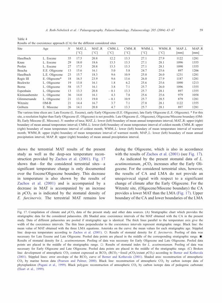
Table 4

Results of the coexistence approach (CA) for the different considered sites

Site Age N MAT_L

[jC]MAT_R

[jC]CMM_L

[jC]CMM_R

[jC]WMM_L

[jC]WMM_R

[jC]MAP_L

[mm]

MAP_R

[mm]

Haselbach L. Eocene 35 17.5 20.8 12.2 13.3 27.1 27.9 1122 1281

Knau L. Eocene 29 18.0 18.6 13.3 13.3 27.1 28.1 1096 1355

Profen L. Eocene 27 17.5 20.8 13.3 13.3 27.1 28.1 1090 1355

Beucha E.E. Oligocene 13 15.6 16.1 5.0 5.8 24.7 25.6 897 1206

Haselbach L.E. Oligocene 23 15.7 18.3 9.6 10.9 25.0 26.0 1231 1281

Regis III E. Oligocene* 18 16.5 23.9 9.6 13.6 26.0 27.9 1187 1281

Bockwitz L. Oligocene 19 13.8 16.1 1.8 6.2 25.6 25.6 1090 1213

Borna L. Oligocene 58 15.7 16.1 3.8 7.1 25.7 26.0 1096 1355

Espenhain L. Oligocene 13 13.3 20.8 � 0.1 13.3 25.7 28.1 897 1355

Kleinsaubernitz L. Oligocene 36 14.0 16.1 4.3 7.8 25.6 25.6 979 1058

Glimmersande L. Oligocene 21 13.3 19.0 � 0.1 10.9 25.7 28.5 879 1281

Witznitz OM-B 21 14.4 16.7 3.7 7.1 27.8 28.1 1122 1355

Grobern E. Miocene 26 14.1 20.8 4.7 13.3 25.7 28.1 897 1281

The various time slices are: Late Eocene (L. Eocene), early Early Oligocene (E.E. Oligocene), late Early Oligocene (L.E. Oligocene). * For this

site, a resolution higher than Early Oligocene (E. Oligocene) is not possible. Late Oligocene (L. Oligocene), Oligocene/Miocene boundary (OM-

B), Early Miocene (E. Miocene). N: number of taxa; MAT_L: lower (left) boundary of mean annual temperature interval; MAT_R: upper (right)

boundary of mean annual temperature interval; CMM_L: lower (left) boundary of mean temperature interval of coldest month; CMM_R: upper

(right) boundary of mean temperature interval of coldest month; WMM_L: lower (left) boundary of mean temperature interval of warmest

month; WMM_R: upper (right) boundary of mean temperature interval of warmest month; MAP_L: lower (left) boundary of mean annual

precipitation interval; MAP_R: upper (right) boundary of mean annual precipitation interval.


shows the terrestrial MAT results of the present

study as well as the deep-sea temperature recon-

struction provided by Zachos et al. (2001). Fig. 17

shows that—for the considered terrestrial sites—a

significant temperature change is only documented

over the Eocene/Oligocene boundary. This decrease

in temperature is also shown by the results of

Zachos et al. (2001) and is accompanied by a

decrease in MAT is accompanied by an increase

in pCO2 as is indicated by the stomatal density of

E. furcinervis. The terrestrial MAT remains low

Fig. 17. Compilation of climate and pCO2 data of the present study an

stratigraphic data for the considered palaeosites. (B) Shaded area: coexi

study. Data of different palaeosites are pooled if stratigraphic age is id

width of the coexistence intervals. The thin lines perpendicular to the

mean value of MAT obtained with the three LMA equations. Asterisks

line: deep-sea temperature according to Zachos et al. (2001). o: Res

necessary for Late Eocene and Late Oligocene. Pooled data points are

Results of stomatal density for L. acutimontanum. Pooling of data was

points are placed in the middle of the stratigraphic range. 5: Results

necessary for Early Oligocene and Late Oligocene. Pooled data points

line: development of atmospheric CO2 content expressed as RCO2 (RCO

(2001). Stippled lines: error envelope of the RCO2 curve of Berner an

CO2 by marine boron data (Pearson and Palmer, 2000). Black line:

phytoplankton (Pagani et al., 1999). Black polygon: reconstruction of

(Ekart et al., 1999).

during the Oligocene, which is also in accordance

with the results of Zachos et al. (2001) (see Fig. 17).

As indicated by the present stomatal data of L.

acutimontanum, pCO2 increases after the Early Oli-

gocene. For the considered terrestrial sites, however,

the results of CA and LMA do not provide an

unequivocal signal with respect to a significant

change of climate after the Early Oligocene. For the

Witznitz site, (Oligocene/Miocene boundary) the CA

provides a lower MAT than the LMA (Fig. 17). Upper

boundary of the CA and lower boundaries of the LMA

d other data sources. (A) Stratigraphic chart which provides the

stence intervals of the MAT obtained with the CA in the present

entical. The thick lines parallel to the temperature axis give the

coexistence intervals represent stratigraphic range. Black line: the

on the curve: the mean values for each stratigraphic age. Stippled

ults of stomatal density for E. furcinervis. Pooling of data was

placed in the middle of the corresponding stratigraphic range. n:

necessary for Early Oligocene and Late Oligocene. Pooled data

of stomatal index for L. acutimontanum. Pooling of data was

are placed in the middle of the stratigraphic range. (C) Broken

2 = fossil pCO2/extant pCO2) according to Berner and Kothavala

d Kothavala (2001). Shaded area: reconstruction of atmospheric

reconstruction of atmospheric CO2 by carbon isotope data of

atmospheric CO2 by carbon isotope data of pedogenic carbonate

Fig. 18. MAT at the various sites in Saxony which provided the

considered leaf materials. The climate parameters were reconstructed

by CA and LMA (see text). o: Results of CA. In the case of the

LMA, three different formulas were used. n: LMA after Wolfe

(1979); 5: LMA after Greenwood (1992); .: LMA after Wilf

(1997). The intervals indicated with the data points represent, in the

case of the CA, the lowest and highest possible mean annual

temperature and, for the three LMA formulas, the binomial sampling

error (see text). LE: Late Eocene; EEO: early Early Oligocene; LEO:

late Early Oligocene; EO: Early Oligocene; LO: Late Oligocene;

OM-B: Oligocene–Miocene boundary; EM: Early Miocene. The

number of taxa for the LMA which were available for the different

sites are: Haselbach (UE): n= 11; Profen: n= 7; Knau: n= 15;

Beucha: n= 12; Haselbach: n= 21; Regis III: n= 10; Bockwitz:

n= 20; Kleinsaubernitz: n= 48; Borna: n= 18; Espenhain: n= 12;

Glimmersande: n= 15; Witznitz: n= 11; Grobern: n= 19.


approaches are, however, close to each other (see Fig.

18). For the site of Grobern (Lower Miocene), the

LMA equations result in lower MAT values than the

CA (with, however, overlapping intervals; see Fig.

18). According to the marine data of Zachos et al.

(2001), however, the temperature increased during the

Late Oligocene (Fig. 17).

4. Discussion

4.1. Stomatal parameters and CO2

In many species, the stomatal density/index is

shown to react on pCO2 with a decrease of stomatal

density/index under increasing pCO2. Stomatal

parameters thus inversely respond to pCO2 (see Sec-

tion 1). This phenomenon can be observed in indi-

viduals as well as over geological periods. In the case

of fossil response, more than 90% of the taxa consid-

ered so far exhibit this inverse relationship between

stomatal density/index and pCO2 (Royer, 2001).

Thus, tracking the stomatal parameters of fossil taxa

over time provides a reliable tool for revealing relative

decreases or increases of pCO2 (Cleal et al., 1999). It

is therefore possible to use these data for studying the

correlation between climate changes and fluctuations

of pCO2 (Cleal et al., 1999).

It is, however, much more difficult to reconstruct

pCO2 quantitatively. In this case, the stomatal ap-

proach requires consideration of an extant representa-

tive species because the reaction on changing pCO2

with respect to stomatal density/index is extremely

species specific. This fact is reflected by the increas-

ing efforts to use ‘‘living fossils’’ for stomatal analysis

(Chen et al., 2001; Retallack, 2001; Royer et al.,

2001; Beerling and Royer, 2002b). The technique of

producing calibration curves by experiments with

extant taxa is based on the assumption that evolution-

ary changes in stomatal parameters as an adaptive

response to pCO2 provide a quantitative CO2 signal

which is equal or at least similar to the individual

reaction which is due to genetic plasticity. The sto-

matal approach thus requires consideration of the

same species if it is used in a quantitative sense. For

extinct species, no calibration curve can be produced.

Application of the semiquantitative SR method, which

is not based on a calibration curve, to the present

dataset (Section 3.1) results in a range of pCO2 values

which fit more or less into the existing range of pCO2

proxy data.

Whereas the quantitative reconstruction of pCO2

appears to be difficult with extinct taxa, documenting

increases and decreases of pCO2 through time quali-

tatively by tracking stomatal parameters is feasible.

However, reconstruction of changes in atmospheric

CO2 content by stomatal parameters is hampered by


strong variance of the data. This variance is due to

several factors and weakens the clarity of the qualita-

tive CO2 signal. One important source of variance is

very probably caused by environmental parameters

(see below), but strong variance can even occur over a

single leaf (Poole and Kurschner, 1999; Poole et al.,

2000). The differences between sun and shade leaves

may also contribute to the data scatter because, at least

for the Kleinsaubernitz site, the shade leaves are

frequent (Walther, 1999). In general, however, the

differences between sun and shade leaves are not

important because sun leaves preferentially enter the

fossil record (Ferguson, 1985; Gastaldo et al., 1996;

Kurschner, 1996).

In the present study, the CO2 signal of the stomatal

indices is not clearer in the present study than that of

the stomatal densities. Numerous observations on

extant material indicate that the stomatal index is less

affected by environmental parameters than the stoma-

tal density (Beerling, 1999). For the present dataset,

however, no significant difference between the sto-

matal density and index is discernible. That the higher

reliability of the stomatal index often tends to vanish

in the case of fossil material was also noted by Royer

(2001). The reason for this phenomenon may be

caused by fundamental differences between extant

and fossil material. If fossil leaves of a certain species

are considered, then strongly heterogeneous material

is used compared to leaves of extant plants, especially

if grown under controlled greenhouse conditions. It is

to be expected that heterogeneity on various levels is

present for fossil material and causes high variances

of stomatal density as well as of stomatal index. Some

possible sources of variance are listed in the following

(there may be numerous other—even unrecognized—

factors).

(1) Fossil leaves of a certain location originate from

many individual plants growing in different

microhabitats and environments over partially

very large time intervals with often low strati-

graphic resolution. It is to be expected that these

environments differed in numerous conditions

such as site topology, soil parameters, nutrient

supply, climatic and biotic factors, etc.

(2) High-resolution studies show that pCO2 can vary

significantly over—in geological terms—short-

time intervals. This is demonstrated, for example,

by ice core data for the last 420,000 years (Petit et

al., 1999). Short-term fluctuations of pCO2 are

also suggested by high-resolution records of

stomatal density data of leaf remains in lake

sediments (McElwain et al., 2002). In the case of

terrestrial fossil plant material, such a strati-

graphically high resolution is often not achieved.

It is therefore probable that leaves of a fossil

assemblage existed during a certain time interval

with varying pCO2 levels and therefore show a

higher variance in stomatal parameters than if

pCO2 was constant during that time interval.

(3) Identification of fossil material is often very

complex and difficult. Even if a fossil can be

identified to the species level, many difficulties

and uncertainties about the detailed systematic

relationships remain (e.g., Mai, 1995). For

example, it is possible that subspecies, local

races or hybrids of a fossil taxon existed which

cannot be identified on the basis of the fossil

material and therefore cannot be separated. It is

also conceivable that different subtaxa may react

on varying pCO2 levels differently. Woodward et

al. (2002) observed how different accessions of

Arabidopsis thaliana show differently strong

responses of stomatal density to pCO2, and that

these responses are influenced differently by

water availability. It is also probable that fossil

species, which existed over a large time span,

experienced an evolutionary development. E.

furcinervis, for example, one of the considered

species, existed in central Europe from the

Middle Eocene to the Oligocene/Miocene boun-

dary (Mai and Walther, 1991). During this time

interval, the leaves of E. furcinervis underwent

certain evolutionary changes: the leaves tend to

be less toothed and more undulated with

decreasing stratigraphic age (Kriegel, 2001).

Possibly, the quantitative relationships between

pCO2 and stomatal parameters are also affected if

evolutionary changes occur in a taxon (see also

Section 2.2).

Despite the high variance of the stomatal data, two

of the three considered species, E. furcinervis and L.

acutimontanum, show significant differences in sto-

matal density/index between certain time slices.

According to the present datasets, pCO2 was lower


during the Late Oligocene, the Oligocene/Miocene

boundary and during the Early Miocene than during

the Late Eocene. The datasets also indicate that pCO2

was lower during the Early Oligocene than during the

Late Oligocene, the Oligocene/Miocene boundary and

during the Early Miocene. No differences in pCO2

between Late Oligocene, the Oligocene/Miocene

boundary and the Early Miocene could be detected

by the stomatal data of the two reacting species.

According to Pearson and Palmer (2000), who ana-

lyzed boron isotope ratios of ancient planktonic fora-

minifera shells, pCO2 decreased from a high level

during the Eocene and attained much lower values

during the Miocene. They provide, however, no data

for the Late Eocene. Stomatal data of Ginkgo also

suggest a decrease in pCO2 at the Eocene/Oligocene

boundary (Retallack, 2002). The data of Pearson and

Palmer (2000) indicate a decrease in pCO2 at the

Oligocene/Miocene boundary, as well as the data of

Pagani et al. (1999). A decrease in pCO2 at the

Oligocene/Miocene boundary is not indicated by the

present dataset (see Fig. 17).

4.2. CA and LMA

All upper limits of the LMA values of the Late

Eocene are much higher than the MAT results

reconstructed by the CA. The reasons can be

attributed to several factors. The datasets of the

Upper Eocene localities for LMA are with n= 15,

11 and 7 rather sparse. In the case of fossil leaf

assemblages, the statistical problem of low number

of available taxa is strongly increased by the

taphonomic processes contributing to the develop-

ment of a fossil assemblage, i.e., preservation po-

tential or differential transport. Uneven species

abundance can also represent a source of error

(Burnham et al., 1992; Wing and DiMichele,

1995). Roth and Dilcher (1978) found that the

proportion of entire-margined leaves of an assem-

blage deposited in a lake bottom was smaller than

the proportion of entire-margined species in the

surrounding flora. This effect does not appear to

be the case in the present study because the MAT

values reconstructed by the LMA are higher than

the values of the CA. Until now, little is known

about possible taphonomic distortions influencing

fossil leaf assemblages (Wolfe and Spicer, 1999).

Even the leaf litter of an extant tropical or subtrop-

ical forest may not reflect forest tree composition

correctly, perhaps due to the high diversity (Burn-

ham, 1994). It is, however, possible that the LMA

yields a more realistic result for the Late Eocene

than the CA, even with the rather sparse material

available for the LMA, because the taxonomic

distance between the extant species used for the

CA and the Late Eocene species is higher than is

the case for younger fossil species.

For other epochs, the CA and LMA results are

generally in good agreement. Exceptions (cases where

no overlap exists between LMA and CA results) are

Borna and Witznitz. For these two locations, compar-

atively few taxa are available for LMA (Borna: n = 18;

Witznitz: n = 11). That a high degree of coincidence of

results of LMA and CA is possible was also observed

by Uhl et al. (2003), who studied the Kleinsaubernitz

site and the Middle Miocene location of Schrotzburg

(southern Germany). An earlier study applied both

CA and leaf characteristics (CLAMP) for climate

reconstruction of the Lower Rhine Embayment from

the Middle Miocene to the Upper Pliocene (Mosbrug-

ger and Utescher, 1997). The MAT results of the leaf

analysis yielded significantly lower temperatures than

the CA in this earlier study. A reason for this deviation

may be represented by the fact that floras adjacent to

riversides tend to be dominated by species with

toothed leaves and can thus distort the results towards

significantly lower MAT values (Burnham et al.,

2001). The same is true for lakes and riparian sites

(Burnham et al., 2001). This may well be the case for

the data of the Lower Rhine Embayment. This effect

does obviously not play a role for the present datasets

because the LMA values of MAT are not systemati-

cally lower than the CA results despite the fact that the

majority of the data stems from the Weisselster river

system.

Besides the generally good agreement between the

MAT results yielded by CA and LMA in the present

study, other parameters represent additional indica-

tions of the quality of the LMA signal. Preconditions

for a strong relationship between percentage of spe-

cies with entire leaf margins and temperature are: (1)

mean temperature of warmest month (WMM)>15 jC,(2) drought-free environment and (3) long growing

season (Wing and Greenwood, 1993; Wilf, 1997;

Wolfe and Spicer, 1999). The climate parameters of


the different palaeosites summarized in Table 3 fulfil

these conditions and thus indicate a high reliability of

the LMA results.

The combined MAT results of CA and LMA reveal

a trend towards lower MAT after the Eocene (Figs. 17

and 18) and are thus in general agreement with all

other evidences about the cooling event which oc-

curred after the Eocene (Diester-Haass and Zahn,

2001; Zachos et al., 2001 and citations therein). Ice

house climate was established during the Early Oli-

gocene (Miller et al., 1991). The data obtained from

oceanic sedimentary archives indicate that a warming

event followed during the Late Oligocene superseded

by a cooling event at the Oligocene/Miocene bound-

ary (Zachos et al., 2001 and citations therein). The

MAT results of the present study summarized in Fig.

18, however, reveal no distinct trend towards higher

temperatures from the Early Oligocene onwards for

the considered sites. The MAT values obtained with

the CA scatter around roughly 15 jC for this time

period. An unequivocal signal for a warming trend in

the Late Oligocene is thus not observed for the

considered locations. The LMA indicates higher tem-

peratures at the Oligocene/Miocene boundary (site of

Witznitz; Fig. 17). Walther (1999) also recognized the

Witznitz flora as reflecting a more subtropical char-

acter and interpreted this as an indication for a short

warming event at this site. For the Early Miocene, the

LMA data indicate cooler MAT. The LMA and CA

results of the Oligocene and Miocene locations thus

do not provide clear evidence for further warming or

cooling events during this time interval at the consid-

ered area.

4.3. Climate parameters and pCO2

E. furcinervis shows an increase in stomatal den-

sity after the Eocene and thus signals a decrease in

pCO2. Coupled to this pCO2 decrease, which is

indicated by the stomatal density of this taxon, a

decrease in temperature can be inferred by the results

of both CA and LMA (see Figs. 17 and 18). When

compared to the global marine temperature data

provided by Zachos et al. (2001), the pCO2 decrease

suggested by the stomatal data of the present study

occurs simultaneously to the cooling event at the

Eocene/Oligocene boundary. This cooling event is

also documented by the LMA/CA results of the

present study. Marine sediments signal a strong in-

crease in marine palaeoproductivity during the Eo-

cene/Oligocene boundary (Diester-Haass and Zahn,

1996, 2001). It was suggested by the authors that—

due to this productivity increase—CO2 was extracted

from the atmosphere and sequestered into marine

sediments (Diester-Haass and Zahn, 2001). This pro-

cess could have resulted in a pCO2 decrease, which

probably amplified global cooling (Diester-Haass and

Zahn, 2001). The pCO2 decrease over the Late Eo-

cene/Early Oligocene indicated by the present dataset

corroborates this hypothesis.

The present dataset further indicates that pCO2

increases from the Early Oligocene to the Late Oli-

gocene, signalled by lower stomatal densities/indices

of the Late Oligocene, if compared to the Early

Oligocene data. This pCO2 increase after the Early

Oligocene appears to be contemporaneous to the Late

Oligocene warming event documented by marine data

(Zachos et al., 2001). This warming event is, however,

not reflected by the LMA and CA data for the

considered sites (see Section 4.2). From the Late

Oligocene onwards, the data indicate no further

change in pCO2. The present dataset thus provides

no signal for decreasing pCO2 during the cooling

event at the Oligocene/Miocene boundary indicated

by marine data (Zachos et al., 2001).

The stomata analysis of the present study thus

reflects general changes in pCO2 during the Late

Eocene and Early Oligocene which appear to be

simultaneous to corresponding cooling/warming

events according to marine data. It should be empha-

sized, however, that no cause-and-effect relationship

can be derived from this temporal accordance sug-

gested by the present datasets. Due to the problem of

temporal resolution, fossil data records which docu-

ment a parallel increase or decrease of temperature,

and pCO2 cannot unequivocally answer the question

of what comes first: pCO2 increase or temperature

increase (Boucot and Gray, 2001). Even high-resolu-

tion records of pCO2 data by ice core technique and

temperature proxy data do not always allow for a final

decision on whether increase pCO2 precedes or fol-

lows temperature increase (Fischer et al., 1999; Petit

et al., 1999). Several authors discuss that various

parameters other than greenhouse gases, especially

tectonic events and eccentricity variations in Earth’s

orbit, are significant factors which cause climate


changes on Earth (e.g., Pagani et al., 1999; Zachos et

al., 2001). It is, however, strongly argued that the

atmospheric CO2 content represents at least an ampli-

fying agent of global climate change (Petit et al.,

1999; Zachos et al., 2001). Further work on possible

coupling/decoupling of pCO2 and temperature at

various geological epochs is therefore required in

order to improve our knowledge about complexity

and dynamics of the Earth’s climate.

5. Conclusions

1. The stomatal data obtained in this study show a

considerable degree of scattering. This variance is

probably due to various classes of heterogeneity

(environmental, genetic and evolutionary factors).

It is, however, possible to detect qualitative pCO2

signals in the case of E. furcinervis and L.

acutimontanum.

2. According to these signals, pCO2 was higher

during the Late Eocene than during the Early

Oligocene, and increased again towards the Late

Oligocene. A decrease in pCO2 from the Late

Eocene to the Early Oligocene is also suggested by

increasing marine palaeoproductivity during this

time interval.

3. No pCO2 change during the time interval Late

Oligocene–Oligocene/Miocene boundary–Early

Miocene could be detected.

4. Results obtained with LMA and CA document a

significant cooling from the Late Eocene to the

Early Oligocene. The data further indicate that the

climate at the considered sites did not change

significantly from the Early Oligocene onwards.

The warming event at the Late Oligocene and the

cooling event occurring at the Oligocene/Miocene

boundary which are indicated by marine data are

thus not reflected by the present dataset at the

considered sites.

5. The pCO2 decrease from the Late Eocene to the

Early Oligocene as signalled by the stomatal data is

thus coupled to a cooling event during this time

which is also recorded by other data sources such

as marine climate archives. This coupling is

reflected in the present study by a significant

correlation between stomatal density and temper-

ature for this time interval.

6. According to the present data, the pCO2 increase

from the Early Oligocene to the Late Oligocene was

not accompanied by a climate change at the

considered area. Marine climate data, however,

suggest a warming event during the Late Oligocene.

7. No change in pCO2 during the cooling event at the

Oligocene/Miocene boundary, which is also in-

dicated by marine data, can be inferred from the

stomatal data raised in this study.

Acknowledgements

We want to acknowledge Kerstin Kriegel for

valuable discussion with respect to the material of

E. furcinervis, Dr. Lutz Kunzmann (Museum for

Mineralogy and Geology, Dresden) for organizing

access to the material and Mrs. Elfi Walcher-Andris

for excellent technical assistance. Helpful comments

of David Greenwood (Victoria University) and an

anonymous reviewer on an earlier version of this

contribution are gratefully acknowledged. We thank

James Nebelsick, Tubingen, for critically reading the

English manuscript. This project was financially

supported by the German Science Foundation

(DFG), project number MO 412/23-1.

References

Arrhenius, S., 1896. On the influence of carbonic acid in the air

upon the temperature of the ground. Philosophical Magazine 41,

237–279.

Arthur, M.A., Hinga, K.R., Pilson, M.E.Q., Whitaker, E., 1991.

Estimates of pCO2 for the last 120 Ma based on the y13C of

marine phytoplankton organic matter (Abstract). EOS Transac-

tions-American Geophysical Union 72, 166 (Spring Meeting,

Supplement).

Bailey, I.W., Sinnott, E.W., 1915. A botanical index of Cretaceous

and Tertiary climates. Science 41, 831–834.

Bailey, I.W., Sinnott, E.W., 1916. The climatic distribution of cer-

tain types of Angiosperm leaves. American Journal of Botany 3,

24–39.

Beerling, D., 1999. Stomatal density and index: theory and appli-

cations. In: Jones, T.P., Rowe, N.P. (Eds.), Fossil Plants and

Spores: Modern Techniques. The Geological Society, London,

pp. 251–256.

Beerling, D.J., Royer, D.L., 2002a. Reading a CO2 signal from

fossil stomata. New Phytologist 153, 387–397.

Beerling, D.J., Royer, D.L., 2002b. Fossil plants as indicators of the

Phanerozoic global carbon cycle. Annual Review of Earth and

Planetary Sciences 30, 527–556.


Beerling, D.J., Chaloner, W.G., Huntley, B., Pearson, J.A., Tooley,

M.J., 1993. Stomatal density responds to the glacial cycle of

environmental change. Proceedings of the Royal Society of

London. Series B 251, 133–138.

Berner, R.A., 1991. A model for atmospheric CO2 over Phanero-

zoic time. American Journal of Science 291, 339–376.

Berner, R.A., Kothavala, Z., 2001. GEOCARB III: a revised model

of atmospheric CO2 over Phanerozoic time. American Journal

of Science 301, 182–204.

Boucot, A.J., Gray, J., 2001. A critique of Phanerozoic climatic

models involving changes in the CO2 content of the atmosphere.

Earth-Science Reviews 56, 1–159.

Burnham, R.J., 1994. Paleoecological and floristic heterogeneity in

the plant-fossil record—an analysis based on the Eocene of

Washington. United States Geological Survey Bulletin 2085-B,

5–32.

Burnham, R.J., Wing, S.L., Parker, G.G., 1992. The reflection of

deciduous forest communities in leaf litter: implications for au-

tochthonous litter assemblages from the fossil record. Paleobi-

ology 18, 30–49.

Burnham, R.J., Pitman, N.C.A., Johnson, K.R., Wilf, P., 2001.

Habitat-related error in estimating temperatures from leaf mar-

gins in a humid tropical forest. American Journal of Botany 88,

1096–1102.

Cerling, T.E., 1991. Carbon dioxide in the atmosphere: evidence

from Cenozoic and Mesozoic paleosols. American Journal of

Science 291, 377–400.

Cerling, T.E., 1999. Stable carbon isotopes in palaeosol carbonates.

Special Publication of the International Association of Sedimen-

tologists 27, 43–60.

Chamberlin, T.C., 1898. An attempt to frame a working hypothesis

of the cause of glacial periods on an atmospheric basis. Journal

of Geology 7, 545–584.

Chen, L.-Q., Li, C.-S., Chaloner, W.G., Beerling, D.J., Sun, Q.-G.,

Collinson, M.-E., Mitchell, P.-L., 2001. Assessing the potential

for the stomatal characters of extant and fossil Ginkgo leaves to

signal atmospheric CO2 change. American Journal of Botany

88, 1309–1315.

Cleal, C.J., James, R.M., Zodrow, E.L., 1999. Variation in stomatal

density in the Late Carboniferous Gymnosperm frond Neuro-

pteris ovata. Palaios 14, 180–185.

Crowley, T.J., Berner, R.A., 2001. CO2 and climate change. Science

292, 871–872.

Diester-Haass, L., Zahn, R., 1996. The Eocene–Oligocene transi-

tion in the Southern Ocean: history of water masses, circulation,

and biological productivity inferred from high resolution records

of stable isotopes and benthic foraminiferal abundances (ODP

Site 689). Geology 24, 16–20.

Diester-Haass, L., Zahn, R., 2001. Paleoproductivity increase at the

Eocene–Oligocene climatic transition: ODP/DSDP sites 763

and 592. Palaeogeography, Palaeoclimatology, Palaeoecology

172, 153–170.

Ekart, D.D., Cerling, T.E., Montanez, I.P., Tabor, N.J., 1999. A 400

million year carbon isotope record of pedogenic carbonate: im-

plications for palaeoatmospheric carbon dioxide. American

Journal of Science 299, 805–827.

Ferguson, D.K., 1985. The origin of leaf assemblages—new light

on an old problem. Review of Palaeobotany and Palynology 46,

117–188.

Fischer, H., Wahlen, M., Smith, J., Mastroianni, D., Deck, B., 1999.

Ice core records of atmospheric CO2 around the last three glacial

terminations. Science 283, 1712–1714.

Freeman, K.H., Hayes, J.M., 1992. Fractionation of carbon isotopes

by phytoplankton and estimates of ancient CO2 levels. Global

Biogeochemical Cycles 6, 185–198.

Gastaldo, R.A., Ferguson, D.K., Walther, H., Rabold, J., 1996.

Criteria to distinguish parautochthonous leaves in cenophytic

alluvial channel-fills. Review of Palaeobotany and Palynology

90, 1–21.

Greenwood, D.R., 1992. Taphonomic constraints on foliar physiog-

nomic interpretations of Late Cretaceous and Tertiary palaeocli-

mates. Review of Palaeobotany and Palynology 71, 149–190.

Greenwood, D.R., Wing, S.L., 1995. Eocene continental climates

and latitudinal temperature gradients. Geology 23, 1044–1048.

Greenwood, D.R., Scarr, D.R., Christophel, D.C., 2003a. Leaf sto-

matal frequency in the Australian tropical rainforest tree Neo-

litsea dealbata (Lauraceae) as a proxy measure of atmospheric

pCO2. Palaeogeography, Palaeoclimatology, Palaeoecology 196,

375–393.

Greenwood, D.R., Moss, P.T., Rowett, A.I., Vadala, A.J., Keefe,

R.L., 2003b. Plant communities and climate change in south-

eastern Australia during the early Paleogene. In: Wing, S.L.,

Gingerich, P.D., Schmitz, B., Thomas, E. (Eds.), Causes and

Consequences of Globally Warm Climates in the Early Paleo-

gene. Special Paper-Geological Society of America, vol. 369,

pp. 365–380.

Heer, O., 1855–1859. Flora Tertiaria Helvetiae, vol. 3. Verl. Doc-

umenta Naturae, Olching.

Hickey, L.J., 1977. Stratigraphy and palaeobotany of the Golden

Valley Formation (early Tertiary) of western North Dakota.

Memoir-Geological Society of America 150, 1–181.

Keeling, C.D., 1993. Global observations on atmospheric CO2. In:

Heimann, M. (Ed.), The Global Carbon Cycle. NATO ASI Ser-

ies, vol. 115. Springer-Verlag, Berlin, pp. 1–29.

Kershaw, A.P., Nix, H.A., 1988. Quantitative palaeoclimatic esti-

mates from pollen data using bioclimatic profiles of extant taxa.

Journal of Biogeography 15, 589–602.

Kriegel, K., 2001. Untersuchung der Blattmorphologie und Blatta-

natomie von Eotrigonobalanus furcinervis (ROSSMASSLER)

WALTHER and KVACEK und seine Vergesellschaftung mit anderen

tertiaren Sippen vom Mitteleozan bis Oligo-/Miozan Mitteleur-

opas. Diploma Thesis, Technische Universitat Dresden, Fakultat

fur Mathematik und Naturwissenschaften.

Kurschner, W.M., 1996. Leaf stomata as biosensors of palaeoatmo-

spheric CO2 levels. PhD thesis, Laboratory of Palaeobotany and

Palynology, Utrecht University.

Kurschner, W.M., van der Burgh, J., Visscher, H., Dilcher, D.L.,

1996. Oak leaves as biosensors of late Neogene and early Pleis-

tocene paleoatmospheric CO2 concentrations. Marine Micropa-

leontology 27, 299–312.

Kurschner, W.M., Wagner, F., Visscher, E.H., Visscher, H., 1997.

Predicting the response of leaf stomatal frequency to a future

CO2-enriched atmosphere: constraints from historical observa-

tions. Geologische Rundschau 86, 512–517.


Kurschner, W.M., Stulen, I., Wagner, F., Kuiper, P.J.C., 1998. Com-

parison of palaeobotanical observations with experimental data

on the leaf anatomy of Durmast Oak [Quercus petraea (Faga-

ceae)] in response to environmental change. Annals of Botany

81, 657–664.

Kurschner, W.M., Wagner, F., Dilcher, D., Visscher, H., 2001. Us-

ing fossil leaves for the reconstruction of Cenozoic palaeoatmo-

spheric CO2 concentration. In: Gerhard, L.C., Harrison, W.E.,

Hanson, B.M. (Eds.), Geological Perspectives of Global Climate

Change. Am. Assoc. Pet. Geol., pp. 155–176.

Kvacek, Z., Walther, H., 1989. Revision der mitteleuropaischen

Fagaceen nach blattepidermalen Charakteristiken: III. T. dryo-

phyllum DEBEY ex SAPORTA und Eotrigonobalanus WALTHER

and KVACEK. Feddes Repertorium 100, 575–601.

Mai, D.H., 1995. Tertiare Vegetationsgeschichte Europas: Method-

en und Ergebnisse G. Fischer, Jena.

Mai, D.H., Walther, H., 1978. Die Floren der Haselbacher Serie

im Weisselster–Becken (Bezirk Leipzig, DDR). Abhandlungen

des Staatlichen Museums fur Mineralogie und Geologie zu

Dresden, 28.

Mai, D.H., Walther, H., 1985. Die obereozanen Floren des Weissel-

ster–Beckens und seiner Randgebiete. Abhandlungen des Staat-

lichen Museums fur Mineralogie und Geologie zu Dresden 33,

5–176.

Mai, D.H., Walther, H., 1991. Die oligozanen und untermiozanen

Floren NW-Sachsens und des Bitterfelder Raumes. Abhandlun-

gen des Staatlichen Museums fur Mineralogie und Geologie zu

Dresden, 38.

Mai, D.H., Walther, H., 2000. Die Fundstellen eozaner Floren des

Weisselster–Beckens und seiner Randgebiete. Altenburger Na-

turwissenschaftliche Forschungen 13, 1–59.

Maximov, N.A., 1929. The Plant in Relation to Water Allen &

Unwin, London.

McElwain, J.C., 1998. Do fossil plants signal palaeoatmospheric

CO2 concentration in the geological past? Philosophical Trans-

actions of the Royal Society of London. Series B 353, 83–96.

McElwain, J.C., Chaloner, W.G., 1995. Stomatal density and index

of fossil plants track atmospheric carbon dioxide in the Palae-

ozoic. Annals of Botany 76, 389–395.

McElwain, J.C., Mayle, F.E., Beerling, D.J., 2002. Stomatal evi-

dence for a decline in atmospheric CO2 concentrations during

the Younger Dryas stadial: a comparison with Antarctic ice core

records. Journal of Quaternary Science 17, 21–29.

Miller, K.G., Fairbanks, R.G., Mountain, G.S., 1987. Tertiary oxy-

gen isotope synthesis, sea level history and continental margin

erosion. Paleoceanography 2, 1–19.

Miller, K.G., Wright, J.D., Fairbanks, R.G., 1991. Unlocking the ice

house: Oligocene–Miocene oxygen isotopes, eustasy, and mar-

gin erosion. Journal of Geophysical Research 96, 6829–6848.

Mora, C.I., Driese, S.G., Colarusso, L.A., 1996. Middle and Late

Paleozoic atmospheric CO2 levels from soil carbonate and or-

ganic matter. Science 271, 1105–1107.

Mosbrugger, V., 1999. The nearest living relative method. In: Jones,

T.P., Rowe, N.P. (Eds.), Fossil Plants and Spores: Modern Tech-

niques. Geological Society, London, pp. 261–265.

Mosbrugger, V., Utescher, T., 1997. The coexistence approach—a

method for quantitative reconstructions of Tertiary terrestrial

palaeoclimate data using plant fossils. Palaeogeography, Palae-

oclimatology, Palaeoecology 134, 61–86.

Neftel, A., Moor, E., Oeschger, H., Stauffer, B., 1985. Evidence

from polar ice cores for the increase in atmospheric CO2 in the

past two centuries. Nature 315, 45–47.

Pagani, M., Arthur, M.A., Freeman, K.H., 1999. Miocene evolution

of atmospheric carbon dioxide. Paleoceanography 14, 273–292.

Pagani, M., Freeman, K.H., Arthur, M.A., 2000. Isotope analysis of

molecular and total organic carbon from Miocene sediments.

Geochimica et Cosmochimica Acta 64, 37–49.

Pearson, P.E., Palmer, M.R., 1999. Middle Eocene seawater pH

and atmospheric carbon dioxide concentrations. Science 284,

1824–1826.

Pearson, P.E., Palmer, M.R., 2000. Atmospheric carbon dioxide

concentrations over the past 60 million years. Nature 406,

695–699.

Petit, J.R., Jouzel, J., Raynaud, D., Barkov, N.I., Barnola, J.-M.,

Basile, I., Bender, M., Chappellaz, J., Davis, M., Delaygue, G.,

Delmotte, M., Kotlyakov, V.M., Legrand, M., Lipenkov, V.Y.,

Lorius, C., Pepin, L., Ritz, C., Saltzmann, E., Stievenard, M.,

1999. Climate and atmospheric history of the past 420,000 years

from the Vostok ice core, Antarctica. Nature 399, 429–436.

Poole, I., Kurschner, W., 1999. Stomatal density and index: the

practice. In: Jones, T.P., Rowe, N.P. (Eds.), Fossil Plants and

Spores: Modern Techniques. The Geological Society, London,

pp. 257–260.

Poole, I., Weyers, J.D.B., Lawson, T., Raven, J.A., 1996. Variations

in stomatal density and index: implications for palaeoclimate

reconstructions. Plant, Cell and Environment 19, 705–712.

Poole, I., Lawson, T., Weyers, J.D.B., Raven, J.A., 2000. Effect of

elevated CO2 on the stomatal distribution and leaf physiology of

Alnus glutinosa. New Phytologist 145, 511–521.

Popp, B.N., Takigiku, R., Hayes, J.M., Louda, J.W., Baker, E.W.,

1989. The post-Palaeozoic chronology of C-13 depletion in

primary marine organic matter. American Journal of Science

289, 436–454.

Prothero, D.R., Berggren, W.A. (Eds.), 1992. Eocene–Oligocene

Climatic and Biotic Evolution. Princeton Univ. Press, Princeton.

Retallack, G.J., 2001. A 300-million-year record of atmospheric

carbon dioxide from fossil plant cuticles. Nature 411, 287–290.

Retallack, G.J., 2002. Carbon dioxide and climate over the past 300

Myr. Philosophical Transactions of the Royal Society of Lon-

don. Series A 360, 659–673.

Roth, J.L, Dilcher, D.L., 1978. Some considerations in leaf size and

leaf margin analysis of fossil leaves. Courier Forschungsinstitut

Senckenberg 30, 165–171.

Royer, D.L., 2001. Stomatal density and stomatal index as indica-

tors of paleoatmospheric CO2 concentration. Review of Palae-

obotany and Palynology 114, 1–28.

Royer, D.L., Wing, S.L., Beerling, D.J., Jolley, D.W., Koch, P.L.,

Hickey, L.J., Berner, R.A., 2001. Paleobotanical evidence for

near present-day levels of atmospheric CO2 during part of the

Tertiary. Science 292, 2310–2313.

Rundgren, M., Beerling, D., 1999. A Holocene CO2 record from

the stomatal index of subfossil Salix herbacea L. leaves from

northern Sweden. Holocene 9, 509–513.

Salisbury, E.J., 1927. On the causes and ecological significance of


stomatal frequency, with special reference to the woodland flora.

Philosophical Transactions of the Royal Society of London.

Series B 216, 1–65.

Schwarzbach, M., 1968. Das Klima des rheinischen Tertiars. Zeits-

chrift der Deutschen Geologischen Gesellschaft 118, 33–68.

Stahl, E., 1883. Ueber den Einfluss des sonnigen und schattigen

Standortes auf die Ausbildung der Laubblatter. Jenaische Zeits-

chrift fur Naturwissenschaft 16, 162–200.

Uhl, D., Mosbrugger, V., Bruch, A., Utescher, T., 2003. Recon-

structing palaeotemperatures using leaf floras—case studies

for a comparison of leaf margin analysis and the coexistence

approach. Review of Palaeobotany and Palynology 126, 49–64.

van der Burgh, J., 1973. Holzer der Niederrheinischen Braunkoh-

leformation, II. Review of Palaeobotany and Palynology 15,

73–275.

van der Burgh, J., Visscher, H., Dilcher, D., Kurschner, W., 1993.

Paleoatmospheric signatures in Neogene fossil leaves. Science

260, 1788–1790.

Wagner, F., Bohncke, S.J.P., Dilcher, D.L., Kurschner, W.M., van

Geel, B., Visscher, H., 1999. Century-scale shifts in Early Hol-

ocene atmospheric CO2 concentration. Science 284, 1971–1973.

Wallmann, K., 2001. Controls on the Cretaceous and Cenozoic

evolution of seawater composition, atmospheric CO2 and cli-

mate. Geochimica et Cosmochimica Acta 65, 3005–3025.

Walther, H., 1999. Die Tertiarflora von Kleinsaubernitz bei Bautzen.

Palaeontographica Abteilung B Palaophytologie 249, 63–174.

Wiemann, M.C., Manchester, S.R., Dilcher, D.L., Hinojosa, L.F.,

Wheeler, E.A., 1998. Estimation of temperature and precipita-

tion from morphological characters of dicotyledonous leaves.

American Journal of Botany 85, 1796–1802.

Wilf, P., 1997. When are leaves good thermometers? A new case for

Leaf Margin Analysis. Paleobiology 23, 373–390.

Wing, S.L., DiMichele, W.A., 1995. Conflict between local and

global changes in plant diversity through geological time. Pal-

aios 10, 551–564.

Wing, S.L., Greenwood, D.R., 1993. Fossils and fossil climate: the

case for equable continental interiors in the Eocene. Philosoph-

ical Transactions of the Royal Society of London. Series B 341,

243–252.

Wolfe, J., 1979. Temperature parameters of humid to mesic forests

of eastern Asia and their relation to forests of other areas of the

Northern Hemisphere and Australasia. U.S. Geological Profes-

sional Paper 1106, 1–37.

Wolfe, J., 1993. A method of obtaining climatic parameters from

leaf assemblages. U.S. Geological Survey Bulletin 2040, 1–71.

Wolfe, J.A., Spicer, R.A., 1999. Fossil leaf character states: multi-

variate analyses. In: Jones, T.P., Rowe, N.P. (Eds.), Fossil Plants

and Spores: Modern Techniques. The Geological Society, Lon-

don, pp. 233–239.

Woodward, F.I., 1987. Stomatal numbers are sensitive to increases

in CO2 concentration from pre-industrial levels. Nature 327,

617–618.

Woodward, F.I., Bazzaz, F.A., 1988. The responses of stomatal

density to CO2 partial pressure. Journal of Experimental Botany

39, 1771–1781.

Woodward, F.I., Kelly, C.K., 1995. The influence of CO2 concen-

tration on stomatal density. New Phytologist 131, 311–327.

Woodward, F.I., Lake, J.A., Quick, W.P., 2002. Stomatal develop-

ment and CO2: ecological consequences. New Phytologist 153,

477–484.

Zachos, J.C., Stott, L.D., Lohmann, K.C., 1994. Evolution of early

Cenozoic marine temperatures. Paleoceanography 9, 353–387.

Zachos, J.C., Pagani, M., Sloan, L., Thomas, E., Billups, K., 2001.

Trends, rhythms, and aberrations in global climate 65 Ma to

present. Science 292, 686–693.

Changes in atmospheric CO 2 concentrations and climate from the Late Eocene to Early Miocene:...

Documents

Transcript of Changes in atmospheric CO 2 concentrations and climate from the Late Eocene to Early Miocene:...