
Center for the Study of Western Hemispheric Trade - TAMIU
382
-
Upload
khangminh22 -
Category
Documents
-
view
0 -
download
0
Transcript of Center for the Study of Western Hemispheric Trade - TAMIU


CENTER FOR THE STUDY OF WESTERN HEMISPHERIC TRADE
The Center for the Study of Western Hemispheric Trade at Texas A&M International University is a
public service institute founded to study globalization with special emphasis on the Western
Hemisphere. The Center is a part of the A.R. Sanchez, Jr. School of Business, and it supports the
college as well as the entire Texas A&M International University community with its various
programs. The Center seeks to increase awareness and knowledge about the Western Hemispheric
countries and their economical, political and social interactions. The Center highlights Texas A&M
International University and the City of Laredo and promotes education.
History
Since its inception in 1993, the Center has become a valuable resource for joint research and faculty
and student exchanges. The Center is a key location for educational entities, businesses and
governments to turn to for up to date and relevant information on the Western Hemisphere. The
Center provides a forum for international discussion and debate for representatives from countries
in the Western Hemisphere regarding issues that affect trade and other economic relations within
the Hemisphere. Through its alliance with educational entities, businesses and governments
throughout the Hemisphere, the Center offers practical and targeted lectures imparted by visiting
faculty, professionals, society leaders and scholars.
Focus
The Center's research focuses on subjects that affect Western Hemispheric Trade, including trade
agreements, tariffs, customs, regional and national economies, politics, business development,
finance, the environment and culture. The Center's publication, The International Trade Journal (ITJ), is
now under the auspices of the International Trade Institute and is a refereed interdisciplinary journal
published for the enhancement of research in international trade. Its editorial objective is to provide
a forum for the scholarly exchange of research findings in, and significant empirical, conceptual, or
theoretical contributions to the field.
Mission
Consistent with the mission of Texas A&M International University and its A. R. Sanchez, Jr.
School of Business, the Center for the Study of Western Hemispheric Trade will conduct and
promote research on globalization and related topics, with special emphasis on Western
Hemisphere, increase awareness and knowledge about the Western Hemispheric countries and their
economic, political, cultural and social institutions and development dynamics, and spotlight Texas
A&M International University as a key resource of information, research, training and conferences
focusing on the Western Hemisphere.

CONTENTS
Welcome ........................................................................................................................................................................... 1 Tagi Sagafi-nejad
SESSION I: ISSUES IN CORPORATE FINANCE
Determinations of Corporate Earnings Forecast Accuracy: Taiwan Market Experience ...................... 3 Ken Hung and Kuo-Hao Lee
Corporate Governance in NAFTA Countries: Need to Reach a Common Agreement? ................... 29 Sandra Gutierrez-Wirsching
Financing Innovations by Venture Capital .............................................................................................. 31 Yochanan Shachmurove
SESSION II: INTERNATIONAL STRATEGY AND NEGOTIATIONS
Internationalization Strategies Followed by Three Mexican Pioneer Companies - Grupo Modelo, Grupo Bimbo and Cemex - Issues and Challenges ................................................... 33
José G. Vargas-Hernández and Mohammad Reza Noruzi
Globalization and Economic Growth: Further Evidence Based on Bootstrap Panel Causality Test .................................................................. 51
Hsiao-Ping Chu, Tsangyao Chang, Saban Nazlioglu, and Tagi Sagafi-nejad
Changing Times: A Study of Information Requirements in Relationships between MNC subsidiaries and their Parents ............................................................................................................... 65
Jifu Wang and Ronald J. Salazar
International Negotiations: Concertacion and Dialogues Between Governments as a Strategic Tool for Peace and Security in Latin America .......................................................................... 77
José Barragán Codina and Felipe Pale
SESSION III: ECONOMIC ISSUES IN MEXICO
The Mexican Business Strategies amid Global Crisis ............................................................................. 83 Juan Antonio Sánchez Ramón and José N. Barragán Codina
La Captación de la Inversión Extranjera Directa en México como Resultado de la Firma del Tratado de Libre Comercio de América del Norte (TLCAN) ........................................ 89 José Gerardo Rodríguez Herrera, Homero Aguirre Milling, Fernando Hernández Contreras, and Luis H. Lope Díaz
Offshoring and Volatility: More Evidence from Mexico’s Maquiladora Industry ........................... 103 Roberto A. Coronado

SESSION IV: EDUCATION
Managing an Online Training Program for ICT Skills Development in Business Professors ....... 173 Gabriela Farías Martínez, Norma Pedraza, and Jesus Lavin
Agile Development of a Virtual Teaching Assistant System for Students in STEM Field ............. 175 Pablo Biswas, Runchang Lin, Avinash Venna, and Induja Rompicherla
Are US Academics And Professionals Ready For IFRS? .................................................................... 177 Murad Moqbel, Peerayuth Charoensukmongkol, and Aziz Bakay
SESSION V: ISSUES IN MANAGEMENT
Global Competence of Employees in Hispanic Enterprises on the U.S./Mexico Border ............. 191 Mónica Blanco Jiménez, Juan Rositas Martínez, and Francisco Marmolejo
Evidence of the Relationship Between Emotional Intelligence and Workplace Spirituality: A Preliminary Analysis .......................................................................................................................... 201 Jose Luis Daniel and Peerayuth Charoensukmongkol
Assessing and Comparing Strategic Leadership Behaviors and Performance of Female and Male Business Leaders .................................................................................................................. 207 Leonel Prieto and Homero Aguirre Milling
SESSION VI: ISSUES IN MANAGEMENT INFORMATION SYSTEMS
An ILP Model for the University Course Timetabling Problem ........................................................ 209 Martin Skrodzki
Investigating Small Business Owner Computer Use ............................................................................ 211 George E. Heilman, Jorge Brusa, and Sathasivam Mathiyalakan
The Effect of Software Piracy on Research and Development Investment at the Country Level: Do Developed Countries and Emerging Economies Suffer the Same Impact? .............. 219 Peerayuth Charoensukmongkol
Significance of Offshoring in the IT Sector – a U.S. Perspective ...................................................... 229 S. Srinivasan

SESSION VII: INTERNATIONAL TRADE
Financial Deepening: As an Explanatory Factor of Foreign Trade: The Case Study of Turkey .................................................................................................................... 231 Aziz Bakay
The Influence of Corruption on International Trade Flow: A Study on China-ASEAN Free Trade Area .................................................................................... 241 Yundong Huang
Trade and the Environment: Biological Diversity Conservation in North America: NAFTA and the Implications of the CEC´s Transgenic Maize Report ....................................... 249 Juan Herrera, Luis Lope, Mayra Garcia, Rene Salinas, Marlene Arriaga, and Pablo Camacho
The Effects of Regional Trades on Local Governments’ Tax Revenues and Budgets:
Evidence from Texas ......................................................................................................................... 263 Wei-Chih Chiang SESSION VIII: MACRO-ECONOMIC ISSUES
Similarity and Structural Change in Southern Cone Exports: 2000/09 .................................................. 265
Orlando M. da Silva and Rafael R. Drumond
Enterprise and (Un)Employment: A Proposal Against Crises ............................................................ 281 Ernesto Peralta
The Decline of the Apparel-Maquila Sector in the DR-CAFTA Region: Is there a choice ahead? ........................................................................................................................ 389 Juan A. Chavarria, Robert D. Morrison, Claudia P. Dole, and Brenda M. Dole
SESSION IX: INVESTMENT AND STATISTICAL MODELS
Optimal Asset Allocation under VaR Criterion: Taiwan Stock Market Example ............................ 295 Ken Hung and Suresh Srivastava
Multi Risk-Premia Model of U.S. Bank Returns: an Integration of CAPM and APT ..................... 313 Suresh Srivastava and Ken Hung
Cluster Elimination by Means of an Affine Matrix Transformation.................................................. 333 Mohammad Alfagih, Peerayuth Charoensukmongkol, Ahmed Elkassabgi, and Aditya Limaye
SESSION X: INTERNATIONAL CURRENCY
Exchange Rate Uncertainty and Trade between U.S. and Canada: Is there Evidence of Third Country Effect? ..................................................................................... 335 Mohsen Bahmani-Oskooee and Marzieh Bolhassani
The Role of Debt and Currency in the Global Financial Crisis .......................................................... 337 Rohitha Goonatilake, Rafic A. Bachnak, and Asela Acosta

SESSION XI: BUSINESS ISSUES: PRODUCTION, ADVERTISING, AND LAW
The Future of the Large Capacity Aircraft Industry ............................................................................. 353 James Cox, Bolortuya Enkhtaivan, and Wei Wang
Advertising Campaign for Blood Donors in a Public Hospital Setting in Monterrey, Mexico ...... 369 Silvia Judith Hernández Martínez and Ma. del Carmen Padilla Rodríguez
From Shampoo and Watches to Textbooks: The Supreme Court’s Split Decision and the International Textbook Gray Market Conundrum .......................................................................... 371 Robert D. Morrison, Jaime Pena, and Claudia P. Dole

WELCOME
Dear Conference Participant:
On behalf of Universidad Regiomontana and the A.R. Sanchez, Jr. School of Business at Texas A&M International University, this year’s co-sponsors, it is my pleasure to welcome you to the 2012 Western Hemispheric Trade Conference. This year’s theme for the Conference is: Western Hemisphere: Common Problems, Contending Approaches. Both - common problems as well as contending approaches to solving them – will undoubtedly be highlighted in the Sixth Summit of the Americas, which is just around the corner from this conference, in Cartagena, Colombia, on April 14-15.
In collaboration with our partner institution and consistent with our mission to increase awareness and knowledge of economic, political, and social issues in the Western Hemisphere, the Center for the Study of Western Hemispheric Trade has again put together an exciting and balanced program involving practitioners, academicians, and community leaders.
In the morning plenary session, we will hear from two well informed observers of the Americas. Mr. Tuto Quiroga, former President of Bolivia, and Mr. Jason Marczak, policy director for Americas Society and Council of the Americas and senior editor of Americas Quarterly, will share their unique insights into the current predicaments and contending approaches being taken in the Western Hemisphere.
Being a border University, we are also interested in promoting collaborative arrangements that bring us together and help us better serve both sides of the border. The U.S. Department of Commerce has recently spearheaded one such initiative, and we will hear more details, hoping to find more ways in which such collaboration across the border academic institutions can be cemented and fortified.
In another plenary session in the evening, we will be challenged by the youth of today, to step up to the plate and to see from the eyes of the youth what challenges are ahead, and how we can meet them.
Multiple academic sessions will occupy the space between the morning plenary and the evening reception. During these sessions, papers by domestic and international scholars will address topics ranging from corporate finance to international strategy, from negotiations to Mexico’s maquiladoras, and from education to international financial reporting standards (IFRS). Case studies of Mexico’s pioneering companies such as Grupo Modelo, Grupo Bimbo, and Cemex will be presented side by side with MNC-subsidiary information relationships, the need for common agreements among NAFTA countries, and methodological issues such as bootstrapping. These are but a few of the topics to be discussed, shared, and debated throughout the conference.
We are pleased to welcome you to this conference and hope that you have a most pleasant and productive visit to Laredo and to our beautiful campus.
Sincerely,
Tagi Sagafi-nejad, Ph.D. Radcliff-Killam Distinguished Professor Director, Center for the Study of Western Hemispheric Trade Editor, International Trade Journal A.R. Sanchez, Jr. School of Business Texas A&M International University

2

Determinations of Corporate Earnings Forecast Accuracy: Taiwan Market Experience
Ken Hung, Texas A&M International University
Kuo-Hao Lee, Texas A&M International University
ABSTRACT Individual investors are actively involved in stock market, and are making investment decision based on publicly available and non-proprietary information, such as corporate earnings forecasts from management and financial analyst. Also, the management forecasts is another important index investors might use. To examine the accuracy of the earnings forecasts, the following tests have been conducted. Multiple regression models are used to examine the effect of six factors: firm size, market volatility, trading volume turnover, corporate earnings variances, type of industry, and experience. If the two-sample groups are related, Wilcoxon two-sample test will be used to determine the relative earnings forecast accuracy. The results indicate that firm size has no effect on management forecast, voluntary management forecast, mandatory management forecast, and analysts’ forecast. There are some indications that forecasting accuracy is affected by market ups and downs. The results also reveal that relative accuracy of earnings forecasts is not a function of trading volume turnover. However, management’s earnings forecast and analysts’ forecasts are sensitive to earnings variances.
Keywords Multiple Regression, Wilcoxon Two-Sample Test, Corporate Earnings Forecasts, Management Earnings Forecasts
3

Determinations of Corporate Earnings Forecast Accuracy: Taiwan Market Experience
1. INTRODUCTION In recent times, individual investors are actively involved in stock market, and are making investment decision based on publicly available and non-proprietary information. Corporate earnings forecasts are an important investment tool for investors. Corporate earnings forecasts come from two sources: company management and financial analyst. As an insider, the management has advantage of possessing more information, and hence provides a more accurate earnings forecast. However, because of the existing relationship of the company with its key investor group, the management may have a tendency to take an optimistic view and overestimate its future earnings. In contrast, the financial analysts are less informed about the company and often rely on management briefings. They have more experiences in the overall market and economies, and are expected to analyze companies with objectively. Hence, analysts should provide reliable and more accurate earnings forecast. Whether investors should rely on the earnings forecast made by management or by analyst is a debatable issue. Many researchers have examined the accuracy of such earnings forecasts. Because there are differences in methodologies, sample selections and time horizons, the findings and conclusions from the previous studies are conflicting and inconclusive. This motivated us to do a new analysis by using a different methodology. According to Regulations for Publishing Corporate Earnings Forecast imposed by the Department of Treasury1, publicly traded Taiwanese companies have to publish their earnings forecasts under the following situations:
1. To issue new stocks or acquired liabilities; 2. When more than 1/3 of the board has been changed; 3. When one of situations as listed in section 185 of the Corporation Regulations happens; 4. Merger and acquisitions; 5. Profit gain/lose up to 1/3 of its annual revenue due to an unexpected event; 6. Revenue lose over 30% compared to last year; 7.Voluntarily publish its earnings forecast.
Since management earnings forecasts are mandatory or voluntary, the focus of this research is to examine the accuracy of management’s overall earnings forecast, management voluntary earnings forecast, management mandatory earnings forecasts, and financial analyst earnings forecast.
2. LITERATURE REVIEW
Jaggi (1980) examined the impact of company size on forecast accuracy using management’s earnings forecasts from the Wall Street Journal, and analysts’ earnings forecasts from Value-line Investment Service for 1971 to 1974. He argued that because larger company has strong financial and human capital resources, its management’s earnings forecast would be more accurate than analyst’s. The sample data were classified into six categories based on size of the firms’ total revenue to examine the factors that attribute to the accuracy of management’s earnings forecast with analyst’s. The result of his research did not support his hypothesis that management’s forecast is more accurate than analyst’s.
1 Securities Regulation Committee, Department of Treasury, series 00588, volume #6, 1997
4

Bhushan (1989) assumed that it is more profitable trading large companies’ stocks because large companies have better liquidity than small ones. Therefore, the availability of information is related to company size. His research results support his hypothesis that larger the company size, the more information is available to financial analysts and the more accurate their earnings forecasts are. Kross, Ro and Schreoder (1990) proposed that brokerage firm’s characteristics influence analysts’ earnings forecasting accuracy. In their analysis, sample analysts’ earnings forecasts from 1980 to 1981 were obtained from Value Line Investment, and the market value of a firm is used as the size of the firm. The results of this study on analysts’ earnings forecasts did not find a positive relation between the company size and the analyst’s forecast accuracy. Xu (1990) used the data range from 1986 to 1990 and the logarithm of average total revenue as a proxy of company earnings and examined factors associated with the accuracy of analysts earrings forecast. The hypothesis that the larger the firm size is, the more accurate the analysts’ earnings forecast would be was supported.
Su (1996) focuses on comparison of relative accuracy of management and analysts’ earnings forecasts by using cross sectional design method. Samples selection includes forecast data during the time period from 1991 to 1994. Company’s “book value” of company’s total assets is used as a proxy for the size of the company in the regression analysis. The author believes that analysts are more attracted to larger companies, and there are more incentives for them to follow large companies than small companies in their forecasting. Therefore, the size of a company will affect the relative accuracy of analyst earnings forecast. On the other hand, large companies possess excessive human and financial resources and information which analysts have no access to, to allow managers to anticipate the corporate future earnings with high accuracy. The study results show that analyst and voluntary earnings forecast accuracy for larger companies are higher than forecast accuracy for small companies.
Yie (1996) examine the factors influencing management and financial analyst earnings forecasting accuracy. Data used in this study are the earnings forecasts during the year of 1991 to 1995. She uses company’s total assets and market value of company’s equity as proxies for company size. The finding of this research reveals that the relative earnings forecast accuracy (management, voluntary management, mandatory management and analyst) are not affected by the size of company when company’s total assets is used as the proxy of company size. The result also indicates that mandatory management’s earnings forecast and analysts’ earnings forecasts are influenced by company size if market value of company’s equity is used.
Xu (1991) examines the relative accuracy of analysts’ earnings forecasts, an hypotheses that market volatility is one of factors that influence the relative accuracy of analyst earnings forecast. In up-market situation, vast amount of information regarding corporate earnings and overwhelming trading activities may hinder analyst from getting realistic and objective information, thus, over-optimistic forecast might be a result. In contrast, when market is experiencing a down turn, individual investors are less speculative and more rational, thus, information about corporate earnings tent to be more accurate. Under this circumstances, analyst tent to provide earnings forecasts with higher level of accuracy. The results of this study support the author’s hypothesis. Jiang (1993) examines the relative accuracy between management’s earnings forecast and analyst earnings forecast. He hypotheses that analysts’ earnings forecast has higher degree of accuracy in down-market compared to up-market situation. He uses samples forecast data from the year of 1991 to 1993 in his analysis, and finds that result of this research supports his argument.
Das, Levine and Sivaramakrishnan (1998) used a cross-sectional approach to study the optimistic behavior of financial analysts. Especially, they focused on the predicative accuracy of past information analysts earnings forecast associated with magnetite of the bias in analysts’ earnings forecasts. The sample selection covers the time period from the 1989 to 1993 with 274 companies’ earnings forecasts information. A regression method was used in this research. The term “optimistic behavior” is refereed to as the optimistic earnings forecasts made by financial analysts. The authors hypothesize the following scenario: there is higher demand for non-public information for firms who’s earnings are more difficult to predict than for firms whose earnings can be
5

accurately forecasted using public information. Their finding supports the hypothesis that analysts will make more optimistic forecasts for low predictability firms with an assumption that optimistic facilitates access to management’s non-public information. Clement (1999) studies the relation between the quality and forecast accuracy of analysts’ reports. It also identifies systematic and time persistence in analysts’ earnings forecast accuracy and examines the factors associated with degree of accuracy. Using the I/B/E/S data base, the author has found that earrings forecast accuracy is positively related with analysts experience (a surrogate for analyst ability and skill) and employer size (a surrogate for resources available), and inversely related with the number of firms and industries followed by the analyst. The sample selection covers the time horizon from1983 to 1994 with earnings forecasts of 9500 companies and 7500 analysts. The author believes that as analyst’s experience increases, his earnings forecast accuracy will increase, which implies that the analyst has a better understanding of the idiosyncrasies of a particular firm’s reporting practices or he might establish a better relationship with insiders and therefore gain better access to the managers’ private information. An analyst’s portfolio complexity is also believed to have association with his earnings forecast accuracy. He hypothesizes that forecast accuracy would decrease with the number of industries/firms followed. The effect of available resources impacts analyst’s earnings forecast in such a way that analysts employed by larger broker firm supplies more accurate forecasts than smaller ones. The rationale behind this hypothesis is that analyst hired by a large brokerage firm has better access to the private information of managers at the companies he follows. Large firms have more advanced networks that allow the firms to better disseminate their analyst’s recommendations into the capital markets. The results of this research support the hypothesis made by the author.
Xiu (1992) studies the relative accuracy of management and analysts’ earnings forecasts using Taiwan database covering the period 1986 to 1990. The management and analyst’s earrings forecasts used in the study are from Business News, Finance News, Central News Paper, and The United Newspaper. The research methodology is to examine management’s earnings forecast accuracy with prior and posterior analyst’s earnings forecasts. The result reveals that a management’s forecast is superior to prior analyst’s forecast, but less accurate than posterior analyst’s earnings forecasts.
Jiang (1993) examined the determinants associated with analysts’ earnings forecast and management and analyst’s earnings accuracy under different assumptions. A sample of Taiwan corporations is collected from The Four-Seasons newspaper. Jiang uses cross-sectional regression analysis to investigate the relations between the forecast accuracy and firm’s size, rate of earnings deviation, forecasting time horizon, market situation, and rate of annual trading volume turnover. His results show that earnings forecast provided by analysts are more accurate than management earrings forecast.
3. TESTABLE HYPOTHESES
3.1 Firm size
The size of a firm is believed to have influence on the accuracy of analyst’s and management’s earnings forecast. Jaggi (1980), Bhushan (1989) and Clement (1999) found that the larger the company is, the more accurate the earnings forecast will be. They believe that holding other factor constant, larger companies have more financial and human resources available that allow the management to draw more precise earnings forecast than smaller companies. Thus, forecasts and recommendations supplies by larger firms are more valuable and accurate than the smaller firms.
6

H1: The accuracy of management’s earnings forecast increases with the size of the firm.
H2: The accuracy of management’s voluntary earnings forecast increases with the size of the firm.
H3: The accuracy of management’s mandatory earnings forecast increases with the size of the firm.
H4. The accuracy of analysts’ earnings forecast increases with the size of the firm.
3.2 Volatility of Market
The accuracy of earnings forecast will be affected by market situation. When market is very volatile and unstable, investors who are looking for the opportunities to profit will act more speculative about what would be the next for the market. In this situation, it is more difficult for analysts to figure out the real useful information for their forecasts, they might have a tendency to over-optimistically forecast the earrings and provide recommendations. When a market is in a relative stable period, investors tent to be rational about the next movement of market, there are less biased information regarding corporate earrings among the general investors, thus the information accessed by analysts will allow then to be more objective in the earnings forecast. In contrast, management has the insights on what is really doing in the aspects of operation, financial, top management changes, and profitability of the business. Even they are less vulnerable regardless what market situation is, voluntary management’s earnings forecast might be affected by market volatility to some extent.
H5: Management’s earnings forecast will not be affected by volatility of market.
H6: Voluntary management’s earrings forecast is a function of the of market volatility.
H7: Mandatory management’s earnings forecast is no affected by market volatility.
H8: Accuracy of analysts’ earnings forecast is affected by market volatility
3.3 Volume Turnover
The relationship between trading volume turnover and accuracy of earnings forecast can be examined based on the hypothesis that daily stock trading volume represents the public investors perception about a company. Larger trading volume during a day for a particulate stock reflects higher the degree of divergence on confidence about the company’s stock, and visa versa. This public perception on a stock might distract management’s and analysts’ judgment, they need more time and strive extra efforts in order to proved accurate earrings forecasts.
H9: Trading volume turnover affects the accuracy of management’s earnings forecast.
H10: Trading volume turnover affects the accuracy of voluntary management’s earnings forecast.
H11: Trading volume turnover affects the accuracy of mandatory management’s earnings forecast.
7

H12: Trading volume turnover affects the accuracy of analysts’ earnings forecast.
3.4 Corporate Earning Variance
Corporate earnings surprises are an important aspect of analysts’ earnings forecast. Larger the earnings surprise is, the less useful the past information will be in earnings forecasting, and the harder it is to make accurate forecasts. Corporate earnings variances represent the earnings surprises a company has in the past; it would affect the accuracy of management and analysts’ earnings forecasts.
H13: Corporate earnings variances affect the accuracy of management’s earnings forecast.
H14: Corporate earnings variances affect the accuracy of voluntary management’s earnings forecast.
H15: Corporate earnings variances affect the accuracy of mandatory management’s earnings forecast.
H16: Corporate earnings variances affect the accuracy of analysts’ earnings forecast
3.5 Type of Industry
There may exist a relationship between type of industry and earnings forecast accuracy. They hypothesize that difference between different industries may result in different level of accuracy on earnings forecast. Some analysts may not possess adequate knowledge necessary in the forecasting in a particular industry, therefore, their forecast may not be as accurate as management’s earnings forecast. Hence, following hypothesis can be tested:
H17: Type of industries influences the accuracy of management‘s earnings forecast.
H18: Type of industries affects the accuracy of voluntary management’s earnings forecast.
H19: Type of industries affects the accuracy of mandatory management’s earnings forecast.
H20: Type of industries affects the accuracy of analysts’ earnings forecast
3.6 Forecasting Experience
Analysts’ accuracy of earnings forecast will improve as their experience and knowledge about companies increase. They learn from their previous forecasts and make the next forecast more accurate. Similar argument can be made about the management’s earning forecast. Hence, the following hypotheses:
H21: Forecasting experience influences the accuracy of management’s earnings forecast.
H22: Forecasting experience affects the accuracy of voluntary management’s earnings forecast.
H23: Forecasting experience affects the accuracy of mandatory management’s earnings forecast.
H24: Forecasting experience affects the accuracy of analysts’ earnings forecast.
8

4. EMPIRICAL RESULTS
4.1 Comparison of management and analyst’s earnings forecast
To compare the relative accuracy of management and analysts’ earnings forecasts, we focus on four major aspects regarding the relative accuracy of earnings forecasts. First, management versus analysts’ earnings forecasts is made to compare the relative accuracy of the forecasts. Secondly, a comparison is made between voluntary management’s forecasts and analysts’ forecasts. Thirdly, mandatory management’s forecasts are compared with analysts’ forecasts to determine the relative accuracy of the forecasts. Finally, tests of hypothesis are been made to further prove the relative accuracy of management and analysts’ earnings forecasts.
Table 2 provides descriptive statistics of management and financial analysts’ earnings forecasts based from 1987 to 1999. It can be observed that absolute error of management earnings forecasts are less than analyst in the year of 1992, 1993, 1995, 1996, 1997, and 1997. It indicates that management’s earnings forecasts are superior to analysts during that time period. But, in other time periods, the absolute errors for management’s earnings forecast are higher than analysts’ indicating analysts provide higher forecast productions. Overall, it is less obvious to conclude who has higher predicate ability for providing more precise earnings forecast.
The last three rows of Table 2 list the mean absolute errors of earnings forecasts by management and analysts during three different time periods. From 1988 to 1992, management’s forecast absolute mean error is 1.796, whereas analyst’s earnings forecast absolute mean error is 1.503. From 1993 to 1999, management’s earnings forecast absolute mean error id 2.031, while analysts’ forecast absolute mean error show higher value of 2.236. If we look at the entire time period from 1987 to 1999, the absolute mean error for management’s forecast is less than the absolute mean error for analysts’ earnings forecast, which is 1.969 and 2.043 respectively. A conclusion can be drown from above results, that management’s earnings forecasts are more accurate than analysts’ forecasts form early 90’s, but less accurate during the late 80’s.
Table 3 shows the results of the Wilcoxon Signed Rank Test used to test the relative accuracy of managements’ forecast and analysts’ forecast. Comparing the negative ranks and positive ranks in Table 3, management’s forecasts are less accurate than analysts’ forecasts in the year of 1987, 1988, 1989, 1990, and 1999; but more accurate in the year of 1995 and 1998. There is no significant difference in the absolute errors for between management’s forecasts and analysts’ forecasts.
If we examine the z-values of the test for entire time period (1986 to 1999), the z-value for Wilcoxon Sighed Ranks Test is –0.346, which is not significant enough to tell the difference between the two samples. This support the hypothesis H1 that there are no significant differences between management’s forecast accuracy and analysts’ forecast accuracy. This also agrees with the findings suggested by Imhoff & Pare(1982) and Baretley & Cameron (1991). They believe the reason for that is due to the similar abilities of forecasters and comparable net works to access company information (public/private) between management and analysts, it is possible that both can provide relative accurate earrings forecasts.
If the entire time period is divided into two sub-samples, one is from 1987 to 1992, and other is from 1993 to 1999, the later sub-sample shows a significant level of 0.05 with a z-value of –2.138, which indicates that management’s forecasts are less reliable than analysts’ forecasts. For the former sub-sample, it shows no contradiction with the results by Imhoff and Pare (1982), and Baretley & Cameron (1991).
9

4.2 Factors Influencing the Absolute Errors of Earnings Forecast
4.2.1 Firm size
We argue that because management possess relative advantage of having private insights that analyst cannot access, and also the fact of larger company has excessive and strong human and financial resources to allow the management forecasts corporate earnings more precisely. On the other hand, a larger company tends to draw attentions and is more likely to be attracted and followed by financial analysts; analysts’ forecasts can be objective and accurate as well; however, the results from our research do not support this argument. Table 5 shows that the p-value of t parameter for the size of a company (0.478) doesn’t reach a significant level, indicating the size of a company is not associated with the accuracy of management’s earnings forecast. This result doesn’t support the hypothesis H1: management’s earnings forecast accuracy increases with the size of company. Table 6 and Table 7 show results of the regression analysis for two sub-samples representing the time period of 1987 to 1992, and 1993 to 1999 to investigate the relationship between company size and accuracy of management’s earnings forecast.
4.2.2 Volatility of Market
Table 5, the p-value of t parameter in column 4 for the volatility of market of a company (0.075) doesn’t reach a significant level, which implicates the accuracy of management’s earnings forecast is not positively associated with the volatility of market. This result supports the hypothesis H1: management’s earnings forecast accuracy will not change with market volatility. Further examining the two sub-tables of Tables 5, 6 and 7, p-value of parameter for the volatility of market of a company (0.310) indicates that management’s earnings forecast accuracy will not change with market volatility during 1987 to 1999. But the t-parameter for the volatility of market is –2.569 indicating management can provide accurate forecast during up-market, but less accurate forecast during down-market.
4.2.3 Trading Volume Turnover
The p-values of t parameter in column 4 for the Trading volume turnover of a company in all three tables do not reach a significant level. The regression analysis doesn’t support the hypothesis H8 that trading volume turn over will affect management earnings forecast accuracy.
4.2.4 Corporate Earnings Variances
In Table 5, the p-values of t parameter (2.74) in column 4 for the Rate of Earrings Divination of a company is 0.01, which shows corporate earnings variances affect management’s earnings forecast accuracy. Positive value of t-parameter means management earnings forecast accuracy decreases as corporate earnings variance increases. This supports the hypothesis H12 corporate earnings variance has affect on management earnings forecast accuracy. From the examination for Table 6 (1993 –1999) and Table 7 (1987-1992), management earnings forecast accuracy is affected by corporate earnings variances during the recent years (1993 to 1999).
4.2.5 Type of Industry
To determine whether and which industry will influence the forecast accuracy, eighteen industries are selected and represented by a dummy variable Ij . From Table 5, I8 is the only industry that has a significant level for the p-values of t parameter of 14.73. According to our assumption, I8 represents the Chemical industry. Thus, we conclude that management’s forecasts are reliable for most of industries studied in this research, except for the Chemical industry.
10

4.2.6 Forecasting Experience
The results of regression analyses for investigating the relationship of forecasting experience and management’s earnings forecast accuracy are shown in Tables 5, 6, and 7. All three p-values of t parameter in column 4 for forecasting experience indicate that management earnings forecast accuracy is not affected by previous forecasting experiences. This conclusion does not support the hypothesis H20 that forecasting experiences affect management’s forecast accuracy. Test of other hypotheses indicate similar results.
5. CONCLUSIONS
The results of our research indicate that company size has no effect on any of the following: management forecast, voluntary management forecast, mandatory management forecast, and analysts’ forecast. This result agrees with Jaggi (1080), and Kross and Schreoder (1990) that analyst’s earnings forecast accuracy is not related with the size of company. But, differes from the results suggested by Bhushan (1989), Das et al (1998), Clement (1999), Xu, (1991), and Jiang (1993) that company size do influence the relative precision of management or analysts’ earnings forecasts.
It can be seen that the relative accuracy of management’s earnings forecast and analyst’s earnings forecast are not affected by market situation across the entire range of sampled forecasts. There are some indications that forecasting accuracy is affected by market ups and downs. For instance, the relative accuracy of voluntary management’s earnings forecast during the entire time period, accuracy of management’s forecast, and analysts’ earnings forecasts during the years of 1978 through1992 are more accurate when market is up, are less accurate during the down market. This result agrees what Su has suggested -- earnings forecast accuracy is affected by market volatility, but in different ways. We believe that, due to the fact that more individual investors who are most likely to chase the market when it’s up saturate the Taiwan stock market. They examine corporate earrings with more cautions, so their expectations for companies in general are more realistic and rational. Therefore, overall earnings forecast accuracy are increased, and vice versa.
The results of this study reveal that relative accuracy of all four kinds of earnings forecasts is not the functions of trading volume turnover. This agrees with the results obtained by Chai but it disagrees with the results of Gilbert (1990), and Jiang (1993). Results of regression analysis indicate that management’s earnings forecast and analysts’ forecasts are sensitive to the corporate earnings variances. This conclusion proves the hypothesis supports H13 through H16, and supports the theories of Kross and Schreoder (1990), and Jiang (1993). We postulate that corporate earnings variance of earnings surprises is an important indication as a company’s profitability and its earnings in its future. Management and analysts use past year’s earnings suspires to forecast future earnings with an assumption of higher forecast inaccuracy are a result of a high degree of earnings deviation. Therefore, they will need to exercise their highest ability in making earnings forecast more accurate. But, we found that the higher the corporate earnings variance is, the lower the forecast accuracy will be for both management and for analysts. Corporate earnings variances should not be used as an important indicator as how a company is operating, but it represents a complicated business environment it operates in. The higher the complicity of business environment is, the lower accurate the prediction/forecast will be.
Analyst earnings forecast and management’s earnings forecast are biased for Chemical industry over the entire time period of sampled forecast; voluntary management’s earnings forecasts for textile, electrical machinery, and paper manufacturing industries are inaccurate during 1993 to 1999. Mandatory management’s earnings forecasts are very inaccurate for the food industry, textile industry, and travel industry in the time period of 1993 to 1999. This supports Kross and Schreoder (1990) who concluded that analyst’s earnings forecast is affected by the type of industry he/she follows.
11

The results reveal that the relative accuracy of management’s earnings forecast and analyst’s earnings forecast do not respond to the differences of forecasters’ previous experiences. But, the relative accuracy of mandatory management’s earnings forecast for forecasters’ affect the entire time period and the sub-sampled voluntary management’s forecast previous earnings forecast experiences. This conclusion agrees with Clement’s (1999) finding.
We rationalize that forecast accuracy is positive related to the forecasting experiences as hypothesis H21 through H24 state. The results from this study indicate otherwise. The forecast accuracy of mandatory and voluntary management’s earnings forecast has negative relationship with previous forecasting experiences. We argue that is because (1) miss-quantifying variable as a proxy of forecasting experiences, and (2) only using the past mandatory management’s earnings forecasts as the base of future focusing without paying a attention to how to reduce the forecasting errors in those forecasts. Therefore, the more forecasting experiences the forecaster has the lower accuracy if forecast will be.
REFERENCES
Bartley, J. W. and Cameron, A. B. 1991. “Long- run earrings forecasts by managers and financial analysts,” Journal Of Business Finance & Accounting, January, 21-41.
Bhushan, R. 1989. “Firm characteristics and analyst following”Journal of Accounting & Economics, 255-274
Chia, Yuxuan. 1994. “Examination of mandatory management earnings forecasts and the rate of trading turnover,” Unpublished thesis, Accounting Department, Politics University.
Clement, B. Michael. 1999. “Analyst forecast accuracy: do ability, resources, and portfolio complexity matter?” Journal of Accounting & Economics 27, 285-303.
Imhoff, E. A. and Pare, P.1982. “Analysis and comparison of earnings forecasts agents,” Journal of Accounting Research, Fall. 429-439.
Jaggi, B. 1980. “Further evidence on the accuracy of management forecasts vis-à-vis analyst’ forecasts,” The Accounting Review January, 96-101.
Jiang, Jianquan. 1993. “Factors associated with analyst’s earnings forecast accuracy under different assumptions in Taiwan,” Unpublished thesis, School of Business, Taiwan University.
Kross, W., Ro, B. and Schreoder, D.1990. “Earnings expectations: the analysts information advantage,” The Accounting Review, April.461-476.
Pettengill, Glenn N; Sundaram, Sridhar; Mathur, Ike. 1995. “The conditional relation between beta and returns,” Journal of Financial and Quantitative Analysis, March.
Securities Regulation Committee, Department of Treasury, series 00588, volume 6, 1997.
Smnath Das, Carolyn B. and Levine, K Sivaramakrishnan.1998. “Earnings predictability and bias in analysts’ earnings forecasts,” Financial Analysts Journal, November/December,35-42.
12

Su, Yongru. 1996. “Comparison of relative accuracy of management and analysts earnings forecast”, Unpublished thesis, Accounting Department, Dong Wu University.
Xu, Jinjuan. 1992. “The effect of management earnings forecast on portfolio management,” unpublished thesis, Accounting Department, College of Politics, Taiwan.
Xu, Xiubin. 1990. “A examination of analysts earnings forecasts accuracy,” Unpublished thesis, Accounting Department, Politics University.
Yie, Meiling. 1996. “Examination on factors in management and financial analyst earnings forecasting accuracy,” Unpublished thesis, Accounting Department, Zhong Zheng University.
Table 1: Sample of Earnings Forecasts by Management and Analysts from
Taiwan Database Selected for the Study
Year Management Management
Voluntary
Management
Mandatory
Analysts
1999 407 236 319 479
1998 408 238 335 430
1997 384 227 288 376
1996 328 201 223 322
1995 281 193 218 279
1994 219 135 112 247
1993 172 137 84 225
1992 139 78 84 200
1991 156 154 16 175
1990 125 125 NA# 154
1989 123 123 NA 130
1988 112 112 NA 106
1987 87 87 NA 87
Total 2941 2046 1679 3210
# Mandatory forecast requirement was introduced in 1991.
13

Table 2: Descriptive Statistics of Management and Analyst’s Earnings Forecast Errors
Management’s Forecast Error Analyst’s Forecast Error
Year Sample Size
Mean Standard error
Maximum value
Minimum value
Mean Standard error
Maximum value
Minimum value
1999 402 1.15 3.64 38.55 0.0006 1.07 3.18 35.76 0.0006
1998 360 1.61 5.80 63.48 0.0017 2.10 7.10 75.81 0.0037
1997 317 0.74 2.20 29.87 0.0040 0.78 3.17 53.23 0.0002
1996 267 1.12 5.41 55.45 0.0007 1.33 6.49 71.34 0.0009
1995 226 0.86 2.93 33.27 0.0001 0.87 2.31 28.42 0.0018
1994 178 0.62 2.17 18.8 0.0015 0.62 2.17 23.86 0.0025
1993 157 12.71 149.1 1869.1 0.0011 13.80 164.1 2057.4 0.0003
1992 126 0.65 1.48 11.58 0.0013 0.73 1.48 8.14 0.0005
1991 144 0.84 2.99 32.93 0.0014 0.65 1.10 5.67 0.0079
1990 120 5.98 32.60 334.94 0.0017 4.86 20.92 187.3 0.0075
1989 116 1.11 2.28 18.66 0.0009 0.91 1.59 10.56 0.0056
1988 96 1.25 3.29 19.57 0.0001 1.08 2.74 15.43 0.0006
1987 78 0.66 1.88 15.73 0.0171 0.57 1.78 14.62 0.0025
1993-99 1907 2.031 0.983 1869.1 0.0001 2.236 1.083 2057. 0.0002
1987-93 680 1.796 0.535 334.93 0.0001 1.503 0.34 187.368 0.0005
1987-99 2587 1.969 37.57 1869.1 0.0001 2.043 40.88 2057.44 0.0002
14

Table 3: Wilcoxon Sign Rank Test for Earnings Forecast Accuracy of Management and Analyst’s Forecasts Errors
Year Sample Size
Negative Ranks Positive Ranks Ties Z-value Sig.
1999 402 150 230 22 -3.119 0.002***
1998 360 209 140 11 -5.009 0***
1997 317 147 140 30 -0.5 0.96
1996 267 143 119 5 -1.567 0.17
1995 226 117 89 20 -2.857 0.004***
1994 178 82 90 6 -0.339 0.734
1993 157 74 79 4 -0.502 0.616
1992 126 60 62 4 -1.136 0.256
1991 144 69 69 6 -0.407 0.684
1990 120 43 76 1 -2.941 0.003***
1989 116 46 67 3 -2.7 0.007***
1988 96 28 60 8 -3.503 0***
1987 78 27 51 0 -3.315 0.001***
1993-99 1299 626 607 66 -1.592 0.111
1987-93 1288 569 665 54 -2.138 0.033**
1987-99 2587 1195 1272 120 -0.346 0.73
Negative Ranks: Absolute error of management’s earnings forecast < absolute error of analyst earnings forecast
Positive Ranks: Absolute error of management’s earnings forecast > absolute error of analyst earnings forecast
Tie: Absolute error of management’s earnings forecast = absolute error of analyst earnings forecast
* Significant level = 0.1, ** Significant level = 0.05, *** Significant level = 0.01
15

Table 4: Taiwan Stock Market Volatility from 1987 to 1999
Year Rm Rf Rm - Rf Market Volatility
1999 27% 4% 23% Up Market
1998 -13% 6% -19% Down Market
1997 14% 5% 9% Up Market
1996 39% 5% 34% Up Market
1995 -24% 5% -29% Down Market
1994 -13% 5% -18% Down Market
1993 55% 6% 49% Up Market
1992 -28% 6% -34% Down Market
1991 13% 6% 7% Up Market
1990 -59% 8% -67% Down Market
1989 51% 7% 44% Up Market
1988 124% 4% 120% Up Market
1987 138% 4% 134% Up Market
Market volatility measure, Rm, suggested by Pettengill, Sundaram and Mathur (1995), is the last month’s market return minus the first month’s market return divided by the first month’s market return in a given year. Rf is the risk-free rate.
16
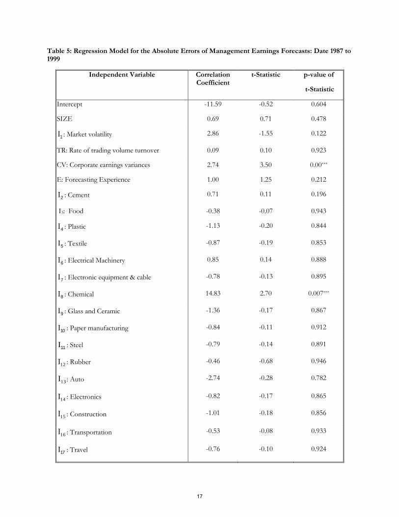
Table 5: Regression Model for the Absolute Errors of Management Earnings Forecasts: Date 1987 to 1999
Independent Variable Correlation Coefficient
t-Statistic p-value of
t-Statistic
Intercept -11.59 -0.52 0.604
SIZE 0.69 0.71 0.478
1I : Market volatility 2.86 -1.55 0.122
TR: Rate of trading volume turnover 0.09 0.10 0.923
CV: Corporate earnings variances 2.74 3.50 0.00***
E: Forecasting Experience 1.00 1.25 0.212
2I : Cement 0.71 0.11 0.196
I3: Food -0.38 -0.07 0.943
4I : Plastic -1.13 -0.20 0.844
5I : Textile -0.87 -0.19 0.853
6I : Electrical Machinery 0.85 0.14 0.888
7I : Electronic equipment & cable -0.78 -0.13 0.895
8I : Chemical 14.83 2.70 0.007***
9I : Glass and Ceramic -1.36 -0.17 0.867
10I : Paper manufacturing -0.84 -0.11 0.912
11I : Steel -0.79 -0.14 0.891
12I : Rubber -0.46 -0.68 0.946
13I : Auto -2.74 -0.28 0.782
14I : Electronics -0.82 -0.17 0.865
15I : Construction -1.01 -0.18 0.856
16I : Transportation -0.53 -0.08 0.933
17I : Travel -0.76 -0.10 0.924
17

18I : Insurance -0.92 -0.14 0.886
19I : Grocery 0.65 0.09 0.925
R-square 0.016
* Significant level = 0.10 ** significant level = 0.05 *** significant level = 0.01
I2. – I19: Dummy variables for industry
Table 6: Regression Model for the Absolute Errors of Management Earnings Forecasts Date 1993 to 1999
Independent Variable Correlation Coefficient
t-Statistic p-value of
t-Statistic
Intercept -18.16 -0.59 0.552
SIZE 1.00 0.76 0.450
1I : Market volatility -2.54 -1.02 0.310
TR: Rate of trading volume turnover 0.04 0.03 0.976
CV: Corporate earnings variances 3.48 3.42 0.001***
E: Forecasting Experience 1.26 1.23 0.218
2I : Cement 1.94 0.21 0.836
I3: Food -0.96 -0.15 0.885
4I : Plastic -2.08 -0.27 0.789
5I : Textile -1.39 -0.23 0.815
6I : Electrical Machinery 1.20 0.14 0.875
7I : Electronic equipment & cable -1.42 -0.18 0.859
8I : Chemical 20.36 2.84 0.005***
9I : Glass and Ceramic -1.91 -0.17 0.854
10I : Paper manufacturing -2.22 -0.19 0.851
11I : Steel -1.13 -0.16 0.875
18

12I : Rubber -0.74 -0.08 0.935
13I : Auto -3.29 -0.26 0.798
14I : Electronics -3.01 -0.50 0.617
15I : Construction -1.55 -0.23 0.822
16I : Transportation -0.37 -0.05 0.964
17I : Travel -0.36 -0.03 0.974
18I : Insurance -1.99 -0.23 0.815
19I : Grocery -0.70 -0.08 0.939
R-square 0.016
* Significant level = 0.10 ** significant level = 0.05 *** significant level = 0.01
I2. – I19: Dummy variables for industry
Table 7: Regression Model for the Absolute Errors of Management Earnings Forecasts Date 1978 to 1992
Independent Variable Correlation Coefficient
t-Statistic p-value of
t-Statistic
Intercept 15.55 0.87 0.386
SIZE -0.68 -0.87 0.383
1I : Market volatility -2.57 -1.78 0.075*
TR (rate of trading volume turn over) 0.25 0.47 0.636
CV (corporate earnings variances -0.39 -0.59 0.555
E: Forecasting Experience 0.57 0.76 0.450
2I : Cement -0.59 -0.11 0.914
3I Food 0.54 0.11 0.913
4I Plastic -0.16 -0.03 0.974
5I Textile 1.17 0.26 0.799
19

6I Electrical Machinery -0.68 -0.12 0.905
7I Electronic equipment & cable 0.40 0.08 0.936
8I Chemical 2.05 0.41 0.680
9I Glass and Ceramic -0.40 -0.06 0.955
10I Paper manufacturing 2.05 0.37 0.709
11I Steel 0.56 0.10 0.923
12I Rubber -0.14 -0.02 0.981
13I Auto 1.94 0.24 0.814
14I Electronics 7.98 1.64 0.102
15I Construction 0.04 0.01 0.994
16I Transportation -0.36 -0.06 0.949
17I Travel -0.96 -0.16 0.876
18I Insurance 1.63 0.29 0.770
19I Grocery 3.78 0.66 0.509
R-square 0.035
* Significant level = 0.10 ** significant level = 0.05 *** significant level = 0.01
I2. – I19: Dummy variables for industry
1. Methodology Appendix
Sample Selection
This research uses cross-sectional design to examine the relative accuracy of management and analysts’ earnings forecast. Due to the disclosure regulation in Taiwan, management’s earnings forecast is classified as two categories: mandatory earnings forecast, and voluntary earnings forecast1. Samples used are management’s and analysts’ earnings forecasts at all publicly traded companies during the time period of 1987 to 1999. The forecasts are compared with actual corporate earnings on an annual basis. Voluntary and mandatory management’s forecast and analysts’ forecast are then used to compare with actual corporate earnings to evaluate the effects of management motivation and behaviors on their earnings forecasts.
20

Management and analysts’ pre-tax earnings forecast data are collected from “Taiwan Business & Finance News” during the time period of 1987 to 1999. Actual corporate earnings are collected from the Department of Education’s “AREMOS” database. Only those firms were included in the samples whose stocks were traded on the Taiwan Stock Exchange before Dec 31, 1999. Also, forecasts made after accounting year and before announcement of earnings were excluded from the sample. Management’s earnings forecast and analysts’ earnings forecast samples for this research are selected to cover the time period from 1987 to 1999. Available database, over the thirteen years period, consisted of 5,594 management’s earnings forecasts, in which, 2,894 management forecasts are voluntary and 2,700 management’ forecasts are mandatory. A total of 17,783 analysts’ forecasts are in the database. The selected samples, presented in Table 1, consist of 2,941 management earnings forecasts, of which 2,046 are voluntary, and 1,679 mandatory forecasts, and 3,210 analysts’ earnings forecasts. Table 1 show that the average number of analysts’ earnings forecasts is more than the number of management’s earnings forecasts. A higher frequency of analysts’ earnings forecasts is expected as an analyst may cover more than one firm. Most of management’s earnings forecasts are made after 1991; it may be attributed by the amendment of “Regulation of Financial Report Of Stock Issuer” imposed by the Taiwan government in 1991. In the new regulation, a new section dealing with earnings forecast was added requiring company’s management to disclose its earnings forecasts to the general public. Comparing the number of management voluntary forecasts and mandatory forecasts, the latter is about 1.5 times more than the former except during the year of 1991 to 1993.
2. Variable Definition
2.1 Absolute earning errors
The mean value of total corporate earnings before tax is used as proxy of earnings forecast. Using earnings before tax in the analysis will eliminate other factors, such as raising cash for capital investment, earning retention for capital investment, and stock distribution from paid-in-capital, that might impact the accuracy of the analysis. Absolute earnings (before tax) forecast error is used to compare the relative accuracy of management and analysts’ earrings forecasts. Management’s forecasts errors are calculated as follows:
n
j
tjimtim FEN
MF1
,,,,,
1
n
j
tjimtim FEN
MF1
,,,,, 11
1
n
j
tjimtim FEN
MF1
,,,,, 21
2
AFE tim ,, =titi
AEAEtim ,,)/(MF ,,
AFE1 tim ,, =titi
AEAEMF tim ,,)/1( ,,
AFE2 tim ,, =titi
AEAEMF tim ,,)/2( ,,
21

t,i,mMF: Mean management’s pre-tax earnings forecast for company i at time t;
timMF ,,1: Mean management’s voluntary pre-tax earnings forecast for company i at time t;
timMF ,,2: Mean management’s mandatory pre-tax earnings forecast for company i at time t;
tjimFE ,,, : Management’s jth pre-tax earnings forecast for company i at time t;
tjimFE ,,,1 : Voluntary management’s jth pre-tax earnings forecast for company i at time t;
tjimFE ,,,2: Mandatory management’s jth pre-tax earnings forecast for company i in year t;
AFE tim ,, : Absolute error of management’s pre-tax earnings forecast for company i at time t;
AFE1 tim ,, : Absolute error of voluntary management’s pre-tax earnings forecast for company i at ime t;
AFE2 tim ,, : Absolute error of mandatory management’s pre-tax earnings forecast for company i at time t;
AE t,i : Actual pre-tax EPS for company i at time t.
Analysts forecast errors are calculated as follows:
n
j
tjiftif FEn
MF1
,,,,,
1
AFE tif ,, =titi
AEAEMF tif ,,)/( ,,
Where,
tifMF ,, : Mean analysts’ pre-tax earnings forecast for company at time t;
tjifFE ,,, : Analysts’ jth pre-tax earnings forecast for company i at time t;
AFE tif ,, : Absolute error of analyst’s pre-tax earnings forecast for company i at time t;
AE t,i : Actual pre-tax EPS for company i at time t.
22

2.2 Company size
Unlike other previous researchers who used market value of company’s equity as a indication of size of a company, in this study, a company’s last year’s total revenue is used as the size of the company. The reason is because Taiwan market is not efficient and investors are not informed fully with information they need during their investment decision making process, speculations among individual investors are the main cause of the stock market volatility, thus market value of company’s equity can not fully represent a company’s real size. In order to better control the company size for our regression analysis, a logarithm of company last year’s total revenue is used as the following:
t,iSIZE = 1t,iTAln
Where,
t,iSIZE: the size of company i at time t;
1t,iTA : Total revenue of company i at time t-1.
2.3 Market volatility
This study adapts what Pettengill, Glenn N; Sundaram, Sridhar; and Mathur, Ike used in their research to measure market volatility. Market volatility is measured as up-market or down-market by using market-adjusted return. This return is calculated as Rm-Rf, in which Rm is the last month’s market return minus the last first month’s market return, and divided by the first month’s market return in a given year. Rf is the risk-free interest rate in the same year.
Return (Market – adjusted) = Rm - Rf
Where,
Up market if Return (Market – adjusted) > 0.
Down Market in Return (Market – adjusted) < 0
A dummy variable is used to identify market volatility. Market Volatility set to1 if a year’s Return
(Market – adjusted) is greater than 0, and set to 0 otherwise. Table 4 reports the market volatility of Taiwan market.
2.4. Trading volume turnover
Trading volume turnover is defined as the value of a company’s stock daily trading volume divided by the company’s number of shares outstanding. To make this proxy better fit in the regression analysis, a logarithm is apply to the value and multiplies by 1,000:
n
1j
t,j,it,i VN
1AV
23

1,
1,
,
ti
ti
tiCS
AV1000lnTR
Where:
t,j,iV: Daily trading volume in day j at time t for company i;
tiAV , : Mean daily trading volume at time t for company i;
1t,iCS : Number of shares outstanding at time t-1for company i;
t,iTR: Rate Of Trading Volume Turn Over at time t for company i.
2.5. Corporate earnings variance
In this research, we only consider the past three years historical earrings surprises as a proxy of a company’s corporate earnings variances. Thus, the corporate earnings variance is defined as the following:
t,iCV =
X
XLN
X =
1n
XXn
1t
2
t
3
t
tY3
X1
1
Where:
t,iCV : Corporate earnings variance at time t for company i;
X : Actual corporate earnings variance for company i;
tX : Actual earnings at time t for company i;
X : Mean EPS (before tax) for company i;
tY : Actual EPS at time t for company i.
24

2.6 Type of industry
There are two major ways to classify industries:
(i) “Industry classification of Republic of China” by State Council in 1987,
(ii) Industry classification used by Stock Exchange House.
In this research, we use the latter one to classify industries, and a variable Ij is set to represent nineteen different industries: Cement, Food, Plastic, Textile, Electrical Machinery, Electronic Equipment & Cable, Chemical, Glass and Ceramic, Paper Manufacturing, Steel, Rubber, Auto, Electronics, Construction, Transportation, Travel, Insurance, and other.
2.7 Proxy for experience
According to research done by previous researchers, although earnings forecast accuracy is positively related to management and analysts’ previous forecasting experiences, it is difficult to quantify the experiences. In this research, we argue that the accuracy of nth management and analyst’s earnings forecast depends on their (n-1) th forecasting experience. Therefore, the proxy of experience is defined as followings:
n
j
tjt EE1
1,i,m,i,m,
n
j
tjt 1E1E1
1,i,m,i,m,
n
j
tjt 2E2E1
1,i,m,i,m,
n
j
tjt EE1
1,i,f,i,f,
Where:
tE i,m, : Total number of times of management’s earnings forecasting experience at time t for company i;
t1E i,m, :Total number of times of voluntary management’s earnings forecasting experience at time t for
company i;
tE i,m,2 :Total number of times of mandatory management’s earnings forecasting experience at time t for
company i;
tE i,f, :Total number of times of analysts’ earnings forecasting experience at time t for company i.
25

3. Regression Model
A multiple regression model is used to examine the effect of six factors: firm size, market volatility, trading volume turnover, corporate earnings variances, type of industry, and experience.
Regression model for management’s forecast absolute error percentage:
i
k
kik
imii
iiim
Ia
EaCVaTRa
IaSIZEaaAFE
23
6
4,
,543
1,210,
(1)
Regression model for voluntary management’s forecast absolute error percentage:
i
k
kik
imii
iiim
Ib
EbCVbTRb
IbSIZEbbAFE
23
6
4,
,543
1,210,
1
1
(2)
Regression model for mandatory management’s forecast absolute error percentage:
i
k
kik
imii
iiim
Ic
EcCVcTRc
IcSIZEccAFE
23
6
4,
,543
1,210,
2
2
(3)
Regression model for analysts’ forecast absolute error percentage:
i
k
kik
ifii
iiif
Id
EdCVdTRd
IdSIZEddAFE
23
6
4,
,543
1,210,
(4)
Where,
i,mAFE: absolute error percentage of management’s forecast for company i;
im1AFE , : absolute error percentage of voluntary management’s forecast for company i;
imAFE ,2: absolute error percentage of mandatory management’s forecast for company i;
26

ifAFE , : absolute error percentage of analysts’ forecast for company i;
iSIZE : size of company i;
1,iI : market volatility (1 if market is up market, 0 if market is down market);
iTR : rate of trading volume turn over for company i;
iCV : Corporate earnings variances for company i;
i,mE :management’s earnings Forecasting Experience for company i;
im1E , : voluntary management’s earnings Forecasting Experience for company i;
imE ,2 : mandatory management’s earnings Forecasting Experience for company i;
ifE , : analyst earnings Forecasting Experience for company i;
192,iI : type of industry for company i.
4. Wilcoxon Two-Sample Test
If the two-sample groups are related, Wilcoxon two-sample test will be used to determine the relative earnings forecast accuracy:
WV
WEWZ
Where,
W1: rank sum of absolute error percentage for management’s earnings forecasts;
W2: rank sum of absolute error percentage for analysts’ earnings forecasts
W: Smaller value between W1 and W2
E(W): Expected values of W-distribution;
WV: Deviation of W-distribution.
27

THIS PAGE INTENTIONALLY LEFT BLANK
28

Corporate Governance in NAFTA Countries: Need to Reach a Common Agreement?
Sandra Gutierrez-Wirsching, Texas A&M International University
ABSTRACT The North American Free Trade Agreement was implemented on January 1, 1994 and allowed Canada, Mexico and the U.S. to have very few trade barriers among them. The friendly relationship among these countries, commercially speaking, also facilitated partnership relationships regarding companies and corporations. But in order to have a successful partnership relation, many issues should be taken into consideration, including the corporate governance systems of the companies in these countries. The governance structure depends on banking and financial systems, ownership and control patterns, industrial policy, and industrial relations. These three countries differ in their corporate governance practices, and the differences remain rooted in the corporate objectives, which are in accordance to societal expectations and ownership rights. The main issue to address in this paper is whether or not these differences in corporate governance have an impact in the success of international partnerships; do any of these countries have to emulate any corporate governance system in order to enhance the success of partnerships, or are there any combinations of governance that suit well? By analyzing these questions we can further our knowledge in the behavior of the market and whether or not modifications in the corporate governance structure should be implemented.
29

THIS PAGE INTENTIONALLY LEFT BLANK
30

Financing Innovations by Venture Capital
Yochanan Shachmurove,
The City College of The City University of New York ABSTRACT
This paper examines the first round of venture capital investment in the United States (U.S.) from 1995Q1 to
2010, taking into consideration both location and industry sector. The data concentrate only on the first sequence of financing. This point is the time when invention becomes innovation and the firm or entrepreneurs seek the cooperation of venture capitalists. In other words, it is the first time that venture capitalists become involved. Venture capitalists can invest in a firm in different stages of its development, be it Seed/Start-Up, Early Stage, Expansion Stage, or a Later Stage. From the point of view of the venture capitalist, investing in a company for the first time is likely riskier than investing in a company in which it already holds equity.
The research question is whether industry and region are important factors in determining the first round of venture capital investment. Furthermore, the paper examines the effects of a wide array of macroeconomic variables on first stage venture capital financing activity. Consequently, the venture capital data are augmented by Real Gross Domestic Product, Gross Domestic Product (GDP), Implicit Price Deflator, Gross Private Domestic Investment, Personal Savings, Producer Price Index, Consumer Price Index, Effective Federal Funds Rate, Bank Prime Rate, 3-Month Treasury Bill Rate, 6-Month Treasury Bill Rate, 3-Year Treasury Bill Rate. In addition, the paper examines long-term trends and the effect of the current economic crisis on first round of venture capital investment.
It is worthwhile to examine the venture capital market, which heavily relies on expectations of future GDP, investment, and innovation. Confidence and uncertainty about the future economic environment are vital factors in committing to financing a new company for the first time. Furthermore, economic geography has recently risen to the frontier of research due to the works of the 2008 Nobel laureate, Paul Krugman, who was awarded the Nobel Prize for his “analysis of trade patterns and location of economic activity.” Although both international economists and industrial organization researchers study economic geography, it has received limited consideration in the venture capital literature.
31

THIS PAGE INTENTIONALLY LEFT BLANK
32

Internationalization Strategies Followed by Three Mexican Pioneer Companies Grupo Modelo, Grupo Bimbo and Cemex Issues and Challenges
José G. Vargas-Hernández,
Universidad de Guadalajara
Mohammad Reza Noruzi,
Islamic Azad University
ABSTRACT The opening of the Mexican economy and globalization bring new opportunities for Mexican companies to expand their markets and get their products around the world. The internationalization process requires a sound strategy for the consolidation in foreign markets. The aim of this study is to analyze the different internationalization strategies followed by three Mexican companies with a global presence: Grupo Modelo, Grupo Bimbo and Cemex. We conclude that the differences in their strategies arise from the characteristics of each of these companies. Keywords: Mexican companies, strategy, expansion, internationalization.
33

Internationalization Strategies Followed by Three Mexican Pioneer Companies Grupo Modelo, Grupo Bimbo and Cemex Issues and Challenges
INTRODUCTION
The landscape of this century requires companies to be increasingly competitive, and that not only have to compete with domestic rivals but new players come in search of a single market. Today's competitive advantages and are no guarantee of success without a solid strategy that will ward. The decision made at the time a local company to expand its market to new countries, must be supported by an internationalization strategy appropriate to the characteristics of the company. It also has a wide range of options for entering new markets, exports, licensing, and joint ventures with foreign partners, strategic alliances, acquisitions, establish subsidiaries, among others. However the best choice will be consistent with its objectives and characteristics. BACKGROUND
Globalization is a phenomenon that accelerated in the late twentieth century, in the last three decades, increased international economic transactions, thus expanding economic relations between countries. The world economy entered a process of numerous scientific and technological advances that changed production patterns worldwide. The deregulation aimed at removing trade barriers between countries was a consequence of globalization, which for some companies has been a growth opportunity, whiles for others a latent threat to the entry of new competitors. In the mid-eighties with the entrance to the General Agreement on Tariffs and Trade (GATT), the Mexican economy began a process of trade liberalization which is consolidated with the entry into force of The Free North American Free Trade Agreement (NAFTA). Thus our country adapts a new economic model: the neoliberal model, which encouraged external competitiveness from trade liberalization (Branches, 2005). The new economic policies of this new model involve change and restructuring of Mexican companies. The Mexican economy opened to international trade and financial markets, gave a strong boost to exports and foreign investment was allowed in more sectors of the economy. All these actions benefited large Mexican companies in their growth and expansion, while allowed to integrate into international production and exports through acquisition of companies abroad (De Gortari, 2005).
Grupo Modelo, Bimbo and Cemex were three large Mexican companies that were consolidated in the country and sought to internationalize through different positioning strategies in international markets. A common denominator among these companies was the use of acquisitions and alliances with foreign partners, but the strategies followed by each were different.
34

DEFINITION OF THE PROBLEM
According to De los Rios (2005) among Mexican multinational companies successfully in the internationalization process are: America Movil, Bimbo, Gruma and Cemex. Clarifying the process of internationalization beyond imports and exports, i.e. involves the establishment of subsidiaries or the acquisition of companies is elsewhere. This research focuses on the analysis of internationalization strategies followed by three of Mexico's most important companies of our country with a presence in international markets: Bimbo, Cemex and Grupo Modelo were chosen because these three companies have been recognized by national and international magazines as successful businesses in foreign markets. According to the ranking made by the group and published on its website CNN Expansion, these companies are among the 500 most important companies in Mexico. Cemex is in the number 6 in the place Grupo Bimbo and Grupo Modelo 11 at number 22 (see Attachment A).
Moreover these companies to analyze different strategies to position it clearly in foreign markets. Hypothesis:
The characteristics of each of these three Mexican companies are a major determinant of the choice of different strategies and ways of entering foreign markets. OBJECTIVE
To analyze the internationalization strategies and positioning in international markets of three Mexican companies with a worldwide presence: Grupo Bimbo, Cemex and Model and demonstrate that these three companies have expanded their market by using mergers and acquisitions as growth strategy.
Analyze the trajectory of each of the three companies in the global context.
Establish the most important factors influencing the success of each of the companies chosen. FRAMEWORK
Cortes de los Rios (2005) says that many of Mexico's most important economic groups were created and managed its expansion, consolidation and development thanks to the acquirers and mergers took place. It analyzes the behavior of the acquisitions in Mexico in the period 1986- 2005, concluding that this type of operation shows a cyclical and economic fluctuation coincide with the country, increasing in the late eighties and early nineties. On the other hand shows that mergers and acquisitions for our country are concentrated in banking, finance and telecommunications. In the study period prevailed horizontal acquisitions, followed by vertical and finally concludes that the process of mergers and acquisitions is indeed, as she defines a "vehicle" for the internationalization of Mexican companies. Moreover, Celso Garrido (2001) a study on cross-border operations during the nineties in Mexico, distinguishing foreign acquisitions made by companies established in Mexico, Mexican takeovers by foreign companies. This study shows results that say the process undertaken grades Mexican companies and groups to internationalize their production activity. Garrido ranks results of acquisitions fleshed out by Mexican companies at three levels: macro, meso and micro.
35

This work is a case study of the different strategies for entering international markets and show that despite the existence of a common denominator among these strategies, as is the case of acquisitions, the company's own resources play a key role to allow them to take different paths to achieve their goal. CONCEPTUAL-THEORETICAL
When a company decides to expand into new markets is essential to plan a strategy to reduce the risk of failure, for this is to consider the advantages and disadvantages of different forms that have to enter these markets and also to consider its position market and the characteristics of your company. In this context we say that an international strategy is one used by a company to sell its products outside its national territory. Internationalization is a process by which a domestic company can extend their productive activities to other countries, according to Peng (2006), is a process where a multinational organization is responsible for any commercial or production of an enterprise located in different parts the world. The reasons that lead companies to make the decision to internationalize your business are the benefits they can acquire if they implement the strategy succeed. These expected benefits are:
1. Increased market size. Expand their productive activities to another country gives them the
opportunity to captivate new customers, new markets to sell their products.
2. Better returns on their investments. It is expected that investments in other countries generate above
average returns.
3. Better economies of scale, scope or learning. Producing under economies of scale production reduces costs and produces the same internationalization synergies, which shares knowledge and learning.
4. A competitive advantage of location. When a company decides to settle in another country with the
intention of reducing costs many times companies are looking for markets where they can get cheap labor, natural resources or cheaper energy or potential new customers in that country (Hitt, Ireland & Hoskisson, 2008).
There are two ways of entering foreign markets, on one hand the non-property, as its name suggests involve entering new markets without the need to use part of its assets or capital. Examples of these: Exports and contractual agreements. Moreover there are still properties, which involve the establishment of subsidiaries in new markets; investment is needed to begin operations. Some examples of these: Joint ventures (joint adventure) and partially owned subsidiaries. This approach gives rise to multinational corporations (MNCs) which are companies that operate with foreign direct investment, its function is the control and management of value-generating activities in foreign countries (Peng, 2006).
If a company decides to export has two possibilities: Direct export is the direct sale of goods to foreign customers or where the indirect export sales to foreign markets is through intermediaries. Contractual agreements are classified as:
A. Licenses / franchises. When a foreign company buys the rights to manufacture and / or sell
36

products in the domestic business. This in exchange for a royalty per unit produced or sold (Hitt, et al., 2008).
B. Projects ready to operate. Projects are paid for certain activities for a business (construction of
facilities or personnel training, etc.)..
C. Research and development contracts. Agreements between companies to assist in research and development one can work for another.
D. Joint marketing. A set of companies agree to jointly market their products.
Property forms Returning to internationalize. a company defines what is a joint venture (EC) which is understood as a company originated and owned by two or more companies This new company can be a minority (when one of the generating company has less than 50% ownership), 50/50 (partners have the same percentage of ownership) or majority (a company has more than
50% of CD).
For their part, wholly owned subsidiaries (SPT) are subsidiaries of the multinational company, located in different countries. In turn, these can be of two types: operations on a blank field, when companies begin operations from the construction of these. Moreover mergers or acquisitions are the most popular form of entering foreign markets. Involve the transfer of assets, knowledge, and control operations between companies. Because the latter is the most sought after by companies wishing to establish themselves in other markets then we pause this for a better understanding. A merger is defined as the combination of assets, operations and management of two companies to establish a new legal entity (Peng, 2006). Meanwhile an acquisition is the transfer of control of the assets, operations and management of a company (object) to another (purchaser), making the object in a unit of the purchaser (Wright, 2002). In reality the acquisitions are more common than mergers. These operations can be carried out in three directions:
A. Horizontal. Are acquisitions between competitors within the same industry? This is the most common type, as it increases the market power of the synergies obtained by exploiting the costs and revenues.
B. Vertical. This type involves the relationships between companies which makes them focus their
suppliers (up) or its buyers (up). With this acquisition the company is vertically integrated, controlling additional parts of the value chain
C. Conglomerate. These are transactions where companies interact unrelated products.
Hitt et al. (2008) adds the related acquisitions occur within an industry closely related and transborder acquisitions are those which as its name says, transcend territorial boundaries. Moreover, this type of transaction may be hostile or friendly, the first concern when management of a target company is against the acquisition, this company is not seeking a takeover bid. Such events increases during downturns in the economies, as it is easier to detect companies that are undervalued mismanaged in relation to its assets (Thornton, Keesnan, Palmeri & Himelsten, 2002). The acquisitions are friendly when both companies are in agreement to carry out the transaction.
37

The table in Annex A summarizes the advantages and disadvantages of each of the modes of entry to foreign markets. A complete model of foreign market entry described in Peng (2006), which considers the tripod base of the strategy as a sound strategy. Considerations based on the industry through the diamond of Porter's five forces suggests a review of the industry environment it belongs to the company, this analysis can uncover opportunities to open new markets. For their part, resource-based considerations, led by the model VRIO (value, rareness, imitation and organization) are a factor to be taken into consideration the managers of a company when deciding to enter international markets. Many times the value of the assets of a company are key factor to compete abroad, likewise if a company with resources much rare and difficult to imitate, has assets that can exploit an opportunity in other markets. Finally considerations institutions are perhaps one of the key firms in search of new markets should consider when embarking on new markets. Knowledge of the rules are vital for easier entry to markets unknown. Although globalization seeks the integration of countries, institutions and culture rules are factors that have not yet unified. After the theoretical review that supports the internationalization of companies in the next section proceeds with the individual analysis of each selected Mexican firms to conclude this section with a comparison of the various factors that influenced the success of internationalization of each company. METHODOLOGY
The methodology for the preparation of this work was the revision of the paths that have these three companies since its inception to the present, past and putting special emphasis on internationalization. It also is evident through its success through the search and tracking of recognition has been given to these companies. The information collected for this analysis comes from the official website of each company, as well as annual reports and additional sources such as empirical studies for these companies.
The next section will be the case study of each selected Mexican firms: Grupo Bimbo, Cemex and Grupo Modelo. ANALYSIS OF MEXICAN COMPANIES GRUPO BIMBO
Founded in 1945, today this company is one of the largest bakery companies in the world and a leader in the Americas has earned recognition for their production and sales volumes. According to its annual report 2010 (Grupo Bimbo, 2010) has 103 plants and over 1000 strategically located distribution centers in 17 countries in America and Asia. One of its most valuable assets is the possession of one of the most extensive distribution networks in the world with over 41,000 routes. Starting operations on December 2, 1945 the first production plant in Mexico, under the direction of Jaime Sendra and Lorenzo Servitje, Bimbo is placed on consumer preferences through the presentation and quality of their products. In 1946 this plant is expanded and begins structuring the area of vehicles, which later became his strategic asset for the growth of the company. The Bimbo distribution network began with an agreement to distribute its products with carriers who distributed newspapers in the province. However this was not enough and had to open routes and outside agencies, the first in Puebla in 1949.
38

The distribution of products of this company took from town to town, following the paths, roads and railways, so vendors were opening up the market.
The growth of this company in our country was the result of knowledge of the needs of its consumers (building products) and vision of its managers to take advantage of opportunities offered by the market, spread around the country through establishment of new silver and the acquisition of some of its competitors. In search of closer integration in 1973, Bimbo began making jam in order to supply one of its lines (Marineo dedicated to making cakes and cookies) of raw material. Also in the late seventies Bimbo executives found themselves in the market for sweets and chocolates retailer an opportunity, as this was poorly attended, and decided to put a small candy manufacturing plant (Ricolino). Thus began a diversification outside the bakery and confectionery.
After consolidating the domestic market, leaving Mexico in 1984 the first trailer with Marinela products, bound for Houston, Texas. And in 1989 began international expansion with the creation of Bimbo Bimbo Central America and Guatemala with the construction of the first plant outside the country. In 1991 created the Latin America Division (OLA) to operate the expansion south of the country. In this decade the company acquired Alesa (Chile) and Holsum, bakery leader in Venezuela. Bimbo is created El Salvador, Costa Rica, Argentina and Peru in Colombia, established a partnership with Noel, the largest biscuit company in the country In 1998, the purchase of American bakery Mrs. Baird's, a leader in Texas that had 11 floors.
In 2001 he made the purchase of Plus Vita from Brazil, which confirmed its leadership Bimbo Latin America and in 2002 acquired the Canadian company George Weston Ltd. Bimbo In this decade, began its presence in Europe with the purchase of the company confectionery Park Lane, located in the Czech Republic. This decade also acquired in Mexico: Bakeries El Globo, La Corona, Gabi Cookies and Joyce. Bought outside the country: Pan Europe (Guatemala), Los Sorchantes (Uruguay), South Lakes (Chile), Lalo's Bakery (Colombia), and finally Laura, and Plus Vita Nutrella LTDA, the latter one of the bakery companies more large and important in Brazil.
In 2010, specifically three strategic acquisitions: Dulces Vero in Jalisco, Mexico, Hong Jin Wei in China and the U.S. Foods Bimar Finally in November of that year announced the purchase of the bakery division of Sara Lee bakery largest U.S., which as a group Grupo Bimbo Baker worldwide.
In short today Grupo Bimbo has 103 plants worldwide, 42 plants in Mexico, 34 in the United
States, 25 in Central and South America and 2 in China. The first quarter reported sales of $
29.312 million pesos, an increase of 3.5% over the previous year. Currently this group has more than 150 brands, the best known are: Bimbo, Marinela, Milpa Real, Aunt Rosa, Oroweat, Entenmann's, Thomas', Boboli, Mrs. Baird's, Barcel, Ricolino, Coronado, La Corona, El Globo bakeries, Suandy, among many others. All group companies are located in four divisions: Bimbo SA, brings together companies bakers and confectioners in Mexico and Central America, Barcel SA, which integrates the business of snacks and Ricolino, Bimbo Bakeries USA (BBU), serving the U.S. market and Organization finally Latin America (OLA), responsible for operations in Latin America.
39

ANALYSIS: GRUPO BIMBO
As we can see, the expansion of Grupo Bimbo is the result of significant investments it has made to establish new production plants, strategic alliances and acquisition of companies. His strategy was to acquire or ally with local companies that will offer something in terms of technology or distribution capacity, choosing only those companies that share their values; if the companies did not meet the latter requirement would enter the market from scratch. One of the key factors that have influenced the success of Grupo Bimbo in the national and international market, innovation is not only their products but to organize the company as the coordination of their plants requires the use computing platforms that support business processes. On the other hand is a company that knows its customers, the distribution network has created allows a more direct and frequent contact with customers, allowing you to identify new growth opportunities and product innovation based on consumer preferences.
In this sense Bimbo has a very important competitive advantage: its ability to reach more distant outlets. Bimbo in our country has to sell their products to an average of less than a mile from each consumer (Grupo Bimbo, 2011). This distribution network is one of the intangibles of the company, which tried to establish the same way in other countries, without a clutch that has found cultural differences that have led to the need to adapt to each country based on their conditions individuals. Finally Grupo Bimbo is a company that just look to expand geographically, also seeks to be a profitable company, which has managed to increase the efficiency of each of its processes. For that seeks to optimize its resources by using technology.
CEMEX
It is a Mexican company initially dedicated to the production and distribution of cement and concrete, but is now a global company that offers products for the construction industry. It began operations in 1906 with Cementos Hidalgo plant in the north. After significant growth for six years, the operation of this company is affected by the Mexican Revolution forced to suspend operations. In 1919, partially resume their operations and not until two years later when the market comes back completely. Cementos Hidalgo in 1931 merged with its competitor Cementos Portland Monterrey, giving rise to what is now known as Cementos Mexicanos SA (CEMEX). For about thirty-five years, this company has a steady growth backed by the expansion of its plants in the northern region. Until 1966, decided to venture into the southern part of the Mexican Republic, acquiring in that year the plant Cementos Maya, Mérida. With this acquisition continues to meet demand in this part dl country through Portland Cement brand Maya. That same year the new plant starts operation Valles, in order to meet the Huasteca region in Mexico. In order to expand across the country in 1967 opened a plant in Torreon through brands pozzolanic Portland cement Portland Cement Monterrey and Monterrey; the plant is responsible for meeting growing demand in the Northeast. Plants installed in all regions continue to grow by increasing its production capacity. In 1973 Cemex acquired Portland cement plant in the Bajio region of central Mexico. 1976 was a watershed for the company as a part begins trading on the Mexican Stock Exchange and on the other side becomes the leading Mexican producer of cement to its acquisition of Cementos Guadalajara.
40
In 1986 starts joint venture with U.S. cement companies, in order to enter that market. In 1987 acquires Cementos Anahuac. And this year it created a solid team of professionals who are in charge of the integration of acquired companies. It also implements a satellite system that allows you to connect all the facilities of the company (CEMEXNET).
When purchasing your competition, Cementos Tolteca Cement Company in Mexico second in
1989, Cemex became even without significant presence in other countries, one of the ten largest cement companies worldwide.
It was not until 1992, when he decides to start its internationalization process, which starts on the European market by acquiring the two largest cements in Spain: Valenciana and Sanson. Two years later ventures into Central and South America, buying Cemento Bayano in Panama and the company expires, Venezuela's largest cement. Also, the purchase of Balcones cements plant in the United States. In 1995 Cemex continues its international expansion this time to acquire Cementos Nacionales, the leading company in the Dominican Republic. A year later became the third largest cement company in the world to be part of your company Cementos Diamante and Samper in Colombia.
Not content with its spectacular growth in such a short time in 1997 the largest cement company in Mexico comes to Asia with the purchase of Rizal Cement and APO Cement in the Philippines two years later. That same year, Cemex ventures into Africa by acquiring Assiut Cement Company, one of the leading cement producers in Egypt also buying Cementos del Pacifico, Costa Rica.
Mexican Cement century starts with the determination to consolidate the already developed markets in 2000 purchase Southdown, Inc. in the United States in 2001 and acquired Nicaragua enters Saraburi Cement Company in Thailand. The operation performed in 2005, doubling its size and expanding its market to more than twenty countries, mainly in Europe. This transaction is the acquisition of the British building materials RMC, which according to a press release on September 27, 2004 posted on the website of the Mexican company and meant a great synergy that will allow the centralization administrative functions, optimization of network marketing, logistics and process standardization.
Far from purchases made by the Mexican company in 2000, implemented an initiative to identify, incorporate and implement standardized best practices within the entire organization (CEMEXway). This initiative consolidates the group that was responsible for the integration of acquired companies.
Finally the integration of the Australian company Rinker Group Limited, the Mexican company consolidates its position as a leader in the cement industry. ANALYSIS: CEMEX
As we see in the above description Cemex in less than twenty years the company extended global territory through the use of acquisitions, it is surprising success of this instrument through which although not clearly mentioned in its path also has been due to the economic and financial company that manages the.
Cementos de Mexico took advantage of the benefits it gives its sector to grow, among them is the oligopolistic power that exists in the cement industry worldwide and on the other hand the technology needed to get started in this industry.
It is also important to highlight the use of information technology as a key tool for coordination and smooth running of all its businesses. In addition to this we believe that one of the intangibles that this company has is the group of professionals responsible for integrating each of the acquired companies, which we believe has been a fundamental part of their success in geographic expansion.
41

Finally for this company innovation is also one of its strategies on the one hand to stay ahead in terms of the needs of the construction industry. On the other hand has also allowed it to innovate the production process which has gained efficiency by getting competitive production costs and has remained a profitable company.
For the first quarter of 2011, record gross profit by 963 million dollars and a profit margin of
28.5 percent. Your total debt to 17,059 million dollars estate Finally, to confirm the success of global expansion strategy we can summarize that has followed it, one of Mexico's most important companies of our country and worldwide presence, has been placed today in 35 countries. In Central and South America is in Argentina, Colombia, Costa Rica, Dominican Republic, Guatemala, Jamaica, Nicaragua, Panama and Puerto Rico and our trading operations in the Caribbean. In Europe in Austria, Croatia, Czech Republic, Denmark, Spain, Finland, France, Germany, Hungary, Ireland, Latvia, Norway, Poland, Sweden and the UK. In Africa and the Middle East with operations in Egypt, Israel and the United Arab Emirates
Finally in Asia is found in Bangladesh, Malaysia, Philippines, Taiwan and Thailand.
This company has continued growth by taking advantage offered by your industry and geographic expansion strategy. The cement industry has a short chain which facilitates the vertical integration (Torres, 2006). In this sense the location of subsidiaries in places where you can extract the raw material, was one of the strategies for geographic expansion. Cemex has a presence in other countries by building or acquiring complementary businesses in these markets, this has been done without the need to accept foreign capital. This type of strategy was successful thanks to the short chain of cement, and innovations necessary minimum the oligopolistic structure of this market (Pozas 2002). According to de Gortari (2005) when Cemex acquisition takes place, first make a review of the country's culture and the target company after that his team, made up of trained professionals in the area of systems, resources human, financial, acquisitions, business relationship management, conducts a comprehensive analysis of the company. If the transaction takes place beginning a process of integration with the aim of unifying the levels of productivity and culture will be outcome. In addition, this company takes advantage of regional economic activity and consumption capacity.
GRUPO MODELO.
Today, Grupo Modelo is the leader in developing, distributing and selling beer in Mexico
Founded in Mexico City in the year by 1925. Since its founding the basis of growth of this company took in two ways, firstly the acquisition of breweries in the country thus acquired new brands and on the other hand the construction of new plants will allow increasing production capacity. In addition to these two pathways, exports have been the tool that this group has chosen to internationalize in markets around the world, which has contributed significantly to its growth. I make the first acquisition was the purchase of Brewing Company in Toluca and Mexico, Victoria Marks and Pilsener in 1935. By 1954 the brewery acquired the Pacific, Mazatlán, Sinaloa and Brewery Star in Guadalajara, Jalisco. In 1960 he joined the group Northwest Cervecería Modelo, Ciudad Obregon, Sonora.
42

Exports of beer of Grupo Modelo in 1933 started albeit sporadically, with the first American foreign market.
In 1964 he established the Cervecería Modelo de Guadalajara in 1964 and in 1967 opened the Cerveceria Modelo Torreon. For the year 1979 built the Tropical Brewing Company, located in Tuxtepec, Oaxaca, but starts to operate until 1984. A strength of this group is the vertical integration that have since not only focused on building new breweries but also worried about the creation of companies that produce the inputs required by the brewer. That is why in 1979 he founded the company Cebadas and Malta Calpulalpan, Tlaxcala and in 1981 the company Inamex Beer and Malta, in Texcoco, Mexico State. In the same year acquired Cervecería Yucatan. We can say that the internationalization of the Mexican company gains importance from 1985 when Grupo Modelo beer exports start to new foreign markets, this time the beer the company heads to Japan, Australia, New Zealand and some European countries. In 1990 Corona beer is exported to Hong Kong, Singapore, Greece, Holland, Germany and Belgium. Zacatecas Brewing Company began operations in 1997. That same year, Corona beer stands as the first imported beer in the United States.
In 2006 Grupo Modelo set up an alliance (Joint Venture) with Constellation Brands, a leading international wine and spirits. This alliance creates Crown Import LLC, headquartered in Chicago. Began operations in 2007 and the main reason being is that Grupo Modelo has a single importer in the North American market. That same year he started building another brewery in
Nava, Coahuila. Grupo Modelo currently exports about 6 brands of beer in 156 countries around the world, these brands include: Corona Extra, Corona Light, Negra Modelo, Modelo Especial, and the Pacific. ANALYSIS: GROUP MODEL
According to the trajectory described by this company, its expansion into territory was through the acquisition of breweries from other companies and the construction of plants characteristic of the group. One of its strengths is its vertical integration which allowed him to strategically integrate companies that provide their own raw materials and packaging. In this sense also has a strategic partnership that gives it mainly American machinery of high technology, which guarantees the efficiency of their processes. With regard to international expansion, as it says Hitt et al. (2007) companies engaged in the production and marketing of beers have few growth opportunities in its home market, which urges them to offer their products abroad. This was the case of the Mexican company, however as some firms internationalize by acquiring companies in other countries, this Mexican company has achieved its goal of placing their products in different countries of the world only through exports. Although exports have certain constraints such as less control of the marketing and distribution, this group has dispelled this disadvantage by establishing offices in strategic locations in order to respond in a timely fashion importers, distributors and customers, it also meets the goal of placing products in a strategic model. When Grupo Modelo decided to venture into new markets, makes a study of the target market considering their economic and cultural conditions, likewise due to their experience have learned to look after intellectual property issues and laws. Finally enter the market with adequate infrastructure in sales, promotion and marketing.
43

CONCLUSIONS
We conclude that a common denominator in its internationalization strategy between the three companies chosen for this work was to use acquisitions to expand its market. But while two of them, Grupo Bimbo and Cemex, these types of transactions conducted in foreign markets, Grupo Modelo now consolidated its position by acquiring companies in the same business only in the country.
Cemex was the three most dynamic in terms of foreign companies compare in terms of time and quantity. Among these companies there are common elements that have been present in their internationalization strategies such as innovation not only in products but in new systems of organization. All three make use of information technology for better coordination of all group companies or company.
Despite having a similar strategy, each of these companies differentiates your strategy based on characteristics of the company. On the one hand Cemex has advantages given the sector where, as it is an industry with few producers of cement. On the other hand Grupo Modelo by the type of good it produces, allows you to use exports, it does not require the installation of plants in each market again.
In this study we recognize intangible assets of two companies, which have been a tool that has helped the success of your business. Cemex has a group of professionals responsible for integrating each of the acquired companies, allowing them to be integrated resources, knowledge and learning specific to the company obtained in each market.
One of the intangible assets was recognized of Grupo Bimbo's distribution network which has enabled it to reach a large number of consumers and be at the forefront in meeting the needs of its consumers. Examples of these needs have been a wide range of products more healthy.
Grupo Modelo because it only makes its internationalization through exports, has expanded to a large number of countries through the establishment of offices in foreign markets not only engaged in the marketing and distribution of their products, but also is responsible for positioning your product in strategic locations. REFERENCES
Branches, M. (2005). Trade openness and economic growth, the impact of NAFTA on Mexico. Observatory of the Latin American economy, 43 (2)
CNNExpansión. The 500 most important companies in Mexico. Retrieved May 22, 2011, from http://www.cnnexpansion.com/tablas/2010/07/08/empresas-500-2010
Contractor, F., Kundu, S. and C. Hsu. (2003). A three-stage theory of international expansion. Journal of
International Business Studies, 34, 5-18. De Gortari, R. (2005). Different strategies of large Mexican companies to manage global-local space.
UAM-Iztapalapa otherness, 15 (029), 23-36. De los Rios, V. (2005). Mergers and acquisitions in Mexico in the recent period 1986-2005.
ECONOMÍAunam, 4 (12), 60-92.
Garrido, C. (2001). Mergers and acquisitions in Mexico during the nineties. ECLAC, Productive Development Series 111, Santiago de Chile.
44

Hitt, Ireland and Hoskisson (2008). Strategic Management: Competitiveness and Globalization. Concepts
and cases (seventh ed.). Mexico: Cengage Learning. Peng, M. (2006). Global Strategy (second ed.). Mexico: Cengage Learning. Pozas, M. (2002). International strategy of the major Mexican company in the early nineties. Mexico: El
Colegio de Mexico. Rendón, A. (1999). Competitive strategies of industrial groups in the context of trade liberalization. In Flor
Brown and Lilia Domínguez Vilalobos Grossman (Coordinator). Mexican manufacturing: Essays in Applied Economics, Faculty of Economics, UNAM, Mexico.
Thornton, E. Keesnan, F. C. Palmeri and L. Himelsten. (2002). It sure is getting hostile. Businessweek. (4),
28-30. Wright, M. and D. Elenkov. (2002). Acquisition performance, increased firm size and compensation of the
Director General. Academy of Management Journal, 45, 599-608. Grupo Modelo. (2011). Retrieved May 29, 2011, from www.gmodelo.com.mx Grupo
Bimbo. (2011). Retrieved May 30, 2011, from ww.grupobimbo.com.mx Cemex. (2011). Retrieved June 2, 2011, from www.cemexmexico.com
45

Appendix
Anexo A. Ranking of the 500 most important companies in Mexico
Busine
ss
Locat
ion
Sect
or
Jobs Orig
in of
capit
al
Net
Sale
(mp
s)
Operat
ing
income
(pesos)
Net
inco
me
(pes
os)
Total
assets
(millio
n
pesos)
Total
liabilitie
s
(camera
)
Equit
y
(milli
on
pesos
)
1 Mexica
n
Petrole
um
DF Petróleo y
gas
147,
294
MX 1,094,
155.00
476,8
12.30
46,13
7.30
1,332,
037.20
1,398,8
77.20
66,
840
.00
2 Americ
an
Mobile
DF Telecomu
nicaciones
55,6
27
MX 394,71
1.00
104,2
09.00
76,91
3.50
453,00
8.00
275,102
.40
177
,90
5.6
0
3 Walmar
t of
Mexico
DF Comercio
autoservic
io
176,
463
EU 270,45
1.20
22,26
8.50
16,80
6.10
133,13
9.20
49,991.
40
83,
147
.80
4 Commi
ssion of
Federal
Electric
ity
DF Electricid
ad
83,8
12
MX 220,03
4.00
39,81
8.00
1,185
.00
803,04
4.00
422,342
.00
380
,70
2.0
0
5 Carso
Global
Teleco
m
DF Holding 77,7
29
MX 209,53
9.10
44,03
5.20
16,00
4.70
369,79
0.20
244,966
.20
124
,82
3.9
0
6 Cemex NL Cemento
y
materiales
47,6
24
MX 197,80
1.00
15,83
3.30
1,409
.20
582,64
7.30
326,288
.80
256
,35
8.5
0
7 Foment
o
Mexica
n
Ecinom
ic
NL Bebidas y
cervezas
127,
179
MX 196,10
3.00
27,01
2.00
15,08
2.00
211,09
1.00
95,262.
00
115
,82
9.0
0
8 Telcel DF Telecomu
nicaciones
17,3
47
MX 142,36
2.20
69,15
4.00
0.00 0.00 0.00 0.0
0
46

9 Grupo
Financi
ero
BBVA-
Banco
mer
DF Servicios
financiero
s
32,5
68
ES
P
137,70
9.20
26,95
5.60
21,61
2.40
1,107,
779.50
993,065
.50
114
,71
4.1
0
1
0
Telepho
ne of
Mexic
DF Telecomu
nicaciones
52,5
86
MX 119,10
0.20
52,31
5.00
20,46
8.70
178,35
5.40
140,034
.60
38,
320
.80
1
1
group
baby
DF Alimentos 102,
000
MX 116,35
3.00
12,05
4.00
6,081
.00
96,713
.00
55,756.
00
40,
957
.00
1
2
Alfa
group
NL Holding 52,3
84
MX 115,63
2.00
8,762.
00
2,020
.60
108,08
8.00
71,729.
40
36,
359
.30
1
3
Group
Financi
ero
Baname
x
DF Servicios
financiero
s
40,0
00
EU 115,53
5.20
21,59
5.00
18,75
5.70
1,124,
690.00
967,893
.00
156
,79
7.0
0
1
4
General
Motors
of
Mexico
DF Armadora 11,0
00
EU 110,42
2.00
0.00 0.00 63,897
.00
52,449.
00
11,
448
.00
1
5
Coca-
Cola
FEMS
A
NL Bebidas y
cervezas
67,4
26
MX 102,22
9.00
15,83
5.00
8,970
.00
110,66
1.00
42,189.
00
68,
472
.00
1
6
Telmex
Internat
ional
DF Telecomu
nicaciones
24,7
69
MX 92,540
.10
11,05
1.80
9,104
.50
174,30
0.70
74,815.
80
99,
485
.00
1
7
Volksw
agen of
Mexico
Pue. Armadora 14,2
55
AL
E
92,531
.30
58.00 203.5
0
47,736
.90
25,410.
90
22,
326
.00
1
8
Nissan
Mexica
na
DF Armadora 0.00 JA
P
90,000
.00
0.00 0.00 0.00 0.00 0.0
0
1
9
Organiz
ación
Soriana
NL Comercio
autoservic
io
76,8
00
MX 88,637
.30
4,584.
00
2,868
.30
65,725
.40
33,794.
90
31,
930
.50
2
0
Grupo
BAL
DF Holding 39,3
03
MX 88,045
.00
12,17
7.00
7,836
.00
145,46
0.00
90,511.
00
54,
949
.00
2
1
Ford
Motor
DF Armadora 7,70
0
EU 86,000
.00
0.00 0.00 0.00 0.00 0.0
0
47

Compa
ny
2
2
Grupo
Modelo
DF Bebidas y
cervezas
36,7
07
MX 81,861
.60
21,73
0.00
8,630
.00
117,36
2.20
21,129.
80
96,
232
.50
2
3
Infonav
it
DF Servicios
financiero
s
3,96
6
MX 67,906
.00
4,575.
00
11,16
8.00
599,40
3.00
539,718
.00
59,
685
.00
2
4
Grupo
Carso
DF Holding 70,3
77
MX 66,035
.60
9,073.
60
7,339
.40
97,677
.50
37,980.
30
59,
697
.30
2
5
Chrysle
r
México
Holding
DF Armadora 6,20
0
EU 65,800
.00
0.00 0.00 0.00 0.00 0.0
0
Source: extracted from the ranking of 500 most important companies in Mexico, CNN
Expansión.
48

Anexo B. Annex B. Forms of internationalization
Modes without capital
advantage disadvantages
exp
ort
direct
Control distribution
Economies of scale
• High transport costs
• Little control over marketing
• Trade barriers (tariffs)
indirect
• Focus on
production
• Do not pay the
export process
Menor control de distribución
Desconocimiento del mercado
extranjero
Acu
erd
os
con
tra
ctu
ale
s
Licenses /
franchises
• Low expansion
• Low risk
• How to expand
yields based on
previous innovations.
• Little control technology
and marketing
• Ability to create competitors
• Low Income
Projects ready for
operation
• Ability to gain
technology from
countries with
restricted FDI
• Ability to create
competitors
• Lack of long-term
presence
Contract R & D • Ability to access
the best
technologies at low
cost
• Difficulty negotiating
• Risk of causing
competitors
• Loss of innovative
capacity
joint marketing Ability to get more
customers
• Coordination Limited
Modes that involve capital
advantage disadvantages
joint
Venture
joint Venture • Risk sharing
• Access to new assets,
knowledge and skills
• objectives and
interests between
partners
• Heritage Limited
• Difficulty
coordinating globally
Wh
oll
y o
wn
ed
sub
sid
iari
es
Greenfield
operations
• Total Ownership
• Control operations
• Protection of knowledge
• Political risks
• High development
costs
• Speed slow entry
acquisitions • Input speed
• Do not add new capacity
• Add new capacity
• Political risks
• High costs
• Low speed
• Integration Issues
Source: Authors' calculations based on data from Peng, 2006 and Hitt et al. 2008.
49

THIS PAGE INTENTIONALLY LEFT BLANK
50

Globalization and Economic Growth: Further Evidence based on Bootstrap Panel Causality Test
Hsiao-Ping Chu, Lin-Tung University
Tsangyao Chang, Feng Chia University
Saban Nazlioglu, Pamukkale University
Tagi Sagafi-nejad, Texas A&M International University
ABSTRACT
This study applies bootstrap panel Granger causality to test the causal relationship between globalization and economic growth using data from 9 OECD countries and China over the period of 1981-2008. Regarding the globalization-economic growth nexus, empirical results indicate that one-way Granger causality running from globalization to economic growth for Netherland and the UK, one-way Granger causality running from economic growth to globalization in the US only, and independence exists for the rest of 6 countries (i.e., Australia, Belgium, Canada, France, Italy, and Japan). Our results have important policy implication for the 9 OECD countries and China under study.
Keywords: Globalization; Economic Growth; OECD Countries; China; Bootstrap Panel Causality Test
51

Globalization and Economic Growth: Further Evidence based on Bootstrap Panel Causality Test
INTRODUCTION
Globalization started after World War II and has accelerated considerably since the mid-1980s. The fast acceleration of the globalization is driven by two main factors. One involves technological advances that have lowered the costs of transportation, communication, and computation to the extent that it is often economically feasible for a firm to locate different phases of production in different countries. The other factor has to do with the increasing liberalization of trade and capital markets: more and more governments are refusing to protect their economies from foreign competition. Globalization is not only one of the most important concepts of economic development but also its effects are one of the most hotly debated and contested. Intriligator (2003) describes it as representing one of the most influential forces in determining the future of the planet. Akinboye (2007) portrays it as one of the most dominant forces in the present day world economy. Zhuang and Koo (2007) have noted that no nation can exist in isolation in today’s world. With unprecedented global interdependence, increased international trade, foreign direct investment inflows and internet linking all countries and regions of the world, we literally live in global village.
As we know that the importance of globalization in economic development has been discussed in the previous research. To gauge the relation between globalization and economic growth, we propose four hypotheses about the relationship between globalization and economic growth in current study. The first hypothesis is one-way Granger causality running from globalization to economic growth, which is growth hypothesis. Globalization has led to the increase in trade between various countries. It has made it possible for a country to sell its goods and services to countries located in different corners of the globe and for that same country to purchase needed goods and commodities from other countries. The sign of globalization is integration of markets and disintegration of production. Globalization stimulates the reciprocal treaty and technical development to integrate the word economy and shrink the word as a global village. Economic activities are not limited by distance and nations through globalization. Many researchers indicate globalization is positive effect on economic growth (e.g., see, Blomstromet al., 1992; Dollar, 1992; Borensztein et al., 1998; Greenaway et al., 1999; Chanda, 2001; Dollar and Kraay, 2001; Dollar, 2004; Lumbila, 2005; Sylwester, 2005; Ndikumana and Verick, 2008).
The second hypothesis is growth-globalization hypothesis that means one-way Granger causality running from economic growth to globalization. When a country’s economic growth has a big jump, the economic position raises in the world. The country will attract foreign capital to invest and foreign people to work. Increased movement of people across territorial borders means that there is a cross transfer of knowledge, expertise and labor. Cross-border trade means that there are more opportunities for the sale of various goods and services. For this reasons, the country will more and more globalized. Globalization increase financial and foreign direct investment flows among nations (Islam, 1999; Aninat, 2002).
The third hypothesis is a two-way Granger causal relationship between globalization and economic growth, which is a feedback hypothesis. The more economic grow, the more economic freedom is. Furthermore, the deeper the globalization is, the stronger competition is. In other words, a country’s economic growth leads to globalize and a country’s globalization stimulate economic growth, vice versa. This means that globalization and economic growth reinforce each other.
The forth hypothesis is independent between globalization and economic growth, which is a neutrality hypothesis. A country’s economic growth and globalization doesn’t have any relationship. Rodrik (1998) as well as Alesina et al. (1994) found no effect of capital account openness on economic growth. Carkovic and Levine (2002) do not find a robust influence of foreign direct investment on growth. This indicates that the major competitions of a country come from its own nature and unsubstitute resource.
52

The notions of globalization and growth are widely discussed in the previous literature. Recent literature studies recognize that the state of economic growth is strictly determined by globalization, and plenty of evidence has been provided and policy recommendations offered. Dreher (2006) use panel data for 123 countries in 1970–2000 it is analyzed empirically whether the overall index of globalization as well as sub-indexes constructed to measure the single dimensions affect economic growth. As the results show, globalization indeed promotes growth. The effects of globalization on growth have also been frequently analyzed with these measures. Until recently, however, most studies examined this employing cross-sections only (Blomstromet al., 1992; Dollar, 1992; Alesina et al., 1994; Rodrik, 1998; Chanda, 2001; Garrett, 2001). All of these studies present, however, only cross-sectional estimates. Moreover, they do not adequately control for endogeneity. Their results might therefore reflect unobserved characteristics which do not vary over time instead of being the consequences of globalization or might reflect reverse causality. Aware of the shortcomings of the cross-section approach, some recent studies use panel data to examine the relationship between some dimensions of globalization and growth (Borensztein et al., 1998; Greenaway et al., 1999; Dollar and Kraay, 2001; Carkovic and Levine, 2002).
More importantly, most past studies have either utilized the ordinary least squares (OLS) method or the traditional panel technique (Alesina et al., 2000) in investigating the causal relationship between the two series, but these analysis procedures do not distinguish between the long-run equilibrium, as well as the long-run and short-run causalities between the variables. We thus believe that if one jointly analyzes the globalization-growth hypothesis with these argument linkages, then traditional studies regarding the relationship between growth and globalization require a revision. Chang and Lee (2010) empirically re-examine the co-movement and the causal relationship among economic growth, the overall globalization index, and its three main dimensions: economic, social, as well as political integrations by using panel data for 23 OECD countries for 1970 to 2006. Certainly, when the political party variable is taken into account as the advanced test is promoted, and they finally discover that all variables move together in the long run. Based on the results of the panel causality test, though the evidence of short-run causality is very weak, it does show long-run unidirectional causality running from the overall index of globalization, economic globalization, and social globalization to growth.
The purpose of our study is to revisit this issue using the recently developed econometric techniques - bootstrap panel Granger causality- propose by Kónya (2006) to test the causal relationship between globalization and economic growth using data from 9 OECD countries and China over the period of 1981-2008. Globalization has many facets, so we use Dreher (2006) globalization index as a proxy of globalization. Dreher (2006) divide globalization in three dimensions: economic integration, social integration, political integration. In this study, we only focus on overall globalization. Our empirical results show significant causal relation only in three cases – one-way Granger causality running from globalization to economic growth in two countries (i.e., Netherland and the UK) and one-way Granger causality running from economic growth to globalization in the US. Interesting is that we do not find any significant causal relation between globalization and economic growth in China.
The plan of this paper is organized as follows. Section II presents the data used in our study. Section III briefly describes the bootstrap panel Granger causality test proposed by Kónya (2006). Section IV first presents our empirical results and then discusses some economic and policy implications of our empirical findings. Section VI concludes the paper.
DATA
The annual data used in this study cover the period from 1981 to 2008 for 9 OECD countries (i.e., Australia, Belgium, Canada, France, Italy, Japan, Netherland, the UK, and the US) and China. The variables used in this study include overall globalization index and real GDP (RGDP). The overall Globalization index is made up of economic globalization (36%), social globalization (38%), and political globalization (26%) three
53

components, taken from the KOFI Index of Globalization website (http://globalization.kof.ethz.ch/).2 Real GDP measured in constant 2005 U.S. dollars comes from the World Development Indicators (WDI, 2009). Tables 1 and 2 report the summary statistics for both data series. We find that Belgium and China have the highest and lowest mean index of 87.71 and 43.27, respectively. The US and Belgium have the highest and lowest mean Real GDP of US$9374.85 billion and US$306.55 billion, respectively.
METHODOLOGY
A. BOOTSTRAP PANEL GRANGER CAUSALITY TEST
The concept of Granger causality means predictive power to forecast values of a variable by using the knowledge on past values of another variable. As mentioned before, since panel data method provide more information and reliable statistical results compared to time series methods, this paper applies the bootstrap panel causality method recently proposed by Kónya (2006) in order to determine the nature of causal linkages between insurance activities and economic growth. As emphasized by Kónya (2006), the bootstrap panel causality method is robust to unit root and cointegration properties of variables, implies that the testing procedure does not require any pre-testing for unit root and cointegration and thereby the variables are used in their level forms irrespective of time series properties. This feature of the bootstrap panel causality arises from generating country-specific critical values from the bootstrapping method and so the variables in the system do not need to be stationary, implying that the variables are used in level form irrespectively of their unit root and cointegration properties (Kónya, 2006).3 It is important to note here that using the level of variable directly in empirical analysis may play a crucial role in determining causal linkages since differencing variables to make them be stationary (i.e., using difference form of variables) may lead to a lose of trend dynamics of series.
The bootstrap panel causality approach of Kónya first entails estimating the system described by means seemingly unrelated regression (SUR) to impose zero restrictions for causality by the Wald principle, followed by generating bootstrap critical values. Note that since country specific Wald tests with the country specific bootstrap critical values are used in this panel causality method, it does not require the joint hypothesis for all countries in the panel.
The system for panel causality analysis includes two sets of equations that can be written for our case as:
1 1
1 1
1 1
1, 1,1 1,1, 1, 1,1, ,1, 1,1,
1 1
2, 1,2 1,2, 2, 1,2, ,2, 1,2,
1 1
, 1, 1, , , 1, , , , 1, ,
1 1
ly lx
t i t i i k t i t
i i
ly lx
t i t i i k t i t
i i
ly lx
N t N N i N t i N i k N t i N t
i i
y y x
y y x
y y x
(1)
2 Kacowicz (1999) claims that globalization means many different things for different people with an intensification
of economic, political, social, and cultural relations across borders. Park (2003) also notices that on the basis of
multi-layer perspectives of globalization, a large body of research is identified that globalization is constructed out
of complex interactions among social, political, and economic processes together with materiality. This multi-scalar
viewpoint shows that globalization is not only a process of economy, but is also constituted by the activities of
society and politics. Therefore, we use the overall Globalization index in our study to test the causal link between
globalization and economic growth. Details about how to construct the index see Dreher (2006). 3 We refer to Kónya (2006) for the details of bootstrapping method on how to generate country—specific critical
values.
54

and
2 2
2 2
2 2
1, 2,1 2,1, 1, 2,1, 1, 2,1,
1 1
2, 2,2 2,2, 2, 2,2, 2, 2,2,
1 1
, 2, 2, , , 2, , , 2, ,
1 1
ly lx
t i t i i t i t
i i
ly lx
t i t i i t i t
i i
ly lx
N t N N i N t i N i N t i N t
i i
x y x
x y x
x y x
(2)
where y denotes the real income, x refers to the indicator of globalization, N is the number of the members
of panel (j=1,…,N), t is the time period (t=1,…,T), l is the lag length. In this system definition, each equation has different predetermined variables while the error terms might be cross-sectionally correlated and hence these sets of equations are the SUR system. To test for Granger causality in this system, alternative causal
relations for a country are likely to be found: (i) there is one-way Granger causality from X to Y if not all 1,i
are zero, but all 2,i are zero. (ii) There is one-way Granger causality from Y to X if all
1,i are zero, but not
all 2,i are zero. (iii) There is two-way Granger causality between X and Y if neither
1,i nor 2,i are zero. (iv)
There is no Granger causality between X and Y if all 1,i and
2,i are zero.
Before proceeding to estimation, the issue to be considered is to determine optimal lag lengths.4 Since the results from the causality test may be sensitive to the lag structure, determining the optimal lag length(s) is crucial for robustness of findings. For large panels, varying lag structure for both equations and variables would cause to substantial computational burden. Following Kónya (2006), maximal lags are allowed to differ
across variables, but to be the same across equations. The system is estimated for each possible pair of 1ly ,
1lx , 2ly , and
2lx respectively by assuming from 1 to 4 lags and then choose the combinations which
minimize the Schwarz Bayesian Criterion.5
B. CROSS-SECTIONAL DEPENDENCE TESTS
One important assumption in the bootstrap panel causality is the existence of cross-sectional dependency among the countries in the panel. In the case of cross-sectionally correlated errors, estimating the system described with the SUR estimator is more efficient than the ordinary least squares estimator (OLS) since the country-by-country OLS estimator is not able take into account cross-sectional dependency. Thereby, testing cross-sectional dependency is crucial for the estimator selection and hence panel causality results.
To test for cross-sectional dependency, the Lagrange multiplier (LM hereafter) test of Breusch and Pagan (1980) is one of the familiar tests. The null hypothesis of no cross-section dependence-
0 : ( , ) 0it jtH Cov u u for all t and i j - is tested against the alternative hypothesis of cross-section
4 As indicated by Kónya (2006), this is a crucial step because the causality test results may depend critically on the
lag structure. In general, too few or too many lags may cause problems. Too few lags mean that some important
variables are omitted from the model and this specification error will usually cause bias in the retained regression
coefficients, leading to incorrect conclusions. On the other hand, too many lags waste observations and this
specification error will usually increase the standard errors of the estimated coefficients, making the results less
precise. 5 In order to save space, results from the lag selection procedure are not here but available upon request.
55

dependence 1 : ( , ) 0it jtH Cov u u , for at least one pair of i j . In order to test the null hypothesis,
Breusch and Pagan (1980) developed the LM test as:
12
1 1
ˆN N
ij
i j i
LM T
(3)
where ij is the sample estimate of the pair-wise correlation of the residuals from Ordinary Least Squares
(OLS) estimation of equation (1) for each i. Under the null hypothesis, the LM statistic has asymptotic chi-
square with ( 1) / 2N N degrees of freedom. It is important to note that the LM test is valid for N relatively
small and T sufficiently large. For the large panels where T first and then N , Pesaran (2004) proposed the scaled version of the LM test as follows:
1/21
2
1 1
1ˆ( 1)
( 1)
N N
lm ij
i j i
CD TN N
(4)
Under the null hypothesis with, the CDlm test converges to the standard normal distribution. The CDlm test subjects to substantial size distortions when N large and T small. Pesaran (2004) developed a more general cross-sectional dependency tests that is valid for the panels where T→∞ and N→∞ in any order. The so-called CD test is as follows:
1
1 1
2ˆ
( 1)
N N
ij
i j i
TCD
N N
(5)
Under the null hypothesis, the CD test has asymptotic standard normal distribution. Pesaran (2004) indicates that the CD test has exactly mean zero for fixed T and N and is robust to heterogeneous dynamic models including multiple breaks in slope coefficients and/or error variances, so as long as the unconditional means
of ity and itx are time-invariant and their innovations have symmetric distributions. However, the CD test
will lack power in certain situations in which the population average pair-wise correlations are zero, but the underlying individual population pair-wise correlations are non-zero (Pesaran et al., 2008, p.106). Pesaran et al. (2008) proposes a bias-adjusted test which is a modified version of the LM test by using the exact mean and variance of the LM statistic. The bias-adjusted LM test is:
21
21 1
( )2ˆ
( 1)
N Nij Tij
adj ij
i j iTij
T kTLM
N N
(6)
where Tij and
2
Tij are respectively the exact mean and variance of 2( ) ijT k , that are provided in
Pesaran et al. (2008, p.108). Under the null hypothesis with first T→∞ and then N→∞, the adjLM test is
asymptotically distributed as standard normal.
C. SLOPE HOMOGENEITY TESTS
56

Another important point in the bootstrap panel causality approach is cross-country heterogeneity. Therefore, one needs to determine whether slope coefficients are homogeneous. In order to test the null hypothesis of slope homogeneity against the alternative hypothesis, the familiar approach is to apply the Wald principle. The Wald principle is valid for cases where the cross section dimension (N) is relatively small and the time dimension (T) of panel is large; the explanatory variables are strictly exogenous; and the error variances are homoscedastic. Swamy (1970) developed the slope homogeneity test that allows for cross-section heteroscedasticity (Pesaran and Yamagata, 2008). However, the Wald and Swamy’s test are applicable for panel data models where N is small relative to T. Pesaran and Yamagata (2008) proposed a standardized
version of Swamy’s test (the so-called test) for testing slope homogeneity in large panels. The test is
valid as ( , )N T without any restrictions on the relative expansion rates of N and T when the error
terms are normally distributed. In the test approach, first step is to compute the following modified version of the Swamy’s test:
21
Ni i
i WFE i WFE
i i
x M xS
(7)
where i is the pooled OLS and WFE is the weighted fixed effect pooled estimation of the regression model
it i i it ity x ; M is an identity matrix, the 2
i is the estimator of 2
i .6 The standardized dispersion
statistic is then defined as:
1
2
N S kN
k
(8)
Under the null hypothesis with the condition of ( , )N T so long as /N T and the error terms
are normally distributed, the test has asymptotic standard normal distribution. The small sample properties
of test can be improved under the normally distributed errors by using the following bias adjusted version:
1 ( )
var( )
itadj
it
N S E zN
z
(9)
where the mean ( )itE z k and the variance var( ) 2 ( 1) / 1itz k T k T .
EMPIRICAL RESULTS, ECONOMIC, AND POLICY IMPLICATIONS
As outlined earlier, testing for the cross-sectional dependence and slope homogeneity in the bootstrap panel causality analysis is crucial for selecting the appropriate estimator and for imposing restriction for causality. Taking into account cross-sectional dependency in empirical analysis is crucial because countries are highly integrated and have a high degree of globalization in economic relations. Thereby, our empirical study starts with examining the existence of cross-sectional dependency and heterogeneity across the countries in concern. To investigate the existence of cross-sectional dependence we carried out four different tests (
6 In order to save space, we refer to Pesaran and Yamagata (2008) for the details of Swamy’s test and the estimators
describe in equation (7).
57

BPCD ,lmCD , CD , and
adjLM ) and illustrated results in Table 3. It is clear that the null of no cross-sectional
dependence is rejected at the conventional levels of significance, implying that the SUR method is appropriate rather than country-by-country OLS estimation as it is assumed in the bootstrap panel causality approach. This finding implies that a shock occurred in one of these 9 OECD countries and/or China seems to be transmitted to other countries.7
Table 3 also reports the results from the slope homogeneity tests of Pesaran and Yamagata (2008). Both tests reject the null hypothesis of the slope homogeneity hypothesis, supporting the country specific heterogeneity. The rejection of slope homogeneity implies that the panel causality analysis by imposing homogeneity restriction on the variable of interest results in misleading inferences. Thereby, direction of causal linkages between globalization and economic growth may differ across the selected countries.
The existence of the cross-sectional dependency and the heterogeneity across OECD countries and China support evidence on the suitability of the bootstrap panel causality approach. The results from the bootstrap panel Granger causality analysis8 are reported in Tables 4-5. Results show one-way Granger causality running from globalization to economic growth for Netherland and the UK. For the rest of 8 countries that show no relation between globalization and economic growth. As regards to the direction of causality between economic growth and globalization, we find one-way Granger causality running from economic growth to globalization for the US only and independence between economic growth and globalization for the rest of 9 countries. Our empirical evidence suggests that globalization materially to economic growth for only two countries (i.e., Netherland and the UK). In sum, our results show that the globalization-growth nexus varies across countries with different conditions.
Several interesting things are to be noted. Firstly, we found one-way Granger causality running from economic growth to globalization in the US only. This further explains that the US is still the dominating country during the globalization process. Secondly, regarding the direction of globalization to economic growth, we find one-way Granger causality running from globalization to economic growth in Netherland and the UK only, but no any significant relationship was found in the rest of 8 countries. These results indicate that the higher the degree of globalization, the higher the economic growth in both Netherland and the UK, but not in other 8 countries. In fact, countries like the OECD countries, we would expect some other factors affect the economic growth in these countries. Our results are consistent with this expectation. Thirdly, we found that the neutrality hypothesis holds for China. This result indeed comes out as a surprise because China has made a significant economic growth for the past decades. China’s average annual economic growth rate over the past two decades (1990-2010) is about 9.818%. We would expect at least a one-way or feedback exists between globalization and economic growth in China. In fact, a study by Chang (2002) indicated that a feedback exists between the degree of openness and economic growth for China, using data from 1987Q1-1999Q4. Our results are not consistent with this expectation. One plausible explanation of the neutrality is that overall globalization index is made up of economic globalization (36%), social globalization (38%), and political globalization (24%) and China has the lowest mean overall globalization
7 The cross-sectional dependency furthermore implies that examining causal linkages between insurance activity
and economic growth in these 9 OECD countries and China requires taking into account this information in
estimations of causality regressions. In the presence of cross-sectional dependency, SUR approach is more efficient
than country-by-country ordinary least-squares (OLS) method (Zellner, 1962). Therefore, the causality results
obtained from SUR estimator developed by Zellner (1962) will be more reliable than those obtained from the
country-specific OLS estimations.
8 We refer to Kónya (2006) for the bootstrap procedure on how the country specific critical values are generated.
58
index of 43.27, compared to the other 9 OECD countries.9 In fact, Chang and Lee (2010) point out that if globalization is only from the economic aspect, then ambiguous debates often exist in earlier empirical evidence, like Vamvakidis (2002) who finds that the positive correlation between openness and growth is only a recent phenomenon using cross-country growth regressions estimated for the period 1920-1990. One can also see some papers that point to strong positive effects of trade openness on growth, while others point out the minor effects. Thus, rather than a single process, globalization is a complex process in cultural, economic, political, social, and technological effects with different dimensions (Held et al., 2000), like Wade (2009) who deeply discusses that the political economy of policy reforms play an important role in global imbalances and re-organizations. That is why Harrison (1996) and Rodrıguez and Rodrik (2001) cast doubt on the statement that growth only benefits from openness.
Based on the results from the panel causality analysis, it is reasonable to conclude that the nature of the causality between globalization and economic growth in Australia, Belgium, Canada, France, Italy, Japan, and China is in general consistent with the neutrality hypothesis. The policy implication for these countries accordingly is that globalization policies do not exert an adverse impact economic growth and that globalization is not affected by economic performance. One can attribute the neutrality between globalization and economic growth to a relatively small contribution of globalization to overall output. Thus, globalization may have little or no impact on economic growth. Our results seem to contrast with those found in Chang and Lee (2010), their findings support the arguments that globalization is one of the most powerful weapons for stimulating economic growth, in particular, in OECD economies (Saich, 2000; Dreher, 2006; Mishkin, 2009).
In concluding, we would like to state that a one size fits all strategy of globalization might not be optimal for all countries especially some OECD countries in our case. In other words, there is no choice between the market and government because neither markets nor governments are, or can ever be perfect. The state and the market are complements rather than substitutes. More importantly, the relationship between the state and the market cannot be defined once-and-for-all in any dogmatic manner but must change over time in an adaptive manner as circumstances change (Nayyar, 2006). So that in the end, though market access and therefore globalization matters, even more important is the fact policy and especially good policy matters. As Fischer (2001) has noted if the process is inevitable, the question then is not whether to globalize or not but rather how best to take advantage of the opportunities that globalization brings while minimizing its negative or adverse effects. Additionally, while the opportunities for growth provided by global integration could be substantial they are not guaranteed
CONCLUSIONS
This study applies bootstrap panel Granger causality to test the causal relationship between globalization and economic growth using data from 9 OECD countries and China over the period of 1981-2008. Regarding the globalization-growth nexus, empirical results indicate that one-way Granger causality running from globalization to economic growth for Netherland and the UK only, and independence exists for the rest of 7 countries (i.e., Australia, Belgium, Canada, China, France, Italy, and Japan). As to the growth- globalization nexus, we find one-way Granger causality running from economic growth to globalization in the US only. This further explains that the US is still the dominating country during the globalization process. Our bootstrap panel Granger causality analysis does support the growth hypothesis for only two countries (i.e., Netherland and the UK). However, our results support the neutrality hypothesis for other 7 countries (i.e., Australia, Belgium, Canada, China, France, Italy, and Japan). Our results have important policy implication for the 9 OECD countries and China under study. Since globalization index is made up of economic
9 We would expect economic globalization will affect economic growth in China. Future study will be in this
direction to test the causal relation between these three components and economic growth for the 10 countries.
59

globalization (36%), social globalization (38%), and political globalization (24%) three components, future study will focus on the causal relation between these three components and economic growth.
ACKNOWLEDGEMENT
We would like to thank László Kónya for providing us with TSP codes for the bootstrap panel causality. We are grateful to Takashi Yamagata for GAUSS codes that modified by Saban Nazlioglu for Swamy’s slope homogeneity test on the basis of Yamagata’s procedure. Any remaining errors are the authors’ own responsibility.
REFERENCES
Akinboye, S. (2007) Globalization and the Challenge for Nigeria’s Development in the 21st
Century. Globalization. ICAAP.
Alesina, A., Grilli, V and Milesi-Ferretti, G. M. (1994) The political economy of capital controls, in Capital Mobility: The Impact on Consumption, Investment and Growth, (Eds) L. Leiderman and A. Razin, Cambridge University Press, Cambridge, pp. 289–321.
Aninat, E. (2002) Surmounting the Challenges of Globalization. Finance and Development, 39 (1):4-7.
Breusch, T. S., & Pagan, A. R. (1980). The Lagrange Multiplier test and its applications to model specification in econometrics. The Review of Economic Studies, 47(1), 239-253.
Chang, C.P. and Lee, C. C. (2010) Globalization and Growth: A Political Economy Analysis for OECD Countries, Global Economic Review. 39(2), 151-173.
Chang, T. (2002) Financial development and economic growth in Mainland China: a note on testing demand-following or supply-leading hypothesis, Applied Economics Letters, 9, 869-873.
Dollar, D. (1992) Outward-oriented developing economies really do grow more rapidly: evidence from 95 LDCs, 1976–85, Economic Development and Cultural Change, 40, 523–44.
Dollar, D.(2004)Globalization, Poverty and Inequality since 1980", World Bank Policy Reserve Paper
3333, Washington, D.C.。
Dollar, D. and Kraay, A. (2001) Trade, growth, and poverty, World Bank Discussion Paper,Washington, DC.
Dreher, Axel. (2006) Does Globalization Affect Growth? Empirical Evidence from a new Index, Applied Economics, 38, 10: 1091-1110
Fischer, S. (2001). The Challenge of Globalization in Africa.
Harrison, A. E. (1996) Openness and Growth: A Time-Series, Cross-Country Analysis for Developing Countries, NBER Working Papers, 5221 (Cambridge, MA: National Bureau of Economic Research).
Held, D., McGrew, A., Goldblatt, D. and Perraton, J. (2000) Rethinking globalization, in: D. Held and A. McGrew (Eds.) The Global Transformations Reader: An Introduction to the Globalization Debate, 1-45 (Cambridge: Polity Press).
Intriligator, M. (2003).Globalization of the world Economy. Potential Benefits and
60

Costs and a net Assessment, Milken Institute Policy Brief, No.33. California
Kónya, L. (2006) Exports and growth: granger causality analysis on OECD countries
with a panel data approach, Economic Modelling, 23, 978–992.
Lumbila, K.N. (2005) What makes FDI Work? A Panel Analysis of the Growth Effect of FDI in Africa. Africa Region Working paper Series, No. 80.
Mishkin, F. S. (2009) Globalization and financial development, Journal of Development Economics, 89, pp. 164_169.
Nayyar, D. (2006) Development through Globalization? Research Paper No. 2006/29.
Pesaran, M.H. (2004) General diagnostic tests for cross section dependence in
Panels. Cambridge Working Papers in Economics No. 0435, Faculty of Economics, University of Cambridge.
Pesaran, M. H. (2006) Estimation and Inference in Large Heterogeneous Panels with Multifactor Error Structure. Econometrica. 74 (4), 967-1012.
Pesaran, M. H., Ullah, A., and Yamagata, T. (2008) A bias-adjusted LM test of error cross-section independence. Econometrics Journal 11, 105–127.
Pesaran, M. H., and Yamagata, T. (2008) Testing slope homogeneity in large panels. Journal of Econometrics 142, 50–93
Rodrıguez, F. and Rodrik, D. (2001) Trade Policy and Economic Growth: A Skeptic’s Guide to the Cross-National Evidence, NBER Working Papers 11058 (Cambridge, MA: National Bureau of Economic Research).
Saich, T. (2000) Globalization, governance, and the authoritarian state: China, in: J. S. Nye and J. D. Donahue (Eds.) Governance in a Globalizing World, pp. 208-228 (Washington, DC: Brookings Institution Press).
Swamy, P.A.V.B. (1970). Efficient inference in a random coefficient regression model. Econometrica, 38, 311–323
Sylwester, K. (2005) Foreign Direct Investment, Growth, and Income Inequality in Less Developed Countries’, International Review of Applied Economics, 19(3): 289–300.
Vamvakidis, A. (2002) How robust is the growth-openness connection? Historical evidence, Journal of Economic Growth, 7, 57-80.
Wade, R. (2009) From global imbalances to global reorganizations, Cambridge Journal of Economics, 33, 539-562.
Zhuang, R and Koo, W. (2007) Economic Growth Under Globalization, Evidence for Panel Data Analysis. Paper prepared for presentation at the American Agricultural Economics Association Annual Meeting, Portland, Oregon.
61

Table 1. Summary Statistics of Globalization Index
Mean Max. Min. Std. Dev. Skew. Kurt. J.-B.
Australia 83.89 92.26 73.61 6.95 -0.16 1.43 2.98
Belgium 87.71 92.78 77.58 5.03 -0.67 2.11 3.04
Canada 83.71 88.76 79.34 3.46 -0.02 1.33 3.27
China 43.27 61.65 23.87 13.99 -0.09 1.47 2.76
France 80.38 88.03 68.45 6.13 -0.35 1.84 2.17
Italy 70.32 81.48 54.19 10.14 -0.37 1.58 2.98
Japan 56.67 70.81 45.49 8.16 0.12 1.69 2.07
Netherland 87.44 92.04 82.58 3.54 -0.09 1.39 3.05
UK 74.49 83.09 68.89 4.95 -0.46 1.78 2.73
US 75.79 81.21 66.16 4.67 -0.88 2.63 3.80
Note: 1. The sample period is from 1981 to 2008.
Table 2. Summary Statistics of Real GDP
Mean Max. Min. Std. Dev. Skew. Kurt. J.-B.
Australia 604.83 1201.29 384.72 187.45 1.66 5.47 20.01***
Belgium 306.55 550.76 161.01 87.61 0.71 3.72 2.91
Canada 729.29 1328.61 511.62 208.39 1.31 3.96 8.99**
China 1161.75 3130.69 658.61 604.50 1.89 5.91 26.59***
France 1628.00 2831.21 875.43 439.67 0.63 3.60 2.25
Italy 1233.97 2003.72 684.63 301.00 0.29 3.18 0.44
Japan 3576.93 5640.00 1248.00 133.06 -0.53 2.05 2.37
Netherland 588.04 1069.93 371.23 185.00 1.35 3.89 9.48***
UK 1719.39 2908.93 1015.59 517.13 0.86 2.96 3.48
US 9374.85 13206.38 5865.93 2365.88 0.18 1.74 2.01
Note: 1. The sample period is from 1981 to 2008.
62

2. ** and *** indicate significance at the 0.05 and 0.01 levels, respectively.
Table 3. Cross-sectional Dependence and Homogeneous Tests
Test Globalization
LM 276.141***
LMCD 28.301***
CD 13.978***
adjLM 55.628***
23.154***
adj 5.239***
Note: 1. *** indicates significance at the 0.01 level.
Table 4.Globalization does not Granger Cause GDP
Wald Statistics
Bootstrap Critical Value
10% 5% 1%
Australia 4.8411 5.7816 8.5843 15.7172
Belgium 3.2820 5.8622 8.4553 16.4531
China 2.0284 5.6418 8.1155 15.0025
Canada 4.1124 6.0625 8.5954 15.4994
France 1.6139 5.3982 8.0412 14.6628
Italy 1.0668 5.6665 8.1984 14.9764
Japan 1.5936 6.3606 9.3566 17.1660
Netherland 12.1679** 5.8666 8.7702 17.5820
United Kingdom 13.4621** 5.3877 7.8499 14.9809
United States 0.4879 5.1813 8.0031 15.2699
Note: 1. ** indicates significance at the 0.05.
63

2. Bootstrap critical values are obtained from 10,000 replications.
Table 5.GDP does not Granger Cause Globalization
Wald Statistics
Bootstrap Critical Value
10% 5% 1%
Australia 0.1104 5.7816 8.5843 15.7172
Belgium 0.1034 5.8622 8.4553 16.4531
China 0.4489 5.3136 8.1155 15.0025
Canada 2.6112 6.0625 8.5854 15.4994
France 3.2117 5.3982 8.0412 14.6628
Italy 2.9891 5.6665 8.1984 14.9764
Japan 4.5209 6.3606 9.3566 17.1650
Netherland 0.1168 5.8666 8.7702 17.5820
United Kingdom 0.4083 5.3877 7.8498 14.9809
United States 6.8206* 5.4995 8.0031 15.2699
Note: 1.* indicates significance at the 0.1 level.
2. Bootstrap critical values are obtained from 10,000 replications.
64

Changing Times: A Study of Information Requirements in Relationships between MNC subsidiaries and their Parents
Jifu Wang, University of Houston-Victoria
Ronald J. Salazar,
University of Houston-Victoria
ABSTRACT
Subsidiaries of MNCs in China face an abundance of opportunity in a vast complex market for goods and services. This article through a review of existing literature and an initial exploratory study contributes to an understanding of the reporting requirements placed on subsidiaries of MNCs in China’s developing economy. This study illustrates that the reporting requirements of parent companies for their subsidiaries in China shift from certain performance indicators in the earliest stages of market entry to others as the acquisition of local market expertise reaches critical trigger points and subsidiaries gain further discretion over the deployment of resources. We find that the subsidiaries we studied in China are further influenced by the internal factors of production that gradually permit subsidiaries to negotiate with parent companies for greater autonomy with respect to reporting frequency, financing alternative and technology adoption.
65

Changing Times: A Study of Information Requirements in Relationships between MNC subsidiaries in China their Parents
LITERATURE REVIEW
Since the 1980s, the study of MNCs has grown exponentially and in richness. Among the factors studied is the nature of the relationship between parent company and subsidiaries of MNCs. It is this broad, rich research stream to which this study contributes.
Julian Birkinshow and Neil Hood (1997) pointed out that much of the current academic research into the relationship between parent company and subsidiaries of MNCs’ theory is based primarily on: business cost theory, resource foundation theory, social network theory, evolution theory and probability theory. Specifically, the relationship of parent company and subsidiaries of MNCS can be divided as three schools, relationship of parent and subsidiaries school, role of subsidiaries school and subsidiaries development school.
Perlmutter found the attitudes of executives in MNCs at headquarters and abroad are an important decision factor. Some scholars point that the international stage of MNCs decides the relationship of parent and subsidiaries. Our findings support this notion. Franko and Ronen targeting MNCs in the U.S. and Japan respectively studied the affect of international stage of MNCs to the relationship of parent and subsidiaries. Ghoshal and Bartlett are also through the empirical study validate the similar conclusion. Meanwhile, they also plot out the role of subsidiaries of MNCs. Ponter and White according to the business difference that responded by subsidiaries, plot out the role of subsidiaries of MNCs.
The samples and contexts studied above seem to have strong universality, however, for specific countries, specific industries, specific sectors of subsidiaries of MNCs, former studies have been so narrow as to limit the amount of specific guidance applicable to a certain situation. Many scholars point subsidiaries of MNCs development experienced international stage may be different; this will give rise to significant challenges to the theories (Fuhou Zhao, 2004). At the same time, the study of relationship between parent company and its subsidiaries must add to our theoretical understanding and be practically relevant. Therefore, this paper takes the subsidiaries of MNCs in China as the study objective to discuss how the relationships change during the process of subsidiaries’ growth and development. We believe this stream of research, examining the interactive relationship of parent companies with other subsidiaries, summarizes and exposes the internal management mechanisms of MNCs in order to help domestic (Chinese) enterprises to learn and cope with the challenge of MNCs and better understand the requirements to be faced in seeking international development partners and funding.
THEORETICAL DEVELOPMENT
The initial entry of the MNCs into China gave birth to hundreds of new subsidiaries in the introduction stage of the product life cycle. At this stage the subsidiary has as its primary mission to take root in a relatively unfamiliar terrain in the Chinese market. Therefore, at this stage subsidiaries in China desire requisite market share to obtain the psychological recognition of consumers and to reach minimum efficient scale thresholds, even at the cost of sacrificing short-term profits. Often these market share and scale requirements have been empirically established by experience in the parent’s home country. At the same time funding for promotional strategies and distribution best practices have not yet been established and local knowledge in these areas is at a premium. Since experience based evidence exists to validate the appropriateness of a penetration strategy the attention of parent managers is rightly focused on monitoring capital costs and top line results more at this stage than would be appropriate at later stages of development. When, after painstaking efforts and much trial and error, subsidiaries of MNCs in China have taken a firm foothold in the Chinese market they enter the rapid growth stage of the life cycle. At this point the subsidiaries approach
66

certain market share thresholds and seek funding for greater development; more attention comes to be paid to profit growth. This may be because of lagging performance in other regions of the world market such as are now being experienced in the current worldwide recession, and executive management of the parent company looks to the potential profit of subsidiaries to bolster corporate performance, to obtain the continued support of the board and the shareholders for offshore expansion. At the same time, MNC subsidiaries may require additional investment capital, such as local R&D funding or for construction of marketing network.
Proposition 1: The central concern of MNC parent companies shifts from market penetration to profit generation from the introduction stage to the growth stage of development
The Chinese context affords us the opportunity to explore this proposition because we have an aging population of aging MNC subsidiaries on which to draw for data. The number of subsidiaries in China and consumer familiarity with them is rising. However we believe that a countervailing factor in the relationship is the fact that as local profits gradually increase there will be a corresponding decline in the dependence of the subsidiary on the parent company. Thus, the Chinese subsidiaries strategic position will gradually increase vis-à-vis other subsidiaries with corresponding changes to the subsidiaries’ ability to negotiate for needed capital. Therefore, the relationship of subsidiaries of MNCs in China with its parent company and other subsidiaries will influenced by parent country environment, internal resources of subsidiaries, and the market position of the subsidiary. The subsidiaries in China in different industry, different develop stage may be exist certain difference with faced market environment and internal resource ability of enterprise. Therefore, pointed out following assumptions:
Proposition 2: Subsidiaries of MNCs in China’s will gain strategic autonomy as they move from the introduction stage to the growth stage.
Proposition 3:There will be a strong degree of correlation of the degree of strategic autonomy across MNC subsidiaries in different industries in China
Poynter and White point out that environment, internal resource, manager’s value view and organization relationship will influence the strategic value of subsidiaries. Environmental factors include competitive environment, technology environment, economic environment; internal resource factors are compared with competitors, thus leading to the subsidiaries’ advantages or disadvantage.
Proposition 4: Subsidiaries of MNCs in different industries will exhibit similar patterns of relations with their parent
In the early stage of development in the Chinese market subsidiaries the unknown nature of the host country will be seen to have a tremendous impact information gathering and reporting requirements. However, as the subsidiary and its parent become familiar with the environment of the host country, with the government, consumers, suppliers and other stakeholders and have form a satisfactory social network, the influence of environment will gradually weaken, thus permitting the influence from internal factors of subsidiaries gradually gain greater influence.
Proposition 5:As the firm moved from the introduction to the growth stage subsidiaries’ internal factors will come to outweigh the effect of environmental factors of concern to the parent company.
Initially, a subsidiary will naturally depend upon the parent company for most aspects of the strategic and day-to-day operations. Gradually however this situation of dependency changes as the subsidiary matures. Generally, subsidiaries in China communicate most closely on the financing, information technology, and communication aspects of their activities, Yet in marketing, procurement, production and quality control looser relationships exist with the parent.
67

Proposition 6:Subsidiaries of MNCs in China will the report to the parent most frequently regarding information technology, financing and communications..
Proposition 7:Subsidiaries of MNCs in China will the report to the parent less frequently regarding marketing, procurement, production and quality control
In the development process of subsidiaries of MNCs in China, might affect the parent company and other subsidiaries at the same time. Subsidiaries of MNCs in China generally go through the parent company to access technology, capital and other core areas of support. Thus, subsidiaries in China will always keep the closest relationships with the parent company. Subsidiaries in China will also keep in touch with other subsidiaries to obtain support on purchasing and distribution. Generally speaking, since services provided by the parent company to subsidiaries in China are core to success, the relationship of subsidiaries in China with its parent company will always be stronger.
Proposition 8:The closeness of the relationship between subsidiaries of MNCs in China with its parent company are greater than other subsidiaries’ relationship.
SAMPLE
This study is based on an interview survey of 128 subsidiaries of MNCs in China. The sample firms were all foreign parent company owned subsidiaries in China. From the law form of the samples, the subsidiaries in China that the samples chose can be divided as three types. First is foreign owned subsidiaries, which is the foreign investment enterprise that foreign owned more 95%; second is foreign investment enterprise that foreign owned equities more than 50% but less than 95%; third is foreign investment enterprise that although the foreign owned equities less than 50%, however the foreign still positioned as the largest shareholder. Among them, the first and second type subsidiaries in China account for 97.7% of total.
From the nationality of samples selected from the respective parent company of subsidiaries of MNCs in China, there are 28 U.S. enterprises in the samples, account 21.9% of total; Japan 22, account 17.2% European has 25, accounted 19.5%; Korean has 43, accounted 33.6%; other countries have 9 (Singapore has 4, Thailand has 2, Australian has 1, Malaysia has 1, and, Switzer land has 1), accounted 7.8%.
The sample was gathered in interviews from more than 30 headquarter cities of subsidiaries of MNCs in China. We interviewed managers in the subsidiaries of MNCs in China. In the case of joint venture subsidiaries, we attempted to interview for both foreign and Chinese manager, in order to obtain the full and accurate information. In the personnel who fill in the surveys, there are total 26 people as board chairman, vice board chairman, director, general management, account 20.3% of total, vice general management and department manager are total 62 people, account 48.4% of total, interview for the executive manager of subsidiaries of MNCs in China account 68.7% of total.
Table 1 Sample Descriptive Statistics
Item N (%)
Korea
U.S.
EU
Japan
43
28
25
22
33.6
21.9
19.5
17.2
68

Other
Singapore
Thailand
Australia
Canada
Malaysia
Switzerland
10
4
2
1
1
1
1
7.8
3.1
1.6
0.8
0.8
0.8
0.8
Foreign owned
Foreign-controlled joint venture
Sino shares
91
34
3
71.1
26.6
2.3
China headquarters
Global headquarters
Asia-Pacific regional headquarters
Greater China headquarters
Missing values
Other
33
31
27
7
17
13
25.8
24.2
21.1
5.5
13.3
10.2
DISCUSSION
Description analysis and frequency analysis for the relative subject in the survey, and according the mean and percentage taxis, get the following result:
Table 2 Factors of most Concern to Parent
Introduction Mean Growth percentage
Sales revenue 4.26 Profit 85.16%
Market share 4.23 Sales revenue 80.47%
Product quality guide 4.21 The training 76.56%
Investment respond ratio 4.19 Investment respond ratio 75.00%
Customer satisfaction 4.09 Market share 74.22%
The safety of employee 3.97 Relationship with the local government and the public
74.22%
69

The degree of completion of the budget
4.09 Product quality guide 74.22%
Shareholders rate of return 4.07 Customer satisfaction 74.22%
Relationship with the local government and the public
3.95 The safety of employee 72.66%
The training 3.94 Social responsibility 71.09%
Productivity 3.92 Productivity 70.31%
Performance indicators 3.91 Relationship with parent company 70.31%
Social responsibility 3.88 Laborers turnover 69.53%
Laborers turnover 3.75 Shareholders rate of return 68.75%
Relationship with parent company 3.74 R&D of company 67.97%
R&D of company 3.74 Performance indicators 67.19%
Annotate:1 representative very non-concerned,5 representative very concerned
Result shows the relationship close degree of subsidiaries of MNCs in China’s industry with other subsidiaries’ significant coefficient expect “technology support and dependent” are all greater than 0.05, which is on the significant level of 0.05, subsidiaries of MNCs in China’s industry with other subsidiaries’ relationship close degree exist pertinence only on the “technology support and dependent”. Proposition4 is not establishment.
The statistics result show, subsidiary internal factor’s mean are all greater than parent company’s factor and host country environment factor’s mean, therefore, the affect factors of subsidiaries of MNCs in China internal network strategic position, subsidiaries internal factor is greater than parent company and host country environment factor. Proposition5 is establishment.
Table 3 Subsidiaries of MNCs in China relations with Parent
The relationship of subsidiaries with its parent company close degree
Samples Mean Standard deviation
The frequency of reporting to the parent company 91 4.00 .882
Technically dependent on the parent company 94 3.94 .971
In the financing dependent on the parent company 95 3.91 .935
Raw materials, spare parts supply deployed on the parent company level
97 3.72 .997
Management of the enterprise culture in the same close relationship with the parent company level
99 3.66 .847
Machinery and equipment imported by the parent 96 3.65 1.005
70

company level
Setting up organizations and business processes in the implementation of decisions of the parent company
92 3.63 .848
Reliance on the parent company's marketing channels 94 3.51 1.105
The proportion of exports of finished products 90 3.50 1.164
The extent of the deployment of staff 89 3.18 .912
Annotate:1 Relations very loose, 5 Relations very tight
According to the statistical result, subsidiaries of MNCs in China have higher degree with its parent company’s on the frequency of reporting to the parent company, technically dependent on the parent company, and financing these three aspects.
Table 4 Dependence ranking on the parent company of subsidiaries of MNCs in China controlled by different level headquarters
Global headquarter
Asia pacific HQ
Greater China HQ
China HQ
The proportion of exports of finished products
3.390 3.560 2.500 3.390
Management of the enterprise culture in the same close relationship with the parent company level
3.610 3.630 3.500 3.740
Technically dependent on the parent company
4.240 4.000 3.250 3.640
Raw materials, spare parts supply deployed on the parent company level
3.570 3.800 4.000 3.770
Machinery and equipment imported by the parent company level
3.650 3.750 3.500 3.400
Reliance on the parent company's marketing channels
3.400 3.680 2.500 3.330
Setting up organizations and business processes in the implementation of decisions of the parent company
3.570 3.500 3.830 3.720
In the financing dependent on the parent company
3.880 4.060 3.400 3.920
The extent of the deployment of staff 3.550 3.310 3.500 2.920
71

The frequency of reporting to the parent company
4.040 3.790 4.000 3.960
Annotate:1 Relation very loose, 5 Relation very tight
In the column of global HQ, technically dependent on the parent is the biggest value, explain the subsidiaries of MNCs in China that controlled by global headquarter have a higher dependent degree on the technically. Mean statistic and self-weighted average for relative subject, M1 representative colligate coefficient of relationship close degree of parent company with its subsidiaries, M2 representative colligate coefficient of relationship close degree between subsidiaries, we get following results:
Table 5 Relation of parent company with its subsidiaries and subsidiaries with subsidiaries
Relation factor of parent with its subsidiaries Mean Relation factor between subsidiaries
Mean
The proportion of exports of finished products 3.500 For the redeployment of funds
3.058
Management of the enterprise culture in the same close relationship with the parent company level
3.657 The extent of the deployment of staff
2.989
Technically dependent on the parent company 3.936 Technical support and dependence
3.348
Raw materials, spare parts supply deployed on the parent company level
3.722 Raw materials, spare parts supply
3.300
Machinery and equipment imported by the parent company level
3.646 The frequency of communications between subsidiaries
3.398
Reliance on the parent company's marketing channels
3.511 The sharing of knowledge and flows
3.702
Setting up organizations and business processes in the implementation of decisions of the parent company
3.630
In the financing dependent on the parent company
3.905
The extent of the deployment of staff 3.180
The frequency of reporting to the parent company
4.000
Correlation coefficient of relationship close degree between parent company with its
subsidiaries (M1)
3.669
Correlation coefficient of relationship close degree between
subsidiaries(M2)
3.299
Annotate:1 Relation very loose, 5 Relation very tightness
72

The result show, M1>M2, therefore the relation close degree of parent with subsidiary is greater the relation between subsidiaries.
Take the subsidiaries of MNCs in China’s strategic autonomy as the grouping variables, for subsidiaries of MNCs in China’s relation of parent with subsidiaries and relation between subsidiaries’ close degree to process the test of non-parametric and independent of different in samples.
Table 6 The difference test for subsidiaries of MNCs in China with different strategic autonomy on the close degree of relation of parent and subsidiaries and relation between subsidiaries
Relation type Chi Square value
Freedom Notable coefficient
The proportion of exports of finished products 1.451 4 0.835
Management of the enterprise culture in the same close relationship with the parent company level
4.376 4 0.357
Technically dependent on the parent company 2.044 4 0.728
Raw materials, spare parts supply deployed on the parent company level
2.388 4 0.665
Machinery and equipment imported by the parent company level
0.618 4 0.961
Reliance on the parent company's marketing channels 3.085 4 0.544
Setting up organizations and business processes in the implementation of decisions of the parent company
4.003 4 0.406
In the financing dependent on the parent company 1.769 4 0.778
The extent of the deployment of staff 0.845 4 0.932
The frequency of reporting to the parent company 2.771 4 0.597
For the redeployment of funds 4.058 4 0.398
The extent of the deployment of staff 4.495 4 0.343
Technical support and dependence 1.826 4 0.768
Raw materials, spare parts supply 1.917 4 0.751
The frequency of communications between subsidiaries 1.955 4 0.744
The sharing of knowledge and flows 4.354 4 0.360
73

The result shows, all notable coefficients are greater than 0.05, which is on the significant level of 0.05; there are no significant difference on the relation of parent with subsidiaries and relation between subsidiaries of subsidiaries of MNCs in China with the different strategic autonomy.
The relation of parent company of subsidiaries of MNCs in China with its subsidiaries and the relation between subsidiaries substantially reflected the control and reporting mechanism between MNCs headquarter with its subsidiaries in China. In order to effectively the duties and power between the parent and subsidiaries, and to ensure the success of the company’s strategy implementation, MNCs need to establish good controls and reporting mechanisms between parent and subsidiaries and subsidiary with subsidiary.
First, as a whole, the relation close degree of subsidiaries of MNCs in China with its parent company is greater than the relation close degree between subsidiaries. We found that subsidiaries of MNCs that were technologically and financially dependent communicated most closely with its parent company.
We have exposed an empirical insight into different aspects of the relationship between parent and subsidies and relationship between subsidiaries, including industry, controlled headquarter and strategic autonomy. Proposition 7 results show, the subsidiaries of MNCs in China that controlled by global headquarters have the higher dependent level on the technology on the parent company. Proposition 9 investigates the influence of relationship between parent with its subsidiaries and relationship between subsidiaries on the strategic independence, the result show, there is no difference on the relationship between parent with its subsidiaries and relationship between subsidiaries with the subsidiaries of MNCs in China in different strategic autocephaly. Proposition 2’s result show that there is no significant difference on the subsidiaries of MNCs in China’s strategic autonomy with different development years, in a number of important functions strategic such financial strategy, R&D strategy and financing strategy embodiment strong centralization trends, limiting the power of subsidiaries, its strategic autonomy consistent with the requirements set by the headquarters.
The internal factors have been shown to be more influential. The strategic position of subsidiaries of MNCs in China in the internal of its parent company has the strength gained from their own experiences and to decide more of their own fate. Proposition5 validates the effects of the factors related to internal network strategic position of subsidiaries of MNCs in China, for the subsidiaries side, that subsidiaries competitive ability and advantage accumulate, the aim of subsidiaries’ growth and development is the most important factor, and the parent company and the host country is a secondary factor.
The strategic position of subsidiaries of MNCs in its parent company impact the close degree of the relationship of parent company with its subsidiaries, however, the subsidiaries of MNCs in China in different culture and different country have different close degree of relationship between parent and subsidiaries and relationship between subsidiaries. We analysis the difference of important degree of relationship of parent with subsidiaries and relationship between subsidiaries from the factor of different country of subsidiaries of MNCs in China, the test result as following:
Table 11 Test of relationship of parent company with subsidiaries and subsidiaries with subsidiaries in different countries
Chi Square value
Freedom Notable coefficient
The proportion of exports of finished products 15.638 3 ***0.001
Management of the enterprise culture in the same close relationship with the parent company level
2.564 3 0.464
74

Technically dependent on the parent company 1.624 3 0.654
Raw materials, spare parts supply deployed on the parent company level
5.524 3 0.137
Machinery and equipment imported by the parent company level
6.340 3 0.096
Reliance on the parent company's marketing channels 19.635 3 ***0.000
Setting up organizations and business processes in the implementation of decisions of the parent company
1.080 3 0.782
In the financing dependent on the parent company 6.425 3 0.093
The extent of the deployment of staff 1.343 3 0.719
The frequency of reporting to the parent company 2.398 3 0.494
For the redeployment of funds 1.568 3 0.667
The extent of the deployment of staff 5.217 3 0.157
Technical support and dependence 1.787 3 0.618
Raw materials, spare parts supply 6.291 3 0.098
The frequency of communications between subsidiaries 4.635 3 0.201
The sharing of knowledge and flows 9.960 3 **0.019
Annotate:** expressed the correlation coefficient in the significant level of 0.05(two-trail test)。
*** expressed the correlation coefficient in the significant level of 0.01(two-trail test)。
From above table we can see, the significant coefficient the relationship of parent with its subsidiaries of “The proportion of exports of finished products”, “Reliance on the parent company's marketing channels” and the relationship between subsidiaries of “the sharing of knowledge and flows” are separate less than 0.01 and 0.02, this explain these three items exist significant difference of subsidiaries of MNCs in different country. It’s obvious that subsidiaries of MNCs in China in different country have big different on the final control of sales of subsidiaries in China and the knowledge sharing of subsidiaries with subsidiaries. Japanese subsidiaries of MNCs in China for the parent company was highly centralized control, and the low level of exchanges between subsidiaries; the European subsidiaries of MNCs in China for the parent company to exercise a high degree of coordination and control mechanism of the separation of powers, the exchange between its subsidiaries have higher degree; American MNCs in China between parent companies and subsidiaries and relationship between subsidiaries living close relationship between the degree.
The performance metrics guiding the control mechanism of parent company of MNCs to its subsidiaries were addressed by Proposition1. Of greatest concern are sales revenue and market share, not investment rate of return and shareholders rate of return. Subsidiaries of MNCs in China are viewed differently than a single enterprise. Later evaluations are often the keyed to growth and return on investment metrics. But subsidiaries of MNCs in China, as an integral part of the parent company's global strategy system are viewed as longer
75

term investments, In line with that logic, the parent company must first maximize global interests on the premise that to pursue of their own strategic interests. Judging from the situation, subsidiaries of MNCs in China in their early contribution, are mainly seeking to promote the expansion of markets and brands, and sales revenues. Thus far profits have not been the most important goal. But in our survey, we found the sales revenue, market share, and product quality report of subsidiaries of MNCs in China to have become the most concerning performance metrics of its parent company; this explains the subsidiaries of MNCs in China have entered a new stage of development.
REFERENCES
White. R. E. T .A. Poynter. Strategies for Foreign-owned Subsidiaries in Canada. Business Quarterly. 1984, 48(4).
Birkinshaw, J. Strategy and Management in MNE Subsidiaries. In A. Rugman. & T. Brewer (Eds.) Oxford handbook of International Business. Oxford University Press.
Andersson U. Subsidiary network embeddedness[ D].Department of Business Studies, Uppasala
University.1997,66- 67.
Jinghua Zhao. The strategic role and evolution trend of subsidiaries of MNCs in China. China’s industrial economy, 2001, (12): 61-66.
Futian Chen. Study of subsidiaries of MNCs orientation—the evolution from hierarchical paradigm to network paradigm. China’s industry economy, 2006, (01)
Qiuzhi Xue, Shijun Hou. Study of overseas subsidiaries orientation: from headquarter angle of view to subsidiaries angle of view. Nankai management review, 2005, (04)
Qingxiao Wang, Zhong Yang. Study of knowledge transfer between subsidiaries of MNCs and its parent company: an affection angle of view. Science and technology management. 2005, (06)
Fuhou Zhao. Study of autonomy confirm in the relationship of subsidiaries of MNCs with its parent company. Nankai management review, 2004, (05).
Minghong Lu. Subsidiaries of MNCs autonomy development model and its apocalypse. Foreign economy and management. 1999, (10)
Guojun Zeng. Seven characters of subsidiaries of MNCs in China strategic evolution. Flexible science,
2005,( 6).
76

International Negotiations: Concertacion and Dialogues between Governments as a Strategic Tool for Peace and Security in Latin America
José Barragán, Autonoums University of Nuevo León, México
Felipe Pale,
Autonoums University of Nuevo León, México
ABSTRACT
This forum, which the Western Hemispheric Trade Center of TAMIU, has prepared for the Congress event, really does allow dialogue in our academic environment to examine the great political and economic challenges which confront our nations in Latin America and to arrive at proposals on the basis of fundamental similarities which unite us, and allow us to provide answers, in order to attend to the aspirations and legitimate demands for the progress and well-being of our nations in Latin America.
The main criteria adapted for the elaboration of this paper stemmed from the essential agreement that it is imperative to deepen the political consultation between the Latin American governments, in order to arrive at the elaboration of proposals which guarantee peace and security in Latin America. The recognition of a community of special interests, without a doubt, the recognition of a community of interests, especially with respect to peace and security, with the same commitment to democracy and development, to justice and independence, with a shared feeling of solidarity with all peoples of our region (Latin America and the Caribbean), is highly motivating for us as students.
Keywords: concertation, agreements, negotiations, alliances
77

International Negotiations: Concertacion and Dialogues between Governments as a Strategic Tool for Peace and Security in Latin America
INTRODUCTION
This broad convergence of interests leads us to assure that the Permanent Mechanism of Popular Consultation, a mechanism which, in Mexico, has not been instituted by the Federal Government yet, has been adopted in states and municipalities in the Republic of Mexico, offering the opportunity and an adequate environment to compile information regarding aspects of peace and security, as well as economic development, human rights and democracy, which are fundamental for the formulation of proposals on these important topics.
INTERNATIONAL NEGOTIATIONS
When these aspects are held in common among Latin American and Caribbean governments (CALDERÓN, HOPENHAYN), they enter into a purposeful international negotiation process. International negotiation requires the joint formation of joint power of influence and decision-making which leads precisely to the adoption of laws and regulations. Consequently, only a better identity and articulation of Latin American and Caribbean interests will reduce the vulnerability of the region to external factors such as terrorist threats and civil confrontations. This purpose responds to the historical advance of our people, as well as a concept of shared responsibility in the solution of the problems which affect the international community
THE ESTABLISHMENT OF POLITICAL DIALOGUE
It is important that dialogue of political character be carried out virtually permanently, in which mainly the industrialised nations have a dynamic participation that permits the overcoming of obstacles to economic development, reordering of the world economy and decision-making with respect to peace and security.
This, in effect, is a fraternal invitation for the Latin American and Caribbean governments to take on a renewed commitment to integration and cooperation in development, which leads to the establishment of a community encompassing all of our nations.
INMMEDIATE ACTIONS
After obtaining the pertinet information, establishing dialogues and formulating proposals, it is necessary to convert the strength of our solidarity into action, and this basically coincides with the purpose of contributing to the definition of a peace and security project for Latin America and the Caribbean, whose uniting force is consultation and interaction for peace, security, democracy and social well-being. The legitimate aspirations for progress among our governments demand this in a very serious way.
IMPACT OF THE INTERNATIONAL SITUATION IN THE REGION
With the advance of the contemporary world, we are focusing our attention on those political and economic events which affect the viability of our development, over which our governments must exert greater influence.
The tensions among the superpowers nurture a nuclear arsenal which threatens the security of all nations, as well as life itself on this planet, provoking the misuse of a great quantity of financial, scientific and technological resources in a movement toward weapons, instead of designating them for development. Such phenomena causes disequilibrium and maladjustments in the international economic system, and intensifies political, strategic and ideological competition among power blocks, exacerbating regional conflicts and
78

transferring tensions to developing countries, affecting their possibilities of progressing peacefully and in a stable manner. In some cases, their capacity for self-determination is affected.
We observe the advances in negotiations between the United States and several other countries around the world to arrive at agreements with respect to short and medium-term nuclear projects, and desire that those agreements be approved. However, these efforts are made within the limitations of the multilateral system, especially the Geneva Disarmament Conference. For this reason, they ought to be complemented with mechanisms contained in the United Nations Charter, looking to the effective participation of the entire international community with respect to security, the preservation of peace and cooperation. It is urgent for these agreements to lead to the reduction of military expenditures and armaments in other aspects, as well as to the end of the tensions that have had such devastating effects in regional conflicts. Finally, there must be complete respect for free determination and the interests of the countries involved.
The maladjustments in the international economic system have profoundly affected our economies and constitute a source of instability and recession. During the present decade, we are confronting a retrenchment in international economic cooperation. The problem of foreign debt, the massive transfer of financial resources abroad, the extraordinary rise in interest rates, the deterioration of exchange rates and the proliferation of protectionism have caused a reduction in the standards of living and in the possibilities for autonomous development throughout most of Latin America.
IMPACT IN LATIN AMERICA
The economic crisis threatens democracy in Latin American regions, because it sterilizes the legitimate efforts in Latin America to improve the quality of life.
This economic crisis is manifested almost in general through the simultaneous and persistent deterioration of production and savings, as well as the fall in real income. In moments when it is necessary to increase investment as part of the adaptation process of Latin American economies to the transformation of the international economy, the countries in our region as a whole have been forced to submit unsustainable proportions of their savings abroad for the service of foreign debt.
In Latin American countries, the social effects of the crisis are also expressed through the reduction of public spending on education, health, housing, infrastructure and services. The capacity to manoeuvre economic and social policy has been limited, despite efforts carried out to maintain those programs or services which benefit the most destitute groups; poverty has increased while opportunities for work and progress have diminished.
In the area of international trade (Filmus, 2006), the obstacles facing Latin American countries are aggravated by recourse to unilateral decisions which directly violate the standards so greatly valued by the World Trade Organization.
This cruel panorama also reverberates negatively in the cultural and educational environments, whose importance for peace, security, democracy, integration and development in Latin America is not always fully recognized.
It is necessary to be willing to defend our cultural assets and creations (López, Mario 2002), conceived as the genuine expression of our Latin American peoples, in the same way that we commit ourselves to strengthening education, which amounts to a fundamental right of our societies, as well to promoting peace.
THE MAIN CHALLENGES FOR LATIN AMERICAN NATIONS
Within this context, we have identified the 10 main challenges which Latin American countries must face in their consultation and development efforts to move forward in a viable project for peace and security:
1. Preservation of peace and security in the Latin American region
79

2. Consolidation of democracy and respect of human rights 3. Recuperation of our societies’ capacity to generate sustained and autonomous economic
development 4. Solution of the foreign debt problem 5. Establishment of a just international trade system, which is open and free from protectionism 6. Promoting the integration process among all Latin American and Caribbean nations 7. More effective participation of Latin American countries in the international economy 8. Stimulation of research and education as a basis for autonomous and accelerated development of
science and technology 9. Strengthening of Latin American countries´ negotiation abilities 10. Reaffirmation of the region’s cultural identity and the exchange of education experiences.
SECURITY IN LATIN AMERICA: PEACE, DEMOCRACY AND DEVELOPMENT
With the purpose of deepening involvement to promote development with democracy, peace, justice and independence, we consider it necessary to affirm the concept that security in Latin America must attend to the aspects of peace and stability as those which cause political, economic and financial vulnerability.
In this sense, an action-oriented commitment is necessary to:
a. Stimulate initiatives for disarmament and international security b. Encourage mutual trust and proper solutions to the problems and conflicts affecting the region c. Contribute to the defence, strengthening and consolidation of democratic institutions through
cooperation and consultation d. Stimulate and broaden political dialogue among other states and groups of states, both within and
outside the region e. Consolidate positions with the aim of strengthening multilateralism and democratization in the
adoption of international decisions f. Promote the establishment of peace and cooperation zones g. Nurture the process of integration and cooperation in order to strengthen the autonomy of the
region h. Undertake an active and coordinated fight to eradicate extreme poverty and homelessness i. Reinforce cooperation against drug traffic, as well as against terrorism.
Peace in Latin America is profoundly linked to respect of the principals of free determination for the people, absence of intervention in the states’ internal matters, peaceful solution of controversies, banishment of the threat or use of force, judicial equality of states and international cooperation for development.
The action of opposition and allied groups constitutes an unprecedented experience for consultation between Latin American nations with respect to peace and security, which has contributed decisively in the forging of the agreement between the five Central American Presidents in Guatemala.
FINAL REMARKS
It is necessary for us to recognize the governments and sectors involved in the Central American societies for these important achievements, which open the road to hope with respect to the shared objective of achieving a stable peace and democracy in the region. In particular, we note the advances already made with respect to national reconciliation, pardon, re establishment of fundamental liberties and the construction of a Latin American Parliament.
We are clearly conscious of the enormous difficulties concerning integral and timely fulfilment of the peace and security agreements in Latin America. As such, the progress already made encourages us to formulate a fervent call so that the advances continue simultaneously on all commitments assumed.
80
In this TAMIU forum, we are formulating a call to Latin American nations with interests in these issues and links the region to genuinely contribute to this process and respect the principals of non-intervention and free determination, which are fundamental for a harmonic relationship among Central American states.
We affirm once more that peace and security in Latin America are priority issues for our governments. Not only the consolidation of democracy and development with free determination for the Latin American people, but also the national interests of our countries are at stake.
REFERENCES
Banco Interamericano Para El Desarrollo. Gobernabilidad y Desarrollo. El Estado de la Cuestión. Washington DC. 2002.
Calderón, F and Hopenhayn Marín. Desarrollo, Ciudadanía y Negación del Otro. En RELEAN Nº1. Caracas. CEPAL – UNESCO. 2006.
Cascon, Paco and Martín Beristain, Carlos. Acción Directa Noviolenta, Como Preparar y Organizar Campañas y Acciones. Movimiento Objeción de Conciencia.
Corporación Región and Diaconia. Declaración Universal de los Derechos Humanos. Pregón LTDA. Medellín 2009.
Del Águila, Rafael. La Participación Política Como Generadora de Educación Cívica y Gobernabilidad. Autónoma de Madrid. .
Filmus, Daniel. Concertación Educativa Y Gobernabilidad Democrática en Latina. AIQUE. 2006.
FILMUS, Daniel and FRIGERIO, G. Educación, Autoritarismo y Democracia. FLACSO. . 2008.
Fluharty Lee, Vernon. La de los Millones 1930-1956.ancora Editores. 2001.Pittsburg.
Garay, Luis Jorge. Repensar a Colombia. Talleres del Milenio PNUD. Queber World Bogotá. 2002.
Gene, Sharp. Las políticas de libertad y el poder social. Porter Sargent. Boston. 2000
Gramsci, Antonio. Cuadernos Desde la Cárcel. 4. edición Era. . 2001.
Hopenhayn, Marín. Conflicto y Violencia: Pantalla Sobre un Horizonte Difuso. CEPAL.
Lafayette, Bernard and Jehnsen, David. Manual de Lideres de la Comunidad. 2008.
Lagos, Marta. Como ve la Gente la Democracia. Entre la Estabilidad y la Crisis en America Latina. Jornal of Democracy Vol 12. 2001.
Lechner, N. La Reforma del Estado y el Problema de la Conducción Política. FLACSO. . 2005.
López, Mario. Algunas Reflexiones Filosófico Políticas. Plan Congruente de Paz. Medellín. 2002.
López, Mario. La Noviolencia como alternativa política. de Granada. . 2001.
Michael, Frühling. Seguridad Democrática y Derechos Humanos. Seguridad. Derechos Humanos y Paz. y Programa Andino para la Democracia y los Derechos Humanos. 2003.
Organización De Estados Interamericanos. Educación, Gobernabilidad Democrática y Gobernabilidad de los Sistemas Educativos. Documento de Trabajo. Madrid.
81
Plan Congruente De Paz De Antioquia. Programa de Social, Organización Comunitaria y Inter-institucional, para la Formulación, Ejecución e Implementación del Gran Pacto Social Antioqueño por la Paz. Documento de Proyecto. del Comisionado de paz de Antioquia. Gobernación de Antioquia. República de Colombia. Versión 2 de mayo de 2002.
Plan Congruente De Paz. Elementos para el Pacto Social. Asamblea Constituyente de Antioquia, el Poder de la Gente. Impresos LTDA. Medellín 2003.
Plan Congruente De Paz. ¿ Qué es la Constituyente de Antioquia?, Conceptos Básicos. Asamblea Constituyente de Antioquia. Impresos LTDA. Medellín. 2003.
Rojas Bolaños, M. La Gobernabilidad en Centro América. FLACSO. . 2005.
Tomassini L. Estado, Gobernabilidad y Desarrollo. En . Nº 3/4. Buenos Aires.
Torres Rivas, E. América Latina, Gobernabilidad y Democracia en Sociedades en Crisis. Nueva Sociedad. Caracas. 2003.
Urzúa, R. Educación, Gobernabilidad Democrática y Gobernabilidad de los Sistemas Educativos. Documento de Trabajo. Talca. 2006.
82

The Mexican Business Strategies amid Global Crisis
Juan Antonio Sánchez Ramón, Universidad Regiomontana
José N. Barragán Codina,
Universidad Regiomontana
83

The Mexican Business Strategies amid Global Crisis INTRODUCTION Today, the European and American markets have provided very broad topics that leave a lot to talk about, because every event that happens in these countries is crucial for making economic and financial decisions worldwide, including Mexico. Of course, Mexican corporations have a very active role in the achievement of these decisions; perhaps for the goods they export to other countries, and in many cases, say that in most cases, the United States, adding to this the impact of the exchange rate fluctuations. An important factor in achieving these decisions in a global environment, no doubt, is innovation, and makes decisions involving risk. In an environment of extreme complexity and change, it is difficult to identify threats and opportunities, formulate strategies and predict outcomes. The success of innovation efforts requires creating a strategy to respond to the questions what, why and when to innovate. Horacio Viana Di Prisco. It is worth mentioning that Mexican companies such as Alfa, Cemex and Gruma despite all problematic for which they have gone through with the governments of other countries such as Venezuela in the case of Cemex and Gruma, have planned their pricing strategies, financial and market to mitigate the risks involved in negotiations with a world in crisis, this through constant innovation of its products, so this essay is intended to highlight their strategies with other countries in spite of the financial and economic uncertainty of the current events. ALFA, THE ONLY MEXICAN FIRM IN INTEGRATED PETROCHEMICAL Unable to invest in Mexico in the extraction of hydrocarbons, this regional giant is currently dabbling in gas exploitation in the United States through Newpek, its new division that complements to Alpek, its petrochemical subsidiary. According to the Law Regulating Article 27 of the Constitution establish the distinction between basic petrochemicals, reserved exclusively to the State (through Pemex) and the partnership known as secondary, in which private individuals can participate. This type of division is unique in the world, because differs from the international experience that observes a vertical integration of the petrochemical chain and introduces a number of constraints to the development of integrated chains, being the basic petrochemical raw material for the development of the secondary. Among the companies that face the scheme of division between basic and secondary petrochemicals is Alpha, who since 2006 has been developing business activities in the exploration and exploitation of natural gas and hydrocarbons in the south of Texas through Newpek, its new subsidiary. Alfa, through Newpek, has established a strategic partnership with Pioneer Natural Resources USA Inc. (Pioneer) and Reliance Eagleford Upstream Holding LP (Reliance), to develop more quickly the business of natural gas and hydrocarbons in Texas. In accordance with the terms of the agreement, Newpek sold to Reliance 45% of its interest at the Eagle Ford Shale formation, located in the southeast of Texas. The amount of the transaction raised approximately $210 million dollars, of which Reliance paid $42 million in cash and assumed the commitment to pay the remaining $168 million over an estimated period of five years. At the end of the third quarter of 2011, Newpek and had 74 producing wells at the Eagle Ford Shale formation, rich in liquid and petroleum, in comparison with the 42 who had until June 2010. Besides the 40 wells that have in the formation Edwards. This company is accelerating the development of terrestrial infrastructure for connecting wells to storage facilities, as well as the development of new wells to tap the areas rich in liquid and petroleum in the south of Texas. The company expects to have 105 wells drilled at the end of 2011.
84

NEWPEK, PIONEER AND RELIANCE, THE PARTNERS: STRATEGIC ALLIANCES FOR EXPLOITING SITE Added to this, Alfa has strategic alliances with three important companies that participate in the international petrochemical industry: British Petroleum, LyondellBasell Industries Holdings BV and BASF Aktiengesellschaft. With its incursion into the business of natural gas and hydrocarbons, Alfa is ready to become the first Mexican company with a real capacity to integrate complete production chains in the petrochemical industry, from basic natural resources to final consumer. In the last three years, Alfa’s revenues derived from the petrochemical has grown at a rate of 9.5% annual average, something than Pemex Petroquímica was unable to obtain, given their earnings from activities in this area have grown at a rate of -1.2%. In contrast, from January to September this year, Newpek generated revenue of $ 319 million dollars, twice what it generated in all of 2010.
Alfa and Pemex Petroquímica petrochemical revenues (Millions of Pesos)
Source: Alfa and Pemex reports. Graph: El Economista (a Mexican newspaper).
In regard to Pemex, the rigidity of the legal framework for petroleum in Mexico and its tax regime has led to the lag of the public entity in the basic petrochemicals. Miriam Grunstein, a researcher from the Center for Economic Research and Teaching --Centro de Investigación y Docencia Económicas (CIDE)--, considered "the public entity should be dedicated to what is really strategic for the State, which is the exploration and production of oil." "Pemex Petroquímica is in a situation of false competition with the private sector that leads to an event of tremendous inefficiency, not only for Pemex but also for firms that participate in the industry," he said. CEMEX AND VENEZUELA REACH A COMPENSATION AGREEMENT: $600 MILLION DOLLARS On December 1st Cemex reached an agreement with the Government of Hugo Chavez so than this one compensates the firm for the expropriated assets in 2008, as the overall amount of the transaction will be $754 million dollars. From this amount $600 million correspond to a cash payment of $240 million dollars and $360 million in four annual installments, starting in 2012, of financial instruments issued by Petróleos de Venezuela (PDVSA) with nominal value of $90 million each. The overall figure is complemented by the cancellation of $154 million dollars in accounts payable of the Cemex’s subsidiaries to the expropriated entity in the South American country. Since 2008, the parties maintained arbitration before a dispute settlement organization attached to the World Bank. Cemex, whose package of shares was 75.7% in the local branch, had requested a $1,300 million dollars as compensation for their participation.
85

Mr. Chavez took control of Venezuela's cement industry completely after the nationalization of the three main producers: Cemex, France's Lafarge and Switzerland's Holcim. The latter two held minority stakes in its Venezuelan subsidiaries. The cement industry is vital for an ambitious housing plan of Mr. Chavez, who after declaring that defeated the cancer, seeks to extend its mandate for the third time in the 2012 presidential election. REACTIVATION OF THE CEMENT INDUSTRY Contrary to the situation that prevail in the United States cement industry, in Mexico the firms of the sector are showing signs of having out of the crisis to register higher sales volumes for 2009 and at the same time historic levels of use of plants, for a single month. The INEGI10 figures report that last September the country's cement factories operated at 83.8% of its production capacity, being this one the second highest level for the same month which the Institute of Statistics has public register, since 2007. But the same database also relates that in 2011 the production of concrete, in the same reference month, reached its highest historical level at 86%, 10.2 percentage points more than in September 2008, before the outbreak of the global economic crisis. The cement industry in Mexico is formed by the firms Cemex, Lafarge, Holcim-Apasco, Cruz Azul, Moctezuma and Cementos Chihuahua. Industry sources in our country have been indicated notwithstanding the utilization data of the plants widespread by the INEGI, the firms of the sector prevent to close the year with an average utilization level of capacity at 60%, because of the fact that the construction of housing and nonresidential edification are still lagging. The growth of the Mexican cement firms in contrast to their counterparts in the United States, since the Portland Cement Association (PCA) from the United States projected in its latest report that in 2011 the sale of cement in that country will grow 1.1%, due to the slow economic recovery in the United States. CREATION OF A JOINT VENTURE BETWEEN GRUMA AND VENEZUELA After a year and 7 months of negotiations, the companies of Grupo Maseca (Gruma) have reached an agreement with the Government of Venezuela to create a joint venture for the operation of their subsidiaries Monaca and Demaseca, which will be well-defined for early 2012. The President's Office reported that one of the companies will be dedicated to the production and marketing of maize flour pre-cooked and rice packaged, which in this case will be Demaíz, while Monaca will be focused on wheat flour, pastas, oat, among other foods. According to an interview by the local newspaper El Norte with Fernando Solis, director of Corporate Communications of Gruma said "We are going to form two joint ventures, since it is clear that we are going to continue working in Venezuela, where we are present for 17 years and we want to continue working in that country because we know their population, their needs of food, the logistics." In May 2010, the Venezuelan government began a process of expropriation with Monaca, it was a forceful acquisition of all personal property that constitutes or uses for their operation or for the production, agroindustrial processing and bulk storage of wheat flour, maize flour, pasta, rice, oil, oat, seafood, marinade and spices, and wanted to do the same with Demaseca. However, the company managed to stop this process, without this implying stop the production, and initiated negotiations with Venezuela, which now will be its partner.
10 The acronym of INEGI in Spanish refers to the Instituto Nacional de Estadística y Geografía, and this Mexican institution is equivalent to the United States Census Bureau.
86

CONCLUSIONS In spite of the global economic turbulence -high levels of debt and the distrust of investors in Europe or the economic slowdown in the United States-, I consider that some solid economic basis of the country will allow Mexico grow on during 2012. In this sense, I would like to highlight some words of the President Felipe Calderon Hinojosa during his message for the Fifth Year of Government in the International Business Centre (Cintermex, by its Spanish acronym) in Monterrey, Nuevo León, the President explained that, to avoid a blow by the financial crisis that happens in Europe must be avoid the mistakes that they themselves made: incur in very large public deficits and have higher debts. On the other hand, explained that, to make the Mexican economy grows up and it doesn’t get stuck the competitiveness must be promoted. He recommended turning the gaze to other countries for regarding sales and don’t limit the exports to European nations or to the United States, whose economies are standstill. "We will sell to those (countries) that are growing", explained. According to some comments of the Finance Minister11 Jose Antonio Meade, emphasized that Mexico's international reserves, which exceed $140 million dollars and the flexible credit line from the International Monetary Fund (IMF) for more than $70,000 million dollars, endows the country of the necessary liquidity to face the external shocks. In my own opinion, I consider that each firm, as the three mentioned above and as many more in this country, does its own to be positioned beyond the likes and preferences of consumers who make up their markets or their industries, whether in the national or international context, the key lies in their strategies are effective and become more competitive companies, more productive and more innovative, with or without economic crisis. REFERENCES Langner, Ana. 09 de diciembre de 2011. México crecerá en la crisis: Calderón. Sección Valores y Dinero.
Periódico El Economista. Pág. 8. Olvera, Silvia. 06 de diciembre de 2011. Crean Gruma y Venezuela sociedad mixta. Sección Negocios.
Periódico El Norte. Pág. 3. Ramírez, Moisés. 06 de diciembre de 2011. Registran cementeras señales de reactivación. Sección Negocios.
Periódico El Norte. Pág. 3. Ramírez, Moisés. 08 de diciembre de 2011. Paga Dls. 240 millones Venezuela a Cemex. Sección Negocios.
Periódico El Norte. Pág. 3. Redacción El Economista con información de Agencias (Reuters). 02 de diciembre de 2011. Cemex y
Venezuela alcanzan acuerdo de indemnización. Sección Empresas y Negocios. Periódico El Economista. Pág. 27. This note can also be found at the following website:
http://eleconomista.com.mx/industria-global/2011/12/01/venezuela-pagara-cemex-600-mdd-filial Sánchez, Edmundo. 09 de diciembre de 2011. Alfa, única firma mexicana en petroquímica integrada. Sección
Empresas y Negocios. Periódico El Economista. Pág. 32. Sánchez, Julio. 07 de diciembre de 2011. México crecerá pese a los embates externos. Sección En Primer
Plano. Periódico El Economista. Págs. 4 y 5.
11 In Mexico, the Ministry of Finance is responsible to charge the public taxes as the Department of the Treasury does in the United States through its bureau of Internal Revenue Service (IRS).
87

THIS PAGE INTENTIONALLY LEFT BLANK
88

La Captación de la Inversión Extranjera Directa en México como Resultado de la Firma del Tratado de Libre Comercio de América del Norte (TLCAN)
José Gerardo Rodríguez Herrera, Universidad Autónoma de Tamaulipas
Homero Aguirre Milling, Universidad Autónoma de Tamaulipas
Fernando Hernández Contreras, Universidad Autónoma de Tamaulipas
Luis H. Lope Díaz, Universidad Autónoma de Tamaulipas
RESUMEN
Durante el desarrollo y vigencia del pacto comercial entre Canadá, Estados Unidos de Norteamérica y México desde 1994, ha dado resultados positivos para la economía de nuestra nación de acuerdo con los datos históricos. La inversión Extranjera Directa ha desempeñado un rol fundamental en la economía de México desde la firma del Tratado y hasta la fecha, convirtiéndose en pilar fundamental para el crecimiento y desarrollo, además de penetrar con sus exportaciones en los mercados más globalizados del mundo.
Por lo tanto además de las ventajas comparativas que nuestro país ofrece, es indispensable sumar estrategias de valor agregado, e innovación como ventajas competitivas para atraer inversiones de países industrializados del mundo y con ello generar más y mejores empleos para México. Este estudio se realizó con información de 164 naciones. La base de datos de donde se capturó la información fue la creada por el Banco Mundial FMI y OCDE.
La aportación más importante de esta investigación es la demostración mediante un modelo de regresión múltiple, un análisis de varianza y transformaciones logarítmicas, que como resultado de la firma del TLCAN, la captación de la IED en México ha sido positiva.
Palabras Clave: IED, Alianzas Estratégicas, Competitividad
89

La Captación de la Inversión Extranjera Directa en México como Resultado de la Firma del Tratado de Libre Comercio de América del Norte (TLCAN)
INTRODUCCIÓN. México ha tenido una relación comercial muy estrecha con los Estados Unidos. La importancia del proceso de apertura y el ingreso de México al GATT (General Agreement on tariffs and trade) en 1986 marcaron la visión de un comercio más intenso sin embargo se acelera y profundiza en 1994 con la entrada en vigor del Tratado de Libre Comercio de América del Norte (TLCAN)12(Dwight,1992:27). Inmediatamente después se acelera el incremento en la afluencia de la IED, en particular IED extra regional hacia México, debido a la combinación de las amplias reformas e incentivos para las empresas exportadoras así como las importadoras como resultado del proceso de desgravación de sus productos hacia Estados Unidos y Canadá y posteriormente ampliados hacia Europa, Asia y Sudamérica con la firma de tratados con esos países.
La posición de México en la arena global ha sido lograda mediante el NAFTA y los requerimientos sanitarios y fitosanitarios necesarios entrar en los mercados internacionales. Las exportaciones nacionales de productos frescos a EE.UU. se han cuadruplicado desde 1990. El envío de frutas a EE.UU. aumentó de cerca de 200 millones de dólares en 1990 a más de 900 millones de dólares en el 2006. Al mismo tiempo, las ventas al exterior de vegetales a EE.UU. aumentaron de 775 millones a 2.5 mil millones de dólares (Huang et al., 2007) (Hu,2007:54). Es importante mencionar que las exportaciones mexicanas en un 88% tienen como destino Estados Unidos por lo que existe una dependencia muy alta de la influencia de la economía y comercio del mercado norteamericano la salud de la balanza comercial mexicana. Es importante puntualizar que en el 2000, la IED de los socios TLCAN en los tres países, alcanzó los $299.9 mil millones de dólares, más del doble de los $136.9 mil millones de dólares registrados en 1993. También ha estimulado el incremento de las inversiones provenientes de países fuera de la región. América del Norte, actualmente recibe alrededor del 23.9 por ciento de la IED global y es la fuente del 25 por ciento de la IED mundial. Desde su entrada en vigor se ha registrado un cambio en la dinámica de los flujos de capital extranjero hacia México. Antes del acuerdo, la inversión extranjera directa promediaba cerca de 3.700 millones de dólares anuales, mientras que, en la década de su vigencia, ha sido de 12.600 millones de dólares por año. En concreto el Tratado de Libre Comercio que envuelve a México le ha permitido una mayor circulación de bienes y servicios e inversiones lo que lo ha convertido en el mercado comercial más grande del mundo13(Emerson,2007:57).
Los resultados obtenidos permitirán a los empresarios, académicos, investigadores y estudiantes del área de comercio exterior explicar el continuo y creciente movimiento internacional de capital bajo la forma de inversión extranjera directa (IED), así como el patrón de concentración constatado tanto a escala internacional como regional, con la finalidad de dar respuesta a las nuevas condiciones que nos impone la globalización con esta investigación se contribuye a mejorar el conocimiento de que México es uno de los principales protagonistas del fenómeno inversor o sea que la captación de la IED como efecto de la firma del TLCAN ha sido positiva en el país.
Para este proceso tomaremos de base la teoría de la ventaja competitiva y mediante el modelo de regresión múltiple nos permitirá analizar el Tratado de Libre Comercio de América del Norte (TLCAN), su impacto y beneficios para México: Análisis de las principales variables de este acuerdo de 1994 al 2004, y así demostrar si la captación de la IED en ese período ha sido positiva y qué variables son las que influyen en este proceso. Existen diferentes teorías que se han elaborado por lo importante y complejo del tema, por lo que es
90

necesario que se desarrolle una estructura o modelo que nos permita responder a este complejo fenómeno. El 1 de enero de 2008 marca un hito importante en la relación comercial y económica entre nuestros tres países. Ese día, los últimos aranceles y cuotas del TLCAN fueron eliminados y América del Norte estará unida mediante un mercado de libre comercio. Planteamiento de la Investigación.
Se presenta el análisis de los estudios previos sobre el tema, particularmente los relacionados con la captación de la IED en México. Se dio especial énfasis a los estudios que buscan encontrar fundamentos en teorías de diferentes disciplinas, que ya han sido estudiadas y aplicadas, y que se relacionan con las mismas. Se define el modelo conceptual teórico, donde se conjunta las conclusiones de estudios previos. Después se realiza un análisis bajo el enfoque de la Teoría de la Ventaja competitiva de Porter. En esta investigación se utilizó el enfoque de la Teoría de la Ventaja Competitiva de Porter para formular el modelo de regresión múltiple. Los resultados de la investigación se presentan y explican mediante el modelo resultante. Por último, se expresan también las conclusiones finales de la investigación donde se indican los resultados globales trascendentes.
OBJETIVO
El objetivo fundamental de este trabajo de investigación fue formular un modelo de regresión múltiple que nos permitiera demostrar y explicar que si la captación de la IED en nuestro país fue positiva como consecuencia de la firma del Tratado de Libre Comercio con América del Norte, además, analizar el TLCAN, su impacto y beneficios para nuestro país y un análisis de la principales variables socioeconómicas en el desarrollo de este acuerdo de 1994-2004. El hecho de proponer un modelo y demostrar la captación de la IED ha sido positiva como resultado de la firma del TLCAN, lo que se pretende es que conozca que este Tratado debe de ser solo un instrumento de política y no la solución y que conlleve a fortalecer el marco de política para que aumente el flujo de las inversiones del extranjero y que se den nuevas oportunidades de empleo y un mejor nivel de vida para sus ciudadanos. Además como un objetivo de contribución al campo de la ciencia es que el modelo propuesto sirva como marco de referencia para el futuro de nuevas investigaciones sobre este tema u otros relacionados de tal forma que de los resultados que arroje este trabajo de investigación pueda complementar el modelo que se propone.
ESTUDIOS PREVIOS.
Se hace una revisión de los estudios que han tenido lugar previamente en los campos de la competitividad de la captación de la IED que pueda impulsar a las empresas, principalmente enfocados a nivel internacional. Con base en lo anterior se trata de identificar cuál es la mejor estructura de investigación que se ha formado hasta el momento, para la problemática que aborda esta investigación. De esta forma logramos ubicar una teoría que puede ser de base para fundamentar la solución y que es la Teoría de la Ventaja Competitiva de Porter (1990).
PRINCIPALES TEORÍAS DE SOPORTE EMPLEADAS
Teoría de la Ventaja Comparativa.
La contribución de Smith a la comprensión de la existencia y beneficios del comercio universal resultó decisiva. Sin embargo, no estaba exenta de deficiencias, principalmente en su criterio para logar la especialización internacional. En este sentido, a principios del siglo XIX, varios autores, entre los que cabe destacar a David Ricardo, realizaron aportaciones novedosas y valiosas para profundizar en la teoría del comercio internacional.14(Borkakoti,1821:36).Ricardo establece la teoría de la ventaja comparativa (o de la ventaja relativa) por la que un país debe especializarse en la producción y exportación de aquellos bienes cuyo importe relativo respecto a otros bienes en el propio país sea menor al correspondiente costo relativo
91

existente en otro país. Se utilizará el célebre ejemplo de Ricardo15(Ricardo,1817:67) sobre el comercio entre Inglaterra y Portugal de tela y vino para ilustrar las diferencias entre el principio de la ventaja absoluta de Smith y el de la ventaja comparativa de Ricardo.
Cuadro N° 1
Horas de trabajo necesarias para producir una unidad de producto
Caso A: ventaja absoluta Caso B: ventaja comparativa
Tela
Vino
Vino/Tela
Tela/Vino
Tela
Vino
Vino/Tela
Tela/Vino
Inglaterra
100 60 0,60 1,66 100 120 1,20 0,83
Portugal 90 80 0,88 1,12 90 80 0,88 1,12
Fuente: adaptado de Blaug (1985).
En el cuadro anterior cada país tiene ventaja absoluta en la elaboración de uno de los bienes y se produce la justificación del comercio internacional para Smith. Ambos países se beneficiarían si Inglaterra vendiese vino a Portugal y comprase telas portuguesas16, algunos autores que cabe citar por sus trabajos en la línea anterior son A. Marshall, F. y. Edgeworth, R. Barone, A Lerner, W leontief, G. Haberler y J. Meade. Pero quizás, las aportaciones neoclásicas más importantes fueron las llevadas a cabo desde una segunda vía, con las investigaciones de los economistas suecos E. Heckscher y B. Ohlin.17(Ohlin,1971:176)
El Modelo Heckscher-Ohlin18.(Ramales,2008:443)
En el último tercio del siglo XIX empezó a cobrar relevancia en el panorama del pensamiento económico lo que, posteriormente, se conocería como la escuela neoclásica, de la que también resultarían decisivas aportaciones a la teoría del comercio internacional. A este cuerpo neoclásico también se le denomina la teoría pura del comercio internacional o la hipótesis de las proporciones factoriales.
El Modelo de H-O puede resumirse en cuatro teoremas:
Teorema de H-O.- Establece que una nación tiene ventaja comparativa en la producción de aquel bien que utiliza más intensivamente el factor abundante en ese país.
Teorema de Igualación de Precios de los Factores.- Establece que el libre comercio internacional iguala los precios de los factores entre países.
Teorema de Stolper – Samuelson.- Establece que un incremento en el precio relativo de un bien incrementa la retribución real del factor utilizado intensivamente en la producción de este, y disminuye la retribución real de otro factor.
92

Teorema de Rybczynski.- Establece que, cuando solamente se incrementa un factor, la producción del bien que utiliza intensivamente ese factor también se expande, mientras que la producción del otro se contrae.
Como anteriormente comentamos, los neoclásicos desterraron la teoría del valor del trabajo empleada por sus antecesores, afirmando que el valor de los bienes debe medirse en función de la utilidad que proporcionan (teoría del valor-utilidad) en vez del trabajo que llevan incorporado19(Hebler,1936:142). La contribución fundamental de esta teoría para el análisis del comercio internacional reside en la explicación de las ventajas comparativas y de la especialización de un país a partir de la dotación factorial. Dicha aportación fue consagrada con el nombre de modelo Heckscher-Ohlin (modelo H-O, en adelante o modelo de Hechscher-Ohlin-Samuelson (o modelo H-O-S).20(Samuelson,1949:97)
Teorías de Localización de la IED.
Las teorías de localización han sido tomadas como marco teórico y cuadro de referencia para el análisis de las estrategias de localización de la IED en el ámbito internacional (Grosse, 1980, p. 16). Buigues y Jacquemin (1992) destacan la importancia tanto de los factores de tipo local −los cuales repercuten directamente en la eficiencia de la empresa inversora− como de los derivados del comportamiento estratégico de las empresas con el objeto de mantener su cuota de mercado. Sin embargo, la inexistencia de un modelo analítico justificativo del efecto de tales ventajas sobre el patrón de localización de la IED constituye una característica común a la mayoría de los estudios realizados en este campo.
La Teoría Japonesa.
La teoría macroeconómica de Kojima (1976) es una extensión de la teoría H-O del comercio internacional relativa a proporciones factoriales como determinantes. Como elemento novedoso, hace referencia explícita a la IED como forma de internacionalización de la producción por medio de un desplazamiento de capital financiero. Pero, nuevamente, se recurre a la dotación factorial relativa para determinar el sentido de los flujos de IED a la vez que se excluyen del análisis de determinados factores que no incluían en las teorías tradicionales tales como la necesidad de aprovechamiento de economías de escala, la diferenciación de productos o los costos de transacción.
La Contribución de Ozawa.
Ozawa (1992), al analizar el impacto de las actividades de IED en los procesos de desarrollo económico, profundiza en los factores que pueden determinar la localización de los flujos de IED. Inicialmente, la IED sería atraída por características oferta-específicas de las economías menos desarrolladas (menores salarios o abundancia de recursos naturales inexplotados, entre otros). La entrada de IED en una localización podría contribuir a un proceso de cambio estructural incrementando la renta y transformando la composición de la demanda nacional.
Teoría de la Ventaja Competitiva como Teoría de Soporte.
El concepto de la ventaja competitiva es una característica esencial que le permite a las empresas de los países generar una posición para poder competir. Porter (1990) afirma que la capacidad para contender internacionalmente depende de las circunstancias locales y las estrategias. Sin embargo, depende de las empresas de los países el aprovechar o no esta oportunidad creando un entorno donde alcancen una ventaja competitiva con otros países21(Fagerberg,1988:362). Dunning (1991) señala que un completo entendimiento de las ventajas competitivas de las empresas y las ventajas estructurales de los países, son determinantes para
93

la creación de este entorno, sus efectos en la globalización y los mercados, puede proveer la base en la teoría de la internacionalización. Aunado a esto, Grant, (1999) y Barney (2001) mencionan que algunos recursos claves y estratégicos (intangibles ) (Wernerfelt, 1984; Barney, 1986; Dierickx y Cool, 1989; Amit y Schoemaker, 1993) son capaces de proporcionar rendimientos económicos a largo plazo, (David Ricardo, 1817), para competir exitosamente permitiéndole mediante éstos recursos una ventaja competitiva a nivel internacional.
Identificación de un Nuevo Modelo.
De acuerdo con esta investigación, se ha identificado hasta este momento que el proceso de que como resultado de la firma del TLCAN la captación de la IED en México ha sido positiva, basada en el modelo de regresión múltiple. Este estudio se realiza en países de diferentes continentes. Las naciones que conforman la muestra son los denominados en vías de desarrollo y emergentes, así como subdesarrollados y de primer mundo y básicamente en la región de América, Asia, Europa y África.
MODELO DE REGRESION:
LOG(IED)= 0.984494-0.453436*LOG(fiscal)+0.1750752*LOG(efectocambio)+ 0.981138*LOG(desregulacion)-0.958569*LOG(% de interés)-0.994461*LOG(costo crimen)+0.326450*LOG(INV_ EDUC)
Definición de las Variables.
Variable dependiente
- Inversión Extranjera Directa (IED)
Variables independientes
Se toman 12 variables independientes:
Medición y cuantificación de variables
Desgravación fiscal. Lo que deja de percibir el Estado por concepto de reformas fiscales y arancelarias.
Tipo de cambio. El valor de la moneda local con respecto al dólar.
Desregulación. Lo que deja de percibir el Estado por concepto de privatización y desregulación de actividades y productos.
Costo de crimen. Presupuesto destinado a seguridad pública.
Inversión en educación Presupuesto destinado a educación.
Nivel de deuda externa. Saldo de deuda externa en dólares.
Déficit fiscal. Saldo de déficit fiscal en moneda nacional.
Balanza comercial. Saldo en dólares de la balanza comercial.
Balanza de capital. Saldo en dólares de la balanza de capital.
Balanza de errores y omisiones. Saldo en dólares de la balanza de errores y omisiones.
Balanza en cuenta corriente. Saldo en dólares de la balanza de cuenta corriente.
- Desgravación fiscal. - Tipo de cambio. - Desregulación. - Tasa de interés. - Costo de crimen. - Inversión en educación.
- Nivel de deuda externa. - Déficit fiscal. - Balanza comercial - Balanza de capital. - Balanza de errores y omisiones. - Balanza en cuenta corriente.
94

Diagnosis del Modelo
Para poder determinar que el modelo explicativo desarrollado es adecuado para realizar las predicciones deseadas, será necesario antes de aplicarlo para tales efectos hacer una revisión de los residuales de tal forma que estos también cumplan con las 3 hipótesis de regresión:
Hipótesis de regresión:
Linealidad y homocedasticidad.
Vemos claramente que los residuales se distribuyen perfectamente a lo largo de la línea recta y que existe una varianza constante por lo que las hipótesis de linealidad y homocedasticidad se cumplen.
Grafica N°1
Independencia.
Vemos que los datos no se acumulan en un punto ni se aglomeran de forma persistente en una sola área.
Grafica N°2
Normalidad.
Vemos que la mayoría de los datos se ubican sobre la línea recta y si nos fijamos en el gráfico de densidad claramente vemos que se forma una campana con un ligero sesgo a la derecha sin llegar a afectar la hipótesis de normalidad.
Grafica N°3
Grafica N°4
Residual Plot
predicted LOG(ROE)
Studenti
zed res
idual
-7.1 -5.1 -3.1 -1.1 0.9-3.7
-1.7
0.3
2.3
4.3
Normal Probability Plot
RESIDUALS
percen
tage
-0.49 -0.29 -0.09 0.11 0.31 0.510.1
15
2050809599
99.9
Density Trace
RESIDUALS
dens
ity
-0.49 -0.29 -0.09 0.11 0.31 0.510
0.5
1
1.5
2
2.5
95

Los residuales efectivamente si cumplen con las tres hipótesis del modelo de regresión por lo que el modelo puede ser utilizado para pronosticar; la linealidad y homocedasticidad al encontrarse los residuales a lo largo de la línea recta y presentar varianza constante; presentan independencia al no aglomerarse en un solo punto o área específica y normalidad al situarse todos la mayoría de los puntos sobre la línea recta y presentar una forma de campana en la gráfica de densidad. Concluimos entonces que por la estructura de los datos, fueron transformados a escala logarítmica y cumplen las 3 hipótesis para poder aplicar regresión. Resultaron 6 variables significativas siendo estas desgravación fiscal, tipo de cambio, desregulación, tasa de interés, presupuesto en seguridad pública, e inversión en educación. Finalmente el modelo es validado tanto para explicar el comportamiento de la IED así como para realizar pronósticos del comportamiento de la IED en periodos futuros con un nivel muy exacto. Para poder aplicar el modelo de regresión se tuvieron que aplicar transformaciones en escala logarítmica pues la estructura de los datos así lo exigía de tal forma que se cumplen las tres hipótesis de regresión: linealidad y homocedasticidad, independencia y normalidad de los datos. Al determinar el modelo de regresión podemos observar que las variables significativas son 6, cada una con su valor beta y cumpliendo los criterios requeridos para aportación de información al modelo mediante el valor estadístico T y el valor P. superior a 2 y menor a .05 para un nivel de confianza del 95% respectivamente. Las variables de mayor peso son, la desregulación, la tasa de interés y la inversión en seguridad pública. Seguidas de la desgravación fiscal, inversión en educación y el tipo de cambio.
RESULTADOS:
FISCAL.
La relación que existe entre la Inversión Extranjera Directa IED y el aspecto fiscal es de tipo positiva. Esto quiere decir que a un incremento en la desgravación fiscal la IED se incrementará. De tal forma de que si la desgravación fiscal se incrementa 10% tendrá un impacto positivo en la IED del 45% permaneciendo los demás factores constantes.
EFECTO CAMBIO.
En torno al tipo de cambio podemos establecer una relación lineal positiva. Esto es, si hay un incremento en el tipo de cambio, también la captación de IED se incrementará. De tal forma que permaneciendo los demás factores constantes si se incrementa en un 10% el tipo de cambio, la captación de IED se incrementará en un 17.5%.
DESREGULACION.
La relación lineal que hay entre la IED y la desregulación es de tipo positiva. Esto es, si se incrementa la desregulación (dinero que el Estado deja de captar por concepto de desregulación de actividades económicas y apertura comercial) también se incrementará la IED. Por tanto, si se incrementa en un 10% la desregulación permaneciendo los demás factores constantes, la IED se incrementará en un 98%.
TASA DE INTERES.
La relación existente entre la tasa de interés y la IED es de tipo negativa. Esto quiere decir que si se incrementan las tasas de interés, la IED decrece. De tal forma que si la tasa de interés se incrementa un punto porcentual permaneciendo los demás factores constantes, la IED disminuirá un .95%.
COSTO CRIMEN.
Entre la IED y el dinero que el Estado destina para combatir el crimen dentro de su presupuesto encontramos que hay una relación lineal positiva. Esto es, si se incrementa el presupuesto a seguridad pública, se incrementará la IED. De tal forma que si se incrementa en un 10% el presupuesto destinado a seguridad pública permaneciendo los demás factores constantes, la IED se incrementará en un 99.4%.
96

INVERSION EN EDUCACION.
La relación lineal que existe entre la inversión destinada a la educación y la captación de IED, es de tipo positiva. Esto es, si se incrementa la educación en México, se incrementará la captación de IED. Entonces tenemos que si incrementamos el presupuesto de educación en un 10% la IED se incrementará en un 32.6%.
LA CONSTANTE.
La constante que es punto en el que la recta de regresión cruza el eje “Y” establece que si los factores significativos son de valor cero, la captación de IED será solo del .98%.
ANALISIS DE VARIANZA
Tabla N°2
Análisis of Variante
---------------------------------------------------------------------------------------------------------------------
Source Sum of Square Df Mean Square F-Ratio P-Value
---------------------------------------------------------------------------------------------------------------------
Model 191.592 5 38.3184 2497.66 0.0000
Residual 2.54699 175 0.0148081
---------------------------------------------------------------------------------------------------------------------
Total (Corr.) 194.139 180
Al resultar en el análisis de varianza un valor P inferior a.05 puesto que trabajamos a un nivel de confianza del 95%, las conclusiones que se puedan sacar del modelo son totalmente aceptables quedando demostrada la validez y pertinencia del modelo econométrico.
CONCLUSIONES.
La aportación más importante en esta investigación es la demostración mediante un modelo de regresión que como resultado de la firma del TLCAN la captación de la IED en México ha sido positiva. En esta investigación basada en el modelo de regresión múltiple se pudo observar que las variables significativas son, la tasa de interés, la desregulación y la inversión en seguridad pública, seguidas de la desgravación fiscal, la inversión en educación y el tipo de cambio. Al resultar en el análisis de varianza un valor P inferior a .05 puesto que trabajamos en un nivel de confianza del 95%, las conclusiones que se pueden sacar del modelo son totalmente aceptables quedando demostrada su validez y pertinencia explicando a entera satisfacción en un 99.64% de coeficiente de determinación o varianza explicada, de la variabilidad de la inversión extranjera directa. Con esto se resuelve el problema planteado, se cumplen los objetivos, se logra comprobar la hipótesis y las condiciones de uso del modelo, con ello, se mejora la posibilidad de la atracción de capitales inversores y la generación de fuentes de empleo.
BIBLIOGRAFÍA
97

Álvarez Montserrat. (2003) “Análisis de los factores determinantes de la inversión extranjera de la Unión
Europea en América latina: El papel de la distancia sociocultural” Universidad de Barcelona. Anderson, Joan. (1990). Las maquiladoras y la industrialización fronteriza: impacto sobre el desarrollo
económico en México, en Frontera Norte. Vol. 2, enero-junio de 1990, publicación semestral de El Colegio de la Frontera Norte.
Arroyo, Alberto. (2000). El TLCAN 5 años después Contenido, Resultados y Propuestas. Ed. Comisión de
Comercio H Cámara de Diputados LVII Legislatura, México, D.F. Aráuz, Alejandro. (2002). ALCA y TLC's: oportunidades y retos para la integración centroamericana. Revista
Libre Comercio, No.1, p.7-10. Banco Mundial (2004). La pobreza mundial se reduce a la mitad desde 1981, pero el progreso es irregular ya
que el crecimiento económico no llega a muchos países. Comunicado de prensa N° 2004 & 309 & 5. Washington
Barton, Jonh. (2007). The Evolution of the Trade Regime: Politics, Law, and Economics of the GATT and
the WTO. Estados Unidos: Princeton University Press. págs. 169-170. Barbosa, Ana Paola. (2002). México en América del Norte hacia una nueva era. En Fernández de Castro
Rafael Cambio y continuidad en la Política Exterior de México. Instituto Tecnológico Autónomo de México. Mexico, D.F. pp 95.
Bolaños Linares.(2002), Inversion Extranjera. Editorial porrua, Mexico 2002. Buckley Peter y Casson Mark, (1981)The Optional Timing of a Foreign Direct Investment in: The Economic Journal,
Vol. 91. Cameron, Maxwell. (2002). The Making of NAFTA: How the Deal was Done, Ithaca: Comell University
Press. pág. 101-103. Cárcoba, Luis. (1991). La proximidad geográfica con el vecino país se ha considerado una ventaja para el
libre comercio. TLCAN: lo deseable, Industria. México. CONCAMIN. V. 3 No. 27. pág. 5. Carkovic Maria y Ross. Levine (2005) “Does foreign direct investment acelérate economic growth” Institute
for Internacional Economics, Washington D.C. Carlsen Laura & Nauman Talli. (2004). 10 años de la Comisión de Cooperación Ambiental del TLCAN en México: ¿Ha hecho la diferencia? Silver City, NM: International
Relations Center. Ceceña Maartorella, Ana Esther.(1996). Las migraciones en el capitalismo, en revista Momento Económico
86, julio-agosto, Instituto de Investigaciones Económicas, UNAM, México, D.F. 1996. Chodnovsky, Daniel y López Andrés (2007) “Inversión Extranjera Directa y Desarrollo. La experiencia del
MERCOSUR” Revista de la CEPAL 92, Agosto 2007. Cooperación Agrícola entre EEUU y México Desafíos del TLCAN. (2007). Analizando problemas en tema
Agrícola en la relación EE.UU. y México Kirsten Appendini.
98

Comisión Económica para América Latina y el Caribe (2007). “La Inversión Extranjera en América Latina y
el Caribe 2006” Santiago de Chile. CEPAL. Controlling Inmigration (1994). A Global Perspective, Stanford University Press. Cubero, Rueda. (2006). Determinantes y efectos económicos de la Inversión Extranjera Directa: Teoría y
evidencia internacional. En López, G. y Umaña, C. (eds.). Inversión extranjera en Centroamérica. San José de Costa Rica: Academia de Centroamérica.
Cuellar Albarez. José Alberto (2005), “El efecto del TLCAN sobre las importaciones agropecuarias
estadounidenses provenientes de México”, serie de estudios y perspectivas, CEPAL. De la Cruz, Rafael. (2005). Consejero Comercial de México en Guatemala. Tratado de Libre Comercio de
America del Norte (TLCAN). Embajada de México en Guatemala. Bancomext. Guatemala. Senado de la Republica.LV Legislatura. (1994).Dictamen sobre el Tratado de Libre Comercio para América
del Norte y Acuerdos Complementarios Dwigth, Schrute. Brothers y Solis, Leopoldo. (1992). México en busca de una nueva estrategia de desarrollo.
Fondo de Cultura Económica. México, D.F. p. 27. Emerson David. , Schwab Susan. . Sojo Eduardo. (2007). Secretaria de Economía. El TLCAN “ El camino
por recorrer”. NAFTA, ALENA, TLCAN. VANCOUVER 2007.
Entebi. (2000). Tratados Comerciales. de México al Mundo. Comercio exterior. No.32. Fagerberg, Jan. (1988). International competitiveness. Economic Journal. Vol. 98. pag. 355-374. García, F., Mareo, B., Molina, A., Francisco, J., y Quer, D. (s.f.). La capacidad de innovación como intangible
empresarial: Una aproximación a través de la gestión del conocimiento [Versión Electrónica] en http://www.pyme.com.mx.
Frankel, Jeffry, (2000). Globalization on the Economy, en Nye and DonahueJohn, Governance in a
Globalized World, (Washington DC: Brookings Institution Press. pag. 45-71. Flores Ruiz, David. (2008) "Competitividad sostenible de los espacios naturales protegidos como destinos turísticos. Un
análisis comparativo de los parques naturales Sierra de Aracena y Picos de Aroche y Sierras de Cazorla, Segura y Las Villas", Edición electrónica gratuita. Texto completo en www.eumed.net/tesis/2008/dfr
Gómez Fernando.(1997). La Supranacionalidad de las evoluciones dictadas en los mecanismos de solución de
controversias del TLC y el estado de derecho. Barra Mexicana de Abogados. Ed. Themis. Grupo Independiente de Trabajo sobre el Futuro de America del Norte, Construcción de una comunidad de
America del Norte, Council on Foreign Relations, Washington DC, p.40. Guzmán, Sala. (2001). Mexico exports competitiveness in the North American Free Trade Agreement. Hitos
de Ciencias. Hale, John. (1999).“El descubrimiento de Europa”, en La civilización del Renacimiento, Madrid, Crític,
Archivo electrónico, resumen de Emiliano, en http://sites.google.com/site/elfinaldelorigen/cultura-
99
ii/archivo Hernández, Fernando.(2006) Propuesta de un modelo integral de competitividad economica para las empresas del municipio
de Nuevo Laredo Tesis doctoral accesible a texto completo en http://www.eumed.net/tesis/2006/fhc/ - Ruifa Hu, Jianmin Cao y Huang, Jikun. (2007), “China’s Agricultural Research Investment and
International Comparison”, China’s Soft-Science 2:53–65. Janvry, Alain. (2007). Ponencia del Orador Principal: “Agricultura para el Desarrollo: los Desafíos Globales”
Alain de Janvry, Director, Reporte de Desarrollo Mundial 2008: Agricultura para el Desarrollo, Banco mundial y Profesor de Recursos para la Economía Agrícola, Universidad de California, Berkeley.
Josling, Tim. (2007). Policy Dynamics in North American Agriculture: Definitions and pressures for
Harmonization, Convergence and Compatibility in Policies and Programs Affecting the Agricultural Sector In: Harmonization/Convergence/compatibility in Agriculture And Agrifood Policy: Canada, United States and Mexico R.M.A Loyins, R.D. Knutson, Meilke, and D. Sumner. pp.7-20. Winnipeg, Canada. Freisen Printers.
Kenen, Peter. (1994). Exchange Rates and the Monetary System, Edward Elgar Publishing Ud., Inglaterra
Kremenyuk, Victor. (2002). International Negotiation: Analysis, approaches San Francisco: Jossey-Bass. págs.
40-43. La Franchi, Howard. A New Plan to Legalize Illegal Workers from Mexico. Christian Science Monitor
[email protected]. Lapeyre, Frédéric. (2004). Globalization and structural adjustment as a development tool, Working Paper No.
31, Policy Integration Department World Commission on the Social Dimension of Globalization International Labour Office Geneva.
Levy Yeyati, Eduardo., Ernesto. Stein y Christian. Daude (2002) “Regional Integration and the location of
FDI”, BID mimeo. Mahía Ramón (2006) “La agenda global europea y el comercio con Latinoamérica ¿Una estrategia oportuna?”
Centro de Estudios Latinoamericanos, Documento de Análisis. Noviembre 2006. Marx, Carlos. s/f. “Sobre la cuestión del libre comercio”, Discurso ante la Asociación Democrática de
Bruselas, 9 de enero de 1848. En: MECW, vol. 6, p. 450 y ss.; consultable en: www.marxists.org/archive/marx/works/1848/01/09ft.htm#marx
Maryse, Robert. (2000). Negotiating NAFTA: Explaining the Outcome in Culture, Textile, Autos, and
Pharmaceuticals, Toronto: University of Toronto. Press. págs. 13-15. Mayer, Frederic (1998). Interpreting NAFTA, Nueva York. Columbia University Press. Meerhaeghe, Van. (1998). International Economic Institutions, Holanda: Springer. págs. 25-27,67,99-104. Mooslechner, Peter. y Shuerz Martin. (1999). International Macroeconomic Policy Coordination: Any
Lessons for EMU? A Selective Survey of the Literature. Empírica, 26 (3): pp.171-199. Mun Thomas, A Discourse of Trade from England unto the East-Indies, 1621
100

Narlikar, Amrita. (2005). The World Trade Organization: A Very Short Introduction, Estados Unidos: Oxford University Press, págs. 23-25.
Newman Sigmund (1990) “The party of democratic integration” en: Mair, P. The West European party
System. Oxford University Press: 46-49. O'neal, Taylor, Fast Track, Trade Policy, and Free Trade Agreements (1994). Why the NAFTA Turned into
a Battle, 28 Geo. Wash. J. Int'1 L. & Econ. (1994) págs. 28-30. Orejas, Diana. (2000). NAFTA and the Environment: Seven Years Later, Institute for International
Economics, Washington, págs. 17-19. Ortiz Ahlf, Loreta, Fernando Vázquez Pando y Luís Miguel Díaz. (1998)Aspectos jurídicos del Tratado de
Libre Comercio de América del Norte y sus acuerdos paralelos. Editorial Themis. México 1998. Pérez Francisco. (2008) “Panorama de la IED de España ante la crisis económica mundial y la
nacionalización de las AFJP”. Centro de estudios latinoamericanos (CESLA). Perezcano Díaz, Hugo. La solución de las Controversias en el mercado del Tratado de Libre Comercio de
América del Norte. México. Pérez Francisco. (2008) “Factores de localización de la IED de España en América Latina y el Caribe”.
Trabajo de estudios avanzados de la Universidad Autónoma de Madrid. Price, Daniel M.(1993). “An Overview of NAFTA Investment Capter. Substantive Rules and Investor-State
Disputes Sttlement”. The International Lawyer. Fall 1993.
Porter, Michael. (1990). VENTAJA COMPETITIVA.Creacion y sostenimiento de un desempeño superior. Editorial Continental, S.A. México.
Ranko, Shiraki Oliver. (1994). "The Twelve Years of NAFTA, the Treaty Gave to Me ... What, Exactly?: An
Assessment of Economic, Social, and Political Developments in Mexico Since 1994 and Their Impact on Mexican Immigration / into the United States," 1 O Harv. Latino L. Rev. 53 pág. 70.
Raynolds, Laura (et al), (2007). Fair Trade: The Challenges of Transforming Globalization. Nueva York:
Routledge. págs. 3-6. Redvers, William. (1993). Capitalism in Crisis: An International Perspective on the 19301s, Nueva Zelanda:
Palgrave Macmillan, pág. 82. Ricardo, David. (1821] (1985), Principios de Economía política y Tributación. Barcelona: Orbis. Rugían, Alan y Micael Gestrin, “Las clausulas de inversion en el TLC”. Steven Globerman y Michael Walter
compiladores, El TLC: un enfoque trinacional. Fondo de Cultura Economica, Mexico 1994. Subsecretaria de Negociaciones Comerciales Internacionales (SNCI),(2004). A diez años de la entrada en
vigor del TLCAN. Sable, Martin. (1989). Las Maquiladoras: Assembly and Manufacturing Plants on the United States-Mexico
Border: An International Guide, (Estados Unidos : Routledge, 1989) págs. 2-5.
101

Salas y Zabludovsky. (2004). Stanford University.
Samuelson, Paul. (2004). Where Ricardo and Mili Rebut and Confirm Arguments of Mainstream Economists
Supporting Globalization, Journal of Economic Perspectives. Secretariado del TLCAN. (2004). Contenido del Tratado. Documentos Internos. México. Tugores, Ques, Juan. (1995). "Integración Comercial", en Economía Internacional e Integración Económica,
Edit. Mcgraw-Hill, Madrid, España. The USA and Canada, (1998). En Regional Surveys of the world, 3rd edition, Europa Publication
Limited,(1998) United Kingdom. Villamar, Alejandro. (2005). TLC Plus. El nuevo desafío a la nación Mexicana, en Coyuntura, No. 125, enero-
febrero de 2005, pp. 48-49. Verea, Mónica, & Gutierrez, Teresa, (1994). Canadá en transición, Centro de Investigaciones sobre América
del Norte (CISAN), México. D. F. Vitlorio, An Di,(2006). An Economic History of Europe, Nueva York: Routledge. págs. 289-304.
Witker, Jorge, Resolución de controversias comerciales en América del Norte. Instituto de Investigaciones Jurídicas, UNAM, México 1994.
Witker, Jorge. Introducción al Derecho Económico. Ed. Harla. México 1995.
Zahniser, Steve. (2008). Agricultura para el Desarrollo. Departamento de Agricultura. Universidad de California, Berkeley. CA. U.S.A
102

Offshoring and Volatility: More Evidence from Mexico’s
Maquiladora Industry
Roberto A. Coronado, Federal Reserve Bank of Dallas
ABSTRACT
In recent papers, Bergin, Feenstra, and Hanson (2007 & 2009, hereafter BFH) analyze the impact that offshoring has in employment and output volatility, particularly on the Mexican maquiladora industry. Their empirical results indicate that employment and output in the offshoring manufacturing plants in Mexico are more volatile than their counterparts in the U.S. Such empirical results suggest that the maquiladora industry (offshoring) can help the U.S. industrial sector to better absorb shocks. In this paper, I expand BFH’s empirical analysis in different directions. The empirical results I provide here suggest that the volatility in employment and output in Mexico’s maquiladoras is greater than the one estimated by BFH. Therefore, offshoring via the maquiladora industry in Mexico can act as a greater cushion for business cycle fluctuations in the U.S.
Keywords: Business Cycles; Offshoring; Maquiladoras; Volatility.
JEL Classification Numbers: E32, F15.
103

Offshoring and Volatility: More Evidence from Mexico’s Maquiladora Industry
INTRODUCTION
The maquiladora industry serves as an ideal example to study offshoring and volatility given that American firms offshore a portion of their production processes to manufacturing plants in Mexico. Mexico is the third most important trading partner for the U.S., after Canada and China. In 2008, almost $367 billion dollars were exchanged in goods and services between the two nations. This figure was roughly $27 billion in 1980, representing a 13-fold increase over the past three decades. Offshoring has been the main channel for such dramatic boom in trade between the U.S. and Mexico. In particular, the maquiladora industry has been the major vehicle behind such vigorous growth in trade. In 2006, the trade related to the maquiladora industry comprised about half of the trade between the U.S. and Mexico. Today, maquiladoras employ 1.2 million people in Mexico, its production accounts for about 4% of the country’s gross domestic product, and are the second source of foreign exchange for the Mexican economy, behind oil.
There is a relatively abundant literature on offshoring, especially on how offshoring affects the volume of trade; however, the literature is scarce on how offshoring affects the variability of economic activity between trading partners. Bergin, Feenstra, and Hanson (2007 & 2009) (BFH) provide seminal work analyzing the volatility that exists in different offshoring sectors in both the U.S. and Mexico. Their analysis considers the impacts of offshoring on the overall transmission of business cycle shocks.
Figures (1) – (6) show that volatility in output, total and production workers employment is higher in Mexico than in the U.S. The higher volatility in Mexico’s maquiladora industries suggests that the U.S. is exporting volatility into Mexico. This in turn means that whenever the U.S. manufacturing sector receives a negative shock (recession) both output and employment are contracted far more in the offshoring plants in Mexico than in their U.S. counterparts. As a result, manufacturing output and workers in the U.S. are more insulated to business cycles because the maquiladora industry in Mexico absorbs the bulk of the shocks.
This paper expands the analysis of BFH in different directions with the main goal of shedding more light on the empirical results obtained by BFH. First, their data is from 1996 to 2005 and I expand the dataset to include data from 1990 to 2006. This will prove valuable not only because of a larger time span but also to include more business cycle fluctuations (Mexican recession of 1994; U.S. recession of 1990-91). Secondly, I include data for other sectors not considered in the BFH analysis. Together these sectors comprise a significant portion of the offshoring in Mexico not considered by BFH. Thirdly, BFH use only two measures of industrial volatility: wage-bill and employment. I propose to expand their analysis by using U.S. industrial production indices for the different offshoring sectors. Industrial production indices are a comprehensive measure of industrial output and provide a better measure for overall volatility in the different manufacturing sectors. For employment, I use total and production workers employment for each sector. Fourth, BFH briefly analyze volatility at the state level, namely California and Texas. I depart from this by expanding the analysis to another border state, Arizona, and also by using the states in the Great Lakes Region.22 A natural venue is to analyze the volatility of Texas’ and California’s manufacturing sectors vis-à-vis Mexico’s overall maquiladora activity given their strong economic ties to Mexico. Ruffin (1999) showed that the first trading partner for Texas is Mexico and that the bulk of the trade between Texas and Mexico is production sharing via the maquiladora industry. However, Arizona also shares a border with Mexico and the states in the Great Lakes area are considered the traditional manufacturing base in the U.S. and thus including them into the analysis will shed more light on how the maquiladora industry acts as a cushion for the overall U.S. industrial offshoring sectors.
22
As defined by the U.S. Bureau of Economic Analysis
104

The empirical results presented here can be summarized as follows. First, I document that employment volatility in Mexico is higher than in the U.S., contrary to conventional wisdom. Second, output fluctuations in Mexico are larger than previously documented by BFH. I show that output is close to 5 times more volatile in Mexico’s maquiladora offshoring industries, controlling for aggregate volatility in both countries, while BFH documented output to be only 1.3 times more volatile in Mexico. Third, I obtain negative correlation coefficients for employment between offshoring industries in Mexico and the U.S. as well as between overall manufacturing. On the other hand, output between the two countries correlates on a positive fashion both at the offshoring sector and aggregate manufacturing sector.
Fourth, regression analysis indicates that employment (both total and production workers) and output in Mexico’s maquiladora offshoring industries observe higher volatility than their counterparts in the U.S. even after controlling for bi-national differences and aggregate volatility. This result is robust to different regions in the U.S. such as Texas, California, Arizona and the Great Lakes region. Therefore, once I control for size, that is to match Mexico to an economy similar in size, the same result emerges in the data. Employment and output regression results indicate that most of the offshoring industries observe higher volatility than aggregate manufacturing.
Fifth, the empirical results for the extensive and intensive margins indicate that in response to an increase in the share of aggregate employment in a maquiladora sector (holding aggregate employment constant); roughly 54 percent of the adjustment in the sector employment occurs at the extensive margin. In addition, the results presented here suggest that in response to an increase in aggregate employment (holding the share of industry employment constant) roughly one-third of the adjustment in sector employment occur at the extensive margin.
This paper is structured as follows. Section 2 briefly discusses the origins and evolution of the maquiladora industry in Mexico, as well as the business cycle ties to the U.S. economy. Previous studies on offshoring and volatility are summarized in Section 3. Section 4 describes the different datasets I employ in this paper. I take a look at the volatility and correlation of employment and output by analyzing standard deviations, relative standard deviations, and correlation coefficients for the offshoring sectors in the U.S. and Mexico in section 5. The econometric methods employed here are summarized in section 6 while the empirical results are described in section 7. Concluding remarks and ideas for future research are provided in section 8.
BACKGROUND ON THE MAQUILADORA INDUSTRY
Mexico has evolved from practically a closed economy to an open economy over the past three decades. Today, Mexico has more free trade agreements with other countries (more than 50) than any other country in the world. During the 1930’s and 1940’s, Mexico closed its economy to the outside world by adopting a strategy based on import substitution industrialization. In the mid-1960’s the U.S. ended the Bracero program, which main objective was to bring in Mexican workers to fulfill labor demand in the agricultural sector. With the end of the Bracero program, many Mexicans returned home and settled in northern Mexico. This in turn resulted in higher unemployment rates and growing poverty along Mexico’s northern border region.
Contrary to the import substitution industrialization regime set in place, in 1965 Mexico launched the Border Industrialization Program, giving birth to the maquiladora industry. The maquiladora program was aimed at subsidizing foreign manufacturers that set up plants on the Mexican side of the border, creating jobs for Mexican nationals. Furthermore, the maquiladora program allowed plants to temporarily import supplies, parts, machinery, and equipment necessary to produce goods in Mexico duty-free as long as the output was exported back to the U.S. The U.S., in turn, taxed only the value-added portion of the manufactured product.23 In general, manufacturing companies carry out activities in the U.S. such as research and
23
For a more detailed discussion on the origins and evolution of the maquiladora industry in Mexico, see Cañas and
Coronado (2002).
105

development, marketing and sales, and customer service; their headquarters are also in the U.S. The maquiladora plants in Mexico engage in the actual assembly and manufacturing of the products. About two-thirds of the maquiladora inputs come from U.S., while the rest comes from Asia. Virtually, all maquiladora production is exported to the U.S.24
The maquiladora industry experienced slow but steady growth during the early years. American manufacturing firms took advantage of the cheap labor force, particularly in the electronics, apparel and automotive sectors. Today, the maquiladora industry accounts for almost half of Mexico’s exports and employs 1.2 million people, which represent roughly 10 percent of total formal employment in that country. Furthermore, the maquiladora industry is the second most important source of foreign exchange for the Mexican economy, after oil. About 80 percent of the maquiladoras in Mexico are of U.S. origin. Some of the American companies that currently have maquiladora plants in Mexico include Delphi Corp., Mattel, Sony Electronics, Ford Motor Co., and ITT Industries, just to name a few. At the same time, there are some maquiladora plants that assemble and manufacture products for different American companies. For instance, a single maquiladora can be the supplier of auto-harnesses to big car corporations like General Motors, Ford, Chrysler, Nisan, Toyota and Honda.
Since its inception, the maquiladora industry has experienced its ups and downs. This was exemplified by the first maquiladora downturn which took place in the mid-1970’s. Employment declined by more than 11 percent as a result of a U.S. recession. Similar episodes occurred in 1982, in the early 1990s, and more recently, in the period of 2001-2003. All of these downturns coincide with U.S. recessions, particularly with contractions in the industrial sector. The opposite of this situation also holds true. The 1990’s, especially the second half of the decade, marked an unprecedented record growth for the maquiladora industry, coinciding again with the boom in the U.S. business cycle.
The maquiladora industry is well anchored to the U.S. business cycle. More importantly, the maquiladora industry typically responds on a greater proportion to the U.S. business cycle. That is, when the U.S. experiences a contraction, the maquiladora industry tends to contract even more. Similarly when the U.S. experiences a boom, the maquiladora industry responds with even more vigorous growth. In spite of the fact that the maquiladora industry is a key element in the economic relationship between Mexico and the U.S., little research has been conducted on how the maquiladora industry acts as a potential cushion and buffer to U.S. business cycles.
LITERATURE REVIEW
The synchronization of business cycles among countries has received considerable attention in international macroeconomics literature over recent decades. Furthermore, recent empirical studies provide evidence that there exists a positive link between business cycle synchronization and bilateral trade (Frankel and Kose, 1998; Clark and van Wincoop, 2001; and Baxter and Kouparitsas, 2005). Many different theoretical mechanisms have been considered when studying such relationships between trade and the propagation of business cycles. In a recent paper, Burstein et al (2008) examine an alternative mechanism: production sharing. They argue that pairs of countries that are more engaged in production sharing also exhibit higher synchronization of business cycles. They develop a model of international business cycles to quantify the role of vertically integrated production sharing links in the transmission of a business cycle. Their results indicate that there is higher co-movement between production-sharing trade flows and output in the source country relative to non-production-sharing trade flows. Furthermore, their model indicates that there exists a positive link between the share of production sharing in total trade and output correlations in manufacturing. Given the strong presence of production-sharing in the bilateral trade between the U.S. and Mexico, Burstein et al
24
For more details regarding the origins of maquiladora inputs, see Cañas et al (2005).
106

(2008) paper provides a good perspective on the synchronization of business cycles between the two countries due to production sharing.
Lopez (2007) employs a simple two-sector small open economy model of real business cycles to analyze production sharing in Mexico’s maquiladora industry. Lopez introduces the transmission channel of business cycles via demand shocks to the traded sector in the U.S. manufacturing sector. Such an RBC model is able to successfully mimic some of the business cycle characteristics of the Mexican economy; in particular the volatility of output and employment in the maquiladora industry, which are within 10 percent range of their data equivalents.
Using industry-level panel data, di Giovanni and Levchenko (2009) study how output volatility is related to trade openness. Their empirical results indicate that higher trade in a sector is associated with higher volatility in that same sector; while more trade also implies that the sector is less correlated to the rest of the local economy. They also find that higher overall trade openness comes with increased specialization in the economy. Furthermore, di Giovanni and Levchenko argue that the channels that link trade and volatility have become stronger over time. Among their findings, an interesting observation is that developing countries experience higher aggregate volatility when compared to developed economies. This last finding is of particular interest for the analysis presented in this paper.
In a recent paper, Zlate (2008) examines the effect of offshoring on the international transmission of business cycles by developing an international real business cycle model. Zlate’s dynamic-stochastic-general-equilibrium (DSGE) model distinguishes between fluctuations in the number of offshoring firms (the extensive margin) and the value added per offshoring firm (the intensive margin) as separate transmission mechanisms. Furthermore, in Zlate’s DSGE model firms are heterogeneous in labor productivity; they face a sunk entry cost in the domestic market and an additional fixed cost to produce offshore. Zlate provides four main empirical results. First, the model replicates the pro-cyclical pattern of offshoring that is consistent with the data from Mexico’s maquiladora industry. More specifically, following an expansion in the parent country, there is an immediate spike in the intensive margin. On the other hand, the extensive margin responds in a more gradual fashion after an expansion in the parent country. Secondly, offshoring enhances the co-movement of output between the countries involved. Thirdly, offshoring reduces the price dispersion across countries. Lastly, offshoring enhances the procyclicality of investment and firm entry in the parent country, as the lower-cost alternative of offshoring increases the profitability of domestic firms.
As stated before, the analysis provided in this paper is based on the work by BFH. Therefore, it is important to summarize their research and empirical results. BFH’s analysis concentrates in four maquiladora sub-sectors: (1) apparel manufacturing; (2) computer and electronic product manufacturing; (3) electrical equipment, appliance, and component manufacturing; and, (4) transportation equipment manufacturing (together these four represent three quarters of Mexico’s offshoring production). BFH document that in all four maquiladora industries the volatility of economic activity in Mexico is significantly higher than in the U.S. In particular, they find that volatility in Mexico is twice as high as in the U.S. Thus, their results can be interpreted as Mexican maquiladoras acting as a cushion for the American industrial sector to better absorb shocks.25
Furthermore, BFH argue that one might suspect that this finding simply is the result of a more volatile Mexican economy. They offer three explanations why this is not the case. First, they document that overall manufacturing employment volatility is lower in Mexico than in the U.S. Secondly, even after controlling for size in Mexico’s offshoring industries by comparing to state economies in the U.S., their results are robust. This indicates that Mexico’s maquiladora sector is more volatile than its counterpart in the American border states in the U.S. Thirdly, one could argue that perhaps it is easier to hire and fire employees in Mexico;
25
Using a difference-in-difference regression, adapted for second moments, BFH find that in all four offshoring
industries the volatility of economic activity in Mexico is significantly higher than in the U.S. Under this
methodology they find similar results in a previous working paper. For more detail see Bergin et al (2007).
107

therefore, we should observe higher volatility in Mexico. However, Botero et al (2004) document that Mexico ties for the most regulated labor market among a sample of 85 countries whereas the labor market in the U.S. ranks as the fifth least regulated. Hence, in spite of tighter labor market regulations, maquiladoras’ payrolls are more volatile than their counterparts in the U.S.
In addition, BFH investigate how volatility in maquiladora employment is allocated between extensive and intensive margins to verify the robustness of their empirical results. Their arguments for this is that higher volatility in offshoring industries in Mexico could be due to changes in scale in existing plants or to plants entering and exiting production. Their results indicate that volatility is present in both the intensive and extensive margins. In fact, they find that adjustments in the extensive margin account for one-third to one-half of the employment volatility in Mexico’s maquiladora industry.
In summary, BFH document, via different techniques, that the maquiladora industry in Mexico is far more volatile than its counterpart in the U.S. Therefore, understanding the dynamics behind this volatility is of crucial importance. The purpose of this paper is to shed more light into this by expanding the BFH analysis into many directions.
DATA
Mexico’s Data
The data used in this paper for the Mexican maquiladora industry come from the maquiladora monthly survey (Estadística de la Industria Maquiladora de Exportación, EIME) carried out by the Instituto Nacional de Estadística Geografía e Informática (INEGI). Under this dataset, INEGI reports data at the national, sector, state, and city level on employment, wages, number of plants, and value-added or output. I use both total employment and production workers employment, number of operating plants and output series at the national and sector level. INEGI publishes data for ten sectors: apparel, chemicals, electronics, food, furniture, leather, machinery, toys, transportation and services. The maquiladora sectors are matched with U.S. counterparts, dropping two sectors (toys and services) due to a lack of exact counterparts in the U.S. data. These eight sectors account for 85 percent of total maquiladora output and for 83 percent of total maquiladora employment.
Table 1 shows how the Mexican offshoring maquiladora sectors are matched with their counterparts in the U.S. For Mexico’s overall manufacturing employment and output, I use data from the monthly manufacturing survey (Encuesta Industrial Mensual) carried out by INEGI as well.26 The data sample is from January 1990 to December 2006. Output is deflated using Mexico’s national consumer price index (CPI). The monthly maquiladora employment and output data are also used to construct quarterly and annual series.27 I then use
26
As pointed out by BFH, the methodology of the Mexico’s monthly manufacturing survey changed in 1994. Prior
to 1994, only 129 manufacturing sectors were monitored. In 1994, the survey coverage increased to 205
manufacturing sectors. In order to include time series for both employment and output for the sample period in
my analysis, I had to create synthetic time series. Fortunately, the survey reports data under both methodologies
during a 2 year overlapping period, 1994-1995. The way I build the synthetic time series is as follows:
OLD
NEW
t
NEW
tX
XXX
951994
951994*
27 For the employment series, I take the average for the months corresponding to the quarter and take the average
over the entire year to construct quarterly and annual employment series, respectively. With respect to output, I add
output for the months corresponding to the quarter and add over the entire year to construct quarterly and annual
output series, respectively.
108

monthly, quarterly, and annual series in the econometric analysis described below.28 I use different data frequencies to check the robustness of the empirical results presented in this paper.
Table 2 provides summary statistics for total employment data while Table 3 reports similar statistics for production workers employment data. Table 4 summarizes the output or value-added data. Over the 1990-2006 period, the maquiladora sector employed, on average, almost 900,000 people with employment concentrated in electronics (296,000 jobs), transportation (188,000 jobs) and apparel (159,000 jobs) sectors. Overall manufacturing employment in Mexico, over the same time period, was close to 2.3 million jobs. Therefore, maquiladora employment in the eight sectors analyzed in this paper was roughly one-third of total manufacturing jobs in Mexico. Table 3 shows that there were roughly 1.7 million production workers, on average, nationwide in Mexico, and again one-third in the eight offshoring maquiladora sectors. Table 4 shows that the electronics, transportation and apparel sectors have the highest levels of production among the offshoring sectors analyzed here. The eight offshoring sectors account for only 7 percent of overall manufacturing output in Mexico over the 1990-2006 period.
U.S. National Data
For the U.S., I use monthly employment data from the Bureau of Labor Statistics and monthly industrial production indices from the Federal Reserve Board as a proxy for output. As mentioned before, BFH (2007) use the wage bill as a proxy for output in each of the four offshoring industries they analyze. However, I propose to use industrial production indices in this paper because they are the broadest monthly measure on real output we have available at the industry level, that is at the 3-digit NAICS.29
The sample includes data from January 1990 to December 2006 for employment (total and production workers) and industrial production indices. Together these eight offshoring sectors account for 46 percent of total manufacturing employment (same figure is true for total employment and production workers employment) in the U.S. and account for almost 38 percent of total manufacturing output in the U.S. during the period of study for this project. Similar to the maquiladora data, I construct quarterly and annual series for employment and industrial production indices.30 I then use monthly, quarterly, and annual series in the econometric analysis described below. 31 Again, the use of different data frequencies is to verify the robustness of the econometric results.
Table 2 reports summary statistics for the total employment data while Table 3 shows summary statistics for the production workers employment. The summary statistic for industrial production indices are provided in Table 4. Over the 1990-2006 period, the manufacturing sector in the U.S. employed, on average, more than 16-million people with employment concentrated in transportation (1.944 million jobs), food (1.529 million jobs), machinery (1.346 million jobs) and chemicals (.968 million jobs). Production workers accounted for 11.7 million jobs over the same time span. Once more, transportation, food, machinery, and chemicals were the sectors that concentrated the most production employment.
U.S. Regional Data
In an attempt to expand and enrich the analysis presented here, I study fluctuations in total manufacturing employment and output volatility for some American border states like Texas and California. Both of these border states have a significant manufacturing presence and also have a strong trading relationship with
28
For the monthly and quarterly series, I use both raw data with monthly and quarterly dummies as well as
seasonally adjusted data. I provide more details on the empirical results under both scenarios in Section 6. 29
Industrial Production and Capacity Utilization: Industrial Production Explanatory Notes, Federal Reserve Board. 30
For both series, I take the average for the months corresponding to the quarter and take the average over the entire
year to construct quarterly and annual series, respectively. 31
For the monthly and quarterly series, I use both raw data with monthly and quarterly dummies as well as
seasonally adjusted data. I provide more details on the empirical results under both scenarios in Section 6.
109

Mexico, via the maquiladora industry.32 Furthermore, for completeness, I include Arizona into the analysis given that it also shares the border with Mexico. I excluded New Mexico because of the insignificant amount of trade it carries with Mexico, in spite of being along the border region.33
I expand BFH analysis by including interior states as well. Historically states in the Midwest are home to a significant portion of the manufacturing carried out in the U.S. I added the Great Lakes Region which comprises of the following states: Illinois, Indiana, Michigan, Ohio, and Wisconsin. I use both employment and output (gross state product) by sector as I do for Texas, California and Arizona.
For employment, I use total employment data from the U.S. Bureau of Economic Analysis Regional Economic Information System that is published on an annual frequency. More specifically, I use annual total employment data from 1990 through 2006 at the 3-digit NACIS.34 At the bottom of Table 2, I report summary statistics for the total employment data at the state level. Over the 1990-2006 period, the Great Lakes Region has by far the largest amount of manufacturing jobs, roughly 3.9 million jobs followed by California with 1.8 million jobs, Texas with 1 million jobs, and Arizona with close to 200,000 jobs. Unfortunately for both Arizona and the Great Lakes Region, transportation employment data are not available for the entire sample period, thus this important sector is dropped from the analysis for both areas.
Similar to employment, the only fine-detail data available (that is, at the 3-digit NAICS level) on output at the state level is gross state product. Such output data are only available with an annual frequency resulting in a significant loss of observations.35 Furthermore, the data has a break in 1997 when the methodology changed from the Standard Industrial Classification (SIC) system to the North American Industrial Classification System (NAICS). To overcome this break in the data, I build a synthetic time series for each of the eight offshoring sectors for the different states by utilizing data from 1990 through 1997 under the SIC methodology and data from 1997 to 2006 under NACICS methodology.36
At the bottom of Table 4, I report summary statistics for the output data at the state level. Over the 1990-2006 period, the Great Lakes Region has by far the largest manufacturing output at $180 billion dollars followed by California with $83 billion, Texas with $54 billion, and Arizona with $11 billion. Unfortunately for the regional level, output data for the leather sector were not available, thus this sector is dropped from the regional analysis.
A FIRST LOOK AT VOLATILITY AND CORRELATION ANALYSIS
Before engaging in the econometric analysis, I calculate simple standard deviations for employment and output series for the different offshoring sectors at the national level using monthly data and for the different offshoring sectors at the state or regional level using annual data. I report these second moment statistics in Tables 5 through 9.37 Each of these tables reports the standard deviation for both total and production workers employment for each of the eight offshoring sectors in the U.S. (σi
US) and in Mexico’s maquiladora (σi
MX); as well as for the overall U.S.’ manufacturing sector (σUS) and for overall Mexico’s manufacturing
32
BFH propose to match Mexico’s maquiladora industry and states in an attempt to control for size differences.
One of the arguments why Mexico’s offshoring industries might be more volatile is that Mexico’s economy is by far
smaller than the U.S. Thus, by matching Mexico to specific states in the U.S., BFH show that their empirical results
hold as well. 33
New Mexico’s top trading partners are China and Malaysia while Mexico comes in third place. 34
Unfortunately, data for production workers are not available. Thus, I just use total employment. 35
Specifically, I only have 64 observations for each equation I am interested in estimating. 36
The way I build the synthetic time series is as follows:
OLD
NEW
t
NEW
tX
XXX
1997
1997*
37 At the national level, I also computed similar tables with quarterly and annual data. I obtained very similar results
as shown in the monthly tables. For brevity, I do not report quarterly nor annual volatility results but are available
upon request.
110

sector (σMX).38 To account for potential differences in volatility due to different sizes in offshoring industries in both countries, I also report a ratio that accounts for volatility in overall manufacturing sector in both the U.S. and Mexico. Similar statistics are reported for output at the bottom of each table.
Table 5 shows that with the exception of the leather and allied product sector both employment and output volatility are higher in Mexico than in the U.S. On average for the eight offshoring sectors, total employment in Mexico is 2.2 times more volatile, production workers in Mexico is 1.9 times more volatile, and output is almost 3 times more volatile. Looking at specific sectors, the chemicals sector in Mexico is the most volatile sector with respect to its counterpart in the U.S. As pointed out by BFH, Mexican offshoring industries may be more volatile than their U.S. counterparts simply because at the aggregate level the Mexican economy is more volatile than the American economy.39 To control for such potential difference in aggregate volatility, I also report relative standard deviations. Once adjusted for overall manufacturing volatility in the U.S. and Mexico, total and production workers employment continue to be more volatile; 1.65 times and 1.5 times, respectively. Both volatility measures declined once I account for overall variation. On the other hand, output volatility increased significantly, once I controlled for overall variation, to close to 5 times more volatile. This is due to the fact that overall output volatility in Mexico is lower than in the U.S. while for both employment measures this is not the case.
Contrary to conventional wisdom, I show in Table 5 that volatility in Mexico’s offshoring and overall manufacturing employment is higher than in their U.S. counterpart. It has been well documented that Mexico’s labor laws are very rigid and it can be very expensive for firms to hire and fire people.40 The results I report here vary significantly from those found by BFH. I find that employment volatility in Mexico is higher both in offshoring industries and in total manufacturing with respect to the U.S. BFH find that volatility in offshoring industries is higher in Mexico but that is not the case for aggregate manufacturing.41 With respect to output, I find that, once I adjust for aggregate volatility, Mexico’s offshoring industries are by far more volatile (4.82 times more volatile) while BHF find volatility to be much smaller (1.33 times more volatile). Given that the results presented here vary widely from those previously documented by BFH, it is worthwhile to investigate the dynamics of offshoring industries in Mexico within the dataset proposed in this paper in the previous section.42
Again, one argument as to why the Mexican offshoring sectors might be more volatile is size discrepancies. One might argue that since the Mexican economy is smaller than the U.S. economy, then it is not surprising that Mexico’s offshoring industries are more volatile than their counterparts in the U.S. In order to partially offset the size differences, BFH compare Mexico to state economies in the U.S. such as Texas and California. I further expand this into incorporating Arizona, another border state that has a significant manufacturing sector and trades heavily with Mexico and also the Great Lakes region, the traditional manufacturing belt in the U.S. Tables 2 through 4 show that these four regional economies in the U.S. are more comparable in size to Mexico.
38
Mexico’s overall manufacturing sector is composed of domestic manufacturing and maquiladoras. For more
detail, see Encuesta Industrial Mensual, Instituto Nacional de Estadística y Geografía (2009). 39
The argument is centered in the idea that since Mexico’s economy is smaller than the U.S. then you would expect
more volatility in economic activity in Mexico when compared to the U.S. 40
Botero et al (2004) ranks countries in terms of job security laws restricting the hiring and firing of workers,
Mexico is ranked among the most regulated among 85 countries included in the study while the U.S. ranks as the
fifth least regulated labor market. 41
The reason why my results differ from those obtained by BFH is most likely due to the fact that they concentrate
in a few offshoring sectors for a shorter time frame, but most importantly they filter the data using HP. Therefore, it
is likely that most of the volatility in the data is removed by such filter. 42
My dataset differs from BFH in three main aspects: (1) sample span is larger (1990-2006 vs. 1996-2005), (2) I
include more offshoring sectors, (3) more importantly I do not filter the data using HP filter.
111

Table 6 compares volatility in Texas and Mexico and shows that employment is 4.2 times more volatile in Mexico, while output is 2.7 times more volatile in Mexico. Once I account for volatility in the aggregate manufacturing, employment in Mexico’s offshoring industries is still 2.3 times more volatile than in their Texas counterparts while output is 3.1 times more volatile. Table 7 reports similar results for California and Mexico and we observe that employment is only 3.8 times more volatile in Mexico than in California while output is close to 4 times more volatile in the maquiladora industry than in California’s manufacturing sector. Again, once I account for volatility in the aggregate manufacturing, employment in Mexico’s offshoring industries is still 2.8 times more volatile than in their California counterparts while output is 3.5 times more volatile.
Table 8 illustrates volatility in Arizona and Mexico’s maquiladora industry with employment south of the border being 2.4 times more volatile while output 3.5 times more volatile. Accounting for volatility in the aggregate manufacturing, employment in Mexico’s offshoring industries is still 1.7 times more volatile than in their Arizona counterparts while output is 5.2 times more volatile. Finally, Table 9 shows that employment is close to 5 times more volatile in Mexico than in the Great Lakes Region while output is 4.8 times more volatile in Mexico. Controlling for aggregate manufacturing volatility, employment in Mexico’s offshoring industries is still 3.8 times more volatile than in their Great Lakes Region counterparts while output is 2.5 times more volatile. In summary, we observe that volatility, both in employment and output, is more severe in Mexico’s offshoring maquiladora industry than overall in the U.S. and at the state level as well, even after accounting for differences in aggregate manufacturing volatility in both sides of the border.
Tables 10 through 14 report correlation coefficients for offshoring industries between and within Mexico and the U.S. Of particular interest is the negative correlation coefficient that exists for total employment and production workers in overall manufacturing and across most offshoring industries between Mexico and the U.S. (see Table 10). On average such correlation coefficients range from -0.21 to -0.28 indicating that employment in both countries moves in the opposite direction. On the other hand, output correlation coefficients show a positive correlation. The correlation in output across offshoring industries averages 0.52 while it is 0.91 for overall manufacturing output. This suggests that manufacturing production clearly moves together in both the U.S. and Mexico in the aggregate and across offshoring industries.
Different patterns emerge in the regional correlation coefficients reported in Tables 11-14. For instance, positive correlation coefficients are present across most of the offshoring industries for both employment and output for Texas (Table 11) and for Arizona (Table 13). However, this is not the case for California (Table 12) and the Great Lakes area (Table 14). The employment correlations for these two regions are very much aligned with their national aggregate manufacturing employment; nonetheless, most of the correlation coefficients are negative between offshoring industries across the border. With respect to output, most of the correlations are positive for Texas, Arizona, and California, yet for the Great Lakes region this is not the case; most of the correlation coefficients are negative between output in Mexico’s offshoring industries and the counterparts in the manufacturing belt in the Great Lakes area.
The results presented here, again, contrast those documented previously by BFH. BFH find positive correlation for both employment and wage bill across all offshoring industries they include in their study. BFH find similar results, positive correlation coefficients, for their state level (regional) analysis across industries. Thus, once I expand the sample-span, include more offshoring sectors, and not filtering the data with the HP filter, I observe different dynamics in my dataset.
ECONOMETRIC ANALYSIS
Measuring volatility in offshoring industries in Mexico
The main purpose of this paper is to examine the volatility, both in employment and output, between the U.S. offshoring manufacturing sectors and the Mexican maquiladora sectors. Figures 1, 2 and 3 illustrate the volatility in output, total employment, and production workers employment, respectively, measured as the
112

difference in logs, for both the U.S. and Mexican manufacturing sectors. Furthermore, Figures 4, 5 and 6 show the volatility in output, total employment, and production workers employment, respectively, for the eight different offshoring sectors studied in this paper. In all figures, we can easily observe that the maquiladora offshoring sectors are by far more volatile than their U.S. counterparts across the board.
Let be the log employment or log output in industry or sector i, in country c (either Mexico or the U.S.) at
time t. I use the squared deviation from the mean, , as a standard measure of volatility, where
is the mean value of either log employment or log output in industry i and country c over the sample
period. Furthermore, I pool observations on for both countries across time and across
offshoring sectors. Also, I include in the sample pooled observations on in aggregate
manufacturing in the two countries, yielding a data set with 2*2*T observations, where T is either the number of months (204 months), the number of quarters (68 quarters), or the number of years (17 years) for each of the eight sectors I am interested in analyzing. Thus, I have either 816 observations for the monthly dataset, 272 observations for the quarterly dataset, or 68 for the yearly dataset for each equation I estimate. Another main difference between the analysis proposed here and the one carried out by BFH is that I do not filter the data; that is, BFH use the Hodrick-Prescott (1997) filter to “clean” the seasonally adjusted data. By doing this, it is likely that much of the data variability is either eliminated or altered and the actual dynamics that lie in the data are not captured in their analysis.43 The data series used here, employment and output, exhibit an upward drift or trend which makes them nonstationary, and standard tests suggest they have a unit root. Cogley and Nason (1995) document that when applied to persistent time series, the HP filter can generate business cycles dynamics even if none are present in the original data.44 Similarly, Murray (2003) documents that the Baxter-King band-pass filter, and in general any band-pass filter, does not isolate the cycle in an unobserved components model with a stochastic trend. Furthermore, it has been documented that filtered I(1) processes exhibit AR(2) cyclical dynamics and strong cross-correlations. To avoid this potential pitfall, I abstain from employing the HP filter.
Following the footsteps of BFH (2007), I formally examine the relative volatility of the U.S. offshoring industries and Mexican maquiladora sectors, controlling for aggregate differences in volatility, by estimating the following regression:
where CD is a country dummy that takes the value of one if country c is Mexico and zero if country c is the U.S.; OD is an offshoring dummy that takes the value of one if industry i is an offshoring industry and zero if
industry i is the aggregate manufacturing sector; and ict is a disturbance term. The main coefficient of
interest is the interaction-term, 3 , which captures the difference in volatility in employment or output of
offshoring industries in Mexican maquiladoras. Furthermore, the regression above controls for aggregate
differences in variability between Mexico and the U.S. captured by 1 (main effect on the Mexico dummy)
and also controls for differences in variability between offshoring industry and aggregate manufacturing
captured by 2 (main effect on the offshoring industry dummy).
Since the above equation is estimated separately for each of the eight offshoring industries, I allow the sector-specific volatility to be incorporated into the econometric analysis. Furthermore, BFH argue that given that the regressand is the square of a variable, the error term is likely to have a non-spherical distribution;
43
I also estimate all regressions using raw data and include dummy variables to control for seasonal factors in the
data. For brevity, I do not report such results but they are available upon request. 44
Cogley and Nason (1995) document that the Hodrick-Prescott band-pass filter provides a spurious cyclical
component for the U.S. gross domestic product.
113

therefore, inference might not be straightforward. In order to overcome this potential econometric issue, I use bootstrap methods to obtain the standard errors for the different coefficient estimates.45
Another look at volatility: the case of the intensive vs. extensive margins
In a more recent paper, BFH (2009) engage into a different econometric analysis from the one described above. Again, the main purpose is to study how volatility in Mexico’s offshoring maquiladora sectors can act as shock absorber for U.S. manufacturing industries. In essence, they study how volatility in employment is allocated between the intensive and extensive margins. In particular, this type of econometric analysis provides evidence whether the volatility in the offshoring industries can be attributed to either changes in scale in existing plants (employment per operating plant) or to plants entering or exiting the production process (number of plants).46 Following their footsteps, I estimate the following regressions, using monthly data for the period 1990:01 through 2006:12 for the eight offshoring maquiladora sectors:
where is the number of plants in industry i at time t, is employment in industry i at time t, is total
maquiladora employment,
is the number of employees per plant in industry i at time t,
is the share of
employment in industry i at time t with respect to total maquiladora employment, and are the idiosyncratic error terms. I conduct the econometric analysis for both total employment and production workers
employment. By construction, , , and . The relative magnitude of the
parameter estimates indicates how aggregate shocks affect the number of plants ( or the extensive margin)
and employment per plant (
or the intensive margin).
ECONOMETRIC RESULTS
National monthly dataset
Table 15 reports the empirical results for total employment under the monthly dataset.47 The country dummy effect is positive but not statistically significant under all individual regressions (except for the Food sector), indicating that volatility in employment is somewhat higher in Mexico than in the U.S. For four offshoring sectors—electronics, apparel, leather and food—volatility is higher than aggregate manufacturing as the positive and statistically significant offshoring dummy estimates indicate. More importantly the coefficient of interest, which is the interaction term, is highly significant and positive for all offshoring sectors except
45
I obtain the standard error of the coefficients by employing bootstrapping techniques, using 10,000 repetitions. 46
The idea here is that firms compare the unit-labor costs across borders. BFH argue that wages tend to be pro-
cyclical so when the U.S. has a boom in demand (shock) this in turn affects the offshoring decision of some firms.
Given the increase in home wages due to boom in demand, home workers become relative more expensive;
therefore, firms that did not offshore before might now find it profitable. “This shift in the extensive margin acts as
a powerful mechanism for the international transmission of shocks, whereby U.S. producers shift unusually high
levels of production abroad during a domestic boom, and the reverse during a recession.” (BFH 2009b, p. 3) 47
The econometric results presented here for the national dataset correspond to monthly seasonally adjusted data. I
alternatively estimated all regressions with raw monthly data and included seasonal dummies. The empirical results
under both methodologies are very similar. For brevity reasons, I only report the monthly seasonally adjusted
results, but the other empirical results are available upon request.
114

leather, suggesting that volatility in Mexico’s offshoring industries is higher than the corresponding industries in the U.S.; even after controlling for the bi-national differences and variability for aggregate manufacturing.48
Table 16 reports empirical results for production workers. The positive and significant offshoring industry dummy regressor indicates that the electronics, apparel, and leather offshoring sectors observe higher variability than the aggregate manufacturing sector. For the food industry the opposite is true. Again, the Mexico dummy coefficient is positive across offshoring sectors but not statistically significant (except for the Food sector); suggesting that production workers employment volatility in Mexico is somewhat higher than in the U.S. Looking at the regressor of interest, the interaction term, all sectors exhibit a positive and significant interaction term, again with the exception of leather, indicating that even after controlling for country and aggregate volatility, production workers employment in the offshoring sectors in Mexico are more volatile than their U.S. counterparts. Therefore, in spite of tighter labor markets in Mexico, offshoring industries in Mexico observe a higher degree of volatility in their payrolls, both in total and production workers employment.
Table 17 reports regression results for output. Similar to the results presented before based on the standard deviation analysis, we observe that output volatility in Mexico is smaller across the offshoring sectors than in the U.S., as the country dummy regressors are negative and statistically significant for most of the sectors. Looking at the output variability for the offshoring industries versus the volatility in the aggregate manufacturing sector, I find mixed results. For three sectors—electronics, transportation, and food—I document that volatility in these offshoring sectors is lower than in the aggregate manufacturing sector; yet for other sectors, such as apparel and leather, volatility in these offshoring sectors is higher than in the overall manufacturing sector. Similar to the empirical results for employment, I find that output volatility is higher in Mexico’s maquiladora industry across sectors, with the exception of leather, even after controlling for bi-national differences (country dummy) and for aggregate volatility (offshoring dummy).
The empirical results offered here indicate that the maquiladora industry is more volatile in terms of total employment, production workers employment, and output than its counterparts in the U.S. This empirical fact holds even after controlling for differences across countries and across aggregate manufacturing volatility. Furthermore, these results corroborate the idea that the maquiladora industry acts as a potential buffer for business cycle shocks experienced in the U.S. (see Zlate (2009) and BFH (2007, 2009)). This empirical finding has not been extensively documented in the economics literature; therefore, the purpose of this paper is to provide more evidence in favor of this empirical fact. It has been well documented that the maquiladora industry provides benefits to the U.S. manufacturing industry mostly via cheaper labor and proximity to final markets, namely consumers. The empirical results provided here exacerbate the benefits of the maquiladora industry to the U.S. manufacturing industry via a potential mechanism for shock absorption.
In addition to the monthly regression analysis presented above, I also engaged in regression analysis employing quarterly and annual data.49 For brevity purposes, I only report here the empirical results for the monthly dataset. However, I obtain the same empirical results under the other two frequency-datasets: quarterly and annual. Such empirical results are available upon request.
U.S. regional empirical results:
Tables 18 and 19 show the regression results for Texas employment and output, respectively.50 The offshoring regressor resulted positive and statistically significant for the employment regressions in two cases,
48
When the opposite is true, such as in the case of the leather sector, the interaction coefficient is negative and
significant, and it implies that variability in Mexico’s offshoring industries is lower than in the corresponding
American industries, even after controlling for variability in bi-national differences and aggregate manufacturing. 49
Similar to the monthly data, for the quarterly dataset I used seasonally adjusted data and raw quarterly data with
quarterly seasonal dummies. I obtained the same empirical results under both regression specifications. 50
Unfortunately, Texas output data for leather (NAICS 316) sector were not available.
115

apparel and leather, suggesting that employment in these two offshoring sectors is more volatile than aggregate manufacturing employment. The main regressor, the interaction term, resulted positive and significant in all regressions with the exception of employment in the apparel and leather sectors. This indicates that volatility in employment, in practically all Mexico’s maquiladora industries, is statistically higher than in Texas. With respect to output, the only regressor that resulted statistically significant across all offshoring industries was the interaction term. This in turn suggests that output is more volatile in Mexico’s offshoring industries than in their counterparts in Texas, even after controlling for differences in regions (country dummy) and overall manufacturing volatility (offshoring dummy).
Tables 20 and 21 show the regression results for California employment and output, respectively.51 Overall the empirical results are quite similar to those for Texas. For employment, the offshoring regressor resulted positive and statistically significant in two cases, transportation and leather, suggesting that employment in these two offshoring sectors is more volatile than aggregate manufacturing employment. The main regressor, the interaction term, resulted positive and significant in all regressions with the exception of employment in the apparel and leather sectors. This indicates that volatility in employment, in practically all Mexico’s maquiladora industries, is statistically higher than in California. For output, the interaction term resulted positive and statistically significant across the sectors, indicating that output in Mexico’s maquiladora industry is higher than in California.
Tables 22 and 23 show the regression results for Arizona employment and output, respectively.52 Again, the empirical results for Arizona are quite similar to those obtained for Texas and California. The offshoring regressor resulted positive and statistically significant in two cases, apparel and leather, suggesting that employment volatility in these two offshoring sectors is higher than aggregate manufacturing employment. The main regressor, the interaction term, resulted positive and significant in all regressions with the exception of employment in the leather sector. This indicates that volatility in both employment and output, in practically all Mexico’s maquiladora industries, is statistically higher than in Arizona.
Tables 24 and 25 show the regression results for the Great Lakes area employment and output, respectively.53 The empirical results for the Great Lakes region are quite similar to those obtained for the other states analyzed here: Texas, California and Arizona. The offshoring regressor resulted positive and statistically significant only for the leather sector suggesting that employment volatility in this offshoring industry is higher than aggregate manufacturing employment. The main regressor, the interaction term, resulted positive and significant in all regressions with the exception of employment in the leather sector. This indicates that volatility in both employment and output, in practically all Mexico’s maquiladora industries, is statistically higher than in the Great Lakes area.
After analyzing into detail the dynamics of volatility between Mexico’s maquiladora offshoring industry and regional economies in the U.S., there are a few general characteristics that surface. First, the country dummy resulted positive but not significant in all employment regression cases indicating that employment is perhaps more volatile in Mexico’s maquiladora industry. Again, these results were not significant, but weakly indicate that employment in Mexico is more volatile across offshoring industries than their counterparts in different regions in the U.S. Secondly, the country dummy for the output regressions indicated mixed results, albeit none of them resulted statistically significant. For Texas and Arizona, the country regressor resulted negative in almost all industries, while for California and the Great Lakes region the opposite is true. Thirdly, the offshoring dummy variable resulted positive in practically all regressions for both employment and output, but only significant in a few cases, indicating that overall offshoring industries observe higher volatility in
51
Similar to Texas, output data for California for the leather (NAICS 316) sector were not available. 52
Employment data for the transportation (NAICS 336) sector and output data for the leather (NAICS 316) sector
were not available. 53
Employment data for the transportation (NAICS 336) sector and output data for the leather (NAICS 316) sector
were not available.
116

employment and output than the aggregate manufacturing industry. Fourthly, and perhaps the most important regional result, the regressor of interest, the interaction term, resulted positive and statistically significant in the vast majority of regressions, suggesting that both employment and output in Mexico’s maquiladora offshoring industries observe higher volatility than their counterparts in the different U.S. regions.
Comparing empirical results to BFH
Even though my results are similar to the ones obtained by BFH, they are different in some aspects. First, under the national output dataset, BFH obtain all regressors positive and significant, specifically the country and offshoring dummies as well as the interaction term. Once BFH engage in the national employment regression analysis, they obtain a negative and significant coefficient for the country dummy, indicating that employment in Mexico is less volatile than in the U.S. However, the results presented here indicate that the country dummy is positive across most of the offshoring sectors and across all regions; however, they are not statistically significant. The reason behind such difference can be found by looking at the standard deviations. I show in Table 5 that the standard deviation in employment is higher in Mexico both at the aggregate manufacturing level as well as the offshoring sector level compared to the U.S. I show similar results for the regional analysis (see Tables 6-10). BFH, on the other hand, obtained a lower standard deviation for aggregate manufacturing employment (both at the national and regional level) in Mexico compared to the U.S. The difference is probably the result of a different time span in the analysis and also due to the different adjustments to the data as previously explained. Therefore, I show in my analysis, that in spite of existing research documenting that Mexico has tighter labor laws (making it difficult for business to adjust payrolls in response to business conditions), employment at the aggregate and at the offshoring sector level is more volatile than in the U.S.
Second, BFH find, for the most part, all three regressors to be statistically significant. On the other hand, the empirical results presented here indicate that the only regressor to be statistically significant across offshoring sectors and across regions is the interaction term, the regressor of interest. Therefore my results provide more succinct empirical evidence that offshoring under Mexico’s maquiladora industry exhibit higher volatility in employment and output with respect to U.S. counterparts.
Extensive vs. intensive margin empirical results
Table 26 reports the regression results for the extensive and intensive margin analysis for both total employment and production workers employment. The data used for the regression are pooled across the eight offshoring maquiladora industries and is monthly from January 1990 through December 2006. Also,
the data have been seasonally adjusted. Under total employment regression results, =0.54 and =0.33,
only is statistically significant. These empirical results suggest that in response to an increase in the share of aggregate employment in a maquiladora sector (holding aggregate employment constant), roughly 54 percent of the adjustment in the sector employment occurs at the extensive margin. Furthermore, these empirical results also suggest that in response to an increase in aggregate employment (holding the share of industry employment constant), roughly one-third of the adjustment in sector employment occurs at the extensive margin.
The results for the production workers regressions analysis are similar. For instance, under production
workers employment regression results, =0.55 and =0.39, only is statistically significant. Again, these empirical results suggest that in response to an increase in the share of aggregate production workers employment in a maquiladora sector (holding aggregate production workers employment constant), roughly 55 percent of the adjustment in the sector production workers employment occurs at the extensive margin. Also, these empirical results also suggest that in response to an increase in aggregate production worker employment (holding the share of industry production worker employment constant), roughly 40 percent of the adjustment in sector production workers employment occurs at the extensive margin.
117

The results presented here differ from those reported by BFH (2009). In a nutshell, the results reported by BFH are the opposite of the ones reported in this paper. That is, BFH report that over one-third of the adjustment in industry employment occurs at the extensive margin, given an increase in the share of aggregate employment in an offshoring industry (holding aggregate employment constant). Also, BFH document that nearly one-half of adjustment in industry employment takes place at the extensive margin in response to an increase in aggregate employment (holding the industry employment share constant). Therefore, once I expand the dataset into more offshoring sectors and greater sample span, and leave the data unfiltered, I obtain different empirical results. Thus, the empirical results are sensitive to both sample period and data adjustments. For comparison purposes, I limited my dataset to the four offshoring industries and to the exact sample span used by BFH; the results obtained are very similar to the ones reported here. Therefore, the main reason behind the difference between empirical results lies on filtering the data using HP.54
CONCLUDING REMARKS AND FUTURE RESEARCH
In this paper, I expand the pioneering empirical research of BFH (2007 & 2009) on how offshoring affects volatility. I use more extensive datasets than BFH such as a larger sample span as well as more offshoring sectors. I further match Mexico’s maquiladora industry to other regions in the U.S. Most importantly, I refrain from filtering the data using the HP filter. My empirical results to some extent are similar to those previously obtained by BFH, but there are clearly differences.
The empirical results presented here can be summarized as follows. First, I document that employment volatility in Mexico is higher than in the U.S. (both at the aggregate and sector level), contrary to conventional wisdom. Second, output fluctuations in Mexico are larger than previously documented by BFH. I show that output is close to 5 times more volatile in Mexico’s maquiladora offshoring industries, after controlling for aggregate volatility in both countries, while BFH documented output to be only 1.3 times more volatile in Mexico. Third, I obtain negative correlation coefficients for total employment and production workers employment between offshoring industries in Mexico and the U.S., as well as between overall manufacturing. On the other hand, output between the two countries correlates on a positive fashion both at the offshoring sector and aggregate manufacturing sector. Fourth, regression analysis indicates that employment (both total and production workers) and output in Mexico’s maquiladora offshoring industries observe higher volatility than their counterparts in the U.S. This result is also robust to different regions in the U.S. such as Texas, California, Arizona and the Great Lakes region. Therefore, once I control for size (that is, match Mexico to an economy similar in size) the same result emerges in the data. Fifth, the empirical results for the extensive and intensive margin indicate that in response to an increase in the share of aggregate employment in a maquiladora sector (holding aggregate employment constant); roughly 54 percent of the adjustment in the sector employment occurs at the extensive margin. Finally, the results presented here suggest that in response to an increase in aggregate employment (holding the share of industry employment constant); roughly one-third of the adjustment in sector employment occurs at the extensive margin.
The empirical results offered here indicate that the maquiladora industry is more volatile in terms of total employment, production workers employment, and output than the counterpart in the U.S. This empirical fact holds even after controlling for differences across countries and across aggregate manufacturing volatility. Furthermore, these results corroborate the idea that the maquiladora industry acts as a potential buffer for business cycle shocks experienced in the U.S. (see Zlate (2009) and BFH (2007,2009)). This empirical finding has not been extensively documented in the literature and as a result the purpose of this paper is to fill this gap. It has been well documented that the maquiladora industry provides benefits to the U.S. manufacturing sector mostly via cheaper labor and proximity to the final market. Therefore, the empirical results provided here exacerbate the benefits of the maquiladora industry to the U.S. manufacturing industry via a potential mechanism for shock absorption.
54
As I show in the volatility and other regression results, my results are different from those obtained by BFH.
Most likely the reason behind this is that they filter the data using HP filter, while I do not filter the data.
118

Given that this research is relatively new, there are still many loose ends that need to be addressed in future research. First, a good idea would be to break the dataset in different time spans to test whether volatility has changed over the past two decades; for instance, (1) pre- and post-Mexico joining NAFTA and (2) pre- and post-2000, as other research suggests that the maquiladora industry changed significantly during 2000-2001 as a result of many factors: China’s entrance to WTO, NAFTA rules change, U.S. recession (see Canas et al (2010)). Secondly, it will prove valuable to match U.S. border states to adjacent Mexican border states and not to the overall maquiladora activity as I just did in this paper. Maquiladora data is available at the state level for the eight offshoring sectors I analyze here; therefore, matching states along the U.S.-Mexico border region will perhaps be more suitable than the approach taken here. Thirdly, Canada is a crucial element in the transportation sector in North America. Thus, incorporating Canada (at least in the transportation sector) into the analysis will be a good idea. Obviously, some of these ideas are more ambitious than others, and some ideas are more feasible than others.
REEFERENCES
Baxter, Marianne and Kouparitsas, Michael A. (2005), “Determinants of business cycle comovement: a robust analysis,” Journal of Monetary Economics, 52(1), 113-158.
Bergin, Paul R., Feenstra, Robert C., and Hanson, Gordon H. (2007), “Offshoring and Volatility,” NBER Working Paper No. 13144.
Bergin, Paul R., Feenstra, Robert C., and Hanson, Gordon H. (2009), “Offshoring and Volatility,” American Economic Review, 99(4), 1664-1671.
Bergin, Paul R., Feenstra, Robert C., and Hanson, Gordon H. (2009b), “Volatility Due to Offshoring: Theory and Evidence,” Working Paper available at http://irps.ucsd.edu/assets/027/9475.pdf.
Burstein, Ariel, Kurz, Christopher, and Tesar, Linda (2008), “Trade, production sharing, and the international transmission of business cycles,” Journal of Monetary Economics, 55(4), 775-795.
Botero, Juan C., Djankov Simeon, La Porta, Rafael, Lopez-de-Silanes, Florencio, and Shleifer, Andrei (2004), “The Regulation of Labor,” Quarterly Journal of Economics, 119(4), 1339-1382
Cañas, Jesus and Coronado, Roberto (2002), “Maquiladora Industry: Past, Present and Future,” Federal Reserve Bank of Dallas, El Paso Branch, Business Frontier, Issue 2.
Cañas, Jesus, Coronado, Roberto and Gilmer, Robert W. (2005), “Texas Border Employment and Maquiladora Growth,” The Face of Texas: Jobs, People, Business, Change, Federal Reserve Bank of Dallas
Cañas, Jesus, Coronado, Roberto, Gilmer, Robert W., and Saucedo, Eduardo (2010), “The Impact of the Maquiladora Industry along the U.S.-Mexico Border” working paper, forthcoming, Federal Reserve Bank of Dallas.
Clark, Todd E., and van Wincoop, Eric (2001), “Borders and business cycles,” Journal of International Economics, 55(1), 59-85.
Cogley, Timothy, and James N. Nason (1995), “Effects of Hodrick-Prescott filter on trend and difference stationary time series: Implications for business cycle research” Journal of Economic Dynamics and Control, Vol. 19, pp. 253-278.
di Giovanni, Julian, and Andrei A. Levchenko (2009), “Trade Openness and Volatility,” The Review of Economic and Statistics, 91(3), pp. 558-585.
119

Frankel, Jeffrey A., and Kose, Andrew K. (1998), “The endogeneity of the optimum currency area criteria,” Economic Journal, 108, 1009-1025.
Hodrick, Robert J., and Edward C. Prescott (1997), “Postwar U.S. Business Cycles: An Empirical Investigation” Journal of Money, Credit and Banking, Vol. 29, No. 1, pp. 1–16.
Instituto Nacional de Estadística y Geografía (2009), “Encuesta Industrial Mensual: Ampliada,” available at: www.inegi.org.mx, July 2009.
Lopez, Jose Joaquin (2007), “Production Sharing and Real Business Cycles in a Small Open Economy,” Federal Reserve Bank of Dallas, Globalization and Monetary Policy Institute Working Paper No. 5.
Murray, Christian J. (2003), “Cyclical Properties of Baxter-King Filtered Time Series," The Review of Economics and Statistics 85: 472-476.
Ruffin, Roy J. (1999), “The Nature and Significance of Intra-Industry Trade,” Economic and Financial Review, Federal Reserve Bank of Dallas
Zlate, Andrei (2008), “Offshore Production and Business Cycle Dynamics with Heterogeneous Firms,” Federal Reserve Board Working Paper.
120

Table 1. Maquiladora sector matching with U.S. industrial sectors
Maquiladora Sector U.S. Industrial Sector
Apparel Apparel (315)
Chemicals Chemicals (325)
Electronics Electrical equipment, appliance and components (335)
Food Food (311)
Furniture Furniture and related products (337)
Leather Leather (316)
Machinery Machinery (333)
Transportation Transportation equipment (336)
Notes: NAICS codes in parentheses. Together these sectors comprise about 85 percent of total
maquiladora output for the 1990-2006 period.
121
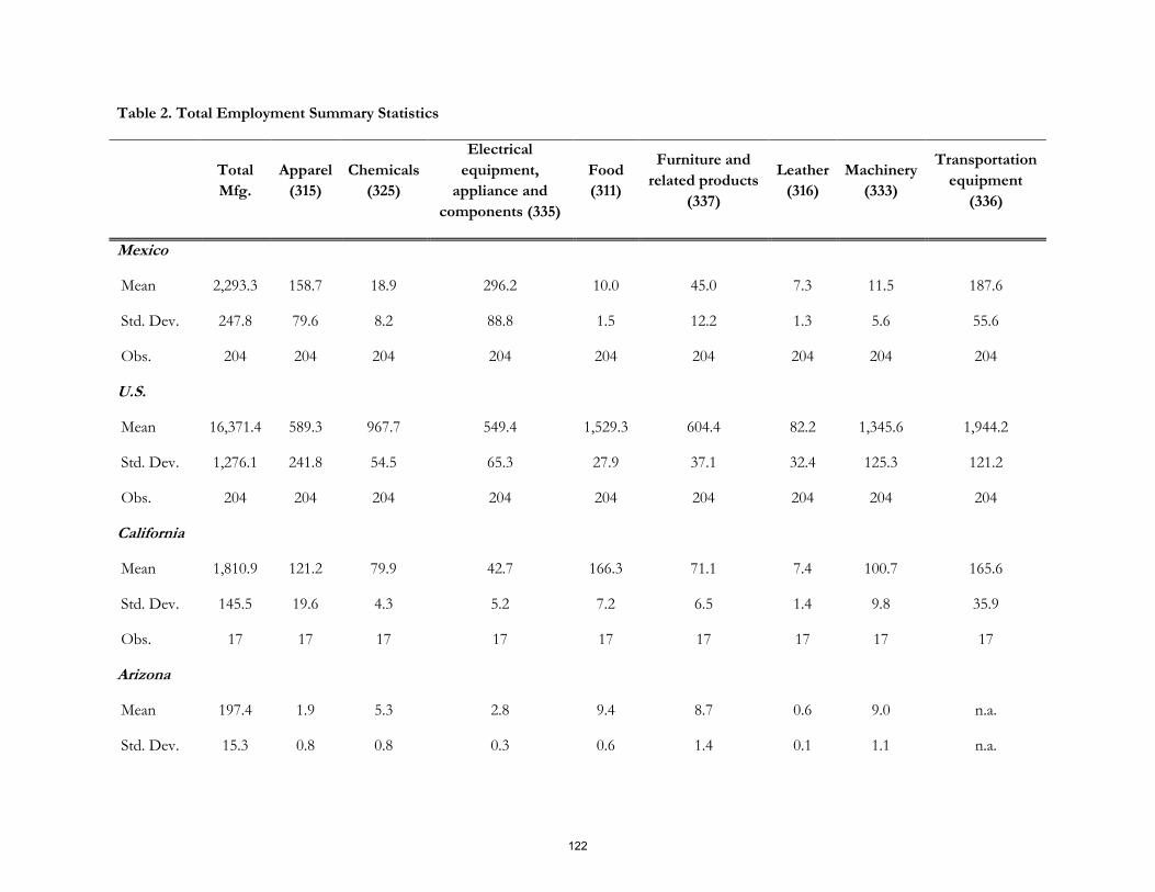
Table 2. Total Employment Summary Statistics
Total
Mfg.
Apparel
(315)
Chemicals
(325)
Electrical
equipment,
appliance and
components (335)
Food
(311)
Furniture and
related products
(337)
Leather
(316)
Machinery
(333)
Transportation
equipment
(336)
Mexico
Mean 2,293.3 158.7 18.9 296.2 10.0 45.0 7.3 11.5 187.6
Std. Dev. 247.8 79.6 8.2 88.8 1.5 12.2 1.3 5.6 55.6
Obs. 204 204 204 204 204 204 204 204 204
U.S.
Mean 16,371.4 589.3 967.7 549.4 1,529.3 604.4 82.2 1,345.6 1,944.2
Std. Dev. 1,276.1 241.8 54.5 65.3 27.9 37.1 32.4 125.3 121.2
Obs. 204 204 204 204 204 204 204 204 204
California
Mean 1,810.9 121.2 79.9 42.7 166.3 71.1 7.4 100.7 165.6
Std. Dev. 145.5 19.6 4.3 5.2 7.2 6.5 1.4 9.8 35.9
Obs. 17 17 17 17 17 17 17 17 17
Arizona
Mean 197.4 1.9 5.3 2.8 9.4 8.7 0.6 9.0 n.a.
Std. Dev. 15.3 0.8 0.8 0.3 0.6 1.4 0.1 1.1 n.a.
122

Obs. 17 17 17 17 17 17 17 17 n.a.
Texas
Mean 1,025.1 40.0 85.4 20.0 95.0 30.3 7.0 81.9 90.1
Std. Dev. 61.0 18.9 5.3 2.6 2.6 4.8 1.2 5.4 5.2
Obs. 17 17 17 17 17 17 17 17 17
Great Lakes
Mean 3,851.5 25.0 188.7 152.7 279.8 127.6 13.5 445.4 n.a.
Std. Dev. 311.2 8.4 5.5 21.4 8.9 8.8 4.6 52.0 n.a.
Obs. 17 17 17 17 17 17 17 17 n.a.
Notes: Data in thousands. NAICS codes in parentheses. For maquiladora and U.S., data is monthly from January 1990 through December 2006.
For the U.S. states data is annual from 1990 through 2006
Sources: For maquiladora data the source is the Instituto Nacional de Estadistica, Geografia e Informatica. For U.S. data the source is the Bureau
of Labor Statistics; and for U.S. state data the source is the Bureau of Economic Analysis
123

Table 3. Production Worker Employment Summary Statistics
Total
Mfg.
Apparel
(315)
Chemicals
(325)
Electrical
equipment,
appliance and
components (335)
Food
(311)
Furniture and
related products
(337)
Leather
(316)
Machinery
(333)
Transportation
equipment
(336)
Mexico
Mean 1,694.2 134.7 15.0 230.9 8.5 36.4 6.1 9.4 147.3
Std. Dev. 198.3 66.9 6.0 68.1 1.4 9.5 1.1 4.5 42.2
Obs. 204 204 204 204 204 204 204 204 204
U.S.
Mean 11,744.3 509.2 571.8 397.9 1,200.9 476.2 68.5 885.6 1,406.2
Std. Dev. 1,021.5 227.1 36.4 55.4 24.0 34.2 29.4 97.6 94.4
Obs. 204 204 204 204 204 204 204 204 204
California
Mean n.a. n.a. n.a. n.a. n.a. n.a. n.a. n.a. n.a.
Std. Dev. n.a. n.a. n.a. n.a. n.a. n.a. n.a. n.a. n.a.
Obs. n.a. n.a. n.a. n.a. n.a. n.a. n.a. n.a. n.a.
Arizona
Mean n.a. n.a. n.a. n.a. n.a. n.a. n.a. n.a. n.a.
Std. Dev. n.a. n.a. n.a. n.a. n.a. n.a. n.a. n.a. n.a.
124
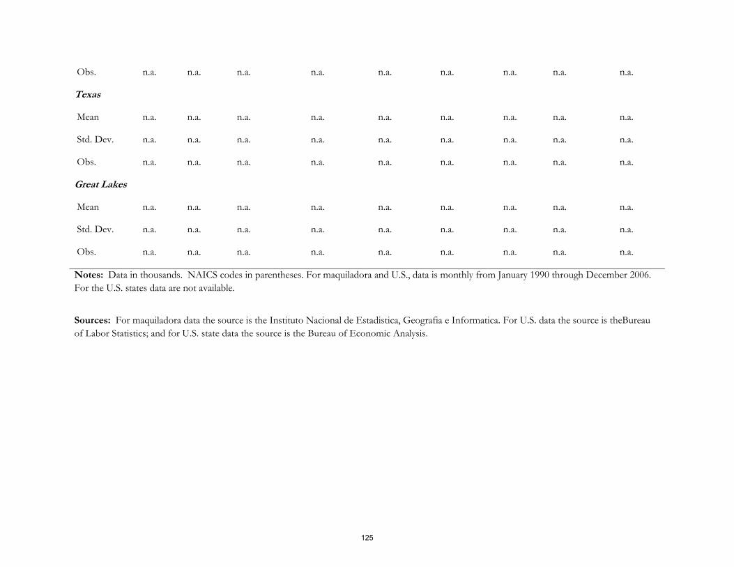
Obs. n.a. n.a. n.a. n.a. n.a. n.a. n.a. n.a. n.a.
Texas
Mean n.a. n.a. n.a. n.a. n.a. n.a. n.a. n.a. n.a.
Std. Dev. n.a. n.a. n.a. n.a. n.a. n.a. n.a. n.a. n.a.
Obs. n.a. n.a. n.a. n.a. n.a. n.a. n.a. n.a. n.a.
Great Lakes
Mean n.a. n.a. n.a. n.a. n.a. n.a. n.a. n.a. n.a.
Std. Dev. n.a. n.a. n.a. n.a. n.a. n.a. n.a. n.a. n.a.
Obs. n.a. n.a. n.a. n.a. n.a. n.a. n.a. n.a. n.a.
Notes: Data in thousands. NAICS codes in parentheses. For maquiladora and U.S., data is monthly from January 1990 through December 2006.
For the U.S. states data are not available.
Sources: For maquiladora data the source is the Instituto Nacional de Estadistica, Geografia e Informatica. For U.S. data the source is theBureau
of Labor Statistics; and for U.S. state data the source is the Bureau of Economic Analysis.
125

Table 4. Output Summary Statistics
Total
Mfg.
Apparel
(315)
Chemicals
(325)
Electrical
equipment,
appliance and
components (335)
Food
(311)
Furniture and
related products
(337)
Leather
(316)
Machinery
(333)
Transportation
equipment
(336)
Mexico
Mean 144,606.9 1,423.4 276.0 4,041.9 190.6 757.7 73.8 181.2 2,458.9
Std. Dev. 16,385.6 809.4 143.4 1,671.1 66.2 370.4 9.1 111.1 936.7
Obs. 204 204 204 204 204 204 204 204 204
U.S.
Mean 88.9 141.7 91.5 102.8 94.0 90.3 164.0 101.8 91.5
Std. Dev. 16.2 39.0 10.5 10.5 7.4 12.0 45.2 11.8 11.9
Obs. 204.0 204.0 204.0 204.0 204.0 204.0 204.0 204.0 204.0
California
Mean 82.7 3.3 6.4 1.9 8.3 1.7 n.a. 4.6 7.4
Std. Dev. 8.8 0.3 2.2 0.5 0.6 0.2 n.a. 0.9 1.4
Obs. 17 17 17 17 17 17 n.a. 17 17
Arizona
Mean 10.6 0.1 0.3 0.1 0.5 0.2 n.a. 0.3 2.2
Std. Dev. 1.7 0.0 0.1 0.0 0.1 0.1 n.a. 0.0 0.5
126

Obs. 17 17 17 17 17 17 n.a. 17 17
Texas
Mean 54.8 1.3 10.1 1.0 4.7 0.7 n.a. 4.0 4.1
Std. Dev. 7.5 0.4 3.3 0.2 0.4 0.1 n.a. 1.0 0.6
Obs. 17 17 17 17 17 17 n.a. 17 17
Great Lakes
Mean 179.8 1.4 17.1 7.8 15.1 4.2 n.a. 18.8 39.3
Std. Dev. 10.8 0.2 2.0 0.8 1.0 0.5 n.a. 2.0 5.1
Obs. 17 17 17 17 17 17 n.a. 17 17
Notes: For maquiladora and U.S., data are monthly from January 1990 through December 2006. For the U.S. states, data are annual from 1990
through 2006. Maquiladora data are in millions of real pesos (CPI 2002=100). U.S. national data corresponds to U.S. Industrial Production
Index, 2002=100. State level data are in billions of real dollars (Chained CPI 1982-84=100).
Sources: For maquiladora data the source is the Instituto Nacional de Estadistica, Geografia e Informatica. For U.S. data the source is the
Federal Reserve Board and for U.S. states the data source is the Bureau of Economic Analysis
127

Table 5. Volatility in Mexico and U.S. Offshoring Industries: Monthly Employment and Output
Electrical Equipment,
Appliance, and
Component
(335)
Transportation
Equipment
(336)
Apparel
(315)
Leather
and Allied
Product
(316)
Furniture
and Related
Product
(337)
Chemical
(325)
Machinery
(333)
Food
(311) Average
TOTAL
EMPLOYMENT
σ(YiMX) 0.33 0.31 0.63 0.18 0.30 0.48 0.52 0.16 0.36
σ(YiUS) 0.13 0.06 0.47 0.43 0.06 0.06 0.10 0.02 0.17
σ(YMX) 0.11 0.11 0.11 0.11 0.11 0.11 0.11 0.11 0.11
σ(YUS) 0.08 0.08 0.08 0.08 0.08 0.08 0.08 0.08 0.08
σ(YiMX) / σ(Yi
US) 2.58 5.01 1.34 0.42 4.94 8.39 5.48 8.69 2.20
σ(YMX) / σ(YUS) 1.34 1.34 1.34 1.34 1.34 1.34 1.34 1.34 1.34
σ(YiMX) / σ(Yi
US) 1.93 3.75 1.00 0.32 3.70 6.28 4.10 6.51 1.65
σ(YMX) / σ(YUS)
PRODUCTION WORKER
EMPLOYMENT
σ(YiMX) 0.32 0.31 0.63 0.19 0.29 0.45 0.52 0.17 0.36
σ(YiUS) 0.15 0.07 0.52 0.47 0.07 0.07 0.11 0.02 0.18
σ(YMX) 0.12 0.12 0.12 0.12 0.12 0.12 0.12 0.12 0.12
128
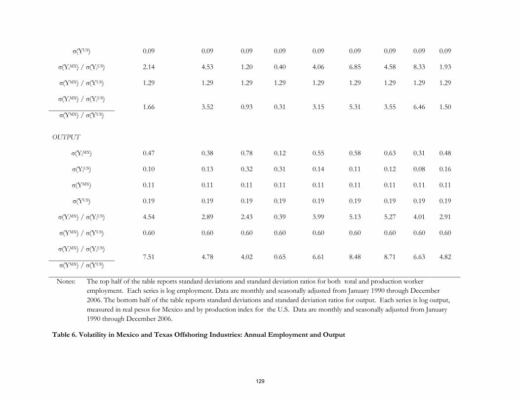
σ(YUS) 0.09 0.09 0.09 0.09 0.09 0.09 0.09 0.09 0.09
σ(YiMX) / σ(Yi
US) 2.14 4.53 1.20 0.40 4.06 6.85 4.58 8.33 1.93
σ(YMX) / σ(YUS) 1.29 1.29 1.29 1.29 1.29 1.29 1.29 1.29 1.29
σ(YiMX) / σ(Yi
US) 1.66 3.52 0.93 0.31 3.15 5.31 3.55 6.46 1.50
σ(YMX) / σ(YUS)
OUTPUT
σ(YiMX) 0.47 0.38 0.78 0.12 0.55 0.58 0.63 0.31 0.48
σ(YiUS) 0.10 0.13 0.32 0.31 0.14 0.11 0.12 0.08 0.16
σ(YMX) 0.11 0.11 0.11 0.11 0.11 0.11 0.11 0.11 0.11
σ(YUS) 0.19 0.19 0.19 0.19 0.19 0.19 0.19 0.19 0.19
σ(YiMX) / σ(Yi
US) 4.54 2.89 2.43 0.39 3.99 5.13 5.27 4.01 2.91
σ(YMX) / σ(YUS) 0.60 0.60 0.60 0.60 0.60 0.60 0.60 0.60 0.60
σ(YiMX) / σ(Yi
US) 7.51 4.78 4.02 0.65 6.61 8.48 8.71 6.63 4.82
σ(YMX) / σ(YUS)
Notes: The top half of the table reports standard deviations and standard deviation ratios for both total and production worker
employment. Each series is log employment. Data are monthly and seasonally adjusted from January 1990 through December
2006. The bottom half of the table reports standard deviations and standard deviation ratios for output. Each series is log output,
measured in real pesos for Mexico and by production index for the U.S. Data are monthly and seasonally adjusted from January
1990 through December 2006.
Table 6. Volatility in Mexico and Texas Offshoring Industries: Annual Employment and Output
129

Electrical Equipment,
Appliance, and
Component
(335)
Transportation
Equipment
(336)
Apparel
(315)
Leather
and Allied
Product
(316)
Furniture
and
Related
Product
(337)
Chemical
(325)
Machinery
(333)
Food
(311) Average
TOTAL EMPLOYMENT
Standard Deviations
σ(YiMX) 0.32 0.31 0.63 0.18 0.30 0.48 0.52 0.14 0.36
σ(YiTX) 0.13 0.06 0.60 0.17 0.16 0.06 0.06 0.03 0.16
σ(YMX) 0.11 0.11 0.11 0.11 0.11 0.11 0.11 0.11 0.11
σ(YTX) 0.06 0.06 0.06 0.06 0.06 0.06 0.06 0.06 0.06
σ(YiMX) / σ(Yi
TX) 2.56 5.65 1.05 1.07 1.82 7.79 8.06 5.24 4.15
σ(YMX) / σ(YTX) 1.85 1.85 1.85 1.85 1.85 1.85 1.85 1.85 1.85
σ(YiMX) / σ(Yi
TX) 1.38 3.06 0.57 0.58 0.98 4.21 4.36 2.84 2.25
σ(YMX) / σ(YTX)
OUTPUT
Standard Deviations
σ(YiMX) 0.46 0.38 0.77 0.10 0.54 0.58 0.63 0.28 0.47
σ(YiTX) 0.19 0.14 0.38 n.a. 0.17 0.28 0.24 0.08 0.21
σ(YMX) 0.11 0.11 0.11 0.11 0.11 0.11 0.11 0.11 0.11
130

σ(YTX) 0.13 0.13 0.13 0.13 0.13 0.13 0.13 0.13 0.13
σ(YiMX) / σ(Yi
TX) 2.45 2.73 2.03 n.a. 3.14 2.06 2.61 3.60 2.66
σ(YMX) / σ(YTX) 0.86 0.86 0.86 0.86 0.86 0.86 0.86 0.86 0.86
σ(YiMX) / σ(Yi
TX) 2.86 3.19 2.38 n.a. 3.68 2.41 3.05 4.21 3.11
σ(YMX) / σ(YTX)
Notes: The top half of the table reports standard deviations and standard deviation ratios for employment. Each series is log employment.
Data are annual from 1990 through 2006. The bottom half of the table reports standard deviations and standard deviation ratios for
output. Each series is log output, measured by real pesos for Mexico and real dollars for Texas.
131

Table 7. Volatility in Mexico and California Offshoring Industries: Annual Employment and Output
Electrical Equipment,
Appliance, and
Component
(335)
Transportation
Equipment
(336)
Apparel
(315)
Leather
and Allied
Product
(316)
Furniture
and
Related
Product
(337)
Chemical
(325)
Machinery
(333)
Food
(311) Average
TOTAL EMPLOYMENT
Standard Deviations
σ(YiMX) 0.32 0.31 0.63 0.18 0.30 0.48 0.52 0.14 0.36
σ(YiCA) 0.12 0.20 0.17 0.20 0.09 0.05 0.10 0.04 0.12
σ(YMX) 0.11 0.11 0.11 0.11 0.11 0.11 0.11 0.11 0.11
σ(YCA) 0.08 0.08 0.08 0.08 0.08 0.08 0.08 0.08 0.08
σ(YiMX) / σ(Yi
CA) 2.76 1.60 3.76 0.88 3.38 9.14 5.42 3.47 3.80
σ(YMX) / σ(YCA) 1.35 1.35 1.35 1.35 1.35 1.35 1.35 1.35 1.35
σ(YiMX) / σ(Yi
CA) 2.05 1.19 2.79 0.66 2.51 6.79 4.02 2.57 2.82
σ(YMX) / σ(YCA)
OUTPUT
Standard Deviations
σ(YiMX) 0.46 0.38 0.77 0.10 0.54 0.58 0.63 0.28 0.47
σ(YiCA) 0.21 0.17 0.08 n.a. 0.13 0.31 0.17 0.07 0.16
132

σ(YMX) 0.11 0.11 0.11 0.11 0.11 0.11 0.11 0.11 0.11
σ(YCA) 0.10 0.10 0.10 0.10 0.10 0.10 0.10 0.10 0.10
σ(YiMX) / σ(Yi
CA) 2.22 2.21 9.16 n.a. 4.23 1.87 3.60 4.22 3.93
σ(YMX) / σ(YCA) 1.13 1.13 1.13 1.13 1.13 1.13 1.13 1.13 1.13
σ(YiMX) / σ(Yi
CA) 1.96 1.95 8.09 n.a. 3.73 1.65 3.18 3.72 3.47
σ(YMX) / σ(YCA)
Notes: The top half of the table reports standard deviations and standard deviation ratios for employment. Each series is log employment.
Data are annual from 1990 through 2006. The bottom half of the table reports standard deviations and standard deviation ratios for
output. Each series is log output, measured by real pesos for Mexico and real dollars for California.
133
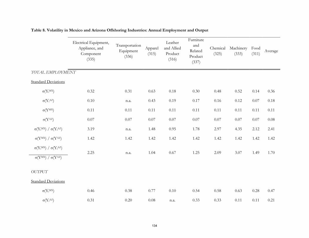
Table 8. Volatility in Mexico and Arizona Offshoring Industries: Annual Employment and Output
Electrical Equipment,
Appliance, and
Component
(335)
Transportation
Equipment
(336)
Apparel
(315)
Leather
and Allied
Product
(316)
Furniture
and
Related
Product
(337)
Chemical
(325)
Machinery
(333)
Food
(311) Average
TOTAL EMPLOYMENT
Standard Deviations
σ(YiMX) 0.32 0.31 0.63 0.18 0.30 0.48 0.52 0.14 0.36
σ(YiAZ) 0.10 n.a. 0.43 0.19 0.17 0.16 0.12 0.07 0.18
σ(YMX) 0.11 0.11 0.11 0.11 0.11 0.11 0.11 0.11 0.11
σ(YAZ) 0.07 0.07 0.07 0.07 0.07 0.07 0.07 0.07 0.08
σ(YiMX) / σ(Yi
AZ) 3.19 n.a. 1.48 0.95 1.78 2.97 4.35 2.12 2.41
σ(YMX) / σ(YAZ) 1.42 1.42 1.42 1.42 1.42 1.42 1.42 1.42 1.42
σ(YiMX) / σ(Yi
AZ) 2.25 n.a. 1.04 0.67 1.25 2.09 3.07 1.49 1.70
σ(YMX) / σ(YAZ)
OUTPUT
Standard Deviations
σ(YiMX) 0.46 0.38 0.77 0.10 0.54 0.58 0.63 0.28 0.47
σ(YiAZ) 0.31 0.20 0.08 n.a. 0.33 0.33 0.11 0.11 0.21
134

σ(YMX) 0.11 0.11 0.11 0.11 0.11 0.11 0.11 0.11 0.11
σ(YAZ) 0.16 0.16 0.16 0.16 0.16 0.16 0.16 0.16 0.16
σ(YiMX) / σ(Yi
AZ) 1.50 1.94 9.30 n.a. 1.65 1.78 5.72 2.45 3.48
σ(YMX) / σ(YAZ) 0.67 0.67 0.67 0.67 0.67 0.67 0.67 0.67 0.67
σ(YiMX) / σ(Yi
AZ) 2.23 2.88 13.83 n.a. 2.46 2.64 8.50 3.65 5.17
σ(YMX) / σ(YAZ)
Notes: The top half of the table reports standard deviations and standard deviation ratios for employment. Each series is log employment.
Data are annual from 1990 through 2006. The bottom half of the table reports standard deviations and standard deviation ratios for
output. Each series is log output, measured by real pesos for Mexico and real dollars for Arizona.
135

Table 9. Volatility in Mexico and Great Lakes Offshoring Industries: Annual Employment and Output
Electrical Equipment,
Appliance, and
Component
(335)
Transportation
Equipment
(336)
Apparel
(315)
Leather
and Allied
Product
(316)
Furniture
and
Related
Product
(337)
Chemical
(325)
Machinery
(333)
Food
(311) Average
TOTAL EMPLOYMENT
Standard Deviations
σ(YiMX) 0.32 0.31 0.63 0.18 0.30 0.48 0.52 0.14 0.36
σ(YiGL) 0.15 n.a. 0.33 0.38 0.07 0.03 0.12 0.03 0.16
σ(YMX) 0.11 0.11 0.11 0.11 0.11 0.11 0.11 0.11 0.11
σ(YGL) 0.08 0.08 0.08 0.08 0.08 0.08 0.08 0.08 0.08
σ(YiMX) / σ(Yi
GL) 2.21 n.a. 1.92 0.47 4.39 16.52 4.43 4.51 4.92
σ(YMX) / σ(YGL) 1.32 1.32 1.32 1.32 1.32 1.32 1.32 1.32 1.32
σ(YiMX) / σ(Yi
GL) 1.68 n.a. 1.46 0.36 3.34 12.55 3.37 3.43 3.74
σ(YMX) / σ(YGL)
OUTPUT
Standard Deviations
σ(YiMX) 0.46 0.38 0.77 0.10 0.54 0.58 0.63 0.28 0.47
136

σ(YiGL) 0.09 0.13 0.13 n.a. 0.12 0.11 0.10 0.07 0.11
σ(YMX) 0.11 0.11 0.11 0.11 0.11 0.11 0.11 0.11 0.11
σ(YGL) 0.06 0.06 0.06 0.06 0.06 0.06 0.06 0.06 0.06
σ(YiMX) / σ(Yi
GL) 5.02 2.83 5.88 n.a. 4.43 5.14 6.11 3.94 4.76
σ(YMX) / σ(YGL) 1.88 1.88 1.88 1.88 1.88 1.88 1.88 1.88 1.88
σ(YiMX) / σ(Yi
GL) 2.67 1.50 3.12 n.a. 2.35 2.73 3.24 2.09 2.53
σ(YMX) / σ(YGL)
Notes: The top half of the table reports standard deviations and standard deviation ratios for employment. Each series is log employment.
Data are annual from 1990 through 2006. The bottom half of the table reports standard deviations and standard deviation ratios for
output. Each series is log output, measured by real pesos for Mexico and real dollars for the Great Lakes region.
137

Table 10. Correlation Coefficients for Mexico and U.S. Offshoring Industries: Monthly Employment and Output
Electrical Equipment,
Appliance, and
Component
(335)
Transportation
Equipment
(336)
Apparel
(315)
Leather and
Allied Product
(316)
Furniture and
Related
Product (337)
Chemical
(325)
Machinery
(333)
Food
(311) Average
TOTAL EMPLOYMENT
corr(YiMX,Yi
US) -0.49 -0.57 -0.72 0.61 0.38 -0.83 -0.53 -0.01 -0.27
corr(YMX,YUS) -0.28 -0.28 -0.28 -0.28 -0.28 -0.28 -0.28 -0.28 -0.28
corr(YiMX,YMX) 0.87 0.82 0.83 0.07 0.84 0.77 0.78 0.47 0.68
corr(YiUS,YUS) 1.00 0.95 0.89 0.87 0.56 0.93 0.95 0.76 0.86
PRODUCTION WORKER
EMPLOYMENT
corr(YiMX,Yi
US) -0.46 -0.39 -0.71 0.55 0.32 -0.71 -0.55 0.31 -0.21
corr(YMX,YUS) -0.26 -0.26 -0.26 -0.26 -0.26 -0.26 -0.26 -0.26 -0.26
corr(YiMX,YMX) 0.89 0.82 0.85 0.16 0.84 0.77 0.77 0.36 0.68
corr(YiUS,YUS) 0.99 0.93 0.89 0.85 0.63 0.98 0.97 0.55 0.85
OUTPUT
corr(YiMX,Yi
US) 0.65 0.93 -0.63 -0.15 0.95 0.94 0.67 0.82 0.52
corr(YMX,YUS) 0.91 0.91 0.91 0.91 0.91 0.91 0.91 0.91 0.91
138

corr(YiMX,YMX) 0.91 0.87 0.85 0.26 0.88 0.90 0.87 0.77 0.79
corr(YiUS,YUS) 0.66 0.97 -0.75 -0.79 0.99 0.96 0.84 0.96 0.48
Notes: The table above shows correlation coefficients. For data details see Table 5.
139

Table 11. Correlation Coefficients for Mexico and Texas Offshoring Industries: Annual Employment and Output
Electrical
Equipment,
Appliance, and
Component
(335)
Transportation
Equipment
(336)
Apparel
(315)
Leather
and
Allied
Product
(316)
Furniture
and
Related
Product
(337)
Chemical
(325)
Machinery
(333)
Food
(311) Average
TOTAL EMPLOYMENT
Correlations
corr(YiMX,Yi
US) 0.92 -0.32 -0.65 0.74 1.05 -0.61 0.87 0.44 0.30
corr(YMX,YUS) 0.25 0.25 0.25 0.25 0.25 0.25 0.25 0.25 0.25
corr(YiMX,YMX) 0.93 0.88 0.88 0.07 0.89 0.82 0.84 0.54 0.73
corr(YiTX,YTX) 0.71 0.04 0.55 0.57 0.24 0.80 0.38 0.38 0.46
OUTPUT
Correlations
corr(YiMX,Yi
US) 0.86 0.75 -0.60 n.a. 1.00 0.55 0.79 0.66 0.57
corr(YMX,YUS) 0.84 0.84 0.84 0.84 0.84 0.84 0.84 0.84 0.84
corr(YiMX,YMX) 0.99 0.94 0.93 0.29 0.96 0.98 0.95 0.91 0.87
corr(YiTX,YTX) 0.78 0.18 -0.68 n.a. 0.77 1.00 1.00 0.55 0.51
Notes: The table above shows correlation coefficients. For data details see Table 6.
140

Table 12. Correlation Coefficients for Mexico and California Offshoring Industries: Annual Employment and Output
Electrical
Equipment,
Appliance, and
Component
(335)
Transportation
Equipment
(336)
Apparel
(315)
Leather
and
Allied
Product
(316)
Furniture
and
Related
Product
(337)
Chemical
(325)
Machinery
(333)
Food
(311) Average
TOTAL EMPLOYMENT
Correlations
corr(YiMX,Yi
US) -0.42 -0.96 -0.34 0.82 0.17 0.97 -0.27 -0.52 -0.07
corr(YMX,YUS) -0.07 -0.07 -0.07 -0.07 -0.07 -0.07 -0.07 -0.07 -0.07
corr(YiMX,YMX) 0.93 0.88 0.88 0.07 0.89 0.82 0.84 0.54 0.73
corr(YiCA,YCA) 0.99 0.79 0.87 0.78 0.80 -0.46 0.94 0.74 0.68
OUTPUT
Correlations
corr(YiMX,Yi
US) 0.62 -0.56 -0.01 n.a. 0.90 0.90 0.27 -0.02 0.30
corr(YMX,YUS) 0.68 0.68 0.68 0.68 0.68 0.68 0.68 0.68 0.68
corr(YiMX,YMX) 0.99 0.94 0.93 0.29 0.96 0.98 0.95 0.91 0.87
corr(YiCA,YCA) 0.94 -0.25 0.70 n.a. 0.80 0.34 0.92 0.00 0.50
Notes: The table above shows correlation coefficients. For data details see Table 7.
141

Table 13. Correlation Coefficients for Mexico and Arizona Offshoring Industries: Annual Employment and Output
Electrical
Equipment,
Appliance, and
Component
(335)
Transportation
Equipment
(336)
Apparel
(315)
Leather
and
Allied
Product
(316)
Furniture
and
Related
Product
(337)
Chemical
(325)
Machinery
(333)
Food
(311) Average
TOTAL EMPLOYMENT
Correlations
corr(YiMX,Yi
US) 0.29 n.a. -0.92 0.33 1.00 -0.53 0.45 0.44 0.15
corr(YMX,YUS) 0.65 0.65 0.65 0.65 0.65 0.65 0.65 0.65 0.65
corr(YiMX,YMX) 0.93 0.88 0.88 0.07 0.89 0.82 0.84 0.54 0.73
corr(YiAZ,YAZ) 0.74 n.a. -0.37 -0.19 0.73 0.38 1.01 0.39 0.38
OUTPUT
Correlations
corr(YiMX,Yi
US) 0.75 0.14 -0.26 n.a. 0.99 0.02 -0.35 0.01 0.19
corr(YMX,YUS) 0.30 0.30 0.30 0.30 0.30 0.30 0.30 0.30 0.30
corr(YiMX,YMX) 0.99 0.94 0.93 0.29 0.96 0.98 0.95 0.91 0.87
corr(YiAZ,YAZ) 0.91 0.46 -0.47 n.a. 0.58 0.59 -0.29 0.50 0.32
Notes: The table above shows correlation coefficients. For data details see Table 8.
142
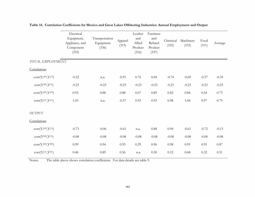
Table 14. Correlation Coefficients for Mexico and Great Lakes Offshoring Industries: Annual Employment and Output
Electrical
Equipment,
Appliance, and
Component
(335)
Transportation
Equipment
(336)
Apparel
(315)
Leather
and
Allied
Product
(316)
Furniture
and
Related
Product
(337)
Chemical
(325)
Machinery
(333)
Food
(311) Average
TOTAL EMPLOYMENT
Correlations
corr(YiMX,Yi
US) -0.52 n.a. -0.91 0.76 0.04 -0.74 -0.69 -0.37 -0.35
corr(YMX,YUS) -0.23 -0.23 -0.23 -0.23 -0.23 -0.23 -0.23 -0.23 -0.23
corr(YiMX,YMX) 0.93 0.88 0.88 0.07 0.89 0.82 0.84 0.54 0.73
corr(YiGL,YGL) 1.03 n.a. -0.37 0.93 0.93 0.98 1.04 0.97 0.79
OUTPUT
Correlations
corr(YiMX,Yi
US) -0.73 -0.06 -0.61 n.a. 0.88 0.94 -0.61 -0.72 -0.13
corr(YMX,YUS) -0.08 -0.08 -0.08 -0.08 -0.08 -0.08 -0.08 -0.08 -0.08
corr(YiMX,YMX) 0.99 0.94 0.93 0.29 0.96 0.98 0.95 0.91 0.87
corr(YiGL,YGL) 0.46 0.89 0.56 n.a. 0.50 0.12 0.68 0.32 0.51
Notes: The table above shows correlation coefficients. For data details see table 9.
143

Table 15. Regression results for variation in Mexico and U.S. Offshoring Industries: Monthly Total Employment
Electrical Equipment,
Appliance, and
Component
(335)
Transportation
Equipment
(336)
Apparel
(315)
Leather and
Allied Product
(316)
Furniture and
Related
Product (337)
Chemical
(325)
Machinery
(333)
Food
(311)
Constant 0.0065** 0.0065*** 0.0065 0.0065 0.0065** 0.0065 0.0065 0.0065***
(0.0033) (0.0027) (0.0147) (0.0055) (0.0031) (0.0089) (0.0064) (0.0012)
Mexico 0.0051 0.0051 0.0051 0.0051 0.0051 0.0051 0.0051 0.0051***
(0.0047) (0.0038) (0.0208) (0.0078) (0.0044) (0.0125) (0.0091) (0.0018)
Offshoring
Industry 0.0094** -0.0026 0.2169*** 0.1806*** -0.0029 -0.0032 0.0026
-
0.0062***
(0.0047) (0.0038) (0.0208) (0.0078) (0.0044) (0.0125) (0.0091) (0.0018)
Mexico times
Offshoring
0.0847*** 0.0898*** 0.1725*** -0.1587*** 0.0798*** 0.2227*** 0.2573*** 0.0198***
(0.0066) (0.0054) (0.0294) (0.0110) (0.0062) (0.0177) (0.0128) (0.0025)
R-squared 0.57 0.62 0.55 0.60 0.50 0.46 0.69 0.39
Adjusted
R-Squared
0.56 0.62 0.54 0.59 0.50 0.45 0.69 0.39
Number of 816 816 816 816 816 816 816 816
144

Observations
Notes: Each column reports ordinary least squares results for a regression of the monthly squared deviation from the mean of log total
employment for the period January 1990 through 2006. Regressors include a constant term, country dummy, offshoring
industry dummy, and interaction term between country and offshoring dummies. Seasonally adjusted data were employed.
Standard errors are in parenthesis. Standard errors are obtained through bootstrapping, using 10,000 repetitions. *** indicates
significant at 1% level; ** indicates significant at 5% level; and * indicates significant at the 10% level.
145

Table 16. Regression results for variation in Mexico and U.S. Offshoring Industries: Monthly Production Worker Employment
Electrical Equipment,
Appliance, and
Component
(335)
Transportation
Equipment
(336)
Apparel
(315)
Leather and
Allied Product
(316)
Furniture and
Related
Product (337)
Chemical
(325)
Machinery
(333) Food (311)
Constant 0.0065* 0.0065*** 0.0081 0.0081 0.0081*** 0.0081 0.0081 0.0081***
(0.0035) (0.0027) (0.0154) (0.0064) (0.0031) (0.0081) (0.0066) (0.0014)
Mexico 0.0051 0.0051 0.0054 0.0054 0.0054 0.0054 0.0054 0.0054***
(0.0049) (0.0038) (0.0218) (0.0091) (0.0043) (0.0114) (0.0093) (0.0020)
Offshoring
Industry
0.0158*** -0.0019 0.2659*** 0.2135*** -0.0032 -0.0039 0.0047 -0.0077***
(0.0049) (0.0038) (0.0218) (0.0091) (0.0043) (0.0114) (0.0093) (0.0020)
Mexico times
Offshoring
0.0747*** 0.0838*** 0.1147*** -0.1918*** 0.0714*** 0.189*** 0.2503*** 0.0219***
(0.0069) (0.0053) (0.0309) (0.0129) (0.0061) (0.0161) (0.0131) (0.0028)
R-squared 0.53 0.61 0.54 0.60 0.48 0.43 0.67 0.39
Adjusted
R-Squared
0.53 0.61 0.54 0.60 0.48 0.43 0.67 0.39
Number of
Observations
816 816 816 816 816 816 816 816
146

Notes: Each column reports ordinary least squares results for a regression of the monthly squared deviation from the mean of log
production workers employment for the period January 1990 through 2006. Regressors include a constant term, country dummy,
offshoring industry dummy, and interaction term between country and offshoring dummies. Seasonally adjusted data were
employed. Standard errors are in parenthesis. Standard errors are obtained through bootstrapping, using 10,000 repetitions. ***
indicates significant at 1% level; ** indicates significant at 5% level; and * indicates significant at the 10% level.
147

Table 17. Regression results for variation in Mexico and U.S. Offshoring Industries: Monthly Output
Electrical Equipment,
Appliance, and
Component
(335)
Transportation
Equipment
(336)
Apparel
(315)
Leather and
Allied
Product
(316)
Furniture and
Related
Product (337)
Chemical
(325)
Machinery
(333)
Food
(311)
Constant 0.0359*** 0.0359*** 0.03591* 0.0359*** 0.0359*** 0.0359*** 0.0359*** 0.0359***
(0.0053) (0.0043) (0.0186) (0.0030) (0.0078) (0.0122) (0.0107) (0.0053)
Mexico
-0.0228*** -0.0228*** -0.0228 -0.0228*** -0.0228** -0.0228 -0.0228
-
0.0228***
(0.0075) (0.0060) (0.0262) (0.0042) (0.0110) (0.0172) (0.0152) (0.0075)
Offshoring
Industry -0.0254*** -0.0184*** 0.0657*** 0.0592*** -0.0171 -0.0230 -0.0215
-
0.0298***
(0.0075) (0.0060) (0.0262) (0.0042) (0.0110) (0.0172) (0.0152) (0.0075)
Mexico times
Offshoring
0.2292*** 0.1513*** 0.5221*** -0.0576*** 0.3044*** 0.3499*** 0.4077*** 0.1148***
(0.0106) (0.0085) (0.0371) (0.0059) (0.0156) (0.0244) (0.0215) (0.0106)
R-squared 0.68 0.61 0.57 0.60 0.65 0.49 0.63 0.33
Adjusted
R-Squared
0.68 0.61 0.57 0.60 0.65 0.49 0.63 0.33
148

Number of
Observations
816 816 816 816 816 816 816 816
Notes: Each column reports ordinary least squares results for a regression of the monthly squared deviation from the mean of log
output for the period January 1990 through 2006. Regressors include a constant term, country dummy, offshoring industry
dummy, and interaction term between country and offshoring dummies. Inflation- and seasonally-adjusted adjusted data were
employed. Standard errors are in parenthesis. Standard errors are obtained through bootstrapping, using 10,000 repetitions.
*** indicates significant at 1% level; ** indicates significant at 5% level; and * indicates significant at the 10% level.
149

Table 18. Regression results for variation in Mexico and Texas Offshoring Industries: Annual Employment
Electrical Equipment,
Appliance, and
Component
(335)
Transportation
Equipment
(336)
Apparel
(315)
Leather
and Allied
Product
(316)
Furniture
and
Related
Product
(337)
Chemical
(325)
Machinery
(333)
Food
(311)
Constant 0.0033 0.0033 0.0033 0.0033 0.0033 0.0033 0.0033 0.0033
(0.0114) (0.0090) (0.0668) (0.0056) (0.0111) (0.0307) (0.0221) (0.0033)
Mexico 0.0080 0.0080 0.0080 0.0080 0.0800 0.0080 0.0080 0.008*
(0.0161) (0.0127) (0.0945) (0.0079) (0.0157) (0.0434) (0.0312) (0.0046)
Offshoring
Industry
0.0127 -0.0003 0.3566*** 0.0246*** 0.0231 0.0004 0.0008 -0.0026
(0.0161) (0.0127) (0.0945) (0.0079) (0.0157) (0.0434) (0.0312) (0.0046)
Mexico times
Offshoring
0.0805*** 0.0866*** 0.0302 -0.004 0.0529*** 0.2164*** 0.2573*** 0.0112*
(0.0228) (0.0179) (0.1336) (0.0112) (0.0223) (0.0614) (0.0441) (0.0065)
R-squared 0.58 0.65 0.50 0.49 0.51 0.46 0.70 0.44
Adjusted
R-Squared
0.56 0.63 0.48 0.46 0.49 0.44 0.68 0.41
Number of 816 816 816 816 816 816 816 816
150

Observations
Notes: Each column reports ordinary least squares results for a regression of the annual squared deviation from the mean of log
employment for the period 1990 through 2006. Regressors include a constant term, country dummy, offshoring industry
dummy, and interaction term between country and offshoring dummies. Standard errors are in parenthesis. Standard
errors are obtained through bootstrapping, using 10,000 repetitions. *** indicates significant at 1% level; ** indicates
significant at 5% level; and * indicates significant at the 10% level.
151

Table 19. Regression results for variation in Mexico and Texas Offshoring Industries: Annual Output
Electrical Equipment,
Appliance, and
Component
(335)
Transportation
Equipment
(336)
Apparel
(315)
Leather
and Allied
Product
(316)
Furniture
and
Related
Product
(337)
Chemical
(325)
Machinery
(333)
Food
(311)
Constant 0.0168 0.0168 0.0168 n.a. 0.0168 0.0168 0.0168 0.0168
(0.0194) (0.0144) (0.0678)
(0.0271) (0.0435) (0.0375) (0.0135)
Mexico -0.0045 -0.0045 -0.0045 n.a. -0.0045 -0.0045 -0.0045 -0.0045
(0.0274) (0.0204) (0.0959)
(0.0383) (0.0616) (0.0530) (0.0190)
Offshoring
Industry
0.0189 0.0024 0.1270 n.a. 0.0132 0.0619 0.0411 -0.0109
(0.0274) (0.0204) (0.0959)
(0.0383) (0.0616) (0.0530) (0.0190)
Mexico times
Offshoring
0.1831*** 0.1287*** 0.4562*** n.a. 0.2715*** 0.2601*** 0.341*** 0.0747***
(0.0388) (0.0289) (0.1357)
(0.0542) (0.0871) (0.0749) (0.0269)
R-squared 0.66 0.61 0.56 n.a. 0.65 0.49 0.64 0.35
Adjusted
R-Squared
0.65 0.60 0.54 n.a. 0.64 0.47 0.62 0.32
Number of 816 816 816 n.a. 816 816 816 816
152

Observations
Notes: Each column reports ordinary least squares results for a regression of the annual squared deviation from the mean of log
output for the period 1990 through 2006. Regressors include a constant term, country dummy, offshoring industry
dummy, and interaction term between country and offshoring dummies. Standard errors are in parenthesis. Standard
errors are obtained through bootstrapping, using 10,000 repetitions. *** indicates significant at 1% level; ** indicates
significant at 5% level; and * indicates significant at the 10% level.
153

Table 20. Regression results for variation in Mexico and California Offshoring Industries: Annual Employment
Electrical Equipment,
Appliance, and
Component
(335)
Transportation
Equipment
(336)
Apparel
(315)
Leather
and Allied
Product
(316)
Furniture
and
Related
Product
(337)
Chemical
(325)
Machinery
(333)
Food
(311)
Constant 0.0062 0.0062 0.0062 0.0062 0.0062 0.0062 0.0062 0.0062*
(0.0115) (0.0109) (0.0463) (0.0078) (0.0107) (0.0308) (0.0221) (0.0035)
Mexico 0.0051 0.0051 0.0051 0.0051 0.0051 0.0051 0.0051 0.0051
(0.0163) (0.0154) (0.0655) (0.0110) (0.0151) (0.0435) (0.0313) (0.0047)
Offshoring
Industry
0.0075 0.0318** 0.0219 0.0347*** 0.0014 -0.0035 0.0029 -0.0046
(0.0163) (0.0154) (0.0655) (0.0110) (0.0151) (0.0435) (0.0313) (0.0047)
Mexico times
Offshoring
0.0857*** 0.0545*** 0.3650 -0.0141 0.0745*** 0.2204*** 0.2552*** 0.0132**
(0.0230) (0.0218) (0.0926) (0.0156) (0.0213) (0.0615) (0.0442) (0.0067)
R-squared 0.57 0.59 0.54 0.42 0.52 0.46 0.70 0.44
Adjusted
R-Squared
0.55 0.57 0.51 0.40 0.49 0.44 0.68 0.41
154

Number of
Observations
816 816 816 816 816 816 816 816
Notes: Each column reports ordinary least squares results for a regression of the annual squared deviation from the mean of
log employment for the period 1990 through 2006. Regressors include a constant term, country dummy, offshoring
industry dummy, and interaction term between country and offshoring dummies. Standard errors are in parenthesis.
Standard errors are obtained through bootstrapping, using 10,000 repetitions. *** indicates significant at 1% level; **
indicates significant at 5% level; and * indicates significant at the 10% level.
155

Table 21. Regression results for variation in Mexico and California Offshoring Industries: Annual Output
Electrical Equipment,
Appliance, and
Component
(335)
Transportation
Equipment
(336)
Apparel
(315)
Leather
and Allied
Product
(316)
Furniture
and
Related
Product
(337)
Chemical
(325)
Machinery
(333)
Food
(311)
Constant 0.0096 0.0096 0.0096 n.a. 0.0096 0.0096 0.0096 0.0096
(0.0207) (0.0153) (0.0641)
(0.0269) (0.0426) (0.0369) (0.0133)
Mexico 0.0027 0.0027 0.0027 n.a. 0.0027 0.0027 0.0027 0.0027
(0.0293) (0.0216) (0.0906)
(0.0380) (0.0602) (0.0522) (0.0188)
Offshoring
Industry
0.0338 0.0198 -0.0025 n.a. 0.0070 0.0861 0.0209 -0.0053
(0.0293) (0.0216) (0.0906)
(0.0380) (0.0602) (0.0522) (0.0188)
Mexico times
Offshoring
0.1683*** 0.1113*** 0.5857*** n.a. 0.2776*** 0.2359*** 0.3613*** 0.0691***
(0.0415) (0.0305) (0.1282)
(0.0537) (0.0851) (0.0739) (0.0266)
R-squared 0.63 0.59 0.57 n.a. 0.66 0.51 0.64 0.35
Adjusted
R-Squared
0.62 0.57 0.55 n.a. 0.64 0.49 0.62 0.32
Number of 816 816 816 n.a. 816 816 816 816
156

Observations
Notes: Each column reports ordinary least squares results for a regression of the annual squared deviation from the mean of log
output for the period 1990 through 2006. Regressors include a constant term, country dummy, offshoring industry
dummy, and interaction term between country and offshoring dummies. Standard errors are in parenthesis. Standard
errors are obtained through bootstrapping, using 10,000 repetitions. *** indicates significant at 1% level; ** indicates
significant at 5% level; and * indicates significant at the 10% level.
157

Table 22. Regression results for variation in Mexico and Arizona Offshoring Industries: Annual Employment
Electrical Equipment,
Appliance, and
Component
(335)
Transportation
Equipment
(336)
Apparel
(315)
Leather
and Allied
Product
(316)
Furniture
and
Related
Product
(337)
Chemical
(325)
Machinery
(333)
Food
(311)
Constant 0.0056 n.a. 0.0056 0.0056 0.0056 0.0056 0.0056 0.0056*
(0.0114)
(0.0493) (0.0066) (0.0116) (0.0309) (0.0221) (0.0034)
Mexico 0.0057 n.a. 0.0057 0.0057 0.0057 0.0057 0.0057 0.0057
(0.0161)
(0.0698) (0.0093) (0.0164) (0.0437) (0.0313) (0.0048)
Offshoring
Industry
0.0046 n.a. 0.176*** 0.0299*** 0.0220 0.0202 0.0086 -0.0012
(0.0161)
(0.0698) (0.0093) (0.0164) (0.0437) (0.0313) (0.0048)
Mexico times
Offshoring
0.0886*** n.a. 0.2108** -0.0093 0.0539** 0.1966*** 0.2495*** 0.0098
(0.0227)
(0.0987) (0.0132) (0.0214) (0.0617) (0.0443) (0.0067)
R-squared 0.57 n.a. 0.55 0.47 0.50 0.46 0.70 0.44
Adjusted
R-Squared
0.55 n.a. 0.53 0.44 0.47 0.44 0.68 0.41
158

Number of
Observations
816 n.a. 816 816 816 816 816 816
Notes: Each column reports ordinary least squares results for a regression of the annual squared deviation from the mean of
log employment for the period 1990 through 2006. Regressors include a constant term, country dummy, offshoring
industry dummy, and interaction term between country and offshoring dummies. Standard errors are in parenthesis.
Standard errors are obtained through bootstrapping, using 10,000 repetitions. *** indicates significant at 1% level; **
indicates significant at 5% level; and * indicates significant at the 10% level.
159

Table 23. Regression results for variation in Mexico and Arizona Offshoring Industries: Annual Output
Electrical Equipment,
Appliance, and
Component
(335)
Transportation
Equipment
(336)
Apparel
(315)
Leather
and Allied
Product
(316)
Furniture
and
Related
Product
(337)
Chemical
(325)
Machinery
(333)
Food
(311)
Constant 0.0272 0.0272* 0.0272 n.a. 0.0272 0.0272 0.0272 0.0272*
(0.0259) (0.0164) (0.0642)
(0.0311) (0.0435) (0.0364) (0.0133)
Mexico -0.0149 -0.0149 -0.0149 n.a. -0.0149 -0.0149 -0.0149 -0.0149
(0.0366) (0.0232) (0.0909)
(0.0440) (0.0616) (0.0515) (0.0188)
Offshoring
Industry
0.0678* 0.0110 -0.0203 n.a. 0.08138* 0.0788 -0.0151 -0.0146
(0.0366) (0.0232) (0.0909)
(0.0440) (0.0616) (0.0515) (0.0188)
Mexico times
Offshoring
0.1342*** 0.1201*** 0.60357*** n.a. 0.2033*** 0.2432*** 0.3973*** 0.0783***
(0.0518) (0.0328) (0.1285)
(0.0623) (0.0871) (0.0728) (0.0266)
R-squared 0.56 0.57 0.57 n.a. 0.62 0.50 0.65 0.36
Adjusted
R-Squared
0.54 0.55 0.55 n.a. 0.60 0.48 0.63 0.33
160

Number of
Observations
816 816 816 n.a. 816 816 816 816
Notes: Each column reports ordinary least squares results for a regression of the annual squared deviation from the mean of log
output for the period 1990 through 2006. Regressors include a constant term, country dummy, offshoring industry
dummy, and interaction term between country and offshoring dummies. Standard errors are in parenthesis. Standard
errors are obtained through bootstrapping, using 10,000 repetitions. *** indicates significant at 1% level; ** indicates
significant at 5% level; and * indicates significant at the 10% level.
161

Table 24. Regression results for variation in Mexico and Great Lakes Offshoring Industries: Annual Employment
Electrical Equipment,
Appliance, and
Component
(335)
Transportation
Equipment
(336)
Apparel
(315)
Leather
and Allied
Product
(316)
Furniture
and
Related
Product
(337)
Chemical
(325)
Machinery
(333)
Food
(311)
Constant 0.0065 n.a. 0.0065 0.0065 0.0065 0.0065 0.0065 0.0065*
(0.0117)
(0.0473) (0.0161) (0.0107) (0.0307) (0.0221) (0.0033)
Mexico 0.0048 n.a. 0.0048 0.0048 0.0048 0.0048 0.0048 0.0048
(0.0165)
(0.0668) (0.0228) (0.0151) (0.0435) (0.0313) (0.0047)
Offshoring
Industry
0.0149 n.a. 0.1014 0.1368*** -0.0021 -0.0057 0.0072 -0.0056
(0.0165)
(0.0668) (0.0228) (0.0151) (0.0435) (0.0313) (0.0047)
Mexico times
Offshoring
0.0783*** n.a. 0.2855*** -0.1161*** 0.078*** 0.2226*** 0.251*** 0.0141**
(0.0233)
(0.0945) (0.0322) (0.0214) (0.0615) (0.0443) (0.0067)
R-squared 0.57 n.a. 0.54 0.56 0.52 0.46 0.70 0.44
Adjusted
R-Squared
0.55 n.a. 0.52 0.54 0.49 0.44 0.68 0.41
162

Number of
Observations
816 n.a. 816 816 816 816 816 816
Notes: Each column reports ordinary least squares results for a regression of the annual squared deviation from the mean of log
employment for the period 1990 through 2006. Regressors include a constant term, country dummy, offshoring industry
dummy, and interaction term between country and offshoring dummies. Standard errors are in parenthesis. Standard
errors are obtained through bootstrapping, using 10,000 repetitions. *** indicates significant at 1% level; ** indicates
significant at 5% level; and * indicates significant at the 10% level.
163

Table 25. Regression results for variation in Mexico and Great Lakes Offshoring Industries: Annual Output
Electrical Equipment,
Appliance, and
Component
(335)
Transportation
Equipment
(336)
Apparel
(315)
Leather
and Allied
Product
(316)
Furniture
and
Related
Product
(337)
Chemical
(325)
Machinery
(333)
Food
(311)
Constant 0.0035 0.0035 0.0035 n.a. 0.0035 0.0035 0.0035 0.0035
(0.0180) (0.0142) (0.0640)
(0.0269) (0.0411) (0.0362) (0.0132)
Mexico 0.0088 0.0088 0.0088 n.a. 0.0088 0.0088 0.0088 0.0088
(0.0254) (0.0201) (0.0905)
(0.0380) (0.0581) (0.0512) (0.0187)
Offshoring
Industry
0.0050 0.0145 0.0137 n.a. 0.0117 0.0092 0.0071 0.0014
(0.0254) (0.0201) (0.0905)
(0.0380) (0.0581) (0.0512) (0.0187)
Mexico times
Offshoring
0.197*** 0.1167*** 0.5695*** n.a. 0.273*** 0.3128*** 0.375*** 0.0623***
(0.0359) (0.0284) (0.1280)
(0.0538) (0.0822) (0.0724) (0.0264)
R-squared 0.69 0.62 0.57 n.a. 0.66 0.51 0.65 0.35
Adjusted
R-Squared
0.67 0.60 0.55 n.a. 0.64 0.48 0.63 0.32
Number of 816 816 816 n.a. 816 816 816 816
164

Observations
Notes: Each column reports ordinary least squares results for a regression of the annual squared deviation from the mean of log
output for the period 1990 through 2006. Regressors include a constant term, country dummy, offshoring industry
dummy, and interaction term between country and offshoring dummies. Standard errors are in parenthesis. Standard
errors are obtained through bootstrapping, using 10,000 repetitions. *** indicates significant at 1% level; ** indicates
significant at 5% level; and * indicates significant at the 10% level.
165

Table 26. Regression results for intensive and extensive margins
Total Employment Production Worker Employment
Number of Plants
(Extensive Margin)
Employment per Plant
(Intensive Margin)
Number of Plants
(Extensive Margin)
Employment per Plant
(Intensive Margin)
Share of employment in
industry
0.5355*** 0.4645***
0.5458*** 0.4542***
(0.1069) (0.1069)
(0.1075) (0.1075)
Aggregate Employment 0.3349 0.6651**
0.3929 0.6071**
(0.2627) (0.2627)
(0.2481) (0.2481)
R-squared 0.82 0.58
0.83 0.56
Number of Observations 1632 1632
1632 1632
Notes: Columns report ordinary least squares regression results for a regression of either the number of plants or
employment per plant, both for total employment and production workers employment. The sample period January
1990 through 2006. Seasonally adjusted data were employed. Industry fixed effects were included but are not
reported. Standard errors (clustered by industry) are in parenthesis. *** indicates significant at 1% level; ** indicates
significant at 5% level; and * indicates significant at the 10% level.
166

Figure 1. Log-difference in Output
Notes: Manufacturing output data for Mexico is real in pesos. Manufacturing output data for the U.S. is the total manufacturing production index. Data are seasonally adjusted and log-transformed.
-.15
-.10
-.05
.00
.05
.10
.15
.20
90 92 94 96 98 00 02 04 06
TOTAL_MEXICO TOTAL_US
167

Figure 2. Log-difference in Total Employment
Notes: Total employment data for both Mexico and the U.S. correspond to total manufacturing employment. Data are seasonally adjusted and log-transformed.
Figure 3. Log-difference in Production Worker Employment
-.016
-.012
-.008
-.004
.000
.004
.008
.012
.016
.020
90 92 94 96 98 00 02 04 06
TOTAL_MEXICO TOTAL_US
-.020
-.015
-.010
-.005
.000
.005
.010
.015
.020
90 92 94 96 98 00 02 04 06
TOTAL_MEXICO TOTAL_US
168

Notes: Production worker employment data for both Mexico and the U.S. correspond to manufacturing production worker employment. Data are seasonally adjusted and log-transformed.
Figure 4. Log-difference in Output by Sector
Notes: Output data for Mexico’s offshoring sectors is real in pesos. Output data for the U.S.’ offshoring sectors is production index. Data are seasonally adjusted and log-transformed.
Figure 5. Log-difference in Total Employment by Sector
-.15
-.10
-.05
.00
.05
.10
.15
.20
90 92 94 96 98 00 02 04 06
MAQ_APPAREL US_APPAREL
-.4
-.3
-.2
-.1
.0
.1
.2
.3
.4
90 92 94 96 98 00 02 04 06
MAQ_CHEMICALS US_CHEMICALS
-.20
-.16
-.12
-.08
-.04
.00
.04
.08
.12
.16
90 92 94 96 98 00 02 04 06
MAQ_ELECTRONICS US_ELECTRONICS
-1.5
-1.0
-0.5
0.0
0.5
1.0
1.5
90 92 94 96 98 00 02 04 06
MAQ_FOOD US_FOOD
-.3
-.2
-.1
.0
.1
.2
.3
90 92 94 96 98 00 02 04 06
MAQ_FURNITURE US_FURNITURE
-.5
-.4
-.3
-.2
-.1
.0
.1
.2
.3
90 92 94 96 98 00 02 04 06
MAQ_LEATHER US_LEATHER
-.5
-.4
-.3
-.2
-.1
.0
.1
.2
.3
.4
90 92 94 96 98 00 02 04 06
MAQ_MACHINERY US_MACHINERY
-.15
-.10
-.05
.00
.05
.10
.15
.20
90 92 94 96 98 00 02 04 06
MAQ_TRANSPORTATIONUS_TRANSPORTATION
169

Notes: Total employment data for offshoring sectors in both Mexico and the U.S. correspond to total manufacturing employment. Data are seasonally adjusted and log-transformed.
Figure 6. Log-difference in Production Worker Employment by Sector
-.06
-.04
-.02
.00
.02
.04
.06
.08
90 92 94 96 98 00 02 04 06
MAQ_APPAREL US_APPAREL
-.06
-.04
-.02
.00
.02
.04
.06
.08
.10
.12
90 92 94 96 98 00 02 04 06
MAQ_CHEMICALS US_CHEMICALS
-.06
-.04
-.02
.00
.02
.04
.06
90 92 94 96 98 00 02 04 06
MAQ_ELECTRONICS US_ELECTRONICS
-.4
-.2
.0
.2
.4
.6
90 92 94 96 98 00 02 04 06
MAQ_FOOD US_FOOD
-.06
-.04
-.02
.00
.02
.04
.06
.08
90 92 94 96 98 00 02 04 06
MAQ_FURNITURE US_FURNITURE
-.100
-.075
-.050
-.025
.000
.025
.050
.075
.100
90 92 94 96 98 00 02 04 06
MAQ_LEATHER US_LEATHER
-.16
-.12
-.08
-.04
.00
.04
.08
.12
.16
.20
90 92 94 96 98 00 02 04 06
MAQ_MACHINERY US_MACHINERY
-.08
-.04
.00
.04
.08
.12
.16
90 92 94 96 98 00 02 04 06
MAQ_TRANSPORTATIONUS_TRANSPORTATION
170

Notes: Production worker employment data for offshoring sectors in both Mexico and the U.S. correspond to manufacturing production worker employment. Data are seasonally adjusted and log-transformed.
-.06
-.04
-.02
.00
.02
.04
.06
.08
90 92 94 96 98 00 02 04 06
MAQ_APPAREL US_APPAREL
-.08
-.04
.00
.04
.08
.12
90 92 94 96 98 00 02 04 06
MAQ_CHEMICALS US_CHEMICALS
-.05
-.04
-.03
-.02
-.01
.00
.01
.02
.03
.04
90 92 94 96 98 00 02 04 06
MAQ_ELECTRONICS US_ELECTRONICS
-.6
-.4
-.2
.0
.2
.4
.6
90 92 94 96 98 00 02 04 06
MAQ_FOOD US_FOOD
-.08
-.06
-.04
-.02
.00
.02
.04
.06
.08
90 92 94 96 98 00 02 04 06
MAQ_FURNITURE US_FURNITURE
-.12
-.08
-.04
.00
.04
.08
.12
90 92 94 96 98 00 02 04 06
MAQ_LEATHER US_LEATHER
-.16
-.12
-.08
-.04
.00
.04
.08
.12
.16
90 92 94 96 98 00 02 04 06
MAQ_MACHINERY US_MACHINERY
-.15
-.10
-.05
.00
.05
.10
.15
90 92 94 96 98 00 02 04 06
MAQ_TRANSPORTATIONUS_TRANSPORTATION
171

THIS PAGE INTENTIONALLY LEFT BLANK
172
Managing an Online Training Program for ICT Skills
Development in Business Professors
Gabriela Farías Martínez, Instituto Tecnologico y de Estudios Superiores de Monterrey
Norma Pedraza,
Universidad Autonoma de Tamaulipas
Jesus Lavin, Universidad Autonoma de Tamaulipas
ABSTRACT
We present the results of research with focus on describing the experience of an online training program aimed at teachers of schools and business schools. This course was designed to develop competencies related to information and communication technologies. Which was used in the CUDI network for Internet 2 videoconferencing and SAKAI learning platform for the management of the educational intervention. The results show the opportunities and difficulties encountered in the development of this program and profile characteristics of teachers whom actually had an advantage of this experience. Participants reported that administrative, academic and technology coordination is essential to improve achievement, the commitment of timely responses feedback from tutors and improve the organization of courses in instructional design and timing of activities. Female professors exceeded the performance of activities with respect to their male colleagues. It would be interesting to investigate in a subsequent study, the extent to which gender determines the attitudes and dispositions towards technology. Also, the results of this research show, that in spite of biological age, the more teaching experience, the greater use of technological resources, previously considered a positive disposition towards them.
173

THIS PAGE INTENTIONALLY LEFT BLANK
174

Agile Development of a Virtual Teaching Assistant System for Students in Stem Field
Pablo Biswas, Texas A&M International University
Runchang Lin, Texas A&M International University
Avinash Venna, Texas A&M International University
Induja Rompicherla, Texas A&M International University
ABSTRACT
This research describes a case study of a project to develop a web-based Virtual Teaching Assistant System (ViTAS) for college students and instructors in Science, Technology, Engineering, and Mathematics (STEM) fields at Texas A&M International University (TAMIU). ViTAS, a digital homework assignments submission and grading system, is an innovative idea to provide homework assignments grading system for the instructors and to provide an interactive learning environment outside the lecture period for the students. Using ViTAS, students will be able to submit the homework assignments online, to engage in anonymous homework review, and to discuss with their peers. Usually in south Texas universities, the students in their freshman and sophomore years have trouble coping with the initial STEM courses. This system also helps the instructors finalize all grades and post them on the website to confirm the students’ learning activities. In particular, this project focuses on the Agile software development process. Also, the research considers that the teams are working cooperatively rather than collaboratively and this cooperation is implemented via articulation work, meaning that the developers had additional tasks to ensure that the user-experience design is accomplished.
Key words: Agile methodology, virtual teaching assistant, user experience design.
175

THIS PAGE INTENTIONALLY LEFT BLANK
176

Are US Academics and Professionals Ready for IFRS?
Murad Moqbel, Texas A&M International University
Peerayuth Charoensukmongkol, Texas A&M International University
Aziz Bakay,
Texas A&M International University
ABSTRACT International Financial Reporting Standards (IFRS) have been adopted by several countries around the world as a common accounting and financial language. However, the US is yet to do so. In this study, in our turn, we examine whether the US academics (accounting and auditing students and professors) as well as practitioners (auditors, accountants, CPAs, and financial analysts) are ready to embrace IFRS as a common accounting and financial reporting language. We discuss the extent to which they are familiar and ready for IFRS as well as their perception about the benefits and challenges in adopting IFRS. We further touch on IFRS Benefits and Challenges, IFRS education, training, and information technology Role.
177

Are US Academics and Professionals Ready for IFRS?
INTRODUCTION AND BACKGROUND The fast pace of globalization and the international financial markets have stimulated the need for a common financial language. This common language is IFRS which is under the auspice of the International accounting Standards Board (IASB), an independent accounting standard-setting body based on London. The IASB morphed from another organization called the international accounting Standards Committee (IASC) that was established in 1973 (Kennedy 2010). Several countries around the world have already adopted IFRS and few are to follow. Around 120 countries have completely or partially embraced International Financial Reporting Standards (IFRS 2010). The European Union has made it mandatory for publicly traded companies to use IFRS to prepare their financial statements (Brackney and Witmer 2005). Other countries soon to follow include Canada and Korea which announced to adopt IFRS by 2011. Mexico is planning to require all listed companies to report using IFRS in 2012. As for the USA, the Financial Accounting Standards Board (FASB) and the International Accounting Standards Board (IASB) in their meeting in September 2002 reached an agreement, called the Norwalk agreement, to converge on a single set of accounting standards. They also agreed to make their existing financial reporting standards fully compatible and to coordinate their future work programs to maintain that compatibility (Hermann and Ian 2006). There around 11,000 firms registered with the U.S. Securities and Exchange Commission (SEC), of which about 1,100 are non-U.S. companies (Oracle Corporation 2008). In 2005, U.S. SEC allowed non-U.S. firms to submit their financial statements in compliance with either U.S. GAAP or IFRS; on the condition they reconcile discrepancies in the results between the two. But in 2007, the U.S. SEC voted to drop the reconciliation requirement for financial statements for the year 2007 (Smith 2008). The United States was scheduled to require all publicly traded companies to prepare their financial statements based on IFRS by 2014 as it was announced by the U.S. SEC in 2008 (Kennedy 2010). However, the U.S. SEC decided in February 2010 that 2015 might be the earliest possible date for IFRS adoption by the U.S., calling for more study of IFRS (Defelice and lamoreaux 2010). The US Generally Accepted Accounting Principles (U.S. GAAP) and International Financial Reporting Standards have some similarities and differences. One of the differences is that U.S. GAAP is rule-based of standards while IFRS is more of a principle-based set of standards (Arthur 2005). The US GAAP is intended to enforce compliance by having detailed rules, while IFRS is intended to improve transparency yet subject to implementers’ judgment. This study attempts to examine whether the US academics (accounting and auditing students and professors) as well as practitioners (auditors, accountants, CPAs, and financial analysts) are ready to converge to IFRS as a common accounting and financial reporting language. We do this by surveying and collecting data on the perception of a sample of academics and practitioners regarding familiarity, readiness, benefits and challenges, and proper plans to be used in the process of convergence in accounting standards. Results shows that (1) the majority of respondents believe that auditors, accountants, and accounting students are ready for the convergence to IFRS; (2) convergence to IFRS can increase global comparability; minimize barriers to global competition for capital, enable investors to evaluate investment options in a global marketplace, enable management and auditors to exercise more professional judgment, create uniformity in global financial reporting including audit reports; (3) initial cost of convergence, required changes in auditing standards, perceived uncertainties surrounding IFRS, lack of sufficient involvement of global regulators in the IASB standard-setting process, transition plan and issues pertaining to IFRS, lack of education, understanding, and experience by preparers of financial reports with the use of IFRS, lack of coverage of IFRS in financial accounting textbooks, lack of coverage of International Standards on Auditing (ISAs) in auditing textbooks should be taken into consideration when making a decision about whether to adopt IFRS or not; (4) a proper plan to transition all U.S. companies to IFRS requires IFRS training for investors, management, auditors, and IFRS education in the accounting curriculum.
178

The perception of both academics and practitioners in this study are of importance to companies, policy makers and regulators, investors, auditors, as well as educators in order to prepare for convergence to the International Financial Reporting Standards endeavor. The remainder of this paper covers IFRS benefits and challenges, IFRS education and training, information technology role, research questions, research methods, results and discussion, and conclusion. IFRS BENEFITS AND CHALLENGES Convergence to IFRS can provide benefits as well as challenges. One of the advantages of having a one common set of financial standards is comparability of apple to apple in terms of financial reporting of global companies (Smith 2008). Using IFRS can enable cross-border investment and facilitates the flow and access to global capital markets (Anderson 1993). Other benefits of IFRS to companies include reduction of diversity, complexity, and the possibility of mistakes in the financial reporting process. As for the challenges, they can be cultural, political, and legal (Rezaee et al 2010). The major challenge of converting to IFRS is costs associated with the adoption. These costs can stem from staff training and education to personnel to prepare them to use IFRS and from implementing information technology systems. The U.S. SEC estimates that the transition to IFRS from U.S. GAAP in the first year of filing will cost U.S. firms between 0.125 percent and 0.13 percent of their revenue, predicting that early adoption will cost a firm $32M in 2010 (Johnson and Leone 2008). Another challenge to convergence is the overcoming of the resistance to change as both academics and practitioners are used to US GAAP and it will be very hard to change (Rezaee et al 2010). Several schools of businesses as well as accounting programs here in the USA have shortages of professors as well as curriculum that help teach IFRS. IFRS EDUCATION AND TRAINING Training accountants, auditors, financial analysts, valuation experts, and actuaries is a very important step for convergence to IFRS. Industry groups as well as professional associations have started to include IFRS in their training materials and testing, and several universities and colleges started including IFRS in their curricula (Kroll 2009). Customized courses offered by international subject matter experts are provided by some training firms such as IASeminars. Those seminars can range from one day to several days customized to client’s needs. The big four have been of a great help in the training and education part of preparation to IFRS. For example, Grant Thornton, in collaboration with IASeminars, has been offering IFRS courses as well as guest speakers in Canada in preparation for IFRS (Grant Thornton 2010). Deloitte Touché Tohmatsu is offering free e-learning modules on IFRS available to download on its website upon registration as a public service (Deloitte Touché Tohmatsu 2010). PricewaterhouseCoopers gave $700,000 grants in 2009 to colleges to speed up the preparation of students for IFRS and international accounting (Kroll 2009). This grant is aimed at updating instruction materials to include IFRS in 26 universities. In addition, PricewaterhouseCoopers is offering “IFRS Ready" program that consists of videos for students that explain IFRS and its impacts (PricewaterhouseCoopers 2010). In further step towards preparation for IFRS, American Institute of Certified Public Accountants (AICPA) announced in 2009 that CPA exams, starting Jan. 1, 2011, for the first time will include testing on International Financial Reporting Standards (Journal of Accountancy 2009). Since IFRS are principle-based standards, the way it has to be taught to concentrate on reasoning and strengthening the judgment abilities rather than basing it on memorization of rules. INFORMATION TECHNOLOGY ROLE Information technology can be of a great help for accounting, financial analysts, and auditors in the process of transition to IFRS. Switching to IFRS will require a great amount of information technology applications change. Firms’ financial departments will need to identify the scope of the information applications needed by specifying the type of information they need from each application. They will need to decide whether their current software such as Enterprise Resource Planning (ERP), a management
179

information system that integrates different areas such as planning, inventory, purchasing, accounting, financing, marketing, human resources, etc, can accommodate IFRS reporting, consider purchasing over-the-shelf software or customized new systems, or even build in-house information systems. Some of information technology applications that enable companies to generate reports that comply with current requirements and respond quickly to new changing standards requirements are SAP ERP Financials, Oracle’s PeopleSoft Financial Management, and Oracle’s enterprise performance management system. Hyperion Financial Management is a web-based application that delivers global financial consolidation, reporting, and analysis in several GAAPs including IFRS (Oracle Corporation 2008). Firms’ financial department will have to take into account whether to procure from small service providers who might not have the expertise or from well-established and reputed partners. Other things to be considered for the transition process to IFRS from the IT perspective are training, time budget for implementation, and costs. RESEARCH QUESTIONS In order to expand our understanding of IFRS and its benefits and challenges, I conducted a survey investigating the different perceptions of academics and practitioners, those who are familiar with IFRS and those who are not, and those who think that they are ready for IFRS. An effective convergence to IFRS requires all stakeholders including companies, executives, auditors, actuaries, accountants, CPAs, and financial analysts, standard setters, regulators as well as educators to be familiar with the differences between the US GAAP and IFRS as well as the needed resources and enforcement (Rezaee et al 2010). Changes in the accounting education and training is imperative in order to prepare for the adoption of IFRS in the US. Those changes needs to be incorporated in the textbooks and training materials. Based on the above discussion, I address the following research questions: RQ1: Do practitioners and academics have different perspectives regarding whether they are ready to embrace IFRS? RQ2: Are those who are more familiar with IFRS more likely to believe that convergence will have more severe consequences than those who are not familiar? RQ3: Do practitioners and academics have different perspectives regarding a proper plan to transition to IFRS? RESEARCH METHODS I adopted most of the questionnaire questions from Rezaee et al (2010). I then conducted a survey of accounting academics and practitioners to measure their perception on the readiness, benefits, challenges, and ways to adopt IFRS (see Appendix A). A survey was distributed to junior, senior, and graduate level accounting students as well as PhD students and faculty members teaching accounting in Texas A&M International University. Another set of surveys was distributed to practitioners through Texas A&M International University accounting and finance alumni emails list. I included a brief statement explaining the purpose of the survey and pledging to share the results of the findings. There are four main sections of the survey. The first section asks for demographic and background information. The next sections ask respondents for their perception on familiarity, readiness, benefits, challenges, and ways to facilitate the adoption of IFRS. I used the t-tes to examine the differences in responses between different respondents’ mean. Panel A of Table 1 shows that 28 responses were received from academics and 35 from practitioners as well as the percentage distribution based on demographics. Panel B shows that less than half of the respondents are familiar with IFRS, with a mean of 2.43 for academics and 2.40 for practitioners based on a 5-point scale. The differences in responses regarding the degree of familiarity with IFRS between academics and practitioners are not statistically significant. These results may tell us that respondents are not familiar with IFRS.
180

RESULTS AND DISCUSSION The perspectives regarding challenges to moving towards IFRS are listed in order based on their importance as represented by the mean coefficient of responses and are shown in table 1: lack of education, understanding, and experience by preparers of financial reports with the use of IFRS; lack of coverage of International Standards on Auditing (ISAs) in auditing textbooks; lack of coverage of IFRS in financial accounting textbooks; required changes in auditing standards; transition plan and issues pertaining to IFRS; Lack of sufficient involvement of global regulators in the IASB standard-setting process; Initial cost of convergence; and last perceived uncertainties surrounding IFRS. As for the perceived challenges for converting to IFRS, costs can lead the list as mentioned earlier that the U.S. SEC estimates the cost of the first year of conversion per company can be between 0.125 percent and 0.13 percent of their revenue (Johnson and Leone 2008). U.S. firms can learn a lot from the experience of Europeans and Canadians in order to mitigate costs and avoid mistakes. [Refer to Table 1] Results of the questions about a proper plan to transition all U.S companies to IFRS are shown in Table 2. The majority of academic respondents (about 80%) reported training for auditors and integration of IFRS education in the accounting curriculum to be proper plant for convergence to IFRS. About 82% of academic respondents also thought that IFRS training for management is important but less important for investors. On the other hand, around 86% of practitioners believe that IFRS education in the accounting curriculum is crucial as a proper way to transition all U.S. companies to IFRS. As for the perceived benefits of convergence to a global set of accounting standards, both categories results combined are listed in order based on their importance as represented by the mean coefficient of responses in table 2: increase global comparability promoting a more informed global marketplace; IFRS create uniformity in global financial reporting including audit reports; minimize barriers to global competition for capital; position IFRS to be the globally accepted accounting language; and IFRS enable management and auditors to exercise more professional judgment. The differences in responses between academics and practitioners are statistically significant only for one of the perceived benefits of IFRS which is create uniformity in global financial reporting including audit reports. [Refer to Table 2] So, from the combined list we can see that the less severe obstacles for convergence to IFRS reported by respondents are: initial cost of convergence; perceived uncertainties surrounding IFRS; and required changes in auditing standards; transition plan and issues pertaining to IFRS to be the least severe obstacles for convergence to IFRS than academicians. To mitigate the lack of education, understanding, and experience by preparers of financial reports with the use of IFRS as well as the lack of coverage of International Standards on Auditing (ISAs) in auditing textbooks, firms can utilize the free online learning materials provided by some of big accounting firms and start the training and preparing plans for their accounting information systems from now. Firms can also make use of the learning experience of other countries such as Canada and the European countries. Schools need to start teaching and embed IFRS into their accounting degree requirement as a preparation for IFRS by the time the U.S. SEC announces its adoption to it. Research questions results are presented in table 1, 2, and 3. RQ1 asks: Do practitioners and academics have different perspectives regarding whether they are ready to embrace IFRS? Table 3 and panel C both present a comparison by academics and practitioners. In panel C, there is no significant difference between academics and practitioners. Also when the answer is confined to those who are familiar with IFRS, still there is no significant difference between the two groups. RQ2 asks: Are those who are more familiar with IFRS more likely to believe that convergence will have more severe consequences than those who are not familiar? Table 3 shows a comparison of respondents by degree of familiarity. Respondents were divided into two categories of “not familiar” and “familiar.” Regarding the extent of familiarity, choices 1, 2, and 3 = not familiar, while choices 4 and 5 = familiar.
181
Significant differences were found on 4 answers. Those answers are the following: initial cost of convergence; and required changes in auditing standards; position IFRS to be the globally accepted accounting language. Those who are familiar with IFRS believed that the initial costs of convergence as well as the required changes in auditing standards are much severe obstacles than those who are not familiar. In terms of the benefits of the adoption of IFRS perceptions, the familiar respondents perceive that positioning IFRS to be the globally accepted accounting language more than those who are not familiar. [Refer to Table 3] RQ3 asks: Do practitioners and academics have different perspectives regarding a proper plan to transition to IFRS? Based on the respondents who are familiar with IFRS, there is only one difference from the four proper plans listed in the questionnaire. This difference is in the proper plan to transition all U.S. companies to IFRS requires adjustments to IFRS training for investors. 80% of those who are familiar with IFRS believe that IFRS training for investors as a proper plan to transition all U.S. companies to IFRS as compared to only 50% of those who are not familiar with IFRS. CONCLUSION Convergence to a global set of accounting standards can help global comparability in financial reporting. Allowing non-U.S. firms to submit their financial statements in compliance with either U.S. GAAP or IFRS in 2005 was a positive sign by the SEC that it has a serious intention to a complete convergence between US GAAP and IFRS which in its turn contributes to the achievement of global comparability. There are still several issues that need to be sorted out before moving towards a complete convergence. The global acceptance of IFRS and its use by several countries around the world urges the US to take serious steps to convergence. In this paper, I examined three research questions, the first asks whether practitioners and academics have different perspectives regarding whether they are ready to embrace IFRS. The second asks whether those who are more familiar with IFRS are more likely to believe that convergence will have more severe consequences than those who are not familiar. The third examines whether practitioners and academics have different perspectives regarding a proper plan to transition to IFRS. The answer to the first question was clearly no. There was no significant difference between academics and practitioners in terms of whether they are ready for IFRS. As for the second question, significant differences were found on 4 questions. Those questions are the initial cost of convergence; required changes in auditing standards; and position IFRS to be the globally accepted accounting language. Those who are familiar with IFRS believed that the initial costs of convergence as well as the required changes in auditing standards are much severe obstacles than those who are not familiar. In terms of the benefits of the adoption of IFRS perceptions, the familiar respondents perceive that positioning IFRS to be the globally accepted accounting language more than those who are not familiar. The answer to the third question was only one difference which is that there is no difference between academics and practitioners in the proper plan to transition all U.S. companies to IFRS. Most respondents believe that comparability and uniformity of financial reporting including audit reports under IFRS are the key principles of moving toward a single set of standards. , Convergence to IFRS is expected to minimize barriers to global competition for capital and benefit all stakeholders including investors.
182

REFERENCES Anderson, A. 1993. The globalization GAAP. Management Accounting (August), 52–54. Brackney, Kennard S. and Philip R Witmer. 2005. The European Union's Role in International Standards
Setting. The CPA Journal. Vol. 75, Iss. 11 (Nov): 18-27. Defelice and lamoreaux 2010. The SEC's IFRS Work Plan. Journal of Accountancy. Accessed at:
http://www.journalofaccountancy.com/Issues/2010/Apr/20102658 Deloitte Touché Tohmatsu. 2010. IFRS e-learning. Available at
http://www.deloitte.com/view/en_GX/global/services/Audit/global-ifrs-offerings-services/ifrs-implementation-services/ifrs-elearning/index.htm
Grant Thornton. 2010. IFRS learning opportunities. Available at
http://www.grantthornton.ca/services/IFRS/IFRS_learning Herrmann, Don and Ian P.N. Hague. 2006. Convergence: In Search of the Best. Journal of Accountancy.
Vol. 201, Iss. 1 (Jan): 69-73. Johnson and Leone. 2008. SEC: Early IFRS Adoption Will Cost Firms $32M. CFO Publishing LLC.
Available at http://www.cfo.com/article.cfm/12625195 Journal of Accountancy. 2009. CPA Exam to Undergo Transformation. Available at
http://www.journalofaccountancy.com/Web/20092194.htm Kroll, Karen. 2009. Is it U.S. GAAP IFRS at U.S. universities? Financial Executive. Available at
http://www.allbusiness.com/education-training/education-systems-institutions/12386671-1.html
PricewaterhouseCoopers. 2010. IFRS Ready. Available at http://www.pwc.com/us/en/faculty-
resource/ifrs-ready.jhtml Oracle Corporation. 2008. Managing the Transition to International Financial Reporting Standards. Available at:
http://www.oracle.com/appserver/business-intelligence/hyperion-financial-performance-management/docs/manage-transition-to-ifrs-whitepaper.pdf
Piper, Arthur. 2005. A Matter of Principles. The Internal Auditor. Vol. 62, Iss. 5 (Oct): 62-68. Rezaee, Z; Smith, M; and Szendi, Z. 2010. Convergence in Accounting Standards: Insights from Academicians and
Practitioners (forthcoming). Smith, L. 2008. Are International Financial Reporting Standards (IFRS) an Unstoppable Juggernaut for
US and Global Financial Reporting? The Business Review, Cambridge 10, no. 1, (July 1): 25-31.
183

Tables and Panels
Panel A: Sample (64 Observations) and Background Data
Gender Classification (%) Professionals
Male 31 Junior 9 Accountant 14
Female 33 Senior 14 CPA 1
PhD Student 1 Financial Analyst 3
Other 16
Professor Length of experience Industry%
Adjunct Professor 2 Mini 0 3 Construction 2
Assistant Professor Max 30 4 Manufacturing 1
Associate Professor 1 Average 5.39 5 TransportationCommunications, Electric, Gas, Sanitation 7
Professor 1 SD 7.7 6 Wholesale Trade 3
7 Retail Trade 3
8 Finance, Insurance & Real Estate 10
9 Services 9
10 Public Administration 8
Panel B: Familiarity with IFRS
Academics Practitioners
t-test significance
Mean Respons
e
Standard Deviation
Mean Respons
e
Standard
Deviation
Please indicate the extent to which you are familiar with IFRS (1 = not familiar; 5 = very familiar).
2.43 1.260 2.40 1.193 .008
T-test, significant at 0.05 level. * T-test, significant at 0.01 level. **
Panel C: Readiness for IFRS
Academics Practitioners
t-test significance
Mean Respons
e
Standard Deviation
Mean Respons
e
Standard
Deviation
Please indicate the extent to which you think auditors, accountants, and accounting students are ready for the convergence to IFRS (1 = not ready; 5 = very ready).
3.04 1.201 2.89 .923 .257
T-test, significant at 0.05 level. * T-test, significant at 0.01 level. **
184

Table (1)
2. Please indicate the extent of severity of the following in a move toward complete convergence to IFRS by circling the appropriate number (1 = not severe; 5 = severe; NA = no opinion).
Academics Practitioners
Mean Response
Standard Deviation
Mean Response
Standard Deviation
F-test significance
1. Initial cost of convergence 3.36 1.420 2.89 1.623 1.465
2. Required changes in auditing standards 3.68 1.335 3.09 1.463 2.760
3. Perceived uncertainties surrounding IFRS 3.11 1.370 3.09 1.422 .004
4. Lack of sufficient involvement of global regulators in the IASB standard-setting process
3.07 1.274 3.31 1.451 .485
5. Transition plan and issues pertaining to IFRS 3.18 1.156 3.37 1.330 .367
6. Lack of education, understanding, and experience by preparers of financial reports with the use of IFRS
3.57 1.574 3.57 1.481 .000
7. Lack of coverage of IFRS in financial accounting textbooks 3.57 1.501 3.40 1.479 .206
8. Lack of coverage of International Standards on Auditing (ISAs) in auditing textbooks
3.61 1.474 3.49 1.422 .110
T-test, significant at 0.05 level. *
T-test, significant at 0.01 level. **
Table (2)
Academics Practitioners
Mean Response
Standard Deviation
Mean Response
Standard Deviation
t-test significance
1. Minimize barriers to global competition for capital 3.54 1.666 3.80 1.410 .465
2. Increase global comparability promoting a more informed global marketplace
3.54 1.815 4.14 1.089 2.706
3. Position IFRS to be the globally accepted accounting language
3.46 1.795 3.74 1.336 .499
4. IFRS enable management and auditors to exercise more professional judgment
3.11 1.685 3.54 1.379 1.274
185

5. IFRS create uniformity in global financial reporting including audit reports
3.12 1.903 4.31 1.078 9.771***
Questionnaire Section 4
a. IFRS training for investors .61 .497 .51 .507 .531
b. IFRS training for auditors .79 .418 .74 .443 .153
d. IFRS training for management .82 .390 .71 .458 .968
e. IFRS education in the accounting curriculum .79 .418 .86 .355 .538
T-test, significant at 0.05 level. * T-test, significant at 0.01 level. **
Table (3) Comparison of Responses between Those Familiar with IFRS and Those Not Familiar
Not Familiar Familiar t-test
significance Mean Response
Standard Deviation
Mean Response
Standard Deviation
Questionnaire Section 1
2. The extent to which you auditors, accountants, and accounting students are ready for the convergence to IFRS
2.97 1.066 3.27 1.335 .668
Questionnaire Section 2
1. Initial cost of convergence 3.03 1.586 3.87 .915 3.526*
2. Required changes in auditing standards 3.17 1.555 4.00 .845 3.725*
3. Perceived uncertainties surrounding IFRS 3.03 1.520 3.53 .915 1.366
4. Lack of sufficient involvement of global regulators in the IASB standard-setting process
2.97 1.497 3.60 .828 2.313
5. Transition plan and issues pertaining to IFRS 3.27 1.388 3.60 .828 .730
6. Lack of education, understanding, and experience by preparers of financial reports with the use of IFRS
3.50 1.614 3.87 1.302 .583
7. Lack of coverage of IFRS in financial accounting textbooks
3.57 1.524 3.60 1.454 .005
8. Lack of coverage of International Standards on Auditing (ISAs) in auditing textbooks
3.53 1.432 3.67 1.397 .088
Questionnaire Section 3
1. Minimize barriers to global competition for capital
3.87 1.408 3.60 1.454 .351
2. Increase global comparability promoting a more informed global marketplace
3.83 1.510 4.33 .816 1.424
3. Position IFRS to be the globally accepted accounting language
3.30 1.664 4.13 1.125 3.046*
186

4. IFRS enable management and auditors to exercise more professional judgment
3.27 1.660 3.27 1.223 .000
5. IFRS create uniformity in global financial reporting including audit reports
3.70 1.643 4.30 1.222 1.560
Questionnaire Section 4
a. IFRS training for investors .50 .509 .80 .414 3.909*
b. IFRS training for auditors .73 .450 .87 .352 1.006
d. IFRS training for management .73 .450 .73 .458 .000
e. IFRS education in the accounting curriculum .73 .450 .93 .258 2.529
T-test, significant at 0.05 level. * T-test, significant at 0.01 level. **
Appendix A
Financial Reporting Convergence Questionnaire Several countries worldwide have recently adopted International Financial Reporting Standards (IFRS) as issued by the International Accounting Standards Board (IASB). The United States of America is strongly considering adopting IFRS by 2015. This questionnaire is intended to examine the relevance and applicability of IFRS as a global single set of financial reporting standards. Your input is greatly appreciated. Demographics - Please check the appropriate category:
Gender: Male ( ), Female ( )
Occupation:
Freshman ( ) sophomore ( ) junior ( )
Senior ( ) Graduate/Master ( ) PhD Student ( )
Student
Adjunct Professor ( ) Assistant Professor ( )
Associate Professor ( ) Professor ( )
Professor: Professional: Accountant ( ), CPA ( ), Financial Analyst ( ) If other, please state here: ____________________________ Years of Work Experience: ____ Years Education:
Less Than High School ( ) High School/GED ( ) Some College ( ) 2-Year College Degree Associate ( )
4-Year College Degree (BA, BS) ( ) Master’s Degree ( ) Doctoral Degree (
187

) Professional Degree (MD, JD) ( )
Industry Classification (SIC) (Please Circle one):
A. Agriculture, Forestry & Fishing B. Mining C. Construction D. Manufacturing
E. Transportation, Communications, Electric, Gas, Sanitation F. Wholesale Trade G. Retail Trade
H. Finance, Insurance & Real Estate I. Services J. Public Administration
1. Please indicate the extent to which you are familiar with International Financial Reporting Standards (IFRS) by circling the appropriate response (1 = not familiar; 5 = very familiar).
Not Familiar
Neither Familiar
nor Unfamiliar
Very Familiar
1 2 3 4 5
1. Please indicate the extent to which you think auditors, accountants, and accounting students are ready for the convergence to International Financial Reporting Standards (IFRS) by circling the appropriate response (1 = not ready; 5 = very ready).
Not Ready Neither Ready nor not Ready
Very Ready
1 2 3 4 5
2. Please indicate the extent of severity of the following in a move toward complete convergence to IFRS by circling the appropriate number (1 = not severe; 5 = severe; NA = no opinion).
Not Severe
Neutral Very Severe
No Opinion
1. Initial cost of convergence 1 2 3 4 5 NA
2. Required changes in auditing standards 1 2 3 4 5 NA
3. Perceived uncertainties surrounding IFRS 1 2 3 4 5 NA
4. Lack of sufficient involvement of global regulators in the IASB standard-setting process
1 2 3 4 5 NA
5. Transition plan and issues pertaining to IFRS 1 2 3 4 5 NA
6. Lack of education, understanding, and experience by preparers of financial reports with the use of IFRS
1 2 3 4 5 NA
188

7. Lack of coverage of IFRS in financial accounting textbooks
1 2 3 4 5 NA
8. Lack of coverage of International Standards on Auditing (ISAs) in auditing textbooks
1 2 3 4 5 NA
5. Please rank the importance of the perceived benefits of convergence to IFRS as a single set of accounting standards by circling the appropriate number (1 = least important; 5 = most important; NA = no opinion).
Least Important
Most Important
No Opinion
1. Minimize barriers to global competition for capital 1 2 3 4 5 NA
2. Increase global comparability promoting a more informed global marketplace
1 2 3 4 5 NA
3. Position IFRS to be the globally accepted accounting language
1 2 3 4 5 NA
4. IFRS enable management and auditors to exercise more professional judgment
1 2 3 4 5 NA
5. IFRS create uniformity in global financial reporting including audit reports
1 2 3 4 5 NA
6. A proper plan to transition all U.S. companies to IFRS requires adjustments to (check all that apply):
___ a. IFRS training for investors ___ d. IFRS training for management
___ b. IFRS training for auditors ___ e. IFRS education in the accounting curriculum
7. What do you think is the single most important reason that the US should switch from US GAAP to IFRS?
8. What do you think is the single most important reason that the US should NOT switch from US GAAP to IFRS?
9. Please provide any additional observations or comments below:
THANK YOU for participating in this study.
189

THIS PAGE INTENTIONALLY LEFT BLANK
190

Global Competence of Employees in Hispanic Enterprises on the U.S./Mexico Border
Mónica Blanco Jiménez, Universidad Autónoma de Nuevo León
Juan Rositas Martínez, Universidad Autónoma de Nuevo León
Francisco Marmolejo, University of Arizona
ABSTRACT
Developing interculturally competent students who can compete successfully in the global market is one of the challenges for institutions of higher education in the United States. A common assumption is that the processes by which people are educated need to be broadly consistent with the way in which organizations operate in a globalizing environment, especially enterprises along the border of the United States and Mexico. The geographical proximity of these countries creates a global dynamic between the two cultures requiring international staff. With this in mind, we turned to managers of Hispanic-owned businesses to report whether they believed their employees possess the competences (knowledge, skills, attitudes, and experiences) deemed necessary for attaining global competency. We developed a questionnaire created by Hunter (2004) to measure global competencies. In our results we found that employees of the Hispanic enterprises that were targeted do not generally have a high level of global competence according to our indicators.
Key Word: Global, Competence, Hispanic, Enterprises, Border USA-Mexico
191

Global Competence of Employees in Hispanic Enterprises on the U.S./Mexico Border
INTRODUCTION
Institutions of higher education in the United States face many challenges in preparing students to become interculturally competent in the global marketplace. Today´s students have the task of remaining intellectually and culturally relevant in a rapidly changing world. Some researchers suggest that universities should make a deeper commitment to prepare graduates worldwide, but the burden of providing an international education falls on both universities and government agencies. They must increase the number of international student and teacher exchanges and create and integrate transnational educational consortia.
If students have better international preparation, they can develop their global competence in multinational or Hispanic enterprises and the companies will therefore perform at a higher level and be more competitive. Multinational companies in the United States, for obvious reasons, have a greater need to have global employees. This is especially true in the case of companies located on the U.S./Mexico border, where there are geographical market dynamics between the two countries. For this reason, the objective of this research was to determine whether employees who work in the Hispanic businesses located in a border region, such as in the city of Tucson, Arizona, have the appropriate level of global competence necessary to work effectively in these international companies, and if American universities in this area adequately preparing their students to be competitive.
But what exactly is global competence?, This is currently a very widely-discussed topic.. In our research, we found definitions that include elements such as having ability to speak other languages, having knowledge of other cultures as well as possessing components of flexibility, empathy, and adaptability to other cultural, political and business environments. (Lambert 1996, Olson and Koege 2001, Curran 2002 , Brustein 2003, Deardorff 2004 and Hunter 2004)
However, we agree that global cross-cultural competenc includes knowledge, skills, attitudes and experiences that enable a person to have effective interaction with people from other cultures. In our study we adopt the definition created by William Hunter (2004) in his research on global competence. Hunter proposed in his study on strategies to internationalize American institutions some elements necessary to becoming globally competent: knowledge of others and one’s self; the skills to interpret, interact and discover; the ability to value the beliefs, values, and behaviors of others; and the ability relativize one’s self. (CITATION)
By analyzing the existing need to have more international education in order to create employees with greater global competence, our research question focused on asking if the employees of Hispanic businesses in the southwestern US/Mexico Border have adequate levels of knowledge, skills, and the attitudes and experiences to be considered globally competent thereby enabling them to perform more competitively?. This work will present a review of the literature, a discussion of the methodology for the examination of the research question, our findings, and some conclusions.
LITERATURE REVIEW INTERNATIONAL EDUCATION To offer an international education, institutions of higher learning should be preparing students in a global environment, which would facilitate their learning about other cultures, which in turn may increase sales or allow them to provide services to other foreign companies. Employees should also peak other languages in order to communicate freely and work multilaterally. They also must learn to interact with people from other countries in order to improve the competitiveness of these businesses especially in the case of multinational corporations. It is equally important that employees have strong knowledge of the geography and history of other countries
192

At present, most countries should work toward offering an international education to students, which would award them greater global competence for when they begin working in international companies. In the case of the United States, the lack of global competency in the educational system became evident in the 1950’s. The National Defense Education Act noted in 1958 that only 15% of all college students were studying a foreign language at that time. They acknowledged America’s need to confront serious deficiencies in many fields, including the inability to communicate with foreign audiences. To rectify this problem, the Educational Act helped create the establishment of foreign language learning centers at universities around the country. Despite this effort, other signs of a lack of global competence appeared such as a very low rate of participation in student exchange and study abroad programs, estimated at 3% by Godbey and Turlington (2002). The problems extended into secondary and primary education where American school children ranked in the bottom third in the subject of world geography (National Geographic Society, 1998 (CITATION) Another study conducted by Merryfield in 1995, shows that many employers are discontented with American colleges and universities because they don’t prepare their graduates to become part of the global workforce. Maxwell (2004) concurred in saying, “The U.S. higher education system is doing a terrible job of preparing globally competent students”.
These studies prove the need to increase global education in universities. In order to achieve truly international education, the educational system also needs to expand the level of globalization in teacher education programs in order to prepare globally-minded teachers who will impart global knowledge to their students. Colleges and universities need to increase international field experiences for the teachers that truly create intercultural competencies, international collaboration and global awareness to teach from a global perspective.
The importance of global education is also supported by Cendant Mobility, a global relocation management firm, they proved the need to impart global education in order to improve the competitiveness of businesses. In a survey conducted in 2002 that polled 180 human resource managers on six continents who collectively managed 200,000 people they found that global competence is critical to the success of cross-border workers (Cendant Mobility, 2002).
Similarity, Broad (1998) proves the necessity of increasing international education, as their results show that mid-level managers, chief executive officers, and human resource professionals consistently state a need for college graduates who are “knowledgeable about the global environment in which they must function and be facile in the cultural diversity it entails.” For this reason, colleges and universities must make a deeper commitment to prepare global-ready graduates
GLOBAL COMPETENCIES The need for employees to have global competence through international education is very important because we're currently working in a globalized world with fewer and fewer business or geographical barriers. As Godbey and Turlington (2002) say, globalization is arguably the central social, cultural, political and economic phenomenon of our times. Work, in both the non-profit and for-profit sectors, is increasingly geographically distributed, technologically mediated, team-based, international collaborative and multicultural (CITATION). It is a phenomenon that represents the emerging world wide interdependence of individuals and countries. College and universities must plan their futures in the context of a globalizing world, where not only economic production, but leisure, social, and welfare policies are now subject to external influences. This phenomenon of globalization has impacted nearly all national and multinational companies. Firms compete daily with other companies in the world; their products can be sold anywhere on the globe. With the advancement of telecommunications and transportation comes a more competitive international market, so companies have to make a greater effort to compete successfully in a global market. For this
193

reason, companies require international employees who have the knowledge, skills, attitudes and experiences (global competence) that enable them to penetrate the world market more easily.
Many authors have worked to define what a person needs in order to claim global competence. Olson and Koeger (2001) surveyed staff and faculty at New Jersey City University to assess the relationship between international experiences, intercultural sensitivity and global competence. Their results led them to define a globally competent person as “one who has enough substantial knowledge, perceptual understanding and intercultural communication and skills to interact effectively in our globally interdependent world.” Lambert (1996) identifies a globally competent person as someone who has knowledge of current affairs, empathizes with others, maintains a positive attitude, has an unspecified level of foreign language competence, and values differences between people and cultures. In the private sector, the Swiss Consulting Group, a transnational management firm, identifies in its Global Competency Report 2002, five essential global skills: intercultural facility, effective two-way communication, diverse leadership, systematic best-practice sharing, and a truly global design process strategy. In the U.S. educational system, William Brustein (2003), Director of the University Center for International Studies at the University of Pittsburgh, defines global competence as “the ability to communicate effectively across cultural and linguistic boundaries and to focus on issues that transcend cultures and continents.” For Brustein, the different aspects of global competence include: the ability to work effectively in different international settings; an awareness of the major currents of global change and the issues arising from such changes; knowledge of global organizations and business activities; the capacity for effective communication across cultural and linguistic boundaries; and a personal adaptability to diverse cultures. The social researcher William Hunter (2004) establishes in his thesis a definition of the term “Global Competence.” Using the Delphi Technique (Group Techniques for Program Planning), he asked a panel composed of 17 experts who were either international educators or human resources managers/directors for transnational corporations and 42 human resources managers to define the term “global competence.” The panel defined global competence as “Having an open mind while actively seeking to understand cultural norms and expectations of others, leveraging this gained knowledge to interact, communicate and work effectively outside one’s environment.” (p.1) In all of these definitions we can find common aspects such as knowledge, skills, attitude and experience with respect to the outside world. If we review the basic concept of competencies we find these topics are closely related.
In this paper we consider it necessary to include the experience one has with the outside world in order to have global competence Not only are the knowledge, skills and behavior (attitude) important but so is the experience with the outside world as it can help further develop global competencies of employees. For this reason we adopt the outline that Hunter presents in his thesis where he integrates an instrument of 22 questions or a “Global Competency Checklist” to measure the knowledge, skills, attitudes, and experiences necessary to becoming globally competent.
The following are some concepts that Hunter (2004) defines in each of the elements of global competence of employees:
Knowledge: Understanding cultural norms and expectations, globalization terms and supranational entities, knowledge of world events and world history.
Skills: Ability to speak English and at least one other language, be linguistically and culturally competent, have the ability to live outside one’s own country, collaborate across cultures, participate in projects with people from other cultures and traditions.
194

Attitudes: Recognition of other cultures, a non-judgmental attitude, openness to new experiences, ability to cope with different cultures.
Experiences: Foreign trips of a long or short duration, experience of culture shock, regular interaction with people of other cultures, study abroad.
METHODOLOGY
Having studied the theoretical framework that allowed us to analyze the elements of global competence that require employees to be internationally competitive and based on the objective of our research, we propose the following Hypothesis "most of the employees working in Hispanic businesses on the southern border of the United States have the necessary skills to be considered globally competent. The employees have a good level of global competence (knowledge, skills, attitudes, and experiences) represented by an agreement that the population mean for each Likert statement is ≥ 4 (Likert scale level = 4: Agree). An alternate hypothesis is that the population mean is less than 4. Hence the null and alternate hypotheses are as follows:
Hypothesis: Ho: µ ≥ 4 (agree), H1: µ < 4
To prove our hypothesis we conducted a survey using the Likert scale choices (1=Strongly disagree, 2= Disagree, 3= Neutral, 4= Agree, 5=Strongly agree). Our survey instrument was based on Hunter’s (2004) consensus definition of the term “global competence,” as devised by the Delphi panel and review of the relevant literature. We integrate 15 questions based on 22 question survey of William Hunter "Global Competency Checklist" which measures global competencies.
We decided to use Hunter’s instrument as a base. Several important reasons influenced the decision to work with the Hunter questionnaire. The first was because the questionnaire was integrated and validated based on the results of work sessions he had with several leaders in the field including experts on international education and human resources managers and directors of transnational corporations who understand the subject of global competence.
The second reason we used Hunter’s instrument is due to the fact that the questionnaire was sent to 133 international educators at higher educational institutions from universities that self-nominated for inclusion in the “Profiles of Success at College and Universities Internationalizing the Campus 2003,” and to 42 human resource directors representing transnational corporations, in order to measure the global competencies of employees. We believe that these aspects validate the use of his survey to measure global competence.
The third reason is due to the fact that in our work, we want to measure the global competence of employees in Hispanic enterprises located on the U.S./Mexico Border, which makes them transnational corporations.
Our survey is divided into three sections. The first section is designed to extract general information about the characteristics of the Hispanic enterprises located in Tucson, Arizona; the second section measures the global competence of the employees; and the third section defines the management style in the employee’s organization in order to characterize the degree of employee participation found in the workplace. In this paper we analyze only the second section of the questionnaire to measure the knowledge, skills, attitudes, and experiences of the employees. The instrument was pilot-tested to ensure that respondents understood the questions, the terms used in the survey, and the potential uses for the data collected. There were some changes. We decided to alter some of Hunter’s questions, to make them more comprehensible, and eliminate others and we also included two more questions to assess whether universities in the U.S. provide global education to their students.
PROCEDURES The data used in this paper was collected from the Tucson Hispanic Chamber of Commerce, it has 643 members including both Hispanic and non-Hispanic-owned businesses. In 1989, the Tucson Hispanic Chamber of Commerce (THCC) was incorporated in the State of Arizona. The purpose of the Chamber
195

is to provide, promote, and advance, on a nonprofit basis, the general welfare and prosperity of the Tucson area. We selected 67 small and medium Hispanic-owned businesses only because we believe that these companies, due to their proximity to the border with Mexico and the dynamic lifestyle in Tucson, Arizona may require even more employees who have global competence in order to successfully run their business and increase their competitiveness.
The questionnaire and cover letter were sent electronically to the owners of the 67 Hispanic enterprises. The e-mail invitation to complete the questionnaire assured the anonymity of the respondents, who were sent to a website accessible to the authors via hyperlink. Additional information was gathered in direct interviews with managers of the Hispanic Chamber enterprises. In this research project we decided to apply the survey to managers or owners of Hispanic businesses located in Tucson based on the size of their businesses. Most of the selected companies (67 of 643) are small to medium businesses. Some of them only consist of a business owner, in some cases a Mexican-American entrepreneurs., The manager of these companies, due to the small number of employees, usually knows more about their employees therefore enabling them to estimate the knowledge, skills, attitudes and experiences that their employees may have in the international arena. We chose to survey managers rather than the employees themselves, because it was more difficult to draw a sample of all the employees of all 67 companies and very difficult to survey each one.
The number of total responses was 40. We sent 67 questionnaires by e-mail and had 13 returned (a 19% response rate). From personal interviews of members of the Tucson Hispanic Chamber of Commerce, 27 more were collected (67% response rate). The final sample size for our research was 40 respondents. We believe that this sample is representative especially if we rely on studies conducted by Iacobucci and Duhacheck (2003) for confidence and reliability measurement of instruments, where it is shown statistically that the minimum sample size for research in management science can be 30 surveys.
RESULTS In order to test the internal consistency of our instrument, we calculated Cronbach’s alpha coefficient for each competency indicator group and contrasted our values with the following values required by standard convention. An alpha value of 0.60 is acceptable for exploratory research; it should be at least 0.70 to be considered adequate; and a minimum criteria of 0.80 is required to be considered a good instrument. According to Nunnaly and Bernstein (1994), an alpha reliability value of 0.70 could be considered satisfactory for exploratory research, but for other scenarios these researchers state that a value of 0.80 or even 0.90 should be required. The reliability of our instrument (Table 1) is good considering these minimum levels. With an alpha value of 0.80 as the cutoff point for adequate consistency, we found adequate Cronbach alpha levels for four groups: knowledge (0.862), skills (0.870), attitudes (0.849) and education (0.800). The remaining group, experience (0.673), did not reach an adequate level, but it could be considered acceptable for exploratory research. Table 1. Instrument Reliability
Cronbach’s Alpha Confidence interval
Lower Bound Upper Bound
Knowledge 0.862 0.774 0.921 Skills 0.870 0.788 0.926 Attitudes 0.849 0.742 0.849 Experience 0.673 0.417 0.827 Education 0.800 0.655 0.890
After analyzing the reliability of our instrument, we analyzed the results of each of the elements of our hypothesis (table 2) based on the Likert type levels: 1= Strongly disagree, 2= Disagree, 3= Neutral, 4= Agree, 5= Strongly agree, we thought that an adequate level for a globally competent employee should start at 4, and we tested our hypothesis for each indicator, we see the results for the Hypothesis: Ho: µ ≥ 4
196

(agree), H1: µ Our null hypothesis for each indicator was: Ho: µ =4 and our alternate hypothesis was that µ ≤ 4 at a 0.01 significance level. The critical value for a 0.01 significance level, where the sample size equals 40 is t = 0.01, n-1 = -2.43. The decision rule was: Accept Ho if t > -2.43, reject otherwise. In table 2, most of the statements of our hypothesis related to intercultural global competencies were not supported. Only two of our 17 questions on global competency hypothesis were supported or accepted, which refers to the following: “Most employees have an understanding of cultural norms and expectations of his or her own culture” (Var 9), and “Most employees have the ability to work with people from other cultures and traditions” (Var 13).
Table 2. Hypothesis Testing for Global competence in Hispanic Enterprises. Several corrections need to be made to the text in the table below: Likert scale : 1=Strongly Disagree, 2=Disagree, 3=Neutral, 4= Agree, 5= Strongly Agree).
197

DISCUSSION
It is interesting to analyze the results of each global competency:
With regard to knowledge: it is curious to see that the employees have knowledge of their own culture but not of other cultures, and that their knowledge of current world events is low. This is evidenced by the lack of understanding of the concept of globalization (see VarKGlob06 in Table 2).
With regard to skills: even though employees have the ability to work with people from other cultures, the managers report that they have less successful participation in projects together, most of them do not speak a second language, and the managers indicate that theyhave problems living outside their own culture.
With regard to attitude: The managers think their employees showed a good international attitude, reflected in risk-taking in pursuit of cross-cultural learning development. They recognize their own world view is not universal, but some had a judgmental reaction to cultural differences between their own and other cultures and traditions.
With regard to international experiences: Though the managers reported the employees having taken multiple short-term trips, only a few was engaged in cross-cultural business interactions, and not all of them spoke a foreign language at work.
With regard to international education: even though half of the respondents held a Bachelor’s degree, they needed additional international competencies to work effectively at the Hispanic enterprises where they were employed.
Finally our general results show that Hispanic business entrepreneurs, located on the Southwest U.S.-Mexico border, think their employees are missing a formal higher education in global competence to make them internationally competitive and they believe colleges and universities in the U.S. need to increase global education.
CONCLUSION
Our conclusion is that there is not enough evidence showing that employees of Hispanic-owned businesshave adequate levels of knowledge, skills, attitudes and experiences to be considered globally competent; even though some of them have international experiences and attitude, they need to increase their international competency in the area of knowledge, and especially international skills.
If the employees that we interviewed seem like the most likely individuals to be globally competent since they work for Hispanic enterprises in a predominantly Anglo country, on the border with Mexico, and since they almost necessarily have to speak Spanish and English, these results seem surprising in that the owners of these companies consider their employees to have such low levels of global competence. .
Another lesson learned worth mentioning is that living on/near the border with a foot in two different worlds does not guarantee global competence. This adds important insight into the study of the nature of global competence and it strengthens the suggestion that universities need to add or increase the global component in their education in order to bolster students’ knowledge and international skills (the two areas most lacking in employees of Hispanic-owned business).
198

REFERENCES
Alfaro C (2008). Global Student Teaching Experiences: Stories Bridging Cultural and Inter-Cultural Differences. Multicultural Education. San Francisco: Summer. 15, 4. Brustein, W. (2003). Personal Communication. Pittsburgh, Pennsylvania. Burnell, T. (2006). The growing momentum and legitimacy behind an alliance for international education. Journal of Research in International Education, 5(2). Cendant Mobility, (2002), New Approaches to Global Mobility, Human resource, Excecutive, I. Chen, G.M. and Starosta, W.J. (1996). Intercultural Communication Competence: A Synthesis. Communication Yeardbook 19. Clarke, V. (2004). Student’s global awareness and attitudes to internationalism in a world of cultural converge. Journal of Research in International Education, 3(1). Crossley, M., & Watson, K. (2006). Comparative and International research in education globalization, context and
difference. New York, Routledge Falmer. Curran, K. (2003). Global Competencies that facilitate working effectively Across Cultures. From:
http://content.monster.com.sg/management/5808. Cushner, K. & Mahon, J. (2002). Overseas student teaching: Affecting personal, professional, and global
competencies in an age of globalization. Journal of Studies in International Education. 6(1). Deardorff, D. (2004). In Search of Intercultural Competences. International Educator. Spring, 13, 2. Deardorff, D. & William, H. (2006). Educating Global-Ready Graduates. International Educator.
May/jun, 15, 3. Gacel-Avila, J. (2005) The Internationalization of higer education: A paradig for global citizenry. Journal
of Studies in International Education. 9(2). Godbey and Turlington (2002). A Collaborative Approach to International Programs. New Directions for
Higher Education. Wiley Periodicals. Winter. Green, M. (2000). Toward Comprehensive Internationalization: An ACE Initiative for Undergraduate
Education. Washington, D.C. American Council on Education. Hayden, M. (2006) Introduction to International Education: International schools and their communities.
London, UK: Sage. Heyl, J. & McCarthy, J. (2003). International education and teacher preparation in the U.S. Paper
presented at the Conference on Global Challenges and the U.S. Higher Education: National Needs and Policy Implications Duke University, Durham, NC.
Hunter, W. (2004). Knowledge, Skills, Attitudes and Experiences Necessary to Become Globally
Competent. Unpublished Dissertation. Bethlelem, PA: Lehigh University. Hunter, W. (2004). Got Global Competency. International Educator. Spring, 13, 2. Academic research
Library. Hunter, W. (2006). What Does It Mean to be Globally Competent?. Journal of Studies in International
Education. Sept. 10, 3.
199

Huntington, S. (1996). The Clash of civilization and the Remaking of the World order. New York. Simon
& Schuster. Iacobucci, D. and Duhacheck, A. (2003). Advancing Alpha: Measuring Reliability With Confidence:
Journal of consumer psychology, 13(4). Lambert, R. (1996). Parsing the Concept of Global Competence, Educational exchange and Global
Competence. New York, Council on International Education Exchange. Luta, W. (2000). The Future of World Population. Population Bulletin, 49(1), 28. Mcmurtrie, B. (2008). Community College take on Global Challenges. The Chronicle of Higher
Education, Washington, 544, no. 32. Malcom, W. (1995). Globalization. London, Routledge, Key Ideas Series. Maxwell (2004), Mead, W. (2004). America`s Sticky Power, Foreign Policy, March/April. Merryfield, M. (1991) Preparing Americans secondary social studies teachers to teach with a global
perspective: A status report. Journal of Teacher Education. 42(1). 11-20. Merryfield, M. (1997). A Framework for teacher education in global perspectives. In M. Merryfield, E.
Jarchow, & S. Pickert (eds). Preparing teachers to teach global perspectives: A handbook for teacher educators (pp. 1-24). Thousand Oaks. CA. Crowing Press.
National Geographic Society (1998), Americans Get Low Grades in Gallup Geography, Test. Washington, D.C.:
Nacional Geographic Society. NAFSA: Association of International Educators (2003). An International Education Agenda for the United
States: Public Policy, Priorities Recommendations. Washington, D.C.: NAFSA: Association of International Educators.
Nunnally, J. C., & Bernstein, I. H. (1994). Psychometric theory (3rd ed.).New York: McGraw-Hill. Norah Omoregie. (2007). The Globally Competent Teacher in Secondary Level of Education. Education. Fall 2007.
128, 1. Academic Research Library. pg. 3. Olson and Koeger. (2001). Global Competency and Intercultural Sensitivity. Journal of Studies in
International Education. 5(2). Purdy, J. (2003). Being America: Liberty, Commerce and Violence in an American World. New York.
Knopf. Srinivasan, R.(2004). End of the American Century, Retrieved, June 18. (http://www.aascu.org/alo/). (http://conahec.org/). (http://ec.europa.eu/education/eu-usa/doc1156_en.htm). (www.ed.gov/offices/OPE/FIPSE/): (http://www2.ed.gov/programs/fipsebrazil/index.html).
200

Evidence of the Relationship between Emotional Intelligence and Workplace Spirituality: A Preliminary Analysis
Jose Luis Daniel, Texas A&M International University
Peerayuth Charoensukmongkol, Texas A&M International University
ABSTRACT
This study investigated the relationship between emotional intelligent and three aspects of workplace spirituality: (1) conditions for community, (2) meaning at work, and (3) inner life. We conducted a survey of 53 university students to obtain preliminary findings. The results analyzed using Partial Least Square showed strong supports for the positive contribution of EQ on all three aspects of workplace spirituality. Keywords: Emotional Intelligence, Workplace spirituality, Partial Least Square
201

Evidence of the Relationship between Emotional Intelligence and Workplace Spirituality: A Preliminary Analysis
INTRODUCTION The concept of workplace spirituality has become an important topic in management. In particular, Ashmos and Duchon (2000) defined workplace spirituality as “the recognition that employees have an inner life that nourishes and is nourished by meaningful work that takes place in the context of community” (Ashmos & Duchon, 2000: p.137). They argued that workplace spirituality can be seen as having three main elements: (1) inner life, (2) meaningful work, and (3) conditions for community. Inner life is about understanding a divine power and how to use it in the workplace. Meaningful work occurs when employees recognize the importance and meaning of daily activities in the workplace. Conditions for community is about feeling a connectedness with other co-workers. These dimensions have been tested in other studies for measuring perceptions of spirituality in the workplace (Duchon & Plowman, 2005; Rego, Cunha, & Souto, 2007). On the other hand, emotional intelligence (EQ) has also emerged as a new kind of intelligence that is believed to be more important than traditional cognitive intelligence (Goleman, 1995). EQ is “the ability to carry out accurate reasoning about emotions and the ability to use emotions and emotional knowledge to enhance thought” (Mayer, Roberts, & Barsade, 2008: p.511). Mayer and Salovey (1997) suggested that EQ consists of four interrelated functions. First, appraise and expression of emotion in the self refers to the ability to understand one’s own deep emotions and be able to express them naturally. Second, appraise and expression of emotion in others refers to the ability to perceive and understand the emotions of other people. It also reflects the level of empathy that people have towards others (Goleman, 1995). Third, regulating of emotion in the self refers to the ability to control one’s own emotion which is crucial for an individual to recover quickly when experiencing a negative emotion. Forth, using emotion to facilitate decision making represents to the ability to direct one’s own emotions to help improve performance. Although the study on workplace spirituality has gained more popularity, little research has conducted regarding its determinants. Therefore, the purpose of this article is to investigate whether EQ can be related to workplace spirituality. Although the linkage of EQ and workplace spirituality was previously theorized by Marques et al (2008), empirical evidence about their relationship has not been tested. HYPOTHESES Emotional Intelligence and Conditions for Community In particular, EQ can promote the sense of community in the workplace as it enhances the quality of interpersonal relationship people develop with others (Goleman, 1995; Mayer, Salovey, & Caruso, 2008; Saarni, 1999). For example, Schutte et al (2001: p.524) argued that EQ “may be related both to characteristics that build relationships and to the quality of those relationships”. Mayer et al (2008: p.511) also argued that “people with high EQ tend to be more socially competent, to have better quality relationships, and to be viewed as more interpersonally sensitive than those lower in EQ”. In addition, it has shown people with high EQ tended to pay more attention to interpersonal dimensions rather than technical dimensions when interacting with others in the workplace (Goleman, 1995). Finally, Rapisarda (2002) also showed that EQ is positively related to the level of cohesiveness among team members. Therefore: Hypothesis 1: EQ is positively related to considerations for community. Emotional Intelligence and Meaning at Work In particular, the ability to manage emotions can explain why employees with high EQ can experience meaning at work. Wong and Law (2002) argued that when employees continually experience positive emotional states, they can easily develop positive affection towards the work environment and the
202

organization. Also, Ashforth and Humphrey (1995) suggested that optimistic people are not only motivated by a rational exchange approach, but are also motivated by the type of work they perform, as well as the extent to which the daily activities in the workplace provide experiences such as joy, excitement, surprise and frustration. Moreover, studies have shown that high EQ individuals tended to experience less stress from work and were able to demonstrate higher organizational commitment compared to those who were low in EQ (Nikolaou & Tsaousis, 2002). Finally, Jordan, Ashkanasy, and Hartel (2002) demonstrated that employees who were high in EQ tended to maintain high level of affective commitment to their organization even when experiencing job insecurity. Therefore:
Hypothesis 2: EQ is positively related to meaning at work. Emotional Intelligence and Inner Life Since EQ encompasses the understanding of own emotions, individuals with high EQ can easily recognize their inner life because they are able to discover their own feelings, values and spiritual needs (Goleman, Boyatzis, & McKee, 2002). Studies have shown that individuals with high EQ tended to have high satisfaction with life and were less likely to experience powerlessness (Law, Chi-Sum, & Song, 2004; Law, Wong, Huang, & Li, 2008). Specifically, individuals with EQ tend to experience optimistic with their life because the ability to recognize and regulate their emotions makes them less susceptible to the influence of negative emotion. When encountering with stressful situations, they are able to direct emotions in a positive direction which results in lower chances to feel depressed (Law et al., 2004). In addition, Sosik and Megerian (1999) argued that high EQ individuals tend to possess personal efficacy and are more motivated to face situation with confidence. Finally, EQ of individuals is also related to high level of self-esteem (Goleman, 1995). Therefore:
Hypothesis 3: EQ is positively related to inner life. METHOD
Participants The survey was conducted using online questionnaire. The total of 53 graduate students participated in the study on a voluntary basis. Of this number, 27 are females (51%) and 26 are males (59%). The mean age is 29 (standard deviation is 6). Average job experience is 4.18 years (standard deviation is 2.86). Measurements For the measurement of EQ, we used the scale developed by Schutte et al (1998) which contains 33 items. These items were used to construct a single formative latent variable. For the measurement of workplace spirituality, we used the scale developed by Ashmos and Duchon (1995) which include 9 items for conditions for community, 7 items for meaning at work, and 5 items for inner life. Each set of items were loaded to reflective latent variables. For all items, participants were asked to rate the extent to which they agreed or disagreed with each question statement on a 7-point scale (1=strongly disagree; 7 strongly agree). Control variables include age, sex, education, and job experience measured in years. Analysis method Partial Least Squares (PLS) was used to analyze the data. PLS is a variance-based structural equation modeling technique which provide more flexibility compared to covariance-based SEM techniques because it allows smaller sample size and does not require data to be normally distributed (Fornell & Bookstein, 1982). These advantages, thus, made it suitable for our preliminary data. RESULTS The correlations matrix and the results from validity and reliability tests were reported in TABLE 1. The construct reliabilities of latent variables were evaluated using Cronbach alphas (α). All values were above 0.7 level which is satisfactory (Fornell & Larcker, 1981). The convergent validity of each item was
203

evaluated using factor loadings. Most of the items had the loadings greater than the requirement of 0.5 (Hair, Black, Babin, & Anderson, 2009). Only the values of two items for conditions for community were slightly below the level. Next, the test for discriminant validity was performed by comparing the average variance extracted (AVE) to the squared correlation coefficient. The results showed that the square root of the AVE were greater than correlations between the constructs, suggesting that discriminant validity was satisfied (Fornell & Larcker, 1981).
<TABLE1>
<FIGURE 1> The results from the PLS analysis are shown in Table 1. The analysis was performed in WarpPLS 3.0. The standardized coefficient and t-values were calculated using a Jackknifing resampling procedure with 100 subsamples. Overall, the results strongly supported all hypotheses at the statistically significant level below 1%. CONCLUSION This study provided some preliminary evidence regarding the contribution of EQ on workplace spirituality. Since workplace spirituality can contribute positively to various organizational outcomes, it is crucial for managers or leaders to enhance the sense of workplace spirituality in the organization. Here, EQ was proposed as a key factor that can help employees generate it. Therefore, we suggest that EQ training should be conducted in order to facilitate the development of workplace spirituality among employees. Despite our findings, however, the current study still lacks the power to make generalization of the results to a larger population. Specifically due to a very small sample size at this state, it is important for the data to be collected in a larger scale in the future. REFERENCES
Ashforth, B. E., & Humphrey, R. H. (1995). Emotion in the Workplace: A Reappraisal. Human Relations,
48(2), 97-125. Ashmos, D., & Duchon, D. (2000). Spirituality at work: conceptualization and measure. Journal of
Management Inquiry, 9(2), 134-145. Duchon, D., & Plowman, D. A. (2005). Nurturing the spirit at work: Impact on work unit performance.
The Leadership Quarterly, 16(5), 807-833. Fornell, C., & Bookstein, F. L. (1982). Two structural equation models: LISREL and PLS applied to
consumer exit-voice theory. Journal of Marketing Research, 19(4), 440–452. Fornell, C., & Larcker, D. (1981). Evaluating structural equation models with unobservable variables and
measurement error. Journal of Marketing Research, 18(1), 39–50. Goleman, D. (1995). Emotional Intelligence. New York, NY: Bantam. Goleman, D., Boyatzis, R. E., & McKee, A. (2002). Primal leadership : realizing the power of emotional intelligence.
Boston, MA: Harvard Business School Press. Hair, J. F., Black, W. C., Babin, B. J., & Anderson, R. E. (2009). Multivariate data analysis (7th ed.). Upper
Saddle River, NJ: Prentice Hall.
204

Jordan, P. J., Ashkanasy, N. M., & Hartel, C. E. J. (2002). Emotional Intelligence as a Moderator of Emotional and Behavioral Reactions to Job Insecurity. The Academy of Management Review, 27(3), 361-372.
Law, K. S., Chi-Sum, W., & Song, L. J. (2004). The Construct and Criterion Validity of Emotional
Intelligence and Its Potential Utility for Management Studies. Journal of Applied Psychology, 89(3), 483-496.
Law, K. S., Wong, C.-S., Huang, G.-H., & Li, X. (2008). The effects of emotional intelligence on job
performance and life satisfaction for the research and development scientists in China. Asia Pacific Journal of Management, 25(1), 51-69.
Marques, J. F., Allevato, E., & Holt, S. (2008). Linking Quality Management and Emotional Intelligence
to Workplace Spirituality. Organization Development Journal, 26(4), 81-88. Mayer, J. D., Roberts, R. D., & Barsade, S. G. (2008). Human abilities: Emotional intelligence. Annual
Review of Psychology, 59, 507–536. Mayer, J. D., & Salovey, P. (1997). What is emotional intelligence? In P. Salovey & D. Sluyter (Eds.),
Emotional development and emotional intelligence: Implications for educators (pp. 3-34). New York, NY: Basic Books.
Mayer, J. D., Salovey, P., & Caruso, D. R. (2008). Emotional Intelligence New Ability or Eclectic Traits?
American Psychologist, 63(6), 503-517. Nikolaou, I., & Tsaousis, I. (2002). Emotional intelligence in the workplace: Exploring its effects on
occupational stress and organizational commitment. International Journal of Organizational Analysis, 10(4), 327.
Rapisarda, B. A. (2002). The impact of emotional intelligence on work team cohesiveness and
performance. International Journal of Organizational Analysis, 10(4), 363. Rego, A., Cunha, M. P. E., & Souto, S. (2007). Workplace Spirituality, Commitment, and Self-Reported
Individual Performance: An Empirical Study. Management Research, 5(3), 163-183. Saarni, C. (1999). The development of emotional competence. New York, NY: Guilford Press. Schutte, N. S., Malouff, J. M., Bobik, C., Coston, T. D., Greeson, C., Jedlicka, C., et al. (2001). Emotional
Intelligence and Interpersonal Relations. Journal of Social Psychology, 141(4), 523-536. Schutte, N. S., Malouff, J. M., Hall, L. E., Haggerty, D. J., Cooper, J. T., Golden, C. J., et al. (1998).
Development and validation of a measure of emotional intelligence. Personality and Individual Differences, 25(2), 167-177.
Sosik, J. J., & Megerian, L. E. (1999). Understanding Leader Emotional Intelligence and Performance.
Group & Organization Management, 24(3), 367-390. Wong, C.-S., & Law, K. S. (2002). The effects of leader and follower emotional intelligence on
performance and attitude: An exploratory study. The Leadership Quarterly, 13(3), 243-274.
205

TABLE1: Correlations matrix, construct reliabilities, and discriminant validity
Variables α 1 2 3 4 5 6 7 8
1.MW .89 (.783)
2.IL .80 .256 (.752)
3.CC .82 .692** .054 (.644)
4.EQ .88 .514** .530** .359** (.473)
5.AGE - .169 -.045 -.088 .085 (1)
6.SEX - .261 .028 .149 .053 -.078 (1)
7.EDU - .042 .071 -.025 -.252 .270* .095 (1)
8.JOBXP - -.002 .006 -.298* -.008 .410** -.144 .105 (1)
Notes: * p < .05; ** p < .01. Average variance extracted of latent variables are shown in the parentheses
.28**
-.20*
-.28*
.23**
R2=.23
R2=.36
R2=.35
.38***
.62***
.52***
MW
IL
CC
EQ
AGE
SEX
EDU
JOBXP
FIGUERE 1: Results from Partial Least Square analysis
* p < .1; ** p < .05; *** p < .01.
Standardized coefficients were reported
Only significant paths are shown in solid lines
206

Assessing and Comparing Strategic Leadership Behaviors and Performance of Female and Male Business Leaders
Leonel Prieto, Texas A&M International University
Homero Aguirre-Milling, Texas A&M International University
ABSTRACT
This article examines whether or not women possess the so-called “feminine leadership advantage” derived from the fact that women value and excel in consensus-building, cooperation, nurturance, charisma, and interpersonal relationships more than men. Seeking to answer such question we integrate strategy and leadership constructs while also considering industry and public and private sector differences in strategic leadership practices and organizational performance.
Keywords: Strategic leadership, leadership styles, strategic effectiveness, female top executives, male top executives.
207

THIS PAGE INTENTIONALLY LEFT BLANK
208

An ILP Model for the University Course Timetabling Problem
Martin Skrodzki, TU Dortmund University
ABSTRACT
Considering a university, one problem occurs every term: How to schedule the classes? No teacher can teach two classes at the same time, the students should have a variety of opportunities and so on. This is the University Course Timetabling Problem. In this presentation we will examine the problem and different approaches for its solution. We will concentrate on an approach using Integer Linear Programming. A model for the University Course Timetabling Problem is given and the model is compared to other models resulting from different approaches. Last the model is tested and suggestions for improvements of the model are given.
209

THIS PAGE INTENTIONALLY LEFT BLANK
210

Investigating Small Business Owner Computer Use
George E. Heilman, Winston-Salem State University
Jorge Brusa, Texas A&M International University
Sathasivam Mathiyalakan, Winston-Salem State University
ABSTRACT
This study investigates factors affecting computer usage by owners of very small businesses. The study finds a significant positive relationship between small business owner perceptions of the usefulness and ease of use of their computer systems and their use of those computer systems.
211

Investigating Small Business Owner Computer Use
INTRODUCTION
Small businesses representing over 99% of the employer firms in the U.S while providing about half of all private sector employment and 44% of total private sector payroll (Office of Advocacy, 2011). The definition of a small business, however, is not clear. The Small Business Administration (SBA) has developed a set of classifications that allows a business to be defined as “small” if it has maximum annual receipts varying from $750,000 to $35,500,000 or a maximum number of employees varying from no more than 50 to as high as 1,500epending on the firm’s primary industry (SBA, 2010). The Office of Advocacy, an SBA department charged with the collection and analysis of small business data, defines a small business as an independent business with fewer than 500 employees. To overcome issues of size variability, many small business researchers develop their own set of cut-offs usually based on employee count. One such categorization focuses on businesses with 50 or fewer employees, sometimes referred to as Very Small Businesses or VSBs (Palvia et al., 1994).
A number of studies show that small business adoption and implementation of information systems may depend on business owner perceptions and attitudes. Owner perceptions of competitive pressure and relative advantage are important determinates in the adoption of information systems (Craig and King, 1993; Jungwoo and Runge, 2001; Premkumar and Roberts, 1999), while the owner’s management style can also influence the quality of those implementations (Winston and Dologite, 2002) and the owner’s computer knowledge and computer skills affects organizational computer use (Jackson and Palvia, 1990, Palvia et al., 1994).
While many studies look at information technology use within VSBs and the traits of the owners of those companies, few look at the factors affecting actual computer use by the owners themselves. Recently Middleton and Byus (2011) examined technology use by Hispanic owners of U.S. based VSBs and found that non-Hispanic VSB owners were more likely to adopt and use a wider range of IT work tools to promote organizational efficiency and effectiveness than Hispanic VSB owner, even though an Urban League study (Lerman et al., 2004) finds that extensive technology use can significantly improve performance in small minority- and women-owned businesses.
To address the issue of minimal research relating to VSB owners’ use of technology, this study seeks to expand the understanding of the role of technology acceptance in VSB owner computer use. The Technology Acceptance Model developed by Davis et al. (1989) suggests that the actual use of a computer system is determined by the perceptions of both the usefulness and the ease of use of the system. Because the Technology Acceptance Model is one of the most tested models within the field of Management Information Systems (Adams et al., 1992), we use the model to investigate the existence of a relationship between the perceptions of the usefulness and ease of use of computer systems in VBSs and the levels of computer usage reported by the VSB owners.
212

METHODOLOGY
SAMPLING PROCEDURE
A survey instrument was sent to small businesses derived from a purchased mailing list of small businesses with 50 or fewer employees, randomly selected from all business sectors. After vetting the list, surveys were mailed to a sampling frame of 967 organizations. A follow-up mailing was sent to non-respondents. 280 surveys (29%) were returned from the two mailings. 140 (50%) of these were incomplete or from non-computerized or not-for-profit organizations. The final sample consisted of the remaining 140 responses from computerized for-profit VSBs. A chi-square goodness of fit test by industry and geographical dispersion confirmed that the final sample was representative of the sampling frame.
CONSTRUCTS TESTED
Usefulness refers to the degree to which a person believes his/her job performance can be enhanced by using computers, and captures the perceived short-term benefits associated with computer usage. It is based on a measure developed by Davis et al. (1992) and is measured by four indicants: (1) “Computers are useful,” (2) “Using computers improves my performance,” (3) “Using computers improves my productivity,” and (4) “Using computers enhances my effectiveness.” Responses are measured on a 5-point scale ranging from “Strongly Disagree” to “Strongly Agree.”
Ease of Use refers to the degree to which computers are perceived to be easy to use. It is based on a construct developed by Davis et al. (1992) and is measured by four indicants: (1) “Computers are easy to learn,” (2) Computers are easy to use,” (3) It is easy to get the computer to do what I want,” and (4) “It is easy to become skillful with computers.” Responses are measured on a 5-point scale ranging from “Strongly Disagree” to “Strongly Agree.”
Usage refers to the level of discretionary computer use. It is derived from the Usage construct of Igbaria et al. (1995) and the Utilization of PCs construct described by Thompson et al. (1991, 1994). It is measured by three indicants: (1) frequency of usage measured on a 6-point scale ranging from “Less Than Once A Month” to “Several Times A Day”; (2) intensity of usage measured on a 6-point scale ranging from “Almost Never” to “More Than 3 Hours A Day”; and (3) a measure of diversity of usage in which respondents rate the extent of their use of a list of software packages on a 5-point scale ranging from “To A Very Little Extent” to “To A Very Great Extent.”
ANALYSIS
RELIABILITY
Reliability refers to the relative level of consistency, dependability, predictability, and accuracy of a construct (Kerlinger, 1986). It is a necessary but not sufficient condition for validity (Kerlinger, 1986). For a construct to be reliable, its indicators must explain the majority of its variation (Ahire et al., 1996). Three methods frequently used to assess construct reliability include coefficient alpha, composite construct reliability index, and variance extracted (Cronbach, 1951; Fornell and Larcker, 1981; Hair et al., 1992; Hatcher, 1996). A construct is considered reliable if it has a coefficient alpha of .70 or higher, a construct reliability index of .70 or higher, and a variance extracted of .50 or higher. For Ease of Use, coefficient alpha was .96, construct reliability was .96 and variance extracted was .85. For Usefulness, coefficient alpha was .98, construct reliability was .98 and variance extracted was .92. For Usage, coefficient alpha was .79, construct reliability was .84 and variance extracted was .67. Each construct exhibits acceptable reliability across all three measures.
CONVERGENT VALIDITY
213

Convergent validity is exhibited when different approaches to construct measurement yield the same results (Campbell and Fiske, 1959). One method for evaluating convergent validity views each item in a construct as a different approach to measurement and examines the results of t-tests on the individual factor loadings. If all the t-tests are significant, then all the indicators are considered to be effective measures of the same construct (Anderson and Gerbing, 1988). T-values greater than 3.29 indicate a significance level less than .001. For Ease of Use, indicant loadings were .96 (t=15.26), .88 (t=13.20), .90 (t=13.59 and .94 (t=14.66). For Usefulness, indicant loadings were .97 (t=15.57), .99 (t=16.31), .95 (t=14.95) and .93 (t=14.52). For Usage, indicant loadings were .88 (t=15.91), .84 (t=15.21), and .53 (t=9.64). The t-values associated with each of the indicants for each construct are significant at the .001 level, indicating that Ease of Use, Usefulness and Computer Usage all exhibit convergent validity.
DISCRIMINANT VALIDITY Discriminant validity implies that one construct can be empirically differentiated from other constructs that may be similar (Kerlinger, 1986). Discriminability may be demonstrated with a chi-square difference test among all possible pairs of constructs. In this test, analyses are performed on two models of the selected pair of constructs. The first model allows for free correlation between the constructs, and the second model fixes the construct correlation to one. The constructs are discriminable if the difference in chi-squares between the models exceeds the chi-square critical value for one degree of freedom (Ahire et al., 1996). In this study, the chi-square critical value is 7.88 at the .005 significance level. The chi-square difference between the Ease of Use and Usefulness constructs, the Ease of Use and Computer Usage constructs, and the Usefulness and Computer Usage constructs are all significant at the .005 level, indicating that the constructs exhibit discriminant validity. STRUCTURAL ANALYSIS
The structural model shown in Figure 1 was tested with LISREL 8. Guidelines for assessing the fit of the model to the data are provided by Browne and Cudeck (1993), Hair et al. (1992), Kerlinger (1986) and Sharma (1996). A chi-square of 162.34 with 41 degrees of freedom (p<.01) indicates a poor fit between model and data. Though always reported, the chi-square test is not considered to be practically meaningful and is typically discounted in favor of other methods for evaluating fit (Bearden et al., 1982). All other fit indices (normed chi-square = 3.69, GFI = .91, AGFI = .82, NFI = .93, NNFI = .97, CFI = .97, RMR = .054) exceed their recommended values, indicating the the model does provide a good fit to the data. The resulting model with loadings, shown in Figure 1, indicates that both Ease of Use and Usefulness have positive and significant relationships with Usage.
214

Figure 1: Structural Representation of the Technology Acceptance Model
=====================================================================
SUMMARY
This study investigates the relationship between the Ease of Use and Usefulness constructs and the Usage construct using a sample of 140 Very Small Business (VSB) owners. Previous research shows that user perceptions of computer systems influence the level of system use. Finding a relationship between these variables will add support to earlier findings that perceptions of the end-users of computing systems are critical to system success.
Our findings support the validity of the Usefulness and Ease of Use constructs and indicates a significant positive relationship to Usage for the VSB owners. We also find that each indicator of Usefulness and Ease of Use significantly contribute to the relationship. These findings are consistent with other studies, and indicate that the model may be helpful in assessing VSB owner behavior and determining why owners may use a system. The findings also support a larger view of the importance that user perceptions play in the use of technology.
.96
.88
.90
.94
.22
p<.05
.88
.53
.84
Ease of Use
C1
C2
E2
E3
E4
E1
C3 Computer
Usage .97
.99
.95
.93
U2
U3
U4
U1
Usefulness .32
p<.005
215

REFERENCES
Adams, D.A., Nelson, R.R. and Todd, P.A. (1992) “Perceived Usefulness, Ease of Use, and Usage Information Technology: A Replication,” MIS Quarterly, (16, 2), 1992, p.227-247.
Ahire, S.L., Golhar, D.Y. and Waller, M.A. (1996) “Development and Validation of TQM Implementation Constructs”, Decision Sciences, (27, 1), p.23-56.
Anderson, J.C. and Gerbing, D.W. (1988) “Structural Equation Modeling in Practice: A Review and Recommended Two-Step Approach”, Journal of Marketing Research, (103), p.411-423.
Bearden, W.O., Sharma, S. and Teel, J.E. (1982) “Sample Size Effects of Chi-Square and Other Statistics Used in Evaluating Causal Models”, Journal of Marketing Research, (19), p.425-430.
Browne, M.W. and Cudeck, R. (1993) Alternate Ways of Assessing Model Fit. Testing Structural Equation Models, (K.A. Bollen and J.S. Long, ed.), Sage Publications, Newbury Park, CA, p.139-154.
Campbell, D.T. and Fiske, D.W. (1959) “Convergent and Discriminant Validation by the Multitrait-Multimethod Matrix”, Psychological Bulletin, (56, 11), p.81-105.
Cronbach, L.J. (1951) “Coefficient Alpha and the Internal Structure of Tests”, Psychometrica, (16, 3), p.297-334.
Davis, F.D., Bagozzi, R.P. and Warshaw, P.R. (1989) “User Acceptance of Computer Technology: A Comparison of Two Theoretical Models,” Management Science, (35, 8), p.982-1003.
Davis, F.D., Bagozzi, R.P. and Warshaw, P.R. (1992) “Extrinsic and Intrinsic Motivation to Use Computers in the Workplace,” Journal of Applied Social Psychology, (22, 14), p.1111-1132.
Fornell, C. and Larcker, D.F. (1981) “Evaluating Structural Equation Models with Unobservable Variables and Measurement Error”, Journal of Marketing Research, (18), p.39-50.
Hair, J.F. Jr., Anderson, R.E., Tatham, R.L. and Black, W.C. (1992) Multivariate Data Analysis with Readings (3rd Ed.). Macmillan Publishing Company, New York, p.426-496.
Hatcher, L.A. (1996) Step-by-Step Approach to Using the SAS System for Factor Analysis and Structural Equation Modeling, SAS Institute, Cary, NC, p.132-133 and 249-436.
Igbaria, M. Iivari, J. and Maragahh, H. (1995) “Why Do Individuals Use Computer Technology? A Finnish Case”, Information & Management, (29, 5), p.227-238.
Jackson, W.M. and Palvia, P. (1990) “The State of Computers and MIS in Smal Business, and Some Predictive Measures of Computer Use,” Journal of Computer Information Systems, (30, 1), p.49-83.
Jungwoo, L. and Runge, J. (2001) “Adoption of Information Technology in Small Business: Testing Drivers of Adoption for Entrepreneurs,” Journal of Computer Information Systems, (42, 1), p.44-57.
Kerlinger, F.N. (1986) Foundations of Behavioral Research (3rd Ed.), Harcourt Brace Jovanovich College Publishers, Fort Worth, TX, p.404-434.
Lerman, R.I., Ratcliffe, C., Salzman, H., Wissoker, D., and Gaudet, J. (2004) Can Expanding the Use of Computers Improve the Performance of Small Minority- and Women-Owned Enterprises? The Urban Institute, Washington D.C.
Middleton, K.L. and Byus, K. (2011) “Information and communications technology adoption and use in
small and medium businesses: The influence of Hispanic ethnicity,” Management Research Review, (34, 1), p.98-110.
216

Office of Advocacy, FAQs: Frequently Asked Questions (2011) Small Business Admnistration Advocacy Small Business Statistics and Research, web.sba.gov/faqs/faqindex.cfm?areaID=24.
Palvia, P., Means, D.B. Jr., and Jackson, W.M. (1994) “Determinants of Computing in Very Small Businesses,” Information & Management, (27, 3), p.161-174.
Premkumar, G. and Roberts, M. (1999) “Adopting of new information technologies in rural small businesses,” Omega, The International Journal of Management Science, (27, 3), p.467-484.
SBA, Table of Small Business Size Standards Matched to North American Industry Classification System Codes (2010) U.S. Small Business Admin., www.sba.gov/sites/default/files/Size_Standards_Table.pdf.
Sharma, S. (1996) Applied Multivariate Techniques, John Wiley and Sons, New York, p.419-454.
Thompson, R.L., Higgins, C.A. and Howell, J.M. (1991) “Personal Computing: Toward a Conceptual Model of Utilization”, MIS Quarterly, (15, 1), p.125-143.
Thompson, R.L., Higgins, C.A. and Howell, J.M. (1994) “Influence of Experience on Personal Computer Utilization”, Journal of Management Information Systems, (11, 1), p.167-187.
Winston, E.R. and Dololgite, D. (2002) “How Does Attitude Impact IT Implementation: A Study of Small Business Owners,” Journal of End-User Computing, (14, 2), p.16-29.
217

THIS PAGE INTENTIONALLY LEFT BLANK
218

The Effect of Software Piracy on Research and Development Investment at the Country Level: Do Developed Countries and Emerging Economies
Suffer the Same Impact?
Peerayuth Charoensukmongkol, Texas A&M International University
ABSTACT
This study investigated the impact of software piracy on research and development intensity at the country-level. Although the negative effect of software piracy on innovation was previously investigated in research, it has been still unclear whether advanced economies and emerging economies tend to suffer the same consequence. Therefore, the objective of the present study is to advance this knowledge. The results from panel-data regression, using samples of 23 advanced economies and 12 emerging economies from 2003 to 2007, suggested that although software piracy negatively affected research and development expenditures, its impact was moderated significantly by the level of economic development. The plots between software piracy and research and development expenditures also showed that while the relationship was clearly negative for developed economies, it was apparently positive for emerging economies. Keywords: software piracy, research and development, innovation, emerging economies
219

The Effect of Software Piracy on Research and Development Investment at the Country Level: Do Developed Countries and Emerging Economies
Suffer the Same Impact?
INTRODUCTION Software piracy is considered a major type of intellectual property violation that has caused a substantial loss for software companies (Jaisingh, 2009). A recent global software piracy study conducted by the Business Software Alliance (BSA) reported that the piracy rate grew 14 percent globally in 2010, resulting in a total loss of $58.8 billion (BSA, 2010). However, its impact is not limited to the software industry. Literature has suggested that software piracy can also cause serious spillover effects to other industries associated with innovation investment. Despite the damaging influence of software piracy on innovation, previous studies have found mixed results regarding its effect (Banerjee & Chatterjee, 2010; Ding & Liu, 2009). Therefore, the objection of this paper is to advance the knowledge about the effect of software piracy in the area of research and development (R&D) at the country level. Although the negative effect of software piracy on innovation has been reported in literature (Marron & Steel, 2000; Traphagan & Griffith, 1998), there is still a lack of evidence whether different groups of countries tend to suffer the same consequence. In the present study, the main question that the author intended to investigate is whether the impact of software piracy could be moderated by the level of economic development. Specifically, the author hypothesized that emerging economies could suffer less from software piracy. Based on a study by Charoensukmongkol and Elkassabgi (2011), the ease to obtain pirated software could benefit emerging economies in terms of the opportunity of people to develop computer technology skills, as well as the increase in computer software deployment, all of which are necessary for R&D activities. The results analyzed using a panel-data regression supported the prediction that the level of economic development strongly moderated the impact of software piracy on R&D expenditures. The remaining of this paper is organized as the following. The next section reviewed related literature and provided the hypotheses of this study. Then, the samples, data, and econometric model were presented. Finally, the author discussed the results, provided implications, and made a conclusion. BACKGROUND AND HYPOTHESES Software piracy Software piracy is the unauthorized copying, distribution, and installation of legal-protected commercial software. Software piracy has emerged since computer programming was changed from hard wiring to data cards (Dakin, 1997). Specifically, the ease of software duplication and transfer is a primarily factor for the widespread. Pirated copies are usually obtained through a purchase from black markets and a sharing among friends or family members (Moores & Esichaikul, 2011). Moreover, the advance in the Internet technology, especially the peer-to-peer (P2P) file sharing such as Bit Torrent, is another major reason that makes software becomes quicker and easier to be shared across global continents (Choi & Perez, 2007). Although software piracy is a global issue, the problem tends to be particularly severe in developing countries. A recent finding from BSA suggested that software piracy rate in emerging countries had nearly doubled from 2003 to 2010, accounting for more than half of the global value of software theft (BSA, 2010). One of the key reasons that make pirated software difficult to control is the income factor (Andrés, 2006). Since people in these countries tend to lack financial resources to purchase legal software, they are more likely to acquire the copies illegally (Moores, 2008). Another key reason is due to the lack of local law enforcement to curb the copyright infringement which makes pirated copies easy to obtained in opened markets (Charoensukmongkol et al., 2012).
220

Software piracy and R&D activities Software piracy reduces R&D initiatives because it is considered one major type of intellectual property theft (Proserpio, 2005). For this reason, the widespread of pirated software in a country tends to reflect the lack of policy makers’ incentive to control the violation of intellectual property right seriously (Robertson et al., 2008). This situation discourages entrepreneurs from undertaking innovative activities because such investments require a substantial amount of financial resource, time, and effort to conduct (Lin et al., 2010). In addition, R&D activity is regarded as a risky investment; and intellectual property theft significantly adds into the risk factors (Kim et al., 2009). Without a guarantee that the rewards will justify all risks associated with the investments, it is unlikely for entrepreneurs to undertake R&D projects (Czarnitzki & Toole, 2011). At the macro level, uncontrollable software piracy problem can damage the reputation of a country, which subsequently deters technology investments from foreign investors. In research, the effect of software piracy on innovation has also been documented. For example, Marron and Steel (2000) reported a negative correlation between the average numbers of software piracy rate and R&D intensity from 1994 to 1997, using an aggregate samples of 42 countries. A study by Ding and Liu (2009) found that software piracy reduced productivity growth of 11 Asian industrialize economies over the period 1994 to 2002. Therefore, the following hypothesis is presented: Hypothesis 1: Software piracy reduces the aggregate R&D activities at the country-level. Although software piracy can have a detrimental impact on R&D activities, its effect may not be significant in some group of nations. Specifically, this study argues that emerging economies tend to suffer less from the presence of software piracy compared to advanced economies. Over the past decades, many emerging countries have shown an impressive growth in technological advancement. However, there is still a gap in their level of development compared to more advanced economies (Elmawazini, 2011). For this reason, emerging economies tend to rely on technology from developed nations to help them improve their knowledge and enhance innovative capabilities (Chen & Puttitanun, 2005). In particular, technological know-how has been proposed as a critical driving force for the success in technology development (Braunerhjelm & Thulin, 2008; Porter, 1990). This knowledge is important for people to develop technical skills and capabilities required for innovative activities. It had been proposed that computerized technology, especially software, has contributed tremendously to innovation and creativity (Durmuşoğlu & Barczak, 2011). Accordingly, the ability to gain access to productive software can be a mean that provides the opportunity for people to enhance their skills and innovativeness, which are essential for R&D related careers (Ding et al., 2010). In this regard, the presence of pirated software in emerging economies may benefit local people in terms of technical skills development from more software usage. For example, a recent study by Charoensukmongkol and Elkassabgi (2011) which found an inverse-u-curve relationship between software piracy and high-tech exports in developed countries, suggested that while high level of software piracy tends to discouraged investment in innovation, the optimal amount of software piracy could indirectly benefit innovation since it increases software deployment of local firms and allows more people to develop computer software skills. Therefore, it may be possible that the ease to obtain illegal copies of powerful software packages at substantially low cost may result in higher rate of skilled technicians which are considered a key resource for local firms to undertake R&D activities. Considering all supported arguments, the following hypothesis is presented: Hypothesis 2: The negative impact of software piracy on the aggregate R&D activities at the country-level is moderated by the level of economic development.
221

METHODOLOGY This study used the sample of 35 countries from 2003 to 2007. The data included 23 developed and 12 emerging countries55. The classification of the level of economic development was adopted from the IMF (2011). The dependent variable is R&D expenditures as a percentage of GDP (Rnd). According to the World Bank, R&D expenditures include “current and capital expenditures on creative work undertaken systematically to increase knowledge, including knowledge of humanity, culture, and society, and the use of knowledge for new applications” (World Bank, 2012). The data was obtained from the World Bank’s World Development Indicator database (WDI). The main independent variable, software piracy rate (Piracy) was obtained from the BSA (2010). This variable was calculated as the total number of units of pirated software put into use divided by the total units of software installed. In addition to the key independent variable, control variables were also included in the equation. First, I controlled for the level of economic development of the countries. This variable was operationaized as a dummy variable indicating whether a country belongs to emerging economies (Emerging). Moreover, five variables that could strongly determine the level of technology advancement of a country were added, including: high-tech exports as a percentage of manufacturing exports (TechExp), the number of patent (Patent), a percentage of Internet users as a percentage of total population (NetUser), the total of technicians in R&D as a percentage of total population (Researchers), and the percentage of urban population to total population (UrbanPop). All controlled variables were obtained from WDI. Finally, year dummy variables were included to control for year-specific unobserved effects. The analyses were performed using a panel data regression. The use of panel data regression was preferred because it allows researchers to control for unobserved country-specific factors (Wooldridge, 2002). The choice of the fixed-effects or the random-effects was determined from the Hausman test. Since the test failed to reject the hypothesis that the regressors are correlated with the error term at above 10% significant level, the random-effects was used (Hausman, 1978). The model specification is presented as the following: Rndit = αit + β1 Piracyit + β2 Emergingi + β3 Piracyit* Emergingi + β4 Patentit + β5 Researchersit + β6 TechExpit + β7 NetUserit + β8 UrbanPopit
+ β9 D94i + β10 D95i + β11 D96i + β12 D97i + ԑit RESULTS The analyses were performed using Stata 11. The correlations between variables were presented in Table 1. The results from the panel data regression were presented in Table 2. To reduce the bias from heteroskedasticity, the robust standard errors were calculated in Stata.
<Table 1>
<Table 2>
The first column of Table 2 reported the result without the interaction term between software piracy and emerging economy dummy. The result revealed that there was a negative association between software piracy and R&D expenditures. However, the relationship was not statistically significant. The second
55
Due to missing data from the sources, the countries that had the missing data of each variable more than one
year were removed from the analysis. The remaining missing values were then replaced by the mean values.
222

column of Table 2 reported the result with the interaction term between software piracy and emerging economy dummy. The result revealed that after the interaction term was included, the negative relationship between software piracy and R&D expenditures became significant at below 5% level. In addition, the coefficient of the interaction term was also positive and significant at below 5% level. This suggested that the level of economic development moderate the negative effect of software piracy on R&D expenditures. Specifically, the impact of software piracy tended to be lower for emerging economies, compared to developed countries. Therefore, all hypotheses were supported.
<Figure 1> In order to obtain a clearer picture about the effect of software piracy based on the regression results, the plots between software piracy and R&D expenditures were preformed separately for developed countries and emerging economies. The graphs were presented in Figure 1. Figure 1A showed the plot for developed countries and Figure 1B showed the plot for emerging economies. For developed countries, the association was clearly negative. Surprisingly, it appeared that there was a positive relationship between software piracy and R&D expenditures in the group of emerging economies. DISCUSSION This study advanced the knowledge about the impact of software piracy on innovation. One the one hand, the author found evidence that software piracy reduced R&D investments at the country-level. This finding is in line with previous studies which emphasize the importance of intellectual property protection and enforcement to help promote innovation (Jaisingh, 2009; Marron & Steel, 2000; Traphagan & Griffith, 1998). On the other hand, this study provided new evidence suggesting that while software piracy was harmful to the innovation in developed nations, this negative impact tends to be attenuated in emerging economies. The additional investigation of the data also revealed that while advanced economies tended to suffer significantly from software piracy problem, emerging economies appeared to benefit from it. The key finding from this study is in line with a recently study by Charoensukmongkol and Elkassabgi (2011) which suggested that the presence of pirated software may benefit a country in terms of more software deployment and higher opportunity for technology learning through software usage. Perhaps, R&D in emerging economies could benefit from software piracy because it allows local firms to easily obtain a pool of skilled technicians which are crucial for R&D activities. In particular, the gap in technology advancement can be a main reason why emerging economies tends to benefit from software piracy while developed countries suffer from the problem. This reasoning is consistent with a literature by Banerjee and Chatterjee (2010) which suggested that in the environment characterized by high market uncertainty and intense competition, software piracy may reduce R&D investment of efficient firms, but increase the R&D investment of non-efficient firms. Pirated software, in this sense, tends to reduce costs associated with technology investment for firms in emerging economies. This argument is also in line with a study by Chen and Puttitanun (2005) which suggested that governments in some developing countries may intentionally reduce the rigidity of intellectual property right protection to allows local firms to quickly absorb technology from developed nations. Despite the significant findings, however, the results should be interpreted with caution. The limitation of this study appears to be a small group of countries employed in the analysis. In addition, the limited availability of the data at the current time only allowed the author to obtain the data for only a short period. Therefore, when more data become more available, future research focusing on larger samples is required to confirm the effect of software piracy on innovation. Finally, this study also provides implications for policy makers. Since R&D has been proposed as a major source of competitive advantage of a nation (Braunerhjelm & Thulin, 2008), policies aimed to substantiate this innovative activities are essential. In particular, two major points are suggested based on the findings. The first implication is regarding a policy to enhance the rigidity of intellectual property protection in emerging economies. Although currently emerging economies may not be affected much from intellectual property violation, the long-term consequences of this violation can be inevitable,
223

especially when these countries move forwards to the advanced stage in technology. The second implication is regarding a policy to increase the opportunity of citizen to gain access to software usage. As computer software can contribute significantly to the ability of people to develop advanced skills in technology which are important for R&D, policies that allow more people to gain access to expensive software should be considered. For example, access to a variety of software packages at computer kiosks in public places can provide people who cannot afford costly commercial software more chance to develop their computer skills. CONCLUSION In summary, this study provided new evidence that software piracy may benefit innovation in some emerging economies. However, the author suggests that even though software piracy may provide benefits for some nations, it is still a serious global problem. Software piracy not only causes financial loss to the economy, but also leads to a dysfunctional social norm regarding the violation of intellectual property rights. Therefore, it is necessary for software piracy problem to be tackled seriously. This may require policy makers to enact rigid enforcement of intellectual property protection law to curb its spread, and also to provide educational program to help people aware of its negative consequences. REFERENCES Andrés, A. R. (2006). Software piracy and income inequality. Applied Economics Letters, 13(2), 101 - 105. Banerjee, D., & Chatterjee, I. (2010). The impact of piracy on innovation in the presence of technological
and market uncertainty. Information Economics and Policy, 22(4), 391-397. Braunerhjelm, P., & Thulin, P. (2008). Can countries create comparative advantages? R&D expenditures,
high-tech exports and country size in 19 OECD countries, 1981-1999. International Economic Journal, 22(1), 95-111.
BSA. (2010). Eight Annual BSA Global Software Piracy Study: 2010 Piracy Study. Washington D.C.:
International Planning and Research Corporation. Charoensukmongkol, P., Daniel, J. L., Sexton, S., & Kock, N. (2012). Analyzing Software Piracy from
Supply and Demand Factors The Competing Roles of Corruption and Economic Wealth. International Journal of Technoethics, 3(1), 28-42.
Charoensukmongkol, P., & Elkassabgi, A. (2011). The inverse U curve relationship between software
piracy and technological outputs in developed nations. Management Research Review, 34(9), 968-979. Chen, Y., & Puttitanun, T. (2005). Intellectual property rights and innovation in developing countries.
Journal of Development Economics, 78(2), 474-493. Choi, D. Y., & Perez, A. (2007). Online piracy, innovation, and legitimate business models. Technovation,
27(4), 168-178. Czarnitzki, D., & Toole, A. A. (2011). Patent protection, market uncertainty, and R&D investment. Review
of Economics & Statistics, 93(1), 147-159. Dakin, K. (1997). What if there were no software piracy? Software, IEEE, 14(1), 20-21. Ding, C. G., & Liu, N.-T. (2009). Productivity Changes Of Asian Economies By Taking Into Account
Software Piracy. Economic Inquiry, 47(1), 135-145.
224

Ding, W. W., Levin, S. G., Stephan, P. E., & Winkler, A. E. (2010). The Impact of Information Technology on Academic Scientists' Productivity and Collaboration Patterns. Management Science, 56(9), 1439-1461.
Durmuşoğlu, S. S., & Barczak, G. (2011). The use of information technology tools in new product
development phases: Analysis of effects on new product innovativeness, quality, and market performance. Industrial Marketing Management, 40(2), 321-330.
Elmawazini, K. (2011). Economic Globalization and the Technology Gap between Nations. Atlantic
Economic Journal, 39(1), 97-98. Hausman, J. A. (1978). Specification Tests in Econometrics. Econometrica, 46(6), 1251-1271. IMF. (2011). World Economic Outlook. Washington, DC: International Monetary Fund. Jaisingh, J. (2009). Impact of piracy on innovation at software firms and implications for piracy policy.
Decision Support Systems, 46(4), 763-773. Kim, T., Maskus, K. E., & Oh, K.-Y. (2009). Effects of Patents on Productivity Growth in Korean
Manufacturing: A Panel Data Analysis Pacific Economic Review, 14(2), 137-154. Lin, C., Lin, P., & Song, F. (2010). Property rights protection and corporate R&D: Evidence from China.
Journal of Development Economics, 93(1), 49-62. Marron, D. B., & Steel, D. G. (2000). Which countries protect intellectual property? The case of software
piracy. Economic Inquiry, 38(2), 159-174. Moores, T. T. (2008). An Analysis of the Impact of Economic Wealth and National Culture on the Rise
and Fall of Software Piracy Rates. Journal of Business Ethics, 81(1), 39-51. Moores, T. T., & Esichaikul, V. (2011). Socialization and Software Piracy: A Study. Journal of Computer
Information Systems, 51(3), 1-9. Porter, M. E. (1990). The competitive advantage of nations. New York: Free Press. Proserpio, L., Salvemini, S. and Ghiringhelli, V. . (2005). Entertainment Pirates: Determinants of Piracy in
the Software. International Journal of Arts Management, 8(1), 33-47. Robertson, C., Gilley, K., & Crittenden, W. (2008). Trade Liberalization, Corruption, and Software Piracy.
Journal of Business Ethics, 78(4), 623-634. Traphagan, M., & Griffith, A. (1998). Software Piracy and Global Competitiveness: Report on Global
Software Piracy. International Review of Law, Computers & Technology, 12(3), 431 - 451. Wooldridge, J. M. (2002). Econometric analysis of cross section and panel data. Cambridge, MA: MIT Press.
World Bank. (2012). Retrieved from http://data.worldbank.org/indicator/GB.XPD.RSDV.GD.ZS, on 2/22/2012.
225

Table 1: correlations matrix
1 2 3 4 5 6 7
1.RnD -
2.Piracy -.697** -
3.Emerging .539** -.734** -
4.Patent .468** -.230** .149* -
5.Researchers .157* -.242** .363** -.279** -
6.TechExp .519** -.349** .376** ,303** .255** -
7.NetUsers .745** -.831** .681** .223** .397** .406** -
8.UrbanPop .393** -.461** .393** -.010 .076 .354** .546**
Notes: ** p <0.01; * p < 0.05
Table 2: Results from panal square regressions
Variables (1) (2)
Piracy -.538
(.532) -2.268**
(.931)
Emerging -.383* (.209)
-1.584** (.616)
Piracy * Emerging - 2.538** (1.136)
Patent .000005** (.000002)
.000005*** (.000002)
Researchers 1.520 (1.062)
1.606 (1.100)
TechExp .004 (.004)
.004 (.004)
NetUsers .809** (.333)
.771** (.332)
UrbanPop .011 (.010)
.010 (.008)
D04 -.048** (.025)
-.062** (.026)
D05 -.057 (.039)
-.065 (.040)
D06 -.056 (.056)
-.069 (.057)
D07 -.026 (.080)
-.051 (.083)
226

Constant .090 (.770)
-.350 (.616)
N 175 175 R-square .623 .701
Notes: *** p<0.01; ** p <0.05; * p < 0.1 Robust standard errors are in parentheses
Figure 1: Linear plots between software piaracy rate and R&D expenditures
0
0.5
1
1.5
2
2.5
3
3.5
4
4.5
0 0.1 0.2 0.3 0.4 0.5 0.6 0.7
R&
D e
xpe
nd
itu
res
(% o
f G
DP
)
Software Piracy (%)
(A) Advanced economies
0
0.5
1
1.5
2
2.5
0 0.2 0.4 0.6 0.8 1
R&
D e
xpe
nd
itu
res
(% o
f G
DP
)
Software piracy (%)
(B) Emerging economies
227

THIS PAGE INTENTIONALLY LEFT BLANK
228

Significance of Offshoring in the IT Sector – a U.S. Perspective
S. Srinivasan, Texas A and M International University
ABSTRACT Offshoring is a form of outsourcing that is used extensively in the service sector. Relative to the organization that is offshoring a service the execution of the activity takes place in a foreign country. Many developed countries resorted to offshoring as one way to reduce cost. With this goal in mind, services were offshored by U.S. and Western European companies to India and China. When the manufacturing sector outsourced production to low-wage countries such as China and South Korea it resulted in significant job losses in the developed countries. With this experience preceding the wave of offshoring that started in the 1990s in the IT sector there was a general feeling that offshoring of services would result in loss of jobs in the origin country. This perception was reinforced by comments by leading politicians in developed countries. To understand this phenomenon better researchers needed reliable data spread over a long period of time and focused on various sectors. When in-depth analysis of offshoring started it became apparent that such detailed data was lacking. This contributed to several studies arriving at conclusions that showed the negative aspects of offshoring. Even though detailed data is still lacking, many organizations around the world have started focusing on gathering relevant data by industry. In U.S., the Bureau of Labor Statistics started producing more reliable data starting in 2007 when they adopted a new classification system for jobs. In this paper we analyze the historical perspective of offshoring, with specific reference to the U.S. experience. We examine data from multiple sources in this context. Our special focus is on the significance of offshoring in the IT sector. The analysis shows both a shift in some jobs abroad and the creation of different types of jobs back in U.S. Given the current level of high unemployment in U.S. it would be difficult for anyone to accept any finding that sheds some positive light on offshoring. We present a balanced view in this paper which shows that offshoring has significantly impacted local jobs in some areas of IT within U.S. and has opened up new avenues for more sophisticated jobs in U.S. for IT professionals. In this analysis we highlight the significance of international trade that is facilitated by the enhanced opportunities that offshoring has opened up in U.S. We use primarily secondary data in our analysis.
229

THIS PAGE INTENTIONALLY LEFT BLANK
230

Financial Deepening: As an Explanatory Factor of Foreign Trade: The Case Study of Turkey
Aziz Bakay, Texas A&M International University
231

Financial Deepening: As an Explanatory Factor of Foreign Trade: The Case Study of Turkey
INTRODUCTION
A vast amount of empirical literature has been carried out testing the relationship between finance and economic growth. Financial depth, development of financial sector, banking in general, ownership of banks, and the characteristics of banking sector are among those that have been studied as correlates of economic growth. The association over a cross-country data has been linked to a variety of variables; including the legal environment of countries, existence of bank-dominated or market-dominated financial systems, inflation of country, human capital, and urban development.
Financial depth is hypothesized to be positively associated with the provision of financial services. Therefore, increasing financial services allows investors to reach more relevant and improved information about market opportunities, companies, managers and investments alternatives. In addition, financial services include monitoring of investments, and creating of intermediation for trading and risk management. Therefore, measures of financial depth can be utilized as factors explaining economic development that is also highly correlated with the foreign trade; imports and exports.
LITERATURE REVIEW
Influence of financial conditions on savings and growth was demonstrated by Fry (1978) utilizing seven Asian countries and the vitality of financial conditions was empirically supported. In a review of finance-growth literature by Levine (2005, pp. 869), he points out that “…the emergence of banks that improve the acquisition of information about firms and managers will undoubtedly alter the allocation of credit. Similarly, financial contracts that make investors more confident that firms will pay them back will likely influence how people allocate their savings”. The functions of the financial system through which it can stimulate economic growth can be classified as follows: Generating information about capital allocation and possible investments opportunities, monitoring investments, exerting corporate governance, provide services for and ease trading, diversification and risk management, create savings pool and mobilize them (Levine, 2005).
The investigation for information creation about any type of firms, markets; investors incur a heavy burden of market research costs. Therefore, the investment that requires excessive research and information decreases its chances of flowing to higher value positions. By the presence of financial intermediaries, the information creation about markets, economic conditions, firms and managers; is made easily available to investors allowing better capital allocation (Levine, 2005).
The earlier studies investigated financial deepening and brought several indicators into light that could be relevant in capturing the size of the financial system. These include real rate of interest, savings and investment (Fry, 1978); monetary items such as M3, claims on private sector, importance of the private banks in comparison to Central Bank etc. (King and Levine, 1993). Ratio of liquid liabilities of the financial system to GDP has been utilized as a measure of financial depth. In the study by King and Levine (1993) proportion of private sector credits to total credits and to GDP is found to be correlated with growth. Besides, the subsequent growth indicators were also predicted by these financial development indicators. The increasing efficiency and capital accumulation by the financial development can be said to lead to economic growth.
The mechanism beneath financial system by which the economic development is achieved has not fully revealed in the literature. By looking investments and growth indicators on a cross-country base, a point is made clear in the study of Watchel (2003) about the investment and growth. For eighty-seven countries, the correlations between the investment to GDP ratios and subsequent growth rates for 1980s and 1990s are 0.43 and 0.24, respectively; in addition, the investment ratios do not differentiate countries with respect to their growth rates. Therefore high rates of investment may not be a remarkable explanatory
232

factor of economic development. In order to effectively channel resources to investments, financial intermediaries should be efficient in carrying out this task. The financial deepening and presence of financial intermediaries are of crucial aspects of a well-functioning economy, however understanding the underlying black-box between financial system and economic growth and how it relates to each other need further attention (Wachtel, 2003). Therefore, exploring the propositions using micro data could illuminate aforementioned gap in this broad research area.
Regional output disparities are often tied into the financial and economic development levels of the regions. Chinese financial system has been studied in the last two decades and it was believed to be the cause of the regional and provincial disparities in output and banking figures (Peng et al., 2010). The financial system is frequently assumed to siphon off the funds from the poor regions for loans in more prosperous regions, and therefore instigating an uneven regional distribution. An econometric analysis by Peng and his colleagues (2010) reveals that there is no empirical reason to propose that financial system in China which consist of mainly state-owned banks transfer deposits from poor regions into loans in wealthy provinces. However, the positive relationship between the financial disparities across regions and output per capita remains significantly important. This study also concludes with empirical evidence supporting the causality of in both short and long runs implying the changes in the disparities of amount of loans would be reflected in the output disparities in provinces. Comparing a drop in the amount of loans by rural credit co-operatives would have an impact on output disparities higher than that of an identical drop in the amount of loans by state-owned banks. Therefore, even though the proportion of state-banks in the economy is remarkable, the policy recommendation in this study focused on the rural (regional) credit co-operatives.
Meslier-Crouzille (2010) investigated the rural banking activities and presence of financial intermediaries with respect to the economic development of the regions in Philippines. The paper contributes by showing no evidence towards a banking-led economic development in general, except moderate positive effect of rural banks on the development of less developed regions, and a stronger impact on the intermediately developed regions in Philippines. It implies a threshold of per capita output that would allow rural banks to stimulate the economic growth. Similar econometric research studied a variety of geographic regions including but not limited to Spain (Valverde & Fernandez, 2004), Cameroon (Johannes et al., 2011), Sub-Saharan African countries (Ahmed, 2010).
The literature suggests the aforementioned positive link between finance and growth, however the causality and the directionality are still vague and needs further exploring. There is ample evidence showing the direction is from financial deepening to economic growth. Considering a regional study, it might be more robust to carry out the statistical testing of this causality due to having similar macroeconomic, legal, political factors across the places in the same region. In a study by Valverde and Fernandez (2004), Spanish banks during a period of 1993-1999 were investigated and results suggest that economic growth can predict the financial deepening. The reason behind was identified to be the bank dependence that could change the likelihood of financial exclusion of some households and firms.
La Porta et al. (2002) using a panel of 92 countries report that government ownership is larger in countries with low levels of per capita income, underdeveloped financial systems and lower productivity growth. Turkey having about one-third of banks owned by state, may be considered to have limited financial development and productivity. However, it can be also argued that state ownership does not always deteriorate the efficiency of the banking activities considering the German and France banking system of which is heavily composed of state-banks; 66% and 75%, respectively. Therefore, the ownership of banks and how this could have stimulation on the economic growth is studied in Onder and Ozyildirim (2011). Thus, in this research, I am not distinguishing state-owned banks, and private banks; using a pooled data of loans and deposits.
In a centrally concentrated banking system, as in Turkey, intermediation of local savings through local branches creates a pool of funds at headquarters. Hence, regional loan demands can be satisfied from this pool without considering the regional deposit bases. In a research by Onder and Ozyildirim (2009), they analyze the impact of bank credit on provincial growth rates of per capita GDP in Turkey and find a paradoxical effect of government-owned bank credit on local growth: even though a positive association is observed in developed provinces, this relationship is negative or insignificant in less-developed
233

provinces. Similary, same authors in a follow up research (Onder and Ozyildirim, 2011) examine the banking industry, and investigate the ownership of banks and how it impacts on the growth in Turkey. This research considers bank credits by government-owned and private banks and results empirically show that only in the well-developed provinces there is support of government-owned banks to the local growth. In addition, the research takes into consideration of the majors’ affiliation in the provinces with the governing party. Using a panel data from 1992-2006, they analyze the association between bank credits and growth of Turkish provinces and whether there is a difference between those majors that have the political support of the governing party or those of not. Study reveals that credits by government-owned banks are not significantly predicting the provincial growth. However, in less-developed and provinces with political support, government-owned bank credits are positively and significantly correlated GDP per capita growth rate. Same results are found for the developed and politically non-advocate provinces. On the other hand, private bank credits are found to be positively and significantly correlated with the per capita income growth, regardless of the development level of the province or the advocacy of the local administration to the central government. See Onder and Ozyildirim (2011) for a good review of Turkish Banking system.
At this junction, I explore the possible explanation by the total bank loans given and total deposits available by all banks in provinces of Turkey. In addition, I investigate the explanatory power of financial depth on the export and imports of provinces rather than employing a growth indicator. This research expands the literature by using the financial depth indicators of number of employees and number of branches of banks in each province. Thus, underlying research develops the field and brings empirical results by explaining the foreign trade figures of provinces in a nation-state, Turkey, using financial depth indicators.
METHODOLOGY A. Model
In this study, I attempt to measure financial deepening through the dollar amounts of total deposits and total loans that are provided in provinces of Turkey, regardless of bank ownership; state, private or foreign banks. The monetary amount of the deposits and loans offered by banks in a province is a reasonable measure to investigate financial deepening or financial depth (Meslier-Crouzille et al., 2010; Onder and Ozyildirim, 2011). The data is pulled from Turkish Banking Association and Turkish Statistical Institute databases. Raw data is classified the data according to types of deposits and loans. Loans include specialized loans; agriculture, real estate, vocational, maritime, tourism, other and non-specialized loans; and non-specialized loans. The deposits include savings deposits, public sector deposits, commercial deposits, interbank deposits, foreign currency deposits, other institutional deposits, precious metal deposits. The presence of banks in various regions of Turkey is measured by the number of employees and number of branches of state-owned and private banks. These two variables may be also relevant as proxies of size of the financial deepening and the financial system across provinces of Turkey. Therefore, in order to obtain robust results, I utilized natural logarithm of deposits and loans by provinces as well as normalizing the number of total employees in banking in provinces and number of total bank branches with the population of provinces. I use natural logs of the foreign trade numbers in the analysis. The empirical model below includes a vector of financial deepening and a vector of control variables.
Y (Foreign trade, export and import) = α + Financial Deepening + Control variables
B. Control Variables
I include a measure of Net Schooling Ratio in order to proxy the human capital that has been studied in prior research as a control variable (King and Levine, 1993; Onder and Ozyildirim 2009). I, following the definition of Turkish Statistical Institute, obtained data by dividing the number of students of a theoretical age group enrolled in a specific level of education by the population in that age group. Therefore, in my sample, this is proportion that ranges from %21.43 to %94.04 in provinces of Ağrı and Bilecik, respectively. Urbanization is another control variable utilized in the prior studies (i.e., Onder and
234

Ozyildirim, 2011). This variable measures the urban population divided by the total population in provinces.
According to Turkish Statistical Institution data, there are five cities whose economic activity is highly important in the sense of their share in the national economy. These cities provide substantial economic growth to the overall national economy. The gross value added figures of these provinces are about 5% or higher of the national gross value added. These provinces are İstanbul, Ankara, İzmir, Bursa and Kocaeli. Besides, in 2010, considering the trade volumes in all the provinces, these provinces happen to have the highest trade volumes in the nation. Their trade shares are; İstanbul (%52.3), Bursa (%9.1), İzmir (%5.9), Kocaeli (%5.6), Ankara (%4.7). In order to rule out the effect of these provinces being a trade hub, I utilize a dummy variable (High trade) to account for this specific factor.
In a report by Turkish Economy Ministry (TREM, 2011), all the provinces in Turkey were examined on the basis of their export and import potentials. The report projects and highlights the sectors from which the provinces may appropriate competitive advantage in global market. The growth expectations of provinces and the relevant sectors were identified in the analysis. The report recognizes some of the provinces that have more focus on foreign trade due to higher exports share than their domestic trade share in the nation. Therefore, these provinces happen to be border towns or to be in close proximity to borders. By utilizing a dummy variable (Border town), this analysis captures the trade dimension only relevant to these provinces. To list; Ağrı, Antep, Artvin Hakkari, Hatay, Iğdır , Kilis , Mardin , Rize, Şırnak, Trabzon are the provinces coded as 1 for this dummy variable.
I utilize random effects regression that incorporates both types; fixed effects and between effects. In the case of a fixed effects regression, the analysis takes into consideration of dummy variables for each province resulting in capturing the special conditions only relevant to each province. At the same time, these factors are assumed to differ across cases but not over time. Similarly, between effects being not very practically used in the research, allows researcher to control for factors that are constant across provinces but change over time. Therefore, it produces results that are parallel to results of time fixed effects. However, in this research, there are factors assumed to vary across provinces but stay constant over time such as culture, attitude towards banks, banking needs, etc. By the same token, there are factors constant across provinces but might change over time, such as macroeconomic conditions and indicators. Aiming to capture the omitted variables with respect to their variation across both provinces and over time, the random effects appear as the most useful panel data analysis (Princeton University, 2007). Nevertheless, running fixed effects regression concurs with the significant and positive impact of loans on foreign trade, imports and exports separately; however, deposits turn out to be significant only with respect to imports. Other control variables become insignificantly related to the dependent variables. The fixed effects results are available upon request from the author.
I have pulled all the banking data from Turkish Banking Association, and other variables from Turkish Statistical Institute from 2007 to 2010. The sample size is 324 including 81 provinces of Turkey. There is no change in the number of provinces throughout this time period. In Table 1 below; mean, minimum and maximum values of the variables of interest are given.
235

Table 1. Mean, Minimum and Maximum Values of the Variables of Provinces for years 2007-2010.
Mean Min Max
Foreign Trade * 3,560,718 19.69 184,814,027 Export * 1,409,506 7.92 73,503,522
Imports * 2,162,236 0.32 111,310,504 Deposits * 3,833,539 49,495 168,662,931
Loans * 2,766,103 48,720 129,306,354 Population 890,085 74,412 13,255,685 Employee 2,094 66 77,814
Population per Branch 12,452.95 4,313 45,056 Urbanization %62 %31 %98
Net Schooling Ratio %63 %21 %94 * Numbers are in 000s of US dollars.
Below is the correlation matrix (Table 2). At first glance, the high correlation between exports, imports and foreign trade can be noticed easily. These are high correlates of each other and economic development. Besides; correlation coefficients of foreign trade, imports and exports with respect to loans, deposits, and sum of loans and deposits are at the 0.70 and 0.80 levels that raise the issue of multicollinearity. Population per branch and population per employee are highly correlated (0.9514), therefore; inclusion of these financial depth variables into models is executed with caution. The results are too distorted when these two variables are included in the models. Thus, models that have one of these two variables are shown in tables 3, 4 and 5.
Table 2. Correlation Matrix
LN
Foreign
Trade
LN Expor
t
LN Impor
t
LN Loans and
Deposits
LN Deposits
LN Loans
POP per
branch
POP per employe
e URB
Schooling ratio
LN Foreign Trade
1
LN Exports 0.9780 1
LN Imports 0.9550 0.8885 1
LN Loans and Deposits
0.8167 0.7845 0.8310 1
LN Deposits 0.8046 0.7736 0.8158 0.9953 1
LN Loans 0.8235 0.7902 0.8407 0.9931 0.9931 1
POP per branch
-0.2979
-0.2777
-0.3271
-0.4848 -0.4964 -0.4647
1
POP per employee
-0.3859
-0.3592
-0.4292
-0.6092 -0.6177 -0.5913
0.9514 1
Urbanization 0.5762 0.5374 0.6018 0.5864 0.5750 0.5901 -0.3339
-0.3772 1
Schooling Ratio
0.2716 0.2507 0.3033 0.3960 0.4083 0.3756 -0.8411
-0.8235 0.3664
1
236

1. RESULTS
Empirical results are shown in Table 3, 4 and 5 for foreign trade, exports and imports as dependent variables, respectively. In three tables and all models, overall R-squared ranges from 63% to 76% that explains the majority of the variances in the dependent variables of foreign trade, exports and imports. Natural log of the sum of deposits and loans are also used in the first three models as the combined measure of financial depth in dollar amounts. The latter three models include deposits and loans as separate independent variables explaining the dependent variable. In model 1, 2 and 3, the inclusion of control variables change as well as the explanation of the variance.
In Table 3, 4 and 5, sum of deposits and loans in all models explain the variance in their respective dependent variables positively and significantly. The coefficients obtained for sum of deposits and loans range from 1.32 to 1.50 all being significant at 1% level. Therefore, the coefficients are highest (from 1.49 to 1.50) in explaining imports and lowest (from 1.32 to 1.35) in explaining foreign trade. The individual influences of deposits and loans vary across the models and across dependent variables. Loans are significant at 1% level on all the models having the highest coefficients (from 1.45 to 1.47) in explaining imports and lowest (from 0.77 to 0.83) in explaining exports. For foreign trade, deposits become significant in only model 6 with a coefficient of 0.41. It could be argued looking to all models that it is marginally
Table 3. Empirical Results of Random Effects Models for
Foreign Trade (dependent variable)
Model 1 Model 2 Model 3 Model 4 Model 5 Model 6
LN (Deposits and Loans) 1.33 *** 1.32 *** 1.35 ***
LN Deposits 0.34 0.35 0.41 *
LN Loans 0.97 *** 0.94 *** 0.92 ***
Population per branch -0.01 -0.01 Population per employee -0.0002 -0.0002
Urbanization 1.90 ** 1.98 ** 1.86 ** 1.84 ** 1.91 ** 1.78 ** Net Schooling Ratio -0.01 *** -0.01 *** -0.01 *** -0.02 *** -0.02 *** -0.01 *** High Trade dummy 0.67 0.69 0.81 0.81
Border town dummy 2.05 *** 2.00 *** 2.03 *** 1.97 ***
Constant -6.82 *** -6.77 *** -7.27 *** -5.69 *** -5.42 *** -6.09 *** N 324 324 324 324 324 324
R-squared within 0.12 0.13 0.13 0.14 0.14 0.14
R-squared between 0.70 0.78 0.78 0.71 0.78 0.78 R-squared overall 0.68 0.76 0.76 0.69 0.76 0.76
Wald test 212.14 326.78 326.78 216.16 335.53 330.64
Note: *, **, ***, indicate 10%, 5%, 1% significance levels respectively.
significant and relevant in explaining the total amount of exports and imports. For exports, in all models deposits are significantly (10% and 5%) and positively predicting the export levels and its coefficients range from 0.50 to 0.62. As far as the imports concerned, the deposits are found to be insignificant in all models and the coefficients are estimated to be practically insignificant.
237

Capturing human capital using schooling ratio for provinces generated inconclusive results. The estimates are significant at 1% levels in all models. However, due to the coefficients’ being negative and practically insignificant (ranges from -0.01 to -0.02), it may be argued that there is no meaningful inference from the schooling ratio in terms of import and export levels of provinces in these models.
Urbanization appears to be statistically and practically significant explanatory variable of imports and exports. Urbanization has the highest coefficients for imports (ranges from 2.27 to 2.66), lowest for foreign trade (ranges from 1.78 to 1.98) and mostly significant at 5%.
The inclusion of dummy variables to capture the effects of five highest trade provinces does not contribute to the overall explanation in the model. The coefficients are insignificant in all
Table 4. Empirical Results of Random Effects Models for Exports (dependent variable)
Model 1 Model 2 Model 3 Model 4 Model 5 Model 6
LN (Deposits and Loans) 1.33 *** 1.37 *** 1.39 ***
LN Deposits 0.50 * 0.58 * 0.62 **
LN Loans 0.83 *** 0.79 *** 0.77 ***
Population per branch -0.02 -0.02 Population per employee -0.0002 -0.0002
Urbanization 1.87 * 1.98 ** 1.88 * 1.84 * 1.94 * 1.85 * Schooling -0.01 *** -0.02 ** -0.02 *** -0.01 *** -0.02 ** -0.02 ***
High Trade dummy 1.11 0.13 0.16 0.16 Border town dummy 2.37 *** 2.33 *** 2.37 *** 2.32 ***
Constant -7.58 *** -8.17 *** -8.1712 -6.59 *** -7.13 *** -7.19 ***
N 323 323 323 323 323 323
R-squared within 0.08 0.09 0.09 0.08 0.09 0.09 R-squared between 0.66 0.76 0.75 0.66 0.76 0.76
R-squared overall 0.63 0.72 0.72 0.63 0.73 0.72
Wald test 168.26 279.40 274.56 169.84 284.32 278.66
Note: *, **, ***, indicate 10%, 5%, 1% significance levels respectively.
238

Table 5. Empirical Results of Random Effects Models for Imports (dependent variable)
Model 1 Model 2 Model 3 Model 4 Model 5 Model 6
LN (Deposits and Loans) 1.49 *** 1.49 *** 1.50 ***
LN Deposits 0.01 -0.01 0.02
LN Loans 1.47 *** 1.45 *** 1.45 ***
Population per branch 0.01 0.007 Population per employee 0.00 -0.00
Urbanization 2.66 ** 2.51 ** 2.51 ** 2.52 ** 2.33 ** 2.27 ** Net Schooling Ratio -0.02 *** -0.02** -0.01 ** -0.02 *** -0.02*** -0.02 ** High Trade dummy 0.61 0.60 0.96 0.95
Border town dummy 1.12 ** 1.12 ** 1.06 ** 1.03 **
Constant -10.26 *** -10.59 -10.99 *** -8.88 *** -8.39 -9.15 *** N 323 323 323 323 323 323
R-squared within 0.06 0.06 0.06 0.09 0.09 0.09
R-squared between 0.72 0.75 0.75 0.73 0.75 0.75 R-squared overall 0.70 0.72 0.72 0.70 0.72 0.72
Wald test 217.88 253.79 256.77 227.84 266.86 267.83
Note: *, **, ***, indicate 10%, 5%, 1% significance levels respectively.
models for the three dependent variables. Nevertheless, the border town dummy variable is estimated to be significantly positive. Its coefficient is ranging from 1.97 to 2.05 for foreign trade, 2.32 to 2.37 for imports and finally 1.03 to 1.12 for exports.
Population per branch and population per employee are estimated separately in order to avoid their high collinearity. The utilization of the number of branches and number of employees in provinces in the regression models did not generate meaningful estimates. All the coefficients from these two variables are statistically insignificant, and mostly negative. The coefficients are too small to infer practical significance.
CONCLUSION
For the time frame of 2007-2010, using disaggregated panel data of exports and imports, total deposits and loans by provinces in Turkey, I investigated the impact of financial depth on the export and import of provinces. Turkish Banking Association and Turkish Statistical Institute are the two sources of geographical data of foreign trade, financial depth indicators, urbanization and human capital. I utilized Economy Ministry report to identify the provinces that are focused more on foreign trade rather than domestic trade. Therefore, incorporating a dummy variable for these provinces in the models would be accurate. Similarly, I identified the five provinces of the biggest gross value added percentage in the nation, allowing another dummy variable to capture the influence of these high profile trade-hubs in the panel data. The size of the financial system in provinces is proxied by the number of branches and number of employees working in banks. Normalized values of these two variables are included in the statistical models.
The results generally concur with the mainstream literature (King and Levine, 1993; Valverde & Fernandez, 2004; Ahmed, 2010; Peng et al., 2010; Onder and Ozyildirim ,2011) that defines financial depth as the source of growth. In this study, results suggest that the financial depth indicators including loans and deposits are statistically and practically relevant factors that explain the exports and imports of provinces. Besides, the population per employee and population per branch in provinces did not appear to be sound factors. The control variables of urbanization and schooling ratio are mostly significant
239

however; schooling ratio does not seem to have practical significance in these models. The provinces are very sensitive to being a border town or being at a close proximity to border. The results suggest the importance of geographical and strategic location of the provinces and the how international trade is levied. This has been revealed by looking for regional characteristics of the provinces in Turkey.
To sum up, size of financial intermediaries and banks measured by the amount of loans and deposits in provinces do matter in the level of foreign trade. Therefore, the banks and financial intermediaries are very important section of the financial sector that correlates with the economic activities and international trades.
REFERENCES
Ahmed, A., D. (2010). Financial liberalization, financial development and growth linkages in Sub-Saharan African countries: An empirical investigation. Studies in Economics and Finance, 27(4), 314-339.
Johannes, T., A., Njong, A., M., and Cletus, N. (2011). Financial development and economic growth in Cameroon, 1970-2005. Journal of Economics and International Finance, 3(6), 367-375.
King, R., G and Levine, R. (1993). Finance and Growth: Schumpeter Might be Right. The Quarterly Journal of Economics, Vol. 108, No. 3 (Aug., 1993), pp. 717-737.
Levine, R. (2005). Finance and Growth: Theory and Evidence, chapter 12 in P. Aghion and S.N. Durlauf (eds), Handbook of Economic Growth, Volume 1A, Elsevier, pp. 865–934.
Maxwell J. Fry (1978) Money and Capital or Financial Deepening in Economic Development? Journal of Money, Credit and Banking, 10(4), 464-475.
Meslier-Crouzille, C., Nys, E., & Sauviat, A.. (2010). Contribution of Rural Banks to Regional Economic Development: Evidence from the Philippines. SSRN Working Paper Series.
Onder and Ozyildirim (2009). Banks, regional development disparity and growth: evidence from Turkey. Cambridge Journal of Economics.
Onder and Ozyildirim (2011). Political Connection, Bank Credits and Growth: Evidence from Turkey. World Economy.
Peng, J., He, J., Li, Z., Yi, Y., & Groenewold, N. (2010). Regional finance and regional disparities in China. Australian Economic Papers, 49(4), 301-322.
Princeton University (2007). Data and Statistical Services. Retrieved from: http://dss.princeton.edu/online_help/stats_packages/stata/panel.htm#models
TREM (2011). Turkish Republic Economy Ministry, Provincial Export Potential Research Report. Retrieved from: http://www.ekonomi.gov.tr/index.cfm?sayfa=index
Wachtel, P. (2003). How much do we really know about growth and finance? Federal Reserve Bank of Atlanta Economic Review, 88(1), 33-47.
Valverde, S., C. & Fernandez, F., R. (2004). The finance-growth nexus: A regional perspective. European Urban and Regional Studies, 11(4), 339-354.
240

The Influence of Corruption on International Trade Flow: A Study on China-ASEAN Free Trade Area
Yundong Huang, Texas A&M International University
241

The Influence of Corruption on International Trade Flow: A Study on China-ASEAN Free Trade Area
INTRODUCTION
This research discusses the correlation between corruption level and bilateral trade flow. Corruption is defined as the misuse of public power for private benefit. Our purpose is to testify a theoretical conclusion that corruption negatively affects bilateral trade flow. The data of this paper is collected from a newly founded free trade area (FTA), China-ASEAN FTA (CAFTA). The level of corruption is measure by Corruption Perception Index (CPI).
Gravity model was used as our basic research design. We tried to apply OLS regression to find out whether corruption has impact on bilateral trade. In this paper, we also designed a unique method called “reductant test” to check OLS regression results. It is a method of using “reductant factor” to modify dependent variable and to see whether the modified dependent variable can improve the significant level the regression model.
Researchers have been argued for a long time on whether corruption negatively affects bilateral trade flow. Theoretically, corruption causes the inefficiency of allocating talent and resources, as well as increasing the cost of trade. It seems to be a significant block for bilateral trade. However, this paper provided a counterexample. Further, the research showed that the difference of corruption level positively affect bilateral trade, which also conflicts with the theoretical conclusion that countries with similar corruption level tend to trade more.
LITERATURE REVIEW
WHAT IS CHINA-ASEAN FTA
The China-ASEAN FTA is the first free trade area agreement signed by China. “China and the Association of South-East Asian Nations (ASEAN) had agreed to completely remove tariffs on merchandise goods by 2010” After 2010, “more than 90 percent products between China and ASEAN nations will enjoy the zero tariff treatment.” (Chinadaily, 2009) For both China and ASEAN members, this new FTA will bring great opportunity, as well as challenge. It is believed that the trade volume within this new FTA will be substantially increased after 2010. “The China-ASEAN bilateral trade volume in January reached 21.48 billion U.S. dollars, up 80 percent year-on-year, of which China exported 10.55 billion U.S. dollars to ASEAN, a year-on-year increase of 52.8 percent, and imported 10.93 billion U.S. dollars from ASEAN, up 117.3 percent year-on-year.” (People's Daily Online, 2010)
“On January 1st (2010) the six richest ASEAN members eliminated remaining tariffs and barriers to investment on 90% of products. But the poorest four ASEAN members, Vietnam, Cambodia, Laos and Myanmar, will not need to cut tariffs to the same levels till 2015. Meanwhile, every country may list dozens of sensitive areas where tariffs can still apply, from ports to cars to popcorn.” (The Economist,2010)
GRAVITY MODEL AND CORRUPTION
Some researchers have already adopted gravity model for this specific FTA. Benjamin A. Roberts’s paper, “A GRAVITY STUDY OF THE PROPOSED CHINA-ASEAN FREE TRADE AREA”, provide a very detailed estimation. “The results of the Gravity model exhibited a good fit in explaining trade flows within CAFTA. The model proved that the CAFTA economies would have to map out policies and strategies to bring about convergence in their income levels should maximum benefits be expected from the proposed Free Trade Area. The model revealed a rather insignificant effect in terms of the potential trade creation that could result from the integration.”(Roberts, 2004) He also pointed out that “The more developed CAFTA economies—Singapore, Malaysia, Thailand, and China—have a crucial role to play if
242

integration is to benefit the less-developed economies of Cambodia, Laos, Myanmar, and Vietnam. Potential economic development opportunities exist for these lesser developed economies but this potential is not automatic and conscious effort would have to be made by the governments of the integrating area to ensure realisation of this potential.” (Roberts, 2004)
On the corruption issue, some researchers emphasize its negative impact on trade and development. “These consequences suggest that widespread corruption is likely both to retard development and to distribute the benefits of development ueaqually. When corrupt countries grow, this implies that corruption has not done so far as to undermine economic fundamental. Growth may, however, be a cause of corruption since it creates gains to share.” (Rose-Ackerman, 1997) However, practically, “corruption does not necessarily prevent growth when other factors are conducive. Indeed, the three ‘most corrupt’ countries in the Business International data for the early 1980s —Zaire, Thailand, and Indonesia — had average growth of 5.1% during the 1980s, substantially above the worldwide average of 3.1%” (Treisman, 2000)
ASSUMPTION
When corruption factor is eliminated, gravity model can better describe the trade flow between countries. That means if we can figure out the original trade flow which has not been influenced by corruption, using this original trade flow instead of the real trade flow will improve the significant level of our gravity model.
Eq.1
is original trade flow between country i and country j. is real trade flow between country i and
country j. Since we believe that blocks the trade flow between country i and country j, the
real trade flow ( ) should be lower than the origin trade flow ( ).
Here, we define
, where G is a constant number that modify CPI score
into the range that corruption affect trade flow. Our assumption is when using same data of independent variable, equation 3 should be more significant than equation 2.
β β
β
β
Eq.2
β
β
β
β
Eq.3
where, is Gross Domestic Product of country i; is Gross Domestic Product of country j;
is the distance between two countries.
HYPOTHESIS
Hypothesis 1: Corruption has negative impact on trade flow.
Adding corruption factor into gravity model, sum of CPI score of country i and j has to be a
significant variable and β should be a positive number. (the higher CPI score, the lower corruption
level.)
β β
β
β
β
Eq. 4
Hypothesis 2: If trading partner has similar corruption level, the corruption impact on trade flow will be reduced.
Adding corruption difference factor into gravity model, absolute subtraction of CPI score between
country i and j has to be a significant variable and β should be a negative number.
β β
β
β
β
Eq. 5
243

Hypothesis 3: If H1 and H2 are both correct, the constant number “G” on corruption rate should be a positive number.
β
β
β
β
Eq. 6
RESEARCH DESIGN
Firstly, we apply gravity model to testify H1 and H2.
β β
β
β
β
β
β Eq.7
Variable Description
Logarithm of trade flow between country i and country j in year t
Logarithm of GDP of country i in year t
Logarithm of GDP of country j (China) in year t
Logarithm of distance between country i and j (China)
Sum of CPI score of country i and j
Absolute subtraction of CPI score between country i and j
Corruption Ratio between country i and j, I = (ABS_CPIij) / (Sum_CPIij)
Per capita government expenditure on health of country i
Secondly, we conduct a “Reductant Test” to testify H3. Similar to the use of reductant in chemistry field, we use corruption rate as a “reductant” to figure out the original trade flow which is not affected by corruption. If H1 and H2 are correct, “Sum_CPI” and “ABS_CPI” can be used as a rate to adjust the real
trade flow back to its origin number which has not influenced by corruption. The which can
improve the significant level of the our model should be larger than . Thus, the constant number
“G” by which we use to manipulate corruption ratio should be a positive number.
Eq.1
β β
β
β
Eq.2
β
β
β
β
Eq.3
DATA
The data of this research is collected from China-ASEAN FTA (CAFTA) in recent 10 years (2000-2009). The source of ASEAN country’s GDP is acquired from ASEAN Statistical Yearbook 2000-2009. GDP of China is acquired from World Bank Country Profile. Country distance is represented by the distance between capital cities. (http://www.geobytes.com/citydistancetool.htm)
China-ASEAN FTA is a very interesting FTA that is quite similar to a solar system, including a giant economic star (China) and ten different size planets (ten members of ASEAN). Due to this unique characteristic, gravity model which imitate the gravity formula is also incredibly suitable for CAFTA. Just like physicist research solar system, we mainly focus on the correlation between China and ASEAN countries respectively, not the correlation between ASEAN countries. We acquired 10 year trade volume data between China and ASEAN countries from Ministry of Commerce of China Department of Asian Affairs (http://yzs2.mofcom.gov.cn/statistic/statistic.html)
The level of corruption is measured by Corruption Perception Index (CPI) which is most widely used indicator for corruption. (http://www.transparency.org/policy_research/surveys_indices/cpi/) Since some ASEAN countries was not listed on the index in some years. The missing data was replaced by the
244

mean of their CPI score. To check the robustness of the model, we also collected the Per capita government expenditure on health at average exchange rate (US$) from World Health Organization Statistical Information System (WHOSIS). (http://www.who.int/whosis/en/index.html) We use this variable to check whether irrelevant data can also be a significant variable.
RESULT
The regression results are shown in Table 1. As we mentioned before, China-ASEAN FTA is quite similar with a solar system that can be well described by gravity formula. In our Model 1, the basic gravity model only includes LogGDP, LogGDPCN, and LogDist. The significant level of Model 1 is very high, as well as the adjusted R2.
In Model 2, we add the trade partners’ sum of CPI, to test H1. The result showed that Sum_CPI is a significant variable with a positive beta. The adjusted R2 also improved a little bit with the new variable. It seems that Model 2 has proved H1 that the higher CPI scores of trade partners are (lower corruption), the larger bilateral trade flow they have. However, Model 2 can only prove that there is correlation between trade flow and corruption. The direction of the effect should be tested further.
Table 1 Regression Result
Model 1 Model 2 Model 3 Model 4 Model 5
LogGDP 0.975*** 0.963*** 1.017*** 1.058*** 1.053***
LogGDPCN 0.078** 0.075** 0.072** 0.064* 0.064**
LogDist (0.095)** (0.145)*** (0.187)*** (0.186)*** (0.199)***
Sum_CPI - 0.118*** (0.042) - -
ABS_CPI - - 0.210*** - -
I - - - 0.176*** 0.173***
LogHealth - - - - 0.039
Adjust R2 0.923 0.930 0.948 0.950 0.946
F 395.152*** 345.841*** 359.553*** 427.932*** 347.573***
* p<0.05 ** p<0.01 *** p<0.001
I=(ABS_CPI)/(Sum_CPI)
(Dependent Variable=LogTF, Bilateral Trade Flow Between Two Countries)
When we use Model 3 to test both H1 and H2, the beta of Sum_CPI turns to be a negative number. In our Model 3, absolute subtraction of CPI scores (ABS_CPI) between bilateral trade partner was added. ABS_CPI in Model 3 is a very significant variable. But, unlike H2 predicted, the beta of ABS_CPI is a positive number. That means the larger difference of corruption level of two countries, the higher trade volume they have. Figure 1 shows the ASEAN countries’ (Exclude Brunei) trend of trade flow with China and ABS_CPI in recent 10 years (2000-2009). To make the chart more readable, we multiply ABS_CPI to 10.
245

Figure1
(Note: Brunei Darussalam was excluded from this chart, because its trade volume with China is very low. Also the CPI index did not include Brunei Darussalam before 2009. TF is the Trade Flow with China (in billion); ABS is the absolute subtraction of CPI scores with china multiplies 10.)
To overcome the conflict of Sum_CPI’s beta in Model 2 and Model 3, we designed Model 4 with a new variable “I”(I=ABS_CPI/ Sum_CPI). “I” is the ratio of ABS_CPI and Sum_CPI. If Model 3 is correct, “I” should be a significant variable with a positive beta. The trend of “I” value shows in Figure 2, where Figure 2a shows the theoretical trend of “I” value, Figure 2b shows the real “I” value of 9 ASEAN countries (exclude Brunei)
The regression result of Model 4 confirms our expectation that variable “I”(corruption ratio) is a significant variable with a positive beta. Furthermore, corruption ratio improves the adjust R2 from 94.8% to 95%. This result indicates that trade flow does not solely affect by “ABS_CPI” or “Sum_CPI”. Corruption ratio “I”, as a whole, positively affects trade flow. Thus, for the country with different CPI score, the interval of favored trade partner’s CPI score is also different. Figure 3a and 3b shows the cross-section drawn (cutaway view) of Figure 2a (CPIj=3 and CPIj=4)
Cambodia Indonesia Lao PDR Malaysia Myanmar Philippines Singapore Thailand Viet Nam
Figure 2a Figure 2 b
246

Figure 3a Figure 3b
Obviously, the corruption ratio curve in figure 3a and 3b are quite different when CPI score changes from 3 to 4. On figure 3b, we can easily find that point A and B have same difference with CPIj, but “I” value is different. The points between A and C have lower “ABS_CPI”, but higher “I” value, which related to higher bilateral trade flow. In sum, our model 4 shows that the correlation between bilateral trade flow and corruption level could be nonlinear.
In our Model 5, we use Per capita government expenditure on health (LogHealth) as addition control variable to check the robustness of our model. As we expected, the irrelevant variable is not significant, and decrease the adjust R2 from 95.0% to 94.6%.
In sum, our regression results rejected both H1 and H2. Corruption and the difference of corruption between trade partners do not influence the bilateral trade in a simple way as we thought before. Although, our Model 4 shows the corruption ratio “I” could be a significant determinant, it is far from making the conclusion that corruption ratio between two countries positively impact on bilateral trade flow.
To further confirm our regression results, “reductant test” is used to check H3, which is under the premise of H1 and H2. As described in previously, we try to figure out what is the original trade flow by applying corruption rate. Since the constant number “G” is unknown, we use “trial method” to test all numbers from 1 to 9.99, with a step length of 0.1. Figure 4 is an example of our trial calculation on Malaysia.
Figure 4
Where, the X Axis is the value of “G”, Y Axis is the year of trade flow between Malaysia and China. Z Axis is trade volume. The points on the surface represent the original trade flow volume in certain year adjusted by a certain “G” value. We use the same method in all rest of countries to figure out what is the “G” value. However, all of the results showed that “G” does not in the interval of [1, 9.9]. Then, we expand the interval to [-9.9, 9.9]. Eventually, out trial calculation showed that “G” value should be around
C(2.70 , 0.2) B(6.00 , 0.20)
A(2.00 , 0.33)
0
0.1
0.2
0.3
0.4
0.5
0.6
0.7
0.00 2.00 4.00 6.00 8.00 10.00
CPI=4
0
0.1
0.2
0.3
0.4
0.5
0.6
0.00 2.00 4.00 6.00 8.00 10.00
CPI=3
247

“-1.3”, a negative number. According to this, we claim that H3 is rejected by “reductant test”. The results also corroborate with our regression results.
CONCLUSION AND DISCUSSION
Hypothesis 1, 2, and 3 are all rejected. Our research shows that corruption level is not a determinant that influences the trade flow, simply negative or positive. The correlation between corruption level and bilateral trade flow is most probably nonlinear (or even more complex). Habib and Zurawick have argued that “there is a negative effect of the difference in corruption levels between the home and host countries on FDI.”(Habib & Zurawick, 2002) However, it seems that bilateral trade does not follow the same pattern as FDI goes.
When we apply linear regression in our research, we assumed that the correlation between corruption level and bilateral trade should be linear. However, our result shows opposite results, a nonlinear variable turns to be very significant. Although our Model 4 reveals that corruption ratio could be a good indicator, we are far from claim a positive impact of corruption ratio on bilateral trade. Further test should be done by applying more data and different measurement scale, because corruption is very hard to measure, none of the measurement is perfect enough.
Overall, we can only claim that corruption does have significant impact on bilateral trade, but the mechanism is still a myth. Any research that apply linear regression have to overcome the results we showed in this paper, before claiming positive, or negative, significant correlation between corruption and bilateral trade.
REFERENCE
China, ASEAN to have full FTA by 2010, 2009, Chinadaily http://www.chinadaily.com.cn/world/2009-08/11/content_8557197.htm
Sheng Lijun,China-ASEAN Free Trade Area: Origins, Developments and Strategic Motivations ISEAS Working Paper: International Politics & Security Issues Series No. 1(2003)
John Wong and Sarah Chan, China-Asean Free Trade Agreement: Shaping Future Economic Relations Asian Survey, Vol. 43, No. 3 (May - Jun., 2003), pp. 507-526
Cheng J.Y-s,The Asean-China free trade area: genesis and implications Australian Journal of International Affairs, Volume 58, Number 2, June 2004 , pp. 257-277(21)
People's Daily Online,China-ASEAN trade volume increases 80% in Jan 2010, February 26, 2010
China, ASEAN see free trade by 2010, Embassy of China in U.S. http://www.china-embassy.org/eng/xw/t168066.htm
The China-ASEAN free-trade agreement Ajar for business Jan 7th 2010, The Economist
Daniel Treisman,The causes of corruption: a cross-national study,Journal of Public Economics 76 (2000) 399–457
Edward B. Barbier, Richard Damania, Daniel Le´onard,Corruption, trade and resource conversion, The SGV Review, 2001, p. 32
Benjamin A. Roberts, a gravity study of the proposed china-asean free trade area, the international trade journal, volume xviii, no. 4, winter 2004.
Susan Rose-Ackerman,1997 The political Economy of Corruption, International Economics, Yale University
Mohsin Habib and Leon Zurawicki, 2002, Journal of International Business Studies, Vol. 33, No. 2 (2nd Qtr., 2002), pp. 291-307
248

Trade and the Environment: Biological Diversity Conservation in North America:
NAFTA and the Implications of the CEC´s Transgenic Maize Report
Juan Herrera, Autonomous University of Tamaulipas
Luis Lope, Autonomous University of Tamaulipas
Mayra Garcia, Autonomous University of Tamaulipas
Rene Salinas, Autonomous University of Tamaulipas
Marlene Arriaga, Autonomous University of Tamaulipas
Pablo Camacho, Texas A&M International University
249

Trade and the Environment: Biological Diversity Conservation in North America:
NAFTA and the Implications of the CEC´s Transgenic Maize Report OVERVIEW
Since its creation, the North American Free Trade Agreement (NAFTA) has been considered one of the greenest trade agreements for its environmental provisions and for the creation of an environmental side agreement that promotes environmental cooperation and law enforcement among the parties, namely, the North American Agreement on Environmental Cooperation (NAAEC).56 NAFTA’s environmental agreement provides for the creation of the Commission for Environmental Cooperation (CEC) to reconcile trade and the environment in this region and to ‘green’ the North American Free Trade Agreement.57
Similar to the World Trade Organization (WTO) Agreements, NAFTA contains provisions on Sanitary and Phytosanitary (SPS) measures allowing states to choose their sanitary level for the protection of human, animal or plant life or health, and encourages them to base such measures on international standards and on scientific evidence.58 NAFTA´s SPS provisions converge, and at times seem to clash, in the preservation of species and the environment with those of Multilateral Environmental Agreements (MEAs), such as the United Nations Convention on Biological Diversity (CBD) and the Cartagena Protocol on Biosafety (Cartagena Protocol). Issues regarding genetic modification and the preservation of biodiversity have been addressed under the NAFTA forum by means of NAFTA’s environmental institution, the Commission of Environmental Cooperation (CEC).
The CEC addressed a complaint regarding the introduction of transgenic maize from the United States into Mexican landraces. The maize was intended for human consumption but was planted by farmers who follow ancient traditions such as saving seeds for future seasons.59 It produced a report based on Article 13 of the NAAEC, which allows the Secretariat to address environmental matters related to the cooperative functions of the Agreement. The CEC Maize Report recognized Mexico’s richness in biological resources, but noted that this country was unable to monitor the introduction of transgenic maize and that it was unable to enforce a moratorium on transgenic maize imports.
The study of NAFTA in the context of Living Modified Organisms (LMOs) is of paramount importance because it establishes, inter alia, phytosanitary rules in North America that impact the transit and movement of these organisms and, like WTO trade Agreements, it covers issues on trade in LMOs that are also dealt with in the Cartagena Protocol. The rest of the Chapter is therefore, focused on the NAFTA regime and its contribution to the potential of biodiversity preservation through its environmental provisions, particularly as regards instituting sanitary and phytosanitary measures by State parties.
Section 2, next, provides an introduction to biodiversity, biotechnology and LMOs. Following that, Section 3 discusses the regime of environmental protection created by the NAAEC and the central role of the CEC in ensuring its observance. It is argued that the CEC could play a more substantial role in
56
North American Agreement on Environmental Cooperation (NAAEC), Sept. 14, 1993, Can.-Mex.-U.S.,32
I.L.M. 1480 (entered into force Jan. 1,1994).
57 Ibid. art. 8.
58 North American Free Trade Agreement (NAFTA), Dec. 17, 1992, Can.-Mex.-U.S., 32 I.L.M. 298 (entered
into force Jan. 1, 1994). art. 712. 59
Maize and Biodiversity: The Effects of Transgenic Maize in Mexico: Key Findings and Recommendations.
Commission for Environmental Cooperation of North America (CEC), (2004), online:
<http://www.cec.org/maize>. This independent report was prepared by the Secretariat of the CEC according to
Article 13 of the North American Agreement of Environmental Cooperation (NAAEC). at 21.
250

preserving Mexico’s biological diversity. For Mexico, the impact of the functioning of the CEC is, thus far, most remarkably demonstrated in the Transgenic Maize Report. Section 4 analyses the CEC’s Transgenic Maize Report in terms of its findings on the potential effects of the unmonitored and unregulated introduction of transgenic maize into Mexican agriculture. It also sums up the Reports’ main recommendations, the reactions of the NAFTA parties to it, and above all, its exposure of policy, institutional and regulatory weaknesses in Mexico’s structure of environment and resources preservation.
In the concluding Section 5, it is argued that free trade promotion obligations under NAFTA have, as illustrated by the Maize Report, made observation of environmental protection obligations a balancing act. In the result, the potential effectiveness of the NAAEC, could hardly ensure serious biodiversity preservation efforts in Mexico for their own sake.
BIODIVERSITY, BIOTECHNOLOGY AND LIVING MODIFIED ORGANISMS Biological diversity is essential for maintaining the earth’s balance. Vegetation and plants preserve nutrients and essential elements in the soil. 60 Clearing vegetation not only decreases soil productivity but also affects the stability of climate.61 Biodiversity plays a role in the survival of ecosystems against environmental shocks. Healthy ecosystems help control most pests and dramatically improve the possibilities of reconstruction in the event of a fire or natural disaster.62
Since its birth, ‘biodiversity’ has been defined in different ways. According to some, there are about eighty-five definitions of this term.63 Definitions of biodiversity vary from ‘variety of life’, ‘life on earth’ to the most comprehensive definition contained in the Biodiversity Convention.64 Biodiversity for others is a complex concept that can be explained but not defined.65 In spite of the variations in the definition of the concept, there are certain points on which academics agree.
First, diversity is an essential element in the preservation of species and organisms.66 Second, biodiversity is closely related to our survival and existence;67 third, biological resources are being depleted,68and lastly, human activities are causing this depletion.69
Biodiversity is defined in Article 2 of the United Nations Convention on Biological Diversity (DBD) as:
The variability among living organisms from all sources including, inter alia, terrestrial, marine and other aquatic ecosystems and the ecological complexes of which they are part; this includes diversity within species, between species and of ecosystems.70
There are two elements in this definition that are of paramount importance: variability of organisms and levels of biodiversity. Diversity of organisms can be seen from two angles, namely, the variety of similar species,71 such as the different types of sharks; and taxonomic diversity, that is the presence of a bigger
60
Singh, B.K., Biodiversity: Conservation and Management,( Jaipur, India: Mangal Deep, 2004) at 70-73. 61
Ibid. 62
Ibid. 63
Gaston, J. Kevin & John Spencer, Biodiversity: An Introduction, (United Kingdom: Blackwell, 2004) at 3-4. 64
Perlman, Dan L. & Adelson, Glenn, Biodiversity: Exploring Values and Priorities in Conservation,
(Cambridge, Massachusetts: Blackwell Science, 1997) at 7-8. See also CBD, supra note 1 art. 2. 65
Ibid. at 11-12. 66
Solbring, O.T. & Endeb Van (eds.), Biodiversity and Global Change, (Wallinford, UK: Cab International,
1994) at 41. 67
Reaka-Kudla, Wilson, Don E. (eds), Biodiversity II: Understanding our Biological Resources, (Washington
D.C. Joseph Henry Press, 1997) at 15-24. 68
Raven Peter (ed), Nature and Human Society, (Washington D.C: National Academy Press, 1997) at 46-60.
See also Gaston, J. Kevin, supra note 65 at 107-109 69
Ibid. at 303-305. 70
United Nations Convention on Biological Diversity (CBD), June 5, 1992, 31 I.L.M. 818, (entered into force
Dec. 29, 1993) Mexico ratified the CBD on March 11, 1993. 71
Gaston, J. Kevin & John Spencer, supra note 8 at 4-5.
251

group in a specie classification. There are seven groups according to which species can be classified: Kingdom, Phylum, Class, Order, Family, Genus, and Species.72
Overpopulation, invasive species and Living Modified Organisms have been identified as potential threats to biological diversity. Overpopulation infringes upon ecosystems, species and genetic diversity.73 An increase in population intensifies the consumption of natural resources, the generation of waste and the transformation of natural ecosystems in urban zones and landing areas.74 Invasive species are also a powerful factor in the depletion of biological resources. They are introduced to different environments by human beings. These factors are considered in turn.
The introduction of alien species, other than habitat destruction, is considered the most important threat to biodiversity.75 Some consider this as the threat of the new millennium.76Species become invasive when they are transported to a different environment in which they alter ecological systems and prey on native species. These species hold the potential to negatively affect terrestrial and aquatic biological diversity by disrupting and destroying ecosystems and by limiting the ability of native species to exist and reproduce.77
Although traditional farmers manipulated crops, the development of biotechnology seems to be inextricable from genetic manipulation. Biotechnology is defined in Article 2 of the CBD as “any technological application that uses biological systems, living organisms or derivatives thereof, to make or modify products or processes for specific use.”78 Biotechnology is closely related to genetic engineering and to biodiversity. It relates to genetic engineering because it deals with the process of manipulating genes across organisms and species.79 It also relates closely to biological diversity because biotechnology employs genetic material essential to manipulate organisms.80 Thus the existence of biotechnology corporations largely depends on the availability of such biological resources.81
Overall, a relationship can be seen between biodiversity and biotechnology. Biodiversity provides biotechnology with particular characteristics of species required to engineer ‘improved’ organisms. Its preservation is essential for the development of this technology.
THE NORTH AMERICAN FREE TRADE AGREEMENT
This Agreement was created in accordance with the international trade regime established in Article XXIV of the General Agreement on Tariffs and Trade.82 NAFTA, in relation to GATT, represents a
72
Nixon, Joshua “Taxonomy”, Michigan State University, (2006), online:< http://www.msu.edu/ ~nixonjos / a r
m adillo/taxonomy.html>. 73
Ibid. 74
Secretariat of the Environment and Natural Resources (SEMARNAT), Mexico’s Environmental Statistics
(2005), at 24-25, online:< http://www.semarnat.gob.mx/informacionambiental/pages/sniarn. aspx>.
at 24-25. 75
Bergmans, Wim & Blom, Esther, Invasive Plants and Animals: Is there a way out?, (Netherlands: IUCN,
2001) at 19. 76
Cox, George W., Alien Species and Evolution: The Evolutionary Ecology of Exotic Plants, Animals,
Microbes, and Interacting Native Species, (Washington: Island Press, 2004) at 4-5. 77
Ibid. 78
CBD, supra note 15 art. 2. 79
Kumar, Har D., Biodiversity and Sustainable Conservation, (Enfield, New Hampshire: Science Publishers,
1999) at 18-19. 80
Bosselmann, Klaus, The International Legal Regime Concerning Biotechnology and Biodiversity, (1996) 7
Colo. J. Int’l Envtl. L. & Pol’y 111. at 116 (LEXIS). 81
Sanjay, Sharma & Nguan Oliver, “The biotechnology industry and strategies of biodiversity conservation:
The influence of managerial interpretations and risk propensity”, (1999) 8 Business Strategy and the
Environment 1 at 47. 82
General Agreement on Tariffs and Trade (GATT), Oct.30, 1947, 61 Stat. A-11 T.I.A.S. 1700 U.N.T.S. 194, as
modified by Marrakech Agreement of the World Trade Organization, Annex 1A, Legal Instruments of the
Uruguay Round vol.1, 33 I.L.M. 1154 (1994). Art. XXIV (5). Regarding regional agreements, this Article
provides “Accordingly, the provisions of this Agreement shall not prevent, as between the territories of
252

regional agreement in North America to further international trade.83 It is a comprehensive Agreement that reduces gradually tariffs among the parties. It regulates market access, rules of origin, energy, agriculture, investments, intellectual property, labor and the environment.84
NAFTA is, for some, the most environmentally conscious trade Agreement in force because several of its provisions refer to the environment.85 In the preamble of this Agreement, the three North American parties, Canada, the United States and Mexico, stated their environmental objectives:
To promote sustainable development… to strengthen the development and enforcement of environmental laws and regulations. 86
In addition, NAFTA’s Article 904 on Standards-Related Measures, refers to the environment and to the protection of human health. This Article on the rights and obligations of the Parties provides that:
Each Party may, in accordance with this Agreement, adopt, maintain or apply any standards-related measure, including any such measure relating to safety, the protection of human, animal or plant life or health, the environment or consumers, and any measure to ensure its enforcement or implementation.87
The aforementioned provision refers to measures other than sanitary and phytosanitary (SPS) measures as a way to deal with the preservation of human health and the environment.88 NAFTA specifically refers to its relationship with MEAs. On this matter, Article 104 states that provisions of the Convention on International Trade in Endangered Species of Wild Fauna and Flora (CITES),89 the Montreal Protocol on Substances that Deplete the Ozone Layer of 198790 and the Basel Convention on the Control of Transboundary Movements of Hazardous Wastes and Their Disposal of 198991 will prevail over those of NAFTA in cases of disagreements “to the extent of the inconsistency, provided that where a Party has a choice among equally effective and reasonably available means of complying with such obligations.”92
contracting parties, the formation of a customs union or of a free-trade area or the adoption of an interim
Agreement necessary for the formation of a customs union or of a free-trade area.” 83
NAFTA’s Article 101 provides that this Agreement was created in consistency with Article XXIV of the
General Agreement on Tariffs and Trade. NAFTA, supra note 3 art. 101. 84
Winham, Gilbert & Grant, Heather, “NAFTA: An Overview” in Barry, Donald, Dickerson, Mark, Gaisford,
James, (eds), Towards a North American Community? Canada, the United States, and Mexico, (Boulder:
Westview Press, 1995) at15. See also Izquiredo, Jordan, “Progress by Mexico in Selected Areas and the North
American Free Trade Agreement” (1998), 31 Transportation Law Institute at 331-332. (Lexis).
85 Hufbauer, Gary C., (et al), NAFTA and the Environment: Seven Years Later, (Washington, DC: Institute for
International Economics, 2000) at 5. 86
NAFTA, supra note 3 see preamble. 87
Ibid. art. 904. See Ludwiszewski, Raymon &Seley, Peter, “Green Language in the NAFTA: Reconciling Free
Trade and Environmental Protection” in Bello, Judith, Holmer, Alan, Norton, Joseph, (eds) The North American
Free Trade Agreement: A New Frontier in International Trade and Investment in the Americas, (Washington:
American Bar Association, 1994) at 375-377. 88
Ibid. 89
Convention on International Trade in Endangered Species of Wild Fauna and Flora (CITES), opened for
signature Mar. 3, 1973, 27 U.S.T 1087, 993 U.N.T.S 243. 90
Montreal Protocol on Substances That Deplete the Ozone Layer, Sept. 16, 1987, 26 I.L.M. 1541 (1987).
91 Basel Convention on the Control of Transboundary Movements of Hazardous Wastes and Their Disposal,
Mar. 22, 1989, 28 I.L.M. 657, 1673 U.N.T.S. 57, online: <http://www.basel.int/text/con-e.pdf>.
92 NAFTA, supra note 3 art. 104.
253

NAFTA contains provisions related to SPS measures which are based on the WTO SPS Agreement93 and encompass the following principles: parties are forbidden from discriminating and from imposing disguised barriers to trade.94 NAFTA’s SPS measures in Chapter 7 allow a State party to choose its level of protection when implementing phytosanitary measures. Article 712 on the matter provides that:
Each Party may, in accordance with this Section, adopt, maintain or apply any sanitary or phytosanitary measure necessary for the protection of human, animal or plant life or health in its territory, including a measure more stringent than an international standard, guideline or recommendation.95
According to NAFTA, State parties must base their protection standards on scientific principles and on risk assessment.96 The assessment of risks adopted in NAFTA must be based on methodologies and techniques set by North American or international standardizing institutions,97 on relevant scientific evidence and inspection, sampling and testing methods.98 In addition to satisfying the risk assessment requirements when adopting an SPS measure, State parties are obliged to establish such levels of protection only as necessary to achieve their goals and keeping in mind economic and technical factors and minimizing, as far as possible, negative effects on trade.99
Non-discrimination is also an essential component of the establishment of SPS measures. States are required to provide equal treatment between their goods and goods from another State party, or between goods of another Party and like goods of any other State, where identical or similar conditions prevail.100 Similar to the WTO’s SPS Agreement, NAFTA allows states in cases of lack of scientific evidence, to impose provisional SPS measures for a ‘reasonable period of time’, thus allowing them to obtain scientific evidence regarding the SPS measure. 101
NAFTA also created a Sanitary and Phytosanitary Commission composed of the representatives of the three countries.102 This Commission consults parties with regard to SPS measures and has the authority to constitute ad hoc committees and groups of experts to address any concerns of NAFTA members. Under the procedural rules of the Phytosanitary Commission, State parties alleging violations of this section by another party or parties have the burden of establishing the inconsistency. 103
Overall, clashes over LMO regulation can potentially take place before the NAFTA forum. This trade Agreement, similar to the WTO’s SPS Agreement, encourages states to base their level of protection on international standards and on scientifically-based risk assessments. However, due to the small membership and to the geographical location of the parties, NAFTA provides more room for interaction and technical cooperation among its members.
In sum, NAFTA seems to provide support and guidance for parties regarding the establishment of SPS measures. The application of the Cartagena Protocol in North America, if it is based on strict scientific
93
Meilke, Karl, “An Appraisal of the SPS Provisions of the North American Free Trade Agreement” (2001)
U.S. Agency for International Development, online: <http://www.satradehub.org/CXA_ html/ docs/reports/
An%20appraisal%20of%20the%20SPS%20provisions%20on%20the%20NAFTA.pdf >. at 7. 94
Ibid. at 7-8. 95
NAFTA, supra note 3 art. 712. 96
Ibid. 97
Four regional and international standards are recognized by NAFTA: the Codex Alimentarius Commission,
the International Office of Epizootics, the International Plant Protection Convention, and the North American
Plant Protection Organization.
98 NAFTA, supra note 3 art. 715.
99 Ibid. art. 712.
100 Ibid. art. 712 (4).
101 Ibid. art. 715 (4).
102Ibid. art. 722.
103 Ibid. arts.722-723.
254

standards, is likely to be deemed compatible with NAFTA’s provisions as long as such measures are based on a scientifically-based risk assessment and on non-discriminatory measures.
Mexico, a party to NAFTA and to the Cartagena Protocol faces enormous pressure to balance its obligations under these Agreements, especially in light of the powerful economic and commercial influence of two of the world’s biggest LMO producers, the United States and Canada. This regional relationship is likely to influence not only Mexico’s policy but also the country’s legislative and institutional structures. One example of such regional influence is the North American Biotechnology Initiative among the three NAFTA countries which will focus of the following section.
THE NORTH AMERICAN BIOTECHNOLOGY INITIATIVE (NABI) The North American Biotechnology Initiative is an example of the implementation of NAFTA SPS measures and of the influence of the Cartagena Protocol with non-parties. This initiative was undertaken at the same time as the CEC’s Advisory group began the analysis of the effects of transgenic maize in Mexico. NABI comprises Mexico Canada104 and the United States as members. It aims to provide uniform documentation requirements for the export and import of LMOs for Food Feed, or Processing (FFPs).105 This Agreement was signed in October of 2003 to harmonize SPS measures since the United States is not party to the Cartagena Protocol and Canada has not ratified this Protocol.106
The documentation Agreement is based on Article 24 of the Cartagena Protocol which, regarding the transfer of LMOs, provides that:
Transboundary movements of living modified organisms between Parties and non-Parties shall be consistent with the objective of this Protocol. The Parties may enter into bilateral, regional and multilateral agreements and arrangements with non-Parties regarding such transboundary movements. The Parties shall encourage non-Parties to adhere to this Protocol and to contribute appropriate information to the Biosafety Clearing-House on living modified organisms released in, or moved into or out of, areas within their national jurisdictions.107
The objective of the documentation Agreement under NABI on LMO-FFPs is to provide the parties with notification that the export “may contain” LMO-FFPs. These notification requirements will be employed with exports that contain more than 5 percent of the commodities that are of transgenic origin.
The implementation of NABI, ideally has the potential to aid Mexico in implementing the Cartagena Protocol by alerting this country to the potential presence of LMO-FFPs. The effectiveness of the initiative, however, similar to the CBD and to the Cartagena Protocol, will depend on Mexico’s will to allocate the required financial resources and to create the structure needed at the point of entry to classify the large amounts of maize imports it receives from the United States. A study of the 2004 CEC’s Transgenic Maize Report in Section 4 will allow us to see the recommendations produced and the prospects for biodiversity preservation that those recommendations offer it they are followed. It will also
104
Cartagena Protocol on Biosafety to the Convention on Biological Diversity (Feb. 23, 2000), Entered into
force 11 September 2003, online: <http://www.biodiv.org/biosafe/BIOSAFETY-PROTOCOL.htm>. (Mexico
ratified the Cartagena Protocol on September 11, 2003 ). Canada signed the Cartagena Protocol on April,
19,2001. See Cartagena Protocol on Biosafety (Montreal, 29 January 2000), Status of Ratification and Entry
Into Force, online:< http://www.biodiv. org/biosafety/ signinglis t.aspx?s ts= rtf &ord=dt >. 105
Documentation Requirements for Living Modified Organisms for Food or Feed, or for Processing
(LMO/FFP's), (October, 2003), online:<http://www.agr.gc.ca/itpd-dpci/english/topics /bsp_trilateral. htm>. See
also Workshop on Technical Cooperation and Information Exchange on Safety in Agricultural Biotechnology,
North American Initiative Biodiversity Initiative, (China, December 2003),
online:<http://www.inspection.gc.ca/english/sci/biotech/capac/pdf/rdeab7.pdf>. at 11-12.
106 Documentation Requirements for Living Modified Organisms for Food or Feed, or for Processing
(LMO/FFP's), Ibid.
107 Cartagena Protocol, supra note 49 art. 24.
255

give us a sense of progress of NABI since its creation in 2003. The institutional context for that Report is the function of the CEC working under NAAEC. To this the discussion now turns.
THE NAAEC AND THE COMMISSION FOR ENVIRONMENTAL COOPERATION The NAAEC was created under political pressure due to the contamination that the manufacturing program of U.S companies (The Maquiladora Program) had visibly caused along the Mexican border.108 The NAEEC, then, was created as a side Agreement to green NAFTA and to balance trade interests with environmental protection in North America.109
NAAEC’s objectives are outlined in Article 1, which among others, provides for increasing cooperation among the parties to protect the environment including wild flora and fauna.110 It also aims to strengthen cooperation for the development and improvement of environmental laws, regulations, procedures, policies and practices and to promote transparency and public participation in the development of environmental laws, regulations and policies.111
NAAEC sets out series of principles for achieving its objectives. It acknowledges that parties have freedom to choose levels of protection and to develop their environmental policies, but encourages them to “ensure that their laws and regulations provide for high levels of environmental protection and that they shall strive to continue to improve those laws and regulations.”112 It asks parties to enforce their environmental laws by
Appointing and training inspectors; monitoring compliance and investigating suspected violations, including through on-site inspections; seeking assurances of voluntary compliance and compliance agreements; promoting environmental audits; using licenses, permits or authorizations.113
One of the major achievements of the NAAEC is the establishment of the Commission of Environmental Cooperation of North America.114 The CEC is a Ministerial Commission similar to a free trade commission.115 This institution is controlled by a Council made up of representatives of Mexico, Canada and the United States. The Council serves as a forum for the discussion of matters related to the environment within the scope of the NAAEC. It oversees the CEC’s Secretariat and addresses the differences among these three countries regarding the interpretation of this Agreement.116
The role of the CEC in protecting the environment and particularly in North America, according to the NAAEC, can be performed in two ways. One is the promotion of environmental protection by means of public reports under Article 13,117 which focuses on activities within NAFTA’s jurisdiction. An example of this is the Mexican Transgenic Maize Report,118 developed by the Secretariat due to public concerns of transgenic sequences in Mexico’s native maize.
The other procedure is to promote national compliance with domestic environmental laws of NAFTA parties by means of a public complaint procedure outlined in Article 14 of NAAEC. 119 The complaint procedure of the CEC was crafted to allow North American non-governmental organizations (NGOs)
108
Weiss, Aimee L., “An Analysis of the North American Agreement on Environmental Cooperation” (1998) 5
ILSA J. Int’t & Comp. L. 185. at 195. 109
Ibid. at 195-196. 110
NAAEC, supra note 1 art. 1. 111
Ibid. 112
Ibid. art. 3. 113
Ibid. art. 5. 114
Bolinger, Christopher N., “Assessing the CEC on its record to date,” (1997) 28 Law and Pol’y in Int’l. Bus.
1107. at 1107-1108. (Proquest). 115
Johnson, Pierre Marc, & Beaulieu, Andre, The Environment and NAFTA: Understanding and Implementing
the New Continental Law (Peterborough, Ontario: Island Press,1996) at 131. 116
NAAEC, supra note 1 art. 10. 117
Ibid. art. 13. 118
See Maize and Biodiversity: The Effects of Transgenic Maize in Mexico, supra note 4. 119
NAAEC, supra note 1 arts. 14-15.
256

and citizens to file public complaints regarding the effective application of a party’s environmental law.120 NAAEC Article 14 (1) establishes that complaints must meet two important considerations: that the complaint is aimed at promoting enforcement and, that the complaint provides sufficient information to substantiate the claimant’s assertions.121
In addition to these requirements, the CEC considers several aspects of requesting a response from the Party, such as if national private remedies have been exhausted, if harm has been brought to the complainant, and if such complaint may further the objectives set forth in NAAEC such as: to foster the preservation and improvement of the environment; to promote sustainable development; to increase cooperation; to support the environmental goals and objectives of the NAFTA and to strengthen cooperation on the development and improvement of environmental laws, regulations, procedures, policies and practices. 122 Successful complaints brought before the CEC may culminate in factual records that outline the background of the problem, the actions of the Party and the facts relevant to the complaint.123 The factual record can be made public by a two-thirds vote of the Council’s members.124
The CEC’s public complaint procedure in the case of LMOs presents several problems. The harm requirement of Article 14(2)125 to request a response from the party that allegedly did not enforce its environmental law is not likely to be met since scientific evidence is not yet conclusive on the effects of LMOs on human health and on the environment. Acquiring such information can potentially represent a burden for individuals, particularly in Mexico, due to the socioeconomic conditions in this country. Consequently, the supporting documentation requirements required in Article 14 (1) are not likely to be met. Lastly, even if a complaint is accepted, it could take years for a decision to be reached since the CEC’s Council lacks time constraints or procedural timelines, particularly in regard to revising and analyzing legal drafts related to a complaint.126
Although the CEC has tangentially addressed issues posed by LMOs, it is simply a political organization that reflects the will of the three countries and which was created to further NAFTA objectives. This Environmental Commission lacks autonomy since recommendations and environmental initiatives must be approved by the Council.127 In this context, it would be fair to say that the CEC has limited capacity to deal with the threats posed by LMOs and to preserve biodiversity in North America. Even so, that limited capacity, especially in terms of reporting on environmental concerns, can be utilized to good effect. The Transgenic Maize Report demonstrates this, and we look at that next.
THE TRANSGENIC MAIZE REPORT The Context
In September 2001, Mexican government officials first reported contamination of traditional maize by transgenic sequences.128 In 2002, the Mexican government confirmed contamination of 13% of maize varieties in 11 indigenous communities.129 Transgenic maize was also found in storage facilities of the government’s Food Distribution Agency (DICONSA).130 A petition was filed in April, 2002 with the CEC by various indigenous communities in the Mexican State of Oaxaca and several NGOs from the NAFTA parties.131 This petition included concerns over the introduction and planting of transgenic maize in that country and requested an evaluation of the possible environmental impacts of transgenic maize; an
120
Ibid. 121
Ibid. art. 14 (1). 122
Ibid. art. 1. 123
Commission for Environmental Cooperation of North America, Bringing Facts to the Light, (2002) at 1-2. 124
Ibid. 125
NAAEC, supra note 1 art. 14 (2). 126
Ibid. art. 14 (1). 127
Ibid. art. 10. 128
Maize and Biodiversity: The Effects of Transgenic Maize in Mexico, supra note 4 at 32. 129
Ibid. 130
Ibid. 131
Ibid at 33.
257

analysis of the gene flow in the native communities where maize was planted, and the degree and source of contamination and recommendations to address such harm.132
Due to the inherent difficulty in proving claims regarding impacts on biodiversity by LMOs, indigenous groups and NGOs were unable to bring the grievance under the public complaint procedures of Article 14 of the NAAEC.133 They did, however, succeed in influencing public opinion and ultimately in getting the CEC’s Secretariat to pursue a report under NAAEC Article 13. The Report was intended to include, inter alia, two program areas within the CEC, namely, Environment, Economy and Trade. 134
The Secretariat took into account in developing this Report, the issue of “insufficient knowledge on the impact of emerging technologies, such as the use of transgenic material, and that this issue was one of North America’s most important concerns to biodiversity.”135 The Secretariat gathered an advisory group composed of scientists and biodiversity experts to consider the issue for purposes of the Report.136
THE SCOPE OF THE MAIZE REPORT Under Article 13 of the NAAEC, the CEC Report was to analyze the potential impacts of the cultivation of transgenic maize on Mexico’s native varieties and the potential alteration in their genetic composition.137 The advisory group commissioned to conduct the Report strove to analyze the risks and benefits to “interested and affected parties in and to maize biodiversity in Mexico.”138
To achieve this goal, the Report focused on examining the potential problems related to direct and indirect gene flow from transgenic varieties of maize and on the conservation of maize biodiversity near its center of origin.139 Several discussion papers were developed, chapters were submitted to the peer review process, symposiums were organized and public participation took place. The findings of the Report were meant to aid the CEC Secretariat in its analysis to enable it provide recommendations to the three NAFTA parties.140
The following section deals with an analysis of the Transgenic Maize Case. It describes issues dealt with in the Report such as gene flow; the effects of transgenic maize on biodiversity and human health; socioeconomic impacts; Mexico’s policy on transgenic maize and recommendations by the CEC’s advisory group.
GENE FLOW The Advisory group pointed out that extreme poverty, large dependence on agriculture and significant indigenous communities in Mexico were important factors that needed to be taken into account in assessing not only ‘gene flow’ but also in general the effects of transgenic maize in that country.141 Regarding gene flow, the advisory group acknowledged that this constitutes a vital factor in the in situ conservation of maize. It pointed out that farmers often trade seeds and allow cross-pollination between
132
Ibid. at 34. 133
The requirements under NAAEC Article 14 under the complaint procedure are the following: (a) Written
complaint in a language designated by that Party in a notification to the Secretariat; (b) identify the person or
organization making the submission; (c) provide sufficient information to allow the Secretariat to review the
submission, including any documentary evidence on which the submission may be based; (d) aimed at
promoting enforcement rather than at harassing industry; (e) indicating that the matter has been communicated
in writing to the relevant authorities of the Party and indicates the Party's response, if any; and (f) filed by a
person or organization residing or established in the territory of a Party. NAAEC, supra note 1 art. 14. 134
Memorandum of the Secretariat to the CEC Council, June 14, 2002, online: < http://www.cec.org /files/P
DF//memo-maize2e.pdf>. 135
Ibid. 136
Advisory group, online :<http://www.cec.org/news/details/index.cfm?varlan=english&ID=2502>. 137
Maize and Biodiversity: The Effects of Transgenic Maize in Mexico, supra note 4 at 8. 138
Ibid. 139
Ibid. at 8-9. 140
Ibid. 141
Ibid. at 15.
258

different strains of maize and that despite the improvement of maize through gene flow, farmers have always been able to select and perpetuate the diverse varieties of landraces and cultivars in Mexico.142
The advisory group noted that the transgenic maize planted by farmers entered Mexico via imports from the United States. It also mentioned that 25 percent of the imported maize from the United States is of transgenic origin.143 It pointed out that the transgenic maize in question was distributed by the Mexican Food Distribution Agency (DICONSA) and that it is a well known fact that many small scale farmers plant transgenic maize distributed from that governmental Agency.144 It also acknowledged that ex situ and in situ conservation strategies were necessary to maintain and preserve the rich genetic diversity found in Mexican landraces.145
TRANSGENIC MAIZE, BIODIVERSITY AND HUMAN HEALTH The advisory group noted that local and indigenous farmers play a fundamental role in the preservation of maize biodiversity146 and that Mexican landraces are the product of a dynamic process, a result in which nature and human selection are substantial factors. Furthermore, on the effects of transgenic maize on biodiversity, the advisory group noted that “neither negative nor positive effects of transgenic maize on the plants and animals occurring with them in the maize fields have been reported” and that additional scientific tests needed to be done to assess the effects of transgenic maize on Mexican maize varieties.147
The advisory group affirmed that due to the biological characteristics of traditional varieties of maize, transgenic or not, they are very unlikely to spread into neighboring communities. The Advisory group noted that the effect of transgenic maize on non-target insects in maize fields is still unknown.148
Regarding the effects of transgenic maize on human health, the advisory group noted that there was not sufficient evidence that transgenic crops were either beneficial or harmful to human beings but that the high consumption of maize in Mexico needed to be taken into account in future introductions of new varieties of transgenic maize.149
TRANSGENIC MAIZE AND SOCIOECONOMIC IMPACTS The advisory group acknowledged that there are about 59 races of maize in Mexico150 and that this grain has significant, symbolic and cultural and spiritual values for Mexicans.151 It also pointed out that Maize is associated with a deity and that parts of the maize plant such as the kernel, ear or leaves were captured in murals or integrated in sculptures of Mexican indigenous groups.152
The advisory group also noted that in the southern Mexican State of Oaxaca, some farmers considered the presence of transgenes in maize as an unacceptable risk for their farming activities and to the cultural, symbolic and spiritual value of maize.153 In other rural areas of the country, the introduction of transgenic maize is also considered a “contamination.”154
In addition, the group acknowledged that Mexico was not self-sufficient in maize production and that the maize industry was regulated under a very complicated scheme including millers, importers, transporters, tortilla production, etc. It noted that traditional and indigenous farming accounted for two-thirds of
142
Ibid. 143
Ibid. at 16. 144
Ibid. 145
Ibid. 146
Ibid. 147
Ibid. at 19. 148
Ibid. at 19. 149
Ibid. at 21. 150
Turrent Antonio & Serratos Antonio, Maize and Biodiversity: The Effects of Transgenic Maize in Mexico,
“Context and Background on Maize and its Wild Relatives in Mexico,” (2004), Secretariat of the Commission
for Environmental Cooperation of North America. at 29. 151
Ibid. 152
Ibid. at 5-6. 153
Maize and Biodiversity: The Effects of Transgenic Maize in Mexico, supra note 4 at 21. 154
Ibid. at 21.
259

maize production in the country.155 It stressed that Mexican farmers, as part of their cultural identities and community traditions, exchange seeds for future planting, experiment with maize landraces, and that indigenous groups had in situ conservation systems to preserve some traditional varieties of maize.156
The advisory group noted too that herbicide tolerance and insect resistance varieties of modified maize had not demonstrated, per se, to be beneficial to Mexican farmers more than traditional varieties of maize.157 It stressed that transgenic maize was introduced into Mexico from the United States and that there had been no formal process of consultation with the interested stakeholders. It recognized that there was a general sentiment of distrust of government officials and there was miscommunication about the benefits and risks of such maize in Oaxaca.158
MEXICO’S POLICY ON TRANSGENIC MAIZE At the time transgenic maize was introduced, it was obvious that Mexican policy on the issue was deficient or non-existent. In any case, financial and institutional resources were lacking to properly monitor the introduction of this maize into Mexico. On these matters, the advisory group acknowledged that Mexico lacked monitoring mechanisms to ensure the protection of Mexican maize. It also mentioned that the introduced and planted transgenic maize did not undergo appropriate risk assessment for environmental, social, health and economic risks. 159 In addition, it was affirmed by the advisory group that:
The official Mexican government positions regarding transgenic maize and the roles and responsibilities of specific government departments to regulate transgenic maize are either unknown or not understood by the public.160
Overall, the advisory group acknowledged that Mexico lacked the capacity to undertake scientific research, regulatory assessment and policy enforcement on the issue.161
RECOMMENDATIONS Based on its key findings and considering background papers and public input, the advisory group made recommendations to the three NAFTA parties on gene flow, the preservation of biodiversity, health and sociocultural matters. Regarding gene flow, it recommended that Mexico should minimize the import of transgenic maize by strengthening the maize moratorium imposed on commercial planting of transgenic maize or by milling the transgenic maize at the point of entry.162
The advisory group recommended that effective programs for in situ and ex situ preservation of maize were needed in the country and that traditional forms of gene flow, derived from traditional farming, should be protected since they promote the foundation of food security and genetic diversity in Mexico’s landraces.163 It concluded that further research was needed to determine the effects of transgenic maize in Mexico’s native landraces and varieties of maize.164
Regarding biodiversity, the advisory group recommended that capacity building be supported in Mexico to allow this country to conduct scientific studies of maize cultivation and maize improvement.165 It recommended that the genetic structure of maize should be monitored on a permanent basis due to the importance of this grain in the country. It noted that maize cultivation should include a consideration of
155
Ibid. 156
Ibid. 157
Ibid. 158
Ibid. 159
Ibid. at 25. 160
Ibid. 161
Ibid. 162
Ibid. at 27-28. 163
Ibid. 164
Ibid. 165
Ibid.
260

the potential risks and benefits of this activity on small scale farmers and that they should be involved in the development of new agricultural practices from the very beginning of the process.166
Regarding human health, the advisory group recommended that further studies be performed, particularly on the high human intake of transgenic maize commodities in Mexico and that the production of maize that is not compatible with human consumption be prohibited from being planted or imported.167Regarding sociocultural matters, the advisory group noted that to lessen the risks associated with transgenic maize imports from the United States, maize should be labeled as “may contain GMOs.”168 It also suggested that imported transgenic maize be directed to mills for processing to avoid further risks.169
The advisory group recommended that harmonization is necessary in addressing biosafety risks and that this objective could be achieved under the North American Biotechnology Initiative (NABI). It asked that this initiative be implemented and that exchange of information among the three NAFTA countries is necessary so that no products are released without the knowledge of the three governments. 170 It also recommended that the Mexican government should initiate a consultation process with the farmers regarding the risks and benefits of transgenic maize. It urged the Mexican government to create programs to educate farmers regarding the dangers of planting transgenic commodities. In addition, it encouraged the three NAFTA parties to create an information exchange mechanism to coordinate GMO regulation efforts in the three countries and to communicate decisions among the three countries.171
Additionally, the Report highlighted the convergence of trade and environmental protection: on the hand, Mexico’s obligations to preserve its vast biological resources, and on the other, its need to abide by NAFTA obligations. The Report demonstrated the lack of consensus and how political the topic of LMO regulation is in North America. This factor came out clearly in the angry response of the three NAFTA parties when the Report recommended that Mexico should reconsider transgenic maize imports from the United States.172
On the subject of the Transgenic Maize Report, the government of Canada stated that there were discrepancies between the key scientific findings and some recommendations on the issue of gene flow.173 It argued that the gene flow recommendations implied that all traits derived from transgenes presented the same risks, and that this otherwise lumps it with the effect of the gene flow that occurs between other non-transgenic varieties.174 It accusatorily pointed out that “without the inputs that have informed the development of these recommendations, it was difficult to reconcile this apparent discrepancy.”175
The United States of America, on the same matter, noted: “We are deeply disappointed that the CEC Secretariat has produced a report under NAAEC Article 13 that ignores key science about biotechnology and fails to focus on efforts that will preserve maize genetic diversity, the stated goal of the report.”176 In its view, an improvement on the implementation of Article 13 of the NAAEC was needed.177
Lastly, Mexico criticized the Report and suggested that several judgments were included in it regarding Mexican culture and Mexican politics: “In the regions of maize landrace cultivation, there is recent
166
Ibid. 167
Ibid. at 30. 168
Ibid. at 31. 169
Ibid. 170
Ibid. 171
Ibid. 172 Ibid. at 41,46, 47.
173 Ibid.
174 Ibid.
175 Ibid.
176 Ibid.
177 Ibid.
261

cultural memory and political history among the indigenous peoples of perceived inequity and injustice at the hands of Mexicans of Spanish origin, Americans, and powerful elites.”178
Notwithstanding the disapproving views of the three governments, the CEC’s Transgenic Maize Report is of paramount importance. It acknowledges the importance maize has for Mexican culture and the necessity of preserving maize biodiversity in that country. It also evidenced the deficiencies in Mexico’s policy, legislation and environmental institutions, not only in the preservation of such an important grain of maize, but also in the preservation of biodiversity in general. This is shown throughout the report in comments on institutional deficiencies and observations about the lack of coordination between Mexico’s Food Distribution Agency DICONSA and other relevant institutions that have related authority in the area of concern in issue.
The Report shows that transgenic maize imports did not undergo risk assessment and public consultations did not take place regarding the potential effects of transgenic maize on traditional farmers and agriculture. Also, farmers who follow the tradition of saving seeds for future seasons and who regularly plant maize from that distribution agency were not warned or educated on the potential effects of planting transgenic commodities.
In the Report, it was also shown that the absence of biosafety legislation was sought to be compensated with a moratorium on planting transgenic maize, but such a measure, unfortunately, could not be enforced. The failure to enforce the moratorium demonstrated Mexico’s lack of monitoring mechanisms, financial resources, and a comprehensive policy on handling transgenic maize in the country. These issues raise important questions regarding the capacity of this country to preserve its biological resources in keeping with its obligations under the Cartagena Protocol and the CBD.
CONCLUSION The preceding discussion demonstrates that under the NAFTA regime, environmental protection in an important component of trade. The creation of the NAAEC with its implementation under the CEC institutionalizes it. In practice, however, we saw that there is a careful balance between encouraging free trade and observing science-based SPS standards set up by each State against international yardsticks to protect biological resources, among others.
This paper demonstrates that efforts to preserve biodiversity are still in their infancy due to the tension between trade promotion and environmental protection obligations. These clashes at the international and regional levels hinder the application of the MEAs such as the CBD and the Cartagena Protocol, and non-political implementation of the NAAEC. In sum, Mexico is trapped in a dilemma between preserving its biological resources and achieving economic development through abiding by the TLCAN.179 The Transgenic Maize Case discussed in this paper illustrates the dilemma.
178
Ibid. 179
Indeed, it must be observed that environmental regime effectiveness is measurable by various criteria.
Essentially, such a regime must show a fair correlation between national environmental conduct and the
practical demands of environmental treaty obligations. see Young, Oran R., (ed) “The Effectiveness of
International Environmental Regimes: Causal Connections and behavioural Mechanisms,” (Cambridge,
Massachusetts, Institute of Technology, 1999).
262

The Effects of Regional Trades on Local Governments’ Tax Revenues and Budgets: Evidence from Texas
Wei-Chih Chiang, D.B.A. University of Houston – Victoria
ABSTRACT
This paper explores the effects of the U.S.-Mexico trade on local tax revenues. Regional trade agreements are expected to increase the cross-border trades. Apparently, a greater volume of cross-border trades provides the potential to increase the border economic activities, thereby increasing local governments’ tax revenues. Specifically, we examine whether the U.S.-Mexico trade increases more tax revenues in the Texas border region than the Texas non-border region. Further, the effects of the U.S.-Mexico trade on the structure of the local governments’ budgets are investigated.
263

THIS PAGE INTENTIONALLY LEFT BLANK
264

Similarity and Structural Change in Southern Cone Exports: 2000/09
Orlando M. da Silva, Universidade Federal de Viçosa
Rafael R. Drumond, Banco Itaú
ABSTRACT
This study used key figures to calculate and compare the patterns of similarity and structural changes of the income content index of exports from the Southern Cone countries (Argentina, Brazil, Chile, Paraguay and Uruguay) from 2000 to 2009. The results showed that the similarity of Brazilian exports is low compared with that of the other countries, and varied considerably up until 2006, having increased thereafter. Argentina's exports are the most similar to those of Brazil, while Chile is the least similar. Exports of Uruguay showed the highest growth rate of similarity compared with the exports of Brazil.
The income content (sophistication) of exports has increased over the years, with rates growing in Paraguay. The decomposition of the sophistication index showed that for all countries analyzed, the major cause of growth in export sophistication was due to the effect of productivity, for those assets of the countries which already had a comparative advantage (agricultural and primary products). The effect of structural change of the Southern Cone countries’ exports was negative, indicating that they have been losing their relative share of product exports of greater sophistication.
Paper financed by FAPEMIG. Fundação de Apoio à Pesquisa do Estado de Minas Gerais.
265

Similarity and Structural Change in Southern Cone Exports: 2000/09
INTRODUCTION
The quest for competitiveness has been a priority for many governments, and can be achieved through the process of regional integration. The hope is, that after taking the initial step to reduce tariff barriers, trade flows with member countries of a regional agreement would evolve, and this evolution be reflected in the specialization of products due to the comparative advantages of each country.
Even before the integration process of MERCOSUR countries, Tavares (1988) had given attention to the exploitation of inter-sectoral complementarities and intra-sectoral comparative advantages, to the birth of binational companies and new business growth strategies of countries, and the possible economic integration between Brazil and Argentina.
In fact, according to Vaillard (2001), with the formalization of the agreement of MERCOSUR, intra-regional trade increased nearly fivefold, as noted when comparing the three year increment 1995/97 to that of 1988/90, the latter occurring prior to the formation of the bloc agreement. That author also showed that for the same period, Brazil's overall exports grew annually at a rate of 5.7%, while for the bloc's countries, they grew 26.6%. Recently, Silva Jr. (2011) showed that in addition to intrabloc growth, exports of MERCOSUR countries increased their share in the global economy, growing 300% between 2000 and 2008. Exports that were $ 90 billion in 2000 grew to $ 357 billion in 2008. Even during a phase of intense growth in world trade, MERCOSUR, which had 1.30% share in world exports in 2000 rose to 1.73% in 2008 and 1.84% in 2010.
Given the confirmed growth in regional exports one might ask: What has happened in terms of competition between countries? Has specialization occurred? Are the leading nations acting as competitors in exports or do they complement each other? An analysis of the trade structure of these countries over the years can help answer these questions.
It is the objective of this study, therefore, to make an evolutionary analysis of the structure of exports from Brazil, Argentina, Paraguay and Uruguay (MERCOSUR member countries) plus Chile (Associated State), through the use of similarity and export sophistication indices. These indices have been used to evaluate the export specialization in a given market, based on the fact that when similar goods are exported by any two countries to a particular market, they can be considered competitors in that market. We also intend to prepare the temporal decomposition of export variation, verifying the importance of structural components and the value of goods for export growth.
To this end, this paper is organized as follows: In addition to this introduction, we have section two which presents the methodology and data used, section three which discusses some indicators of trade in selected countries and the results found in the similarity and sophistication indices, and section 4 which concludes the paper.
METHODOLOGY
The comparison of Brazil’s exports with those of Argentina, Chile, Paraguay and Uruguay, is made with the use of two indicators. The first is the Export Similarity Index (ESI), which measures the export sophistication of a given country, by overlapping its exports with those of another country or group of
266

more developed countries. The development of the ESI is attributed to Krenin and Finger (1970) and can be expressed as:
),min(i
iBiAAB SSESI (1)
where ESI is the export similarity index between countries A and B, and SiA and SiB are the product shares i in total exports of countries A and B, respectively. If countries A and B export the same products, the ESI would be equal to one, but if they export totally different products, the ESI would be equal to zero.
Over time, the ESI is an indicator of the "catching up" of one country over another or others, but it is not an indicator of the surpassing of exports of one country over another or others. In a time series analysis of the ESI, you can check the growth of the ESI of a country relative to another, or other countries, but not the surpassing of their exports with that of the trading partner, since it is the minimum value that will prevail in the calculation of the index.
Loke (2009) used the ESI to analyze the structure of the Asian markets and argued that the ESI can be inflated in the case of the existence of internationalized production chains, where normally an increase in exports and imports of the same product group occurs. According to that author, a high index value between two countries may merely indicate the division of production and not necessarily competition between them in foreign markets. He therefore suggests using the modified index with the net exports in equation (1), which would allow for an analysis of each country’s added value in each product group. With this modification, higher values for the Finger-Krenin index indicate greater similarity and greater competition from foreign markets by specific products. This procedure can be expressed by equation (2):
),min(i
iBiAAB LSLSMESI (2)
where MESI is the modified index of similarity between countries A and B, and LSiA and LSiB and are the net holdings of product i in total value of net exports of countries A and B, respectively, considering only the positive values for net exports. Negative net exports take on the value of zero in equation (2).
The second indicator was developed by Michaely (1984), who called it the "level of export income". It was adapted by Lall et. al. (2005), who called it the "level of export sophistication." This index has been widely used in recent literature (HAUSMAN; HWANG; RODRIK, 2005; SCHOTT, 2006 and 2008; XU, 2007; SILVA; Drummond, 2011) and seeks to capture the level of productivity associated with product exports i by country j, the first step in calculating the relationship:
(3)
where PRODYi is the level of productivity associated with the product i; sic is the share of product i in
total exports of country C; is the sum of product export shares i of all countries that export it,
and Yj is the GDP per capita of country j.
This expression therefore represents a weighted average of income per capita, with the weights corresponding to the revealed comparative advantages of each country that exports the product i. At this stage the exported products can be placed in order by their income content. According to Xu (2007), a single product exported by a country whose per capita income is $ 5,000 would have an income content of $ 5,000. If the same product were to be exported by more than one country, its income content would be obtained by taking the weighted average of each country’s income and the importance of that product to the total trade of the countries.
267

In a second step, the productivity level associated with total exports of a country is defined as:
i
iicc PRODYSEXPY * (4)
Equation (4) indicates the total level of export sophistication from country c, calculated by averaging the individual productivity of each product exported weighted by their shares in total exports of that country. Here, the shares of each product in total exports of a country are used as weights for aggregating the income content of all the products that that country exports. Therefore, growth of exports of a product with a high (low) PRODY would lead to a large increase (decrease) in the index EXPY of the country exporting that product.
The index EXPY, besides being an indicator of the "catching up" of one country over another or others, also indicates when the country surpasses the other in terms of export sophistication, as a direct response to changes in the composition of the export basket.
PRODY values can change over time due to changes in the structure of trade or changes in the per capita income of countries, or both. Therefore, changes in the index EXPY, when the PRODY values are calculated at current prices, can be decomposed to reflect the effects of structural change in exports and the changes in export values, as Davis and Mamede (2011) did. This procedure is also adopted in this
study. To this end, consider as the value of EXPY of the country c in period t, Sic as the product share
i in total exports from country c in period t, and Pi as the value PRODY of product i in period t. The decomposition of the change of index EXPY from period t to period t+n can be obtained as:
(5)
(6)
(7)
(8)
(9)
The first component of the right side of expression (9) represents the pure structural effect, and shows how the indicator EXPY changes when PRODY values of different products do not change between periods t and t+n. The third component represents the effect PRODY, and shows how the indicator EXPY changes when there are no changes in the trade structure between periods t and t + n. The middle component displays a joint effect, and considers the fact that the impact of changes in values PRODY in the index EXPY of a country depends on the changes of its trade structure.
THE DATA
The data used in this paper refer to the years 2000 to 2009 and were obtained from two sources: The trade data from the United Nations Commodity Trade Statistics (COMTRADE), and the income data (GDP)
268

from the World Bank (World Development Indicators). Exports cover over 5,000 different products in 167 countries and correspond to the level of 6-digit Harmonized System of commodity classification (HS6).
RESULTS
Before presenting the results found for the indices, some data on trade between the selected countries are shown.
Table 1 shows, in percentages, the value added to the countries’ GDP by agriculture, industry and services in the years 2000, 2007 and 2009. The choice was made to show the numbers of the years 2007 and 2009 due to the global financial crisis that occurred in 2008, and continued to reflect on the values of 2009. The figures show that Chile had the lowest share of services in GDP and the largest share of the industrial sector in its economy. The country's services sector contributed 55% to the GDP in 2009, while the industrial sector contributed 42%. The agricultural sector is relatively small in Chile and has shown a steady decline in shares of GDP. Brazil’s service sector had the largest share in GDP (69%), while the agricultural sector accounted for only 6% of GDP. The distribution of the three activities in the GDP is relatively similar in Brazil, Argentina and Uruguay. Paraguay is different from the other countries, with a higher share in agriculture.
Tabe 1. Value added to the GDP by agriculture, industry and services. (%)
Agriculture Industry Services
2000 2007 2009 2000 2007 2009 2000 2007 2009
Argentina 7 10 10 25 27 28 68 63 62
Brazil 6 6 6 28 28 25 66 66 69
Chile 6 4 3 38 47 42 55 49 55
Paraguay 17 22 19 22 20 21 61 58 59
Uruguay 7 10 10 25 27 27 69 62 62
Source: World Development Indicators (2011)
With regard to exports however, the numbers are quite different. Data on exports by the HS sections180, from each of the countries for the years 2000 and 2007 are shown in Figures 1 to 5 below.
180
(1) Prod. do Reino Animal; (2)Prod. do Reino Vegetal; (3) Gorduras e Óleos (4); Alimentos, Bebidas e
Fumo; (5) Prod. Minerais; (6)Prod. Químicos; (7) Plásticos e Borrachas; (8) Peles e Couros; (9) Madeira e
Mobiliário; (10) Celulose e Papel; (11) Têxtil e Vestuário; (12) Calçados; (13) Cerâmica e Vidro; (14) Pérolas e
Metais Preciosos; (15) Metais; (16) Máquinas e Equipamentos; (17) Material de Transporte; (18) Inst. de Ótica e
Precisão; (19) Armas e Munições; (20) Diversos; (21) Obras de Arte.
0%
5%
10%
15%
20%
25%
1 2 3 4 5 6 7 8 9 10 11 12 13 14 15 16 17 18 19 20 21
2000 2007
269

Figure 1 – Brazilian Exports by HS sections. 2000 and 2007.
Figure 2 – Argentinean Exports by HS sections. 2000 and 2007.
Figure 3 – Chilean Exports by HS sections. 2000 and 2007.
0%
5%
10%
15%
20%
25%
1 2 3 4 5 6 7 8 9 10 11 12 13 14 15 16 17 18 19 20 21
2000 2007
0%
5%
10%
15%
20%
25%
30%
35%
40%
1 2 3 4 5 6 7 8 9 10 11 12 13 14 15 16 17 18 19 20 21
2000 2007
0%
10%
20%
30%
40%
50%
60%
1 2 3 4 5 6 7 8 9 10 11 12 13 14 15 16 17 18 19 20 21
2000 2007
270

Figure 4 – Paraguayan Exports by HS sections. 2000 and 2007.
Figure 5 – Uruguayan Exports by HS sections. 2000 and 2007.
The export structure of the five countries shows a concentration in sections 4 to 7 (Food, beverages and tobacco, mineral products, chemicals) and 15 to 17 (Metals, Machinery and equipment, transport equipment), with some exceptions. In the case of Paraguay, exports are concentrated in section 2 (products of plant origin) and exports are zero in sections 16 and 17. With Uruguayan exports, those from sections 1 (animal products) and 2 (Vegetable) stand out, while there are few exports in sections 4 to 7, and 15 to 17.
The similarity index calculated between the exports of selected countries compared with those of Brazil, are shown in Table 2 and Figure 6.
In general, the degree of similarity of each countries’ net exports, compared with those of Brazil, is low, with indexes for Chile being the lowest throughout the given time period. The highest index of similarity observed between the Southern Cone countries was that for Argentina, in 2003, where 26.63% of total exports were similar to those of Brazil. The similarity of Argentina’s net exports with those of Brazil grew from the beginning of the decade until 2003, and began to fall from there. Surprisingly, the similarity of Paraguay’s exports with those of Brazil also grew over the years, surpassing the similarity of Argentina in 2009. The decline of some indices starting in 2008 coincides with the international financial crisis that began that year. Uruguay’s net exports, above all others, have shown the highest similarity index growth rates, going from 6.5% in 2001 to approximately 18% in 2008. Figure 6 shows the growing trend of Uruguay’s export index, which comes close to reaching the Argentinean index, and consequently the Brazilian index. It may also be noted that the similarity indices for the four countries were little affected by the financial crisis. The index values for Argentina and Uruguay had minor falls, while those of Chile and Paraguay grew. The reason for this might be that the composition of exports was primarily agricultural, and therefore little affected by the international crisis.
0%
5%
10%
15%
20%
25%
30%
35%
1 2 3 4 5 6 7 8 9 10 11 12 13 14 15 16 17 18 19 20 21
2000 2007
271

Tabe 2. Export similarity of the Southern Cone countries compared with those of Brazil. From 2000 to 2009. Percentage values.
Argentina Chile Paraguay Uruguay
2000 18.71 7.44 16.84 8.74
2001 23.86 8.30 20.95 6.57
2002 25.43 8.54 21.84 9.65
2003 26.63 8.48 22.20 9.94
2004 25.77 8.09 23.21 12.21
2005 22.56 7.49 19.10 14.60
2006 19.42 6.31 18.37 12.51
2007 21.85 6.52 19.33 14.81
2008 23.34 7.54 21.38 17.92
2009 22.20 7.59 23.87 17.34
Source: Author’s calculations
Figure 6. Evolution of similarity in the Southern Cone. 2000-2009.
Indexes or PRODY values were calculated for a total of 5,111 different products (HS6) of 167 countries for each year between 2000 and 2009. They were calculated as a weighted average per capita income of each country exporting a product, with the weights being proportional to the indices of revealed comparative advantage of each country for that product. In 2009 the product with the highest value was HS code 590290 (Tyre cord fabric made of high tenacity nylon yarn or other polyamides, polyesters or viscose rayon) and the product with the lowest value was HS code 410310 (other raw hides and skins, either fresh or salted, dried, limed, "pickled" or otherwise preserved, but not tanned or parched or otherwise prepared – whether they be shaved or split). Table 3 shows the five products with the highest and lowest PRODY values exported by the Southern Cone countries in 2007. It may be noted that Argentina, Brazil and Chile exported the product classified with the highest PRODY value of that year,
0.00%
5.00%
10.00%
15.00%
20.00%
25.00%
30.00%
2000 2001 2002 2003 2004 2005 2006 2007 2008 2009
Argentina Chile Paraguai Uruguai
272

while Argentina and Uruguay exported the product with the lowest value. With respect to products with the lowest PRODY value, it is important to note that except for products with HS code 920910 (Parts and accessories of musical instruments), all others were agricultural or mineral products. Among those with the highest PRODY values one finds products related to textiles and articles thereof, paper and cardboard, plastic flooring, fish and crustaceans, and pieces of iron or steel.
Table 4 shows the number of products exported by each of the Southern Cone countries and the product share in total exports, according to the class of sophistication, as measured by PRODY values for the years 2000, 2007 and 2009. The products were divided into four classes: high, medium high, medium low and low sophistication. The 25% with the highest PRODY values were classified as highly sophisticated, while the 25% with the lowest PRODY values were classified as low-sophistication.
Tabe 3 – Products with the highest and lowest income content for each of the countries. 2007.
5 products with the highest income content (PRODY)
Argentina Brazil Chile Paraguay Uruguay
Product (PRODY)
Product (PRODY)
Product (PRODY)
Product (PRODY)
Product (PRODY)
590290 (82933.8)
590290 (82933.3)
590290 (82933.3)
391810 (57999.2)
391810 (57999.2)
722530 (71187.5)
730110 (80646.2)
721633 (63261.1)
560312 (57352.1)
560312 (57352.1)
721633 (63261.11)
722592 (72202.8)
481121 (59240.3)
560313 (54574.6)
721069 (50674.63)
481121 (59240.3)
722530 (71187.5)
030212 (58162.1)
847130 (48939.1)
847130 (48939.1)
030212 (58162.6)
721633 (63261.1)
391810 (57999.0)
700729 (46225.9)
722550 (47381.3)
5 products with the lowest income content (PRODY)
Product (PRODY)
Product (PRODY)
Product (PRODY)
Product (PRODY)
Product (PRODY)
410310 (249.35)
031371 (409.34)
071331 (409.34)
071331 (409.34)
410310 (249.35)
071331 (409.34)
261590 (413.61)
261590 (413.61)
140390 (416.56)
920910 (442.09)
410619 (421.30)
410619 (421.30)
071390 (444.62)
531010 (425.77)
071390 (444.63)
531010 (425.77)
531010 (425.77)
530720 (465.71)
330121 (534.59)
530720 (465.71)
920910 (442.09)
920910 (442.09)
591110 (517.22)
071339 (596.48)
570110 (592.78)
Source: Author’s calculations
Among the more than five thousand products considered in the classification HS6, Brazil was the Southern Cone country with the largest number of products exported, reaching 4,665 different products in 2007. That year, Argentina exported 4,300, Chile 3,597, and Uruguay 2,367, while Paraguay had only 1,322 products exported. All countries showed a decrease in the number of products exported between 2007 and 2009 due to the international financial crisis, with the largest effects occurring in Paraguay and Argentina. Interestingly, despite the highly sophisticated class having the least amount of products, the number of products divided by sophistication class is more or less equally distributed in each country. The least amount of exported products occurs in the class with high PRODY values and the highest amount is concentrated in the medium high and medium low sophistication classes, with the exception of Paraguay, where the largest number of exported products is found in the class with low PRODY values. That being said, the share of each of the classes in the total export value shows very different numbers. The class of products with high PRODY values has a very small share of the total. The highest share
273

occurred in Brazil in the year 2007 (9%) and the lowest was in Paraguay (1.3%). There was also a drop in shares for all countries between 2007 and 2009, especially in Brazil. The medium low and low sophistication products dominated the exports of all Southern Cone countries, representing more than 70% of the total.
Table 5 shows, in the case of Brazil, the contribution of the different PRODY class products for the export variation between 2000 and 2009. The pattern is similar for the other countries surveyed. According to the data in the Table, the total growth of exports was 183.7% between 2000 and 2007, falling by 2.95% between 2007 and 2009. The largest contribution to overall growth in exports between 2000 and 2007 was that of the medium-low sophistication products (418%). The class of highly sophisticated products, which had been increasing its share over the decade, suffered a significant drop with the international crisis. The only products not affected by the international crisis, were those of low sophistication, which had an increase between 2007 and 2009 of 14.6%.
Tabe 5 – Brazil’s export structure by PRODY class
Class Value (US$) Share (%) Variation (%)
PRODY 2000 2007 2009 2000 2007 2009 2000/07 2007/09
High (25%) 4.93 16.86 12.41 7.67 9.24 7.00 241.9 -26.40 Medium High 12.88 34.86 31.81 20.03 19.10 17.94 170.6 -8.75 Medium Low 15.80 81.84 52.98 24.56 33.37 29.88 417.9 -36.32
Low 30.70 69.90 80.13 47.74 38.29 45.19 127.7 14.63
Total 64.33 182.55 177.33 100.0 100.0 100.0 183.77 -2.95
The PRODY values found for each product were then used to calculate the EXPY sophistication indices of the exports of each country considered. This was done by taking the weighted average of the PRODY values, with the weights being the share of each product in the country’s export basket. The EXPY sophistication indices of exports from the Southern Cone countries are presented in Table 6 and Figure 7. The evolution pattern of sophistication is similar between countries, dropping at the beginning of the decade (especially in Argentina) and increasing thereafter until the year 2008. The highest values were in Brazil, followed by those of Uruguay and Argentina, indicating that these were the countries who exported the most sophisticated products. The lowest values were those of Paraguay, though the country showed a continuous increase throughout the period, growing by 95%. The Chilean export growth rates of sophistication were relatively small, increasing only 29% between 2000 and 2009. With the international financial crisis of 2008, the largest declines of export sophistication occurred in Brazil and Argentina, being precisely the most industrialized countries. For comparison purposes throughout the time period, the sophistication content (EXPY) calculated for 167 countries in the years 2000 and 2007 was plotted in Figure A1 in the Annex. Each dot represents a combination of the sophistication indices in the years 2000 and 2007. Since there is a natural index growth rate due to the growth of GDP per capita in each country, the line in that figure indicates the locus of the points with the same growth rate of income content for all countries in the sample. Points below that line indicate countries for which export sophistication has changed more than average, and points above the line (left) indicate those for which the sophistication has changed less than average. It may be noted that, among the Southern Cone countries, only Paraguay’s value lies below the line, indicating that its growth of income content (sophistication) of exports is higher than the average of the other countries in that time period.
274

Tabe 6. Total export sophistication indices (EXPY) for Southern Cone countries. 2000-2009.
Year Brazil Argentina Chile Paraguay Uruguay
2000 7419.21 7317.82 5850.00 3482.02 7914.90
2001 7096.95 6828.33 5424.74 3369.67 7460.99
2002 7301.03 6359.77 5758.10 3579.41 7266.59
2003 8554.86 7163.17 6465.70 3806.03 7877.10
2004 9360.03 8250.73 6582.19 4348.22 8974.00
2005 9962.01 8961.50 7357.13 4983.19 10104.39
2006 10586.14 9207.75 6763.05 5779.79 9852.77
2007 11639.71 10823.15 7420.12 6055.70 11166.35
2008 12123.06 11286.16 7914.64 6975.89 11713.32
2009 10607.85 10557.70 7572.17 6859.86 11226.60
Figure 7. Evolution of the total export sophistication of Southern Cone countries. 2000-2009.
The decomposition of the variation in EXPY rates of export sophistication between 2000 and 2007 is shown in Table 4. In percentage terms, the greatest variation in the content of export income was that of Paraguay (73.91%), followed by variations of Brazil (56.89%), Argentina (47.90%) and Uruguay (41.08%). Chile's exports held the lowest change, with only 26.84%. Overall, the improvements in the income content of the countries studied can be explained by changes in productivity (PRODY effect), without significant changes having occurred in the export structure. With the exception of Paraguay, where a structural change in exports contributed to an improvement in its income content (26.84%), the structural effect on the countries was negative, indicating a drop in the specialization of products with high income contents in those countries. Silva and Drumond (2011), analyzing the similarity of the BRIC countries'
0
2000
4000
6000
8000
10000
12000
14000
2000 2001 2002 2003 2004 2005 2006 2007 2008 2009
Argentina Brasil Chile Paraguai Uruguai
275
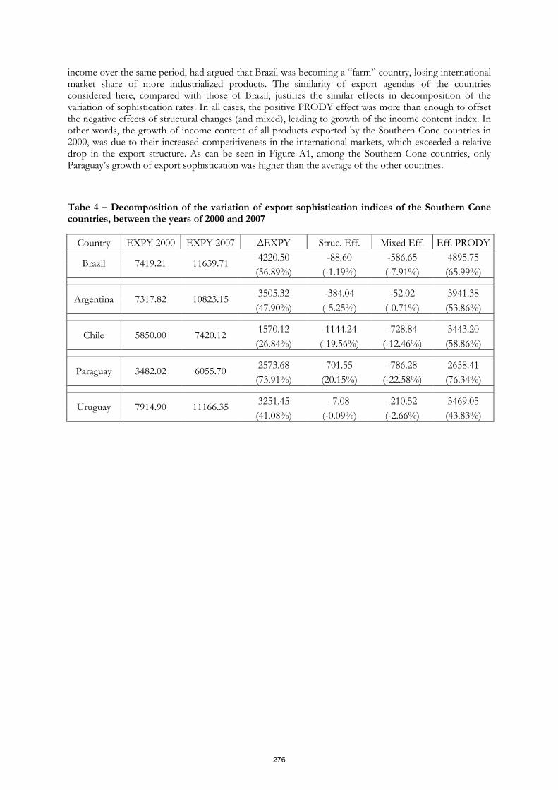
income over the same period, had argued that Brazil was becoming a “farm” country, losing international market share of more industrialized products. The similarity of export agendas of the countries considered here, compared with those of Brazil, justifies the similar effects in decomposition of the variation of sophistication rates. In all cases, the positive PRODY effect was more than enough to offset the negative effects of structural changes (and mixed), leading to growth of the income content index. In other words, the growth of income content of all products exported by the Southern Cone countries in 2000, was due to their increased competitiveness in the international markets, which exceeded a relative drop in the export structure. As can be seen in Figure A1, among the Southern Cone countries, only Paraguay’s growth of export sophistication was higher than the average of the other countries.
Tabe 4 – Decomposition of the variation of export sophistication indices of the Southern Cone countries, between the years of 2000 and 2007
Country EXPY 2000 EXPY 2007 ΔEXPY Struc. Eff. Mixed Eff. Eff. PRODY
Brazil 7419.21 11639.71 4220.50 -88.60 -586.65 4895.75
(56.89%) (-1.19%) (-7.91%) (65.99%)
Argentina 7317.82 10823.15
3505.32 -384.04 -52.02 3941.38
(47.90%) (-5.25%) (-0.71%) (53.86%)
Chile 5850.00 7420.12
1570.12 -1144.24 -728.84 3443.20
(26.84%) (-19.56%) (-12.46%) (58.86%)
Paraguay 3482.02 6055.70
2573.68 701.55 -786.28 2658.41
(73.91%) (20.15%) (-22.58%) (76.34%)
Uruguay 7914.90 11166.35
3251.45 -7.08 -210.52 3469.05
(41.08%) (-0.09%) (-2.66%) (43.83%)
276

Tabe 4 – Number of exported products and share of total export value, by class of net sophistication.
Classes Argentina Brazil Chile Paraguay Uruguay
PRODY 2000 2007 2009 2000 2007 2009 2000 2007 2009 2000 2007 2009 2000 2007 2009
Number of exported products by class of net sophistication
High 990 1065 942 1103 1134 1068 807 805 782 145 186 136 451 488 420 Med. High 1085 1121 1074 1169 1190 1149 935 951 945 212 290 259 555 629 619 Med. Low 1066 1112 1064 1155 1176 1148 988 993 938 278 405 339 587 657 681
Low 984 1002 973 1110 1118 1080 827 848 843 359 441 368 499 593 537
Total 4125 4300 4053 4537 4618 4445 3357 3597 3508 994 1322 1102 2092 2367 2257
Relative share of each sophistication class to the total export value
High .051 .058 .057 .077 .092 .070 .037 .054 .045 .006 .013 .012 .061 .087 .084 Med. High .166 .137 .176 .200 .191 .179 .101 .071 .084 .018 .014 .017 .176 .128 .133 Med. Low .425 .412 .365 .246 .334 .299 .257 .184 .176 .077 .289 .262 .495 .462 .504
Low .357 .393 .402 .477 .383 .452 .605 .691 .696 .899 .684 .709 .268 .323 .279
Total 1.00 1.00 1.00 1.00 1.00 1.00 1.00 1.00 1.00 1.00 1.00 1.00 1.00 1.00 1.00
277

CONCLUSIONS
This study calculated indices of similarity and net income content (sophistication) for exports from the Southern Cone countries from 2000 to 2009. The income content indices were further broken down into their productivity effects (for those products whose countries already had the comparative advantage), structural changes for the set of exported goods, and mixed effects.
In general, the similarity indices of exports were very low, with exports from Argentina and Paraguay appearing to be the most similar to those of Brazil. Argentina’s index increased until 2003 and decreased thereafter, perhaps indicating a specialization between the two major economies of the Mercosur. Chilean exports showed low similarity with those of other countries, while Uruguay’s increased over the years. The low values however, do not indicate fierce competition for revenue from exports between the Southern Cone countries.
Exports from Brazil and Argentina are the most sophisticated in terms of income content. Uruguay’s index of export sophistication drew attention, as it was higher than that of Argentina throughout the entire time period and even went beyond that of Brazil in 2008. It is noteworthy to say that this small country that has the highest per capita income, had the lowest regional share of products with low sophistication in the total value of exports during the period of analysis.
In general, the Southern Cone countries showed a strong dependence on the exports of agricultural commodities for which they already have a competitive advantage in international markets. The increase in levels of sophistication between 2000 and 2009 was relatively small (mean = 49%). The decomposition of the variation of these indices showed that the increase in export sophistication was due to the effect of productivity, or an increase in the competitive advantage of medium-low or low sophistication products. The change in the countries’ export basket structure grew less than the average of other countries during the first decade of 2000, indicating that the Southern Cone countries have struggled to specialize in products with high income contents.
REFERENCES
Antiniani, A. Henke, R. Old and New Partners: Similarity and Competition in the EU Foreign Trade. (2006). The National Institute of Agricultural Economics (INEA), Rome, Italy. 15p. Paper prepared for presentation at the 98 th EAAE Seminar ‘Marketing Dynamics within the Global Trading System: New Perspectives’, Chania, Crete, Greece
Freitas, M.L and Mamede, R.P. Structural Transformation of Portuguese Exports and the role of Foreign
Direct Investment: some descriptive analysis for the period 1990-2005. Paper presented at the Workshop Portugal and the Challenge of Globalization, held at the Ministry of Economy and Innovation, Lisbon, November 5, 2007. 32p.
Hausmann, Ricardo, Jason Hwang, and Dani Rodrik (2007), “What You Export Matters,” Journal of Economic
Growth, 12(1), 1-25. NBER Working Paper No. 11905. Jorge, Marina F. e Kume, Honório. A competitividade do Brasil e da China no mercado norte-americano no
período 2000-2008. ANPEC, 2009. Lall, Sanjaya, John Weiss, and Jinkang Zhang (2006), “The ‘Sophistication’ of Exports: A New Trade
Measure,” World Development, 34(2), 222-237. Loke, Way-Hen. East Asia and Southeast Asia: Similarity in Trade Structures. Paper presented at The
Singapore Economic Review Conference (SERC) 2009. 16p.
278

Vaillard, Marcel. Profundización del proceso de integración económica en bienes. Available at: www.redmercosur.org/el-desafio-de-integrase-para-crescer-balances-y-perspectives-del-mercosur-en-su-primer-decada/ publicacion/85/es/. Acesso em setembro 2011
Schott, P.K. The Relative Competitiveness of China’s Exports to the United States vis a vis other Countries
in Ásia, the Caribbean, Latin American and the OECD. Occasional paper 39. Buenos Aires: IDB-INTAL, July 2006.
Schott, P.K. The Relative Sophistication of Chinese Exports. Economic Policy, vol.23, no 53, January 2008.
Silva, O.M. e Drumond, R.R. Similarity and income content at the international trade: The case of BRICS during the period 2000/09. Paper presented at the IAMO’s Forum 2011. Halle, Germany. June 2011. 19p.
Silva Junior, P. N. A divisão das receitas tarifárias no MERCOSUL: uma proposta baseada na experiência de outras integrações. Dissertação Mestrado, DEE/UFV. Viçosa, MG. 2011. 65p.
Xu, Bin. Measuring China’s Export Sophistication. China Europe International Business School. 41p. October 2007.
UNCTAD – United Nations Conference on Trade and Development. COMTRADE. Available at: http://www.unctad.org
World Bank. Key Development Data & Statistics, 2010. Available at: http://web.worldbank.org/WBSITE/EXTERNAL/DATASTATISTICS.
279

Figure A1. EXPY values calculated for the years 2000 and 2007
0
5000
10000
15000
20000
EXPY 2000
0 10000 20000 30000 40000 EXPY 2009
EXPY Values Adjusted Values Southern Cone EXPY
280

Enterprise And (Un)Employment: A Proposal Against Crises
Ernesto Peralta Tecnológico de Monterrey
ABSTRACT
The purpose of this paper is double: i) to visualize the historical incidence of economic -financial crises, characterized by a general glut (oversupply of goods and services), and ii) to propose a piece of solution trough more employment with attractive salaries in order to diminish the possibility of gluts. It is necessary to emphasize that although this note has a macroeconomic flavor, occupation or employment referred is mainly located in private enterprises; in the United States, on private nonfarm payrolls; in Mexico, 95 percent according to official information (INEGI ENOE); this is why the title includes term enterprise.
281

Enterprise And (Un)Employment: A Proposal Against Crises
The purpose of this paper is double: i) to visualize the historical incidence of economic -financial crises, characterized by a general glut (oversupply of goods and services), and ii) to propose a piece of solution trough more employment with attractive salaries in order to diminish the possibility of gluts. It is necessary to emphasize that although this note has a macroeconomic flavor, occupation or employment referred is mainly located in private enterprises; in the United States, on private nonfarm payrolls; in Mexico, 95 percent according to official information (INEGI ENOE); this is why the title includes term enterprise.
This presentation includes four sections. The hypothesis in the first, the second reviews literature, the third present statistical evidence, and the fourth is for final notes and recommendations.
HYPOTHESIS
The hypothesis is based on historical evidence showing crises, say, overproduction face to face weak markets characterized by a weak purchasing power due to unemployment and unequal income distribution; disequilibrium between supply (overproduction) and demand (weak markets) increases when technological
progress promotes labor substitution by equipment, promoting (unemployment, low labor income and weak markets; then, on one side productivity improves thanks to better technologies but on the other, market power declines. Diagram 1 depicts this panorama, horizontal axis measures labor and the vertical, productivity; originally, without innovation, 100 units of labor give 100 units of product, but when innovation is applied 100 of product requires only 70 units of labor, assuming everything remains unchanged, unemployment would be 30; and full employment could be kept only if 120 units be sold.
Impact of unemployment is treble, i) market is weakened, it cannot buy 120 due to a lower labor income, ii) in the short run, capital income increases thanks to a higher productivity vis a vis a lower production cost given employment 70, but iii) this gives a dark perspective because inventories would increase and the present value of the economy falls, say, a stock - market crack.
Prefix (un) is used because term unemployment does not clarify if it is open or disguised.
0
20
40
60
80
100
120
140
0 10 20 30 40 50 60 70 80 90 100
P
r
o
d
u
c
t
Labor
Diagram1. Product and employment
Product before
Product after
Unemployment
282

A BRIEF REVIEW OF LITERATURE
This topic of crisis has been studied through history. Thomas R. Malthus (1766-1834) raised the possibility of general glut (oversupply of goods and services). Karl Marx (1818-1883) explained how capital accumulation in conjunction with the secularly growing “industrial reserve army” (overpopulation) operates to increase the severity of successive crises. Vilfredo Pareto (1848-1923) made his law of the distribution of income, according to which the inequality of income distribution shows a high degree of constancy for different times and countries. John M. Keynes (1883-1946) took the employment question as a starting point not for humanitarian reasons but in recognition that this is a basic problem for the well-functioning economy. Paul Samuelson (1915-2009) wrote “One common feature of capitalism around the world is the speculative booms and busts that occurred frequently”, and he presented evidence (Diagram 2, 2010: 430) during the 20th century.
Diagram 2
Finally, Robert Heilbroner (1919-2005) wrote: Unemployment has been a persistent problem in the United States from the mid 1970´s …Corporate downsizing has led to the loss of relatively high-paying jobs, and the focus of macroeconomic policy may now have to swift from growth, pure and simple, to a concern with wages, especially those of low-wage workers” (Heilbroner, 2008: 210).
STATISTICAL EVIDENCE
First, we focus on the U.S. during the last years, when consumption declined in 2009 respect to that of 2008 and although experiments recovery during 2010 and 2011, it is still below respect to that of 2008; rates of open unemployment were 9.3, 9.6 and 8. 9 in 2009, 2010 and 2011 respectively, i.e., 14,265; 14,825 and 13,747 thousands of unemployed; but these figures do not represent
workers that were laid off, (so) they joined the pool of people already looking for fobs. This allowed companies to offer lower wages to any new employees they took the impact of downsizing on wages (Heilbroner, 2008, 152),
Then market perspective cannot be good.
Under these circumstances, the American government strategy reinforces markets, but under serious financial problems emerged from public deficit. What can expect?
283

Historical American panorama of both labor work and earnings is presented in Table 1.
Table 1.Historical hours and earnings (dollars of 1984) in the United States
Year Weekly hours
Hourly earnings
Weekly earnings
Unemployment rate
1966 38.5 8.43 325 2.9
1976 36.1 8.89 320 7.7
1986 34.7 8.15 286 7.0
1996 34.3 7.67 263 5.4
2006 33.9 8.31 282 4.6
2007 33.9 8.30 281 4.6
2008 33.6 8.60 289 5.8
2009 33.1 8.63 286 9.3
2010 33.4 8.68 290 9.6
2011 33.6 8.64 293 8.9
Source: Bureau of Labor Statistics.
Weekly hours and earnings declined, hourly earnings remain but unemployment grew, then a worse income distribution is taking place because workers occupied could have retained acceptable earnings, but many are laid off as Heilbroner said:
Perhaps the most effective way to depict the trend (of inequality) is to compare the ratio of the wages of an average male worker with that of a top chief executive officer (CEO).If we take and estimated figure of $25,000 as the average wage of such worker in 1970, the income of this company´s highest paid executive was around $1 million. If we now turn to 2004, the average wage has risen to $43,000, but the top CEO pay now approaches $15 million. The ratio has jumped from 40 to 1 to more than 35 to 1.
(Heilbroner (2008: 154)
Their impact on GDP and consumption rates of change is presented in Table 2.
Table 2. Annual rates of change, percent
Year Hourly earnings GDP Consumption
2009 - 1.9 - 4.6 - 3.6
2010 1.4 3.1 1.7
2011 1.0 2.7 1.8
Source: Bureau of Labor Statistics and Bureau of Economic Analysis.
Trends of consumption and GPD are associated to that of labor income, so it is advisable to improve occupation in order to push labor income, and so GDP and consumption. The recent American economic recovery could be explained not only by an efficient public policy but also by its relative fair functional income distribution (Diagram 3).
284

These problems are more severe in Mexico due to its demographic trends, unequal income distribution, increasing unemployment, poverty and inefficient public policies. GDP annual rate during the 2000´s is too low so that if it remained, to duplicate per capita GDP would take 200 years. The increasing labor force requires 1 million jobs annually but since this is not possible, unemployment grows vigorously. Historical labor figures, in a similar table, are in Table 3.
Table 3. Historical hours and earnings (Pesos of 2010) in Mexico
YEAR Weekly hours
Hourly earnings
Weekly earnings
Unemployment rate
2005 43.3 31.0 1,876 3.5
2006 42.7 32.9 1,850 3.2
2007 42.4 34.0 1,837 3.4
2008 42.9 32.7 1,403 3.5
2009 42.1 32.2 1,356 5.2
2010 42.3 30.8 1,303 5.3
2011 42.4 29.8 1,264 5.2
Source: Bureau of Labor Statistics.
At first glance, the Mexican unemployment rate is less than the American one; but in Mexico unemployment, disguised plus open unemployment, say, open plus partial time unemployment, have the rate grow from 4.8 to 12 percent according to data from the last 2011 quarter; if informal occupation is added, the rate becomes 41.2 percent. Since unemployment implies low income, these figures could explain why poverty includes 50 percent of the Mexican population. In Mexico a CEO made 92,500 dollars per year (Mercer Human Resource Consulting, “El Universal”, January 2005) but an average worker 8,272 (STPS, 249.32 per day taking exchange 11 pesos - dollar), the ratio results 11.2. However, according with Forbes the Mexican executive Carlos Slim is the richest in the world; in 2008, the Mexican per capita GDP was $14,200 dollars; in the United States, $47,000.
Labor-income evolution impact on both GDP and consumption is presented in Table 4.
Table 4. Annual rates of change, percent
Year Hourly earnings GDP GDP per capita Consumption
0%
10%
20%
30%
40%
50%
60%
70%
80%
90%
100%
1987 1989 1991 1993 1995 1997 1999 2001 2003 2005 2007
Source: Bureau of Labor Statistics
Diagram 3. Functional income distribution in the U.S.
Capital income
Labor income
285

2008 1.2 1.2 0.2 1.6
2009 - 1.9 -6.2 -7.1 -5.7
2010 0.5 5.5 4.5 4.7
2011 0.2 3.9 2.9 4.1
Source: Estimations from data of INEGI.
And the unequal functional income distribution, associated to occupation structure, is summarized in Diagram 4.
FINAL NOTES AND RECOMMENDATIONS
The United States and Mexico present problems of increasing unemployment that promotes unequal income distribution that, in turn, produces falls in consumption and GDP.
Occupation and income figures presented are of workers in private sector principally, those who support markets and aggregate demand.
Considering that wages represent a high share of total income, purchasing power, it is advisable to promote employment, wages and a GDP distribution in favor of workers in order to strength markets and diminish gluts.
Otherwise, enterprises would visualize a conflictive perspective in the stock market, and poverty would grow as well as social disturbances.
This panorama was presented for the United States and Mexico; the former has shown a dynamic public policy, but with a conflictive public-debt perspective as we know.
The Mexican shows that historical trends imply increasing unemployment and poverty as well as a more unequal income distribution.
In both cases it is advisable that public policies promote employment in private enterprises because these are the most important source of employment, respective pays and then a more egalitarian income distribution; for this, it is necessary to implement a fiscal & monetary policy under a politicians and entrepreneurs consensus, taking in account that both would gain if there would be market and social stability.
60.2%
28.4%
30.1%
71.6%
9.7%
0%
10%
20%
30%
40%
50%
60%
70%
80%
90%
100%
GDP Employment
Source: constructed with statistics from INEGI.
Diagram 4. Functional distribution of GDP, average 1995-2008
Indirect tax
Labor
Capital
286

REFERENCES
Buchholz, Todd (2007). New Ideas from Dead Economists, Penguin Group, New York.
Bureau of Economic Analysis, http://www.bea.gov.
Bureau of Labor Statistics, http://www.bls.gov.
Consejo Nacional de Población (CONAPO), http://www.conapo.gob.mx.
Heilbroner, Robert and William Milberg (2008). The Making of Economic Society, Pearson- Prentice Hall, New Jersey.
Instituto Nacional de Estadística y Geografía (INEGI), http://www.inegi.org.mx.
Kuhn, W. E. (1975). The Evolution of Economic Thought, South Western Publishing. Co., Cincinnati, Ohio.
Mail, Ludwig (1975). Men and Ideas in Economics. Littlefield, Adams & Co. New Jersey.
Newspaper El Universal, Mexico City, January 2005
Secretaría del Trabajo y Previsión Social (STPS), http://www.stps.gob.mx.
Samuelson, Paul and William Nordhaus (2010). Economics, McGraw-Hill, Singapore.
287

THIS PAGE INTENTIONALLY LEFT BLANK
288

The Decline of the Apparel-Maquila Sector in the DR-CAFTA Region: Is There a Choice Ahead?
Juan A. Chavarria University of Texas Pan American
Robert D. Morrison University of Texas Pan American
Claudia P. Dole University of Texas Pan American
Brenda M. Dole Morehead State University
ABSTRACT
This paper examines the origins of DR-CAFTA and artificial comparative advantages that its unilateral trade agreement predecessors created. We examine the growth of the apparel imports into the US throughout the 1980s and 1990s and the impact of the entry of China into the WTO and the elimination of the limitations under the Multi-Fiber Agreement. We provide suggestions for the industry and government leaders in the DR-CAFTA region in the face of increasing competition from lower wage nations.
289

The Decline of the Apparel-Maquila Sector in the DR-CAFTA Region: Is There a Choice Ahead?
From 807 to CBI to DR-CAFTA
The term maquila o maquiladora was associated with the transaction between a farmer and a miller where a portion of corn or oil was kept by the miller in exchange for provided grinding services (MacLachlan & Aguilar, 1998). Likewise, in the context of apparel the maquila industry refers to the production scheme where value is added by subcontractors at different stages of the garment manufacturing, usually made of imported raw materials (Jansen, 2007). Early antecedents hinting to a possible development of the maquila-apparel in Central America date back to the 60s and 70s when some favorable factors emerged. For instance, in 1963 US tariff schedules opened the possibility to pay import duties only on the valued added over imported garments assembled with US cut and milled fabric (Kunz & Garner, 2007), though subject to import quotas. Further, in the following decade (Chinchilla & Hamilton, 1994) the United States Agency for International development (USAID) began to promote the development of nontraditional exports in Central America. However, the key development that propelled the growth of the apparel-maquila in Central America was the Caribbean Basin Initiative (CBI) sponsored under the administration of President Ronald Regan. CBI emerged as program aiming to provide preferential treatment for Caribbean basin countries exports to the American market with the objective to promote the development of the their economies (Dypski, 2002) and as way to counterbalance the growing Cuban leftist influence in Latin America through a comprehensive aid and trade policy (Baker, 1999). In its role of facilitating the growth of Caribbean economies, CBI relied on the development and expansion of the textile and apparel industry as the one of foundations to generate industrialization of the Caribbean region just as it happened with England and the US in the19th century (Wohn, 2001). However, when CBI was started the attractiveness of the involved nations was not there. The large economic crisis affecting Latin America in the early 80s, and the insurgency and counterinsurgency struggles as a result of leftist guerillas in El Salvador, Nicaragua, and Guatemala generated uncertainty in Central America (Chinchilla & Hamilton, 1994). Further, Central America needed to compete with countries with lower wages that were not engaged in armed conflicts. Thus, to improve the appeal so that investors would support the development of the apparel-maquila in Central America and the Caribbean basin, the Reagan administration enacted in 1986 the 807-A (super 807) which allowed companies to sew garments formed and cut from US fabric by paying import duty, only, on the economic value added and without quota limitations (Dypski, 2002). These changes generated by the Reagan administration quickly reflected in growth of the apparel-maquila and from 1984 through 1989 textiles and apparel exports from the region went from US$310.8 million (Hutchinson & Schumacher, 1994) to over US$1.28 billion in the year of 1989 (OTEXA). As a region, Central America and the Dominican which consolidated as the trading block of DR-CAFTA (by 2004), reached its highest share of US textile and apparel imports in the period that goes from 1997 through 2002 when exports reached 13% of US textile and apparel imports (OTEXA). However, viewed from another perspective, during the period Figure 1.
290

Percentage of US Textile and Apparel Market Share. Source Office of Textiles and Apparel OTEXA. U.S. Imports of Textiles and Apparel <http://otexa.ita.doc.gov/scripts/tqads2.exe/catpage>
that goes from the year of 2000 through 2005 DR-CAFTA consistently exported more than US$9.0 billion with a peak on the year of 2004 when US$9.5 billion were exported to the American market (figure 2, OTEXA).
Figure 2. Exports to the US Market measured in Billions of US$. Source: Office of Textiles and Apparel OTEXA. U.S. Imports of Textiles and Apparel <http://otexa.ita.doc.gov/scripts/tqads2.exe/catpage>
Nevertheless, though DR-CAFTA had its best export years in the beginning of the century, from Figure 1 it can also be seen that between the years of 2001 and 2002 it began to be outperformed by China. From a peak of market share of 18%, DR-CAFTA declined to have 8% of the US market of apparel imports whereas China increased from 9% to 40% of the US import market in the period ending at the year 2011.
A great deal of this reduction of the market share is associated with lower comparative advantages with China and other Asian manufacturers. The specific segment of apparel within the textile and an apparel supply chain is very labor intensive. In labor intensive industries the value added per worker is high and as a result the labor cost of a manufactured product represents an important proportion of the value added (Loftus, 1969). Consequently apparel companies develop strategies to capitalize on cheap labor cost and see it as a major advantage that a region or country could provide. In this respect, for instance, the U.S. International Trade (USITC, 2004) commission reports that in the years of 2002 the hourly rate for labor paid in China was of less than US$0.50 / hour while in Guatemala, Honduras and El Salvador such cost was estimated to be of about US$0.88/hour. Hence, the combined effect of low labor cost, the joining of the World Trade
291

Organization by China, and the elimination of the multi-fiber agreements (MFA) by the United States in January of 2005 are associated with the rising importance of China as the main provider of U.S. textiles and apparel imports.
The statistics shown in Figure 1 for the first 10 years of the 21st century depict a scenario where China has a consolidated its lead and growth as the premier supplier of textiles and apparel of the U.S. market. At the same time, it can be seen that the DR-CAFTA trading block is struggling to keep its market share and has conceded already about five points of it. Abernathy, Volpe, and Weil (2005) indicated that in their survey of academic and popular press literature they have noticed a concurrence to anticipate that countries with low labor cost would take advantage of the end of MFA. Also, they point out that such fast growth was going to cause an important negative impact on the textile and apparel industries of the US and other countries.
Thus, given the circumstances that China and other Asian countries have positioned themselves with the comparative advantage of cheap labor price, DR-CAFTA countries need to focus on a two tier strategy.
1. To Protect and improve the value added in its textile apparel supply chain by focusing on improving productivity, proposing and negotiation trade preference level (TPL) for countries of the trade block in order to be able to use fabric from any origin and gradually integrate vertically the textile-apparel chain from cotton growth to the shipment of end products
2. To focus on developing and evolving a higher level of maquila activity and emulate the proven success of Costa Rica in this sector
The years on which the development of the maquila business relied on special provisions of unique advantages granted for the DR-CAFTA region by the U.S. government are gone. Consequently, DR-CAFTA countries cannot count any more on this type of comparative advantage to attract foreign direct investment. For this reason, the need for a coordinated strategy by the DR-CAFTA countries to take more advantage of what they already have in the textile-apparel maquila and to focus in working diligently to evolve is a must. The DR-CAFTA region cannot afford losing the early steps taken toward the industrialization and economic development of the region and finding a way is an imperative necessity.
REFERENCES
Abernathy, F. H., Volpe, A., & Weil, D. (2005). The future of the apparel and textile industries: prospects and choices for public and private actors. The Harvard Center for Textile and Apparel Research, 1-44.
Baker, M. (1999). Privatization in the developing world : panacea for the economic ills of the third world or
prescription overused? New York Law School journal of international and comparative law New York Law School Journal of International and Comparative Law, 18(2), 233-267.
Chinchilla, N., & Hamilton, N. (1994). Global production : the apparel industry in the Pacific Rim. In E.
Bonacich (Ed.), (pp. 287-304). Philadelphia: Temple University Press. Dypski, M. C. (2002). The Caribbean Basin Initiative : an examination of structural dependency, good
neighbor relations, and American investment. Journal of transnational law & policy Journal of transnational law and policy, 12(1), 95-136.
Hutchinson, G. A., & Schumacher, U. (1994). NAFTA's Threat to Central American and Caribbean Basin
Exports: A Revealed Comparative Advantage Approach. Journal of Interamerican Studies and World Affairs, 36(1), 127-148.
292

Jansen, H. G. P. (2007). The impact of the Central America Free Trade Agreement on the Central American textile
maquila industry. Washington, D.C.: International Food Policy Research Institute. Kunz, G. I., & Garner, M. B. (2007). Going global : the textiles and apparel industry. New York: Fairchild
Publications. Loftus, P. J. (1969). Labour's share in manufacturing. Lloyd's Bank Review, 92, 15-25. MacLachlan, I., & Aguilar, A. G. (1998). Maquiladora Myths: Locational and Structural Change in Mexico's
Export Manufacturing Industry. The Professional Geographer, 50(3), 315-331. doi: 10.1111/0033-0124.00123
USITC. (2004). Textile and apparel: assesment of the competitiveness of certain foreign suppliers to the U.S. market.
Wohn, A. J. H. (2001). Towards GATT integration : circumventing quantitative restrictions on textiles and apparel trade under the multi-fiber arrangement. University of Pennsylvania journal of international economic law University of Pennsylvania journal of international economic law, 22(2), 375-419.
293

THIS PAGE INTENTIONALLY LEFT BLANK
294

Optimal Asset Allocation under VaR Criterion: Taiwan Stock Market Example
Ken Hung, Texas A&M International University
Suresh Srivastava, University of Alaska Anchorage
ABSTRACT
Value at risk (VaR) measures the worst expected loss over a given time horizon under normal market conditions at a specific level of confidence. These days, VaR is the benchmark for measuring, monitoring and controlling downside financial risk. VaR is determined by the left tail of the cumulative probability distribution of expected returns. Expected probability distribution can be generated assuming normal distribution, historical simulation or Monte Carlo simulation. Further, a VaR-efficient frontier is constructed, and an asset allocation model subject to a target VaR constraint is examined.
This paper examines the riskiness of the Taiwan stock market by determining the VaR from the expected return distribution generated by historical simulation. Our result indicates the cumulative probability distribution has a fatter left tail, compared with the left tail of a normal distribution. This implies a riskier market. We also examined a two-sector asset allocation model subject to a target VaR constraint. The VaR efficient frontier of the TAIEX traded stocks recommended, mostly, a corner portfolio.
Key words: Value at risk, asset allocation, cumulative probability distribution, normal distribution, VaR-efficient frontier, historical simulation.
295

Optimal Asset Allocation under VaR Criterion: Taiwan Stock Market Example
INTRODUCTION
Risk is defined as the standard deviation of unexpected outcomes, also known as volatility. Financial market risks are of four types: interest rate risk, exchange rate risk, equity risk and commodity risk. For a fixed-income portfolio, the linear exposure to the interest rate movement is measured by duration. Second-order exposure is measured by convexity. In the equity market, linear exposure to market movement is measured by the systematic risk or beta coefficient. In the derivative markets, the first-order sensitivity to the value of underlying asset is measured by delta, and second-order exposure is measured by gamma. Innovations in the financial markets have introduced complicated portfolio choices. Hence it is becoming more difficult for managers to get useful and practical tools of market risk measurement. The simple linear considerations such as Basis Point Value, or first- or second-order volatility are inappropriate. They can’t accurately reflect risk at the time of dramatic price fluctuation.
VaR (value-at-risk) has become a popular benchmark for the down-side risk measurement.181 VaR converts the risks of different financial products into one common standard: potential loss, so it can estimate market risk for various kinds of investment portfolio. VaR is used to estimate the market risk of financial assets. Special concern of the market risk is the downside risk of portfolio values resulting from the fluctuation of interests, exchange rates, stock prices or commodity prices. VaR is consistent in estimating the financial risk estimation. It indicates risk of dollar loss of portfolio value. Now the risks exposure of different investment portfolios (such as equity and fixed income) or different financial products (such as interest rate swaps and common stock) have a common basis for direct comparison. For decision makers, VaR is not only a statistical summary, it can also be used as a management and risk control tool to decide capital adequacy, asset allocation, synergy-based salary policy and so on.
VaR is a concept widely accepted by dealers, investors and legislative authorities. JP Morgan has advocated VaR and incorporated it in Risk Metrics (Morgan 1966). Risk Metrics contains most of the data and formulas used to estimate daily VaR, including daily-updated fluctuation estimations for hundreds of bonds, securities, currencies, commodities and financial derivatives. Regulatory authorities and central bankers from various countries at Basel Committee meetings agreed to use VaR as the risk-monitoring tool for the management of capital adequacy. VaR has also been widely accepted and employed by securities corporations, investment banks, commercial banks, retirement funds and non-financial institutions. Risk managers have employed VaR in ex-post evaluation, that is, to estimate and justify the current market risk exposure.182 Confidence-based risk measure was first proposed by Roy (1952).
The inclusion of VaR into the asset allocation model means the inclusion of downside risk into model constraints. Within the feasible scope of investment portfolio that meets shortfall constraints, the optimal investment portfolio is decided by maximum expected return. The definition of shortfall constraint is that the probability of investment portfolio value dropping to a certain level is set as the specific disaster probability. The asset allocation framework that takes VaR as one of its constraints has increased the importance of VaR, and has employed VaR as an ex-ante control tool of market risk.
181
Extensive discussion of Value-at-risk can be found in Basak and Shapiro. (2001), Beder (1995), Dowd (1998),
Fong and Vasicek.(1997), Hendricks (1996), Hoppe (1999), Jorion (1997, 1997), Schachter (1998), Smithson and
Minton (1996a, 1996b) and Talmor (1996). 182
Institutional use of VaR can be found in Basel (1995, 1998a, 1998b, 1998c, 1999), Danielsson, de Vries and
Jorgensen (1998) and Danielsson Hartmann and de Vries (1998).
296

VALUE-AT-RISK
One difficulty in estimating VaR is the choice of various VaR methods and corresponding hypotheses. There are three major methods to estimate VaR: Variance-covariance analysis, historical simulation and Monte Carlo simulation. Variance-covariance analysis assumes that market returns for financial products are normally distributed, and VaR can be determined from market return’s variance and covariance. The normal distribution hypothesis of Variance-Covariance Analysis makes it easy to estimate VaR at different reliability and different holding period (See Appendix A). Its major disadvantage is that the return in the financial market is usually not in normal distribution and has fat-tails. This means the probability of extreme loss is more frequent than estimated by variance-covariance analysis.
Historical simulation assumes the future market return of the investment portfolio is identical to the past returns; hence, the attributes of current market can be used to simulate the future market return (Hendricks [1996], Hull and White [1998]). Historical simulation approach does not suffer from the tail-bias problem, for it does not assume normal distribution. It relies on actual market return distribution, and the estimation reflects what happened during the past sample period. It has another advantage over variance-covariance analysis: it can be used for non-linear products, such as commodity derivatives. However, the problem with historical simulation is its sensitivity to sample data. Many scholars pointed out that if October 1987 is included into the observation period, then it would make great difference to the estimation of VaR. Another problem with historical simulation is that the left-tail of actual return distribution is at zero stock prices. In other words, it would not be accurate to assume a zero probability of loss that is greater than the past loss. Lastly, the estimation of historical simulation is more complicated than that of variance-covariance analysis. The VaR needs to be re-estimated every time level of reliability or holding period changes,
Monte Carlo simulation can be used to generate future return distribution for a wide range of financial products. It is done in two steps. First, a stochastic process is specified for each financial variable along with appropriate parameters. Second, simulated prices are determined for each variable, and portfolio loss is calculated. This process is repeated 1,000 times to produce a probability distribution of losses. Monte Carlo simulation the most powerful tool for generating the entire probability distribution function and can be used to calculate VaR for a wide range of financial products. However, it is time consuming and expensive to implement.
Modern investment portfolio theories try to achieve optimal asset allocation via maximizing the risk premium per unit risk, also known as the Sharpe ratio (Elton and Gruber, 1995). Within the framework of mean-variance, market risk is defined as the expected probable variance of investment portfolio. To estimate risk with standard deviation implies investors pay the same attention to the probabilities of negative and positive returns. Yet investors have different aversion to investment’s downside risk than to capital appreciation. Some investors may use semi-variance to estimate the downside risk of investment. However, semi-variance has not become popular.
Campbell, Huisman and Koedijk (2001) have developed an asset allocation model that takes VaR as one of its constraints. This model takes the maximum expected loss preset by risk managers (VaR) as a constraint to maximize expected return. In other words, the optimal investment portfolio deduced from this model meets the constraint of VaR. This model is similar to the mean-variance model that generates the Sharpe index. If the expected return is a normal distribution, then this model is identical with mean-variance model. Details of this model are presented in the Appendix.
Other researchers have examined four models to introduce VaR for ex-ante assets allocation of optimal investment portfolio: mean-variance (MV) model, mini-max (MM) model, scenario-based stochastic programming (SP) model, and a model that combines stochastic programming and aggregation/convergence (SP-A). The investment portfolio constructed using the SP-A model has a higher return in all empirical and
297

simulation tests. Robustness test indicates that VaR strategy results in higher risk tolerance than risk assessment that takes severe loss into consideration. Basak and Shapiro (1999) pointed out that the drawback of risk management lies in its focus on loss probability instead of loss severity. Although loss probability is a constant, when severe loss occurs, it has greater negative consequence than non-VaR risk management.
Lucas and Klaassen (1998) pointed out the importance of correctly assessing the fat-tailed nature of return distribution. If the real return is not in normal distribution, the asset allocation under the hypothesis of normal distribution will result in non-efficiency or non-feasibility. An excellent discussion of VaR and risk measurements is presented by Jorion (2001).
EMPIRICAL RESULTS
In July 1997, financial crisis broke out in Southeast Asian nations, and then proliferated to other Asian regions and led to a series of economic problems. Taiwan had also been attacked by financial crisis in late 1998. Domestic financial markets fluctuated. Corporations and individuals greatly suffered. The proliferation of financial crisis within or among countries makes it impossible for corporations and individuals to ignore market risk. Risk measurement is the first thing to do before investment.
The Taiwan market general weighted stock index, individual weighted stock price indexes and interbank short loan interest rate used in this research paper are obtained from the data base of AREMOS. We divide the historical period into two groups: from 1980-1999 and from 1991-1999, so as to analyze the impact of violent stock market fluctuation on VaR estimation, such as the New York stock market collapse in October 1987 and Taiwan stock market dramatic uprising from 1988 to 1990. The first period is rather long and can indicate the nature of dramatic stock fluctuation. The second period is rather short and can reflect the change of stock market tendency.
This paper employs historical simulation to reproduce the daily fluctuations of returns for electrical machinery, cement, food, pulp and paper, plastics and petroleum, and textile and fiber stocks trading in the Taiwan stock market during the periods of 1980-1999 and 1991-1999. We estimate their VaRs under reliability levels of 95%, 97.5%, and 99%. The expected return of investment portfolio in 1999 is the sum of annual mean returns of various stocks multiplied with their respective weights. We use this expected return to estimate year 1999 optimal stock holding proportion and analyze the impact of different historical simulation periods on optimal asset allocation.
Table 1 presents the summary of TSE general weighted stock index (daily data) and estimated VaR for periods 1980-1999 and 1991-1999. Table 2 presents cumulative probability distributions of TSE daily index return for the 1980-1999 period and daily returns under the assumption of normality. It shows that at confidence level lower than 95.8% (for example, 90%), the left tail probability for historical distribution is higher than the normal return probability (4.2%). Hence, under the normal distribution assumption the VaR is overestimated, and this leads to an over-cautious investment decision. At confidence level higher than 95.8% (for example, 97.5%), the left tail probability for historical distribution is lower than the normal return probability (4.2%). Hence, under the normal distribution assumption the VaR is underestimated, and this leads to an over-active investment decision.
Figure 1 is the graphical presentation of the data in Table 2. The solid blue line represents cumulative probability distributions of TSE daily index return, and the dashed red line represents the normal distribution. The bottom panel is the enlarged view of the left tail. This graph also indicates VaR estimated using extreme values of historical distribution will lead to an over-active investment decision.
Table 3 reports annualized returns and standard deviations for TSE daily index and six selected industries: cement, electrical machinery, food, pulp and paper, plastics and petroleum, and textile and fiber. For the 1980-1999 period, the food industry had the greatest risk with a standard deviation of 53.47% and 15.13% annual return, whereas the overall market had a standard deviation of 50.80% with 23.22% annual return.
298

Textile and fiber was the least risky industry with a standard deviation of 41.21% and 12.78% annual return. For the 1991-1999 period, the electrical machinery industry had the greatest risk with a standard deviation of 42.267% and 26.12% annual return, whereas the overall market had a standard deviation of 36.58% with 9.40% annual return. The cement industry was the least risky industry with a standard deviation of 24.92% and 0.45% annual return. Next we constructed a two-industry optimal portfolio subject to VaR constraint. The optimal asset allocation for the two-industry portfolio is obtained by maximizing S(p) (derivation discussed in Appendix). The resulting VaR efficient frontiers are plotted in Figure 2. The upper panel in Figure 2 refers to VaR efficient portfolios of electrical machinery and plastics and petroleum stocks, and the lower panel in Figure 2 refers to VaR efficient portfolios of cement and food stocks. VaR is set at the 95% confidence level. Table 4 presents portfolio weights for different combinations of industry stocks at different levels of confidence. Asset allocations for most of the industry combinations represent corner solutions, i.e., 100% investment in one industry. For example, when electrical machinery stocks are combined with stocks from any other industry, the optimal portfolio is 100% investment in electrical machinery stocks, for both time periods and the three confidence levels. Asset allocation for cement stocks are dominated by the other five industry stocks. Allocations of food stocks dominate all other stock weights except electrical machinery. The general nature of asset allocation is the same for both time periods and the confidence levels.
Suppose an investor selects the VaR constraint for maximizing S(p) at a specified level of confidence (say 95%) and the actual VaR(c,p*) is at a higher level (97.5%); then VaR(portfolio) will be greater that target VaR*. In this case investors will have to invest a portion of the fund in T-bills (B>0, defined in Appendix). This will make investment VaR(c,p*) equal to the VaR* in the preset constraint. In opposite case, the VaR* constraint is specified at a higher level than the portfolio VaR(c,p*); then investors will borrow money to invest in risky assets (B<0). Table 5 and Table 6 list examples of investment in two-industry stocks and T-bills for periods 1980-1999 and 1991-1999, respectively. In each case, the target VaR* in the preset constraint is at a 95% level of confidence, and 1,000 yuan is invested in the portfolio. In the first panel of Table 5, 1,000 yuan is invested in electrical machinery stocks and 0 in cement stocks. These allocations are from Table 4. Portfolio VaR(c,p*) is 31.12, 42.57 and 53.92 yuan at 95%, 97.5% and 99% respectively. This leads to the lending of 0, 121, 216 yuan to meet the target VaR of 31.12. Thus a 97.5% portfolio consists of 87.9% in electrical machinery stocks, 0 in cement stocks and 21.1% in T-bills.
299

CONCLUSION
TSE daily index was found to be riskier than the market risk under the assumption of normal distribution for market returns. This resulted in the left tail of cumulative return distribution being fatter and a higher value at risk, indicating an over-active investment activity. For asset allocation model under a constrained VaR framework, most of the optimal portfolios have predominant investment in stocks from one industry. Hence, it will be inappropriate to comment on the optimal allocation of future investment portfolio based on the past stock performance of this unique period studied.
REFERENCES Artzner, Phillipe, Freddy Delbaen, Jean-Marc Eber, and David Heath, 1999, “Coherent Measures of Risk,”
Mathematical Finance 9 (July), 203-228.
Basak, S. and A. Shapiro. 2001. “Value-at-Risk Based Risk Management: Optimal Policies and Asset Prices.” The Review of Financial Studies, 14 (2), 371-405.
Basel Committee on Banking Supervision, 1995, Basel Capital Accord: Treatment of Potential Exposure for Off-Balance-Sheet Items, BIS, Basel, Switzerland.
Basel Committee on Banking Supervision, 1998a, Framework for the Evaluation of Internal Control Systems, BIS, Basel, Switzerland.
Basel Committee on Banking Supervision, 1998b, Enhancing Bank Transparency, BIS, Basel, Switzerland.
Basel Committee on Banking Supervision, 1998c, Operational Risk Management, BIS, Basel, Switzerland.
Basel Committee on Banking Supervision, 1999, Credit Risk Modeling: Current Practices and Applications, BIS, Basel, Switzerland.
Beder, T.S. 1995 “VAR: Seductive but Dangerous.” Financial Analysts Journal, 51:5(September-October), 12-24.
Campbell,R. R. Huisman and K. Koedijk. 2001.” Optimal Portfolio Selection in a Value-at-Risk Framework.” Journal of Banking and Finance, 25, 1789-1804.
Danielsson, J., C.G. de Vries, and B.N. Jorgensen. 1998, “The Value of Value at Risk: Statistical, Financial, and Regulatory Considerations.” FRBNY Economic Policy Review (October), 107-108.
Danielsson, J., P. Hartmann and C.G. de Vries. 1998. “The Cost of Conservatism: Extreme Returns, Value-at-Risk, and the Basle ‘Multiplication Factor.” Risk 11(January), 101-113.
Dowd, K. 1998. Beyond Value at Risk: The new science of risk management, John Wiley & Sons.
Elton, E.J. and M.J. Gruber. 1995, Modern Portfolio Theory and Investment Analysis, fifth edition, Wiley & Sons.
Fong, G. and O.A. Vasicek. 1997. “ A Multidimensional Framework for Risk Analysis.” Financial Analysts Journal (July-August), 51-57.
Hendricks, D. 1996. “Evaluation of Value-at-Risk Models Using Historical Data.” FRBNY Economic Policy Review (April), 39-69.
Hoppe, R. 1999. “It’s time we buried Value-at-Risk.”Risk Professional, 1(July/August).
300

Hull, John, and Alan White, 1998, “Incorporating Volatility Updating into the Historical Simulation Method for Value-at-Risk,” Journal of Risk 1 (Fall), 5-19.
Johnson, R., and Wichern, D. 2007. Applied Multivariate Statistical Analysis, Sixth Edition. Pearson Education.
Jorion, P. 1996. “Risk2: Measuring the Risk in Value at Risk.” Financial Analysts Journal (November/December), 47-56.
Jorion, P. 1997. “In Defense of VAR.” Derivatives Strategy 2(April), 20-23.
Jorion, P. 2001. Value at Risk, 2nd edition, McGraw Hill, New York, N.Y.
Lucas, A. and P. Klaassen. 1998. “Extreme Returns, Downside Risk, and Optimal Asset Allocation”. Journal of Portfolio Management, 25:1, 71-79.
Marshall, Chris, and Michael Siegel, 1997, “Value At Risk: Implementing a Risk Measurement Standard,” Journal of Derivatives 4, 91-110.
Morgan, J.P. 1996, RiskMetricsTM—Technical Document, Morgan Guaranty Trust Company, New York.
Roy, Andrew D., 1952. “Safety First and the Holding of Assets.” Econometrica 20, 431-449.
Schachter, B. 1998. “An Irreverent Guide to Value at Risk.” Risks and Rewards (March), 17-18.
Smithson, C. and L. Minton. 1996a. “Value-at-Risk(1): The debate on the use of VaR.” Risk 9(February), 25-27.
. 1996b. “Value-at-Risk(2): The debate on the use of VaR.” Risk, 9(February). Talmor, S. 1996. “History repeat itself.”THE BANKER (March), 75-76. Woolridge, J., 2009. Introductory Econometrics: A Modern Approach, 4th Edition. Cengage Learning
Table 1: Summary of Taiwan Stock Exchange (TSE) Daily Index
Period Mean Return Standard Deviation
Kurtosis VaR*
1980-1999 0.06% 1.67% 2.735 0.0263
1991-1999 0.04% 1.60% 2.464 0.0249
Annualized return for the two periods is 23.64% and 11.87%, respectively. VaR* is the maximum expected return loss for one-day holding period at a reliability level of 95%.
301

Table 2: Cumulative Probability Distribution of TSE Daily Index
Taiwan Index Historical Data Normal Distribution
Return Cumulative Probability Cumulative Probability
-7% 0 1.20946E-05
-6% 0.004723 0.000144816
-5% 0.01102 0.001236891
-4% 0.021165 0.007577989
-3% 0.038482 0.033571597
-2.9% 0.040581 0.0382868
-2.8% 0.042855 0.043528507
-2.7% 0.045828 0.049334718
-2.5% 0.054749 0.062791449
-2.3% 0.066993 0.078949736
-2% 0.082736 0.108825855
-1% 0.185062 0.262753248
0% 0.477873 0.485257048
1% 0.775407 0.712585369
2% 0.905895 0.876745371
3% 0.960994 0.960522967
4% 0.982158 0.990731272
5% 0.992304 0.998424485
6% 0.995977 0.999807736
7% 1 0.999983254
Period: 1980-1999.
302

Table 3: TSE Index and Selected Industry’s Returns and Standard Deviations
Period
Industry
1980-1998 1991-1998
Annual Return
Standard Deviation
Annual Return Standard Deviation
TSE Index 23.22% 50.80% 9.40% 36.58%
Cement 12.48% 48.37% 0.45% 24.92%
Electrical Machinery 19.49% 46.76% 26.12% 42.26%
Food 15.13% 53.47% 9.55% 32.29%
Pulp & Paper 8.50% 45.78% 4.64% 39.41%
Plastics & Petroleum 13.32% 43.99% 11.39% 36.26%
Textile & Fiber 12.78% 41.21% 7.88% 36.62%
Table 4: Optimal Asset Allocation for the Two-Industry Portfolio Obtained by Maximizing S(p) at Different Level of Confidence
Confidence
Level
Portfolio
Choices
95% 97.5% 99%
Electrical Machinery Cement
{1,0}; {1,0}** {1,0}; {1,0} {1,0}; {1,0}
Electrical Machinery Food
{1,0}; {1,0} {1,0}; {1,0} {1,0}; {1,0}
Electrical Machinery Pulp & Paper
{1,0}; {1,0} {1,0}; {1,0} {1,0}; {1,0}
Electrical Machinery Plastics & Petroleum
{1,0}; {1,0} {1,0}; {1,0} {1,0}; {1,0}
303

Electrical Machinery Textile & Fiber
{1,0}; {1,0} {1,0}; {1,0} {1,0}; {1,0}
Cement
Food {0,1}; {0,1} {0,1}; {0,1} {0,1}; {0,1}
Cement
Pulp & Paper {0,1}; {0,1} {0,1}; {0,1} {0,1}; {0,1}
Cement
Plastics & Petroleum {0.12, 0.88}; {0,1} {0.04, 0.96};{0,1} {0.17, 0.83};{0,1}
Cement
Textile & Fiber {0.67, 0.33}; {0,1} {0.6, 0.4}; {0,1} {0.15, 0.85}; {0,1}
Food
Pulp & Paper {1,0}; {1,0} {1,0}; {1,0} {0.98, 0.02}; {0,1}
Food
Plastics & Petroleum {1,0}; {1,0} {1,0}; {1,0} {1,0}; {1,0}
Food
Textile & Fiber {1,0}; {1,0} {1,0}; {1,0} {1,0}; {1,0}
Pulp & Paper
Plastics & Petroleum {0,1}; {0,1} {0,1}; {0,1} {0,1}; {0,1}
Pulp & Paper
Textile & Fiber {0,1}; {0,1} {0,1}; {0,1} {0,1}; {0,1}
Plastics & Petroleum Textile & Fiber
{0.99, 0.01};{1,0} {0.89, 0.11}; {1,0} {1,0}; {1,0}
First set {x, y} refers to the historical simulation for period 1980-98 and second set {x, y} refers to the historical simulation for period: 1991-98. ** {1, 0} represents 100% investment in Electrical Machinery industry and 0% investment in Cement industry
304

Table 5: Optimal Allocation for Two Industry Portfolio (Historical Simulation, Period 1980-1998)
Confidence Level
Cement Food Portfolio VaR(c,p*)
Lending,
B Yuan
VaR* Cement Food Cash
95% 100% 0% 31.12 0 31.12 100% 0% 0%
97.5% 100% 0% 42.57 121 31.12 87.9% 0% 12.1%
99% 100% 0% 53.92 216 31.12 78.4% 0% 21.6%
Confidence Level
Cement Food Portfolio VaR(c,p*)
Lending,
B Yuan
VaR* Cement Food Cash
95% 0% 100% 27.49 0 27.49 0% 100% 0%
97.5% 0% 100% 40.22 139 27.49 0% 86.1% 13.9%
99% 0% 100% 56.27 267 27.49 0% 73.3% 26.7%
Confidence Level
Cement Food Portfolio VaR(c,p*)
Lending,
B Yuan
VaR* Cement Food Cash
95% 12% 88% 27.52 0 27.52 12% 88% 0%
97.5% 4% 96% 41.99 154 27.52 3.4% 81.2% 15.4%
99% 17% 83% 53.42 246 27.52 12.8% 62.6% 24.6%
Confidence Level
Pulp & Paper
Textile & Fiber
Portfolio VaR(c,p*)
Lending,
B Yuan
VaR* Pulp & Paper
Textile & Fiber
Cash
95% 0% 100% 29.58 0 29.58 0% 100% 0%
97.5% 0% 100% 41.97 132 29.58 0% 86.8% 13.2%
99% 0% 100% 53.85 230 29.58 0% 77% 23%
Confidence Level
Cement Textile & Fiber
Portfolio VaR(c,p*)
Lending,
B Yuan
VaR* Cement Textile & Fiber
Cash
95% 67% 33% 25.86 0 25.86 12% 88% 0%
97.5% 60% 40% 41.97 172 25.86 49.7% 33.1% 17.2%
99% 15% 85% 52.51 256 25.86 11.2% 63.2% 25.6%
305

Confidence Level
Plastics & Petroleum
Textile & Fiber
Portfolio VaR(c,p*)
Lending,
B Yuan
VaR* Plastics & Petroleum
Textile & Fiber
Cash
95% 99% 1% 28.43 0 28.43 99% 1% 0%
97.5% 89% 11% 41.35 139 28.43 76.6% 9.5% 13.9%
99% 100% 0% 55.50 253 28.43 74.7% 0% 25.3%
Confidence Level
Food Textile & Fiber
Portfolio VaR(c,p*)
Lending,
B Yuan
VaR* Food Textile & Fiber
Cash
95% 100% 0% 27.49 0 27.49 100% 0% 0%
97.5% 100% 0% 40.22 121 27.49 87.9% 0% 12.1%
99% 100% 0% 56.27 267 27.49 73.3 0% 26.7%
Two industry portfolio with initial investment of 1,000 Yuan.
Allocations for other industry combinations are available to interested readers.
Table 6: Optimal Allocation for Two Industry Portfolio (Historical Simulation, Period 1991-1998)
Confidence Level
Cement Food Portfolio VaR(c,p*)
Lending,
B Yuan
VaR* Cement Food Cash
95% 100% 0% 30.55 0 30.55 100% 0% 0%
97.5% 100% 0% 42.57 128 30.55 87.2% 0% 12.8%
99% 100% 0% 53.92 221 30.55 77.9% 0% 22.1%
Confidence Level
Cement Food Portfolio VaR(c,p*)
Lending,
B Yuan
VaR* Cement Food Cash
95% 0% 100% 24.57 0 24.57 0% 100% 0%
97.5% 0% 100% 34.68 117 24.57 0% 88.3% 11.7%
99% 0% 100% 48.41 238 24.57 0% 76.2% 23.8%
Confidence Level
Cement Food Portfolio VaR(c,p*)
Lending,
B Yuan
VaR* Cement Food Cash
95% 0% 100% 27.19 0 27.19 0% 100% 0%
306

97.5% 0% 100% 35.95 100 27.19 0% 90% 10%
99% 0% 100% 48.59 213 27.19 0% 78.7% 21.3%
Confidence Level
Pulp & Paper
Textile & Fiber
Portfolio VaR(c,p*)
Lending,
B Yuan
VaR* Pulp & Paper
Textile & Fiber
Cash
95% 0% 100% 27.75 0 27.75 0% 100% 0%
97.5% 0% 100% 38.98 124 27.75 0% 87.6% 12.4%
99% 0% 100% 49.06 212 27.75 0% 78.8% 21.2%
Confidence Level
Cement Textile & Fiber
Portfolio VaR(c,p*)
Lending,
B Yuan
VaR* Cement Textile & Fiber
Cash
95% 0% 100% 27.75 0 27.75 0% 100% 0%
97.5% 0% 100% 38.98 124 27.75 0% 87.6% 12.4%
99% 0% 100% 49.06 212 27.75 0% 78.8% 21.2%
Confidence Level
Plastics & Petroleum
Textile & Fiber
Portfolio VaR(c,p*)
Lending,
B Yuan
VaR* Plastics & Petroleum
Textile & Fiber
Cash
95% 100% 0% 27.19 0 27.19 0% 100% 0%
97.5% 100% 0% 35.95 100 27.19 0% 90% 10%
99% 100% 0% 48.59 213 27.19 0% 78.7% 21.3%
Confidence Level
Food Textile & Fiber
Portfolio VaR(c,p*)
Lending,
B Yuan
VaR* Food Textile & Fiber
Cash
95% 100% 0% 24.57 0 24.57 100% 0% 0%
97.5% 100% 0% 34.68 117 24.57 88.3% 0% 11.7%
99% 100% 0% 48.41 238 24.57 76.2 0% 23.8%
Two industry portfolio with initial investment of 1,000 Yuan.
Allocations for other industry combinations are available to interested readers.
307

Fig. 1 Cumulative Probability Distribution of Taiwan Daily Stock Index
Period: 1980-1999
Left Tail of the Cumulative Probability of Taiwan Weighted Daily Stock Index
Period 1980 – 1999. Lower panel shows a fat left tail.
308

Fig. 2 VaR Efficient Frontier
The upper figure refers to investment portfolio of electrical machinery and plastics & petroleum stocks and the lower figure refers to investment portfolio of cement and food stocks. VaR is set at reliability level of 95%. Expected return and VaR are estimated from TSE industry indexes from 1980 to 1998.
309

Appendix A
Value-at-Risk
Let W0 be the initial investment and R be the rate of return of a portfolio. The value of the portfolio at the end of the target horizon will be W = W0(1 + R). Let µ and σ be the expected return and standard deviation of R. The lowest portfolio value at the confidence level c is defined as W* = W0 (1 + R*). The relative VaR is the dollar loss relative to the mean:
VaR(mean) = E(W) – W* = - W0(R* - µ) (A.1)
The absolute VaR is the dollar loss relative to zero:
VaR(zero) = W0 – W* = - W0R* (A.2)
W* and R* are minimum value and cutoff return respectively. In this paper we are discussing absolute VaR. The general form of VaR can be derived from the probability distribution of the future portfolio value f(w). For a given confidence level c, the worst possible portfolio value W* is such that probability of exceeding W* is c:
c =
(A.3)
The probability of a value lower than W*, p = P(w ≤ W*) is 1 – c:
p = P(w ≤ W*) = 1 – c =
∞ (A.4)
Typical confidence level c, is 95%. This computation of VaR does not require estimation of variance-covariance matrix.
When portfolio returns are normally distributed, then distribution f(w) can be translated into a standard
normal distribution (), where has mean zero and standard deviation of one. VaR can be determined from the tables of the cumulative standard normal distribution:
VaR = N(1- c) =
(A.5)
and the cutoff return R* = - zσ + µ. This Appendix is based on Jorion (2001). Details of normal distribution can be found in Johnson and Wichern (2007).
310

Appendix B
Optimal Portfolio under a VaR Constraint
We present an assets allocation model under a value-at-risk constraint. This model sets maximum expected loss not to exceed the VaR for a selected investment horizon, T at a given confidence level. Then asset proportions are allocated across the portfolio such that the wealth at the end of investment horizon is maximized. Suppose W0 is the investor’s initial wealth and B is the amount that investor can borrow (B > 0) or lend (B < 0) at the risk-free interest rate rf. Let n be the number of risky assets, γi be the fraction invested in risky asset i and P(i, t) be the price of asset I at time t. Then the initial value of the portfolio represents the budget constraint.
Let VaR* be the target VaR consistent with investor’s risk aversion and WT be the wealth at the end of the holding period, T. The downside risk constraint can be written as:
Pr { (W0 - WT) ≥ VaR*} ≤ (1 – c) (B.2)
where Pr {.} denotes the expected probability conditioned on information available at time, t = 0 and c be the confidence level. Equation (A2) can be written as:
Pr {WT ≥ (W0 - VaR*)} ≤ (1 – c) (B.3)
Let rp be the total portfolio return at the end of the holding period, T then the expected wealth at the end of holding period, T can be written as:
E(WT) = (W0 + B) (1 + rp) – B(1 + rf) (B.4)
Investor’s constrained wealth maximizing objective can be written as:
0
. ( )
. . Pr{ ( *)} (1 )
T
T
Max E W
s t W W VaR c (B.5)
Performance measure S(p) and borrowed amount can be deduced from equation (B.5). Let p* be the maximizing portfolio and q(c,p) defines the quantile that corresponds to probability (1 – c) which can be obtained from portfolio return’s cumulative density function. Maximizing portfolio p* is defined as:
311

*
0 0
: max ( )( , )
p
fp
r rf
p S pW r W q c p
(B.6)
Initial wealth in the denominator of equation (B.6) is a scale constant and does not affect the asset allocation. Let VaR(c,p) denote portfolio p’s VaR then the denominator of equation (A6) can be written as:
(c,p) = W0rf – VaR(c, p) (B.7)
If we consider rf as the benchmark return then (c,p) represents potential for portfolio losses at the confidence level c. Performance measure S(p) represents Sharpe like reward-risk ratio and optimization problem becomes:
Optimal portfolio,* : max ( )
( , )
p
p
r rf
p S pc p
Optimal portfolio allocation is independent of the initial wealth. It is also independent of the target VaR*.
Risk measure (c, p*) depends on VaR(c, p*) and not on VaR*. Investors first allocates the wealth among risky assets and the decides borrowing or lending depending on the value of {VaR* - VaR(c, p*)}. Borrowed amount, B can be written as:
*
0 ( * ( , ))
'( , ')
W VaR VaR c pB
c p
If {VaR* - VaR(c, p*)} is positive then there is an opportunity to increase the portfolio return by borrowing at the risk free rate and invest it in risky asset. If {VaR* - VaR(c, p*)}is negative then the portfolio risk needs to be reduced by investing a portion of the initial wealth in the risk free asset. In either case the relative proration of funds invested in risky assets remains the same. Since VaR(c, p*) depends on the choice of holding period, confidence level, VaR estimation technique and the assumption regarding the expected return distribution, the borrowing (B > 0) or lending (B < 0) will also change. This Appendix is based on Campbell, Huisman and Koedijk (2001).
312

Multi Risk-Premia Model of U.S. Bank Returns: an Integration of CAPM and APT
Suresh Srivastava, University of Alaska Anchorage
Ken Hung, Texas A&M International University
ABSTRACT
Interest rate sensitivity of bank stock returns has been studied using an augmented CAPM; a multiple regression model with market returns and interest rate as independent variables. In this paper, we test an asset-pricing model in which the CAPM is augmented by three orthogonal factors which are proxies for the innovations in inflation, maturity-risk, and default-risk. The model proposed is an integration of CAPM and APT. The results of the two models are compared to shed light on sources of interest rate risk. Our results using the integrated model indicate the inflation beta to be statistically significant. Hence, innovations in short-term interest rates contain valuable information regarding inflation premium as a result the interest rate risk is priced with respect to the short-term interest rates. Further, it also indicates that innovations in long-term interest rates contain valuable information regarding maturity premium. Consequently the interest rate risk is priced with respect to the long-term interest rates. Using the traditional augmented CAPM, our investigation of the pricing of the interest rate risk is inconclusive. It shows that interest rate risk was priced from 1979-84 irrespective of the choice of interest rate variable. However, during the periods 1974-78 and 1985-90, bank stock returns were sensitive only to the innovations in the long-term interest rates. Key words: CAPM, APT, bank stock return, interest rate risk, orthogonal factors, multiple regression
313

Multi Risk-Premia Model of U.S. Bank Returns: an Integration of CAPM and APT
INTRODUCTION
Interest rate sensitivity of commercial bank stock returns has been the subject of considerable academic research. Stone (1974) proposed a multiple regression model incorporating both the market return and interest rate variables as return generating independent variables. While some studies have found the interest rate variable to be an important determinant of common stock returns of banks [Fama and Schwert (1977), Lynge and Zumwalt (1980), Christie (1981), Flannery and James (1984), Booth and Officer (1985)], others have found the returns to be insensitive [Chance and Lane, (1980)] or only marginally explained by the interest rate factor [Lloyd and Shick (1977)]. A review of the early literature can be found in Unal and Kane (1988). Sweeney and Warga (1986) used the APT framework and concluded that the interest rate risk premium exists but varies over time. Flannery, Hameed and Harjes (1997) tested a two-factor model for a broad class of security returns and found the effect of interest rate risk on security returns to be rather weak. Bae (1990) examined the interest rate sensitivity of depository and nondepository firms using three different maturity interest rate indices. His results indicate that depository institutions’ stocks are sensitive to actual and unexpected interest rate changes, and the sensitivity increases for longer-maturity interest rate variables. Song (1994) examined the two-factor model using time-varying betas. His results show that both market beta and interest rate beta varied over the period 1977-87. Yourougou (1990) found the interest rate risk to be high during a period of great interest rate volatility (post-October 1979) but low during a period of stable interest rates (pre-October 1979). Choi, Elyasiani and Kopecky (1992) tested a three-factor model of bank stock returns using market, interest and exchange rate variables. Their findings about interest rate risk are consistent with the observations of Yourougou (1990).
The issue of interest rate sensitivity remains empirically unresolved. Most of the studies use a variety of short-term and long-term bond returns as the interest rate factor without providing any rationale for their use. The choice of bond market index seems to affect the pricing of the interest rate risk. Yet, there is no consensus on the choice of the interest rate factor that should be used in testing the two-factor model. In this paper, we provide a plausible explanation of why pricing of interest rate risk differs with the choice of interest rate variable. We also suggest a hybrid return-generating model for bank stock returns in which the CAPM is augmented by three APT-type factors to account for unexpected changes in the inflation premium, the maturity-risk premium and the default-risk premium. The use of three additional factors provides a better understanding of the interest rate sensitivity and offers a plausible explanation for the time varying interest rate risk observed by other investigators. Our empirical investigation covers three distinction economic and bank regulatory environments: 1974-78, a period of increasing but only moderately volatile interest rates in a highly regulated banking environment; (2) 1979-84, a period characterized by high level of interest rates with high volatility, in which there was gradual deregulation of the banking industry and; and (3) 1985-90, a low interest rate and low-volatility period during which many regulatory changes were made in response to enormous bank loan losses and bankruptcies. The results of the multi-factor asset-pricing model are compared with those from the two-factor model in order to explain the time varying interest rate risk.
The rest of this paper is divided into five sections. In Section II, we describe the two-factor model of the bank stock return and the pricing of the interest rate risk. The multi risk-premia model and the specification of the factors are discussed in Section III. The data for this analysis is described in Section IV. Section V presents empirical results and Section VI concludes the paper.
314

MULTIPLE REGRESSION MODEL OF BANK RETURN
Stone (1974) proposed the following two-variable bank stock return generating model:
Rjt = αj + β1jRmt + β2jRIt + εjt (1)
where Rjt is the bank common stock return, Rmt is the market return, and RIt is the innovation in the interest rate variable. Coefficients αj and β1j are analogous to the alpha and beta coefficients of the market model, and β2j represents interest rate risk. Since then, numerous researchers have studied the pricing of interest rate risk with varying results. While Stone (1974) and others did not place an a priori restriction on the sign of β2j, the nominal contracting hypothesis implies that it should be positive. This is because the maturity of bank assets is typically longer than that of liabilities.183 Support for this hypothesis was found by Flannery and James (1984) but not by French, Ruback and Schwert (1983).
An important issue in the empirical investigation of the two-factor model is the specification of an appropriate interest rate factor. Theoretical consideration of factor aalysis requires that two factors, Rmt and RIt , be orthogonal whereby choice of the second factor (RIt) would not influence the first factor loading (βlj). The resolution of this constraint requires a robust technique for the determining the unexpected changes in the interest rate that is uncorrelated with the market return. There are three approaches to specify the interest rate factor (Appendix B). In the first approach, the expected change in the interest rate is estimated using the high correlation between the observed interest rate and the market rate. The residual – difference between observed and estimated rates – is used as the interest rate factor. The second approach is to identify and estimate a univariate ARMA model for the interest rate variable and use the residuals from the ARMA model as the second factor. In the third approach, the interest rate variable (RIt) and the market return (Rmt) are treated as the components of a bivariate vector, which is modeled as a vector ARMA process. The estimated model provides the unanticipated change in interest rate variable to be used as the second factor in the augmented CAPM, equation (1).Srivastava, Hamid and Choudhury (1999) discuss the alternate ways of specifying the innovations in the interest rate variable and its influence on the pricing of the interest rate risk. In this paper, the error term from the regression of interest rates on market returns is used as the orthogonal interest rate factor in equation (1).
PRICING OF INTEREST RATE RISK
In addition to changes in the level of expected or unexpected inflation, changes in other economic conditions produce effects on interest rate risk. For example, according to the intertemporal model of the capital market [Merton (1973), Cox, Ingersoll, and Ross (1985)], a change in interest rates alters the future investment opportunity set; as a result, investors require additional compensation for bearing the risk of such changes. Similarly, changes in the investor's degree of risk aversion, default risk or maturity risk of bank financial assets causes additional shifts in the future investment opportunities for the bank stockholders. The specific choice of the bond market index for the two-variable model determines what unexpected change is captured by the coefficient β2j.
The nominal return on a debt security, R, is expressed as:
R = Rrf + MRP + DRP + LP (2)
where Rrf is the real risk-free rate plus an inflation premium, DRP is the default-risk premium, MRP is the maturity-risk premium and LP is the liquidity-risk premium. A change in nominal return consists of changes in the risk-free rate, liquidity-risk, default-risk, and maturity-risk. A change in the short-term risk-free rate can be attributed to changes in real rate or short-term inflation. A sizeable change in the real rate takes place over
183
The sign of β2j is negative when changes in bond yields and not the bond market return are used as the
interest rate variable [see Sweeney and Warga (1986)].
315

a longer time horizon. Therefore, it should not significantly impact monthly stock returns and cause the interest rate risk.184 However, Fama and Gibbons (1982) suggested that changes in real rate may cause changes in the magnitude of interest risk from period to period. Fama and Schwert (1977) argued that, in equilibrium, the risk- premium in the short-term interest rate is compensation to the investor for changes in the level of expected inflation. However, French, Ruback and Schwert (1983) pointed out that the interest rate risk is due to the unexpected changes in inflation. More specifically, the interest rate risk can be viewed as the compensation for expected or unexpected changes in the level of short-term inflation. Maturity risk is associated with the changes in the slope of the yield curve caused a number of economic factors, such as supply and demand of long-term credit, long-term inflation and risk-aversion. Estimates of β2j using short-term T-bill returns as the second factor accounts for the changes in short-term inflation whereas estimates of β2j using long-term T-note returns accounts for the unexpected changes in long-term inflation as well as maturity risk. The inflation expectation horizon approximates that of the maturity of the debt security. Estimating coefficient β2j using BAA bond returns as the interest rate factor explains the fluctuations in bank stock return due to unexpected changes in long-term inflation, maturity-risk premium, default-risk premium or a combination of risk-premia.185
As the risk premia are additive, in equation (2), the magnitude β2j depends on the choice of the interest rate index. A priori expectations about the relative size of β2j are:
β2j {6-month T-bill} > β2j {3-month T-bill}
β2j {7-year T-note} > β2j {6-month T-bill}
β2j {BAA rated bond} > β2j {7-year T-note} (3)
where the debt security within the brackets identifies the choice of the bond market index. A number of researchers have indicated that bank stock returns are sensitive to unexpected changes in long-but not short-term interest rates. This observation is consistent with the expectations expressed in equation (3). However, we are unable to isolate and identify which component of the interest rate risk is being priced when a long-term bond return is used. It is feasible to observe a significant change in stock returns due to unexpected changes in default risk premium (or maturity-risk premium) whether or not nominal contracting hypothesis is valid. The two-factor model can ascertain the pricing of interest rate risk without identifying the source. Commercial banks have a variety of nominal assets and liabilities with different sensitivities to unexpected changes in short-term inflation, maturity-risk and default-risk. In the next section, we propose an asset pricing model in which the interest rate factor of the two-factor model is replaced by three factors, each of which represents a different risk component of the bond return.186
MULTI-RISK PREMIA ASSET PRICING MODEL
184
Federal Reserve’s intervention changes the short-term interest rates. These rate changes take place
after considerable deliberation and are often anticipated by financial markets. Hence, it neither generates
interest rate innovations nor produces interest rate risk. 185
Liquidity-premium is ignored in our discussion and subsequent model construction because our sample
does not include financially distressed banks, so there are insufficient variations in the liquidity premium.
186 An appropriate interest rate variable that should be used to examine the pricing of the interest rate risk
in the two-variable framework is not easily available. However, one could construct an index composed
of long-term U.S. bonds and corporate bonds with duration equal to the net duration of bank assets and
appropriate default risk. This interest rate variable will identify the true pricing of the interest rate risk.
316

We propose a hybrid asset-pricing model to investigate the interest rate sensitivity of bank stock returns.187 The traditional CAPM is augmented by three additional APT type factors to account for unexpected changes in the inflation premium, the maturity-risk premium and the default-risk rating. Hence, the proposed return-generating model is written as:
Rjt = αj + β1jRmt + β2PjΔPt + β2MjΔMRt + β2DjΔDRt + εjt (4)
where ΔPt, ΔMRt and ΔDRt are the proxies for the innovations in inflation, maturity-risk and default-risk, respectively (specification of these principal component factors consistent with APT is discussed in Appendix). Coefficients β1, β2P, β2M and β2D are the measures of market risk, inflation risk, maturity risk and default risk, respectively. The expected return is given by CAPM
E(Rj) = αj + β1jE(Rm) (5)
However, systematic risk is determined by the integrated model.
Total systematic risk = market risk + inflation risk + maturity risk + default risk (6)
The three APT type factors have managerial implications regarding bank’s asset and liability management. The first factor, ΔPt, has implications pertaining to the management of the treasury securities portfolio held by the bank. The value of this portfolio is sensitive to the changes in the short-term interest rate. In addition, these changes impact the short-maturity funding gap. The Null Hypothesis: β2P = 0 implies that management has correctly anticipated future changes in short-term inflation and has taken steps to correctly hedge the pricing risk through the use of derivative contracts and minimize the short-maturity funding gap.
The second factor, ΔMRt, has implications regarding the bank's long-term assets and liabilities. The market value of a bank's net worth is very sensitive to changes in the slope of the term structure. The Null Hypothesis: β2M = 0 conjectures that management has correctly anticipated future changes in the slope of the term structure and has immunized the institution’s net worth by a sensible allocation assets in the loan portfolio, sale of loans to the secondary markets, securitization of loans and the use of derivative contracts. The third factor, ΔDRt, relates to the management of loan losses and overall default-risk rating of bank assets. The Null Hypothesis: β2D = 0 infers that management has correctly anticipated future loan losses due to changes in exogenous conditions and subsequent loan losses, however large, will not adversely affect the stock returns.
DATA DESCRIPTION
Month –end yield for 3-month T-bill, 6-month T-bill, 1-year T-note, 7-year T-note, and BAA corporate bonds, for the period January 1974 to December 1990, were obtained and monthly returns were calculated.188 Return on the CRSP equally weighted index of NYSE stocks was used as the market return. Month-end closing prices and dividends for a sample of 88 banks were obtained from Compustat's Price Dividend and Earning (PDE) data tape and monthly returns were calculated. Availability of continuous data was the sole sample selection criteria. This selection criterion does introduce a survivorship bias. However, it was correctly pointed out by Elyasiani and Iqbal (1998) that the magnitude of this bias could be small and not affect the pricing of interest risk. Equally weighted portfolios of bank returns were calculated for this study. The total observation period is divided into three contrasting economic and bank regulatory periods: (1) an increasing but moderately volatile interest rate period from January 1974 to December 1978 in a highly regulated
187
This model’s conceptual framework is provided by Chen, Roll and Ross (1986). However, Their factor
are not orthogonal. 188
The return on a bond index is calculated from the yield series as: RIt = - (YIt - YI,t-1)/YIt where YIt is the
bond index yield at time t.
317
environment (2) a high interest rate and high-volatility period from January 1979 to December 1984, during which there was gradual deregulation of the industry and (3) a low interest rate and low-volatility period from January 1985 to December 1990, during which many regulatory changes were made in response to banks loan loss problems. The descriptive statistics of the sample are summarized in Table 1. The average monthly inflation, as measured by the relative change in the consumer price index, was highest during 1974-78 and lowest during 1985-90. The average default-risk premium was of the same order of magnitude for all the three periods. The average maturity-risk premium was high during 1985-90 indicating a steeper yield curve. For the period 1979-84, the average maturity-risk premium was low but its standard deviation was high. This indicates a relatively less steep but volatile yield curve.
The bank portfolio’s average return (9.66%), for period 1974-78, was much smaller than the average market return (22.05%). For the period 1979-84, both returns increased dramatically, the portfolio’s average return (22.28%) was about the same as the average market return (22.05%). For period 1985-90, the portfolio and markets average return both dropped dramatically to 6.48% and 8.58% respectively. The estimated portfolio beta increased from about 0.7 in the two earlier periods to about 1.0 in the latest period.
EMPIRICAL RESULTS
TWO VARIABLE REGRESSION MODEL AND PRICING OF INTEREST RATE RISK
The estimated coefficients of the two-variable regression model are presented in Table 2.189 For period 1974-78, a period characterized by low and stable interest rates, the interest rate beta was statistically insignificant with all the interest rate factors except the 7-year T-note returns. For the period 1979-84, the interest rate beta was statistically significant with all the interest factors and its magnitude varied substantially. This period was characterized by a relatively flat but volatile yield curve. For the period 1985-90, the interest rate beta was statistically significant only with the 7-year T-note returns as the interest rate factor. In general, the estimated value of β2j for the periods 1974-78 and 1985-90 are smaller and less statistically significant than the value for the period 1979-84.
The magnitude of interest rate beta, whether significant or not, varies with the choice of the interest rate variable. The size of β2j increases with the choice of securities in the following order: 3-month T-bill, 6-month T-bill, 1-year T-note, 7-year T-note, and BAA rated bond (except β2j estimated using BAA bond return for period 1974-78 and the 6-month T-bill return in 1985-90). This observation validates inequality (3) in all the periods and suggests the expanding nature of the investment opportunity set with increased horizon (Merton, 1973). As stated earlier, the difference between β2j estimated using 7-year T-note returns and that using 3-month T-bill returns measures the effect on the bank stock returns due to the unexpected changes in the maturity risk premium. Further, difference between β2j estimated using BAA bond returns and that using 7-year T-note returns measures the effect on the bank stock returns due to the unexpected changes in the default risk-premium.
The fact that bank stock returns are more sensitive to the long-term interest rates than to short-term interest rates is consistent with our expectation about the size of β2 expressed in inequalities (3). Similar results were reported by other researchers (such as Unal and Kane (1988), and Chen, Roll and Ross (1986). A shift of focus from short-term to long-term inflation expectation could explain this result. An alternative explanation is that bank balance sheet returns are better approximated by long-term than by short-term bond returns. To
189
Test of two-variable model for period 1991 to 2007 indicated that interest rate risk is not priced. Tables can be
provided to interested readers.
318

the extent that balance maturity mismatches occur, they should be related to long-term bond returns. The reason is simply that long-term bond returns include the present value of more future period returns than do short-term bond returns. That is, long-term bond returns include price changes not included in short-term bond returns. The price changes in the long-term bond returns represent price changes in long-term bank contracts. The most representative term equals the term of assets or liabilities, whichever is longer. If the maturity mismatch is a net asset (liability) position, then the long-term bond maturity would reflect the asset (liability) maturity. The estimate of a large, positive coefficient (β2j) for 7-year T-notes and BAA bonds implies that banks mismatch in favor of assets with relatively long maturities.
The plausible causes for the change in the interest risk from period to period are (1) changes in real returns, as reported by Fama and Gibbons (1982), (2) unexpected changes in short-term and long-term inflation expectation, (3) shift of focus from short-term to long-term inflation expectation, (4) unexpected changes in risk aversion, (5) unexpected changes in the default risk of bank's nominal contracts, and (6) structural instability of the systematic interest rate equation used to extract interest rate innovations. The estimated coefficients of multi risk-premia model will shed some light on this issue.
MULTI RISK-PREMIA MODEL
The estimates of the first systematic interest rate equation (A.5), which specifies innovations in the short-term default-free bond returns, are reported in Table 3. The Ordinary Least Square (OLS) estimates were rejected because of the presence of serial auto-correlation as indicated by the Durbin-Watson statistic (see Woolridge 2009). A Durbin-Watson statistic equal to 2 indicates the absence of any serial auto-correlation. The Generalized Least Square (GLS) estimates seemed more appropriate because the Durbin-Watson statistic was approximately equal to 2 and the value of R2 was higher. Results reported in Table 3 exhibit a significant correlation between market return and short-term interest rate variable in the period 1974-78, but not in the periods 1979-84 and 1985-90. However, a low value of R2 indicates that the relationship expressed in equation (8) is not as robust as one would have preferred. This approach of extracting changes in short-term inflation was used by Fama and Schwert (1977) and French, Ruback and Schwert (1983). Their estimation period overlapped our estimation period 1974-78 but not the later ones. In Table 4 we present the results of the second systematic interest rate equations (A.6a and b). The estimated coefficient, θ1, determined the average slope of the yield curve during the estimation period. The OLS estimates were rejected because of the presence of serial correlation indicated by the Durbin-Watson statistics. The term structure coefficient θ1 was significant in all the periods for Specifications a and b. However, coefficients θ2 of Specification b was significant only during 1985-90. The errors from Specification a for periods 1974-78 and 1979-84; and from Specification b for period 1985-90, were used to specify the second risk- factor ΔMRt. Estimates of the third systematic interest rate equations (A.7a and b) are presented in Table 5. As before, the GLS estimates were deemed appropriate. The errors from Specification a for periods 1974-78 and 1979-84; and from Specification b for period 1985-90 were used to specify the unexpected change in default-risk, ΔDRt.
Results of the multi risk-premia model are presented in Table 6. The inflation beta is statistically significant in periods 1979-84 and 1985-90 but not in period 1974-78. It was shown in Table 3 that quasi- differenced short-term interest rates were correlated with the market return for the period 1974-78 but not for the periods 1979-84 and 1985-90. Hence, one could argue that when short-term interest rates are correlated with the market return (i.e., 1974-78), the error term from equation (8) contains no systematic information. This result in the inflation beta being insignificant and the interest rate risk not priced with respect to the short-term rates within the context of the two-factor model. A corollary is that, when short-term interest rates are uncorrelated with the market return (i.e., 1979-84 and 1985-90), the error term from equation (A.5) contains valuable information leading to the inflation beta being significant. The maturity beta was found to be statistically significant in the periods 1974-78 and 1979-84 but not for the period 1985-90. Results in Table 4 (Specification b) showed that long-term interest rates were correlated with the market return for the period 1985-90 but not for the periods 1974-78 and 1979-84. Hence, we posit that when long-term interest rates are correlated with the market return (i.e., 1985-90); the error term from equation (A.6b) contains no systematic
319

information. This results in the maturity beta insignificant. A corollary is that, when long-term interest rates are uncorrelated with the market return (i.e., 1974-78 and 1979-84), the error term from equation (A.6b) contains valuable information producing a significant maturity beta and the interest rate risk is priced with respect to the long-term rates within the context of the two-factor model. The default beta was found to be statistically significant in period 1985-90 but not for periods 1974-78 and 1979-84. The economic factors that lead to significant correlation between market returns and long-term interest rates (equation A.6b) or between market returns and BAA rated bond returns (equation A.7b) caused the interest rate risk to be priced with respect to the long-term rates within the context of the two-factor model (1985-90). Since the correlation between market return and interest rate changes over time, the interest rate risk also changes over time.
Negative inflation and maturity betas for the period 1985-90 need some explanation because it is contrary to a priori expectation. For period 1985-90, the bank portfolio and market return both dropped dramatically to 6.48% and 8.58% respectively. However, the estimated portfolio beta increased from about 0.7 in the two earlier periods to about 1.0 in this period (beta estimated independently by the single-index model). Consequently, the market factor alone will overestimate the bank portfolio’s expected return. The negative values of inflation beta and maturity beta (though insignificant) corrects the overestimation. Economic factors and regulatory changes that fuelled M&A activities during this period must have been such that they increased the portfolio beta without increasing the ex-post portfolio return. Some of these unidentifiable factors are negatively correlated with the interest rates. One of the shortcomings of the factor analytic approach is that factors are at times unidentifiable. In spite of difficulties in explaining some of the results for period 1985-90, the multi risk-premia model does provide greater insight into the pricing of interest rate risk.
CONCLUSIONS
In this paper, we examine the interest rate sensitivity of commercial bank returns covering three distinct economic and regulatory environments. First, we investigate the pricing of the interest rate risk within the framework of the two-factor model. Our results indicate that interest rate risk was priced during 1979-84 irrespective of the choice of interest rate variable. However, during the periods 1974-78 and 1985-90, bank stock returns were sensitive only to the unexpected changes in the long-term interest rates. Next, we tested to an asset-pricing model in which the traditional CAPM is augmented by three additional factors to account for unexpected changes in the inflation, the maturity-premium, and default-premium. Our results show that the inflation beta was significant for periods 1979-84 and 1985-90, but not for period 1974-78; the maturity beta was significant for periods 1974-78 and 1979-84 but not for periods 1985-90; and the default beta was significant for period 1985-90 but not for periods periods 1974-78 and 1978-84. We can infer that when short-term interest rates are correlated with the market return, the innovations in short-term interest rate are indeed white noise. However, innovations in short-term interest rates contain valuable information when short-term interest rates are uncorrelated with the market return. This will lead to a significant inflation beta and the interest rate risk will be priced with respect to the short-term rates within the context of the two-factor model. We can also infer that when long-term interest rates are correlated with the market return, the innovations in long-term interest rate are indeed white noise. However, innovations in long-term interest rates contain valuable information when long-term interest rates are uncorrelated with the market return. This results in a significant maturity beta and priced interest rate risk with respect to the long-term rates within the context of the two-variable model.
320

REFERENCES
Bae, S.C., 1990. “Interest Rate Changes and Common Stock Returns of Financial Institutions: Revised” Journal of Financial Research 13, 71-79.
Booth, J.R., and D.T. Officer, 1985. "Expectations, Interest Rates, and Commercial Bank Stocks." Journal of Financial Research 8, 51-58.
Box, G.E.P., and G.M. Jenkins, 1976. Time Series Analysis, Forecasting and Control, Holden-Day.
Chance, D.M., and W.R. Lane, 1980. "A Re-examination of Interest Rate Sensitivity in the Common Stock of Financial Institutions." Journal of Financial Research 3, 49-55.
Chen, N. R. Roll, and S. Ross, 1986. “Economic Forces and the Stock Market” Journal of Business, 59, 383-404.
Choi, J.J., Elyas Elyasiani, and K. Kopecky, 1992. “The Sensitivity of Bank Stock Returns to Market, Interest, and Exchange Rate Risks” Journal of Banking and Finance 16, 983-1004.
Christie, A.A., 1981. "The Stochastic Behavior of Common Stocks Variances: Value, Leverage and Interest Rate Effects." Journal of Financial Economics 10, 407-432.
Cox, J.C., J.E. Ingersoll, and S.A. Ross, 1985. “An Intertemporal General Equilibrium Model of Asset Prices.” Econometrica 53, 363-84.
Elyasiani, Elyas, and Mansur Iqbal, 1998. “Sensitivity of the bank stock returns distribution to changes in the level and volatility of interest rate: A GARCH-M model” Journal of Banking & Finance 22, 535-563.
Fama, E.F., and M.R. Gibbons, 1982. "Inflation, real returns and capital investment" Journal of Monetary Economics 9, 297-323.
Fama, E.F., and W.G. Schwert, 1977. "Asset returns and Inflation." Journal of Financial Economics 4, 115-146.
Flannery, M.J., and C.M. James, 1984. "The Effect of Interest Rate Changes on the Common Stock Returns of Financial Institutions." Journal of Finance 39, 1141-1153.
Flannery, M.J., A.S. Hameed, and R.H. Harjes, 1997. “Asset Pricing Time-varying Risk Premia and Interest Rate Risk” Journal of Banking and Finance 21, 315-335.
French, K.R., R.C. Ruback, and G.W. Schwert, 1983. "Effects of Nominal Contracting Hypothesis on Stock Returns." Journal of Political Economy 91, 70- 96.
Johnson, R., and Wichern, D. 2007. Applied Multivariate Statistical Analysis, Sixth Edition. Pearson Education.
Llyod, W.P., and R. Shick, 1977. "A Test of Stone's Two Index Models of Returns." Journal of Financial and Quantitative Analysis 12, 363-376.
Lynge, M., and J. Zumwalt, 1980. "An Empirical Study of Interest Rate Sensitivity of Commercial Bank Returns: A Multi Index Approach." Journal of Financial and Quantitative Analysis 15, 731-742.
Merton, R.C., 1973. "An Intertemporal Capital Asset Pricing Model." Econometrica 41, 867-887.
Saunders, A., and P. Yourougou, 1990. “Are Banks Special? The Separation of Banking from Commerce and Interest Rate Risk” Journal of Economics and Business 42, 171-182.
321

Song, F., 1994. “A Two Factor ARCH Model for Deposit-institution Stock Returns” Journal of Money Credit and Banking 26, 323-340.
Srivastava, S. C., S. Hamid and A. H. Choudhury, 1999. "Stock and Bond Market Linkage in the Empirical Study of Interest Rate Sensitivity of Bank Returns." Journal of Applied Business Research 15, 47-58.
Stone, B., 1974. "Systematic Interest Rate Risk in a Two-Index Model of Returns." Journal of Financial and Quantitative Analysis 9, 709-721.
Sweeney, R.J., and A.D. Warga, 1986. "The Pricing of Interest-Rate Risk: Evidence from the Stock Market." Journal of Finance 41, 393-410.
Unal, H., and E.J. Kane, 1987. "Two Approaches to Assessing the Interest-Rate Sensitivity of Deposit-Institutions' Equity Returns." In Research in Finance, 7, Jai Press Inc., Greenwich Conn., 113-132.
Woolridge, J., 2009. Introductory Econometrics: A Modern Approach. Fourth Edition. Cengage Learning.
Yourougou, P., 1990. “Interest Rate and the Pricing of Depository Financial Intermediary Common Stock: Empirical Evidence” Journal of Banking and Finance 14, 803-320.
322

Table 1
Summary Statistics of Portfolio Returns and Interest Rate Yields
1974-78 1979-84 1985-90
Bank portfolio return 9.66%* 22.28% 6.48%
(5.95%) ** (4.93%) (6.17%)
Portfolio beta1 .7091 .7259 1.0102
CRSP market return
22.05% 22.05% 8.58%
(7.63%) (5.39%) (5.36%)
3-month T-bill yield 6.21% 10.71% 6.92%
(1.27%) (2.41%) (1.00%)
6-month T-bill yield 6.48% 10.80% 7.02%
(1.27%) (2.21%) (.95%)
1-year T-note yield 7.05% 11.70% 7.62%
(1.25%) (2.27%) (1.00%)
7-year T-note yield 7.23% 11.91% 8.67%
(.54%) (1.79%) (1.09%)
BAA bond yield 9.66% 14.04% 10.84%
(.68%) (1.97%) (.98%)
Monthly inflation2 .78% .46% .25%
(.69%) (.50%) (.23%)
Maturity-risk premium3
.68% .20% 1.05%
(.88%) (1.32%) (.72)
Default-risk premium4
1.94% 2.13% 2.17%
(.77%) (.76%) (.46%)
* Average returns and yields are reported on annualized basis.
** Standard deviation is in parenthesis.
1 Estimated using single-index market model.
2 Measured by the relative change in consumer price index.
3 Yield-differential between 7-year T-note and 1-year T-note.
4 Yield-differential between BAA rated corporate bond and 7-year T-note.
323

Table 2
Two-Variable Model of the Bank Stock Returns:
Rjt = αj + β1jRmt + β2jRIt + εjt
Interest Rate Variable*
Period
Estimates
3-month
T-bill
6-month
T-bill
1-year
T-note
7-year
T-note
BAA
Bond
1974-78 Constant, α -.0046 -.0045 -.0043 -.0033 -.0042
(-.18)** (-.17) (-.16) (-.14) (-.16)
Market beta, β1 .6921 .6886 .6897 .6845 .6987
(15.05) (14.67) (15.17) (16.47) (15.76)
Interest rate beta, β2 .0566 .0608 .0700 .2893 .2248
(1.01) (1.07) (1.24) (2.77) (0.93)
R2 .828 .828 .830 .845 .828
F-statistic 137.3 137.7 138.8 156.3 136.9
1979-84 Constant, α .0052 .0052 .0052 .0052 .0052
(1.49) (1.53) (1.57) (1.70) (1.62)
Market beta, β1 .7261 .7258 .7262 .7262 .7264
(11.73) (12.01) (12.37) (13.33) (12.74)
Interest rate beta, β2 .1113 .1425 .1714 .3582 .6083
(3.47) (3.99) (4.41) (5.97) (5.15)
R2 .684 .699 .716 .755 .732
F-statistic 74.8 80.1 87.2 106.6 94.4
1985-90 Constant, α -.0018 -.0018 -.0018 -.0018 -.0018
(-.51) (-.51) (-.52) (-.53) (-.52)
Market beta, β1 1.010 1.010 1.010 1.010 1.010
(15.31) (15.30) (15.45) (15.70) (15.57)
Interest rate beta, β2 .0508 .0374 .1036 .1752 .2741
(.51) (.40) (1.22) (1.95) (1.62)
R2 .773 .772 .777 .794 .780
F-statistic 117.3 117.1 120.0 125.1 122.5
* The error term from the regression of interest rate on market return is used as the appropriate orthogonal interest rate variable.
** t-statistics are in the parenthesis.
324
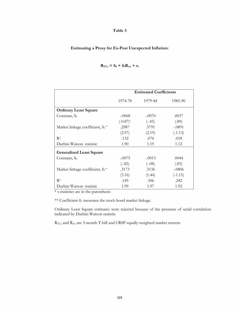
Table 3
Estimating a Proxy for Ex-Post Unexpected Inflation:
RST,t = δ0 + δ1Rmt + εt
Estimated Coefficients
1974-78 1979-84 1985-90
Ordinary Least Square
Constant, δ0 -.0068 -.0070 .0037
(-0.87)* (-.45) (.89)
Market linkage coefficient, δ1** .2987 .5791 -.0891
(2.97) (2.19) (-1.13)
R2 .132 .076 .018
Durbin-Watson statistic 1.90 1.19 1.12
Generalized Least Square
Constant, δ0 -.0075 -.0013 .0044
(-.82) (-.08) (.83)
Market linkage coefficient, δ1** .3173 .3136 -.0806
(3.16) (1.44) (-1.15)
R2 .145 .306 .242
Durbin-Watson statistic 1.99 1.97 1.92
* t-statistics are in the parenthesis
** Coefficient δ1 measures the stock-bond market linkage.
Ordinary Least Square estimates were rejected because of the presence of serial correlation indicated by Durbin-Watson statistic
RST,t and Rmt are 3-month T-bill and CRSP equally-weighted market returns.
325

Table 4
Estimating Alternate Proxies for Maturity-Risk Premia:
Specification a: RLT,t = θ0 + θ1RST,t + εt
Specification b: RLT,t = θ0 + θ1RST,t + θ2Rmt + εt
1974-78 1979-84 1985-90
Specification a: Generalized Least Square
Constant, θ0 -.0028 -.0053 .0017
(-1.02) (-2.11) (.66)
Term structure coefficient, θ1** .3988 .5201 .8183
(10.30) (16.29) (14.96)
R2 .675 .846 .820
Durbin-Watson statistic 1.98 1.83 1.84
Specification b: Generalized Least Square
Constant, θ0 -.0024 -.0064 .0011
(-.84) (-2.47) (.48)
Term structure coefficient, θ1** .4070 .5122 .8105
(10.02) (15.78) (15.34)
Market linkage coefficient, θ2*** -.0216 .0576 .0944
(-.68) (1.07) (2.56)
R2 .677 .849 .835
Durbin-Watson statistic 1.98 1.82 1.80 * t-statistics are in the parenthesis
** Coefficient θ1 measures the average slope of the yield curve.
*** Coefficient θ2 accounts for the stock-bond market linkage.
Ordinary Least Square estimates were rejected because of the presence of serial correlation indicated by Durbin-Watson statistic
RLT,t and RST,t are 7-year T-note and 1-year T-note returns.
326

Table 5
Estimating Alternate Proxies for the Default-Risk Premia:
Specification a: RBAA,t = φ0 + φ1RLT,t + εt
Specification b: RBAA,t = φ0 + φ1RLT,t + φ2Rmt + εt
1974-78 1979-84 1985-90
Specification a: Generalized Least Square
Constant, φ0 -.0021 -.0039 .0010
(-.60) (-1.12) (.66)
Default-risk coefficient, φ1** .0842 .4129 .4734
(2.27) (12.27) (13.47)
R2 .553 .800 .772
Durbin-Watson statistic 1.88 1.97 1.99
Specification a: Generalized Least Square
Constant, φ0 -.0019 -.0051 .0006
(-.54) (-1.41) (.48)
Term structure coefficient, φ1** .0861 .3976 .4637
(2.30) (11.35) (13.83)
Market linkage coefficient, φ2*** -.0066 .0491 .0577
(-.49) (1.49) (2.39)
R2 .555 .806 .785
Durbin-Watson statistic 1.87 1.97 2.00
* t-statistics are in the parenthesis
** Coefficient φ1 measures the average yield-differential between RBAA,t and RLT,t.
*** Coefficient φ2 accounts for the stock-bond market linkage.
Ordinary Least Square estimates were rejected because of the presence of serial correlation indicated by Durbin-Watson statistic.
RBAA,t and RLT,t are BAA corporate bond and 7-year T-note returns.
327

Table 6
Multi Risk-Premia Model of the Bank Stock Returns:
Rjt = α0j + β1jRmt + β2Qj ΔPt + β2Mj ΔMRt + β2Dj ΔDRt + εjt
Estimated Coefficients*
1974-78 1979-84 1985-90
Constant, α0 -.0056 .0041 -.0047
(-1.84)** (1.04) (-1.31)
Market beta, β1 .7397 .6833 .7185
(16.94) (10.55) (17.55)
Inflation beta, β2P .0698 .1292 -.2157
(1.27) (3.45) (-2.29)
Maturity beta, β2M .5350 .4881 -.2476
(2.87) (2.93) (-1.38)
Default beta, β2D -.1973 .1153 -.5696
(-.56) (.43) (-1.94)
R2 .849 .754 .851
Durbin-Watson statistic 2.00 2.04 1.98
* Generalized least square estimates
** t-statistics are in the parenthesis
. Ordinary Least Square estimates were rejected because of the presence of serial correlation indicated by Durbin-Watson statistic.
Portfolio beta estimated using single-index model are .7091, .7259 and 1.0102 for periods 1974-78, 1979-84 and 1985-90, respectively.
328

APPENDIX A
AN INTEGRATION OF CAPM AND APT
The traditional CAPM is augmented by three additional APT type principal component factors
(Johnson and Wichern, 2007) to account for unexpected changes in the inflation premium, the maturity-risk premium and the default-risk rating. Hence, the proposed return-generating model is written as:
Rjt = αj + β1jRmt + β2PjΔPt + β2MjΔMRt + β2DjΔDRt + εjt (A.1)
where ΔPt, ΔMRt and ΔDRt are the proxies for the innovations in inflation, maturity-risk and default-risk, respectively. Coefficients β1, β2P, β2M and β2D are the measures of systematic market risk, inflation risk, maturity risk and default risk, respectively and are consistent with APT.
Principal Component Factor Specification
An important issue in the empirical investigation of this model is the specification of an appropriate inflation, maturity-risk and default-risk factors. Being innovations in economic variables, these factors cannot be predicted using past information. Hence, they must meet the following conditions:
E(ΔPt|t-1) = 0
E(ΔMRt|t-1) = 0
E(ΔDRt|t-1) = 0 (A.2)
where E(.|t-1) is the expectation based on available information at t-1. Theoretical consideration dictates that the choice of a factor (say ΔMRt 1j). Hence, there should not be any contemporaneous cross-correlations between the factors. Hence,
E (ΔPt.ΔMRt) = 0
E (ΔPt.ΔDRt| = 0
E (ΔMRt.ΔDRt) = 0 (A.3)
In addition, there are no common market shocks that may influence any of the risk factors. So following conditions:
E(Rmt.ΔPt)=0
E(Rmt.ΔMRt)=0
E(Rmt.ΔDRt)=0 (A.4)
must be satisfied. We use a generated regressor approach to construct orthogonal inflation-risk, maturity-risk and default-risk factors.
329

Economic factors that lead to changes in the equity market return also induce term structure movements. This leads to a significant correlation between the stock market index and the bond market index. Hence, we use the stock market return to forecast systematic changes in the short-term interest rates. The innovations in the short-term default-free bond return specify the unexpected changes in inflation. Hence, the first systematic interest rate equation is written as:
RST,t = δ0 + δ1Rmt + εIt (A.5)
where Rmt is the return on the stock market index and RST,t is the return on the short-term default-free bond return. The error term in equation (A5), εIt, specifies the unexpected change in inflation and is the generated regressor which serves as a proxy for factor ΔPt. Fama and Schwert (1977) and French, Ruback and Schwert (1983) employ similar approaches to specify a proxy for changes in inflation.
The yield differential between short-term and long-term default-free bond represents the slope of the yield curve. The relationship used to construct the maturity-risk factor is given by the second systematic interest rate equation is:
RLT,t = θ0 + θ1RST,t + εMt (A.6a)
where θ1 measures the average slope of the yield curve. Alternately, we will also test the following systematic interest rate equation:
RLT,t = θ0 + θ1RST,t + θ2Rmt + εMt (A.6b)
Inclusion of the independent variable, Rmt, will control for the stock-bond market linkage. The estimated coefficient θ1 measures the slope of the yield curve and it determines the maturity risk-premium on long-term asset and liabilities. The error term in equation (A.6a or A.6b), εMt, specifies the unexpected change in maturity risk and will be used as the generated regressor which serves as a proxy for factor ΔMRt.
The portfolio of commercial banks used for this study consisted of money center, large national and regional banks. Most of these banks were well capitalized and had acquired a balanced portfolio of assets. The average default risk rating of the portfolio of banks should be close to the default risk rating of a high-grade corporate bond. Hence, the yield differential between BAA corporate bond and long-term treasury security is used to construct the default-risk factor. Our third systematic interest rate equation is written as:
RBAA,t = φ0 + φ1RLT,t + εDt (A.7a)
Alternately, we will also test the following systematic interest rate equation:
RBAA,t = φ0 + φ1RLT,t + φ2Rmt + εDt (A.7b)
where φ1 measures the average default risk on BAA corporate bond. Inclusion of the independent variable, Rmt, will control for the stock-bond market linkage. The error term in equation (A.7a or A.7b), εDt, specifies the unexpected change in default risk and serves as the generated regressor which will be used as the proxy for factor ΔDRt.
330

APPENDIX B
INTEREST RATE INNOVATIONS
An important issue in the empirical investigation of the two-factor model is the specification of an appropriate interest rate factor. Theoretical consideration of factor analysis requires that two factors, Rmt and RIt , be orthogonal whereby choice of the second factor (RIt) would not influence the first factor loading (βlj). The resolution of this constraint requires a robust technique for the determining the unexpected changes in the interest rate that is uncorrelated with the market return. The three approaches to specify the interest rate factor are presented here.
B.1 Orthogonalization Procedure
Economic factors producing changes in the market return also induced term structure movements. This leads to a high correlation between the market factor and the interest rate factor. Hence, market return can be used as an instrument variable to forecast the expected changes in the interest rates. To find the unexpected component of interest rates, the expected interest rate is purged by regressing RIt on Rmt and using the residuals. The systematic interest rate risk equation is:
RIt = δ0 + δ1Rmt + εit (B1)
The residuals, εit, are the unsystematic interest rates and are used to replace RIt in equation (1). The validity of this approach has been questioned on methodological grounds. It is pointed out that this orthogonalization procedure produces biased estimates of coefficients (intercept and β1j in equation 1, and that the deficiency of β2j is not improved. On the other hand, use of an unorthogonal interest rate factor leads to the errors-in-variable problem, i.e., the estimated coefficient β2j also captures some of the effects responsible for changing the market factor and hence, it is not a true measure of the interest rate risk. Another problem using an unorthogonal interest rate factor stems from the fact that interest rate (RIt) is usually autoregressive. Therefore, residuals, εit, from equation (1) are autocorrelated unless GLS parameter estimation procedure is employed. To use the GLS procedure, a variance-covariance matrix has to be specified, which is not an easy task.
B.2 Univariate ARMA model
The second approach is to identify and estimate an ARMA model for the interest rate variable, RIt (Flannery and James (1984)). The unanticipated change in interest rate from the estimated model (i.e., residuals) is used to replace RIt in equation (1). In general, the ARMA model of order (p, q) for the univariate time series, RIt, is written as:
RIt = ф1 RIt-1 + ф2 RIt-2 + … + фp RIt-p + μ – θ1eI,t-1 - … - θqε1,t-q + εIt (B2)
Where εIt, εI,t-1, … are identically and independently distributed random errors with mean zero. The ARMA procedure for the modeling of time series data is outlined in Box and Jenkins (1976). The modeling is usually done in three steps. First, a tentative parsimonious model is identified. Second, the parameters are estimated, and diagnostic (Box-Pierce Q) statistics and residual auto correlation plots are examined. The model is acceptable if the time series of residuals is white noise and the Box-Pierce Q statistics are significant.
This approach leads to unbiased estimates of all the coefficients in equation (1). The shortcoming of the univariate ARMA approach is that valuable information contained in the stock and bond market linkage is ignored. Consequently, coefficient β2j captures some of the effects of economic factors producing stock market changes.
B.3 Vector Arma Model
331

In recent years vector autoregressive moving average (VARMA) models have proved to be useful tools to describe the dynamic relationship between economic variables. A vector autoregressive moving average model of order (p, q) for k-dimensional time series, Rt = (R1t, R2t, … Rkt )T, is generated by the following equation:
Φ(B)Rt = Θ(B)εt (B.3)
Φ(B) = (I – ф1B – ф2B2 - … - фpBp) (B.4)
Θ(B) = (I – θ1B – θ2B2 - … -θqBq) (B.5)
Where B is the back shift operator, I is kxk unit matrix and εt is a sequence of an independent k-dimensional vector with zero mean and positive definite covariance matrix. The interest rate variable RIt, and the market return Rmt, are treated as the components of a bivariate vector. Then vector (RIt, Rmt )T is modeled as a vector AR process. The estimated model provides the unanticipated change in interest rate variable to be used as the second factor in the augmented CAPM model.
332

Cluster Elimination by Means of an Affine Matrix Transformation
Mohammad Alfagih, Najran University
Peerayuth Charoensukmongkol, Texas A&M International University
Ahmed Elkassabgi, Texas A&M International University
Aditya Limaye, Texas A&M International University
ABSTRACT
Cluster Analysis is a multivariate technique used to group objects based on their specific characteristics. Cluster analysis is used in many disciplines including education, psychology, biology, sociology, economics, engineering, and business. Current statistical packages use different techniques to categorize clusters. These different techniques have benefits and drawbacks. We develop and apply a supplemental algorithm to reduce/eliminate the number of clusters in a given data space by means of an Affine Matrix Transformation.
333

THIS PAGE INTENTIONALLY LEFT BLANK
334

Exchange Rate Uncertainty and Trade between U.S. and Canada: Is there Evidence of Third Country Effect?
Mohsen Bahmani-Oskooee, University of Wisconsin-Milwaukee
Marzieh Bolhassani,
Penn State Hazleton
ABSTRACT In a recent article we assessed the impact of exchange rate uncertainty on trade flows of 152 industries that trade between the U.S. and Canada. By using the bounds testing cointegration approach, which distinguishes short-run effects from long-run effects, we found that in the short run, trade flows of almost two-thirds of the industries were affected by exchange rate uncertainty. However, in the long-run, less than one-third of the trade flows were affected. Almost all industries that were affected by exchange rate uncertainty were found to be small, except for road motor vehicles—which makes up to 20 percent of both imports and exports. Exports and imports of this largest industry were adversely affected by exchange rate uncertainty.
We wonder how the results will change if we account for the third-country effect, especially the fluctuation of the U.S. dollar against the currency of the third member of NAFTA, Mexico. We find that, again, in the short run almost 2/3rd of the industries are affected by exchange rate uncertainty. However, in the long-run only 1/3rd of the trade flows are affected. The third-country effect seems to be present in the same number of industries, in the short run as well as in the long run.
JEL Classification: F31
Keywords: Commodity Trade, Exchange Rate Uncertainty, U.S., Canada.
335

THIS PAGE INTENTIONALLY LEFT BLANK
336

The Role of Debt and Currency in the Global Financial Crisis
Rohitha Goonatilake, Texas A&M International University
Rafic A. Bachnak, Texas A&M International University
Asela Acosta, Texas A&M International University
ABSTRACT
When the Euro was established, it intended to favor and solidify the economy of Europe. Soon afterward, the Euro gained ground against the US dollar and other currencies. Meanwhile, the world suffered extremely slow economic growth, and as a result, the debt crisis started to emerge. This article attempts to have a glimpse of understanding about the factors associated with the crisis that led to the current situation and to follow through its path to the present crisis, since it does not seem easy to repair. Additionally, the causes for building up into a large internal debt will be analyzed as the situation was the root cause for this grave uncertainty. The models used to make economic forecasts in the past can shed some light to economists by pondering possible causes to the inception of the crisis that currently affects the state of the world economy.
Keywords: Debts, stocks, housing, properties, budget deficit, IMF, currencies, economy, and investment
337

The Role of Debt and Currency in the Global Financial Crisis
INTRODUCTION
The current slow economic recovery has gradually become stagnant as a result of the European debt crisis and financial turmoil. Some countries such as Portugal, Iceland, Greece, and Italy became the first victims of several waves of economic downturn. Unemployment, the increased cost of living, stock market tumbles, rise of personal and other debts in general, and the expansion of poverty levels are commonly seen among these countries. In fact, actual value of stocks and real estate properties began to diminish as a result of this weathering economic downturn.
As the European crisis unravels, it could shed some light into the situation. Several instances from the past that show how the situation can be eased from the lessons learned from these particular events can be cited. Further, some effects are explained with the use of microeconomic theories which basically study how the market operates by essentially understanding the economic systems.
Since the volatility of the current stock market appears to be too high, it aggregates in relation to other broader measures such as GDP, which are quite substantial and significant. However, they are not out of line by prevailing fluctuations of cash flow holdings by corporations that pay all their expenses to satisfy all of the outside claimants including government agencies (Hall, 2001). The determination of stock prices include the price of an asset that reflects the value of both future payouts earned by holding that current asset, and possible increases in the price of the particular asset. The significance of the future price of an asset for its current price provides a dynamic element into pricing of assets. The efficacy of a given change is comparable to the present values. Subsequently, stock prices move rapidly in response to dividend and expected stock prices under volatile market conditions.
Personal and household debt expands during economic calamity. At the same time, the value of stocks are lowered and devalued causing the housing and property markets to collapse. In terms of mortgages, loans, and credit card debts, all consumers seem to have accumulated personal and household debt. Industry performance declined causing unemployment and their stock prices to plunge. The market demands funds from borrowers for expansion and additional investment opportunities. To a borrower, a higher interest rate has an income and substitution effect that discourages the level of desired borrowing from lenders. Therefore, higher interest rates make it more expensive to finance increased consumption from borrowed funds. Increased government spending and rise of unemployment bring less revenue that undergoes heavy budgetary deficits and ripening conditions for inflation.
MAJOR CURRENCIES AND GDP
Major currency unions have dominated the world causing tension amongst them. The growing importance of the US dollar was a somewhat noticed event at the beginning of the 20th century. The European Union (EU) is a unification of 27 member nations that are presumed to create a politically and economically united community throughout Europe. The Euro became huge news later in the century when it was introduced by EU. One of the largest steps toward European unification took place with the introduction of Euro as the
338

official currency in eleven countries that included, Austria, Belgium, Finland, France, Germany, Ireland, Italy, Luxembourg, Netherlands, Portugal, and Spain on January 1, 1999. However, the first European Union countries that adopted the Euro did not begin using it until January 1, 2002. It created change of currencies in the whole currency map. As a result, the Euro instantly became the second most important currency in the world. The Euro, in the meantime, as opposed to the US and Canadian dollars, has gained ground. Presently, the Euro is one of the world's most powerful currencies, used by more than 320 million Europeans in twenty-three countries. The countries using Euro are: Andorra, Austria, Belgium, Cyprus, Estonia, Finland, France, Germany, Greece, Ireland, Italy, Kosovo, Luxembourg, Malta, Monaco, Montenegro, Netherlands, Portugal, San Marino, Slovakia, Slovenia, Spain, and the Vatican City. Japanese yen, on the other hand, dominated in Asia along with their overseas transactions.
A treaty drafted to save the Euro split the UK from Europe in the later part of 2011. The United Kingdom (UK) abandoned being a signatory to the treaty to save the European debt crisis. The UK stood defiantly against this historical treaty by rejecting demands for treaty change across the EU as part of a rescue plan introduced to save the single currency. This unprecedented move surprised the world putting the UK’s future in the EU into serious doubt as it maintains their currency as the UK pound. The parity rate comparison against UK pound, US dollar (USD), and Canadian dollar is done to bring this point to the attention in Figures 1, 2, and 3.
Figure 1: UK pound rates vs. USD
Source: http://www.exchangerate.com/currency-charts/USD/GBP/from//to/
339

Figure 2: Canadian dollar rates vs. USD
Source: http://www.exchangerate.com/currency-charts/USD/GBP/from//to/
Figure 3: Euro rates vs. USD
Source: http://www.exchangerate.com/currency-charts/USD/GBP/from//to/
340

Figures 1, 2, and 3 also show there were greater volatilities due to many reasons; one of them being its direct effects on commodity markets. It is seen that the US dollar is devalued over the period; therefore, giving unfair advantages to the US economy. Some argue this is as a result of globalization. Another reason is the internal debt associated with major countries including the US. The US debt percentage of GDP is nearly 100% so it is not to be included in the top 10 countries with worst debt-to-GDP ratios listed in Table 1.
Table 1: Current debt of ten major countries as percentages of its GDP
Country Debt as Percent of GDP (2010 est.)
Population in 2010 (millions)
Geographical Area (Sq. Miles)
Japan 225.9 126,475,664 145,882
St. Kitts and Nevis 196.3 50,314 101
Lebanon 139.0 4,143,101 4,015
Jamaica 135.7 2,868,380 4,244
Greece 130.2 10,760,136 50,942
Eritrea 129.7 5,939,484 46,842
Grenada 119.1 108,419 133
Italy 118.4 61,016,804 116,305
Iceland 115.6 311,058 39,768
Barbados 111.6 286,705 166
Source: http://www.tradingeconomics.com
Many countries with such high debt percentages of GDP, for instance, the Caribbean nations of Jamaica, and Barbados, are not among the world's economic superpowers. A more relevant consideration is to look at the United States debt situation within the context of other largest world economies. Among the 10 countries with the largest GDPs, the US ranks third in terms of debt as a percentage of its GDP, only behind by Japan and Italy. One major outlier on the list is China, whose 2010 GDP is estimated to be the world's second-largest, at $5.7 trillion. However, its debt is only equal to 19.1 percent of its GDP, which is well below all other major world economies.
341

Table 2: Debt as percent of GDP of all other major world economies
Country GDP (2010 est., USD) Debt as Percent of GDP (2010 est.)
GDP Growth Rates (2011 Q3)
United States $14.6 trillion 92.7 1.5%
China $5.7 trillion 19.1 9.1%
Japan $5.4 trillion 225.9 -0.7% (negative growth)
Germany $3.3 trillion 75.3 2.5%
France $2.6 trillion 84.2 1.6%
United Kingdom $2.3 trillion 76.7 0.5%
Italy $2.0 trillion 118.4 0.2%
Brazil $2.0 trillion 66.8 2.1%
Canada $1.6 trillion 81.7 3.4%
Russia $1.5 trillion 11.1 4.8%
Source: IMF World Economic Outlook Database, October 2010
Currency manipulation or currency wars harm fair trade practices, thus making some countries have unfair advantages while putting forward drastic economic reforms. It is important to believe that Europe is going to get into the business of counterbalancing China in many ways. Europe as a whole has few strategic interests in Asia as they are trying to establish an economic power. At the same time, they would see China as an emerging market for their products and services. This would be a serious setback to the US. All nations balance against economic threats, and one advantage for this threat is its geographic proximity. If the US decides to balance China it needs all possible allies to help it accomplish that task, by wanting them to be in Asia not in Europe or elsewhere. In addition, there are four newly industrialized Asian economies, namely, Hong Kong SAR, Singapore, Korea, and Taiwan Province of China. They are apparently doing better in this turbulent economy by becoming partners to everyone.
CAUSES OF DEBTS
In the perspectives of Americans, citizens live under three major forms of government: the federal, the state, and the local governments. There are both benefits and costs involved for living under these forms of government. Many of the benefits enjoyed are under the federal government. Some of the major services the federal government provides are national defense, healthcare (Medicare for the elderly), food stamps, social security, and public education for the younger generation. Some of the costs Americans pay to the federal government are personal income taxes (progressive tax), social security contributions (payroll taxes by both employee and employer), and sales and excise taxes (when purchasing items and commodities). The main benefit that the state government provides to its citizens is public education, among many others.
Government overspending and wartime expenditures have largely contributed to the current debts of the US. Unsustainable export and import deficits contributed to the crisis as well. The US federal government has operated with a deficit in every year except for two times since 1957. In 1983 the deficit exceeded $200 billion for the first time in the US history. Most forecasts projected that deficits would remain at that size or grow through 1989 unless taxes were raised or expenditures were reduced drastically. The same goes with current public sentiment and prevailing wisdom.
342

Figure 4: Effects of deficit financing
For a particular investment demand curve, the more sustainable the supply curve (S), the more the private investment will fall as a result of government borrowing (Browning & Browning, 1986). Figure 4 shows that if the government borrowed $B to finance the deficit $D, the corresponding expenditures shifts the demand curve for additional funds supplied by the savers to $(D + B). As a result, interest rate, s% is bid up to the rate of r% and private investment inclined at the same time. The reason for which the public worries about the deficits is that the cost of financing the government expenditure due to borrowing is ultimately a burden on them in the future. It is currently in the tune of $15.2 trillion. For Europe, from Figure 5 the negative trade deficits have been seen in Greece, Portugal, Italy, and Spain. This may have led to their debt crises. The fact that the government competes with private borrowers when borrowing funds from servers, results in higher interest rates and a decrease in private investment as anticipated.
As countries depend on import products (such as oil), the impact of the changes in the prices and their local consumption on trade balances can explode; but there are remedies to offset the changes. This amounts to the fund's projection of the aggregate current deficit of (nonoil) market, compound rates, debt and income. Debt is generated by the gap between domestic saving and prices paid on the imports that also contributed to internal debt (Solomon, Greenspan, Kareken, and Ohlin, 1977).
343

Figure 5: Trade deficit as a percentage of GDP for Greece, Portugal, Italy, and Spain
Global financial crises hit some countries harder than the others leading to their economic slow-down. Accordingly, Greece, Iceland, Portugal, and Italy’s troubles resulted in austerity measures introduced to them by world bodies. These three countries have suffered major financial crises lately and all of them have government debts that far exceed their annual projected GDPs. Appropriate austerity measures need to be placed in the intent to ease the crisis.
RETIREMENT BENEFITS AND LABOR UNIONS
Exorbitant benefits and retirement packages are negotiated with employers by labor unions. American adults also believe that, by joining labor unions, the living standards of workers in the US would be greater than that of the workforce in other countries. The impact of unions on wage rates and employment in the union and nonunion sectors is worth considering when addressing this issue. The theory will provide some answers to the questions.
Formation of a labor union increases the wages and rights in the union sector, but only at the cost of employment reduction. Workers who are unable to find a job in the union sector would increase the workforce in the nonunion sector and as such, wages will dramatically go down in the nonunion sector as in Figure 6. This certainly impacts the underlying economic scenario. The union negotiated benefit and pension plans appear to consume a large portion of the state budget. The impact of labor unions on wages and employment in the union combined with nonunion sectors is vast and potentially contributes to the severe crisis yet to unfold.
344

Figure 6: Union and nonunion sectors vs. wage rates
The aging baby boom generation has demand for entitlements such as social security and Medicare, as well as long-term care services that have many challenges on the federal and state budgets. In the long run, this will lead to a rapid growth in federal entitlement spending in the absence of a meaningful reform to offset an unsustainable burden on future generations and the federal budget. For example, on August 14, 1935, the Social Security Act established a system of old-age benefits for workers, benefits for victims of industrial accidents, unemployment insurance, aid for dependent mothers and children, the blind, and the physically handicapped. The benefits are actually composed of two equal payroll taxes, one collected from the employer and the other from the employee. This large entitlement program together with Medicare provides a safety net for adults and older generations. It also contributed to the unprecedented internal debts in the US. However, when many baby boomers began to retire, the burden of the social security tax became considerable. According to Figure 7, it is projected that Federal spending for Medicaid, Medicare, and social security will double as a share of GDP by 2035. The estimates do not include the state share of Medicaid expenses. These projections were based on intermediate assumptions of the 2001 old-age, survivors, and disability insurance, hospital insurance, and supplementary medical insurance trustees’ reports and the 2002 long-term Medicaid projections by the Congressional Budget Office’s (CBO).
345

Figure 7: Projected federal spending for Medicaid, Medicare, and social security
Source: Office of the Actuary, Centers for Medicare and Medicaid Services; the Office of the Chief Actuary, Social Security Administration; and CBO
Countries such as Brazil, China, India, Indonesia, Israel, Japan, Korea, Malaysia, the Philippines, Singapore, South Africa, Switzerland, Taiwan, and Thailand have recently engaged in exchange markets and capital controls that could curb appreciation of currencies. This would easily provide a weaker rate of one country influencing the stronger rate(s) of another country or countries (Cline and Williamson, 2010). This has already resulted in economic integration and currency regions around the world as seen in Figure 8. Each country has been colored according to the most advanced agreement that it participated into the stages of economic integration.
346

Figure 8: Stages of economic integration around the World
Source: www.oup.com/uk/orc/bin/9780198742869/ch01.pdf
Color Economic Integration and Currencies
Green Economic and Monetary Union (CSME/EC$, EU/€)
Yellowish Green Economic Union (CSME, EU)
Blue Customs and Monetary Union (CEMAC/franc, UEMOA/franc)
Brown Common Market (EEA, EFTA, CES)
Pink Customs union (CAN, CUBKR, EAC, EUCU, MERCOSUR, SACU)
Red Multilateral Free Trade Area (AFTA, CEFTA, COMESA, GAFTA, GCC, NAFTA, SAFTA, SICA, TPP)
PREVIOUS GLOBAL FINANCIAL CRISES
Some argue that to an extent, the recent turbulence in global financial market has been caused by inadequate understanding of sophisticate financial modeling (Shreve, 2005). Glimpses of some crisis that led to inflation are provided below to show that the scenarios under which the recovery was possible with the hope that the current crisis can be soon understood, learned, and subsequently eased. Three main examples, the Japanese Growth Miracle, Vietnam War Inflation, and the Great Depression are discussed in order to bring this point to an attention. Presently, the IMF (International Monetary Fund) provides monitory support to relieve the financial crisis of a country in order for them to have strong footing as the country takes drastic economic reforms to improve the situation. The IMF is an organization comprised of 187 countries, working towards fostering global monetary cooperation, secure financial stability, facilitate international trade, promote high rate of employment and sustainability of their economic growth, and to assist the reduction of poverty around the world. If the IMF was to provide assistance, then the country would be in need of tightening belts by taking strict measures such as curbing expenses while sustaining through these assistances for improving the situations.
347

Figure 9: Theory behind Japanese growth miracle
The Japanese Growth Miracle is the historical event where Japan regained economic growth after World War II (WWII), contributed by US investment and because of the Japanese government economic intervention through their Ministry of International Trade and Industry (MITI). After WWII, business-related burdens made it look like Japan was headed for economic catastrophe. It was thought that economic development could democratize Japan and would be incapable of preventing the reemergence of militarism as a way to stop communism. The US government paid the Japanese government large sums for military procurement equivalent to 27% of Japan’s total export trade. The Japanese economy hit a recession when the US stopped payments and started recovering afterword. By the late 1960s, Japan had risen from the aftermath of WWII to achieve an astoundingly rapid and complete economic recovery. The Japanese government contributed to the economic miracle by stimulating the growth of private sectors. MITI made the Japanese government and private industry prevent the flooding of Japan’s markets by foreign goods. It also regulated all imports with the abolition of the Economic Stabilization Board and the Foreign Exchange Control Board in August 1952. The MITI boosted the industrial sector by untying the importation of technology from the import of other goods. In 1965, Japan's real GDP was estimated at just over $91 billion. Fifteen years later, the real GDP had soared to a record of $1.065 trillion by 1980. By the early 70’s, the GDP was growing at a phenomenal rate of 13.9 percent despite a large protected domestic economy. As seen from Figure 9, Japan had all the components of GDP, but both the US aid and the Japanese government spending assisted the recovery.
348

Figure 10: Government intervention to curb Vietnam War inflation
The inflation occurred during the 1960’s in the United States, is a classic example of Demand-Pull Inflation. This type of inflation is the worst kind because the economy cannot fix itself. The government must intervene immediately if this happens. The escalation of the Vietnam War had resulted in a 40 percent increase in defense expenditures between 1965 and 1967 and another 15 percent increase in 1968. The increase of the government's spending shifted the economy’s aggregate demand curve to the right, which produced the worst inflation in two decades. Actual GDP exceeded potential GDP, and inflation jumped from 1.6 percent in 1965 to 5.7 percent by 1970. Figure 10 showed that the government had an inflationary expenditure gap of about 133 billion dollars. The equilibrium exceeded full employment levels, and as a result, the government had a hard time coping with it. Subsequently, aggregate expenditure went up triggering a large scale unprecedented economic recovery.
349

Figure 11: Dramatic economic downturn lead to great depression
The Great Depression was a dramatic economic downturn that began in 1928 associated with the stock market crash of 1929. The Great Depression was not a sudden total collapse. The stock market turned upward in early 1930, but returned to the levels of 1929 by April of that year and almost dropped 30 percent below the peak of September 1929. In early 1930, credit was available at low rates; however, people were reluctant to add new debt by borrowing. Conditions were worse in farming areas because prices plunged, and in the mining and logging areas, unemployment was high and there were few jobs. People and businesses were in debt as price deflation occurred or demand for their product decreased. Layoffs caused unemployment rates of over 25%. The US Government cut back its expenditures by 10 percent. Trade declined due to increased tariffs. Government expenditures contributed to only 3 percent of the total GDP in the nation. The Great Depression went below the usual recession in the regular business cycle. Real GDP went down by about 25% from 1929 to 1933. The US Government started to decline its spending by a little more than a billion dollars. However, a billion dollars amounted to almost ten percent of total expenditure by the government. This caused the real GDP of the US to go down by more than two hundred billion dollars thus becoming a huge problem for the US. However, after new programs and the military production during WWII, the economy recovered from the depression.
CONCLUSIONS
Evidently, individual country’s internal debt, weak currency market, and poor performance of markets all have contributed to the present crisis. The study of recoveries from the previous global financial crisis would enable us to find a real solution to the crisis until theory provides a definite solution. However, the impact of globalization on the US economy continues to be one of the most debated economic issues discussed in favor and against the economic expansion in the past decade (Dwight, 2008). The extent of what occurred on currency and stock markets influence the other factors and vice versa providing a greater volatility of market condition for stocks that are sold and bought on a daily basis.
350
REFERENCES
Edgar K. Browning and Jacquelene M. Browning, Microeconomic Theory and Applications, Second edition, Little Brown & Company, 1986
William R. Cline and John Williamson, Policy Brief: Currency Wars? Peter G. Peterson Institute for International Economics, Number PB10 - 2 6 November 2010
Jaffee M. Dwight, Globalization, Offshoring, and Economic Convergence: A survey. In C. Beverly & E. A. Fogarty (Eds.), The Impact of Globalization on the United States Westport, CN: Praeger, (2008), pp. 55-59
Davide Furceri, From Currency Unions to a World Currency: A Possibility? International Journal of Applied Economics, 4(2), September 2007, pp. 17-32
Herbert G. Grubela, The Merit of A Canada-US Monetary Union, The North American Journal of Economics and Finance, Vol. 11, Is. 1, pp. 19-40, 2000
Robert E. Hall, Struggling to Understand the Stock Market, The American Economic Review, Vol. 91, No. 2, Papers and Proceedings of the Hundred Thirteenth Annual Meeting of the American Economic Association (May, 2001), pp.1-11
IMF http://www.imf.org/external/index.htm
Danielle Kurtzleben, The 10 Countries with the Most Debt: The United States has the largest debt in the world but other countries face more dire situations, US News & World Report, January 28, 2011
Campbell R. McConnell and Stanley L. Brue, Macroeconomics: Principles, Problems, and Policies, Seventeenth Edition, McGraw-Hill/Irwin; a business unit of The McGraw-Hill Companies, Inc., 2008
Mundell Robert, Currency Areas, Volatility and Intervention, Journal of Policy Modeling, Vol. 22, Is. 3, pp. 281-299, 2000
Steven E. Shreve, Stochastic Calculus for Finance: The Binomial Asset Pricing Model, Vol. 1, Springer, New York, 2005
Robert Solomon, Alan Greenspan, John H. Kareken and Goran Ohlin, A Perspective on the Debt of Developing Countries, Brookings Papers on Economic Activity, Vol. 1977, No. 2 (1977), pp. 479-510, The Brookings Institution
351

THIS PAGE INTENTIONALLY LEFT BLANK
352

The Future of the Large Capacity Aircraft Industry
James Cox, Texas A&M International University
Bolortuya Enkhtaivan, Texas A&M International University
Wei Wang, Texas A&M International University
ABSTRACT
In this paper we consider the conflict between Boeing and Airbus in the light of the WTO resolution process, as well as the factors that have led up to this process. These include duopolistic competition, market share, direct and indirect subsidies, the strategic importance of the LCA industry, positive externalities and spillover effects and the interaction of Porter’s five forces. We finish this article with forecasts for the industry and analyze the possibility of entrance of new competitors.
353

The Future of the Large Capacity Aircraft Industry
INTRODUCTION
The LCA industry is very unique. There is a large variety of competing product families from its two principal companies: Boeing and Airbus. This ensures that competition remains fierce, but several levels of complexity are added when one considers other factors, such as: The close ties between the LCA industry and the development of military equipment, the high entrance barriers exemplified by huge sunk and financing costs as well extremely long product development cycles.
These factors in turn have led to the current condition of the industry: one that is dominated by two main competitors, Boeing and Airbus, each with roughly 50% market share. The strategic advantages that a country or a group of countries obtain from the LCA industry are varied. They can be military, economic or technological. This, in combination with the huge capital costs required of the industry has led to constant conflict between the companies and their host countries regarding the subsidies that each organization receives.
BOEING AND AIRBUS: A DUOPOLY Duopoly: A situation in which two companies own all or nearly all of the market for a given type of product or service. (Investopedia.com)
Boeing and Airbus have achieved a very strong duopoly in the LCA segment of civilian aircraft market (The Industrial College of the Armed Forces, 2010) as well as dominated the civilian aircraft market in general (Harrison, 2011)
THE CURRENT STATE OF THE LCA SEGMENT OF AIRCRAFT MANUFACTURING The LCA industry is unique in the sense that each firm has a large variety of products. Large body aircrafts carrying capacity varies from 100 to 853 seats and travel range varies from 2,645 km to 17,400 km. Airbus produces 21 models while Boeing produces 26 models. Multi-product producers do not undercut prices aggressively to monopolize power, since doing so would do more harm than good. Therefore, competition according to Bertrand’s model is not very intense. Actually, this is proven by Irwin and Pavcnik (Irwin & Pavcnik, 2001) that indeed Bertrand and Cournot’s outcome provided similar results for markup estimates and their simulation result showed that introducing a new aircraft would hurt their own existing models190. Moreover, multiproduct properties studied by Irwin and Pavcnik (Irwin & Pavcnik, 2001) imply that necessary market segmentation of products and imperfect substitutes for each segment due to their specific market focuses.
On the other hand, with learning by doing characteristics of a multi-product firm, both firms could offer initial discounts which can be covered later with increasing markup price and economies of scale. Although literature suggests different numbers and there is lack of transparency in the actual pricing for the launch of the A-380, Airbus offered discount up to 35 percent on their global sales of aircrafts (Pavcnik, 2002) and Boeing offered up to 40 percent of discounts for their commercial aircraft sales in 2010 (Gates, 2011).
THE STRATEGIC IMPORTANCE OF THE LCA SEGMENT OF AIRCRAFT MANUFACTURING The aircraft manufacturing industry is considered strategic for many governments, in the case of United States Government, as stated by The Industrial College of the Armed Forces. There are two main strategic advantages of the industry:
190
Irwin and Pawchnik (2001) found that introduction of Airbus 380 reduced long-range wide body aircraft market
share (estimated by the number of planes sold) by 2.5 percent while medium-range aircraft market share was
reduced by 0.9 percent.
354

1. Trade and support for manufacturing: “Aircraft and automobile manufacturing are considered by many to be the technological backbones of the U. S. manufacturing base” and “The aircraft industry is also critical to the US trade balance, as well as the American workforce”. (The Industrial College of the Armed Forces, 2010)
2. The Defense Industrial Base: “industry consolidation during the past 20-years has negatively influenced the relative strength of the US defense industrial base. While consolidation afforded reduced costs and increased efficiency within industry, it also limited competition and inhibited innovation, with long-term national security implications.” (The Industrial College of the Armed Forces, 2010)
We believe that assuming that other countries with fully developed or developing LCA companies have similar views in the matter is not a stretch of the imagination.
THE IMPORTANCE OF PORTER’S FIVE FORCES Porter’s five forces model is a useful tool to assess where the power lies in a business situation. It could help in figuring out the strength and attractiveness of an organization in an industry structure. To find out a company’s competitive position and plan the future position a firm is going to attain is quite important, especially in an oligopoly or duopoly market structure.
We can analyze the competitive situation of Boeing and Airbus by Porter’s five forces model, and explore the truth of the rivalry and dispute between Boeing and Airbus.
355

Figure 1 Porter’s Five Forces in Aerospace industry
Porter’s Five Forces
Threats of New Entrants
Entrance Barriers
•Capital Requirements
•Economies of Scale
•Government Policies (Subsidies)
Industry Growth Rate
Incumbent’s Defense
Determinants of Buyer Power
Number of Buyers
Product Differentiation
Costs of Switching Products
Buyer Volume
Government Policy
Threat of substitute Prodcuts
Relative Price
Relative Quality
Costs of Switching Products
Technology Leakage
Determinant of Supplier Power
Supplier Concentration
Availability of Supplier inputs
Importance of Industry to Suppliers
Buyer{s Switching Cost
Supplier Threat of Forward
Integration
Rivalry of Existing Competition
Number of Competitors
Relative Size of Competitors
Industry Growth Rate
Fixed vs. Variable Costs
Exit Barriers
Strategic Stakes
Buyer Switching Costs
RIVALRY OF EXISTING COMPETITION Within the highly competitive large civil aircraft (LCA) industry, Boeing and Airbus are the two dominant manufactures. These two companies compete from the aspects of product, outsourcing, technology, etc. For the market share, Airbus was only 31% in 1996, and then steadily increased to 57% in 1999. But in 2000, it decreased to 47% in 2000. By reorganization, Airbus maintained its share in the mid to high 50% until now (pubfin.nccu.edu, 2006).
As to the product, both Boeing and Airbus have a broad product range. If one of them introduced a new product to the market, another one usually followed by and responded to it immediately. For example, in order to compete with Boeing 747, Airbus developed a larger aircraft type A380, and used Airbus A350 to compete with the high end of the Boeing 787 Dreamliner and the Boeing 777 (Robertson, 2006).
In order to gain a competitive advantage, Boeing and Airbus tried to develop their outsourcing. Since 1982, Boeing began to outsource 15% of its manufacturing process to Japan for developing Boeing 787.Now about 70% of the Boeing 787 Dreamliner is manufactures outside the United States. Because of its own European plants, Airbus has fewer opportunities to outsource its significant parts, but it also opened an assembly plant in China for the production of its A320 series aircrafts (Gates, 2010). However, both of Boeing and Airbus need to beware of the side effect of outsourcing. We would analyze it in detail later in our study.
356

THREAT OF NEW ENTRANTS Threat of new entry depends on entry and exit barriers. Barriers to entry are obstacles which make a company difficult to enter a given market and compete with the incumbent companies. The established firm will take advantage of economies of scale by building entry barriers. For example, the incumbent firm could use advertising, capital advantage, control of resources, cost advantages independent of scale, or customer loyalty as tools to build entry barriers. The LCA industry has very high market entry barriers, which make it difficult for new entrants to compete successfully in this industry. As we can see, newcomers require large capital to start a company, and also for the huge research and development (R&D) spending (Caliskan, 2010).
The LCA industry is shifting rapidly these years. As we have mentioned, Boeing and Airbus are still the two dominant manufactures in this industry. Both of them outsource and set plant in other countries. The side effect of outsourcing is technology leakage. Japan and China try to combine the technology and skill they acquired in the manufacture process into their own aircraft development and manufacture. Canada’s Bombardier, China’s Commercial Aircraft Corporation of China and Russia’s Sukhoi Civil Aircraft Company plan to enter the LCA market and compete with Boeing and Airbus. The new entrants of this industry may break this duopoly market. (Andersen, 2009)
BARGAINING POWER OF BUYERS Airline industry is also oligopolistic in many countries. There are a few airlines, and each of them has significant market share. Meanwhile, the LCA products are standardized, so the bargaining power of airlines is powerful. For example, China has become a battleground for Boeing and Airbus. Even though there are couples of airlines in China, the dominant airlines only include Air China, China Eastern Airlines, China Southern Airlines, and Shenzhen Airlines. Besides these airlines, the aircraft leasing companies are also buyers of LCA industry. There are quite a few aircraft leasing companies all over the world, which intensified the competition. The fierce competition between Boeing and Airbus is also due to their contention for the limited buyers.
THREATS OF SUBSTITUTE PRODUCTS As we mentioned in the prior part, in order to compete with Boeing 747, Airbus developed a larger aircraft type A380, and used Airbus A350 to compete with the high end of the Boeing 787 Dreamliner and the Boeing 777. To compete with the A380, Boeing developed 747-8 which is the latest modification of Boeing’s largest airliner. It has a full-length double-deck aircraft now in service (Robertson, 2006). Boeing and Airbus’s family of products have a lot of overlap.
There is also the issue of the cost of changing from one model of aircraft to another: According to Yoffie and Milner “Since customers would have to train their engineers and maintenance personnel for particular planes, there were significant economies to sticking with one aircraft type” (Yoffie & Milner, 1989)
DETERMINANT OF SUPPLIER POWER According to the Industrial College of the Armed Forces “The power of the suppliers for the aircraft industry is moderate overall” (The Industrial College of the Armed Forces, 2010). Possible new competitors, especially the Chinese (Harrison, 2011) could take advantage of suppliers of aircraft parts already established in China.
SPILLOVER EFFECTS, POSITIVE EXTERNALITIES AND RELATED FACTORS Being a huge industry itself, the production of LCAs requires billions of dollars in investment. But it also promises a lot in return to the nation that hosts it in terms of large positive spillover effects. Employment increases with production sites, positive externalities materialize to other industries, real income growth and technological development happen. A country can gain a strategic competitive advantage in the global market, supply chains get established, and national pride and prestige increase.
357

HIGH COSTS AND OTHER REASONS FOR SUBSIDIES LCA is an extremely high cost industry that requires huge sunk costs in a form of R&D and infrastructure. Research and development cost of a new model could be as high as 20 times its final product price for a new aircraft (Sedaei, 2006). For example, Boeing’s introduction of the 747 family of aircrafts in 1966 required as much as three times its total capitalization. (Harrison, 2011)
Moreover it requires a long period of time to deliver an initial order in the LCA industry. During this time there could be different external events that may put at risk the designated delivery time and successful order completion. For instance, a large-scale strike (Sedaei, 2006), extraordinary exogenous effects like the Gulf war in early 1990s and terrorist attacks (Caliskan, 2010)
Figure 2 Evolution of subsidies conflict in aerospace industry
Subsidies
Production
Market share
Employment and economic
growth
positive externaliti
es
Secondary industry
dev.R&D
development
Sunk cost
Long time
Conflict
DEFINITION According to the Merriam-Webster Dictionary: A grant by a Government to a private person or company to assist an enterprise deemed advantageous to the public.
“Subsidies are current unrequited payments that government units make to enterprises on the basis of the level of their production activities or the quantities or values of the services which they produce, sell or import. They are receivable by resident producers or importers...”. (System of National Accounts, 2008)
According to the WTO, the term “subsidy” is rarely defined, although widely used. It can be seen as an antonym of “tax”, in the case of government transfers to a private entity. By extension, a subsidy could also be the reduction of a tax liability. Both are different forms of assistance, so defining a subsidy as a government expenditure would not necessarily be complete. A broader view (and the one that we will consider for this paper) is: A subsidy consists of any benefit of the private sector by a government program. (World Trade Organization, 2006)
358

It is important to note that the definition given in the above paragraph may not be in agreement of what the WTO formally considers a subsidy in different scenarios, industries or conflicts. It also may be inconsistent with what certain governments or corporations consider to be a subsidy. Also relevant to this paper is the fact that this difference of opinion of what constitutes a subsidy between the WTO, governments and corporations has given rise to disputes that are brought before the WTO and become lengthy and involved. A case in point is the ongoing dispute between Boeing and Airbus.
IN THE CASE OF BOEING AND AIRBUS
LCA INDUSTRY CHARACTERISTICS THAT MAKE IT PRONE TO SUBSIDIES: (Caliskan, 2010)
High Entrance Barriers: High cost of Infrastructure, Long development time of new products. Companies (Especially Airbus) typically need government financial assistance in this area.
Huge Research & Development costs. Companies may have trouble raising the needed capital for these ventures. Governments (Especially in the EU) sometimes finance this stage of a project
Colossal Financing Requirements of Sunk Costs and their related high exit barriers. Governments typically offer companies favorable financing in this area.
Long investment cycles to recover R&D costs leads to high cluster risk: Large number of aircraft needs to be sold to recover. Governments (Especially in the EU) can help minimize these risks through investments.
Close ties between the military and civilian segments of each company means that they are of strategic importance to their respective country of origin. This can also carry advantages, since government contracts (Especially in the US) can mean increased economies of scale, operational efficiencies, and transfer of knowledge and expertise from military to commercial aircraft manufacturing.
DEFINITION OF SUBSIDY (According to the WTO Agreement on Subsidies and Counter Measures) (Caliskan, 2010)
Financial contribution by a government or any public body within the territory of a member state
Confers a benefit
For a specific recipient
HISTORY OF SUBSIDIES IN THE INDUSTRY (Caliskan, 2010)
LCA Industry is subject mainly to the Subsidies and Counter Measures (SCM) agreement of 1994, with some more multilateral rules in existence.
US was concerned from the beginning with the alleged subsidies that Airbus was receiving to develop their early models. From the beginning this aid took mainly the form of favorable financing, help with infrastructure, and subsidies to Research and Development.
Since its early days, Airbus has been concerned about Boeing’s indirect support from NASA and the US military. This has been received in the form of government contracts that transfer knowledge to civilian aircraft, the grant of patents, and economies of scale.
1992 EC-US agreement on Trade in LCAs: o Government cannot support more than 33% of costs of development. Has to be through
royalty-based loans (Mainly aimed at the EU). o Indirect support cannot be more than 3% of the nation’s LCA industry turnover (gross
revenue) (Mainly aimed at the US).
359

o Countries must exchange transparency information. o The EU feels that the US does not reveal actual benefits of its military contracts to the
civilian aircraft manufacturing segment.
US now questioning the validity of agreement about European “Launch Aid”
EXAMPLES OF EU SUBSIDIES TO AIRBUS: (Maening & Wittig, 2010)
Direct Research Funding by the EU o 1998-2002: 784 Million Euros o 2002-2006: 857 Million Euros o 2007-2013: More than double for the previous period
Export Financing: Guarantees and public loans to reduce capital cost of buyers and ensure the competitiveness of Airbus.
Financing from the European Export Bank o Partial funding of up to 50% of purchase price o Finances mainly state-owned dominant airlines in Europe o Increasing financing in emerging markets o In 2000-2006 61% of its aircraft sales were for Airbus
Launch Aid for New Models: These can be described as discounted loans from the public sector with subsidized interest rates.
Infrastructure: The Hamburg Senate authorized the expansion of the airport in connection with the assembly of the Airbus A380. This included the expansion of the Airbus factory, and was done through land reclamation. The expansion of the runway and compensatory measures cost Hamburg 693 Million Euros, but since Hamburg was exercising its sovereign right, these were not considered subsidies.
Military Funds: Provides Synergy, transfer of knowledge and experience as well as the enlargement of economies of scale.
360

Figure 3 An illustration of the complex web of dependencies created by government subsidies
SubsidiesEducation Infrastructure
Risk Entrance BarriersMilitaryResearch &
Development
Prodcut Development
Secondary Industry
Prodcution
Social Benefits
Economic Benefits
Technological Benefits
CURRENT CONDITION OF THE LCA INDUSTRY MARKET SHARE Market share of the industry is defined differently in literature due to the variety of products and the price diversities among aircraft families. In their studies Irwin and Pavcnik (Irwin & Pavcnik, 2001) and Pavcnik (Pavcnik, 2002) used number of aircrafts sold as a market share estimate unlike general estimate of sales in dollar value. As of 2005, while Boeing constituted 55% of the dollar value of market, Airbus constituted slightly over 40% of commercial aircraft industry (Sedaei, 2006). Duopolies were compared in terms of orders, deliveries, employee numbers, net sales and revenues in (Caliskan, 2010). Flightglobal media agency reports that Airbus has outdone its competitor Boeing to reach 54% of market sahre in 2010 compared to 50% in previous years by the number of their deliveries.
DISPUTE SETTLEMENT Potential third party entry interests from current small aircraft producers and supply chain productions from several different countries may make the dispute settlements on subsidies linger. A lot of interests from these third parties beside the current conflicted parties could be raised. Requiring billions of investment costs in LCA, subsidies are mandatory to fill some gaps. Subsidies are beneficial to the industry and would reoccur even if all the participants eliminate subsidies simultaneously according to Yu-Ter Wang (Wang, 2009).
361

As for the process itself, if a member country takes some action which other members think it violates WTO agreements, a dispute will arise. In order to make the members of WTO follow the rules and ensure smooth trade flows, the WTO’s procedure for resolving trade quarrels is under the Dispute Settlement Understanding (wto.org, 2009).
After joining the WTO, if the member countries find their fellow members are in violation of trade rules, they cannot take action unilaterally. Instead, they will follow the multilateral system, which normally includes the Dispute Settlement Body (DSB) and Dispute Settlement Understanding, to settle disputes. If a member country considers another member violates the rules and deprives benefit from it, it will call for consultations with other member countries. If the consultation cannot resolve the dispute within 60 days, the complaint party may ask for the establishment of a panel to tackle the issue. The panel is commonly consisted by three members, who are appointed by the Secretariat. They are responsible to receive oral or written submissions of the parties, and then make report for DSB. The parties are not allowed to submit separately from the countries in question. The panel’s final report will be distributed to the parties first, and then after two weeks, it will be circulated to all the member countries of the WTO. Normally, the period from the panel establishment to consideration of the report by the DSB is not longer than nine month. The dispute settlement process of the WTO is showed as the figure below (Understanding The WTO, 2010) (Settling Disputes:a Unique Contribution).
Figure 4 Settling Disputes
THE DISPUTE BETWEEN BOEING AND AIRBUS The main dispute existing between the United States and European Union is the competition between Boeing and Airbus in LCA industry. Because of the impact of LCA industry on economic growth and other aspect of both countries, the dispute between these two parties is quite important.
Because of the special nature of the LCA industry, the dispute between these two parties is complicated. Both Boeing and Airbus complained violations of WTO Agreement of Subsidies and Countervailing Measures (SCM Agreement) and General Agreement on Tariffs and Trade 1994 (GATT 1994). On 6 October 2004
362

(DS316) and 31 January 2006 (DS347), the United States requested consultations with the Governments of France, Germany, Spain and the United Kingdom and with the European Communities concerning measures affecting trade in large civil aircraft. At the same time, European Communities responded to them respectively on 6 October 2004 (DS317) and 27 June 2005 (DS353) (wto.org).
After lingering more than 7 years respective decisions on complaints from both parties were issued just recently. The policy of WTO dispute settlement was to involve third parties from current players in small aircraft production industry to analyze the situation. Final results show that there is no winner and no loser in this game. Probably, if there were any the game of accusing each other may never end. Moreover, potential entry interests from these independent evaluators with unwritten subsidy injection requirement to support the industry might make them hesitant to directly eliminate subsidies to the industry.
INDUSTRY FORECASTS According to Airbus forecast report for next 20 years, they estimate that there is a demand of 26,900 aircraft worth of USD 3.3 trillion, which is more than double its current value.
Figure 5 Global aircraft demand forecast by Airbus in next twenty years from 2011- 2030
Airbus has grown 1.89 times in terms of its turnover and 1.98 times in terms of its deliveries for over ten years between 1998 to 2007 (Airbus summary historical orders, deliveries 1989-2010). Therefore, Airbus in conjunction with Boeing could meet the global demand for next 20 years, which is expected to double in size. Given 54% and 46% of market shares of Airbus and Boeing in their deliveries (Flightglobal media agency, 2011) a third entrant in to the medium and large-body aircraft markets can expect to face many diverse challenges. Even considering Russia’s small share in passenger aircraft of up to 175 seats passenger aircrafts, Boeing and Airbus have a duopoly in this market. Borbardier from Canada, Embraer from Brazil and Russia with their TU-154, Yak-42, IL-62 and China with their COMAC C919 and AVIC ARJ-900 are playing small
363

roles in global 90-175 seats aircraft market that still require a lot from them to expand to the large-body aircraft industry (J.Harrison, 2011).
POSSIBLE ENTRY OF A THIRD PLAYER However, China alone constituting 15% (Boeing, 2011) of global aircraft demand could itself be a main driver to make China be the third player given its already outsourced skilled labor force and financial reserves for funding. China’s centralized government very well could support its infant industry of wide-body aircrafts. Although China Aviation Industry Corporation and state owned Commercial Aircraft Corporation of China are building relationship with other aircraft manufacturers, such as Bombardier, Embraer and Airbus, currently Chinese airlines are reluctant to order from them (J.Harrison, 2011).
Although Harrison (2011) discusses the possibilities of Embraer and Bombardier being a competing force with the current duopoly, there is not much projection at least from the two companies’ near future goals to expand their capacity to enter large-body aircrafts. As for Bombardier it is more specialized in business jet products, which plans to extend its business in North America and Europe (Bombardier, 2011).
“With over ten years of relentless efforts, Embraer is now the major supplier of airplanes up to 120 seats in this country” said Guan Dongyuan, President of Embraer China (Dongyuan, 2011). Embraer expects to deliver up to 4,125 aircrafts with 91-120 seats. This accounts for 57% of total delivery forecasts for the next 20 years. At the same time, Bombardier expects to deliver 5,250 medium jets with up to 150 seats worth of USD 260B for over next 20 years. Even though this gives both of these companies a high potential to enter the LCA segment of commercial aircraft production in a possible later stage (http://www.bombardier.com, http://www.embraer.com), China seems to be better positioned than anyone else to enter into this market because of its position in supplying parts to other aircraft manufacturers, and intention to supply at least a third of its internal market within the next 20 years.
STRATEGIES Requiring a lot of initial capital investments, it is unavoidable to depend on government support and different forms of subsidies to develop the industry. A third player may take advantage of the concept of “Infant Industry” together with the argument of a very strong duopoly of the current two players. This would be similar to the way that the Europeans justified themselves when they first introduced their first Airbus A-300 model (Sedaei, 2006).
364

Figure 6 Entry barriers in aircraft manufacturing industry
CONCLUSION The LCA segment of the civilian aircraft manufacturing industry is very unique and poses especially difficult challenges. While there are many aircraft manufacturers in the world, there are only really two competitors for the LCA segment: Boeing and Airbus. Both compete fiercely for a market that is in a healthy stage of growth and worth many billions of dollars. As an added level of complexity, LCA manufacturers are viewed by their respective national governments as a strategic asset from the point of view of manufacturing military aircraft as well as its implications on technological innovation, and positive externalities.
The above factors make this industrial sector an ideal target for subsidies, conflict and lobbying. New entrants into this industry face very harsh entrance barriers, which will need to be addressed by the host country most likely in the form of subsidies with varying degrees of transparency to international organizations in order to protect its infant industry. The main candidate country for this third entrant appears to be China, as it has a goal to be able to supply a third of its internal demand of passenger aircraft with its future local production.
High capital requirement
R&D investment
Infrastructure
Skill and experience
365

BIBLIOGRAPHY
(n.d.). Retrieved December 04, 2011, from Investopedia.com: http://www.investopedia.com/terms/d/duopoly.asp#ixzz1fc1ZE1UT
(n.d.). Retrieved from QuickMBA: http://www.quickmba.com/strategy/porter.shtml
(n.d.). Retrieved from wto.org: http://www.wto.org/english/tratop_e/dispu_e/dispu_status_e.htm
(2006). Retrieved from pubfin.nccu.edu: http://pubfin.nccu.edu.tw/faculty/jackwu/Airbus.pdf
(2009). Retrieved from wto.org: http://www.wto.org/english/res_e/doload_e/inbr_e.pdf
Airbus summary historical orders, deliveries 1989-2010. (n.d.). Retrieved December 4, 2011, from www.airbus.com: http://www.airbus.com/presscentre/corporate-information/key-documents/
Andersen, P. (2009). NEW CIVIL AIRCRAFT COMPETITORS ON THE HORIZON? USITC Executive Briefings on Trade .
Boeing. (2011). Current Market Outlook 2011-2030. Boeing.
Bombardier. (2011). Market Forecast 2011-2030.
Caliskan, O. (2010). An Analysis if the Aibus-Boeing Dispute From the Perspective of the WTO Process. EGE Academic Review , 1129-1138.
Caliskan, O. (2010). An analysis of the Airbus-Boeing Dispute From the Perspective of the WTO Process. EGE Academic Review , 1129-1238.
Dongyuan, G. (2011). www.embraer.com. Retrieved from http://www.embraer.com/en-US/ImprensaEventos/Press-releases/noticias/Pages/EMBRAER-ANUNCIA-ESTIMATIVAS-PARA-O-MERCADO-DE-AVIACAO-REGIONAL-CHINES-PARA-2011-2030.aspx
Flightglobal media agency. (2011, January 17). Retrieved December 4, 2011, from http://www.flightglobal.com: http://www.flightglobal.com/news/articles/analysis-airbuss-late-push-sees-off-boeing-again-351934/
Gates, D. (2010). Albaugh: Boeing's 'first preference' is to build planes in Puget Sound region. Seattle: The Seattle Times.
Gates, D. (2011, January 06). Business. Retrieved December 04, 2011, from Star Tribune: http://www.startribune.com/business/113047234.html
Harrison, G. J. (2011). Challenge to the Boeing -Airbus Duopoly in Civil Aircraft: Issues for Competitiveness. Congressional Research Service.
Harrison, G. J. (2011). Challenge to the Boeing-Airbus Duopoly in Civil Aircraft: Issues for Competitiveness. Congressional Research Service.
http://www.bombardier.com, http://www.embraer.com. (n.d.).
Irwin, D., & Pavcnik, N. (2001). AIRBUS VERSUS BOEING REVISITED: INTERNATIONAL COMPETITION IN THE AIRCRAFT MARKET. National Bureau of Economic Research, Working Paper 8648 , 1-37.
366
J.Harrison, G. (2011). Challenge to the Boeing-Airbus Duopoly in Civil Aircraft: Issues for Competitiveness. Congressional Research Service.
Maening, W., & Wittig, S. (2010). WTO dispute Settlement Proceedings: European Support for Airbus in the Spotlight. Intereconomics , 180-187.
Maening, W., & Wittig, S. (2010). WTO Dispute Settlement Proceedings: European Support for Airbus in the Spotlight. Intereconomics .
Pavcnik, N. (2002). Trade Disputes in the Commercial Aircraft Industry. The World Economy , 733-751.
Robertson, D. (2006). Airbus will lose €4.8bn because of A380 delays. Time .
Sedaei, S. (2006). Commercial Aircraft Industry.
Settling Disputes:a Unique Contribution. (n.d.). Retrieved from wto.org.
(2008). System of National Accounts. United Nations.
The Industrial College of the Armed Forces. (2010). Aircraft 2010. National Defense University.
Understanding The WTO. (2010, 12 1). Retrieved from wto.org.
Wang, Y.-T. (2009). On the simultaneous elimination of export subsidies under oligopoly. Applied Economics , 629-631.
World Trade Organization. (2006). World Trade Report.
Yoffie, D. B., & Milner, H. V. (1989). an Alternative to Free Trade or Protectionism: Why corporations Seek Strategic Trade Policy. California Management Review , 111-131.
367

THIS PAGE INTENTIONALLY LEFT BLANK
368

Advertising Campaign for Blood Donors in a Public Hospital Setting in Monterrey, Mexico
Silvia Judith Hernández Martínez, Universidad de Monterrey
Ma. Del Carmen Padilla Rodriguez, Universidad Regiomontana
369

Advertising Campaign for Blood Donors in a Public Hospital Setting in Monterrey, Mexico
BACKGROUND: The World Health Organization (W.H.O.) and the Pan-American Health Organization, (PA.H.O.) recommend the promotion of blood donation in Latin-American Countries; and in order to carry it out, they have developed guidelines to develop a communication strategy that requires every nation to research among their population, communities, regional and geographical aspects characteristics, knowledge, and practices concerning blood donations. The aim of this study was to explore through a study of socioeconomic groups the mass media through which the blood donors are informed or they would like to be informed, regarding the implications of the blood donation. MATERIAL AND METHODS: A cross-sectional study of qualitative exploratory type was conducted during the month of June 2008 at the Blood Bank of the medical unit of high specialty No. 34 of the Instituto Mexicano del Seguro Social (IMSS), in Monterrey, N.L., México. For this study, a questionnaire was designed through an adaptation of an instrument of the Mexican Association of Research Agencies of Markets and Public Opinion (AMAI). The variables were grouped into socio-personal, donation awareness and mass media. Data were analyzed by descriptive statistics. RESULTS: Eighty percent of the population that mostly goes to donate blood are male, sixty percent are married, and have an average age of thirty three years, with a socio-economic level "D", with income ranging from $ 6, 800 to $11,599 Mexican Pesos. Ninety eight percent come for replacement purposes, 0.5% donate for altruism purposes and one percent for incentives/pay. The means of communication by which the blood donors would like to stay informed and updated regarding blood donation is Television. CONCLUSION: The mass media campaigns should be by Television, and targeted to married men between the ages of twenty and forty, taking into consideration their socioeconomic level.
370

From Shampoo and Watches to Textbooks: The Supreme Court’s Split Decision and the International Textbook Gray Market Conundrum
Robert D. Morrison University of Texas Pan American
Jaime Pena University of Texas Pan American
Claudia P. Dole University of Texas Pan American
ABSTRACT This paper discusses the potential impact of the recent split decision of the US Supreme Court in Costco Wholesale Corporation v. Omega, S.A on the US college textbook market. In recent years many college students have found international editions of their textbooks offered for sale by foreign third parties, at discounts of up to 50% off the price of the US edition, through online booksellers. Where the 1988 Quality King Distributors, Inc. v. L’Anza Research International, Inc. decision prevented US trademark and copyright holders from moving to prevent the reimportation of their US manufactured goods, commonly referred to as the gray market, the decision in Costco v. Omega sets a different standard for copyrighted goods not manufactured in the US. While the 4-4 split decision currently limits the impact to the Ninth Circuit, the implications are broad and the US college textbook market provides an interesting example.
371

From Shampoo and Watches to Textbooks: The Supreme Court’s Split Decision and the International Textbook Gray Market Conundrum
THE INTERNET’S LIBERALIZATION OF TEXTBOOK TRADE The cost of college textbooks in the US has been rising at about twice the rate of inflation for several years. The average college student can expect to spend about $1,000 per year on the textbooks, and government agencies have taken notice because textbook cost are a factor in determining the allocation of funds for student aid (ACSFA, 2007; GAO, 2005; Hagger, Cave, Clark, & Hall, 2008; NACS, 2006, 2008). Unfortunately, students are captive consumers that have no say in textbook selection; therefore, they must suffer the consequences of the oligopolistic market structure (Koch, 2006; Thompson, 2005) and moral hazards that exist when someone who does not have to pay for the textbook, but likely benefits directly or indirectly in some way, gets to determine which one students must purchase (Cotton, 2010; Minda, 2009). Generally speaking, antitrust law discourages price discrimination practices (Cooper, Froeb, O'Brien, & Tschantz, 2005); however, the leading textbook companies have carried on this practice by publishing English language international editions for sale outside the US and selling them to foreign students at prices that are often 50% less than US students pay for the US edition (Lewin, 2003). Textbook companies have carried on this practice for many years and relied on contractual restrictions to prevent foreign distributors from selling the textbooks to US retailers or directly to US students. In recent years this has not prevented individual arbitrageurs from leveraging the Internet, global express shipping, and the third-party seller feature of online retailers like Barnes and Noble, Amazon, and Ebay to provide US students a lower cost alternative to the same copyrighted intellectual property. However, a recent decision of the US Supreme Court created somewhat of a conundrum in the gray market for the international editions of US textbooks. THE GRAY MARKET Although the term sounds nefarious, gray market goods are quite different from black market goods. Black market goods are counterfeit goods that clearly violate trademark, patent, and copyright laws. The importation of counterfeit goods into the US, and most other countries, can result in confiscation by customs officials and the importer may be subject to both criminal and civil penalties. Gray goods, on the other hand, are genuine goods that were manufactured or created by the owner of the trademark or copyright, or an authorized representative, for sale in a country outside of the owner’s home country. There are multiple reasons why the owner of a trademark or copyright would create or license goods specifically for sale outside of the home country; Lipner (1990) provides detailed insight into the complex gray goods market. Although less of an issue today under the World Trade Organization rules, the laws regarding ownership nationality, trade policies, and the taxation of imports in many countries were such that foreign firms found it necessary to enter into licensing or partnership arrangements to sell their goods in certain markets. For example, to promote local employment a nation may have taxed the importation of finished goods at 80% while only taxing the importation raw materials or components at 10%. In other cases foreign investors were limited to minority ownership so foreign firms had to enter into a joint-venture or licensing agreement with local investors in the host country. In other situations a manufacturer in an industrialized nation may have found it necessary to change the product specifications to reach a lower price point to sell to consumers in lesser developed economies. In many instances these situations created an arbitrage opportunity where legitimate trademarked goods could be purchased in a foreign market and sold in another nation for a significant profit. Although the trademark owners in the US argued that these goods should not be allowed to enter the US market because they were not genuine goods, “In the early 1980s, in a gray market case, the US International Trade Commission addressed the semantical question of whether gray market goods were ‘genuine’”(Lipner, 1990, p. 1).
372

Concerned about the impact of the reimportation of legitimately labeled products, large US trademark owners pursued legal remedies using a wide array of arguments centered on the apparent conflict between two rights granted by the US Copyright Act. First, the right of a copyright holder to regulate the importation of its goods under §§ 602(a)(1) and 106(3) of the Act. Second, § 109(a) of the Act grants the owner of a copyrighted work “lawfully made under this Title” the exclusive right to sell the work without the permission of the copyright holder. This is known as the first-sale doctrine and typically forms the basis for defense from a § 602 Importation Right claim. This section basically provides that once a copyright holder authorized the sale of its copyrighted item, it loses any further control of that item in the marketplace. The federal courts confirmed the position of the US International Trade Commission by stating that the argument that only goods sold through the US trademark owner should be considered genuine was without merit (Yamaha Corporation of America v. ABC International Traders, Corporation, 1988). However, in deciding separate cases the US Third Circuit and the US Ninth Circuit came to different conclusions as to whether the first sale doctrine barred further control of the copyrighted material. The split between the circuit courts set the stage for the Supreme Court to grant certiorari and resolve the conflict. The case highlighted an important development in copyright law; namely, the idea that any business could potentially use copyright law to prevent the importation of its products. Although the original purpose of copyright law is to protect creative works such as sound recordings, art work, books, and so on, a company could extend the power of copyright law by creating a label or packaging that was protected by copyright, place it on a product and control the importation of the product by proxy. Theoretically, there was no limit to how this “label extension” to copyright law could be used. The Supreme Court reached a unanimous decision and reversed the Ninth Circuit. The Court upheld the idea that the first sale doctrine prevented a copyright holder from enjoining the importation of its products after an authorized sale (Quality King Distributors, Inc. v. L’Anza Research International, Inc., 1998). However, the Quality King case addressed a situation where a US trademark owner manufactured goods in the US and sold and exported them to a third party in another country. Therefore, it was clear that US copyright law applied to the goods at the time and place of manufacture. Since the Quality King decision, US retailers, especially discount retailers like Costco, have exploited this arbitrage opportunity to purchase legitimate brand name goods from around the world and offer them to their US customers at lower prices than they could normally buy them. But the Quality King decision did not address the issue of the first sale doctrine applying to goods produced outside of the US. Recently the Omega watch company place the copyright symbol after its trademark and when the Costco purchased the watches from a distributor outside the US and offered them for sale in Costco’s US stores Omega filed suit in the US Ninth Circuit arguing that US copyright law does not extend outside of US territory and therefore the first sale doctrine does not apply. The Ninth Circuit Court agreed with Omega that applying the first sale doctrine to foreign-made copyrighted materials went too far by extending the US Copyright Act extraterritorially in a way that was not an issue in the round-trip sales of US manufactured goods in the Quality King case. The US Supreme Court granted certiorari; however, Justice Kagan recused herself because she had worked on the case as Solicitor General and the resulting 4-4 decision establishes a conundrum where the Court’s curiam opinion affirms the Ninth Circuit, giving it precedential value in that Circuit, but leaving the issue open in other Circuits (Costco Wholesale Corporation v. Omega, S.A, 2010). THE IMPACT ON THE US TEXTBOOK MARKET While the Costco v. Omega case did not involve movies, audio recordings, artworks, or printed materials, its potential effects can be far reaching and the gray goods market for textbooks is certainly one of them. As it stands, under the ruling the copyright holder of a textbook printed outside of the US is entitled to injunctive relief to prevent the sale of those books within the Ninth Circuit and could arguably move to stop the importation through any port-of-entry in the Ninth Circuit, but the same textbook could be imported through ports-of-entry in any other circuit and sold on store shelves. However, many questions are left unanswered. For example, are companies like Amazon and Ebay responsible for limiting the sale of these
373

international textbook editions to customers outside the Ninth Circuit since many of these textbooks are sold by foreign persons or companies directly to US students through their services? Given the public interest in the cost of higher education because of the amount of public funds allocated for student aid, should Congress and the federal courts address the issue of textbook price discrimination and the potential impact that the Costco v. Omega decision could have on the US Textbook market?
REFERENCES ACSFA. (2007). Turn the page: Making college textbooks more affordable. Washington D. C.: United States
Department of Education Retrieved from http://www2.ed.gov/about/bdscomm/list/acsfa/turnthepage.pdf.
Cooper, J. C., Froeb, L., O'Brien, D. P., & Tschantz, S. (2005). Does price discrimination intensify
competition - Implications for antitrust. Antitrust, 72, 327. Costco Wholesale Corporation v. Omega, S.A, 121 378 (Supreme Court 2010). Cotton, R. (2010). Chalk talk: Students call for influence in the textbook market. Journal of Law & Education,
39, 129. GAO. (2005). College textbooks: Enhanced offerings appear to drive recent price increases. (GAO-05-806). Washington
D. C.: Government Accountability Office. Hagger, G., Cave, L., Clark, M., & Hall, C. T. (2008). The cost of college and high school textbooks in Kentucky. (356).
Fankfort, KY: Legislative Research Commision Retrieved from http://finance.ky.gov/NR/rdonlyres/11B31B50-0F5A-4FD9-A2D3-D718647984CE/0/LRCTextBooksStudy.pdf.
Koch, J. V. (2006). An economic analysis of textbook pricing and textbook markets. Washington D. C.:
United States Department of Education. Lewin, T. (2003, October 21). Student finds $100 textbooks cost $50, purchased overseas, The New York
Times. Lipner, S. E. (1990). The legal and economic aspects of gray market goods. Westport, CT: Quorum Books. Minda, G. (2009). Recent developments in New York law: Article: Monopoly pricing on campus: New York's
textbook access act. Pace Law Review, 29, 523. NACS. (2006). The great textbook debated: Examining implications & applications. Oberlin, OH: National
Association of College Stores. NACS. (2008). A brief analysis of the report textbook pricing disparities, the New York State Office of
Comptroller. Oberlin, OH: National Association of College Stores. Quality King Distributors, Inc. v. L’Anza Research International, Inc., 118 135 (Supreme Court 1998). Thompson, J. B. (2005). Books in the digital age: The transformation of academic and higher education publishing in Britain
and the United States. Hoboken, NJ: Polity. Yamaha Corporation of America v. ABC International Traders, Corporation, 703 1398 (C. D. California
1988).
374