Department of Computer ScienceSeries of Publications A

Report A-2013-10

Causal Structure Learning andEffect Identification in

Linear Non-Gaussian Models and Beyond

Doris Entner

To be presented, with the permission of the Faculty of Science ofthe University of Helsinki, for public criticism in Hall 5 (Uni-versity Main Building, Fabianinkatu 33) on November 20, 2013,at twelve o’clock.

University of HelsinkiFinland

SupervisorPatrik O. Hoyer, University of Helsinki, Finland

Pre-examinersJoris Mooij, University of Amsterdam, The NetherlandsIlya Shpitser, University of Southampton, United Kingdom

OpponentKun Zhang, Max Planck Institute for Intelligent Systems, Tubingen,Germany

CustosJyrki Kivinen, University of Helsinki, Finland

Contact information

Department of Computer ScienceP.O. Box 68 (Gustaf Hallstromin katu 2b)FI-00014 University of HelsinkiFinland

Email address: info@cs.helsinki.fiURL: http://www.cs.helsinki.fi/Telephone: +358 9 1911, telefax: +358 9 191 51120

Copyright © 2013 Doris EntnerISSN 1238-8645ISBN 978-952-10-9406-4 (paperback)ISBN 978-952-10-9407-1 (PDF)Computing Reviews (1998) Classification: G.3, G.4, I.2.6Helsinki 2013Unigrafia

Causal Structure Learning and Effect Identification inLinear Non-Gaussian Models and Beyond

Doris Entner

Department of Computer ScienceP.O. Box 68, FI-00014 University of Helsinki, Finlandentnerd@hotmail.comhttp://www.cs.helsinki.fi/u/entner/

PhD Thesis, Series of Publications A, Report A-2013-10Helsinki, November 2013, 79 + 113 pagesISSN 1238-8645ISBN 978-952-10-9406-4 (paperback)ISBN 978-952-10-9407-1 (PDF)

Abstract

In many fields of science, researchers are keen to learn causal connectionsamong quantities of interest. For instance, in medical studies doctors wantto infer the effect of a new drug on the recovery from a particular disease,or economists may be interested in the effect of education on income.

The preferred approach to causal inference is to carry out controlled exper-iments. However, such experiments are not always possible due to ethical,financial or technical restrictions. An important problem is thus the devel-opment of methods to infer cause–effect relationships from passive observa-tional data. While this is a rather old problem, in the late 1980s researchon this issue gained significant momentum, and much attention has beendevoted to this problem ever since. One rather recently introduced frame-work for causal discovery is given by linear non-Gaussian acyclic models(LiNGAM). In this thesis, we apply and extend this model in several di-rections, also considering extensions to non-parametric acyclic models.

We address the problem of causal structure learning from time series data,and apply a recently developed method using the LiNGAM approach totwo economic time series data sets. As an extension of this algorithm, inorder to allow for non-linear relationships and latent variables in time seriesmodels, we adapt the well-known Fast Causal Inference (FCI) algorithm tosuch models.

iii

iv

We are also concerned with non-temporal data, generalizing the LiNGAMmodel in several ways: We introduce an algorithm to learn the causal struc-ture among multidimensional variables, and provide a method to find pair-wise causal relationships in LiNGAM models with latent variables. Finally,we address the problem of inferring the causal effect of one given variableon another in the presence of latent variables. We first suggest an algo-rithm in the setting of LiNGAM models, and then introduce a procedurefor models without parametric restrictions.

Overall, this work provides practitioners with a set of new tools for dis-covering causal information from passive observational data in a variety ofsettings.

Computing Reviews (1998) Categories and SubjectDescriptors:G.3 [Probability and Statistics]: Correlation and regression analysis,

Multivariate statistics, Time series analysisG.4 [Mathematical Software]: Algorithm design and analysisI.2.6 [Artificial Intelligence]: Learning - Parameter learning

General Terms:Algorithms, Theory

Additional Key Words and Phrases:Machine Learning, Causality, Graphical Models, Passive ObservationalData, Latent Variables, Non-Gaussianity

Acknowledgements

First and foremost, I thank my supervisor Patrik Hoyer, without whose ad-vice, support and patience this thesis had not been possible. In particular,the right mixture of freedom and guidance in conducting research as wellas an always-open office door for clarifying and inspiring discussions mademy time as Ph.D. student successful and enjoyable.

I am grateful to the neuroinformatics research group for the good work-ing atmosphere as well as scientific and non-scientific discussions over lunch,in our meetings and study groups. I also thank my co-authors Peter Spirtes,Alessio Moneta and Alex Coad for the fruitful collaboration, significantlyadding to this thesis.

For valuable comments on this manuscript I am indebted in particularto Patrik Hoyer, who repeatedly and untiringly read the draft, as well asto Michael Gutmann and Antti Hyttinen, and the two pre-examiners JorisMooij and Ilya Shpitser.

The Department of Computer Science and the Helsinki Institute forInformation Technology (HIIT) provided a great working and studying en-vironment. Both these institutions as well as the Academy of Finlandand the Helsinki Graduate School in Computer Science and Engineering(HeCSE) financially supported my studies and trips to summer schools,conferences and research visits.

A big thanks goes to my colleagues and friends for their entertainmentoutside of work, in particular for the weekly badminton games and Friday-night drinks and dinners, but also the many other activities.

I am much obliged to my parents Helga and Helmut for their supportthroughout my life, making it possible to fulfill my dreams. I thank mywhole family as well as my friends back home for always welcoming me onmy visits to Austria making it easy to recharge my batteries and enjoy myholidays.

Finally, I thank Dennis for supporting and encouraging me throughoutmy Ph.D. studies, being my personal IT-support, distracting me from workand simply being there.

v

vi

Contents

List of Symbols . . . . . . . . . . . . . . . . . . . . . . . . . . . . ixList of Abbreviations . . . . . . . . . . . . . . . . . . . . . . . . . x

1 Introduction 11.1 Correlation, Causation, and Interventions . . . . . . . . . . 11.2 Research Questions . . . . . . . . . . . . . . . . . . . . . . . 41.3 Outline . . . . . . . . . . . . . . . . . . . . . . . . . . . . . 61.4 Publications and Authors’ Contributions . . . . . . . . . . . 7

2 Background 92.1 Graph Terminology . . . . . . . . . . . . . . . . . . . . . . . 92.2 Probability Theory and Statistics . . . . . . . . . . . . . . . 10

2.2.1 Random Variables . . . . . . . . . . . . . . . . . . . 102.2.2 Statistical Independence . . . . . . . . . . . . . . . . 112.2.3 Linear Regression . . . . . . . . . . . . . . . . . . . . 13

3 Causal Models 153.1 Examples . . . . . . . . . . . . . . . . . . . . . . . . . . . . 153.2 Formal Definitions of CBNs and SEMs . . . . . . . . . . . . 183.3 Causal Markov Condition . . . . . . . . . . . . . . . . . . . 193.4 Causal Sufficiency and Selection Bias . . . . . . . . . . . . . 203.5 Interventions and Causal Effects . . . . . . . . . . . . . . . 213.6 DAGs and Independencies . . . . . . . . . . . . . . . . . . . 243.7 Faithfulness and Linear Faithfulness . . . . . . . . . . . . . 253.8 Time Series Models . . . . . . . . . . . . . . . . . . . . . . . 27

4 Causal Effect Identification 294.1 Formal Definition . . . . . . . . . . . . . . . . . . . . . . . . 304.2 Identifying Effects with DAG Known . . . . . . . . . . . . . 30

4.2.1 Back-Door Adjustment . . . . . . . . . . . . . . . . 314.2.2 Other Approaches . . . . . . . . . . . . . . . . . . . 33

4.3 Identifying Effects with DAG Unknown . . . . . . . . . . . 33

vii

viii Contents

4.3.1 Simple Approaches . . . . . . . . . . . . . . . . . . . 344.3.2 Methods Based on Dependencies and Independencies 35

5 Structure Learning 375.1 Constraint Based Methods . . . . . . . . . . . . . . . . . . . 37

5.1.1 PC Algorithm . . . . . . . . . . . . . . . . . . . . . . 385.1.2 FCI Algorithm . . . . . . . . . . . . . . . . . . . . . 41

5.2 Linear Non-Gaussian Acyclic Model Estimation . . . . . . . 435.2.1 ICA-LiNGAM . . . . . . . . . . . . . . . . . . . . . 435.2.2 DirectLiNGAM . . . . . . . . . . . . . . . . . . . . . 455.2.3 Pairwise Measure of Causal Direction . . . . . . . . 475.2.4 Latent Variable LiNGAM . . . . . . . . . . . . . . . 475.2.5 GroupLiNGAM . . . . . . . . . . . . . . . . . . . . . 48

5.3 Trace Method . . . . . . . . . . . . . . . . . . . . . . . . . . 485.4 SVAR Identification . . . . . . . . . . . . . . . . . . . . . . 495.5 Granger Causality . . . . . . . . . . . . . . . . . . . . . . . 51

6 Contributions to the Research Field 536.1 Structure Learning in Time Series Models . . . . . . . . . . 54

6.1.1 SVAR Identification in Econometrics using LiNGAM 546.1.2 FCI for Time Series Data . . . . . . . . . . . . . . . 56

6.2 Structure Learning in Extended LiNGAM Models . . . . . . 596.2.1 LiNGAM for Multidimensional Variables . . . . . . 596.2.2 Pairwise Causal Relationships in lvLiNGAM . . . . 61

6.3 Effect Identification under the Partial Ordering Assumption 646.3.1 Consistency Test for Causal Effects in lvLiNGAM . 646.3.2 Non-parametric Approach . . . . . . . . . . . . . . . 66

7 Conclusions 69

References 71

ix

List of Symbols

A connection matrix in reduced form of linear SEMsAi connection matrices in VAR models, i = 1, . . . , qB connection matrix in linear SEMsBi connection matrices in SVAR models, i = 0, . . . , qcov(v1,v2) matrix of covariances of v1 and v2

e scalar disturbance or error terme multidimensional disturbance or error termE(v), µv expected value of v, mean of vE set of edges in a graphG graphI identity matrixK causal order of variablesp probability distributionpai, pax parent set of variable vi, or x, respectivelyq order of a VAR or SVAR model, number of time-lagsr scalar residual in a regression modelr multidimensional residual in a regression modelρv1,v2 matrix of correlations of v1 and v2

ρv1,v2·v3 matrix of partial correlations of v1 and v2 given v3

σ2v variance of vΣv covariance matrix of vU set of latent variablesV set of vertices in a graph, set of variablesv, vi scalar random variablev, vi multidimensional random variableW set of observed variablesx scalar random variable denoting the causex multidimensional random variable denoting the causey scalar random variable denoting the effecty multidimensional random variable denoting the effectZ subset of the observed variables W⊥⊥p statistically independent in probability distribution p/⊥⊥p statistically dependent in probability distribution p

⊥⊥G d-separated in graph G/⊥⊥G not d-separated in graph G≺ relation in causal order: vi ≺ vj means that vi is prior to

vj in the causal order

x

List of Abbreviations

CBN Causal Bayesian NetworkDAG Directed Acyclic GraphFCI Fast Causal InferenceICA Independent Component AnalysisLiNGAM Linear Non-Gaussian Acyclic ModellvLiNGAM latent variable LiNGAMMAG Maximal Ancestral GraphOLS Ordinary Least SquaresPAG Partial Ancestral GraphSEM Structural Equation ModelSVAR Structural Vector AutoregressionVAR Vector Autoregression

Chapter 1

Introduction

In the field of machine learning and statistics, scientists are commonlyinterested in inferring regularities and features concerning the real worldfrom data. To model the real world, one may often assume that everythingfollows rules (like physical laws), and that the data (i.e. observations) aregenerated according to these rules. Researchers are then interested in learn-ing (parts of) this data generating process, or certain characteristics of it,from the available observations.

This thesis is concerned with the subfield of causal discovery, aimingat learning cause-effect relationships from data. In this chapter, we firstdiscuss the concept of causality and demonstrate the general problems ofinferring causal relationships from data by means of examples. We thenpose two main research questions in the field of causality, parts of whichare addressed in this thesis, give an overview of the organization of the restof this document, and list the original publications on which this thesis isbased.

1.1 Correlation, Causation, and Interventions

The specific topic we address in this thesis is how to learn causal rela-tionships among variables of interest. One central observation is that acorrelation or dependence between two variables typically results from any(combination) of several causal relationships, as stated in Reichenbach’s(1956) principle of the common cause: A correlation or dependence be-tween two variables x and y usually indicates that x causes y, or y causesx, or x and y are joint effects of a common cause. This is demonstrated inthe following two examples.

1

2 1 Introduction

t = Outside Temperature

s = Swimming Outside i = Icy Streets

f = Falling Down

+ −

+

Figure 1.1: A graph depicting causal relationships. The variables are as-sumed to be binary, so that t can take the values ‘low’ and ‘high’, and allother variables can take the values ‘yes’ and ‘no’. For details see Exam-ples 1.1, 1.2, and 1.3.

Example 1.1 (Correlation due to a Cause-Effect Relationship). Considerthe subgraph over the two variables i and f in Figure 1.1, showing the datagenerating process of i =‘icy streets’ and f =‘falling down’. The arrow fromi to f depicts a direct causal effect, i.e. i is the cause and f is the effect.The ‘+’ indicates a positive causal effect, since the probability of falling isgreater when the streets are icy. This implies a positive correlation betweeni and f .

The joint probability distribution over i and f , p(i, f), can be factorizedin two ways, p(i) p(f | i) and p(f) p(i | f), both representing a statistical de-pendence between i and f . Intuitively, only the former factorization corre-sponds to the data generating process represented by the graph i→ f : Thevalue of the cause i is first sampled from p(i), independently of f . Secondly,the value of the effect f is sampled from p(f | i), which depends on the valueof i.

Example 1.2 (Correlation due to a Common Cause). In the subgraphover the variables t, s, and i in Figure 1.1, the data generating processof the variables i =‘icy streets’, s =‘swimming outside’, and t =‘outsidetemperature’ is depicted. While t has a positive causal effect on s (if thetemperature is high, people are likely to swim outside), it has a negativeeffect on i (if the temperature is low, streets are likely to be icy). As thedata generating process shows, there is no causal effect of i on s, nor of son i.

Nevertheless, there is a negative correlation between i and s: Observingpeople swimming outside suggests that the streets are not icy. Since thiscorrelation is not due to a direct cause-effect relationship, but due to thecommon cause t, the correlation is called spurious.

1.1 Correlation, Causation, and Interventions 3

These two examples illustrate that knowledge solely of correlationsamong the variables (or a probability distribution over them) is not enoughto infer causal relationships. However, as the influential work of Spirteset al. (1993) and Pearl (2000) showed, with appropriate assumptions onthe data generating process, as discussed in detail in later parts of thisthesis, this may well be possible.

The major difference between correlation and causation is that the for-mer is symmetric, i.e. if variable x is correlated with variable y, then y iscorrelated with x. Causation, on the other hand, is (typically) antisym-metric: if x is a cause of y, then y is not a cause of x. Spirtes et al. (1993)stated that causation is usually, in addition to antisymmetric, also transi-tive (if x is a cause of y, and y is a cause of z, then x is an (indirect) causeof z, see Example 1.3), and irreflexive (a variable is not a cause of itself).

Example 1.3 (Transitivity of Causation, Direct and Indirect Causes). Thearrows in the graph of Figure 1.1 represent direct causal relationships, suchthat t is a direct cause of i, and i a direct cause of f , with regard to thevariable set {t, s, i, f}. By transitivity, t is an (indirect) cause of f .

A key tool to discover cause-effect relationships are interventions: Inter-vening on the cause by setting it to a certain value (as opposed to merelyobserving this variable at that value) influences the value of the effect.However, intervening on the effect has no impact on the value of the cause.Thus, interventions break the symmetry of correlation, and add a directionto it.

Example 1.4 (Interventions). In Examples 1.1 and 1.2, by intervening oni =‘icy streets’, for instance by building a heating or cooling system beneaththe streets, we are able to distinguish between causation and absence ofcausation. In Example 1.1, when turning the heating or cooling system on,the value of the variable f =‘falling down’ is affected: For instance, if wemake sure (by intervention) that the streets are not icy, people are less likelyto fall. This allows us to infer that i is a cause of f . In Example 1.2, on theother hand, the variable s =‘swimming outside’ will not be affected by thevalue of the icy street under the intervention, which implies that i is not acause of s. Furthermore, in the former example, intervening on f =‘fallingdown’ (for example by building traps), the value of i would not change andhence, f is not a cause of i.

More realistic applications of inferring causal relations through inter-ventions are, for example, medical drug trials, where patients are randomlyassigned to either taking the drug or a placebo, and the effect of the drug

4 1 Introduction

is measured. Another example is testing whether the use of a fertilizer hasa causal effect on the crop yield, for instance by intervening on the doseof a fertilizer. If such interventions are actively carried out and data arecollected under such an intervention, one talks about experimental data. Inthis case, the desired causal effect can be directly inferred from the data.

However, such experiments cannot always be carried out. In Exam-ple 1.4, for instance, intervening on ‘icy streets’ would be very costly, inter-vening on ‘falling down’ unethical, and intervening on ‘outside temperature’simply technically impossible. Other more realistic situations in which suchinterventions cannot be carried out are, for instance, in epidemiology, whenevaluating the effect of a potentially dangerous substance (like lead in paint,PVC in pipes and flooring) on the health of people, or the effect of drinkingalcohol or smoking during pregnancy on the development of the unborn.

In these cases, causal relationships have to be inferred from passive ob-servational (i.e. non-experimental) data, which are merely observed with-out performing any interventions. One main concern when using passiveobservational data is bias in the causal effect due to confounding, that is dueto variables that are related to both the cause and the effect. For instance,when inferring the effect of drinking alcohol on the unborn from passiveobservational data one has to take into account that women who drink al-cohol during pregnancy may also be less aware of healthy nutrition. If notappropriately controlled for, the diet of a pregnant woman can introducespurious correlation between the drinking of alcohol and the developmentof the unborn, since a poor diet may also have a negative effect on the un-born. Note that this kind of spurious correlation is removed when carryingout experiments: In this example, pregnant women would be randomly as-signed to drink alcohol or not (which is of course ethically not justifiable),and hence both groups (the drinking and non-drinking one) would containwomen from any background (healthy or unhealthy nutrition).

In this thesis we focus on learning causal relationships from passiveobservational data, following the seminal work by Spirtes et al. (1993) andPearl (2000). One main reason for concentrating on such data is thatmany of the collected data sets are in fact non-experimental rather thanexperimental, since it is generally easier to collect passive observationaldata.

1.2 Research Questions

There are at least two core research questions in the field of causal discovery,both of which are partly addressed in this thesis.

1.2 Research Questions 5

Q1: How can one infer the effect of an intervention?

First, it is important to distinguish between predicting a (future) obser-vation in a system that remains undisturbed, and predicting the effect ofan intervention. The former is a purely statistical task, relying on commonoccurrences (i.e. correlations) of two variables. For instance, in Exam-ple 1.2, seeing people swimming outside helps in predicting whether thestreets are icy given that the data generating process is not altered. In prac-tice, prediction problems are often solved using classification or regressionmethods (see for example Hastie et al., 2009). In this thesis, however, weare concerned with the task of predicting the effect of an intervention. Forinstance, in the above example, we want to predict what would happen tothe icy streets if we made sure that people are swimming outside. Althougha (negative) correlation exists between these two variables, it is clear thatthe condition of the streets would not change under this intervention. Thus,for answering Q1 knowledge of correlations is not sufficient.

Question Q1 can be posed in several settings. First of all, what is knownabout the data generating process? In some cases, the graph of this processis given, for instance, by expert knowledge (i.e. we know which variables areinvolved in the process and how they are connected, but not the strength ofthe effects). In other situations, only certain parts of the graph are known,or the data generating process is completely unknown, and we only assumethat the data are generated by such a graph.

Secondly, what kind of observations do we have? As already mentioned,the data set can be passive observational or experimental. A further as-pect to take into account is whether all ‘relevant’ variables of the datagenerating process are observed, or if some variables are unobserved (i.e.no observations are available for these variables).

In the case of experimental data sets, if the intervention of which wewant to predict the effect is carried out, it is possible to infer the effectdirectly from the data. However, if the required intervention was not per-formed, it is interesting to pose Q1 in the various settings above.

In this thesis, however, we will address research question Q1 in the caseof passive observational data when only parts of the relevant variables areobserved. Furthermore, the underlying graph is unknown, though someother background knowledge on the variables is available (such as a partialordering of the variables).

Q2: How can one learn the structure of the underlying causal model?

In many cases, the underlying graph of the data generating processis not known, and the main interest lies in inferring the graph or certain

6 1 Introduction

characteristics of it. This may allow answering Q1, but also gives a deeperinsight into how certain dependencies are produced, and helps to under-stand the system in general.

As for Q1, we can distinguish between the type of data set at hand:Is it an experimental or passive observational data set? Are all relevantvariables of the data generating process observed?

Furthermore, in some cases several data sets may be available. For in-stance, experiments may have been carried out under various interventions,each of which yields a separate data set. Alternatively, data sets (passiveobservational or experimental) may only share parts of the variables, result-ing from different studies on related problems. The aim then is to combinethe information of these data sets to learn a data generating process overthe involved variables.

This thesis addresses research question Q2 in the setting of a single pas-sive observational data set. In some of the presented work not all relevantvariables of the data generating process need to be observed.

Which of the two research questions should be posed depends on theproblem. In general, if the interest lies on inferring the effect of one specificintervention then the less general question Q1 is appropriate, since oneshould not solve a harder problem (Q2) than needed. However, if the maintask is to better understand the causal connections among the involvedvariables and to learn features of the underlying causal system, Q2 is theappropriate question to pose.

1.3 Outline

In Chapters 2 to 5 we discuss the necessary background and existing work:Chapter 2 contains basic concepts and notations of graph theory and prob-ability theory, which are required for the later chapters. The causal modelsconsidered in this thesis as well as related definitions and theorems are intro-duced in Chapter 3. Relevant existing methods towards answering researchquestion Q1 are presented in Chapter 4, whereas the relevant existing workaddressing research question Q2 is given in Chapter 5.

The contributions of this thesis to the research field are presented inChapter 6. The results are based on the publications listed in the followingsection and reprinted at the end of the thesis. Finally, Chapter 7 concludesthe thesis by summarizing the results and pointing out future researchdirections.

1.4 Publications and Authors’ Contributions 7

1.4 Publications and Authors’ Contributions

The thesis is based on the following publications, referred to as Article Ito Article VI. While the authors’ contributions are listed here below eacharticle, the content of the articles is discussed in Chapter 6.

I. Moneta, A., Entner, D., Hoyer, P. O., and Coad, A. (2013). CausalInference by Independent Component Analysis: Theory and Applica-tions. Oxford Bulletin of Economics and Statistics, Volume 75, Issue5, pages 705-730.

The present author implemented the algorithm and performed a largepart of the calculations for the application sections, and assisted inwriting the manuscript. Dr. Moneta drafted most of the article andperformed parts of the data analysis. Dr. Hoyer and Dr. Coad helpedwith analyzing the results and with writing the manuscript.

II. Entner, D. and Hoyer, P. O. (2010). On Causal Discovery from TimeSeries Data using FCI. In Proceedings of the Fifth European Workshopon Probabilistic Graphical Models (PGM-2010), pages 121-128. HIITPublications 2010-2.

The idea was suggested by Dr. Hoyer, and the algorithm was jointlydeveloped with the present author. The present author implementedthe method, performed the data analysis, and wrote the section sum-marizing the results of these experiments, as well as assisted in writingthe other parts of the article.

III. Entner, D. and Hoyer, P. O. (2012). Estimating a Causal Orderamong Groups of Variables in Linear Models. In Artificial NeuralNetworks and Machine Learning - ICANN 2012, LNCS 7553, pages84-91, Springer Berlin Heidelberg.

The idea arose from a discussion between M.Sc. Ali Bahramisharifand the present author. The present author suggested the generalalgorithm. Ideas for the trace method and the pairwise measure werediscussed with Dr. Hoyer and Prof. Aapo Hyvarinen. The presentauthor finalized the methods, performed all simulations, and wrotethe paper. Dr. Hoyer commented on the draft at several stages andassisted in writing in the final stage.

IV. Entner, D. and Hoyer, P. O. (2011). Discovering Unconfounded CausalRelationships using Linear Non-Gaussian Models. In New Frontiers inArtificial Intelligence, JSAI-isAI 2010 Workshops, LNAI 6797, pages181-195, Springer Berlin Heidelberg.

8 1 Introduction

Dr. Hoyer proposed the basic idea, which, after further developmentjointly with the present author, led to the problem statement of thearticle. The present author developed the algorithm and proved thetheorems and lemmas, assisted by Dr. Hoyer. The present author per-formed all the simulations and wrote the article. Dr. Hoyer providedvaluable comments on the draft at several stages, and helped withediting in the later stages.

V. Entner, D., Hoyer, P. O., and Spirtes, P. (2012). Statistical Testfor Consistent Estimation of Causal Effects in Linear Non-GaussianModels. In Proceedings of the Fifteenth International Conference onArtificial Intelligence and Statistics (AISTATS 2012), Journal of Ma-chine Learning Research Workshop and Conference Proceedings 22:364-372.

The motivation of the underlying problem was given by Dr. Hoyer.The present author developed the algorithm, stated the theorems andlemmas, and proved them with the support of Dr. Hoyer. The presentauthor performed all the simulations and drafted most of the article.Dr. Hoyer co-edited the manuscript, and Prof. Spirtes gave valuablecomments at several stages.

VI. Entner, D., Hoyer, P. O., and Spirtes, P. (2013). Data-Driven Co-variate Selection for Nonparametric Estimation of Causal Effects. InProceedings of the Sixteenth International Conference on Artificial In-telligence and Statistics (AISTATS 2013). Journal of Machine Learn-ing Research Workshop and Conference Proceedings 31: 256-264.

The idea came up in a discussion between Dr. Hoyer and the presentauthor, who then jointly developed the novel method, and proved itssoundness and completeness. Prof. Spirtes suggested the comparisonalgorithm based on FCI. The present author implemented the meth-ods, and performed all the simulations. Dr. Hoyer and the present au-thor drafted the article, and obtained valuable comments from Prof.Spirtes at several stages.

Chapter 2

Background

We first introduce the necessary notation and terminology related to graphsused in the causal models of this thesis. Furthermore, we summarize someprinciples of probability theory and statistics, which are relevant to thetheorems and methods stated in later chapters.

2.1 Graph Terminology

Here, we introduce terms and notation related to graphs, following Spirteset al. (1993) and Pearl (2000).

A directed graph G is a pair (V, E), with V = {v1, . . . , vn} being a set ofvertices, and E ⊂ V × V a set of edges. A pair (vi, vj) ∈ E is also denotedas vi → vj . We assume that there is at most one edge between any pair ofvertices, and that there are no self loops, i.e. no edges from any vertex toitself.

A path π between v1 and vk is a sequence of edges (d1, . . . dk−1), dj ∈ E ,j = 1, . . . , k−1, such that there exists a sequence of vertices v1, . . . , vk withedge dj having endpoints vj and vj+1, i.e. (vj , vj+1) ∈ E or (vj+1, vj) ∈ E .A directed path is a path π such that for all edges dj , j = 1, . . . , k − 1,(vj , vj+1) ∈ E , i.e. v1 → . . . → vj → vj+1 → . . . → vk. A directed cycleis a directed path starting and ending in the same vertex, i.e. v1 = vk. Adirected graph not containing any directed cycles is called a directed acyclicgraph (DAG).

If there is an edge vi → vj , then vi and vj are called adjacent, vi is theparent of vj , and vj the child of vi. A node vi is called a root or source if ithas no parents, and a sink if it has no children. If there is a directed pathfrom vi to vj , then vi is called an ancestor of vj , and vj a descendant of vi.

A causal (topological) order among the vertices v1, . . . , vn of a DAG G

9

10 2 Background

is a permutation K = (K1, . . . ,Kn) of the indices 1, . . . , n, such that forevery i > j, vKi is not an ancestor of vKj , also denoted as vKj ≺ vKi .

A triple (vi, vk, vj) is called a collider if (vi, vk) ∈ E and (vj , vk) ∈ E ,i.e. vi → vk ← vj . A collider (vi, vk, vj) is unshielded if there is no edgebetween vi and vj .

The skeleton of a DAG G is an undirected graph, i.e. its edges are of theform vi−vj , which is obtained by removing all arrowheads from the edges ofG. A pattern is obtained from a DAG by removing some of the arrowheads,meaning that it can contain two types of edges, directed (vi → vj) andundirected ones (vk − vl), and cannot contain any directed cycles.

A mixed graph is a graph that can contain three kinds of edges: directed(→), bidirected (↔), and undirected (−); between any pair of vertices,there can be more than one edge type. Directed paths and cycles, parents,children, ancestors and descendants are defined as in directed graphs. Ad-ditionally, if vi ↔ vj in G, then vi is a spouse of vj . If vi − vj in G, thenvi is a neighbor of vj . An almost directed cycle occurs when there exist viand vj , i 6= j, such that vi is a spouse and an ancestor of vj (Richardsonand Spirtes, 2002; Zhang, 2008).

An ancestral graph is a mixed graph with no directed cycles, no almostdirected cycles, and for any undirected edge vi − vj , vi and vj have noparents or spouses. This definition implies that ancestral graphs containat most one edge between any pair of vertices. A partial ancestral graph(PAG) is obtained from an ancestral graph by changing some edge marksinto circles ‘◦’, i.e. it may contain six kinds of edges: −, →, ↔, ◦–, ◦–◦,and ◦→ (Richardson and Spirtes, 2002; Zhang, 2008).

2.2 Probability Theory and Statistics

We give some basic definitions of probabilities, and introduce statisticalconcepts used in this thesis. For further details see for example Wasser-man (2004), or the introductory chapters of Spirtes et al. (1993) and Pearl(2000).

2.2.1 Random Variables

Given a (multidimensional) random variable v = (v1, . . . , vn), we denotethe joint probability distribution as p(v) or p(v1, . . . , vn). We will use lower-case p for probability distributions for both discrete and continuous randomvariables. In the former case p is a probability mass function, in the lattera probability density function.

2.2 Probability Theory and Statistics 11

Let v = (v1,v2) with v1 and v2 being two (possibly) multidimensionalrandom variables. The marginal probability distribution of v1 is given by

p(v1) =

{∫p(v1,v2) dv2 (for continuous variables)∑v2p(v1,v2) (for discrete variables).

(2.1)

Given p(v2) > 0, the conditional probability distribution of v1 given v2 isdefined as

p(v1 |v2) =p(v1,v2)

p(v2). (2.2)

The chain rule is a direct consequence of this definition, stating that thejoint probability distribution can be factorized using conditional probabilitydistributions as follows

p(v1, . . . , vn) =n∏i=1

p(vi | v1, . . . , vi−1). (2.3)

We use standard definitions of the expectation of v (denoted as E(v) orµv), the covariance matrix of v (Σv or cov(v,v), which reduces for scalarvariables to the variance, σ2v), the matrix of (cross-)covariances of v1 andv2 (cov(v1,v2)), the matrix of correlations of v1 and v2 (ρv1,v2), as well asthe matrix of partial correlations of v1 and v2 given v3 (ρv1,v2·v3).

2.2.2 Statistical Independence

Two (multidimensional) random variables v1 and v2 are said to be statis-tically independent, denoted as v1⊥⊥v2 (Dawid, 1979), if and only if theirjoint probability distribution is equal to the product of their marginals, i.e.

v1⊥⊥v2 ⇔ p(v1,v2) = p(v1) p(v2). (2.4)

Conditional independence of v1 and v2 given v3 is defined similarly:

v1⊥⊥v2 | v3 ⇔ p(v1,v2 |v3) = p(v1 |v3) p(v2 |v3). (2.5)

There exist a variety of statistical tests for independence, some of whichare discussed below. The null hypothesis of such tests is that the variablesv1 and v2 are (conditionally) independent (given v3), i.e.

H0 : v1⊥⊥v2 or H0 : v1⊥⊥v2 |v3. (2.6)

From the obtained p-value of such an independence test we can con-clude, given a threshold α, whether the null hypothesis should be rejected.

12 2 Background

There are two types of errors: The null hypothesis is true and is rejected(type 1 error), or the null hypothesis is wrong and is not rejected (type2 error). The rate of type 1 errors can be directly controlled for by thethreshold α. However, if this threshold is set too low in order to avoid type1 errors, typically the number of type 2 errors becomes larger.

A central point in several of the methods discussed in this thesis isto, contrary to standard statistical principles, accept the null hypothesis ifit is not rejected. This can be justified by using consistent tests, i.e. forgrowing sample size, and when appropriately decreasing the threshold α,both the type 1 and the type 2 error rates converge to zero, so that suchmethods are correct in the limit of large sample size. More precisely, thesemethods are pointwise consistent, meaning that for every ε > 0 and forevery probability distribution p there exists a sample size nε,p such that forevery sample larger than nε,p the probability of making a wrong inferenceis smaller than ε. However, they are not uniformly consistent, i.e. thereexists no single sample size nε, which is independent of the probabilitydistribution p, for which the above holds (Spirtes et al., 1993 (2nd edition,Ch.12.4); Robins et al., 2003).

For discrete variables Pearson’s χ2 test is often used to test indepen-dence between variables v1 and v2 given v3. In essence, it compares thenumber of observed counts for p(v1,v2 |v3), and the number of expectedcounts under H0 (i.e. using that p(v1,v2 |v3) = p(v1 |v3) p(v2 |v3)) to de-velop a test statistic, which is χ2-distributed under the null hypothesis.

For continuous variables, we distinguish between Gaussian (i.e. normal)and non-Gaussian (non-normal) ones. For normally distributed variables,independence is equivalent to zero correlation.1 In this case, Fisher’s Z,which follows a standard normal distribution under H0, can be used to testfor zero (partial) correlation.

For non-Gaussian variables, we describe here only two ways of test-ing independence. A recently developed method, termed HSIC (HilbertSchmidt Independence Criterion, Gretton et al., 2008), is a kernel-basedtest for marginal dependence. In the limit of large sample size this testwill detect any form of statistical dependence. However, due to its compu-tational complexity it can only be applied to relatively small sample sizes.Zhang et al. (2011) used a similar kernel-based approach to develop a testfor conditional independence.

The second approach relies on the fact that two variables v1 and v2are independent if and only if for all functions g and h it holds that

1Note that independence implies uncorrelatedness regardless of the form of the distri-bution, but the converse is only true for Gaussian distributions.

2.2 Probability Theory and Statistics 13

E(g(v1)h(v2)) = E(g(v1)) E(h(v2)), see for example Hyvarinen et al. (2001).Thus, we can test independence by testing for vanishing correlations be-tween the transformed variables (for which there exist standard tests). Theobvious drawback is that one can never test all functions g and h. However,a test based on a few carefully selected functions g and h, which detect var-ious forms of dependence, is a computationally efficient alternative to theHSIC test.

Finally, the Darmois-Skitovitch Theorem (Darmois, 1953; Skitovitch,1953) states an interesting property about dependence and independenceof two sums of independent random variables.

Theorem 2.1 (Darmois-Skitovitch Theorem). Let e1, . . . , en be indepen-dent random variables (n ≥ 2), v1 = β1e1+ . . .+βnen and v2 = γ1e1+ . . .+γnen with constants βi, γi, i = 1, . . . , n. If v1 and v2 are independent, thenthose ej which influence both sums v1 and v2 (i.e. βjγj 6= 0) are Gaussian.

This theorem directly implies that if there exists a j such that βjγj 6= 0and ej non-Gaussian, then the variables v1 and v2 are dependent.

2.2.3 Linear Regression

As we use linear regression models in several articles of this thesis, webriefly introduce the ordinary least squares (OLS) estimator and some ofits properties. Let w and v = (v1, . . . , vn) be random variables with zeromean. The linear regression model of w on v is given by

w =n∑i=1

bivi + e (2.7)

with bi, i = 1, . . . , n, constants and e a disturbance term. For the OLS esti-mator, the vector c = (c1, . . . , cn)T is chosen to minimize the sum squarederror between w and its estimate w = cTv. The estimator has the closedform solution

c = cov(v,v)−1cov(v, w). (2.8)

The resulting residuals r = w − w are by construction uncorrelated withthe regressors v, i.e. ρr,v = 0.

If the covariance matrix of v is finite and non-singular, and e has zeromean and is uncorrelated with v, the OLS estimator c is a consistent esti-mator of the regression coefficients b = (b1, . . . , bn)T (Verbeek, 2008).

14 2 Background

Chapter 3

Causal Models

We formalize the notion of causality using models based on directed acyclicgraphs in which edges represent causal relationships (Spirtes et al., 1993;Pearl, 2000), as demonstrated in the graph of Figure 1.1 (page 2). Wefirst introduce models for non-temporal data, in particular causal Bayesiannetworks (CBNs) and structural equation models (SEMs), and some basicconcepts and assumptions relating causality to DAGs. In the later part ofthis chapter, we generalize these models to time series data.

An alternative approach to causal modeling is the potential-outcomeframework of Neyman (1923) and Rubin (1974). Since Pearl (2000) showedthat this approach is equivalent to SEMs, we do not present the potential-outcome framework here. Details can be found, for instance, in the recentbook of Berzuini et al. (2012).

3.1 Examples

We start with demonstrating CBNs and SEMs by examples; formal def-initions are given in the next section. In a CBN or SEM over a DAGG = (V, E), the set V contains random variables v1, . . . , vn, and there is anedge vi → vj in E if and only if vi is a direct cause of vj (with respect tothe full set of variables V).1 These models can be seen as data generatingprocesses, explaining how the real world works. In CBNs conditional prob-ability distributions are directly linked to the variables, whereas in SEMseach variable is associated with a deterministic function and an unknown

1Originally, (non-causal) Bayesian networks were introduced to efficiently representjoint probability distributions, and to facilitate probabilistic reasoning (see for instancePearl, 1988, or Koller and Friedman, 2009). In such models, the edges are not interpretedas causal relationships, but merely reflect statistical dependencies.

15

16 3 Causal Models

p(v4) v4 = 0 v4 = 1

0.7 0.3

p(v3 | v2, v4) v3 = 0 v3 = 1

v2 = 0, v4 = 0 0.9 0.1v2 = 0, v4 = 1 0.4 0.6v2 = 1, v4 = 0 0.3 0.7v2 = 1, v4 = 1 0.2 0.8

v3

v1

v4 v2 p(v2) v2 = 0 v2 = 1

0.8 0.2

p(v1 | v3) v1 = 0 v1 = 1

v3 = 0 0.9 0.1v3 = 1 0.4 0.6

Figure 3.1: Example of a causal Bayesian network (CBN). Each variablein the underlying DAG is associated with a conditional probability table.The variables could for example be v1 = ‘breaking wrist’, v2 = ‘drinkingbeer’, v3 = ‘falling down’, and v4 = ‘icy streets’.

error term. In this way, data can be (stochastically) generated along acausal order K among the variables. The acyclicity assumption implied bythe DAG ensures that at least one such order always exists.

The power of CBNs and SEMs lies in their ability to predict the effectsof interventions. As discussed in the introduction, an intervention occurswhen a variable is forced to take on a specific value, meaning that a causalsystem is actively disturbed by setting a variable to some constant value.

Example 3.1 (Causal Bayesian Network). Figure 3.1 shows an exampleof a CBN over four binary variables. To each variable vi a (conditional)probability table is attached, giving the probability distribution p(vi | pai),i = 1, . . . , 4, with pai the parents of vi in the DAG.

There are two causal orders compatible with this CBN, K = (2, 4, 3, 1),denoted by v2 ≺ v4 ≺ v3 ≺ v1, and K = (4, 2, 3, 1), i.e. v4 ≺ v2 ≺ v3 ≺ v1.

The data are generated along either of these two causal orders, for in-stance for K = (2, 4, 3, 1) we

1. draw v2 using the probability table p(v2),

2. draw v4 using the probability table p(v4),

3. draw v3 using the conditional probability table p(v3 | v2, v4), and

4. draw v1 using the conditional probability table p(v1 | v3).The causal order ensures that the values of the conditioning variables havebeen assigned in a previous step of the data generating process. The jointprobability distribution factorizes according to the underlying DAG as

p(v1, v2, v3, v4) = p(v2) p(v4) p(v3 | v2, v4) p(v1 | v3).

If we intervene, for instance, on v3 by setting its value to 1 (instead ofobserving v3 taking the value 1) we replace the conditional probability table

3.1 Examples 17

v2 v3 v1

e2 e3 e1

b3,2 b1,3

v1v2v3

︸ ︷︷ ︸

v

=

0 0 b1,30 0 00 b3,2 0

︸ ︷︷ ︸

B

v1v2v3

︸ ︷︷ ︸

v

+

e1e2e3

︸ ︷︷ ︸

e

Figure 3.2: Example of a linear structural equation model (linear SEM).The variables of the underlying DAG are linked to linear equations, givenhere in matrix notation. The connection matrix B contains non-zero en-tries representing the edges of the DAG. The disturbances ei, followingdistributions p(ei), i = 1, 2, 3, are unobserved and mutually independent.

p(v3 | v2, v4) with p(v3 = 1) = 1. This affects the data generating process instep 3, and the joint probability distribution under the intervention v3 = 1,termed the postinterventional probability distribution, is given by

p(v1, v2, v4 | do(v3 = 1)) = p(v2) p(v4) p(v1 | v3 = 1),

with do(v3 = 1) indicating the intervention on v3. In the underlying DAGthis translates to deleting the edges from v4 and v2 to v3, since under theintervention the former two variables are no longer causes of v3.

Example 3.2 (Structural Equation Model). Figure 3.2 shows an exam-ple of a linear SEM, in which each variable is associated with an equationdefining its value as a linear combination of its parents and an unobserveddisturbance term. These disturbances are assumed to be mutually indepen-dent.

For this DAG, there is only one compatible causal order, namely K =(2, 3, 1), i.e. v2 ≺ v3 ≺ v1. The data are generated along this causal order:

1. draw e2 from its corresponding distribution and set v2 = e2,

2. draw e3 from its corresponding distribution and set v3 = b3,2 v2 + e3,

3. draw e1 from its corresponding distribution and set v1 = b1,3 v3 + e1.

Similar to CBNs, the causal order ensures that the values of the variablesoccurring in the right hand side of the equations are determined in a pre-vious step of the data generating process.

The probability distribution of each variable given its parents p(vi | pai)is determined by the distributions of the disturbances. For example, if fori = 1, 2, 3, ei ∼ N (µi, σ

2i ) (a Gaussian distribution with mean µi and vari-

ance σ2i ), then p(vi | pai) also follows a Gaussian distribution:

18 3 Causal Models

p(v1 | v3) ∼ N (µ1 + b1,3 v3, σ21),

p(v2) ∼ N (µ2, σ22),

p(v3 | v2) ∼ N (µ3 + b3,2 v2, σ23).

When intervening, for instance, on v3 by setting its value to a constantc3, the equation of v3 = b3,2 v2+e3 is replaced with v3 = c3. The implicationson the joint probability under the intervention as well as on the underlyingDAG of the SEM are as explained for CBNs.

3.2 Formal Definitions of CBNs and SEMs

Following Pearl (2000), we here give the formal definitions of CBNs andSEMs, based on the concept of interventions. As shown in Examples 3.1and 3.2, changing one conditional probability distribution or structuralequation by intervention does not affect the other distributions or equations.Formally, an atomic intervention arises when a variable vi is set to somespecific constant value ci without affecting any other causal mechanism.

Definition 3.1 (Causal Bayesian Network). A causal Bayesian networkconsists of a DAG G = (V, E), a probability distribution over v = (v1, . . . , vn)factorizing according to G as in

p(v1, . . . , vn) =

n∏i=1

p(vi | pai), (3.1)

with pai the parents of vi in G, and postinterventional probability distri-butions resulting from intervening on a set Vk ⊂ V setting vk = ck definedby the truncated factorization formula

p(V \ Vk | do(vk = ck)) =∏

i: vi /∈Vk

p(vi | pai). (3.2)

The second way of defining causal models is via SEMs, which werefirst introduced in the fields of genetics (Wright, 1921), and econometrics(Haavelmo, 1943), and are further discussed for example by Bollen (1989).Over the years the causal language embodied by SEMs has been partlyforgotten, and was revitalized by Pearl (2000).

Definition 3.2 (Structural Equation Model). A (recursive) structural equa-tion model consists of a DAG G = (V, E), a set of probability distributionsp(ei), i = 1, . . . , n, and a set of equations

vi = fi(pai, ei), i = 1, . . . , n, (3.3)

3.3 Causal Markov Condition 19

where fi is a function mapping the parents pai of vi in G and an unobserveddisturbance term ei to vi. The disturbance terms ei are assumed to be mu-tually independent, i.e. p(e1, . . . , en) =

∏ni=1 p(ei). Under an intervention

vk = ck, the structural equation vk = fk(pak, ek) is replaced with vk = ck.

If all functions fi in a SEM are linear, as in Example 3.2, we refer tothe model as a linear SEM.2 Typically, in these models the disturbances ei,i = 1, . . . , n, are assumed to have zero mean, i.e. E(ei) = 0.

CBNs are most often used with discrete random variables, as they givea compact way to represent conditional probability distributions, whereasSEMs are commonly used with continuous random variables. As Exam-ple 3.2 shows, SEMs imply a probability distribution over v, which isuniquely determined by the distributions of the disturbance terms ei, i =1, . . . , n, so that SEMs can be transformed to CBNs. Furthermore, for everyCBN there exists at least one SEM that generates the same joint probabil-ity distribution over the involved variables as the CBN, as well as the samepostinterventional distributions (Druzdzel and Simon, 1993; Pearl, 2000).

Thus, in some way SEMs and CBNs are just two alternative ways torepresent the causal relationships among a set of variables, and both canmodel interventions equally naturally, as the examples and definitions show.Note however that SEMs are inherently more powerful than CBNs whenit comes to counterfactual reasoning (Pearl, 2000, 2nd edition Ch. 1.4.4,Ch. 7). We do not however consider counterfactuals further in this thesis.

3.3 Causal Markov Condition

The data generating process of a CBN or SEM over a DAG G = (V, E)is characterized by local probability distributions p(vi | pai), so that thevalue of a variable vi is determined by the values of its direct causes pai.Once these are known, the values of the indirect causes and other variablesprior to vi in the causal order are irrelevant. For instance, in Example 3.1,once we know a person fell down (v3), the conditions of the street (v4) orwhether the person has drunk beer (v2) contain no further information onthe person breaking the wrist (v1). This is stated formally in the causalMarkov condition (Spirtes et al., 1993; Pearl, 2000).

Definition 3.3 (Causal Markov Condition). In the probability distributiongenerated by a CBN or SEM over a DAG G = (V, E), each variable vi ∈ V is

2While we use the terms ‘linear SEM’ and ‘SEM’ to distinguish between models withlinear functions fi and arbitrary functions fi, the terms ‘SEM’ and ‘non-parametric SEM(NPSEM)’, respectively, are sometimes used instead.

20 3 Causal Models

independent of all its non-effects (non-descendants) given its direct causespai (parents), for all i = 1, . . . , n.3

While Definitions 3.1 and 3.2 imply the causal Markov condition, thiscondition together with the chain rule for probabilities of Equation (2.3)(page 11), yields that the joint probability distribution p(v1, . . . , vn) overthe variables in V factorizes according to the DAG G, as in Equation (3.1).Furthermore, Spirtes et al. (1993) assumed the causal Markov conditionand proved the so called manipulation theorem, a generalization of thetruncated factorization formula of Equation (3.2).

3.4 Causal Sufficiency and Selection Bias

So far, the discussion focused on the data generating process, not on thedata itself. If only part of the variables of a CBN or SEM over a DAGG = (V, E) are observed, the set V is divided into two disjoint sets, Wcontaining the observed variables, and U containing the latent (i.e. hidden,unobserved) variables. The causal Markov condition is only assumed tohold for the set V, i.e. when disregarding, or not observing, some variables,there can be additional dependencies, also termed spurious correlations,among the observed variables, see Example 1.2 (page 2) and Example 3.3below.

The troublesome variables introducing such dependencies are so calledconfounders, which are variables not included in W but having a (director indirect) causal effect on two or more of the observed variables in W,i.e. unobserved common causes of variables in W.4 Towards this end thefollowing assumption is often made (Spirtes et al., 1993; Pearl, 2000).

Definition 3.4 (Causal Sufficiency). A set W of observed variables iscausally sufficient if and only if every common cause of two or more vari-ables in W is contained in W. In this case, we also call the CBN or SEMover the DAG G = (W, E) causally sufficient.

Example 3.3 (Confounder, Causal Sufficiency). In the generating DAGof Example 1.2, redrawn in Figure 3.3 (a) with v1 = ‘outside temperature’,v2 = ‘swimming outside’, and v3 = ‘icy streets’, the causal Markov con-dition holds if all three variables are considered: people swimming (v2) isindependent of the streets being icy (v3) given the outside temperature (v1).

3While the causal Markov condition is stated in terms of non-effects and direct causes,in non-causal Bayesian networks a similar, purely statistical condition, the local Markovcondition, is stated in terms of non-descendants and parents in the underlying graph.

4A common cause of vi and vj is formally defined as a variable having a causal effecton vi that is not via vj , and a causal effect on vj that is not via vi (Spirtes et al., 1993).

3.5 Interventions and Causal Effects 21

(a)

v1

v2 v3

(b)

v2 v3

(c)

v1

v2 v3

Figure 3.3: An example demonstrating causal sufficiency and the causalMarkov condition. In (a) the set {v1, v2, v3} is causally sufficient and thecausal Markov condition holds. When omitting v1 from (a), the set {v2, v3}shown in (b) is causally not sufficient and the causal Markov condition doesnot hold. In (c), the omitted variable v1 is represented by a dashed circle.

On the contrary, setting W = {v2, v3} and U = {v1}, and consideringthe graph over W only, as in Figure 3.3 (b), although there is no causal linkbetween the two variables v2 and v3, they are negatively correlated. Thisspurious correlation is due to the unobserved confounder v1.

To represent unobserved confounders (and other unobserved variables)explicitly in a DAG G underlying a CBN or SEM, we will indicate observedvariables by solid circles, and latent variables by dashed circles, as shownin Figure 3.3 (c) for Example 3.3.

Another way of introducing spurious correlation among two indepen-dent variables is selection bias. This rather is a property of the samplingmethod or design of a study than of the data generating model. Selectionbias occurs when inclusion of a data point in the sample is affected by avariable which is causally related to some variable v ∈ V. To put it differ-ently, the value of a variable influences whether the data point is includedin the data set or not. Selection bias can typically be avoided by appropri-ately collecting the data. For the rest of this thesis we assume that thereis no selection bias.

3.5 Interventions and Causal Effects

In the introduced models, each variable of the associated DAG is linked to a(local) conditional probability distribution (in CBNs) or a structural equa-tion (in SEMs), each representing an autonomous mechanism determininghow the value of the corresponding variable is generated. Intervening onvariable vi only affects the corresponding conditional probability distribu-tion or structural equation, as stated in the respective definitions. In theunderlying DAG, this intervention simply means removing all edges witharrows into vi (see Example 3.4 below). The postinterventional distribution

22 3 Causal Models

of y conditional on x, obtained from the truncated factorization formula ofEquation (3.2), is also termed the causal effect of x on y (Pearl, 2000).5

Definition 3.5 (Causal Effect). Given a CBN or SEM, the causal effectof x on y, denoted as p(y | do(x)), is a function from x to the space ofprobability distributions on y, and is defined as the probability of y whenintervening on x.6

This definition of the causal effect marks the total effect of x on y,combining the direct effect (along the edge x → y) as well as all indirecteffects of x on y (along all directed paths from x to y other than x → y).The definition of the direct effect requires that all paths between x andy other than the edge x → y are intervened on, which can in general beachieved by intervening on all variables other than y, or, if the DAG isknown, by intervening on all parents of y, in addition to x (Pearl, 2000).

In linear SEMs, as in Example 3.2, the causal effect of x on y is typicallynot defined using the full postinterventional distribution. Rather, the (to-tal) causal effect of x on y is defined as the rate of change in the expectedvalue of y when intervening on x (Pearl, 2000), i.e.

∂

∂xE(y | do(x)). (3.4)

Causal effects in linear SEMs can also be read off the SEM directly, usingthe method of path coefficients (Wright, 1921, 1934), as demonstrated inthe following example.

Example 3.4 (Interventions, Causal Effects). In the linear SEM of Fig-ure 3.4 (a), intervening on the variable v2 yields the model of Figure 3.4 (b),where in the DAG the intervened variable is marked with a double circle,and the updated linear equations are given below the DAG.

The joint probability distribution over v1, v2, and v3 in (a) and (b) aregiven by the factorizations of Equations (3.1) and (3.2), respectively:

p(v1, v2, v3) = p(v1)p(v2 | v1)p(v3 | v1, v2) (3.5)

p(v1, v3 | do(v2)) = p(v1)p(v3 | v1, v2). (3.6)

Note that the postinterventional distribution is in general not equal tothe corresponding conditional distribution. Rewriting Equation (3.6) yields

p(v1, v3 | do(v2)) =p(v1, v2, v3)

p(v2 | v1), (3.7)

5We will use the more convenient notation of x and y instead of vi and vj when talkingabout causes and effects.

6Note that for every possible assignment xi of x, the causal effect gives a probabilitydistribution over y, i.e. for each possible assignment yj of y a value p(y = yj | do(x = xi)).

3.5 Interventions and Causal Effects 23

(a)v1

v2 v3

b2,1 b3,1

b3,2

v1 = e1

v2 = b2,1 v1 + e2

v3 = b3,1 v1 + b3,2 v2 + e3

(b)v1

v2 v3

b3,1

b3,2

v1 = e1

v2 = c2

v3 = b3,1 v1 + b3,2 v2 + e3

(c)v1

v2 v3

b3,1

b3,2

v1 = c1

v2 = c2

v3 = b3,1 v1 + b3,2 v2 + e3

Figure 3.4: An example demonstrating interventions. In (a), the DAG andlinear equations of the data generating linear SEM are shown. The DAGand updated structural equations under intervention of v2 are shown in (b),and under intervention of v1 and v2 in (c).

whereas the conditional probability distribution of v1 and v3 given v2 is byEquation (2.2) (page 11) defined as

p(v1, v3 | v2) =p(v1, v2, v3)

p(v2). (3.8)

Using Equation (3.4), the (total) causal effect of v2 on v3 is calculated as

∂

∂v2E(v3 | do(v2)) =

∂

∂v2E(b3,1 v1 + b3,2 v2 + e3) =

∂

∂v2b3,2 v2 = b3,2

since E(b3,1 v1) = b3,1 E(e1) = 0, E(e3) = 0, and E(b3,2 v2) = b3,2 v2 dueto the intervention of v2. Note that in this case the direct and total causaleffects are equal.

Direct causal effects in linear SEMs are given by the corresponding co-efficients in the structural equations. When intervening on v1 and v2, asshown in Figure 3.4 (c), we can calculate the direct causal effect of v1 onv3 as ∂

∂v1E(b3,1 v1 + b3,2 v2 + e3) = b3,1.

In general, Wright (1921, 1934) stated that the total causal effect ofvi on vj in a linear SEM is the sum of the products of the coefficientsalong the various paths from vi to vj. For instance, the total causal effectof v1 on v3 is given by b3,1 + b3,2 b2,1, i.e. by the direct effect (b3,1) plusthe indirect effect along the path via v2 (b3,2 b2,1). Note that while in linearSEMs indirect effects have this straightforward interpretation as products ofcoefficients along indirect paths, there is no such interpretation in generalfor SEMs and CBNs.

24 3 Causal Models

3.6 DAGs and Independencies

The following theorems formally state how the underlying DAG of a CBN orSEM and the associated probability distribution are connected, as alreadyillustrated in the examples using the causal Markov condition. Towards thisend we define d-separation (Pearl, 1988), a concept which allows connectingindependencies in a distribution p to a DAG G.7

Definition 3.6 (d-Separation). Given a DAG G = (V, E), a path π betweenvi and vj is said to be blocked by a set Z ⊆ V \ {vi, vj} if and only if

• π contains a chain vl → vk → vm or a fork vl ← vk → vm withvk ∈ Z, or

• π contains a collider vl → vk ← vm with neither vk nor any descen-dants of vk in Z.

If a path π is not blocked, it is called active or open.A set Z is said to d-separate two vertices vi and vj, i 6= j, if and only

if all paths between vi and vj are blocked by Z, denoted as vi⊥⊥G vj | Z. IfZ = ∅, we simply write vi⊥⊥G vj. If Z does not d-separate vi and vj, thenvi and vj are called d-connected given Z, denoted as vi /⊥⊥G vj | Z.

A set Z is said to d-separate two disjoint sets Vi and Vj if and only ifall pairs (vi, vj) ∈ Vi × Vj are d-separated by Z, denoted as Vi⊥⊥G Vj | Z.If Z does not d-separate Vi and Vj, then Vi and Vj are called d-connectedgiven Z, denoted as Vi /⊥⊥G Vj | Z.

Example 3.5 (d-Separation). In the DAG of Figure 3.1 (Example 3.1) thefollowing d-separation relationships (among others) hold

v4⊥⊥G v2 (by the second point of Definition 3.6)

{v4, v2}⊥⊥G v1 |{v3} (by the first point of Definition 3.6).

These are also reflected in the causal Markov condition. For example, thesecond d-separation relation means that ‘icy streets’ and ‘drinking alco-hol’ are d-separated from ‘breaking wrist’, given ‘falling down’, as statedin Section 3.3 in terms of independencies. We also have, for instance,v4 /⊥⊥G v2 |{v3}, v4 /⊥⊥G v2 |{v1}, and {v4, v2} /⊥⊥G v1.

Denoting d-separation relationships with the symbol ⊥⊥G follows thenotation of conditional (statistical) independence using ⊥⊥p (Dawid, 1979),since these two concepts are closely related, as the following theorem shows(Verma and Pearl, 1988; Geiger and Pearl, 1988; Geiger et al., 1990).

7An equivalent formulation of d-separation, termed moralization, has been introducedby Lauritzen et al. (1990).

3.7 Faithfulness and Linear Faithfulness 25

Theorem 3.1. Given a SEM or CBN with underlying DAG G, for anydisjoint sets of random variables Vi,Vj , and Z hold

(i) Vi⊥⊥G Vj | Z ⇒ Vi⊥⊥p Vj | Z in every probability distribution p whichfactorizes according to G (Global Markov Condition).

(ii) Vi /⊥⊥G Vj | Z ⇒ Vi /⊥⊥p Vj | Z in at least one probability distributionp which factorizes according to G.

Statement (i) of Theorem 3.1 is referred to as the global Markov con-dition and, being a purely statistical property, is equivalent to the localMarkov condition in DAGs (Lauritzen et al., 1990). For linear models,Spirtes et al. (1998) showed a result similar to Theorem 3.1 for partialcorrelations.

Theorem 3.2. Given a linear SEM over a DAG G, for any disjoint setsof random variables Vi,Vj , and Z hold

(i) Vi⊥⊥G Vj | Z ⇒ ρVi,Vj ·Z = 0 for every parameterization of the SEMover G.

(ii) Vi /⊥⊥G Vj | Z ⇒ ρVi,Vj ·Z 6= 0 for at least one parameterization of theSEM over G.

3.7 Faithfulness and Linear Faithfulness

For statement (ii) of Theorem 3.1, one can in fact show a stronger versionsaying that the implication holds for almost all probability distributionsfactorizing according to G (Spirtes et al., 1993). Those distributions whichentail additional independencies to the ones entailed by the causal Markovcondition (i.e. those distributions for which point (ii) of Theorem 3.1 doesnot hold) are said to be unfaithful to the DAG G (Pearl, 1988; Spirteset al., 1993; Pearl, 2000). (In Pearl (2000) such distributions are termed‘unstable’ with respect to the graph.) To get a one-to-one relationshipbetween the d-separation relations of a DAG and the independencies of aprobability distribution generated by a CBN or SEM over this DAG, thefollowing assumption is needed.

Definition 3.7 (Faithfulness). Given a CBN or SEM over a DAG G withprobability distribution p, p is said to be faithful to G if and only if everyconditional independence in p is entailed by the causal Markov condition,i.e. is due to the structure of G.

The following example demonstrates faithfulness, and gives a basic in-tuition for the fact that almost all distributions are faithful to a DAG.

26 3 Causal Models

Example 3.6 (Faithfulness). Consider the graph in Figure 3.4 (a). Clearly,in the graph we have v1 /⊥⊥G v3. However, if (and only if) the parametersb2,1, b3,2, and b3,1 happen to be such that b3,1 + b3,2 b2,1 = 0, we obtain thatv1⊥⊥p v3 in the distribution p due to the canceling paths between the twovariables. Rewriting v3 solely in terms of the disturbances ei, i = 1, 2, 3, as

v3 = b3,1 v1 + b3,2 v2 + e3 = b3,1 e1 + b3,2 (b2,1 v1 + e2) + e3

= (b3,1 + b3,2 b2,1) e1 + b3,2 e2 + e3

shows that if b3,1 + b3,2 b2,1 = 0, the disturbance term e1 has a zero effecton v3, and hence v3 is independent of e1, and thus of v1.

However, the set where this constraint applies to the parameters is of(Lebesgue) measure zero among all possible parameter values, so for almostall parametrization b2,1, b3,2, and b3,1 the resulting distribution p will entaila dependence between v1 and v3.

By adding the faithfulness assumption to Theorem 3.1, we obtain thatd-separation relationships in a DAG G and independencies in a distributionp factorizing according to G are equivalent (Pearl, 2000), i.e. for all disjointsets Vi, Vj , and Z holds

Vi⊥⊥G Vj | Z ⇔ Vi⊥⊥p Vj | Z. (3.9)

This equivalence allows inferring d-separation relations (i.e. informationabout the underlying DAG) from testable dependencies and independen-cies in the observed data, and is used in some structure learning methodsdiscussed in Chapter 5.

Similarly to the faithfulness assumption, we define linear faithfulness(Spirtes et al., 1993, 2nd edition p.47).

Definition 3.8 (Linear Faithfulness). Given a CBN or SEM over a DAGG with probability distribution p, p is said to be linearly faithful to G if andonly if every zero partial correlation in p is entailed by the causal Markovcondition.

In linear SEMs with Gaussian disturbance terms, faithfulness and lin-ear faithfulness are equivalent; for non-Gaussian disturbance terms, linearfaithfulness is a stronger assumption. In non-linear models, neither impliesthe other (Robins, 1999). Adding the linear faithfulness assumption toTheorem 3.2, we obtain the equivalence of Equation (3.9) for linear SEMs,such that for all disjoint sets Vi, Vj , and Z holds

Vi⊥⊥G Vj | Z ⇔ ρVi,Vj ·Z = 0. (3.10)

3.8 Time Series Models 27

v1(t− 2)

v2(t− 2)

v3(t− 2)

v1(t− 1)

v2(t− 1)

v3(t− 1)

v1(t)

v2(t)

v3(t)

v1(t− 3)

v2(t− 3)

v3(t− 3)

v1(t− 4)

v2(t− 4)

v3(t− 4)

v2(t− 5) v1(t+ 1)

v2(t+ 1)

v3(t+ 1)

v1(t+ 2)

v2(t+ 2)

v3(t+ 2)

v3(t+ 2)

Figure 3.5: An example of a data generating structure of a time series.

3.8 Time Series Models

In some situations, variables evolve over time, forming a multivariate timeseries. We here only consider discrete time processes (as opposed to con-tinuous time processes) where observations are obtained at regular timeintervals, and each such observation is assumed to be generated by a com-bination of past and possibly present variables. Effects from variables in thepast are called lagged, and from the present instantaneous effects. Theseinstantaneous effects are assumed to follow a CBN or SEM.

Example 3.7 (Time Series). In Figure 3.5 we show the data generatingprocess of a time series with 3 variables. The instantaneous effects areacyclic, and the model includes lagged effects one and two time steps back.

If we assume linear relationships among the variables (similar to a linearSEM), the corresponding equations are defined asv1(t)v2(t)

v3(t)

︸ ︷︷ ︸

v(t)

=

0 0 0

b(0)2,1 0 b

(0)2,3

0 0 0

︸ ︷︷ ︸

B0

v1(t)v2(t)v3(t)

︸ ︷︷ ︸

v(t)

+

0 b(1)1,2 0

0 0 b(1)2,3

0 0 b(1)3,3

︸ ︷︷ ︸

B1

v1(t− 1)v2(t− 1)v3(t− 1)

︸ ︷︷ ︸

v(t− 1)

+

b(2)1,1 0 0

0 0 00 0 0

︸ ︷︷ ︸

B2

v1(t− 2)v2(t− 2)v3(t− 2)

︸ ︷︷ ︸

v(t− 2)

+

e1(t)e2(t)e3(t)

︸ ︷︷ ︸

e(t)

, (3.11)

with e(t) unobserved disturbances. As we will shortly introduce, this istermed a 2nd-order structural vector autoregressive model.

Chu and Glymour (2008) called the kind of structure of Figure 3.5a repetitive causal graph. It is also closely related to unrolled dynamic

28 3 Causal Models

Bayesian networks (Koller and Friedman, 2009), which typically use onlyone time lag, and in addition contain a Bayesian network for the initialstate. Furthermore, this structure is related to time series chain graphs(Dahlhaus and Eichler, 2003), which represent instantaneous dependenciesas undirected edges. As in the examples of Section 3.1, the data gener-ating process can be realized either by attaching a conditional probabilitydistribution to each variable (as done in CBNs), or by using deterministicfunctional relationships and unobserved disturbance terms (as in SEMs).Most of the work on time series in this thesis uses the latter representa-tion, in particular Structural Vector Autoregressive Models (SVAR), see forexample Hamilton (1994), or Lutkepohl (2005).

Definition 3.9 (Structural Vector Autoregressive Model). A qth-orderstructural vector autoregressive model (SVAR), with q < ∞, over a mul-tivariate time series v(t) = (v1(t), . . . , vn(t)), t = 1, . . . , T, consists of agraph representing the instantaneous and lagged effects, a set of probabilitydistributions over the disturbances e, and linear equations

v(t) = B0v(t) +

q∑i=1

Biv(t− i) + e(t) (3.12)

where B0 is the connection matrix containing the instantaneous effects,and can be permuted to strictly lower triangular form (by the acyclicity ofthe instantaneous effects), and Bi, i = 1, . . . , q, are connection matricescontaining the lagged effects for lags 1, . . . , q. The vector e(t) containsthe unobserved disturbance terms ei(t), i = 1, . . . , n, t = 1, . . . , T , whichare mutually independent both of each other and over time, and identicallydistributed over time.

Note that for q = 0 this model reduces to a linear SEM, as shown inExample 3.2. An example of a 2nd-order SVAR is given in Example 3.7.

All assumptions made in the earlier parts of this chapter are assumedto apply also to the graphs involving time, and hence the theorems hold aswell. Note however that one has to ‘unroll’ the graph sufficiently far backin time in order to capture dependencies happening in the past. Also notethat for a first order SVAR the causal Markov condition implies that thefuture is independent of the past given the present.

Chapter 4

Causal Effect Identification

In this chapter, we present the relevant existing methods addressing re-search question Q1. The main focus lies on identifying a causal effect frompassive observational data, i.e. estimating the postinterventional probabil-ity distribution under a hypothetical intervention. One main obstacle inthis task is bias due to confounding variables which can introduce spuriouscorrelations, as explained in the introduction by means of examples.

We start with formally defining causal effect identification in Section 4.1.In Section 4.2 we then discuss existing methods for identifying causal effectsfrom a causally insufficient CBN or SEM, assuming that the underlyingDAG is known. Finally, in Section 4.3 we present some solutions for esti-mating the effect of certain interventions when neither the DAG is known,nor the full set of variables is observed.

Two widely used approaches for estimating causal effects from passiveobservational data not further addressed are propensity score matching(Rosenbaum and Rubin, 1983), and instrumental variables, see for exam-ple Pearl (2000). Propensity score matching is one way of implementing thetruncated factorization formula (Equation (3.2), page 18) in case of a singleintervention, whereas the method of instrumental variables allows the iden-tification of causal effects in certain linear SEMs. For recent illustrationsof both approaches see Berzuini et al. (2012).

We use the following notation: We denote with x the cause, and withy the effect, and want to estimate the causal effect of x on y (with both xand y observed variables). Observed variables in general are denoted withw, sets of observed variables with W, latent variables with u, and sets oflatent variables with U . If it is not specified whether a variable is observedor latent, we continue using v.

29

30 4 Causal Effect Identification

4.1 Formal Definition

As formally stated in Definition 3.5 (page 22), the causal effect of x on y isgiven by the postinterventional probability distribution p(y | do(x)), whichis, for each value of x, the probability distribution over y when forcingx to that value. Thus, the preferred way of approaching the problem ofestimating the effect of an intervention is to actually intervene and setthe variable to a certain value, and observe the other variables under thisintervention. The postinterventional distribution can then be estimateddirectly from the data set of this experiment. Examples were given in theintroduction.

In many cases such experiments are however not possible, for ethical,financial, or practical reasons, and researchers have to estimate the effect ofan intervention from passive observational (i.e. non-experimental) data, seethe introduction for examples. The formal way of stating this problem is todetermine whether a causal effect is identifiable from passive observationaldata (Pearl, 2000).

Definition 4.1 (Causal Effect Identifiability). The causal effect of x on y isidentifiable from a CBN or SEM over G = (V, E) if and only if p(y | do(x))can be computed uniquely from any positive probability distribution over theobserved variables W ⊆ V.

4.2 Identifying Effects with DAG Known

In this section, the underlying DAG G over V =W ∪ U of a CBN or SEM isassumed to be known, yet the parameters of the model are unknown. Thissituation may arise when enough knowledge about the domain in questionis available, such that experts have a good understanding of which variablesare causally connected. The goal is to determine whether we can identify acausal effect p(y | do(x)), for x ∈ W and y ∈ W, and obtain an expressionfor it based on the probabilities of the observed variables.

Note that if all variables in V are observed, the causal effect of x on y isalways identifiable by adjusting for the parents of the intervened variablex, and is given by

p(y | do(x)) =∑pax

p(y |x, pax) p(pax), (4.1)

where the sum is over all values of the parents of x. This implies in fact thatit is enough that all parents of x are among the observed variables. Equa-

4.2 Identifying Effects with DAG Known 31

tion (4.1) follows from the truncated factorization formula (Equation (3.2),page 18). Pearl (2000) called this Adjustment for Direct Causes.

4.2.1 Back-Door Adjustment

When some arbitrary variables of the DAG are hidden, the following defini-tion together with the back-door adjustment in the theorem below (Pearl,1993a) state one criterion to possibly identify the causal effect.

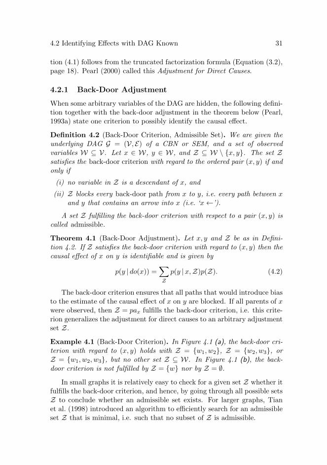
Definition 4.2 (Back-Door Criterion, Admissible Set). We are given theunderlying DAG G = (V, E) of a CBN or SEM, and a set of observedvariables W ⊆ V. Let x ∈ W, y ∈ W, and Z ⊆ W \ {x, y}. The set Zsatisfies the back-door criterion with regard to the ordered pair (x, y) if andonly if

(i) no variable in Z is a descendant of x, and

(ii) Z blocks every back-door path from x to y, i.e. every path between xand y that contains an arrow into x (i.e. ‘x←’).

A set Z fulfilling the back-door criterion with respect to a pair (x, y) iscalled admissible.

Theorem 4.1 (Back-Door Adjustment). Let x, y and Z be as in Defini-tion 4.2. If Z satisfies the back-door criterion with regard to (x, y) then thecausal effect of x on y is identifiable and is given by

p(y | do(x)) =∑Zp(y |x,Z)p(Z). (4.2)

The back-door criterion ensures that all paths that would introduce biasto the estimate of the causal effect of x on y are blocked. If all parents of xwere observed, then Z = pax fulfills the back-door criterion, i.e. this crite-rion generalizes the adjustment for direct causes to an arbitrary adjustmentset Z.

Example 4.1 (Back-Door Criterion). In Figure 4.1 (a), the back-door cri-terion with regard to (x, y) holds with Z = {w1, w2}, Z = {w2, w3}, orZ = {w1, w2, w3}, but no other set Z ⊆ W. In Figure 4.1 (b), the back-door criterion is not fulfilled by Z = {w} nor by Z = ∅.

In small graphs it is relatively easy to check for a given set Z whether itfulfills the back-door criterion, and hence, by going through all possible setsZ to conclude whether an admissible set exists. For larger graphs, Tianet al. (1998) introduced an algorithm to efficiently search for an admissibleset Z that is minimal, i.e. such that no subset of Z is admissible.

32 4 Causal Effect Identification

(a) u w1

w2

w3

x y

(b) u

wx y

Figure 4.1: Adjustment Criterion. In (a) the back-door criterion holds forinstance with Z = {w1, w2}, whereas in (b) the back-door criterion is notfulfilled.

A special case that proves useful for our results is the back-door adjust-ment in linear SEMs, stated in the following theorem (Pearl, 1998).

Theorem 4.2 (Back-Door Adjustment in Linear SEMs). Assume that theunderlying DAG G of a linear SEM is known, and let x, y and Z be as inDefinition 4.2. If Z is an admissible set with regard to (x, y), then the totaleffect of x on y is identifiable, and given by cx, the coefficient of x in theregression of y on x and Z using ordinary least squares:

y = cxx+∑z∈Z

czz + ry. (4.3)

Note that in general a regression coefficient does not need to be relatedin any way to the causal effect, but merely expresses some form of correla-tion between x and y given Z. The back-door adjustment gives a criterionfor when this expression coincides with the total effect (see Pearl, 2000, 2ndedition p.161), illustrated in the following example.

Example 4.2 (Adjustment in Linear SEMs). We use the linear SEM ofFigure 3.4 (a) of Example 3.4 (page 22/23), and we want to estimate thecausal effect of v1 on v3. Wright’s method (1934) for path coefficients tellsus that the total causal effect is given by b3,1 + b3,2 b2,1. Since the emptyset Z = ∅ is admissible with regard to (v1, v3), Theorem 4.2 can be usedto calculate the causal effect directly as the regression coefficient c1 of thefollowing model

v3 = c1v1 + r3,

using the OLS formula of Equation (2.8) (page 13), and assuming that thevariables have zero mean:

c1 =cov(v1, v3)

σ2v1and

4.3 Identifying Effects with DAG Unknown 33

cov(v1, v3) = E(v1 v3) = E(v1 (b3,1 v1 + b3,2 v2 + e3))

= E(e1 (b3,1 e1 + b3,2 (b2,1 v1 + e2) + e3))

= b3,1 E(e21) + b3,2 b2,1E(e21)+

b3,2 E(e1)E(e2) + E(e1)E(e3)

= (b3,1 + b3,2 b2,1)σ2v1 .

4.2.2 Other Approaches

A similar approach to the back-door adjustment of Theorem 4.1 is theFront-Door Adjustment (Pearl, 1993b). This adjustment method allowsthe covariates in the adjustment set Z to lie between the cause x andthe effect y, potentially yielding identifiability of the causal effect in caseswhere back-door adjustment fails (the simplest such example is the graphof Figure 4.1 (b)).

A more general tool to identify causal effects is provided by the threerules of the do-calculus introduced by Pearl (1994, 1995). Iteratively ap-plying these rules may allow transforming a postinterventional distributioninto an expression of observed (conditional) probability distributions only,and hence identifying the causal effect. Huang and Valtorta (2006), andShpitser and Pearl (2006) showed that the do-calculus is complete, in thesense that a causal effect is identifiable if and only if it can be transformedinto an expression over observed conditional probabilities using the threerules of the do-calculus.

One drawback of the do-calculus is that it does not directly provide aprocedure specifying how to reach the transformation from the postinter-ventional distribution to observational probability distributions. Towardsthis end, general algorithms for the identification of (conditional) interven-tional distributions were introduced by Tian and Pearl (2002), Tian (2004),Shpitser and Pearl (2006), and Shpitser et al. (2011).1

4.3 Identifying Effects with DAG Unknown

In many situations the DAG corresponding to the data generating processis not known, so the methods of Section 4.2 cannot be applied directly. Tostill be able to infer causal effects from passive observational data, typically

1Conditional interventional distributions are defined as p(y |z, do(x)) = p(y,z,| do(x))p(z | do(x))

(Shpitser and Pearl, 2006), and are causal effects in a subpopulation determined by thevalues of z, for instance, the effect of alcohol (x) on mortality (y) in the male populationof a specified country (z).

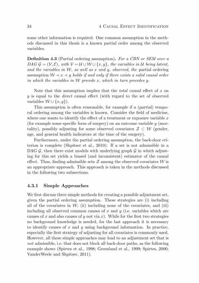
34 4 Causal Effect Identification

some other information is required. One common assumption in the meth-ods discussed in this thesis is a known partial order among the observedvariables.

Definition 4.3 (Partial ordering assumption). For a CBN or SEM over aDAG G = (V, E), with V = U ∪W ∪ {x, y}, the variables in U being latent,and the variables in W, as well as x and y, observed, the partial orderingassumption W ≺ x ≺ y holds if and only if there exists a valid causal orderin which the variables in W precede x, which in turn precedes y.

Note that this assumption implies that the total causal effect of x ony is equal to the direct causal effect (with regard to the set of observedvariables W ∪ {x, y}).

This assumption is often reasonable, for example if a (partial) tempo-ral ordering among the variables is known. Consider the field of medicine,where one wants to identify the effect of a treatment or exposure variable x(for example some specific form of surgery) on an outcome variable y (mor-tality), possibly adjusting for some observed covariates Z ⊂ W (gender,age, and general health indicators at the time of the surgery).

Furthermore, under the partial ordering assumption, the back-door cri-terion is complete (Shpitser et al., 2010): If a set is not admissible in aDAG G, then there exist models with underlying graph G in which adjust-ing for this set yields a biased (and inconsistent) estimator of the causaleffect. Thus, finding admissible sets Z among the observed covariatesW isan appropriate approach. This approach is taken in the methods discussedin the following two subsections.

4.3.1 Simple Approaches

We first discuss three simple methods for creating a possible adjustment set,given the partial ordering assumption. These strategies are (i) includingall of the covariates in W, (ii) including none of the covariates, and (iii)including all observed common causes of x and y (i.e. variables which arecauses of x and also causes of y not via x). While for the first two strategiesno background knowledge is needed, for the last approach it is necessaryto identify causes of x and y using background information. In practice,especially the first strategy of adjusting for all covariates is commonly used.However, all these simple approaches may lead to an adjustment set that isnot admissible, i.e. that does not block all back-door paths, as the followingexample shows (Spirtes et al., 1998; Greenland et al., 1999; Spirtes, 2000;VanderWeele and Shpitser, 2011).

4.3 Identifying Effects with DAG Unknown 35

(a)

w

x y

(b)

w

x y

u1 u2

(c)

x

u

w y

(d)

w x y

(e) u

x yw

Figure 4.2: Figures (a) to (c) demonstrate simple adjustment criteria (fordetails see Example 4.3), with admissible sets with regard to (x, y) givenby (a) Z = {w}, (b) Z = ∅, and (c) Z = {w}. Figures (d) and (e) are usedto illustrate the method of Section 4.3.2.

Example 4.3. Consider the DAGs of the three data generating models inFigure 4.2 (a)-(c). Each of the simple methods for finding an adjustmentset discussed above fails for one or more of these models: Adjusting for allobserved covariates yields an admissible set for (a) and (c), however notfor (b). In contrast, by adjusting for none of the variables we obtain anadmissible set for (b), though not for (a) and (c). Finally, adjusting for allcommon causes, given the required background knowledge, yields in (a) theset Z = {w} and in (b) the set Z = ∅, which are admissible in the respectivemodels. However, in (c) the resulting adjustment set is the empty set, sincew causes y only via x. This adjustment set is not admissible.

VanderWeele and Shpitser (2011) introduced a criterion always yieldingan admissible set, when such a set truly exists. In addition to the partialordering assumption, they require that it is known which covariates arecauses of x or y (as for the strategy of including all common causes). Theyshow that the set of all those observed covariates which are causes of x,or of y, or of both yields an admissible set, i.e. blocks all back-door paths.For the graphs in Figure 4.2 (a)-(c) this criterion indeed yields the correctadjustment sets. However, in case there does not exist an admissible set,the criterion of VanderWeele and Shpitser (2011) fails to detect this.

4.3.2 Methods Based on Dependencies and Independencies

Statistical dependencies and independencies among the observed variablescan be used to identify causal effects without knowing the underlying DAG.

36 4 Causal Effect Identification

We first want to point out one theoretical limitation of this approach.Even with the partial ordering assumption, some models entail the sameset of independencies over the observed variables, even though they implydifferent admissible sets. For instance, the DAGs of Figure 4.2 (a) and(b) both do not entail any independencies among w, x, and y, and it isthus impossible to conclude from dependencies and independencies alonewhether the variable w should be adjusted for to identify the causal effect.However, in some models it may well be possible to reach a conclusion.

Using the faithfulness and partial ordering assumptions, Spirtes andCooper (1999), and Chen et al. (2007) both gave a simple criterion to iden-tify a causal effect with an empty admissible set.2 In essence, they requirean exogenous variable w, i.e. a variable w which is a root in the underlyinggenerating graph, and that x, y and w fulfill the following properties:

(i) x /⊥⊥ y,

(ii) w /⊥⊥ y, and

(iii) w⊥⊥ y |x.

If these conditions hold, then x is a cause of y and there is no confounder(neither latent nor observed) between x and y. Hence, the effect of x on yis identifiable, and equal to the conditional probability p(y |x) (which canbe seen using the back-door criterion with the admissible set Z = ∅).

This criterion is most easily understood with an example. The simplestDAG in which these conditions hold is given by the graph in Figure 4.2 (d).When adding a (latent) confounder between x and y, as in Figure 4.2 (e),the conditional independence of condition (iii) is destroyed. In general, ifthere is an active back-door path between x and y, conditions (i) to (iii)cannot all hold, and hence confounding can be detected.

2In fact, they only assume that x and y are the last two variables in the causal order,but they do not require any specific order among x and y.

Chapter 5

Structure Learning

In this chapter, the relevant existing work addressing research question Q2is presented. We explain methods for learning the underlying DAG of aCBN or SEM from passive observational data. For this task clever searchalgorithms are needed, since the number of DAGs grows superexponen-tially in the number of nodes: for 3 nodes there are 25 DAGs (shown inFigure 5.1), for 4 nodes 543 DAGs, for 5 nodes 29281 DAGs, and for 6nodes already 3781503 DAGs.

There is a vast literature on this topic, and we will only discuss themethods relevant for understanding the novel methods introduced in thisthesis. These include the constraint based approach, and methods for esti-mating linear non-Gaussian acyclic models, as well as applications of thesemethods in SVAR models. One large bundle of alternative methods notconsidered here are score based methods (Heckerman et al., 1995; Meek,1997; Chickering, 2002; Koivisto and Sood, 2004; Silander and Myllymaki,2006). Furthermore, much attention has rather recently been devoted tothe problem of learning non-linear models (Hoyer et al., 2009; Mooij et al.,2009; Zhang and Hyvarinen, 2010; Peters et al., 2011), as well as com-bining information from several (experimental or non-experimental) datasets (Tillman, 2009; Claassen and Heskes, 2010; Tillman and Spirtes, 2011;Tsamardinos et al., 2012; Hyttinen et al., 2012). These methods are how-ever out of the scope of this thesis.

5.1 Constraint Based Methods

Here, we discuss methods for structure learning based on statistical de-pendencies and independencies among the observed variables. We startwith the PC algorithm (after its inventors’ first names, Peter and Clark,

37

38 5 Structure Learning

1 2 3

1 2 3 1 2 3

1 2 3 1 2 3

1 2 3 1 2 3

1 2 3

1 2 3

1 2 3

1 2 3 1 2 3 1 2 3

1 2 3 1 2 3 1 2 3

1 2 3 1 2 3 1 2 3

1 2 3 1 2 3 1 2 3

1 2 3 1 2 3 1 2 3

1 2 3

1 2 3

1 2 3

1 2 3

1 2 3

1 2 3

1 2 3

1 2 3

1 2 3

1 2 3

1 2 3

v1⊥⊥ v2 , v1⊥⊥ v3 , v2⊥⊥ v3v1⊥⊥ v2 | v3 , v1⊥⊥ v3 | v2 , v2⊥⊥ v3 | v1v1⊥⊥ v3 , v2⊥⊥ v3v1⊥⊥ v3 | v2 , v2⊥⊥ v3 | v1v1⊥⊥ v2 , v2⊥⊥ v3v1⊥⊥ v2 | v3 , v2⊥⊥ v3 | v1v1⊥⊥ v2 , v1⊥⊥ v3v1⊥⊥ v2 | v3 , v1⊥⊥ v3 | v2v1⊥⊥ v3

v1⊥⊥ v2

v2⊥⊥ v3

v1⊥⊥ v3 | v2

v1⊥⊥ v2 | v3

v2⊥⊥ v3 | v1

no d-separations

DAGs with 3 nodes Equivalence classes and d-separations

Figure 5.1: The left part of the figure shows all 25 DAGs over three variablesv1, v2, and v3, indicated as numbers 1, 2, and 3 in the graphs. These aregrouped into the 11 equivalence classes in which these 25 DAGs can bedivided, given by the rows of the figure. The pattern of each equivalenceclass and the d-separation relations entailed by the DAGs contained in thisclass are shown in the right part of the figure.

Spirtes and Glymour, 1991), a structure learning method for the causallysufficient case. We then move on to the FCI algorithm (Fast Causal In-ference, Spirtes et al., 1993, 1999), which allows for latent variables andselection bias. These methods are suited for both discrete and continuousdata (linear/non-linear, Gaussian/non-Gaussian), as all that is required isan appropriate independence test, some of which were reviewed in Sec-tion 2.2.2.

5.1.1 PC Algorithm

We assume that we are given a data set generated by a CBN or SEMover a DAG G = (V, E), in which all variables V are observed (i.e. theset of observed variables is causally sufficient), and that the probabilitydistribution p associated with the model is faithful to G.

Since the PC algorithm is based on independencies, we first point out

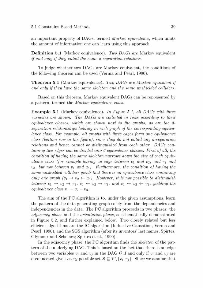
5.1 Constraint Based Methods 39

an important property of DAGs, termed Markov equivalence, which limitsthe amount of information one can learn using this approach.

Definition 5.1 (Markov equivalence). Two DAGs are Markov equivalentif and only if they entail the same d-separation relations.

To judge whether two DAGs are Markov equivalent, the conditions ofthe following theorem can be used (Verma and Pearl, 1990).

Theorem 5.1 (Markov equivalence). Two DAGs are Markov equivalent ifand only if they have the same skeleton and the same unshielded colliders.

Based on this theorem, Markov equivalent DAGs can be represented bya pattern, termed the Markov equivalence class.

Example 5.1 (Markov equivalence). In Figure 5.1, all DAGs with threevariables are shown. The DAGs are collected in rows according to theirequivalence classes, which are shown next to the graphs, as are the d-separation relationships holding in each graph of the corresponding equiva-lence class. For example, all graphs with three edges form one equivalenceclass (bottom row in the figure), since they do not entail any d-separationrelations and hence cannot be distinguished from each other. DAGs con-taining two edges can be divided into 6 equivalence classes: First of all, thecondition of having the same skeleton narrows down the size of each equiv-alence class (for example having an edge between v1 and v2, and v2 andv3, but not between v1 and v3). Furthermore, the condition of having thesame unshielded colliders yields that there is an equivalence class containingonly one graph (v1 → v2 ← v3). However, it is not possible to distinguishbetween v1 → v2 → v3, v1 ← v2 → v3, and v1 ← v2 ← v3, yielding theequivalence class v1 − v2 − v3.

The aim of the PC algorithm is to, under the given assumptions, learnthe pattern of the data generating graph solely from the dependencies andindependencies in the data. The PC algorithm proceeds in two phases: theadjacency phase and the orientation phase, as schematically demonstratedin Figure 5.2, and further explained below. Two closely related but lessefficient algorithms are the IC algorithm (Inductive Causation, Verma andPearl, 1990), and the SGS algorithm (after its inventors’ last names, Spirtes,Glymour and Scheines; Spirtes et al., 1990).

In the adjacency phase, the PC algorithm finds the skeleton of the pat-tern of the underlying DAG. This is based on the fact that there is an edgebetween two variables vi and vj in the DAG G if and only if vi and vj ared-connected given every possible set Z ⊆ V \{vi, vj}. Since we assume that

40 5 Structure Learning

v4

v3

v1

v2

v5 UnknownGenerating

DAG

⇒ Dataset ⇒

IndependenciesAmong

Variables:

v2⊥⊥ v4v2⊥⊥ v5v1⊥⊥ v2 | v3v1⊥⊥ v4 | v3v1⊥⊥ v5 | v3v3⊥⊥ v5 | v4

⇒

AdjacencyPhase

v4

v3

v1

v2

v5

⇒

OrientationPhase

v4

v3

v1

v2

v5

Figure 5.2: Demonstration of the PC algorithm. The data set is gener-ated by an unknown causal model. The PC algorithm uses the (testable)independencies from the data to generate the skeleton of the underlyingDAG in the adjacency phase, and then to orient as many edges as possi-ble in the orientation phase to obtain the pattern representing the Markovequivalence class of the DAG.

the probability distribution p is faithful to G, i.e. d-separation relations inG and (conditional) independencies in p are equivalent (see Equation (3.9),page 26), we thus can remove the edge between two variables vi and vj ifwe can find even a single set Z for which they are (conditionally) indepen-dent. Going through all these independencies is (roughly) done by startingwith the empty conditioning set Z, removing any possible edges, and thencontinuing with conditioning sets of cardinality one, two, and so on.

In the orientation phase, the skeleton of the adjacency phase togetherwith Theorem 5.1 can be used to derive orientation rules, which alloworienting some of the edges to obtain the pattern of the Markov equivalenceclass of the underlying DAG. The first rule orients the unshielded collidersof the pattern: For any triple (vi, vk, vj), with vi − vk − vj in the skeletonand vi not adjacent to vj , we can orient vi → vk ← vj if and only if vkis not in the conditioning set Z yielding vi⊥⊥ vj | Z (by the definition ofd-separation). In addition to these colliders, the orientation of some otheredges may be determined uniquely for the equivalence class. For example,by the acyclicity assumption, if vi → vk → vj and vi−vj are in the skeleton,we must orient vi → vj . In total there are three such additional rules.

Meek (1995) showed that these orientation rules are sound and com-plete, i.e. the pattern contains all and only those orientations which arecommon to all the elements of the equivalence class. It is also straightfor-ward to incorporate background knowledge into the PC algorithm, such asexistence or non-existence of some edges, orientation of some edges, or atime order among the variables (Meek, 1995; Spirtes et al., 1993).

5.1 Constraint Based Methods 41

5.1.2 FCI Algorithm

We here assume again that the data are generated by a CBN or SEM overa DAG G = (V, E). However, as opposed to the setting of the previoussection, the set of observed variables may here only be a subset of V, i.e.V =W ∪U withW observed, and U latent variables. This typically yields asetW of observed variables which is not causally sufficient. Note that we donot need to know the set U of latent variables, but only need to assume thatsuch a set exists. Furthermore, we assume that the distribution associatedwith the model is faithful to G. We can thus discuss the FCI algorithm(Fast Causal Inference, Spirtes et al., 1993, 1999), an extension of the PCalgorithm to the causally insufficient case.1

As working explicitly with latent variables can be cumbersome (seefor example Richardson and Spirtes (2002) for a list of reasons), the FCIalgorithm is based on so called maximal ancestral graphs (MAGs, Richard-son and Spirtes, 2002) over the observed variables W.2 MAGs are ances-tral graphs, in which for any two non-adjacent nodes there exists a set ofvertices that m-separates them, where m-separation is a generalization ofthe d-separation criterion for DAGs to ancestral graphs (Richardson andSpirtes, 2002). Furthermore, MAGs not only can represent latent variables(using bidirected arrows ↔), but can also account for selection bias (usingundirected arrows −). However, for simplicity, we will exclude selectionbias from all following descriptions.

The interpretation of the edges of a MAG is as follows:

• A directed edge w1 → w2 is interpreted as w1 being a (direct orindirect) cause of w2, and w2 not being a cause of w1, and

• a bidirected edge w1 ↔ w2 is interpreted as neither w1 being a causeof w2 nor w2 being a cause of w1.

First of all, note that every DAG is a special case of a MAG (simplynot containing any bidirected edges). Furthermore, for every causal modelover a DAG G = (V, E) with V = W ∪ U as above, there exists a MAGover the observed variables W representing the same independencies (m-separation relations) among the observed variables W as in the DAG, andretaining ancestral relationships of the DAG. For example, the MAG overthe observed variables w, x and y of the DAG in Figure 4.2 (e) (page 35)

1Verma and Pearl (1990) introduced a variant of the IC algorithm also accountingfor latent variables (later termed IC* (Pearl, 2000)). Since the FCI algorithm is moreefficient as well as further developed, we will only consider the FCI algorithm here.

2Earlier versions of the algorithm are based on so called inducing path graphs (Spirteset al., 1993). The algorithm is essentially the same but the interpretation of the outputdiffers.

42 5 Structure Learning

w4

w3

w1

w2

w5

u1

u2

UnknownGenerating

DAG

⇒

Dependenciesand

Independenciesamong theObserved

Variables W

⇒

w4

w3

w1

w2

w5PAG

outputby FCI

⇐

w4

w3

w1

w2

w5MAG corres-ponding tothe DAG

Figure 5.3: Demonstration of the FCI algorithm, MAGs and PAGs. Fordetails see Example 5.2.

is given by the fully connected graph containing the three edges w → x,x→ y, and w → y, since (i) there are edges in the DAG from w to x, andfrom x to y, and (ii) w and y are always d-connected when disregarding u,and w is an ancestor of y. An algorithm to transform a DAG over observedvariablesW and hidden variables U into a MAG over the observed variablesW is given by Richardson and Spirtes (2002). A further example of a MAGis given in Figure 5.3.

Similarly to the PC algorithm, the FCI algorithm uses dependenciesand independencies among the observed variables to construct in two steps(adjacency and orientation phase) a so called partial ancestral graph (PAG,Richardson, 1996), which corresponds to the equivalence class of the under-lying MAG. Uncertainty about the orientation of an edge is indicated witha circle mark ‘◦’ in the PAG. We illustrate FCI in the following example.

Example 5.2 (FCI Algorithm). In Figure 5.3, the graph in the mid-dle depicts the (unknown) data generating process over observed variablesW = {w1, . . . , w5}, and latent variables U = {u1, u2}. This DAG can betransformed into a MAG over the observed variables, which is shown in theleft graph of the figure.

The FCI algorithm uses the testable independencies among the observedvariablesW to infer the PAG representing the equivalence class of the MAG(shown in right graph of the figure). Circle-marks represent unknown ori-entations; for instance, the circle at w2 implies that from independenciesalone it is not possible to infer whether w2 is an ancestor of w3.

While Theorem 5.1 gives a simple necessary and sufficient graphicalcriterion for two DAGs to be Markov equivalent, this condition is onlynecessary for two MAGs to be equivalent. There are different graphicalcriteria to define Markov equivalence for MAGs (Spirtes and Richardson,

5.2 Linear Non-Gaussian Acyclic Model Estimation 43

1997; Zhao et al., 2005; Ali et al., 2009), however describing these is out ofthe scope of this thesis.

Furthermore, Zhang (2008) augmented the rules in the orientation phase(there are in total 11 rules, including the ones handling selection bias) suchthat FCI is sound and complete, i.e. all and only those edge marks whichare common to all MAGs of the equivalence class represented by the PAGare oriented. As for the PC algorithm, it is straightforward to includebackground knowledge about a temporal ordering in FCI. However, it isnot known whether FCI remains complete when including such knowledge.

5.2 Linear Non-Gaussian Acyclic ModelEstimation

The methods presented in the previous section can only identify the under-lying DAG/MAG of a causal model up to Markov equivalence. Here, wereview a class of methods for linear SEMs with non-Gaussian error terms,also termed Linear Non-Gaussian Acyclic Models (LiNGAM, Shimizu et al.,2006). These methods exploit higher order statistics yielding full identifi-ability of the model when no latent variables are present. We start withreviewing two approaches to estimate such models. We then present a mea-sure to infer the causal direction among only two variables, and how it canbe used to estimate a LiNGAM model over several variables. Towards theend of this section we discuss extensions of these methods for models withlatent variables, as well as with multidimensional variables.

5.2.1 ICA-LiNGAM

Given a LiNGAM model over a DAG G, and assuming causal sufficiency forthe observed variables, the ICA-LiNGAM algorithm (Shimizu et al., 2006)outputs, in the large sample limit, the underlying DAG G. Note that thefaithfulness assumption is not needed for this approach.

Estimating a LiNGAM model basically consists of two steps: obtaininga causal order among the variables, and estimating the connection strengthsof the causal effects given the causal order. The second step is simple, andcan be done using OLS by regressing the second variable in the causalorder on the first, the third variable on the first and the second, and soon (or alternatively by using the Cholesky decomposition of the covariancematrix of the variables). Additionally, some of the causal effects (regressioncoefficients) might be set to zero if they are not statistically significant,which means that some of the edges in the DAG are cut out. The crucial

44 5 Structure Learning

point in the algorithm thus is the first step of obtaining a causal order.Towards this end, we write a linear SEM using the matrix equation asshown in Example 3.2 (page 17)

v = Bv + e. (5.1)

In this section we only consider models where the distribution of the dis-turbances e are non-Gaussian, which is essential for full identification ofthe model.

In ICA-LiNGAM, Equation (5.1) is rewritten in its reduced form, corre-sponding to an ICA (Independent Component Analysis, Hyvarinen et al.,2001) model

v = Ae (5.2)

with A = (I−B)−1, so that the observed variables v can be seen as a linearmixture of the independent disturbances e, termed sources in the ICAliterature. In essence, ICA identifies a matrix A by whitening and rotatingthe data such that A−1v yields independent sources e. In this step, non-Gaussianity is required, since Gaussian distributions are rotation symmetric(once they are whitened), and hence any rotation of white Gaussian datayields independent (uncorrelated) sources.

The matrix A inferred from ICA is unique up to arbitrary scaling, signchange and permutation of the columns. These ambiguities can be resolvedusing the acyclicity assumption of the underlying model (Shimizu et al.,2006), so that we obtain a unique matrix A, which in turn yields a uniqueconnection matrix B. Note that the residuals e are only independent whenestimating the matrix B in a correct causal order (which is found using theICA matrix A), as demonstrated in the following example.

Example 5.3 (ICA-LiNGAM). We use the linear SEM of Example 3.2over the DAG v2 → v3 → v1 (Figure 3.2, page 17), with the disturbancesei, i = 1, 2, 3, following a uniform distribution with mean 0 and variance 1.The data are shown in Figure 5.4 (a). In (b) we show the estimated residualsr when estimating the matrix B using the correct causal order. These areindependently and uniformly distributed, representing the distribution of theunderlying disturbances e. The independence of these residuals can be seenfrom the figure since the cube is aligned with the axes. Thus, for any givenvalue of r1, for instance, the values of r2 and r3 do not depend on this value.In contrast, in (c) we plot the residuals when estimating the matrix B alongthe order v1 ≺ v3 ≺ v2, and can see that these are not independent, eventhough they are uncorrelated. The dependence of the residuals is indicatedby the rotated cuboid, such that, for instance, for large values of r1, thevalues of r3 are restricted to be around 0.

5.2 Linear Non-Gaussian Acyclic Model Estimation 45

(a) Data generated by themodel in Figure (3.2)

(b) Residuals when esti-mating B in the correctcausal order v2 ≺ v3 ≺ v1

(c) Residuals when esti-mating B in a wrongcausal order v1 ≺ v3 ≺ v2

Figure 5.4: Demonstration of ICA-LiNGAM. The schematic plots show thedistributions of the data (a), and the residuals when estimating the modelin two different orders, (b) and (c). The cuboid of each plot indicates thearea in which the distribution is non-zero. Inside the cuboid the data aredistributed uniformly.

5.2.2 DirectLiNGAM

Under the same assumptions as for ICA-LiNGAM, DirectLiNGAM (Shimizuet al., 2011) tackles the problem of learning a causal order in an iterativemanner. First, the algorithm searches for an exogenous variable (i.e. a rootvariable in the underlying model, which always exists due to the acyclicityassumption). Then, the effect of this exogenous variable is regressed outfrom all other variables, and the whole process is repeated on this smallerdata set.3 We restate two theorems by Shimizu et al. (2011), formalizingthis method. The first one gives a criterion to find an exogenous variable.

Theorem 5.2. Given that v follows a LiNGAM model, let r(j)i = vi−cijvj,

i 6= j, be the residuals when regressing vi on vj using OLS. Then, vj is

exogenous if and only if vj ⊥⊥ r(j)i for all i 6= j.

For this theorem it is essential that the residuals are non-Gaussian, since

vj and r(j)i are always uncorrelated (by construction of the OLS estimator)

and hence for Gaussian variables they are also independent. The secondtheorem of Shimizu et al. (2011) states that when regressing out the effect of

an exogenous variable vj from all other variables to obtain the residuals r(j)i ,

i 6= j, these residuals follow also a LiNGAM model with the same induced

3Note that for finite sample sizes the result of ICA-LiNGAM may depend on theinitialization of the parameters in the ICA-algorithm, whereas DirectLiNGAM alwaysyields the same solution.

46 5 Structure Learning

(a) First Iteration of DirectLiNGAM (b) Second Iteration

Figure 5.5: Demonstration of DirectLiNGAM, plotting schematically theregressor versus the resulting residuals to find an exogenous variable, seeExample 5.4 for details.

causal order. This allows searching for an exogenous variable among r(j)i

to find a second variable in the causal order. By iterating this process afull causal order can be found.

Theorem 5.3. Given that v follows a LiNGAM model, and vj is exoge-

nous, the obtained residuals r(j)i = vi − cijvj, i 6= j, follow a LiNGAM

model with the same induced causal order.

Example 5.4 (Direct-LiNGAM). We demonstrate the algorithm using thesame model as in Example 5.3. To find an exogenous variable, all pairwise

OLS regressions are performed: For all i 6= j we obtain vi = cijvj+r(j)i and

test whether vj ⊥⊥ r(j)i . Plots of vj versus r(j)i are shown in Figure 5.5 (a).

The plots show that independence with both residuals only holds for v2(since both rectangles are aligned with the axes). Thus, v2 is exogenous andis chosen to be the first variable in the causal order.

To find the second variable in the causal order, we repeat this step withthe residuals of the regressions on v2. We perform the pairwise regressions

of r(2)1 and r

(2)3 in both directions meaning that we estimate r

(2)3 = c31r

(2)1 +

r(2,1)3 , and r

(2)1 = c13r

(2)3 + r

(2,3)1 . The corresponding plots are shown in

Figure 5.5 (b). These plots show that r(2)3 is exogenous among r

(2)1 and

r(2)3 , yielding v3 as the second variable in the causal order.

As now only v1 is left, we found the causal order to be v2 ≺ v3 ≺ v1.

5.2 Linear Non-Gaussian Acyclic Model Estimation 47

5.2.3 Pairwise Measure of Causal Direction

Hyvarinen (2010) discussed the problem of inferring the causal order for atwo variable LiNGAM model

x = ex (5.3)

y = bx+ ey (5.4)

i.e. determining which of the variables x and y is the cause and which isthe effect. The introduced measure is based on the likelihood ratio of thetwo possible models x → y and y → x, and various ways of calculatingthis ratio based on differential entropy approximations, cumulants, andfirst-order approximations are suggested (Hyvarinen, 2010; Hyvarinen andSmith, 2013).

The pairwise measure can also be used to infer a causal order amongn variables v1, . . . , vn following a LiNGAM model, using a DirectLiNGAMstyle approach (Hyvarinen, 2010). Since for an exogenous variable vj , thecausal model vj → vi holds for all i 6= j (by marginalizing out all othervariables), this measure can be used to find an exogenous variable. As inDirectLiNGAM, once an exogenous variable is found, its effect is regressedout from all other variables, and the procedure is repeated on this smallerset of variables.

5.2.4 Latent Variable LiNGAM

So far we have only discussed methods for LiNGAM models without la-tent variables. Hoyer et al. (2008) introduced the latent variable LiNGAMmodel (lvLiNGAM) and a method to estimate it. The generating equationscan again be rewritten as an ICA like model, such that w = Ae, with wthe observed variables, and e the disturbances of the observed variables aswell as the hidden variables. Note that the matrix A has now more columnsthan rows (as opposed to the case without latent variables where A is asquare matrix), termed an overcomplete ICA basis. However, with latentvariables the model is in general not fully identifiable, and estimation ofthe overcomplete ICA basis is computationally very challenging (only up to3 observed variables and one hidden variable were used in the simulationsin Hoyer et al., 2008).

Recently, Tashiro et al. (2012) introduced a DirectLiNGAM style ap-proach, searching for exogenous variables, as well as sink variables, to esti-mate a partial order among the observed variables in lvLiNGAM models.

48 5 Structure Learning

5.2.5 GroupLiNGAM

Kawahara et al. (2010) generalized the LiNGAM model to multidimen-sional variables, also termed groups of variables, i.e. instead of havingv = (v1, . . . , vn) being a vector of scalar random variables, they assumev = (v1, . . . ,vn) being a vector of multidimensional variables. The linearequations can again be written in matrix form as

v = Bv + e (5.5)

with B the connection matrix, which can be permuted to being lower blocktriangular, such that a causal order among the multidimensional variablesv1, . . . ,vn exists, and e = (e1, . . . , en) multidimensional, non-Gaussian dis-turbance terms, such that ei⊥⊥ ej , i 6= j. However, the components of eachei, that is, the disturbances within group i, can be correlated.

In their algorithm, termed GroupLiNGAM, Kawahara et al. (2010)aimed at learning the partition of the variables v, and with it the causal or-der among these variables. This results in statistically and computationallychallenging algorithms (exponential in the number of variables).

5.3 Trace Method

In this section, we describe the basic idea of the Trace Method of Janzinget al. (2010), a method designed to infer the causal order among two mul-tidimensional variables x and y, given linear relationships. The model isgiven as

y = Bx + e (5.6)

where B is an arbitrary connection matrix, which is independently chosenof the covariance matrix Σ of the regressors x, and the disturbances e areindependent of x. No assumptions are made on the distribution of e.

The underlying idea is, intuitively, that in the correct causal direction,i.e. x → y in Equation (5.6), p(x) and p(y |x) originate from some ‘inde-pendent mechanisms’, whereas p(y) and p(x |y) show some form of depen-dence. (Janzing and Scholkopf (2010) formally stated this in terms of algo-rithmic information theory.) The trace method gives an easily computablecriterion to detect such dependencies for two multidimensional variables inlinear models. Janzing et al. (2010) pointed out that the trace method doesnot yield any results for scalar variables, and the performance increases forhigher dimensional variables.

5.4 SVAR Identification 49

5.4 SVAR Identification

SVAR models are introduced in Definition 3.9 (page 28) as

v(t) = B0v(t) +

q∑i=1

Biv(t− i) + e(t), (5.7)

and we here assume that all variables v(t) are observed (i.e. the system iscausally sufficient). SVAR models can be used for policy analysis such asforecasting the effect of an intervention in the system, or analyzing causalinfluences of shocks to some variables, i.e. predicting the response (effect) ofone variable to an impulse (change) in another variable. Before discussingthese in more detail, we explain how SVAR models can be estimated.

Estimation of SVAR models can be done in three steps (see for exampleHamilton (1994), Demiralp and Hoover (2003), Moneta (2003), Lutkepohl(2005), Moneta and Spirtes (2006), and Hyvarinen et al. (2010)):

(i) Estimation of the lagged effects using the reduced form Vector Au-toregressive model (VAR)

v(t) =

q∑i=1

Aiv(t− i) + d(t) (5.8)

which is connected to the SVAR model of Equation (5.7) by Ai =(I−B0)

−1Bi, and d(t) = (I−B0)−1e(t).

(ii) Estimation of the instantaneous effects matrix B0 using the errorterms d(t) of Equation (5.8)

d(t) = B0d(t) + e(t). (5.9)

(iii) Correction of the estimates for the lagged effects using

Bi = (I−B0)Ai. (5.10)

We now discuss steps (i) and (ii) in more detail. In (i), since the VARmodel does not contain instantaneous effects (i.e. the right hand side ofEquation (5.8) does not include v(t)), the matrices Ai, i = 1, . . . , q, can berelatively straightforwardly estimated from the data. One typical require-ment is stability of the VAR process.

50 5 Structure Learning

Definition 5.2 (Stability). The VAR model in Equation (5.8) is calledstable if and only if det(In −A1z − . . . −Aqz

q) 6= 0 for all |z| ≤ 1 (withdet() denoting the determinant of a matrix), i.e. all roots of this expressionlie outside the unit circle.

From the stability condition follows that the time series is stationary,i.e. the first and second moments are time invariant (Lutkepohl, 2005). In astable VAR we can thus estimate the coefficient matrices of Equation (5.8)using OLS.

For non-stationary time series with roots of det(In−A1z− . . .−Aqzq)

on the unit circle, taking differences of the variables may yield a stable VARmodel. Such processes are termed integrated. However, in some other cases,for so called co-integrated processes, it is necessary to estimate the coeffi-cients using a Vector Error Correction Model (VECM, Engle and Granger,1987), from which the estimates of the matrices Ai, i = 1, . . . , q, of Equa-tion (5.8) can be inferred.

Step (ii) of the estimation of an SVAR model is the crucial point toidentify the model. Since the matrix B0 is assumed to be acyclic and thedisturbances e(t) to be independent, Equation (5.9) is a linear SEM, and wecan apply the techniques discussed in Sections 5.1 and 5.2, on the residualsd(t) of the VAR model, to obtain the instantaneous effects.4

In the case of Gaussian disturbances, the PC algorithm of Section 5.1can be used to identify the DAG up to Markov equivalence, typically re-quiring background knowledge for full identification of the matrix B0. Incontrast, for non-Gaussian disturbances, the LiNGAM estimation of Sec-tion 5.2 allows full identification of the matrix B0. Combining VAR estima-tion with the PC algorithm is for example demonstrated by Demiralp andHoover (2003), Moneta (2003), and Moneta and Spirtes (2006), whereasVAR estimation combined with LiNGAM was introduced by Hyvarinenet al. (2010), and termed VAR-LiNGAM.

For forecasting a time series based on observations of the past, giventhat the system does not change (i.e. no interventions or shocks), VARmodels are sufficient. However, for policy analysis it is important to identifythe matrix B0: For predicting the effect of an intervention it is essentialto obtain the correct matrices Bi = (I − B0)Ai, i = 1, . . . , q, and forpredicting the effect of shocks in the disturbances it is important to obtain

4In econometrics it is common to use background knowledge to select a causal orderamong the variables and estimate the matrix B0 using the Cholesky decomposition of thecovariance matrix of the estimated residuals d(t) along this causal order. However, sincein many cases the theory is not sufficient to determine a causal order unambiguously,approaches such as the ones of Sections 5.1 and 5.2 may be required.

5.5 Granger Causality 51

the independent disturbances e(t) = (I − B0)d(t), such that the shockeddisturbance is not correlated with any other disturbances.

The effect of a unit shock in the disturbances e(t − τ), τ ≥ 0 on thevariables v(t) is given by the impulse response functions Ψτ (Hamilton,1994; Lutkepohl, 2005). Identification of these matrices Ψτ requires thematrix B0, which can be seen from the Wold moving average representationof the VAR model of Equation (5.8) (Hamilton, 1994; Lutkepohl, 2005), asexplained below:

v(t) =

∞∑τ=0

Φτd(t− τ) (5.11)

=∞∑τ=0

Φτ (I−B0)(I−B0)−1d(t− τ) =

∞∑τ=0

Ψτe(t− τ). (5.12)

The matrices Φτ of Equation (5.11) are the moving average coefficients ofthe VAR model, which can be transformed to the impulse response func-tions Ψτ only if we know the matrix B0 yielding independent disturbancese(t), as can be seen from Equation (5.12).

5.5 Granger Causality

A commonly used concept for causal analysis in time series is Grangercausality (Granger, 1969). The idea is that a cause x precedes its effect yin time, and hence, x should help in predicting y. More formally, assumingthat we are given all the information in the universe up to and includingtime point t, we predict the value of y(t + h), h ≥ 1, once using all thisinformation, and once using this information excluding x(τ) for all τ ≤ t.If for some h ≥ 1 the prediction error (in the least square sense) of y(t+h)is smaller for the former estimate than the latter, the time series x Grangercauses y (Lutkepohl, 2005). In Example 3.7 (page 27), v3 is a Grangercause of v2, and v2 is a Granger cause of v1, whereas v2 is not a Grangercause of v3.

However, in general we do not observe all the information in the uni-verse, i.e. the system may not be causally sufficient. In this case, Grangercausality is only a necessary, but not sufficient condition for a time series xto be a ‘real’ cause of a time series y. Unobserved confounding time seriescan introduce spurious correlation between x and y, and hence, x may helpin predicting y, even though it is not a cause of y.

52 5 Structure Learning

Chapter 6

Contributions to the ResearchField

After introducing the necessary background on the relevant existing workin Chapters 2 through 5, we are now ready to describe the contributions ofthe publications of this thesis to the research field. Throughout the Ph.D.studies, linear non-Gaussian models played a prominent role (Articles I,III, IV and V), but also more general models were used (Articles II andVI), extending the work on LiNGAM models to non-parametric settings.An overview of which research question the articles address, as well as therequired model assumptions, is given in Figure 6.1.

VI

V IV

I

II

III

nonparam.

LiNGAM

Q1 Q2

causal sufficiency

(linear)} faithfulness{model

Figure 6.1: Overview of the articles. The two circles indicate the two re-search questions: Q1 (effect identification) and Q2 (structure learning).The articles in the intersection (partly) address both questions. The up-per line separates the articles according to the used model (non-parametricmodel or LiNGAM model), the lower line according to additional assump-tions (faithfulness or linear faithfulness but no causal sufficiency, and causalsufficiency but no faithfulness).

53

54 6 Contributions to the Research Field

6.1 Structure Learning in Time Series Models

Articles I and II focus on causal inference from time series data. In Ar-ticle I, we introduce the VAR-LiNGAM method for SVAR identification(Section 5.4) to the econometrics community, and apply it to a micro- anda macroeconomic data set. Article II generalizes the FCI algorithm (Sec-tion 5.1.2) to time series data, which allows learning the structure of a timeseries in the presence of latent variables. Both articles address the problemof structure learning (Q2) from time series data. In addition, the methodused in Article I gives estimates of the causal effects (i.e. addresses Q1 aswell).

6.1.1 SVAR Identification in Econometrics using LiNGAM

In Article I the SVAR model of Definition 3.9 (page 28) is used, assum-ing that the model is causally sufficient, and given that the probabilitydistributions of the disturbances are non-Gaussian (which can be testedusing standard statistical tests). The aim is to demonstrate the character-istics and the potential of the VAR-LiNGAM method to the econometricscommunity by applying it to two economic data sets.

The first time series data set consists of four variables: employment,sales, research and development (R&D) expenditure, and operating income.The data points are observed annually for manufacturing firms in the USfor the years 1972 to 2004, with some years missing for some firms, yieldingan unbalanced panel data set. (The data set is discussed in more detail byCoad and Rao (2010).) Under the standard panel assumption that all firmsfollow the same process, the firms are pooled together in our analysis.

As the process over these four variables is not stationary, we take log-differences yielding a stationary process over the growth rates of the vari-ables, i.e.

vi(t) = log(vi(t))− log(vi(t− 1)) (6.1)

with vi(t) denoting any of employment, sales, R&D expenditure, and oper-ating income at time point t, and vi(t) denoting the respective growth rates.Furthermore, statistical tests show that the variables are non-Gaussian,such that the VAR-LiNGAM method can be applied.

For the first step in the SVAR identification, we use a VAR model withq = 2 time lags, and estimate the coefficients of Equation (5.8) (page 49)using an estimator based on least absolute deviations, since Dasgupta andMishra (2004) and Coad and Rao (2010) suggested that these estimators

6.1 Structure Learning in Time Series Models 55

(a) empl.gr.(t)

op.inc.gr(t+ 1)

+

(b) empl.gr.(t)

sales.gr(t+ 1)

op.inc.gr(t+ 1)

−

+

+

Figure 6.2: Graph over a subprocess of the firm growth data of (a) the VARestimation, and (b) the SVAR estimation of the model, over the variablesemployment growth, operating income growth, and sales growth.

are more robust for non-Gaussian variables.1 Estimating the instantaneouseffects of Equation (5.9) is done with the ICA-LiNGAM approach (Sec-tion 5.2.1). Finally, the corrected lagged effects are calculated as in Equa-tion (5.10).

Comparing the simple VAR coefficients A1 and A2, which disregardthe instantaneous effects, to the SVAR coefficients B1 and B2, which arecorrected for the instantaneous effects, reveals substantial differences insome of the estimates. Consider the subprocess depicted in Figure 6.2.In (a), the coefficient of the VAR estimation for employment growth attime t on operating income growth at time t + 1 is positive. However,in (b), the same coefficient turns into a negative effect in the correctedSVAR estimates. In addition, there is an indirect large positive effect fromemployment growth at time t on operating income growth at time t + 1via sales growth at time t+ 1 (and some other smaller indirect effects), sothat the total effect is positive, but the direct effect is truly negative. Thus,using the SVAR estimates B0, B1, and B2 direct and indirect effects canbe distinguished, giving a better understanding of the underlying system.

The second data set used in Article I consists of six variables: threemacroeconomic variables (GDP, GDP deflator, and the Dow-Jones indexof spot commodity prices), and three policy variables (borrowed bank re-serves, non-borrowed bank reserves, and the federal funds rate), based onthe data set of Bernanke and Mihov (1998).2 The variables are observed

1Note that the OLS estimator is only equal to the maximum likelihood estimator incase of Gaussian variables.

2In the original data set of Bernanke and Mihov (1998), instead of the borrowedreserves, the total reserves were included. However, an important assumption of theVAR-LiNGAM method is independent shocks (disturbance terms). Since non-borrowedreserves are part of the total reserves, it is likely that a shock to one of them is correlatedwith a shock to the other. Hence, to make the independence assumption more plausible,we replace total bank reserves with borrowed bank reserves.

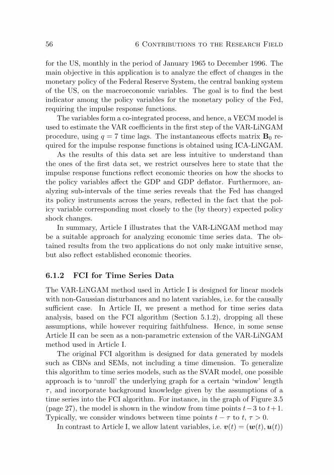
56 6 Contributions to the Research Field

for the US, monthly in the period of January 1965 to December 1996. Themain objective in this application is to analyze the effect of changes in themonetary policy of the Federal Reserve System, the central banking systemof the US, on the macroeconomic variables. The goal is to find the bestindicator among the policy variables for the monetary policy of the Fed,requiring the impulse response functions.

The variables form a co-integrated process, and hence, a VECM model isused to estimate the VAR coefficients in the first step of the VAR-LiNGAMprocedure, using q = 7 time lags. The instantaneous effects matrix B0 re-quired for the impulse response functions is obtained using ICA-LiNGAM.

As the results of this data set are less intuitive to understand thanthe ones of the first data set, we restrict ourselves here to state that theimpulse response functions reflect economic theories on how the shocks tothe policy variables affect the GDP and GDP deflator. Furthermore, an-alyzing sub-intervals of the time series reveals that the Fed has changedits policy instruments across the years, reflected in the fact that the pol-icy variable corresponding most closely to the (by theory) expected policyshock changes.

In summary, Article I illustrates that the VAR-LiNGAM method maybe a suitable approach for analyzing economic time series data. The ob-tained results from the two applications do not only make intuitive sense,but also reflect established economic theories.

6.1.2 FCI for Time Series Data

The VAR-LiNGAM method used in Article I is designed for linear modelswith non-Gaussian disturbances and no latent variables, i.e. for the causallysufficient case. In Article II, we present a method for time series dataanalysis, based on the FCI algorithm (Section 5.1.2), dropping all theseassumptions, while however requiring faithfulness. Hence, in some senseArticle II can be seen as a non-parametric extension of the VAR-LiNGAMmethod used in Article I.

The original FCI algorithm is designed for data generated by modelssuch as CBNs and SEMs, not including a time dimension. To generalizethis algorithm to time series models, such as the SVAR model, one possibleapproach is to ‘unroll’ the underlying graph for a certain ‘window’ lengthτ , and incorporate background knowledge given by the assumptions of atime series into the FCI algorithm. For instance, in the graph of Figure 3.5(page 27), the model is shown in the window from time points t−3 to t+1.Typically, we consider windows between time points t− τ to t, τ > 0.

In contrast to Article I, we allow latent variables, i.e. v(t) = (w(t),u(t))

6.1 Structure Learning in Time Series Models 57

with w(t) observed, and u(t) unobserved variables. Note that the full setof variable-time point nodes fulfill the causal Markov condition in the com-pletely unrolled graph. However, on a finite window of length τ additionaldependencies can occur, even in the case of no latent variables u(t), due tothe marginalization over the variables outside the window. For instance,in Figure 3.5, for any window of length τ , v2(t − τ) and v3(t − τ) are de-pendent since all conditioning sets Z for which v2(t − τ)⊥⊥ v3(t − τ) | Zholds lie outside the window (for instance Z = {v3(t − τ − 1)}). Further-more, when marginalizing out latent variables inside the window, depen-dencies may go back arbitrarily far in time: In the graph of Figure 3.5 withw(t) = (v1(t), v2(t)) and u(t) = v3(t), v2(t) and v2(t−k) are dependent forall k due to the latent variable v3.

In this sense, FCI is precisely the right tool, since it can handle marginalsof DAGs, represented by MAGs, and infer their equivalence class in formof PAGs. We thus apply a modified FCI algorithm (see below) to samplesover the observed variables w(t− τ), . . . ,w(t), which are obtained using a‘sliding window’ approach, i.e. for observations over a period of length Twe obtain T − τ samples (w(1), . . . ,w(τ + 1)), . . ., (w(T − τ), . . . ,w(T )).

To ensure that the distribution over the variables p(v(t − τ), . . . ,v(t))is well-defined, we assume that the whole process has a strictly positivetime invariant probability distribution, as for example is the case for stableVAR models. Furthermore, we assume that p(v(t− τ), . . . ,v(t)) is faithfulto the unrolled graph.

Even though FCI was originally designed for data without a time dimen-sion, it is straightforward to incorporate temporal knowledge: As alreadymentioned by Spirtes et al. (1993), all edges can be oriented ‘forward intime’ (i.e. adding arrowheads pointing into the nodes in the future), sincethe cause must precede the effect. This can be implemented in the orien-tation phase of FCI (see below). In Article II, we additionally incorporatethe knowledge of having a time invariant structure, i.e. a variable vi(t− t1)is a cause of vj(t), t1 ≥ 0 if and only if the same applies for vi(t − t1 − k)and vj(t − k) for all k. This knowledge can be included in the adjacencyphase and the orientation phase of FCI, resulting in the tsFCI (time seriesFCI) algorithm introduced in Article II, and summarized next.

In the adjacency phase, an edge between wi(t − t1) and wj(t − t2),0 ≤ t2 ≤ t1 ≤ τ , is removed if and only if we find a set Z ⊆ {w(t −τ),w(t− τ + 1), . . . ,w(t− t2)} \ {wi(t− t1), wj(t− t2)} such that

wi(t− t1)⊥⊥wj(t− t2) | Z. (6.2)

Note that the set Z only needs to contain variables up to and includingtime point t−t2 (or, if it is assumed that there are no instantaneous effects,

58 6 Contributions to the Research Field

only up to and including time point t− t2− 1). If such a set Z is found, bythe time invariant structure, we also know that there exists a set Zk suchthat

wi(t− t1 − k)⊥⊥wj(t− t2 − k) | Zk, (6.3)

with Zk containing the ‘same’ variables as Z but k time steps earlier. Thus,for all k for which Zk lies inside the window the edge between wi(t− t1−k)and wj(t−t2−k) can be removed (which follows from Lemma 1 of Article II).

Example 6.1 (Adjacency Phase in tsFCI). Taking the time series of Fig-ure 3.5 on a window of length τ = 3, we find that

v1(t)⊥⊥ v1(t− 1) |{v2(t− 1), v1(t− 2)}

and hence we can remove the edge between v1(t) and v1(t− 1). By the in-variant time structure we thus know that in the unrolled graph the followingalso holds:

v1(t− k)⊥⊥ v1(t− 1− k) |{v2(t− 1− k), v1(t− 2− k)}.

However, only for k = 1 the conditioning set Z1 = {v2(t − 2), v1(t − 3)}lies inside the window, and hence we can only additionally remove the edgebetween v1(t−1) and v1(t−2), but not between v1(t−2) and v1(t−3) (sincein the considered window these two variables are not independent).

In the orientation phase, we start by orienting all edges forward in time,i.e. if there is an edge between wi(t− t1) and wj(t− t2) with t1 > t2, thenwe orient it as wi(t − t1) ◦→wj(t − t2). This simply follows from the factthat the cause precedes the effect, and in a PAG (the output of FCI) thearrowhead means that wj(t− t2) is not a cause of wi(t− t1). Furthermore,when applying the complete set of orientation rules of FCI (Zhang, 2008),whenever an endpoint of an edge between wi(t−t1) and wj(t−t2) is oriented,we orient the endpoint in the same way for the edge between wi(t− t1− k)and wj(t− t2 − k), for all k (by Lemma 2 of Article II).

The advantage of using the tsFCI algorithm over applying the origi-nal FCI algorithm to a data set as explained above (including backgroundknowledge about a temporal ordering) is twofold. In both the adjacency andthe orientation phase tsFCI reduces the computation time using the time in-variant structure by (i) restricting the number of independence tests carriedout and (ii) reducing the number of orientation rules applied. Secondly, theoutput PAG of tsFCI always represents a time invariant structure, whereasfor FCI this is not necessarily true due to finite sample effects.

Compared to SVAR identification (Section 5.4) as well as Grangercausality (Section 5.5), the clear advantage of tsFCI is its ability to handlelatent variables.

6.2 Structure Learning in Extended LiNGAM Models 59

6.2 Structure Learning in Extended LiNGAMModels

Articles III through VI address both effect identification (Q1) and structurelearning (Q2) in the case of static data. Most methods continue alongthe line of Article I, using linear SEMs with non-Gaussian error terms.Although designed for static data, using the ‘sliding window’ approach asexplained for tsFCI in Article II, these methods may also be applied totime series data. In this section we discuss the work towards answering Q2,while the work addressing Q1 will be presented in the next section.

6.2.1 LiNGAM for Multidimensional Variables

In Article III, we introduce a set of methods to estimate the causal or-der among multidimensional variables v = (v1, . . . ,vn), assuming that thedata are generated by a similar model to the one in GroupLiNGAM (Sec-tion 5.2.5). The only difference in our model is that the matrix B is assumedto be strictly lower block triangular (as opposed to lower block triangular).However, any model following the definition of the GroupLiNGAM modelcan be transformed into an observationally equivalent model following themodel definition of Article III. An important difference to the work byKawahara et al. (2010) is that we assume to know a priori the partition ofthe variables in v into the vectors (also referred to as groups) v1, . . . ,vn.

The general algorithm follows the idea of DirectLiNGAM (Section 5.2.2),i.e. first finding an exogenous group, then regressing out the effect of theexogenous group on all other groups, and repeating the process on theresulting residuals. We introduce three alternatives to find an exogenousgroup.

In the first approach of finding an exogenous group, we generalize The-orem 5.2 (page 45) to multidimensional variables, stating that a group ofvariables vj is exogenous if and only if it is independent of all the residuals

r(j)i resulting from OLS regressions of vi on vj (Lemma 1 of Article III). As

this result is based on independencies, it is essential that the disturbanceterms ei are non-Gaussian.

The second approach is based on the pairwise measure explained inSection 5.2.3, which also requires non-Gaussian disturbances. The naıveapproach of utilizing this measure would be to test for each pair (vi, vj) ofscalar variables, with vi in group vi and vj in group vj , i 6= j, whether vi is acause of vj . If the error terms within each group were independent then forany variable vj of an exogenous group vj the pairwise measure would infer

60 6 Contributions to the Research Field

the correct causal direction between vi and vj . However, since correlatederror terms within each group are allowed, it is necessary to transform thevariables of the pair (vi, vj) appropriately to meet the model assumptionsof the pairwise measure. After this transformation, we obtain a measurefor each pair (vi, vj), indicating which variable is exogenous among the two.By combining these measures appropriately it is then possible to find anexogenous group.

Lastly, in the third approach we utilize the Trace Method (Section 5.3)to find an exogenous group. This method is designed to find a causalorder among two multidimensional variables, and can be generalized tofind an exogenous group among several groups by applying it to each pair(vi,vj), i 6= j. For an exogenous group vj , the model vj → vi holds forall i (by marginalizing out intermediate groups). Appropriately combiningthese measures yields an exogeneity measure for each group. Note thatthis approach does not require non-Gaussian disturbances, so can also beapplied to Gaussian data.

After finding an exogenous group, a direct generalization of Theorem 5.3(page 46) shows that after regressing out this group from all other variables,the resulting (multidimensional) residuals follow again the same model(Lemma 2 of Article III).

Comparing the three approaches on simulated data shows that themethod based on the pairwise measure performs very well, also for smallsample sizes, whereas the generalization of DirectLiNGAM requires moredata points to reach the same performance. The approach based on thetrace method always makes more mistakes than the former two methods.The simulations also show that for large models and small data sets itmay even be advantageous to use the pairwise measure in the naıve wayexplained above. All three variants outperform the simple approach of re-placing each group with an aggregate, such as the mean over all variables,and then applying methods for scalar variables, like DirectLiNGAM.

The methods introduced in Article III are closely related to the workby Kawahara et al. (2010), both using a DirectLiNGAM-style approach forthe overall algorithm. However, there are some clear distinctions and ad-vances in the methods of Article III. The major difference of our approachto GroupLiNGAM is, as mentioned above, that in our method we assumeto know how the vector v is partitioned into the variables v1, . . . ,vn, yield-ing efficient algorithms to infer the causal order among these variables.In GroupLiNGAM, on the other hand, Kawahara et al. (2010) aimed atlearning this partition, which results in computationally and statisticallymore challenging algorithms. Furthermore, we give three strategies to find

6.2 Structure Learning in Extended LiNGAM Models 61

v4

v1 v5

v2v3

b1,4 b5,4

b5,1

b3,1 b2,1

b2,3

Figure 6.3: An lvLiNGAM model with U = {v4} and W = {v1, v2, v3, v5}.

an exogenous group, whereas Kawahara et al. (2010) only considered thelinear non-Gaussian case.

6.2.2 Pairwise Causal Relationships in lvLiNGAM

In Article IV we assume that we are given data over the observed variablesW, generated by a faithful lvLiNGAM model (Section 5.2.4) over variablesV = W ∪ U . As already mentioned, it is in general impossible to inferthe whole lvLiNGAM model (since generally it is not identifiable), andestimation of models, up to equivalence, is computationally very challeng-ing. Thus, the goal here is to develop more efficient techniques to learn(identifiable) parts of the underlying model.

The basic idea is that there might be subsets Z ⊆ W for which aLiNGAM model (without latent variables) fits. More precisely, as shownin Lemma 1 of Article IV, the variables in Z follow a LiNGAM model ifand only if every confounder of any two variables zi ∈ Z and zj ∈ Z liesin Z (i.e. the set Z is causally sufficient). In Article IV we call such setsunconfounded.

Example 6.2 (Confounded and Unconfounded Sets). For the graph inFigure 6.3, the sets {v1, v5}, {v2, v5}, {v1, v2, v3, v5}, for instance, are con-founded by the latent variable v4, and the set {v2, v3} is confounded by theobserved variable v1. When estimating a LiNGAM model for any of thesesets, the resulting residuals are not independent of each other (no matterwhich causal order is learned). For instance, for v1 and v5 we may obtainthat v1 = r1, and v5 = c5,1 v1 + r5. Expressing r1 and r5 in terms of thedisturbance terms e1, e4, e5 of variables v1, v4, v5 yields

r1 = b1,4 e4 + e1

r5 = v5 − c5,1 v1 = (b5,1 b1,4 + b5,4 − c5,1 b1,4) e4 + (b5,1 − c5,1) e1 + e5.

62 6 Contributions to the Research Field

By the non-Gaussianity assumption of the disturbances and the Darmois-Skitovitch Theorem (Section 2.2.2), for independence between r1 and r5 werequire b1,4 = 0 (yielding b5,1 = c5,1), or b5,1 = c5,1 and b5,1 b1,4 + b5,4 −c5,1 b1,4 = 0, which is only possible when b5,4 = 0. A similar calculationshows that if the LiNGAM model was estimated in the reverse direction,the residuals would also be dependent.

Thus, by testing independence between the residuals, it is possible todetect confounding in the case of non-Gaussian variables. Note that forGaussian variables the residuals r1 and r5 are always independent sincethese two residuals are by construction of the OLS estimator (and also bydefinition of ICA) uncorrelated.

In contrast, the sets {v1, v3}, {v1, v2}, and {v1, v2, v3} are unconfounded(and no other sets of two or more observed variables are), and a LiNGAMmodel fits.

However, going through all subsets of W to test whether they followa LiNGAM model is in general not feasible, as their number grows expo-nentially in the number of variables in W. Fortunately, as the previousexample hints at, unconfounded sets with three or more variables have un-confounded subsets. Thus, an incremental search approach could be usedto find all maximally unconfounded sets, i.e. when adding any variable tothe set its unconfoundedness is destroyed. However, even the number ofthese sets grows exponentially in the worst-case graphs.

Thus, to obtain a computationally efficient algorithm, in Article IV weaddress the problem of determining all pairwise causal relations, for whichthere exists an unconfounded set Z containing this pair. Such pairs arecalled unconfounded with respect to Z, and for each such pair the introducedalgorithm returns which variable is the cause and which the effect, and thetotal effect of the former on the latter. The resulting method is termed the‘pairwise lvLiNGAM’ algorithm.

Example 6.3 (Pairwise lvLiNGAM). Given a data set generated fromthe model of Figure 6.3 with observed variables W = {v1, v2, v3, v5}, theproposed algorithm iteratively searches for all pairs which are part of anunconfounded set.

First, it searches for pairs (vi, vj), i 6= j, vi ∈ W and vj ∈ W, whichare unconfounded by estimating a LiNGAM model over (vi, vj) and testingits fit. As explained in Example 6.2, the only pairs for which the LiNGAMmodel fits are (v1, v2) and (v1, v3), yielding the causal directions from v1to v2, and from v1 to v3, and total causal effects b2,1 + b2,3 b3,1, and b3,1,respectively.

6.2 Structure Learning in Extended LiNGAM Models 63

Next, for any pair (vi, vj) which was not found to be unconfounded yet,the algorithm tries to build up a set Z∪{vi, vj} such that the pair is uncon-founded with regard to this set. The set Z includes all those variables vkfor which (vk, vi) and (vk, vj) were found to be unconfounded in a previousiteration of the algorithm (i.e. any potential confounders of vi and vj). Totest whether Z ∪ {vi, vj} is unconfounded, a LiNGAM model is estimatedand its fit is evaluated. In the example, for the pair (v2, v3) we obtain theset Z = {v1}, and a LiNGAM model fits to {v1, v2, v3}, as mentioned inExample 6.2. Furthermore, this LiNGAM model reveals that v3 is the causeof v2 with total causal effect b2,3.

The algorithm iterates this step until no more new pairs are found to beunconfounded with regard to some set.

As the main result of Article IV, we prove in Theorem 1 that, in thelarge sample limit, the pairwise lvLiNGAM algorithm is sound (i.e. when-ever a pair is judged to be unconfounded with regard to a set, this is correct,and the estimate of the total causal effect converges to the true total ef-fect) and complete (i.e. any pair which is part of an unconfounded subsetis discovered). The completeness in particular means that any pairwisecausal effect which is detectable by fitting a LiNGAM model to a subset ofvariables and testing its fit is detected.

Fitting a LiNGAM model as done in Example 6.3 to find unconfoundedsets is computationally inefficient. In Lemma 3 of Article IV, a more effi-cient procedure is suggested to find such sets: For a set Z and a pair (vi, vj)as in Example 6.3, we estimate the following two regression models

vj = cj,ivi + cTj z + rj (6.4)

vi = ci,jvj + cTi z + ri (6.5)

and conclude as follows:

(i) If rj ⊥⊥ vi and ri /⊥⊥ vj , then vi is a cause of vj with total effect cj,i.

(ii) If rj /⊥⊥ vi and ri⊥⊥ vj , then vj is a cause of vi with total effect ci,j .

(iii) If rj ⊥⊥ vi and ri⊥⊥ vj , and cj,i = ci,j = 0, then vi⊥⊥ vj | Z.

(iv) If none of the above holds, then (vi, vj) is not unconfounded withrespect to Z ∪ {vi, vj}.

In simulations we evaluate the algorithm using two independence tests(HSIC, and non-linear correlations, see Section 2.2.2), and compare the re-sults to ICA-LiNGAM (which does not account for latent variables). For

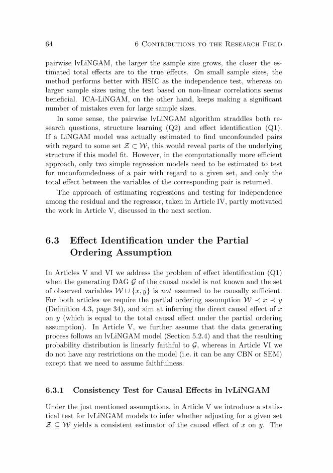
64 6 Contributions to the Research Field

pairwise lvLiNGAM, the larger the sample size grows, the closer the es-timated total effects are to the true effects. On small sample sizes, themethod performs better with HSIC as the independence test, whereas onlarger sample sizes using the test based on non-linear correlations seemsbeneficial. ICA-LiNGAM, on the other hand, keeps making a significantnumber of mistakes even for large sample sizes.

In some sense, the pairwise lvLiNGAM algorithm straddles both re-search questions, structure learning (Q2) and effect identification (Q1).If a LiNGAM model was actually estimated to find unconfounded pairswith regard to some set Z ⊂ W, this would reveal parts of the underlyingstructure if this model fit. However, in the computationally more efficientapproach, only two simple regression models need to be estimated to testfor unconfoundedness of a pair with regard to a given set, and only thetotal effect between the variables of the corresponding pair is returned.

The approach of estimating regressions and testing for independenceamong the residual and the regressor, taken in Article IV, partly motivatedthe work in Article V, discussed in the next section.

6.3 Effect Identification under the PartialOrdering Assumption

In Articles V and VI we address the problem of effect identification (Q1)when the generating DAG G of the causal model is not known and the setof observed variables W ∪ {x, y} is not assumed to be causally sufficient.For both articles we require the partial ordering assumption W ≺ x ≺ y(Definition 4.3, page 34), and aim at inferring the direct causal effect of xon y (which is equal to the total causal effect under the partial orderingassumption). In Article V, we further assume that the data generatingprocess follows an lvLiNGAM model (Section 5.2.4) and that the resultingprobability distribution is linearly faithful to G, whereas in Article VI wedo not have any restrictions on the model (i.e. it can be any CBN or SEM)except that we need to assume faithfulness.

6.3.1 Consistency Test for Causal Effects in lvLiNGAM

Under the just mentioned assumptions, in Article V we introduce a statis-tical test for lvLiNGAM models to infer whether adjusting for a given setZ ⊆ W yields a consistent estimator of the causal effect of x on y. The

6.3 Effect Identification under the Partial Ordering Assumption 65

test for the given set Z is based on two simple OLS regressions:

x = cTx z + rx, and (6.6)

y = cy,xx+ cTy z + ry. (6.7)

If the residual rx is Gaussian (which can be tested using standard tests),the test terminates without conclusion. For non-Gaussian rx, we performa statistical test of dependence between rx and ry, and conclude as follows(based on Theorem 1 of Article V):

(i) If independence is rejected, the estimated effect cy,x of x on y is in-ferred to be inconsistent.

(ii) If independence is not rejected, the effect is inferred to be consistent.

The main result of Article V is that, under the given assumptions,the just described test will, in the large sample limit, correctly identifysets Z which yield a consistent estimator of the causal effect (Theorem 1 ofArticle V). The reason why non-Gaussianity is required becomes clear whenlooking at the residuals rx and ry: By construction of the OLS estimatorcov(rx, ry) = 0, and hence rx and ry are always independent for Gaussianvariables.

Example 6.4 (Statistical Test for Consistency in lvLiNGAM models).We demonstrate the method using lvLiNGAM models over the DAGs inFigures 4.2 (a) and (b) (page 35). We first consider the model in (a), withlinear equations w

xy

=

0 0 0bx,w 0 0by,w by,x 0

wxy

+

ewexey

. (6.8)

Using Z = ∅ in Equations (6.6) and (6.7), the resulting residuals rx and ryare dependent, which can be seen when expressing these residuals in termsof the disturbances e = (ew, ex, ey)

T :

rx = x = (bx,w , 1 , 0) e

ry = y − cy,xx = (by,xbx,w + by,w , by,x , 1) e− cy,x(bx,w , 1 , 0) e

= ((by,x − cy,x)bx,w + by,w , by,x − cy,x , 1) e.

Using the formula for the OLS estimator (Equation (2.8), page 13) or theback-door criterion (Definition 4.2, page 31), one can show that cy,x 6= by,xin the large sample limit,3 and thus the coefficients of ex in both represen-tations rx and ry, marked in bold, are non-zero. By the non-Gaussianity of

3To be more precise, cy,x does not converge in probability to by,x.

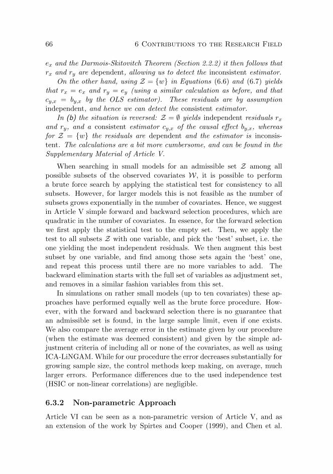
66 6 Contributions to the Research Field

ex and the Darmois-Skitovitch Theorem (Section 2.2.2) it then follows thatrx and ry are dependent, allowing us to detect the inconsistent estimator.

On the other hand, using Z = {w} in Equations (6.6) and (6.7) yieldsthat rx = ex and ry = ey (using a similar calculation as before, and thatcy,x = by,x by the OLS estimator). These residuals are by assumptionindependent, and hence we can detect the consistent estimator.

In (b) the situation is reversed: Z = ∅ yields independent residuals rxand ry, and a consistent estimator cy,x of the causal effect by,x, whereasfor Z = {w} the residuals are dependent and the estimator is inconsis-tent. The calculations are a bit more cumbersome, and can be found in theSupplementary Material of Article V.

When searching in small models for an admissible set Z among allpossible subsets of the observed covariates W, it is possible to performa brute force search by applying the statistical test for consistency to allsubsets. However, for larger models this is not feasible as the number ofsubsets grows exponentially in the number of covariates. Hence, we suggestin Article V simple forward and backward selection procedures, which arequadratic in the number of covariates. In essence, for the forward selectionwe first apply the statistical test to the empty set. Then, we apply thetest to all subsets Z with one variable, and pick the ‘best’ subset, i.e. theone yielding the most independent residuals. We then augment this bestsubset by one variable, and find among those sets again the ‘best’ one,and repeat this process until there are no more variables to add. Thebackward elimination starts with the full set of variables as adjustment set,and removes in a similar fashion variables from this set.

In simulations on rather small models (up to ten covariates) these ap-proaches have performed equally well as the brute force procedure. How-ever, with the forward and backward selection there is no guarantee thatan admissible set is found, in the large sample limit, even if one exists.We also compare the average error in the estimate given by our procedure(when the estimate was deemed consistent) and given by the simple ad-justment criteria of including all or none of the covariates, as well as usingICA-LiNGAM. While for our procedure the error decreases substantially forgrowing sample size, the control methods keep making, on average, muchlarger errors. Performance differences due to the used independence test(HSIC or non-linear correlations) are negligible.

6.3.2 Non-parametric Approach

Article VI can be seen as a non-parametric version of Article V, and asan extension of the work by Spirtes and Cooper (1999), and Chen et al.

6.3 Effect Identification under the Partial Ordering Assumption 67

(2007) (Section 4.3.2) allowing for non-empty admissible sets. Under thestated assumptions, Article VI gives conditions solely based on dependen-cies and independencies among the observed variables to determine whetheran effect is identifiable.

The aim is to reach one of the following decisions:

‘±’ The causal effect is non-zero and can be estimated using a foundadmissible set Z by back-door adjustment (Theorem 4.1, page 31).

‘0’ The causal effect is zero.

‘?’ We do not know, i.e. we cannot infer ‘±’ or ‘0’.

Note that when inferring ‘±’ or ‘0’ the causal effect of x on y is identified.Towards this end, we introduce two simple rules:

R1: If there exists a variable w ∈ W and a set Z ⊆ W \ {w} such that

(i) w /⊥⊥ y | Z, and

(ii) w⊥⊥ y | Z ∪ {x}then infer ‘±’ and give Z as an admissible set.

R2: If there exists a set Z ⊆ W such that

(i) x⊥⊥ y | Z,

or, if there exists a variable w ∈ W and a set Z ⊆ W \{w} such that

(ii) w /⊥⊥x | Z, and

(iii) w⊥⊥ y | Z,

then infer ‘0’.

If neither R1 nor R2 applies, infer ‘?’.

The idea of R1 is as follows: Condition (i) ensures that there exists atleast one active path from w to y, given Z. By condition (ii) these pathsmust pass through x, since including x in the conditioning set blocks allthese paths. This implies that there is at least one active path π fromw to x given Z (pointing into x by the partial ordering assumption). Ifthere existed an active back-door path from x to y, condition (ii) could nothold, since concatenating this back-door path with the active path π at xwould yield an active path from w to y given Z ∪ {x}, with a collider atx. An example for which R1 applies is given by the graph of Figure 4.1 (a)(page 32) with w = w1 and Z = {w2, w3}.

Rule R2 consists of two parts: First, if condition (i) holds, then, by thefaithfulness assumption, there is no edge between x and y in the underlyingDAG and hence, the causal effect is 0. Secondly, condition (ii) and (iii)together also ensure that there is no edge between x and y: By condition

68 6 Contributions to the Research Field

(ii) there exists at least one active path π from w to x given Z. If thereexisted an edge from x to y, appending this edge to the path π would yieldan active path from w to y given Z such that condition (iii) could not hold.Note that the second part of R2 may allow us to detect a zero effect of xon y even in the case of latent confounding.

The main result of Article VI is that these two simple rules are, inthe large sample limit, both sound (i.e. whenever we make a decision, itis correct) and complete (i.e. whenever we infer ‘?’, it is impossible toreliably infer ‘±’ or ‘0’ based on dependencies and independencies alone),as stated in Theorems 2 and 3 of Article VI.

The rules are also related to the FCI algorithm (Section 5.1.2). In fact,when incorporating the background knowledge of the partial ordering, thePAG output by FCI over the observed variablesW∪{x, y} may be utilizedto reach the same decisions as with our rules. However, for FCI withbackground knowledge it is not known whether it is complete, whereas ourrules are.

On finite sample data, combining the (possibly conflicting) results whenapplying the rules with different pairs (w,Z) or sets Z is done using an ad-hoc procedure based on a Bayes classifier. In simulations, the novel rulesand the approach based on the FCI algorithm clearly outperform the simpleadjustment criteria presented in Section 4.3.1, as the former two proceduresmay output ‘?’ if no admissible set exists, or if there is not enough evidenceto make decisions ‘±’ or ‘0’. The simple adjustment criteria, on the otherhand, always output an estimate.

Neither of the two approaches of Articles V and VI subsumes the other.While the two simple rules of Article VI can be applied to any kind ofmodel (not only to lvLiNGAM models), the statistical test of Article Vmay be able to reach conclusions for models, under the given assumptions,in which the rules of Article VI cannot yield a decision: For the two mod-els of Example 6.4, the statistical test of Article V successfully identifieswhether w should be adjusted for. However, the two models imply the sameindependencies over the observed variables (there are none), and hence, thetwo models cannot be distinguished based on the rules of Article VI.

Chapter 7

Conclusions

In this thesis we provided novel methods addressing two important prob-lems in the field of causal discovery: causal effect identification (researchquestion Q1) and structure learning (research question Q2). After describ-ing the existing work related to Articles I to VI in Chapters 2 through5, we discussed the contributions of these articles in Chapter 6. Commonthemes to the articles were the LiNGAM model and the handling of latentvariables. All introduced methods were developed for passive observationaldata.

The main contribution of this thesis is twofold: In Articles I, III, IV andV we used the LiNGAM model and extended it in various directions (partlyincluding latent variables). These articles provide powerful tools addressingQ1 and Q2 in situations where the data are linear and non-Gaussian. Ifthese assumptions are not met, Articles II and VI present solutions to someof the addressed problems in the nonparametric setting.

In particular, in Article I we discussed the application of an SVARidentification method based on LiNGAM requiring the causal sufficiencyassumption. To overcome this limitation, Article II introduced the tsFCIalgorithm, which does not rely on the parametric assumptions of a LiNGAMmodel nor on causal sufficiency. Article III extended the LiNGAM modelto multidimensional variables, and introduced a bundle of methods to learna causal order among these variables. In Article IV, we then presented acomplete algorithm to identify pairwise total causal effects in lvLiNGAMmodels. Finally, in Article V we aimed at identifying one specific directcausal effect in lvLiNGAM models, given the partial ordering assumption;article VI addressed the same problem in the non-parametric setting.

While some gaps in the literature were filled by the contributions ofArticles I to VI, there are many open questions. All methods were basedon models over acyclic causal structures, which in some applications may

69

70 7 Conclusions

not be suitable. It would thus be interesting to develop and apply methodswhich allow for cyclic connections among the variables.

For the problem of SVAR identification, for instance, instead of us-ing the LiNGAM method one could use the LiNG algorithm (Linear non-Gaussian, Lacerda et al., 2008), a generalization of the LiNGAM model tocyclic models. Similarly, the approach using the PC algorithm for SVARidentification could be modified by replacing the PC algorithm by theCCD method (Cyclic Causal Discovery, Richardson, 1996; Richardson andSpirtes, 1999), which is a constraint based method similar to PC for cyclicmodels.

Additionally, in Articles V and VI cyclic connections among the ob-served covariates W could be allowed, even when keeping the partial or-dering assumption, i.e. the assumption that the covariates W precede thetreatment x, which precedes the outcome y. On the other hand, relaxingthe partial ordering assumption in Articles V and VI would also be an in-teresting topic for future research. One such possible scenario is to allow(some of) the observed covariates to lie between x and y. This could yieldadditional possibilities to identify a (direct or indirect) causal effect by, forinstance, utilizing front-door adjustment (Section 4.2.2).

In terms of algorithms, in Article IV it would be interesting to combinethe introduced method with other approaches, such as the ones by Tashiroet al. (2012), or Kawahara et al. (2010), as these methods may learn dif-ferent parts of the model, for example identify a sink, and the combinationcould help to better understand the underlying model. Furthermore, re-placing the forward and backward search procedures of Article V by moresophisticated approaches could be investigated, as the current methods,although working well in simulations, are only heuristics.

Finally, as most of the presented work has focused on theoretical issuesof model identifiability, much work remains in terms of investigating theperformance of the presented methods in various real-world applications.For instance, it would be interesting to apply the method introduced inArticle III to functional magnetic resonance imaging (fMRI) data to analyzefunctional connectivity in the brain, or the algorithms of Articles V and VIto estimate causal effects in various problems in epidemiology or economics.In such applications, it would be important to evaluate to what extentmodel violations may affect the result, as well as to further investigatestatistical issues due to small sample sizes and potentially large numbersof variables.

References

Ali, R. A., Richardson, T. S., and Spirtes, P. (2009). Markov equivalencefor ancestral graphs. The Annals of Statistics, 37(5B):2808–2837.

Bernanke, B. S. and Mihov, I. (1998). Measuring monetary policy. TheQuarterly Journal of Economics, 113(3):869–902.

Berzuini, C., Dawid, P., and Bernardinelli, L., editors (2012). Causality:Statistical Perspectives and Applications. John Wiley & Sons.

Bollen, K. A. (1989). Structural Equations with Latent Variables. JohnWiley & Sons.

Chen, L. S., Emmert-Streib, F., and Storey, J. D. (2007). Harnessing nat-urally randomized transcription to infer regulatory relationships amonggenes. Genome Biology, 8(R219).

Chickering, D. M. (2002). Optimal structure identification with greedysearch. Journal of Machine Learning Research, 3:507–554.

Chu, T. and Glymour, C. (2008). Search for additive nonlinear time seriescausal models. Journal of Machine Learning Research, 9:967–991.

Claassen, T. and Heskes, T. (2010). Causal discovery in multiple modelsfrom different experiments. In Advances in Neural Information Process-ing Systems 23 (NIPS*2010), pages 415–423.

Coad, A. and Rao, R. (2010). Firm growth and R&D expenditure. Eco-nomics of Innovation and New Technology, 19(2):127–145.

Dahlhaus, R. and Eichler, M. (2003). Causality and graphical models intime series analysis. In Green, P. J., Hjort, N. L., and Richardson, S.,editors, Highly structured stochastic systems, pages 115–137. UniversityPress, Oxford.

71

72 References

Darmois, G. (1953). Analyse generale des liaisons stochastiques. Revue del’Institut International de Statistique, 21:2–8.

Dasgupta, M. and Mishra, S. K. (2004). Least absolute deviation estimationof linear econometric models: A literature review. MPRA Paper, 1781.

Dawid, A. P. (1979). Conditional independence in statistical theory. Jour-nal of the Royal Statistical Society. Series B (Methodological), 41(1):1–31.

Demiralp, S. and Hoover, K. D. (2003). Searching for the causal structureof a vector autoregression. Oxford Bulletin of Economics and Statistics,65(s1):745–767.

Druzdzel, M. J. and Simon, H. A. (1993). Causality in bayesian beliefnetworks. In Proceedings of the Ninth Conference on Uncertainty inArtificial Intelligence (UAI-93), pages 3–11. Morgan Kaufmann.

Engle, R. F. and Granger, C. W. J. (1987). Co-integration and error correc-tion: Representation, estimation, and testing. Econometrica, 55(2):251–276.

Geiger, D. and Pearl, J. (1988). On the logic of causal models. In Proceed-ings of the Fourth Conference on Uncertainty in Artificial Intelligence(UAI-88), pages 136–147. AUAI Press.

Geiger, D., Verma, T., and Pearl, J. (1990). Identifying independence inbayesian networks. Networks, 20(5):507–534.

Granger, C. W. J. (1969). Investigating causal relationships by econometricmodels and cross-spectral methods. Econometrica, 37(3):424–438.

Greenland, S., Pearl, J., and Robins, J. M. (1999). Causal diagrams forepidemiologic research. Epidemiology, 10(1):37–48.

Gretton, A., Fukumizu, K., Teo, C. H., Song, L., Scholkopf, B., and Smola,A. J. (2008). A kernel statistical test of independence. In Advances inNeural Information Processing Systems 20 (NIPS*2007), pages 585–592.

Haavelmo, T. (1943). The statistical implications of a system of simulta-neous equations. Econometrica, 11(1):1–12.

Hamilton, J. D. (1994). Time Series Analysis. Princeton University Press.

Hastie, T., Tibshirani, R., and Friedman, J. (2009). The Elements of Sta-tistical Learning: Data Mining, Inference and Prediction. Springer, 2ndedition.

References 73

Heckerman, D., Geiger, D., and Chickering, D. M. (1995). Learningbayesian networks: The combination of knowledge and statistical data.Machine Learning, 20(3):197–243.

Hoyer, P. O., Janzing, D., Mooij, J. M., Peters, J., and Scholkopf, B. (2009).Nonlinear causal discovery with additive noise models. In Advances inNeural Information Processing Systems 21 (NIPS*2008), pages 689–696.

Hoyer, P. O., Shimizu, S., Kerminen, A. J., and Palviainen, M. (2008).Estimation of causal effects using linear non-Gaussian causal modelswith hidden variables. International Journal of Approximate Reasoning,49(2):362–378.

Huang, Y. and Valtorta, M. (2006). Pearl’s calculus of intervention is com-plete. In Proceedings of the Twenty-Second Conference on Uncertaintyin Artificial Intelligence (UAI-06), pages 217–224. AUAI Press.

Hyttinen, A., Eberhardt, F., and Hoyer, P. O. (2012). Causal discoveryof linear cyclic models from multiple experimental data sets with over-lapping variables. In Proceedings of the Twenty-Eighth Conference onUncertainty in Artificial Intelligence (UAI-12), pages 387–396. AUAIPress.

Hyvarinen, A. (2010). Pairwise measures of causal direction in linear non-Gaussian acyclic models. In Proceedings of 2nd Asian Conference onMachine Learning (ACML2010). Journal of Machine Learning ResearchWorkshop and Conference Proceedings 13:1-16.

Hyvarinen, A., Karhunen, J., and Oja, E. (2001). Independent ComponentAnalysis. John Wiley & Sons.

Hyvarinen, A. and Smith, S. M. (2013). Pairwise likelihood ratios for esti-mation of non-Gaussian structural equation models. Journal of MachineLearning Research, 14:111–152.

Hyvarinen, A., Zhang, K., Shimizu, S., and Hoyer, P. O. (2010). Estima-tion of a structural vector autoregression model using non-Gaussianity.Journal of Machine Learning Research, 11:1709–1731.

Janzing, D., Hoyer, P. O., and Scholkopf, B. (2010). Telling cause fromeffect based on high-dimensional observations. In Proceedings of the 27thInternational Conference on Machine Learning (ICML-10), pages 479–486. Omnipress.

74 References

Janzing, D. and Scholkopf, B. (2010). Causal inference using the algo-rithmic markov condition. IEEE Transactions on Information Theory,56(10):5168–5194.

Kawahara, Y., Bollen, K., Shimizu, S., and Washio, T. (2010). Group-LiNGAM: Linear non-Gaussian acyclic models for sets of variables.arXiv, 1006.5041.

Koivisto, M. and Sood, K. (2004). Exact bayesian structure discovery inbayesian networks. Journal of Machine Learning Research, 5:549–573.

Koller, D. and Friedman, N. (2009). Probabilistic Graphical Models: Prin-ciples and Techniques. The MIT Press.

Lacerda, G., Spirtes, P., Ramsey, J., and Hoyer, P. O. (2008). Discoveringcyclic causal models by independent components analysis. In Proceedingsof the Twenty-Fourth Conference on Uncertainty in Artificial Intelligence(UAI-08), pages 366–374. AUAI Press.

Lauritzen, S. L., Dawid, A. P., Larsen, B. N., and Leimer, H.-G. (1990).Independence properties of directed markov fields. Networks, 20(5):491–505.

Lutkepohl, H. (2005). New Introduction to Multiple Time Series Analysis.Springer.

Meek, C. (1995). Causal inference and causal explanation with backgroundknowledge. In Proceedings of the Eleventh Conference on Uncertainty inArtificial Intelligence (UAI-95), pages 403–410. Morgan Kaufmann.

Meek, C. (1997). Graphical Models: Selecting causal and statistical models.PhD thesis, Carnegie Mellon University.

Moneta, A. (2003). Graphical models for structural vector autoregressions.LEM Working Paper 07, Sant’Anna School of Advanced Studies, Pisa,Italy.

Moneta, A. and Spirtes, P. (2006). Graphical models for the identificationof causal structures in multivariate time series. In Proceedings of the 2006Joint Conference on Information Sciences (JCIS 2006). Atlantis Press.

Mooij, J., Janzing, D., Peters, J., and Scholkopf, B. (2009). Regression bydependence minimization and its application to causal inference in ad-ditive noise models. In Proceedings of the 26th International Conferenceon Machine Learning (ICML-09), pages 745–752, Montreal. Omnipress.

References 75

Neyman, J. (1923). Sur les applications de la theorie des probabilites auxexperiences agricoles: Essai des principes. Roczniki Nauk Rolniczych,10:1–51. English translation of excerpts (1990) by D. Dabrowska and T.Speed, in Statistical Science, 5:465-472.

Pearl, J. (1988). Probabilistic Reasoning in Intelligent Systems: Networksof Plausible Inference. Morgan Kaufmann.

Pearl, J. (1993a). Comment: Graphical models, causality and intervention.Statistical Science, 8(3):266–269.

Pearl, J. (1993b). Mediating instrumental variables. Technical Report R-210, University of California, Los Angeles, CA.

Pearl, J. (1994). A probabilistic calculus of actions. In Proceedings ofthe Tenth Conference on Uncertainty in Artificial Intelligence (UAI-94),pages 454–462. Morgan Kaufmann.

Pearl, J. (1995). Causal diagrams for empirical research. Biometrika,82(4):669–688.

Pearl, J. (1998). Graphs, causality, and structural equation models. Soci-ological Methods & Research, 27(2):226–284.

Pearl, J. (2000). Causality: Models, Reasoning, and Inference. CambridgeUniversity Press. (2nd edition 2009).

Peters, J., Mooij, J. M., Janzing, D., and Scholkopf, B. (2011). Iden-tifiability of causal graphs using functional models. In Proceedings ofthe Twenty-Seventh Conference on Uncertainty in Artificial Intelligence(UAI-11), pages 589–598. AUAI Press.

Reichenbach, H. (1956). The Direction of Time. University of CaliforniaPress.

Richardson, T. (1996). A discovery algorithm for directed cyclic graphs.In Proceedings of the Twelfth Conference on Uncertainty in ArtificialIntelligence (UAI-96), pages 454–461. Morgan Kaufmann.

Richardson, T. and Spirtes, P. (1999). Automated discovery of linear feed-back models. In Glymour, C. and Cooper, G. F., editors, Computation,Causation, and Discovery, pages 253–302. AAAI Press/The MIT Press.

Richardson, T. S. and Spirtes, P. (2002). Ancestral graph markov models.The Annals of Statistics, 30(4):962–1030.

76 References

Robins, J. M. (1999). Testing and estimation of direct effects by repa-rameterizing directed acyclic graphs with structural nested models. InGlymour, C. and Cooper, G. F., editors, Computation, Causation, andDiscovery, pages 349–405. AAAI Press/The MIT Press.

Robins, J. M., Scheines, R., Spirtes, P., and Wasserman, L. (2003). Uniformconsistency in causal inference. Biometrika, 90(3):491–515.

Rosenbaum, P. R. and Rubin, D. (1983). The central role of the propensityscore in observational studies for causal effects. Biometrika, 70(1):41–55.

Rubin, D. (1974). Estimating causal effects of treatments in random-ized and nonrandomized studies. Journal of Educational Psychology,66(5):688–701.

Shimizu, S., Hoyer, P. O., Hyvarinen, A., and Kerminen, A. J. (2006).A linear non-Gaussian acyclic model for causal discovery. Journal ofMachine Learning Research, 7:2003–2030.

Shimizu, S., Inazumi, T., Sogawa, Y., Hyvarinen, A., Kawahara, Y.,Washio, T., Hoyer, P. O., and Bollen, K. (2011). DirectLiNGAM: Adirect method for learning a linear non-Gaussian structural equationmodel. Journal of Machine Learning Research, 12:1225–1248.

Shpitser, I. and Pearl, J. (2006). Identification of conditional interventionaldistributions. In Proceedings of the Twenty-Second Conference on Un-certainty in Artificial Intelligence (UAI-06), pages 437–444. AUAI Press.

Shpitser, I., Richardson, T. S., and Robins, J. M. (2011). An efficient algo-rithm for computing interventional distributions in latent variable causalmodels. In Proceedings of the Twenty-Seventh Conference on Uncertaintyin Artificial Intelligence (UAI-11), pages 661–670. AUAI Press.

Shpitser, I., VanderWeele, T., and Robins, J. (2010). On the validity ofcovariate adjustment for estimating causal effects. In Proceedings of theTwenty-Sixth Conference on Uncertainty in Artificial Intelligence (UAI-10), pages 527–536. AUAI Press.

Silander, T. and Myllymaki, P. (2006). A simple approach for find-ing the globally optimal bayesian network structure. In Proceedings ofthe Twenty-Second Conference on Uncertainty in Artificial Intelligence(UAI-06), pages 445–452. AUAI Press.

Skitovitch, W. P. (1953). On a property of the normal distribution. DokladyAkademii Nauk SSSR, 89:217–219.

References 77

Spirtes, P. (2000). The limits of causal discovery from observational data.American Economic Association, Boston, MA.

Spirtes, P. and Cooper, G. F. (1999). An experiment in causal discoveryusing a pneumonia database. In Proceedings of the Seventh InternationalWorkshop on Artificial Intelligence and Statistics (AISTATS 1999). Mor-gan Kaufmann.

Spirtes, P. and Glymour, C. (1991). An algorithm for fast recovery of sparsecausal graphs. Social Science Computer Review, 9(1):62–72.

Spirtes, P., Glymour, C., and Scheines, R. (1990). Causality from probabil-ity. In McKee, G., editor, Evolving Knowledge in Natural and ArtificialIntelligence, pages 181–199. London: Pitman.

Spirtes, P., Glymour, C., and Scheines, R. (1993). Causation, Prediction,and Search. Springer-Verlag, New York. (2nd edition MIT Press 2000).

Spirtes, P., Meek, C., and Richardson, T. (1999). An algorithm for causalinference in the presence of latent variables and selection bias. In Gly-mour, C. and Cooper, G. F., editors, Computation, Causation, and Dis-covery, pages 211–252. AAAI Press/The MIT Press.

Spirtes, P. and Richardson, T. (1997). A polynomial time algorithm fordetermining DAG equivalence in the presence of latent variables andselection bias. In Proceedings of the Sixth International Workshop onArtificial Intelligence and Statistics (AISTATS 1997).

Spirtes, P., Richardson, T., Meek, C., Scheines, R., and Glymour, C. (1998).Using path diagrams as a structural equation modeling tool. SociologicalMethods & Research, 27(2):182–225.

Tashiro, T., Shimizu, S., Hyvarinen, A., and Washio, T. (2012). Estimationof causal orders in a linear non-Gaussian acyclic model: A method robustagainst latent confounders. In Artificial Neural Networks and MachineLearning – ICANN 2012, pages 491–498. Springer Berlin Heidelberg.

Tian, J. (2004). Identifying conditional causal effects. In Proceedings of theTwentieth Conference on Uncertainty in Artificial Intelligence (UAI-04),pages 561–568. AUAI Press.

Tian, J., Paz, A., and Pearl, J. (1998). Finding minimal d-separators.Technical Report R-254, Computer Science Department, University ofCalifornia, Los Angeles, CA.

78 References

Tian, J. and Pearl, J. (2002). A general identification condition for causaleffects. In Proceedings of the Eighteenth National Conference on ArtificialIntelligence (AAAI-02), pages 567–573. The AAAI Press.

Tillman, R. E. (2009). Structure learning with independent non-identicallydistributed data. In Proceedings of the 26th International Conference onMachine Learning (ICML-09), pages 1041–1048, Montreal. Omnipress.

Tillman, R. E. and Spirtes, P. (2011). Learning equivalence classes of acyclicmodels with latent and selection variables from multiple datasets withoverlapping variables. In Proceedings of the Fourteenth InternationalConference on Artificial Intelligence and Statistics (AISTATS 2011).Journal of Machine Learning Research Workshop and Conference Pro-ceedings 15: 3-15.

Tsamardinos, I., Triantafillou, S., and Lagani, V. (2012). Towards integra-tive causal analysis of heterogeneous data sets and studies. Journal ofMachine Learning Research, 13:1097–1157.

VanderWeele, T. J. and Shpitser, I. (2011). A new criterion for confounderselection. Biometrics, 67(4):1406–1413.

Verbeek, M. (2008). A guide to modern econometrics. John Wiley & Sons,3rd edition.

Verma, T. and Pearl, J. (1988). Causal networks: Semantics and expressive-ness. In Proceedings of the Fourth Conference on Uncertainty in ArtificialIntelligence (UAI-88), pages 352–359. AUAI Press.

Verma, T. and Pearl, J. (1990). Equivalence and synthesis of causal mod-els. In Proceedings of the Sixth Conference on Uncertainty in ArtificialIntelligence (UAI-90), pages 255–270. AUAI Press.

Wasserman, L. (2004). All of Statistics: A Concise Course in StatisticalInference. Springer.

Wright, S. (1921). Correlation and causation. Journal of Agricultural Re-search, 20(7):557–585.

Wright, S. (1934). The method of path coefficients. The Annals of Mathe-matical Statistics, 5(3):161–215.

Zhang, J. (2008). On the completeness of orientation rules for causal dis-covery in the presence of latent confounders and selection bias. ArtificialIntelligence, 172(16–17):1873–1896.

References 79

Zhang, K. and Hyvarinen, A. (2010). Distinguishing causes from effectsusing nonlinear acyclic causal models. In Causality: Objectives and As-sessment (NIPS 2008 Workshop). Journal of Machine Learning ResearchWorkshop and Conference Proceedings 6:157-164.

Zhang, K., Peters, J., Janzing, D., and Scholkopf, B. (2011). Kernel-basedconditional independence test and application in causal discovery. In Pro-ceedings of the Twenty-Seventh Conference on Uncertainty in ArtificialIntelligence (UAI-11), pages 804–813. AUAI Press.

Zhao, H., Zheng, Z., and Liu, B. (2005). On the markov equivalence ofmaximal ancestral graphs. Science in China Series A: Mathematics,48(4):548–562.