Identification of linear structural systems using earthquake-induced vibration data
16
Transcript of Identification of linear structural systems using earthquake-induced vibration data
IDENTIFICATION OF LINEAR STRUCTURAL SYSTEMS USING EARTHQUAKE
INDUCED VIBRATION DATA
HILMI LUS�, RAIMONDO BETTI, AND RICHARD W.LONGMAN
Abstract. This paper addresses the issue of system identi�cation for linear structural systems using earth-
quake induced time-histories of the structural response. The proposed methodology is based on the Eigen-
system Realization Algorithm (ERA) and on the Observer/Kalman �lter IDenti�cation (OKID) approach
to perform identi�cation of structural systems using general input-output data via Markov parameters. The
e�ciency of the proposed technique is shown by numerical examples for the case of eight story building
�nite element models subjected to earthquake excitation and by the analysis of the data from the dynamic
response of the Vincent-Thomas cable suspension bridge (Long Beach, CA) recorded during the Whittier
and the Northridge earthquakes. The e�ects of noise in the measurements and of inadequate instrumenta-
tion are investigated. It is shown that the identi�ed models show excellent agreement with the real systems
in predicting the structural response time-histories when subjected to earthquake induced ground motion.
1. Introduction
For the last two decades, the problem of identifying the conditions and properties of structures by mea-
suring their response to external excitation has been receiving considerable attention as the performances
of computational algorithms and hardware have drastically increased, and various approaches have been
investigated by many researchers from diverse �elds of study.
In the �eld of identi�cation of structures, the common practice is to create an analytical model and to
update it by using static and dynamic testing [1, 2, 3]. The initial �nite element model is validated by
comparing the numerical eigendata (natural frequencies and mode shapes) with the eigendata acquired from
the modal tests. Approaches based on frequency response functions and fast Fourier transforms are still
dominant in the model updating philosophy partly due to tradition and to the existence of experienced
personnel [4]. The aim of experimental modal analysis is to recover the system`s modal characteristics,
such as the natural frequencies, mode shapes, generalized masses, and loss factors, from experimental data.
However, such experiments generally require a large number of actuators and sensors to pick up most of the
modal data [5]. There exists a vast literature about modal analysis techniques, the details of which have been
reported and discussed by Ewins [6], while the survey by Mottershead and Friswell [5] covers a good portion of
the literature on model updating methods. An alternative approach to determine an appropriate structural
model is to use input-output relations to create a minimal realization that is capable of reproducing the
initial input-output relations. In this context, two main frameworks, one in the time domain and one in the
frequency domain, have been developed. A comparison of the complimentary papers by Beck and Jennings
[7] and McVerry [8] reveals the inherent di�erences and identities in the two approches; in both investigations
the same concept, namely that of minimizing a cost functional of the output error, is used. As studied in
some later works, the frequency domain approach seems to have the advantage of incorporating soil-structure
interaction e�ects [9], although these analyses are limited to very simpli�ed soil models. On the other end,
a frequency domain approach may not be suitable for problems that require high frequency resolution and
nonlinear identi�cation [10], where a time domain formulation is more appropriate. Recently, time domain
methodologies have become widely established, and Ghanem and Shinozuka [11, 12] have reviewed some of
these algorithms such as the Extended Kalman Filter (EKF) [13, 10] and the recursive least squares. S�afak
1

2 HILMI LUS�, RAIMONDO BETTI, AND RICHARD W.LONGMAN
[14, 15] reviews some adaptive techniques and identi�es a SISO ARMAX model of a structure using the
aftershock records of the 1985 Central Chile earthquake. Other considerable e�orts, discussions and reviews
on system identi�cation of structures can be found in the works by Masri et.al. [16, 17], Lin et.al. [18],
Natke [19], Udwadia [20], Beck and Katafygiotis [21, 22], and Smyth et.al. [23].
During the last three decades, there has been a vast number of studies and algorithms concerning the
construction of state space representations in the time domain for linear dynamical systems, beginning with
the works of Gilbert and Kalman[24, 25]. One of the �rst results obtained in this �eld was about 'minimal
realizations', indicating "a model with the smallest state space dimension among systems realized that has
the same input-output relations within a speci�ed degree of accuracy..."[26]. It was shown by Ho and
Kalman, [27], that the minimum representation problem was equivalent to the problem of identifying the
sequence of real matrices, known as the Markov parameters, which represent the unit pulse responses of a
linear dynamical system. Numerous studies (i.e. [28, 29]) have been conducted on the subject of Markov
parameters and their relations to di�erent representations of linear systems.
Following a time domain formulation and incorporating results from control theory, Juang and Pappa[26]
proposed an Eigensystem Realization Algorithm (ERA) for modal parameter identi�cation and model reduc-
tion of linear dynamical systems, which extends the Ho-Kalman algorithm and creates a minimal realization
that mimics the output history of the system when it is subjected to unit pulse inputs. Later, this algo-
rithm was re�ned to better handle the e�ects of noise and structural nonlinearities, and the ERA with data
correlations (ERA/DC) was proposed [30].
When general input data such as an earthquake induced ground motion is used, di�culties in retrieving the
system Markov parameters can arise related to problem dimensionality and numerical conditioning. Among
the algorithms proposed to overcome these di�culties [31, 32], the Observer/Kalman �lter IDenti�cation
(OKID) algorithm introduces an asymptotically stable observer which increases the stability of the system
and reduces the computation time, improving the performance even when noise and slight nonlinearities are
present. This technique has proven to be quite successful in the aerospace community in the identi�cation
of complex, high-dimension space craft structures.
In this paper, an OKID based approach is presented for the identi�cation of the dynamic characteristics of
multi degree-of-freedom structural systems subjected to seismic loading. The input excitation is represented
by an earthquake-induced ground motion, while the output consists of the corresponding structural response.
Validation of the proposed approach is presented by numerical simulations for 2-D and 3-D models of an
eight story building (from Yang et al., [33]), and by the analysis of experimental data from the Vincent
Thomas Bridge (Long Beach, CA). The e�ects of measurement noise and of the number of sensors used in
the identi�cation are discussed with examples.
2. Basic Formulations
2.1. Input - Output Relations. The dynamic behaviour of an N degree of freedom linear structural
system can be represented by the second order vector di�erential equation
M��(t) + C _�(t) +K�(t) = Bu(t)(1)
where � 2 RN is the structural displacement vector in a �xed system of reference and the notation (_)
indicates di�erentiation with respect to time. The matrices M, C, and K, all 2 RN�N , are the mass,
damping and sti�ness matrix, respectively, while B 2 RN�r indicates the continuous time input matrix,
with r denoting the dimension of the input vector u(t).
When the input is represented by a seismic excitation, the components of �(t) correspond to nodal dis-
placements with respect to a system of reference whose origin is at the base of the structure and moves
together with the base. The external forcing term Bu(t) can now be replaced by �MIN�1�xg(t), with IN�1

IDENTIFICATION OF LINEAR STRUCTURAL SYSTEMS USING EARTHQUAKE INDUCED VIBRATION DATA 3
being the unitary vector and �xg(t) the ground acceleration at time t. In this study, no soil-structure inter-
action has been considered. Although these e�ects are important on the overall structural response, a clear
understanding of such a complex phenomenon is limited to the frequency domain and only to simpli�ed soil
models (e.g. homogeneous isotropic half-space, horizontal layers, etc.). For a frequency domain approach,
it is possible to obtain frequency dependent foundation compliances that can be used for determining the
transfer functions for the various input-output pairs. In time domain formulations of soil-structure inter-
action, there is not a general framework to work with and the various proposed methodologies (FEM with
absorbing boundaries, in�nite elements, and so on) have all shown limitations, i.e. only valid for 1-D wave
propagation problems and/or for a particular type of incident wave. In addition, in most real-world appli-
cations (as for the case considered in this study of the monitoring system of the Vincent-Thomas bridge),
sensors are placed only on the structure (on the foundations and on the superstructure), so that the e�ects
of the dynamic interaction between the foundation and the surrounding soil have been bypassed. It is for
these reasons that, although recognizing their importance and the need for further research in this area, the
soil-structure interaction e�ects have not been included in this study.
The same structural system of eq. (1) can also be represented as a �rst order vector di�erential equation
in state space form as
_x(t) = Ax(t) +Bu(t)(2)
y(t) = Cx(t) +Du(t)(3)
where x = (x1; x2; � � � ; xn)Tis the n-dimensional state vector (n = 2N ), and y 2 Rm is the m-dimensional
output vector. The matrices A 2 Rn�n, B 2 Rn�r, C 2 Rm�n, and D 2 Rm�r represent the time invariant
system matrices. Since we receive measurements of the input and output generated by an earthquake
excitation as sets of discrete data, it is convenient to work in discrete time domain so that equations (2) and
(3) can be expressed as di�erence equations in the following forms;
x(k + 1) = �x(k) + �u(k)(4)
y(k) = Cx(k) +Du(k)(5)
where the integer k denotes the time-step number, i.e. x(k + 1) = x(k(�T ) + �T ) with �T being the
time step interval. The error introduced by the discretization may be made negligible by using a time step
su�ciently small compared with the signi�cant time constant of the system. Since the sampling rate of the
earthquake excitation records is usually 0.01 seconds (corresponding to a cuto� frequency of 100 Hz.), and
civil structures have natural frequencies far below 100 Hz., the zero-order hold sampling assumption can be
successfully used. For a zero order hold approximation and a sampling time �T , the discrete time system
matrices � and � can be evaluated as � = eA(�T ) and � = (R�T0
eA�d�)B, and the solution of equations
(4) and (5) is given by the following convolution sum (for k � 1);
x(k) = �kx(0) +
k�1Xj=0
�(k�1�j)�u(j)(6)
y(k) = C�kx(0) +
k�1Xj=0
C�(k�1�j)�u(j) +Du(k)(7)
For zero initial conditions, as in earthquake related analyses, equation (7) can also be written in matrix
form for a sequence of 'l' consecutive time steps as
ym�l =Mm�rlUrl�l(8)

4 HILMI LUS�, RAIMONDO BETTI, AND RICHARD W.LONGMAN
where
y = [y(0);y(1);y(2); � � � ;y(l � 1)](9)
M =�D;C�;C��; � � � ;C�l�2�
�(10)
and
U =
2666664
u(0)u(1)u(2) � � � u(l � 1)
u(0)u(1) � � � u(l � 2)
.. ....
u(0) u(1)
u(0)
3777775
(11)
The matrix y, of dimensions m � l, is a matrix whose columns are the output vectors for the l time
steps, while the matrixU contains the input vectors for di�erent time steps arranged in an upper-triangular
form. The matrix M contains the parameters known as the Markov parameters [29]. These parameters
are the response of the system to a unit pulse as it can be seen for the case of a single input by putting
u =�1 0 � � � 0
�in eq.(11), leading to y =M in eq.(8).
2.2. ERA and ERA/DC. To present, in a concise form, the fundamental theoretical principles of ERA
and ERA/DC, let us consider that r impulse tests have been performed on a system with m outputs; i.e.
y(k) =�y1(k) y2(k) � � � ym(k)
�T, and u(k) =
�u1(k) u2(k) � � � ur(k)
�T. Let us denote with yj(k) a new
vector, of dimension m, which represents the system's response at time k(�T ) to the unit impulse input ujat time zero. In this way, we can package the data as
Y(k) =�y1(k) y2(k) � � � yr(k)
�; k=1,2,...(12)
and form the ms � rs Hankel data matrix
Hs(k � 1) =
26664
Y(k) Y(k + 1) � � � Y(k + s � 1)
Y(k + 1) Y(k + 2) � � � Y(k + s)...
.... . .
...
Y(k + s � 1)Y(k + s) � � � Y(k + 2(s� 1))
37775(13)
where s is an integer that determines the size of such a matrix. The �rst Markov parameter, i.e. D, can be
readily identi�ed by considering that
D = Y(0)(14)
Having identi�ed theD matrix, we now look for the triplet (C;�;�) that will reproduce the data sequence
Y(k), k = 1; 2; :::. If the data permits a realization, then the full data sequence can be generated from the
triplet (C;�;�) via the following equation
Y(k) = C�k�1�; k=1,2,3,..(15)
Substituting equations (15) into (13) leads to the following representation of the Hankel matrix
Hs(i) =
26664
C�i� C�i+1� � � � C�i+s�1�
C�i+1� C�i+2� � � � C�i+s�...
.... . .
...
C�i+s�1�C�i+s� � � � C�i+2(s�1)�
37775 ; i=0,1,...(16)
which presents the following properties:

IDENTIFICATION OF LINEAR STRUCTURAL SYSTEMS USING EARTHQUAKE INDUCED VIBRATION DATA 7
where
�� = (� +RC)(30)
�� = [(� +RD) (�R)](31)
�(k) =
�u(k)
y(k)
�(32)
The gain matrix R is chosen to make the system represented by eqs.(28) and (29) as stable as desired.
Although eqs.(4) and (28) are mathematically identical, eq.(28) can be considered as an observer equation
and the Markov parameters of this new system, denoted as �M, are called the observer's Markov parameters.
If the matrix R is chosen in such a way that �� is asymptotically stable, then C��h�� � 0 for h � p, and we
can solve for �M from real input-output data using
ym�l � �Mm�((r+m)p+r)V((r+m)p+r)�l(33)
�M = yVy(34)
where
y =�y(0) y(1) y(2) � � � y(p) � � � y(l � 1)
�(35)
�M =�DC��C���� � � � C��p�1��
�(36)
and
V =
2666664
u(0)u(1)u(2) � � � u(p) � � � u(l � 1)
�(0) �(1) � � � �(p� 1) � � � �(l � 2)
�(0) � � � �(p� 2) � � � �(l � 3).. .
... � � �...
�(0) � � � �(l � p � 1)
3777775
(37)
If p is large enough, it can be shown [32] that the identi�ed observer Markov parameters will converge to
those of an optimal Kalman �lter, justifying the name of Observer / Kalman �lter IDenti�cation.
Having identi�ed the observer Markov parameters, the true system's Markov parameters can be retrieved
using the recursive formula:
Mk = �M(1)
k +
k�1Xi=0
�M(2)
i Mk�i�1 + �M(2)
k D(38)
where
�M =��M�1
�M0�M1 � � �
�Mp�1
�(39)
�Mk =C��k��
=�C(� +RC)k(� +RD); �C(� +RC)kR
�=h�M(1)
k ; �M(2)
k
i; k=1,2,3,...(40)
with �M�1 = D. The reader should refer to the work of Juang et.al. [32] for details concerning the direct
identi�cation of the observer gain R and the relation between the identi�ed observer and a Kalman �lter.
Once the System's Markov parameters have been identi�ed, they can be used in the previous ERA
formulation for the identi�cation of the dynamic structural characteristics.

8 HILMI LUS�, RAIMONDO BETTI, AND RICHARD W.LONGMAN
3. Numerical Results
3.1. 8-story shear buiding. In order to validate the proposed approach for the case of seismic excitation
of structural systems, let us �rst consider a discrete mass - dashpot - spring model of an eight story building,
with a oor mass of 345.6 tons and oor sti�ness equal to 340400 kN/m [33]. The damping matrix is set up
so to penalize the identi�cation of higher modes with 2% modal damping for the �rst four modes, and 5%
modal damping for the higher modes. The natural frequencies of such a system (5.79, 17.18, 27.98, 37.83,
46.39, 53.37, 58.53, and 61.7 rad/sec) will be used as benchmark for comparing the various identi�cation
attempts. The input-output data to be used in the identi�cation algorithm is obtained through numerical
simulations using the Northridge 94 9 earthquake ground acceleration record as the input excitation, while
the output measurements are the simulated oor accelerations. We should mention that this set of ground
accelerations does not excite the higher modes of the structure very well (actually quite poorly for the highest
two modes), and that this would be a problem for the more conventional identi�cation techniques. The noise
is simulated by adding a normally distributed disturbance (with zero mean and 0.001 m/sec/sec standard
deviation) to the output, inducing high relative errors when the output is not large in magnitude.
Actual Identi�ed
2 sensors 8 sensors 4 sensors 2 sensors with noise
no noise noise noise 1 and 8 4 and 5 4 and 8
5.791 5.791 5.791 5.791 5.792 5.792 5.791
17.177 17.177 17.177 17.177 17.177 17.177 17.177
27.978 27.978 27.978 27.978 27.978 27.977 27.978
37.826 37.826 37.826 37.826 37.826 37.829 37.826
46.386 46.386 46.386 46.385 46.369 46.489 46.318
53.366 53.366 53.377 53.300 53.571 53.206 53.534
58.529 58.529 58.566 58.732 58.730 60.732 61.188
61.699 61.699 61.757 62.086 170.374 316.978 308.941
Table 1. Identi�ed modal frequencies (rad/sec) with various number of sensors for the 8
story shear building, with and without noise.
Actual Identi�ed
2 sensors 8 sensors 4 sensors 2 sensors with noise
no noise noise noise 1 and 8 4 and 5 4 and 8
2.0 2.0 2.0 2.0 2.0 2.0 2.0
2.0 2.0 2.0 2.0 2.0 2.0 2.0
2.0 2.0 2.0 2.0 2.0 2.0 2.0
2.0 2.0 2.0 2.0 2.0 2.0 2.0
5.0 5.0 5.0 5.0 4.9 4.7 5.2
5.0 5.0 5.0 5.0 5.0 4.8 4.7
5.0 5.0 5.1 5.5 5.8 4.2 5.6
5.0 5.0 5.3 5.5 3.9 13.3 1.2
Table 2. Identi�ed modal damping percentages (%) with various number of sensors for the
8 story shear building, with and without noise.

IDENTIFICATION OF LINEAR STRUCTURAL SYSTEMS USING EARTHQUAKE INDUCED VIBRATION DATA 9
The identi�ed modal frequencies and damping factors are presented in tables 1 and 2, varying the number
and the location of sensors used in the identi�cation. When there is no noise in the measurements, the
system can be identi�ed (for all number of sensors investigated) with perfect accuracy for any p such that
mp � n. However, when there is noise present in the measurements, one needs to have a value for p large
enough so that more data points are employed, leading to a better identi�cation of modal characteristics
(one should identify a higher order system, and then reduce the size by modal reduction, e.g. by comparing
the pulse responses of the initial and reduced models). For comparative purposes, we have identi�ed various
systems using di�erent values of p, and then reduced them to sixteenth order systems; this choice of the
system order is justi�ed by looking at the singular value plots of the initial models. The lower order modes,
which are well excited by the input excitation, can be identi�ed "almost exactly", and they converge very
quickly. Even with only 2 sensors, the �rst 6 frequencies and their associated modal damping values are
identi�ed quite successfully. It can be observed that the location of the sensors a�ects the success of the
identi�cation when the instrumentation is not adequate. For the higher modes that are not well excited,
the convergence requires more data points, and the values are only approximate. Figures 1 and 2 show how
the identi�ed highest natural frequency and the corresponding modal damping percentage converge as more
data is used.
0.0 5.0 10.0 15.0 20.0p
60.0
65.0
70.0
75.0
Iden
tifi
ed
Fre
qu
en
cy
actual8 sensors4 sensors
Figure 1. Identi�ed values of the highest frequency (rad./sec.) for various values of p
We should also mention that when only one sensor is used, the modal characteristics can not be exactly
identi�ed even when there is no noise present, although the relative error in frequencies for the �rst 6 modes
is almost zero. To identify the higher frequencies, more sensors are required.

10 HILMI LUS�, RAIMONDO BETTI, AND RICHARD W.LONGMAN
0.0 5.0 10.0 15.0 20.0p
0.0
0.1
0.2
0.3
0.4
0.5
0.6
0.7
0.8
0.9
1.0
Iden
tifie
d M
odal
Dam
ping
Rat
io
actual8 sensors4 sensors
Figure 2. Identi�ed values of the modal damping ratio associated with the highest fre-
quency for various values of p
3.2. 3 dimensional 8 story building. To test the e�ectiveness of the proposed identi�cation approach
on a more \realistic"case, three dimensional models of an eight story building with rigid oors, of base
dimensions 20 � 10 m. have been considered, using the previous 2-D model as a base. The building has 3
equally spaced frames along the major axis and 2 along the minor axis, with a translational oor sti�ness
of Kmax = 340400 kN/m along the major direction and of Kmin = 255300 kN/m in the minor direction
(Kmin = 3=4Kmax). In order to excite torsional modes, the model is made slightly irregular by increasing
the sti�ness of the two columns of the �rst frame with respect to the other columns on each oor. The
earthquake excitation is represented by recorded time histories of the ground acceleration from the 1994
Northridge earthquake (stations USC0020 and USC0021) applied along two orthogonal directions. The
relative accelerations of the structural joints were obtained through a modal superposition analysis using the
�rst 15 modes of the structure. In this analysis it is assumed that there are three accelerometers on each
oor, with two in major direction and one in minor direction for the odd numbered oors, and two in the
minor direction and one in the major direction for the even numbered oors. Table 3 clearly shows that all
structural modes can be successfully identi�ed with adequate instrumentation even when noise is present. If
only the output measurements of the eighth oor are used, most vibrational modes can be picked up with
high accuracy, although the highest modes need more information for a successful identi�cation.
3.3. Vincent{Thomas bridge. The Vincent{Thomas suspension bridge, constructed in the early 1960s,
is located in Los Angeles Harbor. The bridge superstructure has a center span of 1500 ft., and two side
spans of 506.5 ft. The strong-motion intrumentation is installed and maintained by the California Division of
Mines and Geology; there are 26 sensors located on the superstructure and on the supports. Many reported
studies about the dynamic properties of the bridge exist, here we will refer to the extensive study by Niazy
[36].

IDENTIFICATION OF LINEAR STRUCTURAL SYSTEMS USING EARTHQUAKE INDUCED VIBRATION DATA 11
!; rad:=sec: �,%
Actual Identi�ed Actual Identi�ed
Sensor Location Sensor Location
all all
oors 1,3,5,8 1,8 8 oors 1,3,5,8 1,8 8
8.38 8.38 8.38 8.38 8.38 2 2 2 2 2
10.48 10.48 10.48 10.48 10.48 2 2 2 2 2
15.22 15.22 15.22 15.22 15.22 2 2 2 2 2
24.85 24.85 24.85 24.85 24.85 2 2 2 2 2
31.07 31.07 31.07 31.07 31.07 5 5 5 5 5
40.48 40.48 40.48 40.47 40.43 5 5 5 5 5
45.13 45.14 45.14 45.13 45.14 5 5 5 5 5
50.61 50.61 50.61 50.61 50.61 5 5 5 5 5
54.72 54.72 54.72 54.72 54.68 5 5 5 5 5
67.11 67.13 67.13 67.14 67.54 5 5 5 5 4
68.42 68.42 68.41 68.42 68.40 5 5 5 5 5
73.51 73.60 73.71 73.78 73.66 5 5 5 5 5
77.21 77.32 77.21 77.30 81.92 5 5 5 6 5
83.90 83.91 83.91 83.96 84.07 5 5 5 5 5
84.68 84.74 85.07 85.46 148.14 5 5 6 6 1
Table 3. Identi�ed modal frequencies (!,rad/sec.) and modal damping percentages (�,%)
with various oor accelerations (three per oor) for the 3D structure with noise included
Niazy OKID
Calculated Ambient Whittier Whittier Northridge
(FEM model) Vibrations Earthquake Earthquake Earthquake
! �;% ! �;% ! �;% ! �;% ! �;%
0.201 6.0 0.216 1.6 0.209 4.8 0.234 1.53 0.225 1.72
0.223 3.0 0.234 2.3 0.224 4.8 0.388 38.18 0.304 28.64
0.336 1.0 0.366 0.6 0.363 5.8 0.464 9.69 0.459 1.76
0.344 3.5 - - 0.373 5.4 0.576 9.88 0.533 4.03
0.422 5.0 0.487 0.9 0.448 7.1 0.6170 14.50 0.600 26.20
0.526 3.5 0.579 0.5 0.562 5.4 0.6174 76.77 0.632 13.73
0.772 3.0 0.835 5.6 0.806 0.8 0.769 29.69 0.791 15.58
1.065 0.1 1.121 0.4 - - 0.804 1.44 0.811 0.97
1.082 0.1 1.022 0.5 - - 0.857 11.60 0.974 2.69
1.083 0.1 1.077 0.4 - - 0.947 4.32 1.110 0.60
Table 4. Vertically dominant modal frequencies (Hz.) as reported by Niazy [36], and
frequencies (!,Hz.) and modal damping percentages (�;%) as identi�ed by OKID using
only vertical outputs
In the present analysis, the data obtained during the 1987 Whittier earthquake and the 1994 Northridge
earthquake have been used for the identi�cation of structural parameters. It is known that the response was
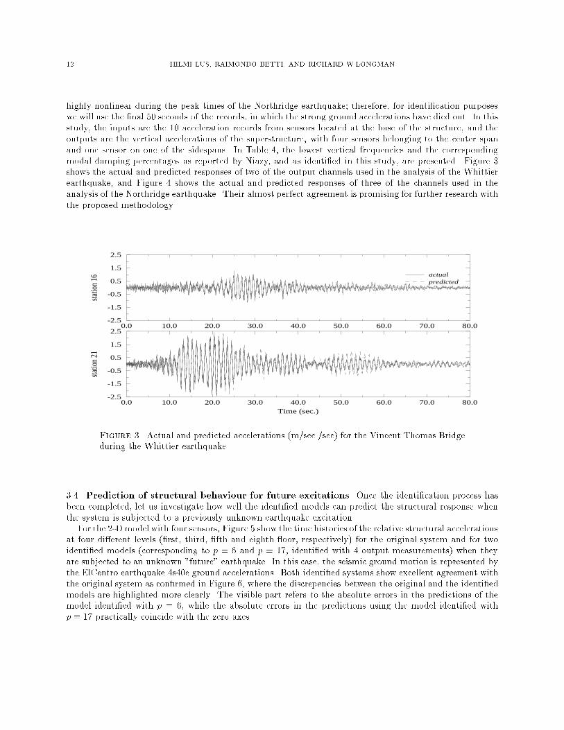
12 HILMI LUS�, RAIMONDO BETTI, AND RICHARD W.LONGMAN
highly nonlinear during the peak times of the Northridge earthquake; therefore, for identi�cation purposes
we will use the �nal 50 seconds of the records, in which the strong ground accelerations have died out. In this
study, the inputs are the 10 acceleration records from sensors located at the base of the structure, and the
outputs are the vertical accelerations of the superstructure, with four sensors belonging to the center span
and one sensor on one of the sidespans. In Table 4, the lowest vertical frequencies and the corresponding
modal damping percentages as reported by Niazy, and as identi�ed in this study, are presented. Figure 3
shows the actual and predicted responses of two of the output channels used in the analysis of the Whittier
earthquake, and Figure 4 shows the actual and predicted responses of three of the channels used in the
analysis of the Northridge earthquake. Their almost perfect agreement is promising for further research with
the proposed methodology.
0.0 10.0 20.0 30.0 40.0 50.0 60.0 70.0 80.0Time (sec.)
-2.5
-1.5
-0.5
0.5
1.5
2.5
statio
n 21
0.0 10.0 20.0 30.0 40.0 50.0 60.0 70.0 80.0-2.5
-1.5
-0.5
0.5
1.5
2.5
statio
n 16 actual
predicted
Figure 3. Actual and predicted accelerations (m/sec./sec) for the Vincent Thomas Bridge
during the Whittier earthquake
3.4. Prediction of structural behaviour for future excitations. Once the identi�cation process has
been completed, let us investigate how well the identi�ed models can predict the structural response when
the system is subjected to a previously unknown earthquake excitation.
For the 2-Dmodel with four sensors, Figure 5 show the time histories of the relative structural accelerations
at four di�erent levels (�rst, third, �fth and eighth oor, respectively) for the original system and for two
identi�ed models (corresponding to p = 6 and p = 17, identi�ed with 4 output measurements) when they
are subjected to an unknown "future" earthquake. In this case, the seismic ground motion is represented by
the ElCentro earthquake 4s40e ground accelerations. Both identi�ed systems show excellent agreement with
the original system as con�rmed in Figure 6, where the discrepencies between the original and the identi�ed
models are highlighted more clearly. The visible part refers to the absolute errors in the predictions of the
model identi�ed with p = 6, while the absolute errors in the predictions using the model identi�ed with
p = 17 practically coincide with the zero axes.

IDENTIFICATION OF LINEAR STRUCTURAL SYSTEMS USING EARTHQUAKE INDUCED VIBRATION DATA 13
70.0 75.0 80.0 85.0 90.0 95.0 100.0 105.0 110.0 115.0 120.0Time (sec.)
-1.4
-0.7
0.0
0.7
1.4
statio
n 21
70.0 75.0 80.0 85.0 90.0 95.0 100.0 105.0 110.0 115.0 120.0-1.4
-0.7
0.0
0.7
1.4
statio
n 18
70.0 75.0 80.0 85.0 90.0 95.0 100.0 105.0 110.0 115.0 120.0-1.4
-0.7
0.0
0.7
1.4sta
tion 1
5
actualpredicted
Figure 4. Actual and predicted accelerations (m/sec./sec) for the Vincent Thomas Bridge
during the Northridge earthquake
0.0 10.0 20.0 30.0 40.0Time (sec.)
-10.0
-5.0
0.0
5.0
10.0
1st fl
oor
0.0 10.0 20.0 30.0 40.0-10.0
-5.0
0.0
5.0
10.0
3rd flo
or
0.0 10.0 20.0 30.0 40.0-10.0
-5.0
0.0
5.0
10.0
5th flo
or
0.0 10.0 20.0 30.0 40.0-12.5
-7.5-2.52.57.5
12.5
8th flo
or
actualp = 17p = 6
Figure 5. Response predictions (relative accelerations, m/sec./sec) of the actual and iden-
ti�ed models (8 story shear building with 4 sensors) subjected to El Centro 4s40e ground
accelerations

14 HILMI LUS�, RAIMONDO BETTI, AND RICHARD W.LONGMAN
0.0 10.0 20.0 30.0 40.0Time (sec.)
-1.0
-0.5
0.0
0.5
1.0
1st f
loor
0.0 10.0 20.0 30.0 40.0-1.0
-0.5
0.0
0.5
1.0
3rd
floor
0.0 10.0 20.0 30.0 40.0-1.0
-0.5
0.0
0.5
1.0
5th
floor
0.0 10.0 20.0 30.0 40.0-1.0
-0.5
0.0
0.5
1.0
8th
floor
p = 17p = 6
Figure 6. Absolute errors in response predictions (m./sec./sec.) of the identi�ed models
(8 story shear building with four sensors)
0.0 10.0 20.0 30.0Time (sec.)
-12.0-8.0-4.00.04.08.0
12.0
join
t 3, m
ajor d
ir.
0.0 10.0 20.0 30.0-12.0-8.0-4.00.04.08.0
12.0
join
t 2, m
inor
dir.
0.0 10.0 20.0 30.0-12.0-8.0-4.00.04.08.0
12.0
join
t 1, m
inor
dir.
actualidentified
Figure 7. Response predictions (relative accelerations, m/sec./sec) of the 3 dimensional
actual and identi�ed models subjected to El Centro 4s40e and 4s50w ground accelerations
For the 3-D model, the unknown \future" ground excitation is represented by the time histories of the El
Centro earthquake 4s40e and 4s50w ground accelerations acting simultaneously along the major and minor
IDENTIFICATION OF LINEAR STRUCTURAL SYSTEMS USING EARTHQUAKE INDUCED VIBRATION DATA 15
directions respectively. For predicting the response, the model identi�ed using only the relative accelerations
of three joints on the eighth oor (2 along the minor direction and one along the major direction) is used.
This particular model was chosen because it showed a poor identi�cation for the higher order modes (see
Table 3). Figure 7 shows the time histories of the actual and the predicted relative accelerations on the eighth
oor for the El Centro ground excitation and con�rms that the predicted response of such an identi�ed model
is very close to the actual response (with the maximum relative error less than 10 percent).
3.5. Comparison with other S.I. methodologies. By comparing the results obtained using the proposed
methodology with those from previous studies, it is possible to highlight the e�ciency and accuracy of the
OKID/ERA technique. Most experiments reported in the literature are either SISO systems [11, 12, 14, 15]
or 2-D structural systems (shear-type or chain-type) with a number of DOFs smaller than the examples
considered in this study [10, 18]. In addition, most of the model updating methods assume uncoupled
modal damping [7]. On the contrary, the proposed OKID/ERA based identi�cation technique has proven
to be e�ective in determining state-space models of complex 3-D large MIMO structural systems, even with
limited information and without any preprocessing of the data. No a priori assumption on the coupling of
the second-order modes is necessary and the proposed technique has proven successful even in cases where
modes are known to be coupled, e.g. the Vincent-Thomas cable suspension bridge.
In general, it is much more di�cult to obtain an adequate input-output mapping and to predict structural
behavior for MIMO systems, especially for complex structures. The numerical results discussed above clearly
indicate that the proposed methodology is quite successful in properly addressing these issues. It should
also be mentioned that during the studies performed on the Hubble space telescope, the OKID methodology
reportedly produced extremely satisfactory results where most other approaches failed [32].
4. Conclusions
In this paper, the authors have presented an e�cient system identi�cation algorithm for application to
civil engineering structures. This algorithm is based on the Eigensystem Realization Algorithm and on
the Observer / Kalman �lter IDenti�cation approach. The proposed methodology uses earthquake induced
ground accelerations and structural vibrations as input-output data sets for identi�cation purposes. It is
shown that the results, from both simulated and recorded data, are promising, even in the presence of
measurement noise and for the cases where the number of output measurements is less than the number of
modes one wishes to identify.
The bene�ts of this method are twofold: i) The proposed identi�cation method identi�es the modal
characteristics, such as natural frequencies and modal damping percentages, very accurately with the use
of an observer; and ii) The realized model mimics the behaviour of the original system very well when
subjected to an unknown ground excitation. This leads to better predictions of the structural behaviour for
future excitations, and thereby reduces the chance of structural failure by making the possibilities known
beforehand. Since accurate results in experimental modal analysis generally require adequate excitation of
all the modes to be identi�ed, the proposed algorithm might reduce the costs for future applications.
5. Acknowledgements
The authors wish to thank Prof. M.Q. Phan of Princeton University for his suggestions and for his
contribution to the computer program. They would also like to acknowledge Prof. A.S. Smyth of Columbia
University for his contribution on the analysis of the recorded bridge data. This research study was sponsored
by the National Science Foundation under research grant CMS-9457305.

16 HILMI LUS�, RAIMONDO BETTI, AND RICHARD W.LONGMAN
References
[1] J.He and D.J. Ewins, "Analytical Sti�ness Matrix Correction Using Measured Vibration Modes",Modal Analysis:The
International Journal of Analytical and Experimental Modal Analysis, 1(3), pp.9-14, 1986.
[2] F.M.Hemez, "Theoretical and Experimental Correlation Between Finite Element Models and Modal Tests in the Context
of Large Flexible Space Structures", Ph.D. Dissertation, Dept. of Aerospace Engineering Sciences, University of Colorado,
Boulder, C.O.,1993.
[3] S.W.Doebling, C.H. Farrar, M.B. Prime, and D.W. Shevitz, "Damage Identi�cation and Health Monitoring of Structural
and Mechanical Systems From Changes In Their Vibration Characteristics: A Literature Review", Los Alamos National
Laboratory Report LA-13070-MS,1996.
[4] J.N.Juang and R.S.Pappa, "A ComparativeOverview of Modal Testing and SystemIdenti�cationfor Control of Structures",
Shock and Vibration Digest, Vol.20, No.5, pp.4-15,May 1988.
[5] J.E.Mottershead and M.I.Friswell, "Model Updating in Structural Dynamics: A Survey", Journal of Sound and Vibration,
165(2), pp.347-375,1993.
[6] D.J.Ewins,Modal Testing: Theory and Practice, Letchworth, Research Studies Press, 1984.
[7] J.L.Beck and P.C.Jennings, "Structural Identi�cation Using Linear Models and Earthquake Records", Earthquake Engi-
neering and Structural Dynamics, Vol.8, pp.145-160, 1980.
[8] G.H.McVerry, "Structural Identi�cation in the Frequency Domain from Earthquake Records", Earthquake Engineering
and Structural Dynamics, Vol.8, pp.161-180, 1980.
[9] J.P.Stewart and G.L.Fenves, "System Identi�cation for Evaluating Soil-Structure Interaction E�ects in Buildings From
Strong Motion Recordings", Earthquake Engineering and Structural Dynamics, Vol.27, pp.869-885, 1998.
[10] C.G.Koh and L.M.See, "Identi�cation and Uncertainty Estimation of Structural Parameters", Journal of Engineering
Mechanics, Vol.120, No.6, pp.1219-1236, 1993.
[11] R.Ghanem and M.Shinozuka, "Structural-System Identi�cation. I:Theory", Journal of Engineering Mechanics, Vol.121,
No.2, pp.255-264, 1995.
[12] M.Shinozuka and R.Ghanem, "Structural-System Identi�cation. II:Experimental Veri�cation", Journal of Engineering
Mechanics, Vol.121, No.2, pp.265-273, 1995.
[13] M.Hoshiya and A.Sutoh, "Kalman Filter-Finite Element Method in Identi�cation", Journal of Engineering Mechanics,
Vol.119, No.2, pp.197-210, 1991.
[14] E.S�afak, "Adaptive Modeling, Identi�cation, and Control of Dynamic structural Systems. I:Theory", Journal of Engineer-
ing Mechanics, Vol.115, No.11, pp.2386-2405, 1989.
[15] E.S�afak, "Adaptive Modeling, Identi�cation, and Control of Dynamic structural Systems. II:Applications", Journal of
Engineering Mechanics, Vol.115, No.11, pp.2406-2426, 1989.
[16] S.F.Masri, R.K.Miller, A.F.Saud, and T.K.Caughey, "Identi�cationof NonlinearVibrating Structures; Part I:Formulation",
J. Appl. Mech. Trans. ASME, 109, pp.918-922, 1987.
[17] S.F.Masri, R.K.Miller, A.F.Saud, and T.K.Caughey, "Identi�cation of Nonlinear Vibrating Structures; Part
I:Applications", J. Appl. Mech. Trans. ASME, 109, pp.923-929, 1987.
[18] C.C.Lin, T.T.Soong, and H.G.Natke, "Real-Time System Identi�cation of Degrading Structures", Journal of Engineering
Mechanics, Vol.116, No.10, pp.2258-2274, 1990.
[19] H.G.Natke, "Recent Trends in System Identi�cation", Structural Dynamics, W. B. Kratzig et.el., eds.,A.A.Balkema,
Netherlands, pp.283-289, 1991.
[20] F.E.Udwadia, "Methodology for Optimum Sensor Locations for Parameter Identi�cation in Dynamic Systems", Journal
of Engineering Mechanics, Vol.120, No.2, pp.368-390, 1994.
[21] J.L.Beck and L.S.Katafygiotis, "Updating Models and Their Uncertainties. I:Bayesian Statistical Framework", Journal of
Engineering Mechanics, Vol.124, No.4, pp.455-461, 1998.
[22] J.L.Beck and L.S.Katafygiotis, "UpdatingModels and Their Uncertainties. II:Model Identi�ability", Journal of Engineering
Mechanics, Vol.124, No.4, pp.463-467, 1998.
[23] A.W.Smyth, S.F.Masri, A.G.Chassiakos, and T.K.Caughey, "On-Line Parametric Identi�cation of MDOF Nonlinear Hys-
teretic Systems", Journal of Engineering Mechanics, Vol.125, No.2, pp.133-142, 1999.
[24] E.G.Gilbert, "Controllability and Observability in Multivariable Control Systems", SIAM Journal on Control, Vol.1, No.2,
pp.128-151, 1963
[25] R.E.Kalman, "MathematicalDescriptionof Linear DynamicalSystems",SIAM Journal on Control, Vol.1, No.2, pp.152-192,
1963
[26] J.N.Juang and R.S.Pappa, "An Eigensystem Realization Algorithm for Model Parameter Identi�cation and Model Reduc-
tion", Journal of Guidance, Control, and Dynamics, Vol.8, No.5, pp.620-627, 1985.
[27] B.L.Ho and R.E.Kalman,"E�ective construction of linear state-variable models from input/output functions",Proc. 3rd
Allerton Conf. Circuit and Systems Theory, pp.449-459, 1965.
IDENTIFICATION OF LINEAR STRUCTURAL SYSTEMS USING EARTHQUAKE INDUCED VIBRATION DATA 17
[28] L.M.Silverman,"Realization of Linear Dynamical Systems",IEEE Transactions on Automatic Control, Vol.AC-16, No.6,
pp.554-567, 1971.
[29] M.Phan, J.N.Juang, and R.W.Longman, "On MarkovParameters in System Identi�cation",NASA Technical Memorandum
104156, 1991.
[30] J.N.Juang, J.E.Cooper, and J.R.Wright, "An Eigensystem Realization Algorithm Using Data Correlations (ERA/DC) for
Model Parameter Identi�cation", Control Theory and Advanced Technology, Vol.4, No.1, pp.5-14, 1988.
[31] M.Phan, L.G.Horta, J.N.Juang, and R.W.Longman, "Linear System Identi�cationVia an AsymptoticallyStableObserver",
Journal of Optimization Theory and Applications, Vol.79, No.1, pp.59-86, 1993.
[32] J.N.Juang, M.Phan, L.G.Horta, and R.W.Longman,"Identi�cationof Observer/KalmanFilter Markov Parameters: Theory
and Exeriments", Journal of Guidance, Control, and Dynamics, Vol.16, No.2, pp.320-329, 1993.
[33] J.N.Yang, A.Akbarpour, and P.Ghaemmaghami, "New Optimal Control Algorithms for Structural Control", Journal of
Engineering Mechanics, Vol.113, No.9, pp.1369-1386, 1987.
[34] D.-H.Tseng,R.W.Longman and J.N.Juang,"Identi�cation of Gyroscopic and Nongyroscopic Second Order Mechnical Sys-
tems Including Repeated Problems", Advances in Astronautical Sciences, Vol.87, pp.145-165, 1994.
[35] D.-H.Tseng,R.W.Longman and J.N.Juang,"Identi�cation of the Structure of the Damping Matrix in Second Order Me-
chanical Systems", Advances in Astronautical Sciences, Vol.87, pp.166-190, 1994.
[36] A.M Niazy, \Seismic PerformanceEvaluation of SuspensionBridges", ph-D Dissertation, University of SouthernCalifornia,
1991.
Hilmi Lus�; Grad. Student, Dept. of Civ. Engrg. and Engrg. Mech., Columbia University, New York, NY, 10027
Raimondo Betti; Assoc. Prof., Dept. of Civ. Engrg. and Engrg. Mech., Columbia University, New York, NY,
10027
Richard W.Longman; Prof., Dept. of Mech. Engrg., Columbia University, New York, NY, 10027