INTERNATIONAL JOURNAL FOR NUMERICAL AND ANALYTICAL METHODS IN GEOMECHANICSInt. J. Numer. Anal. Meth. Geomech. 2004; 00:1–20Prepared using nagauth.cls [Version: 2002/09/18 v1.02]

A new damage model based on nonlocal displacements

Antonio Rodrıguez-Ferran∗, Irene Morata and Antonio Huerta

Laboratori de Calcul Numeric (LaCaN)Edifici C2, Campus Nord, Universitat Politecnica de Catalunya

E-08034 Barcelona, Spain.e-mail:antonio.rodriguez-ferran,irene.morata,antonio.huerta@upc.es

web page: www-lacan.upc.es

key words: nonlocal damage models; nonlocal displacements; gradient models; consistent tangent

matrix; quadratic convergence

SUMMARY

A new nonlocal damage model is presented. Nonlocality (of integral or gradient type) is incorporatedinto the model by means of nonlocal displacements. This contrasts with existing damage models,where a nonlocal strain or strain-related state variable is used. The new model is very attractive froma computational viewpoint, especially regarding the computation of the consistent tangent matrixneeded to achieve quadratic convergence in Newton iterations. At the same time, its physical responseis very similar to that of the standard models, including its regularization capabilities. All these aspectsare discussed in detail and illustrated by means of numerical examples. Copyright c© 2004 John Wiley& Sons, Ltd.

1. INTRODUCTION

Nonlocal damage models are used to model failure of quasi-brittle materials [1]. Nonlocality–needed to correct the pathological mesh-dependence exhibited by local models– can beincorporated into the model in two different ways. In integral-type models [2, 3, 4], a nonlocalstate variable is computed as the weighted average of the local state variable in a neighbourhoodof the point under consideration. In gradient-type models [5], on the other hand, higher-orderderivatives (typically second-order) are added to the partial differential equation that describesthe evolution of the nonlocal variable. Both approaches yield similar results and are in somecases equivalent [6].

Apart from the state variable, other variables can be selected to incorporate nonlocality.Either scalar or tensorial quantities may be transformed into the corresponding nonlocal

∗Correspondence to: Antonio Rodrıguez-Ferran, Departament de Matematica Aplicada III, E.T.S. d’Enginyersde Camins. Edifici C2, Campus Nord, Universitat Politecnica de Catalunya. E-08034 Barcelona, Spain.

Contract/grant sponsor: Ministerio de Educacion y Ciencia; contract/grant number: DPI2004-03000

Copyright c© 2004 John Wiley & Sons, Ltd.

2 A. RODRIGUEZ-FERRAN, I. MORATA AND A. HUERTA

quantities. In fact, a number of proposals can be found in the literature. For integral-typeregularization, some examples are the use of a nonlocal damage parameter [3], nonlocal strains[7] or nonlocal strain invariants [8]. These and other existing approaches are compared in [9]by means of a simple 1D numerical test (bar under uniaxial tension). Various approaches arealso possible for gradient regularization. In [10], for instance, the loading function dependson the Laplacian of the damage parameter. Note that all these strategies involve Gauss-pointbased quantities.

A new proposal is made here: to use nonlocal displacements to regularize the problem. Thetwo versions are proposed, discussed and compared: integral-type (nonlocal displacementsobtained as the weighted average of standard, local displacements), see [11], and gradient-type (nonlocal displacements obtained as the solution of a second-order PDE). As discussedand illustrated by means of numerical examples, the regularization capabilities of this newmodel are very similar to that of the standard model. In addition, it is very attractive from acomputational viewpoint, especially regarding (1) the computation of the consistent tangentmatrix and (2) the simple and straightforward upgrade of a nonlinear FE code to account fornonlocality.

An outline of this paper follows. The basic features of standard nonlocal damage models arereviewed in Section 2. The new model based on nonlocal displacements is presented in Section3. The integral-type and gradient versions are discussed in Sections 3.1 and 3.2 respectively.The regularization capabilities are illustrated by means of a uniaxial tension test. Section 4deals with the consistent linearization of the nonlinear equilibrium equation. It is shown howthe consistent tangent matrix is much simpler to compute for the new model than for thestandard models, both in the integral-type (Section 4.1) and the gradient (Section 4.2) cases.Quadratic convergence is shown for the uniaxial tension test. Section 5 shows how nonlocaldisplacements can be used to incorporate nonlocality into a FE code in a very simple andefficient manner, especially if the gradient regularization is chosen. The concluding remarks ofSection 6 close the paper.

Standard notation is used. Vector fields in the continuum are represented by slanted boldfacetype (uuu: displacement field). Nodal vectors associated to FE discretization are denoted byupright boldface type (u: nodal displacements).

2. OVERVIEW OF DAMAGE MODELS

For simplicity, only elastic-scalar damage models are considered here. However, the conceptof nonlocal displacements can be extended to more complex damage models exhibiting, forinstance, anisotropy or plasticity [4, 12].

2.1. Local damage models

A generic local damage model consists of the following equations, summarized in table I:

• A relation between Cauchy stresses σσσ and small strains εεε —i.e. the symmetrized gradientof displacements uuu, Equation (2)—, where the loss of stiffness (from elastic stiffness Cto zero stiffness) is described by means of a scalar damage parameter D which rangesfrom 0 to 1, Equation (1);

• The definition of a local state variable Y as a function of strain εεε, Equation (3);

Copyright c© 2004 John Wiley & Sons, Ltd. Int. J. Numer. Anal. Meth. Geomech. 2004; 00:1–20Prepared using nagauth.cls

A NEW DAMAGE MODEL BASED ON NONLOCAL DISPLACEMENTS 3

• A damage evolution law, where the local state variable Y drives the evolution of thenon-decreasing damage parameter D, Equation (4).

Table I. General expression of a local damage model

Stress-strain relationship σσσ(xxx, t) =(1−D(xxx, t)

)Cεεε(xxx, t) (1)

Strains εεε(xxx, t) = ∇suuu(xxx, t) (2)

Local state variable Y (xxx, t) = Y(εεε(xxx, t)

)(3)

Damage evolution D(xxx, t) = D(maxτ≤t

Y (xxx, τ))

(4)

The most common particular forms of Equations (3) and (4) are reviewed in [11]. Regardingthe definition of the state variable, both the so-called Mazars model and modified von Misesmodel result in Y = ε in the simple case of uniaxial tension. As for damage evolution, the linearsoftening law is especially suited for conceptual analyses. Between the damage threshold Y0

(inception of damage) and a maximum admissible value Yf (D = 1), damage evolves accordingto

D =Yf

Yf − Y0

(1− Y0

Y

), (5)

which leads to a linear softening branch in a stress-strain diagram.Local damage models are not suitable for computations. Due to softening, the boundary

value problem becomes ill-posed and the finite element solution exhibits a pathological mesh-dependence. It is necessary to regularize the problem by making the model nonlocal [13].

2.2. Integral-type nonlocal damage models

In integral-type models, see table II, nonlocality is incorporated via the definition of a nonlocalstate variable Y as the weighted average of the local state variable Y , Equation (6). Theweighting function α depends on the distance r between two points and contains a characteristiclength lc as a parameter, Equation (7). The nonlocal state variable Y , rather than the localstate variable Y , drives the evolution of damage, Equation (8).

The weighting function α is typically defined as

α(xxx, r; lc) = c0(xxx)α?(r; lc) , (9)

where α? is the Gaussian function [14, 15, 16]

α?(r; lc) = exp

[−

(2r

lc

)2]

(10)

and the normalization factor c0(xxx) is

c0(xxx) = 1/ ∫

Vx

α?(r; lc)dzzz (11)

Copyright c© 2004 John Wiley & Sons, Ltd. Int. J. Numer. Anal. Meth. Geomech. 2004; 00:1–20Prepared using nagauth.cls

4 A. RODRIGUEZ-FERRAN, I. MORATA AND A. HUERTA

Table II. General expression of an integral-type nonlocal damage model

Stress-strain relationship σσσ(xxx, t) =(1−D(xxx, t)

)Cεεε(xxx, t)

Strains εεε(xxx, t) = ∇suuu(xxx, t)

Local state variable Y (xxx, t) = Y(εεε(xxx, t)

)

Nonlocal state variable Y (xxx, t) =∫

Vx

α(xxx,zzz)Y (zzz, t)dzzz (6)

Weighting function α(xxx,zzz) = α(xxx, r; lc) with r = ‖xxx− zzz‖ (7)

Damage evolution D(xxx, t) = D(maxτ≤t

Y (xxx, τ))

(8)

Note that c0(xxx) is not a constant; near the boundaries, the support of α? may lay partiallyoutside the domain, so a lower value of the integral in Equation (11) is obtained. In fact, it isnecessary to modify the Gaussian function α? into the weighting function α as indicated byEquation (9) to ensure reproducibility of constant functions. This guarantees that a constantfield of local state variable Y (xxx) = Y is not modified due to nonlocal averaging (that is,Y (xxx) = Y (xxx) = Y ) and, hence, that a constant strain field εεε results in a constant stress fieldσσσ.

2.3. Gradient nonlocal damage models

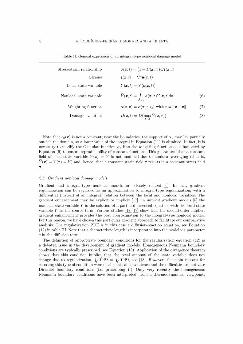
Gradient and integral-type nonlocal models are closely related [6]. In fact, gradientregularization can be regarded as an approximation to integral-type regularization, with adifferential (instead of an integral) relation between the local and nonlocal variables. Thegradient enhancement may be explicit or implicit [17]. In implicit gradient models [5] thenonlocal state variable Y is the solution of a partial differential equation with the local statevariable Y as the source term. Various studies [18, 17] show that the second-order implicitgradient enhancement provides the best approximation to the integral-type nonlocal model.For this reason, we have chosen this particular gradient approach to facilitate our comparativeanalysis. The regularization PDE is in this case a diffusion-reaction equation, see Equation(12) in table III. Note that a characteristic length is incorporated into the model via parameterc in the diffusion term.

The definition of appropriate boundary conditions for the regularization equation (12) isa debated issue in the development of gradient models. Homogeneous Neumann boundaryconditions are typically prescribed, see Equation (13). Application of the divergence theoremshows that this condition implies that the total amount of the state variable does notchange due to regularization,

∫Ω

Y dΩ =∫Ω

Y dΩ, see [18]. However, the main reasons forchoosing this type of condition were mathematical convenience and the difficulties to motivateDirichlet boundary conditions (i.e. prescribing Y ). Only very recently the homogeneousNeumann boundary conditions have been interpreted, from a thermodynamical viewpoint,

Copyright c© 2004 John Wiley & Sons, Ltd. Int. J. Numer. Anal. Meth. Geomech. 2004; 00:1–20Prepared using nagauth.cls

A NEW DAMAGE MODEL BASED ON NONLOCAL DISPLACEMENTS 5

as an insulation condition in the so-called nonlocality energy residual [19].

Table III. General expression of a gradient nonlocal damage model

Stress-strain relationship σσσ(xxx, t) =(1−D(xxx, t)

)Cεεε(xxx, t)

Strains εεε(xxx, t) = ∇suuu(xxx, t)

Local state variable Y (xxx, t) = Y(εεε(xxx, t)

)

Nonlocal state variable Y (xxx, t)− c∇2Y (xxx, t) = Y (xxx, t) in Ω (12)

n∇Y = 0 on ∂Ω (13)

Damage evolution D(xxx, t) = D(maxτ≤t

Y (xxx, τ))

As tables II and III reflect, the standard approach in nonlocal damage models is to define ascalar local state variable Y (as a function of strains) and then to transform it into a nonlocalstate variable Y , which drives the evolution of damage. Note that integral-type and gradientnonlocal damage models only differ in the way Y is computed, cf. Equations (6)–(7) and(12)–(13).

3. NEW MODEL BASED ON NONLOCAL DISPLACEMENTS

A new nonlocal damage model based on nonlocal displacements is presented here. The nonlocaldisplacements uuu are computed from the local (i.e. standard) displacements uuu either as aweighted average (integral-type version, Section 3.1) or as the solution of a second-order PDE(gradient version, Section 3.2).

3.1. Integral-type version

The integral-type version of the proposed model is summarized in table IV. The key ideais the computation of nonlocal displacements as the weighted average of local displacements,Equation (14). After that, the nonlocal strains εεεNL, the nonlocal state variable YNL and, finally,the damage parameter D are obtained. Note that these three variables are computed locally :nonlocality is introduced at the “beginning” of the constitutive model (i.e. at the level ofdisplacements, the primal unknowns in the FE computation).

Regarding the basic ingredients of a nonlocal damage model reviewed in Section 2, the onlyone that requires some modification is the weighting function. Since displacements, ratherthan strains, are averaged, reproducibility of polynomials of degree 1 is needed to ensure thata constant strain field results in a constant stress field. This can be done in a simple andcomputationally efficient manner, as described next.

Moving least-squares fitting, a standard technique in meshless methods [20, 21], suggestshow to define the weighting function. To ensure reproducibility of order 0, the kernel α? is

Copyright c© 2004 John Wiley & Sons, Ltd. Int. J. Numer. Anal. Meth. Geomech. 2004; 00:1–20Prepared using nagauth.cls

6 A. RODRIGUEZ-FERRAN, I. MORATA AND A. HUERTA

Table IV. New model based on nonlocal displacements, integral-type version. Subscript NL denotesquantities with nonlocal information but computed locally.

Stress-strain relationship σσσ(xxx, t) =(1−D(xxx, t)

)Cεεε(xxx, t)

Local strains εεε(xxx, t) = ∇suuu(xxx, t)

Nonlocal displacements uuu(xxx, t) =∫

Vx

α(xxx,zzz)uuu(zzz, t)dzzz (14)

Nonlocal strains εεεNL(xxx, t) = ∇suuu(xxx, t) (15)

Nonlocal state variable YNL(xxx, t) = Y(εεεNL(xxx, t)

)(16)

Damage evolution D(xxx, t) = D(maxτ≤t

YNL(xxx, τ))

multiplied by a polynomial of order 0 in the neighbourhood of each point xxx, see Equation (9).For reproducibility of order 1, more degrees of freedom are needed, so a polynomial of order 1is needed,

α(xxx,zzz) =[c0(xxx) + zzzT ccc1(xxx)

]α?(xxx− zzz) . (17)

Reproducibility of order 1 amounts to requiring that a linear local displacement fielduuu(xxx) = aaa +BBBxxx is transformed into the same linear nonlocal displacement field, uuu(xxx) = aaa +BBBxxxfor arbitrary aaa and BBB. Combined with Equations (17) and (14), this leads to

[ ∫Vx

α?(xxx− zzz)dzzz∫

VxzzzT α?(xxx− zzz)dzzz∫

Vxzzzα?(xxx− zzz)dzzz

∫Vx

zzzzzzT α?(xxx− zzz)dzzz

] c0(xxx)ccc1(xxx)

=

1xxx

. (18)

This small system of linear equations (order: number of space dimensions + 1) needs to besolved at each Gauss point. This is done only once, at the beginning of the computation, andcoefficients c0(xxx) and ccc1(xxx) are stored and reused throughout the analysis.

Is the weighting function α different from the weighting function of the standard approach,Equation (9)? Yes, but only near the boundaries.

Away from the boundaries (that is, when volume Vx is not truncated by the domainboundary), the off-diagonal terms in the matrix of Equation (18) may be expressed as

∫

Vx

zzzα?(xxx− zzz)dzzz =∫

Vx

(zzz − xxx)α?(xxx− zzz)dzzz

︸ ︷︷ ︸I=0

+xxx

∫

Vx

α?(xxx− zzz)dzzz . (19)

The first integral in the RHS of Equation (19) is null due to the symmetry of function α?

and integration domain Vx and the skew-symmetry of function zzz − xxx. Equation (19) impliesthat, in the linear system (18), the first matrix column is proportional to the RHS vector, soccc1(xxx) = 0, c0(xxx) = c0(xxx) and α(xxx,zzz) = α(xxx,zzz).

Near the boundary, on the other hand, the first integral in the RHS of Equation (19)is not zero, because the truncated integration domain Vx is not symmetric, so ccc1(xxx) 6= 0,c0(xxx) 6= c0(xxx) and α(xxx,zzz) 6= α(xxx,zzz).

Copyright c© 2004 John Wiley & Sons, Ltd. Int. J. Numer. Anal. Meth. Geomech. 2004; 00:1–20Prepared using nagauth.cls

A NEW DAMAGE MODEL BASED ON NONLOCAL DISPLACEMENTS 7

In other words: for the new model based on nonlocal displacements, it is only necessaryto modify the weighting function in the Gauss points near the boundaries. Away from theboundaries, reproducibility of order 0 automatically implies reproducibility of order 1.

3.2. Gradient version

The gradient version of the proposed model is summarized in table V. The second-order PDEnow relates nonlocal displacements uuu to local displacements uuu, see Equation (20). Note thatDirichlet boundary conditions (21) are prescribed for uuu. These boundary conditions have aclear physical interpretation: nonlocal displacements must coincide with local displacementsin all the domain boundary (i.e. for both the Dirichlet and Neumann boundaries of themechanical problem). Another important difference between the gradient enhancements of thestate variable and the displacements are the continuity and interpolation requirements. Uponfinite element discretization, the local state variable Y in Equation (12) is a discontinuous(piecewise polynomial, Gauss-point-based) field, but C0 continuity is required for the (nodal-based) nonlocal state variable field Y . In Equation (20), on the contrary, both uuu and uuu areC0 nodal based fields. In fact, the choice of interpolation functions for the two fields (uuu andY ) in a standard gradient-enhanced damage model is a debated issue, see [22]; for the newmodel, on the other hand, it is very natural to use the same interpolation functions for thetwo displacement fields uuu and uuu.

Equation (20) is also used in gradient elasticity [23] to relate the “gradient” displacementfield uuu with the “classical” displacement field uuu. In our proposal, on the contrary, the elasticresponse is local (i.e. uuu and εεε are the displacement and strain solution fields), and uuu is anauxiliary regularized displacement field that drives damage evolution.

Note also that the solution of the boundary value problem (20) is uuu(xxx) ≡ uuu(xxx) if uuu(xxx) is linear.In other words, reproducibility of order 1 is automatically ensured without any modificationof the regularization strategy.

Table V. New model based on nonlocal displacements, gradient version. Subscript NL denotesquantities with nonlocal information but computed locally.

Stress-strain relationship σσσ(xxx, t) =(1−D(xxx, t)

)Cεεε(xxx, t)

Local strains εεε(xxx, t) = ∇suuu(xxx, t)

Nonlocal displacements uuu(xxx, t)− c∇2uuu(xxx, t) = uuu(xxx, t) in Ω (20)uuu = uuu on ∂Ω (21)

Nonlocal strains εεεNL(xxx, t) = ∇suuu(xxx, t)

Nonlocal state variable YNL(xxx, t) = Y(εεεNL(xxx, t)

)

Damage evolution D(xxx, t) = D(maxτ≤t

YNL(xxx, τ))

Copyright c© 2004 John Wiley & Sons, Ltd. Int. J. Numer. Anal. Meth. Geomech. 2004; 00:1–20Prepared using nagauth.cls

8 A. RODRIGUEZ-FERRAN, I. MORATA AND A. HUERTA

3.3. Validation of the new model

The regularization capabilities of the model based on nonlocal displacements are illustratedhere by means of a uniaxial tension test, see Figure 1(a) and [22].

The one-dimensional particularizations of the integral-type and gradient versions, tables IVand V, with Y (ε) ≡ ε and a linear softening law, see Figure 1(b), are used. As a reference, thestandard integral-type model with nonlocal state variable (i.e. nonlocal strains, since Y ≡ ε)is taken.

The central tenth of the bar is weakened (10% reduction in Young’s modulus) to triggerlocalization. The dimensionless geometric and material parameters are summarized in tableVI. The numerical tests are displacement-controlled.

L

LD-

6

¤¤¤¤¤¤¤cc

cc

cc

ccc¥

¥¥¥¥¥¥¥¥@@

@@

@@

@@@

σ

EDε0

Eε0

ε0 εf ε

(a) (b)

Figure 1. Uniaxial tension test: (a) problem statement; (b) linear softening law

Table VI. Uniaxial tension test. Geometric and material parameters [22]

Meaning Symbol ValueLength of bar L 100Cross-section of bar A 1Idem of weaker part LD 10Young’s modulus E 20 000Idem of weaker part ED 18 000Damage threshold ε0 10−4

Final strain εf 1.25× 10−2

The regularization properties of the model based on nonlocal displacements are assessed firstby carrying out the analysis with five different meshes of 40, 80, 160, 320 and 640 elements(corresponding respectively to element sizes h of 2.5, 1.25, 0.625, 0.3125 and 0.15625).

For the integral-type version, a fixed characteristic length lc = 6.25 (correspondingrespectively to 2.5, 5, 10, 20 and 40 elements) is chosen. The results for the various meshes

Copyright c© 2004 John Wiley & Sons, Ltd. Int. J. Numer. Anal. Meth. Geomech. 2004; 00:1–20Prepared using nagauth.cls

A NEW DAMAGE MODEL BASED ON NONLOCAL DISPLACEMENTS 9

are shown in Figure 2. Both the force-displacement curves and the final damage profiles arevirtually superimposed.

0 0.02 0.04 0.06 0.08 0.1 0.12 0.14 0.160

0.2

0.4

0.6

0.8

1

1.2

1.4

1.6

1.8

2

Displacement

For

ce

640 Elem.320 Elem.160 Elem.80 Elem.40 Elem.

0 10 20 30 40 50 60 70 80 90 1000

0.1

0.2

0.3

0.4

0.5

0.6

0.7

0.8

0.9

1

xD

amag

e

(a) (b)

Figure 2. New model based on nonlocal displacements, integral-type version: (a) force-displacementand (b) final damage profiles for various meshes

The same situation is encountered for the gradient version. The results with a constantparameter c = 5 are depicted in Figure 3. Again, the responses for the five meshes are verysimilar. Regularization via nonlocal displacements indeed precludes mesh dependence.

0 0.02 0.04 0.06 0.08 0.1 0.12 0.14 0.160

0.2

0.4

0.6

0.8

1

1.2

1.4

1.6

1.8

2

Displacement

For

ce

640 Elem.320 Elem.160 Elem.80 Elem.40 Elem.

0 10 20 30 40 50 60 70 80 90 1000

0.1

0.2

0.3

0.4

0.5

0.6

0.7

0.8

0.9

1

x

Dam

age

(a) (b)

Figure 3. New model based on nonlocal displacements, gradient version: (a) force-displacement and(b) final damage profiles for various meshes

As a second test, a fixed mesh of 320 elements (h = 0.3125) and four different internallengths are used. For the integral-type model, characteristic lengths lc of 5h, 10h, 20h = 6.25(reference value above) and 40h are taken; for the gradient model, parameters c of 1, 2, 5(reference) and 10.

Copyright c© 2004 John Wiley & Sons, Ltd. Int. J. Numer. Anal. Meth. Geomech. 2004; 00:1–20Prepared using nagauth.cls

10 A. RODRIGUEZ-FERRAN, I. MORATA AND A. HUERTA

The results are depicted in Figures 4 and 5. As desired, both the ductility in the force-displacement response and the width of the final damage profile increase with the internallength scale.

0 0.02 0.04 0.06 0.08 0.1 0.12 0.14 0.160

0.2

0.4

0.6

0.8

1

1.2

1.4

1.6

1.8

2

Displacement

For

ce

Char.len.=40hChar.len.=20hChar.len.=10hChar.len.=5h

0 10 20 30 40 50 60 70 80 90 1000

0.1

0.2

0.3

0.4

0.5

0.6

0.7

0.8

0.9

1

x

Dam

age

(a) (b)

Figure 4. New model based on nonlocal displacements, integral-type version: (a) force-displacementand (b) final damage profiles for various characteristic lengths

0 0.02 0.04 0.06 0.08 0.1 0.12 0.14 0.160

0.2

0.4

0.6

0.8

1

1.2

1.4

1.6

1.8

2

Displacement

For

ce

c=10c=5c=2c=1

0 10 20 30 40 50 60 70 80 90 1000

0.1

0.2

0.3

0.4

0.5

0.6

0.7

0.8

0.9

1

x

Dam

age

(a) (b)

Figure 5. New model based on nonlocal displacements, gradient version: (a) force-displacement and(b) final damage profiles for various parameters c

To sum up: the new model exhibits the same regularization capabilities and qualitativeresponse than the standard model based on nonlocal strains.

A quantitative comparison is carried out next, for the integral-type version. The test with320 elements and lc = 6.25 is analyzed in detail. Apart from the same structural response, seeFigure 6(a), the two models also predict the same evolution of damage profile, see Figure 6(b),and the same stress-strain diagram for three sample points, see Figure 6(c).

Copyright c© 2004 John Wiley & Sons, Ltd. Int. J. Numer. Anal. Meth. Geomech. 2004; 00:1–20Prepared using nagauth.cls

A NEW DAMAGE MODEL BASED ON NONLOCAL DISPLACEMENTS 11

Displacement

Fo

rce

State AState B

State C

State D

NLA(Displac.)

NLA(Strain)

0

0.2

0.4

0.6

0.8

1.0

1.2

1.4

1.6

1.8

2.0

0 0.02 0.04 0.06 0.08 0.10 0.12 0.14 0.16

x

Dam

age

State A

State B

State CState D

0 10 20 30 40 50 60 70 80 90 1000

0.1

0.2

0.3

0.4

0.5

0.6

0.7

0.8

0.9

1

Point 1 Point 2 Point 3

(a) (b)

Strain

Str

ess

State AState B

State C

State D

0

0.2

0.4

0.6

0.8

1.0

1.2

1.4

1.6

1.8

2.0

0 0.1 0.2 0.3 0.4 0.5 0.6 0.7 0.8 0.9 1

x 104

Point 1

0 0.5 1.0 1.5 2.0 2.5 3.0 3.5

x 10-4Strain

Str

ess

State A

State BState C

State D

Point 2

0

0.2

0.4

0.6

0.8

1.0

1.2

1.4

1.6

1.8

2.0

0 0.2 0.4 0.6 0.8 1.0 1.2 1.4 1.6 1.8 2.0Strain

Str

ess

State AState B

State C

State D

0

0.2

0.4

0.6

0.8

1.0

1.2

1.4

1.6

1.8

2.0

x 10-2

Point 3

(c)

Figure 6. Integral-type versions. The new model (nonlocal displacements) and the standard model(nonlocal strains) yield very similar results: (a) force-displacement curve; (b) damage profiles; (c)

stress-strain diagrams at sample points.

3.4. Connection between the standard and the new model

In this section the similarities between the two models are outlined. The goal is to demonstratethat the proposed approach based on nonlocal displacements inherits the regularizationproperties of the standard model. The connection between the two approaches is especiallyclear for the one-dimensional particularization used above (where the state variable is simplythe strain, Y ≡ εεε).

For the integral-type version, this connection relies on the fact that convolution (i.e. weightedaverage) and differentiation commute in an infinite domain. For the gradient version, the twomodels are equivalent. Differentiation of the regularization equation in terms of displacements,Equation (20), leads directly to the usual equation in terms of strains, Equation (12). Moreover,the Dirichlet boundary conditions on displacements and the homogeneous Neumann boundaryconditions on strains are equivalent: substitution of Equation (21) into Equation (20) resultsin d2u/dx2 = dεNL/dx = 0.

The effect of boundary conditions over finite domains (for integral-type regularization) anda multidimensional setting —where the state variable Y is a nonlinear scalar function of thestrain tensor εεε— (for both integral-type and gradient approaches) will be analyzed in detailin a forthcoming contribution.

Copyright c© 2004 John Wiley & Sons, Ltd. Int. J. Numer. Anal. Meth. Geomech. 2004; 00:1–20Prepared using nagauth.cls

12 A. RODRIGUEZ-FERRAN, I. MORATA AND A. HUERTA

4. CONSISTENT LINEARIZATION

The new model based on nonlocal displacements is very attractive from a computationalviewpoint, especially regarding its consistent linearization (i.e. the computation of theconsistent tangent matrix needed to attain quadratic convergence in the full Newton-Raphsonmethod [24]). For both regularization approaches, we first review the expression of theconsistent tangent matrix of the standard model (nonlocal state variable) reported in theliterature. After that, we present the counterpart for the new model based on nonlocaldisplacements and show that it is much simpler to compute.

4.1. Consistent tangent matrix for integral-type models

Integral-type models pose a substantial difficulty: due to nonlocality, there is interactionbetween non-adjacent nodes, and the consistent tangent matrix exhibits a larger bandwidth(with respect to the sparsity pattern of the elastic or secant matrices) [25, 26, 11].

In FE analysis, the internal force vector is typically computed with a Gauss quadrature as

fint(u) =∑

p

wpBTp σσσp(u) (22)

where p ranges the Gauss points, wp are the corresponding integration weights, Bp is the usualmatrix of shape function derivatives at Gauss point p and stresses σσσp are

σσσp(u) =(1−Dp(u)

)CBpu︸︷︷︸

εεεp

. (23)

The consistent tangent matrix is

Ktan :=∂fint

∂u=

∑p

wpBTp

∂σσσp

∂u. (24)

Combining Equations (23) and (24) results in

Ktan = Ksec + Knonlocal (25)

where

Ksec =∑

p

wpBTp (1−Dp)CBp (26)

is the secant stiffness matrix and

Knonlocal = −∑

p

wpBTp Cεεεp

∂Dp

∂u(27)

is the nonlocal tangent contribution which accounts for the variation of the damage parameter.Equations (22)–(27) are general. The specific structure of matrix Knonlocal, however, is quite

different in the standard and new models.

Copyright c© 2004 John Wiley & Sons, Ltd. Int. J. Numer. Anal. Meth. Geomech. 2004; 00:1–20Prepared using nagauth.cls

A NEW DAMAGE MODEL BASED ON NONLOCAL DISPLACEMENTS 13

4.1.1. Standard model (table II) By applying the chain rule, the term ∂Dp/∂u in Equation(27) can be expressed as

∂Dp

∂u= D′(Yp)

∂Yp

∂u. (28)

The integral (6) in table II required for nonlocal averaging is also approximated via anumerical quadrature, so the nonlocal state variable Yp is

Yp =∑

q∈Vp

wqαpqYq , (29)

where q ranges the Gauss points ξξξq in the neighbourhood Vp of Gauss point ξξξp, andαpq = α(r = ‖ξξξp − ξξξq‖).

By differentiating Equation (29), the last term in Equation (28) can be expressed as

∂Yp

∂u=

∑

q∈Vp

wqαpq∂Yq

∂u=

∑

q∈Vp

wqαpq∂Yq

∂εεεBq (30)

where the chain rule and the relation ∂εεεq/∂u = Bq have been used.By replacing Equation (30) into Equation (28) and then into Equation (27), the nonlocal

matrix can be expressed as

Knonlocal,Y = −∑

p,q∈Vp

wpqBTp CεεεpD

′(Yp)∂Yq

∂εεεBq (31)

where wpq = wpwqαpq and the subscript Y denotes the nonlocal quantity. Due to the doubleloop in Gauss points caused by nonlocal interaction, Knonlocal,Y cannot be assembled fromelementary contributions solely.

4.1.2. New model (table IV) Equations (22)–(27) are also valid for the new model. However,the term ∂Dp/∂u is now

∂Dp

∂u= D′(YNLp)

∂Y

∂εεεNL(εεεNLp)

∂εεεNLp

∂u∂u∂u

. (32)

Since nonlocal averaging is performed at the beginning, the rest of the constitutive model is“local”. Note, in particular, that the usual shape functions are used in the FE discretization ofnonlocal displacements and that nonlocal strains εεεNL are computed locally as the symmetrizedgradient of nonlocal displacements, see table IV. This means that

εεεNLp = Bpu =⇒ ∂εεεNLp

∂u= Bp , (33)

where Bp is the same matrix of shape function derivatives used in Equation (22).The last term in (32), ∂u/∂u, reflects the nonlocality of the model. After finite element

discretization and numerical integration, the averaging process (14) leads simply to

u = Aintegralu =⇒ ∂u∂u

= Aintegral , (34)

Copyright c© 2004 John Wiley & Sons, Ltd. Int. J. Numer. Anal. Meth. Geomech. 2004; 00:1–20Prepared using nagauth.cls

14 A. RODRIGUEZ-FERRAN, I. MORATA AND A. HUERTA

where Aintegral is a matrix of nonlocal connectivity. Note that this matrix contains —for standard models where the characteristic length lc or parameter c are not evolution-dependent— purely geometrical information associated to the finite element mesh. It doesnot change as damage evolves, so it can be computed and stored at the beginning of theanalysis (provided, of course, that a fixed mesh is used).

Substitution of Equation (32), (33) and (34) into Equation (27) results in

Knonlocal,u = Klocal,uAintegral (35)

with

Klocal,u = −∑

p

wpBTp CεεεpD

′(YNLp)

∂Y

∂εεεNL(εεεNLp)Bp . (36)

Note that Klocal,u can be computed in the usual way by assembling elementary matrices, likein any local material model. After that, nonlocality is accounted for by means of the constantmatrix Aintegral, which “spreads” the stiffness of Klocal,u into Knonlocal,u.

By replacing Equation (35) in Equation (25), the consistent tangent matrix can be expressedas

Ktan = Ksec + KlocalAintegral . (37)

This simple structure of Ktan is due to the fact that the nonlocal average is performedcompletely “upstream” in the constitutive equation (i.e. with displacements, the primalunknowns in the FE analysis). For any other choice of the nonlocal variable, see Section1, double loops in Gauss points like those in Equation (31) appear.

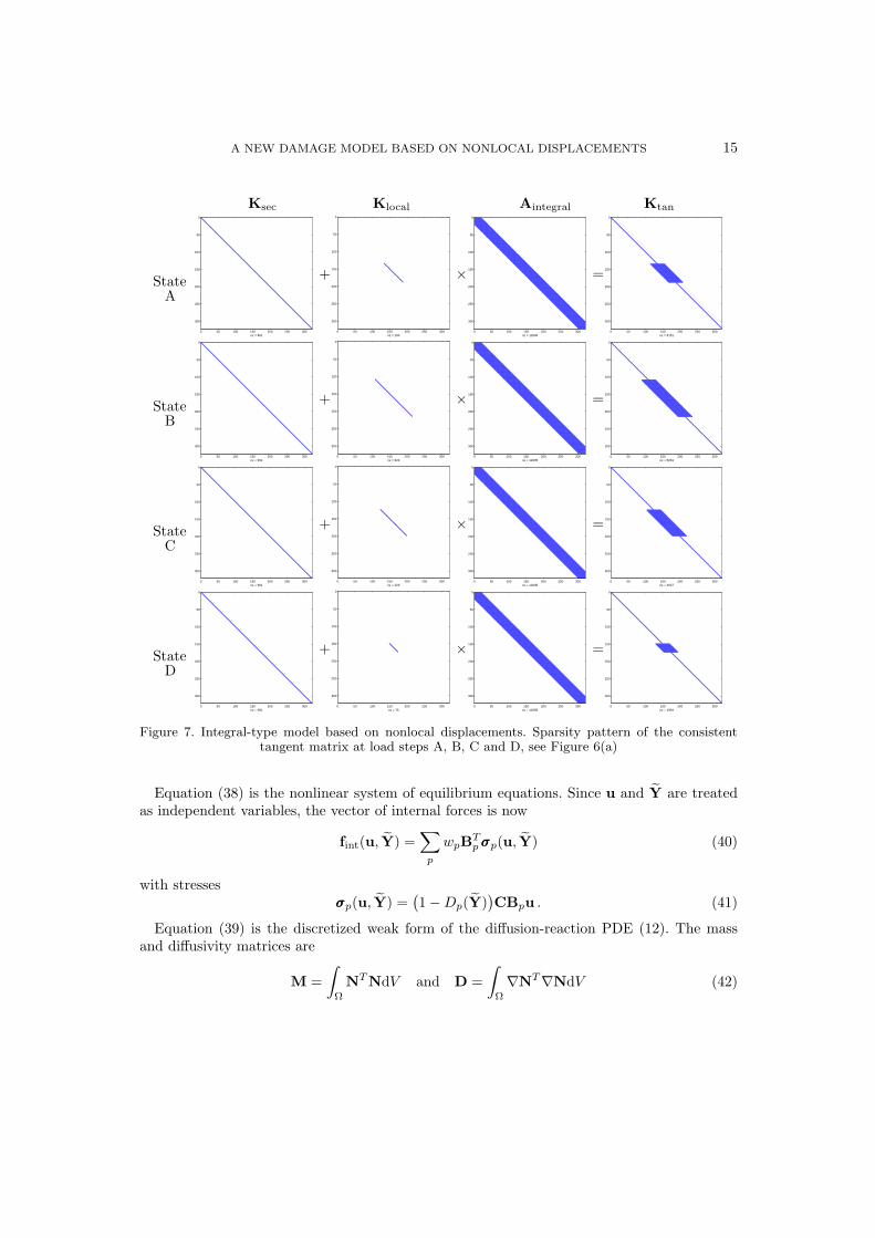
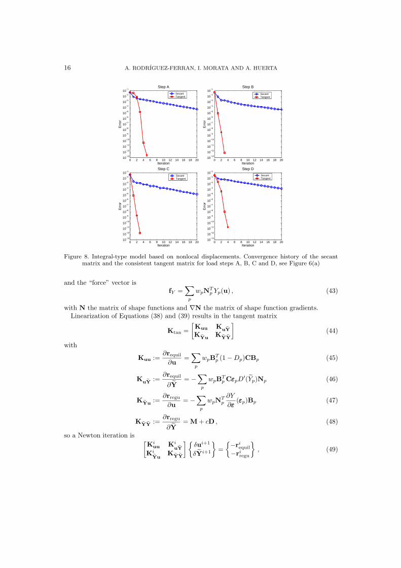
Equation (37) is graphically illustrated by Figure 7, where the pattern of the consistenttangent matrix for the four representative load steps of Figure 6(a). Note how the constantmatrix Aintegral indeed “spreads” the local stiffness matrix Klocal (which is non-zero only wheredamage increases), thus provoking fill-in in the tangent matrix Ktan.

The convergence history at these four load steps is shown in Figure 8. As expected, onlylinear convergence is achieved with the secant stiffness matrix, while the consistent tangentmatrix leads to quadratic convergence.

4.2. Consistent tangent matrix for gradient models

Gradient models are mathematically local. Nonlocal interaction is accounted for locally viahigher-order spatial derivatives. Thanks to this, the consistent tangent matrix is simpler tocompute than for integral nonlocal models.

Gradient models are typically formulated as two-field problems. For the standard model, theunknowns are the nodal vectors of displacements u and nonlocal state variables Y. For the newmodel, on the other hand, unknowns are the nodal vectors of local and nonlocal displacements,u and u.

4.2.1. Standard model (table III) Finite element discretization leads to

requil(u, Y) := fint(u, Y)− fext = 0 (38)

rregu(u, Y) := (M + cD)Y − fY (u) = 0 (39)

Copyright c© 2004 John Wiley & Sons, Ltd. Int. J. Numer. Anal. Meth. Geomech. 2004; 00:1–20Prepared using nagauth.cls

A NEW DAMAGE MODEL BASED ON NONLOCAL DISPLACEMENTS 15

Ksec Klocal Aintegral Ktan

StateA

0 50 100 150 200 250 300

0

50

100

150

200

250

300

nz = 961

+

0 50 100 150 200 250 300

0

50

100

150

200

250

300

nz = 163

×

0 50 100 150 200 250 300

0

50

100

150

200

250

300

nz = 12695

=

0 50 100 150 200 250 300

0

50

100

150

200

250

300

nz = 3151

StateB

0 50 100 150 200 250 300

0

50

100

150

200

250

300

nz = 961

+

0 50 100 150 200 250 300

0

50

100

150

200

250

300

nz = 322

×

0 50 100 150 200 250 300

0

50

100

150

200

250

300

nz = 12695

=

0 50 100 150 200 250 300

0

50

100

150

200

250

300

nz = 5261

StateC

0 50 100 150 200 250 300

0

50

100

150

200

250

300

nz = 961

+

0 50 100 150 200 250 300

0

50

100

150

200

250

300

nz = 229

×

0 50 100 150 200 250 300

0

50

100

150

200

250

300

nz = 12695

=

0 50 100 150 200 250 300

0

50

100

150

200

250

300

nz = 4027

StateD

0 50 100 150 200 250 300

0

50

100

150

200

250

300

nz = 961

+

0 50 100 150 200 250 300

0

50

100

150

200

250

300

nz = 76

×

0 50 100 150 200 250 300

0

50

100

150

200

250

300

nz = 12695

=

0 50 100 150 200 250 300

0

50

100

150

200

250

300

nz = 1994

Figure 7. Integral-type model based on nonlocal displacements. Sparsity pattern of the consistenttangent matrix at load steps A, B, C and D, see Figure 6(a)

Equation (38) is the nonlinear system of equilibrium equations. Since u and Y are treatedas independent variables, the vector of internal forces is now

fint(u, Y) =∑

p

wpBTp σσσp(u, Y) (40)

with stressesσσσp(u, Y) =

(1−Dp(Y)

)CBpu . (41)

Equation (39) is the discretized weak form of the diffusion-reaction PDE (12). The massand diffusivity matrices are

M =∫

Ω

NT NdV and D =∫

Ω

∇NT∇NdV (42)

Copyright c© 2004 John Wiley & Sons, Ltd. Int. J. Numer. Anal. Meth. Geomech. 2004; 00:1–20Prepared using nagauth.cls

16 A. RODRIGUEZ-FERRAN, I. MORATA AND A. HUERTA

0 2 4 6 8 10 12 14 16 18 2010

−13

10−12

10−11

10−10

10−9

10−8

10−7

10−6

10−5

10−4

10−3

10−2

10−1

Step A

Iteration

Err

or

SecantTangent

0 2 4 6 8 10 12 14 16 18 2010

−13

10−12

10−11

10−10

10−9

10−8

10−7

10−6

10−5

10−4

10−3

10−2

10−1

Step B

Iteration

Err

or

SecantTangent

0 2 4 6 8 10 12 14 16 18 2010

−13

10−12

10−11

10−10

10−9

10−8

10−7

10−6

10−5

10−4

10−3

10−2

10−1

Step C

Iteration

Err

or

SecantTangent

0 2 4 6 8 10 12 14 16 18 2010

−13

10−12

10−11

10−10

10−9

10−8

10−7

10−6

10−5

10−4

10−3

10−2

10−1

Step D

Iteration

Err

or

SecantTangent

Figure 8. Integral-type model based on nonlocal displacements. Convergence history of the secantmatrix and the consistent tangent matrix for load steps A, B, C and D, see Figure 6(a)

and the “force” vector isfY =

∑p

wpNTp Yp(u) , (43)

with N the matrix of shape functions and ∇N the matrix of shape function gradients.Linearization of Equations (38) and (39) results in the tangent matrix

Ktan =[Kuu KuYKYu KYY

](44)

with

Kuu :=∂requil

∂u=

∑p

wpBTp (1−Dp)CBp (45)

KuY :=∂requil

∂Y= −

∑p

wpBTp CεεεpD

′(Yp)Np (46)

KYu :=∂rregu

∂u= −

∑p

wpNTp

∂Y

∂εεε(εεεp)Bp (47)

KYY :=∂rregu

∂Y= M + cD , (48)

so a Newton iteration is [Ki

uu KiuY

KiYu

KYY

]δui+1

δYi+1

=

−riequil

−riregu

, (49)

Copyright c© 2004 John Wiley & Sons, Ltd. Int. J. Numer. Anal. Meth. Geomech. 2004; 00:1–20Prepared using nagauth.cls

A NEW DAMAGE MODEL BASED ON NONLOCAL DISPLACEMENTS 17

where i is the iteration counter. Note that Kiuu is the secant stiffness matrix, cf. Equations

(45) and (26), and that KYY is a constant matrix.

4.2.2. New model (table V) The two fields are now u and u. Finite element discretizationresults in

requil(u, u) := fint(u, u)− fext = 0 (50)rregu(u, u) := −Mu + (M + cD)u = 0 (51)

where Equation (51) is a linear system associated to the linear diffusion-reaction equation(20).

The consistent tangent matrix is

Ktan =[Kuu Kuu

Kuu Kuu

](52)

with

Kuu :=∂requil

∂u=

∑p

wpBTp (1−Dp)CBp (53)

Kuu :=∂requil

∂u= −

∑p

wpBTp CεεεpD

′(YNLp)∂Y

∂εεεNL(εεεNLp)Bp (54)

Kuu :=∂rregu

∂u= −M (55)

Kuu :=∂rregu

∂u= M + cD , (56)

so a Newton iteration is[Ki

uu Kiuu

Kuu Kuu

]δui+1

δui+1

=

−riequil

0

. (57)

Some remarks about the tangent matrix (52):

• Matrices Kiuu and Ki

uu are the secant and the local tangent matrices already obtainedfor the integral-type version, cf. Equations (53) and (54) with Equations (26) and (36).

• Matrices Kuu and Kuu are both constant, due to the linearity of the regularizationEquation (51). This fact can be effectively exploited if a quasi-Newton solver is preferredover the Newton-Raphson method for equilibrium iterations, see [27].

• Thanks also to the linear relation between u and u, the residual rregu is zero.

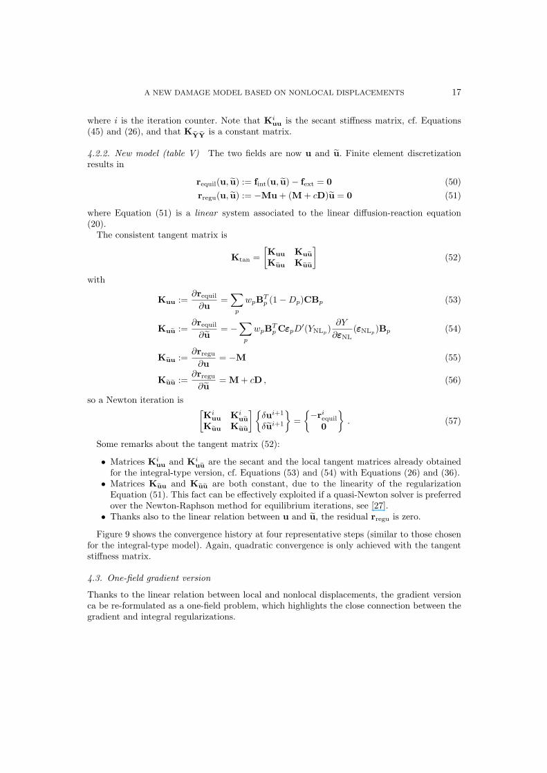
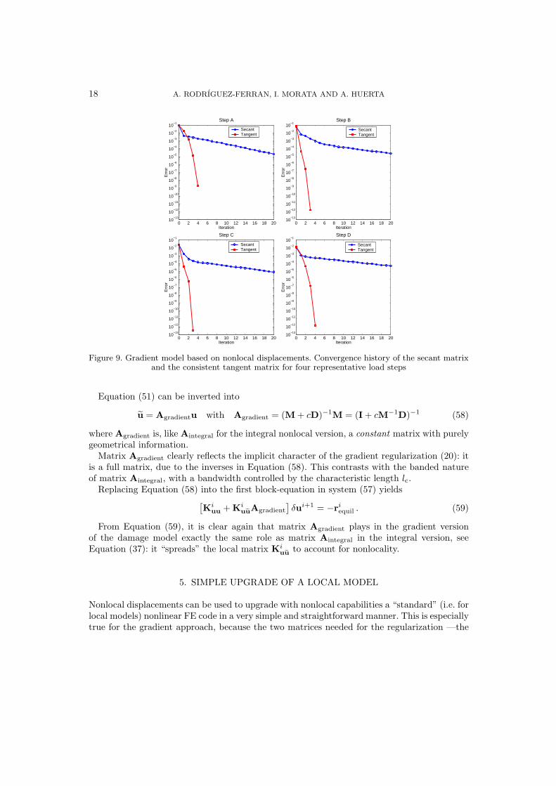
Figure 9 shows the convergence history at four representative steps (similar to those chosenfor the integral-type model). Again, quadratic convergence is only achieved with the tangentstiffness matrix.

4.3. One-field gradient version

Thanks to the linear relation between local and nonlocal displacements, the gradient versionca be re-formulated as a one-field problem, which highlights the close connection between thegradient and integral regularizations.

Copyright c© 2004 John Wiley & Sons, Ltd. Int. J. Numer. Anal. Meth. Geomech. 2004; 00:1–20Prepared using nagauth.cls

18 A. RODRIGUEZ-FERRAN, I. MORATA AND A. HUERTA

0 2 4 6 8 10 12 14 16 18 2010

−13

10−12

10−11

10−10

10−9

10−8

10−7

10−6

10−5

10−4

10−3

10−2

10−1

Step A

Iteration

Err

or

SecantTangent

0 2 4 6 8 10 12 14 16 18 2010

−13

10−12

10−11

10−10

10−9

10−8

10−7

10−6

10−5

10−4

10−3

10−2

10−1

Step B

Iteration

Err

or

SecantTangent

0 2 4 6 8 10 12 14 16 18 2010

−13

10−12

10−11

10−10

10−9

10−8

10−7

10−6

10−5

10−4

10−3

10−2

10−1

Step C

Iteration

Err

or

SecantTangent

0 2 4 6 8 10 12 14 16 18 2010

−13

10−12

10−11

10−10

10−9

10−8

10−7

10−6

10−5

10−4

10−3

10−2

10−1

Step D

Iteration

Err

or

SecantTangent

Figure 9. Gradient model based on nonlocal displacements. Convergence history of the secant matrixand the consistent tangent matrix for four representative load steps

Equation (51) can be inverted into

u = Agradientu with Agradient = (M + cD)−1M = (I + cM−1D)−1 (58)

where Agradient is, like Aintegral for the integral nonlocal version, a constant matrix with purelygeometrical information.

Matrix Agradient clearly reflects the implicit character of the gradient regularization (20): itis a full matrix, due to the inverses in Equation (58). This contrasts with the banded natureof matrix Aintegral, with a bandwidth controlled by the characteristic length lc.

Replacing Equation (58) into the first block-equation in system (57) yields[Ki

uu + KiuuAgradient

]δui+1 = −ri

equil . (59)

From Equation (59), it is clear again that matrix Agradient plays in the gradient versionof the damage model exactly the same role as matrix Aintegral in the integral version, seeEquation (37): it “spreads” the local matrix Ki

uu to account for nonlocality.

5. SIMPLE UPGRADE OF A LOCAL MODEL

Nonlocal displacements can be used to upgrade with nonlocal capabilities a “standard” (i.e. forlocal models) nonlinear FE code in a very simple and straightforward manner. This is especiallytrue for the gradient approach, because the two matrices needed for the regularization —the

Copyright c© 2004 John Wiley & Sons, Ltd. Int. J. Numer. Anal. Meth. Geomech. 2004; 00:1–20Prepared using nagauth.cls

A NEW DAMAGE MODEL BASED ON NONLOCAL DISPLACEMENTS 19

mass matrix M and the diffusivity matrix D— are very simple to compute (they are constant,symmetric definite positive matrices) and readily available in any FE code.

Since matrix Agradient in the one-field formulation of Section 4.3 is a full matrix, we thinkthe best option is the two-field formulation of Section 4.2.2. If assembling and/or factorizingthe non-symmetric tangent matrix (52) poses difficulties, the linear system (57) can be solvedvery effectively by means of the block Gauss-Seidel method. To do so, simply rewrite Equation(57) into

Kiuuδui+1

k+1 = −riequil −Ki

uuδui+1k

(M + cD)δui+1k+1 = Mδui+1

k+1

, (60)

where subscripts k and k+1 are the counters for the inner Gauss-Seidel iterations. The two left-hand-side matrices in Equation (60) are symmetric positive definite, so a standard Choleskyfactorization applies. Once Ki

uu and M + cD are factorized (at the beginning of the currentequilibrium iteration i and at the beginning of the analysis, respectively), the inner Gauss-Seidel iterations have a relatively modest computational cost. Linear convergence is expectedfor these inner iterations k. Note, however, that (1) quadratic convergence is obtained for theexpensive, outer equilibrium iterations i and (2) the tolerance for the inner k loop is usuallynot a constant [28]; a large tolerance is allowed for the initial Newton-Raphson iterations anda strict tolerance is only prescribed when the residual ri

equil tends to zero.

6. CONCLUDING REMARKS

Nonlocal displacements can be effectively used to regularize softening damage models. Aninternal length scale is incorporated into the model, either via the characteristic length lcof the averaging function (integral-type version) or parameter c in the second-order PDE(gradient version), so pathological mesh dependence is precluded.

In exchange for averaging a vectorial field of 2 or 3 displacement components rather than theusual scalar field (which has a very modest overhead, because the weighting function for theintegral version and the mass and diffusivity matrices for the gradient version are constant),the resulting models are mechanically sound and computationally efficient.

For the integral-type regularization, the consistent tangent matrix is much simpler tocompute than for the standard approach (nonlocal state variable), because nonlocal interactionbetween non-adjacent nodes is accounted for by a constant matrix Aintegral, and the need forcumbersome double loops in Gauss points is suppressed.

In the gradient approach, the Dirichlet boundary conditions on the regularization partialdifferential equation have a clear physical interpretation: nonlocal displacements are prescribedto coincide with local displacements in all the boundary. In addition, these simple boundaryconditions are closely connected with the insulation condition represented by the usualhomogeneous Neumann boundary conditions on the state variable. The choice of finite elementshape functions is straightforward, because the two fields (local and nonlocal displacements) areof the same nature. The expression of the consistent tangent matrix is also simpler, thanks tothe linear relation between local displacements u and nonlocal displacements u. This gradient-enhancement of the displacement field is a very simple way to incorporate nonlocality into afinite element code equipped with standard (i.e. local models) nonlinear capabilities.

Copyright c© 2004 John Wiley & Sons, Ltd. Int. J. Numer. Anal. Meth. Geomech. 2004; 00:1–20Prepared using nagauth.cls

20 A. RODRIGUEZ-FERRAN, I. MORATA AND A. HUERTA

REFERENCES

1. J. Lemaitre and J.-L. Chaboche. Mechanics of solid materials. Cambridge University Press, Cambridge,1990.

2. G. Pijaudier-Cabot and Z.P. Bazant. Nonlocal damage theory. J. Eng. Mech.-ASCE, 118(10):1512–1533,1987.

3. Z.P. Bazant and G. Pijaudier-Cabot. Nonlocal continuum damage, localization instability andconvergence. J. Appl. Mech.-Trans. ASME, 55(2):287–293, 1988.

4. J. Mazars and G. Pijaudier-Cabot. Continuum damage theory – application to concrete. J. Eng. Mech.-ASCE, 115(2):345–365, 1989.

5. R. de Borst, J. Pamin, R.H.J. Peerlings, and L.J. Sluys. On gradient-enhanced damage and plasticitymodels for failure in quasi-brittle and frictional materials. Comput. Mech., 17(1–2):130–141, 1995.

6. A. Huerta and G. Pijaudier-Cabot. Discretization influence on regularization by two localization limiters.J. Eng. Mech.-ASCE, 120(6):1198–1218, 1994.

7. Z.P. Bazant and F.B. Lin. Nonlocal smeared cracking model for concrete fracture. J. Eng. Mech.-ASCE,114(11):2493–2510, 1988.

8. C. Comi. A non-local model with tension and compression damage mechanisms. Eur. J. Mech. A-Solids,20(1):1–22, 2001.

9. M. Jirasek. Nonlocal models for damage and fracture: comparison of approaches. Int. J. Solids Struct.,35(31–32):4133–4145, 1998.

10. C. Comi. Computational modelling of gradient-enhanced damage in quasi-brittle materials. Mech.Cohesive-Frict. Mater., 4(1), 1999.

11. A. Rodrıguez-Ferran, I. Morata, and A. Huerta. Efficient and reliable nonlocal damage models. Comput.Methods Appl. Mech. Eng., 193(30–32):3431–3455, 2004.

12. Z.P. Bazant and M. Jirasek. Nonlocal integral formulations of plasticity and damage: survey of progress.J. Eng. Mech.-ASCE, 128(11):1119–1149, 2002.

13. R. de Borst, L.J. Sluys, H.-B. Mulhaus, and J. Pamin. Fundamental issues in finite element analysis oflocalization of deformation. Eng. Comput., 10:99–121, 1993.

14. J. Mazars, G. Pijaudier-Cabot, and C. Saouridis. Size effect and continuous damage in cementitiousmaterials. Int. J. Fract., 51(2):159–173, 1991.

15. P. Pegon and A. Anthoine. Numerical strategies for solving continuum damage problems involvingsoftening: application to the homogenization of masonry. In Proceedings of the Second InternationalConference on Computational Structures Technology, Athens, 1994.

16. A. Rodrıguez-Ferran and A. Huerta. Error estimation and adaptivity for nonlocal damage models. Int.J. Solids Struct., 37(48–50):7501–7528, 2000.

17. H. Askes and L.J. Sluys. Explicit and implicit gradient series in damage mechanics. Eur. J. Mech.A-Solids, 21(3):379–390, 2002.

18. R.H.J. Peerlings, M.G.D. Geers, R. de Borst, and W.A.M. Brekelmans. A critical comparison of nonlocaland gradient-enhanced softening continua. Int. J. Solids Struct., 38(44–45):7723–7746, 2001.

19. C. Polizzotto. Gradient elasticity and nonstandard boundary conditions. Int. J. Solids Struct.,40(26):7399–7423, 2003.

20. P. Lancaster and K. Salkauskas. Surfaces generated by moving least squares methods. Math. Comput.,37(155):141–158, 1981.

21. A. Huerta and S. Fernandez-Mendez. Locking in the incompressible limit for the Element Free Galerkinmethod. Int. J. Numer. Methods Eng., 51(11):1361–1383, 2001.

22. A. Simone, H. Askes, R. H. J. Peerlings, and L. J. Sluys. Interpolation requirements for implicit gradient-enhanced continuum damage models. Commun. Numer. Methods Eng., 19(7):563–572, 2003.

23. C.Q. Ru and E.C. Aifantis. A simple approach to solve boundary-value problems in gradient elasticity.Acta Mech., 101(1–4):59–68, 1993.

24. T. Belytschko, W.K. Liu, and B. Moran. Nonlinear finite elements for continua and structures. JohnWiley & Sons, Chichester, 2000.

25. G. Pijaudier-Cabot and A. Huerta. Finite element analysis of bifurcation in nonlocal strain softeningsolids. Comput. Methods Appl. Mech. Eng., 90(1–3):905–919, 1991.

26. M. Jirasek and B. Patzak. Consistent tangent stiffness for nonlocal damage models. Comput. Struct.,80(14–15):1279–1293, 2002.

27. A. Rodrıguez-Ferran and A. Huerta. Adapting Broyden method to handle linear constraints imposed viaLagrange multipliers. Int. J. Numer. Methods Eng., 46(12):2011–2026, 1999.

28. C.T. Kelley. Iterative methods for linear and nonlinear equations, volume 16 of Frontiers in AppliedMathematics. Society for Industrial and Applied Mathematics, Philadelphia, 1995.

Copyright c© 2004 John Wiley & Sons, Ltd. Int. J. Numer. Anal. Meth. Geomech. 2004; 00:1–20Prepared using nagauth.cls