�����������������

Citation: Traver, J.E.;

Nuevo-Gallardo, C.; Tejado, I.;

Fernández-Portales, J.; Ortega-Morán,

J.F.; Pagador, J.B.; Vinagre, B.M.

Cardiovascular Circulatory System

and Left Carotid Model: A Fractional

Approach to Disease Modeling.

Fractal Fract. 2022, 6, 64. https://

doi.org/10.3390/fractalfract6020064

Academic Editors: Norbert Herencsar

and Manuel Duarte Ortigueira

Received: 30 November 2021

Accepted: 20 January 2022

Published: 26 January 2022

Publisher’s Note: MDPI stays neutral

with regard to jurisdictional claims in

published maps and institutional affil-

iations.

Copyright: © 2022 by the authors.

Licensee MDPI, Basel, Switzerland.

This article is an open access article

distributed under the terms and

conditions of the Creative Commons

Attribution (CC BY) license (https://

creativecommons.org/licenses/by/

4.0/).

fractal and fractional

Article

Cardiovascular Circulatory System and Left Carotid Model:A Fractional Approach to Disease ModelingJosé Emilio Traver 1,* , Cristina Nuevo-Gallardo 1,* , Inés Tejado 1 , Javier Fernández-Portales 2 ,Juan Francisco Ortega-Morán 3 , J. Blas Pagador 3 and Blas M. Vinagre 1

1 Escuela de Ingenierías Industriales, Universidad de Extremadura, 06006 Badajoz, Spain;itejbal@unex.es (I.T.); bvinagre@unex.es (B.M.V.)

2 Hospital San Pedro de Alcántara, 10071 Cáceres, Spain; portales70@hotmail.com3 Centro de Cirugía de Mínima Invasión Jesús Usón, Ctra. N-521 km 41.8, 10071 Cáceres, Spain;

jfortega@ccmijesususon.com (J.F.O.-M.); jbpagador@ccmijesususon.com (J.B.P.)* Correspondence: jetraverb@unex.es (J.E.T.); cnuevog@unex.es (C.N.-G.)

Abstract: Cardiovascular diseases (CVDs) remain the leading cause of death worldwide, accordingto recent reports from the World Health Organization (WHO). This fact encourages research intothe cardiovascular system (CVS) from multiple and different points of view than those given by themedical perspective, highlighting among them the computational and mathematical models thatinvolve experiments much simpler and less expensive to be performed in comparison with in vivoor in vitro heart experiments. However, the CVS is a complex system that needs multidisciplinaryknowledge to describe its dynamic models, which help to predict cardiovascular events in patientswith heart failure, myocardial or valvular heart disease, so it remains an active area of research.Firstly, this paper presents a novel electrical model of the CVS that extends the classic Windkesselmodels to the left common carotid artery motivated by the need to have a more complete modelfrom a medical point of view for validation purposes, as well as to describe other cardiovascularphenomena in this area, such as atherosclerosis, one of the main risk factors for CVDs. The modelis validated by clinical indices and experimental data obtained from clinical trials performed on apig. Secondly, as a first step, the goodness of a fractional-order behavior of this model is discussed tocharacterize different heart diseases through pressure–volume (PV) loops. Unlike other models, itallows us to modify not only the topology, parameters or number of model elements, but also thedynamic by tuning a single parameter, the characteristic differentiation order; consequently, it isexpected to provide a valuable insight into this complex system and to support the development ofclinical decision systems for CVDs.

Keywords: cardiovascular system; electrical model; experimental validation; fractional model; heartdiseases; pressure–volume loops

1. Introduction

Cardiovascular diseases (CVDs) remain the leading cause of death worldwide, accor-ding to recent reports from the World Health Organization (WHO). Moreover, its upwardtrend over the last thirty years continues to increase for almost all countries [1]. In 2019,over 18 million people died from CVDs, which represents 32% of all global deaths; morespecifically, 85% of them were due to heart attack and stroke [2]. This fact has encouragedresearch into cardiovascular system (CVS) models, where experiments involving computa-tional and mathematical models are much simpler and less expensive to be performed incomparison with in vivo or in vitro experiments.

The CVS is a relatively complex system that needs knowledge from several branchesof physics and chemistry to understand all its behavior, which has led to the developmentof models or simulators, in greater or lesser detail, to achieve a global understanding of its

Fractal Fract. 2022, 6, 64. https://doi.org/10.3390/fractalfract6020064 https://www.mdpi.com/journal/fractalfract

Fractal Fract. 2022, 6, 64 2 of 21

operation. In this respect, numerous models have been proposed and approached fromdifferent perspectives, such as from the study of neuroregulation mechanisms, gas exchangeor the hemodynamics of the system; however, the latter approach has always receivedgreater attention due to its possible physiological or clinical applications [3,4]. For suchan approach, the main methodologies used are: (1) lumped parameter models, whichdescribe, in a simplified manner, the predominant behavior of each of the componentsinvolved in the CVS [3,5–9]; (2) distributed parameter models, describing the CVS by one,two or three dimensions based on finite element software [10–12]; or (3) modeling froma hydraulic approach [13–15]. Especially, the three dimensional distributed parametermodels have received a great deal of attention in recent decades as a result of the increasein computing power, but these models are more complex and focus on partial vascularzones, and consequently they need longer simulation time and simpler models to definetheir boundary conditions [16–19].

The models offer the possibility to diagnose or predict the behavior of the CVS when apatient suffers a cardiovascular dysfunction or pathology [20–24], or to study the perfor-mance of auxiliary devices [3,25,26]. This reduces the diagnostic time for certain pathologiesor research time of functional evaluation of devices under development, while reducinganimal experimentation. Nevertheless, the existing models have use limitations in clinicalpractice due to both their physical and computational complexities. Modeling of patholo-gies, or even medical assistance devices, usually requires to modify numerous parametersof the model, which are strongly related to each other, making it necessary sometimes toperform new validations. This fact makes the models with a great number of parametersundesirable for real applications. In this regard, lumped parameter models offer an ad-vantage over the others, demonstrating a higher accuracy to execution time ratio, which issuitable for real-time simulations and applications [27,28]. Despite this, lumped modelsare reduced to describe the main arteries of the CVS [3,5,9,22] or the entire circulatorysystem [29], complicating the study of certain vascular areas due to a greater number ofparameters. This is the case of the carotid artery, for which there are no studies that modelits behavior simply and accurately. In spite of this, it is one of the main arteries affected bystenosis according to clinical studies [30].

In what CVD modeling concerns, it is mainly based on the development of new modelsor the adjustment of numerous parameters to describe a dysfunction or disease accurately.New models require the inclusion of new terms for a better description of the dynamicsystem or, in the case of parameter adjustment, they can achieve a dynamic similar to thedesired one but do not describe it in an accurate way, although it has the advantage ofnot incorporating new terms. When the CVS suffers a disease, such as stenosis, not onlythe vessel presents an obstruction, but the calcification of the lumen also has an impacton the elastance, among other properties; therefore, a disease implies an alteration of thesystem properties, which leads the system to exhibit a different behavior and not only amodification of the resistance or flow capacity. In this regard, fractional calculus can bean adequate tool to describe CVDs. Fractional calculus is a branch of mathematics thatdeals with non-integer- order derivatives and integrals, and has emerged as an efficient andpowerful mathematical tool not only for accurate modeling of many complex phenomenathat can be found in several fields of science and engineering, but also for obtainingadequate exploitable models with few parameters [31,32]. Notably, numerous studies haveshown that fractional calculus provides a better description of the viscoelastic behavior ofthe arterial vessel [33–38], as well as for modeling of pathologies, such as tumors [39,40].

Given this motivation, the contributions of this paper are twofold. Firstly, a novelelectrical model of the CVS is presented. It extends the classical Windkessel model offour elements to the left common carotid artery, motivated by the need to have a morecomplete model from a medical point of view for validation purposes, as well as to describeother cardiovascular phenomena in this area, such as atherosclerosis, one of the main riskfactors for CVDs. This model is validated with experimental data obtained from clinicaltrials performed on a pig and clinical indices. Secondly, a new approach is introduced for

Fractal Fract. 2022, 6, 64 3 of 21

CVD modeling based on fractional calculus. To do so, the CVS is analyzed as a completefractional dynamic system; i.e., the relationship between pressure and flow for arteries orchambers is described with fractional behavior. In this sense, a general model is created,able to describe hemodynamic change due to pathologies, such as loss of elasticity orcontractile capacity and not only due to vessel occlusion or valve or heart dysfunction.Specifically, the case of aortic valve stenosis will be discussed describing the proposedmodel with fractional dynamics and how the order of the system allows us to describe theCVS from a healthy state to a severe degree of stenosis. As an advantage for pathologymodeling, the model parameters can be identified and validated for the healthy state andremain constant, with only slight variations as in the real system. Preliminary results ofthis work can be found in [41,42].

The paper is organized as follows. The functioning of the CVS is briefly explainedin Section 2. Section 3 justifies the use of electrical analogies for the description of CVSand describes the CVS model. Section 4 compares and validates the presented model withclinical indices and experimental data. Section 5 provides a discussion of how fractionalcalculus may be an adequate tool for CVD modeling. Finally, conclusions and future worksare drawn in Section 6.

2. Cardiovascular System

This section is devoted to the description of the CVS from a functional point of view,with special attention to the carotid artery. The cardiac cycle is explained through theleft ventricular pressure–volume (PV) loops, diagrams that also allow the identification ofdysfunctions affecting the CVS. Finally, the most frequent valve pathologies are briefly des-cribed.

2.1. Anatomy and Physiology of the CVS

The CVS can be simply described as a distribution network of blood vessels thatsupplies blood to all the parts of a body thanks to the heart, which performs as a pump.The path followed by the blood is a closed loop, starting in the heart, continuing throughthe arteries, passing through the capillaries, where the exchange of substances takes placeand returning to the heart via the veins. From a functional point of view, the distributionnetwork is divided into two stages: (1) systemic circulation, which transports the oxygenand substances; and (2) pulmonary circulation, which is responsible for the oxygenation ofthe blood [43].

The heart, responsible for pumping the blood, is composed of a double atria-ventriclechamber, where the ventricle is the pump and the atria is a preloaded chamber. The com-pression or contraction of the ventricle generates the necessary pressure to inject bloodthrough the arteries. Specifically, the right side pumps the blood into the pulmonary artery,which carries it to the lungs, and then it returns to the left side that pumps it again to therest of the body. It should be noted that the blood only flows in one way because one-wayvalves are situated between the chambers to prevent reflux, called atrioventricular valves,and at the output of the ventricles, called semilunar valves.

Regarding the systemic circulation, it begins in the ascending aorta, branching intosmaller arteries until it reaches the capillaries, covering the entire body. The main branchesare: (1) right and left subclavian arteries, supplying blood to the thorax, head, neck,shoulder and arms; (2) right and left common carotid arteries, carrying blood to the headand neck; and (3) descendent aorta, which continues to the abdominal aorta. Finally,the return path is composed of veins that converge in the vena cava, which ends in theheart. Within the systemic circulation, the carotid arteries stand out for their high incidenceof strokes [44].

2.2. Cardiac Cycle and Pressure–Volume Loops

The contraction of the heart is a result of a succession of electrical and mechanicalphenomena that occur during a heartbeat, known as the cardiac cycle [43]. The cardiac

Fractal Fract. 2022, 6, 64 4 of 21

cycle is divided into two alternate phases: diastole (dilation period) and systole (contractionperiod), arranged and simplified in four stages. The cardiac cycle starts with the chambersrelaxed and the ventricles partially loaded, and proceeds as follows:

(1) The first stage is the atrial systole and ventricular diastole, in which the atriumcontracts, filling the ventricles;

(2) The second stage is atrial diastole and the beginning of ventricular systole, whichmeans that the atrium relaxes until the next cardiac cycle while the ventricles contract andthe atrioventricular valves close, increasing the pressure but not achieving enough pressureto open the semilunar valves;

(3) The third stage is the end of ventricular systole, when ventricle pressure rises untilit exceeds arterial pressure, opening the semilunar valves and ejecting the blood into thepulmonary and systemic circulation;

(4) The last stage is the ventricular and atrial diastole, when the pressure in ventriclesdecreases rapidly and all the chambers are passively loaded due to their relaxation. Then,a new cycle starts with the atrial systole.

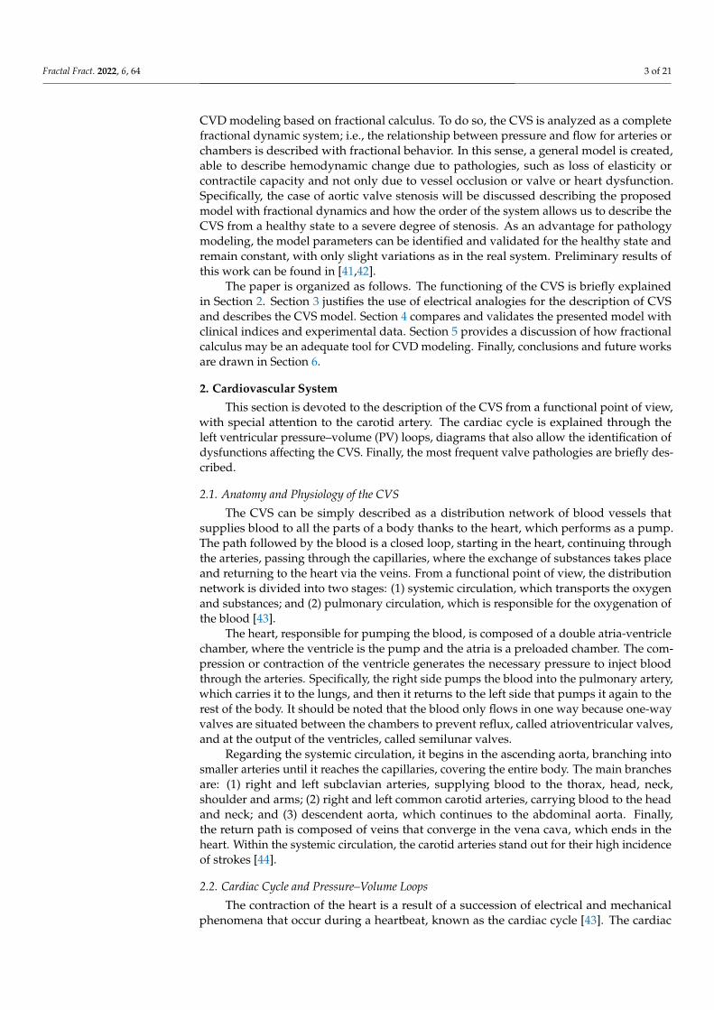
A graphical way to describe and characterize the cardiac cycle is by means of a leftventricle PV loop, which represents the left ventricular pressure (LVP) versus the leftventricular volume (LVV) throughout the four stages, allowing us to identify changes inheart function, such as preload and afterload factors and contractility of the heart [45].Another advantage of PV loops is that they allow rapid detection of CVDs, such as heartfailure, myocardial and valve diseases. An example of a PV loop is shown in Figure 1,where the different stages of a cardiac cycle corresponding to the left ventricle (LV) arerepresented from a thermodynamic point of view:

(1) Passive filling (referred to as A-B);(2) Isovolumetric contraction (denoted as B-C);(3) Ejection (C-D);(4) Isovolumetric relaxation (D-A) [46].

Furthermore, these diagrams also provide information on a wide range of variables, suchas those listed in Table 1.

0 50 100 150 200

0

50

100

150

Figure 1. Example of PV loop and parameters that can be measured. The meaning of acronyms aredetailed in Table 1. Image adapted from [46,47].

Fractal Fract. 2022, 6, 64 5 of 21

Table 1. Parameters measured from PV loops. Data extracted from [46].

Abbreviation Parameter Meaning

EDV End-diastolic volume Left ventricular volume in diastole.ESV End-systolic volume Left ventricular volume in systole.

ESPVR End-systolic PV relationship Maximal pressure of left ventricle.EDPVR End-diastolic PV relationship Left ventricular pressure in diastole.

Ees End-systolic elastance Peak chamber elastance during a beat.Ea Effective arterial elastance Relates EDP and EDV to ESV.SV Stroke volume The difference between ESV and EDV.SW Stroke work The area within the loop.PE Potential energy The area within the loop and ESPVR.

PVA Pressure–volume area Sum of SW and potential energy PE.ME Mechanical efficiency The ratio between SW and PVA.

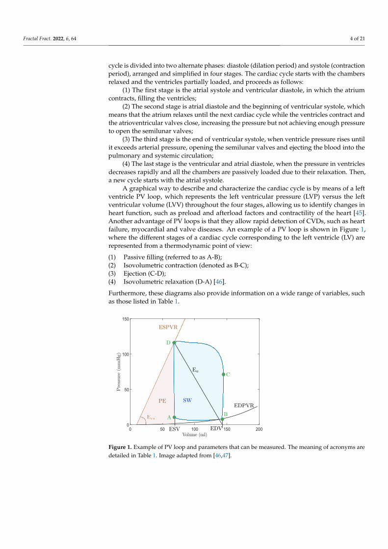
With respect to the factors affecting the functioning of the heart, the preload factorsrefer to the level of distension of the ventricle during diastole, and are proportional toend-diastolic volume (EDV) [43,48]. According to Frank–Starling’s law, an increase inventricular preload leads to an increment of stroke volume (SV), which implies an increasein EDV and the opening pressure of the semilunar valves. These effects are shown inFigure 2a. An increase in preload is associated to an increment in physical exercise andacceleration of heart rate (HR), while an occlusion of the veins or hemorrhages produce areduction in preload.

The afterload is related to end-systolic volume (ESV), although preload factors andinotropy also affect it. ESV is the pressure that the ventricle must exert in order to open thesemilunar valves and propel the blood. In the PV loops, an increase in afterload involves areduction in SV and an increment in ESV, which also leads to an increase in the EDV (seeFigure 2b). The increase in afterload is usually caused by an increased systemic resistancedue to damage of the semilunar valves, stenosis or obstructions in the circulation, as wellas a loss of elasticity in the aortic artery.

With respect to inotropy, understood as the capacity of the ventricles to contract,a rise of this factor implies a higher slope of the end-systolic PV relationship (ESPVR)line, represented in Figure 2c. This variation allows to have a higher SV and reduces EDVand ESV. Reduced ability to contract is observed as a consequence of a prolonged state ofhypoxia, hyponatremia or hypercapnia.

Version January 17, 2022 submitted to Fractal Fract. 5 of 21

(a) (b) (c)Figure 2. Effects on PV diagrams due to changes in: (a) preload, (b) afterload, and (c) inotropy on left ventricular.

The afterload is related to end-systolic volume (ESV), although preload factors and173

inotropy also affect it. ESV is the pressure that the ventricle must exert in order to open174

the semilunar valves and propel the blood. In the PV loops, an increase in afterload175

involves a reduction in SV and an increment in ESV, which also leads to an increase of176

the EDV (see Figure 2b). The increase in afterload is usually caused by an increased177

systemic resistance due to damage of the semilunar valves, stenosis or obstructions in178

the circulation, as well as a loss of elasticity in the aortic artery.179

With respect to inotropy, understood as the capacity of the ventricles to contract, a180

rise of this factor implies a higher slope of the end-systolic PV relationship (ESPVR) line,181

represented in Figure 2c. This variation allows to have a higher SV and reduces EDV182

and ESV. Reduced ability to contract is observed as a consequence of a prolonged state183

of hypoxia, hyponatremia or hypercapnia.184

Table 1. Parameters measured from PV loops. Data extracted from [46].

Abbreviation Parameter Meaning

EDV End-diastolic volume Left ventricle volume in diastole.ESV End-systolic volume Left ventricle volume in systolic.

ESPVR End-systolic PV relationship Maximal pressure of left ventricle.EDPVR End-diastolic PV relationship Left ventricle pressure in diastole.

Ees End-systolic elastance Peak chamber elastance during a beat.Ea Effective arterial elastance Relates EDP and EDV to ESV.SV Stroke volume The difference between ESV and EDV.SW Stroke work The area within the loop.PE Potential energy The area within the loop and ESPVR.

PVA Pressure-volume area Sum of SW and potential energy PE.ME Mechanical efficiency The ratio between SW and PVA.

2.3. Valve pathologies185

The most common valve pathologies are related to the aortic valve and mitral valve,186

and, in both cases, involve the narrowing of the valve (stenosis) and a defect in the187

closure.188

Stenosis in aortic valve refers to the narrowing of the valve during systole, which189

can be caused by a congenital abnormality of the valve or progressive calcium buildup on190

the valve cups due to age [49]. Conversely, a defect in the closure of the aortic valve leads191

to a leakage backward into the LV during diastole, and is called aortic valve regurgitation,192

with similar causes as aortic valve stenosis. In both pathologies, a hypertrophy in the LV193

appears due to the thickening of the LV muscle to undertake the stress, which causes an194

increase in LV pressure.195

Aortic valve pathologies lead to PV loops with higher amplitude and displaced to196

the right with respect to the healthy case [46,50,51], as illustrated in Figure 3a and 3b.197

Figure 2. Effects on left ventricular PV diagrams due to changes in: (a) preload; (b) afterload;(c) inotropy.

2.3. Valve Pathologies

The most common valve pathologies are related to the aortic valve and mitral valve,and, in both cases, involve the narrowing of the valve (stenosis) and a defect in the closure.

Stenosis in aortic valve refers to the narrowing of the valve during systole, which canbe caused by a congenital abnormality of the valve or progressive calcium buildup on the

Fractal Fract. 2022, 6, 64 6 of 21

valve cups due to age [49]. Conversely, a defect in the closure of the aortic valve leads toa leakage backward into the LV during diastole, and is called aortic valve regurgitation,with similar causes as aortic valve stenosis. In both pathologies, a hypertrophy in the LVappears due to the thickening of the LV muscle to undertake the stress, which causes anincrease in LV pressure.

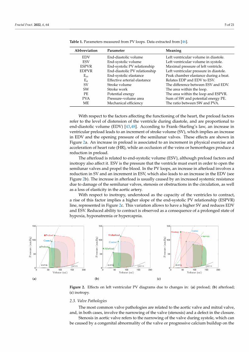
Aortic valve pathologies lead to PV loops with higher amplitude and displaced to theright with respect to the healthy case [46,50,51], as illustrated in Figure 3a,b. The displace-ment of the loop to the right implies higher values of EDV, ESV and SV, also raising thearea within the loop (SW). As SW is higher, the pressure–volume area (PVA) also increases,as it is the sum of SW and potential energy (PE).

With respect to the mitral valve, the pathologies are similar, considering that theleakage is produced during systole from the LV to the left atria (LA). Figure 3c shows thatpatients with mitral valve stenosis present similar PV loops as a healthy patient, whichindicates that this pathology does not affect (to a large extent) the functioning of the LV.On the other hand, patients with mitral valve regurgitation (Figure 3d) present wider PVloops, increasing the afterload and preload and higher amplitude. The shape is slightlydifferent from the healthy case.

Pathology

Control

Pathology

Control

PathologyControl

Pathology

Control

(a) (b)

(c) (d)

Figure 3. Left ventricular PV loops of different valve pathologies: (a) aortic valve stenosis; (b) aorticvalve regurgitation; (c) mitral valve stenosis; (d) mitral valve regurgitation.

3. Description of the CVS Model

This section explains the equivalences between the electrical and hydrodynamic in-dices, allowing us to model the CVS from an electrical point of view. Once the relationshipsand equivalences between an electrical circuit and the behavior described by a segment ofthe CVS have been established, the modeling of such a system, as well as the contractilebehavior of the heart, are addressed.

3.1. Electrical Equivalences

In order to describe the CVS using a zero dimension (0-D) global parameter model,it is firstly required to understand how it is possible to transfer the fluid dynamics of an

Fractal Fract. 2022, 6, 64 7 of 21

environment to a discrete system, such as electrical circuits. The key concept is to analyzethe CVS through segments or compartments, that means defining the relationship betweentheir output and input, which can be calculated either empirically or theoretically.

Applying the Navier–Stokes equations to a blood vessel segment and taking intoaccount the considerations given in [19,52], it is possible to define the relationship betweenpressure and flow within the segment as:

Kcldpdt

+ q2 − q1 = 0

ρlA

dqdt

+ρKRl

A2 q + p2 − p1 = 0 (1)

where p and q are the average segment pressure and flow rate, respectively, p1 and p2 andq1 and q2 are the pressures and the flow rate at the inlet and outlet, respectively, A denotesthe average section of the blood vessel, l is the length of the segment, ρ is the density of theblood, and Kc and KR are variables dependent on the elastic properties of the blood vesseland the viscosity of the blood (see [4,19] for more information).

The system of Equations (1) implies that the flow and pressure of the segment consi-dered is limited by the boundary conditions (q1,2 and p1,2). However, the 0-D modeldoes not have boundary conditions, since there is no continuous dependence on space,but rather an input/output relationship; therefore, to solve such a system of equations,it is necessary to establish initial conditions (p0 = p1 and q0 = q1) and also to makethe following simplifications: p ≈ p2 y q ≈ q1. These assumptions, which are valid forrelatively short blood vessel segments, result in a 0-D global parameter model [19].

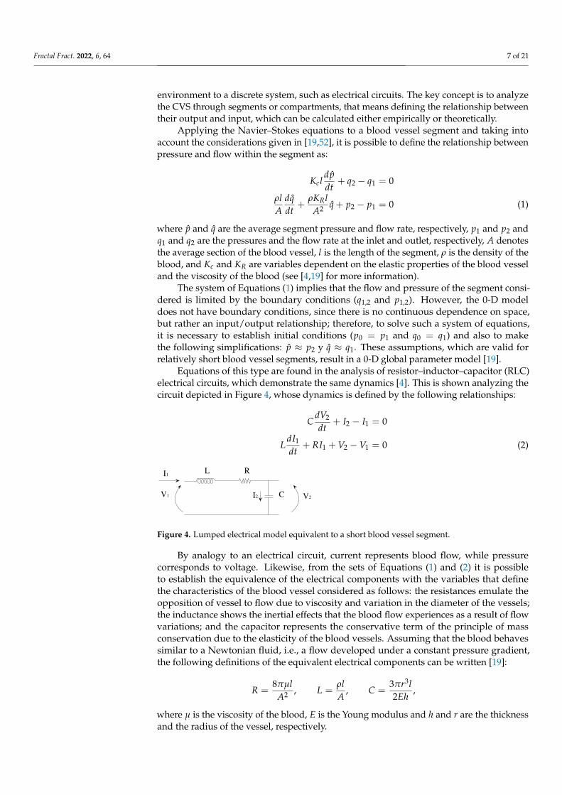
Equations of this type are found in the analysis of resistor–inductor–capacitor (RLC)electrical circuits, which demonstrate the same dynamics [4]. This is shown analyzing thecircuit depicted in Figure 4, whose dynamics is defined by the following relationships:

CdV2

dt+ I2 − I1 = 0

LdI1

dt+ RI1 + V2 −V1 = 0 (2)

V1

I1

V2I2

L R

C

Figure 4. Lumped electrical model equivalent to a short blood vessel segment.

By analogy to an electrical circuit, current represents blood flow, while pressurecorresponds to voltage. Likewise, from the sets of Equations (1) and (2) it is possibleto establish the equivalence of the electrical components with the variables that definethe characteristics of the blood vessel considered as follows: the resistances emulate theopposition of vessel to flow due to viscosity and variation in the diameter of the vessels;the inductance shows the inertial effects that the blood flow experiences as a result of flowvariations; and the capacitor represents the conservative term of the principle of massconservation due to the elasticity of the blood vessels. Assuming that the blood behavessimilar to a Newtonian fluid, i.e., a flow developed under a constant pressure gradient,the following definitions of the equivalent electrical components can be written [19]:

R =8πµl

A2 , L =ρlA

, C =3πr3l2Eh

,

where µ is the viscosity of the blood, E is the Young modulus and h and r are the thicknessand the radius of the vessel, respectively.

Fractal Fract. 2022, 6, 64 8 of 21

3.2. Model

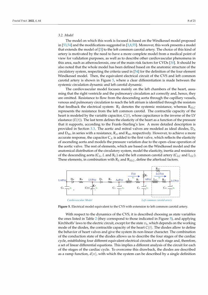
The model on which this work is focused is based on the Windkessel model proposedin [53,54] and the modifications suggested in [3,8,55]. Moreover, this work presents a modelthat extends the model of [3] to the left common carotid artery. The choice of this kind ofartery is motivated by the need to have a more complete model from a medical point ofview for validation purposes, as well as to describe other cardiovascular phenomena inthis area, such as atherosclerosis, one of the main risk factors for CVDs [30]. It should bealso noted that the whole model has been defined based on the anatomic structure of thecirculatory system, respecting the criteria used in [54] for the definition of the four elementWindkessel model. Then, the equivalent electrical circuit of the CVS and left commoncarotid artery is shown in Figure 5, where a clear differentiation is made between thesystemic circulation dynamic and left carotid dynamic.

The cardiovascular model focuses mainly on the left chambers of the heart, assu-ming that the right ventricle and the pulmonary circulation act correctly and, hence, theyare omitted. Resistance to flow from the descending aorta through the capillary vessels,venous and pulmonary circulation to reach the left atrium is identified through the resistorsthat feedback the electrical system: RS denotes the systemic resistance, whereas RSLCrepresents the resistance from the left common carotid. The contractile capacity of theheart is modeled by the variable capacitor, C(t), whose capacitance is the inverse of the LVelastance (E(t)). The last term defines the elasticity of the heart as a function of the pressurethat it supports, according to the Frank–Starling’s law. A more detailed description isprovided in Section 3.3. The aortic and mitral valves are modeled as ideal diodes, DAand DM, in series with a resistance, RA and RM, respectively. However, to achieve a moreaccurate response, the capacitor CA is added to the first valve, which reflects the elasticityof ascending aorta and models the pressure variation due to the open–close operation ofthe aortic valve. The rest of elements, which are based on the Windkessel model and theanatomical distribution of the circulatory system, model the elasticity, inertia and resistanceof the descending aorta (CS, L and RC) and the left common carotid artery (CLC and LLC).These elements, in combination with RS and RSLC, define the afterload factors.

Left common carotid artery

RSLC

RC

CSCAC(t)CR

DM

RS

RM RADA AoP(t)LAP(t) LVP(t) L AP(t)

F(t)

x1x2 x4 x3

x5RLC

CLC

LLCLCP(t)

LCF(t)

x6

x7

Cardiovascular Model

Figure 5. Electrical model equivalent to the CVS with extension to left common carotid artery.

With respect to the dynamics of the CVS, it is described choosing as state variablesthe ones listed in Table 2 (they correspond to those indicated in Figure 5), and applyingKirchhoffs’ laws to the electric circuit, except for the state x1, which depends on the workingmode of the diodes, the contractile capacity of the heart C(t). The diodes allow to definethe behavior of heart valves and give the system its non-linear character. The combinationof the conduction state of the diodes allows us to describe the four stages of the cardiaccycle, establishing four different equivalent electrical circuits for each stage and, therefore,a set of linear differential equations. This implies a different analysis of the circuit for eachof the stages of the cardiac cycle. To overcome this drawback, the diodes are describedas a ramp function, d(x), with which the system can be described by a single definition

Fractal Fract. 2022, 6, 64 9 of 21

throughout the entire cardiac cycle. Taking into account these considerations, the completemodel can be expressed as:

x1 =1

C(t)(− C(t)x1 +

1RM

d(x1 − x2)−1

RAd(x4 − x1)

)

x2 =1

CR

( 1RS

d(x3 − x2) +1

RSLC(x6 − x2)−

1RM

d(x2 − x1))

x3 =1

CS

(x5 − x7 −

1RS

d(x3 − x2))

x4 =1

CA

( 1RA

d(x4 − x1)− x5)

x5 =1L(

x4 − x3 − RCx5)

x6 =1

CLC

( 1RSLC

(x2 − x6) + x7)

x7 =1

LLC

(x3 − x6 − RLCx7

)

(3)

Table 2. State variables of the cardiovascular model.

Variable Abbreviation Clinical Meaning (Unit)

x1(t) LVP(t) Left ventricular pressure (mmHg).x2(t) LAP(t) Left atrial pressure (mmHg).x3(t) AP(t) Descending aorta pressure (mmHg).x4(t) AoP(t) Ascending aorta pressure (mmHg).x5(t) F(t) Total flow (mL/s).x6(t) LCP(t) Left common carotid artery pressure (mmHg).x7(t) LCF(t) Carotid artery flow rate (mL/s).

The detailed analysis of the electrical circuit in Figure 5 can be found in Appendix A.It should be remarked that the above model defines an autonomous switched time-varyingsystem over different phases within the cardiac cycle.

3.3. Elastance

The elastance represents the state of contraction of the LV, relating the pressure andvolumes of the LV according to the Frank–Starling’s law, which is defined as [3,56]:

E(t) =LVP(t)

LVV(t)−V0, (4)

where LVV(t) is the left ventricular volume, whereas V0 is the reference volume thatcorresponds to the theoretical ventricular volume at zero pressure.

The definition of elastance was addressed in different studies [57–59], where they triedto adjust it empirically to a standard function. In particular, most of them agree that thedefinition can be normalized and scaled between the points of maximum and minimumfunctioning of the LV as:

EH(t) = (Emax − Emin)En(tn) + Emin, (5)

where Emax and Emin are constants related to ESV, EDV and ESPVR, and En(tn) is thenormalized elastance, with tn = t/Tmax, Tmax = 0.2 + 0.15tc, being tc = 60/HR thetime period of the heart cycle. In certain pathologies, the elastance can have the samemorphology for a healthy or sick heart [60]. Then, for some cardiac conditions, the elastancemodel (5) is modified to E(t) = δEH(t), with 0 ≤ δ ≤ 1, where lower values of δ represent

Fractal Fract. 2022, 6, 64 10 of 21

CVDs (the more severe the disease, the lower the value of δ), whereas δ = 1 corresponds tothe healthy state.

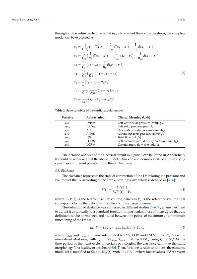
This work focuses in the definition for elastance provided by [57], which describes itfor a healthy person as:

En(tn) = C

(tnB

)αE

1 +(

tnB

)αE

1

1 +(

tnA

)βE

(6)

and whose waveforms are depicted in Figure 6. The first term in the brackets describes theascending part of the curve and the second one, the descending part. The parameter C isthe amplitude of elastance, related to the maximum arterial pressure, αE and βE denote theascending and descending slopes through the LV relaxation time, respectively, and A andB are constants to define the relative appearance of each curve within the heart period.

0 0.2 0.4 0.6 0.8 10

0.5

1

1.5

2

Figure 6. Elastance according to Stergiopulos’s work [57]. The parameters used are shown in Table 3.

4. Validation of the CVS Model

This section presents the validations of the above-described CVS model from differentpoints of view. Firstly, the model is validated in terms of both the main hemodynamicindices and the waveform of the main variables in Table 2, comparing the results in a healthystate (nominal condition) with the collected in the bibliography and with experimentaldata, respectively. Secondly, the consistency of the model is addressed by evaluating theresponse to variations in the preload and afterload factors. The values of the parametersinvolved in the CVS for the different simulations are included in Table 3.

4.1. Clinical Parameters and Experimental Waveforms

Next, the model is validated comparing the hemodynamic parameters resulting fromthe model simulation and those collected in the clinical literature, as well as from experi-mental data. Hence, this first validation allows us to conclude whether the model providesreasonable and coherent results. Secondly, cardiovascular waveforms corresponding tosimulated and experimental data are compared to confirm whether the dynamics is correct.

As for the experimental data, they were obtained from a clinical trial performed on apig, due to its similarities with human anatomy and hemodynamics. For data collection,the animal was under sedation during the whole process and catheterization methods wereused to measure the variables listed in Table 2, with the exception of flow rate, which wasmeasured indirectly by means of cardiac output and the carotid artery flow rate because thespecific instrumentation for such measurement was not available. In order to improve thereproducibility of the data and reduce signal noise at the post-processing step, the pressuresignals and the cardiac output were collected ten and five times, respectively. To make theexperimental data usable, they were previously filtered and, then, synchronized, since allthe signals were not collected at the same time, taking for the analysis the mean of the tenrepetitions. Data were collected with a sample time of 4 ms.

Fractal Fract. 2022, 6, 64 11 of 21

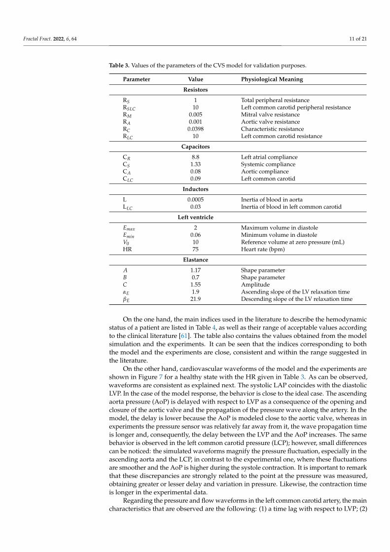
Table 3. Values of the parameters of the CVS model for validation purposes.

Parameter Value Physiological Meaning

Resistors

RS 1 Total peripheral resistanceRSLC 10 Left common carotid peripheral resistanceRM 0.005 Mitral valve resistanceRA 0.001 Aortic valve resistanceRC 0.0398 Characteristic resistanceRLC 10 Left common carotid resistance

Capacitors

CR 8.8 Left atrial complianceCS 1.33 Systemic complianceCA 0.08 Aortic complianceCLC 0.09 Left common carotid

Inductors

L 0.0005 Inertia of blood in aortaLLC 0.03 Inertia of blood in left common carotid

Left ventricle

Emax 2 Maximum volume in diastoleEmin 0.06 Minimum volume in diastoleV0 10 Reference volume at zero pressure (mL)HR 75 Heart rate (bpm)

Elastance

A 1.17 Shape parameterB 0.7 Shape parameterC 1.55 AmplitudeαE 1.9 Ascending slope of the LV relaxation timeβE 21.9 Descending slope of the LV relaxation time

On the one hand, the main indices used in the literature to describe the hemodynamicstatus of a patient are listed in Table 4, as well as their range of acceptable values accordingto the clinical literature [61]. The table also contains the values obtained from the modelsimulation and the experiments. It can be seen that the indices corresponding to boththe model and the experiments are close, consistent and within the range suggested inthe literature.

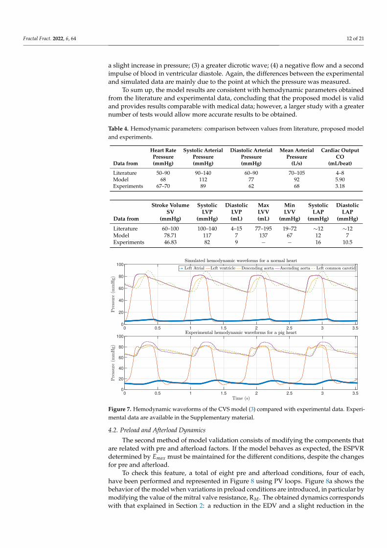
On the other hand, cardiovascular waveforms of the model and the experiments areshown in Figure 7 for a healthy state with the HR given in Table 3. As can be observed,waveforms are consistent as explained next. The systolic LAP coincides with the diastolicLVP. In the case of the model response, the behavior is close to the ideal case. The ascendingaorta pressure (AoP) is delayed with respect to LVP as a consequence of the opening andclosure of the aortic valve and the propagation of the pressure wave along the artery. In themodel, the delay is lower because the AoP is modeled close to the aortic valve, whereas inexperiments the pressure sensor was relatively far away from it, the wave propagation timeis longer and, consequently, the delay between the LVP and the AoP increases. The samebehavior is observed in the left common carotid pressure (LCP); however, small differencescan be noticed: the simulated waveforms magnify the pressure fluctuation, especially in theascending aorta and the LCP, in contrast to the experimental one, where these fluctuationsare smoother and the AoP is higher during the systole contraction. It is important to remarkthat these discrepancies are strongly related to the point at the pressure was measured,obtaining greater or lesser delay and variation in pressure. Likewise, the contraction timeis longer in the experimental data.

Regarding the pressure and flow waveforms in the left common carotid artery, the maincharacteristics that are observed are the following: (1) a time lag with respect to LVP; (2)

Fractal Fract. 2022, 6, 64 12 of 21

a slight increase in pressure; (3) a greater dicrotic wave; (4) a negative flow and a secondimpulse of blood in ventricular diastole. Again, the differences between the experimentaland simulated data are mainly due to the point at which the pressure was measured.

To sum up, the model results are consistent with hemodynamic parameters obtainedfrom the literature and experimental data, concluding that the proposed model is validand provides results comparable with medical data; however, a larger study with a greaternumber of tests would allow more accurate results to be obtained.

Table 4. Hemodynamic parameters: comparison between values from literature, proposed modeland experiments.

Heart Rate Systolic Arterial Diastolic Arterial Mean Arterial Cardiac OutputPressure Pressure Pressure Pressure CO

Data from (mmHg) (mmHg) (mmHg) (L/s) (mL/beat)

Literature 50–90 90–140 60–90 70–105 4–8Model 68 112 77 92 5.90Experiments 67–70 89 62 68 3.18

Stroke Volume Systolic Diastolic Max Min Systolic DiastolicSV LVP LVP LVV LVV LAP LAP

Data from (mmHg) (mmHg) (mL) (mL) (mmHg) (mmHg) (mmHg)

Literature 60–100 100–140 4–15 77–195 19–72 ∼12 ∼12Model 78.71 117 7 137 67 12 7Experiments 46.83 82 9 − − 16 10.5

0 0.5 1 1.5 2 2.5 3 3.50

20

40

60

80

100

0 0.5 1 1.5 2 2.5 3 3.50

20

40

60

80

100

Figure 7. Hemodynamic waveforms of the CVS model (3) compared with experimental data. Experi-mental data are available in the Supplementary material.

4.2. Preload and Afterload Dynamics

The second method of model validation consists of modifying the components thatare related with pre and afterload factors. If the model behaves as expected, the ESPVRdetermined by Emax must be maintained for the different conditions, despite the changesfor pre and afterload.

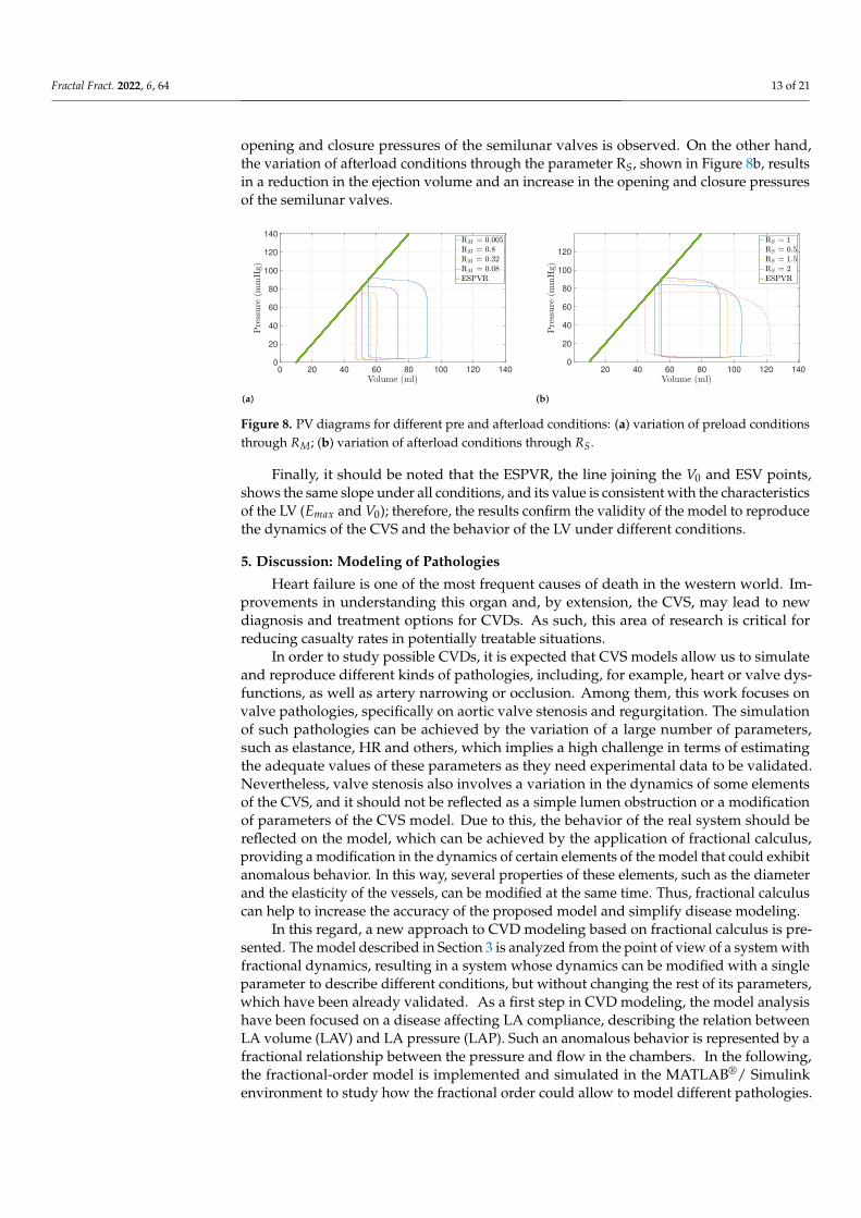
To check this feature, a total of eight pre and afterload conditions, four of each,have been performed and represented in Figure 8 using PV loops. Figure 8a shows thebehavior of the model when variations in preload conditions are introduced, in particular bymodifying the value of the mitral valve resistance, RM. The obtained dynamics correspondswith that explained in Section 2: a reduction in the EDV and a slight reduction in the

Fractal Fract. 2022, 6, 64 13 of 21

opening and closure pressures of the semilunar valves is observed. On the other hand,the variation of afterload conditions through the parameter RS, shown in Figure 8b, resultsin a reduction in the ejection volume and an increase in the opening and closure pressuresof the semilunar valves.

Version January 17, 2022 submitted to Fractal Fract. 12 of 21

0 20 40 60 80 100 120 1400

20

40

60

80

100

120

140

20 40 60 80 100 120 1400

20

40

60

80

100

120

(a) (b)Figure 8. PV diagrams for different pre and afterload conditions: (a) variation of preload conditions through RM, and (b) variation of afterload conditions through RS.

along the artery. In the model, the delay is lower because the AoP is modeled close to the360

aortic valve, whereas in experiments the pressure sensor was relatively far away from it,361

the wave propagation time is longer and, consequently, the delay between the LVP and362

the AoP increases. The same behavior is observed in the left common carotid pressure363

(LCP). However, small differences can be noticed: the simulated waveforms magnify364

the pressure fluctuation, especially in the ascending aorta and the LCP, in contrast to the365

experimental one, where these fluctuations are smoother, and the AoP is higher during366

the systole contraction. It is important to remark that these discrepancies are strongly367

related to the point at the pressure was measured, obtaining greater or lesser delay and368

variation in pressure. Likewise, the contraction time is longer in the experimental data.369

Regarding the pressure and flow waveforms in the left common carotid artery, the370

main characteristics that are observed are the following: 1) a time lag with respect to371

LVP; 2) a slight increase in pressure; 3) a greater dicrotic wave; and 4) a negative flow372

and a second impulse of blood in ventricular diastole. Again, the differences between373

the experimental and simulated data are mainly due to the point at which the pressure374

was measured.375

To sum up, the model results are consistent with hemodynamic parameters obtained376

from the literature and experimental data, concluding that the proposed model is valid377

and provides results comparable with medical data. However, a larger study with a378

greater number of tests would allow more accurate results to be obtained.379

4.2. Preload and afterload dynamics380

The second method of model validation consists of modifying the components that381

are related with pre and afterload factors. If the model behaves as expected, the ESPVR382

determined by Emax must be maintained for the different conditions, despite the changes383

for pre and afterload.384

To check this feature, a total of eight pre and afterload conditions, four of each,385

have been performed and represented in Figure 8 using PV loops. Figure 8a shows386

the behavior of the model when variations in preload conditions are introduced, in387

particular by modifying the value of the mitral valve resistance, RM. The obtained388

dynamics corresponds with that explained in Section 2: a reduction of the EDV and a389

slight reduction of the opening and closure pressures of the semilunar valves is observed.390

On the other hand, the variation of afterload conditions through the parameter RS,391

shown in Figure 8b, results in a reduction of the ejection volume and an increase of the392

opening and closure pressures of the semilunar valves.393

Finally, it should be noted that the ESPVR, the line joining the V0 and ESV points,394

shows the same slope under all conditions, and its value is consistent with the characteris-395

tics of the LV (Emax and V0). Therefore, the results confirm the validity of the model396

Figure 8. PV diagrams for different pre and afterload conditions: (a) variation of preload conditionsthrough RM; (b) variation of afterload conditions through RS.

Finally, it should be noted that the ESPVR, the line joining the V0 and ESV points,shows the same slope under all conditions, and its value is consistent with the characteristicsof the LV (Emax and V0); therefore, the results confirm the validity of the model to reproducethe dynamics of the CVS and the behavior of the LV under different conditions.

5. Discussion: Modeling of Pathologies

Heart failure is one of the most frequent causes of death in the western world. Im-provements in understanding this organ and, by extension, the CVS, may lead to newdiagnosis and treatment options for CVDs. As such, this area of research is critical forreducing casualty rates in potentially treatable situations.

In order to study possible CVDs, it is expected that CVS models allow us to simulateand reproduce different kinds of pathologies, including, for example, heart or valve dys-functions, as well as artery narrowing or occlusion. Among them, this work focuses onvalve pathologies, specifically on aortic valve stenosis and regurgitation. The simulationof such pathologies can be achieved by the variation of a large number of parameters,such as elastance, HR and others, which implies a high challenge in terms of estimatingthe adequate values of these parameters as they need experimental data to be validated.Nevertheless, valve stenosis also involves a variation in the dynamics of some elementsof the CVS, and it should not be reflected as a simple lumen obstruction or a modificationof parameters of the CVS model. Due to this, the behavior of the real system should bereflected on the model, which can be achieved by the application of fractional calculus,providing a modification in the dynamics of certain elements of the model that could exhibitanomalous behavior. In this way, several properties of these elements, such as the diameterand the elasticity of the vessels, can be modified at the same time. Thus, fractional calculuscan help to increase the accuracy of the proposed model and simplify disease modeling.

In this regard, a new approach to CVD modeling based on fractional calculus is pre-sented. The model described in Section 3 is analyzed from the point of view of a system withfractional dynamics, resulting in a system whose dynamics can be modified with a singleparameter to describe different conditions, but without changing the rest of its parameters,which have been already validated. As a first step in CVD modeling, the model analysishave been focused on a disease affecting LA compliance, describing the relation betweenLA volume (LAV) and LA pressure (LAP). Such an anomalous behavior is represented by afractional relationship between the pressure and flow in the chambers. In the following,the fractional-order model is implemented and simulated in the MATLAB®/ Simulinkenvironment to study how the fractional order could allow to model different pathologies.

Fractal Fract. 2022, 6, 64 14 of 21

5.1. Fractional-Order Model

A dysfunction or anomalous behavior of the CVS is expected to be described by afractional model, which can be defined in the form:

Dαz = f (z) (7)

where Dα is the fractional operator of order α ∈ <+, 0 < α < 2, based on Caputo’sdefinition [62], z ∈ <N is a state vector, f (z) ∈ <N is a function vector that models thedynamic of states, and N ∈ ℵ is the number of states.

In the following, the fractional model is focused on LA compliance, which correspondsto state x2 and is mainly described by the capacitor CR in the electrical equivalent circuit.An anomalous operation of this element is modeled as a fractional impedance, and itsdynamics is also governed by Ohm’s law but applying a fractional operator, as follows:

I2 = CRDαx2,

where the differentiation order α allows to describe a fractance, whose behavior varies froma resistor to a capacitor, which, in medical terms, could reflect variation on the volumecapacity or the elasticity of LA. Replacing the above fractional behavior on the modeldescribed in Section 3 and detailed in Appendix A, the differential equation correspondingto state x2 is rewritten as:

Dαx2 =1

CR

( 1RS

d(x3 − x2) +1

RSLC(x6 − x2)−

1RM

d(x2 − x1))

,

while the rest of equations of the CVS model keeps unchanged. The completed model isdetailed in Appendix B, where it is also considered that any compliance element may besubject to anomalous behavior.

This new description of the CVS with fractional dynamics makes up a more completemodel that allows to describe, not only a healthy state, but also different pathologies anddiseases. In this sense, it is not necessary to describe a new topology or parameters of themodels, but rather the dynamic by tunning the differentiation order. As we see in the CVS,its elements remain constant with only slight variations, and it is the functionality of theheart, the ventricle or the valves, among others, that is affected.

5.2. Results

For the analysis of CVD modeling, PV loops are used, because a decrease in thecapacity of the LA is shown when the LA dilates and its contractility decreases, leading tochanges in LA preload and afterload [63,64]. Moreover, it has been demonstrated that LAand LV functions are strongly related, i.e., one is influenced by the other during the cardiaccycle, so changes in LA function can be reflected in PV loops.

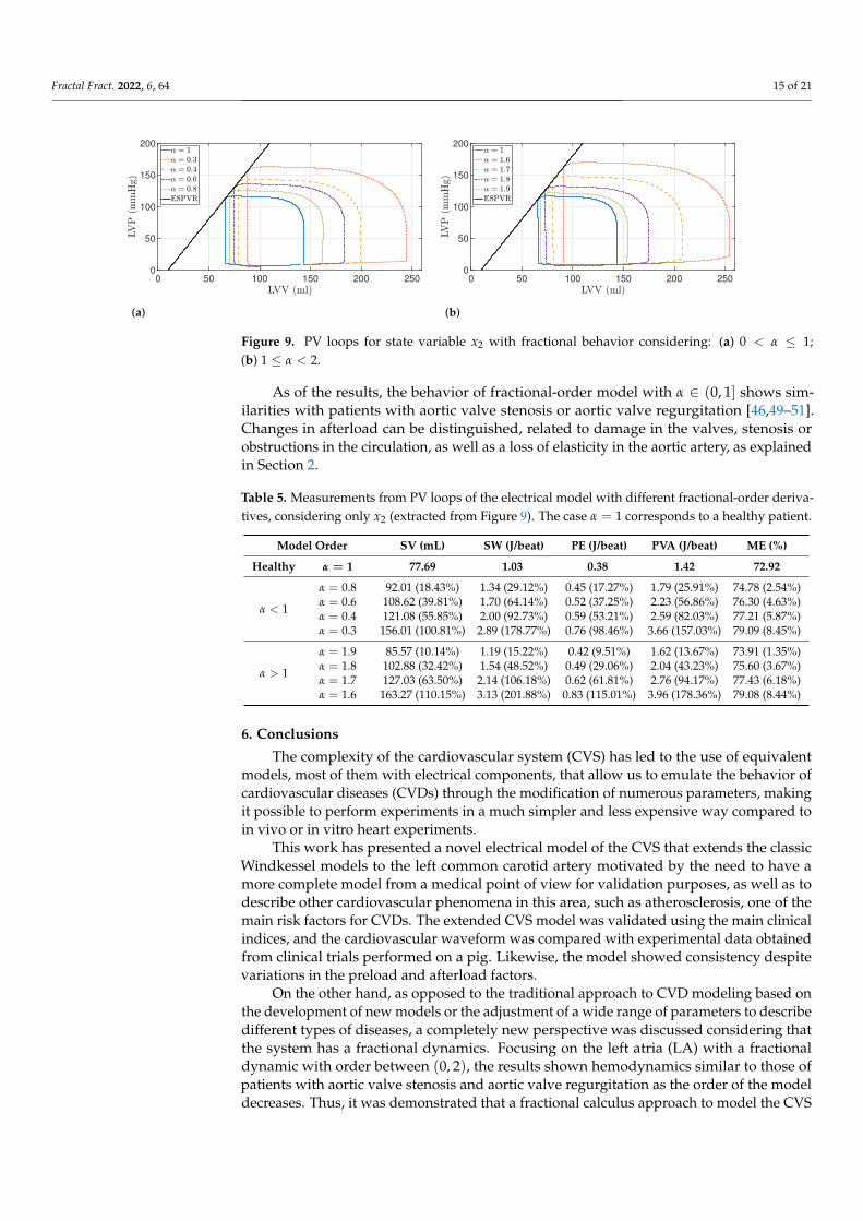
The results for values α ∈ (0, 1], depicted in Figure 9a, show that the ESPVR lineremains constant for every value of α, and thus, the contractility is not affected. The after-load and preload increase due to wider and higher loops, respectively. Table 5 shows theobtained values of the parameters indicated in Table 1, representing α = 1 the healthy case.Taking into account these results, the values of EDV and ESV increase as the order of themodel decreases, as well as the SV. The indices SW, PE, PVA and ME increase in the sameway as SV for all the models. For a better comprehension, the error rate between the healthyand the pathological cases, in percentage, has been included in Table 5 in brackets. For va-lues of α ∈ [1, 2), the model reflects a similar behavior: contractility capacity is maintained,whereas SV increases; however, an increase in pressure in the ESV is also observed. Thisincrease in pressure may be associated with valve or artery occlusion; therefore, the degreeof obstruction can be related to the fractional order, where severe states are described withvalues close to 1.

Fractal Fract. 2022, 6, 64 15 of 21Version January 17, 2022 submitted to Fractal Fract. 14 of 21

0 50 100 150 200 2500

50

100

150

200

0 50 100 150 200 2500

50

100

150

200

(a) (b)Figure 9. PV loops for state variable x2 with fractional behavior considering: (a) 0 < α2 ≤ 1, and (b) 1 ≤ α2 < 2.

volume capacity or the elasticity of LA. Replacing the above fractional behavior on444

the model described in Section 3 and detailed in Appendix A, the differential equation445

corresponding to state x2 is rewritten as:446

Dαx2 =1

CR

( 1RS

d(x3 − x2) +1

RSLC(x6 − x2)−

1RM

d(x2 − x1))

,

while the rest of equations of the CVS model keep unchanged. The completed model is447

detailed in Appendix B, where it is also considered that any compliance element may be448

subject to anomalous behavior.449

This new description of the CVS with fractional dynamics makes up a more com-450

plete model that allows to describe, not only a healthy state, but also different pathologies451

and diseases. In this sense, it is not necessary to describe a new topology or parameters452

of the models, but rather the dynamic by tunning the differentiation order. As it is also453

observed in the CVS, its elements remain constant with only slight variations, and it is454

the functionality of the heart, the ventricle, or the valves, among others, that is affected.455

5.2. Results456

For the analysis of CVD modeling PV loops are used, because a decrease in the457

capacity of the LA is shown when the LA dilates and its contractility decreases, leading458

to changes in LA preload and afterload [63,64]. Moreover, it has been demonstrated that459

LA and LV functions are strongly related, i.e., one is influenced by the other during the460

cardiac cycle, so changes in LA function can be reflected in PV loops.461

The results for values α ∈ (0, 1], depicted in Figure 9a, show that the ESPVR line462

remains constant for every value of α, and thus, the contractility is not affected. The463

afterload and preload increase due to wider and higher loops, respectively. Table 5464

shows the obtained values of the parameters indicated in Table 1, representing α = 1 the465

healthy case. Taking into account these results, the values of EDV and ESV increase as466

the order of the model decreases, as well as the SV. The indices SW, PE, PVA and ME467

increase in the same way as SV for all the models. For a better comprehension, the error468

rate between the healthy and the pathological cases, in percentage, has been included469

in Table 5 in brackets. For values of α2 ∈ [1, 2), the model reflects a similar behavior:470

contractility capacity is maintained, whereas SV increases. However, an increase in471

pressure in the ESV is also observed. This increase in pressure may be associated with472

valve or artery occlusion. Therefore, the degree of obstruction can be related to the473

fractional-order, where severe states are described with values close to 1.474

As of the results, the behavior of fractional-order model with α ∈ (0, 1] shows475

similarities with patients with aortic valve stenosis or aortic valve regurgitation [46,49–476

51]. Changes in afterload can be distinguished, related to damage in the valves, stenosis477

or obstructions in the circulation, as well as a loss of elasticity in the aortic artery, as478

explained in Section 2.479

Figure 9. PV loops for state variable x2 with fractional behavior considering: (a) 0 < α ≤ 1;(b) 1 ≤ α < 2.

As of the results, the behavior of fractional-order model with α ∈ (0, 1] shows sim-ilarities with patients with aortic valve stenosis or aortic valve regurgitation [46,49–51].Changes in afterload can be distinguished, related to damage in the valves, stenosis orobstructions in the circulation, as well as a loss of elasticity in the aortic artery, as explainedin Section 2.

Table 5. Measurements from PV loops of the electrical model with different fractional-order deriva-tives, considering only x2 (extracted from Figure 9). The case α = 1 corresponds to a healthy patient.

Model Order SV (mL) SW (J/beat) PE (J/beat) PVA (J/beat) ME (%)

Healthy α = 1 77.69 1.03 0.38 1.42 72.92

α < 1

α = 0.8 92.01 (18.43%) 1.34 (29.12%) 0.45 (17.27%) 1.79 (25.91%) 74.78 (2.54%)α = 0.6 108.62 (39.81%) 1.70 (64.14%) 0.52 (37.25%) 2.23 (56.86%) 76.30 (4.63%)α = 0.4 121.08 (55.85%) 2.00 (92.73%) 0.59 (53.21%) 2.59 (82.03%) 77.21 (5.87%)α = 0.3 156.01 (100.81%) 2.89 (178.77%) 0.76 (98.46%) 3.66 (157.03%) 79.09 (8.45%)

α > 1

α = 1.9 85.57 (10.14%) 1.19 (15.22%) 0.42 (9.51%) 1.62 (13.67%) 73.91 (1.35%)α = 1.8 102.88 (32.42%) 1.54 (48.52%) 0.49 (29.06%) 2.04 (43.23%) 75.60 (3.67%)α = 1.7 127.03 (63.50%) 2.14 (106.18%) 0.62 (61.81%) 2.76 (94.17%) 77.43 (6.18%)α = 1.6 163.27 (110.15%) 3.13 (201.88%) 0.83 (115.01%) 3.96 (178.36%) 79.08 (8.44%)

6. Conclusions

The complexity of the cardiovascular system (CVS) has led to the use of equivalentmodels, most of them with electrical components, that allow us to emulate the behavior ofcardiovascular diseases (CVDs) through the modification of numerous parameters, makingit possible to perform experiments in a much simpler and less expensive way compared toin vivo or in vitro heart experiments.

This work has presented a novel electrical model of the CVS that extends the classicWindkessel models to the left common carotid artery motivated by the need to have amore complete model from a medical point of view for validation purposes, as well as todescribe other cardiovascular phenomena in this area, such as atherosclerosis, one of themain risk factors for CVDs. The extended CVS model was validated using the main clinicalindices, and the cardiovascular waveform was compared with experimental data obtainedfrom clinical trials performed on a pig. Likewise, the model showed consistency despitevariations in the preload and afterload factors.

On the other hand, as opposed to the traditional approach to CVD modeling based onthe development of new models or the adjustment of a wide range of parameters to describedifferent types of diseases, a completely new perspective was discussed considering thatthe system has a fractional dynamics. Focusing on the left atria (LA) with a fractionaldynamic with order between (0, 2), the results shown hemodynamics similar to those ofpatients with aortic valve stenosis and aortic valve regurgitation as the order of the modeldecreases. Thus, it was demonstrated that a fractional calculus approach to model the CVS

Fractal Fract. 2022, 6, 64 16 of 21

allows us to describe a healthy state and CVD at the same time by modifying only the orderof the model, where a change of order implies a variation of the system properties.

Our future works will focus on: (1) performing a more detailed study to identify otherpossible pathologies; (2) applying fractional-order derivatives to other state variables; and(3) validating the pathology models with experimental data.

Supplementary Materials: The following are available online at https://www.mdpi.com/article/10.3390/fractalfract6020064/s1.

Author Contributions: This work involved all coauthors. J.E.T. and C.N.-G. wrote the originaldraft and contributed to the investigation and the analysis, performed the simulations, edited themanuscript and contributed to the illustrations. J.F.-P. provided support in obtaining the experimentaldata and validating the model from the medical point of view. I.T. and B.M.V. conceived the idea,contributed to the editing and supervised the manuscript. J.F.O.-M. and J.B.P. provided support inobtaining the experimental data and revised the manuscript. All authors have read and agreed to thepublished version of the manuscript.

Funding: This work has been supported in part by the Consejería de Economía, Ciencia y AgendaDigital (Junta de Extremadura) under the project IB18109 and the grant “Ayuda a Grupos de Inves-tigación de Extremadura” (no. GR18159), by the Agencia Estatal de Investigación (Ministerio deCiencia e Innovación) through the project PID2019-111278RB-C22/AEI/10.13039/501100011033, andin part by the European Regional Development Fund “A way to make Europe”.

Institutional Review Board Statement: The study was approved by the Ethical Committee of an-imal experimentation of the Jesús Usón Minimally Invasive Surgery Centre and autorized by theExtremadura Government (Number: EXP-20200518, approved on 20/05/2020). Furthermore, thisstudy was in accordance with the welfare standards based on the FELASA Guidelines.

Informed Consent Statement: Not applicable.

Data Availability Statement: Experimental data associated with this article will be made availableon request.

Acknowledgments: José Emilio Traver would like to thank the Ministerio de Educación, Cultura yDeporte its support through the scholarship no. FPU16/2045 of the FPU Program. All authors wouldlike to thank Jesús Usón Minimally Invasive Surgery Centre for offering the possibility of obtainingthe data used in this work.

Conflicts of Interest: The authors declare no conflict of interest.

AbbreviationsThe following abbreviations are used in this manuscript:

MDPI Multidisciplinary Digital Publishing InstituteCVD Cardiovascular diseaseWHO World Health OrganizationCVS Cardiovascular systemPV Pressure-volumeEDV End-diastolic volumeESV End-systolic volumeESPVR End-systolic PV relationshipEDPVR End-diastolic PV relationshipEes End-systolic elastanceEa Effective arterial elastanceSV Stroke volumeSW Stroke workPE Potential energyPVA Pressure-volume areaME Mechanical efficiencyLV Left ventricle

Fractal Fract. 2022, 6, 64 17 of 21

LA Left atriaLA Left atria volumeLVP Left ventricular pressureLVV Left ventricular volumeHR Heart rateLAP Left atrial pressureAP Descending aorta pressureAoP Ascending aorta pressureF Total flowLCP Left common carotid artery pressureLCF Left common carotid artery flow rate

Appendix A. Integer-Order CVS Model

The mathematical description of the circuit is obtained applying the Kirchoff’s circuitlaw to the electrical circuit depicted in Figure 5 and taking the state variables given inTable 3. With respect to diodes, their behavior is defined by the ramp function:

d(x) =

{x, if x ≥ 00, if x < 0

(A1)

Then, the dynamic equations of the model are obtained as follows. The state x1 isdescribed recalling the Frank–Starling’s law, which states that:

E(t) =LVP(t)

LVV(t)−V0

where LVV(t) =∫(IM − IA)dt is the charge in the capacitor, being IM and IA the currents

through the mitral diode DM and the aortic diode DA, respectively. Therefore, the state x1is defined as:

x1 = E(t)( ∫

(IM − IA)dt−V0

)

Deriving the terms on both sides of the equality and recalling that E(t) = 1/C(t) andE(t) = −C(t)/C2(t), the differential equation for x1 can be written as:

x1 = E(t)( ∫

(Im − Ia)dt−V0

)+ E(t)

ddt

∫(IM − IA)dt

x1 =1

C(t)

(− C(t)x1 +

1RM

d(x1 − x2)−1

RAd(x4 − x1)

)(A2)

Applying the Kirchoff’s first law to CR capacitor, it results that

IS = I2 + IM

where IS, I2 and IM are the currents through the systemic resistance and return from leftcommon carotid, the capacitor CR and the mitral diode DM, respectively. Using the Ohm’slaw, the currents are expressed as a function of voltage:

1RS

(x2 − x3) +1

RSLC(x2 − x3) = CR x2 +

1RM

d(x1 − x2)

Solving for x2, it obtains:

x2 =1

CR

( 1RS

d(x3 − x2) +1

RSLC(x6 − x2)−

1RM

d(x2 − x1))

(A3)

Fractal Fract. 2022, 6, 64 18 of 21

Similarly, the application of Kirchoff’s first law to the x3 node allows obtaining:

x5 = x7 +1

RS(x3 − x2) + I3

where I3 is the current through the capacitor CS. Using the Ohm’s law for I3 and solvingfor x3, it results that:

x3 =1

CS

(x5 − x7 −

1RS

d(x3 − x2))

(A4)

Doing the same analysis for capacitor CA, the sum of currents is:

IA = I4 + x5

where I4 is the current through CA. Applying the Ohm’s law and solving for x4:

x4 =1

CA

( 1RA

d(x4 − x1)− x5

)(A5)

For the differential equation of x5, the Kirchoff’s second law is employed in thex4 − x5 − x3 mesh, formulating:

x4 = Lx5 + RCx5 + x3

Solving for x5, the dynamic of the state is defined by:

x5 =1L(x4 − x3 − RCx5

)

Recalling again the Kirchoff’s first law for the node x6, the currents involved are:

x7 −1

RSLC(x6 − x2)− I6 = 0

where I6 is the current through capacitor CLC. Applying the Ohm’s law and solving for x6,it is obtained:

x6 =1

CLC

( 1RSLC

(x2 − x6) + x7

)(A6)

Finally, the differential equation for the state x7 is solved using the Kirchoff’s secondlaw for the x3 − x6 − x7 mesh:

x3 = LLC x7 + RLCx7 + x6

Solving for x7, the state equation for x7 is defined by:

x7 =1

LLC

(x3 − x6 − RLCx7

)(A7)

Appendix B. Non-Integer-Order CVS Model

The analysis of the non-integer-order model of the CVS is also developed applyingthe Kirchoff’s law to the circuit (see Figure 5), but taking into account that differentialequations use the fractional operator of order αi, i.e., each dynamic element is replaced bya fractional element. As in the integer-order case, the non-integer differential equations canbe obtained as follows.

The state x1 is described according to Frank–Starling’s law (4). In its fractional version,the left ventricular volume is defined as LVV(t) = D−α1(IM − IA)dt. Deriving both sides

Fractal Fract. 2022, 6, 64 19 of 21

of the Equation (4) and recalling that E(t) = 1/C(t) and Dα1 E(t) = −(Dα1 C(t)

)/C2(t),

the state x1 is defined as:

Dα1 x1 = Dα1 E(t)(D−α1(IM − IA)−V0

)+ E(t)Dα1D−α1(IM − IA)

Dα1 x1 =1

C(t)

(−(Dα1 C(t)

)x1 +

1RM

d(x1 − x2)−1

RAd(x4 − x1)

)(A8)

With respect to the differential equation for x2, applying the Kirchoff’s first law tofratance CR and the Ohm’s law, the currents are expressed as a function of voltage by:

1RS

(x2 − x3) +1

RSLC(x2 − x3) = CRDα2 x2 +

1RM

d(x1 − x2)

Solving the previous equation for Dα2 x2, it is obtained:

Dα2 x2 =1

CR

( 1RS

d(x3 − x2) +1

RSLC(x6 − x2)−

1RM

d(x2 − x1))

(A9)

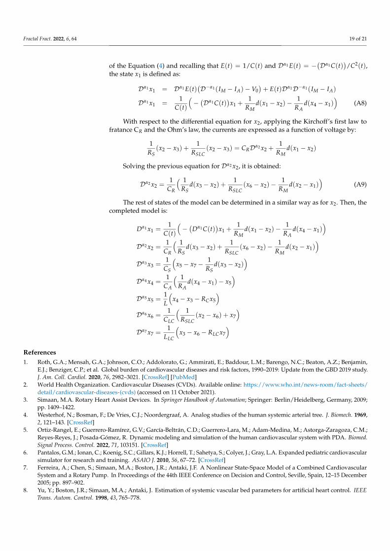
The rest of states of the model can be determined in a similar way as for x2. Then, thecompleted model is:

Dα1 x1 =1

C(t)

(−(

Dα1 C(t))x1 +

1RM

d(x1 − x2)−1

RAd(x4 − x1)

)

Dα2 x2 =1

CR

( 1RS

d(x3 − x2) +1

RSLC(x6 − x2)−

1RM

d(x2 − x1))

Dα3 x3 =1

CS

(x5 − x7 −

1RS

d(x3 − x2))

Dα4 x4 =1

CA

( 1RA

d(x4 − x1)− x5

)

Dα5 x5 =1L

(x4 − x3 − RCx5

)

Dα6 x6 =1

CLC

( 1RSLC

(x2 − x6) + x7

)

Dα7 x7 =1

LLC

(x3 − x6 − RLCx7

)

References1. Roth, G.A.; Mensah, G.A.; Johnson, C.O.; Addolorato, G.; Ammirati, E.; Baddour, L.M.; Barengo, N.C.; Beaton, A.Z.; Benjamin,

E.J.; Benziger, C.P.; et al. Global burden of cardiovascular diseases and risk factors, 1990–2019: Update from the GBD 2019 study.J. Am. Coll. Cardiol. 2020, 76, 2982–3021. [CrossRef] [PubMed]

2. World Health Organization. Cardiovascular Diseases (CVDs). Available online: https://www.who.int/news-room/fact-sheets/detail/cardiovascular-diseases-(cvds) (accessed on 11 October 2021).

3. Simaan, M.A. Rotary Heart Assist Devices. In Springer Handbook of Automation; Springer: Berlin/Heidelberg, Germany, 2009;pp. 1409–1422.

4. Westerhof, N.; Bosman, F.; De Vries, C.J.; Noordergraaf, A. Analog studies of the human systemic arterial tree. J. Biomech. 1969,2, 121–143. [CrossRef]

5. Ortiz-Rangel, E.; Guerrero-Ramírez, G.V.; García-Beltrán, C.D.; Guerrero-Lara, M.; Adam-Medina, M.; Astorga-Zaragoza, C.M.;Reyes-Reyes, J.; Posada-Gómez, R. Dynamic modeling and simulation of the human cardiovascular system with PDA. Biomed.Signal Process. Control. 2022, 71, 103151. [CrossRef]

6. Pantalos, G.M.; Ionan, C.; Koenig, S.C.; Gillars, K.J.; Horrell, T.; Sahetya, S.; Colyer, J.; Gray, L.A. Expanded pediatric cardiovascularsimulator for research and training. ASAIO J. 2010, 56, 67–72. [CrossRef]

7. Ferreira, A.; Chen, S.; Simaan, M.A.; Boston, J.R.; Antaki, J.F. A Nonlinear State-Space Model of a Combined CardiovascularSystem and a Rotary Pump. In Proceedings of the 44th IEEE Conference on Decision and Control, Seville, Spain, 12–15 December2005; pp. 897–902.

8. Yu, Y.; Boston, J.R.; Simaan, M.A.; Antaki, J. Estimation of systemic vascular bed parameters for artificial heart control. IEEETrans. Autom. Control. 1998, 43, 765–778.

Fractal Fract. 2022, 6, 64 20 of 21

9. Ferrari, G.; Di Molfetta, A.; Zielinski, K.; Fresiello, L. Circulatory modelling as a clinical decision support and an educational tool.Biomed. Data J. 2015, 1, 45–50. [CrossRef]

10. Alastruey, J.; Parker, K.; Peiró, J.; Byrd, S.; Sherwin, S. Modelling the circle of Willis to assess the effects of anatomical variationsand occlusions on cerebral flows. J. Biomech. 2007, 40, 1794–1805. [CrossRef]

11. Olufsen, M.S.; Peskin, C.S.; Kim, W.Y.; Pedersen, E.M.; Nadim, A.; Larsen, J. Numerical simulation and experimental validationof blood flow in arteries with structured-tree outflow conditions. Ann. Biomed. Eng. 2000, 28, 1281–1299. [CrossRef]

12. Sherwin, S.; Franke, V.; Peiró, J.; Parker, K. One-dimensional modelling of a vascular network in space-time variables. J. Eng.Math. 2003, 47, 217–250. [CrossRef]

13. Rosalia, L.; Ozturk, C.; Van Story, D.; Horvath, M.A.; Roche, E.T. Object-Oriented Lumped-Parameter Modeling of theCardiovascular System for Physiological and Pathophysiological Conditions. Adv. Theory Simul. 2021, 4, 2000216. [CrossRef]

14. Taylor, C.E.; Miller, G.E. Mock circulatory loop compliance chamber employing a novel real-time control process. J. Med. Devices2012, 6, 450031–450038. [CrossRef]

15. Gwak, K.W.; Paden, B.E.; Antaki, J.F.; Ahn, I.S. Experimental verification of the feasibility of the cardiovascular impedancesimulator. IEEE Trans. Biomed. Eng. 2009, 57, 1176–1183. [CrossRef]

16. Roy, D.; Mazumder, O.; Sinha, A.; Khandelwal, S. Multimodal cardiovascular model for hemodynamic analysis: Simulationstudy on mitral valve disorders. PLoS ONE 2021, 16, e0247921. [CrossRef]

17. Liu, H.; Liang, F.; Wong, J.; Fujiwara, T.; Ye, W.; Tsubota, K.I.; Sugawara, M. Multi-scale modeling of hemodynamics in thecardiovascular system. Acta Mech. Sin. 2015, 31, 446–464. [CrossRef]

18. Blanco, P.; Feijóo, R. A dimensionally-heterogeneous closed-loop model for the cardiovascular system and its applications. MedEng. Phys. 2013, 35, 652–667. [CrossRef]

19. Formaggia, L.; Quarteroni, A.; Veneziani, A. Cardiovascular Mathematics: Modeling and Simulation of the Circulatory System; MS&A;Springer: Milan, Italy, 2010.

20. Keshavarz-Motamed, Z. A diagnostic, monitoring, and predictive tool for patients with complex valvular, vascular and ventriculardiseases. Sci. Rep. 2020, 10, 6905. [CrossRef]

21. Simakov, S.S. Lumped parameter heart model with valve dynamics. Russ. J. Numer. Anal. Math. Model. 2019, 34, 289–300.[CrossRef]

22. Bozkurt, S. Mathematical modeling of cardiac function to evaluate clinical cases in adults and children. PLoS ONE 2019,14, e0224663. [CrossRef]

23. Paeme, S.; Moorhead, K.T.; Chase, J.G.; Lambermont, B.; Kolh, P.; D’orio, V.; Pierard, L.; Moonen, M.; Lancellotti, P.; Dauby, P.C.;et al. Mathematical multi-scale model of the cardiovascular system including mitral valve dynamics. Application to ischemicmitral insufficiency. Biomed. Eng. Online 2011, 10, 86. [CrossRef]

24. Mynard, J.P.; Davidson, M.R.; Penny, D.J.; Smolich, J.J. A simple, versatile valve model for use in lumped parameter andone-dimensional cardiovascular models. Int. J. Numer. Methods Biomed. Eng. 2012, 28, 626–641. [CrossRef]

25. Liu, H.; Liu, S.; Ma, X.; Zhang, Y. A numerical model applied to the simulation of cardiovascular hemodynamics and operatingcondition of continuous-flow left ventricular assist device. Math. Biosci. Eng. 2020, 17, 7519–7543. [CrossRef] [PubMed]

26. Faragallah, G.; Simaan, M.A. An engineering analysis of the aortic valve dynamics in patients with rotary left ventricular assistdevices. J. Healthc. Eng. 2013, 4, 307–327. [CrossRef] [PubMed]

27. Shimizu, S.; Une, D.; Kawada, T.; Hayama, Y.; Kamiya, A.; Shishido, T.; Sugimachi, M. Lumped parameter model for hemodynamicsimulation of congenital heart diseases. J. Physiol. Sci. 2018, 68, 103–111. [CrossRef]

28. Ježek, F.; Kulhánek, T.; Kalecky, K.; Kofránek, J. Lumped models of the cardiovascular system of various complexity. Biocybern.Biomed. Eng. 2017, 37, 666–678. [CrossRef]

29. Wang, Y.; Loghmanpour, N.; Vandenberghe, S.; Ferreira, A.; Keller, B.; Gorcsan, J.; Antaki, J. Simulation of dilated heart failurewith continuous flow circulatory support. PLoS ONE 2014, 9, e85234. [CrossRef] [PubMed]

30. Nichols, W.; O’Rourke, M.; Vlachopoulos, C. McDonald’s Blood Flow in Arteries, Sixth Edition: Theoretical, Experimental and ClinicalPrinciples; CRC Press: Boca Raton, FL, USA, 2011.

31. Sun, H.; Zhang, Y.; Baleanu, D.; Chen, W.; Chen, Y. A new collection of real world applications of fractional calculus in scienceand engineering. Commun. Nonlinear Sci. Numer. Simul. 2018, 64, 213–231. [CrossRef]

32. Magin, R.L. Fractional calculus models of complex dynamics in biological tissues. Comput. Math. Appl. 2010, 59, 1586–1593.[CrossRef]

33. Bahloul, M.A.; Laleg-Kirati, T.M. Three-Element Fractional-Order Viscoelastic Arterial Windkessel Model. In Proceedings of the2018 40th Annual International Conference of the IEEE Engineering in Medicine and Biology Society (EMBC), Honolulu, HI,USA, 17–21 July 2018; pp. 5261–5266.

34. Bahloul, M.A.; Laleg-Kirati, T.M. Arterial viscoelastic model using lumped parameter circuit with fractional-order capacitor. InProceedings of the 2018 IEEE 61st International Midwest Symposium on Circuits and Systems (MWSCAS), Windsor, ON, Canada,5–8 August 2018; pp. 53–56.

35. Perdikaris, P.; Karniadakis, G.E. Fractional-order viscoelasticity in one-dimensional blood flow models. Ann. Biomed. Eng. 2014,42, 1012–1023. [CrossRef]

36. Craiem, D.; Rojo, F.; Atienza, J.; Guinea, G.; Armentano, R.L. Fractional calculus applied to model arterial viscoelasticity. Lat. Am.Appl. Res. 2008, 38, 141–145.

Fractal Fract. 2022, 6, 64 21 of 21

37. Craiem, D.; Rojo, F.J.; Atienza, J.M.; Armentano, R.L.; Guinea, G.V. Fractional-order viscoelasticity applied to describe uniaxialstress relaxation of human arteries. Phys. Med. Biol. 2008, 53, 4543–4554. [CrossRef]

38. Doehring, T.C.; Freed, A.D.; Carew, E.O.; Vesely, I. Fractional Order Viscoelasticity of the Aortic Valve Cusp: An Alternative toQuasilinear Viscoelasticity. J. Biomech. Eng. 2005, 127, 700–708. [CrossRef]

39. Balcı, E.; Öztürk, I.; Kartal, S. Dynamical behaviour of fractional order tumor model with Caputo and conformable fractionalderivative. Chaos Solitons Fractals 2019, 123, 43–51. [CrossRef]

40. Yao, S.W.; Faridi, W.A.; Asjad, M.I.; Jhangeer, A.; Inc, M. A mathematical modelling of a Atherosclerosis intimation withAtangana-Baleanu fractional derivative in terms of memory function. Results Phys. 2021, 27, 104425. [CrossRef]

41. Traver, J.E.; Tejado, I.; Prieto-Arranz, J.; Vinagre, B.M. Comparing Classical and Fractional Order Control Strategies of aCardiovascular Circulatory System Simulator. IFAC-PapersOnLine 2018, 51, 48–53. [CrossRef]

42. Nuevo-Gallardo, C.; Traver, J.E.; Tejado, I.; Vinagre, B.M. Modelling Cardiovascular Diseases with Fractional-Order Derivatives;Springer: Berlin/Heidelberg, Germany, 2022.

43. Martini, F.; Nath, J.; Bartholomew, E. Fundamentals of Anatomy & Physiology; Benjamin-Cummings Publishing Company: SanFrancisco, CA, USA, 2015.

44. Texas Heart Institute. Carotid Artery Disease. Available online: https://www.texasheart.org/heart-health/heart-information-center/topics/carotid-artery-disease/ (accessed on 13 October 2021).

45. Goldstein, J.A.; Kern, M.J. Principles of Normal Physiology and Pathophysiology. In Hemodynamic Rounds; John Wiley and Sons,Ltd.: Hoboken, NJ, USA, 2018; Chapter 1, pp. 1–34.

46. Bastos, M.B.; Burkhoff, D.; Maly, J.; Daemen, J.; den Uil, C.A.; Ameloot, K.; Lenzen, M.; Mahfoud, F.; Zijlstra, F.; Schreuder,J.J.; et al. Invasive left ventricle pressure–volume analysis: Overview and practical clinical implications. Eur. Heart J. 2020,41, 1286–1297. [CrossRef]

47. Hall, J.E. Guyton and Hall Textbook of Medical Physiology; Elsevier Health Sciences: Amsterdam, The Netherlands, 2015.48. Silverthorn, D.U.; Ober, W.C.; Garrison, C.W.; Silverthorn, A.C.; Johnson, B.R. Human Physiology: An Integrated Approach;

Pearson/Benjamin Cummings: San Francisco, CA, USA, 2009.49. Nishimura, R.A. Aortic Valve Disease. Circulation 2002, 106, 770–772. [CrossRef]50. Itu, L.; Sharma, P.; Suciu, C. Patient-Specific Hemodynamic Computations: Application to Personalized Diagnosis of Cardiovascular

Pathologies; Springer: Berlin/Heidelberg, Germany, 2017; pp. 1–227.51. Paul, A.; Das, S. Valvular heart disease and anaesthesia. Indian J. Anaesth. 2017, 61, 721–727. [CrossRef]52. Lee, T.C.; Huang, K.F.; Hsiao, M.L.; Tang, S.T.; Young, S.T. Electrical lumped model for arterial vessel beds. Comput. Methods

Programs Biomed. 2004, 73, 209–219. [CrossRef]53. Otto, F. Die grundform des arteriellen pulses. Ztg. Fur Biol. 1899, 37, 483–586.54. Westerhof, N.; Lankhaar, J.; Westerhof, B.E. The arterial Windkessel. Med Biol. Eng. Comput. 2009, 47, 131–141. [CrossRef]55. Breitenstein, D.S. Cardiovascular Modeling: The Mathematical Expression of Blood Circulation. Master’s Thesis, University of

Pittsburgh, Pittsburgh, PA, USA, 1993.56. Suga, H.; Sagawa, K. Instantaneous pressure-volume relationships and their ratio in the excised, supported canine left ventricle.

Circ. Res. 1974, 35, 117–126. [CrossRef] [PubMed]57. Stergiopulos, N.; Meister, J.; Westerhof, N. Determinants of stroke volume and systolic and diastolic aortic pressure. Am. J.

Physiol. Heart Circ. Physiol. 1996, 270, H2050–H2059. [CrossRef] [PubMed]58. Pacher, M.A.A.; Cingolani, H. Modelo de Ventrículo Izquierdo. Ph.D. Thesis, Universidad Católica de Córdoba, Córdoba,

Argentina, 1997.59. Sheffer, L.; Santamore, W.P.; Barnea, O. Cardiovascular Simulation Toolbox. Cardiovasc. Eng. 2007, 7, 81–88. [CrossRef] [PubMed]60. Westerhof, N.; Stergiopulos, N.; Noble, M. Snapshots of Hemodynamics: An Aid for Clinical Research and Graduate Education; Springer

Science & Business Media: Berlin/Heidelberg, Germany, 2010.61. Ltd., L. Normal Hemodynamic Parameters. Available online: http://www.lidco.com/clinical/hemodynamic.php (accessed on

20 September 2021).62. Monje, C.; Chen, Y.; Vinagre, B.; Xue, D.; Feliu, V. Fractional Order Systems and Control-Fundamentals and Applications; Springer:

Berlin/Heidelberg, Germany, 2010.63. Blume, G.; Mcleod, C.; Barnes, M.; Seward, J.; Pellikka, P.; Bastiansen, P.; Tsang, T. Left atrial function: Physiology, assessment,

and clinical implications. Eur. J. Echocardiogr. 2011, 12, 421–430. [CrossRef]64. Rosca, M.; Lancellotti, P.; Popescu, B.A.; Pierard, L. Left atrial function: Pathophysiology, echocardiographic assessment, and

clinical applications. Heart 2011, 97, 1982–1989. [CrossRef]