Carbon stocks on forestland of the United States,with emphasis on USDA Forest Service ownership

LINDA S. HEATH,1,4,� JAMES E. SMITH,1 CHRISTOPHER W. WOODALL,2 DAVID L. AZUMA,3

AND KAREN L. WADDELL3

1USDA Forest Service, Northern Research Station, Durham, New Hampshire 03824 USA2USDA Forest Service, Northern Research Station, St. Paul, Minnesota 55108 USA

3USDA Forest Service, Pacific Northwest Research Station, Portland, Oregon 97205 USA

Abstract. The U.S. Department of Agriculture Forest Service (USFS) manages one-fifth of the area of

forestland in the United States. The Forest Service Roadmap for responding to climate change identified

assessing and managing carbon stocks and change as a major element of its plan. This study presents

methods and results of estimating current forest carbon stocks and change in the United States for public

and private owners, consistent with the official 2010 U.S. greenhouse gas inventory, but with improved

data sources for three states. Results are presented by National Forest System region, a major

organizational management unit within the Forest Service, and by individual national forest. USFS

forestland in the United States is estimated to contain an average of 192 Mg C/ha (megagrams carbon per

hectare) on 60.4 million ha, for a total of 11,604 Tg C (teragrams C) in the year 2005. Privately-owned

forestland averages 150 Mg C/ha on 173.8 million ha, with forestland of other public owners averaging 169

Mg C/ha on 43.1 million ha. In terms of change, private and USFS ownerships each sequester about a net

150 Tg CO2/yr, but an additional 92 Tg CO2/yr is stored in products from private harvests compared to

about 3 Tg CO2/yr from harvest on USFS land. Emissions from other disturbances such as fires, as well as

corresponding area estimates of disturbance are also important, but the needed datasets are not yet

available. Recommendations are given for improving the estimates.

Key words: carbon density; carbon in HWP; forest carbon accounting; Forest Inventory and Analysis; greenhouse gas

inventory; National Forest System; uncertainty analysis.

Received 11 October 2010; revised 6 December 2010; accepted 7 December 2010; published 19 January 2011.

Corresponding Editor: D. P. C. Peters.

Citation: Heath, L. S., J. E. Smith, C. W. Woodall, D. L. Azuma, and K. L. Waddell. 2011. Carbon stocks on forestland of

the United States, with emphasis on USDA Forest Service ownership. Ecosphere 2(1):art6 doi:10.1890/ES10-00126.1

Copyright: � 2011 Heath et al. This is an open-access article distributed under the terms of the Creative Commons

Attribution License, which permits restricted use, distribution, and reproduction in any medium, provided the original

author and sources are credited.4 Present address: Global Environment Facility, Washington, D.C. 20433 USA.

� E-mail: Lheath@fs.fed.us

INTRODUCTION

Forty-four percent of the area of forestland ofthe United States is in public ownership. TheFederal Government controls one-third of all U.S.forestland, with the USDA Forest Service (USFS)managing one-fifth of all U.S. forestland, makingit the primary owner of Federal forestland in theUnited States (Smith et al. 2009). Thus, manage-ment of these forests can substantially affect the

total forest carbon stocks and change in theUnited States. Recognizing this, the second offour strategic goals of the 2010–2015 USDAstrategic plan (USDA 2010) is to ensure nationalforests and private working lands are conserved,restored, and made more resilient to climatechange, including mitigation considerations. Tohelp implement this plan, the USFS roadmap forresponding to climate change (USDA FS 2010a)identified assessing and managing carbon stocks

v www.esajournals.org 1 January 2011 v Volume 2(1) v Article 6

and change as a major element of its plan. Joyceet al. (2008) discuss potential adaptation ap-proaches and mitigation tradeoffs that the USFSmight adopt to help achieve its goals, but carbonestimates are not included.

Estimates of carbon stocks and change are alsoimportant for other ownerships. The USDAStrategic Plan (USDA 2010) includes the idea ofan ‘‘all-lands’’ approach to U.S. forest manage-ment, which means considering the context ofother ownerships across the landscape whenmaking management decisions on USFS land. Ithas long been known that forest conditions candiffer significantly by ownership, and thatlandowner behavior will continue to affect futureconditions (e.g., Nabuurs et al. 2007), includingforest carbon stocks and change. Ownership mayalso play a factor in carbon finance, with apopular discussion treating publicly owned landdifferently than private (e.g., Olander et al. 2010).

The goal of this study is to derive and presentestimates of forest carbon stocks and change inthe United States by major ownership, with afocus on USFS forestland to help meet the needsof the USFS climate change roadmap. Theestimates are consistent with the 2010 officialU.S. greenhouse gas (GHG) inventory, which isimportant because having several sets of ‘‘offi-cial’’ estimates raises doubts about their accuracy.The U.S. GHG inventory is published annuallyby the U.S. Environmental Protection Agency(USEPA) for all sectors including the forest sector(e.g., USEPA 2010). For forests, these inventoriesinclude forest carbon stocks in units of carbon, aswell as net sequestration in units of carbon andalso in units of carbon dioxide equivalent. Theinventories have been required since the UnitedStates ratified the United Nations FrameworkConvention on Climate Change in the early1990s. By signing, the United States agreed toprovide an annual inventory of carbon stocksand carbon change, with base year 1990. Theprotocols and guidance have evolved over time(IPCC 2003, 2006) based on experience, evolvingpolicy interests, and new technology and scien-tific information. For more information about theoverall U.S. GHG forest inventory, also see Heathet al. (in press) or USEPA (2010).

Older state-level estimates are available (e.g.,USDA 2008), but estimates have not been derivedpreviously by major ownership by major USFS

organizational unit. Forest carbon stocks forUSFS forestland can be calculated using theCOLE suite of web tools (Van Deusen and Heath2010a), such as reported in Ingerson and Ander-son (2010). However, COLE uses a differentalgorithm for statistical analysis (Van Deusenand Heath 2010b) than that currently used in theofficial GHG inventories, and the tool does notyet provide change estimates and uncertainties.The USFS Forest Inventory and Analysis (FIA)program also has tools (USDA FS 2010b) whichcan provide forest carbon stocks by individualnational forest unit. These tools also do notproduce needed estimates because they includenewer algorithms that have not been incorporat-ed into the official GHG inventories such asbiomass equations by Heath et al. (2008), do notinclude carbon change for all states, or focus onannualized data so that not all needed data areincluded.

Although baseline forest stock estimates areimportant, information about the source and fateof harvested wood carbon, such as carbon storedin products or wood burned for energy, can alsobe important when considering carbon benefitsfrom forests. For instance, Heath et al. (in press)note that a recent average 205 teragrams carbondioxide (Tg CO2) has been emitted from woodburned for energy (see last five years of USEPAGHG inventories). If this wood had been leftstanding in the forest, forest carbon stocks wouldincrease, but an additional equivalent amount ofemissions could have been released instead ifmore fossil fuel was burned as the substitutesource of the needed energy. Studies of futureactions to increase carbon mitigation benefitsshould consider all sectors related to forests, aswell as life cycle assessments to inform manage-ment actions. Given the lack of baseline forestcarbon stock information for National ForestSystem (NFS) land and recent improvements inmethodologies and updates in FIA plot data, inthis study we focus on baseline forest carbonstocks and net sequestration, but also provide arudimentary estimate of carbon contributionsfrom harvested wood products (HWP) for amore thorough understanding of the carbonsystem. Explicit information about emissionsfrom other disturbances such as fire, and theircorresponding area disturbed, are also impor-tant, however data sources were not quite yet

v www.esajournals.org 2 January 2011 v Volume 2(1) v Article 6

HEATH ET AL.

available for this study.

METHODS

Definitions and unitsForestland as defined here is ‘‘Land at least

36.6 meters wide and 0.405 hectare in size with atleast 10% cover (or equivalent stocking) by livetrees of any size, including land that formerlyhad such tree cover and that will be naturally orartificially regenerated’’ (Smith et al. 2009). Allcarbon pools on forestland are included (Smith etal. 2006): above- and belowground live treebiomass, understory vegetation, standing deadtrees, down dead wood, forest floor, and soilorganic carbon to the depth of one meter. (SeeAppendix A: Table A1 for definitions of compo-nent pools.) Carbon in HWP is the sum ofchanges in products in use, and changes incarbon in landfills. For reporting carbon change,we convert carbon to units of carbon dioxide bymultiplying by 44/12 (the molecular weight ofCO2/C) because change in greenhouse gas

inventories is reported in terms of CO2. Indeed,the GHG inventories use units of carbon dioxideequivalents, CO2e, which is a way to report onemissions for all types of GHGs, but we use thelabel CO2 for CO2e. In terms of signs, a negativeCO2 change means carbon is taken out of theatmosphere and carbon is increased in forests; apositive CO2 change means carbon is added tothe atmosphere by forest-related emissions. Thissign convention is used for consistency withnational and international GHG reporting. Wepresent stocks in terms of carbon, but when wepresent change we use units of CO2 to indicatehow atmospheric CO2 is affected by changes inforest carbon.

This study focuses on administrative NFSregions (Fig. 1), rather than strictly ecologically-based areas, because management responses willbe implemented by these regions. Regions are amajor organizational unit within the ForestService, and information summarized by regionis important for implementation and interpreta-tion. Individual national forest units within these

Fig. 1. Map of USDA Forest Service, National Forest System regions.

v www.esajournals.org 3 January 2011 v Volume 2(1) v Article 6

HEATH ET AL.

regions are also important for executing carbonmanagement activities. Forest carbon stocks,change and uncertainties are presented by NFSregion by three major ownership categories:USFS, other public (all other publicly-ownedlands including other federal ownerships, states,and municipalities), and privately-owned land.These groupings were chosen because we want-ed a minimum number of broad categories whichcovered all owners.

Forest Inventory and Analysis surveyThe FIA program is the primary source for

information about the extent, condition, statusand trends of forest resources across all owner-ships in the United States (Smith 2002). FIAapplies a nationally consistent sampling protocolwhich began implementation in the late 1990scovering all forestland in the nation following anannualized design (Bechtold and Patterson 2005).An annualized design means a statistically validsubset of plots is measured every year in a state.Several years of data may be required to includeall measurements on all forested plots within astate. The complete set of plot data provides for agreater level of precision geographically, but theaggregated data lose temporal specificity. Oneach permanent inventory plot, field crewscollect data on more than 300 variables, includingland ownership, forest type, tree species, treesize, tree condition, and other site attributes (e.g.,slope, aspect, disturbance, land use) (Smith 2002;Woudenberg et al., in press). Plot intensity formeasurements is approximately one plot forevery 2,400 ha of land (130,000 forested plotsnationally). These data are compiled, and arepublicly available via the Internet (USDA FS2010c).

The FIA data are collected on all ownerships inthe 48 conterminous states, coastal Alaska, andterritories. This study does not include forestlandin interior Alaska and Hawaii because FIA plotdata have either not been collected or are not yetavailable. Puerto Rico data were not available atthe time of this analysis. FIA plot data availablebefore the annualized implementation weresurveyed periodically, and may only be availableat the plot level rather than the tree level. Tocalculate change, an approach must include away to use these older data such that they arecomparable to the newer data.

ApproachThe current FIA survey was not designed nor

was it funded as a carbon inventory. Ourapproach is based on data taken from FIAsurveys (Bechtold and Patterson 2005), butaugmented by a set of basic models which areeither ecologically process-based or statisticalcarbon conversion models (USEPA 2010; Heathet al., in press). Smith et al. (2010) describes themethods used for estimating the density ofcarbon component pools, as well as the approachfor calculating carbon change. In general, ourapproach is to calculate carbon stocks derivedfrom the augmented FIA plot data by multiply-ing area estimates by estimates of carbon densityfor that area. For example, estimates of carbonper hectare for the permanent inventory plotslabeled as NFS ownership are multiplied by theappropriate expansion factors, and then summedover the total area of interest, such as nationalforest. Privately-owned land occasionally occurswithin national forest boundaries; an FIA plot onprivate lands is labeled as privately-owned and issummed in the private ownership. Change incarbon (also called net sequestration) is calculat-ed as the difference between consecutive stocks(each from a specific inventory), which is thendivided by the number of years in the periodbetween the stocks. This approach provides a netannual difference and is known as the stock-change approach.

We used procedures from the computerapplication of Smith et al. (2010), although weduplicated the code in SAS (SAS Institute 2003)to produce consistent estimates by ownership forNFS regions and for individual national forests.An additional step was included to review thedata for consistency in terms of ownership andnational forest designation. About 0.1% of theUSFS field plots did not include a valid nationalforest designation, but these were assigned basedon state or county codes. Methods and datasources are the same as those in USEPA (2010)with one exception. Data from the IntegratedDatabase (IDB, Waddell and Hiserote 2005) wereused for the older forest inventories for Califor-nia, Oregon, and Washington in place of thecorresponding data used for those states asidentified in USEPA (2010). Previously, we hadfocused on using national-level datasets, but werecently recognized that the older data in the IDB

v www.esajournals.org 4 January 2011 v Volume 2(1) v Article 6

HEATH ET AL.

were more consistent with the current annual-ized data for these states, which is a crucialconsideration for the inventory-based methodsused for change (Smith et al. 2010). Recent GHGreporting (USEPA 2010, and similar previousreports) included notable differences in forest-land between past and current inventories forCalifornia, although analyses could not attributethe differences to any specific cause. Incorporat-ing data from the IDB into the GHG inventoryremoved this apparent discontinuity. We appliedadditional updates to the publicly available IDBon parts of 63 plots in eastern Oregon that werepredominantly the juniper forest type becauseguidelines for classifying these plots hadchanged over the last 12 years. The modificationmade the older data more comparable withcurrent inventories in terms of the basis fordetermining forestland.

We do not include the soil pool whenpresenting carbon change because changes inthe land base can result in transfers of largeamounts of soil carbon to other land use whichwill appear to be losses to or gains from theatmosphere. Thus, we use and report the termnonsoil carbon which includes all pools (live treeand standing dead tree, down dead wood,understory, and forest floor) except soil. Werecognize that soil carbon on forestland remain-ing forestland may be emitting or sequesteringGHGs, but this study assumes no change in thatpool. We emphasize that both forestland areachange and carbon density (carbon per area)change can affect total carbon (Smith and Heath2010). That is, an increase in forestland area willresult in increased carbon sequestration if theaverage carbon density is not declining. Anincrease in carbon density will result in increasedcarbon sequestration even if area of forestland isconstant. A decrease in forestland area with anincrease in carbon density can result in anincrease or decrease in carbon sequestration,depending on the amount of change in eachfactor.

Carbon in harvested wood productsCarbon removed from forests as harvested

wood can also remain stored rather than return-ing to the atmosphere for a long time, dependingon the mix of wood products produced orburned as a substitute for fossil fuels. Carbon in

HWP continues to provide carbon benefits,which can be an appreciable part of the overallforest carbon budget (Heath et al., in press). Thenet annual contribution to the total forest carbonbudget depends on harvest, allocation to prod-uct, life-span, and methods of disposal (Skog2008). Analyses can also be performed todetermine the carbon value chain includingaccounting for emissions in manufacturing(Heath et al. 2010a), but the focus of this studyis carbon inventories. For comparison betweenownerships, we provide estimates of net annualstock change of carbon in harvested wooddisaggregated and associated with forests fromthe three major ownerships. The estimates werederived by multiplying national estimates ofcarbon in harvested wood (Skog 2008, USEPA2010) by proportions of harvested wood associ-ated with ownerships from the base scenario foran empirically-based U.S. forest assessment overthe same interval (Haynes et al. 2007, Heath et al.2010b).

UncertaintyEstimates of uncertainty in total forest carbon

stocks and change are based on Monte Carlosimulations (IPCC 2006) of the stock-changemethods from Smith et al. (2010), which weremodified for estimates corresponding to ownerby NFS region and individual national forestunit. The resulting confidence intervals representthe bounds of the central 95% of the distributionproduced from numerical simulations. For easeof comparison, we present the bounds as averagepercentages about the mean. Uncertainty in-cludes inventory-to-carbon conversion factorsand sampling error. Uncertainties about plot-level carbon conversion factors are defined asprobability densities defining carbon density(megagrams carbon per hectare, Mg C/ha) bypool (Smith and Heath 2001, USEPA 2010) andaggregated to national forest, or other populationtotals, by iterative sampling.

Sampling error is estimated according toBechtold and Patterson (2005) by population ofinterest. Mean carbon and uncertainty estimateswere produced for Forest Service forestland oneach national forest by state. Totals for forestsextending over more than one state are simplythe sum of the population estimates of each of thestates, because the state estimates were assumed

v www.esajournals.org 5 January 2011 v Volume 2(1) v Article 6

HEATH ET AL.

to be independent for purposes of combining thesimulated uncertainties. The same process wasfollowed for other ownerships or regional totals.These quantities do not account for all uncer-tainties. For example, the U.S. GHG inventoriesrequire a base year of 1990; inventory data priorto about the year 2000 were collected under aperiodic inventory system, and in some statesmay have not included the entire forestland basenow being surveyed. Although we have madecomparisons and adjustments between thesedatasets to reduce error (e.g., such as for thestate of Oregon with the change to and adjust-ments to the IDB), there may be other area-basedmismatches, as well as additional uncertainties.

RESULTS AND DISCUSSION

Forest carbon stocks and uncertaintiesRelevant U.S. carbon statistics include average

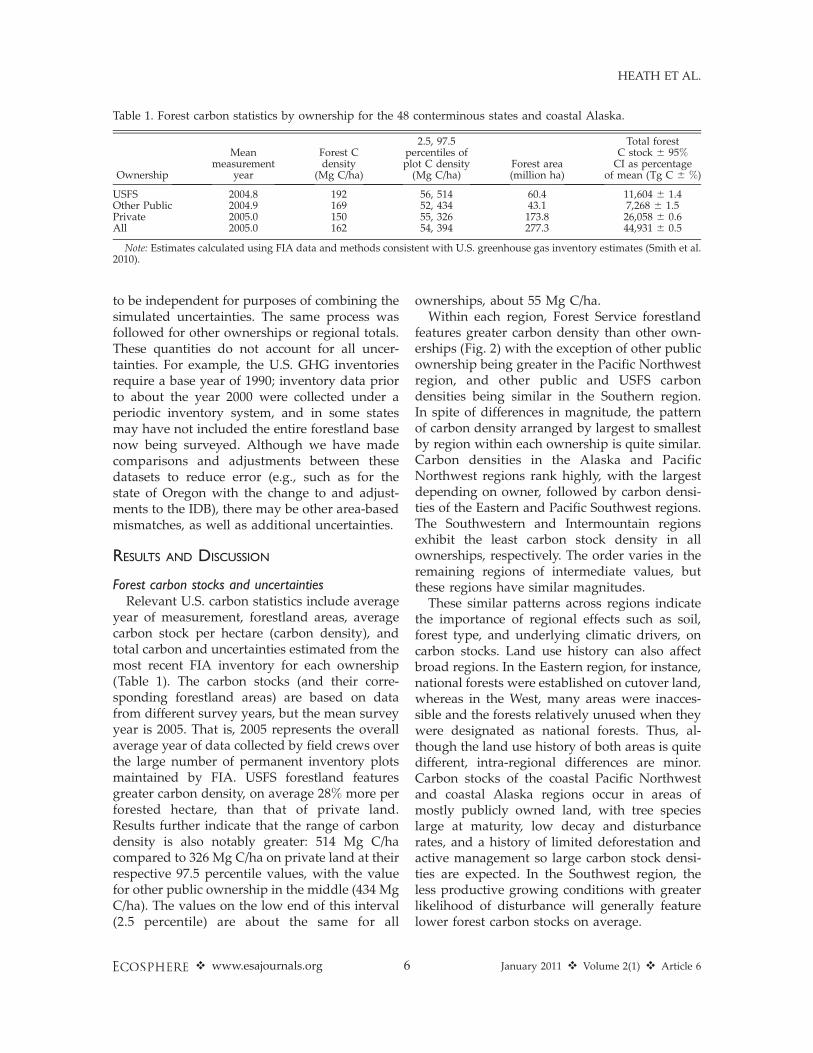
year of measurement, forestland areas, averagecarbon stock per hectare (carbon density), andtotal carbon and uncertainties estimated from themost recent FIA inventory for each ownership(Table 1). The carbon stocks (and their corre-sponding forestland areas) are based on datafrom different survey years, but the mean surveyyear is 2005. That is, 2005 represents the overallaverage year of data collected by field crews overthe large number of permanent inventory plotsmaintained by FIA. USFS forestland featuresgreater carbon density, on average 28% more perforested hectare, than that of private land.Results further indicate that the range of carbondensity is also notably greater: 514 Mg C/hacompared to 326 Mg C/ha on private land at theirrespective 97.5 percentile values, with the valuefor other public ownership in the middle (434 MgC/ha). The values on the low end of this interval(2.5 percentile) are about the same for all

ownerships, about 55 Mg C/ha.Within each region, Forest Service forestland

features greater carbon density than other own-erships (Fig. 2) with the exception of other publicownership being greater in the Pacific Northwestregion, and other public and USFS carbondensities being similar in the Southern region.In spite of differences in magnitude, the patternof carbon density arranged by largest to smallestby region within each ownership is quite similar.Carbon densities in the Alaska and PacificNorthwest regions rank highly, with the largestdepending on owner, followed by carbon densi-ties of the Eastern and Pacific Southwest regions.The Southwestern and Intermountain regionsexhibit the least carbon stock density in allownerships, respectively. The order varies in theremaining regions of intermediate values, butthese regions have similar magnitudes.

These similar patterns across regions indicatethe importance of regional effects such as soil,forest type, and underlying climatic drivers, oncarbon stocks. Land use history can also affectbroad regions. In the Eastern region, for instance,national forests were established on cutover land,whereas in the West, many areas were inacces-sible and the forests relatively unused when theywere designated as national forests. Thus, al-though the land use history of both areas is quitedifferent, intra-regional differences are minor.Carbon stocks of the coastal Pacific Northwestand coastal Alaska regions occur in areas ofmostly publicly owned land, with tree specieslarge at maturity, low decay and disturbancerates, and a history of limited deforestation andactive management so large carbon stock densi-ties are expected. In the Southwest region, theless productive growing conditions with greaterlikelihood of disturbance will generally featurelower forest carbon stocks on average.

Table 1. Forest carbon statistics by ownership for the 48 conterminous states and coastal Alaska.

Ownership

Meanmeasurement

year

Forest Cdensity

(Mg C/ha)

2.5, 97.5percentiles ofplot C density(Mg C/ha)

Forest area(million ha)

Total forestC stock 6 95%CI as percentage

of mean (Tg C 6 %)

USFS 2004.8 192 56, 514 60.4 11,604 6 1.4Other Public 2004.9 169 52, 434 43.1 7,268 6 1.5Private 2005.0 150 55, 326 173.8 26,058 6 0.6All 2005.0 162 54, 394 277.3 44,931 6 0.5

Note: Estimates calculated using FIA data and methods consistent with U.S. greenhouse gas inventory estimates (Smith et al.2010).

v www.esajournals.org 6 January 2011 v Volume 2(1) v Article 6

HEATH ET AL.

In contrast to carbon densities, total forestcarbon is 2.2 times greater (26,058 Tg C com-pared to 11,604 Tg C; Table 1) for privately-owned land, largely because of the almost three-fold difference in forestland area (173.8 Mha(million hectares) private compared to 60.4 MhaUSFS; Table 1). At the national level, about 63%,22%, and 15% of forestland area (Table 1) is inprivate, USFS, and other public ownership. Thereare large regional differences in ownershippatterns, with notably more area of forestlandin private ownership in the Eastern and Southernregions (Fig. 3), and least in Alaska (this is asurvey of only coastal Alaska), and in theIntermountain region. If all forestland in Alaskawere surveyed, there would be substantiallymore forestland area in private and other publicownerships.

Within USFS forestland only (Table 2), thePacific Northwest region has the largest area of

forestland (9.1 Mha), followed closely by theIntermountain and Northern region, with Alaskathe least (4.4 Mha). The carbon stocks (and theircorresponding forestland areas) from differentstates are likely based on data from differentsurvey years, but the mean survey year of mostregions is similar to the mean for all USFS land,2004.8, which we round up for this discussion toyear 2005. That is, 2005 represents the overallaverage of data collected by field crews over thelarge number of permanent inventory plotsmaintained by FIA. The exception to similar yearof data collection is the Southwestern region withmean survey year of 2001 (rounded up from2000.8). Considering the ecological conditions inthe Southwest, the difference in results due to thefour-year average lag time is likely minor. Interms of uncertainties, the percent uncertaintyranges from 61% for all USFS forestland up to6% for USFS forestland in one region only.

Fig. 2. Mean forest carbon density (Mg C/ha) by ownership by National Forest System region, 2005. Horizontal

dashed line represents the overall average carbon stock on U.S. forestland, 162 Mg C/ha. Error bars indicate a

95% confidence interval of uncertainty about the regional average, from carbon conversion factors and sampling

error.

v www.esajournals.org 7 January 2011 v Volume 2(1) v Article 6

HEATH ET AL.

Uncertainty estimates should be interpreted

carefully. In this case, one percent (116.04 Tg C)

of the all USFS carbon stock is still greater in

magnitude than 6% (83.04 Tg C) of the Alaska

region USFS carbon stock.

Forests in the Alaska region have the greatest

Fig. 3. Forestland area (million hectares) by ownership summed by National Forest System region, 2005. Error

bars for a 95% confidence interval of sampling error for forest area are not included because they are too small for

the resolution of the figure.

Table 2. Forest carbon and area statistics for USDA Forest Service forestland only by National Forest System

region.

National ForestSystem region

Meanmeasurement

year

Forest Cdensity

(Mg C/ha)

2.5, 97.5percentiles ofplot C density(Mg C/ha)

Forest area(1000 ha)

Total forestC stock 6 95%CI as percentage

of mean (Tg C 6 %)

Northern 2006.2 172.0 76, 328 8,896 1,530 6 3Rocky Mountain 2004.5 158.6 56, 306 6,265 993 6 4Southwestern 2000.8 100.6 49, 254 6,371 641 6 4Intermountain 2004.9 135.3 54, 286 8,964 1,213 6 4Pacific Southwest 2005.0 222.4 63, 548 6,331 1,408 6 2Pacific Northwest 2005.2 273.3 94, 689 9,107 2,493 6 2Southern 2005.1 160.2 74, 280 5,423 869 6 4Eastern 2005.6 230.7 111, 392 4,652 1,073 6 2Alaska 2006.2 317.1 101, 607 4,363 1,384 6 6All USFS 2004.8 192.1 56, 514 60,372 11,604 6 1

Note: Estimates calculated using FIA data and methods consistent with U.S. greenhouse gas inventory estimates (Smith et al.2010).

v www.esajournals.org 8 January 2011 v Volume 2(1) v Article 6

HEATH ET AL.

carbon density for all pools averaging 317.1 MgC/ha, whereas the Southwest and Intermountainregions have the least carbon densities, at 100.6Mg C/ha and 135.3 Mg C/ha, respectively (Fig. 4).The greatest percentage of aboveground livebiomass carbon is in the Southern region (47%),and lowest (30%) in the Eastern region. TheEastern region has the highest relative soil carbon(51%), followed by the Southern region (30%),with a number of regions in the western UnitedStates in the 20–30% range. The relatively highproportion of forest carbon in forest floor in theSouthwest region is thought to be due to the useof regional models for dead wood and forestfloor pools for hardwood woodland forest types.

Within most regions (Fig. 5), forest carbonstock densities from individual national forestsare relatively similar (e.g., Southern), withdistinct patterns emerging in others. (See Appen-dix B for carbon stock statistics includinguncertainties for USFS forestland by individualnational forest.) For instance, as might beexpected, the carbon densities on the west sideof the Cascades in Oregon and Washington are

large due to the forest types, older forests, andrelatively lush growing conditions, but on theeastern side with less favorable growing condi-tions, carbon densities are relatively smaller. ThePacific Southwest region appears to show thegreatest distinctions between forests within aregion. The highest carbon densities per nationalforest are in the Pacific Northwest and PacificSouthwest regions, and the least in the semi-aridareas in the Intermountain and Southwestregions. Some forested plots fall within nationalgrasslands or other USFS administered lands,and these are included (as additional USFS areasin Appendix B.)

National forest units are not randomly locatedacross the landscape (Fig. 5). For example, theforests are bunched together in much of the West,in mountainous terrain where forests are morelikely to occur or where land had not yet beensettled upon before establishment of the nationalforests. In the Southern region, only 5% of theforestland is in USFS ownership, with 88% inprivate ownership varying from highly produc-tive forestland intensively managed for timber

Fig. 4. Mean forest carbon density (Mg C/ha) by component pools for USDA Forest Service forestland only by

National Forest Service region, 2005. Biomass includes live trees and understory vegetation.

v www.esajournals.org 9 January 2011 v Volume 2(1) v Article 6

HEATH ET AL.

production, to areas of woodlands in west Texas

managed predominantly for grazing. Given this

diversity of forest ecosystems, climate, produc-

tivity, ownership patterns and local preferences,

effective, preferred management activities to

increase carbon benefits will likely need to differ

regionally if not by individual forest.

Net CO2 change and carbon in harvested woodproducts

Over the period 2000–2008, private and USFS

forests sequester about 30% of total average

annual nonsoil net CO2, with other public

forestland accounting for 38% (Table 3). Most of

the statistically significant net sequestration on

NFS land is occurring in the Pacific Northwest

and Southern regions, with net sequestration on

other public and privately owned forestland

higher in the Eastern and Southern regions (Fig.

6). Error bars of 95% confidence indicate relative

large uncertainties with estimates for a number

of the regions not significantly different from

zero. Change is not calculated for forestlandunits smaller than regions because the carbon

changes on smaller areas will likely not be

significantly different from zero.

The increase on other public forestland is duein large part to the estimated increase in

forestland (0.45 million ha/yr) over this period.

Additional data exploration (results not shown)

did not identify specific regions of the United

States or unusual circumstances for this increase.

USFS forest area also increased although the rate

of increase was almost one-quarter of that of

Fig. 5. Mean forest carbon density (Mg C/ha) by individual USDA Forest Service unit, 2005. Shaded areas

indicate national forest or grassland administrative boundaries, and color indicates carbon stock density (Mg C/

ha) category on the Forest Service owned forestland within those areas. Data are not available for Hawaii; data

for Puerto Rico were not available at the time of this analysis.

v www.esajournals.org 10 January 2011 v Volume 2(1) v Article 6

HEATH ET AL.

other public land. Some of this increase may be

due to definitional changes in the FIA survey

over this period, or an artifact of the change from

the periodic to the annualized survey emphasiz-

ing the need to have reconciled FIA datasets

available for analysis of trends.

Net nonsoil change over 2000–2008 of�481 Tg

CO2/yr (Table 3) is about 8% lower than the

corresponding USEPA (2010) 9-year average of

�522 Tg CO2/yr. A minor part of this difference is

Table 3. Average net forest ecosystem and products carbon stock change by ownership over the period 2000–

2008.

Ownership

Nonsoil forestecosystem netcarbon stock

change (Tg CO2/yr)

Uncertainty of netstock change (95% CI

as percentageof mean, %)

Carbon inharvested woodproducts net

change (Tg CO2/yr)

Mean annualchange in forestarea (1000 ha/yr)

USFS �147.3 640 �2.9 107.1Other Public �184.6 628 �6.1 449.0Private �149.2 641 �92.1 �77.2All �481.1 622 �101.1 478.9

Notes: Negative net carbon change indicates less CO2 in the atmosphere and more in the forest. Negative area changeindicates decreasing forest area. Estimates calculated using FIA data and methods consistent with U.S. greenhouse gasinventory estimates (Smith et al. 2010).

Fig. 6. Average annual net sequestration (Tg CO2/yr) in forests by ownership and National Forest System

region over the period 2000–2008. Note that negative values indicate more CO2 is being sequestered by forests

than is being emitted to the atmosphere. Error bars indicate a 95% confidence interval of uncertainty about the

regional average, from carbon conversion factors and sampling error. (Data values listed in Appendix C.)

v www.esajournals.org 11 January 2011 v Volume 2(1) v Article 6

HEATH ET AL.

the effect of disaggregating the stock-changecalculations beyond the structure defined inSmith et al. (2010) to include the three owner-ships. However, most of the difference from theresults of the USEPA (2010) report is the effect ofusing data from the IDB (Waddell and Hiserote2005) for the Pacific Coast states.

Beyond the forest boundary, additional carboncontinues to be stored in HWP, with notableamounts attributed to harvest on privatelyowned land (Table 3; total carbon sequesteredin forests and stored in HWP on average isestimated by summing columns 1 and 3).Products from harvests on private land continueto store an additional 62% of the net carbonsequestration on private forestland, whereas theincrease is 3% at most on publicly owned land.Including the continued storage in HWP resultsin private forestland (and their harvested woodproducts) contributing to 41% of total forestsector carbon sequestration, with USFS at 26%and other public dropping to 33%. Althoughcarbon in HWP from USFS land is minor,considering this pool is important in the contextof landscape-scale management because ceasingharvests in one large area often results inincreasing harvests elsewhere, if demand forproducts remains the same.

Other fates of forest carbon can also besubstantial. We do not present change estimatesfrom carbon benefits from harvested carbon thatwas burned for energy as a substitute for fossilfuel which can be notable for some ownerships.That is, trees harvested for this purpose havebeen subtracted from the amount in the forest,but we have not recognized that this loss mayhave positive benefits of substituting for fossilfuel emissions. Emissions of CO2 from forestwildfires and prescribed burning on averagerival those from emissions from wood burnedfor energy, but we currently do not have theseemissions partitioned by ownership, or by landcover (e.g., forestland or rangeland).

UncertaintyThe relative uncertainties for total forest

carbon stocks are much larger for the individualnational forests (usually in the range 8–25%) ascompared to the regional uncertainties (2–6%),especially those with a smaller area of forestlandor small total carbon. The larger uncertainties are

mainly due to the smaller sample size on smallerareas, but may also be due to uncertainty of datasources. For ease of comparisons, we reporttabular summaries of uncertainties (Table 2;Appendix B tables) as though the bounds aresymmetric, which would be unlikely. However,asymmetry is small, less than 2% off of the meanfor the largest percentages (Table 2) and asym-metry averages under 0.5% off of the mean forindividual national forests in the Appendix Btables.

By comparison, the percent uncertainty aboutestimates of net sequestration are relatively large.One aspect of this uncertainty is the sensitivity ofsmall change between relatively large stocks. Forexample, an additional annual increment of stockequivalent to only 0.1% of current nonsoil carbonstock in the Pacific Southwest region (data notshown) would produce a response of a 33%increase in calculated stock-change (Fig. 6). Acontributing factor to the large percentagedifference in this example is that the change isrelatively close to zero, which further emphasizesthe importance of consistent forest and carbonstock representation between successive invento-ries when examining inventory trends.

Discussion of methodology and possibleimprovements

Forest carbon estimates based on augmentedFIA data have long been considered the standardfor landscape level and larger forestland (e.g.,Pacala et al. 2001, Smith et al. 2006, USEPA GHGinventories, Climate Action Reserve 2010). Ad-vantages of using FIA data are: it has a national-level statistically sound design, the data arepublicly available (with some exceptions relatedto precise location and specific owner), the dataare collected in partnership with state forestryagencies and all major forest components whichrelate to carbon are measured or sampled.However, the survey was not designed specifi-cally for carbon estimation, so additional work isneeded to ensure an efficient framework forcarbon stocks and GHG changes. Further, sampleprecision was designated for state-level report-ing, thus, using these data to represent smallerareas such as individual national forests resultsin higher uncertainties. Consequently, even mod-erate increases in carbon benefits from manage-ment activities may not differ statistically from

v www.esajournals.org 12 January 2011 v Volume 2(1) v Article 6

HEATH ET AL.

zero.A number of near-term improvements could

be made to the existing framework for use infuture U.S. GHG inventories to reduce uncer-tainties and align estimates more closely withmeasured data. These include: using recentmeasurements from a subset of the plots ofnon-live tree pools such as standing dead trees,down dead wood, as well as samples of forestfloor carbon and soil organic carbon; using amore recent tree biomass equation approachbased on regional net volume estimates (Heathet al. 2008) for trees that was recently adopted inFIA’s national publicly available database (USDA2010c; Woudenberg et al., in press); accounting forresults from FIA field data recently available forthe national forest in Puerto Rico; and deliveringthe information produced by the computerapplication CCT (Smith et al. 2010) used in theU.S. GHG inventories via an online tool. Theresulting well-documented online site could thenautomatically produce forest carbon stock andchange estimates for areas chosen by users. Onechallenge in these improvements is that thecarbon changes for the U.S. GHG inventoriesare required to begin with 1990 carbon change,and older surveys generally do not include non-tree measurements. It is crucial that carbonestimates for these older surveys be derived tobe consistent with newer data. Furthermore,some of the older data are only available at theplot-level, so biomass carbon estimates for theolder surveys are also needed that are compara-ble with the newer tree-level data.

In the longer-term, as FIA plots continue to beremeasured, change estimates for most nationalforests in the future should become available at aprecision that allows for change to be detectedwith increased precision. Remeasured plots willallow for gross growth sequestration to becalculated, which is information that will revo-lutionalize the use of FIA field plots in analysis.However, these data will still be limited tempo-rally with remeasurements occurring 5 or 10years apart, such that growth cannot be attribut-able to a specific year. Coupling these growthmeasures with the use of geospatially-specificdatasets (which are under development) will beespecially powerful for explicitly accounting fordisturbances. One annual dataset under devel-opment by the Monitoring Long-Term Burn

Severity project (Eidenshenk et al. 2007) willallow forest wildfire emissions to be calculatedexplicitly by cover type and ownership. Anotherrelevant dataset is the National Land CoverDataset (MRLC 2010), available for the years1991 and 2002, with work ongoing for the year2006. One important lesson learned from thisanalysis is that, no matter what sources are used,data should be carefully screened for impacts ofchanging definitions. Using the dataset tailoredfor the three Pacific Coast states changed nationalnet sequestration by 8%, a notable amount.

Although this study focused on forestland,management activities on all lands are capable ofemitting or sequestering GHGs, including non-CO2 gases. For instance, wetlands or peatlands inparticular can feature much higher carbondensities than forests. Monitoring all land coversand uses with activities that cause significantGHG emissions or sequestration should beconsidered. We have not discussed livestockemissions, but USFS land (and land under otherownerships) can include grazing. Significantlivestock activity should be considered for baseGHG emissions. Finally, because land manage-ment can produce multiple environmental bene-fits on the same land area, the process for makingany inventory and monitoring improvements forcarbon should also consider other importantbenefits.

CONCLUSIONS

Forestland under USFS ownership features thelargest average carbon density among owner-ships, approximately 192 Mg C/ha in the year2005, which is about 28% greater than that ofprivate forestland. All carbon component poolsare included: live and dead standing trees, downwood, forest floor and soil. In terms of totalcarbon stocks, however, private forests containmore carbon: 58%, 26% and 16% of the totalforest carbon is in private, USFS, and other publicownership, reflecting the fact at the national levelthe majority ownership of area of U.S. forestlandis private, about 63% compared to 22% and 15%for USFS and other public.

However, over the period 2000–2008, USFSand private lands have similar total net carbonsequestration in forests (not including soil carboneffects), sequestering about�148 Tg CO2/yr each,

v www.esajournals.org 13 January 2011 v Volume 2(1) v Article 6

HEATH ET AL.

with 40% uncertainty. If carbon in HWP is alsoaccounted for, private lands contribute to anadditional�92 Tg CO2/yr sequestered comparedto an additional�3 Tg CO2/yr from USFS lands.Other public ownerships indicate a larger totalnet sequestration of �185 Tg CO2/yr, heavilyinfluenced by an estimated notable increase inforest area over the period. We could notpinpoint any specific reason or particular regionfor this estimated forest area increase, so we lookto future studies for more information about thisunexpected increase.

In spite of differences between ownerships, thepattern of carbon density arranged by largest tosmallest by region within each ownership is quitesimilar. This shows the importance of regionaleffects such as soil and forest type, and under-lying climatic drivers. However, the pattern oftotal average annual sequestration by ownershipby region differs because totals are influencedgreatly by amount of forest area. The largest netsequestration rates are in the Eastern andSouthern regions for private and other publicownerships, whereas the largest net rates in thePacific Northwest followed by the Southern andthen Rocky Mountain region for USFS owner-ship. Due to the large uncertainties in changecalculations, change for most of the other regionsis not statistically different from zero.

The greatest gains in mitigation effects mini-mize net carbon dioxide emissions to theatmosphere. Because forest carbon has carbonbenefit effects beyond forestland boundaries,managing simply to maximize forestland carbondensity is not necessarily the same as minimizingforest emissions to the atmosphere (or maximiz-ing net sequestration) during the time frame ofinterest. That is, a strategy focusing on onlyincreasing forestland carbon density on a limitedarea over time may produce limited carbonbenefits compared to a more comprehensivestrategy.

These carbon densities and forest areas by NFSregion and individual national forest (AppendixB) could be used as preliminary base estimatesfor planning adaptation and mitigation activities.To consider the effects of specific silviculturalregimes, a tool such as the Forest VegetationSimulator (Crookston and Dixon 2005) could beused to project plots into the future; carbon inforests and harvested wood products is an

output (Hoover and Rebain 2008). A variety ofmanagement activities will be needed to increasecarbon benefits in USFS lands across the matrixof ecological, physical, and social conditions,especially when management needs for adapta-tion are a primary concern. However, demandsand management choices on other ownershipsshould be a consideration in enhancing carbonbenefits. A national-level forest futuring analysisthat includes carbon outputs such as Heath andBirdsey (1993) and USEPA (2005), as well asclimate change effects (Joyce et al. 1995), andglobal trade (Ince et al. 2007) would help ensurethe major effects of large-scale processes areincluded.

ACKNOWLEDGMENTS

We thank Elizabeth LaPoint, USDA Forest Service,National FIA Spatial Data Services, Durham, NH, forher expertise in FIA data and map making, and threeinternal reviewers. We acknowledge the work of manyexcellent field crews, information management spe-cialists, and analysts of the USDA Forest Service,Forest Inventory and Analysis for their daily dedica-tion to providing quality data. Without their efforts,this study would not have been possible.

LITERATURE CITED

Bechtold, W. A., and P. L. Patterson, editors. 2005. Theenhanced Forest Inventory and Analysis pro-gram—national sampling design and estimationprocedures. SRS GTR-80. USDA Forest Service,Southern Research Station, Asheville, North Caro-lina, USA.

Climate Action Reserve. 2010. Forest project protocol,version 3.2. hhttp://www.climateactionreserve.org/wp-content/uploads/2009/03/Forest_Project_Protocol_Version_3.2.pdfi

Crookston, N. L., and G. E. Dixon. 2005. The ForestVegetation Simulator: A review of its structure,content, and applications. Computers and Elec-tronics in Agriculture 49:60–80.

Eidenshenk, J., B. Schwind, K. Brewer, Z. Zhu, B.Quayle, and S. Howard. 2007. A project formonitoring trends in burn severity. Fire Ecology3:3–21.

Haynes, R. W., D. M. Adams, R. J. Alig, P. J. Ince, J. R.Mills, and X. Zhou. 2007. The 2005 RPA timberassessment update. PNW GTR-699. USDA ForestService, Pacific Northwest Research Station, Port-land, Oregon, USA.

Heath, L. S., and R. A. Birdsey. 1993. Impacts ofalternative forest management policies on carbon

v www.esajournals.org 14 January 2011 v Volume 2(1) v Article 6

HEATH ET AL.

sequestration on U.S. timberlands. World ResourceReview 5:171–179.

Heath, L. S., M. H. Hansen, J. E. Smith, W. B. Smith,and P. D. Miles. 2008. Investigation into calculatingtree biomass and carbon in the FIADB using abiomass expansion factor approach. In W. McWil-liams, G. Moisen, and R. Czaplewski, compilers.Proceedings of the FIA [Forest Inventory andAnalysis] Symposium 2008, Park City, Utah,October 21–23, 2008. RMRS-P-56CD. USDA ForestService, Rocky Mountain Research Station, FortCollins, Colorado, USA.

Heath, L. S., V. Maltby, R. Miner, K. E. Skog, J. E.Smith, J. Unwin, and B. Upton. 2010a. Greenhousegas and carbon profile of the U.S. forest productsindustry value chain. Environmental Science andTechnology 44:3999–4005.

Heath, L. S., M. C. Nichols, J. E. Smith, and J. R. Mills.2010b. FORCARB2: An updated version of the U.S.Forest Carbon Budget Model. NRS GTR-67. USDAForest Service, Northern Research Station, New-town Square, Pennsylvania, USA. [1 CD-ROM].

Heath, L. S., J. E. Smith, K. E. Skog, D. Nowak, and C.Woodall. In press. Managed forest carbon estimatesfor the U.S. Greenhouse Gas Inventory, 1990–2008.Journal of Forestry.

Hoover, C., and S. Rebain. 2008. The Kane Experimen-tal Forest carbon inventory: Carbon reporting withFVS. Pages 17–22 in R. N. Havis and N. L.Crookston, compilers. Proceedings of the ThirdForest Vegetation Simulator Conference, Fort Col-lins, Colorado, February 13–15, 2007. RMRS-P-54.USDA Forest Service, Rocky Mountain ResearchStation, Fort Collins, Colorado, USA.

Ince, P., A. Schuler, H. Spelter, and W. Luppold. 2007.Globalization and structural change in the U.S.forest sector: an evolving context for sustainableforest management. FPL GTR-170. USDA ForestService, Forest Products Laboratory, Madison,Wisconsin, USA.

Ingerson, A., and M. Anderson. 2010. Top ten carbonstoring national forests in America. The WildernessSociety hhttp://wilderness.org/content/top-ten-carbon-storing-national-forests-americai

IPCC [Intergovernmental Panel on Climate Change].2003. Good practice guidance and uncertaintymanagement in National Greenhouse Gas Inven-tories. Prepared by the National Greenhouse GasInventories Programme, J. Penman, et al., editors.Institute for Global Environmental Strategies forthe IPCC, Hayama, Japan. hhttp://www.ipcc-nggip.iges.or.jp/public/gpglulucf/gpglulucf.htmli

IPCC. 2006. 2006 IPCC guidelines for NationalGreenhouse Gas Inventories. Vol. 4, Agriculture,forestry and other land use (AFOLU). Prepared bythe National Greenhouse Gas Inventories Pro-gramme, H. S. Eggleston, L. Buendia, K. Miwa, T.

Ngara, and K. Tanabe, editors. Institute for GlobalEnvironmental Strategies, Hayama, Japan. hhttp://www.ipcc-nggip.iges.or.jp/public/2006gl/vol4.htmli

Joyce, L. A., G. M. Blate, J. S. Littell, S. G. McNulty,C. L. Millar, S. C. Moser, R. P. Neilson, K.O’Halloran, and D. L. Peterson. 2008. Nationalforests. Pages 3-1 to 3-127 in S. H. Julius, J. M. West,editors. Preliminary review of adaptation optionsfor climate-sensitive ecosystems and resources.Synthesis and Assessment Product 4.4. U.S. Envi-ronmental Protection Agency, Climate ChangeScience Program, Washington, D.C., USA.

Joyce, L. A., J. R. Mills, L. S. Heath, A. D. McGuire,R. W. Haynes, and R. A. Birdsey. 1995. Forest sectorimpacts from changes in forest productivity underclimate change. Journal of Biogeography 22:703–713.

MRLC [Multi-Resolution Land Characteristic Consor-tium]. 2010. National land cover database. hhttp://www.mrlc.gov/i

Nabuurs, G. J. et al. 2007. Forestry. In B. Metz, O. R.Davidson, P. R. Bosch, R. Dave, and L. A. Meyer,editors. Climate Change 2007: Mitigation. Contri-bution of Working Group III to the FourthAssessment Report of the Intergovernmental Panelon Climate Change. Cambridge University Press,Cambridge, UK.

Olander, L., D. Cooley, and C. Galik. 2010. Thepotential role for management of public land ingreenhouse gas mitigation and climate policy. NIWP 10-12. Nicholas Institute for EnvironmentalPolicy Solutions, Duke, North Carolina, USA.

Pacala, S. W., et al. 2001. Consistent land- andatmosphere-based US carbon sink estimates. Sci-ence 292:2316–2320.

SAS Institute. 2003. SAS Version 9.1. SAS Institute,Cary, North Carolina, USA.

Skog, K. E. 2008. Sequestration of carbon in harvestedwood products for the United States. ForestProducts Journal 58:56–72.

Smith, W. B. 2002. Forest Inventory and Analysis: anational inventory and monitoring program. Envi-ronmental Pollution 116:S233–S242.

Smith, J. E., and L. S. Heath. 2001. Identifyinginfluences on model uncertainty: an applicationusing a forest carbon budget model. EnvironmentalManagement 27:253–267.

Smith, J. E., and L. S. Heath. 2010. Exploring theassumed invariance of implied emission factors forforest biomass: a case study. Environmental Scienceand Policy 13:55–62.

Smith, J. E., L. S. Heath, and M. C. Nichols. 2010. U.S.forest carbon calculation tool: Forestland carbonstocks and net annual stock change. Revised for usewith FIADB4.0. NRS GTR-13. USDA Forest Ser-vice, Northern Research Station, Newtown Square,

v www.esajournals.org 15 January 2011 v Volume 2(1) v Article 6

HEATH ET AL.

Pennsylvania, USA. [DVD-ROM].Smith, J. E., L. S. Heath, K. E. Skog, and R. A. Birdsey.

2006. Methods for calculating forest ecosystem andharvested carbon, with standard estimates forforest types of the United States. NE GTR-343.USDA Forest Service, Northeastern Research Sta-tion, Newtown Square, Pennsylvania, USA.

Smith, W. B. (tech. coordinator), P. D. Miles (datacoordinator), C. H. Perry (map coordinator), andS. A. Pugh (RPA Data Wiz coordinator). 2009.Forest resources of the United States, 2007. WOGTR-78. USDA Forest Service, Washington Office,Washington, D.C., USA.

USDA. 2008. U.S. agriculture and forestry greenhousegas inventory: 1990–2005. Technical Bulletin No.1921. Global Change Program Office, Office of theChief Economist, Washington, D.C., USA.

USDA. 2010. Strategic plan FY 2010–2015. Wash-ington, D.C., USA. hhttp://www.ocfo.usda.gov/usdasp/usdasp.htmi

USDA FS. 2010a. National roadmap for responding toclimate change. Washington, D.C., USA. hhttp://www.fs.fed.us/climatechange/pdf/roadmap.pdfi

USDA FS. 2010b. Forest inventory and analysisnational program data and tools home page.hhttp://fia.fs.fed.us/tools-data/i

USDA FS. 2010c. Forest inventory and analysisnational program—data and tools. FIA data marthhttp://199.128.173.17/fiadb4-downloads/datamart.

htmliUSEPA. 2005. Greenhouse gas mitigation potential in

U.S. forestry and agriculture. EPA 430-R-05-006.Washington, D.C., USA.

USEPA. 2010. Inventory of US greenhouse gasemissions and sinks: 1990–2008. EPA 430-R-10-006. Washington, D.C., USA. hhttp://epa.gov/climatechange/emissions/usinventoryreport.htmli

Van Deusen, P. C., and L. S. Heath. 2010a. COLE webapplications suite. National Council on Air andStream Improvement, Inc. and USDA ForestService, Northern Research Station hhttp://www.ncasi2.org/COLE/i

Van Deusen, P. C., and L. S. Heath. 2010b. Weightedanalysis methods for mapped plot forest inventorydata: Tables, regressions, maps, and graphs. ForestEcology and Management 260:1607–1612.

Waddell, K., and B. Hiserote. 2005. The PNW-FIAIntegrated Database user guide: A database offorest inventory information for California, Ore-gon, and Washington. Pacific Northwest ResearchStation, Portland, Oregon, USA.

Woudenberg, S. W., B. L. Conkling, B. M. O’Connell,E. B. LaPoint, J. A. Turner, and K. L. Waddell. Inpress. The Forest Inventory and Analysis Databaseversion 4.0: database description and users manualfor Phase 2. Gen. Tech. Rep. RMRS-245. USDAForest Service, Rocky Mountain Research Station,Fort Collins, Colorado, USA.

APPENDIX A

Table A1. Forest ecosystem carbon pool definitions (Smith et al. 2006).

Pool Definition

Live trees Live trees with diameter at breast height (d.b.h., 1.37 m) of at least 2.5 cm, including carbonmass of coarse roots (greater than 0.2 to 0.5 cm, published distinctions between fine and coarseroots are not always clear), stems, branches, and foliage.

Standing dead trees Standing dead trees with d.b.h. of at least 2.5 cm, including carbon mass of coarse roots, stems,and branches.

Understory vegetation Live vegetation that includes the roots, stems, branches, and foliage of seedlings (trees less than2.5 cm d.b.h.), shrubs, and bushes.

Down dead wood Woody material that includes logging residue and other coarse dead wood on the ground andlarger than 7.5 cm in diameter, and stumps and coarse roots of stumps.

Forest floor Organic material on the floor of the forest that includes fine woody debris up to 7.5 cm indiameter, tree litter, humus, and fine roots in the organic forest floor layer above mineral soil.

Soil organic carbon Belowground carbon without coarse roots but including fine roots and all other organic carbonnot included in other pools, to a depth of 1 meter.

v www.esajournals.org 16 January 2011 v Volume 2(1) v Article 6

HEATH ET AL.

APPENDIX B

Table B1. USFS Northern Region (R1) forest carbon statistics for USFS forestland by individual national forest.

National Forest

Averagemeasurement

year

Forest carbondensity

(Mg C/ha)

2.5, 97.5percentiles ofplot C density(Mg C/ha)

Forest area(1000 ha)

Total forestC 6 95% CI aspercentage ofmean (Tg 6 %)

Abovegroundlive tree Cdensity

(Mg C/ha)

Beaverhead-Deerlodge 2006.1 170.8 77, 304 1,146 196 6 8 68.1Bitterroot 2006.3 155.5 71, 280 605 94 6 13 54.0Clearwater 2006.7 196.8 88, 385 721 142 6 16 80.2Custer 2006.0 121.1 67, 268 286 35 6 23 33.8Flathead 2006.2 167.6 84, 308 849 142 6 12 59.0Gallatin 2006.0 167.3 70, 266 659 110 6 12 60.9Helena 2006.1 165.4 75, 317 373 62 6 19 66.0Idaho Panhandle 2006.4 188.1 85, 366 927 174 6 11 73.8Kootenai 2006.1 177.5 76, 311 921 163 6 10 68.7Lewis and Clark 2006.2 158.3 70, 311 686 109 6 13 56.8Lolo 2006.1 158.9 73, 280 850 135 6 12 56.6Nez Perce 2006.6 195.8 85, 411 838 164 6 14 80.5Additional USFS� 2006.3 122.0 76, 171 36 4 6 45 21.5Regional total 2006.2 172.0 76, 328 8,896 1530 6 3 65.2

Note: Estimates calculated using FIA data and methods consistent with U.S. greenhouse gas inventory estimates (Smith et al.2010).

� Includes the Little Missouri National Grassland and administrative areas identified as ‘‘Other NFS Areas.’’

Table B2. USFS Rocky Mountain Region (R2) forest carbon statistics for USFS forestland by individual national

forest.

National Forest

Averagemeasurement

year

Forest carbondensity

(Mg C/ha)

2.5, 97.5percentiles ofplot C density(Mg C/ha)

Forest area(1000 ha)

Total forestC 6 95% CI aspercentage ofmean (Tg 6 %)

Abovegroundlive tree Cdensity

(Mg C/ha)

Arapaho-Roosevelt 2005.4 150.8 60, 271 491 74 6 14 62.0Bighorn 2000.6 151.3 55, 318 298 45 6 15 61.1Black Hills 2005.5 118.3 68, 183 478 57 6 6 37.3Grand Mesa-

Uncompahgre-Gunnison

2005.6 164.1 60, 327 901 148 6 11 63.9

Medicine Bow-Routt 2003.7 157.8 55, 306 859 136 6 10 61.3Nebraska� 2006.7 121.2 68, 171 17 2 6 37 33.0Pike and San Isabel 2005.6 146.7 53, 278 738 108 6 12 54.7Rio Grande 2005.6 170.3 57, 292 558 95 6 12 65.4San Juan 2005.6 179.9 65, 358 664 119 6 13 74.3Shoshone 1999.4 156.6 53, 307 600 94 6 12 60.7White River 2005.7 174.8 70, 287 662 116 6 12 68.3Regional total 2004.5 158.6 56, 306 6,265 993 6 4 61.5

Note: Estimates calculated using FIA data and methods consistent with U.S. greenhouse gas inventory estimates (Smith et al.2010).

� Consists of the Buffalo Gap, Fort Pierre and Oglala National Grasslands, and the Nebraska and Samuel R. McKelvieNational Forests.

v www.esajournals.org 17 January 2011 v Volume 2(1) v Article 6

HEATH ET AL.

Table B4. USFS Intermountain Region (R4) forest carbon statistics for USFS forestland by individual national

forest.

National Forest

Averagemeasurement

year

Forest carbondensity

(Mg C/ha)

2.5, 97.5percentiles ofplot C density(Mg C/ha)

Forest area(1000 ha)

Total forestC 6 95% CI aspercentage ofmean (Tg 6 %)

Abovegroundlive tree Cdensity

(Mg C/ha)

Ashley 2004.5 138.0 53, 251 389 54 6 15 49.1Boise 2006.5 151.9 67, 295 686 104 6 15 53.1Bridger-Teton 1999.3 158.0 53, 309 969 153 6 9 60.0Caribou-Targhee 2006.1 148.0 72, 305 839 124 6 12 48.0Dixie 2004.5 111.3 52, 257 584 65 6 13 38.3Fishlake 2004.5 108.3 52, 271 448 48 6 14 33.3Humboldt-Toiyabe 2005.1 92.2 53, 225 1,458 135 6 16 30.7Manti-La Sal 2004.6 120.3 53, 280 441 53 6 16 42.2Payette 2006.6 147.9 71, 313 747 110 6 15 49.0Salmon-Challis 2006.6 151.1 81, 282 1,250 189 6 10 50.7Sawtooth 2006.4 176.3 78, 367 451 79 6 19 67.3Uinta 2004.4 134.7 57, 278 283 38 6 18 44.8Wasatch-Cache 2004.4 142.5 60, 263 417 59 6 14 50.0Additional USFS� 2005.9 64.9 65, 65 2 0 6 126 17.1Regional total 2004.9 135.3 54, 286 8,964 1213 6 4 46.7

Note: Estimates calculated using FIA data and methods consistent with U.S. greenhouse gas inventory estimates (Smith et al.2010).

� Forested area of the Desert Range Experiment Station.

Table B3. USFS Southwestern Region (R3) forest carbon statistics for USFS forestland by individual national

forest.

National Forest

Averagemeasurement

year

Forest carbondensity

(Mg C/ha)

2.5, 97.5percentiles ofplot C density(Mg C/ha)

Forest area(1000 ha)

Total forestC 6 95% CI aspercentage ofmean (Tg 6 %)

Abovegroundlive tree Cdensity

(Mg C/ha)

Apache-Sitgreaves 2005.1 105.3 50, 235 677 71 6 14 39.8Carson 1998.8 132.0 53, 285 522 69 6 14 50.2Cibola 1997.5 86.5 49, 177 568 49 6 12 28.0Coconino 2004.7 97.0 49, 196 613 59 6 14 35.0Coronado 2004.6 83.0 49, 209 515 43 6 16 17.8Gila 1994.4 95.4 49, 242 1,180 113 6 8 34.3Kaibab 2004.9 100.6 51, 216 526 53 6 15 38.0Lincoln 1997.8 97.1 47, 267 391 38 6 15 33.6Prescott 2005.1 70.4 47, 167 259 18 6 23 17.9Santa Fe 1998.6 146.1 51, 315 593 87 6 12 62.4Tonto 2004.8 78.5 49, 172 527 41 6 15 20.0Regional total 2000.8 100.6 49, 254 6,371 641 6 4 35.4

Note: Estimates calculated using FIA data and methods consistent with U.S. greenhouse gas inventory estimates (Smith et al.2010).

v www.esajournals.org 18 January 2011 v Volume 2(1) v Article 6

HEATH ET AL.

Table B6. USFS Pacific Northwest Region (R6) forest carbon statistics for USFS forestland by individual national

forest.

National Forest

Averagemeasurement

year

Forest carbondensity

(Mg C/ha)

2.5, 97.5percentilesof plots

(Mg C/ha)Forest area(1000 ha)

Total forestC 6 95% CI aspercentage ofmean (Tg 6 %)

Abovegroundlive tree Cdensity

(Mg C/ha)

Colville 2005.5 221.1 107, 389 418 92 6 11 71.7Deschutes 2005.0 167.4 86, 389 578 97 6 14 55.4Fremont 2004.7 170.7 89, 394 417 71 6 17 56.3Gifford Pinchot 2005.4 393.1 121, 763 501 197 6 11 181.1Malheur 2004.9 172.9 85, 295 532 92 6 13 53.9Mt. Baker-Snoqualmie 2005.3 387.0 124, 743 608 236 6 12 176.4Mt. Hood 2005.0 380.2 112, 779 420 160 6 12 170.7Ochoco 2005.3 158.7 86, 296 316 50 6 20 44.8Okanogan 2005.5 209.0 101, 435 636 133 6 15 64.9Olympic 2005.6 397.6 165, 752 244 97 6 14 172.8Rogue River 2004.9 328.3 98, 651 260 86 6 20 150.8Siskiyou 2005.2 346.9 114, 828 400 138 6 16 146.3Siuslaw 2005.2 395.2 153, 888 256 101 6 21 178.7Umatilla 2005.3 195.0 86, 366 512 100 6 17 63.6Umpqua 2005.0 418.6 141, 911 381 160 6 16 198.2Wallowa-Whitman 2005.0 187.6 85, 381 717 134 6 12 57.4Wenatchee 2005.8 241.4 97, 518 820 199 6 13 87.5Willamette 2005.0 420.9 133, 944 622 262 6 10 195.6Winema 2005.1 183.6 86, 459 434 80 6 16 66.3Additional USFS� 2005.2 176.6 118, 382 34 6 6 59 37.2Regional total 2005.2 273.3 94, 689 9,107 2493 6 2 109.6

Note: Estimates calculated using FIA data and methods consistent with U.S. greenhouse gas inventory estimates (Smith et al.2010).

� Includes the Columbia River Gorge National Scenic Area and the Crooked River National Grassland.

Table B5. USFS Pacific Southwest Region (R5) forest carbon statistics for USFS forestland by individual national

forest.

National Forest

Averagemeasurement

year

Forest carbondensity

(Mg C/ha)

2.5, 97.5percentiles ofplot C density(Mg C/ha)

Forest area(1000 ha)

Total forestC 6 95% CI aspercentage ofmean (Tg 6 %)

Abovegroundlive tree Cdensity

(Mg C/ha)

Angeles 2005.1 135.6 57, 319 87 12 6 37 47.2Cleveland 2006.8 95.0 65, 162 7 1 6 83 20.3Eldorado 2004.9 281.9 91, 526 232 65 6 20 135.4Inyo 2005.1 138.9 55, 353 456 63 6 15 52.6Klamath 2004.8 264.2 66, 558 638 169 6 12 126.2Lake Tahoe Basin 2005.3 200.5 90, 847 75 15 6 49 86.0Lassen 2005.0 213.9 71, 499 420 90 6 15 91.2Los Padres 2005.1 125.8 54, 330 304 38 6 20 47.6Mendocino 2005.1 221.6 68, 529 307 68 6 19 104.6Modoc 2004.7 142.9 73, 391 517 74 6 15 38.8Plumas 2004.8 252.2 82, 563 454 114 6 13 116.5San Bernadino 2005.0 156.2 62, 314 110 17 6 32 60.1Sequoia 2005.1 203.6 63, 593 393 80 6 17 88.6Shasta-Trinity 2005.1 256.2 75, 551 838 215 6 10 122.0Sierra 2004.9 244.3 72, 581 455 111 6 14 115.5Six Rivers 2004.9 308.8 80, 806 391 121 6 13 166.2Stanislaus 2004.9 235.3 62, 560 320 75 6 18 106.5Tahoe 2005.0 242.1 82, 548 327 79 6 17 111.1Regional total 2005.0 222.4 63, 548 6,331 1408 6 2 100.5

Note: Estimates calculated using FIA data and methods consistent with U.S. greenhouse gas inventory estimates (Smith et al.2010).

v www.esajournals.org 19 January 2011 v Volume 2(1) v Article 6

HEATH ET AL.

Table B7. USFS Southern Region (R8) forest carbon statistics for USFS forestland by individual national forest.

National Forest

Averagemeasurement

year

Forest carbondensity

(Mg C/ha)

2.5, 97.5percentiles ofplot C density(Mg C/ha)

Forest area(1000 ha)

Total forestC 6 95% CIas percentage

of mean (Tg 6 %)

Abovegroundlive tree Cdensity

(Mg C/ha)

Chattahoochee-Oconee 2005.9 180.8 92, 261 343 62 6 15 87.3Cherokee 2005.8 174.3 79, 288 259 45 6 17 94.0Daniel Boone 2003.7 162.1 84, 272 278 45 6 16 85.9El Yunque � � � � � �Francis Marion-Sumter 2005.4 181.2 97, 329 219 40 6 20 64.1George Washington 2005.9 182.0 90, 284 442 80 6 13 90.9Jefferson 2005.9 179.7 78, 292 321 58 6 16 92.2Kisatchie 2003.5 150.8 64, 278 279 42 6 18 68.9NFS in Alabama 2005.6 138.0 69, 231 305 42 6 17 60.8NFS in Florida 2004.9 163.1 79, 315 452 74 6 15 34.5NFS in Mississippi 2006.6 146.5 67, 242 537 79 6 13 66.4NFS in North Carolina 2005.3 187.6 77, 348 480 90 6 14 95.1NFS in Texas 2005.8 154.2 89, 231 279 43 6 17 72.8Ouachita 2003.1 132.1 66, 195 675 89 6 9 58.1Ozark and St. Francis 2004.8 144.9 77, 219 460 67 6 13 71.1Additional USFS� 2005.1 142.6 48, 255 95 14 6 44 67.6Regional total 2005.1 160.2 74, 280 5,423 869 6 4 72.9

Note: Estimates calculated using FIA data and methods consistent with U.S. greenhouse gas inventory estimates (Smith et al.2010).

� Includes administrative areas identified as ‘‘Other NFS Areas.’’� Data for Puerto Rico were not available at time of this analysis.

Table B8. USFS Eastern Region (R9) forest carbon statistics for USFS forestland by individual national forest.

National forest

Averagemeasurement

year

Forest carbondensity

(Mg C/ha)

2.5, 97.5percentiles ofplot C density(Mg C/ha)

Forest area(1000 ha)

Total forestC 6 95% CIas percentage

of mean (Tg 6 %)

Abovegroundlive tree Cdensity

(Mg C/ha)

Allegheny 2004.3 215.2 99, 318 210 45 6 8 90.5Chequamagon-Nicolet 2006.1 262.9 157, 413 579 152 6 4 60.2Chippewa 2006.2 251.2 156, 396 227 57 6 9 52.6Green Mountain 2005.6 221.8 146, 316 166 37 6 9 88.0Hiawatha 2004.8 276.8 143, 443 340 94 6 5 63.2Hoosier 2006.4 178.0 82, 270 78 14 6 11 88.4Huron-Manistee 2004.9 224.1 125, 386 364 82 6 5 61.4Mark Twain 2006.2 151.4 79, 218 612 93 6 4 70.2Monongahela 2006.2 229.3 144, 345 368 84 6 12 106.9Ottawa 2004.8 284.6 172, 446 366 104 6 5 76.2Shawnee 2005.9 171.2 87, 250 117 20 6 11 86.1Superior 2006.3 251.3 145, 391 798 201 6 5 39.5Wayne 2004.6 175.4 86, 295 92 16 6 10 75.1White Mountain 2004.8 223.4 132, 308 326 73 6 7 85.3Additional USFS� 2005.7 183.8 118, 219 11 2 6 85 65.5Regional total 2005.6 230.7 111, 392 4,652 1073 6 2 68.4

Note: Estimates calculated using FIA data and methods consistent with U.S. greenhouse gas inventory estimates (Smith et al.2010).

� Includes the Midewin Tallgrass Prairie and administrative areas identified as ‘‘Other NFS Areas.’’

v www.esajournals.org 20 January 2011 v Volume 2(1) v Article 6

HEATH ET AL.

APPENDIX C

Table B9. USFS Alaska (R10) forest carbon statistics for USFS forestland by individual national forest.

National Forest

Averagemeasurement

year

Forest carbondensity

(Mg C/ha)

2.5, 97.5percentiles ofplot C density(Mg C/ha)

Forest area(1000 ha)

Total forestC 6 95% CIas percentage

of mean (Tg 6 %)

Abovegroundlive tree Cdensity

(Mg C/ha)

Chugach 2006.3 260.1 98, 571 442 115 6 31 94.2Tongass 2006.2 323.5 105, 610 3,921 1269 6 6 123.0Regional total 2006.2 317.1 101, 607 4,363 1384 6 6 120.0

Note: Estimates calculated using FIA data and methods consistent with U.S. greenhouse gas inventory estimates (Smith et al.2010).

Table C1. Data for text Fig. 6. Average annual net CO2 sequestration in forests (Tg CO2/yr; not including changes

in soil) by ownership and National Forest System region for the period 2000–2008.

NFS region

National Forest Other public Private

2.5 Mean 97.5 2.5 Mean 97.5 2.5 Mean 97.5

Northern �41.5 �13.3 12.9 �10.2 �3.8 2.4 �2.7 4.3 11.1Rocky Mountain �32.8 �22.8 �13.4 �17.3 �9.7 �1.2 �15.6 �5.7 4.5Southwestern �27.8 �9.7 9.6 �5.5 �2.6 0.4 �0.2 6.2 12.4Intermountain �20.3 �2.2 17.9 �18.7 �12.0 �5.1 �0.2 3.5 7.5Pacific Southwest �28.1 �3.5 21.4 �29.1 �16.3 �3.2 �27.1 �12.8 1.1Pacific Northwest �71.0 �42.3 �14.9 �50.5 �26.7 �4.3 �8.7 11.5 32.3Southern �58.2 �35.9 �11.2 �68.8 �45.5 �23.3 �120.2 �77.4 �32.3Eastern �28.7 �17.4 �5.6 �95.3 �68.1 �38.4 �113.0 �78.7 �43.3

Notes: The 2.5 and 97.5 columns are the respective percentile value for a 95% confidence interval of uncertainty about theregional mean stock-change estimates from carbon conversion factors and sampling error. Negative values indicate more CO2 issequestered by forests than is being emitted to the atmosphere.

v www.esajournals.org 21 January 2011 v Volume 2(1) v Article 6

HEATH ET AL.