Carbon and Nitrogen Isotopic Survey of Northern Peruvian Plants

Carbon and Nitrogen Isotopic Survey of NorthernPeruvian Plants: Baselines for Paleodietary andPaleoecological StudiesPaul Szpak1*, Christine D. White1, Fred J. Longstaffe2, Jean-Francois Millaire1, Vıctor F. Vasquez

Sanchez3

1 Department of Anthropology, The University of Western Ontario, London, Ontario, Canada, 2 Department of Earth Sciences, The University of Western Ontario, London,

Ontario, Canada, 3 Centro de Investigaciones Arqueobiologicas y Paleoecologicas Andinas (ARQUEOBIOS), Trujillo, Peru

Abstract

The development of isotopic baselines for comparison with paleodietary data is crucial, but often overlooked. We reviewthe factors affecting the carbon (d13C) and nitrogen (d15N) isotopic compositions of plants, with a special focus on thecarbon and nitrogen isotopic compositions of twelve different species of cultivated plants (n = 91) and 139 wild plantspecies collected in northern Peru. The cultivated plants were collected from nineteen local markets. The mean d13C valuefor maize (grain) was 211.860.4 % (n = 27). Leguminous cultigens (beans, Andean lupin) were characterized by significantlylower d15N values and significantly higher %N than non-leguminous cultigens. Wild plants from thirteen sites were collectedin the Moche River Valley area between sea level and ,4,000 meters above sea level (masl). These sites were associated withmean annual precipitation ranging from 0 to 710 mm. Plants growing at low altitude sites receiving low amounts ofprecipitation were characterized by higher d15N values than plants growing at higher altitudes and receiving higheramounts of precipitation, although this trend dissipated when altitude was .2,000 masl and MAP was .400 mm. For C3

plants, foliar d13C was positively correlated with altitude and precipitation. This suggests that the influence of altitude mayovershadow the influence of water availability on foliar d13C values at this scale.

Citation: Szpak P, White CD, Longstaffe FJ, Millaire J-F, Vasquez Sanchez VF (2013) Carbon and Nitrogen Isotopic Survey of Northern Peruvian Plants: Baselines forPaleodietary and Paleoecological Studies. PLoS ONE 8(1): e53763. doi:10.1371/journal.pone.0053763

Editor: John P. Hart, New York State Museum, United States of America

Received October 26, 2012; Accepted December 4, 2012; Published January 16, 2013

Copyright: � 2013 Szpak et al. This is an open-access article distributed under the terms of the Creative Commons Attribution License, which permitsunrestricted use, distribution, and reproduction in any medium, provided the original author and source are credited.

Funding: This research was supported by the Wenner-Gren Foundation (PS, Dissertation Fieldwork Grant #8333), the Social Sciences and Humanities ResearchCouncil of Canada, the Natural Sciences and Engineering Research Council of Canada, the Canada Research Chairs Program, the Canada Foundation forInnovation and the Ontario Research Infrastructure Program. The funders had no role in study design, data collection and analysis, decision to publish, orpreparation of the manuscript.

Competing Interests: The authors have declared that no competing interests exist.

* E-mail: [email protected]

Introduction

Stable isotope analysis is an important tool for reconstructing

the diet, local environmental conditions, migration, and health of

prehistoric human and animal populations. This method is useful

because the carbon and nitrogen isotopic compositions of

consumer tissues are directly related to the carbon and nitrogen

isotopic compositions of the foods consumed [1,2], after account-

ing for the trophic level enrichments of 13C and 15N for any

particular tissue [3,4].

In all cases, interpretations of isotopic data depend on a

thorough understanding of the range and variation in isotopic

compositions of source materials [5]. For instance, studies of

animal migrations using oxygen and hydrogen isotopic analyses

require a thorough understanding of the spatial variation in

surface water and precipitation isotopic compositions [6], and in

that avenue of research, there has generally been an emphasis on

establishing good baselines. With respect to diet and local

environmental conditions, the interpretation of isotopic data

(typically the carbon and nitrogen isotopic composition of bone

or tooth collagen) depends upon a thorough knowledge of the

range and variation in isotopic compositions of foods that may

have been consumed. Although several authors have attempted to

develop such isotopic baselines for dietary reconstruction [7–10],

these studies have typically focused on vertebrate fauna.

Despite the fact that plants are known to be characterized by

extremely variable carbon and nitrogen isotopic compositions

[11,12], few studies have attempted to systematically document

this variability in floral resources at a regional scale using an

intensive sampling program, although there are exceptions [13–

15]. This is problematic, particularly in light of the development

and refinement of new techniques (e.g. isotopic analysis of

individual amino acids), which will increase the resolution with

which isotopic data can be interpreted. If isotopic baselines

continue to be given marginal status, the power of new

methodological advancements will never be fully realized.

With respect to the Andean region of South America, the

isotopic composition of plants is very poorly studied, both from

ecological and paleodietary perspectives. The most comprehensive

study of the latter type was conducted by Tieszen and Chapman

[14] who analyzed the carbon and nitrogen isotopic compositions

of plants collected along an altitudinal transect (,0 to 4,400 masl)

following the Lluta River in northern Chile. Ehleringer et al. [16]

presented d13C values for plants along a more limited altitudinal

transect in Chile (Atacama Desert). A number of other studies

PLOS ONE | www.plosone.org 1 January 2013 | Volume 8 | Issue 1 | e53763

have provided isotopic data on a much more limited scale from

various sites in Argentina [17–21], Chile [22–24], Bolivia [25,26],

Ecuador [26], Colombia [26], and Peru [26–30].

The number of carbon and nitrogen isotopic studies in the

Andean region has increased dramatically in the last ten years,

facilitated by outstanding organic preservation in many areas. The

majority of these studies have been conducted in Peru [31–42] and

Argentina [18–21,43–47]. With respect to northern Peru in

particular, a comparatively small number of isotopic data have

been published [40,48,49], although this will certainly rise in

coming years as biological materials from several understudied

polities (e.g. Viru, Moche, Chimu) in the region are subjected to

isotopic analysis.

The purpose of this study is to systematically examine the

carbon and nitrogen isotopic compositions of plants from the

Moche River Valley in northern Peru collected at various altitudes

from the coast to the highlands. These data provide a robust

baseline for paleodietary, paleoecological, and related investiga-

tions in northern Peru that will utilize the carbon and nitrogen

isotopic compositions of consumer tissues.

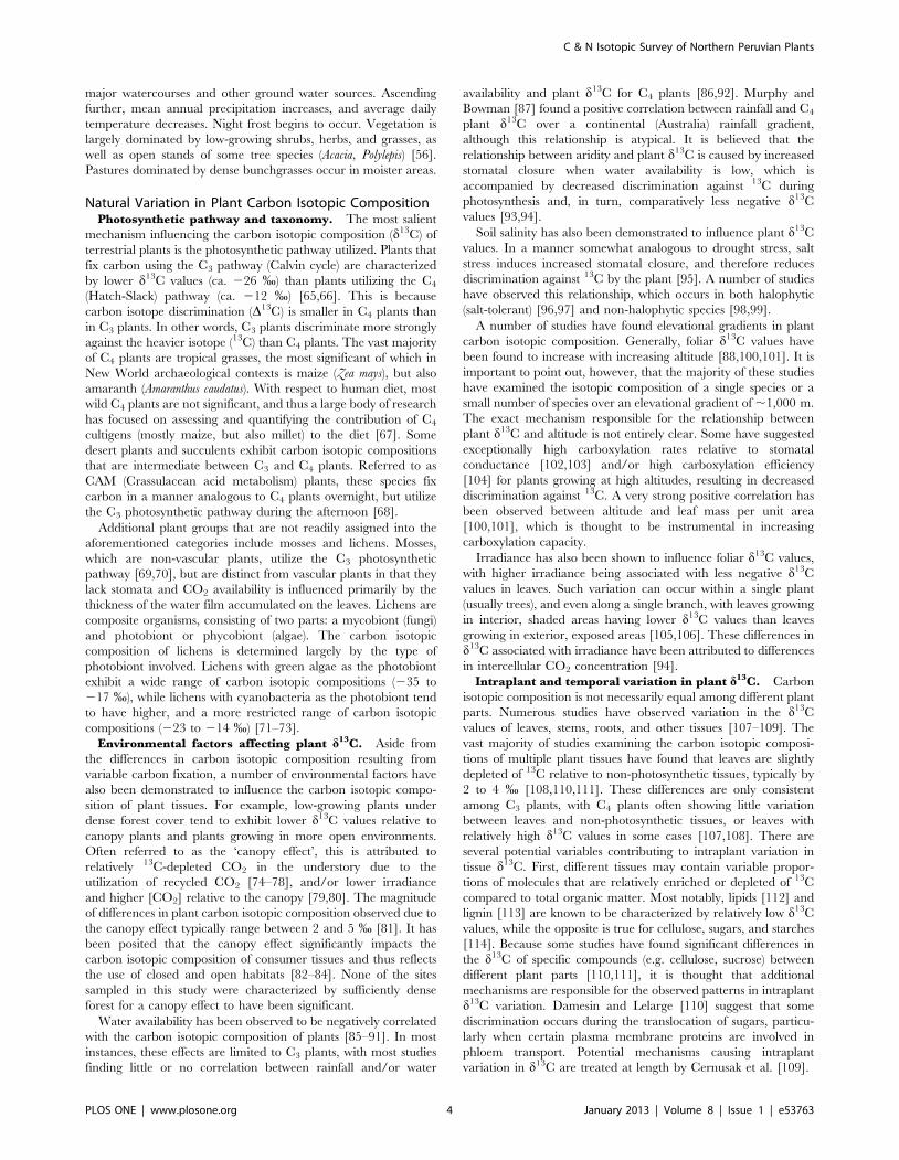
Study AreaThe Andes are an area of marked environmental complexity

and diversity. This diversity is driven largely by variation in

altitude (Figure 1). As one proceeds from the Pacific coast to the

upper limits of the Andes, mean daily temperature declines,

typically by ,5uC per 1,000 m [50], and mean annual precipi-

tation increases (Figure 2). The eastern slope of the Andes, which

connects to the Amazon basin, is environmentally very different

from the western slope. Because this study deals exclusively with

the western slope, the eastern slope is not discussed further. Many

authors have addressed the environment of the central Andes [51–

58], hence only a brief review is necessary here.

Figure 1. Digital elevation model of the study region derived from the Global 30 Arc-Second Elevation (GTOPO30) data set.doi:10.1371/journal.pone.0053763.g001

C & N Isotopic Survey of Northern Peruvian Plants


The coastal region of Peru is dominated by the hyper-arid

Peruvian desert. Cool sea-surface temperatures created by the

northward flowing Peruvian Current, combined with a subtropical

anticyclone, create remarkably stable and relatively mild temper-

atures along the roughly 2,000 km north-south extent of the

Peruvian desert [55]. The phytogeography of the coastal region of

Peru is fairly homogenous, although the composition of the

vegetation varies in accordance with local topography [59]. Except

in El Nino years, precipitation is extremely low or non-existent

along much of the Peruvian coast, but in areas where topography

is steep close to the coast, a fog zone forms (typically between 600

and 900 masl), which allows for the development of ephemeral

plant communities (lomas) [60–62]. Aside from these lomas, riparian

vegetation grows in the relatively lush river valleys that cut into the

Andes, although the vast majority of this land is cultivated.

Thickets of the leguminous algarroba tree regularly occur at low

altitudes, and it is generally believed that much more extensive

forests of these trees existed in the past [63,64]. The coastal zone

usually ends where the oceanic influence becomes minimal,

typically about 1,000 masl [58].

Immediately above the area of oceanic influence and up to an

altitude of ,1,800 m, the environment is cooler, although

generally similar, in comparison to the coastal zone. Although

mean annual precipitation increases, this zone can still be

characterized as dry, with most locations receiving less than

400 mm of annual precipitation. In some circumstances, lomas

may form within this zone [52], although this is not common. In

the Moche River Valley of northern Peru, the vegetation is

dominated by xerophytic scrub vegetation from 500 to 1,800 masl,

and transitions to thorny steppe vegetation between 1,800 and

2,800 masl. Again, the area is still characterized by relatively low

annual precipitation, although water availability is greater close to

Figure 2. Extrapolated mean annual precipitation for study area. Mean annual precipitation data from 493 monitoring stations in Peru [218]were extrapolated using the natural neighbor method in ArcMap (ArcGIS 10.0, ESRI).doi:10.1371/journal.pone.0053763.g002



major watercourses and other ground water sources. Ascending

further, mean annual precipitation increases, and average daily

temperature decreases. Night frost begins to occur. Vegetation is

largely dominated by low-growing shrubs, herbs, and grasses, as

well as open stands of some tree species (Acacia, Polylepis) [56].

Pastures dominated by dense bunchgrasses occur in moister areas.

Natural Variation in Plant Carbon Isotopic CompositionPhotosynthetic pathway and taxonomy. The most salient

mechanism influencing the carbon isotopic composition (d13C) of

terrestrial plants is the photosynthetic pathway utilized. Plants that

fix carbon using the C3 pathway (Calvin cycle) are characterized

by lower d13C values (ca. 226 %) than plants utilizing the C4

(Hatch-Slack) pathway (ca. 212 %) [65,66]. This is because

carbon isotope discrimination (D13C) is smaller in C4 plants than

in C3 plants. In other words, C3 plants discriminate more strongly

against the heavier isotope (13C) than C4 plants. The vast majority

of C4 plants are tropical grasses, the most significant of which in

New World archaeological contexts is maize (Zea mays), but also

amaranth (Amaranthus caudatus). With respect to human diet, most

wild C4 plants are not significant, and thus a large body of research

has focused on assessing and quantifying the contribution of C4

cultigens (mostly maize, but also millet) to the diet [67]. Some

desert plants and succulents exhibit carbon isotopic compositions

that are intermediate between C3 and C4 plants. Referred to as

CAM (Crassulacean acid metabolism) plants, these species fix

carbon in a manner analogous to C4 plants overnight, but utilize

the C3 photosynthetic pathway during the afternoon [68].

Additional plant groups that are not readily assigned into the

aforementioned categories include mosses and lichens. Mosses,

which are non-vascular plants, utilize the C3 photosynthetic

pathway [69,70], but are distinct from vascular plants in that they

lack stomata and CO2 availability is influenced primarily by the

thickness of the water film accumulated on the leaves. Lichens are

composite organisms, consisting of two parts: a mycobiont (fungi)

and photobiont or phycobiont (algae). The carbon isotopic

composition of lichens is determined largely by the type of

photobiont involved. Lichens with green algae as the photobiont

exhibit a wide range of carbon isotopic compositions (235 to

217 %), while lichens with cyanobacteria as the photobiont tend

to have higher, and a more restricted range of carbon isotopic

compositions (223 to 214 %) [71–73].

Environmental factors affecting plant d13C. Aside from

the differences in carbon isotopic composition resulting from

variable carbon fixation, a number of environmental factors have

also been demonstrated to influence the carbon isotopic compo-

sition of plant tissues. For example, low-growing plants under

dense forest cover tend to exhibit lower d13C values relative to

canopy plants and plants growing in more open environments.

Often referred to as the ‘canopy effect’, this is attributed to

relatively 13C-depleted CO2 in the understory due to the

utilization of recycled CO2 [74–78], and/or lower irradiance

and higher [CO2] relative to the canopy [79,80]. The magnitude

of differences in plant carbon isotopic composition observed due to

the canopy effect typically range between 2 and 5 % [81]. It has

been posited that the canopy effect significantly impacts the

carbon isotopic composition of consumer tissues and thus reflects

the use of closed and open habitats [82–84]. None of the sites

sampled in this study were characterized by sufficiently dense

forest for a canopy effect to have been significant.

Water availability has been observed to be negatively correlated

with the carbon isotopic composition of plants [85–91]. In most

instances, these effects are limited to C3 plants, with most studies

finding little or no correlation between rainfall and/or water

availability and plant d13C for C4 plants [86,92]. Murphy and

Bowman [87] found a positive correlation between rainfall and C4

plant d13C over a continental (Australia) rainfall gradient,

although this relationship is atypical. It is believed that the

relationship between aridity and plant d13C is caused by increased

stomatal closure when water availability is low, which is

accompanied by decreased discrimination against 13C during

photosynthesis and, in turn, comparatively less negative d13C

values [93,94].

Soil salinity has also been demonstrated to influence plant d13C

values. In a manner somewhat analogous to drought stress, salt

stress induces increased stomatal closure, and therefore reduces

discrimination against 13C by the plant [95]. A number of studies

have observed this relationship, which occurs in both halophytic

(salt-tolerant) [96,97] and non-halophytic species [98,99].

A number of studies have found elevational gradients in plant

carbon isotopic composition. Generally, foliar d13C values have

been found to increase with increasing altitude [88,100,101]. It is

important to point out, however, that the majority of these studies

have examined the isotopic composition of a single species or a

small number of species over an elevational gradient of ,1,000 m.

The exact mechanism responsible for the relationship between

plant d13C and altitude is not entirely clear. Some have suggested

exceptionally high carboxylation rates relative to stomatal

conductance [102,103] and/or high carboxylation efficiency

[104] for plants growing at high altitudes, resulting in decreased

discrimination against 13C. A very strong positive correlation has

been observed between altitude and leaf mass per unit area

[100,101], which is thought to be instrumental in increasing

carboxylation capacity.

Irradiance has also been shown to influence foliar d13C values,

with higher irradiance being associated with less negative d13C

values in leaves. Such variation can occur within a single plant

(usually trees), and even along a single branch, with leaves growing

in interior, shaded areas having lower d13C values than leaves

growing in exterior, exposed areas [105,106]. These differences in

d13C associated with irradiance have been attributed to differences

in intercellular CO2 concentration [94].

Intraplant and temporal variation in plant d13C. Carbon

isotopic composition is not necessarily equal among different plant

parts. Numerous studies have observed variation in the d13C

values of leaves, stems, roots, and other tissues [107–109]. The

vast majority of studies examining the carbon isotopic composi-

tions of multiple plant tissues have found that leaves are slightly

depleted of 13C relative to non-photosynthetic tissues, typically by

2 to 4 % [108,110,111]. These differences are only consistent

among C3 plants, with C4 plants often showing little variation

between leaves and non-photosynthetic tissues, or leaves with

relatively high d13C values in some cases [107,108]. There are

several potential variables contributing to intraplant variation in

tissue d13C. First, different tissues may contain variable propor-

tions of molecules that are relatively enriched or depleted of 13C

compared to total organic matter. Most notably, lipids [112] and

lignin [113] are known to be characterized by relatively low d13C

values, while the opposite is true for cellulose, sugars, and starches

[114]. Because some studies have found significant differences in

the d13C of specific compounds (e.g. cellulose, sucrose) between

different plant parts [110,111], it is thought that additional

mechanisms are responsible for the observed patterns in intraplant

d13C variation. Damesin and Lelarge [110] suggest that some

discrimination occurs during the translocation of sugars, particu-

larly when certain plasma membrane proteins are involved in

phloem transport. Potential mechanisms causing intraplant

variation in d13C are treated at length by Cernusak et al. [109].



In addition to variation among plant parts, a number of studies

have found variation in d13C within plant parts, over time.

Specifically, emerging leaves, which are not yet photosynthetic and

therefore more closely resemble other non-photosynthetic or

heterotrophic plants parts, tend to have less negative d13C values

(by about 1 to 3 %) relative to fully emerged, photosynthetic leaves

[91,110,111]. Products assimilated via photosynthesis will tend to

have lower d13C values than those acquired heterotrophically, and

this is likely partly responsible for the decrease in leaf d13C over

time [115].

Marine plants. For the purpose of this paper, ‘marine plants’

refers specifically to macroalgae, or plants that are typically

classified as kelps, seaweeds, and seagrasses. One of the most

commonly reported distinctions in carbon isotopic composition is

that marine animals tend to have higher d13C values than

terrestrial animals, except in cases where C4 plants dominate the

diet of the latter. While this distinction holds in the vast majority of

circumstances [8,116,117], the same relationship is not necessarily

true for marine and terrestrial plants.

Marine plants are characterized by a high degree of variability

in carbon isotopic composition. Figure 3 presents the carbon

isotopic compositions for the four major classes of marine

macroalgae. In general, marine plants are characterized by carbon

isotopic compositions that are intermediate in comparison to

terrestrial C3 and C4 plants, with two notable exceptions.

Seagrasses (Zostera sp.), have extremely high d13C values, typically

higher than most terrestrial C4 plants (Figure 3d). There is

evidence to suggest C4 photosynthetic activity in a few species of

marine algae [118], but the comparatively high d13C values

observed in many species, including seagrasses, cannot typically be

explained in this way [119]. The variable use of dissolved CO2(aq)

and HCO32

(aq) is a significant factor, as d13C of HCO32

(aq) is ,9

% less negative than that of CO2(aq) [120]. Moreover, for

intertidal plants, which are exposed to the atmosphere for a

portion of the day, the utilization of atmospheric CO2 further

complicates matters [119]. The thickness of the diffusive boundary

layer is also a potentially important factor with respect to D13C as

it may differ due to variable water velocity [121,122]. Other

environmental factors have also been demonstrated to influence

aquatic plant d13C values, such as: salinity [123], extracellular

CO2 concentration [124,125], light intensity [123], algal growth

rate [126], water velocity [122], and water temperature [127].

Some red algae (Floridiophyceae) are characterized by consis-

tently very low d13C values (,230 %). In general, the brown

algae (kelps) have been noted to contribute significantly to

nearshore ecosystems in terms of secondary production, with

numerous studies examining the relative contributions of offshore

phytoplankton and nearshore macroalgae [128].

Natural Variation in Plant Nitrogen Isotopic CompositionNitrogen Source. Unlike carbon, which is obtained by plants

as atmospheric CO2, nitrogen is actively taken up from the soil in

the vast majority of cases. The two most important nitrogenous

species utilized by plants are nitrate (NO32) and ammonium

(NH4+). In general, nitrate is the most abundant form of

mineralized nitrogen available to plants, but in some instances,

such as waterlogged or acidic soils, ammonium may predominate

[129,130]. Additionally, some plants rely, at least to some extent,

on atmospheric nitrogen (N2), which is obtained by symbiotic

bacteria residing in root nodules (rhizobia) [131]. Plants may also

take up organic nitrogen (e.g. free amino acids) from the soil [132],

although the relative importance of such processes is not well

understood and relatively poorly documented [133,134]. The

extent to which plants rely on these N sources is significant because

they may have distinct nitrogen isotopic compositions due to

fractionations associated with different steps in the nitrogen cycle

(e.g. ammonification, nitrification, denitrification), as well as the

uptake and eventual incorporation of mineralized N into organic

N [135–137].

There are two important aspects of variation in N source

pertinent to the present study. The first relates to N2-fixation by

plants (mostly members of Fabaceae), which are common in both

wild and domestic contexts in many parts of the central Andes.

Plants that utilize significant amounts of atmospheric N2 are

characterized by comparatively low d15N values, typically ,0 %[27,138–140]. These plants acquire such compositions because the

d15N of atmospheric N2 is ,0 % [141] and the assimilation of N

from N2-fixation is not associated with significant fractionation of15N [138–140]. By comparison, soil NO3

2 and NH4+ tend to have

d15N values .0 % [142], and non N2-fixing plants have d15N

values that tend to be .0 %, although these are highly variable for

a number of reasons as discussed in more detail below.

The second potentially significant source-related cause of plant

d15N variation is the uptake of fertilizer-derived N by plants.

Animal fertilizers are characterized by extremely variable d15N

values depending on the relative proportions of N-bearing species

in the fertilizer (e.g. urea, uric acid, ammonium, organic matter)

[143]. Manures consisting primarily of solid waste derived from

terrestrial herbivores tend to have d15N values between 2 and 8 %[144], while those that contain a mix of solid and liquid waste

(slurry fertilizers) tend to have higher d15N values, often between 6

and 15 % [145,146]. The highest d15N values for animal fertilizers

(.25 %) have been recorded for seabird guano [143,147], which

consists primarily of uric acid and is subject to significant NH4+

volatilization. The addition of animal fertilizer N to the soil

therefore adds an N source with an isotopic composition that is

usually enriched in 15N relative to endogenous soil N. This results

in higher d15N values for plants growing in soils fertilized with

animal waste than those plants growing in unfertilized soil or soils

fertilized with chemical fertilizers [143,145–147].

Animal-derived N may be delivered to plants by means other

than purposeful application of manures. Several studies have

documented that the addition of N from animal carcasses (salmon

in particular) provide substantial quantities of N taken up by

plants. These plants tend to be characterized by relatively high

d15N values [148,149]. Increased grazing intensity has also been

suggested to influence plant d15N values due to the concentrated

addition of animal waste, but studies have produced conflicting

results, with some finding grazing to: increase plant d15N values

[150,151], decrease plant d15N values [152,153], have little or no

impact on plant d15N values [154,155], or increase d15N in plant

roots, but decrease d15N in shoots [156].

Taxonomic variation. Strong distinctions in plant d15N

have been related to mycorrhizal (fungal) associations

[12,157,158]. In some ecosystems, particularly those at high

latitudes characterized by soils with low N content, this facilitates

the distinction between plant functional types – trees, shrubs, and

grasses [159–161]. In a global survey of foliar d15N values, Craine

et al. [12] found significant differences in plant d15N on the basis

of mycorrhizal associations, with the following patterns (numbers

in parentheses are differences relative to non-mycorrhizal plants):

ericoid (22 %), ectomycorrhizal (23.2 %), arbuscular (25.9 %).

The comparatively low d15N values of plants with mycorrhizal

associations has been attributed to a fractionation of 8 to 10 %against 15N during the transfer of N from fungi to plants

[162,163], with the lowest values indicating higher retention of

N in the fungi compared to the plant [164].



Intraplant and temporal variation in plant d15N. There

are three main reasons that plants exhibit intraplant and temporal

variation in their tissue d15N values: (1) fractionations associated

with NO32 assimilation in the root vs. shoot, (2) movement of

nitrogenous compounds between nitrogen sources and sinks, (3)

reliance on isotopically variable N sources as tissue forms over

time.

Both NO32 and NH4

+ are taken up by plant roots. NO32 can

be immediately assimilated into organic N in the root, or it may be

routed to the shoot and assimilated there. The assimilation of

NO32 into organic N is associated with a fractionation of 15N of

up to 220 % [137,165]. Therefore, the NO32 that is moved to

Figure 3. Frequency distributions of carbon isotopic compositions of marine macroalgae. Data are taken from published literature [119,219–235].doi:10.1371/journal.pone.0053763.g003

Table 1. Ecological zones used for sampling in this study [54].

Zone Altitude

Coastal desert 0 2 500 masl

Premontane desert scrub 500 2 1,800 masl

Premontane thorny steppe 1,800 2 2,800 masl

Montane moist pasture 2,800 2 3,700 masl

Montane wet pasture 3,700 2 4,200 masl

doi:10.1371/journal.pone.0053763.t001



Figure 4. Images of eight of the wild plant sampling locations. Corresponding geographical data for these sites can be found in Table 6.doi:10.1371/journal.pone.0053763.g004



the shoot has already been exposed to some fractionation

associated with assimilation and is enriched in 15N compared to

the NO32 that was assimilated in the root. On this basis, it is

expected that shoots will have higher d15N values than roots in

plants fed with NO32 [166]. Because NH4

+ is assimilated only in

the root, plants with NH4+ as their primary N source are not

expected to have significant root/shoot variation in d15N [136].

As plants grow they accumulate N in certain tissues (sources)

and, over time, move this N to other tissues (sinks). In many

species, annuals in particular, large portions of the plant’s

resources are allocated to grain production or flowering. In these

cases, significant portions of leaf and/or stem N is mobilized and

allocated to the fruits, grains, or flowers [167]. When stored

proteins are hydrolyzed, moved, and synthesized, isotopic

fractionations occur [168,169]. Theoretically, nitrogen sources

(leaves, stems) should be comparatively enriched in 15N in relation

to sinks (grains, flowers), which has been observed in several

studies [143,145,147].

In agricultural settings, the variation within a plant over time

may become particularly complex due to the application of

nitrogenous fertilizers. The availability of different N-bearing

species from the fertilizer (NH4+, NO3

2) and the nitrogen isotopic

composition of fertilizer-derived N changes over time as various

soil processes (e.g. ammonification, nitrification) occur. The nature

of this variation is complex and will depend on the type of fertilizer

applied [147].

Environmental factors affecting plant d15N. Plant nitro-

gen isotopic compositions are strongly influenced by a series of

environmental factors. The environmental variation in plant d15N

can be passed on to consumers and cause significant spatial

variation in animal isotopic compositions at regional and

continental scales [170–175].

Plant d15N values have been observed to be positively correlated

with mean annual temperature (MAT) [176,177], although this

relationship appears to be absent in areas where MAT # 20.5uC[12]. A large number of studies have found a negative correlation

between plant d15N values and local precipitation and/or water

availability. These effects have been demonstrated at regional or

continental [15,85–87,172,178], and global [12,176,179] scales.

Several authors have hypothesized that relatively high d15N values

in herbivore tissues may be the product of physiological processes

within the animal related to drought stress [171,173,174],

although controlled experiments have failed to provide any

evidence supporting this hypothesis [180]. More recent research

has demonstrated a clear link between herbivore tissue d15N values

Table 2. Environmental data for market plant sampling sites.

Site ID Site Name Latitude Longitude Altitude (masl)

C1 Caraz 29.0554 277.8101 2233

C2 Yungay 29.1394 277.7481 2468

C3 Jesus 27.2448 278.3797 2530

C4 Jesus II 27.2474 278.3821 2573

C5 Ampu 29.2757 277.6558 2613

C6 Shuto 27.2568 278.3807 2629

C7 Carhuaz 29.2844 277.6422 2685

C8 Yamobamba 27.8432 278.0956 3176

C9 Huamachuco 27.7846 277.9748 3196

C10 Curgos 27.8599 277.9475 3220

C11 Poc Poc 27.9651 277.8964 3355

C12 Recuay 29.7225 277.4531 3400

C13 Olleros 29.6667 277.4657 3437

C14 Hierba Buena 27.0683 278.5959 3453

C15 Mirador II 29.7220 277.4601 3466

C16 Yanac 27.7704 277.9799 3471

C17 Mirador I 29.7224 277.4601 3477

C18 Conray Chico 29.6705 277.4484 3530

C19 Catac 29.8083 277.4282 3588


Figure 5. Carbon and nitrogen isotopic compositions of cultigens. Note that the x-axis is not continuous.doi:10.1371/journal.pone.0053763.g005



and plant d15N values, while providing no support for the

‘physiological stress hypothesis’ [172,181].

The nature of the relationship between rainfall and plant d15N

values appears to be extremely complex, with numerous variables

contributing to the pattern. Several authors, including Handley

et al. [179], have attributed this pattern to the relative ‘openness’

of the nitrogen cycle. In comparison to hot and dry systems, which

are prone to losses of excess N, colder and wetter systems more

efficiently conserve and recycle mineral N [176] and are thus

considered less open. With respect to ecosystem d15N, 15N

enrichment will be favored for any process that increases the flux

of organic matter to mineral N, or decreases the flux of mineral N

into organic matter [178]. For instance, low microbial activity, or

high NH3 volatilization would cause an overall enrichment in 15N

of the soil-plant system.

Marine plants. In comparison to terrestrial plants, the

factors affecting the nitrogen isotopic composition of marine

plants have not been investigated intensively other than the

influence of anthropogenic nitrogen. As is the case with terrestrial

plants, marine plant d15N values are strongly influenced by the

forms and isotopic composition of available N [182,183].

Specifically, the relative reliance on upwelled NO32 relative to

recycled NH4+ will strongly influence the d15N of marine

producers, including macroalgae. Systems that are nutrient poor

(oligotrophic) tend to be more dependent on recycled NH4+, and

systems that are nutrient rich (eutrophic) tend to be more

dependent on upwelled NO32. This results in nutrient-rich,

upwelling systems being enriched in 15N relative to oligotrophic

systems [184].

Materials and Methods

Sample CollectionWild plants were collected between 2011/07/18 and 2011/08/

03. We used regional ecological classifications defined by Tosi

[54], which are summarized in Table 1. In each of these five

zones, two sites were selected that typified the composition of local

vegetation. Sampling locations were chosen to minimize the

possibility of significant anthropogenic inputs; in particular, areas

close to agricultural fields and disturbed areas were avoided.

Sampling locations were fairly open and did not have significant

canopy cover. At each sampling location, all plant taxa within a

10 m radius were sampled. Wherever possible, three individuals of

each species were sampled and were later homogenized into a

single sample for isotopic analysis. Images for eight of the wild

plant sampling locations are presented in Figure 4.

Cultigens (edible portions) were collected from local markets

between 2008/10/08 and 2008/11/09 (Table 2). Plants intro-

duced to the Americas were not collected (e.g. peas, barley), even

though these species were common. Entire large cultigens (e.g.

Table 3. Mean carbon and nitrogen isotopic compositions for cultigens (61s).

Common Name Taxonomic Name n d13C (%, VPDB) d15N (%, AIR) %C %N

Beans Phaseolus sp. 24 225.761.6 0.762.0 39.860.7 3.760.6

Beans (Lima) Phaseolus lunatus 2 226.061.4 20.260.4 39.060.3 2.760.5

Chocho (Andean lupin) Lupinus mutabilis 5 226.061.6 0.661.2 48.362.8 6.861.3

Coca Erythroxylum coca 4 229.860.9 2 45.461.5 2

Maize (Grain) Zea mays 27 211.860.4 6.462.2 40.460.5 1.260.2

Maize (Leaf) Zea mays 2 212.960.4 4.561.6 41.964.6 1.361.3

Mashua Tropaeolum tuberosum 3 225.661.9 0.564.7 41.562.8 3.060.7

Oca Oxalis tuberosa 6 226.460.7 5.761.3 43.163.2 1.660.6

Pepper Capsicum annuum 1 229.6 4.2 48.3 2.1

Potato Solanum tuberosum 12 226.361.3 4.065.5 40.561.5 1.460.4

Quinoa Chenopodium quinoa 3 225.660.9 7.961.3 39.962.1 2.660.3

Ulluco Ullucus tuberosus 2 225.860.0 7.561.0 40.660.4 3.461.0


Table 4. Results of ANOVA post-hoc tests (Dunnett’s T3) for cultigen d15N.

Cultigen %N Bean (P. lunatus) Andean lupin Maize Mashua Oca Potato Quinoa Ulluco

Bean (Phaseolus sp.) 0.860 1.000 ,0.001 1.000 0.003 0.798 0.028 0.880

Bean (P. lunatus) 2 0.971 ,0.001 1.000 0.005 0.479 0.037 0.121

Andean lupin 2 2 ,,0.001 1.000 0.006 0.802 0.020 0.060

Maize 2 2 2 0.696 1.000 0.983 0.855 0.917

Mashua 2 2 2 2 0.788 1.000 0.626 0.723

Oca 2 2 2 2 2 1.000 0.626 0.723

Potato 2 2 2 2 2 2 0.688 0.780

Quinoa 2 2 2 2 2 2 2 1.000

Values in boldface are statistically significant (p,0.05).doi:10.1371/journal.pone.0053763.t004



tubers) were selected and subsequently, a thin (ca. 0.5 cm) slice

was sampled. For smaller cultigens (e.g. maize, beans, quinoa) one

handful of material was sampled.

For both wild plants and cultigens, geospatial data were

recorded using a GarminH OregonH 450 portable GPS unit

(GarminH, Olathe, KS, USA). After collection, plants were air-

dried on site. Prior to shipping, plants were dried with a SaltonHDH21171 food dehydrator (Salton Canada, Dollard-des-Or-

meaux, QC, Canada). Plants were separated according to tissue

(leaf, stem, seed, flower). For grasses, all aboveground tissues were

considered to be leaf except where significant stem development

was present, in which case, leaf and stem were differentiated. All

geospatial data associated with these sampling sites are available as

a Google Earth.kmz file in the Supporting Information (Dataset

S1).

Plants were not sampled from privately-held land or from

protected areas. Endangered or protected species were not

sampled. Plant materials were imported under permit

#2011203853 from the Canadian Food Inspection Agency. No

additional specific permissions were required for these activities.

Sample PreparationSamples were prepared according to Szpak et al. [143] with

minor modifications. As described above, plant material was dried

prior to arrival in the laboratory. Whole plant samples were first

homogenized using a Magic BulletH compact blender (Homeland

Housewares, Los Angeles, CA, USA). Ground material was then

sieved, with the ,180 mm material retained for analysis in glass

vials. If insufficient material was produced after sieving, the

remaining material was further ground using a Wig-L-Bug

Figure 6. Dot-matrix plot of nitrogen isotopic compositions of legumes and non-legumes. Horizontal bars represent means. Increment = 0.5 %.doi:10.1371/journal.pone.0053763.g006



mechanical shaker (Crescent, Lyons, IL, USA) and retained for

analysis in glass vials. Glass vials containing the ground material

were dried at 90uC for at least 48 h under normal atmosphere.

Stable Isotope AnalysisIsotopic (d13C and d15N) and elemental compositions (%C and

%N) were determined using a Delta V isotope ratio mass

spectrometer (Thermo Scientific, Bremen, Germany) coupled to

an elemental analyzer (Costech Analytical Technologies, Valencia,

CA, USA), located in the Laboratory for Stable Isotope Science

(LSIS) at the University of Western Ontario (London, ON,

Canada). For samples with ,2% N, nitrogen isotopic composi-

tions were determined separately, with excess CO2 being removed

with a Carbo-Sorb trap (Elemental Microanalysis, Okehampton,

Devon, UK) prior to isotopic analysis.

Sample d13C and d15N values were calibrated to VPDB and AIR,

respectively, with USGS40 (accepted values: d13C = 226.39 %,

d15N = 24.52 %) and USGS41 (accepted values: d13C = 37.63 %,

d15N = 47.6 %). In addition to USGS40 and USGS41, internal

(keratin) and international (IAEA-CH-6, IAEA-N-2) standard refer-

ence materials were analyzed to monitor analytical precision and

accuracy. A d13C value of 224.0360.14 % was obtained for 81

analyses of the internal keratin standard, which compared well with its

average value of 224.04 %. A d13C value of 210.4660.09 % was

obtained for 46 analyses of IAEA-CH-6, which compared well with its

accepted value of 210.45 %. Sample reproducibility was 60.10 % for

d13C and 60.50% for %C (50 replicates). A d15N value of 6.3760.13

% was obtained for 172 analyses of an internal keratin standard, which

compared well with its average value of 6.36 %. A d15N value of

20.360.4 % was obtained for 76 analyses of IAEA-N-2, which

compared well with its accepted value of 20.3 %. Sample reproduc-

ibility was 60.14 % for d15N and 60.10% for %N (84 replicates).

Data Treatment and Statistical AnalysesPlants were grouped into the following major functional

categories for analysis: herb/shrub, tree, grass/sedge, vine. Plants

Figure 7. Dot-matrix plot of nitrogen content of legumes and non-legumes. Horizontal bars represent means. Increment = 0.25%.doi:10.1371/journal.pone.0053763.g007



that are invasive and/or introduced species were included in the

calculation of means for particular sites since their isotopic

compositions should still be impacted by the same environmental

factors as other plants. For all statistical analyses of carbon isotopic

composition, grass/sedge and herb/shrub were further separated

into C3 and C4 categories. For comparisons among plant

functional types, and sampling sites, foliar tissue was used since

other tissues were not as extensively sampled.

Correlations between foliar isotopic compositions and environ-

mental parameters (altitude, mean annual precipitation) were

assessed using Spearman’s rank correlation coefficient (r). One-

way analysis of variance (ANOVA) followed by either a Tukey’s

HSD test (if variance was homoscedastic) or a Dunnett’s T3 test (if

variance was not homoscedastic) was used to compare means. All

statistical analyses and regressions were performed in SPSS 16 for

Windows.

Results

CultigensThe carbon and nitrogen isotopic compositions were analyzed

for a total of 85 cultigen samples from eleven species. Carbon and

nitrogen isotopic compositions for cultigens are presented in

Figure 5. Mean d13C and d15N values for cultigens are presented

in Table 3. Isotopic and elemental data, as well as corresponding

geospatial data for individual cultigens are presented in Table S1.

All isotopic and elemental compositions for cultigens are for

consumable portions of the plant, with one exception (maize

leaves), which is excluded from Table 3 and Figure 5. Mean d13C

values for C3 cultigens ranged from 229.860.9 % (coca) to

225.661.9 % (mashua). The mean d13C value for maize, which

was the only C4 plant examined, was 211.860.4 %. Mean d15N

values for cultigens were typically more variable than d13C values,

ranging from 20.260.4 % (Phaseolus lunatus) to 7.961.3 %(quinoa).

When maize is excluded, there were no significant differences in

d13C among cultigens (F[7,49] = 0.3, p = 0.93), but there were for

d15N (maize included) (F[8,73] = 9.7, p,0.001). Results of post-hoc

Dunnett’s T3 test for d15N differences among individual cultigen

species are presented in Table 4. The three leguminous species

were generally characterized by significantly lower d15N values

than non-leguminous species (Table 4); collectively, legumes were

characterized by significantly lower d15N values than non-legumes

(Figure 6; F[1,80] = 51.8, p,0.001).

Table 5. Results of ANOVA post-hoc tests (Dunnett’s T3) for cultigen N content.

Cultigen %N Bean (P. lunatus) Andean lupin Maize Mashua Oca Potato Quinoa Ulluco

Bean (Phaseolus sp.) 0.637 0.072 ,0.001 0.869 0.009 ,0.001 0.123 1.000

Bean (P. lunatus) 2 0.037 0.462 1.000 0.619 0.505 1.000 0.995

Andean lupin 2 2 0.009 0.034 0.005 0.008 0.021 0.295

Maize 2 2 2 0.232 0.981 0.992 0.101 0.566

Mashua 2 2 2 2 0.019 1.000 0.216 0.009

Oca 2 2 2 2 2 1.000 0.033 0.001

Potato 2 2 2 2 2 2 0.033 0.001

Quinoa 2 2 2 2 2 2 2 0.885


Table 6. Environmental data for wild plant sampling sites and summary of number of C3 and C4 plant species sampled.

Site ID Site Name Latitude LongitudeAltitude(masl) MAP (mm)1

C3 Plant TaxaSampled

C4 Plant TaxaSampled

W1 Las Delicias 28.1956 278.9996 10 7 7 2

W2 Rıo Moche 28.1267 278.9963 33 5 9 1

W3 Ciudad Universitaria 28.1137 279.0373 38 6 2 0

W4 Cerro Campana 27.9900 279.0768 164 11 4 1

W5 La Carbonera 28.0791 278.8681 192 56 5 3

W6 Poroto 28.0137 278.7972 447 113 17 6

W7 Salpo 5 28.0089 278.6962 1181 143 0 2

W8 Salpo 4 28.0047 278.6726 1557 140 9 0

W9 Salpo 3 28.0132 278.6355 2150 141 16 0

W10 Salpo 2 27.9973 278.6481 2421 142 8 0

W11 Salpo 1 28.0132 278.6355 2947 171 9 1

W12 Stgo de Chuco 28.1361 278.1685 3041 702 21 1

W13 Cahuide 28.2235 278.3013 4070 591 15 0

1Mean annual precipitation (MAP) estimated as described in the text.doi:10.1371/journal.pone.0053763.t006



Ta

ble

7.

Car

bo

nan

dn

itro

ge

nis

oto

pic

com

po

siti

on

sfo

ral

lw

ildp

lan

tta

xasa

mp

led

.

Le

af

Ste

mR

oo

tF

low

ers

Se

ed

s

Ta

xo

no

mic

Na

me

Sit

eID

Alt

itu

de

Ty

pe

d1

3C

(%)

d1

5N

(%)

d1

3C

(%)

d1

5N

(%)

d1

3C

(%)

d1

5N

(%)

d1

3C

(%)

d1

5N

(%)

d1

3C

(%)

d1

5N

(%)

Erio

chlo

am

uti

caW

11

0G

rass

21

1.6

21

.52

11

.71

.62

22

22

12

.12

0.2

Dis

tich

iasp

icat

aW

11

0G

rass

21

4.9

23

.22

22

22

22

2

Bac

char

isg

luti

no

saW

11

0Sh

rub

22

7.4

3.3

22

6.6

5.1

22

22

7.0

4.1

22

6.9

4.2

Rau

volf

iasp

.W

11

0Sh

rub

22

8.0

9.8

22

7.9

11

.02

22

22

2

Pla

nta

go

maj

or1

W1

10

He

rb2

28

.67

.52

27

.57

.92

26

.78

.62

22

2

Typ

laan

gu

stif

olia

W1

10

He

rb2

29

.31

.32

22

28

.72

.62

22

2

Blu

me

acr

isp

ata1

W1

10

He

rb2

29

.81

3.7

23

0.4

13

.72

30

.51

1.6

22

22

Ro

sip

pa

nas

tru

tiu

maq

uat

icu

m1

W1

10

He

rb2

30

.11

2.5

22

23

0.0

11

.42

22

2

Oxa

lisco

rnic

ula

taW

11

0H

erb

23

0.6

7.1

23

1.0

6.0

23

1.2

4.7

22

22

Pas

pal

um

race

mo

sum

W2

33

Gra

ss2

12

.70

.82

12

.81

1.7

22

22

22

Salix

hu

mb

old

tian

aW

23

3T

ree

22

6.4

5.2

22

6.5

4.4

22

22

22

Ph

yla

no

dif

lora

W2

33

He

rb2

27

.76

.52

26

.85

.12

27

.12

.82

26

.77

.9

Me

loch

ialu

pu

lina

W2

33

Shru

b2

28

.36

.92

27

.66

.42

22

28

.66

.82

2

Ipo

mo

ea

alb

aW

23

3H

erb

22

8.7

9.3

22

8.1

8.1

22

22

22

7.3

8.9

Pe

rse

aam

eri

can

aW

23

3T

ree

22

8.8

1.9

22

6.8

7.0

22

22

22

Am

bro

sia

pe

ruvi

ana

W2

33

He

rb2

29

.62

.22

30

.01

.72

22

22

2

Aru

nd

od

on

ax1

W2

33

Gra

ss2

30

.38

.52

30

.11

0.2

22

22

22

Aca

cia

hu

aran

go

2W

23

3Sh

rub

23

1.0

3.5

23

0.0

2.3

22

22

9.8

3.4

22

Psi

ttac

anth

us

ob

ova

tus

W2

33

Shru

b(P

aras

itic

)2

31

.95

.12

30

.66

.22

22

22

2

Pro

sop

isp

allid

a2W

33

8T

ree

22

7.9

4.0

22

8.9

1.5

22

22

9.1

5.8

22

Aca

cia

mac

raca

nth

a2W

33

8T

ree

23

0.7

8.3

23

0.1

6.8

22

23

0.5

8.6

22

8.9

5.1

Till

and

sia

usn

eo

ide

sW

41

64

Epip

hyt

e2

13

.63

.72

14

.21

.92

13

.91

4.5

21

3.6

0.0

22

Cry

pto

carp

us

pyr

ifo

rmis

W4

16

4Sh

rub

22

2.5

10

.32

22

.21

0.4

22

22

22

2.4

12

.1

Tri

xis

caca

lioid

es

W4

16

4Sh

rub

22

6.6

9.2

22

6.0

7.6

22

22

22

5.7

9.4

Scu

tia

spic

ata

W4

16

4Sh

rub

22

7.1

4.9

22

5.7

4.4

22

22

22

Cap

par

isan

gu

lata

W4

16

4Sh

rub

22

7.3

10

.02

27

.71

0.7

22

22

22

6.0

11

.6

Pas

pal

idiu

mp

alad

ivag

um

W5

19

2G

rass

21

2.5

10

.52

12

.81

1.0

21

2.0

11

.72

22

12

.31

3.4

Am

aran

thu

sce

losi

od

es

W5

19

2H

erb

21

3.1

9.1

21

2.5

11

.02

22

13

.51

0.9

21

2.2

8.6

Tri

bu

lus

terr

est

ris

W5

19

2H

erb

21

5.6

11

.82

16

.21

4.4

22

22

21

4.0

13

.6

Hyd

roco

tyle

bo

nar

ien

sis

W5

19

2H

erb

22

6.5

9.0

22

22

22

22

Ce

stru

mau

ricu

latu

mW

51

92

Shru

b2

26

.91

0.6

22

6.8

8.5

22

22

22

7.0

12

.1

Cu

cum

isd

ipsa

ceu

sW

51

92

He

rb2

27

.45

.62

26

.84

.22

22

27

.05

.52

28

.16

.5

Arg

em

on

esu

bfu

sifo

rmis

W5

19

2H

erb

22

8.8

6.9

22

8.1

6.3

22

8.8

6.2

22

8.9

5.7

22

Pic

rosi

alo

ng

ifo

liaW

51

92

He

rb2

30

.65

.32

30

.51

.12

22

30

.09

.32

2



Ta

ble

7.

Co

nt.

Le

af

Ste

mR

oo

tF

low

ers

Se

ed

s

Ta

xo

no

mic

Na

me

Sit

eID

Alt

itu

de

Ty

pe

d1

3C

(%)

d1

5N

(%)

d1

3C

(%)

d1

5N

(%)

d1

3C

(%)

d1

5N

(%)

d1

3C

(%)

d1

5N

(%)

d1

3C

(%)

d1

5N

(%)

Cyp

eru

sco

rym

bo

sus

W6

44

7Se

dg

e2

13

.18

.32

11

.28

.82

11

.77

.82

14

.29

.12

2

Ech

ino

chlo

acr

usg

alli1

W6

44

7G

rass

21

3.4

2.8

21

3.8

2.8

22

22

21

3.7

3.9

Cyn

od

on

dac

tylo

n1

W6

44

7G

rass

21

3.9

0.8

22

22

21

4.1

1.2

22

Sorg

hu

mh

ale

pe

nse

1W

64

47

Gra

ss2

14

.02

.52

15

.04

.72

22

22

13

.13

.7

Tri

anth

em

ap

ort

ula

cast

rum

W6

44

7H

erb

21

4.2

17

.32

13

.71

2.3

22

22

22

Am

aran

thu

ssp

ino

sus

W6

44

7H

erb

21

4.4

13

.32

13

.81

6.1

22

21

4.0

15

.32

14

.41

5.3

Gyn

eri

um

sag

itta

tum

W6

44

7G

rass

22

5.8

2.7

22

5.1

2.3

22

5.6

5.3

Alt

ern

anth

era

hal

imif

olia

W6

44

7H

erb

22

6.0

8.4

22

6.1

9.2

22

22

6.1

8.2

22

Cis

sus

sicy

oid

es

W6

44

7V

ine

22

6.6

10

.92

26

.11

2.4

22

22

22

5.1

11

.9

Dal

ea

on

ob

rych

is2

W6

44

7H

erb

22

7.2

8.7

22

7.4

7.8

22

22

22

6.8

7.4

Cle

om

esp

ino

saW

64

47

He

rb2

27

.39

.02

27

.19

.82

22

22

26

.99

.8

Cro

tala

ria

inca

e2

W6

44

7Sh

rub

22

7.3

0.2

22

6.6

22

.42

22

25

.41

.02

26

.02

0.8

Lud

wig

iao

cto

valv

is2

W6

44

7H

erb

22

7.5

0.6

22

6.9

1.3

22

22

22

Pas

sifl

ora

foe

tid

aW

64

47

Vin

e2

27

.59

.52

27

.21

.72

22

27

.57

.82

2

We

de

liala

tilo

folia

W6

44

7Sh

rub

22

8.0

6.4

22

7.3

4.8

22

22

6.4

8.1

22

Bac

char

issa

licif

olia

W6

44

7Sh

rub

22

8.3

6.5

22

7.2

8.4

22

22

22

7.1

8.0

Wal

the

ria

ova

taW

64

47

Shru

b2

28

.46

.12

28

.25

.92

22

27

.76

.02

2

Ve

rbe

na

litto

ralis

W6

44

7H

erb

22

8.8

7.9

22

8.4

5.8

22

22

22

7.7

7.3

Cyp

eru

so

do

ratu

sW

64

47

Sed

ge

22

8.8

9.2

22

7.6

10

.12

22

28

.01

0.2

22

Mim

osa

pig

raW

64

47

Shru

b2

29

.31

.72

28

.50

.32

22

22

29

.11

.3

Caj

anu

sca

jan

1,

2W

64

47

Tre

e2

29

.62

1.4

22

8.4

22

22

28

.30

.32

27

.62

0.7

Po

lyg

on

um

hyd

rop

ipe

roid

es

W6

44

7H

erb

23

0.2

6.8

23

0.6

6.7

22

22

22

7.2

8.1

Mim

osa

alb

ida2

W6

44

7Sh

rub

23

0.5

20

.82

30

.12

1.5

22

22

22

8.8

1.2

Me

linis

rep

en

s1W

71

18

1G

rass

21

3.3

5.6

21

3.4

7.3

22

22

21

4.5

3.1

Ce

nch

rus

myo

suro

ide

sW

71

18

1G

rass

21

3.3

5.7

22

22

22

22

Dic

lipte

rap

eru

vian

aW

81

55

7H

erb

22

4.7

3.9

22

6.3

3.2

22

22

22

5.0

3.2

To

urn

efo

rtia

mic

roca

lyx

W8

15

57

Shru

b2

26

.06

.42

26

.26

.02

22

25

.67

.22

2

Op

hry

osp

oru

sp

eru

vian

us

W8

15

57

Shru

b2

26

.72

.92

23

.91

.82

22

22

24

.02

.6

Alt

ern

anth

era

po

rrig

en

sW

81

55

7H

erb

22

7.8

2.8

22

7.2

2.2

22

22

22

5.7

6.7

Asc

lep

ias

cura

ssav

ica

W8

15

57

Shru

b2

28

.92

.62

28

.74

.22

22

28

.80

.42

28

.00

.2

Bo

erh

avia

ere

cta

W8

15

57

He

rb2

29

.39

.12

28

.39

.22

22

22

2

Ce

nta

ure

am

elit

en

sis

W8

15

57

He

rb2

29

.50

.52

29

.80

.22

22

22

28

.91

.7

Me

ntz

elia

asp

era

W8

15

57

He

rb2

30

.01

.02

27

.66

.82

22

29

.51

.32

2

Sid

asp

ino

saW

81

55

7H

erb

23

0.1

3.1

23

0.1

4.7

22

23

1.3

1.7

22



Ta

ble

7.

Co

nt.

Le

af

Ste

mR

oo

tF

low

ers

Se

ed

s

Ta

xo

no

mic

Na

me

Sit

eID

Alt

itu

de

Ty

pe

d1

3C

(%)

d1

5N

(%)

d1

3C

(%)

d1

5N

(%)

d1

3C

(%)

d1

5N

(%)

d1

3C

(%)

d1

5N

(%)

d1

3C

(%)

d1

5N

(%)

Ru

bu

sro

bu

stu

sW

92

15

0Sh

rub

22

5.0

3.0

22

4.4

2.7

22

22

22

Pu

yasp

.W

92

15

0Su

ccu

len

t2

25

.42

0.7

22

22

22

22

Bar

nad

esi

ad

om

be

yan

aW

92

15

0Sh

rub

22

6.0

22

.02

25

.42

0.3

22

22

5.7

22

.72

2

Ioch

rom

ae

du

leW

92

15

0Sh

rub

22

6.1

8.5

22

5.8

7.6

22

22

22

5.4

7.3

Eup

ato

riu

msp

.W

92

15

0H

erb

22

6.8

2.5

22

22

22

22

Cap

par

issc

abri

da

W9

21

50

Shru

b2

26

.81

.32

26

.30

.92

22

26

.52

.22

2

Vas

qu

ezi

ao

pp

osi

tifo

liaW

92

15

0H

erb

22

7.0

21

.62

22

22

22

26

.92

1.3

Stip

aic

hu

W9

21

50

Gra

ss2

27

.00

.32

22

27

.40

.22

27

.30

.62

2

Lup

inu

ssp

.2W

92

15

0H

erb

22

7.1

1.4

22

7.1

3.4

22

22

6.6

3.2

22

6.7

0.8

Alo

nso

am

eri

dio

nal

isW

92

15

0H

erb

22

7.5

1.3

22

6.4

21

.92

22

22

25

.90

.1

Bro

mu

sca

thar

ticu

sW

92

15

0G

rass

22

7.8

1.1

22

9.3

21

.32

22

22

27

.52

0.7

Bac

char

issp

.W

92

15

0Sh

rub

22

8.9

21

.12

28

.80

.12

22

29

.50

.52

2

Min

tho

stac

hys

mo

llis

W9

21

50

He

rb2

29

.00

.52

28

.12

1.6

22

22

7.2

0.1

22

Satu

reja

sp.

W9

21

50

He

rb2

30

.22

3.2

22

22

22

9.8

22

.32

2

Ach

yro

clin

eal

ata

W9

21

50

Shru

b2

30

.30

.32

27

.81

.22

22

27

.52

.02

2

Po

lyp

og

on

sp.

W9

21

50

Gra

ss2

31

.12

5.3

22

7.9

24

.42

31

.02

.42

27

.82

3.7

22

Bro

wal

liaam

eri

can

aW

10

24

21

He

rb2

25

.42

1.6

22

6.8

22

.52

22

25

.72

0.8

22

Co

niz

asp

.W

10

24

21

He

rb2

26

.76

.12

26

.14

.02

22

22

2

He

liotr

op

ium

sp.

W1

02

42

1H

erb

22

6.9

3.7

22

8.4

2.2

22

22

22

8.2

3.2

Cae

salp

ina

spin

osa

2W

10

24

21

Tre

e2

27

.42

.72

27

.72

0.4

22

22

22

5.1

0.0

Oe

no

the

raro

sea

W1

02

42

1H

erb

22

7.4

4.9

22

7.9

4.6

22

22

22

7.4

2.9

Ave

na

ste

rilis

1W

10

24

21

Gra

ss2

27

.52

.32

27

.22

.12

27

.00

.02

22

22

.52

.2

Be

rbe

ris

sp.

W1

02

42

1Sh

rub

22

7.7

1.1

22

4.6

1.9

22

22

22

6.7

1.9

Alt

ern

anth

era

sp.

W1

02

42

1H

erb

22

8.3

22

.92

27

.52

3.0

22

22

22

7.2

20

.8

Pe

nn

ise

tum

pu

rpu

rem

1W

11

29

47

Gra

ss2

12

.57

.22

12

.86

.62

22

22

15

.57

.1

Ru

elli

afl

ori

bu

nd

aW

11

29

47

He

rb2

23

.74

.52

24

.01

.92

22

23

.54

.92

2

Sch

inu

sm

olle

W1

12

94

7T

ree

22

4.6

2.3

22

3.4

0.3

22

22

1.3

0.8

22

Spar

tiu

mju

nce

um

1,

2W

11

29

47

Shru

b2

26

.51

.12

27

.12

1.1

22

22

3.7

21

.32

25

.40

.8

Aca

cia

aro

ma2

W1

12

94

7T

ree

22

6.8

9.6

22

6.6

9.6

222

22

6.6

10

.12

22

Cro

ton

ova

lifo

lius

W1

12

94

7Sh

rub

22

7.0

7.4

22

7.6

5.8

22

22

22

Leo

no

tis

ne

pe

tifo

lia1

W1

12

94

7Sh

rub

22

8.0

2.2

22

22

22

7.2

3.0

22

6.1

2.0

Lyci

anth

es

lyci

oid

es

W1

12

94

7Sh

rub

22

8.0

20

.32

22

22

22

24

.32

.0

Ph

en

axh

irtu

sW

11

29

47

Shru

b2

28

.32

.52

29

.17

.12

22

22

28

.56

.9

Ing

afe

ulle

u2

W1

12

94

7T

ree

22

8.9

0.3

22

7.6

20

.82

22

22

27

.11

.1



Ta

ble

7.

Co

nt.

Le

af

Ste

mR

oo

tF

low

ers

Se

ed

s

Ta

xo

no

mic

Na

me

Sit

eID

Alt

itu

de

Ty

pe

d1

3C

(%)

d1

5N

(%)

d1

3C

(%)

d1

5N

(%)

d1

3C

(%)

d1

5N

(%)

d1

3C

(%)

d1

5N

(%)

d1

3C

(%)

d1

5N

(%)

An

dro

po

go

nsp

.W

12

30

41

Gra

ss2

13

.52

1.6

22

21

3.2

21

.02

22

2

Seb

asti

ania

ob

tusi

folia

W1

23

04

1Sh

rub

22

3.7

0.8

22

4.7

0.0

22

22

22

4.0

2.5

Lup

inu

sar

idu

lus2

W1

23

04

1H

erb

22

4.3

2.0

22

3.7

2.2

22

22

2.7

4.0

22

2.0

5.4

Sily

bu

mm

aria

nu

m1

W1

23

04

1H

erb

22

5.9

2.2

22

5.8

1.6

22

22

22

5.1

2.2

Ph

ryg

ilan

thu

ssp

.W

12

30

41

Shru

b(P

aras

itic

)2

25

.92

0.5

22

4.7

7.3

22

22

22

Sola

nu

mam

ota

pe

nse

W1

23

04

1Sh

rub

22

5.9

7.9

22

5.2

5.1

22

22

22

4.7

8.3

Aca

cia

sp.2

W1

23

04

1T

ree

22

6.2

21

.02

25

.02

2.5

22

22

22

Bac

char

isse

rpif

olia

W1

23

04

1Sh

rub

22

6.4

2.2

22

7.1

1.5

22

22

6.9

1.0

22

Ari

stid

aad

sen

sio

nis

W1

23

04

1G

rass

22

6.5

22

.62

26

.22

2.0

22

22

6.7

21

.02

2

Bac

char

ise

mar

gin

ata

W1

23

04

1Sh

rub

22

6.5

20

.22

25

.40

.12

22

22

2

Bra

ssic

aca

mp

est

ris

W1

23

04

1H

erb

22

7.1

2.3

22

22

22

22

5.4

4.3

Mau

ria

sp.

W1

23

04

1T

ree

22

7.2

6.1

22

5.8

3.1

22

22

22

Sola

nu

mag

rim

on

iae

foliu

mW

12

30

41

Shru

b2

28

.06

.02

28

.23

.82

22

22

26

.64

.1

Salv

iap

un

ctat

aW

12

30

41

He

rb2

28

.12

3.5

22

22

22

7.7

22

.12

27

.32

1.7

Du

ran

tasp

.W

12

30

41

Shru

b2

28

.41

.32

27

.60

.82

22

22

2

Flo

ure

nsi

aca

jab

amb

en

sis

W1

23

04

1Sh

rub

22

8.6

2.9

22

7.5

2.7

22

22

22

9.4

2.5

Mar

rub

ium

vulg

are

W1

23

04

1H

erb

22

8.8

3.8

22

6.6

1.4

22

7.9

1.0

22

6.9

4.0

22

Scu

tella

ria

sp.

W1

23

04

1H

erb

22

8.8

2.2

22

8.6

0.6

22

22

22

Vig

uie

rap

eru

vian

aW

12

30

41

Shru

b2

28

.95

.32

27

.34

.62

22

22

26

.65

.4

Jun

gia

rug

osa

W1

23

04

1Sh

rub

22

8.9

1.4

22

6.8

1.1

22

22

7.1

2.7

22

Sacc

elli

um

sp.

W1

23

04

1Sh

rub

22

9.0

2.0

22

7.3

1.0

22

22

22

Bac

char

islib

ert

ade

nsi

sW

12

30

41

Shru

b2

29

.63

.82

28

.41

.92

22

22

2

Usn

ea

and

ina

W1

34

07

0Li

che

n2

20

.52

6.5

22

22

22

22

Ast

rag

alu

sg

arb

anci

llo2

W1

34

07

0Sh

rub

22

4.6

4.2

22

5.3

3.0

22

5.1

3.8

22

3.8

3.9

22

2.5

5.4

Luzu

lasp

.W

13

40

70

Sed

ge

22

5.1

0.9

22

22

5.0

3.9

22

5.1

3.2

22

Dis

tich

iam

usc

oid

es

W1

34

07

0G

rass

22

5.3

4.4

22

22

5.2

2.9

22

22

Mu

eh

len

be

ckia

sp.

W1

34

07

0H

erb

22

5.3

6.3

22

22

5.7

4.9

22

22

Urt

ica

sp.

W1

34

07

0Sh

rub

22

5.5

11

.92

25

.19

.02

26

.09

.42

22

26

.61

1.9

Ag

rost

isb

revi

culm

isW

13

40

70

Gra

ss2

25

.92

.12

22

26

.04

.12

25

.52

.42

2

Ch

uq

uir

aga

spin

osa

W1

34

07

0Sh

rub

22

6.0

20

.52

24

.92

1.1

22

4.4

21

.42

24

.32

0.7

22

4.4

20

.2

We

rne

ria

nu

big

en

aW

13

40

70

He

rb2

26

.21

.32

22

25

.81

.82

22

2

Fest

uca

do

lich

op

ylla

W1

34

07

0G

rass

22

6.3

21

.82

22

25

.42

0.3

22

22

6.5

3.6

Hyp

och

aeri

ssp

.W

13

40

70

He

rb2

26

.67

.32

22

26

.98

.22

22

2

Pla

nta

go

tub

ulo

saW

13

40

70

He

rb2

26

.92

5.2

22

22

6.0

23

.02

22

2



Cultigen N content is presented in Table 3 and Figure 7. Mean

%N for cultigens ranged from 1.260.2% (maize) to 6.861.3%

(Andean lupin). Results of post-hoc Dunnett’s T3 test for

differences between individual cultigen species in N content are

presented in Table 5. The three leguminous species were

characterized by significantly higher N contents than non-

leguminous species (Table 5); collectively, legumes were charac-

terized by significantly higher %N values than non-legumes

(Figure 7; F[1,80] = 116.0, p,0.001).

Wild PlantsA total of 139 species were sampled primarily from ten sites

distributed along an altitudinal transect from 10 to 4,070 masl.

The number of taxa sampled and environmental variables for each

of the sampling locations are presented in Table 6. The number of

C4 plant taxa was generally higher at lower altitude sites receiving

low amounts of rainfall. This fits with what is known about the

global distribution of C4 plants [185].

The carbon and nitrogen isotopic compositions were measured

for all 139 species. Foliar tissue was analyzed from all species, and

additional tissues analyzed included: 112 stems, 28 roots, 51

flowers, and 62 seeds. Carbon and nitrogen isotopic compositions

for wild plants are presented in Table 7 according to plant part.

Foliar d13C values for C3 plants ranged from 231.9 to 222.5 %,

with a mean value of 227.661.9 % (n = 122). Foliar d13C values

for C4 plants ranged from 215.6 to 211.6 %, with a mean value

of 213.561.0 % (n = 17). Foliar d15N values for C3 plants ranged

from 24.1 to 13.0%, with a mean value of 3.764.0 %. Foliar

d15N values for C4 plants ranged from 23.2 to 15.0 %, with a

mean value of 5.565.7 %. The single lichen analyzed (Usnea

andina) was characterized by a d13C value intermediate between C3

and C4 plants (220.5 %) and a very low d15N value (26.5 %),

consistent with previously reported results for lichens [71–73].

There were no significant differences in foliar d15N among plant

functional groups (F[3,132] = 1.8, p = 0.15). Foliar d13C differed

significantly among plant functional groups (F[5,130] = 195.0,

p,0.001), although this was driven by differences between C3

and C4 groups; there were no significant differences in foliar d13C

between plant functional groups within C3 and C4 groups

(Table 8).

There was no clear pattern of intraplant variation in d15N (Figure 8)

with differences in d15N between tissues (D15N) being highly

variable: D15Nstem2leaf = 20.362.3 %, D15Nroot2leaf = 0.463.1 %,

D15Nflower2leaf = 0.561.4 %, D15Nseed2leaf = 0.561.7 %. Converse-

ly, foliar tissue was typically characterized by lower d13C values than

all other tissues analyzed (Figure 9), and intraplant variation was

generally smaller: D13Cstem2leaf = 0.560.9 %, D13Croot2leaf = 0.46

0.8 %, D13Cflower2leaf = 0.661.0 %, D13Cseed2leaf = 0.561.7 %. For

C4 plants (n = 17), there was no clear pattern of intraplant variation

in d13C: D13Cstem2leaf = 0.060.8 %, D13Croot2leaf = 0.560.7 %,

D13Cflower2leaf = 20.360.6 %, D13Cseed2leaf = 20.261.3 %.

Foliar nitrogen isotopic compositions for wild legumes (Faba-

ceae) were highly variable, ranging from 21.4 to 9.6 %. Among

Acacia trees and shrubs alone, foliar d15N values ranged from 21.0

to 9.6 %, suggesting that some species are not engaged in active

N2-fixation. While wild legumes were characterized by lower foliar

d15N values relative to non-legumes (4.164.4 %, n = 119 for non-

legumes; 2.763.4 %, n = 17 for legumes), this difference was not

statistically significant (F[1,134] = 1.8, p = 0.18).

Mean wild C3 plant foliar d13C and d15N values for sampling

locations with $5 species sampled are presented in Table 9. Mean

foliar carbon and nitrogen isotopic compositions for these sites are

plotted against altitude in Figure 10 and estimated mean annual

precipitation in Figure 11. Mean foliar d15N values at low altitude

Ta

ble

7.

Co

nt.

Le

af

Ste

mR

oo

tF

low

ers

Se

ed

s

Ta

xo

no

mic

Na

me

Sit

eID

Alt

itu

de

Ty

pe

d1

3C

(%)

d1

5N

(%)

d1

3C

(%)

d1

5N

(%)

d1

3C

(%)

d1

5N

(%)

d1

3C

(%)

d1

5N

(%)

d1

3C

(%)

d1

5N

(%)

Stip

am

ucr

on

ata

W1

34

07

0G

rass

22

7.7

21

.42

22

26

.21

.52

22

26

.51

.5

Ste

nan

dri

um

du

lce

W1

34

07

0H

erb

22

8.4

0.6

22

22

22

22

Sen

eci

on

uta

ns

W1

34

07

0Sh

rub

22

9.4

6.2

22

8.6

5.0

22

7.6

5.3

22

22

1.

Spe

cie

sis

inva

sive

or

intr

od

uce

d.

2.

Me

mb

er

of

the

fam

ilyFa

bac

eae

(le

gu

me

).d

oi:1

0.1

37

1/j

ou

rnal

.po

ne

.00

53

76

3.t

00

7



sites were 2 to 8 % higher than mean foliar d15N values at high

altitude sites. Foliar d15N was negatively correlated with mean

annual precipitation (Spearman’s r = 20.770, p = 0.009) and

altitude (Spearman’s r = 20.782, p = 0.008). Foliar d13C was

positively correlated with mean annual precipitation (Spearman’s

r = 0.879, p = 0.001) and altitude (Spearman’s r = 0.903,

p,0.001). For comparative purposes, mean plant d13C values

for sites sampled along an altitudinal transect in northern Chile are

presented in Figure 12 [14].

Marine PlantsThe carbon and nitrogen isotopic compositions were determined

for a total of 25 marine plant samples from five species. Mean d13C

and d15N values for marine plants are presented in Table 10. Mean

d13C values for marine plants ranged from 218.760.7 %(Gymnogongrus furcellatus) to 214.261.2 % (Grateloupia doryphora).

Mean d15N values for marine plants ranged from 2.560.9 %

(Gymnogongrus furcellatus) to 7.860.1 % (Cryptopleura cryptoneuron).

Overall, marine plants were characterized by d13C values that were

intermediate between C3 and C4 plant isotopic compositions,

although more similar to the latter. In comparison to wild plants

growing at the three sites located closest to the coast, marine plants

were not characterized by significantly higher d15N values when the

plants from the three terrestrial sites are treated separately

(F[3,39] = 0.5, p = 0.71) or grouped together (F[1,41],0.1, p = 0.91).

Discussion

CultigensThe carbon isotopic composition of maize was ,2 % more

enriched in 13C than wild C4 plants (all tissues), similar to

previously determined values for other parts of the world

[186,187]. This suggests that a d13C value of 210.3 % (adjusted

by +1.5 % for the Suess Effect [188,189]) would be appropriate for

Table 8. Results of ANOVA post-hoc tests (Dunnett’s T3) for foliar d13C between plant functional groups.

Foliar d13C C3 Grass/Sedge C4 Herb/Shrub C3 Herb/Shrub Tree Vine

C4 Grass/Sedge ,0.001 0.999 ,0.001 ,0.001 ,0.001

C3 Grass/Sedge 2 ,,0.001 0.993 1.000 1.000

C4 Herb/Shrub 2 2 0.999 ,0.001 ,0.001

C3 Herb/Shrub 2 2 2 0.997 0.994

Tree 2 2 2 2 1.000


Figure 8. Dot-matrix plot of differences in nitrogen isotopic composition between foliar and other tissues (D15N). Horizontal barsrepresent means. Increment = 0.5 %.doi:10.1371/journal.pone.0053763.g008



paleodietary models in the central Andes. There may, however, be

some small-scale environmental effects on maize d13C values along

an altitudinal gradient as discussed in more detail below.

For the most part, the d15N values of the modern cultigens

presented in this study should be interpreted cautiously with

respect to paleodietary studies. The primary factor influencing the

nitrogen isotopic composition of plant tissues is the N source, and

it cannot be assumed that modern N sources are directly

analogous to those used in antiquity. The nitrogen isotopic

composition of locally grown produce sold in Andean markets

today may be influenced by chemical fertilizers (which cause plants

to have relatively low nitrogen isotopic compositions) or by animal

manures (e.g. sheep, cow, pig) that would not have been available

in the region prior to the arrival of the Spanish. The same is true

for nitrogen isotopic data obtained from modern agricultural

plants globally, and as a general rule, the limitations of these data

must be recognized. Nevertheless, some patterns are likely to be

broadly applicable.

In contrast to the vast majority of published literature [27,138–

140,190–200], Warinner et al. [187] showed very little distinction

between the nitrogen isotopic composition of Mesoamerican

legumes and non-legumes, suggesting that the assumption of

lower d15N values in legumes in that region is tenuous. Where the

potential effects of nitrogenous fertilizers on legume d15N values

are unknown (as is the case for the data presented by Warriner

et al. [187]), the interpretation of d15N values in legumes and

Figure 9. Dot-matrix plot of differences in carbon isotopic composition between foliar and other tissues (D13C). Horizontal barsrepresent means. Increment = 0.5 %.doi:10.1371/journal.pone.0053763.g009

Table 9. Mean (61s) isotopic and elemental compositions for sampling locations with .3 plant species sampled (data for C3

plants only).

Site ID Latitude Longitude Altitude (masl) MAP (mm)1 n2 d13C (%, VPDB) d15N (%, AIR)

W1 28.1956 278.9996 10 7 7 229.161.2 7.964.5

W2 28.1267 278.9963 33 5 9 229.261.7 5.562.6

W5 28.0791 278.8681 192 56 5 228.161.7 7.562.2

W6 28.0137 278.7972 447 113 17 228.161.4 5.464.0

W8 28.0047 278.6726 1557 140 9 228.161.9 3.662.7

W9 28.0132 278.6355 2150 141 16 227.661.8 0.463.0

W10 27.9973 278.6481 2421 142 8 227.260.8 2.063.1

W11 28.0132 278.6355 2947 171 9 226.961.8 3.363.3

W12 28.1361 278.1685 3041 702 21 227.361.6 2.162.8

W13 28.2235 278.3013 4070 591 15 226.062.0 2.064.9

1. Mean annual precipitation (MAP) estimated as described in the text.2. Number of C3 plant species sampled.doi:10.1371/journal.pone.0053763.t009



non-legumes is not straightforward. While there was some overlap

in d15N values between legumes and non-legumes in this study,

leguminous cultigens had significantly higher N contents (Figure 7;

Table 5) and significantly lower d15N values (Figure 6; Table 4)

than non-legumes.

Aside from the differences in d15N between legumes and non-

legumes, it is very difficult to generalize the d15N values for

Figure 10. Bivariate plots of foliar d15N and altitude (A) and foliar d13C (B) for C3 plants only. Points represent means 61s for sites with$5 C3 plant species sampled. Equation for d15N and altitude: y = 10.3– logx, r2 = 0.71; p = 0.002. Equation for d13C and altitude: y = x/1,733–28.8,r2 = 0.85; p,0.001.doi:10.1371/journal.pone.0053763.g010



cultigens in this study. Nitrogen isotopic compositions were highly

variable, particularly for potato, which most likely reflected

variable local growing conditions (soil fertility, type of manure

used) rather than any biochemical or physiological process specific

to any particular plant species. Ultimately, the best source of

baseline isotopic data for paleodietary studies may be from

archaeobotanical remains [27,201–203], provided that preserva-

tion of original carbon and nitrogen isotopic compositions can be

demonstrated. Considerable work has been done in this regard for

the isotopic composition of bone collagen [204–208] and to a

lesser extent hair keratin [209], but a solid set of parameters for

detecting preservation versus alteration of original plant carbon

and nitrogen isotopic compositions have not yet been determined.

The excellent organic preservation at many archaeological sites on

the coasts of Peru and Chile provides the potential for such

analyses to be conducted on botanical remains.

Figure 11. Bivariate plots of foliar d15N and mean annual precipitation (A) and foliar d13C (B) for C3 plants only. Points represent means61s for sites with $5 C3 plant species sampled. Equation for d15N and MAP: y = 8.8–1.1 logx, r2 = 0.49; p = 0.03. Equation for d13C and MAP:y = 230.1+0.5 logx, r2 = 0.81; p,0.001.doi:10.1371/journal.pone.0053763.g011



Wild PlantsPlant Functional Group. There were no clear distinctions

between different plant functional groups (grass, herb, shrub, tree,

vine) with respect to either carbon or nitrogen isotopic composi-

tions. While some systematic variation may be expected due to

variable nitrogen acquisition strategies (e.g. rooting depth) or

differential distribution of biomolecules with distinct isotopic

compositions, the diverse range of environmental conditions from

which plants were sampled likely served to blur any isotopic

distinctions between functional groups. Moreover, the sample sizes

for different plant functional groups within any one site were too

small for meaningful comparisons to be made.

There was no consistent pattern in plant d15N with respect to

leguminous trees and shrubs, with some species having foliar d15N

values close to 0 %, and others having relatively high d15N values.

Previous studies have similarly found conflicting patterns of

relatively high and low d15N values in leguminous trees. Codron

et al. [13] found no clear distinction between leguminous and non-

leguminous trees at a regional scale in South Africa. Aranibar

et al. [178] did not observe significant amounts of N2-fixation

among leguminous trees in an arid region of southern Africa, with

trees growing at the most arid sites showing no evidence of N2-

fixation. Fruit-bearing trees of the genus Prosopsis (often called

huarango or algarrobo) are suggested to have been an important

food source for various groups in the Andean region [64,210].

Catenazzi and Donnelly [28] found d15N values typical of N2-

fixing trees (ca. 0 %) in Prosopis pallida from the Sechura Desert of

northern Peru. Conversely, on the basis of the isotopic data

recorded in this study for leguminous trees in the Moche River

Valley, the assumption that Prosopis would be characterized by

significantly lower d15N values relative to other plants is tenuous.

Given the potential importance of these foods in the diet, a more

extensive study of the nitrogen isotopic composition of central

Andean leguminous trees would be beneficial.

Intraplant Variation in Carbon and Nitrogen Isotopic

Compositions. Plant nitrogen isotopic composition did not

systematically vary between different tissues sampled. On the basis

of hydroponic studies, significant intraplant variation (between

roots and shoots) is only expected when plants are fed with NO32

as the N source [166]. Additionally, plant d15N may vary

considerably among tissues due to biochemical processes associ-

ated with growth and senescence over time [143,211–213]. The

lack of any clear pattern of intraplant variation in d15N likely

relates to a number of factors, including: variable reliance on

different N sources (nitrate, ammonium, organic N) by different

plant taxa and between sampling locations, differences in plant life

Figure 12. Bivariate plot of altitude and foliar d13C for plants collected in northern Chile [14].doi:10.1371/journal.pone.0053763.g012

Table 10. Mean (61s) isotopic and elemental compositions for marine algae.

Taxonomic Name Type n d13C (%, VPDB) d15N (%, AIR) %C %N

Ulva lactuca Chlorophyta 5 214.360.4 6.460.1 29.260.4 3.660.2

Gymnogongrus furcellatus Rhodophyta 5 218.760.7 2.560.9 23.362.4 2.160.2

Grateloupia doryphora Rhodophyta 5 214.261.2 6.860.3 29.961.0 3.260.1

Gigartina chamissoi Rhodophyta 5 216.761.0 5.460.5 25.760.4 2.760.1

Cryptopleura cryptoneuron Rhodophyta 5 218.460.4 7.860.1 21.261.6 2.860.4




cycles between different taxa, and spatial variation in the influence

of environmental factors on the isotopic composition of source N.

Foliar tissues tended to be more depleted of 13C than other

tissues (Figure 9). The magnitude of this difference was typically

#1 %, but was absent for C4 plants. This fits with previously

described data for other plants. The small difference in d13C

among plant tissues is not likely to be significant with respect to the

interpretation of isotopic data in the context of paleodietary

studies.

Geographic Variation in Carbon and Nitrogen Isotopic

Compositions. There were strong relationships between sam-

pling site and foliar carbon and nitrogen isotopic compositions.

Foliar d15N was negatively correlated with altitude (Figure 10a)

and mean annual precipitation (Figure 11a), although based on the

large number of studies finding a strong relationship between

rainfall amount and soil, plant, and animal d15N [12,15,85–

87,172,176–179], this relationship is likely driven by rainfall. This

suggests that arid sites are characterized by a fairly open nitrogen

cycle, as described in previous studies [179]. It is unclear to what

extent these processes would act on agricultural plants growing in

relatively arid versus wet sites. Even on the hyper-arid coast where

rainfall is negligible, agriculture is made possible by substantial

irrigation networks. Hence, water availability in agricultural

contexts is markedly higher than in non-irrigated areas. Agricul-

tural products grown in coastal regions of the central Andes may

therefore not be characterized by higher d15N values relative to

those growing at wetter, higher altitude sites. For instance, maize

grown as part of a controlled experiment (no fertilization) located

,6 km from the coast, had grain d15N values of 6.360.3 % [147],

comparable to results for maize growing at higher altitudes in this

study (6.462.2 %). Aside from issues of irrigation, agricultural

plants analyzed in this study were sampled along a relatively

limited altitudinal transect (2233 to 3588 masl) where effects on

tissue d15N values would be expected to be more limited

(Figure 10a).

The positive relationship found between rainfall and foliar d13C

in C3 plants contrasts with most other studies, which have typically

found a negative relationship between rainfall and foliar d13C. The

majority of these studies, however, sampled plants along a large

rainfall gradient (.1,000 mm), but with little difference in

elevation between sites. Conversely, we sampled along a more

restricted rainfall gradient (,700 mm), but a very large altitudinal

gradient (,4,000 m). Increased altitude and increased rainfall

have opposing effects on foliar d13C values, and the results of this

study suggest the predominance of altitudinal effects on foliar

carbon isotopic compositions in northern Peru. A similar pattern

was observed along a comparable altitudinal gradient in northern

Chile (Figure 12). This pattern is most likely related to high

carboxylation rates relative to stomatal conductance at high

altitudes resulting in lower 13C discrimination. Such effects should

be equally apparent in cultivated plants, although they were not

observed in this study because of the limited altitudinal range from

which cultigens were sampled (Table 2).

Variation in plant isotopic compositions along environmental

gradients is particularly important with respect to the reconstruction

of the diet of humans and animals using isotopic data. While the

majority of wild plants analyzed in this study would not have been

consumed by humans, the results are very relevant to the

reconstruction of animal management practices. There is consid-

erable debate in the Andean region with respect to the herding

practices of South American camelids (llama and alpaca), and

whether or not animals recovered from coastal sites were raised

locally, or imported from elsewhere [214]. The results of this study

suggest that animals feeding on wild plants at drier, low altitude sites

would be characterized by higher tissue d15N values than animals

feeding on wild plants at wetter, high altitude sites. The magnitude

of this difference could easily be 4 to 6 %, although the consumption

of agricultural plants dependent on irrigation at lower altitudes

could serve to obscure this difference (as discussed above).

The potential consequences of altitudinal variation in plant d13C

values are more difficult to evaluate. While the positive linear

relationship between altitude and foliar d13C is strong, the relative

distribution of C3 and C4 plants would serve to counter these effects.

Because there will be proportionately more C4 plants at dry, low

altitude sites relative to moister, high altitude sites, the average d13C

value of available forage would still be higher at low altitude sites.

Thus, markedly higher d13C and d15N values observed in some

camelids from low altitude sites [38,215] can be satisfactorily

explained by the consumption of local terrestrial vegetation.

Marine PlantsMarine algae are known to have been an important dietary

resource for many groups of people in the coastal regions of Peru

and Chile [216], but the lack of preservation of marine algae in all

but the most exceptional archaeological contexts makes evaluating

the potential importance of marine algae in the diet extremely

difficult. Marine plants were characterized by d13C values

intermediate between C3 and C4 plants, with d15N values

comparable to terrestrial plants growing on the coast. DeNiro

[215] has suggested that consumption of marine algae may have

been responsible for relatively high d13C and d15N values in

coastal Peruvian camelids. While the number of macroalgal

species sampled in this study is not extensive, the isotopic data

presented here are not consistent with this explanation. With the

exception of instances in which marine plants grow in areas of

exceptionally high influence of marine bird and/or mammalian

excreta [217], there is no reason to expect marine algal d15N

values to be higher than the d15N values of plants growing along

the arid coast of Peru.

Conclusions

Maize from the study area has a mean d13C value of

211.860.4%, which suggests that a d13C value (adjusted for the

Suess Effect) of ca. 210.3 % would be appropriate for

paleodietary models in the region. Leguminous cultigens were

characterized by significantly lower d15N values and higher N

contents than non-leguminous cultigens; this distinction was not as

clear for wild legumes. Marine plants were characterized by d13C

values intermediate between wild terrestrial C3 and C4 vegetation

and d15N values that were very similar to terrestrial plants growing

at low altitudes. C4 plants were generally more abundant at lower

altitude sites. Carbon and nitrogen isotopic compositions of wild

plants were strongly influenced by local environmental factors.

Foliar d13C was positively correlated with altitude and negatively

correlated with mean annual precipitation. Foliar d15N was

negatively correlated with altitude and mean annual precipitation.

While the last twenty years have seen a proliferation of studies

utilizing the isotopic analysis of archaeological materials for the

purpose of reconstructing diet, the development of isotopic

baselines for interpreting such data has lagged behind these

investigations. This hampers our ability to realize the full potential

of isotopic data. This study begins to fill part of that gap by

providing an initial understanding of the baseline isotopic

variation in plants from northern Peru. Further studies of this

nature are required to better understand baseline isotopic

variation in other regions.



Supporting Information

Dataset S1 Sampling site locations for wild and marketplants. This.kmz file can be executed in Google Earth (http://

www.earth.google.com)

(KML)

Table S1 Isotopic and elemental data for all cultigensanalyzed.

(XLS)

Acknowledgments

The authors wish to thank Kim Law and Li Huang of UWO’s Laboratory

for Stable Isotope Science (LSIS) for technical assistance, Sharon Buck and

Tessa Plint for assistance with sample preparation, and Estuardo La Torre

for assisting with sample collection. This is LSIS contribution # 294.

Author Contributions

Conceived and designed the experiments: PS CDW FJL JFM VFVS.

Performed the experiments: PS. Analyzed the data: PS CDW FJL. Wrote

the paper: PS.

References

1. DeNiro MJ, Epstein S (1978) Influence of diet on the distribution of carbonisotopes in animals. Geochimica et Cosmochimica Acta 42: 495–506.

2. DeNiro MJ, Epstein S (1981) Influence of diet on the distribution of nitrogen

isotopes in animals. Geochimica et Cosmochimica Acta 45: 341–351.

3. Szpak P, Orchard TJ, McKechnie I, Grocke DR (2012) Historical ecology oflate Holocene sea otters (Enhydra lutris) from northern British Columbia: isotopic

and zooarchaeological perspectives. Journal of Archaeological Science 39:1553–1571.

4. Caut S, Angulo E, Courchamp F (2009) Variation in discrimination factors

(D15N and D13C): the effect of diet isotopic values and applications for dietreconstruction. Journal of Applied Ecology 46: 443–453.

5. Casey MM, Post DM (2011) The problem of isotopic baseline: Reconstructing

the diet and trophic position of fossil animals. Earth-Science Reviews 106: 131–148.

6. Hobson KA (1999) Tracing origins and migration of wildlife using stable

isotopes: a review. Oecologia 120: 314–326.

7. Katzenberg MA, Weber A (1999) Stable Isotope Ecology and Palaeodiet in theLake Baikal Region of Siberia. Journal of Archaeological Science 26: 651–659.

8. Szpak P, Orchard TJ, Grocke DR (2009) A Late Holocene vertebrate food web

from southern Haida Gwaii (Queen Charlotte Islands, British Columbia).Journal of Archaeological Science 36: 2734–2741.

9. Bosl C, Grupe G, Peters J (2006) A Late Neolithic vertebrate food web based

on stable isotope analyses. International Journal of Osteoarchaeology 16: 296–315.

10. Grupe G, Heinrich D, Peters J (2009) A brackish water aquatic foodweb:

trophic levels and salinity gradients in the Schlei fjord, Northern Germany, inViking and medieval times. Journal of Archaeological Science 36: 2125–2144.

11. Kohn MJ (2010) Carbon isotope compositions of terrestrial C3 plants as

indicators of (paleo)ecology and (paleo)climate. Proceedings of the NationalAcademy of Sciences 107: 19691–19695.

12. Craine JM, Elmore AJ, Aidar MPM, Bustamante M, Dawson TE, et al. (2009)

Global patterns of foliar nitrogen isotopes and their relationships with climate,mycorrhizal fungi, foliar nutrient concentrations, and nitrogen availability.

New Phytologist 183: 980–992.

13. Codron J, Codron D, Lee-Thorp JA, Sponheimer M, Bond WJ, et al. (2005)Taxonomic, anatomical, and spatio-temporal variations in the stable carbon

and nitrogen isotopic compositions of plants from an African savanna. Journalof Archaeological Science 32: 1757–1772.

14. Tieszen LL, Chapman M (1992) Carbon and nitrogen isotopic status of the

major marine and terrestrial resources in the Atacama Desert of northernChile. Proceedings of the First World Congress on Mummy Studies. Santa

Cruz de Tenerife: Museo Arquelogico y Etnografico de Tenerife. 409–425.

15. Hartman G, Danin A (2010) Isotopic values of plants in relation to wateravailability in the Eastern Mediterranean region. Oecologia 162: 837–852.

16. Ehleringer JR, Rundel PW, Palma B, Mooney HA (1998) Carbon isotope ratios

of Atacama Desert plants reflect hyperaridity of region in northern Chile.Revista Chilena de Historia Natural 71: 79–86.

17. Panarello HO, Fernandez J (2002) Stable carbon isotope measurements on hair

from wild animals from altiplanic environments of Jujuy, Argentina.Radiocarbon 44: 709–716.

18. Gil AF, Neme GA, Tykot RH, Novellino P, Cortegoso V, et al. (2009) Stable

isotopes and maize consumption in central western Argentina. InternationalJournal of Osteoarchaeology 19: 215–236.

19. Izeta AD, Laguens AG, Marconetto MB, Scattolin MC (2009) Camelid

handling in the meridional Andes during the first millennium AD: apreliminary approach using stable isotopes. International Journal of Os-

teoarchaeology 19: 204–214.

20. Gil AF, Tykot RH, Neme G, Shelnut NR (2006) Maize on the Frontier:Isotopic and Macrobotanical Data from Central-Western Argentina. In: Staller

JE, Tykot RH, Benz BF, editors. Histories of Maize. Amsterdam: ElsevierAcademic Press. pp. 199–214.

21. Martınez G, Zangrando AF, Prates L (2009) Isotopic ecology and human

palaeodiets in the lower basin of the Colorado River, Buenos Aires province,Argentina. International Journal of Osteoarchaeology 19: 281–296.

22. Falabella F, Planella MT, Aspillaga E (2007) Dieta en sociedades alfareras de

Chile Central: Aporte de analisis de isotopos estables. Chungara (Arica) 39: 5–27.

23. Rundel PW, Gibson AC, Midgley GS, Wand SJE, Palma B, et al. (2002)

Ecological and ecophysiological patterns in a pre-altiplano shrubland of the

Andean Cordillera in northern Chile. Plant Ecology 169: 179–193.

24. Latorre C, Gonzalez AL, Quade J, Farina JM, Pinto R, et al. (2011)

Establishment and formation of fog-dependent Tillandsia landbeckii dunes in the

Atacama Desert: Evidence from radiocarbon and stable isotopes. Journal of

Geophysical Research 116: G03033.

25. Miller MJ, Capriles JM, Hastorf CA (2010) The fish of Lake Titicaca:

implications for archaeology and changing ecology through stable isotope

analysis. Journal of Archaeological Science 37: 317–327.

26. Ehleringer JR, Cooper DA, Lott MJ, Cook CS (1999) Geo-location of heroin

and cocaine by stable isotope ratios. Forensic Science International 106: 27–35.

27. DeNiro MJ, Hastorf CA (1985) Alteration of 15N/14N and 13C/12C ratios of

plant matter during the initial stages of diagenesis: studies utilizing

archaeological specimens from Peru. Geochimica et Cosmochimica Acta 49:

97–115.

28. Catenazzi A, Donnelly MA (2007) Distribution of geckos in northern Peru:

Long-term effect of strong ENSO events? Journal of Arid Environments 71:

327–332.

29. Townsend-Small A, McClain ME, Brandes JA (2005) Contributions of Carbon

and Nitrogen from the Andes Mountains to the Amazon River: Evidence from

an Elevational Gradient of Soils, Plants, and River Material. Limnology and

Oceanography 50: 672–685.

30. Turner BL, Kingston JD, Armelagos GJ (2010) Variation in dietary histories

among the immigrants of Machu Picchu: Carbon and nitrogen isotope

evidence. Revista Chungara. Revista de Antropologia Chilena 42: 515–524.

31. Finucane B, Agurto PM, Isbell WH (2006) Human and animal diet at

Conchopata, Peru: stable isotope evidence for maize agriculture and animal

management practices during the Middle Horizon. Journal of Archaeological

Science 33: 1766–1776.

32. Finucane BC (2007) Mummies, maize, and manure: multi-tissue stable isotope

analysis of late prehistoric human remains from the Ayacucho Valley, Peru.

Journal of Archaeological Science 34: 2115–2124.

33. Finucane BC (2008) Trophy heads from Nawinpukio, Peru: Physical and

chemical analysis of Huarpa-era modified human remains. American Journal

of Physical Anthropology 135: 75–84.

34. Finucane BC (2009) Maize and Sociopolitical Complexity in the Ayacucho

Valley, Peru. Current Anthropology 50: 535–545.

35. Kellner CM, Schoeninger MJ (2008) Wari’s imperial influence on local Nasca

diet: The stable isotope evidence. Journal of Anthropological Archaeology 27:

226–243.

36. Knudson KJ, Aufderheide AE, Buikstra JE (2007) Seasonality and paleodiet in

the Chiribaya polity of southern Peru. Journal of Archaeological Science 34:

451–462.

37. Slovak NM, Paytan A (2011) Fisherfolk and farmers: Carbon and nitrogen

isotope evidence from Middle Horizon Ancon, Peru. International Journal of

Osteoarchaeology 21: 253–267.

38. Thornton EK, Defrance SD, Krigbaum J, Williams PR (2011) Isotopic

evidence for Middle Horizon to 16th century camelid herding in the Osmore

Valley, Peru. International Journal of Osteoarchaeology 21: 544–567.

39. Tomczak PD (2003) Prehistoric diet and socioeconomic relationships within the

Osmore Valley of southern Peru. Journal of Anthropological Archaeology 22:

262–278.

40. White CD, Nelson AJ, Longstaffe FJ, Grupe G, Jung A (2009) Landscape

bioarchaeology at Pacatnamu, Peru: inferring mobility from d13C and d15N

values of hair. Journal of Archaeological Science 36: 1527–1537.

41. Williams JS, Katzenberg MA (2012) Seasonal fluctuations in diet and death

during the late horizon: a stable isotopic analysis of hair and nail from the

central coast of Peru. Journal of Archaeological Science 39: 41–57.

42. Tykot RH, Burger RL, van der Merwe NJ (2006) The Importance of Maize in

Initial Period and Early Horizon Peru. In: Staller JE, Tykot RH, Benz BF,

editors. Histories of Maize. Amsterdam: Elsevier Academic Press. pp. 187–197.

43. Beron MA, Luna LH, Barberena R (2009) Isotopic archaeology in the western

Pampas (Argentina): preliminary results and perspectives. International Journal

of Osteoarchaeology 19: 250–265.



44. Politis GG, Scabuzzo C, Tykot RH (2009) An approach to pre-Hispanic diets

in the Pampas during the Early/Middle Holocene. International Journal of

Osteoarchaeology 19: 266–280.

45. Tessone A, Zangrando AF, Barrientos G, Goni R, Panarello H, et al. (2009)

Stable isotope studies in the Salitroso Lake Basin (southern Patagonia,

Argentina): assessing diet of Late Holocene hunter-gatherers. International

Journal of Osteoarchaeology 19: 297–308.

46. Yacobaccio HD, Morales MR, Samec CT (2009) Towards an isotopic ecology

of herbivory in the Puna ecosystem: new results and patterns on Lama glama.

International Journal of Osteoarchaeology 19: 144–155.

47. Gil AF, Neme GA, Tykot RH (2011) Stable isotopes and human diet in central

western Argentina. Journal of Archaeological Science 38: 1395–1404.

48. Ericson JE, West M, Sullivan CH, Krueger HW (1989) The Development of

Maize Agriculture in the Viru Valley, Peru. In: Price TD, editor. The

Chemistry of Prehistoric Human Bone. Cambridge: Cambridge University

Press. pp. 68–104.

49. Verano JW, DeNiro MJ (1993) Locals or foreigners? Morphological, biometric

and isotopic approaches to the question of group affinity in human skeletal

remains recovered from unusual archaeological context. In: Sandford MK,

editor. Investigations of Ancient Human Tissue: Chemical Analysis in

Anthropology. Langhorne: Gordon and Breach. pp. 361–386.

50. Bush MB, Hansen BCS, Rodbell DT, Seltzer GO, Young KR, et al. (2005) A

17 000-year history of Andean climate and vegetation change from Laguna de

Chochos, Peru. Journal of Quaternary Science 20: 703–714.

51. Brush SB (1982) The Natural and Human Environment of the Central Andes.

Mountain Research and Development 2: 19–38.

52. Sandweiss DH, Richardson JB, III (2008) Central Andean environments. In:

Silverman H, Isbell WH, editors. Handbook of South American Archaeology.

New York: Springer. pp. 93–104.

53. Troll C (1968) The cordilleras of the tropical Americas. In: Troll C, editor.

Geoecology of the Mountainous Regions of the Tropical Americas.

Proceedings of the UNESCO Mexico Symposium Colloqium Geographicum

Volume 9. Bonn: Geographisches Institut der Universtat. pp. 15–56.

54. Tosi JA, Jr. (1960) Zonas de vida natural en el Peru. Lima, Peru: Instituto de

Ciencias Agrıcolas de la OEA, Zona Andina.

55. Rundel PW, Dillon MO, Palma B, Mooney HA, Gulmon SL (1991) The

phytogeography and ecology of the coastal Atacama and Peruvian deserts.

Aliso 13: 1–49.

56. Winterhalder BP, Thomas RB (1978) Geoecology of southern highland Peru.

Boulder: Occasional Paper of the University of Colorado, Institute of Arctic

and Alpine Research No.27.

57. Koepcke H-W (1961) Synokologische Studien an der Westseite der Perua-

nischen Anden. Bonn: Donner Geographische Abhandlingen Heft 29.

58. Koepcke M (1954) Corte ecologica transversal en los Andes del Peru Central

con especial consideracion de los aves. Lima, Peru: Universidad Nacional

Mayor de San Marcos, Museo de Historia Natural ‘‘Javier Pradom’’ Memorias

no.3.

59. de Mera AG, Orellana JAV, Garcia JAL (1997) Phytogeographical Sectoring of

the Peruvian Coast. Global Ecology and Biogeography Letters 6: 349–367.

60. Ono M, editor (1986) Taxonomic and Ecological Studies on the Lomas

Vegetation in the Pacific Coast of Peru. Tokyo: Makino Herbarium, Tokyo

Metropolitan University. 88 p.

61. Pefaur JE (1982) Dynamics of plant communities in the Lomas of southern

Peru. Plant Ecology 49: 163–171.

62. Oka S, Ogawa H (1984) The distribution of lomas vegetation and its climatic

environments along the Pacific coast of Peru. In: Matsuda I, Harayama M,

Suzuki K, editors. Geographical Reports of the Tokyo Metropolitan

University, Number 19. Tokyo: Department of Geography, Tokyo Metropol-

itan University. pp. 113–125.

63. West M (1971) Prehistoric Human Ecology in the Viru Valley. California

Anthropologist 1: 47–56.

64. Beresford-Jones DG, T SA, Whaley OQ, Chepstow-Lusty AJ (2009) The role

of Prosopis in ecological and landscape change in the Samaca Basin, Lower Ica

Valley, South Coast Peru from the Early Horizon to the Late Intermediate

Period. Latin American Antiquity 20: 303–332.

65. Smith BN, Epstein S (1971) Two Categories of 13C/12C Ratios for Higher

Plants. Plant Physiology 47: 380–384.

66. O’Leary MH (1981) Carbon isotope fractionation in plants. Phytochemistry 20:

553–567.

67. Schwarcz HP (2006) Stable Carbon Isotope Analysis and Human Diet. In:

Staller JE, Tykot RH, Benz BF, editors. Histories of Maize. Amsterdam:

Elsevier Academic Press. pp. 315–321.

68. O’Leary MH (1988) Carbon Isotopes in Photosynthesis. Bioscience 38: 328–

336.

69. Rice SK (2000) Variation in carbon isotope discrimination within and among

Sphagnum species in a temperate wetland. Oecologia 123: 1–8.

70. Rundel PW, Stichler W, Zander RH, Ziegler H (1979) Carbon and hydrogen

isotope ratios of bryophytes from arid and humid regions. Oecologia 44: 91–94.

71. Lange O, Green T, Ziegler H (1988) Water status related photosynthesis and

carbon isotope discrimination in species of the lichen genus Pseudocyphellaria

with green or blue-green photobionts and in photosymbiodemes. Oecologia 75:

494–501.

72. Lee Y, Lim H, Yoon H (2009) Carbon and nitrogen isotope composition ofvegetation on King George Island, maritime Antarctic. Polar Biology 32: 1607–

1615.

73. Huiskes A, Boschker H, Lud D, Moerdijk-Poortvliet T (2006) Stable IsotopeRatios as a Tool for Assessing Changes in Carbon and Nutrient Sources in

Antarctic Terrestrial Ecosystems. Plant Ecology 182: 79–86.

74. van der Merwe NJ, Medina E (1989) Photosynthesis and 13C/12C ratios inAmazonian rain forests. Geochimica et Cosmochimica Acta 53: 1091–1094.

75. van der Merwe NJ, Medina E (1991) The canopy effect, carbon isotope ratios

and foodwebs in Amazonia. Journal of Archaeological Science 18: 249–259.

76. Sonesson M, Gehrke C, Tjus M (1992) CO2 environment, microclimate and

photosynthetic characteristics of the moss Hylocomium splendens in a subarctic

habitat. Oecologia 92: 23–29.

77. Medina E, Sternberg L, Cuevas E (1991) Vertical stratification of d13C values

in closed natural and plantation forests in the Luquillo mountains, Puerto Rico.

Oecologia 87: 369–372.

78. Vogel JC (1978) Recycling of CO2 in a forest environment. Oecologia

Plantarum 13: 89–94.

79. Buchmann N, Guehl JM, Barigah TS, Ehleringer JR (1997) Interseasonalcomparison of CO2 concentrations, isotopic composition, and carbon dynamics

in an Amazonian rainforest (French Guiana). Oecologia 110: 120–131.

80. Broadmeadow MSJ, Griffiths H (1993) Carbon isotope discrimination and thecoupling of CO2 fluxes within forest canopies. In: Ehleringer JR, Hall AE,

Farquhar GD, editors. Stable Isotopes and Plant Carbon-Water Relations. SanDiego: Academic Press. pp. 109–129.

81. Heaton THE (1999) Spatial, species, and temporal variations in the 13C/12C

ratios of C3 plants: implications for palaeodiet studies. Journal of Archaeolog-ical Science 26: 637–649.

82. Drucker DG, Bridault A, Hobson KA, Szuma E, Bocherens H (2008) Can

carbon-13 in large herbivores reflect the canopy effect in temperate and borealecosystems? Evidence from modern and ancient ungulates. Palaeogeography,

Palaeoclimatology, Palaeoecology 266: 69–82.

83. Voigt CC (2010) Insights into Strata Use of Forest Animals Using the ‘CanopyEffect’. Biotropica 42: 634–637.

84. Schoeninger MJ, Iwaniec UT, Glander KE (1997) Stable isotope ratios indicate

diet and habitat use in New World monkeys. American Journal of PhysicalAnthropology 103: 69–83.

85. Austin AT, Vitousek PM (1998) Nutrient dynamics on a precipitation gradient

in Hawai’i. Oecologia 113: 519–529.

86. Swap RJ, Aranibar JN, Dowty PR, Gilhooly WP, III, Macko SA (2004) Natural

abundance of 13C and 15N in C3 and C4 vegetation of southern Africa: patternsand implications. Global Change Biology 10: 350–358.

87. Murphy BP, Bowman DMJS (2009) The carbon and nitrogen isotope

composition of Australian grasses in relation to climate. Functional Ecology23: 1040–1049.

88. Lajtha K, Getz J (1993) Photosynthesis and water-use efficiency in pinyon-

juniper communities along an elevation gradient in northern New Mexico.Oecologia 94: 95–101.

89. Scartazza A, Lauteri M, Guido MC, Brugnoli E (1998) Carbon isotope

discrimination in leaf and stem sugars, water-use efficiency and mesophyllconductance during different developmental stages in rice subjected to drought.

Australian Journal of Plant Physiology 25: 489–498.

90. Syvertsen JP, Smith ML, Lloyd J, Farquhar GD (1997) Net Carbon DioxideAssimilation, Carbon Isotope Discrimination, Growth, and Water-use

Efficiency of Citrus Trees in Response to Nitrogen Status. Journal of theAmerican Society for Horticultural Science 122: 226–232.

91. Damesin C, Rambal S, Joffre R (1997) Between-tree variations in leaf d13C of

Quercus pubescens and Quercus ilex among Mediterranean habitats with differentwater availability. Oecologia 111: 26–35.

92. Schulze ED, Ellis R, Schulze W, Trimborn P, Ziegler H (1996) Diversity,

metabolic types and d13C carbon isotope ratios in the grass flora of Namibia inrelation to growth form, precipitation and habitat conditions. Oecologia 106:

352–369.

93. Farquhar G, Richards R (1984) Isotopic Composition of Plant CarbonCorrelates With Water-Use Efficiency of Wheat Genotypes. Australian Journal

of Plant Physiology 11: 539–552.

94. Farquhar G, O’Leary M, Berry J (1982) On the Relationship Between CarbonIsotope Discrimination and the Intercellular Carbon Dioxide Concentration in

Leaves. Australian Journal of Plant Physiology 9: 121–137.

95. Farquhar GD, Ehleringer JR, Hubick KT (1989) Carbon Isotope Discrimi-nation and Photosynthesis. Annual Review of Plant Physiology and Plant

Molecular Biology 40: 503–537.

96. Guy RD, Reid DM, Krouse HR (1980) Shifts in carbon isotope ratios of two C3

halophytes under natural and artificial conditions. Oecologia 44: 241–247.

97. Farquhar GD, Ball MC, Caemmerer S, Roksandic Z (1982) Effect of salinityand humidity on d13C value of halophytes–Evidence for diffusional isotope

fractionation determined by the ratio of intercellular/atmospheric partial

pressure of CO2 under different environmental conditions. Oecologia 52: 121–124.

98. van Groenigen J-W, van Kessel C (2002) Salinity-induced Patterns Of Natural

Abundance Carbon-13 And Nitrogen-15 In Plant And Soil. Soil ScienceSociety of America Journal 66: 489–498.

99. Isla R, Aragues R, Royo A (1998) Validity of various physiological traits as

screening criteria for salt tolerance in barley. Field Crops Research 58: 97–107.



100. Vitousek PM, Field CB, Matson PA (1990) Variation in foliar d13C inHawaiian Metrosideros polymorpha: a case of internal resistance? Oecologia 84:

362–370.

101. Hultine KR, Marshall JD (2000) Altitude trends in conifer leaf morphology andstable carbon isotope composition. Oecologia 123: 32–40.

102. Korner C, Diemer M (1987) In situ Photosynthetic Responses to Light,

Temperature and Carbon Dioxide in Herbaceous Plants from Low and HighAltitude. Functional Ecology 1: 179–194.

103. Friend AD, Woodward FI, Switsur VR (1989) Field Measurements of

Photosynthesis, Stomatal Conductance, Leaf Nitrogen and d13C AlongAltitudinal Gradients in Scotland. Functional Ecology 3: 117–122.

104. Korner C, Farquhar GD, Wong SC (1991) Carbon isotope discrimination by

plants follows latitudinal and altitudinal trends. Oecologia 88: 30–40.

105. Ehleringer JR, Field CB, Lin Z-f, Kuo C-y (1986) Leaf carbon isotope and

mineral composition in subtropical plants along an irradiance cline. Oecologia

70: 520–526.

106. Zimmerman J, Ehleringer J (1990) Carbon isotope ratios are correlated with

irradiance levels in the Panamanian orchid Catasetum viridiflavum. Oecologia 83:

247–249.

107. Badeck F-W, Tcherkez G, Nogues S, Piel C, Ghashghaie J (2005) Post-

photosynthetic fractionation of stable carbon isotopes between plant organs–awidespread phenomenon. Rapid Communications in Mass Spectrometry 19:

1381–1391.

108. Hobbie EA, Werner RA (2004) Intramolecular, compound-specific, and bulkcarbon isotope patterns in C3 and C4 plants: a review and synthesis. New

Phytologist 161: 371–385.

109. Cernusak LA, Tcherkez G, Keitel C, Cornwell WK, Santiago LS, et al. (2009)Why are non-photosynthetic tissues generally 13C enriched compared with

leaves in C3 plants? Review and synthesis of current hypotheses. Functional

Plant Biology 36: 199–213.

110. Damesin C, Lelarge C (2003) Carbon isotope composition of current-year

shoots from Fagus sylvatica in relation to growth, respiration and use of reserves.Plant, Cell & Environment 26: 207–219.

111. Leavitt SW, Long A (1982) Evidence for 13C/12C fractionation between tree

leaves and wood. Nature 298: 742–744.

112. DeNiro MJ, Epstein S (1977) Mechanism of Carbon Isotope FractionationAssociated with Lipid Synthesis. Science 197: 261–263.

113. Benner R, Fogel ML, Sprague EK, Hodson RE (1987) Depletion of 13C in

lignin and its implications for stable carbon isotope studies. Nature 329: 708–710.

114. Gleixner G, Danier HJ, Werner RA, Schmidt HL (1993) Correlations betweenthe 13C Content of Primary and Secondary Plant Products in Different Cell

Compartments and That in Decomposing Basidiomycetes. Plant Physiology

102: 1287–1290.

115. Terwilliger VJ, Huang J (1996) Heterotrophic whole plant tissues show more

13C enrichment than their carbon sources. Phytochemistry 43: 1183–1188.

116. Ambrose SH, Butler BM, Hanson DB, Hunter-Anderson RL, Krueger HW(1997) Stable isotopic analysis of human diet in the Marianas Archipelago,

Western Pacific. American Journal of Physical Anthropology 104: 343–361.

117. Schoeninger MJ, DeNiro MJ (1984) Nitrogen and carbon isotopic compositionof bone collagen from marine and terrestrial animals. Geochimica et

Cosmochimica Acta 48: 625–639.

118. Xu J, Fan X, Zhang X, Xu D, Mou S, et al. (2012) Evidence of Coexistence ofC3 and C4 Photosynthetic Pathways in a Green-Tide-Forming Alga, Ulva

prolifera. PLoS One 7: e37438.

119. Raven JA, Johnston AM, Kubler JE, Korb R, McInroy SG, et al. (2002)Mechanistic interpretation of carbon isotope discrimination by marine

macroalgae and seagrasses. Functional Plant Biology 29: 355–378.

120. Kroopnick PM (1985) The distribution of 13C of SCO2 in the world oceans.Deep Sea Research Part A. Oceanographic Research Papers 32: 57–84.

121. France RL (1995) Carbon-13 enrichment in benthic compared to planktonic

algae: foodweb implications. Marine Ecology Progress Series 124: 307–312.

122. Osmond CB, Valaane N, Haslam SM, Uotila P, Roksandic Z (1981)

Comparisons of d13C values in leaves of aquatic macrophytes from differenthabitats in Britain and Finland; some implications for photosynthetic processes

in aquatic plants. Oecologia 50: 117–124.

123. Cornelisen CD, Wing SR, Clark KL, Bowman MH, Frew RD, et al. (2007)Patterns in the d13C and d15N signature of Ulva pertusa: Interaction between

physical gradients and nutrient source pools. Limnology and Oceanography

52: 820–832.

124. Burkhardt S, Riebesell U, Zondervan I (1999) Effects of growth rate, CO2

concentration, and cell size on the stable carbon isotope fractionation in marine

phytoplankton. Geochimica et Cosmochimica Acta 63: 3729–3741.

125. Kopczynska EE, Goeyens L, Semeneh M, Dehairs F (1995) Phytoplankton

composition and cell carbon distribution in Prydz Bay, Antarctica: relation toorganic particulate matter and its d13C values. Journal of Plankton Research

17: 685–707.

126. Laws EA, Popp BN, Bidigare RR, Kennicutt MC, Macko SA (1995)Dependence of phytoplankton carbon isotopic composition on growth rate

and [CO2]aq: Theoretical considerations and experimental results. Geochimica

et Cosmochimica Acta 59: 1131–1138.

127. Wiencke C, Fischer G (1990) Growth and stable carbon isotope composition of

cold-water macroalgae in relation to light and temperature. Marine Ecology

Progress Series 65: 283–292.

128. Miller R, Page H (2012) Kelp as a trophic resource for marine suspensionfeeders: a review of isotope-based evidence. Marine Biology 159: 1391–1402.

129. Pilbeam DJ (2010) The Utilization of Nitrogen by Plants: A Whole PlantPerspective. Annual Plant Reviews 42: 305–351.

130. Yoneyama T, Ito O, Engelaar WMHG (2003) Uptake, metabolism anddistribution of nitrogen in crop plants traced by enriched and natural 15N:

Progress over the last 30 years. Phytochemistry Reviews 2: 121–132.

131. Vitousek PM, Cassman K, Cleveland C, Crews T, Field CB, et al. (2002)

Towards an ecological understanding of biological nitrogen fixation. Biogeo-

chemistry 57–58: 1–45.

132. Persson J, Nasholm T (2001) Amino acid uptake: a widespread ability among

boreal forest plants. Ecology Letters 4: 434–438.

133. Jones DL, Healey JR, Willett VB, Farrar JF, Hodge A (2005) Dissolved organic

nitrogen uptake by plants–an important N uptake pathway? Soil Biology andBiochemistry 37: 413–423.

134. Nasholm T, Kielland K, Ganeteg U (2009) Uptake of organic nitrogen byplants. New Phytologist 182: 31–48.

135. Hogberg P (1997) Tansley Review No. 95 15N natural abundance in soil-plantsystems. New Phytologist 137: 179–203.

136. Evans RD (2001) Physiological mechanisms influencing plant nitrogen isotopecomposition. Trends in Plant Science 6: 121–126.

137. Robinson D (2001) d15N as an integrator of the nitrogen cycle. Trends inEcology & Evolution 16: 153–162.

138. Delwiche CC, Steyn PL (1970) Nitrogen isotope fractionation in soils andmicrobial reactions. Environmental Science & Technology 4: 929–935.

139. Shearer G, Kohl DH (1986) N2-Fixation in Field Settings: Estimations Basedon Natural 15N Abundance. Australian Journal of Plant Physiology 13: 699–

756.

140. Mariotti A, Mariotti F, Amargar N, Pizelle G, Ngambi JM, et al. (1980)Fractionnements isotopiques de l’azote lors des processus d’absorption des

nitrates et de fixation de l’azote atmospherique par les plantes. PhysiologieVegetale 18: 163–181.

141. Mariotti A (1983) Atmospheric nitrogen is a reliable standard for natural 15Nabundance measurements. Nature 303: 685–687.

142. Shearer G, Kohl DH, Chien S-H (1978) The Nitrogen-15 Abundance In AWide Variety Of Soils. Soil Science Society of America Journal 42: 899–902.

143. Szpak P, Longstaffe FJ, Millaire J-F, White CD (2012) Stable IsotopeBiogeochemistry of Seabird Guano Fertilization: Results from Growth

Chamber Studies with Maize (Zea mays). PLoS One 7: e33741.

144. Bateman AS, Kelly SD (2007) Fertilizer nitrogen isotope signatures. Isotopes in

Environmental and Health Studies 43: 237–247.

145. Choi W-J, Lee S-M, Ro H-M, Kim K-C, Yoo S-H (2002) Natural 15N

abundances of maize and soil amended with urea and composted pig manure.

Plant and Soil 245: 223–232.

146. Yun S-I, Ro H-M, Choi W-J, Chang SX (2006) Interactive effects of N fertilizer

source and timing of fertilization leave specific N isotopic signatures in Chinesecabbage and soil. Soil Biology and Biochemistry 38: 1682–1689.

147. Szpak P, Millaire J-F, White CD, Longstaffe FJ (2012) Influence of seabirdguano and camelid dung fertilization on the nitrogen isotopic composition of

field-grown maize (Zea mays). Journal of Archaeological Science 39: 3721–3740.

148. Ben-David M, Hanley TA, Schell DM (1998) Fertilization of Terrestrial

Vegetation by Spawning Pacific Salmon: The Role of Flooding and Predator

Activity. Oikos 83: 47–55.

149. Hilderbrand GV, Hanley TA, Robbins CT, Schwartz CC (1999) Role of

brown bears (Ursus arctos) in the flow of marine nitrogen into a terrestrialecosystem. Oecologia 121: 546–550.

150. Li C, Hao X, Willms WD, Zhao M, Han G (2010) Effect of long-term cattlegrazing on seasonal nitrogen and phosphorus concentrations in range forage

species in the fescue grassland of southwestern Alberta. Journal of PlantNutrition and Soil Science 173: 946–951.

151. Coetsee C, Stock WD, Craine JM (2011) Do grazers alter nitrogen dynamics ongrazing lawns in a South African savannah? African Journal of Ecology 49: 62–

69.

152. Golluscio R, Austin A, Garcıa Martınez G, Gonzalez-Polo M, Sala O, et al.

(2009) Sheep Grazing Decreases Organic Carbon and Nitrogen Pools in the

Patagonian Steppe: Combination of Direct and Indirect Effects. Ecosystems 12:686–697.

153. Frank DA, Evans RD (1997) Effects of native grazers on grassland in cycling inYellowstone National Park. Ecology 78: 2238–2248.

154. Wittmer M, Auerswald K, Schonbach P, Bai Y, Schnyder H (2011) 15Nfractionation between vegetation, soil, faeces and wool is not influenced by

stocking rate. Plant and Soil 340: 25–33.

155. Xu Y, He J, Cheng W, Xing X, Li L (2010) Natural 15N abundance in soils and

plants in relation to N cycling in a rangeland in Inner Mongolia. Journal ofPlant Ecology 3: 201–207.

156. Frank D, Evans RD, Tracy B (2004) The role of ammonia volatilization in

controlling the natural 15N abundance of a grazed grassland. Biogeochemistry68: 169–178.

157. Hogberg P (1990) 15N natural abundance as a possible marker of theectomycorrhizal habit of trees in mixed African woodlands. New Phytologist

115: 483–486.

158. Michelsen A, Quarmby C, Sleep D, Jonasson S (1998) Vascular plant 15N

natural abundance in heath and forest tundra ecosystems is closely correlatedwith presence and type of mycorrhizal fungi in roots. Oecologia 115: 406–418.



159. Hogberg P, Hogbom L, Schinkel H, Hogberg M, Johannisson C, et al. (1996)15N abundance of surface soils, roots and mycorrhizas in profiles of European

forest soils. Oecologia 108: 207–214.

160. Michelsen A, Schmidt IK, Jonasson S, Quarmby C, Sleep D (1996) Leaf 15N

abundance of subarctic plants provides field evidence that ericoid, ectomycor-

rhizal and non-and arbuscular mycorrhizal species access different sources of

soil nitrogen. Oecologia 105: 53–63.

161. Schulze ED, Chapin FS, Gebauer G (1994) Nitrogen nutrition and isotope

differences among life forms at the northern treeline of Alaska. Oecologia 100:

406–412.

162. Hobbie E, Jumpponen A, Trappe J (2005) Foliar and fungal 15N:14N ratios

reflect development of mycorrhizae and nitrogen supply during primary

succession: testing analytical models. Oecologia 146: 258–268.

163. Hobbie EA, Macko SA, Shugart HH (1999) Insights into nitrogen and carbon

dynamics of ectomycorrhizal and saprotrophic fungi from isotopic evidence.

Oecologia 118: 353–360.

164. Hobbie EA, Colpaert JV (2003) Nitrogen availability and colonization by

mycorrhizal fungi correlate with nitrogen isotope patterns in plants. New

Phytologist 157: 115–126.

165. Ledgard SF, Woo KC, Bergersen FJ (1985) Isotopic fractionation during

reduction of nitrate and nitrite by extracts of spinach leaves. Australian Journal

of Plant Physiology 12: 631–640.

166. Evans RD, Bloom AJ, Sukrapanna SS, Ehleringer JR (1996) Nitrogen isotope

composition of tomato (Lycopersicon esculentum Mill. cv. T-5) grown under

ammonium or nitrate nutrition. Plant, Cell & Environment 19: 1317–1323.

167. Crawford TW, Rendig VV, Broadbent FE (1982) Sources, Fluxes, and Sinks of

Nitrogen during Early Reproductive Growth of Maize (Zea mays L.). Plant

Physiology 70: 1654–1660.

168. Bada JL, Schoeninger MJ, Schimmelmann A (1989) Isotopic fractionation

during peptide bond hydrolysis. Geochimica et Cosmochimica Acta 53: 3337–

3341.

169. Silfer JA, Engel MH, Macko SA (1992) Kinetic fractionation of stable carbon

and nitrogen isotopes during peptide bond hydrolysis: Experimental evidence

and geochemical implications. Chemical Geology 101: 211–221.

170. Szpak P, Grocke DR, Debruyne R, MacPhee RDE, Guthrie RD, et al. (2010)

Regional differences in bone collagen d13C and d15N of Pleistocene

mammoths: Implications for paleoecology of the mammoth steppe. Palaeogeo-

graphy, Palaeoclimatology, Palaeoecology 286: 88–96.

171. Grocke DR, Bocherens H, Mariotti A (1997) Annual rainfall and nitrogen-

isotope correlation in macropod collagen: application as a palaeoprecipitation

indicator. Earth and Planetary Science Letters 153: 279–285.

172. Murphy BP, Bowman DMJS (2006) Kangaroo metabolism does not cause the

relationship between bone collagen d15N and water availability. Functional

Ecology 20: 1062–1069.

173. Sealy JC, van der Merwe NJ, Lee-Thorp JA, Lanham JL (1987) Nitrogen

isotopic ecology in southern Africa: implications for environmental and dietary

tracing. Geochimica et Cosmochimica Acta 51: 2707–2717.

174. Ambrose SH, DeNiro MJ (1986) The isotopic ecology of east African

mammals. Oecologia 69: 395–406.

175. Schwarcz HP, Dupras TL, Fairgrieve SI (1999) 15N enrichment in the Sahara:

in search of a global relationship. Journal of Archaeological Science 26: 629–

636.

176. Amundson R, Austin AT, Schuur EAG, Yoo K, Matzek V, et al. (2003) Global

patterns of the isotopic composition of soil and plant nitrogen. Global

Biogeochemical Cycles 17: 1031.

177. Martinelli LA, Piccolo MC, Townsend AR, Vitousek PM, Cuevas E, et al.

(1999) Nitrogen stable isotopic composition of leaves and soil: Tropical versus

temperate forests. Biogeochemistry 46: 45–65.

178. Aranibar JN, Otter L, Macko SA, Feral CJW, Epstein HE, et al. (2004)

Nitrogen cycling in the soil-plant system along a precipitation gradient in the

Kalahari sands. Global Change Biology 10: 359–373.

179. Handley LL, Austin AT, Stewart GR, Robinson D, Scrimgeour CM, et al.

(1999) The 15N natural abundance (d15N) of ecosystem samples reflects

measures of water availability. Australian Journal of Plant Physiology 26: 185–

199.

180. Ambrose SH (2000) Controlled diet and climate experiments on nitrogen

isotope ratios of rats. In: Ambrose SH, Katzenberg MA, editors. Biogeochem-

ical Approaches to Paleodietary Analysis. New York: Kluwer Academic. 243–

259.

181. Hartman G (2011) Are elevated d15N values in herbivores in hot and arid

environments caused by diet or animal physiology? Functional Ecology 25:

122–131.

182. Ostrom NE, Macko SA, Deibel D, Thompson RJ (1997) Seasonal variation in

the stable carbon and nitrogen isotope biogeochemistry of a coastal cold ocean

environment. Geochimica et Cosmochimica Acta 61: 2929–2942.

183. Waser NAD, Harrison PJ, Nielsen B, Calvert SE, Turpin DH (1998) Nitrogen

Isotope Fractionation During the Uptake and Assimilation of Nitrate, Nitrite,

Ammonium, and Urea by a Marine Diatom. Limnology and Oceanography

43: 215–224.

184. Wu J, Calvert SE, Wong CS (1997) Nitrogen isotope variations in the subarctic

northeast Pacific: relationships to nitrate utilization and trophic structure. Deep

Sea Research Part I: Oceanographic Research Papers 44: 287–314.

185. Sage R, Pearcy R (2004) The Physiological Ecology of C4 Photosynthesis. In:Leegood RC, Sharkey TD, von Caemmerer S, editors. Photosynthesis:

Physiology and Metabolism. New York: Kluwer Academic. 497–532.

186. Tieszen LL, Fagre T (1993) Carbon Isotopic Variability in Modern andArchaeological Maize. Journal of Archaeological Science 20: 25–40.

187. Warinner C, Garcia NR, Tuross N (2012) Maize, beans and the floral isotopicdiversity of highland Oaxaca, Mexico. Journal of Archaeological Science doi:

10.1016/j.jas.2012.07.003.

188. Keeling CD (1979) The Suess effect: 13Carbon-14Carbon interrelations.Environment International 2: 229–300.

189. Yakir D (2011) The paper trail of the 13C of atmospheric CO2 since theindustrial revolution period. Environmental Research Letters 6: 034007.

190. Belane A, Dakora F (2010) Symbiotic N2 fixation in 30 field-grown cowpea

(Vigna unguiculata L. Walp.) genotypes in the Upper West Region of Ghanameasured using 15N natural abundance. Biology and Fertility of Soils 46: 191–

198.

191. Sprent JI, Geoghegan IE, Whitty PW, James EK (1996) Natural abundance of15N and 13C in nodulated legumes and other plants in the cerrado and

neighbouring regions of Brazil Oecologia 105: 440–446.

192. Yoneyama T, Fujita K, Yoshida T, Matsumoto T, Kambayashi I, et al. (1986)

Variation in Natural Abundance of 15N among Plant Parts and in 15N/14N

Fractionation during N2 Fixation in the Legume-Rhizobia Symbiotic System.Plant and Cell Physiology 27: 791–799.

193. Spriggs AC, Stock WD, Dakora FD (2003) Influence of mycorrhizalassociations on foliar d15N values of legume and non-legume shrubs and trees

in the fynbos of South Africa: Implications for estimating N2 fixation using the15N natural abundance method Plant and Soil 255: 495–502.

194. Yoneyama T, Muraoka T, Murakami T, Boonkerd N (1993) Natural

abundance of 15N in tropical plants with emphasis on tree legumes Plantand Soil 153: 295–304.

195. Shearer G, Kohl DH, Virginia RA, Bryan BA, Skeeters JL, et al. (1983)

Estimates of N2-fixation from variation in the natural abundance of 15N inSonoran desert ecosystems. Oecologia 56: 365–373.

196. Delwiche CC, Zinke PJ, Johnson CM, Virginia RA (1979) Nitrogen isotopedistribution as a presumptive indicator of nitrogen fixation. Botanical Gazette

140: S65–S69.

197. Virginia RA, Delwiche CC (1982) Natural 15N abundance of presumed N2-fixing and non-N2-fixing plants from selected ecosystems. Oecologia 54: 317–

325.

198. Steele KW, Bonish PM, Daniel RM, O’Hara GW (1983) Effect of RhizobialStrain and Host Plant on Nitrogen Isotopic Fractionation in Legumes. Plant

Physiology 72: 1001–1004.

199. Kohl DH, Shearer G (1980) Isotopic Fractionation Associated With Symbiotic

N2 Fixation and Uptake of NO32 by Plants. Plant Physiology 66: 51–56.

200. Gathumbi SM, Cadisch G, Giller KE (2002) 15N natural abundance as a toolfor assessing N2-fixation of herbaceous, shrub and tree legumes in improved

fallows. Soil Biology and Biochemistry 34: 1059–1071.

201. Lightfoot E, Stevens RE (2012) Stable isotope investigations of charred barley

(Hordeum vulgare) and wheat (Triticum spelta) grains from Danebury Hillfort:

implications for palaeodietary reconstructions. Journal of ArchaeologicalScience doi: 10.1016/j.jas.2011.10.026.

202. Aguilera M, Araus JL, Voltas J, Rodrıguez-Ariza MO, Molina F, et al. (2008)Stable carbon and nitrogen isotopes and quality traits of fossil cereal grains

provide clues on sustainability at the beginnings of Mediterranean agriculture.

Rapid Communications in Mass Spectrometry 22: 1653–1663.

203. Fiorentino G, Caracuta V, Casiello G, Longobardi F, Sacco A (2012) Studying

ancient crop provenance: implications from d13C and d15N values of charredbarley in a Middle Bronze Age silo at Ebla (NW Syria). Rapid Communications

in Mass Spectrometry 26: 327–335.

204. DeNiro MJ (1985) Postmortem preservation and alteration of in vivo bonecollagen isotope ratios in relation to palaeodietary reconstruction. Nature 317:

806–809.

205. Ambrose SH (1990) Preparation and characterization of bone and tooth

collagen for isotopic analysis. Journal of Archaeological Science 17: 431–451.

206. van Klinken GJ (1999) Bone Collagen Quality Indicators for Palaeodietary andRadiocarbon Measurements. Journal of Archaeological Science 26: 687–695.

207. Nehlich O, Richards M (2009) Establishing collagen quality criteria for sulphur

isotope analysis of archaeological bone collagen. Archaeological and Anthro-pological Sciences 1: 59–75.

208. Szpak P (2011) Fish bone chemistry and ultrastructure: implications fortaphonomy and stable isotope analysis. Journal of Archaeological Science 38:

3358–3372.

209. O’Connell TC, Hedges REM, Healey MA, Simpson AHRW (2001) IsotopicComparison of Hair, Nail and Bone: Modern Analyses. Journal of

Archaeological Science 28: 1247–1255.

210. Towle MA (1961) The Ethnobotany of Pre-Columbian Peru. Chicago: Aldine.

211. Choi W-J, Chang SX, Ro H-M (2005) Seasonal Changes of Shoot Nitrogen

Concentrations and 15N/14N Ratios in Common Reed in a ConstructedWetland. Communications in Soil Science and Plant Analysis 36: 2719–2731.

212. Kolb KJ, Evans RD (2002) Implications of leaf nitrogen recycling on thenitrogen isotope composition of deciduous plant tissues. New Phytologist 156:

57–64.

213. Nasholm T (1994) Removal of nitrogen during needle senescence in Scots pine(Pinus sylvestris L.). Oecologia 99: 290–296.



214. Shimada M, Shimada I (1985) Prehistoric llama breeding and herding on the

north coast of Peru. American Antiquity 50: 3–26.

215. DeNiro MJ (1988) Marine food sources for prehistoric coastal Peruvian

camelids: isotopic evidence and implications. British Archaeological Reports,

International Series 427. In: Wing ES, Wheeler JC, editors. Economic

Prehistory of the Central Andes. Oxford: Archaeopress. pp. 119–128.

216. Masuda S (1985) Algae Collectors and Lomas. In: Masuda S, Shimada I, Morris

C, editors. Andean Ecology and Civilization: An Interdisciplinary Perspective

on Andean Ecological Complementarity. Tokyo: University of Tokyo Press.

pp. 233–250.

217. Wainright SC, Haney JC, Kerr C, Golovkin AN, Flint MV (1998) Utilization

of nitrogen derived from seabird guano by terrestrial and marine plants at St.

Paul, Pribilof Islands, Bering Sea, Alaska. Marine Biology 131: 63–71.

218. Peterson TC, Vose RS (1997) An Overview of the Global Historical

Climatology Network Temperature Database. Bulletin of the American

Meteorological Society 78: 2837–2849.

219. Bode A, Alvarez-Ossorio MT, Varela M (2006) Phytoplankton and

macrophyte contributions to littoral food webs in the Galician upwelling

estimated from stable isotopes. Marine Ecology Progress Series 318: 89–102.

220. Corbisier TN, Petti MV, Skowronski RSP, Brito TS (2004) Trophic

relationships in the nearshore zone of Martel Inlet (King George Island,

Antarctica): d13C stable-isotope analysis. Polar Biology 27: 75–82.

221. Filgueira R, Castro BG (2011) Study of the trophic web of San Simon Bay (Rıa

de Vigo) by using stable isotopes. Continental Shelf Research 31: 476–487.

222. Fredriksen S (2003) Food web studies in a Norwegian kelp forest based on

stable isotope (d13C and d15N) analysis. Marine Ecology Progress Series 260:

71–81.

223. Gillies C, Stark J, Smith S (2012) Small-scale spatial variation of d13C and d15N

isotopes in Antarctic carbon sources and consumers. Polar Biology 35: 813–

827.

224. Gollety C, Riera P, Davoult D (2010) Complexity of the food web structure of

the Ascophyllum nodosum zone evidenced by a d13C and d15N study. Journal of

Sea Research 64: 304–312.

225. Grall J, Le Loc’h F, Guyonnet B, Riera P (2006) Community structure and

food web based on stable isotopes (d15N and d13C) analysis of a North EasternAtlantic maerl bed. Journal of Experimental Marine Biology and Ecology 338:

1–15.

226. Kang C-K, Choy E, Son Y, Lee J-Y, Kim J, et al. (2008) Food web structure ofa restored macroalgal bed in the eastern Korean peninsula determined by C

and N stable isotope analyses. Marine Biology 153: 1181–1198.227. Mayr CC, Forsterra G, Haussermann V, Wunderlich A, Grau J, et al. (2011)

Stable isotope variability in a Chilean fjord food web: implications for N- and

C-cycles. Marine Ecology Progress Series 428: 89–104.228. Nadon MO, Himmelman JH (2010) The structure of subtidal food webs in the

northern Gulf of St. Lawrence, Canada, as revealed by the analysis of stableisotopes. Aquatic Living Resources 23: 167–176.

229. Olsen YS, Fox SE, Teichberg M, Otter M, Valiela I (2011) d15N and d13Creveal differences in carbon flow through estuarine benthic food webs in

response to the relative availability of macroalgae and eelgrass. Marine Ecology

Progress Series 421: 83–96.230. Riera P, Escaravage C, Leroux C (2009) Trophic ecology of the rocky shore

community associated with the Ascophyllum nodosum zone (Roscoff, France): Ad13C vs d15N investigation. Estuarine, Coastal and Shelf Science 81: 143–148.

231. Schaal G, Riera P, Leroux C (2009) Trophic significance of the kelp Laminaria

digitata (Lamour.) for the associated food web: a between-sites comparison.Estuarine, Coastal and Shelf Science 85: 565–572.

232. Schaal G, Riera P, Leroux C (2010) Trophic ecology in a Northern Brittany(Batz Island, France) kelp (Laminaria digitata) forest, as investigated through

stable isotopes and chemical assays. Journal of Sea Research 63: 24–35.233. Schaal G, Riera P, Leroux C (2012) Food web structure within kelp holdfasts

(Laminaria): a stable isotope study. Marine Ecology 33: 370–376.

234. Vizzini S, Mazzola A (2003) Seasonal variations in the stable carbon andnitrogen isotope ratios (13C/12C and 15N/14N) of primary producers and

consumers in a western Mediterranean coastal lagoon. Marine Biology 142:1009–1018.

235. Wang WL, Yeh HW (2003) d13C values of marine macroalgae from Taiwan.

Botanical Bulletin of Academia Sinica 44: 107–112.



Carbon and Nitrogen Isotopic Survey of Northern Peruvian Plants

Documents

Transcript of Carbon and Nitrogen Isotopic Survey of Northern Peruvian Plants