SIADS

Canard Induced Mixed-Mode Oscillations in a Medial Entorhinal

Cortex Layer II Stellate Cell Model

Horacio G. Rotstein∗

Department of Mathematical Sciences,

New Jersey Institute of Technology, Newark, NJ, 07102

Martin Wechselberger†

School of Mathematics and Statistics and Centre for Mathematical Biology,

University of Sydney, NSW, 2006, Australia

Nancy Kopell‡

Department of Mathematics and Center for Biodynamics,

Boston University, Boston, MA, 02215

(Dated: May 13, 2008)

AbstractStellate cells (SCs) of the medial entorhinal cortex (layer II) display mixed-mode oscillatory ac-

tivity, subthreshold oscillations (small amplitude) interspersed with spikes (large amplitude), at

theta frequencies (8 - 12 Hz). In this paper we study the mechanism of generation of such pat-

terns in a SC biophysical (conductance-based) model. In particular, we show that the mechanism

is based on the three-dimensional canard phenomenon and that the subthreshold oscillatory phe-

nomenon is intrinsically nonlinear, involving the participation of both components (fast and slow)

of a hyperpolarization-activated current in addition to the voltage and a persistent sodium current.

We discuss some consequences of this mechanism for the SC intrinsic dynamics as well as for the

interaction between SCs and external inhibitory inputs.

PACS numbers:

∗Electronic address: horacio@oak.njit.edu†Electronic address: wm@maths.usyd.edu.au‡Electronic address: nk@math.bu.edu

1

I. INTRODUCTION

The entorhinal cortex (EC) is the interface between the neocortex and the hippocampus

[1], and it plays a very important role in orchestrating the flow of information between these

two areas of the brain. Neocortical information flows to the hippocampus, to be processed,

through the superficial layers (II and III) of the EC. The spiny stellate cells (SCs) are the

most abundant principal cell type in layer II of the medial EC [1, 2]. These cells give rise to

the main afferent fiber system to the hippocampus. In addition, in layer II of the EC grid

cells are putative SCs. [3] (see references therein). Grid cell are principal neurons that exhibit

multiple phase fields arranged in hexagonal patterns [4–6]. Their recent discovery implies that

the EC contains a neural map of the spatial environment which is then transmitted to the

hippocampus.

In vitro electrophysiological investigations have shown that, when depolarized, SCs develop

small-amplitude rhythmic subthreshold membrane potential oscillations (STOs) at theta fre-

quencies (8 - 12 Hz). If the membrane potential is depolarized further, then SCs fire action

potentials at the peak of the STOs but not necessarily at every STO’s cycle [7]. The amplitude

of STOs and spikes differ roughly in an order of magnitude. We refer to the resulting temporal

patterns (combination of STOs and spikes) as mixed-mode oscillations (MMOs). These are

a distinctive property of SCs in layer II of the MEC [8–10] and they can be also found in in

vivo electrophysiological studies [11].

Theta frequency STOs and MMOs in SCs are an intrinsic single cell phenomena [8] and

have been shown to result from the interaction between two currents: A persistent sodium

current (Ip) and a hyperpolarization activated current (Ih) [9]. Mathematical (conductance

based) models, incorporating Ip and Ih in addition to the spiking currents (transient sodium,

delayed rectifier potassium and leak) have been used to reproduce, via simulations, several

aspects of the SC dynamics [12–14]. However, the mechanistic aspects of the generation of

STOs and MMOs are still not fully understood.

The goal of this paper is to uncover the mechanism of generation of STOs and MMOs in

the biophysical SC model proposed in [12], and to identify the key parameters controlling the

transition among the various types of MMO patterns. We use analytical and computational

techniques to show that, as hypothesized in [10], the generation of STOs and the onset of spikes

in this model is governed by the three-dimensional canard phenomenon [15–17]. Qualitatively

different mechanisms have been proposed to explain the generation of MMOs in other models.

These are: break-up of an invariant torus [18], break-up (loss) of stability of a Shilnikov

homoclinic orbit [19, 20], subcritical Hopf-homoclinic bifurcation [21, 22]. See also [17, 23]

and other articles in the focus issue on MMOs introduced in [24] for a detailed discussion.

2

In Section II we provide some biophysical and mathematical background related to the

generation of MMOs in SCs. We briefly describe the key experimental findings and the bio-

physical SC model we use in this paper. This model is a three-dimensional reduction [10]

of the seven-dimensional model presented in [12]. The former, which we will refer to as the

SC model, is a good approximation to the latter in the subthreshold regime where STOs and

the onset of spikes are observed [10], thus allowing the investigation of the mechanisms of

generation of STOs and MMOs. In addition, we explain some basic aspects on the canard

phenomenon.

In Section III we describe the (dimensional) SC model and nondimensionalize it to uncover

the multiple time-scale nature of the model. In particular, we show that the membrane

potential evolves on a much faster time scale than the h-current gating variables (rf and rs).

Although the former is faster than the latter, there is no significant time scale separation

between the two gates compared with the time scale separation introduced by the fast voltage

dynamics. Therefore both gating dynamics of the h-current are considered as slow. For

the remainder of this paper we use this dimensionless SC model. However, the results will be

presented in terms of both the dimensional and dimensionless values of the relevant parameters.

We also present the result of our simulations using this SC model showing MMO patterns and

their corresponding phase-space diagrams.

In Section IV we analyze the mechanism of generation of MMOs in the SC model using

numerical and analytical techniques. We show that for the relevant (biophysically plausible)

parameters the SC model can be put in the analytic and geometric three-dimensional canard

framework described in [16] for the generation of small amplitude oscillations (see also [17]).

We describe this framework using notation tailored to the model. In addition, we describe the

return mechanism necessary to bring trajectories back to the subthreshold regime after they

escaped it towards the spiking one.

Our approach provides a geometric framework to qualitatively understand and predict the

dynamic properties of the resulting MMO patterns. In particular, it allows us to study the

dependence of these patterns on the relevant parameters: the Ih and Ip maximal conductances,

the applied DC (constant) current, and the initial conditions of the participating variables in

the subthreshold regime. These initial conditions reflect the reset properties of Ih after a spike

has occurred. In addition, following the “canard approach” we explain how inhibitory pulses

applied at different times after a spike has occurred may suppress some of the STOs of the

unperturbed cell and advance the timing of the next spike. This type of calculation is the

first step in the computation of spike-time response curves [12, 25, 26], which are used in the

study of synchronization properties of small neural networks. We discuss our results and their

implications for the understanding of SC dynamics in Section V.

3

II. BACKGROUND

A. Biophysics of subthreshold and mixed-mode oscillations in stellate cells

Voltage changes in single (isolated) neurons are the result of the flow of ionic currents into

and out of the cells. Typically, three currents are involved in the generation of spikes: a tran-

sient sodium current (INa), a delayed-rectifier potassium current (IK) and a leak current (IL)

[27]. We refer to them as the standard spiking currents. Spikes are usually initiated by the

activation of INa and terminated by its inactivation followed by the activation of IK . Addi-

tional (non-standard or non-spiking) currents may be present and play various different roles

in neural dynamics. Two non-standard currents have been implicated in the pacemaking of

single-cell rhythmicity at theta frequencies: a persistent sodium current (Ip) and an h-current

(Ih) [7–9, 13, 28–32] (see also references therein). The former constitutes a depolarization-

activated fast inward current that precisely tracks voltage changes and provides the main

drive for the depolarizing phase of the STOs. The latter is a hyperpolarization-activated

(non-inactivating) current with slow activation kinetics, and it provides a delayed feedback

effect that promotes resonance [33].

B. Mixed-mode oscillations in a biophysically plausible stellate cell model

In recent work, Rotstein et al [10] showed that the biophysical (conductance based) SC

model presented in [12] displays STOs and MMOs, and they initiated a mechanistic study of

these phenomena using computational tools and dynamical systems ideas. In [10], reduction

of dimension techniques were used to reveal a three-dimensional reduced model that is a

good approximation to the “full”, seven-dimensional, SC model in the subthreshold regime

where STOs and the onset of spikes occur. This reduced model describes the evolution of the

membrane potential V (mV) and the two (fast and slow) h-current gating variables rf and rs

(dimensionless). The latter describe the opening/closing of the h-current ion channels. In [10]

it was found that both INa and IK can be neglected in the subthreshold regime where STOs

MMOs are generated, and that the persistent sodium gating variable p has fast dynamics, so

the adiabatic approximation can be made; i.e., p can be well approximated by its corresponding

voltage-dependent activation curve (see Section III). The resulting equations are presented in

Section III, Eqs. (1)-(3). As mentioned above, they describe the generation of STOs and the

onset of spikes, that occurs in the subthreshold regime, but they do not describe the spike

dynamics and the early recovery from spiking, which belong to a different regime (where INa

and IK are the main active currents) [10]. If one is not interested in the spike details, the

4

dynamics of the SC can be approximately described by eqs. (1)-(3) supplemented with an

“artificial spike”, operating in a much shorter time scale and reaching a peak of about 50

mV. This model has been called the Nonlinear Artificially Spiking (NAS) SC model [10], a

class of models that includes the generalized integrate-and-fire models (see [10, 34, 35] for

details). For simplicity, in the remainder of this paper we will refer to it as the SC model.

When working with this (NAS) SC model one has to give appropriate threshold (Vth) and

reset (Vrst) values. The former indicates that the trajectory arrived to the spiking regime.

The latter is the voltage value after a spike has occurred, and represents the initial condition

in the subthreshold regime. Note that, differently from other type of NAS models, Vth is not

part of the mechanism of generation of action potentials which, as shown here and in [10],

result from the dynamics of the so called “canard structure”.

C. The canard phenomenon

Canards [36] were first studied in 2D relaxation oscillators [37–40], in particular in the van

der Pol oscillator. There, the nature of the classical canard phenomenon is the transition from

a small amplitude oscillatory state (STO) created in a Hopf bifurcation to a large amplitude

relaxation oscillatory state within an exponentially small range of a control parameter. This

transition, also called canard explosion, occurs through a sequence of canard cycles which can

be asymptotically stable, but they are hard to observe in an experiment because of sensitiv-

ity to the control parameter. This is well known in the chemical literature where a canard

explosion is classified as a hard transition [41, 42]. Therefore, 2D slow-fast systems display

either STOs or large amplitude oscillations but no MMOs. However MMOs are possible by

the addition of noise [43, 44].

Deterministic 3D slow-fast systems with two slow and one fast variables can produce MMOs

[10, 16, 17, 23, 45–49] (See also the articles in the focus issue on MMOs introduced in [24]).

One way to explain these patterns is based on a generalized canard phenomenon. The reason

is that a special class of canards in 3D called canards of folded node (or folded saddle-node)

type can be responsible for small amplitude oscillations [16, 46]. A good intuition for MMOs

is that a system moves dynamically from a small amplitude oscillatory state to a relaxation

oscillatory state and the feature of the large relaxation oscillation is to bring the system back

to the basin of attraction of the small amplitude oscillatory state. A detailed explanation of

this generalized canard phenomenon is given in Section IV.

5

III. THE MODEL

A. Dimensional formulation

The dimensional equations are

CdV

dt= Iapp − GL (V − EL) − Gp p∞(V ) (V − ENa) − Gh (cf rf + cs rs) (V − Eh), (1)

drf

dt=

rf,∞(V ) − rf

τrf(V )

, (2)

drs

dt=

rs,∞(V ) − rs

τrs(V )

, (3)

where V is the membrane potential (mV ), C is the membrane capacitance (µF/cm2), Iapp

is the applied bias (DC) current (µA/cm2), IL = GL ( V − EL ), Ip = Gp p∞(V ) ( V − ENa )

and Ih = Gh ( cf rf + cs rs ) ( V −Eh ) [10]. The parameters GX and EX (X = L, p, Na, h) are

the maximal conductances (mS/cm2) and reversal potentials (mV ) respectively. The units

of time are ms. The variables rf and rs are the h-current fast and slow gating variables and

the parameters cf and cs represent the fraction of the total h-current corresponding to its fast

and slow components respectively. Unless stated otherwise, we will use the following values

for the parameters [10, 12]: ENa = 55, EL = −65, Eh = −20, GL = 0.5, Gp = 0.5, C = 1,

cf = 0.65 and cs = 0.35. The functions rf,∞(V ), rs,∞(V ) and p∞(V ) are the voltage-dependent

activation/inactivation curves, and the functions τrf(V ) and τrs

(V ) are the voltage-dependent

time scales. They are given by rf,∞(V ) = 1/(1+e(V +79.2)/9.78), rs,∞(V ) = 1/(1+e(V +2.83)/15.9)58,

p∞(V ) = 1/(1 + e−(V +38)/6.5), τrf(V ) = 0.51/(e(V −1.7)/10 + e−(V +340)/52) + 1 and τrs

(V ) =

5.6/(e(V −1.7)/14 + e−(V +260)/43) + 1. The graphs of these functions are shown in Fig. 1.

B. Initial and threshold conditions in the subthreshold regime

The initial conditions in the subthreshold regime are given by the reset values of the par-

ticipating variables after a spike has occurred. For rf and rs these reset values can be derived

from the seven-dimensional stellate cell model [10]. More specifically, during a spike, V in-

creases above zero to a value V ∼ 50 mV . For these values of V , rf,∞(V ) ∼ 0 and rs,∞(V ) ∼ 0.

(see Fig. 1-a). In addition, for these high values of V , both τrf(V ) and τrs

(V ) are very small

(see Fig. 1-b). Therefore, both rf and rs quickly decrease to values close to rf ∼ rs ∼ 0. The

reset value of V ∼ −80mV is estimated from numerical simulations of the seven-dimensional

6

stellate cell model [10]. Unless stated otherwise, we take (V, rf , rs) = (−80, 0, 0) as the initial

conditions of system (1)-(3) and we reset the trajectory to these values after each spike has

occurred.

Since action potentials in this model are initiated at V ∼ −50mV (see e.g., Figure 2) we

may set the voltage threshold value Vth for this event to any value V > −50mV . Here we

choose a value Vth = −40mV which is well above the initiation value. We emphasize that the

spike results from the dynamics of the SC model and, consequently, Vth only indicates that a

spike has occurred and is not a component of the mechanism of spike generation [10].

C. Mixed-mode oscillations in the dimensional model

In Fig. 2 we illustrate various MMO patterns generated by the SC model. The voltage

traces correspond to Gh = 1.5, Gp = 0.5 and a sequence of increasing values of Iapp. We

observe that the ratio of subthreshold oscillations to spikes decreases for increasing values of

Iapp. For values of Iapp below and above these corresponding to Figs. 2-a and -e, the SC

becomes silent and fully spiking respectively (no MMOs). We will use the notation 1s to

indicate that an MMO pattern has a number s of STOs per spike.

Fig. 3 shows the three-dimensional phase space corresponding to the voltage traces pre-

sented in Fig. 2 (d) and (b). The V -nullsurface of the SC model is shown as well as the

corresponding trajectories of MMO patterns. The trajectories move fast from their initial

points towards the lower branch of the V -nullsurface and then along it towards the fold-curve

(curve of knees of the V-nullsurface). Once the trajectories reach the vicinity of the fold-curve,

they start to move almost parallel to the fold-curve and rotate generating STOs. Finally, the

trajectories move rapidly in the direction of increasing values of V , eventually initiating a spike

by activating INa. (The spiking dynamics belongs in a different regime and is not described

by this reduced SC model.)

D. Dimensionless formulation

Here we bring system (1)-(3) to a dimensionless form in order to uncover the different time

scales in which the system operates. We first choose appropriate voltage and time scales, KV

and Kt respectively and define

v =V

KV, t =

t

Kt. (4)

From a dimensional analysis point of view one would choose KV as a combination of the model

parameters. A more standard choice would be KV = |EK | = 90 mV , which is the maximum,

7

in absolute value, reversal potential for the full SC model [10], and an upper bound for V .

Here we choose KV = 100 mV which is a typical voltage scale for neuronal models, for easier

comparison with the original full model as well as with the dimensional reduced model. The

dimensionless voltage threshold and reset values are then given by vrst = −80/KV = −0.8 and

vth = −40/KV = −0.4. The relevant voltage range for our model in terms of the dimensionless

variable v is therefore [−0.8 : −0.4]. We define

Tf = minv∈[−0.8:−0.4]τrf(KV v), Ts = minv∈[−0.8:−0.4]τrs

(KV v), (5)

and we choose KT = Tf ∼ 30 ms as a typical (slow) time scale (see Fig. 1-b).

We also define a reference maximal conductance KG = 1.5 mS/cm2, which is at the top of

the physiologically plausible scale for maximal conductances. This is the value of Gh we used

in the simulations presented in Figs. 2 and 3. We define the following dimensionless variables,

parameters and functions

EL =EL

KV, ENa =

ENa

KV, Eh =

Eh

KV, (6)

Gp =Gp

KG, Gh =

Gh

KG, GL =

GL

KG, Iapp =

Iapp

KG KV, (7)

ǫ =C

KT KG=

C

Tf KG∼ 0.023 ≪ 1, η =

KT

Ts=

Tf

Ts∼ 0.286, (8)

rf,∞(v) = rf,∞(KV v), rs,∞(v) = rs,∞(KV v), p∞(v) = p∞(KV v), (9)

τrf(v) =

τrf(KV v)

Tf, τrs

(v) =τrs

(KV v)

Ts. (10)

Substituting eqs. (4-10) into eqs. (1-3) and deleting the “bar”sign one gets

ǫdv

dt= Iapp − GL (v − EL) − Gp p∞(v) (v − ENa) − Gh (cf rf + cs rs) (v − Eh), (11)

drf

dt=

rf,∞(v) − rf

τrf(v)

, (12)

drs

dt= η

rs,∞(v) − rs

τrs(v)

. (13)

System (11)-(13) is a fast-slow system with v evolving on the fast time scale and both rf and

rs evolving on a slow scale. These two variables evolve on a similar slow time-scale, as it

becomes apparent by comparing the values of ǫ and η (ǫ ≪ η).

8

IV. THE MECHANISM OF GENERATION OF MIXED-MODE OSCILLATIONS

Mixed-mode oscillations (MMOs) consist of subthreshold oscillations (STOs) interspersed

with spikes (large amplitude oscillations occuring on a faster time scale). In this section we

show that the generation of MMOs in the SC model (11)-(13) is governed by the canard

phenomenon. In our explanation we will follow [16, 17]. We use notation tailored to the

model. For simplicity we call

f(v, rf , rs) = Iapp − GL (v − EL) − Gp p∞(v) (v − ENa) − Gh (cf rf + cs rs) (v − Eh), (14)

g(v, rf) =rf,∞(v) − rf

τrf(v)

, (15)

h(v, rs) = ηrs,∞(v) − rs

τrs(v)

. (16)

As we show below, the existence of MMOs for the SC model (11)-(13) is guaranteed by

Theorem 4.1 or Theorem 4.2 in [17]. These theorems require that the v-nullsurface (which we

will refer to as S) is folded (parabolic cylinder shape). STOs occur in the vicinity of the fold-

curve L (the curve of knees of S), defined as the set of points {p ∈ S : fv(p) = 0, fvv(p) < 0}.The lower (Sa) and upper (Sr) branches of the folded manifold S are attracting (fv < 0)

and repelling (fv > 0) respectively. After a finite number of STOs the trajectory moves

away from S and escapes the subthreshold regime towards the spiking one as we explain

in Section IVB. For MMOs to occur, the trajectory should be able to come back to the

subthreshold regime; i.e., a suitable return mechanism should bring the trajectory back to a

region of S where it can evolve towards its curve of knees L (setting the initial conditions

in the subthreshold regime). Different models may have different return mechanisms. The

one corresponding to this model was described in Section IIIB. In the following sections we

describe the mechanism of generation of STOs and the onset of spikes for system (11)-(13)

and we show their dependence on some of the parameters of the model.

We are mainly interested in understanding the contribution of Ih to the observed mixed-

mode oscillatory patterns since Ih is known to change with development and neuromodulators

[50]. Changes in the amounts of Ih are reflected in changes in the maximal conductances

Gh. Other effects include changes to the activation curves (rf,∞(V ) and rs,∞(V )) and the

voltage-dependent time scales through the values of ǫ and η or the reset properties of Ih

(initial conditions in the subthreshold regime). Changes in these values may affect the relative

number of subthreshold oscillations per spike, the oscillatory frequency and the amplitude of

the STOs.

9

A. A geometric singular perturbation theory approach

The SC model (11)-(13) is a singularly perturbed system with one fast (v) and two slow

(rf , rs) variables. This system evolves on a slow time scale t = ετ . The limiting problem

ε → 0 on this slow time scale t is called the reduced problem and describes the evolution of

the slow variables (rf , rs). The phase space of the reduced problem is the critical manifold S

defined by S := {(v, rf , rs) ∈ R3 : f(v, rf , rs) = 0}; i.e., S is the v-nullsurface. We represent

it by

rf = φ(v, rs) =Iapp − GL (v − EL) − Gp p∞(v) (v − ENa)

cf Gh (v − Eh)− cs

cfrs. (17)

Fig. 4 illustrates S for two values of Iapp and other physiologically plausible parameters.

The second limiting problem is called the layer problem, and it is obtained by rescaling time

(τ = t/ǫ) in sytem (11)-(13) and setting ε → 0. The layer problem describes the evolution of

v on the fast time scale for fixed values of the gating variables (rf , rs), i.e. the slow variables

are considered as parameters in this singular limit. Note that the manifold S is a manifold of

equilibria for the layer problem.

These two limiting problems, the reduced problem (2D) and layer problem (1D), are lower

dimensional than the full problem (3D) and are therefore more amenable to analysis. Geomet-

ric singular perturbation theory [17, 51, 52] provides a way to piecing together the information

obtained from these lower dimensional problems in order to provide a unified global description

of the observed mixed-mode oscillations in the full 3D system.

B. Layer problem

By rescaling time (τ = t/ǫ) in eqs. (11)-(13) and setting ǫ = 0 one obtains the layer

problem which describes the fast dynamics away from the critical manifold S, represented by

eq. (17) :

dv

dτ= f(v, rf , rs), (18)

drf

dτ= 0, (19)

drs

dτ= 0. (20)

Trajectories of the layer problem starting at an initial point (v0, rs,0, rf,0) evolve along one

dimensional sets (v, rs,0, rf,0), called fast fibers, near the critical manifold. The critical manifold

10

S is a manifold of equilibria for the layer problem; i.e., the intersection points between S and

vertical lines containing the fast fibers define the fixed-point corresponding to each trajectory.

By linearizing the layer problem at S one obtains information about the transient behaviour of

the solutions along the fast fibers. As we illustrate in Fig. 4, the critical manifold S is folded.

This remains true for parameter variations in the physiologically plausible regime (data not

shown). The lower (Sa) and upper (Sr) branches of the folded manifold S are attracting

(fv < 0) and repelling (fv > 0) respectively. Fig. 4 also illustrates that changes in the key

parameters of the model (e.g. Iapp ) do not affect the shape of the folded slow manifold S

significantly.

C. Initial conditions of the reduced problem on the critical manifold

The relevant trajectory in the subthreshold regime starts at (v, rf , rs) = (−0.8, 0, 0) (see

Sections I and IIID). This trajectory is projected on Sa along the corresponding fast fiber

to the equilibrium point (v0, rf,0 = 0, rs,0 = 0) of the layer problem. This point on the

critical manifold is then used as the initial condition of the reduced flow corresponding to

the initial condition (v, rf , rs) = (−0.8, 0, 0). Note that we use the same notation for initial

conditions on the critical manifold S as for the initial conditions for problem (11)-(13). Figure

4-b shows the critical manifold intersected with the plane rs = 0. For rf = rs = 0 as initial

conditions (reset values) then this figure shows that V ∼ −70mV (v ∼ −0.7) corresponds to

the intersection of the fast fiber through rf = rs = 0 with the critical manifold. Therefore we

will take v0 ∼ −0.7 as initial condition for the reduced problem. The exact initial condition

on the critical manifold depends on the parameters of the model. We make the appropiate

calculations for each parameter set.

D. The reduced flow

The reduced flow is obtained by setting ǫ = 0 in eq. (11). System (11)-(13) becomes

0 = f(v, rf , rs), (21)

drf

dt= g(v, rf), (22)

drs

dt= h(v, rs). (23)

11

These equations describe the evolution of rf and rs on the critical manifold S defined by eq.

(17).

Trajectories evolve on the slow manifold S (actually on Sa), from their initial conditions

(v0, rf,0, rs,0), towards the fold-curve L. Since S is given as a graph φ(v, rs) we project the

reduced system (21)-(23) onto the (v, rs)-plane. By implicitly differentiating the function

f(v, rf , rs) = 0 we obtain the reduced system

(

−fv v′

r′s

)

=

(

frfg + frs

h

h

)

rf=φ(v,rs)

. (24)

This system is singular along the fold-curve L (fv = 0). Therefore we rescale time by a factor

−fv to obtain the desingularized system

(

v

rs

)

=

(

frfg + frs

h

−fv h

)

rf=φ(v,rs)

, (25)

where the overdot represents differentiation with respect to this new time. Note that system

(25) has the same phase portrait as system (24) but the orientation of the flow on Sr (unstable

slow manifold) has to be reversed due to the rescaling of time.

There are two types of singularities in system (25): regular and folded singularities. Regular

singularities are given by h = 0 and g = 0 and are therefore also equilibria of the reduced

flow (24). These singularities will (generically) persist under small perturbations in system

(11)-(13) with ǫ ≪ 1. On the other hand, folded singularities are given by fv = 0, which

defines the fold-curve L, and frfg + frs

h = 0 (for points p on L). Each folded singularity is

classified as a folded saddle, folded node or folded saddle-node based on its classification as a

saddle, node or saddle-node as an equilibrium of (25). Folded singularities are not equilibria of

the reduced system (24). However, as shown in [15, 17], their presence gives the opportunity

for the reduced flow to cross from Sa to Sr through L in finite time. If there are no folded

singularities, then trajectories of the reduced flow which arrive at the fold-curve subsequently

jump along the fast fibers and escape the subthreshold regime without generating any STO.

As we show in Section IVF, the singularities found in the SC model, for the relevant

biophysically plausible parameters, are folded nodes (or folded saddle-nodes). For more details

about folded singularities we refer to [15–17, 45]. Associated with a folded node there exists

a whole sector of trajectories, called singular canards, that are able to pass from Sa to Sr

through the folded node. This sector is called the singular funnel. Two singular canards are

related to the eigendirections of the folded node. They are the weak and strong canards.

They correspond to the smallest and largest (in absolute value) eigenvalues respectively. The

singular funnel is bounded by the fold-curve L and the strong canard. The latter is the strong

12

stable invariant manifold of the folded node. The canards and funnel existing from ǫ > 0

(sufficiently small) arise as perturbation of their singular counterparts. Only trajectories

entering the funnel are able to rotate around the weak canard (see Fig. 5). For a geometric

description of this phenomenon we refer the reader to [16, 17].

E. Existence of MMOs

Based on the singular limit behavior of solutions in both the reduced and the layer problem,

Brøns et al. [17] provided a theorem that guarantees the existence of MMOs for system (11)-

(13) with a sufficiently small 0 < ǫ ≪ 1. This theorem is based on the following assumptions:

Assumption 1: The singularly perturbed system is (locally) a folded surface, as in system

(11)-(13) for parameters sets in the physiologically plausible range. This was shown in Section

IVB.

Assumption 2: The problem possesses a folded node singularity. In Section IVF we will

determine parameter ranges (in the physiologically plausible regime) for which folded nodes

exist.

Assumption 3: There exists a singular periodic orbit (see Figure 5) which consists of a

segment on Sa (blue) within the singular funnel (shadowed region) with the folded node

singularity (black circle) as an endpoint, fast fibers (red) of the layer problem and a global

return mechanism (green). The global return mechanism for the SC model was described in

Sections III B and IVC

If Assumptions 1–3 are fulfilled then Theorem 4.1 in [17] predicts maximal 1s MMO patterns

(for sufficiently small ǫ). There are two limiting cases of the theory related to Assumptions

2 and 3. In Assumption 3, if the global return mechanism is on the border of the singular

funnel (the brown trajectory in Fig. 5) then Theorem 4.2 in [17] predicts sub-maximal MMO

patterns. In the folded saddle-node limit, Assumption 2 is violated but we still expect the

existence of MMOs (with a large number of STOs). The theory for this limiting case has

still to be developed but we can use the folded node theory to make qualitative predictions of

MMOs. We will discuss both limiting cases in Section IVH.

F. The folded node singularity and the canard phenomenon

In order to look for parameter ranges in which system (11)-(13) possesses a folded node

singularity, we numerically calculated the desingularized reduced flow corresponding to (25)

13

for various values of Gh and Iapp. We used XPPAUT [53] for these computations and a Runge-

Kutta method of order II [54] for the numerical simulations of the 3D system (11)-(13). The

results are given in terms of the dimensional values of the parameters. Their corresponding

dimensionless values are given in parenthesis. We will first consider the case Gh = 1.5 (1.0)

for which we found the existence of

• a regular node singularity on Sa, a folded saddle singularity and a regular node singularity

on Sr for Iapp < −2.64 (−0.0176).

• a folded saddle-node singularity and a regular node singularity on Sr for Iapp ≈ −2.64.

• a regular saddle singularity on Sr, a regular node singularity on Sr and a folded node

singularity for −2.64 < Iapp < −1.92 (−0.0128).

• a saddle-node singularity on Sr and a folded node singularity for Iapp ≈ −1.92 (−0.0128)

• a folded node singularity for −1.92 < Iapp < −1.86 (−0.0124).

• a folded focus singularity for Iapp > −1.86.

Therefore a folded node singularity exists for values of Iapp ∈ (−2.64,−1.86). To each

folded node corresponds a singular funnel which is bounded by the strong canard and the

fold-curve. The strong canard is an invariant manifold of the folded node, it is a separatrix of

the flow on the reduced phase space S, and therefore a borderline for qualitatively different

behaviors. Note that the strong canard is related to the strong eigendirection of the folded

node and is therefore unique.

Fig. 6 shows the folded node, the singular strong canard, the fold-curve and the singular

funnel for three values of Iapp and the same values of both Gh and the initial conditions on Sa.

In Fig. 6-a, an initial condition within the singular funnel will be ‘funneled’ into the folded

singularity and gives the possibility of STOs [16] for ǫ > 0. The corresponding voltage trace

showing STOs is given in Fig. 7-a. If an initial condition is outside the funnel (Figure 6-c),

then the reduced flow will reach the fold-curve at an (ordinary) jump point where solutions

jump off the fold and follow a fast fiber, which leads to the spiking regime without displaying

STOs. The corresponding voltage trace showing only spiking activity is given in Fig. 7-c. Figs.

6-b and 7-b correspond to a trajectory within the funnel but very close to its boundary. The

voltage trace shows only one STO per spike. From Fig. 6 and the voltage traces showed in Fig.

7 we observe that as we increase Iapp the folded node moves to the left and, accordingly, the

strong canards (separatrices) intersect the v-axis at higher values. As this occur, trajectories

starting at approximately the same initial values on the critical manifold, v ∈ (−0.69,−0.68),

14

evolve closer to the strong canard, decreasing their number of STOs (per spike) and, for higher

values of Iapp, they are left outside the funnel and generate only spiking activity.

Fig. 8 shows the folded nodes and corresponding strong canards for various values of Iapp.

The range of values of v0 whose corresponding trajectories will be attracted to the funnel

shrinks as Iapp increases. For example, the singular limit analysis predicts that trajectories on

the slow manifold with initial conditions (rf(0), rs(0)) = (0, 0) and the corresponding values

of v0 will not display STOs for Iapp > −2.25 and for Iapp < −2.64 (corresponding to a lower

bound where a folded node singularity exists). Our simulations of the SC model (11)-(13)

show the existence of MMOs for −2.57 < Iapp < −2.27; i.e., both the onset of MMOs and the

change from MMOs to relaxation oscillations occur for slightly higher values than theoretically

predicted. However, in both cases these values are within the order of the singular perturbation

parameter ǫ, and therefore justify the singular prediction made above.

The observed MMO parameter window −2.57 < Iapp < −2.27 for the SC model is also

in good agreement with the MMO parameter window −2.7 < Iapp < −2.4 of the full seven-

dimensional model. The (small) shift to more depolarized values in the SC model (11)-(13)

is basically explained by the lack of the depolarized current INa given by the full seven-

dimensional model. A more detailed comparison of the two models can be found in [55].

G. Transition between subthreshold oscillatory regimes as a consequence of changes

in the h-current reset properties

Changes in the h-current reset properties are reflected in changes in the initial values of its

gating variables rf and rs in the subthreshold regime, and in particular on the slow manifold.

Here we show how this affects the subthreshold oscillatory properties of the MMO 1s patterns,

in particular the number of subthreshold oscillations per spike. This number s depends on

the ratio µ = λ1 / λ2 < 1 between the eigenvalues corresponding to the weak and strong

eigendirections of the folded node in system (25). In the case µ < 1/3, it was shown in

[16] that singularly perturbed systems like (11)-(13) possess [ (1−µ)/(2µ) ] secondary canards

besides the two primary (weak and strong) canards, where [ (1−µ)/(2µ) ] denotes the greatest

integer less or equal than (1 − µ)/(2µ).

These secondary canards divide the singular funnel into sub-sectors (see Fig. 9). Each of

them is associated with a specific value of s in the MMO 1s patterns; i.e., trajectories entering

different sectors display a different number of STOs per spike. This number increases from the

sector bounded by the strong canard to the sector bounded by the fold-curve. The maximum

number of STOs is defined by s∗ := (1 + µ)/(2µ) which is a singular limit prediction. Table

I shows the number of secondary canards and maximum number s∗ STOs for Gh = 1.5 (1.0)

15

Iapp µ (1 − µ)/(2µ) s∗

-2.6 0.0097 51 52

-2.5 0.0480 9 10

-2.4 0.0917 4 5

-2.3 0.1430 2 3

-2.25 0.1725 2 3

-2.1 0.2842 1 2

-2.0 0.3940 0 1

TABLE I: Singular limit predictions of number of secondary canards and maximum number s∗ of

STOs for Gh = 1.5 (1.0) under the variation of Iapp

under the variation of Iapp.

As a consequence of an increase in the initial values of rf and rs, the initial voltage on S

also changes, and trajectories may enter a sector corresponding to a higher or lower number

of STOs. We illustrate this in Figs. 9 to 11. We first vary rs(0) and keep rf(0) = 0 unchanged

for Iapp = −2.4 (dimensionless value: Iapp = −0.0160). We illustrate this schematically in

Fig. 9-a. The voltage traces are presented in Fig. 10. The initial conditions on the slow

manifold S approximate a line passing through the points (v0, rf,0, rs,0) = (−0.69, 0, 0) and

(v0, rf,0, rs,0) = (−0.67, 0, 0.03) (dashed segment in Fig. 9-a). We observe that the transition

from MMO to only spiking patterns occurs for a value of rs(0) slightly higher than 0.02, and

the number s of STOs per spike decreases as we increase rs(0). The result of our simulations

(Fig. 10) are in agreement with this prediction. In Figs. 9-b and 11 we vary rf(0) and keep

rs(0) = 0 unchanged for Iapp = −2.25 (dimensionless value: Iapp = −0.0150). The initial

conditions on S are located on the v-axis at the points (−0.69, 0, 0), (−0.66, 0.025, 0) and

(−0.63, 0.05, 0) (dashed vertical segment in Fig. 9-b). This dashed vertical segment crosses

the strong canard at v ∼ −0.675. According to this, the transition from 11 to 10 (spikes only)

MMO patterns occurs for rs lower than 0.025. The results of our simulations (Fig. 11) are in

agreement with this prediction.

H. MMO theory and the dependence on the singular perturbation parameter

The existence results on MMOs presented here are based on singular perturbation theory

and hold for sufficiently small singular perturbation parameter 0 < ǫ ≪ 1 [16, 17]. In partic-

ular, Theorem 4.1 in [17] states that if Assumptions 1-3 are fulfilled then maximal 1s∗ MMOs

16

are expected for sufficiently small ǫ. Sufficiently small ǫ means here that µ ≫ √ǫ for the

eigenvalue ratio of the folded node as well as that δ ≫ √ǫ where δ defines the distance of the

initial condition on Sa from the strong canard (relative position of the global return within

the funnel). The√

ǫ dependence follows from the canard theory (see e.g. [16, 17, 55]). If one

of these estimates are violated then we still expect to observe MMO pattern but we cannot

predict the exact MMO pattern. Theorem 4.2 in [17] covers the case where δ violates this

condition.

For example, Table I predicts for Iapp = −2.4 four secondary canards and therefore a

maximal number s∗ = 5 of STOs. If we compare the prediction with Figure 2 (d) then we see

that a 13 MMO patterns is realized with that particular choice of initial conditions. Therefore,

Assumption 2 and/or 3 is violated, i.e. µ and/or δ are of order O(√

ǫ) where√

ǫ ∼ 0.15. For

Iapp = −2.4, Table I shows that µ ∼ 0.1 and we estimate from Figure 9 (a) that δ ∼ 0.02.

Hence, both parameters are within the order O(√

ǫ) which explains why we do not find the

maximal MMO pattern predicted by the singular perturbation theory. Nontheless, we can

explain certain trends. For instance, if we increase δ, i.e. if we decrease the initial conditions

on Sa (to physiological irrelevant negative values), then we observe an increase in STOs until

we reach a maximum value of STOs. In the case Iapp = −2.4, 18 MMO is the maximum

pattern which is observed for initial conditions rs < −0.12 (data not shown). Clearly, the

maximum number of STOs, although larger than predicted, is still finite and reflects therefore

the characteristics of a folded node induced MMO pattern. The perturbation ǫ is simply too

large to give precise estimates on STOs. On the other hand, if we sufficiently decrease ǫ then

we should observe the maximal 15 pattern as predicted. In this case, any ǫ < 10−5 gives this

predicted result (data not shown).

Note that in the folded saddle-node limit µ → 0 an unbounded growth of STOs is expected.

Folded saddle-nodes are related to the transition from an excitable to an oscillatory state and

we observe a large number of STOs in our simulations, e.g. for Iapp = 2.55 in Figure 2 (a).

The MMO theory for this limiting case has still to be developed. So far, MMOs related to

folded saddle-node singularities have been studied in [47] for a 3d-autocatalator problem and

in [23] for a dopaminergic neuron model.

I. Dependence of the subthreshold oscillatory frequency on the amount of the h-

current

The dynamic picture described in Section IVF is qualitatively affected by changes in the

amount of the h-current, measured by the parameter Gh. We now consider values of Gh lower

than the one considered in Section IVF. The following table shows that the ranges of values

17

Dimensional Dimensionless

Gh folded nodes for interval size Gh folded nodes for interval size

1.5 −2.64 < Iapp < −1.86 0.78 1.0 −0.0176 < Iapp < −0.0124 0.0052

1.4 −2.43 < Iapp < −1.72 0.71 0.933 −0.0162 < Iapp < −0.0115 0.0047

1.3 −2.21 < Iapp < −1.58 0.63 0.866 −0.0147 < Iapp < −0.0105 0.0042

1.2 −1.98 < Iapp < −1.43 0.55 0.8 −0.0132 < Iapp <= 0.0095 0.0037

1.0 −1.51 < Iapp < −1.12 0.39 0.666 −0.0101 < Iapp < −0.0075 0.0026

0.5 −0.24 < Iapp < −0.11 0.13 0.333 −0.0016 < Iapp < −0.0007 0.0009

TABLE II: Folded node regimes for different Gh values.

of Iapp for which the system (11)-(13) has a folded node shrink with increasing values of Gh

and Gp = 0.5 (dimensionless value: Gp = 0.3333). Note that the decrease in the amount of Ih

results in an increase of the amount of Iapp.

Fig. 12 illustrates the effect that “balanced” changes in the values of Gh and Iapp have on

the MMO patterns for a constant value of Gp. To compensate for the decrease in the amount

of Ih (decrease in Gh) we increased Iapp so that the number of STOs per spike is kept constant,

and for a fixed value of Gh, a lower value of Iapp would produce one less STO per spike. We

observe that as we decrease Gh the STO frequency slightly decreases.

A decrease in the amount of Ih can be also compensated by an increase in the amount of

Ip. In Figs. 13-a and -b the values of Iapp are kept constant and the values of Gh and Gp were

chosen following the principle described in the previous paragraph. Similarly to the previous

case, as we decrease Gh the STO frequency slightly decreases.

J. Inhibitory pulses decrease the number of subthreshold oscillations per spike and

increase the SC firing frequency

Inhibitory pulses typically delay firing in the postsynaptic cell. However, this is partially

reversed when the postsynaptic cell has a h-current [26, 56]. Heuristically, we expect a pulse

of inhibition applied at different times tpert to have a differential effect on the postsynaptic

spike-time. When the pulse of inhibition is applied to a SC whose trajectory is still far away

from the “rotational region”, it will have little effect, since the trajectory will have enough time

to recover before starting to rotate. In contrast, a pulse of inhibition of the same magnitude

applied to a SC that is already rotating may cause it to move from one rotational sector to

another with a lower number of STOs or no STOs at all. As a consequence, the spike-time of

18

the perturbed SC will be considerably advanced with respect to the one of the unperturbed

cell. We illustrate this in Figs. 14 and 15 for two different values of Iapp. In Fig. 14, the

unperturbed SC displays one STO per spike. The pulses of inhibition applied at tpert = 2.66

and tpert = 2.83 move the trajectory outside the funnel and cause the SC to spike with no

STOs. In Fig. 15, the unperturbed SC has three STOs per spike. Pulses of inhibition

applied at tpert = 3.33 and tpert = 5.0 move the trajectory to sectors corresponding to two and

one STOs per spike respectively, and a pulse of inhibition applied at tpert = 5.83 moves the

trajectory outside the funnel and causes the SC to spike with no STOs.

V. DISCUSSION

Stellate cells (SCs) of the medial entorhinal cortex (MEC) display subthreshold oscillations

(STOs) and mixed-mode oscillations (MMOs) at theta frequencies [8, 9]. In these MMO

patterns, spikes occur at the peak of STOs, though not at every cycle. STOs found in single

SCs are the result of the interaction between Ih and Ip [7–9]. It was recently found that their

frequency varies along the dorsal-to-ventral axis of the MEC, scaling with the MEC grid-cells

[3] that are believed to contain a neural map of the spatial environment [4–6].

Previous theoretical work has focused on various aspects of SC dynamics using biophysical

(conductance based) models: Reproducing, via simulations, STOs, MMOs and fully spiking

patterns [10, 12–14, 30], the computational study of resonant properties of SCs [14, 57], and

the computational study of synchronization properties of networks including SCs. [10, 12, 26].

In [10] we initiated a more detailed mechanistic study of the generation of STOs and MMOs

in the seven-dimensional SC model proposed in [12]. We considered there a rather restricted

set of parameters. Using reduction of dimensions techniques we argued that this model can

be approximated in the subthreshold regime by the three-dimensional fast-slow system (1)-(3)

studied in this paper (the dimensional SC model), which acounts for the interactions between

Ip and Ih. Using computational techniques and dynamical systems ideas we hypothesized

that this interaction is intrinsically non-linear and that the generation of STOs and MMOs is

governed by the three-dimensional canard phenomenon.

In this paper we used analytical and computational tools to show that the three-dimensional

canard phenomenon is the main player in the mechanism of generation of STOs in the SC

model (1)-(3) for a broad range of biophysically plausible parameter values that include these

considered in [10]. The underlying dynamic structure also describes the onset of spikes, but

not the spike dynamics. Once the oscillating trajectory escapes the subthreshold regime to

the spiking one, the reset properties of the h-current provide the additional mechanism needed

for the trajectory to return to the subthreshold regime and produce MMOs.

19

From the mathematical point of view, our results show that the SC model (1)-(3) satisfy

the conditions required by the theorems proposed in [17] (see Section IVD) to guarantee the

existence of MMOs. Thus, the SC model becomes a biologically plausible example of the

theory developed in [17]. Care has to be taken in the limiting case of a folded saddle-node

(µ → 0) since the corresponding theory has still to be developed. Nonetheless, trends can be

deduced from the folded node analysis and by sufficiently decreasing the singular perturbation

parameter as shown in section IVH. Examples related to other phenomena include those

studied in [16, 45].

From the mechanistic point of view, our results provide an analytical and geometric frame-

work to study various dynamic aspects of SCs: The role that the participating currents and

their interaction play in shaping the observed MMO patterns, some of the consequences of

these interactions when SCs receive external inputs (sinusoidal or synaptic like) and the predic-

tion of the effect that different amount of the participating currents may have on the observed

MMO patterns. These differences could be due to a heterogeneous distribution of channels in

the EC, to the effect of neuromodulators, or to changes due to development.

A very important component of the framework we refer to above is the singular funnel.

By calculating the strong canard it is possible to make qualitative predictions about whether

STOs are expected within the spiking pattern or not, i.e., which initial conditions in the

subthreshold regime lead to MMOs and which lead to fully spiking patterns. One can be

more explicit about the precise number of STOs by further calculating the secondary canards.

Changes in the parameters of the model are reflected in the singular funnel via changes in

the strong canard, changes in the secondary canards, or changes in the initial conditions in

the subthreshold regime due to variations in the trajectory reset values. So, for example,

the trajectory corresponding to a specific initial condition and a certain set of parameters

may enter the funnel while the trajectory corresponding to the same initial conditions and

a different set of parameters may be left outside. The tools required to make more accurate

quantitative predictions call for further research.

The results of this paper support our previous hypothesis [10] of the existence of a canard

geometric/dynamic structure as the main player in the mechanism of generation of STOs in

SCs. This canard structure is generated by the (nonlinear) nullsurfaces and the time scale

separation between the participating variables, and it has the potential of producing the canard

phenomenon. More specifically, STOs in SCs have been proposed to be sustained by a “push-

pull” interplay between Ip and Ih [7, 8]. In particular, Ih has been proposed to play a major

pacemaker role in the generation of STOs providing a delayed feedback mechanism to the

voltage changes led by Ip. This mechanism depends on the dynamic (kinetic) properties of

Ih. There are various players in this interaction: The amount of Ih and Ip (expressed by the

20

maximal conductances Gh and Gp), the relative speeds of the voltage and gating variables,

and the nonlinearities associated with the dynamic equations. Our results show that these are

encoded in the canard structure. Different sets of parameters lead to similar canard structures

which produce similar voltage traces: In our model, a decrease in Gh (reflecting a decrease in

the amount of Ih) leads to an increase in the “height” of the v-nullsurface. Since the other

nullsurfaces do not depend on the parameter of the model, for fixed values of Iapp and low

enough value of Gh, folded nodes no longer exists and trajectories will be attracted to a stable

fixed-point (see Table in Section IV I). However, this can be reversed by increasing the value

of Iapp, which lowers the V -nullsurface. The facts that MMOs with the same number of STOs

per spike with roughly the same amplitude are obtained for different pairs of (Gh, Iapp) and

(Gh, Gp) (see Figs. 12 and 13) shows that it is not a specific property of Ih and Ip that creates

the STOs but rather a property of the various appropriate balances these currents can create,

which are reflected in the generation of similar or “equivalent” canard structures. This raises

the question of whether internal homeostatic mechanisms exist that keep the number of STOs

per spike unchanged. On the other hand, as we mentioned earlier, the fact that the STO

frequency changes with Ih shows a way in which the canard mechanism can account for the

difference in frequencies experimentally observed in SCs along the ventral-to-dorsal axis of the

entorhinal cortex [3].

Spike-time response curves (STRCs) techniques have been used to study the synchroniza-

tion properties of small networks including SCs [12, 25, 26], in particular to investigate how

synchronization depends on key ionic currents known to be important to the theta rhythm.

STRCs are functions that measure the effect of a spike of a presynaptic cell on the timing of

the next spike of the postsynaptic cell. (STRCs are essentially the same as phase response

curves [58, 59].) Our results also support the hypothesis of the canard structure as an im-

portant component in the mechanism of synchronization in networks including SCs and other

excitatory and inhibitory neurons.

There has been some controversy in the literature about whether the observed subthreshold

oscillations in SCs are intrinsically linear or nonlinear phenomena [14, 57]. As predicted in

[10], our results show that the latter is the most plausible case. Our results also show that the

interaction between Ip and Ih responsible for the generation of STOs involves both components

of Ih, not only the fast one; i.e., the slow component of Ih does not simply play a modulatory

role in the generation of STOs, but rather a dynamic one.

As it occurs for many conductance-based models, the concept of spiking threshold is not

well defined in the SC model we study here (see [60] for a discussion on the topic). There

are two ways in which spikes are generated in the SC model, leading to patterns whose inter-

spike intervals differ roughly by an order of magnitude. The first type corresponds to initial

21

conditions such that the trajectory is “captured” by the slow manifold S. The spiking period

between two such spikes is determined by the time it takes the trajectory to move along the

slow manifold. These trajectories may or may not enter the funnel. In either case, the onset

of spikes occurs when the trajectory moves away from the slow manifold along a fast fiber

towards the spiking regime. Once this occurs, spiking is unavoidable; i.e., the trajectory does

not have to cross any voltage threshold value to spike. In the nonlinear artificially spiking

model, the value of vth only indicates that a spike has occurred so it can be (artificially) added

to the voltage trace. The second type of spike corresponds to initial conditions such that

the trajectory is never “captured”by the slow manifold S. These initial conditions are above

the fold-curve. The period between two such spikes is determined by the time it takes the

trajectory to move along a fast fiber (vertical direction); i.e., its order of magnitude is ǫ. As

for the first type, once the trajectory enters the subthreshold regime a spike will occur without

the need of a voltage threshold value. Spontaneous spikes of the second type are expected

to be rare, since reset voltage values are typically lower than the one corresponding to the

fold-curve. However, trajectories may be forced to change from one spiking regime to the

other by external inputs. This may have consequences for network dynamics in the entorhinal

cortex.

There are several aspects of the SC dynamics not studied in this paper. One of them is

how noise affects the MMO patterns. One important source of noise is the set of persistent

sodium channels [13, 61]. In [10] we showed that STOs are less regular and more robust when

persistent sodium channel noise is added to the SC model studied here. A second aspect is

spike clustering, where two or more spikes occur without interspered STOs. Noisy MMOs and

clustering have been reproduced via simulations in the biophysical (conductance-based) model

presented in [13]. Whether or not this model has an underlying canard structure qualitatively

similar to the one we uncovered in this paper is still an open question.

Acknowledgments

We thank Tasso Kaper for his useful comments on an earlier draft of this manuscript, and

Amit Bose, Morten Brøns, Martin Krupa and John White for discussions.

[1] D. Johnston and D. G. Amaral. Hippocampus. In The Synaptic Organization of the Brain, G.

M. Sheperd, ed. (Oxford University Press), pages 455–498, 2004.

22

[2] H. E. Scharfman, M. P. Witter, and R. Schwarcz. The Parahippocampal region: Implications

for neurological and psychiatric diseases. Annals of the New York Academy of Sciences, V. 911,

2000.

[3] L. M. Giacomo, E. A. Zilli, E. Fransen, and M. E. Hasselmo. Temporal frequency of subthreshold

oscillations scales with entorhinal grid cell field spacing. Science, 315:1719–1722, 2007.

[4] M. Fyhn, S. Molden, M. P. Witter, Moser E. I., and M. B. Moser. Spatial representation in the

entorhinal cortex. Science, 305:1258–1264, 2004.

[5] T. Hafting, M. Fyhn, S. Molden, M. B. Moser, and E. I. Moser. Microstructure of a spatial map

in the entorhinal cortex. Nature, 436:801–806, 2005.

[6] F. Sargolini, M. Fyhn, T. Hafting, B. McNaughton, M. P. Witter, E. I. Moser, and M. B Moser.

Conjunctive representation of position, direction, and velocity in the entorhinal cortex. Science,

312:758–762, 2006.

[7] C. T. Dickson, J. Magistretti, M. H Shalinsky, E. Fransen, M. Hasselmo, and A. A. Alonso.

Properties and role of Ih in the pacing of subthreshold oscillation in entorhinal cortex layer II

neurons. J. Neurophysiol., 83:2562–2579, 2000.

[8] A. A. Alonso and R. R. Llinas. Subthreshold Na+-dependent theta like rhythmicity in stellate

cells of entorhinal cortex layer II. Nature, 342:175–177, 1989.

[9] C. T. Dickson, J. Magistretti, M. Shalinsky, B. Hamam, and A. A. Alonso. Oscillatory activity

in entorhinal neurons and circuits. Ann. N.Y. Acad. Sci., 911:127–150, 2000.

[10] H. G. Rotstein, T. Oppermann, J. A. White, and N. Kopell. A reduced model for medial

entorhinal cortex stellate cells: subthreshold oscillations, spiking and synchronization. Journal

of Computational Neuroscience, 21:271–292, 2006.

[11] A. A. Alonso and E. Garcıa Austt. Neuronal sources of theta rhythm in the entorhinal cortex of

the rat. II. phase relations between unit discharges and theta field potentials. Exp. Brain Res.,

67:493–501, 1987.

[12] C. D. Acker, N. Kopell, and J. A. White. Synchronization of strongly coupled excitatory neurons:

relating network behavior to biophysics. Journal of Computational Neuroscience, 15:71–90, 2003.

[13] E. Fransen, A. A. Alonso, C. T. Dickson, and M. E. Magistretti, J. Hasselmo. Ionic mechanisms

in the generation of subthreshold oscillations and action potential clustering in entorhinal layer

II stellate neurons. Hippocampus, 14:368–384, 2004.

[14] S. Schreiber, I Erchova, U. Heinemann, and A. V. Herz. Subthreshold resonance explains the

frequency-dependent integration of periodic as well as random stimuli in the entorhinal cortex.

J. Neurophysiol., 92:408–415, 2004.

[15] P. Szmolyan and M. Wechselberger. Canards in R3. J. Diff. Eq., 177:419–453, 2001.

[16] M. Wechselberger. Existence and bifurcation of canards in R3 in the case of a folded node.

23

SIAM J. Appl. Dyn. Syst., 4:101–139, 2005.

[17] M. Brøns, M. Krupa, and M. Wechselberger. Mixed mode oscillations due to the generalized

canard phenomenon. Fields Institute Communications, 49:39–63, 2006.

[18] R. Larter and C. G. Steinmetz. Chaos via mixed mode oscillations. Philos. Trans. R. Soc.

London A, 337:291–298, 1991.

[19] A. Arneado, F. Argoul, J. Elezgaray, and P. Richetti. Homoclinic chaos in chemical systems.

Physica D, 62:134–168, 1993.

[20] N. Kopell. Toward a theory of modelling central pattern generators. In A. H. Cohen, S.

Rossignol, S. Grillner, eds. Neural Control of Rhythmic Movements in Vertebrates. Wiley, New

York., pages 369–413, 1988.

[21] J. Guckenheimer, R. Harris-Warrick, Peck J., and A. Willms. Bifurcation, bursting and spike

frequency adaptation. Journal of Computational Neuroscience, 4:257–277, 1997.

[22] J. Guckenheimer and A. R. Willms. Asymptotic analysis of subcritical Hopf-homoclinic bifur-

cation. Physica D, 139:159–216, 2000.

[23] M. Krupa, N. Popovic, N. Kopell, and H. G. Rotstein. Mixed-mode oscillations in a three

time-scale model for the dopaminergic neuron. 18:015106, 2008.

[24] M. Brøns, T. J. Kaper, and H. G. Rotstein. Introduction to focus issue: Mixed mode oscillations:

Experiment, computation, and analysis. 18:015101, 2008.

[25] T. I. Netoff, M. I. Banks, A. D. Dorval, C. D. Acker, J. S. Haas, N. Kopell, and J. A. White.

Synchronization in hybrid neuronal networks of the hippocampal formation. J. Neurophysiol.,

93:1197–1208, 2005.

[26] D. D Pervouchine, T. I. Netoff, H. G. Rotstein, J. A. White, M. O. Cunningham, M. A. Whit-

tington, and N. Kopell. Low-dimensional maps encoding dynamics in entorhinal cortex and

hippocampus. Neural Computation, 18:2617–2650, 2006.

[27] D. Johnston and S. M.-S. Wu. Foundations of cellular neurophysiology. The MIT Press, Cam-

bridge, Massachusetts, 1995.

[28] R. M. Klink and A. A. Alonso. Ionic mechanisms of muscarinic depolarization in entorhinal

cortex layer II neurons. J. Neurophysiol., 77:1829–1843, 1997.

[29] J. Magistretti and A. A. Alonso. Biophysical properties and slow valtage-dependent inactivation

of a sustained sodium current in entorhinal cortex layer-II principal neurons. a whole-cell and

single-channel study. J. Gen. Physiol., 114(4):491–509, 1999.

[30] E. Fransen, C. T. Dickson, J. Magistretti, A. A. Alonso, and M. E. Hasselmo. Modeling the

generation of subthreshold membrane potential oscillations of entorhinal cortex layer II stellate

cells. Soc Neurosci. Abstr., 24:814.815, 1998.

[31] E. Fransen, G. V. Wallestein, A. A. Alonso, C. T. Dickson, and M. E. Hasselmo. A biophysical

24

simulation of intrinsic and network properties of entorhinal cortex. Neurocomputing, 26-27:375–

380, 1999.

[32] R. B. Robinson and S. A. Siegelbaum. Hyperpolarization-activated cation currents: from

molecules to physiological function. Annu. Rev. Physiol., 65:453–480, 2003.

[33] B. Hutcheon and Y. Yarom. Resonance oscillations and the intrinsic frequency preferences in

neurons. Trends in Pharmacological Sciences, 23:216–222, 2000.

[34] M. J. E. Richardson, N. Brunel, and V. Hakim. From subthreshold to firing-rate resonance. J.

Neurophysiol., 89:2538–2554, 2003.

[35] E. M. Izhikevich. Resonate-and-fire neurons. Neural Networks, 14:883–894, 2001.

[36] M. Wechselberger. Canards. Scholarpedia, 2(4):1356, 2007.

[37] E. Benoit, J. L. Callot, F Diener, and Diener M. Chasse au Canard. IRMA, Strasbourg, 1980.

[38] W. Eckhaus. Relaxation oscillations including a standard chase on french ducks. In Lecture

Notes in Mathematics, Springer-Verlag, 985:449–497, 1983.

[39] F. Dumortier and R. Roussarie. Canard cycles and center manifolds. Memoirs of the American

Mathematical Society, 121 (577), 1996.

[40] M. Krupa and P. Szmolyan. Relaxation oscillation and canard explosion. J. Diff. Eq., 174:312–

368, 2001.

[41] M. Brøns and K. Bar-Eli. Canard explosion and excitacion in a model of the Belousov-

Zhabotinsky reaction. J. Phys. Chem., 95:8706–8713, 1991.

[42] B. Peng, V. Gaspar, and K. Showalter. False bifurcations in chemical systems: Canards. Philos.

Trans. R. Soc. London A, 337:275–289, 1991.

[43] V. A. Makarov, V. I. Nekorkin, and M. G. Velarde. Spiking behavior in a noise-driven system

combining oscillatory and excitatory properties. Phys. Rev. Lett., 15:3031–3034, 2001.

[44] C. B. Muratov and E. Vanden-Eijnden. Noise-induced mixed-mode oscillations in a relaxation

oscillator near the onset of a limit cycle. 18:015111, 2008.

[45] J. Rubin and M. Wechselberger. Giant squid - hidden canard: the 3d geometry of the hodgkin-

huxley model. Biol. Cybern., 97:5–32, 2007.

[46] A. Milik and P. Szmolyan. Multiple time scales and canards in a chemical oscillator. in Multiple

Time-Scale Dynamical systems (IMA Volume) edited by C. K. R. T. Jones and A. Khibnik

(Springer - New York), 122, 2000.

[47] A. Milik, P. Szmolyan, H. Loffelmann, and E. Groller. Geometry of mixed-mode oscillations in

the 3d-autocatalator. Int. J. Bif. Chaos, 8:505–519, 1998.

[48] J. Drover, J. Rubin, J. Su, and B. Ermentrout. Analysis of a canard mechanism by which

excitatory synaptic coupling can synchronize neurons at low firing frequencies. SIAM J. Appl.

Math., 65:69–92, 2004.

25

[49] L. P. Shilnikov. A case of the existence of a denumerable set of periodic motions. Sov. Math.

Dokl., 6:163–166, 1965.

[50] H. Richter, R. Klee, U. Heinemann, and Eder C. Developmental changes of inward rectifier

currents in neurons of the rat entorhinal cortex. Neuroscience Letters, 228:139–141, 1997.

[51] N. Fenichel. Persistence and smoothness of invariant manifolds for flows. Ind. Univ. Math. J.,

21:193–225, 1971.

[52] C. K. R. T. Jones. Geometric singular perturbation theory. Lecture Notes in Mathematics,

1609:44–118, 1994.

[53] G. B. Ermentrout. Simulating, analyzing, and animating dynamical systems. A guide to XP-

PAUT for researchers and students. Society for Industrial and Applied Mathematics (Philadel-

phia, PA, USA), 2002.

[54] R. L. Burden and J. D. Faires. Numerical analysis. PWS Publishing Company - Boston, 1980.

[55] M. Wechselberger and W. Weckesser. Bifurcations of mixed-mode oscillations in a stellate cell

model. preprint, 2008.

[56] H. G. Rotstein, N. Kopell, A. Zhabotinsky, and I. R. Epstein. A canard mechanism for local-

ization in systems of globally coupled oscillators. SIAM J. Appl. Math., 63:1998–2019, 2003.

[57] J. S. Haas and White. J. A. Frequency selectivity of layer II stellate cells in the medial entorhinal

cortex. J. Neurophysiol., 88:2422–2429, 2002.

[58] J. Winson. Loss of hippocampal theta rhythm results in spatial memory deficit in the rat.

Science, 201:160–163, 1978.

[59] G. B. Ermentrout, M. Pascal, and B. Gutkin. The effects of spike frequency adaptation and

negative feedback on the synchronization of neural oscillators. Neural Computat., 13:1285–1310,

2001.

[60] E. Izhikevich. Dynamical Systems in Neuroscience: The geometry of excitability and bursting.

MIT Press (Cambridge, Massachusetts), 2006.

[61] J. A. White, R. Klink, A. Alonso, and A. R. A. Kay. Noise from voltage-gated ion channels may

influence neuronal dynamics in the entorhinal cortex. J. Neurophysiol., 80:262–269, 1998.

26

(a) (b)

−1 −0.5 0 0.5 1

0

0.2

0.4

0.6

0.8

1

v

p∞rf,∞

rs,∞

−1 −0.5 0 0.5 10

50

100

150

200

250

300

350

400

v

τ

rf

τrs

FIG. 1: SC model (1)-(3). (a) Activation/inactivation curves: p∞(v), rf,∞(v) and rs,∞(v). (b)

Voltage-dependent time scales: τrf(v) and τrs(v). The dimensionless voltage v is the result of the

rescaling v = V/Kv with Kv = 100 mV.

27

(a) (b) (c)

0 1000 2000 3000 4000−70

−65

−60

−55

−50

−45

−40

t [msec]

V [

mV

]

Gh=1.5 G

p=0.5 I

app=−2.55

0 1000 2000 3000 4000−70

−65

−60

−55

−50

−45

−40

t [msec]

V [

mV

]

Gh=1.5 G

p=0.5 I

app=−2.5

0 1000 2000 3000 4000−70

−65

−60

−55

−50

−45

−40

t [msec]

V [

mV

]

Gh=1.5 G

p=0.5 I

app=−2.45

(d) (e) (f)

0 1000 2000 3000 4000−70

−65

−60

−55

−50

−45

−40

t [msec]

V [

mV

]

Gh=1.5 G

p=0.5 I

app=−2.4

0 1000 2000 3000 4000−70

−65

−60

−55

−50

−45

−40

t [msec]

V [

mV

]G

h=1.5 G

p=0.5 I

app=−2.35

0 1000 2000 3000 4000−70

−65

−60

−55

−50

−45

−40

t [msec]

V [

mV

]

Gh=1.5 G

p=0.5 I

app=−2.3

FIG. 2: Mixed-mode oscillatory patterns for the dimensional SC model (1)-(3) with Vth = −40mV

and Vrst = −80mV . The number of subthreshold oscillations per spike decreases with increasing

values of Iapp. Note that Vth only indicates that a spike occurs and is not part of the mechanism of

spike generation.

28

FIG. 3: Phase-space diagrams for the dimensional SC model (1)-(3); Iapp = −2.4 (left) and Iapp =

−2.5 (right). The folded v-nullsurface is shown as well as the trajectories corresponding to the

time traces shown in Figure 2 (d) and (b). Note, the trajectories evolve approximately along the

v-nullsurface towards the fold-curve where they start to create subthreshold oscillations before they

escape this regime to fire an action potential.

29

-0.4

-0.8

0.0

-0.2

-0.7

v-0.6

rf

0.1

rs

-0.5

0.0

-0.4

0.2

-0.44

-0.8 -0.24

0.0

-0.7

v-0.6

0.1

rf

rs

-0.5

-0.04

-0.4

0.2

FIG. 4: Domains of possible initial conditions on the critical manifolds S for trajectories starting at

the SC reset values. The left and right panels correspond to Iapp = −2.64 (-0.0176) and Iapp = −1.86

(-0.0124) respectively. The dimensionless values of the parameters are given in parenthesis. All

panels correspond to Gh = 1.5 (1.0). This Figure illustrates the facts that Iapp does not change the

geometry of the critical manifold significantly and that Iapp has also no significant influence on the

domain of (biologically relevant) initial conditions.

30

SrSr

L

Sa

v

r

r

f

sL

Sa

FIG. 5: Schematic representation of the ‘canard’ mechanism generating mixed-mode oscillations in

the SC and related models: A folded node singularity, located on the fold-curve L, forms a singular

funnel. A singular periodic orbit which consists of a segment on the attracting manifold Sa (blue)

within the funnel with the folded node singularity as an endpoint. Then it follows a fast fiber of

the layer problem (red) and a global return mechanism (green) projects the singular orbit back into

the singular funnel. The return mechanism for the SC model is based on the reset properties of the

h-current after a spike has occurred. The right panel shows a schematic representation of a trajectory

rotating around the weak canard within the singular funnel.

31

(a)

0 0.01 0.02 0.03 0.04 0.05 0.06 0.07 0.08 0.09 0.1−0.8

−0.75

−0.7

−0.65

−0.6

−0.55

−0.5

−0.45

−0.4

rs

v

Iapp=−2.5

strong canard(separatrix)

folded nodefold

the funnel

IC

(b)

0 0.01 0.02 0.03 0.04 0.05 0.06 0.07 0.08 0.09 0.1−0.8

−0.75

−0.7

−0.65

−0.6

−0.55

−0.5

−0.45

−0.4

rs

v

Iapp=−2.3

strong canard(separatrix)

folded nodefold

the funnel

IC

(c)

0 0.01 0.02 0.03 0.04 0.05 0.06 0.07 0.08 0.09 0.1−0.8

−0.75

−0.7

−0.65

−0.6

−0.55

−0.5

−0.45

−0.4

rs

v

Iapp=−2.2

strong canard(separatrix)

folded nodefold

the funnel

IC

FIG. 6: Schematic representations of the singular funnel for various values of Iapp and for Gh = 1.5

(1.0) and Gp = 0.5 (0.3333). The dimensionless values of the parameters are given in parenthesis.

The singular funnel is bounded by the fold (horizontal) line and the strong canard. The funnel is

located on the attracting part of the slow manifold Sa (below the fold). Trajectories (dashed lines)

start at their initial condicions (IC) on the slow manifold and evolve towards the folded node.

32

(a)

0 5 10 15 20 25 30−0.6

−0.58

−0.56

−0.54

−0.52

−0.5

−0.48

−0.46

t

v

Gh=1.0 (1.5) I

app=−0.0167 (−2.5)

(b)

0 5 10 15−0.6

−0.58

−0.56

−0.54

−0.52

−0.5

−0.48

−0.46

t

v

Gh=1.0 (1.5) I

app=−0.0160 (−2.4)

(c)

0 5 10 15 20

−0.6

−0.5

−0.4

−0.3

−0.2

−0.1

t

v

Gh=1.0 (1.5) I

app=−0.0147 (−2.2)

FIG. 7: Voltage traces for the (dimensionless) SC model (11)-(13). Gh = 0.5 (0.3333). The dimen-

sional values of Gh and Iapp are given in parenthesis. The initial conditions correspond are located

on the slow manifold S. The number of subthreshold oscillations per spike increases with decreasing

values of Iapp.

33

0 0.01 0.02 0.03 0.04 0.05 0.06 0.07 0.08 0.09 0.1−0.8

−0.75

−0.7

−0.65

−0.6

−0.55

−0.5

−0.45

−0.4

rs

v

Variation of strong canards (funnel region)

strong canards(separatrices)

deg. folded nodeIapp=−1.84 folded saddle−node

Iapp=−2.63folded nodeIapp=−2.0

folded nodeIapp=−2.1

folded nodeIapp=−2.2

folded nodeIapp=−2.3

folded nodeIapp=−2.4

folded nodeIapp=−2.5

FIG. 8: Schematic representations of the singular funnel for various values of Iapp and for Gh = 1.5

(1.0) and Gp = 0.5 (0.3333). The dimensionless values of the parameters are given in parenthesis.

Each singular funnel is bounded by the fold (horizontal) line and the corresponding strong canard.

The funnels are located on the attracting part of the slow manifold Sa (below the fold).

34

(a)

0 0.01 0.02 0.03 0.04 0.05 0.06 0.07 0.08 0.09 0.1−0.8

−0.75

−0.7

−0.65

−0.6

−0.55

−0.5

−0.45

−0.4

rs

v

Iapp=−2.4

strong canard(separatrix)

folded nodefold

the funnel

10 MMO

secondary canard

secondary canard

11 MMO12 MMO

13 MMO

(b)

−0.02 0 0.02 0.04 0.06 0.08 0.1−0.8

−0.75

−0.7

−0.65

−0.6

−0.55

−0.5

−0.45

−0.4

rs

v

Iapp=−2.25

strong canard(separatrix)

folded nodefold

the funnel

10 MMO

secondary canard11 MMO

12 MMO

FIG. 9: Schematic illustration of the effect of changes in the initial values of the h-current gating

variables rs and rf on the mixed-mode oscillatory patterns for Gh = 1.5 (1.0), Gp = 0.5 (0.3333)

and (a) Iapp = −2.4 (-0.0160), and (b) Iapp = −2.25 (-0.0150). Each singular funnel is bounded

by the “fold” line and the strong canard. The funnel is located on the attracting part of the slow

manifold Sa (the repelling manifolds Sr are not shown). The secondary canards divide the funnel

into sectors. Each sector corresponds to a 1s mixed mode oscillatory pattern. Trajectories starting in

a given sector display s subthreshold oscillations per spike. Panel (a) corresponds to changes in rs(0)

for fixed values of v(0) and rf (0). The number of subthreshold oscillations per spike, s, decreases

from left to right. The corresponding voltage traces are shown in Fig. 10. Panel (b) corresponds

to changes in rf (0) for fixed values of v(0) and rs(0). The number of subthreshold oscillations per

spike, s, decreases from top to bottom. The corresponding voltage traces are shown in Fig. 11.

35

0 5 10 15−0.7

−0.65

−0.6

−0.55

−0.5

−0.45

−0.4

t

v

rf(0)=0.0 r

s(0)=0.0

0 5 10 15−0.7

−0.65

−0.6

−0.55

−0.5

−0.45

−0.4

t

v

rf(0)=0.0 r

s(0)=0.01

0 5 10 15−0.7

−0.65

−0.6

−0.55

−0.5

−0.45

−0.4

t

v

rf(0)=0.0 r

s(0)=0.02

0 5 10 15−0.7

−0.65

−0.6

−0.55

−0.5

−0.45

−0.4

t

v

rf(0)=0.0 r

s(0)=0.03

FIG. 10: Voltage traces showing the effect of changes in the initial values of rs on the mixed-mode

oscillatory pattenrs corresponding to trajectories starting in a vicinity of the slow manifold for fixed

initial values of rf . The dimensionless values of the parameters are given in parenthesis: Gh = 1.5

(1.0), Gp = 0.5 (0.3333), Iapp = −2.4 (-0.0160). The schematic representation of the corresponding

singular funnel is given in Fig. 9-a.

36

0 5 10 15−0.7

−0.65

−0.6

−0.55

−0.5

−0.45

−0.4

t

v

rf(0)=0.0 r

s(0)=0.0

0 5 10 15−0.7

−0.65

−0.6

−0.55

−0.5

−0.45

−0.4

t

v

rf(0)=0.025 r

s(0)=0.0

0 5 10 15−0.7

−0.65

−0.6

−0.55

−0.5

−0.45

−0.4

t

v

rf(0)=0.05 r

s(0)=0.0

FIG. 11: Voltage traces showing the effect of changes in the initial values of rf on the mixed-mode

oscillatory patterns corresponding to trajectories starting in a vicinity of the slow manifold for fixed

initial values of rs. The dimensionless values of the parameters are given in parenthesis: Gh = 1.5

(1.0), Gp = 0.5 (0.3333), Iapp = −2.25 (-0.0150). The schematic representation of the corresponding

singular funnel is given in Fig. 9-b.

37

(a) (b)

0 2 4 6 8 10 12−0.7

−0.65

−0.6

−0.55

−0.5

−0.45

−0.4

t

v

Gh=1.5 I

app=−2.3 G

p=0.5

0 5 10 15 20−0.7

−0.65

−0.6

−0.55

−0.5

−0.45

−0.4

t

v

Gh=1.5 I

app=−2.4 G

p=0.5

0 2 4 6 8 10 12−0.7

−0.65

−0.6

−0.55

−0.5

−0.45

−0.4

t

v

Gh=1.2 I

app=−1.685 G

p=0.5

0 5 10 15 20−0.7

−0.65

−0.6

−0.55

−0.5

−0.45

−0.4

t

v

Gh=1.2 I

app=−1.79 G

p=0.5

0 2 4 6 8 10 12−0.7

−0.65

−0.6

−0.55

−0.5

−0.45

−0.4

t

v

Gh=1.0 I

app=−1.26 G

p=0.5

0 5 10 15 20−0.7

−0.65

−0.6

−0.55

−0.5

−0.45

−0.4

t

v

Gh=1.0 I

app=−1.36 G

p=0.5

FIG. 12: Voltage traces showing the effect of changes in the values of Gh and Iapp on the mixed-

mode oscillatory patterns corresponding to trajectories starting in a vicinity of the slow manifold.

The dimensionless values of the parameters are given in parenthesis. Gp = 0.5 (0.3333). Top panel:

Gh = 1.5 (1.0) and (a) Iapp = −2.3 (-0.0153), (b) Iapp = −2.4 (-0.0160). Middle panel: Gh = 1.2

(0.8) and (a) Iapp = −1.685 (-0.0112), (b) Iapp = −1.79 (-0.0119). Bottom panel: Gh = 1.0 (0.6667)

and (a) Iapp = −1.26 (-0.0084), (b) Iapp = −1.36 (-0.0091).

38

(a) (b)

0 2 4 6 8 10 12−0.7

−0.65

−0.6

−0.55

−0.5

−0.45

−0.4

t

v

Gh=1.5 I

app=−2.3 G

p=0.5

0 5 10 15 20−0.7

−0.65

−0.6

−0.55

−0.5

−0.45

−0.4

t

v

Gh=1.5 I

app=−2.4 G

p=0.5

0 2 4 6 8 10 12−0.7

−0.65

−0.6

−0.55

−0.5

−0.45

−0.4

t

v

Gh=0.95 I

app=−2.3 G

p=0.6

0 5 10 15 20−0.7

−0.65

−0.6

−0.55

−0.5

−0.45

−0.4

t

v

Gh=0.94 I

app=−2.4 G

p=0.6

FIG. 13: Voltage traces showing the effects of changes in the value of Gh and Gp on the mixed-mode

oscillatory patterns corresponding to trajectories starting in a vicinity of the slow manifold. The

dimensionless values of the parameters are given in parenthesis. (a) Iapp = −2.3 (-0.0153) and (b)

Iapp = −2.4 (-0.0160). Top panel: Gh = 1.5 (1.0) and Gp = 0.5 (0.3333), Bottom panel: Gp = 0.6

(0.4) and (a) Gh = 0.95 (0.6333) and (b) Gh = 0.94 (0.6267).

39

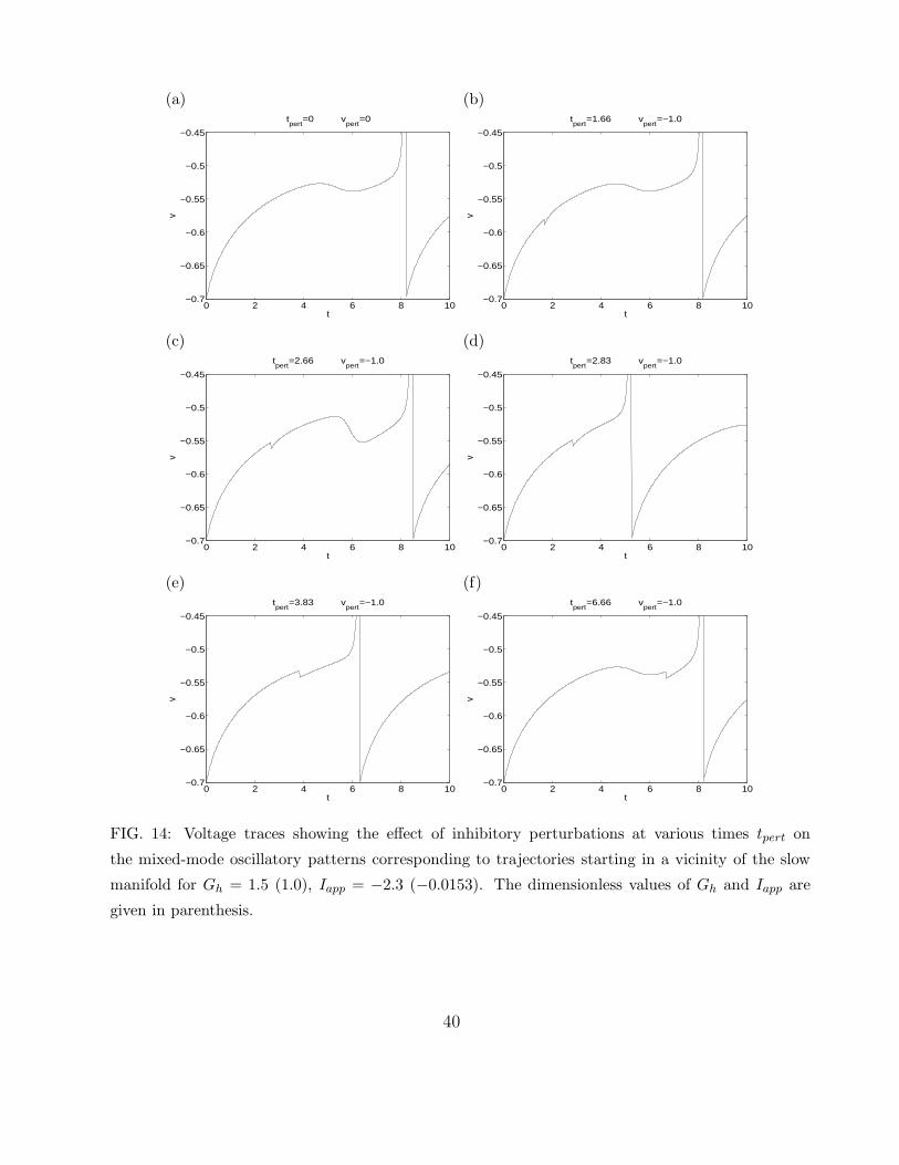
(a) (b)

0 2 4 6 8 10−0.7

−0.65

−0.6

−0.55

−0.5

−0.45

t

v

tpert

=0 vpert

=0

0 2 4 6 8 10−0.7

−0.65

−0.6

−0.55

−0.5

−0.45

t

v

tpert

=1.66 vpert

=−1.0

(c) (d)

0 2 4 6 8 10−0.7

−0.65

−0.6

−0.55

−0.5

−0.45

t

v

tpert

=2.66 vpert

=−1.0

0 2 4 6 8 10−0.7

−0.65

−0.6

−0.55

−0.5

−0.45

t

v

tpert

=2.83 vpert

=−1.0

(e) (f)

0 2 4 6 8 10−0.7

−0.65

−0.6

−0.55

−0.5

−0.45

t

v

tpert

=3.83 vpert

=−1.0

0 2 4 6 8 10−0.7

−0.65

−0.6

−0.55

−0.5

−0.45

t

v

tpert

=6.66 vpert

=−1.0

FIG. 14: Voltage traces showing the effect of inhibitory perturbations at various times tpert on

the mixed-mode oscillatory patterns corresponding to trajectories starting in a vicinity of the slow

manifold for Gh = 1.5 (1.0), Iapp = −2.3 (−0.0153). The dimensionless values of Gh and Iapp are

given in parenthesis.

40

(a) (b)

0 5 10 15 20−0.7

−0.65

−0.6

−0.55

−0.5

−0.45

t

vtpert

=0 vpert

=0

0 5 10 15 20−0.7

−0.65

−0.6

−0.55

−0.5

−0.45

t

v

tpert

=2.0 vpert

=−1.0

(c) (d)

0 5 10 15 20−0.7

−0.65

−0.6

−0.55

−0.5

−0.45

t

v

tpert

=3.33 vpert

=−1.0

0 5 10 15 20−0.7

−0.65

−0.6

−0.55

−0.5

−0.45

t

v

tpert

=5.0 vpert

=−1.0

(e)

0 5 10 15 20−0.7

−0.65

−0.6

−0.55

−0.5

−0.45

t

v

tpert

=5.83 vpert

=−1.0

FIG. 15: Voltage traces showing the effect of inhibitory perturbations at various times tpert on

the mixed-mode oscillatory patterns corresponding to trajectories starting in a vicinity of the slow

manifold for Gh = 1.5 (1.0), Iapp = −2.4 (−0.0160). The dimensionless values of Gh and Iapp are

given in parenthesis.

41