Can Wikipedia Article Traffic Statistics be used

to verify a Technical Indicator? An exploration

into the correlation between Wikipedia Article

Traffic Statistics and the Coppock Technical

Indicator.

Cormac O’Connor

A dissertation submitted in partial fulfilment of the requirements of

Dublin Institute of Technology for the degree of

M.Sc. in Computing (Data Analytics)

March 2015

ii

DECLARATION

I certify that this dissertation which I now submit for examination for the award of

MSc in Computing (Data Analytics), is entirely my own work and has not been taken

from the work of others save and to the extent that such work has been cited and

acknowledged within the test of my work.

This dissertation was prepared according to the regulations for postgraduate study of

the Dublin Institute of Technology and has not been submitted in whole or part for an

award in any other Institute or University.

The work reported on in this dissertation conforms to the principles and requirements

of the Institute’s guidelines for ethics in research.

Signed: _________________________________

Cormac O’Connor

Date: 6th

March 2015

iii

ABSTRACT

Recent studies have shown that, through the quantification of Wikipedia Usage

Patterns as a result of information gathering, stock market moves can be predicted

(Moat et al 2013). There was also research performed to determine the predictive

nature of Wikipedia Data to predict movie box office success (Mestyan et al. 2013).

The goal of any investor, in order to maximize the return of their investments, is to

have an edge over other participants in the markets. Several tools and techniques have

been used over the years to fulfil this, some proving to generate a consistent stream of

income (Gillen 2012). With the improvement of technology and communication links,

what was once considered a closed door, gentleman’s club operation, can now be

tapped into by anybody who has access to a PC and communications link.

It is said that approximately only 20% of investors are consistently successful in their

investments (Terzo 2013). In order be successful, there needs to be a strategy in place

that is strictly adhered to. The objective of these trading systems is to minimize, or

ideally cut out, the human emotion factor and naturally, as a consequence, allow the

strategy operate at its optimum. An example of this is through the use of technical

analysis indicator which, when used correctly, can net the investor considerable,

consistent returns. (Gillen 2012). Technical indicators, such as Coppock, are widely

used in the field of stock market investment to provide traders and investors with an

insight into which direction a stock or index is moving so as to facilitate the optimum

time to enter or exit the market. This project investigates whether Wiki Article Traffic

Statistics can be used to verify trading signals given by the Coppock technical indicator

through the use of a suitable correlation technique.

Keywords: Technical Analysis, Wikipedia, Coppock Indicator, Momentum,

Correlation.

iv

ACKNOWLEDGEMENTS

This dissertation would not have been possible without the help of a number of people,

for which I would like to take this opportunity to thank them.

I would like to express my sincere thanks to my supervisor Luca Longo for his help,

guidance and assistance throughout the course of this dissertation. I would also like to

thank Damian Gordon for reviewing my dissertation as the deadline approached and

helping to put things into perspective.

I would like to thank Mirko Kaempf, who through a series of discussions helped me to

solidify my idea and use the Wikipedia data source as a research topic.

Thanks to my parents who were always on hand to assist at home with my three boys

Cian, Neil and Rory, when I was unavailable due to the demands of the dissertation.

Finally, I would not have been able to achieve this completion only for the love and

support of my wife, Maria. Without her help, I would not have even considered going

the extra mile to achieve this.

v

CONTENTS

DECLARATION ............................................................................................................ ii

ABSTRACT .................................................................................................................. iii

ACKNOWLEDGEMENTS ........................................................................................... iv

TABLE OF FIGURES .................................................................................................. vii

TABLE OF TABLES .................................................................................................... ix

1 INTRODUCTION .................................................................................................. 1

1.1 Background ...................................................................................................... 2

1.2 Research problem ................................................................................................. 3

1.3 Research aim and objectives ................................................................................. 4

1.4 Research methodology.......................................................................................... 5

1.5 Scope and limitations ............................................................................................ 5

1.6 Organisation of dissertation .................................................................................. 6

2. LITERATURE REVIEW ....................................................................................... 8

2.1 What is technical analysis? ................................................................................... 8

2.2 The Coppock indicator ....................................................................................... 12

2.3 Wikipedia article view statistics ......................................................................... 17

2.4 Suitable correlation techniques ........................................................................... 25

2.5 Discussion ........................................................................................................... 28

3. EXPERIMENTAL DESIGN ................................................................................ 29

3.1 Introduction .................................................................................................... 29

3.2 Focus of the experiment ................................................................................. 29

Data ................................................................................................................ 29 3.3

3.3.1 Financial data structure ........................................................................... 30

3.3.2 Wikipedia data structure ......................................................................... 33

3.4 Data Cleansing .................................................................................................... 36

3.5 Transformation of data ................................................................................... 37

3.6 Summary ........................................................................................................ 40

4. EXPERIMENTATION AND EVALUATION .................................................... 41

4.1 Data pre-processing and initial characteristic analysis .................................. 41

4.1.1 Missing stock price data .............................................................................. 41

4.1.2 Missing weekend stock market price data ................................................... 42

4.1.3 Missing Wikipedia article traffic statistics data........................................... 43

4.1.4 Coppock value derivations .......................................................................... 44

4.1.5 Correlation checks ....................................................................................... 48

4.1.6 Strengths and Limitations ............................................................................ 49

vi

4.2 Summary ........................................................................................................ 50

5. RESULTS AND DISCUSSION ........................................................................... 51

5.1 Results ............................................................................................................ 51

5.1.1 Shapiro-Wilk test for Normalisation on Wikipedia data – 2008 ................ 52

5.1.2 Shapiro-Wilk test for normalisation on Wikipedia data – 2014 ................. 53

5.1.3 Shapiro-Wilk test for normalisation on stock price data – 2008 ................ 54

5.1.4 Shapiro-Wilk test for normalisation on stock price data – 2014 ................ 55

5.1.5 Correlation Results – 2008 - German DAX index and shares. ................... 57

5.1.6 Correlation Results – 2008 - DJIA index and shares. ................................. 62

5.1.7 Correlation Results – 2014 - German DAX index and shares. ................... 67

5.1.8 Correlation Results – 2014 - DJIA index and shares. ................................. 71

5.2 Discussion ...................................................................................................... 75

6. CONCLUSIONS AND FUTURE WORK ........................................................... 81

6.1 Problem definition and research overview..................................................... 81

6.2 Contributions to body of knowledge .............................................................. 83

6.3 Experimentation, evaluation and limitations ................................................. 83

6.4 Future work and research ............................................................................... 84

APPENDIX A: ADDITIONAL MATERIAL .............................................................. 85

REFERENCES ............................................................................................................. 89

vii

TABLE OF FIGURES

Figure 2.1: Coppock indicator performance between 1971 and 2014 (inclusive). ......... 2 Figure 2.1: Simple technical chart of the DAX Index, featuring candlesticks and

moving averages. .......................................................................................................... 10 Figure 2.2: Using momentum signals as a method of entering/exiting (buy/sell) a

market position. ............................................................................................................ 11

Figure 2.3: Coppock signals for monthly data. ............................................................ 14 Figure 2.4: Coppock signal on daily data (signalled on zero line cross). ..................... 15

Figure 2.5: Example of Wikipedia Page containing information on the German DAX

Index. ............................................................................................................................ 17 Figure 2.6: Example of Wikipedia Article Traffic Statistics on the German DAX

Index. ............................................................................................................................ 18 Figure 2.7: History of number of English Articles on Wikipedia. ............................... 21

Figure 2.8: Example of Holt-Winters forecasting technique (forecast in blue – 2010.0

onwards). ...................................................................................................................... 25 Figure 2.9: Correlation: strength of association, with positive/negative slope............. 27 Figure 3.1: Example Wikipedia article traffic statistic (Visual and JSON) on Dow

Jones page. .................................................................................................................... 34 Figure 4.1: Raw Holt-Winters forecasted data for ExxonMobil and associated chart

(forecasted values in blue). ........................................................................................... 43 Figure 4.2: Example of Coppock curve derived from the DAX index price data for

2008. ............................................................................................................................. 45 Figure 4.3: Example of SROC applied to the raw Wiki data of the DAX page. .......... 46 Figure 5.1: Shapiro-Wilk test for normality on Wikipedia article traffic statistics (raw,

Log10 and SROC) – 2008. ........................................................................................... 52 Figure 5.2: Shapiro-Wilk test for normality on Wikipedia article traffic statistics (raw,

Log10 and SROC) – 2014. ........................................................................................... 53 Figure 5.3: Shapiro-Wilk test for normality on the raw financial prices and derived

Coppock values – 2008. ................................................................................................ 54

Figure 5.4: Shapiro-Wilk test for normality on the raw financial prices and derived

Coppock values – 2008. ................................................................................................ 55

Figure 5.5: Graph of German DAX index – 1st January, 2008 to 31st December, 2008

(Yahoo Finance). .......................................................................................................... 58

Figure 5.6: Graph of German DJIA index – 1st January, 2008 to 31st December 2008

(Yahoo Finance). .......................................................................................................... 63 Figure 5.7: Graphs representing the Wiki (SROC) versus Coppock value for P&G –

raw data in red, derived data in blue. ............................................................................ 64 Figure 5.8: Graph of German DAX index – 1st January, 2014 to 31st December, 2014

(Yahoo Finance). .......................................................................................................... 68 Figure 5.9: Graph of DJIA index – 1st January, 2014 to 31st December, 2014 (Yahoo

Finance). ....................................................................................................................... 72 Figure 5.10: Graphs representing the Wiki (SROC) versus Coppock value for Exxon.

...................................................................................................................................... 74

Figure 5.11: Smoothed Rate of Change applied to underlying DAX Wikipedia Page

Views – 2008 Data........................................................................................................ 76 Figure 5.12: Coppock curve applied to underlying DAX index prices – 2008 data. ... 77

viii

Figure 0.1: Sample of CSV Wikipedia Article Traffic Statistics for “Dow Jones” Page

Views. ........................................................................................................................... 86

ix

TABLE OF TABLES

Table 2.1: The Coppock indicator: track record of “buy” signals on S&P Index since

1970. ............................................................................................................................. 13 Table 3.1: Structure of data downloaded directly from Yahoo Finance or Bloomberg

Data. .............................................................................................................................. 30 Table 3.2: Structure of financial data for each index and share. .................................. 30

Table 3.3: File names containing stock market price data............................................ 31 Table 3.4: List of highest weighted stock on German DAX Exchange. ....................... 32

Table 3.5: List of highest weighted stocks on Dow Jones Industrial Average Exchange.

...................................................................................................................................... 32 Table 3.6: Structure of raw data files, stored by the hour............................................. 33 Table 3.7: Structure of Wikipedia article traffic statistics for each index and company.

...................................................................................................................................... 35

Table 3.8: Filenames containing associated Wikipedia article traffic statistic data. .... 35 Table 3.9: Time frames by which normality check was performed on the Wikipedia

and financial price data. ................................................................................................ 38 Table 3.10: Sample of Shapiro-Wilk Normality test for each set of data (Raw and

Transformed). ............................................................................................................... 39 Table 4.1: Derivation of adjusted close price from Bloomberg close price. ................ 42

Table 4.2: Set of Coppock values derived from financial prices. ................................. 44 Table 4.3: Sample of calculation of Coppock value on the DJIA index price using

ROC and WMA. ........................................................................................................... 46 Table 4.4: Example of first available Smoothed rate of change on WATS for January

2008. ............................................................................................................................. 47

Table 4.5: Detail of each dataset for correlation check. ............................................... 48 Table 4.6: Timeframe for each correlation check. ........................................................ 49

Table 5.1: Datasets where both results are of normal distribution, indicating Pearson

correlation suitability – 2008/2014. .............................................................................. 56 Table 5.2: Correlation results for 2008 on DAX index and associated shares (ordered

by strength). .................................................................................................................. 57 Table 5.3: Number of Wikipedia page views on the DAX market and associated shares

in 2008. ......................................................................................................................... 61 Table 5.4: Correlation results for 2008 on DJIA Index and associated shares (ordered

by strength). .................................................................................................................. 62 Table 5.5: Number of Wikipedia page views on DJIA market and associated shares in

2008. ............................................................................................................................. 66 Table 5.6: Correlation results for 2014 on DJIA index and associated shares (ordered

by strength). .................................................................................................................. 67

Table 5.7: Number of Wikipedia page views on DAX market and associated shares in

2014. ............................................................................................................................. 70 Table 5.8: Correlation results for 2014 on DJIA index and associated shares (ordered

by strength). .................................................................................................................. 71

Table 5.9: Number of Wikipedia page views on Dow Jones Industrial Average and

associated shares in 2014. ............................................................................................. 75 Table 5.10: Comparison of raw Wiki correlation and SROC (Wiki) against Coppock

values – best correlations in yellow. ............................................................................. 78

x

Table 0.1: Sample of CSV Wikipedia Article Traffic Statistics for “Dow Jones” Page

Views. ........................................................................................................................... 86 Table 0.2: Shapiro-Wilk result on 2008 data (Wikipedia and Stock Price Data). ........ 87 Table 0.3: Shapiro-Wilk result on 2014 data (Wikipedia and Stock Price Data). ........ 88

1

1 INTRODUCTION

It is estimated that the financial crisis of 2008 cost Americans between $6 trillion and

$14 trillion, which translates to $50,000 and $120,000 for every US household

(Luttrell et al. 2013). This financial crisis brought to people’s attention how quickly

and severely one’s wealth can be destroyed, and the importance of preventing this

through proper money management and investment strategy. A number of large US

corporations suffered, as with the collapse of Bear Stearns and Lehman Brothers, and

the near collapse of Fannie Mae and Freddie Mac, the latter two requiring a bailout by

the US Federal Reserve. It is the cause and consequence of these failures that added

fuel to the fire of the financial downturn, and which financially affected such a large

number of innocent institutions and investors.

In order to prevent one’s wealth from being destroyed during a downturn period, it

requires the use of reliable and proven signals called technical indicators. A technical

indicator is a stock analysis methodology which is used to forecast the direction of

share prices and/or stock market indexes through the use of historic market data. These

can be used to signal a potential downturn, and thus, through active steps by the

institution or investor, can save a large amount of capital that is invested in the stock

market. Equally, technical indicators can signal to an investor the optimal time to enter

into the stock market and maximise any potential gains. A number of well-known

technical indicators can assist investors in predicting the market direction. These

include MACD (moving average convergence divergence), RSIs (relative strength

indicators), the stochastic oscillator and the Coppock indicator (Gillen 2012).

Another source of information which can assist an investor is the availability of

Wikipedia article traffic statistics. These statistics are openly available to the public,

providing the number of page views and page edits made by the Wikipedia audience.

Through the use of these statistics, it is possible to determine an interest factor

concerning a particular page, and to build a history of viewership. By using the

Wikipedia article traffic statistics, it may be possible to complement the signal given

by some of these technical indicators, such as the Coppock indicator.

2

1.1 Background

The Coppock indicator was invented by Edwin “Sedge” Coppock, and first published

in Barron’s Magazine on October 15th

, 1962 (Nicholson 2010). The idea came about

as a result of Coppock being approached by his local church minister concerning best

investment strategies, to ensure that they had their money invested to its best potential.

Coppock believed that suffering a loss as a result of a market downturn was like a

bereavement, which also required a period of mourning. Therefore, Coppock, in return,

asked the church minister how long it took, on average, for a person to fully mourn the

death of a loved one. The estimate given was between 11 and 14 months.

Coppock concluded that, as a result of a market drop, the bereavement period would be

similar to the death of a loved one, and, consequentially, the same could be applied to a

loss suffered on the stock market. From this, it could be possible to predict the

optimum time to re-enter the market. Simply put, it is a momentum indicator which

oscillates above and below the X-axis, which, when there is a crossover from negative

to positive, would indicate a time to buy into the market. Figure 1.1 demonstrates the

success of the Coppock indicator on the S&P Index between 1971 and 2014. It has

given 11 buy signals, and has performed well over a 1-year/3-year/5-year period. As

can be understood from the figure, of the 11 Coppock signals given, only one year

(2001) returned a negative return after one year but became profitable, like the other

years, from Year 3 onwards.

Figure 2.1: Coppock indicator performance between 1971 and 2014 (inclusive).

Despite the fact that the Coppock indicator was originally designed to work on

monthly data, and to only be used to indicate a “buy” signal following a period of

decline, this indicator can be used to work on more frequent data – for example, daily

3

price data – and also to be used to give the investor a “sell” signal (Mitchell 2014). As

a result of the facilitation of more frequent time periods and both buy and sell signals,

the Coppock indicator can be used to further increase the potential returns to an

investor.

The biggest drawback with the Coppock indicator relates to the “false” signals which

occur when the Coppock value crosses above or below the X-axis, only to quickly

cross back in the opposite direction immediately after. This can create confusion for

the investor, who thus loses confidence in the signal’s real value and reliability.

Therefore, it is important to have the parameters required for the Coppock calculation

tuned relative to the frequency of data being analysed. In addition, as mentioned,

Coppock originally designed the indicator to signal when the line crossed the X-axis,

but some investors have refined this further, in order to increase profits, so as to enter

or exit the market when there is a change in direction from a trough or peak of the

Coppock time series (Mitchell 2014). Using Wikipedia page view statistics, it may be

possible to verify the signal given by the Coppock indicator by using the data for each

associated Wikipedia page, whether relating to a stock market index (DJIA, DAX) or

individual stock contained in that associated index. Using this confirmation from the

Wikipedia article traffic statistics, it may be possible to verify the signal that the

Coppock indicator gives.

1.2 Research problem

The Coppock indicator has a proven track record when it is applied using its original

design criteria – to provide a buy signal when applied against monthly data (Gillen

2012). For example, on the S&P Index since 1975, there have been 11 buy signals

provided by the Coppock indicator. Only one of these signals, in the year 2001, proved

to be incorrect. Therefore, it can be understood that the Coppock indicator is a very

reliable indicator for the long-term investor when used against monthly data. This is

not very useful, however, in the midst of a financial crisis or any short-term event, as

the damage to one’s wealth will have passed before any suitable signal is given.

Therefore, in order to improve on this, a more detailed analysis is required on the data

given. To facilitate this tighter window, the Coppock signal can also be derived from

daily data.

4

Because the Coppock indicator is a Smoothed momentum oscillator, where the rate-of-

change measures momentum and the weighted moving average performs the

smoothening of the data, the indicator can be run against any time frame. In order to

optimise the financial returns through the use of the Coppock indicator over shorter

time frames (daily in this case), the parameters for calculation may need to be adjusted

to reflect this. Shorter rates-of-change will result in the Coppock curve becoming faster

and more sensitive, while longer settings will make it less sensitive.

A method of confirming the signal given by the Coppock curve through the use of

Wikipedia article traffic statistics may result in a better-performing investor fund by

yielding the investor higher returns.

1.3 Research aim and objectives

The main aim of this dissertation is to determine whether the signal given by the

Coppock indicator can be confirmed through the use of associated Wikipedia article

traffic statistics.

As a consequence, an investor may be able to make better trading decisions through

the Coppock indicator, in conjunction with the confirmation achieved through the

associated Wikipedia signal. The correlation achieved between the Wikipedia article

traffic statistics and Coppock values will verify whether there is value in using the

Wikipedia article view statistics as a verifying indicator.

The main objectives of this dissertation are as follows:

1. To determine correlations between different datasets: Research was conducted

concerning the Coppock indicator, its characteristics and its performance over

different time ranges. A review of existing techniques used to determine

correlations between different datasets was performed.

2. To test whether Wikipedia article traffic statistics verified the existing Coppock

indicator: An experiment was designed to test this. This was achieved by

testing correlations between Wikipedia article traffic statistics for two stock

5

market indexes (Dow Jones, German DAX) and five stocks contained in each

index against associated Wikipedia article traffic statistics for each page on that

stock or index.

3. To confirm whether there is value in using Wikipedia article view statistics: An

analysis was performed on the results obtained from each index and stock to

confirm this. An exercise was used to determine what time series correlation

method worked best, along with a range of different parameters used in the

generation of the Coppock signal (rate of change, weighted moving average).

This would determine the success or failure of the experiment, based on the

results obtained.

4. To identify future areas of research which may improve and assist in

determining a better correlation between both data sets.

1.4 Research methodology

i. Objective 1 has been achieved through a literature review of the Coppock

indicator and the uses of it over different frames other than the monthly time

frame for which it was originally designed. Information concerning the

different correlation techniques was also gained through the literature review.

ii. Objective 2 has been achieved through the detailed design of experiments, in

order to determine whether there is a correlation between the two datasets. This

has been achieved by the use of suitable normality tests and the appropriate

correlation checks performed thereafter.

iii. Objective 3 has been achieved through the execution and gathering of

correlations determined through the research methodology. These results are

evaluated in order to determine the relationship between the two datasets.

1.5 Scope and limitations

Stock market price data and associated Wikipedia article traffic statistic data for two

stock markets were selected: the German DAX exchange and the US Dow Jones

Industrial Average (DJIA) exchange. Five of the largest capitalised stocks were chosen

from each associated index. Two years were chosen for analysis: 2008 and 2014.

Because the Wikipedia datasets contained all traffic for every page on an hourly basis,

it was not feasible to download these for each year in order to extract the selected

6

Wikipedia page traffic. The alternative was to download Wikipedia traffic data through

the manual JSON download facility, and subsequently extract data for each stock and

year/month in question. In a real-world environment, there would be sufficient space to

download a full dataset and perform an analysis on every stock belonging to each stock

market index.

1.6 Organisation of dissertation

The dissertation is organised as follows:

Chapter Two will cover research conducted in the area of technical analysis,

and will then focus specifically on the Coppock indicator, how it is derived and

steps taken to improve its performance depending on the frequency of data to

which it is applied. Following this, research completed using Wikipedia article

traffic statistics in the area of stock market investments, and how it has been

used to better improve returns on investment for the investor, will be addressed.

It will also cover research conducted in regard to correlations between similar

datasets, and how best to use these.

Chapter Three will concentrate on the experiment, its design and the

implementation of the model. It will detail the collection of data, its structure

and evaluation methods for the models. Any data cleaning and transformation

that is required in order to make the data as effective as possible will be

outlined. Finally, a detail of the correlation methodologies used will be

presented, with the results of this discussed.

Chapter Four will focus on the implementation and evaluation of the

experiment, and how the datasets were correlated to determine whether there is

value in including Wikipedia article traffic statistics in order verify the signal

given by the Coppock indicator. This chapter will also cover the issues around

missing weekend/bank holiday data, and how this was addressed in order to

correlate with the Wikipedia article traffic statistics dataset. The evaluation

done in order to determine the effectiveness of the Wikipedia data when added

7

to the Coppock indicator will be outlined. A number of time periods within the

years 2008 and 2014 will be analysed along with various parameter changes to

the Coppock signal and Wikipedia data, to determine the optimal correlation.

Chapter Five will report on the results from the implementation and

experiments, as outlined in Chapter 4. These results will be analysed and

compared to the findings derived from the literature review.

Chapter Six will conclude the dissertation and provide an overview of the

work carried out during the course of the experiment. Further areas of

investigation and research will be highlighted in order to potentially improve

on the results found.

8

2. LITERATURE REVIEW

A vast amount of work has been completed in determining methods of defining new

technical indicators or in the refinement of existing indicators in order to improve the

return on one’s investment. This continues to be done by both large institutions and

private investors alike. Timing in regard to when to enter and exit a trading position on

the stock market has been the quest of investors over the years. As a result, several

techniques have been created to assist traders and investors on when to time the entry

and exit on the market most effectively. Some of these techniques include the 30/50

day moving average strategy, the Dow Theory and the Coppock indicator (Gillen

2012).

In a situation where buyers outnumber sellers, the market moves upwards; when

sellers outnumber buyers, the market moves downwards. Each buyer and seller is

acting on a belief that his/her decision is correct and appropriate relative to what is

occurring in the market at that point in time. Therefore, it is safe to claim that

everyone’s view is priced into the market, and is thus representative of the market

condition at that time (Elder 1993). In the investment book The Intelligent Investor

(Graham 2005), it was determined that there were two key approaches to successful

investing on the stock market. The first is through the identification of stocks that were

priced below their intrinsic value, called value investing. The second approach is

through the timing of the stock market. This popular approach used to time the stock

market and its associated moves is achieved through a technique called technical

analysis.

2.1 What is technical analysis?

Professionals in the stock market are constantly attempting to time the market so that

they can maximise their profits through the strategic closure of open positions before a

drop in the stock markets occurs (bear market) and/or an opening of new positions in

the market occurs again before an established upturn (bull market). According to Pring

(2002), a specific definition of technical analysis can be presented as follows: “The

technical approach to investment is essentially a reflection of the idea that prices move

in trends that are determined by the changing attitudes of investors toward a variety of

9

economic, monetary, political, and psychological forces. The art of technical analysis,

for it is an art, is to identify a trend reversal at a relatively early stage and ride on that

trend until the weight of the evidence shows or proves that the trend has reversed.”

Large revenues are made by training companies which, in many cases, charge high

fees offering the “silver bullet” to time the market perfectly, and which also offer the

purchaser maximum profits with minimum risk (Kemp 2014). Such an approach is

difficult to achieve, as it requires a great deal of study, practice and patience. However,

through sufficient study of technical analysis and the respectful use of the associated

indicators that exist, an investor can achieve consistent returns over the long term.

Therefore, the “noise” that exists through the news and media, of which 90% is of no

value to the investor (Gillen 2012), can be ignored by the investor, and more attention

spent on what the technical indicators are reporting.

Technical analysts use charts to study market action, with the objective of uncovering

recurring market action. The basis of any chart used to perform technical analysis

requires the following values for each day (Elder 1993):

● Opening price: This is generally the opinion of the amateur who has digested

the news from the previous day, and has requested a trade to be placed at the

opening of the market.

● Closing price: This is the price which the professionals consider to be the true

value of the share. Generally, they monitor the behaviour of the amateurs, and

become active as the close of market approaches.

● Daily high: This reflects the battle between the bulls and bears on that day. In

this case, it reveals the strength of the bulls on the day.

● Daily low: Similarly to the daily high, this reveals the battle between the bears

and the bulls, revealing the strength of the bears on the day.

The goal of a technical analyst is to identify patterns that exist when a set of daily data

is produced on a chart, and to profit from the anticipated movement that can be

predicted from these trends. As can be seen in Fig. 2.1 (stockcharts.com), each day is

represented by a candlestick, where the direction of the day is indicated by the colour

10

(red: decrease in stock value; green: increase in stock value). In its simplest form, the

technical analyst will also use some overlay indicators to assist in determining the

strength of direction of the underlying share or index.

Figure 2.1: Simple technical chart of the DAX Index, featuring candlesticks and moving averages.

Moving averages (MAs) are commonly used which indicate to the analyst where the

strength in direction is. The longer the time frame of the moving average line, the

slower it will react to daily market prices. Conversely, the shorter the time frame on

which the moving average line is based, the faster it will react to any daily price

movement. As highlighted by Allen and Karjalainen (1998), a common investment

strategy using the moving averages is one where a “buy” signal is given when the 30-

day MA crosses above the 50-day MA. This signal is strengthened when the 50-day

MA has an upward trend. A “sell” signal is given when the 30-day MA crosses below

the 50-day MA. On top of this, the “sell” signal is strengthened when the 50-day MA

has a downward trend. As recommended by Shipman (2008), the use of the moving

average approach helps to remove short-term volatility apparent in the underlying

market, thereby assisting traders in detecting the trend, and any investment opportunity

that may appear.

A popular set of technical indicators used to determine the strength and direction of a

share or market are known as momentum indicators (Gillen 2012).

11

Momentum is defined as the difference between the current closing price and the

closing price n days ago, determined by the trader/investor.

Therefore, if the current price is higher than the earlier price, it is said to have a

positive momentum. The opposite occurs when the current price is less than the earlier

price, returning a negative momentum. A simple trading strategy can be applied using

a combination of price momentum, where, if combinations of derived momentums

cross from negative to positive, a “buy” signal is generated. The opposite occurs when

the momentum line crosses from positive to negative, thus returning a “sell” signal, as

is demonstrated in Figure 2.2. Bird and Casavecchia (2005) in their study of

investment improvement through the use of momentum indicators found that there was

an increase in investment returns through the use of price momentum.

Figure 2.2: Using momentum signals as a method of entering/exiting (buy/sell) a market position.

Another related indicator is called the rate of change (ROC), which scales the

momentum value by the old close price, thus becoming a fraction.

12

If there is a consistent set of positive momentum values, this indicates that there is an

uptrend in place. Conversely, if there is a consistent set of negative momentum values,

this indicates that there is a downtrend in place. Therefore, if the ROC trend line

crosses the x-axis from negative to positive, this signals a buying opportunity, while, if

the trend line crosses the x-axis from positive to negative, this signals a selling

opportunity. Momentum and ROC are often used to determine the best time to enter or

exit the market.

Technical indicators, therefore, offer investors a strategic method of investing through

the use of historic data in order to best predict which direction a market will take over

the time frame on which the trader/investor is focused. They have been used by a wide

audience of investors, some of which have been successful in their predictions, others

not so successful. Therefore, it is important to choose a technical indicator, or a

number of indicators, that have a proven track record, which work well for that trader,

and which the trader has proven to operate successfully over the long term. This is

normally achieved through trial and error; thus, it advised that a demo account be used,

where fictitious money is used to trade the stock market and prove whether a given

trading strategy using certain technical indicators yields a profitable result. Technical

indicators are used on short-, medium- and long-term time ranges, and are adopted by

short-term, speculative traders and long-term investors.

2.2 The Coppock indicator

A reliable performance momentum technical indicator is the Coppock indicator.

According to Gillen (2012), when used against monthly data on the US S&P 500

Index, the Coppock indicator has given 11 “buy” signals since 1970. Ten out of the 11

signals yielded a positive return after one year of being signalled and more substantial

returns over a longer period. For example, three years after the initial “buy” signal, the

average return amounted to 42% and 88% after five years. Therefore, all factors

combined would indicate that the Coppock indicator is a reliable tool which yields a

respectable return to the investor.

13

Table 2.1: The Coppock indicator: track record of “buy” signals on S&P Index since 1970.

The indicator is derived by calculating the weighted moving average (WMA) of the

rate of change (ROC) of a market index. A weighted moving average assigns a higher

weighting to more current data points, as they are more relevant than the data points in

the past (Elder 1993).

Therefore, the Coppock indicator is calculated by adding both rates of change (11

months and 14 months, respectfully) together and performing a weighted moving

average (10 month) on the result.

Following the original invention of the Coppock indicator, it has since been

customised by more short-term, speculative traders to work over more frequent time

frames (i.e. weekly, daily, etc.). Furthermore, it is also used by traders to signal a

“selling” opportunity, and thus facilitates both the entry and exit of a trade entered on

the stock market. Dependant on the level of risk tolerance the investor possesses, the

sensitivity of the Coppock indicator can be tuned through the adjustment of the ROC

and WMA parameters applied. By decreasing the WMA, this causes the result to signal

14

an entry or exit stock market position slightly earlier. Increasing the WMA causes the

result to signal slightly later for both entry and exit positions.

The Coppock curve can be acted upon in two different ways. Coppock originally

designed the curve to signal a buy signal only, when the line crossed from positive to

negative, and returned back to positive. Coppock anticipated that, when the line

crossed from negative to positive, the “buy” signal would fire. This is shown as the

green vertical line in Figure 2.3. This rule has since been customised by traders to fire

a “sell” signal when the line crosses from positive to negative. This sell signal is

shown as the red vertical line in Figure 2.3. Many traders feel that the X axis crossover

is not as reactive to the cycle change as desired, and thus fires a signal when there is a

turn in the Coppock curve. An example of such a more reactive “buy” signal is given

by the “buy” arrow in Figure 2.3.

Figure 2.3: Coppock signals for monthly data.1

1 “Investopedia (2014) Using the Coppock Curve to Generate Stock Trade Signals [Online]. Available:

http://www.investopedia.com/articles/active-trading/031814/using-coppock-curve-generate-stock-trade-

signals.aspl [Accessed 29 November 2014].”

15

The advantage of entering at the turning point (buy arrow), and not at the x-axis

crossover, means that the position is placed at an earlier time than waiting for the

confirmation x-axis crossover. This means that there is a better chance of making a

larger profit, due to the reduction of that time-loss. The disadvantage of this is that it

can result in a false signal where the initial downturn occurred but was followed by a

resumption upward, thus erasing any initial profit made, and resulting in a potential

overall loss. Other, shorter-term strategists (Mitchell 2014) act on the signal given by

the Coppock Indicator when the Coppock value has dropped from a positive value

(above the X-axis) to a negative value (below the X-axis), and signals “buy” when it

has turned back upward, crossing the X-axis again. This is more suited to a tighter

trading frequency (hourly, daily), when false signals could be given merely by

adopting the upward turn from the bottom of a negative position. Because signals will

be more abundant in tighter frequencies, it is more appropriate, in these cases, to wait

until the line has crossed either above (buy signal) or below (sell signal) the X-axis.

Figure 2.4: Coppock signal on daily data (signalled on zero line cross).2

2 “Investopedia (2014) Using the Coppock Curve to Generate Stock Trade Signals [Online]. Available:

http://www.investopedia.com/articles/active-trading/031814/using-coppock-curve-generate-stock-trade-

signals.asp?rp=i [Accessed 29 November 2014].”

16

As can be seen in Figure 2.4, there are more frequent signals given on the daily chart

than on the monthly chart. Therefore, depending on the frequency of data, the indicator

calculation parameters (WMA and ROC) can be adjusted to result in the Coppock

indicator working more optimally with the data. This can be achieved as follows

(Mitchell 2014):

● Decreasing the ROC will increase the speed of fluctuations, and thus increase

the number of trade signals.

● Increasing the ROC will slow the fluctuations, and therefore produce fewer

signals.

● Decreasing the WMA to receive earlier entry and exit signals.

● Increasing the WMA to receive later entry and exit signals. Some traders prefer

this, in order to obtain confirmation that the momentum is maintained in the

same direction.

● Traders use a longer-term trend to confirm the direction of the market before

placing a position using the shorter-term trends.

Therefore, two further derivations of the Coppock values can be created using

parameters recommended by Mitchell (2014) and StockCharts.com (2015):-

Set 1

14-day Rate of Change (ROC)

11-day Rate of Change (ROC)

6-day Weighted Moving Average (WMA)

Set 2

20-day Rate of Change (ROC)

10-day Rate of Change (ROC)

10-day Weighted Moving Average (WMA)

These parameter sets are more suited to daily data as the Coppock signals are given a

little bit earlier thus facilitating the potential to make a better return of investment.

17

2.3 Wikipedia article view statistics

The advent of the Web 2.0 and social networks have enabled the proposal of

recommendation and reputation models for the assessment of trust of online entities

(Dondio and Longo 2014; Longo et al. 2007) and the design of web-based systems

(Longo et al. 2012). Similarly, the nature of social information exchange has

encouraged the gathering of activity statistics by website hosts complemented the

original method of exchanging information and enabling social search (Longo et al.

2009; Longo et al. 2010).

Several sources of such underlying statistical information are open to the public for

downloading and analysis, including Twitter, Google Trends and Wikipedia. With the

development of open access to this activity data, using proper analytical techniques, it

is possible to use this information to assist in predicting what will most likely happen

in the future. In Figure 2.5 and 2.6, an example is given on the Wikipedia page for the

DAX Stockmarket Index and its associated Article Traffic Statistics. From this, a

profile of the frequency of page views can be determined.

Figure 2.5: Example of Wikipedia Page containing information on the German DAX Index.3

3 "Wikipedia (2014) Wikipedia GUI [Online]. Available: http://www.wikipedia.org [Accessed 29

November 2014]."

18

Figure 2.6: Example of Wikipedia Article Traffic Statistics on the German DAX Index.4

A study conducted by Preis et al. (2012) discovered that there is a relationship between

the economic success of a country, using gross domestic product (GDP), and the

behaviour of information searching among that country’s citizens. In this study, they

found that, the more prosperous a country was, based on its GDP, there was a higher

likelihood of searches focusing more on the future than the past, and vice versa.

Further work by Preis et al. (2013) showed that there was an increase in searches using

Google Trends relating to financial markets shortly before stock markets fell on certain

occasions. Preis et al. (2013) built on the Simons (1955) idea that market participants

begin their decision-making process by attempting to gather information. Therefore,

they concluded that financial data sets reflect the final outcome of a trader’s decision-

making process, regarding the decision to buy or sell a particular stock. As a result, the

volume of searches for words related to financial markets could be used to produce a

profitable trading strategy.

Sakaki et al. (2010) developed an alert system which, through the use of semantic

analysis, used messages posted on Twitter to detect earthquakes almost in real-time.

The work was to highlight that the alert system could warn at a rate faster than the

event itself and thus could help reduce to the damage incurred by these events. Google

Trends provides information about the information people are seeking, while

Wikipedia Statistics provides insights into what information Internet users actually use

4 "Wikipedia (2014) Wikipedia Article Traffic Statistics [Online]. Available:

http://stats.grok.se/en/201410/DAX [Accessed 29 November 2014]."

19

(Kampf et al. 2014). Bollen et al. (2010) proved that it was possible to predict the

movement of a stock market using Twitter data, with an accuracy of up to 86.9%. This

was determined through the use of specific words to determine this change in

sentiment. Interestingly, it was discovered that neutral words such as “calm” provided

the best predictive value. This would reinforce their argument that the use of non-

sentiment-related data could yield a positive result as a predictive indicator. Kamvar

and Harris (2011) developed a method of continuously searching through all blogs

contained on the web every 10 minutes and extracting any sentence containing the

words “I am feeling” or “I feel”. From this, they were able to create a data

visualisation of the mood of the world, and to categorise this into different

components; for example, “Guiltiest Cities”, “Greatest Cities”, “Happiest States”, etc.

Dondio (2012) discovered that the best stock market performance is achieved when

information regarding stock capitalisation is coupled with medium- and long-term web

traffic. The findings revealed that both web traffic and price-related features

outperform a price-only classifier, while a web-traffic-only classifier outperforms all

other classifiers in predicting price increases. Therefore, it is fair to conclude that the

addition of web traffic data has a positive impact on the level of predictability around a

share price or index. Moet et al. (2013) analysed changes in Google query volumes for

search terms related to finance, and uncovered patterns of early warning signs relating

to stock market moves. They discovered that there was an increase in information

gathering when there are trends to sell on the financial market at lower prices. They

found that Google Trends data not only reflected the current state of the stock market,

but also that this data could be used to determine certain future trends. Moat et al.

(2013) continued to show that there was an increase in Wikipedia usage on particular

pages related to companies and other financial topics before a stock market move,

particularly a stock market fall. Due to the open availability of information and data on

the Internet, websites such as Wikipedia are becoming the first point of reference when

information is required. A hypothetical investment strategy was created to trade on the

Dow Jones Industrial Average, where, if the average number of views for week n is

greater than the previous week, the position is sold. As part of this research, they found

that there was a significantly smaller number of Wikipedia page edits relative to the

Wikipedia page views, therefore having little overall impact. As a consequence, they

20

concentrated on the Wikipedia article views, and discarded the use of Wikipedia page

edit data. Their evidence suggests that there is an increase in the number of page views

of companies and other financial topics before stock market moves. From this, they

were able to suggest that online data may allow new insights into the early stages of

information gathering, to assist in decision-making.

Tversky and Kahneman (1991) present a reference-dependent theory of consumer

choice, where they conclude that losses and disadvantage have a greater impact on

decision than gains and advantage. Therefore, Moat et al. (2013) used these findings to

conclude that more effort is devoted to information gathering on Wikipedia, as part of

the early stages of the decision-making process, preceding a fall in stock market prices.

It was also highlighted that people are more loss-averse, in that they are more

concerned about losing £5 than about missing an opportunity to make £5.

Wikipedia is able to provide accurate, hour-by-hour article view statistics concerning

activity on Wikipedia for that period. This popular Wikipedia website maintains a

logging mechanism called Wikipedia article traffic statistics (WATS), created by

Mituzas (2007), which records the number of times every Wikipedia page has been

viewed and edited. The article traffic counter has existed since December 10th

, 2007,

and this information is saved in a separate compressed file on an hourly basis, which is

available to download for free via a dedicated website, Wikipedia Article Traffic

Statistics.5

The English version of Wikipedia has become the seventh most popular website

globally, and the sixth most popular in the United States of America6, recording almost

20 million views for all languages in the month of December, 2014 alone7, of which

9.5 million views relate to the English language alone. Due to the increase in access

and usage, a great deal of potential insight can be obtained from the underlying article

5 "stats.grok.se (2014) Wikipedia Article Traffic Statistics [Online]. Available: http://stats.grok.se/

[Accessed 29 November 2014]." 6 "Wikipedia Popularity (2014) Audience Geography [Online]. Available:

http://www.alexa.com/siteinfo/en.wikipedia.org/wiki/Main_Page [Accessed 7 January 2015]." 7 "Page Views for Wikipedia (2015) [Online]. Available:

http://stats.wikimedia.org/EN/TablesPageViewsMonthlyOriginalCombined.htm [Accessed 7 January

2015]."

21

view data. Since the inception of Wikipedia in 2001, it has grown in popularity, as has

the number of articles available for viewing8.

Figure 2.7: History of number of English Articles on Wikipedia.9

Many users prefer to visit specific pages on Wikipedia, due to the fact that it is not a

means of promotion and advertising10

. These rules concerning hosting consist of

refraining from performing the following:

● Advocacy, propaganda or recruitment

● Opinion pieces

● Scandal mongering

● Self-promotion

● Advertising, marketing or public relations

Wikipedia article traffic statistics offers the following advantages:

● The data is stored on an hourly basis, while Google Trends usage is on a per-

week basis. This allows for a more granular analysis of the data, thus giving the

potential of more insight through the usage statistics.

● Access to data on Wikipedia has been freely available since 2007, while

8 "Wikipedia Number of Articles - Graph [Online]. Available:

http://en.wikipedia.org/wiki/File:EnwikipediaArt.PNG [Accessed 8 January 2015]." 9 "en.wikipedia.org (2015) Wikipedia Number of Articles [Online]. Available:

http://en.wikipedia.org/wiki/File:EnwikipediaArt.PNG [Accessed 14 January 14 2015].” 10

"Funding Wikipedia through advertisements [Online]. Available:

http://en.wikipedia.org/wiki/Wikipedia:Funding_Wikipedia_through_advertisements [Accessed 15

January 2015]."

22

Google Trends restricts the number of words that can be accessed.

● Due to the open availability of Wikipedia, data is freely accessible, unlike the

limitation of Google Trends.

Some research conducted to date has used Wikipedia article view statistics. Early

prediction of movie box office success was performed by Mestyan et al. (2013),

through the analysis of the editing and viewing of Wikipedia information concerning

the movie in question. Using linear regression modelling, they used the Wikipedia

editing and viewing activities concerning 312 movies to predict the first weekend box

office revenue. Because many of the Wikipedia pages were created well in advance of

the movie launch, they were able to follow the popularity of these movies as that

movie launch day approached. The following activity measures were used:

i. Number of views of the Wikipedia article page.

ii. Number of human editors who contributed to the page.

iii. Number of edits performed on the specific page.

iv. Collaborative rigour of the editing trail for the specific article.

It was discovered that their model was more accurate when the movie was more

popular, and when the volume of the related Wikipedia article view data was large.

Alanyali et al. (2013), in their research conducted to quantify the relationship between

financial news and the stock market, discovered that, when there is a greater number of

mentions in the news on a given morning, it corresponded to a greater volume of

trading for that company during that given day. They also discovered that there was a

greater change in price for that company’s stock. Their analysis also provided no

evidence of a relationship between the number of mentions of a company in the

morning news and the change in that company’s share price when the direction of

price change is considered.

Surowiecki (2004) indicates in his book The Wisdom of Crowds that one of humanity’

greatest assets is its unrecognised ability to make accurate collective decisions, as long

as each individual is not influenced by the decision of others and has made the decision

based on his/her own free will. The crowd, ideally, should consist of a broad spectrum

23

of people, from experts to novices, in the area of study. Surowiecki uses an early

example from the 1900s, where, during an experiment in ox-breeding, 787 people were

asked to guess the weight of an ox after it had been slaughtered and dressed. Each

individual guess was incorrect, but the average of all the guesses (1197 lbs) was

extremely close to the actual weight of 1198lbs. He concludes that, through the

following of crowd behaviour, stock market and property bubbles are created, but,

when each individual decision is made independently, there is astonishing accuracy

achieved, and, when values are questioned, the results are also accurate. In a BBC

Documentary, “The Code”, presented by Marcus du Sauto (2011), the wisdom of the

crowd is demonstrated through an experiment which requires people to estimate the

number of jelly beans contained in a glass jar (4,510 in total). Through this

experiment, where each individual was not influenced by another, a guess was made

by each person, and recorded. Following the gathering of guesses, all of these were

totalled and averaged. Amazingly, an average of 4,515 was returned, thus proving the

wisdom of the crowd theory. As many people overestimated as underestimated the

number. A small number of people were very close to the correct number, while a

number were very inaccurate. The key here is that, the higher the number of

participants, the more likely it is that errors are cancelled out, thus revealing a very

accurate estimate of the true amount.

Sanger (2009) observes that “Wikipedia is a global project. Its special feature is that no

one is privileged, and over time, the views of thousands of people are weighed and

mixed in. Such an open, welcoming, unfettered institution has a better claim than any

other to represent the consensus of Humanity”. Similarly, there is potential crowd-

behaviour value from the number of page views on Wikipedia. Kampf et al. (2012)

have discovered that Wikipedia page access is mainly driven by exogenous events or

by gradual shifts in public interest. This, combined with the wisdom of the crowd,

could reinforce the suggestion that Wikipedia article statistics could be used to confirm

or reject the signal given by the Coppock indicator.

Moat et al. (2013) remark that stock market prices capture the mood of the market at

that point in time, but it is not possible to obtain a breakdown of what caused the price

to arrive at the value it has. In their study, due to the availability of social data online,

24

it was possible to obtain the information gathering that occurred before the stock

market moved. Wikipedia is one of the sources of information where it is possible to

build a profile of who was viewing what information at various times. Their work has

uncovered methods of using Wikipedia usage patterns in advance of stock market

moves, thus giving an advance warning of when this will most likely occur. By

analysing the two levels of activity (page views and page edits), a comparison is made

between the changes in views and edits against stock market movement over the same

period, and it is concluded that Wikipedia statistics can be used as a predictor of stock

market moves. It is also highlighted that investors have a tendency to search for more

information about a stock or market before deciding to buy or sell a stock or share. It is

noted that noticeable drops in stock markets are preceded by duration of investor

concern. This concern incentivises the need to research the stock or market to which

the investor is exposed. As a result, there is an increase in information gathering on

that stock or index.

In order to obtain the best signal from noisy data such as Wikipedia article view

statistics, a technique introduced by Schutzman (1991), which overcomes the major

flaw of ROC, is the Smoothed rate of change (SROC). Each data value is responded to

only once, rather than twice, where the SROC compares the values of an EMA instead

of values at two points in time. This results in fewer false signals, and in the indicator

signalling only once. Therefore, due to the volatility in the Wikipedia article view

statistics, there is no reason to suggest that the same SROC approach cannot be applied

to that set of data, thus yielding more definite signals from the dataset. The SROC is

calculated as follows:

SROC = ( Current EMA - Previous EMA ) / ( Previous EMA ) x 100

The use of the EMA, rather than the actual Wikipedia value, removes the erratic

tendencies of the original ROC, thus providing a cleaner, more definite momentum

indicator. This will result in a transformed data set that is more in line with the

Coppock indicator dataset.

25

2.4 Suitable correlation techniques

Before determining the correlations that may exist between two datasets, it is important

to ensure that the data is as clean as possible. Often, in cases of large datasets, there

can be an occurrence of missing data due to various reasons, such as hardware or

software failure, sabotage or flawed source data retrieval methods. These gaps in data

can be rectified in several ways; for example, by using the last available value and

filling it into the remaining missing areas. This is not ideal, especially if there is a large

range of days to facilitate. Another method of filling missing data is through the use of

the Holt-Winters forecasting method (Chatfield and Yar 1988). This uses a technique

called triple exponential smoothening, which was introduced by Holt’s student,

Winters, in 1960 (Winters 1960). As long as the data is seasonal, the Holt-Winters

technique can perform suitable forecasting to determine the missing value. Because the

Wikipedia article traffic data generally is of a weekly, seasonal nature, by using the

existing data up to the missing period, it is possible to obtain a representation of the

data over the missing period in question. Figure 2.8 gives an example of Wikipedia

article traffic data over a period of time. By using the seasonal nature of the data, the

Holt-Winters forecasting model can provide an estimate (in blue below) as to how the

data would most likely be represented.

Figure 2.8: Example of Holt-Winters forecasting technique (forecast in blue – 2010.0 onwards).

26

Several techniques have been used to determine the correlation between financial

market data and other independent sources of data. In order to determine the most

suitable correlation technique between two sets of data, a test for normality is

recommended. Shapiro et al. (1968) have performed statistical procedures using the

following:-

W (Shapiro and Wilk, 1965) (standard third moment), b 2 (standard fourth moment),

KS (Kolmogorov-Smirnov), CM (Cramer-Von Mises), WCM (weighted CM), D

(modified KS), CS (chi-squared) and u (Studentized range).

This revealed that the W statistic provides the superior test for non-normality of data,

and would thus be the most appropriate to use in order to determine non-normality.

Non-normality is determined if the p-value is below the threshold (alpha) set.

Therefore, if the p-value is below the alpha, the null hypothesis is rejected, and it is

concluded that the data is not from a normally distributed population. From this, it is

possible to determine the most appropriate correlation checks on the data. Some

popular correlation checks performed are Pearson’s; Spearman’s and Kendall’s

techniques (Chok 2010):

1) Pearson correlation

Mestyan et al. (2013) use Pearson correlation when performing checks to

determine movie box office success using Wikipedia activity data. In order to

determine the suitability of Pearson correlation, the following four criteria must be

met11

.

i. The two variables must be measured at the continuous level.

ii. There must be a linear relationship between the two variables.

iii. There should be no significant outliers.

iv. Variables must be approximately normally distributed.

11

"Pearson Product-Moment Correlation. [Online]. Available: https://statistics.laerd.com/statistical-

guides/pearson-correlation-coefficient-statistical-guide.php [Accessed 23 Sept 2014]."

27

2) Spearman rank correlation

A Spearman rank correlation of article ratings from external rates and Wikipedia

community assessment was performed by Kraut et al. (2008), and was deemed

significant (r=0.54, p <0.001). Alanyali et al. (2013), when quantifying the

relationship between financial news and the stock market, used the Spearman rank

to determine that the daily mention of “Bank of America” corresponds to a greater

daily transaction volume on the stock market for Bank of America stocks (p=0.43,

p < 0.001). Because Spearman’s correlation is computed on ranks, it depicts

monotonic relationships. Should the normality test (Shapiro-Wilks) reject the null

hypothesis and consider the data set non-Gaussian, the Spearman rank correlation

can be used to determine the existence of any correlation between the variables. In

order to use the Spearman rank correlation, the following criteria must be met:

i. Variables need to be ordinal, interval or ratio-based.

ii. The criteria for Pearson correlation must be markedly violated.

3) Kendall rank correlation

Pries et al. (2013) performed a Kendall correlation check when determining the

relationship between the trading behaviour on financial markets and on Google Trends.

Their findings reveal that there is an increase in Google search volumes for particular

financial key words; for example “debt” or “stocks” before a stock market falls.

Through the use of Kendall tau correlation, they were able to determine that there was

an improvement in investment strategy when correlated with financial relevance (using

the designated set of financial key words).

In order to determine the strength of correlation, the normal guidelines are as follows:-

Figure 2.9: Correlation: strength of association, with positive/negative slope.

28

2.5 Discussion

Through the use of technical analysis, it is possible to determine, within a certain level

of probability, what direction a share or stock market index will next take. Several

such techniques are mentioned as assisting an investor to determine this; for example,

the 30/50 moving average crossover technique (Shipman 2008) or Coppock indicator

(Gillen 2012). The Coppock indicator has a proven track record of achieving a positive

return to the investor over the long term when used with monthly data. This indicator

can also be used to work with more frequent data, but has a tendency to provide a false

signal more frequently when used for daily data (Mitchell 2014). Several sources of

online web traffic information are available for use, some of which provide a

researcher with what the global community is interested in, including Google Trends,

Twitter and Wikipedia article traffic statistics. All of these mentioned datasets have

been used by researchers in recent times as a successful method of predicting what

direction stock markets will take. Wikipedia article traffic statistics have been used to

assist in determining the direction of stock markets (Moat et al. 2013).

The fact that people are able to use Wikipedia of their own accord would suggest that

there is wisdom to be gained from using the collective information stored in Wikipedia

article traffic statistics. In order to remove the noise from highly volatile data such as

Wikipedia article traffic statistics, a method of applying the Smoothed rate of change

(SROC), as advocated by Schutzman (1991), removes the unnecessary noise from the

data, resulting in more definite signals from the data. Applying the SROC against the

Wikipedia data brings the result in line with the Coppock indicator, as both are

categorised as momentum indicators. The available literature suggests that there is a

lack of techniques concerning the confirmation of the signal given by the Coppock

indicator. Through an investigation of correlations between Wikipedia article traffic

statistics and the Coppock indicator, and an examination of the strength of association

that exists between the two datasets, it may be possible to determine, for certain stocks

and indexes over specific time frames, whether the Wikipedia statistics can be used to

confirm the signal provided by the Coppock indicator. The aim of this research is to

determine the optimum time frames where the strongest correlation exists, and for

which stocks or indexes these strong correlations are present.

29

3. EXPERIMENTAL DESIGN

3.1 Introduction

This chapter outlines the design of the experiment being carried out as part of the

research topic. A detailed account of the data used is provided along with information

regarding the cleansing and transformations required in order to produce a complete

data set ready for analysis. Details of how to determine the most suitable correlation

methodologies to be used, the data involved and the results achieved through this

investigation are also discussed.

3.2 Focus of the experiment

The focus of this experiment concerned and tests the correlations that exist between the

two datasets, Wikipedia article traffic statistics and the Coppock indicator. This

verifies whether the Wikipedia data can be used to confirm the signal given by the

Coppock indicator. Several transformations of each set of data were performed to

determine whether there was a correlative improvement between the two datasets, thus

improving the signal confirmation ability of the Wikipedia statistics. This experiment

focused on each of the source datasets, Wikipedia article traffic statistics and the

Coppock indicator (derived from daily closing quoted prices). Details are provided in

regard to determining the most suitable correlation method used, followed by an

exercise in determining the correlation between the two datasets. This includes the

choice of any of the following correlation techniques: those of Pearson, Spearman or

Kendall. An explanation is given in regard to which of these techniques was chosen to

determine the relationship between the two datasets.

Data 3.3

The data used for this experiment was extracted from the following openly available

websites:

30

1. Yahoo Finance Website (finance.yahoo.com).

2. Bloomberg Finance Data (used to fill missing data from Yahoo Finance).

3. Wikipedia Article Traffic Statistics (stats.grok.se).

3.3.1 Financial data structure

The structure of the data downloaded from Yahoo Finance of Bloomberg was as

follows:

Table 3.1: Structure of data downloaded directly from Yahoo Finance or Bloomberg Data.

Of these fields, the Date and Close (from Bloomberg) or Adjusted Close (from Yahoo

Finance) was required for further analysis. Therefore, the resultant set of financial

price data was as follows:

Table 3.2: Structure of financial data for each index and share.

For each index or company being analysed, a separate CSV file was created. These

would be loaded in the RStudio (Interface for the R Programming Language) for

analysis and correlation checks.

31

Stock Price Filename

Allianz_Price_Data.csv

BASF_Price_Data.csv

Bayer_Price_Data.csv

DAX_Price_Data.csv

DJIA_Price_Data.csv

EON_Price_Data.csv

ExxonMobil_Price_Data.csv

GeneralElectric_Price_Data.csv

Microsoft_Price_Data.csv

ProcterGamble_Price_Data.csv

Siemens_Price_Data.csv

Walmart_Price_Data.csv

Table 3.3: File names containing stock market price data.

The data provided by Yahoo Finance consisted of prices which included dividend and

share split information. A dividend is given by a large number of quoted companies as

a return in investment to the investor for owning shares, and is given when that

company is operating profitably. A share split occurs when a share price has grown

positively but needs to be diluted to render it more liquid and available on the market.

Each of these events can happen at various periods during the year. In order to account

for any dividend payments and stock splits, the prices provided by Yahoo Finance are

inherently adjusted to reflect these occurrences. This was chosen, as it means that the

price smoothens out the influence of these events. If the dividends or splits are not

factored into the prices prior to the event, it will appear that there was a large increase

or decrease in the share price. This could give a false signal from a technical analysis

and a correlative point of view, and therefore distort the reality of events which reflect

the share price and any correlation that can be obtained from the data.

Two separate years of data for each data source, 2008 and 2014, were used as part of

this experiment. 2008 was chosen due to the high volatility occurring during the

beginning of the financial crisis, particularly with the collapse of Lehman Brother in

32

September, 2008. This was also the first year when a complete set of yearly data was

recorded for Wikipedia article traffic. Following this, a more recent set of data for

2014 was used to determine the correlative relationship between the two sets and to

discover, due to the increase in Wikipedia traffic in 2014, whether the same correlative

relationships remained.

Financial datasets

The Dow Jones Industrial Average and DAX German Exchange were chosen due to

their characteristic similarity of being comprised of 30 large capitalised stocks, and

also because they relate to different continents. This presented an opportunity to

determine correlation behaviours between both indexes and their associated selected

shares. For each of these stock exchanges, five of the largest capitalised stocks were

selected using the market capital weighting of the stock on its associated exchange.

This selection process was facilitated through the use of Wikipedia (Wikipedia.org),

WikiInvest (wikiinvest.com) and Wolfram Alpha (wolframalpha.com). As a result, the

five stocks per stock market exchange were selected as follows:

German DAX Exchange

Table 3.4: List of highest weighted stock on German DAX Exchange.

Dow Jones Industrial Average (DJIA) Exchange

Table 3.5: List of highest weighted stocks on Dow Jones Industrial Average Exchange.

33

3.3.2 Wikipedia data structure

This data was obtained from the Wikipedia Article Traffic Statistics website

(stats.grok.de), which collects traffic on Wikipedia page views and page edits. These

web views and edits for each Wikipedia page are recorded for a designated set of

spoken languages. This page count recording is produced each hour of every day, 365

days per year. In this experiment, the focus of attention is on page views and pages in

the English language only.

There were two means of obtaining data from the Wikipedia Article Traffic Statistics

website (stats.grok.de):

a) Raw data in fixed field length format

Table 3.6: Structure of raw data files, stored by the hour.

Each data file, for all pages and languages, is archived every hour, 365 days per

year. Therefore, in order to obtain data for specific pages over a particular time

frame, a full download of data for each year being analysed is required. For

2008, this equates to an approximated full download of 300 GB of data. This

was deemed to be too laborious a means of obtaining the subset of data

required for this piece of research.

b) Raw data in the JSON (JavaScript Object Notation) format

An alternative method of downloading was to obtain data specific to the pages

in question – in this case, companies and stock market indexes. Therefore, for

each page queried and each associated month, there was a facility provided to

download that data in JSON format. The structure of this data was as follows:

34

{}JSON

{} Daily_Views

YYYY-MM-DD: 9999 (Number of Views) - 1 record per day for 1 month.

This was the preferred method, as it meant that only the required data was

downloaded, thus reducing the overall download capacity and duration. For

each company/index, the JSON file was downloaded ready for transformation

into CSV format.

As illustrated in Figure 3.1 below, each company or index being analysed was queried

via the Wikipedia article traffic statistics GUI. This data was subsequently downloaded

in the JSON format.

Figure 3.1: Example Wikipedia article traffic statistic (Visual and JSON) on Dow Jones page.

Once the JSON structured data was downloaded for each relevant Wikipedia page, the

following data cleansing was performed to create an associated CSV structured file,

suitable for loading into the R Programming Language:

35

1) The header and trailer records were removed in each monthly extract.

2) Double quotes enclosing each date were cleared.

3) Colon delimitation was replaced with a comma.

This resulted in a set of CSV files, one for each share and index, where each file

contained the daily breakdown of the page view for each required Wikipedia page.

This file consisted of the following structure:

Table 3.7: Structure of Wikipedia article traffic statistics for each index and company.

One CSV file was created for each company and index, which consisted of data for

each day of the year, including weekends and public holidays, named as follows:

Table 3.8: Filenames containing associated Wikipedia article traffic statistic data.

As a result, each of these datasets was in a state ready to be loaded in the R

Programming Language via RStudio.

Wikipedia datasets

For the purpose of this research, the following sets of data were processed:

36

October 1st 2013 to December 2014

Due to the fact that the raw data was transformed in order to allow for different

correlation checks, a number of months prior to each year being analysed were

downloaded. Therefore, for 2014, data from 1st October 2013 to 31

st

December 2014 was downloaded.

December 10th

2007 to December 31st 2008

Similarly, a set of data prior to the year being analysed was required. Because

the recording of Wikipedia article traffic statistics began on 10th

December

2007, data from that first available date was downloaded.

Through the Wikipedia article traffic statistics (stats.grok.de) website, it was possible

to obtain an initial visualisation of the article traffic activity for any month/year

combination, and to extract this for each day of that chosen month/year, since

December 2007. Through this GUI, an option to download that presented data in the

JSON format was granted. Therefore, data for all months in 2008 and 2014 against

each relevant particular Wikipedia page was selected and downloaded. A sample

output of a file used in this experiment is presented in Appendix A. Due to

Wikipedia’s facilitation of multiple languages; it is also possible to obtain the page

views for other languages. For the purpose of this research exercise, and due to the fact

that the English language is the most commonly used on Wikipedia12

, the English

language was chosen.

3.4 Data Cleansing

The majority of data (stock and index) provided by Yahoo Finance was consistent and

clean, with the following exceptions:

i. Missing price data concerning German shares between 29th July 2008 and 15th

August 2008. To fill this data gap, data from Bloomberg was obtained for each

12

"Page Views for Wikipedia (2015) [Online]. Available:

http://stats.wikimedia.org/EN/TablesPageViewsMonthlyOriginalCombined.htm [Accessed 7 January

2015]."

37

day, and filled accordingly.

ii. Wikipedia Article Traffic Statistics contains data for all days of the week, 365

days per year. The associated stock market data does not exist for weekends

and public holidays. Therefore, in order to retain the value of weekend

Wikipedia View Data, during the processing of each set of files (financial and

Wikipedia data), it was decided to fill each stock market missing day, whether

involving a weekend or a public holiday, with the last closing price available

(normally the Friday closing price).

iii. Missing Wikipedia Article Traffic Statistics data from 15th July 2008 to 30th

July 2008. Due to the fact that the data exhibited trends and seasonality, with

weekdays generally busier than weekends, the Holt-Winters approach was

chosen to forecast the missing values. As the period of missing data followed a

sufficient period of time where data existed, it was possible to use the Holt-

Winters approach to obtain a set of forecasted values to fill this period of

missing data.

3.5 Transformation of data

The facilitation of missing data and details of the techniques used to assist in best

populating this data were investigated. Transformations applied to the stock market

prices in order to calculate the Coppock value, along with the different parameters

used, were executed. Other transformations applied to both the price data and

Wikipedia data, in order to determine any improvement in correlation between the two

datasets, were also executed. In order to select the most suitable correlation technique,

the Shapiro-Wilks test for normality was performed. Once identified, a series of

correlation checks were executed against different states of data (raw and transformed)

over a set of different time ranges. Different time ranges of three months, six months,

nine months and 12 months, each beginning on the 1st January of the year in question,

were evaluated in order to identify the correlation behaviour between the datasets.

38

Normality checks

In order to determine the most suitable correlation technique, the Shapiro-Wilks

Normality check was chosen over the following time frames:

Table 3.9: Time frames by which normality check was performed on the Wikipedia and financial

price data.

The basic principle is that, in order to perform the Pearson correlation against two sets

of data, each set of data must return a p-value >= 0.05. If the p-value is less than 0.05,

the null hypothesis is rejected, and there is, therefore, evidence that the data does not

come from a normally distributed population. Alanyali et al. (2013), when

investigating relationships between financial news and the stock market, used the

Spearman rank correlation to uncover links between company mentions in the news on

a given morning and trading volumes later that day. Qie (2011), in a study to

determine the correlation between market volatility and portfolio managers’

performance, concluded that using the Spearman rank correlation was the most

suitable alternative for reflecting this relationship. Therefore, in this research, the

chosen method of determining the relationship between Wikipedia article traffic

statistics and financial price data is through the use of the Spearman rank correlation.

The R Programming Language function “shapiro.test” (Package: stats), was used to

determine the normality of a dataset. A sample of the results from this test can be

viewed in Figure 3.11, below. This is representative of the p-values that were returned.

As can be seen, the majority of p-values were below the alpha value of 0.05. Those

that were above the threshold are highlighted in yellow. A minority of cases,

39

highlighted in blue, involved both datasets being above the alpha value threshold of

0.05, and thus could, therefore, have the Pearson correlation check applied.

Table 3.10: Sample of Shapiro-Wilk Normality test for each set of data (Raw and Transformed).

Software used

This experiment was designed and implemented using the R Statistical Programming

Language, using RStudio. Rattle, which provides a data-mining graphical user

interface executing on top of the R Programming Language, was used to complement

the work done through RStudio. An Oracle database (version 11g) was used to perform

some post-processing analysis and reporting on the result data.

Sample design

Initial analysis was performed on the complete year of 2008. Due to the noisy nature of

the Wikipedia article traffic statistics data, a process of smoothening the data by using

the Smoothed rate of change (SROC), as recommended by Elder (1993), was

performed. In order to achieve the optimal usage of the 2008 window of time, all data

from the earliest available date on Wikipedia was obtained. As this data was from 10th

December 2007 onwards, the consequence of this resulted in the first Smoothed ROC

value beginning on 12th

January 2008. Financial price data was available for all of

2007. Therefore, any corresponding raw price or derived (Coppock) results were

available to match the commencement date of the Wiki data.

40

For the analysis of 2014, there was no restriction on the Wikipedia data availability.

Therefore, data from October 2013 to December 2014, inclusive, was downloaded and

transformed. This provided both raw and transformed data from 1st

January 2014.

Similarly, the corresponding financial data was downloaded in order to allow both raw

and transformed data to commence on 1st January. Tests for normality which applied

the Shaprio-Wilk test were performed on each dataset (raw and transformed).

Dependent on the results from the Shapiro-Wilks test, the appropriate correlation

checks were performed. Based on the correlations obtained, conclusions were made in

order to determine the viability of using Wikipedia article traffic statistics as a means

of verifying the signal given by the Coppock indicator.

3.6 Summary

A description of the focus of this experiment, along with details of the two datasets,

was presented. These datasets consisted of the financial price data which was used to

derive the Coppock indicator and the Wikipedia article traffic statistics. Data cleansing

and transformation of the data were discussed. The structure of each data set was

outlined, along with the use of the Shaprio-Wilk normality check used to determine the

most suitable correlation technique to use against the two datasets.

41

4. EXPERIMENTATION AND EVALUATION

This chapter discusses the data pre-processing performed on the datasets in order to

allow the suitable correlation checks to be performed between the two datasets. Details

of the results of the normality check in order to select the most appropriate correlation

techniques are discussed. Finally, the results from the chosen correlation check

between the financial dataset (Coppock values) and the Wikipedia article view

statistics are outlined.

4.1 Data pre-processing and initial characteristic analysis

4.1.1 Missing stock price data

Some financial price data was unavailable from Yahoo Finance between 29th

July 2008

and 15th

August, inclusive, for each of the following German (DAX) stocks:

Siemens

Allianz

BASF

Bayer

An alternative source of data was available from Bloomberg13

. Bloomberg data, unlike

Yahoo Finance data, is not adjusted for dividends and splits. Therefore, using the

Bloomberg price given and the daily percentage rise or fall derived from this, it was

possible to derive the associated missing adjusted price data from the last available

Yahoo Finance price. This was achieved by applying the percentage gain/loss

calculated through the Bloomberg data against the last most recent Yahoo Finance

price provided. This was repeated for each day up until the next reliable Yahoo

Finance price was available. Therefore, the end result was a complete set of adjusted

prices with the correct share split and dividend factored in.

13

"Bloomberg Data [Online]. Available: http://www.bloomberg.com/markets/stocks/world-indexes

[Accessed 10 January 2015]."

42

The example provided in Table 4.1, below, outlines an example using Siemens

(SIE.DE). Considering the close price from Bloomberg, it was possible to calculate the

“% Gain/Loss”. This “% Gain/Loss” was then applied to the last available Yahoo

value (as of 28th

July 2008) and repeated for each missing adjusted value. As a result, it

was possible to calculate the adjusted close price. To verify the success of this process,

the last derived close price was reconciled with the first associated available close

price on Yahoo Finance. These figures matched, indicating that each daily derivation

was correct. This derived data was then populated into full data set for that company

and repeated for each subsequent company (Allianz, BASF and Bayer).

Table 4.1: Derivation of adjusted close price from Bloomberg close price.

4.1.2 Missing weekend stock market price data

Because the German (DAX) and US (DJIA) markets normally close on Friday and

reopen on Monday, data was missing for weekends and public holidays. However,

Wikipedia article traffics statistics continue to be recorded regardless of whether it is a

weekend or public holiday. Therefore, in order to perform correlation checks between

the finance data and associated Wiki data, each set had to contain the same number of

records to function correctly. The method used to fill the weekend and appropriate

43

bank holiday data was to take the last close price, normally Friday, and fill it into the

missing weekend data. This resulted in the Wikipedia and finance datasets containing

the same number of records.

4.1.3 Missing Wikipedia article traffic statistics data

A set of missing data existed between 13th

July 2008 and 31st July 2008, inclusive,

representing 19 days of missing data. This was consistent across all datasets. One

consideration was to delete the associated financial data in order to allow the

correlation process to execute, but there was a risk of losing important knowledge

value from the data as a consequence. Therefore, a suitable methodology was required

to best fill the data. Because the data had a weekly seasonality, Holt-Winters

forecasting (Chatfield and Yar 1988) was chosen as the best method of populating this

missing data for each company/index being analysed.

R provided a function called “forecast.HoltWinters” (“fma” and “forecast” R packages

required) to derive the missing values based on an existing prior set of seasonal data.

In order to achieve the optimum forecast, it was important to include a sufficient set of

seasonal, historic data from which Holt-Winters could forecast. Because the

seasonality, in this case, was weekly, data from 1st June 2008 to 12

th July was used.

The frequency of data was set to seven days (one week). The resulting set of data

produced for the missing range of data for each stock/index resembled the following:

Figure 4.1: Raw Holt-Winters forecasted data for ExxonMobil and associated chart (forecasted

values in blue).

44

The raw data returned by Holt-Winters for each stock/index was then included in the

relevant Wikipedia dataset.

4.1.4 Coppock value derivations

In order to perform the correlation between the financial dataset and its associated

Wikipedia dataset, a number of pre-processing steps were performed to facilitate this.

As mentioned by Gillen (2012), the original Coppock indicator is the sum of a 14-

month rate of change (ROC) and the 11-month rate of change, which is then smoothed

by a 10-period weighted moving average (WMA). Because the data frequency being

processed was daily, in order to determine any correlative improvement between the

Coppock values and the associated Wikipedia data, the Coppock values were initially

derived using the standard parameters adopted by the monthly calculation.

Following this, two further derivations of the Coppock values were created using

parameters recommended by Mitchell (2014) and StockCharts.com (2015). Based on

this, the next set of Coppock values was generated using the 14-day and 11-day ROCs,

Smoothed by the 6-day WMA. By decreasing the WMA, the signal to enter and exit

trades was provided slightly earlier, which is often suited to daily data. Finally, a third

set of Coppock values was created using the 20-day and 10-day ROC, Smoothed by

the 10-day WMA. These settings make the Coppock curve a little less sensitive, which

is also suited to daily charts.

Table 4.2: Set of Coppock values derived from financial prices.

Each set of Coppock values was used to determine the optimal correlation that could

be achieved between this and the associated Wikipedia dataset. Figure 4.2, below,

demonstrates the raw price data of the DAX Index for 2008, along with the associated

Coppock curve.

45

Figure 4.2: Example of Coppock curve derived from the DAX index price data for 2008.

In order to calculate the Coppock values for each full year in question, 2008 and 2014,

where the first Coppock value begins on 1st January and ends on 31

st December, a set

of stock price data from each previous year (2007 and 2013) was required. Due to the

availability of this stock price data from Yahoo Finance, there was no limitation in

generating the Coppock values commencing on 1st January. In the example given in

Figure 4.4, to derive the Coppock values that commenced on 1st January 2008 using

the default 14 ROC/11 ROC/WMA 10 parameters, the underlying stock price data was

required from 7th

December 2007.

46

Table 4.3: Sample of calculation of Coppock value on the DJIA index price using ROC and WMA.

Wikipedia data transformations

The earliest Wikipedia article traffic statistics (WATS) data was available from 10th

December 2007. Therefore, it was possible to check direct correlations between the

Raw Wiki data against the derived Coppock data from 1st January of each year (2008

and 2014). Due to the fact that the Wikipedia data appeared noisy (refer to Figure 4.3),

a recommended method of obtaining fewer but better quality signals, as advocated by

Elder (1993), was through the application of the Smoothed rate of change (SROC) on

the raw data.

Figure 4.3: Example of SROC applied to the raw Wiki data of the DAX page.

47

This was achieved by applying the exponential moving average (EMA), followed by a

rate of change (ROC), on the raw data. The application of both the EMA and ROC

provided a means of highlighting whether a trend was accelerating, slowing down or

progressing at the same speed. Invented by Schutzman (1991), this Smoothed rate of

change overcame the major flaw of ROC, so that each data value was responded to

only once, rather than twice. The SROC compared the values of an EMA, instead of

prices at two points in time, which provided a more definite signal and fewer false

signals. In order to use this SROC over the Wikipedia article view statistics, Elder

recommended calculating the 13-day EMA, followed by the 21-day ROC. It was

therefore possible to obtain fewer but more effective signals from the Wikipedia data

through the use of SROC. Because the earliest Wikipedia data was available from 10th

December 2007, the earliest resulting SROC value, using the recommended 13-day

EMA and 21-day ROC, occurred on 12th

January 2008 (refer to Table 4.4).

Table 4.4: Example of first available Smoothed rate of change on WATS for January 2008.

Therefore, in order to perform the appropriate Pearson/Spearman or Kendall

correlation checks, it was necessary that each dataset (financial price and Wikipedia

SROC) was of the same size and structure. As a result, the correlations between the

financial data (raw or Coppock) and Wiki SROC values for 2008 could only be

performed on each dataset between 12th

January 2008 and 31st December 2008. This

48

was not an issue for the 2014 datasets, due to the availability of pre-2014 data for both

the Wikipedia data and associated stock price data. As a result, for 2014, this allowed

for the correlation checks between all datasets to commence on 1st January 2014 and

end on 31st December 2014.

4.1.5 Correlation checks

As a result of the normality checks performed during the design stage of the

dissertation and the completion of the Shapiro-Wilks test, conclusions were made to

determine what correlation methods would be applied to each respective dataset for

each date range. Initial analysis, however, indicated that the Spearman rank order

correlation check would be the most suitable in most cases, and thus would be

performed against the majority of dataset combinations. In cases where the normality

test allowed for Pearson correlation, these would be executed. The following table

outlines each available dataset, be it raw or transformed, and the corresponding

datasets that will be correlated against it.

Table 4.5: Detail of each dataset for correlation check.

For example, a correlation check was performed between the SROC (Wikipedia) and

each of the corresponding items in Dataset 2 (share price data). The strongest

correlation for this test was obtained and ranked in strength. This exercise was

performed for each time frame outlined in Table 4.6, and a table of results produced

from this.

49

Table 4.6: Timeframe for each correlation check.

4.1.6 Strengths and Limitations

Strengths

i. Due to the fact that both the Smoothed Rate of Change and Coppock

Indicators are momentum indicators, means that the data is in a

compatible state for correlation checking and more likely to achieve

optimal strengths of association.

ii. A growing set of data being gathered on Wikipedia Article Traffic

Statistics means that, as time goes on, a truer picture of community

attention will be revealed and may result in improved correlations.

iii. Data is constantly available allow for the facilitation of updated

correlations.

Limitations

i. Isolated to one main page on Wikipedia per stock/index which could

limit the true audience attention. A solution suggested would be to bring

in Wikipedia traffic of pages linked to the main page.

ii. Using Friday Stock close for Weekend and Public holidays

50

iii. No one consistent set of Coppock Parameters are used throughout,

although 20/10/10 account for most optimal correlations in 2008 and

2014.

iv. Each share needs to be more closely analysed using charts etc. to

determine individual correlation behaviour.

v. No threshold of correlation to determine what is considering suitable to

backup the Coppock Indicator.

4.2 Summary

An explanation of how data was cleansed, either through the use alternative sources of

data or the facilitation of non-weekend data for stock market prices was provided. A

process of filling missing data within the Wikipedia data source was also provided

With these prepared raw data sets, Wikipedia article traffic statistics and Share Price

data, a set of derived datasets were generated for each source. The Coppock values

were derived from the share price information using recommended Rate of Change and

Weighted Moving Average parameters deemed to create optimal values on daily data.

The Smoothed Rate of Change (SROC) was applied to the raw Wikipedia dataset

resulting in more distinctive signals.

A Shaprio-Wilk normality test was then conducted for each of the raw and derived

datasets for each time frame (three, six, nine and 12 months), and the Spearman

correlation check was performed.

51

5. RESULTS AND DISCUSSION

This chapter reviews the results from the empirical study as described in Chapter 4.

These findings are outlined in the following structure:

i. A normality check performed for each of the datasets, raw and derived, as

indicated in Chapter 4, for each of the timeframes in question: three-month,

six-month, nine-month and twelve-month time frames across the two years

analysed, 2008 and 2014.

ii. The most suitable correlation check is subsequently performed against each

suitable dataset pair, and the findings outlined.

iii. These results are then summarised and compared to the findings presented in

the literature review.

A brief stock market commentary is provided for each period, in order to place the

results into the context of the market at that point in time.

5.1 Results

As discussed in Chapter 2, in order to determine the most suitable correlation method

to apply against the two datasets, the normality of the data needs to be determined. The

following results were obtained for each of the datasets.

52

5.1.1 Shapiro-Wilk test for Normalisation on Wikipedia data – 2008

Figure 5.1: Shapiro-Wilk test for normality on Wikipedia article traffic statistics (raw, Log10 and

SROC) – 2008.

As can be seen in Figure 5.1, only a small percentage of Wikipedia data for each

company and index exceed the alpha value of 0.05. The majority of the datasets fail the

Shapiro-Wilk test for normality, and, as a consequence, the Spearman test will be

performed in the majority of cases. Those which fail the Shapiro-Wilk test are quite

below the p threshold of 0.05. Those which pass the Shapiro-Wilk test are mostly

achieved through the Log10 of the corresponding Wikipedia raw data. In addition, a

number of datasets pass the Shaprio-Wilk test through the application of the Coppock

formula against the raw data, yielding a more normalised dataset.

53

5.1.2 Shapiro-Wilk test for normalisation on Wikipedia data – 2014

Figure 5.2: Shapiro-Wilk test for normality on Wikipedia article traffic statistics (raw, Log10 and

SROC) – 2014.

Similarly, for 2014, against the Wikipedia dataset, only a small percentage of the

stocks/indexes pass the Shapiro-Wilk test for normality by exceeding the alpha value

of 0.05. In this case, the Exxon Mobil stock appears to pass the normality test when

either the raw, Log10 or SROC data are applied to the dataset in each time frame

(three, six and nine months). All other shares and indexes are below the 0.05 threshold,

and are deemed not to be normalised.

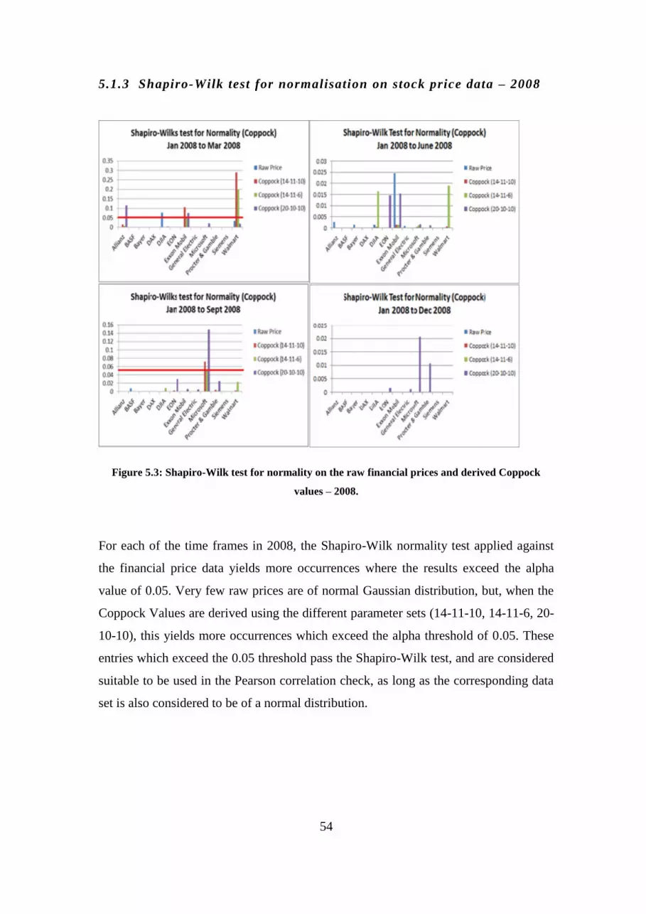
54

5.1.3 Shapiro-Wilk test for normalisation on stock price data – 2008

Figure 5.3: Shapiro-Wilk test for normality on the raw financial prices and derived Coppock

values – 2008.

For each of the time frames in 2008, the Shapiro-Wilk normality test applied against

the financial price data yields more occurrences where the results exceed the alpha

value of 0.05. Very few raw prices are of normal Gaussian distribution, but, when the

Coppock Values are derived using the different parameter sets (14-11-10, 14-11-6, 20-

10-10), this yields more occurrences which exceed the alpha threshold of 0.05. These

entries which exceed the 0.05 threshold pass the Shapiro-Wilk test, and are considered

suitable to be used in the Pearson correlation check, as long as the corresponding data

set is also considered to be of a normal distribution.

55

5.1.4 Shapiro-Wilk test for normalisation on stock price data – 2014

Figure 5.4: Shapiro-Wilk test for normality on the raw financial prices and derived Coppock

values – 2008.

(Threshold of 0.05 represented by horizontal red line.)

In 2014, initially for the first three-month period, there are a high number of

occurrences which pass the Shaprio-Wilk normality test. This, again, is achieved

through the calculation of the Coppock values using the three different parameter sets

(14-11-10, 14-11-6 or 20-10-10). As each period is extended, there is a reduction in the

number of occurrences where the alpha value of 0.05 is exceeded.

One condition required in order to perform a Pearson correlation check requires that

both datasets are of a normal (Gaussian) distribution. Despite the fact that there were

individual occurrences of data passing the Shapiro-Wilk normality test, when these

results (Wikipedia and financial) were combined, the net result of those datasets being

normally distributed was reduced. Appendix A contains the complete Shaprio-Wilk

56

results, and also indicates those companies and/or indexes where both Wikipedia data

and financial data were normally distributed. Table 5.1, below, summarises the stocks

and/or indexes where both Wikipedia data and financial data are both normal, and thus

can have the Pearson correlation check run against them. Due to the low occurrence of

instances where both dataset are normally distributed, the Spearman rank order

correlation check will be applied for all datasets. As part of this research, for the

instances where both datasets are normally distributed, the Pearson correlation check

will be completed to determine whether any correlation improvement is returned when

compared to their corresponding Spearman correlation results.

Table 5.1: Datasets where both results are of normal distribution, indicating Pearson correlation

suitability – 2008/2014.

Correlation checks

Following the completion of the Shaprio-Wilk test, the Spearman correlation test was

chosen, and was performed for each of the time frames mentioned. Each table outlines

the best correlation achieved, along with the data transformation performed (if

applicable) on either/both of the datasets in question. The tables are split into stock

market index and associated shares, and sorted by correlation strength. A breakdown

of each stock market index (DAX and DJIA), along with the associated stock, will be

presented. Each will give the results of the Spearman rank order correlation tests for

the three-, six-, nine- and 12-month period for each year, 2008 and 2014. A stock

market commentary will be initially presented for each stock market index/year. This

will place the “mood” of the market at the time into perspective, and will assist in

understanding the behaviour of the data and associated correlations produced.

57

5.1.5 Correlation Results – 2008 - German DAX index and shares.

Table 5.2: Correlation results for 2008 on DAX index and associated shares (ordered by strength).

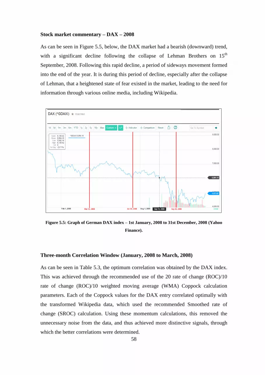
58

Stock market commentary – DAX – 2008

As can be seen in Figure 5.5, below, the DAX market had a bearish (downward) trend,

with a significant decline following the collapse of Lehman Brothers on 15th

September, 2008. Following this rapid decline, a period of sideways movement formed

into the end of the year. It is during this period of decline, especially after the collapse

of Lehman, that a heightened state of fear existed in the market, leading to the need for

information through various online media, including Wikipedia.

Figure 5.5: Graph of German DAX index – 1st January, 2008 to 31st December, 2008 (Yahoo

Finance).

Three-month Correlation Window (January, 2008 to March, 2008)

As can be seen in Table 5.3, the optimum correlation was obtained by the DAX index.

This was achieved through the recommended use of the 20 rate of change (ROC)/10

rate of change (ROC)/10 weighted moving average (WMA) Coppock calculation

parameters. Each of the Coppock values for the DAX entry correlated optimally with

the transformed Wikipedia data, which used the recommended Smoothed rate of

change (SROC) calculation. Using these momentum calculations, this removed the

unnecessary noise from the data, and thus achieved more distinctive signals, through

which the better correlations were determined.

59

Other correlations were also achieved through the recommended alternative set of

Coppock calculation parameters (14 ROC/11 ROC/6 WMA). Using one of these

parameters to generate the Coppock values creates faster signals than the original

monthly parameters (14 ROC/11 TOC/10 WMA). Because the data is daily, this

proves to be effective in creating a better correlation between both datasets. Four out of

the six entries use the 20/10/10 parameters. For each of the other entries, the

correlations are not as strong as the highest achieved by the DAX index entry, but

there is an improvement in correlation strength using the momentum calculations

(Coppock and SROC Wiki) than would be achieved through the use of the raw data on

its own (raw price/raw Wiki). It should be noted that none of these optimum

correlations were achieved using the standard Coppock monthly parameters (14

ROC/11 ROC/10 WMA), and, therefore, this affirms the information gathered during

the literature review14

to use the recommendation parameters on daily data (20

ROC/10 ROC/10 WMA or 14 ROC/11 ROC/6 WMA). These parameters used to

derive the Coppock values, combined with the Smoothed rate of change of the

Wikipedia data, achieved the best correlations.

Six-month correlation window (January, 2008 to June, 2008)

The DAX index achieved the best optimum correlation, with strength of -0.74. This

indicates that the SROC Wikipedia data is negatively correlated with the Coppock

data. This optimum correlation was below the equivalent on the three-month window,

which indicates that more data does not add value. The 20 ROC/10ROC/10WMA

parameters used for the generation of the Coppock Values achieved this optimum

correlation and match the parameters used to achieve the equivalent three-month

correlation. The “Bayer” and “EON” stocks increased in correlation strengths using the

same Wiki and Coppock parameters. EON increased in correlation strength, resulting

in a stronger positive correlation than was achieved in the three-month period.

14

"Using the Coppock Curve to Generate Stock Trade Signals [Online]. Available:

http://www.investopedia.com/articles/active-trading/031814/using-coppock-curve-generate-stock-trade-

signals.asp [Accessed 15 December 2014]."

60

As an example, the EON stock had a medium positive correlation (0.35). This

indicates that, as the share price either dropped or increased, there was also an

associated drop or increase in the Wikipedia views, but not directly due to a small

strength of association which displayed the share price and associated Wikipedia

views. Screenshots of Wikipedia Article Traffic Statistics can be review in more detail

in Appendix A. In particular, there was a small strength of correlation where the EON

share price rose, with the associated Wikipedia view also rising. Towards the end of

June, there was a drop in share price, which was matched with an associated drop in

Wikipedia page views. In order to achieve the optimum correlations for the “BASF”

and “Siemens” stocks, the raw Wiki data was correlated against the Coppock values

(20ROC/10ROC/10WMA), which differed from the same set in the three-month

period.

Nine-month correlation window (January, 2008 to September, 2008)

The DAX index achieved the optimum correlation strength, although it decreased from

both of the previous three- and six-month time frames. In all cases, the transformed

Wiki data (SROC) was used to achieve optimal correlations. All entries remained

negatively correlated, except for EON, similar to the prior periods, where there was a

positive correlation but a reduction from the prior six-month period. All entries used

the recommended Coppock calculation parameters of either 20ROC/10ROC/10WMA

or 14ROC/11ROC/6WMA.

12-month correlation window (January, 2008 to December, 2008)

The DAX remained the best correlated pair, with a negative strength of -0.63. This

remained in the large strength of association. The strength rank order of each of the

other stocks changed when compared to the prior nine-month period, with Siemens

and BASF almost doubling in correlation strength, while the other stocks (Bayer,

Allianz and EON) reduced further in correlation. Therefore, for the longest time

window, the DAX index remained the entry with the largest strength association, and

remained consistently so throughout all periods.

61

Summary

The DAX index consistently returned the best correlation strength for each of the four

periods being analysed in 2008. These strengths were negatively correlated, which

indicates that, as prices decrease, Wikipedia page views increase, and vice versa. This

optimum strength was achieved in the shorter, three-month period but remained strong

through the year. When the number of page views was assessed for the full year 2008,

the DAX was one of the most viewed pages of the companies being analysed. EON

received the least number of page views over the one year period. The associated

correlative strength for EON remained weak, which would indicate that a higher page

view was required to gain stronger correlation. The Average strength in correlation

remained in the same range throughout the year, indicating a fear or concern in the

online community.

Table 5.3: Number of Wikipedia page views on the DAX market and associated shares in 2008.

62

5.1.6 Correlation Results – 2008 - DJIA index and shares.

Table 5.4: Correlation results for 2008 on DJIA Index and associated shares (ordered by

strength).

63

Stock market commentary – DJIA – 2008

As can be seen in Figure 5.2, below, similarly to the DAX index for 2008, there was a

bearish trend (decline) in the DJIA index throughout the year, with a significant

decline following the collapse of Lehman Brothers on 15th

September, 2008 (indicated

by crosshairs in the chart). Following the rapid decline in the latter quarter of the year,

there was a period of relative calm as the market became range-bound between 8000

and 9000, although the swings from positive to negative and vice versa in the final

quarter were quite extreme, indicating that fear remained in the market.

Figure 5.6: Graph of German DJIA index – 1st January, 2008 to 31st December 2008 (Yahoo

Finance).

Three-month correlation window (January, 2008 to March, 2008)

The strongest correlation was achieved by Procter and Gamble, where there was a

negative correlation of -0.91. This is considered a very large strength of association,

and used the transformed Wikipedia data (SROC), in addition to the Coppock values

derived using the 14ROC/11ROC/6WMA parameters. This high correlation was

achieved due to the fact that it was the smaller set of values on which to perform

correlation checks. This indicated that, as the Coppock curve (price) turned negative,

64

there was an increase in the number of Wikipedia page viewings. In Figure 5.3, for

Procter and Gamble, the Wiki and Coppock results can be compared, revealing that, as

the Wiki SROC turned down, the Share Price/Coppock Curve turned up.

Figure 5.7: Graphs representing the Wiki (SROC) versus Coppock value for P&G – raw data in

red, derived data in blue.

Conversely, as the Coppock curve (price) turned positive; there was a decrease in the

Wikipedia page views. Walmart returned a positive correlation with a large strength of

association (0.62), indicating that, for an increase in the Coppock curve, there is a

relative increase in the SROC Wiki line, and visa-versa. This would also indicate that

there is an increase in the associated Wikipedia page as the price increases or

decreases. General Electric, Microsoft and the DJIA index revealed a negative

correlation between their Wikipedia page views and associated Coppock value. This,

again, would indicate that there was a general increase in page views as the prices

decreased, and visa-versa. Exxon Mobil, similarly to Walmart in the same category,

revealed a positive correlation which had a medium strength of association (0.39).

Six-month correlation window (January, 2008 to June, 2008)

General Electric maintained the same correlation strength as achieved in the previous

month, accomplishing the strongest correlation strength in the time range. All other

stocks achieved a negative correlation using both the derived Wikipedia values

(SROC) and associated Coppock value. Similarly to other data ranges, all Coppock

values were derived using either the 20ROC/10ROC/10WMA parameters or

65

14ROC/10ROC/6WMA parameters. This also indicates that, as prices decrease over a

period, there is an increase in Wikipedia page views.

Nine-month correlation window (January, 2008 to September, 2008)

There was a slight increase in correlation (negative) on General Electric which

indicates that, while the financial crisis took hold in September, 2008, with prices

decreasing, there was a gradual increase in associated Wikipedia page views.

Similarly, there was an increase in negative correlation between the DJIA index prices

(Coppock) and the associated Wikipedia page views. This also indicates that there was

awareness and concern as the index dropped in value, thus revealing an increase in

associated Wikipedia page views.

12-month correlation window (January, 2008 to December, 2008)

This window of time included the period when the DJIA Index was soon to reach its

low of 7062, in February, 2009. Thus, there was concern within the community over

the state of the financial markets. As a consequence, there was a higher likelihood of

people having an interest in the markets, in this case the Dow Jones Industrial

Average. This was affirmed by fact that the DJIA index achieved the largest

correlation strength among the set of shares being analysed. This negative correlation

using the SROC Wiki and Coppock value (-0.52), deemed to be of a medium strength

of association, indicates that, as the index value decreased, there was an increase in the

associated Wikipedia page views, most likely indicating the influence of people’s

concern. Similarly, there were negative correlations, of medium and small strength,

which would indicate an interest in the Wikipedia pages as the prices decreased in

value, although not as strongly correlated as the DJIA index.

Summary

Relative to the stock market performance of the Dow Jones Industrial Average, the

majority of correlations were reflective of the stock market for each period. For the

first quarter, there was relative calm in the market; however, midway during the

second quarter, there was an increase in correlation strength on the major index (DJIA)

and General Electric. Over the third quarter of 2008, there was a rapid drop in the

66

stock market and associated shares. This concern was reflected in the increase of

strength in (negative) correlation, again on the DJIA index and General Electric.

Towards the end of the year, when the market appears to have bottomed out for 2008,

the fear subsided in the market, and the corresponding strengths in correlation also

reduce slightly. As shown in Table 5.5 below, the DJIA index and General Electric

were among the most highly viewed pages on Wikipedia, and thus would be more

representative of the market over the period.

Table 5.5: Number of Wikipedia page views on DJIA market and associated shares in 2008.

67

5.1.7 Correlation Results – 2014 - German DAX index and shares.

Table 5.6: Correlation results for 2014 on DJIA index and associated shares (ordered by strength).

Stock market commentary – DAX – 2014

As can be seen in Figure 5.3, below, the market was relatively range-bound for the

year, after having made a large recovery following the financial crisis of 2008. There

was high volatility experienced within the range mentioned, causing sudden declines,

followed by a period of rapid recovery. This would indicate that there was still

uncertainty in the market which was prone to sudden corrections, followed by a swift

recovery of confidence.

68

Figure 5.8: Graph of German DAX index – 1st January, 2014 to 31st December, 2014 (Yahoo

Finance).

Three-month correlation window (January, 2014 to March, 2014)

Both the DAX index and Bayer stock highlighted a negative correlation, with a

medium strength of association. All optimal correlations were achieved through the

use of the derived Wikipedia data using the Smoothed rate of change and the Coppock

value, involving the 20ROC/10ROC/10WMA parameters in all cases except BASF,

which used the 14ROC/11ROC/6WMA parameters, resulting in a positive correlation

of 0.29.

Six-month correlation window (January, 2014 to June, 2014)

There was a decline in correlations across all shares and indexes when compared to the

previous time frame. This, it can be understood, occurred as the stock market

experienced a period of growth in the second quarter. This would have resulted in

reduced concern amongst the community. All optimal correlation strengths were

achieved through the use of the transformed Wikipedia data using the Smoothed rate of

change and the Coppock value, via a combination of 20ROC/10ROC/10WMA and

14ROC/11ROC/10WMA. The highest correlations in the previous period (Bayer and

69

DAX) lost a large amount of correlation strength over this period. Through chart

analysis of Figure 5.3, there is clearly an upward trend in the market over the latter part

of this six-month time frame. Due to the fact that there appeared to be a strong

negative correlation between Wikipedia SROC and Coppock values during the stock

market decline, the fact that the market was increasing over this period could explain

why there was a sudden decrease in correlation – there were less Wikipedia page views

due to newfound confidence in the market over this period. The average strength

almost halved in value between the three-month period and the six-month period.

Nine-month correlation window (January, 2014 to September, 2014)

The DAX Index continued to have the best correlation using the derived Wiki data

(SROC) and the Coppock values (20ROC/10ROC/10WMA). This is almost a 50%

increase in correlation since the prior period. Considering the market at the time, there

was a large sell-off on the DAX exchange up to August, 2014, which would have

increased concern in the market and the wider arena. This would have caused an

increase in Wikipedia page views over that period, thus causing an increase in negative

correlation (as the exchange value falls, the Wikipedia page view increases). EON

maintained almost the same correlation strength. Interestingly, BASF changed to a

positive correlation from its prior period negative correlation. This would indicate that,

as the market declines, there is more of a tendency for the Wikipedia viewership to

decline also, although this correlation is deemed weak (0.10). There was a decrease in

correlation strength for Siemens, Allianz and Bayer, to close to zero, thus indicating no

correlation between their Wikipedia page views (SROC) and corresponding Coppock

values.

12-month correlation window (January, 2014 to December, 2014)

The DAX exchange experienced the highest volatility over the latter quarter of 2014,

with large sell-offs occurring, followed by a rapid recovery. This would indicate that

there was a large element of fear in the market. This may explain why the DAX index

correlation strength between Wikipedia views (SROC) and associated Coppock curve

(14ROC/11ROC/10WMA) maintained the negative correlation strength of -0.34.

Normally, over the 12-month period, there is a decline in correlation strength

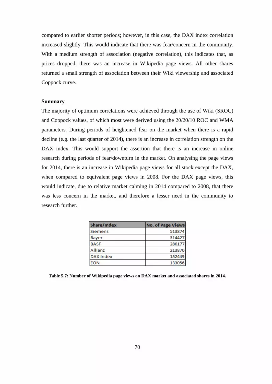
70

compared to earlier shorter periods; however, in this case, the DAX index correlation

increased slightly. This would indicate that there was fear/concern in the community.

With a medium strength of association (negative correlation), this indicates that, as

prices dropped, there was an increase in Wikipedia page views. All other shares

returned a small strength of association between their Wiki viewership and associated

Coppock curve.

Summary

The majority of optimum correlations were achieved through the use of Wiki (SROC)

and Coppock values, of which most were derived using the 20/20/10 ROC and WMA

parameters. During periods of heightened fear on the market when there is a rapid

decline (e.g. the last quarter of 2014), there is an increase in correlation strength on the

DAX index. This would support the assertion that there is an increase in online

research during periods of fear/downturn in the market. On analysing the page views

for 2014, there is an increase in Wikipedia page views for all stock except the DAX,

when compared to equivalent page views in 2008. For the DAX page views, this

would indicate, due to relative market calming in 2014 compared to 2008, that there

was less concern in the market, and therefore a lesser need in the community to

research further.

Table 5.7: Number of Wikipedia page views on DAX market and associated shares in 2014.

71

5.1.8 Correlation Results – 2014 - DJIA index and shares .

Table 5.8: Correlation results for 2014 on DJIA index and associated shares (ordered by strength).

72

Stock market commentary – DJIA – 2014

There was an obvious bullish trend in the market over the full year. This also consisted

of sudden corrections throughout the year, followed by rapid recovery after each

correction. This would indicate that there was a well-established trend and confidence

in the DJIA market. The periods of interest are those where there was high volatility,

with declines followed by quick recovery.

Figure 5.9: Graph of DJIA index – 1st January, 2014 to 31st December, 2014 (Yahoo Finance).

Three-month correlation window (January, 2014 to March, 2014)

There was a high period of decline on the stock market during this period, with a rapid

recovery following this decline. The Dow Jones index correlation proved to be the

strongest over this period, with a negative correlation strength of -0.83. This is

regarded as a large strength of correlation, which indicates that, as the market

decreases there is an increase in the associated Wikipedia page views, and vice versa.

General Electric, Walmart and Exxon Mobil, during this period, also reflect a large

strength of correlation, with Microsoft and Procter and Gamble showing medium and

small strengths of correlation, respectively. All correlations for each stock, except one

(Procter and Gamble), used the same correlation pairs (SROC Wiki and Coppock

73

20/10/10). Due to the high volatility of the market, it is clear that the Wikipedia views

increased as the index decreased.

Six-month correlation window (January, 2014 to June, 2014)

The stock market recovered following the initial three-month period, and formed a

bullish trend. Thus, there was less fear in the market towards the latter part of the six-

month period. The correlation strengths per stock/index seem to reflect this, with a

reduction in strength due to less fear in the market, and thus a lesser need to research

online sources such as Wikipedia. All correlations used the transformed Wikipedia

data (SROC), along with either the Coppock 20ROC/10ROC/10WMA or

14ROC/11ROC/10WMA values. The average correlation strength decreased by 42%

between this time range and the previous three-month period. This can be explained by

the increase in positive sentiment in the market over that period.

Nine-month correlation window (January, 2014 to September, 2014)

The stock market over the latter quarter (June to September) of this period experienced

a pullback (correction), which would have instilled fear into the market. All

shares/index correlations used the derived Wikipedia (SROC) and Coppock values

(using 20ROC/10ROC/10ROC and 14ROC/11ROC/6 ROC). Exxon Mobil

experienced an increase in correlation from the previous six-month time frame. This

would indicate that, as the share price dropped for this share, there was an increase in

page views for that period, thus improving the correlation. The Exxon Mobil

Wikipedia page view figure for August, 2014 was 36,210. This increased to 50,441

page views in September, representing a percentage increase of 40% pages views

between August and September. Figure 5.10 below, outlines the correlation of negative

strength between the Wiki (SROC) and associated Coppock value.

74

Figure 5.10: Graphs representing the Wiki (SROC) versus Coppock value for Exxon.

Microsoft moved from negative correlation to positive correlation, due to a spike in

page views during the month, resulting in an increase in page views as the associated

share price increased.

12-month correlation window (January, 2014 to December, 2014)

Towards the last quarter of 2014, the stock market experienced a sudden pullback

(correction) followed by a quick recovery. This, again, would have instilled fear into

the market, causing an increase in online research. The negative correlations for the

DJIA index decreased to -0.46, thus giving it a medium strength of association. This

indicates that, as the price decreased, there was an increase in Wikipedia page views.

All stocks/index used the transformed Wikipedia data (SROC) and Coppock

generation parameters (20ROC/10ROC/10WMA or 14ROC/11 ROC/6 WMA), except

for Walmart, where the optimum correlation was achieved using the raw Wiki data

against the Coppock values.

Summary

Table 5.9 outlines the number of Wikipedia page views over the 12-month period of

2014.

75

Table 5.9: Number of Wikipedia page views on Dow Jones Industrial Average and associated

shares in 2014.

When compared to 2008, similarly to the comparison concerning the DAX index and

associated shares, there was an increase in page views for the individual shares in 2014

when compared to 2008, but a decrease in page views on the index. This would

indicate that the DJIA index Wikipedia page views served as a better barometer of the

financial community and the concern factor associated with it. In 2008, during the

beginning of the financial crisis, there was an elevated concern in the market which

was highlighted by a high number of Wikipedia page views. Following a period of

recovery, there was a relative reduction in concern in the market, represented by the

reduction of Wikipedia page views in 2014.

5.2 Discussion

The aim of this research was to determine whether Wikipedia article traffic statistics

can be used to confirm the signal provided by the Coppock indicator. Through the

correlation checks between the Wikipedia article traffic statistics and the associated

Coppock value, it is hoped that this confirmation can be achieved by technical

analysts. Specifically, within the context of technical analysis, the objective of this

research was to:

i. Determine the most suitable correlation technique by performing a normality

check on each data set;

ii. Evaluate the correlations achieved between each dataset over the various time

periods for each year in question;

76

iii. Assess the results from the correlations obtained and compare these to what

was expected; and

iv. Propose recommendations for the use of Wikipedia article traffics statistics as

confirmation of the signal given by the Coppock indicator.

This section will revisit the research objectives detailed above, and will summarise the

findings and present conclusions.

Following the Shapiro-Wilk test for normality, and based on the work of Moat et al.

(2013), the Spearman rank order correlation check was chosen to determine the

relationship between Wikipedia article traffic statistics and the associated Coppock

value. Elder (1993) has determined that, in order to obtain a significant signal from a

time series, the Smoothed rate of change (SROC) can be used to achieve this. On that

basis, the SROC was chosen as a method of obtaining a better signal from the

Wikipedia article traffic statistics.

Figure 5.11: Smoothed Rate of Change applied to underlying DAX Wikipedia Page Views – 2008

Data.

As can be seen in Figure 5.11, a more significant set of signals is given by the derived

SROC, which could correlate better with the associated Coppock curve. The original

Coppock Curve was designed to run against monthly data using the following

parameters:-

77

14-month Rate of Change.

11-month Rate of Change.

10-month Weighted Moving Average.

In order to obtain significant signals from the associated daily financial data, a number

of recommended derivation parameters for the calculation of the Coppock curve were

recommended15

. These recommendations consisted of the following parameters:-

14-day Rate of Change.

11-day Rate of Change.

6-day Weighted Moving Average.

Or

20-day Rate of Change.

10-day Rate of Change.

10-day Weighted Moving Average.

As a result of using the recommended daily generation parameters, it resulted in the

optimum correlation being achieved between the Wikipedia Dataset and associated

Coppock Dataset where, the majority of optimum parameters used the

20ROC/10ROC/10WMA.

Figure 5.12: Coppock curve applied to underlying DAX index prices – 2008 data.

15

"Using the Coppock Curve to Generate Stock Trade Signals [Online]. Available:

http://www.investopedia.com/articles/active-trading/031814/using-coppock-curve-generate-stock-trade-

signals.asp [Accessed 15 December 2014]."

78

Using these parameters, a set of Coppock values were obtained, and used to correlate

against the associated Wikipedia SROC results. These achieved various strengths of

correlation. The following are the key findings gained from this research exercise:

i. Using SROC improves correlation with the Coppock curve

In order to achieve an improvement in signal from data, Elder (1993)

recommended the application of the Smoothed rate of change (SROC) against

underlying data. This was applied to the Wikipedia page views, and resulted in

improved correlations with the associated Coppock curve.

Table 5.10: Comparison of raw Wiki correlation and SROC (Wiki) against Coppock values – best

correlations in yellow.

As can be seen above, the correlation test using the Raw Wiki against Coppock

only resulted in one optimum result. There was an improvement in correlation

when the Smoothed rate of change was applied to the raw Wikipedia page view

data. All occurrences except Allianz derived the best correlations from the

SROC against the Coppock values.

ii. Using recommended ROC/WMA parameters on Coppock calculation

improves correlation.

Using either the 14-day ROC/11-day ROC/6-day WMA or the 20-day ROC/10

day ROC/10-day WMA improves the Coppock signal for daily data, as

recommended by Mitchell (2014) and StockCharts.com (2015). As can be seen

in Table 5.10, 7 of the 12 stock/indexes using the (20/10/10) parameter set

facilitated in achieving optimum correlation. Next to this, the recommended

79

(14/11/6) parameter set achieved 3 of the 12 optimum correlations. Therefore,

in summary, 10 out of the 12 optimum correlations were achieved using the

refined parameters suited to daily data.

iii. Majority of optimal correlations are negative.

In the majority of cases, when correlations were tested between the Wikipedia

(SROC) and associated Coppock curve, a negative correlation was obtained.

This indicated that, as the Coppock curve moved down (downward underlying

share price movement), there was an increase in Wikipedia page views and as

the share price or index increased, there was a reduction in Wikipedia Article

Views. This confirmed the research conducted by Moat et al. (2013), which

determined that a higher occurrence of online research through Wikipedia is

conducted before periods of decline and continues as the decline progresses.

iv. Optimum correlation achieved in bear markets (downturn)

During the analysis of all periods in 2008 and 2014, it was notice that there

were correlations of average higher strength in 2008, before and during the

financial crisis, than the corresponding periods in 2014. This backup the

research conducted by Moat et al. (2013) where they concluded that there are

increases in Wikipedia traffic before a stock market fall. Also, these findings

confirm the research done by Tversky and Kahneman (1991), where they

conclude that losses and disadvantage has a greater impact on decision than

gains and advantage. This is reflected during the comparison of the average

strengths between Tables 5.2 and 5.6 (DAX Index and shares) and between

Table 5.4 and 5.8 (DJIA Index and shares) where the average strengths in 2008

are stronger than their equivalents in 2014.

v. DAX Index and DJIA Index best capture the mood of the market.

On analysis of the correlations achieved in 2008 and 2014, the most consistent

correlations are achieved by the DAX and DJIA Index over each of the

timeframes and are most reflective of the stock market during these periods.

This backs up the case made by Surowiecki (2004) which implies that there is

inherent value in the Wisdom of Crowds. Each individual share generally

80

reflects the specific interest in that holding, while interest in the DAX and

DJIA attracts more of a general “crowd” audience, thus producing a higher,

more consistent strength in correlation over all periods and timeframes.

vi. Correlations affirm certain stocks are better barometers of the market.

There are close ranking of strengths in correlation between the DJIA and

General Electric during 2008 and 2014. This affirms the point made by

Chambers (2000) that certain stocks are better barometers of the market.

General Electric would be one of these, as it is only share of the original 12 to

remain in the index since the index was formed in 1896. It can be seen in Table

5.4 for 2008 and Table 5.8 for 2014 that the correlation of General Electric are

the closest to the DJIA index than any of the other chosen stocks.

81

6. CONCLUSIONS AND FUTURE WORK

This chapter revisits the objectives of this research. The key findings that were

discovered during the exercise are described, and conclusions are presented. Areas of

further research are discussed, specifically in relation to this research topic. Finally, the

contribution of this research is also explained.

6.1 Problem definition and research overview

The objective of this research study was to determine whether the signal given by the

Coppock indicator on a particular stock or index can be confirmed through the use of

associated Wikipedia article traffic statistics. Specifically, within the area of technical

analysis, the objectives of this research were to:

i. Determine a suitable correlation technique through the use of a suitable

normality check.

ii. Determine the best rate of change (ROC) and weighted moving average

(WMA) values to use in order to derive the optimal Coppock value.

iii. Apply the recommended Smoothed rate of change (SROC) against the

Wikipedia data, in order to improve the correlation potential between the two

datasets.

iv. Critically assess the correlations achieved through the use of the most

applicable correlation technique.

v. Propose further research for the improvement of signals given by the Coppock

indicator through the use of Wikipedia Article Traffic Statistics.

The goal of every investor is to be able to optimally time the entry and exit of a traded

position on the stock market, in order to yield a profitable return. This can be achieved

through the proper use of technical indicators. These indicators give a signal to an

investor as to when a market or position may be over-bought or over-sold. Improved

profits can be achieved by the investor through the disciplined use of these indicators.

82

The Coppock indicator is considered to be an indicator that has a reliable track record,

and which can yield the investor a decent return (Gillen 2013). Originally designed to

give a “buy” signal on monthly data, the Coppock indicator can also be used by

investors to give a “sell” signal, and also functions over more frequent time frames,

such as weekly and daily data (Mitchell 2014). Depending on the rate of change (ROC)

and weighted moving average (WMA) parameters used to calculate the Coppock

value, different entry and exit positions are returned by the Coppock curve. Two sets

of parameters are regarded as offering the best Coppock signal on daily data. These

consist of the application of the six-day weighted moving average on the product of the

14-day and 10-day rate of change, or the application of the 10-day weighted moving

average on the product of the 20-day rate of change and 10-day rate of change. It was

discovered that the latter (20, 10, 10) derived the optimal Coppock values that returned

the optimal correlation with the Wikipedia article traffic statistics

Wikipedia is frequently used by the online community as a first point of reference, in

order to research and understand a specific topic, stock market or company. Through

the use of the underlying Wikipedia article traffic statistics, it is possible to build a

profile of page views on any Wikipedia page over any period of time since 10th

December, 2007. Through the use of these recorded Wikipedia statistics, it is also

possible to determine whether there is any strength in correlation between Wikipedia

page view traffic on a particular quoted company or stock market index and the

associated Coppock values for that same company or index.

Four window sizes (three, six, nine and 12 months) were chosen for applying the

correlation techniques. Initially, the strongest correlations were derived in the three-

month window, which reduced in strength as the period was increased. It was also

noticed that the strength in correlation remained high relative to each previous time

frame when there was a general downturn in the stock market. This supports the

assertion by Moat et al. (2013) that there was an increased tendency to research when

there was a risk or fear of incurring a loss. It was also discovered that there were

increased strengths in correlation for stock that were deemed to be barometers of the

stock market. An example of this is General Motors (GM), which has been a member

of the Dow Jones index since the inception of the exchange in 1896 (Nicholson 2010),

83

and whose correlation strength of associations were similar to the overall Dow Jones

index.

6.2 Contributions to body of knowledge

This dissertation focused on the Coppock indicator, and how Wikipedia article view

statistics can affirm the signal provided by the Coppock indicator. By obtaining this

confirmation, investors in stocks and shares can gain extra confidence that the signal

given by the Coppock indicator is valid, and can apply this extra Wikipedia correlation

signal to their investment strategy. To the best of the author’s knowledge, no other

piece of research uses Wikipedia article traffic statistics to verify a stock market

technical indicator such as the Coppock indicator. This dissertation offers a

contribution to the use of Spearman’s rank order correlation to determine the strength

of association between two datasets, and, from this, determining whether a stock

market technical indicator is signally correctly.

6.3 Experimentation, evaluation and limitations

The experimentation required that the data was in a suitable state in order to uncover

optimal correlations. This involved the resolution of missing data through the use of

alternative sources. Also, there were issues of incompatibility due to the nonexistence

of weekend or public holiday data contained in the Stock Price Dataset. In order to

avoid knowledge loss, the simple strategy of using the last weekday closing price

resolved this. Missing data was also an issue on the Wikipedia dataset due to system

failure on the host site recording the data. This was resolved through the use of the

Holt Winters technique and appeared to reflect the pattern of data that existed in the

dataset.

Optimal recommend derivation parameters were then used to obtain the

Coppock values for each of the Stock Price datasets. These proved to facilitate the

optimal correlations and did exceed most correlations that were derived when the

monthly parameters were applied. Checks for correlation strength were then performed

for each of the chose time frames over each of the years in question. These were then

84

ranked in order of correlation strength and patterns relative to the characteristics of the

stock market at the time were revealed.

Strengths and limitation were then highlighted with a view to understanding the

process and to come up with recommended areas of future research.

6.4 Future work and research

Future work could concentrate on determining whether other techniques outside

correlation checks can indicate a relationship between the Wikipedia article traffic

statistic and the Coppock curve. One such technique is the Granger causality test. This

was first proposed in 1969 by Clive Granger, which determines whether one time

series is useful for forecasting the other (Baumohl and Vyrost 2010). Further research

could also be performed in the area of event synchronisation, which measures

synchronisation and time delay patterns between signals. One piece of work,

completed by Quiriga et al. (2002), has investigated this in the area of brain waves

between the left and right cortex of the brain. Their recommendation is to extend this

research into other types of data. Therefore, Wikipedia article traffic statistics and the

Coppock indicator could be suitable candidates for this. Finally, research performed by

Kampf et al. (2014) using Wikipedia article statistics to determine relevance

incorporating Wikipedia page view data for pages linked to the main (central) page of

interest. Through this, including the local neighbourhood of pages linked to the central

page of interest (node) may contribute to better correlations between this and the

associated Coppock indicator, and thus could better confirm the signal provided by it.

85

APPENDIX A: ADDITIONAL MATERIAL

86

Figure 0.1: Sample of CSV Wikipedia Article Traffic Statistics for “Dow Jones” Page Views.

Table 0.1: Sample of CSV Wikipedia Article Traffic Statistics for “Dow Jones” Page Views.

87

Table 0.2: Shapiro-Wilk result on 2008 data (Wikipedia and Stock Price Data).

88

Table 0.3: Shapiro-Wilk result on 2014 data (Wikipedia and Stock Price Data).

89

REFERENCES

Alanyali et al. (2013) Quantifying the Relationship Between Financial News and the

Stock Market. Available from Macmillan Publishers Limited [Accessed 10 September

2014]

Allen, F. and Karjalainen, R. (1998) Using genetic algorithms to find technical trading

rules. Available from Journal of Financial Economics [Accessed 18 September 2014]

Baumohl, E. and Vyrost, T. (2010) Stock market integration: Granger causality testing

with respect to nonsynchronous trading effects. Available from Czech Journal of

Economics and Finance. [Accessed 2 February 2015]

Bird,R. and Casavecchia, L. (2005) Value enhancement using momentum indicators:

the European experience. Available from International Journal of Managerial Finance

[Accessed 10 October 2014]

Bollen, J., Maoa, H., Zengb, X. (2011) Twitter mood predicts the stock market.

Available from Journal of Computational Science [Accessed 10 September 2014]

Chatfield, C. and Yar, M. (1988). Holt-Winters Forecasting: Some Practical Issues,

Available from The Statistician, 37, 129-140. [Accessed 10 November 2014]

Chambers, A. (2000) Financial Success in the in the Year 2000 and beyond, CRC

Press, USA.

Chok, N. (2010) Pearson's versus Spearman's and Kendall's Correlation Coefficients

for Continuous Data. MSc (Biostatistics) unpublished dissertation. University of

Pittburgh, USA.

Coughlan, A., (2013) A Little Book of R For Time Series. Retrieved October 8, 2014.

Cowpertwait, P.S.P., Metcalfe, A.V., (2009) Introductory Time Series with R.

Springer, Australia.

Dondio, P. (2012) Predicting Stock Market Using Online Communities Raw Web

Traffic. Available from ARROW@DIT [Accessed 10 September 2014]

Dondio, P.; Longo, L., "Computing Trust as a Form of Presumptive Reasoning," Web

Intelligence (WI) and Intelligent Agent Technologies (IAT), 2014 IEEE/WIC/ACM

International Joint Conferences on , vol.2, no., pp.274,281, 11-14 Aug. 2014

Du Sauto, M. The Code, Video, BBC Documentary, (2011), viewed 15 November

2014, <https://www.youtube.com/watch?v=iOucwX7Z1HU>.

Elder, A. (1993) Trading for a Living, Wiley & Sons, Canada.

Gillen, R. (2012) 3 Steps to Investment Success, Oak Tree Press, Ireland.

90

Graham, B. (2005) The Intelligent Investor (Revised edition), Harper Collins, New

York, USA.

Kampf et al. (2012) Fluctuations in Wikipedia access-rate and edit-event data.

Available from ScienceDirect [Accessed 15 September 2014]

Kampf et al. (2014) Wikipedia Relevance Analysis for Uncovering Emerging Trends.

Available from ScienceDirect [Accessed 15 December 2014]

Kamvar, S. and Harris, J. (2011) We Feel Fine and Searching the Emotional Web.

Available from ACM Digital Library [Accessed 10 September 2014]

Kemp, P. (2012) Testing the get rich quick seminars. Retrieved November 14, 2014

<http://www.bbc.com/news/uk-19909942>.

Kittur, A., Kraut, R., (2008) Harnessing the Wisdom of Crowds in Wikipedia: Quality

Through Coordination. Available from Carnegie Mellon University [Accessed 29

September 2014]

Longo, L.; Dondio, P.; Barrett, S., "Temporal factors to evaluate trustworthiness of

virtual identities," Security and Privacy in Communications Networks and the

Workshops, 2007. SecureComm 2007. Third International Conference on , vol., no.,

pp.11,19, 17-21 Sept. 2007

Longo, L.; Rusconi, F.; Noce, L. & Barrett, S. (2012), The Importance of Human

Mental Workload in Web Design., in Karl-Heinz Krempels & José Cordeiro, ed.,

'WEBIST' , SciTePress, , pp. 403-409 .

Longo, L., Dondio, P., Barrett, S.: Information Foraging Theory as a Form Of

Collective Intelligence for Social Search. In: 1st International Conference on

Computational Collective Intelligence Semantic Web, Social Networks & Multiagent

Systems, Wroclaw, Poland, 5-7 October (2009)

L. Longo, P. Dondio, and S. Barrett, "Enhancing Social Search: A Computational

Collective Intelligence Model of Behavioural Traits, Trust and Time," in Transactions

on Computational Collective Intelligence II, ser. Lecture Notes in Computer Science,

Springer Berlin Heidelberg, 2010, vol. 6450, pp. 46-69.

Luttrell, D., Atkinson, T., & Rosenblum, H. (2013) Assessing the Costs and

Consequences of the 2007-09 Financial Crisis and Its Aftermath. Available from

Federal Reserve Bank of Dallas [Accessed 10 November 2014]

Mestyán M, Yasseri T, Kertész J (2013) Early Prediction of Movie Box Office Success

Based on Wikipedia Activity Big Data. PLoS ONE 8(8): e71226.

doi:10.1371/journal.pone.0071226

91

Mitchell, C. (2014) Using the Coppock Curve to Generate Stock Trade Signals.

Retrieved August 10, 2014 <http://www.investopedia.com/articles/active-

trading/031814/using-coppock-curve-generate-stock-trade-signals.asp>.

Mituzas, D. (2007) Wikipedia page counters. Retrieved September 2, 2014.

<http://dom.as/2007/12/10/wikipedia-page-counters/>.

Nicholson, C. (2010) Building Wealth in the Stock Market, Wiley & Sons, Australia.

Preis, T., Moat, H., Stanley, E., Bishop, S., (2012) Quantifying the Advantage of

Looking Forward. Available from Macmillan Publishers Limited [Accessed 20

September 2014]

Preis, T., Moat, H., Stanley, E., (2013) Quantifying Trading Behaviour in Financial

Markets Using Google Trends. Available from Macmillan Publishers Limited

[Accessed 20 September 2014]

Qie, W. (2011) Market Volatility's Relationship with Pairwise Correlation of Stocks

and Portfolio Managers Performance. MSc (Mathematical Statistics) unpublished

dissertation. Stockholm University, Stockholm.

Quiroga et al., (2002) Event synchronization: A simple and fast method to measure

synchronicity and time delay patterns. Available from American Physical Society

[Accessed 2 February 2015]

Sakaki et al., (2010) Earthquake Shakes Twitter Users: Real-time Event Detection by

Social Sensors. Available from University of Tokyo [Accessed 5 December 2014]

Sanger, L. M., (2009) The Fate of Expertise after Wikipedia. Episteme 6 (1):52-73.

Available from Cambridge University Press [Accessed 1 October 2014]

Schutzman, F. G., (1991) Smoothing Rate of Change: New Twist to Old Study.

Available from Futures Magazine [Accessed 10 December 2014]

Shapiro et al., (1968) A Comparative Study of Various Tests for Normality, Journal of

the American Statistical Association, vol. 63, iss. 324.

Shipman, M., (2008) Big Money Little Effort: Practical and Effective Strategies for

Stock Market Investment, Kogan Page Limited, London.

Simon, H., (1955) A Behavioral Model of Rational Choice. The Quarterly Journal of

Economics, Vol. 69, No. 1, (Feb., 1955), pp. 99-118

Surowiecki, J., (2004) The Wisdom of Crowds, Anchor Books, New York.

Terzo, G., (2013) Percentage of People Successful in the Stock Market [Online].

Available:

<http://wiki.fool.com/Percentage_of_People_Successful_in_the_Stock_Market>

[Accessed: 20th November 2014]

92

Tversky, A., Kahneman, D., (1991) Loss Aversion in Riskless Choice: A reference-

dependent model. The Quarterly Journal of Economics, Vol. 106, No. 4 (Nov., 1991),

pp. 1039-1061

Winters, P. R., (1960) Forecasting Sales by Exponentially Weighted Moving Averages.

Management Science Vol. 6, No. 3 (Jan., 1960), pp. 324 - 342.