l .. _.

Journal of Research of the National Bureau of Standards Vol. 57, NO'. 4, October 1956 Research Paper 2714

Calibration of Vibration Pickups by the Reciprocity Method

Samuel Levy and Raymond R. Bouche

T he reciprocit y t heory for t he relationship between mechanical force and velocit y and electri c current and voltage is presented for a lin ear electrodynamic vibration-picku p cali­brator having a dri ving coi l, a velocity-sensing coil , and a mountin g t able. The t heo!"." takes account of flexibili ty in the calibrator st ructure a nd in the coils , electric coupling be­tween different par ts of the same coil and between par ts of one coil and part of t he other, and flexibili ty in the magnet structure. The theory shows what measurement s arc required in usin g a linea r electrodynamic calibrator for the a bsolu te calibration of vibration pickups.

A description is given of the mechanical arrangement and electri c ci rcuitry usc-d at the National Bureau of Standards in calibrat ing calibrators by the rec iprocity m ethod. A typical veloeity-sensing-coil cali bration curve is prcsented sho\\ing t he etrect of pickup m ass on t he ca libration factor . T ypical exam ples of measurement of calibration factor and me­chan ical impedance of pickups a rc also presented .

P rac tical li mitations of the r eciproci ty method du e t o nonlin earity resulting from Jack of t ightn css of mechan ical joints, resonance eHects, ampli tude effects, etc. , arc discussed .

1. Introduction

An early application of the reciprocity m ethod to the measurement of mechanical quan ti­ties was that by R . K . Cook [1]1 in 1940. He applied the m ethod to the absolute calibratioll of microphones. This was followed in 1948 with papers by H. ~/I. T ren t [2] and A. London [3], who showed how th e reciprocity m ethod could be used for the absolule calibration of vibration pickups. The reciprocity method was applied to the calibra tion of elecl rodynamic tra nsdu cers in 1948 by S. P. Thompson [4J and to the calibration of piezoelecLric accelerometers in 1952 by M. Harrison, A . O. Sykes, and P . G. Marcotte [5] .

Commercially available calibrators for vibration pickups have a mounLing table that is connected by a relatively rigid in ternal structure to a drivin g coil and to a velo city-sen sin g coil. This internal structure is suppor ted from the fram e by flexUJ"e springs or guide wires . John C . Camm, form erly of NBS, in 1953 showed how the reciprocity method could be applied to th e calibraLion of the velocity-sensing coil of such a calibrator in connecLion with work for the Office of Naval R esearch . In 1955 the authors of the present report, ill connection with work for the Diamond Ordnance Fuze Laboratories, extended Camm's theory to take accoun t of pickup mass and flexibility in th e internal structure for the frequently occurring case where th e driving coil, sensing coil, and mounting table are mechanically joined at a point.

The present report gives a broader basis for the application of th e reciprocity m ethod to the calibration of the velocity-sensing coil of calibra tors, by considering both the internal structure and the magn et to be flexible and by taking account of electric-couplin g cHects . It also shows how th e calibrator, once its velocity-sensing coil has b een calibra ted by the reci­procity m ethod , can be used to determine the calibration factor and to measure th e m echanical irnpedance of vibration pickups.

2. Reciprocity Theory for Flexible Vibration-Pickup Calibrators

In the appendix the general reciprocity th eory for a calibrator is presented . This th eory is applicable to a calibrator operating ill any frequency or ampli tude range in which it can be consider ed to be a linear system. Neith er the internal structure )lor the magn et structure need be considereclrigid. The theory is applicable, for example, not only at low frequ encies and at frequencies ncar certain resonances, but also at frequencies above axial resonan ce where

I Figures in brackets indicate the li terature references at t he end o[ this paper.

397105- 5G--5 227

the driving coil and mounting table move in opposite directions. The theory is also applicable where there is electric coupling between differcnt parts of the same coil and between parts of one coil and parts of the other.

The positive terminals of the driving and sensing coils are designated as those having positive voltages when the mounting table is moving inward. Conversely, positive current in the coils produces outward velocity at the mounting table.

When the calibrator is energized with current in the driving coil at any particular fre­quency, the calibration factor, F, is defined as the ratio of the voltage in volts in the velocity­sensing coil to the velocity in inches per second at the surface of the mounting table. It is shown in the appendix that

(1 )

where Yp is the pickup mechanical impedance (lb-secjin. ), and all the symbols represent complex numbers in the manner commonly used for a.lternating-current electrical theory. The calibrator constants, a and b, are determined by the follo''1ing two experiments and com­putational procedure.

Experiment 1: The equipment is shown in figure 1 (a). Attach weights to the mounting table and measure for each weight the transfer admittance in amperes pel' volt, G, between the driving and sensing coils:

(2)

where

I~= current in driving coil. Eg= voltage generated in open-circuited sensing coil. (It is permissible to leave a volt­

meter permanently connected to the sensing coil. If this is done, the open-circuit condition is obtained when no other connection is made to the sensing coil.)

Experiment 2: The equipment is shown in figure 1 (b ). Couple a second vibration exciter to the calibrator being calibrated at the mounting table, and measure the ratio , R, of open­circuited voltages generated in the sensing and driving coils:

(3)

Computational Procedure: Determine the ordinate intercept, J , and the slope, Q, of the function Wj (G- Go) when plotted against the weight, W, attached to the mounting table in experiment 1, where Go is the value of G when W = O. Constants a and b in eq (1) are then given by

a=O.OI711~jwJR, b= 6.601 Q.J R j (jwJ) , (4)

where w is the frequency in radians pel' second, and j is the unit imaginary vector. It is shown in the appendix that the vibration-pickup calibrator calibrated by the reci­

procity method can be used to determine the mechanical im.pedance, Y 1" of a pickup by meas­uring the admittance, G1', eq (2), with the pickup attached to the mounting table, and the admittance, Go, when nothing is attached to the table, by use of the relationship

(5)

To carry out the calibration of a pickup the following procedure is used: The driving coil of the calibrator is energized at the desired frequency and the value of Y1' is determined. The

228

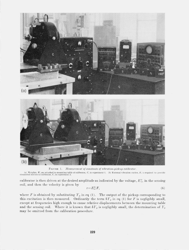
FIGU1~E 1. Jl![easurement of constants of vibm tion-pickup calibmtoT. (a) Weights, lV, are attached to moun ting table of calibrator, C, in exper imen t 1. (b) E xternal vibration exciter, E , is req uired to pro vid e

sinusoidal motioll to calibrator, OJ in (lxperimcnt 2.

calibra tor is th en driven at th e desired amplitude as indicated by the voltage, E~, in th e sensing coil , a nd th en the velocity is given by

v=E~/F, (6)

where F is obtained by substitu ting Y" in eq (1). The output of the pickup corresponding to this excitatioJl is then measured . Ordinarily the term bY p in eq (1) for F is negligibly small, except at frequen cies high enough to cause rela tive displacem ents between the mounting table and th e sensin g coil. vVhere i t is known that bY" is negligibly small, the determin ation of Y p may be omitted from the calibration procedure.

229

3 . Measurement of Constants

3 .1. Accuracy of Weights

The weights attached to the table in carrying out experiment 1 at the Bureau are shown at W in figure 1 (a). The weights increase in O.l-lb steps from 0 to lIb. They vary less than 0.1 percent from their rated values. Their attachment surface has a stud that engages the mounting table and a contacting ring, ~~ in. wide, which provides a connection of high rigidity. A film of oil is wiped on this ring before engagement to eliminate air in the contact surface .

3 .2. Accuracy of Frequency Measurements

The frequency was measured with a calibrated electronic frequency meter. The indicated audio oscillator frequency did not differ from the measured frequency by more than 0.2 percent.

3 .3. Measurement of Transfer Admittance

The circuit shown in figure 2 (a) is used to measure the transfer admittance. 'With the switch in the " up" position, the values of l' and 1'1 are adjusted until the voltage drops lEd across terminals 1 and 2, and IEI31 across terminals 1 and 3, are equal as measured on a high­impedance voltmeter. The magnitude of G is then given by

IGI 1'+ 1'1 + 1'2 (7)

The accuracy of IGI determined in this manner depends only on the accuracy of the circuit elements and the repeatability of the voltmeter reading, but not on th e accuracy of the volt­meter. Values of the resistances are chosen to load the amplifier suitably. Typical values for this calibrator are 1'2, equal to 10 ohms, and 1'+1'1, approximately 1,000 times greater than 1'2'

Voltage lEd across terminals 2 and 3 is then read from the voltmeter. The switch is lowered to the " down" position. The value of 1'1 is adjusted until lE I4 1 equals lEd, and voltages IE131 and lEd are read on the voltmeter. The phase angle, <Pc, of the transfer admittance, G, is the phase angle of 17/ with respect to E~. Because the currents in r, 1'], and 1'2 are in phase with 17/, phase angle <Pc can be determined from a construction of a polygon of vol tages as

(8)

A suitable value of 1'2 is used so that 1']w10 - 6 is greater than 100; then the approximate value of

DRIVER COIL

ID + ~-(

IMF 4

(0)

DRIVER COIL

+

- - ED-· (b)

VELOCITY SENSING

COIL

-~+

~ __ FE-s-_ j. I 3

VELOCITY SENSING

COIL

~+

-:?! __ FE ___ I I s 3

FIGURE 2. Circuits 11sed in the measw'ement oJ constants of vibration-pickup calibmlor.

(a) 1\![casurcmcnt of transfer admittance. ratio.

(h) Measurement of \'oltage

230

CPo can be determined from

( A. ) approx = 900-cos- 1 1- - _ 3_4 . ( 1 IE ZI) 'P o . . 2 1E;31 (9)

The use of both eq (8) and (9) determines th e magnitude and quadra ll t for cf>G' It happell s, though, except near certain resonances, that CPo is ncar ±90°. Small errors in lEd or lEd resu It in large changes in the angle

when cf>o is neal' _ 90°. Difficulty in measuring the small value of IE43 1 resu l ts in error when CPo is near 90°. Therefore, eq (8) is used to determine the magnitude of cf>G and (9) its quadrant.

3.4. Measurement of Voltage Ratio

The circuit shown in figure 2(b) is used to measure the ratio of the open-circuit voltages of the eh·i ving anel sensing coils when the calibrator being calibrated is driven by an external vibration exciter. ·With the switch in the "up" position and with 1'1 set at 10,000 ohms, resistor l' is adjusted until the voltages across terminals 1 and 2 and terminals 1 and 3 are equal. The magnitude of the voltage ratio, R, is then given by

IR I 10,000+ 1" (10)

(In the case of a calibrator for which 10,000 ohms is not effectively an infinite impedance across the driving coil, 1'1 in figure 2(b) should be increased to an adequate value and eq (10) corre­spondingly modified.)

To determine the phase angle of R, lEd and lEd are measured. The witch is theH put in the " clown" position, 1'1 is adjusted until IEI4 1 equals lEd , and IE431 is measured. Then from a construction of a polygon of voltages

(11)

and

(12)

It happens that cf>R is ncar either 0° or 180°. Equation (11) is insel1s iLive for these angles, either because IEn l is very small for cf>R neal' 0° or because the cosine is insensitive to small changes in IE z3 1 near 180°. Therciore, eq (12) is used to determine the magnitude of cf>R and eq (11) only its quadrant.

4 . Typical Results

4.1. Calibration of Sensing Coil

Results obtained in the calibration of the sensing coil of a typical calibra to r having a llominal 50-1b driving-force rating are now presented. All measurements were made afte r thermal oq uilibrium was approached. The positive terminals of the cl riving and sensing coils were determin ed as those having positive voltage when the mounting table had inward velocity. Posit ive veloGity is then outward.

First, th e t ran sfer admittance, G, experiment 1, was measured fot' a sequence of weights , TV, on the mOlll1t ing Lable at each frequenc:-.- for which a calibration was desired. Typical results at frequencies of 900 and 5,000 cps arc presented in figure 3. In figure 4 are the cor­responding plots of Wj (G- Go) against H'. The data were fitted by a weighteclleast-squares procedure for a straight line. The we ighting as determined by a consideration of the expected enor in 1/ (G- Go) was 1, 2, 3, ... , 10 for vr"= O.I , 0.2 , 0.3 , . .. , 1.0 lb. Intercepts J and

231

300.------,-------,------,-------r------~

10L-____ ~ ______ _L ______ ~ ______ L_ ____ ~ 0

I 90 .---+--~--~--+---~~.~.--~--+---__ __ 90

<f)

w 60 60 w

'" <.? W

" 30 - 3D

<.? -s.

0.8 1.0 °0~----'0~.2------~0 .~4----~0~.6~----~------7 00 0 . 2 0.4 0.6 0.8 1.0

(a) W, POUNDS (b)

FIGUHE 3. Fariation of transfer admittance, G, with weight, W , on the mounting table for a typical vibration pickup calibrator at frequencies of (a) 900 cps and (b) 5,000 cps.

0 ~

E

U> Oi

" z ::>

-0.02 i 0 a.

1.% -0.04 i

~ , CI -O.06j

-O.08 j

- O. IOi

-0.002i

IMAGINARY -0.004 i -

IMAGINARY

-0.006i

-0.008i

- O.OIOi . - 0.12 i .,..o ------:::0"'. 2------::0L:.4,------::0"-::.6,------::0:"-:.8~--~1.0 - 0.012j ~o ------::0"-::. 2,------::0"-::.4------::0:"-:.6~----::0:"-:.8~-----"J1.O

(a) W, POUNDS (b)

FIGUltE 4. Plot of W /(G- Go) as a function of W for a ty pical vibration pickup calibrator at fre quencies of (a) 900 cps and (b) 5,000 cps.

slopes Q, determined by this procedure, are at 900 cps J = 0.1089 j- 94 .2° lb-ohm, and Q= 0.00767/11.8° ohm, and at 5,000 cps, J = 0.01094/- 77.4° lb-ohm, and Q= 0.00765/100.4° ohm.

The voltage ratio, H, when driven by an external vibration exciter, experiment 2, was then determined as H= 0.1090/- 2.6° at 900 cps and H = 0.2495/- 2.00 at 5,000 cps. Next the constants a and bin eq (4) were computed. Substituting their values in eq (1) gave calibration factors of the sensing coil with a pickup of mechanical impedance Yp on the mounting table,

232

~ ::r · : · *- ~ j

tj · : -n-.~ 1 20 100 1,000

f, CYClES (SECONO 10,000

FraUHE 5. Fariation oj calibmtion Jactor oj velocity-sensing coil wilh Jrequency and 1)ick­up weight for a typical vibration pickup cal­ibmtor.

O=Olb, X= ~~ lh, . = ll b.

at 900 cps, F = 0.1402/- 3.4° + 0.000674/12.6° Yp v-sec/in. , and at 5,000 cps, F = 0.1 584/5.5° + 0.001360/93 .1 ° Yp v-sec/in.

In figure 5 are shown the magnitude and phase angle of the calibration factor of the velocity-sensing coil of this typical vibration-pickup calibrator as a function of frequency for pickups having a m echani cal impedance Yp corresponding to weights !iV of 0, 0.5, and 1.0 Ib (Y p=jwTiV/386) . It is eviden t that, for th is particular vibration-pickup calibra tor , the cali­bration factor of th e velocity-sensing co il is nearly independen t of frequency and pickup weight up to 900 cps. The curve for l Ib is dotted in the v icinity of 2,700 cps because the plot similar to that shown in figure 4 was no t linear beyond 0.5 lb . The source of this nonlinearity co uld no t be localized. Thi s nonlinearity has not been found in other calibrators of the same make and model number calibra ted at the same f requency.

4 .2 . Calibration of a Variable-Resistance-Type Accelerometer a nd a Piezoelectric-Typ e Accelerometer

R esults obtained in the calibra t ion of a variable-resistance-ty pe accelerometer and piezo­electric-type accelerometer are now presented. In these calibrations the circuit shown in figure 2 (a) wa used with the pickup terminals designated 6 and 7, in place of velocity-sensing­coil terminals 1 and 3. The method given in section 3.3 was then used for t he measurement of Gp , the value of G with t he pickup attached to the mounting table.

For the piezoelectric pickup, the value of Gp obtained at 900 cps was Gp=I':/E~= 28.5] /9l.8° mhos, and at 5,000 cps, Gp= 37.9/43.6° mhos. With terminal 6 grounded and terminal 7 replacing tel'mina1 3, the same procedure gave, at 900 cps, I ': /E p= 16.35/2.5° mhos, and at 5,000 cps, I ':/E p=3.201/- 44.6° mhos, where Ep is the output voltage of the pickup . From eq (5), the mechanical impedance, Y p , of the pickup was computed by using, at 900 cps, Go= 26.81/92 .00 mhos, and at 5,000 cps, Go= 16.5V18.1 ° mhos, and the values of J and Q obtained in section 4.1. This gave, at 900 cps, Y p = 2.712/83.3° Ib-sec/in. and at 5,000 cps, Y p= 18.23/70 .5° Ib-sec/in. Using t hese values of Yp in eq (1), the velocity sensing-coil cali­bration factors at 900 cps and 5,000 cps, respectively, are F = 0.1399/- 2.7° v-sec/in. and F = 0.135?/9 .2° v-sec/in. The pickup acceleration calibration factor , F p , is

where FgJ(jw) is the acceleration calibrat ion factor of the sensin g coil. at 900 cps, Fp= 0 . 016~/-3.4° v/g, and at 5,000 cps, Fp= 0.019~/6.5 ° v/g. complete calibration of the piezoelectric-type accelerometer.

(13)

Usin g this equation, Figure 6 shows the

The calibration of the variable-resistance-type accelerometer, which was performed in a similar manner, is shown in figure 7. To compute t he results on the variable-resistance

233

20

0 z 8 ~ , U> 10

'" :z: u

"" ;;;: 0 :'--:: I

0 1,000

<I>

18U ~

'" 135

'" 0:

::[ ~ 0

of

00 1,000

FIGURE

9 6

0 eno o~ 4 ~, o en Q. W

r 2 u ~

~ 00

180

Ul 135 W W Il:

90 ..... to W 0

>- 45 '" 00

FIGUl~E 7.

I 0.02

'" , <I>

'" 0 > ~ 0 .01

"-

I I I 0 2POO 3,000 4,000 5,000

20 100 1,000 ' 5,000

J 91

~ 45

0: 0 " . ~

I

j Cb"- -45

I I -90 2,000 3,000 4,000 5,000 0

(0) f, CYCLES/SECOND

1,000 2 ,000 5,000 3,000 4,000 (b)

6. Calibmtion of piezoelecll'ic-type accelerometer at a nominal acceleration level of 2 g.

>--J 200 0 >

~ , co

en >- 100 -J 0 > 0 Il:

'" ::!; 0 200 400 600 800 ---=

"-20 100 1000

. . -.

200 400

(0) 600 800 -180 '---------:2,..:0:-::0:------:4-±0"'0----::6-:,0"'0---=-SO:':-0=---'

t, CYCLES/SECOND (b)

Calibmlion of variable-res'istance-type accelerometer at a nominal accelemtion level of 2 g.

pickup at frequencies other than those at which the vibration-pickup calibrator was calibrated, it was necessar:y to interpolate suitably for a, b, R, and Q, and compute J from eq 4. This interpolation was only used at frequencies below 900 cps. In this frequency range, such interpolation results in no appreciable error for this calibrator when the resonant frequencies of the flexures are avoided. The frequencies used for the pickup calibration were not those at which flexure resonance was present.

5 . Effects of Calibrator Construction on Accuracy

Inaccuracy in the reciprocity method, exclusive of electrical measurements, arises primar­ily from deviations from true lil~earity in the calibrator performance. The more important forms of nonlinearity are discussed below.

234

5.1. Resonance Effects

R esonance accen tuates inaccuracy due to nonlinearity because relatively small cha nges in the calibra tor constan ts, which arc caused by very small changes in the structure of the calibra tor and small changes in the excitmg frequency, can cause large changes in the ampli tude of vibra tion . Even when such changes do no t occur, the large ampli tudes associa ted with reso­nance may exceed the lin ear range. The resonance of the driving coil relative to the velocity­sensing coil reduces the accuracy of the reciprocit~~ calibration over a small frequen cy range because IRI is very small and therefore difficult to measure, and because the large ampli tude of the driver coil may exceed its linear range. Operation of the calibrator n car resonance frequencies should therefore be avoided. Some common resonan ce condi tions in th eir usual order of appearance with in creasing frequency follow :

a. R eson ance of moun ting table and coils as a rigid body on the guidin g fl exures . b . Local resonance in th e flexures. c. Transverse vibra tion of the shaft connecting moun ting table and driving coil. d. Longitudinal resonance of shaft conn ecting moun tin g table and driving coil. e. Local resonance in table or coils.

5 .2 . Transverse Motion

T ransverse motion from allY source invalidates the reciprocity method , which requires the moun t ing table to have lU1iaxia.l motion. Transverse motion occurs at the resonance frequencies of the flexures and a t the transverse resonauce frequencies of the shaft on which the moving parts arc m ounted . At resonance, the amplitude will vary substan tially for small changes in fre­quency and the resonance may OCCLlr at a frequency that is a harmonic of Lhe drivillg frequency. Flexures can be detuned by attachi.ng small weigh ts to them .

5 .3. Tightness of Mechanical Joints

The tigh Lll ess of the mechanical joinLs in a calibrator will have lilLIe d reoL 0 11 its perform­ance aL low freque ncies, where Lhe moving assembly of moun ting Lable alld co ils acts as a " rigid bod~· ." At frequ encies approachillg Lhose for in tern al resonance ill Lhe assembly, looseness in the join ts can affect behavior by, for example, changing the stl'uctural sLiffness or by intro­ducing coulomb friction. At very high frequencies, join ts normally though t Lo be t igh t may be a source of erratic behavior, which is difficult to eliminate as tigh tness will ordin arily vfiry with temp erature and time. Coating all join ts wi th oil improves their rigidit~~ .

5.4. Amplitude Effects

The nOl1 uniformi ty of the magnetic fields surrounding the coils is a primary source of nonlineari ty. This effect tend s to be greatest at low frequencies, where the displacement ampli­tude is large for a given acceleration. At h igh frequencies, the displacemen t ampli tude is relativ ely small , and this effect is negligible. The change in equilibrium positioll of the movillg assembly of a calibrator, when its orientation is changed, may cause a change in calibratio ll factor du e to change in the effective field strength.

The structure of a calibrator will ordin arily experience small deformat ions in iLs l inea l' rallge at pel'ln.iss ible current inLensiLies. At resonance, the deformations arc larger. LiLLlc is k ll OWll

abou L the linearity of sLructural damping for a structure as complicated as a calibrator; how­ever, so long as Lhe clampill g is small, its possible lack of litlearit~~ \\~ould affect o nl.\~ the resonan t response.

5.5 . Temperature Effects

Changes in Lemperaturc cause moderate changes in clastic consta nts and ill Lhe t igh tness of joints, and ill Lhis way can a fIect Lhe calibrator performance n car reso na ll ce. Changes in temperature may also affect Lhe field flux density, alld thu s t he electrical characterist ics of the driving coil, but should not ordinarily arfect t he calibraLioH factor of t he velocity-sen sin g coil.

235

5.6. Purity of Electric-Power Sources

If the magn ets are excited by direct curren t containing an alternating-current ripple, this ripple may appear in the velocity output of the calibrator owing to currents included in the driving coil by transformer action from the field. Such a disturbance can readily be detected by exciting the field and observing the velocity of the mounting table with the driving coil short-circuited.

Any harmonic conten t in the power supply to the driving coil will excite the calibrator at the harmonic frequencies, as well as at the primary frequency. The techniques described in this paper are applicable only for excitation at a single frequency.

6. Conclusions

It is concluded that the reciprocity methods described can be used for the accurate cali­bration of vibration pickups and calibrators having linear response. The accuracy is limited primarily by the accuracy of electrical measurement, by deviations from true linearity in con­struction, and by impurities in power supplies to the field and driving coils . The frequency range is limited theoretically only to frequencies for which the mechanical impedance of the weights attached to the mounting table can be computed. Ordinarily this limits the range to that at which the weights act as though they were rigid bodies. Practically, the calibrator used as an example in this report is most suited for use at frequencies of 900 cps and below, where its calibration factor is not affected by the mechanical impedance of most vibration pickups that would be attached to its mounting table. The calibrator is suited for use above 900 cps, however, with some loss in precision primarily du e to the electromechanical properties of the calibrator being less constant with respect to fi eld-coil temperature than they are at lower frequencies. The upper acceleration range of most calibrators, when resonance is avoided, is below 50 g. This would be the limit for calibrating by the reciprocity method.

7 . Appendix. General Reciprocity Theory

7.1 . Reciprocity for Electric Circuit

If a complicated electric circuit is considered to be made up of a number of meshes, the almost trivial fact that the common impedance between meshes i and k, for example, is the same as that between k and i is the basis for the proof of the reciprocity theorem. This proof is elegantly presented by Guillemin on page 152 of reference [6]. Guillemin states on page 276 that the reciprocity theorem can be proved for both transient and steady-state performance. This means, for example, that if we impress a voltage in mesh 5 of a given network and measure the current, say in mesh 2, and then place the voltage in mesh 2 instead of in mesh 5 and meas­ure the current in mesh 5, we will find the current exactly the same in the two cases, both in magnitude and phase.

7.2 . Reciprocity for Mechanical System

If a complicated mechanical system can be replaced by an equivalent system having discrete mass-points joined by springs and dashpots, the fact that the spring and dashpot connecting points i and k is the same as that connecting points k and i makes possible a proof of the reciprocity theorem for mechanical systems completely analogous with that for electric circuits. (Reference [7] gives a proof of this theorem for conservative systems.) In other words, this reciprocity theorem states, for example, that if we impress a force on point 5 of a given system and measure the velocity, say at point 2, we will find the same velocity in mag­nitude and phase when we place the force at point 2 instead of at point 5 and measure the velocity at point 5. It should be mentioned that it is possible to have a mechanical system consisting of discrete elements that is not reciprocal, for example, if it contains gyroscopic elements.

236

7 .3 . Reciprocity for Combined System

In developing the reciprocity theorem for the combined electric-mechanical system of a calibra tor, we will use matrix nota tion . This will permit us to consider the coils as fl exible bodies and take accoun t of electric coupling between coils, as well as deformation in the f-ield and movable structure. The no tation and theorems given by Frazer , Duncan , and Collar [8] will be used.

Currents and voltages in the velocity-sensing coil will be indicated by S and in the drivin g coil by D. We will consider the coils subdivided into a sufficient number of segments so each moves as a rigid body and number them consecutively in the t,vo coils. The subscript 0 will indicate terminal values. Complex notation used in alternating-current electrical theory will be used throughout. All symbols represent vector quan tities, unless otherwise no ted. An English system of units (inches, pounds, and seconds) will be used.

Current I~ at the terminals of the sensing coil is given by

where

E:=voltage at terminals of coil 8.

E~=voltage at terminals of coil D.

z,;;,s= impedance a t terminals of coil 8.

Z,;;,D= tran sfer impedance from terminals of coil 8 to terminals of coil D.

(AI)

[ zS]=[~ ~ , .. ~J' where z~. ,is the transfer impedance from segment n to the termi-Zo l Zo2 Zon nals of COlI S.

{E}= , En is the voltage generated in segment n.

A similar expression can be written for I f . Both of these expressions can be expressed as

(Ala) where

{Io }=[~~}

[Z~s Z;DJ 00 00

[zo]= 1 1

z[!os Z~D

l:~ Z~2 [z]=

1 1 zf" z~

z~] . Zon

237

The current in any segment is given by

{I } = [z]' {Eo } + [Z]{E}, (A2) where

{I }= , I n is the current in segment n ,

I n

1 1 1 Zl1 Zl2 Zln

1 1 1 Z21 Z22 Z2n

[ZJ = , Zmn is the transfer impedance from segment m to segment n,

1 1 1

[Z]' = transpose of [z].

V clocity Vo at th e~mountill gltable, taken positive outward, is given by

(A3)

where

F o= the force at the mounting table.

Yoo= the mechanical impedance at the mounting table.

L I = 2.249 X 10- 7, a conversion factor.

[Y] =L~I Y~2 ~J' where y on is the transfer mechanical impedance from the Yon mountmg table to segment n.

Bill 0 0

o B 2l2 0

o 0 B3l3 [k] =

o o o

o

o

o , where B n is the flux density, and l l1 is the length for segment n .

238

In eq (A3), the product L I B"l,J n gives the force , in pound s, at segment n when I n is the currC'nt, lJl amperes. The velocity of the various segments is given by

{v} = [y]' F o+ L 1[Y] [k] { I }, (.\ 4 )

where

{v}= , Vn is t he velocity of segment n.

vn

[y ]' = transpose of [y].

1 1 1

Yn Y1 2 Yi n

1 1 1 Y 21 Y 22 Y 2n

[Y] =

1 1 1

Y ml Y rn2 Ym n

, Y mn is t he transfer meehanieal impedance from segment m to segment n.

The corresponding velocity in the magnetic field at the various segments is given by

where

v'}{

1 yf[

1 y&f

[Pf]=l l

AT Y ml

(A4a)

, v'}{ is the velocity of the magnetic field at segment n.

1 y~g

1

y~~

1 Y;;{2

1 1 ytf.

1 yg;,

1 AT y."",

, yf,f" is the transfer mechanical impedance from the location of segment m to that of segment n in the magnetic field.

239

y~

;:1 [1fT = , yt~, is the transfer mechanical impedance from the moun Ling table to the l ~ magnetic ,tmctu," oppo,,;te "gruent n.

Yon

The voltage generated in each segment is

(A5)

where L 2 = 2.540 X 10- 8 , a conversion factor. In eq (A5), -L2Bnln (vn- v~f) is the electromotive force generated in segment n, in volts, when the relative velocity between segment n and the magnetic field , in inches per second, is (vn- v~f). Substituting (A2) into (A4) and (A4a) , and substituting the results into (A5) gives

where

[K] = [k)[Y][k] - [k)[yM)[k]. Letting

[11- 1] = [1] + LJL2[K][Z], where

1 0 0 0

0 1 0 0

0 0 1 0 [1] = , the unit matrix,

o 0 0 1

[11-1] = inverse of [V].

{E } = - F oLdV)[k)[y_ yM]' - LJL2[11][K][Z] , {E o}.

Substituting (A9) into (Ala),

{ I o} = [zo]{E o} - F oL 2[z)[V][k)[y _ yM] , - LJL2[Z][V][K][z]' {Eo }.

Substituting (A9) in (A2) and the result in (A3) gives

F vo= yo - L1L2Fo[y _ yM][k][Z][V][k] [y _ yM]' + LJ[y_yM][k][V] , [z]' {E o},

00

usmg

240

(A6)

(A7)

(AS)

(A9 )

(AIO)

(All)

(A12)

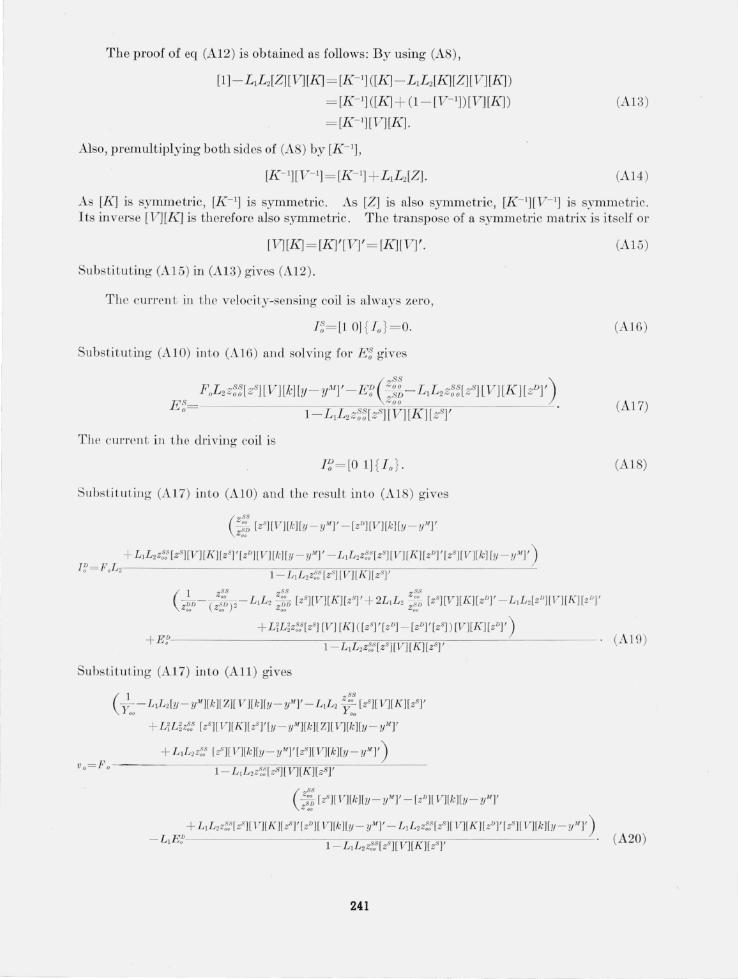
The proof of eq (A12) is obtained as follows: By using (AS),

[1] - L 1L 2[Z][V)[J{] = [J{-l] ([J{] - L 1L 2[J{][Z][V] [K])

= [J{- l] ([J{] + (1- [V- I]) [11] [J{] )

= [J{- I][V][J{] .

Also, premultiplying both sides of (AS) by [J{- l],

[J{-l][V- l] = [J{- l] + L1L 2[Z].

(A13 )

(A14)

As [J{] i ymm etric, [J{- l] is symmetric. As [Z] is also symmetric, [J{- I][V-l] is symmetric. Its inverse [V)[[{] is therefore also symmetric . The transpose of a symmetric matrix is itself 01'

[V)[J{] = [J{]'[V)' = [J{][V)' . (A15)

Subs tituting (A15) in (A13 ) gives (A12).

The currenL in the velocity-sensing coil is always zero,

f~= [l 0] { f o} = 0. (1\.16)

Substituting (A10) into (A16) and solving for E~ gives

FoL2Z~~ [ ZS] [V][k] [y _ yM]' - E~ (~~~ - L1L2Z~~ [ ZS] [V] [J{] [ZD]')

E~ 1- LIL2Z~~ [ ZS] 61][J{][ zS], . (A17)

The current in tho driving coil is

SubstituLing (A17) into (A1O) and th o result inLo (A1S) gives

(~~ [zS][VJ[k][y - y"' ]' - [zD ][V][kJ[y -y"1j'

+ LIL2Z~.s [ZS][V] [J(][zS]' [zD][V][k][y - y"' ] ' - LIL2Z~.s[ZSJ [V][J(][ZD]' [ZS][V][k] [y - yM]' ) ~=~~ •

1- L1L2Z~nZS)[VJ[f(][zsJ '

Subs ti tu ting (A17) into (All ) gives

( ~ •• - L 1L 2[y- yM)[k ][Z][VJ[k)[y - yM]' - L IL 2 ~:: [zS]W][K][ zs],

+ LiL~z~.s [zS)[V][K][zs ],[y- y"' )[kllZ][V][k][y- y'T

+ L1L2Z~.s [zS ]WJ[k)[y _yMJ' [ZS )[V][k)[y- yM]')

vo= Fo ------------~1--~L~lL~2~Z~=~ [~zs=][=V]=[f(==][z~S]~/ ----~-----

( z!-: [zS ][V][k)[y - y'T _ [zD)[V] [k][y _yM], Zoo

(AI )

+ L1L2Z~.s [ ZS)[VJ[K][zS]'[ZD][V][kJ[y - yM]' - L1 L2Z~;' [zS)[V][K][ZD]' [zS )[V][k][y _ yM]' )

- L1E~ 1 - L1L2Z~.S [ ZS] [V][ K)[zs]' . (A20)

241

L

The coefficient of LzFo in equation (A19) equals the coefficient of -L1E~ in (A20). Equa­tions (A19) and (A20) ftre subjected first to the condition vo= O and then to the condition I~=O . Eliminating E~ in (A19), when vo= O, and Fo in (A20), when I~= O , we obtain

This is the reciprocity relation that exists in the combined electromechanical system. Equations (A20), (AI9), and (AI7) can be written for brevity as

where the constants A, B, 0, H, and N depend only on the calibrator construction.

(A21)

(A22 )

(A23)

(A24)

In eq (1) a relationship is given for the calibration factor, defined as F=E~/vo, as a function of the mechanical impedance, Y p , of the object on the mounting table. We will determine this equation in terms of the calibrator constants A, B, 0, El, and N of eq (A22) to (A24). If the force , F o, is only the reaction to driving a mechanical impedance Y at a velocity Vo,

(A25)

Substituting (A25) in (A22) and solving for Fo,

F Ev ALl '0= - '0 0+ l /Y' (A26 )

Substitu ting (A26) into (A24) and (A25) and forming the ratio E~/t·o,

(A27)

WeseethatNjAin eq (A27) isaineq (1) and (NOjA) - Hineq (A27) isbineq (1) when Yis Y p.

a= N /A , b= (NOjA)-H. (A28 )

In experiment 1, section 2, the transfer admittance G=I~/E~ is determined for a series of weights, W, attached to the mounting table. Substituting (A26) into (A23) and (A24) and forming the ratio G,

I~ B + (BO+ A2L2)Y G R~ N + (NO- AH)Y' (A29)

In experiment 1, Y is the mechanical impedancejw W jg, ~where TV is the weight on the mounting table, w the frequency in radians per second , and g the acceleration of gravity, 386 in ./secz• Making this substitution in (A29) and forming W /(G-Go), where Go is the value of G when Y = O, we find

W 386 N2 N 20-AHN G-Go= jw .iFNL2+ABH+ A2NL2+ ABH W. (A30)

242

We see that the intercept J and slope Q found in determining "\T(G- Go) experimentally are

386 N2 J = jw A2NL2+ ABI-I (A31)

N 2C-AI-IN Q A2NL2+ ABI-t (A32)

In experiment 2, section 2, the voltage ratio , R=E~/E'1, is determined when I f: is zero . Eliminating Fo between (A23 ) and (A24 ) and setting I '1 = O, we see that

I-IBL\ + ANL\L2

AL 2 (A33)

Equation (4) is obtained when eq (A31) through (A33) are substituted into (A28 ) and LJ and L 2 have th e values given previously.

From eq (A29), Go= B/N , when Y is zero, that is, Go is the value of G when nothing is attached to the mounting table of the calibra tor. If G1, is the value of eq (A29) when Y = Y p ,

where Yp is the mechanical impedance of a pickup to be determined, we find that

Y p (A 2 L 2N + AI-IB) - (N2 C-AI-IN) ( GJ, - Go) (A 34)

The substitution of eq (A3 1) and (A32) into (A34 ) gives eq (5) for determining the mechanical impedance of a pickup attached to the mounting table of the calibrator.

vVe are indebted to L . R . Sweetman for g uidance in setting up the laborato ry equipmen t, and to Ri cltaJ"('1 Harwell , Jr. , for the careful machining of the masses and the various fixtures used. Ruth ' Voolley performed the least-squares calculations and Carol ' Valdron prepared th e figll res.

8 . Refe rence s [1] Richard K. Coo k, Absolute p ressure calibrations of microphones, J . Rescarch N BS 25, 489- 505 (1940)

RP1 341. [2] Horace M. Tl·cnt, The absolute cali bration of electromechanical pickups, J. Appl. Mec ha nics 15, 49- 52

(1948) . [3] Albert London, The a bsolute cali bration of v ibration pickups, N BS T ech. News Bul. 32, 8- 10 (1948). [4] Sanford P . Thompson, R eciprocity calibrat ion of primary vibration standards, Kaval R ese:Ll'ch Labo ratory

R ept. F- 3337, 8 p . (August 16, 1948). [5] ::\1. H arrison, A. O. Sykes, and P . G. Marcotte, The reciprocity calibration of piezoelectric accelerometers,

David Taylor Mod el Basin R ept. 8ll , 14 p. (March 1952). [6] Ernst A. Guillemin, Communication n etworks (J ohn 'Wiley & Sons, Inc., Kew York, N. Y ., 1931). [7] Horace La mb, On reciprocal t heo rem s in dynamics, Proc. London Mat h. Soc. 19, 144-151 (1889). [8] R. A. Frazer, I V. J . Duncan, a nd A. R. Collar, Elementary matrices (Mac::\filla n Co., New York, K. Y.

1947).

" TASHI NG 'l'ON , ).1arch 12, 1956.

243