CALCULATION OF TURBULENT BOUNDARY LAYER WALL PRESSURE SPECTRA
78
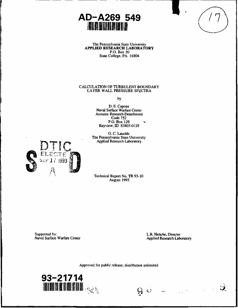
AD-A269 549 (7 The Pennsylvania State University APPLIED RESEARCH LABORATORY P.O. Box 30 State College, PA 16804 CALCULATION OF TURBULENT BOUNDARY LAYER WALL PRESSURE SPECTRA by D. E. Capone Naval Surface Warfare Center Acoustic Research Detachment Code 752 P.O. Box 129 Bayview, ID 83803-0129 G. C. Lauchle The Pennsylvania State University D T J Applied Research Laboratory E . A -'"O Technical Report No. TR 93-10 August 1993 Supported by: L.R. Hettche, Director Naval Surface Warfare Center Applied Research Laboratory Approved for public release; distribution unlimited 93-21714
Transcript of CALCULATION OF TURBULENT BOUNDARY LAYER WALL PRESSURE SPECTRA
AD-A269 549 (7
The Pennsylvania State UniversityAPPLIED RESEARCH LABORATORY
P.O. Box 30State College, PA 16804
CALCULATION OF TURBULENT BOUNDARY
LAYER WALL PRESSURE SPECTRA
by
D. E. CaponeNaval Surface Warfare CenterAcoustic Research Detachment
Code 752P.O. Box 129
Bayview, ID 83803-0129
G. C. LauchleThe Pennsylvania State UniversityD T J Applied Research Laboratory
E .A -'"O
Technical Report No. TR 93-10August 1993
Supported by: L.R. Hettche, DirectorNaval Surface Warfare Center Applied Research Laboratory
Approved for public release; distribution unlimited
93-21714
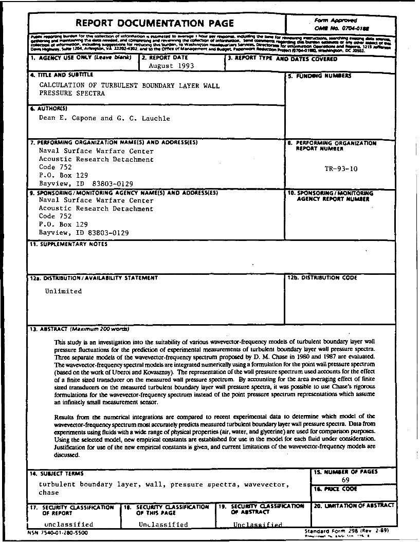
REPORT DOCUMENTATION PAGE Fe P prn
ww" gprfq af Ont tWS ca4(boit f tnsf$W.uW, .esamewad to ~W9uq I how nut resoan. WWMM thn" fo Uwmnm f orsg.inuqan iwitaw~ t~eda neded, Wnd co reeugand tewn9tl 0 i"bfl0 sameo o" mlend -- * r" bnnAd-Wf~t~~ c~s -tb~, @4 fldt~A t~ ?edonl buitiIan. to Weu0%nqJon maadsmw.Ar ServiaL - bn m ZOns .w 1204M. wnd~WUX~~m"32 an ot& fieO aaemt ~ ~ ~ If~aa u~ ,.w 1215 jf
1. AGENCY USE ONLY (Leavv biank) 2. REPORT DATE J 3. REPORT TYPE AND DATES COVERED
4. TITLE AND SUBTTTLE I uut 93S FUNDING N .UPMERSCALCULATION OF TURBULENT BOUNDARY LAYER WALLPRESSURE SPECTRA
C. AUTHOR(S)
Dean E. Capone and G. C. Lauchie
7. PERFORMING ORGANIZATION NAME(S) AND ADORESS(ES) 8. PERFORMING ORGANIZATION
Naval Surface Warfare Center REPORT NUMBERAcoustic Research DetachmentCode 752 TR-93- 10.P.O. Box 129Bayview, ID 83803-0129 ___ __________
9. SPONSORING/ MONITORING AGENCY NAME(S) AND ADDRESS(ES) 10. SPONSORING /MOkNITORINGNaval Surface Warfare Center AGENCY REPORT NUMBERAcoustic Research DetachmentCode 752P.O. Box 129Bayview, ID 83803-0129
11. SUPPLEMENTARY NOTES
12a. DISTRIBUTION / AVAILABILITY STATEMENT 12b. DISTRIBUTION CODE
Unlimited
13. ABSTRACT (maximum 200 words)
This study is an investigation into the suitability of various wavevector-frequency models of turbulent boundary layer wallpressure fluctuations for the prediction of experimental measurements of turbulent boundary layer wall pressure spectra.Three separate models of the wavevector-firequency spectrum proposed by D- M. Chase in 1980 and 1987 are evaluated.The wavevector-frequency spectral models are integrated numerically using a formulation for the point wall pressure spectrum(based on the work of Uberoi and Kovasznay). The representation of the wall pressure spectrum used accounts for the effectof a finite sized transducer on the measured wall pressure spectrum. By accounting for the area averaging effect of finitesized transducers on the measured turbulent boundary layer wall pressure spectra, it was Possible to use Chase's rigorousformulations for the wavevector-frequency spectrum instead of the point pressure spectrum representations which assumean infinitely small measurement sensor.
Results from the numerical integrations are compared to recent experimental data to determine which model of thewavevector-firequency spectrum most accurately predicts measured turbulent boundary layer wall pressure spectra. Data fromexperiments using fluids with a wide range of physical properties (air, water, and glycerine) are used for comparison purposes.Using the selected model, new empirical constants are established for use in the model for each fluid under consideratio3n.Justification for use of the new empirical constants is given, and current limitations of the wavevector-frequency models arediscussed.
14. SUBJECT TERMS 15. NUMBER OF PAGES
turbulent boundary layer, wall, pressure spectra, wavevector, 69
chase 1LFJEco
17. SECURMT CLASSIFICATION 1g. SECURIT CLASSIFICATION 1. SECUOTY CLASSWICATIOU 20. LIMITA-iON OF ABSTRACTOF REPORT OF THIS PAGE OF ABSTRACT
unclassified Un~lassified I Unclagsifige ____________
NSN 740-0.2805500Standard Form 298 (Rev 2-89)

ABSTRACT
This study is an investigation into the suitability of various wavevector-frequency
models of turbulent boundary layer wall pressure fluctuations for the prediction of
experimental measurements of turbulent boundary layer wall pressure spectra. Three
separate models of the wavevector-frequency spectrum proposed by D. M. Chase in 1980
and 1987 are evaluated. The wavevector-frequency spectral models are integrated
numerically using a formulation for the point wall pressure spectrum (based on the work of
Uberoi and Kovasznay). The representation of the wall pressure spectrum used accounts
for the effect of a finite sized transducer on the measured wall pressure spectrum. By
accounting for the area averaging effect of finite sized transducers on the measured
turbulent boundary layer wall pressure spectra, it was possible to use Chase's rigorous
formulations for the wavevector-frequency spectrum instead of the point pressure spectrum
representations which assume an infinitely small measurement sensor.
Results from the numerical integrations are compared to recent experimental data to
determine which model of the wavevector-frequency spectrum most accurately predicts
measured turbulent boundary layer wall pressure spectra. Data from experiments using
fluids with a wide range of physical properties (air, water, and glycerine) are used for
comparison purposes. Using the selected model, new empirical constants are established
for use in the model for each fluid under consideration. Justification for use of the new
empirical constants is given, and current limitations of the wavevector-frequency models
are discussed. -..... _
Y .'. . . . . . .
- : -,

iv
TABLE OF CONTENTS
LIST OF FIGURES ............... ........................ vi
LIST OF SYMBOLS .................................. viiiACKNOWLEDGMENTS ........... ........................ x
Chapter 1. INTRODUCTION ................................... 1
Chapter 2. BACKGROUND .................................... 42.1 Boundary Layer Theory ................................... 4
2.1.1 Turbulent Flow ..................................... 62.2 Poisson's Equation .. ...................................... 8
Chapter 3. MODELING THE TURBULENT BOUNDARY LAYER WALL
PRESSURE SPECTRUM ............................. 123.1 Autospectrum of the Turbulent Boundary Layer Wall Pressure Fluctuations 12
3.2 Wavevector-Frequency Spectrum ............................ 133.2.1 Chase's 1980 M odel .................................. 14
3.2.2 Chase's 1987 M odel .................................. 18
Chapter 4. EXPERIMENTAL MEASUREMENTS OF THE TURBULENT
BOUNDARY LAYER WALL PRESSURE SPECTRUM ....... 23
4.1 M ethodology .......................................... 23
4.2 Glycerine Experiment .................................... 23
4.3 W ater Experiment ...................................... 25
4.4 Air Experiment ........................................ 27
Chapter 5. NUMERICAL INTEGRATION OF THE WAVEVECTOR-
FREQUENCY SPECTRUM ............................ 29
5.1 Two-Dimensional Simpson's 1/3 Method ....................... 29
5.2 General Parameters ...................................... 305.2.1 Constants for Chase's 1980 Model ........................ 31
5.2.2 Constants for Chase's 1987 Models ....................... 31
5.3 Flow Parameters for Glycerine Experiment ...................... 32
5.4 Flow Parameters for Water Experiment ........................ 335.5 Flow Parameters for Air Experiment .......................... 33

V
Chapter 6. RESULTS .. ........................................ 35
6.1 Constants Given By Chase ................................. 35
6.1.1 Comparison to Experimental Results ....................... 38
6.2 Empirical Constants ..................................... 40
6.2.1 Empirical Fit to Experimental Data ........................ 45
Chapter 7. CONCLUSIONS ................................... 51
7.1 Justification for New Empirical Constants ...................... 51
7.2 General Conclusions .................................... 53
REFERENCES .. ............................................ 56
Appendix A. PLOTS OF WAVEVECTOR-FREQUENCY SPECTRUM ...... 58
Appendix B. MATLAB COMPUTER PROGRAM TO CALCULATE
TURBULENT BOUNDARY LAYER WALL PRESSURE
SPECTRUM USING CHASE'S 1987 COMPRESSIBLE MODEL 62

vi
LIST OF FIGURES
Figure 1 - Boundary Layer Mean Velocity Profile 4
Figure 2 - Typical Form of the Wavenumber Frequency Spectrum of the 14Turbulent Boundary Layer Wall Pressure Fluctuations
Figure 3 - Measured Wall-Pressure Spectra for Glycerine Pipe Flow Facility 26at Re= 10890
Figure 4 - Measured Wall Pressure Spectra in Rectangular Water Channel 26
at Rh=25000
Figure 5 - Measured Wall Pressure Spectra for Wind Tunnel at Ree = 1400 28
Figure 6 - Comparison of Chase Models for Glycerine Flow Parameters 36
Figure 7 - Comparison of Chase Models for Water Flow Parameters 36
Figure 8 - Comparison of Chase Models for Air Flow Parameters 37
Figure 9 - Calculated vs. Measured Values for Glycerine Experiment 39
Figure 10 - Calculated vs. Measured Values for Water Experiment 39
Figure 11 - Calculated vs. Measured Values for Air Experiment 41
Figure 12 - Calculated Spectral Levels for Given Constants vs. CT/ 3 for Air 43Experiment
Figure 13 - Calculated Spectral Levels for Given Constants vs. CM/ 3 for Air 43Experiment
Figure 14 - Calculated Spectral Levels for Given Constants vs. b/3 for Air 44Experiment
Figure 15 - Calculated Spectral Levels for Given Constants vs. h/3 for Air 44Experiment
Figure 16 - Experimental Data for Air Experiment vs. Best Fit Data with 1987 46Compressible Model
Figure 17 - Experimental Data for Water Experiment vs. Best Fit Data with 1987 48Compressible Model
Figure 18 - Experimental Data for Glycerine Experiment vs. Best Fit Data with 501987 Compressible Model
"vii
Figure A l - Wavevector-Frequency Spectrum from 1987 Compressible Model 59for Glycerine Flow Parameters at Frequency =100 Hz
Figure A2 - Wavevector-Frequency Spectrum from 1987 Compressible Model 60for Water Flow Parameters at Frequency =100 Hz
Figure A3 - Wavevector-Frequency Spectrum from 1987 Compressible Model 61for Air Flow Parameters at Frequency =100 Hz

viii
LIST OF SYMBOLS
b Scale Coefficient
c Speed of sound in fluid
d+ Transducer diameter i!, viscous wall units, du./ju
G-r (co) Autospectrum of turbulent boundary layer
h Velocity Dispersion Coefficient
IH (k,, k,)J2 In-plane wavenumber response of sensor
k = (k 1 , k 3 ) Shorthand notation for in-plane wavenumber
ki Wavenumber in x, direction
k2 Wavenumber in x2 direction
k3 Wavenumber in x3 direction
kc Convective wavenumber
K=(ki + k2 Magnitude of in-plane wavevector
P(w) Point pressure spectrum
P(k , k3, ) Wavenumber-frequency spectrum
P(k,co) Shorthand notation for the wavenumber-frequency spectrum
R Space-time correlation function
Re Reynolds number
Rh Channel Reynolds number
Re. Reynolds number with respect to momentum thickness
S(x 3 , x',k,co) Cross-spectral density of fluctuating velocities
u,v,w Velocities in x1,x2,x 3 directions respectively
Time averaged velocity component
u Fluctuating velocity component
u. Friction velocity
ix
U11 Pipe flow average velocity
Uc Convective velocity
x1, x2,x 3 Orthogonal coordinate system
x2 Non-dimensionalized distance from the wall, x2 u./u
Greek Symbols
S Boundary layer thickness
Viscosity of fluid
p Density of fluid
0 Momentum thickness
U Kinematic viscosity of fluid
It• j Reynold's stress tensor
"Wall shear stress
Chapter 1
INTRODUCTION
Wall pressure fluctuations beneath turbulent boundary layers have been of interest to
scientists and engineers for many years. Willmarth 1 gives one of the best summaries of our
understanding of the physics involved with pressure fluctuations under turbulent boundary
layers, prior to 1975. In the past, the work performed on wall pressure fluctuations has
been focused in two areas - experimental investigation and theoretical prediction. A
thorough understanding of pressure fluctuations beneath turbulent boundary layers has
importance in many fields, such as underwater sonar applications and aircraft cabin noise.
Due to the efficient coupling between underwater structures and energy in the low
wavenumber region of the turbulent boundary layer, this region of the boundary layer wall
pressure spectrum is of particular interest.
Until recent advances in the areas of sensor technology and signal processing, the
accurate measurement of boundary layer pressure fluctuations had proved difficuit. Low
frequency components of the turbulent boundary layer were often masked by the noise of
the measurement facility. Often times, due to the large size of the pressure transducers
employed, the high frequency components were not measured correctly. The large
pressure transducers resulted in area averaging over the face of the transducer. The area
averaging lowers the measured level of the high frequency components. Since the
established theoretical models relied upon experimental data for implementation, the
accuracy of these models was affected. The recent advances in sensor technology and
signal processing have provided better estimates of the pressure spectrum of the turbulent
boundary layer than were previously available. Examination of the recent experimental
results has led to changes in precious theoretical models. Armed with new theoretical
2
models, it should now be possible to more accurately predict the turbulent boundary layer
wall pressure spectrum.
A review of boundary layer theory is provided in Chapter 2. The source of the
turbulent boundary layer pressure fluctuations is seen to be the fluctuating velocities that
occur in the boundary layer, and Poisson's equation, which relates the fluctuating velocities
to fluctuating pressure, is derived. Finally, the two contributions to the measured wall
pressure spectra are identified as the mean shear-turbulence interaction term, and the
turbulence-turbulence interaction term.
Once the equation relating fluctuating velocities to the fluctuating pressures has been
derived, a review of contemporary models of the wavevector-frequency spectrum is
provided. Chapter 3 begins with the equation which will be used to calculate the wall
pressure spectra once a -nodel of the wavevector frequency spectrum is established. This
equation includes a factor which accounts for the in-plane wavenumber response of the
circular transducers used to make the experimental measurements. A discussion of the
early efforts to model the turbulent boundary layer wavevector-frequency spectrum is
provided. Based on recent experimental measurements, changes to the older models of
wavevector-frequency spectrum are discussed.
The greatest aid to revising the older models of the wavevector-frequency spectrum
are more accurate measurements of the turbulent boundary layer wall pressure fluctuations.
Results from three recent experiments are presented in Chapter 4. Advances in signal
processing now enable an investigator to post-process acquired data and remove much of
the facility noise contamination. Results from two experiments, performed in glycerine and
water, where such techniqu-s have been used are presented. All three experiments

3
discussed also employed extremely small pressure sensors which allow for more accurate
resolution of the high frequency components of the turbulent boundary layer wall pressure
fluctuations.
The techniques used to numerically integrate the double integral, presented in Chapter
3, whiclt yields the calculated wall pressure spectrum, are discussed in Chapter 5. The
integrals are evaluated by the use of a two-dimensional Simpson's rule. All parameters
used for the integrations are presented, including the empirical constants from the
wavevector-frequency models.
Chapter 6 presents the results of the numerical integrations. Calculated results are
compared to the actual measurements. Next, the effect of the empirical constants in the
wavevector-frequency model are explored. Using the information gained, the constants are
adjusted to provide a better fit to the measured data. The results of the integrations are
discussed in Chapter 7. Explanations as to why new empirical constants were needed are
presented. Lastly, recommendations for future work are included.

4
Chapter 2
BACKGROUND
2.1 Boundary Layer Theory
As a body moves through a fluid, the flow characteristics of a thin region of the fluid
located near the surface of the body are affected by the viscosity of the fluid. The region
where the viscosity of the fluid is an important flow parameter is termed the boundary
layer. As an example, Figure 1 illustrates the mean velocity distribution in a boundary
layer on a flat plate.
x 2
U-
Figure 1 - Boundary Layer Mean Velocity Profile
Due to the viscosity of the fluid, the velocity at the wall is zero: this is termed the no-slip
condition. As a result of the zero velocity at the wall, the velocity gradient, au/ax 2 , near
the wall is large. Variation of flow field in the x3 direction, taken to be out of the plane of
the page, is considered negligible. The boundary layer thickness, 5, is defined as the
distance from the wall where the velocity in the x, direction, u, reaches .99 U-, where U-

5
is the free stream velocity.2
As a result of the velocity gradient, au/ax2 , being large within the boundary layer,
the normal wall shear stress
1. = Du ,(2.1)DX2 .=0
where g. is the viscosity of the fluid, becomes an important parameter. Equation 2.1 is
known as Newton's Law of friction. Within the boundary layer, friction and inertia forces
are of comparable magnitude. 3
The Reynolds number,
Re- pU'.x, (2.2)Iit
where p is the density of the fluid and x1 is the streamwise wetted length, is the quantity
used for determination of the dynamic similarity of boundary layer flows. Ignoring the
effects of elastic and gravitational forces, the Reynolds number can be considered the ratio
of inertial forces to frictional forces. As stated above, within turbulent boundary layers, the
frictional and inertial forces are of comparable magnitude. Using the Reynolds number, the
wall shear stress for turbulent flow over a smooth flat plate can be approximated by
t., = 0.029pU2. Re-V5 . (2.3)
As the Reynolds number of a flow increases, transition will occur from a laminar
6
boundary layer to a turbulent boundary layer. A laminar boundary layer flow is
characterized by smooth and steady flow in the direction along the surface. Only small
velocity fluctuations normal to the flow direction occur around a mean value of flow
velocity within a laminar boundary layer. As the flow transitions from laminar to turbulent,
velocity fluctuations within the boundary layer become pronounced. These velocity
fluctuations can range up to 50% of the mean flow velocity. 3 As a result of the dramatic
velocity fluctuations within a turbulent boundary layer, the p:essure at a given point also
fluctuates with time.
2.1.1 TURBULENT FLOW
Due to the random nature of the velocity fluctuations within a turbulent boundary
layer, statistical methods must be used to describe the flow. In three dimensional turbulent
flow, the velocities and pressure are functions of all three spatial variables and time, e.g.
u = u(x 1 ,x 2,x 3,t). (2.4)
The theoretical models examined in this paper consider only turbulent flow over a smooth,
rigid plane without a pressure gradient. The flow is assumed to be homogeneous in the
plane of the wall; therefore, two-dimensional flow will be considered. In order to model
the pressure and velocity within a turbulent boundary layer, the quantities are represented
by their mean and fluctuating components
u=U+u' v=V+v' p=P+p', (2.5)
where U is the time average of the velocity in the x, direction and u' is the fluctuating
7
velocity about U. The time average of a fluctuating quantity is defined as having a zero
mean value.
The influence of the fluctuating components of velocity on the mean flow results in an
apparent increase in viscosity of the fluid. Such effects manifest themselves as a stress
field throughout the turbulent layer. These stresses are called Reynolds stresses; for two-
dimensional flow the stress tensor is3 :
-=(,?- o' =-P(u-" '74). (2.6)
In turbulent flow, these Reynolds stresses act on the fluid in addition to the wall shear
stress, Equation (2.3), which is the dominant factor in laminar flow.
The turbulent boundary layer on a rigid surface is considered to be composed of three
regions. As one progresses away from the wall in the x2 direction, the first region, the
viscous sub-layer, is an extremely thin region near the surface where all components of the
stress tensor are very small. In this region, the viscous stresses, Equation (2.3), dominate
the flow. The viscous sub-layer is sometimes referred to as the laminar sub-layer since the
flow is dominated by viscous stresses. The second region, the buffer or overlap layer, is
an area where the viscous and Reynolds stresses are of a comparable order of magnitude.
In the third region, the inertial sub-layer, the flow is dominated by the Reynolds stresses. 4
The viscous r-ib-layer is also commonly referred to as the inner layer, while the inertial
sub-layer is often referred to as the outer layer.
8
The friction velocity:
l = ,(2.7)
is representative of the shear velocities present very close to the wall in turbulent flow.
Length and velocity scales in turbulent flows are typically non-dimensionalized by use of
u. and u, where U is the kinematic viscosity:
0= ". (2.8)P
Using the friction velocity and the kinematic viscosity, the inner variable, x", is defined
as:
÷ X2U-x2= . (2.9)
White5 defines the overlap layer as between 35 < x+ _< 350 with the outer layer at÷ > 350.
X2--
2.2 POISSON'S EQUATION
To determine the wall pressure spectrum due to the turbulent boundary layer, the
relationship between the fluctuating velocities and pressure must be defined. Following the
example of Kraichnan6 and Blake7 , one begins with the equation of continuity

9
ap + a(pui) =0, (2.10)
at axi
and the momentum equation
aut aui app~~Lt u -q" +U~j ~ - - 'u.V2ui =•0, (2.11)
where i and j=1,2 for two dimensional incompressible flow. Differentiating Equation
(2.11) with respect to xi and Equation (2.10) with respect to time, and subtracting the
results, one obtains:
a2p a2 (uu)* p (2.12)
axiax
8Next, following the work of Farabee , the pressure and velocities are replaced by their
mean and fluctuating quantities, Equation (2.5), which yields:
a2p a~' a2a---a (UiUj + Uiju + ui + U'u). (2.13)
Taking a time average of Equation (2.13) eliminates the linear fluctuating quantities leaving
a2p a2 __ U\a i a--- (UiUj + ii j). (2.14)
Substituting Equation (2.14) back into Equation (2.13) yields:
10
a22(2.15
Noting that V o U = 0, then
a (2 UiU') = 2 G i au'
axix.I Jx axi
and rearrangement of the first term on the right hand side of Equation (2.15) yields:
-x2 -p2 a•i au- . (2.16)
___ au, aui a 2ix
For two-dimensional boundary layer flow, the mean velocity is assumed to be a function of
the x2 direction only; while the fluctuating velocities are considered a function of both the
x, and x2 directions. With these assumptions, Equation (2.16) reduces to the Poisson
equation for the unsteady pressure:
•)P' {•');2 , 7 }xU)~2 x
a2 -X p2 apu, au' a uiu-u . (2.17)Sax 2 aX x, a i ' i
As first noted by Kraichnan the first term on the right-hand side of Equation (2.17)
represents the interaction of the mean shear (See Equation 2.1) in the flow, with the
turbulence. The second term on the right-hand side of the equation represents the
turbulence-turbulence interaction. Equation (2.17) shows that the fluctuating velocities
within the turbulent boundary layer are the source of the pressure fluctuations generated by
the boundary layer. As will be seen in later sections, if one can adequately model the
11
fluctuating velocities within the various turbulent boundary layer regions, a reasonable
estimate of the wall pressure spectrum can be obtained.
12
Chapter 3
MODELING THE TURBULENT BOUNDARYLAYER WALL PRESSURE SPECTRUM
3.1 Autospectrum of the Turbulent Boundary Layer Wall Pressure Fluctuations
Based on the work of Uberoi and Kovasznay9 and in the notation of Lauchle 10 , the
autospectrum of the turbulent boundary layer wall pressure fluctuations is given by:
GTT(o) = 2J fP(k 1,k 3 ,o)jH(k,,k3)j2dk~dk 3, (3.1)
where P(k1 ,k 3,w) is the wavenumber frequency spectral density of the turbulent boundary
layer wall pressure fluctuations, and IH(k1 k3)12 is the in-plane wavenumber response of
the measurement sensor. Equation (3.1) assumes the pressure fluctuations are acting
directly on the face of a single transducer. The wavenumber response function accounts
for area averaging of the pressure spectrum that results from a finite sized transducer. The
wavenumbers result from the snatial Fourier transforms of the fluctuating wall pressure
field. The wavevector in the plane of the wall is:
K= (k2 + k2)1 2 , (3.2)
where k, is the flow direction wavenumber and k3 is the cross-stream wavenumber.
The in-plane wavenumber response for a circular transducer is given by
IH(KR)12 = [2J , (KR) / KR]2, (3.3)
13
where R is the active radius of the sensing element, J1 is a Bessel function of the first kind
of order one, and k = (kJ, k3) is a shorthand notation for the in-plane wavevector.
Using the above formulation for the autospectrum of the turbulent boundary layer, the
sound pressure levels under a turbulent boundary layer can be calculated given P(k,co).
The form of the wavevector-frequency spectrum of the turbulent boundary layer has been
the subject of extensive studies over the years and, as will be seen in the next section,
P(k,to) can be modeled in many different ways.
3.2 Wavevector-Frequency Spectrum
Some of the earliest work performed on modeling the wavevector-frequency
spectrum was by Kraichnan6 . Kraichnan identified two sources to the wall pressure
spectrum; the interaction of the turbulence with the mean shear, and the turbulence
interaction with itself--termed the turbulence-turbulence contribution. Based on his model
of the boundary layer, Kraichnan estimated that the contribution of the turbulence-mean
shear interaction term to the pressure spectrum was considerably more important than the
turbulence-turbulence term. Figure 2 illustrates the wavenumber frequency spectrum of
low Mach number turbulent wall pressure fluctuations as a function of streamwise
wavenumber, k1, for a fixed frequency co. The majority of the energy is concentrated in
what is termed the convective region. This region is centered on the convective
wavenumber, k, = co/U,, where U, is known as the convection velocity. The convection
velocity is the speed at which the large scale eddies within the turbulent boundary layer
travel. The convection velocity ranges typically between 0.5-0.7 U.. 11

14
Convective
P (k, o)) Region
AcousticDomain /
SubconvectiveRegion
co k1
c U,
Figure 2 - Typical Form of the Wavenumber Frequency Spectrum of theTurbulent Boundary Layer Wall Pressure Fluctuations
The acoustic region is defined where k, < wq/c, where c is the speed of sound in the fluid
under consideration. In the past, most theoretical work concentrated on the convective
region and very little information was available regarding the subconvective and acoustic
regions.
3.2.1 Chase's 1980 Model
Modeling the subconvective or low wavenumber region of the turbulent boundary
layer has proven to be a very complex and unresolved task. This is partially due to a lack
of experimental data for this region and partially due to the fact that most of the energy in
the boundary layer is concentrated in the convected region. Chase 12 published a paper in
1980 that included a model of the wavevector frequency spectrum for the incompressible,
inviscid domain which includes convective and subconvective wavenumbers. Chase
defines the region of subconvective wavenumbers, or the low wavenumber tail, as
15
co/c << K << (co - ukj) / 3u.. The flow under consideration in this paper is a
homogeneous turbulent boundary layer flow at low Mach number over a smooth,
stationary, rigid plane with zero pressure gradient.
Chase's development follows that of Kraichnan 6 and is Well summarized by
Howe. 1 1 Chase defined P(k,co) as the Fourier transform of the space-time correlation of
the wall pressure:
P(k,o)- (2t)3 = I R(y.y 3 T)
x exp[-i(ky - cot)]dyldy 3dc,
where
R(y1 ,Y3,t) = (p'(xI,x3,t)p'(x1 +y I, x 3 +Y3,t+t)), (3.5)
is the space time correlation function of the fluctuating pressure, and the brackets represent
ensemble averaging (see for examplel 3 ). Given Equation (3.4), R(y 1 ,y3,t) can also be
defined as the inverse Fourier transform of P(k,co). The point pressure spectrum, P(co),
is defined as the pressure spectrum that would be measured by a sensor small enough so
that no area averaging took place over the face of the sensor. The point pressure spectrum
can be represented at a given frequency by
P(co) = f j P(kco)dkldk3' (3.6)
since IH(KR)12 = 1.0 for an infinitely small transducer (see Equation (3.3)).

16
Chase begins his effort to model the wavevector-frequency spectrum with two basic
assumptions: P(k,to) should tend to zero as K approaches zero, with functional form
P(k,co) - K 2. For K >> (o/c, the most general form for the wavevector-frequency
spectrum is
P(k,c)) = p2u.(•3f ! k-,k8,--/ (3.7)
where it is assumed that dependence on Reynolds number was weak enough to be ignored.
As suggested by Kraichnan 6 , the total wavenumber-frequency spectrum is considered to be
P(k,(o) = PT(k, o) + PM (k,co), (3.8)
where PT(k,wo) is the turbulence-turbulence interaction contribution, and PM (k, o) is the
turbulence-mean shear interaction contribution. The convective region is assumed to be
dominated by the turbulence-mean shear term, and the low wavenumber region by the
turbulence-turbulence term.
One important point to note is that the model does not include the viscous domain,
which is characterized by the viscous variable om/u. in Equation (3.7). Chase points out
that as long as ou/u2. < 2, the effect of the viscous domain on the convective ridge will be
small; and as long as =u/u2 <1/2, the effect on the low wavenumber region will be small.
In order to formulate his final model Chase relies on experimental data. He has noted
that the results from the experiments may only bound the levels within the low
wavenumber region and not be true measurements of the level. This is due to the difficulty

17
in measuring the relatively low pressure levels in the low wavenumber region as compared
to the high levels found in the convective region. The final form that Chase 12 proposes for
the wavevector-frequency spectrum [Equations (68) and (69) in his paper] is
P(k,c) (Cp2 k K3 C 2-5 + CTK 2K 5 ), (3.9)
where
K (2 o Uck 1 )2 / hiuo + K2 +(bi8) 2; i = M,T. (3.10)
In Equation (3.10), M indicates the turbulence-mean shear component; T indicates the
turbulence-turbulence contribution; and 5, the boundary layer thickness, is defined as
shown in Figure 1. One can see by examining Equation (3.9) that the resulting model is
quadratic in wavenumber.
The model contains six dimensionless coefficients: CM, CT, bM, bT, hM, and hT;
which must be determined by fitting the model to experimental data. The constants
hM and hT, termed the velocity dispersion coefficients, arise from the longitudinal cross-
spectral densities. An approximate value for bM, the mean shear scale parameter, was
determined by matching the maximum value of PM(0), as predicted by the model to the
maximum value of P(wo) measured by experiment. An estimate for bT, the turbulence-
turbulence scale parameter, is obtained from the low frequency limit of P(wO); however the
values are questionable due to the reliability of available low frequency data. For
CM, CT, h M and hT, equations are given to calculate their %alues:

18
hi= -U; i = M,T andU.
(3.11)
CT= 3 rTa. CM= 3 rMa÷2nhT 2th M
where a. and rT, the mixture coefficient, are determined from experimental data, and
rM = 1- rT.
Chase uses the data from Bull 14 to establish a set of values for the needed
dimensionless coefficients:
a. = 0.766, rT = 0.389, bM = 0.756
bT =0.378, 9M =9T =0.176, (3.12)
and compares the predicted results to the experimental results of Bull. The results of the
model, Equations (3.9) and (3.10), with the indicated parameter set of Equation (3.12)
agree well with Bull's data.
3.2.2 Chase's 1987 Model
In 1987, Chase 15 formulated a model for the wavevector-frequency spectrum which
attempted to characterize P(k,(o) from the convective domain down into the acoustic
domain. When considering the acoustic domain, some effects of compressibility of the
fluid are taken into consideration.
In the paper he wrote in 1980, Chase assumed that P(k,o) wo,; t. d to zero as K
went to zero as a function of K2 . In this paper, the restrictions on the form of P(k,w0) in

19
the low wavenumber region are not as severe, and consideration is given to functional
forms which may vary between K° to K2. The result is a wall pressure spectrum that is
termed wavevector-white, i.e. the level of the wall pressure is assumed constant for
K _< (bS)-' in the subconvective domain, where b is once again a scale factor. In the region
(o/c < K5 (bB)- , the 1987 model is similar to the 1980 model in that P(k,co) varies as
K2.
The development of the model proceeds upon lines very similar to those used in
Chase's 1980 paper. Source spectra for the turbulence-turbulence interaction and the
turbulence-meap shear interaction are obtained from the Fourier transform of the Poisson
equation for unsteady pressure, Equation (2.17). As an example, the source spectrum for
the turbulence-turbulence interaction term, PT, is S(x 2,x', k,co); which is a sum of cross-
spectral densities of fluctuating velocity products at positions x2 and x', and is assumed to
be of the form
S(x 2,x', k,,) = exp[-(x2 + x2) /b]S°(x 2 ,x, k,Xo), (3.13)
where
S°(x 2 ,x2, k,(O) = fdk2 exp[ik 2(x2 - x)]u. 4 40(k+). (3.14)
In Equation (3.14), ý represents the geometric mean distance from the wall, E = (x2x)•/" 2 ,
k~is defined as:
k =k2 + y2 K, (3.15)

20
and
K 2 = (co - Uck 1 )2 / (hu.) 2 + K2, (3.16)
where y=constant and h is the velocity dispersion coefficient, which is considered a
constant. The function O(z) is approximately (1 + z)x, where 3 < X < 5, although Chase
discusses the behavior of the wall pressure spectrum for many limiting forms of X.
Examination of Equations (3.13)-(3.16) shows the dependence of the source spectrum on
k, k2 , k3 and co.
Integration of the source spectrum, S(x 2,x', k,w(), then yields the contribution of the
turbulence-turbulence interaction to the wall pressure spectrum:
PT(k,() = p2K2J x2 XJeK(2c +)S(X 2, k,k,w). (3.17)0 0
In a similar manner, integration of the source spectrum for the turbulence-mean shear
interaction contribution yields the contribution of PM to the point wall pressure spectrum.
The incompressible model of the wall pressure spectrum, as stated by Equation (39)
in Chase's 1987 paper1 5 , with X = 3, is:
23 [ 2 + (bM) -2 1)[K K2 J+b) +Ckj , (3.18)
where CM and CT are once again constants that must be determined by experimental data.
The compressible model for the wavevector frequency spectrum is given by Chase

21
Equation (40) as:
[ k~c ) ~2U.3 _5/ 2 {[c 1)2(-Ck(-J)
11 (3.19)K2 K...2 + (b8i)-2 + ) 2
+--c 2 -c 3 ] CT K 2 + (bS)_2 (3.19
where c,, c2 and c3 are additional empirical constants. The compressibility enters into
Equation (3.19) in the (K /KI) terms, where K, is:
IK.12 {K 2 -) 2/c 2, K>/c (3.20)IK ) 1-o2/c 2-iK 2 K <,(o/c I
Values for the empirical constants are once again established by comparisons to actual
data. In this paper, Chase uses the data of Martin and Leehey1 6 to determine the values of
the empirical constants h, CM, CT, and b. In summary,
h = 3.0, CT=.004 7 , CM=0.155, b=0.75. (3.21)
In the compressible model, Chase assumes
c2 = c 3 = 1 /6, (3.22)
although he admits there is no substantial experimental evidence to validate the values of
c2 and c3. The value for these constants is arrived at by assuming an arbitrary ratio
between the velocity source spectra.

22
As summarized by Chase, the differences between the 1980 model and the 1987
incompressible model are slight. When comparing the models with the empirical
coefficients given in the respective papers, the contribution of PT to the point pressure
spectrum is lower in the 1987 model than in the 1980 model. In the high frequency limit of
the point pressure spectrum, P(w0) = 1.06p 2u:)-&1 , PM is higher in the 1987 model than in
the 1980 model. This increased contribution of PM in the high frequency limit results in
the mean shear term being predominant in the high frequency limit, where the turbulence-
turbulence contribution was predominant in the 1980 model. Lastly, PT is now considered
to be the main contributor to the wall pressure spectrum in the subconvective range.

23
Chapter 4
EXPERIMENTAL MEASUREMENTS OF THE TURBULENTBOUNDARY LAYER WALL PRESSURE SPECTRUM
4.1 Methodology
Recent advances in the areas of signal processing and sensor technology have
allowed for more accurate measurements of the wall pressure spectrum under a turbulent
boundary layer. Many previous measurements have been contaminated by extraneous
noise generated within the measurement facility. As will be discussed below, by utilizing
additional signal processing techniques on the acquired data, it is possible to remove this
contamination from the final result. The other major problem encountered in the
measurement of the wall pressure spectrum is resolution of the high frequency
components. The important length scale for the high frequency components is 1)/u.,
which is on the order of the viscous sublayer thickness. Therefore, to accurately measure
these components of the wall pressure spectrum, sensor sizes must be extremely small--of
order u/u..
In the following sections, measurements from three different experiments utilizing
one or both of the above mentioned technologies will be presented. Three different fluids,
glycerine, water, and air are represented in order to cover a broad range of experimental
results.
4.2 Glycerine Experiment
An experiment in a glycerine tunnel was performed by Lauchle and Daniels 17

24
utilizing both small transducers and advanced signal processing. The pressure transducers
used allowed for d÷ in the range of 0.7 < d÷ < 1.5, where d*is the transducer diameter in
viscous wall units, du./v. The small pressure transducers combined with the thick
boundary layers generated in glycerine flow allowed better resolution of the high frequency
components of the wall pressure fluctuations than had previously been achieved.
In this work, Lauchle and Daniels used an array of three circumferentially coplanar
wall pressure transducers and radial accelerometers were mounted within the tunnel wall.
The signals measured by the pressure transducers in the wall of the tunnel were considered
to consist of four components: a turbulent boundary layer wall pressure component, a
contribution from the acoustic background noise of the facility, a vibration induced
pressure from the facility, and an electronic noise generated by the instrumentation. The
electronic noise was measured to be more than 60 dB below the measured spectra so it was
ignored. Given that the plane-wave cutoff frequency of the tunnel was calculated to be
4100 Hz, all acoustic noise components below 4100 Hz were considered to be
circumferentially in phase. The contribution of the acoustic noise components to the
measured spectrum below 4100 Hz could be negated by subtracting one pressure signal
from another since the sensors were coplanar. It was postulated that if the vibration
induced contamination was circumferentially coherent, these components could also be
canceled by subtraction of one measured spectrum from another. By utilizing the coherent
output power (COP) between an accelerometer difference signal and a pressure transducer
difference signal, Lauchle and Daniels proved that the contribution of the vibration induced
noise to the measured difference spectra was much lower than the turbulent wall pressure
spectra contribution. This result was verified by another technique termed the cross-

25
difference technique. The cross-difference technique produces the result that the pressure-
spectrum of the turbulent wall pressure is approximately equal to the cross-spectrum
between two pressure transducer difference signals.
Figure 3 reproduces the results of Figure 11 in Lauchle and Daniels 17 for a
Reynolds number based on pipe diameter of Re=10890. The spectra has been smoothed in
the high frequency region to remove fluctuations in the measured level, which are a result
of random errors in the measurement technique.
4.3 Water Experiment
Home and Handler 1 8 performed an experiment in a water filled rectangular channel
flow facility. The same type of pressure transducers as those used by Lauchle and
Daniels17 were utilized in this experiment. With water as the working fluid, these pressure
transducers yielded a d' in the range 20 5 d' < 40. Pressure spectra were gathered and
stored in a digital format for post-processing. The post-processing techniques utilized were
able to remove the low frequency contamination from the measured pressure spectra, while
the small transducers employed allowed for good resolution of the high frequency
components.
Figure 4 shows Home and Handler's fully corrected turbulent boundary layer
spectrum for a tunnel Reynolds number of Rh=25000. The success of the signal
processing techniques used by Home and Handler were based on the validity of two
assumptions: the correlation length of the noise contaminating the measurements was much
larger than the correlation length of the turbulent boundary layer pressure fluctuations, and
the turbulence was homogeneous in the spanwise direction. Using the first assumption,

26
160
•p 150
'• 140
'- 130
M 120
f 110
L3 100
90
1 10 100 1000
Frequency (Hz)
Figure 3 - Measured Wall Pressure Spectra for GlycerinePipe Flow Facility at Re=10890
140
� 130
•., 120
110
100
90
800.1 1 10 100 1000 10000
Frequency (Hz)
Figure 4 - Measured Wall Pressure Spectra in RectangularWater Channel at Rh=25000
27
the pressure spectrum is corrected using a least mean square algorithm. The pressure
spectrum was further corrected using a factor based upon the coherence between the two
sensors.
4.4 Air Experiment
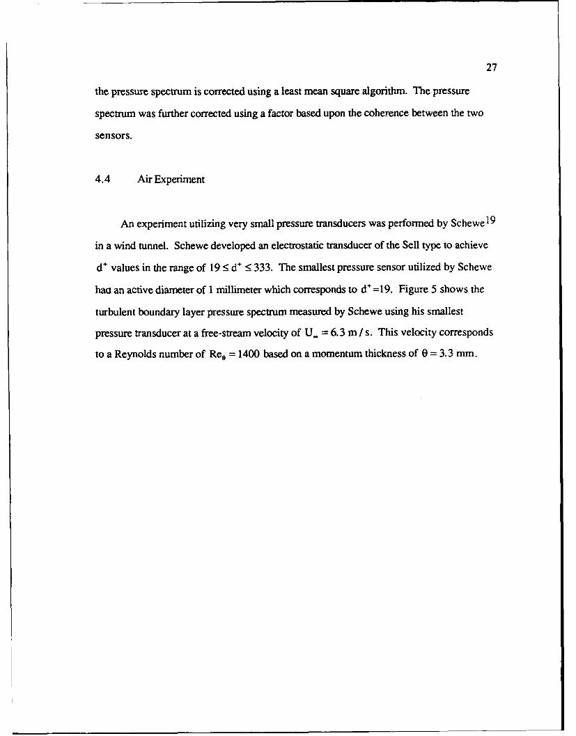
An experiment utilizing very small pressure transducers was performed by Schewe 19
in a wind tunnel. Schewe developed an electrostatic transducer of the Sell type to achieve
d÷ values in the range of 19 < d÷ < 333. The smallest pressure sensor utilized by Schewe
haa an active diameter of 1 millimeter which corresponds to d'=19. Figure 5 shows the
turbulent boundary layer pressure spectrum measured by Schewe using his smallest
pressure transducer at a free-stream velocity of U. = 6.3 m / s. This velocity corresponds
to a Reynolds number of Re. = 1400 based on a momentum thickness of 0 = 3.3 mm.
28
70
~60
:=Lo 50
S40
"• 3003
2010 100 1000 10000
Frequency (Hz)
Figure 5 - Measured Wall Pressure Spectra for Wind Tunnel at Ree=1 4 00

29
Chapter 5
NUMERICAL INTEGRATION OF THEWAVEVECTOR-FREQUENCY SPECTRUM
5.1 Two-Dimensional Simpson's 1/3 Method
Prediction of the turbulent boundary layer pressure fluctuations were obtained by
numerically integrating Equation (3.1). The integration of Equation (3.1) is performed20
using a two dimensional Simpson's 1/3 rule. The integration is carried out by shifting
Simpson's 1/3 rule for one dimension into two dimensions. The general form of the
Simps&i's 1/3 rule, which is used to integrate a function f(x,y), is:
X,1 Y,.] iI = f f (x, y)dxdy=k[-( i= ++1 + + fi +i.j1
Xi-1 Yi-1 (5.1)
+4 h(fi+,.j + 4 fi~j+ f i-1 j)+ h(fi+lj-1 + 4fij-1 + fi-,j-)3 3
To evaluate Equation (3.1), the integration was carried out in the k, and k3 directions. At
each point in wavenumber space where the integration is performed, a rectangle consisting
of nine locations is defined. This rectangle has dimensions of twice the step size in the k1 -
direction by twice the step size in the k3-direction. The function f(x,y) is the wavenumber-
frequency spectra proposed by Chase in both his 1980 and 1987 papers. For the 1980
model equation, Equations (3.9) and (3.10) are used in Equation (5.1) for f(x,y). For the
incompressible model in Chase's 1987 paper, Equation (3.18) is integrated; and for
Chase's compressible model, Equation (3.19) is integrated.

30
5.2 General Parameters
Determination of the general parameters to be used for the integration in all three
cases; air, water and glycerine, is the next step in carrying out the integration. Based upon
an examination of the wavenumber dependence of the turbulent wall pressure spectrum,21
and from previous experience in evaluating Equatioin (3.1) , values for the upper and
lower limits of integration were established. For all cases, in both the k, and the k3
directions, the double integral is evaluated at 80 locations in the range-10k, to 10k,. For
each case, the spectral level for 30 frequency points between the lowest and highest
frequencies of interest are calculated. Due to the finite limits necessary to carry out the
numerical integration the results represent a lower bound on the magnitude of the wall
pressure spectra. The frequency range of interest depends upon the data available for each
fluid. Depending on the author, various frequency dependent values of the convective
velocity have been established. Most of these models show only a weak dependence on
frequency, so a constant value of convective velocity was used for the calculations. For
this paper, as was used by Chase in his 1987 paper, the value of the convective velocity is
taken to be. 65U-. Based on calculations for the wall pressure spectrum with convective
velocities ranging from .6U- to .8U., it is noted that the effect of choice for the convective
velocity was minimal on the results of the calculations.
One important point to note is that the experiment in water was performed in a
rectangular channel facility and the glycerine experiment was performed in a pipe flow
facility. For both of these cases, the turbulent boundary layer was not a free boundary
layer as was modeled by Chase in his two papers. The boundary layer thickness for the
bounded cases were, therefore, considered to be the half-height of the corresponding
facility. 2
31
The friction velocity, and when necessary, the wall shear stress are calculated based
on formulas given by White. 2 The wall shear stress is given by Equation (2.3) and the
friction velocity is given by Equation (2.7). As can be seen by examination of these
equations, the most important factor for calculating these parameters is the Reynolds
number, which was given in Chapter 4 for all three cases of interest.
5.2.1 Constants for Chase's 1980 Model
The empirical constants used in thewavevector-frequency spectra were established
based on the work of Chase 12 and Lauchle 10 . The values for bM and bT are those given
by Chase; and the values for hM, hT, CM, and CT are those given by Lauchle. The
constants used for the integration of Chase's 1980 model are:
bM=0. 7 5 6 bT=0.3 7 8 hM=20.0 (5.2)
hT= 2 0.0 CM=0.05 CT=.00 4 .
5.2.2 Constants for Chase's 1987 Models
To establish the empirical constants for his compressible and incompressible models,
Chase used ihe work of Martin and Leehey 16. The six constants used in the
incompressible and compressible model are:
h=3.0 b=0.75 CT= 0.004 7
CM =0.15 5 3 cl =0.1667 c2 =0.1667, (5.3)
where c2 and c3 are only used for the compressible model.

32
5.3 Flow Parameters for Glycerine Experiment
The glycerine experiment of Lauchle and Daniels 17 was performed in a pipe flow
facility for a range of Reynolds numbers. The experimental facility is designed to change
the Reynolds number by varying the temperature of the working fluid as opposed to
varying the flow velocity. The flow velocity at the centerline of the tunnel is stated as
6.8 m / s:9 U,, -< 7.5 m / s. The mean value of this stated range was chosen for the free-
stream velocity. Fluid properties at 35" C were used for the calculations, boundary layer
thickness was assumed to be the radius of the tunnel, and the sensor diameter was given as
0.5 mm. Based on this information, the following values were used to calculate spectral
levels for the glycerine tunnel experiment:
Re=10890 p=1238kg/m 3 U.,=7.15m/s R=0.25mm
S=a=0.14m Uc=4.648m/s u.=0.44]m/s r,,=240.93Pa (5.4)
u = 1.72xl04 m2 /s c = 1980 m / s
where the values of convection velocity, wall shear stress, and friction velocity were
calculated by the program. Since this flow is in a pipe, the equation used for calculation of
wall shear stress is different from the one used for a flat plate5 :
•,,•t _T T 14_ 14 -/4
T,, = 0.0325pU,, a- (5.5)
where a is the pipe radius and U., is the average pipe flow velocity. The spectral
calculations were performed over the frequency range of 1-1000 Hz. Based on these
parameters, the solid line of Figure Al shows P(k ,,0,(0) computed from the 1987
compressible model, for a frequency of f=100 Hz.
33
5.4 Flow Parameters for Water Experiment
The experiment with water was performed in a rectangular channel flow facility.
Given the channel Reynolds number, channel dimensions, and that the working fluid was
water at approximately 200 C; the following parameters were used for the calculations:
Rh=25000 p=998kg/m 3 U.vl.7m/s R=0.25mm
S=a=0.0125m U,=1.105m/s u.=0.089m/s (5.6)
C,= 7.953Pa u=l.005xl0 6 m 2 /s c=1481m/s.
Once again, the values for convection velocity, wall shear stress, and friction velocity were
calculated by the program. Wall shear stress was calculated using equation (5.5), and
spectral calculations were performed over the frequency range 0.2-2000 Hz. Based on
these parameters, the solid line of Figure A2 shows P(k1 ,0,o) computed from the 1987
compressible model, for a frequency of f=100 Hz.
5.5 Flow Parameters for Air Experiment
The experiment by Schewe 19 was performed in a wind tunnel. For this experiment,
all the necessary flow parameters were given. The only parameter calculated by the
program was the convective velocity. The parameters used for the calculation of the
spectral levels for the experiment in the wind tunnel were:
Re6 =1400p=l.20kg/m 3 U=6.3m/s R=0.5mm 8=30mm
UC=4.095m/s u.=.273m/s T,,=.09Pa c=343m/s.
34
Spectral levels were calculated for the frequency range of 20-2000 Hz. Based on these
parameters, the solid line of Figure A3 shows P(k,,O,co) computed form the 1987
compressible model, for a frequency of f=100 Hz. Due to the slower speed of sound in air
relative to the other fluids, the acoustic wavenumber is present on Figure A3. The acoustic
wavenumber can be seen to effect P(k1 ,0,c0) at k, / (co / U.) =.012.
35
Chapter 6
RESULTS
6.1 Constants Given By Chase
In this section, a comparison of the three models proposed by Chase in his 1980 and
1987 papers will be presented. Spectral levels were first calculated using all three of
Chase's models with the constants specified in Chapter 5. This first comparison will allow
one to assess the differences among the various models proposed by Chase. Figure 6
shows the spectral levels calculated for the glycerine experiment for all three models;
Chase's 1980 model, the 1987 incompressible model, and the 1987 compressible model.
Notice that the 1987 compressible model and the 1987 incompressible model result in the
same predicted spectral levels for the given constants. The 1980 and 1987 models predict
the same spectral shape but with different amplitudes.
Figure 7 shows the spectral predictions for the water flow experiment. The low
frequency region of Figure 7 illustrates one of the main differences between Chase's 1980
and 1987 models. As stated in S 'ction 3.2.2, the assumption that P(k,o) tends to zero as
K2 was relaxed in the 1987 models. This is evident by the change in slope between the
two models in the low frequency region.
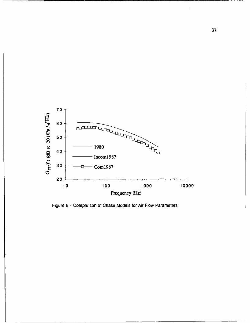
Figure 8 shows the results predicted by the 1980 and 1987 models for the flow
parameters given by Schewe in his wind tunnel experiment. The results in Figure 8 show
similar trends as those in Figure 6 for the glycerine experiment. The low frequency
divergence between the two models can be seen to be starting at the lowest data point, 20
Hz. If the calculations were carried out to lower frequencies, the results would show the

36
160
•p 150
140
"- 130
1980II1 120 -1___Incom1987
'4- 1100--0- Com1987
o 100
9 0 . . . .. . . .. . . .. . . .
1 10 100 1000 10000
Frequency (Hz)
Figure 6 - Comparison of Chase Models for Glycerine Flow Parameters
140
130
S120=L
I 110
- 100100 _____IncomI 987
0 90 -C'oo---- Com9987
80 ..
0.1 1 10 100 1000 10000
Frequency (Hz)
Figure 7 - Comparison of Chase Models for Water Flow Parameters
37
70
=L 5050el
S40- Incom1987
30 - Com1987
2010 100 1000 10000
Frequency (Hz)
Figure 8 - Comparison of Chase Models for Air Flow Parameters

38
same trend as the low frequency data in Figure 7.
6.1.1 Comparison to Experimental Results
A comparison of the spectral levels calculated with the given constants versus the
experimental results are presented in this section. Since the calculated results obtained for
the incompressible and compressible 1987 models were the same, only the compressible
model results will be displayed. Figure 9 shows a comparison between calculated values
and experimental values for the glycerine experiment. A number of discrepancies between
predicted and measured levels can be noted. The spectral levels predicted by all three
models were considerably higher than those measured. The predicted peak level occurs at
around 10 Hz, while the measured peak level occurs at about 20 Hz. The measured levels
decrease rapidly after the peak value while the predicted values decrease at a much slower
rate. This marked difference in spectral level above 100 Hz may be a result of the fact that
Chase's models do not take into account the viscous domain of the turbulent boundary22
layer. Based on the work of Farabee and Casarella , the source of the high frequency
portion of the wall pressure spectrum is proposed as the overlap region of the boundary
layer. The small scale velocity fluctuations in this region are affected by the viscosity of the
fluid. By neglecting the effect of viscosity, Chase may be over predicting the small scale,
high frequency, velocity fluctuations. Another issue to be considered for these
discrepancies is the use of an external flow prediction method for an internal flow.
A comparison between measured and predicted spectral levels for the water tunnel
experiment of Home and Handler 18 is shown in Figure 10. The agreement between
measured and predicted values is much better for this experiment. In the higher frequency
range, above about 100 Hz, Chase's models predict the rate of decrease of the spectral
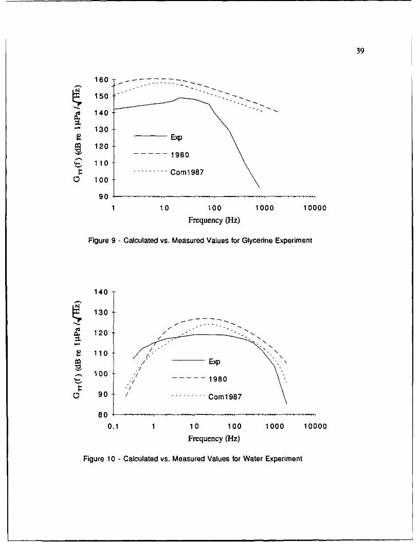
39
160 /.. . .--
S15 0 .-' - ' •. ... . .. .
140
"- 130
S1201980
S110---------. Com1987
0• 100
90,.
1 10 '100 1000 10000
Frequency (Hz)
Figure 9 - Calculated vs. Measured Values for Glycerine Experiment
140
130
S120
110Ep',,
4m 1980S,'/
. 90 / .Com1987
800.1 1 10 100 1000 10000
Frequency (Hz)
Figure 10 - Calculated vs. Measured Values for Water Experiment
40
levels much more accurately for the water experiment than for the glycerine experiment.
By comparing Figures 9 and 10, one can see that above 100 Hz the negative slope of the
measured pressure spectrum is much greater for glycerine than water. In the low
frequency region, below about 5 Hz, all three models decrease more rapidly than the
measured levels. As noted above, the 1987 models decrease less rapidly than the 1980
model in the low frequency region, although the results are still too low.
Figure 11 shows the comparison between measured and calculated spectral levels for
the wind tunnel experiment of Schewe1 9 . The predictions of the 1987 models show
relatively good agreement with the actual measured levels. Once again, the high frequency
region is the area where the agreement between measured and predicted levels is the
poorest. In this case, the predicted levels agree well with the experimental results up to
about 900 Hz.
In general, the agreement between measured and predicted levels for the air and water
data is good. The predictions for the glycerine experiment show poor agreement with
experimental results. The predictions with the 1987 models, both incompressible and
compressible, show better agreement with experimental results than the predictions using
the 1980 model. In all cases, as one progresses to higher frequencies, Chase's models
tend to over predict the measured sound pressure levels. In the following section, an
attempt will be made to obtain a better fit to the experimental data by varying the six
empirical constants utilized by Chase in his 1987 compressible model.
6.2 Empirical Constants
In order to obtain a better agreement between the experimental and calculated results,

41
70
60
=L 50
Exp40
1980
30 -- --------- Com 1987
20
1 10 100 1000 10000
Frequency (Hz)
Figure 11 - Calculated vs. Measured Values for Air Experiment

42
the six parameter values given by Chase for his 1987 incompressible model were
systematically varied. The first step was to vary each parameter individually to quantify the
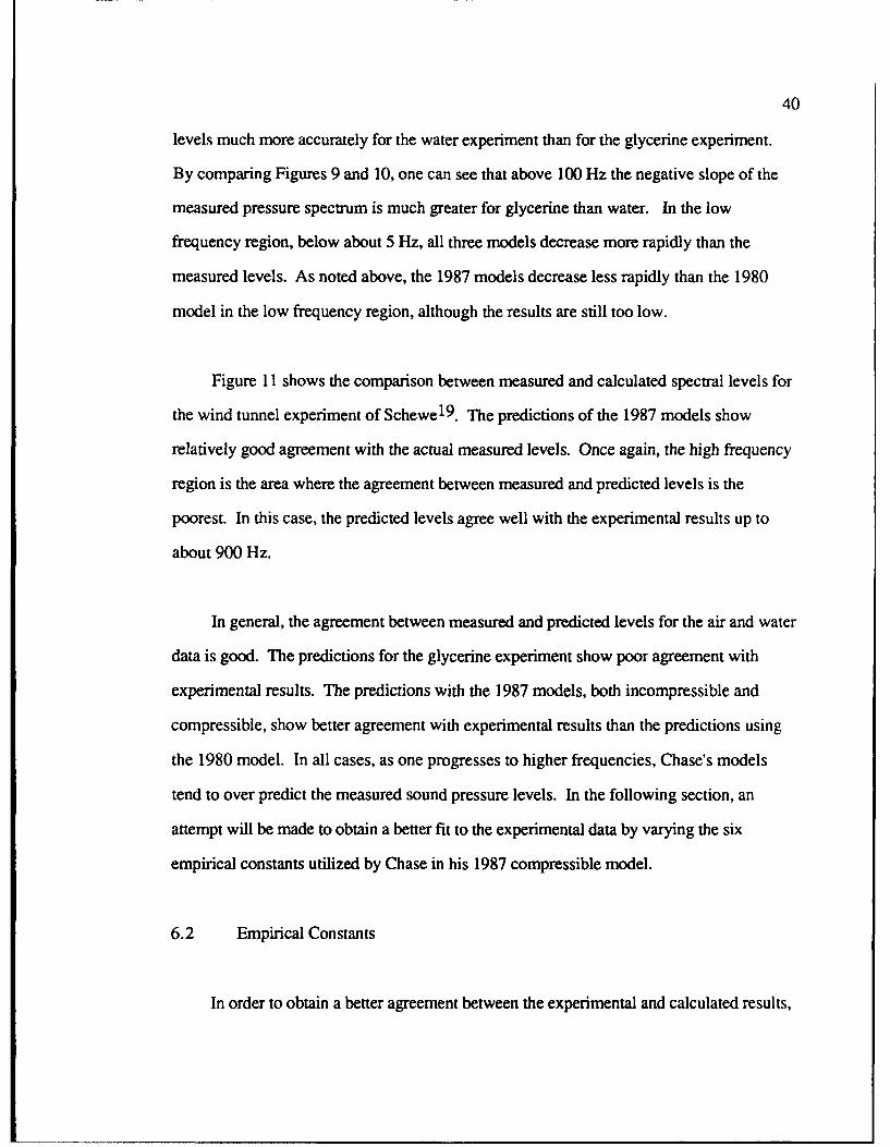
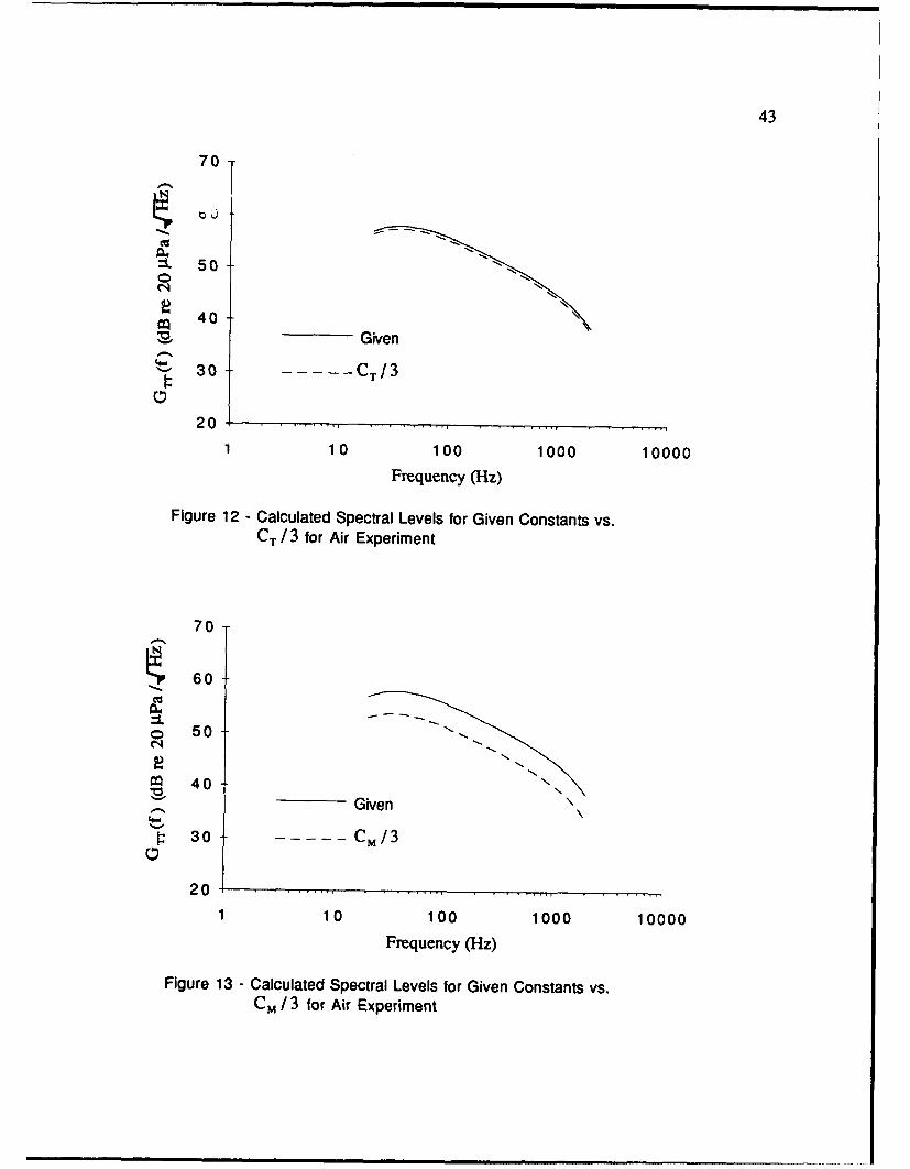
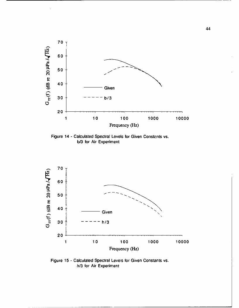
effect each parameter has on the calculated wall pressure spectrum. As an example, Figure
12 is a comparison of the spectral levels calculated for the air experiment with the values
given by Chase versus the spectral levels calculated when CT is reduced by a factor of 3.
All other constants remained the same for this calculation. One can see that reducing the
value of CT by a factor of 3 had very little effect on the calculated spectral levels. Figure
13 shows the result of lowering the value of CM by a factor of 3 while keeping the other
parameters constant. As shown by Figure 13, reducing the value of CM reduced the
overall levels by about 5 dB. Reducing CM by the same factor as CT had a much greater
impact on the predicted levels. This is to be expected since the contribution to the turbulent
boundary layer wall pressure by the mean shear-turbulence interaction term is significantly
larger than the contribution from the turbulence-turbulence interaction term. Another
important feature of both Figures 12 and 13 is that, although the magnitude of the predicted
levels was changed, the shapes of the spectra remained identical. Figure 14 compares the
results for the given constants to the values predicted by the model when b is reduced by a
factor of 3. The effect of b, the scale coefficient, on the low frequency predicted levels is
considerable. Below 300 Hz, the lower value of b causes divergence between the spectral
levels predicted with the original constants. Above about 300 Hz, the new set of data
matches the original predicted levels. Finally, Figure 15 shows calculations when h is
lowered by a factor of 3. The effect of the velocity dispersion coefficient, h, is similar to
that of CM. The level of the entire spectrum is reduced by about 5 dB, but the slope of the
predicted curve remains the same. Varying the parameters c, and c2 had an extremely
small effect on the calculated wall pressure spectrum.
Figure A l shows the results of varying the empirical constants CM, h, and b on
43
70
S. 50 ""
50
2• 40S~Given
S30 CT/3
2010 100 1000 10000
Frequency (Hz)
Figure 12 - Calculated Spectral Levels for Given Constants vs.CT / 3 for Air Experiment
70
~60
0 50
40S Given\
S30 CM/3
20
1 10 100 1000 10000
Frequency (Hz)
Figure 13 - Calculated Spectral Levels for Given Constants vs.CM / 3 for Air Experiment
44
70
K600 50
9 40 S~Given
p4.4 I: 30 - - - - -b/330
2010 100 1000 10000
Frequency (Hz)
Figure 14 - Calculated Spectral Levels for Given Constants vs.b/3 for Air Experiment
70
~60
I-
.o 40 ___-_....
tN
'40 Given ,
: 30 h/3
20.
1 10 100 1000 10000
Frequency (Hz)
Figure 15 - Calculated Spectral Levels for Given Constants vs.h/3 for Air Experiment
45
P(k ,0,wo) for the glycerine experiment flow parameters at a frequency of 100 Hz. Note
the overall level of P(k• ,0,)o) for the original constants vs. the best fit constants. Figure
A2 shows the results c ýarying the empirical constants CM, h, and b on P(k,1 0,o,) for
the water experiment at a frequency of 100 Hz. For the water experiment, the best fit result
for P(k1 ,0, A) is much closer to the original result than is the case for the glycerine
experiment. Figure A3 shows the results of varying the empirical constants CM, h, and b
on P(kI,0,co) for the air experiment at a frequency of 100 Hz.
Inspection of Figures 12-15 shows that the only parameter that changes the general
shape of the spectrum is b. The effect of the scale coefficient, b, is most noticeable in the
low frequency region of the wall pressure spectrum. None of the parameters have any
impact on the slope of the high frequency end of the spectrum. This fact will limit the
effectiveness of fitting the experimental data by varying the empirical constants.
6.2.1 Empirical Fit to Experimental Data
Using the information gained by varying the constants individually, an empirical best
fit to the experimental data was obtained by varying combinations of the empirical
parameters. The combinations used are not necessarily unique. In general, the scale
coefficient, b, was used to fit the slope of the low frequency calculated data to the
experimental data. The overall level was adjusted using combinations of h and CM. Due
to th: relatively minor impact of CT on the calculated pressure spectrum, its value was
unchanged.
Figure 16 is a comparison of the experimental data for the air experiment with the best
fit obtained by varying Chase's empirical parameters. The final parameter values used in
46
70
~60
I 40 \
Best Fit30
20
1 10 100 1000 10000
Frequency (Hz)
Figure 16 - Experimental Data for Air Experiment vs. BestFit Data with 1987 Compressible Model
47
the 1987 compressible model are:
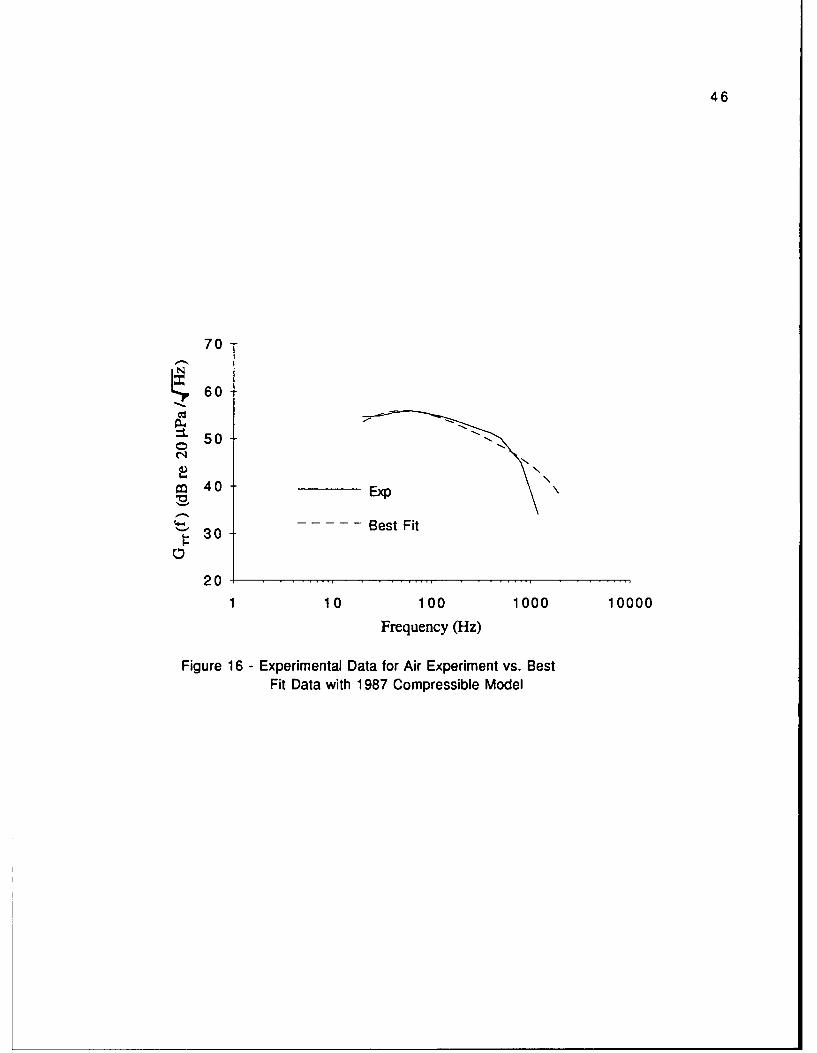
h=3.0 b=0.5 CT=0.00 4 7
CM = 0.2330 cl =-0.1667 c2 =0.1667. (6.1)
Comparison of these values with Equations (5.3), the original value of the constants,
illustrates the changes made. Although b was altered by a significant amount, the
remainder of the values were changed very little. Since the original values of constants
used by Chase were determined by comparison to wind tunnel data, this is not unexpected.
The low frequency portion of the experimental curve was fit by reducing the value of b.
The overall levels were adjusted using a slightly higher value of CM. The calculated
spectral levels agree well with the experimental data up to about 1000 Hz. The measured
peak level is at about 50 Hz and the calculated peak level, with the above values of
experimental parameters, now coincides with this peak. Above 1000 Hz, the model still
over predicts the sound pressure levels. As mentioned above, none of the experimental
parameters can affect solely the high frequency end of predicted pressure spectrum. With
the Chase's present model of the turbulent boundary layer, it is not possible to match the
low frequency and high frequency portions of Schewe's measured pressure spectrum.
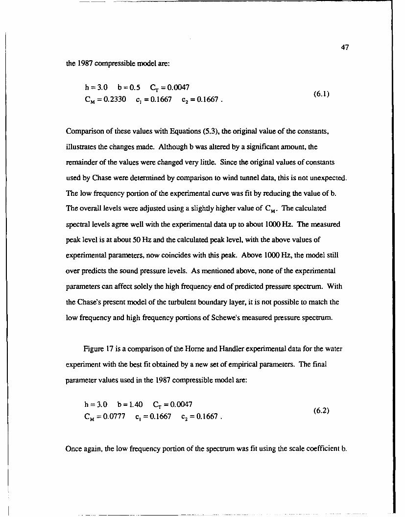
Figure 17 is a comparison of the Home and Handler experimental data for the water
experiment with the best fit obtained by a new set of empirical parameters. The final
parameter values used in the 1987 compressible model are:
h=3.0 b=1.40 CT=0. 0 04 7
CM=0.0 7 7 7 c1 =0.1667 c2 =0.1667. (6.2)
Once again, the low frequency portion of the spectrum was fit using the scale coefficient b.
48
140
S130
•, 120
L 110
S100 Exp
90 Best Fit
80 .0.1 1 10 100 1000 10000
Frequency (Hz)
Figure 17 - Experimental Data for Water Experiment vs. BestFit Data with 1987 Compressible Model
49
After the low frequency end of the spectrum was fit, the overall level was adjusted using
Cm. There is good agreement between the calculated and measured values for the water
experiment in the low and high frequency regions. The peak predicted spectral level of the
wall pressure spectrum was at about 20 Hz. The measured wall pressure spectrum shows
a peak in the same region, although lower in level by about 9 dB. Above 1000 Hz, the
measured and predicted levels begin to diverge, although not as noticeably as in the case of
the air data.
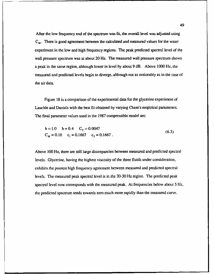
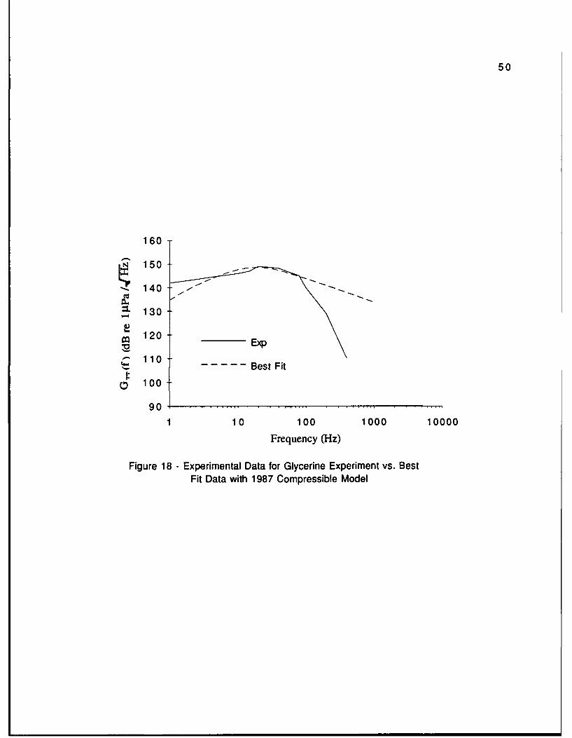
Figure 18 is a comparison of the experimental data for the glycerine experiment of
Lauchle and Daniels with the best fit obtained by varying Chase's empirical parameters.
The final parameter values used in the 1987 compressible model are:
h=1.0 b=0.4 CT =0.0047 (6.3)
CM=0.10 c1 =0.1667 c2 =0.1667.
Above 100 Hz, there are still large discrepancies between measured and predicted spectral
levels. Glycerine, having the highest viscosity of the three fluids under consideration,
exhibits the poorest high frequency agreement between measured and predicted spectral
levels. The measured peak spectral level is in the 20-30 Hz region. The predicted peak
spectral level now corresponds with the measured peak. At frequencies below about 5 Hz,
the predicted spectrum tends towards zero much more rapidly than the measured curve.
50
160
S150
140
:L 130
S12010Exp
"- 110• 110Best Fit
S100
9 0. . . . .. . . .. . . .. . .
1 10 100 1000 10000
Frequency (Hz)
Figure 18 - Experimental Data for Glycerine Experiment vs. BestFit Data with 1987 Compressible Model

51
Chapter 7
CONCLUSIONS
7.1 Justification for New Empirical Constants
In order to obtain a better fit to the measured wall pressure spectra presented in this
paper, the values of the empirical constants used by Chase in his 1987 compressible model
were varied. Having determined the values which are most suitable for the experiments
considered, the reasons why these changes were necessary must be explored. In essence,
two parameter values were varied. The first was the scale coefficient b, which changed the
low frequency portion of the calculated wall pressure spectra. The second was the value
of the product CMh, which changed the overall level of the spectrum.
For the experiment performed in air, significant change in b was required. Chase 15
states that the scale coefficient, b, is used to cut off contributions to the wall pressure
spectrum at wavenumbers less than the reciprocal of the outer scale, i.e. the boundary layer
thickness. As noted, the scale coefficient affects the low frequency portion of the predicted
wall pressure spectrum. Better agreement with Schewe's data was obtained by lowering
the value of b from the value first postulated by Chase. This is to be expected because
Chase 12 notes variability from experiment to experiment for the low frequency portion of
the wall pressure spectrum. Based on this fact, it is not unexpected that the value of b
needed to fit Schewe's data was different than the value of b needed to fit Martin and
Leehey's data. The work done by Schewe was performed in a quiet wind tunnel designed
for flow noise measurements. With this facility, it is possible that Schewe was able to
obtain a better measurement of the low frequency portion of the wall pressure spectrum.

52
The value of the product CMh was increased by 1.5 times over the value used by Chase in
his 1987 paper. This change, in part, was necessitated by the effect that decreasing b had
on the mid frequency portion of the predicted spectrum. The result of this increase in CMh
on the prediction is not significant, about 2-3 dB.
For the experiment performed in the water tunnel, so that the low frequency portions
of the measured and predicted spectra would agree, the scale coefficient had to be increased
by almost 3 times the original value. There are a number of possible causes for the need
for this large increase. The experiment was performed in a rectangular flow facility so the
boundary layer was bounded, not free. As was discussed by Farabee and Casarella 2 2 , the
physical characteristics of channel and flat plate boundary layer flows are different,
especially in the outer regions, which generate the low frequency components of the wall
pressure spectrum. A second possible cause is the presence of low frequency noise
contamination in the measured signal. Although a significant decrease in measured levels
was obtained by post-processing the acquired data to remove background noise, it is still
possible some contamination remains. As was the case for the air experiment, the value of
CMh was adjusted, lowered in this case, to compensate for the increase in b. The decrease
in value of the product CMh did not totally compensate for the increase in h, which resulted
in the mid frequencies of the predicted spectrum being slightly higher than originally
predicted.
For the glycerine experiment, the greatest changes in the values of the constants were
required. The product CMh was lowered by almost a factor of 5 to bring the overall levels
into closer agreement with the measured levels. The velocity dispersion coefficient, h, is
an empirical constant which is used to scale the friction velocity u.. Comparison of the
friction velocity for the air and glycerine shows that u. is twice as large for the glycerine

53
experiment. The large value of u., coupled with the level of the coefficient h established
for wind tunnel data resulted in spectral levels which were too high. The value of the
coefficient used to scale the mean shear-turbulence interaction term, CM, was also
established by Chase based on wind tunnel data. Even if h was lowered by a factor of 2 to
account for a higher friction velocity, CM would still be too high. The value of b was
lowered in an attempt to fit the low frequency portion of the spectrum. Below 5 Hz, the
predicted levels are still decreasing more rapidly than measured. The same possible
explanations apply to this data as for the water tunnel data
It is interesting to note the similarity between the results for the glycerine and water
experiments. In both cases, the measured low frequency spectral levels decrease at a much
slower rate than is predicted by Chase models. Both experiments utilized techniques to
remove low frequency contamination from the acquired data. This leads to the conclusion
that the similar results for the glycerine and water experiments may be the result of these
being bounded shear flows rather than free boundary layers.
7.2 General Conclusions
This paper has attcmpted to evaluate the suitability of applying Chase's
comprehensive wavevector frequency spectrum models 1 2 ,15 to the prediction of measured
turbulent boundary layer wall pressure spectra. In the course of this investigation, a
number of conclusions have been reached:
-The 1987 compressible and incompressible models predict spectral levels that are
closer to measured levels than does the 1980 model.
-In the 1987 models, the functional dependence of the low frequency region of the

54
wavevector frequency spectrum was relaxed from the K 2 dependence of the 1980 model.
Changing the low frequency dependence of the 1987 models resulted in better estimates of
the very low frequency regions of the wall pressure spectrum, as can be noted in
comparison with data from the water tunnel. Although better, the models still tend to over
predict the rate of decrease of the spectral levels in the low frequency region of the
spectrum for the water and glycerine experiments.
-In his 1980 paper, Chase states that the effect of viscosity on the convective
ridge of the wavevector-frequency spectrum will be small provided orn/u! • 2, and that the
effect of viscosity on the low wavenumber domain will be small if o=/u! 5 1/2. For the
glycerine experiment, this corresponds to viscous effects becoming important in the low
wavenumber domain for frequencies above 90 Hz, and for the convective domain at
frequencies above 360 Hz. The final results for the glycerine experiment, Figure 18,
shows the calculated values deviating from the measured values at frequencies above about
90 Hz. For the water experiment, the above criteria correspond to frequencies of f=627 Hz
and f=2508 Hz, for the low wavenumber and convective regions respectively. For the air
experiment, viscous effects become important at frequencies of f=393 Hz and f=1571 Hz,
for the low wavenumber and convective regions respectively.
-In all cases, the models over predict the measured spectral levels in the high
frequency region. The cause of this appears to be that the models do not take into account
the viscous domain of the turbulent boundary layer. Within the viscous sublayer, small
scale, high frequency velocity fluctuations are reduced in magnitude. The best example of
this is the comparison of the glycerine tunnel data to predicted levels.
-The models, in their present form, appear to be most suitable for predicting spectral
levels of free boundary layers in nearly inviscid fluids. This is expected since Chase
arrived at his models with such assumptions.
-A comparison of calculated wall pressure spectra, with the new empirical values

55
arrived at here, to a recent measurement of wall pressure spectral levels for a free boundary
layer in water would be useful. This comparison should answer the questions concerning
the rate of decrease of the low frequency spectral levels of the measured wall pressure
spectra for the water and glycerine experiments.
- Comparisons of calculated wall pressure spectra, with the new empirical values, to
a variety of recent air tunnel measurements would allow one to evaluate the applicability of
the new constants to a range of flow conditions.
-Future work in modeling the wall pressure spectrum of the turbulent boundary with
Chase's models should include an attempt to account for the effects of the viscous region of
the turbulent boundary layer. Once a high frequency dependent term is included in Chase's
wavevector-frequency spectrum model, a better match to the entire measured frequency
spectrum may be obtained.
56
REFERENCES
1 Willmarth, W.W., "Pressure Fluctuations Beneath Turbulent Boundary Layers," AnnualReview of Fluid Mechanics, 7 (1975) 13-37.
2 White, F.M., Fluid Mechanics, McGraw Hill, Inc., 1979
3 Schlichting, H., Boundary Layer Theory, 7th Edition, McGraw Hill Inc., 1979.
4 Tennekes, H., and Lumley, J.L. A First Course in Turbulence, The MIT Press, 1972.
5White, F.M., Viscous Fluid Flow, McGraw Hill, Inc., 1974
6 Kraichnan, R.H., "Pressure Fluctuations in Turbulent Flow over a Flat Plate," J. Acoust.Soc. Amer., 28 (1956) 378-390
7 Blake, W.K., Aero-Hydroacousticsfor Ships, David W. Taylor Naval Ship Research andDevelopment Center, Report No. DTNSRDC-84/010 (1984)
8Farabee, T.M., "An Experimental Investigation of Wall Pressure Fluctuations Beneath
Non-Equilibrium Turbulent Flows," David W. Taylor Naval Ship Research andDevelopment Center Report DTNSDRC-86/047, May 1986
9 Uberoi, M.S., and Kovasznay, L.S.G., "On Mapping and Measurement of RandomFields," Quart. Appl. Math., 10 (1953) 375-393
1 0 Lauchle, G.C., "Effect of Turbulent Boundary Layer Flow on Measurement of AcousticPressure and Intensity," Noise Control Engr. J., 23 Sep-Oct (1984) 52-59
1 1Howe, M.S., "Surface Pressures and Sound Produced by Turbulent Flow Over Smoothand Rough Walls," J. Acoust. Soc. Amer., 90 (2) (1991) 1041-1047
12 Chase, D.M., "Modeling the Wavevector-Frequency Spectrum of Turbulent BoundaryLayer Wall Pressure," J. Sound Vibration., 70 (1) (1980) 29-67
13 Bendat, J.S., and Piersol, A.G., Random Data Analysis and Measurement Procedures,2nd Edition, John Wiley and Sons Inc., 1986
14 Bull, M. K., "Wall-Pressure Fluctuations Associated with Subsonic TurbulentBoundary Layer Flow," J. Fluid Mech., (28) (1967) 719-754
15 Chase, D. M., "The Character of the Turbulent Wall Pressure Spectrum atSubconvective Wavenumbers and a Suggested Comprehensive Model," J. Sound Vib.,(112)(1) (1987) 125-147
57
16 Martin, N.C., and Leehey, P., "Low wavenumber Wall Pressure Measurements Using aRectangular Membrane as a Spatial Filter," J. Sound Vib., (52) (1977) 95-120
17 Lauchle, G. C., and Daniels, M. A., "Wall-Pressure Fluctuations in Turbulent PipeFlow," Phys. Fluids A, (30) (10) (1987) 3019-3024
1 8 Horne, M. P. and Handler, R. A., "Note on the Cancellation of Contaminating Noise inthe Measurement of Turbulent Wall Pressure Fluctuations," Experiments in Fluids, (12)(1991) 136-139
19Schewe, G., "On the Structure and Resolution of Wall-Pressure Fluctuations Associated
with Turbulent Boundary-Layer Flow," J. Fluid Mech., (134) (1983) 311-328
20McCormick, J.W., and Salvadori, M.G., Numerical Methods in FORTRAN, PrenticeHall Publications, 1965
21McEachem, J.F., and Lauchle, G.C., "A Study of Flow Induced Noise on a Bluff
Body," NCA-Vol. 13- Structure and Flow Sound Interactions, eds. T.M. Farabee andM.P. Paidoussis, ASME Book No. G00724, (1992) 23-38
22Farabee, T.M., and Casarella, M.J., "Spectral Features of Wall-Pressure Fluctuations
Beneath Turbulent Boundary Layers," Phys. Fluids A,(3) (10) (1991) 2410-2420

58
Appendix A
PLOTS OF WAVEVECTOR-FREQUENCY SPECTRUM
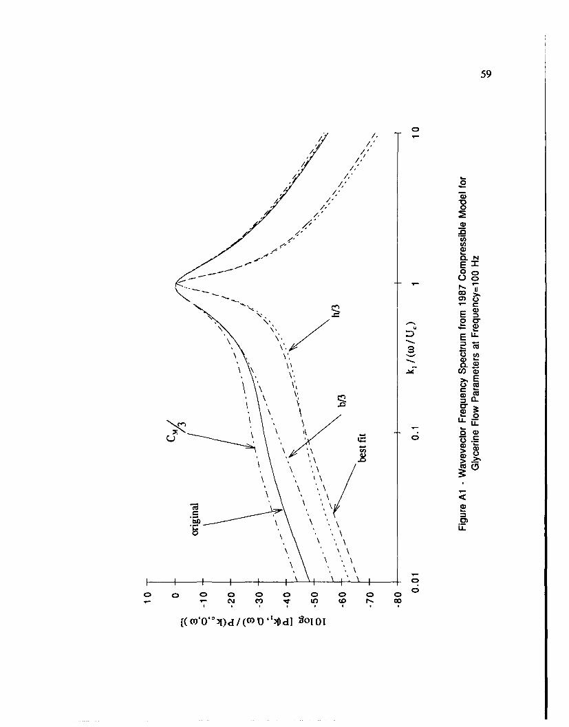
59
00
IC,
0 0>/ I,
(0)
&. E
Cc
0O
-J-
,~>
QLL
cr).0 31 0*o1 3 d oo
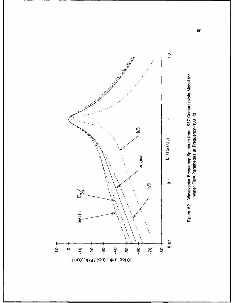
60
00
'*1C
,'1,a
- h..
.. 2.77' 0
>/ 4)
CM
2010I

61
00/12
'IL
-IE
En
CD
CrE0)t
ba 0
> -
(U
j0 I
Cý0
Q 0 0 C 0 0 0CI C? C?
co'o 31 d (o X IV a] ol0
62
Appendix B
MATLAB COMPUTER PROGRAM TO CALCULATE TURBULENTBOUNDARY LAYER WALL PRESSURE SPECTRUM USING
CHASES 1987 COMPRESSIBLE MODEL
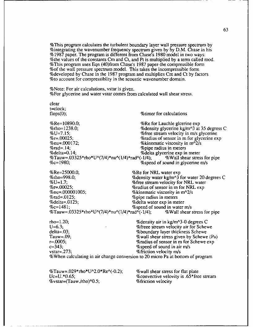
63
%This program calculates the turbulent boundary layer wall pressure spectrum by%integrating the wavenumber frequency spectrum given by by D.M. Chase in his% 1987 paper. The program is different from Chase's 1980 model in two ways:%the values of the constants Cm and Ct, and Pt is multiplied by a term called mod.%This program uses Eqn (40)from Chase's 1987 paper-the compressible form%of the wall pressure spectrum model. This takes the incompressible form%developed by Chase in the 1987 program and multiplies Cm and Ct by factors%to account for compressiblity in the acoustic wavenumber domain.
%Note: For air calculations, vstar is given.%For glycerine and water vstar comes from calculated wall shear stress.
cleart=clock;flops(0); %timer for calculations
%Re= 10890.0; %Re for Lauchle glcerine exp%rho=1238.0; %density glycerine kg/mA3 at 35 degress C%U=7.15; %free stream velocity in m/s glycerine%r=-.00025; %radius of sensor in m for glycerine exp%nu=.000172; %kinematic viscosity in mA2/s%rad=. 14; %pipe radius in meters%delta=0. 14; %delta glycerine exp in meter%Tauw=.03325*rho*UA(7/4)*nuA(1/4)*radA(- 1/4); %Wall shear stress for pipe%c=1980; %speed of sound in glycerine m/s
%Re=25000.0; %Re for NRL water exp%rho=998.0; %density water kg/m^3 for water 20 degrees C%U=1.7; %free stream velocity for NRL water%r=.00025; %radius of sensor in m for NRL exp%nu=.000001005; %kinematic viscosity in mA2/s%rad=.0 125; %pipe radius in meters%delta=.0125; %delta water exp in meter%c=1481; %speed of sound in water m/s%Tauw=.03325*rho*UA(7/4)*nuA(1/4)*radA(-1/4); %Wall shear stress for pipe
rho=1.20; %density air in kg/mA3-0 degrees CU=6.3; %freee stream velocity air for Schewedelta=.03; %boundary layer thickness ScheweTauw=.09; %wall shear stress given by Schewe (Pa)r=.0005; %radius of sensor in m for Schewe expc=343; %speed of sound in air m/svstar=.273; %friction velocity m/s%When calculating in air change conversion to 20 micro Pa at bottom of program
%Tauw=.029*rho*UA2.0*ReA(-0.2); %wall shear stress for flat plateUc=U.*0.65; %convective velovity is .65*free stream%vstar=(Tauw./rho)AO.5; %friction velocity
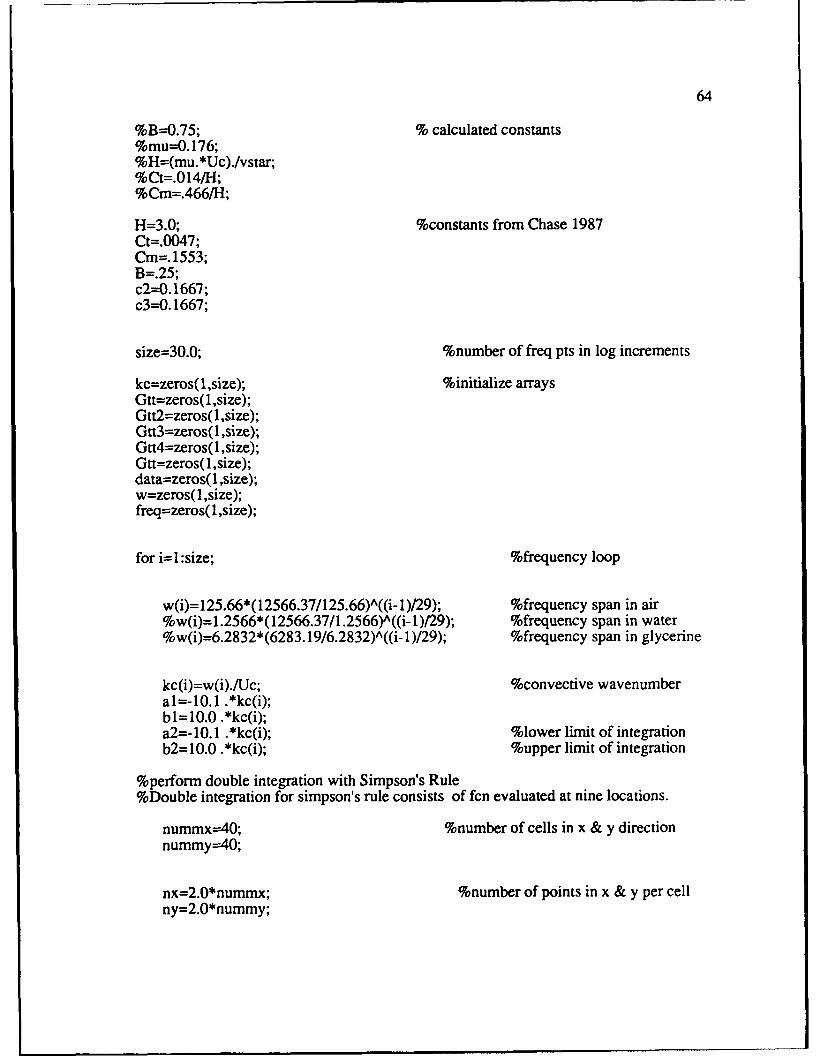
64
%B=0.75; % calculated constants%mu--0.176;%H=(mu.*Uc)./vstar;%Ct=.014/H;%Cm=.466/H;
H=3.0; %constants from Chase 1987Ct=.0047;Cm=. 1553;B=.25;c2--0.1667;c3--0.1667;
size=30.0; %number of freq pts in log increments
kc=zeros(1,size); %initialize arraysGtt=zeros(1,size);Gtt2=zeros(1,size);Gtt3=zeros(1,size);Gtt4=zeros(1,size);Gtt=zeros(1,size);data=zeros(1,size);w=zeros(1,size);freq=zeros(1,size);
for i=l:size; %frequency loop
w(i)=125.66*(12566.37/125.66)A((i-1)/29); %frequency span in air%w(i)=1.2566*(12566.37/1.2566)A((i-1)/29); %frequency span in water%w(i)=6.2832*(6283.19/6.2832)^((i- 1)/29); %frequency span in glycerine
kc(i)=w(i)./Uc; %convective wavenumberal=-10.1 .*kc(i);bl=10.0 .*kc(i);a2=-10.1 .*kc(i); %lower limit of integrationb2= 10.0 .*kc(i); %upper limit of integration
%perform double integration with Simpson's Rule%Double integration for simpson's rule consists of fcn evaluated at nine locations.
nummx-40; %number of cells in x & y directionnummy=-40;
nx=2.0*nummx; %number of points in x & y per cellny=2.0*nummy;
65
h=(bl-al)./nx; %step sizeh2=(b2-a2)./ny
sum=-O.O;k I I=al;k12=kllI+h;k13=kl2+h;
for j=1 :nummxUkI =a2;k32=k3l1+h2;k33=k32+h2;
%calculate componetns of Gtt
%I 1st location
Ksq=k 11 A2+k3 1 A2;
Kcsq=abs((Ksq-W(i)A2./cA2)); %compressibility
corn 1=c2*(KcsqfKsq)+c3*(KsqfKcsq)+ 1-c2-c3; %comnpress. factor for Ctcorn2=Ksq/Kcsq; %comnpress. factor for Cm
kr=(Ksq.AO.5).*r; %calculate hydrophone response fcn
dl=bessel(1,kcr);hyd=((2 .*dl )./kr).A2.O;kplus=(w(i)-Uc. *k 11).A2/(HA2. *vstarA2)+Ksq;mod=(kplus+(B *delta).A (-2))./ (Ksq+(B*delta).A (-2));Kin=(((w(i)-Uc. *k 11).A2/(HA2*vstarA2))+Ksq+(B*delta).A(-2));Kt=(((w(i)-Uc. *kl11).A2/(HA2*vstarA2))+Ksq+(B*delta).A(-2));phi--rhoA2*vstarA3.*(com2*Cm *kl 1A2 *KrnA(-2.5)+coml *Ct*Ksq *modJ *Kt A(-2.5));fi =phi*hyd;
%2nd location
Ksq=kl12.A2+k3 1 A2;
Kcsq=abs((Ksq-W(i)A2./CA2)); %comnpressibility
corn 1 =c2* (KcsqfKsq)±c3 *(Ksq/Kcsq)+ 1 -c2-c3; %compress. factor for Ctcorn2=Ksq/Kcsq;%compress. factor for Cm
kr=(Ksq.AO.5).*r,
66
dl=bessel(1 ,kx);hyd=((2 .*dl )./kr).A2.O;kplus=(w(i)-Uc.*kl2).A2/(HA2. *vstarA2)+Ksq;mod=(kplus+(B*delta).A(-2))./ (Ksq+(B*delta).A(-2));
~m=(((w(i)-Uc.*kl 2).A2/(HA2*vstarA2))+Ksq+(B *delta).A(-2));Kt=(((w(i)-Uc. *kl12).A2/(HA2*vstarA2))+Ksq+(B*delta).A(-2));phi--rhoIA2*vstarA3.*(con12*Cm *kl12A2 *KjMA(..2.5)+coml1*Ct*Ksq *mod *Kt./{.(2.5));f2=phi*hyd;
%3rd location
Ksq=kl 3A2+k3 1 A2;
Kcsq=abs((Ksq-w(i)A2 ./CA2)); %compressibility
corn 1 =c2*(Kcsq/Ksq)+c3*(Ksq/Kcsq)+ 1 -c2-c3; %compress. factor for Ctcom2=KsqfKcsq;%compress. factor for Cm
k=Ksq.AO.5).*r,.dl=bessel(l,kr);hyd=((2.*dl1)./kr).A2.O;kplus=(w(i)-Uc. *kl13).A2/(HA2. *vstarA2)+Ksq;mod=(kplus+(B*delta).A(-2))./ (Ksq+(B *delta).A(..2));Kni=(((w(i)-Uc.*klI3).A2/(HA2*vstarA2))+Ksq+(B *dela).A(-2));Kt=(((w(i)-Uc.*kl13).A2/(HA2*vstarA2))+Ksq+(B*delM).A(..2));phi--rhoi%2*vstarA3.*(com2*Cm *kl 3.A2 *KMjA(-.25)+coml *Ct*Ksq *modc *Kt.A(-..25));f3=phi*hyd;
for k=1 :nummy
%4th location
Ksq=kl 1 A2+k32.A2;Kcsq=abs((Ksq-W(i)A2./cA2)); %compressibility
corn 1=c2*(KcsqfKsq)+c3*(Ksq/Kcsq)+1-c2-c3; %compress. factor for Ctcom2=KsqfKcsq;%compress. factor for Cm
kr=(Ksq.AO.5).*r,dl=bessel(1 ,lr);hyd=((2 .*d 1 ./kr).A2.O;kplus=(w(i)-Uc. *kl11).A2/(HA2. *vstarA2)+Ksq;mod=(kplus+(B *delta). A(-.2))./ (Ksq+(B*delta).A(-2));Km=(((w(i)-Uc. *k 11).A2/(HA2*vstarA2))+Ksq+(B *delta).A(..2));Kt=(((w(i)-Uc. *kl11).A2/(HA2*vstarA2))+Ksq+(B*delta).A(-2));phi=rhoA2*vstarA3.*(com2*Cm *kI 1A2 *KMA(..2.5)+com I*Ct*Ksq *mno *Kt.A(-.25));f4=phi*hyd;
%5th location
6
Ksq=kl12.A2+k32.A2;Kcsq=abs((Ksq-W(i)A2 ./CA2)); %compressibility
com1=c2*(KcsqfKsq)+ic3*(Ksq/Kcsq)+1-c2-c3; %compress. factor for Ctcom2=KsqfKcsq;%compress. factor for Cm
kr=(Ksq.AO.5).*r,dl=bessel(1,kr);hyd=((2 .*d 1 )./kr).A2.O;kplus=(w(i)-Uc.*k12).A2/(HA2. *vstarA2)+Ksq;mod=(kplus+(B*delta).A(-2))./ (Ksq+(B*delta).A (-2));Km=(((w(i)-Uc. *kl12).A2/(HA2*vstarA2))+Ksq+(B*delta).A(-2));Kt=(((w(i)-Uc. *kl 2).A2/(HA2*vstarA2))+Ksq+(B*delta).A(-2));phi--rhoA2*vstarA3.*(com2*Cm*k12.A 2 *KmA(-.25)+com1*Ct*Ksq *mod *KtA(-..25));f5=phi*hyd;
%6th location
Ksq=k 3.A2+k32.A2;Kcsq=abs((Ksq-w(iYA2./cA2)); %compressibility
corn 1=c2*(Kcsq/Ksq)+c3*(KsqfY~csq)+ 1-c2-c3; %compress. factor for Ctcom2=KsqfKcsq;%compress. factor for Cm
kr--(KsqAO.5).*r;dl =bessel(l1,kr);hyd=((2.*d1 )./kr) A2.0;kplus=(w(i)-Uc. *kl13).A2/(HA2. *vstarA2)+Ksq;mod=(kplus+(B *delta).A(.2))./ (Ksq+(B *delta).A(..2));Km=(((w(i)-Uc. *k 1 3).A2/(HA2*vstarA2))+Ksq+(B *delta). A(-2));Kt=(((w(i)-Uc. *k 1 3).A2/(HA2*vstarA2))+Ksq+(B *delta) A(-2));phi--rhOA2*vstari-*3.*(com2*Cm *kl1342 *KmA(..2.5)+coml1*Ct*Ksq*mod *KtA (-2.5));f6=phi*hyd;
%7th location
Ksq=kl 1.A2+k33.A2;
Kcsq=abs((Ksq-W(i)A2./CA2)); %compressibility
coml=c2*(Kcsq/Ksq)+c3*(KsqfKcsq)+l-c2-c3; %compress. factor for Ctcom2=KsqlKcsq;%compress. factor for Cm
68
kr--(Ksq.AO.5).*r,dl=bessel(l1,kr);hyd=((2.*dI)./kr).A2.;kplus=(w(i)-Uc. *kl11).A2/(HA2. *vstarA2)+Ksq;mod=(kplus+(B*delta).A(-2))./ (Ksq+(B*delta).A(-2));Km=(((w(i)-Uc. *kll1).A2/(fjA2*vstarA2))+Ksq+(B *dela).A(..2));Kt=(((w(i)-Uc. *kl11).A2/(HA2*vstarA2))+Ksq+(B*delta).A(-2));phi--rhoA2*vstar*A3.*(com2*Cm *kl 1A2 *KmA(-2.5)+com1 *Ct*Ksq *mod *KtA(..2.5));f-/=phi*hyd;
%8th location
Ksq=kl12.A2+k33.A2;Kcsq=abs((Ksq-w(i)A2./cA2)); %compressibility
corn 1=c2*(Kcsq/Ksq)+c3*(KsqfKcsq)+ 1-c2-c3; %compress. factor for Ctcom2=Ksq/Kcsq;%compress. factor for Cm
kr--(Ksq.AO.5).*r,dl=be-ssel(l,kr);hyd=((2 .*d 1)./k).A20;kplus=(w(i)-Uc. *kl 2).A2/(HA2. *vstarA2)+Ksq;mod=(kplus+(B*delta).A(-2))./ (Ksq+(B*delta).A(-2));Km=(((w(i)-Uc.*k1 2).A2/(HA2*vstarA2))+Ksq+(B*delta).A(-2));Kt=(((w(i)-Uc. *kl12).A2/(HA2*vstarA2))+Ksq+(B*delta).A(-2));phi--rhoIA2*vstarA3.*(com2*Cm*k1 2A2 *KmA(-.25)+coml *Ct*Ksq*mod*Kt.A(-..25));f8=phi*hyd;
%9th location
Ksq=kl 3.A2+k33.A2; %compressibility
corn 1=c2*(KcsqfKsq)+c3*(Ksq/Kcsq)+ 1-c2-c3; %compress. factor for Ctcom2=Ksq/Kcsq;%compress. factor for Cm
jc-(Ksq.AO.5).*r:dl=4,essel(l1,kr);hyd=((2.*dI )./kr).A2.O;kplus=(w(i)-Uc.*k1 3).A2/(HA2. *vstarA2)+Ksq;mod=(kplus+(B*delta).A(-2))./ (Ksq+(B*delta).A(-2));Km=(((w(i)-Uc. *kl13).A2f(HA2*vstarA2))+Ksq+(B *delta).A(-2));Kt=(((w(i)-Uc. *kl13).A2/(HA2*vstarA2))+Ksq+(B*delta).A(-2));phi--rhoA2*vstarA3.*(com2*Cm *kl3A2 *KMA(..2.5)+com1 *Ct*Ksq*mod*KtA(..2.5));f9=phi*hyd;
%sum components of molecule
69
sum=sum+(h*h2./9.0).*(f 1 +f3+f7+f9+4.O .*(f2+f4+f6+f8)+ 16.0 .*f5);
%move :o next molecule
fl=f7;f2=f8;f3=f9;k32=k33+h2;k33=k32+h2;end
kll=k13;k12=kl 1+h;k13=k12+h;end
Gtt(i)=2.0 * sum;
end
Gtt2--Gtt*2*pi ./(4* 1OA(410)); %convert Ott from Pa to dB re 20 microPa%Gtt2--Gtt*2*pi Al(*10lA(-12)); %convert Ott from Pa to dB re 1 microPaGtt3= 10.0 .*log I0(Gtt2);freq=w ./6.28;
semilogx(freq,Gtt3)freqlI=freq';Gtt4--Gtt3';save freq freq 1 /asciisave data Gtt4 /asciietime(clock,t)flops