calculation of core losses of a six-phase induction motor with
120
CALCULATION OF CORE LOSSES OF A SIX-PHASE INDUCTION MOTOR WITH THIRD HARMONIC CURRENT INJECTION A THESIS SUBMITTED TO THE GRADUATE SCHOOL OF NATURAL AND APPLIED SCIENCES OF THE MIDDLE EAST TECHNICAL UNIVERSITY BY AFŞİN BÜYÜKBAŞ IN PARTIAL FULFILMENT OF THE REQUIREMENTS FOR THE DEGREE OF MASTER OF SCIENCE IN THE DEPARTMENT OF ELECTRICAL AND ELECTRONICS ENGINEERING JANUARY 2004
-
Upload
khangminh22 -
Category
Documents
-
view
0 -
download
0
Transcript of calculation of core losses of a six-phase induction motor with

CALCULATION OF CORE LOSSES OF A SIX-PHASE INDUCTION MOTOR WITH
THIRD HARMONIC CURRENT INJECTION
A THESIS SUBMITTED TO
THE GRADUATE SCHOOL OF NATURAL AND APPLIED SCIENCES
OF
THE MIDDLE EAST TECHNICAL UNIVERSITY
BY
AFŞİN BÜYÜKBAŞ
IN PARTIAL FULFILMENT OF THE REQUIREMENTS FOR THE DEGREE OF
MASTER OF SCIENCE
IN
THE DEPARTMENT OF ELECTRICAL AND ELECTRONICS ENGINEERING
JANUARY 2004

Approval of the Graduate School of Natural and Applied Sciences
Prof. Dr. Canan ÖZGEN Director
I certify that this thesis satisfies all the requirements as a thesis for the degree of
Master of Science.
Prof. Dr. Mübeccel DEMİREKLER
Head of Department
This is to certify that we have read this thesis and that in our opinion it is fully
adequate, in scope and quality, as a thesis for the degree of Master of Science
Prof. Dr. H. Bülent ERTAN
Supervisor
Examining Committee Members
Prof. Dr. Muammer ERMİŞ _________________________ Prof. Dr. H. Bülent ERTAN _________________________ Prof Dr Yıldırım ÜÇTUĞ _________________________ Assist. Prof. Dr. Ahmet HAVA _________________________ M.Sc., Eng. Erdal BİZKEVELCİ _________________________

iii
ABSTRACT
CALCULATION OF CORE LOSSES OF A SIX-PHASE INDUCTION
MOTOR WITH THIRD HARMONIC CURRENT INJECTION
BÜYÜKBAŞ, Afşin
M.S., Department of Electrical and Electronics Engineering
Supervisor: Prof. Dr. H. Bülent ERTAN
January 2004, 106 pages
The advantages of using a six-phase induction motor for industrial drives, over the
conventional three-phase drive can be summarized as improved reliability,
reduction on the power ratings for the static converters and harmonic reduction. A
technique of injecting third harmonic zero sequence current components in the
phase currents to improve the machine torque density was presented recently by
another research study.
However, to meaningfully evaluate the performnce of such machines and/or to be
able to make good designs; it is necessary to obtain an accurate mathematical
model for the loss calculation. The calculation of high frequency loss in this
context presents a very difficult problem. In this thesis a modified version of a
loss calculation model, which was developed in another MS thesis will be applied
to a six-phase induction motor with third harmonic current injection.
Key words: Six-phase, harmonic injection, iron losses.
iv
ÖZ
ÜÇÜNCÜ HARMONİK AKIM ENJEKTE EDİLEN ALTI FAZLI BİR
ASENKRON MOTORUN ÇEKİRDEK KAYIPLARININ HESAPLANMASI
BÜYÜKBAŞ, Afşin
Yükek Lisans, Elektrik ve Elektronik Mühendisliği Bölümü
Tez Yöneticisi: Prof. Dr. H. Bülent ERTAN
Ocak 2004, 106 sayfa
Sanayi tipi sürücülerde altı fazlı asenkron motorların kullanılmasının faydaları,
iyileştirilmiş güvenilirlik, statik dönüştürücülerin güç değerlerinde düşüş ve
harmoniklerde oluşan düşüş olarak özetlenebilir. Geçtiğimiz yıllarda, makinenin
tork yoğunluğunun iyileştirilmesi amacıyla faz akımlarına üçüncü harmonik akım
bileşenlerinin enjekte edilmesine ilişkin bir yöntem ortaya atılmıştır.
Ne var ki, bu tip makinaların performansının doğru olarak değerlendirilebilmesi
ve iyi tasarım yapılabilmesi için kayıpların hesabını doğru olarak yapabilen bir
matematiksel modele de ihtiyaç vardır. Bu çerçevde yüksek frekans kayıplarının
hesabı zor bir problem oluşturur. Bu çalışmada, başka bir tez çalışmasında
geliştirilen çekirdek kayıpların bulunmasına ilişkin bir modelin değiştirilmiş bir
hali, üçüncü harmonik akım enjeksiyonu ile çalışan asenkron motora
uygulanmıştır.
Anahtar Kelimeler: Altı faz, harmonik enjeksiyonu, çekirdek kayıpları.

v
DEDICATION
To My Family

vi
ACKNOWLEDGEMENTS
I would like to express my sincere appreciation to my supervisor, Prof. Dr. H.
Bülent ERTAN for his guidance and insight throughout the research.
I owe special thanks to the members of the Intelligent Control Group of
TÜBİTAK-ODTÜ BİLTEN for their support throughout my studies at METU.
Finally, my heartfelt thanks go to my family members, endless support of whom I
felt throughout my studies.

vii
TABLE OF CONTENTS ABSTRACT........................................................................................................... iii
ÖZ…………. ......................................................................................................... iv
DEDICATION........................................................................................................ v
ACKNOWLEDGEMENTS................................................................................... vi
TABLE OF CONTENTS...................................................................................... vii
LIST OF TABLES.................................................................................................. x
LIST OF FIGURES ............................................................................................... xi
1 INTRODUCTION...................................................................................... 1
1.1 BASIS FOR THIS THESIS ................................................................ 1
1.2 PURPOSE AND ORGANIZATION .................................................. 3
2 BACKGROUND........................................................................................ 4
2.1 INTRODUCTION............................................................................... 4
2.2 MULTI-PHASE SYSTEMS ............................................................... 5
2.2.1 Split-phase electrical machines ................................................ 5
2.2.2 Dual-stator electrical machines ................................................ 5
2.3 A METHOD FOR TORQUE DENSITY IMPROVEMENT IN A
SIX-PHASE MACHINE BY INJECTION OF THIRD HARMONIC
CURRENT COMPONENTS .............................................................. 6
2.3.1 Three-phase induction machine ............................................... 7
2.3.2 Six-phase induction machine ................................................. 10
2.3.3 Six-phase induction machine winding diagram ..................... 12
2.3.4 MMF equation of six-phase winding with 1st and 3rd harmonic
current components ................................................................ 18
2.3.5 Flux distribution on an asymmetric six-phase machine with 3rd
harmonic injection.................................................................. 27
2.3.6 Torque density increase with third harmonic injection.......... 31

viii
2.3.7 Experimental setup................................................................. 44
2.3.8 Experimental evaluation of the six-phase system .................. 46
2.4 CONCLUSION ................................................................................. 61
3 MACHINE LOSSES................................................................................ 64
3.1 INTRODUCTION............................................................................. 64
3.2 LOSSES OF INDUCTION MACHINES ......................................... 64
3.2.1 Friction and windage losses: .................................................. 65
3.2.2 Copper losses ......................................................................... 65
3.2.3 Stray load losses..................................................................... 65
3.2.4 Core losses ............................................................................. 65
3.3 FINITE ELEMENT MODEL ........................................................... 67
3.3.1 Creation of the finite element model...................................... 68
3.3.2 Verification of the finite element model ................................ 75
4 CORE LOSS CALCULATION ............................................................... 80
4.1 INTRODUCTION............................................................................. 80
4.2 CALCULATION OF LOSSES......................................................... 80
4.2.1 Calculation of fundamental frequency losses of an induction
motor ...................................................................................... 81
4.2.2 Calculation of high frequency losses of an induction motor.. 81
4.2.3 Implementation of the calculation method of fundamental
frequency core losses ............................................................. 85
4.2.4 Implementation of the calculation method of high frequency
core losses .............................................................................. 86
5 RESULTS AND CONCLUSIONS .......................................................... 91
5.1 INTRODUCTION............................................................................. 91
5.2 THE RESULTS OF THE FUNDAMENTAL FREQUENCY CORE
LOSS CALCULATIONS ................................................................. 91
5.3 THE RESULTS OF THE HIGH FREQUENCY CORE LOSS
CALCULATIONS ............................................................................ 96
5.4 COMPARISON WITH THE EXPERIMENTAL RESULTS ........ 100
5.5 KEY FINDINGS AND RECOMMENDATIONS.......................... 101
5.6 AREAS FOR FURTHER RESEARCH.......................................... 102

ix
REFERENCES ................................................................................................... 103
APPENDIX
CALCULATION OF PARAMETERS NEEDED AS INPUT FOR
FLUX2D SOLUTIONS ......................................................................... 105

x
LIST OF TABLES
2.1 Baseline machine nameplate values........................................................... 8
2.2 Stator geometrical dimensions. .................................................................. 9
2.3 Rotor geometrical dimensions. .................................................................. 9
2.4 Equivalent circuit parameters................................................................... 10
3.1 Necessary calculated values for Flux2D………………………………...74
3.2 MMF Contribution of slots for wt = 86.4o................................................77
4.3 Calculated skin depths of the harmonics, and the skin depth values
used in the loss calculations...…………………………………………...88
4.4 The calculated skin depth region coefficients...........................................89
4.5 Skin depth regions and their lav and δi values............................................89
5.1 Mıcrosoft Excel table used to calculate the fundamental freq. losses.......95
5.2 Mıcrosoft Excel table used to calculate the high frequency losses...........99
5.3 Comparison of the measured and calculated core losses........................100

xi
LIST OF FIGURES
2.1 Three-phase machine connection diagrams. ..................................................... 8
2.2 Stator teeth and rotor bar dimensions, in mm. .................................................. 8
2.3 Measured magnetization curve. Solid line indicates measured values in the
curve................................................................................................................ 9
2.4 Six-phase machine diagrams........................................................................... 11
2.5 Six-phase machine equivalent circuit for sinusoidal steady-state................... 12
2.6 Winding diagram of each phase of the six-phase machine ............................ 15
2.7 Total winding .................................................................................................. 16
2.8 Phase axes of the six-phase machine winding. ............................................... 17
2.9 Winding distribution of a three-phase concentrated winding induction machine
and winding function for phase a .................................................................. 18
2.10 Winding distribution of a three-phase distributed winding induction machine
and winding function for phase a .................................................................. 23
2.11 Winding distribution of asymmetric six-phase machine with concentrated
windings. ....................................................................................................... 24
2.12 Flux density distribution for the same peak air gap flux with and without
third harmonic injection. ............................................................................... 31
2.13 Induction machine steady-state per phase equivalent circuit. ....................... 32
2.14 Induction machine approximated steady-state per phase equivalent circuit.
Negligible rotor leakage inductance.............................................................. 32
2.15 Torque gain in an asymmetric six-phase machine with third harmonic
injection considering reduction in the air gap flux to accommodate the core
flux. ............................................................................................................... 39
2.16 Flux density distribution for same peak core flux with and without third
harmonic injection......................................................................................... 40
2.17 Simplified representation of stator slot and tooth. ........................................ 40

xii
2.18 Percentage variation on slot width as a function of initial tooth width for
different tooth reduction factors.................................................................... 41
2.19 Torque gain in an asymmetric six-phase machine with third harmonic
injection considering reduction in the air gap flux to accommodate the core
flux and increase in the surface current density. ........................................... 43
2.20 Test setup. ..................................................................................................... 45
2.21 Power converter system used in the experiment. .......................................... 46
2.22 No-load operation of the six-phase machine without third harmonic injection.
f = 40 Hz, Vs = 84 V, Trace A: Flux density distribution [0.788T/div]; Trace
3: Phase a current [3.125A/div]; Trace 4: Phase x current [3.125A/div]...... 47
2.23 No-load operation of the six-phase machine with third harmonic injection.
f = 40 Hz, Vs = 84 V, Vs3h = 14 V, Trace A: Flux density distribution
[0.788T/div]; Trace 3: Phase a current [6.25A/div]; Trace 4: Phase x current
[6.25A/div]. ................................................................................................... 48
2.24 No-load operation of the six-phase machine with third harmonic injection. f
= 40 Hz, Vs = 93 V, Vs3h = 14 V, Trace A: Flux density distribution
[0.788T/div]; Trace 3: Phase a current [6.25A/div]; Trace 4: Phase x current
[6.25A/div]. ................................................................................................... 48
2.25 Operation of the six-phase machine without third harmonic injection. Tl = 5
Nm, f = 40 Hz, Vs = 80 V, Trace A: Flux density distribution [0.788T/div];
Trace 3: Phase a current [6.25A/div]; Trace 4: Phase x current [6.25A/div].49
2.26 Operation of the six-phase machine with third harmonic injection. Tl = 5 Nm,
f = 40 Hz, Vs = 80 V, Vs3h = 14 V, Trace A: Flux density distribution
[0.788T/div]; Trace 3: Phase a current [6.25A/div]; Trace 4: Phase x current
[6.25A/div]. ................................................................................................... 49
2.27 Operation of the six-phase machine with third harmonic injection. Tl = 5 Nm,
f = 40 Hz, Vs = 89 V, Vs3h = 14 V, Trace A: Flux density distribution
[0.788T/div]; Trace 3: Phase a current [6.25A/div]; Trace 4: Phase x current
[6.25A/div]. ................................................................................................... 50
2.28 Torque x speed characteristics for 3hp six-phase machine. Six-phase machine
operating with and without third harmonic currents compared to the baseline
three phase machine. ..................................................................................... 51

xiii
2.29 Percentage torque gain, as a function of slip, for the 3hp six-phase machine
compared to the baseline three-phase machine for operation with third
harmonic current injection. ........................................................................... 52
2.30 Magnetic losses at 20Hz. Comparison between the 3hp(Pr=746 W) six-phase
machine with and without third harmonic injection and the baseline three-
phase machine. .............................................................................................. 54
2.31 Magnetic losses at 30Hz. Comparison between the 3hp (Pr = 1,119 W) six-
phase machine with and without third harmonic injection and the baseline
three-phase machine...................................................................................... 54
2.32 Magnetic losses at 40Hz. Comparison between the 3hp (Pr=1,492 W) six-
phase machine with and without third harmonic injection and the baseline
three-phase machine...................................................................................... 55
2.33 Stator copper losses at 20 Hz. Comparison between the 3hp (Pr=746 W) six-
phase machine with and without third harmonic injection and the baseline
three-phase machine...................................................................................... 56
2.34 Stator copper losses at 30 Hz. Comparison between the 3hp (Pr=1,119 W)
six-phase machine with and without third harmonic injection and the baseline
three-phase machine...................................................................................... 56
2.35 Stator copper losses at 40 Hz. Comparison between the 3hp (Pr=1,492 W)
six-phase machine with and without third harmonic injection and the baseline
three-phase machine...................................................................................... 57
2.36 Six-phase machine efficiency at 35Hz. Comparison between the three-phase
machine and the six-phase machine with and without third harmonic current
injection......................................................................................................... 58
2.37 Six-phase machine efficiency at 45Hz. Comparison between the three-phase
machine and the six-phase machine with and without third harmonic current
injection......................................................................................................... 58
2.38 Six-phase machine efficiency different frequencies with third harmonic
current injection. ........................................................................................... 59
2.39 Six-phase machine efficiency different frequencies with third harmonic
current injection…………………………………………………………….65
xiv
2.40 Calculated and measured efficiency for the six-phase machine without third
harmonic current injection for 45Hz. ............................................................ 60
2.41 Calculated and measured efficiency for the six-phase machine with third
harmonic current injection for 45Hz. ............................................................ 60
3.1 Fundamental frequency loss versus peak flux density curves for different
frequecies [21]................................................................................................66
3.2 The geometry drawn for the six phase machine…………………………….70
3.3 The mesh created for the six phase machine..……………………………....71
3.4 Boundary conditions......................................................................................72
3.5 Iron BH curve used in the finite element analysis.........................................72
3.6 Stator circuit of the six phase machine……………………………………..74
3.7 MMF Waveform created by the currents in Table 3.1...................................76
3.8 Bgap waveform for different time instants a) t=0.1473
b) t=1,3473 sec. c) t=1.4973 sec……………………………………............78
4.1 The current path the finite element analysis assumes in a rotor tooth pitch..83
4.2 The current path considering the laminations………………………….…...84
4.3 The elements assumed to exist in one tooth pitch of the stator core…….….85
4.4 Skin depth regions and average current path width values in a rotor tooth...88
5.1 Flux density of the regions at the outermost part of a stator tooth pitch........93
5.2 Flux density of regions at the slot ends in a stator tooth pitch.......................93
5.3 Flux density of the regions in the middle of the tooth in a stator tooth pitch93
5.4 Flux density of the regions at the tooth tip in a stator tooth pitch..................93
5.5 Time variation and harmonic content of eddy currents in region R5 of the 4th
rotor tooth......................................................................................................96
5.6 Time variation and harmonic content of eddy currents in region R11 of the 4th
rotor tooth......................................................................................................96
5.7 Time variation and harmonic content of eddy currents in region R17 of the 4th
rotor tooth......................................................................................................97

1
CHAPTER 1
1 INTRODUCTION 1.1 BASIS FOR THIS THESIS When high power levels are required, the use of six-phase machines is one of the
alternatives in industry. For variable speed applications, power electronic
converters are used to drive the machine and the power level of the converter has
to match the machine and the load. Limitations on the power level of
semiconductor devices establish a barrier to the increase of converter ratings. In
order to get rid of this limitation, multilevel converters have been developed
where switches of reduced rating are used to construct high power level
converters.
Instead of multilevel converters, multi-phase machines can be used. By dividing
the handled power between multiple phases, generally more than three, high
power levels can be achieved even using limited rated power electronic
converters.
There we face with a difficult choice between multi-phase machines and
multilevel converters. The choice is dependent on the application. For example, a
limitation on the insulation level allowed for the feeding cables, can make the use
of high voltage systems prohibitive. So, to increase the power, more converters
operating at lower voltage levels have to be applied, and hence, a multi-phase
machine is chosen.

2
Multi-phase systems expand the universe for drive and control purposes. Having
more phases means added degrees of freedom that can be explored in these
systems.
In addition to using a multi-phase machine, there are some other ways to improve
the machine output. Torque is proportional to the flux in the machine.
Unfortunately the flux cannot be increased at will because of the saturation risk of
iron and, as a result, a limitation in the flux level which should not be exceeded.
However, if a third harmonic component is added to the flux of the machine, a
square-like waveform is obtained for the air gap flux, and hence the fundamental
component can be increased without making the peak flux too high. The reason
why we do this in a six-phase machine but not a three-phase machine is that third
harmonic currents in three-phase machines produce stationary, pulsating fields
and therefore, by interaction with the fundamental field, pulsating torque.
In a six-phase machine, by injection of third harmonic currents, the fundamental
component of the air gap flux can be increased without creating stationary fields.
In addition to getting higher fundamental flux, the interaction between the two
three-phase groups that composes the six-phase machine excited by third
harmonic zero sequence currents, produces an additional rotating field.
Thus, the use of a six-phase machine with injection of third harmonic currents,
increase the torque production by two different mechanisms. First, the
fundamental flux is increased. Second, an additional rotating field, which rotates
at the same frequency as the fundamental one, is created. If we neglect saturation,
an improvement of up to 40% can be expected with this system [1].
However, it is important to map the machine losses in order to obtain the system
overall efficiency more accurately. Obtaining a mathematical model especially for
the core losses is an important tool in the machine design for correct calculation of
losses of the machine. In [18] a method for calculating the core losses of induction
machines are developed and in [19] this model is applied to several types of
induction machines. This method is based on the finite element solution of the

3
motor. In this study, the core losses of the six-phase induction machine with third
harmonic current injection, is calculated after creating the finite element model of
the motor.
1.2 PURPOSE AND ORGANIZATION In this research work; a six-phase induction machine, which operates with third
harmonic current injection and which was realized, analyzed without taking losses
into consideration and tested experimentally by [1], will be explained by going
into derivations, analyzed by using finite element method, and its core losses will
be calculated by using a calculation method evaluated in [18].
This text is organized into five chapters as follows. Chapter 2 presents a brief
review on multi-phase systems and their applications. The theory behind and the
application of a method of injecting third harmonic currents for torque density
improvement in a six-phase induction machine [1] is introduced and the
derivations are clarified.
Chapter 3 is devoted firstly to the explanation of losses of an induction motor, and
after an introduction of the finite element method, the process of creation of the
finite element model of the motor will be presented.
In Chapter 4, the calculation method of core losses evaluated in [18], will be
applied to the subject motor based on the finite element model of the motor in
Chapter 3.
In Chapter 5, the results of the analysis and calculations done in Chapter 4 are
shown. Then the discussions and final conclusions on this thesis and suggestions
for future work are provided.

4
CHAPTER 2 2 BACKGROUND 2.1 INTRODUCTION Three-phase induction machines have become a standard for industrial electrical
drives. They have replaced the old dc drive systems because of the reasons like
cost, reliability, robustness and maintenance free operation. As power electronics
and signal processing systems developed, the issue of control which is the last
disadvantage of such ac systems is eliminated. By using modern techniques of
field oriented vector control, the variable speed control of induction machines is
not a hot spot anymore.
At present, the ratings of power semiconductors, digital signal processing speed
and control techniques to improve system performances are the new hot issues
that limit the application of electrical machines in the most diverse areas and
motivate the researchers. In order to increase system performance, many methods
are being used.
In this chapter, some of the efforts conducted by researchers to achieve the main
goals in industry applications: increase reliability and efficiency and reduce cost,
are presented. The realization, analysis and experimentally testing of a six-phase
induction machine operating with third harmonic current injection, by [1] is
presented. The theory behind and the application of torque density improvement
in the subject machine is introduced by making the derivations.
5
2.2 MULTI-PHASE SYSTEMS The limited power ratings of semiconductor devices forced the researchers to
investigate new machines with higher number of phases in order to reach higher
power levels. Here, a multi-phase system is assumed to be such a system that has
more than the conventional three phases. If the number of phases is more than
three, the machine output power can be divided into two or more solid state
inverters within the same power limits. Moreover, additional phases to control
bring additional degrees of freedom available for further improvements in the
drive system. This section presents some of these efforts, outlining advantages
and disadvantages.
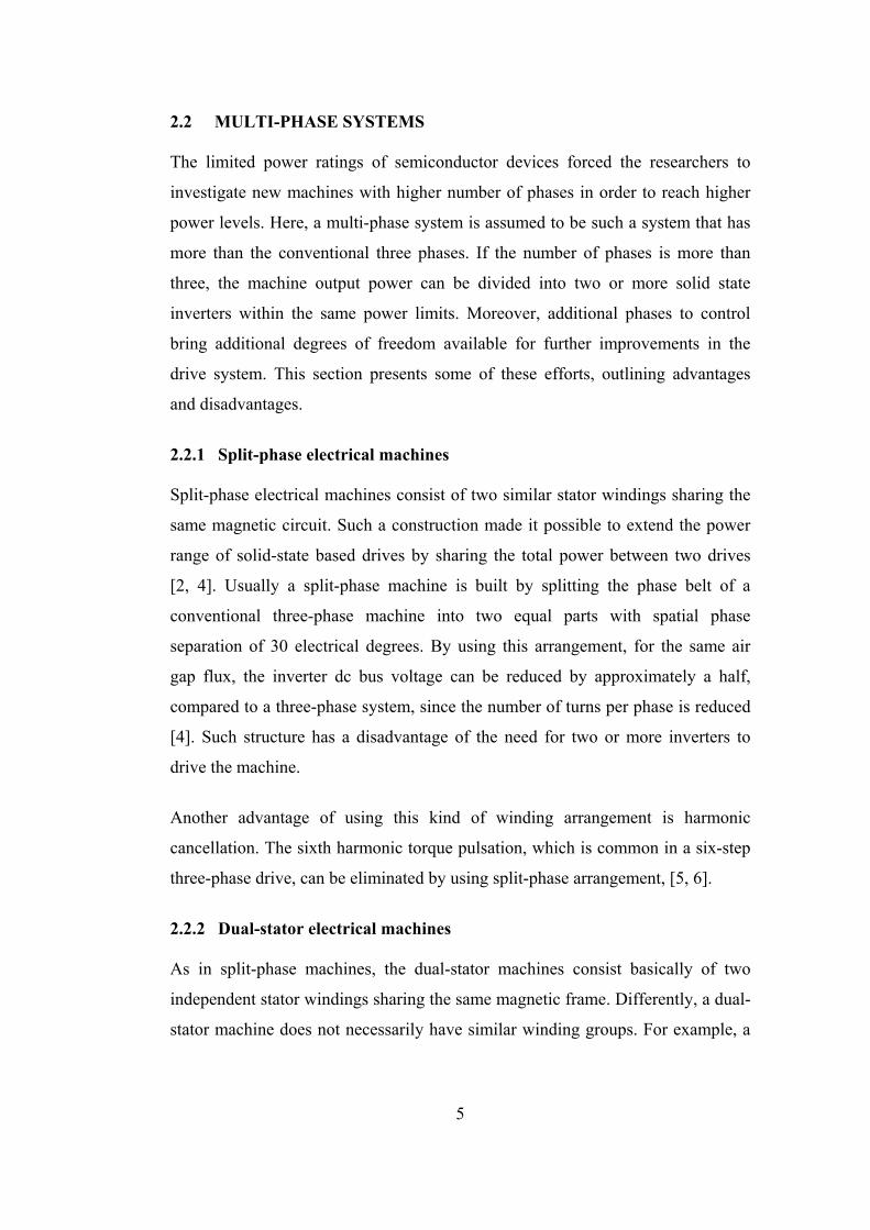
2.2.1 Split-phase electrical machines Split-phase electrical machines consist of two similar stator windings sharing the
same magnetic circuit. Such a construction made it possible to extend the power
range of solid-state based drives by sharing the total power between two drives
[2, 4]. Usually a split-phase machine is built by splitting the phase belt of a
conventional three-phase machine into two equal parts with spatial phase
separation of 30 electrical degrees. By using this arrangement, for the same air
gap flux, the inverter dc bus voltage can be reduced by approximately a half,
compared to a three-phase system, since the number of turns per phase is reduced
[4]. Such structure has a disadvantage of the need for two or more inverters to
drive the machine.
Another advantage of using this kind of winding arrangement is harmonic
cancellation. The sixth harmonic torque pulsation, which is common in a six-step
three-phase drive, can be eliminated by using split-phase arrangement, [5, 6].
2.2.2 Dual-stator electrical machines As in split-phase machines, the dual-stator machines consist basically of two
independent stator windings sharing the same magnetic frame. Differently, a dual-
stator machine does not necessarily have similar winding groups. For example, a
6
different voltage rating or a different number of phases could be used for each
winding group.
For instance, two independent stator windings may be used for an induction
generator system [3]. One set of windings may be responsible for the
electromechanical power conversion (i.e. driving the load) while the second one is
used for excitation purposes. This eliminates the need of a converter rated to full
load power in a vector controlled induction generator [15]. The same idea can be
used for power factor correction in induction motors. One of the two different sets
of three-phase windings may be connected to the main power and carry the active
power responsible for the torque production while the second winding carries the
reactive power.
Using a dual-stator machine which is a particular case of a multi-phase machine,
the power ratings may be extended without the need to use multi-level converters.
Instead of increasing the power rating of a three-phase converter using multi-
levels for the converter, additional phases are added and the current is shared by
additional inverter legs [16].
2.3 A METHOD FOR TORQUE DENSITY IMPROVEMENT IN A SIX-
PHASE MACHINE BY INJECTION OF THIRD HARMONIC
CURRENT COMPONENTS
This section presents a research study [1] which deals with torque density
improvement of a six-phase induction motor by using third harmonic injection. It
studies and characterizes a six-phase induction machine drive operating with third
harmonic current injection. The performance of the system was measured in
comparison with a standard three-phase machine system.
To achieve the objectives above, two machines were analyzed in [1]. To use the
three-phase machine as a baseline for the analysis, the six-phase machine uses the
same peak air gap flux density, similar winding configuration and same frame.

7
By comparing the operation of these two machines, the improvements were
outlined. The machine was analyzed using mathematical models and finite
element simulation.
A control system using PWM current control techniques was developed and
implemented both in simulation and in the experimental setup. By controlling
currents, instead of voltages, the rotor flux can be controlled and the effects of
leakage inductances reduced. This is particularly important for the third harmonic
injection since perfect alignment between fundamental and third harmonic is
necessary. For a voltage fed system, the stator resistance and leakage inductance,
as well as rotor leakage inductance, cause a phase shift between the two
components that is a function of the machine parameters and operating conditions.
This effect deteriorates the performance especially at low speeds.
To summarize, the contributions of [1] include: the development and analysis of a
drive system that is able to operate with third harmonic injection at variable speed
operation; the development of a current control system that enables the
implementation of synchronous frame current regulators for both fundamental and
third harmonic currents and therefore simplifies the design of the outer control
loops; the implementation of a speed control loop using indirect flux orientation
for the six-phase induction machine with third harmonic current injection, the
simplification of the drive system by using six phases with unified windings for
fundamental and third harmonic currents; the experimental evaluation of the iron
losses in comparison with a three-phase machine operation; and the development
of a machine model to be used for calculation of its operating conditions and
evaluation of efficiency.
2.3.1 Three-phase induction machine A three-phase induction machine was used in [1] as baseline for the new machine
design. Table 2.1 shows the nameplate values for the baseline machine. The
connection diagrams for this machine are presented in Figure 2.1 for both parallel
and series Y configurations, 230V and 460V connection respectively.Table 2.2
8
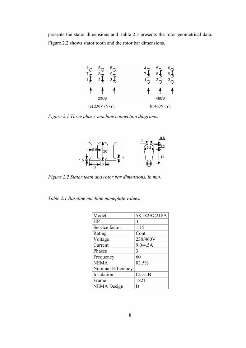
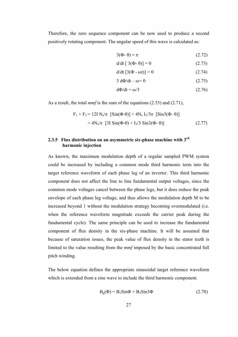
presents the stator dimensions and Table 2.3 presents the rotor geometrical data.
Figure 2.2 shows stator tooth and the rotor bar dimensions.
(a) 230V (Y-Y). (b) 460V (Y).
Figure 2.1 Three phase machine connection diagrams.
Figure 2.2 Stator teeth and rotor bar dimensions, in mm.
Table 2.1 Baseline machine nameplate values.
Model 5K182BC218AHP 3 Service factor 1.15 Rating Cont. Voltage 230/460V Current 9.0/4.5A Phases 3 Frequency 60 NEMA Nominal Efficiency
82.5%
Insulation Class B Frame 182T NEMA Design B

9
Table 2.2 Stator geometrical dimensions.
Table 2.3 Rotor geometrical dimensions.
The BH curve for the three-phase machine iron is shown in Figure 2.3. The solid
line in Figure 2.3 corresponds to the portion measured and the dashed line is an
extrapolation based on a standard grain oriented steel.
Figure 2.3 Measured magnetization curve. Solid line indicates measured values in the curve.
Number of slots 36 Outer diameter 190mm Inner diameter 120mm Stack length 70.5mm
Number of slots 28Outer diameter 119.4mm Inner diameter 32.0mm Stack length 65.5mm End connection 10.0mm Tooth width 6.6mm Bar depth 20.0mm Shaft radius 16.0mm

10
The three-phase machine uses a single layer concentric winding which distributes
itself over 3 slots per pole per phase and has 98 conductors per slot. Using the Y
connection (460V) there are 2 parallel circuits per phase, or in other perspective
there is one circuit with two stranded wires. For the YY connection (230V) 4
parallel circuits, or 2 parallel circuits with two stranded wires, compose the
windings per phase. The conductor diameter is 0.72mm corresponding to a 21
AWG wire.
The equivalent circuit parameters that were calculated by using no-load and
locked-rotor tests are presented in Table 2.4.
Table 2.4 Equivalent circuit parameters.
Rs 0.85 Ω Ls 5.42 mH Lr 5.42 mH Lm 69.77 mH Rr 0.55 Ω
2.3.2 Six-phase induction machine The six-phase machine is a particular case of split-phase or dual-stator machine. It
can be built by splitting a three-phase winding into two groups. These three-phase
groups are shifted by thirty electrical degrees from each other. This composes an
asymmetrical six-phase machine since the angular distance between phases is not
the same. Figure 2.4 shows the representation of the machine stator windings for
Y connection and a simplified construction diagram for a concentrated-winding
two-pole six-phase machine.
A method which is similar to that of a three-phase machine can be adopted in
analyzing a six-phase induction machine. In Figure 2.5, the steady-state
equivalent circuit for sinusoidal excitation [7] which is similar to the one of a
conventional three-phase machine with the addition of an extra stator circuit is
shown.

11
We can reach to a result that, for steady-state operation the six-phase machine can
be analyzed as two three-phase machines sharing the same magnetic circuit as
well as rotor circuit. On the other hand, it should be noted that there can be
currents flowing between the two three-phase stators that do not contribute to
torque generation. This forces the designers to make direct control of stator
currents for such systems.
Basically, the six-phase induction machine was introduced with two objectives.
First, the opportunity to divide the output power into two three-phase groups
allows the increase in the drive system power ratings. Secondly, for use with six-
step inverters, the pulsating torque in a six-phase machine is lower than in a three-
phase machine [6, 8, 9, 10]. Another reason for using six-phase systems is
reliability. When a failure happens in one of the phases, in the machine or in the
power converter, the system can still operate at a lower power rating since each
three-phase group can be made independent from each other. In the case of losing
one phase, the six-phase machine can be operated as a five-phase machine as
described in [11].
(a) Electric diagram. (b) Basic construction.
Figure 2.4 Six-phase machine diagrams.

12
Figure 2.5 Six-phase machine equivalent circuit for sinusoidal steady-state.
2.3.3 Six-phase induction machine winding diagram The six-phase machine in [1] uses the same magnetic frame with the baseline
machine. We have the 4-pole machine with 36 stator slots. In order to keep the
leakage distribution balanced, the phases are displaced among the two stator
layers. The six-phases are constructed such that one three-phase group is displaced
from the other one by 30 electrical degrees. Thus we have an asymmetrical six-
phase machine where;
θm = 2. θe / p (2.1)
θm = 2 . 30° / 4 = 15° mechanical (2.2)
Slot pitch = 360° / 36 = 10° mechanical (2.3)
Hence, the 30 electrical degrees displacement corresponds to 15°/10° = 1,5 slots.
We cannot implement such a configuration and have to use an approximation. This
is how it is done:
One of the three-phase groups has the same structure of the baseline machine with
half of the circuits and winding distributed in 3 slots per pole per phase (qA = 3).
The second group is distributed into 4 slots per pole per phase (qX = 4) but keeping
the same number of conductors per pole per phase. The winding diagrams of each
phase are shown in Figure 2.7. The total winding diagram is presented in Figure
2.6. The number of series connected conductors in each coil is given in the figure

13
and it is shown that to obtain the necessary 30 electrical degrees displacement
between the two three-phase groups A and X, the outer side coils in the X group
have reduced number of conductors.
In Figure 2.9, it can be seen that the difference between the axes of the phases a
and x, b and y, c and z comes out to be 1.5 slot pitches. As an example : Axis of phase a is at the middle point of slots 11 and 12
Axis of phase x is at the slot 13
So the difference between the axes of phases a and x is 1.5 slots.
Regarding the pitching of the windings;
Pole pitch = slot # / pole # = 36 / 4 = 9 slot pitches.
The first entrance of phase a is slot 6 and the first exit of phase a is slot 15
Coil pitch for Group A = 15 – 6 = 9 slot pitches Group A is a full pitch winding.
The first entrance of phase x is slot 7 and the first exit of phase x is slot 16
Coil pitch for Group X = 16 – 7 = 9 slot pitches Group X is a full pitch winding.

14
Figure 2.6 Winding diagram of each phase of the six-phase machine

15
Figure 2.7 Winding diagram of each phase of the six-phase machine (cont.)

16
Figu
re 2
.8 T
otal
win
ding

17
Axe
s of t
he p
hase
s
a
x
c
z
b
y
Figu
re 2
.9 P
hase
axe
s of t
he si
x-ph
ase
mac
hine
win
ding
.

18
2.3.4 MMF equation of six-phase winding with 1st and 3rd harmonic current components
Since the asymmetric six-phase machine is derived from a conventional three-
phase induction machine, we can derive the mmf distribution of an asymmetric six-
phase machine from a conventional three-phase induction machine in four steps.
i) First, the flux distribution on a concentrated winding three-phase machine is
considered. Figure 2.10 shows the winding distribution for a simple two pole
concentrated winding machine with one slot per pole per phase. The winding
function for phase a is also shown in this figure.
Figure 2.10 Winding distribution of a three-phase concentrated winding induction machine and winding function for phase a
Each of the coils is assumed to have 4Ns turns and the mmf acting across the gap
associated with stator currents is:
F = Fa+ Fb+ Fc = Na(Φ) ia + Nb(Φ) ib + Nc(Φ) ic (2.4)
where, the winding functions can be written as sum of odd harmonic components
by Fourier representation as:
Na(Φ) = 4(2Ns)/π [SinΦ + (1/3)Sin3Φ + (1/5) Sin5Φ + (1/7) Sin7Φ + …] (2.5)
Nb(Φ) = 4(2Ns)/π [Sin(Φ-120º) + (1/3)Sin3(Φ-120º) + (1/5) Sin5(Φ-120º)
+ (1/7) Sin7(Φ-120º) + …] (2.6)

19
Nc(Φ) = 4(2Ns)/π [Sin(Φ+120º) + (1/3) Sin3(Φ+120º) + (1/5) Sin5(Φ+120º)
+ (1/7) Sin7(Φ+120º) + …] (2.7)
since the winding function is a typical odd function, even harmonics are zero and
the currents can be written as:
ia = I Cosθ (2.8)
ib = I Cos(θ-120º) (2.9)
ic = I Cos(θ+120º) (2.10)
θ = ωt (2.11)
and the resulting mmf is obtained using the Fourier series representation,
F = ∑Fn = ∑ [Nan(Φ) ia + Nbn(Φ) ib + Ncn(Φ) ic] (2.12)
where n = 1,2,3…∞ Since N(Φ) = 0 for even values of n, even harmonics of F are also zero. Therefore
the mmf can be given as,
F = F1 + F3 + F5 + F7 (2.13)
For the fundamental component,
F1 = Na1(Φ) ia + Nb1(Φ) ib + Nc1(Φ) ic (2.14)
F1 = 4(2Ns)/π [SinΦ ICosθ ] + [ Sin(Φ-120º) ICos(θ-120º)]
+ [Sin(Φ+120º) ICos(θ+120º)]
= 8INs/π [SinΦ Cosθ ] + [ Sin(Φ-120º) Cos(θ-120º)]
+ [ Sin(Φ+120º) Cos(θ+120º)] (2.15)
Since,
SinΦ Cosθ = ½ [Sin(Φ-θ) + Sin(Φ+θ)] (2.16)
F1= 8I Ns/π ½ [Sin(Φ-θ) + Sin(Φ+θ)] + ½ [Sin(Φ-θ) + Sin(Φ+θ-240º)]
+ ½ [Sin(Φ-θ) + Sin(Φ+θ+240º)] (2.17)

20
= 4I Ns /π Sin(Φ-θ) [ 1 + (Sin(Φ+θ)/ Sin(Φ-θ)) + 1 + (Sin(Φ+θ-240º)/ Sin(Φ-θ))
+ 1 + (Sin(Φ+θ+240º)/Sin(Φ-θ))] (2.18)
F1 = 12I Ns/π [Sin(Φ-θ)] (2.19)
Also for the third harmonic component,
F3 = Na3(Φ) ia + Nb3(Φ) ib + Nc3(Φ) ic (2.20)
F3 = 4(2Ns)/π [(1/3)Sin3Φ ICosθ ] + [ (1/3)Sin3(Φ-120º) ICos(θ-120º)]
+ [(1/3)Sin3(Φ+120º) ICos(θ+120º) ] = 8INs/3π [Sin3Φ Cosθ ] + [ Sin3(Φ-120º) Cos(θ-120º)]
+ [Sin3(Φ+120º) Cos(θ+120º)] = 8INs /3π [ Sin3Φ Cosθ ] + [ Sin3Φ Cos(θ-120º)]
+ [Sin3Φ Cos(θ+120º)] = 8INs /3π Sin3Φ [Cosθ + Cos(θ-120º) + Cos(θ+120º)] = 0 (2.21)
F3 = 0 (2.22)
For the 5th harmonic component,
F5 = Na5(Φ) ia + Nb5(Φ) ib + Nc5(Φ) ic (2.23)
F5 = 4(2Ns)/π [(1/5)Sin5Φ ICosθ ] + [ (1/5)Sin5(Φ-120º) ICos(θ-120º)]
+ [(1/5)Sin5(Φ+120º) ICos(θ+120º) ]
= 8INs/5π [Sin5Φ Cosθ ] + [ Sin5(Φ-120º) Cos(θ-120º)]
+ [ Sin5(Φ+120º) Cos(θ+120º)]
= 8INs /5π [ Sin5Φ Cosθ ] + [ Sin(5Φ+120º) Cos(θ-120º)]
+ [ Sin(5Φ-120º) Cos(θ+120º)] (2.24)
Since,
SinΦ Cosθ = ½ [Sin(Φ-θ) + Sin(Φ+θ)] (2.25)
F5 = 4I Ns /5π [Sin(5Φ-θ) + Sin (5Φ+θ)] + [Sin(5Φ-θ +240º) + Sin(5Φ+θ)]
+ [ Sin(5Φ-θ-240º) + Sin (5Φ+θ)]

21
= 4I Ns /5π Sin(5Φ+θ) [ 1 + (Sin (5Φ-θ)/Sin(5Φ+θ))
+ 1 + (Sin(5Φ-θ +240º)/Sin(5Φ+θ))
+ 1 + (Sin(5Φ-θ-240º)/Sin(5Φ+θ)) ] (2.26)
F5 = 12I Ns /5π [Sin(5Φ+θ)] (2.27)
For the 7th harmonic component,
F7 = Na7(Φ) ia + Nb7(Φ) ib + Nc7(Φ) ic (2.28)
F7 = 4(2Ns)/π [(1/7)Sin7Φ ICosθ ] + [ (1/7)Sin7(Φ-120º) ICos(θ-120º)]
+[(1/7)Sin7(Φ+120º) ICos(θ+120º) ]
= 8INs/7π [Sin7Φ Cosθ ] + [ Sin7(Φ-120º) Cos(θ-120º)]
+ [ Sin7(Φ+120º) Cos(θ+120º)]
= 8INs /7π [ Sin7Φ Cosθ ] + [ Sin(7Φ-120º) Cos(θ-120º)]
+ [ Sin(7Φ+120º) Cos(θ+120º)] (2.29)
Since,
SinΦ Cosθ = ½ [Sin(Φ-θ) + Sin(Φ+θ)] (2.30)
F7 = 4I Ns /7π [ Sin(7Φ-θ) + Sin (7Φ+θ) ] + [Sin(7Φ-θ) + Sin(7Φ+θ-240º)]
+ [Sin(7Φ-θ) + Sin (7Φ+θ+240º)]
= 4I Ns /7π Sin(7Φ-θ) [ 1+ (Sin (7Φ+θ)/Sin(7Φ-θ))
+ 1 + (Sin(7Φ+θ-240)/ Sin(7Φ-θ))
+ 1 + (Sin(7Φ+θ+240º)/ Sin(7Φ-θ))] (2.31)
F7 = 12I Ns /7π [Sin(7Φ-θ)] (2.32)
We see that, for a three-phase concentrated winding machine, since F3 is zero,
F = F1 + F5 + F7. A point of maximum amplitude of the fundamental component is
found by setting the argument equal to 90º. The rotational speed of this point is
found by taking the time derivative.
22
For F1 ;
(Φ- θ) = 90º (2.33)
d/dt [ (Φ- θ)] = 0 (2.34)
d/dt [(Φ - ωt)] = 0 (2.35)
dΦ/dt – ω= 0 (2.36)
dΦ/dt = ω (2.37) Thus, the peak of the fundamental component rotates in the direction of increasing
Φ with angular speed ¯
For F5 ;
(5Φ + θ) = 90º (2.37)
d/dt [ (5Φ + θ)] = 0 (2.38)
d/dt [(5Φ + ωt)] = 0 (2.39)
5 dΦ/dt + ω= 0 (2.40)
dΦ/dt = -ω/5 (2.41) The fifth harmonic component rotates in the direction of decreasing Φ at 1/5 the
speed of the fundamental component. This is then a negative sequence component
that produces negative average torque (braking).
For F7 ;
(7Φ - θ) = 90º (2.42)
d/dt [ (7Φ - θ)] = 0 (2.43)
d/dt [(7Φ - ωt)] = 0 (2.44)
7 dΦ/dt - ω= 0 (2.45)
dΦ/dt = ω/7 (2.46)
The seventh harmonic rotates in the direction of increasing Φ at 1/7 the speed of
the fundamental component and therefore is a positive sequence component. While
positively rotating, its synchronous speed is only 1/7 that of the fundamental and
only produces desirable positive torque when the rotor is between 0 and 1/7 of the
synchronous speed corresponding to the fundamental component.

23
When excited at variable frequency, the motor operates continuously at low slip
frequency. Hence, in this case, the fifth and seventh spatial harmonics always
produce undesirable braking torque and both should be minimized.
ii) To minimize the fifth and seventh harmonics we consider the phase winding
distribution over two slots, or two slots per pole per phase. The new winding
distribution and winding function for phase a are shown in Figure 2.11. Here the
machine could be analyzed as a three-phase machine with distributed windings
over two slots per pole per phase, or, if each winding is treated separately, this
configuration corresponds to an asymmetric six-phase machine with 30 degrees
separation between the two three-phase groups. Thus, the six-phase machine is
composed by two three-phase groups spatially shifted by 30 degrees with respect to
each other.
Figure 2.11 Winding distribution of a three-phase distributed winding induction machine and winding function for phase a
The fundamental component of the rotating mmf can be considered as the sum of
two components produced by the two stator groups with the same total number of
turns which are phase shifted spatially by 30 electrical degrees. Thus,
If we substitute Φ by (Φ-30º) in the expressions added to the equations (2.19,27,32)
for the 30º shifted group and take half of the initial turn number for each group:
F1 = 6I Ns/π [ Sin(Φ-θ) + Sin( Φ-30º-θ) ] (2.47)
F5 = 6I Ns/5π [ Sin(5Φ+θ) + Sin( 5Φ-150º-θ) ] (2.48)
F7 = 6I Ns/7π [ Sin(7Φ-θ) + Sin( 7Φ+210º+θ) ] (2.49)

24
iii) Thirdly, we consider phase shifting one of the stator winding groups spatially
by 30 electrical degrees but also shifting the currents in each group by 30 degrees
in time. In effect this configuration becomes a dual three-phase, or asymmetrical
six-phase machine. The winding diagram for this case is shown in Figure 2.12.
Figure 2.12 Winding distribution of asymmetric six-phase machine with concentrated windings.
Three additional currents ixú, iy, and iz are defined to correspond to a three-phase set
of currents which are phase shifted with respect to currents ia, ib and ic by 30
electrical degrees.
ix = I Cos (θ-30º) (2.50)
iy = I Cos (θ-150º) (2.51)
iz = I Cos (θ+90º) (2.52)
The total mmf can again be found by taking the sum of two mmf ’s that are now
phase shifted in space and time:
If we substitute θ by (θ-30º) in the second terms of the equations (2.47,48,49),
F1 = 6I Ns/π [ Sin(Φ-θ) + Sin(( Φ-30º)-(θ-30º)) ]
= 12I Ns/π [Sin(Φ-θ)] (2.53)
F5 = 6I Ns/5π [ Sin(5Φ+θ) + Sin(5(Φ-30º) + (θ-30º)) ]
= 6I Ns/5π [ Sin(5Φ+θ) + Sin(5Φ+θ-180º)] = 0 (2.54)
F7 = 6I Ns/7π [ Sin(7Φ-θ) + Sin( 7(Φ-30º)+(θ-30º) ]
= 6I Ns/7π [ Sin(7Φ-θ) + Sin(7Φ-θ-180º)] = 0 (2.55)

25
So, use of an asymmetrical six-phase machine by shifting one of the stator winding
groups spatially by 30 electrical degrees and also shifting the currents in each
group by 30 degrees in time, produces as much fundamental flux in the air gap as a
full pitched concentrated coil winding while at the same time reducing the 5th and
7th spatial harmonics to zero.
iv) Finally, a zero sequence third harmonic component could be injected in the
phase currents if the neutral connection is present. For the three-phase machine,
this component produces nothing more than a stationary or standing wave which
produces only braking and pulsating torques. For the asymmetrical six-phase
machine however, a particular choice of the zero sequence components produces
rotating waves at the same angular speed as the fundamental and therefore
contributes for the final machine torque.
The zero sequence component must be handled separately and it is assumed that
the stator currents are made up of two components:
ia = I Cosθ + Io (2.56)
ib = I Cos(θ-120º) +I0 (2.57)
ic = I Cos(θ+120º)+I0 (2.58)
θ = ωt (2.59)
ia + ib + ic = [I Cosθ + I0]+ [I Cos(θ-120º) +I0]+ [I Cos(θ+120º) + I0]
= 3 I0 + I [Cosθ + Cos(θ-120º) + Cos(θ+120º)]
= 3 I0 (2.60)
Hence,
I0 = [ia + ib + ic] / 3 (2.61) We inject the zero sequence third harmonic current components as:
I0A = I3 Cos(3θ) (2.62)
I0X = I3 Sin(3θ) (2.63)
26
To analyze the influence of the zero sequence current component it is necessary to
represent the winding functions in a dq0 frame. The winding functions can undergo
a dq0 transformation in much the same manner as voltages and currents. So in a
dq0 stationary frame the zero sequence components of the winding functions of the
two shifted stator winding groups are derived as follows:
The winding functions were: Na(Φ) = 4(2Ns)/π [ SinΦ + (1/3)Sin3Φ + (1/5) Sin5Φ + (1/7) Sin7Φ +…] (2.64) Nb(Φ) = 4(2Ns)/π [ Sin(Φ-120º) + (1/3)Sin3(Φ-120º) + (1/5) Sin5(Φ-120º)
+ (1/7) Sin7(Φ-120º) + …] (2.65)
Nc(Φ) = 4(2Ns)/π [ Sin(Φ+120º) + (1/3) Sin3(Φ+120º) + (1/5) Sin5(Φ+120º)
+ (1/7) Sin7(Φ+120º) + …] (2.66)
Hence we derive the zero sequence components of the winding functions as:
N0A = [ Na(Φ) + Nb(Φ) +Nc(Φ) ] / 3
= 4Ns/π [1/3 Sin3Φ] (2.67)
N0X = [ Nx(Φ) + Ny(Φ) +Nz(Φ) ] / 3
= 4Ns/π [1/3 Sin3(Φ-30º)]
= - 4Ns/π [1/3 Cos3Φ] (2.68)
Therefore the zero sequence mmf for the third harmonic can be considered as the
sum of two components, one for each of the shifted stator winding groups. The
third harmonic mmf is in this case,
F3 = F3A + F3X = N0A(Φ) I0A + N0X(Φ) I0X (2.69)
F3= 4Ns/π [1/3 Sin3Φ] . I3 Cos(3θ) - 4Ns/π [1/3 Cos3Φ] . I3 Sin(3θ)
= 4Ns I3/3π [Sin3Φ Cos(3θ) – Cos3Φ Sin(3θ)] (2.70) F3 = 4Ns I3/3π [Sin3(Φ- θ)] (2.71)
27
Therefore, the zero sequence component can be now used to produce a second
positively rotating component. The angular speed of this wave is calculated as: 3(Φ- θ) = π (2.72)
d/dt [ 3(Φ- θ)] = 0 (2.73)
d/dt [3(Φ - ωt)] = 0 (2.74)
3 dΦ/dt – ω= 0 (2.75)
dΦ/dt = ω/3 (2.76) As a result, the total mmf is the sum of the equations (2.53) and (2.71),
F1 + F3 = 12I Ns/π [Sin(Φ-θ)] + 4Ns I3/3π [Sin3(Φ- θ)]
= 4Ns/π [3I Sin(Φ-θ) + I3/3 Sin3(Φ- θ)] (2.77)
2.3.5 Flux distribution on an asymmetric six-phase machine with 3rd harmonic injection
As known, the maximum modulation depth of a regular sampled PWM system
could be increased by including a common mode third harmonic term into the
target reference waveform of each phase leg of an inverter. This third harmonic
component does not affect the line to line fundamental output voltages, since the
common mode voltages cancel between the phase legs, but it does reduce the peak
envelope of each phase leg voltage, and thus allows the modulation depth M to be
increased beyond 1 without the modulation strategy becoming overmodulated (i.e.
when the reference waveform magnitude exceeds the carrier peak during the
fundamental cycle). The same principle can be used to increase the fundamental
component of flux density in the six-phase machine. It will be assumed that
because of saturation issues, the peak value of flux density in the stator teeth is
limited to the value resulting from the mmf imposed by the basic concentrated full
pitch winding.
The below equation defines the appropriate sinusoidal target reference waveform
which is extended from a sine wave to include the third harmonic component.
Bg(Φ) = B1SinΦ + B3Sin3Φ (2.78)

28
By dividing through by B1, can be written in the per unit form,
b = SinΦ + a . Sin3Φ (2.79)
where,
b = Bg / B1 (2.80)
a = B3 / B1 (2.81) For b to be maximum (bmax), db/dt = d/dt . [SinΦ + a . Sin3Φ] = 0
= dΦ/dt . CosΦ + a . dΦ/dt . 3 . Cos3Φ = 0
= dΦ/dt . [CosΦ + a . 3 . Cos3Φ] = 0 (2.82)
0 = [CosΦ + 3 a . Cos3Φ] (2.83)
On the other hand by using the trigonometric equations :
Cos3Φ = Cos2Φ . CosΦ - Sin2Φ . SinΦ (2.84)
Cos2Φ = CosΦ . CosΦ - SinΦ . SinΦ (2.85)
Sin2Φ = SinΦ . CosΦ + CosΦ . SinΦ. (2.86)
we obtain,
Cos3Φ = Cos3Φ – Sin2Φ . CosΦ – Sin2Φ . CosΦ – Sin2Φ . CosΦ
Cos3Φ = Cos3Φ – 3 . Sin2Φ . CosΦ (2.87)
If we substitute (2.87) in (2.83)
CosΦ + 3 a . (Cos3Φ – 3 . Sin2Φ . CosΦ) = 0
CosΦ . [1 + 3 a . (Cos2Φ – 3 . Sin2Φ)] = 0
[1 + 3 a . (Cos2Φ – 3 . Sin2Φ)] = 0 (2.88)
and since,
Sin2Φ = 1- Cos2Φ, (2.89) [1 + 3 a . (Cos2Φ – 3 + 3 . Cos2Φ)] = 0
[1 + 3 a . (4 . Cos2Φ – 3)] = 0
3 – 1/3a = 4 . Cos2Φ

29
CosΦmax = [(9a – 1) / 12a] ½ (2.90)
SinΦmax = 1- [(9a – 1) / 12a] ½
= [(3.a +1)/ 12.a)] ½ (2.91)
where Φmax is the angle value when b = bmax
Also by using the equations (2.85,86,89) and,
Sin3Φ = Sin2Φ . CosΦ + Cos2Φ . SinΦ (2.92)
we obtain,
Sin3Φ = 2 . Cos2Φ . SinΦ + Cos2Φ . SinΦ- SinΦCos2Φ - SinΦ + Cos2Φ . SinΦ
= 2 . (1- Sin2Φ) . SinΦ + (2 . Cos2Φ –1) . SinΦ
= 2 . SinΦ – 2 Sin3Φ + 2 . SinΦ – 2 Sin3Φ – SinΦ
= 3 . SinΦ – 4 . Sin3Φ (2.93)
If we substitute (2.91) in (2.93), we obtain,
Sin3Φmax = 3. [(3.a +1)/ 12.a)] ½ - 4. [(3.a +1)/ 12.a)] 3/2
= [(3.a +1)/ 12.a)] ½ . 3 – 4 . (3.a +1)/ 12.a
= [(3.a +1)/ 3.a)] ½ . (6.a -1)/ 6.a (2.94)
If we put (2.94) in (2.79) which was b = SinΦ + a . Sin3Φ, we get,
bmax = [(3.a +1)/ 12.a)] ½ + a . [(3.a +1)/ 3.a)] ½ . (6.a -1)/ 6.a
= [(3.a +1)/ 3.a)] ½ . [1/2 + (6.a -1)/ 6]
= [(3.a +1)/ 3.a)] ½ . (3.a +1)/ 3 (2.95)
To determine the amount of 3rd harmonic to be injected, we should deal with,
a = B3 / B1
To find the value of a for b = bmax, dbmax /da = 0
dbmax /da = [(3.a +1)/ 3.a)] ½ - (3.a+1)/3 . [(3.a +1)/ 3.a)] -½ . 1/6a2 = 0
dbmax /da = [(3.a +1)/ 3.a)] -½ . [(3.a +1)/ 3.a)] - (3.a+1)/3 . 1/6a2 = 0 (2.96)

30
[(3.a +1)/ 3.a)] - (3.a+1)/18a2 = 0
(18 a2 + 6a – 3a – 1) / 18 a2 = 0
18 a2 + 6a – 3a – 1 = 0 (2.97)
a = -1/3 and a = 1/6 (2.98)
If we put these values in (2.95), we get,
a = -1/3 b = 0 (2.99)
a = 1/6 b = 0.866 (2.100)
Hence, bmax = 0.866 = Bg/ B1 (2.101)
This means Bgmax decreases to 0.866 times its initial value (B1) when 3rd harmonic
component is added. After the addition of 3rd harmonic component B3, we can
increase B1 by,
1 / 0.866 = 1.1547 (2.102)
factor in order to keep the same Bgmax value. Since a = B3 / B1, when we increase
B1, then B3 also increases.
a = B3 / B1
1/6 = B3 / 1.1547 . Bgmax
B3 = 0.1925 . Bgmax (2.103)
When we substitute the values above in (2.78), Bg(Φ) = B1SinΦ + B3Sin3Φ, we get,
Bg = 1,1547 Bgmax (SinΦ + 1 Sin3Φ) (2.104)
6

31
Figure 2.13 Flux density distribution for the same peak air gap flux with and without third harmonic injection.
In conclusion, harmonic currents may be injected in multi-phase systems to create
an air gap flux that resembles the winding functions of the machine. Adding a
voltage harmonic reference would force harmonic currents to flow in the machine.
However, for a three-phase induction drive without neutral connection, the third
harmonic current cannot flow and therefore the fundamental voltage in the machine
is increased without the penalty of harmonic voltage and current distortion.
Connecting the neutral in a three-phase machine causes third harmonic currents to
flow and torque pulsations to appear. In a six-phase machine, third harmonic zero
sequence currents are used to increase the fundamental flux and to generate extra
torque. These results are only obtained if the currents, not voltages, in the machine
can be correctly controlled.
2.3.6 Torque density increase with third harmonic injection The contribution of using the third harmonic component in the improvement of the
torque density is now investigated. Torque production in any induction machine
can be best analyzed by utilizing the usual per phase equivalent circuit shown in
Figure 2.14.

32
Figure 2.14 Induction machine steady-state per phase equivalent circuit.
From [12], assuming peak values for the variables, the torque can be calculated as,
T = (3/2) P Ir2 rr
’ /s.ωe (2.105) 2 If we substitute Er = Ir rr
’/s
T = (3/2) P Ir Er /ωe (2.106) 2
In order to analyze the benefit of increased flux in torque production, it is necessary
to express torque as a function of the machine back emf. In Figure 2.15, an
approximated equivalent circuit can be obtained by neglecting rotor leakage
reactance. In this circuit, the rotor current is determined by a modified back emf
voltage that corresponds to the rotor flux instead of the air gap flux. This suggests
that the rotor flux is the one to be controlled in order to increase the torque density.
Figure 2.15 Induction machine approximated steady-state per phase equivalent circuit. Negligible rotor leakage inductance.

33
Rotor current can be calculated, for the approximated equivalent circuit as,
Ir = Er s / rr
’ (2.107)
and the torque is,
T = (3/2) P Er2 s / rr
’.ωe (2.108) 2
The peak voltage is proportional to the peak air gap flux density by :
Er = ωe. (2/π) . Bmax
.Apole .Ns (2.109)
where Bmax is the peak flux density allowable for the full pitch, concentrated coil
three-phase machine Apole is the area of one magnetic pole and Ns is the number of
series connected turns. The factor 2/π express the average value of B in terms of the
peak value. In the case of the asymmetric six-phase machine, the maximum allowable
fundamental flux density can be increased by 1,1547 as shown in the equation
(2.104).
T is proportional to Er
2, and Er is directly proportional to B. Since all other
parameters of torque equation remain the same for this machine, the increase in
torque obtained by raising the fundamental component of flux density, while
keeping the same peak tooth and air gap flux density is:
T6-phase fund / T3-phase = (1,1547)2 = 1,33 (2.110)
Thus, there is an addition of 33% in the torque production for the six-phase
machine with third harmonic injection due to the increase in the fundamental flux.
In addition to that, the contribution of the third harmonic component must be
considered. Since the third harmonic circuit is a two-phase system (X0 and A0 zero
sequence components) rather than a three-phase system, the factor 3/2 in the torque
expression is absent.

34
However, the third harmonic component has three times the number of poles so
that the factor 3 must be reintroduced. The torque produced by the third harmonic
currents in the six-phase machine is: T6-phase, 3h = 3P Er3h
2 s3h / r’r3h
. 3ωe (2.111)
2
The third harmonic voltage can be computed as:
Er3h = 3ωe
. (2/π) . B3. Apole 3.Ns = ωe
. (2/π) . B3 . Apole
. Ns (2.112) 3 3 The additional factor of 3 is necessary since all of the three third harmonic poles
having Ns/3 turns each are, necessarily, connected in series so that the total number
of series connected turns is again Ns. The third harmonic flux density is related to
the fundamental component by
B3 = 1,1547 . 1 Bmax (2.113)
6
If we put this in (2.112), we get,
Er3h = 1,1547 . ωe. (2/π) . Bmax
. Apole . Ns (2.114)
6
The slip for the third harmonic which is identical to the slip corresponding to the
fundamental spatial component is:
s3h = [3ωe – 3P ωrm] / 3ωe
2
= [ωe – P ωrm] / ωe
2
= [ωe – ωre] / ωe (2.115)
where ωrm is the actual rotor mechanical speed, ωre is the electrical rotor speed and
3P/2 is the number of pole pairs of the third harmonic.

35
Finally, the rotor resistance as seen by the third harmonic of mmf must be
computed. Rather than work out this expression from basic principles, it is easier to
assume that the relationship will not be far different from the classical expressions
for a squirrel cage machine.
In an induction machine, it can be assumed that the mmfs of the two sides of the
equivalent circuit are equal if the magnetic permeance is taken as infinite [17]. That
is,
F1 = F2 (2.116)
0.9 q1 kw1 N1 i1
’ = 0.9 q2 kw2 N2 i2’’
(2.117) p p
where q1 and q2 are number of phases, kw1 and kw2 are the winding factors, N1 and
N2 are the turn numbers of the stator and rotor side respectively, and i1’ and i2
’’are
the currents transferred to the stator side.
If kws of the stator and rotor are taken as equal,
i2
’’ = q1 N1 i1’ / q2 N2 (2.118)
It can be assumed that the rotor consists of a winding with Sr / p phases and p/2
turns [17]. When we substitute these values,
i2
’’ = ib = q1 N1 i1’ / [(Sr / p) (p/2)] (2.119)
ib / i1
’= 2 q1 N1 / Sr (2.120)
where ib is the current of a bar, Sr is the number of rotor slots and p is the number of
magnetic poles.
On the other hand, the rotor copper loss of a q phase induction machine can be
calculated from, Pr-Cu = q . i1
’2 . r’r = Sr ib
2 . rbe (2.121) where rbe is the resistance of the rotor bar taking into account the effect of the end
ring and r’r is the rotor resistance transferred to the stator side.

36
r’r = Sr ib
2 . rbe / q1 . i1’2
(2.122)
If we substitute equation (2.120) in (2.122),
r’
r = [2 q1 N1
/ Sr]2 . Sr . rbe / q1 (2.123)
r’
r = 4 q1 N1
2 rbe / Sr (2.124)
Then for a three phase machine the secondary resistance for the fundamental
component is, r’
r = 12 N1
2 rbe / Sr (2.125)
and for the third harmonic component,
r’
r3h = 3 . 12 (Ns/3)2 rbe (2.126) Sr
where Ns/3 is the number of series connected turns of one of the three pairs of poles
of the third harmonic. The factor of 3 is used since the three pole pairs of the third
harmonic are connected in series. Inserting these expressions in (2.111),
T6-phase, 3h = 3 P [ωe
. (2/π) . B3 . Apole
. Ns]2 x [ωe – (P/2) ωrm] /ωe
2 ωe 12. Ns2 rbe/Sr
= 3P [ (1,1547/6) . (2/π) . Bmax
. Apole]2 x [ωe – (P/2) ωrm] (2.127) 2 12. rbe/Sr
The corresponding torque expression for the baseline machine is:
T3-phase = 3 P [ωe. (2/π) . Bmax
. Apole . Ns]2
x [ωe – (P/2) ωrm] 2 . 2 ωe
2 12. Ns
2 rbe/Sr
= 3 P [(2/π) . Bmax . Apole ]2
x [ωe – (P/2) ωrm] (2.128) 2 . 2 12. rbe/Sr
37
Taking the ratio (2.127) / (2.128), T6-phase, 3h = (1,1547/6) = 0.0741 (2.129) T3phase ½ Hence, the contribution of the third harmonic is 7.4% of the value produced by the
baseline machine. The total torque improvement is thus from (2.110) and (2.129),
T6-phase,fund + T6-phase,3h – T3-phase 100% = 0,33 + 0,0741 = 40,7 % (2.130)
T3-phase
Therefore, a 40% torque improvement is obtained in the six-phase induction
machine with 3rd harmonic injection compared to the three-phase machine.
The ground rule for this analysis was the air gap flux density, and consequently the
tooth flux density, should be held constant. Nothing has been said about the core
flux density. The flux in the core is essentially the integral of the flux in the air gap
so that, Acore
. Bcore = Ag ∫ Bg dΦ (2.131)
If we substitute the value of Bg from (2.104),
Bcore = Ag ∫ 1,1547 . Bmax [ SinΦ + 1 Sin3Φ] dΦ Acore 6
= - Ag 1,1547 . Bmax [ CosΦ + 1 Cos3Φ] (2.132) Acore 18 The maximum function is clearly the point Φ = 0 at which
Bcore, max = - Ag 1,1547 . Bmax 19 (2.133) Acore 18 For the baseline machine, the air gap flux is:
Bg 3-phase = Bmax SinΦ (2.134) À
and, with the similar analysis, the core flux is:
Bcore, 3-phase = - Ag . Bmax CosΦ (2.135)
Acore

38
that gives for maximum,
Bcore, 3-phase max = - Ag . Bmax (2.136)
Acore The core flux increase with the third harmonic injection is, then
Bcore, max - Bcore, 3-phase max 100% = 22% (2.137) Bcore, 3-phase max
To accommodate the additional flux in the core, if no saturation is not acceptable,
the core cross section area have to be increased what could be impossible in some
applications. Alternatively, the core peak flux can be reduced by reducing the peak
air gap flux. However, doing that causes the gain in torque to reduce accordingly
and it is important to quantify this reduction. Assuming a reduction in the peak air
gap by a factor k, equations (2.110) and (2.129) are corrected to be,
T6-phase fund = (k . 1,1547)2 = 1,33 k2
(2.138)
T3-phase T6-phase, 3h = 0,0741 . k2 (2.139) T3-phase Therefore the total torque gain is now a function of k
T6-phase,fund + T6-phase,3h – T3-phase 100% = (1,407 . k2-1) 100% (2.140)
T3-phase
The torque gain for third harmonic injection considering the air gap flux reduction
for accommodating the core flux is plotted in Figure 2.16. It is clear that for
k<0,845 the torque is indeed reduced with the third harmonic application.
Therefore a trade-off between the core cross-section and the reduction in the air
gap flux must be obtained to guarantee the increase in the machine torque.
If no flux increase in the core is acceptable, the peak air gap flux density has to be
set to a value that keeps the core peak flux in equation (2.133) equal to the core
peak flux for the three-phase machine in equation (2.136). Therefore the peak
fundamental flux has to be reduced by a factor of

39
kΦ = 18 .= 0,8204 (2.141) 19 x 1,1547
Figure 2.16 Torque gain in an asymmetric six-phase machine with third harmonic injection considering reduction in the air gap flux to accommodate the core flux.
The air gap flux is obtained using (2.104) and applying the reduction factor kΦ to
be,
Bg = kΦ
. 1,1547 . Bgmax (SinΦ + 1 Sin3Φ) (2.142) 6
Bg = 18 . Bgmax (SinΦ + 1 Sin3Φ) (2.143) 19 6
Note that the ratio between fundamental and third harmonic is the same as in the
previous case since the optimization is not a function of Bmax . Figure 2.17 shows
the new airgap flux distribution. Both air gap peak flux and fundamental peak flux
decrease as a result of a fixed core peak flux. From Equation (2.140) with k = kΦ =
0.8204 and the total gain is - 5.26 %. Therefore, there is in fact a reduction in the
torque production if the core flux has to be limited to the corresponding three-phase
machine value.

40
Figure 2.17 Flux density distribution for same peak core flux with and without third harmonic injection.
On the other hand, since the peak air gap flux decreases, there is an additional
opportunity for torque density increase. With this lower flux density, the stator
tooth width can be made accordingly smaller still preserving the iron flux levels.
Therefore, stator slots can be made bigger and would accommodate more copper
making the current density to increase. Torque improvement is obtained from the
increase in the current density for a similar air gap flux. For a flux reduction factor
k, the stator tooth width is reduced by the same factor. The increase in the stator
slot width is a function of the initial relation between stator tooth and slot widths.
Figure 2.18 shows a simplified representation of a stator tooth and slot where τs is
the slot pitch, t0 is the tooth width and b0 is the slot width.
Figure 2.18 Simplified representation of stator slot and tooth.

41
The tooth width and the slot width are related to the slot pitch by
t0= γτs and b0 = (1- γ) τs (2.144) such that, t0 + b0 = τs (2.145)
and γ is a coefficient that could assume any value between 0 and 1. For a constant
slot pitch, when a reduction factor k is applied to the stator tooth the slot pitch is
given by,
τs = τ0’ + b0
’ = k γ τs + b0’ (2.146)
and substituting τs the new value for the slot width as a function of the reduction
factor k, the tooth width factor γ 6 and the previous slot width is,
b0
’ = 1-kγ . b0 (2.147) 1-γ
Using the values γ = 0,5 and k = 0,8204 there is an increase of 18% in the slot
width. In Figure 2.19, a graphical representation of slot width increase where the
variation of the percentage increase in the slot width is plotted as a function of the
initial tooth width coefficient 6 for different tooth reduction factors k. . The bigger the
initial tooth width, the bigger the impact on the slot increase for a fixed reduction
factor.
Figure 2.19 Percentage variation on slot width as a function of initial tooth width for different tooth reduction factors.

42
From [13], the output torque for an ac machine can be expressed as,
T3-phase = √2 π2 k1 (Dis2 Ls) Bg1 Js,rms ηgap cos(Φgap) (2.148)
120 where k1 is the winding factor, Dis is the stator inner diameter, Ls is the stator
length, Bg1 is the peak fundamental air gap flux density, Js,rms is the rms current per
unit length of the stator circumference or surface current density, ηgap is the
efficiency as seen from the air gap that includes rotor iron and copper loss and stray
losses, and Φgap is the power factor at the gap of the machine.
The increase in the slot width b0
’ allows the increase on the surface current density
Js,rms by the same factor. Considering the reduction on the fundamental flux density
caused by the necessity of keeping the peak core flux equal as the baseline
machine, the torque for the six-phase machine when the tooth reduction is applied
is given by,
T6-phase,slot = √2 π2 k1 (Dis2 ls) 18 Bg1 1-kγ .Js,rms ηgap cos(Φgap) (2.149)
120 19 1-γ so the torque increase is given by,
T6-phase, slot = 18 1-kγ (2.150) T3-phase 19 1-γ
Again for γ = 0,5 and k = 0,8204 the torque improvement due to the increase in the
surface current density is 12%. Including all effects, for the six-phase machine with
third harmonic injection, the torque gain is given as a function of the flux reduction
factor k as,
%Gain = [(1,407 x k2-1) + 18 1-kγ – 1] 100% (2.151) 19 1-γ The percentage torque gain as a function of the flux reduction factor for different
initial tooth factors γ, is shown in Figure 2.20. The bigger the initial tooth factor,
the bigger the increase in the torque density. For keeping the peak core flux as the
baseline machine, the flux reduction factor has to be kept as k = 0,8204. As an
example, with this value for k and for γ = 0,6 a torque improvement of 15% can be
achieved.

43
Figure 2.20 Torque gain in an asymmetric six-phase machine with third harmonic injection considering reduction in the air gap flux to accommodate the core flux and increase in the surface current density.
As a result, the use of third harmonic current injection in an asymmetric six-phase
machine can contribute to an increase of up to 40% in the torque production. This
is a very significant improvement and it is proper to add up the pros, cons and
restrictions of this approach.
To begin with, the machine efficiency is not expected to be significantly affected
since a corresponding increase in the stator and rotor current must accompany the
increased fundamental component of flux density plus the third harmonic.
The main disadvantage of this type of connection is the number of cables. A six-
phase stator must be fed by seven cables, six phases plus neutral, compared to three
for the three-phase machine. The amount of copper in the seven cables will equal
the amount in the four three-phase cables but, more insulation will be needed and
so that the overall weight of the cables will increase. This must be traded-off versus
the 40% weight reduction that will be possible by the asymmetrical six-phase
design.

44
The zero rotor leakage inductance assumption is convenient since it allowed the
voltage impressed across the air gap, produced by the air gap flux, to be equated to
the voltage across the rotor resistor. The derivation simplified considerably by
using this assumption. If the secondary leakage is considerably high, the voltage
across the leakage inductance has to be calculated. A voltage drop across this
leakage inductance would mean that the voltage across the rotor resistor would be
reduced, decreasing the 40% gain that has been cited.
Lastly, the maximum core flux is shown to increase by 22%. If no saturation is
acceptable then the air gap flux density has to be reduced by 22% which reduces
the torque below the three-phase machine. Instead, the core area cross section can
be increased by 22% to accommodate the increase in core flux. A trade-off between
air gap flux and core cross section area must be done to obtain the optimum
machine design for each particular application. An analysis of stator core losses has
to be conducted to evaluate the actual impact of the increased core peak flux.
Although peak flux increases, the distribution has a peaked up waveform and only
a portion of the core will be under higher flux densities. If no flux increase in the
core is acceptable, the peak air gap flux has to be reduced and with this, stator teeth
are made thinner without increasing the iron losses. Therefore additional copper is
used to increase the torque density. Torque improvement of 15%, without
compromising core flux levels, can be expected with this technique.
2.3.7 Experimental setup This subsection describes the experimental setup that was built in [1] to test the
proposed technique for increasing the torque density in the induction machine.
Figure 2.21 shows the machine test setup composed of the machine under test, a
six-phase induction machine, a torque and speed transducer, a permanent magnet
machine used as load or driving unit, and a digital encoder. The PM machine was
connected in the generator mode through a diode bridge to an adjustable resistive
load that guarantees evenly distribution of load currents in its windings. In the
motor mode, a commercial voltage inverter was used to drive the PM machine.

45
Figure 2.21 Test setup.
The operation in motor mode for the PM machine is necessary when testing the
induction machine at no load, where the rotor has to be spun at synchronous speed.
A digital encoder was used for speed measurement. The control was implemented
in a Digital Signal Processing board.
Two machines were tested in the experiments, the six-phase machine and the three-
phase baseline machine. Since a standard three-phase machine frame was used in
the new machine design, an equally rated three-phase machine was used as a
baseline for comparing the results obtained and to validate the expected
improvement. Two different rotors were used, the standard squirrel cage rotor and a
specially prepared rotor without the rotor bar ending connections that was used in
no-load tests and magnetic losses evaluation.
The airgap flux was measured using a search coil installed in the machine. The
objective of the flux measurement in this system was to demonstrate the reshape of
the air gap flux by injecting third harmonic currents and to determine the ratio
between the fundamental and third harmonic flux components.
Torque was measured using a torque sensor connected directly to the machine
shaft. The torque sensor is composed of a strain gage torquemeter and a transducer
amplifier.

46
A six-phase power inverter using IGBT switches was built to test the six-phase
machine. Figure 2.22 shows the diagram of the power system. The dc bus was fed
directly from the ac mains through a variac and a diode bridge. A middle point
connection was provided in the dc bus to return the neutral connection of the
machine.
Figure 2.22 Power converter system used in the experiment.
2.3.8 Experimental evaluation of the six-phase system In [1], the system described in the previous subsection was tested to verify the
improvement in the torque production and to address the necessary operating
conditions for both machine and power converter.
The basic operation was tested using an open loop voltage source inverter with the
ability of adjusting both phase delay between the two three-phase groups A and X,
and fundamental to third harmonic phase relation. As expected for the three-phase
machine under balanced operation, the air gap flux was mainly composed of a
fundamental component with all harmonics negligible. At this condition the
machine operates with a peak flux density of Bgpeak = 0.84 T.
To obtain the proposed torque improvement in the six-phase motor system, it is
important to keep the correct phase relation between fundamental and third
harmonic flux distributions. Failure to do so could cause misshaping of the
magnetic flux and therefore unwanted iron saturation.

47
Regarding the third harmonic currents, the six-phase machine behaves like a two-
phase machine with each three-phase group being one of the phases of the third
harmonic machine. At no-load, the machine can be driven only by applying the
third harmonic currents. However, the flux level in the machine with only third
harmonic currents remains quite low, what causes high currents to flow.
For no-load, the process of increasing the fundamental flux of the machine is
demonstrated in Figure 2.23, Figure 2.24, Figure 2.25. First operating without third
harmonic at f = 40 Hz and Vs = 84 V the peak air gap flux density is Bgpeak = 0.84 T
(Figure 2.23). It can be seen that groups A and X currents are 30 degrees phase
shifted from each other as necessary for the proposed machine operation.
Figure 2.23 No-load operation of the six-phase machine without third harmonic injection. f = 40 Hz, Vs = 84 V, Trace A: Flux density distribution [0.788T/div]; Trace 3: Phase a current [3.125A/div]; Trace 4: Phase x current [3.125A/div].
Adding third harmonic currents causes the peak flux density to decrease as seen in
Figure 2.24 where a third harmonic voltage of Vs3h = 14 V was added and the peak
flux density reduces to Bgpeak = 0.74 T. This corresponds to a sub-utilization of the
machine iron when compared to the previous case.

48
Figure 2.24 No-load operation of the six-phase machine with third harmonic injection. f = 40 Hz, Vs = 84 V, Vs3h = 14 V, Trace A: Flux density distribution [0.788T/div]; Trace 3: Phase a current [6.25A/div]; Trace 4: Phase x current [6.25A/div].
In order to raise the peak flux again, the fundamental voltage could be increased
until the previous level of flux was reached. This is shown in Figure 2.25 where for
the same third harmonic voltage, the fundamental voltage was raised to Vs = 93 V
and the peak flux density is again Bgpeak = 0.82 T.
Figure 2.25 No-load operation of the six-phase machine with third harmonic injection. f = 40 Hz, Vs = 93 V, Vs3h = 14 V, Trace A: Flux density distribution [0.788T/div]; Trace 3: Phase a current [6.25A/div]; Trace 4: Phase x current [6.25A/div].

49
For loaded case a similar operation can be seen as in Figure 2.26, Figure 2.27,
Figure 2.28. For a load with Tl = 5Nm; with no third harmonic injection, phase
voltages are Vs = 80 V. A third harmonic voltage of Vs3h = 14 V was then added.
Finally, the fundamental voltage component was raised to Vs = 89 V.
Figure 2.26 Operation of the six-phase machine without third harmonic injection. Tl = 5 Nm, f = 40 Hz, Vs = 80 V, Trace A: Flux density distribution [0.788T/div]; Trace 3: Phase a current [6.25A/div]; Trace 4: Phase x current [6.25A/div].
Figure 2.27 Operation of the six-phase machine with third harmonic injection. Tl = 5 Nm, f = 40 Hz, Vs = 80 V, Vs3h = 14 V, Trace A: Flux density distribution [0.788T/div]; Trace 3: Phase a current [6.25A/div]; Trace 4: Phase x current [6.25A/div].

50
Figure 2.28 Operation of the six-phase machine with third harmonic injection. Tl = 5 Nm, f = 40 Hz, Vs = 89 V, Vs3h = 14 V, Trace A: Flux density distribution [0.788T/div]; Trace 3: Phase a current [6.25A/div]; Trace 4: Phase x current [6.25A/div].
The torque x speed characteristics for the six-phase machine was measured
experimentally and compared to the three-phase machine. Two cases were
analyzed, the machine was tested with and without injection of third harmonic
currents. The test was done for three different operating frequencies keeping the
peak flux density constant. Figure 2.29 shows the torque x speed curves for 45 Hz
and 35 Hz. The increase in the torque production for the same size machine can be
seen clearly. At different operating frequencies, the six-phase machine presents
better torque production noted by a lower speed variation for the mechanical torque
application.

51
(a) 35 Hz.
(b) 45 Hz.
Figure 2.29 Torque x speed characteristics for 3hp six-phase machine. Six-phase machine operating with and without third harmonic currents compared to the baseline three phase machine.

52
Figure 2.30 shows the percentage torque improvement when compared to the three-
phase baseline machine torque at a particular value of slip. Since the amount of
third harmonic currents injected as well as the increase in the fundamental
component was not similar in the tests for the two frequencies, the improvement
was different. However, in both cases, the torque improvement when compared to
the three-phase baseline machine is clear. At very low slip, close to no-load
operation, the results for torque increase are not reliable since torque measurement
at very low values is not accurate. Therefore, to quantify the percentage torque
gain, one should take the value at slip close to the rated value. This does not mean
that there was no improvement at low load conditions, but states a limitation on the
torque measurement system.
Figure 2.30 Percentage torque gain, as a function of slip, for the 3hp six-phase machine compared to the baseline three-phase machine for operation with third harmonic current injection.
Iron and copper losses were addressed through the measurement at different
operating frequencies. Improvement in the torque production in the six-phase
induction machine with third-harmonic current injection was obtained by
increasing the fundamental flux without increasing the peak flux in the machine.
53
The extra output power comes from an increase in the stator current and the
reshaping of the magnetic flux distribution. These two factors have an important
impact in the machine magnetic and copper losses and an assessment of those
losses is important in validating the proposed drive system.
Both iron and copper losses were measured experimentally for no-load operation
and the results were compared to the measurement in the baseline three-phase
machine.
Iron losses were measured in the machine operating at no-load and at different
frequencies. For a better measurement of the magnetic losses, the machine has to
be driven at synchronous speed and therefore zero slip. This guarantees that no
currents flow in the rotor circuit for the fundamental component. However, due to
the presence of harmonics in the real machine, simply driving the machine at its
synchronous speed does not guarantee zero currents in the rotor circuit.
By cutting the rotor end windings and therefore increasing the rotor resistance a
drastic reduction in the rotor currents was obtained. The same machine, now with a
rotor lacking of end windings, was driven mechanically at synchronous speed and
the input power is measured. Magnetic power losses are obtained by subtracting the
stator copper losses from the measured power.
Iron losses as a function of the peak air gap flux density were measured at 20, 30
and 40Hz and Figure 2.31, Figure 2.32, Figure 2.33 show the results obtained. For
the three operating frequencies, the magnetic losses for the six-phase machine do
not increase significantly when compared to the baseline three-phase machine up to
approximately 0.8T peak flux density. Since the machine is designed to operate
under this value, no great impact in the iron losses is expected.
The small increase in the iron losses for the six-phase machine is caused by the
increase in the dB/dt of the flux density distribution. However, when comparing the
operation of the six-phase machine to the three-phase one, one have to keep in
mind that the six-phase machine operates with lower peak flux density than the
three-phase one and therefore, the iron loss remains approximately equal.
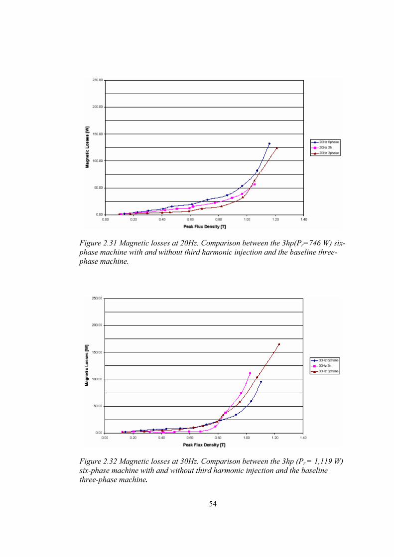
54
Figure 2.31 Magnetic losses at 20Hz. Comparison between the 3hp(Pr=746 W) six-phase machine with and without third harmonic injection and the baseline three-phase machine.
Figure 2.32 Magnetic losses at 30Hz. Comparison between the 3hp (Pr = 1,119 W) six-phase machine with and without third harmonic injection and the baseline three-phase machine.

55
Figure 2.33 Magnetic losses at 40Hz. Comparison between the 3hp (Pr=1,492 W) six-phase machine with and without third harmonic injection and the baseline three-phase machine.
Another important class of power loss is copper losses. They are basically
composed by stator and rotor resistive losses. At no-load, only the stator copper
losses were measured and compared to the baseline three-phase machine. This is
not a problem since both machines use the same rotor structure and are rated at the
same power level. Therefore, the rotor losses are expected to be similar for the two
machines being the stator losses the one that differentiate their operation.
Stator copper losses as a function of the peak air gap flux density were measured
for no-load at different operating frequencies. Figure 2.34, Figure 2.35, Figure 2.36
show the comparison of stator copper losses with the baseline three-phase machine
for operation at 20, 30 and 40Hz respectively. The six-phase machine operating
without third harmonic current injection behaves similarly to the three-phase
machine. With the injection of third harmonic currents, the copper losses increase
in the three frequencies. However, for peak flux levels up to 0.8T, there is not a
significant increase in the losses. It is important to remember that these
measurements were performed in a 3hp machine. Since the higher the rated power,
the lower the stator resistance, the increase in the copper losses for a high power
level induction machine presents no significant problem.

56
Figure 2.34 Stator copper losses at 20 Hz. Comparison between the 3hp (Pr=746 W) six-phase machine with and without third harmonic injection and the baseline three-phase machine.
Figure 2.35 Stator copper losses at 30 Hz. Comparison between the 3hp (Pr=1,119 W) six-phase machine with and without third harmonic injection and the baseline three-phase machine.

57
Figure 2.36 Stator copper losses at 40 Hz. Comparison between the 3hp (Pr=1,492 W) six-phase machine with and without third harmonic injection and the baseline three-phase machine.
The basic effect of the increased copper losses is a reduction on the machine
efficiency. For a fixed frequency, the efficiency of the machine is measured for
different load conditions. Efficiency of the three-phase machine, as the relation
between input electrical power and output mechanical power, was tested at
different frequencies. The efficiency seem to increase with the electric frequency,
as expected since the baseline machine is designed to operate at 60Hz. The six-
phase machine efficiency was measured for both cases, without and with third
harmonic injection. For 35 Hz voltage supply frequency, Figure 2.37 shows the
comparison between the six-phase machine efficiency and the baseline machine.
Without third harmonic injection, the six-phase machine presents an efficiency
close to the baseline machine.
On the other hand, the efficiency drops considerably when third harmonic currents
were injected for light load condition. This occurs at any supply frequency as can
be seen in Figure 2.38 where a similar test was done for 45Hz power supply. For
higher mechanical load, the efficiency of the six-phase machine with the third
harmonic current injection is comparable to the baseline machine, getting
eventually better as the load torque increases beyond rated value and the efficiency
of the baseline machine drops.

58
Figure 2.37 Six-phase machine efficiency at 35Hz. Comparison between the three-phase machine and the six-phase machine with and without third harmonic current injection.
Figure 2.38 Six-phase machine efficiency at 45Hz. Comparison between the three-phase machine and the six-phase machine with and without third harmonic current injection.

59
Since the six-phase machine is designed based on the baseline three-phase
machine, for 60Hz operation, the efficiency also increases with frequency for the
case with injected third harmonic currents. This can be seen in Figure 2.39 where
the efficiency of the six-phase machine, with third harmonic current injection, is
plotted for 35 and 45Hz voltage power supply.
Figure 2.39 Six-phase machine efficiency different frequencies with third harmonic current injection.
For operation at 45Hz, the efficiency obtained experimentally was compared to the
result from the steady-state equivalent circuit. Figure 2.40, Figure 2.41.show the
comparison between the calculated and measured efficiency for the six phase
machine. Since the iron loss and saturation effects are absent in the steady-state
model, the calculated efficiency is higher than the experimental evaluation.

60
Figure 2.40 Calculated and measured efficiency for the six-phase machine without third harmonic current injection for 45Hz.
Figure 2.41 Calculated and measured efficiency for the six-phase machine with third harmonic current injection for 45Hz.

61
As mentioned before, the stator copper losses are the major cause for the decrease
in the efficiency. For higher power level machines, the copper losses are expected
to reduce increasing, therefore, the efficiency at lighter loads.
2.4 CONCLUSION To achieve higher power levels with limited range power converters, multi-phase
systems are broadly used in industry. Additional torque production can be obtained
in these systems if third harmonic currents are injected so to reshape the flux
distribution in the machine and therefore obtain higher fundamental flux densities
without extrapolating the flux limits and forcing the machine into saturation.
The research work in [1] proposes the use of a six-phase induction machine to gain
these benefits. By constructing the machine with two three-phase groups phase
shifted by thirty degrees, for the third harmonic currents, that are zero sequence
currents in a standard three-phase machine, it is possible to create an additional
rotating field that is in synchronism to the fundamental component. This results in,
a reduction in the peak flux density.
By increasing the fundamental flux component to reestablish the air gap flux to its
original peak value, an additional torque is then obtained. However, if applied to a
standard three-phase machine, i.e. if the third harmonic currents are allowed to
flow in that machine by connecting the neutral, pulsating torque will appear as a
consequence of the interaction between the fundamental flux and the stationary
third harmonic one.
It is analytically shown that an increase of up to 40% in the torque production can
be expected with this technique when compared to a standard three-phase machine,
for same peak flux distribution. To obtain the benefits, the winding function of the
machine has to include third harmonic components. This is true for most of
electrical machines due to the discrete construction of the windings that are
distributed in finite number of slots. The best improvement would be obtained by
using a concentrated winding machine since, for this case, the higher third

62
harmonic component in the winding function is obtained. However, distribution of
the windings among a few slots contributes to the reduction of the unwanted
harmonic components. Therefore, a trade off exists between the amplitude of the
third harmonic winding distribution and the reduction of the unwanted harmonics.
The machine designed for the experimental evaluation was a distributed winding
machine. This decision comes from the fact that it is necessary to establish a
baseline for comparison, and, therefore the new machine is designed to have a
similar winding function as the baseline machine. This is closer to the reality since
it is necessary to distribute the coils in multiple slots to avoid large slot opening
and depth.
The necessity of controlling the phase relation between fundamental and third
harmonic flux components, is another fundamental issue in this application. If this
relation is lost, a peaked flux density could be generated instead of the proposed
flattened one. Magnetostatic finite element analysis was used to show the behavior
of air gap and core flux with third harmonic currents.
It was shown that the injection of third harmonic currents increases the flux in the
core but it is now more narrowly distributed. This indicates a possibility of
compensated factors that would keep the core losses similar for the three-phase and
six-phase cases. However experimental results demonstrate that for normal
operating flux levels, iron and copper losses in the six-phase machine are
comparable to the same size three-phase machine. Only when the flux levels are
increased far beyond the rated values, the iron and copper losses become
prohibitive. Copper losses, in per unit, reduces with the machine power rate and
therefore, for large machines, the copper losses are expected to go down
significantly.
The proposed system was tested experimentally to show the expected torque
improvement. It was shown that for voltage fed systems the current sharing
between the two three-phase groups could be uneven what could cause problems.
Therefore the necessity of controlling the currents in the machine was put forward.
The experimental results show that for same air gap peak flux density, the torque is

63
increased with the third harmonic current injection as a result of the increase in the
fundamental component of current and flux. The experimental results validate the
theoretical analysis and prove the improvement in the torque production as
proposed in the mentioned research project.
However, in order to obtain the system overall efficiency correctly, in addition to
experimental values, it is necessary to map the machine losses. Obtaining a
mathematical model for these losses is an important tool in the machine design for
correct calculation of losses of the machine. A model which was developed in
another research thesis [18] for calculating the losses of induction machines
requires the magnetic field distribution for calculations. In this study, the magnetic
field distribution of a six-phase induction motor with third harmonic current
injection is evaluated using a transient solution of a finite element software and the
core losses of the motor is calculated by using a method that was evaluated in [18].
64
CHAPTER 3
3 MACHINE LOSSES
3.1 INTRODUCTION The electrical motors have various types of losses. Some of these losses can be
calculated using analytical methods. On the other hand, there exist no reliable
methods to calculate the high frequency core losses of an induction motor
analytically. The aim of this study is to calculate specifically the core losses of the
motor explained in Chapter 2 by using the calculation method, which was
presented by [18]. Since the calculation method is based on finite element solution,
we need to create the finite element model of the motor.
In this chapter, losses of an induction motor will be briefly explained, and after an
introduction of the finite element method, the process of creation of the finite
element model of the motor will be presented.
3.2 LOSSES OF INDUCTION MACHINES As the electrical motors started to find fast growing areas of application,
calculation of their losses also began to present importance. Other factors to
increase the significance of efficiency - and hence losses - are environmental
pollution and saving primary energy resources.
In general there exist four types of losses in an induction motor [20].

65
3.2.1 Friction and windage losses: This kind of losses are due to the friction between the bearing and the rotor shaft.
The load, peripheral speed of the shaft, the friction coefficient between the shaft
and the bearing are examples of factors affecting the magnitude of these losses.
Peripheral speed of the rotor and construction characteristics of the motor like the
core length and rotor diameter affect on the windage losses. These losses can only
be determined by experiments.
3.2.2 Copper losses Two types may be mentioned, a) Stator copper losses: These losses are due to the stator windings and may be
calculated using the wire size and length of each phase winding. Total loss can be
found by multiplying by the number of phases.
b) Rotor copper losses: These are due to the rotor windings. They are called rotor
I2R losses in squirrel cage rotor motors and can not be measured directly. By
subtracting from the total copper loss which is determined by tests, these losses can
be found.
3.2.3 Stray load losses These are defined as the portion of the total loss in a machine for the load
conditions not accounted for by the sum of friction and windage, stator&rotor I2R
losses and core loss. In fact these are the eddy current losses caused by the increase
and the pulsations in the air gap leakage fluxes, proximity effect and other minor
causes. In various standards these losses are assumed to be approximately 0.5% of
the rated output.
3.2.4 Core losses There are generally two types of core losses: a) Fundamental frequency losses: These are supplied by the stator from the line and
are assumed to exist only in stator teeth and core. That is because the frequency in

66
the rotor and hence the fundamental frequency loss is so low to take into account.
The fundamental frequency losses are generally determined by using loss curves as
in Figure 3.1. These curves are typical for the type of steel used in motor
manufacturing.
02468
101214161820
0 0,2 0,5 1 1,5
Bpeak (T)
Los
s (W
att/k
g) 30 Hz.40 Hz.50 Hz.120 Hz.
Figure 3.1 Fundamental frequency loss versus peak flux density curves for different frequecies. [21]
b) High Frequency losses: High frequency losses can be taken as an additional load
since they are supplied by the mechanical power of rotor. These losses are due to
the permeance variation, saturation, harmonics in the air gap field and the mmf.
The most effective factor is the slotting. The high frequency losses can be
determined by measuring at no load and subtracting the fundamental frequency
losses, friction and windage losses and copper losses.
The task here is to be able to calculate the losses of the six-phase machine
discussed in the previous chapters. If this can be done then it becomes possible to
estimate the complete performance of the motor explained in Chapter 2. Hence
better designs become possible. Alternatively it becomes possible to asses whether
this type of motor is suitable for a given application.
The friction windage losses are usually accounted by using experimentally obtained
data on the fan to be used for a given application. The calculation of copper losses

67
is straight forward. If the machine design details are available a 2D transient field
solution with 3-dimensional effects would reveal the value of phase resistance and
coil currrent. Therefore the Cu lossses can be calculated. The remaining losses are
the calculation of the core losses and stray load losses part of which is high
frequency losses.
The fundamental frequency losses can be calculated from the field solution as
described in section 4.2.1. There is no established solution for the calculation of
high frequency losses. In this chapter, and attempt shall be made to develop a
method for the estimation of fundamental and high frequency core losses. Accurate
analytical calculation of the core losses is not possible. The approach developed
here shall be based on the high frequency loss calculation method developed in
[18]. This approach is based on finite element method. The following sections
shall first discuss modeling of the motor for FE solution.
3.3 FINITE ELEMENT MODEL The finite element method is an analysis process by which thermal, mechanical and
electromagnetic analysis can be performed. In this method, model of the subject
device is divided into very small elements which are formed by three corners so
called the nodes.
The finite element software allows the user to draw the geometry, create the mesh
for the analysis, define the material properties and couple electrical circuits to the
magnetic circuits. If the symmetry of the subject machine is appropriate, only a
quarter of the machine can be modelled and solved. The solution process is easier
for standard machines but in complex machines like the one in this thesis, it
becomes more complex and time consuming to make an analysis.
The FE software uses the Maxwell equations in magnetic analyses. Three kinds of
analyses can be performed using these programs:
a) Static magnetic analysis: Magnetic fields due to dc currents, permanent magnets
are calculated. Time variant effects like eddy currents are not taken into account.
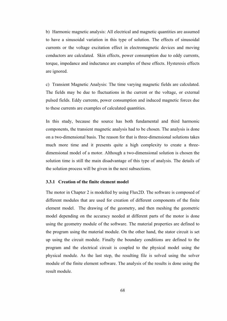
68
b) Harmonic magnetic analysis: All electrical and magnetic quantities are assumed
to have a sinusoidal variation in this type of solution. The effects of sinusoidal
currents or the voltage excitation effect in electromagnetic devices and moving
conductors are calculated. Skin effects, power consumption due to eddy currents,
torque, impedance and inductance are examples of these effects. Hysteresis effects
are ignored.
c) Transient Magnetic Analysis: The time varying magnetic fields are calculated.
The fields may be due to fluctuations in the current or the voltage, or external
pulsed fields. Eddy currents, power consumption and induced magnetic forces due
to these currents are examples of calculated quantities.
In this study, because the source has both fundamental and third harmonic
components, the transient magnetic analysis had to be chosen. The analysis is done
on a two-dimensional basis. The reason for that is three-dimensional solutions takes
much more time and it presents quite a high complexity to create a three-
dimensional model of a motor. Although a two-dimensional solution is chosen the
solution time is still the main disadvantage of this type of analysis. The details of
the solution process will be given in the next subsections.
3.3.1 Creation of the finite element model The motor in Chapter 2 is modelled by using Flux2D. The software is composed of
different modules that are used for creation of different components of the finite
element model. The drawing of the geometry, and then meshing the geometric
model depending on the accuracy needed at different parts of the motor is done
using the geometry module of the software. The material properties are defined to
the program using the material module. On the other hand, the stator circuit is set
up using the circuit module. Finally the boundary conditions are defined to the
program and the electrical circuit is coupled to the physical model using the
physical module. As the last step, the resulting file is solved using the solver
module of the finite element software. The analysis of the results is done using the
result module.

69
3.3.1.1 Drawing the geometry and the mesh The model is created firstly by drawing of the motor geometry. The regions of the
model are assigned as different parts of the motor like stator, rotor, etc. The
possibility of drawing half or a quarter of the motor makes it easier to model. By
this way the number of nodes and the elements are kept to a minimum and the time
elapsed for the solution process decreases. In this study a quarter of the motor is
drawn thanks to the symmetry conditions (Figure 3.2).
When creating the mesh, firstly an automatic mesh is generated using the program,
then the mesh is restructured to supply the needs of this study by placing the
sufficient but at the same time the least number of nodes. That is, the nodes which
are placed automatically and generously by the program, are reduced to sufficient
levels by the user. This is done by increasing the distances between the nodes. As
going away from the air gap towards both to the shaft and to the outermost side of
the stator core, the regions are meshed in a geometrically coarser manner. As can
be seen in Figure 3.3, for example, the stator back core is divided into three
subregions and meshed more coarsely since the accuracy of the values in this
region is less significant than the ones in the regions closer to the air gap and the
field distribution is smoother.
On the other hand; the regions, in which there is a need for more accurate results
that will be used in the loss calculations, are meshed in a tighter manner. The rotor
teeth for instance, are divided into three subregions according to the skin depths
which will be calculated in Chapter 4 depending on the expected eddy current
harmonics, and are meshed more tightly so that the eddy currents in the lamination
are obtained with better precision.
Another significant part of the motor in electromagnetic problems, the air gap, is
modeled as composed of three layers in order to get more accurate results. Hence
more nodes are placed in the air gap region and more realistic measurements are
obtained.

70
Figure 3.2 The geometry drawn for the six phase machine.
Regarding the meshing of the motor geometry, there exists a trade off between the
accuracy of the results and the analysis time. The mesh used in this thesis has
17000 nodes and 8046 elements. The analysis takes a time perod of about 25 hours
to get the results of the 1.5th second of the motor operation.
The stator and rotor slots are also drawn and each of them is assigned as a separate
region since these will be assigned the stator coils in the the electrical circuit in
accordance with the winding arrangement shown in Figure 2.9. In Figure 3.3, the
meshing of the stator and the rotor slots are displayed.
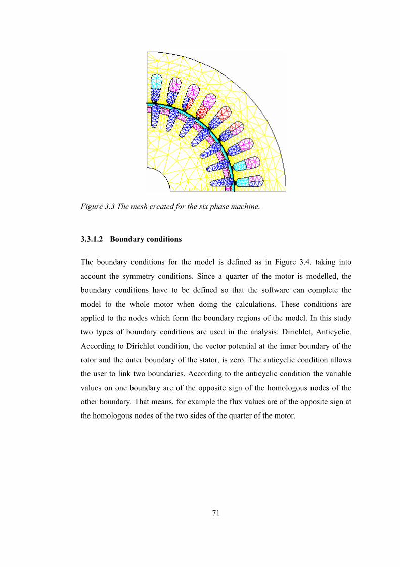
71
Figure 3.3 The mesh created for the six phase machine.
3.3.1.2 Boundary conditions
The boundary conditions for the model is defined as in Figure 3.4. taking into
account the symmetry conditions. Since a quarter of the motor is modelled, the
boundary conditions have to be defined so that the software can complete the
model to the whole motor when doing the calculations. These conditions are
applied to the nodes which form the boundary regions of the model. In this study
two types of boundary conditions are used in the analysis: Dirichlet, Anticyclic.
According to Dirichlet condition, the vector potential at the inner boundary of the
rotor and the outer boundary of the stator, is zero. The anticyclic condition allows
the user to link two boundaries. According to the anticyclic condition the variable
values on one boundary are of the opposite sign of the homologous nodes of the
other boundary. That means, for example the flux values are of the opposite sign at
the homologous nodes of the two sides of the quarter of the motor.

72
Figure 3.4 Boundary conditions
3.3.1.3 Defining the material properties After the creation of the geometric model, the material properties are to be input.
The B-H curve of the stator core and the rotor core, is defined to the program as in
Figure 3.5.
Figure 3.5 Iron BH curve used in the finite element analysis.

73
The subregions created in the rotor teeth in section 3.3.1.1, where the eddy currents
are read from the program, are assumed to be composed of 97% iron and 3%
isolation in order to obtain the magnitudes of the eddy currents in them. Hence the
resistivity of the three subregions in the rotor teeth is taken as,
0.97 x 9.7 x 10-8 + 0.03 x 2.2 x 10-2 = 6 x 10⁻⁴ (3.1)
The rest of the core is assumed to have no resistivity. The reason for this is that
assigning a resistivity to the entire core, elongates the convergence of the solution.
The properties of the stator windings and the rotor bars are also input. The
resistivity of aluminium rotor bars and the copper windings are taken respectively
as 0.263 x 10⁻⁷ Ohm x m. and 0.172 x 10⁻⁷ Ohm x m.
3.3.1.4 Setting up the stator circuit The analysis performed by Flux 2D is a kind of the so called coupled analysis. The
external circuit can be connected to the internal regions of conductors. For this
purpose, the stator circuit is set up as in Figure 3.6. The six phase windings A, B,
C, X, Y, Z, the fundamental and third harmonic current sources for each phase, end
winding resistance and inductance (Table 3.1) are placed in the circuit for a quarter
of the motor. The reason for using current sources instead of voltage sources, is
explained in [1] as the necessity of controlling the phase relation between the
fundamental and third harmonic currents. The values of the above parameters are
input after being divided into the number of symmetrical parts of the motor. The
rotor circuit is set up by the program itself. The end ring resistance and inductance
are taken from the values of a similar induction machine and input to the program
(Table 3.1) since there is no information in [1] on the parameters needed for the
calculation of these values. The method to calculate the end winding and end ring
parameters can be found in Appendix.

74
Table 3.1 Necessary calculated values for Flux2D
End winding resistance 0,172 Ohm End winding inductance 0,136 mH End ring resistance 0,237x10-5 Ohm End ring inductance 0,145x10-4 mH
Figure 3.6 Stator circuit of the six phase machine.
Current source for fundamental and third harmonic components End winding resistance End winding inductance Winding coil
Rotor circuit (including end ring resistance and inductance)
In accordance with [1], the phase currents are defined as,
IA = I Cosθ + I3 Cos3θ (3.2)
IB = I Cos(θ-120) + I3 Cos3θ (3.3)
IC = I Cos(θ+120) + I3 Cos3θ (3.4)
IX = I Cos(θ-30) - I3 Sin3θ (3.5)
IY = I Cos(θ-150) - I3 Sin3θ (3.6)
IZ = I Cos(θ+90) - I3 Sin3θ (3.7)
where I = 0.58 A, I3 = 0.4 A, and,
θelec.= wt = 2 x π x 40 x t = 80π x t (3.8)

75
3.3.1.5 The solution process After coupling the electrical circuit to the physical model using the physical
module of the software, the finite element model becomes ready for solution.
Before the solving process, the precision has to be determined. The default
precision which is 10-3, is used for the analyses in this study. Higher precision rates
extend the analysis time but provide no better results that are worth the longer time.
A Pentium Centrino 1400 MHz computer is used for the analyses. An analysis with
17000 nodes is typically obtained in a time period of 25 hours to get the results for
the 1.5 seconds of the machine operation and the resulting file occupied 3
gigabytes of hard disk space. The time step determines the time period between
two successive solutions of the model, and is adjusted as 0.3 msec. With the 40 Hz.
excitation in the solutions, 5000 time steps correspond to 1.5 sec.
3.3.2 Verification of the finite element model In order to show the currents applied to the circuit are transferred to windings in a
right manner, the instantaneous currents are calculated for an example time instant
of 0.006 sec. and are compared with the current values in the windings read from
Flux2D for the same time instant.
For t = 0.006 sec.
θelec. = 80 x π x 0.006 = 86.4o (3.9) The period of the 40 Hz. current supply is T = 0.025 sec. The same conditions
occur also for the time instants,
t = 36 T + 0.006 = 0.906 sec. and, (3.10)
t = 42 T + 0.006 = 1.056 sec. (3.11)
On the other hand at 40 Hz. the rotor speed of the motor operating at no load
condition is 1200 rpm. Hence the rotor completes a rotation of 360o in 60/1200 =
0.05 sec. Therefore, the rotor positions at t =0.006, t = 0.906 and t = 1.056
respectively are,
θmech. = 0.006 x 360 /0.05 = 43.2o (3.12)

76
θmech. = 0.906 x 360 /0.05 = 6523.2o = 18 rotations + 43.2o (3.13)
θmech. = 1.056 x 360 /0.05 = 7603.2o = 21 rotations + 43.2o (3.14)
This information can be used to verify that the solution has converged. Indeed it is
found that the currents and the rotor positions are the same at the three time
instants. The phase currents calculated in accordance with Eq(3.2) to (3.7) at t =
1.056 sec., and the current values read from Flux2D at t = 0.906 sec. and t = 1.056
sec. are presented in Table 3.2. Also, the mmf contributions of each slot is shown
in the table. As can be seen from Table 3.2, the calculated phase currents are nearly
the same with the values read from the program, and seem to have converged to
their final values. It can be also concluded that the phase currents applied to the
stator circuit, are transferred to the phase windings without any error.
In Figure 3.7, the mmf contribution of each slot calculated in Table 3.2 are plotted
cumulatively. The mmf waveform presents a sinusoidal waveform.
Figure 3.7 MMF Waveform created by the currents in Table 3.2 On the other hand, in order to decide on the convergence of the analysis, the air gap
flux density is plotted for different time instants at which the rotor position is the
same. In Figure 3.8 the air gap flux density waveforms for t=0.1473 sec., t=1,3473
sec. and t=1.4973 sec. can be found. Each notch in the waveform correspond to a
stator slot opening. The air gap flux density seems not to have converged to its final
waveform in Figure 3.8 (a). However, the waveforms and the maximum values of
the curves in Figure 3.8 (b) and (c) are the same indicating convergence. When
compared to the mmf waveform in Figure 3.7, it can be seen that the envelope of
the flux density distribution in Figure 3.8 also presents a sinusoidal waveform
matching the expectations.
-300-250-200-150-100
-500
50
1 2 3 4 5 6 7 8 9 10 11 12 13 14 15 16 17 18
Slot no.
MM
F (A
T)
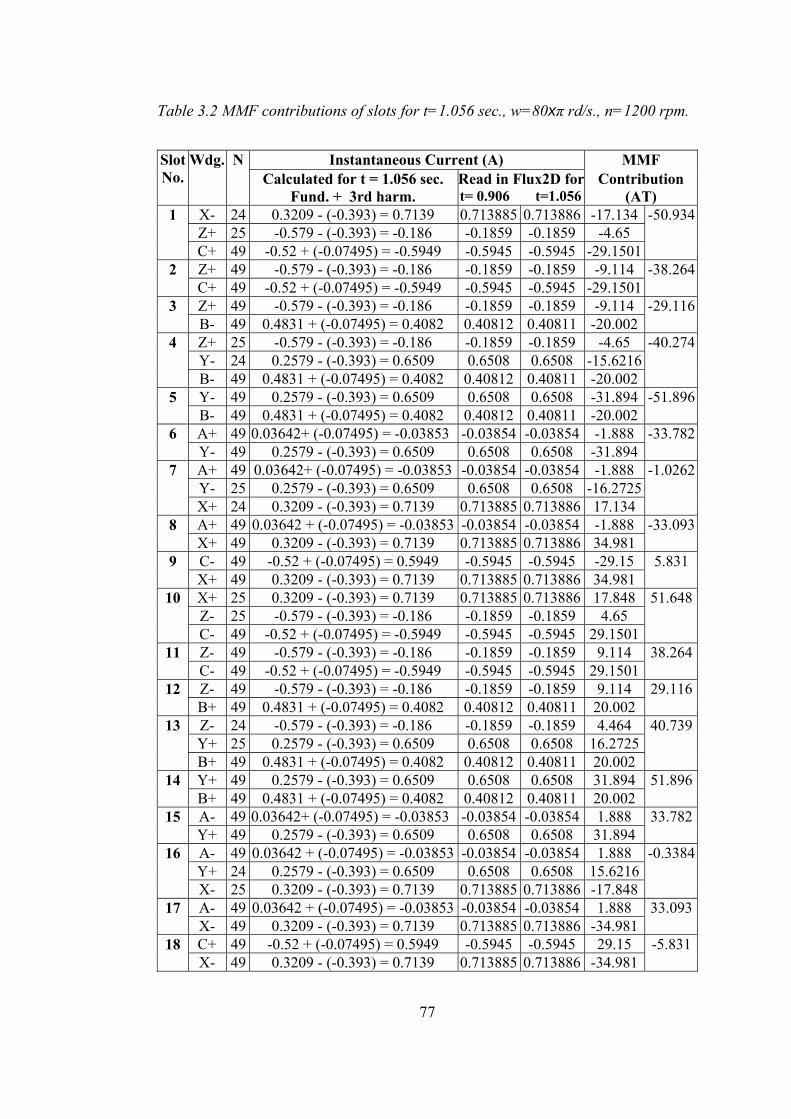
77
Table 3.2 MMF contributions of slots for t=1.056 sec., w=80xπ rd/s., n=1200 rpm.
Instantaneous Current (A) MMF Slot No.
Wdg. NCalculated for t = 1.056 sec.
Fund. + 3rd harm. Read in Flux2D fort= 0.906 t=1.056
Contribution (AT)
X- 24 0.3209 - (-0.393) = 0.7139 0.713885 0.713886 -17.134 Z+ 25 -0.579 - (-0.393) = -0.186 -0.1859 -0.1859 -4.65
1
C+ 49 -0.52 + (-0.07495) = -0.5949 -0.5945 -0.5945 -29.1501
-50.934
Z+ 49 -0.579 - (-0.393) = -0.186 -0.1859 -0.1859 -9.114 2 C+ 49 -0.52 + (-0.07495) = -0.5949 -0.5945 -0.5945 -29.1501
-38.264
Z+ 49 -0.579 - (-0.393) = -0.186 -0.1859 -0.1859 -9.114 3 B- 49 0.4831 + (-0.07495) = 0.4082 0.40812 0.40811 -20.002
-29.116
Z+ 25 -0.579 - (-0.393) = -0.186 -0.1859 -0.1859 -4.65 Y- 24 0.2579 - (-0.393) = 0.6509 0.6508 0.6508 -15.6216
4
B- 49 0.4831 + (-0.07495) = 0.4082 0.40812 0.40811 -20.002
-40.274
Y- 49 0.2579 - (-0.393) = 0.6509 0.6508 0.6508 -31.894 5 B- 49 0.4831 + (-0.07495) = 0.4082 0.40812 0.40811 -20.002
-51.896
A+ 49 0.03642+ (-0.07495) = -0.03853 -0.03854 -0.03854 -1.888 6 Y- 49 0.2579 - (-0.393) = 0.6509 0.6508 0.6508 -31.894
-33.782
A+ 49 0.03642+ (-0.07495) = -0.03853 -0.03854 -0.03854 -1.888 Y- 25 0.2579 - (-0.393) = 0.6509 0.6508 0.6508 -16.2725
7
X+ 24 0.3209 - (-0.393) = 0.7139 0.713885 0.713886 17.134
-1.0262
A+ 49 0.03642 + (-0.07495) = -0.03853 -0.03854 -0.03854 -1.888 8 X+ 49 0.3209 - (-0.393) = 0.7139 0.713885 0.713886 34.981
-33.093
C- 49 -0.52 + (-0.07495) = 0.5949 -0.5945 -0.5945 -29.15 9 X+ 49 0.3209 - (-0.393) = 0.7139 0.713885 0.713886 34.981
5.831
X+ 25 0.3209 - (-0.393) = 0.7139 0.713885 0.713886 17.848 Z- 25 -0.579 - (-0.393) = -0.186 -0.1859 -0.1859 4.65
10
C- 49 -0.52 + (-0.07495) = -0.5949 -0.5945 -0.5945 29.1501
51.648
Z- 49 -0.579 - (-0.393) = -0.186 -0.1859 -0.1859 9.114 11 C- 49 -0.52 + (-0.07495) = -0.5949 -0.5945 -0.5945 29.1501
38.264
Z- 49 -0.579 - (-0.393) = -0.186 -0.1859 -0.1859 9.114 12 B+ 49 0.4831 + (-0.07495) = 0.4082 0.40812 0.40811 20.002
29.116
Z- 24 -0.579 - (-0.393) = -0.186 -0.1859 -0.1859 4.464 Y+ 25 0.2579 - (-0.393) = 0.6509 0.6508 0.6508 16.2725
13
B+ 49 0.4831 + (-0.07495) = 0.4082 0.40812 0.40811 20.002
40.739
Y+ 49 0.2579 - (-0.393) = 0.6509 0.6508 0.6508 31.894 14 B+ 49 0.4831 + (-0.07495) = 0.4082 0.40812 0.40811 20.002
51.896
A- 49 0.03642+ (-0.07495) = -0.03853 -0.03854 -0.03854 1.888 15 Y+ 49 0.2579 - (-0.393) = 0.6509 0.6508 0.6508 31.894
33.782
A- 49 0.03642 + (-0.07495) = -0.03853 -0.03854 -0.03854 1.888 Y+ 24 0.2579 - (-0.393) = 0.6509 0.6508 0.6508 15.6216
16
X- 25 0.3209 - (-0.393) = 0.7139 0.713885 0.713886 -17.848
-0.3384
A- 49 0.03642 + (-0.07495) = -0.03853 -0.03854 -0.03854 1.888 17 X- 49 0.3209 - (-0.393) = 0.7139 0.713885 0.713886 -34.981
33.093
C+ 49 -0.52 + (-0.07495) = 0.5949 -0.5945 -0.5945 29.15 18 X- 49 0.3209 - (-0.393) = 0.7139 0.713885 0.713886 -34.981
-5.831
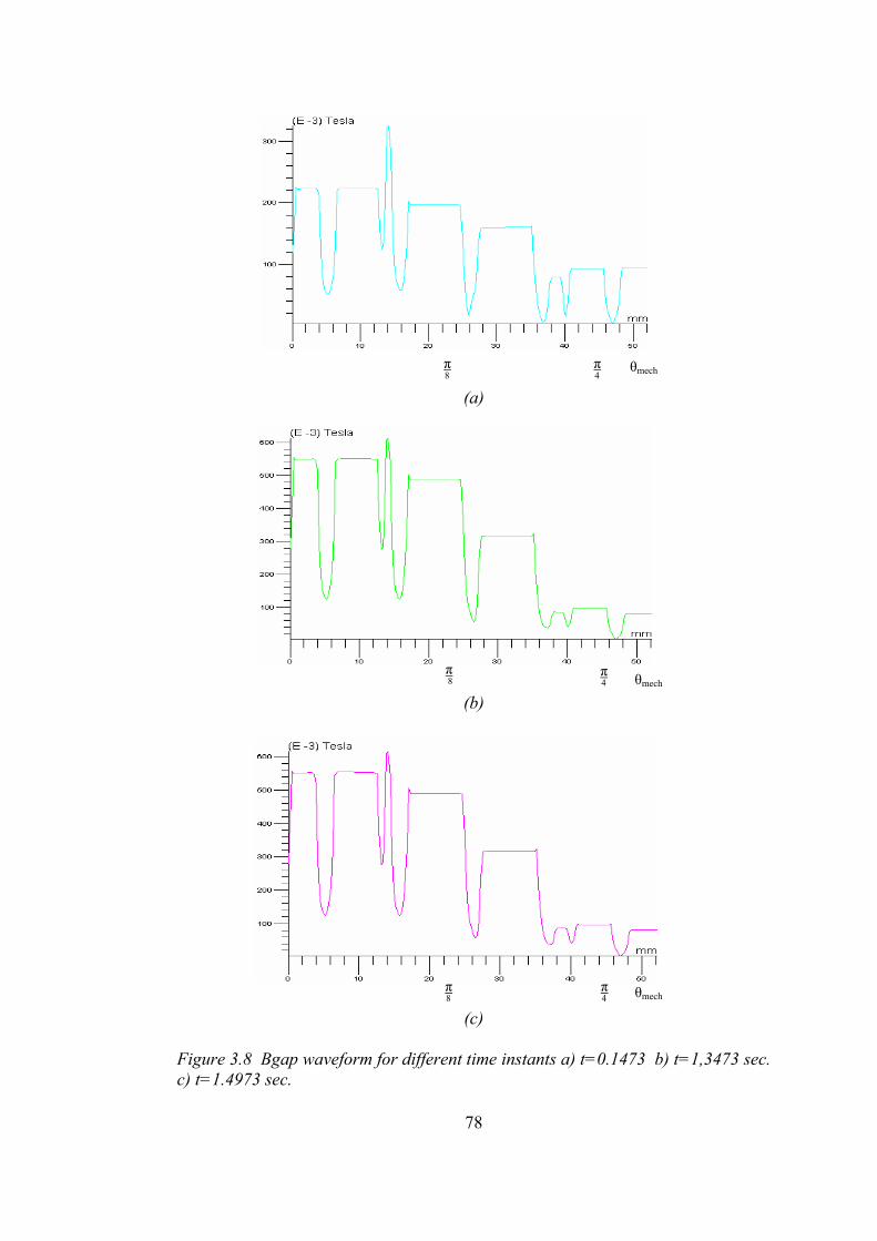
78
(a)
(b)
(a)
(b)
(c)
Figure 3.8 Bgap waveform for different time instants a) t=0.1473 b) t=1,3473 sec. c) t=1.4973 sec.
π 4 θmech π
8
π 4 θmech
π 8
π 4 θmech
π 8

79
However, despite the comparisons above there is no proof of the correctness of the
finite element solution. One way to do this is to solve the model for various load
conditions and compare the experimental results with the finite element model. The
verification of the the correctness of the solution is left to another research study.
80
CHAPTER 4
4 CORE LOSS CALCULATION 4.1 INTRODUCTION As mentioned earlier, the aim of this thesis is to calculate the core losses of the
motor introduced in Chapter 2. However, since the analytical calculation of core
losses presents unreliable results, a method which uses finite element method will
be used to achieve this aim. Hence, after establishing the finite element model of
the motor in the previous chapter, the calculation method of core losses evaluated
in [18], will be applied to the subject motor in this chapter.
In order to establish a rational basis for comparison of the calculations in this thesis
and the experimental results of [1], the motor is assumed to operate at no load. The
reason for this is that, the magnetic losses of the motor is experimentally measured
at no load condition in [1]. This means that we do not take into account the effects
of the rotor currents. However, the method may be verified by doing the
calculations for load conditons.
4.2 CALCULATION OF LOSSES In this section, a method of calculation of core losses of an induction machine from
FEM solutions will be explained. The fundamental frequency losses can be found
by using the results of the finite element solution and the loss curves as explained in
Chapter 3. On the other hand, for the high frequency losses a relatively difficult
method has to be used because of the effect of lamination on eddy currents.
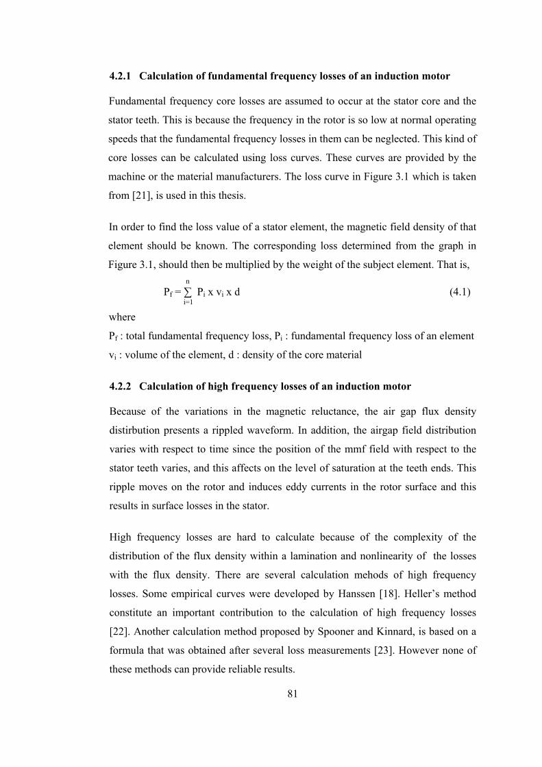
81
4.2.1 Calculation of fundamental frequency losses of an induction motor Fundamental frequency core losses are assumed to occur at the stator core and the
stator teeth. This is because the frequency in the rotor is so low at normal operating
speeds that the fundamental frequency losses in them can be neglected. This kind of
core losses can be calculated using loss curves. These curves are provided by the
machine or the material manufacturers. The loss curve in Figure 3.1 which is taken
from [21], is used in this thesis.
In order to find the loss value of a stator element, the magnetic field density of that
element should be known. The corresponding loss determined from the graph in
Figure 3.1, should then be multiplied by the weight of the subject element. That is, n Pf = ∑ Pi x vi x d (4.1)
i=1
where
Pf : total fundamental frequency loss, Pi : fundamental frequency loss of an element
vi : volume of the element, d : density of the core material
4.2.2 Calculation of high frequency losses of an induction motor Because of the variations in the magnetic reluctance, the air gap flux density
distirbution presents a rippled waveform. In addition, the airgap field distribution
varies with respect to time since the position of the mmf field with respect to the
stator teeth varies, and this affects on the level of saturation at the teeth ends. This
ripple moves on the rotor and induces eddy currents in the rotor surface and this
results in surface losses in the stator.
High frequency losses are hard to calculate because of the complexity of the
distribution of the flux density within a lamination and nonlinearity of the losses
with the flux density. There are several calculation mehods of high frequency
losses. Some empirical curves were developed by Hanssen [18]. Heller’s method
constitute an important contribution to the calculation of high frequency losses
[22]. Another calculation method proposed by Spooner and Kinnard, is based on a
formula that was obtained after several loss measurements [23]. However none of
these methods can provide reliable results.

82
Flux2D provides the eddy currents in the rotor teeth. However, these values are
computed by the program ignoring the laminated core. In the actual machine the
eddy currents are assumed to flow within the lamination since the lamination
surfaces are electrically isolated. Here, we will use a method which is a modified
version of the one used in [18] to include the effect of lamination.
The skin depths of each harmonic are calculated using the Eq.4.2 [20]
δj = Tp x fs / π x fj (4.2)
where,
δj : skin depth of jth harmonic, Tp : stator pole pitch
fs : stator frequency, fj : frequency of jth harmonic
Consider a tooth pitch on the rotor side. The eddy current path in the solution of the
field is in the axial direction. This is shown in Figure 4.1 in which the average rotor
tooth pitch width for a certain length lav in the axial direction at a certain skin depth
is shown. In this figure, ij is used for the current of one lamination flowing in the
axial direction, ej is used for the voltage of one lamination induced in the axial
direction, llam is used for the thickness of the lamination. The induced emf causes
this current to flow against resistance Rj, determined by the skin depth for the
particular harmonic and the average width of the current path (lav) in the radial
direction.
avj
clamclamj l
lA
lR×
==δρρ .. (4.3)
where, Rj: the resistance of one rotor tooth at the skin depth of jth harmonic the
finite element analysis assumes.
ρlam: resistivity of the lamination, lc: core length. A: cross-section of one rotor tooth in one lamination under the skin depth
of jth harmonic.
δj: the skin depth of jth harmonic, lav: average current path width

83
Figure 4.1 The current path the finite element analysis assumes in a rotor tooth pitch If the induced emf in the axial direction has an average magnitude ej, for the
portion of the rotor considered, the average current flowing in the cross section is
as,
clam
avjj
j
jj l
leRe
i×
××==
ρδ
(4.4)
where, ij: the current flowing in the axial direction.
ej: average magnitude of the the emf drop in the axial direction.
In the calculations that follow, the eddy currents are assumed to flow within the
lamination. This naturally reduces the magnitude of eddy currents since any current
must be due to the induced emf in the axial direction. This subsection discusses
how the calculated losses from the FE software can be modified to take into
account the effect of laminations.
Let us now assume that, in fact the eddy currents are confined to a lamination and
current circulate within the lamination over a rotor tooth pitch as shown in Figure
4.2. In this case, the currents circulate due to the emf ei, induced due to the ith
harmonic field in the axial direction. The thickness of the lamination (llam = 0.5
mm.) therefore determines the magnitude of ei. The current path in this case is also

84
considerably elongated as shown in Figure 4.2. Since the thickness of the
lamination is much shorter than the tooth pitch, the resistance of the eddy current
path may be assumed to be 2lav. Also, the center of the lamination region may be
assumed to carry no currents (the emf gets too small). As seen in Figure 4.2, the
current path width varies depending on the skin depth. Since taking into account
the skin depths of all of the harmonics makes the problem more complex, an
averaging has to be made for the current path width and skin depth values.
Figure4.2 The current path considering the laminations
Therefore, the resistance of the circulating eddy current path for the ith harmonic is,
kl
lA
lRlami
avlamlami ××
×==δ
ρρ .2. (4.5)
where,
A : cross-sectional area of the circulating eddy current path in one lamination of one skin depth region.
k : coefficient
δi : radial height of each skin depth in the rotor teeth.

85
The eddy current loss therefore in the considered portion of the rotor tooth is given
by Eq.4.6 for the ith harmonic.
Pi = ei x ii = ei
2 / Ri = (2 x ej)2 / Ri = (2 x ij x Rj)2 / Ri (4.6)
Pi = ij2 x [2 x ρ x lc
2 x llam x k / (δi x lav3)] (4.7)
Then, the total high frequency loss of an induction motor is obtained by doing the
above calculations for each harmonic component in every rotor tooth in the model
and then using the formula below, n
Ptotal = 4 x t x Σ Pi (4.8) i=2
where Pi is the eddy current loss of a harmonic in a quarter of the motor in one
lamination and t is the number of laminations. The factor 4 is used since a quarter
of the motor is modelled.
4.2.3 Implementation of the calculation method of fundamental frequency
core losses By using Flux2D, one stator tooth pitch is divided vertically into two and
horizontally into ten regions as in Figure 4.3. The reason for not calculating the loss
for every mesh element is that the program doesn’t provide us with the volume and
the flux density of each mesh element. Therefore the stator tooth pitch is divided
into regions, the volumes of which are easy to calculate.
Figure 4.3 The regions assumed to exist in one tooth pitch of the stator core

86
Then the corresponding weight values are found by using 7850 kg/m3 as density of
iron. The flux density of the points at the center of gravity of each region is read
from the program along one cycle of the 40 Hz current source. 43 samples are read
from the program along a period of the 40 Hz. source, which is 25 msec. That is, a
sample is taken nearly every 0.6 msec.
The read flux density values are input to Matlab Simulink and the magnitudes of
the spectrum of every region is evaluated. The fundamental and the third harmonic
frequency peak flux density values are taken and the corresponding watt/kg values
in the loss curve of Figure 3.1 are multiplied by the weight of each region in the
stator tooth pitch. The loss of one tooth pitch is found by summing the loss of all
regions. Then the total fundamental frequency loss is calculated by multiplying the
loss of one tooth pitch by 36, which is the number of stator slots. The results of the
fundamental frequency loss calculations will be elaborated on in detail in the next
chapter. In Table 5.1, the fundamental and third harmonic components of the flux
density in each region can be seen.
4.2.4 Implementation of the calculation method of high frequency core losses In this section, by using the method explained in section 4.2.2, the high frequency
core losses of the subject motor are calculated. The calculation procedure started
actually while creating the finite element model of the motor. The rotor teeth are
splitted into 3 regions according to the skin depths of 5th, 11th, 17th as shown in
Figure 4.4. This was essential to avoid creating an excessive number of FE
elements and possibly causing instability in the solution, since some of the element
mesh sizes would have been very small values.
The reason behind the choice of the size of these 3 regions is explained below.
According to [24] the harmonics expected to exist in the rotor are found by the
equations below,
The air gap harmonics of the order n = 6m + 1 rotate in the same direction with
the fundamental.

87
The air gap harmonics of the order n = 6m - 1 rotate in the opposite direction
with the fundamental.
where m is an integer.
According to the rules above; 5th, 7th, 11th, 13th, 17 th, 19th, 23rd, 25th air gap
harmonics are expected to induce currents in the rotor core of the test motor;
On the other hand, the stator slot harmonics are also estimated to occur in the rotor.
The order of the stator slot harmonics can be calculated as [18]:
n = (Ns x nr) / (60 x fs) (4.9)
where, n: order of the expected stator slot harmonic, Ns : number of stator slots = 36,
nr : rotor speed = 1200 rpm., fs : source frequency
For the test motor there are two source frequencies at the same time: 40 Hz. and
120 Hz. because of the third harmonic current injection. Therefore; 6 th and 18 th
harmonics are expected to exist in the rotor core caused by the fundamental and the
third harmonic sources respectively.
In Table 4.3, the skin depths calculated using Eq.(4.2) for the expected harmonics
are presented. By taking into account the approximation of the skin depths to each
other as seen in Table 4.3., an averaging is done for the skin depths and hence the
three skin depth regions are created based on the skin depths for; 5th harmonic, used also for 3rd,6th and 7th harmonics.
11 th harmonic, used also for 9th and 13th harmonics.
17th harmonic. used also for 15th, 18th and 19th harmonics. (Figure 4.4)
In fact more accurate results could be obtained if the rotor teeth were splitted
according to all harmonics. However, this elongates the computation time of the
program and increases the complexity of the problem but it is not worth to face
with these difficulties for too accurate results.
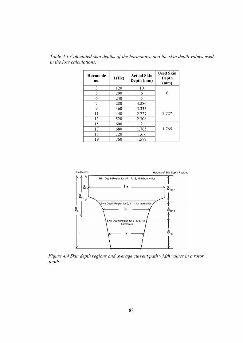
88
Table 4.1 Calculated skin depths of the harmonics, and the skin depth values used in the loss calculations.
Harmonic no. f (Hz) Actual Skin
Depth (mm)
Used Skin Depth (mm)
3 120 10 5 200 6 6 240 5 7 280 4.286
6
9 360 3.333 11 440 2.727 13 520 2.308
2.727
15 600 2 17 680 1.765 18 720 1.67 19 760 1.579
1.765
Figure 4.4 Skin depth regions and average current path width values in a rotor tooth

89
The eddy current values of the three skin depth regions at the rotor teeth are read
from Flux2D, and the harmonic components of the currents (ij) are evaluated along
a period of the 40 Hz supply also in the same program. The magnitudes of the
harmonic components are transferred to the Excel table in Tabel 5.2 and the loss
contribution of each harmonic is calculated for 7 rotor teeth according to Eq. (4.7).
Here, the second term of Eq.(4.7) is named as the skin depth region coefficient as
in Eq.(4.10) and three coefficients are calculated for the three skin depth regions as
in Table 4.2.
ηRi = [2 x ρ x lc
2 x llam x k / (δi x lav3)] (4.10)
where,
ρ = 6 x 10⁻⁴ Ohm x m
lc = 65.5 mm
llam = 0.5 mm.
k = 0.3
Table 4.2 The calculated skin depth region coefficients
Figure 4.4 also shows the lav values which are taken as the width at the middle
point of each skin depth region. The skin depths are found in accordance with
Eq.(4.2). Then the height of each skin depth region (δRi) is substituted for the term
δi in Eq.(4.10) as calculated in Table 4.3.
Table 4.3 Skin depth regions and their lav and δRi values.
Skin Depth Region lav δRi R5 l5 =. 6.62 mm δ5 – δ11 = 3.27 mm.
R11 l11 = 7.12 mm δ11 – δ17 = 0.965 mm. R17 l17 = 10 mm δ17 = 1.765 mm.
ηR5 0,943 ηR11 2,568 ηR17 0,50684

90
Next, the high frequency loss of one rotor tooth of the motor is calculated by
multiplying the loss of one lamination by the number of laminations which is,
t = rotor stack length / lamination thickness
= 65.5 mm / 0.5 mm = 131 (4.11)
And finally, the total high frequency of 28 rotor teeth is calculated by multiplying
the loss of seven rotor teeth by 4 according to according to Eq.(4.8). The results of
the loss calculation will be elaborated in the next chapter in detail.

91
CHAPTER 5
5 RESULTS AND CONCLUSIONS 5.1 INTRODUCTION As stated before, the aim of this thesis is to calculate the core losses of the motor
introduced in Chapter 2. However, since the analytical calculation of core losses
presents unreliable results, a method which uses finite element solutions is used to
achieve this aim. Hence, after establishing the finite element model of the motor in
Chapter 3, the calculation method of core losses developed in [18], is applied to the
test motor described in Chapter 4.
In this chapter the results of the loss calculations in Chapter 4 will be elaborated on
and compared with the experimental results of [1]. Then the discussions and final
conclusions on this thesis and suggestions for future work will be provided.
5.2 THE RESULTS OF THE FUNDAMENTAL FREQUENCY CORE
LOSS CALCULATIONS In this thesis, the fundamental frequency loss of the motor is calculated using the
values read from the loss curves in Figure 3.1. By using Flux 2D, one stator tooth
pitch is divided vertically into two and horizontally into ten regions as in Figure
4.3. By this way the problem is relatively simplified. Therefore the stator tooth
pitch is divided into coarser regions, the volumes of which are easy to calculate.
Taking 7850 kg/m3 as density of iron, the weight values of each region is found.
The flux density of the points at the center of gravity of each region is read from
the program along one cycle of the 40 Hz current source (25 msec.). 43 samples are
read from the program along a period of 25 msec. The smaller number of samples

92
are found not to be sufficient for obtaining the harmonic spectrum of the flux
density.
In Figures 5.1, 5.2, 5.3 and 5.4, the flux density magnitudes at four example pairs
of regions in the first half and the second half of the tooth pitch (Figure 4.3), are
displayed in graphs along a period of 25 msec. These values are read from the
software by writing down a macro for the program to make a recursive analysis.
After obtaining 43 flux density values at every region of a tooth pitch as in the
Figures 5.1 to 5.4., the fundamental and third harmonic flux density components of
every region are obtained using the “fft” function of Matlab Simulink and. Then
the watt/kg values that correspond to the magnitudes of the fundamental and the
third harmonic components of the flux density, using the the loss curve of Figure
3.1.
The corresponding watt/kg values are multiplied by the weight of each region and
the fundamental frequency core loss values are found. The loss of one tooth pitch is
calculated by summing the loss of all regions after finding them as mentioned
above. Then the total fundamental frequency loss is calculated by multiplying the
loss of one tooth pitch by 36, which is the number of stator slots. In Table 5.1, the
fundamental and third harmonic components of the flux density and their loss
contributions in each region can be seen.
Referring to Figure 3.1 and Eq. (4.1), the fundamental frequency losses of the
motor turn out to be at the level of 13 watts. (Table 5.1)
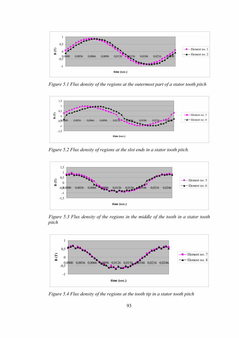
93
-1
-0,5
0
0,5
1
0,0000 0,0036 0,0066 0,0096 0,0126 0,0156 0,0186 0,0216 0,0246
time (sec.)
B (T
) Element no. 1Element no. 2
Figure 5.1 Flux density of the regions at the outermost part of a stator tooth pitch
-1,5
-1
-0,5
0
0,5
1
1,5
0,0000 0,0036 0,0066 0,0096 0,0126 0,0156 0,0186 0,0216 0,0246
time (sec.)
B (T
)
Element no. 3
Element no. 4
Figure 5.2 Flux density of regions at the slot ends in a stator tooth pitch.
-1,5-1
-0,50
0,51
1,5
0,0000 0,0036 0,0066 0,0096 0,0126 0,0156 0,0186 0,0216 0,0246
time (sec.)
B (T
) Element no. 5Element no. 6
Figure 5.3 Flux density of the regions in the middle of the tooth in a stator tooth pitch
-1
-0,5
0
0,5
1
0,0000 0,0036 0,0066 0,0096 0,0126 0,0156 0,0186 0,0216 0,0246
time (sec.)
B (T
) Element no. 7Element no. 8
Figure 5.4 Flux density of the regions at the tooth tip in a stator tooth pitch

94
In Table 5.1, it can be seen that the flux density magnitudes in the regions at the
first and second half of the tooth pitch are quite similar to each other. This verifies
that the number of horizontal regions is more or less sufficient for quite a reliable
calculation except for the tooth tips. The low level of flux density at the tooth tips,
points out the insufficient number of horizontal regions at this part of the tooth
pitch. However, when the tooth tips were splitted into more horizontal regions, the
volume and so the weight of the regions would decrease. This decrease is
considered to keep the calculated loss values at the same level as for now.
Concerning the vertical division of the stator tooth pitch, although it is certainly
clear that; the more the number of regions, the better the accuracy of the
calculations; splitting the tooth pitch into 10 vertical regions is considered a
simplified and a sufficient choice for the requirements of this study.

95
Tabl
e 5.
1 M
icro
soft
Exce
l tab
le u
sed
to c
alcu
late
the
fund
amen
tal f
requ
ency
loss
es
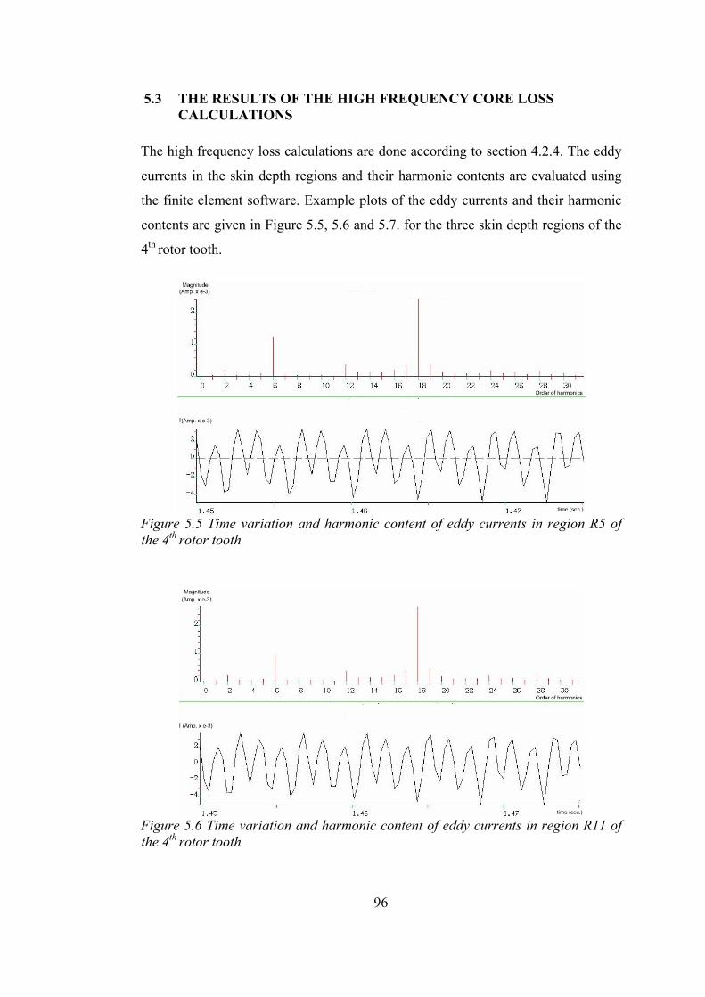
96
5.3 THE RESULTS OF THE HIGH FREQUENCY CORE LOSS CALCULATIONS
The high frequency loss calculations are done according to section 4.2.4. The eddy
currents in the skin depth regions and their harmonic contents are evaluated using
the finite element software. Example plots of the eddy currents and their harmonic
contents are given in Figure 5.5, 5.6 and 5.7. for the three skin depth regions of the
4th rotor tooth.
Figure 5.5 Time variation and harmonic content of eddy currents in region R5 of the 4th rotor tooth
Figure 5.6 Time variation and harmonic content of eddy currents in region R11 of the 4th rotor tooth
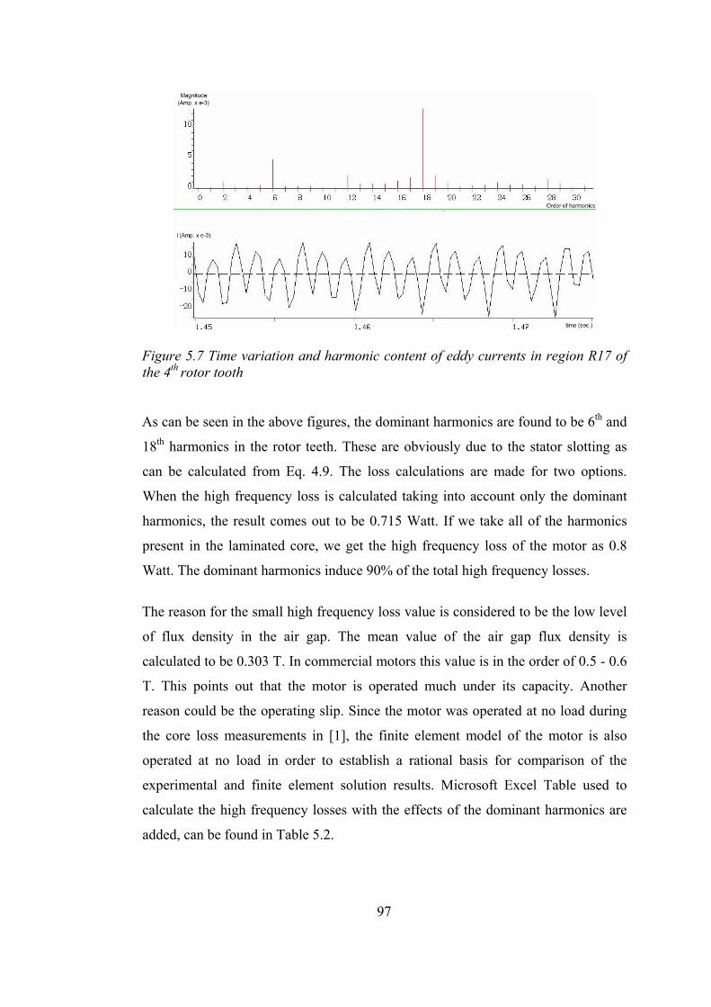
97
Figure 5.7 Time variation and harmonic content of eddy currents in region R17 of the 4th rotor tooth As can be seen in the above figures, the dominant harmonics are found to be 6th and
18th harmonics in the rotor teeth. These are obviously due to the stator slotting as
can be calculated from Eq. 4.9. The loss calculations are made for two options.
When the high frequency loss is calculated taking into account only the dominant
harmonics, the result comes out to be 0.715 Watt. If we take all of the harmonics
present in the laminated core, we get the high frequency loss of the motor as 0.8
Watt. The dominant harmonics induce 90% of the total high frequency losses.
The reason for the small high frequency loss value is considered to be the low level
of flux density in the air gap. The mean value of the air gap flux density is
calculated to be 0.303 T. In commercial motors this value is in the order of 0.5 - 0.6
T. This points out that the motor is operated much under its capacity. Another
reason could be the operating slip. Since the motor was operated at no load during
the core loss measurements in [1], the finite element model of the motor is also
operated at no load in order to establish a rational basis for comparison of the
experimental and finite element solution results. Microsoft Excel Table used to
calculate the high frequency losses with the effects of the dominant harmonics are
added, can be found in Table 5.2.
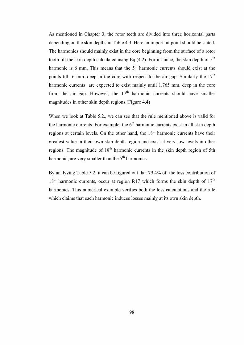
98
As mentioned in Chapter 3, the rotor teeth are divided into three horizontal parts
depending on the skin depths in Table 4.3. Here an important point should be stated.
The harmonics should mainly exist in the core beginning from the surface of a rotor
tooth till the skin depth calculated using Eq.(4.2). For instance, the skin depth of 5th
harmonic is 6 mm. This means that the 5th harmonic currents should exist at the
points till 6 mm. deep in the core with respect to the air gap. Similarly the 17th
harmonic currents are expected to exist mainly until 1.765 mm. deep in the core
from the air gap. However, the 17th harmonic currents should have smaller
magnitudes in other skin depth regions.(Figure 4.4)
When we look at Table 5.2., we can see that the rule mentioned above is valid for
the harmonic currents. For example, the 6th harmonic currents exist in all skin depth
regions at certain levels. On the other hand, the 18th harmonic currents have their
greatest value in their own skin depth region and exist at very low levels in other
regions. The magnitude of 18th harmonic currents in the skin depth region of 5th
harmonic, are very smaller than the 5th harmonics.
By analyzing Table 5.2, it can be figured out that 79.4% of the loss contribution of
18th harmonic currents, occur at region R17 which forms the skin depth of 17th
harmonics. This numerical example verifies both the loss calculations and the rule
which claims that each harmonic induces losses mainly at its own skin depth.

99
Table 5.2 Microsoft Excel table used to calculate the high frequency losses.
Harmonic Currents and Loss Contributions
6 18
Rotor Teeth
Skin
Depth Regions
ij (A) Pi (W) ij (A) Pi (W)
Total Loss of One
Lamination (W)
R 5 0,00064070 0,00000310 0,00117806 0,00001047 0,00001422
R 11 0,00049745 0,00000508 0,00142650 0,00004180 0,00004863 1
(Half) R 17 0,00245512 0,00002444 0,00845845 0,00029010 0,00032301
R 5 0,00099079 0,00000093 0,00211509 0,00000422 0,00000526
R 11 0,00072872 0,00000136 0,00265822 0,00001815 0,00001994 2
R 17 0,00389134 0,00000767 0,01355781 0,00009316 0,00010372
R 5 0,00097079 0,00000089 0,00193577 0,00000353 0,00000454
R 11 0,00079525 0,00000162 0,00264418 0,00001795 0,00001996 3
R 17 0,00440219 0,00000982 0,01367676 0,00009481 0,00010730
R 5 0,00122488 0,00000141 0,00240896 0,00000547 0,00000701
R 11 0,00092045 0,00000218 0,00270417 0,00001878 0,00002132 4
R 17 0,00460355 0,00001074 0,01283531 0,00008350 0,00009621
R 5 0,00201286 0,00000382 0,00325738 0,00001001 0,00001538
R 11 0,00142170 0,00000519 0,00273101 0,00001915 0,00002709 5
R 17 0,00610267 0,00001888 0,01086585 0,00005984 0,00008883
R 5 0,00160405 0,00000243 0,00281734 0,00000748 0,00001019
R 11 0,00105970 0,00000288 0,00237889 0,00001453 0,00001787 6
R 17 0,00437362 0,00000970 0,00975968 0,00004828 0,00005937
R 5 0,00198257 0,00000371 0,00327298 0,00001010 0,00001537
R 11 0,00136179 0,00000476 0,00273393 0,00001919 0,00002668 7
R 17 0,00577296 0,00001689 0,01081721 0,00005931 0,00008578
R 5 0,00054311 0,00000223 0,00115009 0,00000998 0,00001272
R 11 0,00043702 0,00000392 0,00131658 0,00003561 0,00004121 8 (Half)
R 17 0,00231152 0,00002166 0,00740610 0,00022240 0,00025636 Loss contributions of harmonics
0,00016532 0,00119783 0,00142797
ηR5 Coefficient ηR11 Coefficient ηR17 Coefficient
0,943 2,568 0,50684
Plam = t x Σ Pi = 0,178 Watt Total loss of ( 65,5 mm/ 0,5 mm = 131 )
laminations of a quarter of the motor
Ptotal = 4 x t x Σ Pi = 0,715 Watt Total loss of 28 rotor slots
Pi = ij
2 x [2 x ρ x lc2 x llam x k / (δi x lav
3)] ηRi coefficient = [2 x ρ x lc
2 x llam x k / (δi x lav3)]

100
5.4 COMPARISON WITH THE EXPERIMENTAL RESULTS In [1], the magnetic losses of the six phase machine with third harmonic current
injection at 40 Hz. are measured as 13 Watts at a peak air gap flux density of 0.55
T as seen in Figure 2.32. According to [1], the measurement procedure of the
magnetic losses of the motor is as follows: The machine was driven mechanically
at synchronous speed and the input power was measured. Magnetic power losses
were obtained by subtracting the stator copper losses from the measured power.
This value is considered as the sum of fundamental frequency losses and high
frequency losses since the friction and windage losses were supplied by the power
applied to the shaft.
The results of the core loss calculations presented in the previous sections in this
thesis and the experimental loss measurements in [1] are compared to each other in
Table 5.3. The comparison shows that the loss model applied to the motor predicts
the losses very accurately.
Table 5.3 Comparison of the measured and calculated core losses
Fundamental Freq. High Freq. Total Measured in [1] - - 13 Watt Calculated in this thesis 13.4 Watt 0.8 Watt 14.2 Watt
An important point here is that, the measurements on the test motor were done at
no load condition in [1]. While creating the finite element model in this study, the
motor is naturally operated the same conditons for comparison with the
experimental results. This means that in the simulations and tests above the rotor
currents do not exist. The accuracy of the loss calculations may not be the same
under load conditions. Futhermore, the available test results were obtained with a
current source. Therefore none of the electrical measurements nor the mechanical
output torque (torque = 0 for no load) could be compared with the FE solution
results. The method may be verified by doing the FE computations for several
operating conditons under load and comparing with experimental results (currents,
torque output etc.).

101
5.5 KEY FINDINGS AND RECOMMENDATIONS Calculation of the losses of electrical motors using analytical methods while they
are being designed, is hard to achieve. The best way to do this is the production of a
model motor and test it to see if the objective performance criteria are achieved or
not. However, this method can cost not only too much money but also time, which
is a scarce resource for production and marketing. Finite Element Software
products open a way to calculate the losses without production of the physical
models of electrical motors. By using these computer aided design tools, designers
can achieve better performance results in shorter periods of time.
On the other hand, FE software, present some difficulties which are of course can
not be compared to the difficulties above. Examples of the problems faced during
the modelling of the machines are; the long computation time for complex
machines and insufficiently user friendly program interfaces.
Regarding the subject of this thesis for instance; the software does not allow the
user to inject third harmonic currents in magnetodynamic analysis. Therefore the
user has only one choice which is the time consuming transient analysis. Software
products of this type should be further developed and made easier to use.
In addition, parameters like the k coefficient, lamination thickness, the number of
laminations, resistivity of the lamination etc. play an important role in the accuracy
of the results. The k coefficient is taken as 0.3 taking into account the results of
[18] and [19]. However the value of k may be a function of the frequency.
Since the material properties of the motor, core losses of which are calculated in
this study, are not known precisely, the calculations may not reflect the real motor.
Since it was not possible to obtain the loss curve of the motor from [1], a typical
loss curve from [21] is used in the calculations.

102
5.6 AREAS FOR FURTHER RESEARCH In this study, the core loss calculation method evaluated in [18] is applied in
modified form to a 6 phase motor with 3rd harmonic injection introduced in [1]. It is
shown in this work that the high frequency losses can be calculated with good
accuracy using the approach here. However this research work is done within the
framework of a MS research study and is by no means complete. It is thought that
the following investigations are needed to increase reliability of the results obtained
• The modelled motor may be solved for several operating conditions at different
frequencies under load and compared with measurements under the same
conditions to really verify the calculation method.
• High frequency core losses of the motor can be calculated for a normal winding
and can be compared with the case with 3rd harmonic injection via FE simulation.
This would clarify whether the losses increase or not. Of course having
measurements on an actual motor for this condition would also be very useful.
• Measurements can be done on the test motor with increased air gap flux density to
find out the effect of this on losses and motor performance and to determine
whether the design in hand is optimal. The fact that this frame size is normally
capable of providing 5.5 kW output suggests that the motor is poorly designed and
therefore unneccesarily large in size with very small high frequency losses.
• The efficiency of the motor may also be evaluated when fed from a voltage
source, by calculating the core losses and copper losses using 2D harmonic field
solution with 3D effects. In this case superposition of harmonic solutions for the
fundamental and 3rd harmonic frequencies would be needed. Of course this would
first require verification of the validity of the superposition required here.
• The value of k may be studied further especially regarding frequency dependency.
• Another issue to work on is whether making the loss calculations on a small
number of regions (instead of each mesh element) is causing any serious errors.

103
REFERENCES [1] Lyra, R. O. C., “Torque density improvement in a six-phase induction motor
with third harmonic current injection,” PhD thesis, University of Wisconsin, 2002.
[2] Munoz, A. R., Lipo, T. A. “ Dual stator winding induction machine drive,”
IEEE Transactions on Industry Applications, vol. 36, pp. 1369 – 1379, Sept 2000.
[3] Ojo, O., Davidson, I. E. “Pwm - vsi inverter-assisted stand-alone dual stator
winding induction generator,” IEEE Transactions on Industry Applications, vol. 36, pp. 1604 – 1611, Nov 2000.
[4] Gopakumar, K., Ranganathan, T., Bhat, S. R. “Split-phase induction motor
operation from pwm voltage source inverter,” IEEE Transactions on Industry Applications, vol. 29, pp. 927– 932, Sept 1993.
[5] Bakhshai, A. R., Joos, G., Jin, H. “Space vector pwm control of a split-phase
induction machine using the vector classification technique,” Proceedings of Applied Power Electronics Conference and Exposition, 1998, vol. 2, pp. 802 – 808, Feb 1998.
[6] Nelson, R. H., Krause, P. C. “Induction machine analysis for arbitrary
displacement between multiple windings,” IEEE Transactions on Power Apparatus and Systems, vol. 93, pp. 841 – 848, May 1974.
[7] Lipo, T. A. “A d-q model for six phase induction machines,” Proceedings of
the International Conference on Electrical Machines, Athens,, pp. 860 – 867, Sept 1980.
[8] Andresen, E., Bieniek, K., “On the performance of inverter fed induction
motors with six phases,” Proceedings of the International Conference on Electrical Machines, Athens, pp. 909 – 917, Jan 1980.
[9] Vander Duijn, N. P., Gordon, B. M., McMahon, R. A. “Multiphase induction
motors for integrated drives,” Proceedings of the 9th International Conference on Electrical Machines and, pp. 6 – 11, Jan 1999.

104
[10] Abbas, M. A., Christen, R., Jahns, T. M. “Six-phase voltage source inverter driven induction motor,” IEEE Transactions on Industry Applications, vol. 20, pp. 1251 – 1259, Sept 1984.
[11] Fu, J. and Lipo, T. A. “Disturbance free operation of a multiphase current
regulated motor drive,” IEEE Transactions on Industry Applications, vol. 30, pp. 1267 – 1274, Sept 1994.
[12] Novotny, D. W., Lipo, T. A., Vector Control and Dynamics of AC Drives.
New York: Clarendon Press - Oxford, 1996. [13] Lipo, T. A., Introduction to AC Machine Design. Madison - WI: University
of Wisconsin, 1996. [14] Lipo, T. A. “Flux sensing and control of static ac drives by the use of flux
coils,” IEEE Transactions on Magnetics, vol. MAG-13, pp. –, Sept 1997. [15] Miranda, M. S., Lyra, R., Silva, S. R. “An alternative isolated wind electric
pumping system using induction machines,” IEEE Transaction on Energy Conversion, vol. 14, pp. 1611 – 1616, Dec 1999.
[16] Zhao, Y. Lipo, T. A., “Space vector pwm control of dual three-phase
induction machine using vector space decomposition,” IEEE Transactions on Industry Applications, vol. 31, pp. 1100 – 1109, Sept 1995.
[17] Ertan, H.B., Electrical Machine Design Lecture Notes. Ankara: Middle East
Technical University, 1991. [18] Pirgaip, M., “Computation of core losses in three-phase smooth rotor
induction motors using finite element method,” Master’s thesis, Middle East Technical University, September 1998.
[19] Avenoglu, B. “İndüksiyon motorlarında yüksek frekans kayıplarının ve motor
parametrelerinin hesaplanması,” Master’s thesis, Hacettepe University, 2001 [20] Lipo, T.A., Electromagnetic design course notes, Madison, 1990. [21] Roters, H.C. Electromagnetic devices, John Wiley & Sons Ltd., 1941 [22] Heller, B., Hamata, V.,Harmonic field effects in induction machines, Elsevier Scientific Publishing Co., New York, 1977 [23] Veinott, C.Theory and design of small induction motors, McGraw-Hill Book Co.,Inc., New York, 1959.
[24] Say, M.G., The performance and design of alternating current machines,
Pitman Paperbacks, 1958.

105
APPENDIX
CALCULATION OF PARAMETERS NEEDED AS INPUT FOR FLUX2D SOLUTIONS
1. Calculation of End Winding Resistance
Ret = (8 ρ lew Ntsp Nspp) / ( π Nb Nf dw2) = 0.687 Ohm lew = π (Dal +2 hss) + 2 hss
2p
ρ : wire resistivity = 1.72 10-8 Ohmxm. lew : end wdg. length = 0.166 m.
Ntsp : number of turns per slot per phase = 49 Nspp: no. of slots/pole/phase = 6
Nb : number of coils parallel per phase = 3 Nf: no. of wires in series per turn = 2
dw : wire diameter = 0.00072 m. p : number of pole pairs = 2
Dal: stator inner diameter = 0.12 m. hss : stator slot height = 0.02 m.
2. Calculation of End Winding Inductance
Lew = µo (Nss x Ntsp / Nb)2 P = 0.54 mH. lap = π (Dal +2 hss) = 0.11 m. 18p 2p
P = 0.47 lew – 0.3 lap = 0.04502
Nss : number of stator slots = 36 µo : permeability of air = 4π x 10-7
ω : source pulsation = 80 x π rd/sec.

106
3. Calculation of End Ring Resistance
Rer = ρ π p (Dr-Di) x (Dr2p + Di
2p) / (Dr2p - Di
2p) Nr eeqh
Nr: number of rotor bars ρ: end ring resistivity
Dr: end ring equivalent diameter Di: end ring inner diameter
eeq: end ring equivalent thickness h: end ring height
4. Calculation of End Ring Inductance Ler = π µo (De-heq) x λer λer = 0.365 Ln [ 3π x (De- heq ) / ( heq+eeq)] Nr 4
De = Di+h
De : end ring outer diameter heq : end ring equivalent height
eeq : end ring equivalent thickness.