Calculating losses of crops in Denmark caused by high ozone levels
21
Environmental Modeling and Assessment 6: 35–55, 2001. 2001 Kluwer Academic Publishers. Printed in the Netherlands. Calculating losses of crops in Denmark caused by high ozone levels Z. Zlatev a , I. Dimov b , Tz. Ostromsky b , G. Geernaert a , I. Tzvetanov c and A. Bastrup-Birk d a National Environmental Research Institute, Department of Atmospheric Environment Frederiksborgvej 399, P.O. Box 358, DK-4000 Roskilde, Denmark E-mail: {zz, glg, abb}@dmu.dk b Central Laboratory for Parallel Processing, Bulgarian Academy of Sciences, Acad. G. Bonchev str., bl. 25-A, 1113 Sofia, Bulgaria E-mail: [email protected], [email protected] c Institute of Economics of the Bulgarian Academy of Sciences, 3 Aksakov str., 1000 Sofia, Bulgaria E-mail: [email protected] d Danish Forest and Landscape Institute, Hørsholm Kongevej 11, Hørsholm, Denmark In order to help guide air pollution legislation at the European level, harmful air pollution effects on agriculture crops and the consequent economic implications for policy have been studied for more than a decade. Ozone has been labeled as the most serious of the damaging air pollutants to agriculture, where growth rates and consequently yields are dramatically reduced. Quantifying the effects has formed a key factor in policymaking. Based on the widely held view that AOT40 (Accumulated exposure Over Threshold of 40 ppb) is a good indicator of ozone-induced damage, the Danish Eulerian Model (DEM) was used to compute reduced agriculture yields on a 50 km × 50 km grid over Europe. In one set of scenarios, a ten year meteorological time series was combined with realistic emission inventories. In another, various idealized emission reduction scenarios are applied to the same meteorological time series. The results show substantial inter-annual variability in economic losses, due in most part to meteorological conditions which varied much more substantially than the emissions during the same period. It is further shown that, taking all uncertainties into account, estimates of ozone-induced economic losses require that a long meteorological record is included in the analysis, for statistical significance to be improved to acceptable levels for use in policy analysis. In this study, calculations were made for Europe as a whole, though this paper presents results relevant for Denmark. Keywords: air pollution models, AOT40 values for ozone, damaging effects, economical evaluations of losses 1. Damaging effects of high ozone concentrations on crops Since political agendas began to embrace sustainable de- velopment as one of its strategic goals, industrial devel- opment was to be balanced by efforts to increasingly ex- ploit alternative energy sources, improve the efficiency of food production, and invest in ways to reduce the pollution levels to prescribed acceptable levels and/or to keep them there. Anthropogenic emission reductions and environmen- tally friendly human practices were the generally accepted policies to pursue. Air pollution exposure has been labeled as one of the primary concerns in both the industrial and third worlds. Air pollution affects human health, water and soil quality, forests, ecosystems and food production. As part of an effort to quantify air pollution damages to a variety of sectors, i.e., with the hope to establish policies which are acceptable to both government authorities and stake-holders, many efforts were directed at quantifying the damages of air pollution exposures to, for example, agricultural crops. The key pollutant of concern to agricultural yield has been ozone. It has long been recognized that high ozone concentra- tions induce damaging effects in agricultural crops, though little was known until 1990 of the extent of damages world- wide and/or of possible abatement options. During the past ten years, the scientific community expanded their efforts to conduct research on ozone exposure to specific types of crops. Newly designed open top chambers (OTC’s) allowed systematic study, thus leading to quantifiable estimates for use in policy analysis. To report on early progress, a number of meetings were held during the 1990’s, e.g., in Switzerland in 1993 [15], and in Finland in 1995 [22]. Among the rec- ommendations from these meetings, a new parameter called AOT40 was introduced [15,22]. It was suggested that this parameter be applied to agricultural and economic assess- ments and the subsequent modelling of the benefits associ- ated with reduced ozone exposure. The AOT40 parameter is commonly accepted now by the European experts study- ing damaging effects from high air pollution levels and is also recommended in the discussions of the forthcoming EU Ozone Directive (see, for example, [3,12,13]). The selection of 40 ppb was a practical threshold value, below which agricultural damages due to ozone exposure were insignificant, and above which damages could be as- sumed to have a linear relation with increasing ozone con- centration. The data which supported the AOT40 thresh- old and subsequent parameterizations were based on a large number of OTC experiments, both in Europe and in the United States. The results obtained in Europe are discussed in many papers of the proceedings [15,16,22]. In USA the efforts in this direction started earlier. The National Crop Loss Assessment Network (NCLAN) program was initiated in 1980 and finished in 1986. The number of species studied was 17. There were 38 field experiments (see more details in [20]). The results were used for economic assessment of the impact of high ozone levels on the USA agriculture [1]. The data collected during the work on the NCLAN pro- gram has also been used by many European scientists (see again [15,16,22]).
Transcript of Calculating losses of crops in Denmark caused by high ozone levels
Environmental Modeling and Assessment 6: 35–55, 2001. 2001 Kluwer Academic Publishers. Printed in the Netherlands.
Calculating losses of crops in Denmark caused by high ozone levels
Z. Zlatev a, I. Dimov b, Tz. Ostromsky b, G. Geernaert a, I. Tzvetanov c and A. Bastrup-Birk d
a National Environmental Research Institute, Department of Atmospheric Environment Frederiksborgvej 399, P.O. Box 358, DK-4000 Roskilde, DenmarkE-mail: {zz, glg, abb}@dmu.dk
b Central Laboratory for Parallel Processing, Bulgarian Academy of Sciences, Acad. G. Bonchev str., bl. 25-A, 1113 Sofia, BulgariaE-mail: [email protected], [email protected]
c Institute of Economics of the Bulgarian Academy of Sciences, 3 Aksakov str., 1000 Sofia, BulgariaE-mail: [email protected]
d Danish Forest and Landscape Institute, Hørsholm Kongevej 11, Hørsholm, Denmark
In order to help guide air pollution legislation at the European level, harmful air pollution effects on agriculture crops and the consequenteconomic implications for policy have been studied for more than a decade. Ozone has been labeled as the most serious of the damagingair pollutants to agriculture, where growth rates and consequently yields are dramatically reduced. Quantifying the effects has formed a keyfactor in policymaking. Based on the widely held view that AOT40 (Accumulated exposure Over Threshold of 40 ppb) is a good indicatorof ozone-induced damage, the Danish Eulerian Model (DEM) was used to compute reduced agriculture yields on a 50 km × 50 km gridover Europe. In one set of scenarios, a ten year meteorological time series was combined with realistic emission inventories. In another,various idealized emission reduction scenarios are applied to the same meteorological time series. The results show substantial inter-annualvariability in economic losses, due in most part to meteorological conditions which varied much more substantially than the emissionsduring the same period. It is further shown that, taking all uncertainties into account, estimates of ozone-induced economic losses requirethat a long meteorological record is included in the analysis, for statistical significance to be improved to acceptable levels for use in policyanalysis. In this study, calculations were made for Europe as a whole, though this paper presents results relevant for Denmark.
Keywords: air pollution models, AOT40 values for ozone, damaging effects, economical evaluations of losses
1. Damaging effects of high ozone concentrations oncrops
Since political agendas began to embrace sustainable de-velopment as one of its strategic goals, industrial devel-opment was to be balanced by efforts to increasingly ex-ploit alternative energy sources, improve the efficiency offood production, and invest in ways to reduce the pollutionlevels to prescribed acceptable levels and/or to keep themthere. Anthropogenic emission reductions and environmen-tally friendly human practices were the generally acceptedpolicies to pursue. Air pollution exposure has been labeledas one of the primary concerns in both the industrial andthird worlds. Air pollution affects human health, water andsoil quality, forests, ecosystems and food production. Aspart of an effort to quantify air pollution damages to a varietyof sectors, i.e., with the hope to establish policies which areacceptable to both government authorities and stake-holders,many efforts were directed at quantifying the damages of airpollution exposures to, for example, agricultural crops. Thekey pollutant of concern to agricultural yield has been ozone.
It has long been recognized that high ozone concentra-tions induce damaging effects in agricultural crops, thoughlittle was known until 1990 of the extent of damages world-wide and/or of possible abatement options. During the pastten years, the scientific community expanded their effortsto conduct research on ozone exposure to specific types ofcrops. Newly designed open top chambers (OTC’s) allowedsystematic study, thus leading to quantifiable estimates foruse in policy analysis. To report on early progress, a number
of meetings were held during the 1990’s, e.g., in Switzerlandin 1993 [15], and in Finland in 1995 [22]. Among the rec-ommendations from these meetings, a new parameter calledAOT40 was introduced [15,22]. It was suggested that thisparameter be applied to agricultural and economic assess-ments and the subsequent modelling of the benefits associ-ated with reduced ozone exposure. The AOT40 parameteris commonly accepted now by the European experts study-ing damaging effects from high air pollution levels and isalso recommended in the discussions of the forthcoming EUOzone Directive (see, for example, [3,12,13]).
The selection of 40 ppb was a practical threshold value,below which agricultural damages due to ozone exposurewere insignificant, and above which damages could be as-sumed to have a linear relation with increasing ozone con-centration. The data which supported the AOT40 thresh-old and subsequent parameterizations were based on a largenumber of OTC experiments, both in Europe and in theUnited States. The results obtained in Europe are discussedin many papers of the proceedings [15,16,22]. In USA theefforts in this direction started earlier. The National CropLoss Assessment Network (NCLAN) program was initiatedin 1980 and finished in 1986. The number of species studiedwas 17. There were 38 field experiments (see more detailsin [20]). The results were used for economic assessment ofthe impact of high ozone levels on the USA agriculture [1].The data collected during the work on the NCLAN pro-gram has also been used by many European scientists (seeagain [15,16,22]).
36 Z. Zlatev et al. / Calculating losses of crops in Denmark
Policy analysis using agricultural land use practices,emission inventories, and meteorological time series, havegenerally been limited to average conditions extending overperiods of, e.g., one year. Such limitations were imposedin most part due to costly computer resources and to the factthat the needed data bases were not available. However, withthe recent explosion of computer power, combined with eas-ily accessible data bases on high resolution European emis-sion inventories (e.g., EMEP), it is possible now, by usingmodern and fast computers, to obtain answers to some keyquestions pertaining to shorter term episodes and variations,which were beyond reach only a few years ago:
• What are the effects on simulations of the short term ex-posure estimates, in particular during daytime hours ofthe primary growth season, from the beginning of May tothe end of July?
• What are the impacts of strong inter-annual variability ofmeteorological variability, combined with existing emis-sion inventories?
• What is the time span required in order to obtain statisti-cally significant conclusions regarding ozone damage tocrops and benefits of ozone abatement strategies?
Given that answers to such questions involve an exten-sive study in both modelling and simulation, we begin theprocess with the following objective: to evaluate the ozone-induced losses for one of the more important crops, i.e.,wheat, where yield and economic costs are evaluated interms of the model resolution. This objective requires suffi-ciently high spatial and temporal resolution of both meteo-rology and emissions, and a sufficiently long meteorologicalrecord. To provide a realistic assessment of the results ofthis study, Denmark was chosen as the study domain, due toits characteristic and systematic heterogeneous variability inagriculture, emissions, and meteorology. A detailed analysisof the statistical confidence of our results will be presented,on both the national level and for each of the Danish coun-ties.
In this study, economic damages derived from AOT40values were calculated over a period of ten years (from 1989to 1998) using the Danish Eulerian Model. The followingdata files were required for the completion of this compre-hensive task:
• the AOT40 values for Denmark for each year in the pe-riod from 1989 to 1998, based on previous studies car-ried out using the Danish Eulerian Model and verified byperforming comparisons with measurements and with re-sults obtained by other models (the accumulated AOT40values for the three months, May, June and July, in whichthe crops are growing were actually used in this study,but data on a monthly basis for every year in the period1989–1998 are also available in our data-base containingAOT40 values);
• the relationship between the AOT40 values and the croplosses, based on documentation of OTC results presentedat meetings in Switzerland and Finland [15,22,25];
• information about the yield of crops in the different coun-ties of Denmark for each of the ten years under consider-ation (derived from the Danish Statistical Bulletins, see[31–40]; also data from [7] was used); and
• the average market prices of the crops in Denmark for theten years used in our study (this information is also takenfrom the Danish Statistical Bulletins; see again [31–40]).
As is perhaps apparent due to the limited number of avail-able data files, an important assumption was invoked, i.e.,that the environmental controls which affect crop yield areindependent. Controls, such as drought, extreme heat, in-sufficient solar radiation, and ozone, are not necessarily in-dependent and may act together to nonlinearly affect cropyield. The degree of independence is variable, year by year.In this study, we did not have access to such environmentaldetails during the ten year period of study, and all conclu-sions will therefore be in reference to the assumption thatozone can act as an independent parameter affecting yieldand economic costing.
From a computational point of view, the most demand-ing part of this study was the calculation of the complicatedmix of atmospheric chemistry and meteorological transportpatterns, which are used to derive high resolution maps ofthe AOT40 values. Such computations are extremely de-manding, and can successfully be handled only if large mod-ern computers are available and, moreover, if the numericalmethods implemented in the model are running in an opti-mal (or, at least, nearly optimal) way. In this study, fourpowerful supercomputers were used. These were: a vectormachine FUJITSU; a shared memory parallel SGI ORIGIN2000 computer with up to 32 processors; a distributed mem-ory IBM SP computer with up to 32 processors and a mixedshared-distributed memory architecture; an IBM SMP, con-taining two nodes working in a distributed memory modewith four processors on each node working in a shared mem-ory mode. After making the numerical calculations of grid-ded AOT40, the model results were transmitted from thesupercomputers to several workstations at the National En-vironmental Research Institute (NERI). All further calcula-tions, including economic costing and visualizations werecarried out on the NERI work-stations. The sequence ofsteps, i.e., using four parallel supercomputers and perform-ing subsequent calculations on NERI workstations, was theoptimum approach in addressing computer demanding ques-tions, and required a large number of scenarios to achievestatistical significance. Additional details of the computa-tional methods and/or optimization procedures for use in airpollution modelling may be found in the following refer-ences [2,4,18,27,29,42,45,46].
The paper is organized as follows. The definition of theway of measuring long-term exposures to high ozone con-centrations in connection of crops is given in section 2. Thisis followed in section 3 with additional details of the compu-tation techniques for AOT40, including statistical certaintyof the results. The calculation of the agricultural losses interms of differential yield is summarized in section 4, both
Z. Zlatev et al. / Calculating losses of crops in Denmark 37
for individual Danish counties as well as for the whole ofDenmark.
2. Definition of the critical ozone levels for crops
Based on OTC results, it has for practical reasonsbeen assumed that the critical exposure level for crops is3000 ppb.hours, and losses of crops will be avoided if theAOT40 values do not exceed this level. Model calculationshowever show that for most regions of Europe, AOT40 val-ues are on the order of 15000–25000 ppb.hours, and there isenormous inter-annual variability. Statistical variability willtherefore include a significant spatial and temporal character.In addition, the selection of 40 ppb as the practical acceptedthreshold, rather than a small deviation from this value suchas 39 ppb or 41 ppb, for example, adds an additional level ofuncertainty which must be accounted for in this analysis.
We generalize the threshold value by considering the con-centration as a variable, c, such that ozone induced damageto crops is a function of AOT(c). Note for reference thatAOT40 values are equivalent to AOT(c) when the parame-ter c = 40 ppb. The function AOT(c) may be extended to apractical form if defined by the sum:
AOT(c) =N∑
i=1
max(ci − c, 0), (1)
where N is the number of day-time hours in the period un-der consideration (for crops this period contains the monthsMay, June and July), ci is the calculated by some model ormeasured at some station ozone concentration. If a modelis used, then the AOT(c) values can be calculated for eachgrid-square of the model domain.
The AOT(c) function given by (1) is based on the useof discrete values of the concentrations (hourly mean val-ues). Often this function is defined by using a continuousrepresentation of the concentrations; see, for example, [30].The continuous representation given below is a slight gen-eralization of the definition which is commonly used (seeagain [30] for the commonly used definition):
AOT(c(t)
) =M∑i=1
{∫ Ti
ti
max[c(t) − c, 0
]dt
}, (2)
where M is the number of days in the period under consid-eration (in this study this period contains the three monthsMay, June and July; i.e., M = 92), while the independentvariable t varies in the interval from sunrise ti to sunsetTi for the day i, i = 1, 2, . . . ,M . We reiterate here thatc = 40 ppb is used as the threshold in this study.
Some computations were carried out in an attempt toevaluate the error which appears when the continuous rep-resentation (2) is replaced with the discrete formula (1).Indeed, the discrete formula can be considered as a first-order numerical method (the Mid-point Rule, see section 2.1in [8]) for the computation of an approximation of the in-tegral in (2) with �t = 1 hour. A higher order numerical
algorithm (the Simpson’s Rule, see again [8]) has also beapplied with the same value of �t in connection with a fewruns. These additional calculations indicate that the erroris relatively small, about 6%, assuming here that the dis-crepancy between the results obtained by these two formulaegives us an evaluation of the error. This is why the discreteformula (1) is used in this study. It should repeated here thatthe discrete formula (1) is commonly used for calculatingAOT40 values.
2.1. Difficulties in the computation of AOT40 values
As mentioned in the previous sections, the Danish Eule-rian Model (DEM) has been used to compute AOT40 valuesin the Danish grid cells for a period of ten years (1989–1998)and for different scenarios.
In fact, this model calculates AOT40 values for the wholeof Europe, but only the results for the Danish cells are re-ported in this study. The results for the other parts of Europeare, however, stored and will be used in subsequent studiesof other particular regions of Europe.
DEM is fully described in [42]. The numerical methodsin DEM are discussed in [2,43–46]. Information about themodel and results obtained by the model are also given inthe web-site for the model [41].
Before starting to use the AOT40 values calculated byDEM for evaluating the losses of crops, it is necessary (i) todiscuss the sensitivity of the AOT40 values to the (unavoid-able) errors made in the process of computations and (ii) totry to verify the calculated by DEM AOT40 values by com-paring them with AOT40 values measured at appropriate sta-tions (in our study, at stations located either in Denmark orclose to the borders of Denmark).
2.2. Sensitivity of the AOT40 values to errors
The process of computation of AOT40 values is rather un-stable in the sense that small errors, which are caused eitherby the numerical methods used in the model or by uncertain-ties of the input data and/or the physical and chemical mech-anisms implemented in different parts of the model, can leadto large errors in the AOT40 values. A direct implicationof this kind of instability is the fact that the model can pro-duce very poor quality AOT40 values even when the ozoneconcentrations, which are calculated by the same model, arerather accurate. This can be illustrated by the following ex-ample.
Denote by cexacti the exact ozone concentration at hour i,
where i = 1, 2, . . . , N . Assume that the corresponding cal-culated and measured ozone concentrations are denoted byccalculatedi and cmeasured
i , respectively. If the values of thesethree quantities (measured as usual in ppb) are
cexacti = 41, ccalculated
i = cmeasuredi = 42, (3)
38 Z. Zlatev et al. / Calculating losses of crops in Denmark
then the value of the relative error of the calculated ozoneconcentration (in percent) is given by
100|cexacti − ccalculated
i |cexacti
≈ 2.44, (4)
which is as a rule considered an excellent result. Of course,the value of the relative error of the measured ozone concen-tration is in this case precisely the same.
Let us calculate now the relative errors of the calculatedand measured contribution to the AOT40 value for the hour i.It is clear that the result for the contribution to the relativeerror in the calculated AOT40 value for hour i (assumingas always in this paper that c = 40 ppb) is given by theexpression
100|cexacti − ccalculated
i ||cexact
i − c| = 100, (5)
which is a very bad result. Again the same result can beobtained for the contribution to the relative error in the mea-sured AOT40 value for hour i.
Two important conclusions can easily be drawn from thissimple but illustrative example:
• The sensitivity of the results to errors is a consequenceof the definition of the AOT40 and, therefore, it dependsonly on the accuracy of the achieved results but not on theway of producing the results (i.e., the AOT40 values cal-culated both by using a model or by measurements willnecessarily be very sensitive to errors and uncertainties).
• As mentioned above, the model or the measurements cangive very poor AOT40 values even if the calculated (ormeasured) ozone concentrations are rather accurate.
The numerical example given above indicates also thatthe critical regions, where the uncertainties in the calcu-lations of the AOT40 values will normally be very large,are the regions where the AOT40 values are in the neigh-borhood of the critical level of 3000 ppb.hours. Indeed, insuch cases the ozone concentrations will quite often be inthe neighborhood of the threshold of 40 ppb and, thus, theerror of the contributions to the AOT40 values will be, asshown by the above example, very sensitive to errors. Inregions where the AOT40 values are exceeded by a largeamount, such as 5–7 times, usually the contributions to theAOT40 values will be large. The experiments show thatvery often the major contributions are given by concentra-tions greater than 80 ppb, and the numerical uncertainty isreduced considerably when this is so. Indeed, if cexact
i = 82and ccalculated
i = cmeasuredi = 84, then the relative errors of
the calculated and measured concentrations are precisely thesame, about 2.44%, as in (4), while the relative errors ofthe contributions to both the calculated and the measuredAOT40 values at hour i are reduced from 100% in (5) toabout 4.76%.
Similarly, no problems arise in the regions where theAOT40 values are generally under 3000 ppb.hours because
in this case the calculated concentrations will often be under40 ppb and, thus, will not contribute to the AOT40 values.
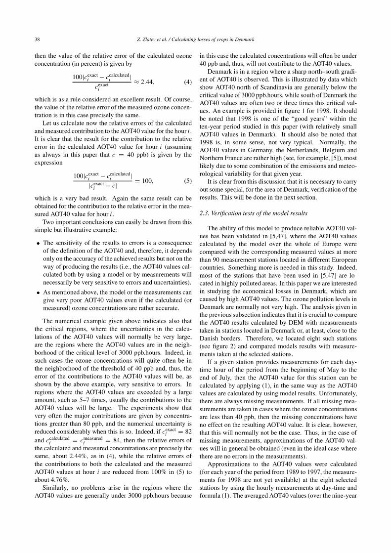
Denmark is in a region where a sharp north–south gradi-ent of AOT40 is observed. This is illustrated by data whichshow AOT40 north of Scandinavia are generally below thecritical value of 3000 ppb.hours, while south of Denmark theAOT40 values are often two or three times this critical val-ues. An example is provided in figure 1 for 1998. It shouldbe noted that 1998 is one of the “good years” within theten-year period studied in this paper (with relatively smallAOT40 values in Denmark). It should also be noted that1998 is, in some sense, not very typical. Normally, theAOT40 values in Germany, the Netherlands, Belgium andNorthern France are rather high (see, for example, [5]), mostlikely due to some combination of the emissions and meteo-rological variability for that given year.
It is clear from this discussion that it is necessary to carryout some special, for the area of Denmark, verification of theresults. This will be done in the next section.
2.3. Verification tests of the model results
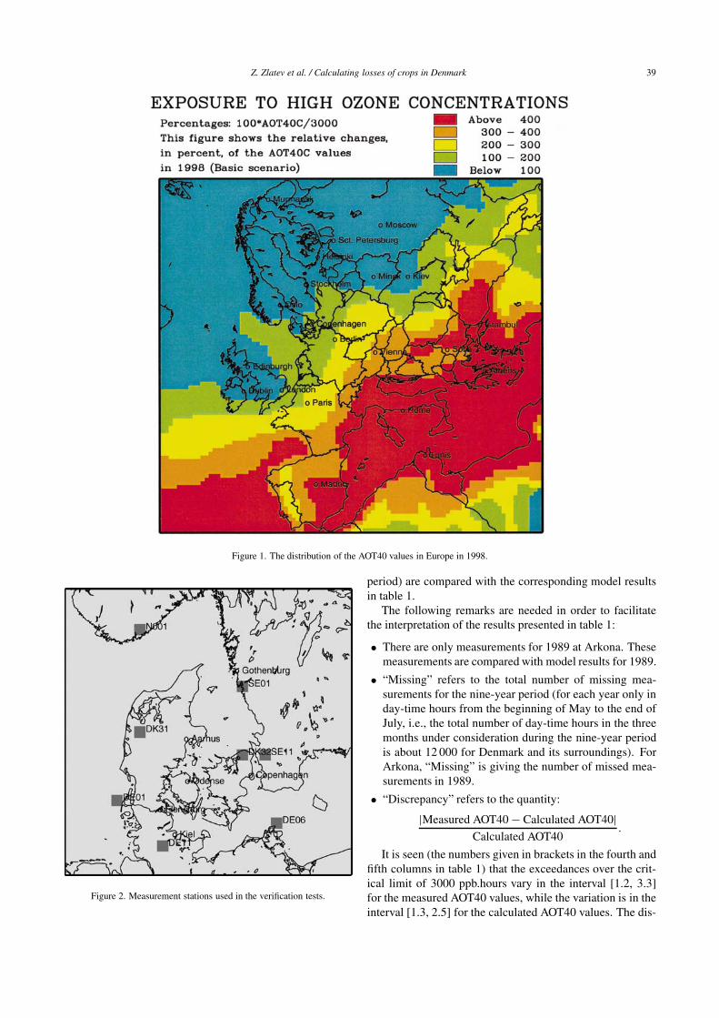
The ability of this model to produce reliable AOT40 val-ues has been validated in [5,47], where the AOT40 valuescalculated by the model over the whole of Europe werecompared with the corresponding measured values at morethan 90 measurement stations located in different Europeancountries. Something more is needed in this study. Indeed,most of the stations that have been used in [5,47] are lo-cated in highly polluted areas. In this paper we are interestedin studying the economical losses in Denmark, which arecaused by high AOT40 values. The ozone pollution levels inDenmark are normally not very high. The analysis given inthe previous subsection indicates that it is crucial to comparethe AOT40 results calculated by DEM with measurementstaken in stations located in Denmark or, at least, close to theDanish borders. Therefore, we located eight such stations(see figure 2) and compared models results with measure-ments taken at the selected stations.
If a given station provides measurements for each day-time hour of the period from the beginning of May to theend of July, then the AOT40 value for this station can becalculated by applying (1), in the same way as the AOT40values are calculated by using model results. Unfortunately,there are always missing measurements. If all missing mea-surements are taken in cases where the ozone concentrationsare less than 40 ppb, then the missing concentrations haveno effect on the resulting AOT40 value. It is clear, however,that this will normally not be the case. Thus, in the case ofmissing measurements, approximations of the AOT40 val-ues will in general be obtained (even in the ideal case wherethere are no errors in the measurements).
Approximations to the AOT40 values were calculated(for each year of the period from 1989 to 1997, the measure-ments for 1998 are not yet available) at the eight selectedstations by using the hourly measurements at day-time andformula (1). The averaged AOT40 values (over the nine-year
Z. Zlatev et al. / Calculating losses of crops in Denmark 39
Figure 1. The distribution of the AOT40 values in Europe in 1998.
Figure 2. Measurement stations used in the verification tests.
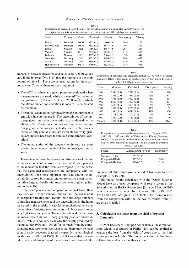
period) are compared with the corresponding model resultsin table 1.
The following remarks are needed in order to facilitatethe interpretation of the results presented in table 1:
• There are only measurements for 1989 at Arkona. Thesemeasurements are compared with model results for 1989.
• “Missing” refers to the total number of missing mea-surements for the nine-year period (for each year only inday-time hours from the beginning of May to the end ofJuly, i.e., the total number of day-time hours in the threemonths under consideration during the nine-year periodis about 12 000 for Denmark and its surroundings). ForArkona, “Missing” is giving the number of missed mea-surements in 1989.
• “Discrepancy” refers to the quantity:
|Measured AOT40 − Calculated AOT40|Calculated AOT40
.
It is seen (the numbers given in brackets in the fourth andfifth columns in table 1) that the exceedances over the crit-ical limit of 3000 ppb.hours vary in the interval [1.2, 3.3]for the measured AOT40 values, while the variation is in theinterval [1.3, 2.5] for the calculated AOT40 values. The dis-
40 Z. Zlatev et al. / Calculating losses of crops in Denmark
Table 1Comparison of averaged (over the nine-year period) measured and calculated AOT40 values. The
figures in brackets show by how much the critical value of 3000 ppb.hours is exceeded.
Station Country Code Measured Calculated Discrepancy Missing
Ulborg Denmark DK31 4328 (1.4) 6100 (2.0) 29% 2123Frederiksborg Denmark DK32 4812 (1.6) 4811 (1.6) 0% 1362Rörvik Sweden SE1 5866 (2.0) 4667 (1.6) 26% 816Vavihill Sweden SE11 7232 (2.4) 5140 (1.7) 41% 686Birkenes Norway NO1 3677 (1.2) 3806 (1.3) 3% 447Westerland Germany DE1 5971 (2.0) 7480 (2.5) 20% 672Arkona Germany DE6 9889 (3.3) 7410 (2.5) 33% 18Hohenwestedt Germany DE11 4969 (1.7) 6533 (2.2) 24% 686
crepancies between measured and calculated AOT40 valuesvary in the interval [0%, 41%] (see the numbers in the sixthcolumn of table 1). There are several reasons for these dis-crepancies. Three of them are very important:
• The AOT40 values at a given point are evaluated whenmeasurements are used, while a mean AOT40 value atthe grid-square (50 km × 50 km = 2500 km2), in whichthe station under consideration is located, is calculatedby the model.
• The model calculations rely heavily on the anthropogenicemission inventories used. The uncertainties of the an-thropogenic emission inventories are evaluated to beabout 30%. These uncertainties increase when the an-thropogenic emissions are actually used in the models(because only annual values are available for every grid-square and it is necessary to simulate some temporal vari-ations).
• The uncertainties of the biogenic emissions are evengreater than the uncertainties of the anthropogenic emis-sions.
Taking into account the above short discussion of the un-certainties, one could consider the calculated discrepanciesas an indication that the results are “good” (in the sensethat the calculated discrepancies are comparable with theuncertainties of the most important input data and/or the un-certainties caused by comparing representative mean valueson rather large grid-cells with measurements at given pointswithin the cells).
If the discrepancies are compared on annual basis, thenthey vary on a wider interval, but can still be consideredas acceptable (taking into account both the large numbersof missing measurements and the uncertainties in the inputdata used in the model). It should be emphasized here thatthe number of missing measurements at Ulborg seems to bevery high (for some years). The results obtained for the Dan-ish measurement station Ulborg, year by year, are shown intable 2. While is not very clear why the results produced bythe model for 1990 and 1997 differ so much from the corre-sponding measurements, we suspect that there may be localsubgrid scale processes (caused by specific meteorologicalconditions in 1990 and 1997). It is well known that this cantake place, and this is one of the reasons to recommend tak-
Table 2Comparison of measured and calculated annual AOT40 values at Ulborg(Denmark, DK31). The figures in brackets show by how much the critical
value of 3000 ppb.hours is exceeded.
Year Measured Calculated Discrepancy Missing
1989 7340 (2.4) 7770 (2.6) 6% 1161990 1361 (0.5) 7650 (2.6) 82% 3471991 4356 (1.5) 4920 (1.6) 11% 6371992 8619 (2.9) 7290 (2.4) 18% 4211993 4675 (1.6) 5400 (1.8) 13% 2791994 5588 (1.9) 8250 (2.8) 32% 521995 3340 (1.1) 6780 (2.3) 51% 1761996 2198 (0.7) 2700 (0.9) 19% 461997 1473 (0.5) 4140 (1.4) 64% 49
Average 4328 (1.4) 6100 (2.0) 29% 2123
Table 3Comparison of measured and calculated averaged (for years 1989,1990, 1992, 1993 and 1994) AOT40 values at Ulborg (Denmark,DK31). The figures in brackets show by how much the criticalvalue of 3000 ppb.hours is exceeded. The IIASA results are taken
from [3, table 2.8].
Source Averaged AOT40 value Discrepancy
Measured (Ulborg) 5517 (1.8) –Computed (DEM) 7272 (2.4) 24%Computed (IIASA) 8000 (2.7) 31%
ing mean AOT40 values over a period of five years (see, forexample, [3,5,15,22]).
The model results calculated with the Danish EulerianModel have also been compared with results given in theSeventh Interim IIASA Report (see [3, table 2.8]). AOT40values, which are averaged for the years 1989, 1990, 1992,1993 and 1994, are given in [3, table 2.8]. Some resultsfrom the comparison with the the AOT40 values from [3]are given in table 3.
3. Calculating the losses from the yield of crops inDenmark
If AOT40 exceeds 3000 ppb.hours, then a linear relation-ship, which is discussed in Pleijel [25], can be applied toevaluate the loss from the yield of crops due to the highozone pollution levels. The implementation of this linearrelationship is described in this section.
Z. Zlatev et al. / Calculating losses of crops in Denmark 41
The EMEP grid has to be mapped on the regional divisionof Denmark. This has been done by preparing a rectangularmatrix A. The rows of A correspond to the fourteen Danishcounties, while the columns correspond to (10 × 7) sub-gridof the EMEP grid (this sub-grid contains 70 cells and cov-ers the whole of Denmark together with some surroundingareas). Let Vi be the area of the ith Danish region. Let vij
be the part of the ith Danish region contained in the j th cell(i = 1, 2, . . . , 14, j = 1, 2, . . . , 70). Then aij = vij /Vi .This implies that the sum of the elements in each row is equalto one.
Let us assume that the yield over each region is evenlydistributed over the entire area of the region. Then it is clearthat having calculated matrix A (a special program whichdoes this has been run to calculate and store for future usematrix A) and having the AOT40 values, we can calculatethe losses by using a relationship obtained by linear regres-sion. Provided that y is the actual yield, y + z is the ex-pected yield without any ozone exposure, ξ is the AOT40 inppb.hours, the following formula is actually used to calculatethe losses:
100y/(y + z) = αξ + β (α < 0, β ≈ 100), (6)
where α and β are statistically determined coefficients. Thevalues α = −0.00151 and β = 99.5 have been used tocalculate the losses from the yield of crops in each Danishcounty as well as for the whole country in the time periodfrom 1989 to 1998. These values of α = −0.00151 andβ = 99.5 are recommended for wheat and for Scandina-vian conditions in Pleijel [25]. In the same paper Pleijeluses other values for the rest of Europe (α = −0.00177and β = 99.6). The values of the first pair (α, β) are de-termined by analyzing a large amount of experimental datataken in the Scandinavian countries, while the values of thesecond pair (α, β) are derived by using experimental datawhich are representative for the whole of Europe ([25], seealso [14,17,21]).
4. Calculating the cost of the losses
The market prices for the years in the period from 1989to 1998 have been taken from the official Danish statistics.Having the losses from the yields of crops and the prices ofthe crops for the years under consideration, it is not difficultto evaluate the cost of the losses under an assumption thatthe prices will remain the same for the expected yield (i.e.,the yield which will be obtained if the critical ozone levelswere not exceeded). This has been done for each year inthe studied period. The results obtained in these calculationswill be presented in section 6.
It would probably be more beneficial to apply somestrategies for dynamical evaluation of the prices as a func-tion of both the amount of the yield and the internationaleconomical conjuncture. Such a study requires some moreadvanced economical models. There are plans to carry outsuch a study in the future.
5. Selection of different scenarios
It is not sufficient to calculate results concerning lossesof yield from crops caused by the actual emissions. It isalso necessary to attempt to give an answer to any of thefollowing questions:
1. Is it at all possible to avoid the exceedance of the criticallevel of 3000 ppb.hours in Denmark and/or in Europe?
2. Will the critical level of 3000 ppb.hours be exceeded ifthe reduction of the appropriate emissions is very sub-stantial?
3. What will happen if the traffic emissions are drasticallyreduced?
The Danish Eulerian Model has been run with all anthro-pogenic emissions in Europe reduced to zero (but keepingthe biogenic emissions in the whole of Europe unchanged)in order to obtain an answer to the first question. The runswith this scenario, the Zero Scenario, indicate that the an-swer to the first question is positive. The AOT40 values cal-culated by using this removal were under the critical levelof 3000 ppb.hours for the whole of Europe. The mean val-ues of the ozone concentrations in Denmark were between8–15 ppb. While the removal of all anthropogenic emis-sions is not a solution which can be used in practice, theresults obtained by using this scenario are indicating that theexceedances of the AOT40 values over the critical level of3000 ppb.hours are due to anthropogenic emissions.
The Big Reductions Scenario, with large reductions of theanthropogenic emissions in Europe (again keeping the bio-genic emissions unchanged), was run to address the secondquestion. The anthropogenic NOx , VOC and CO emissionswere reduced to 15% of the 1989 levels. Also, in this case,the calculated AOT40 values were under the critical level of3000 ppb.hour in the whole of Europe. The mean values ofthe ozone concentrations in Denmark were between 19 and23 ppb.
The emissions due to traffic were reduced by a bigamount, 90%, in the attempt to answer the third question(information about the traffic emissions given in the SeventhInterim Report of IIASA [3] has been used to perform the
Table 4Comparison of the total anthropogenic NOx emissions in Europe obtainedby three scenarios. (The emissions of Scenario 2010 do not change fromone year to another, they are calculated from the emissions for 1990 byusing specific factors for each country.) The units are 1000 tonnes N per
year.
Year Basic Scenario Traffic Scenario Scenario 2010
1989 23752 10688 149801990 23277 10475 149801991 22564 10154 149801992 21614 9726 149801993 20664 9299 149801994 20189 9085 149801995 19714 8871 149801996 19239 8658 14980
42 Z. Zlatev et al. / Calculating losses of crops in Denmark
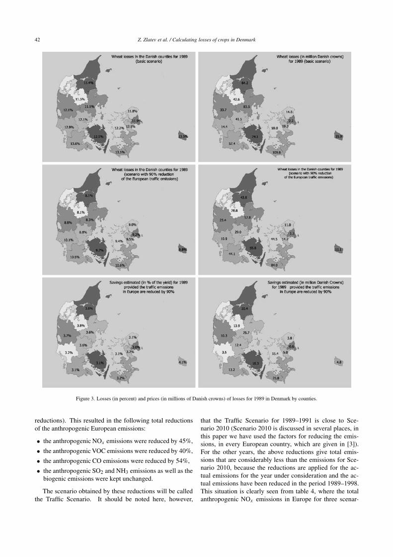
Figure 3. Losses (in percent) and prices (in millions of Danish crowns) of losses for 1989 in Denmark by counties.
reductions). This resulted in the following total reductionsof the anthropogenic European emissions:
• the anthropogenic NOx emissions were reduced by 45%,
• the anthropogenic VOC emissions were reduced by 40%,
• the anthropogenic CO emissions were reduced by 54%,
• the anthropogenic SO2 and NH3 emissions as well as thebiogenic emissions were kept unchanged.
The scenario obtained by these reductions will be calledthe Traffic Scenario. It should be noted here, however,
that the Traffic Scenario for 1989–1991 is close to Sce-nario 2010 (Scenario 2010 is discussed in several places, inthis paper we have used the factors for reducing the emis-sions, in every European country, which are given in [3]).For the other years, the above reductions give total emis-sions that are considerably less than the emissions for Sce-nario 2010, because the reductions are applied for the ac-tual emissions for the year under consideration and the ac-tual emissions have been reduced in the period 1989–1998.This situation is clearly seen from table 4, where the totalanthropogenic NOx emissions in Europe for three scenar-
Z. Zlatev et al. / Calculating losses of crops in Denmark 43
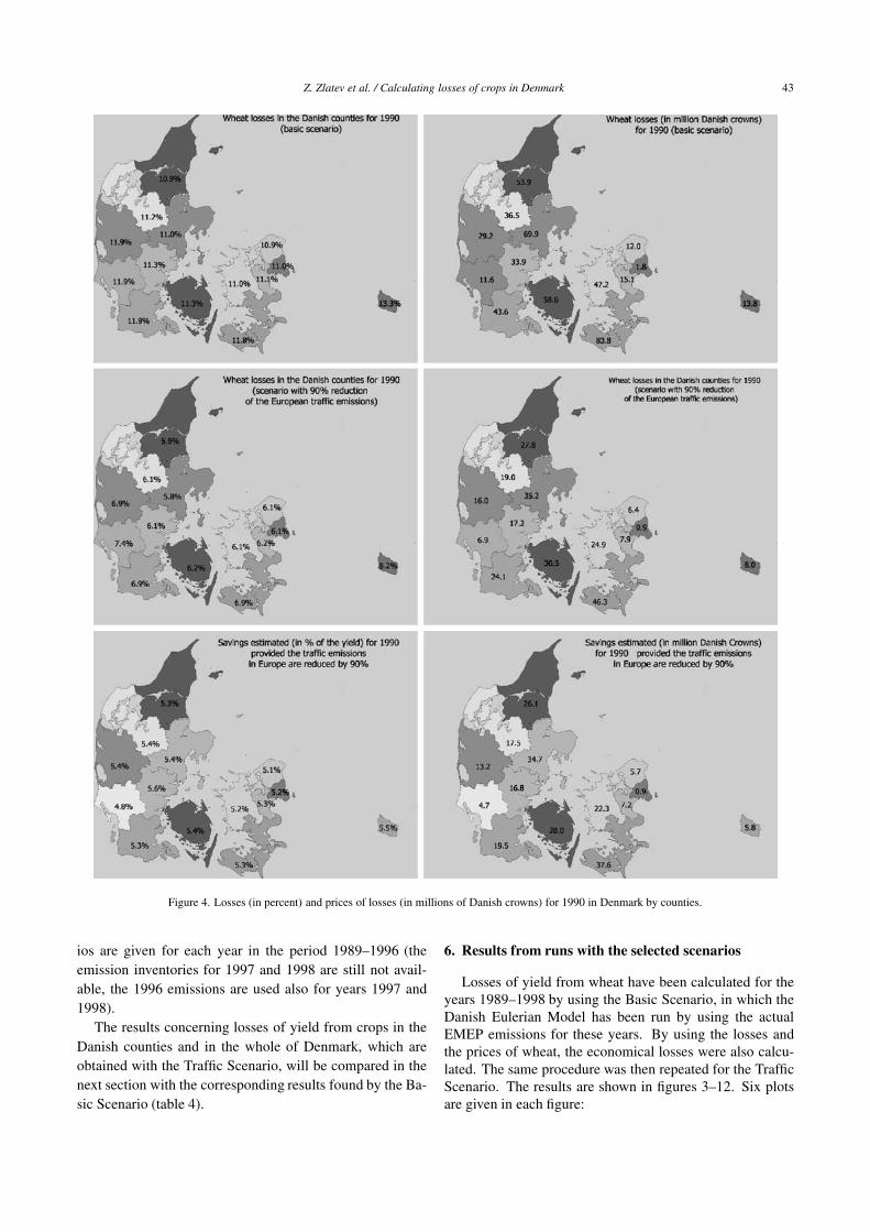
Figure 4. Losses (in percent) and prices of losses (in millions of Danish crowns) for 1990 in Denmark by counties.
ios are given for each year in the period 1989–1996 (theemission inventories for 1997 and 1998 are still not avail-able, the 1996 emissions are used also for years 1997 and1998).
The results concerning losses of yield from crops in theDanish counties and in the whole of Denmark, which areobtained with the Traffic Scenario, will be compared in thenext section with the corresponding results found by the Ba-sic Scenario (table 4).
6. Results from runs with the selected scenarios
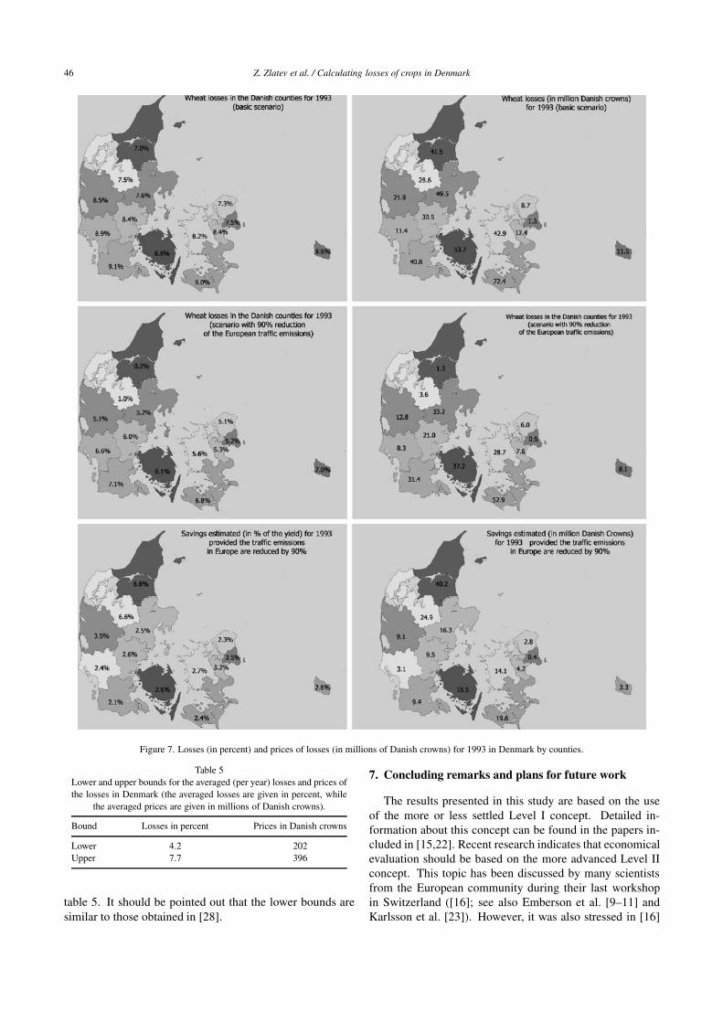
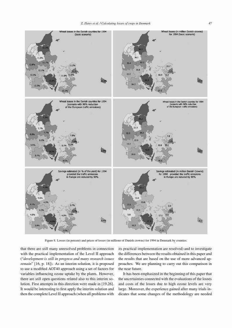
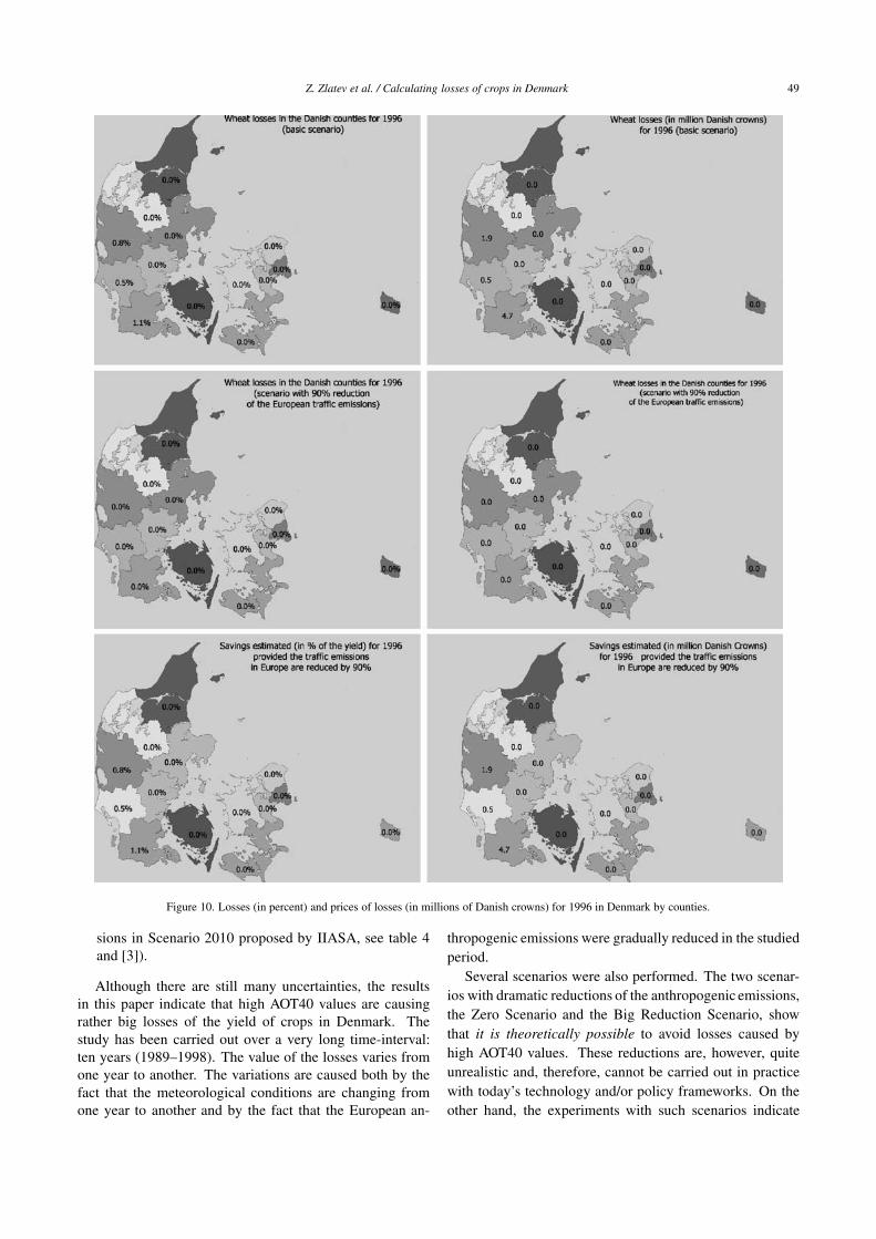
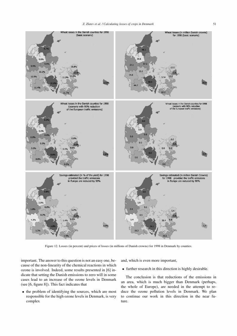
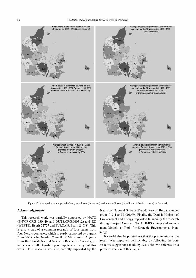
Losses of yield from wheat have been calculated for theyears 1989–1998 by using the Basic Scenario, in which theDanish Eulerian Model has been run by using the actualEMEP emissions for these years. By using the losses andthe prices of wheat, the economical losses were also calcu-lated. The same procedure was then repeated for the TrafficScenario. The results are shown in figures 3–12. Six plotsare given in each figure:
44 Z. Zlatev et al. / Calculating losses of crops in Denmark
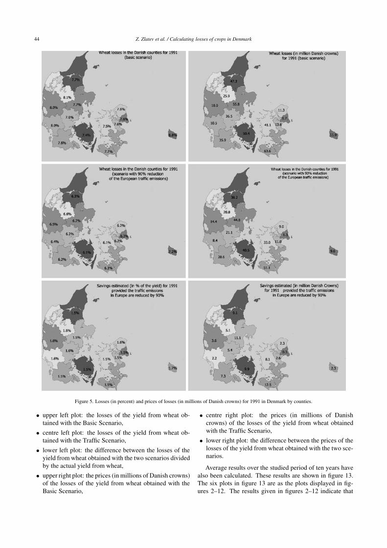
Figure 5. Losses (in percent) and prices of losses (in millions of Danish crowns) for 1991 in Denmark by counties.
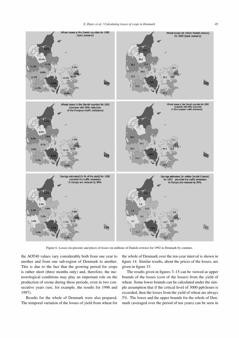
• upper left plot: the losses of the yield from wheat ob-tained with the Basic Scenario,
• centre left plot: the losses of the yield from wheat ob-tained with the Traffic Scenario,
• lower left plot: the difference between the losses of theyield from wheat obtained with the two scenarios dividedby the actual yield from wheat,
• upper right plot: the prices (in millions of Danish crowns)of the losses of the yield from wheat obtained with theBasic Scenario,
• centre right plot: the prices (in millions of Danishcrowns) of the losses of the yield from wheat obtainedwith the Traffic Scenario,
• lower right plot: the difference between the prices of thelosses of the yield from wheat obtained with the two sce-narios.
Average results over the studied period of ten years havealso been calculated. These results are shown in figure 13.The six plots in figure 13 are as the plots displayed in fig-ures 2–12. The results given in figures 2–12 indicate that
Z. Zlatev et al. / Calculating losses of crops in Denmark 45
Figure 6. Losses (in percent) and prices of losses (in millions of Danish crowns) for 1992 in Denmark by counties.
the AOT40 values vary considerably both from one year toanother and from one sub-region of Denmark to another.This is due to the fact that the growing period for cropsis rather short (three months only) and, therefore, the me-teorological conditions may play an important role on theproduction of ozone during these periods, even in two con-secutive years (see, for example, the results for 1996 and1997).
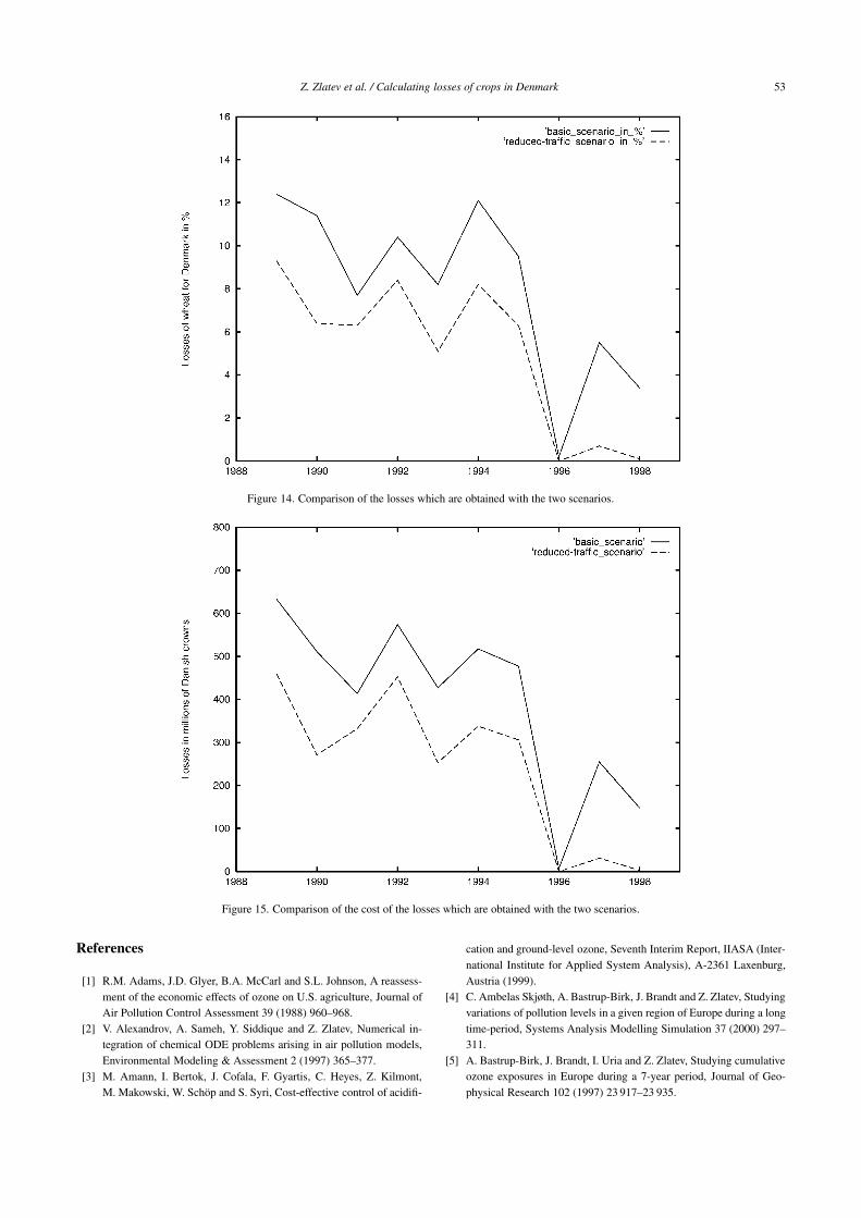
Results for the whole of Denmark were also prepared.The temporal variation of the losses of yield from wheat for
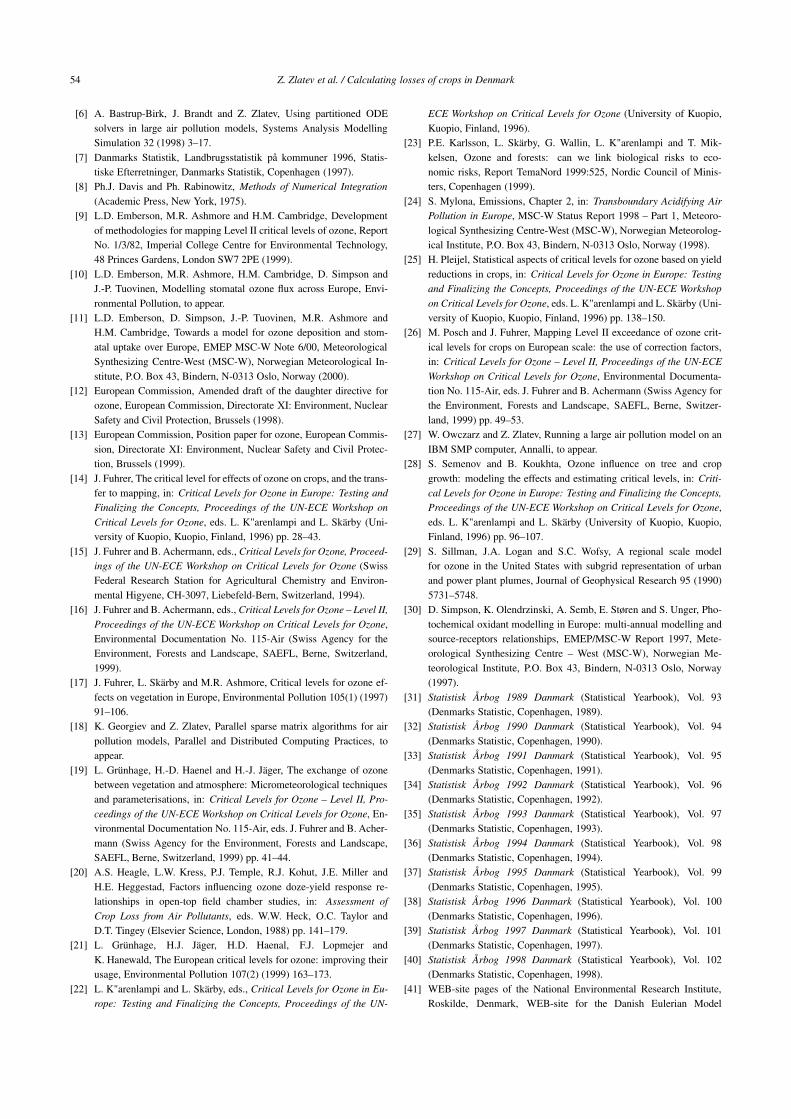
the whole of Denmark over the ten-year interval is shown infigure 14. Similar results, about the prices of the losses, aregiven in figure 15.
The results given in figures 3–15 can be viewed as upperbounds of the losses (cost of the losses) from the yield ofwheat. Some lower bounds can be calculated under the sim-ple assumption that if the critical level of 3000 ppb.hours isexceeded, then the losses from the yield of wheat are always5%. The lower and the upper bounds for the whole of Den-mark (averaged over the period of ten years) can be seen in
46 Z. Zlatev et al. / Calculating losses of crops in Denmark
Figure 7. Losses (in percent) and prices of losses (in millions of Danish crowns) for 1993 in Denmark by counties.
Table 5Lower and upper bounds for the averaged (per year) losses and prices ofthe losses in Denmark (the averaged losses are given in percent, while
the averaged prices are given in millions of Danish crowns).
Bound Losses in percent Prices in Danish crowns
Lower 4.2 202Upper 7.7 396
table 5. It should be pointed out that the lower bounds aresimilar to those obtained in [28].
7. Concluding remarks and plans for future work
The results presented in this study are based on the useof the more or less settled Level I concept. Detailed in-formation about this concept can be found in the papers in-cluded in [15,22]. Recent research indicates that economicalevaluation should be based on the more advanced Level IIconcept. This topic has been discussed by many scientistsfrom the European community during their last workshopin Switzerland ([16]; see also Emberson et al. [9–11] andKarlsson et al. [23]). However, it was also stressed in [16]
Z. Zlatev et al. / Calculating losses of crops in Denmark 47
Figure 8. Losses (in percent) and prices of losses (in millions of Danish crowns) for 1994 in Denmark by counties.
that there are still many unresolved problems in connectionwith the practical implementation of the Level II approach(“development is still in progress and many research issuesremain” [16, p. 18]). As an interim solution, it is proposedto use a modified AOT40 approach using a set of factors forvariables influencing ozone uptake by the plants. However,there are still open questions related also to this interim so-lution. First attempts in this direction were made in [19,26].It would be interesting to first apply the interim solution andthen the complete Level II approach (when all problems with
its practical implementation are resolved) and to investigatethe differences between the results obtained in this paper andthe results that are based on the use of more advanced ap-proaches. We are planning to carry out this comparison inthe near future.
It has been emphasized in the beginning of this paper thatthe uncertainties connected with the evaluations of the lossesand costs of the losses due to high ozone levels are verylarge. Moreover, the experience gained after many trials in-dicates that some changes of the methodology are needed

48 Z. Zlatev et al. / Calculating losses of crops in Denmark
Figure 9. Losses (in percent) and prices of losses (in millions of Danish crowns) for 1995 in Denmark by counties.
(see the previous paragraph). Therefore one should be care-ful when the results presented in this paper are interpreted.Three important conclusions can be drawn in spite of the dif-ficulties due to the uncertainties discussed in this paragraph:
• The results given in the figures and tables indicate thatthe losses due to high ozone levels are significant.
• The results obtained with different scenarios indicate thatthe losses can be fully avoided only if unrealistically highemission reductions are performed.
• The results indicate also that the losses can be reducedsignificantly (but not avoided) if very large reductionsof the traffic emissions are made. It should be pointedout that it is hard to believe that such big reductions ofthe traffic emissions can be achieved. However, the totalemissions in Europe can be reduced approximately to thesame level by reducing not only the traffic emissions, butalso the emissions from other sectors (it has been pointedout in section 7 that the total European emissions for theTraffic Scenario do not differ too much from the emis-
Z. Zlatev et al. / Calculating losses of crops in Denmark 49
Figure 10. Losses (in percent) and prices of losses (in millions of Danish crowns) for 1996 in Denmark by counties.
sions in Scenario 2010 proposed by IIASA, see table 4and [3]).
Although there are still many uncertainties, the resultsin this paper indicate that high AOT40 values are causingrather big losses of the yield of crops in Denmark. Thestudy has been carried out over a very long time-interval:ten years (1989–1998). The value of the losses varies fromone year to another. The variations are caused both by thefact that the meteorological conditions are changing fromone year to another and by the fact that the European an-
thropogenic emissions were gradually reduced in the studiedperiod.
Several scenarios were also performed. The two scenar-ios with dramatic reductions of the anthropogenic emissions,the Zero Scenario and the Big Reduction Scenario, showthat it is theoretically possible to avoid losses caused byhigh AOT40 values. These reductions are, however, quiteunrealistic and, therefore, cannot be carried out in practicewith today’s technology and/or policy frameworks. On theother hand, the experiments with such scenarios indicate

50 Z. Zlatev et al. / Calculating losses of crops in Denmark
Figure 11. Losses (in percent) and prices of losses (in millions of Danish crowns) for 1997 in Denmark by counties.
that the exceedances are entirely due to anthropogenic emis-sions.
The runs with the Traffic Scenario indicate that reduc-tions of the emissions which are less than those suggestedin the well-known Scenario 2010 (but comparable with it)will reduce the amount of losses due to high AOT40 values.However, the losses will in general not be avoided, even inthe Danish area. On the other hand, the results in this paperare important to the assessment of benefits associated withtraffic emissions reduction policy.
The question of finding the optimal (which in this con-text means, roughly speaking, the smallest) reductions forthe European emissions by which the critical value of 3000ppb.hours will not be exceeded is still open. Probably, it willnot be possible to implement in practice such optimal reduc-tions when these are found (these reductions will still be toobig, which is indicated from the previous conclusion aboutthe Traffic Scenario).
Finally, the question of identifying the emission sources,which are most important for the ozone levels in Denmark, is
Z. Zlatev et al. / Calculating losses of crops in Denmark 51
Figure 12. Losses (in percent) and prices of losses (in millions of Danish crowns) for 1998 in Denmark by counties.
important. The answer to this question is not an easy one, be-cause of the non-linearity of the chemical reactions in whichozone is involved. Indeed, some results presented in [6] in-dicate that setting the Danish emissions to zero will in somecases lead to an increase of the ozone levels in Denmark(see [6, figure 8]). This fact indicates that
• the problem of identifying the sources, which are mostresponsible for the high ozone levels in Denmark, is verycomplex
and, which is even more important,
• further research in this direction is highly desirable.
The conclusion is that reductions of the emissions inan area, which is much bigger than Denmark (perhaps,the whole of Europe), are needed in the attempt to re-duce the ozone pollution levels in Denmark. We planto continue our work in this direction in the near fu-ture.
52 Z. Zlatev et al. / Calculating losses of crops in Denmark
Figure 13. Averaged, over the period of ten years, losses (in percent) and prices of losses (in millions of Danish crowns) in Denmark.
Acknowledgements
This research work was partially supported by NATO(ENVIR.CRG 930449 and OUTS.CRG.960312) and EU(WEPTEL Esprit 22727 and EUROAIR Esprit 24618). Thisis also a part of a common research of four teams fromfour Nordic countries, which is partly supported by a grantfrom NMR (the Nordic Council of Ministers). A grantfrom the Danish Natural Sciences Research Council gaveus access to all Danish supercomputers to carry out thiswork. This research was also partially supported by the
NSF (the National Science Foundation) of Bulgaria undergrants I-811 and I-901/99. Finally, the Danish Ministry ofEnvironment and Energy supported financially the researchthrough Project Contract No. 4: IMIS (Integrated Assess-ment Models as Tools for Strategic Environmental Plan-ning).
It should also be pointed out that the presentation of theresults was improved considerably by following the con-structive suggestions made by two unknown referees on aprevious version of this paper.
Z. Zlatev et al. / Calculating losses of crops in Denmark 53
Figure 14. Comparison of the losses which are obtained with the two scenarios.
Figure 15. Comparison of the cost of the losses which are obtained with the two scenarios.
References
[1] R.M. Adams, J.D. Glyer, B.A. McCarl and S.L. Johnson, A reassess-ment of the economic effects of ozone on U.S. agriculture, Journal ofAir Pollution Control Assessment 39 (1988) 960–968.
[2] V. Alexandrov, A. Sameh, Y. Siddique and Z. Zlatev, Numerical in-tegration of chemical ODE problems arising in air pollution models,Environmental Modeling & Assessment 2 (1997) 365–377.
[3] M. Amann, I. Bertok, J. Cofala, F. Gyartis, C. Heyes, Z. Kilmont,M. Makowski, W. Schöp and S. Syri, Cost-effective control of acidifi-
cation and ground-level ozone, Seventh Interim Report, IIASA (Inter-national Institute for Applied System Analysis), A-2361 Laxenburg,Austria (1999).
[4] C. Ambelas Skjøth, A. Bastrup-Birk, J. Brandt and Z. Zlatev, Studyingvariations of pollution levels in a given region of Europe during a longtime-period, Systems Analysis Modelling Simulation 37 (2000) 297–311.
[5] A. Bastrup-Birk, J. Brandt, I. Uria and Z. Zlatev, Studying cumulativeozone exposures in Europe during a 7-year period, Journal of Geo-physical Research 102 (1997) 23 917–23 935.
54 Z. Zlatev et al. / Calculating losses of crops in Denmark
[6] A. Bastrup-Birk, J. Brandt and Z. Zlatev, Using partitioned ODEsolvers in large air pollution models, Systems Analysis ModellingSimulation 32 (1998) 3–17.
[7] Danmarks Statistik, Landbrugsstatistik på kommuner 1996, Statis-tiske Efterretninger, Danmarks Statistik, Copenhagen (1997).
[8] Ph.J. Davis and Ph. Rabinowitz, Methods of Numerical Integration
(Academic Press, New York, 1975).[9] L.D. Emberson, M.R. Ashmore and H.M. Cambridge, Development
of methodologies for mapping Level II critical levels of ozone, ReportNo. 1/3/82, Imperial College Centre for Environmental Technology,48 Princes Gardens, London SW7 2PE (1999).
[10] L.D. Emberson, M.R. Ashmore, H.M. Cambridge, D. Simpson andJ.-P. Tuovinen, Modelling stomatal ozone flux across Europe, Envi-ronmental Pollution, to appear.
[11] L.D. Emberson, D. Simpson, J.-P. Tuovinen, M.R. Ashmore andH.M. Cambridge, Towards a model for ozone deposition and stom-atal uptake over Europe, EMEP MSC-W Note 6/00, MeteorologicalSynthesizing Centre-West (MSC-W), Norwegian Meteorological In-stitute, P.O. Box 43, Bindern, N-0313 Oslo, Norway (2000).
[12] European Commission, Amended draft of the daughter directive forozone, European Commission, Directorate XI: Environment, NuclearSafety and Civil Protection, Brussels (1998).
[13] European Commission, Position paper for ozone, European Commis-sion, Directorate XI: Environment, Nuclear Safety and Civil Protec-tion, Brussels (1999).
[14] J. Fuhrer, The critical level for effects of ozone on crops, and the trans-fer to mapping, in: Critical Levels for Ozone in Europe: Testing andFinalizing the Concepts, Proceedings of the UN-ECE Workshop on
Critical Levels for Ozone, eds. L. K"arenlampi and L. Skärby (Uni-versity of Kuopio, Kuopio, Finland, 1996) pp. 28–43.
[15] J. Fuhrer and B. Achermann, eds., Critical Levels for Ozone, Proceed-ings of the UN-ECE Workshop on Critical Levels for Ozone (SwissFederal Research Station for Agricultural Chemistry and Environ-mental Higyene, CH-3097, Liebefeld-Bern, Switzerland, 1994).
[16] J. Fuhrer and B. Achermann, eds., Critical Levels for Ozone – Level II,
Proceedings of the UN-ECE Workshop on Critical Levels for Ozone,Environmental Documentation No. 115-Air (Swiss Agency for theEnvironment, Forests and Landscape, SAEFL, Berne, Switzerland,1999).
[17] J. Fuhrer, L. Skärby and M.R. Ashmore, Critical levels for ozone ef-fects on vegetation in Europe, Environmental Pollution 105(1) (1997)91–106.
[18] K. Georgiev and Z. Zlatev, Parallel sparse matrix algorithms for airpollution models, Parallel and Distributed Computing Practices, toappear.
[19] L. Grünhage, H.-D. Haenel and H.-J. Jäger, The exchange of ozonebetween vegetation and atmosphere: Micrometeorological techniquesand parameterisations, in: Critical Levels for Ozone – Level II, Pro-
ceedings of the UN-ECE Workshop on Critical Levels for Ozone, En-vironmental Documentation No. 115-Air, eds. J. Fuhrer and B. Acher-mann (Swiss Agency for the Environment, Forests and Landscape,SAEFL, Berne, Switzerland, 1999) pp. 41–44.
[20] A.S. Heagle, L.W. Kress, P.J. Temple, R.J. Kohut, J.E. Miller andH.E. Heggestad, Factors influencing ozone doze-yield response re-lationships in open-top field chamber studies, in: Assessment of
Crop Loss from Air Pollutants, eds. W.W. Heck, O.C. Taylor andD.T. Tingey (Elsevier Science, London, 1988) pp. 141–179.
[21] L. Grünhage, H.J. Jäger, H.D. Haenal, F.J. Lopmejer andK. Hanewald, The European critical levels for ozone: improving theirusage, Environmental Pollution 107(2) (1999) 163–173.
[22] L. K"arenlampi and L. Skärby, eds., Critical Levels for Ozone in Eu-rope: Testing and Finalizing the Concepts, Proceedings of the UN-
ECE Workshop on Critical Levels for Ozone (University of Kuopio,Kuopio, Finland, 1996).
[23] P.E. Karlsson, L. Skärby, G. Wallin, L. K"arenlampi and T. Mik-kelsen, Ozone and forests: can we link biological risks to eco-nomic risks, Report TemaNord 1999:525, Nordic Council of Minis-ters, Copenhagen (1999).
[24] S. Mylona, Emissions, Chapter 2, in: Transboundary Acidifying AirPollution in Europe, MSC-W Status Report 1998 – Part 1, Meteoro-logical Synthesizing Centre-West (MSC-W), Norwegian Meteorolog-ical Institute, P.O. Box 43, Bindern, N-0313 Oslo, Norway (1998).
[25] H. Pleijel, Statistical aspects of critical levels for ozone based on yieldreductions in crops, in: Critical Levels for Ozone in Europe: Testingand Finalizing the Concepts, Proceedings of the UN-ECE Workshop
on Critical Levels for Ozone, eds. L. K"arenlampi and L. Skärby (Uni-versity of Kuopio, Kuopio, Finland, 1996) pp. 138–150.
[26] M. Posch and J. Fuhrer, Mapping Level II exceedance of ozone crit-ical levels for crops on European scale: the use of correction factors,in: Critical Levels for Ozone – Level II, Proceedings of the UN-ECE
Workshop on Critical Levels for Ozone, Environmental Documenta-tion No. 115-Air, eds. J. Fuhrer and B. Achermann (Swiss Agency forthe Environment, Forests and Landscape, SAEFL, Berne, Switzer-land, 1999) pp. 49–53.
[27] W. Owczarz and Z. Zlatev, Running a large air pollution model on anIBM SMP computer, Annalli, to appear.
[28] S. Semenov and B. Koukhta, Ozone influence on tree and cropgrowth: modeling the effects and estimating critical levels, in: Criti-cal Levels for Ozone in Europe: Testing and Finalizing the Concepts,Proceedings of the UN-ECE Workshop on Critical Levels for Ozone,eds. L. K"arenlampi and L. Skärby (University of Kuopio, Kuopio,Finland, 1996) pp. 96–107.
[29] S. Sillman, J.A. Logan and S.C. Wofsy, A regional scale modelfor ozone in the United States with subgrid representation of urbanand power plant plumes, Journal of Geophysical Research 95 (1990)5731–5748.
[30] D. Simpson, K. Olendrzinski, A. Semb, E. Støren and S. Unger, Pho-tochemical oxidant modelling in Europe: multi-annual modelling andsource-receptors relationships, EMEP/MSC-W Report 1997, Mete-orological Synthesizing Centre – West (MSC-W), Norwegian Me-teorological Institute, P.O. Box 43, Bindern, N-0313 Oslo, Norway(1997).
[31] Statistisk Årbog 1989 Danmark (Statistical Yearbook), Vol. 93(Denmarks Statistic, Copenhagen, 1989).
[32] Statistisk Årbog 1990 Danmark (Statistical Yearbook), Vol. 94(Denmarks Statistic, Copenhagen, 1990).
[33] Statistisk Årbog 1991 Danmark (Statistical Yearbook), Vol. 95(Denmarks Statistic, Copenhagen, 1991).
[34] Statistisk Årbog 1992 Danmark (Statistical Yearbook), Vol. 96(Denmarks Statistic, Copenhagen, 1992).
[35] Statistisk Årbog 1993 Danmark (Statistical Yearbook), Vol. 97(Denmarks Statistic, Copenhagen, 1993).
[36] Statistisk Årbog 1994 Danmark (Statistical Yearbook), Vol. 98(Denmarks Statistic, Copenhagen, 1994).
[37] Statistisk Årbog 1995 Danmark (Statistical Yearbook), Vol. 99(Denmarks Statistic, Copenhagen, 1995).
[38] Statistisk Årbog 1996 Danmark (Statistical Yearbook), Vol. 100(Denmarks Statistic, Copenhagen, 1996).
[39] Statistisk Årbog 1997 Danmark (Statistical Yearbook), Vol. 101(Denmarks Statistic, Copenhagen, 1997).
[40] Statistisk Årbog 1998 Danmark (Statistical Yearbook), Vol. 102(Denmarks Statistic, Copenhagen, 1998).
[41] WEB-site pages of the National Environmental Research Institute,Roskilde, Denmark, WEB-site for the Danish Eulerian Model
Z. Zlatev et al. / Calculating losses of crops in Denmark 55
(DEM), http://www.dmu.dk/AtmosphericEnvironment/DEM, Na-
tional Environmental Research Institute, Roskilde, Denmark (1999).
[42] Z. Zlatev, Computer Treatment of Large Air Pollution Models
(Kluwer Academic Publishers, Dordrecht, 1995).
[43] Z. Zlatev, J. Christensen and A. Eliassen, Studying high ozone
concentrations by using the Danish Eulerian Model, Atmospheric
Environment 27A (1993) 845–865.
[44] Z. Zlatev, J. Christensen and Ø. Hov, An Eulerian air pollution
model for Europe with nonlinear chemistry, Journal of Atmospheric
Chemistry 15 (1992) 1–37.
[45] Z. Zlatev, I. Dimov and K. Georgiev, Studying long-range transportof air pollutants, Computational Science and Engineering 1 (1994)45–52.
[46] Z. Zlatev, I. Dimov and K. Georgiev, Three-dimensional version ofthe Danish Eulerian Model, Zeitschrift für Angewandte Mathematikund Mechanik 76 (1996) 473–476.
[47] Z. Zlatev, J. Fenger and L. Mortensen, Relationships betweenemission sources and excess ozone concentrations, Computers andMathematics with Applications 32 (1996) 101–123.