1

C H A P T E R 1

Introductory Background

1.1 Introduction

Although pavement design has gradually evolved from art to science, empirical

methodologies still play an important role up to date. Prior to early 1920s,

determination of pavement thickness was based purely on experience.

Generally, the same thickness would be used for different sections of varying

pavement soil conditions. As experience was gained and following pavement

research throughout the years, various methods were developed by different

agencies for determination of the required pavement thickness. It is not feasible

to document all design methods that have evolved and applied. However, in this

study, only a few typical methods will be cited and discussed to indicate the

trend. [6]

Rigid (or concrete) pavements (RPs) are constructed of Portland cement

concrete (PCC). The first concrete pavement was built in Bellefontaine, Ohio in

1893 (Fitch, 1996), 15 years earlier than the one constructed in Detroit,

Michigan, in 1908. As of 2001, there were about 59,000 miles (95,000 km) of

rigid pavements in the United States. The development of design methods for

rigid pavements is not as dramatic as that of flexible pavements, because the

flexural stress in concrete has long been considered as a major design factor.

Concrete pavements can be classified into four types: jointed plain concrete

pavement (JPCP), jointed reinforced concrete pavement (JRCP), continuous

reinforced concrete pavement (CRCP), and pre-stressed concrete pavement

(PCP). Except for PCP with lateral pre-stressing, a longitudinal joint should be

installed between two traffic lanes to prevent longitudinal cracking. The JPCP,

requiring no steel reinforcements and thus the least expensive to construct, is a

popular form of construction. Depending on the thickness of the slab, typical

2

joint spacings for plain concrete pavements are between 10 and 20 ft (3 and 6

m). For slabs with joint spacing greater than 6 m, steel reinforcements have to

be provided for crack control, giving rise to the use of JRCP and CRCP. [6]

Structural design of rigid pavements includes thickness and reinforcement

designs. Two major approaches for RP thickness design methods are applied in

this study: The first approach relies on empirical relationships derived from

performance of full-scale experimental pavements and in-service pavements

performed by the American Association of State Highway and Transportation

Officials (AASHTO, 1993). The second one develops relationships in terms of

the properties of pavement materials as well as load-induced and thermal

stresses, calibrating these relationships with pavement performance data. The

Portland Cement Association (PCA) method of design adopted this approach

(1984).

In this research investigation, thickness design for JPCP by AASHTO and PCA

methods was determined for the case study pavement. However, reinforced

design by AASHTO procedure was performed for the JRCP suggested to be

used in the construction of the proposed road. A computer program with Visual

Basic software was developed, entitled GalalM-RP program, to determine the

rigid pavement design thickness in accordance with PCA method. Comparison

was then made for the rigid pavement design thickness between the manual

method and GalalM-RP program.

Sparseness and increasing cost of construction materials along with heavy axle

loads, environmental conditions and inadequate design and construction lead to

premature failure of roads and force engineers to consider more economical and

long life pavement design methods to build roads using indigenous pavement

materials and advanced construction techniques. The situation becomes even

more critical in underdeveloped countries (Ali, 2003). Additionally, in order to

achieve minimum production costs, it is considered necessary to have cost-

3

effective construction of roads with optimum performance and low maintenance

costs. (Ali et al., 2012) and Ali and Gasim (2014) conducted comparative

studies for JPCP versus flexible pavement for Sudan highways and urban roads

under different soil strength and traffic conditions. It was found that:

1. Using rigid pavement reduces construction costs by 10 to 35 % depending on

subgrade strength and ESAL compared to flexible.

2. Considering the fact that the natural ground in most residential areas targeted

with road project is black cotton soil with high plasticity, it was shown that

using rigid pavement would reduce the overall construction cost.

3. The availability of natural gravel and sand in many areas in the country will

further reduce the cost of rigid pavement compared to flexible pavement due to

their suitability for use in rigid pavement compared to costly crushed aggregate

foe asphalt pavement. [5]

Similar studies were carried out in India (Prasad, 2007) and Turkey (Ukar et al.,

2007) [10] and [12] . In the present investigation, comparison was made

between two types of rigid pavements: Jointed plain concrete pavement (JPCP)

versus jointed reinforced concrete pavement (JRCP). [4]

1.2 Problem Statement and Significance

Selecting a pavement type is an important decision. Similar to other aspects of

pavement design, such as traffic loading and materials, the 1993 AASHTO

Guide indicates that the selection of pavement type is based on many varying

factors, material selection representing along with design traffic the main factors

related to desired pavement performance. Proper selection of materials and

understanding of how they perform in the field within the composite pavement

structure must be based on careful consideration of expected traffic loads with

all related variables, the environment, construction practices and evaluation.

Other considerations, such as availability of materials and economics, will often

influence which materials are ultimately selected. While it is preferred to use the

4

highest quality of materials for all road projects, materials must be of sufficient

uniformity and quality to provide the following performance indicators under

expected traffic loading and environmental conditions:

Adequate serviceability at minimum cost;

Best serviceability according to available funds; and

Maximum mobility at minimum cost.

Pavement distresses and their causes, in addition to long-term performance, are

other important factors for selection and adoption of pavement type. For

instance, the pavement type selected should in general provide the following

required improvements: reduced life-cycle cost, shorter construction periods,

less disruption to traffic, residents and business, and safe and manageable field

activities (Ali et al., 2012). Additionally, utility cuts, a major concern, should be

minimized, knowing that poor performance is getting difficult to manage.

As a result of the several steps involved in the PCA design method with trial

thicknesses, development of a computer program was considered necessary to

assist an contribute in reducing the time for iterations.

1.3 The Design Methods and Procedures Two methods of design methods were selected for both pavement types. A case

study and applications included an urban-rural highway (Al-Ilaifoun Road).

Thickness design for JPCP by AASHTO and PCA methods was determined for

the case study pavement. However, reinforced design by AASHTO procedure

was performed for the JRCP suggested to be used in the construction of the

proposed road. A computer program with Visual Basic software was developed,

entitled GalalM-RP program, to determine the rigid pavement design thickness

in accordance with PCA method.

5

1.4 Objectives and Scope of Research

The general objectives of the study are:

1- Design thickness of rigid pavement obtained through manual and Galal R.P.

which uses Visual Basic software with PCA procedure.

2- Application of popular structural design methods for the purpose of

comparing costs was another objective of undertaking this study

1.5 Out Line of Thesis

This thesis has six chapters (in addition to this one) and two appendices.

Chapter 2 describes rigid pavement types and design methodology for Joint

Plan and Jointed Reinforce Concrete Pavements .Chapter 3 describes Location

and Characteristics, ESAL of the case study road project. Chapter 4 designs of

Joint Plan and Jointed Reinforce Concrete Pavement for case study road project.

Chapter 5 application of software program and introduces the computer

software tool developed under the project. Chapter 6 summarizes the results.

Chapter 7 summarizes the thesis conclusions and recommendations. Appendix

A contains the PCA design method tables and Charts. Appendix B contains the

AASHTO design method tables and Charts.

6

C H A P T E R 2

RIGID PAVEMENT TYPES AND DESIGN

METHODOLOGIES FOR JOINTED PLAIN AND JOINTED

REINFORCED CONCRETE PAVEMENTS

2.1 Introduction

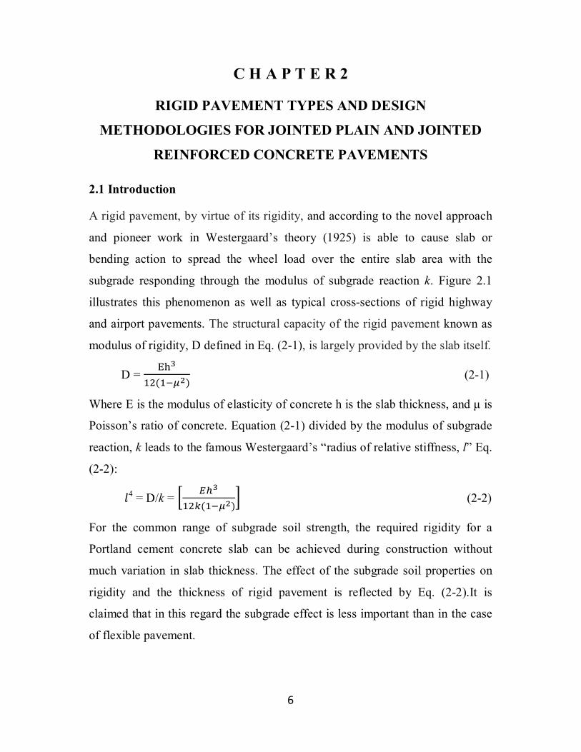
A rigid pavement, by virtue of its rigidity, and according to the novel approach

and pioneer work in Westergaard’s theory (1925) is able to cause slab or

bending action to spread the wheel load over the entire slab area with the

subgrade responding through the modulus of subgrade reaction k. Figure 2.1

illustrates this phenomenon as well as typical cross-sections of rigid highway

and airport pavements. The structural capacity of the rigid pavement known as

modulus of rigidity, D defined in Eq. (2-1), is largely provided by the slab itself.

D = ( )

(2-1)

Where E is the modulus of elasticity of concrete h is the slab thickness, and μ is

Poisson’s ratio of concrete. Equation (2-1) divided by the modulus of subgrade

reaction, k leads to the famous Westergaard’s “radius of relative stiffness, l” Eq.

(2-2):

푙4 = D/k = ( )

(2-2)

For the common range of subgrade soil strength, the required rigidity for a

Portland cement concrete slab can be achieved during construction without

much variation in slab thickness. The effect of the subgrade soil properties on

rigidity and the thickness of rigid pavement is reflected by Eq. (2-2).It is

claimed that in this regard the subgrade effect is less important than in the case

of flexible pavement.

7

Regarding the base course for rigid pavement, sometimes subbase might suffice,

is often provided to prevent pumping resulting from ejection of foundation

material through cracks or joints due to vertical movement of slabs under traffic.

The base course is generally required to provide good drainage and resistance to

the erosive action of water. When dowel bars are not provided in short jointed

pavements, it is common practice to construct cement-treated base (CTB) to

assist in load transfer across the joints. [7]

FIGURE 2.1 Rigid Pavement rigidity and Typical Thickness

Concrete is material which is strong in compression, but relatively weak when

placed in tension. Tensile stresses may build up in concrete pavements because

of shrinkage during the hydration process, temperature and moisture changes,

and/or traffic loadings. When the tensile stresses are great enough, cracks occur.

Joints are often used as a means of relieving stresses to control cracking. Joints

can also serve to protect adjacent structures, or to accommodate paving

operations. [11]

8

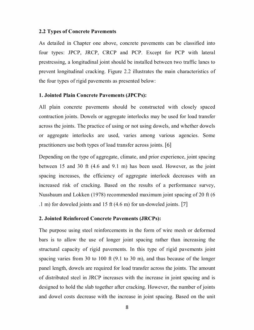
2.2 Types of Concrete Pavements

As detailed in Chapter one above, concrete pavements can be classified into

four types: JPCP, JRCP, CRCP and PCP. Except for PCP with lateral

prestressing, a longitudinal joint should be installed between two traffic lanes to

prevent longitudinal cracking. Figure 2.2 illustrates the main characteristics of

the four types of rigid pavements as presented below:

1. Jointed Plain Concrete Pavements (JPCPs):

All plain concrete pavements should be constructed with closely spaced

contraction joints. Dowels or aggregate interlocks may be used for load transfer

across the joints. The practice of using or not using dowels, and whether dowels

or aggregate interlocks are used, varies among various agencies. Some

practitioners use both types of load transfer across joints. [6]

Depending on the type of aggregate, climate, and prior experience, joint spacing

between 15 and 30 ft (4.6 and 9.1 m) has been used. However, as the joint

spacing increases, the efficiency of aggregate interlock decreases with an

increased risk of cracking. Based on the results of a performance survey,

Nussbaum and Lokken (1978) recommended maximum joint spacing of 20 ft (6

.1 m) for doweled joints and 15 ft (4.6 m) for un-doweled joints. [7]

2. Jointed Reinforced Concrete Pavements (JRCPs):

The purpose using steel reinforcements in the form of wire mesh or deformed

bars is to allow the use of longer joint spacing rather than increasing the

structural capacity of rigid pavements. In this type of rigid pavements joint

spacing varies from 30 to 100 ft (9.1 to 30 m), and thus because of the longer

panel length, dowels are required for load transfer across the joints. The amount

of distributed steel in JRCP increases with the increase in joint spacing and is

designed to hold the slab together after cracking. However, the number of joints

and dowel costs decrease with the increase in joint spacing. Based on the unit

9

costs of sawing, mesh, dowels, and joint sealants, Nussbaum and Lokken (1978)

found that the most economical joint spacing was about 40 ft (12.2 m).

Maintenance costs generally increase with the increase in joint spacing, and

hence the selection of 40 ft (12 .2 m) as the maximum joint spacing appears to

be warranted.[6]

FIGURE 2.2 Four types of concrete pavements (1 ft = 0 .305 m)

3. Continuous Reinforced Concrete Pavements (CRCPs):

Elimination of joints prompted the first experimental use of CRCP in 1921 on

Columbia Pike near Washington, D.C. The advantages of the joint-free design

were widely accepted by many agencies. In the United States of America (USA)

more than two dozen States have used CRCP with a two-lane mileage totaling

over 20,000 miles (32,000 km). It was originally reasoned that joints were the

weak spots in rigid pavements and that the elimination of joints would decrease

the required thickness of pavement. As a result, the thickness of CRCP has been

10

empirically reduced by 1 to 2 in. (25 to 50 mm) or arbitrarily taken as 70 to 80%

of the conventional pavement.

Formation of transverse cracks at relatively close intervals is a distinct

characteristic of CRCP. These cracks are held tightly by the reinforcements and

should be of no concern as long as they are uniformly spaced. The distress that

occurs most frequently in CRCP is punch out at the pavement edge. Occurrence

of failure at the pavement edge rather than at the joint, does not necessarily

justify using thinner CRCP. The 1986 AASHTO design guide suggests using

the same equation or nomograph for determining the thickness of JRCP and

CRCP. The amount of longitudinal reinforcing steel should be designed to

control the spacing and width of cracks and the maximum stress in the steel.[6]

4. Prestressed Concrete Pavements (PCPs):

The thickness of concrete pavement required is governed by its modulus of

rupture, MR which varies with the tensile strength of concrete. The pre-

application of compressive stress to the concrete, greatly reduces the tensile

stress caused by the traffic loads and thus decreases the required thickness of

concrete. Prestressed concrete pavements have less probability of cracking and

fewer transverse joints and therefore result in less maintenance and longer

pavement life. They have been used more frequently in airport pavements than

in highway pavements because the saving in thickness for airport pavements is

much greater than that for highway pavements. Prestressed concrete pavements

are still at the experimental stage, and their design arises primarily from the

application of experience and engineering judgment (Huang, 2004)[6]. In this

thesis investigation, jointed plain concrete pavement (JPCP) and jointed

reinforced concrete pavement (JRCP) have been selected for comparative study.

11

2.3 Joints and Dowel Bars

Pavement joints are vital to control pavement cracking and pavement

movement. Without joints, most concrete pavements would be riddled with

cracks within one or two years after placement. Water, ice, salt and loads would

eventually cause differential settlement and premature pavement failures. These

same effects may be caused by incorrectly placed or poorly designed pavement

joints. Joint spacing in feet for plain concrete pavements should not greatly

exceed twice the slab thickness in inches, and the ratio of slab width to length

should not be greater than 1.25. There are four types of joints in common use:

contraction, expansion, construction, and longitudinal joints. Contraction joints

are usually placed at regular intervals perpendicular to the center line of

pavements. Expansion joints are used only at the connection between pavement

sections and structures adjacent to the road. Longitudinal joints are used to

relieve curling and warping stresses. Details of these joints, design and

dimensions may be found elsewhere (AASHTO, 2003; Huang, 2004). [1]

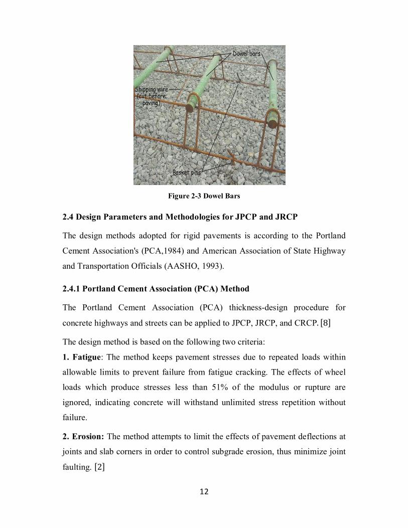
Dowel bars (figure2-3) are used at joints on long slabs or where load transfer by

interlock is suspect. Interlock depends upon many factors including the distance

a joint will open as a result of shrinkage and/or temperature contraction. Joints

without dowels are generally satisfactory if the joint opening is 0.04 inch or

less. For doweled joints, the opening should be 0.25 inch or less. Hence, short

slab pavements generally do not use dowels. However, it has become the

practice of many engineers to use dowels regardless of joint spacing. It is to be

recalled that the short slabs on the AASHO Road Test contained dowels. [13]

12

Fiigure 2.3 Dowel Bars

Figure 2-3 Dowel Bars

2.4 Design Parameters and Methodologies for JPCP and JRCP

The design methods adopted for rigid pavements is according to the Portland

Cement Association's (PCA,1984) and American Association of State Highway

and Transportation Officials (AASHO, 1993).

2.4.1 Portland Cement Association (PCA) Method

The Portland Cement Association (PCA) thickness-design procedure for

concrete highways and streets can be applied to JPCP, JRCP, and CRCP. [8]

The design method is based on the following two criteria:

1. Fatigue: The method keeps pavement stresses due to repeated loads within

allowable limits to prevent failure from fatigue cracking. The effects of wheel

loads which produce stresses less than 51% of the modulus or rupture are

ignored, indicating concrete will withstand unlimited stress repetition without

failure.

2. Erosion: The method attempts to limit the effects of pavement deflections at

joints and slab corners in order to control subgrade erosion, thus minimize joint

faulting. [2]

13

2.4.1.1 Design factors

Based on the selection of doweled joints and concrete shoulders, the thickness

design is governed by five design factors, namely concrete modulus of rupture

(MR), modulus of subgrade reaction (k), subbase elastic modulus (ESB), design

period (n) and design traffic (Cumulative ESAL). These factors are discussed

below.

1. Concrete Modulus of Rupture (MR)

The flexural strength of concrete represents the modulus of rupture determined

at 28 days using ASTM C78-84 Standard Test Method specified for Flexural

Strength of Concrete which applies simple-beam, third-point loading. In view of

the fact that variations in MR have greater effect on design thickness than those

in other material properties, the procedure recommends reduction of design MR

by one coefficient of variation (CV). A CV of 15 % was incorporated into the

design charts and tables, along with the effect of 28-day strength gain. [6]

2. Subgrade k and Subbase ESB

If granular subbase or cement-treated base / subbase are used; the subgrade k is

modified (increased) to obtain design k using Table A-1 or Fig A-1 of Appendix

A.

3. Design Period

Design period is typically represented by the traffic analysis period. Because of

variation in reliability of traffic prediction for longer periods, 20 years are

generally a common pavement design period. However, shorter or longer design

periods may be considered if economically justified.

14

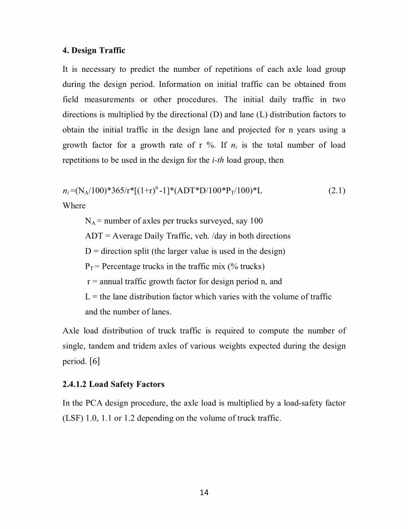
4. Design Traffic

It is necessary to predict the number of repetitions of each axle load group

during the design period. Information on initial traffic can be obtained from

field measurements or other procedures. The initial daily traffic in two

directions is multiplied by the directional (D) and lane (L) distribution factors to

obtain the initial traffic in the design lane and projected for n years using a

growth factor for a growth rate of r %. If ni is the total number of load

repetitions to be used in the design for the i-th load group, then

ni =(NA/100)*365/r*[(1+r)n -1]*(ADT*D/100*PT/100)*L (2.1)

Where

NA = number of axles per trucks surveyed, say 100

ADT = Average Daily Traffic, veh. /day in both directions

D = direction split (the larger value is used in the design)

PT = Percentage trucks in the traffic mix (% trucks)

r = annual traffic growth factor for design period n, and

L = the lane distribution factor which varies with the volume of traffic

and the number of lanes.

Axle load distribution of truck traffic is required to compute the number of

single, tandem and tridem axles of various weights expected during the design

period. [6]

2.4.1.2 Load Safety Factors

In the PCA design procedure, the axle load is multiplied by a load-safety factor

(LSF) 1.0, 1.1 or 1.2 depending on the volume of truck traffic.

15

2.4.1.3 Design Methodology

For the details and application of the design procedure, refer to the work sheet

illustrated in Figure 6.5 of Chapter 6 on result and discussion. The design steps

which are in tabular form are summarized hereunder:

1. Enter all design parameters and data

2. Assume a Trial thickness

3. Multiply Axle Loads by Load Safety Factor.

4. Compute the estimated projected (expected) repetition (ni) for i-th load group

using Eqn. (2.1).

5. If granular subbase or cement-treated base / subbase is used; modify the

subgrade k to obtain the design k using Table A-1 or Figure A-1.

6. Determine the equivalent load stress for single / tandem axles from Table A-

3. Use Table A-4 for erosion..

7. Divide stresses by MR to get stress ratio factors.

8. from Figure A.2 obtain allowable repetition (Ni) for i-th load group

corresponding to the load stress ratios (column 4); use Figure A.3 for erosion

stress ratios.

9. Divide ni by Ni to obtain fatigue ratio, and erosion damage. Report the sum

for each and identify the larger value of the two as the design control criteria,

normally fatigue:

10. If the total damage ratio (Dr) accumulated over the design period resulting

from all load groups (Eqn. 2.2) is much greater than 1, the thickness is increased

by successive 0.5 in. (127 mm) until the ratio is less than 1, and vice versa if the

total damage ratio (Dr) is much less than 1 until the ratio is close to 1.[2]

Dr = ∑ 푛N ≤ 1 (2.2)

16

2.4.2 AASHTO Method

The design guide for rigid and flexible pavements was concurrently developed

and published in the same manual. The design is based on empirical equations

obtained from the AASHO Road Test, with further modifications based on

theory, calibration and experience. [1]

2.4.2.1 Design Variables

a. Time Constraints: To achieve the best use of available funds, AASHTO

design guide encourages using longer analysis period for high-volume facilities

b. Design Traffic: The design procedures are based on cumulative expected 18-

kip (80-kN) equivalent single-axle load (ESAL) as in Table A.13

c. Reliability: Reliability is a means of incorporating degree of certainty into

the design process to ensure that the various design alternatives will last the

analysis period. The level of reliability to be used for design should increase as

the volume of traffic, difficulty of diverting traffic, and public expectation of

availability increase.

Application of the reliability concept requires the selection of a representative

standard deviation, S0. Recommended values of S0 range between 0.25 and 0.35.

[6]

d. Serviceability: Initial and terminal serviceability indices must be established

to compute the change in serviceability, ∆PSI used in the design equations.

The initial serviceability index PSIi is a function of pavement type and

construction quality. A typical value from the AASHO Road Test was 4.5 for

rigid pavements. The terminal serviceability index PSIt is the lowest value

tolerated before rehabilitation, resurfacing and reconstruction are required. An

index of 2.5 is suggested for design of major highways and 2.0 for highways

with lower traffic.[6]

17

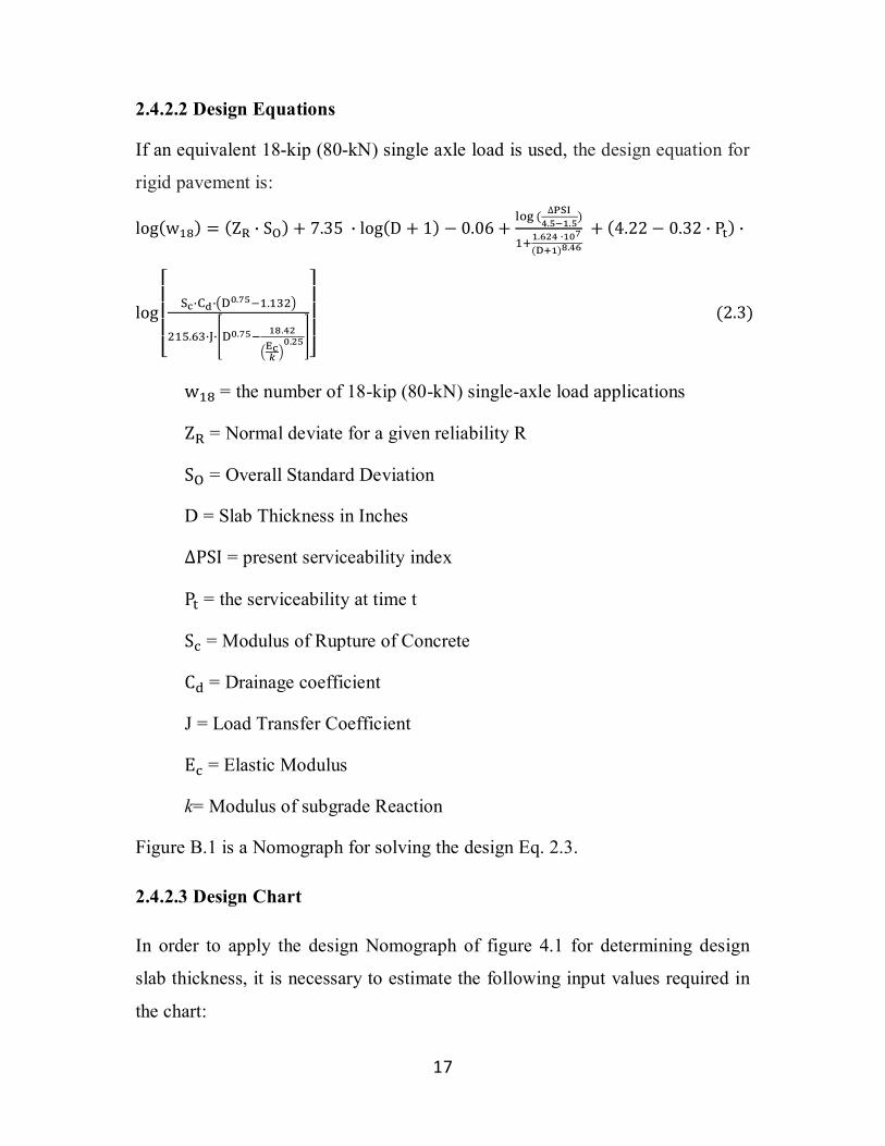
2.4.2.2 Design Equations

If an equivalent 18-kip (80-kN) single axle load is used, the design equation for

rigid pavement is:

log(w ) = (Z ∙ S ) + 7.35 ∙ log(D + 1) − 0.06 + ( ∆

. . ). ∙

( ) . + (4.22 − 0.32 ∙ P ) ∙

log

⎣⎢⎢⎢⎡

∙ ∙ . .

. ∙ ∙ . ..⎦⎥⎥⎥⎤ (2.3)

w = the number of 18-kip (80-kN) single-axle load applications

Z = Normal deviate for a given reliability R

S = Overall Standard Deviation

D = Slab Thickness in Inches

∆PSI = present serviceability index

P = the serviceability at time t

S = Modulus of Rupture of Concrete

C = Drainage coefficient

J = Load Transfer Coefficient

E = Elastic Modulus

k= Modulus of subgrade Reaction

Figure B.1 is a Nomograph for solving the design Eq. 2.3.

2.4.2.3 Design Chart

In order to apply the design Nomograph of figure 4.1 for determining design

slab thickness, it is necessary to estimate the following input values required in

the chart:

18

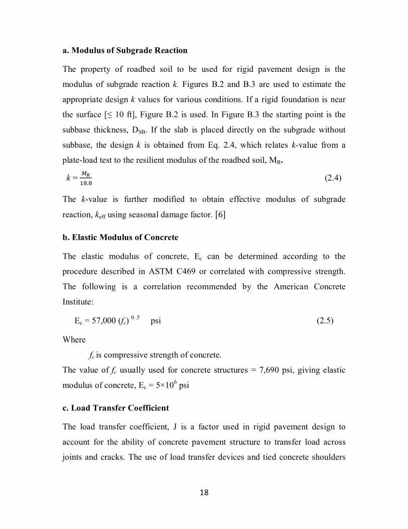
a. Modulus of Subgrade Reaction

The property of roadbed soil to be used for rigid pavement design is the

modulus of subgrade reaction k. Figures B.2 and B.3 are used to estimate the

appropriate design k values for various conditions. If a rigid foundation is near

the surface [≤ 10 ft], Figure B.2 is used. In Figure B.3 the starting point is the

subbase thickness, DSB. If the slab is placed directly on the subgrade without

subbase, the design k is obtained from Eq. 2.4, which relates k-value from a

plate-load test to the resilient modulus of the roadbed soil, MR.

k = .

(2.4)

The k-value is further modified to obtain effective modulus of subgrade

reaction, keff using seasonal damage factor. [6]

b. Elastic Modulus of Concrete

The elastic modulus of concrete, Ec can be determined according to the

procedure described in ASTM C469 or correlated with compressive strength.

The following is a correlation recommended by the American Concrete

Institute:

Ec = 57,000 (fc) 0 .5 psi (2.5)

Where

fc is compressive strength of concrete.

The value of fc usually used for concrete structures = 7,690 psi, giving elastic

modulus of concrete, Ec = 5×106 psi

c. Load Transfer Coefficient

The load transfer coefficient, J is a factor used in rigid pavement design to

account for the ability of concrete pavement structure to transfer load across

joints and cracks. The use of load transfer devices and tied concrete shoulders

19

increases the amount of load transfer and decreases the load-transfer

coefficient.[6]

Table B.1 shows the recommended load transfer coefficients for various

pavement types and design conditions. The AASHO Road Test conditions

represent a J value of 3.2, because all joints were doweled and there were no

tied concrete shoulders.[1]

f. Drainage Coefficient

The drainage coefficient, Cd has similar effect as the coefficient J. As Eq. 2.3

indicates, increase in Cd is equivalent to increase in J, both causing increase in

W18. Table B.2 provides the recommended Cd values based on the quality of

drainage and the percentage of time during which the pavement structure would

normally be exposed to moisture levels approaching saturation.

2.5 Other Design Features

The performance of rigid pavements is affected by a variety of design features,

including slab thickness, base type, joint spacing, reinforcement, load transfer,

dowel bar, longitudinal joint design, tied concrete shoulders, and sub-drainage.

2.5.1 Joint spacing

The JPCP and JRCP design concept is to provide a sufficient slab thickness and

joint spacing to minimize the development of transverse cracking.[9]

2.5.1.1 Jointed Plain Concrete Pavement (JPCP)

The spacing of joints in JPCPs depends more on the shrinkage characteristics of

the concrete rather than on the stress in the concrete. Longer joint spacing

causes the joint to open wider and decrease the efficiency of load transfer.

Allowable joint spacing or slab length, L can be computed approximately by Eq.

2.6 (Darter and Barenberg, 1977). For JPCP, typical length of slabs range from

7.75 to 30 ft (2.4 to 9.1 m). In general, reducing the slab length decreases both

20

the magnitude of the joint faulting and the amount of transverse cracking

(Huang, 2004).[6]

L = ∆

( ×∆ ) (2.6)

Where

∆L= the joint opening caused by temperature change and drying

shrinkage of concrete

C = is the adjustment factor due to slab-subbase friction, 0.65 for

stabilized base and 0 .8 for granular subbase.

훼 = The coefficient of thermal expansion of concrete, generally 5 t o

6 x 10-6 /°F (9 to 10.8 x 10-6/°C)

∆T = is the temperature range, which is the temperature at placement

minus the lowest mean monthly temperature, and

휖 = The drying shrinkage coefficient of concrete, approximately

0.5 to 2.5x10-4

If ∆L > 0.05 dowels are used.

∆퐿

Figure 2.4 Joint Opening

2.5.1.2 Jointed Reinforced Concrete Pavement (JRCP)

For JRCP, typical length of slabs range between 21 and 78 ft (6.4 - 23.9 m).

Generally, shorter joint spacing performs better, as measured by the deteriorated

transverse cracks, joint faulting, and joint spalling (Huang, 2004). Eq. 2.7 is also

applicable for JRCP.[6]

21

2.5.2 JRCP Reinforcement

Wire fabric or bar mats may be used in concrete slabs for control of temperature

cracking. These reinforcements do not increase the structural capacity of the

slab but are used for two purposes: to increase the joint spacing and to tie the

cracked concrete together and maintain load transfers through aggregate

interlock. When steel reinforcements are used, it is assumed that all tensile

stresses are taken by the steel alone,

As = (2.8)

Where

As = is the area of steel required per unit width

훾 = is the unit weight of the concrete

h = is the thickness of the slab

L = is the joint spacing or slab length

푓 = Average friction coefficient between slab and foundation usually

taken as 1.5, and

푓 = is the allowable stress in steel.

The steel is usually placed at the mid depth of the slab and discontinued at the

joint. The amount of steel obtained from Eq. 2.8 is at the center of the slab and

can be reduced toward the end. However, in actual practice the same amount of

steel is used throughout the length of the slab. Pavement sections with less than

0.1% reinforcing steel often display significant deteriorated transverse cracking.

Thus, a minimum of 0.1% reinforcing steel is recommended.[6]

22

C H A P T E R 3

CASE STUDY ROAD PROJECT

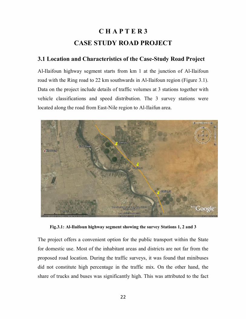
3.1 Location and Characteristics of the Case-Study Road Project

Al-Ilaifoun highway segment starts from km 1 at the junction of Al-Ilaifoun

road with the Ring road to 22 km southwards in Al-Ilaifoun region (Figure 3.1).

Data on the project include details of traffic volumes at 3 stations together with

vehicle classifications and speed distribution. The 3 survey stations were

located along the road from East-Nile region to Al-Ilaifun area.

Fig.3.1: Al-Ilaifoun highway segment showing the survey Stations 1, 2 and 3

The project offers a convenient option for the public transport within the State

for domestic use. Most of the inhabitant areas and districts are not far from the

proposed road location. During the traffic surveys, it was found that minibuses

did not constitute high percentage in the traffic mix. On the other hand, the

share of trucks and buses was significantly high. This was attributed to the fact

23

that use of this part of the road is mandatory for Interstate buses and trucks to

and from Al-Jazeera and River Nile States.

The region for the study was defined to encompass the area of the expected

policy impact. The study area is bound by the parts influenced by the

transportation system. It is anticipated that Al-Ilaifoun road will impose impact

on the domestic transport system in future, as well as having immediate effect

on freight transport.

Interactions with the area outside the cordon are defined via external stations

which effectively serve as doorways to trips. This includes trips from and to

other States by buses, trucks or passenger cars), and traffic through the study

area.

Once the study area was defined, it was then divided into a number of small

traffic-analysis zones (TAZs) represented by Stations 1, 2 and 3 (Figure 3.1).

The external zones were defined by the catchment area of the major transport

links from other States to and from Khartoum State in terms of trucks and

interstate buses. Three stations were used for traffic surveys in this study, the

proposed triple carriageway highway road is represented by existing single

carriageway road type by now, the study were chose the most typical points in

existed road to represent as close as much circumstances and features of the

proposed highway. Summary of the traffic data from the 3 stations of the study

area were as follows:

Station 1: Daily volume: 12716 vpd Passenger cars, 61% Trucks and buses

39%.

Station 2: Daily volume: 11288 vpd Passenger cars, 69% Trucks and buses

31%.

Station 3: Daily volume: 8266 vpd Passenger cars, 58% Trucks and buses 42%.

24

3.2 ESAL for the Case Study

For ESAL computations, recently, the Ministry of Interior converted the

operation of Khartoum-Medani Highway west side of the Blue Nile one-way to

Al-Jazeera State for trucks and buses. North-bound commercial traffic from Al-

Jazeera was directed to use east side of the Blue Nile. As such, the percentage of

trucks and buses in this direction was taken as 53 %. Since the proposed design

is providing 3 lanes for each direction, so percentage of trucks in design lane

was taken as 80%. Table 3.1 summarizes the results of traffic analyses at the 3

stations for pavement design purposes.

TABLE 3.1 Traffic Analyses for Pavement Design

Station 1 Station 2 Station 3

Traffic Composition and Parameters:

Analysis Period (years) 20 20 20

AADT (vpd) 12716 11288 8266

Percentage of heavy trucks (above class 4) 39 31 42

Directional split of truck traffic, % 53 53 53

Percentage of trucks in the design lane 70 70 70

Truck equivalency factor 1.35 1.35 1

Annual truck-volume growth rate, % 3 3 3

Annual truck weight growth rate, % 0.6 0.6 0.6

Traffic Analysis for Pavement Design

Traffic volume growth factor 1.75 1.75 1.75

Truck growth factor 1.12 1.12 1.12

Design year AADT 22, 298 19, 794 14, 494

Average AADT 17, 507 15, 541 11, 380

Design year truck factor 1.12 1.51 1.12

Average truck factor 1.06 1.43 1.06

AADT in one direction 9, 279 8, 237 6, 032

Truck AADT in one direction 3, 619 2, 553 2, 533

Number of Daily 80-kN (18-kip) ESALs 3836 3654 2686

Design 80-kN (18 kip) ESALs 19.6E+06 18.6E+06 13.7E+06

25

3.3 Upgrading of Al-Ilaifoun Road to Dual Highway

Later the Project Administration upgraded Al-Ilaifoun highway to two-way

divided facility in order to accommodate the increasing traffic from neighboring

States as well as reducing traffic accidents (Figure 3.2).

Figure 3.2: Al-Ilaifoun Highway Upgrading Under Construction

3.4 Pavement Structural Design Methodology

The present study included independent structural design of JPCP and JRCP for

the road project and compare design thickness of rigid pavement obtained

through manual and GalalM-RP software program.

In general, the main pavement design factor is the design traffic in term of

cumulative equivalent standard axle load (ESAL). Data were collected for the

road project including study of traffic reports. Traffic analysis was carried out to

26

determine the design-life ESAL for rigid pavement design. The procedure is

detailed in Chapter four.

The recommendations in the Material reports for the road project are presented

in chapter 4. The strength parameters of the various pavement layer materials

were measured in term of California Bearing Ratio (CBR). The design CBR

was carried out in accordance with AASHTO. Established correlations were

applied to obtain the resilient modulus, MR values and reported in Chapter Four

and Appendix B. Furthermore, Chapter Four also includes AASHTO

modification of the modulus of sub-grade reaction k to determine the combined

k for rigid-pavement design. AASHTO and PCA structural design methods

were then selected for jointed plain concrete pavement (JPCP) and jointed

reinforced concrete pavement (JRCP).

GalalM-RP software program for the design thickness of JPCP and JRCP were

prepared for PCA design method.

27

C H A P T E R 4

DESIGN OF JPCP AND JRCP FOR CASE STUDY ROAD

4.1 Introduction

In this chapter the structural design of JPC and JRC road pavements are

presented. The 22-km Al-Ilaifoun Highway segment introduced in Chapter 3

will be able to accommodate all traffic generated in future. In this proposed road

the percentage trucks in design lane is taken as 80 %. Al-Ilaifoun highway

location, characteristics and all relevant data were detailed in chapter 3. For

design consideration, the following design aspects are discussed:

Load Stresses, subgrade resilient modulus, MR and modulus of subgrade

reaction, k

Thickness design

Joint spacing, reinforcement design, longitudinal joint design, ties bars and

transverse joints and design of dowels.

4.2 Load Stresses

A rigid pavement for highways consists of relatively thin concrete slab placed

on the sub-grade or a base course/subbase. The load-carrying capacity of the

pavement base-subgrade structure is brought about largely by the beam action

of the pavement. Since the concrete slab is the major component of the

structure, stresses in concrete pavements have been given detailed consideration

by various investigators. Stresses in rigid pavements can result from several

causes in addition to wheel loads. These include volumetric changes in the

subgrade and/or subbase, changes in moisture and restrained temperature

variations introducing curling stresses.

The anticipated traffic carried by a highway pavement related to equivalent

18,000-lb single-axle loads (ESALs), average daily traffic (ADT), or average

28

daily truck traffic (ADTT). Since truck traffic is the major stress-inducing load

to pavements compared to passenger cars, the estimate of trucks using the

pavement is critical to the structural design for the pavement life.

4.3 Subgrade Resilient Modulus MR and Reaction Modulus k

The resilient modulus, MR represents the elastic modulus of subgrade in

conjunction with the elastic theory, although most paving materials are not

elastic as they experience some permanent deformation as well after each load

application. However, for small repeated loads compared to the material

strength, the deformation under each load repetition is mostly recoverable and

proportional to the load and as such may be assumed elastic.

Determination of a specific subgrade strength parameter required for design,

whether MR, k or California Bearing Ratio (CBR), depends on available test

equipment. In the event of non-availability of the particular device to directly

determine MR (Level 1), this study resorted to correlations with other parameters

that can be determined (Level 2). Typical relationships include the following:

Asphalt Institute (AI) equation (Heukelom and Klomp, 1962)

MR (psi) = 1500*(CBR) (4-1a)

MR (MPa) = 10.342*(CBR) (4-1b)

These correlations have the limitation that they were developed for fine-grained,

non-expansive soils with soaked CBR 10. To account for materials with CBR

greater than 10, the Mechanistic Design Guide (NCHRP 1-37A, 2002)

recommended (4-2).

MR (psi) = 2555*(CBR) 0.64 (4-2a)

MR (MPa) = 17*(CBR) 0.64 (4-2b)

The soils encountered along the alignment of the proposed road are not suitable

for embankment construction and should be removal and replaced with fill

29

material for a depth of at least 6 in. (300 mm). As the existing subgrade material

had an average CBR of 4 only, the value of 12 was selected as satisfactory for

design.

Hence, design MR = 2555 (CBR) 0.64 = 2555 (12) 0.64 =12, 500 psi (86.2 MPa)

According to AASHTO, the modulus subgrade reaction, k is then obtained from

equation (2.4):

ksubgrade = .

= 83 lb/in.3 (MPa/mm3)

4.4 Design of Slab thickness for JPCP and JRCP

The two design methods applied in this study included the Portland cement

Association Method (PCA, 1984) and AASHTO Method (1993)

4.4.1 Portland Cement Association Design Method

The design parameters and factors for PCA Design Method depend on the

selected design category. In the present case the design uses doweled joints

without concrete shoulders and thus the main four design factors are:

1. Concrete modulus of rupture (MR): From Section 2.4.1.1the MR = 650 psi

2. Subgrade and Subbase combined support (k): With an 8-in. (203.2-mm)

untreated subbase placed on the subgrade of k value = 83 Ib/in.3, from Figure

A-1 (a) the design k was found to be 125 Ib/in.3

3. Design period = 20 years

4. Design Traffic: Annual traffic growth rate was typically assumed to be 5 %

for the project design life. The data gathered from the selected three stations

was analyzed to determine the average daily traffic volumes for the different

types of vehicles using the proposed route and as tabulated in Table 4.1:

30

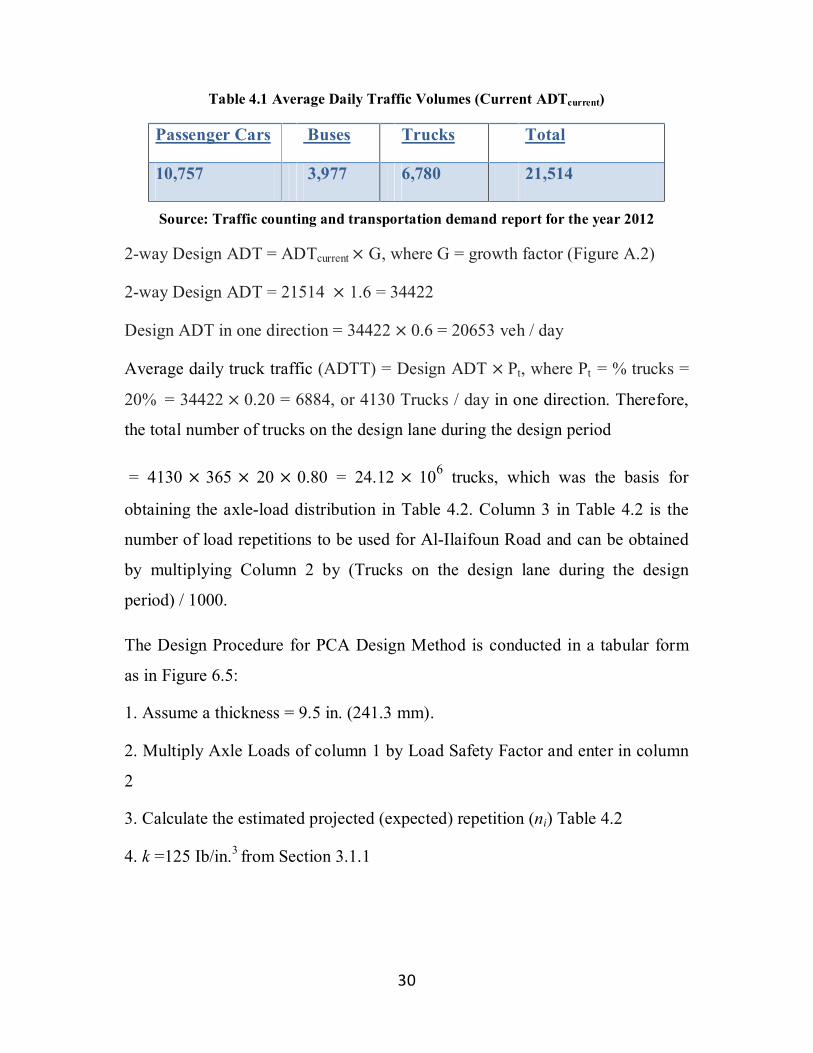
Table 4.1 Average Daily Traffic Volumes (Current ADTcurrent)

Passenger Cars Buses Trucks Total

10,757 3,977 6,780 21,514

Source: Traffic counting and transportation demand report for the year 2012

2-way Design ADT = ADTcurrent × G, where G = growth factor (Figure A.2)

2-way Design ADT = 21514 × 1.6 = 34422

Design ADT in one direction = 34422 × 0.6 = 20653 veh / day

Average daily truck traffic (ADTT) = Design ADT × Pt, where Pt = % trucks =

20% = 34422 × 0.20 = 6884, or 4130 Trucks / day in one direction. Therefore,

the total number of trucks on the design lane during the design period

= 4130 × 365 × 20 × 0.80 = 24.12 × 106 trucks, which was the basis for

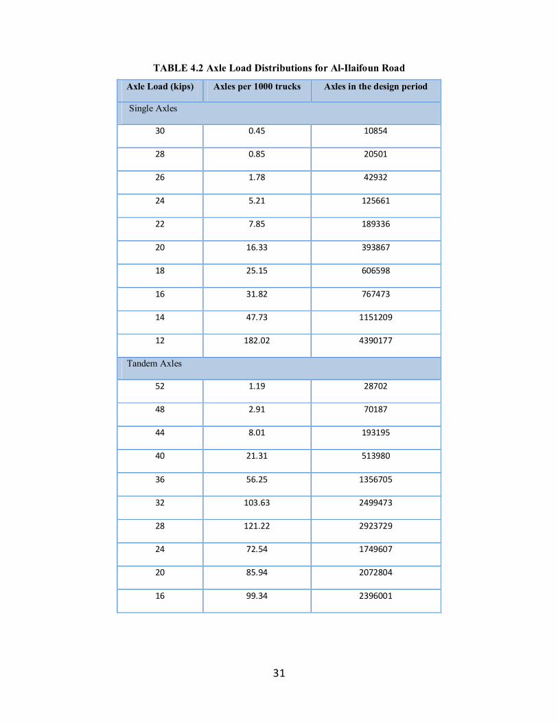
obtaining the axle-load distribution in Table 4.2. Column 3 in Table 4.2 is the

number of load repetitions to be used for Al-Ilaifoun Road and can be obtained

by multiplying Column 2 by (Trucks on the design lane during the design

period) / 1000.

The Design Procedure for PCA Design Method is conducted in a tabular form

as in Figure 6.5:

1. Assume a thickness = 9.5 in. (241.3 mm).

2. Multiply Axle Loads of column 1 by Load Safety Factor and enter in column

2

3. Calculate the estimated projected (expected) repetition (ni) Table 4.2

4. k =125 Ib/in.3 from Section 3.1.1

31

TABLE 4.2 Axle Load Distributions for Al-Ilaifoun Road

Axle Load (kips) Axles per 1000 trucks Axles in the design period

Single Axles

30 0.45 10854

28 0.85 20501

26 1.78 42932

24 5.21 125661

22 7.85 189336

20 16.33 393867

18 25.15 606598

16 31.82 767473

14 47.73 1151209

12 182.02 4390177

Tandem Axles

52 1.19 28702

48 2.91 70187

44 8.01 193195

40 21.31 513980

36 56.25 1356705

32 103.63 2499473

28 121.22 2923729

24 72.54 1749607

20 85.94 2072804

16 99.34 2396001

32

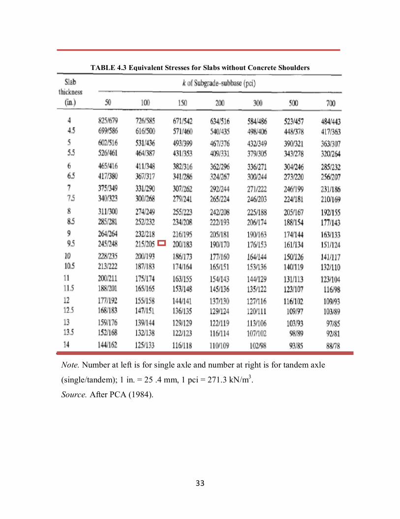
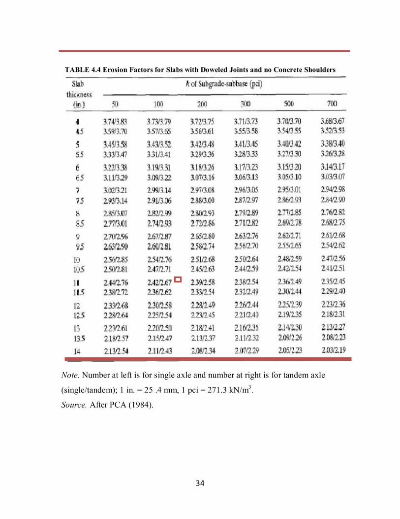
5. The equivalent stress 207.5/(194 axles) from Table 4.3 (items 9 and 12,

respectively). Use Table 4.4 for erosion 2.595/2.793 (items 11 and 12,

respectively).

6. Divide stresses by MR to get stress ratio factors 0.319/0.298 (items 10 and 13,

respectively).

7. From Figure A.3 obtain allowable repetition (Ni) for i-th load group

corresponding to the stress ratios (column 5); use figure A.4 for erosion

(column 7).

8. Divide ni by Ni and to get fatigue ratio (column 6), and erosion damage (col.

8).

9. the damage ratio (Dr) accumulated over the design period resulting all m load

groups (sum of column 6 = 98.5 %) is for fatigue and (sum of column 8 = 64 %)

is for erosion damage, Both are less than 100%, with fatigue criteria being

critical.

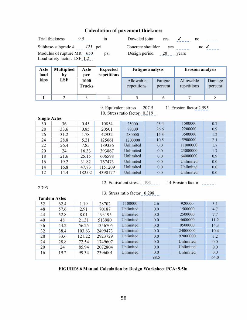
However, 98.5 % is much less than 100 % indicating the slab thickness of 9.5

in. (241.3 mm) is over design. Thus, the design was repeated using 9-in (229

mm) thickness resulting in fatigue damage of 193.9%, much higher than 100 %

(under design). Therefore, a slab thickness of 9.49 in. (241 mm) would be

adequate. In general, fatigue criteria will normally control the design of

pavements subjected to light to medium traffic. Erosion criteria will usually

control the design of pavements subjected to heavy traffic with doweled joints.

33

TABLE 4.3 Equivalent Stresses for Slabs without Concrete Shoulders

Note. Number at left is for single axle and number at right is for tandem axle

(single/tandem); 1 in. = 25 .4 mm, 1 pci = 271.3 kN/m3.

Source. After PCA (1984).

34

TABLE 4.4 Erosion Factors for Slabs with Doweled Joints and no Concrete Shoulders

Note. Number at left is for single axle and number at right is for tandem axle

(single/tandem); 1 in. = 25 .4 mm, 1 pci = 271.3 kN/m3.

Source. After PCA (1984).

35

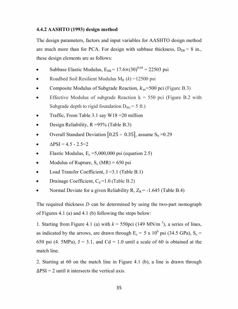
4.4.2 AASHTO (1993) design method

The design parameters, factors and input variables for AASHTO design method

are much more than for PCA. For design with subbase thickness, DSB = 8 in.,

these design elements are as follows:

Subbase Elastic Modulus, ESB = 17.6×(30)0.64 = 22503 psi

Roadbed Soil Resilient Modulus MR (k) =12500 psi

Composite Modulus of Subgrade Reaction, 푘 =500 pci (Figure B.3)

Effective Modulus of subgrade Reaction k = 550 pci (Figure B.2 with

Subgrade depth to rigid foundation DSG = 5 ft.)

Traffic, From Table 3.1 say W18 =20 million

Design Reliability, R =95% (Table B.3)

Overall Standard Deviation 0.25 – 0.35 , assume S0 =0.29

ΔPSI = 4.5 - 2.5=2

Elastic Modulus, Ec =5,000,000 psi (equation 2.5)

Modulus of Rupture, Sc (MR) = 650 psi

Load Transfer Coefficient, J =3.1 (Table B.1)

Drainage Coefficient, Cd =1.0 (Table B.2)

Normal Deviate for a given Reliability R, ZR = -1.645 (Table B.4)

The required thickness D can be determined by using the two-part nomograph

of Figures 4.1 (a) and 4.1 (b) following the steps below:

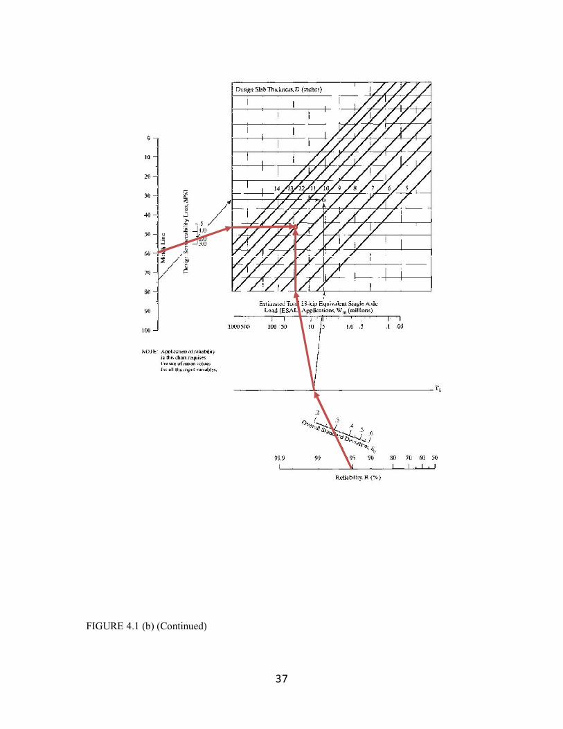
1. Starting from Figure 4.1 (a) with k = 550pci (149 MN/m 3), a series of lines,

as indicated by the arrows, are drawn through Ec = 5 x 106 psi (34.5 GPa), Sc =

650 psi (4. 5MPa), J = 3.1, and Cd = 1.0 until a scale of 60 is obtained at the

match line.

2. Starting at 60 on the match line in Figure 4.1 (b), a line is drawn through

∆PSI = 2 until it intersects the vertical axis.

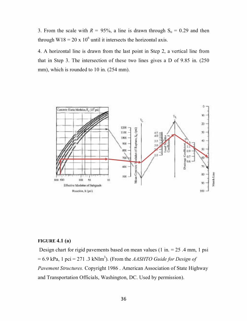
36

3. From the scale with R = 95%, a line is drawn through So = 0.29 and then

through W18 = 20 x 106 until it intersects the horizontal axis.

4. A horizontal line is drawn from the last point in Step 2, a vertical line from

that in Step 3. The intersection of these two lines gives a D of 9.85 in. (250

mm), which is rounded to 10 in. (254 mm).

FIGURE 4.1 (a)

Design chart for rigid pavements based on mean values (1 in. = 25 .4 mm, 1 psi

= 6.9 kPa, 1 pci = 271 .3 kNIm3). (From the AASHTO Guide for Design of

Pavement Structures. Copyright 1986 . American Association of State Highway

and Transportation Officials, Washington, DC. Used by permission).

37

FIGURE 4.1 (b) (Continued)

38

4.4.3 Other design features:

1. Joint spacing for JPCP:

∆T = 145°F (63°C)

α =6 x 10-6/°F (9.9 x 10-6/°C)

ΔL = 0.25 in (doweled joint)

C = 0.8 for granular sub-base.

휖 = 2.5 x 10-4

From Eqn. (2.7)

L = .. ( × × . × )

= 279 in. = 23 ft = 5.8 m

2. Joint spacing for JRCP:

∆T = 120°F (49°C)

α =5 x 10-6/°F (9.9 x 10-6/°C)

ΔL = 0.25 in (doweled joint)

C = 0.8 for granular sub-base.

휖 = 0.5 x 10-4

From Equation (2.7)

L = .. ( × × . × )

= 480.8in. =40ft = 12.2 m

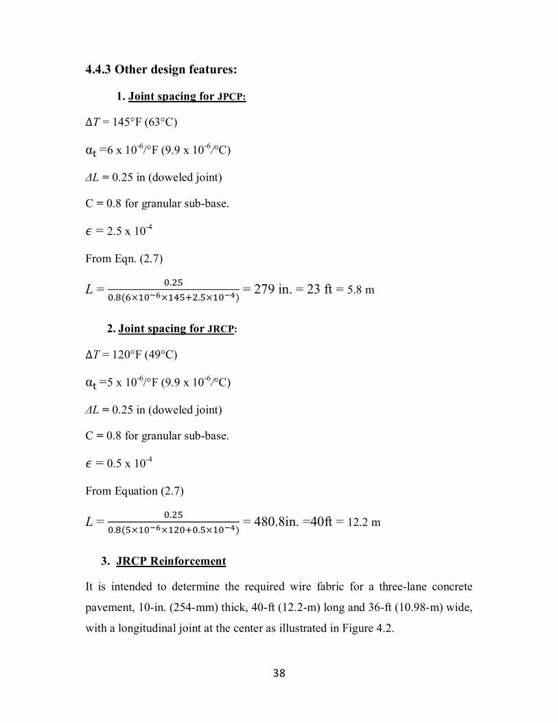
3. JRCP Reinforcement

It is intended to determine the required wire fabric for a three-lane concrete

pavement, 10-in. (254-mm) thick, 40-ft (12.2-m) long and 36-ft (10.98-m) wide,

with a longitudinal joint at the center as illustrated in Figure 4.2.

39

Figure 4.2: Schematic illustration of wire reinforcement

Pavement thickness, ℎ = 10 in.

훾 = 150 pcf = 0.0868 pci (23.6 kN/m3); fa = 1.5

fs = 43, 000 psi, smooth, cold-drawn wire (Table B.4)

Computation of the required longitudinal steel is as follows:

L = 40ft = 480 in.

From equation (2.8):

As = . × × × .

× = 0.00727 .

. = 0.08724 .

The required transverse steel: 12' (lane) +12 (' lane) + 12 (' lane)

L = 36ft = 432 in.

From equation (2.8):

As = . × × × .

× = 0.006540 .

. = 0.07848 .

40 ft

36 ft

12 ft ℎ = 10 in.

Style of Wire fabric

40

From Table (B.5), use 6 × 12 – W4.5 × W8 with cross sectional areas of 0.09

in.2 (58 mm2) for longitudinal wires and 0 .08 in .2 (52 mm2) for transverse

wires.

4. Longitudinal Joint Design for JPCP and JRCP

The longitudinal joint design was found to be a critical design element. Both

inadequate forming techniques and insufficient depths of joint can contribute to

the development of longitudinal cracking. There was evidence of the advantage

of sawing the joints over the use of inserts. The depth of longitudinal joints is

generally recommended to be one-third of the actual, not designed, slab

thickness, but might have to be greater when stabilized bases are used.

Longitudinal Joints run parallel to the pavement length (along the lane) and

serve to control longitudinal cracking. These joints are produced by either

sawing the slab early in the curing process, or by placing an insert in the plastic

concrete at the desired joint location. Longitudinal joints are normally placed at

the edges of traffic lanes.

5. Tie Bars

Tie bars are placed along the longitudinal joint to tie the two slabs together so

that the joint will be tightly closed and the load transfer across the joint can be

ensured. The amount of steel required for tie bars can be determined in the same

way as the longitudinal or transverse reinforcements.

The length of tie bars is governed by the allowable bond stress 휇. For deformed

bars, an allowable bond stress of 350 psi (2.4 MPa) may be assumed. The length

of bar should be based on the full strength of the bar, namely,

t = (4.3)

The length t should be increased by 3 in. (76 mm) for misalignment. It should

be noted that many agencies use a standard tie-bar design to simplify the

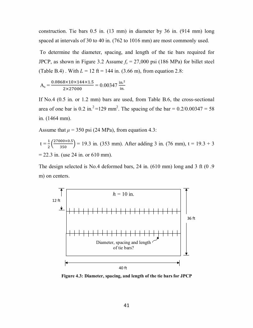
41

construction. Tie bars 0.5 in. (13 mm) in diameter by 36 in. (914 mm) long

spaced at intervals of 30 to 40 in. (762 to 1016 mm) are most commonly used.

To determine the diameter, spacing, and length of the tie bars required for

JPCP, as shown in Figure 3.2 Assume fs = 27,000 psi (186 MPa) for billet steel

(Table B.4) . With L = 12 ft = 144 in. (3.66 m), from equation 2.8:

As = . × × × .

× = 0.00347 .

.

If No.4 (0.5 in. or 1.2 mm) bars are used, from Table B.6, the cross-sectional

area of one bar is 0.2 in.2 =129 mm2. The spacing of the bar = 0.2/0.00347 = 58

in. (1464 mm).

Assume that μ = 350 psi (24 MPa), from equation 4.3:

t = × . = 19.3 in. (353 mm). After adding 3 in. (76 mm), t = 19.3 + 3

= 22.3 in. (use 24 in. or 610 mm).

The design selected is No.4 deformed bars, 24 in. (610 mm) long and 3 ft (0 .9

m) on centers.

Figure 4.3: Diameter, spacing, and length of the tie bars for JPCP

ℎ = 10 in.

Diameter, spacing and length

of tie bars?

36 ft

12 ft

40 ft

42

6. Transverse Joints for JPCP and JRCP

Transverse Joints run perpendicular to the pavement length (across the lane) and

serve different functions depending on the pavement type. Expansion Joints

allow for expansion of the pavement due to temperature changes. Expansion

joints are typically 2 inches wide, although widths up to 4 inches are sometimes

used. Due to the width of the joint, load transfer devices are necessary. These

are usually dowel bars with caps that allow the pavement and bar to move

independently in the longitudinal direction. Expansion joints are costly to

construct and maintain.

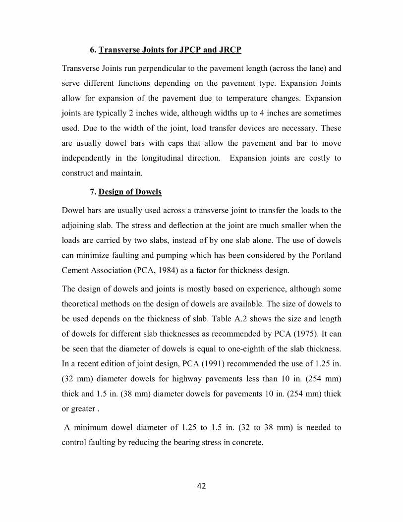
7. Design of Dowels

Dowel bars are usually used across a transverse joint to transfer the loads to the

adjoining slab. The stress and deflection at the joint are much smaller when the

loads are carried by two slabs, instead of by one slab alone. The use of dowels

can minimize faulting and pumping which has been considered by the Portland

Cement Association (PCA, 1984) as a factor for thickness design.

The design of dowels and joints is mostly based on experience, although some

theoretical methods on the design of dowels are available. The size of dowels to

be used depends on the thickness of slab. Table A.2 shows the size and length

of dowels for different slab thicknesses as recommended by PCA (1975). It can

be seen that the diameter of dowels is equal to one-eighth of the slab thickness.

In a recent edition of joint design, PCA (1991) recommended the use of 1.25 in.

(32 mm) diameter dowels for highway pavements less than 10 in. (254 mm)

thick and 1.5 in. (38 mm) diameter dowels for pavements 10 in. (254 mm) thick

or greater .

A minimum dowel diameter of 1.25 to 1.5 in. (32 to 38 mm) is needed to

control faulting by reducing the bearing stress in concrete.

43

Dowel bars were found to be effective in reducing the amount of joint faulting

when compared with non doweled sections of comparable designs. The

diameter of dowels had an effect on performance, because larger diameter bars

provided better load transfer and control of faulting under heavy traffic than did

smaller dowels. It appeared that a minimum dowel diameter of 1.25 in. (32 mm)

was necessary to provide good performance.

44

CHPTER 5

APPLICATION OF SOFTWARE PROGRAM

5.1 Introduction

GalalM-RP computer program was written in Visual Basic and can be run on

computers with visual studio 2008 Windows 95 or higher. Details on the use of

the software can be found in this chapter.

The GalalM-RP computer program applies only to rigid pavements with

doweled joints and without Concrete shoulder. It can be applied only to layered

systems under single, dual, dual-tandem with each layer behaving differently.

Galal-R.P has been developed for design thickness by Portland Cement

Association's (PCA) thickness-design procedure for concrete highways and

streets 1984 as same as in chapter 4, and it is educational and training tool as

well as a design tool. The user is assisted in selecting design inputs by using the

recommended values are shown on the screen along with a brief explanation

during the design process.

To facilitate entering and editing data, some tables and charts can be used. The

program uses menus and data entry forms to create and edit the data file.

Although the large number of input parameters appears overwhelming, default

values are provided to many of them, so only a limited number of inputs will be

required.

Rigid pavement computer screens divided into three screens as follows:

Screen one: main Screens

Screens two: PCA traffic Analysis and it is divided into two data input (user

input) and data output (program calculates).

Screen three: calculations of pavement thickness

45

The program described in this chapter has been applied to several examples to

test its accuracy and suitability for the proposed applications. Case study was

prepared to include all software applications in the fild of pavements design.

5.2 MAIN SCREEN:

Galal-R.P has been designed screens and windows of the program by clicks and

mouse movement light.

Figure 5.1 main screen

To open new file click File open PCA (Figure 5.1)

46

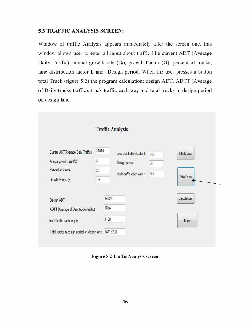
5.3 TRAFFIC ANALYSIS SCREEN:

Window of traffic Analysis appears immediately after the screen one, this

window allows user to enter all input about traffic like current ADT (Average

Daily Traffic), annual growth rate (%), growth Factor (G), percent of trucks,

lane distribution factor L and Design period. When the user presses a button

total Truck (figure 5.2) the program calculation: design ADT, ADTT (Average

of Daily trucks traffic), truck traffic each way and total trucks in design period

on design lane.

Figure 5.2 Traffic Analysis screen

47

5.4 CALCULATIONS OF PAVEMENT THICKNESS SCREEN:

When we click a button calculation in screen two the program open calculations

of pavement thickness screen figure 5.3 show the screen.

User input in this window is: Trial thickness, subbase-subgrade k, modulus of

rupture MR, Load safety factor LSF, however the default values are

recommended and represent the values assumed Then the program does all the

other calculation by clicks and mouse movement.

This screen is provided for the user's information and may be skipped as it is

repeated by new parameter. This screen is particularly useful when analyzing

the impact of one design variable. Suppose the user wants to see the impact of

increasing subbase-subgrade k while keeping modulus of rupture MR, Load

safety factor LSF constant. By entering the same design period, the user can

immediately see the change in thickness required for each change in weight.

Likewise, any variable can be changed while holding other variables constant.

When the user presses a button display Result, total fatigue percent and total

damage percent via trail thickness design regarding the design is displayed on

the summary screen. The summary display is dynamic and will change

depending upon design features.

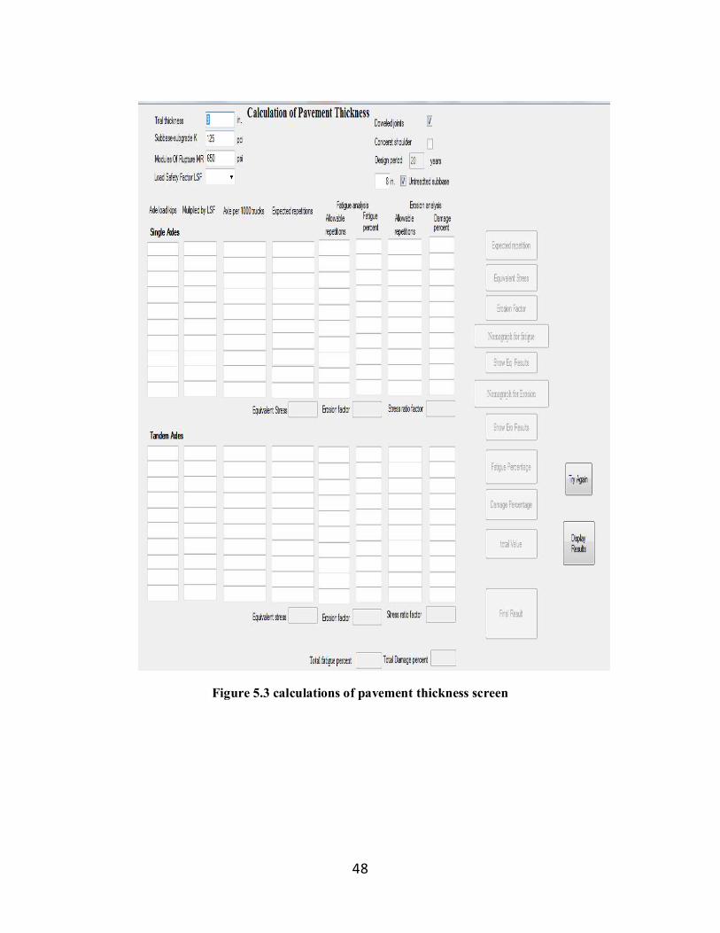
48

Figure 5.3 calculations of pavement thickness screen

49

Figure 5.4 Display Result Screen

The objective of processing controls in GalalM-RP is to provide reasonable

assurance that data processing has been performed accurately, without any

omission or duplication of transactions. Examples of processing controls

include:

Run-to-run total: total such as expected repetition, equivalent

Stress, erosion factor obtained at the end of one processing run are

distributed to the next run and corresponding totals produced at the

end of the second run.

Control total reports: Control totals, such as equivalent Stress,

erosion factor, can be calculated during processing and reconciled

to input totals or totals from earlier processing runs.

File and operator controls: External and internal table and figure

ensure that the proper files are used in applications.

50

The objective of output controls is to ensure that only authorized persons

receive output or have access to files produced by the system. Some common

output controls include:

Control total reports: Compare controls totals to input and run-to-

run control totals produced during transaction processing.

Master file changes: Any changes to master file information

should be properly authorized by the entity and reported in detail to

the user department from which the request for change originated.

Output distribution: Systems output should only be distributed to

persons authorized to receive the output.

51

CHAPTER 6

RESULTS AND DISCUSSION

6.1 Results

As presented in Chapter 2 PCA design method, the follow up specifies design

input layer strength parameters design traffic thereafter, its assumes a trial

thickness and evaluates total fatigue and erosion doesn’t exceed 100%. The

GalalM-RP develop converts the above manual procedure into systematic

computer program analysis. The results obtained from GalalM-RP are presented

and discussed below.

Results of PCA Traffic Analysis when using the program GalalM-RP give:

Design ADT = 34422

ADTT (Average of Daily trucks traffic) = 6884 Trucks / day

Truck traffic each way is = 4130

Total number of trucks on the design lane during the design period =

24119200 trucks

Figure 6.1 GalalM-RP Results of PCA Traffic Analysis

52

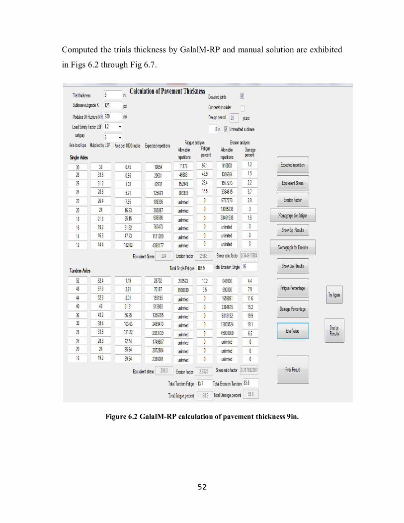
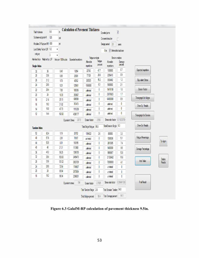
Computed the trials thickness by GalalM-RP and manual solution are exhibited

in Figs 6.2 through Fig 6.7.

Figure 6.2 GalalM-RP calculation of pavement thickness 9in.

53

Figure 6.3 GalalM-RP calculation of pavement thickness 9.5in.

54

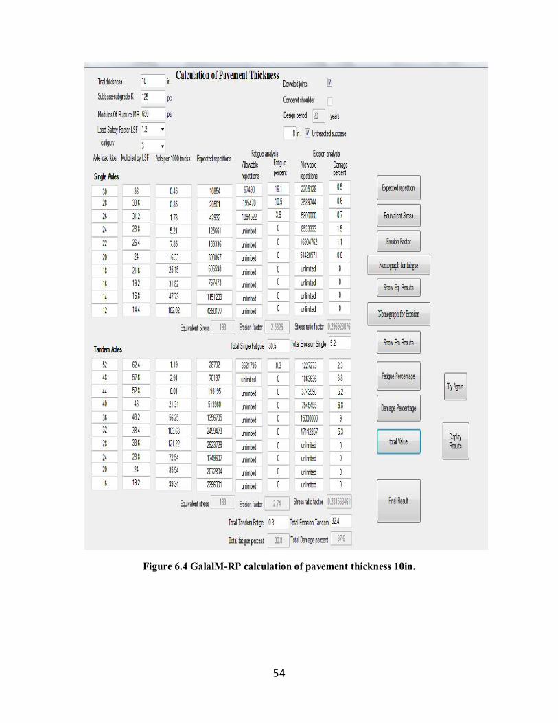
Figure 6.4 GalalM-RP calculation of pavement thickness 10in.

55

Calculation of pavement thickness Trial thickness 9 in Doweled joint yes ✓ no

Subbase-subgrade k 125 pci Concrete shoulder yes no ✓ Modulus of rupture MR 650 psi Design period 20 years Load safety factor. LSF 1.2 Axle load kips

Multiplied by

LSF

Axle per

Expected repetitions

Fatigue analysis Erosion analysis

1000 Trucks

Allowable repetitions

Fatigue percent

Allowable repetitions

Damage percent

1 2 3 4 5 6 7 8

9. Equivalent stress 224 11.Erosion factor 2.665 10. Stress ratio factor 0.345 Single Axles

30 36 0.45 10854 12000 90.45 910000 1.2 28 33.6 0.85 20501 46000 44.6 1400000 1.5 26 31.2 1.78 42932 150000 28.6 2000000 2.1 24 28.8 5.21 125661 800000 15.7 3600000 3.5 22 26.4 7.85 189336 Unlimited 0.0 6800000 2.8 20 24 16.33 393867 Unlimited 0.0 13000000 3 18 21.6 25.15 606598 Unlimited 0.0 36000000 1.7 16 19.2 31.82 767473 Unlimited 0.0 Unlimited 0.0 14 16.8 47.73 1151209 Unlimited 0.0 Unlimited 0.0 12 14.4 182.02 4390177 Unlimited 0.0 Unlimited 0.0

12. Equivalent stress 206.5 14.Erosion factor 2.853 13. Stress ratio factor 0.318 Tandem Axles

52 62.4 1.19 28702 270000 10.6 640000 4.5 48 57.6 2.91 70187 1800000 3.9 890000 7.9 44 52.8 8.01 193195 Unlimited 0.0 1700000 11.3 40 48 21.31 513980 Unlimited 0.0 3300000 15.6 36 43.2 56.25 1356705 Unlimited 0.0 6800000 20 32 38.4 103.63 2499473 Unlimited 0.0 14000000 17.9 28 33.6 121.22 2923729 Unlimited 0.0 46000000 6.4 24 28.8 72.54 1749607 Unlimited 0.0 unlimited 0.0 20 24 85.94 2072804 Unlimited 0.0 unlimited 0.0 16 19.2 99.34 2396001 Unlimited 0.0 unlimited 0.0

Total 193.9 Total 99.4

FIGURE6.5 Manual Calculation by Design Worksheet PCA: 9in.

56

Calculation of pavement thickness Trial thickness 9.5 in Doweled joint yes ✓ no

Subbase-subgrade k 125 pci Concrete shoulder yes no ✓ Modulus of rupture MR 650 psi Design period 20 years Load safety factor. LSF 1.2 Axle load kips

Multiplied by

LSF

Axle per

Expected repetitions

Fatigue analysis Erosion analysis

1000 Trucks

Allowable repetitions

Fatigue percent

Allowable repetitions

Damage percent

1 2 3 4 5 6 7 8

9. Equivalent stress 207.5 11.Erosion factor 2.595 10. Stress ratio factor 0.319 Single Axles

30 36 0.45 10854 25000 43.4 1500000 0.7 28 33.6 0.85 20501 77000 26.6 2200000 0.9 26 31.2 1.78 42932 280000 15.3 3500000 1.2 24 28.8 5.21 125661 1200000 10.5 5900000 2.1 22 26.4 7.85 189336 Unlimited 0.0 11000000 1.7 20 24 16.33 393867 Unlimited 0.0 23000000 1.7 18 21.6 25.15 606598 Unlimited 0.0 64000000 0.9 16 19.2 31.82 767473 Unlimited 0.0 Unlimited 0.0 14 16.8 47.73 1151209 Unlimited 0.0 Unlimited 0.0 12 14.4 182.02 4390177 Unlimited 0.0 Unlimited 0.0

12. Equivalent stress 194 14.Erosion factor 2.793 13. Stress ratio factor 0.298 Tandem Axles

52 62.4 1.19 28702 1100000 2.6 920000 3.1 48 57.6 2.91 70187 Unlimited 0.0 1500000 4.7 44 52.8 8.01 193195 Unlimited 0.0 2500000 7.7 40 48 21.31 513980 Unlimited 0.0 4600000 11.2 36 43.2 56.25 1356705 Unlimited 0.0 9500000 14.3 32 38.4 103.63 2499473 Unlimited 0.0 24000000 10.4 28 33.6 121.22 2923729 Unlimited 0.0 92000000 3.2 24 28.8 72.54 1749607 Unlimited 0.0 Unlimited 0.0 20 24 85.94 2072804 Unlimited 0.0 Unlimited 0.0 16 19.2 99.34 2396001 Unlimited 0.0 Unlimited 0.0

98.5 64.0

FIGURE6.6 Manual Calculation by Design Worksheet PCA: 9.5in.

57

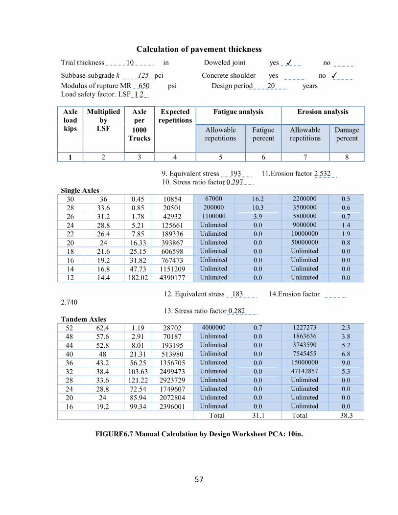
Calculation of pavement thickness Trial thickness 10 in Doweled joint yes ✓ no

Subbase-subgrade k 125 pci Concrete shoulder yes no ✓ Modulus of rupture MR 650 psi Design period 20 years Load safety factor. LSF 1.2 Axle load kips

Multiplied by

LSF

Axle per

Expected repetitions

Fatigue analysis Erosion analysis

1000 Trucks

Allowable repetitions

Fatigue percent

Allowable repetitions

Damage percent

1 2 3 4 5 6 7 8

9. Equivalent stress 193 11.Erosion factor 2.532 10. Stress ratio factor 0.297 Single Axles

30 36 0.45 10854 67000 16.2 2200000 0.5 28 33.6 0.85 20501 200000 10.3 3500000 0.6 26 31.2 1.78 42932 1100000 3.9 5800000 0.7 24 28.8 5.21 125661 Unlimited 0.0 9000000 1.4 22 26.4 7.85 189336 Unlimited 0.0 10000000 1.9 20 24 16.33 393867 Unlimited 0.0 50000000 0.8 18 21.6 25.15 606598 Unlimited 0.0 Unlimited 0.0 16 19.2 31.82 767473 Unlimited 0.0 Unlimited 0.0 14 16.8 47.73 1151209 Unlimited 0.0 Unlimited 0.0 12 14.4 182.02 4390177 Unlimited 0.0 Unlimited 0.0

12. Equivalent stress 183 14.Erosion factor 2.740 13. Stress ratio factor 0.282 Tandem Axles

52 62.4 1.19 28702 4000000 0.7 1227273 2.3 48 57.6 2.91 70187 Unlimited 0.0 1863636 3.8 44 52.8 8.01 193195 Unlimited 0.0 3743590 5.2 40 48 21.31 513980 Unlimited 0.0 7545455 6.8 36 43.2 56.25 1356705 Unlimited 0.0 15000000 9.0 32 38.4 103.63 2499473 Unlimited 0.0 47142857 5.3 28 33.6 121.22 2923729 Unlimited 0.0 Unlimited 0.0 24 28.8 72.54 1749607 Unlimited 0.0 Unlimited 0.0 20 24 85.94 2072804 Unlimited 0.0 Unlimited 0.0 16 19.2 99.34 2396001 Unlimited 0.0 Unlimited 0.0

Total 31.1 Total 38.3

FIGURE6.7 Manual Calculation by Design Worksheet PCA: 10in.

58

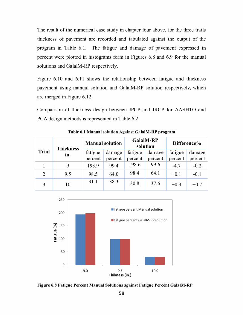
The result of the numerical case study in chapter four above, for the three trails

thickness of pavement are recorded and tabulated against the output of the

program in Table 6.1. The fatigue and damage of pavement expressed in

percent were plotted in histograms form in Figures 6.8 and 6.9 for the manual

solutions and GalalM-RP respectively.

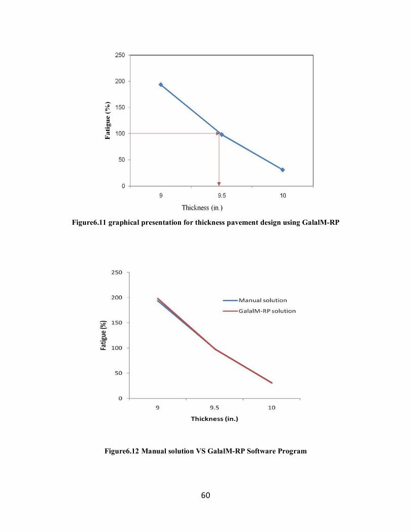
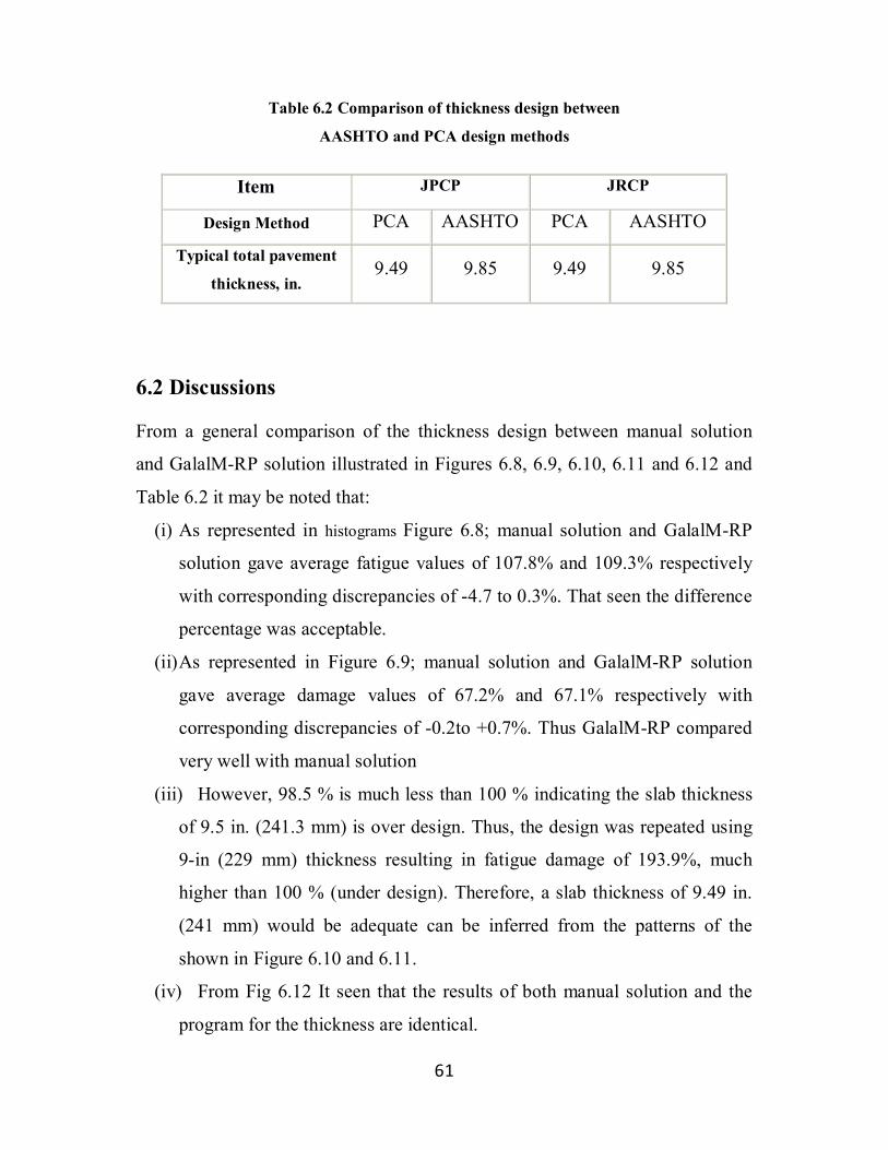
Figure 6.10 and 6.11 shows the relationship between fatigue and thickness

pavement using manual solution and GalalM-RP solution respectively, which

are merged in Figure 6.12.

Comparison of thickness design between JPCP and JRCP for AASHTO and

PCA design methods is represented in Table 6.2.

Table 6.1 Manual solution Against GalalM-RP program

Trial Thickness in.

Manual solution GalalM-RP solution

Difference%

fatigue percent

damage percent

fatigue percent

damage percent

fatigue percent

damage percent

1 9 193.9 99.4 198.6 99.6 -4.7 -0.2 2 9.5 98.5 64.0 98.4 64.1 +0.1 -0.1

3 10 31.1

38.3

30.8 37.6 +0.3 +0.7

Figure 6.8 Fatigue Percent Manual Solutions against Fatigue Percent GalalM-RP

0

50

100

150

200

250

9.0 9.5 10.0

Fati

gue

(%)

Thikness (in.)

fatigue percent Manual solution

fatigue percent GalalM-RP solution

59

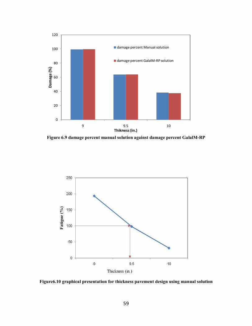
Figure 6.9 damage percent manual solution against damage percent GalalM-RP

Figure6.10 graphical presentation for thickness pavement design using manual solution

0

20

40

60

80

100

120

9 9.5 10

Dam

age

(%)

Thikness (in.)

damage percent Manual solution

damage percent GalalM-RP solution

60

Figure6.11 graphical presentation for thickness pavement design using GalalM-RP

Figure6.12 Manual solution VS GalalM-RP Software Program

61

Table 6.2 Comparison of thickness design between

AASHTO and PCA design methods

6.2 Discussions

From a general comparison of the thickness design between manual solution

and GalalM-RP solution illustrated in Figures 6.8, 6.9, 6.10, 6.11 and 6.12 and

Table 6.2 it may be noted that:

(i) As represented in histograms Figure 6.8; manual solution and GalalM-RP

solution gave average fatigue values of 107.8% and 109.3% respectively

with corresponding discrepancies of -4.7 to 0.3%. That seen the difference

percentage was acceptable.

(ii) As represented in Figure 6.9; manual solution and GalalM-RP solution

gave average damage values of 67.2% and 67.1% respectively with

corresponding discrepancies of -0.2to +0.7%. Thus GalalM-RP compared

very well with manual solution

(iii) However, 98.5 % is much less than 100 % indicating the slab thickness

of 9.5 in. (241.3 mm) is over design. Thus, the design was repeated using

9-in (229 mm) thickness resulting in fatigue damage of 193.9%, much

higher than 100 % (under design). Therefore, a slab thickness of 9.49 in.

(241 mm) would be adequate can be inferred from the patterns of the

shown in Figure 6.10 and 6.11.

(iv) From Fig 6.12 It seen that the results of both manual solution and the

program for the thickness are identical.

Item JPCP JRCP

Design Method PCA AASHTO PCA AASHTO

Typical total pavement

thickness, in. 9.49 9.85 9.49 9.85

62

(v) As represented in Table 6.2 the difference in slab thickness was only 3.8

% with AASHTO design thicker. Since both methods do not differentiate

between JPCP and JRCP.

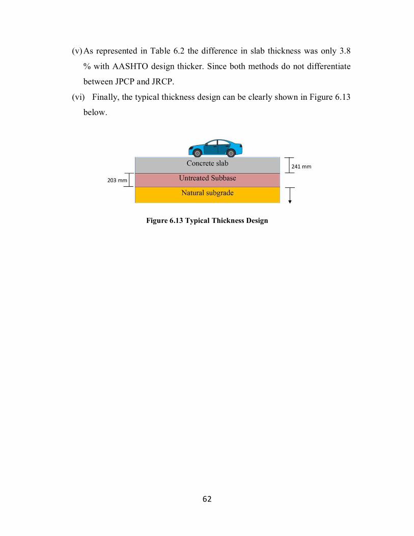
(vi) Finally, the typical thickness design can be clearly shown in Figure 6.13

below.

Figure 6.13 Typical Thickness Design

63

CHAPTER SEVEN

SUMMARY, CONCLUSIONS AND RECOMMENDATIONS

7.1 Summary

In this research investigation, thickness design for JPCP by AASHTO and PCA

methods was determined for the case study road. However, reinforced design by

AASHTO procedure was performed for the JRCP suggested to be used in the

construction of the proposed road. A computer program with Visual Basic

software was developed, entitled GalalM-RP program, to determine the rigid

pavement design thickness in accordance with PCA method. Comparison was

then made for the rigid pavement design thickness between the manual method

and GalalM-RP program.

Comparison of the results for the design thickness between manual solution and

the program was very favorable.

7.2 Conclusions

Within the scope of this study and the design conditions applied for the case

study, the following conclusions are warranted:

1. A computer program (GalalM-RP) in Visual Basic was developed which

was not easy that took a lot of effort and time. GalalM-RP program

proved to possess simplicity with comprehensiveness in treating and

translating design PCA procedure to computer application.

2. The case-study rigid pavement design was determined by AASHTO and

PCA methods for both JPCP and JRCP. The difference in slab thickness

was only 3.8 % with AASHTO design thicker. Since both methods do not

differentiate between JPCP and JRCP, there was difference in the basic

design thickness.

64

3. Comparison of the program results with the manual-computational design

were very favorable varying within 5 %

4. According to AASHTO and PCA design methods used in this study and

the results achieved with favorable comparison with manual design, it is

justifiable to conclude that the GalalM-RP program can be used reliably

as design thickness program for rigid pavements with doweled joints

without concrete shoulders.

7.3 Recommendations

The following are several recommendations that can be considered for future

work:

1. Computer programmers have access to computer room. Modify access

procedures to restrict access to the computer room to computer operators

only.

2. Deficient documentation, Documentation of program changes, systems

software, and testing should be required.

3. No computer Subbase-subgrade k. For manual entry process, Subbase-

subgrade k should not need to manually enter. This information should be

accessed from a computer file.

4. Program cannot design in the case of Slabs without doweled joints and

with concrete shoulders. The Galal R.P. system should be programmed to

design in the case of slabs without doweled joints and with concrete

shoulders.

5. Control totals determined by the trail thickness do not appear to be used

appropriately. The economical of thickness should be used by the

computer.

6. No range checks or limit or reasonableness tests in nomograph for fatigue

if the Stress ratio factors were not in range of (0.3-0.4).

65

References:

1. AASHTO (2003). Guidelines pavement design, the American

Association of State Highway and Transportation Officials, Washington,

DC, USA.

2. Ali, GA (2010-2014). Lecture Notes and Handouts, Sudan University of

Science and Technology, unpublished.

3. Ali, G., Elniema, A. and El-Obeid, H., (2012), “Feasibility of Using

Concrete Pavements in Developing, Hot-Climate Countries: A Case

Study for Conditions of Khartoum State in Sudan”, 9th International

Conference on Concrete, Bahrain, 12-14 Feb 2012.

4. Bezabih, A. G. and Satish, C. (2009). Comparative Study of Flexible and

Rigid Pavements for Different Soil and Traffic Conditions”, Journal of

the Indian Roads Congress, July-September, Paper No. 554, pp. 153-162.

5. Gasim, F., (2014), “Rigid and Flexible Pavements for National Highways

and State Roads: Comparative Design, Construction and Economic

Analysis”, MScm Thesis, SUST, Sudan. Supervisor Ali, Galal.

6. Huang, Yang H (2004). Pavement Analysis and Design, 2nd Ed, Pearson

Prentice-Hall, NJ, USA.

7. NUSSBAUM, P. J., and E. C. LOKKEN, 1978. Portland Cement

Concrete Pavements, Performance Related to Design-Construction-

Maintenance, Report No. FHWA-TS-78-202, Prepared by PCA for

Federal Highway Administration.

66

8. Packard, R. G., "Thickness Design for Concrete Highway and Street

Pavements", Portland Cement Association, Skokie, Illinois, 1984.

9. PCA, 1984. Thickness Design for Concrete Highway and Street

Pavements; Portland Cement Association, Skokie, IL.

10. .PCA, 1991. Design and Construction of Joints for Concrete Highways,

Concrete Paving Technology; Portland Cement Association.

11. Prasad, B., (2007), “Life Cycle Cost Analysis of Cement Concrete Roads

vs. Bituminous Roads”, Indian Highways, Vol.35, No.9, 19-26.

12. Taylor and Francis (2006). The Hand Book of Highway Engineering,

London, CRC.

13. Ukar, S., Akakin, T., and Engin, Y. (2007), “Cost Comparison of Rigid

and Flexible Pavements: Applications in Turkey”, ERMCO Seville

Congress, June 2007.

14. Yoder, E and Witczak MW (1975). Principles of Pavement Design, 2nd

Ed, John Wiley & Sons.

67

APPENDIX A

PCA DESIGN METHOD: TABLES AND CHARTS

A.1 PCA Design Method: Tables

TABLE A.1 Effect of Untreated Subbase on k Values

Note. 1 in. = 25.4 mm, 1 pci = 271.3 kN/m3.

Source. After PCA (1984).

TABLE A.2 Recommended Dowel Size and Length

Note. All dowels spaced at 12 in. on centers, 1 in. = 25.4 mm.

Source. After PCA (1975).

68

A.2 PCA Design Method: Charts

Figure A-1 Effect of various thicknesses of granular subbase on K values

69

FIGURE A-2

Stress ratio factors versus allowable load repetitions both with and without concrete

shoulders

(1 kip = 4.45KN). (After PCA (1984))

70

FIGURE A-3

Erosion factors versus allowable load repetitions without concrete shoulders (1 kip =

4.45KN).

(After PCA (1984)).

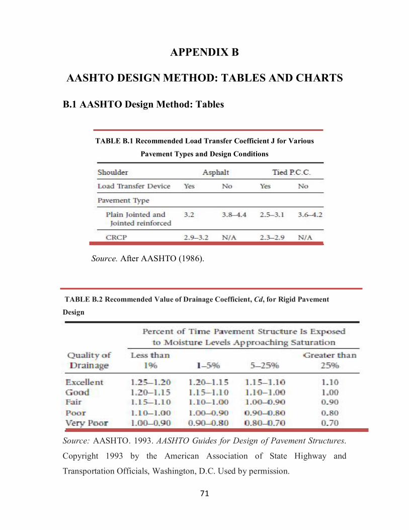
71

APPENDIX B

AASHTO DESIGN METHOD: TABLES AND CHARTS

B.1 AASHTO Design Method: Tables

TABLE B.1 Recommended Load Transfer Coefficient J for Various

Pavement Types and Design Conditions

Source. After AASHTO (1986).

TABLE B.2 Recommended Value of Drainage Coefficient, Cd, for Rigid Pavement

Design

Source: AASHTO. 1993. AASHTO Guides for Design of Pavement Structures.

Copyright 1993 by the American Association of State Highway and

Transportation Officials, Washington, D.C. Used by permission.

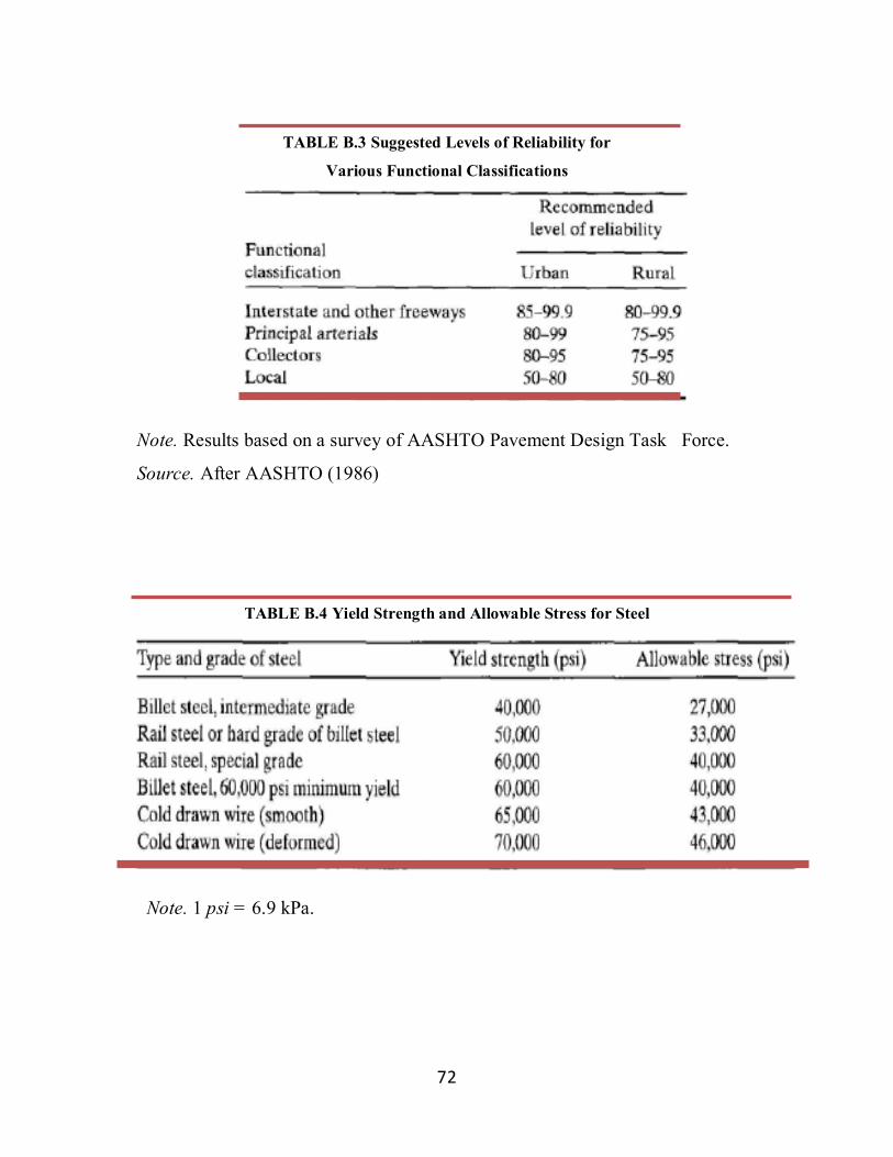
72

TABLE B.3 Suggested Levels of Reliability for

Various Functional Classifications

Note. Results based on a survey of AASHTO Pavement Design Task Force.

Source. After AASHTO (1986)

TABLE B.4 Yield Strength and Allowable Stress for Steel

Note. 1 psi = 6.9 kPa.

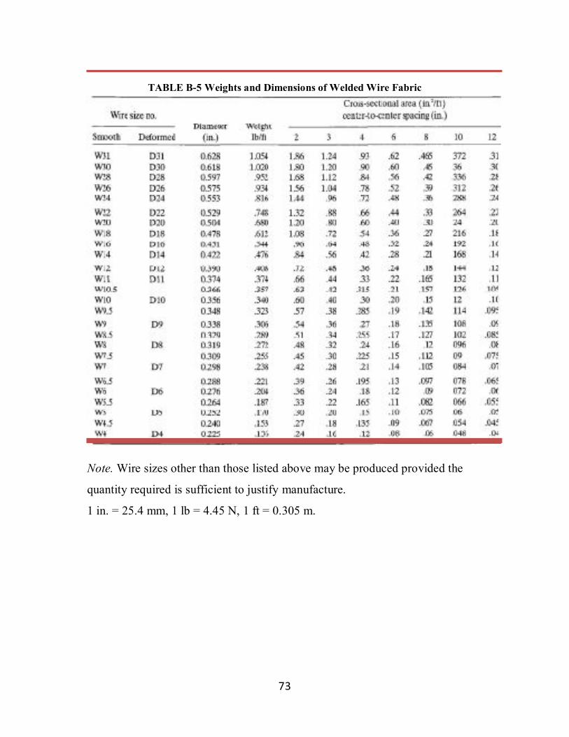
73

TABLE B-5 Weights and Dimensions of Welded Wire Fabric

Note. Wire sizes other than those listed above may be produced provided the

quantity required is sufficient to justify manufacture.

1 in. = 25.4 mm, 1 lb = 4.45 N, 1 ft = 0.305 m.

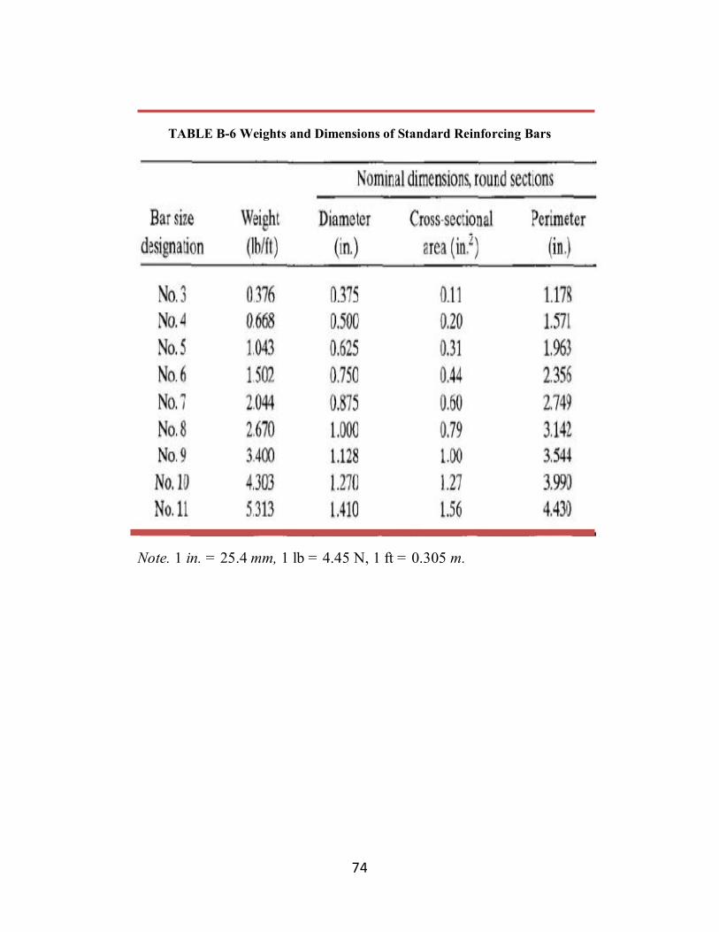
74

TABLE B-6 Weights and Dimensions of Standard Reinforcing Bars

Note. 1 in. = 25.4 mm, 1 lb = 4.45 N, 1 ft = 0.305 m.

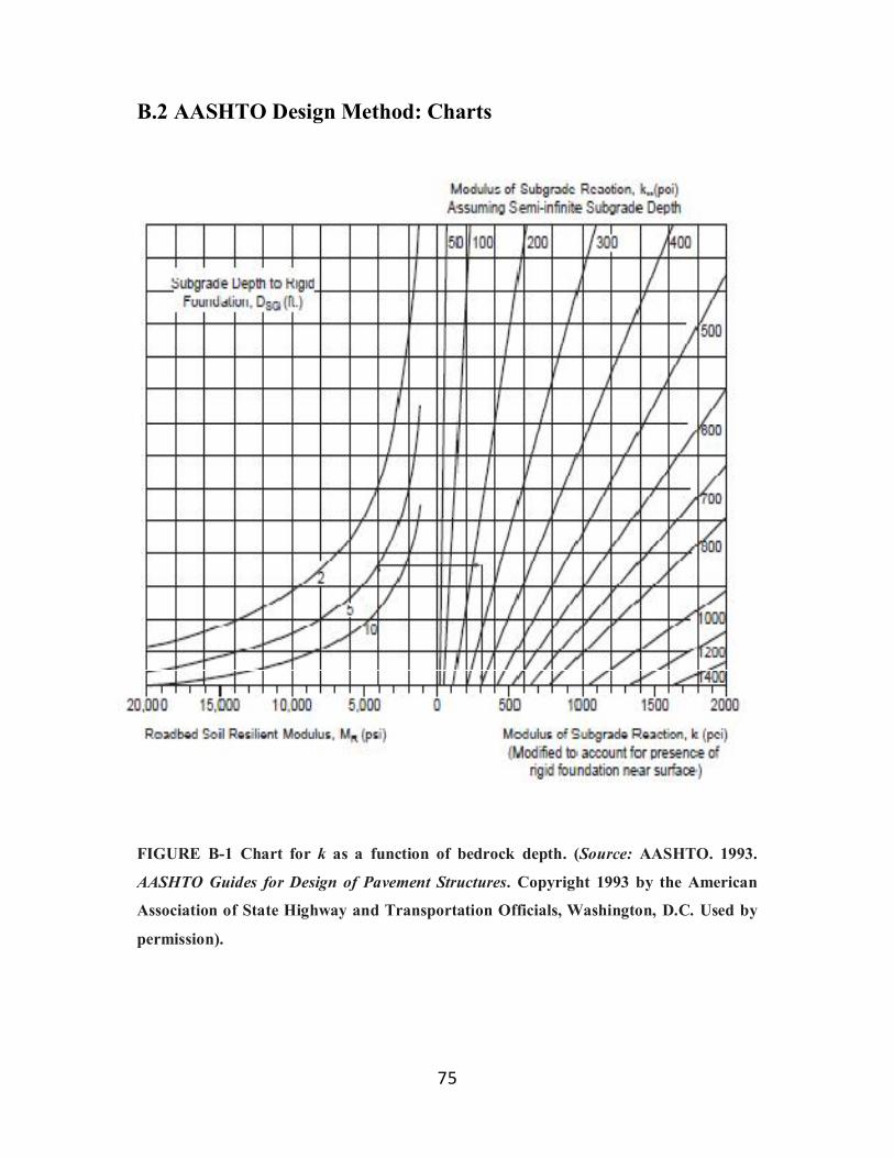
75

B.2 AASHTO Design Method: Charts

FIGURE B-1 Chart for k as a function of bedrock depth. (Source: AASHTO. 1993.

AASHTO Guides for Design of Pavement Structures. Copyright 1993 by the American

Association of State Highway and Transportation Officials, Washington, D.C. Used by

permission).

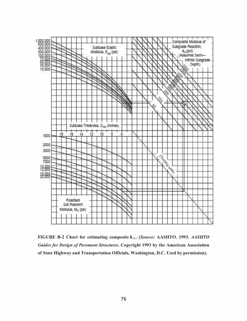
76

FIGURE B-2 Chart for estimating composite 풌 . (Source: AASHTO. 1993. AASHTO

Guides for Design of Pavement Structures. Copyright 1993 by the American Association

of State Highway and Transportation Officials, Washington, D.C. Used by permission).