Buckling of Thin-Walled Cylindrical & Conical Metal Tanks
498
Buckling of Thin-Walled Cylindrical & Conical Metal Tanks: Analysis, Test Evaluation & Design Dissertation by Medhanye B. TEKLEAB, M.Sc. submitted to Faculty of Civil Engineering Sciences Graz University of Technology Reviewed by Werner GUGGENBERGER, Ao.Univ.-Prof. Dr.techn. Institute for Steel & Shell Structures, Graz University of Technology and Ali LIMAM, Prof. Dr. URGC-Structures, Department of Civil Engineering, INSA Lyon, France Graz, December 2009
-
Upload
khangminh22 -
Category
Documents
-
view
3 -
download
0
Transcript of Buckling of Thin-Walled Cylindrical & Conical Metal Tanks

Buckling of Thin-Walled Cylindrical& Conical Metal Tanks:
Analysis, Test Evaluation & Design
Dissertation by
Medhanye B. TEKLEAB, M.Sc.
submitted to
Faculty of Civil Engineering Sciences
Graz University of Technology
Reviewed by
Werner GUGGENBERGER, Ao.Univ.-Prof. Dr.techn.
Institute for Steel & Shell Structures, Graz University of Technology
and
Ali LIMAM, Prof. Dr.
URGC-Structures, Department of Civil Engineering, INSA Lyon, France
Graz, December 2009


Acknowledgements
My heart-felt thanks will go to my supervisor Ao.Univ.-Prof. Dipl.-Ing. Dr.techn. Werner Guggen-berger for his tireless, patience full, very close, smart and critical way of advising and the manyimportant discussions we had during the course of my study. I really am in shortage of words toexpress my appreciation to him. I thank Prof. Ali Limam for reviewing my work who also is myexternal examiner. I would like to thank Univ.-Prof. Dipl.-Ing. Dr.techn. Richard Greiner, head ofthe Institute for Steel and Shell Structures at Graz University of Technology, for his valuable com-ments, encouragement and kind treatment. I am grateful to the institute and its nice hard workingpeople for the resource-full and very good working environment I had during my stay. I speciallythank Dipl.-Ing. Burkhard Krenn who has been a good friend to me and who helped me a lot in alladministrative matters both in and off the university starting from the very first day I arrived inGraz.
My special thanks will also go to Gent University, Belgium, and specially to Prof. Guy Lagae andDr. Wesley Vanlaere for providing me with a complete data and necessary explanations on the lab-oratory tests made at Gent University over 30 years ago.
This work wouldn’t be true with out the financial support I was granted from the Austrian Aca-demic Exchange Service through the North-South Dialogue scholarship for which I am gratefuland would like to express my gratitude to all its staff members. I thank the Afro-Asian Institute inGraz and its staff members for the support I had with regard to housing matters. I thank MekelleUniversity, Ethiopia, the young yet vibrant university, of which I am an employee since nine years,for offering me a study leave even though there was shortage of lecturers with an increase in thenumber of incoming students.
Last but not least, I would like to acknowledge my father Biedebrhan Tekleab and my motherMe’aza Baraki for their unending true love, encouragement and moral assistance they showed meall the way in life.
Medhanye B. Tekleab


AbstractThis work re-searches the stability of cylindrical and conical thin-walled tank shells from the basiclevel in view of both analysis and previous test results. Detailed discussions on failure modes, nu-merical simulations and re-investigation of test results have been made. The axisymmetric elastic-plastic buckling phenomena, buckling modes and strengths of meridionally compressed and inter-nally pressurized perfect and imperfect cylindrical and conical shells have been investigated in de-tail. The effects of imperfection wavelength, location along the meridian, orientation, andamplitude of sinusoidal & local imperfections have been thoroughly studied. The worst possiblecombined effect of an edge restraint and an imperfection in destabilizing such shells has also beendiscussed. All results are represented and interpreted in such a way that they can easily be under-stood and used for design purposes. Simplified expressions are obtained for the prediction of axi-symmetric elastic-plastic buckling strength of general thin-walled cylindrical and conical shellsunder the mentioned loading situations. Design recommendations have been proposed. Compari-sons with and critical review of few previous research works have as well been thoroughly carriedout.
Detailed investigation of the numerous Gent laboratory test results (obtained about 30 years ago atthe Laboratory of Model Testing at Gent University, Belgium) on liquid-filled conical shells,shortly called LFC, that have been made in response to a structural disaster in Belgium along withdetailed discussions, explanations, and conclusions have been done. Previous LFC-relatedresearch works on nonlinear simulation of liquid-filled conical shells with and without geometricimperfections have as well been discussed and few cases have been re-examined for confirmationand further studying purposes. Relevant explanations and conclusions have been given to theoutcomes of those works. Moreover, the Belgium (1972) and Canada (1990) steel water towerfailure cases have been carefully examined to check and compare their elastic buckling strengthswith the applied loads during failure; and to check for any possible roles played by plasticity effectsduring the collapse. Previous research works related to the collapse of the water towers have alsobeen discussed. The notion of a “corresponding cylinder” of a liquid-filled conical shell has beenintroduced which behaves in exactly the same way as the LFC. Detailed and comprehensiveinvestigation of this “corresponding cylinder” was then made with the simple outcome that theliquid-filled cone behaves like a “wet cylinder”, i.e. with respect to its axisymmetric deformationand buckling behavior.

Contents I
Contents1 Introduction and state-of-the-art 1
1.1 Motivation 2
1.2 Overview 5
1.3 State-of-the-art 7
2 Problem statement, goal and scope of the work 9
2.1 Problem statement 10
2.2 Goal of the work 12
2.3 Solution methods 13
2.4 Scope of the work 14
3 Axisymmetric elastic-plastic buckling of cylindricalshells under axial compression & internal pressure 21
3.1 Introduction 22
3.2 Problem statement 24
3.3 Linear shell analysis (LA) 25 3.3.1 Pure membrane behavior 26 3.3.2 Edge-bending effects 28 3.3.3 Numerical finite element linear analysis (LA) 32
3.4 Linear elastic buckling strength of an ideally perfect cylinder 36 3.4.1 Approximate linear buckling analysis based on linear shell analysis 37 3.4.2 Linear buckling analysis using an analytical model based on theory of second order 38 3.4.3 Numerical finite element linear buckling analysis (LBA) 38
3.5 Elastic buckling strength of an imperfect cylinder 40 3.5.1 Elastic buckling strength: history 40 3.5.2 Elastic imperfection reduction factor, EN1993-1-6 50
3.6 Pure plastic strength of cylindrical shells 54 3.6.1 Plastic strength according to von Mises membrane criteria 54 3.6.2 Stress resultant oriented approximate yield criteria 55 3.6.3 Small displacement materially nonlinear finite element analysis (MNA) 57
3.7 Elastic-plastic buckling phenomena, analysis, and strength 59 3.7.1 General concept of buckling phenomena 59 3.7.2 Elastic buckling strength 62 3.7.3 Elastic-plastic buckling in the free shell interior 66 3.7.4 Axisymmetric elastic-plastic buckling of perfect cylindrical shells 71
3.7.4.1 Geometrically and materially nonlinear finite element analysis (GMNA) 71

II Contents
3.7.4.2 Analytical model based on theory of second order with material nonlineareffects 79
3.8 Axisymmetric elastic-plastic buckling of imperfect cylindrical shells 83 3.8.1 Geometrically and materially nonlinear finite element analyses with
axisymmetric imperfections (GMNIA) 83 3.8.1.1 Introduction 83 3.8.1.2 Linear elastic buckling (LB) eigenmode-affine imperfection 84 3.8.1.3 Understanding axisymmetric elastic-plastic buckling phenomenon of
thin-walled shells 87 3.8.1.4 Local axisymmetric imperfection shapes near the boundary 92 3.8.1.5 Local axisymmetric imperfection in the free shell interior 102
3.9 New buckling design recommendation 106 3.9.1 General characteristic buckling strength 106 3.9.2 Characteristic buckling strength prediction recommendation 114
3.9.2.1 Method-1: Elastic-plastic interaction using pressure dependent interactionparameters in such a way that EFoot strength is directly included 122
3.9.2.2 Method-2: Envelope of the different buckling strengths 128 3.9.2.3 Method-4: Elastic-plastic interaction using a completely new interaction
parameter 131
3.10 Comparison of the new buckling design recommendation with EN 1993-1-6 bucklingdesign regulation 137
3.10.1 Perfect elephant’s foot buckling strength using EN 1993-1-6 137 3.10.2 EN 1993-1-6 buckling design regulation 145 3.10.3 Summary of EN 1993-1-6 design regulation 152 3.10.4 Related previous study and results 156
3.11 Summary and conclusions 158
4 Axisymmetric elastic-plastic buckling ofliquid-filled conical shells (LFC) 159
4.1 Introduction 160
4.2 Problem statement 162
4.3 Linear shell analysis (LA) 163 4.3.1 Pure membrane behavior 163 4.3.2 Edge-bending effects 165 4.3.3 Numerical finite element linear analysis (LA) 166
4.4 Loading procedure for numerical analysis purposes 170
4.5 Linear buckling strength of an ideally perfect liquid-filled cone 175 4.5.1 Approximate linear buckling analysis 175 4.5.2 Linear buckling analysis using numerical finite element method 182
4.6 Elastic buckling strength of an imperfect liquid-filled cone 186 4.6.1 Elastic imperfection reduction factor, EN1993-1-6 186 4.6.2 Elastic buckling strength 187 4.6.3 Re-investigation of Gent’s experimental test results 188
4.7 Pure plastic strength of liquid-filled conical shells 189

Contents III
4.7.1 Plastic strength according to von Mises membrane criterion 189 4.7.2 Stress resultant oriented approximate yield criteria 191 4.7.3 Small displacement materially nonlinear finite element analysis (MNA) 193
4.8 Elastic-plastic buckling phenomena, analysis and strength 202 4.8.1 Elastic-plastic non-axisymmetric buckling 202 4.8.2 Axisymmetric elastic-plastic buckling 204
4.8.2.1 Geometrically and materially nonlinear finite element analysis ofperfect conical shells (GMNA) 204
4.8.2.2 Analytical model based on theory of second order withmaterial nonlinear effects 217
4.9 Buckling design recommendation 218
4.10 Summary and conclusions 219
5 Re-investigation of Gent test results:Elastic buckling of liquid-filled cones 221
5.1 Introduction 222
5.2 Problem statement 226
5.3 Liquid-filled conical shell parameters and representation 227
5.4 Fluid-filled conical shells: comparison of gas-filled vs. liquid-filled conical shells 233
5.5 Test results and Gent University design proposal 237
5.6 Comparison of parameter choices and representations 244
5.7 Detail re-investigation of test results 262 5.7.1 Cleaning the test data 262 5.7.2 Detailed study of test results based on the slenderness ratio parameter (r1/tcosβ) 271
5.8 Detailed comparison based on the LFC-elastic buckling limits 279
5.9 LFC-imperfection reduction factor 286 5.9.1 Belgium collapsed steel water tower 286 5.9.2 Canada collapsed steel water tower 287
5.10 Summary and Conclusion 291
6 Re-investigation of Gent test results:Mercury-filled steel cones 293
6.1 Investigation of Gent mercury-test results 294 6.1.1 Gent mercury-test data 294 6.1.2 Current investigation 294
6.2 Geometrically and materially nonlinear analysis of imperfect cones 299
6.3 Summary and conclusions 304
7 Re-examination of two tank failure cases 305
7.1 Steel water tower failure cases 306

IV Contents
7.2 Confronting previous research work results related to the collapse of steel water towers 311
7.3 Summary and conclusions 316
8 The notion of the “corresponding cylinder” 317
8.1 Introduction 318
8.2 “Equivalent cylinder” of a conical shell 318
8.3 “Corresponding cylinder” of a conical shell 326 8.3.1 Linear elastic buckling strength of the “corresponding cylinder” 333 8.3.2 Materially nonlinear yield- and geometrically & materially nonlinear
buckling- strengths of the “corresponding cylinder” 336
8.4 Summary and conclusions 338
9 General summary & conclusion 339
9.1 General summary & conclusions 340
9.2 Outlook & proposed future work 343
9.3 Proposed European design recommendation (EDR) & European Standard EN 1993-1-6modifications 344
10 References 345
ANNEX
A Ilyushin yield criterion and related approximations 353
A.1 Introduction 354
A.2 Ilyushin’s yield criterion for plates & shells 355 A.2.1 Ilyushin’s exact yield criterion 355 A.2.2 Ilyushin’s linear approximation 357 A.2.3 Ivanov’s approximations 362
A.2.3.1 Ivanov’s approximate yield condition 362 A.2.3.2 Simple cases of Ivanov approximate yield criterion 364
A.2.4 Rewriting different yield criteria 366 A.2.4.1 Ivanov’s yield criterion-I 366 A.2.4.2 Ivanov’s yield criterion-II 367 A.2.4.3 “Simple” yield criterion 367 A.2.4.4 Ilyushin’s linear approximate yield criterion 368 A.2.4.5 EN 1993-1-6 proposed yield criterion 368 A.2.4.6 “First-yield” yield criterion 369
A.2.5 Example: comparison of different yield conditions 370

Contents V
B Axisymmetric rigid plastic plate & shell analysis 373
B.1 Introduction 374
B.2 Rigid plastic analysis of axisymmetric circular & annular plates 375 B.2.1 Equilibrium relationships 377 B.2.2 Kinematic (geometry) relationships 378 B.2.3 Yield functions and yield criterion based on stress resultants 380
B.2.3.1 Yield function 380 B.2.3.2 Yield condition 380
B.2.4 Associated flow/normality rule 381 B.2.5 Summary of equations for rigid plastic analysis of circular plates 381
B.2.5.1 Simplification of equations 382 B.2.5.2 Boundary conditions 383
B.2.6 Introduction of non-dimensional parameters 384 B.2.7 Condensed rigid plastic equations of annular/solid circular plates 385 B.2.8 Solution procedure 387 B.2.9 Examples, result plots and comparison 387
B.3 Rigid plastic analysis of cylindrical shells under axisymmetric radial loading 394 B.3.1 Equilibrium relationships 396
B.3.1.1 Equilibrium of forces 396 B.3.1.2 Equilibrium of moments 396
B.3.2 Kinematic (geometry) conditions 397 B.3.3 Yield functions and yield criteria based on stress resultants 398
B.3.3.1 Yield function 398 B.3.3.2 Yield condition 398
B.3.4 Associated flow/normality rule 398 B.3.5 Summary of equations for rigid plastic analysis of cylindrical shells
under radial ring load 399 B.3.6 Introduction of non-dimensional parameters 400 B.3.7 Simplification of equations 401 B.3.8 Condensed rigid plastic equations of cylindrical shells under radial ring load 403 B.3.9 Derivatives of the yield function 404 B.3.10 Determination of plastic section forces, plastic deformation, slope, curvature
and plastic loading parameter λplastic 405 B.3.11 Complete section force distributions along the meridian 406 B.3.12 Illustrative examples, results and comparison 410
B.3.12.1 Long cylindrical shell under radial ring loading 411 B.3.12.2 Long cylindrical shell under radial ring loading with axial compressive
and internal pressure loads 419
B.4 Summary and conclusion 424
C Analytical elastic buckling analysis of cylindrical shells425
C.1 Introduction 426
C.2 Theory of second order 428
C.3 Basic differential equations for an axisymmetric cylindrical shell 430

VI Contents
C.4 Basic differential equations for a beam on elastic foundation analogy model 431 C.4.1 Deformation geometry relationships (Kinematics) 431 C.4.2 Material relationships (Constitution) 431 C.4.3 Equilibrium relationships (Kinetics) 431 C.4.4 Kinematics + Constitution + Kinetics (all - in - one beam equation matrix) 432 C.4.5 Correspondence of axisymmetric cylinder and beam on elastic foundation 432 C.4.6 Reduction of the set of 1st order differential equations into a single
4th order differential equation 433 C.4.6.1 Solution for the 4th order differential equation - homogeneous
fundamental solution 434 C.4.6.2 General solution of the homogeneous differential equation 434
C.5 Different solution cases of the 4th order homogeneous o.d.e.: fundamental functionand accompanying derivative matrix 435
C.5.1 Case - 1 435 C.5.2 Case - 2 436 C.5.3 Case - 3 436
C.6 Derivation of beam stiffness matrix 437 C.6.1 General - for all solution cases 437
C.6.1.1 Displacement vector 437 C.6.1.2 Beam-end displacements and homogeneous edge-displacement matrix 437 C.6.1.3 Computation of the integration constants vector c 437 C.6.1.4 Section and edge forces 438 C.6.1.5 computation of the transversal section force 438 C.6.1.6 Global edge-forces vector 439 C.6.1.7 Stiffness matrix using theory of second order 439
C.6.2 Specific - for each solution case 440 C.6.2.1 Case - 1 440 C.6.2.2 Case - 2 444 C.6.2.3 Case - 3 446
C.7 Procedure for analytical computation of elastic buckling strengths and buckling eigenmodes448
C.8 Illustrative examples, results and comparison 450 C.8.1 Elastic buckling strength computation 451
C.8.1.1 Example-1: Pinned bottom and top edges 451 C.8.1.2 Example-2: Pinned bottom and rotationally restrained top edges 458 C.8.1.3 Example-2: Fixed bottom and free top edges 463 C.8.1.4 Example-4: Fixed bottom and rotationally restrained top edges 468
C.8.2 Elastic buckling eigenmode computation 472 C.8.2.1 Fixed bottom and free top edges 472 C.8.2.2 Fixed bottom and rotationally restrained top edges 474
C.9 Summary and conclusion 481

A Notation
Notation
Cylindrical shells:
R radius
t shell wall thickness
R/t shell slenderness ratio
L meridional length of the shell
x running length parameter starting from bottom of shell, in axial direction
s arc length in meridian direction
normalized meridional length parameter
X meridional direction
θ circumferential direction
r running radius of shell middle surface, perpendicular to the axis of rotation
R10 radius of curvature in meridional direction, located on the shell normal
R20 radius of curvature in circumferential direction, located on the shell normal
U meridional deformation
W radial deformation
meridional rotation
σx meridional normal membrane stress
σθ circumferential normal membrane stress
Nx meridional normal section force
Nθ circumferential normal section force
Qx transverse shear section force
Mx meridional bending section moment
Mθ circumferential bending section moment
normalized meridional section force ( = Nx/Npl)
normalized circumferential section force ( = Nθ/Npl)
ξ
βX
nx
nθ

Notation B
normalized meridional section moment ( = Mx/Mpl)
normalized circumferential section moment ( = Mθ/Mpl)
N1 principal normal section force in “1”-direction
N2 principal normal section force in “2”-direction
M1 principal section moment in “1”-direction
M2 principal section moment in “2”-direction
normalized principal section force in “1”-direction ( = N1/Npl)
normalized principal section force in “2”-direction ( = N2/Npl)
normalized principal section moment in “1”-direction ( = M1/Mpl)
normalized principal section moment in “2”-direction ( = M2/Mpl)
E modulus of elasticity
fy yield strength
ν Poisson’s ratio
G shear modulus
p internal pressure
σx,1 meridional normal membrane stress at bottom support
σθ,1 circumferential normal membrane stress at bottom support
σx,Rcr elastic critical buckling stress of an axially compressed cylinder (0.605 Et/R)
mx
mθ
n1
n2
m1
m2

C Notation
Conical shells:
h’ height of liquid surface level above base level ’1’
h height of cone above base level ’1’
L meridional length of the cone
r running radius of cone middle surface, perpendicular to the axis of rotation
r1 small radius at the base of the cone
r2 large radius at the upper end of cone
r’2 large radius at the liquid surface level
t wall thickness of the conical shell
β apex half angle of the cone
γ' specific weight of the liquid filling
z running height parameter above the base level ’1’
ζ running geometry parameter, (z.tanβ/r1)
ζ' geometry parameter, (h’.tanβ/r1)
ρ running nondimensional coordinate parameter, (r/r1)
ρ' nondimensional coordinate parameter at the liquid surface level, (r’2/r1)
σx,1 meridional normal membrane stress at the cone support
σθ,1 circumferential normal membrane stress at the cone support
σx,Rcr elastic critical buckling stress of an axially compressed conical shell (0.605.Etcosβ/r1)
p internal pressure parameter (σθ,1/σx,Rcr)
ψ ratio of meridonal to circumferential membrane stress at the cone support
R radius of an equivalent cone at cone-base (r1/cosβ)
p pressure at cone-base (γ'h’)

Notation D
General & EN 1993-1-6:
p critical-stress-related internal pressure parameter ( = σθ,1/σx,Rcr)
μ yield-related internal pressure parameter ( = σθ,1/fy)
ψ ratio of meridional to circumferential membrane stress at the bottom support
αx unpressurized elastic imperfection reduction factor of EN 1993-1-6, Annex-D
αxpe pressurized elastic imperfection reduction factor of EN 1993-1-6, Annex-D
αxpp pressurized plastic imperfection reduction factor
FEM finite element method using ABAQUS Version 6.7-1 (2007)
LA Linear Analysis
LB Linear Buckling
LBA Linear Buckling Analysis
MNL Materially Nonlinear
MNA Material Nonlinear Analysis
GMNL Geometrically and Materially Nonlinear
GMNA Geometrically and Materially Nonlinear Analysis
GMNLI Geometrically and Materially Nonlinear with Imperfections
GMNIA Geometrically and Materially Nonlinear Analysis with Imperfections
lb Buckle length
Leff effective length
Aeff effective area
σcr elastic buckling stress
σk characteristic buckling stress
λ relative buckling slenderness parameter
λο relative buckling slenderness parameter
λp relative buckling slenderness parameter
χ buckling reduction factor
plastic range factor
elastic-plastic buckling interaction exponent
β
η

Chap. 1 Introduction and state-of-the-art 1
1
Introduction and state-of-the-art

2 Chap. 1 Introduction and state-of-the-art
1.1 Motivation
Cylindrical and conical shells have a wide range of applications in engineering, in general, and instructural engineering, in particular. To mention some, these shells are used as pressure vessels,pipes, tanks, silos, roof structures. In many of these practical engineering applications, cylindricaland conical shells are subjected to axisymmetric type of loading such as gravity (self-weight,snow), hydrostatic pressure, internal or external gas pressure. More specifically pipes, tanks andsilo structures are mainly subjected to the simultaneous effects of meridional compression andinternal pressurization coming from the contained material. Such types of loading cause bi-axialstress state: meridional membrane compression and circumferential (hoop) membrane tension.
The appropriate functioning of such structures requires a proper design that takes all possiblefailure conditions in to account. One of such possible and most dominant failure conditions for thinshells is failure by buckling (stability considerations). There have been buckling failure cases ofcivil engineering thin-walled metal cylindrical and conical shells under axial compressive loadswith co-existent internal pressure. Many of the buckling failures in cylindrical shells happenedforming outward bulges near the supported edge (elephant’s-foot buckling phenomenon) resultingfrom earthquake induced effects. Figure 1.1 to Figure 1.4 show pictures of few of such failurecases.
The elephant’s-foot type buckling phenomenon may generally occur in cylindrical and conicalshells so long as they are subjected to meridional compression and circumferential tension near theboundary. More specifically, axisymmetric elastic-plastic buckling near a boundary may happenin thin-walled cylindrical and conical shells with constant/varying meridional compression andhydrostatic internal pressure. Since a liquid-filled conical shell falls into such a loading category,an axisymmetric elastic-plastic buckling near the boundary is possible and hence the bucklingstrength of conical shells associated to an elephant’s-foot buckling phenomenon needs to beinvestigated in detail. Besides, there have been buckling failure cases of conical shells as in thecases of the Belgium water tower in 1972 and Canada water tower in 1991 for which the real causesneed to be invetigated.
There, as well, have been a lot of research attempts, both theoretically and experimentally, todetermine the exact buckling capacity of cylindrical and conical shells under axial compressiveloads with co-existent internal pressure. Despite the number of research attempts so far, theirprediction of the buckling strengths do have serious insupportable problems.
This work will mainly address the axisymmetric elastic-plastic buckling strength of isotropicunstiffened cylindrical and conical shells and re-investigates the numerous experimental resultsperformed in Gent on the elastic and elastic-plastic buckling of conical shells.

Chap. 1 Introduction and state-of-the-art 3
Figure 1.1 Elephant’s foot buckling (JM Rotter)
Figure 1.2 Elephant’s foot buckling (JM Rotter)
rerseits be-Biegebean-
rt wiederum
beulen“amkeit gewidmet
hungszu-oppelt mit– ist unge-mit erheb-
andelt, voll-udem auch in

4 Chap. 1 Introduction and state-of-the-art
Figure 1.3 Elephant’s foot buckling (Gould)
Figure 1.4 Elephant’s foot buckling above a column support (Guggenberger)

Chap. 1 Introduction and state-of-the-art 5
1.2 Overview
The general behaviour of cylindrical & conical shells under meridional compression andcircumferential tension will be analyzed using analytical and numerical linear analysis techniquesfrom which the pure membrane and edge-bending effects can be separately seen. These effects willlater be used in reasoning out special buckling phenomenon. The results will be compared with afinite element linear analysis results for verification purposes. The small displacement linearbuckling strengths of these shell types will then be computed approximately and investigatednumerically. This strength will later be used as a reference to express other buckling strengthsaccording to the frame work of EN 1993-1-6.
The effects of imperfections on the elastic buckling strength of thin-walled cylindrical and conicalshells will be discussed in detail for different fabrication quality classes as recommended in EN1993-1-6 and comparisons between the cylinder and cone will be made. Explanations will be givenabout the LFC-specific buckling phenomenon and corresponding strengths. Simplified expressionsfor the prediction of linear buckling strengths of liquid-filled general cones with pinned and fixedbottom boundary conditions will be obtained. In doing so, the numerous laboratory experimentsmade on liquid-filled conical shells will be re-examined. Comparisons of the perfect and imperfectlinear buckling strengths of cylindrical and conical shells will be made.
Nonlinear buckling and plastic strengths of cylindrical and conical shells will be computedapproximately using analytical models with second order effects included and numerically using afinite element package (ABAQUS). The pure plastic limit strengths of the shells will be computedapproximately using von Mises membrane yield criterion taking the membrane stresses at theshell-base as references; and using stress resultant oriented approximate yield criteria. The effectsof material nonlinearity, geometric nonlinearity and imperfections will be numericallyinvestigated. Comparisons of the results obtained using the analytical model and numericalanalysis will be made. Detailed comments and explanations on the results will be given.
The numerical simulation results will be used to derive a set of basic data that can be used in astraight forward buckling design by hand calculations in-line with the underlying structure of theEuropean standard EN1993-1.6. Design recommendations will finally be proposed which will becompared with previous research results and code recommendations. Additional comments andexplanations concerning the results will also be included.
Detailed investigation of Gent mercury test results along with detailed discussions, explanations,and conclusions will be done. Previous LFC-related research works on nonlinear simulation ofliquid-filled conical shells with/out geometric imperfections will as well be discussed and fewcases will be re-examined for confirmation and further studying purposes. Relevant explanations

6 Chap. 1 Introduction and state-of-the-art
and conclusions will be given to the outcomes of those works.
Moreover, the Belgium and Canada steel water tower failure cases will be re-examined to checkfor any possible roles played by plasticity effects during the collapse. Previous research worksrelated to the collapse of the water towers will also be discussed.
A “corresponding” cylinder of a liquid-filled conical shell will be introduced which behaves inexactly the same way as the LFC. Detailed invetigation of the “corresponding” cylinder will thenbe made which will turn out to be that the liquid-filled cone is nothing but a “wet-cylinder”.

Chap. 1 Introduction and state-of-the-art 7
1.3 State-of-the-art
Many shell stability related research works have been done so far. The results of such researchworks have been included in design standards. The latest design standard which is believed toinclude many of the research results is discussed below. For this reason, in the discussions of thecurrent study, references to and comparisons with this standard will be made.
In the buckling strength assessment of thin-walled general metal shells-of-revolution, theEuropean Standard EN1993-1-6 recommends to use three different approaches (methods) whichapply to all geometries, all loading conditions, and all material conditions. The hierarchy of thesegeneral buckling design procedures are summarized as follows:
method-1: buckling stress design or LA-based buckling design approach
method-2: LBA/MNA-based buckling design approach using simplified global numerical analysis
method-3: GMNIA-based buckling design approach using advanced global numerical analysis
The buckling stress design approach is based on a membrane theory or linear bending theoryanalysis. The elastic critical buckling stress is computed/estimated based on linear analysis. Thus,buckling stress design is usually performed by “hand calculation“ using formulas and/or diagramsprepared for this purpose. In this method, the linear elastic stress field (meridional, circumferential,and shear) are computed at every point of the midsurface of the shell. The elastic critical bucklingstresses of the perfect shell for each stress component are then determined on which imperfectionreduction factors are applied to obtain the elastic buckling stresses of the imperfect shell. Using theelastic critical buckling stresses of the perfect shell and the uni-axial yield stress of the material,relative buckling slenderness parameters are computed for each stress component upon which thebuckling strength reduction factors depend. These buckling strength reduction factors whichaccount for plasticity effects are then each applied to the uni-axial yield stress to obtain therespective characteristic buckling stresses. Interaction formulas are used to account for anypossible interaction between the effects of the different stress components. The design value of thebuckling stress components are then computed by applying partial safety factors on thecharacteristic strengths.
Buckling strength assessment using design by global numerical LBA/MNA procedure,according to EN1993-1-6, is also a reduction factor approach. The steps involved in the LBA/MNA procedure to predict the buckling strength of the shell have a similar format to those of thebuckling stress design aproach. In the LBA/MNA approach, however, the elastic critical bucklingstress and plastic collapse strength are evaluated accurately using the more rigorous globalnumerical analysis methods.

8 Chap. 1 Introduction and state-of-the-art
The GMNIA procedure, on the other hand, uses advanced global (geometrically and materiallynonlinear) numerical analysis with the consideration of possible imperfections to accuratelysimulate the buckling strength of real shells and to directly obtain the characteristic elastic-plasticbuckling strength of a practical shell.

Chap. 2 Problem statement, goal & scope of the work 9
2
Problem statement, goal & scope of the work

10 Chap. 2 Problem statement, goal & scope of the work
2.1 Problem statement
It has been repeatedly reported in many literatures that thin-walled cylindrical shells usually buckleelastically under pure axial compression. The respective buckling strength for such axially loadedcylindrical shells is usually lower than the theoretical elastic critical stress, the difference account-ing for the decrease in buckling strength caused by the presence of various imperfections and geo-metric nonlinearity. The presence of an accompanying internal pressure, however, reduces thisstrength-weakening effect of the imperfections there by increasing the buckling strength of theshell. However, when the intensity of the internal pressure exceeds a certain value, the circumfer-ential membrane stress becomes significant causing bi-axiality effect to come into play.
An unpressurized cylindrical shell under pure axial compressive load tends to radially expand dueto Poisson’s effect. An internally pressurized cylindrical shell under axial compressive load tendsto radially expand due to the combined effects of both the internal pressurization and Poisson’s ef-fect. The presence of boundary conditions, however, constricts this expansion causing local bend-ing under the action of the axial compressive load. Similar local bending effects may occur atlocations of change in wall thicklness, ring stiffeners, or local axisymmetric imperfections causingimmature buckling under a small meridional compression. Thus, the presence of significant inter-nal pressure will have a destabilizing effect there by reducing the buckling strength of the shell.Such a buckling type, caused by local bending adjacent to the boundary, is termed as an “ele-phant’s-foot” type buckling and the corresponding strength as elephant-foot buckling strength.Moreover, when combined with ill-natured axisymmetric imperfections, the weakening effect ofthe significant internal pressure along with the edge constriction effect, will be more pronouncedthat the cylinder buckles at a very low axial compressive load.
However, a question which still remains unanswered in many of the researches and studies doneso far is the physically possible critical (worst) imperfection shape, wavelength, amplitude, orien-tation, and location along the meridian, each of which has an influence on the buckling behaviorand buckling strength of the shell.
On the other hand, the meridional membrane section force distribution in liquid-filled conicalshells is maximum at the lower supported edge and decreases nonlinearly and rapidly up the me-ridian. Such a distribution of the meridional compressive section force superimposed with the edgeconstriction effects of the bottom boundary conditions will restrict the elastic-plastic buckling phe-nomenon to a region very close to the supported lower edge causing elephant’s-foot type buckling.Despite this fact, not much has been done to investigate the possible elephant’s-foot bucklingstrength of conical shells. Such type of buckling in liquid-filled conical shells, may specially hap-pen when there exist a global bending effect which may result, say, from geometric eccentricity(global tilting) of the cone. This geometric eccentricity, even upon filling may result in global

Chap. 2 Problem statement, goal & scope of the work 11
bending effect which shortens the life span of the structure with the formation of a possible ele-phant’s-foot type buckling phenomenon. Apart from this, a perfect liquid-filled conical shell maybuckle in such an axisymmetric elastic-plastic buckling mode near the supported edge so long asa bi-axial state of stress, similar to that of the cylindrical shell, exists.

12 Chap. 2 Problem statement, goal & scope of the work
2.2 Goal of the work
The true nature of buckling in real-world thin-walled shell structures is at most simulated, at leastnumerically, by analysis models that take the effect of geometric and material nonlinearity into ac-count. For this reason, it is believed and has been applied in the buckling strength determination ofthin-walled shells that the geometrically and materially nonlinear finite element analysis (GMNA)with physically possible imperfections (GMNIA) predicts closer results to the buckling strength ofreal-world thin-walled shells.
It is, therefore, the ultimate goal of this work to numerically simulate cylindrical and conical shellaxisymmetric buckling and finally come up with a set of basic data that can be used in a straightforward buckling design by hand calculations. This work also aims to investigate the effects of ax-isymmetric imperfection shapes on the elastic-plastic buckling strengths of axisymmetric shellsand finally recommend a physically possible worst axisymmetric local imperfection.
It is also the goal of this study to re-investigate the numerous laboratory tests performed in Gentusing liquid-filled conical shells and propose a recommendation for future works and design pur-poses.
A comparison of the results with the previous research works and existing design recommendation,EN1993-1-6, will then be made.

Chap. 2 Problem statement, goal & scope of the work 13
2.3 Solution methods
In the course of investigating the axisymmetric elastic-plastic buckling phenomena and corre-sponding buckling strengths of thin-walled cylindrical and conical shells, a combination of bothanalytical and numerical (using finite element program) analysis methods will be used to assess theapplied loads, depending on the nature and complexity of the problem type under consideration.For this reason, the mentioned shells will be analysed using membrane theory, linear shell bendingtheory (LA), linear buckling analysis (LBA), small displacement materially nonlinear analysis(MNA), perfect geometrically and materially nonlinear analysis (GMNA), and geometrically andmaterially nonlinear analysis with imperfections (GMNIA).
In all the analyses, no hardening of any kind (material or geometric) will be considered. The buck-ling failure criteria will be interpreted, more generally, relative to each analysis result but mainly,in-line with the underlying structure of the European standard EN1993-1.6, relative to the two ref-erence strengths: small displacement linear buckling analysis (LBA) and small displacement ma-terially nonlinear analysis (MNA).
The numerical study will be done computationally using the program ABAQUS, which is provento be able to follow the post-buckling response of the complete phenomenon of shell buckling. The3-node general-purpose axisymmetric shell element with axisymmetric deformation, SAX2, willbe used throughout the study. Comprehensive parametric studies will be carried out for differentshell slenderness ratios, shell lower bundary conditions, and the intensity of the internal pressur-ization. Linear and nonlinear numerical analyses will be made for different shell slenderness (R/tfor the cylinder & r1/tcosβ for the cone) values which span from 100 to 1500 representing the prac-tical range of cylindrical shells in civil engineering constructions. The lengths of the cylinders willbe taken in such a way that no boundary-effect interactions are possible between the top and bottomboundary condtions. The material considered throughout the study will be mild steel with an idealelastic-plastic von Mises yield criterion and a yield stress fy = 240 MPa, elastic modulus E = 210GPa, and Poisson’s ratio ν = 0.3. The results will all be expressed interms of non-dimensional vari-ables and hence can be used to address other practical sets of conditions as well.

14 Chap. 2 Problem statement, goal & scope of the work
2.4 Scope of the work
This work is mainly concerned with the axisymmetric elastic-plastic buckling of thin-walled cy-lindrical and conical metal shells. Detailed re-investigation of the numerous Gent laboratory testresults of liquid-filled conical shells was the other concern of this study. A brief discussion on thegeneral scope of the work is given below:
Chapter 3 - Axisymmetric elastic-plastic buckling of cylindrical shells under axial compression & internal pressure
3.1 - Introduction
A brief introduction about thin-walled cylindrical shells, the load types that they are usually sub-jected to, the resulting stresses and what this study is generally going to address.
3.2 - Problem statement
A brief discussion of the problem statement specific to thin-walled cylindrical shells will be dis-cussed. Besides, the solution method that will be used to address the problem will be discussedalong with the way how the results will be represented.
3.3 - Linear shell analysis (LA)The pure membrane behavior and edge bending effects of meridionally compressed and internallypressurized cylindrical shells will be computed using considerations of static equilibrium for thepure membrane situation and using an effective-ring model analogy for the edge bending effects.The total results (membrane + edge bending) will be compared with the finite element linear anal-ysis results for verification purposes.
3.4 - Linear elastic buckling strength of an ideally perfect cylinderThe linear buckling strengths of meridionally compressed and internally pressurized perfect cylin-drical shells will be computed approximately and investigated numerically. An analytical model ofa beam on an elastic foundation will also be used to simulate the elastic buckling behavior andstrength of cylindrical shells.
3.5 - Elastic buckling strength of an imperfect cylinder
The effects of imperfections on the elastic buckling strength of cylindrical shells under meridionalcompression with/out internal pressurization will be discussed. The history about the treatment ofimperfections in design considerations will be summarized. The effect of different imperfectionamplitudes depending on the fabrication quality classes as recommended in EN 1993-1-6 will alsobe discussed.

Chap. 2 Problem statement, goal & scope of the work 15
3.6 - Pure plastic strength of cylindrical shellsThe pure plastic limit strengths of meridionally compressed and internally pressurized cylindricalshells will be computed approximately using von Mises membrane yield criterion taking the puremembrane stresses. The plastic strength using stress resultant oriented approximate yield criteriawill also be discussed. Moreover, small displacement materially nonlinear numerical simulationswill be done to compute the exact plastic capacity of meridionally compressed and internally pres-surized cylindrical shells.
3.7 - Elastic-plastic buckling phenomena, analysis, and strengthIn this chapter, the general buckling phenomena of meridionally compressed with/out internallypressurized cylindrical shells will be discussed. The effects of plasticity and edge constriction onbuckling strengths will also be discussed.
3.8 - Axisymmetric elastic-plastic buckling of imperfect cylindrical shellsThe elephant’s-foot buckling strengths of meridionally compressed and internally pressurizedperfect cylinders will also be investigated in detail after which simplified expressions are obtainedfor the prediction of the axisymmetric elastic-plastic buckling strength of general thin-walledcylinders under such loading. Axisymmetric sinusoidal and local imperfections will be investigat-ed in detail. A practically possible worst local imperfection will also be studied and explained. Dif-ferent buckling modes and corresponding buckling strengths will be discussed and will becompared one another.
3.9 - New buckling design recommendation
This chapter discusses about a design recommendation which will be proposed for design purposesand future research works. Different possibilities for representing and interpreting the results willalso be shown. Detailed explanations will as well be included.
3.10 - Comparison of the new buckling design recommendation withEN 1993-1-6 buckling design regulationThe new design recommendation obtained from the current work will be compared with the exist-ing design regulation and other related research work results.
3.11 - Summary and conclusionsA brief summary of what has been done in the chapters and general conclusion of the results ob-tained will be given.

16 Chap. 2 Problem statement, goal & scope of the work
Chapter 4 - Axisymmetric elastic-plastic buckling of liquid-filled conical shells (LFC)
4.1 - Introduction
A brief introduction about thin-walled liquid-filled conical shells, the resulting stresses & distribu-tions and how the elastic-plastic buckling investigation is addressed in this study.
4.2 - Problem statement
A brief discussion of the problem statement specific to the thin-walled liquid-filled conical shellswill be discussed. Besides, the solution methods that will be used to address the problem will bediscussed along with the way how the results will be represented.
4.3 - Linear shell analysis (LA)The pure membrane behavior and edge bending effects of liquid-filled conical shells will be com-puted using considerations of static equilibrium for the pure membrane situation and using an ef-fective-ring model analogy for the edge bending effects. The total results (membrane + edgebending) will be compared with the finite element linear analysis results for verification purposes.
4.4 - Loading procedure for numerical analysis purposesThe possible loading procedures in dealing with liquid-filled conical shells will be discussed. Be-sides, which loading procedure should be used in what circumstances and for what purposes willbe pointed out.
4.5 - Linear buckling strength of an ideally perfect liquid-filled coneThe linear buckling strengths of liquid-filled perfect cones will be computed approximately andinvestigated numerically. Explanations will be given about the LFC-specific buckling phenome-non and corresponding strengths. Simplified expressions for the prediction of linear bucklingstrengths of liquid-filled general cones with pinned and fixed bottom boundary conditions will beobtained.
4.6 - Elastic buckling strength of an imperfect liquid-filled coneThe effects of imperfections on the elastic buckling strength of conical shells under meridionalcompression with/out internal pressurization will be discussed. The effect of different imperfectionamplitudes depending on the fabrication quality classes as recommended in EN 1993-1-6 will alsobe discussed.
4.7 - Pure plastic strength of liquid-filled conical shellsThe pure plastic limit strengths of liquid-filled conical shells will be computed approximately us-ing von Mises membrane yield criterion taking the membrane stresses at the cone-base as referenc-es. The plastic strength using stress resultant oriented approximate yield criteria will also bediscussed. Moreover, small displacement materially nonlinear numerical simulations will be doneto compute the exact plastic capacity of liquid-filled cones. Simplified expressions along with de-tailed explanations will be obtained to predict the materially nonlinear limit strength of both pinned

Chap. 2 Problem statement, goal & scope of the work 17
and fixed bottom liquid-filled general cones.
4.8 - Elastic-plastic buckling phenomena, analysis and strengthThe consideration of the effect of plasticity on elastic buckling with non-axisymmetric bucklingfailure mode will be discussed. The elephant’s-foot buckling strengths of perfect cones due to liq-uid-loading will also be investigated in detail after which simplified expressions are obtained forthe prediction of the axisymmetric elastic-plastic buckling strength of general thin-walled liquid-filled cones.
4.9 - Buckling design recommendation
This chapter discusses about a design recommendation which will be proposed for design purposesand future research works.
4.10 - Summary and conclusions
A brief summary of what has been done in the chapters and conclusion of the results obtained willwill be given.
Chapter 5 - Re-investigation of Gent test results: Elastic buckling of liquid-filled cones In this whole chapter, a detailed re-investigation and re-examination of the numerous laboratorytests performed using liquid-filled cones in Gent for more than a decade will be made. Detailedcomparisons of results, representations and interpretations will be made. An overview of this par-ticular chapter is given as follows:
5.1 - Introduction
A brief introduction about steel tower failure cases and Gent laboratory tests on buckling of liquid-filled conical shells.
5.2 - Problem statement
This chapter discusses how the test results were analyzed and interpreted. It also discusses the de-sign proposal given by Vandepitte et. al. and what was missing while interpreting and what shouldhave been included.
5.3 - Liquid-filled conical shell parameters and representationThe basic parameters which play the major role in interpreting and representing analysis and testresults of liquid-filled conical shells will be listed.
5.4 - Fluid-filled conical shells: comparison of gas-filled vs. liquid-filled conical shellsThis chapter discusses the difference in the stress distribution of a gas-filled cone and liquid-filledcone. The overall relative buckling strengths of a cone under the two loading situations will be dis-cussed. The strength gains due to internal pressurization under the same state of meridional mem-brane compression at the cone-base will also be discussed in detail.
18 Chap. 2 Problem statement, goal & scope of the work
5.5 - Test results and Gent University design proposalThis chapter gives a detailed overview of the test set up. The liquid types used, boundary conditionsand the overall procedure for data recording, analyzing and interpreting will be discussed. Besides,an overall tabular summary of the test data will be given.
5.6 - Comparison of parameter choices and representationsA comparative study of the LFC basic parameters of this study and Gent’s basic parameters willbe made. Both mathematical and graphical detailed comparisons of the corresponding representa-tions will also be made.
5.7 - Detail re-investigation of test resultsThis chapter discusses a detailed re-investigation of the Gent laboratory test results by taking theshell slenderness ration in to account. Separation of the data into different groups will be made de-pending on their slenderness ratio, material type, bottom boundary conditions etc.
5.8 - Detailed comparison based on the LFC-elastic buckling limitsThis chapter discusses the linear buckling behavior of perfect liquid-filled conical shells and com-pares the test results with the elastic buckling strengths of liquid-filled conical shells.
5.9 - LFC-imperfection reduction factorThis chapter confirms the imperfection reduction factor of cylindrical and conical shells to be sim-ilar and examines the Belgium and Canada steel water tower failure cases. Corresponding com-ments and conclusions will also be made.
5.10 - Summary and Conclusion
A brief summary of the works that have been done in the whole chapter will be given. Conclusionswill also be included.
Chapter 6 - Re-investigation of Gent test results: Mercury-filled steel conesDetailed investigation of Gent mercury test results along with detailed discussions, explanations,and conclusions will be made. Previous LFC-related research works on nonlinear simulation of liq-uid-filled conical shells with/out geometric imperfections will as well be discussed and few caseswill be re-examined for confirmation and further studying purposes. Relevant explanations andconclusions will be given to the outcomes of those works.
Chapter 7 - Re-examination of two tank failure casesIn this chapter, the Belgium and Canada steel water tower failure cases will be re-examined tocheck for any possible roles played by plasticity effects during the collapse. Previous researchworks related to the collapse of the water towers will also be discussed.

Chap. 2 Problem statement, goal & scope of the work 19
Chapter 8 - The notion of the “corresponding” cylinderA “corresponding cylinder” of a liquid-filled conical shell will be introduced which behaves in ex-actly the same way as the LFC. Detailed investigation of the “corresponding cylinder” will then bemade which will turn out to be that the liquid-filled cone is nothing but a “wet-cylinder”.
Chapter 9 - General summary & conclusion
In this chapter, the general summary of the whole work and accompanying conclusions will be giv-en. An outlook and possible future work will be proposed. Besides, modifications on the EuropeanStandard EN 1993-1-6 will be proposed.
Annex A - Ilyushin yield criterion and related approximations
This chapter discusses Ilyushin’s stress resultant oriented yield criterion and the approximationsmade to simplify the expression for Ilyushin’s yield surface. Different approximate yield criteriawill be discussed and comparisons of one another will be made using illustrative meridionallycompressed & internally pressurized cylindrical and conical shells. Comparisons of these stress re-sultant oriented approximate yield criteria will also be made with that of the pure membrane Misesyield criterion.
Annex B - Axisymmetric rigid plastic plate & shell analysisIn this chapter, Ilyushins yield criterion and the related approximations will be used to compute therigid plastic strength of circular and annular plates uniform or ring lateral loads. Besides, the plasticstrength of cylindrical shells under radial ring loads with and without axial loading and internalpressurization will be computed.
Annex C - Analytical elastic buckling analysis of cylindrical shellsIn this chapter, the elastic buckling behaviour and strength of cylindrical shells will be computedanalytically. Moreover, the analytical model along with the stress resultant oriented yield criteriaa will be used to assess the approximate geometrically and materially nonlinear buckling strengthsof cylindrical shells.

20 Chap. 2 Problem statement, goal & scope of the work

Chap. 3 Axisymmetric elastic-plastic buckling of cylindrical shells under axial compression & internal pressur 21
3
Axisymmetric elastic-plastic buckling of cylindrical shells under axial compression & internal pressur

22 Chap. 3 Axisymmetric elastic-plastic buckling of cylindrical shells un-
3.1 Introduction
Cylindrical shells have a wide range of applications in engineering, in general, and in structuralengineering, in particular. To mention some, cylindrical shells are used as pressure vessels, pipes,tanks, silos, roof structures. In many of these practical engineering applications, cylindrical shellsare subjected to axisymmetric type of loading such as gravity (self-weight, snow), hydrostaticpressure, internal or external gas pressure. More specifically pipes, tanks and silo structures aremainly subjected to meridional compression simultaneously with internal pressure coming fromthe contained material. Such types of loading cause bi-axial stress state: meridional membranecompression and circumferential (hoop) membrane tension.
The appropriate functioning of such structures requires a proper design that takes all possiblefailure conditions in to account. One of such possible and most dominant failure conditions for thinshells is failure by buckling (stability considerations) and hence this work is much concerned withthe considerations of failure by buckling. In the buckling strength assessment of thin-walledgeneral metal shells-of-revolution, the European Standard EN1993-1-6 recommends to use threedifferent approaches (methods) which apply to all geometries, all loading conditions, and allmaterial conditions. The hierarchy of these general buckling design procedures have been summarizedin the discussion on the state-of-the-art.
This study is concerned with thin-walled metal cylindrical shell structures with pinned or fixedbottom boundary conditions under the action of axisymmetric meridional compressive ring loadand uniform internal pressure, Figure 3.1. The cylindrical shell will be analysed using membranetheory, linear shell bending theory (LA), linear bifurcation analysis (LBA), small displacementmaterially nonlinear analysis (MNA), perfect geometrically and materially nonlinear analysis(GMNA), and geometrically and materially nonlinear analysis with imperfections (GMNIA). Acombination of both analytical and numerical (using finite element program) analysis methods willbe used depending on the nature and complexity of the problem type in consideration. In all theanalyses, no hardening of any kind (material or geometric) is considered. The buckling failurecriteria will be interpreted, more generally, relative to each analysis result but mainly, in-line withthe underlying structure of the European standard EN1993-1.6, relative to the two referencestrengths: small displacement linear bifurcation analysis (LBA) and small displacement materiallynonlinear analysis (MNA).

Chap. 3 Axisymmetric elastic-plastic buckling of cylindrical shells under axial compression & internal pressur 23
Figure 3.1 Geometry, loading, and boundary conditions
pL
R
w*
βx
tp
x, ξ
Nx Nx
FIX
PIN
x --> Meridional directionθ --> Circumferential direction

24 Chap. 3 Axisymmetric elastic-plastic buckling of cylindrical shells un-
3.2 Problem statement
There have been buckling failure cases of civil engineering thin-walled metal cylindrical shellsunder axial compressive loads with co-existent internal pressure, many of which happened formingoutward bulges near the supported edge (elephant’s-foot buckling phenomenon) resulting fromearthquake induced effects. There, as well, have been a lot of research attempts, both theoreticallyand experimentally, to determine the exact elastic-plastic buckling capacity of cylindrical shellsunder axial compressive loads with co-existent internal pressure. Despite the number of researchattempts so far, their prediction of the elastic-plastic buckling strengths do have seriousinsupportable problems. This work addresses the axisymmetric elastic-plastic buckling strength ofisotropic unstiffened cylindrical shells using numerical parametric simulations, with the ultimategoal of deriving a set of basic data that can be used in a straight forward buckling design by handcalculations. A comparison with the previous research works and existing design recommendation,EN1993-1-6, will then be made. Eventhough the effects of possible axisymmetric imperfectionsare investigated in detail, the design recommendation resulting from this work will be made basedon the GMNA (perfect elephant’s foot) numerical results of the perfect shell. This is because of thesimple fact that there is no common agreement between the researchers about the “practical andworst” imperfection type and nature.
The study was done computationally using the program ABAQUS, which is proven to be able tofollow the post-buckling response of the complete phenomenon of shell buckling. The 3-nodegeneral-purpose axisymmetric shell element with axisymmetric deformation, SAX2, is usedthroughout the study. Linear and nonlinear numerical analyses were made for different shellslenderness (R/t) values which span from 100 to 1500 representing the practical range ofcylindrical shells in civil engineering constructions. The lengths of the cylinders are taken in sucha way that no boundary-effect interactions are possible between the top and bottom boundarycondtions. The material considered throughout the study is mild steel with an ideal elastic-plasticvon Mises yield criterion and a yield stress fy = 240 MPa, elastic modulus E = 210 GPa, andPoisson’s ratio ν = 0.3. The results are all expressed interms of non-dimensional variables andhence can be used to address other practical sets of conditions. In many of the upcomingdiscussions, a cylindrical shell with the following set of conditions will be used for illustrationpurposes.
Geometry: R/t = 500; t = 1.0 cm; L/R = 1.0
Boundary conditions: pinned or fixed bottom and rotational restaraint at top
Loading: meridional ring tip-loading and uniform internal pressure p
Material properties: E = 21000 kN/cm2; ν = 0.3; fy = 24.0 kN/cm2

Chap. 3 Axisymmetric elastic-plastic buckling of cylindrical shells under axial compression & internal pressur 25
3.3 Linear shell analysis (LA)
The basic problem of linear shell theory for general shells of revolution with symmetric conditionscan be split into two effects: the axisymmetric membrane and axisymmetric edge-bendingeffects as shown below.
Figure 3.2 Decomposition of the general solution into particular and homogeneous parts
PARTICULAR HOMOGENEOUS
MEMBRANE SOLUTION
+
HOMOGENEOUS
EDGE-BENDING SOLUTION
GENERALSOLUTION
R∗m
Rβ b,RW b,

26 Chap. 3 Axisymmetric elastic-plastic buckling of cylindrical shells un-
3.3.1 Pure membrane behaviorFor Axisymmetric type of shells, with all axisymmetric conditions, the cross-sectional stress state ofa shell segment is primarily governed by membrane action due to the continuously distributed loadswhich the shell is subjected to.
Figure 3.3 Loading and geometry: (a) vertical ring load; (b) internal uniform pressure
The pure membrane behavior can easily be computed and is given, interms of the deformations andsection forces, as
Axial Ring (tip) load case:
. . . membrane section forces (Eq. 3.1)
. . . membrane deformations (Eq. 3.2)
Uniform Internal pressure case:
. . . membrane section forces (Eq. 3.3)
pL
R t
w*
βx
R
(a) (b)
w*
βx
Nx q σx t const=⋅–= =Nθ 0=
w∗ ν qE t⋅---------R– ν
σx t⋅E t⋅------------R const== =
βx 0=
Nx 0=Nθ p R⋅ const= =

Chap. 3 Axisymmetric elastic-plastic buckling of cylindrical shells under axial compression & internal pressur 27
. . . membrane deformations (Eq. 3.4)w∗ p R2⋅E t⋅
-------------=
βx 0=

28 Chap. 3 Axisymmetric elastic-plastic buckling of cylindrical shells un-
3.3.2 Edge-bending effects Even though, the primary stresses are pure membrane stresses, additional secondary bendingeffects occur at shell discontinuities due to compatibility requirements. Shell discontinuityincludes stepped wall thickness, cylinder-cone transition junction, heavy T-bar ring stiffener, lap-jointed bolted wall connection, and boundary supports, Guggenberger (2004a).
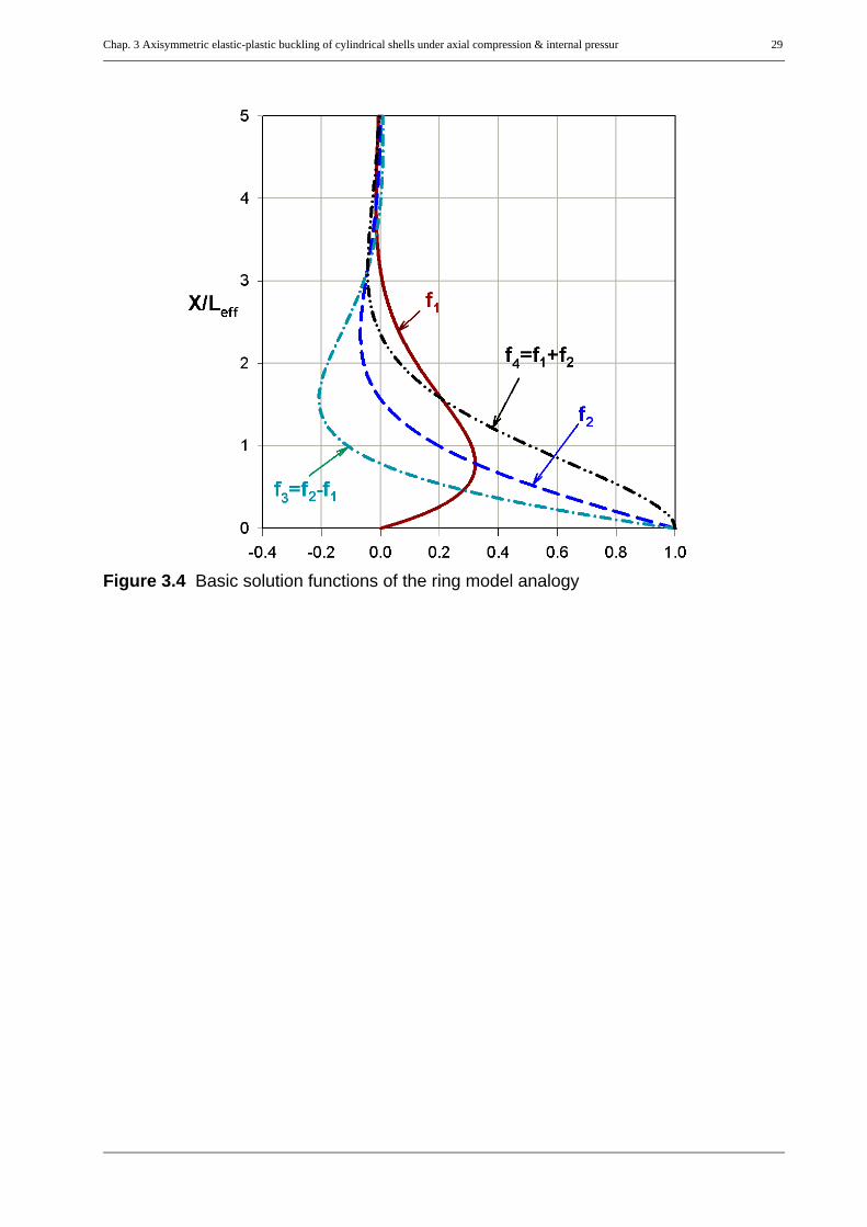
A general linear elastic stress analysis approach to analyze axisymmetric stress states at arbitraryshell junctions of thin-walled axisymmetric shell structures is presented by Linder (2001). Thisanalysis method is based on a newly developed effective-ring analogy model and it is used, in thiswork, to compute the edge bending effects due to different support conditions. The basic edgebending solution-functions, Figure 3.4, used by the effective-ring analogy model are given by:
(Eq. 3.5)
(Eq. 3.6)
Where
(Eq. 3.7)
(Eq. 3.8)
(Eq. 3.9)
f1 e χξ– χξsin⋅=
f2 e χξ– χcos ξ⋅=
f3 f2 f1– e χξ– χcos ξ χξsin–( )= =
f4 f1 f2+ e χξ– χcos ξ χξsin+( )= =
χ LLeff-------- 3 1 ν2–( ) 1
t R⋅---------⋅ L⋅= =
L0.778 R t⋅--------------------------- ... for ν 0.3==
ξ xL---=
χξ xLeff--------=
LeffR t⋅
3 1 ν2–( )---------------------------=
0.778 R t⋅ ... for ν 0.3==
Chap. 3 Axisymmetric elastic-plastic buckling of cylindrical shells under axial compression & internal pressur 29
Figure 3.4 Basic solution functions of the ring model analogy

30 Chap. 3 Axisymmetric elastic-plastic buckling of cylindrical shells un-
These basic solution functions and their linear combinations are used throughout the solution ofthe edge bending problem. Condensed mathematical expressions are also presented by Linder(2001) for the overall (membrane and edge bending) analysis of shell problems.
The stiffness of the equivalent ring model of the cylindrical shell for edge bending effects is givenby:
(Eq. 3.10)
For edge displacement disturbances w*A and βx,A at the bottom edge ”A” of the shell, therestraining edge forces can be computed using the stiffness of the ring model as
(Eq. 3.11)
For a cylindrical shell, the total deformation and section forces (edge bending effects included)according to the effective-ring analogy model are genrally computed as follows. The actualditributions along the meridian of the shell will depend on the type of bottom boundary conditionconsidered.
Deformations:
(Eq. 3.12)
Section forces:
(Eq. 3.13)
(Eq. 3.14)
(Eq. 3.15)
KEAeff
2R2------------
2 Leff–
Leff– Leff2
⋅=
RH A,
RM A,
K– wA∗
βx A,
⋅EAeff
2R2------------–
2 Leff–
Leff– Leff2
wA∗
βx A,
⋅ ⋅= =
w∗βx
f1 f2+( ) Leff f1⋅–2f1Leff-------- f2 f1–( )
wA∗
βx A,
wA∗
βx A, part
–⎝ ⎠⎜ ⎟⎜ ⎟⎛ ⎞
⋅ w∗βx part
+=
Qx f2 f1–( ) 2f1Leff--------
RH A,
RM A,
⋅=
Nx Nx part,=
NθEtr1----- f1 f2+( ) Leff f1⋅–
wA∗
βx A,
wA∗
βx A, part
–⎝ ⎠⎜ ⎟⎜ ⎟⎛ ⎞
⋅ ⋅ Nθ part,+=

Chap. 3 Axisymmetric elastic-plastic buckling of cylindrical shells under axial compression & internal pressur 31
(Eq. 3.16)
(Eq. 3.17)
The section moments are assumed positive when outer side of the shell is under compression.
For the particular shell and loading cases of this study, the total deformation and section forcesaccording to this method are given as follows
Deformations:
(Eq. 3.18)
Section forces:
(Eq. 3.19)
Section moments:
Mx Leff f1⋅ f1 f2+( )–RH A,
RM A,
⋅=
Mθ ν M⋅ x=
w∗ RE t h⋅ ⋅----------------- ν σx t⋅ ⋅ p R⋅+( ) f2 1–( ) h for pinned bottom⋅
f1 f+ 2 1–( ) h for fixed bottom⋅⎩⎪⎨⎪⎧
⋅–=
βxR
E t h⋅ ⋅----------------- ν σx t⋅ ⋅ p R⋅+( ) f1 f+ 2 for pinned bottom
2f1 for fixed bottom⎩⎪⎨⎪⎧
⋅–=
Nx Nx membrane, σx t for both pinned and fixed bottoms⋅–= =
Nθ p R ν σx t⋅ ⋅ p R⋅+( ) f2 for pinned bottomf1 f+ 2 for fixed bottom
⎩⎪⎨⎪⎧
⋅–⋅=
QxAeffR t⋅--------- ν σx t⋅ ⋅ p R⋅+( )
0.5 f1 f2–( ) for pinned bottom
1 hLeff--------–⎝ ⎠
⎛ ⎞ f1 f2–( ) for fixed bottom⎩⎪⎨⎪⎧
⋅=

32 Chap. 3 Axisymmetric elastic-plastic buckling of cylindrical shells un-
(Eq. 3.20)
Where
(Eq. 3.21)
For illustration purposes, consider the cylindrical shell stated above loaded with a tip-compressivering load equal to the classical buckling stress σxRcr and a uniform internal pressure p of magnitude0.5py (half of the pressure which causes uni-axial yielding in the circumferential direction), i.e.
(Eq. 3.22)
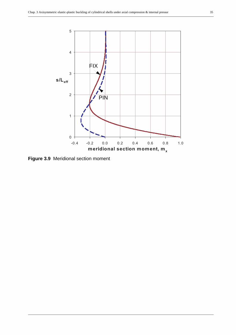
The deformations and section force results from the linear shell analysis method discussed abovewould then be as shown on the plots, Figure 3.5 to Figure 3.9. The normal section force andbending moments shown in these plots are normalized with respect to the corresponding un-axialyield section force, Npl = t.fy, and section moment, Mpl = t2.fy/4, respectively. The meridionalsection force Nx and the circumferential bending moment Mθ distributions along the meridian arenot included as the first is constant through out the meridian and the later is the product of thepoison’s ratio ν and the meridional bending moment Mx.
3.3.3 Numerical finite element linear analysis (LA)Numerical finite element small displacement linear analyses of the illustrative cylindrical shell
under the aforementioned meridional tip-compressive ring loading with uniform internal pressure
were made for verification purposes. The deformation and section force results obtained from
ABAQUS finite element linear analysis are exactly the same as those obtained using the effective-
ring-model analogy, Figure 3.5 to Figure 3.9.
MxAeff
2R t⋅-------------h ν σx t⋅ ⋅ p R⋅+( ) f1 for pinned bottom
f1 f– 2 for fixed bottom⎩⎪⎨⎪⎧
⋅–=
Mθ ν Mx for both pinned and fixed bottoms⋅=
Aeff Leff t⋅=
σx σxRcr 0.605E tR---= =
p 0.5py 0.5fytR---= =

Chap. 3 Axisymmetric elastic-plastic buckling of cylindrical shells under axial compression & internal pressur 33
Figure 3.5 Radial deformation
Figure 3.6 Meridional rotation
FIX
PIN
FIX
PIN

34 Chap. 3 Axisymmetric elastic-plastic buckling of cylindrical shells un-
Figure 3.7 Circumferential section force
Figure 3.8 Transverse shear force
FIX
PIN
FIX
PIN
Chap. 3 Axisymmetric elastic-plastic buckling of cylindrical shells under axial compression & internal pressur 35
Figure 3.9 Meridional section moment
FIX
PIN

36 Chap. 3 Axisymmetric elastic-plastic buckling of cylindrical shells un-
3.4 Linear elastic buckling strength of an ideallyperfect cylinder
In elastic buckling design assessments according to EN1993-1-6, the characterstic bucklingstrength of an imperfect elastic shell, σk, is related to the elastic critical buckling stress of theperfect shell, σcr, using an elastic imperfection reduction (knock-down) factor α which quanitifiesthe combined effect of geometric nonlinearity and all types of possible imperfections. Therelationship is generally given by
(Eq. 3.23)
Since the effect of geometric nonlinearities are included in the imperfection reduction factor α, theelastic critical buckling stress of the perfect shell, σcr, represents the small displacement linearelastic bifurcation stress of the perfect shell and not the snap-through buckling stress which isassociated with geometric nonlinearity.
In line with the “stress-design” (LA-stress-based) approach, the elastic critical buckling stress ofthe perfect shell, σcr, is computed using linear elastic shell analysis. This stress will then becompared with the buckling stress from FE-based LBA only for verification purposes.
The pure elastic buckling strength of the perfect shell will later be used as a reference strength inevaluating the shell buckling relative slenderness parameter λx.
σk α σcr⋅=

Chap. 3 Axisymmetric elastic-plastic buckling of cylindrical shells under axial compression & internal pressur 37
3.4.1 Approximate linear buckling analysis based on linear shell analysis In the general LBA sense, a shell subjected to an axial loading (no matter where the axial loadingand related section forces come from) buckles at a section located a meridional distance “x” fromthe supported base, when the membrane meridional section stress σx(x) due to the applied axialloading reaches the section’s limiting value for elastic buckling, σxcr(x), which is given by
(Eq. 3.24)
Generally speaking, even though the stress at the supported base reaches its buckling limitingvalue, buckling will not take place at the base. Instead, it occurs at a small distance away from thebase (along the meridian). This is because of the two facts that (i) it is restrained and (ii) there isno enough space for buckling to occur.
Buckling practically occurs when the stress at the location for the “center of buckle” reaches thecritical stress for that particular section. In other words, the stress distribution should be increased,after reaching the critical stress at the base, by a load factor so that the stress at the center of bucklereaches its limiting value for buckling, thereby producing buckling.
The above discussion, however, will be more clear and applicable for elastic buckling of conicalshells than the cylindrical shells. Hence, the same discussion would be repeated later wheninvestigating the approximate elastic buckling strength of perfect conical shells.
For a cylindrical shell of constant thickness, the elastic critical section force is constant, since t(x)and r(x) are constant, throughout the height of the shell. Besides, the meridional stress at any pointalong the meridian is equal to the membrane meridional compression resulting from the appliedtip-compressive loading. As a result, the approximate elastic buckling stress is equal to thetheoretical elastic buckling stress given by
(Eq. 3.25)
σxcr x( ) 1
3 1 ν2–( )--------------------------- E t x( )⋅
r x( )-----------------⋅=
σxcr x( ) 1
3 1 ν2–( )--------------------------- E t⋅
R---------⋅=
0.605E t⋅R
--------- for ν 0.3==

38 Chap. 3 Axisymmetric elastic-plastic buckling of cylindrical shells un-
3.4.2 Linear buckling analysis using an analytical model based on theoryof second order
The linear elastic buckling load and the corresponding buckling mode of an axially ring-compressed cylindrical shell (which is independent of the internal pressure) can be analyticallyobtained using a stability analysis (Theory of second order) of an equivalent beam on an elasticfoundation. The foundation modulus of the elastic beam will be obtained from the consideration ofstiffness of the shell in the radial direction and is given by
(Eq. 3.26)
See Annex-C for the full discussion.
3.4.3 Numerical finite element linear buckling analysis (LBA)Only for verification purposes, numerical finite element linear buckling analyses (LBA) ofcylindrical shells with a reference axial tip-compressive ring loading equal to the theoretical elasticcritical buckling stress and varying the intensity of a uniform internal pressure were made. In thiscase, the critical load factor is taken as the lowest buckling load. The combined effect of the shellslenderness, bottom boundary conditions, and the intensity of internal pressurization is very smalland hence is generally neglected. It should, however, be clear here that a high internalpressurization means a relatively bigger contribution to the axial compression due to poisson’seffect. This fact can be observed from the somehow declining buckling load results as the internalpressurization increases. The results are plotted in the LBA/Rcr vs. μ representation as shown inFigure 3.10 and Figure 3.11 for fixed and pinned bottom boundary conditions, respectively.
The maximum deviation being for the relatively thick shell, 0.98% for the fixed bottom cylindricalshell and 0.2% for the pinned bottom case, one can see that the approximate linear bucklinganalysis result predicts well the FE LBA result. As a result, the LBA_approximate will be usedinstead of the FE LBA in the upcoming computations and discussions.
Cf E t⋅( ) R2⁄=

Chap. 3 Axisymmetric elastic-plastic buckling of cylindrical shells under axial compression & internal pressur 39
Figure 3.10 Finite element LBA analyses results: Fixed bottom
Figure 3.11 Finite element LBA analyses results: Pinned bottom

40 Chap. 3 Axisymmetric elastic-plastic buckling of cylindrical shells un-
3.5 Elastic buckling strength of an imperfectcylinder
3.5.1 Elastic buckling strength: historyThe elastic buckling load of cylindrical shells predicted by the classical stability theory isapplicable only to an idealized mathematical model of the structure. The actual shell structure,however, is far from the perfect idealized model as it usually has initial imperfections of any type(geometric, loading, boundary conditions, and material.). This fact has been a secret for a long timeduring the past when buckling loads measured in experiments often were as small as a quarter(even smaller) of the theoretical critical buckling load showing high imperfection sensitivity.
Following a large number of laboratory experimental investigations on buckling loads,specifications concerning design loads with respect to stability were proposed for thin-walledcylindrical shells under simple types of loads and imperfections not exceeding certain limits. Theexperimental investigations made on axially loaded cylindrical shells included pure meridionalcompression (with no internal pressure) and combined loading of meridional compression andinternal pressure. It has been shown that the elastic buckling strength of an axially compressedimperfect thin-walled cylindrical shell with co-existent internal pressure increases with internalpressurization as the circumferential membrane tensile stress smooths out the imperfectionsthereby reducing their negative effect. The specifications introduced an elastic buckling reductionfactor α which is equal to the ratio of the experimental elastic buckling load to the theoreticalcritical buckling load of the perfect idealized shell and hence always less than unity. Themagnitude of the reduction factor depends on the imperfection type & amplitude, internal pressureintensity, shell slenderness ratio R/t, and the type of loading.
In 1976, a task group of the European Convention for Constructional Steelwork (ECCS 1976)recomended to use imperfection reduction factors (obtained from lower bounds of scatter bands ofnumerous laboratory test results) for both unpressurized (α0) and pressurized (αp) given by (Eq.3.28) and (Eq. 3.29), respectively. This recommendation was limited to medium height cylindricalshells with imperfection amplitude, w, not exceeding 0.01 r (Eq. 3.27) measured from a straight rodof length held anywhere against any meridian of the shell. It apparently prohibits shellswith larger imperfection amplitudes. Moreover, nothing has been reported with respect to thenature of the imperfections of the laboratory tests on which the specification was based. Thus, itpredicts a buckling strength of a shell irrespective of the fabrication methods used and resultingimperfection nature. The imperfections might, however, be random (therefore non-axisymmetric)as laboratory model cylinders are commonly fabricated by wrapping a single sheet of materialaround a form and making a longitudinal (meridional) joint, Teng & Rotter (1992). On the otherhand, the same recommendation shows the enormous influence of a small axisymmetricinitial imperfection on the buckling strength of an axially loaded cylindrical shell. It,
lr 4 Rt=

Chap. 3 Axisymmetric elastic-plastic buckling of cylindrical shells under axial compression & internal pressur 41
however, does not recommend to consider such imperfections believing that initial defects inreal shell structures are not axisymmetric but randomly distributed.
(Eq. 3.27)
(Eq. 3.28)
(Eq. 3.29)
where
(Eq. 3.30)
(Eq. 3.31)
In 1984, the task group of the European Convention for Constructional Steelwork (ECCS 1984)recomended to use the same imperfection reduction factors as ECCS 1976. This recommendation,like ECCS-1976, was limited to medium height cylindrical shells with imperfection amplitudes notexceeding 0.01 r. Besides, it recommends to consider half of the imperfection reduction factors (α0/2 for buckling under pure axial load and αp/2 for buckling under axial load with internal pressure)when the imperfection amplitude is equal to 0.02 and to linearly interpolate for values ofamplitudes lying in between. The imperfection amplitudes according to this recommendation aremeasured from a straight rod and a circular template of length held anywhere againstany meridian, Figure 3.12a, and against any parallel circle along the circumference, Figure 3.12b,respectively. In case of circular welds, the specification recommends to use a rod of length
, Figure 3.12c, for imperfection amplitude mesurements.
In the relatively latest recommendation, ECCS 1988, nothing has been changed from ECCS 1984with respect to imperfection amplitude measurement, shell length limitation, imperfectionamplitude restriction, and the strength prediction for buckling under axial loading with or withoutaccompanying internal pressure.
wmax 0.01l= r 0.04 Rt=wmax
t------------ 1
25------ R
t---=⇒
α0
0.831 0.01R t⁄+
--------------------------------- for R/t < 212
0.700.1 0.01R t⁄+
-------------------------------------- for R/t > 212 ⎩⎪⎪⎨⎪⎪⎧
=
αp α0 1 α0–( ) ρρ 0.007+-----------------------+=
ρ pREt------- R
t--- 0.605 p⋅
R t⁄---------------------= =
p pRt σRcr⋅-----------------=
lr 4 Rt=
lr 25t=
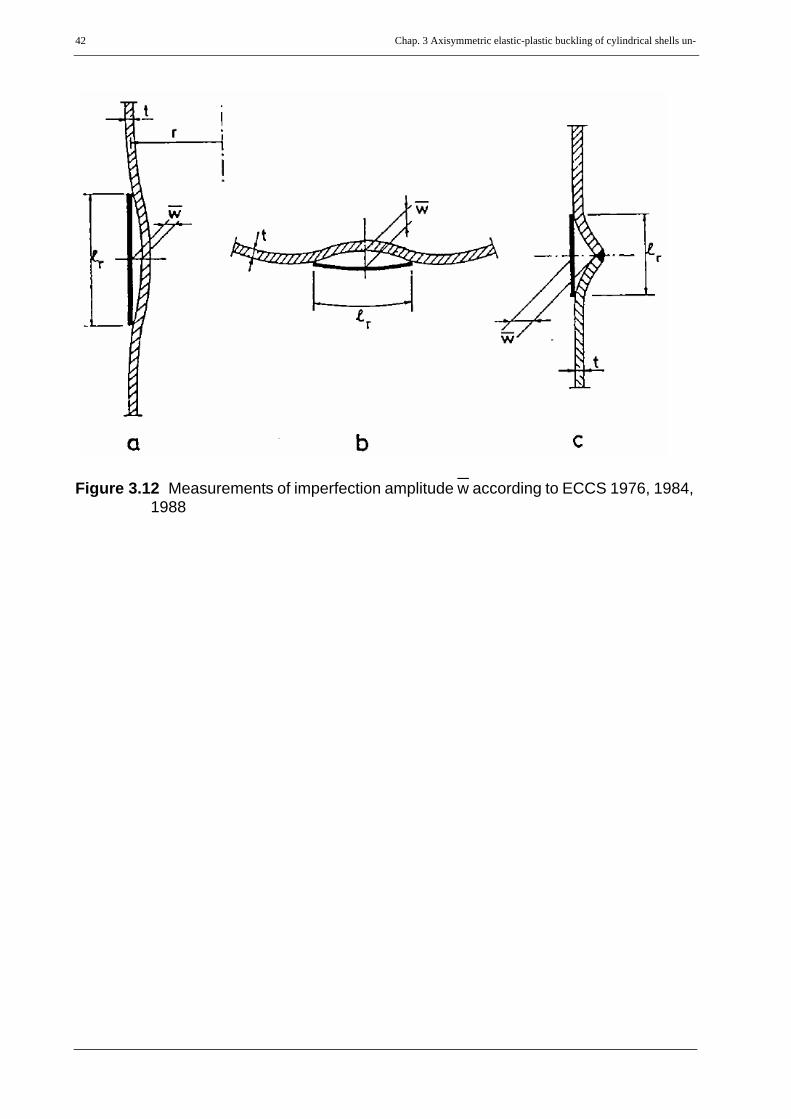
42 Chap. 3 Axisymmetric elastic-plastic buckling of cylindrical shells un-
Figure 3.12 Measurements of imperfection amplitude w according to ECCS 1976, 1984, 1988
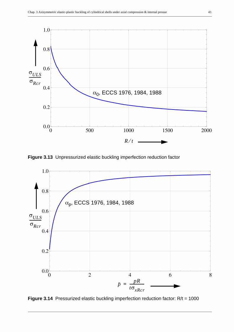
Chap. 3 Axisymmetric elastic-plastic buckling of cylindrical shells under axial compression & internal pressur 43
Figure 3.13 Unpressurized elastic buckling imperfection reduction factor
Figure 3.14 Pressurized elastic buckling imperfection reduction factor: R/t = 1000
0 500 1000 1500 20000.0
0.2
0.4
0.6
0.8
1.0
α0, ECCS 1976, 1984, 1988
R t⁄
σULSσRcr-------------
0 2 4 6 80.0
0.2
0.4
0.6
0.8
1.0
αp, ECCS 1976, 1984, 1988
σULSσRcr-------------
p pRtσxRcr----------------=

44 Chap. 3 Axisymmetric elastic-plastic buckling of cylindrical shells un-
On the other hand, Hutchinson (1965), after mathematically investigating the imperfectionsensitivity of axially compressed and internally pressurized cylindrical shells by consideringaxisymmetric, non-axisymmetric, and mixed imperfection modes indicated that different modes ofinitial geometric imperfections not only produce different unpressurized buckling strengths but arealso affected differently by internal pressure. The buckling strength of an unpressurized cylindricalshell with pure axisymmetric imperfection is found to be lower and gains less strength with internalpressurization than that of a cylinder with pure non-axisymmetric or mixed modes ofimperfections. The pressurized elastic imperfection reduction factor of a cylindrical shell with pureaxisymmetric sinusoidal imperfection according to the mathematical model of Hutchinson iscomputed using (Eq. 3.32) for known values of the internal pressure parameter, p, and theimperfection amplitude to shell thickness ratio, δ0/t. The unpressurized elastic imperfectionreduction factor is also computed from the same expression by setting p = 0 (Eq. 3.33). Animperfection which has mixed modes of both axisymmetric and non-axisymmetric imperfectionsgives a strength higher than the pure axisymmetric but lower than the pure non-axisymmetricimperfections. In addition, Hutchinson compared his results with the lower bound result of thelaboratory tests on which the aforementioned specifications were based and found out that theimperfections of the laboratory tests were close to his results of the non-axisymmetric typeimperfections and hence confirmed the argument given above by Teng & Rotter (1992).
(Eq. 3.32)
(Eq. 3.33)
4 1 p αxpe–+( ) 1 αxpe–( ) 3 1 ν2–( ) 2 αxpe+( )δ0t
-----– 0=
4 1 αxpe–( )2 3 1 ν2–( ) 2 αxpe+( )δ0t
-----– 0=

Chap. 3 Axisymmetric elastic-plastic buckling of cylindrical shells under axial compression & internal pressur 45
Figure 3.15 Hutchinson’s pressurized elastic buckling strength for pure axisymmetric imperfections
Figure 3.16 Hutchinson’s pressurized elastic buckling strength for pure axisymmetric imperfections
0 2 4 6 80.0
0.2
0.4
0.6
0.8
1.0
p pRtσxRcr----------------=
σULSσRcr-------------
δ0 t⁄ 2.0=
1.0
0.750.5
0.250.1
0.0 0.5 1.0 1.5 2.00.0
0.2
0.4
0.6
0.8
1.0
σULSσRcr--------------
δ0 t⁄
p 0=
0.51.0
2.0
4.06.0
8.0

46 Chap. 3 Axisymmetric elastic-plastic buckling of cylindrical shells un-
Later, Rotter & Teng (1989), Teng & Rotter (1992) opposed the idea which says that initialdefects in real shell structures are not axisymmetric but randomly distributed. They genuinelyargued that civil engineering shell structures can have axisymmetric depresions resulting fromcircumferential welding and recommended the consideration of the effects of axisymmetricimperfections on buckling strength predictions of cylindrical shells. They studied the elasticbuckling of thin-walled unstiffened cylindrical shells under axial load and internal pressure withsinusoidal, local inward, and local outward axisymmetric imperfections. Their results werecompared with that of Hutchinson’s sinusoidal imperfection and ECCS recommendation. Here ithas to be noted, however, that Teng & Rotter (1992) used an incorrect Hutchinson’s strengthcurve when comparing their results with and led them to incorrect conclusions. In thecomparison, they took Hutchinson’s buckling strength curve with an imperfection amplitudeequal to half of the wall thickness (instead of one wall thickness, Figure 3.15) and comparedit with their results where the imperfection amplitude was equal to one wall thickness. Thecorrected comparison of the results is shown in Figure 3.21. Eventhough all such imperfectionswere found to be worst in the sense that they lead to lower results than the ECCS recommendations,the sinusoidal and outward local axisymmetric imperfections were then dropped as they are notpractically relevant. The inward local axisymmetric weld depression was then considered practicaland further studies has been done to determine the worst possible shape of weld depressions, Rotter& Teng (1989). The introduction of the effects of these axisymmetric weld depressions into thespecifications was then recommended. Besides, the elastic imperfection reduction factors for bothunpressurized and pressurized buckling are recommended to be modified in such a way that theytake care of different fabrication qualities. These recommendations are included in EN1993-1-6.
According to EN1993-1-6, the elastic pressurized buckling strength of cylindrical shells is giveninterms of elastic pressurized imperfection reduction factor which depends on the shell slender-ness, loading condition, and imperfection amplitude which in turn depends on the fabrication qual-ity class. The imperfection amplitudes are measured at every position in both the meridional andcircumferential directions using the same guages as in ECCS 1988. In addition, this specificationrecommends to use guages of lengths and separately acrosswelds, Figure 3.17. The expression for computing the imperfection reduction factor as given inEN1993-1-6, (Eq. 3.34) to (Eq. 3.37), will be used throughout the upcoming discussions.
A comparison of both the unpressurized and pressurized imperfection reduction factors accordingto the different recommendations and study results discussed above have been made in the currentwork. Figure 3.18 shows a comparative plot of the unpresssurized elastic buckling imperfectionreduction factors according to the different specifications versus the shell slenderness ratio, R/t.
lgx 4 Rt= lgw 25tmin 500mm≤=

Chap. 3 Axisymmetric elastic-plastic buckling of cylindrical shells under axial compression & internal pressur 47
Figure 3.17 Measurements of depths Δw0 of initial dimples according to EN1993-1-6

48 Chap. 3 Axisymmetric elastic-plastic buckling of cylindrical shells un-
Figure 3.18 Unpressurized elastic buckling imperfection reduction factors
Figure 3.19 Pressurized elastic buckling imperfection reduction factors: R/t = 1000
0 500 1000 1500 20000.0
0.2
0.4
0.6
0.8
1.0
R t⁄
σULSσRcr--------------
ABC
ABC
α0, ECCS 1976, 1984, 1988
Hutchinson (1965)sinusoidal axisym. imperfection
EN 1993-1-6
0 2 4 6 80.0
0.2
0.4
0.6
0.8
1.0
σULSσRcr--------------
p pRtσxRcr-----------------=
ABC
ABC
αp, ECCS 1976, 1984, 1988
Hutchinson (1965)sinusoidal axisym. imperfection
EN 1993-1-6

Chap. 3 Axisymmetric elastic-plastic buckling of cylindrical shells under axial compression & internal pressur 49
Figure 3.20 Pressurized elastic buckling imperfection reduction factors: R/t = 1000, δ0/t = 1.0
Figure 3.21 Pressurized elastic buckling imperfection reduction factors: R/t = 1000
�
�
�
�
�
��
� ��
� �
����
�
�
�
��
�
��
0 2 4 6 80.0
0.2
0.4
0.6
0.8
1.0
EN1993-1-6
Teng_FEM local inward axisym. imperfection
αp, ECCS 1976, 1984, 1988
Teng_FEM sinusoidal axisym. imperfection
σULSσRcr--------------
p pRtσxRcr-----------------=
�
�
�
�
�
��
� ��
� �
����
�
�
�
��
�
��
0 2 4 6 80.0
0.2
0.4
0.6
0.8
1.0
Hutchinson (1965)
EN1993-1-6, class-B
Teng_FEM local inward axisym. imperfection
αp, ECCS 1976, 1984, 1988
Teng_FEM sinusoidal axisym. imperfection
σULSσRcr--------------
p pRtσxRcr-----------------=

50 Chap. 3 Axisymmetric elastic-plastic buckling of cylindrical shells un-
3.5.2 Elastic imperfection reduction factor, EN1993-1-6In accordance to the frame work of the European standard EN1993-1-6, the elastic imperfectionreduction factor is a factor applied to the small displacement linear bifurcation buckling strengthof a perfect shell, Figure 3.24, to account for geometric imperfections and the effect of geometricnonlinearity, Figure 3.25. It depends on the shell geometry, loading condition, and imperfectionamplitude. The linear bifurcation buckling strength of a perfect cylindrical shell is independent ofthe internal pressure intensity. The elastic imperfection reduction factor of cylindrical (and conicalshells, for that matter) subjected to meridional compression with/without co-existent internal pres-sure is given as follows:
• elastic imperfection reduction for pressurized cases
(Eq. 3.34)
• elastic imperfection reduction for unpressurized cases
(Eq. 3.35)
with the characteristic imperfection amplitude parameter, Δwk given as
(Eq. 3.36)
where
(Eq. 3.37)
Q is fabrication quality parameter and should be taken, depending on the fabrication tolerancequality class, from
Fabrication tolerance quality class Description Q
Class A Excellent 40
Class B High 25
Class C Normal 16
Table 3.1 Values of fabrication quality parameter Q
αxpe αx 1 αx–( ) pp 0.3 αx⁄+-------------------------------+=
αx0.62
1 1.91 Δwk t⁄( )1.44+-------------------------------------------------=
Δwk1Q---- R
t--- t⋅ ⋅=
pσθ
σxRcr------------- pR t⁄
σxRcr------------- μ λx
2⋅= = =

Chap. 3 Axisymmetric elastic-plastic buckling of cylindrical shells under axial compression & internal pressur 51
Figure 3.22 EN1993-1-6 pressurized elastic buckling imperfection reduction factor
Figure 3.23 EN1993-1-6 pressurized elastic buckling imperfection reduction factor
0 2 4 6 80.0
0.2
0.4
0.6
0.8
1.0
δ0 t⁄ 0.0 0.1 0.25 0.5 0.75 1.0 2.0, , , , , ,=
0.0
δ0 t⁄ 2.0=
σULSσRcr--------------
p pRtσxRcr-----------------=
0.0 0.5 1.0 1.5 2.00.0
0.2
0.4
0.6
0.8
1.0
Δwk t⁄
p 0=
0.5
1.0
2.04.0
6.08.0
σULSσRcr--------------

52 Chap. 3 Axisymmetric elastic-plastic buckling of cylindrical shells un-
Figure 3.24 Perfect elastic buckling strength depending on shell slenderness ratio (independent of internal pressure)
μ pRtfy-------=
χxσULS
fy--------------=
λxfy
σxRcr---------------=

Chap. 3 Axisymmetric elastic-plastic buckling of cylindrical shells under axial compression & internal pressur 53
Figure 3.25 Effect of imperfections on elastic buckling strength: perfect and imperfect elastic buckling strengths
μ pRtfy-------=
χxσULS
fy--------------=
λxfy
σxRcr---------------=

54 Chap. 3 Axisymmetric elastic-plastic buckling of cylindrical shells un-
3.6 Pure plastic strength of cylindrical shells
The pure plastic (yield) strength represents the load (stress) which, with no stability phenomenaintervening, causes an unacceptably large plastic deformation. The plastic strength of shells can becomputed using membrane stresses approximately, using finite element small displacement theory(MNA) analysis, or using yield functions based on stress resultants which will be discussed laterin detail.
3.6.1 Plastic strength according to von Mises membrane criteriaFor axisymmetric shells under axisymmetric loading and boundary conditions where 2D principalmembrane stresses exist, the von Mises membrane yield criteria is given by
(Eq. 3.38)
with an upper limiting (yield) curve given by
(Eq. 3.39)
For a cylindrical shell under the actions of uniform axial compression with co-existent uniforminternal pressure, the limiting plasticity curve can be obtained using the following two differentways depending on the load aplication procedure. Different loading parameters are used torepresent the two procedures. This separation will be more useful later in the finite elementnumerical analysis.
1 Pre-specified pressure load: For a specified intensity of internal pressure (Eq. 3.40), com-pute the meridional membrane stress (Eq. 3.41) which will cause yielding and the corre-sponding plastic load factor (Eq. 3.42).
(Eq. 3.40)
(Eq. 3.41)
(Eq. 3.42)
σx2 σθ
2 σxσθ–+ fy2≤
σx2 σθ
2 σxσθ–+ fy2=
μ ppyield-------------
σθfy------ p R⋅
t fy⋅-----------= = =
σx pl,4 3μ2– μ–
2------------------------------- fy⋅=
ΛMisesσx pl,
σx Rcr,--------------- 4 3μ2– μ–
2------------------------------- λx
2⋅= =
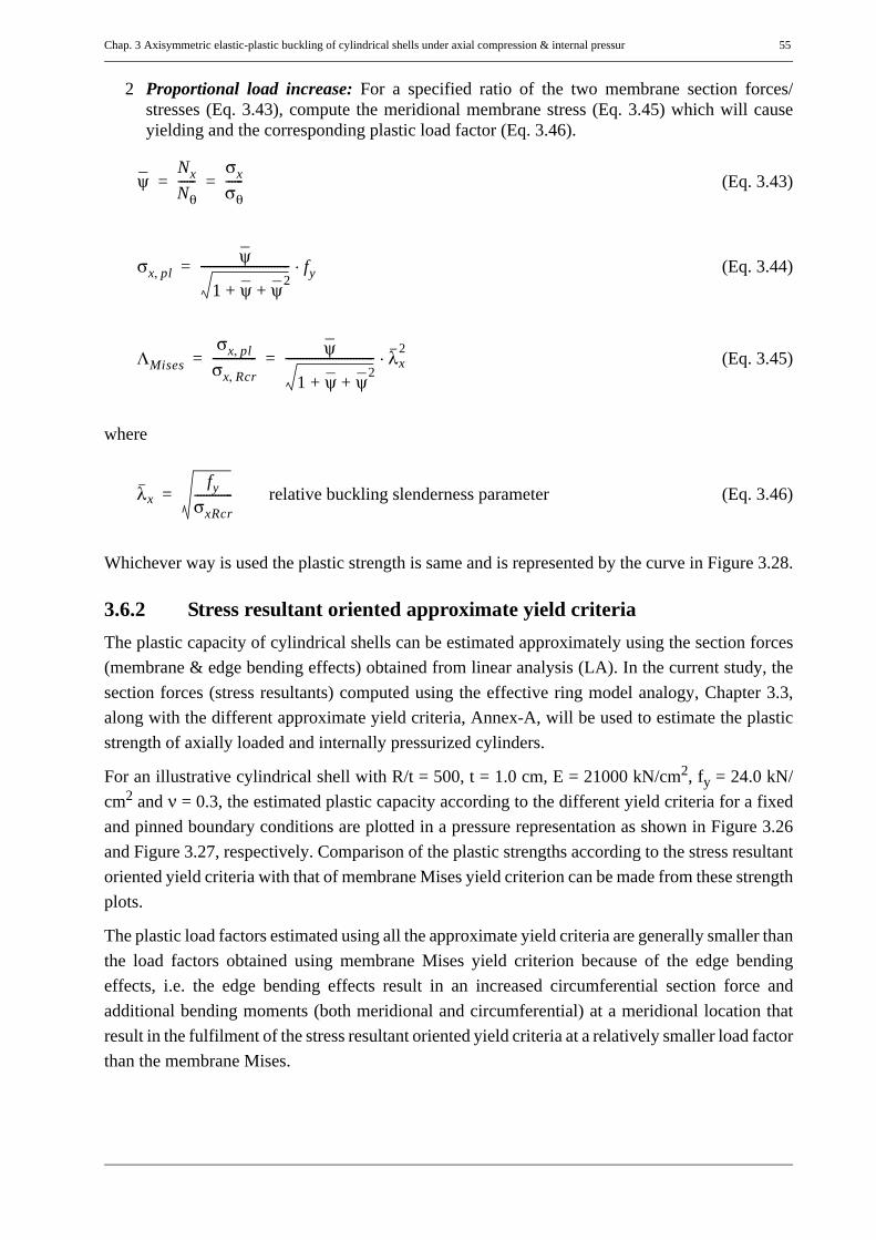
Chap. 3 Axisymmetric elastic-plastic buckling of cylindrical shells under axial compression & internal pressur 55
2 Proportional load increase: For a specified ratio of the two membrane section forces/stresses (Eq. 3.43), compute the meridional membrane stress (Eq. 3.45) which will causeyielding and the corresponding plastic load factor (Eq. 3.46).
(Eq. 3.43)
(Eq. 3.44)
(Eq. 3.45)
where
(Eq. 3.46)
Whichever way is used the plastic strength is same and is represented by the curve in Figure 3.28.
3.6.2 Stress resultant oriented approximate yield criteria The plastic capacity of cylindrical shells can be estimated approximately using the section forces(membrane & edge bending effects) obtained from linear analysis (LA). In the current study, thesection forces (stress resultants) computed using the effective ring model analogy, Chapter 3.3,along with the different approximate yield criteria, Annex-A, will be used to estimate the plasticstrength of axially loaded and internally pressurized cylinders.
For an illustrative cylindrical shell with R/t = 500, t = 1.0 cm, E = 21000 kN/cm2, fy = 24.0 kN/cm2 and ν = 0.3, the estimated plastic capacity according to the different yield criteria for a fixedand pinned boundary conditions are plotted in a pressure representation as shown in Figure 3.26and Figure 3.27, respectively. Comparison of the plastic strengths according to the stress resultantoriented yield criteria with that of membrane Mises yield criterion can be made from these strengthplots.
The plastic load factors estimated using all the approximate yield criteria are generally smaller thanthe load factors obtained using membrane Mises yield criterion because of the edge bendingeffects, i.e. the edge bending effects result in an increased circumferential section force andadditional bending moments (both meridional and circumferential) at a meridional location thatresult in the fulfilment of the stress resultant oriented yield criteria at a relatively smaller load factorthan the membrane Mises.
ψNxNθ------
σxσθ------= =
σx pl,ψ
1 ψ ψ2+ +------------------------------ fy⋅=
ΛMisesσx pl,
σx Rcr,--------------- ψ
1 ψ ψ2+ +------------------------------ λx
2⋅= =
λxfy
σxRcr------------- relative buckling slenderness parameter=

56 Chap. 3 Axisymmetric elastic-plastic buckling of cylindrical shells un-
Figure 3.26 Approximate yield criteria R/t = 500: fixed bottom
Figure 3.27 Approximate of yield criteria R/t = 500: pinned bottom
membrane-MisesIvanov-I&II
Ilyushin-Linear
simple
first yield
EDR5
membrane-total
membrane-Mises
Ilyushin-Linear
simple
first yield
EDR5
membrane-total
Ivanov-I&II

Chap. 3 Axisymmetric elastic-plastic buckling of cylindrical shells under axial compression & internal pressur 57
3.6.3 Small displacement materially nonlinear finite element analysis(MNA)
Numerical finite element small displacement materially non-linear analyses of cylindrical shellswith a reference meridional tip-compressive ring loading equal to theoretical elastic criticalbuckling stress and varying the intesnisty of the internal uniform pressure were made. The resultsare plotted in the pressure representation (MNA/fy vs. μ) representation as shown Figure 3.28.
It can be seen from the results that there is no difference between the materially nonlinear finiteelement analysis results and the results according to Von Mises pure membrane yield criterion.Hence, the results from the membrane Mises yield criterion will be used instead of the smalldisplacement FE MNA results in the upcoming computations and discussions.
The fact that the finite element LBA and MNA for the cylindrical shell under consideration areequal with the membrane-based approximateb-LBA and Mises yield condition, respectively,makes the upcoming numerical analysis studies adaptable to the simple and straight forward stressdesign procedure as outlined in EN1993-1-6.

58 Chap. 3 Axisymmetric elastic-plastic buckling of cylindrical shells un-
Figure 3.28 FE MNA for both fixed & pinned bottom; and bi-axial membrane Mises yield strength

Chap. 3 Axisymmetric elastic-plastic buckling of cylindrical shells under axial compression & internal pressur 59
3.7 Elastic-plastic buckling phenomena, analysisand strength
3.7.1 General concept of buckling phenomenaIt has been repeatedly reported in many literatures that thin-walled cylindrical shells usually buckleelastically under pure axial compression. The respective buckling strength for such axially loadedcylindrical shells is usually lower than the theoretical elastic critical stress, the differenceaccounting for the decrease in buckling strength caused by the presence of various imperfectionsand geometric nonlinearity. The presence of an accompanying internal pressure, however, reducesthis strength-weakening effect of the imperfections there by increasing the buckling strength of theshell. However, when the intensity of the internal pressure exceeds a certain value, thecircumferential membrane stress becomes significant causing bi-axiality effect to come into play.
An unpressurized thin-walled cylindrical shell under an axial load buckles elastically forming adiamond type buckling mode, Esslinger & Geier (1975). Generally speaking, the diamond typeelastic buckling phenomenon of an unpressurized cylindrical shell happens at locations ofgeometric imperfections in the shell interior (where there exist no edge constriction effects)forming two or three layers of buckles, Figure 3.29a.
As the internal pressurization increases, the weakening effect of the geometric imperfections willbe reduced due to the stretching (strengthening effect) resulting from internal pressurization; andat the same time, the edge constriction (boundary condition) effects become stronger whencompared with the unpressurized cylinder case. This edge constriction effect produces a decayingwave type prebuckling radial deformation leading to buckling phenomenon in a region close to theboundary. For this reason, at low internal pressure levels, the elastcic buckling mode will have atendency of shifting towards the boundary condition resulting in an intermediate zigzag typebuckling mode, Figure 3.29b. At medium internal pressure levels, the effect of imperfections ishighly weakend and the effect of boundary condition becomes responsible for buckling, restrictingthe elastic buckling phenomenon to happen in a region close to the boundary, Figure 3.29c. On theother hand, as the internal pressurization further increases the buckles will become shorter in themeridonal direction and longer in the circumferential direction thereby producing localized bucklemode.
At very high internal pressure level, the localized prebuckling radial deformation which resultsfrom the very high edge constriction effect may suffer local yielding due to bending leading toelastic-plastic buckling near the boundary condition under very small axial load. This type ofelastic-plastic buckling is known as elephant’s foot type buckling. Figure 3.30 shows bucklingmodes at different internal pressure levels and the evolution (as the intensity of the internalpressure increases) and happening of the elephant’s foot type buckling phenomenon under the

60 Chap. 3 Axisymmetric elastic-plastic buckling of cylindrical shells un-
action of a very high internal pressure and bending moment.
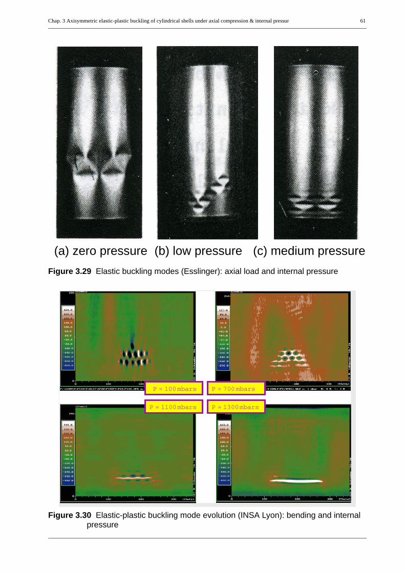
Chap. 3 Axisymmetric elastic-plastic buckling of cylindrical shells under axial compression & internal pressur 61
Figure 3.29 Elastic buckling modes (Esslinger): axial load and internal pressure
Figure 3.30 Elastic-plastic buckling mode evolution (INSA Lyon): bending and internal pressure
(a) zero pressure (b) low pressure (c) medium pressure
P = 100mbars P = 700mbars
P = 1300mbarsP = 1100mbars

62 Chap. 3 Axisymmetric elastic-plastic buckling of cylindrical shells un-
3.7.2 Elastic buckling strengthThe pure elastic pressurized buckling strength of a cylindrical shell, computed using αxpe, areplotted in the pressure representation (χx vs μ plot), Figure 3.31, for different shell slenderness, R/t, values of 250, 500, 750, 1000, and 1500 for fabrication tolerance quality class-A and for internalpressure intensity, μ = 0 to 1. The buckling strength for relatively thick shells are much greater thanthe uni-axial yield strength, fy, and can not be seen in this plot where a maximum buckling strengthequal to fy is plotted. The strength values corresponding to the intersections of each of those curvesand the ordinate of the graph represent the elastic-unpressurized buckling strengths of the respec-tive clyinders. The bi-axial membrane Mises plasticity is also shown with uni-axial yield strengthsat μ values of 0 and 1 corresponding to uni-axial meridional and uni-axial circumferential yielding,respectively. At other values of μ bi-axial membrane plasticity takes place. The same informationis shown, Figure 3.32, in the capacity representation (χx vs λx plot) for different values of theinternal pressure parameter μ. Both the pressure and capacity representations are combined to givethe 3D plot, Figure 3.33, of the pure elastic imperfect characterstic buckling strength.
When there exist no elastic-plastic buckling interaction, the ultimate strength of the cylinder willbe governed either by pure elastic imperfect buckling or pure plastic collapse depending on theinternal pressure level and shell slenderness ratio. The envelope of these two strengths is shown inFigure 3.34.

Chap. 3 Axisymmetric elastic-plastic buckling of cylindrical shells under axial compression & internal pressur 63
Figure 3.31 Pressurized pure elastic buckling strength for class-A & bi-axial membrane Mises
Figure 3.32 Pressurized pure elastic buckling strength for class-A & Euler’s curve

64 Chap. 3 Axisymmetric elastic-plastic buckling of cylindrical shells un-
Figure 3.33 Imperfect elastic buckling strength for quality class-C (depends on pres-sure, shell slenderness ratio, and fabrication quality class)
μ pRtfy-------=
χxσULS
fy--------------=
λxfy
σxRcr---------------=

Chap. 3 Axisymmetric elastic-plastic buckling of cylindrical shells under axial compression & internal pressur 65
Figure 3.34 Envelope of imperfect elastic buckling strength and perfect bi-axial mem-brane Mises yield strength
μ pRtfy-------=
χxσULS
fy--------------=
λxfy
σxRcr---------------=
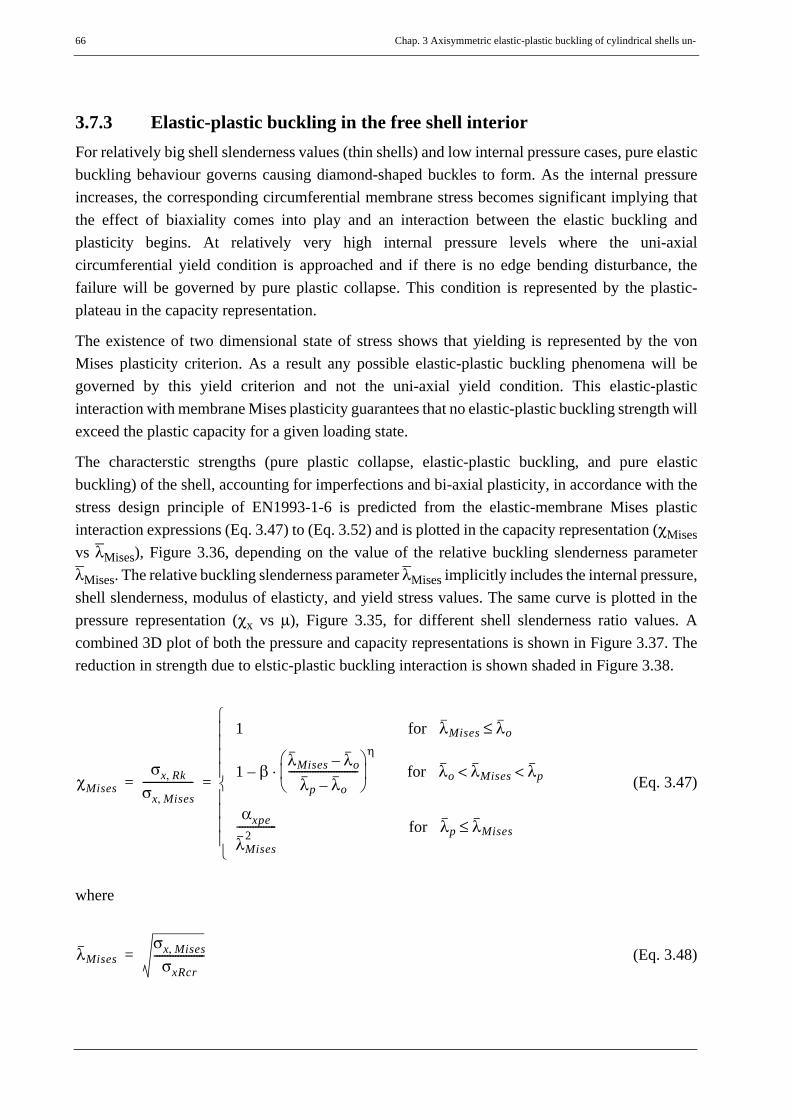
66 Chap. 3 Axisymmetric elastic-plastic buckling of cylindrical shells un-
3.7.3 Elastic-plastic buckling in the free shell interiorFor relatively big shell slenderness values (thin shells) and low internal pressure cases, pure elasticbuckling behaviour governs causing diamond-shaped buckles to form. As the internal pressureincreases, the corresponding circumferential membrane stress becomes significant implying thatthe effect of biaxiality comes into play and an interaction between the elastic buckling andplasticity begins. At relatively very high internal pressure levels where the uni-axialcircumferential yield condition is approached and if there is no edge bending disturbance, thefailure will be governed by pure plastic collapse. This condition is represented by the plastic-plateau in the capacity representation.
The existence of two dimensional state of stress shows that yielding is represented by the vonMises plasticity criterion. As a result any possible elastic-plastic buckling phenomena will begoverned by this yield criterion and not the uni-axial yield condition. This elastic-plasticinteraction with membrane Mises plasticity guarantees that no elastic-plastic buckling strength willexceed the plastic capacity for a given loading state.
The characterstic strengths (pure plastic collapse, elastic-plastic buckling, and pure elasticbuckling) of the shell, accounting for imperfections and bi-axial plasticity, in accordance with thestress design principle of EN1993-1-6 is predicted from the elastic-membrane Mises plasticinteraction expressions (Eq. 3.47) to (Eq. 3.52) and is plotted in the capacity representation (χMisesvs λMises), Figure 3.36, depending on the value of the relative buckling slenderness parameterλMises. The relative buckling slenderness parameter λMises implicitly includes the internal pressure,shell slenderness, modulus of elasticty, and yield stress values. The same curve is plotted in thepressure representation (χx vs μ), Figure 3.35, for different shell slenderness ratio values. Acombined 3D plot of both the pressure and capacity representations is shown in Figure 3.37. Thereduction in strength due to elstic-plastic buckling interaction is shown shaded in Figure 3.38.
(Eq. 3.47)
where
(Eq. 3.48)
χMisesσx Rk,
σx Mises,-------------------
1 for λMises λo≤
1 βλMises λo–
λp λo–--------------------------⎝ ⎠⎜ ⎟⎛ ⎞ η
for λo λMises λp< <⋅–
αxpe
λMises2
--------------- for λp λMises≤
⎩⎪⎪⎪⎪⎨⎪⎪⎪⎪⎧
= =
λMisesσx Mises,
σxRcr-------------------=

Chap. 3 Axisymmetric elastic-plastic buckling of cylindrical shells under axial compression & internal pressur 67
(Eq. 3.49)
the elastic-plastic buckling parameters η, λo, and β are given as
Interaction exponent:
(Eq. 3.50)
Squash limit relative slenderness:
(Eq. 3.51)
Plastic range factor:
(Eq. 3.52)
Since no geometrically and materially nonlinear analysis of imperfect cylindrical shells and testswere undertaken to investigate the actual elastic-plastic buckling interaction in the free shellinterior of an axially compressed internally pressurized cylindrical shell, the plastic bucklingparameters of an axially compressed unpressurized cylinder are adopted in the elastic-plasticinteraction procedure to predict the elastic-plastic buckling strengths for buckling in the free shellinterior. As will be seen later in this work, however, few GMNLI analyses were made to check thevalidity of the mentioned strength prediction procedure for imperfection-led elastic-plasticbuckling in the shell interior where no edge constiction exists. Despite these few geometrically andmaterially nonlinear analysis results for imperfection-led elastic-plastic buckling in the shellinterior, the aforementioned procedure with the basic plastic interaction parameters will be referredto whenever buckling in the free shell interior is involved. This is because of the open questionabout the choice of a worst possible imperfection nature.
λpαxpe1 β–------------=
η 1.0=
λo 0.2=
β 0.6=

68 Chap. 3 Axisymmetric elastic-plastic buckling of cylindrical shells un-
Figure 3.35 E-P interaction using bi-axial membrane Mises & basic plastic parameters
Figure 3.36 E-P interaction using membrane Mises & basic plastic parameters

Chap. 3 Axisymmetric elastic-plastic buckling of cylindrical shells under axial compression & internal pressur 69
Figure 3.37 Elastic-plastic buckling interaction using bi-axial membrane Mises yield condition & basic plastic buckling parameters
μ pRtfy-------=
χxσULS
fy--------------=
λxfy
σxRcr---------------=

70 Chap. 3 Axisymmetric elastic-plastic buckling of cylindrical shells un-
Figure 3.38 Comparison of elastic-plastic buckling interaction using basic plastic buck-ling parameters with the envelope of imperfect elastic buckling strength & per-fect bi-axial membrane Mises yield strength
μ pRtfy-------=
χxσULS
fy--------------=
λxfy
σxRcr---------------=

Chap. 3 Axisymmetric elastic-plastic buckling of cylindrical shells under axial compression & internal pressur 71
3.7.4 Axisymmetric elastic-plastic buckling of perfect cylindrical shells
3.7.4.1 Geometrically and materially nonlinear finite element analysis (GMNA)As discussed in the previous section, an unpressurized cylindrical shell under pure axialcompressive load tends to radially expand due to Poisson’s effect. An internally pressurizedcylindrical shell under axial compressive load tends to radially expand due to the combined effectsof both the internal pressurization and Poisson’s effect. The presence of boundary conditions,however, constricts this expansion causing local bending under the action of the axial compressiveload. Similar local bending effects can be observed at locations of change in wall thicklness, ringstiffeners, or local axisymmetric imperfections causing immature buckling under a smallmeridional compression. Thus, the presence of significant internal pressure will have adestabilizing effect there by reducing the buckling strength of the shell. Such a buckling type,caused by local bending adjacent to the boundary, is termed as an “elephant’s-foot” type bucklingand the corresponding strength as elephant-foot buckling strength. The main focus of the currentstudy is to investigate the elastic-plastic buckling phenomenon and corresponding bucklingstrength close to the lower supported shell boundary where local edge bending disturbances play aleading role.
Comprehensive parametric studies are carried out varying the shell slenderness, shell lowerbundary conditions, and the intensity of the internal pressurization. More specifically,geometrically and materially nonlinear finite element analyses which resulted in localizedaxisymmetric buckling modes were made on cylindrical shells with R/t = 100, 250, 500, 1000,1500 by varying the internal pressure value from zero-pressure (pure axial loading case) to apressure value that produces circumferential uni-axial yielding, i.e. a circumferential membranestress equal to the yield stress of the material. Boundary conditions of PIN or FIX at bottom androtational restraint at top were examined for each R/t and varying the internal pressure value. Smalldisplacement linear buckling analysis (LBA) and small displacement materially nonlinear analysis(MNA) results are used for reference purposes. Those reference strengths are given (see discussionabove) by the classical elastic critical buckling stress and bi-axial membrane Mises yield condition,respectively. All the results are plotted in both the pressure (χx vs. μ) and capacity curve (χ vs. λpl)representations.

72 Chap. 3 Axisymmetric elastic-plastic buckling of cylindrical shells un-
Figure 3.39 Geometrically & materially nonlinear (elephant’s-foot) strength: fixed
Figure 3.40 Geometrically & materially nonlinear (elephant’s-foot) strength: fixed
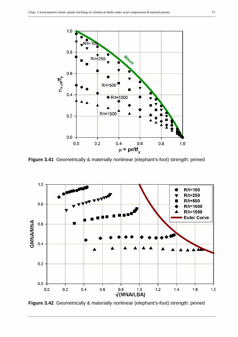
Chap. 3 Axisymmetric elastic-plastic buckling of cylindrical shells under axial compression & internal pressur 73
Figure 3.41 Geometrically & materially nonlinear (elephant’s-foot) strength: pinned
Figure 3.42 Geometrically & materially nonlinear (elephant’s-foot) strength: pinned

74 Chap. 3 Axisymmetric elastic-plastic buckling of cylindrical shells un-
The geometrically and materially nonlinear effects in the GMNA results are responsible for thelocalized axisymmetric buckling at the pinned (or fixed) cylindrical shell boundaries and for thelower capacity when compared with the geometrically linear but materially nonlinear MNAcounterpart. When the geometric nonlinearity effects are very small as in the case of relativelythick-walled cylindrical shells, the GMNL buckling strengths will be closer (or atmost equal) tothe pure plastic strength of the shell. On the other hand, when both the geometric and materialnonlinearity effects are very small as in the case of relatively thin-walled cylindrical shells andlower internal pressure values, the GMNL buckling strengths will be closer (or atmost equal) to thepure elastic buckling strength of the perfect shell. These facts can be observed from the plots of theGMNA results shown in Figure 3.39 to Figure 3.42 for both the fixed and pinned bottom boundaryconditions.
It can be deduced from the above discussion (with the help of Figure 3.39 to Figure 3.42) that thegeometric and material nonlinear (GMNL) load carrying capacity, which is upper-bounded by thefulfillment of either the membrane Mises yield condition or the elastic critical buckling stress(whichever is smaller), can be put into direct relationship with the small displacement materiallynonlinear (MNL) counterpart which corresponds to the pure bi-axial membrane Mises loadcarrying capacity. This relationship between the geometrically and materially nonlinear bucklingstrength and pure plastic carrying capacity of the shell, accounting for the large displacement(geometric nonlinearity) effects which is relevant for localized axisymmetric buckling at the pin-ended or fix-ended cylindrical shell boundaries, depends on the shell slenderness ratio and can bedealt with in two different ways depending on the curve fitting to be used and representationprocedure to be followed. These are:
• depending on both the shell slenderness and the intensity of the internal pressure• depending on the shell slenderness alone (i.e. independent of internal pressurization)
These two different ways are discussed in detail in the following section. It has to, however, beemphasized that in both procedures the same GMNA numerical results are at the background. Thequestion, therefore, has to be put after the right choice of the reference parameters for non-dimensional representation purposes and the best but suitable choice of fitting curve type.

Chap. 3 Axisymmetric elastic-plastic buckling of cylindrical shells under axial compression & internal pressur 75
GMNA versus MNA strength: internal pressure dependent relationshipThe effects of internal pressurization varation on the perfect elephant’s-foot buckling strength canbe seen from the capacity representations. One way of expressing this strength with respect to thepure plastic capacity of the shell is obtained using straight-line fitting of the GMNL strengths fromthe capacity representation. The resulting linear relationship, for a given R/t, between the GMNLto MNL strength ratio and the shell buckling slenderness value, λMises, results in a nonlinearrelationship of the strength ratio and the internal pressure parameter μ. This nonlinear relationshipis written as follows:
(Eq. 3.53)
(Eq. 3.54)
(Eq. 3.55)
(Eq. 3.56)
These approximate perfect elephant’s-foot strength according to the pressure-dependent reductionof the plastic strength is plotted in the pressure representation, Figure 3.43 and Figure 3.44, forfixed and pinned bottom boundary conditions, respectively, and for the different shell slendernessratio values, where the corresponding numerical GMNL strength results are also shown forcomparison purposes. There is a good fit between the approximate expression and the numericalanalyses results for the entire pressure range. At very low internal pressure levels, however, theapproximate expressions result in strength values somehow higher than the pure elastic bucklingstrength of the perfect shell which should not generally be the case. In such cases the fitting curveshould always be cut-off by the pure elastic buckling strength of the perfect shell. However, theelephant-foot type buckling, as previously discussed, is relevant only for very high internalpressure values. For this reason it is better to use a somewhat simpler expression to relate the twostrengths and at the same time fitting the numerical GMNA results in the high pressure range wherethe elephant’s-foot buckling phenomenon governs failure.
GMNAMises------------------ 1 βEFoot– dvar k λx 4 3μ2– μ–⋅ ⋅+= =
dvar0.2 e
1.751.15 ρ+--------------------⎝ ⎠⎛ ⎞
for pinned bottom⋅
0.3 e2.75
2.3 ρ+-----------------⎝ ⎠⎛ ⎞
for fixed bottom⋅⎩⎪⎪⎨⎪⎪⎧
=
k 0.25 0.35ρ 0.11ρ2 for pinned bottom+–
0.1 0.25ρ 0.08ρ2 for fixed bottom+–⎩⎪⎨⎪⎧
=
ρ R t⁄1000------------=

76 Chap. 3 Axisymmetric elastic-plastic buckling of cylindrical shells un-
Figure 3.43 GMNL strength as μ & R/t dependent reduction of MNL strength: fixed
Figure 3.44 GMNL strength as μ & R/t dependent reduction of MNL strength: pinned

Chap. 3 Axisymmetric elastic-plastic buckling of cylindrical shells under axial compression & internal pressur 77
GMNA versus MNA strength: internal pressure independent relationshipIn this case, the reduction in buckling strength due to geometric nonlinearity is taken to be constantfor a given shell slenderness ratio independent of the internal pressure intensity in such a way thatthere will be a good conservative fit for relatively high internal pressure levels ( about)where the elephant’s-foot type buckling becomes deterministic.
For all the pressure levels, the geometric and material noninear buckling strength can be expressedas a constant reduction of the plastic (MNL or membrane Mises) strength. This constant reductionof the plastic strength depends only on the shell slenderness, R/t, and fits well to the GMNLstrengths at relatively high internal pressure levels ( about) for all R/t ratio, where theelephant’s-foot buckling becomes deterministic. Once again, for very low internal pressure levels,the fitting curve results in strength values higher than the pure elastic buckling strength of theperfect shell which should not be the case and therefore should always be cut-off by the laterstrength curve. The constant reduction factor relating the perfect elephant’s-foot buckling strengthwith the pure bi-axial plastic strength is given by
(Eq. 3.57)
(Eq. 3.58)
(Eq. 3.59)
The perfect elephant-foot strengths according to the pressure-independent constant reduction of theplastic strength are plotted in the pressure representation, Figure 3.45 and Figure 3.46, for fixedand pinned bottom boundary conditions respectively and for the different shell slenderness values,where the GMNA results from finite element numerical analysis are also shown for comparisonpurposes. It can be seen from the plots that there is a good conservative fit between the approximateexpression and the numerical analysis results for the relatively high internal pressure intensityrange as it should be.
μ 0.5>
μ 0.5>
dc 1 βEFoot– GMNAMises------------------= =
βEFoot0.8 1 e 1.15ρ––( ) for pinned-bottom
0.75 1 e 0.75ρ––( ) for fixed-bottom⎩⎪⎨⎪⎧
=
ρ R t⁄1000------------=

78 Chap. 3 Axisymmetric elastic-plastic buckling of cylindrical shells un-
Figure 3.45 GMNL strength as R/t dependent reduction of MNL strength: fixed
Figure 3.46 GMNL strength as R/t dependent reduction of MNL strength: pinned

Chap. 3 Axisymmetric elastic-plastic buckling of cylindrical shells under axial compression & internal pressur 79
3.7.4.2 Analytical model based on theory of second order with material nonlinear effectsThe geometric and material nonlinear effects of a cylindrical shell can be analytically modelledapproximately using a combination of theory of second order (Th.2.o.) and the stress resultantoriented approximate yield criteria. In doing so, the beam on an elastic foundation model of acylindrical shell has been used, see Annex.
In the analytical model, the elastic-plastic buckling loads are computed in an iterative manner asdiscussed below. Once the second order effect due to an axial compression is considered in theforce equilibrium equation (in the transverse direction), a trial load factor is applied with which thesection force distributions along the meridian are computed. Using these section forces (stressresultants), a check is made for possible yield at each point along the meridian using one of theapproximate yield criteria already discussed, Chapter 3.6. If yield criteria is not fulfilled, applyanother load factor depending on the result obtained, i.e. if the yield surface defined by theapproximate yield function is exceeded, apply a smaller load factor; if the result lies with in theyield surface, apply a larger load factor. This procedure is repeatedly used until the yield criterionis exactly fulfilled. The fulfilment of the yield criterion shows through-thickness yielding; andtherefore, when combined with Th.2.o, represents an approximate elastic-plastic buckling.
Such analysis using Ivanov’s approximate yield criterion has been made in the current study forboth fixed & pinned-bottom cylindrical shells of slenderness ratio R/t = 500 & 1000 with t = 1.0cm, E = 21000 kN/cm2, fy = 24.0 kN/cm2 and ν = 0.3. The results obtained from the analyticalmodel along with the geometrically and materially nonlinear analysis results obtained usingABAQUS are shown in Figure 3.47 & Figure 3.48 for R/t = 500; and Figure 3.49 & Figure 3.50for R/t = 1000.
A second analysis using the “first-yield” approximate yield criterion has been done for the cylinderwith shell slenderness ratio R/t = 1000 and the results are shown in Figure 3.51 & Figure 3.52,along with Ivanov’s yield criterion and ABAQUS results, for the fixed and pinned bottomboundary conditions, respectively.
At very high internal pressure levels where the axial compression needed to cause elastic-plasticbuckling is very small, the strength results from theory of second order are close to the approximateplastic strength of the shell. As it has been already discussed, at relatively high internal pressurelevels, the edge bending effects cause approximate yield at relatively low load factors. Apart fromthis, an overall assessment of the results obtained from the analytical model tells that such analysisgives relatively bigger load factors than the ABAQUS results when compared relative to thecorresponding plastic strengths. One possible reason for this effect can be the fact that in the caseof a finite element numerical analysis, the stiffness of the shell is updated at each load incrementthus any effects of plasticity are automatically applied thereby reducing the stiffness and hence,needs a relatively smaller load factor to cause elastic-plastic buckling. Whereas in the combinedconsideration of the Th.2.o. and approximate yield criterion, the shell remains elastic which isrelatively stiff and hence, needs a relatively higher load factor to fulfil approximate elastic-plasticbuckling.
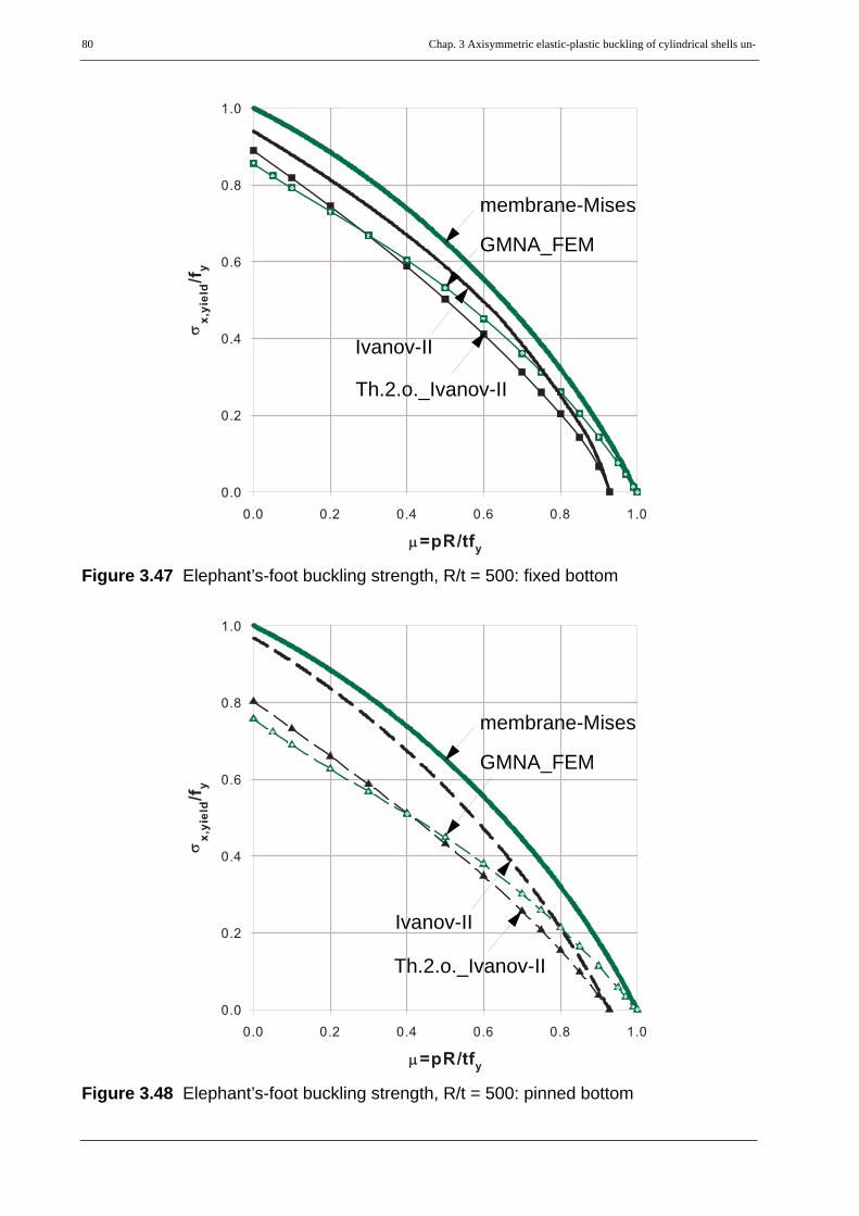
80 Chap. 3 Axisymmetric elastic-plastic buckling of cylindrical shells un-
Figure 3.47 Elephant’s-foot buckling strength, R/t = 500: fixed bottom
Figure 3.48 Elephant’s-foot buckling strength, R/t = 500: pinned bottom
membrane-Mises
Th.2.o._Ivanov-II
GMNA_FEM
Ivanov-II
membrane-Mises
Th.2.o._Ivanov-II
GMNA_FEM
Ivanov-II

Chap. 3 Axisymmetric elastic-plastic buckling of cylindrical shells under axial compression & internal pressur 81
Figure 3.49 Elephant’s-foot buckling strength, R/t = 1000: fixed bottom
Figure 3.50 Elephant’s-foot buckling strength, R/t = 1000: pinned bottom
membrane-Mises
Th.2.o._Ivanov-II
Ivanov-II
GMNA_FEM
membrane-Mises
Th.2.o._Ivanov-II
Ivanov-II
GMNA_FEM

82 Chap. 3 Axisymmetric elastic-plastic buckling of cylindrical shells un-
Figure 3.51 Elephant’s-foot buckling strength, R/t = 1000: fixed bottom
Figure 3.52 Elephant’s-foot buckling strength, R/t = 1000: pinned bottom
membrane-Mises
Th.2.o.
Ivanov-II
Ivanov-II
GMNA_FEM
first-yield
Th.2.o.first-yield
membrane-Mises
Th.2.o._Ivanov-II
GMNA_FEM
first-yieldIvanov-II
Th.2.o.first-yield

Chap. 3 Axisymmetric elastic-plastic buckling of cylindrical shells under axial compression & internal pressur 83
3.8 Axisymmetric elastic-plastic buckling ofimperfect cylindrical shells
3.8.1 Geometrically and materially nonlinear finite element analyses withaxisymmetric imperfections (GMNIA)
3.8.1.1 IntroductionIt is known that the major factor which plays a great role in the reduction of the buckling strengthof thin-walled shells is the presence of various types of imperfections such as loading, boundaryconditions, geometry, and material. Loading imperfections include non-uniformity of the loaddistribution and load eccentricities. Boundary condition imperfections include non-uniformity ofsupport conditions, for example, causing unintended edge moments. Geometrical imperfectionsinclude out-of-straightness, out-of-roundness (ovality), deviations from nominal thickness.Material imperfections include material inhomogeneity and residual stresses. For structuralmodelling and analysis purposes, all imperfections are equivalently expressed in terms of thegeometric imperfection with specific imperfection shape, imperfection wave length, imperfectionamplitude, imperfection orientation (inward or depression vs. outward or bulge), and imperfectionlocation along the meridian of the shell. Each of these properties of an equivalent geometricimperfection has an influence on the buckling behavior and buckling strength of the shell. In orderto clearly show the influence of geometric imperfections on the axisymmetric elastic-plasticbuckling strength of shells, an imperfection sensitivity study using axisymmetric LBA eigenmode-affine, nonlinear eigenmode-affine, and local imperfection shapes has been made numerically ona cylindrical shell with the following set of geometry, boundary, loading, and shell materialconditions. The results will all be expressed interms of dimensionless quanitities and therefore canbe interpreted in such a way that they are applicable to other sets of conditions as well.
Geometry: shell slenderness ratio, R/t = 500; meridional length to radius ratio, L/R = 1.0
Boundary conditions: pinned or fixed (clamped) bottom and rotationally restrained top
Loading: uniform meridional (axial) tip compression with co-existent uniform internal pressure
Material properties:
Modulus of elasticity, E = 21000 kN/cm2;
Mises yield criterion with uni-axial yield strength, fy = 24 kN/cm2;
Poisson’s ratio, ν = 0.3

84 Chap. 3 Axisymmetric elastic-plastic buckling of cylindrical shells un-
3.8.1.2 Linear elastic buckling (LB) eigenmode-affine imperfectionIn cases where a different unfavourable imperfection pattern can not be justified, EN1993-1-6recommends to use a linear elastic critical eigenmode based on an LBA of the perfect shell. For theillustrative fixed-bottom cylindrical shell discussed above, a typical LBA basic eigenmode isshown in Figure 3.53. A typical LBA basic eigenmode of the pinned-bottom cylinder is also shownin Figure 3.55. Despite the fact that such imperfection shapes are very far from existing in realshells, imperfection sensitivity studies have been done considering the LBA eigenmodes (first half-wave oriented outward in both boundary conditions) as an imperfection shape and varying theimperfection amplitude for both bottom boundary conditions. The materially and geometricallynonlinear elastic-plastic buckling strength of the imperfect cylinder (GMNIA), normalized with re-spect to the perfect (GMNA) shell strength, versus the imperfection amplitude for the fixed andpinned bottom boundary condition are shown in Figure 3.54 & Figure 3.56, respectively, fordifferent values of meridional to circumferential membrane stresses ratio given by according to the proportional load increase procedure. The value of ψ is indirectly proportional tothe internal pressure level, i.e. a bigger value of ψ indicates a smaller internal pressurization. Thus,the LBA eigenmode-affine imperfection led to very low buckling strengths.
It should, however, be noted here that if the cylinder is ideally perfect or if the strength-reducingeffect of imperfections are negligible, the effect of edge constriction alone will be responsible forinstability resulting in a bulge type buckling mode near the edge. If there exist a worst imperfectionat the same location as the edge constriction; or when both are closely located and able to interact,it is clear that the two effects help each other in destabilizing the shell. On the other hand, in caseswhen both exist on a shell but at different locations along the meridian with no interaction of anykind among them, an imperfection-led buckling phenomenon may happen at the imperfectionlocation depending on the imperfection-nature.
An imperfection-led buckling phenomenon is what is exactly happening in the fixed-bottomcylinder where the LBA eigenmode-affine imperfection considered has its peak value at the other(top) end of the shell. With such imperfection shape but low internal pressure levels, the edgeconstriction effect is relatively small and hence an imperfection-led buckling will happen at the topedge of the shell even for small amplitudes of the imperfection. For high internal pressure levels,however, the edge constriction effect becomes larger and the cylinder buckles near the edge forrelatively small amplitudes of the LBA eigenmode-affine imperfection. As the imperfectionamplitude increases, irrespective of the internal peressure level, buckling happens at the top edgeof the cylinder where the LBA eigenmode has its peak value.
On the other hand, for a pinned-bottom cylinder where the LBA eigenmode has the same amplitudeat top-end of the shell and close to the bottom boundary, such an LBA eigenmode-affineimperfection along with the edge-constriction effect will restrict the axisymmetric elastic-plasticbuckling phenomenon to happen close to the bottom boundary unless it is oriented in such a waythat it opposes the edge bending effect. In cases when the imperfection-orientation opposes theedge-constriction effect, the shell may get strengthened at bottom and the buckling phenomenonwill be shifted up and happens somewhere along the meridian.
ψ σx σθ⁄=

Chap. 3 Axisymmetric elastic-plastic buckling of cylindrical shells under axial compression & internal pressur 85
Figure 3.53 LBA basic eigenmode: fixed bottom
Figure 3.54 Imperfection amplitude sensitivity, LBA eigenmode-affine imperfection: fixed
0.3
ψ = 0.05
1.0
3.0
ψ ∞=

86 Chap. 3 Axisymmetric elastic-plastic buckling of cylindrical shells un-
Figure 3.55 LBA basic eigenmode: pinned bottom
Figure 3.56 Imperfection amplitude sensitivity, LBA eigenmode affine imperfection: pinned
0.3
ψ = 0.05
1.0
3.0
ψ ∞=
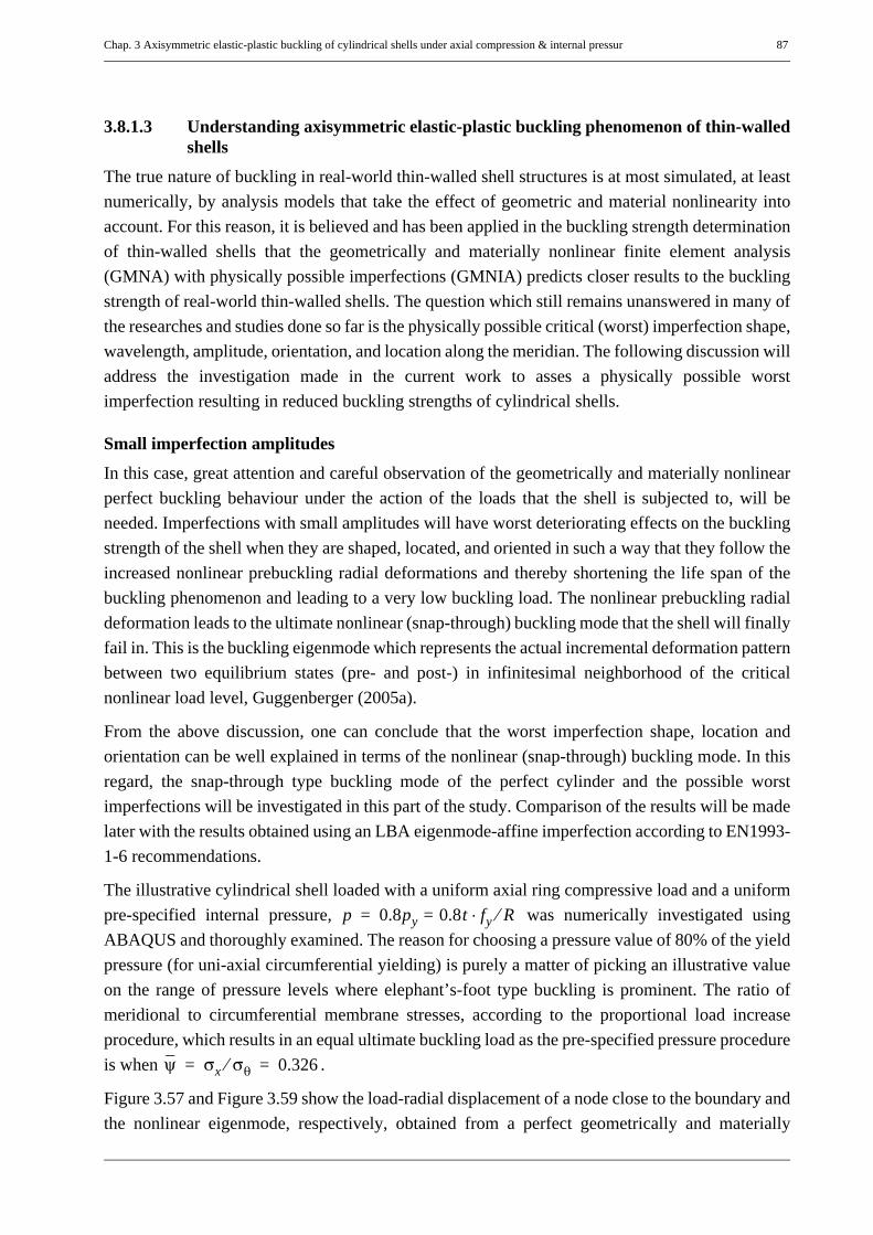
Chap. 3 Axisymmetric elastic-plastic buckling of cylindrical shells under axial compression & internal pressur 87
3.8.1.3 Understanding axisymmetric elastic-plastic buckling phenomenon of thin-walledshells
The true nature of buckling in real-world thin-walled shell structures is at most simulated, at leastnumerically, by analysis models that take the effect of geometric and material nonlinearity intoaccount. For this reason, it is believed and has been applied in the buckling strength determinationof thin-walled shells that the geometrically and materially nonlinear finite element analysis(GMNA) with physically possible imperfections (GMNIA) predicts closer results to the bucklingstrength of real-world thin-walled shells. The question which still remains unanswered in many ofthe researches and studies done so far is the physically possible critical (worst) imperfection shape,wavelength, amplitude, orientation, and location along the meridian. The following discussion willaddress the investigation made in the current work to asses a physically possible worstimperfection resulting in reduced buckling strengths of cylindrical shells.
Small imperfection amplitudes
In this case, great attention and careful observation of the geometrically and materially nonlinearperfect buckling behaviour under the action of the loads that the shell is subjected to, will beneeded. Imperfections with small amplitudes will have worst deteriorating effects on the bucklingstrength of the shell when they are shaped, located, and oriented in such a way that they follow theincreased nonlinear prebuckling radial deformations and thereby shortening the life span of thebuckling phenomenon and leading to a very low buckling load. The nonlinear prebuckling radialdeformation leads to the ultimate nonlinear (snap-through) buckling mode that the shell will finallyfail in. This is the buckling eigenmode which represents the actual incremental deformation patternbetween two equilibrium states (pre- and post-) in infinitesimal neighborhood of the criticalnonlinear load level, Guggenberger (2005a).
From the above discussion, one can conclude that the worst imperfection shape, location andorientation can be well explained in terms of the nonlinear (snap-through) buckling mode. In thisregard, the snap-through type buckling mode of the perfect cylinder and the possible worstimperfections will be investigated in this part of the study. Comparison of the results will be madelater with the results obtained using an LBA eigenmode-affine imperfection according to EN1993-1-6 recommendations.
The illustrative cylindrical shell loaded with a uniform axial ring compressive load and a uniformpre-specified internal pressure, was numerically investigated usingABAQUS and thoroughly examined. The reason for choosing a pressure value of 80% of the yieldpressure (for uni-axial circumferential yielding) is purely a matter of picking an illustrative valueon the range of pressure levels where elephant’s-foot type buckling is prominent. The ratio ofmeridional to circumferential membrane stresses, according to the proportional load increaseprocedure, which results in an equal ultimate buckling load as the pre-specified pressure procedureis when .
Figure 3.57 and Figure 3.59 show the load-radial displacement of a node close to the boundary andthe nonlinear eigenmode, respectively, obtained from a perfect geometrically and materially
p 0.8py 0.8t fy⋅ R⁄==
ψ σx σθ⁄ 0.326= =
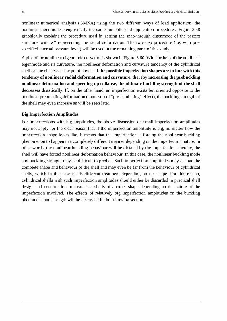
88 Chap. 3 Axisymmetric elastic-plastic buckling of cylindrical shells un-
nonlinear numerical analysis (GMNA) using the two different ways of load application, thenonlinear eigenmode bieng exactly the same for both load application procedures. Figure 3.58graphically explains the procedure used in getting the snap-through eigenmode of the perfectstructure, with w* representing the radial deformation. The two-step procedure (i.e. with pre-specified internal pressure level) will be used in the remaining parts of this study.
A plot of the nonlinear eigenmode curvature is shown in Figure 3.60. With the help of the nonlineareigenmode and its curvature, the nonlinear defomation and curvature tendency of the cylindricalshell can be observed. The point now is, if the possible imperfection shapes are in line with thistendency of nonlinear radial deformation and curvature, thereby increasing the prebucklingnonlinear deformation and speeding up collapse, the ultimate buckling strength of the shelldecreases drastically. If, on the other hand, an imperfection exists but oriented opposite to thenonlinear prebuckling deformation (some sort of “pre-cambering“ effect), the buckling strength ofthe shell may even increase as will be seen later.
Big Imperfection Amplitudes
For imperfections with big amplitudes, the above discussion on small imperfection amplitudesmay not apply for the clear reason that if the imperfection amplitude is big, no matter how theimperfection shape looks like, it means that the imperfection is forcing the nonlinear bucklingphenomenon to happen in a completely different manner depending on the imperfection nature. Inother words, the nonlinear buckling behaviour will be dictated by the imperfection, thereby, theshell will have forced nonlinear deformation behaviour. In this case, the nonlinear buckling modeand buckling strength may be difficult to predict. Such imperfection amplitudes may change thecomplete shape and behaviour of the shell and may even be far from the behaviour of cylindricalshells, which in this case needs different treatment depending on the shape. For this reason,cylindrical shells with such imperfection amplitudes should either be discarded in practical shelldesign and construction or treated as shells of another shape depending on the nature of theimperfection involved. The effects of relatively big imperfection amplitudes on the bucklingphenomena and strength will be discussed in the following section.

Chap. 3 Axisymmetric elastic-plastic buckling of cylindrical shells under axial compression & internal pressur 89
Figure 3.57 Load-radial displacement curve
Figure 3.58 Load-radial displacement curve: snap-through eigenmode explanation
Radial deformation, w*
ΛGMNAΛRcr
-------------------

90 Chap. 3 Axisymmetric elastic-plastic buckling of cylindrical shells un-
Figure 3.59 Nonlinear (snap-through) eigenmode of the perfect cylinder (elephant’s foot buckling)
Figure 3.60 Nonlinear (snap-through) eigenmode curvature: possible tendency
1.48 Rt∼
3.35 Rt∼
5.84 Rt∼

Chap. 3 Axisymmetric elastic-plastic buckling of cylindrical shells under axial compression & internal pressur 91
The snap-through eigenmodeTo elaborate the above discussion, geometrically and materially nonlinear finite element analyseswith imperfections (GMNIA) have been made to compute the buckling strength of the thin-walledcylindrical shell. First the nonlinear eigenmode has been used as an imperfection shape to studythe sensitivity of the cylindrical shell to this mode. It should be clear at this stage that a nonlineareigenmode-affine imperfection shape will well be in-phase with the edge constriction effects (sincethe shape resulted from the edge effect) leading to a very low buckling strength with an imperfectelephant’s foot bulge near the edge. A graphical comparison of the buckling strengths resultingfrom the LBA and snap-through buckling eigenmode-affine imperfections has been made, Figure3.61. This comparison, however, shows only the buckling strengths (hence only numbers) and notthe buckling phenomena since each happen at different locations along the meridian and eachcaused by different primary agents (imperfection shapes) as already discussed. For the relativelylarger imperfection amplitudes, an imperfection-led buckling phenomenon occurs (for the LBAeigenmode-affine imperfection buckling will occur at the top-end of the shell) and thereforecomparative conclusions can not be drawn.
Eventhough the snap-through eigenmode affine imperfection leads to relatively lower bucklingstrengths for small imperfection amplitudes than the LBA eigenmode-affine imperfection, aquestion needs to be raised about the practicability of both imperfection shapes. Studies, Rotter &Teng (1989), Teng & Rotter (1992), show that the most probable axisymmetric type imperfectionson civil engineering cylindrical shells being local-type shapes and not sinusoidal as in theeigenmodes discussed previously. For this reason, the upcoming discussion is fully devoted to thedetailed investigation made on “practically possible” local-type axisymmetric imperfection shapeswith the help of the snap-through buckling eigenmode discussed above. For commonunderstanding (see Figure 3.60), the bottom region is called the "bottom-inward-worst" zone; thenext upper region is called the "bottom-outward-worst" zone; the next upper region is called the"second-inward-worst" zone; and it goes on like that. The approximate lengths of these regions areobtained by subtracting the ordinate values of the plot in Figure 3.60.
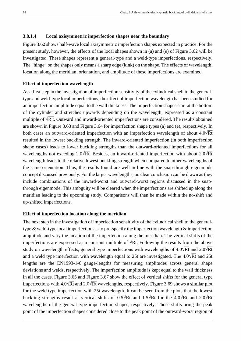
92 Chap. 3 Axisymmetric elastic-plastic buckling of cylindrical shells un-
3.8.1.4 Local axisymmetric imperfection shapes near the boundaryFigure 3.62 shows half-wave local axisymmetric imperfection shapes expected in practice. For thepresent study, however, the effects of the local shapes shown in (a) and (e) of Figure 3.62 will beinvestigated. These shapes represent a general-type and a weld-type imperfections, respectively.The “hinge” on the shapes only means a sharp edge (kink) on the shape. The effects of wavelength,location along the meridian, orientation, and amplitude of these imperfections are examined.
Effect of imperfection wavelength
As a first step in the investigation of imperfection sensitivity of the cylindrical shell to the general-type and weld-type local imperfections, the effect of imperfection wavelength has been studied foran imperfection amplitude equal to the wall thickness. The imperfection shapes start at the bottomof the cylinder and stretches upwards depending on the wavelength, expressed as a constantmultiple of √R.t. Outward and inward-oriented imperfections are considered. The results obtainedare shown in Figure 3.63 and Figure 3.64 for imperfection shape types (a) and (e), respectively. Inboth cases an outward-oriented imperfection with an imperfection wavelength of about 4.0√Rtresulted in the lowest buckling strength. The inward-oriented imperfection (in both imperfectionshape cases) leads to lower buckling strengths than the outward-oriented imperfections for allwavelengths not exeeding 2.0√Rt. Besides, an inward-oriented imperfection with about 2.0√Rtwavelength leads to the relative lowest buckling strength when compared to other wavelengths ofthe same orientation. Thus, the results found are well in line with the snap-through eigenmodeconcept discussed previously. For the larger wavelengths, no clear conclusion can be drawn as theyinclude combinations of the inward-worst and outward-worst regions discussed in the snap-through eigenmode. This ambguity will be cleared when the imperfections are shifted up along themeridian leading to the upcoming study. Comparisons will then be made within the no-shift andup-shifted imperfections.
Effect of imperfection location along the meridian
The next step in the investigation of imperfection sensitivity of the cylindrical shell to the general-type & weld-type local imperfections is to pre-specify the imperfection wavelength & imperfectionamplitude and vary the location of the imperfection along the meridian. The vertical shifts of theimperfections are expressed as a constant multiple of √Rt. Following the results from the abovestudy on wavelength effects, general type imperfections with wavelengths of 4.0√Rt and 2.0√Rtand a weld type imerfection with wavelength equal to 25t are investigated. The 4.0√Rt and 25tlengths are the EN1993-1-6 gauge-lengths for measuring amplitudes across general shapedeviations and welds, respectively. The imperfection amplitude is kept equal to the wall thicknessin all the cases. Figure 3.65 and Figure 3.67 show the effect of vertical shifts for the general typeimperfections with 4.0√Rt and 2.0√Rt wavelengths, respectively. Figure 3.69 shows a similar plotfor the weld type imperfection with 25t wavelength. It can be seen from the plots that the lowestbuckling strengths result at vertical shifts of 0.5√Rt and 1.5√Rt for the 4.0√Rt and 2.0√Rtwavelengths of the general type imperfection shapes, respectively. Those shifts bring the peakpoint of the imperfection shapes considered close to the peak point of the outward-worst region of

Chap. 3 Axisymmetric elastic-plastic buckling of cylindrical shells under axial compression & internal pressur 93
the nonlinear eigenmode. This fact leads to the investigation of imperfection shapes havingcoinciding peak points as the snap-through eigenmode and will be discussed at the end of thissection. For the 4.0√Rt wavelength imperfection, the outward-orientation leads to lower bucklingstrengths for all the locations considered than the inward-orientation. The inward-oriented 2.0√Rtwavelength imperfection leads to lower buckling load only when there is no upward shift. Asimilar observation on the weld imperfection shows an outward-oriented imperfection leads to thelowest buckling load when it is located at about 1.2√Rt. The inward-oriented weld imperfectionleads to lower results when the upward shift is not exeeding 0.6√Rt . Once again, the results foundfrom this investigation are all in line with the snap-through eigenmode concept already discussed.
Effect of imperfection amplitudeImperfection amplitude-sensitivity of the aforementioned wavelengths and locations along themeridian has been then made to verify the conclusions drawn so far. Figure 3.66 and Figure 3.68show the effect of imperfection amplitudes for different imperfection locations of the general typeimperfections with 4.0√Rt and 2.0√Rt wavelengths, respectively. Figure 3.70 shows a similar plotfor the weld type imperfection with 25t wavelength. All the results coincide with the snap-througheigenmode concept.
Outward-oriented worst local imperfection
As a final step in the investigation, imperfection wavelengths were varied in such a way that thepeak points of the imperfection shapes remain at the peak point of the outward-worst region of thenonlinear eigenmode. The imperfection amplitude was kept the same for all shapes and equal tothe wall thickness. The results are shown in Figure 3.71. Once again, one can see that the worstimperfection orientation is outwards and its length is approximately 2.0√R.t which again isapproximately equal to the length of the outward-worst region, as expected. To further highlightthis behaviour, imperfection amplitude-sensitivity analyses were made for the 2.0√R.t and 4.0√R.twavelength general-type local imperfections and both outward and inward orientations. Theseresults along with the results obtained using the nonlinear eigenmode-affine imperfection areshown in Figure 3.72.
The following question can be raised here: why did the outward-oriented local imperfections leadto relatively lower buckling loads than the nonlinear eigenmode-affine imperfection? It is becausethe nonlinear eigenmode-affine imperfection, even though it has the same curvature as thenonlinear eigenmode itself, its shape-deviations are not exactly in-phase with the worst shape-deviation discussed in the curvature of the nonlinear eigenmode, Figure 3.60.
Figure 3.73 to Figure 3.76 show the effects of imperfection orientations on the ultimate radialdeformations corresponding to the ultimate buckling load factors. Comparisons of these ultimatebuckling loads and their corresponding radial deformations for the perfect cylinder, imperfectcylinder with outward-oriented imperfection, and imperfect cylinder with inward-orientedimperfection can be easily made for the different imperfection shapes. These comparisons willstrengthen the concept of using the nonlinear eigenmode oriented local imperfections as the worstpossible imperfections. Besides, it contributes much to the basic understanding of worstaxisymmetric imperfections.
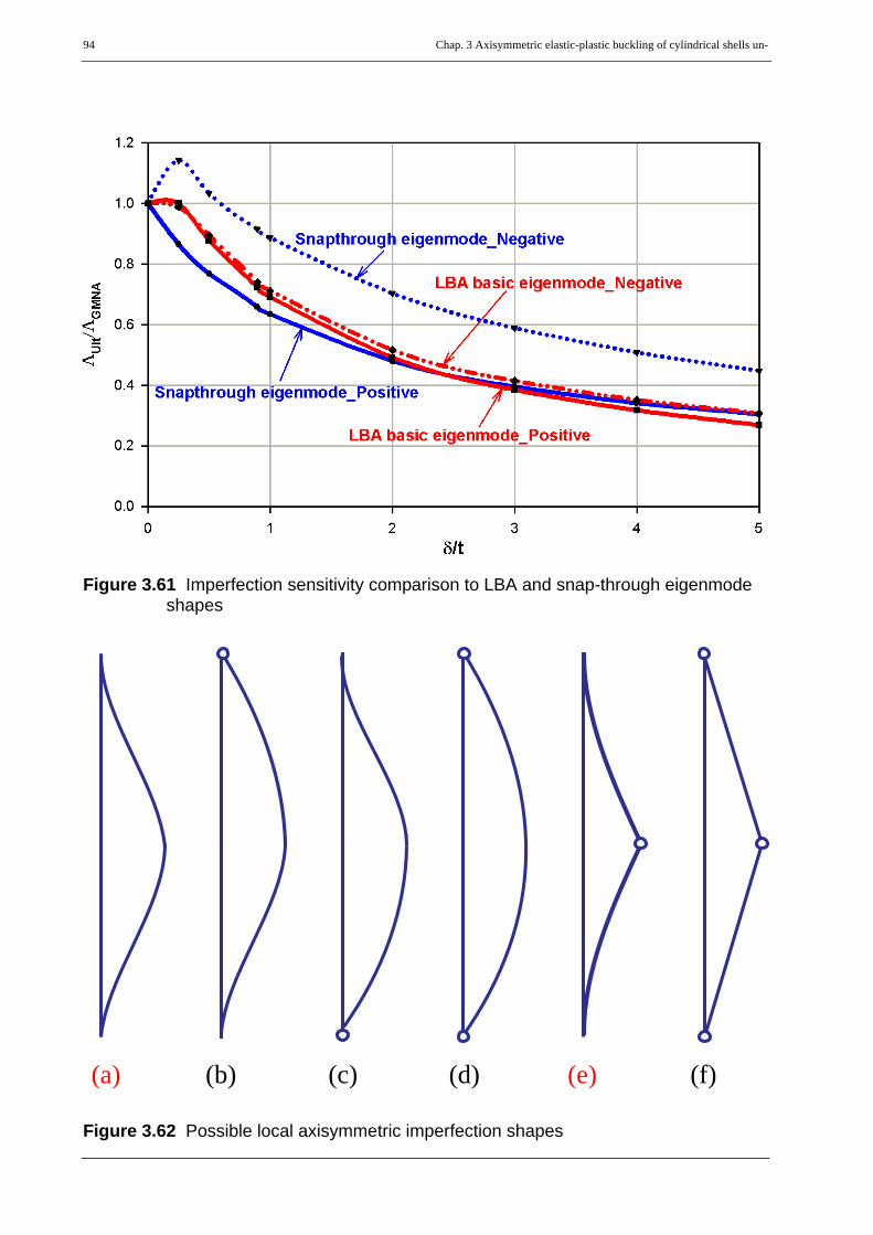
94 Chap. 3 Axisymmetric elastic-plastic buckling of cylindrical shells un-
Figure 3.61 Imperfection sensitivity comparison to LBA and snap-through eigenmode shapes
Figure 3.62 Possible local axisymmetric imperfection shapes
(a) (b) (c) (d) (e) (f)

Chap. 3 Axisymmetric elastic-plastic buckling of cylindrical shells under axial compression & internal pressur 95
Figure 3.63 Effect of imperfection wavelength: type-(a) imperfection
Figure 3.64 Effect of imperfection wavelength: type-(e) imperfection

96 Chap. 3 Axisymmetric elastic-plastic buckling of cylindrical shells un-
Figure 3.65 Effect of imperfection location: type-(a) imperfection & wavelength = 4.0√Rt
Figure 3.66 Imperfection sensitivity for different up-shifts: type-(a) imperfection & wave-length 4.0√Rt

Chap. 3 Axisymmetric elastic-plastic buckling of cylindrical shells under axial compression & internal pressur 97
Figure 3.67 Effect of imperfection location: type-(a) imperfection & wavelength = 2.0√Rt
Figure 3.68 Imperfection sensitivity for different up-shifts: type-(a) imperfection & wave-length 2.0√Rt

98 Chap. 3 Axisymmetric elastic-plastic buckling of cylindrical shells un-
Figure 3.69 Effect of imperfection location: type-(e) imperfection & wavelength = 25t
Figure 3.70 Imperfection sensitivity for different up-shifts: type-(e) imperfection & wave-length = 25t

Chap. 3 Axisymmetric elastic-plastic buckling of cylindrical shells under axial compression & internal pressur 99
Figure 3.71 Effect of imperfection wavelength: type-(a) imperfection & amplitude = wall thickness
Figure 3.72 Imperfection sensitivity: snap-through eigenmode & type-(e) imperfection
snap-through
4.0 R t⋅
2.0 R t⋅

100 Chap. 3 Axisymmetric elastic-plastic buckling of cylindrical shells un-
Figure 3.73 Radial deformation: snap-through eigenmode-affine imperfection
Figure 3.74 Radial deformation: type-(a) imperfection, wavelength 4.0√Rt and up-shift 0.5√Rt
perfect outward-deviation inward-deviation
ΛULSΛRcr-------------- 0.246=
ΛULSΛRcr-------------- 0.218=
ΛULSΛRcr-------------- 0.156=
ΛULSΛRcr-------------- 0.246=
ΛULSΛRcr-------------- 0.215=
ΛULSΛRcr-------------- 0.154=
perfect outward-deviation inward-deviation

Chap. 3 Axisymmetric elastic-plastic buckling of cylindrical shells under axial compression & internal pressur 101
Figure 3.75 Radial deformation: type-(a) imperfection, wavelength 2.0√Rt and up-shift 1.5√Rt
Figure 3.76 Radial deformation: type-(e) imperfection, wavelength = 25t and no up-shift
ΛULSΛRcr-------------- 0.246=
ΛULSΛRcr-------------- 0.220=
ΛULSΛRcr-------------- 0.149=
perfect outward-deviation inward-deviation
ΛULSΛRcr-------------- 0.246=
ΛULSΛRcr-------------- 0.213=
ΛULSΛRcr-------------- 0.280=
perfect outward-deviation inward-deviation

102 Chap. 3 Axisymmetric elastic-plastic buckling of cylindrical shells un-
3.8.1.5 Local axisymmetric imperfection in the free shell interiorAs it has already been discussed, when the internal pressure level acting on a thin-walledcylindrical shell is medium-to-high, it weakens the elastic-plastic buckling strength of the shell byraising the circumferential membrane stress to such an extent where bi-axial plasticty effect leadsto buckling at a relatively low axial compressive load. Generally speaking, the elastic-plasticbuckling behavior and buckling strength of an axially compressed and internally pressurized thin-walled metal cylindrical shells depend on the imperfection nature (shape, wavelength, amplitude,orientation, and location along the meridian), edge constriction effects, and resulting bucklingmodes. For an ideally perfect cylinder or if the strength-reducing effect of imperfections arenegligible, the effect of edge constriction comes into play resulting in a bulge type buckling modenear the edge. The effect of pure edge constriction on the buckling phenomenon and bucklingstrength of a perfect cylinder has already been discussed. On the other hand, when combined withill-natured axisymmetric imperfections, the weakening effect of the medium-to-high internalpressure, will be more pronounced that the cylinder buckles at a very low axial compressive load.Such imperfection-led buckling phenomenon happens at the location of the imperfection. In caseswhere there exist a worst imperfection at locations of edge constriction or when both are closelylocated and able to interact, it is clear that the two effects help each other in destabilizing the shell.The worst possible combined effect of an edge constriction and an imperfection in destabilizingthe cylindrical shell has also been already discussed.
It is, however, not clearly understood so far that when both exist on a shell but at different locationsalong the meridian with no interaction of any kind among them, a very closer look and comparisonneed to be made on the resulting buckling modes and buckling strengths. This study addresses animperfection-led axisymmetric elastic-plastic buckling caused by an axisymmetric localimperfections. This will be done by applying a local axisymmetric imperfection up the meridianon a location where there exist no edge constriction effects (free shell interior). To investigate thistype of buckling phenomenon and the corresponding buckling strength, materially andgeometrically nonlinear analyses of the illustrative cylindrical shell with local axisymmetricimperfection types (a) and (e), Figure 3.62, have been made with wavelengths of 4.0√Rt and 25t,respectively, and imperfection amplitudes allowed for fabrication quality classes A, B, and C as given inEN1993-1-6. Both outward and inward orientations of the imperfections and their effects are considered inthe investigation.
The results of the GMNLI analyses and their comparisons with the buckling strengths obtainedfrom the elastic-plastic interaction using the basic plastic interaction parameters, pure effects ofedge constriction (perfect elephant’s-foot buckling strength), and combined effects of edgeconstriction and imperfection (imperfect elephant’s-foot buckling strength) are discussed asfollows.
Surprisingly, an inward-oriented class-A general-type (type-(a)) local axisymmetric imperfectionwith wavelength of 4.0√Rt in the free shell interior (no edge constriction effects) has the same re-duction effect in the elastic-plastic buckling strength as the edge constriction of the perfect shell(perfect elephant’s-foot buckling), Figure 3.78. For the lower quality classes of the inward-oriented
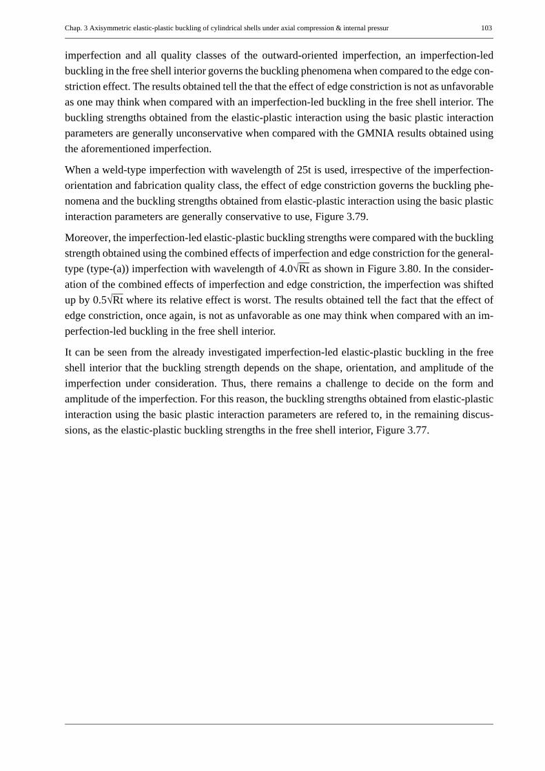
Chap. 3 Axisymmetric elastic-plastic buckling of cylindrical shells under axial compression & internal pressur 103
imperfection and all quality classes of the outward-oriented imperfection, an imperfection-ledbuckling in the free shell interior governs the buckling phenomena when compared to the edge con-striction effect. The results obtained tell the that the effect of edge constriction is not as unfavorableas one may think when compared with an imperfection-led buckling in the free shell interior. Thebuckling strengths obtained from the elastic-plastic interaction using the basic plastic interactionparameters are generally unconservative when compared with the GMNIA results obtained usingthe aforementioned imperfection.
When a weld-type imperfection with wavelength of 25t is used, irrespective of the imperfection-orientation and fabrication quality class, the effect of edge constriction governs the buckling phe-nomena and the buckling strengths obtained from elastic-plastic interaction using the basic plasticinteraction parameters are generally conservative to use, Figure 3.79.
Moreover, the imperfection-led elastic-plastic buckling strengths were compared with the bucklingstrength obtained using the combined effects of imperfection and edge constriction for the general-type (type-(a)) imperfection with wavelength of 4.0√Rt as shown in Figure 3.80. In the consider-ation of the combined effects of imperfection and edge constriction, the imperfection was shiftedup by 0.5√Rt where its relative effect is worst. The results obtained tell the fact that the effect ofedge constriction, once again, is not as unfavorable as one may think when compared with an im-perfection-led buckling in the free shell interior.
It can be seen from the already investigated imperfection-led elastic-plastic buckling in the freeshell interior that the buckling strength depends on the shape, orientation, and amplitude of theimperfection under consideration. Thus, there remains a challenge to decide on the form andamplitude of the imperfection. For this reason, the buckling strengths obtained from elastic-plasticinteraction using the basic plastic interaction parameters are refered to, in the remaining discus-sions, as the elastic-plastic buckling strengths in the free shell interior, Figure 3.77.
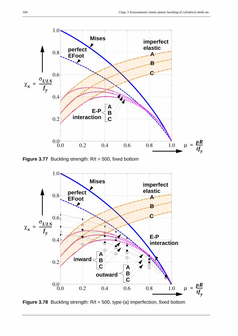
104 Chap. 3 Axisymmetric elastic-plastic buckling of cylindrical shells un-
Figure 3.77 Buckling strength: R/t = 500, fixed bottom
Figure 3.78 Buckling strength: R/t = 500, type-(a) imperfection, fixed bottom
0.0 0.2 0.4 0.6 0.8 1.00.0
0.2
0.4
0.6
0.8
1.0
μ pRtfy-------=
χxσULS
fy--------------=
A
C
B
perfectimperfectMises
EFootelastic
ABC
E-Pinteraction
��
��
�
�
�
�
��
��
�
�
�
�
��
��
�
�
�
�
�
�
�
�
�
�
�
�
��
�
�
�
�
�
�
��
��
�
�
�
�
0.0 0.2 0.4 0.6 0.8 1.00.0
0.2
0.4
0.6
0.8
1.0
μ pRtfy-------=
χxσULS
fy--------------=
Mises
A
C
B
perfectimperfect
EFootelastic
E-Pinteraction
ABC A
BC
outward
inward
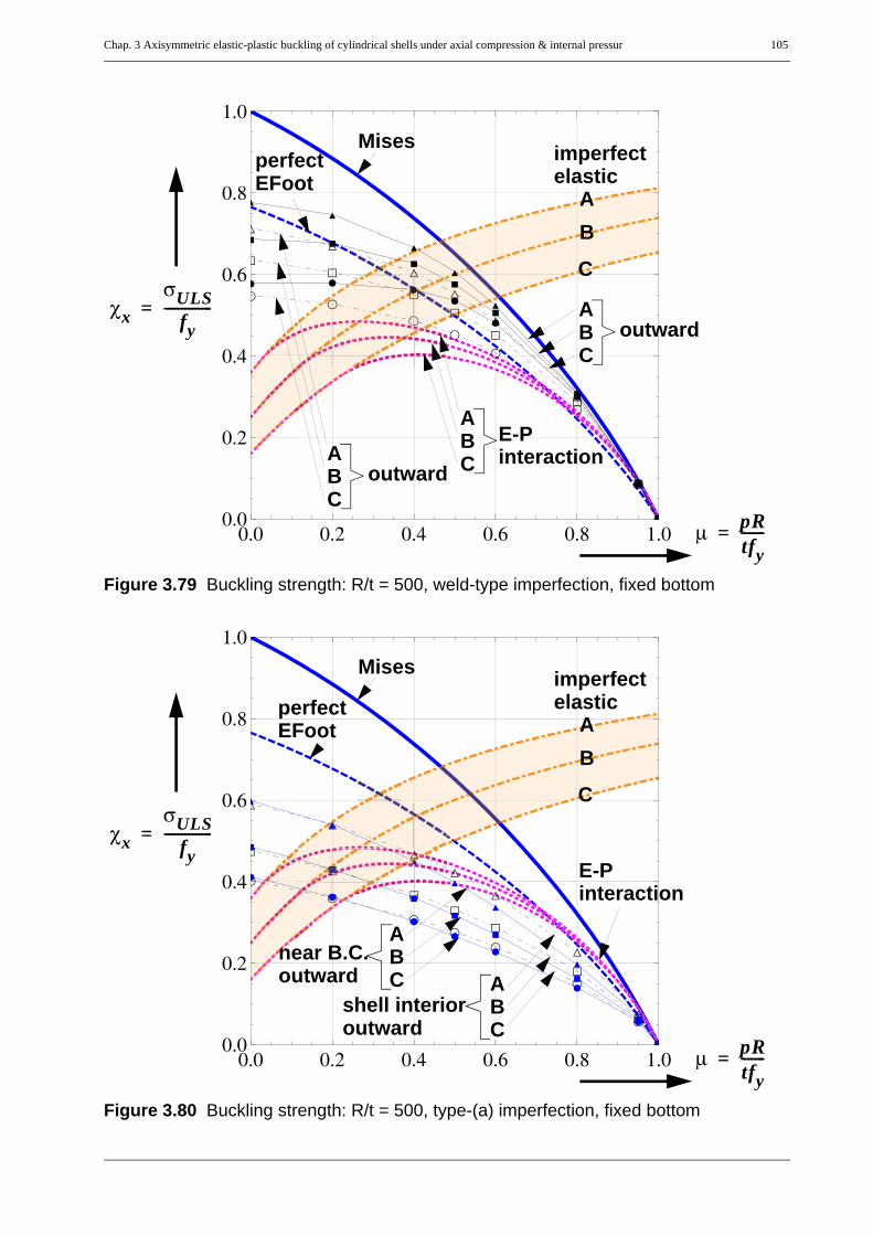
Chap. 3 Axisymmetric elastic-plastic buckling of cylindrical shells under axial compression & internal pressur 105
Figure 3.79 Buckling strength: R/t = 500, weld-type imperfection, fixed bottom
Figure 3.80 Buckling strength: R/t = 500, type-(a) imperfection, fixed bottom
��
�
�
�
�
�
�
��
��
�
�
�
�
� ��
��
�
�
�
��
�
�
�
�
�
�
� �
�
�
�
�
�
�
� ��
�
�
�
�
�
0.0 0.2 0.4 0.6 0.8 1.00.0
0.2
0.4
0.6
0.8
1.0
μ pRtfy-------=
χxσULS
fy--------------=
Mises
A
C
B
perfect imperfectEFoot elastic
ABC
E-PinteractionA
BC
outward
ABC
outward
��
��
�
�
�
�
��
��
�
�
�
�
��
��
�
�
�
�
�
�
�
�
�
�
�
�
�
�
�
�
�
�
�
�
�
�
��
�
�
�
�
0.0 0.2 0.4 0.6 0.8 1.00.0
0.2
0.4
0.6
0.8
1.0
μ pRtfy-------=
χxσULS
fy--------------=
E-Pinteraction
Mises
A
C
B
ABC A
BC
perfectimperfect
EFootelastic
shell interioroutward
near B.C.outward

106 Chap. 3 Axisymmetric elastic-plastic buckling of cylindrical shells un-
3.9 New buckling design recommendation
3.9.1 General characteristic buckling strengthFigure 3.81 and Figure 3.82 (for fixed and pinned bottom boundary conditions, respectively) showthe combined plots of pure elastic imperfect buckling strength, shell interior elastic-plasticimperfect buckling strength, and near boundary perfect elastic-plastic (perfect elephant-foot)buckling strength in the pressure representation.
Figure 3.83 shows a 3D plot of the elastic-plastic buckling interaction using the basic plastic bucklingparameters and the elephan’s-foot buckling strength. Both modes are dominated and limited by the bi-axial Mises membrane yield condition. The minimum strength (envelope) of the two strengths is shownin Figure 3.84. Figure 3.85 shows the reduction in strength due to edge constriction of a pinned bottom cyl-inder causing elephant’s-foot buckling when compared with the elastic-plastic buckling in the free shell in-terior as computed by using the basic plastic interaction parameters. This reduction is even smaller whenthe bottom boundary condition of the cylinder is clamped (fixed). From this comparison, it turns out thatthe boundary elastic-plastic buckling mode is not significantly more unfavourable than the relatedfree-shell-interior elastic-plastic buckling mode. This is in contrast to some of the existinginterpretations and explanations that compare the edge constriction effects with the smalldisplacment elastic and platic strengths as shown in Figure 3.86. The combined effects ofimperfection and edge bending disturbance in destablizing the shell have already been discussedin the GMNIA investigation.
Explanatory plots of all characteristic buckling strengths corresponding to the different bucklingphenomena are shown in Figure 3.87 to Figure 3.90. For a clear understanding of the differentrepresentations, the same characteritsic buckling strengths are shown in pressure representation(Figure 3.87), capacity representation (Figure 3.88), membrane Mises-related interactionrepresentation (Figure 3.89), and perfect elephant’s-foot-related interaction representation (Figure3.90). Basic understanding of these different representations will help in easy manipulation of thebuckling strength results and ultimately leading to the best representation where simpleexpressions can be formulated that are able to accurately predict the characteristic bucklingstrength of the cylinder.
It should again be noted that as far as elastic-plastic buckling of the imperfect cylindrical shells isconcerned, there should be a well defined (at least for numerical simulation purposes), practicallypossible (both from safety and economic considerations), and worst (in that it leads to lowerbuckling strength of the shell) imperfection. Once such imperfections are known and agreed uponby the research and practical engineers community, a unified and simplified design proposals canbe made. In spite of this fact, different possible proposals are discussed in the following section,out of which the simplest yet best approach will be recommended for design and future researchs.

Chap. 3 Axisymmetric elastic-plastic buckling of cylindrical shells under axial compression & internal pressur 107
Figure 3.81 Perfect elephant’s-foot buckling strength: fixed bottom
Figure 3.82 Perfect elephant’s-foot buckling strength: pinned bottom

108 Chap. 3 Axisymmetric elastic-plastic buckling of cylindrical shells un-
Figure 3.83 Comparison of elastic-plastic buckling interaction using basic plastic buck-ling parameters with elephant’s-foot strength
μ pRtfy-------=
χxσULS
fy--------------=
λxfy
σxRcr---------------=

Chap. 3 Axisymmetric elastic-plastic buckling of cylindrical shells under axial compression & internal pressur 109
Figure 3.84 Envelope of elastic-plastic buckling interaction using basic plastic buckling parameters and elephant’s-foot strength
μ pRtfy-------=
χxσULS
fy--------------=
λxfy
σxRcr---------------=

110 Chap. 3 Axisymmetric elastic-plastic buckling of cylindrical shells un-
Figure 3.85 Buckling strength reduction due to edge constriction effects causing ele-phant’s-foot buckling when compared with elastic-plastic buckling in the free shell interior
μ pRtfy-------=
χxσULS
fy--------------=
λxfy
σxRcr---------------=

Chap. 3 Axisymmetric elastic-plastic buckling of cylindrical shells under axial compression & internal pressur 111
Figure 3.86 Buckling strength reduction due to edge constriction effects causing ele-phant’s-foot buckling when compared with pure elastic and pure plastic strengths of the perfect shell
μ pRtfy-------=
χxσULS
fy--------------=
λxfy
σxRcr---------------=

112 Chap. 3 Axisymmetric elastic-plastic buckling of cylindrical shells un-
Figure 3.87 Comparison of different buckling strengths in pressure representation
Figure 3.88 Comparison of different buckling strengths in capacity representation
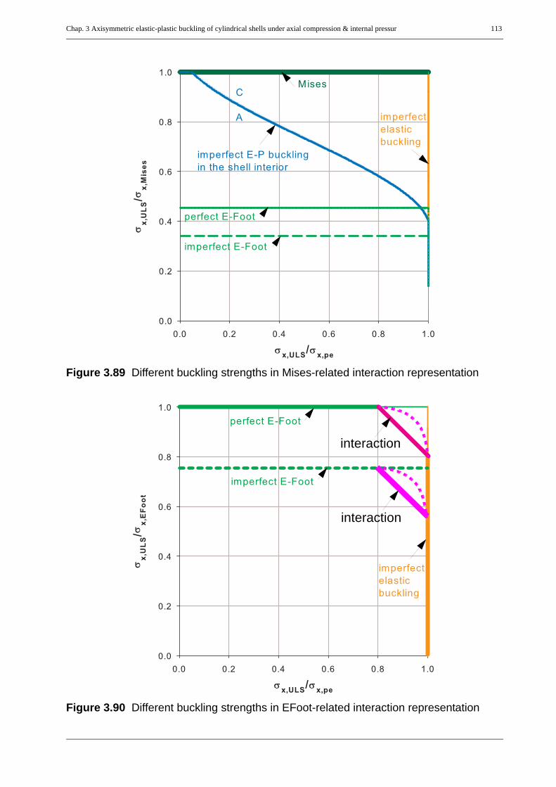
Chap. 3 Axisymmetric elastic-plastic buckling of cylindrical shells under axial compression & internal pressur 113
Figure 3.89 Different buckling strengths in Mises-related interaction representation
Figure 3.90 Different buckling strengths in EFoot-related interaction representation
interaction
interaction

114 Chap. 3 Axisymmetric elastic-plastic buckling of cylindrical shells un-
3.9.2 Characteristic buckling strength prediction recommendationBased on the results obtained so far for the different buckling phenomena and their correspondingbuckling strengths, five different methods can be applied in the prediction of the charactersticbuckling strength of thin-walled cylindrical shells under uniform axial compression and internalpressure loading. In all the methods separation is made for the different types of bottom boundarycondtions (fixed versus pinned).
An overview of the five possible options for predicting the characterstic buckling strengths ofcylindrical shells is given below. Detailed discussion on each approach will then follow.
Method -1. elastic-plastic interaction with the bi-axial membrane Mises to directly catch thepure elastic, elastic-plastic buckling in the shell interior, and elephant’s-foot bucklingstrengths using a new set of plastic buckling interaction parameters (see Figure 3.91).
Method - 2a. envelope of the pure elastic and elephant’s-foot strengths with no interaction ofany kind. This method results in somehow unconservative buckling strength predic-tion when compared to the other methods. The left part in the envelope (see Figure3.92) represents pure elastic buckling strength of the imperfect shell and the right partfor elastic-plastic buckling near the boundary of the perfect shell.
Method - 2b. envelope of the pure elastic, elastic-plastic interaction with bi-axial membraneMises using the basic plastic buckling parameters, and the perfect elephant’s footbuckling strength. The first (left) part in the envelope (see Figure 3.93) representspure elastic buckling strength of the imperfect shell; the second (middle) part repre-sents the elastic-plastic buckling strength in the free shell interior; and the third (right)for elastic-plastic buckling near the boundary.
Method - 3. elastic-plastic buckling interaction of the pure elastic strength curve with the ele-phant’s foot strength curve using the basic plastic buckling parameters β = 0.6; λ0 =0.2; and η = 1.0. This approach leads to very big interaction and too conservativestrength predictions (see Figure 3.94).
Method - 4. elastic-plastic buckling interaction of the pure elastic strength curve with the ele-phant’s-foot strength curve using a completely new single buckling parameterΔβEFoot. This method, depending on the value of ΔβEFoot, predicts the separate char-acteristic buckling strengths: pure elastic, elephant’s-foot near the boundary, and apossible interaction in between (see Figure 3.95 for ΔβEFoot = 0.1). This method, as itwill be seen later, is the simplest, easy to understand, easy to apply, easy to modify,straight forward, and yet accurate (specially when compared to method-1). Hence, itis the best approach of all the methods discussed so far.
All the above procedures (except method-3) predict same or very close strength results in the pureelastic (low pressure level) and elastic-plastic elephant’s-foot buckling near the boundary (highpressure level). They, however, differ in the strength prediction of the elastic-plastic buckling inthe free shell interior. These differences are left open till test or GMNIA results are performed forelastic-plastic buckling in the free shell interior. Since the bi-axial membrane Mises yield condition

Chap. 3 Axisymmetric elastic-plastic buckling of cylindrical shells under axial compression & internal pressur 115
is on the background, all the methods by default guarantee that no buckling strength exceeds thepure plastic capacity. An illustrative comparison of the different methods (a combination of Figure3.91 to Figure 3.95) has been done for a cylinder with fixed bottom boundary condition and shellslenderness ratio R/t = 1000 and is shown in the pressure representation, Figure 3.96. For very thinshells the characteristic buckling strength prediction using method-1 is equal to that of method-2,i.e the elastic-plastic buckling interaction according to method-1 diminishes as the shell getsthinner.
A detailed discussion on the above methods is given below. Method-3 will be skipped in thediscussion as it predicts buckling strengths much too low when compared to the other methods. Itis upto the designer’s choice which one of the above procedures to use for the prediction of thecharacterstic buckling strength. It should, however, be noted here that the elephant’s-foot typebuckling near the bounadary for the imperfect cylinder is not included and hence that of a perfectcylinder is used in all the methods as there is no common agreement on the “practical and worst”imperfection shape, wavelength, amplitude, location along the meridian of the shell, and theorientation of the imperfection in the inward-outward sense. Once a common agreement is reachedon the imperfection type, the geometrically and materially nonlinear analysis results of theimperfect shell can directly be applied to method-2 (the envelope method) and easily be adoptedto all other methods.

116 Chap. 3 Axisymmetric elastic-plastic buckling of cylindrical shells un-
Figure 3.91 Characteristic buckling strength prediction: R/t = 1000, method-1
method-1
membrane Mises
perfect EFootperfect elastic
imperfect elastic
E-Pinteraction

Chap. 3 Axisymmetric elastic-plastic buckling of cylindrical shells under axial compression & internal pressur 117
Figure 3.92 Characteristic buckling strength prediction: R/t = 1000, method-2a
method-2a
membrane Mises
perfect EFootperfect elastic
imperfect elastic
E-Pinteraction

118 Chap. 3 Axisymmetric elastic-plastic buckling of cylindrical shells un-
Figure 3.93 Characteristic buckling strength prediction: R/t = 1000, method-2b
method-2b
membrane Mises
perfect EFootperfect elastic
imperfect elastic
E-Pinteraction

Chap. 3 Axisymmetric elastic-plastic buckling of cylindrical shells under axial compression & internal pressur 119
Figure 3.94 Characteristic buckling strength prediction: R/t = 1000, method-3
method-3
membrane Mises
perfect EFootperfect elastic
imperfect elastic
E-Pinteraction
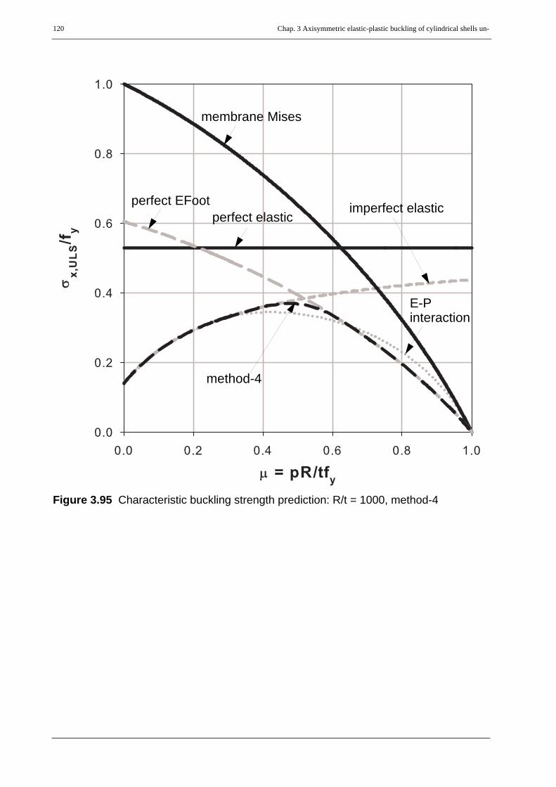
120 Chap. 3 Axisymmetric elastic-plastic buckling of cylindrical shells un-
Figure 3.95 Characteristic buckling strength prediction: R/t = 1000, method-4
method-4
membrane Mises
perfect EFootperfect elastic
imperfect elastic
E-Pinteraction

Chap. 3 Axisymmetric elastic-plastic buckling of cylindrical shells under axial compression & internal pressur 121
Figure 3.96 Characteristic buckling strength prediction: R/t = 1000, comparison of methods
methods-1&2a
method-2bmethod-4
method-3
membrane Mises
perfect EFootperfect elastic
imperfect elastic
E-Pinteraction

122 Chap. 3 Axisymmetric elastic-plastic buckling of cylindrical shells un-
3.9.2.1 Method-1: Elastic-plastic interaction using pressure dependent interactionparameters in such a way that EFoot strength is directly included
In this method the elastic-plastic interaction for the prediction of characteristic buckling strengthsusing membrane Mises yield condition will be extended and made in such a way that it directlyincludes the pure elastic buckling, elastic-plastic buckling in the free shell interior, and elephant-foot type buckling near boundary conditions. This will be achieved with the help of thegeometrically and materially nonlinear numerical analysis results (for both the fixed and pinnedbottom boundary conditions) using internal pressure dependent plastic buckling parameters
, , and instead of the basic constant values of an axially compressed andinternally unpressurized cylinder. These new set of plastic buckling parameters do have the samevalues for unpressurized buckling conditions as those of the basic ones.
The pressurized elastic buckling strength of the imperfect thin-walled cylindrical shell, which havealready been discussed, will be used in the following discussion on the new elastic-plastic bucklinginteraction formulation.
Plastic Buckling:
Pressure dependent plastic buckling parametersInteraction exponent:
(Eq. 3.60)
Squash limit relative slenderness:
(Eq. 3.61)
Plastic range factor:
(Eq. 3.62)
where ηo, λo,o, and βo are the basic plastic buckling parameters and stay valid for the unpressurizedcylinder condition.
(Eq. 3.63)
(Eq. 3.64)
(Eq. 3.65)
and the βEFoot factor which takes care of the pressure-independent reduction in strength (whencompared with the pure plastic capacity of the perfect shell) due to geometric nonlinearity (largedeformation) effects is repeated here as follows
λo μ( ) η μ( ) β μ( )
η ηo f0 μ( )⋅=
λo λo o, f0 μ( )⋅=
β βo βEFoot βo–( )+ 1 fβ μ( )–( )⋅=
ηo η μ 0=( ) 1.0= =
λo o, λo μ 0=( ) 0.2= =
βo β μ 0=( ) 0.6= =

Chap. 3 Axisymmetric elastic-plastic buckling of cylindrical shells under axial compression & internal pressur 123
(Eq. 3.66)
in which
(Eq. 3.67)
(Eq. 3.68)
(Eq. 3.69)
The value of the exponent “a” in the expressions for the f0 and fβ is equal to 4 for the fixed-bottomcylinder and 8 for the pinned-bottom case. The variations of βEFoot as a function of the shellslenderness parameter ρ; and f0 & fβ for R/t = 1000 as a function of the internal pressure parameterμ are shown in Figure 3.97 and Figure 3.98, respectively, for both fixed and pinned bottomboundary conditions.
The characterstic buckling strength plots according to this method are shown using the pressurerepresentation in Figure 3.99 and Figure 3.100 for both the fixed and pinned bottom boundaryconditions, respectively. For a better view and comparison, the same plots are shown in Figure3.101 and Figure 3.102 using the capacity representation, respectively. The difference in thecharacteristic buckling strength caused by the two types of bottom boundary conditions can beclearly seen from the plots. Figure 3.103 shows the 3D plot of the characteristic buckling strengthof a cylindrical shell with fabrication quality class-C and pinned bottom boundary condition.
βEFoot0.8 1 e 1.15ρ––( ) for pinned bottom
0.75 1 e 0.75ρ––( ) for fixed bottom⎩⎪⎨⎪⎧
=
ρ R t⁄1000------------=
f0 μ( ) 1 μ2–( )a
=
fβ μ( ) 1 μ1.5 λx–⎝ ⎠⎛ ⎞
a=
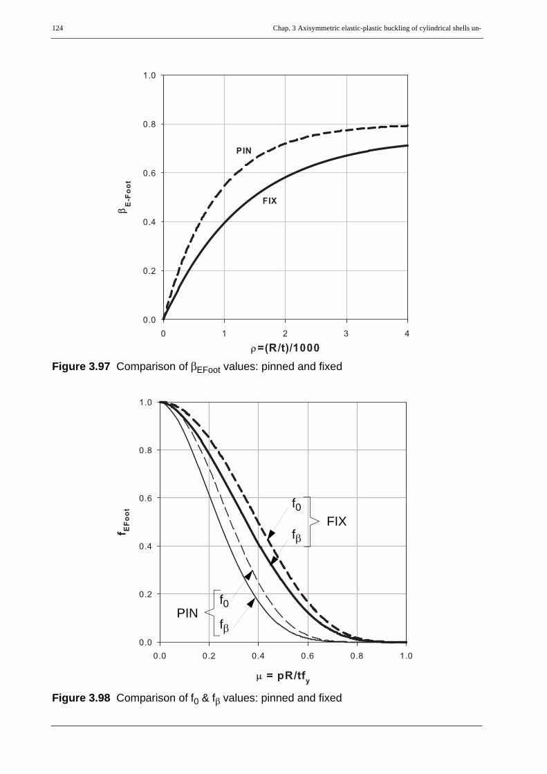
124 Chap. 3 Axisymmetric elastic-plastic buckling of cylindrical shells un-
Figure 3.97 Comparison of βEFoot values: pinned and fixed
Figure 3.98 Comparison of f0 & fβ values: pinned and fixed
f0
fβ FIX
f0
fβ PIN

Chap. 3 Axisymmetric elastic-plastic buckling of cylindrical shells under axial compression & internal pressur 125
Figure 3.99 characteristic buckling strength according to method-1: fixed bottom
Figure 3.100 characteristic buckling strength according to method-1: pinned bottom
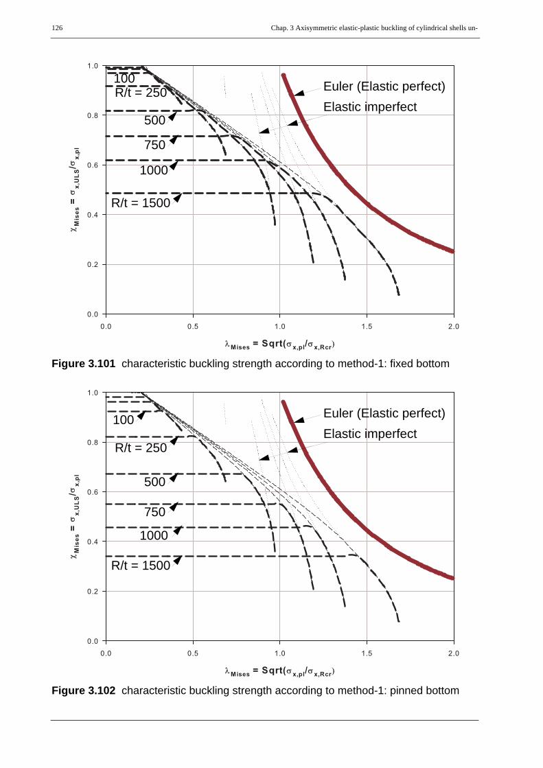
126 Chap. 3 Axisymmetric elastic-plastic buckling of cylindrical shells un-
Figure 3.101 characteristic buckling strength according to method-1: fixed bottom
Figure 3.102 characteristic buckling strength according to method-1: pinned bottom
R/t = 1500
Elastic imperfectEuler (Elastic perfect)
1000
750
500
R/t = 250100
R/t = 1500
Elastic imperfectEuler (Elastic perfect)
1000
750
500
R/t = 250
100

Chap. 3 Axisymmetric elastic-plastic buckling of cylindrical shells under axial compression & internal pressur 127
Figure 3.103 3D representation of the characteristic buckling strength of axially com-pressed and internally pressurized cylindrical shells according to method-1: pinned bottom
μ pRtfy-------=
χxσULS
fy--------------=
λxfy
σxRcr---------------=

128 Chap. 3 Axisymmetric elastic-plastic buckling of cylindrical shells un-
3.9.2.2 Method-2: Envelope of the different buckling strengthsThis method introduces no new plastic buckling parameters but instead recommends to take theenvelope of the separate strengths, i.e. the minimum of the buckling strengths under considerationdepending on the choice as discussed below. In comparison with the first method, this method onone hand, clearly represents the different buckling phenomena and on the other hand, gives moreroom for direct inclusion of future test or GMNIA results representing the imperfect elastic-plasticbuckling phenomena in the free shell interior and near the boundary.
Method-2a: Envelope of pure elastic and elephant’s-foot buckling strengthsThis method results in the minimum of the pure elastic buckling strength of the imperfect cylinderand the elastic-plastic buckling near the boundary (elephant’s-foot buckling) strengths. Hence,only two distinct buckling phenomena can be represented by this method namely:
• pure elastic buckling of the imperfect cylinder at relatively low-to-medium internal pressure levels
• perfect elastic-plastic buckling near the boundary (perfect elephant’s-foot buckling) at rela-tively medium-to-high internal pressure levels
This method, though it is the easiest and straight forward of all, gives higher (henceunconservative) buckling strengths than the remaining methods. Illustrative plots of the bucklingstrength according to this method are shown in Figure 3.92 and Figure 3.96.
Method-2b: Envelope of pure elastic, elastic-plastic in the free shell interior, and elephant’s-foot buckling strengths
This method results in the minimum of the pure elastic buckling strength of the imperfect cylinder,elastic-plastic interaction using bi-axial membrane Mises yield condition (adopting the plasticbuckling parameters of an axially compressed internally unpressurized cylinder), and the elastic-plastic buckling near the boundary (elephant’s-foot buckling) strengths. In this case the bucklingstrength obtained from the elastic-plastic interaction using the bi-axial membrane Mises yieldcondition represents the strength of an imperfection-led elastic-plastic buckling in the free shellinterior where edge constrcition effects do not exist. Hence, three distinct buckling phenomena canbe represented by this method namely:
• pure elastic buckling of the imperfect cylinder at relatively low internal pressure levels
• imperfection-led elastic-plastic buckling in the free shell interior of the cylinder at medium internal pressure levels
• edge constriction-led elastic-plastic buckling near the boundary conditions of the perfect cylinder (perfect elephant’s-foot buckling) at relatively high internal pressure levels
This method, when compared to method-2a, results in somehow conservative results at mediumpressure levels. The characteristic buckling strength according to this method are shown in Figure

Chap. 3 Axisymmetric elastic-plastic buckling of cylindrical shells under axial compression & internal pressur 129
3.104 and Figure 3.105 using the pressure representation for the fixed and pinned bottom cases,respectively. A 3D plot of the characterstic buckling strength of a pinned bottom cylindrical shellobtained using this method has been shown in Figure 3.84.

130 Chap. 3 Axisymmetric elastic-plastic buckling of cylindrical shells un-
Figure 3.104 characteristic buckling strength according to method-2b: fixed bottom
Figure 3.105 characteristic buckling strength according to method-2b: pinned bottom

Chap. 3 Axisymmetric elastic-plastic buckling of cylindrical shells under axial compression & internal pressur 131
3.9.2.3 Method-4: Elastic-plastic interaction using a completely new interactionparameter
This method introduces a completely new plastic buckling parameter . By the introductionof this single plastic interaction parameter, the different buckling phenomena can be explicitlyexpressed namely:
• pure elastic buckling of the imperfect cylinder at relatively low internal pressure levels
• imperfection-led elastic-plastic buckling in the free shell interior of the cylinder at medium internal pressure levels
• edge constriction-led elastic-plastic buckling near the boundary conditions of the perfect cylinder (perfect elephant’s-foot buckling) at relatively high internal pressure levels
Illustrative characteristic buckling strength curves that will fully explain about this particularmethod are, once gain, shown in the membrane Mises-related interaction representation (Figure3.106), perfect elephant’s-foot-related interaction representation (Figure 3.107), and pressurerepresentation (Figure 3.108).
Elephant’s-foot-related interaction expression
With the help of the characteristic buckling strengths shown in Figure 3.107, the followinginteraction expression can easily be formulated.
(Eq. 3.70)
where
... shell buckling relative slenderness (Eq. 3.71)
... elastic limit relative slenderness (Eq. 3.72)
... EFoot limit relative slenderness (Eq. 3.73)
ΔβEFoot
χEFootσx Rk,
σx EFoot,--------------------
1.0 for λEFoot λo≤
2 ΔβEFoot–( ) 1
1λEFoot
2
αxpe---------------+
-------------------------
⎝ ⎠⎜ ⎟⎜ ⎟⎜ ⎟⎜ ⎟⎛ ⎞
f⋅ for λo λEFoot λp< <⋅
αxpe
λEFoot2
--------------- for λp λEFoot≤⎩⎪⎪⎪⎪⎪⎨⎪⎪⎪⎪⎪⎧
= =
λEFootσx EFoot,
σxRcr-------------------- λMises 1 βEFoot–= =
λpαxpe
1 ΔβEFoot–( )---------------------------------=
λ0 αxpe 1 ΔβEFoot–( )⋅=
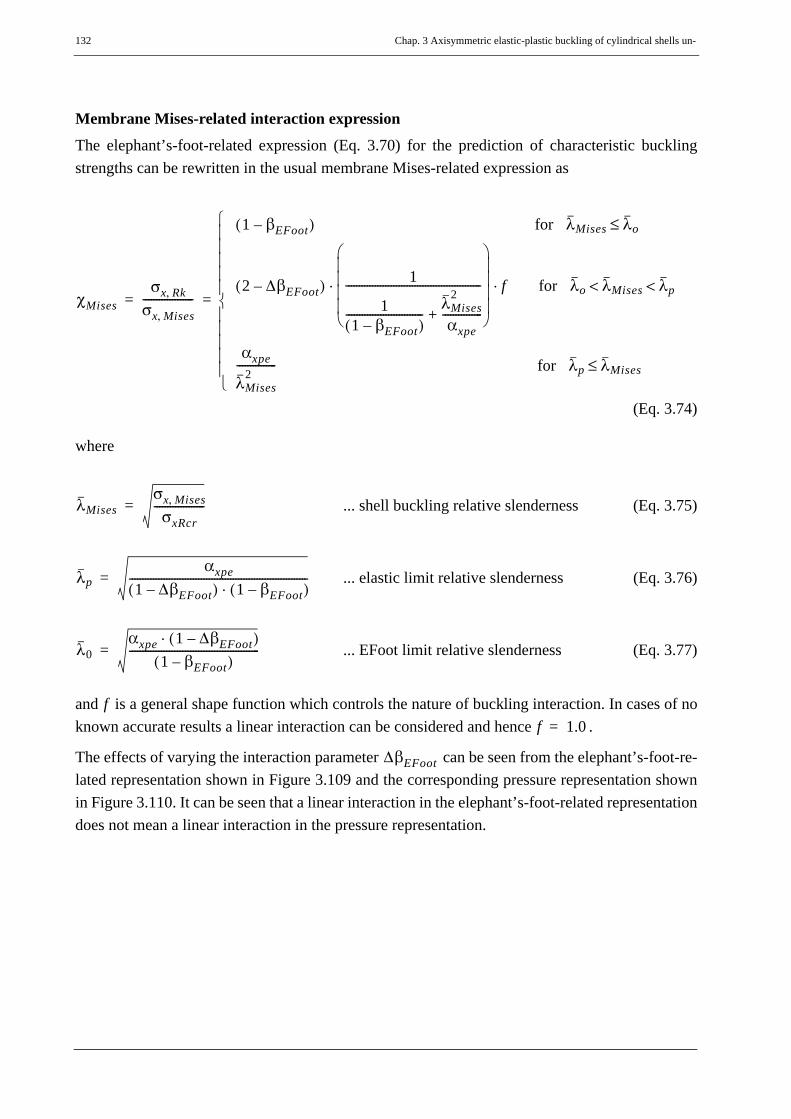
132 Chap. 3 Axisymmetric elastic-plastic buckling of cylindrical shells un-
Membrane Mises-related interaction expressionThe elephant’s-foot-related expression (Eq. 3.70) for the prediction of characteristic bucklingstrengths can be rewritten in the usual membrane Mises-related expression as
(Eq. 3.74)
where
... shell buckling relative slenderness (Eq. 3.75)
... elastic limit relative slenderness (Eq. 3.76)
... EFoot limit relative slenderness (Eq. 3.77)
and is a general shape function which controls the nature of buckling interaction. In cases of noknown accurate results a linear interaction can be considered and hence .
The effects of varying the interaction parameter can be seen from the elephant’s-foot-re-lated representation shown in Figure 3.109 and the corresponding pressure representation shownin Figure 3.110. It can be seen that a linear interaction in the elephant’s-foot-related representationdoes not mean a linear interaction in the pressure representation.
χMisesσx Rk,
σx Mises,-------------------
1 βEFoot–( ) for λMises λo≤
2 ΔβEFoot–( ) 1
11 βEFoot–( )
----------------------------- λMises2
αxpe---------------+
---------------------------------------------------
⎝ ⎠⎜ ⎟⎜ ⎟⎜ ⎟⎜ ⎟⎛ ⎞
f⋅ for λo λMises λp< <⋅
αxpe
λMises2
--------------- for λp λMises≤⎩⎪⎪⎪⎪⎪⎨⎪⎪⎪⎪⎪⎧
= =
λMisesσx Mises,
σxRcr-------------------=
λpαxpe
1 ΔβEFoot–( ) 1 βEFoot–( )⋅-------------------------------------------------------------------=
λ0αxpe 1 ΔβEFoot–( )⋅
1 βEFoot–( )-------------------------------------------------=
ff 1.0=
ΔβEFoot
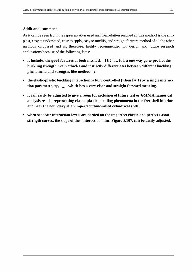
Chap. 3 Axisymmetric elastic-plastic buckling of cylindrical shells under axial compression & internal pressur 133
Additional commentsAs it can be seen from the representation used and formulation reached at, this method is the sim-plest, easy to understand, easy to apply, easy to modify, and straight forward method of all the othermethods discussed and is, therefore, highly recommended for design and future researchapplications because of the following facts:
• it includes the good features of both methods - 1&2, i.e. it is a one-way go to predict the buckling strength like method-1 and it strictly differentiates between different buckling phenomena and strengths like method - 2
• the elastic-plastic buckling interaction is fully controlled (when f = 1) by a single interac-tion parameter, ΔβEFoot, which has a very clear and straight forward meaning.
• it can easily be adjusted to give a room for inclusion of future test or GMNIA numerical analysis results representing elastic-plastic buckling phenomena in the free shell interior and near the boundary of an imperfect thin-walled cylindrical shell.
• when separate interaction levels are needed on the imperfect elastic and perfect EFoot strength curves, the slope of the “interaction” line, Figure 3.107, can be easily adjusted.

134 Chap. 3 Axisymmetric elastic-plastic buckling of cylindrical shells un-
Figure 3.106 Buckling strength in Mises-related interaction representation: method-4
Figure 3.107 Buckling strength in EFoot-related interaction representation: method-4
ΔβEFoot
βEFoot
Membrane Mises
perfect EFoot
imperfectelastic
interaction
ΔβEFoot
1
1perfect EFoot
imperfectelastic
interaction

Chap. 3 Axisymmetric elastic-plastic buckling of cylindrical shells under axial compression & internal pressur 135
Figure 3.108 Characteristic buckling strength in pressure representation: method-4
ΔβEFoot
interaction
membrane Mises
perfectperfect imperfect
elasticelasticEFoot

136 Chap. 3 Axisymmetric elastic-plastic buckling of cylindrical shells un-
Figure 3.109 Effect of varying : EFoot-related interaction representation
Figure 3.110 Effect of varying : pressure representation
ΔβEFoot = 0.5 0.4
0.3 0.2
0.1
ΔβEFoot = 0.1, 0.2, 0.3, 0.4, 0.5
perfect EFoot
imperfectelastic
interaction
ΔβEFoot
1
1
ΔβEFoot
ΔβEFoot = 0.5
0.1
ΔβEFoot = 0.1, 0.2, 0.3, 0.4, 0.5
interaction
membrane Mises
perfectperfect imperfect
elasticelasticEFoot
ΔβEFoot

Chap. 3 Axisymmetric elastic-plastic buckling of cylindrical shells under axial compression & internal pressur 137
3.10Comparison of the new buckling designrecommendation with EN 1993-1-6 bucklingdesign regulation
This section first discusses the buckling design recommendation according to EN 1993-1-6 designregulation and then compares it with the new buckling design recommendation of this work. Theoverall difference between the two recommendations lie only on the elastic-plastic bucklingstrength prediction and not on the pure elastic buckling strength as both recommendations use thesame unpressurized and pressurized elastic imperfection reduction factors. Hence, the discussionson the unpressurized and pressurized, perfect and imperfect pure elastic buckling strengths madepreviously apply to both recommendations. The EN 1993-1-6 procedure for computingcharacteristic buckling strengths of cylindrical shells is discussed below.
3.10.1 Perfect elephant’s foot buckling strength using EN 1993-1-6Following geometrically and materially nonlinear numerical analyses, the elastic-plastic bucklingstrength of a perfect cylindrical shell for buckling near the boundary (perfect elephant’s-footbuckling strength) is given interms of a fitting curve of the analyses results. The fitting curve isexpressed as a reduction factor, αxpp, called plastic pressurized imperfection reduction factorwhich is a ratio of the elastic-plastic buckling load to the elastic classical buckling load of the shell.
The name given to this factor is quite confusing as it has nothing to do with imperfections.This name might have been given as it, like that of the pressurized elastic imperfectionreduction factor, is a ratio of the buckling load to the classical critical load. It should,however, be noted here that this factor is not an imperfection reduction factor as the nameimplies but instead a reduction factor, when referred to the classical elastic bucklingstrength, accounts for material and geometric nonlinearities. It can also be interpreted as areduction factor, when referred to the pure plastic capacity of the shell, accounts forgeometric nonlinearities. Despite this fact, it will still be called plastic pressurizedimperfection reduction factor in the remaining parts of the discussion so that it will not beconfused whenever reference to EN 1993-1-6 is made.
The elephant’s foot buckling strength obtained using αxpp for different shell slenderness ratios areshown in the pressure representation, Figure 3.111, where a quantitative comparison can be madewith the pure bi-axial plastic strength of the shell. The same buckling strength is shown in Figure3.112 using the capacity represnetation. A combined 3D plot of the same strength is shown inFigure 3.113. For shell slenderness ratio , the elephant foot buckling strength predictionusing the αxpp expression is higher than the pure bi-axial plastic strength of the cylinder as can beseen from Figure 3.111 and more clearly from Figure 3.114.
R t⁄ 145≤

138 Chap. 3 Axisymmetric elastic-plastic buckling of cylindrical shells un-
Why EN 1993-1-6 elephant’s-foot strength prediction is higher than the pure plastic capac-ity of the cylinder?
This problem arises because, upon fitting, the expression for αxpp (Eq. 3.78) bases on a pressuredependent quadratic curve which has nothing to do with bi-axial plasticity and applyingtwo separate pressure independent correction factors as follows:
(Eq. 3.78)
with
a geometry correction factor, fg (Eq. 3.79):
(Eq. 3.79)
and a material correction factor, fm (Eq. 3.80).
(Eq. 3.80)
where
(Eq. 3.81)
(Eq. 3.82)
(Eq. 3.83)
An illustrative plot for R/t = 1000, fy = 24 kN/cm2, E =21000 kN/cm2, and ν = 0.3 is shown inFigure 3.115. The geometry correction factor depends purely on the shell slenderness ratio R/twhile the material correction factor depends on the combined effects of the material properties(uni-axial yield strength fy, modulus of elasticity E, and Poisson’s ratio ν) and the shell slendernessratio R/t. A close look at the material correction factor reveals that it is very close to unity for thestandard steel properties and varies little with varying R/t values.
1 μ2–( )
αxpp 1 μ2–{ } fg fm⋅ ⋅=
fg 1 11.12 s3 2⁄+--------------------------–⎝ ⎠
⎛ ⎞=
fms2 1.21λx
2+s s 1+( )
---------------------------⎝ ⎠⎜ ⎟⎛ ⎞
=
μσθfy------ pR t⁄
fy------------= =
s R t⁄400---------=
λx2 fy
σxRcr-------------=

Chap. 3 Axisymmetric elastic-plastic buckling of cylindrical shells under axial compression & internal pressur 139
Figure 3.111 Elephant’s-foot buckling strength of the perfect cylinder: pinned bottom
Figure 3.112 Elephant’s-foot buckling strength of the perfect cylinder: pinned bottom
μ 0.0 0.1 … 0.9, , ,=
0.8μ 0.9=
0.7
μ 0.0=
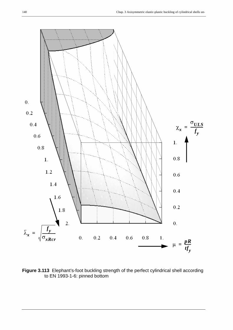
140 Chap. 3 Axisymmetric elastic-plastic buckling of cylindrical shells un-
Figure 3.113 Elephant’s-foot buckling strength of the perfect cylindrical shell according to EN 1993-1-6: pinned bottom
μ pRtfy-------=
χxσULS
fy--------------=
λxfy
σxRcr---------------=

Chap. 3 Axisymmetric elastic-plastic buckling of cylindrical shells under axial compression & internal pressur 141
Figure 3.114 Elephant’s-foot buckling strength of the perfect cylindrical shell according to EN 1993-1-6 and bi-axial membrane Mises cut-off: pinned bottom
μ pRtfy-------=
χxσULS
fy--------------=
λxfy
σxRcr---------------=
membrane Misescut-off
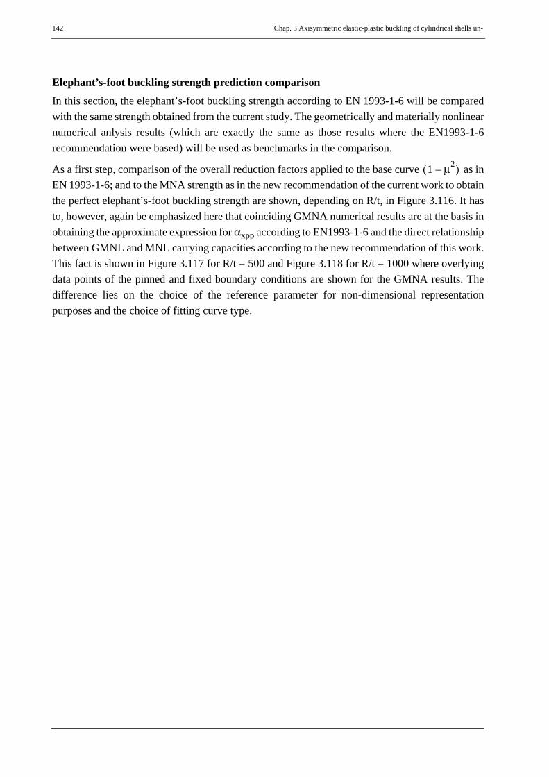
142 Chap. 3 Axisymmetric elastic-plastic buckling of cylindrical shells un-
Elephant’s-foot buckling strength prediction comparisonIn this section, the elephant’s-foot buckling strength according to EN 1993-1-6 will be comparedwith the same strength obtained from the current study. The geometrically and materially nonlinearnumerical anlysis results (which are exactly the same as those results where the EN1993-1-6recommendation were based) will be used as benchmarks in the comparison.
As a first step, comparison of the overall reduction factors applied to the base curve as inEN 1993-1-6; and to the MNA strength as in the new recommendation of the current work to obtainthe perfect elephant’s-foot buckling strength are shown, depending on R/t, in Figure 3.116. It hasto, however, again be emphasized here that coinciding GMNA numerical results are at the basis inobtaining the approximate expression for αxpp according to EN1993-1-6 and the direct relationshipbetween GMNL and MNL carrying capacities according to the new recommendation of this work.This fact is shown in Figure 3.117 for R/t = 500 and Figure 3.118 for R/t = 1000 where overlyingdata points of the pinned and fixed boundary conditions are shown for the GMNA results. Thedifference lies on the choice of the reference parameter for non-dimensional representationpurposes and the choice of fitting curve type.
1 μ2–( )

Chap. 3 Axisymmetric elastic-plastic buckling of cylindrical shells under axial compression & internal pressur 143
Figure 3.115 EN1993-1-6 elephant’s-foot buckling strength of the perfect cylinder: R/t = 1000
Figure 3.116 Comparison of elephant’s-foot buckling strengths of the perfect cylinder
0.0 0.2 0.4 0.6 0.8 1.00.0
0.2
0.4
0.6
0.8
1.0
μ pRt f⋅ y----------=
s2 1.21λx2+
s s 1+( )---------------------------⎝ ⎠⎜ ⎟⎛ ⎞
1 11.12 s3 2⁄+--------------------------–⎝ ⎠
⎛ ⎞
1 μ2–( )membrane Mises
perfect EFoot
0 500 1000 1500 20000.0
0.2
0.4
0.6
0.8
1.0
R t⁄
1
λx2
----- 1 11.12 s3 2⁄+--------------------------–⎝ ⎠
⎛ ⎞⋅s2 1.21λx
2+s s 1+( )
---------------------------⎝ ⎠⎜ ⎟⎛ ⎞
1 βEFoot FIX,–
1 βEFoot PIN,–

144 Chap. 3 Axisymmetric elastic-plastic buckling of cylindrical shells un-
Figure 3.117 Elephant’s-foot buckling strengths of the perfect cylinder: R/t = 500
Figure 3.118 Elephant-foot buckling strengths of the perfect cylinder: R/t = 1000
���
�
�
�
�
�
��
�
�
�
����
���
�
��
�
�
���������
0.0 0.2 0.4 0.6 0.8 1.00.0
0.2
0.4
0.6
0.8
1.0
μ pRt f⋅ y----------=
σULSfy
-------------
EN 1993-1-6
GMNA_fix (FEM)Membrane Mises
GMNA_fix (fitting)
GMNA_pin (FEM)
GMNA_pin (fitting)
� � ��
��
��
�����
����
� � ��
��
��
���������
0.0 0.2 0.4 0.6 0.8 1.00.0
0.2
0.4
0.6
0.8
1.0
μ pRt f⋅ y----------=
EN 1993-1-6
GMNA_fix (FEM)Membrane Mises
GMNA_fix (fitting)
GMNA_pin (FEM)
GMNA_pin (fitting)
σULSfy
-------------

Chap. 3 Axisymmetric elastic-plastic buckling of cylindrical shells under axial compression & internal pressur 145
3.10.2 EN 1993-1-6 buckling design regulationThe steps involved in the stress design procedure, according to EN 1993-1-6, for the prediction ofthe characteristic buckling strength of axially compressed and internally pressurized cylindricalshells are summarized below.
• compute the elastic pressurized imperfection reduction factor, αxpe, at the location of the point being assessed from, see (Eq. 3.34) to (Eq. 3.37) and Figure 3.31 to Figure 3.33,
(Eq. 3.84)
• compute the plastic pressurized imperfection reduction factor, αxpp, at the location of the point being assessed from, see (Eq. 3.81) to (Eq. 3.83) and Figure 3.111 to Figure 3.118,
(Eq. 3.85)
where
(Eq. 3.86)
• compute the value of the pressurized imperfection reduction factor, αxp, which is taken as the smaller of αxpe and αxpp.
(Eq. 3.87)
• compute the bucking strength reduction factor of the cylinder from
(Eq. 3.88)
where
relative shell buckling slenderness parameter (Eq. 3.89)
αxpe αx 1 αx–( ) pp 0.3 αx
0.5⁄+------------------------------+=
αxpp 1 p
λx2
-----⎝ ⎠⎜ ⎟⎛ ⎞ 2
–⎩ ⎭⎨ ⎬⎧ ⎫
1 11.12 s3 2⁄+--------------------------–⎝ ⎠
⎛ ⎞ s2 1.21λx2+
s s 1+( )---------------------------⎝ ⎠⎜ ⎟⎛ ⎞
=
pσθ
σxRcr------------- pR t⁄
σxRcr------------- μ λx
2⋅= = =
αp Min αxpe αxpp( , )=
χxσx Rk,
fy-------------
1 for λx λo≤
1 βλx λo–λp λo–-----------------⎝ ⎠⎜ ⎟⎛ ⎞ η
for λo λx λp< <⋅–
αxp
λx2
-------- for λp λx≤
⎩⎪⎪⎪⎪⎨⎪⎪⎪⎪⎧
= =
λxfy
σxRcr-------------=

146 Chap. 3 Axisymmetric elastic-plastic buckling of cylindrical shells un-
plastic limit buckling slenderness (Eq. 3.90)
interaction exponent (Eq. 3.91)
squash limit relative slenderness (Eq. 3.92)
plastic range factor (Eq. 3.93)
• the characteristic buckling strength will then be computed from
(Eq. 3.94)
The characteristic buckling strengths obtained from the separate use of the elastic αxpe and plasticαxpp imperfection reduction factors have been shown in Figure 3.31 to Figure 3.33 for the elasticand Figure 3.111 to Figure 3.113 for the plastic. The envelope of these two strengths (with noelastic-plastic interaction) is shown in Figure 3.119 and will be used for later comparisons.
Figure 3.120 and Figure 3.121 (χx vs μ plot for different shell slendernesses and χx vs λx plot fordifferent internal pressures, respectively) show the elastic-plastic buckling strength resulting fromthe interaction expression (Eq. 3.88) with αxp = αxpe. This interaction guarantees that no elastic-plastic buckling strength exceeds the uni-axial yield strength fy. This situation, without consideringthe elastic-plastic buckling adjacent to the boundary (i.e. not taking αxpp into account), representsthe elastic-plastic buckling in the shell interior. A 3D combination of the pressure and capacityrepresentations is also shown in Figure 3.122. On the other hand, an elastic-plastic bucklingstrength resulting from the interaction expression (Eq. 3.88) with αxp = αxpp is shown in Figure3.123
The characteristic buckling strength according to EN 1993-1-6 (from the interaction expression(Eq. 3.88) with αxp = Min(αxpe,αxpp) ) is shown in Figure 3.124. The same characteristic bucklingstrength will be obtained from a separate interaction of the the pressurized elastic buckling strengthand pressurized plastic buckling strength with the uni-axial yield strength (as has already beendone and shown in Figure 3.122 and Figure 3.123, respectively) and then taking the minimum ofthe two results.
λpαxp
1 β–------------=
η 1.0=
λo 0.2=
β 0.6=
σx Rk, χx fy⋅=
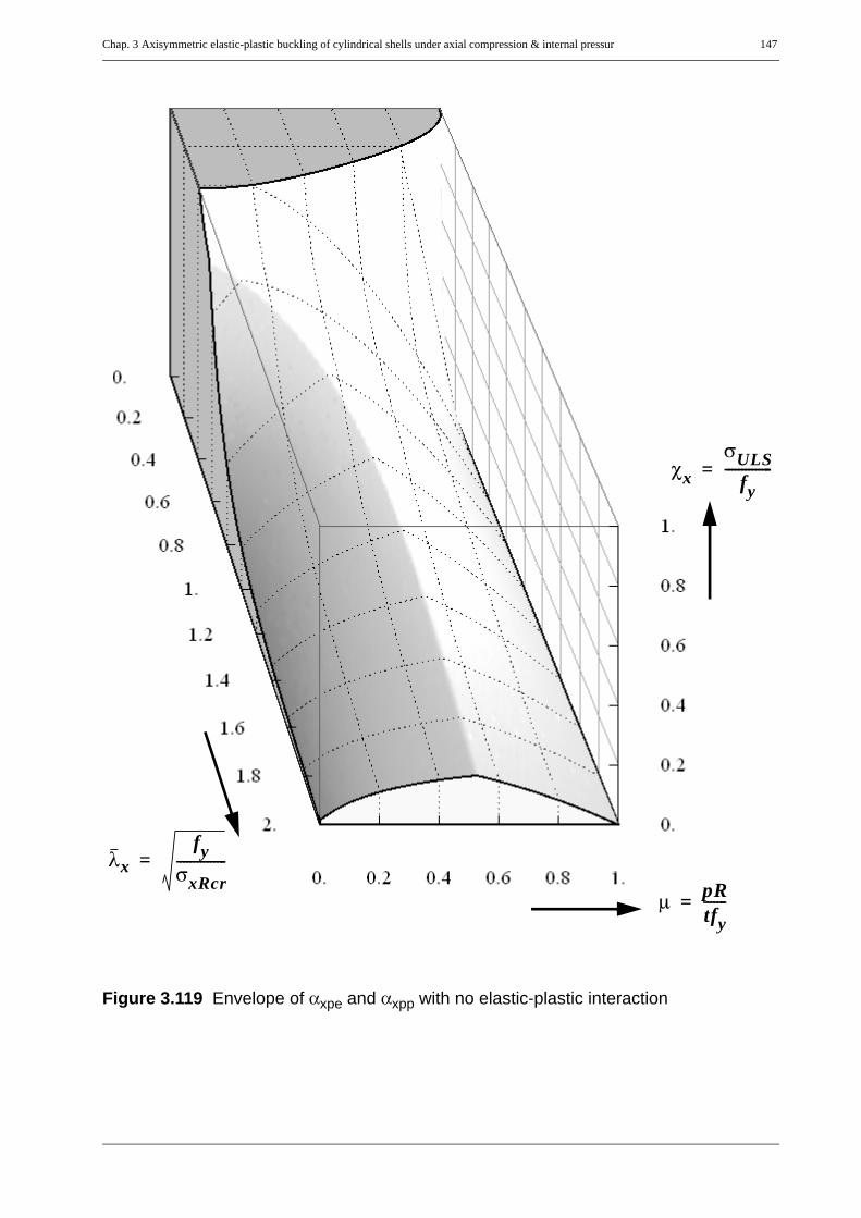
Chap. 3 Axisymmetric elastic-plastic buckling of cylindrical shells under axial compression & internal pressur 147
Figure 3.119 Envelope of αxpe and αxpp with no elastic-plastic interaction
μ pRtfy-------=
χxσULS
fy--------------=
λxfy
σxRcr---------------=

148 Chap. 3 Axisymmetric elastic-plastic buckling of cylindrical shells un-
Figure 3.120 Elastic-plastic interaction with uni-axial yield for class-A and bi-axial mem-brane Mises
Figure 3.121 Elastic-plastic interaction with uni-axial yield for class-A and Euler’s curve
μ 0.0 0.1 … 0.9, , ,=
0.8
Elastic imperfectμ increase
μ 0.0=
Euler (elastic perfect)

Chap. 3 Axisymmetric elastic-plastic buckling of cylindrical shells under axial compression & internal pressur 149
Figure 3.122 Elastic-plastic interaction of αxp = αxpe with uni-axial yield
μ pRtfy-------=
χxσULS
fy--------------=
λxfy
σxRcr---------------=

150 Chap. 3 Axisymmetric elastic-plastic buckling of cylindrical shells un-
Figure 3.123 Elastic-plastic interaction of αxp = αxpp with uni-axial yield
μ pRtfy-------=
χxσULS
fy--------------=
λxfy
σxRcr---------------=

Chap. 3 Axisymmetric elastic-plastic buckling of cylindrical shells under axial compression & internal pressur 151
Figure 3.124 Characteristic buckling strength according to EN 1993-1-6: pinned bottom
μ pRtfy-------=
χxσULS
fy--------------=
λxfy
σxRcr---------------=

152 Chap. 3 Axisymmetric elastic-plastic buckling of cylindrical shells un-
3.10.3 Summary of EN 1993-1-6 design regulationThe elastic-plastic buckling strength according to EN 1993-1-6 for buckling phenomenon in theshell interior where there exist no edge constriction effects is predicted using an interactionformula which considers uni-axial yield conditions. This procedure results in elastic-plasticbuckling strengths higher than the pure bi-axial plastic capacity of the shell, Figure 3.120 andFigure 3.122.
The geometrically and materially nonlinear (GMNL) buckling strength prediction of the perfectcylindrical shell using the pressurized imperfection reduction factor, αxpp, may predict strengthshigher than the bi-axial plastic capacity (MNL strength) of the shell. This situation is mainly seenin relatively thick cylindrical shells ( ) and hence the pressurized imperfection reductionfactor can not be applied to all shell slendernesses, Figure 3.111 and Figure 3.114.
In using the interaction expression to predict the characteristic elastic-plastic buckling strength ofa cylindrical shell, the imperfection reduction factor, αxp, is taken as the smaller of the pressurizedelastic, αxpe, and the pressurized plastic, αxpp, imperfection reduction factor values; and plasticinteraction is applied using the basic plastic interaction parameters λo, η, and β. This procedureresults in the same buckling strength as making a separate use of the pressurized elastic andpresurized plastic imperfection reduction factors in the interaction expression and taking thesmaller of the final results obtained. However, in cases of smaller αxpp values than αxpe, applyingthe interaction means that applying the effect plasticity for the second time since αxpp (obtainedfrom geometric and material nonlinear numerical analyses) itself includes such effect from thebeginning; a procedure which makes no logical sense.
Besides, when using the procedure, the resulting characteristic buckling strength may even behigher than not only the bi-axial plastic capacity of the cylindrical shell but also the already higherelephant’s foot strength values obtained using αxpp (see Figure 3.125 and Figure 3.127). A thirdplasticity condition should therefore be applied to garantee that no elastic-plastic buckling strengthexceeds the bi-axial plastic capacity of the shell.
Evenif a third separate plasticity condition (cut-off by membrane Mises yield condition, Figure3.128) is applied to it, the strength results are inconsistent with those computed numerically, exceptfor the relatively very thin cylindrical shells.
Moreover, this procedure produces an inconsistency in strength prediction at very low pressurelevel thereby producing a jump between a very small pressure level and a non-pressurized (Zeropressure level) cases. This effect is shown in Figure 3.126 and Figure 3.127.
The αxpp factor is not an imperfection reduction factor as it is used in EN1993-1-6 and has nothingto do with imperfections but instead a reduction factor, when referred to the classical elasticbuckling strength, accounts for material and geometric nonlinearities; or when referred to the pureplastic capacity of the shell, accounts for geometric nonlinearities.
R t⁄ 145≤
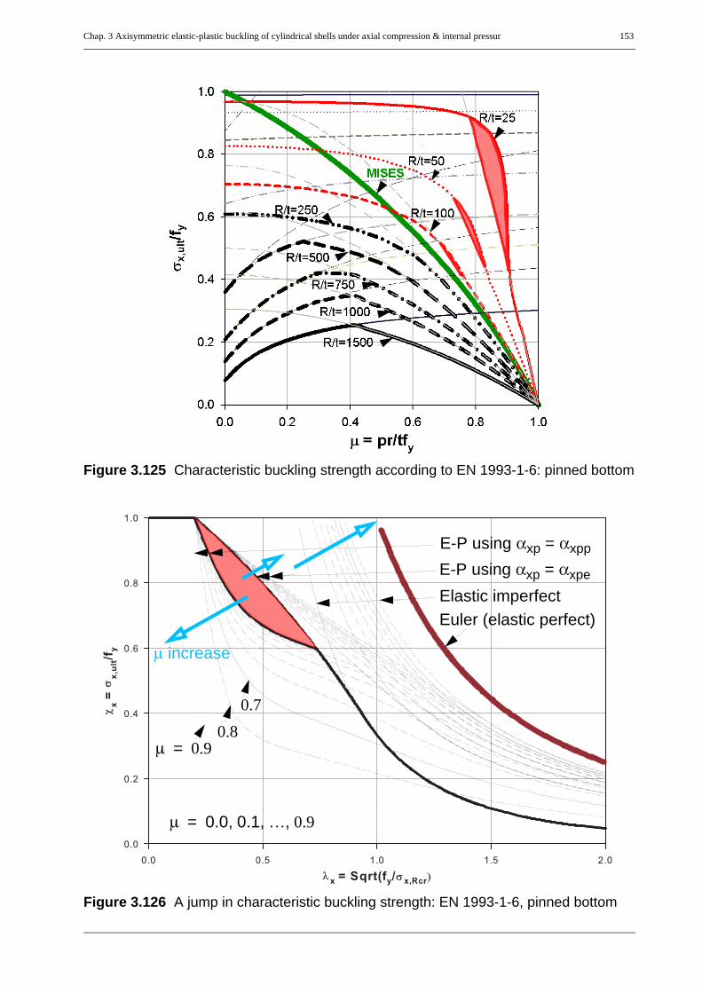
Chap. 3 Axisymmetric elastic-plastic buckling of cylindrical shells under axial compression & internal pressur 153
Figure 3.125 Characteristic buckling strength according to EN 1993-1-6: pinned bottom
Figure 3.126 A jump in characteristic buckling strength: EN 1993-1-6, pinned bottom
μ 0.0 0.1 … 0.9, , ,=
0.8μ 0.9=
0.7
Elastic imperfectE-P using αxp = αxpe
E-P using αxp = αxpp
Euler (elastic perfect)
μ increase

154 Chap. 3 Axisymmetric elastic-plastic buckling of cylindrical shells un-
Figure 3.127 Characteristic buckling strength according to EN 1993-1-6: pinned bottom
μ pRtfy-------=
χxσULS
fy--------------=
λxfy
σxRcr---------------=
due tointeraction
due tointeraction

Chap. 3 Axisymmetric elastic-plastic buckling of cylindrical shells under axial compression & internal pressur 155
Figure 3.128 Characteristic buckling strength according to EN1993-1-6 and bi-axial membrane Mises cut-off
μ pRtfy-------=
χxσULS
fy--------------=
λxfy
σxRcr---------------=
membrane Misescut-off

156 Chap. 3 Axisymmetric elastic-plastic buckling of cylindrical shells un-
3.10.4 Related previous study and resultsLeaving everything the same (except the plastic buckling parameters) as it was discussed in EN1993-1-6 buckling design recommendation, Rotter (2006a) presented a way to directly andprecisely extract the plastic buckling interaction parameters to be used in the buckling interactionexpression (instead of the constant values , , and ) from an interactionrepresentation (GMN(i)A/MNA versus GMN(i)A/LBA plot). Using his procedure, Rotterextracted the follwoing plastic buckling parameters:
(Eq. 3.95)
(Eq. 3.96)
(Eq. 3.97)
with
(Eq. 3.98)
The characteristic buckling strength of the cylindrical shell using these plastic interactionparameters and the procedure discussed in the EN1993-1-6 buckling design recommendation areshown in the pressure representation, Figure 3.129, and capacity representation, Figure 3.130.
The results obtained using this procedure, when compared to EN1993-1-6, results in somewhatlesser interaction between the elastic and plastic buckling which means higher buckling strengthfor medium internal pressure level. Besides, this procedure avoids the problem of getting anincreased buckling strength due to interaction. However, since the same αxpp strength factor, likein EN 1993-1-6, is on the foundation the problem of predicting higher strengths than the bi-axialplastic capacity of the shell and inconsistency with the nonlinear numerical analyis results remainunchanged.
λo 0.2= β 0.6= η 1.0=
λo 0=
β 0.25 αxpe 2αxpe2+( )=
η 1 k–( )ln β( )ln–1 β–( )ln
-----------------------------------------=
k1 αxpe 4⁄+
αxpe2
---------------------------⎝ ⎠⎜ ⎟⎛ ⎞
12αxpe
2
1 αxpe 4⁄+( )2----------------------------------+
⎝ ⎠⎜ ⎟⎛ ⎞ 1 2⁄
1–⋅=

Chap. 3 Axisymmetric elastic-plastic buckling of cylindrical shells under axial compression & internal pressur 157
Figure 3.129 Characteristic buckling strength according to Rotter (2006a): pinned
Figure 3.130 Characteristic buckling strength according to Rotter (2006a): pinned
R/t = 1500
1000
750
500
R/t = 250100
Mises
50 25
Elastic_imperfectPlastic_perfect
μ 0.0 0.1 … 0.9, , ,=
0.8
μ 0.9=
0.70.6
0.5
Elastic imperfectEuler (elastic perfect)Plastic perfect

158 Chap. 3 Axisymmetric elastic-plastic buckling of cylindrical shells un-
3.11Summary and conclusions
EN1993-1-6 buckling design recommendation:
• the overall procedure in predicting the characteristic buckling strength of cylindrical shellinvolves many steps
• the reduction factor αxpp, which really is a plastic buckling reduction factor, is being treatedas if it is an elastic reduction factor. Besides, it is referred to as an imperfection reductionfactor while it has nothing to do with imperfections.
• applies plasticity conditions twice, first in αxpp itself as it basically includes material andgeometric nonlinear effects and a second elastic-plastic buckling interaction of αxpp withthe uni-axial yield condition
• predicts elastic-plastic buckling strengths higher than the pure bi-axial plastic resistance ofthe cylinder
• needs additional separate plasticity check against bi-axial yielding
• even if separate plasticity condition is applied to it, the strength results are inconsistent withthose computed numerically
• inconsistency in buckling strength predictions at very low pressure level and zero-pressurelevel resulting in a jump of strength
• applies only for pinned bottom cases (with more safety for fixed cases?)
Buckling design recommendation of the current work:
• considers bi-axial plasticity from the very beginning
• strictly differentiates typical buckling failure modes: buckling in the free shell interior andbuckling adjacent to the boundary (elephant’s-foot buckling mode)
• it is easy to follow and apply; straight forward approach
• differentiates pinned and fixed bottom boundary condition cases

Chap. 4 Axisymmetric elastic-plastic buckling of liquid-filled conical shells (LFC) 159
4
Axisymmetric elastic-plastic buckling of liquid-filled conical shells (LFC)

160 Chap. 4 Axisymmetric elastic-plastic buckling of liquid-filled conical
4.1 Introduction
The axisymmetric elastic-plastic (elephant’s-foot) buckling phenomenon and strength of axiallyring-compressed and internally uniformly pressurized thin-walled cylindrical shells have alreadybeen investigated in detail. The elephant’s-foot type buckling phenomenon, however, is not onlyrestricted to uniformly (meridionally and internally) loaded cylinders but to general cylindrical andconical shells so long as they are subjected to meridional compression and circumferential tensionnear the boundary. More specifically, axisymmetric elastic-plastic buckling near a boundary mayhappen in thin-walled cylindrical and conical shells with constant/varying meridional compressionand hydrostatic internal pressure. Since a liquid-filled conical shell falls into such a loadingcategory, an axisymmetric elastic-plastic buckling near the boundary is possible and hence thebuckling strength of conical shells associated to an elephant’s-foot buckling phenomenon needs tobe investigated in detail.
Unlike that of a uniformly loaded cylindrical shell which results in uniform meridional andcircumferential membrane section force ditributions, the meridional membrane section forcedistribution in the liquid-filled conical shell is maximum at the lower supported edge and decreasesnonlinearly and rapidly up the meridian. Such a distribution of the meridional compressive sectionforce superimposed with the edge constriction effects of the bottom boundary conditions willrestrict the elastic-plastic buckling phenomenon to a region very close to the supported lower edgecausing elephant’s-foot type buckling.
This study is concerned with thin-walled metal liquid-filled conical shell structures with pinned orfixed bottom boundary conditions, Figure 4.1. In the course of investigating the elastic-plasticbuckling strength, liquid-filled conical shells will be analysed using membrane theory, linear shellbending theory (LA), linear bifurcation analysis (LBA), small displacement materially nonlinearanalysis (MNA), perfect geometrically and materially nonlinear analysis (GMNA), andgeometrically and materially nonlinear analysis with imperfections (GMNIA). A combination ofboth analytical and numerical (using finite element program) analysis methods will be useddepending on the nature and complexity of the problem type in consideration. In all the analyses,no hardening of any kind (material or geometric) is considered. The buckling failure criteria willbe interpreted, more generally, relative to each analysis result but mainly, in-line with theunderlying structure of the European standard EN1993-1.6, relative to the two reference strengths:small displacement linear bifurcation analysis (LBA) and small displacement materially nonlinearanalysis (MNA).

Chap. 4 Axisymmetric elastic-plastic buckling of liquid-filled conical shells (LFC) 161
Figure 4.1 Geometry, loading, and boundary conditions
β
γ'
h
r1
h’U.tanβ
h’Ut
x --> Meridional directionθ --> Circumferential directionr2’
r2
PIN FIX
1γ'.h’
γ'.(h’-z)z
base level ’1’(reference level)
ultimate (critical)water level above ’1’

162 Chap. 4 Axisymmetric elastic-plastic buckling of liquid-filled conical
4.2 Problem statement
Despite the fact that there have been conical steel water tower collapse cases, of which the realcauses are not surely known yet, not much has been done to investigate the possible elephant’s-foot buckling strength of conical shells. Such type of buckling may happen in liquid-filled conicalshells, specially when there exist a global bending effect which may result, say, from geometriceccentricity (global tilting) of the cone. This geometric eccentricity, even upon filling may resultin global bending effect which shortens the life span of the structure with the formation of apossible elephant’s-foot type buckling phenomenon. Apart from this, a perfect liquid-filled conicalshell may buckle in such an axisymmetric elastic-plastic buckling mode near the supported edgeso long as a bi-axial state of stress, similar to that of the cylindrical shell, exists.
This work, therefore, addresses the axisymmetric elastic-plastic buckling strength of isotropicunstiffened liquid-filled conical shells using numerical parametric simulations, with the ultimategoal of deriving a set of basic data that can be used in a straight forward buckling design approachby hand calculations.
Once again, the study was done computationally using ABAQUS and using the 3-node general-purpose axisymmetric shell element with axisymmetric deformation, SAX2. Linear and nonlinearnumerical analyses were made for different shell slenderness (r1/t) values which span from 100 to1500 and an apex-half angle β = 45°, representing the practical range of conical shells in civilengineering constructions. The lengths of the cones are taken in such a way that no boundary-effectinteractions are possible between the top and bottom boundary conditions. The material consideredthroughout the study is mild steel with an ideal elastic-plastic von Mises yield criterion and a yieldstress fy = 240 MPa, elastic modulus E = 210 GPa, and Poisson’s ratio ν = 0.3. The results are allexpressed interms of non-dimensional variables and hence can be used to address other practicalsets of conditions. In many of the upcoming discussions, a conical shell with the following set ofconditions will be used for illustration purposes.
Geometry: r1/t = 500 cm and t = 1.0 cm
Boundary conditions: pinned or fixed bottom and rotational restaraint at top
Loading: liquid-filling with specific weight γ’
Material properties: E = 21000 kN/cm2; ν = 0.3; fy = 24.0 kN/cm2

Chap. 4 Axisymmetric elastic-plastic buckling of liquid-filled conical shells (LFC) 163
4.3 Linear shell analysis (LA)
4.3.1 Pure membrane behaviorGenerally speaking, for axisymmetric shells with axisymmetric loading and boundary conditions, thecross-sectional stress state of a shell segment is primarily governed by pure membrane action due tothe continuously distributed loads which the shell is subjected to.
The pure membrane behavior of a liquid-filled conical shell can easily be computed and is given,interms of the deformations and section forces, as
. . . membrane section forces (Eq. 4.1)
. . . . membrane deformations (Eq. 4.2)
Nxγ'h'r
βcos------------ 1
r1 r–βtan
-------------+⎝ ⎠⎛ ⎞ 1
6---
r1r----⎝ ⎠⎛ ⎞
2 rr1---- 1– h' βtan
r1----------------–⎝ ⎠
⎛ ⎞ 2 rr1---- 1 h' βtan
r1----------------+ +⎝ ⎠
⎛ ⎞⋅ ⋅ ⋅ ⋅=
Nθγ'h'r
βcos------------ 1
r1 r–βtan
-------------+⎝ ⎠⎛ ⎞⋅=
w∗ γ'r3
6Et βsin-------------------- 2 ν 3–( ) 3 ν 2–( )
r1r----– 1 h' βtan
r1----------------+⎝ ⎠
⎛ ⎞ νr1r----⎝ ⎠⎛ ⎞
31 h' βtan
r1----------------+⎝ ⎠
⎛ ⎞ 3+⋅⋅=
βxγ'r2
6Et βcos--------------------- 16 9
r1r----– 1 h' βtan
r1----------------+⎝ ⎠
⎛ ⎞ r1r----⎝ ⎠⎛ ⎞
3– 1 h' βtan
r1----------------+⎝ ⎠
⎛ ⎞ 3⋅⋅=

164 Chap. 4 Axisymmetric elastic-plastic buckling of liquid-filled conical
Figure 4.2 Ring model analogy, loading and geometry
h’
r1
γ
β
Leff
t
h’
r1
γ
R20
Leff*cosβ
Aeff/2
Aeff/2
Leff
h’
r1
γ
β
r1β
R20
X
βφ
w*r
X0
X1
γ h’

Chap. 4 Axisymmetric elastic-plastic buckling of liquid-filled conical shells (LFC) 165
4.3.2 Edge-bending effects The stiffness of the equivalent ring model of the conical shell for edge bending effects, Linder(2001), is given by:
(Eq. 4.3)
for edge displacement disturbances w*A and βx,A at the bottom edge ”A” of the cone, therestraining edge forces can be computed using the stiffness of the equivalent ring model as
(Eq. 4.4)
For a liquid-filled conical shell, the total deformation and section forces (edge bending effectsincluded) according to the effective-ring analogy model are generally computed as given below.The actual distributions along the meridian of the cone will depend on the type of bottom boundarycondition considered.
Deformations:
(Eq. 4.5)
Section forces:
(Eq. 4.6)
(Eq. 4.7)
(Eq. 4.8)
KEAeff
2r12
------------2 Leff βcos⋅–
Leff β cos⋅– Leff βcos⋅( )2⋅=
RH A,
RM A,
K– wA∗
βx A,
⋅EAeff
2r12
------------–2 Leff βcos⋅–
Leff β cos⋅– Leff βcos⋅( )2wA∗
βx A,
⋅ ⋅= =
w∗βx
f1 f2+( ) Leff βcos( ) f1⋅–2f1
Leff βcos( )-------------------------- f2 f1–( )
wA∗
βx A,
wA∗
βx A, part
–⎝ ⎠⎜ ⎟⎜ ⎟⎛ ⎞
⋅ w∗βx part
+=
Qx f2 f1–( ) βcos 2f1Leff--------
RH A,
RM A,
⋅=
Nx Qx– βtan⋅ Nx part,+=
NθEtr1----- f1 f2+( ) Leff βcos( ) f1⋅–
wA∗
βx A,
wA∗
βx A, part
–⎝ ⎠⎜ ⎟⎜ ⎟⎛ ⎞
⋅ ⋅ Nθ part,+=

166 Chap. 4 Axisymmetric elastic-plastic buckling of liquid-filled conical
(Eq. 4.9)
(Eq. 4.10)
The section moments are assumed positive when outer side of the shell is under compression.
For the conical shell of this study, pinned- or fixed-bottom boundary conditions are consideredwhere the distributions of the deformations and section forces under the action of liquid-loadingcan easily be computed.
Where
(Eq. 4.11)
For illustration purposes, consider a conical shell with the following geometry, material, loading,and boundary conditions:
Geometry: r1 = 500 cm; t = 1.0 cm; β = 45°; h’/r1 = 3.0
Boundary conditions: pinned- and fixed-bottom
Loading: liquid filling γ’ = 5.64669 .10-6 kN/cm3
Material properties: E = 21000 kN/cm2; ν = 0.3; fy = 24 kN/cm2
The liquid density is chosen in such a way that the meridional membrane compressive stress at thecone-base is equal to the classical elastic critical buckling stress of the cone. The deformations andsection force results obtained from the linear shell analysis using the ring model analogy discussedabove would then be as shown on the plots in Figure 4.3 to Figure 4.8. The normal section forceand bending moments shown in these plots are normalized with respect to the corresponding un-axial yield section force, Npl = t.fy, and section moment, Mpl = t2.fy/4. The circumferential bendingmoment Mθ distribution along the meridian is not plotted as it is the product of the poison’s ratioν and the meridional bending moment Mx.
4.3.3 Numerical finite element linear analysis (LA)Numerical finite element small displacement linear analyses of liquid-filled conical shells were
made for verification purposes. The deformation and section force results obtained from
ABAQUS finite element linear analysis are exactly the same as those obtained using the effective-
ring-model analogy, Figure 4.3 to Figure 4.8.
Mx Leff βcos( ) f1⋅ f1 f2+( )–RH A,
RM A,
⋅=
Mθ ν M⋅ x=
Leff 0.778r1 t⋅
βcos------------=
Aeff Leff t⋅=

Chap. 4 Axisymmetric elastic-plastic buckling of liquid-filled conical shells (LFC) 167
Figure 4.3 Radial deformation
Figure 4.4 Meridional rotation
FIX
PIN
FIX
PIN

168 Chap. 4 Axisymmetric elastic-plastic buckling of liquid-filled conical
Figure 4.5 Meridional section force
Figure 4.6 Circumferential section force
FIXPIN
FIX
PIN

Chap. 4 Axisymmetric elastic-plastic buckling of liquid-filled conical shells (LFC) 169
Figure 4.7 Transverse shear force
Figure 4.8 Meridional section moment
FIX
PIN
FIX
PIN
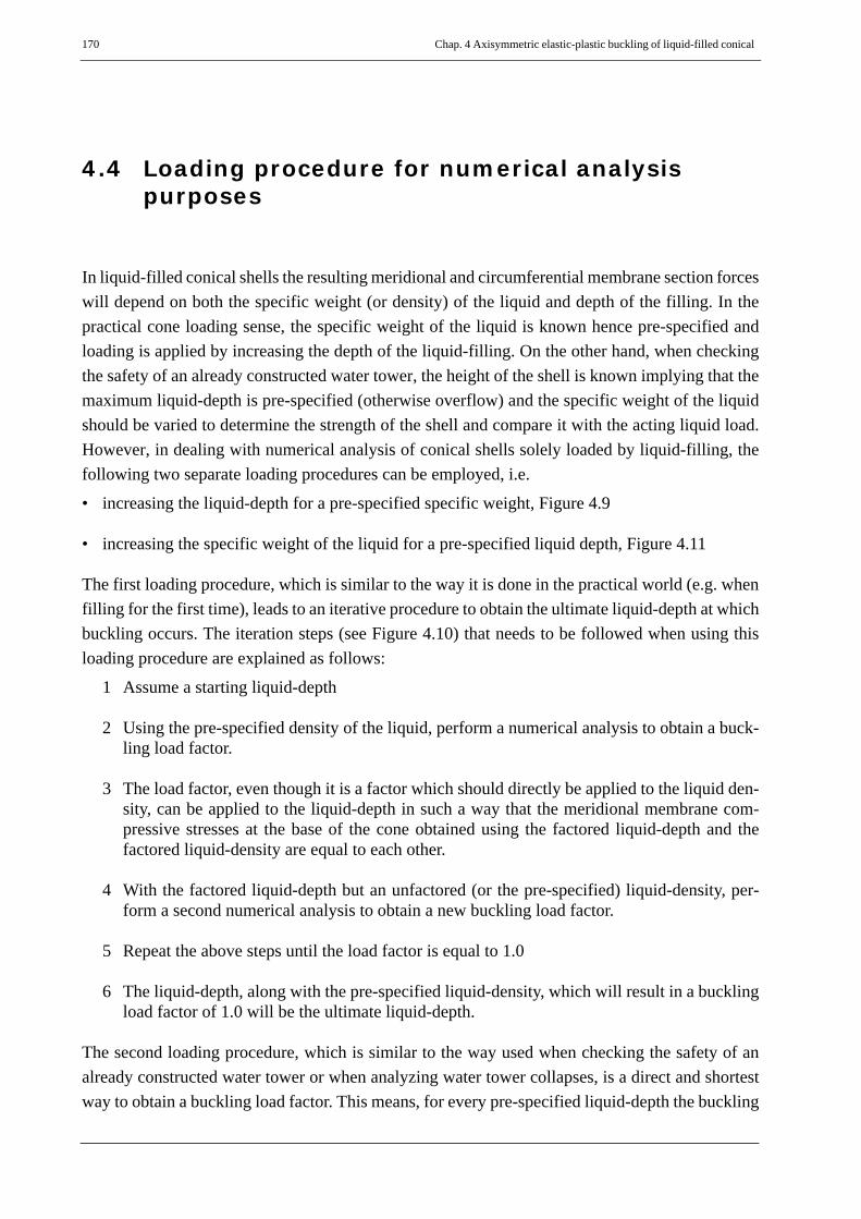
170 Chap. 4 Axisymmetric elastic-plastic buckling of liquid-filled conical
4.4 Loading procedure for numerical analysispurposes
In liquid-filled conical shells the resulting meridional and circumferential membrane section forceswill depend on both the specific weight (or density) of the liquid and depth of the filling. In thepractical cone loading sense, the specific weight of the liquid is known hence pre-specified andloading is applied by increasing the depth of the liquid-filling. On the other hand, when checkingthe safety of an already constructed water tower, the height of the shell is known implying that themaximum liquid-depth is pre-specified (otherwise overflow) and the specific weight of the liquidshould be varied to determine the strength of the shell and compare it with the acting liquid load.However, in dealing with numerical analysis of conical shells solely loaded by liquid-filling, thefollowing two separate loading procedures can be employed, i.e.
• increasing the liquid-depth for a pre-specified specific weight, Figure 4.9
• increasing the specific weight of the liquid for a pre-specified liquid depth, Figure 4.11
The first loading procedure, which is similar to the way it is done in the practical world (e.g. whenfilling for the first time), leads to an iterative procedure to obtain the ultimate liquid-depth at whichbuckling occurs. The iteration steps (see Figure 4.10) that needs to be followed when using thisloading procedure are explained as follows:
1 Assume a starting liquid-depth
2 Using the pre-specified density of the liquid, perform a numerical analysis to obtain a buck-ling load factor.
3 The load factor, even though it is a factor which should directly be applied to the liquid den-sity, can be applied to the liquid-depth in such a way that the meridional membrane com-pressive stresses at the base of the cone obtained using the factored liquid-depth and thefactored liquid-density are equal to each other.
4 With the factored liquid-depth but an unfactored (or the pre-specified) liquid-density, per-form a second numerical analysis to obtain a new buckling load factor.
5 Repeat the above steps until the load factor is equal to 1.0
6 The liquid-depth, along with the pre-specified liquid-density, which will result in a bucklingload factor of 1.0 will be the ultimate liquid-depth.
The second loading procedure, which is similar to the way used when checking the safety of analready constructed water tower or when analyzing water tower collapses, is a direct and shortestway to obtain a buckling load factor. This means, for every pre-specified liquid-depth the buckling

Chap. 4 Axisymmetric elastic-plastic buckling of liquid-filled conical shells (LFC) 171
load factor which should only be applied to the liquid-density is computed. Hence, only the firsttwo steps of the first loading procedure are used here. In the general invetigation of bucklingstrengths of liquid-filled conical shells, these two steps are repeatedly used for different pre-spec-ified liquid-depths.
Comparing the two separate loading procedures, the first procedure is limited to a specific liquid-filled cone situation and the important buckling parameter is the ultimate liquid-depth hence theintermediate iterative results are not needed. Whereas the second procedure can be applied forgeneral cases specially when extraction of useful data for general buckling design purposes isrequired. The second method, in other words, when performed repeatedly by varying the liquid-depth is similar to the first procedure without dropping the load factors at each iteration step.
On the other hand, the first method, when used in numerical studies, needs separate iterations foreach analysis type (e.g. LBA, MNA, GMNA, GMNIA etc.) making it a very expensive methodinterms computational costs. The second method is useful in numerical studies because eachanaylsis type is performed with no iterations for a pre-specified liquid-depth (or ψ) and hence adirect comparison can be made for a given ψ value. Since the main purpose of this study is toextract useful data for general buckling purposes, the second loading procedure will be usedthroughout the study.

172 Chap. 4 Axisymmetric elastic-plastic buckling of liquid-filled conical
Figure 4.9 Loading by increasing liquid-depth for a pre-specified liquid-density
1
ψ
σθ
σx
small ψ
big ψ
r11
r11
1
ψ = 3.0
ψ = 1.5
ψ = 0.5Nθ
Nx
NθNx
NθNx
Ultimate liquid-filling load levelparameters, using membrane theory
ζ'Uh'U βtan
r1-------------------=
ψσx U 1, ,σθ U 1, ,----------------
ζ'U6
-------= 3 ζ'U+( )⋅=
αxpeσx U 1, ,σx Rcr,---------------=
pσθ U 1, ,σx Rcr,----------------=
ψαxpe
p----------=
LOADINCREASE

Chap. 4 Axisymmetric elastic-plastic buckling of liquid-filled conical shells (LFC) 173
Figure 4.10 Iterative computation of critical buckling liquid-depth for a pre-specified liq-uid density
step-1
step-3
step-4
step-2
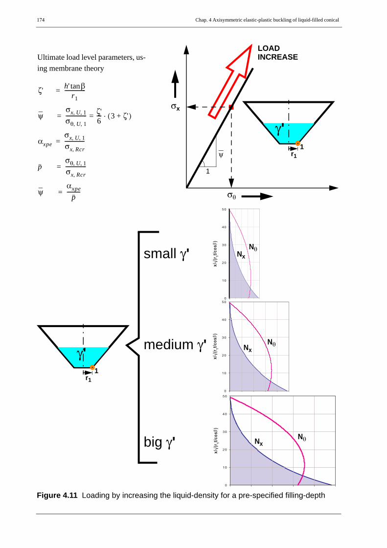
174 Chap. 4 Axisymmetric elastic-plastic buckling of liquid-filled conical
Figure 4.11 Loading by increasing the liquid-density for a pre-specified filling-depth
1
ψ
σθ
σx
big γ'
medium γ'
small γ'
NθNx
LOADINCREASEUltimate load level parameters, us-
ing membrane theory
ζ' h' βtanr1
----------------=
ψσx U 1, ,σθ U 1, ,---------------- ζ'
6----= 3 ζ'+( )⋅=
αxpeσx U 1, ,σx Rcr,---------------=
pσθ U 1, ,σx Rcr,----------------=
ψαxpe
p----------=
r11
r11
NθNx
NθNx
γ'
γ'

Chap. 4 Axisymmetric elastic-plastic buckling of liquid-filled conical shells (LFC) 175
4.5 Linear buckling strength of an ideally perfectliquid-filled cone
4.5.1 Approximate linear buckling analysisIn the LBA sense, a conical shell subjected to axial loading (no matter where the axial loading andrelated section forces come from) buckles at a section located a meridional distance “x” from thesupported base, when the membrane meridional section stress σx(x) due to the applied axialloading reaches the critical value, σxCr(x), which is given by
. . . from theory! (Eq. 4.12)
For steel conical shells, where the poisson’s ratio ν = 0.3, the critical buckling stress is given by
(Εθ. 4.13)
The critical buckling stress at the base of the cone will then be
(Εθ. 4.14)
In bottom-supported conical shells, even though the stress at the supported base reaches itsbuckling limiting value, buckling will not take place at the base. Instead, it occurs at a smalldistance away from the base (along the meridian). This is because of the two facts that (i) it isrestrained & hence stiffer and (ii) there is no enough space for buckling to occur.
Buckling practically occurs when the stress at the location for potential “center of buckle” reachesthe critical stress for that particular section. In other words, the meridional membrane compressivestress distribution with a critical stress at the base and fast decaying up the meridian, should beincreased by a load factor higher than 1.0 so that the stress at the center of potential buckle reachesits limiting value thereby producing buckling.
Mathematically, for buckling to occur at the potential center of buckle, the respective stress shouldbe equal to
(Eq. 4.15)
σxCr x( ) E
3 1 ν2–( )--------------------------- 1
r x( ) t βcos( )⁄---------------------------------⋅=
σxCr x( ) 0.605 E t βcos⋅r x( )
----------------------⋅=
σxRCr σ= xCr x 0=( ) 0.605 E t βcos⋅r1
----------------------⋅=
σx b, σxCr b, 0.605 E t βcos⋅rb
----------------------⋅= =

176 Chap. 4 Axisymmetric elastic-plastic buckling of liquid-filled conical
Besides, the ratio of the meridional membrane stress at any location along the meridian to thecircumferential membrane stress at the base of the cone is given by
(Eq. 4.16)
whic can be re-worked to obtain a relationship between the acting meridional membrane stress atany location along the meridian and the corresponding critical meridional membrane stress of thecone at the same location as follows
(Eq. 4.17)
(Eq. 4.18)
The previous statement about the occurrence of buckling can now be mathematically explained,using (Eq. 4.18), as
(Eq. 4.19)
On the other hand, the ratio of the meridional membrane compressive stress at any location alongthe meridian to the meridional membrane compressive stress at the base of the cone is given by
(Eq. 4.20)
At the buckling load level, (Eq. 4.20) will be written as
(Eq. 4.21)
where is the corresponding meridional membrane stress at the base of the cone when thestress at the potential buckle center reaches its critical value.
The buckling load factor, , when written in terms of the membrane stressesat the cone base will then be given by
σx x( )σθ 1,
------------- 16--- ρ' ρ–( )2
ρ' 1–--------------------- 3 ρ' ρ–
ρ-------------+⎝ ⎠
⎛ ⎞⋅ ⋅=
σx x( )σθ 1,
-------------σx x( ) σxCr x( )⁄σθ 1,
σxRCr--------------
σxRCrσxCr x( )-------------------⋅
--------------------------------------σx x( ) σxCr x( )⁄
p ρ⋅------------------------------------= =
σx x( )σxCr x( )-------------------⇒ 1
6---p ρ' ρ–( )2
ρ' 1–--------------------- ρ' 2ρ+( )⋅ ⋅=
σx x( )σxCr x( )------------------- 1=
p⇒ 6ρ' 2ρ+( )
---------------------- ρ' 1–ρ' ρ–( )2
---------------------⋅=
σx x( )σx 1,
------------- ρ' ρ–ρ' 1–-------------⎝ ⎠⎛ ⎞ 2 ρ' 2ρ+
ρ ρ' 2+( )----------------------⋅=
σx U, x( )σx 1 U, ,
-------------------σxCr x( )σx 1 LBA, ,--------------------- ρ' ρ–
ρ' 1–-------------⎝ ⎠⎛ ⎞ 2 ρ' 2ρ+
ρ ρ' 2+( )----------------------⋅= =
σx 1 LBA, ,
αLBA σ= xCr x( ) σx x( )⁄

Chap. 4 Axisymmetric elastic-plastic buckling of liquid-filled conical shells (LFC) 177
(Eq. 4.22)
(Eq. 4.23)
using (Eq. 4.19), (Eq. 4.23) can be re-written as
(Eq. 4.24)
Since for liquid-filled conical shells, where the meridional membrane compressive stress decaysrapidly up the meridian, buckling occurs somewhere close to the base of the cone and hence forrelatively longer conical shells the value of the running parameter ρ is very close to 1.0. For sucha situation, (Eq. 4.24) can be approximately re-written (applying linearization) as
(Eq. 4.25)
Let the length of buckle be lb which, generally, is given as a function of the shell slenderness ratioby
(Eq. 4.26)
the buckle center is then located at lb/2 and the corresponding ρ = ρb is given by
(Eq. 4.27)
Letting and ,
(Eq. 4.28)
Substituting (Eq. 4.28) into (Eq. 4.25), one gets
(Eq. 4.29)
For an axisymmetric buckling type, the buckle length factor . This axisymmetricbuckle starts at the base of the cone for simply supported (pinned-) bottom boundary condition andhas a shift of for a fixed bottom boundary condition. As a result, theapproximate LBA buckling load for “FIX” and “PIN” bottom support types is given by
αLBAσx 1 LBA, ,
σxRCr---------------------
σxCr x( )σxRCr
------------------- ρ' 1–ρ' ρ–-------------⎝ ⎠⎛ ⎞ 2 ρ ρ' 2+( )
ρ' 2ρ+----------------------⋅ ⋅= =
α⇒ LBAρ' 1–ρ' ρ–-------------⎝ ⎠⎛ ⎞ 2 ρ' 2+( )
ρ' 2ρ+------------------⋅=
αLBA 1 3ρ' ρ2 1–( ) 2 ρ3 1–( )–6 ρ' 1–( )
-------------------------------------------------------- p⋅+=
αLBA 1 ρ 1–( ) p⋅+=
lb kr1t
βcos------------⋅=
ρbrbr1---- 1
lb2r1-------- βsin+= = 1 k
2---+ βtan
r1 t βcos( )⁄--------------------------------=
b k 2⁄= εbβtan
r1 t βcos( )⁄--------------------------------=
ρb 1– bεb=
αLBA 1 bεb p⋅+=
k 1.72 2.0≈ ≈
1.0 r1t βcos⁄≈

178 Chap. 4 Axisymmetric elastic-plastic buckling of liquid-filled conical
(Eq. 4.30)
with
αLBA approx,σLBA approx,
σRcr-------------------------------- 1.0 b βtan
r1t βcos--------------
------------------ p⋅
⎝ ⎠⎜ ⎟⎜ ⎟⎜ ⎟⎛ ⎞
+= =
b2.0……FIX1.0……PIN⎩
⎨⎧
=

Chap. 4 Axisymmetric elastic-plastic buckling of liquid-filled conical shells (LFC) 179
Figure 4.12 Approximate buckle center
lb/2r1
Lrb
rb/cosβ
lb

180 Chap. 4 Axisymmetric elastic-plastic buckling of liquid-filled conical
Figure 4.13 Meridional membrane section force distribution & approximate buckling load
Nx,RcrNx,1,U
Nxβ
γ'
r1
h’.tanβ
r2’r2
Nx,TIP
1
z’b
rb
γ'.h’
h’
xb Nx(xb)
Nxcr(xb)
Nxcr(x=0) = NxRcr
Center of potential buckle
Meridional membrane sec-tion force distribution
Elastic critical meridional mem-brane section force distribution
(b)
(a)

Chap. 4 Axisymmetric elastic-plastic buckling of liquid-filled conical shells (LFC) 181
Figure 4.14 Normalized meridional membrane section force distribution

182 Chap. 4 Axisymmetric elastic-plastic buckling of liquid-filled conical
4.5.2 Linear buckling analysis using numerical finite element methodLinear finite element buckling analyses were made using ABAQUS for different shell slendernessratios, ranging from r1/tcosβ = 140 to 2100 (or r1/t = 100 to 1500 for an apex-half angle of 45°),and varying the liquid depth which in other words means varying the internal pressure parameter,p value.
Basic buckle mode shapes of liquid-filled conical shells with h’tanβ/r1 values of 0.5, 1.0, and 3.0are shown in Figure 4.15 and Figure 4.16 for both the “fixed” and “pinned” bottom boundaryconditions, respectively. In doing so, the lengths of the cones were kept constant so that an easyqualitative comparison can be made from the eigenmodes. Moreover, a fourth plot showing thebuckle mode shape of a meridional “tip” loaded conical shell case is included in each of theaforementioned figures. The effects of the meridional “tip” loading case, when compared at thepotential critical location (cone bottom zone), is equivalent to the effects of a very big liquid-depth(h’tanβ/r1 value).
Comparison of the radial deviations from the unbuckled perfect shape of the shell has been donefor the different h’tanβ/r1 values already mentioned and for a unit normalized maximum referenceamplitude along the meridian. These comparisons, in the lower critical part of the cone, are shownin Figure 4.17 and Figure 4.18 for both bottom boundary condition types with positive valuesshowing outward deviations, away from the axis of revolution.
Curve-fitting of the numerical analysis results from αLBA vs. p plot, see Figure 4.19 and Figure4.20, were then done for both “fixed” and “pinned” bottom boundary conditions, respectively. Theresulting linear buckling loads can then be calculated from
with (Eq. 4.31)αLBAσLBAσRcr------------- 1.0 a βtan
r1t βcos--------------
------------------ p⋅
⎝ ⎠⎜ ⎟⎜ ⎟⎜ ⎟⎛ ⎞ 0.6
+= = a1.55……FIX0.76……PIN⎩
⎨⎧
=

Chap. 4 Axisymmetric elastic-plastic buckling of liquid-filled conical shells (LFC) 183
Figure 4.15 Linear buckling eigenmodes: h’tanβ/r1 = 0.5, 1.0, 3.0, tip: fixed bottom
Figure 4.16 Linear buckling eigenmodes: h’tanβ/r1 = 0.5, 1.0, 3.0, tip; pinned bottom
Viewport: 1 ODB: c:/Documents and Settings...00_h’r1−0.5_45deg_FIX.odb Viewport: 2 ODB: c:/Documents and Settings...00_h’r1−1.0_45deg_FIX.odb
Viewport: 3 ODB: c:/Documents and Settings...00_h’r1−3.0_45deg_FIX.odb Viewport: 4 ODB: c:/Documents and Settings...’r1−3.0_45deg_FIX_TIP.odb
Viewport: 1 ODB: c:/Documents and Settings...00_h’r1−0.5_45deg_PIN.odb Viewport: 2 ODB: c:/Documents and Settings...00_h’r1−1.0_45deg_PIN.odb
Viewport: 3 ODB: c:/Documents and Settings...00_h’r1−3.0_45deg_PIN.odb Viewport: 4 ODB: c:/Documents and Settings...’r1−3.0_45deg_PIN_TIP.odb

184 Chap. 4 Axisymmetric elastic-plastic buckling of liquid-filled conical
Figure 4.17 Eigenmode amplitude in the critical zone: fixed bottom
Figure 4.18 Eigenmode amplitude in the critical zone: pinned bottom

Chap. 4 Axisymmetric elastic-plastic buckling of liquid-filled conical shells (LFC) 185
Figure 4.19 FEM LBA: fixed bottom
Figure 4.20 FEM LBA: pinned bottom
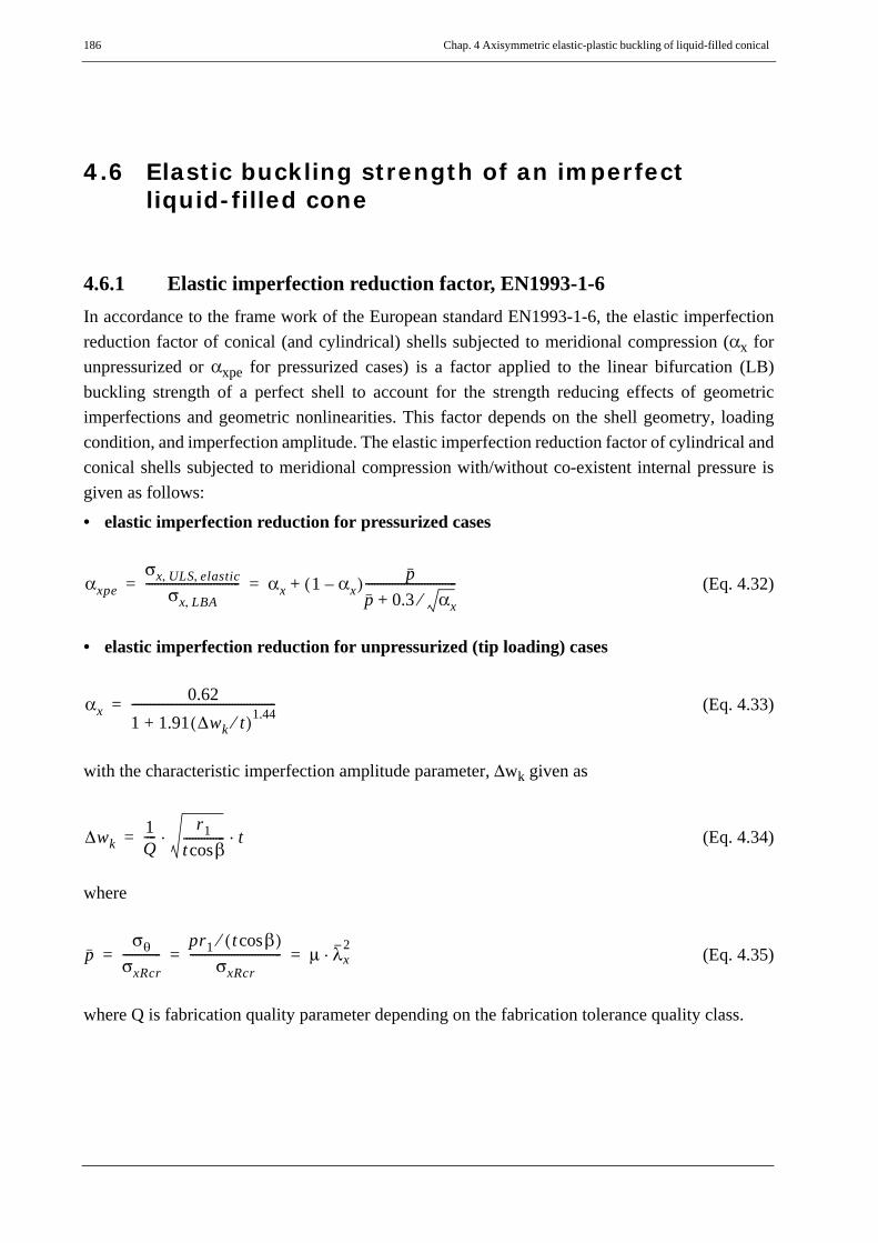
186 Chap. 4 Axisymmetric elastic-plastic buckling of liquid-filled conical
4.6 Elastic buckling strength of an imperfectliquid-filled cone
4.6.1 Elastic imperfection reduction factor, EN1993-1-6In accordance to the frame work of the European standard EN1993-1-6, the elastic imperfectionreduction factor of conical (and cylindrical) shells subjected to meridional compression (αx forunpressurized or αxpe for pressurized cases) is a factor applied to the linear bifurcation (LB)buckling strength of a perfect shell to account for the strength reducing effects of geometricimperfections and geometric nonlinearities. This factor depends on the shell geometry, loadingcondition, and imperfection amplitude. The elastic imperfection reduction factor of cylindrical andconical shells subjected to meridional compression with/without co-existent internal pressure isgiven as follows:
• elastic imperfection reduction for pressurized cases
(Eq. 4.32)
• elastic imperfection reduction for unpressurized (tip loading) cases
(Eq. 4.33)
with the characteristic imperfection amplitude parameter, Δwk given as
(Eq. 4.34)
where
(Eq. 4.35)
where Q is fabrication quality parameter depending on the fabrication tolerance quality class.
αxpeσx ULS elastic,,
σx LBA,-------------------------------- αx 1 αx–( ) p
p 0.3 αx⁄+-------------------------------+= =
αx0.62
1 1.91 Δwk t⁄( )1.44+-------------------------------------------------=
Δwk1Q----
r1t βcos-------------- t⋅ ⋅=
pσθ
σxRcr-------------
pr1 t βcos( )⁄σxRcr
------------------------------- μ λx2⋅= = =

Chap. 4 Axisymmetric elastic-plastic buckling of liquid-filled conical shells (LFC) 187
4.6.2 Elastic buckling strengthFor relatively big shell slenderness ratio values (thin shells) and low internal pressurization (veryhigh liquid depths), pure elastic buckling behaviour governs the failure phenomena causingdiamond-shaped buckling mode close to the boundary because of the relatively big meridionalcompressive stress at this zone and its fast decaying distribution. As the internal pressure increasesand the corresponding circumferential membrane stress becomes significant, the effect of bi-axiality comes into play and an interaction between the elastic buckling and plasticity begins. Inliquid-filled conical shells with a pre-specified liquid-density, the circumferential tension becomesrelatively big (when compared to the meridional compression) as the liquid-depth gets smaller.
For the case of an axially uniformly compressed and internally pressurized cylindrical shell, thelinear bifurcation load of the perfect shell is independent of internal pressurization and is equal tothe classical critical buckling load and therefore the elastic characteristic buckling strength iscomputed from:
(Eq. 4.36)
(Eq. 4.37)
However, for a liquid-filled conical shell, the fast decaying meridional compression (whencompared to the tip-loaded cone stress, which itself is decaying as well) is interlinked with theinternal pressurization, i.e. at the region where buckling occurs, the acting meridional compressionis lower than the corresponding classical critical buckling load and hence needs a load factor higherthan 1.0 to bring it to the buckled state. The value of the linear buckling load factor, therefore,depends on the liquid-depth and hence the internal pressurization. For conical shells the linearbifurcation load is equal to the classical critical buckling load only for tip-loaded cases becauseunder this load every point on the meridian of the shell is loaded to its critical value. Therefore, theelastic characteristic buckling strength of a liquid-filled conical shell is computed from:
(Eq. 4.38)
(Eq. 4.39)
In other words, when dealing with liquid-filled conical shells, the following relationships shouldbe kept in mind so as to easily differentiate between elastic buckling strength of conical andcylindrical shells:
αxpe CYL,σx ULS elastic,,
σx LBA,--------------------------------
σx ULS elastic,,σx Rcr,
--------------------------------= =
σx ULS elastic,, αxpe CYL, σx LBA,⋅ αxpe CYL, σx Rcr,⋅= =
αxpe LFC,σx ULS elastic,,
σx LBA,--------------------------------
σx ULS elastic,,σx Rcr,
--------------------------------σx LBA,σx Rcr,------------------⋅= =
σx ULS elastic,,σx Rcr,
-------------------------------- αLBA⋅=
⎧ ⎨ ⎩
σx ULS elastic,, αxpe LFC, σx LBA,⋅ αxpe LFC, αLBA σx Rcr,⋅ ⋅= =

188 Chap. 4 Axisymmetric elastic-plastic buckling of liquid-filled conical
(Eq. 4.40)
(Eq. 4.41)
4.6.3 Re-investigation of Gent’s experimental test resultsFollowing the collapse of the conical steel water tower in belgium, a huge amount of laboratorytests (over 800) on liquid-filled cones and numerical (using BOSOR) studies were made for morethan a decade (1977-1987) at Gent university by D. Vandepitte et. al. The results of the study werereported in many papers. A detailed re-investigation of the test results has been done in the currentwork in line with the discussions so far. The full discussion is covered in next chapter.
σx ULS elastic,,σx LBA,
-------------------------------- αxpe LFC,=
σx ULS elastic,,σx Rcr,
-------------------------------- αxpe LFC, αLBA⋅=

Chap. 4 Axisymmetric elastic-plastic buckling of liquid-filled conical shells (LFC) 189
4.7 Pure plastic strength of liquid-filled conicalshells
Once again, the pure plastic (yield) strength represents the load (stress) which, with no stabilityphenomena intervening, causes an unacceptably large plastic deformation. The plastic strength ofconical shells can be computed approximately using membrane Mises yield criterion or using yieldcriteria based on LA-based stress resultants; or accurately using finite element small displacementmaterially nonlinear analysis.
4.7.1 Plastic strength according to von Mises membrane criterion For axisymmetric shells under axisymmetric loading and boundary conditions where bi-axialprincipal membrane stresses exist, the von Mises membrane yield criteria is given by
(Eq. 4.42)
with an upper limiting (yield) curve given by
(Eq. 4.43)
For a liquid-filled conical shell, the limiting plasticity curve should be obtained using the methodof proportional load increase as follows: for a specified liquid-depth or specified ratio of the twomembrane section forces/stresses at the base of the cone (Eq. 4.44), compute the meridionalmembrane stress (Eq. 4.46) which will cause yielding according to the von Mises yield criterionand the corresponding plastic load factor (Eq. 4.47).
(Eq. 4.44)
(Eq. 4.45)
(Eq. 4.46)
where
σx2 σθ
2 σxσθ–+ fy2≤
σx2 σθ
2 σxσθ–+ fy2=
ψNx 1,Nθ 1,-----------
σx 1,σθ 1,----------= =
σx pl,ψ
1 ψ ψ2+ +------------------------------ fy⋅=
ΛMisesσx pl,
σx Rcr,--------------- ψ
1 ψ ψ2+ +------------------------------ λx
2⋅= =

190 Chap. 4 Axisymmetric elastic-plastic buckling of liquid-filled conical
(Eq. 4.47)λxfy
σxRcr-------------=
Chap. 4 Axisymmetric elastic-plastic buckling of liquid-filled conical shells (LFC) 191
4.7.2 Stress resultant oriented approximate yield criteria The plastic capacity of conical shells can be estimated approximately using the section forces(membrane & edge bending effects) obtained from linear analysis (LA). In the current study, thesection forces (stress resultants) computed using the effective ring model analogy, Chapter 4.3,along with the different approximate yield criteria, Annex-A , will be used to estimate the plasticstrength of the liquid-filled conical shell.
For an illustrative liquid-filled conical shell with r1/t = 500, t = 1.0 cm, β = 45°, E = 21000 kN/cm2,fy = 24.0 kN/cm2 and ν = 0.3, the estimated plastic capacity according to the different yield criteriafor a fixed and pinned boundary conditions are plotted in the pressure representation as shown inFigure 4.21 and Figure 4.22, respectively. Comparison of the plastic strengths according to thestress resultant oriented yield criteria with that of membrane Mises yield criterion can be madefrom these strength plots.

192 Chap. 4 Axisymmetric elastic-plastic buckling of liquid-filled conical
Figure 4.21 Approximate yield criteria, r1/t = 500, β = 45°: fixed bottom
Figure 4.22 Approximate yield criteria, r1/t = 500, β = 45°: pinned bottom
membrane-Mises
Ivanov-I&II
Ilyushin-Linear
simple
first yield
EDR5
membrane-total
membrane-Mises
Ilyushin-Linear
first yield
EDR5
Ivanov-I&II
membrane-total
simple

Chap. 4 Axisymmetric elastic-plastic buckling of liquid-filled conical shells (LFC) 193
4.7.3 Small displacement materially nonlinear finite element analysis(MNA)
In order to obtain the exact plastic limit capacities of liquid-filled conical shells, numerical FEsmall displacement materially non-linear analyses, with a reference liquid-density chosen in sucha way that the meridional membrane compressive stress at the base of the cone is equal to thetheoretical elastic critical stress and varying the liquid-depth (and therefore the liquid-density),were made. The results are plotted in different representations as shown in Figure 4.23 to Figure4.32. An MNA/fy vs. ζ’ ( = h’tanβ/r1) plots are shown in Figure 4.23 and Figure 4.24 for the fixedand pinned bottom cases, respectively. The same plastic strengths are plotted using the pressurerepresentation (MNA/fy vs. μ) in Figure 4.29 and Figure 4.31 for the fixed and pinned bottomcases, respectively.
As can be seen from the results, unlike that of a cylindrical shell under axial ring-compression anduniform internal pressure, the pure plastic strength of liquid-filled conical shells is not governedby the pure bi-axial membrane Mises plasticity condition at the cone-base. This is because: (i) thereference stresses are taken at the supported base of the cone and hence pure membrane plasticitycondition will not occur at boundary conditions; and (ii) at the locations where edge bendingeffects are negligble (and hence pure membrane stresses act), the effective bi-axial stress state issmaller as the membrane stresses rapidly decay away from the cone-base. The second reason issomehow similar to the reason given for the “potential elastic-buckle center”. The exact locationswhere perfect elastic buckling and pure plastic yielding may be slightly different but very close toeach other. This fact can be examined through the comparison of the exact MNA/LBA with theratio of the corresponding reference values taken at the base, i.e. Mises/Rcr. It turns out that thetwo ratios are apparently equal and hence both locations are close to each other, Figure 4.25 andFigure 4.26.
Moreover, the apparent equality of the two ratios, MNA/LBA and Mises/Rcr, makes the relativebuckling slenderness parameter , Figure 4.27 and Figure 4.28, to becomputed using either of the two ratios, i.e.
(Eq. 4.48)
Therefore, the membrane stresses-related expression for the relative buckling slendernessparameter will be used in the upcoming discussions. The plastic strengths are re-plotted using thecapacity representation (MNA/Mises vs. λMises) in Figure 4.30 and Figure 4.32 for the fixed andpinned bottom cases, respectively.
λMNA MNA LBA⁄=
λMNAMNALBA------------- Mises
Rcr--------------- λMises= = =

194 Chap. 4 Axisymmetric elastic-plastic buckling of liquid-filled conical
Figure 4.23 Small displacement materially nonlinear analysis: fixed bottom
Figure 4.24 Small displacement materially nonlinear analysis: pinned bottom
membrane Mises
r1 t⁄ 100 250 500 1000 1500, , , ,=
r1 t⁄ 100=
membrane Mises
r1 t⁄ 100 250 500 1000 1500, , , ,=
r1 t⁄ 100=

Chap. 4 Axisymmetric elastic-plastic buckling of liquid-filled conical shells (LFC) 195
Figure 4.25 Reference strengths ratio: Fix &Pin
Figure 4.26 Reference strengths ratio: Fix &Pin
r1 t⁄ 100=
250
r1 t⁄ 1500=
500
1000
r1 t⁄ 100=
250
r1 t⁄ 1500=
500
1000

196 Chap. 4 Axisymmetric elastic-plastic buckling of liquid-filled conical
Figure 4.27 Relative buckling slenderness parameter: Fix &Pin
Figure 4.28 Relative buckling slenderness parameter: Fix &Pin
r1 t⁄ 100=
250
r1 t⁄ 1500=
5001000
r1 t⁄ 100=
250
r1 t⁄ 1500=
5001000

Chap. 4 Axisymmetric elastic-plastic buckling of liquid-filled conical shells (LFC) 197
Figure 4.29 Small displacement materially nonlinear analyses: fixed bottom
Figure 4.30 Small displacement materially nonlinear analyses: fixed bottom
membrane Mises
r1 t⁄ 100 250 500 1000 1500, , , ,=
r1 t⁄ 100=
r1 t⁄ 100 250 500 1000 1500, , , ,=
r1 t⁄ 1500=
membrane Mises
Euler

198 Chap. 4 Axisymmetric elastic-plastic buckling of liquid-filled conical
Figure 4.31 Small displacement materially nonlinear analyses: pinned bottom
Figure 4.32 Small displacement materially nonlinear analyses: pinned bottom
membrane Mises
r1 t⁄ 100 250 500 1000 1500, , , ,=
r1 t⁄ 100=
r1 t⁄ 100 250 500 1000 1500, , , ,=
r1 t⁄ 1500=
membrane Mises
Euler

Chap. 4 Axisymmetric elastic-plastic buckling of liquid-filled conical shells (LFC) 199
The pure plastic capacities for liquid-filled conical shells, as can be seen from the plots discussedabove, are higher than the pure membrane Mises yield strength at the base of the cone dependingon the shell slenderness ratio and intensity of internal pressurization. For the smaller liquid-depthcases, the liquid-density should be extra high to cause yielding of the cone. Even with such extrahigh liquid-densities, which were chosen in such a way that the resulting membrane compressivestress at the base of the cone equals the classical critical buckling stress, the load factors needed tocause yielding are relatively higher forming a “tail” of the curves for higher internal pressures.These “tailes” can be seen in on the right-hand sides of the plots in Figure 4.29 & Figure 4.31 andleft-hand side of the plots shown in Figure 4.30 & Figure 4.32.
In the practical sense, however, for thin-walled conical shells solely loaded by liquid, yieldingunder shallow liquid depths is far from happening because the specific-weights of the commonlycontained liquids are relatively very low. For this reason, in the process of extracting usefulinformations for practical design purposes the impractical range is somehow cut-off andapproximated by simpler buckling strength prediction expressions (partial fitting of the MNAreults) as shown in Figure 4.33 and Figure 4.35. The expressions for those simpler approximateexpressions are given as follows:
(Eq. 4.49)
where “a1” is a constant equal to 0.2 for fixed bottom and 0.15 for pinned bottom boundaryconditions.
With this approximate expression for the materially nonlinear strength of the shell interms of themembrane Mises yield strength at the bottom edge, the pressure representation of the MNA FEMresults along with the partial-fitting are re-plotted in Figure 4.34 and Figure 4.36.
MNAMises--------------- 1
a1
1 Mises Rcr⁄+------------------------------------------+ 1
a1
1 λMises+------------------------+= =

200 Chap. 4 Axisymmetric elastic-plastic buckling of liquid-filled conical
Figure 4.33 Small displacement materially nonlinear analyses: fixed bottom
Figure 4.34 Small displacement materially nonlinear analyses: fixed bottom
r1 t⁄ 100 250 500 1000 1500, , , ,=
r1 t⁄ 1500=
membrane
Euler
MisesMNA_partial fitting
membrane Mises
r1 t⁄ 100 250 500 1000 1500, , , ,=
r1 t⁄ 100=
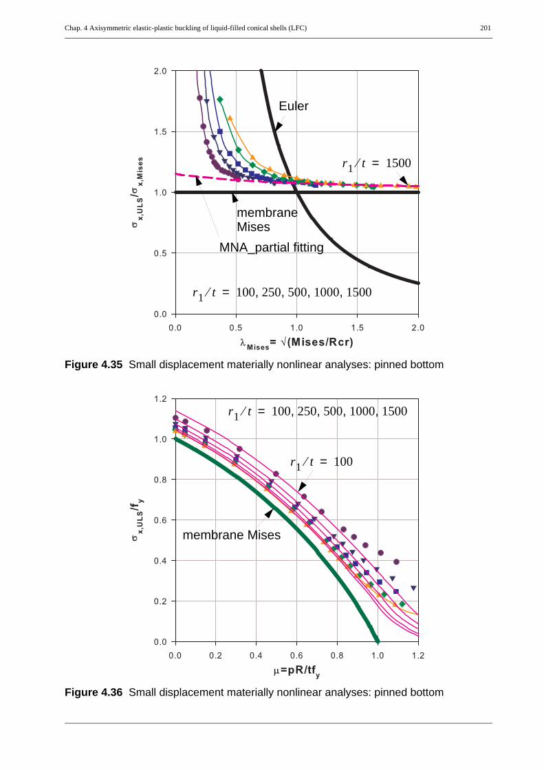
Chap. 4 Axisymmetric elastic-plastic buckling of liquid-filled conical shells (LFC) 201
Figure 4.35 Small displacement materially nonlinear analyses: pinned bottom
Figure 4.36 Small displacement materially nonlinear analyses: pinned bottom
r1 t⁄ 100 250 500 1000 1500, , , ,=
r1 t⁄ 1500=
Euler
membraneMises
MNA_partial fitting
membrane Mises
r1 t⁄ 100 250 500 1000 1500, , , ,=
r1 t⁄ 100=

202 Chap. 4 Axisymmetric elastic-plastic buckling of liquid-filled conical
4.8 Elastic-plastic buckling phenomena, analysisand strength
4.8.1 Elastic-plastic non-axisymmetric bucklingA tip-loaded perfect cone behaves the same way as that of a cylindrical shell under pure axial tip-load and elastic buckling phenomenon equally happens everywhere along the meridian of the shell.However, if there exists an imperfection, the buckling phenomenon will happen at the location ofthe imperfection under a lower buckling load. For a given fabrication quality class of a cone, theimperfection amplitude to wall-thickness ratio, , will be higher atevery point (and gets even higher up the meridian) than that of the base (because of the wideninggeometry of the cone) implying that for a tip-loaded cone the most probable location for elasticbuckling will be somewhere up the meridian depending on the boundary condition at the top endof the cone. Moreover, an imperfection of quality class-A at the shell interior of a tip-loaded conemay govern the buckling phenomenon eventhough there exists an imperfection of qulaity class-Cat the cone-base depending on the ratio of the radii at the respective locations. On the other hand,as long as plasticity of a given material is concerned, the relative buckling slenderness of the cone,
, (where ) will be smaller at the cone base and henceplasticity effect will play a greater role in buckling near the cone-base than in the shell interior.
Unlike that of a tip-compressed cone, in liquid-filled conical shells both elastic and elastic-plasticbuckling phenomena occur at a region near the bottom boundary. The elastic-plastic bucklingphenomenon may happen at relatively low or high internal pressurization depending on thegeometric and material properties of the shell. For the elastic-plastic buckling phenomenon, whichhappens at relatively high internal pressurization, the edge constriction effect, in addition to thedecaying meridional compressive stress, plays a great role results in axisymmetric buckling modenear the boundary. This type of buckling phenomenon along with the corresponding bucklingstrength will be investigated later in detail. For an elastic-plastic buckling at relatively low internalpressurization, a non-axisymmetric buckling mode near the boundary occurs the charactersticbuckling strength of which may be computed using an interaction expression where elasticbuckling interacts with bi-axial plasticity of the liquid-filled conical shell. The plastic bucklingparameters of that of a tip-loaded cone (or an unpressurized cylindrical shell under pure axialcompression) are used to assess such strengths. The bi-axial plastic capacity of liquid-filled conicalshells will be taken as the partial fitting of the plastic capacity obtained using the MNA results andexpressed as a function of the mebrane Mises yield capacity at the base of the cone (has alreadybeen discussed above) and will be named as σx,Mises+, the “+” sign showing that the materialnonlinear limit strength of the cone is expressed as an “up-scaled” membrane Mises strength.
Δwk t⁄ 1 Q⁄ r t βcos⁄( )⋅=
λx fy σxcr⁄= σxcr r( ) 0.605Et βcos r⁄=

Chap. 4 Axisymmetric elastic-plastic buckling of liquid-filled conical shells (LFC) 203
(Eq. 4.50)
where
(Eq. 4.51)
(Eq. 4.52)
and the plastic buckling parameters , , and .
The characterstic buckling strength related to the bi-axial membrane Mises yield strength can thenbe computed as follows:
(Eq. 4.53)
where “a1” is a constant equal to 0.2 for fixed bottom and 0.15 for pinned bottom boundaryconditions.
χMises +σx ULS,
σx Mises +,--------------------------
1 for λMises + λo≤
1 β0λMises + λo–
λp λo–---------------------------------⎝ ⎠⎜ ⎟⎛ ⎞ η
for λo λMises + λp< <⋅–
αxpe
λMises +2
---------------------- for λp λMises +≤
⎩⎪⎪⎪⎪⎨⎪⎪⎪⎪⎧
= =
λMises +σx Mises +,
σx LBA,--------------------------=
λpαxpe
1 β0–--------------=
η 1.0= λo 0.2= β 0.6=
χMisesσx ULS,
σx Mises,-------------------
σx ULS,σx Mises +,--------------------------
σx Mises +,σx Mises,
--------------------------⋅= =
χMises + 1a1
1 λMises+------------------------+⎝ ⎠
⎛ ⎞⋅=

204 Chap. 4 Axisymmetric elastic-plastic buckling of liquid-filled conical
4.8.2 Axisymmetric elastic-plastic buckling
4.8.2.1 Geometrically and materially nonlinear finite element analysis of perfect conicalshells (GMNA)
Unlike that of an axially loaded and internally pressurized cylindrical shell where the loadingprocedure can be done in two different ways, the loading in liquid-filled conical shells can not besplitted into a part which causes meridional compression and another part causing circumferentialtension. The resulting meridional compression and circumferential tension section forces of aliquid-filled conical shell are therefore interlinked to each other. Apart from this fact, the elastic-plastic buckling phenomenon already discussed in the buckling investigation of the cylindricalshell applies to the case of liquid-filled conical shells as well. It should, however, be clear that theelastic-plastic buckling strengths of liquid-filled conical shells will be somehow different from theuniformly loaded cylindrical shells because of the following possible reasons:
• the difference in geometry of the shell
• the difference in along-meridian distribution of each component of the section force/stress and the overall distribution of the bi-axial stress state
In other words, when a one-to-one comparison of the cylinder and cone is sought, an equivalencyin geometry and loading conditions along with boundary conditions needs to be met. The detailedinvestigation of such equivalency has been made in this work and will be discussed later.
On the other hand, unlike that of a uniformly loaded cylindrical shell which results in uniformmeridional and circumferential membrane section force ditributions, the meridional membranesection force ditribution in the liquid-filled conical shell is maximum at the lower supported edgeand decreases nonlinearly and rapidly up the meridian. Such a distribution of the meridionalcompressive section force superimposed with the edge constriction effects of the bottom boundaryconditions will restrict the elastic-plastic buckling phenomenon to a region very close to thesupported lower edge causing elephant’s-foot type buckling. This study, therefore, addresses thistype of elastic-plastic buckling phenomenon and strengths of liquid-filled conical shells.
Comprehensive parametric studies are carried out varying the shell slenderness (r1/tcosβ), shelllower bundary conditions (fixed versus pinned), and the liquid depth parameter (ζ’ = h’tanβ/r1)which indirectly determines the intensity of the internal pressurization. The membrane sectionforces ratio (ψ = Nx,1/Nθ,1) at the base level of the conical shell which directly depends on theliquid depth parameter (ζ’ = h’tanβ/r1) is used as a measure of the reference loading. Geometricallyand materially nonlinear finite element analyses which resulted in localized axisymmetric bucklingmodes were made on liquid-filled conical shells with an apex-half angle β = 45 degrees and r1/t =100, 250, 500, 1000, 1500 by varying the liquid depth parameter (ζ’ = h’tanβ/r1) from very small(or very high internal pressurization compared to meridional compression) to very high (or veryhigh meridional compression compared with internal pressurization). Boundary conditions of PINor FIX at bottom and rotational restraint at top were examined for each r1/tcosβ. Small

Chap. 4 Axisymmetric elastic-plastic buckling of liquid-filled conical shells (LFC) 205
displacement linear bifurcation analysis (LBA) and small displacement materially nonlinearanalysis (MNA) results are used for reference purposes.
In an exactly similar loading procedure as in the investigation of the material nonlinear strength,geometrically and materially nonlinear analyses (GMNA) of liquid-filled perfect cones have beenmade to compute the elephant’s-foot buckling strength. The results obtained are plotted in differentrepresentations as shown in Figure 4.37 to Figure 4.50. A GMNA/fy vs. ζ’ ( = h’tanβ/r1) plots areshown in Figure 4.37 and Figure 4.38 for the fixed and pinned bottom cases, respectively. Thesame elastic-plastic buckling strengths are re-plotted using the pressure representation (GMNA/fyvs. μ) in Figure 4.39 & Figure 4.41 and in the capacity representation (GMNA/Mises vs. λMises)in Figure 4.40 and Figure 4.42 for the fixed and pinned bottom cases, respectively.
For the shallow liquid-depth cases, the same “tail” effect with the same explanations as in the MNAcase can be seen from the elephant’s-foot buckling strengths.

206 Chap. 4 Axisymmetric elastic-plastic buckling of liquid-filled conical
Figure 4.37 Geometrically and materially nonlinear analysis: fixed bottom
Figure 4.38 Geometrically and materially nonlinear analysis: pinned bottom
membrane Mises
r1 t⁄ 100=
250
r1 t⁄ 1500=
500
1000
membrane Misesr1 t⁄ 100=
250
r1 t⁄ 1500=
500
1000

Chap. 4 Axisymmetric elastic-plastic buckling of liquid-filled conical shells (LFC) 207
Figure 4.39 GMNA results (elephant’s-foot strength): fixed bottom
Figure 4.40 GMNA results (elephant’s-foot strength): fixed bottom
r1 t⁄ 100=
250
r1 t⁄ 1500=
500
1000
membrane Mises
r1 t⁄ 100 250 500 1000 1500, , , ,=
r1 t⁄ 1500=
membrane Mises
Euler

208 Chap. 4 Axisymmetric elastic-plastic buckling of liquid-filled conical
Figure 4.41 GMNA results (elephant’s-foot strength): pinned bottom
Figure 4.42 GMNA results (elephant’s-foot strength): pinned bottom
r1 t⁄ 100=
250
r1 t⁄ 1500=
5001000
membrane Mises
r1 t⁄ 100 250 500 1000 1500, , , ,=
r1 t⁄ 1500=
membrane Mises
Euler

Chap. 4 Axisymmetric elastic-plastic buckling of liquid-filled conical shells (LFC) 209
The geometric nonlinearity effects in reducing the buckling strength of conical shells can be seenfrom the GMNA results when compared to the geometrically linear but materially nonlinear(MNL) strength. This relative strength (GMNL/MNL), where one can directly see the effects ofgeometric nonlinearities for different shell slenderness ratios, is shown in Figure 4.43 for the fixedbottom cone and Figure 4.44 for the pinned bottom.
When the geometric nonlinearity effects are very small as in the case of relatively thick-walledconcal shells, the GMNL buckling strengths will be closer (or atmost equal) to the pure plastic(MNL) strength of the shell. On the other hand, when both the geometric and material nonlinearityeffects are very small as in the case of relatively thin-walled cylindrical shells and lower internalpressure values, the GMNL buckling strengths will be closer (or atmost equal) to the pure elasticbuckling (LB) strength of the perfect shell. These facts can be observed from the plots of theGMNL results shown in Figure 4.43 to Figure 4.44 for both the fixed and pinned bottom boundaryconditions.

210 Chap. 4 Axisymmetric elastic-plastic buckling of liquid-filled conical
Figure 4.43 Elephant’s-foot strength: fixed bottom
Figure 4.44 Elephant’s-foot strength: pinned bottom
r1 t⁄ 100 250 500 1000 1500, , , ,=
r1 t⁄ 1500=
membrane Mises
Euler
r1 t⁄ 100 250 500 1000 1500, , , ,=
r1 t⁄ 1500=
membrane Mises
Euler

Chap. 4 Axisymmetric elastic-plastic buckling of liquid-filled conical shells (LFC) 211
Since the meridional and circumferential membrane section forces in liquid-filled conical shellsare always interlinked to each other through the membrane stress ratio parameter ψ, the intensityof internal pressurization is expressed interms of this parameter which inturn depends on theliquid-depth parameter ζ’. Since the intensity of the internal pressurization is indirectlyproportional to ψ (or ζ’), a high internal pressurization causing higher circumferential tension willbe obtained at smaller values of ψ (or ζ’), i.e. at relatively shallow liquid-depths. This, however,needs a liquid loading with very high specific weight (as high as 10*γmercury or even more) to causea very high circumferential tension somehow closer to the uni-axial yield strength of the shell andwhen superimposed with the edge constriction effect causes local bending which ultimately leadsto an elastic-plastic buckling under the small acting meridional compression near the boundary.Even for such a liquid loading with very high specific weight, the characterstic elastic-plasticbuckling load factor is relatively high because of the rapid decay leading to an even smallermeridional compression at the buckle center when compared with the existing small meridionalcompression at the supported base.
Once again, as alreday explained in the discussion of LFC MNL strengths, for thin-walled conicalshells solely loaded by liquid, such a buckling phenomenon under shallow liquid depths is far fromhappening because the specific weights of the commonly contained liquids are relatively very low.For this reason, in the process of extracting useful informations for practical design purposes theimpractical range is cut-off and approximated by simpler buckling strength prediction expressions(partial fitting of the GMNA reults) as will be discussed below. In the course of doing this, theratios of the MNL and GMNL strengths with respect to the partial-fit of the MNL strengths (i.e.MNL/MNA_partial-fit and GMNL/MNA_partial-fit) are computed and shown in Figure 4.45 andFigure 4.46 for both the fixed and pinned bottom boundary conditions, respectively. Using theseplots and a cut-off with the MNL-partial-fitting curve (the 1.0 line curves in the plots), finalexpressions for the characteristic buckling strengths of liquid-filled conical shells can be easilydrawn as discussed below.

212 Chap. 4 Axisymmetric elastic-plastic buckling of liquid-filled conical
Figure 4.45 Nonlinear analysis results: fixed bottom
Figure 4.46 Nonlinear analysis results: pinned bottom
r1 t⁄ 100 250 500 1000 1500, , , ,=
Euler
membraneMises
MNA
GMNA
r1 t⁄ 100 250 500 1000 1500, , , ,=
membrane
Euler
Mises
MNA
GMNA

Chap. 4 Axisymmetric elastic-plastic buckling of liquid-filled conical shells (LFC) 213
From the capacity representations of the geometrically and materially nonlinear analyses results(see Figure 4.47 & Figure 4.49), the values of the squash limit relative buckling slendernessparameter λ0 (below which stability effects are neglected and hence full plastic collapse is assumedto occur) and the plastic limit relative buckling slenderness parameter λp (at which materialnonlinearity effect starts to come into play and interact with stability effects) can be directlyextracted. For shell cases with λMises values which are greater than λp, pure elastic buckling willgovern the design as far as buckling is concerned. For values of λMises greater than λ0 but less thanλp, an elastic-plastic buckling phenomenon governs the design for which the characterstic bucklingstrengths should be obtained, generally speaking, either from tests or from geometrically andmaterially nonlinear analyses. In cases where such results do not exist a linear interpolation can beused as is recommended in EN1993-1-6. In cases where such results exist, shape functions are usedwhich accurately represent the elastic-plastic buckling strengths of the shell under consideration.In the current study, since geometric and material nonlinear analyses are performed from whichthe best fit shape functions are chosen to represent the computed values in the elastic-plastic range(i.e. ) for the different bottom boundary conditions as will be discussed below.
(Eq. 4.54)
where
(Eq. 4.55)
(Eq. 4.56)
(Eq. 4.57)
(Eq. 4.58)
the elastic-plastic buckling parameters: interaction exponent η, squash limit relative slendernessλo, and plastic range factor β are given as follows depending on the type of bottom boundarycondition.
λ0 λMises λp< <
χMisesσx ULS,
σx Mises,------------------- 1
a1
1 λMises+------------------------+⎝ ⎠
⎛ ⎞
1 for λMises λo≤
1 β0 f ξ( ) for λo λMises λp< <⋅–1
λMises2
--------------- for λp λMises≤
⎩⎪⎪⎪⎨⎪⎪⎪⎧
⋅= =
ξλMises λo–
λp λo–--------------------------=
f ξ( ) ξη 1 a2 1 ξ–( )η⋅+( )⋅=
λMisesσx Mises,
σxRcr-------------------=
λp1
1 β0–--------------=

214 Chap. 4 Axisymmetric elastic-plastic buckling of liquid-filled conical
Alternatively, for a liquid-filled conical shell with pinned bottom boundary condition the values and can be used instead.
With this approximate expression for the geometrically and materially nonlinear strength of theshell interms of the membrane Mises yield strength at the bottom edge, the pressure representationof the GMNA FEM results along with the GMNA partial-fitting are re-plotted in Figure 4.48 andFigure 4.50.
a1 a2 η λo βFixed bottom 0.20 0.00 1.0 0.45 0.6
Pinned bottom 0.15 0.75 1.0 0.35 0.8
Table 4.1 Values of plastic buckling parameters
a2 1.0= η 1.1=

Chap. 4 Axisymmetric elastic-plastic buckling of liquid-filled conical shells (LFC) 215
Figure 4.47 GMNA results (elephant’s-foot strength): fixed bottom
Figure 4.48 GMNA results (elephant’s-foot strength): fixed bottom
r1 t⁄ 100 250 500 1000 1500, , , ,=
r1 t⁄ 1500=
Euler
membraneMises
GMNA_partial fitting
r1 t⁄ 100=
250
r1 t⁄ 1500=
500
1000
membrane Mises

216 Chap. 4 Axisymmetric elastic-plastic buckling of liquid-filled conical
Figure 4.49 GMNA results (elephant’s-foot strength): pinned bottom
Figure 4.50 GMNA results (elephant’s-foot strength): pinned bottom
r1 t⁄ 100 250 500 1000 1500, , , ,=
r1 t⁄ 1500=
Euler
membraneMises
GMNA_partial fitting
r1 t⁄ 100=
250
r1 t⁄ 1500=
5001000
membrane Mises
Chap. 4 Axisymmetric elastic-plastic buckling of liquid-filled conical shells (LFC) 217
4.8.2.2 Analytical model based on theory of second order with material nonlinear effectsThe same basic idea, as used in the discussion on an anlytical model of cylindrical shells, can beapplied to conical shells. In other words, the geometric and material nonlinear effects of a a liquid-filled conical shell can be analytically modelled approximately using a combination of theory ofsecond order and the stress resultant oriented approximate yield criteria. However, this has notbeen covered in the current study.

218 Chap. 4 Axisymmetric elastic-plastic buckling of liquid-filled conical
4.9 Buckling design recommendation
Once the pure elastic buckling strength of an imperfect liquid-filled conical shell, which is relatedto a non-axisymmetric failure mode, and the elastic-plastic buckling strength of the perfect (orimperfect, for that matter, when a worst practical imperfection nature is agreed upon) liquid-filledconical shell, which is related to an axisymmetric buckling mode can be predicted using simplerexpressions, exactly the same methods as those discussed in the buckling investigation of thecylindrical shell can be used. More specifically, method-4 is the best of all the methods discussedand is, therefore, highly recommended for design and future research applications because of thefacts already stated during the discussion, chapter-3.

Chap. 4 Axisymmetric elastic-plastic buckling of liquid-filled conical shells (LFC) 219
4.10Summary and conclusions
The pure membrane behavior and edge bending effects of a liquid-filled conical shell have beencomputed using considerations of static equilibrium for the pure membrane situation and using aneffective-ring model analogy for the edge bending effects. The total results (membrane + edgebending) have been compared with the finite element linear analysis results for verificationpurposes.
The possible loading procedures in dealing with liquid-filled conical shells have been discussed.Besides, which loading procedure should be used in what circumstances and for what purposes hasbeen pointed out.
The linear buckling strengths of liquid-filled perfect cones have been computed approximately andinvestigated numerically. Explanations have been given about the LFC-specific bucklingphenomenon and corresponding strengths. Simplified expressions for the prediction of linearbuckling strengths of liquid-filled general cones with pinned and fixed bottom boundary conditionshave been obtained. The effect of imperfections on the elastic buckling strength have beendiscussed as well for different fabrication quality classes as recommended in EN 1993-1-6.
The pure plastic limit strengths of liquid-filled conical shells have been computed approximatelyusing von Mises membrane yield criterion taking the membrane stresses at the cone-base asreferences. The plastic strength using stress resultant oriented approximate yield criteria have alsobeen included. Moreover, small displacement materially nonlinear numerical simulations havebeen done to compute the exact plastic capacity of liquid-filled cones. Simplified expressionsalong with detailed explanations have been obtained to predict the materially nonlinear limitstrength of both pinned and fixed bottom liquid-filled general cones.
The consideration of the effect of plasticity on elastic buckling with non-axisymmetric bucklingfailure mode have been discussed. This type of elastic-plastic interaction happens for relativelysmaller internal pressurization situations. The elephant’s-foot buckling strengths of perfect conesdue to liquid-loading have also been investigated in detail after which simplified expressions areobtained for the prediction of the axisymmetric elastic-plastic buckling strength of general thin-walled liquid-filled cones.
Elephant’s-foot type buckling in liquid-filled conical shells, where the only loading is liquid-filling, may not be probable unless there exist a worst imperfection or a global bending momentresulting from, say, earthquake causing one-sided buldge. A very little global bending effect, in thegeneral case of cones supported from bottom (i.e. on the smaller radius), will have a very bigmeridional compression on one side of the cone due to the shorter lever-arm at the smaller radius.It is this big meridional compression along with the existing circumferential stretching whichresults in bi-axial state of stress causing local yielding and hence elephant’s-foot buckling.

220 Chap. 4 Axisymmetric elastic-plastic buckling of liquid-filled conical
On the other hand, if there exists an additional, say, roof loading on top of the existing liquid-loading, an additional meridional compression will result. This higher meridional commpressionalong with the existing circumferential tension (plus small addition due to poisonn’s effect) maytherefore lead to the possibility of elephant’s-foot type buckling.

Chap. 5 Re-investigation of Gent test results: Elastic buckling of liquid-filled cones 221
5
Re-investigation of Gent test results:
Elastic buckling ofliquid-filled cones
222 Chap. 5 Re-investigation of Gent test results: Elastic buckling of liquid-
5.1 Introduction
The term liquid-filled conical shells, in the context of this work, refers to truncated conical shellsused as liquid storage tanks with a vertical axis of rotation and supported from below at their small-er radius edge. Apart from tanks, conical shells can also be found on the lower portion of silo struc-tures. In cases where they are used as liquid containment vessels, as in steel water towers, thecontained liquid exerts an internal hydrostatic pressure which results in meridional compressionand tension in the hoop (circumferential) direction.
Though metal shells are the main interest of this study, such structures can also be constructed us-ing reinforced concrete. The bottom edge of the LFC shells are mainly supported in two ways:
• the lower part is welded to an upper part of a short stiff conical or cylindrical shell where itin turn is welded to a rigid plate (e.g. the steel water tower failed in 1990, Fredericton, Can-ada)
• the lower part is welded directly to the rigid plate (e.g. the steel water tower failed in 1972,Belgium)
In the first type of supports, even though there is some rotational stiffness coming from the weld,the shell can conservatively be treated as “pin” supported. Where as in the second case the shellcan be treated as “fixed” as long as the rigid plate helps the shell keep its conicity. For this reason,the “pin” and “fix” type of supports are the main concerns in this shell buckling study.
In 1972, a time when there were no buckling design regulations to refer to and even no enoughbuckling knowledge to rely to, a 1500 m3 capacity steel water tower suddenly collapsed in Belgiumupon filling for the first time, right before (1.74m below) the overflow level is reached. The failureoccurred by buckling which started somewhere on the bottom region (i.e. close to the boundary).The bottom region comprised of two cone segments with the lower cone relatively thicker andshorter.
Following the collapse, a huge amount of experimental researches and numerical (using BOSOR)studies were made for more than a decade (1977-1987) at Gent university by D. Vandepitte et. al.The results of the study were reported in many papers (see Figure 5.1) and a design recommenda-tion was then proposed based on straight line bounds of all the test results from a doubly logarith-mic ψ - ω plot.
Figure 5.2 and Figure 5.3 show photos taken of the collapsed steel water tower from two differentviewing angles. A laboratory experimental setup used in Gent and an explanatory sketch showingthe geometry, loading, and boundary conditions are shown in Figure 5.4 and Figure 4.1, respec-tively.

Chap. 5 Re-investigation of Gent test results: Elastic buckling of liquid-filled cones 223
Figure 5.1 Summary of previous works related to the Gent experiments
Year: 1972 1977 1982 1987 19901983
1984
Steel water towercollapse, Seneffe,Belgium
Vandepitte D.
Model investigation of the collapse ofa steel water tower: In PreliminaryReport of 2nd International Collo-quium on Stability of Shell Structures,Liege
Vandepitte, D., Rathé, J., Verhegghe, B.,Paridaens, R., Verschaeve, G.
Experimental investigation of buckling ofhydro-statically loaded, conical shells andpractical evaluation of the buckling load:In Proceedings of a State-of-the-Art Col-loquium on Buckling of Shells. Stuttgart
Vandepitte, D., Lagae, G.
Theoretical and experimental investi-gation of buckling of liquid-filledconical shells: In Preliminary Report,Third International Colloquium onStability of Metal Structures, Paris
European Recommendationsfor Steel Construction: Buck-ling of Shells, Third Edition,October 1984 - European Con-vention for ConstructionalSteelwork, Brussels.
Steel water tow-er collapse, Fre-dericton,
Paridaens, R., Vandepitte, D., Lagae,G., Rathé, J., Van den Steen, A.
Design equations accounting forelastic buckling of liquid-filled coni-cal shells: In Colloquium on Stabilityof Plate and Shell Structures, GhentUniversity

224 Chap. 5 Re-investigation of Gent test results: Elastic buckling of liquid-
Figure 5.2 Collapsed steel water tower, 1972, Belgium
Figure 5.3 Collapsed steel water tower, 1972, Belgium
Supportingshaft
Conicalpart
Supportingshaft Conical
part

Chap. 5 Re-investigation of Gent test results: Elastic buckling of liquid-filled cones 225
Figure 5.4 Gent laboratory experimental setup

226 Chap. 5 Re-investigation of Gent test results: Elastic buckling of liquid-
5.2 Problem statement
With the help of the numerous Gent laboratory tests and numerical (using BOSOR) verificationsD. Vandepitte et. al. proposed a design recommendation for the prediction of elastic bucklingstrengths of liquid-filled conical shells based on straight line bounds of all the test results from adoubly logarithmic ψ - ω plot.
The Gent proposal for the elastic carrying capacity of liquid-filled perfect and imperfect conicalshells is given in terms of three equations of straight bounding lines. In a log-log representation ofthe Gent non-dimensional basic parameters ψ and ω, those straight lines are bounds for all (over800) test data points irrespective of the very wide range of shell slenderness ratios, r1/tcosβ = 77 -3760. A series of researches have been made afterwards but most of them based on the straight linebounds already proposed. The same design proposal has also been used as a reference to compareother independent research results and failure cases with.
The shell slenderness, r1/tcosβ is a basic parameter that greatly affects the buckling strength ofshells and plays the most important and decisive role in describing the load carrying behavior ofshells.
It is, therefore, the primary purpose of this study to re-investigate and re-interpret the Gent test re-sults in such a way that the resulting LFC-imperfection reduction factor, which directly is used inthe prediction of the load carrying capacity of liquid-filled conical shells, takes the shell slender-ness into account. A different set of LFC dimensionless parameters, including the shell slendernessparameter, will also be used in the investigation. Finally, a new elastic buckling design recommen-dation for liquid-filled conical shells will be proposed.
Chap. 5 Re-investigation of Gent test results: Elastic buckling of liquid-filled cones 227
5.3 Liquid-filled conical shell parameters andrepresentation
Basic non-dimensional system parametersParameter No. 1:
liquid depth parameter
Parameter No. 2:
cone apex angle parameter
Parameter No. 3:
shell slenderness parameter
Parameter No. 4:
internal pressure parameter
h'r1----
βtan
r1t βcos--------------
pσθ 1,
σx Rcr,-------------- 1.65γ' h'⋅
E------------
r1t βcos--------------⎝ ⎠⎛ ⎞
2⋅= =

228 Chap. 5 Re-investigation of Gent test results: Elastic buckling of liquid-
Figure 5.5 Demonstration of LFC variables and membrane section forces
Nθ,1
Nθ
Nx
β
γ'
r1
h’.tanβ
r2’r2
1
z
rh’
for example: ζ’ = 3.0Nx,1
Liquid surface level dimensionless variables
Running dimensionless variables
ζ'r2' r1–
r1---------------- h' βtan
r1----------------= =
ρ'r2'r1----- 1 ζ'+= =
ζr r1–
r1------------- z βtan
r1--------------= =
ρ rr1---- 1 ζ+= =
Membrane section forces
... Meridional membrane section force
... Circumferential membrane section force
... Meridional membrane section force at cone support
... Circumferential membrane section force at cone support
Nx
Nθ
Nx 1,
Nθ 1,
β
γ'
r1
Nx,1
Nθ,1 Nθ,1Nx,1

Chap. 5 Re-investigation of Gent test results: Elastic buckling of liquid-filled cones 229
Membrane section stress distributionsThe meridional and circumferential membrane stresses along the meridian are given
• as functions of the ρ and ρ’ parameters
(Eq. 5.1)
(Eq. 5.2)
• as functions of the ζ and ζ’ parameters
(Eq. 5.3)
(Eq. 5.4)
Membrane section stresses at cone support
(Eq. 5.5)
(Eq. 5.6)
(Eq. 5.7)
The membrane section forces can be computed from the product of the thickness of the shell andthe respective membrane stress, i.e.
(Eq. 5.8)
Figure 5.6 and Figure 5.7 show the meridional and circumferential membrane section force distri-butions, respectively, along the meridian normalized with respect to the circumferential membranesection force at the cone support, Nθ,1. In each plot the liquid depth variable, ρ’ is varied to producea set of curves. For better understanding of different liquid-filling depths and corresponding pa-rameters, see Figure 4.9.
σxγ'h'r1t βcos-------------- 1
6--- ρ' ρ–( )2
ρ' 1–---------------------⋅ ⋅ 3 ρ' ρ–
ρ-------------+⎝ ⎠
⎛ ⎞⋅=
σθγ'h'r1t βcos-------------- ρ ρ' ρ–
ρ' 1–-------------⎝ ⎠⎛ ⎞⋅ ⋅=
σxγ'h'r1t βcos-------------- 1
6--- ζ' ζ–( )2
ζ'-------------------- 3 ζ' ζ–
1 ζ+-------------+⎝ ⎠
⎛ ⎞⋅ ⋅ ⋅=
σθγ'h'r1t βcos-------------- 1 ζ+( ) ζ' ζ–
ζ'-------------⎝ ⎠⎛ ⎞⋅ ⋅=
r r1= ρ⇒ 1;= ζ 0=
σx 1,γ'h'r1t βcos-------------- 1
6--- ζ' 3 ζ'+( )⋅ ⋅ ⋅=
σθ 1,γ'h'r1t βcos--------------=
Nx t σx;⋅= Nθ t σθ⋅=
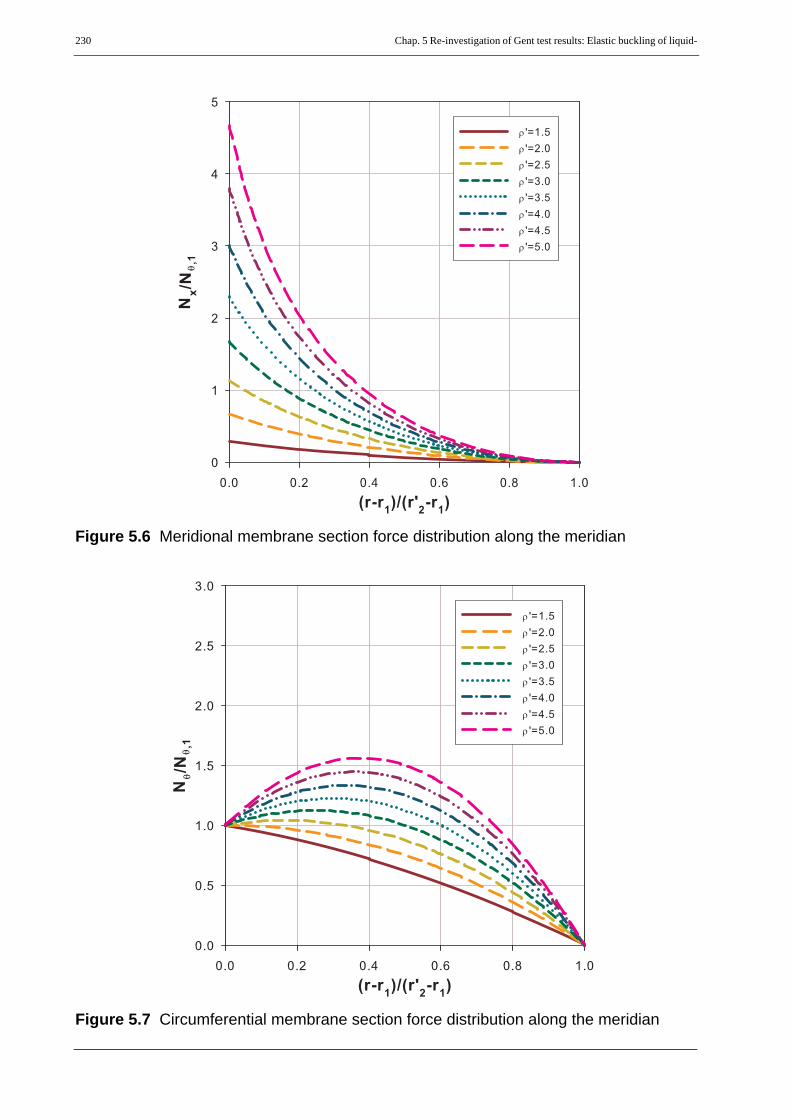
230 Chap. 5 Re-investigation of Gent test results: Elastic buckling of liquid-
Figure 5.6 Meridional membrane section force distribution along the meridian
Figure 5.7 Circumferential membrane section force distribution along the meridian

Chap. 5 Re-investigation of Gent test results: Elastic buckling of liquid-filled cones 231
Elastic imperfection reduction factorsIn accordance to the frame work of the European standard EN 1993-1-6, the elastic imperfectionreduction factor (a factor applied to the linear bifurcation buckling strength of a perfect shell to ac-count for geometric imperfections and the effect of geometric nonlinearity) of cylindrical and con-ical shells subjected to meridional compression with/without co-existent internal pressure has beendiscussed in chapter-3 and chapter-4.
Figure 5.8 shows cylindrical and conical shells with different loading situations where the discus-sion on the pressurized or unpressurized elastic imperfection reduction factor can be applied. Fig-ure 5.9 shows a plot of αxpe vs. p for different shell slenderness, r1/tcosβ, values ranging from 100(upper most curve) to 3500 (lower most curve) and assuming fabrication tolerance quality class C.
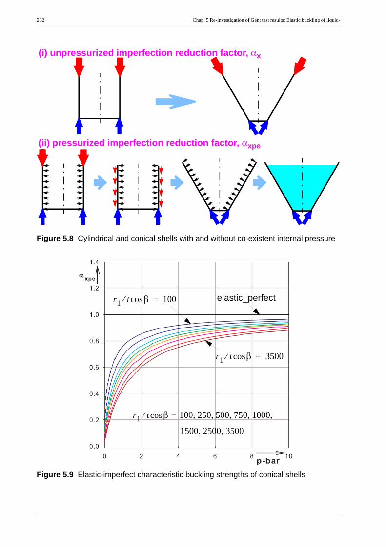
232 Chap. 5 Re-investigation of Gent test results: Elastic buckling of liquid-
Figure 5.8 Cylindrical and conical shells with and without co-existent internal pressure
Figure 5.9 Elastic-imperfect characteristic buckling strengths of conical shells
(i) unpressurized imperfection reduction factor, αx
(ii) pressurized imperfection reduction factor, αxpe
r1 t βcos⁄ 100=
r1 t βcos⁄ 3500=
r1 t βcos⁄ 100 250 500 750 1000, , , , ,=
1500 2500 3500, ,
elastic_perfect

Chap. 5 Re-investigation of Gent test results: Elastic buckling of liquid-filled cones 233
5.4 Fluid-filled conical shells: comparison ofgas-filled vs. liquid-filled conical shells
The susceptibility of fluid-filled conical (FFC) shells to buckling depends on the magnitude of thestabilizing effect of the circumferential tensioning as a result of internal pressurization. The inter-nal pressurization may be uniform along the meridional length of the shell as in the gas-filled con-ical (GFC) shells or may vary linearly as in the hydrostatic pressure distribution of liquid-filledconical (LFC) shells. A comparison between the GFC and LFC shells has been made as follows.
Figure 5.10 (a) GFC; (b) LFC
The membrane circumferential, σθ,1 and meridional, σx,1 stresses at the bases of the cones can eas-ily be calculated from membrane theory and are given by
• LFC (hydrostatic internal pressure) case
(Eq. 5.9)
(Eq. 5.10)
(Eq. 5.11)
• GFC (gas/uniform internal pressure) case
(Eq. 5.12)
(a) (b)
h’
ζ' h' βtanr1
----------------=
σθ 1 LFC, ,γ'h'r1t βcos--------------=
σx 1 LFC, , σθ 1, ψLFC⋅=
ψLFCζ'6---- 3 ζ'+( )=
σθ 1 GFC, ,pr1
t βcos--------------=

234 Chap. 5 Re-investigation of Gent test results: Elastic buckling of liquid-
(Eq. 5.13)
(Eq. 5.14)
The comparison between the above two cone loading situations can be done in two different waysas discussed below.
1. For a reference meridional membrane stress at cone-base:
To produce the same meridional membrane stress, σx,1 at the base of the cone, the relationship be-tween the intensities of the internal pressure at the cone-base for the two loading situations will begiven as follows:
(Eq. 5.15)
(Eq. 5.16)
This means, when compared at the cone base, a lesser uniform internal pressure, p is required toproduce the same meridional stress than the corresponding hydrostatic pressure, γ’h’ showing thata lesser stabilizing effect in the GFC case due to a lesser circumferential tensioning than in the LFCcase (see Figure 5.11a).
2. For a reference circumferential membrane stress at cone-base:To produce the same circumferential membrane stress, σθ,1 at the base of the cone, the relationshipbetween the intensities of the internal pressure at the cone-base for the two loading situations willbe given as follows:
(Eq. 5.17)
(Eq. 5.18)
When compared at the cone base, they both have the same stabilizing effect due to circumferentialtension but, at the same time, the GFC case produces a higher meridional compressive stress which
σx 1 GFC, , σθ 1, ψGFC⋅=
ψGFCζ'2---- 2 ζ'+( )=
σx 1, σ= x 1 LFC, , σx 1 GFC, ,=
γ'h'r1t βcos--------------⇒ ζ'
6---- 3 ζ'+( )
pr1t βcos-------------- ζ'
2---- 2 ζ'+( )⋅=⋅
p⇒ 13--- 3 ζ'+
2 ζ'+-------------⎝ ⎠⎛ ⎞ γ'h'⋅=
→ pζ' 0→lim γ'h'
2-------=
→ pζ' ∞→lim γ'h'
3-------=
σθ 1, σ= θ 1 LFC, , σθ 1 GFC, ,=
γ'h'r1t βcos--------------
pr1t βcos--------------=⇒
p⇒ γ'h'=

Chap. 5 Re-investigation of Gent test results: Elastic buckling of liquid-filled cones 235
makes the conical shell prone to buckling failure (see Figure 5.11b).
In both the above cases, one can see that under similar conditions of material properties, boundaryconditions, imperfection types and amplitudes, and low to medium internal pressure magnitudesthe GFC case is the favorable loading situation for buckling to happen.

236 Chap. 5 Re-investigation of Gent test results: Elastic buckling of liquid-
Figure 5.11 σx,1 vs. σθ,1 plots: (a) same stabilizing effect; (b) same meridional compres-sion at cone-base
1
σθ,1
σx,1,LFC
ψLFC
1
ψGFC
σx,1
σx,1,GFC
σθ,1
1
σθ,1σθ,1,LFC
ψLFC
1
ψGFC
σx,1
σθ,1,GFC
σx,1
(a)
(b)

Chap. 5 Re-investigation of Gent test results: Elastic buckling of liquid-filled cones 237
5.5 Test results and Gent University designproposal
Hundreds of model cones have been tested at Gent university with the following general setup. Allmodels were loaded by increasing the liquid depth until they collapsed. A detailed summary of allthe tests performed, including the rejected ones, is presented in Table 5.1. A complete information,in addition to the summary in Table 5.1, of all the tests (i.e. material properties, loading situations,and boundary conditions) are given below:
• Materials usedAluminium, Steel, Brass, and Mylar
• Liquid loadingWater, water with molasses (1.333 to 1.362 times heavier than water), water with barium sul-
fate suspension (1.950 to 2.075 times heavier than water), and mercury
• Bottom boundary conditionsSimple sliding, Simple support, and clamped
Test procedure, test data recording, test data analysis and interpretation
The overall step-by-step procedure that has been followed during testing, test data recording, testdata analysis and interpretation of the Gent laboratory tests can be put as follows:
• What was known before testing?
cone geometry, liquid property, boundary condition, cone material properties, and imperfec-tion amplitudes
• What types of imperfection shapes were considered, how were they produced, and how were the amplitudes measured?
The imperfections considered were of arbitrary shapes as the imperfect cones used for testingwere the already tested (collapsed) cones by straightening out the buckles from previoustests. The imperfection amplitudes were measured as the largest inward depression of the un-loaded test cone from a straight rod of length placed against the genera-trices in the lower part of the cone.
• How was the liquid-loading applied and what was measured during testing?
the liquid-depth was gradually increased until collapse occurs and the ultimate liquid depth,h’U at which collapse happens was recorded
l 3.6 r1t βcos⁄=20 r1t βcos⁄

238 Chap. 5 Re-investigation of Gent test results: Elastic buckling of liquid-
• What was computed after testing?
the meridional membrane normal stress at the base of the cone corresponding to the ultimateliquid depth, h’U
(Eq. 5.19)
• How were the test data analyzed?
A big scatter of test data was obtained for which non-dimensional analyses were done andfinally two non-dimensional basic parameters, ω and ψ were used for representing each testdata. The ω parameter for each test, however, depends purely on the geometric, liquid, andcone material properties and therefore it was known before performing the test. The ψ pa-rameter, on the other hand, was computed using the data obtained from the test, (Eq. 5.21).
(Eq. 5.20)
(Eq. 5.21)
• How were the scatter of the test data interpreted and what was deduced?
All the test data, which were approved to be with no setup faults, were plotted together on alog-log scale of ψ vs. ω plot so that the scatter band is reasonably narrow for bounding curvesto be applied (see Figure 5.12). Three straight bounding lines were chosen, two lowerstraight-line bounds for two different imperfection amplitude ranges, poor and good cones,and an upper straight-line bound for perfect cones (see Figure 5.13). The general mathemat-ical expressions for these bounding lines are given in the linear-linear and log-log writing,respectively, by
(Eq. 5.22)
(Eq. 5.23)
σx 1 U, ,γ'h'U
2 βtan6t βcos
----------------------- 3h'U βtan
r1-------------------+⎝ ⎠
⎛ ⎞⋅=
ω1000 r1⋅t βcos⋅---------------------
γ' r1⋅E
------------ 1 ν2–σθ 1 U, ,σx Rcr,---------------- 1
3 10 6–⋅----------------------
r1h'U-------⎝ ⎠⎛ ⎞⋅ ⋅=⋅=
ψ σx 1 U, ,t βcos⋅γ' r1
2⋅------------------
σx 1 U, ,σθ 1 U, ,----------------
h'Ur1-------⎝ ⎠⎛ ⎞⋅=⋅=
ψ b ω d–⋅=
ψlog b d ωlog⋅–log=

Chap. 5 Re-investigation of Gent test results: Elastic buckling of liquid-filled cones 239
No. Classification based on
types used number of tests made
total Remark
1 material type
Aluminium 45
811Steel 132
Brass 77
Mylar 557
2 bottom boundary condition
simple 627
811simple sliding 146 all with in 20° - 60°
clamped 37
? 1
3 apex half angle, β
10° 39
811
(1) Mylar only(2) very big imperfection amplitudes
20° - 60° 727
75° 45 (1) Mylar only(2) very small imperfection amplitudes
4 test evaluation by Gent
accepted 768811rejected 43
5reason for test refusal (for the rejected tests)
cone failed sideways (out of conicity)
22
43
(i) 16 have sliding bottom boundary condition(ii) relatively narrow base and high h’tanβ/r1
cone failed within the supporting device
10
cone with overlapping meridional seam in the critical zone
4
faulty test setup 7
Table 5.1 Summary of Gent test data

240 Chap. 5 Re-investigation of Gent test results: Elastic buckling of liquid-
Figure 5.12 Log-Log plot of the test data points
Figure 5.13 Log-Log plot of the test data points and Gent-bounding straight lines

Chap. 5 Re-investigation of Gent test results: Elastic buckling of liquid-filled cones 241
Imperfection amplitudes and quality classesThe three straight bounding lines which represent the three quality classes (perfect, good, and poor)according to Gent nomenclature depends on the Gent imperfection amplitude parameter, w of theconical shell as given in Table 5.2.
The Gent imperfection amplitude parameter, w, is the largest inward depression of the unloadedtest cone from a straight rod of length placed against the generatrices in thelower part of the cone. It is given in terms of another recorded parameter, “IMP” in%, which is related to the length of the straight rod as follows:
(Eq. 5.24)
Gent design proposalThe final design proposal by Vandepitte et. al. based on the scatter band of the test results from thedoubly logarithmic plot, Figure 5.13, is expressed in terms equations of the bounding straight lines.These equations, for the different quality classes can be re-written in the doubly linear and doublylogarithmic way of writing as follows:
In a linear - linear representation, the equations of the three straight bounding lines are given by
for ’perfect’ cones (Eq. 5.25)
for ’ good’ cones (Eq. 5.26)
for ’poor’ cones (Eq. 5.27)
In a log - log representation, the equations of the three straight bounding lines are given by
for ’perfect’ cones (Eq. 5.28)
for ’ good’ cones (Eq. 5.29)
for ’poor’ cones (Eq. 5.30)
Quality class name Imperfection amplitude parameter, w
Perfect cones 0
Good cones
Poor cones
Table 5.2 Gent quality class naming & imperfection amplitude values
l 3.6 r1t βcos⁄=20 r1t βcos⁄
w l IMP⋅100
-----------------=
w 0.008l≤
0.008 l w 0.02l≤<
ψ 471250 ω 1.974–⋅=
ψ 44620 ω 1.724–⋅=
ψ 39030 ω 1.713–⋅=
ψlog 5.673 1.974 ωlog⋅–=
ψlog 4.650 1.724 ωlog⋅–=
ψlog 4.591 1.713 ωlog⋅–=

242 Chap. 5 Re-investigation of Gent test results: Elastic buckling of liquid-
The test data points and Gent bounding straight-lines are re-plotted on a linear-linear scale (see Fig-ure 5.14) to show the role of the scale type used on the graphical representation. For comparisonpurposes, the same bounding curves are plotted for h’/r1 values of 2.0 and 8.0 (see Figure 5.15) inthe αxpe vs. p representation, together with the family of LFC curves (slenderness ratios of 100-3500).
Before going to the detailed investigation of the test results, a rough look at the data points in thedifferent representations is important. For example, the following basic questions can be raisedonly from a qualitative look at the plot in Figure 5.15:
• What is really going on at the very small pressure values?
• Why is there a wide gap between the LFC curves and the Gent curves for medium pres-sure values?
• What happens at high pressure values where an elastic-plastic interaction is expected?

Chap. 5 Re-investigation of Gent test results: Elastic buckling of liquid-filled cones 243
Figure 5.14 Linear-Linear plot of the test data points and Gent-bounding straight lines
Figure 5.15 Qualitative comparison of LFC and Gent curves
?
??
???

244 Chap. 5 Re-investigation of Gent test results: Elastic buckling of liquid-
5.6 Comparison of parameter choices andrepresentations
A comparison of the parameters chosen in the two different representations, namely αxpe vs. p andψ vs. ω, has been made in the current work. Both qualitative and quantitative (mathematical) com-parisons were made. The qualitative similarities and exact relationships between these parametersare explained below.
• Proportionality relationships (for a given h’/r1)
(Eq. 5.31)
(Eq. 5.32)
(Eq. 5.33)
which show that the LFC ψ and Gent ψ parameters are linearly related to each other; whereas theLFC parameters αxpe & p are nonlinearly related to the Gent parameters ψ & ω, respectively.
• Mathematical relationships between the different scaling and parameters used
The mathematical relationships between the LFC ψ, αxpe & p parameters and Gent ψ & ω param-eters are discussed below. These relationships will later be used for the transfer of comparativecurves from the Gent log-log plot to the LFC αxpe - p log-log and linear-linear plots and vise versa.
Linear-linear relationship:
(Eq. 5.34)
(Eq. 5.35)
(Eq. 5.36)
ψ ψ∝
αxpe ψ ω2⋅∝
p ω2∝
ψ ψh'U r1⁄( )
----------------------=
αxpe 3 10 6– ψω2⋅=
pαxpe
ψ-----------= 3 10 6– ψω2⋅
ψ h'U r1⁄( )⁄----------------------------------- 3 10 6– h'U
r1--------ω2⋅= =

Chap. 5 Re-investigation of Gent test results: Elastic buckling of liquid-filled cones 245
Log-log relationship:
(Eq. 5.37)
Showing a non-linear relationship between the corresponding linear-linear representations and alinear relationship between the corresponding log-log representations. It can be seen from the lin-ear-linear relationship that a pre-specified value for h’U/r1 is needed to directly compare two cor-responding parameters from the different representations.
What are not OK with the Gent proposal & what should be re-investigated?Figure 5.16 shows a plot of the LFC family of curves, all test data points, and Gent bounding curvesin the αxpe - p representation. The following list of questions can be raised by just having a roughlook at this plot, see Figure 5.17. Brief remarks are also included for each question on how eachissue has been addressed and re-investigated in this study.
• What is happening at the zero-pressure (tip-loading) or small-pressure (very high liquid depth) situation?
a closer look at the small pressure levels has been done.
• Why are there NO data points in the central αxpe - p region, between the LFC family of curves and Gent bounding curves? BIG SURPRISE!!
a detailed investigation on the Gent original data, their parameter representation, and scaling ap-plied has been done
• What will happen at higher pressure values where elastic-plastic type buckling phenome-non is expected?
a detailed study on elephant’s-foot type buckling has been done
• Why are there so many data points above the αxpe = 1.0 line?
a detailed study on buckling nature of LFC shells has been done
• Why are the very wide shell-slenderness ranges mixed all up in one?
detailed view at the data by considering the r1/tcosβ - dependency has been done, i.e. a check ifslenderness ratio related data points are really above their corresponding buckling curves wasdone
αxpelog
plog1 10 1
ψlog2 ωlog
h'Ur1--------⎝ ⎠⎜ ⎟⎛ ⎞ 0
1⋅ 5.761 1
1–log+=

246 Chap. 5 Re-investigation of Gent test results: Elastic buckling of liquid-
Figure 5.16 LFC curves, test data points and Gent bounding curves
Figure 5.17 Comparison of LFC curves, test data points & Gent bounding curves
?
??
???
?????????

Chap. 5 Re-investigation of Gent test results: Elastic buckling of liquid-filled cones 247
Basic demonstration: same curves in different representationsFor basic demonstration and easy comparison purposes of the αxpe - p linear-linear and ψ - ω log-log representations, a step-by-step procedure has been followed. The overall idea here is to see andcompare how curves and data points are represented in the two different plot types. Following isan overview of what has been done:
1 The αxpe - p plot of the LFC curves, all test data points, and Gent bounding curves is, onceagain, shown in Figure 5.18. The same curves and test data points are also shown on ψ - ωlog-log plot, Figure 5.19.
2 A single curve (with a slenderness ratio of 2500), out of the family of LFC curves (see Fig-ure 5.20 and Figure 5.21), is considered for detailed comparison of the two different repre-sentations (see Figure 5.22 and Figure 5.23) for h’/r1 = 2.0
3 Analytic derivation of different illustrative curve types and their slopes in the two differentrepresentations are shown in (Eq. 5.38) to (Eq. 5.65). More details about the curve typesillustrative curve types considered will come later.
4 Step-by-step plots of the different curves considered and their explanations are listed below.The Gent bounding curves are plotted for h’/r1 = 2.0
Figure 5.24 & Figure 5.25 show the curve for r1/tcosβ = 2500 and its lower limit line
Figure 5.26 & Figure 5.27 include an upper limit line
Figure 5.28 & Figure 5.29 include a tangent line, line-1, to the r1/tcosβ = 2500 curve at p = 0
Figure 5.30 & Figure 5.31 include a second tangent line, line-2
Figure 5.32 & Figure 5.33 include a third tangent line, line-3
Figure 5.34 is same as Figure 5.32 but on a log-log scale and Figure 5.35 same as Figure 5.33
Figure 5.36 & Figure 5.37 include r1/tcosβ = 100 curve and show log-log representations ofboth αxpe - p and ψ - ω

248 Chap. 5 Re-investigation of Gent test results: Elastic buckling of liquid-
Figure 5.18 Linear-linear plot: LFC curves, test data points and Gent bounding curves
Figure 5.19 Log-log plot: LFC curves, test data points and Gent bounding curves

Chap. 5 Re-investigation of Gent test results: Elastic buckling of liquid-filled cones 249
Figure 5.20 Linear-linear plot: picking out a single curve for comparison purposes
Figure 5.21 Log-log plot: picking out a single curve for comparison purposes

250 Chap. 5 Re-investigation of Gent test results: Elastic buckling of liquid-
Figure 5.22 LFC linear-linear plot: curve selected for comparison
Figure 5.23 Gent log-log plot: curve selected for comparison
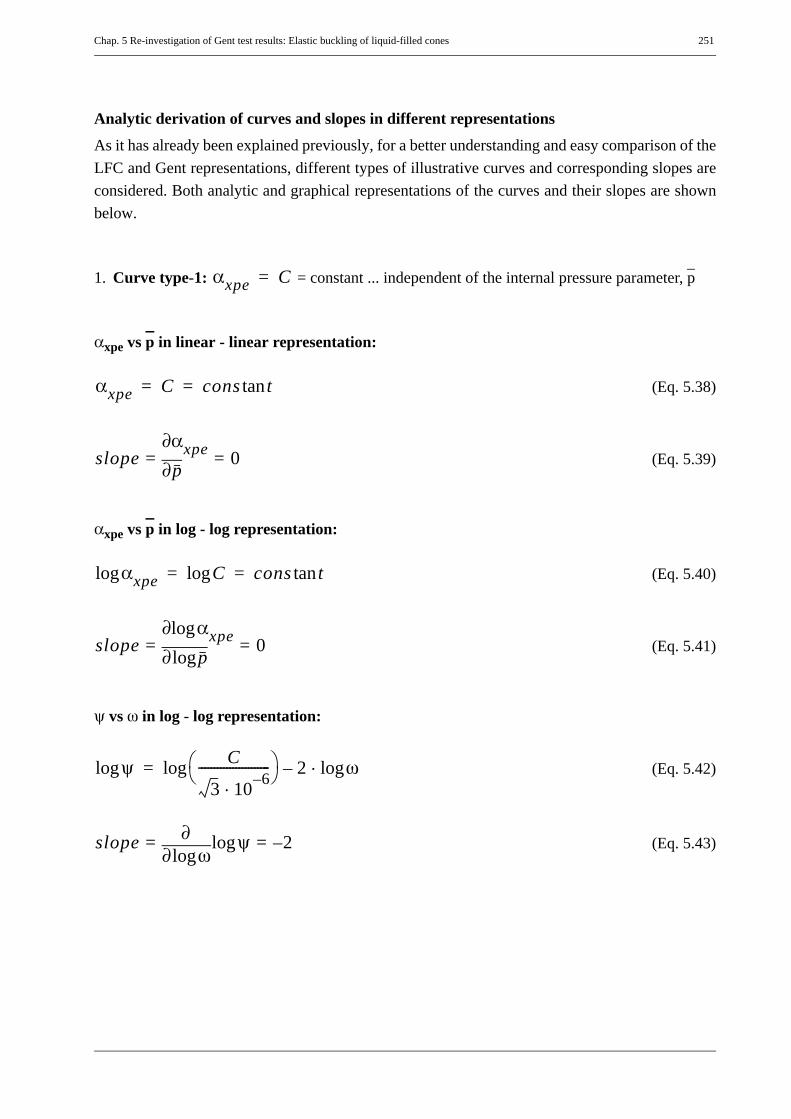
Chap. 5 Re-investigation of Gent test results: Elastic buckling of liquid-filled cones 251
Analytic derivation of curves and slopes in different representationsAs it has already been explained previously, for a better understanding and easy comparison of theLFC and Gent representations, different types of illustrative curves and corresponding slopes areconsidered. Both analytic and graphical representations of the curves and their slopes are shownbelow.
1. Curve type-1: = constant ... independent of the internal pressure parameter, p
αxpe vs p in linear - linear representation:
(Eq. 5.38)
(Eq. 5.39)
αxpe vs p in log - log representation:
(Eq. 5.40)
(Eq. 5.41)
ψ vs ω in log - log representation:
(Eq. 5.42)
(Eq. 5.43)
αxpe C=
αxpe C cons ttan= =
slope p∂∂αxpe 0= =
αlog xpe Clog cons ttan= =
slope plog∂∂ αlog xpe 0= =
ψlog C
3 10 6–⋅-----------------------⎝ ⎠⎛ ⎞log 2 ωlog⋅–=
slopeωlog∂
∂ ψlog 2–= =

252 Chap. 5 Re-investigation of Gent test results: Elastic buckling of liquid-
2. Curve type-2: ... linear function of the internal pressure parameter, p
αxpe vs p in linear - linear representation:
(Eq. 5.44)
(Eq. 5.45)
αxpe vs p in log - log representation:
(Eq. 5.46)
(Eq. 5.47)
(Eq. 5.48)
(Eq. 5.49)
ψ vs ω in log - log representation:
(Eq. 5.50)
(Eq. 5.51)
(Eq. 5.52)
(Eq. 5.53)
αxpe αo k p⋅+=
αxpe αo k p⋅+=
slope p∂∂αxpe k= =
αlog xpe αo k p⋅+( )log=
slope plog∂∂ αlog xpe 1
1αo
k p⋅----------+
-------------------= =
slopep ∞–→loglim slope
p 0→lim 0==
slopep ∞→loglim slope
p ∞→lim 1.0==
ψlog k h'r1-----⋅
αo
3 10 6– ω2⋅ ⋅----------------------------------+
⎝ ⎠⎜ ⎟⎛ ⎞
log=
slopeωlog∂
∂ ψlog2– αo⋅
αo 3+ 10 6– k h'r1----- ω⋅ ⋅
2⋅ ⋅
----------------------------------------------------------------= =
slopeω ∞–→loglim slope
ω 0→lim 2–==
slopeω ∞→loglim slope
ω ∞→lim 0==
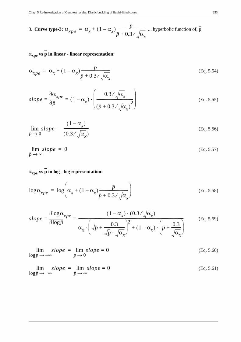
Chap. 5 Re-investigation of Gent test results: Elastic buckling of liquid-filled cones 253
3. Curve type-3: ... hyperbolic function of, p
αxpe vs p in linear - linear representation:
(Eq. 5.54)
(Eq. 5.55)
(Eq. 5.56)
(Eq. 5.57)
αxpe vs p in log - log representation:
(Eq. 5.58)
(Eq. 5.59)
(Eq. 5.60)
(Eq. 5.61)
αxpe αx 1 αx–( ) pp 0.3 αx⁄+-------------------------------+=
αxpe αx 1 αx–( ) pp 0.3 αx⁄+-------------------------------+=
slope p∂∂αxpe 1 αx–( )
0.3 αx⁄
p 0.3 αx⁄+( )2
---------------------------------------⎝ ⎠⎜ ⎟⎜ ⎟⎛ ⎞
⋅= =
slopep 0→lim
1 αx–( )
0.3 αx⁄( )--------------------------=
slopep ∞→lim 0=
αlog xpe αx 1 αx–( ) pp 0.3 αx⁄+-------------------------------+
⎝ ⎠⎜ ⎟⎛ ⎞
log=
slope plog∂∂ αlog xpe 1 αx–( ) 0.3 αx⁄( )⋅
αx p 0.3p αx⋅
----------------------+⎝ ⎠⎜ ⎟⎛ ⎞ 2
⋅ 1 αx–( ) p 0.3αx
----------+⎝ ⎠⎜ ⎟⎛ ⎞
⋅+
---------------------------------------------------------------------------------------------------------------= =
slopep ∞–→loglim slope
p 0→lim 0==
slopep ∞→loglim slope
p ∞→lim 0==

254 Chap. 5 Re-investigation of Gent test results: Elastic buckling of liquid-
ψ vs ω in log - log representation:
(Eq. 5.62)
(Eq. 5.63)
(Eq. 5.64)
(Eq. 5.65)
ψlog Clog– 2 ωlog– αx 1 αx–( ) 1
1 0.3
C h'r1-----ω2 αx⋅⋅
------------------------------------+---------------------------------------------+
⎝ ⎠⎜ ⎟⎜ ⎟⎜ ⎟⎜ ⎟⎜ ⎟⎜ ⎟⎛ ⎞
log+=
slopeωlog∂
∂ ψlog 2 1
1 0.3
C h'r1-----ω2 αx⋅⋅
------------------------------------+---------------------------------------------
0.6 1 αx–( )
0.3αx C h'r1-----ω2 αx⋅⋅+
--------------------------------------------------------⋅+–= =
slopeω ∞–→loglim slope
ω 0→lim 2–==
slopeω ∞→loglim slope
ω ∞→lim 2–==
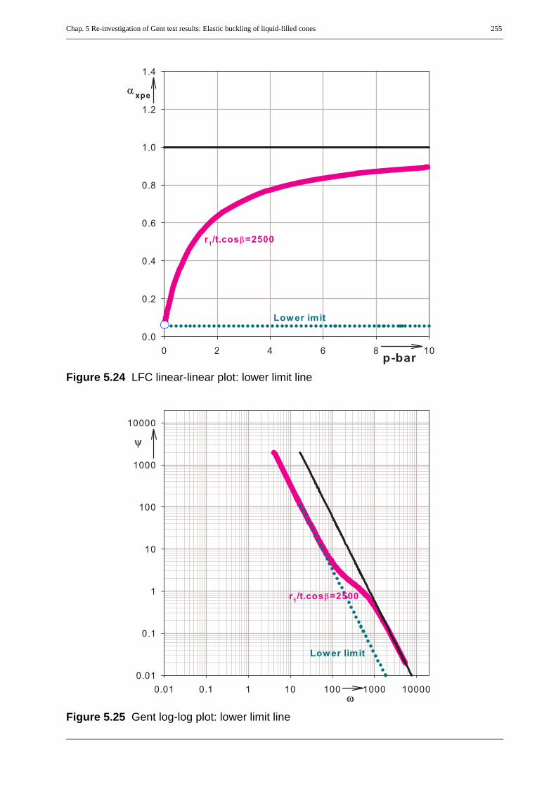
Chap. 5 Re-investigation of Gent test results: Elastic buckling of liquid-filled cones 255
Figure 5.24 LFC linear-linear plot: lower limit line
Figure 5.25 Gent log-log plot: lower limit line
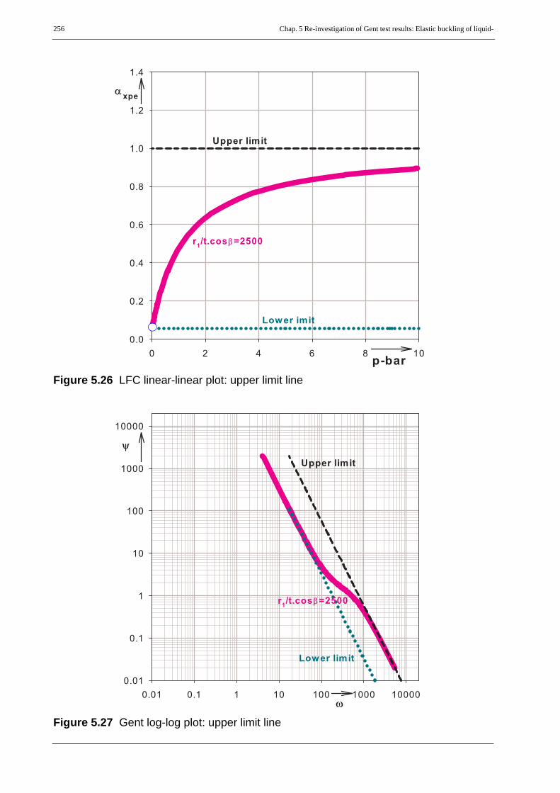
256 Chap. 5 Re-investigation of Gent test results: Elastic buckling of liquid-
Figure 5.26 LFC linear-linear plot: upper limit line
Figure 5.27 Gent log-log plot: upper limit line

Chap. 5 Re-investigation of Gent test results: Elastic buckling of liquid-filled cones 257
Figure 5.28 LFC linear-linear plot: tangent line-1
Figure 5.29 Gent log-log plot: tangent line-1

258 Chap. 5 Re-investigation of Gent test results: Elastic buckling of liquid-
Figure 5.30 LFC linear-linear plot: tangent line-2
Figure 5.31 Gent log-log plot: tangent line-2

Chap. 5 Re-investigation of Gent test results: Elastic buckling of liquid-filled cones 259
Figure 5.32 LFC linear-linear plot: tangent line-3
Figure 5.33 Gent log-log plot: tangent line-3

260 Chap. 5 Re-investigation of Gent test results: Elastic buckling of liquid-
Figure 5.34 LFC log-log plot: all curves
Figure 5.35 Gent log-log plot: all curves

Chap. 5 Re-investigation of Gent test results: Elastic buckling of liquid-filled cones 261
Figure 5.36 LFC log-log plot: inclusion of LFC curve with slenderness value of 100
Figure 5.37 Gent log-log plot: inclusion of LFC curve with slenderness value of 100

262 Chap. 5 Re-investigation of Gent test results: Elastic buckling of liquid-
5.7 Detail re-investigation of test results
Starting the Gent test results anew, a detailed analysis of all the test data, both rejected and accepted(see Table 5.1), has been made taking the slenderness ratio parameter, r1/tcosβ into account. A sep-aration is made between the different material types and different slenderness ratio values. In sub-sequent plots, different solid shapes have been used to represent the type of materials and differentcoloring was used to differentiate between slenderness ratio values. Figure 5.38 and Figure 5.39show the use of the different shapes and colors for the different materials and slenderness ratio val-ues in αxpe - p linear-linear and Gent ψ - ω log-log representations, respectively.
5.7.1 Cleaning the test dataBy cleaning, it means that dropping those test data that are either not practical in civil engineeringconstruction or having any kind of defect. Cleaning of the test data has been made in a step-by-stepprocedure. Figure 5.40 and Figure 5.41 show a comparison between αxpe - p linear-linear and αxpe- p log-log representations, respectively, of the curves and all test data points including those to becleaned out.
extreme β angle ranges
the lower and upper extreme β values have been dropped since they are not practical apex-half an-gles for civil engineering liquid-filled conical shells. This means that only the β = 20° - 60° rangehas only be considered, the remaining being all 10° or 75°. See Figure 5.42 and Figure 5.43.
global tilting failuresthis is a different buckling phenomenon where a global bending type loading is included, resultingin non uniform meridional compression (may even be compression on one side and tension on theother side) on the base of the cone. This type of failure happened mostly for the cones with rela-tively narrow bases and/or high h’tanβ/r1 values. A very small deviation from the upright positionof the cone may lead to such type of failures in narrow cone-bases and relatively high liquid depths.See Figure 5.44 and Figure 5.45.
’bad’ test configurationsthis group includes test data points which had faulty experimental setup, cones with overlappingmeridional seam in the critical zone of buckling, and cones failed with in the supporting device.See Figure 5.46 and Figure 5.47.

Chap. 5 Re-investigation of Gent test results: Elastic buckling of liquid-filled cones 263
sliding bottom boundary conditionthese are the cones where their bottom edges were allowed to deform freely perpendicular to themeridian and are dropped because they are not practical. See Figure 5.48 and Figure 5.49.
clamped bottom boundary conditionthese are the tests which were completely clamped at their bottom edge. They are dropped becausethey are few in number and they need different treatment. See Figure 5.50 and Figure 5.51. How-ever, they will be re-considered later when discussing the effect of fixed bottom boundary condi-tions, Figure 5.67 to Figure 5.73.

264 Chap. 5 Re-investigation of Gent test results: Elastic buckling of liquid-
Figure 5.38 Linear-linear plot: different material types and different slenderness values
Figure 5.39 Gent log-log plot: different material types and different slenderness values
SLENDERNESS: r1/tcosβ
BLUE . . . 77 - 250CYAN . . . 250 - 500GREEN . . . 500 - 750ORANGE . . . 750 - 1000PINK . . . 1000 - 1500RED . . . 1500 - 2500DARK RED . . . 2500 - 3500
MATERIAL. . . Aluminium. . . Steel. . . Brass. . . Mylar

Chap. 5 Re-investigation of Gent test results: Elastic buckling of liquid-filled cones 265
Figure 5.40 LFC linear-linear plot: cleaning out of the test data
Figure 5.41 LFC log-log plot: cleaning out of the test data
Cleaning out. . . β = 10°. . . β = 75°. . . global tilting. . . bad tests. . . sliding bottom. . . clamped bottom

266 Chap. 5 Re-investigation of Gent test results: Elastic buckling of liquid-
Figure 5.42 LFC linear-linear plot: cleaning out tests with extreme apex half-angles
Figure 5.43 LFC log-log plot: cleaning out tests with extreme apex-half angles

Chap. 5 Re-investigation of Gent test results: Elastic buckling of liquid-filled cones 267
Figure 5.44 LFC linear-linear plot: cleaning out tests which failed sideways (global tilting)
Figure 5.45 LFC log-log plot: cleaning out tests which failed sideways (global tilting)
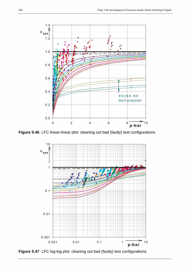
268 Chap. 5 Re-investigation of Gent test results: Elastic buckling of liquid-
Figure 5.46 LFC linear-linear plot: cleaning out bad (faulty) test configurations
Figure 5.47 LFC log-log plot: cleaning out bad (faulty) test configurations

Chap. 5 Re-investigation of Gent test results: Elastic buckling of liquid-filled cones 269
Figure 5.48 Linear-linear plot: cleaning out tests with sliding bottom boundary condition
Figure 5.49 LFC log-log plot: cleaning out tests with sliding bottom boundary condition

270 Chap. 5 Re-investigation of Gent test results: Elastic buckling of liquid-
Figure 5.50 Linear-linear plot: cleaning out tests with clamped boundary condition
Figure 5.51 LFC log-log plot: cleaning tests with clamped bottom boundary condition

Chap. 5 Re-investigation of Gent test results: Elastic buckling of liquid-filled cones 271
5.7.2 Detailed study of test results based on the slenderness ratioparameter (r1/tcosβ)
The cones tested in the Gent experiment cover a very wide slenderness ratio range r1/tcosβ = 77 -3760. In this detailed study, the test data are separated according to their slenderness ratio andgrouped them in seven groups having smaller slenderness ratio ranges of 100-250 (includes alsothose less than 100), 250-500, 500-750, 750-1000, 1000-1500, 1500-2500, and 2500-3500 (in-cludes also those larger than 3500). Besides, for each bounding slenderness ratio value of the testresults, LFC curves with fabrication tolerance quality classes A and C are used for comparison pur-poses. Investigations of the different slenderness ratio ranges of the test data have been done oneafter the other. For a better view, specially for small p values, and parallel comparison of the re-sults, the αxpe - p log-log representation is plotted in addition to the αxpe - p linear-linear represen-tation.
The previously cleaned out results and the Gent lower-bounding curves are also included in eachplot for the sake of clarity and better comparison. An overall explanation of the plots is shown inTable 5.3.
Figure No. r1/tcosβ range of test data points
r1/tcosβ of group-bounding LFC curves
quality classes considered
Remark
Figure 5.52 77 - 250 100 and 250
A and C
(1) the LFC lower-bounding curves on each plot, when seen from top down, are class-A of the smaller slenderness, class-A of the larger slenderness, class-C of the smaller slenderness, and class-C of the larger slenderness, respectively.
(2) the gray shading is between quality classes A and C of the slender LFC curve in each group
(3) the Gent bounding curves are com-puted for h’/r1 values of 2.0 and 8.0
Figure 5.53Figure 5.54 250 - 500 250 and 500Figure 5.55Figure 5.56 500 - 750 500 and 750Figure 5.57Figure 5.58 750 - 1000 750 and 1000Figure 5.59Figure 5.60 1000 - 1500 1000 and 1500Figure 5.61Figure 5.62 1500 - 2500 1500 and 2500Figure 5.63Figure 5.64 2500 - 3760 2500 and 3500Figure 5.65
Table 5.3 Summary of figures (Figure 5.52 - Figure 5.65)

272 Chap. 5 Re-investigation of Gent test results: Elastic buckling of liquid-
Figure 5.52 LFC linear-linear plot: r1/tcosβ = 77 - 250
Figure 5.53 LFC log-log plot: r1/tcosβ = 77 - 250
A
C

Chap. 5 Re-investigation of Gent test results: Elastic buckling of liquid-filled cones 273
Figure 5.54 LFC linear-linear plot: r1/tcosβ = 250 - 500
Figure 5.55 LFC log-log plot: r1/tcosβ = 250 - 500
A
C

274 Chap. 5 Re-investigation of Gent test results: Elastic buckling of liquid-
Figure 5.56 LFC linear-linear plot: r1/tcosβ = 500 - 750
Figure 5.57 LFC log-log plot: r1/tcosβ = 500 - 750
A
C

Chap. 5 Re-investigation of Gent test results: Elastic buckling of liquid-filled cones 275
Figure 5.58 LFC linear-linear plot: r1/tcosβ = 750 - 1000
Figure 5.59 LFC log-log plot: r1/tcosβ = 750 - 1000
A
C

276 Chap. 5 Re-investigation of Gent test results: Elastic buckling of liquid-
Figure 5.60 LFC linear-linear plot: r1/tcosβ = 1000 - 1500
Figure 5.61 LFC log-log plot: r1/tcosβ = 1000 - 1500
A
C

Chap. 5 Re-investigation of Gent test results: Elastic buckling of liquid-filled cones 277
Figure 5.62 LFC linear-linear plot: r1/tcosβ = 1500 - 2500
Figure 5.63 LFC log-log plot: r1/tcosβ = 1500 - 2500
A
C

278 Chap. 5 Re-investigation of Gent test results: Elastic buckling of liquid-
Figure 5.64 LFC linear-linear plot: r1/tcosβ = 2500 - 3760
Figure 5.65 LFC log-log plot: r1/tcosβ = 2500 - 3760
A
C

Chap. 5 Re-investigation of Gent test results: Elastic buckling of liquid-filled cones 279
5.8 Detailed comparison based on the LFC-elasticbuckling limits
All the discussions so far were for an imperfection reduction factor which is applied to the casewhere the perfect elastic linear buckling (LBA) strength is given by the horizontal line αxpe = 1.0,i.e. when the perfect elastic buckling stress, σx,LBA, is scaled down to the classical reference buck-ling stress, σx,Rcr. However, unlike that of an axially compressed and internally pressurized cylin-drical shell where the internal pressurization does not have a significant effect on the perfect elasticlinear buckling strength (αxpe = 1.0), liquid-filled conical shells’ LBA strength vary with the valueof the internal pressure parameter p. Therefore, as has been previously discussed, LFC imperfec-tion reduction factors should be applied to the varying LBA buckling strength (with varying p) ofthe liquid-filled conical shells instead of the αxpe = 1.0 line.
As a result, all the LFC curves that have been used for the different slenderness ratios of each groupand representing the elastic buckling strength of the imperfect liquid-filled conical shells shouldall be scaled up in line with the LBA results of the LFC. Figure 5.66 shows the LFC LBA curvesfor the thicker and thinner shells (for both fixed and pinned bottom) in the grouping, the test datapoints and Gent curves.
This up scaling is applied to each r1/tcosβ group values discussed so far and is shown in Figure5.67 to Figure 5.73. To avoid congestion, only the LFC curves representing the slender shell ineach group with quality class-C is considered. Both the “fixed” and “pinned” bottom boundarycondition cases are shown. The gray shaded area shows the region between the upper (perfect elas-tic) and lower (imperfect elastic) bounding curves of the slender shell in each group with “pinned”bottom boundary condition.
It can be seen from the plots that about 25 test data points lie outside this range, below the corre-sponding lower (imperfect elastic) curves for quality class-C. A comparison of the imperfectionamplitudes in these test specimens and that of quality class-C has been made as shown in Table 5.4and it turns out that 22 of the test data points have imperfection amplitudes larger than that permit-ted for quality class-C and hence can not be compared with the strength curves of that specificgroup. These test data points are shown in all the plots with an overlying bigger circular rings.
All the clamped bottom test data (shown with square shaped hollow symbols) have also been in-cluded in the respective group plots. These data points should be compared with their correspond-ing strength curves, i.e. they should be compared with the “FIX” curves.

280 Chap. 5 Re-investigation of Gent test results: Elastic buckling of liquid-
Figure 5.66 LFC linear-linear plot: LBA curves, Gent bounding curves & test data points
FIXPIN
3500100

Chap. 5 Re-investigation of Gent test results: Elastic buckling of liquid-filled cones 281
r1/tcosβ range of test data points
r1/tcosβ value p αxpe
test normalized imperfec-tion amplitude, wo/t
quality class-C normalized imperfection amplitude, Δwk/t
77 - 250 97.90 0.00102 0.11976 0.802 0.618192.73 0.00249 0.20957 1.649 0.868243.62 0.00302 0.12902 1.719 0.976
250 - 500 288.66 0.00555 0.11462 1.609 1.062303.58 0.00652 0.14587 2.095 1.089
500 - 750 726.63 0.66857 0.50642 4.454 1.685735.64 0.65632 0.49678 4.589 1.695
750 - 1000 889.38 1.00545 0.61289 2.942 1.864917.68 1.03357 0.61306 4.100 1.893
1000 - 1500 1079.37 1.05528 0.58472 4.908 2.0531108.42 1.09798 0.57061 4.351 2.0811195.30 1.41317 0.62181 3.622 2.1611330.15 1.62068 0.70918 4.609 2.2791344.37 1.66048 0.66509 6.283 2.2921367.01 1.50640 0.57150 6.056 2.3111471.93 3.10387 0.88680 6.726 2.3981491.08 3.03136 0.79619 5.852 2.413
1500 - 2500 1967.31 4.10510 0.81113 7.457 2.7721981.56 3.94071 0.80790 9.263 2.7822020.80 4.18952 0.88842 7.768 2.810
2500 - 3760 3037.87 7.00335 1.01484 7.917 3.4453293.50 5.86658 0.93006 4.856 3.587
Table 5.4 Comparison of test imperfection amplitudes vs. LFC quality class-C imperfection amplitudes

282 Chap. 5 Re-investigation of Gent test results: Elastic buckling of liquid-
Figure 5.67 LFC curve: r1/tcosβ = 250; pinned and fixed bottom
Figure 5.68 LFC curve: r1/tcosβ = 500; pinned and fixed bottom
FIX PIN
ECyl u.l.
Imp-range(αxpe)
FIX PIN
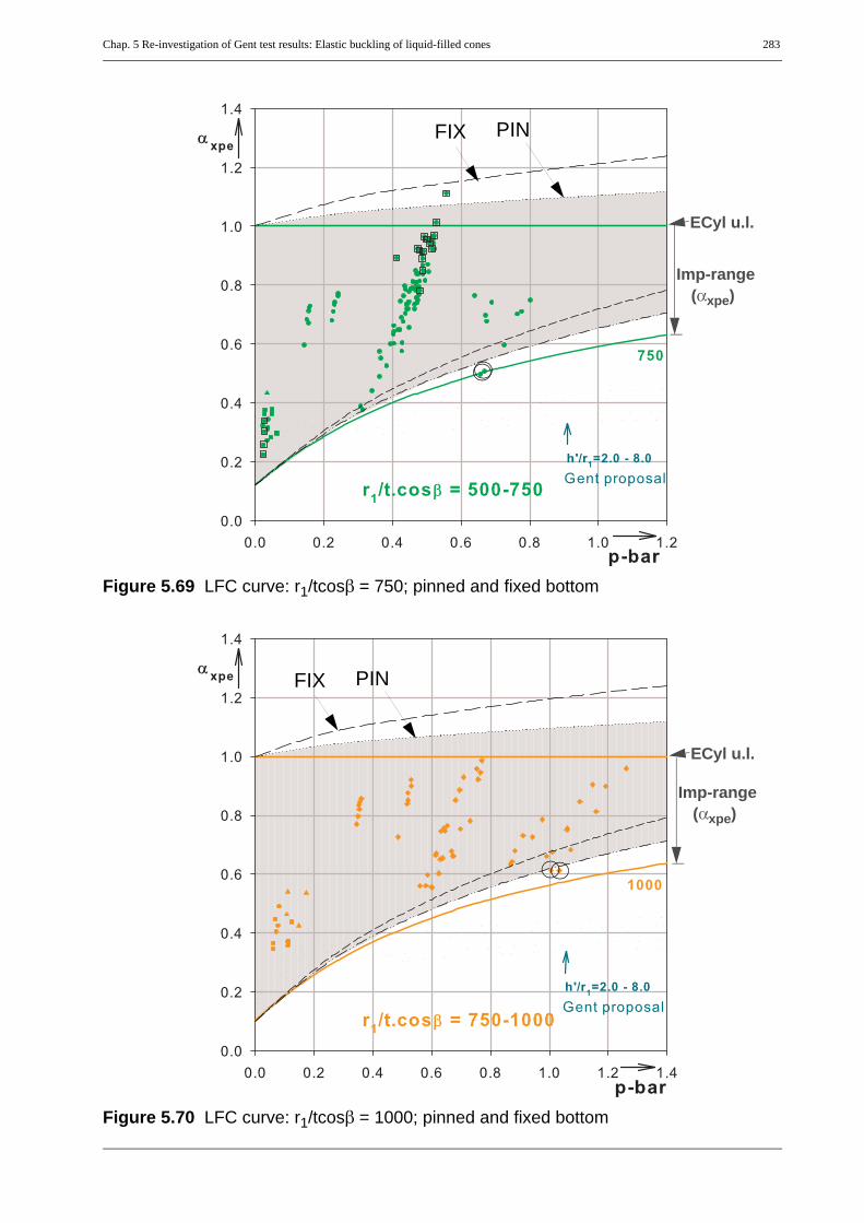
Chap. 5 Re-investigation of Gent test results: Elastic buckling of liquid-filled cones 283
Figure 5.69 LFC curve: r1/tcosβ = 750; pinned and fixed bottom
Figure 5.70 LFC curve: r1/tcosβ = 1000; pinned and fixed bottom
ECyl u.l.
Imp-range(αxpe)
FIX PIN
ECyl u.l.
Imp-range(αxpe)
FIX PIN

284 Chap. 5 Re-investigation of Gent test results: Elastic buckling of liquid-
Figure 5.71 LFC curve: r1/tcosβ = 1500; pinned and fixed bottom
Figure 5.72 LFC curve: r1/tcosβ = 2500; pinned and fixed bottom
ECyl u.l.Imp-range
(αxpe)
FIX PIN
FIX PIN
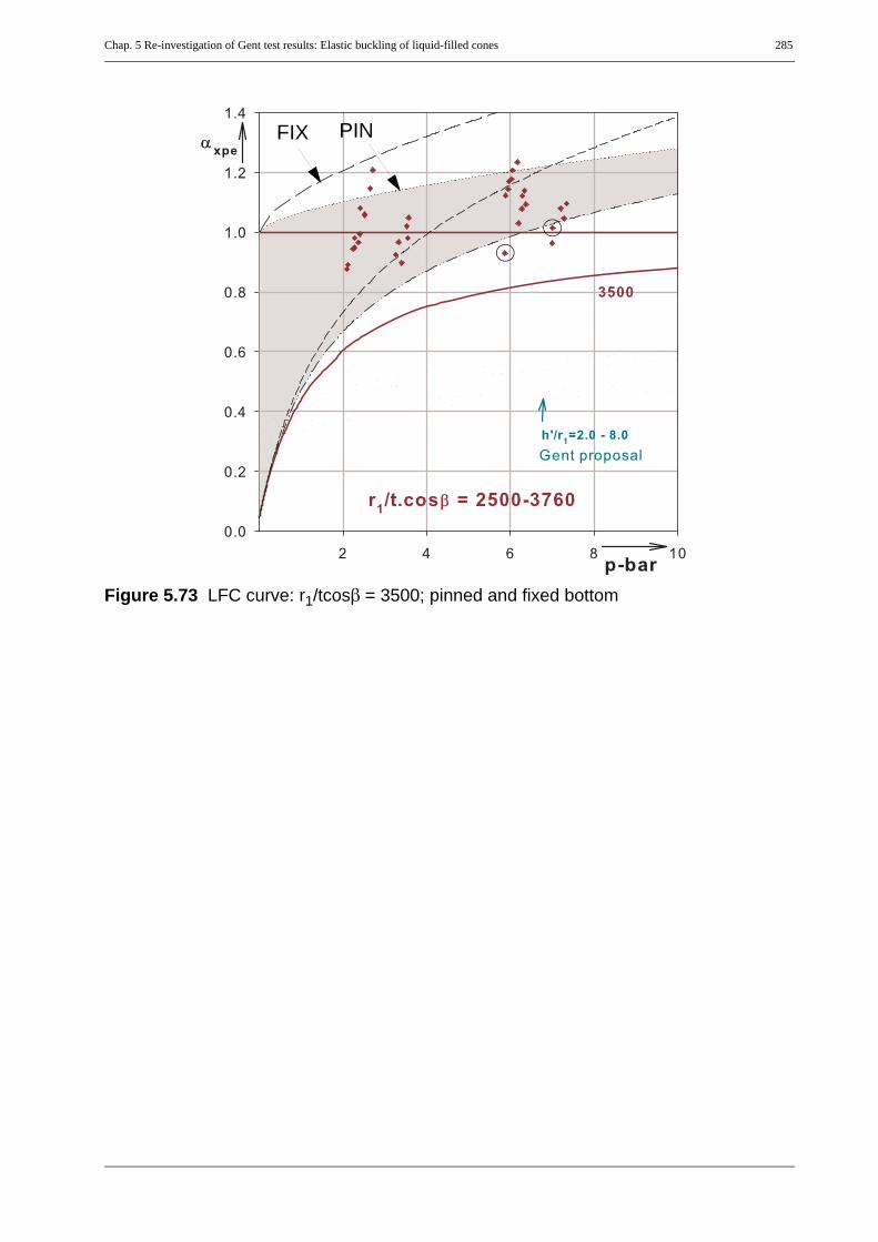
Chap. 5 Re-investigation of Gent test results: Elastic buckling of liquid-filled cones 285
Figure 5.73 LFC curve: r1/tcosβ = 3500; pinned and fixed bottom
FIX PIN

286 Chap. 5 Re-investigation of Gent test results: Elastic buckling of liquid-
5.9 LFC-imperfection reduction factor
From the detailed investigation of the Gent test results and an interpretation which is in line withthe stress design and LBA-MNA buckling design principles, liquid-filled conical shells have thesame strength reduction due to imperfections as those of cylindrical shells under axial compressionand internal pressure.
(Eq. 5.66)
For verification purposes, the Belgium and Canada collapsed steel water towers have been ana-lyzed and checked as follows.
5.9.1 Belgium collapsed steel water towerThe shell had two cone segments, lower and upper, with different thicknesses and apex-half angles.A complete buckling check has been made at the most critical locations of the tower: the lowercone base and upper cone base (junction between the two cones). The analyses made are summa-rized in Table 5.5. Additional comments and conclusions are also given at the end of this section.
Basic geometry, loading, and material variables (dimensions used: kN, mm)
lower cone base: upper cone base:
h’U = 6960 h’U = 6210
r1 = 2920 r1 = 3794
β = 49.4 β = 51.0
t = 15.0 t = 8.0
γ' = 9.81*10-9 ... the only loading considered, i.e. shell own weight and roof loading excluded
Material properties (for both cones)
E = 196.2
fy = 0.236 (will not be used in the present elastic buckling check!)
ν = 0.3
αxpe LFC, αxpe CYLINDER,≈

Chap. 5 Re-investigation of Gent test results: Elastic buckling of liquid-filled cones 287
5.9.2 Canada collapsed steel water towerThe shell had three cone segments: lowest, lower, and upper with different thicknesses but sameapex half angle and a cylinder topping. The liquid surface level during buckling was within the cy-lindrical topping. The lowest, short (215.0 mm long) and thick (19.05 mm thickness), cone acts asa transition ring connecting the base plate and the lower cone. A complete buckling check has beenmade at two different critical locations: the lower cone base (junction between the lowest and lowercones) and upper cone base (junction between the lower and upper cones). The analyses made aresummarized in Table 5.5. Additional comments and conclusions are also given at the end of thissection.
Basic geometry, loading, and material variables (dimensions used: kN, mm)
lower cone base: upper cone base:
h’U = 8781.0 ... for σθ,1 computation, existing liquid depth h’U = 6825.2 ... for σθ,1 computation
h’U = 8313.17...for σx,1 computation, replaced by full coneh’U = 6357.37...for σx,1 computation
r1 = 5105.0 r1 = 7060.8
β = 45.0 β = 45.0
t = 11.11 t = 9.525
γ' = 9.81*10-9 ... the only loading considered, i.e. shell own weight and roof loading excluded
Material properties
lower cone base: upper cone base:
E = 255 E = 214
fy = 0.297 (will not be used in the elastic buckling check!) fy = 0.462
ν = 0.3 ν = 0.3
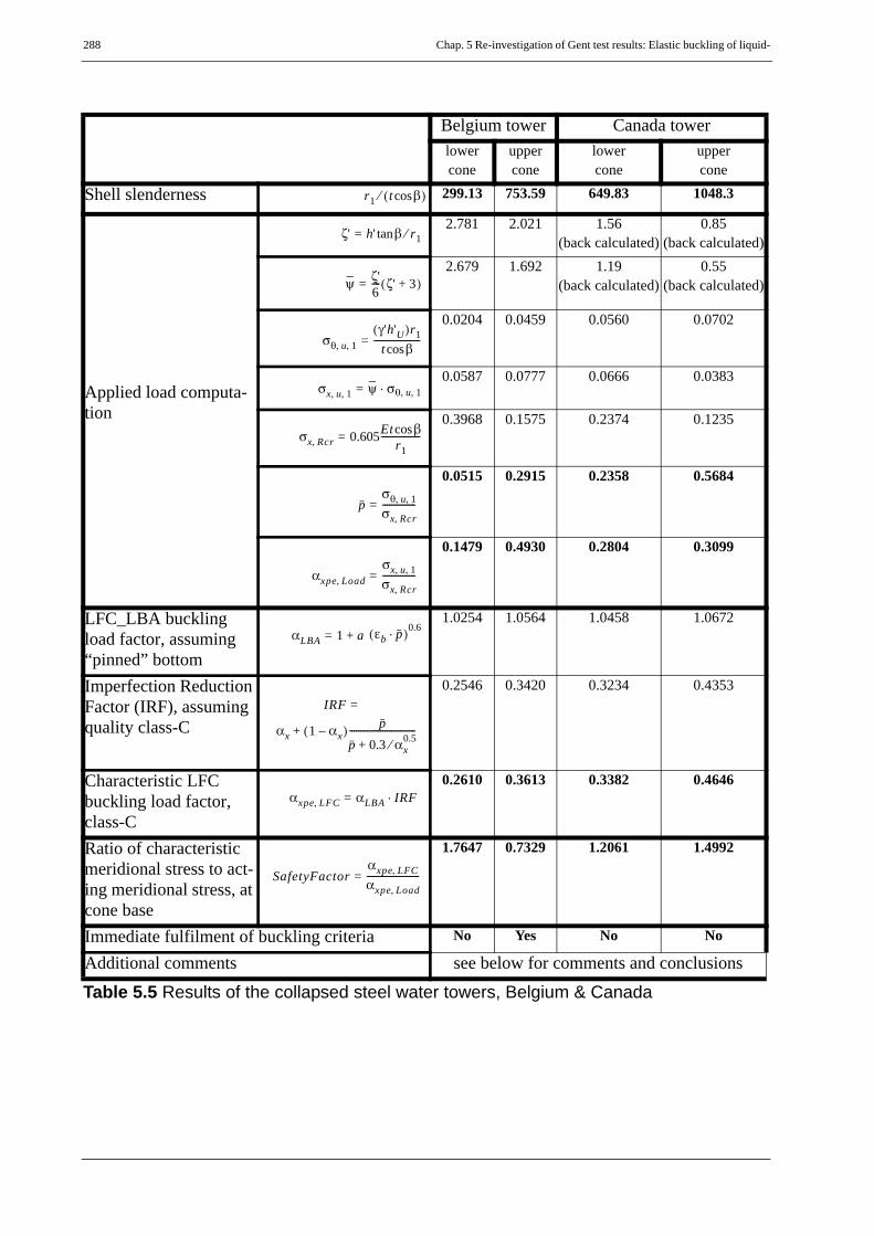
288 Chap. 5 Re-investigation of Gent test results: Elastic buckling of liquid-
Belgium tower Canada towerlowercone
uppercone
lowercone
uppercone
Shell slenderness 299.13 753.59 649.83 1048.3
Applied load computa-tion
2.781 2.021 1.56(back calculated)
0.85(back calculated)
2.679 1.692 1.19(back calculated)
0.55(back calculated)
0.0204 0.0459 0.0560 0.0702
0.0587 0.0777 0.0666 0.0383
0.3968 0.1575 0.2374 0.1235
0.0515 0.2915 0.2358 0.5684
0.1479 0.4930 0.2804 0.3099
LFC_LBA buckling load factor, assuming “pinned” bottom
1.0254 1.0564 1.0458 1.0672
Imperfection Reduction Factor (IRF), assuming quality class-C
0.2546 0.3420 0.3234 0.4353
Characteristic LFC buckling load factor, class-C
0.2610 0.3613 0.3382 0.4646
Ratio of characteristic meridional stress to act-ing meridional stress, at cone base
1.7647 0.7329 1.2061 1.4992
Immediate fulfilment of buckling criteria No Yes No No
Additional comments see below for comments and conclusions
Table 5.5 Results of the collapsed steel water towers, Belgium & Canada
r1 t βcos( )⁄
ζ' h' βtan r1⁄=
ψ ζ'6---- ζ' 3+( )=
σθ u 1, ,γ'h'U( )r1t βcos
---------------------=
σx u 1, , ψ σ⋅ θ u 1, ,=
σx Rcr, 0.605Et βcosr1
------------------=
pσθ u 1, ,σx Rcr,---------------=
αxpe Load,σx u 1, ,σx Rcr,---------------=
αLBA 1 a+= εb p⋅( )0.6
IRF =
αx 1 αx–( ) pp 0.3 αx
0.5⁄+------------------------------+
αxpe LFC, αLBA IRF⋅=
SafetyFactorαxpe LFC,αxpe Load,------------------------=
Chap. 5 Re-investigation of Gent test results: Elastic buckling of liquid-filled cones 289
Additional comments on the steel water tower collapse casesFrom the above computations, the buckling phenomenon of the Belgium collapsed steel water tow-er should have been started on the base of the thin upper cone. The immediate fulfilment of thebuckling criteria, even without considering any additional roof loading, own weight and load fac-tor, indicates the fact that there was no any know-how about the possible occurrence of bucklingat the time.
In the case of the Canada collapsed steel water tower, the safety factor (1.2061) obtained for thelower cone (without considering the loads coming from the tank wall and roofing) is too small toaccount for all (loading, boundary conditions, workmanship, material etc.) types of uncertainties.When the additional loading coming from the wall and roof ( = 650 kN) is considered, the resultingadditional meridional stress at the base of the cone is 0.0026, raising the value for αxpe,load to0.2914 and reducing the safety factor to 1.16. Therefore, if the collapse was really initiated bybuckling, the buckling phenomenon of the Canada collapsed steel water tower should have beenstarted on the base of the lower cone.
The loading situations during failure of both the Belgium upper cone and Canada lower cone seg-ments already discussed are plotted in the classical critical buckling stress related pressure repre-sentation (αxpe - p representation) along with the laboratory test results which lie on the same groupof slenderness ratio values as shown in Figure 5.74.

290 Chap. 5 Re-investigation of Gent test results: Elastic buckling of liquid-
Figure 5.74 Water tower collapse situations & laboratory test results: r1/tcosβ = 500-750
Belgium
Canada
FIX PIN
Chap. 5 Re-investigation of Gent test results: Elastic buckling of liquid-filled cones 291
5.10Summary and Conclusion
• Shell Slenderness parameter, r1/tcosβ, plays the most important role in every shell bucklingphenomenon. The buckling strength of a shell depends on its slenderness ratio. The slender-ness ratio parameter of conical shells is a function of the base radius, wall thickness, andapex half-angle of the cone and is given by r1/tcosβ
• First, a rough comparison of the buckling behavior of “tip” compressed cones with thebuckling behavior of an axially compressed internally unpressurized cylindrical shells; andliquid-filled conical shells with axially compressed internally pressurized cylindrical shellswas made.
• Second, advanced judgment based on LFC-specific LBA behavior and consistent withcylinder imperfection reduction (αxpe). The liquid-filled conical shells, because of the fastdecaying meridional membrane section force distribution, have a higher LBA strength thancylindrical shells.
• The elastic buckling nature and the buckling strength reduction due to geometric imperfec-tions of conical and cylindrical shells is similar.
• The Gent experimental results, according to the new interpretation and representation, showthe quality of tests done. However, the Gent interpretation was not as clear as it is done inthis study, to say the least. For example, the data points which are above the Gent perfectbounding lines were interpreted as might be caused by “unintended rotational restraint atthe cone base instead of strictly simple support”. The points, however, are high up becauseof the favorable buckling nature of liquid-filled conical shells. This fact has already beenshown.
• At very low internal pressures, as p approaches zero (ψ very large), a straight forward limitfor the buckling strength of liquid-filled conical shells (same as for cylindrical shells) canbe observed.
• At medium internal pressures, liquid-filled conical shells offer higher stabilizing effectdue to internal pressurization than suggested by Gent proposal, i.e. the Gent proposal is tooconservative for medium pressure values.
• Based on the new way of interpreting the test results, recommendations are made for thedesign of liquid-filled conical shells
• At high internal pressures, where plastic interaction is expected, elephant’s-foot type buck-ling failure may happen close to the boundary and has already been investigated.
• Few additional specific numerical confirmation would be of interest and helpful.

292 Chap. 5 Re-investigation of Gent test results: Elastic buckling of liquid-

Chap. 6 Re-investigation of Gent test results: Mercury-filled steel cones 293
6
Re-investigation of Gent test results:
Mercury-filled steel cones

294 Chap. 6 Re-investigation of Gent test results: Mercury-filled steel cones
6.1 Investigation of Gent mercury-test results
6.1.1 Gent mercury-test dataFollowing the extensive number of tests (more than 800) on elastic buckling strength assessmentusing water filling, relatively few (about 40, out of which only 38 are accepted) tests were madeusing mercury filling to measure the elastic-plastic buckling loads of liquid-filled thin-walled steelconical shells. The idea of using mercury filling as loading (instead of water) was to make use ofits heavier specific weight in producing higher internal pressurization.
All the tests performed were made using steel cones with smaller radius of r1 = 10 cm, apex-halfangle of β = 40° and varying the thickness between 0.05 cm and 0.1 cm. In terms of the shell slen-derness ratio, the cones tested varies from r1/tcosβ = 130 to 250. The material properties measuredwere modulus of elasticity E = 20000 kN/cm2, Poisson’s ratio ν = 0.29, and uni-axial yield strengthfy varying between 15.3 kN/cm2 and 33.3 kN/cm2. Imperfection amplitudes were measured usinga length stick in a wide region (sometimes even wider) alongthe meridian. The liquid-depth level at buckling was measured and recorded.
6.1.2 Current investigationIn the current investigation, the ultimate measured liquid-depth in terms of which the magnitudeof the meridional membrane compressive stress and circumferential tensile stress at the base of thecone are computed step-by-step as follows:
(Eq. 6.1)
(Eq. 6.2)
(Eq. 6.3)
(Eq. 6.4)
The intensity of internal pressurization is therefore inversely proportional to the liquid-depth mea-sured when buckling occurs. All the above quantities have been calculated for all the mercury testsmade and the results are compared with the elastic-plastic characteristic buckling strength comput-ed using the interaction expression discussed above. As far as plasticity effect is concerned, yieldstrength related representations are used for graphical comparison of the results. The 38 mercury
3.6 r1 t βcos( )⁄ 15 r1 t βcos( )⁄
ζ' h' βtan⋅r1
--------------------=
ψ ζ'6---- 3 ζ'+( )=
σx 1,γ'h'r1t βcos-------------- ψ⋅=
σθ 1,γ'h'r1t βcos--------------
σx 1,
ψ----------= =

Chap. 6 Re-investigation of Gent test results: Mercury-filled steel cones 295
tests are re-grouped into three categories depending on the shell slenderness ratio value. The firstgroup comprises of cones with shell slenderness ratio values varying between r1/tcosβ = 130 and150, the results of which are plotted in the pressure representation shown in Figure 6.1. The secondand third group comprise of cones with shell slenderness ratio values varying from r1/tcosβ = 165to 190 and r1/tcosβ = 220 to 250, the results of which are shown in Figure 6.2 and Figure 6.3, re-spectively. The imperfection amplitudes measured during testing are compared with the maximumallowed for different fabrication quality class as recommended by EN 1993-1-6 and classificationhas been done accordingly. Different symbols are used for the different quality classes as shownin the respective figures. Quality class-D in this discussion refers to those measured imperfectionamplitudes which are higher than that of class-C. In each of the plots the elastic and elastic-plasticcharacteristic buckling strengths of conical shells with the two bounding shell slenderness valuesof each group are included for fabrication tolerance quality classes A&C. Besides, the elastic-plas-tic interaction with membrane Mises plasticity using the basic plastic buckling parameters (as hasbeen done for the cylindrical shell) is shown for comparison purposes.
Despite the above discussion and comparison of results, it should be noted here that the only im-perfection information measured and recorded during testing was the amplitude (maximum de-pression from a measuring gauge) and nothing has been reported about the imperfection shape,imperfection wavelength, and exact imperfection location along the meridian. Even the imperfec-tion amplitude reported for each test setup might have been as far located as (theregion assessed during testing) while the buckling (elastic or elastic-plastic) phenomenon is morelikely to happen in the bottom one-quarter of this length. This fact can clearly be seen from theinconsistency in the imperfection amplitudes measured and the buckling strength obtained duringtesting, i.e. a conical shell with an imperfection amplitude less than that allowed for quality class-A (close to perfect cone) failed at a load much lower than a similar cone having class-C imperfec-tion amplitude; and a conical shell with an imperfection amplitude much larger than that allowedfor quality class-C failed at a load as high as that of class-A. Generally speaking, the tests per-formed were not that consistent, to say the least, and much can not be drawn from the test results.Moreover, even though mercury filling has been used to make use of its heavier specific weight inproducing higher internal pressurization, it was not as high as it might have been intended as theabove discussion and re-examining of the test results reveal, see Figure 6.1 to Figure 6.3. In con-clusion, a maximum of three tests would have been enough to get the same information obtainedfrom performing all the 40 expensive tests which all result in similar and very low internal pres-surization, i.e. all tests were done for a (nearly) constant big ψ value showing that the effect of in-ternal pressurization on bi-axial plasticity can not be seen.
15 r1 t βcos( )⁄

296 Chap. 6 Re-investigation of Gent test results: Mercury-filled steel cones
Figure 6.1 Gent mercury test data points r1/tcosβ = 130 - 150
Fabrication quality class. . . class-A. . . class-B. . . class-C. . . class-D
μ pRtfy-------=
σULSfy
--------------
MNA
imperfect
A
C
C
elastic_LFC
imperfectelastic_CYL
interaction_CYL
interaction_LFC membraneMises
r1/t = 150

Chap. 6 Re-investigation of Gent test results: Mercury-filled steel cones 297
Figure 6.2 Gent mercury test data points r1/tcosβ = 165 - 190
Fabrication quality class. . . class-A. . . class-B. . . class-C. . . class-D
μ pRtfy-------=
σULSfy
--------------
MNA
imperfect
A
C
Celastic_LFC
imperfectelastic_CYL
interaction_CYL
interaction_LFCmembraneMises
r1/t = 165
r1/t = 190
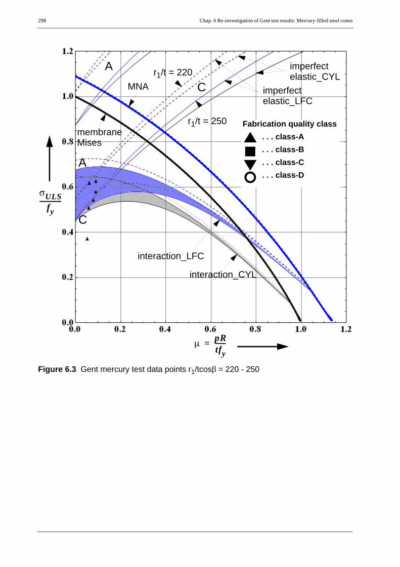
298 Chap. 6 Re-investigation of Gent test results: Mercury-filled steel cones
Figure 6.3 Gent mercury test data points r1/tcosβ = 220 - 250
Fabrication quality class. . . class-A. . . class-B. . . class-C. . . class-D
μ pRtfy-------=
σULSfy
--------------
MNA imperfect
A
C
A
Celastic_LFC
imperfectelastic_CYL
interaction_CYL
interaction_LFC
membraneMises
r1/t = 220
r1/t = 250

Chap. 6 Re-investigation of Gent test results: Mercury-filled steel cones 299
6.2 Geometrically and materially nonlinearanalysis of imperfect cones
Following the laboratory tests using mercury filling, Ramm (1991) made few nonlinear numericalanalyses using axisymmetric shell model for pre-specified liquid-depths, three of which were takenfrom the Gent mercury tests. These three specific cases were modelled as used in the laboratorysetup, i.e. informations concerning cone geometry, material, loading, bottom boundary condition,and imperfection amplitude were adopted from the report of the laboratory tests. Since there are noinformations about the shape, wavelength, and along-meridian location of the measuredimperfections, Ramm considered a linear buckling eigenmode-affine imperfection and madegeometrically and materially nonlinear numerical analyses of the imperfect cones to compare hisresults with the results obtained from laboratory testing. He obtained 1% difference for two of thecones and 5% difference for the third cone concluding that there is a good correlation between thetest results and his numerical analyses. It should, however, be recalled that the use of an LBAeigenmode-affine imperfection to simulate the laboratory test imperfection conditions may not befair (to say the least) and the 1% and 5% correlation obtained should be a chance occurence.
A nonlinear numerical analyes have been made in the current work for one of the cones tested inthe laboratory and also that analysed by Ramm (F275SAD), on one hand, to confirm Ramm’sresults and, on the other broader hand, to make an imperfection sensitivity study of the mercury-filled cone to an LBA eigenmode-affine imperfection by varying the imperfection amplitude.Besides, materially nonlinear analysis and geometrically & materially nonlinear analysis of theperfect cone will be compared to that of Ramm’s corresponding results. It should, however, againbe noted that an LBA eigenmode-affine imperfection shape is very far from the possibleimperfection shape in laboratory experiments and, generally speaking, the results obtained fromthe numerical analyses will have no direct relation with the result obtained from testing. The detailsof the cone under consideration are as follows:
Geometry: r1 = 10 cm; t = 0.05166 cm; β = 40°; h’ = 60 cm
Boundary conditions: pinned bottom
Loading: mercury filling γ’ = 132.916 .10-6 kN/cm3
Material properties: E = 17459 kN/cm2; ν = 0.29; fy = 21.73 kN/cm2
It can be seen from Figure 6.6 that for an LBA eigenmode-affine imperfection and an amplitudeadopted from the test, Ramm’s results differ by about 5% from the results obtained in this work.This difference in the GMNIA results, taking the overlapping MNA and GMNA results obtainedinto consideration, may result from a possible procedural difference in measuring an imperfectionamplitude. In this work the imperfection amplitude is measured according to the guage length
300 Chap. 6 Re-investigation of Gent test results: Mercury-filled steel cones
procedure of EN 1993-1-6, i.e. method-1 in Figure 6.4. The results of the imperfection sensitivitystudy is also shown in Figure 6.5 where the normalized strength, GMNIA/GMNA versus theimperfection amplitude (ratio with respect to the wall thickness) of an LBA eigenmode-affineimperfection is plotted. To investigate the effect of imperfection-orientation on the shell bucklingstrength, the eigenmode has been considered twice once with first half wave oriented outward andonce with first half wave oriented inward. Both results are included in Figure 6.5.
On the other hand, Vanlaere (2008) did nonlinear numerical simulations using full cone models ofseven liquid-filled cones (one of which was purely elastic) and compared his results with thoseobtained using the procedure recommended by EN 1993-1-6. In his numerical simulations,Vanlaere used the iterative load increase procedure discussed above to compute the ultimate liquid-depth which will result in a buckling load factor of 1.0 when water is used as loading. He performedGNIA, GMNA, and GMNIA for all the seven cones with separate iterations for each analysis type.An LBA eigenmode-affine imperfection with an amplitude equal to that of fabrication qualityclass-C was used when simulating the buckling strengths of the imperfect cones.
Despite the use of full cone models in the numerical analyses, the buckling modes for the LBA,GMNA and GMNIA cases were all axisymmetric where he later used an axisymmetric cone modelwith pre-specified liquid-depth to re-compute the nonlinear buckling strengths of one of his cones(cone-2) and obtained the same results. The buckling strength results he obtained for cone-2 usingthe different loading procedures, shown as “Gent, 2008”, along with the results of this study areshown in Figure 6.7. The details of Vanlaere’s cone-2 are as follows:
Geometry: r1 = 300 cm; t = 1 cm; β = 45°
Boundary conditions: pinned bottom
Loading: water filling
Material properties: E = 21000 kN/cm2; ν = 0.3; fy = 24 kN/cm2

Chap. 6 Re-investigation of Gent test results: Mercury-filled steel cones 301
Figure 6.4 Linear buckling basic eigenmode: Pinned bottom
Figure 6.5 Geometrically and materially nonlinear analyses using an LBA eigenmode-affine imperfection: Pinned bottom
3.5 r1 t βcos⋅( )⁄
method-2
method-1
D
A
B
C
test
first half wave inward
first half wave outward

302 Chap. 6 Re-investigation of Gent test results: Mercury-filled steel cones
Figure 6.6 F275SAD test and numerical analysis results: r1/tcosβ = 255
MNA (Ramm & current study)
D
DC
CB
A
AB
GMNA (Ramm & current study)
μ pRtfy-------=
σULSfy
--------------
GMNIA (Ramm)testamplitude from test
... first half wave outward
... first half wave inward
EFoot_exact
EFoot_partial-fit

Chap. 6 Re-investigation of Gent test results: Mercury-filled steel cones 303
Figure 6.7 Vanlaere cone-2 numerical analysis results: r1/tcosβ = 425
GMNA (Gent, 2008 & current study)MNA (Gent, 2008 & current study)
μ pRtfy-------=
σULSfy
--------------
GMNIA(C-axisymmetric)
GMNA(Gent, 2008)
GNIA(Gent, 2008)
(Gent, 2008)1
ψ = 1.95
EFoot_exact
EFoot_partial-fit

304 Chap. 6 Re-investigation of Gent test results: Mercury-filled steel cones
6.3 Summary and conclusions
Detailed investigation of Gent mercury test results along with detailed discussions, explanations,and conclusions have been done. Previous LFC-related research works on nonlinear simulation ofliquid-filled conical shells with/out geometric imperfections have as well been discussed and fewcases have been re-examined for confirmation and further studying purposes. Relevantexplanations and conclusions have been given to the outcomes of those works.

Chap. 7 Re-examination of two tank failure cases 305
7
Re-examination of two tank failure cases

306 Chap. 7 Re-examination of two tank failure cases
7.1 Steel water tower failure cases
The failure cases of the steel water towers in Senefe, Belgium in 1972 and in Fredricton, Canadain 1990 are re-examined in this section to check if plasticity effects played a role during thecollapse. It can be recalled that the Belgium tower had two cones, lower and upper, with differentthicknesses and apex-half angles and hence the buckling check will be done at the base of eachcone segment. Similarly, the Canada tower had three cone segments: lowest, lower, and upper withdifferent wall thicknesses but same apex-half angle. With the lowest thick cone acting as a transi-tion ring connecting the base plate and the lower cone, the buckling check has been made at thelower and upper cone bases of the tower.
The check has been done based on the procedure for liquid-filled conical shells discussed so far theresults of which are plotted in the pressure representation as shown in Figure 7.1 to Figure 7.4where the charactertsic buckling strength of the different conical shell segments are shown forfabrication quality classes of A, B, and C according to EN 1993-1-6 with which the loadings at thecone segments during collapse are compared. Figure 7.1 and Figure 7.2 show the results for thelower and upper cone segments, respectively, of the Belgium tower. Similarly, Figure 7.3 andFigure 7.4 show the results for the lower and upper cone segments, respectively, of the Canadatower.
It can be seen from these plots that there was no role played by plasticity effects in the failurephenomenon and hence the elastic buckling check and corresponding explanations which havealready been done in the discussion of pure elastic buckling is sufficient.
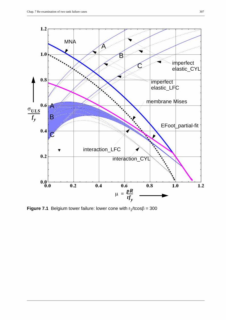
Chap. 7 Re-examination of two tank failure cases 307
Figure 7.1 Belgium tower failure: lower cone with r1/tcosβ = 300
μ pRtfy-------=
σULSfy
--------------
MNA
imperfect
membrane Mises
EFoot_partial-fit
AB
C
AB
C
elastic_LFC
imperfectelastic_CYL
interaction_CYL
interaction_LFC

308 Chap. 7 Re-examination of two tank failure cases
Figure 7.2 Belgium tower failure: upper cone with r1/tcosβ = 755
μ pRtfy-------=
σULSfy
--------------
MNAmembrane Mises
EFoot_partial-fit
A
C
A B C
imperfectelastic_LFC
imperfectelastic_CYL
LBA_CYLLBA_LFC
Binteraction_CYL
interaction_LFC

Chap. 7 Re-examination of two tank failure cases 309
Figure 7.3 Canada tower failure: lower cone with r1/tcosβ = 650
μ pRtfy-------=
σULSfy
--------------
MNAmembrane Mises
EFoot_partial-fit
ABC
AB
C
imperfectelastic_LFC
imperfectelastic_CYL
LBA_CYLLBA_LFC
Binteraction_CYL
interaction_LFC

310 Chap. 7 Re-examination of two tank failure cases
Figure 7.4 Canada tower failure: upper cone with r1/tcosβ = 1050
μ pRtfy-------=
σULSfy
--------------
MNA
imperfect
membrane Mises
ABC
elastic_LFC
EFoot_partial-fit
LBA_CYLLBA_LFC imperfect
elastic_CYL
interaction_CYLinteraction_LFC

Chap. 7 Re-examination of two tank failure cases 311
7.2 Confronting previous research work resultsrelated to the collapse of steel water towers
Following the design proposal for elastic buckling of liquid-filled conical shells given by Vande-pitte et al. which was based on the results of the extensive laboratory tests performed in Gent, manyresearch works and collapse strength comparisons have been done with respect to this (Gent) de-sign proposal. One of those cases where the Gent proposal was used to examine the situation offailure was the collapse of the Canada water tower. Vandepitte (1999), in his paper titled “The con-frontation of shell buckling research results with the collapse of a steel water tower” examined thebuckling failure of the conical steel tank of the Canada water tower and concluded that the collapseconfirms the validity of his design proposal.
As the detailed re-examination done in the current work shows, however, the Gent proposal whichwas based on bounding straight lines in a log-log plot of the test results had interpretation problemsleading to several questions. All the questions had been addressed during the detailed investigationof the current work which generally was based on different way of interpreting the test results.
As far as the failure of the Canada water tower is considered, however, the same conclusions asthat of Vandepitte’s would be reached. Even though the conclusion he made is similar to the con-clusion arrived from the current work, the design proposals are completely different as already ex-plained in the previous discussions. The two conclusions given are similar by chance only becausethe strength curves of the Canada steel cone as predicted by the two proposals coincide for the spe-cific failure situation of the water tower.
A graphical comparison of the failure cases of both the Belgium and Canada water towers with theGent proposal and that of the current work are shown in Figure 7.5 & Figure 7.6 for the steel conesegments of the Belgium tower and Figure 7.7 & Figure 7.8 for that of the Canada tower.

312 Chap. 7 Re-examination of two tank failure cases
Figure 7.5 Belgium tower failure: lower cone with r1/tcosβ = 300
μ pRtfy-------=
σULSfy
--------------
MNA
imperfect
membrane Mises
EFoot_partial-fit
AB
C
AB
C
elastic_LFC
imperfectelastic_CYL
interaction_CYL
interaction_LFC
Gent_proposal

Chap. 7 Re-examination of two tank failure cases 313
Figure 7.6 Belgium tower failure: upper cone with r1/tcosβ = 755
μ pRtfy-------=
σULSfy
--------------
MNAmembrane Mises
EFoot_partial-fit
A
C
A B C
imperfectelastic_LFC
imperfectelastic_CYL
LBA_CYLLBA_LFC
Binteraction_CYL
interaction_LFC
Gent_proposal

314 Chap. 7 Re-examination of two tank failure cases
Figure 7.7 Canada tower failure: lower cone with r1/tcosβ = 650
μ pRtfy-------=
σULSfy
--------------
MNAmembrane Mises
EFoot_partial-fit
A
C
AB
C
imperfectelastic_LFC
imperfectelastic_CYL
LBA_CYLLBA_LFC
Binteraction_CYL
interaction_LFC
Gent_proposal

Chap. 7 Re-examination of two tank failure cases 315
Figure 7.8 Canada tower failure: upper cone with r1/tcosβ = 1050
μ pRtfy-------=
σULSfy
--------------
MNA
imperfect
membrane Mises
ABC
elastic_LFC
EFoot_partial-fit
LBA_CYLLBA_LFC imperfect
elastic_CYL
interaction_CYLinteraction_LFC
Gent_proposal

316 Chap. 7 Re-examination of two tank failure cases
7.3 Summary and conclusions
The Belgium and Canada steel water tower failure cases have been re-examined to check for anypossible roles played by plasticity effects during the collapse. Previous research works related tothe collapse of the water towers have also been discussed.

Chap. 8 The notion of the “corresponding cylinder” 317
8
The notion of the “corresponding cylinder”
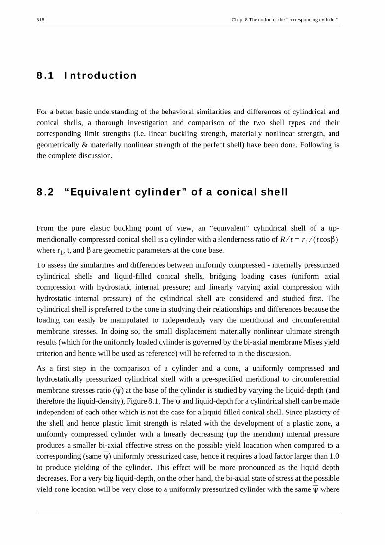
318 Chap. 8 The notion of the “corresponding cylinder”
8.1 Introduction
For a better basic understanding of the behavioral similarities and differences of cylindrical andconical shells, a thorough investigation and comparison of the two shell types and theircorresponding limit strengths (i.e. linear buckling strength, materially nonlinear strength, andgeometrically & materially nonlinear strength of the perfect shell) have been done. Following isthe complete discussion.
8.2 “Equivalent cylinder” of a conical shell
From the pure elastic buckling point of view, an “equivalent” cylindrical shell of a tip-meridionally-compressed conical shell is a cylinder with a slenderness ratio of where r1, t, and β are geometric parameters at the cone base.
To assess the similarities and differences between uniformly compressed - internally pressurizedcylindrical shells and liquid-filled conical shells, bridging loading cases (uniform axialcompression with hydrostatic internal pressure; and linearly varying axial compression withhydrostatic internal pressure) of the cylindrical shell are considered and studied first. Thecylindrical shell is preferred to the cone in studying their relationships and differences because theloading can easily be manipulated to independently vary the meridional and circumferentialmembrane stresses. In doing so, the small displacement materially nonlinear ultimate strengthresults (which for the uniformly loaded cylinder is governed by the bi-axial membrane Mises yieldcriterion and hence will be used as reference) will be referred to in the discussion.
As a first step in the comparison of a cylinder and a cone, a uniformly compressed andhydrostatically pressurized cylindrical shell with a pre-specified meridional to circumferentialmembrane stresses ratio (ψ) at the base of the cylinder is studied by varying the liquid-depth (andtherefore the liquid-density), Figure 8.1. The ψ and liquid-depth for a cylindrical shell can be madeindependent of each other which is not the case for a liquid-filled conical shell. Since plasticty ofthe shell and hence plastic limit strength is related with the development of a plastic zone, auniformly compressed cylinder with a linearly decreasing (up the meridian) internal pressureproduces a smaller bi-axial effective stress on the possible yield loacation when compared to acorresponding (same ψ) uniformly pressurized case, hence it requires a load factor larger than 1.0to produce yielding of the cylinder. This effect will be more pronounced as the liquid depthdecreases. For a very big liquid-depth, on the other hand, the bi-axial state of stress at the possibleyield zone location will be very close to a uniformly pressurized cylinder with the same ψ where
R t⁄ r= 1 t βcos( )⁄

Chap. 8 The notion of the “corresponding cylinder” 319
the bi-axial yield strength is governed by the membrane Mises yield criterion. Plots of smalldisplacement materially nonlinear numerical analysis results for a uniformy compressed andhydrostatically pressurized cylindrical shell with R/t = 707 (equivalent cylinder of a cone with r1/t = 500 and apex-half angle β = 45°), ψ = 2/3, and fixed bottom boundary condition are shown inFigure 8.2 and Figure 8.3 where the effect of liquid-depth on the yield strength can be seen. Similarstudies are done for different pre-specified values of ψ and varying the liquid-depth as shown inFigure 8.4.
The second step (which is one step closer to the LFC case) in the comparison of cylindrical shellsand liquid-filled conical shells is to tip-compress the cylinder as in the first case but directly relatethe parameter ψ with the liquid-depth in the same way as in the LFC, i.e. where
is taken from the LFC, Figure 8.5. Very big liquid-depth means very big ψ andhence very big meridional compression compared to the circumferential tension. This situation, forinfinitely big ψ, is similar to the pure axial compression of the cylinder where uni-axial meridionalyielding governs the strength. In other words, as the liquid-depth increases, the materiallynonlinear strength of the shell gets closer to the yield strength as predicted by the membrane Misescriterion. On the other hand, when the liquid-depth is very small, the relative magnitude ofcircumferential stretching at the possible yield zone of the shell is relatively small, compared to theuniform internally pressurized case, which results in a smaller effective bi-axial state of stresswhich inturn requires a bigger load factor to bring it to the plastic limit level, i.e. the smaller theliquid-depth gets the bigger the platsic load factor becomes and the more deviation from the yieldstrength predicted using the membrane Mises criterion. The results obtained from such treatmentof the cylindrical shell are plotted on the pressure representation as shown in Figure 8.6. Acomparison of these results with the materially nonlinear strengths of the liquid-filled conical shell(with the same ψ variations) is also shown in Figure 8.7.
The third step in the comparison of a cylinder and an LFC is the consideration of an unpressurized(or pure axial compression condition) cylinder and the corresponding yield strengths. In this case,however, it should be noted that pure axial compression doesn’t only mean tip-compression. Auniformly tip-compressed cylinder is compared to a cylinder loaded with linearly varying axialcompression (i.e. uniform laoding along the meridian). The length upon which the linearly varyingaxial compression is acting will be varied (h/R = 0.2, 1, 10, 100 where “h” is the loaded meridionallength of the cylinder) in such a way that an infinitely long compressed length apparently means atip-compressed cylinder. In the numerical analysis of this comparison, a meridional tip-loading anda uniform along the meridian axial compressve loading are applied to both cylinders in such a waythat the resulting meridional compressive stress at the base of both cylinders is equal to the uni-axial yield strength of the material under consideration. The effects of the loaded length on thematerially nonlinear strength of the cylinder can be seen from the plot in Figure 8.8.
On the other hand, for a liquid-filled conical shell, an unpressurized situation means an infinitelybig liquid-depth which technically is equivalent to the tip-meridionally-compressed cone. Onceagain, in the numerical analysis of this comparison, a meridional tip-loading is applied to both shelltypes in such a way that the resulting meridional compressive stress at the base is equal to the uni-axial yield strength of the material under consideration. It should then be clear that the tip-
ψ ζ' 3 ζ'+( ) 6⁄=ζ' h' βtan⋅ r1⁄=
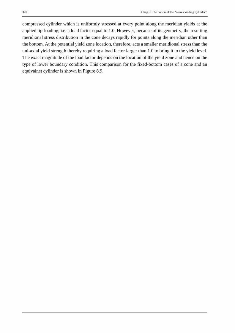
320 Chap. 8 The notion of the “corresponding cylinder”
compressed cylinder which is uniformly stressed at every point along the meridian yields at theapplied tip-loading, i.e. a load factor equal to 1.0. However, because of its geometry, the resultingmeridional stress distribution in the cone decays rapidly for points along the meridian other thanthe bottom. At the potential yield zone location, therefore, acts a smaller meridional stress than theuni-axial yield strength thereby requiring a load factor larger than 1.0 to bring it to the yield level.The exact magnitude of the load factor depends on the location of the yield zone and hence on thetype of lower boundary condition. This comparison for the fixed-bottom cases of a cone and anequivalnet cylinder is shown in Figure 8.9.
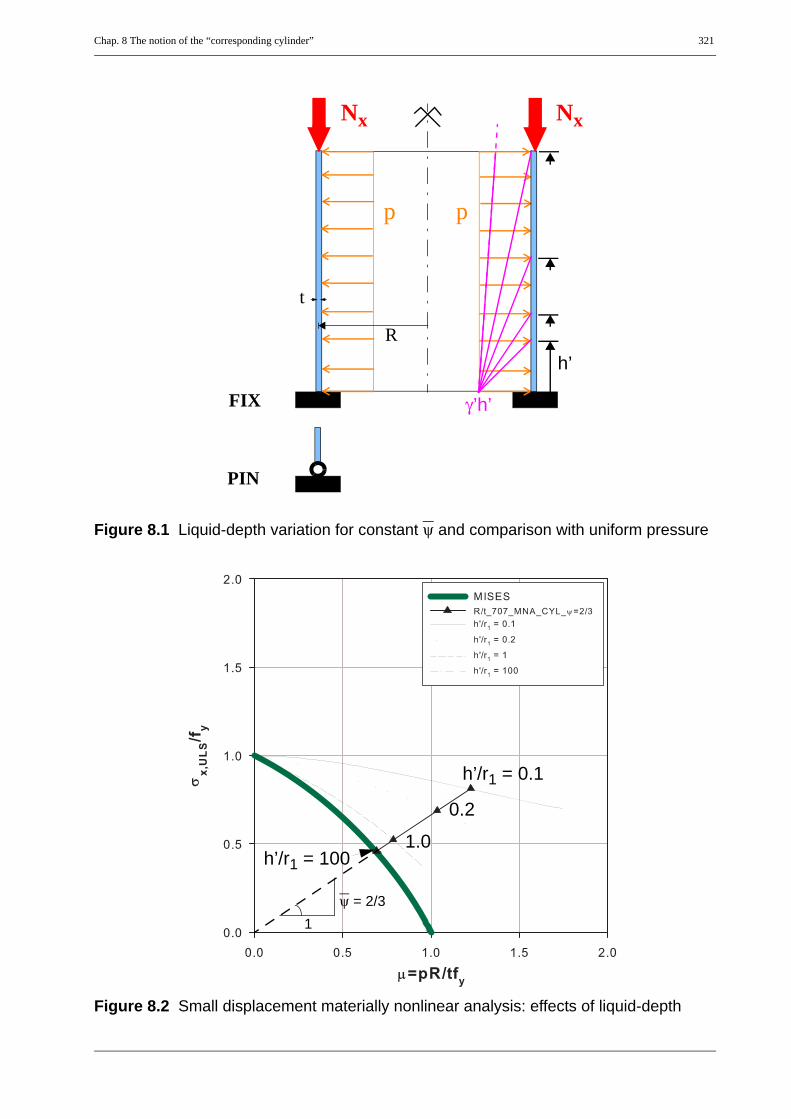
Chap. 8 The notion of the “corresponding cylinder” 321
Figure 8.1 Liquid-depth variation for constant ψ and comparison with uniform pressure
Figure 8.2 Small displacement materially nonlinear analysis: effects of liquid-depth
p
R
t
p
Nx Nx
FIX
PIN
γ’h’
h’
1ψ = 2/3
0.2
h’/r1 = 0.1
h’/r1 = 1001.0

322 Chap. 8 The notion of the “corresponding cylinder”
Figure 8.3 Small displacement materially nonlinear analysis: effects of liquid-depth
Figure 8.4 Small displacement materially nonlinear analysis: fixed bottom
1ψ = 0.4
1
ψ = 3

Chap. 8 The notion of the “corresponding cylinder” 323
Figure 8.5 Liquid-depth variation for constant ψ and comparison with uniform pressure
Figure 8.6 Small displacement materially nonlinear analysis: fixed bottom
pR
t
Nx Nx
FIX
PIN
γ’h’
h’
1ψ

324 Chap. 8 The notion of the “corresponding cylinder”
Figure 8.7 Small displacement materially nonlinear analysis: fixed bottom
Figure 8.8 Small displacement materially nonlinear analysis: fixed bottom
h/R = 100 (CYL tip-loading)h/R = 10h/R = 1h/R = 0.2

Chap. 8 The notion of the “corresponding cylinder” 325
Figure 8.9 Small displacement materially nonlinear analysis: fixed bottom
LFC very big liquid-depth(tip-loading)
CYL tip-loading

326 Chap. 8 The notion of the “corresponding cylinder”
8.3 “Corresponding cylinder” of a conical shell
A “corresponding” cylindrical shell of a conical shell is an “equivalent cylinder” having not onlygeometric equivalency but also loading equivalency. For a liquid-filled conical shell, where themeridional membrane compression rapidly decays up the meridian, buckling and plasticity occuron a region very close to the bottom boundary condition. For this reason an equivalent loading ofan LFC to be used for the “corresponding” cylinder is computed as discussed below.
An equivalent meridional loading of the “corresponding cylinder” will be taken as a linearlyvarying meridional compressive loading which produces the same membrane stress at the cylinderbase as in the LFC. The length (along the meridian) of the loaded part of the “correspondingcylinder” will be computed from the tangent of the meridional section force distribution of theLFC. Similarly, the equivalent internal pressure loading will be taken as a linearly varying pressurewith a circumferential membrane section force distribution having the same tangent and producingthe same membrane stress at the bottom of the cylinder as in the LFC. The length along themeridian of the corresponding cylinder over which the equivalent internal pressure should act willbe the same as that of the meridional loading of the “corresponding cylinder”. The equivalentsection force distributions of the “corresponding” cylinder are shown in Figure 8.10.
The tangent lines to the meridional and circumferential membrane section force distributions of theLFC can be computed as follows. The meridional and circumferential membrane stresses along themeridian of a liquid-filled conical shell are given as functions of the liquid-depth parameters ζ andζ’ by
(Eq. 8.1)
(Eq. 8.2)
where
is a running depth parameter with z measured from bottom up of the cone, and
is the maximum liquid level parameter with z = h’.
At the cone base and hence the membrane section forces at the cone base become
(Eq. 8.3)
σxγ'h'r1t βcos-------------- 1
6--- ζ' ζ–( )2
ζ'-------------------- 3 ζ' ζ–
1 ζ+-------------+⎝ ⎠
⎛ ⎞⋅ ⋅ ⋅=
σθγ'h'r1t βcos-------------- 1 ζ+( ) ζ' ζ–
ζ'-------------⎝ ⎠⎛ ⎞⋅ ⋅=
ζ z βtan⋅r1
------------------=
ζ' h' βtan⋅r1
--------------------=
r r1;= ζ 0=
σx 1,γ'h'r1t βcos-------------- 1
6--- ζ' 3 ζ'+( )⋅ ⋅ ⋅=

Chap. 8 The notion of the “corresponding cylinder” 327
(Eq. 8.4)
The slope of the tangent line to the meridional membrane section force distribution will then begiven interms of the normalized membrane section force Nx/Nx,1 = σx/σx,1 shown in Figure 8.11by
(Eq. 8.5)
(Eq. 8.6)
where “s” is a running meridional length parameter measured from bottom up the meridian of thecone and it is related to “z” using . Hence
(Eq. 8.7)
(Eq. 8.8)
Therefore,
(Eq. 8.9)
which gives
(Eq. 8.10)
Substituting ζ = 0 gives the slope of the tangent to the normalized section force at the cone basewhich is
(Eq. 8.11)
The term in brackets on the right hand side of (Eq. 8.11) is plotted as a function of the maximumliquid-depth parameter ζ' as shown in Figure 8.12. The slope of the tangent to the un-normalizedsection force at the cone base will then be
σθ 1,γ'h'r1t βcos--------------=
NxNx 1,---------- 1 ζ
ζ'----–⎝ ⎠
⎛ ⎞ 2 3 ζ' 2ζ+ +3 ζ'+( ) 1 ζ+( )⋅
----------------------------------------⋅=
sdd Nx( ) Nx 1, sd
d NxNx 1,----------⎝ ⎠⎛ ⎞⋅=
s z βcos⁄=
ζ z βtan⋅r1
------------------ s βsin⋅r1
------------------= =
sdd ( ) βsin
r1-----------
ζdd ( )⋅=
sdd Nx
Nx 1,----------⎝ ⎠⎛ ⎞ βsin
r1-----------
ζdd Nx
Nx 1,----------⎝ ⎠⎛ ⎞⋅=
sdd Nx
Nx 1,----------⎝ ⎠⎛ ⎞ βsin
r1-----------– 1 ζ ζ'⁄–
3 ζ'+( ) 1 ζ+( )⋅---------------------------------------- 1 ζ
ζ'----–⎝ ⎠
⎛ ⎞ 1 ζ'+1 ζ+-------------⋅ 2
ζ'---- 3 ζ' 2ζ+ +( )⋅+⎝ ⎠
⎛ ⎞⋅ ⋅=
sdd Nx
Nx 1,----------⎝ ⎠⎛ ⎞
ζ 0=
βsinr1
-----------– 1 2ζ'---- 2
3 ζ'+-------------–+⎝ ⎠
⎛ ⎞⋅=

328 Chap. 8 The notion of the “corresponding cylinder”
(Eq. 8.12)
Similarly. the slope of the tangent line to the circumferential membrane section force distributionof the LFC will be given interms of the normalized membrane section force Nθ/Nθ,1 = σθ/σθ,1shown in Figure 8.13 by
(Eq. 8.13)
(Eq. 8.14)
with
(Eq. 8.15)
gives
(Eq. 8.16)
Substituting ζ = 0 gives the slope of the tangent to the normalized section force at the cone basewhich is
(Eq. 8.17)
The term in brackets on the right hand side of (Eq. 8.11) is plotted as a function of the maximumliquid-depth parameter ζ' as shown in Figure 8.12. The slope of the tangent to the un-normalizedsection force at the cone base will then be
(Eq. 8.18)
sdd Nx( )
ζ 0=
βsinr1
-----------– 1 2ζ'---- 2
3 ζ'+-------------–+⎝ ⎠
⎛ ⎞ Nx 1,⋅ ⋅=
NθNθ 1,----------- 1 ζ+( ) 1 ζ
ζ'----–⎝ ⎠
⎛ ⎞⋅=
sdd Nθ( ) Nθ 1, sd
d NθNθ 1,-----------⎝ ⎠⎛ ⎞⋅=
sdd Nθ
Nθ 1,-----------⎝ ⎠⎛ ⎞ βsin
r1-----------
ζdd Nθ
Nθ 1,-----------⎝ ⎠⎛ ⎞⋅=
sdd Nθ
Nθ 1,-----------⎝ ⎠⎛ ⎞ βsin
r1----------- 1 1 2ζ+
ζ'---------------–⎝ ⎠
⎛ ⎞⋅=
sdd Nθ
Nθ 1,-----------⎝ ⎠⎛ ⎞
ζ 0=
βsinr1
----------- 1 1ζ'----–⎝ ⎠
⎛ ⎞⋅=
sdd Nθ( )
ζ 0=
βsinr1
----------- 1 1ζ'----–⎝ ⎠
⎛ ⎞ Nθ 1,⋅ ⋅=
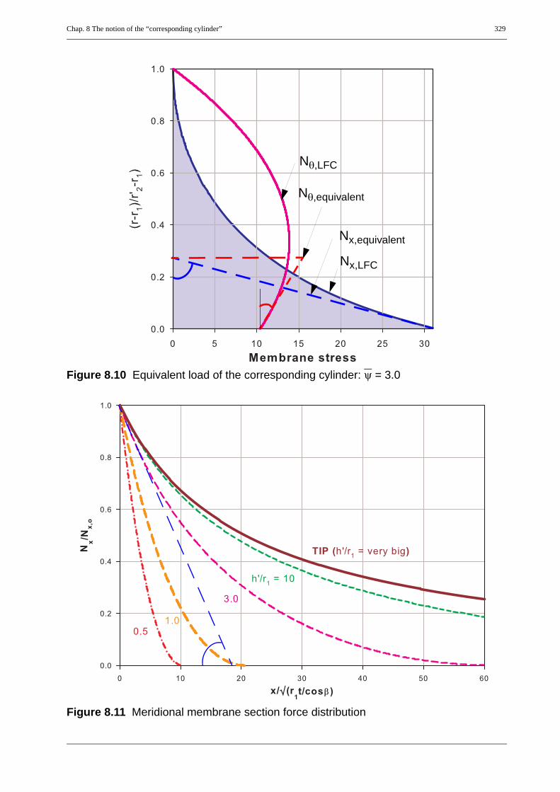
Chap. 8 The notion of the “corresponding cylinder” 329
Figure 8.10 Equivalent load of the corresponding cylinder: ψ = 3.0
Figure 8.11 Meridional membrane section force distribution
Nx,equivalent
Nθ,LFC
Nx,LFC
Nθ,equivalent

330 Chap. 8 The notion of the “corresponding cylinder”
Figure 8.12 Slope of meridional membrane section force distribution at cone base
Figure 8.13 Slope of circumferential membrane section force distribution at cone base
0 5 10 15 20�2.5
�2.0
�1.5
�1.0
�0.5
0.0
ζ'
1 2ζ'---- 2
3 ζ'+-------------–+⎝ ⎠
⎛ ⎞
0 5 10 15 20�1.0
�0.5
0.0
0.5
1.0
ζ'
1 1ζ'----–⎝ ⎠
⎛ ⎞

Chap. 8 The notion of the “corresponding cylinder” 331
Using the slope of the tangent to the normalized section force at the cone base (Eq. 8.12), the lengthof the region on the “corresponding cylinder” to be internally pressurized linearly to produceequivalent circumferential membrane section force and uniformly axially loaded to produce alinearly varying section force distribution with a maximum at the base (equal to that of the LFC),see Figure 8.10, will be given as follows:
(Eq. 8.19)
(Eq. 8.20)
For an infinitely big liquid-depth (or ζ’) of the LFC, the second term on the right hand side of (Eq.8.20) will be equal to 1.0 and the axially loaded region of the corresponding cylinder will have alength of
(Eq. 8.21)
The magnitude of the uniformly ditributed axial compressive loading of the corresponding cylinderwill be given by
(Eq. 8.22)
and the linearly varying internal pressure of the cylinder can be splitted into a uniform andhydrostaic pressure parts. With Nθ,2 representing the circumferential membrane section force attop-end of the loaded region, the uniform, pz, and hydrostatic, ph, part (amplitude at the base ofcylinder) of the linearly varying internal pressure are given by
(Eq. 8.23)
(Eq. 8.24)
(Eq. 8.25)
sdd Nx( )
ζ 0=
βsinr1
-----------– 1 2ζ'---- 2
3 ζ'+-------------–+⎝ ⎠
⎛ ⎞ Nx 1,⋅ ⋅=
Laxial equivalent,r1
βsin----------- 1
1 2ζ'---- 2
3 ζ'+-------------–+⎝ ⎠
⎛ ⎞--------------------------------------⋅=
Laxial equivalent TIP,,r1
βsin-----------=
pxNx 1,
Laxial equivalent,-------------------------------------=
Nθ 2, Nθ 1, sdd Nθ( )
ζ 0=Laxial equivalent,⋅+=
Nθ 1, 1 1 1 ζ'⁄–
1 2ζ'---- 2
3 ζ'+-------------–+⎝ ⎠
⎛ ⎞--------------------------------------+
⎝ ⎠⎜ ⎟⎜ ⎟⎜ ⎟⎛ ⎞
⋅=
pzNθ 2,
R-----------=
phNθ 1, N– θ 2,
R-------------------------=

332 Chap. 8 The notion of the “corresponding cylinder”
Figure 8.14 Meridional membrane section force distribution & approximate buckling load
Nx,TIP
Nx
Nx,1
β
γ'
r1
h’.tanβ
r2’r2
1
zs
γ'.h’
h’
zbNx(zb)
Nx,cyl(zb)
Nxcr(z=0) = NxRcr
Center ofpotentialbuckle
Meridional membranesection force distribution
Elastic criticalmeridional membranesection force distribution
(b)
(a)
Nxcr(zb)
sdd Nx( )
ζ 0=
Nxcr,cyl

Chap. 8 The notion of the “corresponding cylinder” 333
8.3.1 Linear elastic buckling strength of the “corresponding cylinder”Since the linear elastic buckling strength of a perfect cylindrical shell is independent of the internalpressurization, the equivalent meridional loading of the “corresponding cylinder” alone will beconsidered in the computation of the elastic buckling strength which will then be compared withthe elastic buckling strength of the liquid-filled conical shell. In the course of doing this, thebuckling strength of an LFC with an infinitely big liquid-depth (or a tip-loaded cone) will bequalitatively and quantitatively compared with that of the “corresponding” cylindrical shell underan equivalent axial loading as discussed above and the same reference meridional membrane stressat the bottom. It is, however, worth mentioning here that a meridionally-loaded cylindrical shellwith exactly the same meridional membrane section force ditribution along the meridian as the tip-loaded cone buckles at a higher load factor (depending on the bottom boundary condition type)than the LFC. This is because of the the difference in buckling strength of the two shell types at thepotential center of buckle, see Figure 8.14(b). The buckling load factor may even get higher whenthe ”corresponding cylinder” is considered with the equivalent axial loading instead of the actualdistribution on the LFC, see Figure 8.14(b). This discussion applies similarly to smaller liquid-depth cases of the LFC.
The results of a linear elastic buckling analysis of an LFC and a “corresponding” cylinder for afixed-bottom cone (r1/t = 500; β = 45°; E = 21000 kN/cm2; fy = 24 kN/cm2; ν = 0.3 and varyingthe liquid-depth) are shown in Figure 8.17. The relative increase of the buckling load factor of the“corresponding cylinder” when compared to that of the LFC, however, decreases and hence comescloser to that of the LFC as the liquid-depth gets smaller since the equivalent section forcedistribution of the “corresponding cylinder” becomes more closer to the actual section forceditribution of the LFC. To qualitatively show this, a random 10% constant reduction has beenapplied to the buckling strengths of the corresponding cylinder and re-compared to the bucklingstrength of the LFC, see Figure 8.18. Had the geometric and section force equivalency of the LFCand “corresponding cylinder” been considered at the potential center of elastic buckling, theresulting buckling load would have been the same for both.
Basic linear buckling eigenmodes of the liquid-filled conical shell and its “corresponding cylinder”are shown in Figure 8.16 and Figure 8.17 for ψ values of 3.0 and tip-compressed (or ψ infinitelybig), respectively.

334 Chap. 8 The notion of the “corresponding cylinder”
Figure 8.15 Basic buckling eigenmodes: ψ = 3
Figure 8.16 Basic buckling eigenmodes: very high liquid-depth (ψ = infinity)
Step: Step 2, LINEAR BUCKLING ANALYSIS (LBA)Mode 1: EigenValue = 1.3028Primary Var: S, MisesDeformed Var: U Deformation Scale Factor: +1.500e+02
Step: Step 2, LINEARE BUCKLING(LBA) ANALYSISMode 1: EigenValue = 1.1200Primary Var: S, MisesDeformed Var: U Deformation Scale Factor: +1.500e+02
Step: Step 2, LINEAR BUCKLING ANALYSIS (LBA)Mode 1: EigenValue = 1.2437Primary Var: S, MisesDeformed Var: U Deformation Scale Factor: +1.500e+02
Step: Step 2, LINEARE BUCKLING(LBA) ANALYSISMode 1: EigenValue = 1.0004Primary Var: S, MisesDeformed Var: U Deformation Scale Factor: +1.500e+02

Chap. 8 The notion of the “corresponding cylinder” 335
Figure 8.17 Linear buckling strengths of the perfect cone and “corresponding” cylinder
Figure 8.18 Linear buckling strengths of the perfect cone and “corresponding” cylinder
“correspondingcylinder”
LFC
“correspondingcylinder”
LFC
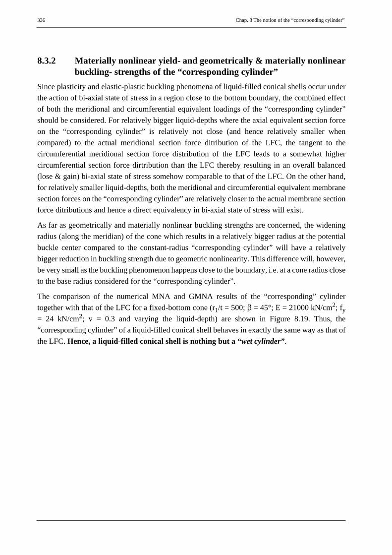
336 Chap. 8 The notion of the “corresponding cylinder”
8.3.2 Materially nonlinear yield- and geometrically & materially nonlinearbuckling- strengths of the “corresponding cylinder”
Since plasticity and elastic-plastic buckling phenomena of liquid-filled conical shells occur underthe action of bi-axial state of stress in a region close to the bottom boundary, the combined effectof both the meridional and circumferential equivalent loadings of the “corresponding cylinder”should be considered. For relatively bigger liquid-depths where the axial equivalent section forceon the “corresponding cylinder” is relatively not close (and hence relatively smaller whencompared) to the actual meridional section force ditribution of the LFC, the tangent to thecircumferential meridional section force distribution of the LFC leads to a somewhat highercircumferential section force dirtribution than the LFC thereby resulting in an overall balanced(lose & gain) bi-axial state of stress somehow comparable to that of the LFC. On the other hand,for relatively smaller liquid-depths, both the meridional and circumferential equivalent membranesection forces on the “corresponding cylinder” are relatively closer to the actual membrane sectionforce ditributions and hence a direct equivalency in bi-axial state of stress will exist.
As far as geometrically and materially nonlinear buckling strengths are concerned, the wideningradius (along the meridian) of the cone which results in a relatively bigger radius at the potentialbuckle center compared to the constant-radius “corresponding cylinder” will have a relativelybigger reduction in buckling strength due to geometric nonlinearity. This difference will, however,be very small as the buckling phenomenon happens close to the boundary, i.e. at a cone radius closeto the base radius considered for the “corresponding cylinder”.
The comparison of the numerical MNA and GMNA results of the “corresponding” cylindertogether with that of the LFC for a fixed-bottom cone (r1/t = 500; β = 45°; E = 21000 kN/cm2; fy= 24 kN/cm2; ν = 0.3 and varying the liquid-depth) are shown in Figure 8.19. Thus, the“corresponding cylinder” of a liquid-filled conical shell behaves in exactly the same way as that ofthe LFC. Hence, a liquid-filled conical shell is nothing but a “wet cylinder”.

Chap. 8 The notion of the “corresponding cylinder” 337
Figure 8.19 Small displacement materially nonlinear analysis: fixed bottom

338 Chap. 8 The notion of the “corresponding cylinder”
8.4 Summary and conclusions
The “corresponding cylinder” of a liquid-filled conical shell has been introduced which behaves inexactly the same way as the LFC. Detailed investigation of the “corresponding cylinder” was thenmade which turned out to be that the liquid-filled cone is nothing but a “wet-cylinder”.

Chap. 9 General summary & conclusion 339
9
General summary& conclusion

340 Chap. 9 General summary & conclusion
9.1 General summary & conclusions
The general behaviour of thin-walled cylindrical & conical shells under meridional compressionand circumferential tension has been analyzed using analytical and numerical linear analysis tech-niques from which the pure membrane and edge-bending effects on the section force distributionhave been discussed. The general effects of edge restraining on the elastic-plastic buckling phe-nomena of such shells had been explained. The small displacement linear buckling (LB) strengthsof cylindrical & conical shells have then been computed approximately and investigated numeri-cally. The linear buckling strength has been used as a reference, throughout the whole study, to ex-press other buckling strengths according to the frame work of EN 1993-1-6.
The possible loading procedures in dealing with liquid-filled conical shells have been discussedand clearly explained. Besides, which loading procedure should be used in what circumstances andfor what purposes has been pointed out.
The effects of axisymmetric and non-axisymmetric imperfections on the elastic buckling strengthof thin-walled cylindrical and conical shells have been discussed in detail for different fabricationquality classes as recommended in EN 1993-1-6 and comparisons between the cylinder and conehave been made. LFC-specific buckling phenomenon and corresponding elastic buckling strengthshave been throughly discussed and clearly explained. Simplified expressions for the prediction oflinear buckling strengths of liquid-filled general cones with pinned and fixed bottom boundaryconditions have been obtained. The numerous Gent laboratory tests made on liquid-filled conicalshells have been examined and re-investigated in detail. Comparisons of the perfect and imperfectlinear buckling strengths of cylindrical and conical shells have been made.
Nonlinear buckling and plastic strengths of cylindrical and conical shells have been computed ap-proximately using analytical models with second order effects included and numerically using afinite element package (ABAQUS). The pure plastic limit strengths of the two shell types havebeen computed approximately using von Mises membrane yield criterion taking the membranestresses at the shell-base as references; and using generalized stress resultant oriented approximateyield criteria. The effects of material nonlinearity, geometric nonlinearity and imperfections on thebuckling strength of thin-walled cylindrical and conical shells have been numerically investigated.Comparisons of the results obtained using the analytical model and numerical simulations havebeen made on which detailed comments and explanations were given.
The numerical simulation results have been used to derive a set of basic data that can be used in astraight forward buckling design by hand calculations in-line with the underlying structure of theEuropean standard EN1993-1.6. Design recommendations were proposed which have been com-pared with previous research results and code recommendations. Additional comments and de-
Chap. 9 General summary & conclusion 341
tailed explanations concerning the results have been given. The comparison in buckling strengthprediction between the design recommendation of the current work and the existing design regu-lation according EN 1993-1-6 for the cylindrical shell is summarized as follows:
EN1993-1-6 buckling design recommendation:
• the overall procedure in predicting the characteristic buckling strength of cylindrical shellinvolves many steps
• the reduction factor αxpp, which really is a plastic buckling reduction factor, is being treatedas if it is an elastic reduction factor. Besides, it is referred to as an imperfection reductionfactor while it has nothing to do with imperfections.
• applies plasticity conditions twice, first in αxpp itself as it basically includes material andgeometric nonlinear effects and a second elastic-plastic buckling interaction of αxpp withthe uni-axial yield condition
• predicts elastic-plastic buckling strengths higher than the pure bi-axial plastic resistance ofthe cylinder
• needs additional separate plasticity check against bi-axial yielding
• even if separate plasticity condition is applied to it, the strength results are inconsistent withthose computed numerically
• inconsistency in buckling strength predictions at very low pressure level and zero-pressurelevel resulting in a jump of strength
• applies only for pinned bottom cases (with more safety for fixed cases?)
Buckling design recommendation of the current work:
• considers bi-axial plasticity from the very beginning
• strictly differentiates typical buckling failure modes: buckling in the free shell interior andbuckling adjacent to the boundary (elephant’s-foot buckling mode)
• it is easy to follow and apply; straight forward approach
• differentiates pinned and fixed bottom boundary condition cases
On the other hand, from the axisymmetric elastic-plastic buckling analysis results of the liquid-filled conical shells, it can be concluded that that elephant’s-foot type buckling in such shells,where the only loading is liquid-filling, may not be probable unless there exist a worst imperfectionor a global bending moment resulting from, say, earthquake causing one-sided buldge or globaltilting of the shell. A very little global bending effect, in the general case of cones supported frombottom (i.e. on the smaller radius), will have a very big meridional compression on one side of the

342 Chap. 9 General summary & conclusion
cone due to the shorter lever-arm at the smaller radius. It is this big meridional compression alongwith the existing circumferential stretching which results in bi-axial state of stress causing localyielding and hence elephant’s-foot buckling. On the other hand, if there exists an additional, say,roof loading on top of the existing liquid-loading, an additional meridional compression will result.This higher meridional commpression along with the existing circumferential tension (plus smalladdition due to poisonn’s effect) may therefore lead to the possibility of elephant’s-foot type buck-ling.
Detailed investigation of Gent mercury-filled laboratory test results along with detailed discus-sions, explanations, and conclusions have been done. Previous LFC-related research works on non-linear simulation of liquid-filled conical shells with or without geometric imperfections have beendiscussed and few cases have been re-examined for confirmation and further studying purposes.Relevant explanations and conclusions were given to the outcomes of those works. Moreover, theBelgium and Canada steel water tower failure cases have been re-examined to check if they reallywere under designed for elastic buckling and check for any possible roles played by plasticity ef-fects during the collapse. Previous research works related to the collapse of the water towers havealso been discussed.
A “corresponding” cylinder of a liquid-filled conical shell has been introduced which behaves inexactly the same way as the liquid-filled conical shell. Detailed invetigation of the “corresponding”cylinder has then been made.

Chap. 9 General summary & conclusion 343
9.2 Outlook & proposed future work
Axisymmetric shell models have been used in all the numerical simulations performed to study theaxisymmetric elastic-plastic buckling phenomena, buckling modes and strengths of meridionallycompressed and internally pressurized perfect and imperfect cylindrical and conical shells.Axisymmetric imperfection shapes have been used to study the effects of sinusoidal & localimperfections on the elastic-plastic buckling strengths of the aforementioned shells for differentimperfection wavelengths, locations along the meridian, orientations, and imperfectionamplitudes. On the other hand, in the study on the elastic-plastic buckling of liquid-filled conicalshells, the cones considered were solely loaded with liquid. For these reasons, following is a list ofpossible areas where, in the eye of the current work, further researching is needed.
• Investigation of real (i.e. that can be found in practical civil engineering shells) imperfec-tion shapes, imperfection amplitudes, possible locations along the meridian, orientationsand their effects on the elastic-plastic buckling strength of thin-walled cylindrical andconical shells.
• Investigation of the effects of local non-axisymmetric imperfection shapes and the corre-sponding buckling modes and buckling strengths for different internal pressurization.
• Investigation on the effects of an imperfection in the form of global tilting on the elasticand elastic-plastic buckling phenomena and buckling strength of liquid-filled conicalshells.
• Investigation on the effects of using elephant’s-foot buckling mitigation mechanisms andresulting elastic-plastic buckling phenomena and buckling strength of thin-walled cylin-drical shells.

344 Chap. 9 General summary & conclusion
9.3 Proposed European design recommendation
(EDR) & European Standard EN 1993-1-6
modifications
The following list is a brief summary of what has been obtained from the whole work which candirectly be integrated as modifications and/or incorporations into the existing European design rec-ommendation and European Standard EN 1993-1-6.
i Proposal for modification of buckling strength prediction of cylindrical shells underaxial compression with co-existent internal pressure
Buckling strength prediction using simple expressions which resulted through systematic interpre-tation of nonlinear buckling analysis results which considered bi-axial plasticity from the very be-ginning have been presented in Chapter-3 of this work. These modifications strictily differentiatesbetween pinned and fixed bottom boundary condition cases.
ii Establishing a new proposal for the buckling strength prediction of conical shellsunder meridional compression with co-existent internal pressure
A similar-to-the-cylinder buckling strength prediction of meridionally compressed and internallypressurized conical shells can be established.
iii Proposal for modification and integration to the existing buckling strength predictionof liquid-filled conical shells (LFC)
Liquid-filled-specific buckling behavior and consistent with cylinder imperfection reduction(αxpe) have been presented in Chapter-4 and Chapter-5.8. Simplified expressions for the predictionof buckling strengths of liquid-filled conical shells with pinned and fixed bottom boundaryconditions have been obtained and hence proposed for future design purposes.
iv Proposal for modification of the linear-analysis-based plastic limit strength estimationusing Ilyushin yield criterion
Ilyushin’s yield criterion is incorrectly refered to in EN 1993-1-6 and hence, it needs to be modifiedaccording to the discussion in Annex-A of this work. Ivanov-I yield criterion is recommended tobe used as it is accurate enough for 1D and axisymmetric conditions and simple to apply.
v Generalization of EN elastic-plastic buckling representationThe elastic-plastic buckling interaction expression given using an exponent parameter η should bemodified using possible general shape functions as presented in Chapter-4.8.2.1.

Chap. 10 References 345
10
References
346 Chap. 10 References
ABAQUS (2002). ABAQUS/Standard: Theory Manual & User’s Manual, Abaqus Version 6.3.Hibbit, Karlson & Sorensen, Inc.
Bornscheuer, F. W., Bornscheuer, F. (1987). Contribution to Simplified Handling of the ShellBuckling Concept without α-coefficient. ECCS Colloquium on Stability of Plate and ShellStructures, Ghent, Belgium, 261-272.
Burgoyne, C. J., Brennan, M. G. (1993). Exact Ilyushin Yield Surface. Int. J. Solids Structures,Vol. 30, No. 8, 1113 - 1131.
Bushnell, D. (1985). Computerized Buckling Analysis of Shells. Mechanics of Elastic Stability 9,Martinus Nijhoff Publishers, Dordrecht, The Netherlands.
Calladine, C. R. (1983). Theory of Shell Structures. Cambridge University Press, Cambridge,England.
Chryssanthopoulos, M. K., Poggi, C. (2001). Collapse Strength of Unstiffened Conical Shellsunder Axial Compression. Journal of Constructional Steel Research 57, 165-184.
Dawe, J. L., Seah, C. K., Abdel-Zahr, A. K. (1993). Investigation of the Regent Street Water TowerCollapse. Management & Operations, AWWA Journal , 34-47.
ECCS (1976). European Recommendations for Steel Construction: Buckling of Shells. EuropeanConvention for Constructional Steelwork, Brussels, Second Edition.
ECCS (1984). European Recommendations for Steel Construction: Buckling of Shells. EuropeanConvention for Constructional Steelwork, Brussels, Third Edition.
ECCS (1988). European Recommendations for Steel Construction: Buckling of Shells. EuropeanConvention for Constructional Steelwork, Brussels, Fourth Edition.
El Damatty, A. A., El-Attar, M., Korol, R. M. (1999). Simple Design Procedure for Liquid-FilledSteel Conical Tanks. Journal of Structural Engineering, Vol. 125, No. 8, 879-890.
EN 1993-1-6 (2006). Eurocode-3. Design of Steel Structures, part 1-6: Strength and Stability ofShells, CEN, Brussels.
Esslinger, M., Geier, B. (1975). Postbuckling Behavior of Structures. CISM, Springer-Verlag,Wien-New York.
Flügge, W. (1973). Stresses in Shells. Springer-Verlag, Berlin, Second Edition.
Guggenberger, W. (1994). Collapse Design of Large Steel Digester Tanks. Thin-Walled Structures20, 109-128.
Guggenberger, W., Linder, C. (2004a). Analogy Model for the Axisymmetric Elastic EdgeBending problem in Shells of Revolution based on Geckeler's Approximation. In: Zingoni, A.(editor). Progress in Structural Engineering, Mechanics and Computation, Taylor & Francis,London, 269–274.
Guggenberger, W. (2004b). Proposed Modified Hierarchy of Shell Buckling Design Procedures in

Chap. 10 References 347
Eurocode EN 1993-1-6. submission to ECCS TWG 8.4 “Buckling of Steel Shells“, April 2004.
Guggenberger, W. (2005a). Imperfection Assumptions and their Effects on Elastic Shell Buckling.Proceedings of the 5th IASS/IACM International Conference on Computation of Shell and SpatialStructures, Salzburg, Austria.
Guggenberger, W. (2005b). Discretely Supported Thin-Walled Steel Silo Shells: AdvancedBuckling Design and Modelling Aspects. Paper 51, Proceedings of the Tenth InternationalConference on Civil, Structural and Environmental Engineering Computing, Rome, 30 August-2September 2005.
Guggenberger, W. (2007). Lecture notes: Plates and Shell Structures, Institute for Steel and ShellStructures, Graz University of Technology.
Guggenberger, W. (2008). Lecture notes: Stability of Structures, Institute for Steel and ShellStructures, Graz University of Technology.
Guggenberger, W. (2009). Lecture notes: Nonlinear Structural Analysis, Institute for Steel andShell Structures, Graz University of Technology.
Hamadan, F. H. (2000). Seismic Behavior of Cylindrical Steel Liquid Storage Tanks. Journal ofConstructional Steel Research 53, 307-333.
Hamilton, R., Boyle, J. T. (2002). Simplified Lower Bound Limit Analysis of Transversely LoadedThin Plates using Generalized Yield Criteria. Thin-Walled Structures 40, 503 - 522.
Haroun, M. A. (2005). Mitigation of Elephant-foot Bulge Formation in Seismically-excited SteelStorage Tanks. 18th International Conference on Structural Mechanics in Reactor Technology(SMiRT 18), Beijing, China, 3664-3675.
Hutchinson, J. (1965). Axial Buckling of Pressurized Imperfect Cylindrical Shells. AIAA Journal,Vol. 3, No. 8, 1461-1466.
Ilyushin, A.A, (1948). Plasticity. Gostekhizdat, Moscow (in Russian).
Jullien, J. F. (1991). Buckling of Shell Structures, on Land, in the Sea and in the Air. ElsevierApplied Science, London.
Khamlichi, A., Bezzazi, M., Limam, A. (2004). Buckling of Elastic Cylindrical Shells consideringthe Effect of Localized Axisymmetric Imperfections. Thin-Walled Structures 42, 1035-1047.
Lagae, G. and Vanlaere, W. (2008, 2009). Private communications, University of Gent, Belgium.
Linder, C. (2001). Theorie der allgemeinen Rotationsschale und Entwicklung einesKreisringträger-Analogiemodells zur Berechnung Axialsymmetrischer Biegerandstörungen.Diploma Thesis, Institut für Stahlbau und Flächentragwerke, Technische Universität Graz.
Mathon, C., Limam, A. (2006). Experimental Collapse of Thin Cylindrical Shells submitted toInternal Pressure and Pure Bending. Thin-Walled Structures 44, 39-50.
NASA (1968). Buckling of Thin-Walled Truncated Cones. NASA Space Vehicle Design Criteria,National Aeronautics and Space Administration, NASA SP-8019.

348 Chap. 10 References
Paridaens, R., Vandepitte, D., Lagae, G., Rathe, J., Van Den Steen, A. (1987). Design Equationsaccounting for Elastic Buckling of Liquid-Filled Conical Shells. ECCS Colloquium on Stability ofPlate and Shell Structures, Ghent, Belgium, 425-430.
Pircher, M., Bridge, R. (2001). The Influence of Circumferential Weld-Induced Imperfections onthe Buckling of Silos and Tanks. Journal of Constructional Steel Research 57, 569-580.
Pircher, M. (2004). The Influence of Weld-Induced Axisymmetric Imperfections on the Bucklingof a medium-length Silo under Wind Loading. International Journal of Solids and Structures 41,5595-5610.
Ramm, E., Büchter, N. (1991). Buckling of Cylindrical and Conical Shells under ConcentratedLoading. In: Jullien J.F. (editor). Buckling of Shell Structures, on Land, in the Sea and in the Air,313-322
Robinson, M. (1971). A Comparison of Yield Surfaces for Thin Shells. Int. J. Mech. Sci., Vol. 13,345 - 354.
Robinson, M. (1988). The Yield Surface for Axisymmetric Thin Cylinders. Int. J. Mech. Sci., Vol.30, No. 12, 959 - 962.
Rotter, J. M., Seide, P. (1987). On the Design of Unstiffened Cylindrical Shells subject to AxialLoad and Internal Pressure. Proceedings of an International Colloquium on Stability of Plate andShell Structures, Ghent, Belgium, 539-548.
Rotter, J. M., Teng, J. G. (1989). Elastic Stability of Cylindrical Shells with Weld Depressions.Journal of Structural Engineering, Vol. 115, No. 5, 1244-1263.
Rotter, J. M. (1990). Local Collapse of Axially Compressed Pressurized Thin Steel Cylinders.Journal of Structural Engineering, Vol. 116, No. 7, 1955-1970.
Rotter, J. M. (1998). Shell structures: The New European Standard and Current Research Needs.Thin-Walled Structures 31, 3-23.
Rotter, J. M. (2001). Guide for the Economic Design of Circular Metal Silos. Spon Press, London.
Rotter, J. M. (2006a). Elephant’s Foot Buckling in Pressurized Cylindrical Shells. Stahlbau 75,Heft 9, Ernst & Sohn Verlag.
Rotter, J. M. (2006b). The Practical Design of Shell Structures Exploiting Different Methods ofAnalysis. In: Shell Structures: Theory and Applications, Edited by Pietraszkiewicz & Szymczak,Taylor & Francis Group, London.
Seitzberger, M. (2000). Contributions to an Efficient Numerical Analysis of the Plastic CollapseBehavior of Thin-Walled Structures. Fortschritt-Berichte VDI, Reihe 18, Nr. 247, Düsseldorf
Singer, J., Arbocz, J., Weller, T. (eds). (2002). Buckling Experiments: Experimental Methods inBuckling of Thin-Walled Structures. Volume-2, John & Wiley, Inc., New York.
Teng, J. G., Rotter, J. M. (1992). Buckling of Pressurized Axisymmetrically Imperfect Cylindersunder Axial Loads. Journal of Engineering Mechanics, Vol. 118, No. 2, 229-247.
Teng, J. G., Rotter, J. M. (eds). (2004). Buckling of Thin Metal Shells. Spon Press.

Chap. 10 References 349
Vandepitte, D., Rathe, J., Verhegghe, B., Paridaens, R., Verschaeve, C. (1982). ExperimentalInvestigation of Buckling of Hydrostatically Loaded Conical Shells and Practical Evaluation of theBuckling Load. Proceedings State-of-the-Art Colloquium, Springer-Verlag, Stuttgart, Germany,375-399.
Vandepitte, D., Van Den Steen, A., Paridaens, R., Van Impe, R., Lagae, G., Rathe, J. (1988).Elastic and Elastic-Plastic Buckling of Liquid-Filled Conical Shells. Buckling of Structures,Elishakoff et. al. (eds), Elsevier, Amsterdam, The Netherlands, 433-449.
Vandepitte, D. (1999). Confrontation of Shell Buckling Research Results with the Collapse of aSteel Water Tower. Journal of Constructional Steel Research 49, 303-314.
Vanlaere W., Lagae G., Guggenberger, W., Van Impe, R. (2008). Numerical study of ImperfectLiquid-Filled Conical Shells: Verifying the Present Design Rule. EUROSTEEL 2008, Graz,Austria.
Weingarten, V. I., Morgan, E. J., Seide, P. (1965). Elastic Stability of Thin-Walled Cylindrical andConical Shells under Axial Compression. AIAA Journal, Vol. 3, No. 3, 500-505.
Winterstetter, Th. A., Schmidt, H. (2002). Stability of Circular Cylindrical Steel Shells underCombined Loading. Thin-Walled Structures 40, 893-909.
Wolfram, S. (2008). Mathematica, Version 6, Wolfram Research, Inc.
Yamaki, N. (1984). Elastic Stability of Circular Cylindrical Shells. North-Holland, Amsterdam,Netherlands.
Zotter, J. (2007). Automatisierte Modellbildung und Berechnung komplexer Metallsilo-konstruktionen. Doctoral Dissertation, Institut für Stahlbau und Flächentragwerke, TechnischeUniversität Graz.

350 Chap. 10 References

Annex A 351
ANNEX

352 Annex A

Annex A Ilyushin yield criterion and related approximations 353
A
Ilyushin yield criterion and related approximations

354 Annex A Ilyushin yield criterion and related approximations
A.1 Introduction
In the estimation of plastic limit loads of plate and shell structures, the small displacementmaterially nonlinear numerical analysis is known to give accurate results. In cases of nosophisticated numerical analysis packages other simpler ways are sought to estimate the plasticlimit load. For pure membrane stress states, the Von Mises membrane yield criterion gives exactestimates. When there exist bending stresses (or secondary stresses) in addition to the membranestresses (or primary stresses), other simple methods are used. EN 1993-1-6 (2006) proposesalternative ways of estimating the plastic limit load based on linear analysis results. Two of suchmethods which use linear analyis results are the first outer-surface-yield at a point of the shell’sbounding surfaces (parallel to the mid-surface), corresponding to the first outer-fiber-yield inbeams; and “Ilyushin’s” through-the-thickness yield criterion. This section discusses the Ilyushinyield criterion and different related approximate yield criteria (in addition to those proposed by EN1993-1-6) and their corresponding limit load estimates which, for an illustrative shell structure,will later be compared with the plastic limit loads obtained from small displacement materiallynonlinear analysis (MNA).
Annex A Ilyushin yield criterion and related approximations 355
A.2 Ilyushin’s yield criterion for plates & shells
A.2.1 Ilyushin’s exact yield criterionIlyushin (1948), developed a parametrically expressed stress resultant (section forces N1, N2 & N12and section moments M1, M2 & M12) based generalized plasticity criterion which deals withthrough-the-thickness yielding in plates and shells with elastic-perfectly-plastic isotropic plasticitybased on the Von Mises yield criterion. In other words, when Ilyushin’s yield criterion is satisfiedat a point of the shell mid-surface, yielding occurs over the full thickness of the structure at thisparticular location. Ilyushin used three basic non-dimensional yield parameters (qN, qM, and qNM)which are quadratic functions of the normalized section forces and section moments (n1, n2, n12,m1, m2, and m12). The normalization is achieved by relating the actual section force and sectionmoment components to the respective plastic limit components Npl and Mpl, (Eq. A.7), in the uni-axial case.
Ilyushin’s original representation of the exact through-the-thickness yield criterion was given inparametric form, expressing his three basic non-dimensional yield parameters (qN, qM, and qNM)as functions of two abstract parameters. Because of its complexity in practical applications,Ilyushin later proposed a linear approximation (the best known linear approximation) to his yieldsurface given in implicit form, Figure A.1, which is easier to apply and lies between 6% on the safeside and 3.5% on the unsafe side (Robinson, 1971).

356 Annex A Ilyushin yield criterion and related approximations
Figure A.1 Exact and approximate Ilyushin yield surfaces (Burgoyne, 1993)

Annex A Ilyushin yield criterion and related approximations 357
A.2.2 Ilyushin’s linear approximationIlyushin’s linear approximate yield criterion is given as follows:
(Eq. A.1)
with the three basic parameters qN, qM, and qNM given as
(Eq. A.2)
(Eq. A.3)
(Eq. A.4)
where the normalized section force and moment components are given by
(Eq. A.5)
(Eq. A.6)
in which
and (Eq. A.7)
Note:i If applied to the 1D-stress situation of beams under bending and normal force, the terms qN,
qM, and qNM become:
; and (Eq. A.8)
(Eq. A.9)
The 1D-plastic interaction n1-m1 in the linear-ilyushin-representation turns out to besymmetric with respect to the axis.
ii The linear-Ilyushin-representation does not exactly match the correct plastic interaction forthe 1D-situation but is very close to it with a maximum deviation of about 5%. The correctinteraction for beams with rectangular cross-sections is not symmetric with respect to the
axis.
F qN qM qNM, ,( ) q= N qM13
-------qNM± 1–+ 0=
qN n12 n2
2 n1n2– 3n122+ +=
qM m12 m2
2 m1m2– 3m122+ +=
qNM n1m1 n2m212--- n1m2 n2m1+( )– 3n12m12+ +=
n1N1Npl-------- n2
N2Npl-------- n12
N12Npl--------=;=;=
m1M1Mpl-------- m2
M2Mpl-------- m12
M12Mpl---------=;=;=
Npl fy t⋅= Mpl fyt2
4----⋅=
qN n12= qM m1
2= qNM n1m1=
F qN qM qNM, ,( ) n12 m+ 1
2n1m1± 0= =
n1 m1±=
n1 m1±=

358 Annex A Ilyushin yield criterion and related approximations
Figure A.2 Yielding under 1D bending and normal section forces situation
�1.0 �0.5 0.0 0.5 1.0
�1.0
�0.5
0.0
0.5
1.0
Exact &Ivanov
First-yieldEDR5
Ilyushin-linear
n1
m1

Annex A Ilyushin yield criterion and related approximations 359
Example:For illustration purposes, consider an axisymmetric axially compressed and internally uniformlypressurized cylindrical shell loaded in such a way that the pure membrane yield condition qN = 1.0is fulfilled in the free shell interior (i.e. in the bending free region). The cylindrical shell will havethe following set of conditions:
Geometry: R/t = 500 cm; t = 1.0 cm; L/R = 1.0
Boundary conditions: pinned or fixed bottom
Loading: axial compressive loading & uniform internal pressure p = 0.5 t fy/R
Material properties: E = 21000 kN/cm2; ν = 0.3; fy = 24.0 kN/cm2
The internal pressure value (p = 0.5 t fy/R) is chosen only for demonstration purposes. Applyingsuch an internal pressure intensity means 50% membrane plastic utilization in the circumferentialdirection. With this internal pressure,
(Eq. A.10)
Assuming tensile forces as positive and compressive forces as negative, the circumferential tensilemembrane section force will be positive and an axial compressive section force
as negative. Hence, an axial compressive section force nx which, alongwith nφ, produces a pure membrane yield condition qN = 1.0 in the free shell interior is computedas follows:
(Eq. A.11)
(Eq. A.12)
Solving for nx will then give .
Under the aforementioned loading conditions, the elastic normalized section forces (nx, nφ, mx, andmφ), Ilyushin’s basic parameters (qN, qM, and qNM), and Ilyushin’s linear approximation( ) of the illustrative cylindrical shell have been computed. The results obtainedare shown in Figure A.3 and Figure A.4.
nφ membrane, μ p R⋅t fy⋅----------- 0.5= = =
nx membrane, Nx Npl⁄=
qN nx2 nφ
2 nxnφ–+=
qN nx2 nφ
2 nx nφ⋅+ +=
nx 0.651=
qN qM qNM 3⁄±+

360 Annex A Ilyushin yield criterion and related approximations
Figure A.3 Normalized elastic section forces
nx
FIX & PIN
PIN
FIX
nθ
mx
PIN
FIX
mθ
PIN FIX

Annex A Ilyushin yield criterion and related approximations 361
Figure A.4 Ilyushin’s yield parameters
qN
PIN
FIX
qM
FIX
PIN
qNM
PINFIX
PIN
FIX
qN qM13
-------qNM±+

362 Annex A Ilyushin yield criterion and related approximations
A.2.3 Ivanov’s approximationsFollowing Ilyushin’s stress resultant oriented yield criterionand his linear approximation, furtherimproved approximations to the exact Ilyushin yield surface have been made. Ivanov used aquadratic approximation to Ilyushin’s exact yield surface which has been proved to be moreaccurate than the Ilyushin’s linear approximation and found to lie within 0.5% of the exact Ilyushinyield surface, Robinson (1971). In addition, Ivanov’s approximate yield criterion, when comparedto Ilyushin’s linear approximation, avoids corner discontinuity problems of the yield surface whenplotted on a 3D qN-qM-qNM-space (Burgoyne & Brennan, 1993). For this reason, Ivanov’sapproximate yield criterion will be considered and discussed first.
Besides, other somehow crude yield criteria are commonly used in structural engineering includingthe first yield criterion and one that is proposed in EN 1993-1-6 and named as “Ilyushin yieldcriterion” eventhough it behaves like a 3-layer Von Mises sandwich shell yield criterion as will beexplained later. Moreover, the two forms of Ivanov’s approximate yield expressions (I and II),valid for beam-like 1D and “proportional” axisymmetric situations, are re-written in an alternativeformat which will help easily recognize the correct 1D plastic interactions.
A.2.3.1 Ivanov’s approximate yield conditionIvanov proposed two approximate yield surfaces which differ in a single correction term (Eq.A.14). Ivanov’s yield criterion-II (will shortly be written as Ivanov-II in the upcoming discussions)is given by (Eq. A.15) whereas Ivanov-I yield criterion neglects the effects of the term in (Eq.A.14) and hence it is relatively easy to use. Ivanov-II yield criterion and its applications to specialsimple cases will be first discussed. Ivanov-I yield criterion, along with the other approximate yieldcriteria, will be discussed afterwards where a comparison will also be made using an illustrativeshell example.
Ivanov-I approximate yield criterion:
(Eq. A.13)
Ivanov-II approximate yield criterion:With
. . . nonlinear correction term (Eq. A.14)
Ivanov-II yield criterion is given by:
(Eq. A.15)
fI qN=qM2
------qM
2
4------ qNM
2++ + 1=
ε 14---
qNqM qNM2–
qN 0.48qM+------------------------------⎝ ⎠⎜ ⎟⎛ ⎞
=
fII fI= ε– qNqM2
------qM
2
4------ qNM
2+ ε–+ + 1= =

Annex A Ilyushin yield criterion and related approximations 363
(Eq. A.15) can be rewritten as
(Eq. A.16)
(Eq. A.17)
It can easily be shown directly that with
(Eq. A.18)
(Eq. A.17) now becomes,
(Eq. A.19)
The terms and ε are explicitly computed as follows
(Eq. A.20)
(Eq. A.21)
qM2
4------ qNM
2+ 1 qNqM2
------– ε+–⎝ ⎠⎛ ⎞
2=
qNM2 1 qN–( )2 qNqM qM– 2ε 1 qN–
qM2
------– ε2---+⎝ ⎠
⎛ ⎞+ +=
q̃NM qNqM qNM2–=
1 qN–( )2 qM– q̃NM 2ε 1 qN–qM2
------– ε2---+⎝ ⎠
⎛ ⎞+ + 0=
q̃NM
q̃NM 3n1m2 n2m1–
2-------------------------------⎝ ⎠⎛ ⎞
23 m12
2 qN 2n12m12qNM– n122 qM+( )+=
ε 14---
q̃NMqN 0.48qM+------------------------------⎝ ⎠⎛ ⎞⋅=

364 Annex A Ilyushin yield criterion and related approximations
A.2.3.2 Simple cases of Ivanov approximate yield criterion
Case-1: uni-axial normal force and bending moment
(Eq. A.22)
(Eq. A.23)
(Eq. A.24)
(Eq. A.25)
(Eq. A.26)
Refer to Figure A.2 for the m-n plot of (Eq. A.26).
Case-2: fixed ratio of bending-to-membrane section forces
(Eq. A.27)
(Eq. A.28)
(Eq. A.29)
(Eq. A.30)
Compute qN as function of f.
Case-3: Principal section forcesNo shear and twisting components or axisymmetric condition (n12 = m12 = 0)
• general axisymmetric case:
(Eq. A.31)
(Eq. A.32)
n1 n= ; m1 m= ; n2 m2 n12 m12 0= = = =
qN n2=⇒ ; qM m2= ; qNM n m⋅= ;
qN qM⋅ qNM2= ε 0=→⇒
qM⇒ 1 qN–( )2=
m⇒ 1 n2–=
m1n1------
m2n2------
m12n12--------- f= = =
qM f2 qN⋅=⇒ ; qNM f qN⋅= ; qN qM⋅ qNM2= ε 0=→
qM⇒ 1 qN–( )2=
f2 qN⋅⇒ 1 qN–( )2=
qN n12 n2
2 n1n2–+=
qM m12 m2
2 m1m2–+=
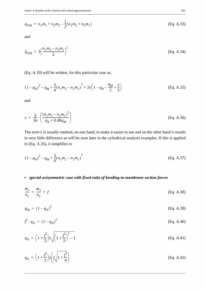
Annex A Ilyushin yield criterion and related approximations 365
(Eq. A.33)
and
(Eq. A.34)
(Eq. A.19) will be written, for this particular case as,
(Eq. A.35)
and
(Eq. A.36)
The term ε is usually omitted, on one hand, to make it easier to use and on the other hand it resultsin very little difference as will be seen later in the cylindrical analysis examples. If this is appliedto (Eq. A.35), it simplifies to
(Eq. A.37)
• special axisymmetric case with fixed ratio of bending-to-membrane section forces
(Eq. A.38)
(Eq. A.39)
(Eq. A.40)
(Eq. A.41)
(Eq. A.42)
qNM n1m1 n2m212--- n1m2 n2m1+( )–+=
q̃NM 3n1m2 n2m1–
2-------------------------------⎝ ⎠⎛ ⎞
2=
1 qN–( )2 qM– 34--- n1m2 n2m1–( )+
22ε 1 qN–
qM2
------– ε2---+⎝ ⎠
⎛ ⎞+
ε 316------
n1m2 n2m1–( )2
qN 0.48qM+--------------------------------------⎝ ⎠⎜ ⎟⎛ ⎞⋅=
1 qN–( )2 qM– 34--- n1m2 n2m1–( )+
2
m1n1------
m2n2------ f= =
qM 1 qN–( )2=
f2 qN⋅ 1 qN–( )2=
qN 1 f2
2----+⎝ ⎠
⎛ ⎞ 1 f2
2----+⎝ ⎠
⎛ ⎞2
1–±=
qN 1 f2
2----+⎝ ⎠
⎛ ⎞ f 1 f2
4----+
⎝ ⎠⎜ ⎟⎛ ⎞
±=

366 Annex A Ilyushin yield criterion and related approximations
A.2.4 Rewriting different yield criteriaIn this section, different yield criteria will be discussed and compared one another. In doing so, thedifferent yield criteria are grouped into two main groups depending on the capability ofrepresenting exact 1D-beam plasticity and other specific situations.
Group-1:The first group (named as the “nonlinear-group” because the non-dimensional yield parameters qN,qM and qNM are combined nonlinearly) comprising of three yield criteria (Ivanov-I, Ivanov-II and“Simple”) which exactly represent 1D-beam plasticity will be discussed first. For the sake ofclarity and easy comparison, these yield criteria will be re-written in the same format as will bediscussed below.
Group-2:
The second group (named as the “linear-group” because the non-dimensional yield parameters qN,qM and qNM are combined linearly) comprises of three yield criteria (Linear-Ilyushin, EDR5 andFirst-yield) which are not capable of representing exact 1D-beam plasticity. The “linear-group”yield criteria will be discussed later.
GROUP-1: THE “NONLINEAR GROUP”
A.2.4.1 Ivanov’s yield criterion-I
(Eq. A.43)
Then Ivanov’s yield surface-I can be rewritten in a step by step simplification as
(Eq. A.44)
Squaring both sides will give
(Eq. A.45)
(Eq. A.46)
(Eq. A.47)
(Eq. A.48)
qNqM2
------qM
2
4------ qNM
2++ + 1=
qM2
4------ qNM
2+ 1 qNqM2
------+⎝ ⎠⎛ ⎞–=
qM2
4------ qNM
2+ 1 qNqM2
------+⎝ ⎠⎛ ⎞–⎝ ⎠
⎛ ⎞2
=
qNM2 1 qN
2 qNqM 2qN qM––+ +=⇒
1 qN–( )2 qM qNqM qNM2–+– 0=⇒
⎧ ⎪ ⎨ ⎪ ⎩
q̃NM
1 qN–( )2 qM– q̃NM+ 0=⇒

Annex A Ilyushin yield criterion and related approximations 367
A.2.4.2 Ivanov’s yield criterion-II
(Eq. A.49)
Using 0.5 instead of 0.48 in the denominator of the “usually” omitted term ε (applying a smallchange on the very small term is almost negligible) will give:
(Eq. A.50)
Following a step by step simplification as above,
(Eq. A.51)
Squaring both sides will give
(Eq. A.52)
expanding and rearranging will then give
(Eq. A.53)
(Eq. A.54)
(Eq. A.55)
A.2.4.3 “Simple” yield criterionThis “Simple” yield criterion which exactly is the same as that of Ivanov-II yield criterion whenthe fixed ratio of bending-to-membrane section forces, see (Eq. A.27) to (Eq. A.29) or (Eq. A.38)to (Eq. A.39) for axisymmetric cases, is considered here as a separate yield criterion. This yieldcriterion gives the exact yield capacity for beams under uni-axial situation, i.e. uni-axial normalforce and bending moment.
(Eq. A.56)
qNqM2
------qM
2
4------ qNM
2+ ε–+ + 1=
ε 14---
q̃NMqN 0.5qM+---------------------------⎝ ⎠⎛ ⎞=
qM2
4------ qNM
2+ 1 qNqM2
------+⎝ ⎠⎛ ⎞–= ε+
qM2
4------ qNM
2+ 1 qNqM2
------+⎝ ⎠⎛ ⎞– ε+⎝ ⎠
⎛ ⎞2
=
1 qN–( )2 qM– q̃NM ε2 2ε 1 qNqM2
------––⎝ ⎠⎛ ⎞+ + + 0=⇒
1 qN–( )2 qM– q̃NM 1 12--- 1
qN 0.5qM+( )-------------------------------- 1–⎝ ⎠⎛ ⎞ 1
4--- ε
qN 0.5qM+( )--------------------------------+++ 0=⇒
⎧ ⎪ ⎪ ⎪ ⎪ ⎪ ⎪ ⎪ ⎨ ⎪ ⎪ ⎪ ⎪ ⎪ ⎪ ⎪ ⎩
ε∗
1 qN–( )2 qM– q̃NM 1 ε+ ∗( )⋅+ 0=⇒
1 qN–( )2 qM– 0=

368 Annex A Ilyushin yield criterion and related approximations
GROUP-2: THE “LINEAR GROUP”
A.2.4.4 Ilyushin’s linear approximate yield criterion
(Eq. A.57)
Ilyushin’s linear yield criterion has been fully discussed on the beginning of the current chapter.
A.2.4.5 EN 1993-1-6 proposed yield criterionThis yield criterion named in EN 1993-1-6 (EDR5) as “Ilyushin’s yield criterion” is not reallyIlyushin’s yield criterion but instead a Von Mises sandwich shell (a shell with three through-thickness layers) yield criterion where the middle layer is modelled to carry transverse shearstresses (assumed negligble in the present discussion) and the outer two layers carrying combined(normal and bending) stress effects equal to n1+m1, n2+m2, n12+m12 on one of the two outer layersand n1-m1, n2-m2, n12-m12 on the other outer layer. It is true that for few special conditions the VonMises sandwich shell yield criterion will be equal to the Ilyushin yield criterion (Robinson, 1971)but generally this is not true as will be seen later with the help of an illustrative shell example.
The EDR5 yield criterion is given as follws:
(Eq. A.58)
Expanding, simplifying & re-arranging (Eq. A.58) will give:
(Eq. A.59)
Re-writing the complete equation for EDR5 yield criterion will then give:
(Eq. A.60)
Thus, the EDR5 yield criterion will be equivalent to the Ilyushin-linear-approximate yield criterionwhen the mixed term qNM is zero. This condition is fulfilled only in situations where the followingexpression holds true:
(Eq. A.61)
For a 1D bending (m) and normal force (n) situation the non-dimensional yield parameters qN, qMand qNM will be . The EDR5 yield criterion will begiven by:
(Eq. A.62)
Refer to Figure A.2 for the m-n plot of (Eq. A.62).
qN qM13
-------qNM±+ 1=
n1 m1±( )2 n2 m2±( )2 n1 m1±( ) n2 m2±( )⋅ 3 n12 m12±( )2+–+ 1=
n12 n2
2 n1n2– 3n122+ +( ) m1
2 m22 m1m2– 3m12
2+ +( ) 2 n1m1 n2m2n1m2 n2m1+
2--------------------------------– 3n12m12+ +⎝ ⎠
⎛ ⎞±+ 1=
⎧ ⎪ ⎪ ⎪ ⎪ ⎨ ⎪ ⎪ ⎪ ⎪ ⎩ ⎧ ⎪ ⎪ ⎪ ⎪ ⎨ ⎪ ⎪ ⎪ ⎪ ⎩ ⎧ ⎪ ⎪ ⎪ ⎪ ⎪ ⎪ ⎪ ⎪ ⎨ ⎪ ⎪ ⎪ ⎪ ⎪ ⎪ ⎪ ⎪ ⎩qN qM qNM
qN qM 2qNM±+ 1=
m2m1------
2 n2 n1⁄( )–2 n2 n1⁄( ) 1–--------------------------------–=
qN n2= ; qM m2= ; qNM n m⋅=
n2 m2 2nm±+ n m±( )2 1= = n m± 1±=⇒

Annex A Ilyushin yield criterion and related approximations 369
A.2.4.6 “First-yield” yield criterionThe “first-yield” yield criterion is the same as the EDR5 yield criterion except the fact that thisyield criterion is fulfilled when the combined elastic stress on either of the two outer surfacesreaches the 1D-yield strength of the material. Hence, the section moments should be related to thesection moment at first-yield, i.e. the reference plastic moment should be usedinstead of . The reference plastic normal force remains since first-yield undermembrane stress results in through-the-thickness yielding. Thus, the “first-yield” yield criterion isfulflled when:
(Eq. A.63)
Expanding, simplifying & re-arranging (Eq. A.63) will give:
(Eq. A.64)
Re-writing the complete equation for the “first-yield” yield criterion will then give:
(Eq. A.65)
For a 1D bending (m) and normal force (n) situation the non-dimensional yield parameters qN, qMand qNM will be . The “first-yield” yield criterionwill be given by:
(Eq. A.66)
Refer to Figure A.2 for the m-n plot of (Eq. A.66).
Mpl fy t2⋅ 6⁄=fy t2⋅ 4⁄ Npl fy t⋅=
n132---m1±⎝ ⎠
⎛ ⎞ 2n2
32---m2±⎝ ⎠
⎛ ⎞ 2n1
32---m1±⎝ ⎠
⎛ ⎞ n232---m2±⎝ ⎠
⎛ ⎞⋅ 3 n1232---m12±⎝ ⎠
⎛ ⎞ 2+–+ 1=
n12 n2
2 n1n2– 3n122+ +( ) 9
4--- m1
2 m22 m1m2– 3m12
2+ +( ) 3 n1m1 n2m2n1m2 n2m1+
2--------------------------------– 3n12m12+ +⎝ ⎠
⎛ ⎞±+ 1=
⎧ ⎪ ⎪ ⎪ ⎪ ⎨ ⎪ ⎪ ⎪ ⎪ ⎩ ⎧ ⎪ ⎪ ⎪ ⎪ ⎨ ⎪ ⎪ ⎪ ⎪ ⎩ ⎧ ⎪ ⎪ ⎪ ⎪ ⎪ ⎪ ⎪ ⎪ ⎨ ⎪ ⎪ ⎪ ⎪ ⎪ ⎪ ⎪ ⎪ ⎩qN qM qNM
qN 2.25qM 3qNM±+ 1=
qN n2= ; qM m2= ; qNM n m⋅=
n2 2.25m2 3nm±+ n 32---m±⎝ ⎠
⎛ ⎞ 21= = n 3
2---m± 1±=⇒

370 Annex A Ilyushin yield criterion and related approximations
A.2.5 Example: comparison of different yield conditionsTo compare the degree of “safety” of using each yield criterion, a numerical comparison of thecorresponding limit load factors is given in Table A.1. In this comparison, the plastic limit loadfactor according to Ivanov-II yield criterion is used as a reference. The information in Table A.1should be interpreted relative to the plastic limit load factor according to Ivanov-II yield criterion,for example, for the plastic limit load factor according to Ilyushin’s linear approximate yieldcriterion, it will be as follows:
(Eq. A.67)
where Λ is the plastic limit load factor based on elastic section forces.
Moreover, along meridian comparison of the different yield criteria can be made as shown in Fig-ure A.5 and Figure A.6 for the illustrative axially compressed and internally uniformly pressurizedcylindrical shell discussed above with fixed and pinned bottom boundary conditions, respectively.The circumferential membrane utilization due to internal pressure is considered to be
. The membrane Mises yield criterion is included for reference purposes.Besides, the influences of the edge bending effect on the different yield criteria can be seen.
The approximate plastic strengths for cylindrical and conical shells have been computed using thesection forces and moments obtained using linear elastic shell analysis for different intensities ofinternal pressurization. The results have been included in the respective discussions on the plasticstrengths of cylindrical and conical shells in this work.
Ivanov-I Ivanov-II Ilyushin_linear EDR5 Simple
Minimum 0.9554 1 0.9377 0.8000 0.8338
Maximum 1 1 1.0343 1 1
Table A.1 Ivanov-II as a reference
0.9377 ΛIvanov II–⋅ ΛIlyushin linear– 1.0343 Λ⋅ Ivanov II–≤ ≤
μ σθ fy⁄ 0.5= =

Annex A Ilyushin yield criterion and related approximations 371
Figure A.5 Comparison of yield function for R/t = 500, μ = 0.5: fixed bottom
Figure A.6 Comparison of yield function for R/t = 500, μ = 0.5: pinned bottom
membrane Mises
EDR5
first yield
simple
Ivanov-I&IIIlyushin-Linear
Value of yield function
membrane MisesIvanov-I&II
Ilyushin-LinearsimpleEDR5
first yield
Value of yield function

372 Annex A Ilyushin yield criterion and related approximations
Annex B Axisymmetric rigid plastic plate & shell analysis 373
B
Axisymmetric rigid plastic plate & shell analysis

374 Annex B Axisymmetric rigid plastic plate & shell analysis
B.1 Introduction
This chapter is concerned with the anayltical computation of rigid-perfect-plastic limit strengthsand corresponding section force distributions of axisymmetric plate and shell structures. In doingso, Ilyushin’s yield criterion and the related approximations will be used along with the basicequations, i.e. equilibrium and kinematic relationships. To show this, a circular plate and acylindrical shell under different loading and boundary conditions will be considered.
First, circular and annular plates under uniform or ring lateral loads and fixed or pinned outer edgeswill be analyzed. Later, cylindrical shells under radial ring loading with and without axial loading& internal pressurization will be considered. All the results will be compared with therecommendations according to EN 1993-1-6 and with small displacement materially nonlinearnumerical analysis (ABAQUS) results.
The general concept of rigid-perfectly-plastic analysis will comprise of the following basiccomponents:
• Equilibrium condition should be fulfilled
• Kinematic relationships should hold true
• Elastic deformations and strains are neglected and hence the total strain is equal to the plastic strain
• No strain hardening is considered and hence perfect plastic
• A yield criterion which will be expressed by using a yield function should be fulfilled
• A plastic flow/normality rule that relates plastic strains with the yield function should be fulfilled

Annex B Axisymmetric rigid plastic plate & shell analysis 375
B.2 Rigid plastic analysis of axisymmetric circular& annular plates
In this section, the rigid plastic limit strengths of uniformly or ring laterally loaded (i.e. normal tothe plate surface) and outer-edge supported solid circular and annular plates will be computed. Theradial distributions of of the deformations and section forces corresponding to the rigid plastic limitload will as well be computed and plotted. Axisymmetric loading and boundary conditions areconsidered. The following assumptions are taken into account:
• isotropic & homogeneous material behavior
• Kirchhoff’s hypothesis, i.e., a straight fiber perpendicular to the middle plane before bend-ing remains straight after bending and hence transverse shear strains are neglected (γrz = 0)
• small deflection theory, i.e. the vertical deflection of the plate middle plane is assumed tobe very small compared to the plate thickness; and hence, there will be no role to be playedby membrane actions that may result from large deflections
A solid circular plate and an annular plates are shown in Figure B.1(a) and Figure B.1(b),respectively. The different geometrical, loading and boundary condition terminologies used are asfollows:
t plate thickness
R plate outer radius
a inner radius (for both geometry and loading)
b loading outer radius ( , i.e. would mean a solid circular plate underconcentrated central load)
r running radius
q lateral load
The “FIX” and “PIN” outer boundary conditions are shown in Figure B.1(a) & (b). A cut-outelement along with the possible internal section forces is shown in Figure B.1(c) & (d).
The basic equations which will be needed in computing the rigid plastic limit strength and itscorresponding deformation and section force distributions will be obtained as will be discussed inthe following sections.
a b R≤ ≤ a b 0= =
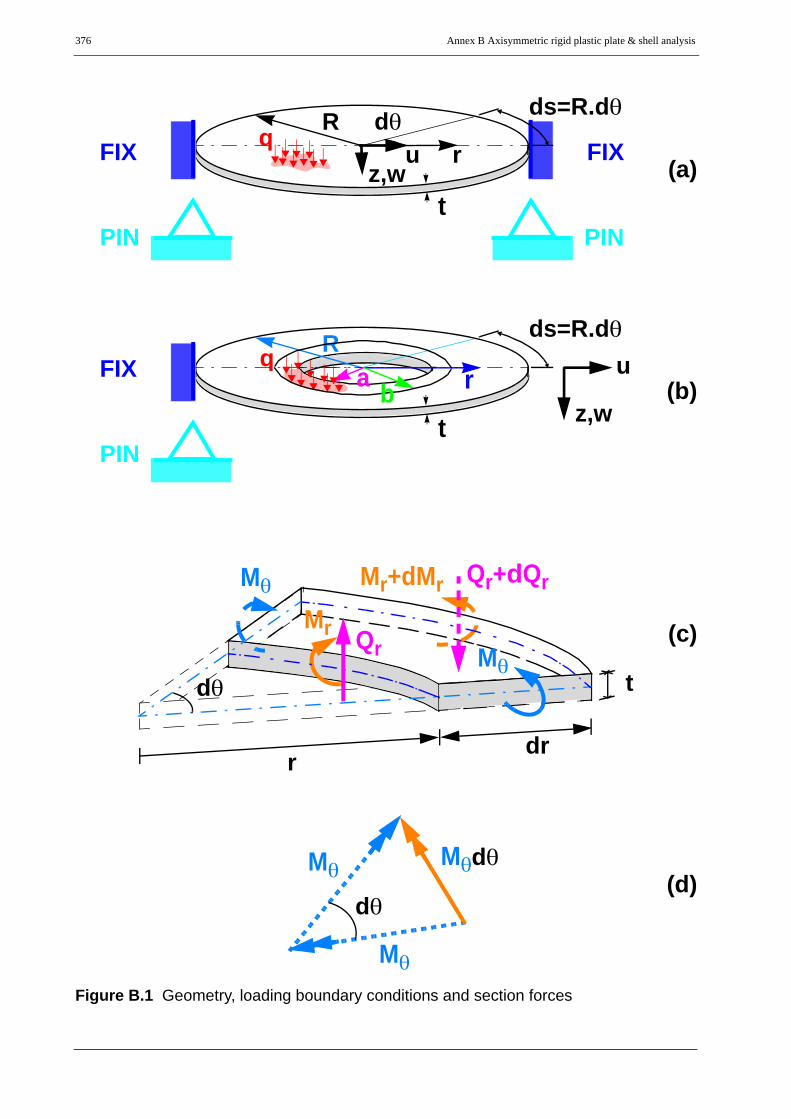
376 Annex B Axisymmetric rigid plastic plate & shell analysis
Figure B.1 Geometry, loading boundary conditions and section forces
PIN
FIX
ds=R.dθ
t
Rr
dθ
PIN
FIX q
ds=R.dθ
t
Rr
qra b
PIN
FIX
dφ t
dθ
Mθ
Mθ Mr+dMr
dθ
rdr
Qr
Qr+dQr
Mθ
Mθ Mθdθ
Mr
(a)
(b)
(d)
(c)
u
z,w
uz,w

Annex B Axisymmetric rigid plastic plate & shell analysis 377
B.2.1 Equilibrium relationshipsEquilibrium of forces along the transverse direction:
(Eq. B.1)
(Eq. B.2)
Equilibrium of moments:
(Eq. B.3)
(Eq. B.4)
When written in matrix form, a summary of the equilbrium equations will be given as
(Eq. B.5)
The transverse shear section force can be eliminated using the two equilibrium equations (i.e.substituting (Eq. B.4) in (Eq. B.2)) to give the following relationship:
(Eq. B.6)
Qrr θd QrQ∂ rr∂
--------- rd+⎝ ⎠⎛ ⎞ r rd+( ) θd– q r rd+( ) rd dθ– 0=
rdd⇒ rQr( ) qr–=
Mrr θd ΜrΜ∂ rr∂
−−−−−−dr+⎝ ⎠⎛ ⎞ r dr+( ) θ Mθ rd θd+d– rQr rd θd+ 0=
rdd⇒ rMr( ) rQr Mθ+=
rdd ( ) 0 0
1– rd
d ( ) 1–
rQr
rMr
Mθ
⋅ rq0
+ 00
=
r2
2
dd ( )
rdd ( )–
rMr
Mθ
⋅ rq+ 0=

378 Annex B Axisymmetric rigid plastic plate & shell analysis
B.2.2 Kinematic (geometry) relationships3D axisymmetric Strains:
(Eq. B.7)
3D displacement assumption:
(Eq. B.8)
or in matrix form:
(Eq. B.9)
The 3D axisymmetric strains will then be given by
(Eq. B.10)
from Kirchhoff’s hypothesis, the transverse shear strain is zero
(Eq. B.11)
εr
εθ
γrz 3D
r∂∂ ( ) 0
1r--- 0
z∂∂ ( ) r∂
∂ ( )
uw 3D
⋅=
u z βr⋅=w W = constant with z=
uw 3D
z 00 1
βr
W⋅=
εr
εθ
γrz 3D
r∂∂ ( ) 0
1r--- 0
z∂∂ ( ) r∂
∂ ( )
z 00 1
βr
W⋅ ⋅
z r∂∂ ( ) 0
zr-- 0
1 r∂∂ ( )
βr
W⋅= =
γrz βr r∂∂W+ 0= = βr⇒ r∂
∂W–=
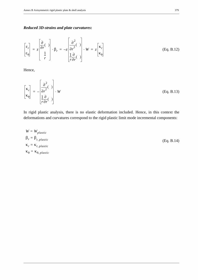
Annex B Axisymmetric rigid plastic plate & shell analysis 379
Reduced 3D-strains and plate curvatures:
(Eq. B.12)
Hence,
(Eq. B.13)
In rigid plastic analysis, there is no elastic deformation included. Hence, in this context thedeformations and curvatures correspond to the rigid plastic limit mode incremental components:
(Eq. B.14)
εr
εθ
z r∂∂ ( )
1r---
βr⋅ z r2
2
∂∂ ( )
1r---
r∂∂ ( )
W⋅– zκr
κθ
= = =
κr
κθ
r2
2
∂∂ ( )
1r---
r∂∂ ( )
– W⋅=
W Wplastic=βr β= r plastic,
κr κr plastic,=κθ κθ plastic,=

380 Annex B Axisymmetric rigid plastic plate & shell analysis
B.2.3 Yield functions and yield criterion based on stress resultants
B.2.3.1 Yield function
(Eq. B.15)
B.2.3.2 Yield condition
(Eq. B.16)
Table B.1 lists the different yield function approximations to Ilyushin exact yield function. Thecorrection term ε* in Ivanov-II yield function is given by (See Annex-A):
(Eq. B.17)
For the particular case of the considered circular (i.e. solid and annular) plates where the deflectionis assumed to be very small and hence no membrane effects, the following condition will apply
(Eq. B.18)
With these conditions, all approximate yield criteria, except the “first-yield” for which a 2.25 factorshould be applied to qM in the following equation, will be given by
(Eq. B.19)
When re-written in terms of the section moments, the yield function in (Eq. B.19) will be
(Eq. B.20)
yield criterion yield function, FIvanov-I
Ivanov-II
Simple
Ilyushin Linear
EDR5
First-yield
Table B.1 Approximate yield functions
F qN qM qNM, ,( )
F qN qM qNM, ,( ) 0=
ε∗ 12--- 1
qN 0.5qM+( )-------------------------------- 1–⎝ ⎠⎛ ⎞ 1
4--- ε
qN 0.5qM+( )--------------------------------+=
1 qN–( )2 qM– q̃NM+
1 qN–( )2 qM– q̃NM 1 ε+ ∗( )⋅+
1 qN–( )2 qM–
qN qM13
-------qNM± 1–+
qN qM 2qNM± 1–+
qN 2.25qM 3qNM± 1–+
qN 0;= qNM 0=
F qM( ) qM 1–= 0=
F Mr M, θ( ) Mr2 Mθ
2 MrMθ– Mpl2 0=–+=

Annex B Axisymmetric rigid plastic plate & shell analysis 381
B.2.4 Associated flow/normality ruleThe incremental plastic curvatures are proportional to the gradient of the yield surface. Using aplastic load increment parameter, , the associated flow rule is given by
(Eq. B.21)
B.2.5 Summary of equations for rigid plastic analysis of circular platesA detailled summary of the different relationships needed for rigid plastic analysis of circularplates is shown in Table B.2. In this table, the different relationships along with the total numberand type of unknown terms to be computed & the number of equations available in eachrelationship are given. The mathematical solvability of the whole problem will depend on the totalnumbers of unknown terms and available equations. In the particular circular plate problem, thereexist as many unknowns as available equations, hence it is solvable (determinate).
relationship unknown terms # unknowns # equations
equilibrium
[(Eq. B.5)], (Eq. B.6)
(Qr)
Mr
Mθ
(3)
2
(2)
1
kinematics
(Eq. B.13)
κr,plastic
κθ,plastic
Wplastic
3 2
yield function
(Eq. B.20)
- 0 1
flow rule
(Eq. B.21)
λplastic 1 2
Total (7) 6 (7) 6Table B.2 Number of unknowns and unknown terms
λplastic
κplasticκr
κθ plastic
λplasticMr∂∂ ( )
Mθ∂∂ ( )
F⋅= =
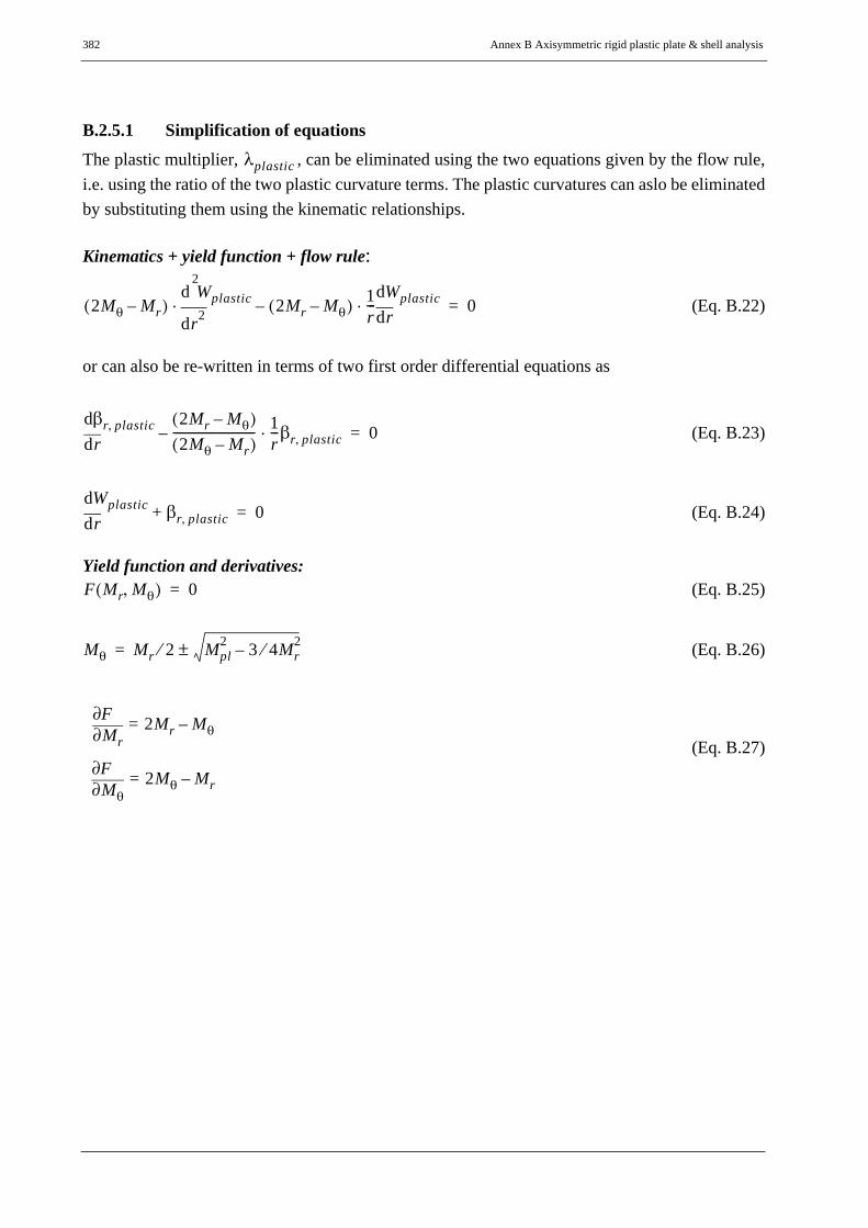
382 Annex B Axisymmetric rigid plastic plate & shell analysis
B.2.5.1 Simplification of equationsThe plastic multiplier, , can be eliminated using the two equations given by the flow rule,i.e. using the ratio of the two plastic curvature terms. The plastic curvatures can aslo be eliminatedby substituting them using the kinematic relationships.
Kinematics + yield function + flow rule:
(Eq. B.22)
or can also be re-written in terms of two first order differential equations as
(Eq. B.23)
(Eq. B.24)
Yield function and derivatives: (Eq. B.25)
(Eq. B.26)
(Eq. B.27)
λplastic
2Mθ Mr–( )r2
2
d
d Wplastic⋅ 2Mr Mθ–( ) 1r---
rddWplastic⋅– 0=
rddβr plastic, 2Mr Mθ–( )
2Mθ Mr–( )---------------------------- 1
r---βr plastic,⋅– 0=
rddWplastic βr plastic,+ 0=
F Mr Mθ,( ) 0=
Mθ Mr 2⁄ Mpl2 3 4⁄ Mr
2–±=
Mr∂∂F 2Mr Mθ–=
Mθ∂∂F 2Mθ Mr–=

Annex B Axisymmetric rigid plastic plate & shell analysis 383
With the above simplifications and the equilibrium equations given in (Eq. B.5) and (Eq. B.6), thesummary of equations for rigid plastic analysis of circular plates will reduce to:
B.2.5.2 Boundary conditionsThe boundary conditions of the considered circular plate which will be required in solving the setof differential equations are given as follows:
Interior free edge (r = a):; and ; (Eq. B.28)
Exterior supported edge (r = R):Pin supported:
; and ; (Eq. B.29)
Clamped edge:
; and ; (Eq. B.30)
relationship unknown terms # unknowns # equations
equilibrium
[(Eq. B.5)], (Eq. B.6)
(Qr)
Mr
Mθ
(3)
2
(2)
1
yield function
(Eq. B.26)
- 0 1
kinematics +yield function +flow rule
(Eq. B.23) &(Eq. B.24)
Wplastic
βr,plastic
2 2
Total (5) 4 (5) 4Table B.3 Number of unknowns and unknown terms
Qr 0= Mr 0=
Mr 0= Wplastic 0=
Wplastic 0= βr r∂∂Wplastic– 0= =

384 Annex B Axisymmetric rigid plastic plate & shell analysis
B.2.6 Introduction of non-dimensional parameters
Geometry-related non-dimensional parameters:
(Eq. B.31)
(Eq. B.32)
the relationship between the derivatives will then become
(Eq. B.33)
(Eq. B.34)
Section forces and deformations-related non-dimensional parameters:
(Eq. B.35)
(Eq. B.36)
(Eq. B.37)
ρ rR---= ; ρa
aR---= ; ρb
bR---=
ξ r a–R a–------------
ρ ρa–1 ρa–---------------= =
d( )dr
----------- ( )'=⇒ 1R 1 ρa–( )----------------------- d( )
dξ-----------⋅ 1
R 1 ρa–( )----------------------- ( )·⋅= =
d2( )dr2
------------- ( )''=⇒ 1
R2 1 ρa–( )2
---------------------------- d2( )dξ2
-------------⋅ 1
R2 1 ρa–( )2
---------------------------- ( )··⋅= =
Qr∗Qr R⋅Mpl
--------------=
q ∗ q R2⋅Mpl
-------------=
βr plastic, ∗ R βr plastic,⋅=
λplastic∗ R2Mpl λ⋅ plastic=
κr plastic, ∗ R2 κ⋅ r plastic,=
κθ plastic, ∗ R2 κ⋅ θ plastic,=
mrMrMpl--------;= mθ
MθMpl-------- ;= Mpl fy
t2
4----⋅=

Annex B Axisymmetric rigid plastic plate & shell analysis 385
B.2.7 Condensed rigid plastic equations of annular/solid circular platesThe equations which completely describe circular plate rigid plasticity will reduce to the followingset of erdinary differential equations. The yield condition, F(Mr,Mθ) = 0, has been used toeliminate Mθ.
(Eq. B.38)
(Eq. B.39)
(Eq. B.40)
(Eq. B.41)
Thus, the rigid plastic limit analysis of circular plates has been reduced to four first order ordinarydifferential equations with four unkown non-dimensional section force and deformation quantities( ).
Boundary conditions in terms of the non-dimensional parameters:Interior free edge (ρ = ρa):
; and (Eq. B.42)
Exterior supported edge (ρ = 1):
Pin supported:
; and (Eq. B.43)
Clamped edge:
; and (Eq. B.44)
Qr∗ρa
1 ρa–-------------- ξ+⎝ ⎠⎛ ⎞ Qr
· ∗⋅ q∗ 1 ρa–( )+ρa
1 ρa–-------------- ξ+⎝ ⎠⎛ ⎞+ 0=
mr 2ρa
1 ρa–-------------- ξ+⎝ ⎠⎛ ⎞mr
· 4 3mr2–– 2– 1 ρa–( )
ρa1 ρa–-------------- ξ+⎝ ⎠⎛ ⎞Qr∗+ 0=
4 3mr2– β· r plastic,
∗( )⋅ 12--- 1
ρa1 ρa–-------------- ξ+⎝ ⎠⎛ ⎞-----------------------------⋅– 3mr 4 3mr
2––( ) βr plastic, ∗( )⋅ 0=
βr plastic, ∗( ) 11 ρa–( )
-------------------W· plastic+ 0=
Qr∗ mr Wplastic and βr plastic, ∗, , ,
Qr∗ 0= mr 0=
mr 0= Wplastic 0=
Wplastic 0= βr plastic, ∗ 0=

386 Annex B Axisymmetric rigid plastic plate & shell analysis
Back calculated section force and deformation variables:Once the four quantities ( ) are computed using the set of ordinarydifferential equations, the following section force and deformation variables can then be backcalculated.
(Eq. B.45)
(Eq. B.46)
(Eq. B.47)
(Eq. B.48)
(Eq. B.49)
Qr∗ mr Wplastic and βr plastic, ∗, , ,
mθ 0.5mr 1 0.75mr2–+=
qM mr2 mθ
2 mrmθ–+=
λplastic∗1
1 ρa–( )2---------------------- 1
ρa1 ρa–-------------- ξ+⎝ ⎠⎛ ⎞----------------------------- 1
2mθ mr–( )---------------------------W· plastic–=
κr plastic, ∗ 11 ρa–( )2
----------------------W·· plastic–=
κθ plastic, ∗ 11 ρa–( )2
---------------------- 1ρa
1 ρa–-------------- ξ+⎝ ⎠⎛ ⎞-----------------------------W· plastic–=
Annex B Axisymmetric rigid plastic plate & shell analysis 387
B.2.8 Solution procedureThe condensed set of first order differential equations (o.d.e.) has been solved with the help of theboundary conditions and using MATHEMATICA program package (Wolfram, 2008). Thissoftware has the ability to accurately solve set of differential equations both analytically andnumerically. Thus it enables to solve the set of o.d.e. and compute the lateral plastic load q* andcorresponding section force and deformation variables in such a way that the boundary conditionsare fulfilled. This way of solving equations to fulfill constraint conditions (it is like adjustingconditions at one end to satisfy requirements the other end) is usually called SHOOTING!
Since the presentaion of the condensed set of differential equations is in non-dimensionalgeometric, section force and deormation variables, the solution of the problem can be applied todifferent geometry conditions.
B.2.9 Examples, result plots and comparisonRigid-plastic analyses of circular plates with varying values of the interior radius a and loadingouter radius b have been done. For illustration purposes, the results of a rigid plastic analysis of asolid circular plate (a = 0) under uniform lateral loading (b = R) have been perfeormed. The circularplate has the following set of conditions:
Geometry: general for all R and t values
Boundary conditions: pinned or fixed outer edges
Loading: uniform lateral load q
Material properties: general for all material properties
For the solid circular plate under the uniform loading, MATHEMATICA has been used tonumerically compute the rigid plastic load and the corresponding section force and deformationdistributions along the radius of the plate. The results obtained are plotted as shown in Figure B.3to Figure B.10.
A materially nonlinear numerical analysis (MNA) has been done using ABAQUS for a solidcircular plate with similar geometry and loading conditions. In this case geometric variables withR = 500 cm and t = 1 cm has been used. The results obtained, however, have been converted intonon-dimensional form in order to be able to make comparisons with those of theMATHEMATICA results discussed above. The ABAQUS materially nonlinear numerical analyisresults are also shown in the same plots shown in Figure B.3 to Figure B.10. The materiallynonlinear plastic deflection and slope are computed as normalized differences between thedeflections and slopes of two neighbouring increments on the plastic plateau of the load-deflectiondiagram, Figure B.2.
Figure B.11 shows the effects of local load distribution (varying b/R) on the plastic load capacityof the solid circular plate and corresponding plastic load as predicted by EN 1993-1-6recommendations. In all the computations both fixed and pinned outer-edge boundary conditionshave been considered and shown. It can be seen from all the comparisons that a good fit existsbetween the analytical and numerical results & the analytical and EN 1993-1-6 recommendations.

388 Annex B Axisymmetric rigid plastic plate & shell analysis
Figure B.2 Load-deflection diagram: FEM
FIX
PIN
wi wi+1
ΛMNA

Annex B Axisymmetric rigid plastic plate & shell analysis 389
Figure B.3 Radial plastic moment, mr
Figure B.4 Circumferential plastic moment, mθ
�� � � � ��
��
�
�
�
��
�� � � � � � ��
��
���
0.0 0.2 0.4 0.6 0.8 1.0�2
�1
0
1
2
PIN
FIX
Analytic
FEM
r R⁄
mr
�� � � � � � � � ��
�
�
�
�� � � � � � � � � � � ��
0.0 0.2 0.4 0.6 0.8 1.0�2
�1
0
1
2
PIN
FIX
Analytic
FEM
r R⁄
mθ

390 Annex B Axisymmetric rigid plastic plate & shell analysis
Figure B.5 Transverse shear, r.Qr*
Figure B.6 Lateral plastic deflection, Wplastic
�� � ��
�
�
�
�� � � ��
�
�
�
�
�0.0 0.2 0.4 0.6 0.8 1.0�2
�1
0
1
2
PIN
FIX
Analytic
FEM
r R⁄
r Qr∗⋅
�� ���
�
�
�
�
�
�
�
��
�� � � ��
�
�
�
�
�
�
��0.0 0.2 0.4 0.6 0.8 1.0
0.0
0.2
0.4
0.6
0.8
1.0
1.2
PIN
FIXAnalytic
FEM
r R⁄
Wplastic

Annex B Axisymmetric rigid plastic plate & shell analysis 391
Figure B.7 Radial plastic rotation, R. βr,plastic
Figure B.8 Radial plastic curvature, R2.kr,plastic
�
�
�
�
�
�
� � ��
��
��
�
�
�
�
�
�
��
� � � ���
0.0 0.2 0.4 0.6 0.8 1.00.0
0.5
1.0
1.5
2.0
PIN
FIX
Analytic
FEM
r R⁄
βr plastic, ∗
�� ���
��
�� � � �
�
�
�� � � ��
�� � � � � ��
0.0 0.2 0.4 0.6 0.8 1.0�10
�5
0
5
10
PIN
FIX
Analytic
FEM
r R⁄
κr plastic, ∗

392 Annex B Axisymmetric rigid plastic plate & shell analysis
Figure B.9 Circumferential plastic curvature, R2.kθ,plastic
Figure B.10 Plastic section moments: Analytic & FEM
�� � � ��
�� � � � � ��
�� � � � � � � � � � � ��
0.0 0.2 0.4 0.6 0.8 1.0�10
�5
0
5
10
PIN
FIX
Analytic
FEM
r R⁄
κθ plastic, ∗
�2 �1 0 1 2�2
�1
0
1
2
FIX
PIN
mr
mθ

Annex B Axisymmetric rigid plastic plate & shell analysis 393
Figure B.11 Plastic limit load: effects of local load distribution; Analytic & EN 1993-1-6
�
� � � ��
��
�
�
�
�
�
��
�
�
��
�
�
�
0.0 0.2 0.4 0.6 0.8 1.00
2
4
6
8
10
FIXPIN
Analytic
EN 1993-1-6
b R⁄
qR2
2Mpl------------
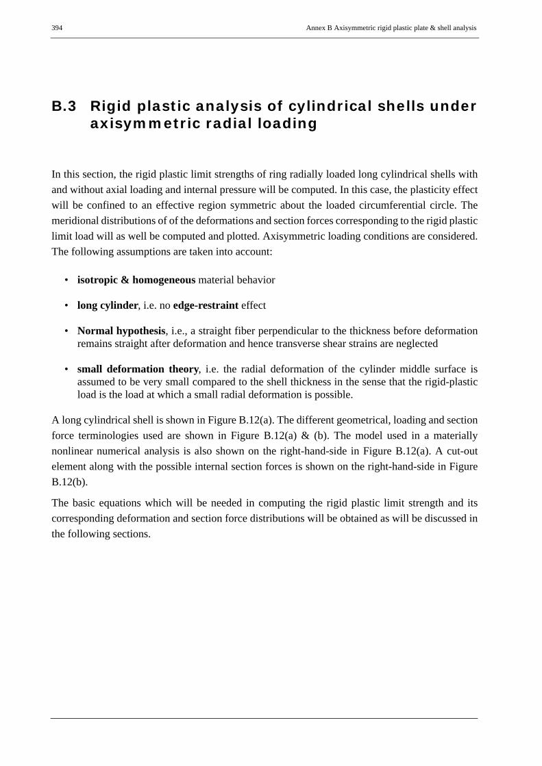
394 Annex B Axisymmetric rigid plastic plate & shell analysis
B.3 Rigid plastic analysis of cylindrical shells underaxisymmetric radial loading
In this section, the rigid plastic limit strengths of ring radially loaded long cylindrical shells withand without axial loading and internal pressure will be computed. In this case, the plasticity effectwill be confined to an effective region symmetric about the loaded circumferential circle. Themeridional distributions of of the deformations and section forces corresponding to the rigid plasticlimit load will as well be computed and plotted. Axisymmetric loading conditions are considered.The following assumptions are taken into account:
• isotropic & homogeneous material behavior
• long cylinder, i.e. no edge-restraint effect
• Normal hypothesis, i.e., a straight fiber perpendicular to the thickness before deformationremains straight after deformation and hence transverse shear strains are neglected
• small deformation theory, i.e. the radial deformation of the cylinder middle surface isassumed to be very small compared to the shell thickness in the sense that the rigid-plasticload is the load at which a small radial deformation is possible.
A long cylindrical shell is shown in Figure B.12(a). The different geometrical, loading and sectionforce terminologies used are shown in Figure B.12(a) & (b). The model used in a materiallynonlinear numerical analysis is also shown on the right-hand-side in Figure B.12(a). A cut-outelement along with the possible internal section forces is shown on the right-hand-side in FigureB.12(b).
The basic equations which will be needed in computing the rigid plastic limit strength and itscorresponding deformation and section force distributions will be obtained as will be discussed inthe following sections.
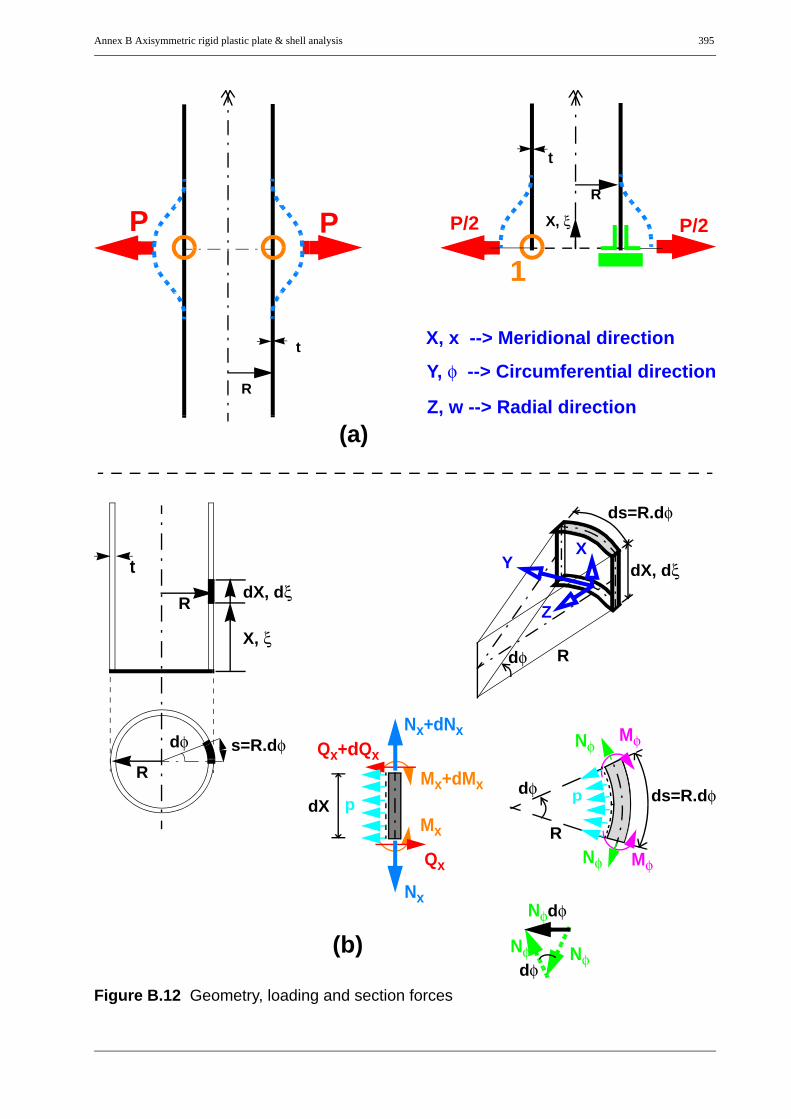
Annex B Axisymmetric rigid plastic plate & shell analysis 395
Figure B.12 Geometry, loading and section forces
R
t
PPR
t
P/2P/2
1
X, ξ
R
tdX, dξ
X, ξ
dφ s=R.dφ
R
dφ
ds=R.dφ
dX, dξ
dφ
R
ds=R.dφ
Mx
Mx+dMx
Qx
Qx+dQx
Nφ
Nφ
Mφ
Mφ
dX
Nφ Nφdφ
Nφdφ
R
XY
Z
p p
Nx
Nx+dNx
X, x --> Meridional direction
Y, φ --> Circumferential direction
Z, w --> Radial direction(a)
(b)

396 Annex B Axisymmetric rigid plastic plate & shell analysis
B.3.1 Equilibrium relationships
B.3.1.1 Equilibrium of forcesin the axial direction:
(Eq. B.50)
(Eq. B.51)
in the radial direction:
(Eq. B.52)
(Eq. B.53)
B.3.1.2 Equilibrium of moments
(Eq. B.54)
(Eq. B.55)
When written in matrix form, a summary of the equilbrium equations will be given as
(Eq. B.56)
Nx– Nx Nxd+( )+( ) R φd⋅ 0=
Nx' 0=
Qx– Qx Qxd+( )+( ) R φd⋅ Nφ φd xd p R φd xd⋅+ + 0=
Qx'NφR------ p 0=+ +
M– x Mx dMx+( )+( ) Rdφ Qx– Rdφdx⋅⋅ 0=
Qx Mx'=
xdd ( ) 0 0 0
0 1R--- xd
d ( ) 0
0 0 1– xdd ( )
Nx
Nφ
Qx
Mx
⋅0p0
+000
=

Annex B Axisymmetric rigid plastic plate & shell analysis 397
B.3.2 Kinematic (geometry) conditionsThe general relationship between the strains and deformations of thin-walled cylindrical shellswith normal hypothesis is given as follows, Linder (2001):
(Eq. B.57)
For cylindrical shells under axisymmetric conditions, all the derivatives with respect to φ will bezero because of symmetry. The kinematic relationships will then reduce to:
(Eq. B.58)
Once again, it should be noted that the rigid-plastic deformation and strain quantities refer to theincremental rigid-plastic eigenmode.
εx
εφ
κx
κφ
x∂∂ ( ) 0 0
0 1R---
φ∂∂ ( ) 1
R---–
0 0 x2
2
∂∂ ( )–
0 1R2------
φ∂∂ ( ) 1
R2------–
φ2
2
∂∂ ( )
UVW
⋅=
εx
εφ
κx
κφ
x∂∂U
WR-----–
x2
2
∂∂ W–
0
=

398 Annex B Axisymmetric rigid plastic plate & shell analysis
B.3.3 Yield functions and yield criteria based on stress resultants
B.3.3.1 Yield function
(Eq. B.59)
B.3.3.2 Yield condition
(Eq. B.60)
Refer to Table B.1 for a list of the different approximate yield functions. As it will be seen later,Ivanov-II yield criterion has been used for illustrative purposes.
B.3.4 Associated flow/normality ruleThe incremental plastic strains and curvatures are proportional to the gradient of the yield surface.Using a plastic load increment parameter, , the associated flow rule is given by
(Eq. B.61)
F qN qM qNM, ,( )
F qN qM qNM, ,( ) 0=
λplastic
εx
εφ
κx
κφ plastic
λplastic
Nx∂∂ ( )
Nφ∂∂ ( )
Mx∂∂ ( )
Mφ∂∂ ( )
⋅ F=
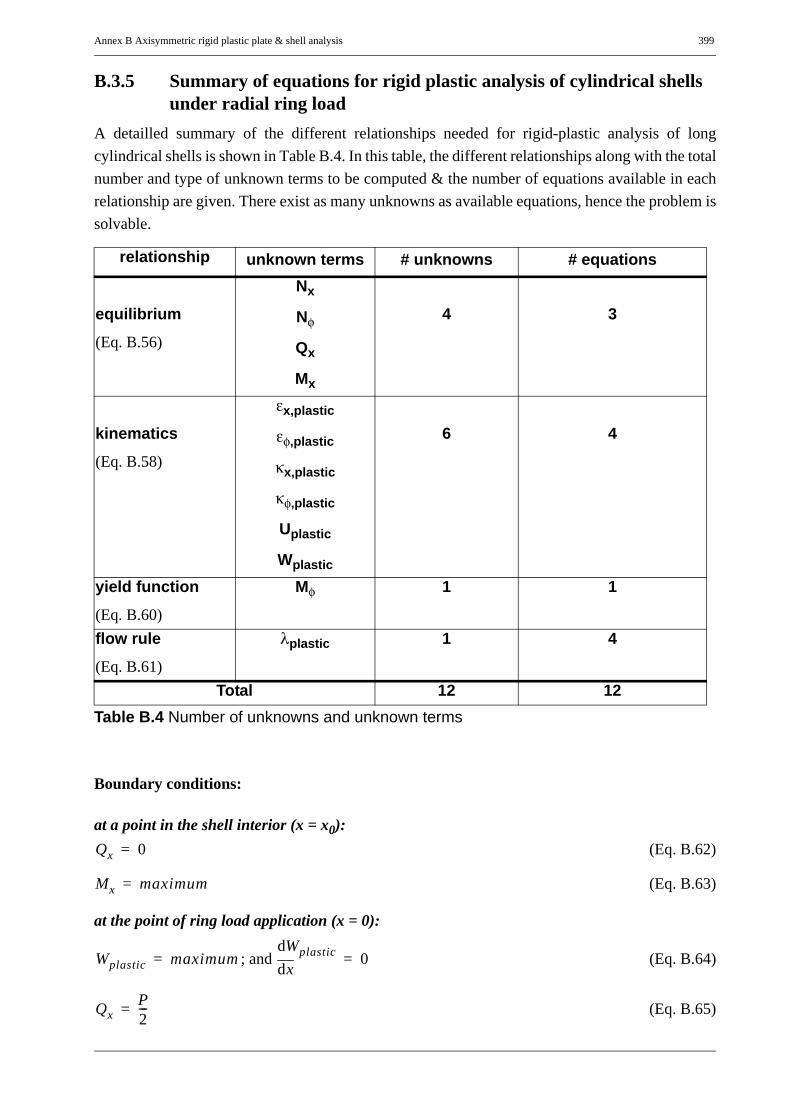
Annex B Axisymmetric rigid plastic plate & shell analysis 399
B.3.5 Summary of equations for rigid plastic analysis of cylindrical shellsunder radial ring load
A detailled summary of the different relationships needed for rigid-plastic analysis of longcylindrical shells is shown in Table B.4. In this table, the different relationships along with the totalnumber and type of unknown terms to be computed & the number of equations available in eachrelationship are given. There exist as many unknowns as available equations, hence the problem issolvable.
Boundary conditions:
at a point in the shell interior (x = x0): (Eq. B.62)
(Eq. B.63)
at the point of ring load application (x = 0):
; and (Eq. B.64)
(Eq. B.65)
relationship unknown terms # unknowns # equations
equilibrium
(Eq. B.56)
Nx
Nφ
Qx
Mx
4 3
kinematics
(Eq. B.58)
εx,plastic
εφ,plastic
κx,plastic
κφ,plastic
Uplastic
Wplastic
6 4
yield function
(Eq. B.60)
Mφ 1 1
flow rule
(Eq. B.61)
λplastic 1 4
Total 12 12Table B.4 Number of unknowns and unknown terms
Qx 0=
Mx maximum=
Wplastic maximum= xddWplastic 0=
QxP2---=

400 Annex B Axisymmetric rigid plastic plate & shell analysis
B.3.6 Introduction of non-dimensional parameters
Geometry-related non-dimensional parameters:
(Eq. B.66)
with the following derivative relationships
(Eq. B.67)
(Eq. B.68)
Section forces and deformations-related non-dimensional parameters:
(Eq. B.69)
(Eq. B.70)
(Eq. B.71)
(Eq. B.72)
(Eq. B.73)
(Eq. B.74)
ξ xR t⋅
--------------=
d( )dξ
-----------⇒ ( )· R t⋅ d( )dx
-----------⋅ R t⋅ ( )'⋅= = =
( )··⇒ R t⋅( )( )''=
nxNxNpl--------;= nφ
NφNpl--------;= mx
MxMpl--------;= mφ
MφMpl--------;= μ pR
fyt-------=
Npl fy t;⋅= Mpl fyt2
4----⋅=
Qx∗Qxfyt------ R
t---⋅=
βx plastic, ∗ βx plastic, Rt⋅=
λplastic∗ λplasticRt
Mpl--------⋅=
κx plastic, ∗ κx plastic, Rt⋅=

Annex B Axisymmetric rigid plastic plate & shell analysis 401
B.3.7 Simplification of equations The equations which completely describe rigid plasticity of ring-loaded cylindrical shells reduceto:
Equilibrium equations:
(Eq. B.75)
Elimination of transverse shear:
The second and third rows of (Eq. B.75) can be combined and reduced to a single differentialequation of second order given by
(Eq. B.76)
Plastic/yield condition:
(Eq. B.77)
Kinematic + flow rule:
Using the zero circumferential curvature of an axisymmetric cylindrical shell, the followingrelationship will be obtained:
(Eq. B.78)
The plastic multiplier, , can be eliminated using the εφ,plastic and κx,plastic equations givenby the flow rule, i.e. using the ratio of the two plastic strain terms. The εφ,plastic and κx,plastic canthen be eliminated by substituting them using the respective kinematic relationships. Combiningthe kinematic and flow rule relationships with further simplification will then give:
d( )dξ
----------- 0 0 0
0 1 d( )dξ
----------- 0
0 0 1– 14---d( )
dξ-----------
nx
nφ
Qx∗
mx
⋅0μ0
+000
=
0.25 m··⋅ x nφ μ 0=+ +
F nx n, φ mx mφ, ,( ) 0=
κφ plastic, λplastic Mφ∂∂F⋅ 0= =
mφ∂∂F 0=⇒
λplastic

402 Annex B Axisymmetric rigid plastic plate & shell analysis
(Eq. B.79)
(Eq. B.80)
(Eq. B.79) and (Eq. B.80) can also be combined and reduced to a single differential equation ofsecond order given by
(Eq. B.81)
nφ∂∂F– β· x plastic,
∗ 4 mx∂∂F Wplastic
R------------------⋅–⋅ 0=
βx plastic, ∗ W· plastic–=
nφ∂∂F W·· plastic 4 mx∂
∂F WplasticR
------------------⋅–⋅ 0=

Annex B Axisymmetric rigid plastic plate & shell analysis 403
B.3.8 Condensed rigid plastic equations of cylindrical shells under radialring load
The equations which completely describe rigid plasticity of radially ring loaded cylindrical shellswith or without axial load and internal pressure reduce to:
(Eq. B.82)
(Eq. B.83)
(Eq. B.84)
(Eq. B.85)
(Eq. B.86)
Boundary conditions in terms of the non-dimensional section force & deformation variables
at a point in the shell interior (x = x0): and (Eq. B.87)
at the point of ring load application (x = 0): and (Eq. B.88)
(Eq. B.89)
relationship unknown terms # unknowns # equations
equilibrium
(Eq. B.82) &(Eq. B.83)
nx
nφ
mx
3 2
yield function
(Eq. B.84)
mφ 1 1
kinematic +flow rule
(Eq. B.85) &(Eq. B.86)
w 1 2
Total 5 5Table B.5 Number of unknowns and unknown terms
n· x 0=
0.25 m··⋅ x nφ μ 0=+ +
F nφ mx mφ, ,( ) 0=
mφ∂∂F 0=
nφ∂∂F W·· plastic 4 mx∂
∂F WplasticR
------------------⋅–⋅ 0=
m· x 0= mx maximum=
Wplastic maximum= W· plastic 0=
Qx∗P2--- 1
fyt----- R
t---⋅=

404 Annex B Axisymmetric rigid plastic plate & shell analysis
B.3.9 Derivatives of the yield functionThe general expression for the derivative of the yield function with respect to thenormalized section force parameters nφ, mx, mφ is given as follows:
(Eq. B.90)
(Eq. B.91)
(Eq. B.92)
in which
(Eq. B.93)
(Eq. B.94)
(Eq. B.95)
and the derivatives of the yield function with respect to , for example, for Ivanov-IIyield function will be given by
(Eq. B.96)
F qN qM qNM, ,( )
nφ∂∂F
qN∂∂F
nφ∂∂qN
qM∂∂F
nφ∂∂qM
qNM∂∂F
nφ∂∂qNM⋅+⋅+⋅=
mx∂∂F
qN∂∂F
mx∂∂qN
qM∂∂F
mx∂∂qM
qNM∂∂F
mx∂∂qNM⋅+⋅+⋅=
mφ∂∂F
qN∂∂F
mφ∂∂qN
qM∂∂F
mφ∂∂qM
qNM∂∂F
mφ∂∂qNM⋅+⋅+⋅=
nφ∂∂
qN
qM
qNM
2nφ nx–0
2mφ mx–( ) 2⁄
=
mx∂∂
qN
qM
qNM
02mx mφ–
2nx nφ–( ) 2⁄
=
mφ∂∂
qN
qM
qNM
02mφ mx–
2nφ nx–( ) 2⁄
=
qN qM qNM, ,
qN∂∂
qM∂∂
qNM∂∂
F
1qM 4⁄
qN 0.48qM+------------------------------–
qNqM qNM2–( )
4 qN 0.48qM+( )2-----------------------------------------+
12---
qM 2⁄
qM2 4qNM
2+------------------------------------
qN2 0.48qNM
2+( )
4 qN 0.48qM+( )2-------------------------------------------–+
qNM2
qM2 4qNM
2+------------------------------------ 0.5
qN 0.48qM+------------------------------+
⎝ ⎠⎜ ⎟⎛ ⎞
=

Annex B Axisymmetric rigid plastic plate & shell analysis 405
B.3.10 Determination of plastic section forces, plastic deformation, slope,curvature and plastic loading parameter λplastic
The axial section force term nx is constant and can be directly computed using the applied axialloading, i.e. pure axial membrane section force. For the computation of other section force terms,the following solution procedure is followed:
Using (Eq. B.83) to (Eq. B.85) and starting conditions at a point in the shell interior (i.e. at ameridional distance ξ0 from the ring-load location) of zero transverse shear (or ) andmaximum mx without violating the equilibrium, yield and flow rule conditions. The later startingcondition is equivalent to producing a maximum transverse shear section force at the ring-loadlocation which can be reached without violating the equilibrium, yield and flow rule conditions(SHOOTING!).
While shooting for the maximum possible transverse shear at the ring-load location, thecorresponding plastic section force terms ( ) at the ring-load location cansimultaneously be computed. With these plastic section force terms and fulfillment of deformationconditions at ξ = 0 (i.e. Wplastic = maximum, which is chosen to be 1.0 in the current computationand ) as initial conditions, the set of differential equations (Eq. B.83) to (Eq. B.86)can then be mathematically solved to give the complete rigid-plastic solution.
Directly computed section force and deformation variables:
(Eq. B.97)
Back calculated section force and deformation variables:
(Eq. B.98)
(Eq. B.99)
(Eq. B.100)
m· x 0=
nφ m· x m, x mφ, ,
W· plastic 0=
nφ mx mφ Wplastic, , ,
Qx∗14--- m· x⋅=
βx plastic, ∗ W· plastic–=
κx plastic, ∗ W·· plastic–=
λplastic∗ λplasticR t⋅Mpl---------⋅=
406 Annex B Axisymmetric rigid plastic plate & shell analysis
B.3.11 Complete section force distributions along the meridianRigid-plastic analyses of long cylindrical shells with different loading situtaions have been done.It should be noted here that the plastic section forces will be distributed along a limited length alongthe meridian (plastic zone) symmetric about the the ring-loaded circumferential circle. Allmeridional points out of this plastic zone of the long cylinder will behave elastically and hence, thesection force distributions along these points will be governed by pure elastic relationships. Hence,there should be a transition point along the meridian which should fulfill both rigid-plastic and pureelastic properties. For this reason, the elastic behavior is discussed below which will later be usedto compute the complete section force distributions along the meridian of the shell.
Elastic section force and deformation relationshipThe elastic section forces and deformations at the boundary point of the elastic region of a longcylindrical shell are related, Linder (2001), using:
(Eq. B.101)
where
(Eq. B.102)
(Eq. B.103)
W is the total radial deformation and Wpart represents the particular (or membrane) solution. Foran axially loaded and internally uniformly pressurized cylinder, the membrane solution using thesign convention shown in Figure B.12 is given by:
(Eq. B.104)
(Eq. B.101) can be reduced to a single equation by substituting βx from one row to the other to givethe following relationship:
(Eq. B.105)
On the other hand, considerations of kinematic and elastic constitutive relationships in thecircumferential direction, the following equation can be obtained:
(Eq. B.106)
Qx
Mx
EAeff
2R2------------– 2 h–
h– h2
Wedge-effect
βx⋅ ⋅=
Wedge-effect W Wpart–=
h Leff1
3 1 ν2–( )4--------------------------- R t⋅= =
Wpart νNx R⋅E t⋅
--------------⋅ p R2⋅E t⋅
-------------+=
QxMxh
-------+EAeff
2R2------------– W Wpart–( )⋅=
NφEtR-----– W⋅ ν Nx⋅+=

Annex B Axisymmetric rigid plastic plate & shell analysis 407
Substituting W from (Eq. B.106) into (Eq. B.105) will give:
(Eq. B.107)
When (Eq. B.107) is combined with the equilibrium equations (Eq. B.53) and (Eq. B.55), it willgive the following reduced relationship for elastic section moment, mx:
(Eq. B.108)
For example, for ν = 0.3 (Eq. B.108) will be:
(Eq. B.109)
(Eq. B.108) represents the complete relationship for an elastic cylindrical shell from which theother section forces will be computed as will be discussed later.
Meridional plastic-elastic transition pointThe rigid plastic section forces computed previously should be checked at every meridional point(starting from the radial-ring-load location) for the fulfillment of the elastic section forcerelationship given in (Eq. B.107). at the transtion point to the elastic region of the shell. This inother words means, the rigid plastic meridional section moment mx and its derivatives should bechecked for the fulfillment of the relationship given in (Eq. B.108) at every meridional point. Therewill be a single meridional point (the transition point from plastic to elastic zone of the cylinder)where the plastic section forces will exactly fulfill the elastic relationships. That is, when the plasticsection forces are used in the elastic relationships (Eq. B.107) and (Eq. B.108) will respectivelylead to:
(Eq. B.110)
and
(Eq. B.111)
Upon fulfillment of (Eq. B.110) or (Eq. B.111), the meridional coordinate of the transition pointand all the corresponding section forces and moments can be computed. These section forces andmoments represent the coincident of the plastic and elastic section forces and section moments atthe trasnsition point. From the transition point onwards, the shell behaves elasticically.
QxMxh
------- h2---
NφR------ p+⎝ ⎠⎛ ⎞⋅–+ 0=
mx·· 2 R t⋅
h-------------- mx
·⋅ 2R t⋅h2
--------- mx⋅+ + 0=
mx·· 2.5705mx
· 3.3042mx+ + 0=
Qx plastic,Mx plastic,
h----------------------- h
2---
Nφ plastic,R
---------------------- p+⎝ ⎠⎛ ⎞⋅–+ 0=
m·· x plastic, 2 R t⋅h
-------------- m· x plastic,⋅ 2R t⋅h2
--------- mx plastic,⋅+ + 0=

408 Annex B Axisymmetric rigid plastic plate & shell analysis
Elastic section force and section moment distributionsWith those computed values for the location of the transition point, section forces and sectionmoments at the transition point, two different approaches can be utilized for the computation of thedistribution of elastic section forces and section moments as will be discussed below.
Alternative-1:The computed values of the section forces and section moments at the transition point can be usedas boundary values to numerically solve (using MATHEMATICA) the ordinary differentialequation of the elastic cylinder given in (Eq. B.108) to directly compute along-the-meridiondistribution of the meridional section moment mx and its derivatives from which the other sectionforces can be back calculated using the following expressions:
(Eq. B.112)
Alternative-2:The same ordinary differential equation (Eq. B.108) can also be solved analytically as will beshown in the following discussion. For simplicity, a modified non-dimensional length parameteris defined as follows:
(Eq. B.113)
with the following derivative relationships
(Eq. B.114)
(Eq. B.115)
With this modified non-dimensional length parameter, the elastic relationship (Eq. B.108) will begiven as:
(Eq. B.116)
The general solution of such second order ordinary differential equations is given by
(Eq. B.117)
nφ el, 0.25m·· x el, μ+( )–=
Qx el, ∗ 0.25m· x el,=mφ el, ν m⋅ x el,=
ξ∗ xLeff--------=
d( )dξ∗-----------⇒ ( )· Leff
d( )dx
-----------⋅ Leff ( )'⋅= = =
( )··⇒ Leff2 ( )''=
Mx·· 2Mx
· 2Mx+ + 0=
Mx cM eλ ξ∗⋅⋅=

Annex B Axisymmetric rigid plastic plate & shell analysis 409
The characteristic equation of the differential equation will be:
(Eq. B.118)
Thus, with the substituion of λ into (Eq. B.117), the meridional elastic section moment will begiven by:
(Eq. B.119)
where the solution functions f1 and f2 are given by
(Eq. B.120)
The derivatives of the solution functions will then be
(Eq. B.121)
With the plastic-to-elastic transition point considered as (the starting point of the elasticzone), the values of the solution functions and their derivatives at this location is given by
(Eq. B.122)
The constants c1M and c2M will be computed from the shear force and meridional momentconditions at the transition point. These section force and section moment values at the transitionpoint are equal to those obtained from the rigid-plastic analysis and hence they are known, i.e.
(Eq. B.123)
(Eq. B.124)
λ2 2λ 2+ + 0=( ) λ 1– i±=⇒
Mx c1M f1⋅ c2M f2⋅+=
f1
f2
e ξ∗– ξ∗sinξ∗cos
⋅=
f1·
f2·
1– 11– 1–
f1
f2
⋅=
ξ∗ 0=
f1
f2
f1·
f2·
ξ∗ 0=
0111–
=
Mx elastic,
Qx elastic, ξ∗ 0=
Mx elastic,
M'x elastic, ξ∗ 0=
=
Mx elastic,
Qx elastic, ξ∗ 0=
c1M c2M
1Leff-------- c1M c2M+( )⋅– 1
Leff-------- c1M c2M–( )⋅
f1
f2 ξ∗ 0=
⋅Mx plastic,
Qx plastic, ξ∗ 0=
= =

410 Annex B Axisymmetric rigid plastic plate & shell analysis
Using the values of the solution functions f1 and f2 at the boundary point given by (Eq.B.122), the constants c1M and c2M will give:
(Eq. B.125)
The meridional distribution of the elastic section forces Mx and Qx can then be computed using(Eq. B.119) and its derivative, i.e.
(Eq. B.126)
The other section forces can then be back-calculated.
B.3.12 Illustrative examples, results and comparisonFor illustration purposes, the results of a rigid plastic analysis of a cylindrical shell under pureradial ring loading, Figure B.13, will be discussed first. The separately computed rigid-plastic andelastic section force distributions including the transition point along the meridian are shown inFigure B.14 to Figure B.16 for the circumferential section force, transverse shear force andmeridional section moment, respectively. Comparative plots of the analytically solved completesection force ( ) distributions and those computed using materially nonlinearnumerical analyis (MNA) are shown in Figure B.17 to Figure B.24.
A second illustrative example has been done for a cylindrical shell under radial ring loading withaxial compressive and internal pressure loads as shown in Figure B.25. For this loading situation,the comparative plots of the analytically solved complete section force ( )distributions and those computed using materially nonlinear numerical analyis (MNA) are shownin Figure B.26 to Figure B.33.
In both of the above illustrative examples, Ivanov-II yield criterion has been used.
ξ∗ 0=
c1M
c2M
1 Leff
1 0
Mx plastic,
Qx plastic, ξ∗ 0=
⋅=
Mx elastic,
Leff Q⋅ x elastic,
c1M c2M
c1M c2M+( )– c1M c2M–( )
f1
f2
⋅=
nφ mx mφ Qx∗, , ,
nφ mx mφ Qx∗, , ,

Annex B Axisymmetric rigid plastic plate & shell analysis 411
B.3.12.1 Long cylindrical shell under radial ring loading
Figure B.13 Ring-loaded long cylindrical shell
R
t
+Pn,0+Pn,0

412 Annex B Axisymmetric rigid plastic plate & shell analysis
Figure B.14 Circumferential section force, nφ
x/√
(Rt)
nφ
elastic
plastic & elastic
plastic
transitionpoint

Annex B Axisymmetric rigid plastic plate & shell analysis 413
Figure B.15 Transverse shear force, Qx*
x/√
(Rt)
Qx*
elastic
plastic & elastic
plastic
transitionpoint

414 Annex B Axisymmetric rigid plastic plate & shell analysis
Figure B.16 Meridional section moment, mx
x/√
(Rt)
mx
elastic
plastic & elastic
plastic
transitionpoint

Annex B Axisymmetric rigid plastic plate & shell analysis 415
Figure B.17 Circumferential section force, nφ: Analytic
Figure B.18 Circumferential section force, nφ: FEM
x/√
(Rt)
nφ
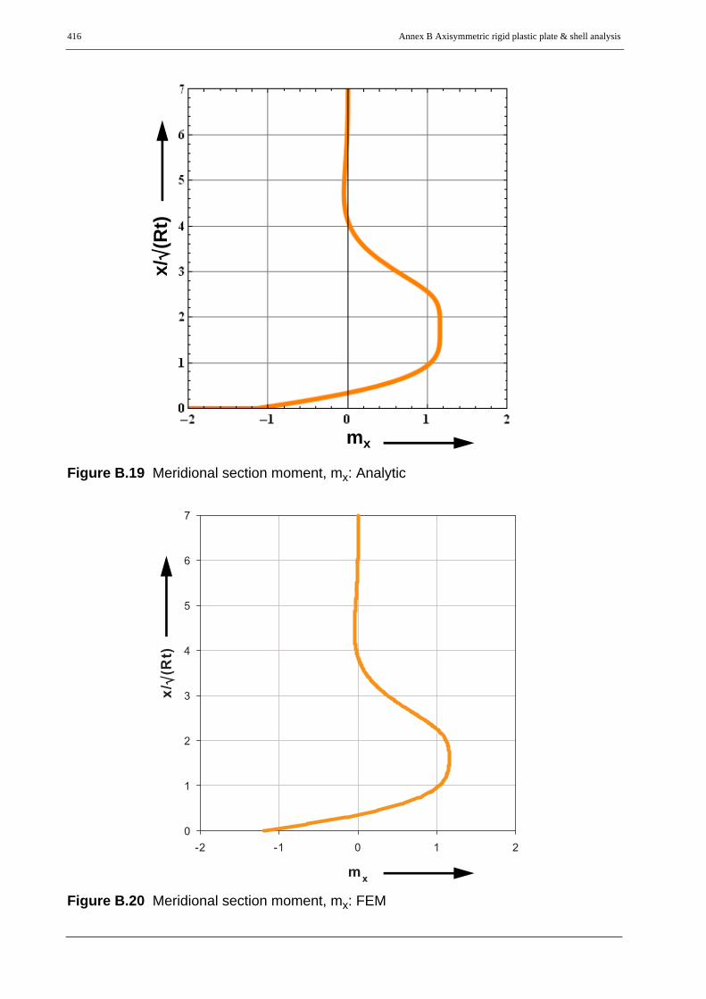
416 Annex B Axisymmetric rigid plastic plate & shell analysis
Figure B.19 Meridional section moment, mx: Analytic
Figure B.20 Meridional section moment, mx: FEM
x/√
(Rt)
mx
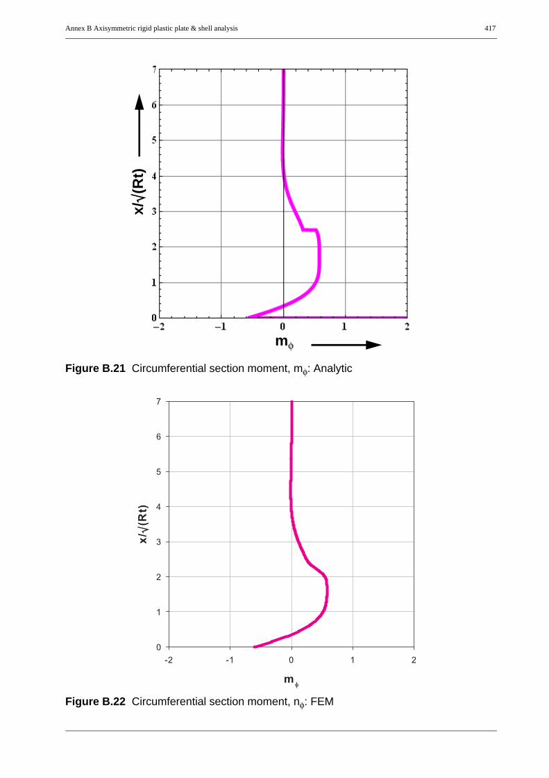
Annex B Axisymmetric rigid plastic plate & shell analysis 417
Figure B.21 Circumferential section moment, mφ: Analytic
Figure B.22 Circumferential section moment, nφ: FEM
x/√
(Rt)
mφ

418 Annex B Axisymmetric rigid plastic plate & shell analysis
Figure B.23 Transverse shear force, Qx*: Analytic
Figure B.24 Transverse shear force, Qx*: FEM
x/√
(Rt)
Qx*
Qx*

Annex B Axisymmetric rigid plastic plate & shell analysis 419
B.3.12.2 Long cylindrical shell under radial ring loading with axial compressive andinternal pressure loads
Figure B.25 Ring-loaded long cylindrical shell with axial load & internal pressure
R
t
Pn,0Pn,0 sθ,0
sx,0
sx,0sθ,0 = 0.5
sx,0 = 0.5

420 Annex B Axisymmetric rigid plastic plate & shell analysis
Figure B.26 Circumferential section force, nφ: Analytic
Figure B.27 Circumferential section force, nφ: FEM
x/√
(Rt)
nφ

Annex B Axisymmetric rigid plastic plate & shell analysis 421
Figure B.28 Meridional section moment, mx: Analytic
Figure B.29 Meridional section moment, mx: FEM
x/√
(Rt)
mx

422 Annex B Axisymmetric rigid plastic plate & shell analysis
Figure B.30 Circumferential section moment, mφ: Analytic
Figure B.31 Circumferential section moment, nφ: FEM
x/√
(Rt)
mφ

Annex B Axisymmetric rigid plastic plate & shell analysis 423
Figure B.32 Transverse shear force, Qx*: Analytic
Figure B.33 Transverse shear force, Qx*: FEM
x/√
(Rt)
Qx*
Qx*

424 Annex B Axisymmetric rigid plastic plate & shell analysis
A.4 Summary and conclusion
The chapter was concerned with the anayltical computation of rigid-perfect-plastic limit strengthsand corresponding section force distributions of axisymmetric plate and shell structures. In doingso, Ilyushin’s yield criterion related approximations have been used along with the equilibrium andkinematic relationships.
Circular and annular plates under uniform or ring lateral loads and fixed or pinned outer edges havebeen analyzed. Besides, long cylindrical shells under radial ring loading with and without axialloading & internal pressurization have been considered. The results have been compared withrecommendations according to EN 1993-1-6 and with small displacement materially nonlinearnumerical analysis (ABAQUS) results which turns out that the analytical rigid-plastic analysiswith the help of the approximate stress resultant oriented yield criteria produces accurate results.

Annex C Analytical elastic buckling analysis of cylindrical shells 425
C
Analytical elastic buckling analysis of cylindrical shells
426 Annex C Analytical elastic buckling analysis of cylindrical shells
C.1 Introduction
The axisymmetric linear and nonlinear buckling behavior and buckling strength of axiallycompressed and internally pressurized cylindrical shells have been computed in Chapter-3 of thisthesis. In all the numerical simulations, the cylinder was modeled using an axisymmetric shellelement. i.e. a one-dimensional segment in meridional direction with two-dimensional loading,deformation and section force distributions has been used to model and simulate the completeaxisymmetric behavior of the three-dimensional cylindrical shell problem. All the computationshave been made numerically using the finite element package ABAQUS, Version 6.7-1 (2007).
This chapter, like Chapter-3, deals with the axisymmetric elastic buckling behavior and strength ofaxially compressed cylindrical shells modeled as a one-dimensional shell segment in meridonaldirection with two-dimensional loading, deformation and section forces but will be solvedanalytically. In doing so, a beam on elastic foundation with the same axial and flexural rigiditiesas that of a unit circumferential length of the cylinder will be used. The circumferential membranestiffness of the cylindrical shell will be modeled as an elastic foundation spring with a springstiffness equal to the circumferential membrane stretching stiffness of the cylinder, usually knownas foundation modulus, C.
The basic relationships (equilibrium, kinematics and constitutive equations) including secondorder effects will be presented first and the necessary set of ordinary differential equations whichwill be used in the buckling analysis will be derived. Figure C.1 shows the equivalent geometry,loading and section force components of a cylindrical shell and a beam on an elastic foundation.
Once the basic relationships including second order effects and the complete set of analyticalsolutions are at hand, they will be used to assess the approximate elastic-plastic buckling loads ofcylindrical shells with the help of the stress resultant oriented Ilyushin-related yield criteria (SeeAnnex-A and B). The elastic-plastic buckling strengths obtained in this way will approximatelyrepresent the geometrically and materially nonlinear strength of the perfect cylindrical shell, theresults of which have already been fully discussed in Chapter 3.7.

Annex C Analytical elastic buckling analysis of cylindrical shells 427
Figure C.1 Geometry, loading and section forces
(a)
(b)
pL
R
w
βx
tp
x, ξ
Nx Nx
FIX
PIN
p
w
βx
t
x, ξ
Nx
c
dφ
ds=R.dφ=1
dX, dξ
dφ
R
ds=R.dφ=1
Mx
Mx+dMx
Qx
Qx+dQx
Nφ
Nφ
Mφ
Mφ
dX
Nφ Nφdφ
Nφdφ
R
X
Y
Z
Nx
Nx+dNx
X, x --> Meridional directionY, φ --> Circumferential directionZ, w --> Radial direction
Mx
Mx+dMx
Qx
Qx+dQx
dX
Nx
Nx+dNx
c.w

428 Annex C Analytical elastic buckling analysis of cylindrical shells
C.2 Theory of second order
Generally speaking, stability criterion is related to the nonlinear characterization of a specificproblem. In this chapter, the geometic nonlinear (deformation) effects will be considered by takingthe second order effects into account. These second order effects will inturn be considered bytaking the deformed geometry of the structure as a reference for the fulfillment of equilibriumequations, i.e. the section force variables are defined with respect to the cross-section of thedeformed structure thereby the equilibrium equations will be based on the deformed configurationof the structure. In doing so, the global longitudinal and transverse section forces which correspondto the undeformed geometry will be computed from the deformed geometry. Figure C.2(a) showsgeometry, loading and boundary conditions of a beam on an elastic foundation. Figure C.2(b)shows the section forces on the undeformed and deformed configurations of the beam structure.The relationships between the global-oriented and local-oriented section forces is graphicallyshown on the right-hand-side of Figure C.2(b). The meanings of the variables used in this figureare listed below:
L global longitudinal section force
Tx global transverse section force
Nxo local axial section force tangent to the neutral axis
Qx local shear force parallel to the cross-section
w’ rotation of the neutral axis
βx rotation of the cross-section
γxz shear strain (angular deformation)
It can easily be seen, with the help of Figure C.2(b), that the second order effect can be included inthe shear equilibrium equation, i.e. an additional shear section force equal to Nxo.w’ will result dueto second order effects. This effect can also be considered as an additional distributed lateral loadequal to (Nxo.w’)’ which in turn is equal to Nxo.w’’ for a constant axial loading. The directions ofthe additional shear force or distributed lateral load will depend on the direction (tensile orcompressive) of the axial loading.
In the upcoming discussions, the equilibrium equations will first be written in terms of the localsection forces along with the consideration of the second order effects. Later, when discussingabout edge forces in the global orientation, the global oriented section forces will be used.

Annex C Analytical elastic buckling analysis of cylindrical shells 429
Figure C.2 Geometry, loading and section forces
(a)
(b)Undeformed Deformed
Tx
L L
Tx
NxoQx
+ w’
+ w’
+ βx
L
Tx
Nxo
Qx
+ w’
+ βx
w
βx
t
x, ξ
Nx
pz
px
mx
γxz
L

430 Annex C Analytical elastic buckling analysis of cylindrical shells
C.3 Basic differential equations for anaxisymmetric cylindrical shell
The basic differential equations for an axisymmetric cylindrical shell with out considering thesecond order effects have been discussed in ANNEX-B. The second order effect (See Figure C.2b)will appear in the force equilibrium equation along the radial direction. It can equivalently betreated as a radial distributed pressure loading with magnitude (axial loading assumed tensile)equal to:
; . . . tension (Eq. C.1)
With this additional radial distributed loading coming from theory of second order, the basicdifferential equations (equilibrium, kinematics and constitution) for an axisymmetric cylindricalshell with normal hypothesis (i.e. transverse shear deformation neglected) can be summarized asgiven below. Thereby it is assumed that the axial normal force is a known quantitiy (Nxo) and theshell is able to deform freely in axial direction.
(Eq. C.2)
with the following parameters being used:
. . . plate flexural rigidity (Eq. C.3)
. . . circumferential membrane stiffness (Eq. C.4)
elastic modulus
wall thickness
cylinder radius
applied radial pressure loading
Note: The membrane solution for the axial loading Nxo accounting for the Poisson’s effect in circumferential direction has to be separately superimposed.
pz Th 2– O–, Nxo w''⋅= Nxo 0>
∂( )∂x
-----------
wβx
Qx
Mx
11K----–
C–NxoK
--------–
1–
wβx
Qx
Mx
⋅
00pz
mx
+ +
0000
=
K E t3⋅12 1 ν2–( )-------------------------=
C E t⋅R2
---------=
E
t
R
pz

Annex C Analytical elastic buckling analysis of cylindrical shells 431
C.4 Basic differential equations for a beam onelastic foundation analogy model
The basic system ordinary differential equations (equilibrium, kinematics and constitution)including second order effects of a beam are discussed below. In all the discussions, the shearrigidity of the beam is assumed to be infinitely large and hence the transverse shear deformation isnegligible. Once again, it is assumed that the axial force is a known quantitiy (Nxo) and the beamis able to deform freely in axial direction.
C.4.1 Deformation geometry relationships (Kinematics)This is the relationship between the strains and displacements, and is given by:
(Eq. C.5)
with the normal hypothesis,
C.4.2 Material relationships (Constitution)The constitutive or strain - section force (stress) relationship will be as follows
with or (Eq. C.6)
C.4.3 Equilibrium relationships (Kinetics)The equilbrium (or section forces - applied loads) relationship will be given by:
(Eq. C.7)
where
(Eq. C.8)
results from consideration of second order effects (Nxo assumedtension) and results from the stiffness of the elastic foundation.
γxz
κx
x∂∂ ( ) 1
0x∂∂ ( )
wβx
⋅=
γxz x∂∂w βx+ 0= = βx⇒ x∂
∂w–=
γxz
κx
1Sxz------- 0
0 1K----
Qx
Mx⋅= Sxz G t⋅= ∞→ 1
Sxz------- 0→
x∂∂ ( ) 0
1–x∂∂ ( )
Qx
Mx⋅
pz pz total,+mx
+ 00
=
pz total, pz p+ z Th 2– O–, p+= z foundation, pz N+ xo w''⋅ C– w⋅=
pz Th 2– O–, N+ xo w''⋅=pz foundation, C– w⋅=
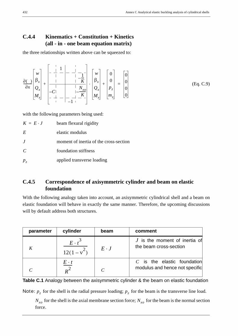
432 Annex C Analytical elastic buckling analysis of cylindrical shells
C.4.4 Kinematics + Constitution + Kinetics(all - in - one beam equation matrix)
the three relationships written above can be squeezed to:
(Eq. C.9)
with the following parameters being used:
beam flexural rigidity
elastic modulus
moment of inertia of the cross-section
foundation stiffness
applied transverse loading
C.4.5 Correspondence of axisymmetric cylinder and beam on elasticfoundation
With the following analogy taken into account, an axisymmetric cylindrical shell and a beam onelastic foundation will behave in exactly the same manner. Therefore, the upcoming discussionswill by default address both structures.
Note: for the shell is the radial pressure loading; for the beam is the transverse line load.
for the shell is the axial membrane section force; for the beam is the normal section force.
parameter cylinder beam comment
is the moment of inertia ofthe beam cross-section
is the elastic foundationmodulus and hence not specific
Table C.1 Analogy between the axisymmetric cylinder & the beam on elastic foundation
∂( )∂x
-----------
wβx
Qx
Mx
11K----–
C–NxoK
--------–
1–
wβx
Qx
Mx
⋅
00pz
mx
+ +
0000
=
K E J⋅=
E
J
C
pz
KE t3⋅
12 1 ν2–( )-------------------------- E J⋅
J
CE t⋅
R2---------
C
C
pz pz
Nxo Nxo

Annex C Analytical elastic buckling analysis of cylindrical shells 433
C.4.6 Reduction of the set of 1st order differential equations into a single4th order differential equation
The set of ordinary differential equations (Eq. C.9) can be reduced to the following fourth orderdifferential equation:
(Eq. C.10)
Introducing a non-dimensional running parameter ξ, with the following relationships:
(Eq. C.11)
The differential equation will then be given by:
(Eq. C.12)
(Eq. C.13)
K w''''⋅ Nxo w⋅– '' C+ w⋅ mx' p+ z( )– 0=
⎧ ⎪ ⎨ ⎪ ⎩
pz∗
ξ XL---= ⇒ ( )' ( )·
L-------;= ( )'' ( )··
L2-------=
KL4----- w···⋅
Nxo
L2-------- w··⋅– C+ w⋅
m· xL
------ pz+⎝ ⎠⎛ ⎞– 0=
⎧ ⎪ ⎨ ⎪ ⎩pz∗
·
w···NxoL2
K--------------– w·· CL4
K----------w+ L4
K-----pz∗=·

434 Annex C Analytical elastic buckling analysis of cylindrical shells
C.4.6.1 Solution for the 4th order differential equation -homogeneous fundamental solution
The analytic solution to the elastic buckling problem will be obtained by solving the homogeneousdifferential equation (i.e. no external loading) which can be written in a general form as:
(Eq. C.14)
(Eq. C.15)
Note: represents the critical buckling load for the infinitely long beam and appears here as a unified reference value (See Chapter C.8.1 where it appears as ).
Assuming a solution of the form:
(Eq. C.16)
the characteristic equation becomes:
(Eq. C.17)
C.4.6.2 General solution of the homogeneous differential equationThe solution to the characteristic polynomial will be given by:
(Eq. C.18)
where
(Eq. C.19)
the general homogeneous solution will then be
(Eq. C.20)
or it can also be written as
(Eq. C.21)
w··· 2β2w·· α4w+ + 0=·
β2 NxoL2
2K--------------;= α4 CL4
K----------;= κ β2
α2------
Nxo
2 C K⋅--------------------
NxoNxo cr ∞,,--------------------= = =
Nxo cr ∞,,Nxo cr,
w ξ( ) eλξ= ⇒ λ4 2β2λ2 α4+ +( )eλξ 0=
λ4 2β2λ2 α4+ + 0=
λ1 2, β2– β4 α4–+± α± κ– κ2 1–+ i± α κ κ2 1––⎝ ⎠⎛ ⎞ i± μ1= = = =
λ3 4, β2– β4 α4––± α± κ– κ2 1–– i± α κ κ2 1–+⎝ ⎠⎛ ⎞ i± μ2= = = =
μ1 α κ κ2 1–– ;= μ2 α κ κ2 1–+=
W ξ( ) c1 e⋅iμ1ξ c2 e⋅
i– μ1ξ c3 e⋅iμ2ξ c4 e⋅
i– μ2ξ+ + +=
W ξ( ) fT ξ( ) c;⋅= c c1 c2 c3 c4T
=

Annex C Analytical elastic buckling analysis of cylindrical shells 435
C.5 Different solution cases of the 4th orderhomogeneous o.d.e.: fundamental functionand accompanying derivative matrix
Depending on the value of the parameter κ, three distinct fundamental solution cases may exist.These distinct solution cases are discussed below:
C.5.1 Case - 1
(Eq. C.22)
Fundamental solution function:
(Eq. C.23)
Derivative and derivative matrix of the function:
(Eq. C.24)
κ β2
α2------ 1<=
μ1 α 1 κ–2
------------=
μ2 α 1 κ+2
------------=
f
eμ1ξ–
μ2ξ( )sin⋅
eμ1ξ–
μ2ξ( )cos⋅
eμ1 1 ξ–( )–
μ2 1 ξ–( )( )sin⋅
eμ1 1 ξ–( )–
μ2 1 ξ–( )( )cos⋅
=
f· D f⋅= ⇒ D
μ1– μ2 0 0
μ2– μ1– 0 00 0 μ1 μ2–0 0 μ2 μ1
=

436 Annex C Analytical elastic buckling analysis of cylindrical shells
C.5.2 Case - 2
(Eq. C.25)
Fundamental solution function:
(Eq. C.26)
Derivative and derivative matrix of the function:
(Eq. C.27)
C.5.3 Case - 3
(Eq. C.28)
Fundamental solution function:
(Eq. C.29)
Derivative and derivative matrix of the function:
(Eq. C.30)
κ β2
α2------ 1== μ μ1 μ2 α β= = = =
f
μξ( )sinμξ( )cos
1 ξ–( ) μ 1 ξ–( )( )sin⋅1 ξ–( ) μ 1 ξ–( )( )cos⋅
=
f· D f⋅= ⇒ D
0 μ 0 0
μ– 0 0 0
0 0 11 ξ–-----------– μ–
0 0 μ 11 ξ–-----------–
=
κ β2
α2------ 1>=
μ1 α κ κ2 1––=
μ2 α κ κ2 1–+=
f
μ1ξ( )sinμ1ξ( )cosμ2ξ( )sinμ2ξ( )cos
=
f· D f⋅= ⇒ D
0 μ1 0 0μ1– 0 0 00 0 0 μ2
0 0 μ2– 0
=

Annex C Analytical elastic buckling analysis of cylindrical shells 437
C.6 Derivation of beam stiffness matrix
C.6.1 General - for all solution cases
C.6.1.1 Displacement vectorThe general expression for the displacement vector will be given as follows:
(Eq. C.31)
(Eq. C.32)
(Eq. C.33)
C.6.1.2 Beam-end displacements and homogeneous edge-displacement matrix
With “A” and “E” representing the starting edge and ending edge of the beam, the edgedisplacements will be given by:
(Eq. C.34)
C.6.1.3 Computation of the integration constants vector cOnce the beam-end displacements and the homogeneous edge-displacement matrix Uhom areknown, the integration constants vector c can be computed from:
(Eq. C.35)
(Eq. C.36)
whom ξ( ) fT ξ( ) c;⋅= c c1 c2 c3 c4T
=
βhom ξ( )w· hom ξ( )
L--------------------–= 1
L---– f·
Tξ( ) c⋅= ⇒ L βhom ξ( )⋅ f– T DT c⋅ ⋅=
W* WL β⋅
fT
f–·T
c⋅ fT I 4 4,( )⋅
fT DT–( )⋅c⋅ fT 0
0 fT
I
D– Tc⋅ ⋅= = = =
⎧ ⎪ ⎨ ⎪ ⎩
F 2 8,( )T
W*ˆ W*A
W*E
WA
L βA⋅
WE
L βE⋅
FAT
FET
I
D– T⋅ c⋅= = =
⎧ ⎪ ⎪ ⎨ ⎪ ⎪ ⎩
Uhom
W*ˆ Uhom c⋅=
c Uhom1– W*ˆ⋅=

438 Annex C Analytical elastic buckling analysis of cylindrical shells
C.6.1.4 Section and edge forces
Local section forces:
(Eq. C.37)
... section-forces vector (Eq. C.38)
(Eq. C.39)
Global section forces:The global transversal and longitudinal section forces of the beam including second order effectsare given, Figure C.2, by:
... Transversal section force (Eq. C.40)
... Longitudinal section force (Eq. C.41)
C.6.1.5 computation of the transversal section force
(Eq. C.42)
• Section-forces vector in terms of the transversal force T:
(Eq. C.43)
Mx K βx'⋅ K W''⋅– KL2----- W··⋅–= = =
Qx Mx' K W'''⋅– K 1L3----- W···⋅ ⋅–= = =
Q*Qx
MxL
-------K 1
L3----- f···T
f··Tc⋅– K
L3----- fT D⋅ 3T
fT D⋅ 2Tc–= = =
Q* KL3----- fT 0T
0T fTD3T
D2Tc–=
⎧ ⎪ ⎨ ⎪ ⎩
FT
Tx Qx Nxo W'⋅–=
L N0x Qx W'⋅+ Nxo≈=
Tx Qx Nxo W'⋅– K W''' Nxo W'⋅–⋅– KL3----- W···
NxoL
-------- ∂W∂ξ--------⋅–⋅–= = =
TxKL3----- W···
Nxo L2⋅K
------------------- W·⋅+⎝ ⎠⎜ ⎟⎛ ⎞⋅– K
L3----- W··· 2β2W·+( )⋅–= =
T*Tx
Mx L⁄KL3----- W··· 2β2 W·⋅+
W··⋅– K
L3----- fT 0T
0T fTD3T 2β2D
T+
D2Tc⋅ ⋅ ⋅–= = =
⎧ ⎪ ⎨ ⎪ ⎩
FT

Annex C Analytical elastic buckling analysis of cylindrical shells 439
C.6.1.6 Global edge-forces vector
(Eq. C.44)
C.6.1.7 Stiffness matrix using theory of second order
... edge-forces vector (Eq. C.45)
... edge displacements vector (Eq. C.46)
(Eq. C.47)
... beam stiffness matrix (Eq. C.48)
... matrix to convert from section force orientation to global edge force sign-convention (Eq. C.49)
T*̂T*A
T*E
TA
MA L⁄TE
ME L⁄
KL3-----–
FAT
FET
D3T 2β2DT
+
D2T⋅ ⋅ c⋅= = =
⎧ ⎪ ⎪ ⎪ ⎪ ⎪ ⎨ ⎪ ⎪ ⎪ ⎪ ⎪ ⎩
Shom
T*̂ SHom c⋅ SHom UHom1–⋅( ) W*ˆ⋅
TA
MA L⁄TE
ME L⁄
= = =
W*ˆ
WA
βA L⋅WE
βE L⋅
=
R*ˆ K*ˆ W*ˆ⋅=
K*ˆ T SHom UHom1–⋅ ⋅( )=
T
1– 0 0 00 1– 0 00 0 1 00 0 0 1
=

440 Annex C Analytical elastic buckling analysis of cylindrical shells
C.6.2 Specific - for each solution case
C.6.2.1 Case - 1
(Eq. C.50)
• Displacement vector
(Eq. C.51)
• Beam-end displacements and homogeneous edge-displacement matrix
(Eq. C.52)
(Eq. C.53)
where
κ β2
α2------ 1<=
μ1 α 1 κ–2
------------=
μ2 α 1 κ+2
------------=
W*
eμ1ξ–
μ2ξ( )sin eμ1ξ–
μ1 μ2ξ( ) μ2– μ2ξ( )cossin[ ]
eμ1ξ–
μ2ξ( )cos eμ1ξ–
μ2 μ2ξ( ) μ1 μ2ξ( )cos+sin[ ]
eμ1 1 ξ–( )–
μ2 1 ξ–( )( )sin eμ1 1 ξ–( )–
μ– 1 μ2 1 ξ–( )( )sin μ2 μ2 1 ξ–( )( )cos+[ ]
eμ1 1 ξ–( )–
μ2 1 ξ–( )( )cos e–μ1 1 ξ–( )–
μ2 μ2 1 ξ–( )( )sin μ1 μ2 1 ξ–( )( )cos+[ ]
T
c⋅=
W*ˆ Uhom c⋅=
Uhom
a1 f c g–
b a2 e– d–
c g a1 f
e d b– a2–
=

Annex C Analytical elastic buckling analysis of cylindrical shells 441
(Eq. C.54)
• Computation of the integration constants vector c
(Eq. C.55)
(Eq. C.56)
where
(Eq. C.57)
(Eq. C.58)
a1 0=
a2 μ1=
b μ– 2=
c eμ1–
μ2( )sin⋅=
d eμ1–
μ1 μ2( ) μ2 μ2( )sin+cos[ ]⋅=
e eμ1–
μ1 μ2( ) μ2 μ2( )cos–sin[ ]⋅=
f 1=
g eμ1–
μ2( )cos⋅=
c Uhom1– W*ˆ⋅=
Uhom1– 1
N----
a1 f c g–
b a2 e d–
c g a1 f–
e d b a2–
=
N det Uhom( ) e2μ1–
4μ12 μ2( )2 μ2
2 1– e2μ– 1+( )+sin[ ]= =
a1 μ12e
2μ1–2μ2( ) μ1μ2 1 e
2μ1–2μ2( )cos–( )+sin[ ]–=
a2 2e2– μ1 μ1 μ2( )2sin⋅=
b μ– 22 e
2– μ1 2μ12 μ2( )2 μ1μ– 2 2μ2( ) μ2
2+sinsin[ ]⋅+=
c eμ1–
2μ12 μ2( ) μ1μ– 2 1– e
2μ– 1+( ) μ2( ) μ22 1– e
2μ– 1+( ) μ2( )sin–cossin[ ]⋅=
d eμ1–
μ2 1– e2μ– 1+( ) μ2( )sin⋅=
e μ2eμ1–
μ1 1 e2μ– 1+( ) μ2( ) μ– 2 1– e
2μ– 1+( ) μ2( )cossin[ ]⋅=
f μ2 e–2– μ1 μ1 2μ2( ) μ2+sin[ ]⋅=
g e–μ1–
2μ1 μ2( ) μ2 1– e2μ– 1+( ) μ2( )cos+sin[ ]⋅=
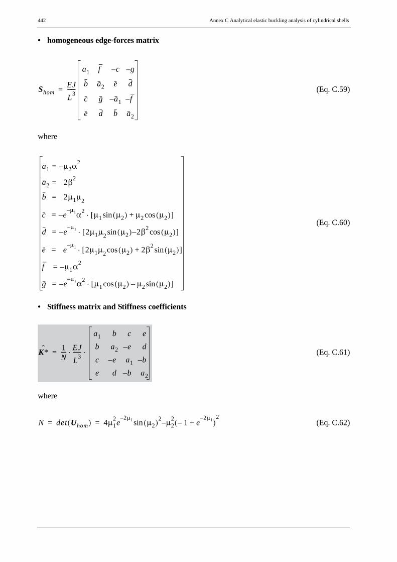
442 Annex C Analytical elastic buckling analysis of cylindrical shells
• homogeneous edge-forces matrix
(Eq. C.59)
where
(Eq. C.60)
• Stiffness matrix and Stiffness coefficients
(Eq. C.61)
where
(Eq. C.62)
ShomEJL3------
a1 f c– g–
b a2 e d
c g a1– f–
e d b a2
=
a1 μ2– α2=
a2 2β2=
b 2μ1μ2=
c eμ1–α2– μ1 μ2( ) μ2 μ2( )cos+sin[ ]⋅=
d eμ1–
– 2μ1μ2 μ2( ) 2– β2 μ2( )cossin[ ]⋅=
e eμ1–
2μ1μ2 μ2( ) 2β2 μ2( )sin+cos[ ]⋅=
f μ1– α2=
g eμ1–α2– μ1 μ2( ) μ2 μ2( )sin–cos[ ]⋅=
K*ˆ 1N---- EJ
L3------
a1 b c eb a2 e– dc e– a1 b–e d b– a2
⋅ ⋅=
N det Uhom( ) 4μ12e
2μ1–μ2( )2 μ2
2– 1– e2μ– 1+( )
2sin= =

Annex C Analytical elastic buckling analysis of cylindrical shells 443
(Eq. C.63)
These non-dimensional stiffness coefficients can be brought into a compact unified shape byintroducing the parameters μ and κ and thus replacing μ1 and μ2 as follows:
(Eq. C.64)
(Eq. C.65)
with
and therefore,
(Eq. C.66)
(Eq. C.67)
For vanishing axial force , we have also and therefore holds. Thesesubstitutions enable therefore a compact and unified representation for all values of the axialnormal force which is hidden in the parameter κ.
a1 2μ1μ2 μ12 μ2
2+( ) μ2 1– e4μ1–
+( ) 2μ1e2μ1–
2μ2( )sin–[ ]=
a2 2μ1μ2 μ2 1– e4μ1–
+( ) 2μ1e2μ1–
2μ2( )sin+[ ]=
b μ12 μ2
2+( ) 4μ12e
2μ1–μ2( )2sin μ2
2 1– e2μ1–
+( )2
–[ ]=
c 4μ1μ2 μ12 μ2
2+( )eμ1–
μ1 1 e2μ1–
+( ) μ2( )sin μ2 1– e2μ1–
+( ) μ2( )cos–[ ]=
d 4– μ1μ2eμ1–
μ1 1 e2μ1–
+( ) μ2( )sin μ2 1– e2μ1–
+( ) μ2( )cos+[ ]=
e 4– μ1μ2 μ12 μ2
2+( )eμ1–
1– e2μ1–
+( ) μ2( )sin=
μ1α2
------- 1 κ– μ 1 κ–= =
μ2α2
------- 1 κ+ μ 1 κ+= =
μ α 2⁄=
μ1 μ⋅ 2 μ2 1 κ–=
μ12 μ2
2+ μ2 1 κ–( ) 1 κ+( )+( )⋅ 2μ2= =
Nx0 0→ κ 0→ μ1 μ= 2 μ=

444 Annex C Analytical elastic buckling analysis of cylindrical shells
C.6.2.2 Case - 2
(Eq. C.68)
• Displacement vector
(Eq. C.69)
• Beam-end displacements and homogeneous edge-displacement matrix
(Eq. C.70)
(Eq. C.71)
• Computation of the integration constants vector c
(Eq. C.72)
(Eq. C.73)
(Eq. C.74)
κ β2
α2------ 1== μ μ1 μ2 α β= = = =
W*
μξ( )sin μ μξ( )cos–μξ( )cos μ μξ( )sin
1 ξ–( ) μ 1 ξ–( )( )sin μ 1 ξ–( )( )sin μ 1 ξ–( ) μ 1 ξ–( )( )cos+1 ξ–( ) μ 1 ξ–( )( )cos μ– μ 1 ξ–( )( )sin μ 1 ξ–( )( )cos+
T
c⋅=
W*ˆ Uhom c⋅=
Uhom
0 1 μ( )sin μ( )cosμ– 0 μ( )sin μ+ μ( )cos μ μ( )sin– μ( )cos+
μ( )sin μ( )cos 0 0μ μ( )cos– μ μ( )sin 0 1
=
c Uhom1– W*ˆ⋅=
Uhom1– 1
N----
μ( )cos– μ( )sin μ μ( )cos+[ ] μ( ) μ( )cossin μ( ) μ μ( )cos μ– μ( )sin[ ]+sin μ μ( )cos
μ( )sin μ( )sin μ μ( )cos+[ ] μ( )sin 2– μ– μ( )sin μ+ μ( )cos[ ] μ– μ( )sin
μ2 μ( )sin– μ( )sin μ– μ( )cos μ μ( )2sin μ μ( ) μ( )cossin–
μ μ( )sin μ μ( )cos+[ ]– μ μ( )sin μ μ μ( ) μ( )cossin+[ ] μ( )2sin
=
N det Uhom( ) 12--- 1 2μ– 2 2μ( )cos–[ ]= =

Annex C Analytical elastic buckling analysis of cylindrical shells 445
• homogeneous edge-forces matrix
(Eq. C.75)
• Stiffness matrix and Stiffness coefficients
(Eq. C.76)
(Eq. C.77)
(Eq. C.78)
ShomEJL3------
μ3– 0 μ– 2 μ( )sin μ3 μ( )cos+ μ3 μ( )sin– μ2 μ( )cos–
0 μ2 μ2 μ( )sin 2μ μ( )cos– 2μ μ( )sin μ2 μ( )cos+
μ3– μ( )cos μ3 μ( )sin 0 μ– 2
μ2 μ( )sin μ2 μ( )cos 2μ– 0
=
K*ˆ 1N---- EJ
L3------
a1 b c eb a2 e– dc e– a1 b–e d b– a2
⋅ ⋅=
N det Uhom( ) 12--- 1 2μ– 2 2μ( )cos–[ ]= =
a1 2– μ3 μ μ( ) μ( )cossin+[ ]=a2 μ 2μ– 2μ( )sin+[ ]=
b 12---μ2 1 2μ+ 2 2μ( )cos–[ ]=
c 2μ3 μ( )sin μ μ( )cos+[ ]=d 2– μ μ( )sin μ μ( )cos–[ ]=
e 2μ3 μ( )sin=

446 Annex C Analytical elastic buckling analysis of cylindrical shells
C.6.2.3 Case - 3
(Eq. C.79)
• Displacement vector
(Eq. C.80)
• Beam-end displacements and homogeneous edge-displacement matrix
(Eq. C.81)
(Eq. C.82)
• Computation of the integration constants vector c
(Eq. C.83)
(Eq. C.84)
(Eq. C.85)
(Eq. C.86)
κ β2
α2------ 1>=
μ1 α κ κ2 1–– β2 β4 α4––= =
μ2 α κ κ2 1–+ β2 β4 α4–+= =
W* μ1ξ( )sin μ1ξ( )cos μ2ξ( )sin μ2ξ( )cosμ1 μ1ξ( )cos– μ1 μ1ξ( )sin μ2 μ2ξ( )cos– μ2 μ2ξ( )sin
c⋅=
W*ˆ Uhom c⋅=
Uhom
0 1 0 1μ– 1 0 μ– 2 0
μ1( )sin μ1( )cos μ2( )sin μ2( )cosμ1 μ1( )cos– μ1 μ1( )sin μ2 μ2( )cos– μ2 μ2( )sin
=
c Uhom1– W*ˆ⋅=
Uhom1– 1
N----
μ22c1s2 μ1μ2s1c2– μ1s1s2 μ2 1 c1c2–( )– μ1μ2s1 μ2
2s2– μ2 c2 c1–( )
μ1μ2 1 c1c2–( ) μ22s1s2– μ1c1s2 μ2s1c2– μ1μ2 c1 c2–( ) μ2s1 μ1s2–
μ12s1c2 μ1μ2c1s2– μ2s1s2 μ1 1 c1c2–( )– μ1μ2s2 μ1
2s1– μ1 c1 c2–( )
μ1μ2 1 c1c2–( ) μ12s1s2– μ2s1c2 μ1s2c1– μ1μ2 c2 c1–( ) μ1s2 μ2s1–
=
N det Uhom( ) 2α2 1 μ1( )cos μ2( )cos–[ ] 2β2 μ1( )sin μ2( )sin–= =
s1 μ1( )sin= c1 μ1( )cos=
s2 μ2( )sin= c2 μ2( )cos=

Annex C Analytical elastic buckling analysis of cylindrical shells 447
• homogeneous edge-forces matrix
(Eq. C.87)
• Stiffness matrix and Stiffness coefficients
(Eq. C.88)
(Eq. C.89)
(Eq. C.90)
ShomEJL3------
μ1 μ12 2β2–( ) 0 μ2 μ2
2 2β2–( ) 0
0 μ12 0 μ2
2
μ1c1 μ12 2β2–( ) μ1s1 μ1
2 2β2–( )– μ2c2 μ22 2β2–( ) μ– 2s2 μ2
2 2β2–( )
μ12s1 μ1
2c1 μ22s2 μ2
2c2
=
K*ˆ EJL3------
a1 b c eb a2 e– dc e– a1 b–e d b– a2
⋅=
N det Uhom( ) 2α2 1 μ1( )cos μ2( )cos–[ ] 2β2 μ1( )sin μ2( )sin–= =
a1 α2 μ12 μ2
2–( ) μ1 μ1( )sin μ2( )cos μ2 μ1( )cos μ2( )sin–[ ]=
a2 μ12 μ2
2–( ) μ2 μ1( )sin μ2( )cos μ1 μ1( )cos μ2( )sin–[ ]=
b 2α4 μ1( )sin μ2( )sin 2α2β2 1 μ1( )cos μ2( )cos–[ ]–=
c α2 μ12 μ2
2–( ) μ2 μ2( )sin μ1 μ1( )sin–[ ]=
d μ12 μ2
2–( ) μ1 μ2( )sin μ2 μ1( )sin–[ ]=
e α2 μ12 μ2
2–( ) μ1( )cos μ2( )cos–[ ]=

448 Annex C Analytical elastic buckling analysis of cylindrical shells
C.7 Procedure for analytical computation of elasticbuckling strengths and buckling eigenmodes
In order to make the above discussion clearer, following is a step-by-step procedure for the analyticcomputation of elastic buckling strengths and buckling eigenmodes of perfect cylindrical shellsunder axiall compressive loading.
• Assume a solution case:
(Eq. C.91)
• Select a fundamental solution function, f, corresponding to the solution case
• Compute , and
... beam stiffness matrix (Eq. C.92)
with
... matrix to convert from section force orientation to global edge force Sign-convention (Eq. C.93)
• Compute the reduced stiffness matrix, , by applying the boundary conditions on
• Set the determinant of to zero and symbolically compute μ, μ1, μ2 depending on the specific solution case
• Compute the corresponding parameters β, α and κ
• Check if κ agrees with the assumption made in the first step. If not, assume another solution case and repeat the above steps. If yes, follow the next steps:
κ β2
α2------ 1=
<=>
Uhom Shom
K*ˆ T SHom UHom1–⋅ ⋅( )=
T
1– 0 0 00 1– 0 00 0 1 00 0 0 1
=
K*ˆ red K*ˆ
K*ˆ red

Annex C Analytical elastic buckling analysis of cylindrical shells 449
• Compute the critical buckling load: plot κ vs. α, i.e. when the Ncr,min is used as a reference
axial loading on the beam, it will be equivalent to saying ΛLBA vs. where
for ν = 0.3
• For a given α value, compute the different κ values corresponding to different buckling modes. Compute the corresponding μ, μ1, μ2 values for each α and κ combination and substitute them
in
• Compute from the given boundary conditions
and eigenvector of corresponding to the zero eigenvalue
• Compute from for a given (α, κ) pair
• Compute the buckling eigenmode using the fundamental solution function for the respective
solution case . Vary the value of the already computed κ values to produce other buckling modes
2 L Leff⁄⋅
Leff 0.778 Rt=
K*ˆ red
W*ˆ WA, L β⋅ A, WE, L β⋅ ET
=
K*ˆ red
c c1, c2, c3, c4T
= W*ˆ Uhom c⋅=
w ξ( ) fT ξ( ) c⋅=

450 Annex C Analytical elastic buckling analysis of cylindrical shells
C.8 Illustrative examples, results and comparison
For illustration purposes, the elastic buckling strength and buckling eigenmodes of a cylindricalshell, Figure C.3, with the following same set of geometric, material and loading conditions butwith different boundary conditions will be analytically computed.
Geometry: R/t = 500; t = 1.0 cm; L/R = 1.0
Loading: meridional ring compressive loading
Material properties: E = 21000 kN/cm2; ν = 0.3; fy = 24.0 kN/cm2
In the analytical computation of the elastic buckling strength and buckling eigenmodes, the step-by-step procedure discussed in Chapter C.7 will be followed.
Figure C.3 Axially compressed cylindrical shell
R
t
Nx,0Nx,0
x, ξ
L
PIN FIX
PINRotation
FREErestrained

Annex C Analytical elastic buckling analysis of cylindrical shells 451
C.8.1 Elastic buckling strength computation
C.8.1.1 Example-1: Pinned bottom and top edgesFrom the given boundary conditions,
(Eq. C.94)
Using the already developed beam stiffness matrix and the boundary conditions of the currentproblem, it can be seen that the reduced beam stiffness matrix will be a 2 x 2 matrix. To obtain thebuckling eigenvalues, the determinant of the reduced beam stiffness matrix should be zero. Indoing so, a solution case is assumed and the parameters μ, μ1, μ2 will be computed depending onthe specific solution case which will be used in computing the corresponding parameters β, α andκ. A check will be made if the value of the computed κ agrees with the assumed value. If there isno such agreement or if there exist no solution to the case considered, a different case is assumedand the computations are repeated until a solution which agrees with the assumption exists. Thisprocedure is discussed below for the current problem.
Case - 1:
(Eq. C.95)
Setting the determinant of the reduced beam stiffness matrix to zero will give
(Eq. C.96)
which leads to
(Eq. C.97)
(Eq. C.97) will lead to a single possible solution with μ1 = μ2 = 0 at which the left and right-hand-side expressions intersect. For a given α, this solution leads to no specific value for κ. Hence, nobuckling is possible under this solution case and therefore another solution case needs to beconsidered, as discussed below.
w ξ 0=( ) w ξ 1=( ) 0= =
κ β2
α2------ 1<=
μ1 α 1 κ–( )2
-----------------=
μ2 α 1 κ+( )2
-----------------=
1 e4μ1+( ) 2e
2μ1 2μ2( )cos– 0=
2μ2( )cos 1 e4μ1+( )
2e2μ1
-----------------------=

452 Annex C Analytical elastic buckling analysis of cylindrical shells
Case - 2:
(Eq. C.98)
Setting the determinant of the reduced beam stiffness matrix to zero will give
(Eq. C.99)
which leads to
(Eq. C.100)
with n representing the number of buckle half-waves. It can also be written as
(Eq. C.101)
Substituting the expresssion for α, (Eq. C.101) gives the number of buckle half-waves for bucklingunder the current solution case as:
(Eq. C.102)
The buckle half-wave length can then be computed from the axial length of the beam (ormeridional length of the cylinder) and using the number of buckle half-waves as follows:
(Eq. C.103)
(Eq. C.104)
Substituting the expresssion for β and using (Eq. C.102), (Eq. C.101) gives the expression for thebuckling load as
(Eq. C.105)
This axial load will be the minimum possible buckling load if there will exist a solution under case-3 (i.e. κ > 0) or will be the only buckling load if there will exist no possible buckling solution undercase-3. The first argument comes from the fact that the buckling load is proportional to the κ valueand the κ value in solution case-3 is greater than that of solution case-2.
κ β2
α2------ 1== μ μ1 μ2 α β= = = =
μ( )sin 0=
μ n π⋅ α β= = =
α2 β2 n2 π2⋅= =
n2 L2
π2----- c
EJ------⋅=
lhalf wave–Ln--- π EJ
c------4⋅ π
2------- R t⋅
3 1 ν2–( )4---------------------------⋅= = =
lhalf wave–π2
------- Leff⋅ 2.444 R t⋅2
--------------= =
Nxo cr, 2 n2π2
L2----------- EJ⋅ ⋅= 2 c EJ⋅=

Annex C Analytical elastic buckling analysis of cylindrical shells 453
Case - 3:
(Eq. C.106)
Setting the determinant of the reduced beam stiffness matrix to zero will give
(Eq. C.107)
There are different possibilities which make (Eq. C.107) true. One of these possibilities is when μ1= μ2 which will lead to κ = 1, contradicting the solution case and therefore can not be a solution.The other possibilities are when or or both are zero at the same time.The general solution for this particular situation is when
(Eq. C.108)
(Eq. C.109)
with the following two necessary conditions:
• otherwise it contradicts the current solution case; and
• and m having any value or vice versa (i.e. only the letter changes: n or m, otherwise the same).
The following discussion uses the variable n as the integer. It can be checked that using m as theinteger will result in the same expressions as will be obtained using n as an integer.
(Eq. C.110)
which can be re-written as
(Eq. C.111)
(Eq. C.112)
Substituting the values for β and α & letting , the buckling load can be expressed as
κ β2
α2------ 1>=
μ1 α κ κ2 1–– β2 β4 α4––= =
μ2 α κ κ2 1–+ β2 β4 α4–+= =
μ12 μ2
2–( )2
μ1( )sin μ2( )sin 0=
μ1( )sin 0= μ2( )sin 0=
μ1 n π⋅=
μ2 m π⋅=
n m≠
n Integer∈
μ12 n π⋅( )2 β2 β4 α4––= =
n2π2 β2–( )2
β4 α4–=
2β2 n2π2 α4
n2π2-----------+=
γ α4 π4⁄=

454 Annex C Analytical elastic buckling analysis of cylindrical shells
(Eq. C.113)
(Eq. C.114)
When n = 1 and there is no elastic foundation (c = 0), (Eq. C.114) represents the Euler’s bucklingload for a pin-ended column, i.e.
(Eq. C.115)
Thus the buckling load in (Eq. C.114) can be expressed in terms of the Euler’s buckling load for apin-ended column as follows
(Eq. C.116)
The buckling load according to the current solution case (i.e. case-3) can also be expressed in termsof the minimum buckling load obtained using solution case-2 as follows:
(Eq. C.117)
where
(Eq. C.118)
On the other hand, it can easily be checked that when a reference axial loading equal to the classicalbuckling load of a cylindrical shell is used, the variable κ represents the buckling load factor ΛLBA,i.e.
(Eq. C.119)
Nxo cr n,,n2π
2E⋅ J
L2---------------------- 1 α
nπ------⎝ ⎠⎛ ⎞ 4
+⎝ ⎠⎛ ⎞⋅=
Nxo cr n,,π2 E⋅ J
L2---------------- n2 γ
n2-----+⎝ ⎠
⎛ ⎞⋅=
Ncr Euler,π2 E⋅ J
L2----------------=
Nxo cr n,,Ncr Euler,--------------------- n2 γ
n2-----+ n2 γ
n------⎝ ⎠⎛ ⎞
2+= =
Nxo cr n,,Nxo cr min,,------------------------ 1
2 γ---------- n2 γ
n------⎝ ⎠⎛ ⎞
2+⎝ ⎠
⎛ ⎞⋅=
Nxo cr min,,Ncr Euler,------------------------ 2 γ=
κ β2 α2⁄ ΛLBANxo cr n,,
Nxo cr min,,------------------------= = =

Annex C Analytical elastic buckling analysis of cylindrical shells 455
Figure C.4 Linear elastic buckling strength: Pin-pin, case-3
Figure C.5 Linear elastic buckling strength: Pin-pin, case-3
0 20 40 60 80 1000
5
10
15
20
25
30
γ
Nxo cr n,,Ncr Euler,------------------------
n = 1
n = 5
n = 4
n = 2
n = 3
Nxo cr min,,Ncr Euler,
----------------------------
0 5 10 15 200
10
20
30
40
50
√γ
Nxo cr n,,Ncr Euler,------------------------
n = 1
n = 6
n = 5
n = 2
n = 4 Nxo cr min,,Ncr Euler,
----------------------------
n = 3

456 Annex C Analytical elastic buckling analysis of cylindrical shells
Figure C.6 Linear elastic buckling strength: Pin-pin, case-3
Figure C.7 Linear elastic buckling strength: Pin-pin, case-3
0 5 10 15 200.0
0.5
1.0
1.5
2.0
√γ
Nxo cr n,,Ncr min,----------------------
n = 1
n = 6
n = 5
n = 2 n = 4n = 3
0 5 10 15 200
10
20
30
40
50
α
Nxo cr n,,Ncr Euler,------------------------
n = 1
n = 6
n = 5
n = 2
n = 4
Nxo cr min,,Ncr Euler,
----------------------------n = 3

Annex C Analytical elastic buckling analysis of cylindrical shells 457
Figure C.8 Linear elastic buckling strength: Pin-pin, case-3
0 5 10 15 200.0
0.5
1.0
1.5
2.0
α
Nxo cr n,,Ncr min,----------------------
n = 1
n = 6
5 4 3 2

458 Annex C Analytical elastic buckling analysis of cylindrical shells
C.8.1.2 Example-2: Pinned bottom and rotationally restrained top edgesFrom the given boundary conditions,
(Eq. C.120)
Using the already developed beam stiffness matrix and the boundary conditions of the currentexample, it can be seen that the reduced beam stiffness matrix will be a 2 x 2 matrix. To obtain thebuckling eigenvalues, the determinant of the reduced beam stiffness matrix should be zero. Indoing so, a solution case is assumed and the parameters μ, μ1, μ2 will be computed depending onthe specific solution case which will be used in computing the corresponding parameters β, α andκ. A check will be made if the value of the computed κ agrees with the assumed value. If there isno such agreement or if there exist no solution to the case considered, a different case is assumedand the computations are repeated until a solution which agrees with the assumption exists. Thisprocedure is discussed below for the current example.
Case - 1:
(Eq. C.121)
Setting the determinant of the reduced beam stiffness matrix to zero will give
(Eq. C.122)
which leads to
(Eq. C.123)
(Eq. C.123) will lead to no possible solution since the left and right-hand-side expressions do notintersect. Hence, no buckling is possible under this solution case and therefore another solutioncase needs to be considered, as discussed below.
w ξ 0=( ) βx ξ 1=( ) 0= =
κ β2
α2------ 1<=
μ1 α 1 κ–( )2
-----------------=
μ2 α 1 κ+( )2
-----------------=
1 e4μ1+( ) 2e
2μ1 2μ2( )cos+ 0=
2μ2( )cos 1 e4μ1+( )
2e2μ1
-----------------------–=

Annex C Analytical elastic buckling analysis of cylindrical shells 459
Case - 2:
(Eq. C.124)
Setting the determinant of the reduced beam stiffness matrix to zero will give
(Eq. C.125)
which leads to
(Eq. C.126)
with n representing the number of buckle half-waves. It can also be written as
(Eq. C.127)
Substituting the expresssion for α, (Eq. C.127) gives the number of buckle half-waves for bucklingunder the current solution case as:
(Eq. C.128)
The buckle half-wave length can then be computed from the axial length of the beam (ormeridional length of the cylinder) and using the number of buckle half-waves as follows:
(Eq. C.129)
(Eq. C.130)
Substituting the expresssion for β and using (Eq. C.128), (Eq. C.127) gives the expression for thebuckling load as
(Eq. C.131)
This axial load will be the minimum possible buckling load if there will exist a solution under case-
κ β2
α2------ 1== μ μ1 μ2 α β= = = =
μ( )cos 0=
μ n π⋅2
---------- α β= = =
α2 β2 n2 π2⋅4
---------------= =
n2 4L2
π2----- c
EJ------⋅=
lhalf wave–Ln--- π
2--- EJ
c------4⋅ π
2 2---------- R t⋅
3 1 ν2–( )4---------------------------⋅= = =
lhalf wave–π
2 2---------- Leff⋅ 1.222 R t⋅
2--------------= =
Nxo cr,12--- n2π2
L2----------- EJ⋅ ⋅= 2 c EJ⋅=
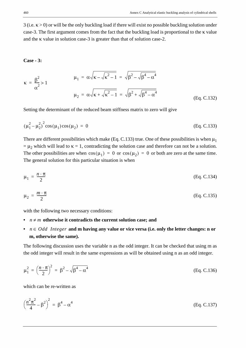
460 Annex C Analytical elastic buckling analysis of cylindrical shells
3 (i.e. κ > 0) or will be the only buckling load if there will exist no possible buckling solution undercase-3. The first argument comes from the fact that the buckling load is proportional to the κ valueand the κ value in solution case-3 is greater than that of solution case-2.
Case - 3:
(Eq. C.132)
Setting the determinant of the reduced beam stiffness matrix to zero will give
(Eq. C.133)
There are different possibilities which make (Eq. C.133) true. One of these possibilities is when μ1= μ2 which will lead to κ = 1, contradicting the solution case and therefore can not be a solution.The other possibilities are when or or both are zero at the same time.The general solution for this particular situation is when
(Eq. C.134)
(Eq. C.135)
with the following two necessary conditions:
• otherwise it contradicts the current solution case; and
• and m having any value or vice versa (i.e. only the letter changes: n or m, otherwise the same).
The following discussion uses the variable n as the odd integer. It can be checked that using m asthe odd integer will result in the same expressions as will be obtained using n as an odd integer.
(Eq. C.136)
which can be re-written as
(Eq. C.137)
κ β2
α2------ 1>=
μ1 α κ κ2 1–– β2 β4 α4––= =
μ2 α κ κ2 1–+ β2 β4 α4–+= =
μ12 μ2
2–( )2
μ1( )cos μ2( )cos 0=
μ1( )cos 0= μ2( )cos 0=
μ1n π⋅
2----------=
μ2m π⋅
2------------=
n m≠
n Odd Integer∈
μ12 n π⋅
2----------⎝ ⎠⎛ ⎞ 2
β2 β4 α4––= =
n2π2
4----------- β2–⎝ ⎠⎛ ⎞
2β4 α4–=

Annex C Analytical elastic buckling analysis of cylindrical shells 461
(Eq. C.138)
Substituting the values for β and α & letting , the buckling load can be expressed as
(Eq. C.139)
(Eq. C.140)
When n = 1 and there is no elastic foundation (c = 0), (Eq. C.140) represents the Euler’s bucklingload for a column pinned at one edge and rotationally restrained at the other edge, i.e.
(Eq. C.141)
Thus the buckling load in (Eq. C.114) can be expressed in terms of the Euler’s buckling load for asuch a column as follows
(Eq. C.142)
The buckling load according to the current solution case (i.e. case-3) can also be expressed in termsof the minimum buckling load obtained using solution case-2 as follows:
(Eq. C.143)
where
(Eq. C.144)
It can again be checked that when a reference axial loading equal to the classical buckling load ofa cylindrical shell is used, the variable κ represents the buckling load factor ΛLBA, i.e.
(Eq. C.145)
2β2 n2π2
4----------- 4α4
n2π2-----------+=
γ α4 π4⁄=
Nxo cr n,,n2π
2E⋅ J
4L2---------------------- 1 2α
nπ-------⎝ ⎠⎛ ⎞ 4
+⎝ ⎠⎛ ⎞⋅=
Nxo cr n,,π2 E⋅ J
L2---------------- n2
4----- 4γ
n2-----+
⎝ ⎠⎜ ⎟⎛ ⎞⋅=
Ncr Euler,π2 E⋅ J
4L2----------------=
Nxo cr n,,Ncr Euler,--------------------- n2 16γ
n2--------+ n2 4 γ
n----------⎝ ⎠⎛ ⎞
2+= =
Nxo cr n,,Nxo cr min,,------------------------ 1
8 γ---------- n2 4 γ
n----------⎝ ⎠⎛ ⎞
2+⎝ ⎠
⎛ ⎞⋅=
Nxo cr min,,Ncr Euler,------------------------ 8 γ=
κ β2 α2⁄ ΛLBANxo cr n,,
Nxo cr min,,------------------------= = =

462 Annex C Analytical elastic buckling analysis of cylindrical shells
Figure C.9 Linear elastic buckling strength: Pin-RotFix, case-3
Figure C.10 Linear elastic buckling strength: Pin-RotFix & Pin-Pin, case-3
0 5 10 15 200
2
4
6
8
10
α
Nxo cr n,,Ncr min,----------------------
n = 1
n = 27
n = 1,3,5,...,27
0 5 10 15 200
2
4
6
8
α
Nxo cr n,,Ncr min,----------------------

Annex C Analytical elastic buckling analysis of cylindrical shells 463
C.8.1.3 Example-2: Fixed bottom and free top edgesFrom the given boundary conditions,
(Eq. C.146)
Using the already developed beam stiffness matrix and the boundary conditions of the currentexample, it can be seen that the reduced beam stiffness matrix will be a 2 x 2 matrix.. To obtain thebuckling eigenvalues, the determinant of the reduced beam stiffness matrix should be zero. Indoing so, a solution case is assumed and the parameters μ, μ1, μ2 will be computed depending onthe specific solution case which will be used in computing the corresponding parameters β, α andκ. A check will be made if the value of the computed κ agrees with the assumed value. If there isno such agreement or if there exist no solution to the case considered, a different case is assumedand the computations are repeated until a solution which agrees with the assumption exists. Thisprocedure is discussed below for the current problem.
Case - 1:
(Eq. C.147)
Setting the determinant of the reduced beam stiffness matrix to zero will give
(Eq. C.148)
(Eq. C.148) can be directly expressed interms of α and κ, (Eq. C.147), where the relationship canbe plotted (κ vs. α) from which the buckling load factor can be read, Figure C.11.
w ξ 0=( ) βx ξ 0=( ) 0= =
κ β2
α2------ 1<=
μ1 α 1 κ–( )2
-----------------=
μ2 α 1 κ+( )2
-----------------=
4μ14e
2μ1 μ2( )sin 2 μ12μ2
2 3 4e2μ1 3e
4μ1 6e2μ1 2μ2( )cos+ + +( )⋅ μ2
4–+ 1– e2μ1+( )
20=

464 Annex C Analytical elastic buckling analysis of cylindrical shells
Case - 2:
(Eq. C.149)
Setting the determinant of the reduced beam stiffness matrix to zero will give
(Eq. C.150)
This relationship will only be true for μ = which means α = β = 1.1896 and hence, a singlepossible solution occurs only when . This solution will not be applicable tothe illustrative example since for the considered cylindrical shell α = 40.65.
Case - 3:
(Eq. C.151)
Setting the determinant of the reduced beam stiffness matrix to zero will give
(Eq. C.152)
(Eq. C.152) can be directly expressed interms of α and κ, (Eq. C.151), where the relationship canbe plotted (κ vs. α) from which the buckling load factor can be read, Figure C.12. A comparisonplot is also shown in Figure C.13 where the current solution case is compared with that of thepinned bottom and rotationally restrained top edges beam. The number of half-wave buckles for agiven cylindrical shell of the current example type and solution case can be estimated with the helpof the comparison with the solution for the pinned bottom and rotationally restrained top edgesbeam.
κ β2
α2------ 1== μ μ1 μ2 α β= = = =
5 2μ2– 3 2μ( )cos+ 0=
1.1896±α κ,( ) 1.1896 1,( )=
κ β2
α2------ 1>=
μ1 α κ κ2 1–– β2 β4 α4––= =
μ2 α κ κ2 1–+ β2 β4 α4–+= =
2μ12μ2
2 μ1μ2 μ12 μ2
2+( )– μ1( )sin μ2( )sin μ14 μ2
4+( ) μ1( )cos μ2( )cos– 0=

Annex C Analytical elastic buckling analysis of cylindrical shells 465
Figure C.11 Linear elastic buckling strength: Fix-Free, case-1
0 5 10 15 200.0
0.2
0.4
0.6
0.8
1.0
α
κ
case-1

466 Annex C Analytical elastic buckling analysis of cylindrical shells
Figure C.12 Linear elastic buckling strength: Fix-Free, case-3
0 10 20 30 40 500
2
4
6
8
10
α
κ

Annex C Analytical elastic buckling analysis of cylindrical shells 467
Figure C.13 Linear elastic buckling strength: Fix-Free & Pin-RotFix, case-3
0 5 10 15 20 25 300
2
4
6
8
α
κ
n = 1
n = 3
n = 5
n = 7
n = 9

468 Annex C Analytical elastic buckling analysis of cylindrical shells
C.8.1.4 Example-4: Fixed bottom and rotationally restrained top edgesFrom the given boundary conditions,
(Eq. C.153)
Using the already developed beam stiffness matrix and the boundary conditions of the currentproblem, it can be seen that the reduced beam stiffness matrix will have a single element. To obtainthe buckling eigenvalues, the determinant of the reduced beam stiffness matrix should be zero.This, in the current context, means the single element of the reduced stiffness matrix should set tozero. In doing so, a solution case is assumed and the parameters μ, μ1, μ2 will be computeddepending on the specific solution case which will be used in computing the correspondingparameters β, α and κ. A check will be made if the value of the computed κ agrees with theassumed value. If there is no such agreement or if there exist no solution to the case considered, adifferent case is assumed and the computations are repeated until a solution which agrees with theassumption exists. This procedure is discussed below for the current problem.
Case - 1:
(Eq. C.154)
Setting the determinant of the reduced beam stiffness matrix to zero will give
(Eq. C.155)
(Eq. C.156)
(Eq. C.97) will lead to no possible solution as the left and right-hand-terms will not intersect eachother. Hence, no buckling is possible under this solution case and therefore another solution caseneeds to be considered, as discussed below.
w ξ 0=( ) βx ξ 0=( ) βx ξ 1=( ) 0= = =
κ β2
α2------ 1<=
μ1 α 1 κ–( )2
-----------------=
μ2 α 1 κ+( )2
-----------------=
μ2 1 e4μ1–
–( ) 2μ1e2μ1 2μ2( )sin– 0=
2μ2( )sinμ2
---------------------- 1 e4μ1–
–( )
2μ1e2μ1
-------------------------=

Annex C Analytical elastic buckling analysis of cylindrical shells 469
Case - 2:
(Eq. C.157)
Setting the determinant of the reduced beam stiffness matrix to zero will give
(Eq. C.158)
(Eq. C.159)
This relationship will only be true for μ = 0 which means α = β = 0 and hence, no buckling willoccur under this solution case and therefore another solution case needs to be considered.
Case - 3:
(Eq. C.160)
Setting the determinant of the reduced beam stiffness matrix to zero will give
(Eq. C.161)
(Eq. C.162)
μ1 = μ2 would lead to κ = 1 which contradicts the assumption κ > 1. Instead, (Eq. C.162) can bedirectly expressed interms of α and κ, (Eq. C.160), where the relationship can be plotted (κ vs. α)from which the buckling load factor can be read, Figure C.14 (or when zoomed Figure C.15). Acomparison plot is also shown in Figure C.16 where the current solution case is compared with thatof the pinned bottom and top edges beam. The number of half-wave buckles for a given cylindricalshell of the current example type and solution case can be estimated with the help of thecomparison with the solution for the pinned bottom and top edges beam.
κ β2
α2------ 1== μ μ1 μ2 α β= = = =
μ μ( ) μ( )cossin+ 0=
2μ 2μ( )sin+ 0=
κ β2
α2------ 1>=
μ1 α κ κ2 1–– β2 β4 α4––= =
μ2 α κ κ2 1–+ β2 β4 α4–+= =
μ1 μ1( )sin μ2( )cos μ2 μ1( )cos μ2( )sin– 0=
μ1 μ1( )tan μ2 μ2( )tan– 0=

470 Annex C Analytical elastic buckling analysis of cylindrical shells
Figure C.14 Linear elastic buckling strength: Fix-RotFix, case-3
Figure C.15 Linear elastic buckling strength: Fix-RotFix, case-3 (Figure C.14 zoomed)
0 10 20 30 40 500
2
4
6
8
10
α
κ
α 40.65=
0 10 20 30 40 500.0
0.5
1.0
1.5
2.0
α
κ
α 40.65=
Illustrativeexample

Annex C Analytical elastic buckling analysis of cylindrical shells 471
Figure C.16 Linear elastic buckling strength: Fix-RotFix & Pin-Pin, case-3
0 5 10 15 20 25 300
2
4
6
8
α
κ
n = 1
n = 2
n = 3
n = 4

472 Annex C Analytical elastic buckling analysis of cylindrical shells
C.8.2 Elastic buckling eigenmode computationOnce the k versus a relationships are known for a given cylindrical shell and a specific solutioncase, the following step-by-step procedure (part of the procedure discussed in Chapter C.7) will beused to compute the elastic buckling eigenmodes.
• For a given α value, compute the different κ values corresponding to different buckling modes. Compute the corresponding μ, μ1, μ2 values for each α and κ combination and substitute them
in
• Compute from the given boundary conditions
and eigenvector of corresponding to the zero eigenvalue
• Compute from for a given (α, κ) pair
• Compute the buckling eigenmode using the fundamental solution function for the respective
solution case . Vary the value of the already computed κ values to produce other buckling modes
For the illustrative cylindrical shell example considered,
(Eq. C.163)
where
(Eq. C.164)
C.8.2.1 Fixed bottom and free top edgesThe analytical solution for the first elastic buckling eigenmode (for solution case-1) andcorresponding buckling strength for the illustrative cylindrical shell with fixed bottom and free topedges are shown in Figure C.17. The respective finite element small displacement linear bucklinganalysis results are also shown in Figure C.18 for comparison purposes.
K*ˆ red
W*ˆ WA, L β⋅ A, WE, L β⋅ ET
=
K*ˆ red
c c1, c2, c3, c4T
= W*ˆ Uhom c⋅=
w ξ( ) fT ξ( ) c⋅=
α L c EJ⁄4⋅ 2 L Leff⁄⋅ 40.65= = =
Leff1
3 1 ν2–( )4--------------------------- R t⋅=

Annex C Analytical elastic buckling analysis of cylindrical shells 473
Figure C.17 Analytic linear elastic buckling eigenmode-1: ΛLBA = 0.5, Fix-RotFix
Figure C.18 FEM linear elastic buckling eigenmode-1: ΛLBA = 0.5, Fix-RotFix
μ1 20.32=
μ2 35.20=

474 Annex C Analytical elastic buckling analysis of cylindrical shells
C.8.2.2 Fixed bottom and rotationally restrained top edgesThe analytical solution for the first six elastic buckling eigenmodes (for solution case-3) andcorresponding buckling strengths for the illustrative cylindrical shell with fixed bottom androtationally restrained top edges are shown in Figure C.19 to Figure C.30. The respective finiteelement small displacement linear buckling analysis results are also shown for comparisonpurposes.

Annex C Analytical elastic buckling analysis of cylindrical shells 475
Figure C.19 Analytic linear elastic buckling eigenmode-1: ΛLBA = 1.0030, Fix-RotFix
Figure C.20 FEM linear elastic buckling eigenmode-1: ΛLBA = 1.0024, Fix-RotFix
μ1 39.11=
μ2 42.24=

476 Annex C Analytical elastic buckling analysis of cylindrical shells
Figure C.21 Analytic linear elastic buckling eigenmode-2: ΛLBA = 1.0120, Fix-RotFix
Figure C.22 FEM linear elastic buckling eigenmode-2: ΛLBA = 1.0113, Fix-RotFix
μ1 37.62=
μ2 43.92=

Annex C Analytical elastic buckling analysis of cylindrical shells 477
Figure C.23 Analytic linear elastic buckling eigenmode-3: ΛLBA = 1.0270, Fix-RotFix
Figure C.24 FEM linear elastic buckling eigenmode-3: ΛLBA = 1.0263, Fix-RotFix
μ1 36.20=
μ2 45.64=

478 Annex C Analytical elastic buckling analysis of cylindrical shells
Figure C.25 Analytic linear elastic buckling eigenmode-4: ΛLBA = 1.0472, Fix-RotFix
Figure C.26 FEM linear elastic buckling eigenmode-4: ΛLBA = 1.0462, Fix-RotFix
μ1 34.88=
μ2 47.37=

Annex C Analytical elastic buckling analysis of cylindrical shells 479
Figure C.27 Analytic linear elastic buckling eigenmode-5: ΛLBA = 1.0764, Fix-RotFix
Figure C.28 FEM linear elastic buckling eigenmode-5: ΛLBA = 1.0754, Fix-RotFix
μ1 33.47=
μ2 49.36=
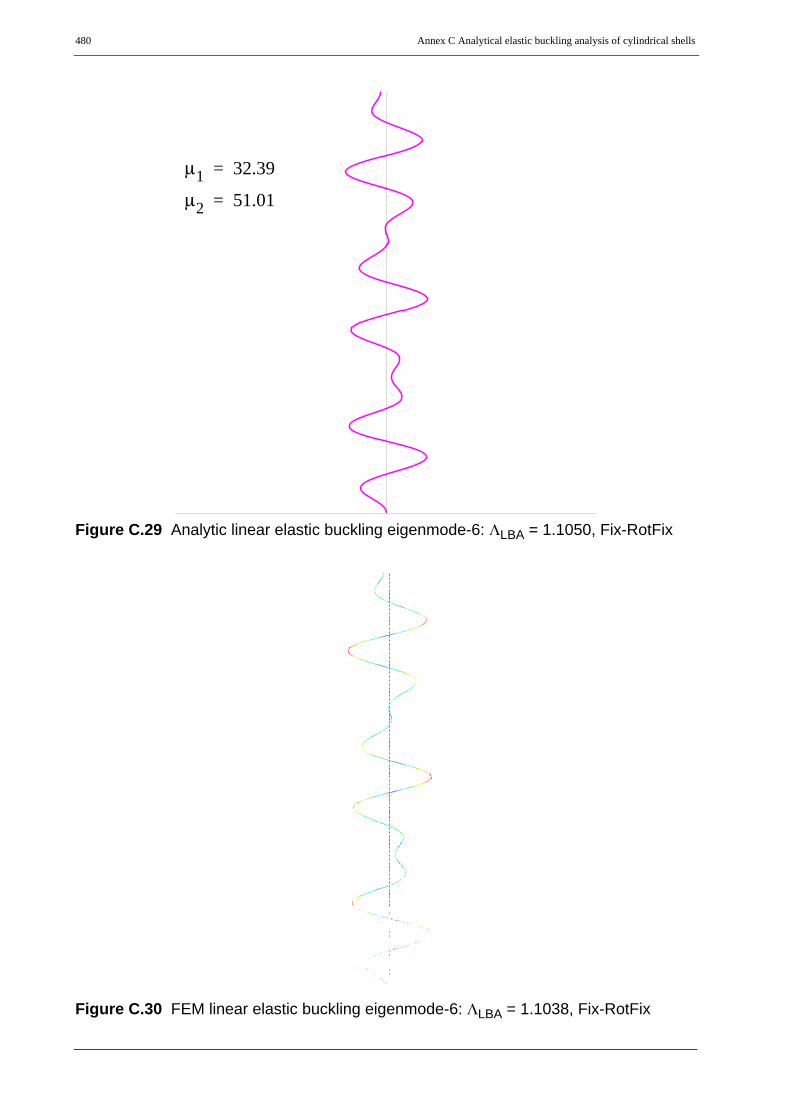
480 Annex C Analytical elastic buckling analysis of cylindrical shells
Figure C.29 Analytic linear elastic buckling eigenmode-6: ΛLBA = 1.1050, Fix-RotFix
Figure C.30 FEM linear elastic buckling eigenmode-6: ΛLBA = 1.1038, Fix-RotFix
μ1 32.39=
μ2 51.01=

Annex C Analytical elastic buckling analysis of cylindrical shells 481
C.9 Summary and conclusion
The axisymmetric elastic buckling behavior and strength of axially compressed cylindrical shellsexihibts a direct analogy to a one-dimensional beam on elastic foundation. For this structuralsystem the general solution for deformations and section forces has been obtained analytically.These analytical results have been compared with the corresponding results obtained from smalldisplacement linear buckling numerical analysis. A perfect match between the bucklingeigenmodes and the buckling strengths has been obtained (the differences in buckling strengthsbeing insignificant).
Approximate plastic buckling analysis based on elastic-second-order analysisOn the other hand, the beam-on-elastic-foundation model of a cylindrical shell has been used toanalytically compute the geometric and material nonlinear effects of a cylindrical shell using acombination of the theory-of-second-order and the stress-resultant-oriented approximate Ilyushinyield criteria. The elastic-plastic buckling loads, Figure 3.47 to Figure 3.52, were computed in aninherently iterative manner. Once the second order effect due to axial compression is consideredin the force equilibrium equation (in the transverse direction), a trial load factor has been appliedwith which the section force distributions along the meridian were computed. Using these sectionforces (stress resultants), a check has been made for possible yield at each point along the meridianusing one of the approximate yield criteria discussed. When the yield criterion is not fulfilled withthe trial load factor, another trial load factor has been applied depending on the result obtained, i.e.if the yield surface defined by the approximate yield function is exceeded, a smaller load factor hasbeen applied; if the result lies within the yield surface, a larger load factor has been applied. Thisprocedure has been repeatedly used until the yield criterion was exactly fulfilled. Thus thefulfilment of the plastic yield criterion, when combined with the theory of second order, representsan approximate elastic-plastic buckling condition. This procedure in shells corresponds directly tothe well-known second-order plastic-hinge approach in beams. Comparison of these analyticapproximate results with those results obtained using the geometrically and materially nonlinearnumerical analysis have been discussed in Chapter 3.7.

482 Annex C Analytical elastic buckling analysis of cylindrical shells