HAL Id: hal-03043193https://hal.archives-ouvertes.fr/hal-03043193

Submitted on 7 Dec 2020

HAL is a multi-disciplinary open accessarchive for the deposit and dissemination of sci-entific research documents, whether they are pub-lished or not. The documents may come fromteaching and research institutions in France orabroad, or from public or private research centers.

L’archive ouverte pluridisciplinaire HAL, estdestinée au dépôt et à la diffusion de documentsscientifiques de niveau recherche, publiés ou non,émanant des établissements d’enseignement et derecherche français ou étrangers, des laboratoirespublics ou privés.

Broadband tunable lossy metasurface with independentamplitude and phase modulations for acoustic

holographyShi-Wang Fan, Yifan Zhu, Liyun Cao, Yan-Feng Wang, A- Li Chen, Aurélien

Merkel, Yue-Sheng Wang, B. Assouar

To cite this version:Shi-Wang Fan, Yifan Zhu, Liyun Cao, Yan-Feng Wang, A- Li Chen, et al.. Broadband tunablelossy metasurface with independent amplitude and phase modulations for acoustic holography. SmartMaterials and Structures, IOP Publishing, 2020, 29 (10), pp.105038. �10.1088/1361-665X/abaa98�.�hal-03043193�

1 / 35

Broadband tunable lossy metasurface with independent amplitude and

phase modulations for acoustic holography

Shi-Wang Fan1,2, Yifan Zhu2, Liyun Cao2, Yan-Feng Wang3, A-Li Chen1, Aurélien Merkel2, Yue-Sheng Wang1,3,*, Badreddine Assouar2,*

1Institute of Engineering Mechanics, Beijing Jiaotong University, Beijing, 100044, China 2Institut Jean Lamour, CNRS, Universite de Lorraine, Nancy, 54000, France

3Department of Mechanics, School of Mechanical Engineering, Tianjin University, Tianjin, 300350, China

*Corresponding authors. E-mail addresses: yswang@tju.edu.cn and badreddine.assouar@univ-lorraine.fr

Abstract

Metasurface-based acoustic hologram projectors fabricated with fixed microstructures can only

generate the predesigned images at a single or few discrete frequencies. Here, a variety of acoustic

holographic applications can be realized in broadband by a matched helical design of the tunable

lossy acoustic metasurface (TLAM). The proposed TLAM unit is composed of a grating channel and

an adjustable internal absorber to achieve the independent amplitude and phase modulations (APM)

in a continuous frequency range. We demonstrate the excellent performance of the scattering-free

anomalous refection by the APM method for tuning loss without foam materials. Then, the

multi-plane acoustic holograms and the broadband holographic images are demonstrated by the

flexible reconfigurations of one designed TLAM. Due to the compact design and the great flexibility,

this proposal may be more practical to achieve the high-quality holograms with multi-scale fine

manipulation and multiplexed acoustic communication with high information content.

Keywords acoustic metamaterials, metasurfaces, holography, independent modulation, continuous

tunability

2 / 35

1. Introduction

Acoustic holography (AH) has emerged to reconstruct and visualize the desired complex sound

fields [1], which offers excellent capabilities for ultrasonic treatment [2] and particle manipulation [3,

4]. The direct approach to realize AH normally relies on the phased source arrays with many

individually controlled transducer [2-4]. These sources can actively modulate the imaging fields, but

is also usually bulky and costly, and needs careful calibration circuit systems. Subsequently, as a

class of artificial metamaterials [5], acoustic metasurfaces (AMs) [6-8] have been proposed to

manipulate the uniform signal from a single source, and passively implement the low-cost acoustic

holograms with ultrathin structure thickness [9-15]. The conventional AM approaches for AH

images based on the single phase modulation (SPM) [9, 10] are very complicated for optimization,

and result in significant clutter outside the controlled region for many target fields. Recently, AMs

with independent amplitude and phase modulations (APM) [11-15] have been used to generate

high-fidelity acoustic holograms. In the context of complete acoustic modulation, both amplitude and

phase are simultaneously manipulated [16-19]. The additional degree of freedom leads to a marked

simplification of the AH design process. The AH may be realized by back-propagating the target

field to the structure plane and then creating the conjugate field over this surface (i.e., time-reversal

technique) [20], instead of using the complex optimization algorithms.

However, the above AMs with APM method can only operate at one [11-13] or four [14] designed

3 / 35

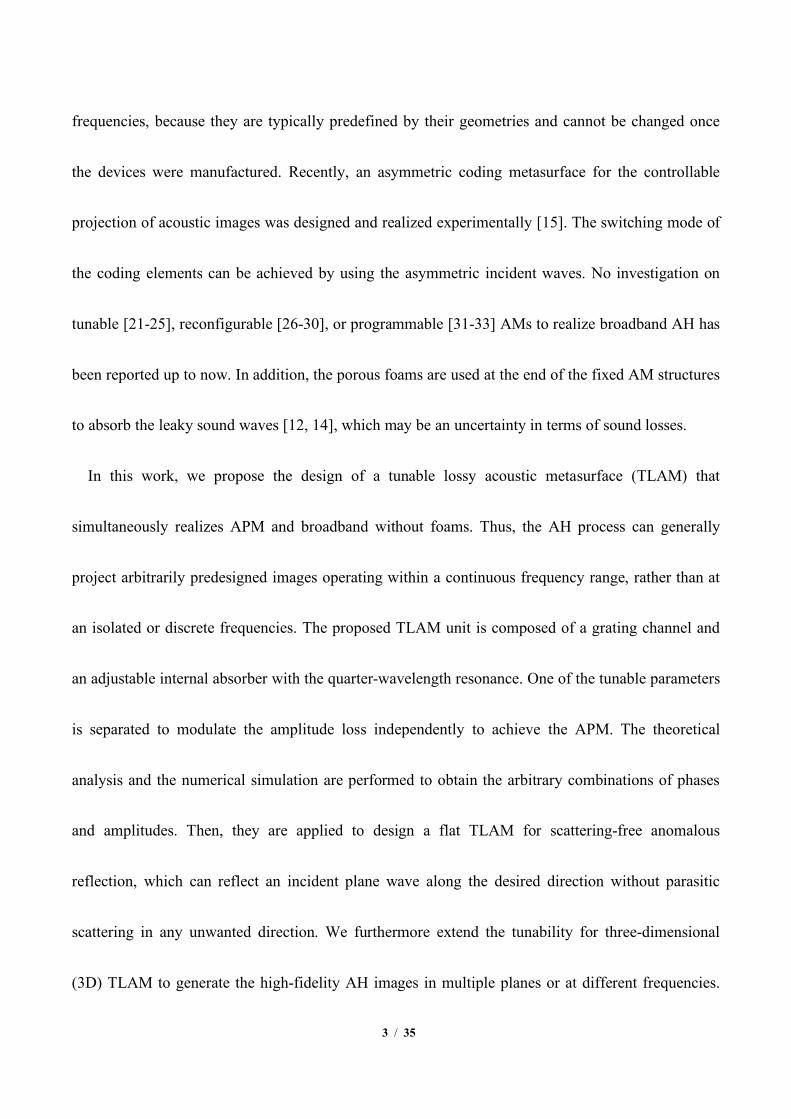
frequencies, because they are typically predefined by their geometries and cannot be changed once

the devices were manufactured. Recently, an asymmetric coding metasurface for the controllable

projection of acoustic images was designed and realized experimentally [15]. The switching mode of

the coding elements can be achieved by using the asymmetric incident waves. No investigation on

tunable [21-25], reconfigurable [26-30], or programmable [31-33] AMs to realize broadband AH has

been reported up to now. In addition, the porous foams are used at the end of the fixed AM structures

to absorb the leaky sound waves [12, 14], which may be an uncertainty in terms of sound losses.

In this work, we propose the design of a tunable lossy acoustic metasurface (TLAM) that

simultaneously realizes APM and broadband without foams. Thus, the AH process can generally

project arbitrarily predesigned images operating within a continuous frequency range, rather than at

an isolated or discrete frequencies. The proposed TLAM unit is composed of a grating channel and

an adjustable internal absorber with the quarter-wavelength resonance. One of the tunable parameters

is separated to modulate the amplitude loss independently to achieve the APM. The theoretical

analysis and the numerical simulation are performed to obtain the arbitrary combinations of phases

and amplitudes. Then, they are applied to design a flat TLAM for scattering-free anomalous

reflection, which can reflect an incident plane wave along the desired direction without parasitic

scattering in any unwanted direction. We furthermore extend the tunability for three-dimensional

(3D) TLAM to generate the high-fidelity AH images in multiple planes or at different frequencies.

4 / 35

This can be more practical by using the same TLAM to continuously engineer the sound fields.

2. Analytical mechanism for APM design

Although the purpose of this work is to design a 3D tunable unit and array it into two-dimensional

(2D) metasurface, for simplicity while without losing generality to illustrate the principle, we first

focus on a very simple 2D lossy unit of which the geometric schematic is inserted in the middle of

figure 1(c). The unit consists of four uniformly distributed gaps with width w and length l.

Figure 1. The pressure fields including the reflected amplitude and the phase shift for the analytical

4leff/λ

1.0

-4

-2

-6

0

0.8

0.6

0.4

0.2

0.0

-8

φ/π

A/A

0

2 60 8

(a)

(b)

1.001.251.501.75

w (mm) A/A

0

1.0

0.8

0.6

0.2

0.0

0.4

-4 φ/π-3 0-1

(c) Ww

h

l

Pi Pr

Possible

Forbidden

z

1.0

0.8

0.6

0.2

0.0

0.4

A/A

0

∆φ

∆A

h0= 0l0= 0.673λ

h2= 0.426λl2 = 0.711λ

h1= 0.093λl1= l0

φ/π210210210

φ/πφ/π

(g) (h)

C2

C1

∆φ∆A

C0

(i)

C0λ

l0

h1

l1

h2

l2

∆φ∆A

(d) (e) (f)

-1 1Pressure

5 / 35

interpretations of a lossy unit with a quarter-wavelength resonator. (a) The amplitude spectrum of the unit with

four different gap widths. (b) The corresponding phase spectrum. (c) The amplitude and phase ranges. The gray

regions are the analytically possible range for combinations of phases and amplitudes, whereas the rest (white)

regions denote the forbidden range. The illustration in (c) presents the topological schematic geometry of the unit.

(d), (e) and (f) are the pressure fields for three different units. (g) The phase and amplitude ranges corresponding to

the initial structure in (d). (h) The possible range of values corresponding to the structures in (e) and (f). (i) The

merged region of (g) and (h). Black, red and blue dots mark the positions for the three cases.

A plane acoustic wave propagating into the gaps along the z axis can be written as Pi=p0exp(ikz)

with k=2π/λ being the wave number in which λ=c0/f is the wavelength with f being the incident

frequency and c0 the sound velocity. At the closed end of the gaps, total reflection occurs and the

reflected wave is denoted as Pr=p0exp(-ikz). Therefore, the total pressure in the gaps is the

superposition of the incident waves and their reflections, which is expressed as Pt=Pi+Pr=2p0cos(kz).

It should be noticed that the total pressure field in the air gaps is a standing wave field. If the wave

node of the standing wave is located at the open end of the gaps, i.e., Pt=0 at z=l, then kl =(2n-1)π/2

and the sound will not leak out by re-radiation. As a result, the efficient gap length must satisfy the

following requirement as:

, (1)

where n is a positive integer and leff =l+∆l in which ∆l =8w/3π represents the end correction caused

by the radiation mass at the open end of the gaps [34]. This means that the efficient gap length with

(2 1) / 4, 1,2,3...effl n nl= - =　

6 / 35

an odd number integer multiple of quarter-wavelength can guarantee the perfect trapping the sound

in the gap, which is also known as the quarter-wavelength resonance [35-39].

Alternatively, we can also interpret this effect by the impedance transfer equation. The definitions

of the acoustic impedances Zcl at z=0 (closed end) and Zop at z=l (open end) can be made in the

background medium of air with the mass density ρ0. Hence the input impedance of the resonator can

be expressed as:

, (2)

where Za=ρ0c0/4w is the characteristic impedance of the air gaps. Because the impedance of the rigid

closed end is considered infinitely large, the input impedance reduces to Zop=-iZacot(kl). As long as

kl=(2n-1)π/2, we have Zop=0. Acoustically, a zero impedance corresponds to an acoustic short

circuit phenomenon. In other words, the sound wave can radiate into the gaps without any restriction.

In this model, the width w of the gaps is set in the millimeter order, which is very small in

comparison to λ in kilohertz range. The viscous loss is significant, which results in a high absorption.

Based on the above resonant trapping effect, the quasi-perfect absorption can be realized by

exploiting the inherent viscosity effect in the background medium of air, without involving any extra

sound-absorption foam materials.

Considering the viscosity of the medium in narrow gaps, the attenuation coefficient of sound is

approximately [34-36]

cl aop a

a cl

tan( )tan( )

Z iZ klZ ZZ iZ kl

+=

+

7 / 35

, (3)

where η is the dynamic viscosity coefficient. For the purpose of acquiring a clearer physical

mechanism of the underlying design principles, we further analyze the relationship between the

reflected fields (including amplitude and phase) and the geometric parameters by combining the

finite element method based on COMSOL Multiphysics 5.5 software. The unit width and the gap

length are W=20mm and l=80mm, respectively. The parameter h=0 is excluded in the initial state.

We calculate the amplitudes A (normalized by the incident amplitude A0) and the phases (normalized

by π) for the reflected waves as functions of wavelength λ (normalized by leff) at four different gap

widths (w) and plot the results with colored solid lines in figures 1(a) and (b), respectively. The

different gap widths are equivalent to changing the acoustic impedance. One can clearly observe that

the strong absorption (i.e., low reflected amplitude) occurs at the quarter-wavelength resonance point

where the phase equals to (1-2n)π. In physics for transmission, this phenomenon is known as the

Fabry-Pérot (FP) resonances which always lead to a full amplitude regardless of the impedance,

bringing a constraint of amplitudes and phases as the so-called “FP binding” [16, 40]. We further

give the possible range of values for combinations of phases and amplitudes by reducing the

impedance as shown by the gray region in figure 1(c), in which the colored solid lines correspond to

the results in figures 1(a) and (b), and the rest white regions denote the forbidden amplitudes. Then,

we expect to find a way to fill up the forbidden ranges in the combinations and achieve the APM in a

0 0

22wchwar

»

8 / 35

broadband range.

To clearly show the expanding coverage of the phase-amplitude diagram, we choose three typical

units and plot the reflected pressure fields, as shown in figures 1(d), (e) and (f), respectively. Their

combinations of the amplitudes and phases (reduced in 2π range) are A=0.7 and φ=π/2 for the initial

case of C0, A=0.7 and φ=π/8 for C1 , and A=0.3 and φ=π/2 for C2.

For the initial case, the structure can be an arbitrary one of the units with h0=0 as we discussed

above. When we choose l0=0.673λ, the pressure field shows a reflected amplitude 0.7 with phase π/2.

The gray region in figure 1(g) is the same as a half in figure 1(c). The black dot marks the

combination for C0 as a reference. At point C1, other geometric parameters are the same to those in

C0, but an extra space of the air layer is added with the depth h1=0.093λ. Then, the amplitude 0.7 is

also observed because the absorption gaps has not been changed and the specific amount of the

sound attenuation is remained. However, the reflected phase has a shift to π/8 because the phase at

the output surface of the unit has decreased due to the extra air layer, as shown by the red arrow in

figure 1(h). As a result, the corresponding possible range for C1 is shown by the magenta region in

figure 1(h), which has the same geometry as that of C0, but with the region shifting 2kh1 to the left

side. For modulating the amplitude from C0 to C2, the length of gaps are elongated up to l2=0.711λ to

move further away from the FP resonance, meanwhile the phase also will be changed, as shown by

the cyan region in figure 1(h). Thus, we also adjust the depth of the air layer into h2=0.426λ to match

9 / 35

the required phase value, because the amplitude is not affected by the depth. The blue dots mark the

combination for C2, whose amplitude decreases to 0.3 with the same phase π/2 as C0, as shown by

the blue arrow in figure 1(h). Therefore, a particular amplitude can be independently combined with

other phases by changing the length of the gaps and the air layer depth.

By extension, the possible range for combination of phases and amplitudes will expand due to the

additional choices from C0 to C1 and C2, as shown by the gray region in figure 1(i), which is merged

from the regions in figures 1(g) and (h). Similarly, if the depth h can be any value in the range of λ/2

and l in the range of λ/4, the merged range will cover the entire range of values including the phase

change of 2π and amplitude change of 1 at any frequency in principle. That means that the arbitrary

combination of phases and amplitudes is available to achieve the APM as long as the design of the

double-parameter tunable AM structure within a certain frequency range.

3. The tunability design

The proposed concept of the broadband TLAM for the AH is presented in figure 2(a). As

illustrated, the incident waves in a frequency range can be reflected by the TLAM from the structure

plane and projected onto the image plane at a given distance. Figure 2(b) shows that the TLAM unit

consists of a grating channel (blue) and an adjustable internal absorber. For the absorber design, the

matched screw-and-nut mechanism [22, 27, 41] is used to significantly compress the thickness of the

helical gap (brown). The absorber is constructed by a matched helix (green) rotated into the helical

10 / 35

gap from bottom to top, and then it can move up and down as a whole along the grating channel.

Thus, there are two tunable parameters (i.e., the rotational angle r of the matched helix and the

varying height h of the whole absorber) in the individual unit. Note that the relatively obvious

rotational operation of the matched helix can characterize the small variation of the gap length, so the

matched helical design can decrease the adjustable system sensitivity to reduce the tuning error [22,

23].

Figure 2. Schematic of the proposed broadband acoustic hologram metasurface with tunable inside

f(kH

z)

2.22.42.62.83.0

2.080

020

4060

027018090

f(kH

z)

2.22.42.62.83.0

2.080

02040

60

027018090

180

f(kH

z)

2.22.42.62.83.0

2.080

02040

60

027018090

f(kH

z)

2.22.42.62.83.0

2.080

02040

60

027018090

(d)

r (deg)

h(m

m)

20

40

60

80

00 1359045

f =2 kHz Amplitude (a.u.)(h)

h r

(b)

(f)

(e) (g)

r (deg)

h(m

m)

20

40

60

80

00 1359045

(i) f =2 kHz Phase (p)1

-1

1

0

(a)

Broadband Acoustic wavesfi

Image plane

H

t(c) w1w

W

H1

W1

TD1

D

w

11 / 35

absorbers. (a) The schematic diagram of the broadband tunable AH. (b) The TLAM unit. (c) The geometric details

of the tunable components. (d, e) The reflected amplitude and phase of the designed unit varying with the height

h=[0, 85]mm and the rotational angle r=[0, 270]° at the frequency domain f=[2, 3] kHz. (f, g) The horizontal slices

in (d) and (e) at f=2, 2.5, 3 kHz. (h, i) The local spectrums of the reflected amplitude and phase response varying

with h and r at the frequency of f=2 kHz.

As illustrated in figure 2(c), the total height is H=100 mm, the side length is W=20 mm, and the

wall thickness is t=0.5 mm. The height of the helical gap is H1=10 mm and the side length W1=19

mm. The gap width is w=1 mm and the length w1=6 mm. The external and internal diameters of the

matched helix are D=18 mm and D1=6 mm, respectively. The blade thickness is the same as the gap

width w; and the thread lead T=8 mm. It should be noted that four matched helixes are attached

together with a thin sheet and set up a ring gear by distributing grooves on its edge to facilitate the

rotation.

To show the broadband tunability, we should first obtain the relation between the reflected

amplitude-phase and the tunable parameters in a continuous frequency domain. The thermoviscous

acoustics model is employed in the gaps of the TLAM unit with both the viscous friction and thermal

diffusion being considered, see Appendix C for details.

Figures 2(d) and 2(e) show the reflected amplitude and phase of the designed unit varying with the

height h=[0, 85] mm and the rotational angle r=[0, 270]° in the frequency domain f=[2, 3] kHz,

respectively. In order to see the distributions inside the 3D spectrums, the horizontal slices in (d) and

12 / 35

(e) at f=2, 2.5, 3 kHz are shown in figures 2(f) and 2(g), respectively. For more clarity, the local

spectra are zoomed in to figures2(h) and 2(i) at the frequency of f=2 kHz. It is found that the full

modulation of the amplitude and phase can be achieved by using the TLAM unit. It is also noted that

the manipulation of the amplitude is nearly decoupled from the parameter h, because it is almost

constant in the vertical direction. That means we can individually adjust the amplitude by rotating the

angle r, i.e., A=A(r). However, the phase can be determined by combining two parameters, i.e.,

φ=φ(r, h), see figure 2(i). Note that the smallest amplitude appears at r =61°, where the quasi-perfect

absorption [42] occurs with the phase always being around π, as we mentioned in the last section.

Therefore, it is necessary to avoid this position when we extract the tunable parameters according to

the desired amplitude and phase.

f=2.0 kHz r = 72 deg. r = 90 deg. Sim.Exp.

(c)

(A, φ)Computer with

PULSE LABSHOP

(b)

Power amplifier Generator and collector

Loudspeaker

Mic.1 Mic.2

TLAMunit

l1 l2

(a)1 cm

13 / 35

Figure 3. The simulated and measured amplitude and phase varying with the height h at two particular

rotational angles r at the frequency of 2 kHz. (a) Photographs of the fabricated TLAM unit. (b) Schematic of the

experimental set up. (c) The simulated (Sim.) and experimental (Exp.) results of the amplitude (blue) and phase

(red).

The experiment is carried out to evidence the acoustic amplitude and phase tuned by the designed

TLAM unit. The components of the TLAM unit made of epoxy resin via 3D printing with enough

precision (0.1mm) are shown in figure 3(a). Figure 3(b) shows the schematic diagram of the

experimental setup. We refer to Appendix C for the details of the devices and the measurement

processes. To illustrate the extraction of the tunable parameters from a quantitative perspective, we

present the numerical and experimental results of the amplitude and phase varying with the height h

at the rotational angles of r =72° and 90° at the frequency of 2 kHz in figure 3(c). The results clearly

show that the TLAM unit can provide a full-range phase control (-π ~ +π) with nearly constant

amplitudes being around 0.25 and 0.65 by tailoring h, which means that we can first determine the

rotational angle r based on the needed amplitude, and then search the corresponding height h

according to the required phase in a 2π range, eventually achieve the decoupling of the APM. It

should be pointed out that if the desired amplitude is very small (A<0.1) or very large (A>0.95), it

should be taken as 0.1 or 0.95.

4. The fine manipulation of sound fields for broadband acoustic holography

14 / 35

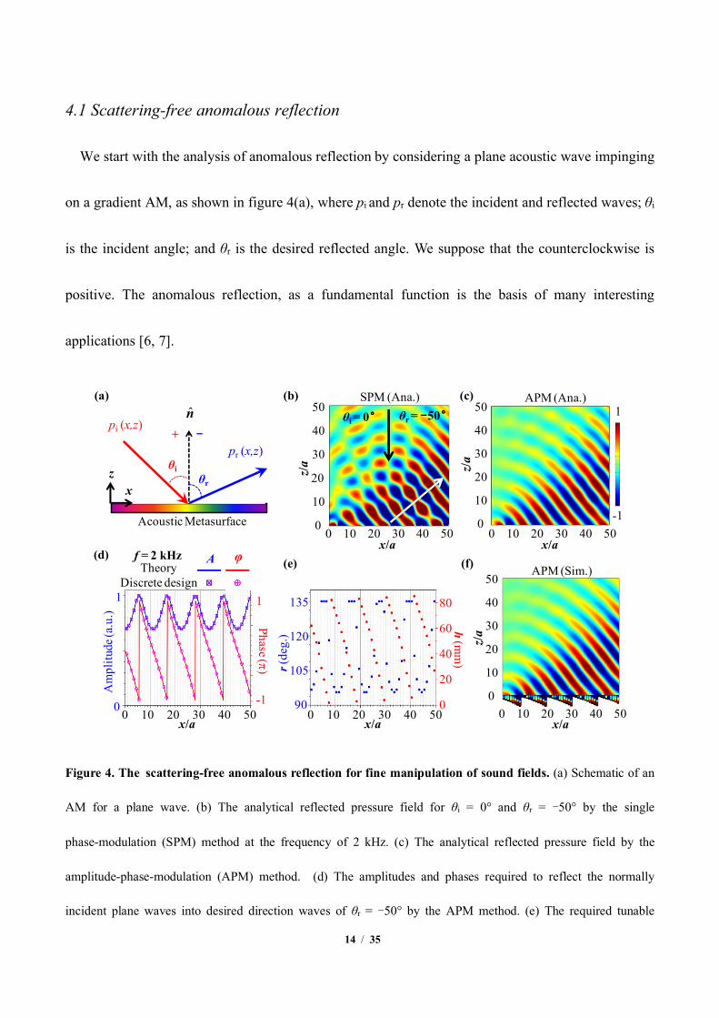
4.1 Scattering-free anomalous reflection

We start with the analysis of anomalous reflection by considering a plane acoustic wave impinging

on a gradient AM, as shown in figure 4(a), where pi and pr denote the incident and reflected waves; θi

is the incident angle; and θr is the desired reflected angle. We suppose that the counterclockwise is

positive. The anomalous reflection, as a fundamental function is the basis of many interesting

applications [6, 7].

Figure 4. The scattering-free anomalous reflection for fine manipulation of sound fields. (a) Schematic of an

AM for a plane wave. (b) The analytical reflected pressure field for θi = 0° and θr = -50° by the single

phase-modulation (SPM) method at the frequency of 2 kHz. (c) The analytical reflected pressure field by the

amplitude-phase-modulation (APM) method. (d) The amplitudes and phases required to reflect the normally

incident plane waves into desired direction waves of θr = -50° by the APM method. (e) The required tunable

(f)

x/a

50

40

30

10

0

20

400 10 20 30 50

APM (Sim.)

z/ah

(mm

)

80

0

20

40

60

135

90

105

120

r(de

g.)

x/a400 10 20 30 50

(e)

Phase (p)

Am

plitu

de (a

.u.)

1

-10

1

x/a400 10 20 30 50

(d) A φTheory

Discrete design

(a)

θiθr

Acoustic Metasurface

pr (x,z)

pi (x,z)

xz

n̂+ -

(c)

x/a

50

40

30

10

0

20

400 10 20 30 50

z/a

-1

1APM (Ana.) SPM (Ana.) (b)

x/a

z/a

50

40

30

10

0

20

400 10 20 30 50

θi = 0° θr = -50°

f = 2 kHz

15 / 35

parameters including the height h and the rotational angle r for each unit of the designed TLAM. (f) The

corresponding simulated pressure field by the APM method .

The conventional designs based on the generalized Snell’s law are to introduce a linear gradient

phase shift [φx=kx(sinθr-sinθi)] in the artificial AM. That means the AM is characterized by SPM

method and the local reflection coefficient with the unit amplitude is R0=exp(iφx). The reflection

coefficient is related with the surface impedance as R0=(ZS-Zi)/(ZS+Zi), where Zi=ρ0c0/cosθi

represents the characteristic impedance of the incident wave. Thus, the surface impedance of the AM

can be inversely derived as

. (4)

We model the AM as an impedance boundary described by Eq. (4) and analyze its reflected field

in figure 4(b) for θi=0° and θr=-50° at the frequency of 2 kHz. Clearly, in addition to the desired

anomalously reflected wave, some waves along other directions will be excited in this field due to

the parasitic diffraction [43]. Then the simple design philosophy by SPM method does not ensure the

perfect energy conversion between the incident and reflected plane waves.

Inspired by the leaky-wave antennas [44], undesired diffraction is expected to be suppressed by

allowing power absorption in our tunable unit. Then the APM method can be used to design a flat

TLAM for scattering-free anomalous reflection [45]. Assuming the time-harmonic factor, the

acoustic pressures and the velocity vectors associated with the space pressure fields are

OPMS 0 0 r i i( ) cot[ (sin sin )] / cosZ x i c kxr q q q= -

16 / 35

(5)

where Ar is a constant which relates the amplitude of the reflected pressure field normalized by the

incident one. The surface impedance can be expressed as:

. (6)

where is the unit vector along the normal direction; and ptot=pi+pr and denote the

total acoustic pressure and velocity, respectively. The real part of the surface impedance will become

negative (gain) when θi>|θr|, meaning that additional energy has to be introduced in the system [45].

It is not suitable for the passive loss structure we designed.

In order to eliminate parasitic scattering, there must be no power flowing in the unwanted

direction from any point on the surface. Then, the local emerging power at the surface can be

expressed in terms of the normal component of the intensity vector

, (7)

i 0 i i

r r 0 r r

i i i i 0 0

r r r r 0 0

( , ) exp[ ( sin cos )],( , ) exp[ ( sin cos )],

ˆ ˆ( , ) ( , )( sin cos ) ,ˆ ˆ( , ) ( , )( sin cos ) ,

p x z p ik x zp x z A p ik x zv x z p x y x z cv x z p x y x z c

q qq q

q q rq q r

= - -= - += -= +

!

!

APM totS

tot i

0 0

r

r

r

( ) [1 exp(i )]( )ˆ ( ) cos cos exp(i )

x

x

p xZ cx An Av x q

r jq j

+= =- × -!

n̂ i rtotv v v= +! ! !

n tot tot 0

220

i r r0

i r0

r

1ˆ Re2

cos (cos cos )cos cos 2

y

x

P n p v

p Ac

Aq q j qr

q

+*

®é ù= × ë û

é ù= - + - +ë û

!

　　

17 / 35

where “∗” represents the complex conjugate. Enforcing Pn≤0 for all x points of the TLAM, it is

found that the maximum value of Ar is min[1, cosθi/cosθr]. The conditions θi≤|θr| and Ar=1 can

satisfy this situation. Thus, the surface impedance can be written as:

. (8)

Figure. 4(c) shows the analytical pressure field with modeling the TLAM as an impedance boundary

described by Eq. (8), corresponding to the previous case in figure 4(b), for θi=0° and θr=-50° at the

frequency of 2 kHz. By comparing figure 4(b) and (c), it clearly appears that the reflected wave from

the TLAM propagates only along the desired direction without parasitic waves. These results

confirm the excellent performance of the anomalous reflection by APM method.

The corresponding local reflection coefficient are

. (9)

To show the performance of the designed TLAM structure, full-wave simulation of the reflected field

will be carried out with COMSOL in the same case for overall comparisons. Figure 4(d) presents the

amplitude [A=abs(Ra)] and phase [φ=arg(Ra)] required to achieve the scattering-free anomalous

reflection by the APM method. The discretized amplitudes and phases of the 50 units are marked by

squares and circles, respectively. The associated h and r for each unit can be obtained from figure 2

and plotted by the scattered dots in figure 4(e). By employing these parameters, the corresponding

0APM i r

i r

0S

i r

[exp( sin ) exp( sin )]( )cos exp( sin ) cos exp( sin )

ikx ikxZ xik

cx ikx

qr qq q q q

- + -=

- - -

APMS i r rAPMS i i i r r

(cos cos )exp( sin )( )2cos exp( sin ) (cos cos )exp( sin )i

ai ikxRZ

xikx ikx

Z ZZ

q q qq q q q q+

+ -= =

- + - --

18 / 35

reflected acoustic field is simulated and illustrated in figure 4(f). The result indicates that the

designed TLAM by APM method can perfectly realize the scattering-free function to reflect the

waves in the desired direction, which is as good as the analysis in figure 4(c) and significantly better

than the one by SPM method in figure 4(b).

4.2 Scattering-free multi-plane acoustic hologram images

Figure 5. The scattering-free multi-plane acoustic hologram images. (a) Schematic of the predesigned images

for a multi-plane AH (letters B, J, U and L at different positions from 4λ to 7λ by step of λ at the frequency of 2

kHz). (b) The required amplitude and phase profiles on the hologram plane for projecting these four images at

multiple planes. (c) The corresponding needed parameters (i.e., the varying height h and the rotational angle r) for

the designed TLAM structure. (d) The scattering intensity field of the holographic images by the APM method.

Due to the scattering-free property of the TLAM, we show the fine control of acoustic waves by

(a)

λ

x

y

z

4λ

p (xs, ys, 0)(As, φs) P (xnm, ynm, zn)

(Anm, φnm)

(b)

A (a.u.)

0

1

φ (2π) 10

1.5

-1.5

0.5

-1.5

1.5-0.5

0.5-0.5

0.5

135

(c) h (mm) 800

r (deg)

45

1.5

-1.5

90

-1.5

1.5

0.5

-0.5

-0.5

0.5

(d)

f=3.0 kHz

0

1

(i)

25cmImage plane 1 Image plane 2 Image plane 3 Image plane 4

19 / 35

hologram projection of multi-plane images. The general principle for acoustic hologram

reconstruction at multiple planes is depicted in figure 5(a).

The phase and amplitude profiles at the structure plane are calculated using time-reversal acoustics

[12, 20]. First, the Nth predesigned image is discretized into M2 pixels, and then each “image pixel”

is defined as pnm= Anmexp(iφnm), where Anm and φnm are the amplitude and initial phase of the point

(xnm, ynm, zn) at the image plane. Therefore, the acoustic pressure with amplitude As and phase φs on

the structure plane of the TLAM can be calculated by superposing the wave components from those

image pixels, as follows

, (10)

where is the distance between the image pixel and the TLAM

unit with a coordinate of (xs, ys, 0) at the structure plane. Then, the holographic image will agree with

the predesigned one due to the time-reversal symmetry, which can be characterized by

, (11)

where S is the total number of the structure pixels, i.e., the number of the units. The distance between

the spatial point and the structure pixel of the TLAM is . Thus, it is

important to introduce the simultaneous modulation of the amplitude and phase, which is

straightforward by controlling (As, φs) at the structure plane to generate (Anm, φnm) at the multiple

( ) ( )2

1 1

( , ,0) exp expN M

nms s s s s snm nm

n m snm

p dx y i AAd

i kj j= =

= = +é ùë ûåå

2 2 2( ) ( )snm s nm s nm nd x x y y z= - + - +

( )1

( , , ) expS

ss s

s s

P kA dxd

y z i j=

= - -é ùë ûå

2 2 2( ) ( )s s sx x y y zd = - + - +

20 / 35

image planes. Note that the positions of the images should avoid superposition in the reflected

direction along z-axis, because the scattering-free reflection is valid for deviating from the

propagation direction.

Consider the case that the reflective direction is normal to the structure plane, as shown in figure

5(a), where the holographic images are predesigned to be letters B, J, U, and L at four different

planes (N=4). They are spaced from 4λ to 7λ by a step of λ away from the structure plane at the

frequency of 2 kHz. Each target image comprises 79×79 image pixels (M=79). The size of the

effective holographic regions at each image plane is 1.5×1.5 m2 with locations at different quadrants

in their x-y plane. We record amplitude and phase distributions in figure 5(b), and then extract the

corresponding heights and the rotational angles in figure 5(c) for each image with 75×75 units. The

number of the units (S) is chosen by comprehensively considering the complexity of the predesigned

images within next section, because we expect to implement arbitrary images in broadband by using

the same designed TLAM due to its reconfigurability. Then, figure 5(d) illustrates the simulated

distributions of acoustic intensity by the APM method. The results agree well with the predesigned

ones for the four image planes, which demonstrates the excellent multi-plane holographic imaging of

the TLAM.

4.3 High-fidelity acoustic hologram in broadband

Yet the success of our proposed TLAM in generating multi-plane acoustic holograms is by no means

21 / 35

a limit of its potential application. The engineering of the tunable loss in AMs is indeed significant

for controlling sound fields at will and may have applications in various scenarios [46, 47]. As

typical examples, we then further systematically investigate the projections of the arbitrary images in

a broadband range.

Figure 6. The broadband high-fidelity images of the acoustic hologram. (a) Schematic diagram of hologram

reconstruction in the distance of 7λ at different frequencies. The target images about three university badges with

complex pixel distributions are shown in (b), (c) and (d), respectively. The required amplitude and phase profiles on

the hologram plane (e) and the needed tunable parameters of the designed TLAM (f) are calculated and exported to

project the image (b) at the frequency of 2 kHz. (g) The corresponding simulated result of the holographic image

(b). (h) and (i) are the holographic image (b) at the frequencies of 2.5 and 3.0 kHz, respectively. The holographic

50cm

(c) (d)(b)

(g) (h)f=2.0 kHz RCL=0.811 f=2.5 kHz RCL=0.851

f=3.0 kHz RCL=0.875

0

1

0

1

0

1(i) f=3.0 kHz RCL=0.912(j) f=3.0 kHz RCL=0.767(k)

(a)

T LAM

p (xs, ys, 0)( f, r, h )

P (xm, ym, zm)( f, Am, φm )

7λ

(f)

1.5

-1.5

0.5-0.5

-1.5-0.5

0.51.5

r (deg.)

45

13590

h (mm) 800

A (a.u.)

0

1

φ (2π) 10

1.5

-1.5

0.5-0.5

-1.5-0.5

0.51.5

0.5

(e)

22 / 35

images (c) and (d) are shown in (j) and (k) at the frequency of 3.0 kHz, respectively.

Figure 6(a) shows the schematic of hologram reconstructions at different frequencies. The

holographic images are located at a distance of 7λ from the structure surface of the TLAM. Then, the

target images about three university badges with relatively complex pixel distributions (M=201) are

shown in figures 6(b), 6(c) and 6(d), respectively. To project the image figure 6(b) at the frequency

of 2 kHz, the required amplitude-phase profile on the structure plane and the corresponding tunable

parameters of the designed TLAM are calculated and exported in figures 6(e) and 6(f). The simulated

result of the holographic image is displayed in figure 6(g). In order to exhibit the broadband

tunability, figures 6(h) and 6(i) present the same image at the frequencies of 2.5 and 3.0 kHz,

respectively. It is shown that the imaging performances are acceptable intuitively although there is a

slight difference in detail at different frequencies. We also reveal the different predesigned images

(i.e., figures 6(c) and 6(d)) in figures 6(j) and 6(k) at the same frequency of 3 kHz. The results

demonstrate the effectiveness and flexibility of our TLAM design in AH reconstruction. The

corresponding required parameter profiles are given clearly in Appendix A for projecting figures

6(h), 6(i), 6(j) and 6(k).

For a more quantitative evaluation of the AH quality, we introduce the following correlation

coefficient [48] to calculate the similarity between the generated holographic image and the original

predesigned one:

23 / 35

, (12)

where A and B are the data matrices of the two images; and are the mean values of the

elements in these two matrices, respectively. Note that the contrast of the data matrices requires the

images to be shown in grayscale without transparency, see Appendix B. The calculated correlations

for figure 6(b) are 0.811, 0.851, 0.875 at the frequencies of 2.0, 2.5 and 3.0 kHz, respectively, which

indicates that the qualities of the holograms are enhanced with the frequency increasing. This can be

explained by the fact that each frequency can be designed as the target one in the present broadband

range due to the structural tunability, and then the higher frequencies are equivalent to the increased

resolution of the diffraction effect. In striking contrast, the performances of the traditional fixed AMs

[6, 12, 49] will be weakened with deviating from the designed frequency even for high frequencies.

In addition, the comparisons for RCL at the frequency of 3 kHz illustrate that the quality of the AH is

also determined by the complexity of the predesigned images. Then, all of the holographic images

have a good projection quality with the correlation coefficient greater than 0.76. The results reveal

that our designed TLAM based on APM method has a relatively high-fidelity AH performance in a

continuous frequency range.

5. Conclusion

( )( )

( ) ( )1 1

CL2 2

1 1 1 1

M M

uv uvu v

M M M M

uv uvu v u v

A A B

AR

A B

B

B

= =

= = = =

- -=

é ù é ù- -ê ú ê úë û ë û

åå

åå åå

A B

24 / 35

In summary, we have proposed a systematic design of the TLAM by engineering the intrinsic

losses in broadband based on the matched helical mechanism. Unlike the previous reported schemes,

we designed a tunable lossy systems without the foamed materials to independently modulate the

reflected amplitude and phase, and discussed the fundamental physics behind their generations. The

excellent performance of the TLAM is demonstrated by the scattering-free anomalous reflection as

an important basic function, and then illustrated by the multi-plane acoustic holograms and the

broadband holographic images. The variety of acoustic projecting applications can be realized by the

flexible reconfiguration of one designed metasurface. Therefore, the developed tunable mechanism

can significantly increase the degrees of freedom for the classical AMs, which could open up an

flexible way to deal with the general idea of multiple acoustic communications, broadband particle

manipulations, and stereo sound-field reconstructions, etc.

Acknowledgment

This work is supported by the National Natural Science Foundation of China (Nos. 11872101 and

11991031), by la Région Grand Est, and by the Institut CARNOT ICEEL. The first author is grateful

for the support of the National Natural Science Foundation of China (No. 11502123), the Natural

25 / 35

Science Foundation of Inner Mongolia Autonomous Region of China (No. 2015JQ01), and China

Scholarship Council (CSC No. 201807090043).

26 / 35

Appendix A: Distributions of the amplitude-phase and tunable parameters for

the designed broadband AH images

For convenience and clarity, the following figure A1 shows the distributions of the amplitudes and

phases as well as the tunable two parameters (i.e., the varying height h and rotational degree r) for

the AH images in figure 6 at different frequencies. As checked and referenced values, these data may

be used to tune the functions of the designed TLAM.

Figure A1. The required amplitude and phase profiles on the structure plane and the corresponding needed tunable

parameters of the designed TLAM for projecting the images of figure 6(h) at the frequency of 2.5 kHz and figures

6(i), 6(j) and 6(k) at the frequency of 3.0 kHz are shown in (a), (b), (c) and (d), respectively.

(c)

1.5

-1.5

0.5-0.5

-1.5-0.5

0.51.5

A (a.u.)

0

1

1.5

-1.5

0.5-0.5

-1.5-0.5

0.5

φ (2π)1

0

0.5

(a) f=2.5 kHz Fig. 6(h)

0.51.5

4030

h (mm)

0

6050

1020

1.5

-1.5

0.5-0.5

-1.5-0.5

0.51.5

r (deg.)

135

225180

0

70

4030

50

1020

60

h (mm)

(d)

1.5

-1.5

0.5-0.5

-1.5-0.5

0.51.5

0

φ (2π)1

0.5

1.5

-1.5

0.5-0.5

-1.5-0.5

0.51.5

r (deg.)

180

270225

A (a.u.)

0

10.5

(b)

1.5

-1.5

0.5-0.5

f=3.0 kHz Fig. 6(i) f=3.0 kHz Fig. 6(j) f=3.0 kHz Fig. 6(k)

27 / 35

Appendix B: Quantitative evaluation of the quality of acoustic holograms

The correlation coefficients are evaluated between the predesigned images and the holographic

ones rendered in grayscale, as shown in figure B1.

Figure B1. (a) The original predesigned images and the generated holographic ones to be shown in grayscale

without transparency. (b) The corresponding correlation coefficients for images at different frequencies.

Appendix C: Numerical simulation and experimental measurement

The numerical results are calculated in the range from 2 to 3 kHz by using the

Acoustics-Thermoviscous Acoustics Interaction Module in COMSOL Multiphysics 5.5 software.

The thermoviscous acoustic module is employed in the regions of helical gaps. This interface solves

the following continuity equation, momentum equation (Navier-Stokes equation), and energy

equation [34], respectively,

TD 3 kHz

(b)

2 2.5

RC

L (a

.u.)

3.0Frequency (kHz)

BJ

UL

TD

1.0

0.9

0.8

0.7

BJ 2.5 kHz2 kHz 3 kHz

UL 3 kHz

(a)

0 1

28 / 35

(C.1)

where η=18.1 µPa·s is the dynamic viscosity and describes losses due to shear friction [27, 46]. The

thermal conductivity K=0.0257 W/(m·K) is a basic property of the air in the isotropic ray acoustics.

The acoustic intensity vector I is defined as the time average of the instantaneous rate of energy

transfer per unit area. The sound velocity c0=343 m/s and the density ρ0=1.21 kg/m3 are the default

values at the equilibrium pressure p0=1 atm and temperature T0=293.15 K (that is, 20°C). Then, the

pressure p, temperature T and velocity u are the dependent variables. The density variation can be

expressed as

(C.2)

where Cp=1005.4 J/(kg·K) is the heat capacity; γ=1.4 is the dimensionless ratio of specific heats. All

the structures are considered as ideal rigid walls. Non-slip and isothermal conditions are imposed on

the solid boundaries. The pressure acoustic module is used for the incident and reflected areas. The

acoustic-thermoviscous coupling boundary is taken into account. To guarantee calculation precision,

the boundary layer properties with thickness δ of the mesh are set on the inner surfaces of the helical

gaps.

0

0

0 0 0 0

( ) 0,

[ ( ) ] (2 / 3)( ) ,

( ) ( ) ( ),

T

p p

i

i p

C i T T T i p p K T

wr r

wr h h

r w a w

+Ñ× =

é ù=Ñ× - + Ñ + Ñ - Ñ×ë û+ ×Ñ - + ×Ñ =Ñ× Ñ

u

u I u u u I

u u

0 T 0 0

2T 0 0

( ), ( 1) / ,

/ ( ), 0.22[mm] 100[Hz] / ,

p p pp T C T c

c f

r r b a a g

b g r d

= - = -

= =

　 　

　

29 / 35

Figure C1. Experimental measurement setup.

As shown in figure C1, the experimental setup consists of a rectangular waveguide connected with

an impedance tube kit (Type 4206, Brüel & Kjær). The connecting part is 8 cm in length and is

surrounded with the porous foam. The rectangular tube is 38 cm in total length and has a square

cross section with each internal side of 2 cm. Its wall thickness is 1 cm. Two 1/4-inch microphones

(Type 4187, Brüel & Kjær) are situated at designated positions with distance of l1=3 cm to sense

local pressure. The distance between the second microphone and the unit sample is l2=6 cm. A 3D

printer (PILOT 450, UnionTech) is used to fabricate the components of the TLAM unit with epoxy

resin.

Regarding the measurement process, we first use a computer with the software PULSE LABSHOP

Signal generator and collector(Type 3160-A-042, Brüel & Kjær)

Microphones (Type 4187, Brüel & Kjær)

Power amplifier(Type 2735, Brüel & Kjær)

Computer with the software PULSE LABSHOP

Loudspeaker (Type 4206, Brüel & Kjær impedance tube kit)

Sample (Epoxy resin 8000)3D Printer (PILOT 450, UnionTech)

l1l2

30 / 35

to generate a continuous sound wave signal with a bandwidth of 3.2 kHz. The signal is modulated by

a power amplifier module (Type 2735, Brüel & Kjær) and then input to the loudspeaker in the

impedance tube. The microphone signals are collected by a LAN-XI data-acquisition hardware (Type

3160-A-042, Brüel & Kjær). Based on the transfer function method [12, 27], the reflected factor can

be obtained as follows

(C.3)

where P12= P2/P1 is the transfer function between the acoustic pressure measured by the microphones.

Then, the reflected amplitude and phase can be directly calculated from A=abs(Re) and ϕ=arg(Re) by

the Brüel & Kjær PULSE Multi-analyzer system.

Note that the small discrepancies between the simulated and measured results in Fig. 3(c) may be

caused by several factors. Since the 3D printed rectangular waveguide cannot guarantee perfect

sound insulation, when h is small, the internal absorber is located at the end of the channel, which

may cause a slight sound leakage. Inevitably, there exist some tuning errors in operation and the

machining errors in fabrication. These errors can affect the resonance effects and may enhance or

weaken the sound absorption, resulting in the small discrepancies of the reflected amplitude. In

addition, the phase mainly depends on the varying height h (the wide channel length) with low error

sensitivity, then its measurement accuracy is higher than the amplitude. All the results from the

simulations and experiments are in good agreement.

( ) 12 0 10 1 2

0 1 12

exp( )exp exp[2 ( )]exp( )P ik lRe ik l l

ik l PA ij - -

= = +-

31 / 35

Appendix D: The conceptual design of a programmable acoustic holography by

using the real-time TLAM

Real-time steering of acoustic waves in a continuous frequency range is one of the key functions

required for acoustic programmable holograms. Although the controllable images have been

demonstrated based on the designed TLAM, they still have a limitation in dynamic modulation of the

acoustic projection, which is a crucial feature for real-world applications in a more smart and

convenient way.

Figure D1. A schematic representation of real-time tunable mechanisms for the programmable acoustic holography.

The illustration at the bottom right shows the structure connective components of the mechanical control system.

Here, we propose a conceptual design of a programmable automatic control system by using our

TLAM units, as shown in figure D1. When a holographic image is predesigned to be projected at a

1. Acoustic holographic image (img.) is predesigned at a certain frequency (freq.).

freq.img.

2. Image analysis module obtains the pixel information.

3. Image processing module yields the requiredamplitude and phase based on Eqs. (10) and (11).

4. Interpolation calculator acquires the neededangle and height based on the data in Figure 2.

5. Mechanical control system adjusts theindividual unit by a rotating and stepping motor.

6. The system achieves theacoustic hologram, then resetsthe programmable TLAM.

pnm=Anmexp(iφnm)

(As, φs)

(r, h) Motor

32 / 35

certain frequency, the image analysis module can obtain the pixel information [pnm=Anmexp(iφnm)],

then the image processing module yields the required amplitude As and phase φs based on Eqs. (10)

and (11). We can set an interpolation calculator based on all the data in figure 2 to get the necessary

angle r and height h. The angle and height of each unit can be easily controlled by using a robust

rotating and stepping motor. The mechanical control system is the key to achieve the automatic

regulation. Its partial details are shown in the illustration at the bottom right. The proposed tunable

absorber (white block), 3D printed connector (yellow gear) and a small motor (metallic grey) are

assembled into an individually mechanical unit to fabricate a continuously and dynamically tunable

system. On the other side of the system, the source receives the frequency information and emits the

sound signal. Then the developed tunable system can achieve the acoustic images, and be reset again

to program for controlling another designed hologram. This merit of the conceptual design lays the

foundation for automatically manipulating acoustic projection using our TLAM structure.

33 / 35

References

[1] Zhang J., Tian Y., Cheng Y. and Liu X. 2020 Acoustic holography using composite metasurfaces Appl. Phys. Lett. 116 030501 [2] Hertzberg Y. and Navon G. 2011 Bypassing absorbing objects in focused ultrasound using computer generated holographic technique Med. Phys. 38 6407 [3] Marzo A., Seah S. A., Drinkwater B. W., Sahoo D. R., Long B. and Subramanian S. 2015 Holographic acoustic elements for manipulation of levitated objects Nat. Commun. 6 8661 [4] Marzo A. and Drinkwater B. W. 2019 Holographic acoustic tweezers Proc. Natl. Acad. Sci. USA 116 84 [5] Wang Y. F., Wang Y. Z., Wu B., Chen W. and Wang Y. S. 2020 Tunable and Active Phononic Crystals and Metamaterials Appl. Mech. Rev. 72 040801 [6] Assouar B., Liang B., Wu Y., Li Y., Cheng J. C. and Jing Y. 2018 Acoustic metasurfaces Nat. Rev. Mater. 3 460 [7] Yu N., Genevet P., Kats M. A., Aieta F., Tetienne J. P., Capasso F. and Gaburro Z. 2011 Light propagation with phase discontinuities: generalized laws of reflection and refraction Science 334 333 [8] Cao L., Yang Z., Xu Y., Fan S. W., Zhu Y., Chen Z., Vincent B. and Assouar B. 2020 Disordered Elastic Metasurfaces Phys. Rev. Appl. 13 014054 [9] Melde K., Mark A. G., Qiu T. and Fischer P. 2016 Holograms for acoustics Nature 537 518 [10] Zhang J., Yang Y., Zhu B., Li X., Jin J., Chen Z., Chen Y. and Zhou Q. 2018 Multifocal point beam forming by a single ultrasonic transducer with 3D printed holograms Appl. Phys. Lett. 113 243502 [11] Tian Y., Wei Q., Cheng Y. and Liu X. 2017 Acoustic holography based on composite metasurface with decoupled modulation of phase and amplitude Appl. Phys. Lett. 110 191901 [12] Zhu Y., Hu J., Fan X., Yang J., Liang B., Zhu X. and Cheng J. 2018 Fine manipulation of sound via lossy metamaterials with independent and arbitrary reflection amplitude and phase Nat. Commun. 9 1632 [13] Brown M. D. 2019 Phase and amplitude modulation with acoustic holograms Appl. Phys. Lett. 115 053701 [14] Zhu Y. and Assouar B. 2019 Systematic design of multiplexed-acoustic-metasurface hologram with simultaneous amplitude and phase modulations Phys. Rev. Mater. 3 045201 [15] Zuo S., Tian Y., Cheng Y., Deng M., Hu N. and Liu X. 2019 Asymmetric coding metasurfaces for the controllable projection of acoustic images Phys. Rev. Mater. 3 065204 [16] Ghaffarivardavagh R., Nikolajczyk J., Glynn Holt R., Anderson S. and Zhang X. 2018 Horn-like space-coiling metamaterials toward simultaneous phase and amplitude modulation Nat. Commun. 9 1349

34 / 35

[17] Zuo S.-Y., Tian Y., Wei Q., Cheng Y. and Liu X.-J. 2018 Acoustic analog computing based on a reflective metasurface with decoupled modulation of phase and amplitude J. Appl. Phys. 123 091704 [18] Zhu X. F. and Lau S. K. 2019 Reflected wave manipulation via acoustic metamaterials with decoupled amplitude and phase Appl. Phys. A 125 392 [19] Cheng B., Hou H. and Gao N. 2018 An acoustic metasurface with simultaneous phase modulation and energy attenuation Mod. Phys. Lett. B 32 1850276 [20] Fink M., Cassereau D., Derode A., Prada C., Roux P., Tanter M., Thomas J.-L. and Wu F. 2000 Time-reversed acoustics Rep. Prog. Phys. 63 1933 [21] Ma G., Fan X., Sheng P. and Fink M. 2018 Shaping reverberating sound fields with an actively tunable metasurface Proc. Natl. Acad. Sci. USA 115 6638 [22] Zhao S. D., Chen A. L., Wang Y. S. and Zhang C. 2018 Continuously Tunable Acoustic Metasurface for Transmitted Wavefront Modulation Phys. Rev. Appl. 10 054066 [23] Fan S. W., Zhao S. D., Chen A. L., Wang Y. F., Assouar B. and Wang Y. S. 2019 Tunable Broadband Reflective Acoustic Metasurface Phys. Rev. Appl. 11 044038 [24] Chen A. L., Tang Q. Y., Wang H. Y., Zhao S. D. and Wang Y. S. 2020 Multifunction Switching by A Flat Structurally Tunable Acoustic Metasurface for Transmitted Waves Sci. China: Phys., Mech. Astron. 63 244611 [25] Fan S. W., Wang Y. F., Cao L., Zhu Y., Chen A. L., Vincent B., Assouar B. and Wang Y. S. 2020 Acoustic vortices with high-order orbital angular momentum by a continuously tunable metasurface Appl. Phys. Lett. 116 163504 [26] Yuan S. M., Chen A. L. and Wang Y. S. 2020 Switchable multifunctional fish-bone elastic metasurface for transmitted plate wave modulation J. Sound Vib. 470 115168 [27] Fan S. W., Zhao S. D., Cao L., Zhu Y., Chen A. L., Wang Y. F., Donda K., Wang Y. S. and Assouar B. 2020 Reconfigurable curved metasurface for acoustic cloaking and illusion Phys. Rev. B 101 024104 [28] Li X. S., Wang Y. F., Chen A. L. and Wang Y. S. 2019 Modulation of out-of-plane reflected waves by using acoustic metasurfaces with tapered corrugated holes Sci. Rep. 9 15856 [29] Xia J. P., Zhang X. T., Sun H. X., Yuan S. Q., Qian J. and Ge Y. 2018 Broadband Tunable Acoustic Asymmetric Focusing Lens from Dual-Layer Metasurfaces Phys. Rev. Appl. 10 014016 [30] Zhu Y., Fei F., Fan S. W., Cao L., Donda K. and Assouar B. 2019 Reconfigurable Origami-Inspired Metamaterials for Controllable Sound Manipulation Phys. Rev. Appl. 12 034029 [31] Tian Z., Shen C., Li J., Reit E., Gu Y., Fu H., Cummer S. A. and Huang T. J. 2019 Programmable Acoustic Metasurfaces Adv. Funct. Mater. 29 1808489 [32] Li X. S., Wang Y. F., Chen A. L. and Wang Y. S. 2020 An arbitrarily curved acoustic metasurface for three-dimensional reflected wave-front modulation J. Phys. D: Appl. Phys. 53 195301 [33] Zhou H.-T., Fan S.-W., Li X.-S., Fu W.-X., Wang Y.-F. and Wang Y.-S. 2020 Tunable arc-shaped

35 / 35

acoustic metasurface carpet cloak Smart Mater. Struct. 29 065016 [34] Kinsler L. E., Frey A. R., Coppens A. B. and Sanders J. V. 2000 Fundamentals of Acoustics (John Wiley & Sons, New York) [35] Jiang X., Liang B., Li R., Zou X., Yin L. and Cheng J. C. 2014 Ultra-broadband absorption by acoustic metamaterials Appl. Phys. Lett. 105 243505 [36] Zhang C. and Hu X. 2016 Three-Dimensional Single-Port Labyrinthine Acoustic Metamaterial: Perfect Absorption with Large Bandwidth and Tunability Phys. Rev. Appl. 6 064025 [37] Yang M., Chen S., Fu C. and Sheng P. 2017 Optimal sound-absorbing structures Mater. Horiz. 4 673 [38] Zhu Y., Donda K., Fan S., Cao L. and Assouar B. 2019 Broadband ultra-thin acoustic metasurface absorber with coiled structure Appl. Phys. Express 12 114002 [39] Donda K., Zhu Y., Fan S.-W., Cao L., Li Y. and Assouar B. 2019 Extreme low-frequency ultrathin acoustic absorbing metasurface Appl. Phys. Lett. 115 173506 [40] Li P., Du Q., Liu M. and Peng P. 2019 Space-coiling acoustic metasurface with independent modulations of phase and amplitude https://arxiv.org/abs/1901.02726 [41] Gao N. and Zhang Y. 2018 A low frequency underwater metastructure composed by helix metal and viscoelastic damping rubber J. Vib. Control 25 538 [42] Huang S., Zhou Z., Li D., Liu T., Wang X., Zhu J. and Li Y. 2020 Compact broadband acoustic sink with coherently coupled weak resonances Sci. Bull. 65 373 [43] Cao L., Yang Z., Xu Y. and Assouar B. 2018 Deflecting flexural wave with high transmission by using pillared elastic metasurface Smart Mater. Struct. 27 075051 [44] Diaz-Rubio A., Asadchy V. S., Elsakka A. and Tretyakov S. A. 2017 From the generalized reflection law to the realization of perfect anomalous reflectors Sci. Adv. 3 e1602714 [45] Díaz-Rubio A. and Tretyakov S. A. 2017 Acoustic metasurfaces for scattering-free anomalous reflection and refraction Phys. Rev. B 96 125409 [46] Li Y., Shen C., Xie Y., Li J., Wang W., Cummer S. A. and Jing Y. 2017 Tunable Asymmetric Transmission via Lossy Acoustic Metasurfaces Phys. Rev. Lett. 119 035501 [47] Wang X., Fang X., Mao D., Jing Y. and Li Y. 2019 Extremely Asymmetrical Acoustic Metasurface Mirror at the Exceptional Point Phys. Rev. Lett. 123 214302 [48] Yoo J. C. and Han T. H. 2009 Fast Normalized Cross-Correlation Circuits Syst. Signal. Process. 28 819 [49] Zhu Y., Fan X., Liang B., Cheng J. and Jing Y. 2017 Ultrathin Acoustic Metasurface-Based Schroeder Diffuser Phys. Rev. X 7 021034