Ajj[f|yAj|Q|^ CHARACTERISTICS OF

MODES IN A TEM-CELL WITH A LOSSY DIELECTRIC SLAB

John C. Tippet

David C. Chang

Department of Electrical Engineering

University of Colorado

Boulder, Colorado 80309

Sponsored by:

Electromagnetic Fields Division

National Engineering Laboratory

National Bureau of Standards

Boulder, Colorado 80303

i— QG

100

.056

79-1615

1979

August 1979

r

NBSIR 79-1615

DISPERSION AND ATTENUATION CHARACTERISTICS OF

MODES IN A TEM-CELL WITH A LOSSY DIELECTRIC SLAB

John C. Tippet

David C. Chang

Department of Electrical Engineering

University of Colorado

Boulder, Colorado 80309

Sponsored by:

Electromagnetic Fields Division

National Engineering Laboratory

National Bureau of Standards

Boulder, Colorado 80303

August 1979

U.S. DEPARTMENT OF COMMERCE, Juanita M. Kreps, Secretary

Luther H. Hodges, Jr., Under Secretary

Jordan J. Baruch, Assistant Secretary for Science and Technology

Q

NATIONAL BUREAU OF STANDARDS, Ernest Ambler, Director

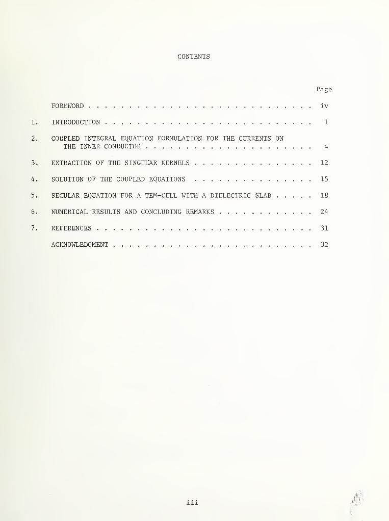
CONTENTS

Page

FOREWORD iv

1. INTRODUCTION I

2. COUPLED INTEGRAL EQUATION FORMULATION FOR THE CURRENTS ONTHE INNER CONDUCTOR 4

3. EXTRACTION OF THE SINGULAR KERNELS 12

4. SOLUTION OF THE COUPLED EQUATIONS 15

5. SECULAR EQUATION FOR A TEM-CELL WITH A DIELECTRIC SLAB 18

6. NUMERICAL RESULTS AND CONCLUDING REMARKS 24

7. REFERENCES 31

ACKNOWLEDGMENT 32

FOREWORD

This report describes a theoretical analysis developed by the staffof the University of Colorado at Boulder under a contract sponsored by

the National Bureau of Standards (NBS). Professor David C. Chang of theElectromagnetic Laboratory heads the University team. Mark T. Ma of the

NBS Electromagnetic Fields Division serves as the current technicalcontract monitor.

The work included in this report represents a further aspect of

theoretical analyses of Transverse Electromagnetic (TEM) TransmissionLine cells developed at NBS. The purpose of this effort is to evaluatethe use of TEM cells for (i) measuring the total rf power radiated by a

device Inserted into the cell for test, or (il) performing necessarysusceptibility tests on a small electronic device.

Previous results Indicate that the useful frequency range of suchTEM cells is limited by the possible presence of higher-order modes. It

has been suggested that the useful frequency range may be extended byloading the cell with an absorbing material or a lossy dielectric slab.In this report, the problem of loading the lower half of the cell with a

lossy dielectric slab is formulated with coupled integral equations.The position of the center septum inside the cell is not restricted.Dispersion and attenuation characteristics of the dominant m.ode as wellas of the higher-order modes are investigated. Numerical results arealso Included. It is found that while an insertion of a lossy materialcan indeed lower the Q-factor of the higher order modes and thus helpextend the useful frequency range, it also attenuates the dominant mode.Therefore, an appropriate correction factor to this effect must beconsidered before trying to predict radiation/susceptibility results ina free-space environment based on the measured data taken inside thecell.

Previous publications under the same effort include:

J. C. Tippet and D. C. Chang, Radiation characteristics of dipolesources located inside a rectangular coaxial transmission line,NBSIR 75-829, January 1976.

J. C. Tippet, D. C. Chang and M. L. Crawford, An analytical andexperimental determination of the cut-off frequencies of higher-order TE modes in a TEM cell, NBSIR 76-841, June 1976.

J. C. Tippet and D. C. Chang, Higher order modes in rectangularcoaxial line with infinitely thin inner conductor, NBSIR 78-873,March 1978.

I. Sreenlvasiah and D. C. Chang, A variational expression for thescattering matrix of a coaxial line step discontinuity and its

application to an over moded coaxial TEM cell, NBSIR 79-1606, May1979.

IV

DISPERSION AND ATTENUATION CHARACTERISTICS OF MODES

IN A TEM-CELL WITH A LOSSY DIELECTRIC SLAB

Dispersion and attenuation characteristics of thedominant mode in a TEM cell, loaded with a lossy dielectricslab, are investigated. It is shown that, while the insertionof the lossy material can indeed lower the Q-factor of thehigher-order modes, the attenuation of the dominant mode alsoincreases drastical ly as frequency increases. Correction to

that effect must be taken before measurements in the cell areused to correlate to those taken in a free-space environment.

Key words: Attenuation; coupled integral equations; dispersion;

lossy dielectric slab; modes considerations; TEM-cell.

1 . INTRODUCTION

It has been suggested that in the design of a TEM-cell, a loading of

the cell with absorbing material is sometimes desirable in reducing the

Q-factor of the higher-order modes and thus, can extend the useful frequency

range [1] . Since the absorbing material also perturbs the distribution

of the dominant mode and causes additional attenuation, such an arrange-

ment will certainly complicate the correction factor one seeks to relate

measurements within the TEM cell and those taken in a free-space environ-

ment. Thus, our aim in this report is to investigate theoretically the

dispersion as well as attenuation characteristics of the dominant mode

in the case when the lower half of the cell is lined with a lossy dielectric

slab. The structure resembles that of a shielded stripline which is

extensively investigated in the literature, with the only exception that

the strip (or center septum) is now elevated instead of lying on the

dielectric interface.

In early analyses of the stripline problem [2] , the dominant mode of

propagation was usually assumed to be a pure TEM mode. The justification

was made that for high dielectric constants and low frequencies, the field

was mainly confined in the dielectric layer; thus, approximate solutions

could be obtained using conformal transformation methods. Recently, more

rigorous solutions have appeared which involve expansions in terms of hybrid

modes. These solutions are generally not restricted to the low frequency

range, and in some cases data are presented for the propagation constants of

higher-order modes. Most of these analyses begin with a coupled-integral-

equation formulation. The method of solution of the resulting integral

equations distinguishes the various approaches to the problem which can be

roughly divided into three categories: (1) finite difference or finite

element methods [3-5], (2) generalized moment methods [6-12], and (3) the

singular integral equation method [13-15] . The approach taken in this work

is one based on the singular integral equation method developed in our

earlier report [16]; thus, it would fall into the last category mentioned

above. In common with the other singular integral equation approaches,

this method enables one to obtain accurate values for the propagation con-

stants by inverting relatively small-order matrices (as compared to categories

(1) and (2)). There are some important differences in our approach, however,

and these can be suinmarized as follows: (1) since we have not assumed a

symmetrically located inner conductor, we do not restrict our solution to

modes with even symmetry, (2) the location of the inner conductor is not

restricted to the dielectric interface, (3) we have used a dual formulation

in terms of the currents on the inner conductor rather than the fields in

the gap region, and (4) the nonsingular kernel is expanded in terms of

Chebyshev polynomials which leads to a set of canonical integrals which can

be evaluated in closed-form in terms of complete elliptic integrals. The

asymptotic forms of these elliptic integrals for modulus near zero or one

can then be used to obtain approximate secular equations valid in the

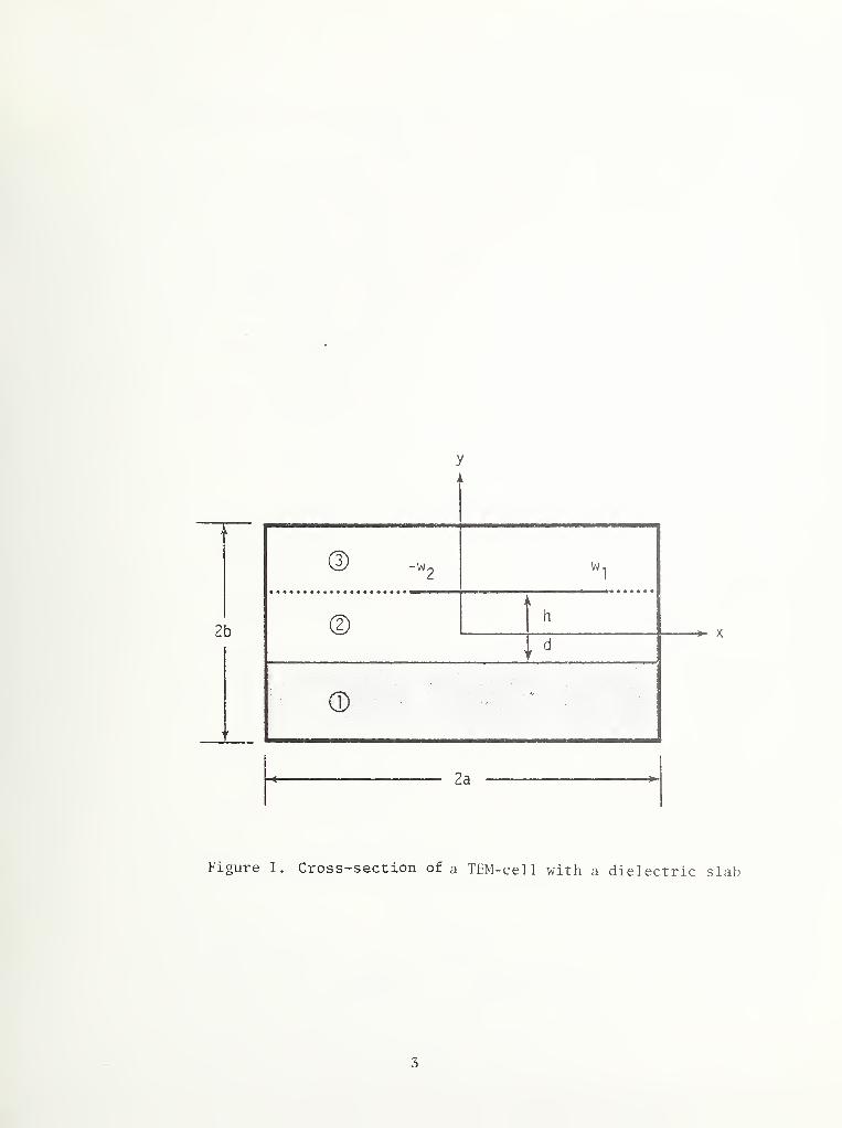
narrow-strip or small gap regions. Cross section of the device is shown in

Fig. 1. This structure consists of a R.ectangular Cross Section Transmission

Line which is loaded with a layer of dielectric material. The dielectric

layer is modeled by region 1 and is assumed to have a complex relative

permittivity permeability while those of the remaining regions are

assumed to be unity.

2

T

2b

y

(D -«2 Wi

(D

j

h

'

2a

Figure 1. Cross-section of a TEM-cell with a dielectric slab

3

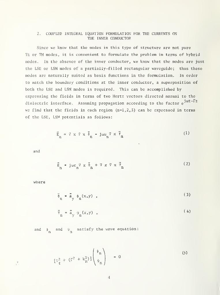
2. COUPLED INTEGRAL EQUATION FORMULATION FOR THE CURRENTS ONTHE INNER CONDUCTOR

Since we know that the modes in this type of structure are not pure

TE or TM modes, it is convenient to formulate the problem in terms of hybrid

modes. In the absence of the inner conductor, we know that the modes are just

the LSE or LSM modes of a partially-filled rectangular waveguide; thus these

modes are naturally suited as basis functions in the formulation. In order

to match the boundary conditions at the inner conductor, a superposition of

both the LSE and LSM modes is required. This can be accomplished by

expressing the fields in terms of two Hertz vectors directed normal to the

dielectric interface. Assuming propagation according to the factor

we find that the fields in each region (n=l,2,3) can be expressed in terms

of the LSE, LSM potentials as follows:

E 7 X 7 X - j con 7 X T (On n n n

and

H = iwe 7x^> + 7x7x't'n n n n

( 2 )

where

( 3 )

(4)

and 3 andn n

satisfy the wave equation

:

0C5)

4

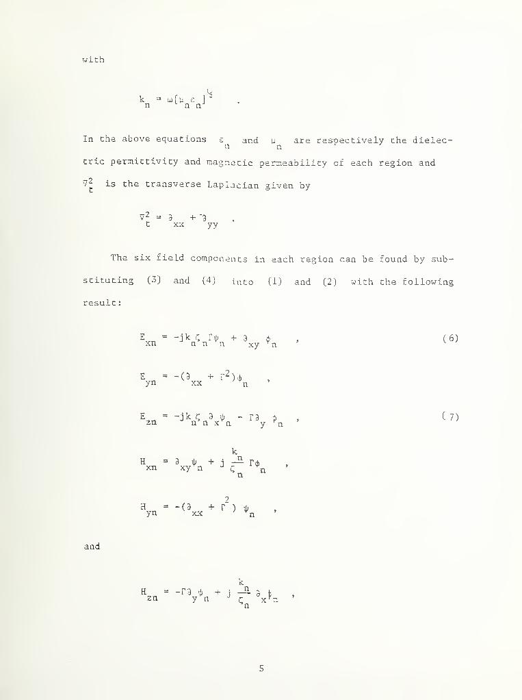
with

k = (j r u £ 1

n n n

In Che above equations £ and u are respectively the dielec-n n

trie permittivity and magnetic permeability of each region and

72 is the transverse Laplacian given by

V2 = 3 + -3

t XX yy

The six field components in each region can be found by sub-

stituting (3) and (4) into (1) and (2) with Che following

result

:

E = -jk C 4- 3 i ,xn n n n xy ' n( 6 )

E --(3 +r')j)yn XX ^

E =-jk^;3;|; - P3 i ,zn n n x^n y ^n(7)

H - 3 + j — Pd) ,xn xy n qn

H = -(3 + r ) If;

yn XX ’

and

H — — t 3 ti + i

zn y*^n'

kn

3 \X ' n>

5

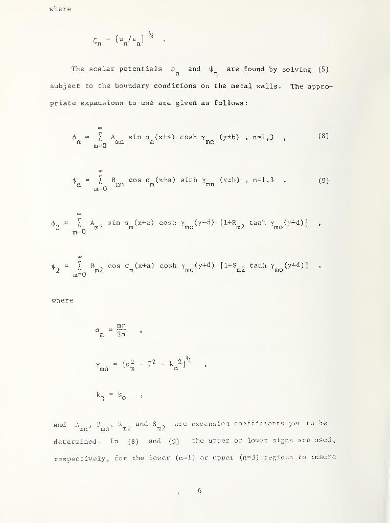
where

[u /e ]n n

1̂

The scalar potentials J) and ip are found by solvin? (5)n n o V y

subject to the boundary conditions on the metal walls. The appro-

priate expansions to use are given as follows:

d) = y A sin a (x+a) cosh y (y^b) , n=l,3 ,(8)

n _ mn m innm=0

CO

= y B cos a (x-fa) sinh y (y±b) , n=l,3 , (91n „ mn m mn ^

m=0

6^ = y A ^ sin a (x+a) cosh v (y+d) [1+R „ tanh y (v+d)],

’ y ^ rrt ? m mr\ ‘•mx mn "*'2 ^ ‘ m2 mm=U

mo m4 mo

= y B - cos a (x+a) cosh y (y+^) [1+S tanh y (y+d)] ,

2 ^ m2 mm=0

mz mo

where

muam 2a

\n =[0 ^ -m

f2 - k2]"'^

n -* >

IC3 = ^0 ’

and A , Bmn am , R and

mzsm2

are expansion coefficients yet to be

determined

.

In (8) and (9) the upper or lower signs are used

respectively, for the lower (n-1) or upper (n=3) regions to insure

o

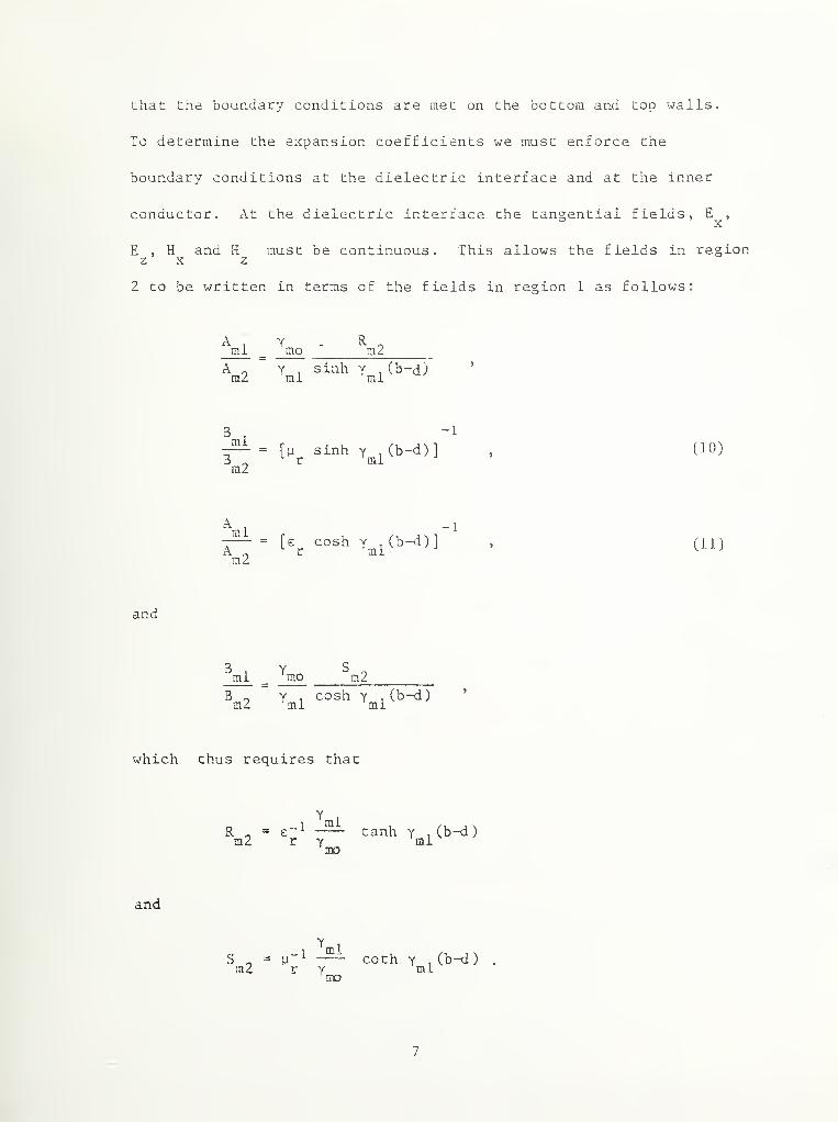
that the boundary conditions are met on the bottom and top walls.

To determine the expansion coefficients we must enforce the

boundary conditions at the dielectric interface and at the inner

conductor. At the dielectric interface the tangential fields, E ,

E ,H and R must be continuous. This allows the fields in region

Z X z

2 to be written in terms of the fields in region 1 as follows:

^mo

sinh T^j^(b-d)

-1

[u sinh Y 1(b-d)

]

r mi( 10 )

-1

[e cosh Y 1(b-d)

]

r mi

and

B

B

ml

m2

mo m2

Y ,cosh Y 1

(b-d)mi mi

( 11 )

which thus requires that

and

1

m2 r Ymo

tanh Y ,(b-d

)

mi

Y

S,m2 r Y

ml

mo

coth Y 1(b-d )

mi

7

At the inner conductor we require that the electric field be

continuous and that the magnetic field be discontinuous due to the

surface currents on the inner conductor. If we expand these sur-

face currents using a Fourier superposition, then this last condi-

tion can be written as follows:

JX

“ Im=0

y=*n

Jxm

cos a (x+a)m

and

( 12 )

Jz

CO

y=h

Im=0

Jzm

sin a (x+a)m (13)

where J and J are the Fourier components of the currentsxm zm

yet to be determined. By enforcing continuity of the tangential

electric fields at the inner conductor we can write the fields in

region 2 in terms of the fields in region 3 as follows:

sinh Y (b-h) p -——-v" - R + tanh y (d+h)

cosh Y (d+h) m2 momo ^ -

(14)

and

B

B

m2

m3

sinh Ymocosh Ymo

(b-h)

(d+h)1 + S

m2tanh Y (d+h)

mo _)

-1

(15)

If we now impose conditions (12) and (13) and use (14) and

(15) can express A^^ and B^^ solely in terms of the Fourier

8

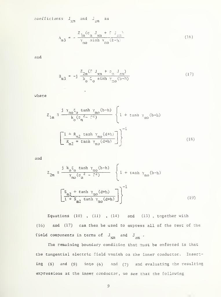
coef f iciancs J and J as:<m zm

Z, (a J + r J ^

-un m xm zm'm3 Y sinh y (b-h'

mo mo '

( 16 )

and

Z„ (r J + a J )

_ _ . 2m xm m zmm3 ^ k s sinh y (b-h)

o o mo

(17)

where

' Im

j Y C tanh y (b-h)mo o mo

k (a r'^')o m

1 -r R ^ tanh y (d+h;md mo

R ^ + tanh y (d+h)i— mz mo

1 4- tanh Y (b-h)mo

-1

(18)

and

‘

2m

j k C tanh y (b-h)[

= —f-yymT-rT) i - wnh v^^(b-h)mo m

S „ + tanh y (d+h)m2 m^

1 + S „ tanh y (d+h)-m2 mo

-1

(19)

Equations (10) , (11) , (14) and (15) ,together with

(16) and (17) can then be used to express all of the rest of the

field comoonents in terms of J and Jxm zm

riie remaining boundary condition that must be enforced is that

the tangential electric field vanish on the inner conductor. Insert-

ing( 8 )

and( 9 )

into( 6 )

and( 7 )

and evaluating the resulting

expressions at the inner conductor, we see t'nat the following

9

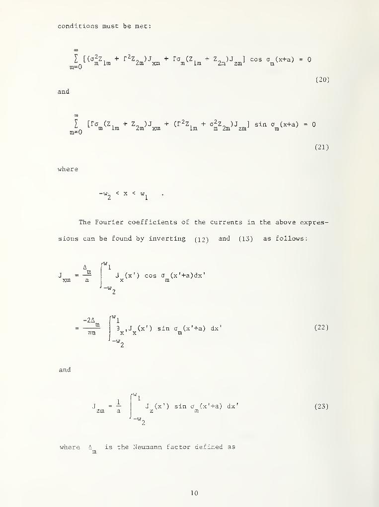
conditions must be met:

m=0m Im

r^z9

)J2m xm

ra (Z,m Im

Zo )J]2m zm

cos a ( x+a

)

ra

and

0

( 20 )

y [Fa (Z + Z )J + (F^Z + a^Z )J ] sin a (x+a) = 0m Im 2m xm Im m 2m zm-" mm=0

( 21 )

where

-w^ < X <

The Fourier coefficients of

sions can be found by inverting

the currents in the above expres-

(12) (13) as follows:

Jxm

rw.

_ma

J (x') cos a (x'+a)dx'X m

-w.

-2Arw.

mTTm

9 ,J (x’) sin a (x'+a) dx'X X m

-w.

( 22 )

and

Jzm

rw

.

-w.

J (x') sin a (x'-ra) dx

'

z m

where A is the Neumann factor defined asm

( 23 )

10

1/2 ,m = 0

L ,m > 0

The integrations in (22) and (23) are only over the inner con-

ductor since the currents must vanish outside this range. In (22)

we have integrated by oarts in order that the unknown 3 (x')XXhave the same singularity behaVior near the edges of the inner con-

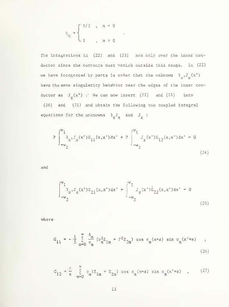
ductor as J (x*) We can now insert (22) and (23) intoz

(20) and (21) and obtain the following two coupled integral

equations for the unknowns 3 J and J :

X X z

ri9,^,d^^(x' )Gii (x,x' )dx' + ?

I

(x’

0

-w. J.w.

(24)

and

rw. 'W.

3 ,J (x')G (x,x')dx' 4-j

J (x’)G (x,x')dx' = 0XX 2ij

z 22

-w^ ' -w^

(25)

where

oo /\

G,,

= - — y — (cj^Z, 4- r^Z- ) cos a (x4-a) sin a (x'4-a)LI 2 a m Im 2m m m

m=0 m

(26)

G12

to

— y o(Z, 4-Z„)coso (x4-a) sin a (x’4-a)a ra Im 2m m m

m=0

(27)

11

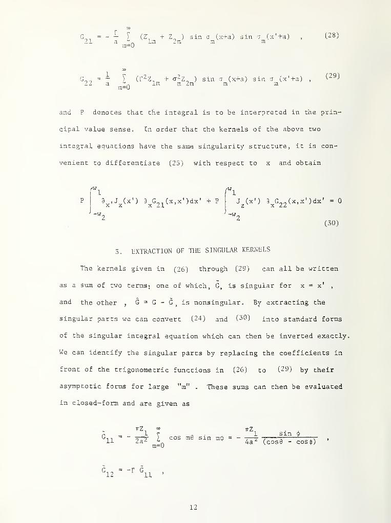
G21

00p

— y (Z", +Z^)sina (x+a) sin 7 (x'+a)a Im 2m m m

m=0

C28)

G92

00

1 r - -)

—) (F'^Z- + <X^Z- ) sin a (x+a) sin a (x'+a) ,

a Ini m 2ra m mm=0

(29)

and P denotes that the integral is to be interpreted in the prin-

cipal value sense. In order that the kernels of the above two

integral equations have the same singularity structure, it is con-

venient to differentiate (25) with respect to x and obtain

3 ,J (x') 3 G_ (x,x')dx’ + P

-w.

J (x') 3 G-^(x,x')dx' = 0Z X 4Z

-w.

(30)

3. EXTRACTION OF THE SINGULAR KERNELS

The kernels given in (26) through (29) can all be written

as a sum of two termsj one of which, G, is singular for x = x’ ,

and the other,

G = G - G,is nonsingular. By extracting the

singular parts we can convert (24) and (2*^) into standard forms

of the singular integral equation which can then be inverted exactly.

We can identify the singular parts by replacing the coefficients in

front of the trigonometric functions in (26) to (29) by their

asymptotic forms for large "m" . These sums can then be evaluated

in closed-form and are given as

11

tZ^ ttZ^

^ cos m9 sin mcp = - yqprsin i

2a2m=0

4a"^ (cos0 - cosb)

G12

= -r G11

12

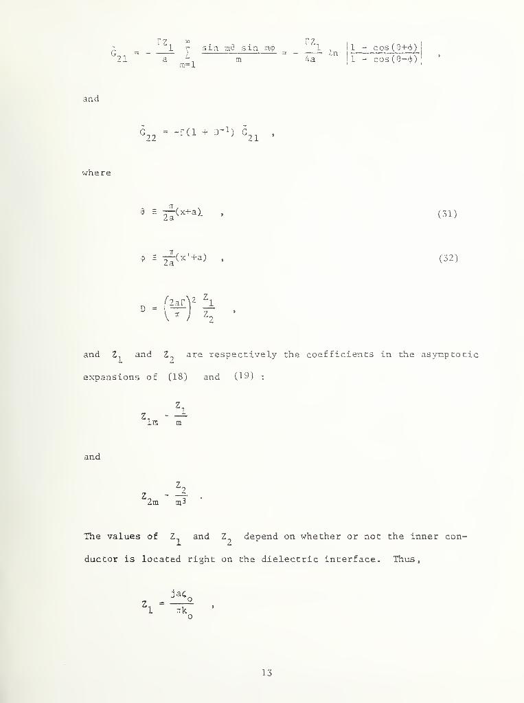
G21 I

m=l

sin m9 sin m<p

m

T-1 ft

' 1,

I 1 - COS (8+6)I

4a I 1 - cos ( 0-'^)) :

and

-r(i + d~M ,

where

9 = yj(x+a).Z 3.

(31)

'P=

> (32)

D = 2ar^^

^ / Z.

and and are respectively the coefficients in the asymptotic

expansions of (18) and (19) :

'Im m

and

‘2m m3

The values of Z^ and Z^ depend on whether or not the inner con-

ductor is located right on the dielectric interface. Thus,

,

'1 tk

13

2

Z9

and

if

(d+h) 0

and

2jac,

7Tk (1+e )

^2 =

2ak

f1+e

r

] 1+U-lJ-

and

l+y“^r

1+er —

'

if

(d+h) = 0 .

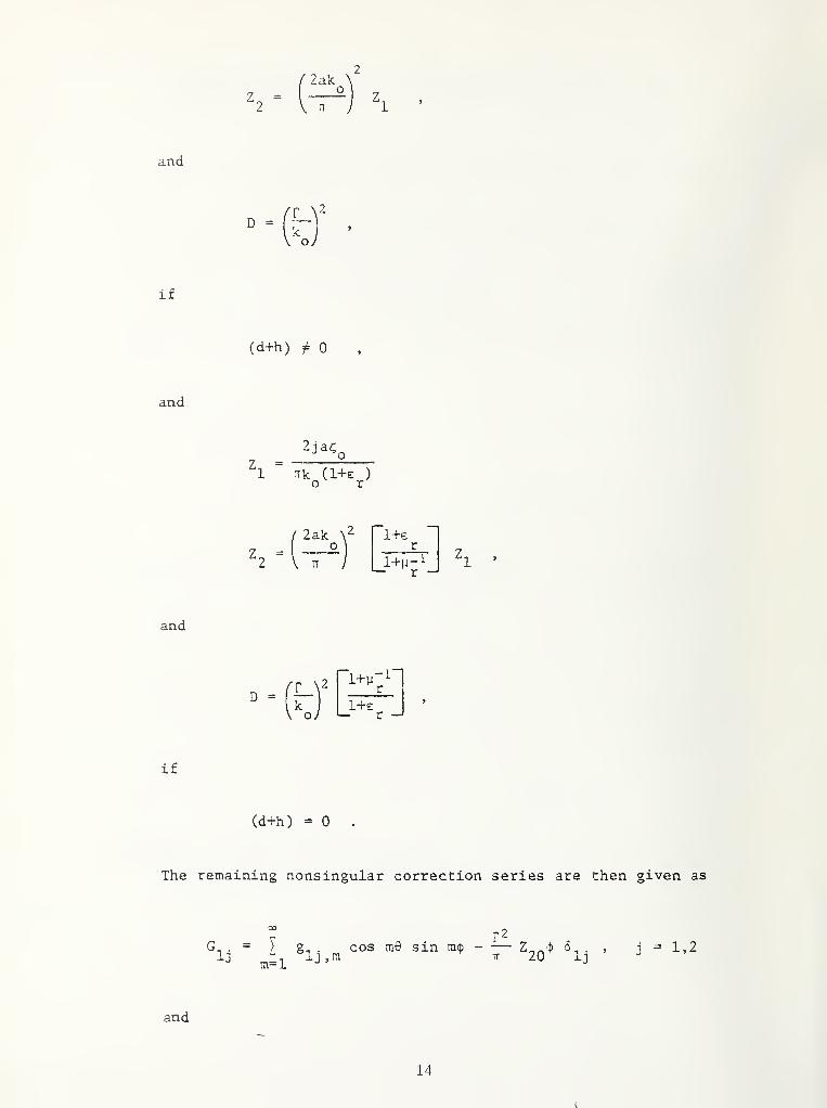
The remaining nonsingular correction series are then given as

GIj

CO

Im=l

g^ . cos m6 sin md - —lj,m TT 20 j 1,2

and

14

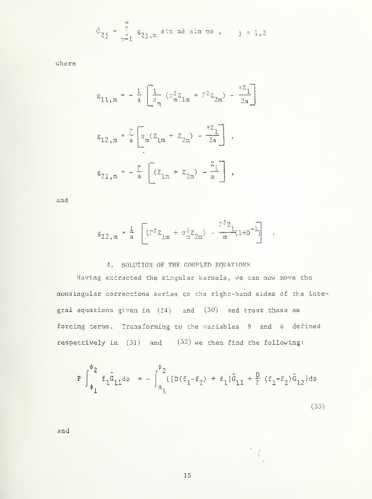
where

and

G = ' cr

2j -2j,nisin 010 sin mcp

, j = 1,2

• ttZ— i- f2z„ )- —

-

a m Ini 2mL_ m

g12 ,

m a

-tZ.

a (Z, + Z, )- —

m Im 2m 2a

’21, m a(Z. + Z„ )

- —Im 2m m

g22 ,m a

(r^z 4- ajz )- "vAi+d ^Im m 2m m

4. SOLUTION OF THE COUPLED EQUATIONS

Having extracted the singular kernels, we can now move the

nonsingular corrections series to the right-hand sides of the inte-

gral equations given in (24) and (30) and treat these as

forcing terms. Transforming to the variables 9 and d defined

respectively in (31) and (32) we then find the following:

P f^G^ldbr

(33)

and

15

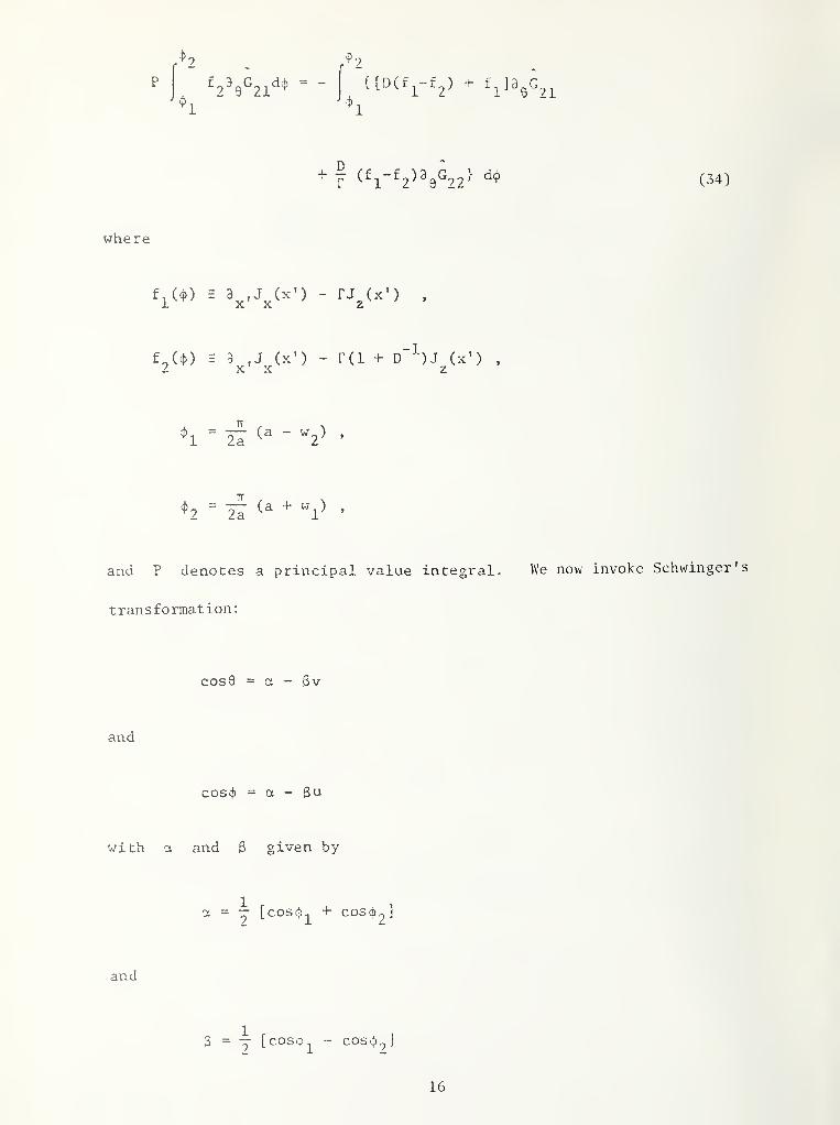
/2

+ f (^r^2>^8°22' (34)

where

f (cp) E 8 J (x') - rj (x’) ,•L ^ ^ ^

f^(4>) E 5_^,J^(x') - r(i + d“^)j^(x’) ,

IT

2a(a + w^)

anci P denotes a principal value integral. We now invoke Schwinger's

transformation:

cos9 = a - 3v

and

cos4> = a - 3u

with a and S given by

a = ~ [cosp^ + coscb^]

and

3 = j [cos9^ - cosb^

]

16

in order to transform (33) and (34) into canonical forms of

the singular integral equation;

T^[F.(u)] = H.(v),

i = 1,2

where

TV[F.(u)]

Ju-v

-1

du

wi th

F^(u) = f^Cq) ,

F^Cu) = f^C^) ,

H^(v) =

and

^ V =11 =12>

(35)

?a f

UDCf^-f^) ^ q]3e=21^7(V^2>^=22> •

(36)

Again, we expand H (v) into a series of Chebyshev polynomials ofi

the second kind U asm

H,(v) = I .U (v)> ^ rnd-l , 1 m

m=0(37)

17

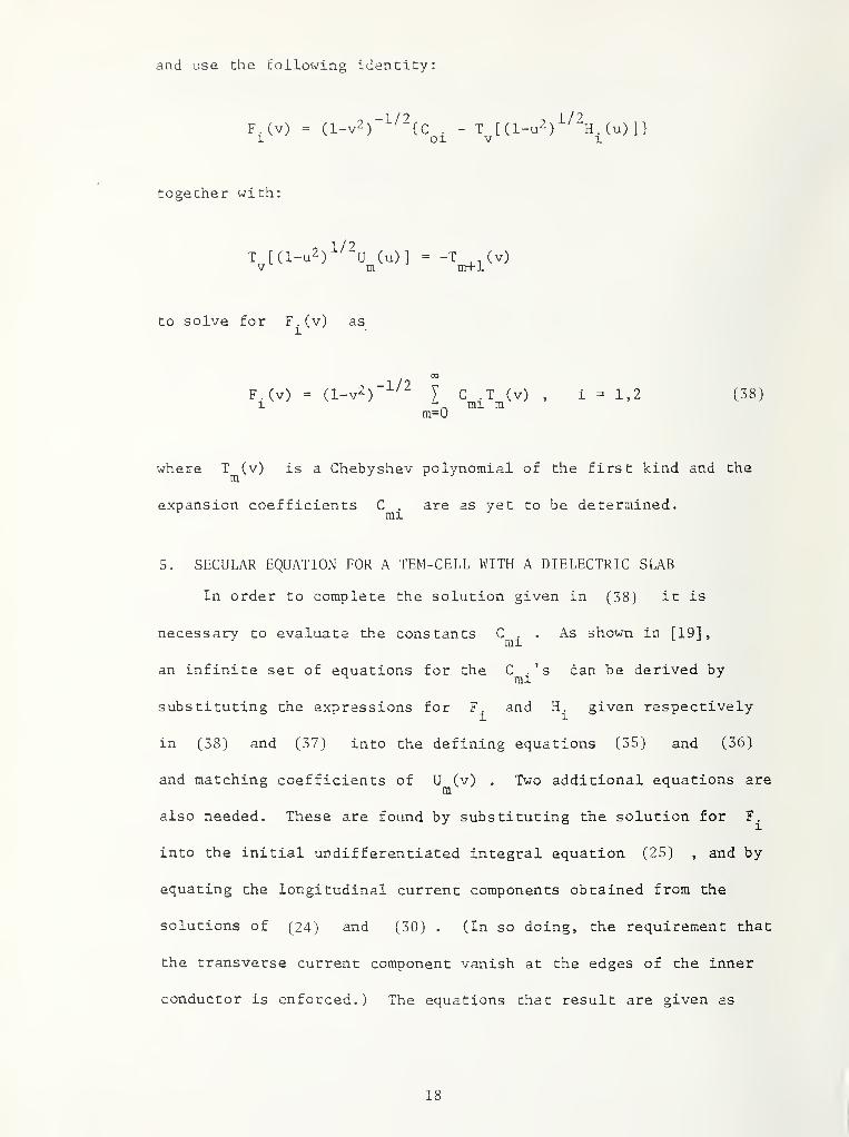
and use the following identity:

— 1 10 1 /?F.(v) = (l-v2) .

- T [(1-u^) H.(u)]}1 Ol V 1

together with:

T [(l-u2)^/“U (u)] = -T^.(v)V ra m+1

to solve for F^(v) as

CO

F (v) = I C T (v) , i = 1,2 (38)1 ^ ml m

m=0

where T (v) is a Chebyshev polynomial of the first kind and them

expansion coefficients C . are as yet to be determined.ml

5. SECULAR EQUATION FOR A TEM-CELL WITH A DIELECTRIC SLAB

In order to complete the solution given in (38) it is

necessary to evaluate the constants . As shown in [19],

an infinite set of equations for the ^ derived by

substituting the expressions for F^ and given respectively

in (38) and (37) into the defining equations (35) and (36)

and matching coefficients of U (v) . Two additional equations arem

also needed. These are found by substituting the solution for F^

into the initial undifferentiated integral equation (25) , and by

equating the longitudinal current components obtained from the

solutions of (24) and (30) . (In so doing, the requirement that

the transverse current component vanish at the edges of the inner

conductor is enforced.) The equations that result are given as

18

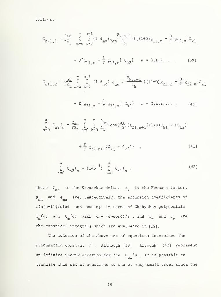
follows

:

C ^2aS

n+1 , 1 ttZ^

^ n-1

I I (1-5m=n k=0

)q { [ (1+D)^ + ?rno^^nm A, ^^ll,m T °12,ni-Sl

(39)

C .n.-rl

, 2I ([(1+D)S„ _ + 7 g,0 JC,rz

1 ni=n k=0’21,m r °22,in^'^kl

°*-^21,m ^r ^22, ^2^ ^ 0,1,2, (40)

n o.r ^ r 2a ^ "kn ^

i k.2k " n: k ,k“

u=0 '1 n=0 k=0 k21,n+l^^^^°^\l

-°^k2-

^r °22,n+l*^\l ^k2^^ ’

(41)

n=0k2k =

In=0

C ,Inl n

(42)

where 6 is the Kronecker delta. A, is the Neumann factor,mo ’ k

p and q are, respectively, the expansion coefficients ofmn mn

sin(n+l) 4>/sinp and cos n<p in terms of Chebyshev polynomials

T (u) and U (u) with u = (a-cosp)/3 , and I and J aremm n n

the canonical integrals which are evaluated in [19].

The solution of the above set of equations determines the

propagation constant f . Although (39) through (42) represent

an infinite matrix equation for the 0^^ ' s , it is possible to

truncate this sat of equations to one of very small order since the

19

coefficients g. .of the nonsingular kernels, in most cases,

1 j ,m

converge extremely rapidly with "m"

.

In the following, we will assume that ~ 0

n > 0 so that the infinite matrix equation reduces to just a simple

2x2 matrix. This approximation places some restrictions on the

various dimensions of the strip line which one can allow and still

obtain accurate values for the propagation constant.

The nature of this approximation can best be understood by

examining the form of the current as given by (38) . The dominant

9 - 1/2feature of this solution is contained in the factor (l-v'^)

which governs the behavior near the sharp edges of the inner conduc-

tor. The remaining Chebyshev expansion tailors the distribution

away from the edges. The constant part of this expansion is retained

in the 2x2 matrix approximation. In most cases, one would expect

this to represent the exact distribution fairly accurately. This

would not be the case, however, when one of the following occurs:

(1) either the top or bottom wall of the outer conductor approaches

the inner conductor, (2) the dielectric layer is close to but not

quite touching the inner conductor, (3) the inner conductor is located

at the dielectric interface and is relatively wide compared to the

width of the dielectric layer, or (4) one is interested in a higher-order

mode with a large cutoff frequency.

The limitation encountered with the first of the above cases

is analogous to that which was found earlier for the RCTL

without dielectric [16]. The approximate solution breaks down for small

b/a (i.e., when the inner conductor- is close to the top and bottom

walls of the outer conductor).

2.0

The reason for the restriction in the second case mentioned above can

best be seen by examining the expressions for and as given,

respectively, in (18) and (19). In extracting the asymptotic forms of these

expressions for large "m" we obtained two different results depending upon

whether or not (d +h) = 0, When (d +h) was close to but not quite zero

(i.e., the dielectric layer was near the inner conductor) then a larger value

of "m” was needed in order to make tanh y^^(d+h) approach 1. Therefore,

since the nonsingular kernels do not converge as rapidly, the 2x2 approxi-

mation breaks down. When the inner conductor is exactly on the interface,

the 2x2 approximation is again quite accurate as the correct asymptotic

form was extracted (i.e., tanh v (d+h) 0).mo

In the third case, one would expect the current distribution to

approach that of a parallel stripline formed by the inner conductor and

its image about the bottom wall of the outer conductor. Since we know that

the current distribution in this case is significantly different from that

predicted by (38) , again the 2x2 approximation breaks down.

Finally, for very high-order modes, the expressions for Z^^ and

do not converge very rapidly, and the 2x2 approximation breaks down.

Summarizing the above restrictions, we can say that for the dominant

mode and the first few higher-order modes, one would expect the 2x2

approximation to be quite accurate as long as the inner conductor is not

too close to either the top or bottom walls of the outer conductor or the

dielectric layer. As will be demonstrated, very accurate results for the

propagation constants can be obtained assuming this rather simplified

current distirbution. This should not be too surprising since we know

that a variational expression for the propagation constant can be formulated

which is not too sensitive to the exact distribution used for the current.

21

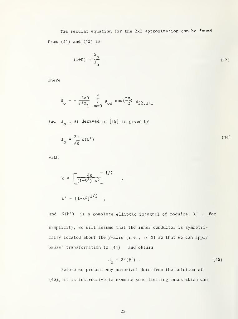
The secular equation for the 2x2 approximation can be found

from (41) and (42) as

(1+D) (43 )

where

So

4aDE

m=0on

.niT.cos (—

)

’22,n+l

and,

as derived in [19] is given by

Jo ^ K(k')

/b

with

k = 4B

_(l+62)-a2

1/2

k' = [l-k2]^/2^

(44)

and K(k') is a complete elliptic integral of modulus k' . For

simplicity, we will assume that the inner conductor is symmetri-

cally located about the y-axis (i.e., a=0) so that we can apply

Gauss' transformation to (44) and obtain

= 2K(3') . (45)

Before we present any numerical data from the solution of

(43), it is instructive to examine some limiting cases which can

22

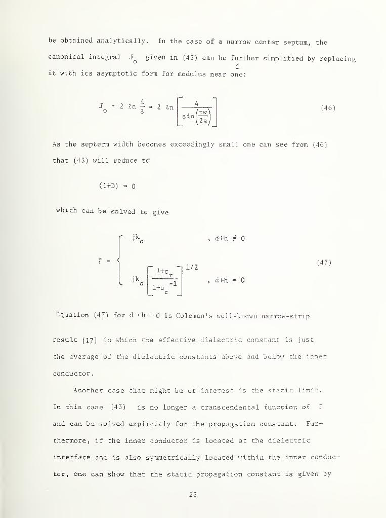
be obtained analytically. In the case of a narrow center septum, the

canonical integral given in (45) can be further simplified by replacing1

it with its asyiiiptotic form for modulus near one:

Jo

2 in - =3

in (46)

As the septerm width becomes exceedingly small one can see from (46)

that (43) will reduce to'

(M) = 0

which can be solved to give

r 1k, d+h 7^ 0

r = <

l+e1/2

l+a-1 , d+h - 0

(47)

Equation (47) for d +h= 0 is Coleman's well-known narrow-strip

result [17] in which the effective dielectric constant is just

the average or the dielectric constants above and below the inner

conductor

.

Another case that might be of interest is the static limit.

In this case (43) is no longer a transcendental function of I

and can be solved explicitly for the propagation constant. Fur-

thermore, if the inner conductor is located at the dielectric

interface and is also symmetrically located within the inner conduc-

tor, one can show that the static propagation constant is given by

23

that in (47) for d +h = 0 independent of the width of the inner conductor.

As shown in [18] this is an exact result of the related problem where the

side walls are removed to infinity when the dielectric layer fills exactly

half the guide.

As a final comment one can easily show that f = jk is a solution too

(43) in the trivial case when e = y =1, since g„. = 0 when F = jk .

^ r r ’

^^22,n o

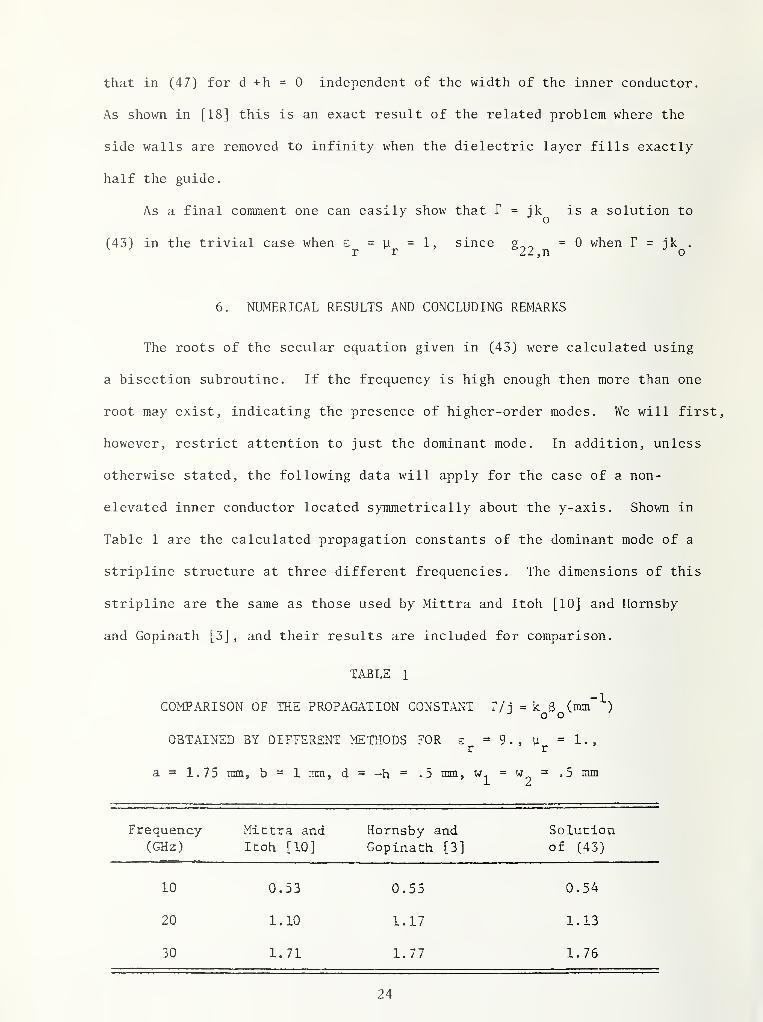
6. NUMERICAL RESULTS AND CONCLUDING REMARKS

The roots of the secular equation given in (43) were calculated using

a bisection subroutine. If the frequency is high enough then more than one

root may exist, indicating the presence of higher-order modes. We will first,

however, restrict attention to just the dominant mode. In addition, unless

otherwise stated, the following data will apply for the case of a non-

elevated inner conductor located symmetrically about the y-axis. Shown in

Table 1 are the calculated propagation constants of the dominant mode of a

stripline structure at three different frequencies. The dimensions of this

stripline are the same as those used by Mittra and Itoh [10] and Hornsby

and Gopinath [3], and their results are included for comparison.

TABLE 1

COMPARISON OF THE PROPAGATION CONSTANT T/j = k B (mm“^)0 0

OBTAINED BY DIFFERENT METHODS FOR s = 9., U =1.,r r

a = 1.75 Tmn, b = 1 mm. d = -h = .5 mm. = .5 mm

Frequency Mittra and Hornsby and Solution(GHz) Itoh [10] Gopinath [3] of (43)

10 0.53 0.55 0.54

20 1.10 1.17 1.13

30 1.71 1.77 1.76

24

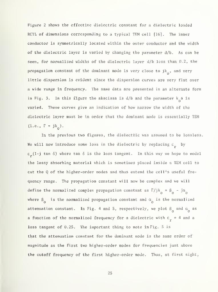
Figure 2 shows the effective dielectric constant for a dielectric loaded

RCTL of dimensions corresponding to a typical TEM cell [16]. The inner

conductor is symmetrically located within the outer conductor and the width

of the dielectric layer is varied by changing the parameter d/b. As can be

seen, for normalized widths of the dielectric layer d/b less than 0.2, the

propagation constant of the dominant mode is very close to and very

little dispersion is evident since the dispersion curves are very flat over

a wide range in frequency. The same data are presented in an alternate form

in Fig. 3. In this figure the abscissa is d/b and the parameter k^a is

varied. These curves give an indication of how narrow the width of the

dielectric layer must be in order that the dominant mode is essentially TEM

(i.e. , r = jk^)

.

In the previous two figures, the dielectric was assumed to be lossless.

We will now introduce some loss in the dielectric by replacing by

e^(l-j tan 6) where tan d is the loss tangent. In this way we hope to model

the lossy absorbing material which is sometimes placed inside a TEM cell to

cut the Q of the higher-order modes and thus extend the cell's useful fre-

quency range. The propagation constant will now be complex and we will

define the normalized complex propagation constant as T/jk^ =3^

- jot^

where3^

is the normalized propagation constant and is the normalized

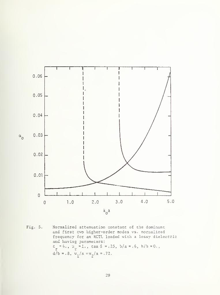
attenuation constant. In Fig. 4 and 5, respectively, we plot 3^and as

a function of the normalized frequency for a dielectric with = 4 and a

loss tangent of 0.25. The important thing to note in Fig. 5 is

that the attenuation constant for the dominant mode is the same order of

magnitude as the first two higher-order modes for frequencies just above

the cutoff frequency of the first higher-order mode. Thus, at first sight.

25

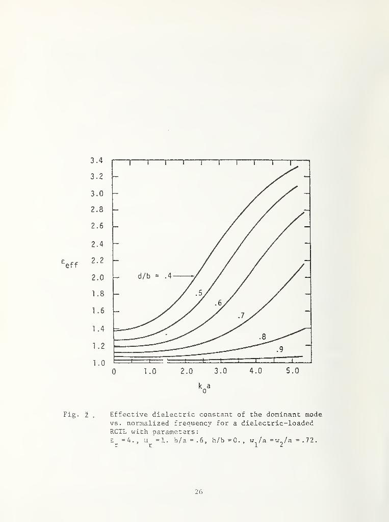
Fig. 2 .EffecCive dielectric constant of the dominant modevs. normalized frequency for a dielectric-loadedRCTL with parameters:

£^=4., u^=l. b/a=.6, h/b=0., 3. =v!^/ a. - .11.

26

d/b

Effective dielectric constant of the dominant modevs. d/b for a dielectric-loaded RCTL with parameter

= 4. ,

= 1 • ,b/a = . 6 , h/b = 0

. ,w^/a = w^/a = . 12 .

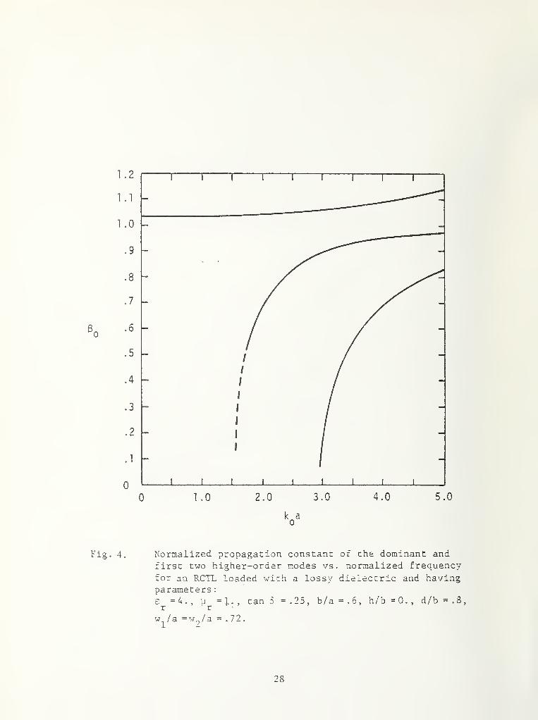
Fig. 4. Normalized propagation constant of the dominant and

first two higher-order modes vs. normalized frequency

for an RCTL loaded wich a lossy dielectric and havingparameters

:

£ = 4. ,

u = I. ,

tan 5 = . 25 , b/a = . 6 ,h/b = 0

. ,d/b = . 8

,

r ' r '

w^/a =w^/a = .72.

28

k a0

Fig. 5. Normalized attenuation constant of the dominantand first two higher-order modes vs. normalizedfrequency for an RCTL loaded with a lossy dielectricand having param.eters:

£ =4., U =1-, tan 5 = .25, b/a=.6, h/b=0.,r r

d /b = . 8

,

w^ /a = w^ /a = .72.

29

it would appear that the lossy dielectric layer does not act as a very good

mode filter. However, for an absorber loaded TEM cell, one must remember

that the RCTL is terminated in two tapered sections which represent reactive

loads on the transmission line. Thus, from a resonance standpoint, the

introduction of a small amount of loss in the propagation constant of the

higher-order modes could substantially reduce the Q of these modes

without adversely affecting the dominant TEM mode.

30

7. REFERENCES

[1] M.L. Crawford, J.L. Workman and C.L. Thomas, "Expanding the bandwidthof TEM cells for EMC measurements," IEEE Trans. EMC, vol. 20, no. 3,

pp. 368-375, Aug. 1978.

[2] H.E. Stinehelfer, Sr., "An accurate calculation of uniformmicrostrip transmission lines," IEEE Trans. Microwave TheoryTech . . vol. MTT-16, pp. 439-444, July 1968.

[3] .J.S. Hornsby and A. Gopinath, "Numerical analysis of a dielec-tric-loaded waveguide with a micros trip line-finite-differencemethods," IEEE Trans. Microwave Theory Tech ., vol. MTT-17,pp. 684-690, Sept. 1969.

[4] D.G. Corr and J.B. Davies, "Computer analysis of the funda-mental and higher-order modes in single and coupled micro-strip," IEEE Trans. Microwave Theory Tech ., vol. MTT-20

,

pp. 669-677, Oct. 1972.

[5] ?. Daly, "Hybrid-mode analysis of microstrip by finite-elementmethods," IEEE Trans. Microwave Theory Tech ., vol. MTT-19,pp. 19-25, Jan. 1971.

[6] L.N. Deryugin, O.A. Kurdyumov, and V.E. Sotin, "Fundamentaland parasitic wave modes of a shielded microstrip line,"Radiophvs

.Quantum Electron ., vol. 16, pp . 89-96, Jan. 1973.

[7] M.K. Krage and G.I. Haddad, "Frequency-dependent character-istics of microstrip transmission lines," IEEE Trans . Micro-wave Theory Tech ., vol. MTT-20, pp . 678-688, Oct. 1972.

[8] J. Dekleva and V. Roje, "Modovi oklopljene mikrostrip linije,"Elektrotehnika (Zagreb) , vol. 18, pp. 293-296, 1975.

[9] Y. Fujiki, T. Kitazawa and M. Suzuki, "Analysis of higher-

order modes in single, coupled and asymmetrical striplines,"Electron. Comir.un. in Jan. ,

vol. 57-3, pp . 89-95, Oct. 1974.

[10] T. Itoh and R. Mittra, "A technique for computing dispersion

characteristics of shielded microstrip lines," IEEE Trans

.

Microwave Theory Tech . , vol. MTT-22, pp . 896-898, Oct. 1974.

[11] R. Jansen, "Zur numerischen berechnung geschirmter streifen-leitungs-strukturen, " Arch. Elek. Ubertragung

.

,vol. 29,

pp . 241-247, June 19 75.

[12] G. Kowalski and R. Pregla, "Dispersion characteristics of

shielded microstrips with finite thickness," Arch. Elek.

Ubertragung

.

,voi. 25, pp. 193-196, Apr. 1971.

31

[13] R. Mittra and T. Itoh, "A new technique for the analysis of thedispersion characteristics of microstrip lines," IEEE Trans. Micro-wave Theory Tech ., vol. MTT-19, pp. 47-56, Jan. 1971.

[14] G. Essayag and B. Sauve, "Effects of geometrical parameters of a

microstrip on its dispersive properties," Electron. Lett .,

vol. 8, pp. 529-530, Oct. 1972.

[15] G. Essayag and B. Sauve, "Study of higher-order modes in a microstripstructure," Electron. Lett ., vol. 8, pp. 564-566, Nov. 1972.

[16] J.C. Tippet and D.C, Chang, "Properties of a rectangular cross-sectiontransmission line with an offset inner conductor," accepted forpublication in IEEE Trans. Micrw. Theory and Tech ., vol. MTT-27, 1979.

[17] B.L. Coleman, "Propagation of electromagnetic disturbances along a

thin wire in a horizontally stratified medium," Phil . Mag . , vol. 41,

ser. 7, pp. 276-288, Mar. 1950.

[18] G. Kowalski and R. Pregla, "Calculation of the distributed capacitancesof coupled microstrips using a variational integral," Arch. Elek .

Ubertragung . , vol. 27, pp. 51-52, Jan. 1973.

[19] J.C. Tippet, Modal characteristics of rectangular coaxial transmission-

line, Ph.D. Thesis, Department of Electrical Engineering, University of

Colorado, Boulder, CO, 1978.

ACKNOWLEDGMENT

The authors are indebted to Professors L. Lewin and E.F. Kuester,

University of Colorado; Professor M.T. Ma and Mr. M. Crawford,

NBS Boulder Laboratories, for their very useful comments and

suggestions. The work is supported under Contract No. CST-8447.

32

NBS-114A (REV. 8-70)

u.S. GOVERNMENT PRINTING O F FIC E : !1 9 79-0-6 77-07 2/ 1 30 0 USCOMM-DC