t 102 (2006) 250–263www.elsevier.com/locate/rse

Remote Sensing of Environmen

Bridging between SeaWiFS and MODIS for continuity of chlorophyll-aconcentration assessments off Southeastern China

Caiyun Zhang a,b, Chuanmin Hu c, Shaoling Shang a, Frank E. Müller-Karger c, Yan Li a,Minhan Dai a, Bangqin Huang a, Xiuren Ning d, Huasheng Hong a,⁎

a State Key Laboratory of Marine Environmental Science, Xiamen University, Xiamen, Fujian 361005, Chinab Department of Oceanography, College of Oceanography and Environmental Sciences, Xiamen University, Xiamen, Fujian 361005, China

c College of Marine Science, University of South Florida, 140 7th Avenue South, St. Petersburg, FL 33701, USAd Key Lab of Marine Ecosystems and Biogeochemistry of State Oceanic Administration, Hangzhou, Zhejiang 310012, China

Received 12 August 2005; received in revised form 25 December 2005; accepted 11 February 2006

Abstract

Chlorophyll-a (Chl) concentration in the Taiwan Strait (TWS) and in the South China Sea (SCS) was estimated using time series of satellite datacollected with the MODIS/Aqua and SeaWiFS instruments, and validated with in situ measurements from three cruises conducted in winter andsummer 2004. For Chl between 0.1 and 10mg m�3, both SeaWiFS and MODIS agreed well with in situ data. Errors for turbid coastal waters werelarger than for offshore waters but the overall RMS (root mean square) error in log scale was within 0.35. The percentage RMS error was muchlarger, varying between 60% and 170% for open ocean and most of the shallow (<30 m), coastal regions. However, there was no large systematicerror or significant bias in either satellite data set, and these numbers were comparable to those for other global oceans and not significantly largerthan the algorithm “noise” (0.22 in RMS error in log scale). Further, SeaWiFS and MODIS showed similar spatial and temporal patterns betweenJuly 2002 and October 2004, as well as nearly identical concentrations for Chl between 0.1 and 4mg m�3. RMS difference between the two datasets of monthly mean Chl for several sub-regions was generally <11% and <0.05 (after logarithmic transformation). For each individual month, thestatistics (mean, mode, median) of the two data sets for the entire study region (6–9×105 satellite pixels at ∼1km resolution) were very similar,with RMS differences typically between 30% and 40% and between 0.10 and 0.15 (after logarithmic transformation), where no significant bias wasfound. Therefore, it would be possible to continue the time series using only one sensor such as MODIS, in the eventual absence of SeaWiFS.Further research is needed to improve the remote sensing algorithms for application in turbid coastal waters.© 2006 Elsevier Inc. All rights reserved.

Keywords: Remote sensing; Ocean color; Continuity; Chlorophyll a; SeaWiFS; MODIS; Taiwan Strait; South China Sea

1. Introduction

Assessment of environmental change over long periods oftime requires a time-series of consistent observations.Phytoplankton pigment concentrations such as chlorophyll-a(Chl) provide a measure of the biological state of the surfaceocean. Satellite sensors designed to observe the Visible SeaSpectral Reflectance (VSSR, traditionally called ocean color)provide estimates of short-term (seasonal and inter-annual) to

⁎ Corresponding author. Tel.: +86 592 2182216; fax: +86 592 2095242.E-mail addresses: hhuasheng@gmail.com, hshong@xmu.edu.cn (H. Hong).

0034-4257/$ - see front matter © 2006 Elsevier Inc. All rights reserved.doi:10.1016/j.rse.2006.02.015

long-term (decadal) changes in the global ocean Chl (e.g.,Behrenfeld et al., 2001; Gregg & Conkright, 2002; Gregg etal., 2003). However, for a particular region, especially acoastal region, the accuracy of the long-term trend is oftenunknown due to uncertainties associated with satellite dataproducts.

Of particular interest are observations from the Sea-viewingWide Field-of-view Sensor (SeaWiFS) that has operated since1997 (McClain et al., 1998) and from the two ModerateResolution Imaging Spectroradiometers (MODIS), includingTerra MODIS (since 1999) and Aqua MODIS (since 2002)(Esaias et al., 1998). These satellite sensors provide near-dailycoverage of the global ocean. Continuity in coverage is

251C. Zhang et al. / Remote Sensing of Environment 102 (2006) 250–263

expected with the future National Polar-Orbiting OperationalEnvironmental Satellite System (NPOESS) and the NPOESSPreparatory Mission (NPP; expected launch in 2008), whichwill carry the Visible/Infrared Imager/Radiometer Suite (VIIRS)instruments, which are similar in capability to SeaWiFS andMODIS.

Some efforts have been made to merge global time seriesfrom different VSSR (i.e., ocean color) sensors, primarily theCoastal Zone Color Scanner and SeaWiFS (Gregg & Conkright,2001; Siegel & Maritorena, 2000; Yoder et al., 2001). But littlehas been done on merging global-scale SeaWiFS and MODISseries. SeaWiFS is a well-calibrated and stable sensor (McClainet al., 2004). In comparison, there is a general perception thatMODIS data are of lower quality due to the publicity thatseveral artifacts in sensor design have received (for examplestray light, polarization, and data striping). The futureavailability of SeaWiFS data is not clear, since the missionhas exceeded its 5-year life design. However, MODIS isexpected to continue into the future and provide a bridge toVIIRS. To enable a smooth transition from SeaWiFS toMODIS, it is necessary to assess differences between thesesensors. Such comparison is particularly useful to regionalinvestigators, given that some limited regional comparisonshave shown large variations (Blondeau-Patissier et al., 2004;Darecki & Stramski, 2004). Here we present the first validationand comparison results for observations of Chl in the TaiwanStrait (TWS) and the northern South China Sea (SCS) to assessthe utility of MODIS in case that SeaWiFS data may not beavailable in the future.

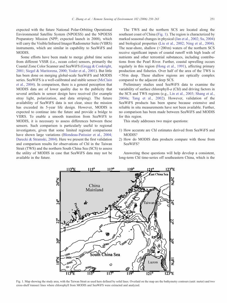
Fig. 1. Map showing the study area, with the Taiwan Strait as used here defined by socross-shelf transect lines where chlorophyll from MODIS and SeaWiFS were extrac

The TWS and the northern SCS are located along thesoutheast coast of China (Fig. 1). The region is characterized bymarked seasonal changes in physical (Jan et al., 2002; Su, 2004)and biological properties (Liu et al., 2002; Ning et al., 2004).The near-shore, shallow (<200m) waters of the northern SCSreceive significant inputs of coastal runoff with high loads ofnutrients and other terrestrial substances, including contribu-tions from the Pearl River. Further, coastal upwelling occursregularly in this region (Hong et al., 1991), affecting primaryproduction and fisheries. Over half of the area of the TWS is<50m deep. These shallow regions are optically complexcompared to the adjacent deep SCS.

Preliminary studies used SeaWiFS data to examine thevariability of surface chlorophyll-a (Chl) and driving factors inthe SCS and TWS regions (e.g., Lin et al., 2003; Shang et al.,2004a; Tang et al., 2002). However, validation of theSeaWiFS products has been sparse because extensive andreliable in situ measurements have not been available. Further,no comparison has been made between SeaWiFS and MODISfor this region.

This study addresses two major questions:

1) How accurate are Chl estimates derived from SeaWiFS andMODIS?

2) How do MODIS data products compare with those fromSeaWiFS?

Answering these questions will help develop a consistent,long-term Chl time-series off southeastern China, which is the

lid lines. Overlaid on the map are the bathymetry contours (unit: meter) and twoted and analyzed.

252 C. Zhang et al. / Remote Sensing of Environment 102 (2006) 250–263

first step leading to a better understanding on temporal patternsof Chl in response to physical fluctuations and their relationshipwith local and remote forcing.

2. Data and methods

2.1. Cruise survey

In situ data were collected from three cruises (Fig. 1) in2004. Two cruises were conducted in the northern SCS from 9February to 6 March 2004 (identified below as February2004) and from 6 to 23 July 2004 (identified below as July2004). A third cruise was conducted in the southern TWSfrom 26 July to 7 August 2004 (identified below as August2004). Water samples were collected with 1.7L Niskin bottlesmounted on a rosette equipped with a SBE19 CTD. Sampling

Fig. 2. Composite Chl images from the MODIS (upper panels) and SeaWiFS (middleJuly, and 26 July–7 August. White crosses (+) on the MODIS images mark in situ saship transect lines from which SeaWiFS and MODIS data were available for compariand MODIS data were available within ±2h (red), ±24h (blue), and ±48h (black) ocruise periods.

locations are shown in Fig. 2. Samples were filtered withWhatman GF/F glass fiber filters, and chlorophyll-a concen-tration (Chl) was determined by extracting pigments inacetone and measuring fluorescence emission on a fluorometer(Parsons et al., 1984). During the summer cruises, surfacetemperature, salinity, and chlorophyll fluorescence weremeasured along the ship track using a SeaBird SBE21thermosalinograph and a WETLabs WETStar fluorometer.The mean and standard deviation for the Chl data from thediscrete water samples in July 2004 were 0.49 and 1.05, andin August 2004 cruises were 0.59 and 0.46. They were used tocalibrate/convert the flow-through fluorescence as follows:Chl=7.840(±0.296)⁎fluorescence�0.561(±0.055), 0.05<Chl<5.14, r=0.98, n=34 for July 2004 cruise; and Chl=4.029(±1.009)⁎fluorescence�0.157(±0.204), 0.08 <Chl < 1.73,r=0.73, n=16 for August 2004 cruise.

panels) sensors for the three cruise periods in 2004: 9 February–6 March, 6–23mpling locations. The white line shown on the SeaWiFS images (S1–S4) showson within 24h of each other. The bottom panels show locations where SeaWiFSf in situ flow-through Chl observations during the July 2004 and August 2004

0.01 0.1 1 10

in situ Chl (mg m-3)

0.01

0.1

1

10

Sat

ellit

e-de

rived

Chl

(m

g m

-3)

0.01 0.1 1 10

in situ Chl (mg m-3)

0.01

0.1

1

10

Sat

ellit

e-de

rived

Chl

(m

g m

-3)

0.01 0.1 1 10

in situ Chl (mg m-3)

0.01

0.1

1

10

Sat

ellit

e-de

rived

Chl

(m

g m

-3)

a) b)

c)

Fig. 3. Comparison of Chl obtained from in situ sampling, SeaWiFS (▴), and MODIS (▵) for the three cruise periods in February 2004 (a), July 2004 (b), and August2004 (c). The satellite data were extracted from the composite images and therefore may not be strictly concurrent with the in situ measurements.

253C. Zhang et al. / Remote Sensing of Environment 102 (2006) 250–263

2.2. Satellite (SeaWiFS and MODIS) data

SeaWiFS daily Level-1A data between September 1997 andOctober 2004 were obtained from the NASA Distributed ActiveArchive Center (DAAC). They were processed to Level 2 Chldata products using the SeaWiFS Data Analysis System(SeaDAS4.6) software, and then mapped to a cylindricalequidistant projection at ∼1km/pixel resolution. Atmosphericeffects were removed with the Gordon and Wang (1994)algorithm to obtain the normalized spectral water-leavingradiance (nLw(λ)), which were then used in the OC4v4 band-ratio algorithm (O'Reilly et al., 2000) to estimate Chl. The dailydata were used to generate monthly composite (arithmeticmean) images while discarding suspicious pixels associated

Table 1Comparison between satellite and in situ Chl (discrete samples, Fig. 3)

Cruises SeaWiFS (swf) vs. in situ Chl (chl)

Slope Intercept R n RMS (%) Bias (%) log_RMS log

February 2004 1.10 0.30 0.92 19 203 136 0.395 0.2July 2004 0.81 �0.03 0.81 26 159 69 0.335 0.11August 2004 0.57 0.02 0.50 32 171 94 0.392 0.1

Note that the satellite data are from the composite data set covering the entire cruise

with various flags (e.g., cloud/stray light, large solar/sensorangle, high aerosol optical thickness).

Daily MODIS/Aqua data covering the study region (July2002 to October 2004) were processed by the NASA GoddardSpace Flight Center (GSFC) using similar atmosphericcorrection algorithms as for SeaWiFS (Collection 4) but withthe OC3 (O'Reilly et al., 2000) bio-optical algorithm. Thesedata were mapped and averaged in a manner similar to that usedfor SeaWiFS.

2.3. Comparison between in situ and satellite data

A rigorous comparison requires that in situ data be collectedwithin ±2–3h of the satellite overpass (Bailey et al., 2000).

MODIS (mod) vs. in situ Chl (chl)

_bias Slope Intercept R n RMS (%) Bias (%) log_RMS log_bias

90 0.92 0.19 0.88 29 151 91 0.350 0.1929 0.85 0.08 0.85 42 112 78 0.313 0.19264 0.43 0.06 0.40 32 249 146 0.444 0.243

period, therefore are not strictly concurrent with the in situ measurements.

Fig. 4. Comparison of in situ flow-through, SeaWiFS, and MODIS Chl during the July 2004 and August 2004 cruise periods. Colors indicate the time differencebetween in situ measurements and satellite overpass: ±2h (red), ±24h (blue), and ±48h (black). Solid lines are 1:1 lines.

254 C. Zhang et al. / Remote Sensing of Environment 102 (2006) 250–263

However, due to frequent cloud cover in the study region, thematching data pairs are often limited. Thus, two methods wereused in the comparison.

The first method compared in situ Chl data from discretewater samples with those derived from the composite satelliteimages at the corresponding cruise survey locations. The secondmethod compared calibrated flow-through data with satellite

Table 2Comparison between satellite and in situ Chl (calibrated flow-through data, Fig. 4)

Cruises July 2004

Timedifference

Slope Intercept R n RMS(%)

Bias(%)

log_RMS l

SeaWiFS 2h – a – – 3 – – –24h 1.05 0.05 0.92 827 106 28 0.24948h 1.04 0.03 0.91 894 104 25 0.259

MODIS 2h 1.58 0.49 0.96 81 105 79 0.29524h 1.08 �0.05 0.83 1265 66 �1.2 0.279 �48h 1.01 �0.06 0.87 2470 61 �1.8 0.256 �

The time difference is between satellite and in situ measurements.a “–”: too few matching pairs to derive meaningful statistics.

estimates, where the matching pairs had the time differences of:(A) ±2h; (B) ±24h; and (C) ±48h.

To minimize errors associated with the satellite sensor/algorithm noise, a 3×3 median filter was used according to Huet al. (2001). Similarly, a median value from the multiple in situflow-through data points collected within an image pixel(∼1×1km2) was used.

August 2004

og_bias Slope Intercept R n RMS(%)

Bias(%)

log_RMS log_bias

– 0.66 0.21 0.44 97 134 111 0.341 0.2920.0272 0.94 0.23 0.63 917 142 100 0.333 0.2450.0121 1.04 0.26 0.70 1472 141 100 0.333 0.2490.2130 0.61 0.10 0.59 42 86 72 0.251 0.2180.0876 1.58 0.38 0.84 603 175 95 0.330 0.2120.0619 1.38 0.34 0.84 1296 171 110 0.349 0.259

Table 3Time difference (local time) between in situ, SeaWiFS, and MODISmeasurements for transects S1, S2, S3, and S4 (Fig. 2e and f)

Section Time range of flow-through data MODIS SeaWiFS

S1 July 19 1:22–July 19 7:35 July 18 13:55 July 18 13:02S2 July 19 7:35–July 19 11:53 July 18 13:55 July 18 13:02S3 July 22 23:15–July 23 04:15 July 22 13:30 July 22 12:27S4 August 6 19:33–August 7 02:19 August 7 13:30 August 6 12:46

255C. Zhang et al. / Remote Sensing of Environment 102 (2006) 250–263

In comparing satellite and in situ data, several differentmethods have been used in the literature to estimate the errors.Two methods were used in this study to put our results in thecontext of the published literature. First, following Darecki andStramski (2004), we used the root mean square (RMS) andmean difference (bias) as measures to describe the similarity/difference between the two different data sets. These errors (inpercentage) are defined as follows:

RMS ¼ffiffiffiffiffiffiffiffiffiffiffiffiffiffiffiffiffiffiffiffiffi1n

Xni¼1

xið Þ2s

� 100

bias ¼ x̄ ¼ 1n

Xni¼1

xi

!� 100

x ¼ S � II

ð1Þ

where S stands for satellite data, I for in situ data, and n is thenumber of matching pairs. For a normally distributed data set(i.e., x) RMS should equal to standard deviation. Further,because the natural distribution of Chl is lognormal (Campbell,1995), error estimates were also made on the logarithmicallytransformed (base 10) data:

log RMS ¼ffiffiffiffiffiffiffiffiffiffiffiffiffiffiffiffiffiffiffiffiffiffiffiffiffiffiffiffiffiffiffiffiffiffiffiffiffiffiffiffiffiffiP½ðlogðSÞ � logðIÞ�2

n

s

log bias ¼P½logðSÞ � logðIÞ�

nð2Þ

These errors estimates have been used in recent literature todescribe the performance of the ocean color algorithms(O'Reilly et al., 2000) and to validate SeaWiFS global estimatesof Chl (Gregg & Casey, 2004). Note that after logarithmic

0 100 200

N

0.1

1

10

Chl

(m

g m

-3)

S1 S2

Fig. 5. Chl from in situ flow-through (solid line), SeaWiFS (+), and MODIS (▵) alonMost of the S3 and S4 data were collected from waters of <30m depth.

transformation, these errors cannot be expressed as percentage(Campbell & Feng, 2005).

3. Results and discussion

3.1. Comparison between in situ and satellite data

Fig. 3 and Table 1 show the comparison between in situ Chlbased on discrete sample measurements (locations shown inFig. 2a–c) and satellite Chl derived from the composite data/image for each cruise survey. Overall, both SeaWiFS andMODIS overestimated Chl by 0.119 to 0.290 in terms oflog_bias, while log_RMS errors were within 0.30–0.45. Theerrors are considerably larger before logarithmic transforma-tion, with RMS errors ranging between 112% and 249% andbias errors between 69% and 146%. Moreover, Table 1 showsdifferent regression slopes for the relationship between satelliteand in situ Chl among three cruises, especially between theslopes in the TWS and in the northern SCS. This impliesdynamic and complex oceanographic conditions at differenttime and space scales, as well as some uncertainties in both thesatellite and in situ data sets.

Fig. 4 and Table 2 show that the agreement between in situflow-through Chl (locations shown in Fig. 2g–j) and satelliteestimates is better than between the satellite and discrete sampledata (see Fig. 3). Log_RMS errors are within 0.35 under allcircumstances (Table 2). The July 2004 satellite data showed thehighest accuracy, with log_bias<±0.10 except within the 2-h window. Less bias errors were found for comparisons within<24h and 48h, where more matching pairs led to morestatistically meaningful results. Similar to the comparisonresults from the discrete samples, the percentage RMS errorsare significantly larger, varying between 61% and 106% for theJuly cruise. However, except for the 2-h window where largeerrors were found because a significant portion of the datapoints are from coastal waters (Figs. 2h and 4), the slopes areclose to 1.0, and the intercepts are nearly zero, suggesting thatthese RMS errors will not cause significant bias in large-scalestudies.

During the August 2004 cruise in the southern TWS, errorsin both SeaWiFS and MODIS estimates are larger than thosefound in July 2004, with log_RMS errors >0.3 and log_biaserrors >0.20, This is likely due to the extensive turbid coastalwaters (depth <30m) encountered (Fig. 2i and j) where most of

300 400

umber

S3 S4

g the ship transect lines S1–S4 during the July and August 2004 cruises (Fig. 2).

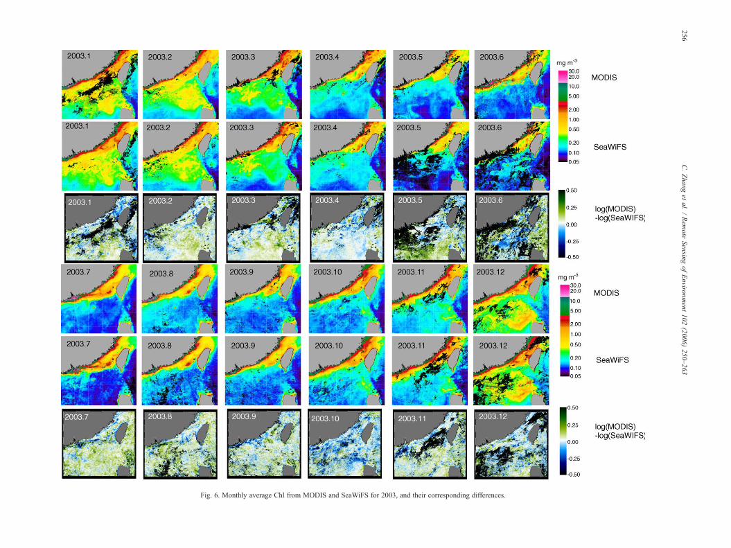
Fig. 6. Monthly average Chl from MODIS and SeaWiFS for 2003, and their corresponding differences.

256C.Zhang

etal.

/Rem

oteSensing

ofEnvironm

ent102

(2006)250–263

Fig. 7. SeaWiFS versus MODIS Chl for the whole study area (Fig. 6) for 2003. Color scale indicates the density function (histogram).

257C.Zhang

etal.

/Rem

oteSensing

ofEnvironm

ent102

(2006)250–263

258 C. Zhang et al. / Remote Sensing of Environment 102 (2006) 250–263

the Chl values are >0.3mg m�3 (Fig. 4). Consequently, Chl wasoverestimated (positive bias).

To determine whether the different sensors showed differentspatial features, data extracted along the four cruise transects(S1 to S4 in Fig. 2; Table 3) were examined (Fig. 5).Synoptically, SeaWiFS and MODIS Chl data detected nearlyidentical patterns along the transect lines. These also agreedwell with in situ measurements. For transects S3 and S4,satellite Chl estimates were higher than the in situ valuesbecause S3 and S4 are in the southern TWS coastal regionwhere enhanced colored dissolved organic matter, suspendedsediments loads, and shallow bottom interfered with the satellitealgorithms. This result is consistent with those shown in Fig. 4and Table 2, i.e., errors in coastal waters are generally larger.

MODIS and SeaWiFS Chl estimates are subject to errorsfrom atmospheric correction and bio-optical models, which maypartially explain the discrepancies found between satellite andin situ data. The atmosphere over the TWS is often hazy,resulting in larger errors than in regions with cleareratmosphere. The annual mean aerosol optical thickness at865nm for the entire TWS, derived from SeaWiFS, is about0.17 (±0.05, n=213days), compared with a typical value of0.08 for the North Atlantic. Furthermore, the turbid coastalwaters invalidate the near-IR “black pixel” assumption in theatmospheric correction (Hu et al., 2000; Ruddick et al., 2000;Siegel et al., 2000). Although an iterative approach is used tocircumvent this difficulty (Arnone et al., 1998; Stumpf et al.,2003), residual errors are likely due to the deviation of theparticle backscattering spectral shape (a function of particle sizedistribution) from that assumed in the model. These errors,combined with those from the imperfect bio-optical inversionmodel for Chl (i.e., blue/green band ratios), propagate and aremagnified in the derived Chl data products. Clearly, moreresearch is needed to improve algorithms in such areas of turbidatmosphere and water.

A second source of error is the discrepancy in time and spacebetween the satellite and in situ sampling coverage. Specifically,the error is due to (1) time difference and (2) sample size. As wepointed out earlier, the time difference between satellite and insitu measurements was relaxed from two hours to several daysto obtain enough matching pairs for statistically meaningful

Table 4Statistical results of the monthly Chl data from SeaWiFS and MODIS for the entire

Month MODIS (mod) vs. SeaWiFS (swf) [range: 0.05–60mg m�3]

Slope Intercept R n (×105) RMS (%) Bias (%)

January 0.93 �0.03 0.95 7.0 32 3.7February 0.95 �0.01 0.96 8.4 25 6.0March 0.96 �0.01 0.95 7.9 40 8.0April 0.98 �0.03 0.97 8.2 35 �0.7May 0.85 �0.09 0.94 6.2 41 12June 0.85 �0.10 0.89 6.0 86 15July 0.90 �0.04 0.97 8.6 54 13August 0.92 �0.03 0.96 7.9 40 11September 0.89 �0.07 0.95 8.3 36 6.5October 0.94 �0.08 0.96 8.3 29 �5.7November 0.92 �0.05 0.96 7.5 41 5.9December 0.90 �0.05 0.93 6.6 40 2.2

comparison. This can create uncertainties in dynamic waters(Balch et al., 1989; Doerffer & Fischer, 1994; Hu et al., 2003).In addition, a satellite pixel is about 1km2, while the in situsample represents a much smaller distance or a point at theship's water intake. Unless the water mass within the 1km2 ishomogeneous, this results in additional uncertainty (Hu et al.,2004). Indeed, one of the reasons why the errors betweensatellite and flow-through data are smaller than between satelliteand discrete-samples is that the time difference is smaller in theformer where a median value of all flow-through data coveringthe same pixel was used to compare with the satellite estimate.

The uncertainty of the in situ measurements may be anadditional source of error, especially the uncertainties in thecalibrated flow-through Chl data. The flow-through in vivofluorescence was calibrated to Chl using a uniform conversionfactor for the entire region under study. Because of the unknownyet possible variations in fluorescence efficiency, the conver-sion factor may differ in different waters (Shang et al., 2004b).However, variations appeared to be random in space and time(i.e., there was no systematic error), and thus would unlikelycause bias errors in large-scale comparisons.

The RMS error specified by the SeaWiFS mission goal was<35% in Chl estimates for open ocean waters where the opticalproperties are dominated by phytoplankton and its directdegradation products (CDOM and detritus) (Hooker et al.,1992; McClain et al., 1998), equivalent to about 0.13 afterlogarithmic transformation (i.e., log_RMS defined in Eq. (2)).Despite the findings in Gregg and Casey (2004) where log_RMSwas incorrectly expressed in percentage to lead to the conclusionthat such a goal for the global ocean was generallymet, we foundthat such a claim is still premature because log_RMS errors aremuch less than the relative (or percentage) RMS errors. Indeed,most of our log_RMS errors are comparable to those reported inGregg and Casey (2004) for most ocean basins, and much lessthan those for the Baltic Sea (Darecki & Stramski, 2004), yet ourpercentage RMS errors are generally between 60% and 100%(July 2004 flow-through data). However, considering theinherent uncertainties in the OC4v4 algorithm itself(log_RMS∼0.22, O'Reilly et al., 2000), the large dynamicrange (Chl∼0.1–10mg m�3), a large portion of coastal watersin our study region, and the nearly 1:1 slope and small bias, the

study region for 2003

Median Mean Mode

log_RMS log_bias swf mod swf mod swf mod

0.122 �0.001 0.333 0.352 0.656 0.648 0.143 0.1620.099 0.014 0.275 0.301 0.474 0.464 0.125 0.1210.118 0.017 0.193 0.201 0.380 0.397 0.103 0.1010.102 �0.016 0.137 0.129 0.364 0.368 0.137 0.1290.138 0.029 0.100 0.110 0.289 0.284 0.080 0.1000.190 0.014 0.115 0.105 0.354 0.348 0.095 0.0950.127 0.037 0.100 0.103 0.512 0.480 0.080 0.0930.125 0.029 0.120 0.130 0.456 0.465 0.110 0.1100.127 0.009 0.111 0.116 0.384 0.351 0.101 0.1060.134 �0.043 0.150 0.131 0.513 0.449 0.120 0.1110.122 0.008 0.140 0.145 0.476 0.456 0.130 0.1350.153 �0.015 0.340 0.333 0.730 0.668 0.120 0.103

259C. Zhang et al. / Remote Sensing of Environment 102 (2006) 250–263

performance of SeaWiFS and MODIS observations in the studyregion may be regarded as satisfactory.

3.2. Comparison between MODIS and SeaWiFS data

MODIS and SeaWiFS Chl data were nearly identical for thethree periods examined along specific transects (Figs. 2 and 5).A time-series of monthly mean Chl from July 2002 to October2004 was also examined. During May and June 2003 the gap inSeaWiFS data is significantly larger than that in MODIS data,probably due to more cloud cover, and also due to changes inSeaWiFS tilt angles with time.

Fig. 6 shows that the monthly spatial patterns of SeaWiFSand MODIS are very similar. Similar spatial patterns occurredalso in 2002 and 2004 (not shown here), and the log differencesappear to be small (within ±0.1) and random in all nearshoreand offshore regions. A quantitative comparison between

7 8 9 10 11 12 1 2 3 4 5 6 7 8 9

Month

7 8 9 10 11 12 1 2 3 4 5 6 7 8 9

Month

7 8 9 10 11 12 1 2 3 4 5 6 7 8 9

Month

7 8 9 10 11 12 1 2 3 4 5 6 7 8 9

Month

0.0

0.5

1.0

1.5

2.0

Chl

(m

g m

-3)

Chl

(m

g m

-3)

Chl

(m

g m

-3)

Chl

(m

g m

-3)

2002 2003

2002 2003

2002 2003

2002 2003

0.0

0.5

1.0

1.5

0.0

0.2

0.4

0.0

0.5

1.0

1.5

2.0

a)

b)

c)

d)

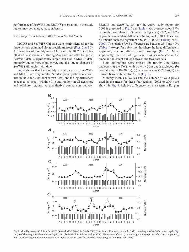
Fig. 8. Monthly average Chl from SeaWiFS (▴) and MODIS (▵) for (a) the TWS (da1), (c) offshore region (>200m water depth), and (d) the shallow Taiwan bank (<30used in calculating the monthly mean is also shown in vertical bars for SeaWiFS (d

MODIS and SeaWiFS Chl for the entire study region for2003 is presented in Fig. 7 and Table 4. On average, about 89%of pixels have relative differences (in log scale) <0.2, and 65%of pixels have relative differences (in log scale) <0.1. These areall smaller than the algorithm “noise” (∼0.22, O'Reilly et al.,2000). The relative RMS differences are between 25% and 40%(Table 4) except for a few months where the large difference isapparently due to different cloud coverage (Fig. 6). Moreimportantly, there is not significant bias, as indicated in theslope and intercept values between the two data sets.

Four sub-regions were chosen for further time seriesanalyses: (a) the TWS, with waters <30m depth excluded; (b)coastal waters (30–200m); (c) offshore waters (>200m); d) theTaiwan bank with depths <30m (Fig. 1).

Monthly mean Chl values and the number of valid pixelsused in the mean for these four regions (2002 to 2004) areshown in Fig. 8. Relative difference (i.e., the x term in Eq. (1))

10 1 2 3 4 5 6 7 8 9 1011 12

10 1 2 3 4 5 6 7 8 9 1011 12

10 1 2 3 4 5 6 7 8 9 1011 12

10 1 2 3 4 5 6 7 8 9 1011 12

0.0

1.0

2.0

3.0

Num

bers

(x1

05 )N

umbe

rs (

x105 )

Num

bers

(x1

05 )

2004

2004

2004

2004

0.0

2.0

4.0

6.0

0.0

5.0

10.0

15.0

20.0

0.0

1.0

2.0

3.0

4.0

Num

bers

(x1

04 )

ta from <30m waters excluded), (b) coastal region (30–200m water depth; Fig.m). The number of valid (cloud-free, good flags) pixels, after data compositing,ark grey) and MODIS (light grey).

260 C. Zhang et al. / Remote Sensing of Environment 102 (2006) 250–263

between MODIS and SeaWiFS for most months is <±10%. Forthe 28 months from July 2002 to October 2004, RMSdifferences of the mean Chl are 9.8% (TWS, Fig. 8a), 10.7%(20–200m coastal region, Fig. 8b), 8.4% (>200m offshoreregion, Fig. 8c), and 23.4% (Taiwan bank, Fig. 8d), respec-tively. The corresponding log_RMS differences are 0.044,0.049, 0.035, and 0.084, respectively. The large difference forJanuary 2003 and January 2004 over the Taiwan bank maysimply be due to differences in data gaps between the twosensors (see gaps in Fig. 6).

Other than in January, the seasonal patterns from MODISand SeaWiFS are very similar for all four regions. The offshoreregion experiences winter blooms and summer minima.Interannual variation was observed in the TWS and in the30–200m coastal waters with more complex hydrologicaldynamics. In the TWS, the satellite Chl patterns agreed wellwith the in situ observations, except for the high satellite Chlvalues seen in winter (e.g., January). Previous studies suggestthat low temperatures in winter may limit phytoplankton growthin the TWS (Zhang et al., 1997).

While an in-depth, detailed study of the physical forcingbehind these observed patterns is outside the scope of this paper,the spatial and temporal patterns are consistent with existingknowledge based on limited historical oceanographic studies.The summer Chl peak in the TWS is primarily a response tomonsoon-driven upwelling, and its magnitude likely dependson the monsoon strength. For example, satellite scatterometerdata showed much stronger wind in the TWS in summer 2003than in summer 2004 (data not shown here), consistent with thehigher Chl peak in summer 2003 than in summer 2004. Overall,the seasonal patterns observed between MODIS and SeaWiFSare consistent between sensors.

For most of the months, the number of valid pixels iscomparable between MODIS and SeaWiFS. Further, the

7 8 9 10 11 12 1 2 3 4 5 6 7M

7 8 9 10 11 12 1 2 3 4 5 6 7M

0

20

40

60

80

100

Per

cent

age(

%)

2002 2003

0

10

20

30

40

Num

bers

2002 2003

a)

b)

Fig. 9. Average percentage cloud cover in the Taiwan Strait (a) and number of days usJuly 2002 to October 2004.

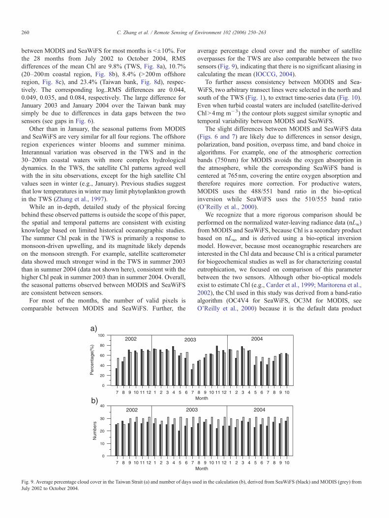
average percentage cloud cover and the number of satelliteoverpasses for the TWS are also comparable between the twosensors (Fig. 9), indicating that there is no significant aliasing incalculating the mean (IOCCG, 2004).

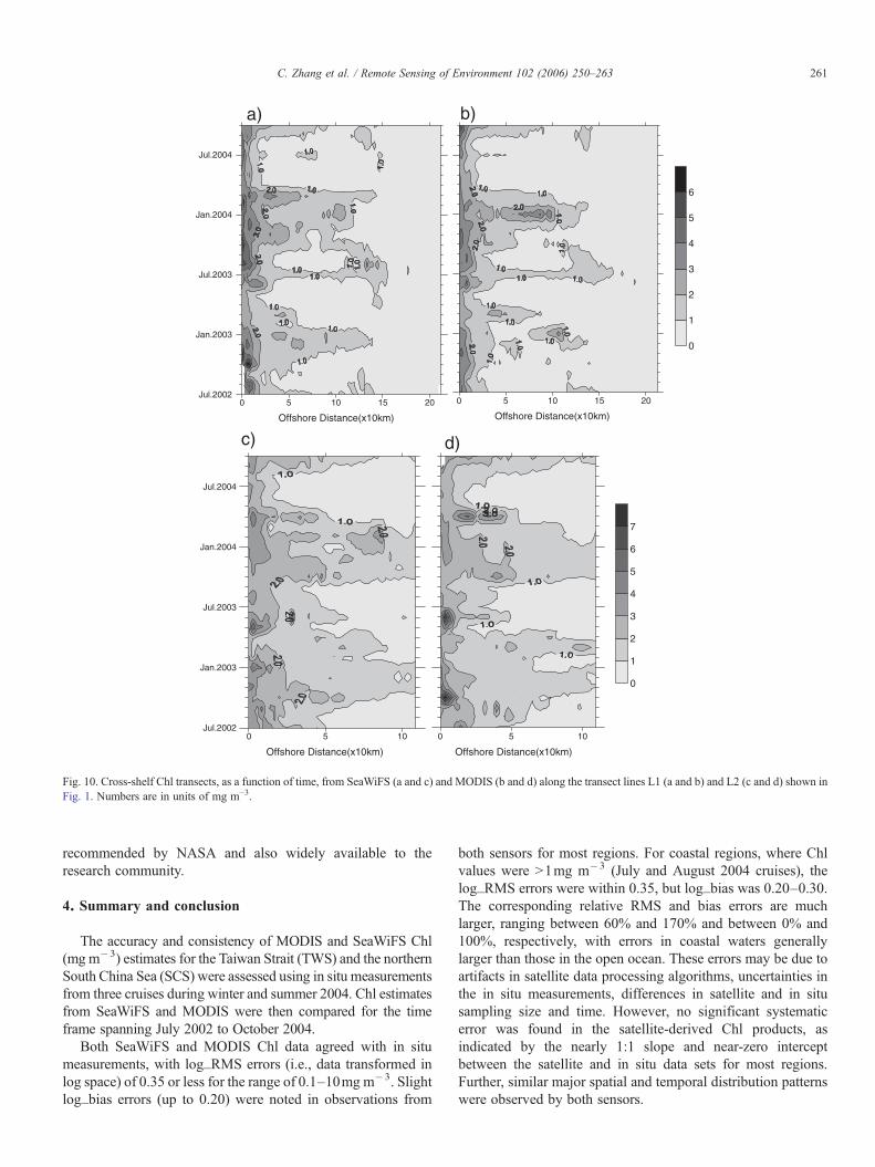
To further assess consistency between MODIS and Sea-WiFS, two arbitrary transect lines were selected in the north andsouth of the TWS (Fig. 1), to extract time-series data (Fig. 10).Even when turbid coastal waters are included (satellite-derivedChl>4mg m�3) the contour plots suggest similar synoptic andtemporal variability between MODIS and SeaWiFS.

The slight differences between MODIS and SeaWiFS data(Figs. 6 and 7) are likely due to differences in sensor design,polarization, band position, overpass time, and band choice inalgorithms. For example, one of the atmospheric correctionbands (750nm) for MODIS avoids the oxygen absorption inthe atmosphere, while the corresponding SeaWiFS band iscentered at 765nm, covering the entire oxygen absorption andtherefore requires more correction. For productive waters,MODIS uses the 488/551 band ratio in the bio-opticalinversion while SeaWiFS uses the 510/555 band ratio(O'Reilly et al., 2000).

We recognize that a more rigorous comparison should beperformed on the normalized water-leaving radiance data (nLw)fromMODIS and SeaWiFS, because Chl is a secondary productbased on nLw, and is derived using a bio-optical inversionmodel. However, because most oceanographic researchers areinterested in the Chl data and because Chl is a critical parameterfor biogeochemical studies as well as for characterizing coastaleutrophication, we focused on comparison of this parameterbetween the two sensors. Although other bio-optical modelsexist to estimate Chl (e.g., Carder et al., 1999; Maritorena et al.,2002), the Chl used in this study was derived from a band-ratioalgorithm (OC4V4 for SeaWiFS, OC3M for MODIS, seeO'Reilly et al., 2000) because it is the default data product

8 9 10 1 2 3 4 5 6 7 8 9 1011 12onth

8 9 10 1 2 3 4 5 6 7 8 9 1011 12onth

2004

2004

ed in the calculation (b), derived from SeaWiFS (black) and MODIS (grey) from

0 5 10 15 20

Offshore Distance(x10km)

0 5 10 15 20

Offshore Distance(x10km)

0

1

2

3

4

5

6

Jul.2002

Jan.2003

Jul.2003

Jan.2004

Jul.2004

0 5 10

Offshore Distance(x10km)

0 5 10

Offshore Distance(x10km)

0

1

2

3

4

5

6

7

Jul.2002

Jan.2003

Jul.2003

Jan.2004

Jul.2004

a) b)

c) d)

Fig. 10. Cross-shelf Chl transects, as a function of time, from SeaWiFS (a and c) and MODIS (b and d) along the transect lines L1 (a and b) and L2 (c and d) shown inFig. 1. Numbers are in units of mg m−3.

261C. Zhang et al. / Remote Sensing of Environment 102 (2006) 250–263

recommended by NASA and also widely available to theresearch community.

4. Summary and conclusion

The accuracy and consistency of MODIS and SeaWiFS Chl(mg m�3) estimates for the Taiwan Strait (TWS) and the northernSouth China Sea (SCS) were assessed using in situ measurementsfrom three cruises during winter and summer 2004. Chl estimatesfrom SeaWiFS and MODIS were then compared for the timeframe spanning July 2002 to October 2004.

Both SeaWiFS and MODIS Chl data agreed with in situmeasurements, with log_RMS errors (i.e., data transformed inlog space) of 0.35 or less for the range of 0.1–10mg m�3. Slightlog_bias errors (up to 0.20) were noted in observations from

both sensors for most regions. For coastal regions, where Chlvalues were >1mg m�3 (July and August 2004 cruises), thelog_RMS errors were within 0.35, but log_bias was 0.20–0.30.The corresponding relative RMS and bias errors are muchlarger, ranging between 60% and 170% and between 0% and100%, respectively, with errors in coastal waters generallylarger than those in the open ocean. These errors may be due toartifacts in satellite data processing algorithms, uncertainties inthe in situ measurements, differences in satellite and in situsampling size and time. However, no significant systematicerror was found in the satellite-derived Chl products, asindicated by the nearly 1:1 slope and near-zero interceptbetween the satellite and in situ data sets for most regions.Further, similar major spatial and temporal distribution patternswere observed by both sensors.

262 C. Zhang et al. / Remote Sensing of Environment 102 (2006) 250–263

The difference between MODIS and SeaWiFS Chl data issmaller than between satellite and in situ data. The relativedifferences between the two data sets are generally <±10%for most months. The log_RMS differences in the monthlymeans between July 2002 and October 2004 from both thesesensors for several sub-regions within the study area are lessthan 0.05 except for the shallow (<30m) Taiwan bank(∼0.08). The corresponding percentage RMS differences areslightly larger, but are <11% for most sub-regions and <24%for the Taiwan bank. The seasonal patterns observed by thetwo sensors (as well as the statistical results of median, mean,mode) are very similar. In addition, the seasonal patterns ofChl variation for the TWS, for example high Chl in summerowing to upwelling, agree well with those from historical insitu measurements.

Time-series analysis from two arbitrarily selected cross-shelftransect lines showed similar results between the MODIS andSeaWiFS data sets. The slight differences are likely due todifferent sensor design and processing algorithms, and alsopossibly due to the time differences between the satelliteoverpasses (∼2h). On average, cloud-free coverage is compa-rable between the two sensors, therefore will not create biasesduring data composition.

In conclusion, except in most shallow (<30m), coastalwaters, both MODIS and SeaWiFS retrieved Chl to within0.35 uncertainty (in log-transformed Chl). Although therelative RMS errors are significantly larger (∼60% for openocean waters to 170% for coastal waters), these estimates arecomparable to those found for other global regions and arenot significantly larger than the uncertainties in the algorithmused to derive the satellite data product. Further, there is nolarge systematic error or significant bias in either satellite dataset, and MODIS and SeaWiFS Chl are very similar in theirabsolute values as well as in the spatial patterns. It istherefore possible to use MODIS Chl data in the TWS and itsadjacent waters with confidence in the absence of SeaWiFSdata.

Acknowledgements

This work was supported by China National Natural ScienceFoundation through grants 40331004, 90211021, 49825111 and40521003, by Program for New Century Excellent Talents inUniversity (Xiamen University) by the US NASA (grantNNG04GG04G to F. Muller-Karger and C. Hu), and by anIOCCG Fellowship to C. Zhang. We thank J. Wu, Z. Cao, J. Hu,Z. Chen, W. Zhai, and Y. Li from Xiamen University, and B.Murch from University of South Florida for their assistance indata collection and processing. We thank the NASA SeaWiFSand MODIS Project teams for providing satellite sea spectralreflectance data. We also thank Dr. Janet Campbell ofUniversity of New Hampshire and another anonymous reviewerfor their detailed and constructive comments and in particularfor their suggestions in the error estimates. Use of the SeaWiFSdata in this study is in accordance with the SeaWiFS ResearchData Use Terms and Conditions Agreement IMaRS contribu-tion #103.

References

Arnone, R. A., Martinolich, P., Gould Jr., R. W., Stumpf, R., & Ladner, S. (1998November 10–13). Coastal optical properties using SeaWiFS. Ocean OpticsXIV, Kailua Kona, Hawaii, USA, SPIE proceedings.

Bailey, S. W., McCLain, C. R., Werdell, P. J., & Schieber, B. D. (2000).Normalized water-leaving radiance and chlorophyll a match-up analyses.In S. B. Hooker, & E. R. Firestone (Eds.), NASA Tech. Memo. 2000-206892SeaWiFS postlaunch calibration and validation analyses, part 2,vol. 10 (pp. 45–52). Greenbelt, Maryland: NASA Goddard Space FlightCenter.

Balch, W. M., Abbott, M. R., & Eppley, R. W. (1989). Remote sensing ofprimary production: A comparison of empirical and semi-analyticalalgorithms. Deep-Sea Research, 36, 281–295.

Behrenfeld, M. J., Randerson, J. T., McClain, C. R., Feldman, G. C., Los, S.O., Tucker, C. J., et al. (2001). Biospheric primary production during anENSO transition. Science, 291, 2594–2597.

Blondeau-Patissier, D., Tilstone, G. H., Marinez-Vicente, V., & Moore, G. F.(2004). Comparison of bio-physical marine products from SeaWiFS,MODIS and a bio-optical model with in situ measurements from NorthernEuropean waters. Journal of Optics. A, Pure and Applied Optics, 6,875–889.

Campbell, J. W. (1995). The lognormal distribution as a model for bio-opticalvariability in the sea. Journal of Geophysical Research, 100(C7),13237–13254.

Campbell, J. W., & Feng, H. (2005). Quantifying the performance of achlorophyll algorithm: Demonstration using the OC4.v4 algorithm andNOMAD data. Ocean Color Bio-optical Algorithm Mini Workshop(OCBAM) Durham: University of New Hampshire.

Carder, K. L., Chen, F. R., Lee, Z. P., Hawes, S., & Kamykowski, D. (1999).Semi-analytic MODIS algorithms for chlorophyll-a and absorption with bio-optical domain based on nitrate-depletion temperatures. Journal ofGeophysical Research, 104, 5403–5421.

Darecki, M., & Stramski, D. (2004). An evaluation of MODIS and SeaWiFSbio-optical algorithms in the Baltic Sea. Remote Sensing of Environment, 89,326–350.

Doerffer, R., & Fischer, J. (1994). Concentrations of chlorophyll, suspendedmatter, and gelbstoff in Case II waters derived from satellite coastal zonecolor scanner data with inverse modeling methods. Journal of GeophysicalResearch, 99, 7457–7466.

Esaias, W. E., Abbott, M. R., Barton, I., Brown, O. B., Campbell, J. W.,Carder, K. L., et al. (1998). An overview of MODIS capabilities for oceanscience observations. IEEE Transactions on Geoscience and RemoteSensing, 36, 1250–1265.

Gordon, H. R., & Wang, M. (1994). Retrieval of water-leaving radiance andaerosol optical thickness over the oceans with SeaWiFS: A preliminaryalgorithm. Applied Optics, 33, 443–452.

Gregg, W. W., & Casey, N. W. (2004). Global and regional evaluation of theSeaWiFS chlorophyll data set. Remote Sensing of Environment, 93,463–479.

Gregg, W. W., & Conkright, M. E. (2001). Global seasonal climatologies ofocean chlorophyll: Blending in situ and satellite data for the Coastal ZoneColor Scanner era. Journal of Geophysical Research, 106, 2499–2515.

Gregg, W. W., & Conkright, M. E. (2002). Decadal changes in global oceanchlorophyll. Geophysical Research Letters, 29(5). doi:10.1029/2002GL014689

Gregg, W. W., Conkright, M. E., Ginoux, P., O'Reilly, J. E., & Casey, N. W.(2003). Ocean primary production and climate: Global decadal changes.Geophysical Research Letters, 30(15), 1809. doi:10.1029/2003GL016889

Hong, H. S., Qiu, S. Y., Ruan, W. Q., & Hong, G. C. (1991). Minnan-Taiwan Bank fishing ground upwelling ecosystem study. In H. S. Hong,S. Y. Qiu, W. Q. Ruan, & G. C. Hong (Eds.), Minnan-Taiwan Bankfishing ground upwelling ecosystem study (pp. 1–10). Beijing: SciencePress (in Chinese).

Hooker, S. B., Esaias, W. E., Feldman, G. C., Gregg, W. W., & McClain, C. R.(1992). In S. B. Hooker, & E. R. Firestone (Eds.), An overview of SeaWiFSand Ocean Color, NASA Tech. Memo. 104566, vol. 1 (pp. 24). Greenbelt,Maryland: NASA Goddard Space Flight Center.

263C. Zhang et al. / Remote Sensing of Environment 102 (2006) 250–263

Hu, C., Carder, K. L., & Muller-Karger, F. E. (2000). Atmospheric correction ofSeaWiFS imagery over turbid coastal waters: A practical method. RemoteSensing of Environment, 74, 195–206.

Hu, C., Carder, K. L., & Muller-Karger, F. E. (2001). How precise are SeaWiFSocean color estimates? Implications of digitization-noise errors. RemoteSensing of Environment, 76, 239–249.

Hu, C., Muller-Karger, F. E., Biggs, D. C., Carder, K. L., Nababan, B.,Nadeau, D., et al. (2003). Comparison of ship and satellite bio-opticalmeasurement on the continental margin of the NE Gulf of Mexico.International Journal of Remote Sensing, 13, 2597–2612.

Hu, C., Nababan, B., Biggs, D. C., & Muller-Karger, F. E. (2004). Variabilityof bio-optical properties at sampling stations and implications for remotesensing: A case study in the NE Gulf of Mexico. International Journal ofRemote Sensing, 25, 2111–2120.

IOCCG. (2004). Guide to the creation and use of ocean-colour, level-3, binneddata products. In D. Antoine (Ed.), Reports of the International Ocean-Colour Coordinating Group, vol. 4. Dartmouth, Canada: IOCCG.

Jan, S., Wang, J., Chern, C. -S., & Chao, S. -Y. (2002). Seasonal variation of thecirculation in the Taiwan Strait. Journal of Marine Systems, 35, 249–268.

Lin, I., Liu, W. T., Wu, C. C., Wong, G. T. F., Hu, C., Chen, Z., et al. (2003).New evidence for enhanced ocean primary production triggered by tropicalcyclone. Geophysical Research Letters, 30(13), 1718. doi:10.1029/2003GL017141

Liu, K. -K., Chao, S. -Y., Shaw, P. -T., Gong, G. -C., Chen, C. -C., & Tang, T.Y. (2002). Monsoon-forced chlorophyll distribution and primary productionin the South China Sea: observations and a numerical study. Deep-SeaResearch I, 49, 1387–1412.

Maritorena, S., Siegel, D. A., & Peterson, A. (2002). Optimization of a semi-analytical ocean color model for global scale applications. Applied Optics,41, 2705–2714.

McClain, C. R., Cleave, M. L., Feldman, G. C., Gregg, W. W., Hooker, S. B.,& Kuring, N. (1998). Science quality SeaWiFS data for global biosphereresearch. Sea Technology, 39, 10–16.

McClain, C. R., Feldman, G. C., & Hooker, S. B. (2004). An overview of theSeaWiFS project and strategies for producing a climate research qualityglobal ocean bio-optical time series. Deep-Sea Research II, 51, 5–42.

Ning, X., Chai, F., Xue, H., Cai, Y., Liu, C., & Shi, J. (2004). Physical–biological oceanographic coupling influencing phytoplankton and primaryproduction in the South China Sea. Journal of Geophysical Research, 109,C10005. doi:10.1029/2004JC002365

O'Reilly, J. E., Maritorena, S., Siegel, D., O'Brien, M. C., Toole, D., Mitchell,B. G., et al. (2000). Ocean color chlorophyll a algorithms for SeaWiFS,OC2, and OC4: Version 4. In S. B. Hooker, & E. R. Firestone (Eds.),SeaWiFS postlaunch technical report seriesSeaWiFS postlaunch calibration

and validation analyses, part 3, vol. 11 (pp. 9–23). Greenbelt, Maryland:NASA Goddard Space Flight Center.

Parsons, T. R., Maita, Y., & Lalli, C. M. (1984). A manual of chemicaland biological methods for seawater analysis. Oxford: Pergamon Press,pp. 107–109, 115–122.

Ruddick, K. G., Ovidio, F., & Rijkeboer, M. (2000). Atmospheric correction ofSeaWiFS imagery for turbid coastal and inland waters. Applied Optics, 39,897–912.

Shang, S. L., Zhang, C. Y., Hong, H. S., Shang, S. P., & Chai, F. (2004a).Short-term variability of chlorophyll associated with upwelling events in theTaiwan Strait during the southwest monsoon of 1998.Deep Sea Research II,51, 1113–1127.

Shang, S. L., Zhang, C. Y., & Zeng, Y. D. (2004b). Field calibration ofchlorophyll fluorometer for the Pearl River Estuary and its adjacent SouthChina Sea waters. Journal of Tropical Oceanography, 23, 69–74 (inChinese).

Siegel, D., & Maritorena, S. (2000). Spectral data assimilation for merging satelliteocean color imagery. In G. S. Fargion, & C. R. Mcclain (Eds.),SIMBIOS Project 2000 Annual Report, NASA TM 2001-209976 (pp.117–124). Greenbelt, Maryland: NASA Goddard Space Flight Center.

Siegel, D. A., Wang, M., Maritorena, S., & Robinson, W. (2000). Atmosphericcorrection of satellite ocean color imagery: The black pixel assumption.Applied Optics, 39, 3582–3591.

Stumpf, R. P., Arnone, R. A., Gould, R. W., Martinolich, P. M., &Ransibrahmanakul, V. (2003). A partially coupled ocean–atmosphere modelfor retrieval of water-leaving radiance from SeaWiFS in coastal waters. In S.B. Hooker, & E. R. Firestone (Eds.), SeaWiFS postlaunch technical reportseries, NASA Tech. Memo 2003-206892, vol. 22. (pp. 51–59), Greenbelt,Maryland: NASA Goddard Space Flight Center.

Su, J. (2004). Overview of the South China Sea circulation and its influence onthe coastal physical oceanography outside the Pearl River Estuary.Continental Shelf Research, 24, 1745–1760.

Tang, D. L., Kester, D. R., Ni, I. H., Kawamura, H., & Hong, H. S. (2002).Upwelling in the Taiwan Strait during the summer monsoon detected bysatellite and shipboard measurements. Remote Sensing of Environment, 83,457–471.

Yoder, J. A., Moore, J. K., & Swift, R. N. (2001). Putting together the bigpicture: Remote-sensing observations of ocean color. Oceanography, 14,33–40.

Zhang, F., Yang, Y., & Huang, B. Q. (1997). Effect of physical input of nutrientson chlorophyll a content in Taiwan Strait. In H. S. Hong (Ed.),Oceanography in China (7): Primary productivity and its controllingmechanism in Taiwan Strait Regions (pp. 81–88). Beijing: China OceanPress (in Chinese).