Branch Target Buffer Design and Optimization

396 IEEE TRANSACTIONS ON COMPUTERS, VOL. 42, NO. 4, APRIL 1993

Branch Target Buffer Design and Optimization Chris H. Perleberg and Alan Jay Smith, Fellow, IEEE

Absfract-A Branch Target Buffer (BTB) can reduce the performance penalty of branches in pipelined processors by predicting the path of the branch and caching information used by the branch. This paper discusses two major issues in the design of BTB’s, with the goal of achieving maximum performance with a limited number of bits allocated to the BTB implementation. First is the issue of BTB management-when to enter and discard branches from the BTB. Higher performance can be obtained by entering branches into the BTB only when they experience a branch taken execution. A new method for discarding branches from the BTB is examined. This method discards the branch with the smallest expected value for improving performance, outperforming the LRU strategy by a small margin, at the cost of additional complexity.

The second major issue discussed is the question of what information to store in the BTB. A BTB entry can consist of one or more of the following: branch tag (Le., the branch instruction address), prediction information, the branch target address, and instructions at the branch target. A variety of BTB designs, with one or more of these fields, are evaluated and compared. This study is then extended to multilevel BTB’s, in which different levels in the BTB have different amounts of in- formatian per entry. For the specific implementation assumptions used, multilevel BTB’s improved performance over single level BTB’s only slightly, also at the cost of additional complexity. Multilevel BTB’s may, however, provide significant performance improvements for other machines implementations.

Design target miss ratios for BTB’s are developed, so that the performance of BTB’s for real workloads may be estimated.

Index Terms-Branch, branch problem, branch target buffer, cache memory, CPU design, CPU performance evaluation, pipeline, pipelining.

I. INTRODUCTION OST modem computers use pipelining to significantly M increase performance. Pipelining divides the execu-

tion of each instruction into several phases, normally called pipeline stages. A typical pipeline might have five stages, including instruction fetch, instruction decode, operand fetch, execution, and result writeback. It is important that the operation time of each pipeline stage be almost identical, since the rate at which instructions flow through the pipeline is limited by the slowest pipeline stage. In the optimal case for this pipeline, five instructions could be operated on simultaneously.

Manuscript received January 15, 1990; revised September 11, 1991, and July 26, 1992. The work was based on research supported in part by the National Science Foundation under Grants MIP-8713274 and MIP-9116578, by NASA under Consortium Agreement NCA2-128, by the State of California under the MICRO program, and by the Digital Equipment Corporation, Philips Laboratories/Signetics, International Business Machines Corporation, Apple Computer Corporation, Mitsubishi Corporation, Sun Microsystems, and Intel Corporation.

The authors are with the Department of Electrical Engineering and Com- puter Science, University of California, Berkeley, Berkeley, CA 94720.

IEEE Log Number 9207177.

This optimal case, though seldom achieved in practice, would produce a fivefold performance gain over the same processor designed without a pipeline. More details about pipelining can be found in [42] and [29].

Branch instructions can reduce the performance of pipelines by interrupting the steady flow of instructions into the pipeline. To execute a branch, the processor must identify the instruction as a branch, decide whether the branch is taken, calculate the branch’s target address, and then, if the branch is taken, fetch instructions from the target address. Branches hurt performance because the pipelined processor needs to know the path of the branch (in order to fetch more instructions) before the path of the branch has been determined. Thus when a branch appears, the processor has two choices, either wait for the branch to finish executing before fetching more instructions, or continue fetching instructions, possibly from the wrong path. Either choice hurts performance, although the second choice hurts less on the average, since with some probability the instructions fetched will actually come from the correct path.

The Branch Target Buffer (BTB) can be used to reduce the performance penalty of branches by predicting the path of the branch and caching information about the branch [30]. This paper considers two major issues in the the design of BTB’s, with the goal of achieving maximum performance for a given number of bits allocated to the BTB design. First, the question of BTB management: when to enter branches into the BTB, and when to discard branches from the BTB. Second, the question of what information to keep in the BTB. Four types of information can be kept in BTB’s, including branch tags, the branch target address, prediction information, and instruction bytes from the branch target address. A BTB may contain any subset of these four types of information, where performance generally increases with the amount of information retained. It is also possible to create a multilevel BTB, with different designs at each level, each containing a different subset of these items. We also compare BTB and instruction cache miss rates, and show that BTB miss rates can be derived from instruction cache miss ratios; we use this approach to obtain design target miss ratios for BTB’s [491-

This paper is organized as follows. In the following section, a number of solutions to the branch problem are reviewed. The methodology used to generate the results in this paper (trace driven simulation) is then presented, followed by a discussion of various optimizations in the design of BTB’s. Branch prediction and the issue of BTB management are covered. A discussion of miss rates of BTB’s and instruction caches is followed by a consideration of the issue of what information to keep in a BTB. Conclusions are then provided.

0018-9340/93$03.00 0 1993 IEEE

PERLEBERG AND SMITH: BRANCH TARGET BUFFER DESIGN AND OPTIMIZATION 397

11. SOLUTIONS TO THE BRANCH PROBLEM

This survey of solutions to the branch problem is intended to give a brief explanation of each solution, and provide the names of a few machines that have used each solution. Further discussion is available in [6], [ l l ] , [30], [32], and [34].

Static Branch Prediction: As discussed in the Introduction, if the path of a branch can be correctly predicted, the branch penalty can be reduced. Predicting all branches as not taken or predicting all branches as taken (Lee and Smith found 68% of branches to be taken [30]; we find 70% of branches to be taken) is the simplest type of static prediction. Predicting branches based on the direction of the branch (forward or backward) and/or the branch opcode is also possible [50]. The National Semiconductor NS32532 uses the branch opcode and the branch direction to predict 71% of conditional branches correctly. A static prediction bit in each branch instruction, used to indicate which path the branch will probably take, is also effective. The bit can be set using heuristics and execution profiling [34]. The Ridge Computers Ridge-32 [13], the Intel 80960 [20], and the AT&T CRISP [9] all use a static prediction bit. An average prediction rate of 85% has been reported for the static prediction bit method [34].

Dynamic Branch Prediction: Dynamic branch prediction predicts branch paths based on the run-time execution history (the sequence of taken and not-taken executions, represented with one bit per execution) of each branch. One proposed dynamic method uses a two bit counter state machine which takes the branch execution history as input and outputs the predicted branch path for the next branch execution [50], [30]. Another method examines the last n executions (taken or not- taken) of a branch, and using statistics gathered beforehand to calculate the chance of a taken branch, predicts the branch path [30], [59]. Widdoes proposes keeping bits with each instruction in the instruction cache to store branch execution history [59]. Machines that use dynamic branch prediction include the S-1, the MUS [43], several TRON microprocessors [45], the Edgecore Edge 2000 (Motorola 680x0 compatible) [33], [%I, and the forthcoming NexGen processor (Intel x386 compatible) [52].

Delayed Branch: The idea of a delayed branch is to execute the n instructions immediately after the branch, and then continue with the branch target or fall through path. This often allows useful instructions to be executed while the branch path is resolved and branch target address calculated. The n instructions (usually n = 1) are called delay instructions. It is not always possible to find useful delay instructions, however, and the delay slot(s) are often filled with noops. For more flexibility, some machines allow the execution of the delay instructions to be skipped, depending on the value of a “squash” bit in the branch [34]. The delayed branch technique is used in most RISC processors, and requires intelligent compilers for effective use [7], [17], [34], [38].

Loop Buffers: Loop buffers are small, high speed buffers used for instruction prefetching and fast execution of instruction loops. If a loop is completely contained within a loop buffer, the loop instructions can be fetched solely from the high speed buffer, instead of fetching from slower main

memory. Multiple loop buffers allow noncontiguous loops to execute from the buffers. Machines using loop buffers include the CDC-6600 with eight 60-bit words [54], the CDC-7600 with twelve 60-bit words [12], the IBM 360/91 and the IBM 360/195 with eight 64-bit words [3], [36], the Cray-1 with four 128-byte buffers [44], and the Cray-XMP with four 256 byte buffers [22]. Loop buffers are useful primarily when memory is slow and there is no cache.

Multiple Instruction Streams: To avoid the penalty of a wrong branch prediction, both paths of a branch can be fetched and executed, and the results of the incorrect path discarded once the branch is resolved. This method requires duplication of hardware, early calculation of the branch target address, high memory and register file bandwidth, and a method for dealing with the occurrence of still another branch before a previous one has been resolved. This technique has been used in mainframes, including the IBM 370/168 and the IBM 3033

Prefetch Branch Target: Most computers follow the fall through path for branches, and then pay a penalty if the branch is found to be taken. This penalty may be reduced if instructions from the branch target address are fetched while the branch and the instructions in the not-taken branch path are executing. The IBM 360/91 prefetches two double-words (each 64 bits long) from the target address [3]. The Amdahl 470 accomplishes this same function by fetching the branch target as if it were an operand [47].

Prepare to Branch: The “Prepare-to-Branch” and “Load- Look-Ahead” instructions of the Texas Instruments ASC computer direct the machine to prefetch from the target address of an upcoming branch, rather than from the sequential addresses after the branch [15]. The CHoPP supercomputer has a similar instruction [28]. Use of these instructions with usually taken branches can increase performance.

Shared Pipeline Multiprocessor: It is possible to design a machine which executes n instruction streams simultaneously by fetching in round robin order an instruction from each of the n streams. If the pipeline is n or fewer stages, then within an individual instruction stream, each instruction completes execution before the next instruction begins execution, so a branch instruction completes before the next instruction needs to be fetched, and there are no branch delays. Each independent instruction stream receives a l /n fraction of total processor power. The shared pipeline multiprocessor concept was implemented in the Denelcor HEP computer [25], and is examined in [46].

Branch Folding: The AT&T CRISP processor was the first to use a technique called branch folding to reduce branch execution time to zero [9], CRISP uses a decoded instruction cache; each nonbranch instruction is transformed into a line of microcode in a cache of decoded instructions. Each entry includes a next address field pointing to the next line of microcode to be executed. Unconditional branches are simply “folded into the next address field of the previous line of microcode. No branch execution time is necessary once the unconditional branch is in the decoded cache. Conditional branches make use of a second next address field in the microcode and static branch prediction. A bit in the branch

~ 3 1 , ~ 4 1 .


instruction predicts whether the branch will be taken or not, and the predicted next address field is selected to find the next line of microcode to execute. If the predicted path is found to be wrong once the condition flag is resolved, the incorrect path results are discarded, and the correct path is executed. Like the unconditional branch, the conditional branch has been folded into the previous line of microcode, resulting in a zero cycle execution time for a correctly predicted branch in the decoded cache.

Note that branch folding does not require a decoded instruction cache. The IBM RS/6000 folds many branches by using a branch processor that examines branches early in the pipeline and folds them whenever their outcome (taken/not- taken) is known [4]. Branch folding can also be implemented with a BTB that caches instructions from both the taken and not taken branch paths of each branch in the BTB.

Closely related to branch folding is what we call “early determination,” by which the branch condition and/or target is computed with special mechanisms earlier than the stage in the pipeline at which this would normally be done. Such an apparatus is described by [41].

Branch Target Buffer: The Branch Target Buffer (BTB) can be used to reduce the performance penalty of branches by predicting the path of the branch and caching information about the branch [30]. Up to four types of information have been cached in a BTB: a tag identifying the branch the information corresponds to (usually the branch address), prediction information for predicting the path of the branch (takenhot-taken), the branch target address, and instruction bytes at the branch target address. A BTB with all four types of information works as follows. As each instruction is fetched from memory, the instruction address is used to index into the BTB. If a valid BTB entry is found for that address, the instruction is a branch. (We are ignoring the possibility of self modifying code.) The branch path is predicted using the branch’s prediction information. If the branch is predicted taken, the pipeline is supplied with the cached instructions in the BTB, and the processor begins fetching instructions from the target address, offset by the number of bytes of instructions cached in the BTB. If the branch is predicted not-taken, the processor continues fetching sequentially after the branch. After the processor finishes executing the branch, it checks to see if the BTB correctly predicted the branch. If it has, all is well, and the processor can continue sequentially. If the branch was predicted incorrectly (or the branch was taken and the target address changed), the processor must flush the pipeline and begin fetching from the correct branch path. In either case, the branch prediction information and branch target address (if changed) must be updated after the branch. Machines that use a variation of the BTB include: the Advanced Micro Devices Am29000 [ l ] and the General Electric RPM40 [31] with branch target caches (no prediction information, just a cache of target instructions); the Mitsubishi M32 with a BTB containing dynamic prediction information, branch tag, and instructions from the target address (no mention of target address being stored) [60]; the Edgecore Edge 2000 with a direct mapped 1024 entry BTB containing one dynamic prediction bit, a branch tag, and the branch target address for each entry

[58]; and the NexGen processor with a fully associative LRU replacement BTB containing prediction information, branch tag, branch target address, and instructions from the target address [52], [53].

An extension to the BTB concept is the idea of a special callheturn stack [26]. The idea is that a return instruction may return to a different address each time, in which case the ordinary BTB is of little use. By using a special BTB for returns, it is possible to successfully capture those branches as well. This special case is not considered in the work presented here.

The BTB’s considered in this paper all predict taken/not- taken based on the previous history for that branch. In [37], it is observed that by conditioning on the previous history of other recently executed branches, the prediction accuracy can be increased. [56], [S7] use a more complex, two-level history, which may include other branches as well.

111. METHODOLOGY

A. Trace Driven Simulation

Because there is no generally accepted model for instruction stream or branch behavior, we have used trace driven simulation for our studies. Trace driven simulation has the advantage of fully and accurately reflecting real instruction streams, but with the possible shortcomings of using short samples, and those samples possibly not being representative of the “real” workload, whatever that may be [SI, [48]. As noted below, we have used a very wide variety of traces of both small and large programs from a number of different machines and believe that our results are representative of what could be expected in practice. Our results are consistent with other published measurements, when such measurements exist.

B. Description of Traces

A total of 32 program traces are used for results presented in this paper. Four processors are represented in the traces, including the MIPS Co. R2000 (MIPS), the Sun Microsystems SPARC (SPARC), the DEC VAX 11/780 (VAX), and the Motorola 68010 (68k) [8], [14], [27], [35]. The traces are divided into six workloads, so the individual characteristics of the workloads can be observed in the results [30]. The workloads include COMP (MIPS traces of the MIPS Co. assembler, C compiler, Fortran compiler, Pascal compiler, link editor, microcode generator, microcode optimizer), FP (MIPS traces of floating point programs: d0duc.f <high energy physics> [lo], integra1.f <integration>, mo1dyn.f <molecular dynamics>, spice2g6 <circuit simulation> [SS]), TEXT (MIPS traces of text processing programs GNU Emacs and Grep, MIPS Co. nroff and vi), SPARC (SPARC traces of Sun 4 C compiler, espresso <logic minimization>, GNU Bison), VAX (VAX traces of awk, Is, otmdl <parser/constructor>, sedx, spice, troff, ymerge <parse table compacter>) [ 181, 68k (68010 traces of the unix assembler, egrep, fortran matrix manipulation program coptimized and unoptimized versions>, Is, stat <trace analyzer, optimized and unoptimized versions>) [16]. Statistics gathered for the six workloads are given in


TABLE I AVERAGE WORKLOAD AND TRACE STATISTICS

COMP TEXT FP SPARC VAX 68k Work Ave Trace Ave CPU MIPS MIPS MIPS SPARC VAX 68k

Dynamic Instr 2261788 2428066 2439411 1976181 1045501 681475 1805404 1666244 Dynamic Branch 401927 487369 247695 433537 283996 157743 335377 317079 Static Instr 15737 11696 14157 4860 2832 3978 8877 8619 Object Instr 54516 48287 60658 43235 na na na na Object Bytes 218064 193148 242632 172940 na na na na

Stat Branch Instr 17.47 19.93 12.29 21.11 26.05 23.69 20.09 20.71

Stat Branch Bytes 17.47 19.93 12.29 21.11 13.06 20.76 17.44 17.23 Stat Cond Instr 9.74 12.97 8.03 11.77 16.04 11.60 11.69 11.90

Stat Uncond Instr 7.73 6.96 4.26 9.34 10.01 12.10 8.40 8.81

Branch Taken 72.84 67.80 69.91 59.29 70.79 69.50 68.36 69.39 Cond Taken 64.48 63.44 59.49 44.18 61.14 56.62 58.23 59.73

Dyn Blk Instr 5.65 5.00 10.38 4.60 3.38 4.27 5.55 5.26

Dyn Blk Bytes 22.61 19.98 41.53 19.72 14.26 11.97 21.68 20.22

Stat Blk Instr 5.86 5.03 8.92 4.75 3.96 4.25 5.46 5.27 Stat Blk Bytes 23.46 20.10 35.68 19.01 17.60 14.25 21.68 20.85 Obj Blk Instr 5.38 4.70 7.08 4.46 na na na na Obj Blk Bytes 21.52 18.79 26.56 17.85 na na na na

Definitions Dynamic Instr Dynamic Branch Static Instr Object Instr

Stat Branch Instr Stat Branch Bytes Stat Cond Instr Stat Uncond Instr Branch Taken Cond Taken Dyn Blk Instr Dyn Blk Bytes Stat Blk Instr Stat Blk Obj Blk Instr Obj Blk Bytes Work Ave Trace Ave

Average number of dynamic instructions Average number of dynamic branch instructions Average number of static instructions Average number of instructions in the entire program (object text segment) Object Bytes Average number of bytes in the entire program (object text segment) Percentage static branch instructions of all static instructions Percentage bytes of static branch instructions of all static instruction bytes Percentage static conditional branch instructions of all static instructions Percentage static unconditional branch instructions of all static instructions Percentage of dynamic branches that are taken Percentage of dynamic conditional branches that are taken Dynamic basic block size in instructions, including branch instruction Dynamic basic block size in bytes, including branch instruction Static basic block size in instructions, including branch instruction Bytes Static basic block size in bytes, including branch instruction Object (text segment) basic block size in instructions, including branch instruction Object (text segment) basic block size in bytes, including branch instruction Average of all the workload average values Average of all of the individual trace values

This table contains statistics on the 32 traces we used. The values are all averages, including the workload averages (COMP, TEXT, FP, SPARC, VAX, and 68k), the overall trace average for the 32 traces (Trace Ave), and the average of the workload averages (Workload Ave). See [39] for more detailed data.

Table I. (Note: the statistics and simulation data presented in this paper are a subset of the data available in [39], in which much more extensive and detailed tables and graphs are presented. For brevity, we show summary and aggregate results in this paper only.)

In Table I and in our discussions, static, dynamic, and object instructions are referred to. Object instructions are all of the instructions that exist in a program (in the text segment). Static instructions are those object instructions that are executed (one or more times) in a trace of a program. Dynamic instructions are the instructions that appear in the instruction trace of a program, i.e., each static instruction is a dynamic instruction one or more times. Thus, in a trace of a two instruction loop that is executed 10 times, there are two static instructions, and

20 dynamic instructions.

IV. BTB DESIGN OPTIMIZATION

The goal of this paper is to maximize BTB performance with a limited number of bits allocated to the BTB implementation. Describing this problem mathematically helps to clarify the issues. To begin, it is necessary to understand the performance impact of different amounts and types of information stored for each branch in the BTB.

Potential BTB performance increases as the information content of each entry of the BTB increases, and as the number of entries increases. Increased information content requires more bits of storage, as does an increased number of


entries. A low complexity BTB with low performance potential contains only branch prediction information. A medium complexity BTB which gives equal or better performance contains the branch tag (branch instruction address), prediction information, and the branch target address. A high complexity BTB with even better performance contains the branch tag, prediction information, target address, and instruction bytes from the target address. Increasing the number of types of information (e.g., prediction information, branch tag, target address, target instruction bytes) stored for each branch improves performance as well as increasing (per entry) the amount (bits of storage) of each type of information. As always, tradeoffs between simplicity and complexity raise additional concerns including design time, design area, and the effect on cycle time.

An optimization problem exists if a maximum performance BTB is to be designed with a limited number of bits. As both more entries and more information per entry increase performance, the problem is selecting the number of entries and the amount of information per entry that will maximize performance. Which design provides better performance, many entries with little information per entry, or few entries with a lot of information per entry?

The following simple mathematical BTB model is intended to help clarify the problem. This model gives insight into how to maximize the performance of a BTB design that has been added onto a processor that normally predicts all branches not- taken. The equation presents the average savings per branch of an optimal BTB designed with N storage bits. Some simplifications have been made in setting up this equation, as noted below.

1 Max h(i)[t(i)ptt(i)V(i) - (1 - t(i))ptnt(i)W(i)] ii such that ~ n u m - h i t s ( i ) 5 N

z

number of storage bits in the BTB probability that branch i is referenced (executed) probability that branch i will be taken probability of predicting branch i taken, given that branch i is taken probability of predicting branch i taken, given that branch i is not-taken cycle savings for correct taken prediction of branch i cycle cost for incorrect taken prediction of branch i number of bits in BTB allocated to branch i .

Note that ptt(i) and ptnt(i) are zero for branches not in the BTB, so the sum is only affected by branches in the BTB.

The first product in the equation, when summed up, is the expected cycle savings due to the BTB for a correct taken prediction. The second product in the equation, summed up, is the expected cycle cost of an incorrect taken prediction. The

difference of these two sums is the net cycle savings per branch due to the BTB. The BTB does not improve performance for a correct not-taken prediction (branch folding is ignored here), so this case does not appear in the equation. In addition, for an incorrect not-taken prediction, the cost is the same with and without the BTB (ignoring possible target instructions in the BTB), so this case is also not included in the equation.

The problem of selecting the best BTB design is described by the equation above. For a fixed number of bits, increasing the performance of entries in the BTB is equivalent to increasing V( i ) , decreasing W(i ) , and decreasing the number of branch entries. Increasing the number of entries in the BTB adds more branches into the sum, decreases V ( i ) and increases W(i) , lowering branch information per entry. (Increasing V ( i ) and decreasing W ( i ) means that more bits must be allocated to each entry. Since the number of bits is fixed, this means that the number of entries decreases. Conversely, decreasing V(z) and increasing W ( i ) is accomplished by allocating fewer bits to each entry and thereby increasing the number of entries that fit in the BTB.) Finding the best performance for a limited number of total bits in the BTB requires a careful balance between performance per entry and number of entries.

The simple BTB model supports three concepts used later in this paper.

If a branch does not have potential for improving performance, do not enter it into the BTB. The BTB model indicates that the BTB should be filled with the branches that have the most potential for improving performance. Placing into the BTB branches with no performance value displaces branches that may have performance value. This differs from previous studies in which all branches were cached in the BTB. When it is necessary to discard a branch from the BTB, discard the branch with the minimum performancepoten- tial. The BTB should contain the branches with the most potential for improving performance. A replacement strategy based on this concept might discard the branch that is least likely to be referenced AND least likely to be taken. The BTB does not improve the performance of a not-taken branch (ignoring branch folding), so discarding a branch that is not likely to be taken has little penalty. A multilevel BTB, each level possibly containing different amountsltypes of information per entry, may be able to maximize performance by achieving a better balance of number of entries and quantity of information per entry. Note that V( i ) and W ( i ) in the BTB model are functions of i. The BTB performance may be maximized if V ( i ) and W ( i ) are not constant. If branches with high performance potential are allocated more bits per entry, and branches that have less performance potential are allocated fewer bits per entry (but more entries), higher overall performance may be achieved for a limited total number of bits.

V. BRANCH PREDICTION In this paper a dynamic method of branch prediction is used


which treats equally all branch instructions; this includes both conditional and unconditional control transfer instructions, which are 19% of all dynamic instructions. To understand the method, it is necessary to understand the concept of branch history. A record of each branch execution (T=Taken, N=Not-taken) can be represented as a single bit, known as a prediction bit. A branch history of size n is a string of n prediction bits recording the history of the n most recent executions of a branch. From the execution history of the branches in the 32 traces, the probability of a taken branch as a function of the branch history of length n was calculated. For example, with 2 prediction bits, the probability of a taken branch after each of the four possible branch histories is: P(NN)=O.ll, P(NT)=0.61, P(TN)=0.54, P(lT)=0.97. Table IX provides the probability of a taken branch and the probability of occurrence for each of the 8 possible branch histories that occur for three prediction bits. Similar tables for six prediction bits are provided in [39]. The maximum prediction accuracy is obtained by predicting branch taken whenever the probability of a taken branch is greater than 50%. Note that predictions based on these probabilities are the best possible predictions (yielding the highest correct prediction rate) for the 32 traces of any fixed (Le., nonlearning or nonadaptive) method that only uses n bits of history for that branch as input.

Achieving the highest prediction rate is not the same as achieving the highest performance. When a prediction is made, four different cases and cycle costs are possible, as shown in Table 11. The cycle cost is equivalent to the number of cycles required above the minimum branch execution time, so C,, is zero. Maximizing the prediction rate is accomplished by predicting branch taken whenever the probability p of a taken branch is greater than 50%. Maximizing performance (minimizing cycle cost) is accomplished by predicting branch taken when the cost of predicting taken is less than the cost of predicting not-taken. That is, predict taken when

where p is the probability of branch taken. As this equation requires implementation dependent numbers Cnt, Ct,, Ctt, all prediction rates presented in this paper are based on predicting taken if the probability of taken is greater than 50%. Later, with multilevel BTB’s for which a single prediction rate is not a useful measure, performance is maximized using a set of cycle costs (Cnt, C,,, Ctt).

A. Best Case Prediction Rates

As a reference point, it is useful to know the realistic upper limit for prediction rates. To determine this upper limit, two infinite size BTB simulators were designed (BTB#l and BTB#2). Design BTB#1 takes in branches on their first execution and keeps them in the BTB until the end of the trace. Design BTB#2 takes in branches on their first branch taken execution and keeps them in the BTB until the end of the trace. Both BTB’s predict all instructions that are not in the BTB as not-taken, since a prediction of taken, without the target address or target bytes, is of little use.

TABLE I1 THE FOUR POSSIBLE CASE AND THEIR CYCLE COSTS FOR A BRANCH PREDICTION

Cycle Cost Prediction Branch not-taken not-taken not-taken taken taken not-taken taken taken

BTB#1 and BTB#2 correct prediction rates are presented in Table 111. The prediction rates in each column under a workload name are simple workload averages, and the Average column is the average of the workload averages. Table I11 includes the effect of target address changes in the prediction rate by considering a target change occurring during a taken branch to be a misprediction. Note that target changes do not affect a BTB that does not contain target addresses and instructions. It happens that virtually all target changes occur for branches that are always taken (e.g., subroutine returns, case statements) and thus the effect of target changes is to decrease prediction accuracy by a constant amount. Those constants can be found in Table IV, and are identical for BTB#1 and BTB#2. Equivalent constants for the six workloads of Lee and Smith are shown in Table V [30]. Fig. 1 shows the average prediction rate for BTB#2 (including and not including the effect of target changes) as a function of the number of prediction bits.

The BTB#1 and BTB#2 prediction rates are very similar, except for the case of zero prediction bits, for which the BTB#2 prediction rate is higher than the BTB#l’s prediction rate. This is due to the fact that for zero prediction bits, BTB#2 only predicts as taken those branches that are in the BTB. Since BTB#2 only enters branches into the BTB on a taken branch execution, branches that are never taken or are initially not-taken are correctly predicted, thus boosting the prediction rate. BTB#1 enters branches into the BTB on the first execution, predicting the branches as taken thereafter for the zero prediction bit case. Thus, the prediction rate of BTB#1 is approximately the average percentage of taken branches. Note that even with zero prediction bits, a BTB can be useful by caching the target address and target instructions; in such a design, all branches in the BTB are predicted as taken.

The prediction rates we observe are very close to those of Lee and Smith [30], as may be seen in Table VI; the data from [30] is for a design equivalent to BTB#l. These prediction rates do not include the effect of target address changes, so our values are from Table 111 with the Average constant from Table IV added in.

B. Effect of Context Switching on Prediction Rates

Multitasking computer systems frequently experience context switches, during which the active process changes. If the BTB entries are not tagged with a process ID, then the BTB must be flushed. Even when entries are tagged with the process ID, it is unlikely, unless the BTB is very large, that any entries for a given process will remain when that process is restarted. This flushing lowers the prediction rate in two ways. First, the BTB hit ratio drops, since after every flush there are no entries


TABLE 111 (INCLUDING TARGET CHANGE EFFECTS) BRANCH PREDICTION

COMP TEXT FP SPARC VAX 68k Average Prediction BTB Bits Design

0 BTB#l 67.21 66.13 61.78 56.80 68.85 64.96 64.29 0 BTB#2 81.27 80.86 81.04 73.04 81.54 76.68 79.07 1 BTB#l 86.30 94.83 85.03 87.51 89.71 85.55 88.15 1 BTB#2 86.30 94.83 85.03 87.51 89.71 85.55 88.15 2 BTB#1 87.81 95.45 86.72 88.69 91.56 86.27 89.42 2 BTB#2 87.81 95.45 86.72 88.69 91.56 86.27 89.42 4 BTB#ll 88.66 96.02 87.85 90.61 93.36 88.21 90.79 4 BTB#2 88.66 96.02 87.84 90.61 93.35 88.20 90.78 8 BTB#l 89.19 96.18 89.28 91.78 93.70 89.00 91.52 8 BTB#2 89.19 96.18 89.27 91.77 93.67 88.97 91.51

16 BTB#l 90.14 96.40 89.90 92.93 95.25 91.48 92.68 16 BTB#2 90.13 96.39 89.89 92.91 95.22 91.45 92.67

Prediction Rates for BTB#l and BTB#2, both of infinite size. BTB#l enters all branches as they are executed. B W 2 enters branches only as they are taken. These prediction rates are upper limits on the prediction rates possible from finite size BTB's. For zero prediction bits, we always predict taken.

BTB#2 Prediction Rate

0 1 2 3 4 5 6 7 8 9 10111213141516 Number of Prediction Bits Fig. 2. Effect of context switching on the prediction rate of BTB#2. Each of

Fig. 1. BTB#2 (best case) prediction rates as a function of number of the curves is for BTB#2 with a constant number of prediction bits.

prediction bits.

10 000,31 600,100 000,316 000, and 1 000 000. The results are shown in Fig. 2, with curves for 0, 1, 2, 4, 8, and 16 prediction bits. Each curve represents the average prediction

TEXT FP SPARC 68k Average rate of the six workload averages. The prediction rates include 5.20 1.41 7.78 2.35 4.18 3.75 the effect of branch target changes (Le., target change on This table indicates the constant percentage reduction of the prediction rate a taken branch is considered a misprediction). Note that

context switching intervals as short as 3000 instructions have been reported to one of the authors for heavily loaded time shared mainframes; average switching intervals for single user workstations are unlikely to be larger than 100 000 instructions.

Examining Fig. 2, it is apparent that context switching significantly reduces the prediction rate, and correspondingly, the performance benefit of a BTB. With N=10 000, two

TABLE IV PREDICTION RATE REDUCTION DUE TO TARGET CHANGE

due to the effect of target address changes.

in the BTB. Second, each entry that is added to the previously flushed BTB starts with an empty branch history, and so only poorer quality predictions are possible. In order to observe the effect of context switching, the infinite size B W 2 simulator was altered to flush the BTB after every N instructions. Prediction rates were generated for N equal to 1000, 3160,


Table V LEE AND SMITH’S PERCENTAGE OF TARGET CHANGES [30]

IBMICPL IBMBUS IBM/SCI IBM/SUP PDPl 1 CDC6400 Average 4.2 2.1 4.4 1.4 12.0 2.9 4.5

Lee and Smith’s percentage probability of target change for their workloads [30].

TABLE VI PREDIC~ION RATE COMPARISON

BTB#l BTB#2 Prediction Lee Bits & Smith

0 67.4 68.0 82.8 1 88.7 91.9 91.9 2 92.0 93.2 93.2 3 92.7 93.6 93.6 4 93.3 94.5 94.5 5 93.5 94.7 94.7

Comparison of BTB#1 and BTB#2 prediction rates to those of Lee and Smith [30].

prediction bits attain an 84% accurate prediction rate, while with no context switching they attain an 89% prediction rate. For context switches that occur less than every 10 000 instructions, the effectiveness of adding additional prediction bits to increase the prediction rate is limited. For N above 10 000 instructions, adding prediction bits has a stronger effect on the prediction rate.

The curve for zero prediction bits in Fig. 2 is surprising. Apparently, with zero prediction bits, context switching can increase the prediction rate. This anomaly is due to the characteristics of the zero prediction bit BTB discussed in the previous section. The zero prediction bit BTB correctly predicts taken branches that are in the BTB, and not-taken branches that are not in the BTB. Context switches clear the BTB of branches that are mostly not-taken, allowing them to be predicted correctly. These correct predictions counter the mispredictions it takes to get taken branches back into the BTB.

VI. BTB MANAGEMENT

Management of BTB’s is concerned with the issue of entering and discarding branches from the BTB, and good management schemes can significantly improve the performance of a BTB. In this section, the first two optimization concepts presented in the BTB Design Optimization section are studied.

A. Entering Branches into the BTB

The first concept presented in the BTB Design Optimization section is: If a branch does not have the potential for improving performance, do not enter it into the BTB. Two methods for entering branches into the BTB are evaluated here. The first method is simply to enter each branch into the BTB when it is first executed (design BTB#3). The second method, an attempted optimization, is to enter a branch into the BTB on its first taken execution (design BTBW). This design attempts to reduce the intake of branches that have little performance value. Both BTB#3 and BTB#4 are 4-way set associative and

use LRU replacement. Table VI1 presents average prediction rates for the two BTB designs; the results include the effect of target address changes. As shown in Table VII, BTB#4 outperforms BTB#3 in every

case, although by only a small amount except when there are low numbers of entries in the BTB. This improvement occurs because not-taken branches are unlikely to be taken in the future, and thus BTB#4 is not cluttered up with useless entries, allowing it to hold more genuinely useful entries. For the 32 traces, 12% of all dynamic and 17% of all static branches are never taken. Note that if target instructions are stored in the BTB, BTB#4 has a further advantage over BTB#3, since it enters the target instructions into the BTB on a taken branch when the instructions are already available from the instruction fetch stage, eliminating the need for extra memory bandwidth to fetch instructions which are not currently being executed.

Table VI1 shows that the number of entries in a BTB has a significant impact on the prediction. With two prediction bits, prediction rates range from 64% with 16 entries to 89% with 2048 entries. The growth in prediction rates (as a function of BTB size) levels off after 512 entries, so for the traces used, a 512 entry BTB would have about the same performance as a 2048 entry BTB, at a much lower cost.

B. Discarding Branches from the BTB

The second concept presented in the BTB Design Optimiza- tion section is: When it is necessary to discard a branch from the BTB, discard the branch with the minimum performance potential. The Least Recently Used (LRU) algorithm is known by experience to work well for replacing (discarding) entries in memory systems, such as main memory pages and cache lines. (Note that for small caches, random has sometimes been observed to yield better performance, since LRU is poor when there are loops in code or data reference patterns that are larger than the cache size [51].) Design BTB#4, described above, uses LRU replacement.

BTB entries are useful only to the extent that they successfully predict taken branches. BTB entries for branches that are seldom taken, or for branches that are seldom executed, are of minimal use. LRU ordering tends to indicate which branches are likely to be executed, and the probability of a successful positive prediction when that branch is executed can be estimated from the branch history for that branch. What is needed is an algorithm that replaces the branch that is least likely to be used and least likely to be taken. The Minimum Performance Potential (MPP) algorithm replaces that entry with the minimum performance potential, that is, the entry with the minimum product of the probability of reference and the probability of branch taken. The probability of reference is obtained empirically as a function of LRU bits that the algorithm maintains. The probability of branch taken


TABLE VI1 COMPARISON OF METHODS OF ENTERING BRANCHES INTO A BTB

Number of BTB Entries

16 32 64 128 256 512 1024 2048

0 BTB#3 4 47.60 50.63 55.58 58.97 61.46 63.18 63.92 64.18 0 BTB#4 4 62.72 69.47 74.68 77.10 78.32 78.96 79.00 79.05 1 BTB#3 4 59.39 67.68 75.31 80.67 84.20 86.58 87.63 88.01 1 B W 4 4 63.61 71.27 77.92 82.11 85.28 87.10 87.83 88.08

Prediction BTB Set Bits Design Size

2 BTB#3 4 59.74 68.20 76.22 81.72 85.36 87.81 88.88 89.27 2 BTB#4 4 64.01 72.03 78.88 83.21 86.47 88.33 89.09 89.33 4 BTB#3 4 59.97 68.59 76.89 82.65 86.51 89.11 90.23 90.64 4 BTB#4 4 64.25 72.50 79.57 84.19 87.65 89.64 90.43 90.70 8 BTB#3 4 60.13 68.81 77.31 83.15 87.13 89.79 90.95 91.37 8 BTB#4 4 64.43 72.85 80.01 84.70 88.30 90.34 91.16 91.42 16 BTB#3 4 60.29 69.02 77.61 83.71 87.94 90.82 92.07 92.52 16 BTB#4 4 64.60 73.09 80.41 85.35 89.19 91.40 92.29 92.58

Comparison of two methods of entering branches into a BTB. Higher prediction rate indicates higher performance. BTM3 enters branches into the BTB on the first branch execution, while BTB#4 enters branches on the first branch taken execution.

TABLE VI11 PROBABILITY OF REFERENCE (SET SIZE OF 4)

TABLE IX PROBABILITY OF TAKEN BRANCH

_____ ~~

LRU bitsyOrder of Reference

0 1 2 3 BTB Entries ~~.

16 0.5111 0.2199 0.1464 0.1225 32 0.5504 0.2123 0.1405 0.0969 64 0.6147 0.2030 0.1073 0.0750 128 0.7016 0.1729 0.0812 0.0443 256 0.7771 0.1401 0.0550 0.0277 512 0.8450 0.1060 0.0337 0.0153 1024 0.8967 0.0781 0.0188 0.0064 2048 0.9417 0.0474 0.0084 0.0025

For several sizes of a 4 way set associative BTB, this table gives the probability of reference to an entry as a function of its LRU status. The most recently accessed entry of each set has LRU bits=O, while the least recently accessed entry of each set has LRU bits=3.

~ Probability of Probability

Taken of

Branch Occurrence

NNN 0.1305 0.0780

Branch History

N = Not-taken T = Taken

NNT 0.0151 0.3405 ” 0.0207 0.5186 Nl-r 0.0249 0.6794 T” 0.0154 0.3258 TNT 0.0307 0.6469 m 0.0250 0.7914 m 0.7377 0.9766

As a function of a branch’s history, this table gives the probability that the next execution of the branch will be taken, and the probability with which this branch history will occur.

is obtained from the branch prediction statistics. Table VI11 gives the probability of reference values for eight BTB sizes (LRU replacement) and a set size of four. Table IX gives the probability of a taken branch as a function of three prediction bits of branch history. Table X presents an ordered list of the possible MPP products with a 128 entry 4-way set associative three prediction bit BTB @e., a combination of Tables VI11 and IX). Probability of taken and probability of occurrence statistics for 6 prediction bits can be found in [39].

The MPP algorithm should be implementable in combina- tional logic or via a simple set of comparisons. A set size of two or four entries is common in caches, so only one or two LRU bits are required. As shown in Fig. 1, more than four prediction bits provide little benefit, so one to four prediction bits is reasonable. Probability of reference is a function of the LRU bits, and probability of taken is a function of the prediction bits. Therefore, six bits of input or less are required to calculate each entry’s MPP product. Six input bits indicate 64 possible MPP products. Each branch’s product can therefore be encoded into six bits, and can be generated by a table with six bits of input. (Note that only a subset of the possible products are actually considered. In Table X, for

example, of the 32 products only the 13 smallest products are actually replaced since there always exists an entry with LRU bits equal to three. This indicates that table values can be mapped into fewer bits, or that an “inefficient” numbering system can be used to allow fast compares.) The six bit products of the branches in a set can then be compared to find the branch with the minimum product.

To compare the LRU and MPP algorithms, two BTB designs were simulated. Design BTB##4, used above, is set associative, uses LRU replacement, and enters branches on taken executions. Design BTB#5 is identical except for using MPP replacement. Both BTB’s contain branch tags and prediction bits. Table XI contains prediction rate data for BTB#4 and BTB#5 with set size of four and number of predictions bits 0, 1, 2, 4, 8, and 16. The prediction rates presented are averages of workload averages and include the effect of target changes.

As seen in Table XI, MPP (BTB#5) and LRU (BTB#4) have identical performance for zero prediction bits, as is to be expected. With prediction bits, BTB#5 slightly outperforms BTB#4 in most cases, especially for small BTB sizes and low numbers of prediction bits, but not enough to justify the additional complexity of the MPP design. Why isn’t


TABLE X ORDER OF POSSIBLE MPP PRODUCTS FOR 128 ENTRY 4

WAY SET ASSOCIATIVE THREE PREDICTION BIT BTB _ _ ~

LRU Bits Prediction Bits MPP Products 0 m 0.6852 0 m 0.5552 0 m 0.4767 0 TNT 0.4539 0 " 0.3638 0 NNT 0.2389 0 T" 0.2286 1 m 0.1689 1 m 0.1368 1 m 0.1175 1 TNT 0.1118 1 " 0.0897 2 m 0.0793 2 " 0.0643 1 NNT 0.0589 1 T" 0.0563 2 m 0.0552 0 NNN 0.0547 2 TNT 0.0547 3 m 0.0433 2 " 0.0421 3 " 0.0351 3 N l T 0.0301 3 TNT 0.0287 2 NNT 0.0276 2 T" 0.0230 3 NTN 0.0230 3 NNT 0.0151 3 TNN 0.0144 1 NNN 0.0135 2 NNN 0.0063 3 NNN 0.0035

Table lists in order of MPP product value the 32 possible products for a 128 entry 4-way set associative BTB with three prediction bits. Note that the MPP algorithm would replace the entry (one of four) that has the minimum product value.

the MPP strategy more effective? Using the Probability of Occurrence values from Table IX, we can calculate from Table X (considering only the last 13 entries of Table X, the only entries that MPP will replace for a 128 entry, 4-way set associative, 3 prediction bit BTB) that MPP will replace a different entry than LRU for 25% of all replacements. This indicates that MPP has the potential to perform significantly better than LRU. However, the problem is the statistics in Table IX. These statistics were gathered from the branches that entered infinite size BTB#2 (enter on branch taken) and do not include the effect of replacements. When replacements occur with a BTB that enters branches only on branch taken, the BTB tends to filter out branches with a record of not- taken branches (such as a branch history of N" in Table IX). Assuming the history NNN does not occur in the BTB in Table X (worst case), MPP will replace a different entry than LRU for only 5% of replacements, giving MPP little

potential to increase performance over LRU. MPP does not significantly improve performance because the entry method, enter branches on taken branches, already does the job.

VII. RELATIONSHIP BETWEEN BTB AND INSTRUCTION CACHE MISS RATES

The hit ratio of a BTB is, along with prediction accuracy, one of the two important factors in determining how frequently branches are successfully predicted. We therefore considered how to obtain "standard" hit ratios for BTB's. We hypothesized that a BTB and an instruction cache should have approximately the same miss ratios if the following conditions are met:

1) The cache line is one instruction in length. 2) The cache size is the BTB size (number of entries)

multiplied by the average basic block size. Our reasoning is that a BTB is simply an instruction cache that only holds branches. Assume the average basic block size is n instructions (lines). One branch exists in every basic block. Therefore, the instruction cache has n misses for every miss in the BTB and n hits for every hit in the BTB. If the two conditions above are met, the miss ratio should be the same.

The hypothesis was tested with a BTB and a cache simulator. The BTB simulator (design BTB#3, used previously) is set associative with LRU replacement and enters branches on their first execution. The BTB sizes are powers of two. The cache simulator is set associative with LRU replacement and a four byte line size. The cache size is equal to the BTB size multiplied by the basic block size. Each workload used its own average basic block size to size the cache. The BTB and cache miss rates can thus be compared for equality within each workload.

Fig. 3 displays the cache and BTB#3 miss rates for the COMP, TEXT, and FP workloads with set size of four. The cache and BTB miss rates are nearly equivalent, verifying the hypothesis; similar data for the other workloads is presented in [39]. The four byte line size worked well with the four byte instructions of the MIPS (COMP, TEXT, FP) traces.

A. BTB Design Target Miss Ratios

Given the relationship that we have obtained between BTB and instruction cache miss ratios, we can derive design target miss ratios for BTB's. Design target miss ratios are those to be expected for an "average" workload on a real machine in normal operation. They were defined and created in [48], [49], and [19]; the methodology is described in those papers. To convert instruction cache design target miss ratios to BTB design target miss ratios, the average basic block size and the average instruction size in the workloads used are required. We have combined our data with that from some other published sources. Examining seven IBM 370 traces, Peuto and Shustek found an average basic block size of 24.22 bytes and an average instruction size of 3.68 bytes [40]. Assuming an average instruction size of 3.68 bytes, the four IBM 370 workloads (15 traces) used by Lee and Smith have an average basic block size of 18.98 bytes [30]. Our 7 VAX traces have an average instruction size of 4.2 bytes and average basic block


TABLE XI COMPARISON OF BTB REPLACEMENT STRATEGIES

Number of BTB Entries

16 32 64 128 256 512 1024 2048

0 BTB#4 4 62.72 69.47 74.68 77.10 78.32 78.96 79.00 79.05 0 BTB#5 4 62.72 69.47 74.68 77.10 78.32 78.96 79.00 79.05 1 BTB#4 4 63.61 71.27 77.92 82.11 85.28 87.10 87.83 88.08 1 BTB#5 4 63.92 71.50 78.14 82.28 85.35 87.13 87.84 88.08 2 BTB#4 4 64.01 72.03 78.88 83.21 86.47 88.33 89.09 89.33 2 BTB#5 4 64.17 72.11 79.02 83.26 86.52 88.35 89.09 89.34 4 BTB#4 4 64.25 72.50 79.57 84.19 87.65 89.64 90.43 90.70 4 BTB#5 4 64.50 72.56 79.68 84.25 87.71 89.65 90.44 90.70 8 BTB#4 4 64.43 72.85 80.01 84.70 88.30 90.34 91.16 91.42 8 BTB#5 4 64.69 72.91 80.11 84.77 88.34 90.35 91.16 91.43

16 BTB#4 4 64.60 73.09 80.41 85.35 89.19 91.40 92.29 92.58 16 BTB#5 4 64.85 73.14 80.46 85.33 89.19 91.39 92.29 92.57

Prediction BTB Set Bits Design Size

This table contains a comparison of the MPP and LRU replacement strategies. BTB#4 uses LRU replacement and BTB#5 uses MPP replacement. The MPP strategy has a slightly higher prediction rate in most cases.

Y S 8

R a t e

64*BB 128*BB 256*BB 512*BB 1024*BB BTB and Cache Size (4 way set assoc)

Fig. 3. BTB#3 and corresponding instruction cache miss rates for the workloads COMP, TEXT, and FP.

size of 14.26 bytes. The average instruction sizes bracket 4 bytes, so for simplicity, 4 bytes per instruction is assumed in the conversion calculations. The basic block sizes bracket our 32 trace average of 20.22 bytes so this basic block size is assumed.

Using instruction cache design target miss ratios from [49] for a 4-way set associative instruction cache with 4-byte line size, LRU replacement, and cache sizes from 32 bytes to 32 768 bytes, BTB design target miss ratios were calculated for BTB#3. Miss ratios for BTB#4 were obtained from the ratio of the miss ratios for BTB#3 to BTB#4. Fig. 4 contains

75.0 70.0 65.0 60.0 55.0

i 50.0 S S

R a t i 0

0.0 ' . . .--..; ' " . - . - - ; ' ' . . . * - - : "'.....i 1 .o 10.0 100.0 1Ooo.o 1oooo.o

Number Entries in BTB Fig. 4. BTB design target miss ratios, converted from cache design target

miss ratios in [49].

the calculated BTB design target miss ratios for BTB#3 and BTBW (four way set associative, LRU replacement). Table XI1 contains BTB design target miss ratios for 2 to 1024 BTB entries.

VIII. INFORMATION STORED IN THE BTB

The information stored in a BTB strongly influences the performance of the design. Four types of information have been stored in BTB's: branch tags (uniquely identifying the branch), prediction information, branch target address, and target instruction bytes. In addition, in a branch folding BTB


Table XI1 DESIGN TARGET MISS hnos

Number Miss Miss BTB Ratio Ratio

Entries BTB#3 BTB#4 2 70.8 40.4 4 65.4 37.3 8 60.7 34.6 16 58.2 33.2 32 54.2 30.9 64 46.6 26.6 128 35.0 20.0 256 23.8 13.6 512 16.4 9.3 1024 12.9 7.4

BTB design target miss ratios, converted from cache design target miss ratios in [49].

design described below, the instruction bytes immediately following the branch instruction are stored in the BTB, allowing the elimination of branch execution time. In order to get an idea of the performance potential of the above types of information, we will consider their effect using the five stage pipeline mentioned in the Introduction. Seven possible single-level BTB designs will be discussed using this example pipeline.

To take a branch, a processor needs four pieces of information. It needs the identity of the instruction (as a branch), the target address of the branch, the conditional state (for conditional branches), and the target instructions. Therefore, the cycle time of the branch penalty of a taken branch can be represented as follows:

Cbp = max (Cz, Ct, Cc) + Cf

where:

Ci = cycles needed to identify the branch instruction Ct = cycles needed to obtain the target address C, = cycles needed to obtain conditions C f = extra cycles needed to fetch the first target instruction

C,, Ct, and C, are measured relative to the end of the instruction fetch cycle. c b p is defined to be the additional cycles required to execute a taken branch, above the number of cycles needed to execute a not-taken branch (assuming a pipelined processor that predicts (without a BTB) all branches not-taken, and executes a not-taken branch in a single cycle).

Our example pipeline has five pipeline stages: instruction fetch, instruction decode, operand fetch, execution, and result writeback. We assume a simple pipeline in which all the pipeline stages normally take one cycle to execute. A branch is identified as a branch after the instruction decode stage, so C; = 1. For a processor with branch instructions that have a simple uniform target address encoding, the target address can be available after the instruction decode stage, if all instructions (branch and nonbranch, since the instruction type is not determined until after decode) undergo target address calculations during the instruction decode stage. This

early calculation is assumed to occur in the example pipeline, so Ct = 1. The conditions for a conditional branch are stable at the end of the operand fetch stage (i.e., at the end of the execution stage of the previous instruction), so C, = 2. Memory is assumed to be static column (2 cycle initial column access, 1 cycle access in that column thereafter). Since the target address may be in a different row than the branch instruction address, a 2 cycle fetch is used for the first target instruction (one cycle more than normal), so C f = 1. Using the equation above, we can calculate that c b p = max (1,1,2) + 1 = 3. Therefore, the branch penalty of the pipeline for a taken branch is three. This penalty is larger than for many RISC designs, in which the branch penalty is usually 1 cycle, but is smaller than for some CISC designs, in which penalties of 4 cycles or more are common.

Each type of information stored in a BTB reduces one of the cycle time variables given above. The BTB is accessed with the branch instruction address during the instruction fetch cycle and provides the branch information at the end of this cycle. A branch tag reduces C; to zero by identifying the branch at the end of the instruction fetch cycle. A target address reduces C, to zero by providing the target address at the end of the instruction fetch cycle. Prediction information reduces C, to zero by predicting the path of the branch at the end of the instruction fetch cycle, thus eliminating the immediate need for the conditional state. Target instructions reduce Cf (to zero in our pipeline) by reducing or eliminating the extra delay in fetching the first target instruction.

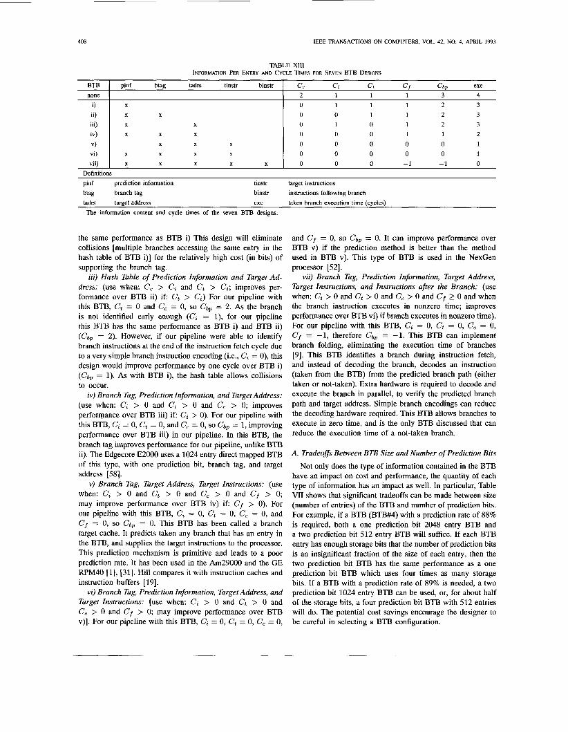
The existence of four types of information (branch tag, prediction information, target address, and target instructions) implies the possibility of 16 BTB designs, each with a different combination of types of information. We have examined these possible designs, and below we discuss six designs that have been used in the past or seem to have some possibility of being used in the future. A seventh design that includes an additional type of information, the branch folding BTB, is discussed as well. The designs are roughly in order of increasing performance. Table XI11 summarizes the information on the BTB designs. Note once again that a BTB (nonbranch folding) does not improve the performance of a not-taken branch so only the performance of the taken branch case (with needed information in the BTB) is considered below.

i) Hush Table of Prediction Information: (use when: C, > C; and C, > Ct). For our pipeline with this BTB, C, = 0, so c b p = 2. This hash table BTB is accessed with the branch instruction address (modulo the table size) during the instruction fetch stage to obtain prediction information. If the decoded instruction is a branch, the predicted branch path is fetched. Note that the hash table (in which no branch tag exists) allows collisions to occur (multiple branches accessing the same entry) which reduces the prediction rate. The Mitsubishi GMICR0/100 uses a one prediction bit 256 entry BTB of this

ii) Brunch Tag and Prediction Information: (use when: C, > Ct and C, > Ct; improves performance over BTB i) if Ci > Ct and C, > Ct). For our pipeline with this BTB, c, = 0 and c, = 0, so cap = 2. As the target address is not available early enough (Ct = l), for our pipeline this BTB has

type WI.


BTB none

i) ii) iii)

iv) v) vi) vii)

pinf btag tadrs tinstr binstr C C C, Ct Cf c b p exe 2 1 1 1 3 4

X 0 1 1 1 2 3 X X 0 0 1 1 2 3 X X 0 1 0 1 2 3 X X X 0 0 0 1 1 2

X X X 0 0 0 0 0 1 X X X X 0 0 0 0 0 1 X X X X X 0 0 0 -1 -1 0

pinf prediction information tinstr target instructions btag branch tag binstr instructions following branch tadrs target address exe taken branch execution time (cycles)

The information content and cycle times of the seven BTB designs.

the same performance as BTB i) This design will eliminate collisions [multiple branches accessing the same entry in the hash table of BTB i)] for the relatively high cost (in bits) of supporting the branch tag.

iii) Hash Table of Prediction Information and Target Ad- dress: (use when: C, > Ci and Ct > Ci; improves performance over BTB ii) i f Ct > C;) For our pipeline with this BTB, Ct = 0 and C, = 0, so c a p = 2. As the branch is not identified early enough (C; = l), for our pipeline this BTB has the same performance as BTB i) and BTB ii) ( c b p = 2). However, if our pipeline were able to identify branch instructions at the end of the instruction fetch cycle due to a very simple branch instruction encoding (Le., C; = 0), this design would improve performance by one cycle over BTB i) ( c b p = 1). As with BTB i), the hash table allows collisions to occur.

iv) Branch Tag, Prediction Information, and Target Address: (use when: C; > 0 and Ct > 0 and C, > 0; improves performance over BTB iii) i f C; > 0). For our pipeline with this BTB, ci = 0, ct = 0, and c, = 0, so c a p = 1, improving performance over BTB iii) in our pipeline. In this BTB, the branch tag improves performance for our pipeline, unlike BTB ii). The Edgecore E2000 uses a 1024 entry direct mapped BTB of this type, with one prediction bit, branch tag, and target address [ S I .

v) Branch Tag, Target Address, Target Instructions: (use when: Ci > 0 and Ct > 0 and C, > 0 and C f > 0; may improve performance over BTB iv) i f C f > 0). For our pipeline with this BTB, Ci = 0, Ct = 0, C, = 0, and C f = 0, so c b p = 0. This BTB has been called a branch target cache. It predicts taken any branch that has an entry in the BTB, and supplies the target instructions to the processor. This prediction mechanism is primitive and leads to a poor prediction rate. It has been used in the Am29000 and the GE RPM40 [l], [31]. Hill compares it with instruction caches and instruction buffers [19].

vi) Branch Tag, Prediction Information, Target Address, and Target Instructions: [use when: Ci > 0 and Ct > 0 and C, > 0 and C f > 0; may improve performance over BTB v)]. For our pipeline with this BTB, Ci = 0, Ct = 0, C, = 0,

and C f = 0, so c a p = 0. It can improve performance over BTB v) if the prediction method is better than the method used in BTB v). This type of BTB is used in the NexGen processor [52].

vii) Branch Tag, Prediction Information, Target Address, Target Instructions, and Instructions after the Branch: (use when: Ci > 0 and Ct > 0 and C, > 0 and C f 2 0 and when the branch instruction executes in nonzero time; improves performance over BTB vi) if branch executes in nonzero time). For our pipeline with this BTB, Ci = 0, Ct = 0, C, = 0, cf = -1, therefore c b p = -1. This BTJ3 can implement branch folding, eliminating the execution time of branches [9]. This BTB identifies a branch during instruction fetch, and instead of decoding the branch, decodes an instruction (taken from the BTB) from the predicted branch path (either taken or not-taken). Extra hardware is required to decode and execute the branch in parallel, to verify the predicted branch path and target address. Simple branch encodings can reduce the decoding hardware required. This BTB allows branches to execute in zero time, and is the only BTB discussed that can reduce the execution time of a not-taken branch.

A. Tradeoffs Between BTB Size and Number of Prediction Bits

Not only does the type of information contained in the BTB have an impact on cost and performance, the quantity of each type of information has an impact as well. In particular, Table VI1 shows that significant tradeoffs can be made between size (number of entries) of the BTB and number of prediction bits. For example, if a BTB (BTW4) with a prediction rate of 88% is required, both a one prediction bit 2048 entry BTB and a two prediction bit 512 entry BTB will suffice. If each BTB entry has enough storage bits that the number of prediction bits is an insignificant fraction of the size of each entry, then the two prediction bit BTB has the same performance as a one prediction bit BTB which uses four times as many storage bits. If a BTB with a prediction rate of 89% is needed, a two prediction bit 1024 entry BTB can be used, or, for about half of the storage bits, a four prediction bit BTB with 512 entries will do. The potential cost savings encourage the designer to be careful in selecting a BTB configuration.

PERLEBERG AND SMITH: BRANCH TARGET BUFFER DESIGN AND OPTIMIZATION

C n n

C n t Ct n c, t

~

409

0 0 0 0 0 0 4 4 4 4 4 4 4 4 4 4 4 4 0 2 3 0 1 2

B. Multilevel BTB’s

The third concept presented in the BTB Design Optimization section is: A multilevel BTB, each level possibly containing different amountsltypes of information per entry, may be able to maximize performance by achieving a better balance of number of entries and quantity of information per entry. Within the constraint of a finite number of storage bits allocated to a BTB design, a multilevel BTB may maximize performance.

To test this concept, four multilevel BTE3 designs are examined. The multilevel BTB designs have up to three levels. The first level, the highest performance level, contains a branch tag, prediction bits, target address, and target instruction bytes for each entry. The second level, the medium performance level, contains a branch tag (one design eliminates this), prediction bits, and a target address for each entry. The third level, the lowest performance level, is a hash table of prediction bits. High performance levels require more storage bits than low performance levels.

The performance of a multilevel BTB cannot be measured by a simple prediction rate since the value of predicting a branch may be different in each level of the BTB. To obtain a measure of performance (average number of cycles saved per branch), implementation dependent cycle costs C,,, C,t , Ct,, and Ctt are required (see Table 11) for each level. l b o sets of cycle costs, costx and costy, are used, and appear in Table XIV. Cost set cos& is for a computer that executes one 4-byte instruction per cycle with static column memory (3 cycle initial access, one cycle access in that column thereafter) with a pipeline that provides the target address one cycle after fetching a branch and the conditions (for conditional branches) two cycles after fetching the branch. For this computer, the first level of the BTB stores two target instructions (8 bytes) per entry to eliminate the extra two cycle penalty in fetching the target instructions. Cost set costy is for a computer that executes one 4 byte instruction per cycle with static column memory (2 cycle initial access, one cycle access in that column thereafter) with a pipeline that provides the target address one cycle after fetching a branch and the conditions three cycles after fetching the branch. For this computer, the first level of the BTB stores one target instruction (4 bytes) per entry to eliminate the extra one cycle penalty in fetching the target instructions. For both cost sets, C,, is zero for all levels, as is to be expected. For simplicity, the two incorrect prediction costs, Cnt and Ct,, have the cycle cost of 4 cycles for all levels and cost sets, which is not unreasonable, as the Amdahl 470 VI6 had a 4 cycle penalty when a branch is taken [l], and the CLIPPER has a 3 to 5 cycle penalty [21]. In general, Cnt and C,, are not identical as the sequential instruction stream is normally available, allowing C,, to be less than Cnt.

The four simulated multilevel BTB’s (BTB#6 to BTB#9) use global LRU replacement when needed so small regular size changes can be made in the various levels. In a real implementation, levels one and two would be set associative. Branches in lower performance levels are moved to the highest level on a branch taken execution; this has the benefit that the target instructions can be fetched without increasing memory demands. Entries at higher performance levels are moved to

Table XIV CYCLE COST SETS COSTX AND C o s n

I costx I COStV

The cycle coss for the two cost sets, cos& and costy, as a function of BTB level and the four possible cycle costs (see Table 11).

lower performance levels one level at a time as they are replaced. The number of prediction bits used in all levels is fixed at two. Table XV indicates the information content of each entry of the BTB’s as a function of cost set and level. Table XVI contains the approximate number of bits required by each entry of the designs.

A few comments are needed to complete the description of the multilevel BTB’s (beyond the information in Table XV). Level two of BTB#6 uses a hash table organization (no branch tag) which requires fewer bits per entry but allows collisions to occur (two or more branches accessing the same entry). This level depends on a simple branch instruction encoding that allows the branch to be identified at the end of instruction fetch. BTB#6 can be directly compared with BTB#7 which does include the branch tag in level two, requiring more bits per entry. In the simulations below, various configurations of BTB#6 and BTB#7 are explored by varying the bit allocation between levels one and two. The full three level BTB, BTB#8, has a fixed number of entries (1024) in level three. BTBW design space is explored by varying the bit allocation between levels one and two. In BTB#9, the bit allocation is varied between level one and three.

1) Results of Simulating Multilevel BTB’s: Each of the four multilevel BTB designs was simulated with the two cost sets (costx and costy), three values for total number of bits in the BTB (4096,8192,16 384), and various bit allocations between the levels of the BTB’s. Tables XVII to Table XIX present the average cycle savings per branch (costy) for three BTB sizes (4096, 8192, 16 384). The results of the remaining studies are shown in [39].

The cycle savings results for costy shown in the tables indicate that there is little advantage in allocating bits to any level other than the highest performance level one; the results for costx, not shown, indicate this as well. BTB#9 achieved the maximum performance gain (10%) over all bits in level one, for the configuration of costy, 4096 bits total, 32 level one entries, and 512 level three entries. To give an idea of the effect on CPU performance of this best case, assuming one cycle per nonbranch instruction, basic block size of 5.26 instructions, and 70% of branches taken, BTB# speeds up the CPU by 32%, and a BTB with all bits in level one (42 level one entries) speeds up the CPU by 28%. In practice, the speedup would be less since the average nonbranch instruction will not execute in one cycle.

A few things should be noted. BTB#6 and BTB#7, basically identical except that BTB#6 uses a hash table level two that


6 1 6 2 X

6 3 7 1

TABLE XV INFORMATION PER ENTRY FOR THE FOUR MULTILEVEL BTB’s

I costx I costy BTB Lev Hash I ubits btag tadrs instr I Dbit btae tadrs instr

X X X 8 X X X 4 X X X X

X X X 8 X X X 4 7 2 7 3 8 1 8 2

X X X

X X X 8 X X X

X X X

8 3 X I X I x

X X X 4

X X X

BTB#6

9 1 9 2 9 3 X

BTB#7 I BTB#8 BTB#9

X X 8

COStX costy

X X X 4

X

costx costy costx costy costx costy

Definitions

level1 level2 level3

pbits prediction bits (2 bits) btag branch tag (-32 bits) tadrs target address (-32 bits)

128 96 128 96 128 96 128 96 32 32 64 64 64 64

2 2 2 2

instr(X) Hash Hash table organization Lev BTB Level

X bytes of target instructions

Information content of the multilevel BTB’s, as a function of cost set and BTB level.

Number of storage bits required per entry of the four multilevel BTB’s,

requires fewer bits per entry but which allows collisions, have virtually identical performance. BTW8 receives no performance benefit from allocating bits to level two. The results for all the multilevel BTB designs indicate that allocating bits to the medium performance level two has no advantage. The effect of number of bits in the BTB design should be noted as well. As number of bits increases, the results indicate that a multilevel BTB is less beneficial.

The limited speedup of a multilevel BTB compared to a single level BTB suggests that the additional complexity of the multilevel BTB is not cost effective. A simple single level BTB has reduced design time and, in this world of cheap bits, basically equal performance. It should be remembered, however, that multilevel BTB’s are strongly dependent on the implementation (cycle costs and bit allocations). RISC processors, with delayed branches and very small (usually one cycle) branch penalties, probably will not find that multilevel BTB’s, or any BTB for that matter, significantly improve performance. Conversely, some CISC processors, with deep pipelines and larger branch penalties, may indeed find multilevel BTB’s useful, and almost certainly will find that a single level BTB significantly improves performance. We note also that we have presented only a small variety of multilevel BTB designs. The small performance gains observed from the cases studied suggested to us that further exploration of the design space would not be productive at this time.

as a function of cost set and BTB level.

Ix . SUMMARY AND CONCLUSIONS

A Branch Target Buffer (BTB) can be used to decrease the performance penalty of branches in pipelined processors by predicting the path of each branch and caching the information each branch needs to execute quickly. Using a set of 32 program traces and software BTB simulators, BTB performance data was generated in order to explore several issues in BTB design.

Branch prediction rates were measured using branch histories of up to 16 bits, and for finite and infinite size BTB’s. The prediction accuracy increases sharply for up to four prediction bits, after which it increases slowly. Context switching is shown to have a significant negative impact on the prediction rates of BTB’s.

BTB management, when and how to discard branches from the BTB, is explored. Entering branches into the BTB only on branch taken executions is found to yield better results than entering branches on both taken and not-taken branch executions. As the BTB can only improve the performance of taken branches, entering a not-taken branch into the BTB has little performance benefit, and may displace a useful branch. A new method of discarding entries from the BTB is examined. The Minimum Performance Potential (MPP) replacement strategy is found to only slightly outperform the Least Recently Used (LRU) replacement. The MPP strategy

PERLEBERG AND SMITH: BRANCH TARGET BUFFER DESIGN AND OPTIMIZATTON

BTB#6 Entries levl lev2 lev3

0 128 0 10 96 0 21 64 0 32 32 0 42 0 0

411

B W 7 Entries BTB#8 Entries BTB#9 Entries Cycle Savings levl lev2 lev3 levl lev2 lev3 levl lev2 lev3 BTB#6 BTB#7 BTB#8 BTB#9

0 64 0 0 32 1024 0 0 2048 1.465 1.420 1.506 1.136 10 48 0 5 24 1024 10 0 1536 1.747 1.719 1.733 1.711 21 32 0 10 16 1024 21 0 1024 1.793 1.774 1.805 1.867 32 16 0 16 8 1024 32 0 512 1.802 1.792 1.847 1.945

1.777 1.867 1.777 42 0 0 21 0 1024 42 0 0 1.777

0 256 0 0 128 0 I 0 96 1024 I 0 0 4096 I 1.545 1.520 1.595 1.145 21 192 0 42 128 0 64 64 0 85 0 0

21 96 0 16 72 1024 21 0 3072 1.932 1.909 1.967 1.887 42 64 0 32 48 1024 42 0 2048 1.982 1.978 2.047 2.035 64 32 0 48 24 1024 64 0 1024 2.007 2.009 2.087 2.111 85 0 0 64 0 1024 85 0 0 2.008 2.008 2.111 2.008

discards branch information that is both not likely to be referenced (Le., low in the LRU stack) and not likely to be useful (i.e., predicts not-taken).

A relationship is found between the miss ratios for BTB’s and instruction caches, making it possible to convert cache miss rates to BTB miss rates and vice versa. Using this capability, design target miss ratios for instruction caches have been converted to design target miss ratios for BTB’s.

Finally, the nature of BTB entries is discussed. The type and amount of information stored in a BTB has a significant impact on the performance of the BTB. Several different BTB designs are presented and evaluated, including those with entries with one or more of the following types of information: branch tag, prediction bits, branch target address, and branch target instructions. Varying the amount of individual types of information has a significant performance impact, as shown by examining the tradeoffs possible between number of prediction bits and number of entries in the BTB. Multilevel BTB’s are considered, i.e., BTB’s that vary the information content in each of several levels in the BTB. The multilevel BTB’s simulated, with specific cycle cost and implementation assumptions, did outperform single level BTB’s, but by a very small margin. For different pipeline and memory timings, however, multilevel BTB’s might improve performance significantly.

BTB#6 Entries levl lev2 lev3

0 512 0 42 384 0 85 256 0

128 128 0 170 0 0

REFERENCES

Advanced Micro Devices, Am29000 Streamlined Instruction Processor User Manual, Advanced Micro Devices, 1988. Amdahl, Amdahl470 VI6 Machine Reference Manual, Amdahl, Sunny- vale, CA, 1976. D. W. Anderson, F. J. Sparacio, and R.M. Tomasulo, “The IBM System/360 Model 91: Machine philosophy and instruction-handling,” IBM J. Res. Develop., pp. 8-24 Jan. 1967. H. B. Bakoglu, G. F. Grohoski, and R.K. Montoye, “The IBM RISC System 6000 Processor: Hardware overview,” IBMJ. Res. Develop., vol. 34, no. 1, pp. 12-22, Jan. 1990. A. Borg, R. E. Kessler, and D. W. Wall, “Generation and analysis of very long address traces,” in Proc. 17th Ann. Symp. Comput. Architecture, June 1990, pp. 270-279. B. K. Bray and M. J. Flynn, “Strategies for branch target buffers,” Stanford Comput. Syst. Lab., Tech. Rep. CSL-TR-91-480, June 1991. J. A. DeRosa and H. M. Levy, “An evaluation of branch architectures,” in Proc. 14th Annu. Symp. Comput. Architecture, 1987, pp. 10-16. Digital Equipment Corp., VAX I U780 Architecture Handbook, Digital Equipment Corp., 1977 D. R. Ditzel and H. R. McLellan, “Branch folding in the CRISP Microprocessor: Reducing branch delay to zero,” in Proc. 14th Annu. Symp. Comput. Architecture, 1987, pp. 2-9. N. Doduc, “Fortran execution time benchmark,” unpublished report, V.20, Mar. 1989. P. Dubey and M. J. Flynn, “Branch strategies: Modeling and optimization,” IEEE Trans. Comput., vol. 40, no. 10, pp. 1159-1167, Oct. 1991. T. H. Elrod, “The CDC 7600 and SCOPE 76,” Datamation, pp. 80-85, Apr. 1970. D. Folger and E. Basart, “Computer architecture - Designing for speed,” in Proc. Spring COMPCON 1983, pp. 25-31.

BTB#7 Entries BTB#8 Entries BTB#9 Entries Cycle Savings levl lev2 lev3 levl lev2 lev3 levl lev2 lev3 BTB#6 BTB#7 BTB#8 BTB#9

0 256 0 0 224 1024 0 0 8192 1.604 1.633 1.644 1.148 42 192 0 37 168 1024 42 0 6144 2.084 2.102 2.113 2.045 85 128 0 74 112 1024 85 0 , 4096 2.131 2.145 2.175 2.157

128 64 0 112 56 1024 128 0 2048 2.127 2.147 2.188 2.190 170 0 0 149 0 1024 170 0 0 2.138 2.138 2.197 2.138

Fujitsu Microelectronics, Inc., MB86900 RISC Processor Architectwe Manual, Fujitsu Microelectronics, Inc., 1987. S. N. Gadding and D. P. Madison, Jr., “Optimization of scalar instructions for the advanced scientific computer,” in Proc. Spring COMPCON

E. T. Grochowski, “An instruction tracer for the Motorola 68010,” U.C. Berkeley Masters Rep., 1986. T. R. Gross and J. L. Hennessy, “Optimizing delayed branches,” in Proc. 15th Annu. Workshop Microprogramming, Oct. 1982, pp. 114-120. R. R. Henry, “VAX address and instruction traces,” unpublished report, 1983. M. D. Hill, “Aspects of cache memory and instruction buffer performance,” U.C. Berkeley Tech. Rep. UCB/CSD 87/381, Nov. 1987. G. Hinton, “80960 - Next generation,” in Proc. Spring COMPCON1989,

W. Hollingsworth, H. Sachs, and A.J. Smith, “The CLIPPER processor: Instruction set architecture and implementation,” Commun. ACM, pp. 200-219, Feb. 1989. K. Hwang and F. A. Briggs, Computer Architecture and Parallel Processing. IBM, “IBM Maintenance Library System/370 Model 168 Theory of OperationDiagrams Manual,” vol. 2, IBM, Poughkeepsie, NY, 1973. __ , “IBM Maintenance Library 3033 Processor Complex Theory of OperationDiagrams Manual,” vols. 1-3, IBM, Poughkeepsie, NY, Jan. 1978. H. F. Jordan, “Performance measurements on HEP - A pipelined MIMD computer,” in Proc. 10th Annu. Symp. Comput. Architecture, 1983, pp.

D. Kaeli and P. Emma, “Branch history table prediction of moving target branches due to subroutine returns,” in Proc. 18th ISCA, and Comput. Architecture News, vol. 19, no. 3, pp. 34-41 May 1991. G. Kane, MIPS RISC Architecture. Englewood Cliffs, NJ: Prentice- Hall, 1989. S. P. Kartashev and S. I Kartashev, Supercomputing Systems. New York: Van Nostrand Reinhold, 1990, pp. 106-153. P. M. Kogge, The Architecture of Pipelined Computers. New York: McGraw-Hill, 1981. J. K. F. Lee and A. J. Smith, “Branch prediction strategies and branch target buffer design,” IEEE Comput. Mag., pp. 6-22, Jan. 1984. D. K. Lewis, J. P. Costello, and D. M. O’Connor, “Design tradeoffs for a 40 MIPS (peak) CMOS 32-bit microprocessor,” in Proc. IEEE Int. Conj Comput. Design: VLSI Comput. Processors, Oct. 1988, pp. 110-113. D. J. Lilja, “Reducing the branch penalty in pipelined processors,” IEEE Comput. Mag., pp. 47-55, July 1988. T. Manuel, “Getting mainframe power out of a CISC Supermicro,” Electronics, pp. 66-69, Sept. 3, 1987. S. McFarling and J. Hennessy, “Reducing the cost of branches,” in Proc. 13th Annu. Symp. Comput. Architecture, 1986, pp. 396-403. Motorola, M68000 841 6-132-Bit Microprocessors User’s Manual. En- glewood Cliffs, NJ: Prentice-Hall, 1989. J. 0. Murphey and R. M. Wade, “The IBM 3601195,” Datamation, pp. 72-79, Apr. 1970. S.-T. Pan, K. So, and J. T. Rahmeh, “Improving the accuracy of dynamic branch prediction using branch correlation,” in Proc. ASPLOS V, Boston, MA, Oct. 1992. D. A. Patterson and H. Sequin, “RISC-I: A reduced instruction set VLSI computer,” in Proc. Eighth Symp. Comput. Architecture, May 1981, pp. 443-458. C. H. Perleberg, “Branch target buffer design,” U.C. Berkeley Comput. Sci. Division Technical Rep. UCB/CSD 89/553, Dec. 1989. B. L. Peuto and L. J. Shustek, “An instruction timing model of CPU performance,” in Proc. 4th Annu. Symp. Comput. Architecture, Mar.

M. Putrino, S. Vassiliadis, A. Huffman, and A. Ngai, “Apparatus for branch prediction for computer instructions,” US. Patent 4 914 579, April 3, 1990. C. V. Ramamoorthy and H. F. Li, “Pipeline architectures,” Comput. Surveys, pp. 61-102, Mar. 1977. B. R. Rau and G. E. Rossman, “The effect of instruction fetch strategies upon the performance of pipelined instruction units,” in Proc. 4thAnnu. Symp. Comput. Architecture, 1977, pp. 80-87. R. M. Russell, “The CRAY-1 computer system,” Commun. ACM, pp. 63-72, Jan. 1978. K. Sakamura, TRON Project 2987. Berlin, Germany: Springer-Verlag, 1987. L. E. Shar and E. S. Davidson, “A multiminiprocessor system implemented through pipelining,” IEEE Comput. Mag., pp. 42-51, Feb. 1974. A. J. Smith, “Sequential program prefetching in memory hierarchies,”

1975, pp. 189-193.

pp. 13-17.

New York McGraw-Hill, 1984, pp. 714-729.

207-212.

1977, pp. 165-178.

IEEE TRANSACTIONS ON COMPUTERS, VOL. 42, NO. 4, APRIL 1993

IEEE Comput. Mag., vol. 11, no. 12, pp. 7-21, Dec. 1978. [48] -, “Cache evaluation and the impact of workload choice,” in Proc.

12th Symp. Comput. Architecture, June 1985, pp. 64-74. [49] -, “Line (block) size choice for CPU cache memories,” IEEE

Trans. Comput., pp. 1063-1075, Sept. 1987. [50] J. E. Smith, “A study of branch prediction strategies,” in Proc. Eighth

Symp. Comput. Architecture, May 1981, pp. 135-148. [51] J. E. Smith and J. R. Goodman, “A study of instruction cache or-

ganizations and replacement policies,” in Proc. 10th Symp. Comput. Architecture, June 1983, pp. 132-137.

[52] D. R. Stiles and H. L. McFarland, “Pipeline control for a single cycle VLSI implementation of a complex instruction set computer,” in Proc. Spring COMPCON 1989, pp. 504-508.

[53] D. R. Stiles (of NexGen microsystems), personal interview concerning branch prediction cache of NexGen processor, Sept. 25, 1989.

1541 J. E. Thomton, “Parallel operation in the Control Data 6600,” in Proc. AFIPS Fall Joint Comp. Conj, 1964, pp. 33-40.

[55] U.C. Berkeley C A D K Group, “SPICE2G.6,” Mar. 1987. [56] T.-Y. Yeh and Y. Patt, ‘‘’nvo level adaptive training branch prediction,”

in Proc. MICRO-24, Nov. 1991, pp. 51-61. 1571 ~, “Alternative implementations of two-level adaptive branch pre-

diction,” in Proc. ISCA-19 and Comput. Architecture News, vol. 20, no. 2, pp. 124-135. May 1992.

[58] S. Walter (of Edgecore), personal interview concerning branch cache in Edge 2000, Sept. 20, 1989.

[59] L. C. Widdoes, Jr., “Jump prediction,” Stanford Univ., unpublished draft, Feb. 1977.

[60] T. Yoshida and T. Enomoto, “The Mitsubishi VLSI CPU in the TRON Project,” IEEE Micro, p. 24, Apr. 1987.

Chris H. Perleherg received the B.S. degree in electrical engineering from U.C. Santa Barbara and the M.S. degree in electrical engineering from U.C. Berkeley (based on this paper).

His engineering interests include computer architecture, hardware design, and software design. He is currently traveling through Central and South America.

Alan Jay Smith (S’73-M’74-SM’83-F’89) was raised in New Rochelle, NY. He received the B.S. degree in electrical engineering from the Massachu- setts Institute of Technology, Cambridge, in 1971, and the M.S. and Ph.D. degrees in computer science from Stanford University, Stanford, CA, the latter in 1974. He was an NSF Graduate Fellow.

He is currently a Professor in the Computer Science Division of the Department of Electrical Engineering and Computer Sciences, University of California, Berkeley, where he has been on the

faculty since 1974, and was vice chairman of the EECS department from July 1982 to June 1984. His research interests include the analysis and modeling of computer systems and devices, computer architecture, and operating systems. He has published a large number of research papers, including one which won the IEEE Best Paper Award for the best paper in the IEEE TRANSACTIONS ON COMPUTERS in 1979. He also consults widely with computer and electronics companies.

Dr. Smith is a member of the Association for Computing Machinery, IFIP Working Group 7.3, the Computer Measurement Group, Eta Kappa Nu, Tau Beta Pi, and Sigma Xi. He is Chairman of the ACM Special Interterest Group on Computer Architecture (1991-1993), was Chairman of the ACM Special Interest Group on Operating Systems (SIGOPS) from 1983 to 1987, was on the board of directors of the ACM Special Interest Group on Measurement and Evaluation (SIGMETRICS) from 1985-1989, was an ACM National Lecturer (1985-1986) and an IEEE Distinguished Visitor (1986-1987), is an Associate Editor of the ACM Transactions on Computer Systems (TOCS), a subject area editor of the Journal of Parallel and Distributed Computing and is on the editorial board of the Journal of Microprocessors and Microsystems. He was Program Chairman for the Sigmetrics’89/Performance’89 Conference, Program Co-chair for the Second (1990) Hot Chips Conference, and has served on numerous program committees.

Branch Target Buffer Design and Optimization

Documents

Transcript of Branch Target Buffer Design and Optimization