BOUNDARY VALUE PROBLEMS FOR

QUATERNIONIC MONOGENIC FUNCTIONS

ON NON-SMOOTH SURFACES

Ricardo Abreu Blaya and Juan Bory ReyesDepartment of Mathematics, Faculty of ScienceUniversity of Oriente, Santiago of Cuba, 90500, Cuba.jbory@bioeco.ciges.inf.cu

(Received: October 19, 1998; Accepted: November 30, 1999)

Abstract. In this paper, analogous of the Compound Riemann-Hilbert boundaryvalue problems are investigated for quaternionic monogenic functions. The solution(explicitly) of the problem is established over continuous surface, with little smooth-ness, which bounds a bounded domain of R3. In particular, smoothness property forhigh-dimensional Cauchy type integral are computed. We also use Zygmund typeestimates to adapt existing one-variable complex results to ilustrate the Holder-boundedness of the singular integral operator on 2-dimensional Ahlfors regular sur-faces. At the end, uniqueness of solution for the Riemann boundary value problemhave already being built taking as a base the general Operator Theory.

Key words: Clifford analysis, Riemann-Hilbert problem, Cauchy type integral.AMS. Subject Class (1991) 30E25, 30G35.

1. Introduction

One of the most important actually ways to generalize the classical-posed ofthe Riemann-Hilbert type boundary value problems and related subjects, tohigh dimension, is the consideration of functions with values in a Clifford al-gebra.Very interesting results involving Clifford Analysis within Riemann HilbertBoundary Value Problems Theory have been developed in [16, 38, 39, 40,41, 42]. It should be noted that the stage was also set applying Vector FieldTheory to study Riemann-Hilbert type boundary value problems; see for in-

Advances in Applied Clifford Algebras 9 No. 1, 1-22 (1999)

2 Boundary Value Problems for Quaternionic . . .R. Abreu Blaya, J. Bory Reyes

stance [29, 36].Some basic results of the Complex Riemann-Hilbert Problems Theory are notbeen carried in the Clifford Analysis setting, e.g; the role that the index playand the possibility to find a “good enough” factorization for functions definedon the boundary of the domain considered. To this end, two open problemshave been provided by Klaus Gurlebeck and Zhenyuan Xu in the problem booksection of the proceeding of the “Conference of Clifford Algebras in Analysisand Related Topics”, held in Fayetteville, Arkansas, April 8-10 th. 1993 [30].For this reason, an explicit solution of the analogues of the Riemann boundaryvalue problem for monogenic functions with values in a Clifford algebras, canbe obtained only for the particular case of the jump problem of linear conju-gation.Using General Operator Theory, one can show that there exists a unique solu-tion of the hypercomplex Riemann problem under certain hypotheses. We referthe reader to [40, 39] for a detailed discusion of these results. Their approachconsider the Riemann problems over domains bounded by smooth surfaces.This paper is devoted to study a Compound Riemann-Hilbert problem forhomogeneous Dirac equation in the upper half space and over a non-smoothsurface. For the sake of simplicity we restrict our investigation to the case ofthe Quaternionic Analysis.

2. Preliminaries

We consider the real skew-field of quaternionic H generated by the orthonormalbasis ej3

j=1 of R3. For each a =∑3

j=0 ajej , where e0 = 1 is the identity of H,the norm of a is defined to be |a| = (

∑3j=0 a2

j )12 . Introducing the abbrevation

a =∑3

j=1 ajej we obtain a = a0e0 + a, the real part of a is defined by <a = a0.The Dirac operator in R3 is defined by D =

∑3j=1 ej

∂∂xj

, here D2 = −∆ theLaplacian.For Ω a domain in R3, a differentiable function u =

∑3j=0 ejuj : Ω −→ H, is

said to be (left) monogenic in the domain Ω ⊂ R3 if it is in C1(Ω) and satisfiesDu = 0 in Ω. Many facts on Monogenic Function Theory can be found inthe books by Brackx, Delanghe and Sommen [3]; Gilbert and Murray [14],Gurlebeck and Sprossig [15]; Ryan [30] and others.

3. Surfaces in R3

Throughout the paper we shall consider the continuous surface Γ which boundsa bounded and simply conected domain Ω+ in R3. Let Ω− denote the comple-

Advances in Applied Clifford Algebras 9, No. 1 (1999) 3

mentary space of Ω+ ∪ Γ.Let Hλ, λ > 0, denote the λ-dimensional Hausdorff measure in R3 and λ(Γ)be the Hausdorff-Besikovish dimension of Γ defined by the infimum of the pos-itive numbers λ such that Hλ(Γ) < ∞, [10, 11, 22, 26] for a detailed discussionof this dimension.

Remark:a) We have Hλ(Γ) = ∞ for λ < λ(Γ) and Hλ(Γ) = 0 for λ > λ(Γ). Moreover,

we have in general Hλ(Γ)(Γ) ∈ [0,∞], for most of the classical “fractals”considered in [10, 26], however we have 0 < Hλ(Γ)(Γ) < ∞.

b) The larger λ(Γ), the more extraneous Γ. Further we always have 2 ≤λ(Γ) ≤ 3 since Γ = ∂Ω+ [22], corollary 2.2. We say that Γ is a fractalsurface if λ(Γ) ∈ (2, 3].

Following [11] we have:

Definition 3.1: A surface Γ in R3 is called 2-rectifiable if it is the Lipschitzimage of some bounded set of R2.In [11], using a general geometric concept of exterior normal vector n(x), Fed-erer proved that, if H2(Γ) < ∞, then for each function u ∈ C1(Ω+) ∩ C(Ω+)the following Gauss-Green formula holds:∫

Γ

〈u(x), n(x)〉dH2(x) =∫

Ω+divu(x)dL3(x) (1)

where L3 denotes the usual Lebesgue measure in R3.When the boundary Γ is sufficiently “smooth” (e.g. C1, Lipschitz or 2-recti-fiable) and taking into account that each Lipschitz continuous function is dif-ferentiable almost everywhere, then the outward pointing normal vector isdefined, in the usual sense, for almost all point of Γ [31], consequently theformula (1) reads as the classical formula.We now briefly recall the definition and the main properties of the cell dimen-sion (it is also called the upper metric dimension) of the surface Γ, [10, 12, 21].Suppose R0 denotes a grid consisting of cubes with sides of length 1 and ver-tices with integer coordinates. The grid Rk is obtained from R0 by dividingof each of the cubes in R0 into 23k different cubes with sides 2−k. Denote bymk(Γ) the number of cubes of the grid Rk, which intersect Γ. The quantitylimk→∞

log2mk(Γ)k , is called cell dimension of surface Γ and will be denoted

α(Γ).In general, we have 2 ≤ λ(Γ) ≤ α(Γ) ≤ 3. The estimate α(Γ) ≤ 3 follows fromthe fact that mk(Γ)2−3k is the volume of the covering of Γ by cubes of thegrid Rk; the estimate λ(Γ) ≤ α(Γ) follows from the definition of the Hausdorff

4 Boundary Value Problems for Quaternionic . . .R. Abreu Blaya, J. Bory Reyes

dimension, ([26], p.359)

Proposition 3.1: If Γ is a 2-rectifiable surface, then α(Γ) = λ(Γ) = 2.

Proof: Let Γ = Λ(E), where E is bounded set of R2. Take any closed square Qsuch that E ⊂ Q. Suppose d is the diameter of the square Q, c is the Lipschitzconstant of Λ, δk = 2−k

2c . Then Q can be divided into n ≤ ([ dδk

] + 1)2 squaresQj of diameter not exceeding δk, and Λ(Qj ∩ E) intersects not more than 8cubes of the grid Rk.Hence mk(Γ) ≤ 8nk ≤ 8([ d

δk] + 1)2, then for sufficiently large k, we have the

estimate mk(Γ) ≤ c22k, and the proposition is proved.In the sequel, for the sake of convenience in notation, we shall denote by ccertain generic constant not necesarily the same in different occurrences.

4. A Property of Whitney Extension Operator

Let us now consider the space C(Γ,H) of all continuous functions defined onΓ, with values in H. We denote by X the characteristic function of domain Ω+.For g ∈ C(Γ,H) we set gw = XW0(g), where W0 is the Whitney extensionoperator [37].The following theorem is a “hypercomplex” version of the results due to Stein([37], p. 206).

Theorem 4.1: Let g ∈ Hν(Γ,H), 0 < ν ≤ 1. Thena) gw ∈ Hν(Ω+,H).b) In Ω+ the function gw is infinitely differentiable and the following inequal-

ity holds: |Dgw(x)| ≤ c(dist(x,Γ))ν−1.At all time Hν(E,H), E ⊂ R3, denotes the set of Holder continuous functionsdefined on E with values on H and the Holder exponent is ν.

Proposition 4.1: Suppose α(Γ) < 3, 0 < ν < 1 and g ∈ Hν(Γ,H). ThenDgw ∈ Lp for p < 2−α(Γ)

1−ν .

Proof: For the proof, we have to recall the construction of the Whitney par-tition [37].Introduce the layers Ωk = x ∈ R3 : 2

√32−k ≤ dist(x,Γ) ≤ 4

√32−k, and

consider the collection Vk of cubes of grid Rk intersecting the layer Ωk. Afterremoving from the set V ′ =

⋃k≥0 Vk those cubes which are contained in larger

cubes of V’, we obtain the Whitney partition V. It has the properties ([37], p.

Advances in Applied Clifford Algebras 9, No. 1 (1999) 5

199):

R3/Γ =⋃

Q∈V

Q, (2)

and

diamQ ≤ dist(Q,Γ) ≤ 4diamQ,Q ∈ V. (3)

Denote by vk the number of cubes of the grid Rk, appearing in V. It is easyto see that vk ≤ mk(Ωk). Suppose Q is a cube of Rk intersecting with Ωk.Then one can prove that there is a cube Q’ intersecting with Γ such that Qlie inside the cube with side 15(2−k), the center of which coincides with thecenter of Q’. Hence vk ≤ mk(Ωk) ≤ 153mk(Γ). Fix a number α′ ∈ (α(Γ), 3).By the definition of the grid dimension a constant c can be found such thatmk(Γ) ≤ c2kα′ .According to (2), to show that the series

∑Q∈V

∫Q|Dgw(x)|pdL3(x) converges

is enough in order to get the complete proof of the proposition. ApplyingTherem 4.1 and in accordance with (3) we obtain:∫

Q

|Dgw(x)|pdL3(x) ≤ c2pk(1−ν)

∫dL3(x) = c2k(p(1−ν)−3), Q ∈ Vk.

Hence∑Q∈V

∫Q

|Dgw(x)|pdL3(x) ≤ c

∞∑k=0

2k(p(1−ν)−3+α′).

For p < 3−α′

1−ν this series converges. In view of arbitrary choice of α′ the propo-sition is proved.

5. Jump Problem and Cauchy Type Integral

The simplest particular case of the Riemann problem for analytic complexfunctions over a Jordan closed curve γ which bounds a domain U+ in the com-plex plane C, is the following jump problem: To find a function φ(x) analyticin C \ γ, which satisfies the jump condition

φ+(x)− φ−(x) = g(x) , x ∈ γ, (4)

where g is a function given on γ, and φ+(x) and φ−(x) are the limit values ofthe desired function φ at a point x as this point approached from U+ and from

6 Boundary Value Problems for Quaternionic . . .R. Abreu Blaya, J. Bory Reyes

U− = C \ U+ ∪ γ respectively. The solution of the problem (4) is well knownfor smooth enough curves [13, 24, 28].In [18, 19, 20], Kats presented a new method for solving the jump problem(4), a method that does not use contour integration and can thus be used onnon-rectifiable and fractal curves.In this section we turn to look at the analogue of the jump problem for quater-nionic monogenic functions; namely: To find a monogenic function u(x) inR3 \ Γ such that u(∞) = 0 and satisfies the boundary condition

u+(x)− u−(x) = g(x) , x ∈ Γ, (5)

where g ∈ C(Γ,H), and u±(x) are the limit values of the desired function u(x)at a point x ∈ Γ as this point approach from Ω± respectively.Following similar techniques to those used by Kats, the solution of the jumpproblem can be now described. We begin with the following version of defini-tion from ([20], p. 11) which will be used in the sequel.

Definition 5.1: A function u ∈ C1(R3 \ Γ,H) is called a quasi-solution ofthe problem (5) if there exist the limit values of the function u and satisfy thecondition (5).For example, a quasi-solution u0 of the jump problem (5) can be obtained fromthe formula u0(x) = gw(x).We now proceed to establish:

Theorem 5.1: The jump problem (5) is solvable if and only if there exists aquasi-solution u(x) such that the support of Du is compact and Du ∈ Lp(R3)for some p > 3.

Proof: The necessity is obvious. Let u(x) be a quasi-solution satisfying theabove requeriment. We shall show that the following function is solution of(5):

u0(x) = u(x)− TDu(x),

where

Tf = − 14π

∫R3

y − x

|y − x|3f(y)dL3(y)

Taking into account the equality DTf = f ([15], p. 53), then Du0 = 0. Henceu0 is a monogenic function in R3 \ Γ.

Advances in Applied Clifford Algebras 9, No. 1 (1999) 7

Furthemore, the operator T maps functions of the class Lp, p > 3, with compactsupport, into continuous functions in R3 vanishing at x = ∞ ([15], p.49).Hence one has that the function u0(x) satisfies (5).An immediate consequence of the Proposition 4.1 and Theorem 5.1 is the fol-lowing.

Theorem 5.2: [1] Suppose g ∈ Hν(Γ,H). If 1 ≥ ν > α(Γ)3 , then a solution of

the problem (5) can be obtained from the formula

u0(x) = gw(x) +14π

∫R3

y − x

|y − x|3Dgw(y)dL3(y). (6)

When the surface Γ is 2-rectifiable, then the Gauss-Green formula (1) leads tothe following Borel-Pompeiu formula for the function gw(x):

gw(x) =

=14π

∫Γ

y − x

|y − x|3n(y)g(y)dH2(y)− 1

4π

∫R3

y − x

|y − x|3Dgw(y)dL3(y). (7)

According to (6), (7), and Proposition 3.1, we obtain the following

Theorem 5.3: Let Γ be a 2-rectifiable surface, and suppose that g(x) ∈Hν(Γ,H). Then for 1 ≥ ν > 2

3 , the Cauchy type integral:

CΓg(x) =14π

∫Γ

y − x

|y − x|3n(y)g(y)dH2(y) (8)

is continuosly extendable from both sides into all points of Γ.

6. A Dolzhenko Theorem for H-Valued Functions

We now turn to look at a higher-dimensional extension of the Dolzhenko’stheorem [2, 9, 23], under which essentially enable us to obtain the uniquenessof the solution of the jump problem (5). The proof of the theorem is donefollowing similar arguments to those described in [9].Let use denote by Hh the Hausdorff measure corresponding to the measurefunction h : [0,+∞] −→ [0,+∞] [10, 26].

Theorem 6.1: Let u : Ω −→ H, have modulus of continuity ω(u, r) and bemonogenic off a compact set F ⊂ Ω having Hh(F ) = 0 for the measure func-tion h(r) = r2ω(u, r). Then u is monogenic on Ω.

8 Boundary Value Problems for Quaternionic . . .R. Abreu Blaya, J. Bory Reyes

Proof: Without loss of generality, we can assume that u(x) is a non constantfunction and ω(u, r) ≥ cr, where c is a positive constant which does not dependon r.Since r3 ≤ ch(r), then L3(F ) = 0 and hence F is nowhere dense in Ω. LetB be a ball lying in Ω where C = ∂B is the boundary of B. Now, fix η > 0.One can assure the existence of a sufficiently small number ε > 0 such thatB \ F3ε 6= ∅, where F3ε = x ∈ R3 : dist(x, F ) ≤ 3ε.Since F ∩B is compact it is always possible to cover F ∩B with finitely manyballs Bn = B(an, rn) with center an and radius rn ≤ ε and such that∑

n

r2nω(u, rn) < ηε2.

For the sake of simplicity we assume that the set of balls Bn has beenenumerated in decreasing order of their radii and Bj \

⋃n 6=j Bn 6= ∅.

Let Ω1 = B ∩ B1 , Ωn = B ∩ (Bn \⋃n−1

k=1 Bk). Then Ωn ⊂ Bn and Ωn iscompound by a finite number of nonintersecting domains Ωn,k ⊂ Bn withsmooth enough boundary Γn,k. Moreover∑

k

H2(Γn,k) ≤ H2(Cn) = 4πr2n ,

where Cn denote the boundary of the ball Bn.Since u(x) is monogenic in B \ F and

⋃n,k Ωn,k ⊂ F2ε, then according to the

Cauchy formula [15], for instance, we obtain

u(x) =14π

∫C

y − x

|y − x|3n(y)u(y)dH2(y)−

=14π

∑n,k

∫Γn,k

y − x

|y − x|3n(y)u(y)dH2(y) (9)

Let us denote by R(x) the second summand in the right side of (9). Then, itis not difficult to verify that

|R(x)| ≤ 14πε2

∑n

ω(u, rn)∑

k

H2(Γn,k) < η

In view of the arbitrary choice of η, we have R(x) ≡ 0 for x ∈ B \ F2ε, and inaccordance with arbitrarity of ε we obtain R(x) ≡ 0 in B \ F .

Advances in Applied Clifford Algebras 9, No. 1 (1999) 9

Taking into account that B \F is dense in B, and the fact that R(x) is continu-ous in B we obtain the equality R(x) ≡ 0, for x ∈ B. Hence u is monogenic in Ω.

Corollary 6.1: Let Γ ⊂ Ω be a 2-rectifiable surface. If u is monogenic functionin Ω \ Γ which is continuous in Ω, then u is monogenic in Ω.

Corollary 6.2: Let Γ ⊂ Ω such that λ(Γ) < ν+2(0 < ν ≤ 1). If u is monogenicfunction in Ω \ Γ which belongs to the class Hν(Ω,H), then u is monogenic inΩ.Preparing the following investigation we start with some auxiliary remarks.Let O be an unbounded set, we recall that a bounded function u defined on Owith values in H belongs to the class Hν(O,H), if u ∈ Hν(O∩K,H) for everycompact set K in R3 and

|u(x)− u(∞)| ≤ 1|x|ν

as x →∞ (10)

If the order ν is not emphasized, it may be denoted briefly H(O,H).We will place the function u monogenic in R3 \ Γ into the class Hµ, 0 < µ ≤ 1if u+ ∈ Hµ(Ω+,H) and u− ∈ Hµ(Ω−,H).

Theorem 6.2: Suppose λ(Γ) < 3, g ∈ Hν(Γ,H) and λ(Γ)− 2 < µ < 3ν−α(Γ)3−α(Γ) ,

then the function (6) is the unique solution of the problem (5) of the class Hµ.

Proof: Uniqueness of solution follows immediately from Corollary 6.2 andcondition λ(Γ) < µ + 2. At the same time, if f ∈ Lp, p > 3, has compactsupport, then Tf belongs to the class H p−3

p(R3,H). Therefore u0 ∈ Hµ for

µ < 3ν−α(Γ)3−α(Γ) .

When Γ is a 2-rectifiable surface, according to Corollary 6.1 we obtain thefollowing

Theorem 6.3: Suppose 1 ≥ ν > 23 and g ∈ Hν(Γ,H). Then, the Cauchy type

integral CΓg is the unique solution of the jump problem (5) and belongs to theclass Hµ, for 0 < µ < 3ν − 2.

7. Compound Riemann-Hilbert Boundary Value Problem

In the present section, the amalgamation of the Riemann and Hilbert problems(Compound Problem) is considered.We first consider the Hilbert problem in the upper half space [41, 42]. Assumed

10 Boundary Value Problems for Quaternionic . . .R. Abreu Blaya, J. Bory Reyes

R3+ = x ∈ R3 : x3 > 0 be the upper half space and R3

0 = x ∈ R3 : x3 = 0its boundary in R3; here R3

0 may be identified with R2.The problem is: Find a function w(x) monogenic in R3

+, bounded in R3+ and

continuous in R3+, such that

<(w(x)F ) = f(x) onR30, (11)

where F denote a non-zero quaternionic constant and f(x) is a real functionthat belongs to the class H(R3

0,R).We define the Cauchy type integral of f on R3

0 by setting

Cf(x) =14π

∫R3

0

y − x

|y − x|3e3f(y)dH2(y) , x ∈ R3

+.

If we regard it as an ordinary improper integral, then it does not exist ingeneral. But if it is understood as the Cauchy principal value, i.e.,

Cf(x) = limR→+∞14π

∫R3

0∩|y|≤R

y − x

|y − x|3e3f(y)dH2(y),

then it exists, and

Cf(x) =14π

∫R3

0

y − x

|y − x|3e3(f(y)− f(∞))dH2(y) +

12f(∞),

where the integral in the right side (according to (10)) exists in the impropersense.This formula is a straighforward consequence of the relation

(C1)(x) =14π

∫R3

0

x3

|y − x|3dy1dy2 +

2∑j=1

14π

∫R3

0

eje3yj − xj

|y − x|3dy1dy2

and the following two equalities

14π

∫R3

0

x3

|y − x|3dy1dy2 =

12

limR→+∞14π

∫R3

0∩|y|≤Reje3

yj − xj

|y − x|3dy1dy2 = 0.

Remark: Note that the integrand of the first above equality is namely thePoisson kernel in the upper half space R3

+.

Advances in Applied Clifford Algebras 9, No. 1 (1999) 11

We recall that the Cauchy type integral reduces to Hilbert transform if x ∈ R30.

Moreover if f ∈ H(R30,H), then the Hilbert transform is well defined in the

Cauchy’s principal value sense. As, [17], the Cauchy type integral can be con-tinuously extended to the hyperplane R3

0, and also the Plemelj formula holds.

Theorem 7.1: The Hilbert problem (11) has a solution represented as w0(x)+(ae1 + be2 + ce3)F−1, where a, b, c are arbitrary constants and w0 is given by:

w0(x) =12π

∫R3

0

y − x

|y − x|3e3f(y)F−1dH2(y) , x ∈ R3

+. (12)

Proof: Since f ∈ H(R30,H), then in accordance with the Plemelj formula and

the fact that f is a real valued function we obtain that

<(w+0 F ) = f(x), x ∈ R3

0.

By the above argument, it is clear that the function w0(x) is a particularsolution to the problem (11).Let us now consider the Compound Riemann Hilbert problem.Assume that Γ is a surface inside R3

+ which satisfies the conditions decribedin the previous section 3.The Compound Riemann Hilbert Problem in R3

+ is: To find the monogenicfunction u(x) in R3

+ \ Γ whose boundary values from inside and outside thesurface Γ satisfy:

u+(x)− u−(x)G = g(x), x ∈ Γ, u(∞) = 0, (13)

where g ∈ Hν(Γ,H) and

<(u+(x)F ) = f(x) , x ∈ R30 , (14)

where f ∈ H(R30,H) and F and G are non zero quaternionic constants.

We use the idea of the Elimination Method [24, 29].Let us first find a function u1(x) monogenic in R3

+ \ Γ and continuous to R30

satifying (13), disregard (14) for the time being.Following the technique used in section 5, one can prove that if 1 ≥ ν > α(Γ)

3 ,then the function

u1(x) = gw(x)G−1X(x) +14π

∫y − x

|y − x|3Dgw(y)G−1X(x)dL3(y) (15)

is a solution of this problem, where

X(x) =

G, if x ∈ Ω+

1, if x ∈ Ω−

12 Boundary Value Problems for Quaternionic . . .R. Abreu Blaya, J. Bory Reyes

Moreover, this solution u1(x) belongs to the class Hµ for µ < 3ν−α(Γ)3−α(Γ) .

After u1(x) is obtained, u(x) is transformed to a new unknown function u2(x)by:

u(x) = u2(x)X(x) + u1(x), (16)

which is monogenic in R3+ and continuous to R3

+. Then, the proposed com-pound problem is transferred to the following problem: Find a function u2(x)monogenic in R3

+ and continuous to R3+, such that it satifies the corresponding

condition (14), which is, by substituting (16) in (14),

<(u+2 (x)F ) = f∗(x) , x ∈ R3

0, (17)

where we put f∗(x) = f(x)−<u+1 (x)F.

Because f(x) and <(u+1 (x)F ) belong to the class H(R3

0,R), so do f∗(x). Usingtheorem 7.1, we have the following results.

Theorem 7.2: If 1 ≥ ν > α(Γ)3 , the compound problem (13)-(14) has a solution

represented as

u(x) = w∗0(x)X(x) + gw(x)G−1X(x)+

+14π

∫y − x

|y − x|3Dgw(y)G−1X(x)dL3(y), (18)

where

w∗0(x) =

12π

∫R3

0

y − x

|y − x|3e3f

∗(y)F−1dH2(y). (19)

Corollary: Suppose Γ is a 2-rectifiable surface. If 1 ≥ ν > 23 , then the function

(18) is a unique solution of the problem (13)-(14).

8. Cauchy Integral Operator and Singular Operator on Regular Sur-faces

We start out this section with the following remark:It is an interesting problem to find an appropriate extension of many aspectsof one-variable Complex Analysis to Clifford Analysis. A great amount of workhas been done by many authors along this line. In particular, in [17], Iftimiesets up basic results on Cauchy tranform over domain in Rn and establishes

Advances in Applied Clifford Algebras 9, No. 1 (1999) 13

Plemelj formulae for Holder continuous function defined over compact Lia-punov surface. More recently, these results have been extended to Lp-spacesover the boundary of Lipschitz domain in Rn, see, for instance [22, 25, 32].Subsequently Coifman, McIntosh and Meyer [6] proved the L2-boundedness ofthe double-layer potential operator over Lipschitz graphs in Rn.In this section we shall establish the Holder-boundedness of the singular in-tegral operator over 2-dimensional (Ahlfors) regular surface [7, 8, 33, 34, 35].Let us remark here that these results on Holder-boundedness of the singularintegral operator are necessary for a classical continuous formulation of theRiemann boundary value problem stated in Holder space.For the following we need to recall the definition of regular surface (in the senseof Ahlfors).

Definition 8.1: A surface Γ is (Ahlfors) regular with dimension 2 if there isa constant c > 1 such that

c−1r2 ≤ H2(Γr(x)) ≤ cr2 (20)

whenever x ∈ Γ and 0 < r ≤ diamΓ = d, where Γr(x) = Γ ∩ B(x, r) andB(x, r) denotes the closed ball with center x and radius rCondition (19) is satified by planes and compact C1 manyfolds, and also bygraphs of the Lipschitz functions [33, 34].Let Γ such that H2(Γ) < +∞. Let us introduce the following characteristic ofsurface Γ

θx(r) = H2(Γr(x)) , x ∈ Γ , r ∈ (0, d],

θ(r) = supx∈Γθx(r) , r ∈ (0, d].

The functions θx(r) and θ(r) are nondecreasing on (0, d].In the two-dimensional case, when γ is a closed Jordan curve in the complexplane, the condition H1(γ) < +∞ leads to the rectifiability of the curve γ,[33, 11]. Using his own terminology, Salaev in [32] introduced the above char-acteristic. [4].Remark: The results established in the present section can be considered asa three-dimensional extension of some results that appeared in [32, 4].In the sequel we shall need the following two lemmas.

Lemma 8.1: Let ϕ(t) be a nonnegative function which does not increase in(0, d], d = diamΓ. Then, for every positive numbers r′, r′′ ∈ (0, d], r′′ > r′, the

14 Boundary Value Problems for Quaternionic . . .R. Abreu Blaya, J. Bory Reyes

following formula holds:∫Γr′′ (x)\Γr′ (x)

ϕ(|y − x|)dH2(y) =∫ r′′

r′ϕ(t)dθx(t).

Proof: Let us choose the positive numbers ri, i = 0, ., N in such a fashion thatr′ = r0 < r1 < ... < rN = r′′.Then∫

Γr′′ (x)\Γr′ (x)

ϕ(|y − x|)dH2(y) =N−1∑i=0

∫Γri+1 (x)\Γri

(x)

ϕ(|y − x|)dH2(y).

If y ∈ Γri+1(x) \ Γri(x), then ϕ(ri+1) ≤ ϕ(|y − x|) ≤ ϕ(ri) and

N−1∑i=0

ϕ(ri+1)(θx(ri+1)− θx(ri)) ≤∫

Γr′′ (x)\Γr′ (x)

ϕ(|y − x|)dH2(y) ≤

≤N−1∑i=0

ϕ(ri)(θx(ri+1)− θx(ri)).

Setting maxi=0,N−1(ri+1 − ri) → 0, thus we are done.

Lemma 8.2: Suppose H2(Γ) < +∞, then

|∫

Γ\Γr(x)

y − x

|y − x|3n(y)dH2(y)| ≤ 4π.

Proof: Let C(x, r) = ∂B(x, r), x ∈ Γ, and consider the set Ω+ \ B(x, r). Theconnected components of this set will be denoted by Ω+

i , i = 0, 1, .., N ≤ ∞.Then ∂Ω+

i ⊂ Γ ∪ C(x, r), and

Γ \ Γr(x) =N⋃

i=0

∂Ω+i \ C(x, r).

Since x /∈ Ω+i , i = 0, N , then the function y−x

|y−x|3 is monogenic in Ω+i and

continuous in Ω+i . Then, in accordance with the quaternionic version of the

Cauchy theorem, we have∫∂Ω+

i

y − x

|y − x|3n(y)dH2(y) = 0 .

Advances in Applied Clifford Algebras 9, No. 1 (1999) 15

Consequently

|∫

Γ\Γr(x)

y − x

|y − x|3n(y)dH2(y)| ≤

∫C(x,r)

dH2(y)|y − x|2

= 4π .

Let u(x) ∈ C(Γ,H) and consider the singular integral operator defined by

SΓu(x) =12π

∫Γ

y − x

|y − x|3n(y)(u(y)− u(x))dH2(y) + u(x) , x ∈ Γ, (21)

(understood in the sense of Cauchy principal value).The following Zygmund type estimate holds.

Theorem 8.1 Let Γ be as above. Let u(x) be a quaternionic continuous func-tion on Γ, such that∫ d

0

ωu(τ)τ2

dθ(τ) < +∞ ,

where ωu(τ) = τSupξ≥τξ−1ω(u, τ) is the Stieskin’s rectification of the modulusof continuity ω(u, τ) [5].Then, for t ∈ (0, d] we have:

ωSΓu(t) ≤ c(∫ t

0

ωu(τ)τ2

dθ(τ) + t

∫ d

t

ωu(τ)τ3

dθ(τ) + ωu(t)). (22)

Proof: Let x1, x2 ∈ Γ, |x1 − x2| = t.

SΓu(x1)− SΓu(x2) =12π∫

Γt(x1)

y − x1

|y − x1|3n(y)(u(y)− u(x1))dH2(y)−

−∫

Γt(x2)

y − x2

|y − x2|3n(y)(u(y)− u(x2))dH2(y) +

+∫

Γ\Γt(x1)∪Γt(x2)

(y − x1

|y − x1|3− y − x2

|y − x2|3)n(y)(u(y)− u(x1))dH2(y) +

+∫

Γ\Γt(x1)∪Γt(x2)

y − x2

|y − x2|3n(y)(u(y)− u(x1))dH2(y) +

+∫

Γt(x2)

y − x1

|y − x1|3n(y)(u(y)− u(x1))dH2(y) +

+∫

Γt(x1)

y − x2

|y − x2|3n(y)(u(y)− u(x2))dH2(y)+ (u(x1)− u(x2)).

16 Boundary Value Problems for Quaternionic . . .R. Abreu Blaya, J. Bory Reyes

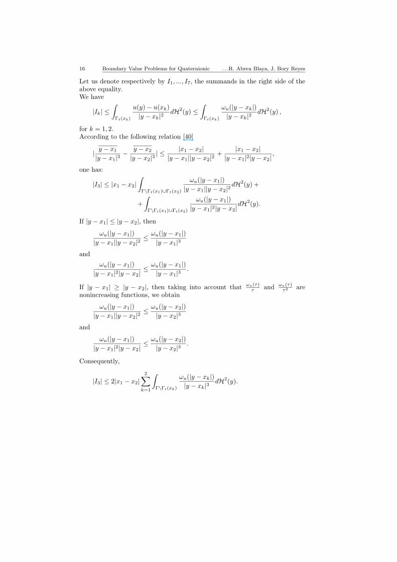
Let us denote respectively by I1, ..., I7, the summands in the right side of theabove equality.We have

|Ik| ≤∫

Γt(xk)

u(y)− u(xk)|y − xk|2

dH2(y) ≤∫

Γt(xk)

ωu(|y − xk|)|y − xk|2

dH2(y) ,

for k = 1, 2.According to the following relation [40]

| y − x1

|y − x1|3− y − x2

|y − x2|3| ≤ |x1 − x2|

|y − x1||y − x2|2+

|x1 − x2||y − x1|2|y − x2|

,

one has:

|I3| ≤ |x1 − x2|∫

Γ\Γt(x1)∪Γt(x2)

ωu(|y − x1|)|y − x1||y − x2|2

dH2(y) +

+∫

Γ\Γt(x1)∪Γt(x2)

ωu(|y − x1|)|y − x1|2|y − x2|

dH2(y).

If |y − x1| ≤ |y − x2|, then

ωu(|y − x1|)|y − x1||y − x2|2

≤ ωu(|y − x1|)|y − x1|3

and

ωu(|y − x1|)|y − x1|2|y − x2|

≤ ωu(|y − x1|)|y − x1|3

.

If |y − x1| ≥ |y − x2|, then taking into account that ωu(τ)τ and ωu(τ)

τ2 arenonincreasing functions, we obtain

ωu(|y − x1|)|y − x1||y − x2|2

≤ ωu(|y − x2|)|y − x2|3

and

ωu(|y − x1|)|y − x1|2|y − x2|

≤ ωu(|y − x2|)|y − x2|3

.

Consequently,

|I3| ≤ 2|x1 − x2|2∑

k=1

∫Γ\Γt(xk)

ωu(|y − xk|)|y − xk|3

dH2(y).

Advances in Applied Clifford Algebras 9, No. 1 (1999) 17

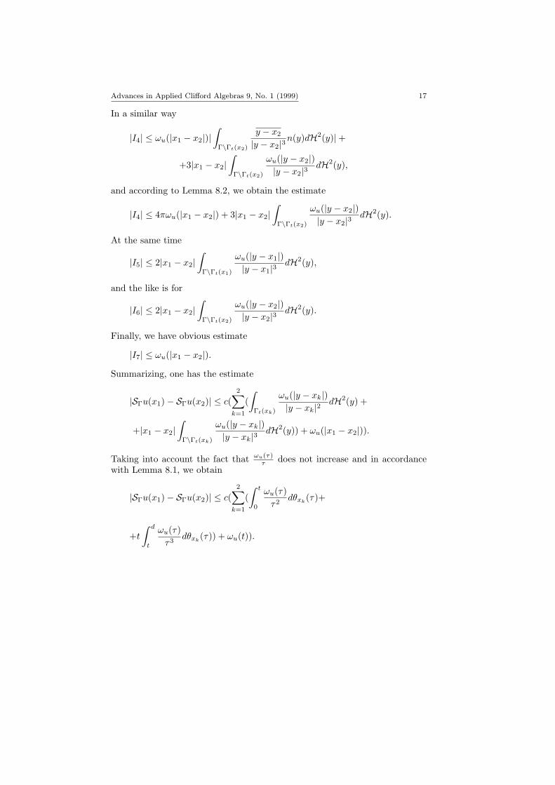
In a similar way

|I4| ≤ ωu(|x1 − x2|)|∫

Γ\Γt(x2)

y − x2

|y − x2|3n(y)dH2(y)|+

+3|x1 − x2|∫

Γ\Γt(x2)

ωu(|y − x2|)|y − x2|3

dH2(y),

and according to Lemma 8.2, we obtain the estimate

|I4| ≤ 4πωu(|x1 − x2|) + 3|x1 − x2|∫

Γ\Γt(x2)

ωu(|y − x2|)|y − x2|3

dH2(y).

At the same time

|I5| ≤ 2|x1 − x2|∫

Γ\Γt(x1)

ωu(|y − x1|)|y − x1|3

dH2(y),

and the like is for

|I6| ≤ 2|x1 − x2|∫

Γ\Γt(x2)

ωu(|y − x2|)|y − x2|3

dH2(y).

Finally, we have obvious estimate

|I7| ≤ ωu(|x1 − x2|).

Summarizing, one has the estimate

|SΓu(x1)− SΓu(x2)| ≤ c(2∑

k=1

(∫

Γt(xk)

ωu(|y − xk|)|y − xk|2

dH2(y) +

+|x1 − x2|∫

Γ\Γt(xk)

ωu(|y − xk|)|y − xk|3

dH2(y)) + ωu(|x1 − x2|)).

Taking into account the fact that ωu(τ)τ does not increase and in accordance

with Lemma 8.1, we obtain

|SΓu(x1)− SΓu(x2)| ≤ c(2∑

k=1

(∫ t

0

ωu(τ)τ2

dθxk(τ)+

+t

∫ d

t

ωu(τ)τ3

dθxk(τ)) + ωu(t)).

18 Boundary Value Problems for Quaternionic . . .R. Abreu Blaya, J. Bory Reyes

Finally, using the inequality θxk(τ) ≤ θ(τ), and the preceding estimate, one is

able to get the desired estimate.

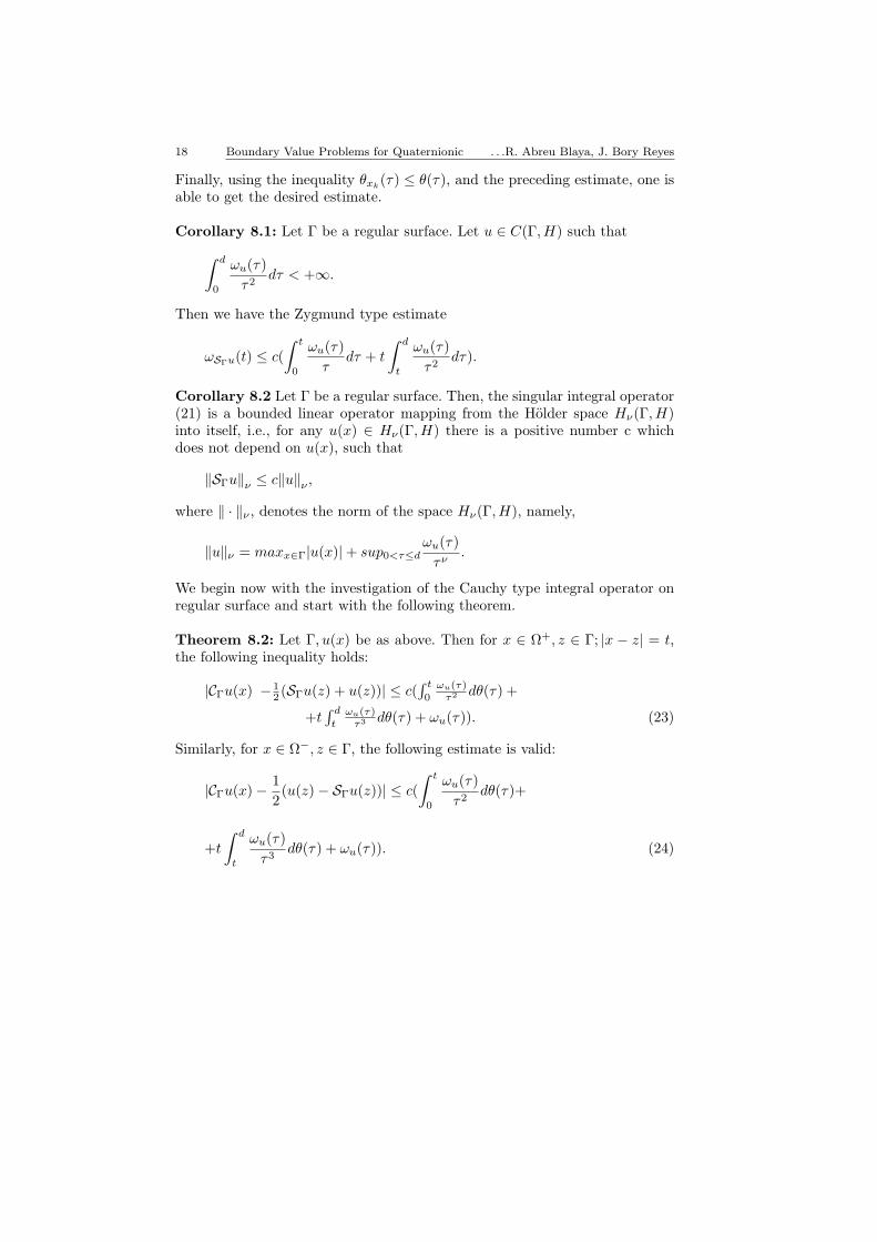
Corollary 8.1: Let Γ be a regular surface. Let u ∈ C(Γ,H) such that∫ d

0

ωu(τ)τ2

dτ < +∞.

Then we have the Zygmund type estimate

ωSΓu(t) ≤ c(∫ t

0

ωu(τ)τ

dτ + t

∫ d

t

ωu(τ)τ2

dτ).

Corollary 8.2 Let Γ be a regular surface. Then, the singular integral operator(21) is a bounded linear operator mapping from the Holder space Hν(Γ,H)into itself, i.e., for any u(x) ∈ Hν(Γ,H) there is a positive number c whichdoes not depend on u(x), such that

‖SΓu‖ν ≤ c‖u‖ν ,

where ‖ · ‖ν , denotes the norm of the space Hν(Γ,H), namely,

‖u‖ν = maxx∈Γ|u(x)|+ sup0<τ≤dωu(τ)

τν.

We begin now with the investigation of the Cauchy type integral operator onregular surface and start with the following theorem.

Theorem 8.2: Let Γ, u(x) be as above. Then for x ∈ Ω+, z ∈ Γ; |x − z| = t,the following inequality holds:

|CΓu(x) − 12 (SΓu(z) + u(z))| ≤ c(

∫ t

0ωu(τ)

τ2 dθ(τ) +

+t∫ d

tωu(τ)

τ3 dθ(τ) + ωu(τ)). (23)

Similarly, for x ∈ Ω−, z ∈ Γ, the following estimate is valid:

|CΓu(x)− 12(u(z)− SΓu(z))| ≤ c(

∫ t

0

ωu(τ)τ2

dθ(τ)+

+t

∫ d

t

ωu(τ)τ3

dθ(τ) + ωu(τ)). (24)

Advances in Applied Clifford Algebras 9, No. 1 (1999) 19

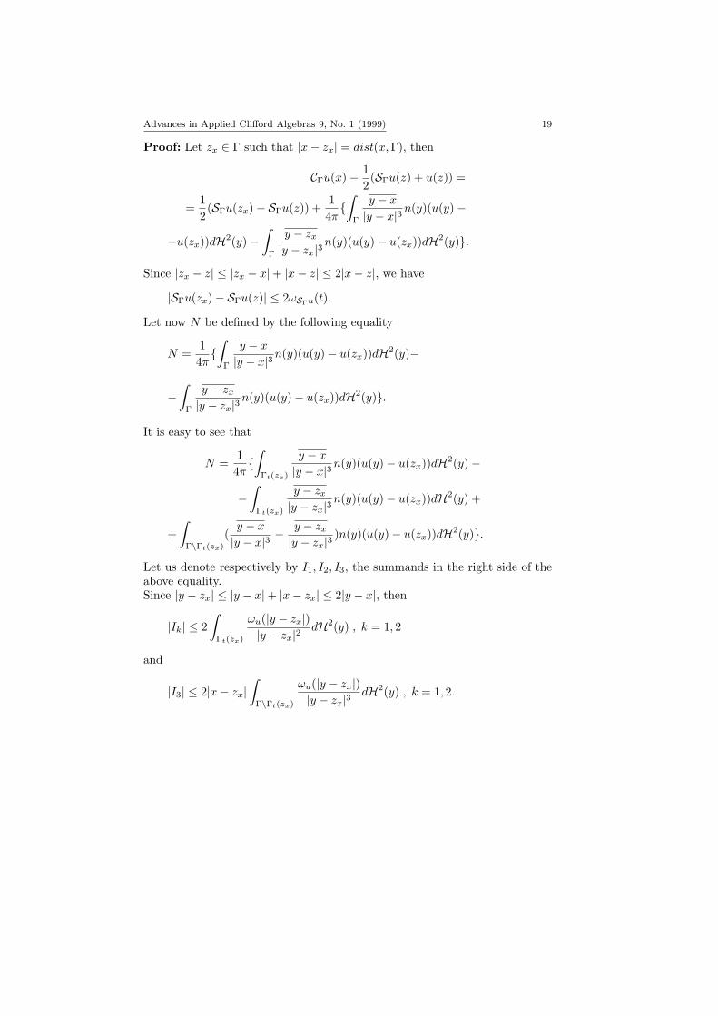
Proof: Let zx ∈ Γ such that |x− zx| = dist(x,Γ), then

CΓu(x)− 12(SΓu(z) + u(z)) =

=12(SΓu(zx)− SΓu(z)) +

14π∫

Γ

y − x

|y − x|3n(y)(u(y)−

−u(zx))dH2(y)−∫

Γ

y − zx

|y − zx|3n(y)(u(y)− u(zx))dH2(y).

Since |zx − z| ≤ |zx − x|+ |x− z| ≤ 2|x− z|, we have

|SΓu(zx)− SΓu(z)| ≤ 2ωSΓu(t).

Let now N be defined by the following equality

N =14π∫

Γ

y − x

|y − x|3n(y)(u(y)− u(zx))dH2(y)−

−∫

Γ

y − zx

|y − zx|3n(y)(u(y)− u(zx))dH2(y).

It is easy to see that

N =14π∫

Γt(zx)

y − x

|y − x|3n(y)(u(y)− u(zx))dH2(y)−

−∫

Γt(zx)

y − zx

|y − zx|3n(y)(u(y)− u(zx))dH2(y) +

+∫

Γ\Γt(zx)

(y − x

|y − x|3− y − zx

|y − zx|3)n(y)(u(y)− u(zx))dH2(y).

Let us denote respectively by I1, I2, I3, the summands in the right side of theabove equality.Since |y − zx| ≤ |y − x|+ |x− zx| ≤ 2|y − x|, then

|Ik| ≤ 2∫

Γt(zx)

ωu(|y − zx|)|y − zx|2

dH2(y) , k = 1, 2

and

|I3| ≤ 2|x− zx|∫

Γ\Γt(zx)

ωu(|y − zx|)|y − zx|3

dH2(y) , k = 1, 2.

20 Boundary Value Problems for Quaternionic . . .R. Abreu Blaya, J. Bory Reyes

Combining the relation |x − zx| ≤ |x − z| with Theorem 8.1 and Lemma 8.1,we obtain the desired estimate (23).

Corollary 8.3: Let Γ and u(x) be the same as in Corollary 8.1. Then thefunction

U (x) =CΓu(x), if x ∈ Ω+

12 [u(x) + SΓu(x)], if x ∈ Γ

is continuous onto Ω+.Moreover, if u(x) ∈ Hν(Γ,H), then U (x) ∈ Hν(Ω+,H).Using the previous theorem one can easily adapt arguments given in [40] todeduce the following

Theorem 8.3: Let Γ be a regular surface. Suppose G(x) and g(x) are givenHolder continuous function on Γ with values in H, and G(x) satisfies the fol-lowing condition:

‖1−G(x)‖ν <1

c + 1,

where c is a positive constant mentioned in Corollary 8.2.Then, there exists a unique solution of the Riemann problem

u+(x)−G(x)u−(x) = g(x), x ∈ Γ, u−(∞) = 0.

References

[1] Abreu R. and J. Bory, Solvability of a Riemann linear conjugation problem ona fractal surface, Extracta Matematicae, 13 (2), 239-141 (1998).

[2] Abreu R. and J. Bory, Removable singularities for quaternionic monogenic func-tions of Zygmund class, Journal of Natural Geometry, (to appear) (1999).

[3] Brackx F., R. Delanghe and F. Sommen, “Clifford Analysis”, Boston, Pitman(1982).

[4] Babaev A. A. and V. V. Salaev, Boudary value problem and singular integralequation on a rectifiable contour, Mat. Zam, 31 (4), 571-580 (1982).

[5] Bari N. K. and S. B. Stieshkin, Best approximations and differential propertiesof conjugate functions, Tr. Mosk. Obsh. Tom., 5, 483-522 (1956).

[6] Coifman R. R., A. McIntosh and Y. Meyer, L’integrale de Cauchy definite unoperator bourne sur L2 pour les courves lipschitziennes, Anaals of Mathematic,116, 361-387 (1982).

[7] David G., Operatours integraux singuliers sur certaines courbes du plan com-

plexe, Ann. Sci. Ecole Norm., Sup 17, 157-189 (1984).[8] David G., Morceaux de graphes Lipschitziens el integrales singularies sur un

surface, Rev. Mat. Iberoamericana, 4, 73-114 (1988).

Advances in Applied Clifford Algebras 9, No. 1 (1999) 21

[9] Dolzhenko E. P., On the removal of singularities of analytic functions, Am.Math. Soc. Transl., 97 (2), 33-41 (1970).

[10] Falconer K. J., “The geometry of fractal sets”, Cambridge. Univ. Press, Cam-bridge (1985).

[11] Federer H., Geometric Measure Theory, Springer-Verlag, Heidelberg/New York(1969).

[12] Feder J., Fractals, Plenum Press, New York (1988).[13] Gajov F. D., Boundary value problems, 3rd ed; “Nauka”, Moskow; English

transl. of 2 nd ed, Pergamon Press, Oxford, (1977); and Addison-Wesley, Read-ing, MA (1966).

[14] Gilbert J. and M. Murray, “Clifford algebras and Dirac operator in harmonicanalysis”, Cambridge University Press, Cambridge (1991).

[15] Gurlebeck K. and W. Sprossig, “Quaternionic analysis and elliptic boundaryvalue problems”, Birkhausser, Boston (1990).

[16] Gurlebeck K., U. Kahler, J. Ryan and W. Sprossig, Clifford analysis over un-bounded domains, Advances in Applied Mathematics, 19, 216-239 (1997).

[17] Iftimie V., Fonctions hypercomplexes, Bull. Math. Soc. Sci. Math. R. S. Ru-manie, 9, 279-332 (1965).

[18] Kats B. A., The Riemann problem on a closed Jordan curve, Sov. Math. (IzVUZ), 27, 83-98 (1983).

[19] Kats B. A., On the Riemann boundary value problem on a fractal curve, Russ.Acad. Sci. Dokl. Math., 48 (3), 559-561 (1994).

[20] Kats B. A., On a version of the Riemann boundary value problem on a fractalcurve, Iz. Vyssh Ochebn Zaved. Mat, 4 (383), 10-20 (1994).

[21] Kolmogorov A. N. and V. M. Tikhomirov, Uspekhi Mat. Nauk., 14 No.2 (86),3-86 (1959); English transl. in Amer. Math. Soc. Transl, (2) 17 (1961).

[22] Lapidus M. L, Fractal drum, inverse spectral problems for elliptic operatorsand a partial resolution of the Weyl-Berry conjeture, Trans. Am. Math. Sci.,325 No.2, 465-529 (1991).

[23] Lord D. L. and A. G. O’Farrell, Removable Singularities for Analytic Functionsof Zygmund Class, Proc. Royal. Irish. Acad., 91A (2), 195-204 (1991).

[24] Lu J. K., “Boundary value problems for analytic functions”, World ScientificPublish. Singapure, New Jersey, London Hong Kong (1993).

[25] Alan McIntosh, Clifford algebras and the higher dimensional Cauchy integral,“Approximation Theory and Function Spaces”, Banach Center. Publications22, 253-267 (1989).

[26] Mandelbrot B. B., The fractal geometry of nature, rev. and enl. ed., W. H.Freeman, New York, N. Y. (1983).

[27] Murray Margaret, The Cauchy integral, Calderon commutators and conjuga-tions of singular integrals in Rm, Transactions of the Am. Math. Soc., 289,497-518 (1985).

[28] Mushelisvili N. I., “Singular integral equations”, Nauka, Moskow, (1968); Eng-lish transl. of 1st ed., Noodhoff, Groningen, (1953); reprint, (1972).

22 Boundary Value Problems for Quaternionic . . .R. Abreu Blaya, J. Bory Reyes

[29] Oboloshvili E., “Effective solution of some boundary value problems in twoand three dimensional cases”, Proceeding of Functional Analytic Methods inComplex Analysis and applications to Partial Diff Equations, World Scientific,149-172 (1988).

[30] Ryan J., “Clifford algebras in analysis and related topics”, CRC Press. BocaRaton, New York. London. Tokyo (1993).

[31] Ryan J., Dirac operator on spheres and hyperbolae, Bol. Soc. Mat. Mexicana,(3) 3, (1996).

[32] Salaev V. V., Direct and inverse estimates for singular Cauchy integral overclosed curves, Tom. 19, No. 3, 365-380 (1976).

[33] Semmes S. W., “Finding structure in sets with little smoothness”, Proceedingsof the International Congress of Mathematics. Zurich, Switzerland, 875-885(1994).

[34] Semmes S. W., Analysis vs. Geometry on a class of rectifiable hypersurfaces inRn, Indiana Univ. Math. Journal, 39 (4), 1005-1035 (1990).

[35] Semmes S. W., Differentiable function theory on hypersurfaces in Rn (Withoutbounds of their smoothness), Indiana Univ. Math. Journal, 39 (4), 1005-1035(1990).

[36] Seifulaev R. K., Boundary values of multidimensional integrals of potentialtype, Russian Academy of Science. Dok. Math., 47 (1), 104-107 (1993).

[37] Stein E. M., “Singular integrals and differentiability property of functions”,Princenton Univ, Press, Princenton, N J (1970).

[38] Shapiro M. and N. Vasilievsky, Quaternionic ψ- hyperholomorphic functions,singular integral operator and boundary value problems I, ψ-hypercomplexfunction theory, Complex Variables, 27, 17-46 (1995).

[39] Shapiro M. and N. Vasilievsky, Quaternionic ψ-hyperholomorphic functions,singular integral operator and boundary value problems II. Algebras of singu-lar integral operators and Riemann type boundary value problems, ComplexVariables, 27, 67-96 (1995).

[40] Xu Z., On linear and nonlinear Riemann-Hilbert problem for regular functionwith values in a Clifford algebras, Chin. Am. of Math., 11B: 3, 349-358 (1990).

[41] Xu Z. and C. Zhou, On boundary value problems of Riemann-Hilbert type formonogenic functions in a half space of Rn, (n ≥ 2), Complex Variables TheoryAppl., 3-4 (1993).

[42] Xu Z. and C. Zhou, “On Riemann-Hilbert problems for nonhomogeneous Diracequation in a half space of Rn”, (n ≥ 2), Clifford algebras in analysis and relatedtopics, Edited by J. Ryan. CRC. Press. Boca Raton, New York. London. Tokyo,285-295 (1996).