Boundary lines within petrologic diagrams which use oxides of ...

Lithos, 22 (1989) 247-263 247 Elsevier Science Publishers B.V., Amsterdam - - Printed in The Netherlands

Boundary lines within petrologic diagrams which use oxides of major and minor elements PETER C. RICKWOOD

Department of Applied Geology, University of New South Wales, Kensington, N.S. W 2033 (Australia)

LITHOS Rickwood, P.C., 1989. Boundary lines within petrologic diagrams which use oxides of major and minor elements. Lithos, 22: 247-263.

Use of some petrologic diagrams applied to analyses of volcanic rocks is unnecessarily difficult due to lack of data for construction of discriminant lines between rock series. Coordinates are provided for sufficient points to enable accurate plotting of the boundary lines within seven diagrams, viz.: ( 1 ) T A S -

total alkalies (Na20+K20) vs. SIO2; (2) K20 vs. SiO2; (3) AFM; (4) Jensen; (5) KTP - K20-TiO~- P205; (6 )FMS- (FeO*/MgO) vs. SIO2; and (7) TAKTIP- K20/(Na20+K20) vs. TiOz/P2Os. Differ- ent versions of these boundaries are collated to indicate their variable position, and it is demonstrated that inter-laboratory analytical precision suffices to account for almost all of their spread on the TAS and K20 vs. SiO2 diagrams.

(Received November 4, 1986; revised and accepted December 28, 1988 )

I. Introduction

It is quite commonplace for geologists to plot analyses of igneous rocks on various diagrams either to ascertain a rock name (e.g., Le Bas et al., 1986) or to identify the rock series to which their data have greatest affinity (e.g., Irvine and Baragar, 1971). Generally, it is inadvisable to plot new analyses di- rectly on the originators' published diagrams because:

( 1 ) most of them have been printed at a size too small for convenient re-use, e.g. Irvine and Baragar ( 1971, fig. 2A, p.528; fig. 3B, p.532);

(2) the grid lines needed for accurate plotting are usually omitted, e.g. Kuno ( 1968, fig. 14, p.649);

(3) they are often cluttered with data points plotted by the originator, e.g. MacDonald and Katsura ( 1964, fig. 1, p.87);

(4) journal, or monograph, vandalism is not popular with librarians and, in any case, data can only be plotted on the original diagram on a small number of occasions before erasure of previous data becomes incomplete, or causes irreparable damage.

Even if a particular diagram is printed at an ade- quate size and tracing paper is superimposed, then

item (2) usually proves to be a serious stumbling block. Most of these diagrams have only one set of scales for each parameter, e.g. Kuno ( 1966, fig. 2, p. 198) so that grid lines have to be constructed as- suming that no distortion occurred during photo- graphic reproduction of the original line drawing or during printing. Enlargement, either photographi- cally, or by a photocopier, often results in distortion although some modern, better quality, equipment introduces very little. Hence it is usually necessary to redraw the scales and discriminant lines on a new piece of graph paper, and what at first appears to be a simple procedure proves difficult because few originators of such graphs have published coordinates for points on their demarcat ion lines.

The purpose of this paper is to provide coordinates for the boundary lines on a number of diagrams that utilise the major and minor elements which are conventionally reported as oxide percentages. Similar diagrams utilising trace elements (e.g., Pearce and Cann, 1973; J.H. Wilkinson and Cann, 1974; Floyd and Winchester, 1975; Winches- ter and Floyd, 1976, 1977 ) warrant separate discussion at another time.

The different boundary lines that have been pub-

0024-4937/89/$03.50 © 1989 Elsevier Science Publishers B.V.

248

lished are collated on the figures given here. These lines are empirical and were constructed by their originators on the basis of the data at hand. As such, the lines should not be construed as rigid boundaries and the variation in their position is some in- dication of their wooliness; a demarcation band or zone is probably more applicable in most cases but less easy to work with.

2. Discrimination between rock series

2.1. The TAS diagram - Alkaline~sub-alkaline rock series (I)

The weight % total alkalies ( N a 2 0 + K 2 0 ) vs. SiO 2 Harker diagram, which Le Maitre (1984) called TAS, is one of the most frequently used by petrologists. It enables both assignment of volcanic rock names (e.g., Cox et al., 1979; Kremenetskiy et al., 1980; Middlemost, 1980; Le Maitre, 1984; Le Bas et al., 1986) as well as discrimination between rocks of the alkaline and sub-alkaline series. For the latter purpose MacDonald and Katsura ( 1964, fig. 1, p.87) and MacDonald ( 1968, fig. l, p.481; fig. 7, p.514) published dividing lines based on analyses of Hawaiian volcanic rocks, whereas Kuno's ( 1966, fig. 2, p.198; 1968, fig. 2, p.627) line was based on analyses of Cenozoic basalts from Eastern Asia. The Hawaiian data were divided by straight lines which are essentially one and the same, although they differ in length (Fig. 1 ). However, Kuno ( 1966, fig. 2, p. 198; 1968, fig. 2, p.627 ) found it necessary to utilise a curved dividing line which is very similar in position to the Hawaiian lines in the region of 46- 56% SiO2 but curves to lower total alkali values at high SiO 2 concentrations. Based on analyses of rocks from a large number of areas, Irvine and Baragar ( 1971, p.531 ) obtained a curved dividing line that is mostly above all other lines, but their equation (Irvine and Baragar, 1971, p.547) yields a second line that is in a slightly different position, particularly at high and low silica values.

Coordinates for all of these lines are given in Ta- ble 1 and they have all been plotted on Fig. 1, together with the template of the IUGS classification for which Le Bas et al. (1986, fig. 1, p.746) gave coordinates; this template differs only slightly from its precursor (Le Maitre, 1984; fig. 1, p.245). To avoid confusion, the schemes of Cox et al. (1979,

fig. 2.2, p.14), Kremenetskiy et al. (1980, fig. 2, p.58) and Middlemost (1980, fig. 1, p.54) have been omitted as they appear to have been superseded. Kuno ( 1966, fig. 2, p. 198; 1968, fig. 2, p.627) also plotted a line discriminating high-alu- mina basalts from tholeiites but this is less com- monly utilised at the present time so it too has been left off this already complex figure.

All of the proposers of the lines given in Fig. 1 regarded them as separating the alkaline rock series from the tholeiitic rock series, although Kuno ( 1966, p. 197 ) suggested "pigeonitic rock series" as an alternative name for the latter. Chayes (1966) cogently argued for substitution of the term "subalkaline" for "tholeiitic" but J.F.G. Wilkinson ( 1968, p. 171 ) included both the tholeiitic and calc-alkali series under the heading "subalkaline" - a practice that has been widely adopted. An objection to use of geological names that include "alkaline" was raised by Miyashiro ( 1974, p. 322 ) as that term has a different meaning to chemists; instead he preferred to use "alkalic", e.g. "non-alkalic" and "calc- alkalic", but this has not been followed by many geologists.

There is a continuous gradation between analyses of rocks from these series (Miyashiro, 1974, p. 323 ) and so any boundary is necessarily artificial. The magnitude of difference in position between these published boundary lines is discussed in Section 4, and here it suffices to note that rocks with analyses which plot within the band defined by extreme variations of these lines cannot be reliably assigned to either alkaline or sub-alkaline groups. This band is approximately defined by points with coordinates (40, 0.45), (45, 2.8), (50, 4.75), (55, 6.5), (60, 8.0), (65, 9.6), (70, 11.1 [by extrapolation] ) and (40, 0.3), (45, 2.2), (50, 3.9), (55, 5.7), (60, 6.8), (65, 7.35), (70, 7.85).

2.2. The K20 vs. Si02 diagram - Shoshonite/sub- alkaline rock series (II)

Discrimination between analyses of rocks of the shoshonite and sub-alkaline orogenic series can be made using the diagram of weight % K20 vs. SiO2 that was published by Peccerillo and Taylor ( 1976, fig. 2, p.66 ). This was extended to more basic rocks by Ewart (1979; 1982, fig. 1, p.40) and was modified by Innocenti et al. ( 1982, fig. 3b, p.334), Carr ( 1985, fig. 4, p. 174) and also by Middlemost ( 1985,

249

0

0

Z

o~

_E O3

(D

16 , I i ~ I ' ' i , I i , , , I ' ' ' ' ] ' ' ' ' I ' ~ i i I r i i i I ' F , , I '

Alkaline Series

/ ~ / / - - . . . . . - -~"

4

//J.//~ Sub alkaline or Tholeiite Series

/ . / . /

40 50 60 70

Weight % SiO 2

Fig. 1. The TAS diagram - Weight % total alkalies ( N a 2 0 + K 2 0 ) vs. SiO2 on an H20- and CO2-free basis. Symbols: + = M a c - Donald and Katsura ( 1964, fig. 1, p.87 ); × = M a c D o n a l d ( 1968, fig. 1, p,481 ), • = MacDona ld ( 1968, fig. 7, p.514 ); • = Kuno ( 1966, fig. 2, p. 198); 0 = Irvine and Baragar ( 1971, fig. 3B, p .532) ; • = Irvine and Baragar ( 1971, p .547) . Coord ina tes for the solid lines jo in ing these symbols are given in Table 1. Dotted lines are boundar ies to l U G S volcanic rock names specified by Le Bas et al. (1986) .

TABLE1

Coordinates for points on boundary lines on the TAS diagram (Fig. 1 )

Symbol in Fig. 1

Author (s) Coordinates (SiO> totaI alkalies ) Line type

+ MacDonald and Katsura ( 1964, (41.75, 1 ) to (52.5, 5 ) straight fig. 1, p.87)

× MacDonald ( 1968, fig. 1, p.481 (39.8, 0.35 ) to (65.5, 9.7) straight • MacDonald ( 1968, fig. 7, p.514) (38.8, 0) to (60, 7.5) straight • Kuno (1966, fig. 2, p.198; 1968, (45.85, 2.75), (46.85, 3), (50,3.9), (50.3, 4), (53.1, 5), (55, 5.8), curved

fig. 2, p.627) (55.6, 6), (60, 6.8), (61.5, 7), (65,7.35), (70, 7.85), (71.6,8), (75, 8.3), (76.4, 8.4)

(39.2,0), (40, 0.4), (43.2, 2), (45, 2.8), (48, 4), (50, 4.75), (53.7,6), (55, 6.4), (60, 8), (65, 9.6), (66.4, 10)

(39, 0), (41.56, 1 ), (43.28, 2), (45,47, 3), (48.18, 4), (51.02, 5), (53.72, 6), (56.58, 7), (60.47, 8), (66.82, 9), (77.15, 10)

• Irvine and Baragar ( 1971, fig. 3B, p.532)

• lrvine and Baragar ( 1971, p.547)

curved

curved (computed)

fig. 6.1.1, p.121 ). In each of these diagrams the shoshonite (sometimes called an association, e.g. Morrison, 1980, p.97), high-K talc-alkaline, calc- alkaline and tholeiite [sometimes called island arc tholeiite, e.g. Jakeg and Gill ( 1970, p. 18 ) or low-K, e.g. Ewart (1982, p.29)] series occur at progres- sively decreasing weight % K20 and are separated

by single or compound straight lines of positive slope. Vertical lines (constant, integer, weight % SiO2) serve to subdivide the series into rock types, but authors differ on the position of these and also on the starting and terminating points of the slop- ing lines. Details of these variations are given in Ta- ble 2 where K20 coordinates are given that have

250

T A B L E 2

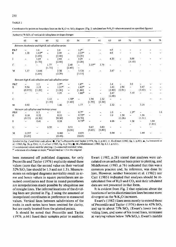
Coordinates for points on boundary lines on the K20 vs. SiO2 diagram ( F i g . 2 ; tabulated are % K20 values measured on specified figures)

Author ( s ) % S i O 2 of vertical dividing lines or slope changes

4 5 4 8 4 9 5 2 5 3 5 6 5 7 6 1 6 3 6 9 7 0 7 5 7 6 7 8

Between shoshonite and high-K calc-alkaline series."

P & T 1 . 6 2 . 4 - 3 . 2 *l - 4 . 0 - -

E 1 . 3 8 1 . 6 3 *~ - 2 . 3 9 - 3 . 2 2 *~ - 4 . 0 - -

[ 1 . 6 0 1 [ 2 . 4 0 ] [ 3 . 2 0 ]

1 1 . 6 9 - 2 . 4 3 - 3 . 2 9 - 4 . 2 0 - 5 . 0 9

[ 1 . 7 0 ] [ 2 . 5 0 ] [ 3 . 3 0 ] [ 5 . 1 0 ]

C 1 . 7 7 - 2 . 4 8 - 3 . 1 5 *~ 3 . 7 5 - - -

[ 1 . 7 5 ] - [ 2 . 4 5 ] -

M 1 . 3 7 1 . 6 4 6 - 2 . 3 8 - 3 . 1 2 6 - 3 . 8 7 - -

[ 1 . 6 5 ] ( 2 . 3 9 ) [ 3 . 1 3 ]

Between high-K calc-alkaline and calc-alkaline series:

P & T 1 . 2 - 1 . 5 *2 - 1 . 8 *~ - - 2 . 4 - 3 . 0 - - -

E 0 . 9 4 1 . t 9 - 1 . 5 1 *~ - 1 . 8 2 *~ - - 2 . 4 2 2 . 9 4 - 3 . 4 7 - -

( 0 . 9 7 5 ) [ 1 . 2 0 ] - [ 1 . 5 0 ] - [ 1 . 8 0 1 - - [ 2 . 4 0 ] ( 2 . 9 1 ) - ( 3 . 4 3 ) - -

I - - 1 . 3 5 1 . 8 6 *~ - - 2 . 4 7 - 3 . 1 0 - - -

( 2 . 4 8 )

C - 1 . 1 2 - 1 . 5 8 " 1 . 9 4 2 . 3 2 . . . . . .

[ 1 . 1 0 ] [ 1 . 6 0 ] [ 1 . 9 5 ] [ 2 . 3 0 ]

M 0 . 9 2 - - 1 . 4 6 1 . 7 7 - - 2 . 3 2 - - 3 . 2 5 - -

Between calc-alkaline and tholeiite series: P & T - 0 . 3 - 0 . 5 0 . 7 *~ - - 1 . 0 - 1 . 3 *~ - - 1 . 6

E 0 . 1 8 0 . 3 2 - 0 . 5 2 0 . 7 2 *~ - - 1 . 0 1 . 3 0 - 1 . 5 6 - -

( 0 . 1 5 ) [ 0 . 3 0 ] [ 0 . 5 0 ] [ 0 . 7 0 ] ( 1 . 2 6 ) ( 1 . 5 1 )

I - 0 . 4 1 - 0 . 5 8 0 . 7 5 *~ - - 1 . 0 6 - 1 . 3 8 - 1 . 6 4 - - [1.65]

C - - 0 . 3 5 - 0 . 5 1 0 . 6 7 0 . 8 3 . . . . .

[ 0 . 5 0 1 [ 0 . 6 5 ) [ 0 . 8 0 1 -

M 0 . 1 9 7 - - 0 . 4 8 1 0 . 6 5 1 - - 0 . 9 4 - 1 . 4 4 -

[ 0 . 2 0 ] ( 0 . 4 9 ) ( 0 . 6 5 )

Symbol in Fig. 2 and letter code above: 0 , P & T = Peccerillo and Taylor ( 1 9 7 6 , f i g . 2 , p . 6 6 ) ; X , E = E w a r t ( 1 9 8 2 , f ig . 1, p . 4 0 ) ; A , I = I n n o c e n t i e t

al. ( 1 9 8 2 , f ig . 3 b , p . 3 3 4 ) ; + , C = C a r r ( 1 9 8 5 , f i g . 4 , p . 7 4 ) ; I , M = M i d d l e m o s t ( 1 9 8 5 , f i g . 6 . 1 . 1 , p . 1 2 1 ) .

( ) =computed values used for plotting; [ ] = a s s u m e d rounded value. , 1 = location of a change in slope; *2misprinted as 1 . 3 in the original.

been measured off published diagrams, for only Peccerillo and Taylor (1976) explicitly stated these values (note that the second value on their vertical 52% SiO2 line should be 1.5 and not 1.3 ). Measure- ments on enlarged diagrams inevitably result in er- ror and hence values in square parentheses are assumed coordinates and those in round parentheses are interpolations made possible by ubiquitous use of straight lines. The inferred locations of the dividing lines are plotted in Fig. 2 using the assumed or interpolated coordinates in preference to measured values. Vertical lines between subdivisions of the rocks in each series have been omitted for clarity, but are easily located from the plotted points.

It should be noted that Peccerillo and Taylor ( 1976, p.66 ) fused their samples prior to analysis,

Ewart (1982, p.28) stated that analyses were calculated on an anhydrous basis prior to plotting, and Middlemost ( 1985, p.76) indicated that this was a common practice and, by inference, was done by him. However, neither Innocenti et al. (1982 ) nor Carr (1985) indicated that analyses should be recalculated free of H20 and COz and their tabulated data are not presented in that form.

It is evident from Fig. 2 that opinions about the locations of series discrimination lines become more divergent as the % KzO increases.

Ewart's (1982) lines seem mostly to extend those of Peccerillo and Taylor ( 1976 ) down to 45% SiO2 and up to about 75% S i O 2 (Ewart's lower two dividing lines, and some of his trend lines, terminate at varying values below 76% SiO2). Ewart's middle

251

. . . . I . . . . I . . . . I . . . . I . . . . I . . . . I

i - 5 - f

S h o s h o n i t e S e r i e s 7 / "

J -"

j i 7

f • •

o ~ 3 / ~ . ~ . / ~ i g h - K ( C a l c - a l k a l i n e ) S e r ~ s / ~ . Y j ~ ' ' ' ~

I ~ ' ~ . J C a l c - a l k a l i n e S e r i e s / / 2 x . . . ~ . . / " ~

l . . . . I . . . . I , , , , I , , , , I , , , , I , , , , I , , 4 5 5 5 6 5 7 5

Weight % SiO 2

Fig. 2. The KyO vs. SiO2 diagram - weight percentages on an H20- and COy-free basis. Symbols: • = Peccerillo and Taylor ( 1976, fig. 2, p.66); × =Ewart ( 1982, fig. l, p.40); • =Innocenti et al. ( 1982, fig. 3b, p.334); + =Carr ( 1985, fig. 4, p.74); I=Mid- dlemost ( 1985, fig. 6. I. 1., p. 121 ). Broken lines, joining triangles, signify less reliability. Coordinates for points marked by various symbols are given in Table 2.

line appears to have a change in slope at 52% SiO2 whereas Peccerillo and Taylor drew no such deflec- tion, and, conversely, Ewart's lower line is straight above 56% SiO2 yet PecceriUo and Taylors' coordinates signify a slope change at 70% SiO2. But these are trivial differences, the first of which has not been indicated in Fig. 2 where the originators' version has been preferred.

Innocenti et al. ( 1982, fig. 3 caption, p.334) stated that their inset was a modified version of Peccerillo and Taylor's (1976) diagram, but it lacks a vertical scale so could not be used to obtain coordinates. The drafting of their figures is such that series dividing lines have similar shapes in both the inset and fig. 3b (all being compound and changing slope at 56% SiOy) yet in fig. 3a the middle line is virtually straight, and the slope of the lower line decreases above 56% SiO2 whereas it increases in the other two diagrams. For these reasons all coordinates have been determined from fig. 3b, despite its poor drafting quality; they must, therefore, be regarded as very

approximate. Consequently, the series dividing lines of Innocenti et al. are plotted as broken lines in Fig. 2 and have only been retained because they are based on more potassic rocks than other authors analysed - the upper line therefore being of particular interest. Their upper and lower series dividing lines are above all others, and the middle line only crosses those of other authors towards its lowest point, the position of which is likely to have been guided by the misprinted coordinates (52, 1.3) of Peccerillo and Taylor ( 1976, fig. 2, p.66).

Carr's (1985, fig. 4, p.74) graph only extended over the range 49-61% SiO2 but his upper and lower series dividing lines are the lowest encountered. The upper half of his middle line duplicates that of ln- nocenti et al. and as such is higher than others, yet below 53% SiOz it crosses them all.

Middlemost ( 1985, fig. 6.1.1, p. 121 ) utilised the same silica range as Ewart (1982) but his three lines are distinctly different from those proposed by other

252

authors and above 61% SiO2 all three of his lines are the lowest of their group.

Peccerillo and Taylor ( 1976 ) subdivided the four series by vertical lines and allocated 16 rock names to the pigeon holes so formed. Ewart (1982) added two new names [basalt (high-K) and rhyolite (high- K) ] and moved the 70% SiO2 divider to 69%. Later, Innocenti et al. (1982) substituted shoshonitic basalt and latite for absarokite and banakite, respectively, and introduced a pigeon hole for trachyte by extending the upper series dividing line. However, they retained the vertical lines of Peccerillo and Taylor. Carr's ( 1985, fig. 4, p.74) modifications of the Peccerillo and Taylor diagram are the most drastic. His vertical boundaries to series subdivisions are quite different and he recognised only basalts, basaltic andesites and andesites. Middlemost (1985) did not indicate preferred rock names and only retained the vertical dividers at 52%, 56% and 63% SiO2. These differences in position and names of pigeon holes have been omitted from Fig. 2 for the sake of clarity.

Analyses which plot within bands that embrace these various lines cannot be reliably assigned to a rock series. Coordinates of points on upper and lower boundary lines of such bands are:

Shoshonite high-K series: (45, 1.38), (48, 1.7), (56, 3.3), (63, 4.20), (70, 5.1) and (45, 1.37), (48, 1.6), (56, 2.98), (63, 3.87), (70, 4.61 [by

extrapolation ] )

High-K/ calc-alkaline series: (45, 0.98), (49, 1.28), (52, 1.5), (63, 2.48), (70, 3.1), (75,

3.43) and (45, 0.92), (49, 1.1 ), (52, 1.35), (63, 2.32), (70, 2.86), (75,

3.25)

Calc-alkaline/~w-Kseri~: (45, 0.2), (48, 0.41), (61, 0.97), (70, 1.38), (75, 1.51) and (45,0.15),(48,0.3), (61,0.8), (70,1.23),(75, 1.44)

2. 3. The A F M diagram - Tholeiite/calc-alkaline rock series (III)

Subdivision of sub-alkaline rocks into tholeiite and calc-alkaline series can be made on the basis of the plotted position of chemical data in an A F M diagram, where the apices are weight % (Na20 + K20), (total Fe as FeO) and MgO. For this purpose, Kuno (1968, fig. 14, p.649) published a dividing line which was empirically derived from Japanese rocks, whereas Irvine and Baragar ( 1971, fig. 2A, p.528) used analyses of rocks from many suites to locate a dividing line but they also pre-

I

sented an equation (Irvine and Baragar, 1971, p.547) which purported to represent it. Coordi- nates of various points on these lines as measured on the published diagrams, together with those calculated from Irvine and Baragar's (1971, p.547) equation, are given in Table 3 and all three lines are plotted in Fig. 3. Kuno's boundary line yields a smaller area for the tholeiite series than do those of Irvine and Baragar, being markedly divergent from the latter near the F - M tie line. The equation given by Irvine and Baragar yields a line which deviates slightly from their plotted boundary, particularly near the A-Ftie line, but it seems to be a reasonable mathematical equivalent.

It should be noted that Irvine and Baragar ( 1971, p.528) referred to F as (FeO+0.8998Fe203); the factor simply being that to convert weight % Fe203 to weight % FeO. Many users of the diagram merely label the F-apex (FeO+Fe203), e.g. Rivalenti

TABLE 3

Coordinates for points on boundary lines on the AFM diagram (Fig. 3 )

Symbol in Fig. 3

Author(s) Coordinates (A,F,M)

• Kuno ( 1968, fig. 14, p.649)

* lrvine and Baragar ( 1971, fig. 2A, p.528)

• Irvine and Baragar ( 1971, equation, p.547 )

(72, 24, 4), (50,39.5, 10.5), (34.5, 50, 15.5), (21.5, 57, 21.5), (16.5, 58, 25.5), (12.5, 55.5, 32), (9.5, 50.5, 40)

(58.8, 36.2, 5), (47.6, 42.4, 10), (29.6, 52.6, 17.8), (25.4, 54.6, 20), (21.4, 54.6, 24), (19.4, 52.8, 27.8), (18.9,51.1,30), (16.6, 43.4, 40), (15,35,50)

(70, 30, 0), (62.1, 32.9, 5), (47.4, 42.6, 10), (34.3, 50.7, 15), (25.7, 54.3, 20), (21.1, 53.9, 25), (19.2,50.8, 30), (18.3,46.7, 35), (17.5, 42.5, 40), (16.1, 38.9, 45), (14.4,35.6, 50), (12.6, 32.4, 55), (11.2, 28.8, 60), (10.4,24.6, 65), (10.1, 19.9, 70), ( 10.3, 14.7, 75), ( 10.3, 9.7, 80), ( 10.0, 5.0, 85), (9.2, 0.8, 90).

Key: A = (Na20 + K20); F= total Fe as FeO; M= MgO - all weight percentages.

F

A M

Fig. 3. The AFMdiagram- weight % (Na20+K20), (total Fe as FeO), MgO. Symbols: I =Kuno ( 1968, fig. 14, p.649 ); , = Irvine and Baragar ( 1971, fig. 2A, p.528); • = Irvine and Baragar (1971, p.547 - equation). Coordinates for marked points on the boundary lines are given in Table 3.

( 1975, fig. 2, p .724) as indeed did K u n o ( 1968, fig. 14, p .649) , but whereas the lat ter d id state in the text (p .632) that the apex was " F e O + F e 2 0 3 (as F e O ) " , the fo rmer offered no such explanat ion and one is forced to conclude that no ad jus tmen t o f Fe203 was made . Pearce et al. ( 1975, p .420) specifically referred to the " A F M diagram ( Fe203 + FeO )- M g O - ( N a 2 0 + K 2 0 ) , all in weight pe rcen t" so seemingly leaving no doubt that raw percentages were used. The mos t clear, unambiguous , labelling o f the F-apex is that o f Johnson et al. ( 1985, fig. 8, p .298) who stated " i ron-ox ide (F, total Fe as F e O ) " .

To invest igate the effect o f ignoring this conver- sion, calculat ions were made using weight percentages of total alkalies = MgO = 5 (so that da ta plot on the perpendicu la r to the A - M l ine) and weight % FeO = weight % Fe203 = 1 to 15. It was found that if Fe203 is adjus ted to equivalent FeO then, com- pared to unadjus ted data, the F-coord ina te decreases by about 1% (e.g., 16.6 to 16, 37.5 to 36.3, 50 to 48.7, 70.6 to 69.5) . Thus failure to make the ad jus tment is unlikely to produce serious misplot - ting, nevertheless the p roponen t s of the discr imi- nant lines did in tend that the ad jus tment should be done to compensa te for oxidat ion.

As a caut ionary step it should be no ted tha t Mi- yashiro (1974) wrote that the calc-alkaline and tholeii te series (p. 325):

"... do not represent two discrete trends of magmatic evo-

253

lution but represent two artificially defined divisions of continuously variable and diverse trends."

and (p. 327) that:

'%.. use of alkali contents in the distinction ... may be misleading."

Subsequently, the A F M diagram was specifically criticized by Jensen ( 1976, p.5 ) as somet imes being:

"... misleading in discerning rock chemical trends."

and Morr i son (1980, p .98) caut ioned that shosh- onit ic rocks usually plot in the alkaline rock series field of the TAS diagram but occur in the calc-alkaline field of the A F M diagram.

2.4. The Jensen diagram - Komatii te/tholeii te/ calc-alkaline series (IV)

Geologists working with komat i i tes have adopted the Jensen ( 1976, fig. 1, p .7) d iagram for chemical classification o f their rocks. Its au thor advoca ted even wider uses for it and d iscr iminat ion between tholeiite, calc-alkaline and komat i i t e rock series is

FeO + Fe203 + TiO 2

AI203 MgO

Cation %

Fig. 4. The Jensen diagram - cation % A1203, (FeO+Fe203+TiO2), MgO. Solid lines separate tholeiite (T), calc-alkaline (C) and komatiite (K) fields, and broken lines subdivide these. Solid circles are locations on the one curved line and their coordinates are given in Table 4 together with coordinates of end-points for all other boundary lines. The lines making an isolated, inverted, K are boundaries proposed by Viljoen et al. ( 1982, fig. 4.6, p.69 ); the solid line separating komatiites from tholeiites with the latter subdivided by broken lines into Mg-, normal and Fe-tholeiites. All other lines are from Jensen and Pyke (1982, fig. 11.3, p.149).

254

TABLE 4

Coordinates for points on boundary lines on the Jensen diagram (Fig. 4)

Author (s) Coordinates (A,F,M)

Jensen (1976);Jensen and Pyke(1982)

Viljoen etal.(1982)


Jensen and Pyke (1982)

Viljoen et al. (1982)

Jensen (1976);Jensen and Pyke(1982) Jensen (1976)


SERIES BOUNDARY

Tholeiite-komatiite series:

Tholeiite-calc-alkaline series:

SUB DIVISIONS

Komatiite series: basaltic komatiite-ultramafic komatiite

(komatiitic peridotite ) Tholeiite series: normal tholeiite-Mg-tholeiite normal tholeiite-Fe-tholeiite high-Fe tholeiitic basalt-high-Mg tholeiitic basalt andesite-high-Fe tholeiitic basalt

Tholeiite series: Calc-alkaline series: andesite-dacite basalt-andesite dacite-rhyolite andesite-dacite

dacite-rhyolite

(50, 0, 50) to (22.5, 55, 22.5)

(24, 76, 0) to (48.5, 0, 51.5 ) between F60 and F28.5 contours

(locations shown by solid circles ) (90, 10, 0), (50.7, 27.6, 21.7), (51.5,29,9.5),

(53.5,28.5, 18), (50.5, 27.5, 22), (50.3,25,25.7), (50.8, 20, 29.2), (51.5, 12.5, 36)

(40, 0, 60) to (0, 40, 60)

(48.5, 30, 21.5) to (35.7, 40, 24.3) (45, 46, 9) to (35.7, 40, 24.3) (33.3, 33.3, 33.3) to (50, 25, 25) (50, 50,0) to (50, 35, 15) (50, 33.5, 16.5) to (51.5, 29, 9.5)

(60, 40, 0) to (60, 10, 30) (70, 30, 0) to (70, 0, 30) (80, 20, 0) to (80, 0, 20)

Key: A = A1203; F= (FeO + Fe203 + TiO2);M= MgO - all cation percentages. Sources: Jensen ( 1976, fig. 1, p.7 ); Jensen and Pyke ( 1982, fig. 11.3, p. 149 ); Viljoen et al. ( 1982, fig. 4.6, p.68 ).

of paramount importance to the present discussion. This scheme is shown in Fig. 4 together with the variation proposed by Viljoen et al. ( 1982, fig. 4.6, p.69 ) who found it necessary to move the boundary between tholeiites and komatiites towards the A1203 apex. At the same time, Viljoen et al. subdivided tholeiites into Fe-, normal and Mg-types, so that their boundaries form an isolated, inverted, K in Fig. 4. On another copy of his diagram, Jensen (1976, fig. 2, p.8 ) helpfully indicated the locations of tholeiitic, calc-alkaline and komatiitic trends which occur in widely separated areas, passing through or near the letters T, C and K given in Fig. 4. Jensen ( 1976, pp.2 and 3) explained that:

"..., the curved line dividing tholeiitic and calc-alkalic fields corresponds closely to those employed on the A F M diagram ... by Irvine and Baragar ( 1971 ) ."

and the broken lines subdividing the tholeiite and calc-alkaline series were also based on proposals by

them. The publication containing this original diagram

can be difficult to procure but a later version is readily available (Jensen and Pyke, 1982, fig. 11.3, p. 149); it differs only by expansion of the ultramafic komatiite field by 10% MgO and by omission of a small straight line closing offthe andesite field. This later version has been used in Fig. 4, and the small omission has been reinstated; Table 4 contains coordinates for points on all of the lines in Fig. 4.

It was emphasised by Jensen (1976, p.2) that deuteric and metamorphic processes, which tend to change the concentrations of K20, Na20, CaO and/ or SiO2, have little effect on the components re- quired to plot an analysis in a Jensen diagram. Yet another advantage is that it uses cation percentages of A1203, (FeO + Fe203 + TiO2) and MgO so there are no conflicts about adjustment of iron oxides.

255

0 4

% 12-

C"

~ 2

' ' I

/

J /

' I ' I I . . . . I . . . . I

o 1

Tholeiite Series

÷

Calc-alkaline Series 1 - !

/

f

/

f

J /

o . . . . I . . . . I . . . . I , , , , I , , , , I , , , , I , , , , 50 60 70 80

Weight % SiO 2

Fig. 5. The F M S diagram - weight % FeO*/MgO vs. SiO2. FeO* is total Fe expressed as FeO. S y m b o l s : + = signifies points given by Miyashiro (1974, p.323); • = signify end-points of the range of successful discrimination for which coordinates are (55.6, 2.0) and (74.8, 5.0).

2.5. The F M S diagram - Calc-alkaline/tholeiite series ( V)

Miyashiro ( 1973, p.219 ) claimed that it was possible to distinguish between analyses of rocks of the calc-alkaline and tholeiite series using two diagrams in which the ratio FeO*/MgO is the abscissa and either weight % SiO2 or weight % FeO* is the ordinate (where FeO* signifies iron totally recalculated to the divalent oxide). Although he was quite ex- plicit in stating that a continuity existed between these rock series he did assign an arbitrary boundary on each of his diagrams - this being straight on the SiO2 diagram and curved on the FeO* diagram. In practice he favoured use of the former which is here called the F M S diagram.

By reversing the ordinate and abscissa that Mi- yashiro used, the F M S diagram becomes a typical Harker diagram and that orientation will be more "comfortable" to most geologists (Fig. 5). Miya- shiro ( 1974, p.325 ) gave coordinates for two points on the boundary line, (46, 0.5) and (62, 30), but later (p.326) indicated that it was successful only between 2.0 < FeO*/MgO < 5.0 so more useful reference points are (55.6, 2.0) and (74.8, 5.0). In Fig.

5 this line has been drawn in solid form only over the range recommended for its use; it is represented by the equation:

FeO*/MgO = 0.15625 SiO2 - 6.6875

3. Environmental discrimination

Geochemical data have also been used to discriminate between environments of igneous activ- ity, and in both of the instances cited here the discriminant diagrams were evolved as a result of analysis of data from many regions of the world.

3.1. The KTP diagram - Oceanic~continental basalts (VI)

Pearce et al. (1975) reported success in use of a triangular diagram (Fig. 6) of the "incompatible" elements K, Ti and P (in their oxide weight percentages) to separate basalts of oceanic and non- oceanic environments. The dividing line is straight, between (K20, 45.5%; TiO2, 54.5%; P2Os, 0%) and (K20, 0%; TiO2, 79.6%; P205, 20.4%) with ocean-

256

T i 0 2

(K O,T79,6,P20.4)

• , 4. ,

K 2 0 P 2 0 5

Fig. 6. The KTP diagram - weight % K20 , TiO2, P205 (Pearce et al., 1975).

floor basalts plotting near the TiO2 apex. They cautioned that this diagram may not work for fractionated and alkaline rocks so these have to be screened out using a weight % A F M diagram with the dividing line being the A = 20% isopleth; analyses of ac- ceptable rocks have A < 20%.

Basalts that seem to plot in the wrong area of the KTP diagram may be either:

( 1 ) Otherwise possessing continental characteristics yet plot in the oceanic area, e.g. (a) Tertiary basalts of the Scoresby Sund area of east Green- land; (b) basalts of west Greenland and Baffin Is- land; (c) basalts of the Deccan Plateau. These were interpreted as indicating (Pearce et al., 1975, p. 421):

"initial rifting of the continent and generation of sea floor"

of the Atlantic Ocean, Labrador Sea and Indian Ocean, respectively.

(2) Otherwise possessing oceanic characteristics yet plot in the continental area of the KTP diagram, e.g. minor volumes o f " 'alkaline' capping basalts" of Oahu and Mauna Kea, Hawaii. However, oceanic basalts rarely plot outside of the oceanic area even when altered or have been metamorphosed, so the diagram is of use for ascertaining provenance of Ar- chaean basalts (Pearce et al., 1975, p.423 ):

"If a metamorphosed basalt analysis plots in the oceanic area then it is very likely of oceanic origin"

3.2. The TAKTIP diagram - Plateau~rift environments (VII)

Chandrasekharam and Parthasarthy ( 1978 ) con- curred with the interpretation by Pearce et al. ( 1975, p.421 ) of the Deccan Plateau basalts, but for their own study of the dykes of that area they wished to discriminate between "rift" volcanics in areas of crustal fragmentation and "plateau" volcanics of true continental origin. To enable this discrimination they utilised a diagram (Fig. 7 ) in which ratios of weight percentages of K20/( to ta l alkalies) were plotted against ratios of weight percentages of TiO2/ P205. The curved discriminant line roughly corresponds to a K20/ ( to ta l alkalies) ratio of 0.2; more accurately it passes through the points ( 1.2, 0.245 ), (2, 0.235), (4, 0.21), (6, 0.2), (8, 0.195), (10, 0.25), (12, 0.325), (13.6, 0.40) where coordinates are TiOz/P2Os, K20 / (Na20 + K20 ).

This method was successfully applied to Scandi- navian dykes by Solyom et al. ( 1985, fig. 4, p.169) who added to the diagram an arrow labelled "To- wards Spreading Axis".

4. Variability of boundary lines

On several of the diagrams presented here there are a number of alternative lines which purport to discriminate between the same rock series, viz. Figs. 1-4, and on each diagram there is a considerable difference between the locations of some of these lines. As these lines were empirically derived by different workers, using analyses obtained in different laboratories, it is pertinent to enquire whether this spread could merely be due to inter-laboratory analytical precision. Almost all of these lines were fit- ted by eye so they lack the status of regression lines, for which confidence bands can be assigned. More- over, two of these diagrams, Figs. 3 and 4, are triangular and data are adjusted to sum to 100% prior to plotting, so complicating any study of the type envisaged. However, Figs. 1 and 2 are more amenable to scrutiny, albeit not necessarily a rigorous evaluation.

4.1. The TAS diagram

There appears to be two distinct sets of lines on Fig. 1; a high set (Irvine and Baragar, 1971 ) and a

257

o cv

Z

+

o c~

© c~

xl

o~ t -

1.0

0 .5

O ~ Q ~

P l a t e a u V o l c a n i c s

. . . . . j ' J

R i f t V o l c a n i c s

o , , , , I ~ f , a I ~ , , 0 5 10 15

W e i g h t % T i O 2 / P 2 0 s

Fig. 7. The TAKTIP diagram - weight % K20/total alkalies (Na20-]-K20) VS. TiOz/P2Os. Chandrasekharam and Parthasarthy ( 1978, fig. 2, p.220 ) with arrow due to Solyom et al. ( 1985, fig. 4, p. 169 ). Coordinates for points on the dividing line are given in the text.

low set (MacDonald and Katsura, 1964; Kuno, 1966, 1968; MacDonald, 1968). Although the sets converge at 39% SiO2, and even have a partial con- vergence at the higher extremity, there is a considerable difference in their location between 40% and 60% SiO2.

The analyses, on which these lines are based, were all made in the late 1950's and 1960's and, as the authors did not state the analytical methods used, it is reasonable to assume that the techniques were largely classical gravimetric. Indeed, MacDonald et al. (1972, p.128) reported that analyses of Ha- waiian lavas were made in Honolulu (150), Tokyo (92) and

"..., about the same number by standard methods in the Denver Rock Analysis Laboratory of the U.S. Geological Survey ...".

MacDonald et al. (1972) arranged for eight rocks to be analysed at both Tokyo and Denver but whilst this replication yielded sufficient data for a quali- tative assessment of bias to be made (MacDonald et al., 1972, p. 139) it did not suffice to quantify inter-laboratory precision. It is fortunate that, at about the period that many of these analyses were made, there was published a collation of data obtained in

a world-wide cooperative investigation of analytical precision. Stevens et al. (1960, tables 3 and 4, pp.31 and 32) reported inter-laboratory precision (expressed as coefficients of variation) for the reference samples W-1 and G-1 as being, respectively, 0.58% and 0.26% for SiO2, 9.46% and 5.74% for Na20, and 6.49% and 5.36% for K20. However, the T A S diagram uses the combined (Na20 q- K20 ) and for this sum the coefficients of variation are 11.47% (W-1) and 7.85% (G-1). Hence if one laboratory obtains analytical results for these rocks that are equal to the mean values reported by Stevens et al., and if some other laboratories were to attempt the analysis using gravimetric techniques, it is probable that 95% would obtain results that are

% SIO2:52.55 + 0.60, 72.46 + 0.37 % (Na20+K20): 2.77+_0.62 and 8.81 _+ 1.36 for W-1 and

G- 1, respectively

It can be seen from Fig. 1 that one of the lines produced by the originator of this subdivision (MacDonald, 1968, fig. 7 ) is the lowest line of all. A point on this line at ( N a 2 0 + K 2 0 ) = 2 . 7 7 % also has a value of 46.63% SiO2 and around that point one can construct an "uncertainty rectangle" with comers, calculated from the data given above, being

258

16

12

© (M

+

o

Z 8

o~

E 03

4 I

, , ~ , r l l , , i . . . . i , , , l l , , i r l , l l l l l , l l t , ~ l ~ l l l

Alkaline Series

i,~/~. Sub-alkaline or Tholeiite Series

i S i , J i

4O 50 6O 70

Weight % SiO 2

t . . . . I . . . . I . . . . I . . . . I . . . . I . . . .

5 ./" / i

S h o s h o n i t e Se r ies /

/ / . •

~ / / A

t ~ _ ~ + ~ ÷ - - L o w - K (Tholeiite) Series

. . . . L . . . . t ", , , , I . . . . I , , , , I . . . . I , ,

45 55 65 75

W e i g h t % S i O 2

Fig. 8. Effect of inter-laboratory precision on the TAS and K20 vs. SiO2 diagrams. Coordinates of comers of"uncertainty rectangles" are given in the text and Table 5. Captions to Figs. 1 and 2 explain the symbols.

TABLE5

Probableinter-laborato~ precision ~rpointsonboundarylinesintheK2Ovs. SiO2di~ram (Fig. 8)

259

Rock Wt.%K20 Corresponding % SiO2 on the boundary lines of Peccerillo and Taylor ( 1976 )

x* ~ 6-% *2 lower middle upper

W-I 0.639 5.0 54.78 BCR-I 1.69 4.2 - 54.53 48.45 AGV-I 2.90 4.9 - 68.83 54.50 G-2 4.49 4.0 - 67.29 *3

Rock Wt.% Si02

x*~ 6%*2

W-1 52.55 1.1 BCR-1 54.35 1.5 AGV-1 59.25 1.7 GSP-1 67.37 1.3 G-2 69.04 1.7

Coordinates (% SiO2, % K20) of"uncertainty rectangles" around points on Peccerillo and Taylor lines

Intersection point Rectangle corners .4

Lowerline:

(54.78,0.639)

Middleline:

(54.53,1.69) (68.83,2.90)

Upperline:

(48.45,1.69) (54.50,2.90) (67.29,4.49)

(56.39,0.576),(56.39,0.702),(53.17,0.576),(53.17,0.702)

(56.13,|.551), (56.13,1.829),(52.93,1.551),(52.93,1.829) (71.12,2.621), (71.12,3.179),(66.54,2.621), (66.54, 3.179)

(49.49, 1.551), (49.49, 1.829), (47.41, 1.551), (47.41, 1.829) (56.10, 2.621 ), (56.10, 3.179), (52.90, 2.621 ), (52.90, 3.179) (69.00, 4.138), (69.00, 4.842), (65.58, 4.138), (65.58, 4.842)

Key and sources of data on geological reference samples: *~x=oxide mean (Gladney et al., 1983, table 2, pp. 15 and 16). *2Coefficient of variation, C=s/mean. 100; Gladney et al. ( 1983, tables 5-12) gave s and mean for % K and % Si. *31ntersection by extrapolation. *4"Uncertainty rectangle" corners are at x_ 1.96. C~ lO0.x where C for SiO 2 was derived from the reference sample with the most similar % SiO2.

at (46.10, 2.15), (46.10, 3.39), (47.16, 2.15), (47.16, 3.39 ). The coefficient of variation for SiO2 in W-1 was used to calculate the tolerance value in SiO2 although at this lower concentration the precision would almost certainly be worse. Few would accept that analytical precision alone would be likely to yield analyses which plot beyond these extremities but as the uppermost line intersects this rectangle (Fig. 8) there is a reasonable probability that the analyses used to define both lines differ in this region as a result of inter-laboratory analytical precision. Towards the higher SiOz values, only one of the originator's lines (MacDonald, 1968, fig. 1 ) persists to (Na20+K20) = 8.81% at which SiO2 is

63.05%. The corners of the "uncertainty rectangle" around this point are therefore (62.73, 7.45), (62.73, 10.17), (63.37, 7.45), (63.37, 10.17) with the same caveat as before. Both of Irvine and Bara- gar's (1971) lines intersect this rectangle but Ku- no's (1966) line is some distance below it and so appears to be a distinct entity.

Hence, mere inter-laboratory analytical precision suffices to account for the spread of lines purport- ing to separate alkaline from sub-alkaline rocks on the TAS diagram, with the sole exception of Kuno's line above about 61.5% SIO2. Data points that plot within this band of lines cannot be assigned to either rock series and may best be regarded as intermedi-

260

ate in character. Moreover, data that plots at a lesser distance than traced by corners of "uncertainty rectangles" constructed on the uppermost and lower- most lines (very roughly about a band width from these lines), also has a reasonable probability of being wrongly allocated to a series for even these extreme lines could be the "true" discrimination line - if such exists.

4.2. The 1£20 vs. SiO: diagram

The Peccerillo and Taylor (1976, fig. 2, p.66) diagram is amenable to a similar evaluation but in this case there are three boundaries that have to be considered.

Gravimetric analytical procedures had been largely superseded by the time that Peccerillo and Taylor ( 1976, p.66 ) made their study and they analysed fused samples with an electron micro-probe, whereas Carr ( 1985, p. 172) mainly used XRF. Both Ewart (1982, p.28) and Innocenti et al. (1982, p.329) plotted data from several sources so no analytical techniques were specified; Middlemost ( 1985, p. 120) utilised Ewart's data. Thus to assess the K20 vs. SiO2 diagram it is appropriate to use measures of inter-laboratory precision for X-ray analytical techniques and these data have been com- piled by Gladney et al. ( 1983, tables 5-12) for eight geological reference samples. Table 5 contains relevant extracts from this source, the samples cited having % SiO2 and % K20 which occur within the range of the boundary lines in Fig. 2 and for which precision data are given for X-ray methods.

It is desirable to assess these boundary lines where opinions differ most on their location, i.e. near their extremities. The mean values of K20 for BCR-1 and AGV- 1 can be plotted on the upper line of Peccer- illo and Taylor (1976) and serve to assess the lower and middle sections; by extrapolation, G-2 can be plotted to enable the upper section to be investi- gated. BCR-1 and AGV-1 can be used to study the middle line but only W- 1 has a % K20 that is in the range of their lower line and extrapolation yields no other useful intersection. The corresponding % SiO2 coordinates have been calculated for points on the relevant Peccerillo and Taylor line at each of these mean % K20 values. The resultant % SiO2 values have been matched with mean SiO2 values for geological reference samples so as to obtain appropriate precision estimates in order to enable construc-

tion of "uncertainty rectangles" in the manner described in the previous section. Coordinates for these intersection points, and corners of these "uncertainty rectangles", are given in Table 5.

In all of these six instances, the "uncertainty rectangle" around points on the Peccerillo and Taylor boundary lines would be intersected by all of the alternative lines (Fig. 8 ). Nicholls ( 1974, p. 154 ) gave intra-laboratory reproducibility for the analytical techniques used by Peccerillo and Taylor (1974) and for the same reference samples as listed in Ta- ble 5. "Uncertainty rectangles" derived from these data are more restricted in area than for inter-laboratory results but, nevertheless, even they are intersected by all of the alternative boundary lines ex- cept for that at the high silica end of the upper line where assessment is less certain because only Inno- centi et al. (1982) have published a boundary in that region.

It is evident, therefore, that there is no need to look beyond inter-laboratory precision to account for this spread and, at present, the boundaries are best expressed as bands rather than lines.

5. Preparation of data

Irvine and Baragar (1971, p.525) intended that their diagrams be used with analyses of both unal- tered and metamorphosed volcanic rocks, whereas Le Maitre (1984, p.244) reported that the lUGS scheme was designed only for analyses of fresh volcanic rocks. Both require screening and adjustment of data, and Irvine and Baragar ( 1971, p. 525 ) noted that realistic adjustments can only be made for H20, CO2 and 02.

5.1. Screening

Irvine and Baragar (1971, p.525) assumed that analyses of severely altered rocks were to be rejected but gave no specific guidance whereas Le Maitre (1984, p.244) and Le Bas et al. (1986, p.748) omitted analyses with H20 + greater than 2% and/or CO2 greater than 0.5%. For their specific purpose, Pearce et al. (1975, p.420) rejected analyses that were likely to be of fractionated and alkaline rocks and which plotted above an isoalkaline line of 20% on an AFM diagram.

5.2. Adjustments

( 1 ) Oxidation of iron has long been considered a problem and to overcome this, Irvine and Baragar (1971, p.526) limited the weight % Fe203 to (% TiO2 + 1.5 ); excess Fe203 was recalculated to FeO. Weigand and Ragland (1970, p. 198 ) did not sepa- rately determine FeO [a common practice when analysis is performed entirely by instrumental procedures, e.g. electron probe micro-analysis (Peccer- illo and Taylor, 1976, p.66) ] so, based on 58 analyses ofdolerite,

"..., a constant F%O3/Fe_,O3* ratio was assumed, ..."

and the value of 0.3 was used. However, Hughes and Hussey (1979) recommended adjustment of Fe203/ FeO to 0.2 for all analyses of fine-grained mafic rocks. Le Maitre ( 1984, p.244) cautioned

"... if the ratio of FeO to FezOs is adjusted .... the onus must be placed on the user to show that the use of such data is justified.",

and Le Bas et al. ( 1986, p.748) only recommended making adjustments if the ratio had not been determined. Le Maitre ( 1976, p.189) previously wrote that if any adjustments to the FeO and Fe203 values are to be made then the new values should be calculated from regression equations based on his file of 25,894 analyses. This is the same scheme as ad- vocated by the IUGS (Le Base t al., 1986, p.748) and the equations, which have been conveniently represented as isopleths on a TAS diagram (Le Maitre, 1976, p. 189), are expressed in weight percentages, viz.:

for volcanic rocks,

FeO / (FeO + Fez 03 ) =

0 . 9 3 - 0.0042SIO2 - 0.022 (Na20 + K 2 0 )

and for plutonic rocks

FeO / (FeO + Fe2 03 ) =

0 . 8 8 - 0.0016SIO2 - 0.027 (Na20 + K20)

The ratios Fe203/Fe20~=0.3 (Weigand and Ragland, 1970) and Fe203/FeO = 0.2 (Hughes and Hussey, 1979) convert to 0.6774 and 0.8333 FeO/ (FeO + Fe203), respectively. Le Maitre's (1976) equations, used in conjunction with the TAS diagram (Fig. 1 ), revealed the following plausible relationships:

261

FeO SiO 2 Rock type (FeO+Fe203)

alkaline sub- alkaline

0.6774 < 45% > 46.5% volcanics 0.6774 < 49.5% > 51.7% plutonics

However, the F e O / ( F e O + Fe203) ratio of 0.8333 is highly improbable in nature for it is only compat- ible with Le Maitre's (1976) equations if SiO2 < 23% (volcanics) or < 29.2% (plutonics); at these specific SiO~ values (Na20 + K20) has to 0% so necessitating lesser silica concentrations for positive percentages of alkalies.

Changes of this type affect absolute magnitudes of other oxides (after the recalculation to be described next), but not relative amounts. In the con- text of this paper, iron is used in the AFM and FMS diagrams for which it is all converted to one oxidation state. Hence, it is the effect of this adjustment on magnitudes of other oxides that is of relevance here - not the actual values of FeO and F%O3.

(2) Before plotting data onto their respective diagrams Irvine and Baragar ( 1971, p. 526 ), Ewart (1982, p.28), Le Maitre (1984, p.244), Le Bas et al. (1986, p.748) and, by inference, Middlemost (1985, p.76) recalculated analyses to 100% on an H20- and CO2-free basis. Justification for this was cogently discussed by Irvine and Baragar. Whilst adjustment of Fe203 seems dubious there is good reason to utilise data free of H20 and CO2, which is convenient for those who prepare samples by fusion, e.g. Peccerillo and Taylor (1976, p.66) and/ or who do not determine these components di- rectly. Nevertheless, Sabine et al. ( 1985, p. 1 ) have argued against recalculation prior to use of the TAS diagram, for it conceals alteration.

6. Conclusions

Discrimination between analyses of rocks from different series, using various petrologic diagrams, is facilitated by provision of coordinates of points on published discriminant lines. Alternative locations for some of these empirically derived lines could be due to inter-laboratory analytical precision, and seldom can one line be designated supe- rior to the others. Accordingly, discriminant bands are preferable to discriminant lines for subdivision of geochemical analyses, with some data inevitably

262

being unassignable. Analyses for inves t iga t ion by

such diagrams should have H 2 0 less than 2% and

CO2 less than 0.5% and, before plott ing, such data should be recalculated to 100% on an H20- and CO2 o free basis.

Acknowledgement

I am grateful to Dr. P.D. Lark for discussion and advice on statistical aspects of this study.

References

Carr, P.F., 1985. Geochemistry of Late Permian shoshonitic lavas from the southern Sydney Basin. In: F.L. Suther- land, B.J. Franklin and A.E. Waltho (Editors), Volca- nism in Eastern Australia. Geol. Soc. Aust., N.S.W. Div. Publ., No. 1, pp. 165-183.

Chandrasekharam, D. and Parthasarthy, A., 1978. Geochem- ical and tectonic studies on the coastal and inland Deccan Trap Volcanics and a model for the evolution of Deccan Trap volcanism. Neues Jahrb. Mineral., Abh., 132:214- 229.

Chayes, F., 1966. Alkaline and subalkaline basalts. Am. J. Sci., 264: 128-145.

Cox, K.G., Bell, J.D. and Pankhurst, R.J., 1979. The Inter- pretation of Igneous Rocks. George Allen & Unwin Lim- ited, London, 450 pp.

Ewart, A., 1979. A review of the mineralogy and chemistry of Tertiary-Recent dacitic, rhyolitic, and related salic volcanic rocks. In: F. Barker (Editor), Trondhjemites, Dac- ires and Related Rocks. Elsevier, Amsterdam, pp. 13-121 (not sighted ).

Ewart, A., 1982. The mineralogy and petrology of Tertiary- Recent orogenic volcanic rocks with special reference to the andesitic-basaltic compositional range. In: R.S. Thorpe (Editor), Andesites. Wiley, Chichester, pp. 25-87.

Floyd, P.A. and Winchester, J.A., 1975. Magma type and tectonic setting discrimination using immobile elements. Earth Planet. Sci. Lett., 27:211-218.

Gladney, E.S., Burns, C.E. and Roelandts, I., 1983. 1982 compilation of elemental concentrations in eleven United States Geological Survey rock standards. Geostand. Newsl., 7." 3-226.

Hughes, C.J. and Hussey, E.M., 1979. Standardized procedure for presenting corrected Fe203/FeO ratios in analyses of fine grained mafic rocks. Neues Jahrb. Mineral., 12: 570-572.

Innocenti, F., Manetti, P., Mazzuoli, R., Pasquare, G. and Villari, L., 1982. Anatolia and north-western Iran. In: R.S. Thorpe (Editor), Andesites. Wiley, Chichester, pp. 327- 349.

Irvine, T.N. and Baragar, W.R.A., 1971. A guide to the chemical classification of the common volcanic rocks. Can. J. Earth Sci., 8: 523-548.

Jakeg, P. and Gill, J., 1970. Rare earth elements and the is-

land arc tholeiitic series. Earth Planet. Sci. Lett., 9:17- 28.

Jensen, L.S., 1976. A new cation plot for classifying subal- kalic volcanic rocks. Ont. Div. Mines, Misc. Pap. No. 66, 21 pp.

Jensen, L.S. and Pyke, D.R., 1982. Komatiites in the Ontario portion of the Abitibi belt. In: N.T. Arndt and E.G. Nisbet (Editors), Komatiites. George Allen & Unwin, London, pp. 147-157.

Johnson, R.W., Jaques, A.L., Hickey, R.L., McKee, C.O. and Chappell, B.W., 1985. Manam Island, Papua New Guinea; petrology and geochemistry of a low-TiO2 basaltic island- arc volcano. J. Petrol., 26: 283-323.

Kremenetskiy, A.A., Vushko, N.A. and Budyanskiy, D.D., 1980. Geochemistry of the rare alkalis in sediments and effusives. Geochem. Int., 178 (4): 54-72.

Kuno, H., 1966. Lateral variation of basalt magma type across continental margins and island arcs. Bull. Volcanol., 29: 195-222.

Kuno, H., 1968. Differentiation of basalt magmas. In: H.H. Hess and A. Poldervaart (Editors), Basalts: The Polder- vaart Treatise on Rocks of Basaltic Composition, Vol. 2. Interscience, New York, N.Y., pp. 623-688.

Le Bas, M.J., Le Maitre, R.W., Streckheisen, A. and Zanettin, B., 1986. A chemical classification of volcanic rocks based on the Total Alkali-Silica Diagram. J. Petrol., 27: 745-750.

Le Maitre, R.W., 1976. Some problems of the projection of chemical data in mineralogical classifications. Contrib. Mineral. Petrol., 56: 181-189.

Le Maitre, R.W., 1984. A proposal by the IUGS Subcommis- sion on the Systematics of Igneous Rocks for a chemical classification of volcanic rocks based on the total alkali silica (TAS) diagram. Aust. J. Earth Sci., 31; 243-255.

MacDonald, G.A., 1968. Composition and origin of Ha- waiian lavas. In." R.R. Coats, R.L. Hay and C.A. Anderson (Editors), Studies in Volcanology: A Memoir in Honor of Howel Williams. Geol. Soc. Am. Mem., 116, pp. 477-522.

MacDonald, G.A. and Katsura, T., 1964. Chemical composition of Hawaiian lavas. J. Petrol., 5: 82-133.

MacDonald, G.A., Powers, H.A. and Katsura, T., 1972. In- terlaboratory comparison of some chemical analyses of Hawaiian volcanic rocks. Bull. Volcanol., 36:127-139.

Middlemost, E.A.K., 1980. A contribution to the nomencla- ture and classification of volcanic rocks. Geol. Mag., 117: 51-57.

Middlemost, E.A.K., 1985. Magmas and Magmatic Rocks. Longman, London, 266 pp.

Miyashiro, A., 1973. The Troodos ophiolitic complex was probably formed as an Island Arc. Earth Planet. Sci. Lett., 19: 218-224.

Miyashiro, A., 1974. Volcanic rock series in Island Arcs and active continental margins. Am. J. Sci., 274: 321-355.

Morrison, G.W., 1980. Characteristics and tectonic setting of the shoshonite rock association. Lithos, 13: 97-108.

Nicholls, I.A., 1974. A direct fusion method of preparing silicate rock glasses for energy-dispersive electron micro- probe analysis. Chem. Geol., 14:15 l - 157.

Pearce, T.H. and Cann, J.R., 1973. Tectonic setting of basic volcanic rocks determined using trace element analysis. Earth Planet. Sci. Lett., 19: 290-300.

Pearce, T.H., Gorman, B.E. and Birkett, T.C., 1975. The TiO2- K20-P205 diagram: a method of discriminating between oceanic and non-oceanic basalts. Earth Planet. Sci. Lett., 24: 419-426.

Peccerillo, R. and Taylor, S.R., 1976. Geochemistry of Eocene calc-alkaline volcanic rocks from the Kastamonu area, Northern Turkey. Contrib. Mineral. Petrol., 58:63-81.

Rivalenti, G., 1975. Chemistry and differentiation of mafic dikes in an area near Fisken~esset, West Greenland. Can, J. Earth Sci., 12: 721-730.

Sabine, P.A., Harrison, R.K. and Lawson, R.J., 1985. Classi- fication of volcanic rocks of the British Isles. on the total alkali oxide-silica diagram and the significance of alteration. Rep. Br. Geol. Surv., 17(4): 1-9.

Solyom, Z., Andreasson, P.G. and Johansson, I., 1985. Petro- chemistry of Late Proterozoic rift volcanism in Scandi- navia: mafic dyke swarms in constructive and abortive arms. Int. Conf. on Mafic Dyke Swarms, Univ. of To- ronto, Erindale Campus, Ont., June 4-7, 1985, Abstr., pp. 164-171.

Stevens, R.E., Niles, W.W., Chodos, A.N., Filby, R.H., Lein- inger, R.K., Ahrens, L.H., Fleischer, M. and Flanagan, F.J., 1960. Second report on a cooperative investigation of the

263

composition of two silicate rocks. U.S. Geol. Surv., Bull. No. 1113, 126 pp.

Viljoen, M.J., Viljoen, R.P. and Pearton, T.N., 1982. The nature and distribution of Archean komatiite volcanics in South Africa. In: N.T. Arndt and E.G. Nisbet (Editors), Komatiites. George Allen & Unwin, London, pp. 53-79.

Weigand, P.W. and Ragland, P.C., 1970. Geochemistry of Mesozoic dolerite dykes from Eastern North America. Contrib. Mineral. Petrol., 29:195-214.

Wilkinson, J.F.G., 1968. The petrography of basaltic rocks. In: H.H. Hess and A. Poldervaart (Editors), Basalts, Vol. 1. Interscience-Wiley, New York, N.Y., pp. 163-214.

Wilkinson, J.H. and Cann, J.R., 1974. Trace elements and tectonic relationships of basaltic rocks in the Ballantrae igneous complex, Ayrshire. Geol. Mag., 111:35-41.

Winchester, J.A. and Floyd, P.A., 1976. Geochemical magma type discrimination: application to altered and metamorphosed basic igneous rocks. Earth Planet. Sci. Lett., 28: 459-469.

Winchester, J.A. and Floyd, P.A., 1977. Geochemical discrimination of different magma series and their differentiation products using immobile elements. Chem. Geol., 20: 325-343.

Boundary lines within petrologic diagrams which use oxides of ...

Documents

Transcript of Boundary lines within petrologic diagrams which use oxides of ...