PSZ 19:16 (pind. 1/97)

UNIVERSITI TEKNOLOGI MALAYSIA

BORANG PENGESAHAN STATUS TESIS

JUDUL: THE PERFORMANCE OF PERVIOUS CONCRETE

PAVEMENT FOR REDUCING THE RUNOFF

DISCHARGE USING MONTE CARLO SIMULATION

SESI PENGAJIAN : 2008/2009

Saya SITI NUR AMALINA BINTI KAMARUDDIN

(HURUF BESAR)

mengaku membenarkan tesis (PSM/Sarjana/Doktor Falsafah)* ini disimpan di Perpustakaan

Universiti Teknologi Malaysia dengan syarat-syarat kegunaan seperti berikut :

1. Tesis adalah hak milik Universiti Teknologi Malaysia.

2. Perpustakaan Universiti Teknologi Malaysia dibenarkan membuat salinan untuk tujuan

pengajian sahaja.

3. Perpustakaan dibenarkan membuat salinan tesis ini sebagai bahan pertukaran antara institusi

pengajian tinggi.

4. **Sila tandakan ( )

(Mengandungi maklumat yang berdarjah keselamatan atau

kepentingan Malaysia seperti yang termaktub di dalam

AKTA RAHSIA RASMI 1972)

(Mengandungi maklumat TERHAD yang telah ditentukan

oleh organisasi/badan di mana penyelidikan dijalankan )

Disahkan oleh

( TANDATANGAN PENULIS ) ( TANDATANGAN PENYELIA )

Alamat Tetap: 1226 KG SURAU PENDEK DR SUPIAH SHAMSUDIN

JALAN SALOR, 15100 Nama Penyelia

KOTA BHARU, KELANTAN

Tarikh : 4 Mei 2009 Tarikh : 4 Mei 2009

CATATAN: * Potong yang tidak berkena

** Jika tesis ini SULIT atau TERHAD, sila lampirkan surat daripada pihak

berkuasa/organisasi berkenaan dengan menyatakan sekali sebab dan tempoh tesis ini

perlu dikelaskan sebagai SULIT atau TERHAD.

Tesis dimaksudkan sebagai tesis bagi Ijazah Doktor Falsafah dan Sarjana secara penyelidikan, atau disertai bagi pengajian secara kerja kursus atau penyelidikan, atau

Laporan Projek Sarjana Muda (PSM).

SULIT

TERHAD

TIDAK TERHAD

―I hereby declare that i have read this dissertation and in my opinion this dissertation is

sufficient in terms of scope and quality for the award of the degree of Bachelor of Civil

Engineering‖

Signature : -----------------------------------

Name of Supervisor : P.M. DR. SUPIAH SHAMSUDIN

Date : 4th May 2009

THE PERFORMANCE OF PERVIOUS CONCRETE PAVEMENT FOR

REDUCING THE RUNOFF DISCHARGES USING MONTE CARLO

SIMULATION

SITI NUR AMALINA BINTI KAMARUDDIN

A report submitted in partial fulfilment of the

requirements for the award of the degree of

Bachelor of Civil Engineering

Fakulti Kejuruteraan Awam

Universiti Teknologi Malaysia

APRIL 2009

ii

I declare that this dissertation is the result of my own research except as been cited

in the references. This dissertation has not been accepted for any degree and not

concurrently sumitted in candidature by any other degree.

Signature : ...............................................................

Name : Siti Nur Amalina Binti Kamaruddin

Date : 4th May 2009

iii

In dedication to my beloved parents and family whom always be a source for my

strength and support. Not forgotten my dear friends whom never hesitate to lend a

hand whenever i leap

THANK YOU VERY MUCH

iv

ACKNOWLEDGEMENT

First of all, i would like to express my highest gratitude to Allah S.W.T for

always helps me getting through all the hard times. Without His kindness and

blessing, i will never be as i am today. My deepest appreciation goes to P.M. Dr

Supiah Shamsudin whom always give her best counsel and share her ideas during the

process of completing this dissertation. Without her i will never be able to complete

this dissertation. Thank you for your patient on helping me in order to make this

research possible.

I would like to thank all the technicians in Makmal Struktur and Makmal

Hidrologi, especially En. Ismail, for always giving me a hand during my struggles in

carrying out the experiment. Their willingness and assistance will always be

remembered.

I also would like to thank all my friend who directly or indirectly involved in

my dissertation. To Nur Hanim,, Emiwati, and Azizah thank you for lending me a

hand during my experiment. I will never forget that. To Farah, Lat Da, Ebby and

Azuan, thank you for always sharing all the informations regarding to the dissertation.

Thank you for your thought

And last by not least, to my family whom always cheering me from behind

and support me all the way until the end of my day in Universiti Teknologi Malaysia,

i have owed all of you the most. And i promise to pay back all the kindness one day.

Thank you very much.

v

ABSTRACT

The development of impervious area such as streets, and parking lots in urban areas

reduce the infiltration capacity of urban watersheds and produces a corresponding

increase in runoff rates and volumes. In order to mitigate such problems, pervious

pavement has been introduced to provide a control strategy for the urban runoff.

While pervious concrete can be used for a suprising number of applications, its

primary use is in pavement. This report will focus on the pavement applications of

the material, which also has been referred to as porous concrete, permeale concrete,

no-fines concrete, gap graded concrete, and enhanced porosity concrete. Moreover,

this study is undertaken in order to determine the infiltration rate and the runoff rates

and volumes by using pervious concrete. This study will apply Monte Carlo

Simulation combinal normal distribution to obtain the maximum and most likely

range of the inflow, infiltration rate and runoff. From this study, The maximum

occurrence value for observed inflow is 1.32 x 10-4

m3/s (14.81%). The maximum

occurrence infiltration rate is 4.31 cm/min (14.74 %) and the maximum occurrence

for the runoff rate to occur is 8.2 x 10-5

m3/s (14.22%). For the watershed area of

Universiti Teknologi Malaysia of 13.61 km2, the maximum occurrence value for

observed inflow is 5.58x1010

m3/year (17.22%). The maximum occurrence

infiltration rate is 23000000 mm/year (17.79%) and the maximum occurrence for the

runoff volume to occur is 3.5 x1010

m3/year (14.82%)

vi

ABSTRAK

Pembangunan bagi kawasan yg tidak telap di seperti jalan dan kawasan pakir di

kawasan bandar akan mengurangkan keupayaan bagi penyusupan kawasan tadahan

yang boleh mengakibatkan peningkatan kadar air larian dan isipadu air larian. Bagi

menyelesaikan masalah berikut, konkrit telap telah diperkenalkan sebagai langkah

pencegahan bagi air larian. Walaupun banyak kegunaan bagi kokrit telap, namun

kegunaan utama adalah sebagai permukaan jalan. Kajian ini akan bertumpu kepada

kegunaan konkrit telap yang digunakan secara meluas sebagai permukaan jalan.

Kajian ini juga dijalankan untuk menentukan kadar penyusupan and kadar air larian

dan isipadu air larian sekiranya konkrit telap ini diaplikasikan secara meluas. Kajian

ini akan menggunakan simulasi Monte Carlo yang akan menunjukkan taburan

normal untuk mendapat nilai yang tertinggi dan nilai yang kerap berlaku bagi aliran

masuk, kadar penyusupan, kadar air larian dan isipadu air larian. Dari kajian yang

telah dijalankan didapati, nilai aliran masuk maksimum adalah 1.32 x 10-4

m3/s

(14.81%). Nilai kadar pesnyusupan maksimum adalah 4.31 cm/min (14.74 %) dan

nilai kadar air larian maksimum adalah 8.2 x 10-5

m3/s (14.22%). Untuk kawasan

tadahan bagi Universiti Teknologi Malaysia yang dianggarkan seluas 13.61

km2,didapati nilai air larian maksimum adalah 25.58x10

10 m

3/tahun (17.22%). Nilai

kadar penyusupan maksimum adalah 23000000 mm/tahun (17.79%) dan isipadu air

larian adalah 3.5 x1010

m3/tahun (14.82%).

vii

CONTENT

CHAPTER TITLE PAGE

TITLE PAGE i

DECLARATION ii

DEDICATION iv

ACKNOWLEDGEMENTS v

ABSTRACT (English) vi

ABSTRAK (Bahasa Malaysia) vii

TABLE OF CONTENT viii

LIST OF TABLES xi

LIST OF FIGURES xii

LIST OF SYMBOL xiii

LIST OF APPENDICES xiv

1 INTRODUCTION 1

1.1 General 1

1.2 Problem Statement 2

1.3 Objectives 3

1.4 Scope of Study 4

1.5 Outcome of the Study 4

1.6 Importance of the Study 4

viii

2 LITERATURE REVIEW 7

2.1 Introduction 7

2.2 Application 9

2.3 Performance 10

2.4 Benefits 11

2.5 Design 13

2.5.1 Hydrological Design Consideration 14

2.5.1.1 Runoff Characteristic 14

2.5.1.2 Rainfall 17

2.5.1.3 Pavement Hydrological Design 17

2.5.1.4 Subbase and Subgrade Soil 20

2.6 Infiltration 22

2.7 Water Quality 23

2.8 Monte Carlo Simulation 24

3 METHODOLOGY 28

3.1 Introduction 26

3.2 Experimental Work Methodology 28

3.2.1 Designing the Pervious Concrete 28

3.2.1.1 Procedure of Trial Mix 30

3.2.1.2 Test on Trial Mix 30

3.2.2 Set up of Experiment for Estimating the

Infiltration 31

3.2.2.1 Procedures of Estimating the

Infiltration 32

3.3 Measuring Methods and Equipment 33

3.3.1 Inflow 33

3.3.2 Infiltration Efficiency 33

3.3.3 Determination of Infiltration Rate

Using Double Ring Infiltrometer 34

3.4 Monte Carlo Simulation (RiskAMP) 36

ix

3.4.1 Hands-on Guide on Monte Carlo Simulation 37

4 ANALYSIS OF RESULTS AND DISCUSSION 47

4.1 Introduction 47

4.2 Data Analysis 47

4.2.1 Runoff Rate 49

4.2.2 Runoff Volume 50

4.3 Result of Monte Carlo Simulation 51

4.3.1 Result of Inflow 52

4.3.2 Result of Infiltration Rate 53

4.3.3 Result of Runoff Rate 55

4.3.4 Result of Inflow 57

4.3.5 Result of Infiltration Rate 58

4.3.6 Result of Runoff Volume 60

5 CONCLUSION AND RECOMMENDATION 62

5.1 Conclusion 62

5.2 Recommendation 63

6 REFERENCES 65

7 APPENDICES 66

x

LIST OF TABLES

TABLE NO. TITLE PAGE

2.1 Application of Pervious Concrete Pavement 9

2.2 Results of the study on the Long-Term Pollutant 13

Removal in Porous Pavement 20

3.1 Condition and Variables of Experiment 28

3.2 Physical properties of aggregates 29

3.3 Mix Proportions of Pervious Concrete 29

4.1 Inflow of the experiment 49

4.2 Summary of Results of the Runoff Rate 50

4.3 Summary of Results of the Runoff Volume 51

4.4 Output Summary from the Monte Carlo Simulation

Analysis with Best Normal Distribution 56

4.5 Output Summary from the Monte Carlo Simulation

Analysis with Best Normal Distribution 61

xi

LIST OF FIGURES

FIGURE NO. TITLE PAGE

2.1 Runoff Hydrograph 15

2.2 Runoff Hydrograph 15

2.3 Cross section of a Pervious Concrete 27

3.1 Flow of Work 32

3.2 Design for Pervious Concrete 34

3.3 Double Ring Infiltrometer 35

3.4 Set Up of Double Ring Infiltrometer 36

3.5 Insertion of Random Value 37

3.6 Run the Monte Carlo Simulation 38

3.7 Histograms and Chart Wizard 39

3.8 Select a Source Cell 40

3.9 Select a Target Range 41

3.10 Select Results Table 42

3.11 Run a Monte Carlo Simulation 44

3.12 The Wizard for Histogram and Chart is Complete 45

4.1 Histogram of Observed Inflow, I (m3/s) for 10,000

Trials of Monte Carlo Simulation 52

4.2 Probability Density Function of Observed Inflow,

I (m3/s) for 10,000 Trials of Monte Carlo Simulation 53

4.3 Histogram of Observed Infiltration Rate, f (m3/s) for

10,000 Trials of Monte Carlo Simulation 54

4.4 Probability Density Function of Infiltration Rate, f (m3/s)

For 10,000 Trials of Monte Carlo Simulation 54

4.5 Histogram of Observed Runoff Rate, R (m3/s) for 10,000

Trials of Monte Carlo Simulation 55

xii

4.6 Probability Density Function of Observed Runoff Rate,

f, for 10,000 Trials of Monte Carlo Simulation 56

4.7 Histogram of Observed Inflow, I (m3/s) for 10,000

Trials of Monte Carlo Simulation 57

4.8 Probability Density Function of Observed Inflow, I (m3/s)

for 10,000 Trials of Monte Carlo Simulation 58

4.9 Histogram of Observed Inflow, I (m3/s) for 10,000

Trials of Monte Carlo Simulation 59

4.10 Probability Density Function of Observed Inflow, I (m3/s)

for 10,000 Trials of Monte Carlo Simulation 59

4.11 Histogram of Observed Inflow, I (m3/s) for 10,000

Trials of Monte Carlo Simulation 60

4.12 Probability Density Function of Observed Inflow, I (m3/s)

for 10,000 Trials of Monte Carlo Simulation 61

xiii

LIST OF SYMBOL

I - Inflow

f - Infiltration Rate

R - Runoff Rate

d - Diameter of Container

V - Volume of the Container

t - Time

Qin - Inflow from the inlet (hose)

Qout - Outflow from the outlet (square opening)

xiv

LIST OF APPENDICES

APPENDIX TITLE PAGE

A Data obtained from Double Ring Infiltrometer 66

for the Pervious Concrete Pavement

B Photos taken during the Experiment 76

CHAPTER 1

INTRODUCTION

1.1 General

Road surface or pavement is the durable surface material laid down on an

area intended to sustain traffic (vehicular or foot traffic). Such surfaces are

frequently marked to guide traffic. The most common modern paving methods

are asphalt and concrete. In the past, brick was extensively used, as was

metaling. Today, permeable or pervious paving methods are beginning to be used

more for low-impact roadways and walkways.

Pervious pavement is an alternative for the typical stormwater handling

method by allowing vertical movement of water and air through the pavement

and base directly into subgrade soils and groundwater. Properly designed

pervious pavements can reduce the total runoff volumes and peak flow. Although

some porous paving materials appear nearly indistinguishable from nonporous

materials, their environmental effects are qualitatively different.

Whether porous asphalt, concrete, paving stones or bricks, all these

pervious materials allow precipitation to percolate through areas that would

traditionally be impervious and instead infiltrates the stormwater through to the

soil below. The infiltration capacity of the native soil is a key design

consideration for determining the depth of base rock for stormwater storage or

for whether an underdrain system is needed. This study will focus on pervious

concrete pavement which is one of the types of pervious pavement.

1.2 Problem Statement

The development of impervious areas such as roofs, streets, and parking

lots in urban areas reduces the infiltration capacity of urban watersheds and

produces a corresponding increase in runoff rates and volumes. Stormwater

runoff from developed areas has been recognized as a source of contaminat

loading to surface and ground water resources. Heavy metals, oils and other

hydrocarbons from automobiles and machinery, suspended solids from dust and

dirt accumulation and airborne pollutants washed out during precipitation events

are typically contaminants present in urban stormwater runoff.

Stormwater management generally consists of collecting and transporting

overland runoff in a conveyance system of storm sewers and possibly channels

which are tributary to a nearby stream or lake.

Although local flooding problems may be solved by this method, the

shorter time of concentration and higher peak flow which are generated may

create more severe flood problems downstream.

The increase in flow velocities in the improved channels creates a high

erosion and scour potential, thus making the problem of pollutant transport to

receiving water body worse.

Pervious paving surfaces are highly desirable because of the problems

associated with water runoff from paved surfaces. Part of the problem is creating

an unnatural volume of runoff from precipitation, which causes serious erosion

and siltation in streams and other bodies of waters. Part of the problem is also the

washing off of vehicular pollutants into water bodies.

Pervious paving surfaces keep the pollutants in place in the soil or other

material underlying the roadway, and allow water seepage to groundwater

recharge while preventing the stream erosion problems. They capture the heavy

metals that fall on them, preventing them from washing downstream and

accumulating inadvertently in the environment. In the void spaces, naturally

occurring micro-organisms digest car oils, leaving little but carbon dioxide and

water; the oil ceases to exist as a pollutant. Rainwater infiltration its built-in

stormwater management, is usually less than that of an impervious pavement

with a separate stormwater management facility somewhere downstream.

Porous pavements give urban trees the rooting space they need to grow to

full size. A ―structural-soil‖ pavement base combines structural aggregate with

soil; a porous surface admits vital air and water to the rooting zone.

This integrates healthy ecology and thriving cities, with the living tree

canopy above, the city‘s traffic on the ground, and living tree roots below.

1.3 Objectives

The objectives of the study are:

i. To set up an experiment for estimating the infiltration through

pervious concrete pavement.

ii. To evaluate the infiltration efficiency through the pervious media.

iii. To incorporate uncertainty estimation for infiltration using Monte

Carlo Simulation.

1.4 Scope of the Study

This study will analyze the hydrologic characteristic of pervious concrete

pavement which will be located at a particular area in University Technology of

Malaysia (UTM), Skudai, Johor.

1.5 Outcomes of the Study

This study is hoped to yield the benefits and further knowledge as such:

i. The infiltration rates for the pervious concrete pavements.

ii. The runoff rate for the water flowing above the pervious concrete.

iii. The value of uncertainty estimation for infiltration by using Monte

Carlo Simulation.

1.6 Importance of the Study

As a develop country, Malaysia will experience the problem regarding to

the uncontrolled stormwater runoff. Recently in United States, the usage of

pervious concrete has begun to increase. Since the use of pervious concrete

meets the needs of Best Management Practices (BMP) by the Environmental

Protection Agency (EPA), it is essential for Malaysia to widen the usage of the

pervious concrete pavement. In Japan, pervious concrete has been utilized in

place of porous asphalt surface courses in order to improve safety and ride

quality. Pervious concrete is also a potential solution for eliminating stormwater

runoff. The interconnected macroporosity in previous concrete effectively

minimizes runoff from paved aread. From the advantages of the usage of

pervious concrete, it can be seen that this study is essential in understanding the

characteristic of pervious concrete pavement in mitigating the problem from the

false handling of the stormwater.

CHAPTER 2

LITERATURE REVIEW

2.1 Introduction

Pervious concrete pavement is a unique and effective means to meet

growing environmental demands. By capturing rainwater and allowing it to seep

into the ground, pervious concrete is instrumental in recharging groundwater,

reducing stormwater runoff, and meeting U.S .Environmental Protection Agency

(EPA) stormwater regulations. In fact, the use of pervious concrete is among the

Best Management Practices (BMP) recommended by the EP and by other

agencies and geotechnical engineers across the country for the management of

stormwater runoff on a regional and local basis.

This pavement technology creates more efficient land use by eliminating

the need for retention ponds, swales, and other stormwater management devices.

In doing so, pervious concrete has the ability to lower overall project costs on a

first-cost basis. In pervious concrete, carefully controlled amounts of water and

cementitious materials are used to create a paste that forms a thick coating

around aggregate particles.

A pervious concrete mixture contains little or no sand, creating a

substantial void content. Using sufficient paste to coat and bind the aggregate

particles together creates a system of highly permeable, interconnected voids that

drains quickly. Typically, between 15% and 25% voids are achieved in the

hardened concrete, and flow rates for water through pervious concrete typically

are around 480 in./hr (0.34 cm/s, which is5 gal/ft2/ min or 200 L /m2/min),

although they can be much higher. Both the low mortar content and high porosity

also reduce strength compared to conventional concrete mixtures, but sufficient

strength for many applications is readily achieved. While pervious concrete can

be used for a surprising number of applications, its primary use is in pavement.

2.2 Application

The high flow rate of water through a pervious concrete pavement allows

rainfall to be captured and to percolate into the ground, reducing stormwater

runoff, recharging groundwater, supporting sustainable construction, providing a

solution for construction that is sensitive to environmental concerns.

This unique ability of pervious concrete offers advantages to the

environment, public agencies, and building owners by controlling rainwater on-

site and addressing stormwater runoff issues. This can be of particular interest in

urban areas or where land is very expensive.

Depending on local regulations and environment, a pervious concrete

pavement and its subbase may provide enough water storage capacity to

eliminate the need for retention ponds, swales, and other precipitation runoff

containment strategies. This provides for more efficient land use and is one

factor that has led to a renewed interest in pervious concrete.

Other applications that take advantage of the high flow rate through

pervious concrete include drainage media for hydraulic structures, parking lots,

tennis courts, greenhouses, and pervious base layers under heavy duty

pavements. Its high porosity also gives it other useful characteristics: it is

thermally insulating (for example, in walls of buildings) and has good acoustical

properties (for sound barrier walls). Although pavements are the dominant

application for pervious concrete in the U.S., it also has been used as a structural

material for many years in Europe (Malhotra 1976).

Applications include walls for two-story houses, load-bearing walls for

high-rise buildings (up to 10 stories), and infill panels for high-rise buildings, sea

groins, roads, and parking lots. Table 2.1 lists examples of applications for which

pervious concrete has been used successfully. All of these applications take

advantage of the benefits of pervious concrete‘s characteristics. However, to

achieve these results, mix design and construction details must be planned and

executed with care.

Pervious concrete is not difficult to place, but it is different from

conventional concrete, and appropriate construction techniques are necessary to

ensure its performance. It has a relatively stiff consistency, which dictates its

handling and placement requirements. The use of a vibrating screed is important

for optimum density and strength. After screeding, the material usually is

compacted with a steel pipe roller. There are no bullfloats, darbies, trowels, etc.

used in finishing pervious concrete, as those tools tend to seal the surface. Joints,

if used, may be formed soon after consolidation, or installed using conventional

sawing equipment.(However, sawing can induce raveling at the joints.)

Table 2.1 Application of Pervious Concrete Pavement

Applications for Pervious Concrete

Low-volume pavements

Residential roads, alleys, and driveways

Sidewalks and pathways

Parking lots

Low water crossings

Tennis courts

Subbase for conventional concrete pavements

Patios

Artificial reefs

Slope stabilization

Well linings

Tree grates in sidewalks

Foundations/floors for greenhouses, fish

hatcheries,

aquatic amusement centers, and zoos

Hydraulic structures

Swimming pool decks

Pavement edge drains

Groins and seawalls

Noise barriers

Walls (including load-bearing)

2.3 Performance

After placement, pervious concrete has a textured surface which many

find aesthetically pleasing and which has been compared to a Rice Krispies treat.

Its low mortar content and little (or no) fine aggregate content yield a mixture

with a very low slump, with a stiffer consistency than most conventional

concrete mixtures. In spite of the high voids content, properly placed pervious

concrete pavements can achieve strengths in excess of 3000 psi(20.5 MPa) and

flexural strengths of more than 500 psi (3.5 MPa).

This strength is more than adequate for most low-volume pavement

applications, including high axle loads for garbage truck and emergency vehicles

such as fire trucks. More demanding applications require special mix designs,

structural designs, and placement techniques.

Pervious concrete is not difficult to place, but it is different from

conventional concrete, and appropriate construction techniques are necessary to

ensure its performance. It has a relatively stiff consistency, which dictates its

handling and placement requirements. The use of a vibrating screed is important

for optimum density and strength. After screeding, the material usually is

compacted with a steel pipe roller. There are no bullfloats, darbies, trowels, etc.

used in finishing pervious concrete, as those tools tend to seal the surface. Joints,

if used, may be formed soon after consolidation, or installed using conventional

sawing equipment.(However, sawing can induce raveling at the joints.)

Some pervious concrete pavements are placed without joints. Curing

with plastic sheeting must start immediately after placement and should continue

for at least seven days. Careful engineering is required to ensure structural

adequacy, hydraulic performance, and minimum clogging potential

2.4 Benefits

As mentioned earlier, pervious concrete pavement systems provide a

valuable stormwater management tool under the requirements of the EPA Storm

Water Phase II Final Rule (EPA 2000). Phase II regulations provide programs

and practices to help control the amount of contaminants in our waterways.

Impervious pavements particularly parking lots collect oil, anti-freeze,

and other automobile fluids that can be washed into streams, lakes, and oceans

when it rains. EPA Storm Water regulations set limits on the levels of pollution

in streams and lakes. To meet these regulations, local official shave considered

two basic approaches:

i) Reduce the overall runoff from an area, and

ii) Reduce the level of pollution contained in runoff.

Efforts to reduce runoff include zoning ordinances and regulations that

reduce the amount of impervious surfaces in new developments (including

parking and roof areas),increased green space requirements, and implementation

of ―stormwater utility districts‖ that levy an impact fee on a property owner

based on the amount of impervious area. Efforts to reduce the level of pollution

from stormwater include requirements for developers to provide systems that

collect the ―first flush‖ of rainfall, usually about 1 in.(25 mm), and ―treat‖ the

pollution prior to release.

Pervious concrete pavement reduces or eliminates runoff and permits

―treatment‖ of pollution: two studies conducted on the long-term pollutant

removal in porous pavements suggest high pollutant removal rates. The results of

the studies are presented in Table 2.2 .By capturing the first flush of rainfall and

allowing it to percolate into the ground, soil chemistry and biology are allowed

to ―treat‖ the polluted water naturally. Thus, stormwater retention areas may be

reduced or eliminated, allowing increased land use. Furthermore, by collecting

rainfall and allowing it to infiltrate, groundwater and aquifer rechargeis

increased, peak water flow through drainage channels is reduced and flooding is

minimized. In fact, the EPA named pervious pavements as a BMP for

stormwater pollution prevention because they allow fluids to percolate into the

soil.

Another important factor leading to renewed interest pervious concrete

is an increasing emphasis on sustainable construction. Because of its benefits in

controlling stormwater runoff and pollution prevention, pervious concrete has the

potential to help earn a credit point in the U.S. GreenBuilding Council‘s

Leadership in Energy & Environmental Design (LEED) Green Building Rating

System, increasing the chance to obtain LEED project certification. This credit is

in addition to other LEED credits that may be earned through the use of concrete

for its other environmental benefits, such as reducing heat island effects, recycled

content, and regional materials. The light color of concrete pavements absorbs

less heat from solar radiation than darker pavements, and the relatively open pore

structure of pervious concrete stores less heat, helping to lower heat island

effects in urban areas.

Trees planted in parking lots and city sidewalks offer shade and produce

a cooling effect in the area, further reducing heat island effects. Pervious

concrete pavement is ideal for protecting trees in a paved environment. Many

plants have difficulty growing in areas covered by impervious pavements,

sidewalks and landscaping, because air and water have difficulty getting to the

roots. Pervious concrete pavements or sidewalks allow adjacent trees to receive

more air and water and still permit full use of the pavement. Pervious concrete

provides a solution for landscapers and architects who wish to use greenery in

parking lots and paved urban areas. Although high-traffic pavements are not a

typical use for pervious concrete, concrete surfaces also can improve safety

during rainstorms by eliminating ponding (and glare at night), spraying, and risk

of hydroplaning.

Table 2.2 Results of the study on the long-term pollutant removal in porous

pavements

2.5 Design

Two factors determine the design thickness of pervious pavements: the

hydraulic properties, such as permeability and volume of voids, and the

mechanical properties, such as strength and stiffness. Pervious concrete used in

pavement systems must be designed to support the intended traffic load and

contribute positively to the site specific stormwater management strategy. The

designer selects the appropriate material properties, the appropriate pavement

thickness, and other characteristics needed to meet the hydrological requirements

and anticipated traffic loads simultaneously. Separate analyses are required for

both the hydraulic and the structural requirements, and the larger of the two

values for pavement thickness will determine the final design thickness.

2.5.1 Hydrologic Design Consideration

The design of a pervious concrete pavement must consider many factors.

The three primary considerations are the amount of rainfall expected, pavement

characteristics, and underlying soil properties. However, the controlling

hydrological factor in designing a pervious concrete system is the intensity of

surface runoff that can be tolerated.

2.5.1.1 Runoff Characteristic

An important factor in site development is often the amount of excess

surface runoff that can be tolerated for a specific site, area, or watershed.

Estimating the volume and rate of runoff is a key part of the hydrologic

design.

Excess surface runoff is the amount of rain which falls less that amount

intercepted by ground cover, that held in depression storage , or that which

infiltrates into the soil. Excess storm water runoff will occur with virtually all

natural groundcover for any rainfall event of practical interest.

With impervious surfaces runoff accumulates more rapidly and more

pollutants can wash into streams than with vegetated surfaces. Once

precipitation begins, rain will build up in excess of that caught on vegetation

or in small depressions and begin to flow overland in sheets.

The overland flow quickly becomes channelized and the flow will

continue into streams and creeks, then downstream into rivers and larger

bodies of water. As runoff from the more distant part of the watershed area

accumulates, the quantity and speed of the water in the channel increases.

After the rain ends, the runoff subsides. A graph, the runoff hydrograph,

which shows the rate of runoff over time at some particular point of interest

such as a culvert location, has the typical shape shown in Figure 2.1. The rain

itself may be shown as ―falling‖ from the top of the graph. The peak

discharge of the hydrograph is shown in Figure 2.1 as Qp, normally in cubic

feet per second in US customary units, or cubic meters per second in metric

units. The volume of runoff is the area under the curve, often converted to

acre-ft or m3.

Urbanization results in a shift of the runoff hydrograph as shown in

Figure 2.2, due to the increase in impervious surface which promotes faster

runoff and more rapid accumulation. The peak flow of the hydrograph not

only increases but occurs sooner. In addition, the area under the curve

increases; that is, there is more runoff, since there is less infiltration than with

impervious surfaces.

Structural BMPs such as detention or retention ponds are intended to

reduce the peak runoff by holding some portion of the runoff for some period

of time; infiltration of some part of the runoff into the soil may also occur.

Qp

Figure 2.1 Runoff Hydrograph

Figure 2.2 Runoff Hydrograph

A common goal of hydrologic analysis of smaller watersheds, such as

residential developments or a shopping center, is the design of an ―outlet

structure,‖ such as a channel (swale), storm sewer, or culvert, to carry the

excess runoff in a particular rainfall event (design storm) without flooding.

The design of the outlet structure is often based on the peak discharge the

structure is intended to handle.

The design of retention or detention structures, such as pervious

concrete pavement systems or ponds, however, is based on the volume which

must be captured. Both types of design require determination of the

hydrologic characteristics of the watershed, selection of an appropriate design

storm, and application of the appropriate design method.

The amount of runoff is less than the total rainfall because a portion of

the rain is captured in small depressions in the ground (depression storage),

some infiltrates into the soil, and some is intercepted by the ground cover.

Runoff also is a function of the soil properties, particularly the rate of

infiltration: sandy, dry soils will take in water rapidly, while tight clays may

absorb virtually no water during the time of interest for mitigating storm runoff.

Runoff also is affected by the nature of the storm itself; different sizes of

storms will result indifferent amounts of runoff, so the selection of an

appropriate design storm is important. In many situations, pervious concrete

simply replaces an impervious surface.

In other cases, the pervious concrete pavement system must be designed

to handle much more rainfall than will fall on the pavement itself. These two

applications may be termed ―passive‖ and ―active‖ runoff mitigation,

respectively. A passive mitigation system can capture much, if not all, of the

―first flush,‖ but is not intended to offset excess runoff from adjacent

impervious surfaces. An active mitigation system is designed to maintain

runoff at a site at specific levels. Pervious concrete used in an active mitigation

system must treat runoff from other features on-site as well, including

buildings, areas paved with conventional impervious concrete, and buffer

zones, which may or may not be planted. When using an active mitigation

system, curb, gutter, site drainage, and ground cover should ensure that flow of

water into a pervious pavement system does not bring in sediment and soil that

might result in clogging the system.

2.5.1.2 Rainfall

An appropriate rainfall event must be used to design pervious concrete

elements. Two important considerations are the rainfall amount for a given

duration and the distribution of that rainfall over the time period specified. For

example, in one location in the mid-Atlantic region, 3.6 in. (9 cm) of rain is

expected to fall in a 24-hour period, once every two years, on average. At that

same location, the maximum rainfall anticipated in a two-hour duration every

two years is under 2 in. (5 cm).Selection of the appropriate return period is

important because that establishes the quantity of rainfall which must be

considered in the design. The term ―two-year‖ storm means that a storm of that

size is anticipated to occur only once in two years. The two-year storm is

sometimes used for design of pervious concrete paving structures, although local

design requirements may differ.

2.5.1.3 Pavement Hydrological Design

When designing pervious concrete stormwater management systems, two

conditions must be considered: permeability and storage capacity. Excess surface

runoff caused by either excessively low permeability or inadequate storage

capacity—must be prevented.

i) Permeability.

In general, the concrete permeability limitation is not a critical design

criteria. Consider a passive pervious concrete pavement system overlying a well-

draining soil. Designers should ensure that permeability is sufficient to

accommodate all rain falling on the surface of the pervious concrete. For

example, with a permeability of 3.5 gal/ft2/min (140 L/m2/min), a rainfall in

excess of 340 in./hr (0.24 cm/s)would be required before permeability becomes a

limiting factor. The permeability of pervious concretes is not a practical

controlling factor in design. However, the flow rate through the subgrade may be

more restrictive.

ii) Storage capacity.

The total storage capacity of the pervious concrete pavement system

includes the capacity of the pervious concrete pavement, plus that of any base

course used, and may be increased with optional storage features such as curbs or

underground tanks. The amount of runoff captured should also include the

amount of water which leaves the system by infiltration into the underlying soil.

All of the voids in the pervious concrete will not be filled in service because

some may be disconnected, some may be difficult to fill, and air may be difficult

to expel from others. It is more appropriate to discuss effective porosity, that

portion of the pervious concrete which can be readily filled in service. If the

pervious concrete has 15% effective porosity, then every inch (25 mm) of

pavement depth can hold 0.15 in. (3.8 mm) of rain. Thus, a pervious concrete

pavement 4 in. (100 mm) thick with 15% effective porosity can hold up to 0.6 in.

(15 mm) of rain.

An important source of storage is the base course. Compacted, clean

stone (#67 stone, for example) used as a base course has a design porosity of

about 40%; a conventional aggregate base course, with a higher fines content,

will have a lower porosity (on the order of 20%). From the example above, if 4

in. (100 mm) of pervious concrete with 15% porosity were placed on 6 in. (150

mm) of clean stone, the nominal storage capacity would be 3.0 in. (75 mm) of

rain: The effect of the base course on the storage capacity of the pervious

concrete pavement system is significant.

Pavement + Base = Total

(15%) 4 in. + (40%) 6 in. = 3.0 in.

(15%)

100mm +

(40%) 150

mm = 75mm

A third potential source of storage is available with curbed pavement

systems. Where curbs are provided for traffic control, edge-load carrying

capacity, or safety, and the accumulation of standing water is permitted, the

depth of water impounded by the curb will also provide storage capacity. A

design incorporating ponded water up to the depth of the curbs is not normally

included at mercantile establishments or other areas anticipating significant foot

traffic or public exposure during an intense storm. This feature may be included,

however, in applications such as low-use or low-traffic parking areas,

particularly with well draining soils where the impoundment will be brief. This

feature would also not normally be used if an extended impoundment time is

anticipated in an area which is also subject to freezing.

When used, a curb provides essentially 100% porosity, so the height of

the curb adds directly to the storage capacity of the pavement system (Figure 2.3)

in a flat area. To continue the example above, the total storage capacity of the

pavement including 4-in. high curbs will be 7 in. (175 mm):

Additional storage capacity can also be obtained by adding underground

storage devices or tanks. These ―cistern‖ type applications are often used to store

water for purposes other than simple runoff control.

Ponding Zone*

Pervious

Concrete

Stone Base**

Geotextile***

Soil Subbase

Figure 2.3. Example cross-section of a pervious

concrete pavement system. Curbs (on both sides)

will increase the storage capacity.

2.5.1.4 Subbase and Subgrade Soils

Infiltration into subgrade is important for both passive and active

systems. Estimating the infiltration rate for design purposes is imprecise, and the

actual process of soil infiltration is complex.

Pavement + Base + Curb = Total

(15%) 4 in. + (40%) 6 in. + (100%) 4 in. = 7.0 in.

(15%)

100mm +

(40%) 150

mm +

(100%) 100

mm = 175mm

A simple model is generally acceptable for these applications and initial

estimates for preliminary de signs can be made with satisfactory accuracy using

conservative estimates for infiltration rates.

Guidance on the selection of an appropriate infiltration rate to use in

design can be found in texts and Soil Surveys published by the Natural

Resources Conservation Service (http://soils.usda.gov). TR-55(USDA 1986)

gives approximate values.

As a general rule, soils with a percolation rate of 1⁄2 in./hr(12 mm/hr) are

suitable for subgrade under pervious pavements. A double-ring infiltrometer

(ASTM D 3385) provides one means of determining the percolation rate. Clay

soil sand other impervious layers can hinder the performance of pervious

pavements and may need to be modified to allow proper retention and

percolation of precipitation.

In some cases, the impermeable layers may need to be excavated and

replaced. If the soils are impermeable, a greater thickness of porous subbase

must be placed above them. The actual depth must provide the additional

retention volume required for each particular project site. Open-graded stone or

gravel, open-graded portland cement subbase (ACPA 1994), and sand have

provided suitable subgrades to retain and store surface water runoff, reduce the

effects of rapid storm runoffs, and reduce compressibility.

For existing soils that are predominantly sandy and permeable, an open-

graded subbase generally is not required, unless it facilitates placing equipment.

A sand and gravel subgrade is suitable for pervious concrete placement. In very

tight, poorly draining soils, lower infiltration rates can be used for design. But

designs in soils with a substantial silt and clay content—or a high water table

should be approached with some caution.

It is important to recall that natural runoff is relatively high in areas with

silty or clayey soils, even with natural ground cover, and properly designed and

constructed pervious concrete can provide a positive benefit in almost all

situations. For design purposes, the totaldrawdown time (the time until 100% of

the storage capacity has been recovered) should be as short as possible, and

generally should not exceed five days (Malcolm 2003)

.Another option in areas with poorly draining soils is to install wells or

drainage channels through the subgrade to more permeable layers or to

traditional retention areas. These are filled with narrowly graded rock to create

channels to allow stormwater to recharge groundwater. In thiscase, more

consideration needs to be given to water quality issues, such as water-borne

contaminants.

2.6 Infiltration

Stormwater quality infiltration Best Manangement Practices (BMPs) are

becoming more widespread in use in developed nations. Infiltration facilities rely

on the percolation of stormwater runoff through surface soils, where it can

remove pollution and recharge ground water. Pollutants are captured by soil

particles as the filtered water percolates down into groundwater (MSMA, 2008)

Their application in Malaysian environment is expected to play a

significant role in reducing general pollutants in urban runoff, primarily at on-

site and community levels. They can offer reduced loadings to downstream

major runoff quality BMPs, such as wet ponds or wetlands. The main types of

quality infiltration BMPs discussed in MSMA are:

• Infiltration Trench

• Infiltration Basin

• Porous Pavement

They can be located on-site or along public drainage, depending on

runoff contributing areas, pollution intensity and landuse practices being dealt

with.

The infiltration facilities must be carefully selected, located, designed,

and maintained to achieve their design benefits as well as to protect areas where

groundwater quality is of concern. Experience overseas has shown that

infiltration can be successfully utilised if adherence to proper design,

construction, and maintenance standards is followed. However, design life or

lifecycle performance should become important criteria in these BMPs

2.7 Water Quality

Water quality issues for small watersheds have become increasingly

important. Pervious concrete paving systems can form an important part of

current storm water discharge plans required for Municipal Separate Storm

Sewer Systems permits by improving water quality, reducing peak discharge

and increasing base flow. The EPA‘s BMP

The primary goals of structural BMPs are to control flow, (i.e. reduce

the peak discharge and volume of runoff), and to reduce pollutant loadings.

While flow control is traditionally related to flood control, it is also strongly

related to overall water quality because a reduction in runoff volume means

more infiltration and a reduction in peak discharge results in lower stream

velocities and erosion.

Infiltrating more of the runoff means that rain is returned to the water

table and the base flow of streams is maintained at higher levels, improving

habitats and maintaining desirable ecosystems.

Another contribution to water quality provided by pervious concrete

paving is a reduction in the temperature of stormwater runoff or discharge.

Water temperature is an important measure of water quality and pervious

concrete paving systems not only capture that part of the runoff warmed by

flowing over initially hot pavements, but they also can reduce the heat island

effect, which is common with asphalt pavements.

Pervious concrete paving systems also capture a portion of the

pollutants before they flow into the receiving waters. The source of much of

the material washing into streams, rivers, and eventually into ground water,

can be classified as either an excess of intentionally applied materials such as

fertilizers and nutrients, pesticides, and road salts, or accidentally or casually

applied materials such as gasoline and petroleum products from drips,

spillage, and tire abrasion, plus other residue such as litter, spills, animal

waste, and fine dust.

2.8 Monte Carlo Simulation

Monte Carlo simulation is a problem solving technique used to

approximate the probability of certain outcomes by running multiple trial runs,

called simulations, using random variables. In a Monte Carlo simulation, a

random value is selected for each of the tasks, based on the range of estimates.

The model is calculated based on this random value. The result of the

model is recorded, and the process is repeated. A typical Monte Carlo simulation

calculates the model hundreds or thousands of times, each time using different

randomly-selected values. When the simulation is complete, we have a large

number of results from the model, each based on random input values. These

results are used to describe the likelihood, or probability, of reaching various

results in the model.

CHAPTER 3

METHODOLOGY

3.1 Introduction

This chapter will explain the execution methods of the project to attain

the objectives. Stated are the concepts of the research, equipments employed,

data needed

and the flow of work.

There are three main stages that have been identified in conducting this

research.

Firstly is the preliminary stage and literature review. This stage also includes the

planning of activities. The second stage involves data and information gathering.

This is to be achieved by conducting data collection of the hydrologic properties

such as inflow, outflow, infiltration, etc. Finally is the analysis of the data

collected.

The appropriate methods have to be applied in analyzing the data so that

the results are reliable and the error can be minimized. The conclusion can be

drawn from the analysis of the data and the suitable recommendation will be

proposed for future research. Figure 3.1 shows the overall flow of work for this

study.

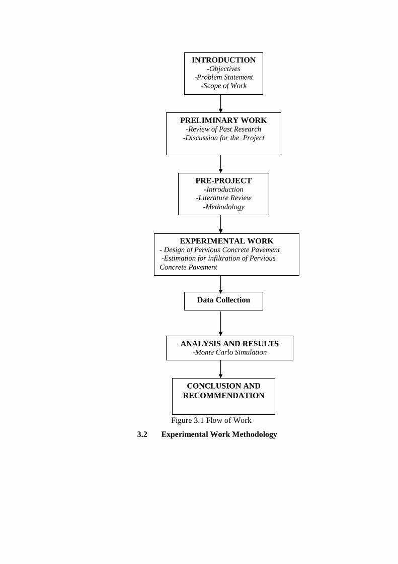
Figure 3.1 Flow of Work

3.2 Experimental Work Methodology

PRELIMINARY WORK -Review of Past Research

-Discussion for the Project

INTRODUCTION -Objectives

-Problem Statement

-Scope of Work

PRE-PROJECT -Introduction

-Literature Review

-Methodology

EXPERIMENTAL WORK - Design of Pervious Concrete Pavement -Estimation for infiltration of Pervious

Concrete Pavement

Data Collection

ANALYSIS AND RESULTS -Monte Carlo Simulation

CONCLUSION AND

RECOMMENDATION

3.2.1 Designing the Pervious Concrete

The proposed site works for the hydrologic analysis of Pervious Concrete

pavement will be carried out at a particular location in UTM. Before the

installation of the pavement, the Pervious Concrete must be designed with the

correct mixture proportion. Table 1 shows the condition and variables of the

experiment to examine the physical and mechanical characteristics of pervious

concrete according to the target void ratio, and recycled aggregate content.

Table 3.1: Condition and variables of experiment

Conditions Variables

W/C (%) 25

Target void ratio (%) 25

Target flow (%) 200

Aggregate Crushed and

recycled

aggregate

gradation:

5-13mm

Content of recycled aggregate (vol. %) 30,50,100

Test item

Physical and mechanical properties Void ratio

Compressive

Strength

The cement used is normal Portland cement whose specific gravity is

3.14. Crushed aggregate and recycled waste concrete aggregate of 5-13 mm size

are used. Table 3.2 shows their physical properties.

Table 3.2: Physical properties of aggregates

Items Gradation Density Water Absolute Unit

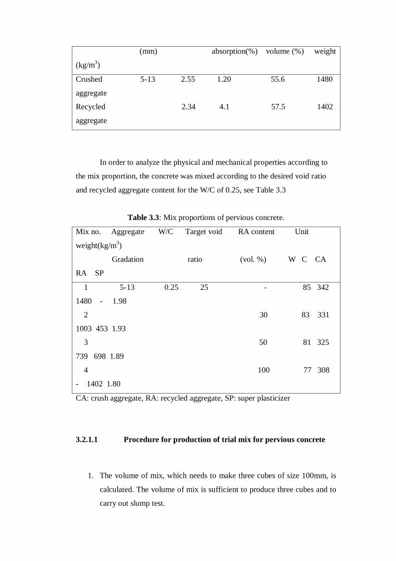
(mm) absorption(%) volume (%) weight

(kg/m3)

Crushed 5-13 2.55 1.20 55.6 1480

aggregate

Recycled 2.34 4.1 57.5 1402

aggregate

In order to analyze the physical and mechanical properties according to

the mix proportion, the concrete was mixed according to the desired void ratio

and recycled aggregate content for the W/C of 0.25, see Table 3.3

Table 3.3: Mix proportions of pervious concrete.

Mix no. Aggregate W/C Target void RA content Unit

weight(kg/m3)

Gradation ratio (vol. %) W C CA

RA SP

1 5-13 0.25 25 - 85 342

1480 - 1.98

2 30 83 331

1003 453 1.93

3 50 81 325

739 698 1.89

4 100 77 308

- 1402 1.80

CA: crush aggregate, RA: recycled aggregate, SP: super plasticizer

3.2.1.1 Procedure for production of trial mix for pervious concrete

1. The volume of mix, which needs to make three cubes of size 100mm, is

calculated. The volume of mix is sufficient to produce three cubes and to

carry out slump test.

2. The volume of mix is multiplied with the constituent contents obtained

from the mix design process to get the batch weights for the trial mix.

3. The mixing of concrete is according to the mixture proportion.

4. Firstly, Portland cement, crush and recycled aggregates, and super

plasticizer are mixed in a mixer for 1 minute.

5. Then, water added into the mixer and the mixture is mixed approximately

for another 1 minute.

6. When the mix is ready, the tests on mix are proceeding.

3.2.1.2 Tests on trial mix

1. The slump tests are conducted to determine the workability of pervious

concrete.

2. Concrete is placed and compacted in three layers by a tamping rod with

25 times, in a firmly held slump cone. On the removal of the cone, the

difference in height between the uppermost part of the slumped concrete

and the upturned cone is recorded in mm as the slump.

3. Three cubes are prepared in 100mm x 100mm each. The cubes are cured

before testing. The procedures for making and curing are as given in

laboratory guidelines. Thinly coat the interior surfaces of the assembled

mould with mould oil to prevent adhesion of concrete. Each mould filled

with two layers of concrete, each layer tamped 25 times with a 25mm

square steel rod. The top surface finished with a trowel and the date of

manufacturing is recorded in the surface of the concrete. The cubes are

stored undisturbed for 24 hrs at a temperature of 18 to 220C and a relative

humidity of not less than 90%. The concrete all are covered with wet

gunny sacks. After 24 hrs, the mould is striped and the cubes are cured

further by immersing them in water at temperature 19 to 21oC until the

testing date.

4. Compressive strength tests are conducted on the cubes at the age of 7

days. Then, the mean compressive strengths are calculated

3.2.2 Setup of Experiment for Estimating the Infiltration.

After the required compressive strength is achieved, the pervious

concrete is ready to be installed for the infiltration estimation. The proposed area

for the site works is approximate to be 3 m2 (1.7m x 1.7m) where the area for the

pavement is 1.0 m2 (1.0m x1.0m). The size of the pervious concrete pavement to

be used is 200mmx200mm. The totals of pervious concrete pavement that need

to be installed are twenty-five (25) pieces where the thickness is 100mm for each

pieces. The design for the analysis of the Pervious Concrete pavement is as in

figure 3.2. The inlet is the pipe hose attached to the pipe near the location of

experiment.

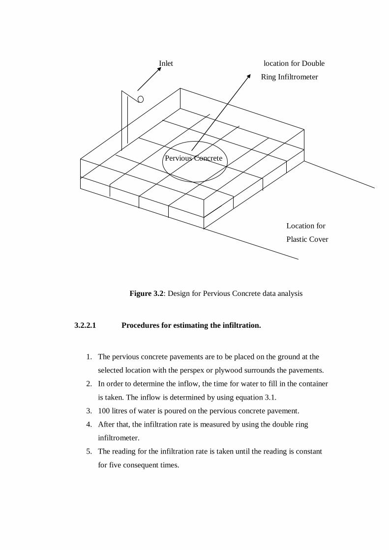
Inlet location for Double

Ring Infiltrometer

Pervious Concrete

Location for

Plastic Cover

Figure 3.2: Design for Pervious Concrete data analysis

3.2.2.1 Procedures for estimating the infiltration.

1. The pervious concrete pavements are to be placed on the ground at the

selected location with the perspex or plywood surrounds the pavements.

2. In order to determine the inflow, the time for water to fill in the container

is taken. The inflow is determined by using equation 3.1.

3. 100 litres of water is poured on the pervious concrete pavement.

4. After that, the infiltration rate is measured by using the double ring

infiltrometer.

5. The reading for the infiltration rate is taken until the reading is constant

for five consequent times.

3.3 Measuring Methods and Equipments

3.3.1 Inflow

To measure the inflow and outflow, the equation of 3.1 is used

Q = V (3.1)

t

Q = Inflow (m3/s)

V = Volume of the container (m3)

t = Time to fill in the container (s)

3.3.2 Infiltration Efficiency

For the infiltration efficiency, the equation used is

Qin - Qout

(3.2)

Qin

Where:

Qin = Inflow from the inlet (hose) (m3/s)

Qout = Outflow from the outlet (square opening) (m3/s)

3.3.3 Determination of Infiltration Rate using Double Ring Infiltrometer

Infiltration is the process by which water arriving at the soil surface

enters the soil. This process affects surface runoff, soil erosion, and groundwater

recharge. The double-ring infiltrometer is often used for measuring infiltration

rates.

Double Ring Infiltrometer consists of a large outer ring and a smaller

inner ring. The diameter of outer ring used is 52 cm and the diameter of inner

ring is 30 cm. Figure3.3 shows Double Ring Infiltrometer and Figure 3.4 shows

how the equipment is been placed.

Figure 3.3 : Double Ring Infiltrometer

52 cm

30 cm

Outer Ring

Inner Ring Water

Level

Figure 3.4 : Set up of Double Ring Infiltrometer

Double-ring infiltrometers minimize the error associated with the single-

ring method because the water level in the outer ring forces vertical infiltration of

water in the inner ring. Another possible source of error occurs when driving the

ring into the ground, as there can be a poor connection between the ring wall and

the soil. This poor connection can cause a leakage of water along the ring wall

and an overestimation of the infiltration rate. Placing a larger concentric ring

around the inner ring and keeping this outer ring filled with water so that the

water levels in both rings are approximately constant can reduce this leakage .

The double-ring infiltrometer test is a well recognized and documented

technique for directly measuring soil infiltration rates. The double-ring

infiltrometer as often being constructed from thin-walled steel pipe with the inner

and outer cylinder diameters being 20 and 30 cm, respectively; however, other

diameters may be used.

There are two operational techniques used with the double-ring

infiltrometer for measuring the flow of water into the ground. In the constant

head test, the water level in the inner ring is maintained at a fixed level and the

volume of water used to maintain this level is measured. In the falling head test,

the time that the water level takes to decrease in the inner ring is measured. In

both constant and falling head tests, the water level in the outer ring is

maintained at a constant level to prevent leakage between rings and to force

vertical infiltration from the inner ring. Numerical modeling has shown that

falling head and constant head methods give very similar results for fine textured

soils, but the falling head test underestimates infiltration rates for coarse textured

soils.

3.4 Monte Carlo Simulation ( RiskAMP)

After the experiment is been carried out, the results from the experiment

will be incorporated with the Monte Carlo Simulation in order to estimate the

uncertainty for infiltration.

In a Monte Carlo simulation, a random value is selected for each of the

tasks, based on the range of estimates. The model is calculated based on this

random value. The result of the model is recorded, and the process is repeated. A

typical Monte Carlo simulation calculates the model hundreds or thousands of

times, each time using different randomly-selected values. When the simulation

is complete, we have a large number of results from the model, each based on

random input values. These results are used to describe the likelihood, or

probability, of reaching various results in the model.

RiskAMP is a Monte Carlo simulation engine that works with Microsoft

Excel. The RiskAMP Addin adds comprehensive probability simulation to

spreadsheet models and Excel applications. The Add-in includes 22 random

distributions, 17 statistical analysis functions, a wizard for creating charts and

graphs, and VBA support.

3.4.1 Hands-on Guide on the Monte Carlo Simulation

Example on how to create and run a Monte Carlo simulation in just a few steps:

Step 1: Insert a random value.

In a new spreadsheet, select any empty cell. Enter the formula

=NormalValue(100,10)

This will insert a random variable using the normal distribution, with a mean of

100 and a standard deviation of 10 (Figure 3.5).

Figure 3.5: Insertion of Random Value

Step 2 : Run a Monte Carlo simulation.

To run a Monte Carlo simulation, select Monte Carlo -> Run Simulation

from the Excel menu. This will launch the simulation dialog box. Enter the

number of iterations to run, or leave the existing value. To begin the simulation,

click 'Start'.(Figure 3.6)

Figure 3.6 : Run the Monte Carlo Simulation

The simulation can be cancel at any time while its running. The progress

bar should give the idea of how long the simulation will take to complete. The

Allow Screen Updates checkbox toggles whether calculations are updated to the

screen. Hiding screen updates will speed up the simulation significantly, but it is

necessary to see the updates to ensure the appropriate result. This box can be

checked or un-checked at any time during the simulation.

The dialog box will close automatically when the simulation completes.

Then, review or analyze the data generated in the simulation, using the

simulation functions

Step 3 : Use the Wizard to plot out the simulation data.

Open the Monte Carlo menu and select "Histograms and Charts Wizard".

This will open the Wizard dialog (Figure 3.7) . From the first page of the Wizard,

click Next to start.

Figure 3.7: Histograms and Charts Wizard

a) Select a Source Cell

The first step in using the Wizard is selecting a source data cell. This cell

contains the data used for analyzing in the simulation. It might contain a simple

probability function, or it might be the output of a complex function.

Select the cell with the mouse in the Excel spreadsheet, and the cell

location should appear in the dialog box (Figure 3.8).

Figure 3.8: Select a Source Cell

b) Select the target range

The next step is selecting a target range. There are two basic options here:

select a target range, somewhere in the workbook, that will contain the data

table; or, in the alternative, create a new worksheet that contains several results

tables (Figure 3.9).

Creating a new worksheet is the simplest way to get results data from the

simulation. The new worksheet will contain statistical data such as the mean,

median, deviation, and so on, as well as data tables and charts.

Figure 3.9: Select a Target Range

Selecting a target range allows the results of simulation to be included in

an existing workbook, and gives the user more control over the layout and format

of results.

If the user wants to select a target range for the data, highlight the range

of cells with the mouse. Please note that any existing data in the target range will

be erased. The range can be in a horizontal or vertical range. If the range is one

row (or one column) deep, the data table will include values over the simulation

Click Next to continue.

c) Select Results Data

Each results type displays a different aspect of simulation. Remember that the

Wizard can be run multiple times to include different data tables (Figure 3.10).

Figure 3.10 : Select Results Table

i) Histogram Table

A histogram displays the frequency of occurence of particular values over

the simulation. The histogram arranges values into "bins", which are regularly

spaced between the minimum and maximum values of the source cell in the

simulation.

Histograms can easily show the most-commonly and least-commonly

occuring values, as well as the relative likelihood of a reaching a particular value.

ii) Percentile Results

A percentile table uses the SIMULATIONPERCENTILE function to

create a table of percentiles (probability of occurence) and corresponding values

of the source cell during the simulation.

This data table can show the value the source cell will reach with any

given probability.

iii) Interval Results

An interval table displays the probability of the source cell reaching a

particular value during the simulation. This data is similar to a histogram, but

uses percentiles (likelihood of occurence) rather than absolute counts to display

the results data.

The interval table can be used to determine the likelihood of reaching a

particular value. The user can include similar interval analyses in their

spreadsheet using the SIMULATIONINTERVAL function, which returns the

likelihood of the source cell falling within any given interval.

The checkbox marked "Include Column (Row) Titles" allows user to

include column (or row) headers for data tables. If this box is checked, the first

row (or column) will include titles. Click Next to continue.

Step 4 : Run a Monte Carlo Simulation

This screen will only appear if there is no simulation data for the source cell.

Figure 3.11: Run a Monte Carlo Simulation

Click the button to run a simulation. This will hide the Wizard and open

the simulation dialog.

When the simulation dialog is visible, run a Monte Carlo simulation by

clicking the Start button. For more information, see the section on Running a

Simulation, above. The simulation can be ran at any time, and the results data

will be updated automatically.

Click Next to continue.

Step 5 :The Wizard is Complete

The Wizard is now complete. The data table should be populated within

the spreadsheet. If the user wants to create a chart of the data, make sure the box

is checked (Figure 3.12).

Figure 3.12 : The Wizard for Histogram and Chart is Complete

Step 6 : Re-run and modify the simulation.

Once the simulation tables are created, the user can re-run a simulation at

any time using the Monte Carlo menu, and the results tables and charts will

automatically update. Or, the user can modify the cell modeled to display

different data, and then run a new simulation.

First, try running a new simulation. Open the Monte Carlo menu and

select "Run Monte Carlo Simulation..." to open the simulation dialog. Click Start

to run the simulation. The user should see the charts and tables update as the

simulation runs.

Next, try changing the data in your reference cell. Go back to the first

worksheet, and select the cell where the user entered the random data function.

Change this cell (make sure it's the same cell) to read

=TriangularValue(0,10,100)

Now click back to the spreadsheet containing the results table, and run a

new simulation from the Monte Carlo menu. There should be a very different

results in the data tables.

CHAPTER 4

ANALYSIS OF RESULT AND DISCUSSION

4.1 Introduction

In this chapter, the results for the experiment conducted using pervious

concrete pavement will be analyzed. After that the watershed area of Universiti

Teknologi Malaysia (UTM) will be considered in the calculation in order to

determine the result of runoff volume for the application of pervious concrete

pavement.

4.2 Data Analysis

The experiments have been carried out for six (6) times, during six (6) different

days starting on 4th

March 2009 until 31st March 2009. The Inflow for the

experiment is measured using the equation 3.1.The source of the water is from

the pipe that is located near the location of the experiment. The volume of water

is assumed to be the same with the pile volume. The volume of pile is measured

using the equation 4.1

Volume of pile = ∏d2t (4.1)

4

Where,

d = diameter of pile (cm)

t = height of pile ( cm)

In this experiment, the value of diameter is 29 cm and the height of pile is 35 cm.

The volume of pile is:

V = ∏ (29)2(35) = 23118 cm

3

4

V = 23118 cm3 x 1 m

3 = 0.023118 m

3

(100)3 cm

3

For experiment 1, the time taken for the water to fill in the pile is 175 s. thus, the

inflow for experiment 1 is:

Inflow = 0.023118 m3

= 1.321 x 10-4

m3/s

175 s

In Table 4.1 shows the result of Inflow for six (6) of experiments of six (6)

different days.

Table 4.1: Inflow of the experiment

Experiment Time (s) Volume (m) Inflow (m3/s)

x10-4

1 175 0.023118 1.32

2 170 0.023118 1.36

3 171 0.023118 1.35

4 182 0.023118 1.27

5 179 0.023118 1.29

6 189 0.023118 1.22

4.2.1 Runoff Rate

After the inflow is been determined, the infiltration rate is been measured by

using Double Ring Infiltrometer. The method of measuring is as been discussed

in Chapter 3. After the infiltration has been determined, the runoff rate can be

calculated by using equation 4.2

Runoff Rate (m3/s) = Inflow (m

3/s) – Infiltration Rate (m

3/s) (4.2)

From the experiment 1, the total of infiltration rate is 5.07x10-5

m3/s. Thus, the

Runoff Rate for experiment 1 is

Runoff Rate, R (m3/s) = 1.32 x 10

-4 m

3/s - 5.07x10

-5 m

3/s

= 8.13 x 10-5

m3/s

The summary of the Runoff Rate with the corresponding Inflow and Infiltration

Rate for each experiment are as in Table 4.2 . The results show that, after placing

the pervious concrete as a pavement, the infiltration efficiency is 38.37 %, the

percentage of runoff is reduced to 61.63 %, the runoff rate is 8.13 x 10-5

m3/s and

the total infiltration rate is 4.3 cm/min

Table 4.2 : Summary of the Results of the Runoff Rate

Experiment

Inflow

(m3/s)

x10-4

Total

Infiltration

rate

(cm/min)

Runoff

Rate

(m3/s)

x10-5

Infiltration

Efficiency

(%)

Percentage

of runoff

(%)

1 1.32 4.3 8.13 38.37 61.63

2 1.36 4.2 8.65 36.38 63.62

3 1.35 4.4 8.32 38.39 61.61

4 1.27 4.7 7.16 43.60 56.40

5 1.29 4.1 8.07 37.44 62.56

6 1.22 4.0 7.49 38.62 61.38

4.2.2 Runoff Volume

In order to determine the Runoff Volume, the area of watershed for UTM must

be taking into account during the calculation. The total area of watershed in

UTM is measured to be 13.61 km2. The inflow for the given watershed is:

Inflow = 1.32 x 10-4

m3

x 1 x 13.61 km2 x (10

3)

2 m

2 x 3600 s x 24 hr x 365

day

s 1 m2 1 km 1hr 1 day 1

year

= 5.67 x 1010

m3/year

The Infiltration rate of experiment 1 for the given watershed is:

Infiltration Rate = 4.3 cm x 10 mm x 60 min x 24 hr x 365 day

min 1cm 1hr 1 day 1 year

= 22600800 mm/year

Runoff Volume = 5.67 x 1010

m3/year – 2.174 x 10

10 m

3/year

= 3.49 x 1010

m3/year

The summary of the Runoff Volume with the corresponding Inflow and

Infiltration Rate for each experiment are as in Table 4.3. For experiment 1, the

runoff percentage which has been estimated to have the percentage of 100 % is

reduced to 61.63 % after the pervious concrete pavement has been placed.

Meanwhile, the infiltration efficiency is 38.37 % with the runoff volume of 3.49

m3/year.

Table 4. 3: Summary of the Results for Runoff Volume

Experiment

Inflow

(m3/yr)

x1010

Total

Infiltration

rate

(mm/yr)

Runoff

Volume

(m3/yr)

x1010

Infiltration

Efficiency

(%)

Percentage

of runoff

(%)

1 5.67 22600800 3.49 38.37 61.63

2 5.84 22075200 3.7 36.38 63.62

3 5.79 23126400 3.57 38.39 61.61

4 5.45 24703200 3.07 43.60 56.40

5 5.54 21549600 3.46 37.44 62.56

6 5.24 21024000 3.21 38.62 61.38

4.3 Result of Monte Carlo Simulation

After the result from the experiment is obtained, the next step is to do the

simulation of the result by using Monte Carlo Simulation. The simulation

process was run by using the mean and standard deviation value from the

experiment. The simulation starts by entering the various numbers of trials to

complete the simulation. Each simulation will produce new value of mean and

standard deviation. In this study the 10 000 number of trials has been used during

simulation. The mean and standard deviation entered using the equation 4.4:

= NormalValue (Mean, Standard Deviation) (4.4)

For example, from the pervious calculated Inflow, the value of mean and

standard deviation are as follows:

=NormalValue (1.30 x 10-4

, 5.2694 x 10-6

)

With the value entered, the next step is to run the simulation by choose ‗

Run Monte Carlo Simulation‘ with 10,000 trials. The simulation will give a new

value for the Inflow with mean of 1.302 x 10-4

and standard deviation of 5.25315

x 10-6

. The result can be represented by histogram and the probability density

function as in Figure 4.1 and Figure 4.2. Same calculation is carried out for

infiltration rate, and runoff.

4.3.1 Results of Inflow using Monte Carlo Simulation

Figure 4.1 shows the Histogram of Inflow represent the range of inflow after

placing the pervious concrete pavement. The most likely range of inflow to occur

can be determined by taking fourth highest values from the histogram or

probability density curve. Figure 4.1 shows that the most likely range for inflow

is from 1.28 x 10-4

m3/s until 1.34 x 10

-4 m

3/s with the percentage range from

12.81 % until 13.60 %.

Figure 4.1: Histogram of observed Inflow, I (m3/s) for 10,000 trials of Monte

Carlo

Simulation

Figure 4.2 shows the probability density function (PDF) which can represent the

maximum probability of occurrence value for Inflow. It shows that the

maximum occurrence of Inflow is 1.32 x 10-4

m3/s with the percentage of 14.74

%.

Figure 4.2: Probability Density Function of observed Inflow, I (m3/s) for

10,000 trials of Monte Carlo Simulation

4.3.2 Results of Infiltration Rate by using Monte Carlo Simulation

Figure 4.3 shows the Histogram of Infiltration Rate represent the range of

infiltration rate after placing the pervious concrete pavement. The most likely

range of infiltration rate to occur can be determined by taking fourth highest

values from the histogram or probability density curve. Figure 4.3 shows that the

most likely range for infiltration rate is from 4.22 cm/min until 4.49 cm/min with

the percentage range from 13.29 % until 11.72 %.

Imax = 1.32 x 10-4

m3/s (14.81 %)

Figure 4.3: Histogram of observed Infiltration Rate, f (cm/min) for 10,000 trials

of Monte Carlo Simulation

Figure 4.4 shows the probability density function (PDF) which can represent the

maximum probability of occurrence value for Infiltration rate. It shows that the

maximum occurrence of Infiltration rate is 4.31 cm/min with the percentage of

14.74 %.

Figure 4.4: Probability Density Function of observed Infiltration Rate, f

(cm/min) for 10,000 trials of Monte Carlo Simulation

4.3.3 Results of Runoff Rate using Monte Carlo Simulation

fmax = 4.31 c m/min (14.74 %)

Figure 4.5 shows the Histogram of Runoff Rate represent the range of inflow

after placing the pervious concrete pavement. The most likely range of runoff

rate to occur can be determined by taking fourth highest values from the

histogram or probability density curve. Figure 4.4 shows that the most likely

range for runoff rate is from 7.80 x 10-5

m3/s until 8.40 x10

-5 m

3/s with the

percentage range from 12.85 % until 11.52 %.

Figure 4.4: Histogram of observed Runoff Rate, R (m3/s) for 10,000 trials of

Monte Carlo Simulation

Figure 4.5 shows the probability density function (PDF) which can represent the

maximum probability of occurrence value for Runoff Rate. It shows that the

maximum occurrence of Runoff Rate is 8.20 x10-5

m3/s with the percentage of

14.22 %.

Figure 4.5: Probability Density Function of observed Runoff Rate, R (m3/s) for

10,000 trials of Monte Carlo Simulation

The summary of the result for estimating the probability of occurrence for the

inflow, infiltration rate and runoff rate is showed in Table 4.4

Table 4.4 :The output summary from the Monte Carlo Simulation analysis with

best normal distribution

Note Max.

Value

Max.

Percent *

(%)

Most

Likely range

Most Likely

Percent

* *(%)

Inflow

( m3/s) x 10

-4

1.32 14.81 1.28-1.34 12.81-13.60

Infiltration

Rate (cm/min)

4.31 14.74 4.22-4.49 13.29-11.72

Runoff rate ( m3/s) x

10-5

8.20 14.22 7.80-8.40 12.85-11.52

*Max. Percent is the percent of the max. value of inflow, infiltration rate and runoff rate obtained

for the particular simulation.

**Most Likely Range is the percent of the most likely range value of inflow, infiltration rate and

runoff rate obtained for the particular simulation.

Rmax = 8.2 x 10-5

m3/s (14.22 %)

4.3.4 Results of Inflow for Watershed Area of UTM using Monte Carlo

Simulation

After the simulation of the maximum occurrence for the inflow,

infiltration rate and runoff rate is done, there is need to determine the maximum

occurrence for the inflow, infiltration rate and runoff volume over the year by

consider the area of watershed of UTM. Figure 4.6 shows the Histogram of

Inflow represent the range of inflow after placing the pervious concrete

pavement. The most likely range of inflow to occur can be determined by taking

fourth highest values from the histogram or probability density curve. Figure 4.6

shows that the most likely range for inflow is from 5.48 x 1010

m3/year until 5.78

x 1010

m3/s with the percentage range from 13.67 % until 13.86

Figure 4.6: Histogram of observed Inflow, I (m3/year) for 10,000 trials of

Monte Carlo Simulation

Figure 4.7 shows the probability density function (PDF) which can represent the

maximum probability of occurrence value for Inflow. It shows that the

maximum occurrence of Inflow is 5.58 x 1010

m3/s with the percentage of 17.22

%.

Figure 4.7: Probability Density Function of observed Inflow, I (m3/year) for

10,000 trials of Monte Carlo Simulation

4.3.5 Results of Infiltration Rate for Watershed Area of UTM using Monte

Carlo Simulation

Figure 4.8 shows the Histogram of Infiltration Rate represent the range of

infiltration rate after placing the pervious concrete pavement. The most likely

range of infiltration rate to occur can be determined by taking fourth highest

values from the histogram or probability density curve. Figure 4.8 shows that the

most likely range for infiltration rate is from 2.18 x 107 mm/year until 2.36 x 10

7

mm/year with the percentage range from 13.56 % until 13.86 %.

Imax = 5.58 x 1010

m3/year (17.22 %)

Figure 4.8: Histogram of observed Infiltration Rate, f (mm/year) for 10,000

trials of Monte Carlo Simulation

Figure 4.9 shows the probability density function (PDF) which can represent the

maximum probability of occurrence value for Infiltration rate. It shows that the

maximum occurrence of Infiltration Rate is 2.3 x107 mm/year with the

percentage of 17.79 %.

Figure 4.9: Probability Density Function of observed Infiltration Rate, f

(mm/year) for 10,000 trials of Monte Carlo Simulation

fmax = 2.3 x 107 mm/year (17.79%)

4.3.6 Results of Runoff Volume for Watershed Area of UTM using Monte

Carlo Simulation

Figure 4.10 shows the Histogram of Runoff Volume represent the range of runoff

volume after placing the pervious concrete pavement. The most likely range of

runoff volume to occur can be determined by taking fourth highest values from

the histogram or probability density curve. Figure 4.10 shows that the most likely

range for runoff volume is from 3.32 x 1010

m3/year until 3.59 x 10

10 m

3/s with

the percentage range from 12.56 % until 13.14 %.

Figure 4.10 : Histogram of observed Runoff Volume, R (m3/year) for 10,000

trials of Monte Carlo Simulation

Figure 4.11 shows the probability density function (PDF) which can represent

the maximum probability of occurrence value for runoff volume. It shows that

the maximum occurrence of runoff volume is 3.5 x 1010

m3/s with the percentage

of 14.82 %.

Figure 4.11: Probability Density Function of observed Runoff Volume, R

(m3/year) for 10,000 trials of Monte Carlo Simulation

The summary of the result for estimating the probability of occurrence for the

inflow, infiltration rate and runoff rate is showed in Table 4.5.

Table 4.5: The output summary from the Monte Carlo Simulation analysis with

best normal distribution

Note Max.

Value

Max.

Percent *(%)

Most

Likely range

Most Likely

Percent

* *(%)

Inflow

( m3/year) x 10

10

5.58 17.22 5.48-5.78 13.67-13.86

Infiltration

Rate

(mm/year) x 107

2.3 17.79 2.18-2.36 13.56-15.84

Runoff rate ( m3/s) x

1010

3.5 14.82 3.32-3.59 12.56-13.14

*Max. Percent is the percent of the max. value of inflow, infiltration rate and runoff volume obtained for the particular simulation.

**Most Likely Range is the percent of the most likely range value of inflow, infiltration rate and runoff volume obtained for the particular simulation.

Rmax = 3.5x 1010

m3/year (14.82 %)

CHAPTER 5

CONCLUSION AND RECOMMENDATION

5.1 Conclusion

This study is been carried out in order to determine the performance of pervious

concrete pavement for reducing runoff using Monte Carlo Simulation. Monte

Carlo would represent the simplest application to calculate the probability of

occurrence of the inflow, infiltration and runoff of the pervious concrete

pavement. The simulation shows that

i) The maximum occurrence value for observed inflow is 1.32 x 10-4

m3/s (14.81%). The maximum occurrence infiltration rate is 4.31

cm/min (14.74 %) and the maximum occurrence for the runoff rate to

occur is 8.2 x 10-5

m3/s (14.22%).

ii) The maximum occurrence value for observed inflow is 5.58x1010

m3/year (17.22%). The maximum occurrence infiltration rate is

23000000 mm/year (17.79%) and the maximum occurrence for the

runoff volume to occur is 3.5 x1010

m3/year (14.82%)

5.2 Recommendation

From the result, the runoff discharge is definitely reduced since there is

infiltration rate recorded through the pervious concrete pavement. Thus, in order

to enhance the performance of the pervious concrete, the future study must

taking into account the following factors:

i) Vegetation positively affects the stability of soil structure. A

combination of this vegetation and the root penetration of the upper

surface stimulate the rate. Consequently the penetration rate of a soil

containing little or no vegetation is less than that of vegetated soil.

ii) Permeability increases correspondingly with increased pore volume.

In a sandy soil, the pore volume between the particles specifically

affects the permeability. Fine sand, with smaller pores between the

particles than coarser sand, has a slower rate of permeability. The

permeability of a clay soil is especially affected by the soil structure.

The presence of cracks or passageways in a clay soil can speed up the

rate of permeability significantly.

iii) If an arid area is flooded with water the rate of infiltration is initially

high, reducing slowly until a constant value is reached (―basic

infiltration rate‖). This reduces much quicker in a dry soil than a

previously moistened soil.

iv) Infiltration occurs vertically in a homogenous, un-layered soil. It is

usual, however, that moist soil is layered but for simplicity it is

assumed that each layer is homogenous. This assumption is applied

for irrigation investigations. It is possible to measure the rate of

infiltration for each layer separately.

v) The soil moisture in each location where the experiment is been

carried out must be determined. This is to ensure that the value for the

infiltration rate is more accurate and more reliable.

vi) Soil compacted by pedestrians or wheeled vehicles is liable to have a

lesser rate of infiltration, especially clay or sandy clay types.

Measuring results may therefore largely vary from site to site.

vii) The rate of infiltration and capacity of a soil are completely

influenced by the changing of the seasons due to varying factors:

change of water temperature, variance in viscosity, moisture content

of the soil, vegetation growth and life in the soil surface.

For future research there is need to search for a new method to determine the

infiltration by using the pervious concrete pavement for example by referring to

the related journal or other standard (BS or ASTM) that is suitable in determine

the infiltration rate of pervious concrete pavement.

REFERENCES

Dayalan Rainoo Raj (2007). Evaluation for Design Criteria for Inflow and

Infiltration of Medium Scale Sewerage Catchment System. Degree Thesis.

Universiti Teknologi Malaysia

Goforth, G.F.,Diniz E.V.,Rauhut.J.B. (1983). Municipal Environmental

Reasearch

Laboratory. Stormwater Hydrological Characteristic of Porous and

Conventional Paving System.

Joung Y., Grasley Z.C.(2008). Texas Transportation Institute. Evaluation and

Optimization of Durable Pervious Concrete for Use in Urban Areas

Jayasuriya ,L.N.N., Kadurupokune N., M. Othman and Jesse, K.(2007).

Contributing To The Sustainable Use Of Stormwater: The Role Of

Pervious

Pavements.

Mohd Fazli, Y. Nor Azazi, Z., Aminuddin, A.G.,Rozi,A., Chang,C.K.(2005).

Infiltration Study for Urban Soil : Case Studies-Butterworth and

Engineering

Campus, Universiti Sains Malaysia

Mohd. Razali, A.R.(2008). Menganggar Pemebanan Fosforus di Takungan Air

Layang Menggunakan Simulasi Monte Carlo, Degree Thesis, Universiti

Teknologi Malaysia.

Tennis P.D, Leming M.L., Akers D.J.(2004) Portland Cement Association.

Pervious

Concrete Pavement.

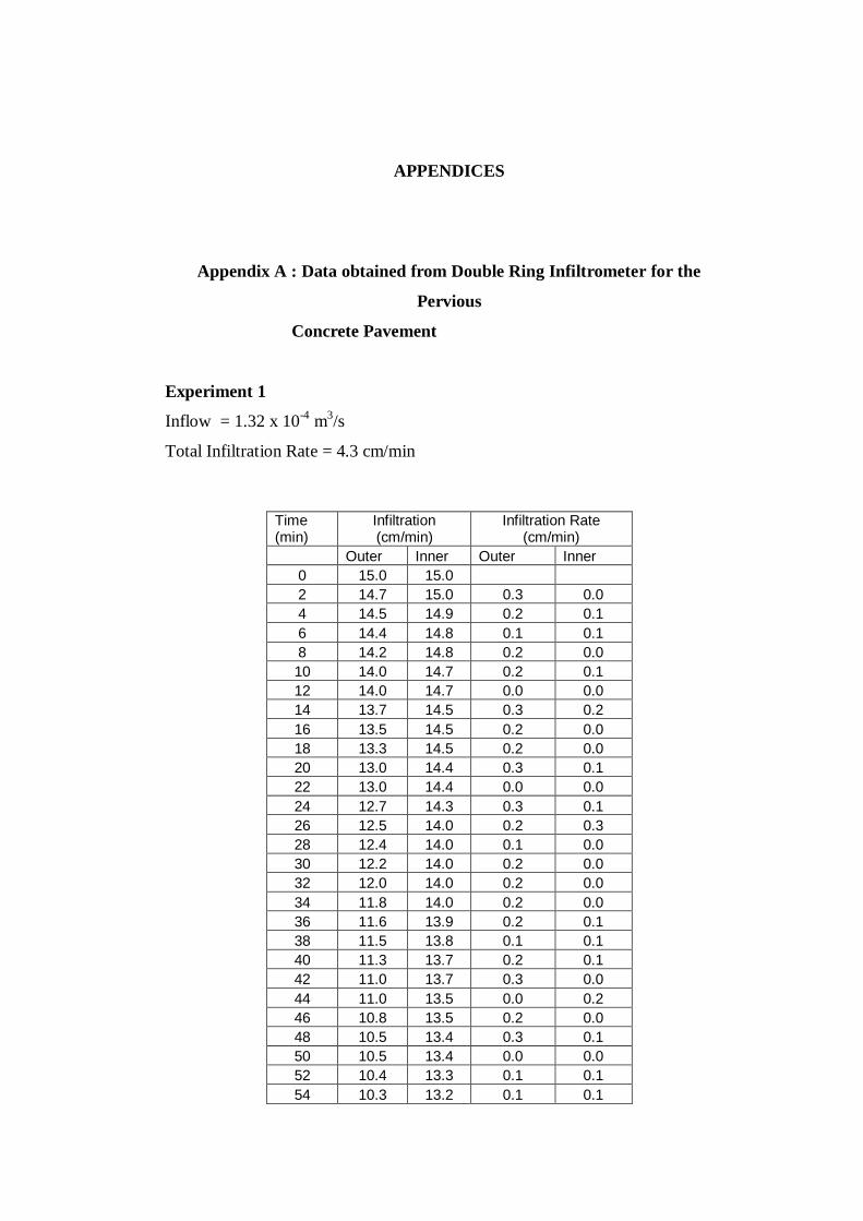
APPENDICES

Appendix A : Data obtained from Double Ring Infiltrometer for the

Pervious

Concrete Pavement

Experiment 1

Inflow = 1.32 x 10-4

m3/s

Total Infiltration Rate = 4.3 cm/min

Time (min)

Infiltration (cm/min)

Infiltration Rate (cm/min)

Outer Inner Outer Inner

0 15.0 15.0

2 14.7 15.0 0.3 0.0

4 14.5 14.9 0.2 0.1

6 14.4 14.8 0.1 0.1

8 14.2 14.8 0.2 0.0

10 14.0 14.7 0.2 0.1

12 14.0 14.7 0.0 0.0

14 13.7 14.5 0.3 0.2

16 13.5 14.5 0.2 0.0

18 13.3 14.5 0.2 0.0

20 13.0 14.4 0.3 0.1

22 13.0 14.4 0.0 0.0

24 12.7 14.3 0.3 0.1

26 12.5 14.0 0.2 0.3

28 12.4 14.0 0.1 0.0

30 12.2 14.0 0.2 0.0

32 12.0 14.0 0.2 0.0

34 11.8 14.0 0.2 0.0

36 11.6 13.9 0.2 0.1

38 11.5 13.8 0.1 0.1

40 11.3 13.7 0.2 0.1

42 11.0 13.7 0.3 0.0

44 11.0 13.5 0.0 0.2

46 10.8 13.5 0.2 0.0

48 10.5 13.4 0.3 0.1

50 10.5 13.4 0.0 0.0

52 10.4 13.3 0.1 0.1

54 10.3 13.2 0.1 0.1

56 10.1 13.2 0.2 0.0

58 10.0 13.0 0.1 0.2

60 9.8 12.9 0.2 0.1

62 9.7 12.9 0.1 0.0

64 9.5 12.8 0.2 0.1

66 9.4 12.8 0.1 0.0

68 9.1 12.6 0.3 0.2

70 9.0 12.5 0.1 0.1

72 8.9 12.5 0.1 0.0

74 8.9 12.4 0.0 0.1

76 8.7 12.3 0.2 0.1

78 8.5 12.3 0.2 0.0

80 8.4 12.1 0.1 0.2

82 8.1 12.0 0.3 0.1

84 8.0 12.0 0.1 0.0

86 8.0 11.9 0.0 0.1

88 7.8 11.7 0.2 0.2

90 7.7 11.7 0.1 0.0

92 7.5 11.6 0.2 0.1

94 7.5 11.5 0.0 0.1

96 7.5 11.5 0.0 0.0

98 7.3 11.4 0.2 0.1

100 7.0 11.3 0.3 0.1

102 7.0 11.2 0.0 0.1

104 6.8 11.0 0.2 0.2

106 6.7 11.0 0.1 0.0

108 6.5 10.9 0.2 0.1

110 6.5 10.8 0.0 0.1

112 6.4 10.7 0.1 0.1

114 6.4 10.7 0.0 0.0

116 6.4 10.7 0.0 0.0

118 6.4 10.7 0.0 0.0

120 6.4 10.7 0.0 0.0

Experiment 2

Inflow = 1.36 x 10-4

m3/s

Total Infiltration Rate = 4.2 cm/min

Time (min)

Infiltration (cm/min)

Infiltration Rate (cm/min)

Outer Inner Outer Inner

0 15.0 15.0

2 15.0 15.0 0.0 0.0

4 14.5 15.0 0.5 0.0

6 14.0 15.0 0.5 0.0

8 14.0 15.0 0.0 0.0

10 13.9 15.0 0.1 0.0

12 13.8 14.9 0.1 0.1

14 13.7 14.9 0.1 0.0

16 13.5 14.9 0.2 0.0

18 13.3 14.9 0.2 0.0

20 13.0 14.7 0.3 0.2

22 13.0 14.5 0.0 0.2

24 13.0 14.5 0.0 0.0

26 12.9 14.2 0.1 0.3

28 12.5 14.0 0.4 0.2

30 12.0 13.9 0.5 0.1

32 12.0 13.6 0.0 0.3

34 12.0 13.5 0.0 0.1

36 12.0 13.5 0.0 0.0

38 11.9 13.2 0.1 0.3

40 11.5 13.2 0.4 0.0

42 11.5 12.9 0.0 0.3

44 11.5 12.8 0.0 0.1

46 11.4 12.5 0.1 0.3

48 11.4 12.5 0.0 0.0

50 11.2 12.3 0.2 0.2

52 11.0 12.0 0.2 0.3

54 11.0 12.0 0.0 0.0

56 10.5 11.9 0.5 0.1

58 10.5 11.6 0.0 0.3

60 10.5 11.5 0.0 0.1

62 10.3 11.4 0.2 0.1

64 10.3 11.4 0.0 0.0

66 10.0 11.0 0.3 0.4

68 10.0 11.0 0.0 0.0

70 9.5 10.9 0.5 0.1

72 9.4 10.8 0.1 0.1

74 9.4 10.8 0.0 0.0

76 9.4 10.8 0.0 0.0

78 9.4 10.8 0.0 0.0

80 9.4 10.8 0.0 0.0

Experiment 3

Inflow = 1.35 x 10-4

m3/s

Total Infiltration Rate = 4.4 cm/min

Time (min) Infiltration (cm/min)

Infiltration Rate (cm/min)

Outer Inner Outer Inner

0 15.0 15.0

2 14.8 14.9 0.2 0.1

4 14.7 14.8 0.1 0.1

6 14.6 14.8 0.1 0.0

8 14.4 14.8 0.2 0.0

10 14.3 14.7 0.1 0.1

12 14.2 14.6 0.1 0.1

14 14.0 14.5 0.2 0.1

16 13.9 14.5 0.1 0.0

18 13.7 14.4 0.2 0.1

20 13.6 14.4 0.1 0.0

22 13.4 14.4 0.2 0.0

24 13.0 14.3 0.4 0.1

26 12.8 14.0 0.2 0.3

28 12.6 14.0 0.2 0.0

30 12.4 13.9 0.2 0.1

32 12.2 13.9 0.2 0.0

34 11.8 13.8 0.4 0.1

36 11.6 13.7 0.2 0.1

38 11.5 13.7 0.1 0.0

40 11.3 13.6 0.2 0.1

42 11.0 13.6 0.3 0.0

44 11.0 13.5 0.0 0.1

46 10.8 13.5 0.2 0.0

48 10.5 13.4 0.3 0.1

50 10.4 13.4 0.1 0.0

52 10.4 13.3 0.0 0.1

54 10.3 13.2 0.1 0.1

56 10.1 13.1 0.2 0.1

58 10.0 13.0 0.1 0.1

60 9.8 12.9 0.2 0.1

62 9.7 12.9 0.1 0.0

64 9.5 12.8 0.2 0.1

66 9.4 12.8 0.1 0.0

68 9.1 12.6 0.3 0.2

70 9.0 12.5 0.1 0.1

72 8.9 12.5 0.1 0.0

74 8.9 12.4 0.0 0.1

76 8.7 12.3 0.2 0.1

78 8.5 12.3 0.2 0.0

80 8.4 12.1 0.1 0.2

82 8.1 12.0 0.3 0.1

84 8.0 12.0 0.1 0.0

86 8.0 11.9 0.0 0.1

88 7.8 11.7 0.2 0.2

90 7.7 11.7 0.1 0.0

92 7.5 11.6 0.2 0.1

94 7.5 11.5 0.0 0.1

96 7.5 11.5 0.0 0.0

98 7.3 11.4 0.2 0.1

100 7.0 11.3 0.3 0.1

102 7.0 11.2 0.0 0.1

104 6.8 11.0 0.2 0.2

106 6.7 11.0 0.1 0.0

108 6.5 11.0 0.2 0.0

110 6.5 10.9 0.0 0.1

112 6.4 10.8 0.1 0.1

114 6.4 10.7 0.0 0.1

116 6.4 10.6 0.0 0.1

118 6.4 10.6 0.0 0.0

120 6.3 10.6 0.1 0.0

122 6.2 10.6 0.0 0.0

124 6.2 10.6 0.0 0.0

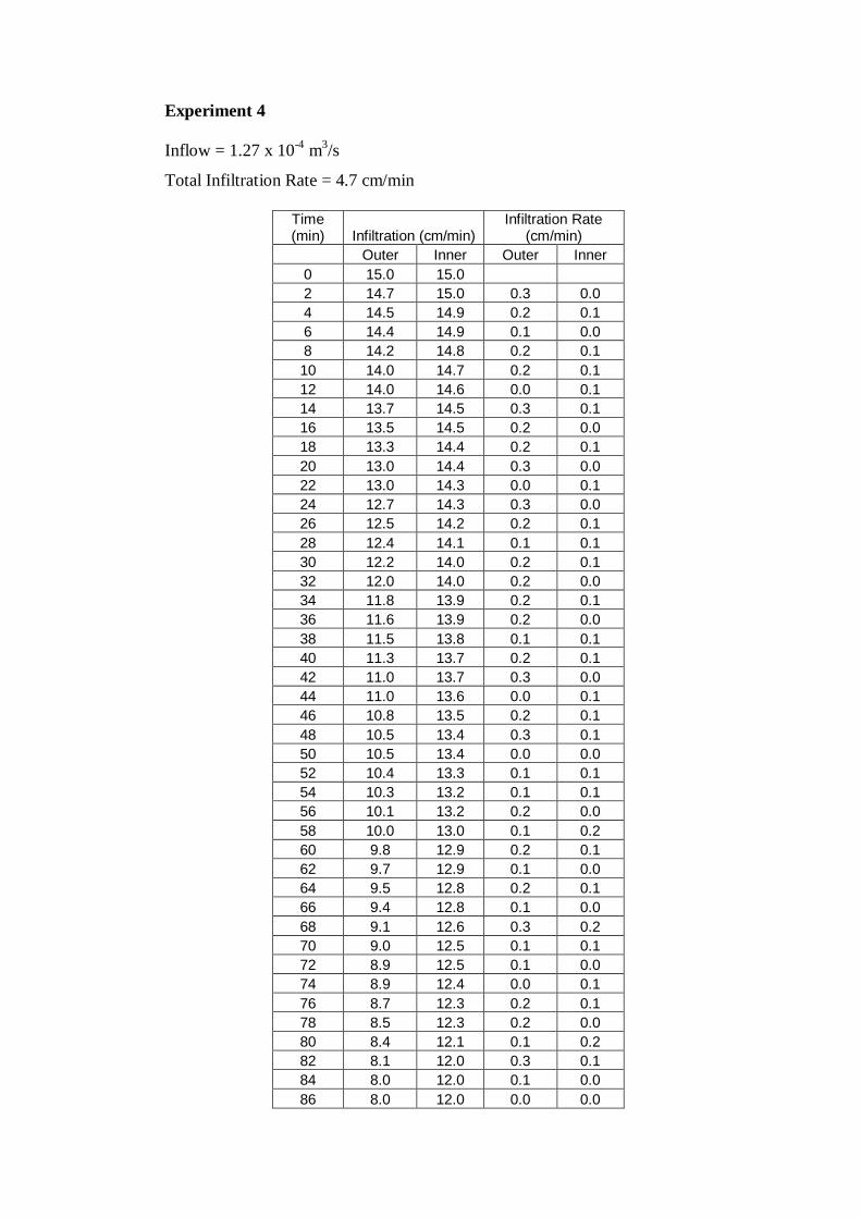
Experiment 4

Inflow = 1.27 x 10-4

m3/s

Total Infiltration Rate = 4.7 cm/min

Time (min) Infiltration (cm/min)

Infiltration Rate (cm/min)

Outer Inner Outer Inner

0 15.0 15.0

2 14.7 15.0 0.3 0.0

4 14.5 14.9 0.2 0.1

6 14.4 14.9 0.1 0.0

8 14.2 14.8 0.2 0.1

10 14.0 14.7 0.2 0.1

12 14.0 14.6 0.0 0.1

14 13.7 14.5 0.3 0.1

16 13.5 14.5 0.2 0.0

18 13.3 14.4 0.2 0.1

20 13.0 14.4 0.3 0.0

22 13.0 14.3 0.0 0.1

24 12.7 14.3 0.3 0.0

26 12.5 14.2 0.2 0.1

28 12.4 14.1 0.1 0.1

30 12.2 14.0 0.2 0.1

32 12.0 14.0 0.2 0.0

34 11.8 13.9 0.2 0.1

36 11.6 13.9 0.2 0.0

38 11.5 13.8 0.1 0.1

40 11.3 13.7 0.2 0.1

42 11.0 13.7 0.3 0.0

44 11.0 13.6 0.0 0.1

46 10.8 13.5 0.2 0.1

48 10.5 13.4 0.3 0.1

50 10.5 13.4 0.0 0.0

52 10.4 13.3 0.1 0.1

54 10.3 13.2 0.1 0.1

56 10.1 13.2 0.2 0.0

58 10.0 13.0 0.1 0.2

60 9.8 12.9 0.2 0.1

62 9.7 12.9 0.1 0.0

64 9.5 12.8 0.2 0.1

66 9.4 12.8 0.1 0.0

68 9.1 12.6 0.3 0.2

70 9.0 12.5 0.1 0.1

72 8.9 12.5 0.1 0.0

74 8.9 12.4 0.0 0.1

76 8.7 12.3 0.2 0.1

78 8.5 12.3 0.2 0.0

80 8.4 12.1 0.1 0.2

82 8.1 12.0 0.3 0.1

84 8.0 12.0 0.1 0.0

86 8.0 12.0 0.0 0.0

88 7.8 11.9 0.2 0.1

90 7.7 11.8 0.1 0.1

92 7.5 11.6 0.2 0.2

94 7.5 11.5 0.0 0.1

96 7.5 11.5 0.0 0.0

98 7.3 11.4 0.2 0.1

100 7.0 11.3 0.3 0.1

102 7.0 11.2 0.0 0.1

104 6.8 11.0 0.2 0.2

106 6.7 11.0 0.1 0.0

108 6.5 10.9 0.2 0.1

110 6.5 10.8 0.0 0.1

112 6.4 10.7 0.1 0.1

114 6.4 10.6 0.0 0.1

116 6.4 10.6 0.0 0.0

118 6.4 10.5 0.0 0.1

120 6.4 10.4 0.0 0.1

122 6.4 10.4 0.0 0.0

124 6.4 10.3 0.0 0.1

126 6.4 10.3 0.0 0.0

128 6.4 10.3 0.0 0.0

130 6.4 10.3 0.0 0.0

132 6.4 10.3 0.0 0.0

Experiment 5

Inflow = 1.29 x 10-4

m3/s

Total Infiltration Rate = 4.1 cm/min

Time (min) Infiltration (cm/min)

Infiltration Rate (cm/min)

Outer Inner Outer Inner

0 15.0 15.0

2 14.7 15.0 0.3 0.0

4 14.5 15.0 0.2 0.0

6 14.4 14.9 0.1 0.1

8 14.2 14.8 0.2 0.1

10 14.0 14.7 0.2 0.1

12 14.0 14.6 0.0 0.1

14 13.7 14.5 0.3 0.1

16 13.5 14.5 0.2 0.0

18 13.3 14.4 0.2 0.1

20 13.0 14.4 0.3 0.0

22 13.0 14.3 0.0 0.1

24 12.7 14.2 0.3 0.1

26 12.5 14.1 0.2 0.1

28 12.4 14.1 0.1 0.0

30 12.2 14.0 0.2 0.1

32 12.0 14.0 0.2 0.0

34 11.8 13.9 0.2 0.1

36 11.6 13.8 0.2 0.1

38 11.5 13.7 0.1 0.1

40 11.3 13.6 0.2 0.1

42 11.0 13.5 0.3 0.1

44 11.0 13.5 0.0 0.0

46 10.8 13.5 0.2 0.0

48 10.5 13.4 0.3 0.1

50 10.5 13.3 0.0 0.1

52 10.4 13.2 0.1 0.1

54 10.3 13.2 0.1 0.0

56 10.1 13.1 0.2 0.1

58 10.0 13.0 0.1 0.1

60 9.8 12.9 0.2 0.1

62 9.7 12.8 0.1 0.1

64 9.5 12.8 0.2 0.0

66 9.4 12.7 0.1 0.1

68 9.1 12.5 0.3 0.2

70 9.0 12.5 0.1 0.0

72 8.9 12.4 0.1 0.1

74 8.9 12.4 0.0 0.0

76 8.7 12.3 0.2 0.1

78 8.5 12.3 0.2 0.0

80 8.4 12.1 0.1 0.2

82 8.1 12.0 0.3 0.1

84 8.0 12.0 0.1 0.0

86 8.0 11.9 0.0 0.1

88 7.8 11.7 0.2 0.2

90 7.7 11.7 0.1 0.0

92 7.5 11.6 0.2 0.1

94 7.5 11.5 0.0 0.1

96 7.5 11.5 0.0 0.0

98 7.3 11.4 0.2 0.1

100 7.0 11.3 0.3 0.1

102 7.0 11.2 0.0 0.1

104 6.8 11.0 0.2 0.2

106 6.7 11.0 0.1 0.0

108 6.5 10.9 0.2 0.1

110 6.5 10.9 0.0 0.0

112 6.4 10.9 0.1 0.0

114 6.4 10.9 0.0 0.0

116 6.4 10.9 0.0 0.0

Experiment 6

Inflow = 1.22 x 10-4

m3/s

Total Infiltration Rate = 4.0 cm/min

Time (min) Infiltration (cm/min)

Infiltration Rate (cm/min)

Outer Inner Outer Inner

0 15.0 15.0

2 14.8 15.0 0.2 0.0

4 14.6 15.0 0.2 0.0

6 14.4 14.8 0.2 0.2

8 14.2 14.8 0.2 0.0

10 14.0 14.8 0.2 0.0

12 14.0 14.5 0.0 0.3

14 13.7 14.5 0.3 0.0

16 13.5 14.4 0.2 0.1

18 13.3 14.2 0.2 0.2

20 13.0 14.0 0.3 0.2

22 13.0 14.0 0.0 0.0

24 12.7 14.0 0.3 0.0

26 12.5 13.9 0.2 0.1

28 12.4 13.9 0.1 0.0

30 12.2 13.7 0.2 0.2

32 12.0 13.7 0.2 0.0

34 11.8 13.6 0.2 0.1

36 11.6 13.5 0.2 0.1

38 11.5 13.5 0.1 0.0

40 11.3 13.5 0.2 0.0

42 11.0 13.4 0.3 0.1

44 11.0 13.3 0.0 0.1

46 10.8 13.3 0.2 0.0

48 10.5 13.3 0.3 0.0

50 10.5 13.1 0.0 0.2

52 10.4 13.1 0.1 0.0

54 10.3 13.1 0.1 0.0

56 10.1 13.1 0.2 0.0

58 10.0 13.0 0.1 0.1

60 9.8 12.9 0.2 0.1

62 9.7 12.8 0.1 0.1

64 9.5 12.8 0.2 0.0

66 9.4 12.6 0.1 0.2

68 9.1 12.6 0.3 0.0

70 9.0 12.6 0.1 0.0

72 8.9 12.5 0.1 0.1

74 8.9 12.5 0.0 0.0

76 8.7 12.5 0.2 0.0

78 8.5 12.5 0.2 0.0

80 8.4 12.4 0.1 0.1

82 8.1 12.3 0.3 0.1

84 8.0 12.2 0.1 0.1

86 8.0 12.1 0.0 0.1

88 7.8 12.1 0.2 0.0

90 7.7 12.0 0.1 0.1

92 7.5 12.0 0.2 0.0

94 7.5 11.9 0.0 0.1

96 7.5 11.8 0.0 0.1

98 7.3 11.8 0.2 0.0

100 7.0 11.6 0.3 0.2

102 7.0 11.6 0.0 0.0

104 6.8 11.5 0.2 0.1

106 6.7 11.5 0.1 0.0

108 6.5 11.5 0.2 0.0

110 6.5 11.5 0.0 0.0

112 6.4 11.3 0.1 0.2

114 6.4 11.3 0.0 0.0

116 6.4 11.3 0.0 0.0

118 6.4 11.1 0.0 0.2

120 6.4 11.1 0.0 0.0

122 6.4 11.0 0.0 0.1

124 6.4 11.0 0.0 0.0

126 6.4 11.0 0.0 0.0

128 6.4 11.0 0.0 0.0

130 6.4 11.0 0.0 0.0

Appendix B : Photos during the Experiment

The Pervious Concrete has been laid down on the ground

To Level the Outer and Inner Ring

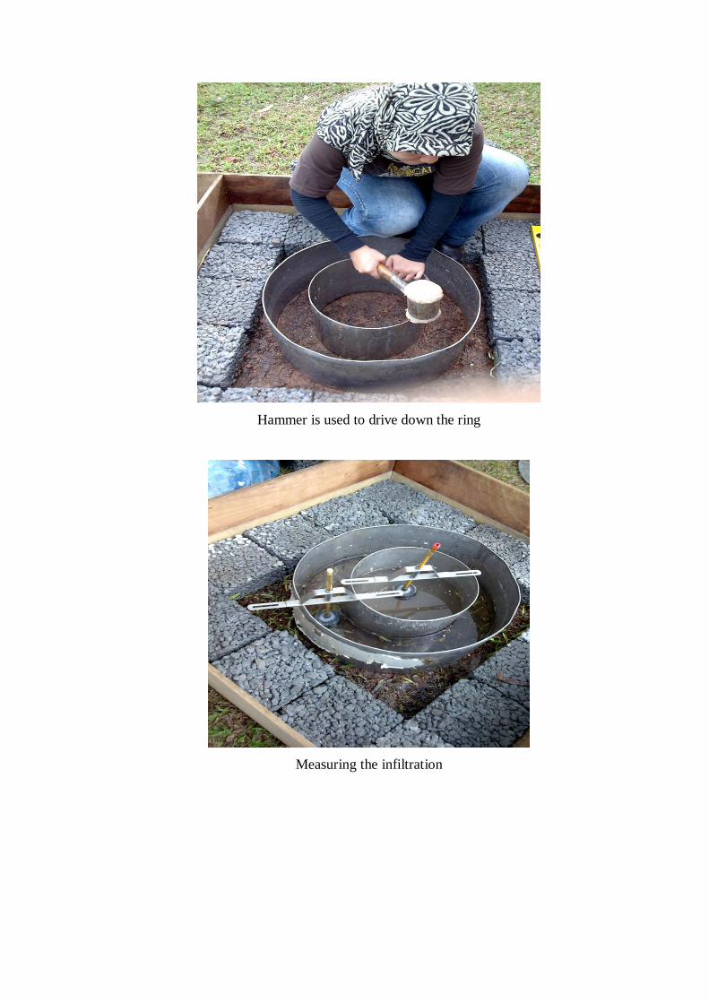
Hammer is used to drive down the ring

Measuring the infiltration