Annals of Biomedical Engineering, Vol. 34, No. 4, April 2006 ( C© 2006) pp. 575–592DOI: 10.1007/s10439-005-9074-4

Blood Flow in Compliant Arteries: An Effective Viscoelastic ReducedModel, Numerics, and Experimental Validation

SUNCICA CANIC,1 CRAIG J. HARTLEY,2 DOREEN ROSENSTRAUCH,3 JOSIP TAMBACA,4

GIOVANNA GUIDOBONI,1 and ANDRO MIKELIC5

1Department of Mathematics, University of Houston, Houston TX, 77204-3008; 2Sections of Cardiovascular Sciences, Department ofMedicine, Baylor College of Medicine, Houston, TX 77030; 3Texas Heart Institute and the University of Texas Health Science Center at

Houston, TX, 77204; 4Department of Mathematics, University of Zagreb, Bijenicka 30, Croatia; and 5Department of Mathematics,Universite Claude Bernard Lyon 1, 69622, Villeurbanne Cedex, France

(Received 31 August 2005; accepted 22 December 2005; published online: 21 March 2006)

Abstract—The focus of this work is on modeling blood flow inmedium-to-large systemic arteries assuming cylindrical geometry,axially symmetric flow, and viscoelasticity of arterial walls. Theaim was to develop a reduced model that would capture certainphysical phenomena that have been neglected in the derivation ofthe standard axially symmetric one-dimensional models, while atthe same time keeping the numerical simulations fast and simple,utilizing one-dimensional algorithms. The viscous Navier–Stokesequations were used to describe the flow and the linearly vis-coelastic membrane equations to model the mechanical propertiesof arterial walls. Using asymptotic and homogenization theory, anovel closed, “one-and-a-half dimensional” model was obtained.In contrast with the standard one-dimensional model, the newmodel captures: (1) the viscous dissipation of the fluid, (2) theviscoelastic nature of the blood flow – vessel wall interaction, (3)the hysteresis loop in the viscoelastic arterial walls dynamics, and(4) two-dimensional flow effects to the leading-order accuracy.A numerical solver based on the 1D-Finite Element Method wasdeveloped and the numerical simulations were compared with theultrasound imaging and Doppler flow loop measurements. Lessthan 3% of difference in the velocity and less than 1% of differ-ence in the maximum diameter was detected, showing excellentagreement between the model and the experiment.

Keywords—Blood flow modeling, Viscoelasticity of arterialwalls, Fluidstructure interaction.

INTRODUCTION

Local hemodynamics and temporal wall shear stressgradient are thought to be important factors in triggeringthe onset of focal atherogenesis leading to various com-plications in the cardiovascular function. Elevated tempo-ral shear stress gradient, for example, has been shown tostimulate endothelial cell proliferation,16 which is a precur-sor for graft limb thrombosis in bifurcated endografts usedin endovascular treatment of aortic abdominal aneurysm.

Address correspondence to Suncica Canic, Department of Mathemat-ics, University of Houston, Houston, TX, 77204-3008. Electronic mail:canic@math.uh.edu

Many clinical treatments can only be studied in detail if areliable model describing the response of the arterial wallto the pulsatile blood flow is considered.

Due to the immense complexity of the cardiovascularsystem, studying the interaction between blood flow andvessel walls is exceedingly difficult. Whenever possible,simplifying assumptions such as, for example, axial sym-metry of endovascular prostheses and size of a consideredartery, need to be taken into account.

In this vein, this work focuses on modeling blood flow inmedium-to-large compliant arteries. The main interest wasin modeling arterial sections that can be approximated bythe cylindrical geometry allowing axially symmetric flows.The viscous incompressible Navier–Stokes equations wereused to model the flow, and the linearly viscoelastic mem-brane equations to model the mechanical properties of thewall. The aim was to develop a fluid–structure interactionmodel that captures certain important physical phenomenathat have been either neglected or oversimplified in thederivation of the standard one-dimensional models such as:the viscous dissipation of the fluid, the viscoelasticity ofvessel walls, and the wall shear stress. At the same time, agoal was to keep the complexity of the numerical algorithmequivalent to those of one-dimensional solvers.

One-dimensional models have been studied by manyauthors. The first comprehensive study showing the deriva-tion of the one-dimensional model was presented in.3For adetailed analysis of the model equations see, for example,Refs.7,14 The one-dimensional model is obtained by aver-aging the three-dimensional incompressible Navier–Stokesequations over the cross-section of the vessel. In this pro-cess of dimension reduction a typical question of “closure”needs to be resolved. More precisely, averaging over thecross-section of the vessel does not lead to a well-posedproblem unless extra information is provided. An ad hocassumption in the form of an axial velocity profile is usedto resolve this issue. Giving the form of the velocity profile

575

0090-6964/06/0400-0575/0 C© 2006 Biomedical Engineering Society

576 CANIC et al.

a priori, instead of recovering it from the solution of theproblem, leads to the loss of accuracy in the quantities thatare sensitive to the form of the velocity profile such as, forexample, the wall shear stress.

In this work a closed, “one-and-a-half dimensionalmodel” is obtained using techniques based on the asymp-totic and homogenization theory for porous media flows.The equations are closed in the sense that the axial velocityprofile is calculated as one of the components of the solutionto the problem. Thus, the axial velocity profile, as all theother components of the solution, depends on the data (theinlet and outlet pressure and vessel wall properties). As aresult, the solution to the obtained closed model predictsthe flow, the wall shear stress, and wall dynamics with ahigher accuracy than the one-dimensional models.

In addition, the “one-and-a-half dimensional model”proposed in this work keeps the viscous dissipation of thefluid to the leading order. This is, again, in contrast with theone-dimensional models, where the effects of fluid viscosityare encountered as a sink in the axial momentum, oversim-plifying the smoothing properties of the fluid viscosity interms of a viscous drag force.

Perhaps the most interesting feature of the model studiedin this work is its simple form which is capable of explicitlycapturing two distinct phenomena that contribute to the vis-coelastic behavior of vessel walls. One is the influence offluid viscosity on the vessel wall dynamics, and a separateone is the vessel walls viscoelastic mechanical properties.The viscoelastic mechanical properties of vessel walls weremodeled by utilizing a simple viscoelastic membrane model(2.3) which is based on the Kelvin–Voigt viscoelasticity(2.2). Our numerical simulations reveal the hysteresis be-havior in the pressure–diameter diagram observed in themeasurements reported in Refs.1,2,4 In contrast, we showthat fluid viscosity does not, to the leading order, effectthe hysteresis behavior of vessel walls. Rather, we foundthat the viscous fluid imparts long-term memory effectson the dynamics of the vessel walls (see the section on“Viscoelasticity of the Fluid–Structure Interaction”).

Understanding particular viscoelastic contributions tothe vessel wall dynamics is important, among other things,in the measurements of the mechanical properties of vesselwalls. If the measurements are performed in vivo, the con-tributions of the viscous fluid need to be factored out beforequantifying the mechanical, viscoelastic properties of thearterial walls.

A numerical algorithm based on the one-dimensionalFinite Element Method (FEM) was developed for the nu-merical calculation of the solution to the fluid–structureinteraction problem. The results of the numerical simu-lations were compared with experimental measurements.A mock circulatory pulsatile flow loop with (compliant)latex tubing was assembled at the Research Laboratory atthe Texas Heart Institute. Ultrasound measurements andDoppler methods were used to detect the wall behavior and

fluid velocity. Nondairy coffee creamer was dispersed inwater to enable ultrasound measurements of the fluid ve-locity. Excellent agreement between the numerically calcu-lated and experimentally measured quantities was obtained.

DESCRIPTION OF THE PROBLEM

This work focuses on the study of blood flow in majorsystemic arteries such as the aorta or iliac arteries. A typicalvessel is modeled as an axisymmetric compliant cylinder.

Using � to denote cylinder’s reference state, assumedat the reference pressure pref , in cylindrical coordinates(r, z, θ ) domain � is defined by

� = {x = (r cos θ, r sin θ, z) ∈ R3 : r ∈ (0, R(z)),

θ ∈ (0, 2π ), z ∈ (0, L)} .

Here z is the axis of symmetry of the cylinder, L isits length, R(z) is the reference radius, and r and θ arethe polar coordinates describing each cross-section of thecylinder. The reference radius R(z) can vary along the cylin-der’s length to describe vessel tapering, mild stenoses oraneurysms. In typical systemic arteries the aspect ratio,defined by

ε = Rmax

L, (2.1)

is small, namely ε � 1. In this work, a system of equationswill be derived approximating the flow to the ε2-accuracy.

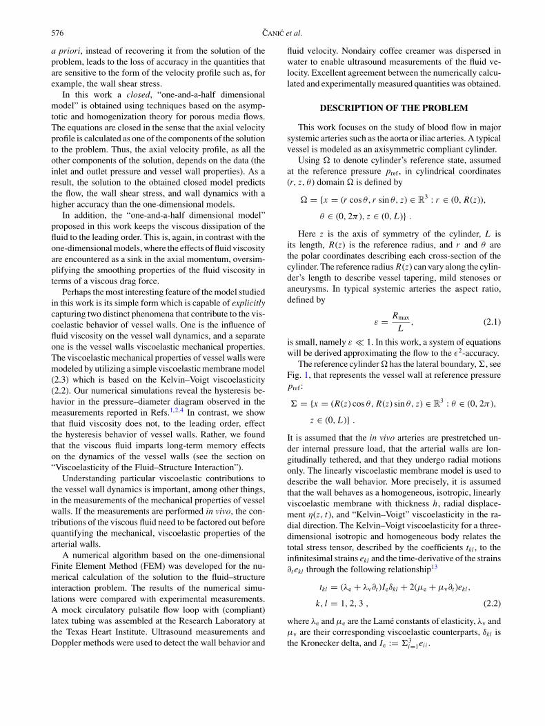
The reference cylinder � has the lateral boundary, �, seeFig. 1, that represents the vessel wall at reference pressurepref :

� = {x = (R(z) cos θ, R(z) sin θ, z) ∈ R3 : θ ∈ (0, 2π ),

z ∈ (0, L)} .

It is assumed that the in vivo arteries are prestretched un-der internal pressure load, that the arterial walls are lon-gitudinally tethered, and that they undergo radial motionsonly. The linearly viscoelastic membrane model is used todescribe the wall behavior. More precisely, it is assumedthat the wall behaves as a homogeneous, isotropic, linearlyviscoelastic membrane with thickness h, radial displace-ment η(z, t), and “Kelvin–Voigt” viscoelasticity in the ra-dial direction. The Kelvin–Voigt viscoelasticity for a three-dimensional isotropic and homogeneous body relates thetotal stress tensor, described by the coefficients tkl , to theinfinitesimal strains ekl and the time-derivative of the strains∂t ekl through the following relationship13

tkl = (λe + λv∂t )Ieδkl + 2(µe + µv∂t )ekl,

k, l = 1, 2, 3 , (2.2)

where λe and µe are the Lame constants of elasticity, λv andµv are their corresponding viscoelastic counterparts, δkl isthe Kronecker delta, and Ie := �3

i=1eii .

Blood Flow in Viscoelastic Arteries 577

FIGURE 1. The reference domain �.

The motion of the wall is described by the secondNewton’s law of motion relating the force with wall accel-eration, wall velocity, and wall displacement. Assumingexternal transverse (radial) loading and zero longitudinaldisplacement, the second Newton’s law of motion reads6

fr = hρw∂2η

∂t2+ Eh

1 − σ 2

1

R2η + pref

η

R+ hCv

R2

∂η

∂t. (2.3)

Here, fr describes the radial component of the externalforce acting on the thin shell, ρw is the wall density, E is theYoungs modulus of elasticity, σ is the Poisson ratio, and Cv

is the viscosity constant. The following relationship holdsbetween the parameters in (2.3) and the Lame constants:

E

1 − σ 2= 2µλ

λ + 2µ+ 2µ, Cv = 2µvλv

λv + 2µv+ 2µv .

Equation (2.3) says that the external force fr is counter-balanced by the total force of the wall which is a resultant ofthe following three contributions: (1) the rate of change ofmomentum, i.e. wall acceleration described by the first termon the right-hand side, (2) the total internal stress caused bythe wall stretching described by the second and third termson the right-hand side, and (3) viscous dissipation effecting

the velocity of the wall motion, described by the last termin (2.3). Equation (2.3) describes dynamic equilibrium forwhich the sum of total forces must equal zero.

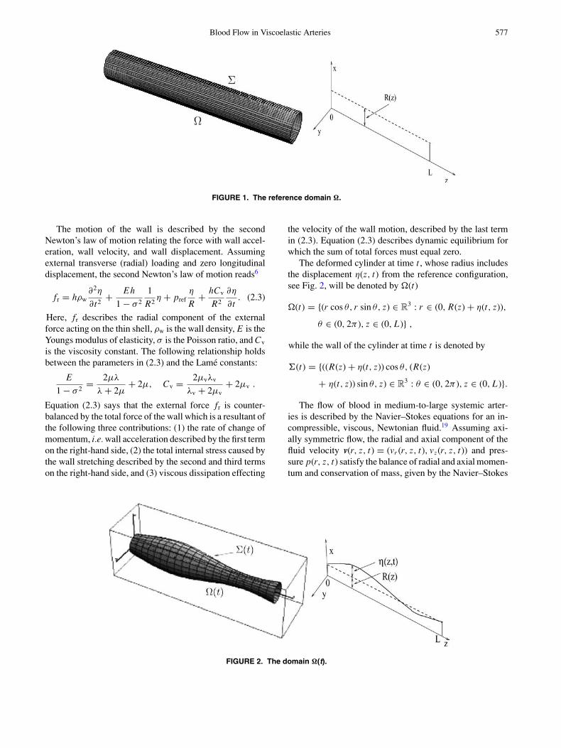
The deformed cylinder at time t , whose radius includesthe displacement η(z, t) from the reference configuration,see Fig. 2, will be denoted by �(t)

�(t) = {(r cos θ, r sin θ, z) ∈ R3 : r ∈ (0, R(z) + η(t, z)),

θ ∈ (0, 2π ), z ∈ (0, L)} ,

while the wall of the cylinder at time t is denoted by

�(t) = {((R(z) + η(t, z)) cos θ, (R(z)

+ η(t, z)) sin θ, z) ∈ R3 : θ ∈ (0, 2π ), z ∈ (0, L)}.

The flow of blood in medium-to-large systemic arter-ies is described by the Navier–Stokes equations for an in-compressible, viscous, Newtonian fluid.19 Assuming axi-ally symmetric flow, the radial and axial component of thefluid velocity v(r, z, t) = (vr (r, z, t), vz(r, z, t)) and pres-sure p(r, z, t) satisfy the balance of radial and axial momen-tum and conservation of mass, given by the Navier–Stokes

FIGURE 2. The domain �(t).

578 CANIC et al.

equations in cylindrical coordinates:

ρF

(∂vr

∂t+ vr

∂vr

∂r+ vz

∂vr

∂z

)+ ∂p

∂r

= µ

(∂2vr

∂r2+ ∂2vr

∂z2+ 1

r

∂vr

∂r− vr

r2

)(2.4)

ρF

(∂vz

∂t+ vr

∂vz

∂r+ vz

∂vz

∂z

)+ ∂p

∂z

= µ

(∂2vz

∂r2+ ∂2vz

∂z2+ 1

r

∂vz

∂r

)(2.5)

∂vr

∂r+ ∂vz

∂z+ vr

r= 0. (2.6)

Here µ is the fluid dynamic viscosity coefficient and ρF

is the fluid density. The three terms on the left of the firsttwo equations, multiplying ρF, describe fluid inertia. Theother terms describe the sum of all forces acting on thefluid. The last equation describing conservation of massis derived by postulating that mass can neither be creatednor destroyed. It is also known as the incompressibilitycondition. These equations describe how fluid velocity andpressure change, subject to certain initial and boundaryconditions. The following inlet and outlet boundary datalead to a well-defined problem:

• Inlet data (z = 0):

(i) p + ρF(vz)2/2 = P0(t) + pref (the dynamicpressure is prescribed),

(ii) vr = 0 (fluid is entering the tube parallel tothe axis of symmetry)

(iii) η = 0 (zero displacement at the inlet; in thereduced model, see the section on “The One-and-a-Half-Dimensional Reduced Model,”the zero displacement condition is relaxed;this is typical for reduced models where theboundary layer phenomena near the edgeswith high stress concentrations are lost)

• Outlet data (z = L):

(i) p + ρF(vz)2/2 = PL (t) + pref (same as atthe inlet),

(ii) vr = 0 (same as at the inlet),(iii) η = 0 (same as at the inlet).

Initially the fluid is assumed to be at rest, with zerodisplacement from the reference cylinder:

• Initial data: η = ∂η

∂t = 0, v = 0.

This set of initial and boundary data gives rise toa well-posed problem which can be solved numeri-cally.

The cylinder’s lateral boundary �(t) pulsates in time asblood flows through the cylinder. The fluid flows throughthe cylinder due to the pressure gradient between the inletand the outlet, and due to the forces exerted by the cylinder’selastic/viscoelastic wall. More precisely, as the left ventriclecontracts and expels blood into the aorta, it imparts kineticenergy to the blood, which stretches the aorta as aorticpressure reaches its systolic peak. In diastole the walls ofthe aorta recoil, releasing the potential energy stored duringsystole. This maintains adequate pressure on the reducingblood volume and keeps the flow moving forward. This in-teraction between blood flow and elastic/viscoelastic wall,known in the mathematical literature as the fluid–structureinteraction, is described by two conditions:

• The no-slip condition describes the fact that theparticles of the fluid stick to the wall. They movewith the same velocity as the vessel wall itself:

vr (R + η(z, t), z, t) = ∂η(z, t)

∂t,

vz(R + η(z, t), z, t) = 0. (2.7)

Notice that only the radial component of the ves-sel wall velocity is nonzero since only the radialcomponent of the displacement is assumed to benon-zero.

• Balance of forces states that the contact force actingby the wall to the fluid is counter-balanced by thecontact force acting by the fluid to the wall:

fr = [(p − pref)I − 2µD(v)]n · er

(1 + η

R

)

×√

1 + (∂zη)2 , (2.8)

where fr is given by the viscoelastic membraneequation (2.3) and the right-hand side of (2.8) de-scribes the contact force of the fluid. Here D(v) isthe rate-of-strain tensor or the symmetrized gradi-ent of the velocity, n is the vector normal to thedeformed boundary �(t), and er is the radial unitvector.

These two conditions are evaluated at the lateral bound-ary �(t).

Thus, the problem of finding the axially symmetric flowof an incompressible, viscous fluid through a cylindricaldomain with a compliant wall consists of solving the fluidequations (2.4)–(2.6) in the cylindrical domain �(t), withthe initial conditions and the inlet and outlet boundary dataspecified above, and with the lateral boundary conditionsdescribed by (2.7) and (2.8). This is a difficult problemfrom both the numerical and mathematical point of view.The main difficulties lie in the fact that the fluid equationsare nonlinear due to the quadratic convection terms in equa-tions (2.4) and (2.5) (those are the second and third termdescribing convection by the fluid with velocity v which is

Blood Flow in Viscoelastic Arteries 579

not known a priori), and that the shape of the domain �(t)is not known a priori, but depends on the solution as well.Real-time simulations of this problem are still unfeasible.Whenever possible, simplified models are called for. In thiswork a simplified, effective, model is derived, holding forsmall aspect ratios ε, namely, for the aspect ratios and flowconditions that are typical for the abdominal aorta or iliacarteries.

THE REDUCED MODEL EQUATIONS

Using asymptotic analysis coupled with the ideas fromhomogenization theory of porous media flows, a set of re-duced, simplified equations was obtained. The derivation ofthe equations is not described in detail. Rather, the readershould consult Refs.8–11,24 for the details of the analysis.To simplify matters, the nondimensional analysis describedbelow is given for a constant reference radius R. The finalequations in dimensional form, presented in the sectionon “The One-and-a-Half Dimensional Reduced Model,”hold for a nonconstant, slowly varying radius R = R(z).A novelty here is including viscosity in the wall model,which was not considered in Refs.8–11,24 The main stepsin the derivation of the reduced model equations can besummarized as follows.

The Two-Dimensional Reduced Equations

To detect the small terms in the underlying problem it isa custom to write the model equations in nondimensionalform. For that purpose the nondimensional independentvariables r , z and t are introduced via

r = Rr , z = Lz, t = 1

ωt,

where

ω = 1

L

√1

ρF

(hE

R(1 − σ 2)+ pref

). (3.9)

The time scale 1/ω is determined by the frequency of os-cillations of the vessel wall caused by the pressure wave inthe fluid. The units describing ω are 1/s. The form of ω isobtained in Ref.10 from an energy estimate.

Next, the nondimensional velocity v, displacement η

and pressure p are introduced via v = V v, η = �η andp = ρFV 2 p. Expanding the unknown functions η, v, and pin terms of the small parameter ε gives

v = V {v0 + εv1 + · · ·},where

2V = P√ρF

(hE

R(1 − σ 2)+ pref

)− 12

(3.10)

η = �{η0 + εη1 + · · ·},

where

2� = PR

(hE

R(1 − σ 2)+ pref

)−1

, (3.11)

p = ρFV 2{ p0 + ε p1 + · · ·}. (3.12)

Here, the leading-order coefficients V and � measurethe magnitude of the velocity and the displacement interms of the parameters of the problem. They were cal-culated from the a priori solution estimates, presentedin Ref.9 Letter P denotes a norm that measures themagnitude of the inlet and outlet pressure, the pres-sure drop, and the averaged pressure in one cardiac cy-cle: P2 := supz,t | p|2 + (supz

∫ t0 | pt |dτ )2 + T

∫ t0 |PL (τ ) −

P0(τ )|2dτ , where p(t) = PL (t)−P0(t)L z + P0(t).

Following standard ideas in asymptotic theory these ex-pansions are substituted in the original equations. The termsof order ε2 and smaller are neglected giving rise to thefollowing ε2 approximations9:

• The ε2-approximation of the balance of radial mo-mentum is ∂ p/∂ r = 0. This implies that the ε2-approximation of the problem considered here isa hydrostatic one, namely, that the pressure p =p0 + ε p1 is constant across the cross-section of thetube. Thus p = p(z, t)

• The leading order approximation of the radial com-ponent of the velocity, v0

r , is zero. Namely, vr =V (εv1

r + . . .) while vz = V (v0z + εv1

z + . . .), whichsays that the radial component of the velocity issmaller than the axial component of the velocity bya factor of ε. This follows from the leading-orderterms in the conservation of mass equation.9

• The ε2-approximation of the contact condition(2.8), derived in Ref.9 shows that the fluid pres-sure term in (2.8) is the only term that affects themotion of the lateral boundary to the leading order.More precisely, the ε2-approximation of (2.8) innondimensional variables reads:

p − pref = 1

ρF V 2

{(Eh

(1 − σ 2)R+ pref

)�

Rη

+ h

RCvω

�

R

∂η

∂ t

}. (3.13)

• The following two-dimensional initial-boundaryvalue problem, defined on the scaled domain r ∈(0, 1), z ∈ (0, 1), t > 0, describes an ε2 approxima-tion of the fluid–structure interaction problem:The fluid equations:

Sh∂ vz

∂ t+ vz

∂ vz

∂ z+ vr

∂ vz

∂ r+ ∂ p

∂ z

= 1

Re

{1

r

∂

∂ r

(r∂ vz

∂ r

)}, (3.14)

580 CANIC et al.

∂

∂ r(r vr ) + ∂

∂ z(r vz) = 0, (3.15)

∂ p

∂ r= 0. (3.16)

Lateral Boundary Conditions:{

Equation (3.13)

(vr , vz)|(1,z,t) = (∂η

∂ t |(z,t), 0)}

for z ∈ (0, 1),

t > 0. (3.16)

Inlet/Outlet Boundary Data:

η|(z=0/L ,t) = 0, p|(z=0/L ,t) = (P0/L (t)+pref )ρFV 2 ,

with p given by (3.13),

vr |(1,z=0/L ,t) = 0

Initial Data:

v|(r ,z,0) = 0, η|(z,0) = 0.

Here vr : v1r + εv2

r so that vεr = εV (vr + O(ε2)), vz :=

v0z + εv1

z so that vεz = V (vz + O(ε2)), p := p0 + ε p1 so

that pε = ρF V 2( p + O(ε2)) and η := η0 + εη1 so thatηε = �(η + O(ε2)). The Stronuhal and the Reynolds num-bers are given by

Sh = Lω

Vand Re = ρFV R2

µL. (3.17)

In dimensional variables the pressure equation (3.13)with Cv = 0 reads

p(z, t) − pref =(

hE

R(1 − σ 2)+ pref

)η(z, t)

R, (3.18)

which is known as the Law of Laplace, typically used in liter-ature to model the vessel wall behavior in one-dimensionalblood flow models.7,15,20 Here, the pref term on the right-hand side takes into account the fact that arteries in vivoare prestressed and that η measures the displacement fromthe prestressed radius R. Furthermore, notice that the ε2-approximation of the inlet and outlet boundary conditionsconsists of prescribing only the pressure and not the dy-namic pressure.

This two-dimensional reduced problem is still rathercomplex to solve numerically because of the nonlinearityin the fluid equations and because the equations are definedon the domain �(t) that is bounded by a moving boundarywhose location depends on the solution. To simplify thisproblem even further, a typical approach in literature isto average the fluid equations across the cross-section andobtain a one-dimensional model. The resulting model issummarized next.

The One-Dimensional Model

After integrating equations (3.14)–(3.15) across thecross-section, the following system is obtained

∂ A

∂ t+ �

R

∂m

∂ z= 0 , (3.19)

Sh∂m

∂ t+ ∂

∂ z

(α

m2

A

)+ A

∂ p

∂ z= 2

Re

√A

[∂ vz

∂ r

]�

. (3.20)

Here A = (1 + �R η)2 is the (scaled) cross-sectional

area, m = AU is the flow rate, U = 2A

∫ 1+ �R η

0 vzrdris the average cross-sectional fluid velocity and α =

2AU 2

∫ 1+ �R η

0 v2z rdr is a coefficient depending on the axial ve-

locity profile vz(r , z, t). This system is not closed since thecoefficient α and the wall shear stress term [ ∂ vz

∂ r ]� dependon the axial velocity profile which needs to be prescribed.To obtain a closed, well-defined problem which can besolved numerically, an assumption on the form of the axialvelocity profile, i.e. an ad hoc closure, needs to be used.Typical axial velocity profile used in the literature is thefollowing polynomial relationship between vz and r :

vz(r , z, t) = γ + 2

γU (z, t)

(1 −

(r

1 + �R η(z, t)

)γ ). (3.21)

Here exponent γ = 2 corresponds to the Poiseuille velocityprofile and γ = 9 approximates an “almost flat” velocityprofile.23 Other suggestions include a flat velocity profilewith a small linear boundary layer (Bingham flow).20 Usingthe closure (3.21) gives a one-dimensional system, whichreads (in dimensional variables):

∂ A

∂t+ ∂m

∂z= 0, (3.22)

∂m

∂t+ ∂

∂z

(α

m2

A

)+ A

ρF

∂p

∂z= −2µ

ρF(γ + 2)

m

A. (3.23)

For γ = 9 one gets α = 1.1. Here A = (R + η)2 and m =AU , where U is the cross-sectional average of the axialfluid velocity.

To completely specify the problem, the pressure needsto be given in terms of the unknown functions A and/orm. This describes the wall behavior. A typical choice inliterature is the Law of Laplace

p = pref + Eh

(1 − σ 2)R

(√A

A0− 1

)(3.24)

where A0 = R2 is the reference cross-sectional area.This is Eq. (3.18) assuming zero stress at referenceconfiguration. The resulting system is a hyperbolic system

Blood Flow in Viscoelastic Arteries 581

of partial differential equations for the unknown functionsA and m.

The viscoelastic model (3.13) with Cv �= 0, can be usedto model the viscoelastic wall behavior using the one-dimensional model (3.22), (3.23). Equation (3.13) writtenin terms of the cross-sectional area, in dimensional vari-ables, reads

p = pref +(

Eh

(1 − σ 2)R+ pref

) (√A

A0− 1

)

+ hCv

R

∂

∂t

(√A

A0

). (3.25)

Drawbacks of the One-Dimensional Model

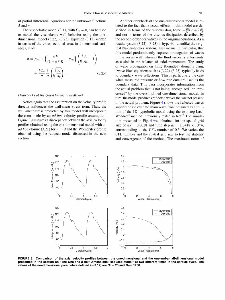
Notice again that the assumption on the velocity profiledirectly influences the wall-shear stress term. Thus, thewall-shear stress predicted by this model will incorporatethe error made by an ad hoc velocity profile assumption.Figure 3 illustrates a discrepancy between the axial velocityprofiles obtained using the one-dimensional model with anad hoc closure (3.21) for γ = 9 and the Womersley profileobtained using the reduced model discussed in the nextsection.

Another drawback of the one-dimensional model is re-lated to the fact that viscous effects in this model are de-scribed in terms of the viscous drag force − 2µ

ρF(γ + 2) m

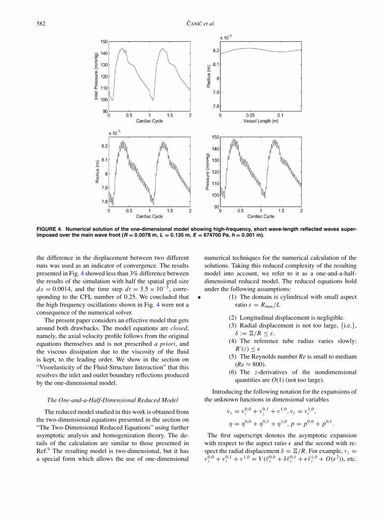
Aand not in terms of the viscous dissipation described bythe second-order derivatives in the original equations. As aresult, system (3.22), (3.23) is hyperbolic, unlike the orig-inal Navier–Stokes system. This means, in particular, thatthis model predominantly captures propagation of wavesin the vessel wall, whereas the fluid viscosity enters onlyas a sink in the balance of axial momentum. The studyof wave propagation on finite (bounded) domains using“wave-like” equations such as (3.22), (3.23), typically leadsto boundary wave reflections. This is particularly the casewhen measured pressure or flow rate data are used as theboundary data. This data incorporates information fromthe actual problem that is not being “recognized” or “pro-cessed” by the oversimplified one-dimensional model. Inturn, the model produces reflected waves that are not presentin the actual problem. Figure 4 shows the reflected wavessuperimposed over the main wave front obtained as a solu-tion of the 1D hyperbolic model using the two-step Lax–Wendroff method, previously tested in Ref.7 The simula-tion presented in Fig. 4 was obtained for the spatial gridsize of dx = 0.0028 and time step dt = 1.3418 × 10−4,corresponding to the CFL number of 0.5. We varied theCFL number and the spatial grid size to test the stabilityand convergence of the method. The maximum norm of

0 0.5 1 1.5 270

80

90

100

110

120

130

Inle

t Pre

ssur

e (m

mH

g)

Cardiac Cycle0 2 4 6 8

0

0.2

0.4

0.6

0.8

1

1.2

1.4

Vessel Radius (mm)

Vel

ocity

(m

/s)

2D profile1D profile

0 0.5 1 1.5 270

80

90

100

110

120

130

Cardiac Cycle

Inle

t pre

ssur

e (m

mH

g)

0 2 4 6 80.2

0.1

0

0.1

0.2

0.3

0.4

0.5

Vessel Radius (mm)

Vel

ocity

(m

/s/)

2D profile1D profile

FIGURE 3. Comparison of the axial velocity profiles between the one-dimensional and the one-and-a-half-dimensional modelpresented in the section on “The One-and-a-Half-Dimensional Reduced Model” at two different times in the cardiac cycle. Thevalues of the nondimensional parameters defined in (3.17) are Sh = 26 and Re = 1200.

582 CANIC et al.

FIGURE 4. Numerical solution of the one-dimensional model showing high-frequency, short wave-length reflected waves super-imposed over the main wave front (R = 0.0078 m, L = 0.135 m, E = 674700 Pa, h = 0.001 m).

the difference in the displacement between two differentruns was used as an indicator of convergence. The resultspresented in Fig. 4 showed less than 3% difference betweenthe results of the simulation with half the spatial grid sizedx = 0.0014, and the time step dt = 3.5 × 10−5, corre-sponding to the CFL number of 0.25. We concluded thatthe high frequency oscillations shown in Fig. 4 were not aconsequence of the numerical solver.

The present paper considers an effective model that getsaround both drawbacks. The model equations are closed,namely, the axial velocity profile follows from the originalequations themselves and is not prescribed a priori, andthe viscous dissipation due to the viscosity of the fluidis kept, to the leading order. We show in the section on“Visoelasticity of the Fluid-Structure Interaction” that thisresolves the inlet and outlet boundary reflections producedby the one-dimensional model.

The One-and-a-Half-Dimensional Reduced Model

The reduced model studied in this work is obtained fromthe two-dimensional equations presented in the section on“The Two-Dimensional Reduced Equations” using furtherasymptotic analysis and homogenization theory. The de-tails of the calculation are similar to those presented inRef.9 The resulting model is two-dimensional, but it hasa special form which allows the use of one-dimensional

numerical techniques for the numerical calculation of thesolutions. Taking this reduced complexity of the resultingmodel into account, we refer to it as a one-and-a-half-dimensional reduced model. The reduced equations holdunder the following assumptions:

• (1) The domain is cylindrical with small aspectratio ε = Rmax/L

(2) Longitudinal displacement is negligible.(3) Radial displacement is not too large, {i.e.},

δ := �/R ≤ ε.(4) The reference tube radius varies slowly:

R′(z) ≤ ε

(5) The Reynolds number Re is small to medium(Re ≈ 800).

(6) The z-derivatives of the nondimensionalquantities are O(1) (not too large).

Introducing the following notation for the expansions ofthe unknown functions in dimensional variables

vz = v0,0z + v0,1

z + v1,0, vr = v1,0r ,

η = η0,0 + η0,1 + η1,0, p = p0,0 + p0,1.

The first superscript denotes the asymptotic expansionwith respect to the aspect ratio ε and the second with re-spect the radial displacement δ = �/R. For example, vz =v0,0

z + v0,1z + v1,0 = V (v0,0

z + δv0,1z + εv1,0

z + O(ε2)), etc.

Blood Flow in Viscoelastic Arteries 583

The reduced “one-and-a-half-dimensional” equations hold-ing in cylindrical domains with slowly varying referenceradius R = R(z) then read:

The 0th order approximation: Find (η0,0, v0,0z ) such

that

∂η0,0

∂t+ 1

R

∂

∂z

∫ R

0rv0,0

z dr = 0,

�F∂v0,0

z

∂t− µ

1

r

∂

∂r

(r∂v0,0

z

∂r

)= −∂p0,0

∂z, (3.26)

v0,0z |r=0 − bounded, v0,0

z |t=R = 0, v0,0z |t=0 = 0,

η0,0|t=0 = 0, p0,0|z=0 = P0, p0,0|z=L = PL ,

where

p0,0 =(

Eh

(1 − σ 2)R+ pref

)η0,0

R+ hCv

R2

∂η0,0

∂t. (3.27)

The δ correction: Find (η0,1, v0,1z ) such that

∂η0,1

∂t+ 1

R

∂

∂z

∫ R

0rv0,1

z dr = − 1

2R

∂

∂t(η0,0)2,

�F∂v0,1

z

∂t− µ

1

r

∂

∂r

(r∂v0,1

z

∂r

)= −∂p0,1

∂z(3.28)

v0,1z |r=0 − bounded, v0,1

z |r=R = −η0,0 ∂v0,0z

∂r|r=R,

v0,1z |t=0 = 0, η0,1|t=0 = 0, η0,1|z=0 = 0, η0,1|z=L = 0 ,

where

p0,1 =(

Eh

(1 − σ 2)R+ pref

)(η0,1

R−

(η0,0

R

)2)

+ hCv

R2

(∂η0,1

∂t− η0,0

R

∂η0,1

∂t

). (3.29)

The ε correction: Find (v1,0r , v1,0

z ) such that

v1,0r (r, z, t) = 1

r

(R

∂η0,0

∂t

+∫ R

rξ∂η0,0

z

∂z(ξ, z, t)dξ

), (3.30)

ρF∂v1,0

z

∂t− µ

1

r

∂

∂r

(r∂v1,0

z

∂r

)

= −ρF

(v1,0

r

∂v0,0z

∂r+ v0,0

z

∂v0,0z

∂z

), (3.31)

v1,0z |r=0 − bounded, v1,0

z |r=R = 0, v1,0z |t=0 = 0.

Final solution:

vz = v0,0z + v0,1

z + v1,0, vr = v1,0r ,

η = η0,0 + η0,1 + η1,0. (3.32)

For the elastic membrane model, namely for Cv = 0, itwas proved in Ref. 9 that under assumptions (1)–(6), thefunctions (3.32) satisfying (3.26)–(3.31), solve the three-dimensional axially symmetric problem described in thesection on “Description of the Problem to the ε2-accuracy.

Remarks on the reduced model (3.26)–(3.31):

• The first equation in each of the three problems(3.26)–(3.31) all follow from the conservation ofmass principle.

• The second equation in each of the three problems(3.26)–(3.31) correspond to the balance of momen-tum. The quadratic advection terms appear only inthe ε-correction as the right-hand side of equation(3.31). In addition, they are linearized around the(0, 0)-approximation and thus present no additionaldifficulty in the numerical simulation of the model.

• The original moving boundary problem, posed onthe domain with a moving lateral boundary �(t),has now been approximated by a series of threeproblems (3.26)–(3.31) each defined on a fixed do-main with radius R = R(z).

This model enabled us to study, among other things,wave propagation in arteries influenced by two distinct vis-cous effects. One is the influence of fluid viscosity and theother is the influence of vessel wall viscosity. We shall seebelow how they have different viscoelastic impact on thevessel wall dynamics. We first present the numerical algo-rithm for calculation of the solution of the model equations(3.26) and (3.28).

NUMERICAL ALGORITHM

To solve problems (3.26) and (3.28) numerically it isconvenient to rewrite each of the systems of equations asa second-order hyperbolic-parabolic problem. Namely, af-ter differentiating the first equation in (3.26) with respectto time, and plugging the second equation into the first,problem (3.26) can be rewritten as

∂2η0,0

∂t2− R

2ρF

∂2 p0,0

∂z2= − µ

ρF

∂

∂z

(∂v0,0

z

∂r|r=R

), (4.33)

ρF∂v0,0

z

∂t− µ

1

r

∂

∂r

(r∂v0,0

z

∂r

)= −∂p0,0

∂z, (4.34)

with the initial and boundary conditions specified in (3.26)where p0,0 is substituted by (3.27). Similarly, problem(3.28) can be written as

∂2η0,1

∂t2− R

2ρF

∂2 p0,1

∂z2= − µ

ρF

∂

∂z

(∂v0,0

z

∂r|r=R

)

− 1

2R

∂2

∂t2(η0,0)2, (4.35)

584 CANIC et al.

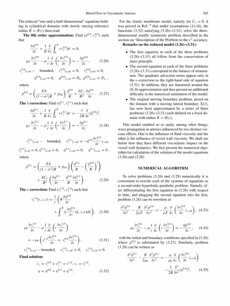
FIGURE 5. A snap-shot of the radial (top) and longitudinal (middle picture) component of the velocity with the superimposedstreamlines, calculated at the beginning of the cardiac (LVAD) output. The circle at the bottom graph shows the time in the cardiaccycle when the snap-shot is taken.

ρF∂v0,1

z

∂t− µ

1

r

∂

∂r

(r∂v0,1

z

∂r

)= −∂p0,1

∂z, (4.36)

with initial and boundary conditions given in (3.28), andp0,1 substituted by (3.29).

The first equation in both subproblems can be thoughtoff as a one-dimensional wave equation in z and t, and thesecond as the one-dimensional heat equation in r and t. Thesystems for the 0, 0 and 0, 1 approximations have the sameform. They are solved using a 1D Finite Element Method.Since the mass and stiffness matrices are the same for bothproblems, up to the boundary conditions, they are generatedonly once. Both systems are solved simultaneously usinga time-iteration procedure. First the parabolic equation issolved for v0,0

z at the time step ti+1 by explicitly evaluat-ing the right-hand side at the time-step ti . Then the waveequation is solved for η0,0 with the evaluation of the right-hand side at the time-step ti+1. Using these results for v0,0

zand η0,0, computed at ti+1, a correction at ti+1 is calculatedby repeating the process with the updated values of theright-hand sides. This method is a version of the Douglas–Rachford time-splitting algorithm which is known to be offirst-order accuracy.

Calculating approximation 1,0 is straightforward oncethe approximations 0, 0 and 0,1 are obtained.

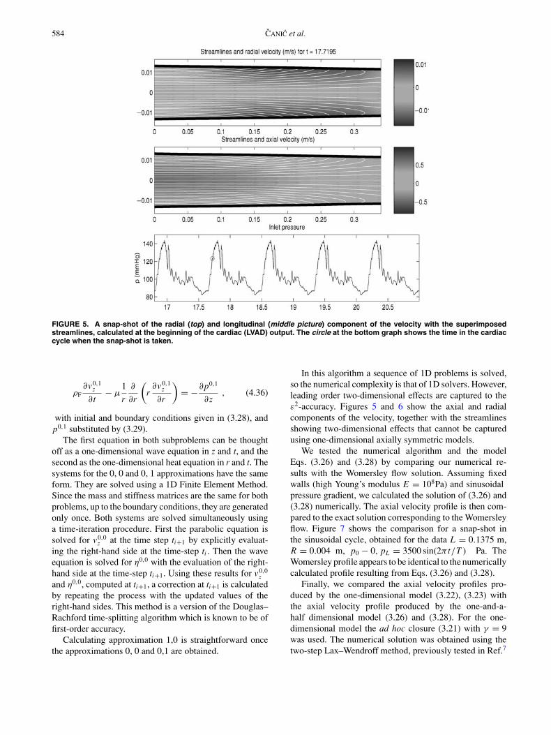
In this algorithm a sequence of 1D problems is solved,so the numerical complexity is that of 1D solvers. However,leading order two-dimensional effects are captured to theε2-accuracy. Figures 5 and 6 show the axial and radialcomponents of the velocity, together with the streamlinesshowing two-dimensional effects that cannot be capturedusing one-dimensional axially symmetric models.

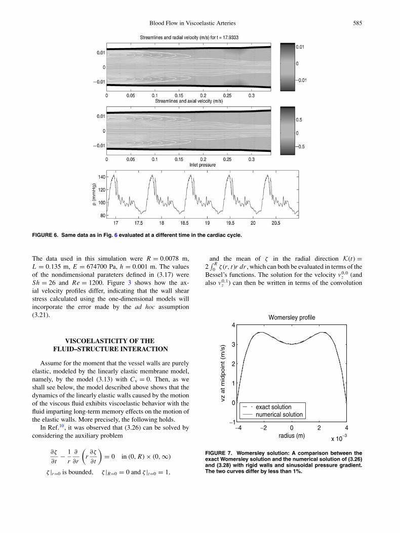
We tested the numerical algorithm and the modelEqs. (3.26) and (3.28) by comparing our numerical re-sults with the Womersley flow solution. Assuming fixedwalls (high Young’s modulus E = 108Pa) and sinusoidalpressure gradient, we calculated the solution of (3.26) and(3.28) numerically. The axial velocity profile is then com-pared to the exact solution corresponding to the Womersleyflow. Figure 7 shows the comparison for a snap-shot inthe sinusoidal cycle, obtained for the data L = 0.1375 m,R = 0.004 m, p0 − 0, pL = 3500 sin(2π t/T ) Pa. TheWomersley profile appears to be identical to the numericallycalculated profile resulting from Eqs. (3.26) and (3.28).

Finally, we compared the axial velocity profiles pro-duced by the one-dimensional model (3.22), (3.23) withthe axial velocity profile produced by the one-and-a-half dimensional model (3.26) and (3.28). For the one-dimensional model the ad hoc closure (3.21) with γ = 9was used. The numerical solution was obtained using thetwo-step Lax–Wendroff method, previously tested in Ref.7

Blood Flow in Viscoelastic Arteries 585

FIGURE 6. Same data as in Fig. 6 evaluated at a different time in the cardiac cycle.

The data used in this simulation were R = 0.0078 m,L = 0.135 m, E = 674700 Pa, h = 0.001 m. The valuesof the nondimensional parateters defined in (3.17) wereSh = 26 and Re = 1200. Figure 3 shows how the ax-ial velocity profiles differ, indicating that the wall shearstress calculated using the one-dimensional models willincorporate the error made by the ad hoc assumption(3.21).

VISCOELASTICITY OF THEFLUID–STRUCTURE INTERACTION

Assume for the moment that the vessel walls are purelyelastic, modeled by the linearly elastic membrane model,namely, by the model (3.13) with Cv = 0. Then, as weshall see below, the model described above shows that thedynamics of the linearly elastic walls caused by the motionof the viscous fluid exhibits viscoelastic behavior with thefluid imparting long-term memory effects on the motion ofthe elastic walls. More precisely, the following holds.

In Ref.10, it was observed that (3.26) can be solved byconsidering the auxiliary problem

∂ζ

∂t− 1

r

∂

∂r

(r∂ζ

∂t

)= 0 in (0, R) × (0,∞)

ζ |r=0 is bounded, ζ |R=0 = 0 and ζ |t=0 = 1,

and the mean of ζ in the radial direction K(t) =2∫ R

0 ζ (r, t)r dr , which can both be evaluated in terms of theBessel’s functions. The solution for the velocity v0,0

z (andalso v0,1

z ) can then be written in terms of the convolution

−4 −2 0 2 4

x 10−3

−1

0

1

2

3

4Womersley profile

vz a

t m

idp

oin

t (m

/s)

radius (m)

exact solutionnumerical solution

FIGURE 7. Womersley solution: A comparison between theexact Womersley solution and the numerical solution of (3.26)and (3.28) with rigid walls and sinusoidal pressure gradient.The two curves differ by less than 1%.

586 CANIC et al.

integral(K �

∂η0,0

∂z

)(z, t) :=

∫ t

0K

(µ(t − τ )

ρF

)∂η0,0

∂z(z, τ ) dτ,

(5.37)where K is the decreasing exponential function

exp(−λµ(t − τ )/ρF) where λ is the first zero of the Bessel’sfunction J0. Now the problem for η0,0 consists of solvingthe following initial-boundary value problem of “Biot type”with memory5:

∂η0,0

∂t(z, t) = C

2ρF R

∂

∂z

(K �

∂η0,0

∂z

)(z, t) on (0, L)

×(0,+∞) (5.38)

η0,0|z=0 = P0/C, η0,0|z=L = PL/C

and

η0,0|t=0 = 0,

where C = Eh/[(1 − σ 2)R2] + pref/R.The time integral in the convolution term uncovers the

viscoelastic nature of the coupling between the motion of anelastic structure and a viscous fluid, explicitly. The viscouscontribution of the fluid to the wave propagation in theelastic structure has a long-term memory effect. Due tothe exponentially decaying kernel K, history that happenedlong time ago affects the solution at the current time muchless than the most recent history. To get a better feeling forthe wave propagation described by Eq. (5.38), differentiate(5.38) with respect to time to obtain

∂2η0,0

∂t2= C1

∂2η0,0

∂z2− µ

ρFC2

∂

∂z

(K′ �

∂η0,0

∂z

). (5.39)

Here C1 and C2 are constants that do not involve the vis-cosity coefficient µ. Thus, if µ = 0, the radial displace-ment η satisfies a constant-coefficient wave equation whichdescribes propagation of waves in an elastic string. Withµ �= 0, Eq. (5.39) describes wave propagation in a vis-coelastic string with long-term memory.

The numerical method described in the section on “Nu-merical Algorithm,” was used to obtain a solution ofEq. (5.39) with µ �= 0. Figure 8 shows the solution withµ = 3.5 × 10−3 kg/m/s. The solution contains only themain wave front, without the reflected waves appearingin one-dimensional models with Dirichlet boundary data,shown in Fig. 4. A direct comparison between the two solu-tions, one obtained by solving the one-dimensional systemand the other by solving the one-and-a-half dimensionalsystems, is shown in Fig. 9. The data used in both simula-tions were R = 0.0078 m, L = 0.135 m, E = 674700 Pa,h = 0.001 m.

It is interesting to mention that the viscoelastic effectdiscussed in this section does not contribute to the hystere-sis in the pressure-diameter diagram, typically observedin the vessel wall dynamics experimental measurements,

see Refs.1,4 The hysteresis behavior is solely due to theviscoelastic nature of the mechanical properties of vesselwalls.

VISCOELASTICITY OF VESSEL WALLS

Determining the viscoelastic behavior of vessel wallsis a complex problem. In Ref.1, measurements of the vis-coelastic aortic properties in dogs, and the derivation ofthe constitutive relation for the aortic wall behavior wereobtained. In particular, the magnitude of the viscous mod-ulus, corresponding to our coefficient hCv/R is measured.The values corresponding to dogs aortas, reported in Ref.1.belong to the interval

hCv

R|(dog aorta) ∈ (3.8 ± 1.3 × 104, 7.8 ± 1.1 × 104)

dyn · s/cm2

= (3.8 ± 1.3 × 103, 7.8 ± 1.1 × 103) Pa · s.

Taking into account the radius of the studied aortas (≈0.008 m) and the average wall thickness (≈ 0.0014 m), oneobtains

Cv|(dog aorta) ∈ (2.17 × 104, 4.45 × 104) Pa · s (6.39)

This coefficient appears to be slightly higher than thecoefficient Cv describing the wall properties of the hu-man femoral and carotid arteries, although their viscousmoduli hCv/R appear to be of the same order of magni-tude. Namely, measurements reported in Ref.2 imply thatin healthy humans the magnitude of the coefficient multi-plying the term ∂ D/∂t . where D is the vessel diameter, isestimated to be equal to 266×Pa·s/m. Using the values forthe measured femoral artery diameter (0.00625 m) and thewall thickness (0.001 m), one obtains

Cv|(human femoral) ≈ 5.2 × 103 Pa · s. (6.40)

Thus, the corresponding viscous modulus hCv/R is

hCv

R|(human femoral) ≈ 1.6 × 103 Pa · s, (6.41)

which is of the same order of magnitude as the viscousmodulus corresponding to the dogs aortas.

In the present work these measurements were used asa guide in determining the order of magnitude of the co-efficient hCv/R that appears in the “effective” pressure–displacement relationship (3.13), which in dimensionalvariables reads

p − pref =(

Eh

(1 − σ 2)R+ pref

)η

R+ hCv

R2

∂η

∂t. (6.42)

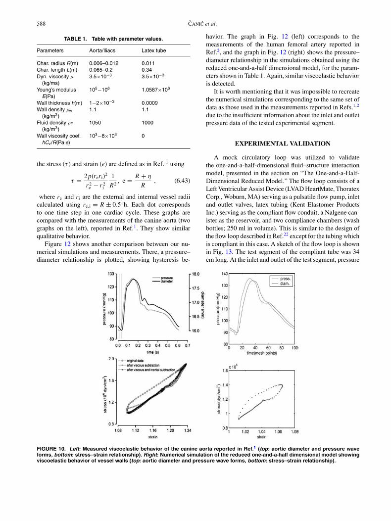
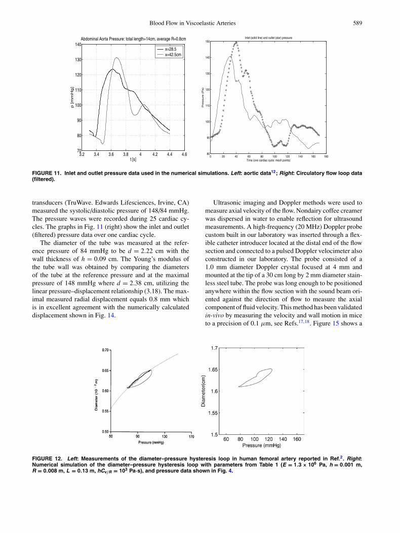
Using this constitutive model for the vessel wall behavior,coupled with the reduced equations (3.26)–(3.31), numeri-cal simulations with the data given in Table 1 were obtained.Figure 10 (right) shows the results of the numerical simula-tions for the inlet and outlet pressure data shown in Fig. 11

Blood Flow in Viscoelastic Arteries 587

0 0.5 1 1.5 270

80

90

100

110

120

130

Inle

t Pre

ssur

e (m

mH

g)

Cardiac Cycle0 0.05 0.1

7.8

7.9

8

8.1

8.2

x 103

Rad

ius

(m)

Vessel Length (m)

0 0.5 1 1.5 27.8

7.9

8

8.1

8.2

x 103

Rad

ius

(m)

Cardiac Cycle0 0.5 1 1.5 2

70

80

90

100

110

120

130

Cardiac CycleP

ress

ure

(m/s

)

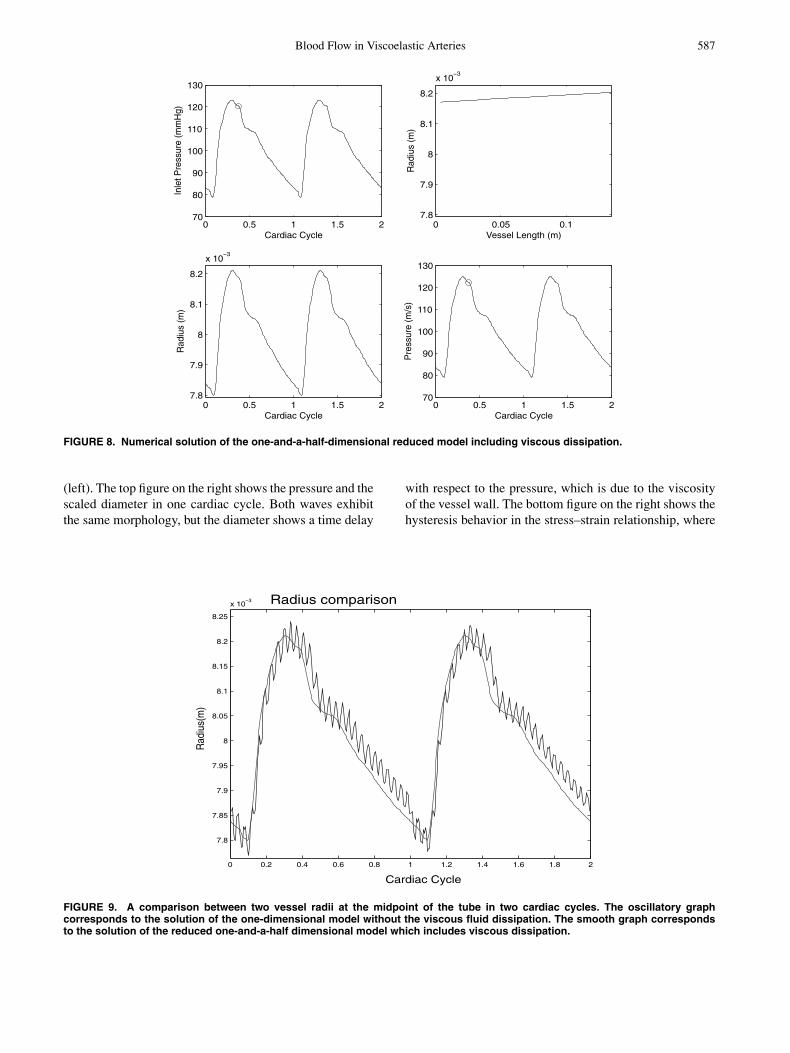
FIGURE 8. Numerical solution of the one-and-a-half-dimensional reduced model including viscous dissipation.

(left). The top figure on the right shows the pressure and thescaled diameter in one cardiac cycle. Both waves exhibitthe same morphology, but the diameter shows a time delay

with respect to the pressure, which is due to the viscosityof the vessel wall. The bottom figure on the right shows thehysteresis behavior in the stress–strain relationship, where

0 0.2 0.4 0.6 0.8 1 1.2 1.4 1.6 1.8 2

7.8

7.85

7.9

7.95

8

8.05

8.1

8.15

8.2

8.25

x 103

Cardiac Cycle

Radius comparison

Rad

ius(

m)

FIGURE 9. A comparison between two vessel radii at the midpoint of the tube in two cardiac cycles. The oscillatory graphcorresponds to the solution of the one-dimensional model without the viscous fluid dissipation. The smooth graph correspondsto the solution of the reduced one-and-a-half dimensional model which includes viscous dissipation.

588 CANIC et al.

TABLE 1. Table with parameter values.

Parameters Aorta/Iliacs Latex tube

Char. radius R(m) 0.006–0.012 0.011Char. length L(m) 0.065–0.2 0.34Dyn. viscosity µ

(kg/ms)3.5×10−3 3.5×10−3

Young’s modulusE(Pa)

105−106 1.0587×106

Wall thickness h(m) 1−2×10−3 0.0009Wall density ρw

(kg/m2)1.1 1.1

Fluid density ρF

(kg/m3)1050 1000

Wall viscosity coef.hCv/R(Pa·s)

103−8×103 0

the stress (τ ) and strain (e) are defined as in Ref. 1 using

τ = 2p(reri)2

r2e − r2

i

1

R2, e = R + η

R, (6.43)

where re and ri are the external and internal vessel radiicalculated using re,i = R ± 0.5 h. Each dot correspondsto one time step in one cardiac cycle. These graphs arecompared with the measurements of the canine aorta (twographs on the left), reported in Ref.1. They show similarqualitative behavior.

Figure 12 shows another comparison between our nu-merical simulations and measurements. There, a pressure–diameter relationship is plotted, showing hysteresis be-

havior. The graph in Fig. 12 (left) corresponds to themeasurements of the human femoral artery reported inRef.2, and the graph in Fig. 12 (right) shows the pressure–diameter relationship in the simulations obtained using thereduced one-and-a-half dimensional model, for the param-eters shown in Table 1. Again, similar viscoelastic behavioris detected.

It is worth mentioning that it was impossible to recreatethe numerical simulations corresponding to the same set ofdata as those used in the measurements reported in Refs.1,2

due to the insufficient information about the inlet and outletpressure data of the tested experimental segment.

EXPERIMENTAL VALIDATION

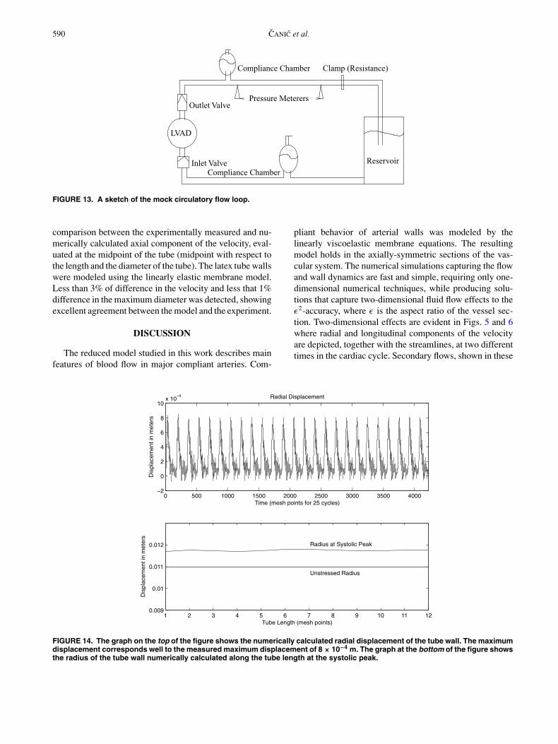
A mock circulatory loop was utilized to validatethe one-and-a-half-dimensional fluid–structure interactionmodel, presented in the section on “The One-and-a-Half-Dimensional Reduced Model.” The flow loop consists of aLeft Ventricular Assist Device (LVAD HeartMate, ThoratexCorp., Woburn, MA) serving as a pulsatile flow pump, inletand outlet valves, latex tubing (Kent Elastomer ProductsInc.) serving as the compliant flow conduit, a Nalgene can-ister as the reservoir, and two compliance chambers (washbottles; 250 ml in volume). This is similar to the design ofthe flow loop described in Ref.22 except for the tubing whichis compliant in this case. A sketch of the flow loop is shownin Fig. 13. The test segment of the compliant tube was 34cm long. At the inlet and outlet of the test segment, pressure

FIGURE 10. Left: Measured viscoelastic behavior of the canine aorta reported in Ref.1 (top: aortic diameter and pressure waveforms, bottom: stress–strain relationship). Right: Numerical simulation of the reduced one-and-a-half dimensional model showingviscoelastic behavior of vessel walls (top: aortic diameter and pressure wave forms, bottom: stress–strain relationship).

Blood Flow in Viscoelastic Arteries 589

3.2 3.4 3.6 3.8 4 4.2 4.4 4.670

80

90

100

110

120

130

140Abdominal Aorta Pressure: total length=14cm, average R=0.8cm

t [s]

p [m

mH

g]

x=28.5x=42.5cm

0 20 40 60 80 100 120 140 160 18080

90

100

110

120

130

140

150Inlet (solid line) and outlet (star) pressure

Time (one cardiac cycle: mesh points)

Pre

ssure

(P

a)

FIGURE 11. Inlet and outlet pressure data used in the numerical simulations. Left: aortic data12; Right: Circulatory flow loop data(filtered).

transducers (TruWave. Edwards Lifesciences, Irvine, CA)measured the systolic/diastolic pressure of 148/84 mmHg.The pressure waves were recorded during 25 cardiac cy-cles. The graphs in Fig. 11 (right) show the inlet and outlet(filtered) pressure data over one cardiac cycle.

The diameter of the tube was measured at the refer-ence pressure of 84 mmHg to be d = 2.22 cm with thewall thickness of h = 0.09 cm. The Young’s modulus ofthe tube wall was obtained by comparing the diametersof the tube at the reference pressure and at the maximalpressure of 148 mmHg where d = 2.38 cm, utilizing thelinear pressure–displacement relationship (3.18). The max-imal measured radial displacement equals 0.8 mm whichis in excellent agreement with the numerically calculateddisplacement shown in Fig. 14.

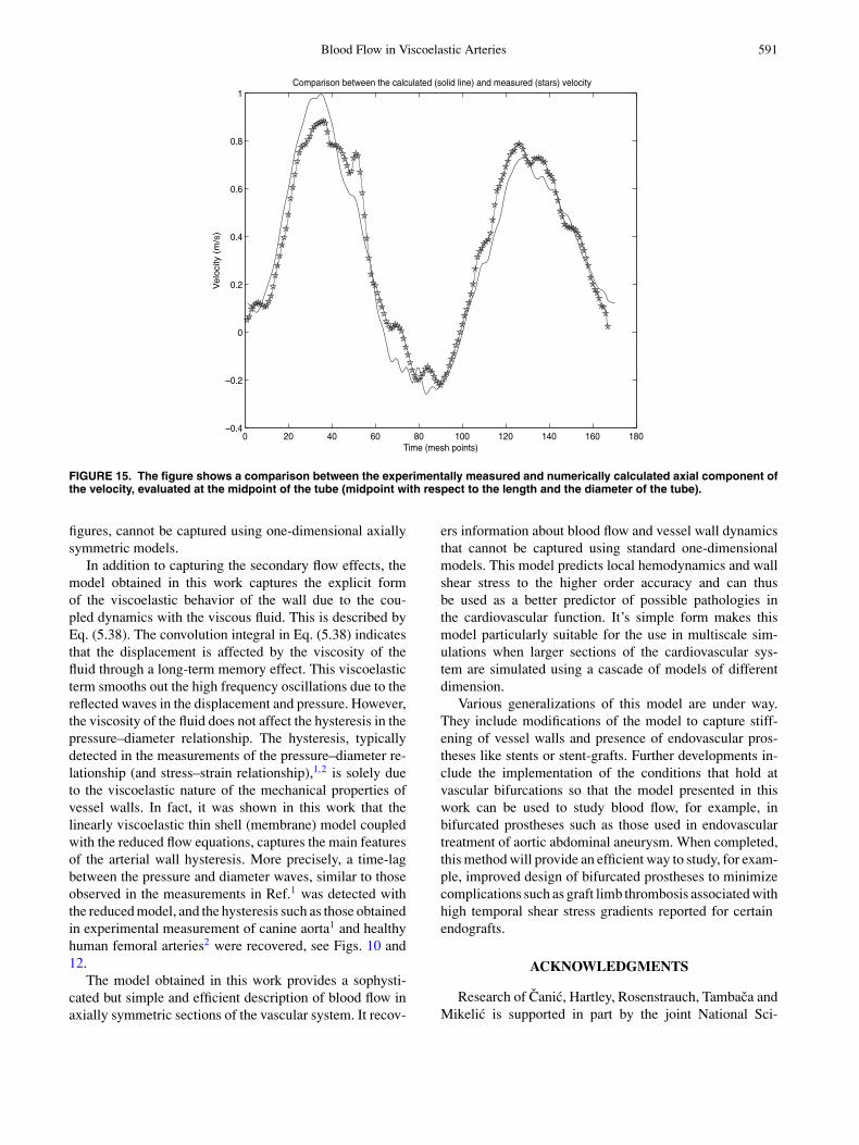
Ultrasonic imaging and Doppler methods were used tomeasure axial velocity of the flow. Nondairy coffee creamerwas dispersed in water to enable reflection for ultrasoundmeasurements. A high-frequency (20 MHz) Doppler probecustom built in our laboratory was inserted through a flex-ible catheter introducer located at the distal end of the flowsection and connected to a pulsed Doppler velocimeter alsoconstructed in our laboratory. The probe consisted of a1.0 mm diameter Doppler crystal focused at 4 mm andmounted at the tip of a 30 cm long by 2 mm diameter stain-less steel tube. The probe was long enough to be positionedanywhere within the flow section with the sound beam ori-ented against the direction of flow to measure the axialcomponent of fluid velocity. This method has been validatedin-vivo by measuring the velocity and wall motion in miceto a precision of 0.1 µm, see Refs.17,18. Figure 15 shows a

FIGURE 12. Left: Measurements of the diameter–pressure hysteresis loop in human femoral artery reported in Ref.2. Right:Numerical simulation of the diameter–pressure hysteresis loop with parameters from Table 1 (E = 1.3 × 106 Pa, h = 0.001 m,R = 0.008 m, L = 0.13 m, hCv/R = 103 Pa·s), and pressure data shown in Fig. 4.

590 CANIC et al.

LVAD

Inlet Valve

Outlet ValvePressure Meterers

Compliance Chamber

Compliance Chamber

Reservoir

Clamp (Resistance)

FIGURE 13. A sketch of the mock circulatory flow loop.

comparison between the experimentally measured and nu-merically calculated axial component of the velocity, eval-uated at the midpoint of the tube (midpoint with respect tothe length and the diameter of the tube). The latex tube wallswere modeled using the linearly elastic membrane model.Less than 3% of difference in the velocity and less that 1%difference in the maximum diameter was detected, showingexcellent agreement between the model and the experiment.

DISCUSSION

The reduced model studied in this work describes mainfeatures of blood flow in major compliant arteries. Com-

pliant behavior of arterial walls was modeled by thelinearly viscoelastic membrane equations. The resultingmodel holds in the axially-symmetric sections of the vas-cular system. The numerical simulations capturing the flowand wall dynamics are fast and simple, requiring only one-dimensional numerical techniques, while producing solu-tions that capture two-dimensional fluid flow effects to theε2-accuracy, where ε is the aspect ratio of the vessel sec-tion. Two-dimensional effects are evident in Figs. 5 and 6where radial and longitudinal components of the velocityare depicted, together with the streamlines, at two differenttimes in the cardiac cycle. Secondary flows, shown in these

0 500 1000 1500 2000 2500 3000 3500 40002

0

2

4

6

8

10x 10

4 Radial Displacement

Dis

plac

emen

t in

met

ers

Time (mesh points for 25 cycles)

1 2 3 4 5 6 7 8 9 10 11 120.009

0.01

0.011

0.012

Dis

plac

emen

t in

met

ers

Tube Length (mesh points)

Unstressed Radius

Radius at Systolic Peak

FIGURE 14. The graph on the top of the figure shows the numerically calculated radial displacement of the tube wall. The maximumdisplacement corresponds well to the measured maximum displacement of 8 × 10−4 m. The graph at the bottom of the figure showsthe radius of the tube wall numerically calculated along the tube length at the systolic peak.

Blood Flow in Viscoelastic Arteries 591

0 20 40 60 80 100 120 140 160 1800.4

0.2

0

0.2

0.4

0.6

0.8

1Comparison between the calculated (solid line) and measured (stars) velocity

Time (mesh points)

Ve

loci

ty (

m/s

)

FIGURE 15. The figure shows a comparison between the experimentally measured and numerically calculated axial component ofthe velocity, evaluated at the midpoint of the tube (midpoint with respect to the length and the diameter of the tube).

figures, cannot be captured using one-dimensional axiallysymmetric models.

In addition to capturing the secondary flow effects, themodel obtained in this work captures the explicit formof the viscoelastic behavior of the wall due to the cou-pled dynamics with the viscous fluid. This is described byEq. (5.38). The convolution integral in Eq. (5.38) indicatesthat the displacement is affected by the viscosity of thefluid through a long-term memory effect. This viscoelasticterm smooths out the high frequency oscillations due to thereflected waves in the displacement and pressure. However,the viscosity of the fluid does not affect the hysteresis in thepressure–diameter relationship. The hysteresis, typicallydetected in the measurements of the pressure–diameter re-lationship (and stress–strain relationship),1,2 is solely dueto the viscoelastic nature of the mechanical properties ofvessel walls. In fact, it was shown in this work that thelinearly viscoelastic thin shell (membrane) model coupledwith the reduced flow equations, captures the main featuresof the arterial wall hysteresis. More precisely, a time-lagbetween the pressure and diameter waves, similar to thoseobserved in the measurements in Ref.1 was detected withthe reduced model, and the hysteresis such as those obtainedin experimental measurement of canine aorta1 and healthyhuman femoral arteries2 were recovered, see Figs. 10 and12.

The model obtained in this work provides a sophysti-cated but simple and efficient description of blood flow inaxially symmetric sections of the vascular system. It recov-

ers information about blood flow and vessel wall dynamicsthat cannot be captured using standard one-dimensionalmodels. This model predicts local hemodynamics and wallshear stress to the higher order accuracy and can thusbe used as a better predictor of possible pathologies inthe cardiovascular function. It’s simple form makes thismodel particularly suitable for the use in multiscale sim-ulations when larger sections of the cardiovascular sys-tem are simulated using a cascade of models of differentdimension.

Various generalizations of this model are under way.They include modifications of the model to capture stiff-ening of vessel walls and presence of endovascular pros-theses like stents or stent-grafts. Further developments in-clude the implementation of the conditions that hold atvascular bifurcations so that the model presented in thiswork can be used to study blood flow, for example, inbifurcated prostheses such as those used in endovasculartreatment of aortic abdominal aneurysm. When completed,this method will provide an efficient way to study, for exam-ple, improved design of bifurcated prostheses to minimizecomplications such as graft limb thrombosis associated withhigh temporal shear stress gradients reported for certainendografts.

ACKNOWLEDGMENTS

Research of Canic, Hartley, Rosenstrauch, Tambaca andMikelic is supported in part by the joint National Sci-

592 CANIC et al.

ence Foundation and the National Institutes of Healthgrant DMS-0443826. In addition, research of Canic is sup-ported in part by the National Science Foundation undergrants DMS-0245513, DMS-0337355, and the research ofHartley is supported in part by the National Institutes ofHealth under Grant HL22512. The experimental designand the in vitro work at Dr. Rosenstrauch’s laboratory atthe Texas Heart Institute was partially supported by a grantfrom the Roderick Duncan McDonald Foundation at theSt. Luke’s Episcopal Hospital. Kent Elastomer Inc. do-nation of latex tubing is also acknowledged. The authorswould like to thank undergraduate student Joy Chavez forthe help with data collection and flow loop experiments.Chavez’s research was supported by the NSF under grantDMS-0337355.

REFERENCES

1Armentano, R. L., J. G. Barra, J. Levenson, A. Simon, and R. H.Pichel. Arterial wall mechanics in conscious dogs: Assessmentof viscous, iner-tial, and elastic moduli to characterize aorticwall behavior. Circ. Res. 76:468–478, 1995.

2Armentano, R. L., J. L. Megnien, A. Simon, F. Bellenfant, J. G.Barra, and J. Levenson. Effects of hypertension on viscoelas-ticity of carotid and femoral arteries in humans. Hypertension26:48–54, 1995.

3Barnard, A. C. L, W. A. Hunt, W. P. Timlake, and E. Varley. Atheory of fluid flow in compliant tubes. Biophys. J. 6:717–724,1966.

4Bauer R. D., R. Busse, A. Shabert, Y. Summa, and E. Wetterer.Separate determination of the pulsatile elastic and viscous forcesdeveloped in the arterial wall in vivo. Pflugers Arch. 380:221–226, 1979.

5Biot, M. A. Theory of propagation of elastic waves in a fluid-saturated porous solid. I. Lower frequency range, and II. Higherfrequency range. J. Acoust. Soc. Am. 28(2):168–178, 179–191,1956.

6Canic, S., J. Tambaca, G. Guidoboni, A. Mikelic, C. J.Hartley, and D. Rosenstrauch. Modeling viscoelastic behaviorof arterial walls and their interaction with pulsatile blood flow.Submitted.

7Canic, S., and E. H. Kim. Mathematical analysis of the quasi-linear effects in a hyperbolic model of blood flow throughcompliant axisym-metric vessels. Math. Methods Appl. Sci.26(14):1161–1186, 2003.

8Canic, S., and A. Mikelic. Effective equations modeling theflow of a viscous incompressible fluid through a long elastictube arising in the study of blood flow through small arteries.SIAM J. Appl. Dyn. Sys. 2(3):431–463, 2003.

9Canic, S., A. Mikelic, D. Lamponi, and J. Tambaca. Self-consistent effective equations modeling blood flow in medium-

to-large compliant arteries. SIAM J. Multisc. Anal. Simul.3(3):559–596, 2005.

10Canic, S., A. Mikelic, and J. Tambaca. A two-dimensional effec-tive model describing fluid–structure interaction in blood flow:Analysis, simulation and experimental validation. Comptes Ren-dus Mech. Acad. Sci. Paris 333:867–883, 2005.

11Canic, S., J. Tambaca, A. Mikelic, C. J. Hartley, D. Mirkovic,and D. Rosenstrauch. Blood flow through axially symmetricsections of compliant vessels: New effective closed models. In:Proceedings of the 26th Annual International Conference. IEEEEng. Med. Bio. Soc., 2004, 10–13 pp.

12Chmielewski, C. Master of Science Thesis, Department of Math-ematics, North Carolina State University, 2003.

13Eringen, A. Cemal. Mechanics of continua. New York: Wiley,1967, 365 pp.

14Formaggia, L., D. Lamponi, and A. Quarteroni. One-dimensional models for blood flow in arteries. J. Eng. Math.47:251–276, 2003.

15Formaggia, L., F. Nobile, and A. Quarteroni. A one-dimensionalmodel for blood flow: Application to vascular prosthesis. In:Mathematical Modeling and Numerical Simulation in Contin-uum Mechanics, edited by Babuska, Miyoshi, and Ciarlet), Lect.Notes Comput. Sci. Eng. 19:137–153, 2002.

16Haidekker, M. A., C. R. White, and J. A. Frangos. Analysis oftemporal shear stress gradients during the onset phase of flowover a backward-facing step. J. Biomech. Eng. 123:455–463,2001.

17Hartley, C. J. Ultrasonic blood flow and velocimetry. In:McDonald’s Blood Flow in Arteries, Theoretical, Experimentaland Clinical Principles, 4th edn. Ch. 7, edited by W. W. Nicholsand M. F. O’Rourke. London: Arnold, 1998, pp. 154–169.

18Hartley, C. J. G. Taffet, A. Reddy, M. Entman, and L. Michael.Noninvasive cardiovascular phenotyping in mice. ILAR J.43:147–158, 2002.

19Nichols, W. W., and M. F. O’Rourke. McDonald’s Blood Flowin Arteries: Theoretical, Experimental and Clinical Principles,4th edn. New York: Arnold and Oxford University Press,2000.

20Olufsen, M. S., C. S. Peskin, W. Y. Kim, E.M. Pedersen, A.Nadim, and J. Larsen. Numerical simulation and experimentalvalidation of blood flow in arteries with structured-tree outflowconditions. Ann. Biomed. Eng. 28:1281–1299, 2000.

21Pontrelli, G. Modeling the fluid–wall interaction in a blood ves-sel. Prog. Biomed. Res. 6(4):330–338, 2001.

22Scott-Burden, T., J. P. Bosley, D. Rosenstrauch, K. Hender-son, F. Clubb, H. Eichstaedt, K. Eya, I. Gregoric, T. Myers, B.Radovancevic, and O. H. Frazier. Use of autologous auricularchondrocytes for lining artificial surfaces: A feasibility study.Ann. Thor. Surg. 73(5):1528–1533, 2002.

23Smith, N. P., A. J. Pullan, and P. J. Hunter. An anatomicallybased model of transient coronary blood flow in the heart. SIAMJ. Appl. Math. 62(3):990–1018, 2002.

24Tambaca, J., S. Canic, and A. Mikelic. Effective model of thefluid flow through elastic tube with variable radius. Grazer Math.Ber., ISSN1016 7692 Bericht Nr. 3:1–22, 2005.