Block-1 (Data Communication Fundamentals) Unit-1 Introduction to ...
502
Block-1 (Data Communication Fundamentals) Unit-1 Introduction to Networking 1.1 Learning Objectives 1.2 Introduction 1.3 Historical Background 1.4 Network Technologies 1.4.1 Classification Based on Transmission Technology 1.4.1.1 Broadcast Networks 1.4.1.2 Point-to-Point Networks 1.4.2 Classification based on Scale 1.4.2.1 Local Area Network (LAN) 1.4.2.2 Metropolitan Area Networks (MAN) 1.4.2.3 Wide Area Network (WAN) 1.4.2.4 The Internet 1.5 The Internet 1.6 Applications 1.7 Check Your Progress 1.8 Answer to Check Your Progress 1.1 Learning Objectives
-
Upload
khangminh22 -
Category
Documents
-
view
0 -
download
0
Transcript of Block-1 (Data Communication Fundamentals) Unit-1 Introduction to ...
Block-1
(Data Communication Fundamentals)
Unit-1
Introduction to Networking
1.1 Learning Objectives
1.2 Introduction
1.3 Historical Background
1.4 Network Technologies
1.4.1 Classification Based on Transmission Technology
1.4.1.1 Broadcast Networks
1.4.1.2 Point-to-Point Networks
1.4.2 Classification based on Scale
1.4.2.1 Local Area Network (LAN)
1.4.2.2 Metropolitan Area Networks (MAN)
1.4.2.3 Wide Area Network (WAN)
1.4.2.4 The Internet
1.5 The Internet
1.6 Applications
1.7 Check Your Progress
1.8 Answer to Check Your Progress
1.1 Learning Objectives

After going through this unit the learner will be able to:
• Define Computer Networks
• State the evolution of Computer Networks
• Categorize different types of Computer Networks
• Specify some of the application of Computer Networks
1.2 Introduction
The concept of Network is not new. In simple terms it means an interconnected set of some
objects. For decades we are familiar with the Radio, Television, railway, Highway, Bank and other
types of networks. In recent years, the network that is making significant impact in our day-to-day
life is the Computer network. By computer network we mean an interconnected set of
autonomous computers. The term autonomous implies that the computers can function
independent of others. However, these computers can exchange information with each other
through the communication network system. Computer networks have emerged as a result of the
convergence of two technologies of this century- Computer and Communication as shown in Fig.
1.1 The consequence of this revolutionary merger is the emergence of a integrated system that
transmit all types of data and information. There is no fundamental difference between data
communications and data processing and there are no fundamental differences among data, voice
and video communications.
Figure 1.1 Evolution of computer networks
1.3 Historical Background

The history of electronic computers is not very old. It came into existence in the early 1950s and
during the first two decades of its existence it remained as a centralized system housed in a single
large room. In those days the computers were large in size and were operated by trained personnel.
To the users it was a remote and mysterious object having no direct communication with the users.
Jobs were submitted in the form of punched cards or paper tape and outputs were collected in the
form of computer printouts. The submitted jobs were executed by the computer one after the other,
which is referred to as batch mode of data processing. In this scenario, there was long delay
between the submission of jobs and receipt of the results.
In the 1960s, computer systems were still centralize, but users provided with direct access through
interactive terminals connected by point-to-point low-speed data links with the computer. In this
situation, a large number of users, some of them located in remote locations could simultaneously
access the centralized computer in time-division multiplexed mode. The users could now get
immediate interactive feedback from the computer and correct errors immediately. Following the
introduction of on-line terminals and time-sharing operating systems, remote terminals were used
to use the central computer.
With the advancement of VLSI technology, and particularly, after the invention of
microprocessors in the early 1970s, the computers became smaller in size and less expensive, but
with significant increase in processing power. New breed of low-cost computers known as mini
and personal computers were introduced. Instead of having a single central computer, an
organization could now afford to own a number of computers located in different departments and
sections.
Side-by-side, riding on the same VLSI technology the communication technology also advanced
leading to the worldwide deployment of telephone network, developed primarily for voice
communication. An organization having computers located geographically dispersed locations
wanted to have data communications for diverse applications. Communication was required
among the machines of the same kind for collaboration, for the use of common software or data or
for sharing of some costly resources. This led to the development of computer networks by
successful integration and cross-fertilization of communications and geographically dispersed
computing facilities. One significant development was the APPANET (Advanced Research
Projects Agency Network). Starting with four-node experimental network in 1969, it has
subsequently grown into a network several thousand computers spanning half of the globe, from
Hawaii to Sweden. Most of the present-day concepts such as packet switching evolved from the

ARPANET project. The low bandwidth (3KHz on a voice grade line) telephone network was the
only generally available communication system available for this type of network.
The bandwidth was clearly a problem, and in the late 1970s and early 80s another new
communication technique known as Local Area Networks (LANs) evolved, which helped
computers to communicate at high speed over a small geographical area. In the later years use of
optical fiber and satellite communication allowed high-speed data communications over long
distances.
1.4 Network Technologies
There is no generally accepted taxonomy into which all computer networks fit, but two dimensions
stand out as important: Transmission Technology and Scale. The classifications based on these
two basic approaches are considered in this unit.
1.4.1 Classification Based on Transmission Technology
Computer networks can be broadly categorized into two types based on transmission technologies:
• Broadcast networks
• Point-to-point networks
1.4.1.1 Broadcast Networks
Broadcast network have a single communication channel that is shared by all the machines on the
network as shown in Fig.1.2 and 1.3. All the machines on the network receive short messages,
called packets in certain contexts, sent by any machine. An address field within the packet
specifies the intended recipient. Upon receiving a packet, machine checks the address field. If
packet is intended for itself, it processes the packet; if packet is not intended for itself it is simply
ignored.
Figure 1.2 Example of a broadcast network based on shared bus

Figure 1.3 Example of a broadcast network based on satellite communication
This system generally also allows possibility of addressing the packet to all destinations (all nodes
on the network). When such a packet is transmitted and received by all the machines on the
network. This mode of operation is known as Broadcast Mode. Some Broadcast systems also
supports transmission to a sub-set of machines, something known as Multicasting.
1.4.1.2 Point-to-Point Networks
A network based on point-to-point communication is shown in Fig. 1.4. The end devices that wish
to communicate are called stations. The switching devices are called nodes. Some Nodes connect
to other nodes and some to attached stations. It uses FDM or TDM for node-to-node
communication. There may exist multiple paths between a source-destination pair for better
network reliability. The switching nodes are not concerned with the contents of data. Their purpose
is to provide a switching facility that will move data from node to node until they reach the
destination.

Figure 1.4 Communication network based on point-to-point communication
As a general rule (although there are many exceptions), smaller, geographically localized networks
tend to use broadcasting, whereas larger networks normally use are point-to-point communication.
1.4.2 Classification based on Scale
Alternative criteria for classifying networks are their scale. They are divided into Local Area
(LAN), Metropolitan Area Network (MAN) and Wide Area Networks (WAN).
1.4.2.1 Local Area Network (LAN)
LAN is usually privately owned and links the devices in a single office, building or campus of up
to few kilometers in size. These are used to share resources (may be hardware or software
resources) and to exchange information. LANs are distinguished from other kinds of networks by
three categories: their size, transmission technology and topology.
LANs are restricted in size, which means that their worst-case transmission time is bounded and
known in advance. Hence this is more reliable as compared to MAN and WAN. Knowing this
bound makes it possible to use certain kinds of design that would not otherwise be possible. It also
simplifies network management.
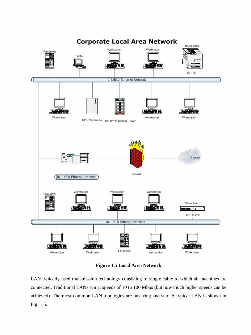
Figure 1.5 Local Area Network
LAN typically used transmission technology consisting of single cable to which all machines are
connected. Traditional LANs run at speeds of 10 to 100 Mbps (but now much higher speeds can be
achieved). The most common LAN topologies are bus, ring and star. A typical LAN is shown in
Fig. 1.5.
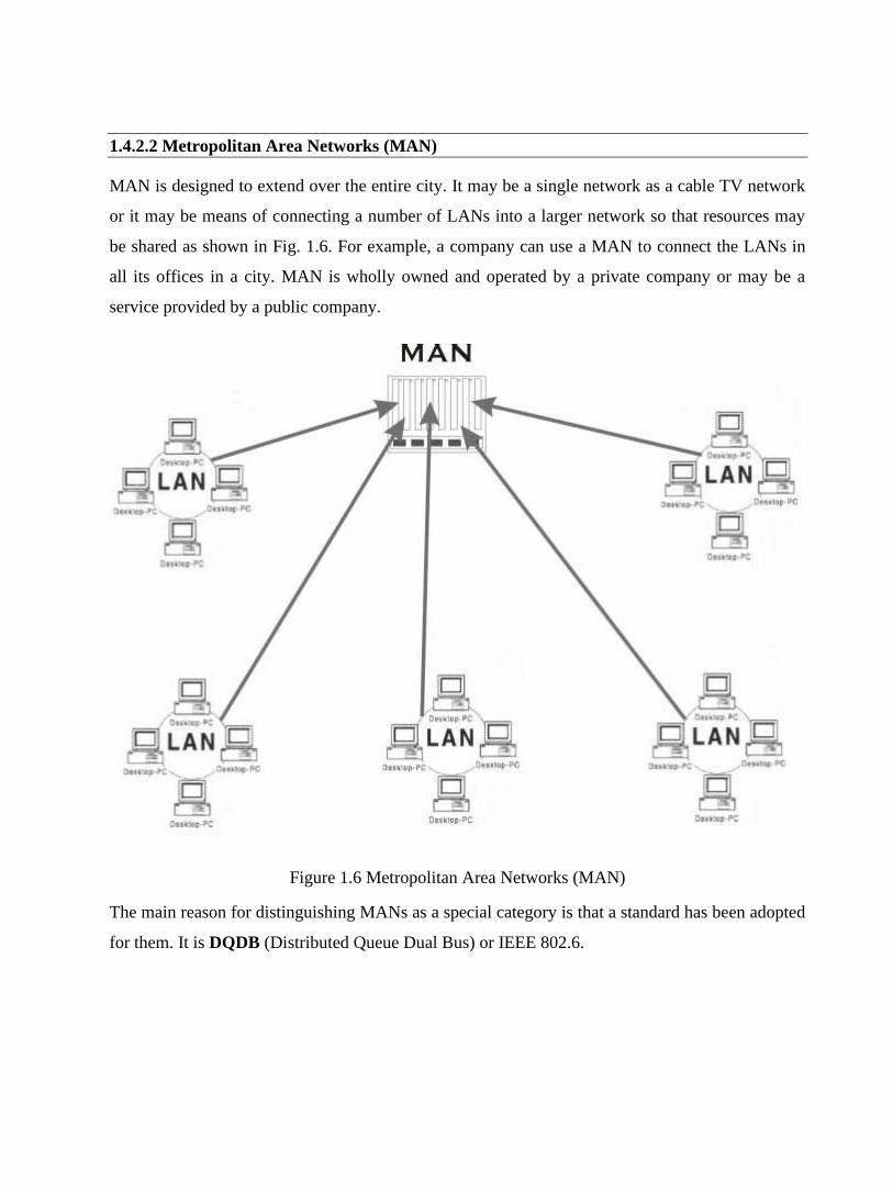
1.4.2.2 Metropolitan Area Networks (MAN)
MAN is designed to extend over the entire city. It may be a single network as a cable TV network
or it may be means of connecting a number of LANs into a larger network so that resources may
be shared as shown in Fig. 1.6. For example, a company can use a MAN to connect the LANs in
all its offices in a city. MAN is wholly owned and operated by a private company or may be a
service provided by a public company.
Figure 1.6 Metropolitan Area Networks (MAN)
The main reason for distinguishing MANs as a special category is that a standard has been adopted
for them. It is DQDB (Distributed Queue Dual Bus) or IEEE 802.6.

1.4.2.3 Wide Area Network (WAN)
WAN provides long-distance transmission of data, voice, image and information over large
geographical areas that may comprise a country, continent or even the whole world. In contrast to
LANs, WANs may utilize public, leased or private communication devices, usually in
combinations, and can therefore span an unlimited number of miles as shown in Fig.1.7. A WAN
that is wholly owned and used by a single company is often referred to as enterprise network.
Figure 1.7 Wide Area Network

1.5 The Internet
Internet is a collection of networks or network of networks. Various networks such as LAN and
WAN connected through suitable hardware and software to work in a seamless manner. Schematic
diagram of the Internet is shown in Fig.1.8. It allows various applications such as e-mail, file
transfer, remote log-in, World Wide Web, Multimedia, etc run across the internet. The basic
difference between WAN and Internet is that WAN is owned by a single organization while
internet is not so. But with the time the line between WAN and Internet is shrinking, and these
terms are sometimes used interchangeably.
Figure 1.8 Internet – network of networks
1.6 Applications
In a short period of time computer networks have become an indispensable part of business,
industry, entertainment as well as a common-man's life. These applications have changed
tremendously from time and the motivation for building these networks are all essentially
economic and technological.
Initially, computer network was developed for defense purpose, to have a secure communication
network that can even withstand a nuclear attack. After a decade or so, companies, in various
fields, started using computer networks for keeping track of inventories, monitor productivity,
communication between their different branch offices located at different locations. For example,
Railways started using computer networks by connecting their nationwide reservation counters to
provide the facility of reservation and enquiry from any where across the country.
And now after almost two decades, computer networks have entered a new dimension; they are
now an integral part of the society and people. In 1990s, computer network started delivering

services to private individuals at home. These services and motivation for using them are quite
different. Some of the services are access to remote information, person-person communication,
and interactive entertainment. So, some of the applications of computer networks that we can see
around us today are as follows:
Marketing and sales: Computer networks are used extensively in both marketing and sales
organizations. Marketing professionals use them to collect, exchange, and analyze data related to
customer needs and product development cycles. Sales application
includes teleshopping, which uses order-entry computers or telephones connected to order
processing network, and online-reservation services for hotels, airlines and so on.
Financial services: Today's financial services are totally depended on computer networks.
Application includes credit history searches, foreign exchange and investment services, and
electronic fund transfer, which allow user to transfer money without going into a bank (an
automated teller machine is an example of electronic fund transfer, automatic pay-check is
another).
Manufacturing: Computer networks are used in many aspects of manufacturing including
manufacturing process itself. Two of them that use network to provide essential services are
computer-aided design (CAD) and computer-assisted manufacturing (CAM), both of which allow
multiple users to work on a project simultaneously.
Directory services: Directory services allow list of files to be stored in central location to speed
worldwide search operations.
Information services: A Network information service includes bulletin boards and data banks. A
World Wide Web site offering technical specification for a new product is an information service.
Electronic data interchange (EDI): EDI allows business information, including documents such
as purchase orders and invoices, to be transferred without using paper.
Electronic mail: probably it's the most widely used computer network application.
Teleconferencing: Teleconferencing allows conference to occur without the participants being in
the same place. Applications include simple text conferencing (where participants communicate
through their normal keyboards and monitor) and video conferencing where participants can even
see as well as talk to other fellow participants. Different types of equipments are used for video
conferencing depending on what quality of the motion you want to capture (whether you want just
to see the face of other fellow participants or do you want to see the exact facial expression).
Voice over IP: Computer networks are also used to provide voice communication. This kind of
voice communication is pretty cheap as compared to the normal telephonic conversation.

Video on demand: Future services provided by the cable television networks may include video
on request where a person can request for a particular movie or any clip at anytime he wish to see.
Summary: The main area of applications can be broadly classified into following categories:
Scientific and Technical Computing
Client Server Model, Distributed Processing Parallel Processing, Communication Media
Commercial
Advertisement, Telemarketing, Teleconferencing
Worldwide Financial Services
Network for the People (this is the most widely used application nowadays)
Telemedicine, Distance Education, Access to Remote Information, Person-to-Person
Communication, Interactive Entertainment
1.7 Check Your Progress
Fill in the blanks
1. …………….network have a single communication channel that is shared by all the machines
on the network
2. ……………..is a collection of networks or network of networks.
3. Various networks such as ………………..connected through suitable hardware and software
to work in a seamless manner.
4. ………….provides long-distance transmission of data, voice, image and information over
large geographical areas that may comprise a country, continent or even the whole world.
1.8 Answer to Check Your Progress
1. Broadcast
2. Internet
3. LAN and WAN
4. WAN
Unit-2
Data and Signal
1.1 Learning Objective
1.2 Introduction to data communication
1.3 Data
1.4 Signal
1.5 Signal Characteristics
1.5.1 Time-domain concepts
1.5.2 Frequency domain concepts
1.5.3 Frequency Spectrum
1.6 Digital Signal
1.7 Baseband and Broadband Signals
1.8 Check Your Progress
1.9 Answer to Check Your Progress

1.1 Learning Objective
After going through this unit the learner will be able to:
• Explain what is data
• Distinguish between Analog and Digital signal
• Explain the difference between time and Frequency domain representation of signal
• Specify the bandwidth of a signal
• Specify the Sources of impairment
• Explain Attenuation and Unit of Attenuation
• Explain Data Rate Limits and Nyquist Bit Rate
• Distinguish between Bit Rate and Baud Rate
• Identify Noise Sources
1.2 Introduction to data communication
A simplified model of a data communication system is shown in Fig. 2.1. Here there are five basic
components:
Source: Source is where the data is originated. Typically it is a computer, but it can be any other
electronic equipment such as telephone handset, video camera, etc, which can generate data for
transmission to some destination. The data to be sent is represented by x(t).
Figure 2.1 Simplified model of a data communication system
Transmitter: As data cannot be sent in its native form, it is necessary to convert it into signal.
This is performed with the help of a transmitter such as modem. The signal that is sent by the
transmitter is represented by s(t).
Communication Medium: The signal can be sent to the receiver through a communication
medium, which could be a simple twisted-pair of wire, a coaxial cable, optical fiber or wireless
communication system. It may be noted that the signal that comes out of the communication
medium is s’(t), which is different from s(t) that was sent by the transmitter. This is due to various
impairments that the signal suffers as it passes through the communication medium.
Receiver: The receiver receives the signal s’(t) and converts it back to data d’(t) before forwarding
to the destination. The data that the destination receives may not be identical to that of d(t),
because of the corruption of data.
Destination: Destination is where the data is absorbed. Again, it can be a computer system, a
telephone handset, a television set and so on.
1.3 Data
Data refers to information that conveys some meaning based on some mutually agreed up rules or
conventions between a sender and a receiver and today it comes in a variety of forms such as text,
graphics, audio, video and animation.
Data can be of two types; analog and digital. Analog data take on continuous values on some
interval. Typical examples of analog data are voice and video. The data that are collected from the
real world with the help of transducers are continuous-valued or analog in nature. On the contrary,
digital data take on discrete values. Text or character strings can be considered as examples of
digital data. Characters are represented by suitable codes, e.g. ASCII code, where each character is
represented by a 7-bit code.
1.4 Signal
It is electrical, electronic or optical representation of data, which can be sent over a communication
medium. Stated in mathematical terms, a signal is merely a function of the data. For example, a
microphone converts voice data into voice signal, which can be sent over a pair of wire. Analog
signals are continuous-valued; digital signals are discrete-valued. The independent variable of the
signal could be time (speech, for example), space (images), or the integers (denoting the
sequencing of letters and numbers in the football score). Figure 2.2 shows an analog signal.

Figure 2.2 Analog signal
Digital signal can have only a limited number of defined values, usually two values 0 and 1, as
shown in Fig. 2.3.
Figure 2.3 Digital signal
Signaling: It is an act of sending signal over communication medium
Transmission: Communication of data by propagation and processing is known as transmission.
1.5 Signal Characteristics
A signal can be represented as a function of time, i.e. it varies with time. However, it can be also
expressed as a function of frequency, i.e. a signal can be considered as a composition of different
frequency components. Thus, a signal has both time-domain and frequency domain representation.
1.5.1 Time-domain concepts
A signal is continuous over a period, if

limt->a s (t) = s (a), for all a,
i.e., there is no break in the signal. A signal is discrete if it takes on only a finite number of values.
A signal is periodic if and only if
s (t+T) = s (t) for - α < t < α ,
where T is a constant, known as period. The period is measured in seconds.
In other words, a signal is a periodic signal if it completes a pattern within a measurable time
frame. A periodic signal is characterized by the following three parameters.
Amplitude: It is the value of the signal at different instants of time. It is measured in volts.
Frequency: It is inverse of the time period, i.e. f = 1/T. The unit of frequency is Hertz (Hz) or
cycles per second.
Phase: It gives a measure of the relative position in time of two signals within a single period. It is
represented by φ in degrees or radian.
A sine wave, the most fundamental periodic signal, can be completely characterized by its
amplitude, frequency and phase. Examples of sine waves with different amplitude, frequency and
phase are shown in Fig. 2.4. The phase angle φ indicated in the figure is with respect to the
reference waveform shown in Fig. 2.4(a).
Figure 2.4 Examples of signals with different amplitude, frequency and phase
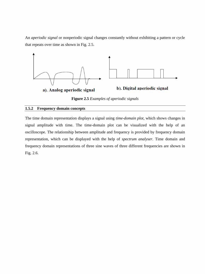
An aperiodic signal or nonperiodic signal changes constantly without exhibiting a pattern or cycle
that repeats over time as shown in Fig. 2.5.
Figure 2.5 Examples of aperiodic signals
1.5.2 Frequency domain concepts
The time domain representation displays a signal using time-domain plot, which shows changes in
signal amplitude with time. The time-domain plot can be visualized with the help of an
oscilloscope. The relationship between amplitude and frequency is provided by frequency domain
representation, which can be displayed with the help of spectrum analyser. Time domain and
frequency domain representations of three sine waves of three different frequencies are shown in
Fig. 2.6.
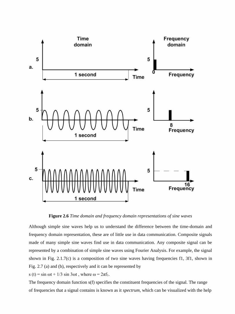
Figure 2.6 Time domain and frequency domain representations of sine waves
Although simple sine waves help us to understand the difference between the time-domain and
frequency domain representation, these are of little use in data communication. Composite signals
made of many simple sine waves find use in data communication. Any composite signal can be
represented by a combination of simple sine waves using Fourier Analysis. For example, the signal
shown in Fig. 2.1.7(c) is a composition of two sine waves having frequencies f1, 3f1, shown in
Fig. 2.7 (a) and (b), respectively and it can be represented by
s (t) = sin ωt + 1/3 sin 3ωt , where ω = 2πf1.
The frequency domain function s(f) specifies the constituent frequencies of the signal. The range
of frequencies that a signal contains is known as it spectrum, which can be visualized with the help

of a spectrum analyser. The band of frequencies over which most of the energy of a signal is
concentrated is known as the bandwidth of the signal.
Figure 2.7 Time and frequency domain representations of a composite signal
Many useful waveforms don’t change in a smooth curve between maximum and minimum
amplitude; they jump, slide, wobble, spike, and dip. But as long as these irregularities are
consistent, cycle after cycle, a signal is still periodic and logically must be describable in same
terms used for sine waves. In fact it can be decomposed into a collection of sine waves, each
having a measurable amplitude, frequency, and phase.

1.5.3 Frequency Spectrum
Frequency spectrum of a signal is the range of frequencies that a signal contains.
Example: Consider a square wave shown in Fig. 2.8(a). It can be represented by a series of sine
waves S(t) = 4A/πsin2πft + 4A/3πsin(2π(3f)t) + 4A/5πsin2π (5f)t + . . . having frequency
components f, 3f, 5f, … and amplitudes 4A/π, 4A/3π, 4A/5π and so on. The frequency spectrum of
this signal can be approximation comprising only the first and third harmonics as shown in Fig.
2.8(b)
(a)
(b)
Figure 2.8 (a) A square wave, (b) Frequency spectrum of a square wave
Bandwidth: The range of frequencies over which most of the signal energy of a signal is
contained is known as bandwidth or effective bandwidth of the signal. The term ‘most’ is
somewhat arbitrary. Usually, it is defined in terms of its 3dB cut-off frequency. The frequency
spectrum and spectrum of a signal is shown in Fig. 2.9. Here the fl and fh may be represented by
3dB below (A/√2) the maximum amplitude.

Figure 2.9 Frequency spectrum and bandwidth of a signal
1.6 Digital Signal
In addition to being represented by an analog signal, data can be also be represented by a digital
signal. Most digital signals are aperiodic and thus, period or frequency is not appropriate. Two new
terms, bit interval (instead of period) and bit rate (instead of frequency) are used to describe digital
signals. The bit interval is the time required to send one single bit. The bit rate is the number of bit
interval per second. This mean that the bit rate is the number of bits send in one second, usually
expressed in bits per second (bps) as shown in Fig. 2.10.
Figure 2.1.10 Bit Rate and Bit Interval
A digital signal can be considered as a signal with an infinite number of frequencies and
transmission of digital requires a low-pass channel as shown in Fig. 2.11. On the other hand,
transmission of analog signal requires band-pass channel shown in Fig. 2.12.

Figure 2.11 Low pass channel required for transmission of digital signal
Figure 2.12 Low pass channel required for transmission of analog signal
Digital transmission has several advantages over analog transmission. That is why there is a shift
towards digital transmission despite large analog base. Some of the advantages of digital
transmission are highlighted below:
• Analog circuits require amplifiers, and each amplifier adds distortion and noise to the
signal. In contrast, digital amplifiers regenerate an exact signal, eliminating cumulative
errors. An incoming (analog) signal is sampled, its value is determined, and the node then
generates a new signal from the bit value; the incoming signal is discarded. With analog
circuits, intermediate nodes amplify the incoming signal, noise and all.
• Voice, data, video, etc. can all by carried by digital circuits. What about carrying digital
signals over analog circuit? The modem example shows the difficulties in carrying digital
over analog. A simple encoding method is to use constant voltage levels for a “1'' and a
``0''. Can lead to long periods where the voltage does not change.
• Easier to multiplex large channel capacities with digital.
• Easy to apply encryption to digital data.
• Better integration if all signals are in one form. Can integrate voice, video and digital data.

1.7 Baseband and Broadband Signals
Depending on some type of typical signal formats or modulation schemes, a few terminologies
evolved to classify different types of signals. So, we can have either a base band or broadband
signalling. Base-band is defined as one that uses digital signalling, which is inserted in the
transmission channel as voltage pulses. On the other hand, broadband systems are those, which
use analog signalling to transmit information using a carrier of high frequency.
In baseband LANs, the entire frequency spectrum of the medium is utilized for transmission and
hence the frequency division multiplexing (discussed later) cannot be used. Signals inserted at a
point propagates in both the directions, hence transmission is bi-directional. Baseband systems
extend only to limited distances because at higher frequency, the attenuation of the signal is most
pronounced and the pulses blur out, causing the large distance communication totally impractical.
Since broadband systems use analog signalling, frequency division multiplexing is possible, where
the frequency spectrum of the cable is divided into several sections of bandwidth. These separate
channels can support different types of signals of various frequency ranges to travel at the same
instance. Unlike base-band, broadband is a unidirectional medium where the signal inserted into
the media propagates in only one direction. Two data paths are required, which are connected at a
point in the network called headend. All the stations transmit towards the headend on one path and
the signals received at the headend are propagated through the second path.
1.8 Check Your Progress
Fill in the blanks
1. The range of frequencies over which most of the signal energy of a signal is contained is
known as………………
2. Communication of data by propagation and processing is known as……………..
3. …………….take on continuous values on some interval.
4. ……………………………..are used to describe digital signals.
1.9 Answer to Check Your Progress
1. bandwidth.
2. transmission.
3. Analog data
4. bit interval (instead of period) and bit rate (instead of frequency)

Unit-3
Transmission Media and Transmission Impairments and Channel Capacity
1.1 Learning Objective
1.2 Introduction to transmission media
1.3 Guided transmission media
1.3.1 Twisted Pair
1.3.2 Base band Coaxial
1.3.3 Broadband Coaxial
1.3.4 Fiber Optics
1.4 Unguided Transmission
1.4.1 Satellite Communication
1.5 Introduction to Transmission Impairments and Channel Capacity
1.6 Attenuation
1.7 Delay distortion
1.8 Noise
1.9 Bandwidth and Channel Capacity
1.10 Check Your Progress
1.11 Answer to Check Your Progress

1.1 Learning Objective
After going through this unit the learner will be able to:
• Classify various Transmission Media
• Distinguish between guided and unguided media
• Explain the characteristics of the popular guided transmission media:
• Twisted-pair
• Coaxial cable
• Optical fiber
• Specify the Sources of impairments
• Explain Attenuation and unit of Attenuation
• Specify possible types of distortions of a signal
• Explain Data Rate Limits and Nyquist Bit Rate
• Distinguish between Bit Rate and Baud Rate
• Identify Noise Sources
• Explain Shannon Capacity in a Noisy Channel
1.2 Introduction
Transmission media can be defined as physical path between transmitter and receiver in a data
transmission system. And it may be classified into two types as shown in Fig. 2.1.
Guided: Transmission capacity depends critically on the medium, the length, and whether the
medium is point-to-point or multipoint (e.g. LAN). Examples are co-axial cable, twisted pair, and
optical fiber.
Unguided: provides a means for transmitting electro-magnetic signals but do not guide them.
Example wireless transmission.
Characteristics and quality of data transmission are determined by medium and signal
characteristics. For guided media, the medium is more important in determining the limitations of
transmission. While in case of unguided media, the bandwidth of the signal produced by the
transmitting antenna and the size of the antenna is more important than the medium. Signals at
lower frequencies are omni-directional (propagate in all directions). For higher frequencies,
focusing the signals into a directional beam is possible. These properties determine what kind of
media one should use in a particular application. In this lesson we shall discuss the characteristics
of various transmission media, both guided and unguied.

Figure 2.1 Classification of the transmission media
1.3 Guided transmission media
In this unit we shall discuss about the most commonly used guided transmission media such as
twisted-pair of cable, coaxial cable and optical fiber.
1.3.1 Twisted Pair
Figure 2.2 CAT5 cable (twisted cable)
In twisted pair technology, two copper wires are strung between two points:
• The two wires are typically ``twisted'' together in a helix to reduce interference between the
two conductors as shown in Fig.2.2. Twisting decreases the cross-talk interference between
adjacent pairs in a cable. Typically, a number of pairs are bundled together into a cable by
wrapping them in a tough protective sheath.
• Can carry both analog and digital signals. Actually, they carry only analog signals.
However, the ``analog'' signals can very closely correspond to the square waves
representing bits, so we often think of them as carrying digital data.
• Data rates of several Mbps common.
• Spans distances of several kilometers.

• Data rate determined by wire thickness and length. In addition, shielding to eliminate
interference from other wires impacts signal-to-noise ratio, and ultimately, the data rate.
• Good, low-cost communication. Indeed, many sites already have twisted pair installed in
offices -- existing phone lines!
Typical characteristics: Twisted-pair can be used for both analog and digital communication.
The data rate that can be supported over a twisted-pair is inversely proportional to the square of
the line length. Maximum transmission distance of 1 Km can be achieved for data rates up to 1
Mb/s. For analog voice signals, amplifiers are required about every 6 Km and for digital
signals, repeaters are needed for about 2 Km. To reduce interference, the twisted pair can be
shielded with metallic braid. This type of wire is known as Shielded Twisted-Pair (STP) and
the other form is known as Unshielded Twisted-Pair (UTP).
Use: The oldest and the most popular use of twisted pair are in telephony. In LAN it is
commonly used for point-to-point short distance communication (say, 100m) within a building
or a room.
1.3.2 Base band Coaxial
With ``coax'', the medium consists of a copper core surrounded by insulating material and a
braided outer conductor as shown in Fig. 2.3. The term base band indicates digital transmission (as
opposed to broadband analog).
Figure 2.3 Co-axial cable
Physical connection consists of metal pin touching the copper core. There are two common ways
to connect to a coaxial cable:
1. With vampire taps, a metal pin is inserted into the copper core. A special tool drills a hole
into the cable, removing a small section of the insulation, and a special connector is
screwed into the hole. The tap makes contact with the copper core.

2. With a T-junction, the cable is cut in half, and both halves connect to the T-junction. A T-
connector is analogous to the signal splitters used to hook up multiple TVs to the same
cable wire.
Characteristics: Co-axial cable has superior frequency characteristics compared to twisted-
pair and can be used for both analog and digital signaling. In baseband LAN, the data rates lies
in the range of 1 KHz to 20 MHz over a distance in the range of 1 Km. Co-axial cables
typically have a diameter of 3/8". Coaxial cables are used both for baseband and broadband
communication. For broadband CATV application coaxial cable of 1/2" diameter and 75 Ω
impedance is used. This cable offers bandwidths of 300 to 400 MHz facilitating high-speed
data communication with low bit-error rate. In broadband signaling, signal propagates only in
one direction, in contrast to propagation in both directions in baseband signaling. Broadband
cabling uses either dual-cable scheme or single-cable scheme with a head end to facilitate flow
of signal in one direction. Because of the shielded, concentric construction, co-axial cable is
less susceptible to interference and cross talk than the twisted-pair. For long distance
communication, repeaters are needed for every kilometer or so. Data rate depends on physical
properties of cable, but 10 Mbps is typical.
Use: One of the most popular use of co-axial cable is in cable TV (CATV) for the distribution
of TV signals. Another importance use of co-axial cable is in LAN.
1.3.3 Broadband Coaxial
The term broadband refers to analog transmission over coaxial cable. (Note, however, that the
telephone folks use broadband to refer to any channel wider than 4 kHz). The technology:
• Typically bandwidth of 300 MHz, total data rate of about 150 Mbps.
• Operates at distances up to 100 km (metropolitan area!).
• Uses analog signaling.
• Technology used in cable television. Thus, it is already available at sites such as
universities that may have TV classes.
• Total available spectrum typically divided into smaller channels of 6 MHz each. That is, to
get more than 6MHz of bandwidth, you have to use two smaller channels and somehow
combine the signals.
• Requires amplifiers to boost signal strength; because amplifiers are one way, data flows in
only one direction.
Two types of systems have emerged:
1. Dual cable systems use two cables, one for transmission in each direction:
o One cable is used for receiving data.
o Second cable used to communicate with headend. When a node wishes to transmit
data, it sends the data to a special node called the headend. The headend then
resends the data on the first cable. Thus, the headend acts as a root of the tree, and
all data must be sent to the root for redistribution to the other nodes.
2 . Midsplit systems divide the raw channel into two smaller channels, with each sub channel
having the same purpose as above.
Which is better, broadband or base band? There is rarely a simple answer to such questions. Base
band is simple to install, interfaces are inexpensive, but doesn't have the same range. Broadband is
more complicated, more expensive, and requires regular adjustment by a trained technician, but
offers more services (e.g., it carries audio and video too).
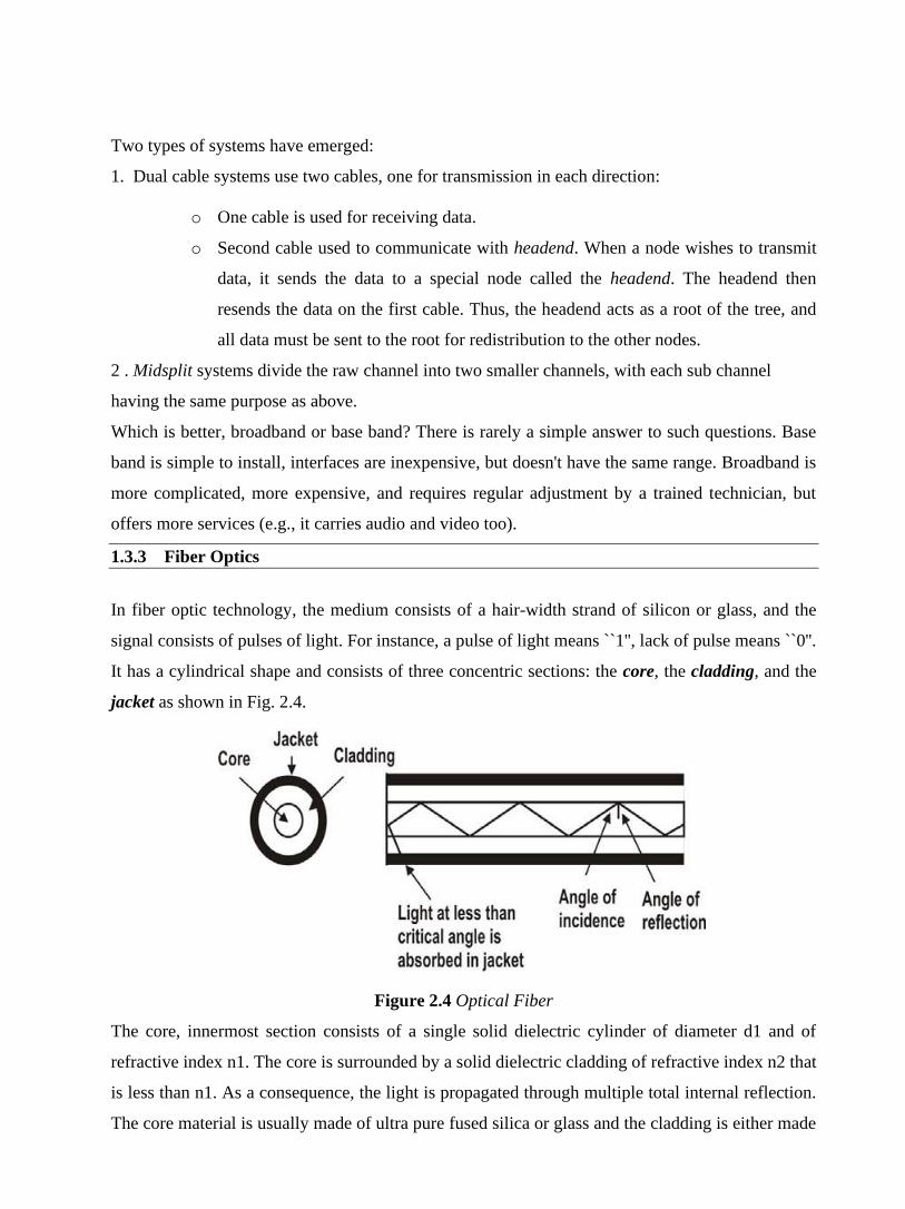
1.3.3 Fiber Optics
In fiber optic technology, the medium consists of a hair-width strand of silicon or glass, and the
signal consists of pulses of light. For instance, a pulse of light means ``1'', lack of pulse means ``0''.
It has a cylindrical shape and consists of three concentric sections: the core, the cladding, and the
jacket as shown in Fig. 2.4.
Figure 2.4 Optical Fiber
The core, innermost section consists of a single solid dielectric cylinder of diameter d1 and of
refractive index n1. The core is surrounded by a solid dielectric cladding of refractive index n2 that
is less than n1. As a consequence, the light is propagated through multiple total internal reflection.
The core material is usually made of ultra pure fused silica or glass and the cladding is either made

of glass or plastic. The cladding is surrounded by a jacket made of plastic. The jacket is used to
protect against moisture, abrasion, crushing and other environmental hazards.
Three components are required:
1. Fiber medium: Current technology carries light pulses for tremendous distances (e.g., 100s
of kilometers) with virtually no signal loss.
2. Light source: typically a Light Emitting Diode (LED) or laser diode. Running current
through the material generates a pulse of light.
3. A photo diode light detector, which converts light pulses into electrical signals.
Advantages:
1. Very high data rate, low error rate. 1000 Mbps (1 Gbps) over distances of kilometers
common. Error rates are so low they are almost negligible.
2. Difficult to tap, which makes it hard for unauthorized taps as well. This is responsible for
higher reliability of this medium.
How difficult is it to prevent coax taps? Very difficult indeed, unless one can keep the entire cable
in a locked room!
3. Much thinner (per logical phone line) than existing copper circuits. Because of its thinness,
phone companies can replace thick copper wiring with fibers having much more capacity for same
volume. This is important because it means that aggregate phone capacity can be upgraded without
the need for finding more physical space to hire the new cables.
4. Not susceptible to electrical interference (lightning) or corrosion (rust).
Disadvantages:
• Difficult to tap. It really is point-to-point technology. In contrast, tapping into coax is
trivial. No special training or expensive tools or parts are required.
• One-way channel. Two fibers needed to get full duplex (both ways) communication.
Optical Fiber works in three different types of modes (or we can say that we have 3 types of
communication using Optical fiber). Optical fibers are available in two varieties; Multi-Mode
Fiber (MMF) and Single-Mode Fiber (SMF). For multi-mode fiber the core and cladding diameter
lies in the range 50-200μm and 125-400μm, respectively. Whereas in single-mode fiber, the core
and cladding diameters lie in the range 8-12μm and 125μm, respectively. Single-mode fibers are
also known as Mono-Mode Fiber. Moreover, both single-mode and multi-mode fibers can have
two types; step index and graded index. In the former case the refractive index of the core is
uniform throughout and at the core cladding boundary there is an abrupt change in refractive

index. In the later case, the refractive index of the core varies radially from the centre to the core-
cladding boundary from n1 to n2 in a linear manner. Fig. 2.5 shows the optical fiber transmission
modes.
Figure 2.5 Schematics of three optical fiber types, (a) Single-mode step-index, (b) Multi-
mode step-index, and (c) Multi-mode graded-index
Characteristics: Optical fiber acts as a dielectric waveguide that operates at optical
frequencies (1014 to 1015 Hz). Three frequency bands centered around 850,1300 and 1500
nanometers are used for best results. When light is applied at one end of the optical fiber
core, it reaches the other end by means of total internal reflection because of the choice of
refractive index of core and cladding material (n1 > n2). The light source can be either light
emitting diode (LED) or injection laser diode (ILD). These semiconductor devices emit a
beam of light when a voltage is applied across the device. At the receiving end, a
photodiode can be used to detect the signal-encoded light. Either PIN detector or APD
(Avalanche photodiode) detector can be used as the light detector.
In a multi-mode fiber, the quality of signal-encoded light deteriorates more rapidly than
single-mode fiber, because of interference of many light rays. As a consequence, single-
mode fiber allows longer distances without repeater. For multi-mode fiber, the typical
maximum length of the cable without a repeater is 2km, whereas for single-mode fiber it is
20km.
Fiber Uses: Because of greater bandwidth (2Gbps), smaller diameter, lighter weight, low
attenuation, immunity to electromagnetic interference and longer repeater spacing, optical
fiber cables are finding widespread use in long-distance telecommunications. Especially,

the single mode fiber is suitable for this purpose. Fiber optic cables are also used in high-
speed LAN applications. Multi-mode fiber is commonly used in LAN.
• Long-haul trunks-increasingly common in telephone network (Sprint ads)
• Metropolitan trunks-without repeaters (average 8 miles in length)
• Rural exchange trunks-link towns and villages
• Local loops-direct from central exchange to a subscriber (business or home)
• Local area networks-100Mbps ring networks.
1.4 Unguided Transmission
Unguided transmission is used when running a physical cable (either fiber or copper) between two
end points is not possible. For example, running wires between buildings is probably not legal if
the building is separated by a public street.
Infrared signals typically used for short distances (across the street or within same room),
Microwave signals commonly used for longer distances (10's of km). Sender and receiver use
some sort of dish antenna as shown in Fig. 2.6.
Figure 2.6 Communication using Terrestrial Microwave
Difficulties:
1. Weather interferes with signals. For instance, clouds, rain, lightning, etc. may adversely
affect communication.
2. Radio transmissions easy to tap. A big concern for companies worried about competitors
stealing plans.
3. Signals bouncing off of structures may lead to out-of-phase signals that the receiver must
filter out.

1.4.1 Satellite Communication
Satellite communication is based on ideas similar to those used for line-of-sight. A communication
satellite is essentially a big microwave repeater or relay station in the sky. Microwave signals from
a ground station is picked up by a transponder, amplifies the signal and rebroadcasts it in another
frequency, which can be received by ground stations at long distances as shown in Fig. 2.7.
To keep the satellite stationary with respect to the ground based stations, the satellite is placed in a
geostationary orbit above the equator at an altitude of about 36,000 km. As the spacing between
two satellites on the equatorial plane should not be closer than 40, there can be 360/4 = 90
communication satellites in the sky at a time. A satellite can be used for point-to-point
communication between two ground-based stations or it can be used to broadcast a signal received
from one station to many ground-based stations as shown in Fig. 2.8. Number of geo-synchronous
satellites limited (about 90 total, to minimize interference). International agreements regulate how
satellites are used, and how frequencies are allocated. Weather affects certain frequencies. Satellite
transmission differs from terrestrial communication in another important way: One-way
propagation delay is roughly 270 ms. In interactive terms, propagation delay alone inserts a 1
second delay between typing a character and receiving its echo.
Figure 2.7 Satellite Microwave Communication: point –to- point

Figure 2.8 Satellite Microwave Communication: Broadcast links
Characteristics: Optimum frequency range for satellite communication is 1 to 10 GHz. The most
popular frequency band is referred to as 4/6 band, which uses 3.7 to 4.2 GHz for down link and
5.925 to 6.425 for uplink transmissions. The 500 MHz bandwidth is usually split over a dozen
transponders, each with 36 MHz bandwidth. Each 36 MHz bandwidth is shared by time division
multiplexing. As this preferred band is already saturated, the next highest band available is referred
to as 12/14 GHz. It uses 14 to 14.5GHz for upward transmission and 11.7 to 12.2 GHz for
downward transmissions. Communication satellites have several unique properties. The most
important is the long communication delay for the round trip (about 270 ms) because of the long
distance (about 72,000 km) the signal has to travel between two earth stations. This poses a
number of problems, which are to be tackled for successful and reliable communication.
Another interesting property of satellite communication is its broadcast capability. All stations
under the downward beam can receive the transmission. It may be necessary to send encrypted
data to protect against piracy.
Use: Now-a-days communication satellites are not only used to handle telephone, telex and
television traffic over long distances, but are used to support various internet based services such
as e-mail, FTP, World Wide Web (WWW), etc. New types of services, based on communication
satellites, are emerging.
Comparison/contrast with other technologies:
1. Propagation delay very high. On LANs, for example, propagation time is in
nanoseconds -- essentially negligible.
2. One of few alternatives to phone companies for long distances.

3. Uses broadcast technology over a wide area - everyone on earth could receive a
message at the same time!
4. Easy to place unauthorized taps into signal.
Satellites have recently fallen out of favor relative to fiber.
However, fiber has one big disadvantage: no one has it coming into their house or building,
whereas anyone can place an antenna on a roof and lease a satellite channel.
1.5 Introduction to Transmission Impairments and Channel Capacity
When a signal is transmitted over a communication channel, it is subjected to different types of
impairments because of imperfect characteristics of the channel. As a consequence, the received
and the transmitted signals are not the same. Outcome of the impairments are manifested in two
different ways in analog and digital signals. These impairments introduce random modifications in
analog signals leading to distortion. On the other hand, in case of digital signals, the impairments
lead to error in the bit values. The impairment can be broadly categorised into the following three
types:
• Attenuation and attenuation distortion
• Delay distortion
• Noise
In this unit these impairments are discussed in detail and possible approaches to overcome these
impairments. The concept of channel capacity for both noise-free and noisy channels have also
been introduced.
1.6 Attenuation
Irrespective of whether a medium is guided or unguided, the strength of a signal falls off with
distance. This is known as attenuation. In case of guided media, the attenuation is logarithmic,
whereas in case of unguided media it is a more complex function of the distance and the material
that constitutes the medium.
An important concept in the field of data communications is the use of on unit known as decibel
(dB). To define it let us consider the circuit elements shown in Fig. 2.9. The elements can be either
a transmission line, an amplifier, an attenuator, a filter, etc. In the figure, a transmission line
(between points P1 and P2) is followed by an amplifier (between P2 and P3). The input signal
delivers a power P1 at the input of an communication element and the output power is P2. Then the
power gain G for this element in decibles is given by G = 10log2 P2/ P1. Here P2/ P1 is referred to
as absolute power gain. When P2 > P1, the gain is positive, whereas if P2 < P1, then the power gain
is negative and there is a power loss in the circuit element. For P2 = 5mW, P1 = 10mW, the
power gain G = 10log 5/10 = 10 × -3 = -3dB is negative and it represents attenuation as a signal
passes through the communication element.
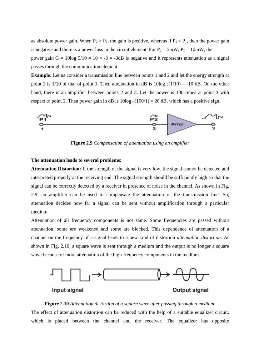
Example: Let us consider a transmission line between points 1 and 2 and let the energy strength at
point 2 is 1/10 of that of point 1. Then attenuation in dB is 10log10(1/10) = -10 dB. On the other
hand, there is an amplifier between points 2 and 3. Let the power is 100 times at point 3 with
respect to point 2. Then power gain in dB is 10log10(100/1) = 20 dB, which has a positive sign.
Figure 2.9 Compensation of attenuation using an amplifier
The attenuation leads to several problems:
Attenuation Distortion: If the strength of the signal is very low, the signal cannot be detected and
interpreted properly at the receiving end. The signal strength should be sufficiently high so that the
signal can be correctly detected by a receiver in presence of noise in the channel. As shown in Fig.
2.9, an amplifier can be used to compensate the attenuation of the transmission line. So,
attenuation decides how far a signal can be sent without amplification through a particular
medium.
Attenuation of all frequency components is not same. Some frequencies are passed without
attenuation, some are weakened and some are blocked. This dependence of attenuation of a
channel on the frequency of a signal leads to a new kind of distortion attenuation distortion. As
shown in Fig. 2.10, a square wave is sent through a medium and the output is no longer a square
wave because of more attenuation of the high-frequency components in the medium.
Figure 2.10 Attenuation distortion of a square wave after passing through a medium.
The effect of attenuation distortion can be reduced with the help of a suitable equalizer circuit,
which is placed between the channel and the receiver. The equalizer has opposite

attenuation/amplification characteristics of the medium and compensates higher losses of some
frequency components in the medium by higher amplification in the equalizer. Attenuation
characteristics of three popular transmission media are shown in Fig. 2.11. As shown in the figure,
the attenuation of a signal increases exponentially as frequency is increased from KHz range to
MHz range. In case of coaxial cable attenuation increases linearly with frequency in the Mhz
range. The optical fibre, on the other hand, has attenuation characteristic similar to a band-pass
filter and a small frequency band in the THz range can be used for the transmission of signal.
Figure 2.11 Attenuation characteristics of the popular guided media
1.7 Delay distortion
The velocity of propagation of different frequency components of a signal are different in guided
media. This leads to delay distortion in the signal. For a bandlimited signal, the velocity of
propagation has been found to be maximum near the center frequency and lower on both sides of
the edges of the frequency band. In case of analog signals, the received signal is distorted because
of variable delay of different components. In case of digital signals, the problem is much more
severe. Some frequency components of one bit position spill over to other bit positions, because of
delay distortion. This leads to inter symbol interference, which restricts the maximum bit rate of
transmission through a particular transmission medium. The delay distortion can also be
neutralised, like attenuation distortion, by using suitable equalizers.

1.8 Noise
As signal is transmitted through a channel, undesired signal in the form of noise gets mixed up
with the signal, along with the distortion introduced by the transmission media. Noise can be
categorised into the following four types:
• Thermal Noise
• Intermodulation Noise
• Cross talk
• Impulse Noise
The thermal noise is due to thermal agitation of electrons in a conductor. It is distributed across
the entire spectrum and that is why it is also known as white noise (as the frequency encompass
over a broad range of frequencies).
When more than one signal share a single transmission medium, intermodulation noise is
generated. For example, two signals f1 and f2 will generate signals of frequencies (f1 + f2) and (f1
- f2), which may interfere with the signals of the same frequencies sent by the transmitter.
Intermodulation noise is introduced due to nonlinearity present in any part of the communication
system.
Cross talk is a result of bunching several conductors together in a single cable. Signal carrying
wires generate electromagnetic radiation, which is induced on other conductors because of close
proximity of the conductors. While using telephone, it is a common experience to hear
conversation of other people in the background. This is known as cross talk.
Impulse noise is irregular pulses or noise spikes of short duration generated by phenomena like
lightning, spark due to loose contact in electric circuits, etc. Impulse noise is a primary source of
bit-errors in digital data communication. This kind of noise introduces burst errors.
1.9 Bandwidth and Channel Capacity
Bandwidth refers to the range of frequencies that a medium can pass without a loss of one-half of
the power (-3dB) contained in the signal. Figure 2.12 shows the bandwidth of a channel. The
points Fl and Fh points correspond to –3bB of the maximum amplitude A.
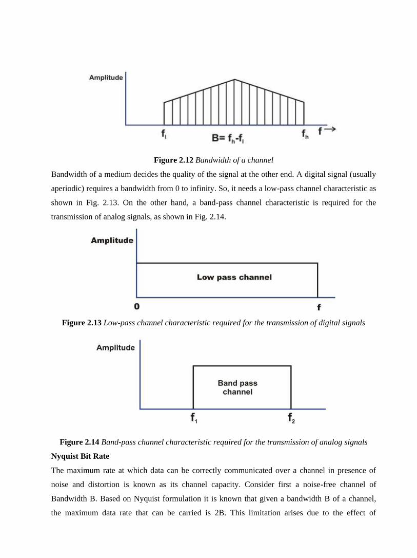
Figure 2.12 Bandwidth of a channel
Bandwidth of a medium decides the quality of the signal at the other end. A digital signal (usually
aperiodic) requires a bandwidth from 0 to infinity. So, it needs a low-pass channel characteristic as
shown in Fig. 2.13. On the other hand, a band-pass channel characteristic is required for the
transmission of analog signals, as shown in Fig. 2.14.
Figure 2.13 Low-pass channel characteristic required for the transmission of digital signals
Figure 2.14 Band-pass channel characteristic required for the transmission of analog signals
Nyquist Bit Rate
The maximum rate at which data can be correctly communicated over a channel in presence of
noise and distortion is known as its channel capacity. Consider first a noise-free channel of
Bandwidth B. Based on Nyquist formulation it is known that given a bandwidth B of a channel,
the maximum data rate that can be carried is 2B. This limitation arises due to the effect of

intersymbol interference caused by the frequency components higher than B. If the signal consists
of m discrete levels, then Nyquist theorem states:
Maximum data rate C = 2 B log2 m bits/sec,
where C is known as the channel capacity, B is the bandwidth of the channel and m is the number
of signal levels used.
Baud Rate: The baud rate or signaling rate is defined as the number of distinct symbols transmitted
per second, irrespective of the form of encoding. For baseband digital transmission m = 2. So, the
maximum baud rate = 1/Element width (in Seconds) = 2B
Bit Rate: The bit rate or information rate I is the actual equivalent number of bits transmitted per
second. I = Baud Rate × Bits per Baud
= Baud Rate × N = Baud Rate × log2m
For binary encoding, the bit rate and the baud rate are the same; i.e., I = Baud Rate.
Example: Let us consider the telephone channel having bandwidth B = 4 kHz. Assuming there is
no noise, determine channel capacity for the following encoding levels:
(i) 2, and (ii) 128.
Ans: (i) C = 2B = 2×4000 = 8 Kbits/s
(ii) C = 2×4000×log2128 = 8000×7 = 56 Kbits/s
Effects of Noise
When there is noise present in the medium, the limitations of both bandwidth and noise must be
considered. A noise spike may cause a given level to be interpreted as a signal of greater level, if it
is in positive phase or a smaller level, if it is negative phase. Noise becomes more problematic as
the number of levels increases.
Shannon Capacity (Noisy Channel)
In presence of Gaussian band-limited white noise, Shannon-Hartley theorem gives the maximum
data rate capacity
C = B log2 (1 + S/N),
where S and N are the signal and noise power, respectively, at the output of the channel. This
theorem gives an upper bound of the data rate which can be reliably transmitted over a thermal-
noise limited channel.
Example: Suppose we have a channel of 3000 Hz bandwidth, we need an S/N ratio (i.e. signal to
noise ration, SNR) of 30 dB to have an acceptable bit-error rate. Then, the maximum data rate that
we can transmit is 30,000 bps. In practice, because of the presence of different types of noises,
attenuation and delay distortions, actual (practical) upper limit will be much lower.
In case of extremely noisy channel, C = 0
Between the Nyquist Bit Rate and the Shannon limit, the result providing the smallest channel
capacity is the one that establishes the limit.
Example: A channel has B = 4 KHz. Determine the channel capacity for each of the following
signal-to-noise ratios: (a) 20 dB, (b) 30 dB, (c) 40 dB.
Answer: (a) C= B log2 (1 + S/N) = 4×10³×log2 (1+100) = 4×103×3.32×2.004 = 26.6 kbits/s
b) C= B log2 (1 + S/N) = 4×10³×log2 (1+1000) = 4×103×3.32×3.0 = 39.8 kbits/s
(c) C= B log2 (1 + S/N) = 4×10³×log2 (1+10000) = 4×103×3.32×4.0 = 53.1 kbits/s
Example: A channel has B = 4 KHz and a signal-to-noise ratio of 30 dB. Determine maximum
information rate for 4-level encoding.
Answer: For B = 4 KHz and 4-level encoding the Nyquist Bit Rate is 16 Kbps. Again for B = 4
KHz and S/N of 30 dB the Shannon capacity is 39.8 Kbps. The smallest of the two values has to
be taken as the Information capacity I = 16 Kbps.
Example: A channel has B = 4 kHz and a signal-to-noise ratio of 30 dB. Determine maximum
information rate for 128-level encoding.
Answer: The Nyquist Bit Rate for B = 4 kHz and M = 128 levels is 56 kbits/s. Again the Shannon
capacity for B = 4 kHz and S/N of 30 dB is 39.8 Kbps. The smallest of the two values decides the
channel capacity C = 39.8 kbps.
Example: The digital signal is to be designed to permit 160 kbps for a bandwidth of 20 KHz.
Determine (a) number of levels and (b) S/N ratio.
(a) Apply Nyquist Bit Rate to determine number of levels.
C = 2B log2 (M),
or 160×103 = 2×20×103 log2 (M),
or M = 24, which means 4bits/baud.
(b) Apply Shannon capacity to determine the S/N ratio
C = B log2 (1+S/N),
or 160×103 = 20×103 log2 (1+S/N) ×103 log2 (M) ,
or S/N = 28 - 1,
or S/N = 255,
or S/N = 24.07 dB.
1.10 heck Your Progress
Fill in the blanks
1. ……………….can be defined as physical path between transmitter and receiver in a data
transmission system.
2. The most commonly used guided transmission media such as………………………
3. ………………can be used for both analog and digital communication.
4. The term …………………refers to analog transmission over coaxial cable.
5. Multi-mode fiber is commonly used in……………….
6. ……………refers to the range of frequencies that a medium can pass without a loss of one-
half of the power (-3dB) contained in the signal.
1.11 Answer to Check Your Progress
1. Transmission media
2. twisted-pair of cable, coaxial cable and optical fiber.
3. Twisted-pair
4. Broadband
5. LAN
6. Bandwidth

Unit-4
Transmission of Digital Signal and Analog Data to Analog Signal
1.1 Learning Objective
1.2 Introduction
1.3 Line coding characteristics
1.4 Line Coding Techniques
1.5 Analog Data, Digital Signals
1.5.1 Pulse Code modulation
1.5.2 Delta Modulation (DM)
1.6 Introduction to Analog Data to Analog Signal
1.7 Amplitude Modulation (AM)
1.8 Angle Modulation
1.8.1 Frequency modulation
1.8.2 Phase modulation
1.9 Check your Progress
1.10 Answer to Check Your Progress

1.1 Learning Objective
After going through this unit the learner will able to:
• Explain the need for digital transmission
• Explain the basic concepts of Line Coding
• Explain the important characteristics of line coding
• Distinguish among various line coding techniques
o Unipolar
o Polar
o Bipolar
• Distinguish between data rate and modulation rate
• Explain the need for Modulation
• Distinguish different modulation techniques
• Identify the key features of Amplitude modulation
• Explain the advantages of SSB and DSBSC transmission
• Explain how the baseband signal can be recovered
1.2 Introduction
A computer network is used for communication of data from one station to another station in the
network. We have seen that analog or digital data traverses through a communication media in the
form of a signal from the source to the destination. The channel bridging the transmitter and the
receiver may be a guided transmission medium such as a wire or a wave-guide or it can be an
unguided atmospheric or space channel. But, irrespective of the medium, the signal traversing the
channel becomes attenuated and distorted with increasing distance. Hence a process is adopted to
match the properties of the transmitted signal to the channel characteristics so as to efficiently
communicate over the transmission media. There are two alternatives; the data can be either
converted to digital or analog signal. Both the approaches have pros and cons. What to be used
depends on the situation and the available bandwidth.
Now, either form of data can be encoded into either form of signal. For digital signalling, the data
source can be either analog or digital, which is encoded into digital signal, using different
encoding techniques.

The basis of analog signalling is a constant frequency signal known as a carrier signal, which is
chosen to be compatible with the transmission media being used, so that it can traverse a long
distance with minimum of attenuation and distortion. Data can be transmitted using these carrier
signals by a process called modulation, where one or more fundamental parameters of the carrier
wave, i.e. amplitude, frequency and phase are being modulated by the source data. The resulting
signal, called modulated signal traverses the media, which is demodulated at the receiving end and
the original signal is extracted. All the four possibilities are shown in Fig. 2.1.
Figure 2.1 Various approaches for conversion of data to signal
This unit will be concerned with various techniques for conversion digital and analog data to
digital signal, commonly referred to as encoding techniques.
1.3 Line coding characteristics
The first approach converts digital data to digital signal, known as line coding, as shown in Fig.
2.2. Important parameters those characteristics line coding techniques are mentioned below.
Figure 2.2 Line coding to convert digital data to digital signal

No of signal levels: This refers to the number values allowed in a signal, known as signal levels,
to represent data. Figure 2.3(a) shows two signal levels, whereas Fig. 2.3(b) shows three signal
levels to represent binary data.
Bit rate versus Baud rate: The bit rate represents the number of bits sent per second, whereas the
baud rate defines the number of signal elements per second in the signal. Depending on the
encoding technique used, baud rate may be more than or less than the data rate.
DC components: After line coding, the signal may have zero frequency component in the
spectrum of the signal, which is known as the direct-current (DC) component. DC component in a
signal is not desirable because the DC component does not pass through some components of a
communication system such as a transformer. This leads to distortion of the signal and may create
error at the output. The DC component also results in unwanted energy loss on the line.
Signal Spectrum: Different encoding of data leads to different spectrum of the signal. It is
necessary to use suitable encoding technique to match with the medium so that the signal suffers
minimum attenuation and distortion as it is transmitted through a medium.
Synchronization: To interpret the received signal correctly, the bit interval of the receiver should
be exactly same or within certain limit of that of the transmitter. Any mismatch between the two
may lead wrong interpretation of the received signal. Usually, clock is generated and synchronized
from the received signal with the help of a special hardware known as Phase Lock Loop (PLL).
However, this can be achieved if the received signal is self-synchronizing having frequent
transitions (preferably, a minimum of one transition per bit interval) in the signal.
Cost of Implementation: It is desirable to keep the encoding technique simple enough such that it
does not incur high cost of implementation.
(a) (b)
Figure 2.3 (a) Signal with two voltage levels, (b) Signal with three voltage levels
1.4 Line Coding Techniques
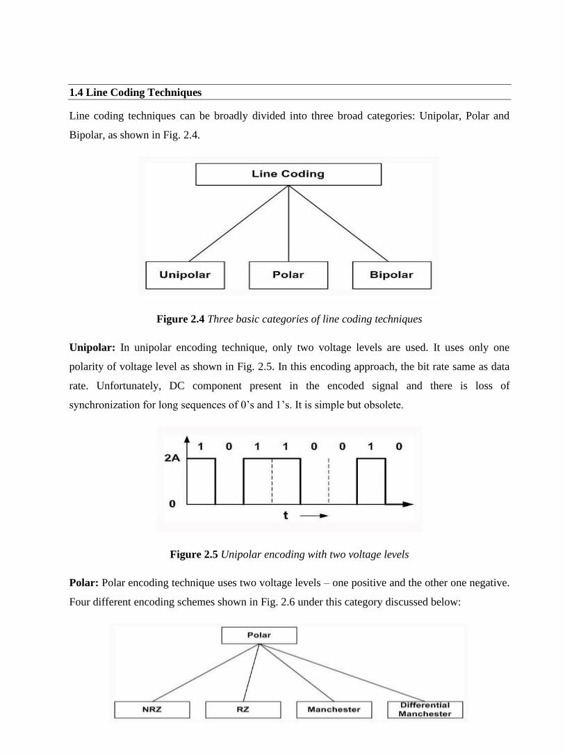
Line coding techniques can be broadly divided into three broad categories: Unipolar, Polar and
Bipolar, as shown in Fig. 2.4.
Figure 2.4 Three basic categories of line coding techniques
Unipolar: In unipolar encoding technique, only two voltage levels are used. It uses only one
polarity of voltage level as shown in Fig. 2.5. In this encoding approach, the bit rate same as data
rate. Unfortunately, DC component present in the encoded signal and there is loss of
synchronization for long sequences of 0’s and 1’s. It is simple but obsolete.
Figure 2.5 Unipolar encoding with two voltage levels
Polar: Polar encoding technique uses two voltage levels – one positive and the other one negative.
Four different encoding schemes shown in Fig. 2.6 under this category discussed below:

Figure 2.6 Encoding Schemes under polar category
Non Return to zero (NRZ): The most common and easiest way to transmit digital signals is to use
two different voltage levels for the two binary digits. Usually a negative voltage is used to
represent one binary value and a positive voltage to represent the other. The data is encoded as the
presence or absence of a signal transition at the beginning of the bit time. As shown in the figure
below, in NRZ encoding, the signal level remains same throughout the bit-period. There are two
encoding schemes in NRZ: NRZ-L and NRZ-I, as shown in Fig. 2.7.
Figure 2.7 NRZ encoding scheme
The advantages of NRZ coding are:
• Detecting a transition in presence of noise is more reliable than to compare a value to a
threshold.
• NRZ codes are easy to engineer and it makes efficient use of bandwidth.
The spectrum of the NRZ-L and NRZ-I signals are shown in Fig. 2.8. It may be noted that most of
the energy is concentrated between 0 and half the bit rate. The main limitations are the presence of
a dc component and the lack of synchronization capability. When there is long sequence of 0’s or
1’s, the receiving side will fail to regenerate the clock and synchronization between the transmitter
and receiver clocks will fail.

Figure 2.8 Signal Spectrum of NRZ Signals
Return to Zero RZ: To ensure synchronization, there must be a signal transition in each bit as
shown in Fig. 2.4.9. Key characteristics of the RZ coding are:
• Three levels
• Bit rate is double than that of data rate
• No dc component
• Good synchronization
• Main limitation is the increase in bandwidth
Figure 2.9 RZ encoding technique
Biphase: To overcome the limitations of NRZ encoding, biphase encoding techniques can be
adopted. Manchester and differential Manchester Coding are the two common Biphase techniques
in use, as shown in Fig. 2.10. In Manchester coding the mid-bit transition serves as a clocking
mechanism and also as data.

In the standard Manchester coding there is a transition at the middle of each bit period. A binary 1
corresponds to a low-to-high transition and a binary 0 to a high-to-low transition in the middle.
In Differential Manchester, inversion in the middle of each bit is used for synchronization. The
encoding of a 0 is represented by the presence of a transition both at the beginning and at the
middle and 1 is represented by a transition only in the middle of the bit period.
Key characteristics are:
• Two levels
• No DC component
• Good synchronization
• Higher bandwidth due to doubling of bit rate with respect to data rate
The bandwidth required for biphase techniques are greater than that of NRZ techniques, but due to
the predictable transition during each bit time, the receiver can synchronize properly on that
transition. Biphase encoded signals have no DC components as shown in Fig. 2.11. A Manchester
code is now very popular and has been specified for the IEEE 802.3 standard for base band coaxial
cables and twisted pair CSMA/CD bus
LANs.
Manchester Encoding
Differential Manchester
Encoding
Figure 2.10 Manchester encoding schemes

Figure 2.11 Frequency spectrum of the Manchester encoding techniques
Bipolar Encoding: Bipolar AMI uses three voltage levels. Unlike RZ, the zero level is used to
represent a 0 and a binary 1’s are represented by alternating positive and negative voltages, as
shown in Fig 2.12
Figure 2.12 Bipolar AMI signal
Pseudoternary: This encoding scheme is same as AMI, but alternating positive and negative
pulses occur for binary 0 instead of binary 1. Key characteristics are:
• Three levels
• No DC comp
• Loss of synchroniza
• Lesser bandwidth

Modulation Rate: Data rate is expressed in bits per second. On the other hand, modulation rate is
expressed in bauds. General relationship between the two ate given below:
D=R/b=R/log2L
Where, D is the modulation rate in bauds, R is the data rate is bps, L is the number of different
signal elements and b is the number of bits per signal element. Modulation rate for different
encoding techniques in shown in fig. 2. 13.
Fig. 2.13 Modulation rate for different encoding techniques
Frequency spectrum of different encoding schemes have been compared in Fig. 2.14
Fig. 2.14 Frequency spectrum of different encoding schemes
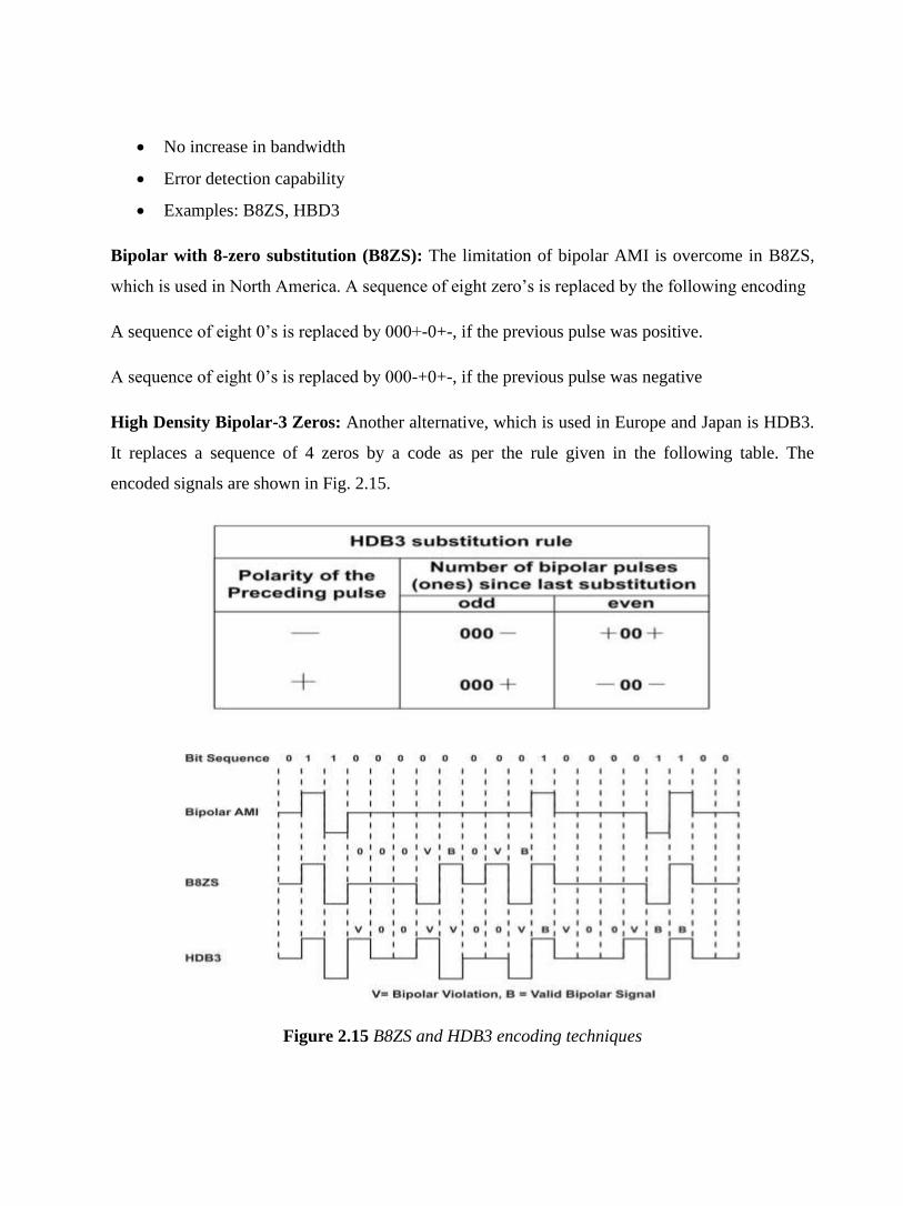
Scrambling Schemes: Extension of Bipolar AMI. Used in case of long distance applications.
Goals:
• No dc component
• No long sequences of 0-level line signal
• No increase in bandwidth
• Error detection capability
• Examples: B8ZS, HBD3
Bipolar with 8-zero substitution (B8ZS): The limitation of bipolar AMI is overcome in B8ZS,
which is used in North America. A sequence of eight zero’s is replaced by the following encoding
A sequence of eight 0’s is replaced by 000+-0+-, if the previous pulse was positive.
A sequence of eight 0’s is replaced by 000-+0+-, if the previous pulse was negative
High Density Bipolar-3 Zeros: Another alternative, which is used in Europe and Japan is HDB3.
It replaces a sequence of 4 zeros by a code as per the rule given in the following table. The
encoded signals are shown in Fig. 2.15.
Figure 2.15 B8ZS and HDB3 encoding techniques
1.5 Analog Data, Digital Signals
Analog data such as voice, video and music can be converted into digital signal communication
through transmission media. This allows the use of modern digital transmission and switching
equipment’s. The device used for conversion of analog data to digital signal and vice versa is
called a coder (coder-decoder). There are two basic approaches:
-Pulse Code Modulation (PCM)
-Delta Modulation (DM)
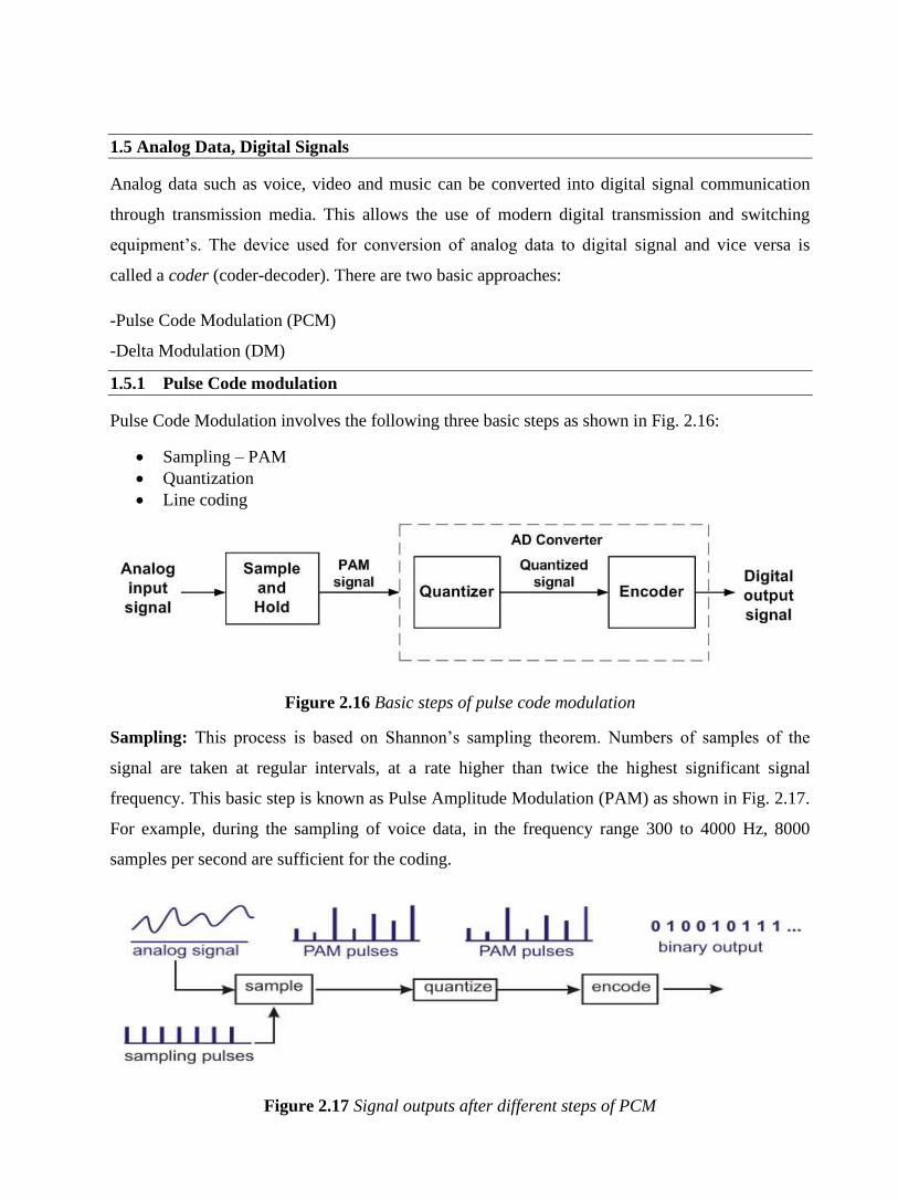
1.5.1 Pulse Code modulation
Pulse Code Modulation involves the following three basic steps as shown in Fig. 2.16:
• Sampling – PAM
• Quantization
• Line coding
Figure 2.16 Basic steps of pulse code modulation
Sampling: This process is based on Shannon’s sampling theorem. Numbers of samples of the
signal are taken at regular intervals, at a rate higher than twice the highest significant signal
frequency. This basic step is known as Pulse Amplitude Modulation (PAM) as shown in Fig. 2.17.
For example, during the sampling of voice data, in the frequency range 300 to 4000 Hz, 8000
samples per second are sufficient for the coding.
Figure 2.17 Signal outputs after different steps of PCM
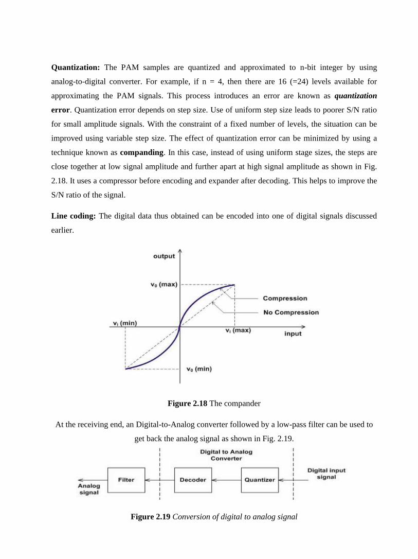
Quantization: The PAM samples are quantized and approximated to n-bit integer by using
analog-to-digital converter. For example, if n = 4, then there are 16 (=24) levels available for
approximating the PAM signals. This process introduces an error are known as quantization
error. Quantization error depends on step size. Use of uniform step size leads to poorer S/N ratio
for small amplitude signals. With the constraint of a fixed number of levels, the situation can be
improved using variable step size. The effect of quantization error can be minimized by using a
technique known as companding. In this case, instead of using uniform stage sizes, the steps are
close together at low signal amplitude and further apart at high signal amplitude as shown in Fig.
2.18. It uses a compressor before encoding and expander after decoding. This helps to improve the
S/N ratio of the signal.
Line coding: The digital data thus obtained can be encoded into one of digital signals discussed
earlier.
Figure 2.18 The compander
At the receiving end, an Digital-to-Analog converter followed by a low-pass filter can be used to
get back the analog signal as shown in Fig. 2.19.
Figure 2.19 Conversion of digital to analog signal
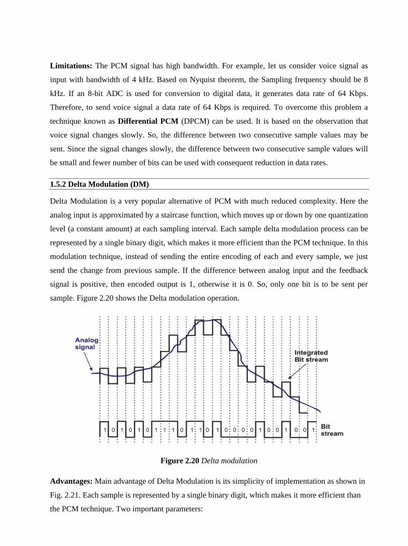
Limitations: The PCM signal has high bandwidth. For example, let us consider voice signal as
input with bandwidth of 4 kHz. Based on Nyquist theorem, the Sampling frequency should be 8
kHz. If an 8-bit ADC is used for conversion to digital data, it generates data rate of 64 Kbps.
Therefore, to send voice signal a data rate of 64 Kbps is required. To overcome this problem a
technique known as Differential PCM (DPCM) can be used. It is based on the observation that
voice signal changes slowly. So, the difference between two consecutive sample values may be
sent. Since the signal changes slowly, the difference between two consecutive sample values will
be small and fewer number of bits can be used with consequent reduction in data rates.
1.5.2 Delta Modulation (DM)
Delta Modulation is a very popular alternative of PCM with much reduced complexity. Here the
analog input is approximated by a staircase function, which moves up or down by one quantization
level (a constant amount) at each sampling interval. Each sample delta modulation process can be
represented by a single binary digit, which makes it more efficient than the PCM technique. In this
modulation technique, instead of sending the entire encoding of each and every sample, we just
send the change from previous sample. If the difference between analog input and the feedback
signal is positive, then encoded output is 1, otherwise it is 0. So, only one bit is to be sent per
sample. Figure 2.20 shows the Delta modulation operation.
Figure 2.20 Delta modulation
Advantages: Main advantage of Delta Modulation is its simplicity of implementation as shown in
Fig. 2.21. Each sample is represented by a single binary digit, which makes it more efficient than
the PCM technique. Two important parameters:
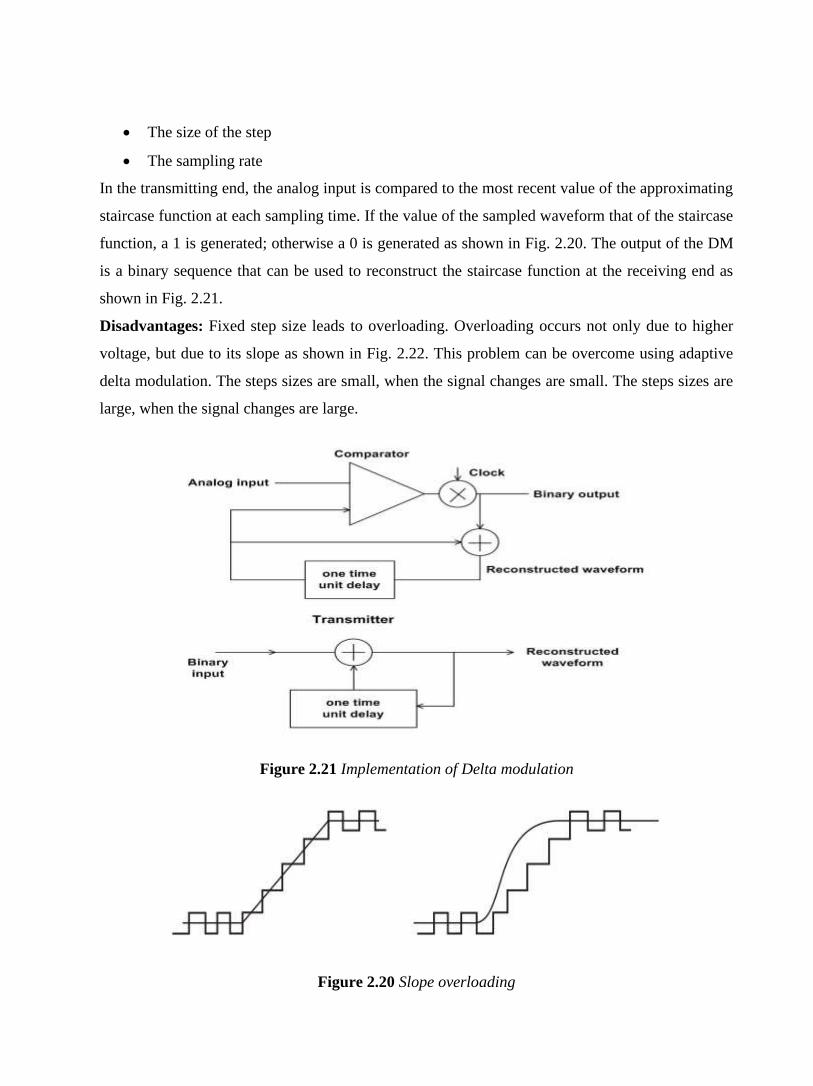
• The size of the step
• The sampling rate
In the transmitting end, the analog input is compared to the most recent value of the approximating
staircase function at each sampling time. If the value of the sampled waveform that of the staircase
function, a 1 is generated; otherwise a 0 is generated as shown in Fig. 2.20. The output of the DM
is a binary sequence that can be used to reconstruct the staircase function at the receiving end as
shown in Fig. 2.21.
Disadvantages: Fixed step size leads to overloading. Overloading occurs not only due to higher
voltage, but due to its slope as shown in Fig. 2.22. This problem can be overcome using adaptive
delta modulation. The steps sizes are small, when the signal changes are small. The steps sizes are
large, when the signal changes are large.
Figure 2.21 Implementation of Delta modulation
Figure 2.20 Slope overloading

1.6 Introduction to Analog Data to Analog Signal
Although transmission of digital signal is preferred, it is not always feasible to transmit in digital
form because it requires channel of high bandwidth having low pass characteristics. On the other
hand, an analog transmission requires lower bandwidth having band pass characteristics. The
process involved in analog transmission is known as modulation, which requires manipulation of
one or more of the parameters of the carrier that characterizes the analog signal. Figure 2.21
depicts the modulation process to get analog signal.
Figure 2.21 Translation of analog data to analog signal
Some of the important advantages of modulation are summarized below:
Frequency translation: Modulation translates the signal from one region of frequency domain to
another region. This helps to transmit the modulated signal with minimum attenuation through a
particular medium.
Practical size of antenna: Modulation translates baseband signal to higher frequency, which can
be transmitted through a bandpass channel using an antenna of smaller size. This has made
communication practical.
Narrowbanding: As modulation translates a signal from lower frequency domain to higher
frequency domain, the ratio between highest to lowest frequency of the modulated signal becomes
close to 1.
Multiplexing: Different base band signals originating from different sources can be translated to
different frequency ranges. This allows transmission of different signals through the same medium
using frequency division multiplexing (FDM) to be discussed in the following lesson.
The modulation technique can be broadly divided into two basic categories; Amplitude modulation
and Angle modulation. The Angle modulation can be further divided into two more categories;
Frequency and Phase modulations as shown in Fig. 2.22. Various modulation techniques are
discussed in the following sections.

Figure 2.22 Categories of modulation techniques
1.7 Amplitude Modulation (AM)
This is the simplest form of modulation where the amplitude of the carrier wave is modulated by
the analog signal known as the modulating signal. A signal to be modulated, a carrier and the
modulated signal are shown in Fig. 2.23. Let the modulating waveform is given by em(t) = Em cos
(2πfmt) and the carrier signal is given by ec(t) = Ec cos (2πfct + Φc). Then the equation of the
modulated signal is given by
s(t) = (Ec + Em cos 2πfmt) cos 2πfct
Modulation Index: The modulation index, represented by m, is given by
m = (Emax - Emin )/ (Emax + Emin ) = Em / Ec,
where Emax = Ec + Em ,
Emin = Ec - Em, and s(t) = Ec (1 + m cos 2πfmt) cos 2πfct,
The envelope of the modulated signal is represented by 1+m em(t) for m < 1. The envelope of the
modulated signal for different modulation index is shown in Fig. 2.5.4. Loss of information occurs
when m > 1.

Figure 2.23 Amplitude Modulation
Figure 2.24 (a) Envelope of the signal 1+m em(t) for m < 1

Figure 2.24 (b) Envelope of the signal 1+m em(t) for m = 1

Figure 2.24 (c) Envelope of the signal 1+m em(t) for m > 1
Frequency Spectrum: Frequency spectrum of the sinusoidal AM signal can be represented by
It may be noted that there are three frequency components; Carrier wave of amplitude Ec, Lower
sideband of amplitude m/2 Ec and Higher sideband of amplitude m/2 Ec, as shown in Fig.2.25.

Figure 2.25 Spectrum of a modulated signal
Example: A carrier of 1 MHz with peak value of 10V is modulated by a 5 KHz sine wave
amplitude 6V. Determine the modulation index and frequency spectrum.
Answer: The modulation index m = 6/10 = 0.6. The side frequencies are (1000 – 5) = 995 KHz and
(1000 + 5) = 1005 KHz having amplitude of 0.6 × 10/2 = 3V, as shown in Fig. 2.26.
Figure 2.26 Spectrum of the modulated signal of the above example

Modulation using Audio signal: Let the bandwidth of the modulating signal is an audio signal
with bandwidth equal to Bm. Then the bandwidth of the modulated signal is 2 Bm, as shown in Fig.
2.27
Fig. 2.27 Bandwidth of an audio signal
Power: Average power developed across a resistor R for the carrier signal is Pc = Ec2/2R.
For each of the sideband frequencies the power is PSF = (mEc / 2)2/ 2R = Pc
m2/4. So, the total power required for transmission is = Pc (1 + 2(m2/4)) = Pc (1 + m2/2).
To minimize power for transmission, there are two other alternatives:
Double-Sideband with Suppressed Carrier (DSBSC) Modulation
Single Side Band (SSB) Modulation
Double-Sideband with Suppressed Carrier (DSBSC) Modulation, as shown in Fig. 2.28, utilizes
the transmitted power more efficiently than DSB AM. On the other hand, Single Side Band (SSB)
Modulation not only conserves energy, it also reduces bandwidth as shown in Fig. 2.29. It may be
noted that one of the two side bands needs to be transmitted.
Figure 2.28 Double-Sideband with Suppressed Carrier (DSBSC) Modulation

Figure 2.29 Single Sideband (SSB) Modulation
Recovery of the Base band Signal
At the receiving end the signal is being demodulated to get the original data. Let a base band signal
m(t) is translated out by multiplication with the carrier signal cosWct to get m(t) CosWct, the
modulated signal. By multiplying second time with the carrier we get (m(t) CosWct) CosWct
It may be noted that
• The base band signal reappears along with two spectral components of
frequencies 2fc - fm to 2fc + fm
• The spectral components 2fc - fm to 2fc + fm can be easily removed by a low-pass filter.
This process is known Synchronous detection
The synchronous detection approach has the disadvantage that the carrier signal used in the second
multiplication has to be precisely synchronous. A very simple circuit, as shown in Fig. 2.30, can
accomplish the recovery of the base and signal using envelope detection.
Figure 2.30 Recovery of the baseband signal using envelope detection

Another approach is to use Superhetrodyne approach. In this approach the modulated signal
received at the receiving end is greatly attenuated and mixed with noise. There may be other
channels adjacent to it. The signal has to be amplified before detection and the noises are to be
removed by suitable filtering. Superhetrodyne approach, as shown in Fig. 2.31, is commonly used
because it provides many advantages.
• It is used to improve adjacent channel selection
• To provide necessary gain
• To provide better S/N ratio
This is the commonly used technique of the popular AM receivers, as shown in Fig. 2.31. The
received AM signal is amplified with the help of a RF amplifier. Then a mixer stage translates the
signal to an intermediate frequency (IF) by mixing the RF signal with a local oscillator (shown in
B). The IF signal is amplified (shown in C) and then a detector stage is used to get back the base
band audio signal (shown in C). The audio signal can be amplified before allying it to a speaker.
Figure 2.31 Operation of a superheterodyne AM radio receiver
1.8 Angle Modulation
Angle modulation is shown in Fig. 2.32. It may me noted that the amplitude of the modulated
signal is constant. Frequency Modulation (FM) and Phase Modulation (PM) are the special cases
of Angle modulation. For Phase Modulation, the phase is proportional to the modulating signal,
whereas for frequency modulation, the derivative of the phase is proportional to the modulating
signal.

Figure 2.32 Angle modulation
1.8.1 Frequency modulation
In case of frequency modulation, the modulating signal em(t) is used to vary the carrier frequency.
The change is frequency is proportional to the modulating voltage kem(t), where k is a constant
known as frequency deviation constant, expressed in Hz/V. The instantaneous frequency of the
modulated signal can be represented by fi (t) = fc+kem(t), where fc is the carrier frequency.
For sinusoidal modulation
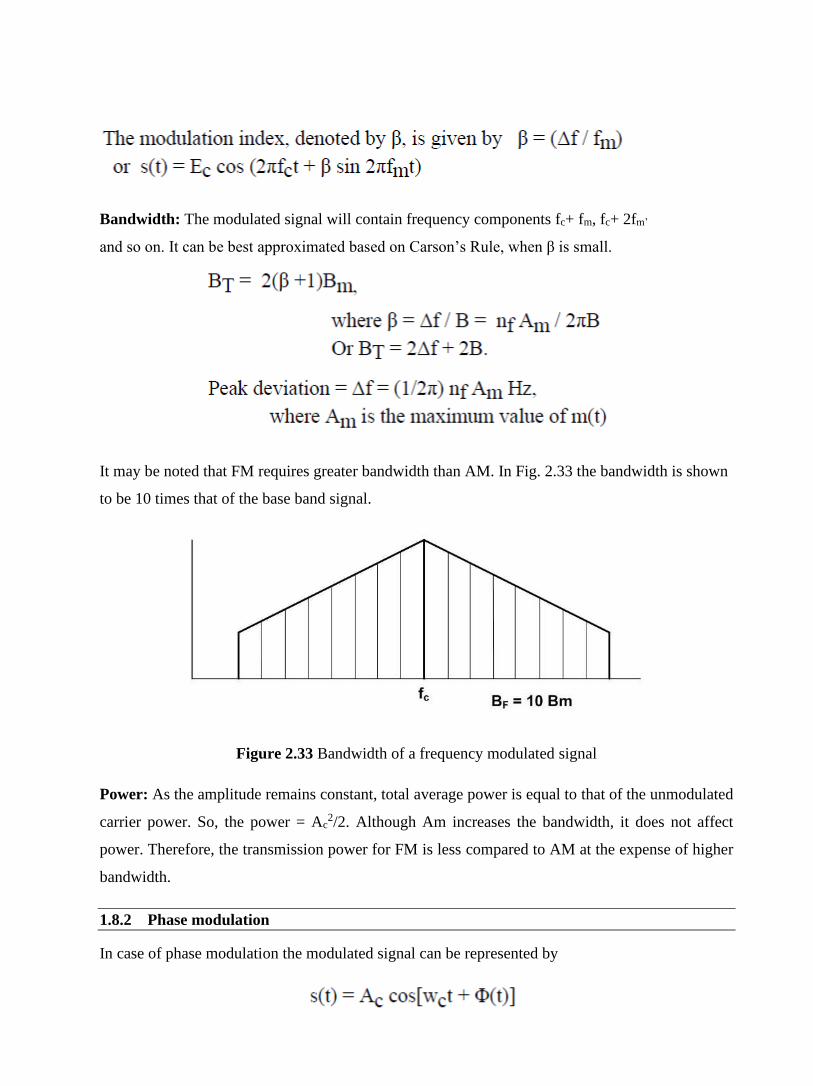
Bandwidth: The modulated signal will contain frequency components fc+ fm, fc+ 2fm’
and so on. It can be best approximated based on Carson’s Rule, when β is small.
It may be noted that FM requires greater bandwidth than AM. In Fig. 2.33 the bandwidth is shown
to be 10 times that of the base band signal.
Figure 2.33 Bandwidth of a frequency modulated signal
Power: As the amplitude remains constant, total average power is equal to that of the unmodulated
carrier power. So, the power = Ac2/2. Although Am increases the bandwidth, it does not affect
power. Therefore, the transmission power for FM is less compared to AM at the expense of higher
bandwidth.
1.8.2 Phase modulation
In case of phase modulation the modulated signal can be represented by
The angle (wct + Φ(t)) undergoes a modulation around the angle θ = wct. The signal is
therefore an angular-velocity modulated signal. When the phase is directly proportional to
the modulating signal, i.e, Φ(t) = np m(t), we call it phase modulation, where np is the
phase modulation index. The instantaneous frequency of a phase modulated signal is given by
Relationship between FM and PM
The relationship between the two types of angle modulated signal depicted in Fig. 2.34.
Let m(t) be derived as an integral of the modulated signal em(t), so that m(t) =k’’ ∫ e(t)),
Then with k = k’k’’, we get s(t) = Ec cos (Wct + k ∫ e(t)). The instantaneous angular
frequency of s(t) is 2πfi(t) = d/dt [2πfct + k ∫ e(t)]
or fi(t) = fc + (1/2π)ke(t)]
The waveform is therefore modulated in frequency
In summary, these two together are referred to as angle modulation and modulated signals have
similar characteristics. In this process, since the frequency or phase of the carrier wave is being
modulated by the signal and the modulation lies near the base band, the external noise or
electromagnetic interference cannot affect much the modulated signal at the receiving end. Analog
data to Analog signal modulation techniques at a glance are shown in Fig. 2.35.
Figure 2.34 Difference between frequency and phase modulation
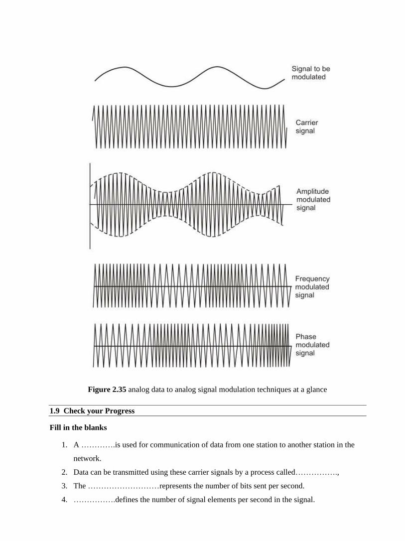
Figure 2.35 analog data to analog signal modulation techniques at a glance
1.9 Check your Progress
Fill in the blanks
1. A ………….is used for communication of data from one station to another station in the
network.
2. Data can be transmitted using these carrier signals by a process called…………….,
3. The ………………………represents the number of bits sent per second.
4. …………….defines the number of signal elements per second in the signal.

5. ………………..such as voice, video and music can be converted into digital signal
communication through transmission media.
6. ………………..is a very popular alternative of PCM with much reduced complexity.
7. The process involved in analog transmission is known as………………….
8. This is the simplest form of modulation where the amplitude of the carrier wave is
modulated by the analog signal known as the………………………………….
1.10 Answer to Check Your Progress
1. computer network
2. modulation
3. bit rate
4. baud rate
5. Analog data
6. Delta Modulation
7. Modulation
8. modulating signal
Unit-5
Digital Data, Analog Signals and Multiplexing of Signals
1.1 learning objectives
1.2 Introduction to digital data, analog signals
1.3 Amplitude-shift keying (ASK)
1.4 Frequency-Shift Keying (FSK)
1.5 Phase Shift Keying (PSK)
1.6 Introduction to Multiplexing of signals
1.7 Frequency-Division Multiplexing (FDM)
1.8 Wavelength-Division Multiplexing
1.9 Time-Division Multiplexing (TDM)
1.10 Statistical Time-division Multiplexing
1.11 Orthogonal Frequency Division Multiplexing
1.12 Check Your Progress
1.13 Answer to Check Your Progress
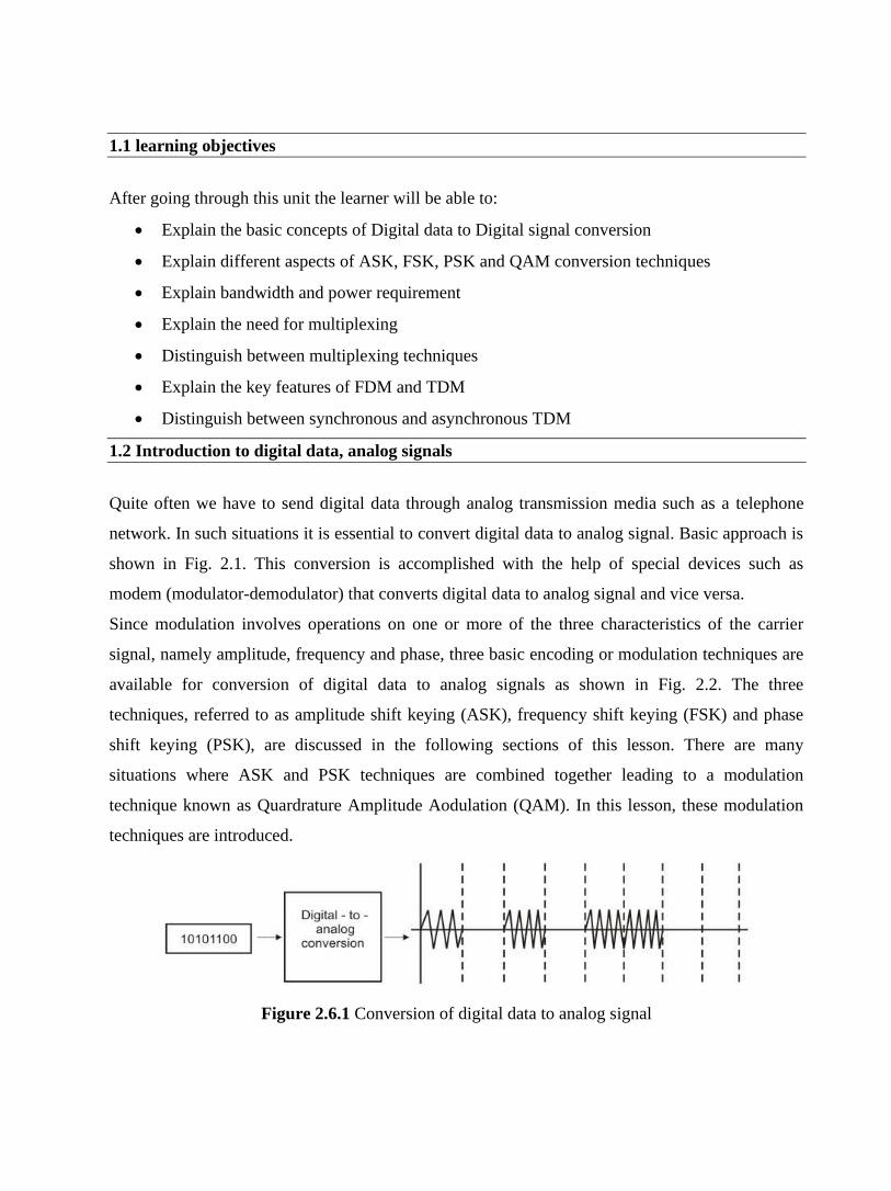
1.1 learning objectives
After going through this unit the learner will be able to:
• Explain the basic concepts of Digital data to Digital signal conversion
• Explain different aspects of ASK, FSK, PSK and QAM conversion techniques
• Explain bandwidth and power requirement
• Explain the need for multiplexing
• Distinguish between multiplexing techniques
• Explain the key features of FDM and TDM
• Distinguish between synchronous and asynchronous TDM
1.2 Introduction to digital data, analog signals
Quite often we have to send digital data through analog transmission media such as a telephone
network. In such situations it is essential to convert digital data to analog signal. Basic approach is
shown in Fig. 2.1. This conversion is accomplished with the help of special devices such as
modem (modulator-demodulator) that converts digital data to analog signal and vice versa.
Since modulation involves operations on one or more of the three characteristics of the carrier
signal, namely amplitude, frequency and phase, three basic encoding or modulation techniques are
available for conversion of digital data to analog signals as shown in Fig. 2.2. The three
techniques, referred to as amplitude shift keying (ASK), frequency shift keying (FSK) and phase
shift keying (PSK), are discussed in the following sections of this lesson. There are many
situations where ASK and PSK techniques are combined together leading to a modulation
technique known as Quardrature Amplitude Aodulation (QAM). In this lesson, these modulation
techniques are introduced.
Figure 2.6.1 Conversion of digital data to analog signal

Figure 2.2 Types of digital-to-analog modulation
1.3 Amplitude-shift keying (ASK)
In ASK, two binary values are represented by two different amplitudes of the carrier frequency as
shown in the Fig. 2.6.3. The unmodulated carrier can be represented by
Special case: On/Off Keying (OOK), the amplitude A2 = 0
ASK is susceptible to sudden gain changes and OOK is commonly used to transmit digital data
over optical fibers.
Frequency Spectrum: If Bm is the overall bandwidth of the binary signal, the bandwidth of the
modulated signal is BT = Nb, where Nb is the baud rate. This is depicted in Fig. 2.4.
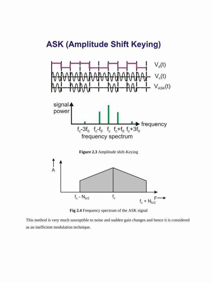
Figure 2.3 Amplitude shift-Keying
Fig 2.4 Frequency spectrum of the ASK signal
This method is very much susceptible to noise and sudden gain changes and hence it is considered
as an inefficient modulation technique.
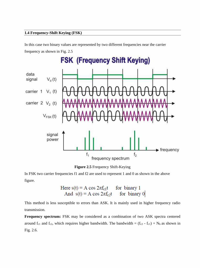
1.4 Frequency-Shift Keying (FSK)
In this case two binary values are represented by two different frequencies near the carrier
frequency as shown in Fig. 2.5
Figure 2.5 Frequency Shift-Keying
In FSK two carrier frequencies f1 and f2 are used to represent 1 and 0 as shown in the above
figure.
This method is less susceptible to errors than ASK. It is mainly used in higher frequency radio
transmission.
Frequency spectrum: FSK may be considered as a combination of two ASK spectra centered
around fc1 and fc2, which requires higher bandwidth. The bandwidth = (fc2 - fc1) + Nb as shown in
Fig. 2.6.

Figure: 2.6 Frequency Spectrum of the FSK signal
1.5 Phase Shift Keying (PSK)
In this method, the phase of the carrier signal is shifted by the modulating signal with the phase
measured relative to the previous bit interval. The binary 0 is represented by sending a signal of
the same phase as the preceding one and 1 is represented by sending the signal with an opposite
phase to the previous one as shown in Fig. 2.7.
Figure 2.7 Phase-shift keying
In 2-PSK the carrier used to represent 0 or 1.
The signal set can be shown geometrically in Fig. 2.8. This representation is called a constellation
diagram, which provides a graphical representation of the complex envelope of each possible
symbol state. The x-axis of a constellation diagram represents the in-phase component of the
complex envelope, and the y-axis represents the quadrature component of the complex envelope.
The distance between signals on a constellation diagram indicates how different the modulation
waveforms are, and how well a receiver can differentiate between all possible symbols in presence
of noise.
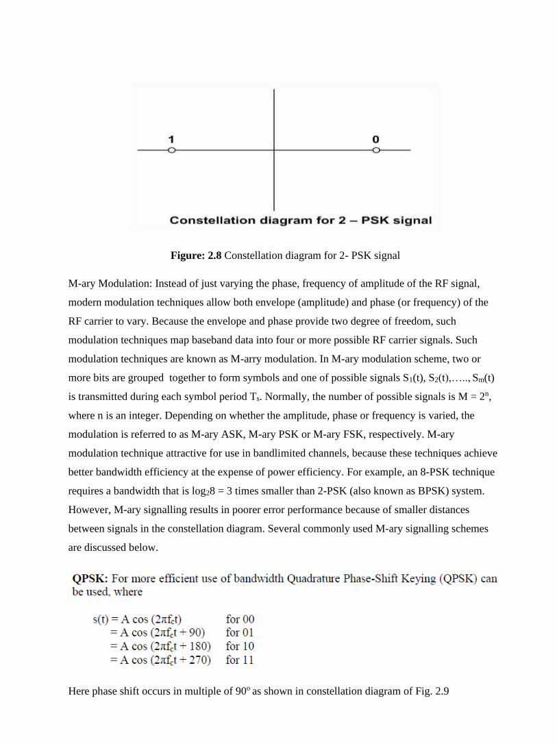
Figure: 2.8 Constellation diagram for 2- PSK signal
M-ary Modulation: Instead of just varying the phase, frequency of amplitude of the RF signal,
modern modulation techniques allow both envelope (amplitude) and phase (or frequency) of the
RF carrier to vary. Because the envelope and phase provide two degree of freedom, such
modulation techniques map baseband data into four or more possible RF carrier signals. Such
modulation techniques are known as M-arry modulation. In M-ary modulation scheme, two or
more bits are grouped together to form symbols and one of possible signals S1(t), S2(t),….., Sm(t)
is transmitted during each symbol period Ts. Normally, the number of possible signals is M = 2n,
where n is an integer. Depending on whether the amplitude, phase or frequency is varied, the
modulation is referred to as M-ary ASK, M-ary PSK or M-ary FSK, respectively. M-ary
modulation technique attractive for use in bandlimited channels, because these techniques achieve
better bandwidth efficiency at the expense of power efficiency. For example, an 8-PSK technique
requires a bandwidth that is log28 = 3 times smaller than 2-PSK (also known as BPSK) system.
However, M-ary signalling results in poorer error performance because of smaller distances
between signals in the constellation diagram. Several commonly used M-ary signalling schemes
are discussed below.
Here phase shift occurs in multiple of 90o as shown in constellation diagram of Fig. 2.9
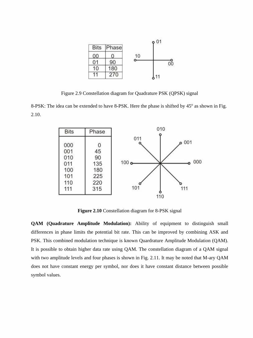
Figure 2.9 Constellation diagram for Quadrature PSK (QPSK) signal
8-PSK: The idea can be extended to have 8-PSK. Here the phase is shifted by 45o as shown in Fig.
2.10.
Figure 2.10 Constellation diagram for 8-PSK signal
QAM (Quadrature Amplitude Modulation): Ability of equipment to distinguish small
differences in phase limits the potential bit rate. This can be improved by combining ASK and
PSK. This combined modulation technique is known Quardrature Amplitude Modulation (QAM).
It is possible to obtain higher data rate using QAM. The constellation diagram of a QAM signal
with two amplitude levels and four phases is shown in Fig. 2.11. It may be noted that M-ary QAM
does not have constant energy per symbol, nor does it have constant distance between possible
symbol values.
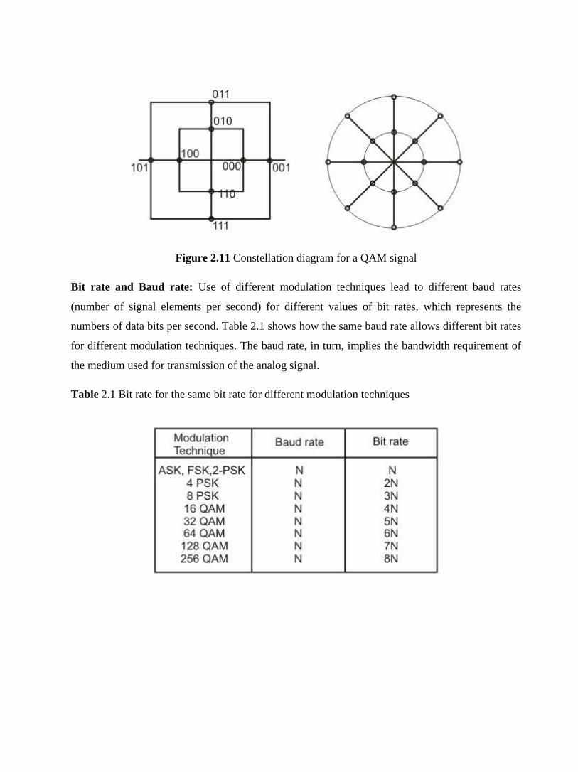
Figure 2.11 Constellation diagram for a QAM signal
Bit rate and Baud rate: Use of different modulation techniques lead to different baud rates
(number of signal elements per second) for different values of bit rates, which represents the
numbers of data bits per second. Table 2.1 shows how the same baud rate allows different bit rates
for different modulation techniques. The baud rate, in turn, implies the bandwidth requirement of
the medium used for transmission of the analog signal.
Table 2.1 Bit rate for the same bit rate for different modulation techniques

1.6 Introduction to Multiplexing of signals
It has been observed that most of the individual data-communicating devices typically require
modest data rate. But, communication media usually have much higher bandwidth. As a
consequence, two communicating stations do not utilize the full capacity of a data link. Moreover,
when many nodes compete to access the network, some efficient techniques for utilizing the data
link are very essential. When the bandwidth of a medium is greater than individual signals to be
transmitted through the channel, a medium can be shared by more than one channel of signals. The
process of making the most effective use of the available channel capacity is called Multiplexing.
For efficiency, the channel capacity can be shared among a number of communicating stations just
like a large water pipe can carry water to several separate houses at once. Most common use of
multiplexing is in long-haul communication using coaxial cable, microwave and optical fibre.
Figure 2.12 depicts the functioning of multiplexing functions in general. The multiplexer is
connected to the demultiplexer by a single data link. The multiplexer combines (multiplexes) data
from these ‘n’ input lines and transmits them through the high capacity data link, which is being
demultiplexed at the other end and is delivered to the appropriate output lines. Thus, Multiplexing
can also be defined as a technique that allows simultaneous transmission of multiple signals across
a single data link.
Figure 2.12 Basic concept of multiplexing
Multiplexing techniques can be categorized into the following three types:
• Frequency-division multiplexing (FDM): It is most popular and is used extensively in
radio and TV transmission. Here the frequency spectrum is divided into several logical
channels, giving each user exclusive possession of a particular frequency band.
• Time-division Multiplexing (TDM): It is also called synchronous TDM, which is
commonly used for multiplexing digitized voice stream. The users take turns using the
entire channel for short burst of time.
• Statistical TDM: This is also called asynchronous TDM, which simply improves on the
efficiency of synchronous TDM.
In the following sections these techniques have been considered in detail.

1.7 Frequency-Division Multiplexing (FDM)
In frequency division multiplexing, the available bandwidth of a single physical medium is
subdivided into several independent frequency channels. Independent message signals are
translated into different frequency bands using modulation techniques, which are combined by a
linear summing circuit in the multiplexer, to a composite signal. The resulting signal is then
transmitted along the single channel by electromagnetic means as shown in Fig. 2.13. Basic
approach is to divide the available bandwidth of a single physical medium into a number of
smaller, independent frequency channels. Using modulation, independent message signals are
translated into different frequency bands. All the modulated signals are combined in a linear
summing circuit to form a composite signal for transmission. The carriers used to modulate the
individual message signals are called sub-carriers, shown as f1, f2, …, fn in Fig. 2.14 (a).
Figure 2.13 Basic concept of FDM
At the receiving end the signal is applied to a bank of band-pass filters, which separates individual
frequency channels. The band pass filter outputs are then demodulated and distributed to different
output channels as shown in Fig. 2.14(b).

Figure 2.14 (a) FDM multiplexing process, (b) FDM demultiplexing process
Figure 2.15 Use of guard bands in FDM
If the channels are very close to one other, it leads to inter-channel cross talk. Channels must be
separated by strips of unused bandwidth to prevent inter-channel cross talk. These unused channels
between each successive channel are known as guard bands as shown in Fig. 2.15.
FDM are commonly used in radio broadcasts and TV networks. Since, the frequency band used for
voice transmission in a telephone network is 4000 Hz, for a particular cable of 48 KHz bandwidth,
in the 70 to 108 KHz range, twelve separate 4 KHz sub channels could be used for transmitting
twelve different messages simultaneously. Each radio and TV station, in a certain broadcast area,
is allotted a specific broadcast frequency, so that independent channels can be sent simultaneously
in different broadcast area. For example, the AM radio uses 540 to 1600 KHz frequency bands
while the FM radio uses 88 to 108 MHz frequency bands.

1.8 Wavelength-Division Multiplexing
Wavelength-division multiplexing (WDM) is conceptually same as the FDM, except that the
multiplexing and demultiplexing involves light signals transmitted through fibre-optic channels.
The idea is the same: we are combining different frequency signals. However, the difference is that
the frequencies are very high. It is designed to utilize the high data rate capability of fibre-optic
cable. Very narrow band of light signal from different source are combined to make a wider band
of light. At the receiver the signals are separated with the help of a demultiplexer as shown in Fig.
2.16.
Figure 2.16 Basic WDM multiplexing and demultiplexing
Multiplexing and demultiplexing of light signals can be done with the help of a prism as shown in
Fig. 2.17. From the basic knowledge of physics we know that light signal is bent by different
amount based on the angle of incidence and wavelength of light as shown by different colours in
the figure. One prism performs the role of a multiplexer by combining lights having different
frequencies from different sources. The composite signal can be transmitted through an optical
fibre cable over long distances, if required. At the other end of the optical fibre cable the

composite signal is applied to another prism to do the reverse operation, the function of a
demultiplexer.
Figure 2.17 Multiplexing and demultiplexing of light signals with help of prisms
1.9 Time-Division Multiplexing (TDM)
In frequency division multiplexing, all signals operate at the same time with different frequencies,
but in Time-division multiplexing all signals operate with same frequency at different times. This
is a base band transmission system, where an electronic commutator sequentially samples all data
source and combines them to form a composite base band signal, which travels through the media
and is being demultiplexed into appropriate independent message signals by the corresponding
commutator at the receiving end. The incoming data from each source are briefly buffered. Each
buffer is typically one bit or one character in length. The buffers are scanned sequentially to form a
composite data stream. The scan operation is sufficiently rapid so that each buffer is emptied
before more data can arrive. Composite data rate must be at least equal to the sum of the individual
data rates. The composite signal can be transmitted directly or through a modem. The multiplexing
operation is shown in Fig. 2.18
Figure 2.18 Time division multiplexing operation
As shown in the Fig 2.18 the composite signal has some dead space between the successive
sampled pulses, which is essential to prevent interchannel cross talks. Along with the sampled

pulses, one synchronizing pulse is sent in each cycle. These data pulses along with the control
information form a frame. Each of these frames contain a cycle of time slots and in each frame,
one or more slots are dedicated to each data source. The maximum bandwidth (data rate) of a
TDM system should be at least equal to the same data rate of the sources.
Synchronous TDM is called synchronous mainly because each time slot is preassigned to a fixed
source. The time slots are transmitted irrespective of whether the sources have any data to send or
not. Hence, for the sake of simplicity of implementation, channel capacity is wasted. Although
fixed assignment is used TDM, devices can handle sources of different data rates. This is done by
assigning fewer slots per cycle to the slower input devices than the faster devices. Both
multiplexing and demultiplexing operation for synchronous TDM are shown in Fig. 2.19.
Figure 2.19 Multiplexing and demultiplexing in synchronous TDM
1.10 Statistical Time-division Multiplexing
One drawback of the TDM approach, as discussed earlier, is that many of the time slots in the
frame are wasted. It is because, if a particular terminal has no data to transmit at particular instant
of time, an empty time slot will be transmitted. An efficient alternative to this synchronous TDM is
statistical TDM, also known as asynchronous TDM or Intelligent TDM. It dynamically allocates
the time slots on demand to separate input channels, thus saving the channel capacity. As with
Synchronous TDM, statistical multiplexers also have many I/O lines with a buffer associated to
each of them. During the input, the multiplexer scans the input buffers, collecting data until the
frame is filled and send the frame. At the receiving end, the demultiplexer receives the frame and

distributes the data to the appropriate buffers. The difference between synchronous TDM and
asynchronous TDM is illustrated with the help of Fig. 2.20. It may be noted that many slots remain
unutilised in case synchronous TDM, but the slots are fully utilized leading to smaller time for
transmission and better utilization of bandwidth of the medium. In case of statistical TDM, the
data in each slot must have an address part, which identifies the source of data. Since data arrive
from and are distributed to I/O lines unpredictably, address information is required to assure
proper delivery as shown in Fig. 2.21. This leads to more overhead per slot. Relative addressing
can be used to reduce overhead.
Figure 2.20 Synchronous versus asynchronous TDM
Figure 2.21 Address overhead in asynchronous TDM
1.11 Orthogonal Frequency Division Multiplexing
Frequency division multiplexing (FDM) is a technology that transmits multiple signals
simultaneously over a single transmission path, such as a cable or wireless system. Each signal
travels within its own unique frequency range (carrier), which is modulated by the data (text,
voice, video, etc.).
Orthogonal FDM’s (OFDM) spread spectrum technique distributes the data over a large number of
carriers that are spaced apart at precise frequencies. This spacing provides the “orthogonality” in

this technique, which prevents the demodulators from seeing frequencies other than their won.
Basic approach of OFDM is illustrated in Fig. 2.22.
The benefits of OFDM are high spectral efficiency, resiliency to RF interference, and lower multi-
path distortion. This is useful because in a typical terrestrial broadcasting scenario there are
multipath-channels (i.e. the transmitted signal arrives at the receiver suing various there are
multipath-channels (i.e. the transmitted signal arrives at the receiver using various paths of
different length). Since multiple versions of the signal interfere with each other (inter symbol
interference (ISI) it becomes very hard to extract the original information.
OFDM is a transmission technique that has been around for years, but only recently became
popular due to the development of digital signal processors (DSPs) that can handle its heavy
digital processing requirements. OFDM is being implemented in broadband wireless access system
as a way to overcome wireless transmission problems and to improve bandwidth. OFDM is also
used in wireless LANs as specified by the IEEE 802.11a and the ETSI HiperLAN/2 standards. It is
also used for wireless digital radio and TV transmissions, particularly in Europe, OFDM is
sometime called multicarrier or discrete multi-tone modulation.
Figure: 2.22 Difference between band-width requirements in FDM Vs OFDM
OFDM is similar to DFM but much more spectrally efficient by spacing the sub channels much
closer together (until they are actually overlapping). This is done by finding frequencies that are
orthogonal, which means that they are perpendicular in a mathematical sense, allowing the
spectrum of each sub-channel to overlap another without interfering.
1.12 Check Your Progress
Fill in the blanks
1. …………………….is a technology that transmits multiple signals simultaneously over a
single transmission path, such as a cable or wireless system.
2. An efficient alternative to this synchronous TDM is statistical TDM, also known
as……………….
3. ……………………………..is conceptually same as the FDM, except that the multiplexing and
demultiplexing involves light signals transmitted through fibre-optic channels.
4. …………………..the available bandwidth of a single physical medium is subdivided into
several independent frequency channels.
1.13 Answer to Check Your Progress
1. Frequency division multiplexing (FDM)
2. asynchronous TDM.
3. Wavelength-division multiplexing (WDM)
4. In frequency division multiplexing
Block-2(Data Link control)
Unit-1
Interfacing to the media and synchronization
1.1 Learning Objectives
1.2 Introduction
1.3 Possible Modes of communication
1.4 Framing and Synchronization
1.4.1 Why Framing and Synchronization?
1.4.2 Synchronization
1.4.3 Synchronous communication (bit-oriented)
1.4.4 Asynchronous communication (word-oriented)
1.5 Character Oriented Framing
1.5.1 Character stuffing
1.5.2 Data Rate Measures
1.6 DTE-DCE Interface
1.6.1 The RS-232 C
1.6.2 Null Modem
1.6.3 MODEMS
1.7 Check Your Progress
1.8 Answer to Check Your Progress
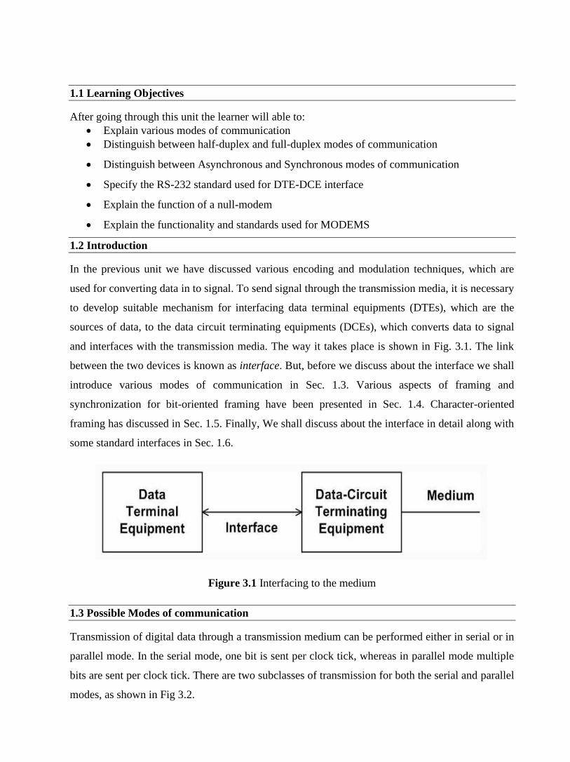
1.1 Learning Objectives
After going through this unit the learner will able to:
• Explain various modes of communication
• Distinguish between half-duplex and full-duplex modes of communication
• Distinguish between Asynchronous and Synchronous modes of communication
• Specify the RS-232 standard used for DTE-DCE interface
• Explain the function of a null-modem
• Explain the functionality and standards used for MODEMS
1.2 Introduction
In the previous unit we have discussed various encoding and modulation techniques, which are
used for converting data in to signal. To send signal through the transmission media, it is necessary
to develop suitable mechanism for interfacing data terminal equipments (DTEs), which are the
sources of data, to the data circuit terminating equipments (DCEs), which converts data to signal
and interfaces with the transmission media. The way it takes place is shown in Fig. 3.1. The link
between the two devices is known as interface. But, before we discuss about the interface we shall
introduce various modes of communication in Sec. 1.3. Various aspects of framing and
synchronization for bit-oriented framing have been presented in Sec. 1.4. Character-oriented
framing has discussed in Sec. 1.5. Finally, We shall discuss about the interface in detail along with
some standard interfaces in Sec. 1.6.
Figure 3.1 Interfacing to the medium
1.3 Possible Modes of communication
Transmission of digital data through a transmission medium can be performed either in serial or in
parallel mode. In the serial mode, one bit is sent per clock tick, whereas in parallel mode multiple
bits are sent per clock tick. There are two subclasses of transmission for both the serial and parallel
modes, as shown in Fig 3.2.

Figure 3.2 Different modes of transmission
Parallel Transmission
Parallel transmission involves grouping several bits, say n, together and sending all the n bits at a
time. Figure 3.3 shows how parallel transmission occurs for n = 8. This can be accomplishes with
the help of eight wires bundled together in the form of a cable with a connector at each end.
Additional wires, such as request (req) and acknowledgement (ack) are required for asynchronous
transmission.
Primary advantage of parallel transmission is higher speed, which is achieved at the expense of
higher cost of cabling. As this is expensive for longer distances, parallel transmission is feasible
only for short distances.
Figure 3.3 Parallel mode of communication with n = 8
Serial Transmission
Serial transmission involves sending one data bit at a time. Figure 3.4 shows how serial
transmission occurs. It uses a pair of wire for communication of data in bit-serial form.
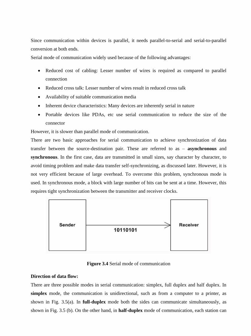
Since communication within devices is parallel, it needs parallel-to-serial and serial-to-parallel
conversion at both ends.
Serial mode of communication widely used because of the following advantages:
• Reduced cost of cabling: Lesser number of wires is required as compared to parallel
connection
• Reduced cross talk: Lesser number of wires result in reduced cross talk
• Availability of suitable communication media
• Inherent device characteristics: Many devices are inherently serial in nature
• Portable devices like PDAs, etc use serial communication to reduce the size of the
connector
However, it is slower than parallel mode of communication.
There are two basic approaches for serial communication to achieve synchronization of data
transfer between the source-destination pair. These are referred to as – asynchronous and
synchronous. In the first case, data are transmitted in small sizes, say character by character, to
avoid timing problem and make data transfer self-synchronizing, as discussed later. However, it is
not very efficient because of large overhead. To overcome this problem, synchronous mode is
used. In synchronous mode, a block with large number of bits can be sent at a time. However, this
requires tight synchronization between the transmitter and receiver clocks.
Figure 3.4 Serial mode of communication
Direction of data flow:
There are three possible modes in serial communication: simplex, full duplex and half duplex. In
simplex mode, the communication is unidirectional, such as from a computer to a printer, as
shown in Fig. 3.5(a). In full-duplex mode both the sides can communicate simultaneously, as
shown in Fig. 3.5 (b). On the other hand, in half-duplex mode of communication, each station can

both send and receive data, as shown in Fig. 3.5 (c). But, when one is sending, the other one can
only receive and vice versa.
(a)
(b)
(c)
Figure 3.5 Direction of data flow
1.4 Framing and Synchronization
1.4.1 Why Framing and Synchronization?
Normally, units of data transfer are larger than a single analog or digital encoding symbol. It is
necessary to recover clock information for both the signal (so we can recover the right number of
symbols and recover each symbol as accurately as possible), and obtain synchronization for larger
units of data (such as data words and frames). It is necessary to recover the data in words or blocks
because this is the only way the receiver process will be able to interpret the data received; for a
given bit stream. Depending on the byte boundaries, there will be seven or eight ways to interpret
the bit stream as ASCII characters, and these are likely to be very different. So, it is necessary to
add other bits to the block that convey control information used in the data link control procedures.
The data along with preamble, postamble, and control information forms a frame. This framing is
necessary for the purpose of synchronization and other data control functions.

1.4.2 Synchronization
Data sent by a sender in bit-serial form through a medium must be correctly interpreted at the
receiving end. This requires that the beginning, the end and logic level and duration of each bit as
sent at the transmitting end must be recognized at the receiving end. There are three
synchronization levels: Bit, Character and Frame. Moreover, to achieve synchronization, two
approaches known as asynchronous and synchronous transmissions are used.
Frame synchronization is the process by which incoming frame alignment signals (i.e., distinctive
bit sequences) are identified, i.e. distinguished from data bits, permitting the data bits within the
frame to be extracted for decoding or retransmission. The usual practice is to insert, in a dedicated
time slot within the frame, a non-information bit that is used for the actual synchronization of the
incoming data with the receiver.
In order to receive bits in the first place, the receiver must be able to determine how fast bits are
being sent and when it has received a signal symbol. Further, the receiver needs to be able to
determine what the relationship of the bits in the received stream have to one another, that is, what
the logical units of transfer are, and where each received bit fits into the logical units. We call
these logical units frames. This means that in addition to bit (or transmission symbol)
synchronization, the receiver needs word and frame synchronization.
1.4.3 Synchronous communication (bit-oriented)
Timing is recovered from the signal itself (by the carrier if the signal is analog, or by regular
transitions in the data signal or by a separate clock line if the signal is digital). Scrambling is often
used to ensure frequent transitions needed. The data transmitted may be of any bit length, but is
often constrained by the frame transfer protocol (data link or MAC protocol).
Bit-oriented framing only assumes that bit synchronization has been achieved by the underlying
hardware, and the incoming bit stream is scanned at all possible bit positions for special patterns
generated by the sender. The sender uses a special pattern (a flag pattern) to delimit frames (one
flag at each end), and has to provide for data transparency by use of bit stuffing (see below). A
commonly used flag pattern is HDLC's 01111110 flag as shown in Fig. 3.6. The bit sequence
01111110 is used for both preamble and postamble for the purpose of synchronization. A frame
format for bit-oriented synchronous frame is shown in Fig. 3.7. Apart from the flag bits there are
control fields. This field contains the commands, responses and sequences numbers used to
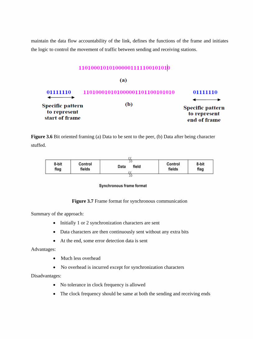
maintain the data flow accountability of the link, defines the functions of the frame and initiates
the logic to control the movement of traffic between sending and receiving stations.
Figure 3.6 Bit oriented framing (a) Data to be sent to the peer, (b) Data after being character
stuffed.
Figure 3.7 Frame format for synchronous communication
Summary of the approach:
• Initially 1 or 2 synchronization characters are sent
• Data characters are then continuously sent without any extra bits
• At the end, some error detection data is sent
Advantages:
• Much less overhead
• No overhead is incurred except for synchronization characters
Disadvantages:
• No tolerance in clock frequency is allowed
• The clock frequency should be same at both the sending and receiving ends

Bit stuffing: If the flag pattern appears anywhere in the header or data of a frame, then the
receiver may prematurely detect the start or end of the received frame. To overcome this problem,
the sender makes sure that the frame body it sends has no flags in it at any position (note that since
there is no character synchronization, the flag pattern can start at any bit location within the
stream). It does this by bit stuffing, inserting an extra bit in any pattern that is beginning to look
like a flag. In HDLC, whenever 5 consecutive 1's are encountered in the data, a 0 is inserted after
the 5th 1, regardless of the next bit in the data as shown in Fig. 3.8. On the receiving end, the bit
stream is piped through a shift register as the receiver looks for the flag pattern. If 5 consecutive
1's followed by a 0 is seen, then the 0 is dropped before sending the data on (the receiver destuffs
the stream). If 6 1's and a 0 are seen, it is a flag and either the current frame are ended or a new
frame is started, depending on the current state of the receiver. If more than 6 consecutive 1's are
seen, then the receiver has detected an invalid pattern, and usually the current frame, if any, is
discarded.
Figure 3.8 Bit oriented (a) Data to be sent to the peer, (b) Data after being bit stuffed.
With bit stuffing, the boundary between two frames can be unambiguously recognized by the flag
pattern. Thus, if receiver loses track of where it is, all it has to do is to scan the input for flag
sequence, since they can only occur at frame boundaries and never within data. In addition to
receiving the data in logical units called frames, the receiver should have some way of determining
if the data has been corrupted or not. If it has been corrupted, it is desirable not only to realize that,
but also to make an attempt to obtain the correct data. This process is called error detection and
error correction, which will be discussed in the next lesson.
1.4.4 Asynchronous communication (word-oriented)
In asynchronous communication, small, fixed-length words (usually 5 to 9 bits long) are
transferred without any clock line or clock is recovered from the signal itself. Each word has a start
bit (usually as a 0) before the first data bit of the word and a stop bit (usually as a 1) after the last

data bit of the word, as shown in Fig. 3.9. The receiver's local clock is started when the receiver
detects the 1-0 transition of the start bit, and the line is sampled in the middle of the fixed bit
intervals (a bit interval is the inverse of the data rate). The sender outputs the bit at the agreed-
upon rate, holding the line in the appropriate state for one bit interval for each bit, but using its
own local clock to determine the length of these bit intervals. The receiver's clock and the sender's
clock may not run at the same speed, so that there is a relative clock drift (this may be caused by
variations in the crystals used, temperature, voltage, etc.). If the receiver's clock drifts too much
relative to the sender's clock, then the bits may be sampled while the line is in transition from one
state to another, causing the receiver to misinterpret the received data. There can be variable
amount of gap between two frames as shown in Fig. 3.10.
Figure 3.9 Character or word oriented format for asynchronous mode
Figure 3.10 Data units sent with variable gap sent in asynchronous mode
Advantages of asynchronous character oriented mode of communication are summarized below:
• Simple to implement
• Self synchronization; Clock signal need not be sent
• Tolerance in clock frequency is possible
• The bits are sensed in the middle hence ± ½ bit tolerance is provided
This mode of data communication, however, suffers from high overhead incurred in data
transmission. Data must be sent in multiples of the data length of the word, and the two or more
bits of synchronization overhead compared to the relatively short data length causes the effective
data rate to be rather low. For example, 11 bits are required to transmit 8 bits of data. In other
words, baud rate (number of signal elements) is higher than data rate.
1.5 Character Oriented Framing
The first framing method uses a field in the header to specify the number of characters in the
frame. When the data link-layer sees the character count, it knows how many characters follow,
and hence where the end of the frame is. This technique is shown in Fig. 3.11 for frames of size 6,
4, and 8 characters, respectively. The trouble with this algorithm is that the count can be garbled
by a transmission error. For example, if the character count of 4 in the second frame becomes 5, as
shown in Fig. 3.11(b), the destination will get out of synchronization and will be unable to locate
the start of next frame. Even if the checksum is incorrect so the destination knows that the frame is
bad, it still had no way of telling where the next frame starts. Sending a frame back to the source
and asking for retransmission does not help either, since the destination doesn’t know how many
characters to skip over to the start of retransmission. For this reason the character count method is
rarely used.
Character-oriented framing assumes that character synchronization has already been achieved by
the hardware. The sender uses special characters to indicate the start and end of frames, and may
also use them to indicate header boundaries and to assist the
receiver gain character synchronization. Frames must be of an integral character length. Data
transparency must be preserved by use of character as shown in Fig. 3.12.
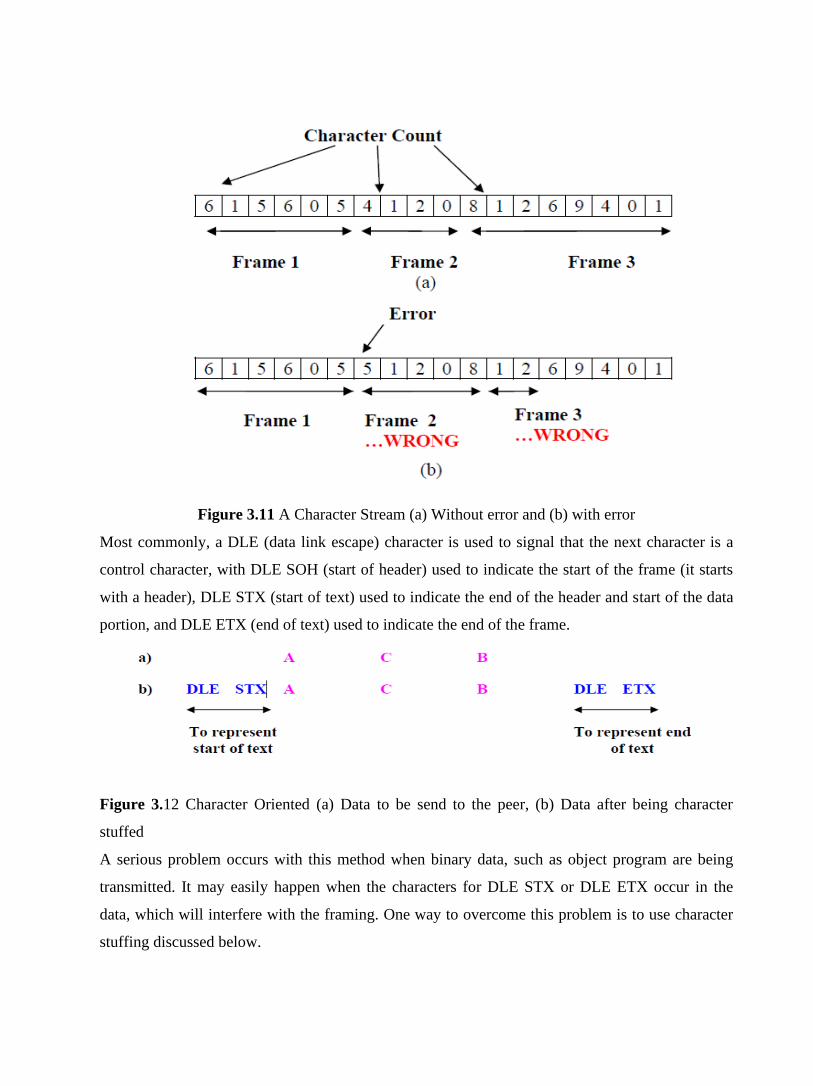
Figure 3.11 A Character Stream (a) Without error and (b) with error
Most commonly, a DLE (data link escape) character is used to signal that the next character is a
control character, with DLE SOH (start of header) used to indicate the start of the frame (it starts
with a header), DLE STX (start of text) used to indicate the end of the header and start of the data
portion, and DLE ETX (end of text) used to indicate the end of the frame.
Figure 3.12 Character Oriented (a) Data to be send to the peer, (b) Data after being character
stuffed
A serious problem occurs with this method when binary data, such as object program are being
transmitted. It may easily happen when the characters for DLE STX or DLE ETX occur in the
data, which will interfere with the framing. One way to overcome this problem is to use character
stuffing discussed below.
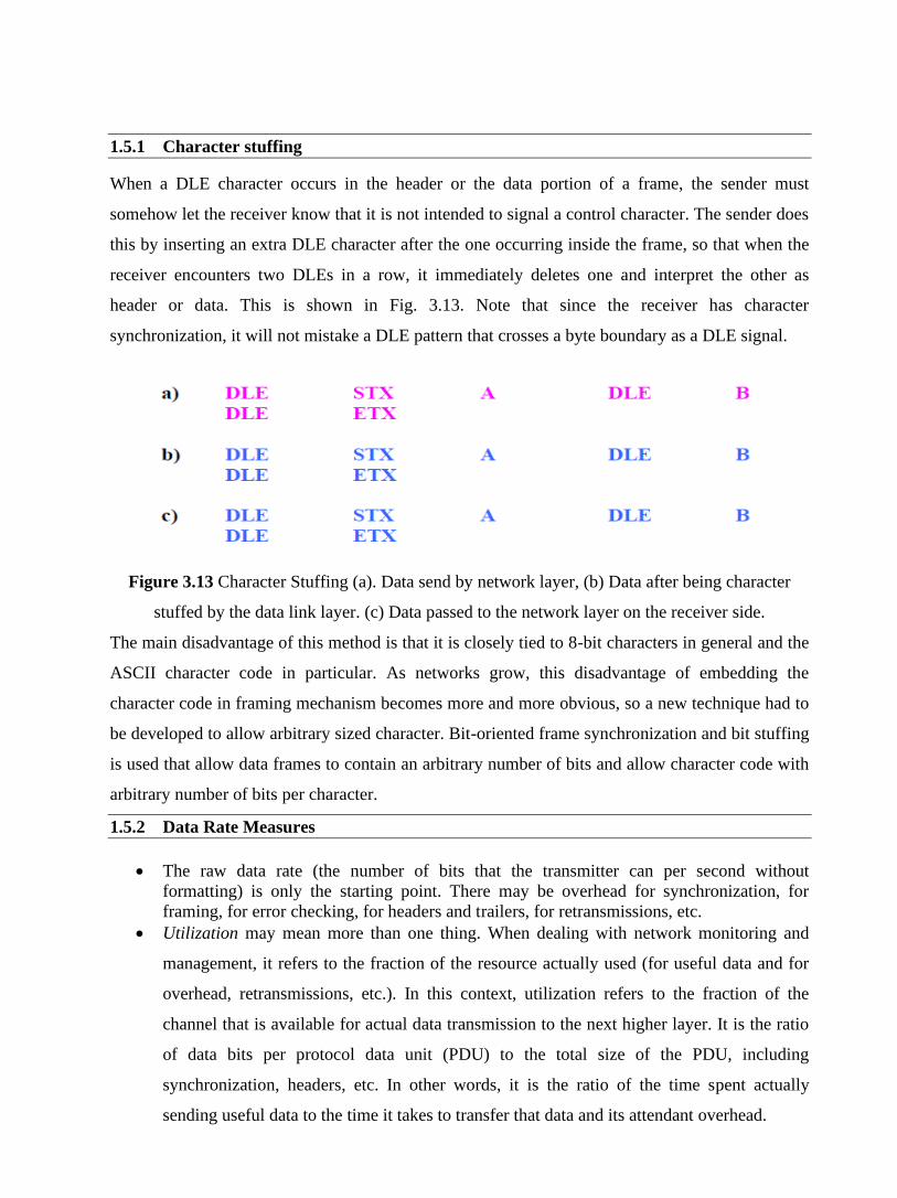
1.5.1 Character stuffing
When a DLE character occurs in the header or the data portion of a frame, the sender must
somehow let the receiver know that it is not intended to signal a control character. The sender does
this by inserting an extra DLE character after the one occurring inside the frame, so that when the
receiver encounters two DLEs in a row, it immediately deletes one and interpret the other as
header or data. This is shown in Fig. 3.13. Note that since the receiver has character
synchronization, it will not mistake a DLE pattern that crosses a byte boundary as a DLE signal.
Figure 3.13 Character Stuffing (a). Data send by network layer, (b) Data after being character
stuffed by the data link layer. (c) Data passed to the network layer on the receiver side.
The main disadvantage of this method is that it is closely tied to 8-bit characters in general and the
ASCII character code in particular. As networks grow, this disadvantage of embedding the
character code in framing mechanism becomes more and more obvious, so a new technique had to
be developed to allow arbitrary sized character. Bit-oriented frame synchronization and bit stuffing
is used that allow data frames to contain an arbitrary number of bits and allow character code with
arbitrary number of bits per character.
1.5.2 Data Rate Measures
• The raw data rate (the number of bits that the transmitter can per second without
formatting) is only the starting point. There may be overhead for synchronization, for
framing, for error checking, for headers and trailers, for retransmissions, etc.
• Utilization may mean more than one thing. When dealing with network monitoring and
management, it refers to the fraction of the resource actually used (for useful data and for
overhead, retransmissions, etc.). In this context, utilization refers to the fraction of the
channel that is available for actual data transmission to the next higher layer. It is the ratio
of data bits per protocol data unit (PDU) to the total size of the PDU, including
synchronization, headers, etc. In other words, it is the ratio of the time spent actually
sending useful data to the time it takes to transfer that data and its attendant overhead.

The effective data rate at a layer is the net data rate available to the next higher layer. Generally
this is the utilization times the raw data rate.
1.6 DTE-DCE Interface
As two persons intending to communicate must speak in the same language, for successful
communication between two computer systems or between a computer and a peripheral, a natural
understanding between the two is essential. In case of two persons a common language known to
both of them is used. In case of two computers or a computer and an appliance, this understanding
can be ensured with the help of a standard, which should be followed by both the parties.
Standards are usually recommended by some International bodies, such as, Electronics Industries
Association (EIA), The Institution of Electrical and Electronic Engineers (IEEE), etc. The EIA and
ITU-T have been involved in developing standards for the DTE-DCE interface known as EIA-232,
EIA-442, etc and ITU-T standards are known as V series or X series. The standards should
normally define the following four important attributes:
Mechanical: The mechanical attribute concerns the actual physical connection between the two
sides. Usually various signal lines are bundled into a cable with a terminator plug, male or female
at each end. Each of the systems, between which communication is to be established, provide a
plug of opposite gender for connecting the terminator plugs of the cable, thus establishing the
physical connection. The mechanical part specifies cables and connectors to be used to link two
systems.
Electrical: The Electrical attribute relates to the voltage levels and timing of voltage changes.
They in turn determine the data rates and distances that can be used for communication. So the
electrical part of the standard specifies voltages, Impedances and timing requirements to be
satisfied for reliable communication.
Functional: Functional attribute pertains to the function to be performed, by associating meaning
to the various signal lines. Functions can be typically classified into the broad categories of data
control, timing and ground. This component of standard specifies the signal pin assignments and
signal definition of each of the pins used for interfacing the devices.
Procedural: The procedural attribute specifies the protocol for communication, i.e. the sequence
of events that should be followed during data transfer, using the functional characteristic of the
interface.

A variety of standards exist, some of the most popular interfaces are presented in this section
Figure 3.14 The DTE-DCE interface
1.6.1 The RS-232 C
Most digital data processing devices such as computers and terminals are incapable of transmitting
the digital data, which usually is in NRZ-L form, through physical transmission media over long
distances. The data processing devices, commonly referred to as Data Terminal Equipment (DTE),
utilizes the mediation of another equipment called Data Circuit communication Equipment (DCE)
to interface with the physical transmission media. An example of a DCE is a MODEM. On the one
side, the DCE is responsible for transmitting and receiving bit-serial data in a suitable form for
efficient communication through some transmission media such as telephone line. On the other
side, the DCE interacts with the DTE by exchanging both data and control information. This is
done over a set of wires referred to as interchange circuits. For successful operation of this scheme
a high degree of cooperation is required on data processing equipment manufacturers and users,
nature of interface between the DTE and DCE. The Electronic Industries Association (EIA)
developed the standard RS-232C as an interface between the DTE and DCE as shown in Fig. 3.14.
Although developed in 1960, it is still widely used for serial binary data interchange. It specifies
all the four attributes mentioned above.
Mechanical: A 25-pin connector (DB-25) or 9-pin connector (DB-9) is commonly used for
establishing mechanical connection. In most of the applications, however, fewer number of control
lines than specified in the standard are used, as not all the systems require their use. The interface
established connection between two types of systems, Data terminal Equipment (DTE) and Data
communication Equipment (DCE). The equipment that generates, processes and displays the data
is called DTE. Computers and monitors are considered as DTEs. A MODEM, which converts
digital data into analog form by modulation and also demodulates analog signal to generate digital
data, are considered as data communication equipments (DCEs). Modems are used to establish

connection through (Transmission media) analog communication channel, such as a telephone line
as shown in Fig. 3.14.
Electrical: The electrical characteristics specify the signaling between DTE and DCE. It uses
single-ended, bipolar voltage and unterminated circuit. The single-ended form uses a single
conductor to send and another conductor to receive a signal with the voltage reference to a
common ground. The bipolar voltage levels are +3 to + 25V for logic 0 and
–3 to –25V for logic 1. No termination with a resistor either at input or at output is necessary. The
most striking feature is that, the voltage levels are not TTL compatible. This necessitates separate
voltage supplies and extra hardware for level conversion from TTL-to-RS 232C and vice versa.
The single-ended unterminated configuration is susceptible to all forms of electromagnetic
interference. Noise and cross-talk susceptibility are proportional to the cable length and bandwidth.
As a result, the RS-232 C is suitable for serial binary data interchange over a short distance (up to
57 ft) and at low rates (up to 20K baud).
Functional: The functional specification of most of the important lines is given in Table 3.1.1.
There are two data lines, one for each direction, facilitating full-duplex operation. There are
several control and ground lines. The pin number with respect to the connector, abbreviated name
and function description of the important lines are given in the table. These nine lines are
commonly used.
Procedural: The procedural specification gives the protocol, is the sequence of events to be
followed to accomplish data communication.
(i) When a DTE is powered on, after self-test it asserts the Data terminal ready (DTR)
signal (pin) to indicate that it is ready to take part in communication. Similarly, when

the DCE is powered on and gone through its own self-test, it asserts the Data set Ready
(DSR) signal (pin 6) to indicate that it is ready to take part in the communication. When
the MODEM detects a carrier on the telephone line, it asserts Data carrier detect (DCD)
signal (pin 8).
(ii) When the DTE is ready to send data, it asserts request to send (RTS) signal (pin 4).
DCE in turn responds with clear to send (CTS) signal (pin 5), when it is ready to
receive data and MODEM start sending carrier over the medium indicating that data
transmission is eminent. The CTS signal enables the DTE to start transmission of a data
frame.
The procedural specification deals with the legal sequence of events on the action-
reaction pair of signal lines. For example, the RTS-CTS control lines form an action-
reaction pair. Before sending a data, the DTR-DSR pair should be active and then the
DTE asserts the RTS signal. In response to this the modern should generate the CTS
signal when ready; thereby indicating that data may be transmitted over the TXD. In
this manner the action-reaction pairs of lines allows handshaking needed for
asynchronous mode of date communication. It also leads to flow-control, the rate at
which the two systems can communicate with each other.
1.6.2 Null Modem
In many situations, the distance between two DTEs may be so close that use of modems (DCE), as
shown in Fig. 3.15 (a), is unnecessary. In such a case the RS-232 C interface may still be used, but
with out the DCEs. A scheme known as null modem is used, in which interconnection is done in
such a why that both the DTEs are made to feel as if they have been connected through modems.
Essentially, null modem is a cable with two connectors at both ends for interfacing with the DTEs.
The reason for this behavior is apparent from the swapping interconnection shown in Fig. 3.15 (b).
(a)
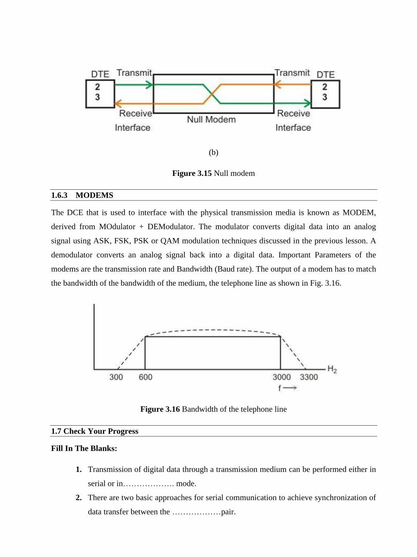
(b)
Figure 3.15 Null modem
1.6.3 MODEMS
The DCE that is used to interface with the physical transmission media is known as MODEM,
derived from MOdulator + DEModulator. The modulator converts digital data into an analog
signal using ASK, FSK, PSK or QAM modulation techniques discussed in the previous lesson. A
demodulator converts an analog signal back into a digital data. Important Parameters of the
modems are the transmission rate and Bandwidth (Baud rate). The output of a modem has to match
the bandwidth of the bandwidth of the medium, the telephone line as shown in Fig. 3.16.
Figure 3.16 Bandwidth of the telephone line
1.7 Check Your Progress
Fill In The Blanks:
1. Transmission of digital data through a transmission medium can be performed either in
serial or in………………. mode.
2. There are two basic approaches for serial communication to achieve synchronization of
data transfer between the ………………pair.
3. In …………….mode, the communication is unidirectional, such as from a computer to
a printer
4. In ……………………….mode both the sides can communicate simultaneously
5. In ………………….communication, small, fixed-length words (usually 5 to 9 bits
long) are transferred without any clock line or clock is recovered from the signal itself.
6. Most digital data processing devices such as ………………….are incapable of
transmitting the digital data
7. The DCE that is used to interface with the physical transmission media is known as
……………….
1.8 Answer to Check Your Progress
1. parallel
2. source-destination
3. simplex
4. full-duplex
5. asynchronous
6. computers and terminals
7. MODEM

Unit-2
Error Detection and Correction
1.1 Learning Objectives
1.2 Introduction
1.3 Types of errors
1.4 Error Detecting Codes
1.4.1 Simple Parity Checking or One-dimension Parity Check
1.4.2 Two-dimension Parity Check
1.4.3 Checksum
1.4.4 Cyclic Redundancy Checks (CRC)
1.5 Error Correcting Codes
1.5.1 Single-bit error correction
1.6 Check Your Progress
1.7 Answer to Check Your Progress

1.1 Learning Objectives
• After going through this unit the learner will able to:
• Explain the need for error detection and correction
• State how simple parity check can be used to detect error
• Explain how two-dimensional parity check extends error detection capability
• State how checksum is used to detect error
• Explain how cyclic redundancy check works
• Explain how Hamming code is used to correct error
1.2 Introduction
Environmental interference and physical defects in the communication medium can cause random
bit errors during data transmission. Error coding is a method of detecting and correcting these
errors to ensure information is transferred intact from its source to its destination. Error coding is
used for fault tolerant computing in computer memory, magnetic and optical data storage media,
satellite and deep space communications, network communications, cellular telephone networks,
and almost any other form of digital data communication. Error coding uses mathematical
formulas to encode data bits at the source into longer bit words for transmission. The "code word"
can then be decoded at the destination to retrieve the information. The extra bits in the code word
provide redundancy that, according to the coding scheme used, will allow the destination to use
the decoding process to determine if the communication medium introduced errors and in some
cases correct them so that the data need not be retransmitted. Different error coding schemes are
chosen depending on the types of errors expected, the communication medium's expected error
rate, and whether or not data retransmission is possible. Faster processors and better
communications technology make more complex coding schemes, with better error detecting and
correcting capabilities, possible for smaller embedded systems, allowing for more robust
communications. However, tradeoffs between bandwidth and coding overhead, coding complexity
and allowable coding delay between transmissions, must be considered for each application.
Even if we know what type of errors can occur, we can’t simple recognize them. We can do this
simply by comparing this copy received with another copy of intended transmission. In this
mechanism the source data block is send twice. The receiver compares them with the help of a
comparator and if those two blocks differ, a request for re-transmission is made. To achieve
forward error correction, three sets of the same data block are sent and majority decision selects
the correct block. These methods are very inefficient and increase the traffic two or three times.

Fortunately there are more efficient error detection and correction codes. There are two basic
strategies for dealing with errors. One way is to include enough redundant information (extra bits
are introduced into the data stream at the transmitter on a regular and logical basis) along with
each block of data sent to enable the receiver to deduce what the transmitted character must have
been. The other way is to include only enough redundancy to allow the receiver to deduce that
error has occurred, but not which error has occurred and the receiver asks for a retransmission. The
former strategy uses Error-Correcting Codes and latter uses Error-detecting Codes.
To understand how errors can be handled, it is necessary to look closely at what error really is.
Normally, a frame consists of m-data bits (i.e., message bits) and r-redundant bits (or check bits).
Let the total number of bits be n (m + r). An n-bit unit containing data and check-bits is often
referred to as an n-bit codeword.
Given any two code-words, say 10010101 and 11010100, it is possible to determine how many
corresponding bits differ, just EXCLUSIVE OR the two code-words, and count the number of 1’s
in the result. The number of bits position in which code words differ is called the Hamming
distance. If two code words are a Hamming distance d-apart, it will require d single-bit errors to
convert one code word to other. The error detecting and correcting properties depends on its
Hamming distance.
• To detect d errors, you need a distance (d+1) code because with such a code there is no
way that d-single bit errors can change a valid code word into another valid code word.
Whenever receiver sees an invalid code word, it can tell that a transmission error has
occurred.
• Similarly, to correct d errors, you need a distance 2d+1 code because that way the legal
code words are so far apart that even with d changes, the original codeword is still closer
than any other code-word, so it can be uniquely determined.
1.3 Types of errors
These interferences can change the timing and shape of the signal. If the signal is carrying binary
encoded data, such changes can alter the meaning of the data. These errors can be divided into two
types: Single-bit error and Burst error.
Single-bit Error
The term single-bit error means that only one bit of given data unit (such as a byte, character, or
data unit) is changed from 1 to 0 or from 0 to 1 as shown in Fig. 2.1.

Figure 2.1 Single bit error
Single bit errors are least likely type of errors in serial data transmission. To see why, imagine a
sender sends data at 10 Mbps. This means that each bit lasts only for 0.1 μs (micro-second). For a
single bit error to occur noise must have duration of only 0.1 μs (micro-second), which is very
rare. However, a single-bit error can happen if we are having a parallel data transmission. For
example, if 16 wires are used to send all 16 bits of a word at the same time and one of the wires is
noisy, one bit is corrupted in each word.
Burst Error
The term burst error means that two or more bits in the data unit have changed from 0 to 1 or vice-
versa. Note that burst error doesn’t necessary means that error occurs in consecutive bits. The
length of the burst error is measured from the first corrupted bit to the last corrupted bit. Some bits
in between may not be corrupted.
Figure 2.2 Burst Error
Burst errors are mostly likely to happen in serial transmission. The duration of the noise is
normally longer than the duration of a single bit, which means that the noise affects data; it affects
a set of bits as shown in Fig. 2.2. The number of bits affected depends on the data rate and duration
of noise.
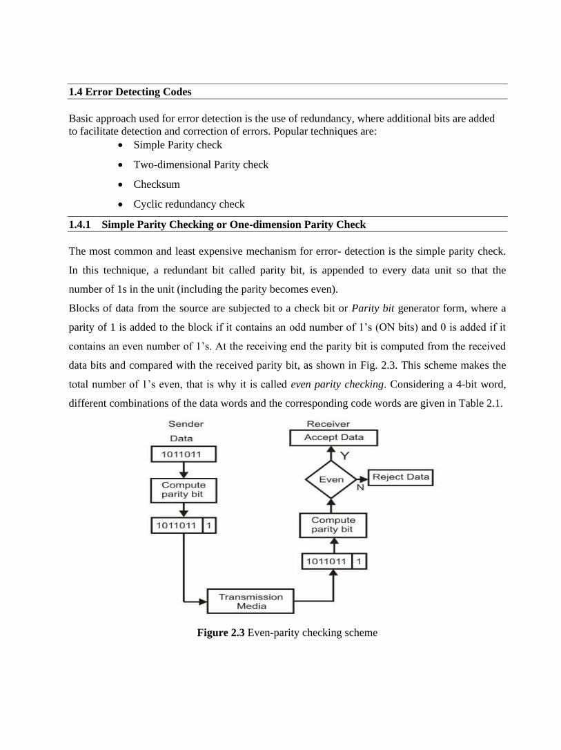
1.4 Error Detecting Codes
Basic approach used for error detection is the use of redundancy, where additional bits are added
to facilitate detection and correction of errors. Popular techniques are:
• Simple Parity check
• Two-dimensional Parity check
• Checksum
• Cyclic redundancy check
1.4.1 Simple Parity Checking or One-dimension Parity Check
The most common and least expensive mechanism for error- detection is the simple parity check.
In this technique, a redundant bit called parity bit, is appended to every data unit so that the
number of 1s in the unit (including the parity becomes even).
Blocks of data from the source are subjected to a check bit or Parity bit generator form, where a
parity of 1 is added to the block if it contains an odd number of 1’s (ON bits) and 0 is added if it
contains an even number of 1’s. At the receiving end the parity bit is computed from the received
data bits and compared with the received parity bit, as shown in Fig. 2.3. This scheme makes the
total number of 1’s even, that is why it is called even parity checking. Considering a 4-bit word,
different combinations of the data words and the corresponding code words are given in Table 2.1.
Figure 2.3 Even-parity checking scheme

Table 2.1 Possible 4-bit data words and corresponding code words
Note that for the sake of simplicity, we are discussing here the even-parity checking, where the
number of 1’s should be an even number. It is also possible to use odd-parity checking, where the
number of 1’s should be odd.
Performance
An observation of the table reveals that to move from one code word to another, at least two data
bits should be changed. Hence these set of code words are said to have a minimum distance
(hamming distance) of 2, which means that a receiver that has knowledge of the code word set can
detect all single bit errors in each code word. However, if two errors occur in the code word, it
becomes another valid member of the set and the decoder will see only another valid code word
and know nothing of the error. Thus errors in more than one bit cannot be detected. In fact it can
be shown that a single parity check code can detect only odd number of errors in a code word.
1.4.2 Two-dimension Parity Check
Performance can be improved by using two-dimensional parity check, which organizes the block
of bits in the form of a table. Parity check bits are calculated for each row, which is equivalent to a
simple parity check bit. Parity check bits are also calculated for all columns then both are sent
along with the data. At the receiving end these are compared with the parity bits calculated on the
received data. This is illustrated in Fig. 2.4.

Figure 2.4 Two-dimension Parity Checking
Performance
Two- Dimension Parity Checking increases the likelihood of detecting burst errors. As we have
shown in Fig. 2.4 that a 2-D Parity check of n bits can detect a burst error of n bits. A burst error of
more than n bits is also detected by 2-D Parity check with a high-probability. There is, however,
one pattern of error that remains elusive. If two bits in one data unit are damaged and two bits in
exactly same position in another data unit are also damaged, the 2-D Parity check checker will not
detect an error. For example, if two data units: 11001100 and 10101100. If first and second from
last bits in each of them is changed, making the data units as 01001110 and 00101110, the error
cannot be detected by 2-D Parity check.
1.4.3 Checksum
In checksum error detection scheme, the data is divided into k segments each of m bits. In the
sender’s end the segments are added using 1’s complement arithmetic to get the sum. The sum is
complemented to get the checksum. The checksum segment is sent along with the data segments as
shown in Fig. 2.5 (a). At the receiver’s end, all received segments are added using 1’s complement
arithmetic to get the sum. The sum is complemented. If the result is zero, the received data is
accepted; otherwise discarded, as shown in Fig. 2.5 (b).
Performance
The checksum detects all errors involving an odd number of bits. It also detects most errors
involving even number of bits.

(a) (b)
Figure 2.5 (a) Sender’s end for the calculation of the checksum, (b) Receiving end for checking
the checksum
1.4.4 Cyclic Redundancy Checks (CRC)
This Cyclic Redundancy Check is the most powerful and easy to implement technique. Unlike
checksum scheme, which is based on addition, CRC is based on binary division. In CRC, a
sequence of redundant bits, called cyclic redundancy check bits, are appended to the end of data
unit so that the resulting data unit becomes exactly divisible by a second, predetermined binary
number. At the destination, the incoming data unit is divided by the same number. If at this step
there is no remainder, the data unit is assumed to be correct and is therefore accepted. A remainder
indicates that the data unit has been damaged in transit and therefore must be rejected. The
generalized technique can be explained as follows.
If a k bit message is to be transmitted, the transmitter generates an r-bit sequence, known as Frame
Check Sequence (FCS) so that the (k+r) bits are actually being transmitted. Now this r-bit FCS is
generated by dividing the original number, appended by r zeros, by a predetermined number. This
number, which is (r+1) bit in length, can also be considered as the coefficients of a polynomial,
called Generator Polynomial. The remainder of this division process generates the r-bit FCS. On
receiving the packet, the receiver divides the (k+r) bit frame by the same predetermined number
and if it produces no remainder, it can be assumed that no error has occurred during the
transmission. Operations at both the sender and receiver end are shown in Fig. 2.6.
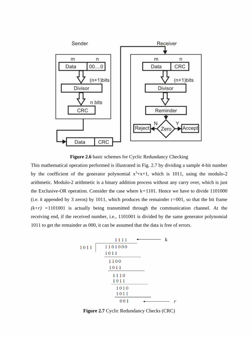
Figure 2.6 basic schemes for Cyclic Redundancy Checking
This mathematical operation performed is illustrated in Fig. 2.7 by dividing a sample 4-bit number
by the coefficient of the generator polynomial x3+x+1, which is 1011, using the modulo-2
arithmetic. Modulo-2 arithmetic is a binary addition process without any carry over, which is just
the Exclusive-OR operation. Consider the case where k=1101. Hence we have to divide 1101000
(i.e. k appended by 3 zeros) by 1011, which produces the remainder r=001, so that the bit frame
(k+r) =1101001 is actually being transmitted through the communication channel. At the
receiving end, if the received number, i.e., 1101001 is divided by the same generator polynomial
1011 to get the remainder as 000, it can be assumed that the data is free of errors.
Figure 2.7 Cyclic Redundancy Checks (CRC)

The transmitter can generate the CRC by using a feedback shift register circuit. The same circuit
can also be used at the receiving end to check whether any error has occurred. All the values can
be expressed as polynomials of a dummy variable X. For example, for P = 11001 the
corresponding polynomial is X4+X3+1. A polynomial is selected to have at least the following
properties:
o It should not be divisible by X.
oIt should not be divisible by (X+1).
The first condition guarantees that all burst errors of a length equal to the degree of polynomial are
detected. The second condition guarantees that all burst errors affecting an odd number of bits are
detected.
CRC process can be expressed as XnM(X)/P(X) = Q(X) + R(X) / P(X)
Commonly used divisor polynomials are:
Performance
CRC is a very effective error detection technique. If the divisor is chosen according to the
previously mentioned rules, its performance can be summarized as follows:
• CRC can detect all single-bit errors
• CRC can detect all double-bit errors (three 1’s)
• CRC can detect any odd number of errors (X+1)
• CRC can detect all burst errors of less than the degree of the polynomial.
• CRC detects most of the larger burst errors with a high probability.
• For example CRC-12 detects 99.97% of errors with a length 12 or more.
1.5 Error Correcting Codes
The techniques that we have discussed so far can detect errors, but do not correct them. Error
Correction can be handled in two ways.
o One is when an error is discovered; the receiver can have the sender retransmit the entire
data unit. This is known as backward error correction.
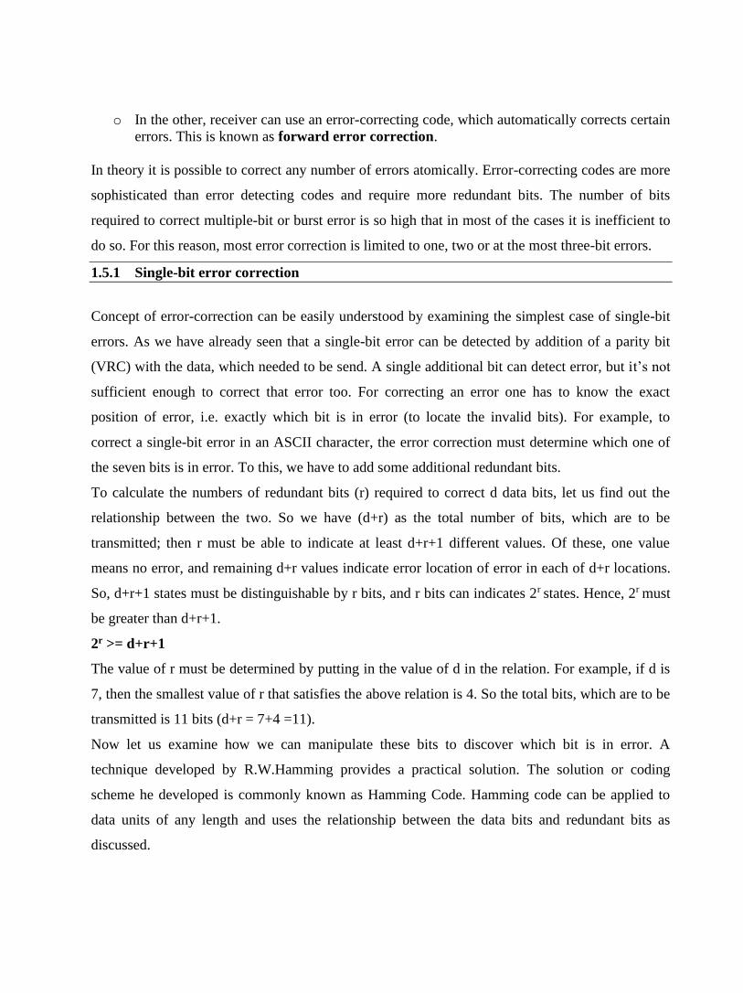
o In the other, receiver can use an error-correcting code, which automatically corrects certain
errors. This is known as forward error correction.
In theory it is possible to correct any number of errors atomically. Error-correcting codes are more
sophisticated than error detecting codes and require more redundant bits. The number of bits
required to correct multiple-bit or burst error is so high that in most of the cases it is inefficient to
do so. For this reason, most error correction is limited to one, two or at the most three-bit errors.
1.5.1 Single-bit error correction
Concept of error-correction can be easily understood by examining the simplest case of single-bit
errors. As we have already seen that a single-bit error can be detected by addition of a parity bit
(VRC) with the data, which needed to be send. A single additional bit can detect error, but it’s not
sufficient enough to correct that error too. For correcting an error one has to know the exact
position of error, i.e. exactly which bit is in error (to locate the invalid bits). For example, to
correct a single-bit error in an ASCII character, the error correction must determine which one of
the seven bits is in error. To this, we have to add some additional redundant bits.
To calculate the numbers of redundant bits (r) required to correct d data bits, let us find out the
relationship between the two. So we have (d+r) as the total number of bits, which are to be
transmitted; then r must be able to indicate at least d+r+1 different values. Of these, one value
means no error, and remaining d+r values indicate error location of error in each of d+r locations.
So, d+r+1 states must be distinguishable by r bits, and r bits can indicates 2r states. Hence, 2r must
be greater than d+r+1.
2r >= d+r+1
The value of r must be determined by putting in the value of d in the relation. For example, if d is
7, then the smallest value of r that satisfies the above relation is 4. So the total bits, which are to be
transmitted is 11 bits (d+r = 7+4 =11).
Now let us examine how we can manipulate these bits to discover which bit is in error. A
technique developed by R.W.Hamming provides a practical solution. The solution or coding
scheme he developed is commonly known as Hamming Code. Hamming code can be applied to
data units of any length and uses the relationship between the data bits and redundant bits as
discussed.
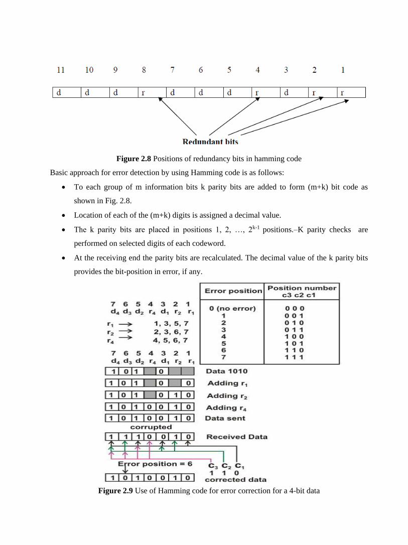
Figure 2.8 Positions of redundancy bits in hamming code
Basic approach for error detection by using Hamming code is as follows:
• To each group of m information bits k parity bits are added to form (m+k) bit code as
shown in Fig. 2.8.
• Location of each of the (m+k) digits is assigned a decimal value.
• The k parity bits are placed in positions 1, 2, …, 2k-1 positions.–K parity checks are
performed on selected digits of each codeword.
• At the receiving end the parity bits are recalculated. The decimal value of the k parity bits
provides the bit-position in error, if any.
Figure 2.9 Use of Hamming code for error correction for a 4-bit data

Figure 2.9 shows how hamming code is used for correction for 4-bit numbers (d4d3d2d1) with the
help of three redundant bits (r3r2r1). For the example data 1010, first r1 (0) is calculated considering
the parity of the bit positions, 1, 3, 5 and 7. Then the parity bits r2 is calculated considering bit
positions 2, 3, 6 and 7. Finally, the parity bits r4 is calculated considering bit positions 4, 5, 6 and 7
as shown. If any corruption occurs in any of the transmitted code 1010010, the bit position in error
can be found out by calculating r3r2r1 at the receiving end. For example, if the received code word
is 1110010, the recalculated value of r3r2r1 is 110, which indicates that bit position in error is 6, the
decimal value of 110.
Example:
Let us consider an example for 5-bit data. Here 4 parity bits are required. Assume that during
transmission bit 5 has been changed from 1 to 0 as shown in Fig. 2.11. The receiver receives the
code word and recalculates the four new parity bits using the same set of bits used by the sender
plus the relevant parity (r) bit for each set (as shown in Fig. 2.11). Then it assembles the new parity
values into a binary number in order of r positions (r8, r4, r2, r1).
Calculations:
Parity recalculated (r8, r4, r2, r1) = 01012 = 510.
Hence, bit 5th is in error i.e. d5 is in error.
So, correct code-word which was transmitted is:
Figure 2.11 Use of Hamming code for error correction for a 5-bit data
1.6 Check Your Progress
Fill In The Blanks:
1. ……………is a method of detecting and correcting these errors to ensure information is
transferred intact from its source to its destination.
2. The number of bits position in which code words differ is called the………………
3. The term …………………means that two or more bits in the data unit have changed from
0 to 1 or vice-versa
4. The …………….detects all errors involving an odd number of bits.
5. In CRC, a sequence of redundant bits, called………………………..
1.7 Answer to Check Your Progress
1. Error coding
2. Hamming distance.
3. burst error
4. checksum
5. cyclic redundancy check bits.

Unit-3
Flow Control and Error Control and HDLC
1.1 Learning Objectives
1.2 Introduction
1.3 Flow Control
1.3.1 Stop-and-Wait
1.3.2 Sliding Window
1.4 Error Control Techniques
1.4.1 Stop-and-Wait ARQ
1.4.2 Go-back-N ARQ
1.4.3 Selective-Repeat ARQ
1.5 Introduction to HDLC
1.6 HDLC Stations and Configurations
1.7 HDLC Operational Modes
1.8 HDLC Non-Operational Modes
1.9 HDLC Frame Structure
1.10 HDLC Commands and Responses
1.11 HDLC Subsets
1.12 Check Your Progress
1.13 Answer to Check Your Progress
1.1 Learning Objectives
After going through this unit the learner will able to:
• State the need for flow and error control
• Explain how Stop-and-wait flow control works
• Explain how Sliding-window protocol is used for flow control
• Explain how Stop-and-wait ARQ works
• Explain how Go-back-N ARQ works
• Explain how Selective-repeat ARQ works
• Explain how High-Level Data Link Control (HDLC) works
• Explain how piggybacking is done in HDLC
• Explain how data transparency is maintained in HDLC
1.2 Introduction
As we have mentioned earlier, for reliable and efficient data communication a great deal of
coordination is necessary between at least two machines. Some of these are necessary because of
the following constraints:
• Both sender and receiver have limited speed
• Both sender and receiver have limited memory
It is necessary to satisfy the following requirements:
• A fast sender should not overwhelm a slow receiver, which must perform a certain amount
of processing before passing the data on to the higher-level software.
• If error occur during transmission, it is necessary to devise mechanism to correct it
The most important functions of Data Link layer to satisfy the above requirements are error control
and flow control. Collectively, these functions are known as data link control, as discussed in this
unit.
Flow Control is a technique so that transmitter and receiver with different speed characteristics
can communicate with each other. Flow control ensures that a transmitting station, such as a server
with higher processing capability, does not overwhelm a receiving station, such as a desktop
system, with lesser processing capability. This is where there is an orderly flow of transmitted data
between the source and the destination.
Error Control involves both error detection and error correction. It is necessary because errors are
inevitable in data communication, in spite of the use of better equipment and reliable transmission

media based on the current technology. In the preceding lesson we have already discussed how
errors can be detected. In this lesson we shall discuss how error control is performed based on
retransmission of the corrupted data. When an error is detected, the receiver can have the specified
frame retransmitted by the sender. This process is commonly known as Automatic Repeat
Request (ARQ). For example, Internet's Unreliable Delivery Model allows packets to be
discarded if network resources are not available, and demands that ARQ protocols make
provisions for retransmission.
1.3 Flow Control
Modern data networks are designed to support a diverse range of hosts and communication
mediums. Consider a 933 MHz Pentium-based host transmitting data to a 90 MHz 80486/SX.
Obviously, the Pentium will be able to drown the slower processor with data. Likewise, consider
two hosts, each using an Ethernet LAN, but with the two Ethernets connected by a 56 Kbps
modem link. If one host begins transmitting to the other at Ethernet speeds, the modem link will
quickly become overwhelmed. In both cases, flow control is needed to pace the data transfer at an
acceptable speed.
Flow Control is a set of procedures that tells the sender how much data it can transmit before it
must wait for an acknowledgment from the receiver. The flow of data should not be allowed to
overwhelm the receiver. Receiver should also be able to inform the transmitter before its limits
(this limit may be amount of memory used to store the incoming data or the processing power at
the receiver end) are reached and the sender must send fewer frames. Hence, Flow control refers
to the set of procedures used to restrict the amount of data the transmitter can send before waiting
for acknowledgment.
There are two methods developed for flow control namely Stop-and-wait and Sliding-window.
Stop-and-wait is also known as Request/reply sometimes. Request/reply (Stop-and-wait) flow
control requires each data packet to be acknowledged by the remote host before the next packet is
sent. This is discussed in detail in the following subsection. Sliding window algorithms, used by
TCP, permit multiple data packets to be in simultaneous transit, making more efficient use of
network bandwidth.
1.3.1 Stop-and-Wait
This is the simplest form of flow control where a sender transmits a data frame. After receiving the
frame, the receiver indicates its willingness to accept another frame by sending back an ACK
frame acknowledging the frame just received. The sender must wait until it receives the ACK

frame before sending the next data frame. This is sometimes referred to as ping -pong behavior,
request/reply is simple to understand and easy to implement, but not very efficient. In LAN
environment with fast links, this isn't much of a concern, but WAN links will spend most of their
time idle, especially if several hops are required.
Figure 2.1 illustrates the operation of the stop-and-wait protocol. The blue arrows show the
sequence of data frames being sent across the link from the sender (top to the receiver (bottom).
The protocol relies on two-way transmission (full duplex or half duplex) to allow the receiver at
the remote node to return frames acknowledging the successful transmission. The
acknowledgements are shown in green in the diagram, and flow back to the original sender. A
small processing delay may be introduced between reception of the last byte of a Data PDU and
generation of the corresponding ACK.
Major drawback of Stop-and-Wait Flow Control is that only one frame can be in transmission at a
time, this leads to inefficiency if propagation delay is much longer than the transmission delay.
Figure 2.1 Stop-and Wait protocol
Some protocols pretty much require stop-and-wait behavior. For example, Internet's Remote
Procedure Call (RPC) Protocol is used to implement subroutine calls from a program on one
machine to library routines on another machine. Since most programs are single threaded, the
sender has little choice but to wait for a reply before continuing the program and possibly sending
another request.
Link Utilization in Stop-and-Wait
Let us assume the following:
Transmission time: The time it takes for a station to transmit a frame (normalized to a value of 1).
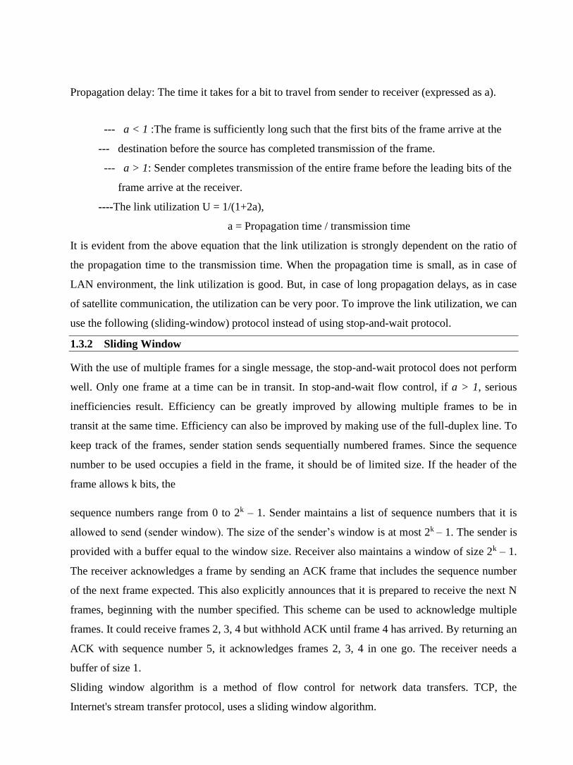
Propagation delay: The time it takes for a bit to travel from sender to receiver (expressed as a).
--- a < 1 :The frame is sufficiently long such that the first bits of the frame arrive at the
--- destination before the source has completed transmission of the frame.
--- a > 1: Sender completes transmission of the entire frame before the leading bits of the
frame arrive at the receiver.
----The link utilization U = 1/(1+2a),
a = Propagation time / transmission time
It is evident from the above equation that the link utilization is strongly dependent on the ratio of
the propagation time to the transmission time. When the propagation time is small, as in case of
LAN environment, the link utilization is good. But, in case of long propagation delays, as in case
of satellite communication, the utilization can be very poor. To improve the link utilization, we can
use the following (sliding-window) protocol instead of using stop-and-wait protocol.
1.3.2 Sliding Window
With the use of multiple frames for a single message, the stop-and-wait protocol does not perform
well. Only one frame at a time can be in transit. In stop-and-wait flow control, if a > 1, serious
inefficiencies result. Efficiency can be greatly improved by allowing multiple frames to be in
transit at the same time. Efficiency can also be improved by making use of the full-duplex line. To
keep track of the frames, sender station sends sequentially numbered frames. Since the sequence
number to be used occupies a field in the frame, it should be of limited size. If the header of the
frame allows k bits, the
sequence numbers range from 0 to 2k – 1. Sender maintains a list of sequence numbers that it is
allowed to send (sender window). The size of the sender’s window is at most 2k – 1. The sender is
provided with a buffer equal to the window size. Receiver also maintains a window of size 2k – 1.
The receiver acknowledges a frame by sending an ACK frame that includes the sequence number
of the next frame expected. This also explicitly announces that it is prepared to receive the next N
frames, beginning with the number specified. This scheme can be used to acknowledge multiple
frames. It could receive frames 2, 3, 4 but withhold ACK until frame 4 has arrived. By returning an
ACK with sequence number 5, it acknowledges frames 2, 3, 4 in one go. The receiver needs a
buffer of size 1.
Sliding window algorithm is a method of flow control for network data transfers. TCP, the
Internet's stream transfer protocol, uses a sliding window algorithm.

A sliding window algorithm places a buffer between the application program and the network data
flow. For TCP, the buffer is typically in the operating system kernel, but this is more of an
implementation detail than a hard-and-fast requirement.
Figure 2.2 Buffer in sliding window
Data received from the network is stored in the buffer, from where the application can read at its
own pace. As the application reads data, buffer space is freed up to accept more input from the
network. The window is the amount of data that can be "read ahead" - the size of the buffer, less
the amount of valid data stored in it. Window announcements are used to inform the remote host of
the current window size.
Sender sliding Window: At any instant, the sender is permitted to send frames with sequence
numbers in a certain range (the sending window) as shown in Fig. 2.3.
Figure 2.3 Sender’s window
Receiver sliding Window: The receiver always maintains a window of size 1 as shown in Fig.
2.4. It looks for a specific frame (frame 4 as shown in the figure) to arrive in a specific order. If it
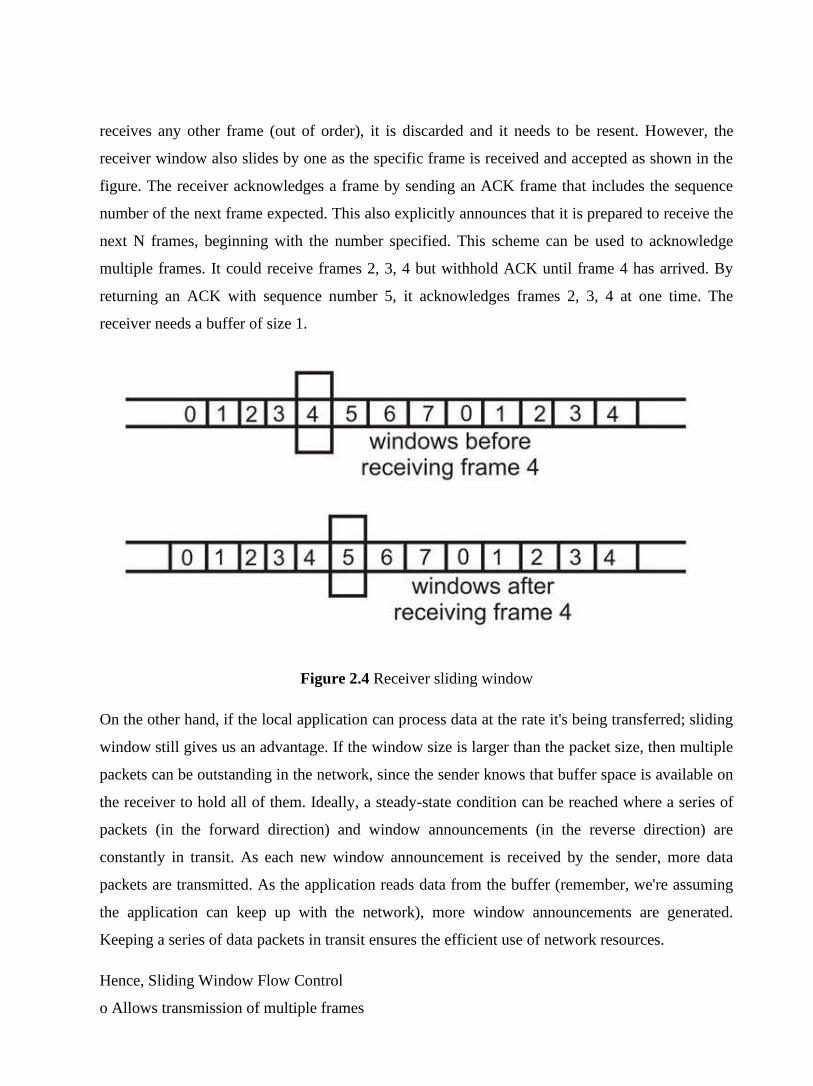
receives any other frame (out of order), it is discarded and it needs to be resent. However, the
receiver window also slides by one as the specific frame is received and accepted as shown in the
figure. The receiver acknowledges a frame by sending an ACK frame that includes the sequence
number of the next frame expected. This also explicitly announces that it is prepared to receive the
next N frames, beginning with the number specified. This scheme can be used to acknowledge
multiple frames. It could receive frames 2, 3, 4 but withhold ACK until frame 4 has arrived. By
returning an ACK with sequence number 5, it acknowledges frames 2, 3, 4 at one time. The
receiver needs a buffer of size 1.
Figure 2.4 Receiver sliding window
On the other hand, if the local application can process data at the rate it's being transferred; sliding
window still gives us an advantage. If the window size is larger than the packet size, then multiple
packets can be outstanding in the network, since the sender knows that buffer space is available on
the receiver to hold all of them. Ideally, a steady-state condition can be reached where a series of
packets (in the forward direction) and window announcements (in the reverse direction) are
constantly in transit. As each new window announcement is received by the sender, more data
packets are transmitted. As the application reads data from the buffer (remember, we're assuming
the application can keep up with the network), more window announcements are generated.
Keeping a series of data packets in transit ensures the efficient use of network resources.
Hence, Sliding Window Flow Control
o Allows transmission of multiple frames

o Assigns each frame a k-bit sequence number
o Range of sequence number is [0…2k-1], i.e., frames are counted modulo 2k.
The link utilization in case of Sliding Window Protocol
U = 1, for N > 2a + 1
N/(1+2a), for N < 2a + 1
Where N = the window size,
and a = Propagation time / transmission time
1.4 Error Control Techniques
When an error is detected in a message, the receiver sends a request to the transmitter to retransmit
the ill-fated message or packet. The most popular retransmission scheme is known as Automatic-
Repeat-Request (ARQ). Such schemes, where receiver asks transmitter to re-transmit if it detects
an error, are known as reverse error correction techniques. There exist three popular ARQ
techniques, as shown in Fig. 2.5.
Figure 2.5 Error control techniques
1.4.1 Stop-and-Wait ARQ
In Stop-and-Wait ARQ, which is simplest among all protocols, the sender (say station A) transmits
a frame and then waits till it receives positive acknowledgement (ACK) or negative
acknowledgement (NACK) from the receiver (say station B). Station B sends an ACK if the frame
is received correctly, otherwise it sends NACK. Station A sends a new frame after receiving ACK;
otherwise it retransmits the old frame, if it receives a NACK. This is illustrated in Fig 2.6.
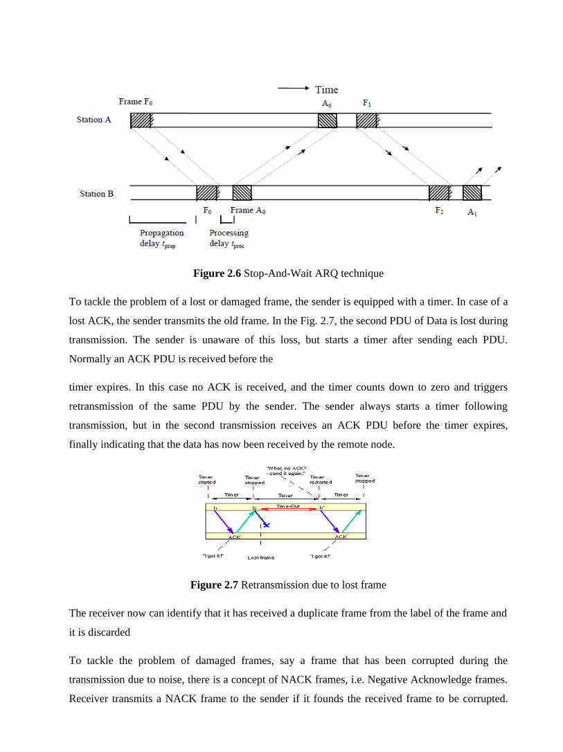
Figure 2.6 Stop-And-Wait ARQ technique
To tackle the problem of a lost or damaged frame, the sender is equipped with a timer. In case of a
lost ACK, the sender transmits the old frame. In the Fig. 2.7, the second PDU of Data is lost during
transmission. The sender is unaware of this loss, but starts a timer after sending each PDU.
Normally an ACK PDU is received before the
timer expires. In this case no ACK is received, and the timer counts down to zero and triggers
retransmission of the same PDU by the sender. The sender always starts a timer following
transmission, but in the second transmission receives an ACK PDU before the timer expires,
finally indicating that the data has now been received by the remote node.
Figure 2.7 Retransmission due to lost frame
The receiver now can identify that it has received a duplicate frame from the label of the frame and
it is discarded
To tackle the problem of damaged frames, say a frame that has been corrupted during the
transmission due to noise, there is a concept of NACK frames, i.e. Negative Acknowledge frames.
Receiver transmits a NACK frame to the sender if it founds the received frame to be corrupted.

When a NACK is received by a transmitter before the time-out, the old frame is sent again as
shown in Fig. 2.8.
Figure 2.8 Retransmission due to damaged frame
The main advantage of stop-and-wait ARQ is its simplicity. It also requires minimum buffer size.
However, it makes highly inefficient use of communication links, particularly when ‘a’ is large.
1.4.2 Go-back-N ARQ
The most popular ARQ protocol is the go-back-N ARQ, where the sender sends the frames
continuously without waiting for acknowledgement. That is why it is also called as continuous
ARQ. As the receiver receives the frames, it keeps on sending ACKs or a NACK, in case a frame is
incorrectly received. When the sender receives a NACK, it retransmits the frame in error plus all
the succeeding frames as shown in Fig.2.9. Hence, the name of the protocol is go-back-N ARQ. If
a frame is lost, the receiver sends NAK after receiving the next frame as shown in Fig. .2.10. In
case there is long delay before sending the NAK, the sender will resend the lost frame after its
timer times out. If the ACK frame sent by the receiver is lost, the sender resends the frames after
its timer times out as shown in Fig. 2.11.
Assuming full-duplex transmission, the receiving end sends piggybacked acknowledgement by
using some number in the ACK field of its data frame. Let us assume that a 3-bit sequence number
is used and suppose that a station sends frame 0 and gets back an RR1, and then sends frames 1, 2,
3, 4, 5, 6, 7, 0 and gets another RR1.This might either mean that RR1 is a cumulative ACK or all 8

frames were damaged. This ambiguity can be overcome if the maximum window size is limited to
7, i.e. for a k-bit sequence number field it is limited to 2k-1. The number N (=2k-1) specifies how
many frames can be sent without receiving acknowledgement.
Figure 2.9 Frames in error in go-Back-N ARQ
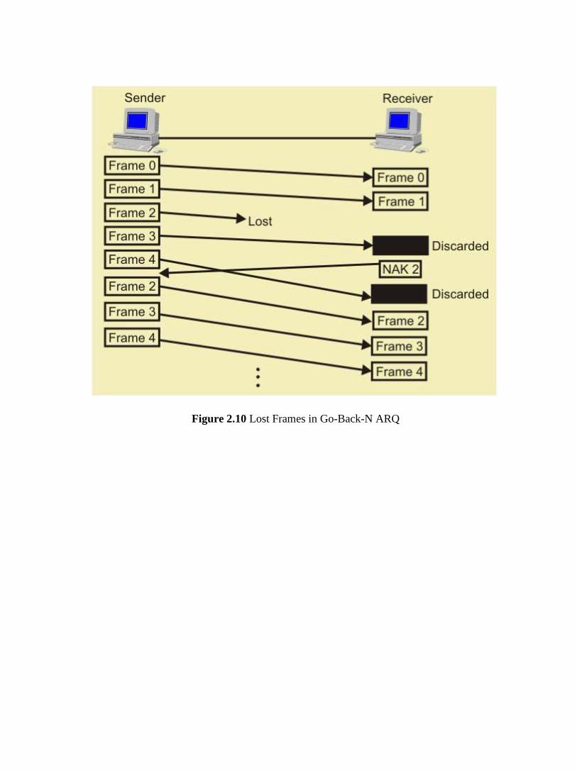
Figure 2.10 Lost Frames in Go-Back-N ARQ

Figure 2.11 Lost ACK in Go-Back-N ARQ
If no acknowledgement is received after sending N frames, the sender takes the help of a timer.
After the time-out, it resumes retransmission. The go-back-N protocol also takes care of damaged
frames and damaged ACKs. This scheme is little more complex than the previous one but gives
much higher throughput.
Assuming full-duplex transmission, the receiving end sends piggybacked acknowledgement by
using some number in the ACK field of its data frame. Let us assume that a 3-bit sequence number
is used and suppose that a station sends frame 0 and gets back an RR1, and then sends frames 1, 2,
3, 4, 5, 6, 7, 0 and gets another RR1.This might either mean that RR1 is a cumulative ACK or all 8
frames were damaged. This ambiguity can be overcome if the maximum window size is limited to
7, i.e. for a k-bit sequence number field it is limited to 2k-1. The number N (=2k-1) specifies how
many frames can be sent without receiving acknowledgement. If no acknowledgement is received
after sending N frames, the sender takes the help of a timer. After the time-out, it resumes
retransmission. The go-back-N protocol also takes care of damaged frames and damaged ACKs.
This scheme is little more complex than the previous one but gives much higher throughput.

1.4.3 Selective-Repeat ARQ
The selective-repetitive ARQ scheme retransmits only those for which NAKs are received or for
which timer has expired, this is shown in the Fig.2.12. This is the most efficient among the ARQ
schemes, but the sender must be more complex so that it can send out-of-order frames. The
receiver also must have storage space to store the post-NAK frames and processing power to
reinsert frames in proper sequence.
Figure 2.12 Selective-repeat Reject
1.5 Introduction to HDLC
HDLC is a bit-oriented protocol. It was developed by the International Organization for
Standardization (ISO). It falls under the ISO standards ISO 3309 and ISO 4335. It specifies a
packitization standard for serial links. It has found itself being used throughout the world. It has
been so widely implemented because it supports both half-duplex and full-duplex communication
lines, point-to-point (peer to peer) and multi-point networks, and switched or non-switched
channels. HDLC supports several modes of operation, including a simple sliding-window mode for
reliable delivery. Since Internet provides retransmission at higher levels (i.e., TCP), most Internet
applications use HDLC's unreliable delivery mode, Unnumbered Information.
Other benefits of HDLC are that the control information is always in the same position, and
specific bit patterns used for control differ dramatically from those in representing data, which

reduces the chance of errors. It has also led to many subsets. Two subsets widely in use are
Synchronous Data Link Control (SDLC) and Link Access Procedure-Balanced (LAP-B).
In this unit we shall consider the following aspects of HDLC:
• Stations and Configurations
• Operational Modes
• Non-Operational Modes
• Frame Structure
• Commands and Responses
• HDLC Subsets (SDLC and LAPB)
1.6 HDLC Stations and Configurations
HDLC specifies the following three types of stations for data link control:
• Primary Station
• Secondary Station
• Combined Station
Primary Station
Within a network using HDLC as its data link protocol, if a configuration is used in which there is
a primary station, it is used as the controlling station on the link. It has the responsibility of
controlling all other stations on the link (usually secondary stations). A primary issues commands
and secondary issues responses. Despite this important aspect of being on the link, the primary
station is also responsible for the organization of data flow on the link. It also takes care of error
recovery at the data link level (layer 2 of the OSI model).
Secondary Station
If the data link protocol being used is HDLC, and a primary station is present, a secondary station
must also be present on the data link. The secondary station is under the control of the primary
station. It has no ability, or direct responsibility for controlling the link. It is only activated when
requested by the primary station. It only responds to the primary station. The secondary station's
frames are called responses. It can only send response frames when requested by the primary
station. A primary station maintains a separate logical link with each secondary station.
Combined Station
A combined station is a combination of a primary and secondary station. On the link, all combined
stations are able to send and receive commands and responses without any permission from any
other stations on the link. Each combined station is in full control of itself, and does not rely on
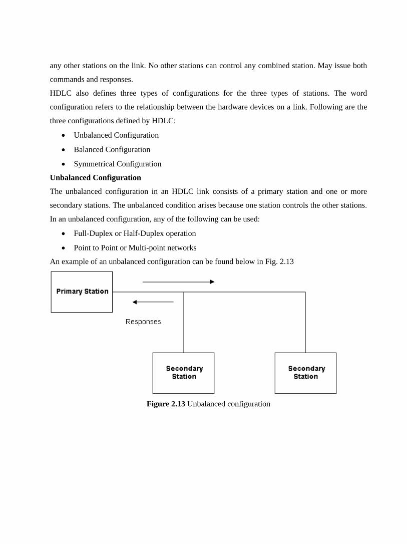
any other stations on the link. No other stations can control any combined station. May issue both
commands and responses.
HDLC also defines three types of configurations for the three types of stations. The word
configuration refers to the relationship between the hardware devices on a link. Following are the
three configurations defined by HDLC:
• Unbalanced Configuration
• Balanced Configuration
• Symmetrical Configuration
Unbalanced Configuration
The unbalanced configuration in an HDLC link consists of a primary station and one or more
secondary stations. The unbalanced condition arises because one station controls the other stations.
In an unbalanced configuration, any of the following can be used:
• Full-Duplex or Half-Duplex operation
• Point to Point or Multi-point networks
An example of an unbalanced configuration can be found below in Fig. 2.13
Figure 2.13 Unbalanced configuration
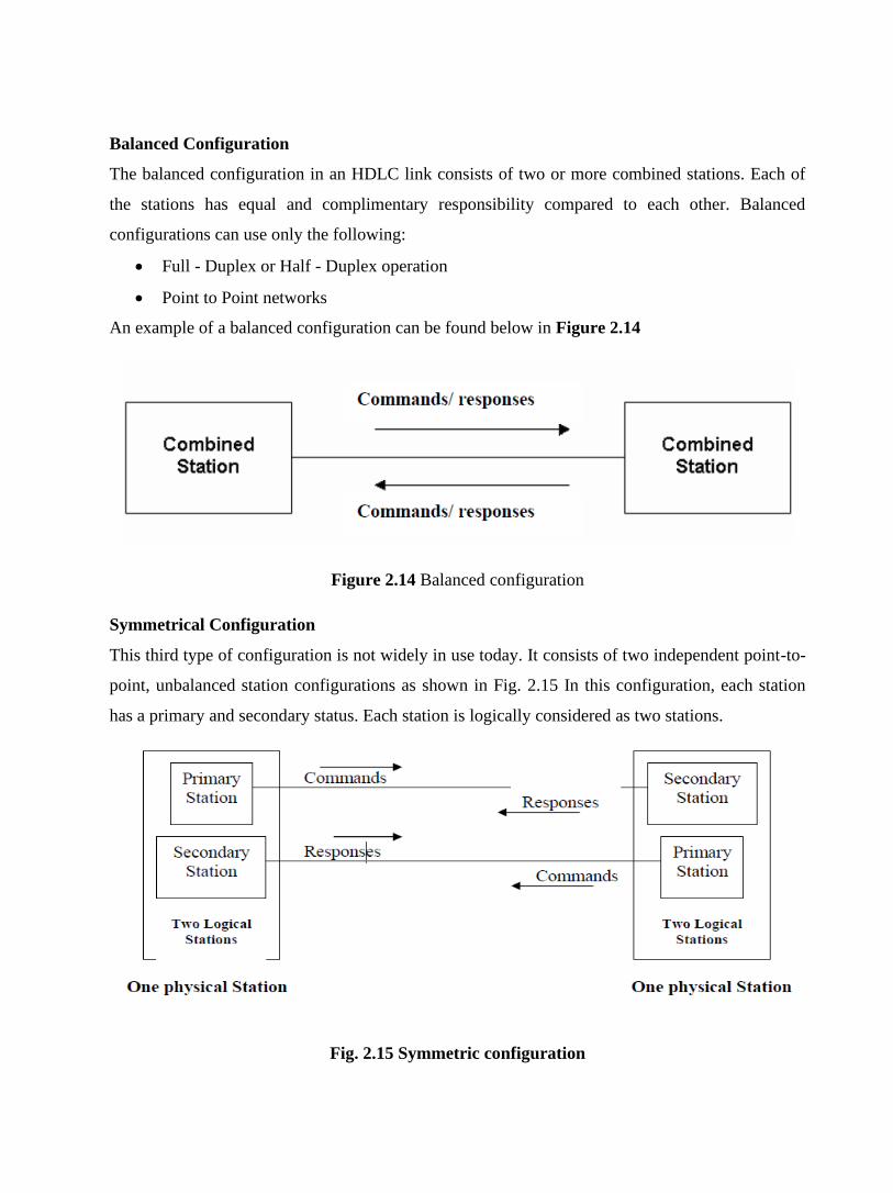
Balanced Configuration
The balanced configuration in an HDLC link consists of two or more combined stations. Each of
the stations has equal and complimentary responsibility compared to each other. Balanced
configurations can use only the following:
• Full - Duplex or Half - Duplex operation
• Point to Point networks
An example of a balanced configuration can be found below in Figure 2.14
Figure 2.14 Balanced configuration
Symmetrical Configuration
This third type of configuration is not widely in use today. It consists of two independent point-to-
point, unbalanced station configurations as shown in Fig. 2.15 In this configuration, each station
has a primary and secondary status. Each station is logically considered as two stations.
Fig. 2.15 Symmetric configuration
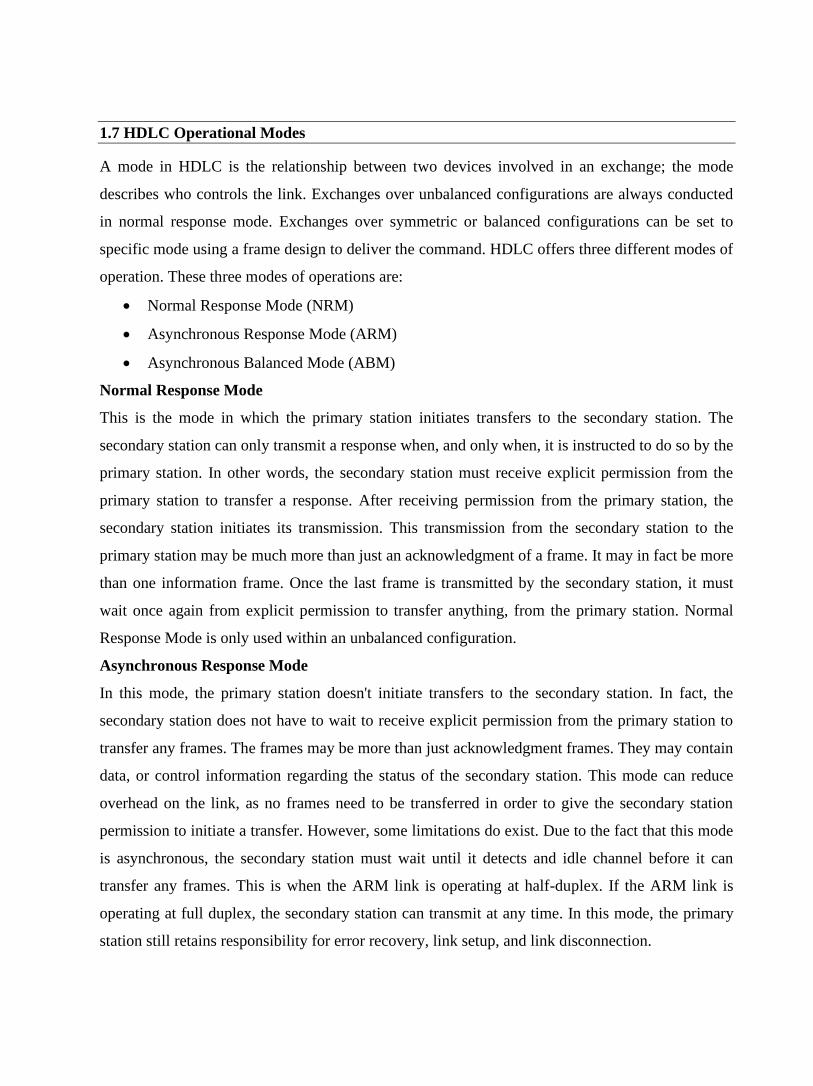
1.7 HDLC Operational Modes
A mode in HDLC is the relationship between two devices involved in an exchange; the mode
describes who controls the link. Exchanges over unbalanced configurations are always conducted
in normal response mode. Exchanges over symmetric or balanced configurations can be set to
specific mode using a frame design to deliver the command. HDLC offers three different modes of
operation. These three modes of operations are:
• Normal Response Mode (NRM)
• Asynchronous Response Mode (ARM)
• Asynchronous Balanced Mode (ABM)
Normal Response Mode
This is the mode in which the primary station initiates transfers to the secondary station. The
secondary station can only transmit a response when, and only when, it is instructed to do so by the
primary station. In other words, the secondary station must receive explicit permission from the
primary station to transfer a response. After receiving permission from the primary station, the
secondary station initiates its transmission. This transmission from the secondary station to the
primary station may be much more than just an acknowledgment of a frame. It may in fact be more
than one information frame. Once the last frame is transmitted by the secondary station, it must
wait once again from explicit permission to transfer anything, from the primary station. Normal
Response Mode is only used within an unbalanced configuration.
Asynchronous Response Mode
In this mode, the primary station doesn't initiate transfers to the secondary station. In fact, the
secondary station does not have to wait to receive explicit permission from the primary station to
transfer any frames. The frames may be more than just acknowledgment frames. They may contain
data, or control information regarding the status of the secondary station. This mode can reduce
overhead on the link, as no frames need to be transferred in order to give the secondary station
permission to initiate a transfer. However, some limitations do exist. Due to the fact that this mode
is asynchronous, the secondary station must wait until it detects and idle channel before it can
transfer any frames. This is when the ARM link is operating at half-duplex. If the ARM link is
operating at full duplex, the secondary station can transmit at any time. In this mode, the primary
station still retains responsibility for error recovery, link setup, and link disconnection.
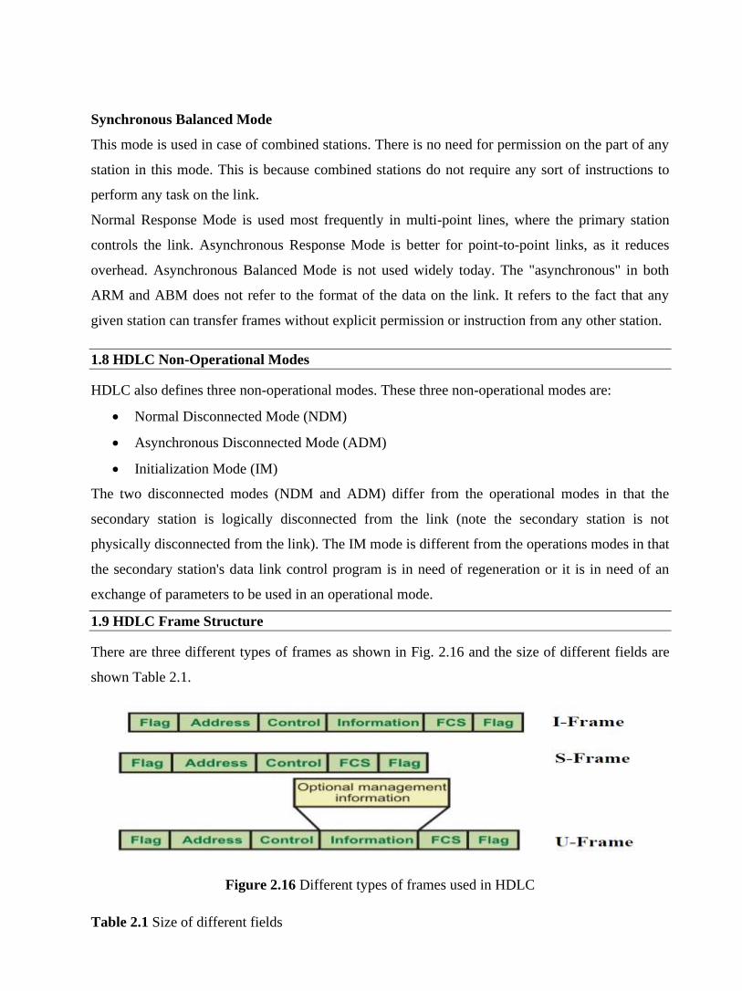
Synchronous Balanced Mode
This mode is used in case of combined stations. There is no need for permission on the part of any
station in this mode. This is because combined stations do not require any sort of instructions to
perform any task on the link.
Normal Response Mode is used most frequently in multi-point lines, where the primary station
controls the link. Asynchronous Response Mode is better for point-to-point links, as it reduces
overhead. Asynchronous Balanced Mode is not used widely today. The "asynchronous" in both
ARM and ABM does not refer to the format of the data on the link. It refers to the fact that any
given station can transfer frames without explicit permission or instruction from any other station.
1.8 HDLC Non-Operational Modes
HDLC also defines three non-operational modes. These three non-operational modes are:
• Normal Disconnected Mode (NDM)
• Asynchronous Disconnected Mode (ADM)
• Initialization Mode (IM)
The two disconnected modes (NDM and ADM) differ from the operational modes in that the
secondary station is logically disconnected from the link (note the secondary station is not
physically disconnected from the link). The IM mode is different from the operations modes in that
the secondary station's data link control program is in need of regeneration or it is in need of an
exchange of parameters to be used in an operational mode.
1.9 HDLC Frame Structure
There are three different types of frames as shown in Fig. 2.16 and the size of different fields are
shown Table 2.1.
Figure 2.16 Different types of frames used in HDLC
Table 2.1 Size of different fields
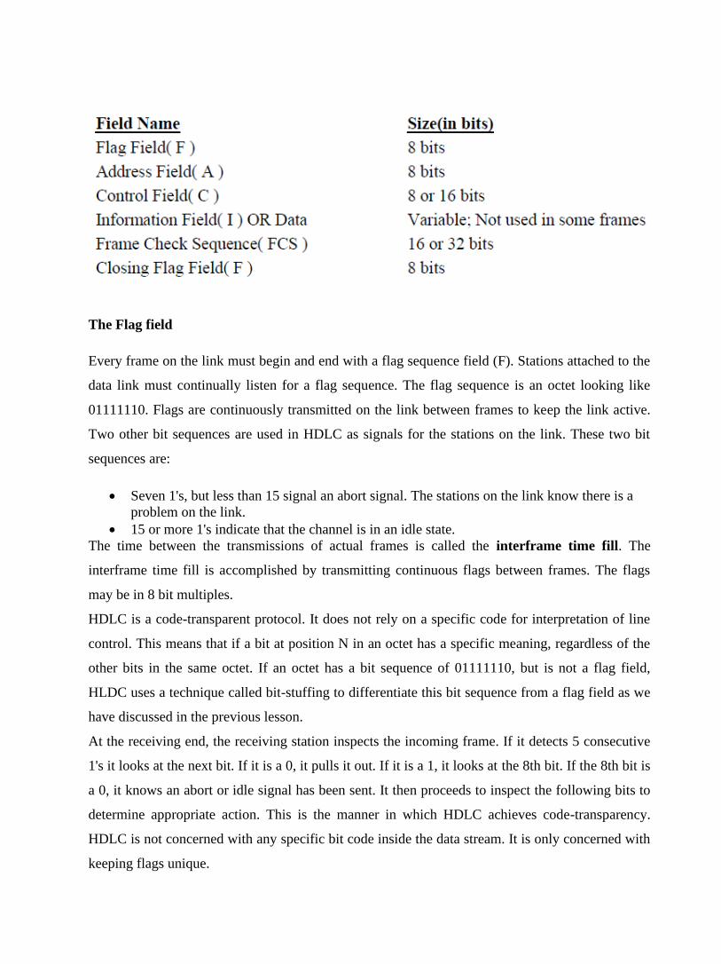
The Flag field
Every frame on the link must begin and end with a flag sequence field (F). Stations attached to the
data link must continually listen for a flag sequence. The flag sequence is an octet looking like
01111110. Flags are continuously transmitted on the link between frames to keep the link active.
Two other bit sequences are used in HDLC as signals for the stations on the link. These two bit
sequences are:
• Seven 1's, but less than 15 signal an abort signal. The stations on the link know there is a
problem on the link.
• 15 or more 1's indicate that the channel is in an idle state.
The time between the transmissions of actual frames is called the interframe time fill. The
interframe time fill is accomplished by transmitting continuous flags between frames. The flags
may be in 8 bit multiples.
HDLC is a code-transparent protocol. It does not rely on a specific code for interpretation of line
control. This means that if a bit at position N in an octet has a specific meaning, regardless of the
other bits in the same octet. If an octet has a bit sequence of 01111110, but is not a flag field,
HLDC uses a technique called bit-stuffing to differentiate this bit sequence from a flag field as we
have discussed in the previous lesson.
At the receiving end, the receiving station inspects the incoming frame. If it detects 5 consecutive
1's it looks at the next bit. If it is a 0, it pulls it out. If it is a 1, it looks at the 8th bit. If the 8th bit is
a 0, it knows an abort or idle signal has been sent. It then proceeds to inspect the following bits to
determine appropriate action. This is the manner in which HDLC achieves code-transparency.
HDLC is not concerned with any specific bit code inside the data stream. It is only concerned with
keeping flags unique.

The Address field
The address field (A) identifies the primary or secondary stations involvement in the frame
transmission or reception. Each station on the link has a unique address. In an unbalanced
configuration, the A field in both commands and responses refer to the secondary station. In a
balanced configuration, the command frame contains the destination station address and the
response frame has the sending station's address.
The Control field
HDLC uses the control field (C) to determine how to control the communications process. This
field contains the commands, responses and sequences numbers used to maintain the data flow
accountability of the link, defines the functions of the frame and initiates the logic to control the
movement of traffic between sending and receiving stations. There three control field formats:
• Information Transfer Format: The frame is used to transmit end-user data between two
devices.
• Supervisory Format: The control field performs control functions such as
acknowledgment of frames, requests for re-transmission, and requests for temporary
suspension of frames being transmitted. Its use depends on the operational mode being
used.
• Unnumbered Format: This control field format is also used for control purposes. It is
used to perform link initialization, link disconnection and other link control functions.
The Poll/Final Bit (P/F)
The 5th bit position in the control field is called the poll/final bit, or P/F bit. It can only be
recognized when it is set to 1. If it is set to 0, it is ignored. The poll/final bit is used to provide
dialogue between the primary station and secondary station. The primary station uses P=1 to
acquire a status response from the secondary station. The P bit signifies a poll. The secondary
station responds to the P bit by transmitting a data or status frame to the primary station with the
P/F bit set to F=1. The F bit can also be used to signal the end of a transmission from the
secondary station under Normal Response Mode.
The Information field or Data field
This field is not always present in a HDLC frame. It is only present when the Information Transfer
Format is being used in the control field. The information field contains the actually data the
sender is transmitting to the receiver in an I-Frame and network management information in U-
Frame.
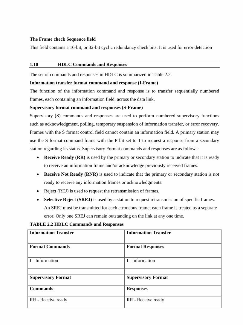
The Frame check Sequence field
This field contains a 16-bit, or 32-bit cyclic redundancy check bits. It is used for error detection
1.10 HDLC Commands and Responses
The set of commands and responses in HDLC is summarized in Table 2.2.
Information transfer format command and response (I-Frame)
The function of the information command and response is to transfer sequentially numbered
frames, each containing an information field, across the data link.
Supervisory format command and responses (S-Frame)
Supervisory (S) commands and responses are used to perform numbered supervisory functions
such as acknowledgment, polling, temporary suspension of information transfer, or error recovery.
Frames with the S format control field cannot contain an information field. A primary station may
use the S format command frame with the P bit set to 1 to request a response from a secondary
station regarding its status. Supervisory Format commands and responses are as follows:
• Receive Ready (RR) is used by the primary or secondary station to indicate that it is ready
to receive an information frame and/or acknowledge previously received frames.
• Receive Not Ready (RNR) is used to indicate that the primary or secondary station is not
ready to receive any information frames or acknowledgments.
• Reject (REJ) is used to request the retransmission of frames.
• Selective Reject (SREJ) is used by a station to request retransmission of specific frames.
An SREJ must be transmitted for each erroneous frame; each frame is treated as a separate
error. Only one SREJ can remain outstanding on the link at any one time.
TABLE 2.2 HDLC Commands and Responses
Information Transfer
Information Transfer
Format Commands
Format Responses
I - Information
I - Information
Supervisory Format
Supervisory Format
Commands
Responses
RR - Receive ready
RR - Receive ready
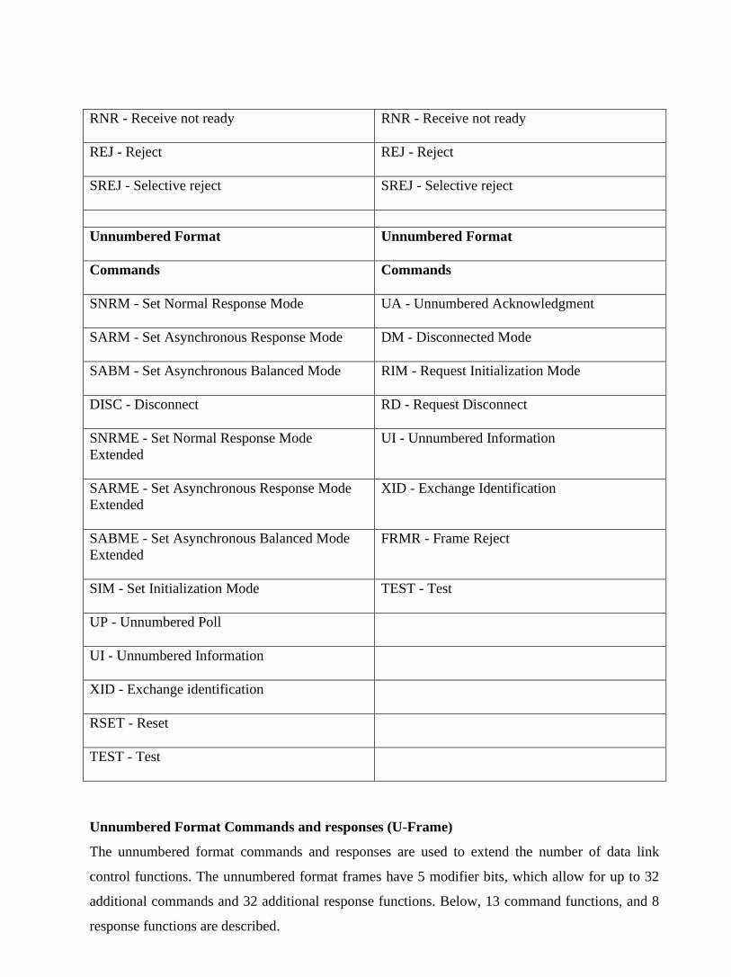
RNR - Receive not ready
RNR - Receive not ready
REJ - Reject
REJ - Reject
SREJ - Selective reject
SREJ - Selective reject
Unnumbered Format
Unnumbered Format
Commands
Commands
SNRM - Set Normal Response Mode
UA - Unnumbered Acknowledgment
SARM - Set Asynchronous Response Mode
DM - Disconnected Mode
SABM - Set Asynchronous Balanced Mode
RIM - Request Initialization Mode
DISC - Disconnect
RD - Request Disconnect
SNRME - Set Normal Response Mode
Extended
UI - Unnumbered Information
SARME - Set Asynchronous Response Mode
Extended
XID - Exchange Identification
SABME - Set Asynchronous Balanced Mode
Extended
FRMR - Frame Reject
SIM - Set Initialization Mode
TEST - Test
UP - Unnumbered Poll
UI - Unnumbered Information
XID - Exchange identification
RSET - Reset
TEST - Test
Unnumbered Format Commands and responses (U-Frame)
The unnumbered format commands and responses are used to extend the number of data link
control functions. The unnumbered format frames have 5 modifier bits, which allow for up to 32
additional commands and 32 additional response functions. Below, 13 command functions, and 8
response functions are described.

• Set Normal Response Mode (SNRM) places the secondary station into NRM. NRM does
not allow the secondary station to send any unsolicited frames. Hence the primary station
has control of the link.
• Set Asynchronous Response Mode (SARM) allows a secondary station to transmit
frames without a poll from the primary station.
• Set Asynchronous Balanced Mode (SABM) sets the operational mode of the link to
ABM.
• Disconnect (DISC) places the secondary station in to a disconnected mode.
• Set Normal Response Mode Extended (SNRME) increases the size of the control field to
2 octets instead of one in NRM. This is used for extended sequencing. The same applies for
SARME and SABME.
• Set Initialization Mode (SIM) is used to cause the secondary station to initiate a station-
specific procedure(s) to initialize its data link level control functions.
• Unnumbered Poll (UP) polls a station without regard to sequencing or acknowledgment.
• Unnumbered Information (UI) is used to send information to a secondary station.
• Exchange Identification (XID) is used to cause the secondary station to identify itself and
provide the primary station identifications characteristics of itself.
• Reset (RSET) is used to reset the receive state variable in the addressed station.
• Test (TEST) is used to cause the addressed secondary station to respond with a TEST
response at the first response opportunity. It performs a basic test of the data link control.
• Unnumbered Acknowledgment (UA) is used by the secondary station to acknowledge the
receipt and acceptance of an SNRM, SARM, SABM, SNRME, SARME, SABME, RSET, SIM,
or DISC commands.
• Disconnected Mode (DM) is transmitted from a secondary station to indicate it is in
disconnected mode(non-operational mode.)
• Request Initialization Mode (RIM) is a request from a secondary station for initialization
to a primary station. Once the secondary station sends RIM, it can only respond to SIM,
DSIC, TEST or XID commands.
• Request Disconnect (RD) is sent by the secondary station to inform the primary station
that it wishes to disconnect from the link and go into a non-operational mode(NDM or
ADM).

• Frame Reject (FRMR) is used by the secondary station in an operation mode to report
that a condition has occurred in transmission of a frame and retransmission of the frame
will not correct the condition.
1.11 HDLC Subsets
Many other data link protocols have been derived from HDLC. However, some of them reach
beyond the scope of HDLC. Two other popular offsets of HDLC are Synchronous Data Link
Control (SDLC), and Link Access Protocol, Balanced (LAP-B). SDLC is used and developed by
IBM. It is used in a variety of terminal to computer applications. It is also a part of IBM's SNA
communication architecture. LAP-B was developed by the ITU-T. It is derived mainly from the
asynchronous response mode (ARM) of HDLC. It is commonly used for attaching devices to
packet-switched networks.
1.12 Check Your Progress
Fill In The Blanks
1. The most important functions of ……………….to satisfy the above requirements are error
control and flow control.
2. ………………..is a technique so that transmitter and receiver with different speed
characteristics can communicate with each other.
3. ARQ stands for…………………….
4. Flow Control is a set of procedures that tells the sender how much data it can transmit
before it must wait for an ………………..from the receiver.
5. There are two methods developed for flow control namely Stop-and-wait and…………….
6. The most popular ARQ protocol is the ………………..where the sender sends the frames
continuously without waiting for acknowledgement.
7. ………………..is a bit-oriented protocol.
1.13 Answer to Check Your Progress
1. Data Link layer
2. Flow Control
3. Automatic Repeat Request
4. Acknowledgment
5. Sliding-window.
6. go-back-N ARQ

7. HDLC
Unit-4
Switching Techniques: Circuit Switching
1.1 Learning Objectives
1.2 Introduction
1.3 Circuit switching Technique
1.4 Switching Node
1.5 Public Switched Telephone Networks
1.6 Message Switching
1.7 Packet Switching
1.7.1 Virtual Circuit Packet Switching Networks
1.7.2 Datagram Packet Switching Networks
1.7.3 Packet Size
1.7.4 Virtual Circuit Versus Datagram Packet Switching
1.7.5 External and Internal Operations
1.8 Check Your Progress
1.9 Answer to Check Your Progress
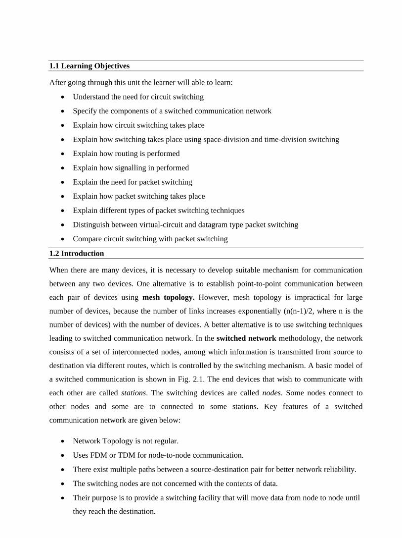
1.1 Learning Objectives
After going through this unit the learner will able to learn:
• Understand the need for circuit switching
• Specify the components of a switched communication network
• Explain how circuit switching takes place
• Explain how switching takes place using space-division and time-division switching
• Explain how routing is performed
• Explain how signalling in performed
• Explain the need for packet switching
• Explain how packet switching takes place
• Explain different types of packet switching techniques
• Distinguish between virtual-circuit and datagram type packet switching
• Compare circuit switching with packet switching
1.2 Introduction
When there are many devices, it is necessary to develop suitable mechanism for communication
between any two devices. One alternative is to establish point-to-point communication between
each pair of devices using mesh topology. However, mesh topology is impractical for large
number of devices, because the number of links increases exponentially (n(n-1)/2, where n is the
number of devices) with the number of devices. A better alternative is to use switching techniques
leading to switched communication network. In the switched network methodology, the network
consists of a set of interconnected nodes, among which information is transmitted from source to
destination via different routes, which is controlled by the switching mechanism. A basic model of
a switched communication is shown in Fig. 2.1. The end devices that wish to communicate with
each other are called stations. The switching devices are called nodes. Some nodes connect to
other nodes and some are to connected to some stations. Key features of a switched
communication network are given below:
• Network Topology is not regular.
• Uses FDM or TDM for node-to-node communication.
• There exist multiple paths between a source-destination pair for better network reliability.
• The switching nodes are not concerned with the contents of data.
• Their purpose is to provide a switching facility that will move data from node to node until
they reach the destination.
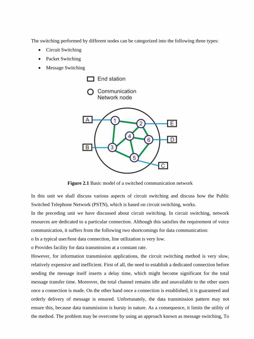
The switching performed by different nodes can be categorized into the following three types:
• Circuit Switching
• Packet Switching
• Message Switching
Figure 2.1 Basic model of a switched communication network
In this unit we shall discuss various aspects of circuit switching and discuss how the Public
Switched Telephone Network (PSTN), which is based on circuit switching, works.
In the preceding unit we have discussed about circuit switching. In circuit switching, network
resources are dedicated to a particular connection. Although this satisfies the requirement of voice
communication, it suffers from the following two shortcomings for data communication:
o In a typical user/host data connection, line utilization is very low.
o Provides facility for data transmission at a constant rate.
However, for information transmission applications, the circuit switching method is very slow,
relatively expensive and inefficient. First of all, the need to establish a dedicated connection before
sending the message itself inserts a delay time, which might become significant for the total
message transfer time. Moreover, the total channel remains idle and unavailable to the other users
once a connection is made. On the other hand once a connection is established, it is guaranteed and
orderly delivery of message is ensured. Unfortunately, the data transmission pattern may not
ensure this, because data transmission is bursty in nature. As a consequence, it limits the utility of
the method. The problem may be overcome by using an approach known as message switching, To
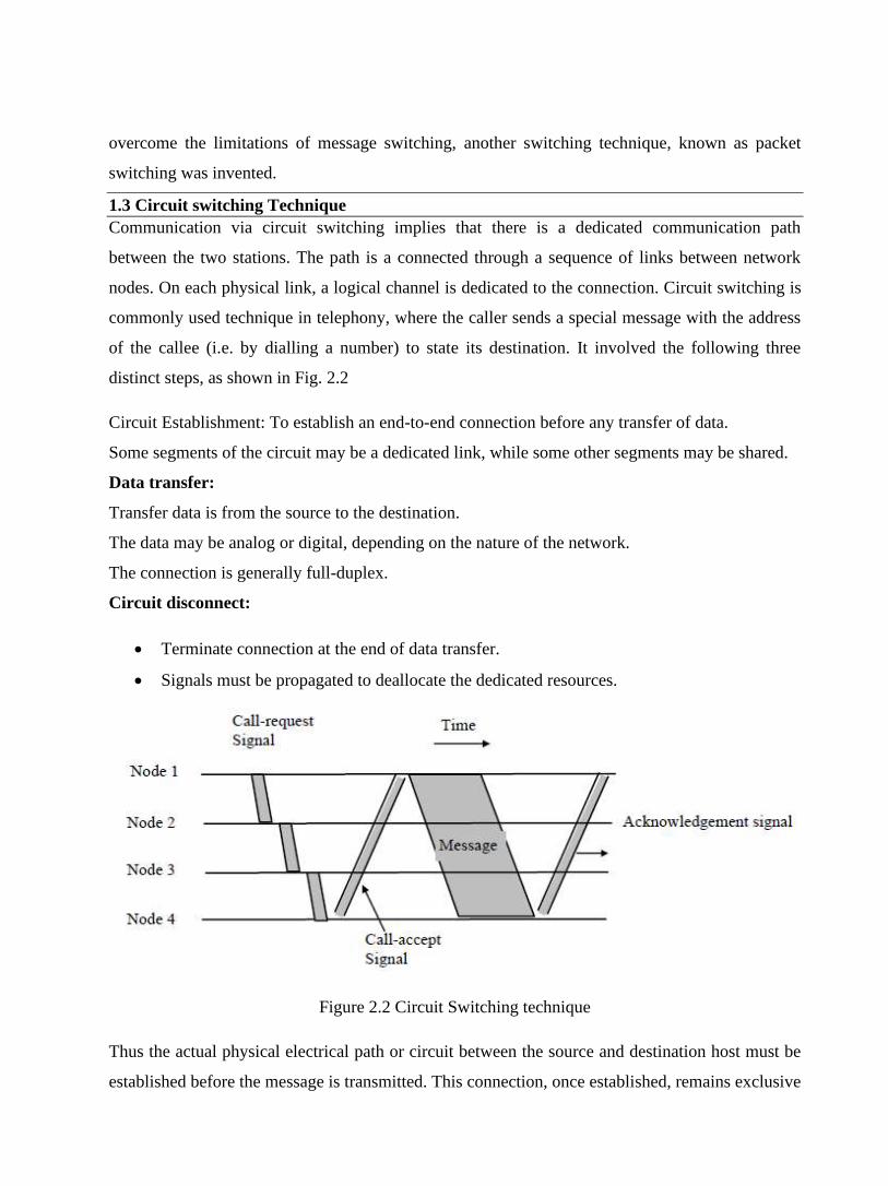
overcome the limitations of message switching, another switching technique, known as packet
switching was invented.
1.3 Circuit switching Technique
Communication via circuit switching implies that there is a dedicated communication path
between the two stations. The path is a connected through a sequence of links between network
nodes. On each physical link, a logical channel is dedicated to the connection. Circuit switching is
commonly used technique in telephony, where the caller sends a special message with the address
of the callee (i.e. by dialling a number) to state its destination. It involved the following three
distinct steps, as shown in Fig. 2.2
Circuit Establishment: To establish an end-to-end connection before any transfer of data.
Some segments of the circuit may be a dedicated link, while some other segments may be shared.
Data transfer:
Transfer data is from the source to the destination.
The data may be analog or digital, depending on the nature of the network.
The connection is generally full-duplex.
Circuit disconnect:
• Terminate connection at the end of data transfer.
• Signals must be propagated to deallocate the dedicated resources.
Figure 2.2 Circuit Switching technique
Thus the actual physical electrical path or circuit between the source and destination host must be
established before the message is transmitted. This connection, once established, remains exclusive

and continuous for the complete duration of information exchange and the circuit becomes
disconnected only when the source wants to do so.
1.4 Switching Node
Let us consider the operation of a single circuit switched node comprising a collection of stations
attached to a central switching unit, which establishes a dedicated path between any two devices
that wish to communicate.
Major elements of a single-node network are summarized below:
• Digital switch: That provides a transparent (full-duplex) signal path between any pair of
attached devices.
• Network interface: That represents the functions and hardware needed to connect digital
devices to the network (like telephones).
• Control unit: That establishes, maintains, and tears down a connection.
The simplified schematic diagram of a switching node is shown in Fig. 2.3. An important
characteristic of a circuit-switch node is whether it is blocking or non-blocking. A blocking
network is one, which may be unable to connect two stations because all possible paths between
them are already in use. A non-blocking network permits all stations to be connected (in pairs) at
once and grants all possible connection requests as long as the called party is free. For a network
that supports only voice traffic, a blocking configuration may be acceptable, since most phone
calls are of short duration. For data applications, where a connection may remain active for hours,
non-blocking configuration is desirable.

Figure 2.3 Schematic diagram of a switching node.
Circuit switching uses any of the three technologies: Space-division switches, Time-division
switches or a combination of both. In Space-division switching, the paths in the circuit are
separated with each other spatially, i.e. different ongoing connections, at a same instant of time,
uses different switching paths, which are separated spatially. This was originally developed for the
analog environment, and has been carried over to the digital domain. Some of the space switches
are crossbar switches, Multi-stage switches (e.g. Omega Switches). A crossbar switch is shown in
Fig. 2.4. Basic building block of the switch is a metallic crosspoint or semiconductor gate that can
be enabled or disabled by a control unit.
Figure 2.4 Schematic diagram of a crossbar switch
Example: Xilinx crossbar switch using FPGAs. It is based on reconfigurable routing
infrastructure. It is a high-speed high capacity nonblocking type switch with sizes varying from
64X64 to 1024X1024 and data rate of 200 Mbps.
Limitations of crossbar switches are as follows:
• The number of crosspoints grows with the square of the number of attached stations.
• Costly for a large switch.
• The failure of a crosspoint prevents connection between the two devices whose lines
intersect at that crosspoint.
• The crosspoints are inefficiently utilized.

• Only a small fraction of crosspoints are engaged even if all of the attached devices are
active.
Some of the above problems can be overcome with the help of multistage space division switches.
By splitting the crossbar switch into smaller units and interconnecting them, it is possible to build
multistage switches with fewer crosspoints.
Figure 2.5 A three-stage space division switch
Figure 2.6 Block nature of the switch
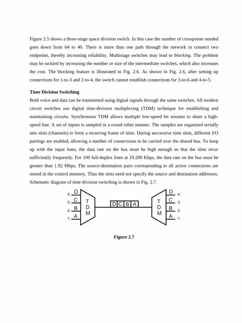
Figure 2.5 shows a three-stage space division switch. In this case the number of crosspoints needed
goes down from 64 to 40. There is more than one path through the network to connect two
endpoints, thereby increasing reliability. Multistage switches may lead to blocking. The problem
may be tackled by increasing the number or size of the intermediate switches, which also increases
the cost. The blocking feature is illustrated in Fig. 2.6. As shown in Fig. 2.6, after setting up
connections for 1-to-3 and 2-to-4, the switch cannot establish connections for 3-to-6 and 4-to-5.
Time Division Switching
Both voice and data can be transmitted using digital signals through the same switches. All modern
circuit switches use digital time-division multiplexing (TDM) technique for establishing and
maintaining circuits. Synchronous TDM allows multiple low-speed bit streams to share a high-
speed line. A set of inputs is sampled in a round robin manner. The samples are organized serially
into slots (channels) to form a recurring frame of slots. During successive time slots, different I/O
pairings are enabled, allowing a number of connections to be carried over the shared bus. To keep
up with the input lines, the data rate on the bus must be high enough so that the slots recur
sufficiently frequently. For 100 full-duplex lines at 19.200 Kbps, the data rate on the bus must be
greater than 1.92 Mbps. The source-destination pairs corresponding to all active connections are
stored in the control memory. Thus the slots need not specify the source and destination addresses.
Schematic diagram of time division switching is shown in Fig. 2.7.
Figure 2.7

Figure 2.8 TDM with Switching using TSI
Time-division switching uses time-division multiplexing to achieve switching, i.e. different
ongoing connections can use same switching path but at different interleaved time intervals. There
are two popular methods of time-division switching namely, Time-Slot Interchange (TSI) and the
TDM bus. TSI changes the ordering of the slots based on desired connection and it has a random-
access memory to store data and flip the time slots as shown in Fig. 2.8. The operation of a TSI is
depicted in Fig. 2.9. As shown in the figure, writing can be performed in the memory sequentially,
but data is read selectively. In TDM bus there are several input and outputs connected to a high-
speed bus. During a time slot only one particular output switch is closed, so only one connection at
a particular instant of time as shown in Fig. 2.10.
Figure 2.9 Operation of a TSI

Figure 2.10 TDM bus switching
1.5 Public Switched Telephone Networks
Public switched telephone network (PSTN) is an example of circuit-switched network. It’s also
known as Plain Old Telephone Service (POTS). The switching centres used for the switching are
organised in different levels, namely: Regional offices (class 1), Section offices (class 2), primary
offices (class 3), Toll offices (class 4) and finally End offices
(class 5) as shown in Fig. 2.11. Level 1 is at the highest level and Level 5 is the lowest level.
Subscribers or the customers are directly connected to these end offices. And each office is
connected directly to a number of offices at a level below and mostly a single office at higher
level.
Subscriber Telephones are connected, through Local Loops to end offices (or central offices). A
small town may have only one end office, but large cities have several end offices. Many end
offices are connected to one Toll office, which are connected to primary offices. Several primary
offices are connected to a section office, which normally serves more than one state. All regional
offices are connected using mesh topology. Accessing the switching station at the end offices is
accomplished through dialling. In the past, telephone featured rotary or pulse dialling, in which
digital signals were sent to the end office for each dialled digit. This type of dialling was prone to
errors due to inconsistency in humans during dialling. Presently, dialling is accomplished by
Touch-Tone technique. In this method the user sends a small burst of frequency called dual tone,

because it is a combination of two frequencies. This combination of frequencies sent depends on
the row and column of the pressed pad.
Figure 2.11 Basic organization of a Public Switched Telephone Network (PSTN)
The connections are multiplexed when have to send to a switching office, which is one level up.
For example, Different connections will be multiplexed when they are to be forwarded from an
end-office to Toll office. Figure 2.12 shows a typical medium distance telephone circuit.
Figure 2.12 Typical medium distance telephone circuit

1.6 Message Switching
In this switching method, a different strategy is used, where instead of establishing a dedicated
physical line between the sender and the receiver, the message is sent to the nearest directly
connected switching node. This node stores the message, checks for errors, selects the best
available route and forwards the message to the next intermediate node.
Figure 2.13 Message Switching Technique
The line becomes free again for other messages, while the process is being continued in some
other nodes. Due to the mode of action, this method is also known as store-and-forward
technology where the message hops from node to node to its final destination. Each node stores the
full message, checks for errors and forwards it.
In this switching technique, more devices can share the network bandwidth, as compared with
circuit switching technique. Temporary storage of message reduces traffic congestion to some
extent. Higher priority can be given to urgent messages, so that the low priority messages are
delayed while the urgent ones are forwarded faster. Through broadcast addresses one message can
be sent to several users. Last of all, since the destination host need not be active when the message
is sent, message switching techniques improve global communications.
However, since the message blocks may be quite large in size, considerable amount of storage
space is required at each node to buffer the messages. A message might occupy the buffers for
minutes, thus blocking the internodal traffic.
Basic idea:
Each network node receives and stores the message
Determines the next leg of the route, and
Queues the message to go out on that link.
Advantages:

Line efficiency is greater (sharing of links).
Data rate conversion is possible.
Even under heavy traffic, packets are accepted, possibly with a greater delay in delivery.
Message priorities can be used, to satisfy the requirements, if any.
Disadvantages: Message of large size monopolizes the link and storage
1.7 Packet Switching
The basic approach is not much different from message switching. It is also based on the same
‘store-and-forward’ approach. However, to overcome the limitations of message switching,
messages are divided into subsets of equal length called packets. This approach was developed for
long-distance data communication (1970) and it has evolved
over time. In packet switching approach, data are transmitted in short packets (few Kbytes). A long
message is broken up into a series of packets as shown in Fig. 2.14. Every packet contains some
control information in its header, which is required for routing and other purposes
Figure 2.14 A message is divided into a number of equal length short packets
Main difference between Packet switching and Circuit Switching is that the communication lines
are not dedicated to passing messages from the source to the destination. In Packet Switching,
different messages (and even different packets) can pass through different routes, and when there
is a "dead time" in the communication between the source and the destination, the lines can be
used by other sources.
There are two basic approaches commonly used to packet Switching: virtual-circuit packet
switching and datagram packet switching. In virtual-circuit packet switching a virtual circuit is
made before actual data is transmitted, but it is different from circuit switching in a sense that in
circuit switching the call accept signal comes only from the final destination to the source while in
case of virtual-packet switching this call accept signal is transmitted between each adjacent

intermediate node as shown in Fig. 2.15. Other features of virtual circuit packet switching are
discussed in the following subsection.
1.7.1 Virtual Circuit Packet Switching Networks
An initial setup phase is used to set up a route between the intermediate nodes for all the packets
passed during the session between the two end nodes. In each intermediate node, an entry is
registered in a table to indicate the route for the connection that has been set up. Thus, packets
passed through this route, can have short headers, containing only a virtual circuit identifier (VCI),
and not their destination. Each intermediate node passes the packets according to the information
that was stored in it, in the setup phase. In this way, packets arrive at the destination in the correct
sequence, and it is guaranteed that essentially there will not be errors. This approach is slower than
Circuit Switching, since different virtual circuits may compete over the same resources, and an
initial setup phase is needed to initiate the circuit. As in Circuit Switching, if an intermediate node
fails, all virtual circuits that pass through it are lost. The most common forms of Virtual Circuit
networks are X.25 and Frame Relay, which are commonly used for public data networks (PDN).
Figure 2.15 Virtual circuit packet switching technique
1.7.2 Datagram Packet Switching Networks
This approach uses a different, more dynamic scheme, to determine the route through the network
links. Each packet is treated as an independent entity, and its header contains full information
about the destination of the packet. The intermediate nodes examine the header of the packet, and
decide to which node to send the packet so that it will reach its destination. In the decision two
factors are taken into account:
• The shortest ways to pass the packet to its destination - protocols such as RIP/OSPF are
used to determine the shortest path to the destination.

• Finding a free node to pass the packet to - in this way, bottlenecks are eliminated, since
packets can reach the destination in alternate routes.
Thus, in this method, the packets don't follow a pre-established route, and the intermediate nodes
(the routers) don't have pre-defined knowledge of the routes that the packets should be passed
through.
Figure 2.16 Datagram Packet switching
Packets can follow different routes to the destination, and delivery is not guaranteed (although
packets usually do follow the same route, and are reliably sent). Due to the nature of this method,
the packets can reach the destination in a different order than they were sent, thus they must be
sorted at the destination to form the original message. This approach is time consuming since
every router has to decide where to send each packet. The main implementation of Datagram
Switching network is the Internet, which uses the IP network protocol.
Advantages:
• Call setup phase is avoided (for transmission of a few packets, datagram will be faster).
• Because it is more primitive, it is more flexible.
• Congestion/failed link can be avoided (more reliable).
Problems:
• Packets may be delivered out of order.
• If a node crashes momentarily, all of its queued packets are lost.

1.7.3 Packet Size
In spite of increase in overhead, the transmission time may decreases in packet switching
technique because of parallelism in transmission as shown in Fig. 2.17.
Figure 2.17 Reduction of transmission time because of parallelism in transmission in packet
switching technique.
However, question arises about the optimal size of size of a packet. As packet size is decreased,
the transmission time reduces until it is comparable to the size of control information. There is a
close relationship between packet size and transmission time as shown in Fig. 2.18. In this case it
is assumed that there is a virtual circuit from station X to Y through nodes a and b. Times required
for transmission decreases as each message is divided into 2 and 5 packets. However, the
transmission time increases if each message is divided into 10 packets.
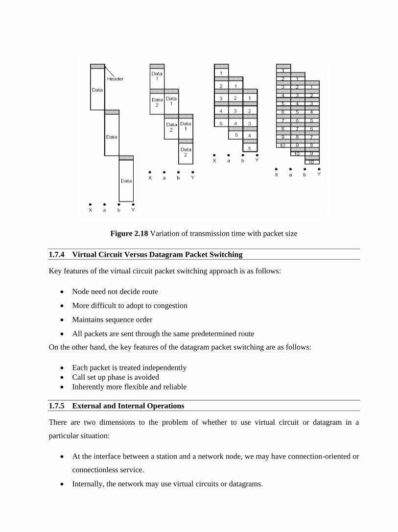
Figure 2.18 Variation of transmission time with packet size
1.7.4 Virtual Circuit Versus Datagram Packet Switching
Key features of the virtual circuit packet switching approach is as follows:
• Node need not decide route
• More difficult to adopt to congestion
• Maintains sequence order
• All packets are sent through the same predetermined route
On the other hand, the key features of the datagram packet switching are as follows:
• Each packet is treated independently
• Call set up phase is avoided
• Inherently more flexible and reliable
1.7.5 External and Internal Operations
There are two dimensions to the problem of whether to use virtual circuit or datagram in a
particular situation:
• At the interface between a station and a network node, we may have connection-oriented or
connectionless service.
• Internally, the network may use virtual circuits or datagrams.

This leads us to four different scenarios using different VC/DG combinations, which are discussed
below.
Scenario 1: External virtual circuit, Internal virtual circuit
In this case a user requests a virtual circuit and a dedicated route through the network is
constructed. All packets follow the same route as shown in Fig. 2.19.
Figure 2.19 External virtual circuit and internal virtual circuit
Scenario 2: External virtual circuit, Internal datagram
In this case, the network handles each packet separately. Different packets for the same external
virtual circuit may take different routes as shown in Fig. 2.20. The network buffers packets, if
necessary, so that they are delivered to the destination in the proper order.
Scenario 3: External datagram, Internal datagram
In this case each packet is treated independently from both the user’s end and the network’s point
of view as shown in Fig. 2.21.
Scenario 4: External datagram, Internal virtual circuit
In this case, an external user does not see any connections - it simply sends packets one at a time
as shown in Fig. 2.22. The network sets up a logical connection between stations for packet
delivery. May leave such connections in place for an extended period, so as to satisfy anticipated
future needs.
A comparison of different switching techniques is given in Table 2.1

Figure 2.20 External virtual circuit and internal datagram
Figure 2.21 External datagram and internal datagram
Figure 2.22 External datagram and internal virtual circuit
Table 2.1 Comparison of the three switching techniques

1.8 Check Your Progress
Fill In the Blanks:
1. ________ uses the entire capacity of the link.
2. In ________ switching, each packet of a message need not follow the same path from
sender to receiver.
3. In ________ switching all the datagrams of a message follows the same channel of a path.
4. PSTN is an example of _______________ network
5. PSTN is also known as ____________.
6. A switched virtual circuit involves _____________.
7. A permanent virtual circuit involves _____________.
8. Two basic approaches are common to Packet Switching are_____________ packet
switching and _________ packet switching
9. X.25 is a standard for _________ communications.
1.9 Answer to check your progress
1. Circuit switching
2. Datagram packet
3. virtual circuit
4. circuit switching
5. plain old telephone service (POTS)
6. creation of link as and when needed
7. permanent link
8. virtual circuit … datagram
9. packet switched communication

Unit-5
Synchronous Optical Network (SONET)
1.1 Learning Objective
1.2 Introduction
1.3 Synchronization of Digital Signals
1.3.1 Basic SONET Signal
1.4 Why Synchronize?
1.4.1 Synchronization Hierarchy
1.4.2 Synchronizing SONET
1.5 Physical Configuration and Network Elements
1.5.1 Section, Line and paths
1.5.2 SONET Network Elements
1.6 Frame Format Structure
1.7 OVERHEAD
1.8 Virtual Tributaries and Pointers
1.9 Check Your Progress
1.10 Answer to Check Your Progress

1.1 Learning Objective
After going through this unit the learner will able to learn:
• Explain the operation of a SONET network
• Explain the function of different SONET layers
• Specify SONET frame format
1.2 Introduction
To satisfy the requirements of ever increasing data rate for diverse applications, ANSI developed a
standard known as Synchronous Optical Network (SONET) by utilizing the enormous bandwidth
of optical fiber. Another very similar standard developed by ITU-T is known as Synchronous
Digital Hierarchy (SDH). It is a synchronous TDM system controlled by a master clock, which
adds predictability. The comprehensive SONET/synchronous digital hierarchy (SDH) standard is
expected to provide the transport infrastructure for worldwide telecommunications for at least the
next two or three decades.
The increased configuration flexibility and bandwidth availability of SONET provides significant
advantages over the older telecommunications system. These advantages include the following:
• Reduction in equipment requirements and an increase in network reliability.
• Provision of overhead and payload bytes - the overhead bytes permit management of the
payload bytes on an individual basis and facilitate centralized fault sectionalization.
• Definition of a synchronous multiplexing format for carrying lower level digital signals
(such as DS–1, DS–3) and a synchronous structure that greatly simplifies the interface to
digital.switches, digital cross-connect switches, and add-drop multiplexers.
• Availability of a set of generic standards that enable products from different vendors to be
connected.
• Definition of a flexible architecture capable of accommodating future applications, with a
variety of transmission rates.
In brief, SONET defines optical carrier (OC) levels and electrically equivalent synchronous
transport signals (STSs) for the fiber-optic–based transmission hierarchy.

1.3 Synchronization of Digital Signals
To understand the concepts and details of SONET correctly, it is important to follow the meaning
of synchronous, asynchronous, and plesiochronous. In a set of synchronous signals, the digital
transitions in the signals occur at exactly the same rate. There may, however, be a phase difference
between the transitions of the two signals, and this would lie within specified limits. These phase
differences may be due to propagation delays or jitter introduced into the transmission network. In
a synchronous network, all the clocks are traceable to one primary reference clock (PRC).
If two digital signals are plesiochronous, their transitions occur at almost the same rate, with any
variation being constrained within tight limits. For example, if two networks must interwork, their
clocks may be derived from two different primary reference clocks (PRCs). Although these clocks
are extremely accurate, there is a difference between one clock and the other. This is known as a
plesiochronous difference.
In the case of asynchronous signals, the transitions of the signals do not necessarily occur at the
same nominal rate. Asynchronous, in this case, means that the difference between two clocks is
much greater than a plesiochronous difference. For example, if two clocks are derived from free-
running quartz oscillators, they could be described as asynchronous.
1.3.1 Basic SONET Signal
SONET defines a technology for carrying many signals of different capacities through a
synchronous, flexible, optical hierarchy. This is accomplished by means of a byte-interleaved
multiplexing scheme. Byte interleaving simplifies multiplexing and offers end-to-end network
management.
The first step in the SONET multiplexing process involves the generation of the lowest level or
base signal. In SONET, this base signal is referred to as synchronous transport signal–level 1, or
simply STS–1, which operates at 51.84 Mbps. Higher-level signals are integer multiples of STS–1,
creating the family of STS–N signals in Table 1. An STS–N signal is composed of N byte-
interleaved STS–1 signals. This table also includes the optical counterpart for each STS–N signal,
designated optical carrier level N (OC–N).

Table 1.3.1 Synchronous transport signals and optical carriers
1.4 Why Synchronize?
In a synchronous system such as SONET, the average frequency of all clocks in the system will be
the same (synchronous) or nearly the same (plesiochronous). Every clock can be traced back to a
highly stable reference supply. Thus, the STS–1 rate remains at a nominal 51.84 Mbps, allowing
many synchronous STS–1 signals to be stacked together when multiplexed without any bit-
stuffing. Thus, the STS–1s are easily accessed at a higher STS–N rate.
Low-speed synchronous virtual tributary (VT) signals are also simple to interleave and transport at
higher rates. At low speeds, DS–1s are transported by synchronous VT–1.5 signals at a constant
rate of 1.728 Mbps. Single-step multiplexing up to STS–1 requires no bit stuffing, and VTs are
easily accessed.
Pointers accommodate differences in the reference source frequencies and phase wander and
prevent frequency differences during synchronization failures.
1.4.1 Synchronization Hierarchy
Digital switches and digital cross-connect systems are commonly employed in the digital network
synchronization hierarchy. The network is organized with a master-slave relationship with clocks
of the higher-level nodes feeding timing signals to clocks of the lower-level nodes. All nodes can
be traced up to a primary reference source, a Stratum 1 atomic clock with extremely high stability
and accuracy. Less stable clocks are adequate to support the lower nodes.
1.4.2 Synchronizing SONET
The internal clock of a SONET terminal may derive its timing signal from a building integrated
timing supply (BITS) used by switching systems and other equipment. Thus, this terminal will
serve as a master for other SONET nodes, providing timing on its outgoing OC–N signal. Other
SONET nodes will operate in a slave mode called loop timing with their internal clocks timed by
the incoming OC–N signal. Current standards specify that a SONET network must be able to
derive its timing from a Stratum 3 or higher clock.
1.5 Physical Configuration and Network Elements
Three basic devices used in the SONET system are shown in Fig. 5.1. Functions of the three
devices are mentioned below:
• Synchronous Transport Signal (STS) multiplexer/demultiplexer: It either multiplexes signal
from multiple sources into a STS signal or demultiplexes an STS signal into different
destination signals.
• Regenerator: It is a repeater that takes a received optical signal and regenerates it. It
functions in the data link layer.
• Add/drop Multiplexer: Can add signals coming from different sources into a given path or
remove a desired signal from a path and redirect it without demultiplexing the entire signal.
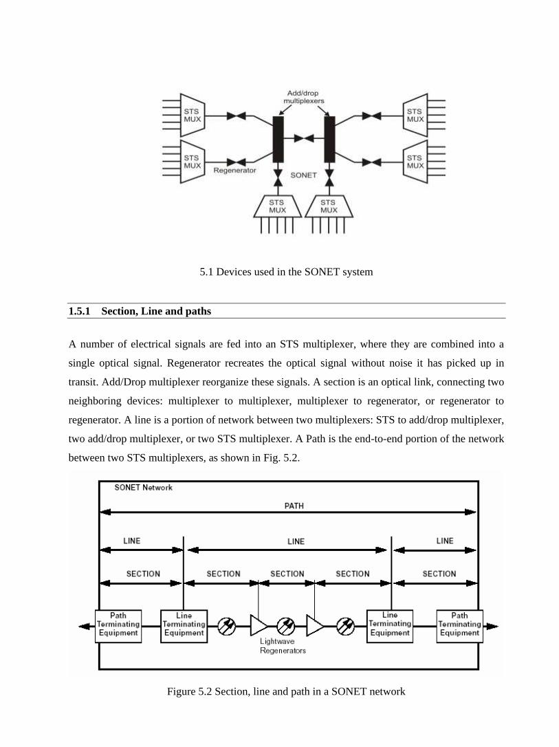
5.1 Devices used in the SONET system
1.5.1 Section, Line and paths
A number of electrical signals are fed into an STS multiplexer, where they are combined into a
single optical signal. Regenerator recreates the optical signal without noise it has picked up in
transit. Add/Drop multiplexer reorganize these signals. A section is an optical link, connecting two
neighboring devices: multiplexer to multiplexer, multiplexer to regenerator, or regenerator to
regenerator. A line is a portion of network between two multiplexers: STS to add/drop multiplexer,
two add/drop multiplexer, or two STS multiplexer. A Path is the end-to-end portion of the network
between two STS multiplexers, as shown in Fig. 5.2.
Figure 5.2 Section, line and path in a SONET network

1.5.2 SONET Network Elements
Terminal Multiplexer
The path terminating element (PTE), an entry-level path-terminating terminal multiplexer, acts as a
concentrator of DS–1s as well as other tributary signals. Its simplest deployment would involve
two terminal multiplexers linked by fiber with or without a regenerator in the link. This
implementation represents the simplest SONET link (a section, line, and path all in one link; see
Figure 5.3).
Figure 5.3 Terminal Multiplexer
Regenerator
A regenerator is needed when, due to the long distance between multiplexers, the signal level in
the fiber becomes too low. The regenerator clocks itself off of the received signal and replaces the
section overhead bytes before retransmitting the signal. The line overhead, payload, and POH are
not altered (see Figure 5.4).
Figure5.4Regenerator
Add/Drop Multiplexer (ADM)
A single-stage multiplexer/ demultiplexer can multiplex various input into an OCN signal. It can
add signals coming from different sources into a given path or remove a desired signal from a path
and redirect it without demultiplexing the entire signal, as shown in Fig. 4.3.5. Instead of relying

on timing and bit positions, add/drop multiplexer uses header information such as addresses and
pointers to identify individual streams.
Figure 5.5 Add/drop Multiplexer
In rural applications, an ADM can be deployed at a terminal site or any intermediate location for
consolidating traffic from widely separated locations. Several ADMs can also be configured as a
survivable ring. SONET enables drop and repeat (also known as drop and continue)—a key
capability in both telephony and cable TV applications. With drop and repeat, a signal terminates
at one node, is duplicated (repeated), and is then sent to the next and subsequent nodes.
The add/drop multiplexer provides interfaces between the different network signals and SONET
signals. Single-stage multiplexing can multiplex/demultiplex one or more tributary (DS–1) signals
into/from an STS–N signal. It can be used in terminal sites, intermediate (add/drop) sites, or hub
configurations. At an add/drop site, it can drop lower-rate signals to be transported on different
facilities, or it can add lower-rate signals into the higher-rate STS–N signal. The rest of the traffic
simply continues straight through.
Wideband Digital Cross-Connects
A SONET cross-connect accepts various optical carrier rates, accesses the STS–1 signals, and
switches at this level. It is ideally used at a SONET hub as shown in Fig. 5.6. One major difference
between a cross-connect and an add/drop multiplexer is that a cross-connect may be used to
interconnect a much larger number of STS–1s. The broadband cross-connect can be used for
grooming (consolidating or segregating) of STS–1s or for broadband traffic management. For
example, it may be used to segregate high-bandwidth from low-bandwidth traffic and send it
separately to the high-bandwidth (e.g., video) switch and a low-bandwidth (voice) switch. It is the
synchronous equivalent of a DS–3 digital cross-connect and supports hubbed network.

Figure 5.6 Wideband digital cross-connect
1.6 Frame Format Structure
SONET uses a basic transmission rate of STS–1 that is equivalent to 51.84 Mbps. Higher-level
signals are integer multiples of the base rate. For example, STS–3 is three times the rate of STS–1
(3 x 51.84 = 155.52 Mbps). An STS–12 rate would be 12 x 51.84 = 622.08 Mbps. SONET is based
on the STS-1 frame. STS-1 Frame Format is shown in Fig. 5.7.
• STS-1 consists of 810 octets
o 9 rows of 90 octets
o 27 overhead octets formed from the first 3 octets of each row
▪ 9 used for section overhead
▪ 18 used for line overhead
o 87x9 = 783 octets of payload
▪ one column of the payload is path overhead - positioned by a pointer in the
line overhead
o Transmitted top to bottom, row by row from left to right
• STS-1 frame transmitted every 125 us: thus a transmission rate of 51.84 Mbps.
The synchronous payload envelope can also be divided into two parts: the STS path overhead
(POH) and the payload. Transport overhead is composed of section overhead and line overhead.
The STS–1 POH is part of the synchronous payload envelope. The first three columns of each
STS–1 frame make up the transport overhead, and the last 87 columns make up the SPE. SPEs can
have any alignment within the frame, and this alignment is indicated by the H1 and H2 pointer
bytes in the line overhead.

Figure 5. 7 STS1 Frame format
1.7 OVERHEAD
SONET overhead is not added as headers or trailers as we have seen in other protocols. Instead,
SONET inserts overhead at a variety of locations in middle of the frame. The meaning s and
location of these insertions are discussed below. The overhead information has several layers,
which will also be discussed in this section.
SONET Layers: SONET defines 4 layers, namely photonic layer, Section layer, Line layer and
Path layer. The photonic layer is the lowest and performs the physical layer activities while all
other 3 layers correspond to Data link layer of OSI model. The photonic layer includes physical
specifications for the optical fiber channel, the sensitivity of the receiver, multiplexing functions
and so on. It uses NRZ encoding.
• Section Layer and Overhead: This layer is responsible for movement of a signal across a
physical section. It handles framing, scrambling, and error control. Section overhead which
is added in this layer contains 9 bytes of the transport overhead accessed, generated, and
processed by section-terminating equipment.
This overhead supports functions such as the following:
• performance monitoring (STS–N signal)
• local orderwire
• data communication channels to carry information for OAM&P

• framing
Figure 5.8 Section Overhead
Let’s discuss these overhead bytes in a bit more detail.
Framing bytes (A1, A2)—These two bytes indicate the beginning of an STS–1 frame. These are
used for framing and synchronization. These Bytes are also called as Alignment Bytes
Section trace (J0)/section growth (Z0)—This is also known as Identification Byte. It carries a
unique identifier for STS1 frame. This byte is necessary when multiple STS1 frames are multiplied
to create higher rate STS. Information in this byte allows the various signals to de-multiplex easily.
Parity byte (B1) —This is a for bit-interleaved parity (even parity), BIP used to check for
transmission errors over a regenerator section. Its value is calculated over all bits of the previous
STS–N frame after scrambling then placed in the B1 byte of STS–1 before scrambling. Therefore,
this byte is defined only for STS–1 number 1 of an STS–N signal
Orderwire byte (E1)—This byte is allocated to be used as a local orderwire channel for voice
communication between regenerators, hubs, and remote terminal locations.
User channel byte (F1)—This byte is set aside for the users' purposes. It terminates at all section-
terminating equipment within a line. It can be read and written to at each section-terminating
equipment in that line.
Data communications channel (DCC) bytes or Management byte (D1, D2, D3)—Together,
these 3 bytes form a 192–kbps message channel providing a message-based channel for OAM&P
between pieces of section-terminating equipment. The channel is used from a central location for
alarms, control, monitoring, administration, and other communication needs. It is available for
internally generated, externally generated, or manufacturer-specific messages.

• Line Layer and Overhead: This layer is responsible for the movement of a signal across a
physical line. STS multiplexer and add/drop multiplexers provide line layer functions. Line
overhead contains 18 bytes of overhead accessed, generated, and processed by line-
terminating equipment.
This overhead supports functions such as the following:
• locating the SPE in the frame
• multiplexing or concatenating signals
• performance monitoring
• automatic protection switching
• line maintenance
Line overhead is found in rows 4 to 9 of columns 1 to 9
Figure 5.9 Line Overhead
Let’s discuss these overhead bytes in a bit more detail.
STS payload pointer (H1 and H2)—Two bytes are allocated to a pointer that indicates the offset in
bytes between the pointer and the first byte of the STS SPE. The pointer bytes are used in all STS–1s
within an STS–N to align the STS–1 transport overhead in the STS–N and to perform frequency
justification. These bytes are also used to indicate concatenation and to detect STS path alarm indication
signals (AIS–P).
Pointer action byte (H3)—The pointer action byte is allocated for SPE frequency justification
purposes. The H3 byte is used in all STS–1s within an STS–N to carry the extra SPE byte in the event of
a negative pointer adjustment. The value contained in this byte when it is not used to carry the SPE byte
is undefined.
Line bit-interleaved parity code (BIP–8) byte (B2)—This parity code byte is used to determine if a
transmission error has occurred over a line. It is even parity and is calculated over all bits of the line
overhead and STS–1 SPE of the previous STS–1 frame before scrambling. The value is placed in the B2
byte of the line overhead before scrambling. This byte is provided in all STS–1 signals in an STS–N
signal.
Automatic protection switching (APS channel) bytes (K1, K2)—These 2 bytes are used for
protection signaling between line-terminating entities for bidirectional automatic protection switching
and for detecting alarm indication signal (AIS–L) and remote defect indication (RDI) signals.
Line Data communications channel (DCC) bytes (D4 to D12)—These 9 bytes form a 576–kbps
message channel from a central location for OAM&P information (alarms, control, maintenance, remote
provisioning, monitoring, administration, and other communication needs) between line entities. They
are available for internally generated, externally generated, and manufacturer-specific messages. A
protocol analyzer is required to access the line–DCC information.
Synchronization status (S1)—The S1 byte is located in the first STS–1 of an STS–N,
and bits 5 through 8 of that byte are allocated to convey the synchronization status of the network
element.
Growth (Z1)—The Z1 byte is located in the second through Nth STS–1s of an STS–N (3 <= N <= 48)
and are allocated for future growth. Note that an OC–1 or STS–1 electrical signal does not contain a Z1
byte.
STS–1 REI–L (M0)—The M0 byte is only defined for STS–1 in an OC–1 or STS–1 electrical signal.
Bits 5 through 8 are allocated for a line remote error indication function (REI–L, formerly referred to as
line FEBE), which conveys the error count detected by an LTE (using the line BIP–8 code) back to its
peer LTE.
STS–N REI–L (M1)—The M1 byte is located in the third STS–1 (in order of appearance in the byte-
interleaved STS–N electrical or OC–N signal) in an STS–N (N >= 3) and is used for a REI–L function.
Growth (Z2)—The Z2 byte is located in the first and second STS–1s of an STS–3 and the first, second,
and fourth through Nth STS–1s of an STS–N (12 <= N <= 48). These bytes are allocated for future
growth. Note that an OC–1 or STS–1 electrical signal does not contain a Z2 byte.
Orderwire byte (E2)—This orderwire byte provides a 64–kbps channel between line entities for an
express orderwire. It is a voice channel for use by technicians and will be ignored as it passes through
the regenerators.
1.8 Virtual Tributaries and Pointers
• Virtual Tributary
SONET is designed to carry broadband payloads. Current digital hierarchy data rates are lower
than STS1, so to make SONET backward compatible with the current hierarchy its frame
design includes a system of Virtual Tributaries (VTs). A virtual tributary is a partial payload
that can be inserted into an STS1 and combined with other partial payloads to fill out the
frame. Instead of using 86 payload columns of an STS1 frame for data from one source, we
can sub-divide the SPE and call each component as a VT.
• Pointers
SONET uses a concept called pointers to compensate for frequency and phase variations. Pointers
allow the transparent transport of synchronous payload envelopes (either STS or VT) across
plesiochronous boundaries (i.e., between nodes with separate network clocks having almost the
same timing). The use of pointers avoids the delays and loss of data associated with the use of
large (125-microsecond frame) slip buffers for synchronization.

Pointers provide a simple means of dynamically and flexibly phase-aligning STS and VT
payloads, thereby permitting ease of dropping, inserting, and cross-connecting these payloads in
the network. Transmission signal wander and jitter can also be readily minimized with pointers.
STS–1 pointers (H1 and H2 bytes) are the ones which allow the SPE to be separated from the
transport overhead. The pointer is simply an offset value that points to the byte where the SPE
begins.
• VT Mappings
There are several options for how payloads are actually mapped into the VT. Locked-mode VTs
bypass the pointers with a fixed byte-oriented mapping of limited flexibility. Floating mode
mappings use the pointers to allow the payload to float within the VT payload. There are three
different floating mode mappings—asynchronous, bit-synchronous, and byte-synchronous.
VT Type Bit Rate
(Mbps)
Size of VT
VT 1.5 1.728 9 rows, 3
columns
VT 2 2.304 9 rows, 4
columns
VT 3 3.456 9 rows, 6
columns
VT 6 6.912 9 rows, 12
columns
Figure 5.10 VTs
To accommodate mixes of different VT types within an STS–1 SPE, the VTs are grouped together.
An SPE can carry a mix of any of the seven groups. The groups have no overhead or pointers; they
are just a means of organizing the different VTs within an STS–1 SPE. Because each of the VT
groups is allocated 12 columns of the SPE, a VT group would contain one of the following
combinations:
• Four VT1.5s (with 3 columns per VT1.5)
• Three VT2s (with 4 columns per VT2)
• Two VT3s (with 6 columns per VT3)
• One VT6 (with 12 columns per VT6)

1.9 Check Your Progress
Fill in the blanks:
1. ………………developed a standard known as Synchronous Optical Network (SONET) by
utilizing the enormous bandwidth of optical fiber.
2. Digital switches and digital cross-connect systems are commonly employed in the
………………..synchronization hierarchy.
3. SONET is designed to carry ……………….
4. SONET uses a concept called …………………to compensate for frequency and phase
variations
1.10 Answer to Check Your Progress
1. ANSI
2. digital network
3. broadband payloads.
4. pointers

Block-3
Unit-1
X.25 and Frame Relay
1.1 Learning Objective
1.2 Introduction
1.3 Devices and Protocol Operation
1.4 X.25 session establishment and virtual circuits
1.5 X.25 Protocol Suite
1.6 Introduction to Frame Relay
1.7 Frame Relay Devices
1.8 Virtual Circuits
1.8.1 Switched Virtual Circuits
1.8.2 Permanent Virtual Circuits
1.8.3 Data-Link Connection Identifier (DLCI)
1.8.4 DLCIs inside the network
1.9 Frame Relay Layers
1.10 Check Your Progress
1.11 Answer to Check Your Progress
1.1 Learning Objective
After going through this unit the learner will able to:
• State the key features of X.25
• Explain the frame format of X.25
• Specify the function of the Packet layer of X.25
• State the limitations of X.25
• State the limitations of X.25
• Explain the key features of Frame Relay
• Specify the Frame relay frame format
• Explain how congestion control is performed in Frame relay network
1.2 Introduction
In the early 1970's there were many data communication networks (also known as Public
Networks), which were owned by private companies, organizations and governments agencies.
Since those public networks were quite different internally, and the interconnection of networks
was growing very fast, there was a need for a common network interface protocol.
In 1976 X.25 was recommended as the desired protocol by the International Consultative
Committee for Telegraphy and Telephony (CCITT) called the International
Telecommunication Union (ITU) since 1993.
X.25 is a standard for WAN communications that defines how connections between user devices
and network devices are established and maintained. X.25 is designed to operate effectively
regardless of the type of systems connected to the network. It is typically used in the packet-
switched networks (PSNs) of common carriers, such as the telephone companies. Subscribers are
charged based on their use of the network.
1.3 Devices and Protocol Operation
X.25 network devices fall into three general categories: data terminal equipment (DTE), data
circuit-terminating equipment (DCE), and packet-switching exchange (PSE) as shown in Fig. 1.1.
Data terminal equipment (DTE) devices are end systems that communicate across the X.25
network. They are usually terminals, personal computers, or network hosts, and are located on the
premises of individual subscribers. Data communication Equipments (DCEs) are communications
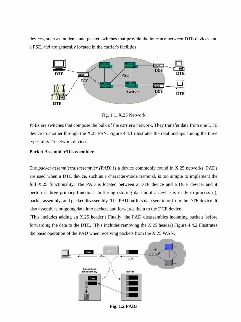
devices, such as modems and packet switches that provide the interface between DTE devices and
a PSE, and are generally located in the carrier's facilities.
Fig. 1.1. X.25 Network
PSEs are switches that compose the bulk of the carrier's network. They transfer data from one DTE
device to another through the X.25 PSN. Figure 4.4.1 illustrates the relationships among the three
types of X.25 network devices
Packet Assembler/Disassembler
The packet assembler/disassembler (PAD) is a device commonly found in X.25 networks. PADs
are used when a DTE device, such as a character-mode terminal, is too simple to implement the
full X.25 functionality. The PAD is located between a DTE device and a DCE device, and it
performs three primary functions: buffering (storing data until a device is ready to process it),
packet assembly, and packet disassembly. The PAD buffers data sent to or from the DTE device. It
also assembles outgoing data into packets and forwards them to the DCE device.
(This includes adding an X.25 header.) Finally, the PAD disassembles incoming packets before
forwarding the data to the DTE. (This includes removing the X.25 header) Figure 4.4.2 illustrates
the basic operation of the PAD when receiving packets from the X.25 WAN.
Fig. 1.2 PADs
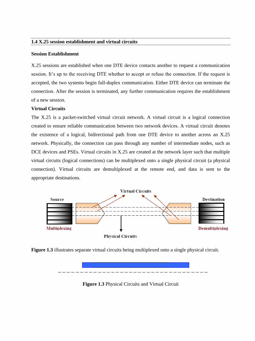
1.4 X.25 session establishment and virtual circuits
Session Establishment
X.25 sessions are established when one DTE device contacts another to request a communication
session. It’s up to the receiving DTE whether to accept or refuse the connection. If the request is
accepted, the two systems begin full-duplex communication. Either DTE device can terminate the
connection. After the session is terminated, any further communication requires the establishment
of a new session.
Virtual Circuits
The X.25 is a packet-switched virtual circuit network. A virtual circuit is a logical connection
created to ensure reliable communication between two network devices. A virtual circuit denotes
the existence of a logical, bidirectional path from one DTE device to another across an X.25
network. Physically, the connection can pass through any number of intermediate nodes, such as
DCE devices and PSEs. Virtual circuits in X.25 are created at the network layer such that multiple
virtual circuits (logical connections) can be multiplexed onto a single physical circuit (a physical
connection). Virtual circuits are demultiplexed at the remote end, and data is sent to the
appropriate destinations.
Figure 1.3 illustrates separate virtual circuits being multiplexed onto a single physical circuit.
Figure 1.3 Physical Circuits and Virtual Circuit
Two types of X.25 virtual circuits exist: switched and permanent. Switched virtual circuits (SVCs)
are temporary connections used for sporadic data transfers. They require that two DTE devices to
establish, maintain, and terminate a session each time the devices need to communicate. Permanent
virtual circuits (PVCs) are permanently established connections used for frequent and consistent
data transfers. PVCs do not require that sessions be established and terminated. Therefore, DTEs
can begin transferring data whenever necessary because the session is always active.
The basic operation of an X.25 virtual circuit begins when the source DTE device specifies the
virtual circuit to be used (in the packet headers) and then sends the packets to a locally connected
DCE device. At this point, the local DCE device examines the packet headers to determine which
virtual circuit to use and then sends the packets to the closest PSE in the path of that virtual circuit.
PSEs (switches) pass the traffic to the next intermediate node in the path, which may be another
switch or the remote DCE device.
When the traffic arrives at the remote DCE device, the packet headers are examined and the
destination address is determined. The packets are then sent to the destination DTE device. If
communication occurs over an SVC and neither device has additional data to transfer, the virtual
circuit is terminated.
1.5 X.25 Protocol Suite
The X.25 protocol suite maps to the lowest three layers of the OSI reference model as shown in
Figure 1.4. The layers are:
• Physical layer: Deals with the physical interface between an attached station and the link
that attaches that station to the packet-switching node.
o X.21 is the most commonly used physical layer standard.
• Frame layer: Facilitates reliable transfer of data across the physical link by transmitting
the data as a sequence of frames. Uses a subset of HDLC known as Link Access Protocol
Balanced (LAPB), bit oriented protocol.
• Packet layer: Responsible for end-to-end connection between two DTEs. Functions
performed are:
o Establishing connection
o Transferring data
o Terminating a connection
o Error and flow control

o With the help of X.25 packet layer, data are transmitted in packets over external virtual
circuits.
Figure 1.4 X.25 Layer mapping with OSI model
Physical Layer
At the physical layer X.21 is specifically defined for X.25 by ITU-T. The X.21 interface operates
over eight interchange circuits (i.e., signal ground, DTE common return, transmit, receive, control,
indication, signal element timing and byte timing) their functions is defined in recommendation of
X.24 and their electrical characteristics in recommendation of X.27. The recommendation specifies
how the DTE can setup and clear calls by exchanging signals with the DCE.
The physical connector has 15 pins, but not all of them are used. The DTE uses the T and C
circuits to transmit data and control information. The DCE uses the R and I circuits for data and
control. The S circuit contains a signal stream emitted by the DCE to provide timing information
so the DTE knows when each bit interval starts and stops. The B circuit may also provide to group
the bits into byte frames. If this option is not provided the DCE and DTE must begin every control
sequence with at least two SYN characters to enable each other to deduce the implied frame
boundary.
Figure 1.5 X.21 signals

Link Layer
The link layer (also called level 2, or frame level) ensures reliable transfer of data between the
DTE and the DCE, by transmitting the data as a sequence of frames (a frame is an individual data
unit which contains address, control, information field etc.).
The functions performed by the link level include:
• Transfer of data in an efficient and timely fashion.
• Synchronization of the link to ensure that the receiver is in step with the transmitter.
• Detection of transmission errors and recovery from such errors
• Identification and reporting of procedural errors to higher levels, for recovery.
The link level uses data link control procedures, which are compatible with the High Level Data
Link (HDLC) standardized by ISO, and with the Advanced Data Communications Control
Procedures (ADCCP) standardized by the U.S. American National Standards Institute (ANSI).
There are several protocols, which can be used in the link level:
• Link Access Protocol, Balanced (LAPB) is derived from HDLC and is the most
commonly used. It enables to form a logical link connection besides all the other
characteristics of HDLC.
• Link Access Protocol (LAP) is an earlier version of LAPB and is seldom used today.
• Link Access Procedure, D Channel (LAPD) is derived from LAPB and it is used for
Integrated Services Digital Networks (ISDN) i.e. it enables data transmission between
DTEs through D channel, especially between a DTE and an ISDN node.
• Logical Link Control (LLC) is an IEEE 802 Local Area Network (LAN) protocol, which
enables X.25 packets to be transmitted through a LAN channel.
Now let us discuss the most commonly used link layer protocol, i.e. LAPB. LAPB is a bit-oriented
protocol that ensures that frames are correctly ordered and error-free. There are three kinds of
frames:
1. Information: This kind of frame contains the actual information being transferred and
some control information. The control field in these frames contains the frame sequence
number. I-frame functions include sequencing, flow control, and error detection and
recovery. I-frames carry send- and receive-sequence numbers.
2. Supervisory: The supervisory frame (S-frame) carries control information. S-frame
functions include requesting and suspending transmissions, reporting on status, and

acknowledging the receipt of I-frames. S-frames carry only receive-sequence numbers.
There are various types of supervisory frames.
o RECEIVE READY-Acknowledgment frame indicating the next frame expected.
o REJECT-Negative acknowledgment frame used to indicate transmission error
detection.
o RECEIVE NOT READY (RNR)-Just as RECEIVE READY but tells the sender
to stop sending due to temporary problems.
3. Unnumbered: This kind of frames is used only for control purposes. U-frame functions
include link setup and disconnection, as well as error reporting. U frames carry no
sequence numbers.
Packet Level
This level governs the end-to-end communications between the different DTE devices. Layer 3 is
concerned with connection set-up and teardown and flow control between the DTE devices, as
well as network routing functions and the multiplexing of simultaneous logical connections over a
single physical connection. PLP is the network layer protocol of X.25.
Call setup mode is used to establish SVCs between DTE devices. A PLP uses the X.121
addressing scheme to set up the virtual circuit. The call setup mode is executed on a per-virtual-
circuit basis, which means that one virtual circuit can be in call setup mode while another is in data
transfer mode. This mode is used only with SVCs, not with PVCs. To establish a connection on an
SVC, the calling DTE sends a Call Request Packet, which includes the address of the remote DTE
to be contacted. The destination DTE decides whether or not to accept the call (the Call Request
packet includes the sender's DTE address, as well as other information that the called DTE can use
to decide whether or not to accept the call). A call is accepted by issuing a Call Accepted packet,
or cleared by issuing a Clear Request packet. Once the originating DTE receives the Call
Accepted packet, the virtual circuit is established and data transfer may take place.

Figure 1.6 Different Modes of PLP
Different phases of call set-up, data transfer, call release has been shown in Fig. 1.6. The PLP
operates in five distinct modes: call setup, data transfer, idle, call clearing, and restarting.
• Data transfer mode is used for transferring data between two DTE devices across a virtual
circuit. In this mode, PLP handles segmentation and reassembly, bit padding, and error and
flow control. This mode is executed on a per-virtual-circuit basis and is used with both
PVCs and SVCs.
• Idle mode is used when a virtual circuit is established but data transfer is not occurring. It
is executed on a per-virtual-circuit basis and is used only with SVCs.
• Call clearing mode is used to end communication sessions between DTE devices and to
terminate SVCs. This mode is executed on a per-virtual-circuit basis and is used only with
SVCs. When either DTE wishes to terminate the call, a Clear Request packet is sent to the
remote DTE, which responds with a Clear Confirmation packet.
• Restarting mode is used to synchronize transmission between a DTE device and a locally
connected DCE device. This mode is not executed on a per-virtual-circuit basis. It affects
all the DTE device's established virtual circuits.
Four types of PLP packet fields exist:
• General Format Identifier (GFI)—Identifies packet parameters, such as whether the
packet carries user data or control information, what kind of windowing is being used, and
whether delivery confirmation is required.
• Logical Channel Identifier (LCI)—identifies the virtual circuit across the local
DTE/DCE interface.
• Packet Type Identifier (PTI)—identifies the packet as one of 17 different PLP packet
types.
• User Data—Contains encapsulated upper-layer information. This field is present only in
data packets. Otherwise, additional fields containing control information are added.
1.6 Introduction to Frame Relay
Frame Relay is a high-performance WAN protocol that operates at the physical and data link
layers of the OSI reference model. Frame Relay originally was designed for use across Integrated
Services Digital Network (ISDN) interfaces. Today, it is used over a variety of other network
interfaces as well. Frame Relay is a simplified form of Packet Switching, similar in principle to
X.25, in which synchronous frames of data are routed to different destinations depending on
header information. The biggest difference between Frame Relay and X.25 is that X.25 guarantees
data integrity and network managed flow control at the cost of some network delays. Frame Relay
switches packets end to end much faster, but there is no guarantee of data integrity at all.
As line speeds have increased from speeds below 64kbps to T1/E1 and beyond, the delays inherent
in the store-and-forward mechanisms of X.25 become intolerable. At the same time, improvements
in digital transmission techniques have reduced line errors to the extent that node-to-node error
correction throughout the network is no longer necessary. The vast majority of Frame Relay traffic
consists of TCP/IP or other protocols that provide their own flow control and error correction
mechanisms. Much of this traffic is fed into the Internet, another packet switched network without
any built-in error control.
Because Frame Relay does not 'care' whether the frame it is switching is error-free or not, a Frame
Relay node can start switching traffic out onto a new line as soon as it has read the first two bytes
of addressing information at the beginning of the frame. Thus a frame of data can travel end-to-
end, passing through several switches, and still arrive at its destination with only a few bytes'
delay. These delays are small enough that network latency under Frame Relay is not noticeably
different from direct leased line connections. As a result, the performance of a Frame Relay
network is virtually identical to that of a leased line, but because most of the network is shared,
costs are lower.
Frame Relay is an example of a packet-switched technology. Packet-switched networks enable
end stations to dynamically share the network medium and the available bandwidth. The following
two techniques are used in packet-switching technology:
• Variable-length packets
• Statistical multiplexing
Variable-length packets are used for more efficient and flexible data transfers. These packets are
switched between the various segments in the network until the destination is reached.
Statistical multiplexing techniques control network access in a packet-switched network. The
advantage of this technique is that it accommodates more flexibility and more efficient use of
bandwidth. Most of today's popular LANs, such as Ethernet and Token Ring, are packet-switched
networks.
1.7 Frame Relay Devices
Devices attached to a Frame Relay WAN fall into the following two general categories:
• Data terminal equipment (DTE)
• Data circuit-terminating equipment (DCE)
DTEs generally are considered to be terminating equipment for a specific network and typically
are located on the premises of a customer. In fact, they may be owned by the customer. Examples
of DTE devices are terminals, personal computers, routers, and bridges.
DCEs are carrier-owned internetworking devices. The purpose of DCE equipment is to provide
clocking and switching services in a network, which are the devices that actually transmit data
through the WAN. In most cases, these are packet switches.
The connection between a DTE device and a DCE device consists of both a physical layer
component and a link layer component. The physical component defines the mechanical,
electrical, functional, and procedural specifications for the connection between the devices. One of
the most commonly used physical layer interface specifications is the recommended standard
(RS)-232 specification. The link layer component defines the protocol that establishes the
connection between the DTE device, such as a router, and the DCE device, such as a switch.
1.8 Virtual Circuits
Frame Relay is a virtual circuit network, so it doesn’t use physical addresses to define the DTEs
connected to the network. Frame Relay provides connection-oriented data link layer
communication. This means that a defined communication exists between each pair of devices and
that these connections are associated with a connection identifier. However, virtual circuit
identifiers in Frame relay operate at the data link layer, in contrast with X.25, where they operate
at the network layer. This service is implemented by using a Frame Relay virtual circuit, which is a
logical connection created between two data terminal equipment (DTE) devices across a Frame
Relay packet-switched network (PSN).
Virtual circuits provide a bidirectional communication path from one DTE device to another and
are uniquely identified by a data-link connection identifier (DLCI). A number of virtual circuits
can be multiplexed into a single physical circuit for transmission across the network. This
capability often can reduce the equipment and network complexity required to connect multiple
DTE devices.
A virtual circuit can pass through any number of intermediate DCE devices (switches) located
within the Frame Relay PSN. Before going into the details of DLCI let us first have a look at the
two types of Frame Relay Circuits, namely: switched virtual circuits (SVCs) and permanent virtual
circuits (PVCs).
1.8.1 Switched Virtual Circuits
Switched virtual circuits (SVCs) are temporary connections used in situations requiring only
sporadic data transfer between DTE devices across the Frame Relay network. A communication
session across an SVC consists of the following four operational states:
• Call setup—The virtual circuit between two Frame Relay DTE devices is established.
• Data transfer—Data is transmitted between the DTE devices over the virtual circuit.
• Idle—The connection between DTE devices is still active, but no data is transferred. If an
SVC remains in an idle state for a defined period of time, the call can be terminated.
• Call termination—The virtual circuit between DTE devices is terminated.
After the virtual circuit is terminated, the DTE devices must establish a new SVC if there is
additional data to be exchanged. It is expected that SVCs will be established, maintained, and
terminated using the same signaling protocols used in ISDN.

1.8.2 Permanent Virtual Circuits
Permanent virtual circuits (PVCs) are permanently established connections that are used for
frequent and consistent data transfers between DTE devices across the Frame Relay network.
Communication across PVC does not require the call setup and termination states that are used
with SVCs. PVCs always operate in one of the following two operational states:
▪ Data transfer: Data is transmitted between the DTE devices over the virtual circuit.
▪ Idle: The connection between DTE devices is active, but no data is transferred.
Unlike SVCs, PVCs will not be terminated under any circumstances when in an idle state. DTE
devices can begin transferring data whenever they are ready because the circuit is permanently
established.
1.8.3 Data-Link Connection Identifier (DLCI)
Frame Relay virtual circuits are identified by data-link connection identifiers (DLCIs). DLCI
values typically are assigned by the Frame Relay service provider (for example, the telephone
company). Frame Relay DLCIs have local significance, which means that their values are unique
in the LAN, but not necessarily in the Frame Relay WAN. The local DTEs use this DLCI to send
frames to the remote DTE.
(a). Connection from A to D (b). Connection from D to E

(c). Connection from D to A
Figure 1.7 DLCIs connection between different DTEs
Figure 1.7 shows the assignments of DLCIs, 3 connections have been shown namely, between A
to D, D to E, and D to B. Point Here to be noted is that connection in fig.(a) and in fig.(c) uses the
same DLCI, this can be done because these DLCIs are used by local DTEs. Bothe the connectons
are valid as they define different virtual circuits originating from different DTEs.
1.8.4 DLCIs inside the network
DLCIs are not only used to define the virtual circuit between a DTE and a DCE, but also to define
the virtual circuit between two DCEs (switches) inside the network. A switch assigns a DLCI to
each virtual connection in an interface. This means that two different connections belonging to two
different interfaces may have the same DLCIs (as shown in the above figure). In other words,
DLCIs are unique for a particular interface.
A connection between DTE A and DTE D has been shown in this figure, DLCI assigned inside the
Frame Relay network is also shown in the network. DCEs inside the network use incoming
interface – DLCI combination to decide the outgoing interface – DLCI combination to switch out
the frame, from that DCE.

Figure 1.8 DLCIs inside Frame relay network
Each switch in a Frame relay network has a table to route frames The table matches the incoming
interface- DLCI combination with an outgoing interface-DLCI combination. Figure 1.9 shows two
frames arriving at the switch on interface2, one with DLCI=11 and other with DLCI= 213.
Figure 1.9 Frame Relay switch table
1.9 Frame Relay Layers
Frame Relay has only 2 layers, namely Physical layer and Data Link layer. And as compared to
other layer of packet switching network such as X.25, frame relay has only 1.5 layers whereas
X.25 has 2 layers. Frame Relay eliminates all network layer functions and a portion of
conventional data-link layer functions.

Physical Layer
No specific protocol is defined for physical layer in frame relay. Frame relay supports any one of
the protocols recognized by ANSI, and thus the choice of physical layer protocol is up to the
implementer.
Data Link Layer
At Data-link Layer Frame employs a simpler version of HDLC. Simpler version is used because
HDLC provides extensive error and flow control fields that are not needed in frame relay.
To understand much of the functionality of Frame Relay, it is helpful to understand the structure of
the Frame Relay frame. Figure 1.10 depicts the basic format of the Frame Relay frame. Flags
indicate the beginning and end of the frame. Three primary components make up the Frame Relay
frame: the header and address area, the user-data portion, and the frame check sequence (FCS).
The address area, which is 2 bytes in length, is comprised of 10 bits representing the actual circuit
identifier and 6 bits of fields related to congestion management. This identifier commonly is
referred to as the data-link connection identifier (DLCI).
Figure 1.10 Frame Relay frame format
• Flags—Delimits the beginning and end of the frame. The value of this field is
always the same and is represented either as the hexadecimal number 7E or as the
binary number 01111110.
• Address—Contains the following information:
DLCI—The 10-bit DLCI is the essence of the Frame Relay header. This value represents the
virtual connection between the DTE device and the switch. Each virtual connection that is
multiplexed onto the physical channel will be represented by a unique DLCI. The DLCI values
have local significance only, which means that they are unique only to the physical channel on
which they reside. Therefore, devices at opposite ends of a connection can use different DLCI

values to refer to the same virtual connection. The first 6-bits of the first byte make up part 1 of the
DLCI, and second part of DLCI uses the first 4-bits of second byte.
Extended Address (EA)—The EA is used to indicate whether the byte in which the EA value is 1
is the last addressing field. If the value is 1, then the current byte is determined to be the last DLCI
octet. Although current Frame Relay implementations all use a two-octet DLCI, this capability
does allow longer DLCIs to be used in the future. The eighth bit of each byte of the Address field
is used to indicate the EA.
C/R—The C/R is the bit that follows the most significant DLCI byte in the Address field. The C/R
bit is not currently defined.
Congestion Control—This consists of the 3 bits that control the Frame Relay congestion-
notification mechanisms. These are the FECN, BECN, and DE bits, which are the last 3 bits in the
Address field.
Forward-explicit congestion notification (FECN) is a single-bit field that can be set to a value of 1
by a switch to indicate to an end DTE device, such as a router, that congestion was experienced in
the direction of the frame transmission from source to destination as shown in Fig. 1.11. The
primary benefit of the use of the FECN and BECN fields is the capability of higher-layer protocols
to react intelligently to these congestion indicators. Today, DECnet and OSI are the only higher-
layer protocols that implement these capabilities.
Figure 1.11 Forward-explicit congestion notification
Backward-explicit congestion notification (BECN) is a single-bit field that, when set to a value of 1
by a switch, indicates that congestion was experienced in the network in the direction opposite of
the frame transmission from source to destination.
Discard eligibility (DE) is set by the DTE device, such as a router, to indicate that the marked
frame is of lesser importance relative to other frames being transmitted. Frames that are marked as
"discard eligible" should be discarded before other frames in a congested network. This allows for
a basic prioritization mechanism in Frame Relay networks.

Figure 1.12 Backward-explicit congestion notification
• Data—Contains encapsulated upper-layer data. Each frame in this variable-length field
includes a user data or payload field that will vary in length up to 16,000 octets. This field
serves to transport the higher-layer protocol packet (PDU) through a Frame Relay network.
• Frame Check Sequence—Ensures the integrity of transmitted data. This value is
computed by the source device and verified by the receiver to ensure integrity of
transmission.
1.10 Check Your Progress
Fill in the blanks:
1. Frame Relay is a high-performance ______ protocol.
2. Frame Relay operates at the __________ and _____________ layers of the OSI reference
model.
3. Frame Relay requires Error Checking at the _________ layer.
4. Frame Relay is a simplified form of ______________ switching, similar in principle to
_______.
5. Frame Relay is a ___________________ network
6. Frame Relay virtual circuits are identified by ___________.
7. ______ bit in address field in frame relay is set to one to signify the last address bit.
8. Routing and switching in Frame Relay is performed by ________ layer.
9. ________ data are allowed on a Frame Relay Network.
10. Frame relay is not suited well for ______ due to the delay resulting from varying sizes of
Frame.

1.11 Answer to Check Your Progress
1. WAN
2. Physical, data link
3. Data link
4. Circuit, X.25
5. Virtual switched
6. DLCIs.
7. Extended Address (EA)
8. Data link layer
9. Encapsulated upper layer
10. Real time traffic
Unit-2
Asynchronous Transfer Mode Switching (ATM)
1.1 Learning Objectives
1.2 Introduction
1.3 Benefits of ATM
1.4 ATM Devices and the Network Environment
1.5 ATM Cell Format
1.6 ATM Virtual Connections
1.7 ATM Reference Model
1.8 ATM Applications
1.9 Check Your Progress
1.10 Answer to Check Your Progress

1.1 Learning Objectives
After going through this unit the learner will able to learn:
• State the need for ATM
• Explain the concept of cell switching
• Specify the architecture of ATM
• Explain the operation of Virtual connections and switching types used
• Explain switching fabric of ATM
• Explain the functions of the three ATM layers
1.2 Introduction
Asynchronous Transfer Mode (ATM) is an International Telecommunication Union-
Telecommunications Standards Section (ITU-T) standard for cell relay wherein information for
multiple service types, such as voice, video, or data, is conveyed in small, fixed-size cells. ATM
networks are connection-oriented. Asynchronous transfer mode (ATM) is a technology that has its
history in the development of broadband ISDN in the 1970s and 1980s. Technically, it can be
viewed as an evolution of packet switching. Like packet switching protocols for data (e.g., X.25,
frame relay, Transmission Control Protocol and Internet protocol (TCP IP]), ATM integrates the
multiplexing and switching functions, is well suited for bursty traffic (in contrast to circuit
switching), and allows communications between devices that operate at different speeds. Unlike
packet switching, ATM is designed for high-performance multimedia networking. ATM
technology has been implemented in a very broad range of networking devices. The most basic
service building block is the ATM virtual circuit, which is an end-to-end connection that has
defined end points and routes but does not have bandwidth dedicated to it. Bandwidth is allocated
on demand by the network as users have traffic to transmit. ATM also defines various classes of
service to meet a broad range of application needs. This lesson provides an overview of ATM
protocols, services, and operation.
1.3 Benefits of ATM
The high-level benefits delivered through ATM services deployed on ATM technology using
international ATM standards can be summarized as follows:

• Dynamic bandwidth for bursty traffic meeting application needs and delivering high
utilization of networking resources; most applications are or can be viewed as inherently
bursty, for example voice is bursty, as both parties are neither speaking at once nor all the
time; video is bursty, as the amount of motion and required resolution varies over time.
• Smaller header with respect to the data to make the efficient use of bandwidth.
• Can handle Mixed network traffic very efficiently: Variety of packet sizes makes traffic
unpredictable. All network equipments should incorporate elaborate software systems to
manage the various sizes of packets. ATM handles these problems efficiently with the
fixed size cell.
• Cell network: All data is loaded into identical cells that can be transmitted with complete
predictability and uniformity.
• Class-of-service support for multimedia traffic allowing applications with varying
throughput and latency requirements to be met on a single network.
• Scalability in speed and network size supporting link speeds of T1/E1 to OC–12 (622
Mbps).
• Common LAN/WAN architecture allowing ATM to be used consistently from one
desktop to another; traditionally, LAN and WAN technologies have been very different,
with implications for performance and interoperability. But ATM technology can be used
either as a LAN technology or a WAN technology.
• International standards compliance in central-office and customer-premises
environments allowing for multivendor operation.
1.4 ATM Devices and the Network Environment
ATM is a cell-switching and multiplexing technology that combines the benefits of circuit
switching (guaranteed capacity and constant transmission delay) with those of packet switching
(flexibility and efficiency for intermittent traffic). It provides scalable bandwidth from a few
megabits per second (Mbps) to many gigabits per second (Gbps). Because of its asynchronous
nature, ATM is more efficient than synchronous technologies, such as time-division multiplexing
(TDM).
With TDM, each user is assigned to a time slot, and no other station can send in that time slot as
shown in Fig. 2.1. If a station has much data to send, it can send only when its time slot comes up,
even if all other time slots are empty. However, if a station has nothing to transmit when its time
slot comes up, the time slot is sent empty and is wasted.

Figure 2.1 Normal TDM operation
Because ATM is asynchronous, time slots are available on demand with information identifying
the source of the transmission contained in the header of each ATM cell. Figure 2.2 shows how
cells from 3 inputs have been multiplexed. At the first clock tick input 2 has no data to send, so
multiplexer fills the slot with the cell from third input. When all cells from input channel are
multiplexed then output slot are empty.
Figure 2.2 Asynchronous multiplexing of ATM
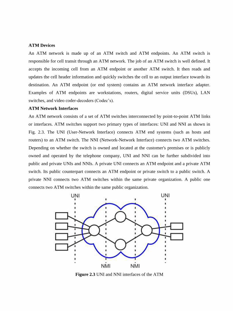
ATM Devices
An ATM network is made up of an ATM switch and ATM endpoints. An ATM switch is
responsible for cell transit through an ATM network. The job of an ATM switch is well defined. It
accepts the incoming cell from an ATM endpoint or another ATM switch. It then reads and
updates the cell header information and quickly switches the cell to an output interface towards its
destination. An ATM endpoint (or end system) contains an ATM network interface adapter.
Examples of ATM endpoints are workstations, routers, digital service units (DSUs), LAN
switches, and video coder-decoders (Codec’s).
ATM Network Interfaces
An ATM network consists of a set of ATM switches interconnected by point-to-point ATM links
or interfaces. ATM switches support two primary types of interfaces: UNI and NNI as shown in
Fig. 2.3. The UNI (User-Network Interface) connects ATM end systems (such as hosts and
routers) to an ATM switch. The NNI (Network-Network Interface) connects two ATM switches.
Depending on whether the switch is owned and located at the customer's premises or is publicly
owned and operated by the telephone company, UNI and NNI can be further subdivided into
public and private UNIs and NNIs. A private UNI connects an ATM endpoint and a private ATM
switch. Its public counterpart connects an ATM endpoint or private switch to a public switch. A
private NNI connects two ATM switches within the same private organization. A public one
connects two ATM switches within the same public organization.
Figure 2.3 UNI and NNI interfaces of the ATM

1.5 ATM Cell Format
ATM transfers information in fixed-size units called cells. Each cell consists of 53 octets, or bytes
as shown in Fig. 2.4. The first 5 bytes contain cell-header information, and the remaining 48
contain the payload (user information). Small, fixed-length cells are well suited to transfer voice
and video traffic because such traffic is intolerant to delays that result from having to wait for a
large data packet to download, among other things.
Figure 2.4 ATM cell Format
An ATM cell header can be one of two formats: UNI or NNI. The UNI header is used for
communication between ATM endpoints and ATM switches in private ATM networks. The NNI
header is used for communication between ATM switches. Figure 2.5 depicts the ATM UNI cell
header format, and the ATM NNI cell header format. Unlike the UNI, the NNI header does not
include the Generic Flow Control (GFC) field. Additionally, the NNI header has a Virtual Path
Identifier (VPI) field that occupies the first 12 bits, allowing for larger trunks between public ATM
switches.
Figure 2.5(a) UNI Cell Format Figure2.5 (b) NNI Cell Format
ATM Cell Header Fields
The following descriptions summarize the ATM cell header fields shown in Fig. 2.5.
• Generic Flow Control (GFC)—Provides local functions, such as identifying multiple
stations that share a single ATM interface. This field is typically not used and is set to its
default value of 0 (binary 0000).

• Virtual Path Identifier (VPI)—In conjunction with the VCI, identifies the next
destination of a cell as it passes through a series of ATM switches on the way to its
destination.
• Virtual Channel Identifier (VCI)—In conjunction with the VPI, identifies the next
destination of a cell as it passes through a series of ATM switches on the way to its
destination.
• Payload Type (PT)—Indicates in the first bit whether the cell contains user data or control
data. If the cell contains user data, the bit is set to 0. If it contains control data, it is set to 1.
The second bit indicates congestion (0 = no congestion, 1 = congestion), and the third bit
indicates whether the cell is the last in a series of cells that represent a single AAL5 frame
(1 = last cell for the frame).
• Cell Loss Priority (CLP)—Indicates whether the cell should be discarded if it encounters
extreme congestion as it moves through the network. If the CLP bit equals 1, the cell
should be discarded in preference to cells with the CLP bit equal to 0.
• Header Error Control (HEC)—Calculates checksum only on the first 4 bytes of the
header. HEC can correct a single bit error in these bytes, thereby preserving the cell rather
than discarding it.
1.6 ATM Virtual Connections
ATM standard defines two types of ATM connections: virtual path connections (VPCs), which
contain virtual channel connections (VCCs) as shown in Fig. 2.6. A virtual channel connection (or
virtual circuit) is the basic unit, which carries a single stream of cells, in order, from user to user. A
collection of virtual circuits can be bundled together into a virtual path connection. A virtual path
connection can be created from end-to-end across an ATM network. In this case, the ATM
network does not route cells belonging to a particular virtual circuit. All cells belonging to a
particular virtual path are routed the same way through the ATM network, thus resulting in faster
recovery in case of major failures. In this case, all the switches within the ATM network are only
VP switches, i.e. they switch the cells only on the basis of VPIs. Only the switches, which are
connected to the subscribers are VP/VC switches, i.e. they use both VPIs and VCIs to switch the
cell. This configuration is usually followed so that the intermediate switches can do switching
much faster.

Figure 2.6 Virtual channel connections of ATM
An ATM network also uses virtual paths internally for the purpose of bundling virtual circuits
together between switches. Two ATM switches may have many different virtual channel
connections between them, belonging to different users. These can be bundled by two ATM
switches into a virtual path connection. This can serve the purpose of a virtual trunk between the
two switches. This virtual trunk can then be handled as a single entity by perhaps, multiple
intermediate virtual paths cross connects between the two virtual circuit switches.
ATM Switching Operations
The basic operation of an ATM switch is straightforward: The cell is received across a link with a
known VPI/VCI value. The switch looks up the connection value in a local translation table to
determine the outgoing port (or ports) of the connection and the new VPI/VCI value of the
connection on that link. The switch then retransmits the cell on that outgoing link with the
appropriate connection identifier.
Figure 2.7 A VP/VC ATM switch table

Because all VCIs and VPIs have only local significance across a particular link, these values are
remapped, as necessary, at each switch. Figure 2.7 and Fig. 2.8 shows a VP-VC switch and an only
VP switch, respectively. Usually the intermediate switches are only VPI switches while switches
connected to the users are VPI/VCI switches.
Figure 2.8 VP ATM switch table
To make the switching more efficient, ATM uses two types of switches namely, VP switch and
VP-VC switch. A VP switch route cells only on the basis of VPI, here VPIs change but VCIs
remain same during switching. On the other hand, VP-VC switch uses the complete identifier, i.e.
both VPI and VCI to route the cell. We can think of a VP-VC switch as a combination of Only VP
and Only VC switch.
1.7 ATM Reference Model
The ATM architecture uses a logical model to describe the functionality that it supports. ATM
functionality corresponds to the physical layer and part of the data link layer of the OSI reference
model.
The ATM reference model, as shown in Fig. 2.9, consists of the following planes, which span all
layers:
• Control—This plane is responsible for generating and managing signaling requests.
• User—This plane is responsible for managing the transfer of data.
• Management—This plane contains two components:

o Layer management manages layer-specific functions, such as the detection of failures and
protocol problems.
o Plane management manages and coordinates functions related to the complete system.
The ATM reference model consists of the following ATM layers:
• Physical layer—Analogous to the physical layer of the OSI reference model, the ATM
physical layer manages the medium-dependent transmission.
Figure 2.9 ATM reference model
• ATM layer—Combined with the ATM adaptation layer, the ATM layer is roughly
analogous to the data link layer of the OSI reference model. The ATM layer is responsible
for the simultaneous sharing of virtual circuits over a physical link (cell multiplexing) and
passing cells through the ATM network (cell relay). To do this, it uses the VPI and VCI
information in the header of each ATM cell.
• ATM adaptation layer (AAL)—Combined with the ATM layer, the AAL is roughly
analogous to the data link layer of the OSI model. The AAL is responsible for isolating
higher-layer protocols from the details of the ATM processes. The adaptation layer
prepares user data for conversion into cells and segments the data into 48-byte cell
payloads.
Finally, the higher layers residing above the AAL accept user data, arrange it into packets, and
hand it to the AAL.
The ATM Physical Layer
The main functions of the ATM physical layer are as follows:
• Cells are converted into a bit stream,
• The transmission and receipt of bits on the physical medium are controlled,
• ATM cell boundaries are tracked,
• Cells are packaged into the appropriate types of frames for the physical medium.
The ATM physical layer is divided into two parts: the physical medium-dependent (PMD) sub
layer and the transmission convergence (TC) sub layer.
The PMD sub layer provides two key functions.
• It synchronizes transmission and reception by sending and receiving a continuous flow of
bits with associated timing information.
• It specifies the physical media for the physical medium used, including connector types and
cable.
The TC sub layer has four functions:
• Cell delineation, it maintains ATM cell boundaries, allowing devices to locate cells within
a stream of bits.
• Generates and checks the header error control code to ensure valid data.
• Cell-rate decoupling, maintains synchronization and inserts or suppresses idle (unassigned)
ATM cells to adapt the rate of valid ATM cells to the payload capacity of the transmission
system.
• Transmission frame adaptation packages ATM cells into frames acceptable to the particular
physical layer implementation.
ATM Layer
The ATM layer provides routing, traffic management, switching and multiplexing services. It
processes outgoing traffic by accepting 48-byte segment from the AAL sub-layers and
transforming them into 53-byte cell by addition of a 5-byte header.
Adaptation Layers
ATM adaptation layers allow existing packet networks to connect to ATM facilities. AAL Protocol
accepts transmission from upper layer services (e.g.: packet data) and map them into fixed-sized
ATM cells. These transmissions can be of any type, variable or fixed data rate. At the receiver, this
process is reversed and segments are reassembled into their original formats and passed to the
receiving services. Instead of one protocol for all types of data, the ATM standard divides the AAL

layer into categories, each supporting the requirements of different types of applications. There are
four types of data streams that are identified: Constant-bit rate, variable bit-rate, connection
oriented packet data transfer, connectionless packet data transfer. In addition to dividing AAL by
category (AAL1, AAL2 and so on), ITU-T also divides it on the basis of functionality. Each AAL
layer is actually divided into two layers: the convergence sub-layer and Segmentation and
reassembly (SAR) sub-layer. Table 1.1 below gives a brief description of these data streams and
various ATM adaptation layers which are used for each of them.
Table 1.1 Mapping of various data types and ATM adaptation layers
Service Class Quality of Service Parameter
ATM Adaptation layers
Constant Bit rate (CBR) This class is used for emulating
circuit switching. The cell rate
is constant with time. CBR
applications are quite sensitive
to cell-delay variation.
Examples of applications that
can use CBR are telephone
traffic (i.e., nx64 kbps),
videoconferencing, and
television.
AAL1: AAL1, a connection-
oriented service, is suitable for
handling constant bit rate
sources (CBR), such as voice
and videoconferencing. AAL1
requires timing
synchronization between the
source and the destination. For
this reason, AAL1 depends on
a medium, such as SONET,
that supports clocking. The
AAL1 process prepares a cell
for transmission in three steps.
First, synchronous samples (for
example, 1 byte of data at a
sampling rate of 200
microseconds) are inserted into
the Payload field. Second,
Sequence Number (SN) and
Sequence Number Protection
(SNP) fields are added to
provide information that the
receiving AAL1 uses to verify
that it has received cells in the
correct order. Third, the
remainder of the Payload field
is filled with enough single
bytes to equal 48 bytes.
Variable Bit Rate - non-real This class allows users to send AAL 2: The AAL2 process
uses 44 bytes of the cell

time (VBR–NRT) traffic at a rate that varies with
time depending on the
availability of user
information. Statistical
multiplexing is provided to
make optimum use of network
resources. Multimedia e-mail
is an example of VBR–NRT.
payload for user data and
reserves 4 bytes of the payload
to support the AAL2 processes.
VBR traffic is characterized as
either real-time (VBR-RT) or
as non-real-time (VBR-NRT).
AAL2 supports both types of
VBR traffic.
Connection oriented packet
transfer
or
available bit rate (ABR)
This class of ATM services
provides rate-based flow
control and is aimed at data
traffic such as file transfer and
e-mail. Although the standard
does not require the cell
transfer delay and cell-loss
ratio to be guaranteed or
minimized, it is desirable for
switches to minimize delay and
loss as much as possible.
Depending upon the state of
congestion in the network, the
source is required to control its
rate. The users are allowed to
declare a minimum cell rate,
which is guaranteed to the
connection by the network.
AAL3/4: AAL3/4 supports
both connection-oriented and
connectionless data. AAL3/4
prepares a cell for transmission
in four steps. First, the
convergence sub layer (CS)
creates a protocol data unit
(PDU) by prepending a
beginning/end tag header to the
frame and appending a length
field as a trailer. Second, the
segmentation and reassembly
(SAR) sub layer fragments the
PDU and prepends a header to
it. Then the SAR sub layer
appends a CRC-10 trailer to
each PDU fragment for error
control. Finally, the completed
SAR PDU becomes the
Payload field of an ATM cell
to which the ATM layer
prepends the standard ATM
header.
Connectionless data transfer or
unspecified bit rate (UBR)
This class is the catch-all, other
class and is widely used today
for TCP/IP.
AAL 5: AAL5 is the primary
AAL for data and supports
both connection-oriented and
connectionless data. It is used
to transfer most non-SMDS
data, such as classical IP over
ATM and LAN Emulation
(LANE). AAL5 also is known
as the simple and efficient
adaptation layer (SEAL)
1.8 ATM Applications
ATM is used in both LANs and WANs; let’s have a look at few of the possible applications.
ATM WANs: ATM is basically a WAN technology that delivers cell over long distances. Here
ATM is mainly used to connect LANs or other WANs together. A router between ATM network
and the other network serves as an end point. This router has two stacks of protocols: one
belonging to ATM and other belonging to other protocol.
ATM LANs: High data rate (155 and 622 Mbps) of ATM technology attracted designers to think
of implementing ATM technology in LANs too. At the surface level, to implement an ATM LAN
ATM switch will replace the traditional Ethernet switch, in a switched LAN. But few things have
to be kept in mind and software modules would be needed to map the following differences
between the two technologies:
• Connectionless versus connection-oriented: ATM is a virtual connection oriented
technology, while traditional Ethernet uses connectionless protocols.
• Physical address versus virtual circuit identifier: In the Traditional LAN packets are
routed based on the source and destination addresses, while in ATM cells are routed based
on the virtual circuit identifiers (VPI-VCI pair).
LAN Emulation: LAN Emulation (LANE) is a standard defined by the ATM Forum that gives to
stations attached via ATM the same capabilities that they normally obtain from legacy LANs, such
as Ethernet and Token Ring. As the name suggests, the function of the LANE protocol is to
emulate a LAN on top of an ATM network. Specifically, the LANE protocol defines mechanisms
for emulating either an IEEE 802.3 Ethernet or an 802.5 Token Ring LAN.
Multimedia virtual private networks and managed services: Service providers are building on
their ATM networks to offer a broad range of services. Examples include managed ATM, LAN,
voice and video services (these being provided on a per-application basis, typically including
customer-located equipment and offered on an end-to-end basis), and full-service virtual private-
networking capabilities (these including integrated multimedia access and network management).
Frame-relay backbones: Frame-relay service providers are deploying ATM backbones to meet
the rapid growth of their frame-relay services to use as a networking infrastructure for a range of
data services and to enable frame relay to ATM service internetworking services.
Internet backbones: Internet service providers are likewise deploying ATM backbones to meet
the rapid growth of their frame-relay services, to use as a networking infrastructure for a range of
data services, and to enable Internet class-of-service offerings and virtual private intranet services.
Residential broadband networks: ATM is the networking infrastructure of choice for carriers
establishing residential broadband services, driven by the need for highly scalable solutions.
Carrier infrastructures for the telephone and private-line networks: Some carriers have
identified opportunities to make more-effective use of their SONET/SDH fiber infrastructures by
building an ATM infrastructure to carry their telephony and private-line traffic.
1.9 Check Your Progress
Fill In The Blanks:
1. ATM is abbreviated as ________________ Mode.
2. ATM is an ITU-T standard for _______ relay.
3. ATM is a technology that has its history in the development of _____________ in the 1970s
and 1980s
4. ATM is _________________ that’s why the cells, which follow the same path may not
reach destination in order.
5. _________ layer in ATM reformats the data received from other network.
6. _________ AAL type supports the data stream that has constant bit rate.
7. AAL3/4 supports both __________________ and __________ data.
8. ________ supports connectionless data transfer or unspecified bit rate (UBR).
9. VCI is abbreviated as __________________ identifier.
10. VPI is abbreviated as __________________ identifier.
1.10 Answer to Check Your Progress
1. Asynchronous Transfer
2. Cell
3. Broadband ISDN
4. virtual circuit switching
5. ATM physical layer
6. AAL1
7. Connection oriented, connectionless
8. AAL5
9. Virtual Circuit
10. Virtual Path

Unit-3
Network Topology
1.1 Learning Objectives
1.2 Introduction
1.3 Mesh Topology
1.4 Bus Topology
1.5 STAR Topology
1.6 Ring topology
1.7 Tree Topology
1.8 Unconstrained Topology
1.9 Combination of topology and transmission media
1.10 Check Your Progress
1.11 Answer to Check Your Progress

1.1 Learning Objectives
After going through this unit the learner will able to learn:
• Specify what is meant by network topology
• Classify different Network topologies
• Categorize various Network topologies
• Explain the characteristics of the following topologies:
o Mesh
o Bus
o Star
o Ring
o Tree
o Unconstrained
1.2 Introduction
Topology refers to the way in which the network of computers is connected. Each topology is
suited to specific tasks and has its own advantages and disadvantages. The choice of topology is
dependent upon type and number of equipment being used, planned applications and rate of data
transfer required, response time, and cost. Topology can also be defined as the geometrically
interconnection pattern by which the stations (nodes/computers) are connected using suitable
transmission media (which can be point-to-point and broadcast). Various commonly used
topologies are discussed in the following sections.
1.3 Mesh Topology
In this topology each node or station is connected to every other station as shown in Fig. 3.1. The
key characteristics of this topology are as follows:
Figure 3.1 Mesh Topology

Key Characteristics:
o Fully connected
o Robust – Highly reliable
o Not flexible
o Poor expandability
Two nodes are connected by dedicated point-point links between them. So the total number of
links to connect n nodes = n(n-1)/2; which is proportional to n2 . Media used for the connection
(links) can be twisted pair, co-axial cable or optical fiber. With this topology there is no need to
provide any additional information, that is from where the packet is coming, along with the packet
because two nodes have a point-point dedicated link between them. And each node knows which
link is connected to which node on the other end.
Mesh Topology is not flexible and has a poor expandability as to add a new node n links have to
be laid because that new node has to be connected to each of the existing nodes via dedicated link
as shown in Fig. 3.2. For the same reason the cost of cabling will be very high for a larger area.
And due to these reasons this topology is rarely used in practice.
Figure 3.2 Adding a new node in Mesh Topology
1.4 Bus Topology
In Bus Topology, all stations attach through appropriate hardware interfacing known as a tap,
directly to a linear transmission medium, or bus as shown in Fig. 3.3. Full-duplex operation
between the station and the tap allows data to be transmitted onto the bus and received from the
bus. A transmission from any station propagates the length of the medium in both directions and
can be received by all other stations. At each end of the bus there is a terminator, which absorbs
any signal, preventing reflection of signal from the endpoints. If the terminator is not present, the
endpoint acts like a mirror and reflects the signal back causing interference and other problems.
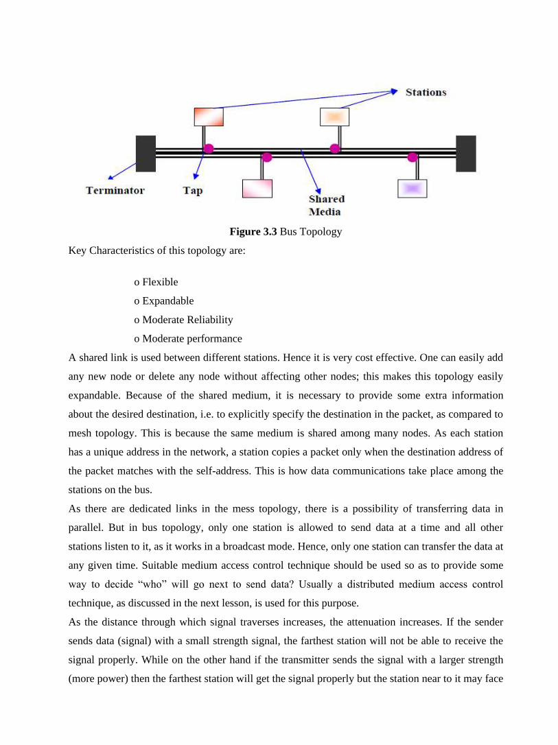
Figure 3.3 Bus Topology
Key Characteristics of this topology are:
o Flexible
o Expandable
o Moderate Reliability
o Moderate performance
A shared link is used between different stations. Hence it is very cost effective. One can easily add
any new node or delete any node without affecting other nodes; this makes this topology easily
expandable. Because of the shared medium, it is necessary to provide some extra information
about the desired destination, i.e. to explicitly specify the destination in the packet, as compared to
mesh topology. This is because the same medium is shared among many nodes. As each station
has a unique address in the network, a station copies a packet only when the destination address of
the packet matches with the self-address. This is how data communications take place among the
stations on the bus.
As there are dedicated links in the mess topology, there is a possibility of transferring data in
parallel. But in bus topology, only one station is allowed to send data at a time and all other
stations listen to it, as it works in a broadcast mode. Hence, only one station can transfer the data at
any given time. Suitable medium access control technique should be used so as to provide some
way to decide “who” will go next to send data? Usually a distributed medium access control
technique, as discussed in the next lesson, is used for this purpose.
As the distance through which signal traverses increases, the attenuation increases. If the sender
sends data (signal) with a small strength signal, the farthest station will not be able to receive the
signal properly. While on the other hand if the transmitter sends the signal with a larger strength
(more power) then the farthest station will get the signal properly but the station near to it may face
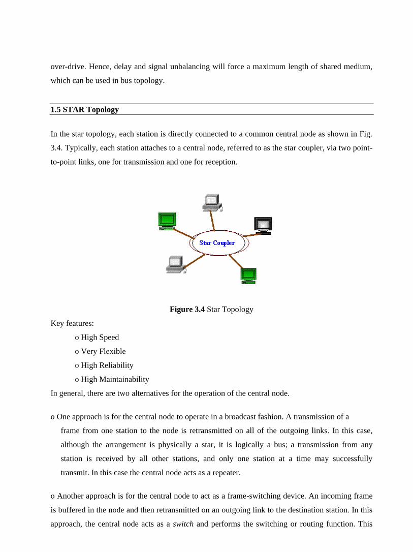
over-drive. Hence, delay and signal unbalancing will force a maximum length of shared medium,
which can be used in bus topology.
1.5 STAR Topology
In the star topology, each station is directly connected to a common central node as shown in Fig.
3.4. Typically, each station attaches to a central node, referred to as the star coupler, via two point-
to-point links, one for transmission and one for reception.
Figure 3.4 Star Topology
Key features:
o High Speed
o Very Flexible
o High Reliability
o High Maintainability
In general, there are two alternatives for the operation of the central node.
o One approach is for the central node to operate in a broadcast fashion. A transmission of a
frame from one station to the node is retransmitted on all of the outgoing links. In this case,
although the arrangement is physically a star, it is logically a bus; a transmission from any
station is received by all other stations, and only one station at a time may successfully
transmit. In this case the central node acts as a repeater.
o Another approach is for the central node to act as a frame-switching device. An incoming frame
is buffered in the node and then retransmitted on an outgoing link to the destination station. In this
approach, the central node acts as a switch and performs the switching or routing function. This
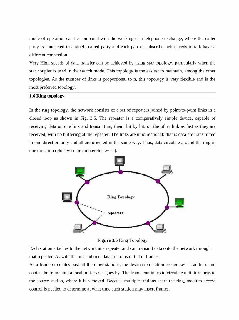
mode of operation can be compared with the working of a telephone exchange, where the caller
party is connected to a single called party and each pair of subscriber who needs to talk have a
different connection.
Very High speeds of data transfer can be achieved by using star topology, particularly when the
star coupler is used in the switch mode. This topology is the easiest to maintain, among the other
topologies. As the number of links is proportional to n, this topology is very flexible and is the
most preferred topology.
1.6 Ring topology
In the ring topology, the network consists of a set of repeaters joined by point-to-point links in a
closed loop as shown in Fig. 3.5. The repeater is a comparatively simple device, capable of
receiving data on one link and transmitting them, bit by bit, on the other link as fast as they are
received, with no buffering at the repeater. The links are unidirectional; that is data are transmitted
in one direction only and all are oriented in the same way. Thus, data circulate around the ring in
one direction (clockwise or counterclockwise).
Figure 3.5 Ring Topology
Each station attaches to the network at a repeater and can transmit data onto the network through
that repeater. As with the bus and tree, data are transmitted in frames.
As a frame circulates past all the other stations, the destination station recognizes its address and
copies the frame into a local buffer as it goes by. The frame continues to circulate until it returns to
the source station, where it is removed. Because multiple stations share the ring, medium access
control is needed to determine at what time each station may insert frames.
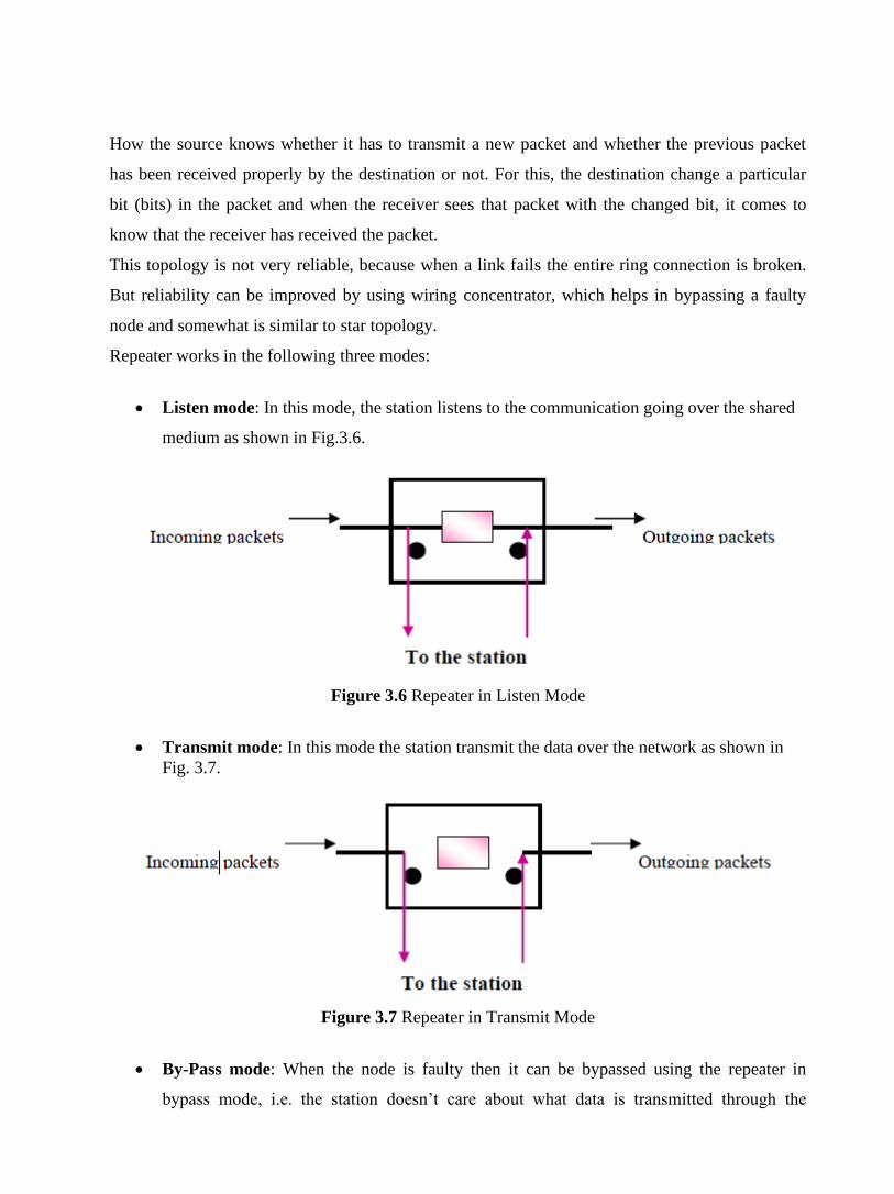
How the source knows whether it has to transmit a new packet and whether the previous packet
has been received properly by the destination or not. For this, the destination change a particular
bit (bits) in the packet and when the receiver sees that packet with the changed bit, it comes to
know that the receiver has received the packet.
This topology is not very reliable, because when a link fails the entire ring connection is broken.
But reliability can be improved by using wiring concentrator, which helps in bypassing a faulty
node and somewhat is similar to star topology.
Repeater works in the following three modes:
• Listen mode: In this mode, the station listens to the communication going over the shared
medium as shown in Fig.3.6.
Figure 3.6 Repeater in Listen Mode
• Transmit mode: In this mode the station transmit the data over the network as shown in
Fig. 3.7.
Figure 3.7 Repeater in Transmit Mode
• By-Pass mode: When the node is faulty then it can be bypassed using the repeater in
bypass mode, i.e. the station doesn’t care about what data is transmitted through the

network, as shown in Fig. 3.8. In this mode there is no delay introduced because of this
repeater.
Figure 3.8 Repeater in Bypass Mode
1.7 Tree Topology
This topology can be considered as an extension to bus topology. It is commonly used in cascading
equipments. For example, you have a repeater box with 8-port, as far as you have eight stations,
this can be used in a normal fashion. But if you need to add more stations then you can connect
two or more repeaters in a hierarchical format (tree format) and can add more stations. In the Fig.
3.9, R1 refers to repeater one and so on and each repeater is considered to have 8-ports.
Figure 3.9 Tree Topology
This tree topology is very good in an organization as incremental expansion can be done in this
way. Main features of this topology are scalability and flexibility. This is because, when the need
arises for more stations that can be accomplished easily without affecting the already established
network.

1.8 Unconstrained Topology
All the topologies discussed so far are symmetric and constrained by well-defined interconnection
pattern. However, sometimes no definite pattern is followed and nodes are interconnected in an
arbitrary manner using point-to-point links as shown in Fig 3.10. Unconstrained topology allows a
lot of configuration flexibility but suffers from the complex routing problem. Complex routing
involves unwanted overhead and delay.
Figure 3.10 Unconstrained Topology
1.9 Combination of topology and transmission media
Topology and transmission media are interrelated. For example, all the important criteria of a
network such as reliability, expandability and performance depend on both the topology and the
transmission media used in the network. As a consequence, these two aspects are interrelated. Let
us have a look at the various transmission media, which are used for different topologies.
• Twisted pair is suitable for use in star and ring topologies
---Cat 3: voice grade UTP, data rate up to 10 Mbps
---Cat 5: data grade UTP, data rate up to 100 Mbps
• Coaxial cable is suitable for use in bus topology
---Baseband coaxial cable supports data rates of 20 Mbps at distances up to 2 Km.
• Fiber optics is suitable for use in ring and star topology
---Gigabit data rates and longer distances.
• Unguided media are suitable for star topology

1.10 Check Your Progress
Fill In The Blanks.
1. Number of links to connect n nodes in a mesh topology is = _______.
2. Mesh Topology is _______ flexible and has a ________ expandability
3. In BUS topology, at each end of the bus is a ____________, which absorbs any signal,
removing it from the bus.
4. In BUS topology, One can easily add any new node or delete any node with-out affecting
other nodes; this makes this topology easily _____________.
5. _________ and ______________ will force a maximum length of shared medium which
can be used in BUS topology.
6. The two alternatives for the operation of the central node in STAR topology are:
__________ and ___________.
7. In Ring Topology, the links are _____________; that is, data are transmitted in
__________ direction only and all are oriented in the same way
8. In Ring Topology, Repeater works in 3 modes: ____________, _____________ and
______________.
9. ___________ topology can be considered as an extension to BUS topology.
10. ______________ is suitable for use in star and ring topologies
11. Coaxial cable is suitable for use in __________ topology.
1.11 Answer to Check Your Progress
1. n(n-1)/2
2. not, poor
3. terminator
4. expandable.
5. Delay, signal unbalancing
6. repeater, switch
7. unidirectional, one
8. Listen, Transmit, By-Pass
9. Tree
10. Twisted pair
11. BUS

Unit-4
Medium Access Control (MAC) Techniques
1.1 Learning Objectives
1.2 Introduction
1.3 Goals of MACs
1.4 Round Robin Techniques
1.4.1 Polling
1.4.2 Token Passing
1.5 Contention-based Approaches
1.5.1 ALOHA
1.6 CSMA
1.7 CSMA/CD
1.8 Check Your Progress
1.9 Answer to Check Your Progress
1.1 Learning Objectives
After going through this unit the learner will able to learn:
• Explain the goals and requirements of Medium Access Control (MAC) techniques
• Identify the key issues related to MAC techniques.
• Give an outline of possible MAC techniques.
• Distinguish between Centralized and Distributed MAC techniques.
• Classify various contention based techniques such as ALHOA, CSMA, CSMA/CD and
CSMA/CA
• Compare performance of contention based techniques
• Explain round robin based MAC techniques.
o Polling
o Token passing
1.2 Introduction
A network of computers based on multi-access medium requires a protocol for effective sharing of
the media. As only one node can send or transmit signal at a time using the broadcast mode, the
main problem here is how different nodes get control of the medium to send data, that is “who
goes next?”. The protocols used for this purpose are known as Medium Access Control (MAC)
techniques. The key issues involved here are - Where and How the control is exercised.
‘Where’ refers to whether the control is exercised in a centralised or distributed manner. In a
centralised system a master node grants access of the medium to other nodes. A centralized
scheme has a number of advantages as mentioned below:
o Greater control to provide features like priority, overrides, and guaranteed bandwidth.
o Simpler logic at each node.
o Easy coordination.
Although this approach is easier to implement, it is vulnerable to the failure of the master node and
reduces efficiency. On the other hand, in a distributed approach all the nodes collectively perform
a medium access control function and dynamically decide which node to be granted access. This
approach is more reliable than the former one.

How’ refers to in what manner the control is exercised. It is constrained by the topology and trade
off between cost-performance and complexity. Various approaches for medium access control are
shown in Fig. 4.1. The MAC techniques can be broadly divided into four categories; Contention-
based, Round-Robin, Reservation-based and. Channelization-based. Under these four broad
categories there are specific techniques, as shown in Fig. 4.1. In this lesson we shall concentrate of
the MACs of the first two categories, which have been used in the legacy LANs of the IEEE
standard. The CSMA/CA, a collision-free protocol used in wireless LAN.
Figure 4.1 Possible MAC techniques
1.3 Goals of MACs
Medium Access Control techniques are designed with the following goals in mind.
• Initialisation: The technique enables network stations, upon power-up, to enter the state
required for operation.
• Fairness: The technique should treat each station fairly in terms of the time it is made to
wait until it gains entry to the network, access time and the time it is allowed to spend for
transmission.
• Priority: In managing access and communications time, the technique should be able to
give priority to some stations over other stations to facilitate different type of services
needed.

• Limitations to one station: The techniques should allow transmission by one station at a
time.
• Receipt: The technique should ensure that message packets are actually received (no lost
packets) and delivered only once (no duplicate packets), and are received in the proper
order.
• Error Limitation: The method should be capable of encompassing an appropriate error
detection scheme.
• Recovery: If two packets collide (are present on the network at the same time), or if notice
of a collision appears, the method should be able to recover, i.e. be able to halt all the
transmissions and select one station to retransmit.
• Reconfigurability: The technique should enable a network to accommodate the addition or
deletion of a station with no more than a noise transient from which the network station can
recover.
• Compatibility: The technique should accommodate equipment from all vendors who build
to its specification.
• Reliability: The technique should enable a network to confine operating inspite of a failure
of one or several stations.
1.4 Round Robin Techniques
In Round Robin techniques, each and every node is given the chance to send or transmit by
rotation. When a node gets its turn to send, it may either decline to send, if it has no data or may
send if it has got data to send. After getting the opportunity to send, it must relinquish its turn after
some maximum period of time. The right to send then passes to the next node based on a
predetermined logical sequence. The right to send may be controlled in a centralised or distributed
manner. Polling is an example of centralised control and token passing is an example of distributed
control as discussed below.
1.4.1 Polling
The mechanism of polling is similar to the roll-call performed in a classroom. Just like the teacher,
a controller sends a message to each node in turn. The message contains the address of the node
being selected for granting access. Although all nodes receive the message, only the addressed
node responds and then it sends data, if any. If there is no data, usually a “poll reject” message is
sent back. In this way, each node is interrogated in a round-robin fashion, one after the other, for

granting access to the medium. The first node is again polled when the controller finishes with the
remaining codes.
The polling scheme has the flexibility of either giving equal access to all the nodes, or some nodes
may be given higher priority than others. In other words, priority of access can be easily
implemented.
Figure 4.2 Polling using a central controller
Polling can be done using a central controller, which may use a frequency band to send outbound
messages as shown in Fig. 4.2. Other stations share a different frequency to send inbound
messages. The technique is called frequency-division duplex approach (FDD). Main drawbacks of
the polling scheme are high overhead of the polling messages and high dependence on the
reliability of the controller.
Polling can also be accomplished without a central controller. Here, all stations receive signals
from other stations as shown in Fig. 4.3. Stations develop a polling order list, using some protocol.
Figure 4.2 Polling in a distributed manner
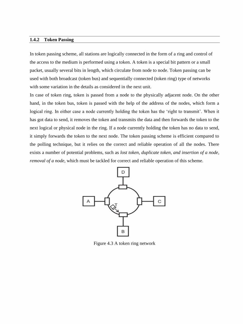
1.4.2 Token Passing
In token passing scheme, all stations are logically connected in the form of a ring and control of
the access to the medium is performed using a token. A token is a special bit pattern or a small
packet, usually several bits in length, which circulate from node to node. Token passing can be
used with both broadcast (token bus) and sequentially connected (token ring) type of networks
with some variation in the details as considered in the next unit.
In case of token ring, token is passed from a node to the physically adjacent node. On the other
hand, in the token bus, token is passed with the help of the address of the nodes, which form a
logical ring. In either case a node currently holding the token has the ‘right to transmit’. When it
has got data to send, it removes the token and transmits the data and then forwards the token to the
next logical or physical node in the ring. If a node currently holding the token has no data to send,
it simply forwards the token to the next node. The token passing scheme is efficient compared to
the polling technique, but it relies on the correct and reliable operation of all the nodes. There
exists a number of potential problems, such as lost token, duplicate token, and insertion of a node,
removal of a node, which must be tackled for correct and reliable operation of this scheme.
Figure 4.3 A token ring network

Figure 4.4 Token passing mechanism
Performance: Performance of a token ring network can be represented by two parameters;
throughput, which is a measure of the successful traffic, and delay, which is a measure of time
between when a packet is ready and when it is delivered. A station starts sending a packet at t = t0,
completes transmission at t = t0 + a, receives the tail at t0 + 1 + a. So, the average time (delay)
required to send a token to the next station = a/N. and throughput, S = 1/(1 + a/N) for a<1 and S =
1/a(1 + 1/N) for a>1.
1.5 Contention-based Approaches
Round-Robin techniques work efficiently when majority of the stations have data to send most of
the time. But, in situations where only a few nodes have data to send for brief periods of time,
Round-Robin techniques are unsuitable. Contention techniques are suitable for bursty nature of
traffic. In contention techniques, there is no centralised control and when a node has data to send,
it contends for gaining control of the medium. The principle advantage of contention techniques is
their simplicity. They can be easily implemented in each node. The techniques work efficiently
under light to moderate load, but performance rapidly falls under heavy load.

1.5.1 ALOHA
The ALOHA scheme was invented by Abramson in 1970 for a packet radio network connecting
remote stations to a central computer and various data terminals at the campus of the university of
Hawaii. A simplified situation is shown in Fig. 4.5. Users are allowed random access of the central
computer through a common radio frequency band f1 and the computer centre broadcasts all
received signals on a different frequency band f2. This enables the users to monitor packet
collisions, if any. The protocol followed by the users is simplest; whenever a node has a packet to
sent, it simply does so. The scheme, known as Pure ALOHA, is truly a free-for-all scheme. Of
course, frames will suffer collision and colliding frames will be destroyed. By monitoring the
signal sent by the central computer, after the maximum round-trip propagation time, an user comes
to know whether the packet sent by him has suffered a collision or not.
Figure 4.5 Simplified ALOHA scheme for a packet radio system

Figure 4.6 Collision in Pure ALOHA
It may be noted that if all packets have a fixed duration of τ (shown as F in Figure 4.7), then a
given packet A will suffer collision if another user starts to transmit at any time from τ before to
until τ after the start of the packet A as shown in Fig. 4.6. This gives a vulnerable period of 2τ.
Based on this assumption, the channel utilization can be computed. The channel utilization,
expressed as throughput S, in terms of the offered load G is given by S=Ge-2G.
Figure 4.7 Vulnerable period in Pure ALOHA
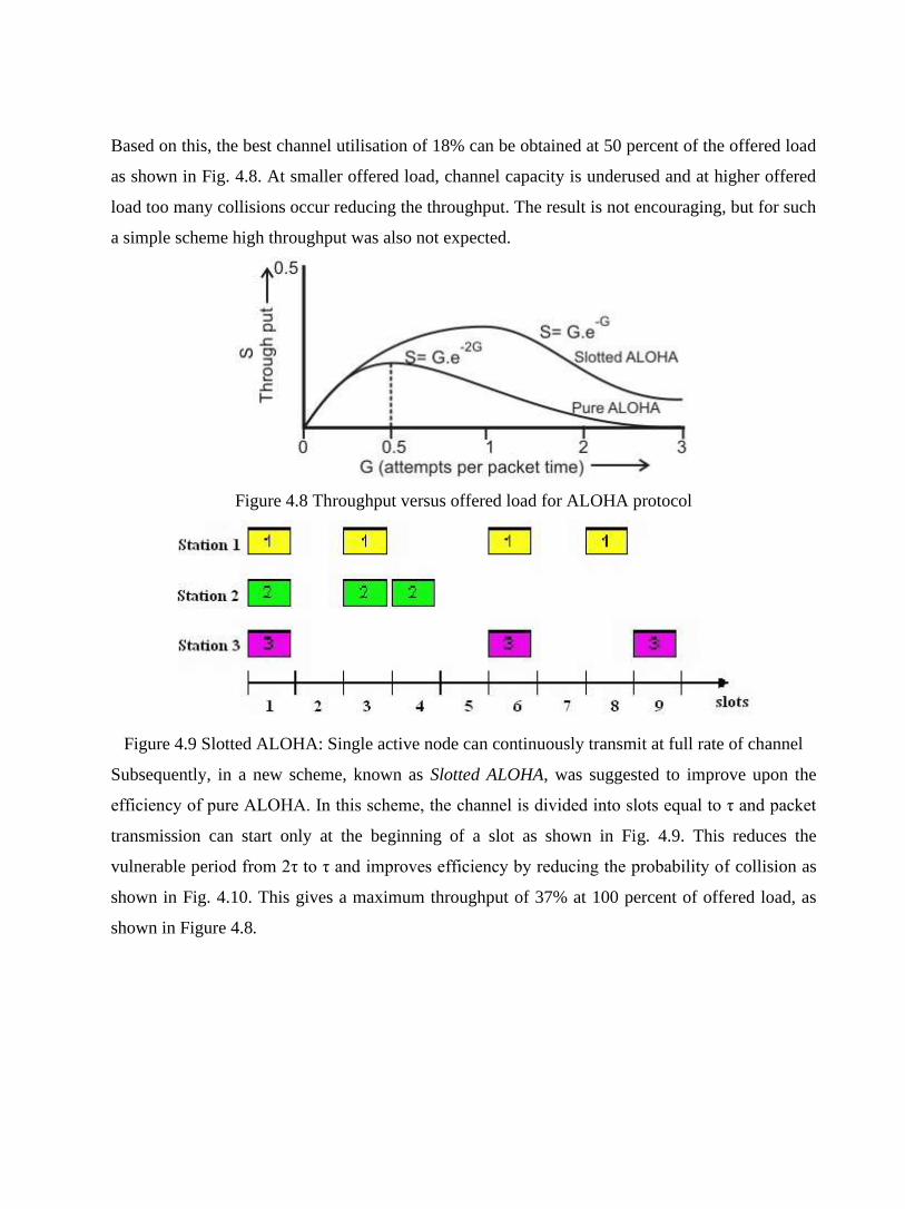
Based on this, the best channel utilisation of 18% can be obtained at 50 percent of the offered load
as shown in Fig. 4.8. At smaller offered load, channel capacity is underused and at higher offered
load too many collisions occur reducing the throughput. The result is not encouraging, but for such
a simple scheme high throughput was also not expected.
Figure 4.8 Throughput versus offered load for ALOHA protocol
Figure 4.9 Slotted ALOHA: Single active node can continuously transmit at full rate of channel
Subsequently, in a new scheme, known as Slotted ALOHA, was suggested to improve upon the
efficiency of pure ALOHA. In this scheme, the channel is divided into slots equal to τ and packet
transmission can start only at the beginning of a slot as shown in Fig. 4.9. This reduces the
vulnerable period from 2τ to τ and improves efficiency by reducing the probability of collision as
shown in Fig. 4.10. This gives a maximum throughput of 37% at 100 percent of offered load, as
shown in Figure 4.8.

Figure 8.10 Collision in Slotted ALOHA
1.6 CSMA
The poor efficiency of the ALOHA scheme can be attributed to the fact that a node start
transmission without paying any attention to what others are doing. In situations where
propagation delay of the signal between two nodes is small compared to the transmission time of a
packet, all other nodes will know very quickly when a node starts transmission. This observation is
the basis of the carrier-sense multiple-access (CSMA) protocol. In this scheme, a node having data
to transmit first listens to the medium to check whether another transmission is in progress or not.
The node starts sending only when the channel is free, that is there is no carrier. That is why the
scheme is also known as listen-before-talk. There are three variations of this basic scheme as
outlined below.
(i) 1-persistent CSMA: In this case, a node having data to send, start sending, if the
channel is sensed free. If the medium is busy, the node continues to monitor until the
channel is idle. Then it starts sending data.
(ii) Non-persistent CSMA: If the channel is sensed free, the node starts sending the packet.
Otherwise, the node waits for a random amount of time and then monitors the channel.
(iii) p-persistent CSMA: If the channel is free, a node starts sending the packet. Otherwise
the node continues to monitor until the channel is free and then it sends with probability
p.
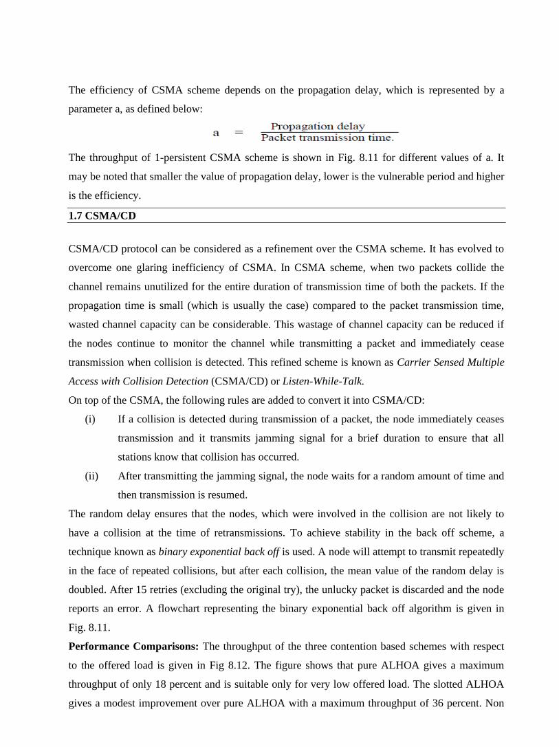
The efficiency of CSMA scheme depends on the propagation delay, which is represented by a
parameter a, as defined below:
The throughput of 1-persistent CSMA scheme is shown in Fig. 8.11 for different values of a. It
may be noted that smaller the value of propagation delay, lower is the vulnerable period and higher
is the efficiency.
1.7 CSMA/CD
CSMA/CD protocol can be considered as a refinement over the CSMA scheme. It has evolved to
overcome one glaring inefficiency of CSMA. In CSMA scheme, when two packets collide the
channel remains unutilized for the entire duration of transmission time of both the packets. If the
propagation time is small (which is usually the case) compared to the packet transmission time,
wasted channel capacity can be considerable. This wastage of channel capacity can be reduced if
the nodes continue to monitor the channel while transmitting a packet and immediately cease
transmission when collision is detected. This refined scheme is known as Carrier Sensed Multiple
Access with Collision Detection (CSMA/CD) or Listen-While-Talk.
On top of the CSMA, the following rules are added to convert it into CSMA/CD:
(i) If a collision is detected during transmission of a packet, the node immediately ceases
transmission and it transmits jamming signal for a brief duration to ensure that all
stations know that collision has occurred.
(ii) After transmitting the jamming signal, the node waits for a random amount of time and
then transmission is resumed.
The random delay ensures that the nodes, which were involved in the collision are not likely to
have a collision at the time of retransmissions. To achieve stability in the back off scheme, a
technique known as binary exponential back off is used. A node will attempt to transmit repeatedly
in the face of repeated collisions, but after each collision, the mean value of the random delay is
doubled. After 15 retries (excluding the original try), the unlucky packet is discarded and the node
reports an error. A flowchart representing the binary exponential back off algorithm is given in
Fig. 8.11.
Performance Comparisons: The throughput of the three contention based schemes with respect
to the offered load is given in Fig 8.12. The figure shows that pure ALHOA gives a maximum
throughput of only 18 percent and is suitable only for very low offered load. The slotted ALHOA
gives a modest improvement over pure ALHOA with a maximum throughput of 36 percent. Non
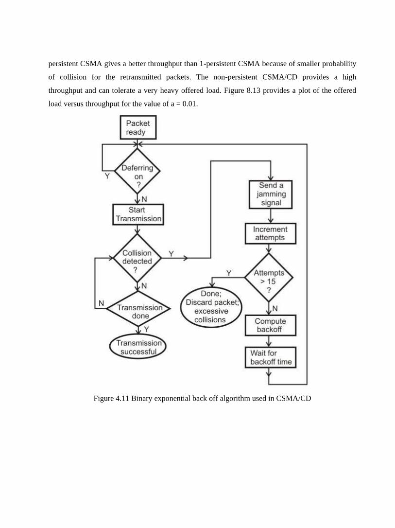
persistent CSMA gives a better throughput than 1-persistent CSMA because of smaller probability
of collision for the retransmitted packets. The non-persistent CSMA/CD provides a high
throughput and can tolerate a very heavy offered load. Figure 8.13 provides a plot of the offered
load versus throughput for the value of a = 0.01.
Figure 4.11 Binary exponential back off algorithm used in CSMA/CD
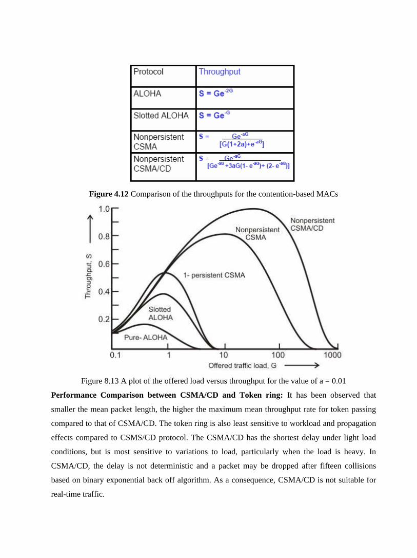
Figure 4.12 Comparison of the throughputs for the contention-based MACs
Figure 8.13 A plot of the offered load versus throughput for the value of a = 0.01
Performance Comparison between CSMA/CD and Token ring: It has been observed that
smaller the mean packet length, the higher the maximum mean throughput rate for token passing
compared to that of CSMA/CD. The token ring is also least sensitive to workload and propagation
effects compared to CSMS/CD protocol. The CSMA/CD has the shortest delay under light load
conditions, but is most sensitive to variations to load, particularly when the load is heavy. In
CSMA/CD, the delay is not deterministic and a packet may be dropped after fifteen collisions
based on binary exponential back off algorithm. As a consequence, CSMA/CD is not suitable for
real-time traffic.

1.8 Check Your Progress
Fill In The Blanks:
1. The basic question which has to be answered by the medium-access control techniques is
“How Goes ________”?
2. In _______________ technique, each node gets a chance to access the medium by rotation.
3. The key issues involved in MAC protocol are - Where and ______ the control is exercised.
4. ‘Where’ refers to whether the control is exercised in a _____________ or ______________
manner.
5. The _______________ techniques can be broadly categorized into three types; Round-
Robin, Reservation and___________.
6. ______________ is an example of centralized control and ______________ is an example
of distributed control
7. In Polling technique, if there is no data, usually a ______________ message is sent back.
8. In pure ALOHA, channel utilization, expressed as throughput S, in terms of the offered
load G is given by _________
9. In slotted ALOHA, a maximum throughput of ________ percent at 100 percent of offered
load can be achieved, while it is ______ percentage for pure ALOHA.
10. _________________ is abbreviated as CSMA/CD and is also known as __________.
11. To achieve stability in CSMA/CD back off scheme, a technique known as
______________ is used
1.9 Answer to Check Your Progress
1. Next
2. token passing
3. How
4. centralized, distributed
5. asynchronous, Contention
6. Polling, token passing
7. poll reject
8. S=Ge-2G.
9. 37, 18
10. Carrier Sensed Multiple Access with Collision Detection, Listen-While-Talk .
11. binary exponential back off

Unit-5
IEEE CSMS/CD based LANs
1.1 Learning Objectives
1.2 Introduction
1.3 IEEE 802.3 and Ethernet
1.3.1 Ethernet - A Brief History
1.3.2 5.3.2.2 Ethernet Architecture
1.3.3 Encoding for Signal Transmission
1.3.4 The Ethernet MAC Sublayer
1.3.5 The Basic Ethernet Frame Format
1.3.6 Other important issues
1.4 Check Your Progress
1.5 Answer to Check Your Progress

1.1 Learning Objectives
• Explain the basic characteristics of LANs
• Explain the operation of IEEE 802 LANs
o 802.3 - CSMA/CD-based (Ethernet)
1.2 Introduction
A LAN consists of shared transmission medium and a set of hardware and software for interfacing
devices to the medium and regulating the ordering access to the medium. These are used to share
resources (may be hardware or software resources) and to exchange information. LAN protocols
function at the lowest two layers of the OSI reference model: the physical and data-link layers. The
IEEE 802 LAN is a shared medium peer-to-peer communications network that broadcasts
information for all stations to receive. As a consequence, it does not inherently provide privacy. A
LAN enables stations to communicate directly using a common physical medium on a point-to-
point basis without any intermediate switching node being required. There is always need for an
access sublayer in order to arbitrate the access to the shared medium.
The network is generally owned, used, and operated by a single organization. This is in contrast to
Wide Area Networks (WANs), which interconnect communication facilities in different parts of a
country or are used as a public utility. These LANs are also different from networks, such as back
plane buses, that are optimized for the interconnection of devices on a desktop or components
within a single piece of equipment.
• Key features of LANs are summarized below:
• Limited geographical area – which is usually less than 10 Km and more than 1 m.
• High Speed – 10 Mbps to 1000 Mbps (1 Gbps) and more
• High Reliability – 1 bit error in 1011 bits.
• Transmission Media – Guided and unguided media, mainly guided media is used; except in
a situation where infrared is used to make a wireless LAN in a room.
• Topology – It refers to the ways in which the nodes are connected. There are various
topologies used.
• Medium-Access Control Techniques –Some access control mechanism is needed to decide
which station will use the shared medium at a particular point in time.
In this lesson we shall discuss various LAN standards proposed by the IEEE 8.2 committee with
the following goals in mind:

• To promote compatibility
• Implementation with minimum efforts
• Accommodate the need for diverse applications
For the fulfillment of the abovementioned goals, the committee came up with a bunch of LAN
standards collectively known as IEEE 802 LANs as shown in Fig. 5.1.To satisfy diverse
requirements, the standard includes CSMA/CD, Token bus, Token Ring medium access control
techniques along with different topologies. All these standards differ at the physical layer and
MAC sublayer, but are compatible at the data link layer.
Figure 5.1 IEEE 802 Legacy LANs
The 802.1 sublayer gives an introduction to set of standards and gives the details of the interface
primitives. It provides relationship between the OSI model and the 802 standards. The 802.2
sublayer describes the LLC (logical link layer), which is the upper part of the data link layer. LLC
facilitate error control and flow control for reliable communication. It appends a header containing
sequence number and acknowledgement number. And offers the following three types of services:
• Unreliable datagram service
• Acknowledged datagram service
• Reliable connection oriental service
The standards 802.3, 802.4 and 802.5 describe three LAN standards based on the CSMA/CD,
token bus and token ring, respectively. Each standard covers the physical layer and MAC sublayer
protocols. In the following sections we shall focus on these three LAN standards.

1.3 IEEE 802.3 and Ethernet
1.3.1 Ethernet - A Brief History
The original Ethernet was developed as an experimental coaxial cable network in the 1970s by
Xerox Corporation to operate with a data rate of 3 Mbps using a carrier sense multiple access
collision detection (CSMA/CD) protocol for LANs with sporadic traffic requirements. Success
with that project attracted early attention and led to the 1980 joint development of the 10-Mbps
Ethernet Version 1.0 specification by the three-company consortium: Digital Equipment
Corporation, Intel Corporation, and Xerox Corporation.
The original IEEE 802.3 standard was based on, and was very similar to, the Ethernet Version 1.0
specification. The draft standard was approved by the 802.3 working group in 1983 and was
subsequently published as an official standard in 1985 (ANSI/IEEE Std.
802.3-1985). Since then, a number of supplements to the standard have been defined to take
advantage of improvements in the technologies and to support additional network media and
higher data rate capabilities, plus several new optional network access control features. From then
onwards, the term Ethernet refers to the family of local-area network (LAN) products covered by
the IEEE 802.3 standard that defines what is commonly known as the CSMA/CD protocol. Three
data rates are currently defined for operation over optical fiber and twisted-pair cables:
• 10 Mbps—10Base-T Ethernet
• 100 Mbps—Fast Ethernet
• 1000 Mbps—Gigabit Ethernet
Ethernet has survived as the major LAN technology (it is currently used for approximately 85
percent of the world's LAN-connected PCs and workstations) because its protocol has the
following characteristics:
• It is easy to understand, implement, manage, and maintain
• It allows low-cost network implementations
• It provides extensive topological flexibility for network installation
• It guarantees successful interconnection and operation of standards-compliant products,
regardless of manufacturer
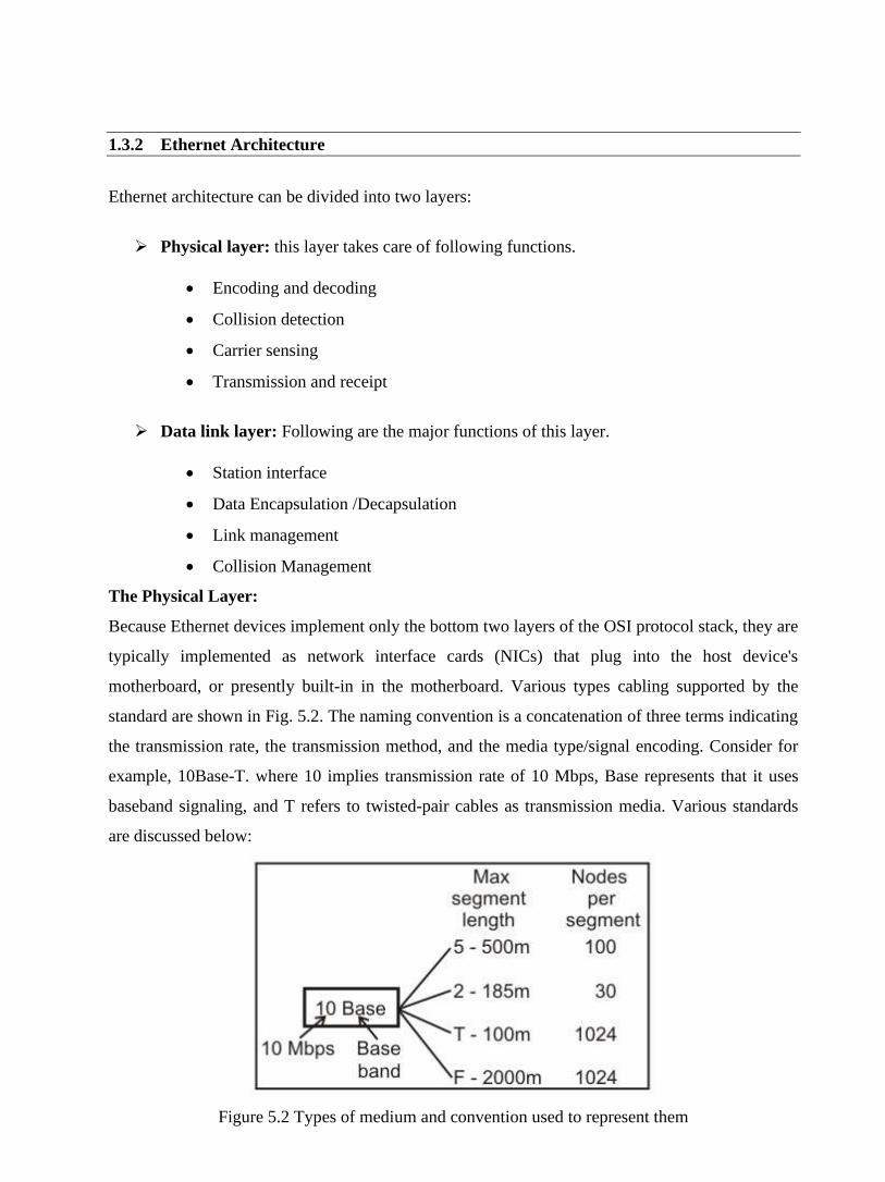
1.3.2 Ethernet Architecture
Ethernet architecture can be divided into two layers:
➢ Physical layer: this layer takes care of following functions.
• Encoding and decoding
• Collision detection
• Carrier sensing
• Transmission and receipt
➢ Data link layer: Following are the major functions of this layer.
• Station interface
• Data Encapsulation /Decapsulation
• Link management
• Collision Management
The Physical Layer:
Because Ethernet devices implement only the bottom two layers of the OSI protocol stack, they are
typically implemented as network interface cards (NICs) that plug into the host device's
motherboard, or presently built-in in the motherboard. Various types cabling supported by the
standard are shown in Fig. 5.2. The naming convention is a concatenation of three terms indicating
the transmission rate, the transmission method, and the media type/signal encoding. Consider for
example, 10Base-T. where 10 implies transmission rate of 10 Mbps, Base represents that it uses
baseband signaling, and T refers to twisted-pair cables as transmission media. Various standards
are discussed below:
Figure 5.2 Types of medium and convention used to represent them

10Base-5: It supports 10 Mbps baseband transmission. The standard specifies 0.5 inch coaxial
cable, known as yellow cable or thick Ethernet. The manner of interfacing a computer is shown in
Fig. 5.3. Each cable segment can be maximum 500 meters long (which is indicated by 5 in the
convention). Up to a maximum of 5 cable segments can be connected using repeaters, with
maximum length 2500 meters. At most 1024 stations is allowed on a single LAN. Some other
characteristics for this media are:
• Tap: Not necessary to cut a cable to add a new computer
• Transceiver: It performs send/receive, collision detection, provides isolation
• AUI: Attachment Unit Interface is directly placed on the cable after vampire wire tap on
the cable
• AUI drop Cable: This cable is used to interface the network interface unit of the computer
with the AUI.
Figure 5.3 Interfacing a Computer in 10Base-5 standard
10Base-2: It also support 10 Mbps baseband transmission. The standard specifies 0.25 inch
coaxial cable known as cheapernet or thin Ethernet. Each cable segment can be maximum 185
meters long. Up to a maximum of 5 cable segments can be connected using repeaters, with
maximum length of 925 meters. The interfacing mechanism of a computer is shown in Fig. 5.4. It
may be noted that in this case there is no need for AUI drop cable, which is required in case of
10Base-5 standard.
Some other characteristics are:
• Use for office LAN/departmental LAN
• BNC connector is used to interface a computer
• Drop cable is not required

Figure: 5.4 Interfacing a computer in 10Base-2 standard
10Base-T: This standard supports 10 Mbps baseband transmission and uses 24WG Unshielded
Twisted Pair (UTP) cable of both Cat-3 and Cat-5 category cables. A HUB functions as a multi-
port repeater with stations connected to it with RJ45 connector.
Maximum length of a cable segment is 100 meters. It uses star topology as shown in Fig. 5.5. This
allows easy to maintenance and diagnosis of faults. As a consequence, this is the most preferred
approach used for setting up of a LAN.
Figure: 5.5 Interfacing a computer in 10Base-T standard
10Base-F: It allows long distance connections using optical fiber. The topology is same as
10Base-T, but the medium is a pair of optical fiber instead of twisted-pair of wire. It has the
following divisions:
• 10BaseFP: A passive-star topology, up to 1 km link
• 10BaseFL: An asynchronous point-to-point link, up to 2km
• 10BaseFB: A synchronous point-to-point link, up to 2 km with 15 cascaded repeaters
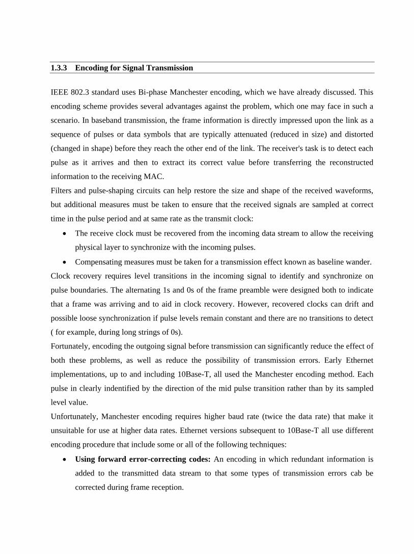
1.3.3 Encoding for Signal Transmission
IEEE 802.3 standard uses Bi-phase Manchester encoding, which we have already discussed. This
encoding scheme provides several advantages against the problem, which one may face in such a
scenario. In baseband transmission, the frame information is directly impressed upon the link as a
sequence of pulses or data symbols that are typically attenuated (reduced in size) and distorted
(changed in shape) before they reach the other end of the link. The receiver's task is to detect each
pulse as it arrives and then to extract its correct value before transferring the reconstructed
information to the receiving MAC.
Filters and pulse-shaping circuits can help restore the size and shape of the received waveforms,
but additional measures must be taken to ensure that the received signals are sampled at correct
time in the pulse period and at same rate as the transmit clock:
• The receive clock must be recovered from the incoming data stream to allow the receiving
physical layer to synchronize with the incoming pulses.
• Compensating measures must be taken for a transmission effect known as baseline wander.
Clock recovery requires level transitions in the incoming signal to identify and synchronize on
pulse boundaries. The alternating 1s and 0s of the frame preamble were designed both to indicate
that a frame was arriving and to aid in clock recovery. However, recovered clocks can drift and
possible loose synchronization if pulse levels remain constant and there are no transitions to detect
( for example, during long strings of 0s).
Fortunately, encoding the outgoing signal before transmission can significantly reduce the effect of
both these problems, as well as reduce the possibility of transmission errors. Early Ethernet
implementations, up to and including 10Base-T, all used the Manchester encoding method. Each
pulse in clearly indentified by the direction of the mid pulse transition rather than by its sampled
level value.
Unfortunately, Manchester encoding requires higher baud rate (twice the data rate) that make it
unsuitable for use at higher data rates. Ethernet versions subsequent to 10Base-T all use different
encoding procedure that include some or all of the following techniques:
• Using forward error-correcting codes: An encoding in which redundant information is
added to the transmitted data stream to that some types of transmission errors cab be
corrected during frame reception.
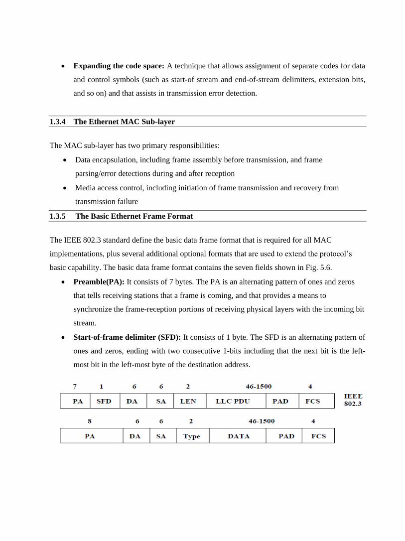
• Expanding the code space: A technique that allows assignment of separate codes for data
and control symbols (such as start-of stream and end-of-stream delimiters, extension bits,
and so on) and that assists in transmission error detection.
1.3.4 The Ethernet MAC Sub-layer
The MAC sub-layer has two primary responsibilities:
• Data encapsulation, including frame assembly before transmission, and frame
parsing/error detections during and after reception
• Media access control, including initiation of frame transmission and recovery from
transmission failure
1.3.5 The Basic Ethernet Frame Format
The IEEE 802.3 standard define the basic data frame format that is required for all MAC
implementations, plus several additional optional formats that are used to extend the protocol’s
basic capability. The basic data frame format contains the seven fields shown in Fig. 5.6.
• Preamble(PA): It consists of 7 bytes. The PA is an alternating pattern of ones and zeros
that tells receiving stations that a frame is coming, and that provides a means to
synchronize the frame-reception portions of receiving physical layers with the incoming bit
stream.
• Start-of-frame delimiter (SFD): It consists of 1 byte. The SFD is an alternating pattern of
ones and zeros, ending with two consecutive 1-bits including that the next bit is the left-
most bit in the left-most byte of the destination address.

Figure 5.6 Ethernet Frame Format
• Destination address (DA): It onsists of 6 bytes. The DA field identifies which station(s)
should receive the frame. The left-most bit in the DA field indicates whether the address is
an individual address (indicated by a 0) or a group address (indicated by a 1). The second
bit from the left indicates whether the DA is globally administered (indicated by a 0) or
locally administered (indicated by a 1). The remaining 46 bits are a uniquely assigned
value that identifies a single station, a defined group of stations, or all stations on the
network as shown in Fig. 5.7.
Figure 5.7 Ethernet MAC Address
• Source addresses (SA): It consists of 6 bytes. The SA field identifies the sending station.
The SA is always an individual address and the left-most bit in the SA field is always 0.
• Length/Type: It consists of 4 bytes. This field indicates either the number of MAC-client
data bytes that are contained in the data field of the frame, or the frame type ID if the frame

is assembled using an optional format. If the Length/Type field value is less than or equal
to 1500, the number of LLC bytes in the Data field is equal to the Length/Type field value.
If the Length/Type field value is greater than 1536, the frame is an optional type frame, and
the Length/Type field value identifies the particular type of frame being sent or received.
• Data: It is a sequence of n bytes of any value, where n is less than or equal to 1500. If the
length of the Data field is less than 46, the Data field must be extended by adding a filler (a
pad) sufficient to bring the Data field length to 46 bytes.
• Frame check sequence (FCS): It consists of 4 bytes. This sequence contains a 32-bit
cyclic redundancy check (CRC) value, which is created by the sending MAC and is
recalculated by the receiving MAC to check for damaged frames. The FCS is generated
over the DA, SA, Length/Type, and Data fields.
1.3.6 Other important issues
There are some more important issues, which are briefly discussed below.
• Inter-frame Gap: There is mandatory requirement of 9.6 ms interval between two frames
to enable other stations wishing to transmit to take over after a frame transmission is over.
In other words, a 96 bit-time delay is provided between frame transmissions.
• How are collisions detected? A station sends frame and continues to sense the medium. If
the signal strength sensed by a station exceeds the normal signal strength, it is treated as
collision detection.
• What the station does? The transmitting station sends a jamming signal after collision is
detected.
o 32-bit jam signal: 10101010 --- 10101010
o 48-bit jam signal: 10101010 --- 10101010
The jam signal serves as a mechanism to cause non-transmitting stations to wait until the jam
signal ends.
Minimum Frame Size: A frame must take more than 2τ time to send, where τ is the propagation
time for preventing the situation that the sender incorrectly concludes that the frame was
successfully sent. This slot time is 51.2μsec corresponding to 512 bit = 64 bytes. Therefore the
minimum frame length is 64 bytes (excluding preamble), which requires that the data field must
have a minimum size of 46 bytes.

1.4 Check Your Progress
Fill In The Blanks
1. The 802.2 standard describes the ____________, which is the upper part of the data link
layer.
2. LLC offers three types services: Unreliable datagram service, ________________ and
_______________.
3. IEEE 802 bundle also includes a MAN standard IEEE 802.6 which is also known as
______________.
4. 100Base-T2 means _______________________________
5. 100 Mbps, baseband, long wavelength over optical fiber cable will be abbreviated as
________________
6. Ethernet uses __________ encoding
1.5 Answer to Check Your Progress
1. LLC (logical link layer)
2. Acknowledged datagram service, Reliable connection oriental service
3. Distributed Queue Dual Bus (DQDB)
4. 100 Mbps, baseband, over two twisted-pair cables
5. 1000Base F
6. Bi-phase Manchester

Block-4
Unit-1
IEEE Ring LANs and High Speed LANs –
Token Ring Based
1.1 Learning Objectives
1.2 Introduction
1.3 Token Ring (IEEE 802.5)
1.3.1 Token Ring Operation
1.3.2 Priority System
1.3.3 Ring Maintenance
1.3.4 Physical Layer
1.3.5 Frame Format
1.4 Token Bus (IEEE 802.4)
1.4.1 Functions of a Token Bus
1.4.2 Frame Form
1.4.3 Logical ring maintenance
1.4.4 Relative comparison of the three standards
1.5 Introduction to High Speed LANs – Token Ring Based
1.6 FDDI
1.6.1 Medium
1.6.2 Topology
1.6.3 Fault Tolerance
1.6.4 Frame Format
1.6.5 Media Access Control
1.6.6 FDDI and the OSI model
1.6.7 Comparison
1.7 Check Your Progress
1.8 Answer to Check Your Progress

1.1 Learning Objectives
After going through this unit the learner will able to learn:
• Explain the operation of IEEE 802 LANs
o 802.4 – Token bus-based
o 802.5 – Token ring-based
• Compare performance of the three LANs
• Explain different categories of High Speed LANs
• Distinguish FDDI from IEEE80 2.5 Token ring LAN
• Explain how FDDI provides higher reliability
1.2 Introduction
In the preceding lesson we have mentioned that for the fulfillment of different goals, the IEEE 802
committee came up with a bunch of LAN standards collectively known as LANs as shown in Fig.
1.1. We have already discussed CSMA/CD-based LAN proposed by the IEEE 802.3
subcommittee, commonly known as Ethernet. In this lesson we shall discuss Token bus, Token
Ring based LANs proposed by the IEEE 802.4 and IEEE 8.2.5 subcommittees.
Figure 1.1 IEEE 802 Legacy LANs
1.3 Token Ring (IEEE 802.5)
Originally, IBM developed Token Ring network in the 1970s. It is still IBM's primary local-area
network (LAN) technology. The related IEEE 802.5 specification is almost identical to and
completely compatible with IBM's Token Ring network. In fact, the IEEE 802.5 specification was
modeled after IBM Token Ring, and on the same lines. The term Token Ring is generally used to
refer to both IBM's Token Ring network and IEEE 802.5 networks.
Before going into the details of the Token Ring protocol, let’s first discuss the motivation behind
it. As already discussed, the medium access mechanism used by Ethernet (CSMA/CD) may results
in collision. Nodes attempt to a number of times before they can actually transmit, and even when
they start transmitting there are chances to encounter collisions and entire transmission need to be
repeated. And all this become worse one the traffic is heavy i.e. all nodes have some data to
transmit. Apart from this there is no way to predict either the occurrence of collision or delays
produced by multiple stations attempting to capture the link at the same time. So all these
problems with the Ethernet gives way to an alternate LAN technology, Token Ring.
Token Ring and IEEE802.5 are based on token passing MAC protocol with ring topology. They
resolve the uncertainty by giving each station a turn on by one. Each node takes turns sending the
data; each station may transmit data during its turn. The technique that coordinates this turn
mechanism is called Token passing; as a Token is passed in the network and the station that gets
the token can only transmit. As one node transmits at a time, there is no chance of collision. We
shall discuss the detailed operation in next section.
Stations are connected by point-to-point links using repeaters. Mainly these links are of shielded
twisted-pair cables. The repeaters function in two basic modes: Listen mode, Transmit mode. A
disadvantage of this topology is that it is vulnerable to link or station failure. But a few measures
can be taken to take care of it.
Differences between Token Ring and IEEE 802.5
Both of these networks are basically compatible, although the specifications differ in some ways.
• IEEE 802.5 does not specify a topology, although virtually all IEEE 802.5
implementations are based on the star topology. While IBM's Token Ring network
explicitly specifies a star, with all end stations attached to a device called a Multi-Station
Access Unit (MSAU).
• IEEE 802.5 does not specify a media type, although IBM Token Ring networks use
twisted-pair wire.
• There are few differences in routing information field size of the two.
1.3.1 Token Ring Operation
Token-passing networks move a small frame, called a token, around the network. Possession of the
token grants the right to transmit. If a node receiving the token has no information to send, it

passes the token to the next end station. Each station can hold the token for a maximum period of
time.
If a station possessing the token does have information to transmit, it seizes the token, alters 1 bit
of the token (which turns the token into a start-of-frame sequence), appends the information that it
wants to transmit, and sends this information to the next station on the ring. While the information
frame is circling the ring, no token is on the network (unless the ring supports early token release),
which means that other stations wanting to transmit must wait. Therefore, collisions cannot occur
in Token Ring networks. If early token release is supported, a new token can be released
immediately after a frame transmission is complete.
The information frame circulates around the ring until it reaches the intended destination station,
which copies the information for further processing. The information frame makes a round trip and
is finally removed when it reaches the sending station. The sending station can check the returning
frame to see whether the frame was seen and subsequently copied by the destination station in
error-free form. Then the sending station inserts a new free token on the ring, if it has finished
transmission of its packets.
Unlike CSMA/CD networks (such as Ethernet), token-passing networks are deterministic, which
means that it is possible to calculate the maximum time that will pass before any end station will
be capable of transmitting. Token Ring networks are ideal for applications in which delay must be
predictable and robust network operation is important.
1.3.2 Priority System
Token Ring networks use a sophisticated priority system that permits certain user-designated,
high-priority stations to use the network more frequently. Token Ring frames have two fields that
control priority: the priority field and the reservation field.
Only stations with a priority equal to or higher than the priority value contained in a token can
seize that token. After the token is seized and changed to an information frame, only stations with
a priority value higher than that of the transmitting station can reserve the token for the next pass
around the network. When the next token is generated, it includes the higher priority of the
reserving station. Stations that raise a token's priority level must reinstate the previous priority
after their transmission is complete.
1.3.3 Ring Maintenance
There are two error conditions that could cause the token ring to break down. One is the lost token
in which case there is no token the ring, the other is the busy token that circulates endlessly. To

overcome these problems, the IEEE 802 standard specifies that one of the stations be designated as
‘active monitor’. The monitor detects the lost condition using a timer by time-out mechanism and
recovers by using a new free token. To detect a circulating busy token, the monitor sets a ‘monitor
bit’ to one on any passing busy token. If it detects a busy token with the monitor bit already set, it
implies that the sending station has failed to remove its packet and recovers by changing the busy
token to a free token. Other stations on the ring have the role of passive monitor. The primary
job of these stations is to detect failure of the active monitor and assume the role of active monitor.
A contention-resolution is used to determine which station to take over.
1.3.4 Physical Layer
The Token Ring uses shielded twisted pair of wire to establish point-point links between the
adjacent stations. The baseband signaling uses differential Manchester encoding. To overcome the
problem of cable break or network failure, which brings the entire network down, one suggested
technique, is to use wiring concentrator as shown in Fig. 1.2.
Figure 1.2 Star Connected Ring topology
It imposes the reliability in an elegant manner. Although logically the network remains as a ring,
physically each station is connected to the wire center with two twisted pairs for 2-way
communication. Inside the wire center, bypass relays are used to isolate a broken wire or a faulty
station. This Topology is known as Star-Connected Ring.
1.3.5 Frame Format
Token Ring and IEEE 802.5 support two basic frame types: tokens and data/command frames.
Tokens are 3 bytes in length and consist of a start delimiter, an access control byte, and an end
delimiter. Data/command frames vary in size, depending on the size of the Information field. Data
frames carry information for upper-layer protocols, while command frames contain control
information and have no data for upper-layer protocols.

Token Frame Fields
Start Delimiter Access Control Ending
delimiter
Token Frame contains three fields, each of which is 1 byte in length:
• Start delimiter (1 byte): Alerts each station of the arrival of a token (or data/command
frame). This field includes signals that distinguish the byte from the rest of the frame by
violating the encoding scheme used elsewhere in the frame.
• Access-control (1 byte): Contains the Priority field (the most significant 3 bits) and the
Reservation field (the least significant 3 bits), as well as a token bit (used to differentiate a
token from a data/command frame) and a monitor bit (used by the active monitor to
determine whether a frame is circling the ring endlessly).
• End delimiter (1 byte): Signals the end of the token or data/command frame. This field
also contains bits to indicate a damaged frame and identify the frame that is the last in a
logical sequence.
Data/Command Frame Fields
Start
Delimiter
Access
Control
Frame
Control
Destinati
on
address
Source
addres
s
Dat
a
Frame
check
sequenc
e
End
Delimit
er
Frame
Status
Data/command frames have the same three fields as Token Frames, plus several others. The
Data/command frame fields are described below:
• Frame-control byte (1 byte)—Indicates whether the frame contains data or control
information. In control frames, this byte specifies the type of control information.
• Destination and source addresses (2-6 bytes)—Consists of two 6-byte address fields that
identify the destination and source station addresses.
• Data (up to 4500 bytes)—Indicates that the length of field is limited by the ring token
holding time, which defines the maximum time a station can hold the token.
• Frame-check sequence (FCS- 4 byte)—Is filed by the source station with a calculated
value dependent on the frame contents. The destination station recalculates the value to
determine whether the frame was damaged in transit. If so, the frame is discarded.

• Frame Status (1 byte)—This is the terminating field of a command/data frame. The Frame
Status field includes the address-recognized indicator and frame-copied indicator.
1.4 Token Bus (IEEE 802.4)
Although Ethernet was widely used in the offices, but people interested in factory automation did
not like it because of the probabilistic MAC layer protocol. They wanted a protocol which can
support priorities and has predictable delay. These people liked the conceptual idea of Token Ring
network but did not like its physical implementation as a break in the ring cable could bring the
whole network down and ring is a poor fit to their linear assembly lines. Thus a new standard,
known as Token bus, was developed, having the robustness of the Bus topology, but the known
worst-case behavior of a ring. Here stations are logically connected as a ring but physically on a
Bus and follows the collision-free token passing medium access control protocol. So the
motivation behind token bus protocol can be summarized as:
• The probabilistic nature of CSMA/ CD leads to uncertainty about the delivery time; which
created the need for a different protocol.
• The token ring, on the hand, is very vulnerable to failure.
• Token bus provides deterministic delivery time, which is necessary for real time traffic.
• Token bus is also less vulnerable compared to token ring.
1.4.1 Functions of a Token Bus
It is the technique in which the station on bus or tree forms a logical ring, that is the stations are
assigned positions in an ordered sequence, with the last number of the sequence followed by the
first one as shown in Fig. 1.3. Each station knows the identity of the station following it and
preceding it.

Figure 1.3 Token Bus topology
A control packet known as a Token regulates the right to access. When a station receives the token,
it is granted control to the media for a specified time, during which it may transmit one or more
packets and may poll stations and receive responses when the station is done, or if its time has
expired then it passes token to next station in logical sequence. Hence, steady phase consists of
alternate phases of token passing and data transfer.
The MAC sublayer consists of four major functions: the interface machine (IFM), the access
control machine (ACM), the receiver machine (RxM) and the transmit machine (TxM).
IFM interfaces with the LLC sublayer. The LLC sublayer frames are passed on to the ACM by the
IFM and if the received frame is also an LLC type, it is passed from RxM component to the LLC
sublayer. IFM also provides quality of service.
The ACM is the heart of the system. It determines when to place a frame on the bus, and
responsible for the maintenance of the logical ring including the error detection and fault recovery.
It also cooperates with other stations ACM’s to control the access to the shared bus, controls the
admission of new stations and attempts recovery from faults and failures.
The responsibility of a TxM is to transmit frame to physical layer. It accepts the frame from the
ACM and builds a MAC protocol data unit (PDU) as per the format.
The RxM accepts data from the physical layer and identifies a full frame by detecting the SD and
ED (start and end delimiter). It also checks the FCS field to validate an error-free transmission.
1.4.2 Frame Form
The frame format of the Token Bus is shown in Fig. 1.4. Most of the fields are same as Token
Ring. So, we shall just look at the Frame Control Field in Table 1.1
Figure 1.4 Token Bus frame format
Table 1.1 The Frame Control Field
Frame Control Name Use
0000 0000 Claim-Token Ring Initialization
0000 0001 Solicit-successor -1 Addition to the Ring
0000 0010 Solicit-successor -2 Addition to the Ring
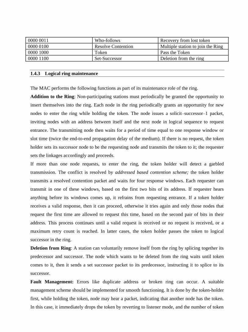
0000 0011 Who-follows Recovery from lost token
0000 0100 Resolve Contention Multiple station to join the Ring
0000 1000 Token Pass the Token
0000 1100 Set-Successor Deletion from the ring
1.4.3 Logical ring maintenance
The MAC performs the following functions as part of its maintenance role of the ring.
Addition to the Ring: Non-participating stations must periodically be granted the opportunity to
insert themselves into the ring. Each node in the ring periodically grants an opportunity for new
nodes to enter the ring while holding the token. The node issues a solicit–successor–1 packet,
inviting nodes with an address between itself and the next node in logical sequence to request
entrance. The transmitting node then waits for a period of time equal to one response window or
slot time (twice the end-to-end propagation delay of the medium). If there is no request, the token
holder sets its successor node to be the requesting node and transmits the token to it; the requester
sets the linkages accordingly and proceeds.
If more than one node requests, to enter the ring, the token holder will detect a garbled
transmission. The conflict is resolved by addressed based contention scheme; the token holder
transmits a resolved contention packet and waits for four response windows. Each requester can
transmit in one of these windows, based on the first two bits of its address. If requester hears
anything before its windows comes up, it refrains from requesting entrance. If a token holder
receives a valid response, then it can proceed, otherwise it tries again and only those nodes that
request the first time are allowed to request this time, based on the second pair of bits in their
address. This process continues until a valid request is received or no request is received, or a
maximum retry count is reached. In latter cases, the token holder passes the token to logical
successor in the ring.
Deletion from Ring: A station can voluntarily remove itself from the ring by splicing together its
predecessor and successor. The node which wants to be deleted from the ring waits until token
comes to it, then it sends a set successor packet to its predecessor, instructing it to splice to its
successor.
Fault Management: Errors like duplicate address or broken ring can occur. A suitable
management scheme should be implemented for smooth functioning. It is done by the token-holder
first, while holding the token, node may hear a packet, indicating that another node has the token.
In this case, it immediately drops the token by reverting to listener mode, and the number of token

holders drops immediately from one to zero. Upon completion of its turn, it immediately issues a
data or token packet. The sequence of steps are as follows:
i. After sending the token, the token issuer will listen for one slot time to make sure that its
predecessor is active.
ii. If the issuer does not hear a valid packet, it reissues the token to the same successor one
more time.
iii. After two failures, the issuer assumes that its successor has failed and issues a “who-
follows” packet, asking for the identity of the node that follows the failed node. The issuer
should get back a set successor packet from the second node down the time. If so, the
issuer adjusts its linkage and issues a token (back to step i).
iv. If the issuing node gets a response to its “who-follows” packet, it tries again.
v. If the “who-follows” tactic fails, the node issues a solicit-successor-2 packet with full
address range (i.e. every node is invited to respond). If this packet works then the ring is
established and procedure continues.
vi. If two attempts in step (v) fail, it assumes that a catastrophe has happened; perhaps the
node receiver has failed. In any case, the node ceases the activity and listen the bus.
Ring Initialization: Ring is to be initialized by starting the token passing. This is necessary when
the network is being setup or when ring is broken down. Some decentralized algorithms should
take care of, who starts first, who starts second, etc. it occurs when one or more stations detects a
lack of bus activity lasting longer than a specific time. The token may get lost. This can occur on a
number of occasions. For example, when network has been just powered up, or a token holding
station fails. Once its time out expires, a node will issue a claim token packet. Contending clients
are removed in a similar fashion to the response window process.
1.4.4 Relative comparison of the three standards
A comparison of the three standards for different functions is shown in Table 1.2 and results of the
analysis of the performance of the three standards are summarized below:
• The CSMA/CD protocol shows strong dependence on the parameter ‘a’, which is the ratio
of the propagation time to the transmission time. It offers shortest delay under light load
and it is most sensitive under heavy load conditions.
• Token ring is least sensitive to different load conditions and different packet sizes.
• Token bus is highly efficient under light load conditions.

Table 1.2 Comparison of the three standards
Function CSMA/CD
Token bus Token ring
Access determination Contention
Token Token
Packet length
restriction 64 bytes (Greater than
2.Tprop)
None None
Priority Not supported
Supported Supported
Sensitivity to work
load Most sensitive
Sensitive Least
sensitive
Principle advantage Simplicity, wide
installed base
Regulated/fair
access Regulated/fai
r access
Principle disadvantage Nondeterministic
delay
Complexity Complexity
1.5 Introduction to High Speed LANs – Token Ring Based
The IEEE 802.3 and 802.5 LANs, discussed in the previous sections, having data transfer rate in
the range of 10 Mb/s to 16 Mb/s have served the purpose very well for many years. But with the
availability of powerful computers at a low cost and emergence of new applications, particularly
based on multimedia, there is a growing demand for higher network bandwidth. The combined
effect of the growth in the number of users and increasing bandwidth requirement per user has led
to the development of High Speed LANs with data transfer rate of 100 Mb/s or more.
The high speed LANs that have emerged can be broadly categorized into three types based on
token passing, successors of Ethernet and based on switching technology. In the first category we
have FDDI and its variations, and high-speed token ring. In the second category we have the fast
Ethernet and Gigabit Ethernet. In the third category we have ATM, fiber channel and the Ether
switches. In this lesson we shall discuss details of FDDI – the token ring based high speed LAN.
1.6 FDDI
Fiber Distributed Data Interface (FDDI), developed by American National Standards Institute
(ANSI) is a token passing ring network that operates at 100 Mb/s on optical fiber-medium. Its
medium access control approach has close similarity with the IEEE 802.5 standard, but certain
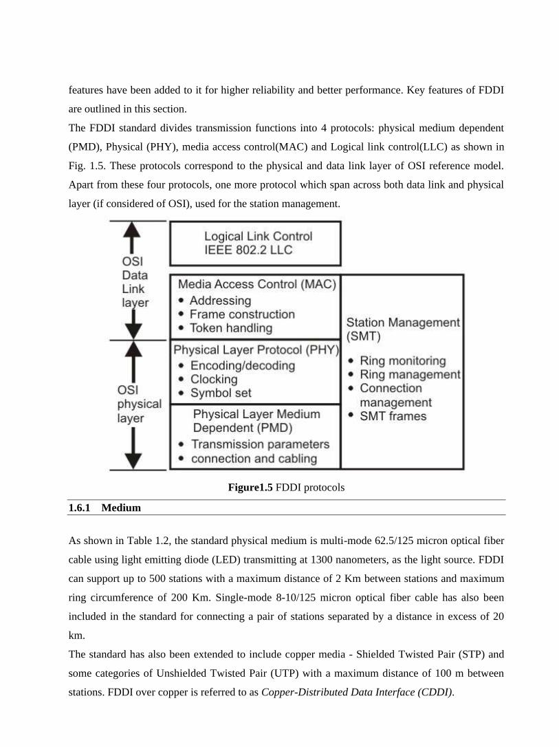
features have been added to it for higher reliability and better performance. Key features of FDDI
are outlined in this section.
The FDDI standard divides transmission functions into 4 protocols: physical medium dependent
(PMD), Physical (PHY), media access control(MAC) and Logical link control(LLC) as shown in
Fig. 1.5. These protocols correspond to the physical and data link layer of OSI reference model.
Apart from these four protocols, one more protocol which span across both data link and physical
layer (if considered of OSI), used for the station management.
Figure1.5 FDDI protocols
1.6.1 Medium
As shown in Table 1.2, the standard physical medium is multi-mode 62.5/125 micron optical fiber
cable using light emitting diode (LED) transmitting at 1300 nanometers, as the light source. FDDI
can support up to 500 stations with a maximum distance of 2 Km between stations and maximum
ring circumference of 200 Km. Single-mode 8-10/125 micron optical fiber cable has also been
included in the standard for connecting a pair of stations separated by a distance in excess of 20
km.
The standard has also been extended to include copper media - Shielded Twisted Pair (STP) and
some categories of Unshielded Twisted Pair (UTP) with a maximum distance of 100 m between
stations. FDDI over copper is referred to as Copper-Distributed Data Interface (CDDI).

Optical fiber has several advantages over copper media. In particular, security, reliability, and
performance are all enhanced with optical fiber media because fiber does not emit electrical
signals. A physical medium that does emit electrical signals (copper) can be tapped and therefore
vulnerable to unauthorized access to the data that is transmitted through the medium. In addition,
fiber is immune to radio frequency interference (RFI) and electromagnetic interference (EMI).
Fiber historically has supported much higher bandwidth (throughput potential) than copper,
although recent technological advances have made copper capable of transmitting at 100 Mbps or
more. Finally, FDDI allows 2 Km between stations using multimode fiber, and even longer
distances using a single mode fiber.
Table 1.2 FDDI Physical layer specification
Trans. Medium Optical Fiber
62.5/125 um
Twisted pair
CAT5-UTP
Data Rate 100 Mbps 100Mbps
Signaling Technique 4B/5B/NRZ-I
125 Mbaud
MTL-3
Max. No. Repeaters 100 100
Max. distance 2Km 100m
FDDI uses 4B/5B code for block coding. The 5-bit code is selected such that it has no more than
one leading zero and no more than two trailing zeros and more than three consecutive 0’s do not
occur. Table 1.3 shows the encoded sequence for all the 4-bit data sequences. The This is normally
line coded with NRZ-I.
Table 1.3 4B/5B encoding

1.6.2 Topology
The basic topology for FDDI is dual counter rotating rings: one transmitting clockwise and the
other transmitting counter clockwise as illustrated in the Fig. 1.6. One is known as primary ring
and the other secondary ring. Although theoretically both the rings can be used to achieve a data
transfer rate of 200 Mb/s, the standard recommends the use of the primary ring for data
transmission and secondary ring as a backup.
In case of failure of a node or a fiber link, the ring is restored by wrapping the primary ring to the
secondary ring as shown in Fig. 1.7. The redundancy in the ring design provides a degree of fault
tolerance, not found in other network standards. Further improvement in reliability and availability
can be achieved by using dual ring of trees and dual homing mechanism.

Figure 1.6 FDDI dual counter-rotating ring topology
1.6.3 Fault Tolerance
FDDI provides a number of fault-tolerant features. In particular, FDDI's dual-ring environment,
the implementation of the optical bypass switch, and dual-homing support make FDDI a resilient
media technology.
Dual Ring
FDDI's primary fault-tolerant feature is the dual ring. If a station on the dual ring fails or is
powered down, or if the cable is damaged, the dual ring is automatically wrapped (doubled back
onto itself) into a single ring. When the ring is wrapped, the dual-ring topology becomes a single-
ring topology. Data continues to be transmitted on the FDDI ring without performance impact
during the wrap condition.

(a) (b)
Figure 1.7 FDDI ring with a (a) broken link, (b) defective station
When a cable failure occurs, as shown in Fig. 1.7 (a), devices on either side of the cable fault wrap.
Network operation continues for all stations. When a single station fails, as shown in Fig. 1.7 (b),
devices on either side of the failed (or powered-down) station wrap, forming a single ring.
Network operation continues for the remaining stations on the ring. It should be noted that FDDI
truly provides fault tolerance against a single failure only. When two or more failures occur, the
FDDI ring segments into two or more independent rings that are incapable of communicating with
each other.
Optical Bypass Switch
An optical bypass switch provides continuous dual-ring operation if a device on the dual ring fails.
This is used both to prevent ring segmentation and to eliminate failed stations from the ring. The
optical bypass switch performs this function using optical mirrors that pass light from the ring
directly to the DAS (dual-attachment station) device during normal operation. If a failure of the
DAS device occurs, such as a power-off, the optical bypass switch will pass the light through itself
by using internal mirrors and thereby will maintain the ring's integrity.
Figure 1.8 The Optical Bypass switch uses internal mirrors to maintain a network
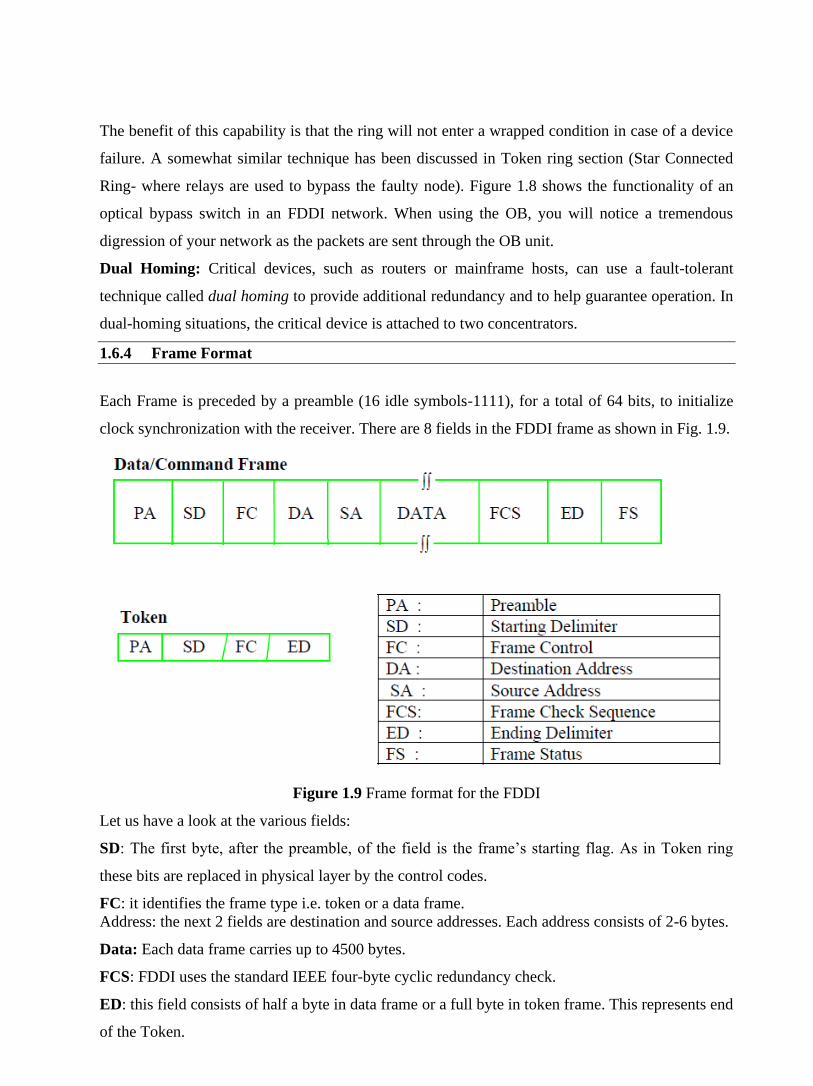
The benefit of this capability is that the ring will not enter a wrapped condition in case of a device
failure. A somewhat similar technique has been discussed in Token ring section (Star Connected
Ring- where relays are used to bypass the faulty node). Figure 1.8 shows the functionality of an
optical bypass switch in an FDDI network. When using the OB, you will notice a tremendous
digression of your network as the packets are sent through the OB unit.
Dual Homing: Critical devices, such as routers or mainframe hosts, can use a fault-tolerant
technique called dual homing to provide additional redundancy and to help guarantee operation. In
dual-homing situations, the critical device is attached to two concentrators.
1.6.4 Frame Format
Each Frame is preceded by a preamble (16 idle symbols-1111), for a total of 64 bits, to initialize
clock synchronization with the receiver. There are 8 fields in the FDDI frame as shown in Fig. 1.9.
Figure 1.9 Frame format for the FDDI
Let us have a look at the various fields:
SD: The first byte, after the preamble, of the field is the frame’s starting flag. As in Token ring
these bits are replaced in physical layer by the control codes.
FC: it identifies the frame type i.e. token or a data frame.
Address: the next 2 fields are destination and source addresses. Each address consists of 2-6 bytes.
Data: Each data frame carries up to 4500 bytes.
FCS: FDDI uses the standard IEEE four-byte cyclic redundancy check.
ED: this field consists of half a byte in data frame or a full byte in token frame. This represents end
of the Token.
FS: FDDI FS field is similar to that of Token Ring. It is included only in data/Command frame and
consists of one and a half bytes.
1.6.5 Media Access Control
The FDDI media access control protocol is responsible for the following services.
(i) Fair and equal access to the ring by using a timed token protocol. To transmit on the
ring, a station must first acquire the token. A station holds the token until it has
transmitted all of its frames or until the transmission time for the appropriate service is
over. Synchronous traffic is given a guaranteed bandwidth by ensuring that token
rotation time does not exceed a preset value. FDDI implements these using three
timers, Token holding Timer (THT), which determines how long a station may continue
once it has captured a token. Token Rotation Timer (TRT) is reset every time a token is
seen. When timer expires, it indicates that the token is lost and recovery is started. The
Valid Transmission Timer (VTT) is used to time out and recover from some transmit
ring errors.
(ii) Construction of frames and tokens are done as per the format shown in Figure 1.9. The
frame status (FS) byte is set by the destination and checked by the source station, which
removes its frame from the ring and generates another token.
(iii) Transmitting, receiving, repeating and stripping frames and tokens from the ring, unlike
IEEE 802.5, is possible for several frames on the ring simultaneously. Thus a station
will transmit a token immediately after completion of its frame transmission. A station
further down the ring is allowed to insert its own frame. This improves the potential
throughput of the system. When the frame returns to the sending station, that station
removes the frame from the ring by a process called stripping.
(iv) It also does ring initialization, fault isolation and error detection as we have discussed
for IEEE 802.5.
1.6.6 FDDI and the OSI model
The relationship between the OSI model and the FDDI layered architecture is shown in Fig. 1.5.
The physical layer is divided into two sub layers: PMD and PHY. The lower sub layer is defined
by Physical Layer Medium Dependent (PMD) standards, which specify requirements such as
media and connection types. The upper sub layer is defined in the physical layer protocol (PHY)
standard, which is medium-independent. It defines symbols, line status, encoding/decoding
techniques, clocking requirements and data framing requirements.

The Data Link Layer is divided into two sub layers, MAC and LLC. The lower sub layer, the
FDDI Media Access Control (MAC) standard defines addressing conventions, frame formats and
the timed token protocol. The upper sub layer is defined in the IEEE 802.2 LLC standard, which
provides a means for exchanging data between LLC users.
The Station Management (SMT) standard provides services that monitor and control a FDDI
station. SMT include facilities for connection management, node configuration, recovery from
error condition, and encoding of SMT frames.
The FDDI has been successfully used as a backbone LAN in an enterprise network or in a campus
network.
1.6.7 Comparison
Important features of the FDDI with the two popular IEEE 802 LAN standards are given in the
Table 1.4.
Table 1.4.Comparison of the standards
COMPARISON AMONG STANDARDS
Parameters FDDI IEEE 802.3 IEEE 802.5
BANDWIDTH
100Mb/s 10Mb/s 4 or 16Mb/s
NUMBER OF STATIONS
500 1024 250
MAX. DISTANCE BETWEEN
STATIONS
2Km (MMF)
20Km (SMF)
2.8Km 300m (4Mb/s)
100m (RECO.)
MAX. NETWORK EXTENT
100Km 2.8Km VARIED
WITH
CONFIGURAT
ION
LOGICAL TOPOLOGY
DUAL RING,
DUAL RING
OF TREES
BUS SINGLE RING
PHYSICAL TOPOLOGY
RING, STAR
HIERARCHI
CAL STAR
BUS, STAR RING BUS
HIERARCHIC
AL STAR
MEDIA
OPTICAL
FIBER
OPTICAL
FIBRE,
TWISTED-
WIRE,
COAXIAL
CABLE
TWISTED-
WIRE
OPTICAL
FIBER

ACCESS METHOD
TIMED-
TOKEN
PASSING
CSMA/CD TOKEN
PASSING
TOKEN ACQUISITION
CAPTURES
THE TOKEN
- BY SETTING
A STATUS
BIT
TOKEN RELEASE
AFTER
TRANSMIT - AFTER
STRIPPING
OR AFTER
TRANSMIT
(16)
FRAMES ON LAN
MULTIPLE SINGLE SINGLE
FRAMES TRANSMITTED PER ACCESS
MULTIPLE SINGLE SINGLE
MAX. FRAME SIZE
4500 BYTES 1518 BYTES 4500 BYTES
(4)
17,800 BYTES
(16)
1.7 Check Your Progress
Fill In The Blanks
1. Originally, ______________ developed Token Ring network in the ________.
2. A disadvantage of this topology is that it is vulnerable to _________ or _____ failure
3. Unlike CSMA/CD networks (such as Ethernet), token-passing networks are
________________, which means that it is possible to calculate the maximum time that
will pass before any end station will be capable of transmitting.
4. Token Ring frames have two fields that control priority: ___________ and the
___________field.
5. In Token Ring inside the wire center, _____________ are used to isolate a broken wire or a
faulty station.
6. The Mac sublayer in Token BUS consists of four major functions: ____________, the
access control machine (ACM), ______________________and ____________.
7. ___________ determines when to place a frame on the bus, and responsible for the
maintenance of the logical ring including the error detection and fault recovery.
8. The high speed LANs that have emerged can be broadly categorized into three
types______________, successors of Ethernet and ___________.
9. ATM, fiber channel and the Etherswitches comes under high speed LANs based on
________________.
10. ______________________ is abbreviated as FDDI.
11. FDDI over copper is referred to as __________________________.
12. The basic topology for FDDI is _____________________.
13. An _____________ provides continuous dual-ring operation if a device on the dual ring
fails
14. Each data frame in FDDI carries up to ____________ bytes
1.8 Answer to Check Your Progress
1. IBM, 1970
2. link, station
3. deterministic
4. the priority field, reservation
5. bypass relays
6. the interface machine (IFM), the receiver machine (RxM), the transmit machine (TxM).
7. Access control machine (ACM)
8. based on token passing, based on switching technology.
9. based on switching technology.
10. Fiber Distributed Data Interface
11. Copper-Distributed Data Interface (CDDI).
12. dual counter rotating rings
13. optical bypass switch
14. 4500

Unit-2
High Speed LANs – CSMA/CD based
1.1 Learning Objectives
1.2 Introduction
1.3 Successors of Ethernet
1.3.1 Switched Ethernet
1.3.2 Fast Ethernet
1.3.3 Gigabit Ethernet and Brief History and the IEEE 802.3z Task Force
1.3.4 Similarities and advances over Ethernet (IEEE 802.3)
1.3.5 Gigabit Ethernet Protocol Architecture
1.3.6 GMII (Gigabit Media Independent Interface)
1.3.7 Media Access Control Layer
1.4 Check Your Progress
1.5 Answer to Check Your Progress

1.1 Learning Objectives
After going through this unit, the learner will able to learn:
• Distinguish between switched versus shared LAN
• Explain the key features of Fast Ethernet
• Explain the key features of the Gigabit Ethernet
1.2 Introduction
In the preceding unit we have seen that high speed LANs have emerged broadly into three types -
based on token passing, successors of Ethernet and based on switching technology. we have
discussed FDDI and its variations in the preceding lesson. In the second category we have the fast
Ethernet and Gigabit Ethernet. In the third category we have ATM, fiber channel and the Ether
switches. In this lesson we shall discuss the second and the third categories of LANs starting with
successors of Ethernet.
1.3 Successors of Ethernet
On a regular Ethernet segment, all stations share the available bandwidth of 10 Mb/s. With the
increase in traffic, the number of packet collisions goes up, lowering the overall throughput. In
such a scenario, there are two basic approaches to increase the bandwidth.
One is to replace the Ethernet with a higher speed version of Ethernet. Use of Fast Ethernet
operating at 100 Mb/s and Gigabit Ethernet operating at 1000 Mb/s belong to this category. This
approach requires replacement of the old network interface cards (NICs) in each station by new
ones.
The other approach is to use Ethernet switches (let us call it switched Ethernet approach) that use a
high-speed internal bus to switch packets between multiple (8 to 32) cable segments and offer
dedicated 10 Mb/s bandwidth on each segment/ports. In this approach, there is no need to replace
the NICs; replacement of the hub by a switch serves the purpose. This approach is discussed in the
following section.
1.3.1 Switched Ethernet
Switched Ethernet gives dedicated 10 Mb/s bandwidth on each of its ports. On each of the ports
one can connect either a thick/thin segment or a computer.
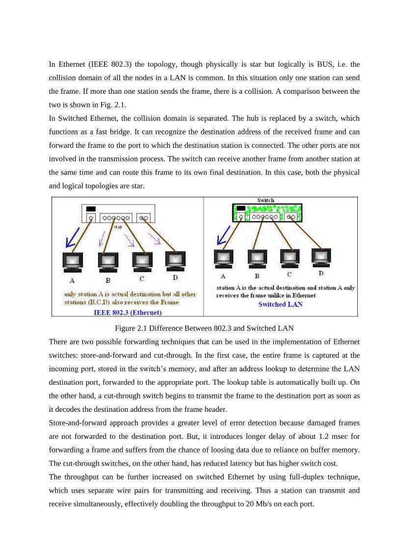
In Ethernet (IEEE 802.3) the topology, though physically is star but logically is BUS, i.e. the
collision domain of all the nodes in a LAN is common. In this situation only one station can send
the frame. If more than one station sends the frame, there is a collision. A comparison between the
two is shown in Fig. 2.1.
In Switched Ethernet, the collision domain is separated. The hub is replaced by a switch, which
functions as a fast bridge. It can recognize the destination address of the received frame and can
forward the frame to the port to which the destination station is connected. The other ports are not
involved in the transmission process. The switch can receive another frame from another station at
the same time and can route this frame to its own final destination. In this case, both the physical
and logical topologies are star.
Figure 2.1 Difference Between 802.3 and Switched LAN
There are two possible forwarding techniques that can be used in the implementation of Ethernet
switches: store-and-forward and cut-through. In the first case, the entire frame is captured at the
incoming port, stored in the switch’s memory, and after an address lookup to determine the LAN
destination port, forwarded to the appropriate port. The lookup table is automatically built up. On
the other hand, a cut-through switch begins to transmit the frame to the destination port as soon as
it decodes the destination address from the frame header.
Store-and-forward approach provides a greater level of error detection because damaged frames
are not forwarded to the destination port. But, it introduces longer delay of about 1.2 msec for
forwarding a frame and suffers from the chance of loosing data due to reliance on buffer memory.
The cut-through switches, on the other hand, has reduced latency but has higher switch cost.
The throughput can be further increased on switched Ethernet by using full-duplex technique,
which uses separate wire pairs for transmitting and receiving. Thus a station can transmit and
receive simultaneously, effectively doubling the throughput to 20 Mb/s on each port.

1.3.2 Fast Ethernet
The 802.u or the fast Ethernet, as it is commonly known, was approved by the IEEE 802
Committee in June 1995. It may not be considered as a new standard but an addendum to the
existing 802.3 standard. The fast Ethernet uses the same frame format, same CSMA/CD protocol
and same interface as the 802.3, but uses a data transfer rate of 100 Mb/s instead of 10 Mb/s.
However, fast Ethernet is based entirely on 10-Base-T, because of its advantages (Although
technically 10-BASE-5 or 10-BASE-2 can be used with shorter segment length).
Fortunately, the Ethernet is designed in such a way that the speed can be increased if collision
domain is decreased. The only two changes made in the MAC layer are the data rate and the
collision domain. The data rate is increased by a factor of 10 and collision domain is decreased by
a factor of 10. To increase the data rate without changing the minimum size of the frame (576 bits
or 76 bytes in IEEE 802.3), it is necessary to decrease the round-trip delay time. With the speed of
100Mbps the round-trip time reduce to 5.76 microseconds (576 bits/100 Mbps; which was 57.6
microsecond for 10Mbps Normal Ethernet). This means that the collision domain is decreased 10
fold from 2500 meters (in IEEE802.3) to 250 meters (fast Ethernet).
IEEE has designed two categories of Fast Ethernet: 100Base-X and 100Base-T4. 100Base-X uses
two-wire interface between a hub and a station while 100Base-T4 uses four-wire interface. 100-
Base-X itself is divided into two: 100Base-TX and 100base-FX as shown in Fig. 2.2.
100 BASE-T4:
This option is designed to avoid overwriting. It is used for half-duplex communication using four
wire-pairs of the existing category 3 UTP cables, which are already available for telephone
services in homes/offices. Two of four pairs are bi-directional; other two are unidirectional. This
means that there are 3 pairs to be used for carrying data, in each direction (2 bi-directional and 1
uni-directional) as shown in Fig. 2.3. Because 100Mbps data cannot be handled by voice-grade
UTP, this specification splits the 100 Mbps flow into three 33.66 Mbps flows.

Figure 2.2 Fast Ethernet implementations
Figure 2.3 100Base-T4 implementation
100 BASE TX:
This option uses two pairs of category 5 UTP or two shielded twisted-pair (STP) cable to connect a
station to hub as shown in Fig. 2.4. One pair is used to carry frames from the hub to the station and
other to carry frames from station to hub. It uses 4B/5B encoding to handle 100 Mbps using NRZ-I
signaling. The distance between station and hub should be less than 100 meters.
Figure 2.4 100Base-TX implementation
100 BASE FX:
This option uses two Fiber optic cables, one carry frames from station to hub and other from hub
to station as shown in Fig. 2.5. The encoding is using 4B/5B and it uses NRZ-I signaling. The
distance between station and hub should be less than 2000 meters.
Figure 2.5 100Base-FX implementation
1.3.3 Gigabit Ethernet and Brief History and the IEEE 802.3z Task Force

As applications increased, the demand on the network, newer, high-speed protocols such as FDDI
and ATM became available. However, in the last couple of years, Fast Ethernet has become the
backbone of choice because it’s simplicity and its reliance on Ethernet. The primary goal of
Gigabit Ethernet is to build on that topology and knowledge base to build a higher-speed protocol
without forcing customers to throw away existing networking equipment.
In March 1996, the IEEE 802.3 committee approved the 802.3z Gigabit Ethernet Standardization
project. At that time as many as 54 companies expressed there intent to participate in the
standardization project. The Gigabit Ethernet Alliance was formed in May 1996 by 11 companies.
The Alliance represents a multi-vendor effort to provide open and inter-operable Gigabit Ethernet
products. The objectives of the alliance are:
• Supporting extension of existing Ethernet and Fast Ethernet technology in response to
demand
for higher network bandwidth.
• Developing technical proposals for the inclusion in the standard
• Establishment of inter-operability test procedures and processes
1.3.4 Similarities and advances over Ethernet (IEEE 802.3)
As its name implies, Gigabit Ethernet - officially known as 802.3z - is the 1 Gb/s extension of the
802.3 standard already defined for 10 and 100 Mb/s service. Gigabit Ethernet builds on top of the
Ethernet protocol, but increases speed tenfold over Fast Ethernet to 1000 Mbps, or 1 gigabit per
second (Gbps). It retains the Carrier Sense Multiple Access/ Collision Detection (CSMA/CD) as
the access method. It supports full duplex as well as half duplex modes of operation. Initially,
single-mode and multi mode fiber and short-haul coaxial cable were supported. Standards for
twisted pair cables were subsequently added. The standard uses physical signaling technology used
in Fiber Channel to support Gigabit rates over optical fibers. Since Gigabit Ethernet significantly
leverages on Ethernet, customers will be able to leverage their existing knowledge base to manage
and maintain gigabit networks. Initially, Gigabit Ethernet was expected to be used as a backbone
system in existing networks. It can be used to aggregate traffic between clients and "server farms",
and for connecting Fast Ethernet switches. It can also be used for connecting workstations and
servers for high-bandwidth applications such as medical imaging or CAD. But, gigabit Ethernet is
not simply a straight Ethernet running at 1 Gb/s. In fact, the ways it differs from its predecessors
may be more important than its similarities. Some of the important differences are highlighted
below.
(i) The cabling requirement of gigabit Ethernet is very different. The technology is based
on fiber optic cable. Multi-mode fiber is able to transmit at gigabit rate to at least 580
meters and with single-mode runs exceeding 3 km. Fiber optic cabling is costly. In
order to reduce the cost of cabling, the 802.3z working group also proposed the use of
twisted-pair or cable or coaxial cable for distances up to 30 meters.
(ii) Gigabit Ethernet also relies on a modified MAC layer. At gigabit speed, two stations
200 meters apart will not detect a collision, when both simultaneously send 64-byte
frames. This inability to detect collision leads to network instability. A mechanism
known as carrier extension has been proposed for frames shorter than 512 bytes. The
number of repeater hops is also restricted to only one in place of two for 100 Base-T.
(iii) Flow Control is a major concern in gigabit Ethernet because of buffer overflow and
junked frames in heavily loaded condition. The solution proposed by IEEE
subcommittee is the 802.3x. The X-on/X-off protocol works over any full-duplex
Ethernet, fast Ethernet or gigabit Ethernet link. When a switch buffer is close to
capacity, the receiving device signals the sending station and tells it to stop transmitting
until the buffer becomes empty.
(iv) Finally, one important feature, which Ethernet technology lacks, is the Quality of
Service (QoS). The gigabit Ethernet is a connectionless technology that transmits
variable length frames. As such, it simply cannot guarantee that the real-time packets
get the preferential treatment they require. The IEEE subcommittee developed two
specifications that will help Ethernet provide the required QoS. 802.lq tags traffic for
VLANs and for prioritization. 802.lp is a signaling scheme that lets end station request
priority and allows switches to pass these requests along the path.
The gigabit Ethernet comes into its own as an internetworking switch link (ISL) that
aggregates 10-and100-Mb/s feeds from the desktops and servers. Presently, gigabit Ethernet is
already matured with a large installation base as a backbone network technology.
1.3.5 Gigabit Ethernet Protocol Architecture
In order to accelerate speeds from 100 Mbps Fast Ethernet up to 1 Gbps, several changes were
required to be made to the physical interface. It was decided that Gigabit Ethernet will look
identical to Ethernet from the data link layer upward. The challenges involved in accelerating to 1
Gbps have been resolved by merging two technologies together: IEEE 802.3 Ethernet and ANSI
X3T11 FiberChannel as shown in Fig. 2.6.
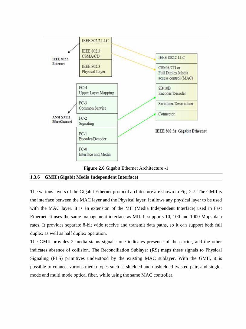
Figure 2.6 Gigabit Ethernet Architecture -1
1.3.6 GMII (Gigabit Media Independent Interface)
The various layers of the Gigabit Ethernet protocol architecture are shown in Fig. 2.7. The GMII is
the interface between the MAC layer and the Physical layer. It allows any physical layer to be used
with the MAC layer. It is an extension of the MII (Media Independent Interface) used in Fast
Ethernet. It uses the same management interface as MII. It supports 10, 100 and 1000 Mbps data
rates. It provides separate 8-bit wide receive and transmit data paths, so it can support both full
duplex as well as half duplex operation.
The GMII provides 2 media status signals: one indicates presence of the carrier, and the other
indicates absence of collision. The Reconciliation Sublayer (RS) maps these signals to Physical
Signaling (PLS) primitives understood by the existing MAC sublayer. With the GMII, it is
possible to connect various media types such as shielded and unshielded twisted pair, and single-
mode and multi mode optical fiber, while using the same MAC controller.

Figure 2.7 Gigabit Ethernet Architecture-2
• PCS (Physical Coding Sublayer)
This is the GMII sublayer, which provides a uniform interface to the Reconciliation layer for
all physical media. It uses 8B/10B coding like Fiber Channel. In this type of coding, groups of
8 bits are represented by 10 bit "code groups". Some code groups represent 8-bit data symbols.
Others are control symbols. The extension symbols used in Carrier Extension are an example
of control symbols. Carrier Sense and Collision Detect indications are generated by this
sublayer. It also manages the auto-negotiation process by which the NIC (Network Interface)
communicates with the network to determine the network speed (10,100 or 1000 Mbps) and
mode of operation (half-duplex or full-duplex).
• PMA (Physical Medium Attachment)
sublayer provides a medium-independent means for the PCS to support various serial bit-
oriented physical media. This layer serializes code groups for transmission and deserializes
bits received from the medium into code groups.
• PMD (Physical Medium Dependent)
This sublayer maps the physical medium to the PCS. This layer defines the physical layer
signalling used for various media. The MDI (Medium Dependent Interface), which is a
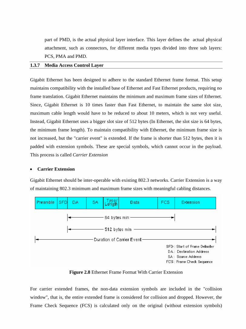
part of PMD, is the actual physical layer interface. This layer defines the actual physical
attachment, such as connectors, for different media types divided into three sub layers:
PCS, PMA and PMD.
1.3.7 Media Access Control Layer
Gigabit Ethernet has been designed to adhere to the standard Ethernet frame format. This setup
maintains compatibility with the installed base of Ethernet and Fast Ethernet products, requiring no
frame translation. Gigabit Ethernet maintains the minimum and maximum frame sizes of Ethernet.
Since, Gigabit Ethernet is 10 times faster than Fast Ethernet, to maintain the same slot size,
maximum cable length would have to be reduced to about 10 meters, which is not very useful.
Instead, Gigabit Ethernet uses a bigger slot size of 512 bytes (In Ethernet, the slot size is 64 bytes,
the minimum frame length). To maintain compatibility with Ethernet, the minimum frame size is
not increased, but the "carrier event" is extended. If the frame is shorter than 512 bytes, then it is
padded with extension symbols. These are special symbols, which cannot occur in the payload.
This process is called Carrier Extension
• Carrier Extension
Gigabit Ethernet should be inter-operable with existing 802.3 networks. Carrier Extension is a way
of maintaining 802.3 minimum and maximum frame sizes with meaningful cabling distances.
Figure 2.8 Ethernet Frame Format With Carrier Extension
For carrier extended frames, the non-data extension symbols are included in the "collision
window", that is, the entire extended frame is considered for collision and dropped. However, the
Frame Check Sequence (FCS) is calculated only on the original (without extension symbols)

frame. The extension symbols are removed before the FCS is checked by the receiver. So the LLC
(Logical Link Control) layer is not even aware of the carrier extension. Figure 2.8 shows the
Ethernet frame format when Carrier Extension is used.
• Packet Bursting
Carrier Extension is a simple solution, but it wastes bandwidth. Up to 448 padding bytes may
be sent for small packets. This results in lower throughput. In fact, for a large number of small
packets, the throughput is only marginally better than Fast Ethernet.
Packet Bursting is an extension of Carrier Extension. Packet Bursting is "Carrier Extension
plus a burst of packets". When a station has a number of packets to transmit, the first packet is
padded to the slot time if necessary using carrier extension. Subsequent packets are transmitted
back to back, with the minimum Inter-packet gap (IPG) until a burst timer (of 1500 bytes)
expires. Packet Bursting substantially increases the throughput. Figure 2.9 shows how Packet
Bursting works.
Figure 2.9 Packet Bursting
GBIC: Gigabit Ethernet Interface Carrier allows network managers to configure each port on a
port-by-port basis, including long-haul (LH) to support a distance of 5-10 Km using SMF as
shown in Fig. 2.10.
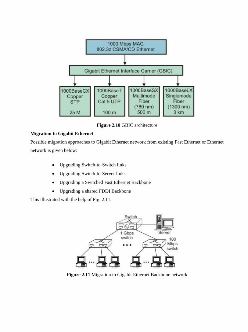
Figure 2.10 GBIC architecture
Migration to Gigabit Ethernet
Possible migration approaches to Gigabit Ethernet network from existing Fast Ethernet or Ethernet
network is given below:
• Upgrading Switch-to-Switch links
• Upgrading Switch-to-Server links
• Upgrading a Switched Fast Ethernet Backbone
• Upgrading a shared FDDI Backbone
This illustrated with the help of Fig. 2.11.
Figure 2.11 Migration to Gigabit Ethernet Backbone network

1.4 Check Your Progress
Fill In The Blanks:
1. Switched Ethernet gives dedicated 10 Mb/s bandwidth on __________ of its ports.
2. In Ethernet (IEEE 802.3) the topology, though physically is _________ but logically is
BUS. i.e. the collision domain of all the nodes in a LAN is _________.
3. In Switched Ethernet, collision domain is separated. Hub is replaced by a ________.
4. There are two techniques used in the implementation of Ethernet switches: _____________
and ________
5. IEEE has designed two categories of Fast Ethernet: ____________ and __________.
6. 100-Base-X itself is divided into two: __________ and __________
7. The Gigabit Ethernet Alliance was formed in ___________ by ______ companies.
8. The GMII is the interface between the ________ layer and the ___________ layer.
9. ________, a sublayer of GMII provides a medium-independent means for the PCS to
support various serial bit-oriented physical media.
10. Packet Bursting is an extension of ______________. Packet Bursting is "Carrier Extension
plus a ____________".
1.5 Answer to Check Your Progress
1. each
2. star, common
3. switch
4. store-and-forward, cut-through
5. 100Base-X, 100Base-T4
6. 100Base-TX, 100base-FX.
7. May 1996, 11
8. MAC, Physical
9. PMA (Physical Medium Attachment)
10. Carrier Extension, burst of packets

Unit-3
Wireless LANs
1.1 Learning Objectives
1.2 Introduction
1.3 Transmission Media
1.4 Infrared
1.4.1 Microwave
1.4.2 Radio
1.5 Topology
1.6 Medium Access Control
1.7 Carrier Sense Multiple Access with Collision Avoidance (CSMA-CA)
1.8 Framing
1.9 Security
1.10 IEEE 802.11 extensions
1.11 Check Your Progress
1.12 Answer to Check Your Progress
1.1 Learning Objectives
After going through this unit, the learner will able to learn:
• Explain the need for wireless LAN
• Identify the limitations and challenges of wireless LAN
• Understand different aspects of IEEE 802.11 WLAN
o Transmission media
o Topology
o Medium Access Control
o Security
1.2 Introduction
In the last two decades the wired version of LAN has gained wide popularity and large-scale
deployment. The IEEE 802.3 standard has been revised and extended every few years. High-speed
versions with transmission rate as high as 1000 Mbps are currently available. Until recently
wireless version of LANs were not popular because of the following reasons:
• High cost: Previously the equipments cost more.
• Low data rate: Initially, the data rate supported by the WLAN is too less, so it supports
only a few applications.
• Occupational safety concerns
• Licensing requirements
In the last couple of years the situation has changed significantly. Cheaper, smaller and powerful
notebook computers and other mobile computing equipment have proliferated in homes and
offices. These devices share various resources such as printers, files and Broadband Internet
connections. This has opened up the need for wireless LAN. Wireless LANs also offer a number of
other advantages compared to their wired counterpart.
Before going into the technical details of Wireless LAN let us first look at various reasons which
have led to the development of WLANs. Some of the advantages are mentioned below:
• Availability of low-cost portable equipments: Due to the technology enhancements, the
equipment cost that are required for WLAN set-up have reduced a lot.
• Mobility: An increasing number of LAN users are becoming mobile. These mobile users
require that they are connected to the network regardless of where they are because they
want simultaneous access to the network. This makes the use of cables, or wired LANs,

impractical if not impossible. Wireless LAN can provide users mobility, which is likely to
increase productivity, user convenience and various service opportunities.
• Installation speed and simplicity: Wireless LANs are very easy to install. There is no
requirement for wiring every workstation and every room. This ease of installation makes
wireless LANs inherently flexible. If a workstation must be moved, it can be done easily
and without additional wiring, cable drops or reconfiguration of the network.
• Installation flexibility: If a company moves to a new location, the wireless system is much
easier to move than ripping up all of the cables that a wired system would have snaked
throughout the building. This also provides portability. Wireless technology allows
network to go anywhere wire cannot reach.
• Reduced cost of ownership: While the initial cost of wireless LAN can be higher than the
cost of wired LAN hardware, it is envisaged that the overall installation expenses and life
cycle costs can be significantly lower. Long-term cost-benefits are greater in dynamic
environment requiring frequent moves and changes.
• Scalability: Wireless LAN can be configured in a variety of topologies to meet the users
need and can be easily scaled to cover a large area with thousands of users roaming within
it.
However, wireless LAN technology needs to overcome a number of inherent limitations and
challenges. Some of the limitations and challenges are mentioned below:
• Lower reliability due to susceptibility of radio transmission to noise and interference.
• Fluctuation of the strength of the received signal through multiple paths causing fading.
• Vulnerable to eavesdropping leading to security problem.
• Limited data rate because of the use of spread spectrum transmission techniques
enforced to ISM band users.
In this unit we shall introduce the wireless LAN technology based on IEEE 802.11 standard. Its
predecessor the IEEE 802.3, commonly referred to as the Ethernet, is the most widely deployed
member of the family. IEEE 802.11 is commonly referred to as wireless Ethernet because of its
close similarity with the IEEE 802.3. Like IEEE 802.3, it also defines only two bottom levels of
ISO’s open system Interconnection (OSI) model as shown in Fig. 3.1. As it shares the upper layers
with other LAN standards, it is relatively easy to bridge the IEEE 802.11 wireless LANs to other
IEEE 802.11 wired LANs to form an extended interconnected wired and wireless LAN network.
Although initially wireless LANs were perceived to be as a substitute to wired LANs, now it is
recognized as an indispensable adjunct to wired LANs.

Figure 3.1 OSI Reference Model and IEEE 802.11
The IEEE 802.11 standard basically defines the physical and data link layer. In the later sections
we shall look at detailed implementations.
1.3 Transmission Media
There are three media that can be used for transmission over wireless LANs. Infrared, radio
frequency and microwave. In 1985 the United States released the industrial, scientific, and medical
(ISM) frequency bands. These bands are 902 - 928MHz, 2.4 - 2.4853 GHz, and 5.725 - 5.85 GHz
and do not require licensing by the Federal Communications Commission (FCC). This prompted
most of the wireless LAN products to operate within ISM bands. The FCC did put restrictions on
the ISM bands however. In the U.S. radio frequency (RF) systems must implement spread
spectrum technology. RF systems must confine the emitted spectrum to a band. RF is also limited
to one watt of power. Microwave systems are considered very low power systems and must
operate at 500 milliwatts or less.
1.4 Infrared
Infrared systems (IR systems) are simple in design and therefore inexpensive. They use the same
signal frequencies used on fiber optic links. IR systems detect only the amplitude of the signal and
so interference is greatly reduced. These systems are not bandwidth limited and thus can achieve
transmission speeds greater than the other systems. Infrared transmission operates in the light

spectrum and does not require a license from the FCC to operate. There are two conventional ways
to set up an IR LAN.
The infrared transmissions can be aimed. This gives a good range of a couple of kilometer and can
be used outdoors. It also offers the highest bandwidth and throughput.
The other way is to transmit omni-directionally and bounce the signals off of everything in every
direction. This reduces coverage to 30 - 60 feet, but it is area coverage. IR technology was initially
very popular because it delivered high data rates and relatively cheap price.
The drawbacks to IR systems are that the transmission spectrum is shared with the sun and other
things such as fluorescent lights. If there is enough interference from other sources it can render
the LAN useless. IR systems require an unobstructed line of sight (LOS). IR signals cannot
penetrate opaque objects. This means that walls, dividers, curtains, or even fog can obstruct the
signal. InfraLAN is an example of wireless LANs using infrared technology.
1.4.1 Microwave
Microwave (MW) systems operate at less than 500 milliwatts of power in compliance with FCC
regulations. MW systems are by far the fewest on the market. They use narrow-band transmission
with single frequency modulation and are set up mostly in the 5.8GHz band. The big advantage to
MW systems is higher throughput achieved because they do not have the overhead involved with
spread spectrum systems. RadioLAN is an example of systems with microwave technology.
1.4.2 Radio
Radio frequency systems must use spread spectrum technology in the United States. This spread
spectrum technology currently comes in two types: direct sequence spread spectrum (DSSS) and
frequency hopping spread spectrum (FHSS). There is a lot of overhead involved with spread
spectrum and so most of the DSSS and FHSS systems have historically had lower data rates than
IR or MW.
Direct Sequence Spread Spectrum (DSSS) Scheme
Direct Sequence Spread Spectrum (DSSS) represents each bit in the frame by multiple bits in the
transmitted frame. DSSS represents each data 0 and 1 by the symbol –1 and +1 and then multiplies
each symbol by a binary pattern of +1’s and –1’s to obtain a digital signal that varies more rapidly
occupying larger band. The IEEE 802.11 uses a simple 11-chip Barker sequence B11 [-1, +1, -1, -
1, +1, -1, -1, -1, +1, +1, +1] with QPSK or BPSK modulation as shown in Figure 3.2. The DSSS
transmission system takes 1 Mbps data, converts it into 11 Mbps signal using differential binary
phase shift keying (DBPSK) modulation.

The Barker sequence provides good immunity against interference and noise as well as some
protection against multi-path propagation. In both cases of spread spectrum transmission, the
signal look like noise to any receiver that does not know the pseudorandom sequence. The third
transmission media is based on infrared signal in the near visible range of 850 to 950 nanometers.
Diffused transmission is used so that the transmitter and receivers do not have to point to each
other and do not require a clear line of sight communication. The transmission distance is limited
to 10 to 20 meters and is limited to inside the buildings only.
Figure 3.2 Direct-sequence spread spectrum technique using Barker sequence
With direct sequence spread spectrum the transmission signal is spread over an allowed band (for
example 25MHz). A random binary string is used to modulate the transmitted signal. This random
string is called the spreading code. The data bits are mapped to into a pattern of "chips" and
mapped back into a bit at the destination. The number of chips that represent a bit is the spreading
ratio. The higher the spreading ratio, the more the signal is resistant to interference. The lower the
spreading ratio, the more bandwidth is available to the user. The FCC dictates that the spreading
ratio must be more than ten. Most products have a spreading ratio of less than 20 and the new
IEEE 802.11 standard requires a spreading ratio of eleven. The transmitter and the receiver must
be synchronized with the same spreading code. If orthogonal spreading codes are used then more
than one LAN can share the same band. However, because DSSS systems use wide sub channels,

the number of co-located LANs is limited by the size of those sub channels. Recovery is faster in
DSSS systems because of the ability to spread the signal over a wider band. Current DSSS
products include Digital's RoamAbout and NCR's WaveLAN.
Figure 3.3 shows a typical DSSS implementation. Here, the data stream and pseudo-random
sequence are both converted into analog signals before combining, rather than performing the
exclusive-OR of the two streams and than modulating. Eleven channels have been defined to
operate in the 2.4 GHz ISM band in US. Channels can operate without interference with each other
if their center frequencies are separated by at least 30MHz. The 802.11 DSSS physical layer also
defines an option for 2 Mbps operation using Differential Quadrature PSK (DQPSK).
(a) Transmitter (b) Receiver
Figure 3.3 Direct Sequence Spread Spectrum (DSSS) system,
Frequency Hopping Spread Spectrum (FHSS)
The idea behind spread spectrum is to spread the signal over a wider frequency band, so as to
make jamming and interception more difficult and to minimize the effect of interference from
other devices In FH it is done by transmitting the signal over a random sequence of frequencies;
that is, first transmitting at one frequency, then second, then a third and so on. The random
sequence of frequencies is generated with the help of a pseudorandom number generator. As both
the receiver and sender use the same algorithm to generate random sequence, both the devices hop
frequencies in a synchronous manner and frames transmitted by the sender are received correctly
by the receiver. This is somewhat similar to sending different parts of one song over several FM
channels. Eavesdroppers hear only unintelligible blips and any attempt to jam the signal results in
damaging a few bits only.
Typical block diagram of a frequency-hopping system is shown in Figure 3.4.
As shown in Figure 3.4(a) the digital data is first encoded to analog signal, such as frequency-shift
keying (FSK) or Binary-phase shift keying (BPSK). At any particular instant, a carrier frequency is
selected by the pseudo-random sequence. The carrier frequency is modulated by the encoder
output a then transmitted after band pass filtering At the receiving end, the spread-spectrum signal
is demodulated using the same sequence of carrier frequencies generated with the help of same
pseudo-random sequence in synchronization with the transmitter, and the demodulated signal
filtered using a band-pass filter before decoding as shown in Fig. 3.4(b).
This technique splits the band into many small sub channels (each of 1MHz). The signal then hops
from sub channel to sub channel transmitting short bursts of data on each channel for a set period
of time, called dwell time. The hopping sequence must be synchronized at the sender and the
receiver or information is lost.
The 802.11 frequency hopping physical layer uses 79 non-overlapping 1 MHz Channels to
transmit 1 Mbps data signal over 2.4 GHz ISM band. There is option to transmit at the rate of 2
Mbps. A channel hop occurs every 224 μsec. The standard defines 78 hopping patterns that are
divided into three sets of 26 patterns each. Each hopping pattern jumps a minimum of six channels
in each hop and the hopping sequences are derived via a simple modulo 79 calculation. The
hopping patterns from each set collide three times on the average and five times in the worst case
over a hopping cycle. Each 802.11 network must use a particular hopping pattern. The hopping
patterns allow up to 26 networks to be collocated and still operate simultaneously.
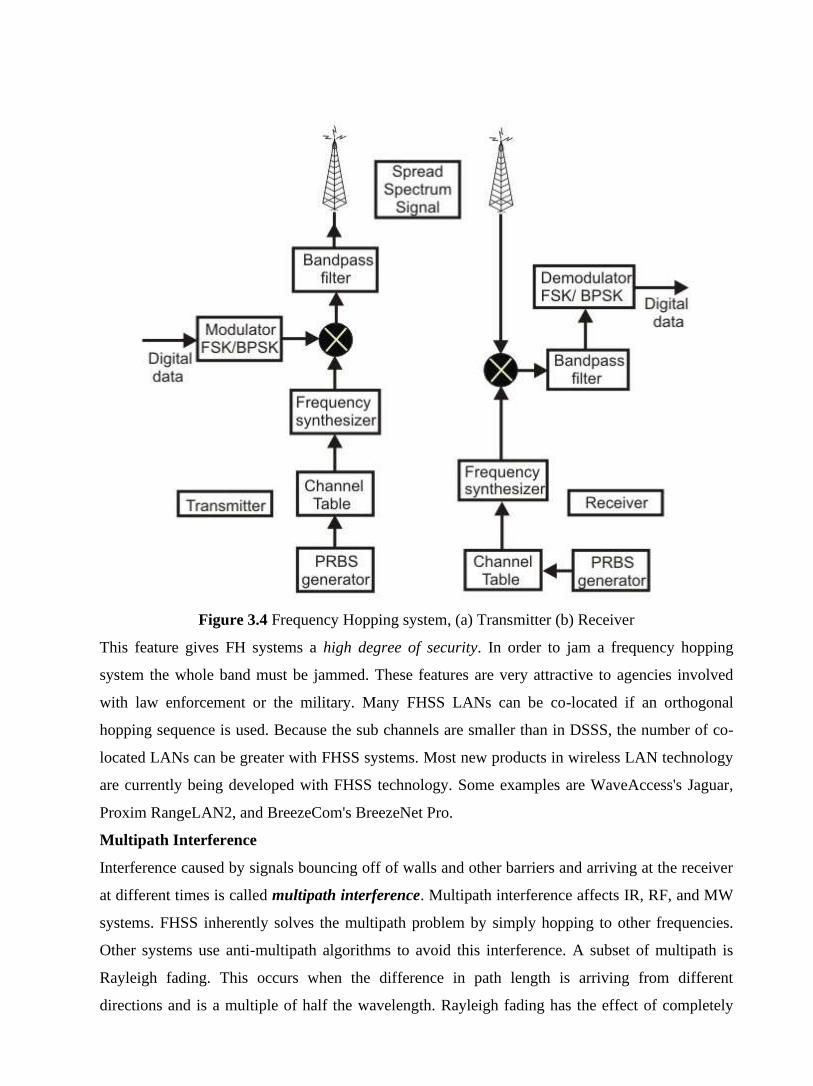
Figure 3.4 Frequency Hopping system, (a) Transmitter (b) Receiver
This feature gives FH systems a high degree of security. In order to jam a frequency hopping
system the whole band must be jammed. These features are very attractive to agencies involved
with law enforcement or the military. Many FHSS LANs can be co-located if an orthogonal
hopping sequence is used. Because the sub channels are smaller than in DSSS, the number of co-
located LANs can be greater with FHSS systems. Most new products in wireless LAN technology
are currently being developed with FHSS technology. Some examples are WaveAccess's Jaguar,
Proxim RangeLAN2, and BreezeCom's BreezeNet Pro.
Multipath Interference
Interference caused by signals bouncing off of walls and other barriers and arriving at the receiver
at different times is called multipath interference. Multipath interference affects IR, RF, and MW
systems. FHSS inherently solves the multipath problem by simply hopping to other frequencies.
Other systems use anti-multipath algorithms to avoid this interference. A subset of multipath is
Rayleigh fading. This occurs when the difference in path length is arriving from different
directions and is a multiple of half the wavelength. Rayleigh fading has the effect of completely
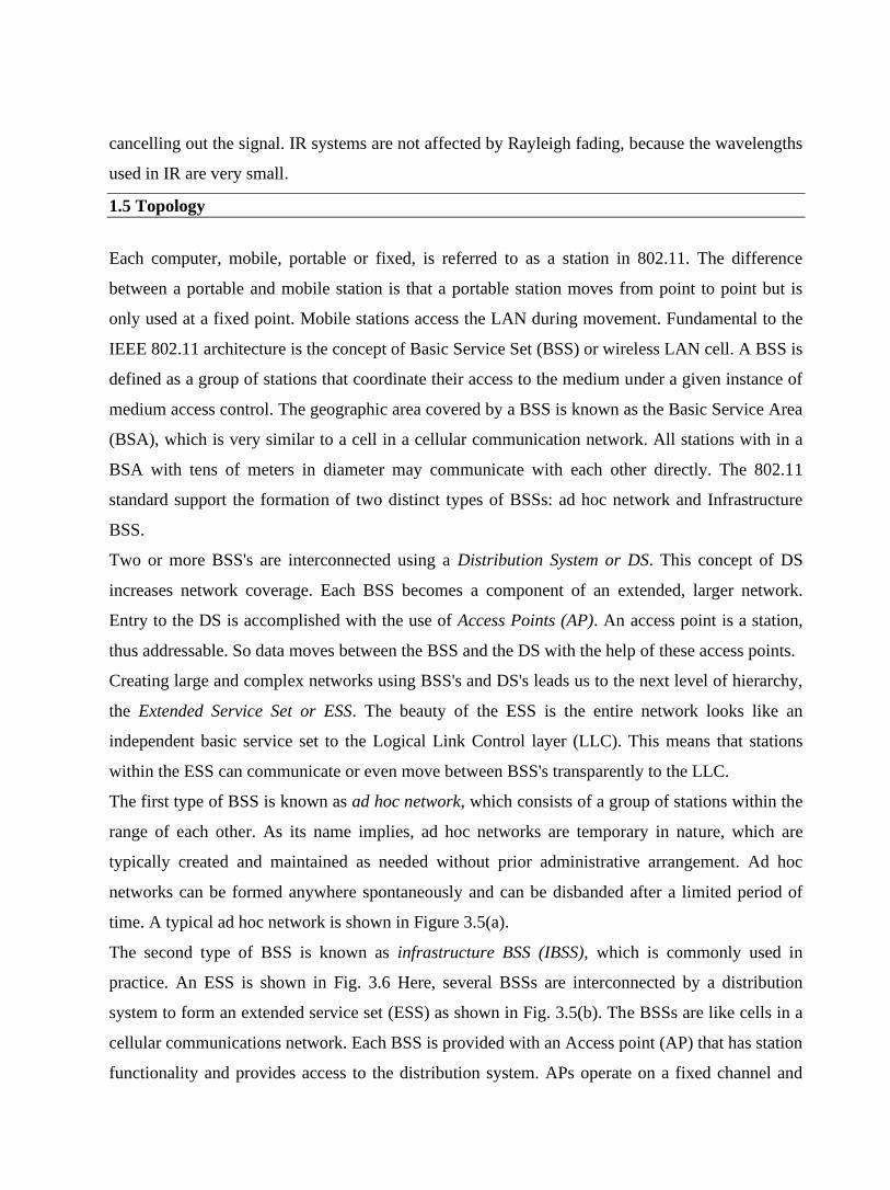
cancelling out the signal. IR systems are not affected by Rayleigh fading, because the wavelengths
used in IR are very small.
1.5 Topology
Each computer, mobile, portable or fixed, is referred to as a station in 802.11. The difference
between a portable and mobile station is that a portable station moves from point to point but is
only used at a fixed point. Mobile stations access the LAN during movement. Fundamental to the
IEEE 802.11 architecture is the concept of Basic Service Set (BSS) or wireless LAN cell. A BSS is
defined as a group of stations that coordinate their access to the medium under a given instance of
medium access control. The geographic area covered by a BSS is known as the Basic Service Area
(BSA), which is very similar to a cell in a cellular communication network. All stations with in a
BSA with tens of meters in diameter may communicate with each other directly. The 802.11
standard support the formation of two distinct types of BSSs: ad hoc network and Infrastructure
BSS.
Two or more BSS's are interconnected using a Distribution System or DS. This concept of DS
increases network coverage. Each BSS becomes a component of an extended, larger network.
Entry to the DS is accomplished with the use of Access Points (AP). An access point is a station,
thus addressable. So data moves between the BSS and the DS with the help of these access points.
Creating large and complex networks using BSS's and DS's leads us to the next level of hierarchy,
the Extended Service Set or ESS. The beauty of the ESS is the entire network looks like an
independent basic service set to the Logical Link Control layer (LLC). This means that stations
within the ESS can communicate or even move between BSS's transparently to the LLC.
The first type of BSS is known as ad hoc network, which consists of a group of stations within the
range of each other. As its name implies, ad hoc networks are temporary in nature, which are
typically created and maintained as needed without prior administrative arrangement. Ad hoc
networks can be formed anywhere spontaneously and can be disbanded after a limited period of
time. A typical ad hoc network is shown in Figure 3.5(a).
The second type of BSS is known as infrastructure BSS (IBSS), which is commonly used in
practice. An ESS is shown in Fig. 3.6 Here, several BSSs are interconnected by a distribution
system to form an extended service set (ESS) as shown in Fig. 3.5(b). The BSSs are like cells in a
cellular communications network. Each BSS is provided with an Access point (AP) that has station
functionality and provides access to the distribution system. APs operate on a fixed channel and

remain stationary like base stations in a cellular communication system. APs are located such that
the BSSs they serve overlap slightly to provide continuous service to all the stations.
(a) (a)
Figure 3.5 (a) Basic Service set (BSS), (b) Infrastructure BSS (ESS)
Figure 3.6 Extended service set (ESS)
An ESS can also provide gateway access for wireless users into a wired network. Each end station
associates itself with one access point. Figure 3.6 shows three BSSs interconnected through three
APs to a distribution system. If station A associated with AP-1 wants to send a frame to another
station associated with AP-2, the first sends a frame to its access point (AP-1), which forwards the
frame across the distribution system to the access point AP-2. AP-2 finally delivers it to the
destination station. For forwarding frames across the APs, bridging protocol may be used, which is
beyond the scope of IEEE 802.11 standard. However, the 802.11 standard specifies how stations
select their access points. The technique used for this purpose is known as scanning, which
involves the following steps:
• A station sends a probe frame.
• All APs within reach reply with a probe response frame.

• The station selects one of the access points, and sends the AP an Association Request
frame.
• The AP replies with an Association Response frame.
The above protocol is used when a station joins a network or when it wants to discontinue
association with the existing AP because of weakened signal strength or some other reason. The
discontinuation of association takes place whenever a station acquires a new AP and the new AP
announces it in step 4 mentioned above. For example, assume that station B is moving away from
the BSS of AP-1 towards the BSS of AP-2. As it moves closer to the BSS of AP-2, it sends probe
frames, which is responded eventually by AP-2. As some of point of time station B prefers AP-2
over AP-1 and associates itself with the access point AP-2. The above mechanism is known as
active scanning, as the node is actively searching for an access point. An access point also
periodically sends Beacon frame that advertises the capabilities of the access point. In response, a
station can associate to the AP simply by sending it an Association request frame. This is known as
passive scanning.
1.6 Medium Access Control
Most wired LANs products use Carrier Sense Multiple Access with Collision Detection
(CSMA/CD) as the MAC protocol. Carrier Sense means that the station will listen before it
transmits. If there is already someone transmitting, then the station waits and tries again later. If no
one is transmitting then the station goes ahead and sends what it has. But when more than one
station tries to transmit, the transmissions will collide and the information will be lost. This is
where Collision Detection comes into play. The station will listen to ensure that its transmission
made it to the destination without collisions. If a collision occurred then the stations wait and try
again later. The time the station waits is determined by the back off algorithm. This technique
works great for wired LANs but wireless topologies can create a problem for CSMA/CD.
However, the wireless medium presents some unique challenges not present in wired LANs that
must be dealt with by the MAC used for IEEE 802.11. Some of the challenges are:
• The wireless LAN is prone to more interference and is less reliable.
• The wireless LAN is susceptible to unwanted interception leading to security problems.
• There are so called hidden station and exposed station problems.
In the discussion of both the problem, we shall assume that all radio transmitters have fixed range.
When the receiver is in the range of two active transmitters then the signal will be garbled. It is
important to note that not all stations are in range of two transmitters.
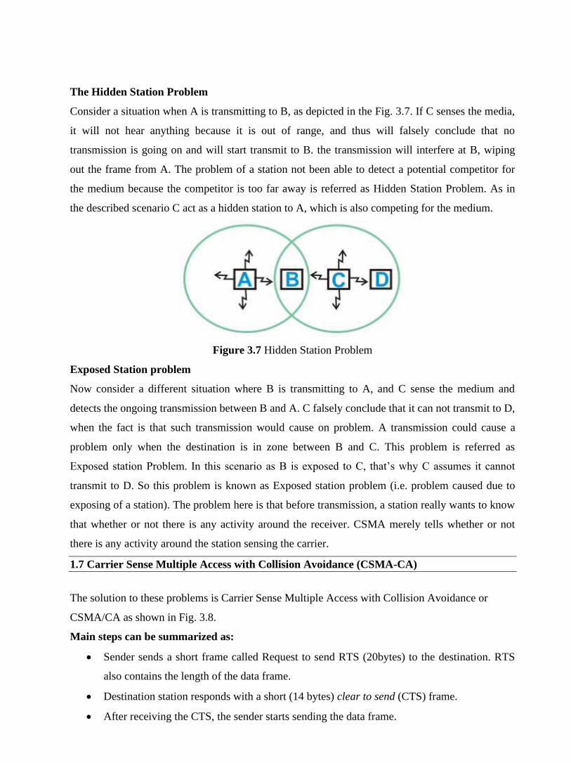
The Hidden Station Problem
Consider a situation when A is transmitting to B, as depicted in the Fig. 3.7. If C senses the media,
it will not hear anything because it is out of range, and thus will falsely conclude that no
transmission is going on and will start transmit to B. the transmission will interfere at B, wiping
out the frame from A. The problem of a station not been able to detect a potential competitor for
the medium because the competitor is too far away is referred as Hidden Station Problem. As in
the described scenario C act as a hidden station to A, which is also competing for the medium.
Figure 3.7 Hidden Station Problem
Exposed Station problem
Now consider a different situation where B is transmitting to A, and C sense the medium and
detects the ongoing transmission between B and A. C falsely conclude that it can not transmit to D,
when the fact is that such transmission would cause on problem. A transmission could cause a
problem only when the destination is in zone between B and C. This problem is referred as
Exposed station Problem. In this scenario as B is exposed to C, that’s why C assumes it cannot
transmit to D. So this problem is known as Exposed station problem (i.e. problem caused due to
exposing of a station). The problem here is that before transmission, a station really wants to know
that whether or not there is any activity around the receiver. CSMA merely tells whether or not
there is any activity around the station sensing the carrier.
1.7 Carrier Sense Multiple Access with Collision Avoidance (CSMA-CA)
The solution to these problems is Carrier Sense Multiple Access with Collision Avoidance or
CSMA/CA as shown in Fig. 3.8.
Main steps can be summarized as:
• Sender sends a short frame called Request to send RTS (20bytes) to the destination. RTS
also contains the length of the data frame.
• Destination station responds with a short (14 bytes) clear to send (CTS) frame.
• After receiving the CTS, the sender starts sending the data frame.

• If collision occurs, CTS frame is not received within a certain period of time.
CSMA/CA works as follows: the station listens before it sends. If someone is already transmitting,
wait for a random period and try again. If no one is transmitting then it sends a short message. This
message is called the Ready To Send message (RTS). This message contains the destination
address and the duration of the transmission. Other stations now know that they must wait that
long before they can transmit. The destination then sends a short message, which is the Clear To
Send message (CTS). This message tells the source that it can send without fear of collisions. Each
packet is acknowledged. If an acknowledgement is not received, the MAC layer retransmits the
data. This entire sequence is called the 4-way handshake protocol.
Figure 3.8 Four-Way handshake protocol
Carrier Sensing
In IEEE 802.11, carrier sensing is performed in two levels known as physical carrier sensing and
virtual carrier sensing.
Physical carrier sensing is performed at the radio interface by sensing the presence of other IEEE
802.11 stations by analyzing all detected packets and relative strength from other sources.
Virtual carrier sensing is used by a source station to inform all other stations in the BSS about
the length of the data frame that it intends to send. The headers of the RTS and CTS control frames
contain the duration field (in μsec). Stations detecting a duration field adjust their Network
Allocation Vector (NAV), which indicates the duration the station must wait before channel can be

sampled again for sensing status of the medium. The protocol may be considered as a 4-way
handshake protocol is shown in Figure 3.9.
The above protocol known as Multiple Access Carrier Avoidance (MACA) was subsequently
extended to improve its performance and the new protocol, with the following three additions, was
renamed as MACAW. First, the receiver sends an ACK frame after receiving a frame and all
stations must wait for this ACK frame before trying to transmit. Second, the back-off algorithm is
to run separately for each data stream, rather than for each station. This change improves the
fairness of the protocol. Finally, some mechanism was added for stations to exchange information
about configuration, and way to make the back-off algorithm react less violently to temporary
problem.
The IEEE 802.11 protocol is specified in terms of coordination function that determine when a
station in a BSS is allowed to transmit and when it may be able to receive data over the wireless
medium. The distributed coordination function (DCF) provides support for asynchronous data
transfer on a best-effort basis. Four following types of inter frame spaces (IFSs) are used:
• Short IFS (SIFS): This is the period between the completion of packet transmission and the
start of ACK frame.
• Point coordination IFS (PIFS): This is SIFS plus a slot time.
• Distributed IFS (DIFS): This PIFS Plus a slot time.
• Extended IFS (EIFS): This is longer than IFS used by a station that has received a packet
that it could not understand. This is needed to prevent collisions. The sequence of events
that take place at the source, destination and other stations is shown in Figure 3.9.
Figure 3.9 CSMA/CA Back-off algorithm timing sequence

1.8 Framing
The frame format of the IEEE 802.11 is shown in Figure 3.10(a). The frames can be categorized
into three types; management frame, control frame and data frame. The management frames are
used for association and disassociation of stations with at the AP, authentication and de-
authentication, and timing and synchronization. The detailed Frame Format is shown in Fig. 3.10.
(c)
Figure 3.10 Frame format for 802.11
Each frame consists of a MAC header, a frame body and a frame check sequence (FCS). The basic
frame can be seen in Figure 3.11 below.

Figure 3.11 802.11 Frame (also shown in 3.10(a))
AC header will be described in a little while. Frame Body varies from 0-2312 bytes. At last is the
FCS field. The frame check sequence is a 32-bit cyclic redundancy check which ensures there are
no errors in the frame. For the standard generator polynomial see IEEE P802.11.
The MAC header consists of seven fields and is 30 bytes long. The fields are frame control,
duration, address 1, address 2, address 3, sequence control, and address 4. The frame control field
is 2 bytes long and is comprised of 11 subfields as shown in Fig. 3.12 below.
Figure 3.12 802.11 MAC Header
Frame Control Field (in MAC header)
• The protocol version field is 2 bits in length and will carry the version of the 802.11
standard. The initial value of 802.11 is 0; all other bit values are reserved.
• Type and subtype fields are 2 and 4 bits, respectively. They work together hierarchically
to determine the function of the frame.
• The remaining 8 fields are all 1 bit in length.
• The To DS field is set to 1 if the frame is destined for the distribution system.
• From DS field is set to 1 when frames exit the distribution system. Note that frames which
stay within their basic service set have both of these fields set to 0.
• The More Frag field is set to 1 if there is a following fragment of the current MSDU.
• Retry is set to 1 if this frame is a retransmission.
• Power Management field indicates if a station is in power save mode (set to 1) or active
(set to 0).

• More data field is set to 1 if there is any MSDUs are buffered for that station.
• The WEP field is set to 1 if the information in the frame body was processed with the WEP
algorithm.
• The Order field is set to 1 if the frames must be strictly ordered.
• The Duration/ID field is 2 bytes long. It contains the data on the duration value for each
field and for control frames it carries the associated identity of the transmitting station.
• The address fields identify the basic service set, the destination address, the source
address, and the receiver and transmitter addresses. Each address field is 6 bytes long.
• The sequence control field is 2 bytes and is split into 2 subfields, fragment number and
sequence number.
• Fragment number is 4 bits and tells how many fragments the MSDU is broken into.
• The sequence number field is 12 bits that indicates the sequence number of the MSDU.
The frame body is a variable length field from 0 - 2312. This is the payload.
1.9 Security
Wireless LANs are subjected to possible breaches from unwanted monitoring. To overcome this
problem, IEEE 802.11 specifies an optional MAC layer security system known as Wired
Equivalent Privacy (WEP). The objective is to provide a level of privacy to the wireless LAN
similar to that enjoyed by wired Ethernets. It is achieved with the help of a 40-bit shared key
authentication service. By default each BSS supports up to four 40-bit keys that are shared by all
the clients in the BSS. Keys unique to a pair of communicating clients and direction of
transmission may also be used. Advanced Encryption Standard (AES) (802.11i) for authentication
and encryption is recommended as a long-term solution.
1.10 IEEE 802.11 extensions
As the first standard was wrapping up, the creation of a new standards activity begun in the 802.11
standards body. The new activity gave rise to two more standards; IEEE 802.11 b and IEEE
802.11a.
• 802.11b: This standard was developed by IEEE with the support from the consortium
Wireless Ethernet Compatibility Alliance (WECA). This standard is backward compatible
with the original standard that added two new data rates 5.5 mbps and 11 Mbps using two
coding techniques; the mandatory coding mode known as Complementary Coding Keying
(CCK) modulation and Packet Binary Convolution Coding (PBCC). Because of backward

compatibility with the 802.11, this standard has gained wide popularity with millions of
installed base, which is growing rapidly.
• 802.11a: The successor to 802.11b is 802.11a with greater speed and at a different
frequency. It operates at radio frequencies between 5 GHz incorporating a coded multi-
carrier scheme known as Orthogonal Frequency Division Multi-carrier (OFDM). The 5
GHz band is currently unlicensed and less congested than the 2.4 GHz ISM band. The
802.11a specifies data speed as high as 54 mbps, also supports 6, 12, 24, and 34 mbps.
There is trade off between bandwidth and range - lower bandwidth cases offering increases
range. For 54 mbps, the typical range is 20-30 meters. The 802.11a and 802.11b devices
can coexist without interference or reduced performance.
• 802.11g: The success of 802.11b has led to another extension that provides 22 Mbps
transmission. It retains backward compatibility with the popular 802.11b standard. This
standard will become 802.11g.
Upper Layers
802.11 FHSS 802.11 DSSS 802.11a
OFDM
802.11b HR-
DSSS
802.11g
OFDM
WiFi: Any of the above wireless LAN standards are referred to by the brand name “WiFi”. It
essentially denotes a set of Wireless LAN standards developed by the working group 11 of the
IEEE LAN/MAN Standards Committee (IEEE 802).
WiMAX: The story of wireless LAN cannot be complete without the mention of WiMAX, which
stands for Worldwide Interoperability for Microwave Access by the WiMAX Forum. The forum
was formed in June 2001 to promote conformance and interoperability of the IEEE 802.16
standard, officially known as Wireless (Metropoliton Area Network) MAN. The Forum describes
WiMAX as "a standards-based technology enabling the delivery of last mile wireless broadband
access as an alternative to cable and DSL". It supports point to multi-point (PMP) broadband
wireless access. WiMAX can deliver a maximum of 70 Mbit/s, over a maximum distance of 70
miles (112.6 kilometers). It has some similarities to DSL in this respect, where one can either have
high bandwidth or long range, but not both simultaneously. The other feature to consider with
WiMAX is that available bandwidth is shared between users in a given radio sector, so if there are
many active users in a single sector, each will get reduced bandwidth.

1.11 Check Your Progress
Fill In The Blanks:
1. Initial cost of wireless LAN can be ____________ than the cost of wired LAN hardware.
2. Wireless LANs have Lower ___________ due to susceptibility of radio transmission to
noise and _____________.
3. Limited data rate because of the use of ______________ transmission techniques enforced
to ISM band users.
4. The big advantage to Micro wave systems is higher __________ achieved because they do
not have the overhead involved with _________ systems.
5. _______________ is an example of systems with microwave technology.
6. Spread spectrum technology currently comes in two types: ___________________ and
______________.
7. _________________ represents each bit in the frame by multiple bits in the transmitted
frame.
8. In DSSS, a random binary string is used to modulate the transmitted signal. This random
string is called the _______________.
9. In DSSS, the data bits are mapped to into a pattern of "chips" and mapped back into a bit at
the destination. The number of chips that represent a bit is the____________.
10. The higher the spreading ratio, the more the signal is ____________ to interference.
1.12 Answer to Check Your Progress
1. higher
2. reliability, interference
3. spread spectrum
4. throughput, spread spectrum
5. RadioLAN
6. direct sequence spread spectrum (DSSS), frequency hopping spread spectrum (FHSS).
7. Direct Sequence Spread Spectrum (DSSS)
8. spreading code
9. spreading ratio
10. resistant

Unit-4
Bluetooth
1.1 Learning Objectives
1.2 Introduction
1.3 Topology
1.4 Bluetooth Architecture
1.5 Bluetooth Layers
1.5.1 Layer 1: Radio Layer
1.5.2 Layer 2: Baseband Layer
1.5.3 Layer 3: Link Manager Protocol
1.5.4 Layer 4: Host Controller Interface
1.5.5 Logical Link Control and Adaptation Protocol
1.5.6 Layer 6: Radio Frequency Communication (RFCOMM)
1.5.7 Layer 7: Service Discovery Protocol
1.5.8 Telephony Control Protocol Spec (TCS)
1.5.9 Application Program Interface (API) libraries
1.6 Check Your Progress
1.7 Answer to Check Your Progress
1.1 Learning Objectives
After going through this unit, the learner will able to learn:
• Explain the need for a Personal Area Network
• Explain different aspects of Bluetooth
o Transmission media
o Topology
o Medium Access Control
1.2 Introduction
Bluetooth wireless technology is a short-range radio technology, which is developed for Personal
Area Network (PAN). Bluetooth is a standard developed by a group of electronics manufacturers
that allows any sort of electronic equipment -- from computers and cell phones to keyboards and
headphones -- to make its own connections, without wires, cables or any direct action from a user.
It is an ad hoc type network operable over a small area such as a room. Bluetooth wireless
technology makes it possible to transmit signals over short distances between telephones,
computers and other devices and thereby simplify communication and synchronization between
devices. It is a global standard that:
• Eeliminates wires and cables between both stationary and mobile devices
• Facilitates both data and voice communication
• Offers the possibility of ad hoc networks and delivers the ultimate synchronicity between
all your personal devices
Bluetooth is a dynamic standard where devices can automatically find each other, establish
connections, and discover what they can do for each other on an ad hoc basis.
Bluetooth is intended to be a standard that works at two levels:
• It provides agreement at the physical level -- Bluetooth is a radio-frequency standard.
• It also provides agreement at the next level up, where products have to agree on when bits
are sent, how many will be sent at a time and how the parties in a conversation can be sure
that the message received is the same as the message sent.
It is conceived initially by Ericsson, before being adopted by a myriad of other companies,
Bluetooth is a standard for a small, cheap radio chip to be plugged into computers, printers,
mobile phones, etc. A Bluetooth chip is designed to replace cables by taking the information
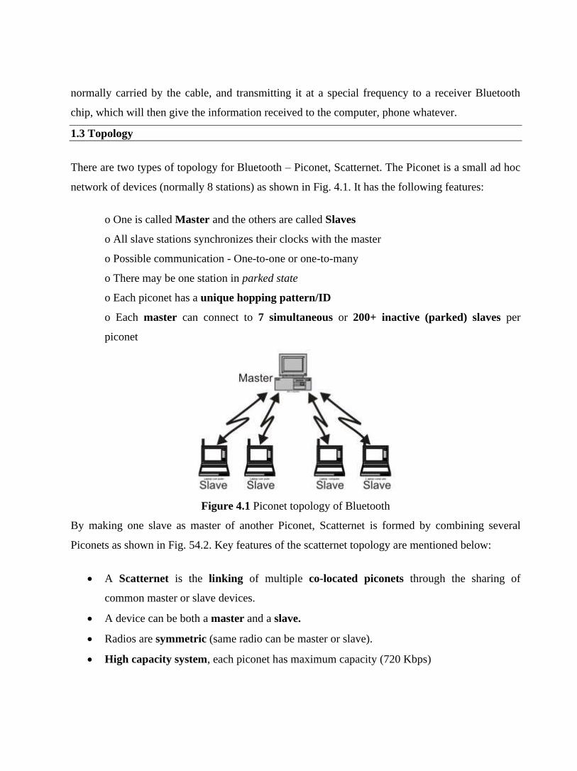
normally carried by the cable, and transmitting it at a special frequency to a receiver Bluetooth
chip, which will then give the information received to the computer, phone whatever.
1.3 Topology
There are two types of topology for Bluetooth – Piconet, Scatternet. The Piconet is a small ad hoc
network of devices (normally 8 stations) as shown in Fig. 4.1. It has the following features:
o One is called Master and the others are called Slaves
o All slave stations synchronizes their clocks with the master
o Possible communication - One-to-one or one-to-many
o There may be one station in parked state
o Each piconet has a unique hopping pattern/ID
o Each master can connect to 7 simultaneous or 200+ inactive (parked) slaves per
piconet
Figure 4.1 Piconet topology of Bluetooth
By making one slave as master of another Piconet, Scatternet is formed by combining several
Piconets as shown in Fig. 54.2. Key features of the scatternet topology are mentioned below:
• A Scatternet is the linking of multiple co-located piconets through the sharing of
common master or slave devices.
• A device can be both a master and a slave.
• Radios are symmetric (same radio can be master or slave).
• High capacity system, each piconet has maximum capacity (720 Kbps)

Figure 4.2 Scatternet topology
1.4 Bluetooth Architecture
The Bluetooth architecture, showing all the major layers in the Bluetooth system, are depicted in
the Fig. 4.3. The layers below can be considered to be different hurdles in an obstacle course. This
is because all the layers function one after the other. One layer comes into play only after the data
has been through the previous layer.
Figure 4.3 The Bluetooth architecture
• Radio: The Radio layer defines the requirements for a Bluetooth transceiver operating in
the 2.4 GHz ISM band.
• Baseband: The Baseband layer describes the specification of the Bluetooth Link
Controller (LC), which carries out the baseband protocols and other low-level link routines.
It specifies Piconet/Channel definition, “Low-level” packet definition, Channel sharing.

• LMP: The Link Manager Protocol (LMP) is used by the Link Managers (on either side)
for link set-up and control.
• HCI: The Host Controller Interface (HCI) provides a command interface to the
Baseband Link Controller and Link Manager, and access to hardware status and control
registers.
• L2CAP: Logical Link Control and Adaptation Protocol (L2CAP) supports higher level
protocol multiplexing, packet segmentation and reassembly, and the conveying of quality
of service information.
• RFCOMM: The RFCOMM protocol provides emulation of serial ports over the L2CAP
protocol. The protocol is based on the ETSI standard TS 07.10.
• SDP: The Service Discovery Protocol (SDP) provides a means for applications to discover,
which services are provided by or available through a Bluetooth device. It also allows
applications to determine the characteristics of those available services.
Now we shall be study each layer in detail (in next few sections) so that we come to know the
function of each layer.
1.5 Bluetooth Layers
1.5.1 Layer 1: Radio Layer
This is the lowest layer in the Bluetooth protocol stack. Bluetooth uses a technique called
frequency hopping, as explained in the context of wireless LANs, in establishing radio links
with other Bluetooth devices. Suppose we have a data packet then the whole packet is never
transmitted at the same frequency. It is always split into different parts and transmitted at
different frequencies. This is the frequency hopping technique (already discussed previously in
Wireless LAN lesson). This partly gives the necessary protection to the transmitted data and
avoids tampering. Standard hop values are 79 hops, which are spaced at an interval of 1 MHz.
In some countries like France, due to government regulations 23 hops are used.
Transmitter characteristics: Each device is classified into 3 power classes, Power Class 1, 2
& 3.
• Power Class 1: is designed for long range (~100m) devices, with a max output power of
20 dBm,
• Power Class 2: for ordinary range devices (~10m) devices, with a max output power of 4
dBm,

• Power Class 3: for short range devices (~10cm) devices, with a max output power of 0
dBm.
The Bluetooth radio interface is based on a nominal antenna power of 0dBm. Each device can
optionally vary its transmitted power. Equipment with power control capability optimizes the
output power in a link with LMP commands (see Link Manager Protocol). It is done by measuring
RSSI and reporting it back, if the power is required to be increased or decreased.
Modulation Characteristics: The Bluetooth radio module uses GFSK (Gaussian Frequency Shift
Keying) where a binary one is represented by a positive frequency deviation and a binary zero by a
negative frequency deviation. BT is set to 0.5 and the modulation index must be between 0.28 and
0.35.
Radio Frequency Tolerance: The transmitted initial center frequency accuracy must be ±75 kHz
from Fc. The initial frequency accuracy is defined as being the frequency accuracy before any
information is transmitted. Note that the frequency drift requirement is not included in the ±75
kHz.
Receiver Characteristics: The receiver must have a sensitivity level for which the bit error rate
(BER) 0.1% is met. For Bluetooth this means an actual sensitivity level of 70dBm or better.
1.5.2 Layer 2: Baseband Layer
The baseband is the digital engine of a Bluetooth system. It is responsible for constructing and
decoding packets, encoding and managing error correction, encrypting and decrypting for secure
communications, calculating radio transmission frequency patterns, maintaining synchronization,
controlling the radio, and all of the other low level details necessary to realize Bluetooth
communications.
Bluetooth operates in the 2.4 GHz ISM band. In the US and Europe, a band of 83.5 MHz width is
available; in this band, 79 RF channels spaced 1 MHz apart are defined. In France, a smaller band
is available; in this band, 23 RF channels spaced 1 MHz part are defined.
The channel is represented by a pseudo-random hopping sequence hopping through the 79 or 23
RF channels. Two or more Bluetooth devices using the same channel form a piconet. The hopping
sequence is unique for the piconet and is determined by the Bluetooth device address (BD_ADDR)
of the master; the phase in the hopping sequence is determined by the Bluetooth clock of the
master. The channel is divided into time slots where each slot corresponds to an RF hop frequency.
Consecutive hops correspond to different RF hop frequencies. Figure 4.4 shows the
communication between the master and a slave. In this case, the master uses even numbered slots
and the slave communicates in the odd numbered slots in a half-duplex mode.

Figure 4.4 Master-slave communication
Figure 4.5 Master and multi-slave communication
The data exchange takes place with every clock tick. The clock synchronization is with respect to
that of the master. Transmission takes place by way of TIME DIVISION DUPLEXING (TDD).
The channel is divided into time slots, each 625 μs in length. The time slots are numbered
according to the Bluetooth clock of the piconet master. A TDD scheme is used where master and
slave alternatively transmit. The master shall start its transmission in even-numbered time slots
only, and the slave shall start its transmission in odd-numbered time slots only. The packet start
shall be aligned with the slot start.
Always remember that the 'slave has to adjust itself to the whims of its master'. If a slave is to
establish a connection with the master, then the slave has to synchronize its own clock according
to that of the master. In the multiple-slave scenario, the slave uses even numbered slots, but only
one slave communicates in the next odd-numbered slot if the packet in the previous slot was
addressed to it. This is shown in Fig. 4.5.
The Baseband handles three types of links:
• SCO (Synchronous Connection-Oriented): The SCO link is a symmetric point-to-point
link between a master and a single slave in the piconet. The master maintains the SCO link
by using reserved slots at regular intervals (circuit switched type). The SCO link mainly
carries voice information. The master can support up to three simultaneous SCO links
while slaves can support two or three SCO links. SCO packets are never retransmitted.
SCO packets are used for 64 kB/s speech transmission.
• Polling-based (TDD) packet transmissions: In this link type one slot is of 0.625msec
(max 1600 slots/sec) and master/slave slots (even-/odd-numbered slots).
• ACL (Asynchronous Connection-Less) link: The ACL link is a point-to-multipoint link
between the master and all the slaves participating on the piconet. In the slots not reserved
for the SCO links, the master can establish an ACL link on a per-slot basis to any slave,
including the slave already engaged in an SCO link (packet switched type). Only a single
ACL link can exist. For most ACL packets, packet retransmission is applied.
Device Addressing: Four possible types of addresses can be assigned to bluetooth units.
• BD_ADDR: Bluetooth Device Address : Each Bluetooth transceiver is allocated a unique
48-bit device address. It is divided into a 24-bit LAP field, a 16-bit NAP field and a 8-bit
UAP field.
• AM_ADDR: Active Member Address: It is a 3-bit number. It is only valid as long as the
slave is active on the channel. It is also sometimes called the MAC address of a Bluetooth
unit.
• PM_ADDR: Parked Member Address: It is a 8-bit member (master-local) address that
separates the parked slaves. The PM_ADDR is only valid as long as the slave is parked.
• AR_ADDR: Access Request Address : This is used by the parked slave to determine the
slave-to master half slot in the access window it is allowed to send access request messages
in. It is only valid as long as the slave is parked and is not necessarily unique.
1.5.3 Layer 3: Link Manager Protocol
The Link Manager is responsible for managing the physical details for Bluetooth connections. It is
responsible for creating the links, monitoring their health, and terminating them gracefully upon
command or failure. The link manager is implemented in a mix of hardware and software.
The Link Manager carries out link setup, authentication, link configuration and other protocols. It
discovers other remote LM’s and communicates with them via the Link Manager Protocol (LMP).
To perform its service provider role, the LM uses the services of the underlying Link Controller
(LC).
The Link Manager Protocol essentially consists of a number of PDU (protocol Data Units), which
are sent from one device to another, determined by the AM_ADDR in the packet header.
1.5.4 Layer 4: Host Controller Interface
This is the layer of the stack that contains the firmware i.e. the software that actually controls all
the activities happening in the Baseband and Radio layers. It provides a common interface between
the Bluetooth host and a Bluetooth module. It manages the hardware links with the scatternets. It
also contains the drivers for the hardware devices used in the connection. Basically the BIOS is
loaded in the HCI Layer.
1.5.5 Logical Link Control and Adaptation Protocol
The Logical Link Control and Adaptation Layer Protocol (L2CAP) is layered over the Baseband
Protocol and resides in the data link layer.
The L2CAP is the big picture brains of a Bluetooth system. It manages the high level aspects of
each connection (who is connected to who, whether to use encryption or not, what level of
performance is required, etc.). In addition it is responsible for converting the format of data as
necessary between the APIs and the lower level Bluetooth protocols. The L2CAP is implemented
in software and can execute either on the host system processor or on a local processor in the
Bluetooth system. L2CAP provides connection oriented and connectionless data services to upper
layer protocols with protocol multiplexing capability, segmentation and reassembly operation, and
group abstractions. L2CAP permits higher-level protocols and applications to transmit and receive
L2CAP data packets up to 64 kilobytes in length.
Two link types are supported for the Baseband layer: Synchronous Connection-Oriented (SCO)
links and Asynchronous Connection-Less (ACL) links. SCO links support real-time voice traffic

using reserved bandwidth. ACL links support best effort traffic. The L2CAP Specification is
defined for only ACL links and no support for SCO links is planned.
1.5.6 Layer 6: Radio Frequency Communication (RFCOMM)
This is the most important layer in the Bluetooth architecture. RFCOMM takes care of the
communication channel between two devices or between a master and a slave. It connects the
serial ports of all the devices according to the requirement.
RFCOMM basically has to accommodate two kinds of devices:
1. Communication end-points such as computers or printers.
2. Devices that are a part of communication channel such as Modems.
RFCOMM protocol is not aware of the distinction between these two kinds of devices. Hence to
prevent any loss of data, it passes on all the information to both the devices. The devices in turn
distinguish between the data and filter it out.
1.5.7 Layer 7: Service Discovery Protocol
The service discovery protocol (SDP) provides a means for applications to discover which services
are available and to determine the characteristics of those available services.
A specific Service Discovery protocol is needed in the Bluetooth environment, as the set of
services that are available changes dynamically based on the RF proximity of devices in motion,
qualitatively different from service discovery in traditional network-based environments. The
service discovery protocol defined in the Bluetooth specification is intended to address the unique
characteristics of the Bluetooth environment.
Bluetooth is basically a universal protocol. Manufacturers may embed Bluetooth ports in their
devices. SDP is very important when devices from different companies and from different parts of
the world are brought together. The devices try to recognize each other through SDP.
1.5.8 Telephony Control Protocol Spec (TCS)
Basic function of this layer is call control (setup & release) and group management for gateway
serving multiple devices.
1.5.9 Application Program Interface (API) libraries
These are software modules which connect the host application program to the Bluetooth
communications system. As such they reside and execute on the same processing resource as the
host system application.

1.6 Check Your Progress
Fill In The Blanks
1. Bluetooth wireless technology is a ________________ radio technology, which is
developed for ____________ Network.
2. The two types of topology for Bluetooth are __________ and ___________.
3. The Radio layer defines the requirements for a Bluetooth transceiver operating in the
______ GHz ISM band.
4. The ________________________ Protocol is used by the Link Managers (on either side)
for link set-up and control.
5. The ______________ protocol provides emulation of serial ports over the L2CAP protocol.
6. ______________________Protocol supports higher level protocol multiplexing, packet
segmentation and reassembly, and the conveying of quality of service information.
7. The Bluetooth radio module uses _______________ modulation technique, where a binary
one is represented by a positive frequency deviation and a binary zero by a negative
frequency deviation.
8. The channel is represented by a __________________ hopping through the 79 or 23 RF
channels
9. The Baseband handles three types of links: _____________________, _____________ and
_______________.
10. _________________ provides a common interface between the Bluetooth host and a
Bluetooth module. It also manages the hardware links with the scatternets.
11. ___________________Protocol is layered over the Baseband Protocol and resides in the
data link layer.
12. Basic function of _______________________ layer is call control (setup & release) and
group management for gateway serving multiple devices.
1.7 Answer to check Your Progress
1. short-range, Personal Area
2. Piconet, Scatternet
3. 2.4
4. Link Manager
5. RFCOMM
6. Logical Link Control and Adaptation

7. GFSK (Gaussian Frequency Shift Keying)
8. pseudo-random hopping sequence
9. SCO (Synchronous Connection-Oriented), Polling-based (TDD) packet transmissions,
ACL (Asynchronous Connection-Less) link
10. Host Controller Interface
11. The Logical Link Control and Adaptation Layer
12. Telephony Control Protocol Spec (TCS)

Unit-5
Cellular Telephone Networks
1.1 Learning Objectives
1.2 Introduction
1.3 Cellular Telephone System
1.4 Frequency Reuse Principle
1.5 Transmitting and Receiving
1.6 Mobility Management
1.7 Medium Access Control Techniques
1.8 First GenerationSecond Generation System
1.9 Second Generation
1.10 Third Generation
1.11 Check Your Progress
1.12 Answer to Check Your Progress

1.1 Learning Objectives
After going through this unit, the learner will able to learn:
• Explain the operation of Cellular Telephone networks
• Explain the operation of the first generation cellular network - AMPS
• Distinguish between first generation and second-generation cellular networks
• Explain the operation of the second-generation cellular networks
• State the goals of 3G cellular networks
1.2 Introduction
In the early years of mobile radio systems, a large coverage was achieved by using a single high-
powered transmitter with the antenna mounted on tall tower. Although a large coverage could be
attained by this approach, it does not allow the reuse of the same radio frequencies due to
interference. The cellular concept was invented in solving the spectral congestion and user
capacity. Cellular telephony is a system-level concept, which replaces a single high power
transmitter with a large number of low-power transmitters for communication between any two
devices over a large geographic area. Primary goal of the cellular telephone network is to provide
wireless communication between two moving devices, called mobile stations or between one
mobile unit and a stationary unit, commonly referred to as land-line unit. To accommodate a large
number of users over a large geographic area, the cellular telephone system uses a large number of
low-power wireless transmitters to create cells. Variable power levels allow cells to be sized
according to subscriber density and demand within a particular region. As mobile users travel from
cell to cell, their conversations are handed off between cells. Channels (frequencies) used in one
cell can be reused in another cell some distance away, which allows communication by a large
number stations using a limited number of radio frequencies. To summarize, the basic concept of
reuse allows a fixed number of channels to serve an arbitrarily large number of users.
1.3 Cellular Telephone System
As shown in Fig. 5.1, a cellular system comprises the following basic components:
• Mobile Stations (MS): Mobile handsets, which is used by an user to communicate with
another user.
• Cell: Each cellular service area is divided into small regions called cell (5 to 20 Km).

• Base Stations (BS): Each cell contains an antenna, which is controlled by a small office.
• Mobile Switching Center (MSC): Each base station is controlled by a switching office,
called mobile switching center
Figure 5.1 Schematic diagram of a cellular telephone system
1.4 Frequency Reuse Principle
Cellular telephone systems rely on an intelligent allocation and reuse of channels. Each base
station is given a group of radio channels to be used within a cell. Base stations in neighbouring
cells are assigned completely different set of channel frequencies. By limiting the coverage areas,
called footprints, within cell boundaries, the same set of channels may be used to cover different
cells separated from one another by a distance large enough to keep interference level within
tolerable limits as shown in Fig. 5.9.2. Cells with the same letter use the same set of frequencies,
called reusing cells. N cells which collectively use the available frequencies (S = k.N) is known as
cluster. If a cluster is replicated M times within a system, then total number duplex channels
(capacity) is C = M.k.N= M.S

Reuse factor: Fraction of total available channels assigned to each cell within a cluster is 1/N.
Example showing reuse factor of ¼ is shown in Fig. 5.2 (a) and Fig. 5.2(b) shows reuse factor of
1/7.
(a) (b)
Figure 5.2 (a) Cells showing reuse factor of ¼, (b) Cells showing reuse factor of 1/7
As the demand increases in a particular region, the number of stations can be increased by
replacing a cell with a cluster as shown in Fig. 5.3. Here cell C has been replaced with a cluster.
However, this will be possible only by decreasing the transmitting power of the base stations to
avoid interference.
Figure 5.3 A cell is replaced by a cluster as demand increases
1.5 Transmitting and Receiving
Basic operations of transmitting and receiving in a cellular telephone network are discussed in this
section.
Transmitting involves the following steps:

• A caller enters a 10-digit code (phone number) and presses the send button.
• The MS scans the band to select a free channel and sends a strong signal to send the
number entered.
• The BS relays the number to the MSC.
• The MSC in turn dispatches the request to all the base stations in the cellular system.
• The Mobile Identification Number (MIN) is then broadcast over all the forward control
channels throughout the cellular system. It is known as paging.
• The MS responds by identifying itself over the reverse control channel.
• The BS relays the acknowledgement sent by the mobile and informs the MSC about the
handshake.
• The MSC assigns an unused voice channel to the call and call is established.
Receiving involves the following steps:
• All the idle mobile stations continuously listens to the paging signal to detect messages
directed at them.
• When a call is placed to a mobile station, a packet is sent to the callee’s home MSC to find
out where it is.
• A packet is sent to the base station in its current cell, which then sends a broadcast on the
paging channel.
• The callee MS responds on the control channel.
• In response, a voice channel is assigned and ringing starts at the MS.
1.6 Mobility Management
A MS is assigned a home network, commonly known as location area. When an MS migrates out
of its current BS into the footprint of another, a procedure is performed to maintain service
continuity, known as Handoff management. An agent in the home network, called home agent,
keeps track of the current location of the MS. The procedure to keep track of the user’s current
location is referred to as Location management. Handoff management and location management
together are referred to as Mobility management.
Handoff: At any instant, each mobile station is logically in a cell and under the control of the
cell’s base station. When a mobile station moves out of a cell, the base station notices the MS’s
signal fading away and requests all the neighbouring BSs to report the strength they are receiving.
The BS then transfers ownership to the cell getting the strongest signal and the MSC changes the
channel carrying the call. The process is called handoff. There are two types of handoff; Hard
Handoff and Soft Handoff. In a hard handoff, which was used in the early systems, a MS
communicates with one BS. As a MS moves from cell A to cell B, the communication between the

MS and base station of cell A is first broken before communication is started between the MS and
the base station of B. As a consequence, the transition is not smooth. For smooth transition from
one cell (say A) to another (say B), an MS continues to talk to both A and B. As the MS moves
from cell A to cell B, at some point the communication is broken with the old base station of cell
A. This is known as soft handoff.
Roaming: Two fundamental operations are associated with Location Management; location
update and paging. When a Mobile Station (MS) enters a new Location Area, it performs a
location updating procedure by making an association between the foreign agent and the home
agent. One of the BSs, in the newly visited Location Area is informed and the home directory of
the MS is updated with its current location. When the home agent receives a message destined for
the MS, it forwards the message to the MS via the foreign agent. An authentication process is
performed before forwarding the message.
1.7 Medium Access Control Techniques
Channelization is a multiple access method in which the available bandwidth of a link is shared in
time, frequency or using code by a number of stations. Basic idea of these approaches can be
explained in simple terms using the cocktail party theory. In a cocktail party people talk to each
other using one of the following modes:
FDMA: When all the people group in widely separated areas and talk within each group.
TDMA: When all the people are in the middle of the room, but they take turn in speaking.
CDMA: When all the people are in the middle of the room, but different pairs speak in different
languages.
Basic principle of these approaches are briefly explained below:
FDMA: The bandwidth is divided into separate frequency bands. In case of bursty traffic, the
efficiency can be improved in FDMA by using a dynamic sharing technique to access a particular
frequency band; channels are assigned on demand as shown in Fig. 5.4
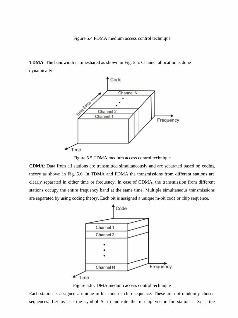
Figure 5.4 FDMA medium access control technique
TDMA: The bandwidth is timeshared as shown in Fig. 5.5. Channel allocation is done
dynamically.
Figure 5.5 TDMA medium access control technique
CDMA: Data from all stations are transmitted simultaneously and are separated based on coding
theory as shown in Fig. 5.6. In TDMA and FDMA the transmissions from different stations are
clearly separated in either time or frequency. In case of CDMA, the transmission from different
stations occupy the entire frequency band at the same time. Multiple simultaneous transmissions
are separated by using coding theory. Each bit is assigned a unique m-bit code or chip sequence.
Figure 5.6 CDMA medium access control technique
Each station is assigned a unique m-bit code or chip sequence. These are not randomly chosen
sequences. Let us use the symbol Si to indicate the m-chip vector for station i. Si is the

complement of Si. All chip sequences are pair-wise orthogonal, i.e. the normalized inner product
of any two distinct codes is 0. For example: S1 = {+1, -1, +1, -1} and S2 = {+1, +1, -1, -1}, Now S1
. S2 = +1 -1 -1 +1 = 0. On the other hand S1 . S1 = +1 +1 +1 +1 = 4/m = 1 and S1. S1 = 0. The
orthogonal property allows parallel transmission and subsequent recovery. Walsh table can be used
to generate orthogonal sequences in an iterative manner. If the table for N sequences is known, the
table for 2N sequences can be created. The multiplexing and demultiplexing operations are shown
in Figs. 5.7.
Figure 5.7 Multiplexing and demultiplexing operations in CDMA
1.8 First GenerationSecond Generation System
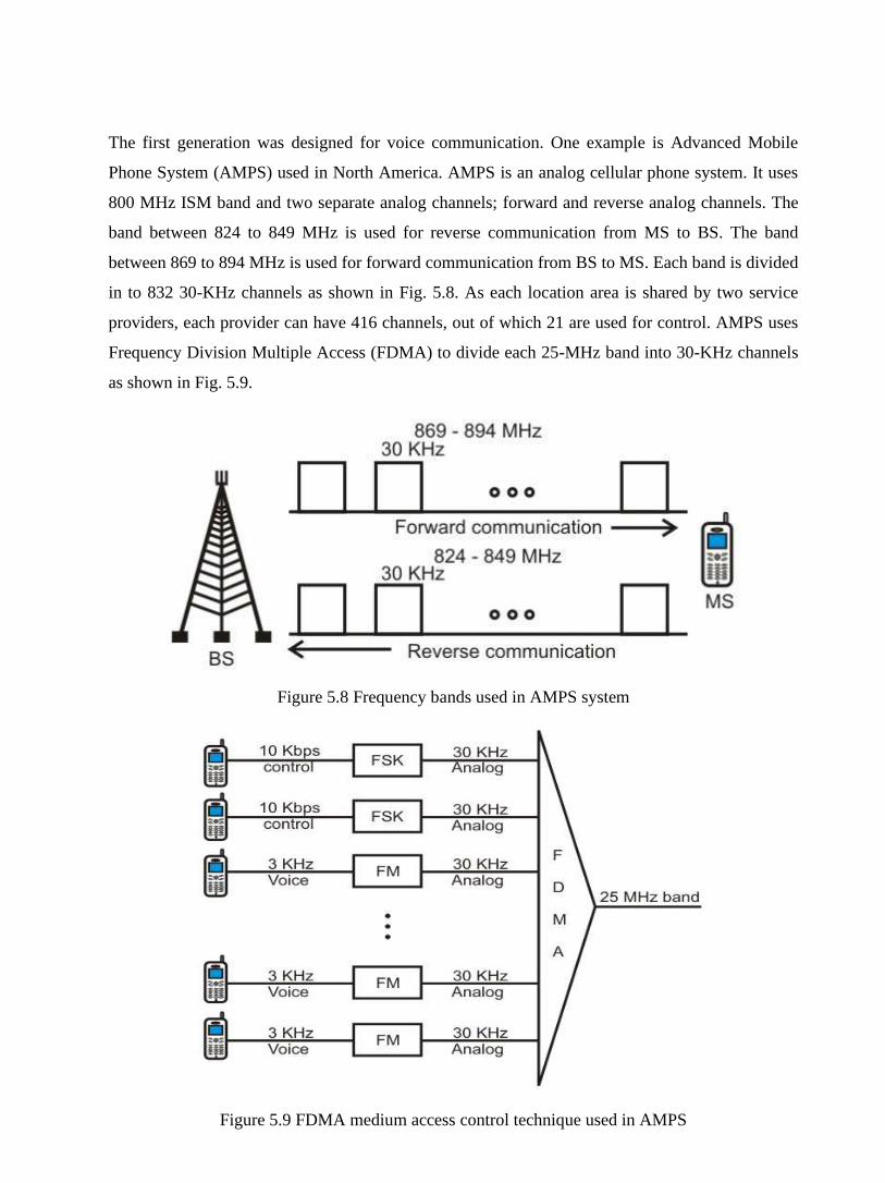
The first generation was designed for voice communication. One example is Advanced Mobile
Phone System (AMPS) used in North America. AMPS is an analog cellular phone system. It uses
800 MHz ISM band and two separate analog channels; forward and reverse analog channels. The
band between 824 to 849 MHz is used for reverse communication from MS to BS. The band
between 869 to 894 MHz is used for forward communication from BS to MS. Each band is divided
in to 832 30-KHz channels as shown in Fig. 5.8. As each location area is shared by two service
providers, each provider can have 416 channels, out of which 21 are used for control. AMPS uses
Frequency Division Multiple Access (FDMA) to divide each 25-MHz band into 30-KHz channels
as shown in Fig. 5.9.
Figure 5.8 Frequency bands used in AMPS system
Figure 5.9 FDMA medium access control technique used in AMPS

1.9 Second Generation
The first generation cellular network was developed for analog voice communication. To provide
better voice quality, the second generation was developed for digitized voice communication.
Three major systems were evolved, as shown in Fig. 5.10.
Figure 5.10 FDMA medium access control technique used in AMPS
D-AMPS: D-AMPS is essentially a digital version of AMPS and it is backward compatible with
AMPS. It uses the same bands and channels and uses the frequency reuse factor of 1/7. 25 frames
per second each of 1994 bits, divided in 6 slots shared by three channels. Each slot has 324 bits-
159 data, 64 control, 101 error-correction as shown in Fig. 5.11. As shown in the figure, it uses
both TDMA and FDMA medium access control techniques.

Figure 5.11 D-AMPS
GSM: The Global System for Mobile (GSM) communication is a European standard developed to
replace the first generation technology. Uses two bands for duplex
communication. Each voice channel is digitized and compressed to a 13Kbps digital signal. Each
slot carries 156.25 bits, 8 slots are multiplexed together creating a FDM frame, 26 frames are
combined to form a multiframe, as shown in Fig. 5.12. For medium access control, GSM combines
both TDMA and FDMA. There is large amount of overhead in TDMA, 114 bits are generated by
adding extra bits for error correction. Because of complex error correction, it allows a reuse factor
as low as 1/3.
Figure 5.12 Multiframe components
IS-95 CDMA: IS-95 is based on CDMA/DSSS and FDMA medium access control technique. The
forward and backward transmissions are shown in Fig. 5.13 and Fig. 5.14, respectively.

Figure 5.13 Forward transmission in IS-95 CDMA
Figure 5.14 Backward transmission in IS-95 CDMA
1.10 Third Generation
We are presently using the second generation technologies and the development of the third
generation technologies are in progress. Goals of the third generation (3G) technologies are
mentioned below:
• Allow both digital data and voice communication.
• To facilitate universal personnel communication.
• Listen music, watch movie, access internet, video conference, etc.
Criteria for 3G Technologies are:
• Voice quality: Same as present PSTN network.
• Data rate: 144Kbps (car), 384 (pedestrians) and 2Mbps (stationary).
• Support for packet-switched and circuit-switched data services.
• Bandwidth of 2 MHz.
• Interface to the internet.

ITU developed a blueprint called Internet Mobile Communication for year 2000 (IMT-2000). All
five Radio Interfaces adopted by IMT-2000 evolved from the second generation technologies as
shown in Fig. 5.15.
Figure 5.15 Third generation cellular technologies
1.11 Check Your Progress
1. What is the relationship between a base station and a mobile switching center?
2. What is reuse factor? Explain whether a low or a high reuse factor is better?
3. What is AMPS and in what way it differs from D-AMPS?
4. What is mobility management?
1.12 Answer to check Your Progress
1. A number of BSs are under the control of a single MSC. A base station is equipped with a
transmitter/receiver for transmission and reception with the MSs in its footprint. On the
other hand, the MSC coordinates communication among the base stations and the PSTN
network. It is a computer-controlled system responsible for connecting calls, recording call
information and billing.
2. Fraction of total available channels assigned to each cell within a cluster (1/N) is known as
the reuse factor. Capacity (total number of channels available for communication) of a
cellular telephone system depends on the reuse factor.
3. AMPS is a purely analog cellular telephone system developed by Bell Labs and use North
America and other countries. On the other hand D-AMPS is a backward compatible digital
version of AMPS.
4. Mobility management deals with two important aspects; Handoff management and location
management. Handoff management maintains service continuity when an MS migrates out
of its current BS into the footprint of another BS. To do this it is necessary to keep track of

the user’s current location. The procedure performed for this purpose is known as Location
management.

Block-5
Unit-1
Satellite Networks
1.1 Learning Objectives
1.2 Introduction
1.3 Orbits of Satellites
1.4 Footprint of Satellites
1.5 Categories of Satellites
1.6 Frequency Bands
1.7 Low Earth Orbit Satellites
1.8 Medium Earth Orbit Satellites
1.9 GEO Satellites
1.10 VSAT Systems:
1.11 MAC Protocols
1.12 Check Your Progress
1.13 Answer to Check Your Progress

1.1 Learning Objectives
After going through this unit, the learner will able to learn:
• Explain different type of satellite orbits
• Explain the concept of footprint of a satellite
• Specify various categories of satellites
• Specify frequency bands used in satellites
• Explain the uses of different categories of satellites
• Specify the MAC techniques used in satellites communications
1.2 Introduction
Microwave frequencies, which travel in straight lines, are commonly used for wideband
communication. The curvature of the earth results in obstruction of the signal between two earth
stations and the signal also gets attenuated with the distance it traverses. To overcome both the
problems, it is necessary to use a repeater, which can receive a signal from one earth station,
amplify it, and retransmit it to another earth station. Larger the height of a repeater from the
surface of the earth, longer is the distance of line-of-sight communication. Satellite networks were
originally developed to provide long-distance telephone service. So, for communication over long
distances, satellites are a natural choice for use as repeaters in the sky. In this lesson, we shall
discuss different aspects of satellite networks.
1.3 Orbits of Satellites
Artificial satellites deployed in the sky rotate around the earth on different orbits. The orbits can be
categorized into three types as follows:
• Equatorial
• Inclined
• Polar
Time required to make a complete trip around the earth, known as period, is determined by
Kepler’s Law of period: T2 = (4π2/GM) r3, where T is the period, G is the gravitational constant, M
is the mass of the central body and r is the radius.

(a) (b) (c)
Figure 1.1 Three different orbits of satellites; (a) equatorial, (b) inclined and (c) polar
1.4 Footprint of Satellites
Signals from a satellite is normally aimed at a specific area called the footprint. Power is
maximum at the center of the footprint. It decreases as the point moves away from the footprint
center. The amount of time a beam is pointed to a given area is known as dwell time.
(a) (b)
Figure 1.2 (a) Footprint using a global beam, (b) Footprint using a phased array antenna
Figure 1.3 Categories of satellites
1.5 Categories of Satellites
As shown in Fig. 1.3, the satellites can be categorized into three different types , based on the
location of the orbit. These orbits are chosen such that the satellites are not destroyed by the high-
energy charged particles present in the two Van Allen belts, as shown in Fig. 1.4. The Low Earth
Orbit (LEO) is below the lower Van Allen belt in the altitude of 500 to 2000 Km. The Medium
Earth Orbit (MEO) is in between the lower Van Allen belt and upper Van Allen belt in the altitude
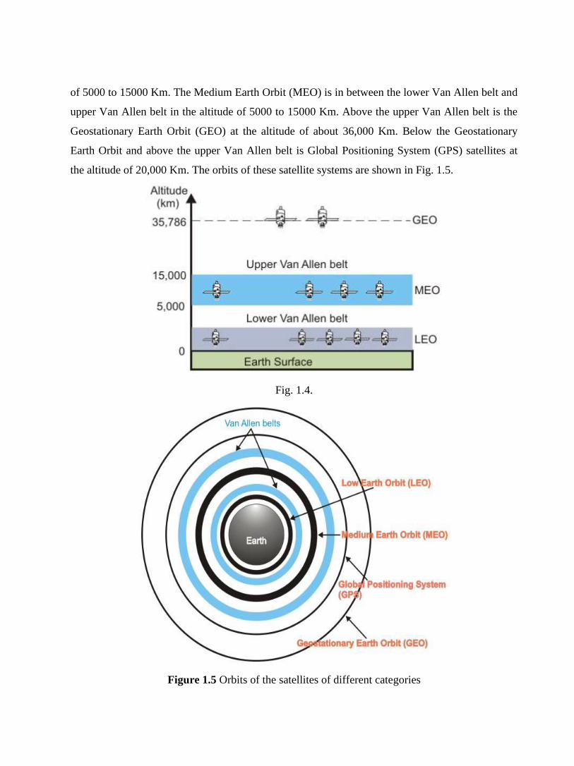
of 5000 to 15000 Km. The Medium Earth Orbit (MEO) is in between the lower Van Allen belt and
upper Van Allen belt in the altitude of 5000 to 15000 Km. Above the upper Van Allen belt is the
Geostationary Earth Orbit (GEO) at the altitude of about 36,000 Km. Below the Geostationary
Earth Orbit and above the upper Van Allen belt is Global Positioning System (GPS) satellites at
the altitude of 20,000 Km. The orbits of these satellite systems are shown in Fig. 1.5.
Fig. 1.4.
Figure 1.5 Orbits of the satellites of different categories

1.6 Frequency Bands
Two frequencies are necessary for communication between a ground station and a satellite; one for
communication from the ground station on the earth to the satellite called uplink frequency and
another frequency for communication from the satellite to a station on the earth, called downlink
frequency. These frequencies, reserved for satellite communication, are divided in several bands
such as L, S, Ku, etc are in the gigahertz (microwave) frequency range as shown in Table 1.1.
Higher the frequency, higher is the available bandwidth.
Table 1.1 Frequency bands for satellite communication
1.7 Low Earth Orbit Satellites
The altitude of LEO satellites is in the range of 500 to 1500 Km with a rotation period of 90 to 120
min and round trip delay of less than 20 ms. The satellites rotate in polar orbits with a rotational
speed of 20,000 to 25,000 Km. As the footprint of LEO satellites is a small area of about 8000 Km
diameter, it is necessary to have a constellation of satellites, as shown in Fig. 1.6, which work
together as a network to facilitate communication between two earth stations anywhere on earth’s
surface. The satellite system is shown in Fig. 1.7. Each satellite is provided with three links; the
User Mobile Link (UML) for communication with a mobile station, the Gateway Link (GWL) for
communication with a earth station and the Inter-satellite Link (ISL) for communication between
two satellites, which are close to each other. Depending on the frequency bands used by different
satellites, these can be broadly categorized into three types; the little LEOs operating under 1 GHz
and used for low data rate communication, the big LEOs operating in the range 1 to 3 GHz and the
Broadband and the broadband LEOs provide communication capabilities similar to optical
networks.

Figure 1.6 LEO satellite network
Figure 1.7 LEO satellite system
Iridium System
The Iridium system was a project started by Motorola in 1990 with the objective of providing
worldwide voice and data communication service using handheld devices. It took 8 years to
materialize using 66 satellites. The 66 satellites are divided in 6 polar orbits at an altitude of 750
Km. Each satellite has 48 spot beams (total 3168 beams). The number of active spot beams is
about 2000. Each spot beam covers a cell as shown in Fig. 1.8.
Figure 1.8 Overlapping spot beams of the Iridium system
The Teledesic System
The Teledesic project started in 1990 by Craig McCaw and Bill Gates in 1990 with the objective
of providing fiber-optic like communication (Internet-in-the-sky). It has 288 satellites in 12 polar

orbits, each orbit having 24 satellites at an altitude of 1350 Km. Three types of communications
that are allowed in Teledasic are as follows;
• ISL: Intersatellite communication allows eight neighbouring satellites to communicate with
each other.
• GWL: Communication between a satellite and a gateway.
• UML: Between an user and a satellite.
The surface of the earth is divided into thousands of cells and each satellite focuses it beams to a
cell during dwell time. It uses Ka band communication with data rates of 155Mbps uplink and
1.2Gbps downlink.
1.8 Medium Earth Orbit Satellites
MEO satellites are positioned between two Van Allen Belts at an height of about 10,000 Km with
a rotation period of 6 hours. One important example of the MEO satellites is the Global
Positioning System (GPS) as briefly discussed below:
GPS
The Global Positioning System (GPS) is a satellite-based navigation system. It comprises a
network of 24 satellites at an altitude of 20,000 Km (Period 12 Hrs) and an inclination of 55° as
shown in Fig. 1.9. Although it was originally intended for military applications and deployed by
the Department of Defence, the system is available for civilian use since 1980. It allows land, sea
and airborne users to measure their position, velocity and time. It works in any weather conditions,
24 hrs a day. Positioning is accurate to within 15 meters. It is used for land and sea navigation
using the principle of triangulation as shown in Fig. 1.10. It requires that at any time at least 4
satellites to be visible from any point of earth. A GPS receiver can find out the location on a map.
Figure 1.11 shows a GPS receiver is shown in the caption’s cabin of a ship. GPS was widely used
in Persian Gulf war.

Figure 1.9 Global positioning system
Figure 1.10 Triangulation approach used to find the position of an object
Figure 1.11 GPS receiver in a ship
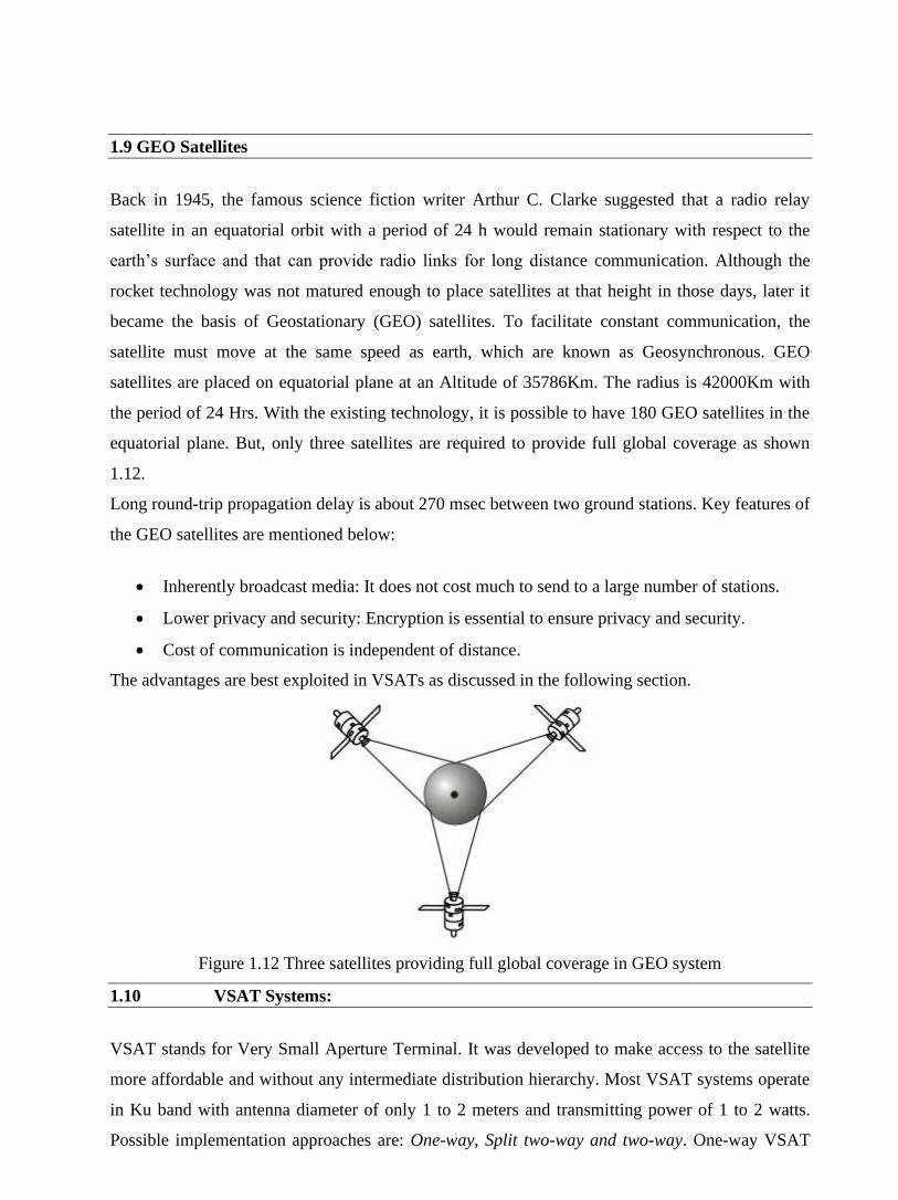
1.9 GEO Satellites
Back in 1945, the famous science fiction writer Arthur C. Clarke suggested that a radio relay
satellite in an equatorial orbit with a period of 24 h would remain stationary with respect to the
earth’s surface and that can provide radio links for long distance communication. Although the
rocket technology was not matured enough to place satellites at that height in those days, later it
became the basis of Geostationary (GEO) satellites. To facilitate constant communication, the
satellite must move at the same speed as earth, which are known as Geosynchronous. GEO
satellites are placed on equatorial plane at an Altitude of 35786Km. The radius is 42000Km with
the period of 24 Hrs. With the existing technology, it is possible to have 180 GEO satellites in the
equatorial plane. But, only three satellites are required to provide full global coverage as shown
1.12.
Long round-trip propagation delay is about 270 msec between two ground stations. Key features of
the GEO satellites are mentioned below:
• Inherently broadcast media: It does not cost much to send to a large number of stations.
• Lower privacy and security: Encryption is essential to ensure privacy and security.
• Cost of communication is independent of distance.
The advantages are best exploited in VSATs as discussed in the following section.
Figure 1.12 Three satellites providing full global coverage in GEO system
1.10 VSAT Systems:
VSAT stands for Very Small Aperture Terminal. It was developed to make access to the satellite
more affordable and without any intermediate distribution hierarchy. Most VSAT systems operate
in Ku band with antenna diameter of only 1 to 2 meters and transmitting power of 1 to 2 watts.
Possible implementation approaches are: One-way, Split two-way and two-way. One-way VSAT
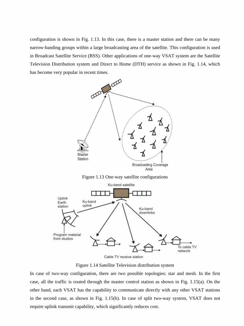
configuration is shown in Fig. 1.13. In this case, there is a master station and there can be many
narrow-banding groups within a large broadcasting area of the satellite. This configuration is used
in Broadcast Satellite Service (BSS). Other applications of one-way VSAT system are the Satellite
Television Distribution system and Direct to Home (DTH) service as shown in Fig. 1.14, which
has become very popular in recent times.
Figure 1.13 One-way satellite configurations
Figure 1.14 Satellite Television distribution system
In case of two-way configuration, there are two possible topologies: star and mesh. In the first
case, all the traffic is routed through the master control station as shown in Fig. 1.15(a). On the
other hand, each VSAT has the capability to communicate directly with any other VSAT stations
in the second case, as shown in Fig. 1.15(b). In case of split two-way system, VSAT does not
require uplink transmit capability, which significantly reduces cost.

(a) (b)
Figure 1.15 (a) Two-way VSAT configuration with star topology, (b) Two-way VSAT
configuration with mesh topology
1.11 MAC Protocols
One of the key design issues in satellite communication is how to efficiently allocate transponder
channels. Uplink channel is shared by all the ground stations in the footprint of a satellite, as
shown in Fig. 1.16.
Figure 1.16 Uplink frequency is shared and downlink signal is broadcasted
The round robin and contention-based medium access control schemes have been found to be
suitable for local area networks. But most of the schemes are unsuitable for communication
satellite medium used in wide area networks. Apart from the nature of traffic, unique features of

the satellite channels are to be taken into consideration for designing suitable medium access
control protocol for them. The most important feature of the satellite channels is their long up-and-
down prorogation delay, which is about one fourth of a second. The second most important feature
of the satellite channels is that, after about one fourth a second a station has ceased transmission, it
knows whether the transmission was successful or suffered a collision. These two features along
with the nature of traffic, whether bursty or streamed are the determining factors for the designing
of medium access control schemes.
As more than half a second is necessary to get response of a poll, polling scheme is inefficient for
satellite channels. The CSMA-based schemes are also impractical because of long propagation
delay; whatever a station senses now was actually going on about on quarter of a second ago.
For a satellite system with a limited number of ground stations and all of them having continuous
traffic, it makes sense to use FDM or TDM. In FDM, each transponder channel is divided into
disjoint subchannels at different frequencies, with guard bands to reduce interference between
adjacent channels. In TDM, the channel is divided into slots, which are grouped into frames. Each
slot is allocated to each of the ground stations for transmission.
But, in situations where the number of ground stations is large and stations have bursty nature of
traffic, both TDM and FDM are inefficient because of poor utilization of the slots and
subchannels, respectively. A third category of medium access scheme, known as reservation has
been invented for efficient utilization of satellite channels. In all the reservation schemes, a fixed
frame length is used, which is divided into a number of time slots. For a particular station, slots in
the future frames are reserved in some dynamic fashion, using ALOHA or S-ALOHA. The
schemes differ primarily in the manner the reservations are made and released using either a
distributed or a centralised policy as discussed in the following subsections.
Contention-free protocols:
Fixed assignment protocols using FDMA or TDMA: Allocation of channel assignment is static;
suitable when number of stations is small. These provide deterministic delay, which is important in
real-time applications.
Demand assignment protocols: Suitable when the traffic pattern is random and unpredictable.
Efficiency is improved by using reservation based on demand. The reservation process can be
implicit or explicit.

Figure 1.17 TDMA MAC technique
Random access protocols:
• Pure ALOHA
• Selective-reject ALOHA
• Slotted ALOHA
• Reservation Protocols
• Reservation ALOHA (R-ALOHA)
• Hybrid of random access and reservation protocols
• Designed to have the advantages of both random access and TDMA
Distributed Protocols
A large number of reservation schemes have been proposed. A few representative schemes are
briefly outlined below. It is assumed that there are n stations and m slots per frame.
R-ALOHA: The simplest of the schemes, proposed by Crowther et al (1973) is known as R-
ALOHA. As illustrated in Fig 1.18, the scheme assumes that the number of stations is larger than
the number of slots (n>m) and with time the number of active stations is varying dynamically. A
station wishing to transmit one or more packets of data monitors the slots in the current frame. The
station contends for a slot in the next frame, which is either free or contains a collision in current
frame. Successful transmission in a slot serves as a reservation for the corresponding slot in the
next frame and the station can send long stream of data by repeated use of that slot position in the
subsequent frames. The scheme behaves like a fixed assignment TDMA when the stations send
long streams of data. On the other hand, if most of the traffic is bursty, the scheme behaves like the
slotted ALOHA. In fact, the performance can be worse than S-ALOHA.
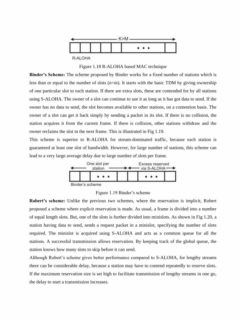
Figure 1.18 R-ALOHA based MAC technique
Binder’s Scheme: The scheme proposed by Binder works for a fixed number of stations which is
less than or equal to the number of slots (n<m). It starts with the basic TDM by giving ownership
of one particular slot to each station. If there are extra slots, these are contended for by all stations
using S-ALOHA. The owner of a slot can continue to use it as long as it has got data to send. If the
owner has no data to send, the slot becomes available to other stations, on a contention basis. The
owner of a slot can get it back simply by sending a packet in its slot. If there is no collision, the
station acquires it from the current frame. If there is collision, other stations withdraw and the
owner reclaims the slot in the next frame. This is illustrated in Fig 1.19.
This scheme is superior to R-ALOHA for stream-dominated traffic, because each station is
guaranteed at least one slot of bandwidth. However, for large number of stations, this scheme can
lead to a very large average delay due to large number of slots per frame.
Figure 1.19 Binder’s scheme
Robert’s scheme: Unlike the previous two schemes, where the reservation is implicit, Robert
proposed a scheme where explicit reservation is made. As usual, a frame is divided into a number
of equal length slots. But, one of the slots is further divided into minislots. As shown in Fig 1.20, a
station having data to send, sends a request packet in a minislot, specifying the number of slots
required. The minislot is acquired using S-ALOHA and acts as a common queue for all the
stations. A successful transmission allows reservation. By keeping track of the global queue, the
station knows how many slots to skip before it can send.
Although Robert’s scheme gives better performance compared to S-ALOHA, for lengthy streams
there can be considerable delay, because a station may have to contend repeatedly to reserve slots.
If the maximum reservation size is set high to facilitate transmission of lengthy streams in one go,
the delay to start a transmission increases.

Figure 1.20 Robert’s scheme
Centralized Protocols
Distributed reservation schemes suffer from the disadvantage of higher processing burden on each
station and vulnerable to a loss of synchronization. These problems can be overcome by using
centralized schemes. Two such schemes are discussed below.
FPODA: The Fixed-Priority Oriented Demand Assignment (FPODA) technique is an extension of
the Robert’s scheme that functions in a centralized manner. In this scheme, each frame begins with
a number of minislots, each dedicated to one of the stations. In a particular implementation of the
scheme, there are six stations as shown in Fig 1.21. Minislots are used for sending short data or
reservation, which specifies the type of service required- priority, normal or bulk. Priority requests
specify the amount of data to be sent with high priority and normal requests indicate an estimation
of required future throughput. One of the six stations acts as a central controller and allocates time
based on reservation requests. The controller allocates the remaining part of the frame into six
variable length slots, one to each of the six stations. The controller station maintains a queue of
requests and allocates time based on the requests. On a first-come first-serve basis the priority
requests are kept at the front. After allocating to the priority requests, remaining time of the frames
are allocated to normal requests. Remaining time after allocating to normal request is divided
equally among the bulk requests.
Figure 1.21 A Fixed-Priority Oriented Demand Assignment (FPODA) frame
PDAMA: The frame format for PDAMA, as shown in Fig. 5.10.22, has four types of slots, a
leader control slots, a guard slot, a reservation minislots and data slots. The leader slot is used by
the master station to communicate acknowledgement of received reservations and allocation of
slots to other stations. The guard ring helps other stations to hear the leader control slot and
prepare for further reservations. It can also be used for the purpose of ranging. The reservation
minislots are reservation requests using S-ALOHA.
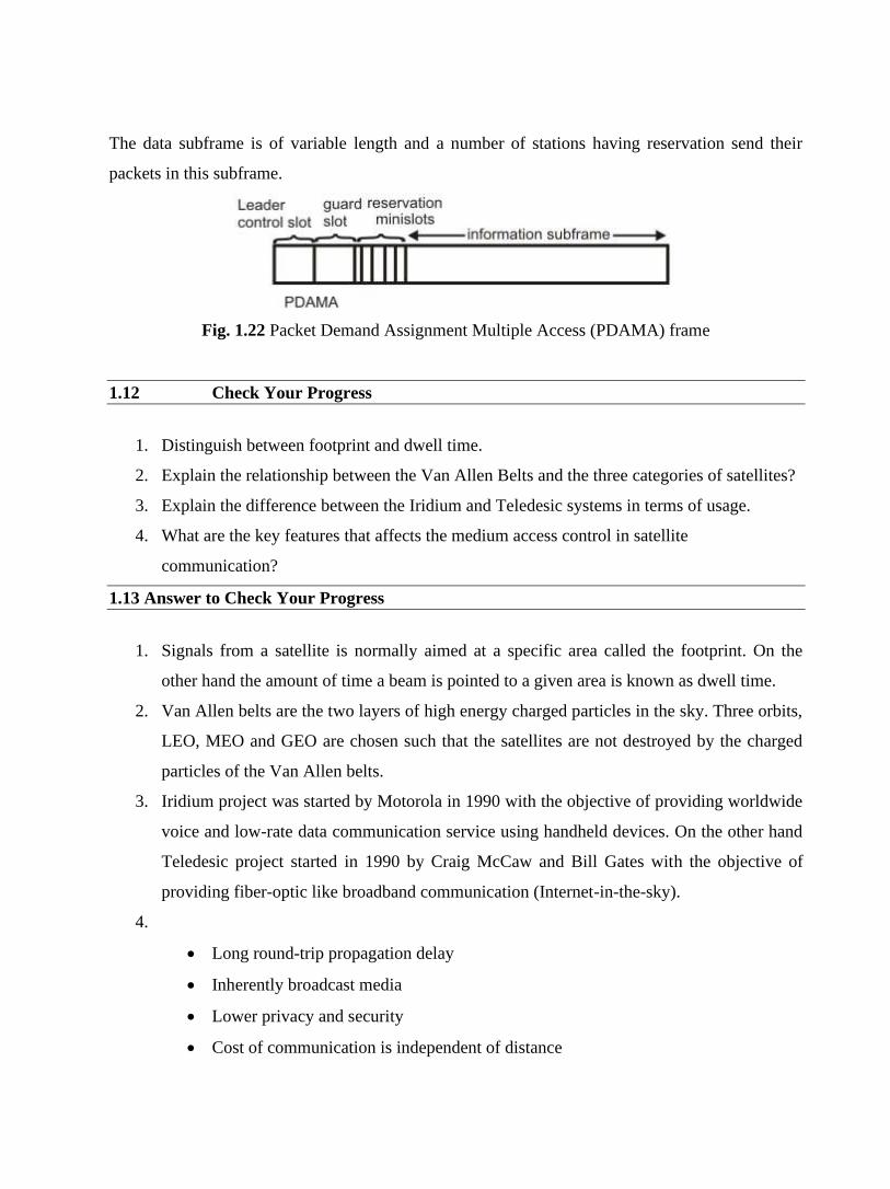
The data subframe is of variable length and a number of stations having reservation send their
packets in this subframe.
Fig. 1.22 Packet Demand Assignment Multiple Access (PDAMA) frame
1.12 Check Your Progress
1. Distinguish between footprint and dwell time.
2. Explain the relationship between the Van Allen Belts and the three categories of satellites?
3. Explain the difference between the Iridium and Teledesic systems in terms of usage.
4. What are the key features that affects the medium access control in satellite
communication?
1.13 Answer to Check Your Progress
1. Signals from a satellite is normally aimed at a specific area called the footprint. On the
other hand the amount of time a beam is pointed to a given area is known as dwell time.
2. Van Allen belts are the two layers of high energy charged particles in the sky. Three orbits,
LEO, MEO and GEO are chosen such that the satellites are not destroyed by the charged
particles of the Van Allen belts.
3. Iridium project was started by Motorola in 1990 with the objective of providing worldwide
voice and low-rate data communication service using handheld devices. On the other hand
Teledesic project started in 1990 by Craig McCaw and Bill Gates with the objective of
providing fiber-optic like broadband communication (Internet-in-the-sky).
4.
• Long round-trip propagation delay
• Inherently broadcast media
• Lower privacy and security
• Cost of communication is independent of distance

Unit-2
Internetworking Devices
1.1 Learning Objectives
1.2 Introduction
1.3 Repeaters
1.4 Hubs
1.5 Bridges
1.6 Transparent Bridges
1.6.1 Bridge Forwarding
1.6.2 Bridge Learning
1.7 Source Routing Bridges
1.8 Switches
1.9 Routers
1.10 Gateways
1.11 A Simple Internet
1.12 Check Your Progress
1.13 Answer to Check Your Progress
1.1 Learning Objectives
After going through this unit, the learner will able to learn:
• Specify the need for internetworking
• State various issues related to internetworking
• Explain the operation of various internetworking devices:
o Hubs
o Bridges
▪ Bridge forwarding and learning
▪ Transparent and source routing bridges
o Switches
o Routers
o Gateways
1.2 Introduction
HILI subcommittee (IEEE802.1) of the IEEE identified the following possible internetworking
scenarios.
• A single LAN
• Two LANs connected together (LAN-LAN)
• A LAN connected to a WAN (LAN-WAN)
• Two LANs connected through a WAN (LAN-WAN-LAN)
Various internetworking devices such as hubs, bridges, switches, routers and gateways are
required to link them together. These internetworking devices are introduced in this unit.
1.3 Repeaters
A single Ethernet segment can have a maximum length of 500 meters with a maximum of 100
stations (in a cheapernet segment it is 185m). To extend the length of the network, a repeater may
be used as shown in Fig. 2.1. Functionally, a repeater can be considered as two transceivers joined
together and connected to two different segments of coaxial cable. The repeater passes the digital
signal bit-by-bit in both directions between the two segments. As the signal passes through a
repeater, it is amplified and regenerated at the other end. The repeater does not isolate one segment
from the other, if there is a collision on one segment, it is regenerated on the other segment.
Therefore, the two segments form a single LAN and it is transparent to rest of the system. Ethernet
allows five segments to be used in cascade to have a maximum network span of 2.5 km. With
reference of the ISO model, a repeater is considered as a level-1 relay as depicted in Fig. 2.2. It
simply repeats, retimes and amplifies the bits it receives. The repeater is merely used to extend the
span of a single LAN. Important features of a repeater are as follows:
• A repeater connects different segments of a LAN
• A repeater forwards every frame it receives
• A repeater is a regenerator, not an amplifier
• It can be used to create a single extended LAN
Figure 2.1 Repeater connecting two LAN segments
Figure 2.2 Operation of a repeater as a level-1 relay
1.4 Hubs
Hub is a generic term, but commonly refers to a multiport repeater. It can be used to create
multiple levels of hierarchy of stations. The stations connect to the hub with RJ-45 connector
having maximum segment length is 100 meters. This type of interconnected set of stations is easy

to maintain and diagnose. Figure 6.1.3 shows how several hubs can be connected in a hierarchical
manner to realize a single LAN of bigger size with a large number of nodes.
Figure 2.3 Hub as a multi-port repeater can be connected in a hierarchical manner to form a single
LAN with many nodes
1.5 Bridges
The device that can be used to interconnect two separate LANs is known as a bridge. It is
commonly used to connect two similar or dissimilar LANs as shown in Fig. 2.4. The bridge
operates in layer 2, that is data-link layer and that is why it is called level-2 relay with reference to
the OSI model. It links similar or dissimilar LANs, designed to store and forward frames, it is
protocol independent and transparent to the end stations. The flow of information through a bridge
is shown in Fig. 2.5. Use of bridges offer a number of advantages, such as higher reliability,
performance, security, convenience and larger geographic coverage. But, it is desirable that the
quality of service (QOS) offered by a bridge should match that of a single LAN. The parameters
that define the QOS include availability, frame mishaps, transit delay, frame lifetime, undetected
bit errors, frame size and priority. Key features of a bridge are mentioned below:
• A bridge operates both in physical and data-link layer
• A bridge uses a table for filtering/routing
• A bridge does not change the physical (MAC) addresses in a frame
• Types of bridges:
o Transparent Bridges
o Source routing bridges

A bridge must contain addressing and routing capability. Two routing algorithms have been
proposed for a bridged LAN environment. The first, produced as an extension of IEEE 802.1 and
applicable to all IEEE 802 LANs, is known as transparent bridge. And the other, developed for
the IEEE 802.5 token rings, is based on source routing approach. It applies to many types of LAN
including token ring, token bus and CSMA/CD bus.
Figure 2.4 A bridge connecting two separate LANs
Figure 2.5 Information flow through a bridge
1.6 Transparent Bridges
The transparent bridge uses two processes known as bridge forwarding and bridge learning. If
the destination address is present in the forwarding database already created, the packet is
forwarded to the port number to which the destination host is attached. If it is not present,
forwarding is done on all parts (flooding). This process is known as bridge forwarding. Moreover,
as each frame arrives, its source address indicates where a particular host is situated, so that the

bridge learns which way to forward frames to that address. This process is known as bridge
learning. Key features of a transparent bridge are:
• The stations are unaware of the presence of a transparent bridge .
• Reconfiguration of the bridge is not necessary; it can be added/removed without being
noticed.
• If performs two functions:
o Forwarding of frames
o Learning to create the forwarding table
1.6.1 Bridge Forwarding
Bridge forwarding operation is explained with the help of a flowchart in Fig. 2.6. Basic function of
the bridge forwarding are mentioned below:
• Discard the frame if source and destination addresses are same.
• Forward the frame if the source and destination addresses are different and destination
address is present in the table.
• Use flooding if destination address is not present in the table.
Figure 2.6 Bridge Forwarding
1.6.2 Bridge Learning
At the time of installation of a transparent bridge, the database, in the form of a table, is empty. As
a packet is encountered, the bridge checks its source address and build up a table by associating a
source address with a port address to which it is connected. The flow chart of Fig. 2.7 explains the
learning process. The table building up operation is illustrated in Fig 2.8.
Figure 2.7 Bridge learning

Figure 2.8 Creation of a bridge-forwarding table
Loop Problem
Forwarding and learning processes work without any problem as long as there is no redundant
bridge in the system. On the other hand, redundancy is desirable from the viewpoint of reliability,
so that the function of a failed bridge is taken over by a redundant bridge. The existence of
redundant bridges creates the so-called loop problem as illustrated with the help of Fig. 2.9.
Assuming that after initialization tables in both the bridges are empty let us consider the following
steps:
Step 1. Station-A sends a frame to Station-B. Both the bridges forward the frame to LAN Y and
update the table with the source address of A.
Step 2. Now there are two copies of the frame on LAN-Y. The copy sent by Bridge-a is received
by Bridge-b and vice versa. As both the bridges have no information about Station B, both will
forward the frames to LAN-X.
Step 3. Again both the bridges will forward the frames to LAN-Y because of the lack of
information of the Station B in their database and again Step-2 will be repeated, and so on.
So, the frame will continue to loop around the two LANs indefinitely.
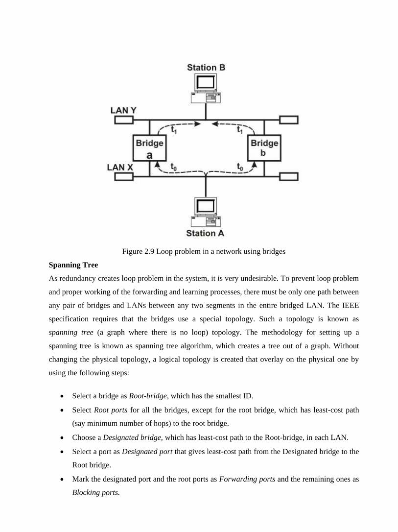
Figure 2.9 Loop problem in a network using bridges
Spanning Tree
As redundancy creates loop problem in the system, it is very undesirable. To prevent loop problem
and proper working of the forwarding and learning processes, there must be only one path between
any pair of bridges and LANs between any two segments in the entire bridged LAN. The IEEE
specification requires that the bridges use a special topology. Such a topology is known as
spanning tree (a graph where there is no loop) topology. The methodology for setting up a
spanning tree is known as spanning tree algorithm, which creates a tree out of a graph. Without
changing the physical topology, a logical topology is created that overlay on the physical one by
using the following steps:
• Select a bridge as Root-bridge, which has the smallest ID.
• Select Root ports for all the bridges, except for the root bridge, which has least-cost path
(say minimum number of hops) to the root bridge.
• Choose a Designated bridge, which has least-cost path to the Root-bridge, in each LAN.
• Select a port as Designated port that gives least-cost path from the Designated bridge to the
Root bridge.
• Mark the designated port and the root ports as Forwarding ports and the remaining ones as
Blocking ports.

The spanning tree of a network of bridges is shown in Fig.2.10. The forwarding ports are shown as
solid lines, whereas the blocked ports are shown as dotted lines.
Fi gure 2.10
Spanning tree of a network of bridges
1.7 Source Routing Bridges
The second approach, known as source routing, where the routing operation is performed by the
source host and the frame specifies which route the frame is to follow. A host can discover a route
by sending a discovery frame, which spreads through the entire network using all possible paths to
the destination. Each frame gradually gathers addresses as it goes. The destination responds to
each frame and the source host chooses an appropriate route from these responses. For example, a
route with minimum hop-count can be chosen. Whereas transparent bridges do not modify a frame,
a source routing bridge adds a routing information field to the frame. Source routing approach
provides a shortest path at the cost of the proliferation of discovery frames, which can put a serious
extra burden on the network. Figure 2.11 shows the frame format of a source routing bridge.

Figure 2.11 Source routing frame
1.8 Switches
A switch is essentially a fast bridge having additional sophistication that allows faster processing
of frames. Some of important functionalities are:
• Ports are provided with buffer
• Switch maintains a directory: #address - port#
• Each frame is forwarded after examining the #address and forwarded to the proper port#
• Three possible forwarding approaches: Cut-through, Collision-free and Fully-buffered as
briefly explained below.
Cut-through: A switch forwards a frame immediately after receiving the destination address. As a
consequence, the switch forwards the frame without collision and error detection.
Collision-free: In this case, the switch forwards the frame after receiving 64 bytes, which allows
detection of collision. However, error detection is not possible because switch is yet to receive the
entire frame.
Fully buffered: In this case, the switch forwards the frame only after receiving the entire frame.
So, the switch can detect both collision and error free frames are forwarded.
Comparison between a switch and a hub
Although a hub and a switch apparently look similar, they have significant differences. As shown
in Fig. 2.12, both can be used to realize physical star topology, the hubs works like a logical bus,
because the same signal is repeated on all the ports. On the other hand, a switch functions like a
logical star with the possibility of the communication of separate signals between any pair of port
lines. As a consequence, all the ports of a hub belong to the same collision domain, and in case of
a switch each port operates on separate collision domain. Moreover, in case of a hub, the

bandwidth is shared by all the stations connected to all the ports. On the other hand, in case of a
switch, each port has dedicated bandwidth. Therefore, switches can be used to increase the
bandwidth of a hub-based network by replacing the hubs by switches.
Figure 2.12 Difference between a switch and a bridge
1.9 Routers
A router is considered as a layer-3 relay that operates in the network layer, that is it acts on
network layer frames. It can be used to link two dissimilar LANs. A router isolates LANs in to
subnets to manage and control network traffic. However, unlike bridges it is not transparent to end
stations. A schematic diagram of the router is shown on Fig. 2.13. A router has four basic
components: Input ports, output ports, the routing processor and the switching fabric. The
functions of the four components are briefly mentioned below.
• Input port performs physical and data-link layer functions of the router. As shown in Fig.
2.14 (a), the ports are also provided with buffer to hold the packet before forwarding to the
switching fabric.
• Output ports, as shown in Fig. 2.14(b), perform the same functions as the input ports, but in
the reverse order.
• The routing processor performs the function of the network layer. The process involves
table lookup.

• The switching fabric, shown in Fig. 2.15, moves the packet from the input queue to the
output queue by using specialized mechanisms. The switching fabric is realized with the
help of multistage interconnection networks.
• Communication of a frame through a router is shown in Fig. 2.16.
Figure 2.13 Schematic diagram of a router
(a)
(b)
Figure 2.14 Schematic diagram of a router
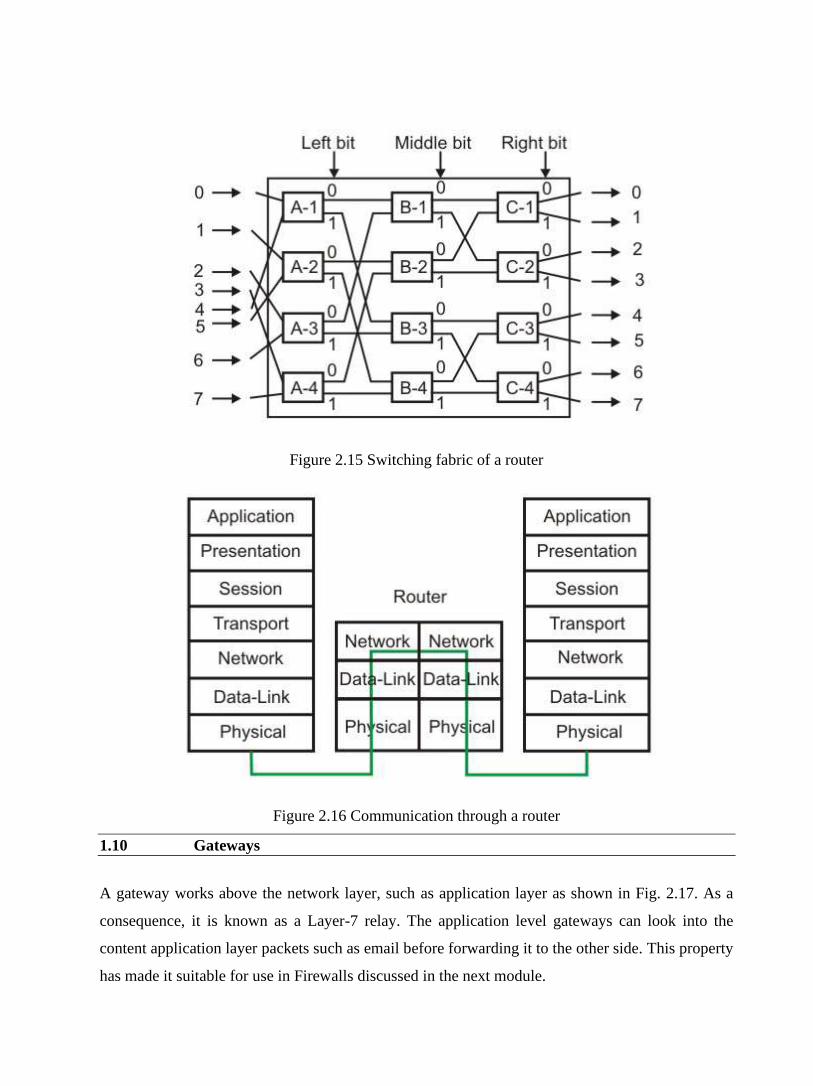
Figure 2.15 Switching fabric of a router
Figure 2.16 Communication through a router
1.10 Gateways
A gateway works above the network layer, such as application layer as shown in Fig. 2.17. As a
consequence, it is known as a Layer-7 relay. The application level gateways can look into the
content application layer packets such as email before forwarding it to the other side. This property
has made it suitable for use in Firewalls discussed in the next module.

Figure 2.17 Communication through a gateway
1.11 A Simple Internet
A simple internet comprising several LANs and WANs linked with the help of routers is shown in
Fig. 2.18.
Figure 2.18 Simple internet showing interconnection of LANs and WANs
1.12 Check Your Progress
1. Why do you need internetworking?
2. Why a repeater is called level-1 relay?
3. What is bridge? How it operates in the internetworking scenario?
4. Why spanning tree topology is necessary for routing using a bridge?
1.13 Answer to Check Your Progress
1. As stations connected to different LANs and WANs want to communicate with each other,
it is necessary to provide this facility. Internetworking creates a single virtual network over
which all stations in different network can communicate seamlessly and transparently.
2. A repeater operates in the physical layer. Data received on one of its ports is relayed on the
remaining port bit-by-bit without looking into the contents. That is why repeater is called a
level-1 relay.
3. A bridge operates in the Data link layer. It looks into various fields of a frame to take
various actions. For example, it looks at the destination address field so that it can forward
the frame to a port where destination stations is connected. It also looks at the FCS field to
check error in the received frame, it any. A bridge helps to create a network having
different collision domains.
4. If there exit more than one path between two LANs through different bridges, there is a
possibility of continuous looping of a frame between the LANs. To avoid the loop problem,
spanning tree topology is used. It is essentially an overlay of tree topology on the physical
graph topology, providing only one path between any two LANs.

Unit-3
Internet Protocol (IP)
1.1 Learning Objectives
1.2 Introduction
1.3 Addressing
1.4 IP Addressing
1.5 Subnetting
1.6 Network Address Translation (NAT)
1.7 Address Resolution Protocol (ARP)
1.8 IP Datagram
1.9 Multiplexing and Demultiplexing
1.10 Fragmentation and Reassembly
1.11 ICMP
1.12 IPV6
1.13 Check Your Progress
1.14 Answer to Check Your Progress

1.1 Learning Objectives
After going through this unit, the learner will able to learn:
• Explain the relationship between TCP/IP and OSI model
• Explain different classes of IP addresses
• Explain the concept of subnetting and subnet masking
• Explain the ARP/RARP protocol
• Explain fragmentation and reassembly
• Explain the ICMP protocols
• State the key features of IPv6
1.2 Introduction
In the previous unit we have discussed various devices required for internetworking. In addition to
these devices, several protocols are required to provide necessary functionality for
internetworking. The software that provide these protocols is known as Transmission Control
Protocol/Internet Protocol (TCP/IP). TCP/IP acts as a glue to link different types of LAN and
WAN to provide Internet, a single integrated network for seamless communication. The IP
provides unreliable, connectionless best-effort datagram delivery service, whereas TCP provides
reliable, efficient and cost-effective end-to-end delivery of data. The relationship between TCP/IP
and the OSI model is shown in Fig. 3.1. This lesson introduces the IP protocol and various issues
related to it.
1.3 Addressing
To send a packet from a source node to a destination node correctly through a network, the packet
must contain enough information about the destination address. It is also common to include the
source address, so that retransmission can be done, if necessary. The addressing scheme used for
this purpose has considerable effect on routing.
There are two possible approaches used for addressing; flat and hierarchical. In flat addressing
every possible node is assigned a unique number. When a new node is added to the network, it
must be given an address within the allowed address range. Addressing used in Ethernet is an
example of flat addressing, where addresses (48-bits long) are allocated centrally, blocks of
addresses are apportioned to manufactures, so that no two devices in the world will have the same
address. Flat addressing has the advantage that if a node is moved from one location to another, it
can retain its unique address.

Figure 3.1 Relationship between the TCP/IP and the OSI model
In hierarchical addressing, each address consists of a number of fields; as each field is inspected,
the packet is taken nearer to the destination. This is very similar to the addressing used in postal
system. A significant advantage of hierarchical addressing is that it is possible to relate a
hierarchical address structure to the topology of the network, so that routing is simplified. This
scheme has the disadvantage that if a host moves from one location to another, a new address
needs to be allocated to it, in the same manner that an address change is required as we change
house.
1.4 IP Addressing
Every host and router on the internet is provided with a unique standard form of network address,
which encodes its network number and host number. The combination is unique; no two nodes
have the same IP addresses. The IP addresses are 32-bit long having the formats shown in Fig 3.2.
The three main address formats are assigned with network addresses (net id) and host address (host
id) fields of different sizes. The class A format allows up to 126 networks with 16 million hosts
each. Class B allows up to 16,382 networks with up to 64 K hosts each. Class C allows 2 million
networks with up to 254 hosts each. The Class D is used for multicasting in which a datagram is
directed to multiple hosts. Addresses beginning with 11110 are reserved for future use. Network
addresses are usually written in dotted decimal notation, such as 126.12.15.220, where each byte is
written in decimal number corresponding to the binary value. Figure 3.3 illustrates how the dotted
decimal representation is obtained for a particular IP address in binary form. Range of IP addresses
for different classes is given in Fig. 3.4. Some IP addresses, which are used in special situations
such as the same host, a host the same network, broadcast on the same network, broadcast on a

distant network, or loopback are given in Fig. 3.5. This approach of representing IP addresses in
terms of classes is known as classful addressing. In mid 90’s another approach known as classlees
addressing has been proposed, which may supersede the existing classful addressing approach in
future.
Figure 3.2 IP address formats
Figure 3.3 Dotted decimal representation
Figure 3.4 Dotted decimal notation of the IP addresses

Figure 3.5 Special IP addresses
1.5 Subnetting
To filter packets for a particular network, a router uses a concept known as masking, which filters
out the net id part (by ANDing with all 1’s) by removing the host id part (by ANDing with all 0’s).
The net id part is then compared with the network address as shown in Fig. 3.6. All the hosts in a
network must have the same network number. This property of IP addressing causes problem as
the network grows. To overcome this problem, a concept known as subnets is used, which splits a
network into several parts for internal use, but still acts like a single network to the outside world.
To facilitate routing, a concept known as subnet mask is used. As shown in Fig. 3.7, a part of
hostid is used as subnet address with a corresponding subnet mask. Subnetting reduces router table
space by creating a three-level hierarchy; net id, subnet id followed by hosted.
Figure 3.6 Masking with the help of router

Figure 3.7 Subnet masking with the help of router
1.6 Network Address Translation (NAT)
With the increasing number of internet users requiring an unique IP address for each host, there is
an acute shortage of IP addresses (until everybody moves to IPV6). The Network Address
Translation (NAT) approach is a quick interim solution to this problem. NAT allows a large set of
IP addresses to be used in an internal (private) network and a handful of addresses to be used for
the external internet. The internet authorities has set aside three sets of addresses to be used as
private addresses as shown in Table 3.1. It may be noted that these addresses can be reused within
different internal networks simultaneously, which in effect has helped to increase the lifespan of
the IPV4. However, to make use of the concept, it is necessary to have a router to perform the
operation of address translation between the private network and the internet. As shown in Fig.
3.8, the NAT router maintains a table with a pair of entries for private and internet address. The
source address of all outgoing packets passing through the NAT router gets replaced by an internet
address based on table look up. Similarly, the destination address of all incoming packets passing
through the NAT router gets replaced by the corresponding private address, as shown in the figure.
The NAT can use a pool of internet addresses to have internet access by a limited number of
stations of the private network at a time.
Table 3.1 Addresses for Private Network
Range of addresses Total number
10.0.0.0 to 10.255.255.255 224
172.16.0.0 to 172.31.255.255 220
192.168.0.0 to 192.168.255.255 216
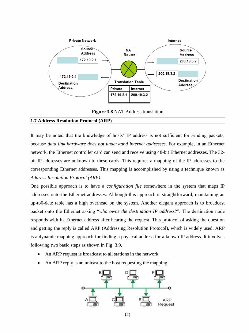
Figure 3.8 NAT Address translation
1.7 Address Resolution Protocol (ARP)
It may be noted that the knowledge of hosts’ IP address is not sufficient for sending packets,
because data link hardware does not understand internet addresses. For example, in an Ethernet
network, the Ethernet controller card can send and receive using 48-bit Ethernet addresses. The 32-
bit IP addresses are unknown to these cards. This requires a mapping of the IP addresses to the
corresponding Ethernet addresses. This mapping is accomplished by using a technique known as
Address Resolution Protocol (ARP).
One possible approach is to have a configuration file somewhere in the system that maps IP
addresses onto the Ethernet addresses. Although this approach is straightforward, maintaining an
up-to0-date table has a high overhead on the system. Another elegant approach is to broadcast
packet onto the Ethernet asking “who owns the destination IP address?”. The destination node
responds with its Ethernet address after hearing the request. This protocol of asking the question
and getting the reply is called ARP (Addressing Resolution Protocol), which is widely used. ARP
is a dynamic mapping approach for finding a physical address for a known IP address. It involves
following two basic steps as shown in Fig. 3.9.
• An ARP request is broadcast to all stations in the network
• An ARP reply is an unicast to the host requesting the mapping
(a)

(b)
Figure 3.9 (a) ARP request with a broadcast to all the stations and
(b) ARP response is a unicast only to the requesting host
Various optimizations are commonly used to improve the efficiency of the ARP protocol. One
possible approach is to use cache memory to hold the recently acquired frame containing the
physical address. As a consequence, no broadcasting is necessary in near future. Figure 3.10 shows
how an ARP packet is encapsulated into the data field of a MAC frame.
Reverse ARP (RARP)
The TCP/IP protocols include another related protocol known as reverse ARP, which can be used
by a computer such as a diskless host to find out its own IP address. It involves the following
steps:
• Diskless host A broadcasts a RARP request specifying itself as the target
• RARP server responds with the reply directly to host A
• Host A preserves the IP address in its main memory for future use until it reboots
Figure 3.10 An ARP packet is encapsulated directly into the data field a MAC frame

1.8 IP Datagram
As we have mentioned earlier, IP is an unreliable and connectionless best-effort delivery service
protocol. By best effort we mean that there is no error and flow control. However, IP performs
error detection and discards a packet, if it is corrupted. To achieve reliability, it is necessary to
combine it with a reliable protocol such as TCP. Packets in IP layer are called datagrams. The IP
header provides information about various functions the IP performs. The IP header format is
shown in Fig. 3.11. The 20 to 60 octets of header has a number of fields to provide:
• Source and destination IP addresses
• Non transparent fragmentation
• Error checking
• Priority
• Security
• Source routing option
• Route Recording option
• Stream identification
• Time stamping
Figure 3.11 IP packet format
A brief description of each of the fields are given below:
• VER (4 bits): Version of the IP protocol in use (typically 4).
• HLEN (4 bits): Length of the header, expressed as the number of 32-bit words. Minimum
size is 5, and maximum 15.
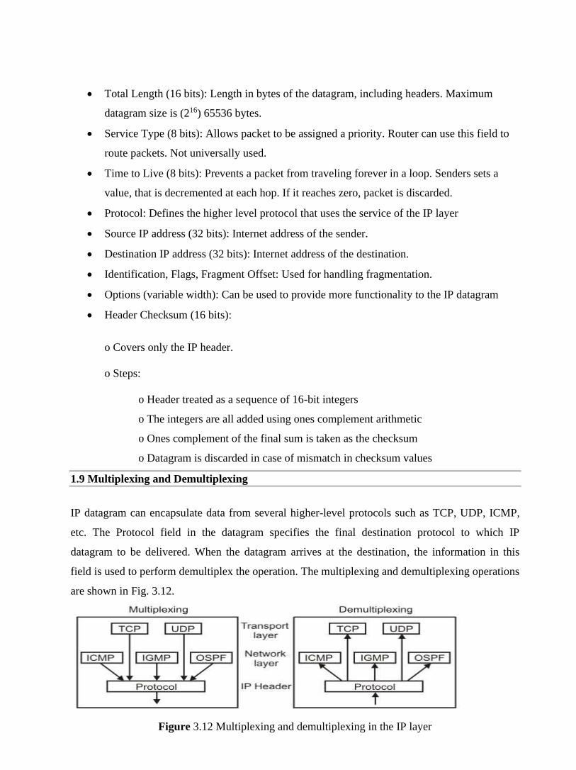
• Total Length (16 bits): Length in bytes of the datagram, including headers. Maximum
datagram size is (216) 65536 bytes.
• Service Type (8 bits): Allows packet to be assigned a priority. Router can use this field to
route packets. Not universally used.
• Time to Live (8 bits): Prevents a packet from traveling forever in a loop. Senders sets a
value, that is decremented at each hop. If it reaches zero, packet is discarded.
• Protocol: Defines the higher level protocol that uses the service of the IP layer
• Source IP address (32 bits): Internet address of the sender.
• Destination IP address (32 bits): Internet address of the destination.
• Identification, Flags, Fragment Offset: Used for handling fragmentation.
• Options (variable width): Can be used to provide more functionality to the IP datagram
• Header Checksum (16 bits):
o Covers only the IP header.
o Steps:
o Header treated as a sequence of 16-bit integers
o The integers are all added using ones complement arithmetic
o Ones complement of the final sum is taken as the checksum
o Datagram is discarded in case of mismatch in checksum values
1.9 Multiplexing and Demultiplexing
IP datagram can encapsulate data from several higher-level protocols such as TCP, UDP, ICMP,
etc. The Protocol field in the datagram specifies the final destination protocol to which IP
datagram to be delivered. When the datagram arrives at the destination, the information in this
field is used to perform demultiplex the operation. The multiplexing and demultiplexing operations
are shown in Fig. 3.12.
Figure 3.12 Multiplexing and demultiplexing in the IP layer

1.10 Fragmentation and Reassembly
Each network imposes a limit on maximum size, known as maximum transfer unit (MTU) of a
packet because of various reasons. One approach is to prevent the problem to occur in the first
place, i.e. send packets smaller than the MTU. Second approach is to deal with the problem using
fragmentation. When a gateway connects two networks that have different maximum and or
minimum packet sizes, it is necessary to allow the gateway to break packets up into fragments,
sending each one as an internet packet. The technique is known as fragmentation. The following
fields of an IP datagram are related to fragmentation:
• Identification: A16-bit field identifies a datagram originating from the source host.
• Flags: There are 3 bits, the first bit is reserved, the second bit is do not fragment bit, and
the last bit is more fragment bit.
• Fragmentation offset: This 13-bit field shows the relative position of the segment with
respect to the complete datagram measured in units of 8 bytes.
Figure 3.13 shows a fragmentation example, where a packet is fragmented into packets of 1600
bytes. So, the offset of the second fragmented packet is 1600/8 = 200 and the offset of the third
fragmented packet is 400 and so on.
The reverse process, known as reassembly, which puts the fragments together, is a more difficult
task. There are two opposing strategies for performing the re-assembly. In the first case, the
fragmentation in one network is made transparent to any subsequent networks. This requires that
packets to be reassembled before sending it to subsequent networks as shown in Fig. 3.14(a). This
strategy is used in ATM. As re-assembly requires sufficient buffer space for storage of all the
fragments, this approach has large storage overhead. To overcome this problem in the second
strategy, re-assembly is done only at the ultimate destination. This approach does not require large
buffer but additional fields are to be added to each packet for independent addressing and to
indicate the fragment number as shown in Fig. 3.14(b).

Figure 3.13 Fragmentation example
(a)
(b)
Figure 3.14 (a) Transparent Fragmentation (ATM), (b) Nontransparent fragmentation (IP)
1.11 ICMP
To make efficient use of the network resources, IP was designed to provide unreliable and
connectionless best-effort datagram delivery service. As a consequence, IP has no error-control
mechanism and also lacks mechanism for host and management queries. A companion protocol
known as Internet Control Message Protocol (ICMP), has been designed to compensate these two
deficiencies. ICMP messages can be broadly divided into two broad categories: error reporting
messages and query messages as follows.
• Error reporting Messages: Destination unreachable, Time exceeded, Source quench,
Parameter problems, Redirect

• Query: Echo request and reply, Timestamp request and reply, Address mask request and
reply
The frame formats of these query and messages are shown in Fig. 3.15.
Figure 3.15 ICMP message formats
1.12 IPV6
The network layer that is present in use in commonly referred to as IPv4. Although IPv4 is well
designed and has helped the internet to grow rapidly, it has some deficiencies, These deficiencies
has made it unsuitable for the fast growing internet. To overcome these deficiencies, Internet
Protocol, Version 6 protocol has been proposed and it has evolved into a standard. Important
features of IPv6 are highlighted below:

• IPv6 uses 128-bit address instead of 32-bit address to provide larger address space
• Uses more flexible header format, which simplifies and speeds up the routing process
• Basic header followed by extended header
• Resource Allocation options, which was not present in IPv4
• Provision of new/future protocol options
• Support for security with the help of encryption and authentication
• Support for fragmentation at source
1.13 Check Your Progress
Fill in the blanks:
1. Two possible addressing techniques are _______ addressing and _________ addressing.
2. Ethernet address is an example of ________ addressing while IP address is an example of
__________ addressing.
3. The Class C address class can have _____ networks and about _____ hosts in each network
4. The mapping of the IP address to the corresponding Ethernet Address is done by a protocol
named as ______.
1.14 Answer to check Your Progress
1. flat, hierarchical
2. Flat,hierarchical
3. 254, 2 million
4. ARP

Unit-4
Transport and Application Layer Protocols
1.1 Learning Objectives
1.2 Introduction
1.3 User Datagram protocol (UDP)
1.4 Transmission Control Protocol (TCP)
1.5 Client-Server Paradigm and its Applications
1.6 Check Your Progress
1.7 Answer to Check Your Progress

1.1 Learning Objectives
After going through this unit, the learner will able to learn:
• Explain how UDP allows two applications running in two remote locations can
communicate
• State the limitations of UDP
• Explain how TCP provides connection-oriented service
• Explain how TCP incorporates reliability in internet communication
• Explain how DNS allows the use of symbolic names instead of IP address
• Explain the use of client-server model for
o Remote login
o Mail transfer
o File transfer
1.2 Introduction
So far we have discussed the delivery of data in the following two ways:
• Node-to-node delivery: At the data-link level, delivery of frames take place between two
nodes connected by a point-to-point link or a LAN, by using the data-link layers address,
say MAC address.
• Host-to-host delivery: At the network level, delivery of datagrams can take place between
two hosts by using IP address.
From user’s point of view, the TCP/IP-based internet can be considered as a set of application
programs that use the internet to carry out useful communication tasks. Most popular internet
applications include Electronic mail, File transfer, and Remote login. IP allows transfer of IP
datagrams among a number of stations or hosts, where the datagram is routed through the internet
based on the IP address of the destination. But, in this case, several application programs
(processes) simultaneously running on a source host has to communicate with the corresponding
processes running on a remote destination host through the internet. This requires an additional
mechanism called process-to-process delivery, which is implemented with the help of a transport-
level protocol. The transport level protocol will require an additional address, known as port
number, to select a particular process among multiple processes running on the destination host.
So, there is a requirement of the following third type of delivery system.

• Process-to-process delivery: At the transport level, communication can take place
between processes or application programs by using port addresses.
Basic communication mechanism is shown in Fig. 4.1. The additional mechanism needed to
facilitate multiple application programs in different stations to communicate with each other
simultaneously can be provided by a transport level protocol such as UDP or TCP, which are
discussed in this lesson.
Figure 4.1 Communication mechanism through the internet
1.3 User Datagram protocol (UDP)
UDP is responsible for differentiating among multiple source and destination processes within one
host. Multiplexing and demultiplexing operations are performed using the port mechanism as
depicted in Fig. 4.2.
Figure 4.2 Multiplexing and demultiplexing mechanism of UDP
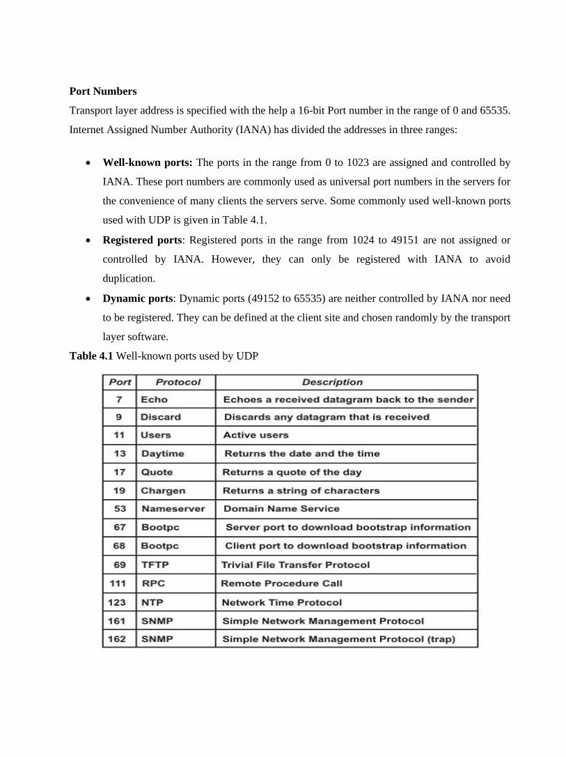
Port Numbers
Transport layer address is specified with the help a 16-bit Port number in the range of 0 and 65535.
Internet Assigned Number Authority (IANA) has divided the addresses in three ranges:
• Well-known ports: The ports in the range from 0 to 1023 are assigned and controlled by
IANA. These port numbers are commonly used as universal port numbers in the servers for
the convenience of many clients the servers serve. Some commonly used well-known ports
used with UDP is given in Table 4.1.
• Registered ports: Registered ports in the range from 1024 to 49151 are not assigned or
controlled by IANA. However, they can only be registered with IANA to avoid
duplication.
• Dynamic ports: Dynamic ports (49152 to 65535) are neither controlled by IANA nor need
to be registered. They can be defined at the client site and chosen randomly by the transport
layer software.
Table 4.1 Well-known ports used by UDP

Figure 4.3 UDP Datagram Format
UDP Datagram
The UDP datagram format is shown in Fig. 4.3. A brief description of different fields of the
datagram are given below:
• Source port (16 bits): It defines the port number of the application program in the host of
the sender.
• Destination port (16 bits): It defines the port number of the application program in the host
of the receiver.
• Length: It provides a count of octets in the UDP datagram, minimum length = 8.
• Checksum: It is optional, 0 in case it is not in use
Characteristics of the UDP
Key characteristics of UDP are given below:
• UDP provides an unreliable connectionless delivery service using IP to transport messages
between two processes.
• UDP messages can be lost, duplicated, delayed and can be delivered out of order.
• UDP is a thin protocol, which does not add significantly to the functionality of IP.
• It cannot provide reliable stream transport service.
The above limitations can be overcome by using connection-oriented transport layer protocol
known as Transmission Control Protocol (TCP).
1.4 Transmission Control Protocol (TCP)
TCP provides a connection-oriented, full-duplex, reliable, streamed delivery service using IP to
transport messages between two processes.
Reliability is ensured by:
• Connection-oriented service
• Flow control using sliding window protocol
• Error detection using checksum

• Error control using go-back-N ARQ technique
• Congestion avoidance algorithms; multiplicative decrease and slow-start
TCP Datagram
The TCP datagram format is shown in Fig. 4.4. A brief explanation of the functions of different
fields are given below:
• Source port (16 bits): It defines the port number of the application program in the host of
the sender.
• Destination port (16 bits): It defines the port number of the application program in the host
of the receiver.
• Sequence number (32 bits): It conveys the receiving host which octet in this sequence
comprises the first byte in the segment.
• Acknowledgement number (32 bits): This specifies the sequence number of the next octet
that receiver expects to receive.
• HLEN (4 bits): This field specifies the number of 32-bit words present in the TCP header.
• Control flag bits (6 bits): URG: Urgent pointer.
• ACK: Indicates whether acknowledge field is valid
• PSH: Push the data without buffering
• RST: Resent the connection
• SYN: Synchronize sequence numbers during connection establishment
• FIN: Terminate the connection
• Window (16 bits): Specifies the size of window
• Checksum (16 bits): Checksum used for error detection.
• User pointer (16 bits): Used only when URG flag is valid
• Options: Optional 40 bytes of information
The well-known ports used by TCP are given in Table 4.2 and the three types of addresses used in
TCP/IP are shown in Fig. 4.5. TCP establishes a virtual path between the source and destination
processes before any data communication by using two procedures, connection establishment to
start reliably and connection termination to terminate gracefully, as discussed in the following
subsection.
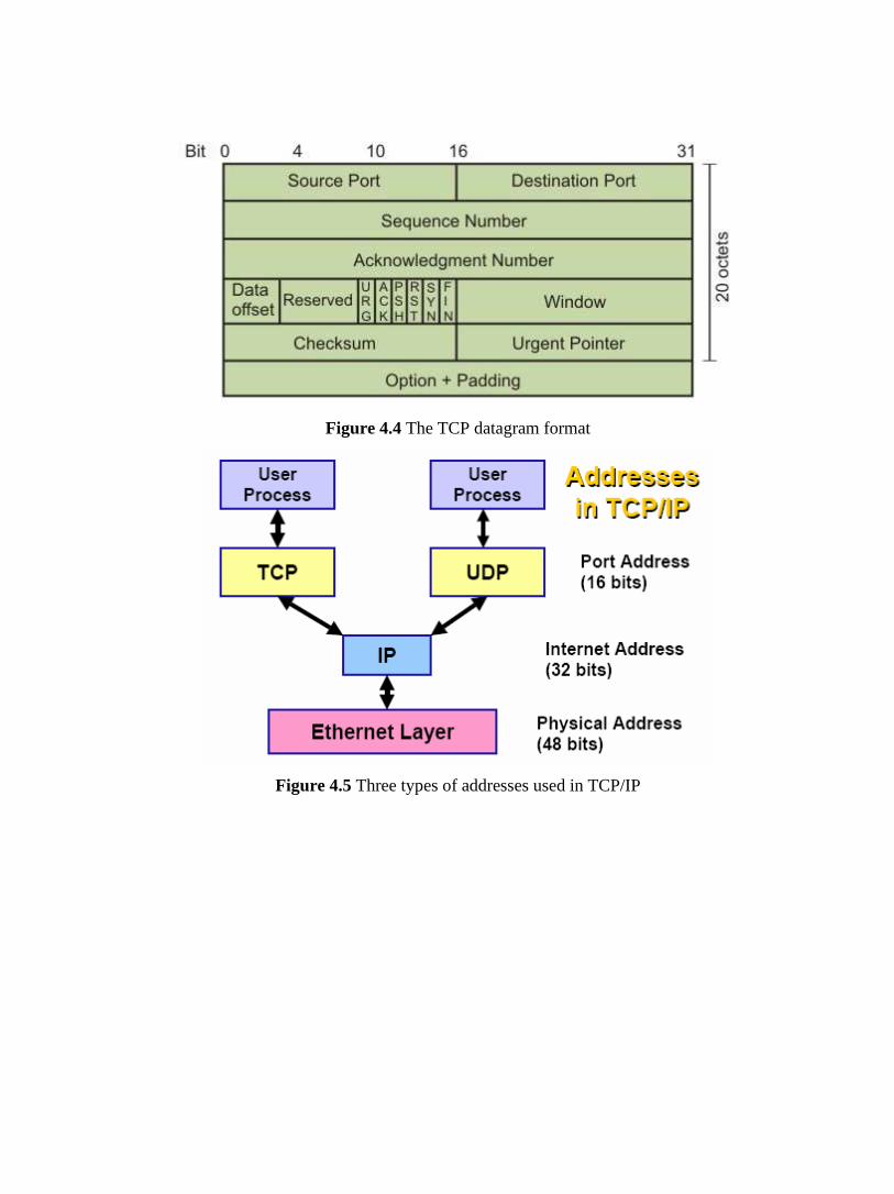
Figure 4.4 The TCP datagram format
Figure 4.5 Three types of addresses used in TCP/IP

Table 4.2 Well-known ports used by TCP
Connection-oriented service
TCP performs data communication in full-duplex mode, that is both the sender and receiver
processes can send segments simultaneously. For connection establishment in full-duplex mode, a
four-way protocol can be used. However, the second and third steps can be combined to form a
three-way handshaking protocol with the following three steps as shown in Fig. 4.6.
Step 1: The client sends SYN segment, which includes, source and destination port numbers, and
an initialization sequence number (ISN), which is essentially the byte number to be sent from the
client to the server.
Step 2: The server sends a segment, which is a two-in-one segment. It acknowledges the receipt of
the previous segment and it also acts as initialization segment for the server.
Step3: The sends an ACK segment, which acknowledges the receipt of the second segment.
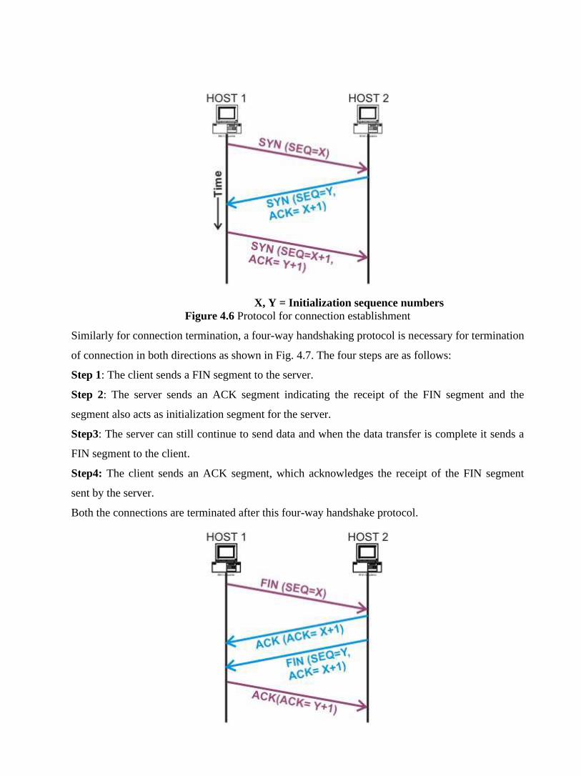
X, Y = Initialization sequence numbers
Figure 4.6 Protocol for connection establishment
Similarly for connection termination, a four-way handshaking protocol is necessary for termination
of connection in both directions as shown in Fig. 4.7. The four steps are as follows:
Step 1: The client sends a FIN segment to the server.
Step 2: The server sends an ACK segment indicating the receipt of the FIN segment and the
segment also acts as initialization segment for the server.
Step3: The server can still continue to send data and when the data transfer is complete it sends a
FIN segment to the client.
Step4: The client sends an ACK segment, which acknowledges the receipt of the FIN segment
sent by the server.
Both the connections are terminated after this four-way handshake protocol.
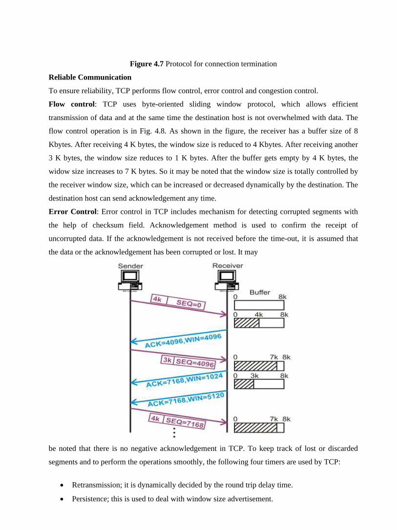
Figure 4.7 Protocol for connection termination
Reliable Communication
To ensure reliability, TCP performs flow control, error control and congestion control.
Flow control: TCP uses byte-oriented sliding window protocol, which allows efficient
transmission of data and at the same time the destination host is not overwhelmed with data. The
flow control operation is in Fig. 4.8. As shown in the figure, the receiver has a buffer size of 8
Kbytes. After receiving 4 K bytes, the window size is reduced to 4 Kbytes. After receiving another
3 K bytes, the window size reduces to 1 K bytes. After the buffer gets empty by 4 K bytes, the
widow size increases to 7 K bytes. So it may be noted that the window size is totally controlled by
the receiver window size, which can be increased or decreased dynamically by the destination. The
destination host can send acknowledgement any time.
Error Control: Error control in TCP includes mechanism for detecting corrupted segments with
the help of checksum field. Acknowledgement method is used to confirm the receipt of
uncorrupted data. If the acknowledgement is not received before the time-out, it is assumed that
the data or the acknowledgement has been corrupted or lost. It may
be noted that there is no negative acknowledgement in TCP. To keep track of lost or discarded
segments and to perform the operations smoothly, the following four timers are used by TCP:
• Retransmission; it is dynamically decided by the round trip delay time.
• Persistence; this is used to deal with window size advertisement.
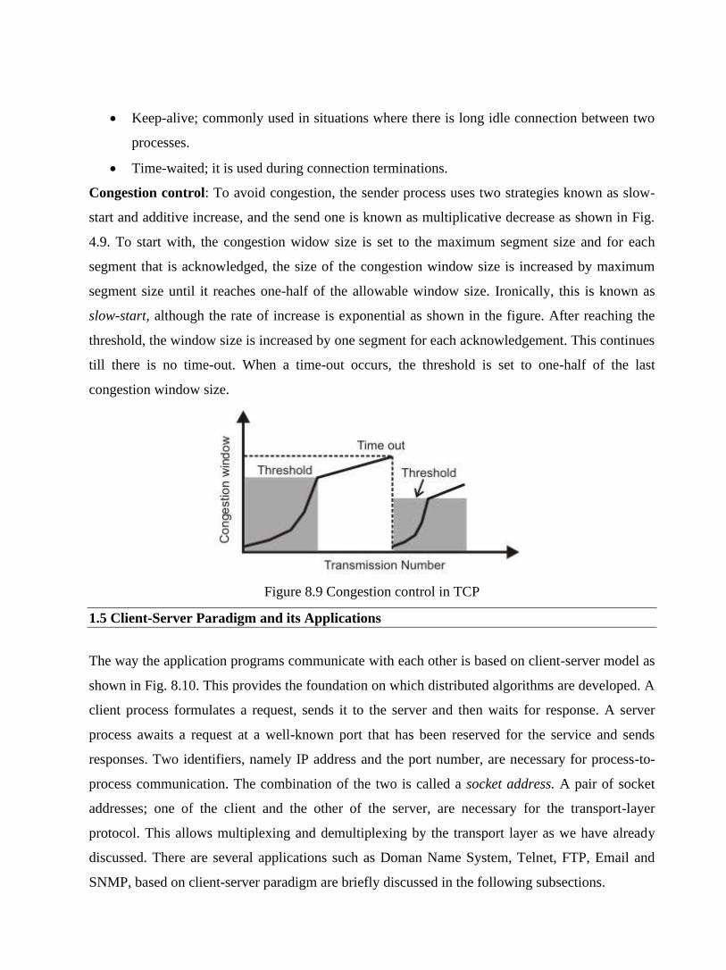
• Keep-alive; commonly used in situations where there is long idle connection between two
processes.
• Time-waited; it is used during connection terminations.
Congestion control: To avoid congestion, the sender process uses two strategies known as slow-
start and additive increase, and the send one is known as multiplicative decrease as shown in Fig.
4.9. To start with, the congestion widow size is set to the maximum segment size and for each
segment that is acknowledged, the size of the congestion window size is increased by maximum
segment size until it reaches one-half of the allowable window size. Ironically, this is known as
slow-start, although the rate of increase is exponential as shown in the figure. After reaching the
threshold, the window size is increased by one segment for each acknowledgement. This continues
till there is no time-out. When a time-out occurs, the threshold is set to one-half of the last
congestion window size.
Figure 8.9 Congestion control in TCP
1.5 Client-Server Paradigm and its Applications
The way the application programs communicate with each other is based on client-server model as
shown in Fig. 8.10. This provides the foundation on which distributed algorithms are developed. A
client process formulates a request, sends it to the server and then waits for response. A server
process awaits a request at a well-known port that has been reserved for the service and sends
responses. Two identifiers, namely IP address and the port number, are necessary for process-to-
process communication. The combination of the two is called a socket address. A pair of socket
addresses; one of the client and the other of the server, are necessary for the transport-layer
protocol. This allows multiplexing and demultiplexing by the transport layer as we have already
discussed. There are several applications such as Doman Name System, Telnet, FTP, Email and
SNMP, based on client-server paradigm are briefly discussed in the following subsections.

Domain Name System
Although IP addresses are convenient and compact way for identifying machines and are
fundamental in TCP/IP, it is unsuitable for human user. Meaningful high-level symbolic names are
more convenient for humans. Application software permits users to use symbolic names, but the
underlying network protocols require addresses. This requires the use of names with proper syntax
with efficient translation mechanism. A concept known as Domain Name System (DNS) was
invented for this purpose. DNS is a naming scheme that uses a hierarchical, domain-based naming
scheme on a distributed database system. The basic approach is to divide the internet into several
hundred top-level domains, which come in two flavors - generic and countries. Nearly all
organizations in USA, are under generic name, where each domain is partitioned into subdomains,
and these are further partitioned, and so on, as represented in the form of a tree as shown in Fig.
8.11. The leaves of the tree represent domains that contain no subdomains, represent single hosts,
or a company or contains a thousand of hosts. Naming follows organizational boundaries, not
physical networks. The hierarchical naming system, which is used by DNS has many advantages
over flat addressing scheme used earlier. Key features of the two approaches are highlighted
below:
Figure 4.10 Client-server model
Figure 4.11 Partial Domain Name Space
Flat namespace
• Each machine is given a unique (by NIC) name
• Special file is used to keep name-address mapping
• All hosts must know the current mapping for all other hosts with which they want to
communicate
• Large mapping file, if communication with a large number of machines is required
• Not a good scheme for communicating to arbitrary machines over large networks such as
Internet
Hierarchical Namespace
• Break complete namespace into domains
• Domains broken up recursively into one or more subdomains, each of which is basically a
domain again
• Further division to create any level of hierarchy – Namespace Tree
• Delegate task of name allocation/resolution of parts of the tree to distributed name servers
Name-address Resolution
Although the names used by the DNS is very convenient to humans, it cannot be used for
communication through the internet. This requires mapping a name to an address known as Name-
address Resolution. The mapping of the name to the address can be done using a name server,
where a look-up table is maintained. A single name server could contain the entire DNS database
and respond to all queries about it. However, the server would be very much overloaded and when
it would fail, the entire Internet would be crippled. To avoid this problem, the entire name space is
divided into non-overlapping zones. Each zone contains some part of the tree and also contains
name servers holding the authorization information about the zone. In practice, a zone will have a
primary name server and one or more secondary name servers, which get their information from
the primary name servers. This is how smaller databases are maintained in a distributed manner as
shown in Fig. 4.12.
To map a name onto an IP address, an application program calls a library procedure known as
resolver. The resolver sends a UDP packet to a local DNS server, which searches for the name in
its database. If the name is found, it returns the IP address to the resolver, which in turn informs it
to the client. After having the IP address, the client then establishes a TCP connection with a
destination node. However, if the local DNS server does not have the requested information, it
seeks the help from other servers and finally reports back. This is known as recursive resolution,

as shown in Fig. 4.13. The client may not ask for a recursive answer and in that case the mapping
can be done iteratively. If a server is an authority for the name, the reply is sent. Otherwise, it
sends the IP address of another server that is likely to resolve the query. The client sends query to
the second server and so on. This process is known as iterative resolution.
To avoid another search when a query is received for a name that is not in its domain, the
information is stored in the cash memory of the server. This mechanism is known as caching. This
improves the efficiency of resolution. However, the mapping is not stored in the cache memory
indefinitely. A time-to-live TTL) counter is associated with each mapping and when the time
expires, the mapping is purged.
Figure 4.12 DNS servers

Figure 4.13 Recursive resolution performed in ARP protocol
Electronic Mail
Electronic mail is among the most widely available application services. Each user, who intends to
participate in email communication, is assigned a mailbox, where out-going and incoming
messages are buffered, allowing the transfer to take place in the background. The message contains
a header that specifies the sender, recipients, and subject, followed by a body that contains
message. The TCP/IP protocol that supports electronic mail on the internet is called Simple Mail
Transfer Protocol (SMTP), which supports the following:
• Sending a message to one or more recipients
• Sending messages that include text, voice, video, or graphics
A software package, known as User Agent, is used to compose, read, reply or forward emails and
handle mailboxes. The email address consists of two parts divided by a @ character. The first part
is the local name that identifies mailbox and the second part is a domain name.
Figure 4.14 Simple Mail Transfer Protocol (SMTP)

Telnet
Telnet is a simple remote terminal protocol that provides a remote log-on capability, which enables
a user to log on to a remote computer and behaves as if it is directly connected to it. The following
three basic services are offered by TELNET:
o It defines a network virtual terminal that provides a standard interface to remote systems
o It includes a mechanism that allows the client and server to negotiate options from a
standard set
o It treats both ends symmetrically
File Transfer Protocol (FTP)
File Transfer Protocol (FTP) is a TCP/IP client-server application for transfer files between two
remote machines through internet. A TCP connection is set up before file transfer and it persists
throughout the session. It is possible to send more than one file before disconnecting the link. A
control connection is established first with a remote host before any file can be transferred. Two
connections required are shown in Fig. 4.15. Users view FTP as an interactive system
Figure 4.15 File Transfer Protocol (FTP)
Simple Network Management Protocol (SNMP)
Network managers use network management software that help them to locate, diagnose and
rectify problems. Simple Network Management Protocol (SMTP) provides a systematic way for
managing network resources. It uses transport layer protocol for communication. It allows them to
monitor switches, routers and hosts. There are four components of the protocol:
• Management of systems
• Management of nodes; hosts, routers, switches
• Management of Information Base; specifies data items a host or a router must keep and the
operations allowed on each (eight categories)
• Management of Protocol; specifies communication between network management client
program a manager invokes and a network management server running on a host or router

1.6 Check Your Progress
1. What is the relationship between TCP/IP and Internet?
2. Distinguish between TCP and UDP?
3. What is the main function of UDP protocol?
1.7 Answer to Check Your Progress
1. Internet is a network of different types of network. TCP/IP is a set of rules and procedures
that govern the exchange of messages between hosts linked to different networks. TCP/IP
creates an environment as if all hosts are connected to a single logical network.
2. Both TCP and UDP belong to transport layer. The UDP is simpler with much less
overhead. UDP provides unreliable connectionless service. On the other hand, TCP
provides connection oriented reliable service with the help of suitable flow control and
error control protocols. As a consequence, TCP has much more overhead.
3. UDP protocol provides user programs the ability to communicate using unreliable
connectionless packet delivery service with minimum overhead.

Unit-05
Routing and Congestion Control
1.1 Learning Objectives
1.2 Introduction
1.3 Classification of Routers
1.4 Routing Algorithm Metrics
1.5 Fixed or Static Routing
1.6 Flooding
1.7 Intradomain versus Interdomain
1.8 Check Your Progress
1.9 Answer to Check Your Progress
1.1 Learning Objectives
After going through this unit, the learner will able to learn:
• Understand the need for routing
• Understand desirable properties of routing
• Understand various Routing algorithms
• Fixed (Static) routing
• Understand Flooding
1.2 Introduction
Routing is the act of moving information across an inter-network from a source to a destination.
Along the way, at least one intermediate node typically is encountered. It’s also referred to as the
process of choosing a path over which to send the packets. Routing is often contrasted with
bridging, which might seem to accomplish precisely the same thing to the casual observer. The
primary difference between the two is that bridging occurs at Layer 2 (the data link layer) of the
OSI reference model, whereas routing occurs at Layer 3 (the network layer). This distinction
provides routing and bridging with different information to use in the process of moving
information from source to destination, so the two functions accomplish their tasks in different
ways. The routing algorithm is the part of the network layer software responsible for deciding
which output line an incoming packet should be transmitted on, i.e. what should be the next
intermediate node for the packet.
Routing protocols use metrics to evaluate what path will be the best for a packet to travel. A metric
is a standard of measurement; such as path bandwidth, reliability, delay, current load on that path
etc; that is used by routing algorithms to determine the optimal path to a destination. To aid the
process of path determination, routing algorithms initialize and maintain routing tables, which
contain route information. Route information varies depending on the routing algorithm used.
Routing algorithms fill routing tables with a variety of information. Mainly Destination/Next hop
associations tell a router that a particular destination can be reached optimally by sending the
packet to a particular node representing the "next hop" on the way to the final destination. When a
router receives an incoming packet, it checks the destination address and attempts to associate this
address with a next hop. Some of the routing algorithm allows a router to have multiple “next hop”
for a single destination depending upon best with regard to different metrics. For example, let’s
say router R2 is be best next hop for destination “D”, if path length is considered as the metric;

while Router R3 is the best for the same destination if delay is considered as the metric for making
the routing decision.
Figure 5.1 Typical routing in a small network
Figure 5.1 shows a small part of a network where packet destined for node “D”, arrives at router
R1, and based on the path metric i.e. the shortest path to destination is forwarded to router R2
which forward it to the final destination. Routing tables also can contain other information, such as
data about the desirability of a path. Routers compare metrics to determine optimal routes, and
these metrics differ depending on the design of the routing algorithm used. Routers communicate
with one another and maintain their routing tables through the transmission of a variety of
messages. The routing update message is one such message that generally consists of all or a
portion of a routing table. By analyzing routing updates from all other routers, a router can build a
detailed picture of network topology. A link-state advertisement, another example of a message
sent between routers, informs other routers of the state of the sender's links. Link information also
can be used to build a complete picture of network topology to enable routers to determine optimal
routes to network destinations.
Desirable properties of a router are as follows:
• Correctness and simplicity: The packets are to be correctly delivered. Simpler the routing
algorithm, it is better.
• Robustness: Ability of the network to deliver packets via some route even in the face of
failures.
• Stability: The algorithm should converge to equilibrium fast in the face of changing
conditions in the network.
• Fairness and optimality: obvious requirements, but conflicting.
• Efficiency: Minimum overhead

While designing a routing protocol it is necessary to take into account the following design
parameters:
• Performance Criteria: Number of hops, Cost, Delay, Throughput, etc
• Decision Time: Per packet basis (Datagram) or per session (Virtual-circuit) basis
• Decision Place: Each node (distributed), Central node (centralized), Originated node
(source)
• Network Information Source: None, Local, Adjacent node, Nodes along route, All nodes
• Network Information Update Timing: Continuous, Periodic, Major load change,
Topology change
1.3 Classification of Routers
Routing algorithms can be classified based on the following criteria:
• Static versus Adaptive
• Single-path versus multi-path
• Intra-domain versus inter-domain
• Flat versus hierarchical
• Link-state versus distance vector
• Host-intelligent versus router-intelligent
Static versus Adaptive
This category is based on how and when the routing tables are set-up and how they can be
modified, if at all. Adaptive routing is also referred as dynamic routing and Non-adaptive is also
known as static routing algorithms. Static routing algorithms are hardly algorithms at all; the
table mappings are established by the network administrator before the beginning of routing. These
mappings do not change unless the network administrator alters them. Algorithms that use static
routes are simple to design and work well in environments where network traffic is relatively
predictable and where network design is relatively simple. Routing decisions in these algorithms
are in no way based on current topology or traffic.
Because static routing systems cannot react to network changes, they generally are considered
unsuitable for today's large, constantly changing networks. Most of the dominant routing
algorithms today are dynamic routing algorithms, which adjust to changing network circumstances
by analyzing incoming routing update messages. If the message indicates that a network change

has occurred, the routing software recalculates routes and sends out new routing update messages.
These messages permeate the network, stimulating routers to rerun their algorithms and change
their routing tables accordingly. Dynamic routing algorithms can be supplemented with static
routes where appropriate.
Single-Path versus Multi-path
This division is based upon the number of paths a router stores for a single destination.
Single path algorithms are where only a single path (or rather single next hop) is stored in the
routing table. Some sophisticated routing protocols support multiple paths to the same destination;
these are known as multi-path algorithms. Unlike single-path algorithms, these multipath
algorithms permit traffic multiplexing over multiple lines. The advantages of multipath algorithms
are obvious: They can provide substantially better throughput and reliability. This is generally
called load sharing.
Intradomain versus Interdomain
Some routing algorithms work only within domains; others work within and between domains.
The nature of these two algorithm types is different. It stands to reason, therefore, that an optimal
intra-domain-routing algorithm would not necessarily be an optimal inter-domain-routing
algorithm.
Flat Versus Hierarchical
Some routing algorithms operate in a flat space, while others use routing hierarchies. In a flat
routing system, the routers are peers of all others. In a hierarchical routing system, some routers
form what amounts to a routing backbone. Packets from non-backbone routers travel to the
backbone routers, where they are sent through the backbone until they reach the general area of the
destination. At this point, they travel from the last backbone router through one or more non-
backbone routers to the final destination.
Routing systems often designate logical groups of nodes, called domains, autonomous
systems, or areas. In hierarchical systems, some routers in a domain can communicate with routers
in other domains, while others can communicate only with routers within their domain. In very
large networks, additional hierarchical levels may exist, with routers at the highest hierarchical
level forming the routing backbone.
The primary advantage of hierarchical routing is that it mimics the organization of most companies
and therefore supports their traffic patterns well. Most network communication occurs within

small company groups (domains). Because intradomain routers need to know only about other
routers within their domain, their routing algorithms can be simplified, and, depending on the
routing algorithm being used, routing update traffic can be reduced accordingly.
Link-State versus Distance Vector
This category is based on the way the routing tables are updated.
Distance vector algorithms (also known as Bellman-Ford algorithms): Key features of the distance
vector routing are as follows:
• The routers share the knowledge of the entire autonomous system
• Sharing of information takes place only with the neighbors
• Sharing of information takes place at fixed regular intervals, say every 30 seconds.
Link-state algorithms (also known as shortest path first algorithms) have the following key feature
• The routers share the knowledge only about their neighbors compared to all the routers in
the autonomous system
• Sharing of information takes place only with all the routers in the internet, by sending small
updates using flooding compared to sending larger updates to their neighbors
• Sharing of information takes place only when there is a change, which leads to lesser
internet traffic compared to distance vector routing
Because convergence takes place more quickly in link-state algorithms, these are somewhat less
prone to routing loops than distance vector algorithms. On the other hand, link-state algorithms
require more processing power and memory than distance vector algorithms. Link-state
algorithms, therefore, can be more expensive to implement and support. Link-state protocols are
generally more scalable than distance vector protocols.
Host-Intelligent Versus Router-Intelligent
This division is on the basis of whether the source knows about the entire route or just about the
next-hop where to forward the packet. Some routing algorithms assume that the source end node
will determine the entire route. This is usually referred to as source routing. In source-routing
systems, routers merely act as store-and-forward devices, mindlessly sending the packet to the next
stop. These algorithms are also referred to as Host-Intelligent Routing, as entire route is specified
by the source node.

Other algorithms assume that hosts know nothing about routes. In these algorithms, routers
determine the path through the internet based on their own own strategy. In the first system, the
hosts have the routing intelligence. In the latter system, routers have the routing intelligence.
1.4 Routing Algorithm Metrics
Routing tables contain information used by switching software to select the best route. In this
section we will discuss the different nature of information they contain, and the way they
determine that one route is preferable to others?
Routing algorithms have used many different metrics to determine the best route. Sophisticated
routing algorithms can base route selection on multiple metrics, combining them in a single
(hybrid) metric. All the following metrics have been used:
• Path length
• Delay
• Bandwidth
• Load
• Communication cost
• Reliability
Path length is the most common routing metric. Some routing protocols allow network
administrators to assign arbitrary costs to each network link. In this case, path length is the sum of
the costs associated with each link traversed. Other routing protocols define hop count, a metric
that specifies the number of passes through internetworking products, such as routers, that a packet
must pass through in a route from a source to a destination.
Routing delay refers to the length of time required to move a packet from source to destination
through the internet. Delay depends on many factors, including the bandwidth of intermediate
network links, the port queues (receive and transmit queues that are there in the routers) at each
router along the way, network congestion on all intermediate network links, and the physical
distance to be traveled. Because delay is a conglomeration of several important variables, it is a
common and useful metric.
Bandwidth refers to the available traffic capacity of a link. All other things being equal, a 10-
Mbps Ethernet link would be preferable to a 64-kbps leased line. Although bandwidth is a rating of
the maximum attainable throughput on a link, routes through links with greater bandwidth do not

necessarily provide better routes than routes through slower links. For example, if a faster link is
busier, the actual time required to send a packet to the destination could be greater.
Load refers to the degree to which a network resource, such as a router, is busy. Load can be
calculated in a variety of ways, including CPU utilization and packets processed per second.
Monitoring these parameters on a continual basis can be resource-intensive itself.
Communication cost is another important metric, especially because some companies may not
care about performance as much as they care about operating expenditures. Although line delay
may be longer, they will send packets over their own lines rather than through the public lines that
cost money for usage time.
Reliability, in the context of routing algorithms, refers to the dependability (usually described in
terms of the bit-error rate) of each network link. Some network links might go down more often
than others. After a network fails, certain network links might be repaired more easily or more
quickly than other links. Any reliability factor can be taken into account in the assignment of the
reliability ratings, which are arbitrary numeric values, usually assigned to network links by
network administrators.
1.5 Fixed or Static Routing
In fixed routing a route is selected for each source-destination pair of nodes in the network. The
routes are fixed; they may only change if there is a change in the topology of the network. A
central routing matrix is created based on least-cost path, which is stored at a network control
center. The matrix shows, for each source-destination pair of nodes, the identity of the next node
on the route. Figure 5.2(a) shows a simple packet switching network with six nodes (routers), and
Fig. 5.2 (b) shows the central routing table created based on least-cost path algorithm. Figure 5.3
shows the routing tables that can be distributed in different nodes of the network.

Figures 5.2 (a) A simple packet switching network with six nodes (routers), (b) The central routing
table created based on least-cost path
Figures 5.3 Routing tables that can be stored in different nodes of the network.
1.6 Flooding
Flooding requires no network information whatsoever. Every incoming packet to a node is sent out
on every outgoing line except the one it arrived on. All possible routes between source and
destination are tried. A packet will always get through if a path exists. As all routes are tried, at
least one packet will pass through the shortest route. All nodes, directly or indirectly connected,
are visited. Main limitation flooding is that it generates vast number of duplicate packets. It is
necessary to use suitable damping mechanism to overcome this limitation. One simple is to use
hop-count; a hop counter may be contained in the packet header, which is decremented at each
hop, with the packet being discarded when the counter becomes zero. The sender initializes the
hop counter. If no estimate is known, it is set to the full diameter of the subnet. Another approach
is keep track of packets, which are responsible for flooding using a sequence number and avoid
sending them out a second time. A variation, which is slightly more practical, is selective flooding.
The routers do not send every incoming packet out on every line, only on those lines that go in
approximately in the direction of destination. Some of the important utilities of flooding are:
• Flooding is highly robust, and could be used to send emergency messages (e.g., military
applications).
• It may be used to initially set up the route in a virtual circuit.
• Flooding always chooses the shortest path, since it explores every possible path in parallel.
• Can be useful for the dissemination of important information to all nodes (e.g., routing
information).
1.7 Intradomain versus Interdomain
In this section we shall discuss the difference between inter-domain and intra-domain routing
algorithms or as they are commonly known as Exterior-gateway protocols and Interior gateway
protocols respectively. Before going into the details of each of these routing algorithms, let’s
discuss the concept of Autonomous systems, which is the major differentiator between the two.
Autonomous Systems
As internet is a network of network that spans the entire world and because it’s not under the
control of a single organization or body, one cannot think of forcing a single policy for routing
over it. Thus, comes the concept of autonomous system.
An Autonomous System (AS) is a connected segment of a network topology that consists of a
collection of subnetworks (with hosts attached) interconnected by a set of routes. The subnetworks
and the routers are expected to be under the control of a single operations and maintenance (O&M)
organization i.e., an AS is under the same administrative authority. These ASs share a common
routing strategy. An AS has a single "interior" routing protocol and policy. Internal routing
information is shared among routers within the AS, but not with systems outside the AS. However,
an AS announces the network addresses of its internal networks to other ASs that it is linked to.
An AS is identified by an Autonomous System number.
Border gateway protocols: To make the network that is hidden behind the autonomous systems
reachable throughout the internet each autonomous system agrees to advertise network reachability
information to other Autonomous systems. An autonomous system shares routing information with
other autonomous systems using the Border Gateway Protocol (BGP). Previously, the Exterior
Gateway Protocol (EGP) was used. When two routers exchange network reachability information,
the message carry the AS identifier (AS number) that router represents.

Figure 5.4 Two AS, each of which are using different IGPs internally and one BGP to
communicate between each other
Figure 5.4 shows a conceptual view of two Autonomous systems (AS1 and AS2), each of which is
using a different Interior gateway protocol (IGP1 and IGP2) as a routing protocol internally to the
respective AS, while one router from each of the autonomous systems (R1 and R7) communicate
among themselves to exchange the information of their respective Autonomous systems using a
Border Gateway protocol, BGP. These two routers (R1 and R7) understands both interior and
border gateway protocols.
Interior gateway protocols: In small and slowly changing network the network administrator can
establish or modify routes by hand i.e. manually. Administrator keeps a table of networks and
updates the table whenever a network is added or deleted from the autonomous system. The
disadvantage of the manual system is obvious; such systems are neither scalable nor adaptable to
changes. Automated methods must be used to improve reliability and response to failure. To
automate the task this task, interior router (within a autonomous system) usually communicate
with one another, exchanging network routing information from which reachability can be
deduced. These routing methods are known as Interior gateway Protocols (IGP).
1.8 Check Your Progress
1. Routing is the act of _________ information across an inter-network from a source to a
destination.
2. Bridging occurs at _________ layer of the OSI reference model, whereas routing occurs at
_________ layer.
3. IP is an example of ________ protocol
4. The entire process of routing can be divided into two main activities namely,
_______________ and ___________.

5. Path bandwidth, reliability, delay, current load on that path are examples of
________________.
6. Network devices without the capability to forward packets between subnetworks are called
_______________, whereas network devices with these capabilities are called
_______________ .
7. ISs are further divided into those that can communicate within routing domains
________________ and those that communicate both within and between routing domains.
8. Adaptive routing is also referred as ___________ routing and Non-adaptive is also known
as __________ routing algorithms.
9. Some routing algorithms assume that the source end node will determine the entire route.
Such algorithms are referred to as ______________
1.9 Answer to Check Your Progress
1. moving
2. Data Link Layer, Network layer
3. routed
4. Path Determination, switching
5. path metric
6. end systems (ESs), intermediate systems (ISs)
7. intradomain ISs, interdomain ISs
8. dynamic, static
9. source routing

Block-6
Unit-1
RIP – Routing Information Protocol
1.1 Learning Objectives
1.2 Introduction
1.3 Routing Table Format
1.4 RIP Timers
1.5 Hop-Count Limit
1.6 Solution To Slow Convergence Problem.
1.7 RIP Message Format
1.8 RIP version 2
1.9 Check Your Progress
1.10 Answer to Check Your Progress
1.1 Learning Objectives
After going through this unit, the learner will able to learn:
• Explain the operation of the RIP protocol
• State the function of different fields of RIP packet format
• State the RIP routing table format
• Explain the use of different timers used in RIP
• Explain the solution to different problems encountered in RIP
1.2 Introduction
The Routing Information Protocol (RIP) is one of the most commonly used Interior Gateway
Protocol on internal networks which helps a router dynamically adapt to changes of network
connections by communicating information about which networks each router can reach and how
far away those networks are. Although RIP is still actively used, it is generally considered to have
been obsolete by Link-state routing protocol such as OSPF.
RIP was first developed in 1969 as a part of ARAPNET. One of the important thing to note about
RIP is that is was built and widely adopted before a formal standard is written. It is a distance-
vector protocol, which employs Hop Count as the metric. In the RIP metric, a router defined to be
one hop from directly connected networks, two hops from networks that are reachable from one
other router and so on. Thus, the Hop count along the path refers to the routers the datagram passes
though while going from source to destination. The maximum number of hops allowed with RIP is
15. It runs above Network layer of the Internet protocol suite, using UDP port 520 to carry its
data.
RIP uses a distributed version of Bellman-Ford algorithm. Bellman-Ford algorithm computes
single-source shortest paths in a weighted graph (where some of the edge weights may be
negative). Bellman Ford runs in O(VE) time, where V and E are the number of vertices and edges.
The algorithm is distributed because it involves a number of nodes (routers) within an
Autonomous system. It consists of the following steps:
• Each node calculates the distances between itself and all other nodes within the AS and
stores this information as a table.
• Each node sends its table to all neighbouring nodes.
• When a node receives distance tables from its neighbours, it calculates the shortest routes
to all other nodes and updates its own table to reflect any changes.

The main disadvantages of Bellman-Ford algorithm in this setting are
• Does not scale well
• Changes in network topology are not reflected quickly since updates are spread node-by-
node.
• Counting to infinity
Few modifications, which will be discussed later in this section, are made in Bellman-ford
algorithm to overcame the abovementioned disadvantages.
RIP partitions participiants (node within the AS) into active and passive (slient) nodes. Active
routers advertise their routes to others; passive node just listen and updates their routes based on
the advertisements. Passive nodes donot advertise. Only routers can run RIP in active mode; other
host run RIP in passive mode. A router running in active mode broadcasts a messege or
advertisement every 30 seconds. The message contains information taken from the router’s current
routing database. Each message consists of pairs, where each pair contains a IP network address
and a integer distance to that network. All active and passive nodes listen to the advertisements
and updates their route tables. Lets discuss an example for better understanding. Consider the
Autonomous system consisting of 4 routers (R1, R2, R3, R4) shown in Fig. 1.1.
Figure 1.1 Example of an autonomous system
R2 will broadcast a message on network 3 (Net 3) containing a pair (2, 1), meaning that it can
reach network 2 at a cost of 1. Router R1 and R3 will receive this broadcast and install a route for
network 2 (Net 2) in their respective routing tables, through R2 (at a cost of 2, as now there are
two routers in between either (R1 or R2) or (R2 and R3). Later on Router R3 will broadcast a
message with pair (2, 2) on network 4 (Net 4). Eventually all router will have a entry for Network
2 (Net 2) in their routing tables, and same is the case with the routes for other networks too.

RIP specifies that once a router learns a route from another router, it must keep that route until it
learns a better one. In our example, if router R3 and R5 both advertise network 2 (Net 2) or
network 1 (Net 1) at cost of 2; router R2 will install a route through the one that happens to
advertise first. Hence, to prevent routes from oscillating between two or more equal cost paths,
RIP specifies that existing routes should be retained until a new route has strictly lower cost.
In this unit we shall discuss the most important features of RIP. First we will have a look at the
basic functioning of RIP, and then we shall discuss table format and the various timers used in
RIP. After that we shall focus on the problem of Slow Convergence and some of its solutions.
Then we shall have a look at the Message Format of RIP. Finally, we shall discuss RIP Version 2
and it’s Message Format.
Table 1.1 A distance vector routing table
1.3 Routing Table Format
As RIP is a distance vector routing protocol, it represents the routing information in terms of the
cost of reaching the specific destination. Circuit priorities are represented using numbers between
1 and 15. This scale establishes the order of use of links. The router decides the path to use base on
the priority list.
Once the priorities are established, the information is stored in a RIP routing table. Each entry in a
RIP routing table provides a variety of information, including the ultimate destination, the next hop
on the way to that destination, and a metric. The metric indicates the distance in number of hops to
the destination. Other information can also be present in the routing table, including various timers
associated with the route; these timers will be discussed in the next section. A distance vector
routing table is shown in Table 1.1.
RIP maintains only the best route to a destination thus whenever new information provides a better
route, it would replaces the old route information. Network topology alterations can provoke

changes to routes, causing, for example, a new route to become the best route to a particular
destination.
When network topology changes occur, they are reflected in routing update messages. For
example, when a router detects a link or router failure, it recalculates its routes and sends routing
update messages. Each router receiving a routing update message that includes a change updates
its tables and propagates the change.
1.4 RIP Timers
Like other routing protocols, RIP uses certain timers to regulate its performance. The biggest
drawback to a RIP router is the broadcast it makes. RIP uses numerous timers to regulate its
performance. These include a routing-update timer, a route-timeout timer, and a route-flush timer.
The routing-update timer clocks the interval between periodic routing updates, each router
periodically transmits it entire routing table to all the other routers on the network. Generally, it is
set to 30 seconds, with a small random amount of time added whenever the timer is reset. This is
done to help prevent congestion, which could result from all routers simultaneously attempting to
update their neighbors. The update timer ensures that each router will send a complete copy of its
routing table to all neighbors every 30 seconds. While this alone is not a major detriment to
network traffic, the routers also transmit a route response packet.
This is controlled by the route invalid timer (or route-timeout timer), which determines how much
time must expire without a router having heard about a particular route before that route is
considered invalid. Each routing table entry has a route-timeout timer associated with it. When the
route-timeout timer expires, the route is marked invalid and neighbors are notified of this fact.
Typical initial value of route invalid timer is 90 sec.
This notification of invalid route must occur prior to expiration of the route flush timer. When the
route flush timer expires, the route is removed from the routing table. Typical initial value for
route flush timer is 270 seconds.
Hence, routing update timer determines what the clock interval between two routing updates; route
invalid timer determines when a route should be marked as Invalid, without having heard about the
same; and finally router flush timer determines when to remove a route from the table.

1.5 Hop-Count Limit
RIP prevents routing loops from continuing indefinitely by implementing a limit on the number of
hops allowed in a path from the source to a destination. The maximum number of hops in a path is
15. If a router receives a routing update that contains a new or changed entry, and if increasing the
metric value by 1 causes the metric to be infinity (that is, 16), the network destination is
considered unreachable. The downside of this stability feature is that it limits the maximum
diameter of a RIP network to less than 16 hops. An example would if Router 2's link to Network A
is via Router 1's link i.e. R2 has learned about a route to network A from R1 initially.
Figure 1.2 Count to infinity problem
If Router 1's link to network A fails, R1 will update its routing table immediately to make the
distance 16 (infinite). In the next broadcast, R1 will report the higher cost route. Now suppose r2
advertise a route to Network A via R1 in its normal advertisement message, just after R1’s
connection to network A fails. If so R1 will receive this update message and sees that Router 2 has
a two-hop link (which is actually via Router 1) to Network A, according to the normal vector-
distance algorithm it will install a new route to network A via R2, of length 3.
After this, it would began advertising it has a three-hop link to Network A and then route all traffic
to Network A through R2. This would create a routing loop, since when Router 2 (R2) sees that
Router 1 get to Network A in three hops, it alters it own routing table entry to show it has a four-
hop path to Network A.
This is known as Count-to Infinity problem, i.e. bad news travel slowly through the network and to
advertise a bad news throughout the entire network will take a long time. This problem is also
called as slow convergence problem.In the next section we shall discuss some of the possible
solutions to this slow convergence problem.
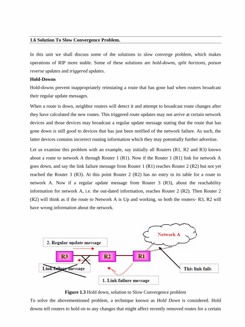
1.6 Solution To Slow Convergence Problem.
In this unit we shall discuss some of the solutions to slow converge problem, which makes
operations of RIP more stable. Some of these solutions are hold-downs, split horizons, poison
reverse updates and triggered updates.
Hold-Downs
Hold-downs prevent inappropriately reinstating a route that has gone bad when routers broadcast
their regular update messages.
When a route is down, neighbor routers will detect it and attempt to broadcast route changes after
they have calculated the new routes. This triggered route updates may not arrive at certain network
devices and those devices may broadcast a regular update message stating that the route that has
gone down is still good to devices that has just been notified of the network failure. As such, the
latter devices contains incorrect routing information which they may potentially further advertise.
Let us examine this problem with an example, say initially all Routers (R1, R2 and R3) knows
about a route to network A through Router 1 (R1). Now if the Router 1 (R1) link for network A
goes down, and say the link failure message from Router 1 (R1) reaches Router 2 (R2) but not yet
reached the Router 3 (R3). At this point Router 2 (R2) has no entry in its table for a route to
network A. Now if a regular update message from Router 3 (R3), about the reachability
information for network A, i.e. the out-dated information, reaches Router 2 (R2). Then Router 2
(R2) will think as if the route to Network A is Up and working, so both the routers- R3, R2 will
have wrong information about the network.
Figure 1.3 Hold down, solution to Slow Convergence problem
To solve the abovementioned problem, a technique known as Hold Down is considered. Hold
downs tell routers to hold on to any changes that might affect recently removed routes for a certain

period of time, usually calculated just to be greater than the period of time necessary to update the
entire network with a route change. This prevents count-to-infinity problem. As per our example, it
means that once R2 has removed the route to Network A, after receiving a link failure message
from R1, It will not change or add any new route to network A, until a certain amount of time has
passed. This time duration is known as Hold Down time. Typically hold down time is around 60
sec. So the idea is to wait long enough to ensure that all machines receive the bad news (link
failure news) and not mistakenly accepts a message that is out dated.
Split Horizons
It is never useful to send information about a route back in the direction from which it came and
thus split horizons is used to prevent updates that are redundant to the network. For this purpose
Router records the interface over which it received a particular route and does not propagates its
information about that route back to the same interface.
Let us consider an example in which Router 1 advertises that it has a route to Network A. If Router
2 is sending traffic to Network A via Router 1, there is no reason for Router 2 to include the route
info in its update back to Router 1, because Router 1 is closer to Network A.
Figure 1.4 Split Horizon, solution to Slow Convergence problem
Without split horizon rule in place, Router 2 would continue to inform Router 1 that it can actually
get to Network A through 2 hops which is via Router 1. If there is a failed direct connection to
Network A, Router 1 may direct traffic to Router 2 thinking it’s an alternative route to Network A
and thus causing a routing loop.
Split horizon in this instance serve as an additional algorithm to achieve stability.
Poison Reverse Updates
This is yet another technique used to solve the slow convergence problem. Larger routing loops
prevented using poison reverse updates. Once a connection disappears, the router advertising the

connection retains the entry for several update periods, and include an infinite cost in the
broadcast. The updates are sent to remove downed route and place it in hold-down.
Figure 1.5 Poison Reverse, other solution to Slow Convergence problem
To make Poison reverse more efficient, it must be combined with Triggered Updates. Triggered
updates force a router to send an immediate broadcast when receiving bad news, instead of waiting
for the next periodic broadcast. By sending an update immediately, a router minimizes the time it
is vulnerable to believing in good news.
Figure 1.6 Poison Reverse along with triggered Update
1.7 RIP Message Format
The following section focuses on the RIP packet format. RIP messages can be broadly classified
into two types: routing information messages and messages used to request information. Both uses
same format, which consists of fixed header information followed by optional list of network and
distance pairs. Figure 1.7 illustrates the IP RIP packet format.

Figure 1.7 RIP Message
After first 32- bit header, the RIP message contains a sequence of pairs, where each pair consists
of a network IP address and a integer distance to that network.
Command: Indicates whether the packet is a request or a response. The request asks that a router
send all or part of its routing table. The response can be an unsolicited regular routing update or a
reply to a request. Responses contain routing table entries. Multiple RIP packets are used to
convey information from large routing tables. COMMAND specifies an operation according to the
Table 1.2:
Table 7.2.2 Meaning for different values of command field

Version number—Specifies the RIP version used. This field can signal different potentially
incompatible versions.
Zero—This field is not actually used by RFC 1058 RIP; it was added solely to provide backward
compatibility with prestandard varieties of RIP. Its name comes from its defaulted value: zero.
Address-family identifier (AFI)—Specifies the address family used. RIP is designed to carry
routing information for several different protocols. Each entry has an address-family identifier to
indicate the type of address being specified. The AFI for IP is 2.
Address—Specifies the IP address for the entry.
Metric—Indicates how many internetwork hops (routers) have been traversed in the trip to the
destination. This value is between 1 and 15 for a valid route, or 16 for an unreachable route.
A router or host can ask another router for routing information by sending a request command.
Router replies to request using Response command. In most of the cases router broadcast
unsolicited response messages periodically.
RIP messages do not contains explicit length field. RIP assumes that underlying delivery
mechanism will tell the receiver about the incoming message length. As RIP operates on UDP port
520, so it depends on UDP for this purpose.
1.8 RIP version 2
Most of the slow convergence problems are handled by split horizon, poison reverse, and triggered
updates. However, RIP cannot increase network diameter or disseminate network bit masks needed
to properly interpret routes thus it is a poor choice for modern network. An updated version of
RIP, known as RIPv2, solves this problem.
RIP Version 2 (RIPv2) RIP Version 2 adds a "network mask" and "next hop address" field to the
original RIP packet while remaining completely compatible with RIP. Thus RIPv2 routers can
coexist with RIP routers without any problems.
The subnet mask field contains the network bit mask associated with the destination; it also allows
the implementation of CIDR addressing. This will allow RIP to function in a variety of
environments, which may implement variable subnet masks on a network.
The "next hop address" field provides the address of the gateway thus allowing optimization of
routes in an environment which uses multiple routing protocols thus having to ability to understand
other routing protocol which may provide a better route path to a destination.
Authentication is another improvement RIPv2 offers over RIP-1. It defines password
authentication mechanism for RIPv2 routers to prevent accidental updates for misconfigured hosts.

In addition to the above, RIPv2 uses multicasting instead of broadcast to reduce the load on
systems that do not want RIPv2 updates and for sharing information which RIP-1 routers will not
hear. In multicasting, only a set of hosts listening on a specific IP multicast address will hear the
information. Other remaining fields like routing domain and route tag are presently still limited in
usage.
RIP 2 Message Format
The RIP 2 specification (described in RFC 1723) allows more information to be included in RIP
packets and provides a simple authentication mechanism that is not supported by RIP. Figure 1.8
shows the IP RIP 2 packet format. Functions of different fields are summarized below:
Command—Indicates whether the packet is a request or a response. The request asks that a router
send all or a part of its routing table. The response can be an unsolicited regular routing update or a
reply to a request. Responses contain routing table entries. Multiple RIP packets are used to
convey information from large routing tables.
Version—Specifies the RIP version used. In a RIP packet implementing any of the RIP 2 fields or
using authentication, this value is set to 2.
Address-family identifier (AFI)—Specifies the address family used. RIPv2's AFI field functions
identically to RIP's AFI field, with one exception: If the AFI for the first entry in the message is
0xFFFF, the remainder of the entry contains authentication information. Currently, the only
authentication type is simple password.
Route tag—Provides a method for distinguishing between internal routes (learned by RIP) and
external routes (learned from other protocols).
IP address—Specifies the IP address for the entry.
Subnet mask—Contains the subnet mask for the entry. If this field is zero, no subnet mask has
been specified for the entry.
Next hop—Indicates the IP address of the next hop to which packets for the entry should be
forwarded.
Metric—Indicates how many internetwork hops (routers) have been traversed in the trip to the
destination. This value is between 1 and 15 for a valid route, or 16 for an unreachable route.

Figure 1.8 RIP2 packet format
1.9 Check Your Progress
Fill In The Blanks
1. RIP and OSPF are __________ Gateway Protocol.
2. RIP is abbreviated as _____________________.
3. RIP uses a _________________ vector algorithm
4. RIP employs ___________ as the metric
5. The maximum number of hops allowed with RIP is _____.
6. RIP runs above Network layer, using ___________ at port _____ to carry its data.
7. RIP uses a distributed version of ______________ algorithm
8. Active routers _________ their routes to others; passive node just __________ and updates their
routes based on the advertisements.
9. __________ nodes donot advertise.
10. Command field in RIP header equal to one means ________________________
11. RIPv2 adds a ___________ and _______________ field to the original RIP packet
1.10 Answer to Check Your Progress
1. Interior
2. Routing Information Protocol
3. Distance
4. Hop count
5. 15
6. User datagram protocol (UDP) , 520

7. Bellman-Ford
8. advertise, listen
9. Passive
10. Request for partial or full routing information
11. network mask, next hop address
Unit-2
Open Shortest Path First (OSPF) and Border Gateway Protocol (BGP)
1.1 Learning Objectives
1.2 Introduction
1.3 Link-State Algorithm
1.4 Routing Hierarchy in OSPF
1.5 OSPF Message Format
1.6 Additional OSPF Features
1.7 Introduction to Border Gateway Protocol
1.8 BGP Characteristics
1.9 BGP Functionality and Route Information Management
1.10 BGP Attributes
1.11 BGP Path Selection
1.12 BGP Message type
1.12.1 BGP Fixed Header Format
1.12.2 BGP OPEN Message
1.12.3 BGP UPDATE Message
1.12.4 BGP NOTIFICATION Message
1.12.5 BGP KEEPALIVE Message
1.13 Check Your Progress
1.14 Answer to Check Your Progress

1.1 Learning Objectives
After going through this unit, the learner will able to learn:
• Explain the operation of the OSPF protocol
• Explain the routing algorithm used in OSPF
• State the OSPF message format
• Explain how shortest path is calculated using Dijkstra’s algorithm
• Explain the routing hierarchy used in OSPF
• Explain the operation of the BGP protocol
• Explain the routing algorithm used in BGP
• Explain various attributes used in BGP
• State various message types used in BGP
1.2 Introduction
Open Shortest Path First (OSPF) is another Interior Gateway Protocol. It is a routing protocol
developed for Internet Protocol (IP) networks by the Interior Gateway Protocol (IGP) working
group of the Internet Engineering Task Force (IETF). The working group was formed in 1988 to
design an IGP based on the Shortest Path First (SPF) algorithm for use in the Internet. OSPF was
created because in the mid-1980s, the Routing Information Protocol (RIP) was increasingly
incapable of serving large, heterogeneous internetworks. OSPF being a SPF algorithm scales better
than RIP. Few of the important features of OSPF are as follows:
• This protocol is open, which means that its specification is in the public domain. It means
that anyone can implement it without paying license fees. The OSPF specification is
published as Request For Comments (RFC) 1247.
• OSPF is based on the SPF algorithm, which is also referred to as the Dijkstra’s algorithm,
named after the person credited with its creation.
• OSPF is a link-state routing protocol that calls for the sending of link-state advertisements
(LSAs) to all other routers within the same hierarchical area. Information on attached
interfaces, metrics used, and other variables are included in OSPF LSAs. As a link-state
routing protocol, OSPF contrasts with RIP, which are distance-vector routing protocols.

Routers running the distance-vector algorithm send all or a portion of their routing tables in
routing-update messages only to their neighbors.
• OSPF specifies that all the exchanges between routers must be authenticated. It allows a
variety of authentication schemes, even different areas can choose different authentication
schemes. The idea behind authentication is that only authorized router are allowed to
advertise routing information.
• OSPF include Type of service Routing. It can calculate separate routes for each Type of
Service (TOS), for example it can maintain separate routes to a single destination based on
hop-count and high throughput.
• OSPF provides Load Balancing. When several equal-cost routes to a destination exist,
traffic is distributed equally among them.
• OSPF allows supports host-specific routes, Subnet-specific routes and also network-
specific routes.
• OSPF allows sets of networks to be grouped together. Such a grouping is called an Area.
Each Area is self-contained; the topology of an area is hidden from the rest of the
Autonomous System and from other Areas too. This information hiding enables a
significant reduction in routing traffic.
• OSPF uses different message formats to distinguish the information acquired from within
the network (internal sources) with that which is acquired from a router outside (external
sources).
In this lesson we shall discuss the important features of OSPF. The lesson is divided into five
sections. First we shall look at various distinguishing features of OSPF, which stand it apart from
other routing protocols. Then we shall briefly discuss the Link-state Routing. In the next section
we will look into the Routing Hierarchy of OSPF. In the fourth section we discuss the various
message formats used in OSPF. And finally we will have a look at some of its additional features.
1.3 Link-State Algorithm
Just like any other Link state routing, OSPF also has the following features:
• Advertise about neighborhood: Instead of sending its entire routing table, a router sends
information about its neighborhood only.
• Flooding: Each router sends this information to every other router on the internetwork, not
just to its neighbors. It does so by a process of flooding. In Flooding, a router sends its
information to all its neighbors (through all of its output ports). Every router sends such

messages to each of its neighbor, and every router that receives the packet sends copies to
its neighbor. Finally, every router has a copy of same information.
• Active response: Each outer sends out information about the neighbor when there is a
change.
Initialization: When an SPF router is powered up, it initializes its routing-protocol data structures
and then waits for indications from lower-layer protocols that its interfaces are functional.
After a router is assured that its interfaces are functioning, it uses the OSPF Hello protocol (sends
greeting messages) to acquire neighbors, which are routers with interfaces to a common network.
The router sends hello packets to its neighbors and receives their hello packets. These messages
are also known as greeting messages. It then prepares an LSP (Link State packet) based on the
results of this Hellow protocol.
An example of an internet is shown in Fig. 2.1, where R1 is a neighbor of R2 and R4, R2 is a
neighbor of R1, R3 and R4, R3 is a neighbor of R2 and R4, R4 is a neighbor of R1, R2 and R3. So
each router will send greeting messages to its entire neighbors.
Figure 2.1 An example internet
Information from neighbors: A router gets its information about its neighbor by periodically
sending them a short greeting packet (this is known as Hello Message format). If neighbor
responds to this greeting message as expected, it is assumed to be alive and functioning. If it does
not, a change is assumed to have occurred and the sending router then alerts the rest of the network
in its next LSP, about this neighbor being down. These Greeting messages are small enough that
they do not use network resources to a significant amount, unlike the routing table updates in case
of a vector-distance algorithm.
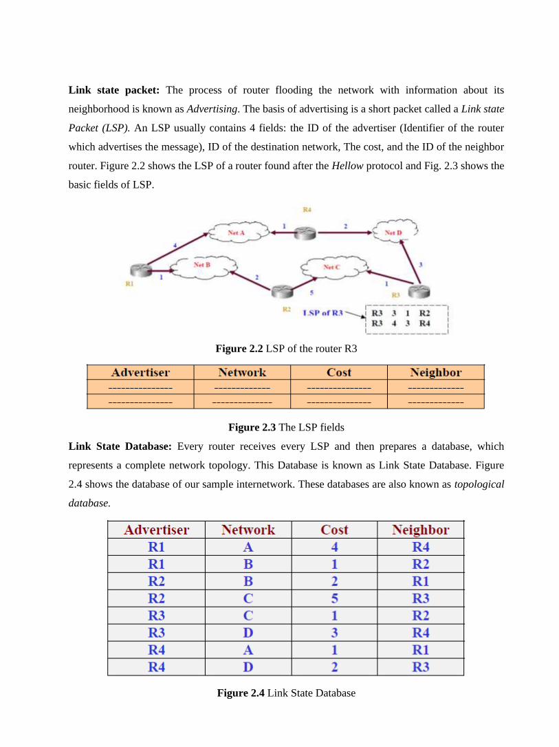
Link state packet: The process of router flooding the network with information about its
neighborhood is known as Advertising. The basis of advertising is a short packet called a Link state
Packet (LSP). An LSP usually contains 4 fields: the ID of the advertiser (Identifier of the router
which advertises the message), ID of the destination network, The cost, and the ID of the neighbor
router. Figure 2.2 shows the LSP of a router found after the Hellow protocol and Fig. 2.3 shows the
basic fields of LSP.
Figure 2.2 LSP of the router R3
Figure 2.3 The LSP fields
Link State Database: Every router receives every LSP and then prepares a database, which
represents a complete network topology. This Database is known as Link State Database. Figure
2.4 shows the database of our sample internetwork. These databases are also known as topological
database.
Figure 2.4 Link State Database

Because every router receives the same LSPs, every router builds the same database. Every router
uses it to calculate its routing table. If a router is added or deleted from the system, the whole
database must be changed accordingly in all routers.
Shortest Path calculation: After gathering the Link State database, each router applies an
algorithm called the Dijkstra algorithm to calculate the shortest distance between any two nodes.
The Dijkstra’s algorithm calculates the shortest path between two points on a network using a
graph made up of nodes and arcs, where nodes are the Routers and the network, while connection
between router and network is refer to as arcs.
The algorithm begins to build a tree by identifying its root as shown in Fig. 2.5. The router is the
root itself. The algorithm then attaches all other nodes that can be reached from that router; this is
done with the help of the Link state database.
Figure 2.5 Path calculation for router R1
From this shortest path calculation each router makes its routing table, as per our example internet
table for router R1 is given in Fig. 2.6. All other routers too have a similar routing table made up
after this point.
Network Cost Next Router
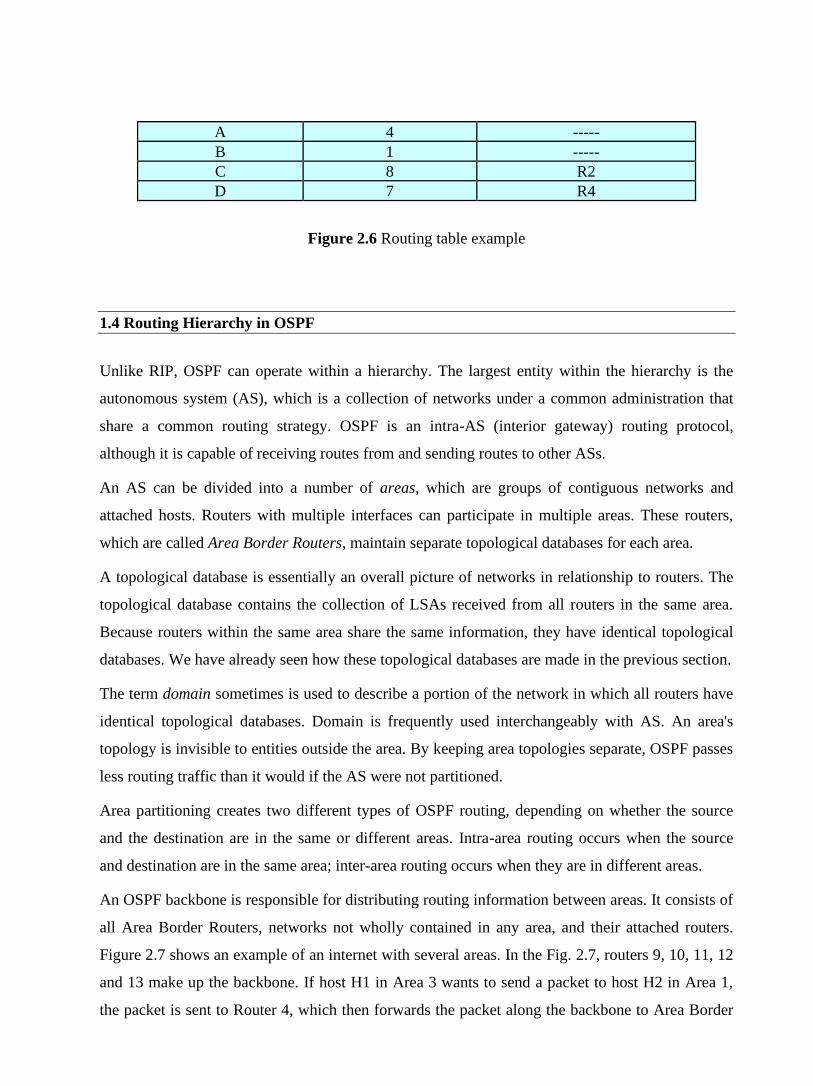
A 4 -----
B 1 -----
C 8 R2
D 7 R4
Figure 2.6 Routing table example
1.4 Routing Hierarchy in OSPF
Unlike RIP, OSPF can operate within a hierarchy. The largest entity within the hierarchy is the
autonomous system (AS), which is a collection of networks under a common administration that
share a common routing strategy. OSPF is an intra-AS (interior gateway) routing protocol,
although it is capable of receiving routes from and sending routes to other ASs.
An AS can be divided into a number of areas, which are groups of contiguous networks and
attached hosts. Routers with multiple interfaces can participate in multiple areas. These routers,
which are called Area Border Routers, maintain separate topological databases for each area.
A topological database is essentially an overall picture of networks in relationship to routers. The
topological database contains the collection of LSAs received from all routers in the same area.
Because routers within the same area share the same information, they have identical topological
databases. We have already seen how these topological databases are made in the previous section.
The term domain sometimes is used to describe a portion of the network in which all routers have
identical topological databases. Domain is frequently used interchangeably with AS. An area's
topology is invisible to entities outside the area. By keeping area topologies separate, OSPF passes
less routing traffic than it would if the AS were not partitioned.
Area partitioning creates two different types of OSPF routing, depending on whether the source
and the destination are in the same or different areas. Intra-area routing occurs when the source
and destination are in the same area; inter-area routing occurs when they are in different areas.
An OSPF backbone is responsible for distributing routing information between areas. It consists of
all Area Border Routers, networks not wholly contained in any area, and their attached routers.
Figure 2.7 shows an example of an internet with several areas. In the Fig. 2.7, routers 9, 10, 11, 12
and 13 make up the backbone. If host H1 in Area 3 wants to send a packet to host H2 in Area 1,
the packet is sent to Router 4, which then forwards the packet along the backbone to Area Border

Router 12, which sends the packet to Router 11, and Router 11 forwards it to Router 10. Router 10
then sends the packet through an intra-area router (Router 3) to be forwarded to Host H2.
The backbone itself is an OSPF area, so all backbone routers use the same procedures and
algorithms to maintain routing information within the backbone that any area router would. The
backbone topology is invisible to all intra-area routers, as are individual area topologies to the
backbone. Areas can be defined in such a way that the backbone is not contiguous. In this case,
backbone connectivity must be restored through virtual links. Virtual links are configured between
any backbone routers that share a link to a nonbackbone area and function as if they were direct
links.
Figure 2.7 Different areas in an Autonomous system
1.5 OSPF Message Format
In this unit we will discuss various message formats used by OSPF, first we will see fixed header,
which is common to all messages and then we will look at various variable part, different for
different messages used in OSPF.
Fixed Header: All OSPF packets begin with a 24-byte header, as illustrated in Figure 2.8.
Summary of the functions of different fields are given below:

• Version number—Identifies the OSPF version used.
• Type—Identifies the OSPF packet type as one of the following:
o Hello—Establishes and maintains neighbor relationships.
o Database description—Describes the contents of the topological database. These
messages are exchanged when an adjacency is initialized.
o Link-state request—Requests pieces of the topological database from neighbor routers.
These messages are exchanged after a router discovers (by examining database-description
packets) that parts of its topological database are outdated.
o Link-state update—Responds to a link-state request packet. These messages also are
used for the regular dispersal of LSAs. Several LSAs can be included within a single link-
state update packet.
o Link-state acknowledgment—Acknowledges link-state updates packets.
• Message length—Specifies the packet length, including the OSPF header, in bytes.
• Source Router IP address—Identifies the source of the packet.
• Area ID—Identifies the area to which the packet belongs. All OSPF packets are associated
with a single area.
• Checksum—Checks the entire packet contents for any damage suffered in transit.
• Authentication type—Contains the authentication type. All OSPF protocol exchanges are
authenticated. The authentication type is configurable on per-area basis.
• Authentication—Contains authentication information.
• Data—Contains encapsulated upper-layer information.
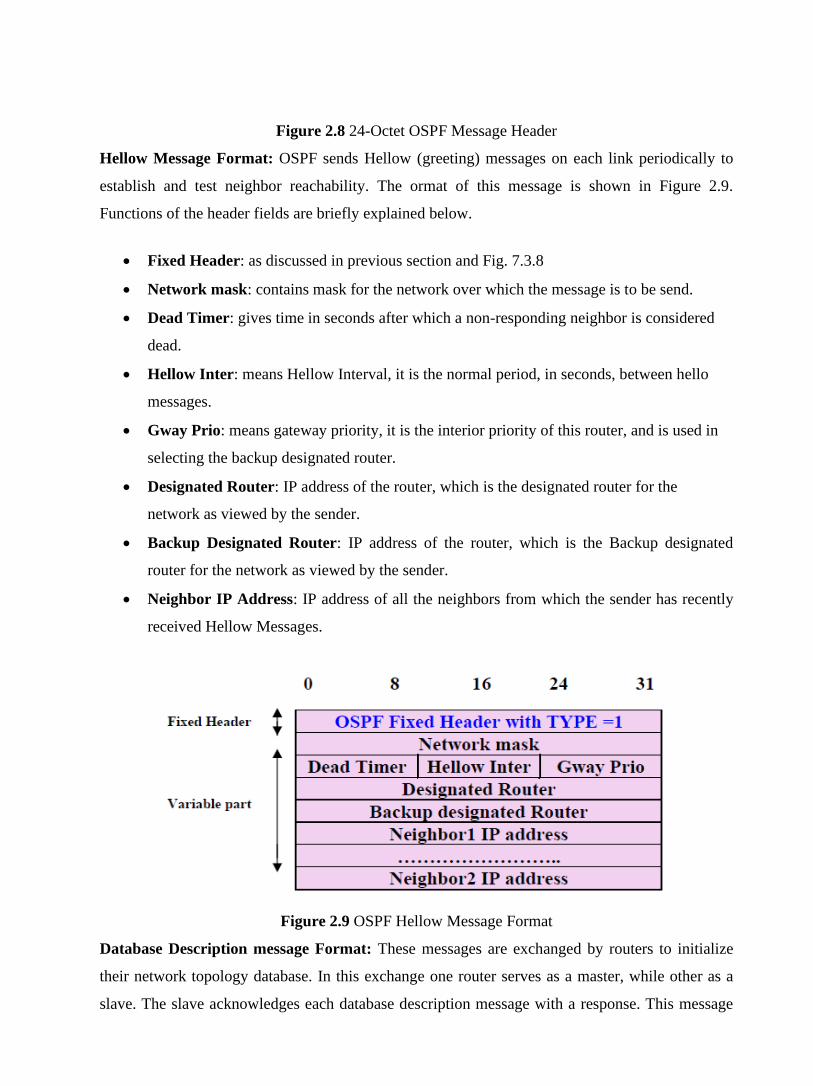
Figure 2.8 24-Octet OSPF Message Header
Hellow Message Format: OSPF sends Hellow (greeting) messages on each link periodically to
establish and test neighbor reachability. The ormat of this message is shown in Figure 2.9.
Functions of the header fields are briefly explained below.
• Fixed Header: as discussed in previous section and Fig. 7.3.8
• Network mask: contains mask for the network over which the message is to be send.
• Dead Timer: gives time in seconds after which a non-responding neighbor is considered
dead.
• Hellow Inter: means Hellow Interval, it is the normal period, in seconds, between hello
messages.
• Gway Prio: means gateway priority, it is the interior priority of this router, and is used in
selecting the backup designated router.
• Designated Router: IP address of the router, which is the designated router for the
network as viewed by the sender.
• Backup Designated Router: IP address of the router, which is the Backup designated
router for the network as viewed by the sender.
• Neighbor IP Address: IP address of all the neighbors from which the sender has recently
received Hellow Messages.
Figure 2.9 OSPF Hellow Message Format
Database Description message Format: These messages are exchanged by routers to initialize
their network topology database. In this exchange one router serves as a master, while other as a
slave. The slave acknowledges each database description message with a response. This message
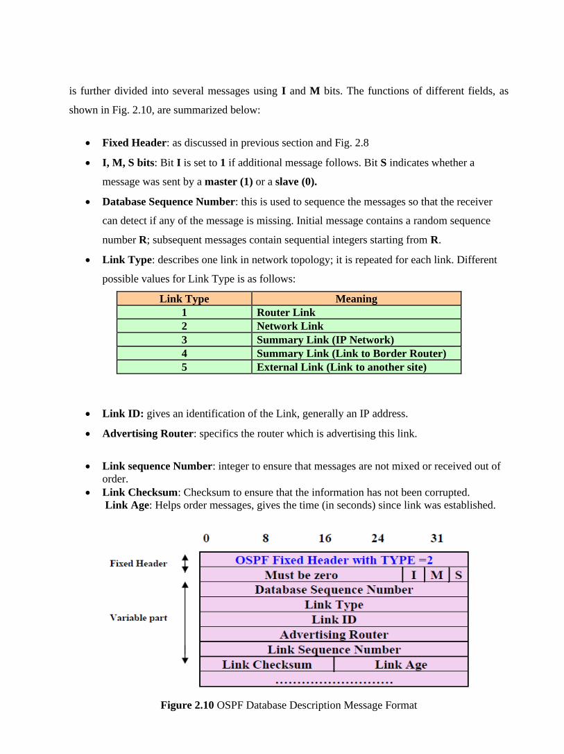
is further divided into several messages using I and M bits. The functions of different fields, as
shown in Fig. 2.10, are summarized below:
• Fixed Header: as discussed in previous section and Fig. 2.8
• I, M, S bits: Bit I is set to 1 if additional message follows. Bit S indicates whether a
message was sent by a master (1) or a slave (0).
• Database Sequence Number: this is used to sequence the messages so that the receiver
can detect if any of the message is missing. Initial message contains a random sequence
number R; subsequent messages contain sequential integers starting from R.
• Link Type: describes one link in network topology; it is repeated for each link. Different
possible values for Link Type is as follows:
Link Type Meaning
1 Router Link
2 Network Link
3 Summary Link (IP Network)
4 Summary Link (Link to Border Router)
5 External Link (Link to another site)
• Link ID: gives an identification of the Link, generally an IP address.
• Advertising Router: specifics the router which is advertising this link.
• Link sequence Number: integer to ensure that messages are not mixed or received out of
order.
• Link Checksum: Checksum to ensure that the information has not been corrupted.
Link Age: Helps order messages, gives the time (in seconds) since link was established.
Figure 2.10 OSPF Database Description Message Format

Link Status Request Message: After exchanging Database Description message, router may
discover that some part of its database is outdated. Link Status message is used to request the
neighbor to supply the updated information. The message lists specific links, as shown in Figure
2.11. The neighbor responds with the most current information it has about those links. The three
fields as shown are repeated for each link, about which status is requested. More than one request
message is required if list is long. All the fields have usual meaning as discussed in previous
message format.
Figure 2.11 OSPF Link Status Request Message Format
Link Status Update Message: Routers broadcast the status of links with Link Status Update
message. Each update consists of a list of advertisements. Figure 2.12 (a) shows the format of link
status update message, and Fig. 2.12 (b) shows an elaborated view of a single Link Status
advertisement (which is within the Link Status Update message).
Figure 2.12(a) Link Status Update Message, (b) Format of each Link Advertisement
1.6 Additional OSPF Features
Additional OSPF features include equal-cost, multipath routing, and routing based on upper-layer
type-of-service (TOS) requests. TOS-based routing supports those upper-layer protocols that can
specify particular types of service. An application, for example, might specify that certain data is
urgent. If OSPF has high-priority links at its disposal, these can be used to transport the urgent
datagram.

OSPF supports one or more metrics. If only one metric is used, it is considered to be arbitrary, and
TOS is not supported. If more than one metric is used, TOS is optionally supported through the use
of a separate metric (and, therefore, a separate routing table) for each of the eight combinations
created by the three IP TOS bits (the delay, throughput, and reliability bits). For example, if the IP
TOS bits specify low delay, low throughput, and high reliability, OSPF calculates routes to all
destinations based on this TOS designation.
IP subnet masks are included with each advertised destination, enabling variable-length subnet
masks. With variable-length subnet masks, an IP network can be broken into many subnets of
various sizes. This provides network administrators with extra network-configuration flexibility.
1.7 Introduction to Border Gateway Protocol
The Border Gateway Protocol (BGP) is an inter-autonomous system routing protocol. An
autonomous system (AS) is a network or group of networks under a common administration and
with common routing policies. BGP is used to exchange routing information for the Internet and is
the protocol used between Internet service providers (ISP), which are different ASes.
One of the most important characteristics of BGP is its flexibility. The protocol can connect
together any internetwork of autonomous systems using an arbitrary topology. The only
requirement is that each AS have at least one router that is able to run BGP and that this router
connect to at least one other AS's BGP router. Beyond that, “the sky's the limit,” as they say. BGP
can handle a set of ASs connected in a full mesh topology (each AS to each other AS), a partial
mesh, a chain of ASes linked one to the next, or any other configuration. It also handles changes to
topology that may occur over time.
The primary function of a BGP speaking system is to exchange network reachability information
with other BGP systems. This network reachability information includes information on the list of
Autonomous Systems (ASs) that reachability information traverses. BGP constructs a graph of
autonomous systems based on the information exchanged between BGP routers. As far as BGP is
concerned, whole Internet is a graph of ASs, with each AS identified by a Unique AS number.
Connections between two ASs together form a path and the collection of path information forms a
route to reach a specific destination. BGP uses the path information to ensure the loop-free inter-
domain routing.
Another important assumption that BGP makes is that it doesn't know anything about what
happens within the AS. This is of course an important prerequisite to the notion of an AS being
autonomous - it has its own internal topology and uses its own choice of routing protocols to
determine routes. BGP only takes the information conveyed to it from the AS and shares it with
other ASs.
When a pair of autonomous systems agrees to exchange routing information, each must designate
a router that will speak BGP on its behalf; the two routers are said to become BGP peers of one
another. As a router speaking BGP must communicate with a peer in another autonomous system,
usually a machine, which is near to the edge (Border) of the autonomous system is selected for
this. Hence, BGP terminology calls the machine a Border Gateway Router.
In this unit we shall discuss the important features of BGP. First we will look at the basics of BGP.
Then in next unit we shall have a look at BGP characteristics that make it stand apart from other
routing protocols.
1.8 BGP Characteristics
BGP is different from other routing protocols in several ways. Most important being that BGP is
neither a pure distance vector protocol nor a pure link state protocol. Let’s have a look at some of
the characteristics that stands BGP apart from other protocols.
• Inter-Autonomous System Configuration: BGP’s primary role is to provide
communication between two autonomous systems.
• Next-Hop paradigm: Like RIP, BGP supplies next hop information for each destination.
• Coordination among multiple BGP speakers within the autonomous system: If an
Autonomous system has multiple routers each communicating with a peer in other
autonomous system, BGP can be used to coordinate among these routers, in order to ensure
that they all propagate consistent information.
• Path information: BGP advertisements also include path information, along with the
reachable destination and next destination pair, which allows a receiver to learn a series of
autonomous system along the path to the destination.
• Policy support: Unlike most of the distance-vector based routing, BGP can implement
policies that can be configured by the administrator. For Example, a router running BGP
can be configured to distinguish between the routes that are known from within the
Autonomous system and that which are known from outside the autonomous system.
• Runs over TCP: BGP uses TCP for all communication. So the reliability issues are taken
care by TCP.
• Conserve network bandwidth: BGP doesn’t pass full information in each update
message. Instead full information is just passed on once and thereafter successive messages
only carries the incremental changes called deltas. By doing so a lot of network Bandwidth
is saved. BGP also conserves bandwidth by allowing sender to aggregate route information
and send single entry to represent multiple, related destinations.
• Support for CIDR: BGP supports classless addressing (CIDR). That it supports a way to
send the network mask along with the addresses.
• Security: BGP allows a receiver to authenticate messages, so that the identity of the sender
can be verified.
1.9 BGP Functionality and Route Information Management
The job of the Border Gateway Protocol is to facilitate the exchange of route information between
BGP devices, so that each router can determine efficient routes to each of the networks on an IP
internetwork. This means that descriptions of routes are the key data that BGP devices work with.
But in a broader aspect, BGP peers perform three basic functions. The First function consists of
initial peer acquisition and authentication. Both the peers establish a TCP connection and perform
message exchange that guarantees both sides have agreed to communicate. The second function
primarily focus on sending of negative or positive reachability information, this step is of major
concern. The Third function provides ongoing verification that the peers and the network
connection between them are functioning correctly. Every BGP speaker is responsible for
managing route descriptions according to specific guidelines established in the BGP standards.
BGP Route Information Management Functions
Conceptually, the overall activity of route information management can be considered to
encompass four main tasks:
• Route Storage: Each BGP stores information about how to reach networks in a set of
special databases. It also uses databases to hold routing information received from other
devices.
• Route Update: When a BGP device receives an Update from one of its peers, it must
decide how to use this information. Special techniques are applied to determine when and
how to use the information received from peers to properly update the device's knowledge
of routes.

• Route Selection: Each BGP uses the information in its route databases to select good
routes to each network on the internetwork.
• Route Advertisement: Each BGP speaker regularly tells its peers what it knows about
various networks and methods to reach them. This is called route advertisement and is
accomplished using BGP Update messages.
1.10 BGP Attributes
BGP Attributes are the properties associated with the routes that are learned from BGP and used to
determine the best route to a destination, when multiple routes are available. An understanding of
how BGP attributes influence route selection is required for the design of robust networks. This
section describes the attributes that BGP uses in the route selection process:
• AS_path
• Next hop
• Weight
• Local preference
• Multi-exit discriminator
• Origin
• Community
AS_path Attribute: When a route advertisement passes through an autonomous system, the AS
number is added to an ordered list of AS numbers that the route advertisement has traversed.
Figure 2.13 shows the situation in which a route is passing through three autonomous systems.
Figure 2.13 BGP AS-path Attribute
AS1 originates the route to 172.16.1.0 and advertises this route to AS 2 and AS 3, with the
AS_path attribute equal to {1}. AS 3 will advertise back to AS 1 with AS-path attribute {3, 1},

and AS 2 will advertise back to AS 1 with AS-path attribute {2, 1}. AS 1 will reject these routes
when its own AS number is detected in the route advertisement. This is the mechanism that BGP
uses to detect routing loops. AS 2 and AS 3 propagate the route to each other with their AS
numbers added to the AS_path attribute. These routes will not be installed in the IP routing table
because AS 2 and AS 3 are learning a route to 172.16.1.0 from AS 1 with a shorter AS_path list.
Next-Hop Attribute: The EBGP next-hop attribute is the IP address that is used to reach the
advertising router. For EBGP peers, the next-hop address is the IP address of the connection
between the peers. For IBGP, the EBGP next-hop address is carried into the local AS, as illustrated
in Fig. 2.14.
Figure 2.14 BGP Next-Hop Attribute
Router C advertises network 172.16.1.0 with a next hop of 10.1.1.1. When Router A propagates
this route within its own AS, the EBGP next-hop information is preserved. If Router B does not
have routing information regarding the next hop, the route will be discarded. Therefore, it is
important to have an IGP running in the AS to propagate next-hop routing information.
Weight Attribute: Weight is a Cisco-defined attribute that is local to a router. The weight attribute
is not advertised to neighboring routers. If the router learns about more than one route to the same
destination, the route with the highest weight will be preferred.
In Fig. 2.15, Router A is receiving an advertisement for network 201.12.23.0 from routers B and
C. When Router A receives the advertisement from Router B, the associated weight is set to 50.
When Router A receives the advertisement from Router C, the associated weight is set to 100.
Both paths for network 201.12.23.0 will be in the BGP routing table, with their respective weights.
The route with the highest weight will be installed in the IP routing table

Figure 2.15 BGP Weight Attribute
Local Preference Attribute: The local preference attribute is used to prefer an exit point from the
local autonomous system (AS). Unlike the weight attribute, the local preference attribute is
propagated throughout the local AS. If there are multiple exit points from the AS, the local
preference attribute is used to select the exit point for a specific route.
In Fig. 2.16, AS 287 is receiving two advertisements for network 201.12.23.0 from AS 123. When
Router A receives the advertisement for network 201.12.23.0, the corresponding local preference
is set to 150. When Router B receives the advertisement for same network, the corresponding local
preference is set to 251. These local preference values will be exchanged between routers A and B.
Because Router B has a higher local preference than Router A, Router B will be used as the exit
point from AS 287 to reach network 201.12.23.0 in AS 123.
Figure 2.16 Local Preference Attribute
Multi-Exit Discriminator Attribute: The multi-exit discriminator (MED) or metric attribute is
used as a suggestion to an external AS regarding the preferred route into the AS that is advertising
the metric. The term suggestion is used because the external AS that is receiving the MEDs may be
using other BGP attributes for route selection.

In Fig. 2.17, Router C is advertising the route 201.12.23.0 with a metric of 23, while Route D is
advertising 201.12.23.0 with a metric of 5. The lower value of the metric is preferred, so AS 287
will select the route to router D for network 201.12.23.0 in AS 123. MEDs are advertised
throughout the local AS.
Figure 2.17 Multi-Exit Discriminator Attribute
Origin Attribute: The origin attribute indicates how BGP learned about a particular route. The
origin attribute can have one of three possible values:
• IGP—The route is interior to the originating AS. This value is set when the network router
configuration command is used to inject the route into BGP.
• EGP—The route is learned via the Exterior Border Gateway Protocol (EBGP).
• Incomplete—The origin of the route is unknown or learned in some other way. An origin
of incomplete occurs when a route is redistributed into BGP.
The origin attribute is used for route selection.
Community Attribute: The community attribute provides a way of grouping destinations, called
communities, to which routing decisions (such as acceptance, preference, and redistribution) can
be applied. Route maps are used to set the community attribute. Predefined community attributes
are listed here:
• No-export—Do not advertise this route to EBGP peers.
• No-advertise—Do not advertise this route to any peer.
• Internet—Advertise this route to the Internet community; all routers in the network belong
to it.
Figure 2.18 demonstrates the third community attribute namely, Internet community attribute.
There are no limitations to the scope of the route advertisement from AS 1.

Figure 2.19 illustrates the no-export community. AS 1 advertises 172.16.1.0 to AS 2 with the
community attribute no-export. AS 2 will propagate the route throughout AS 2 but will not send
this route to AS 3 or any other external AS.
Figure 2.19 BGP no-export Community Attribute
In Fig. 2.20, AS 1 advertises 172.16.1.0 to AS 2 with the community attribute no-advertise. Router
B in AS 2 will not advertise this route to any other router, i.e. the advertisement for this route is
not even made within the Autonomous system, it would be restricted just to the Router B.
Figure 2.20 BGP no-advertise Community Attribute

Figure 2.21 BGP Internet Community Attribute
1.11 BGP Path Selection
BGP could possibly receive multiple advertisements for the same route from multiple sources.
BGP selects only one path as the best path. When the path is selected, BGP puts the selected path
in the IP routing table and propagates the path to its neighbors. BGP uses the following criteria, in
the order presented, to select a path for a destination:
• If the path specifies a next hop that is inaccessible, drop the update.
• Prefer the path with the largest weight.
• If the weights are the same, prefer the path with the largest local preference.
• If the local preferences are the same, prefer the path that was originated by BGP running on
this router.
• If no route was originated, prefer the route that has the shortest AS_path.
• If all paths have the same AS_path length, prefer the path with the lowest origin type
(where IGP is lower than EGP, and EGP is lower than incomplete).
• If the origin codes are the same, prefer the path with the lowest MED attribute.
• If the paths have the same MED, prefer the external path to the internal path.
• If the paths are still the same, prefer the path through the closest IGP neighbor.
• Prefer the path with the lowest IP address, as specified by the BGP router ID.

1.12 BGP Message type
For all the functions described above, BGP defines four basic message types namely, OPEN,
UPDATE, NOTIFICATION, KEEPALIVE. In this section we shall discuss these message formats.
1.12.1 BGP Fixed Header Format
Each BGP message begins with a fixed header that identifies the message type. Figure 2.22
illustrates this fixed header format.
Figure 2.22 BGP Fixed header Format
Fields in the fixed header
• MARKER: The 16-octect MARKER field contains a value that both sides agree to use to
mark the beginning of the message. This is basically used for synchronization. In the initial
message it contains all 1’s and if the peers agree to use authentication mechanism, the
marker can contain the authentication information.
• LENGTH: The 2-octect LENGTH field Specifies the Total message length measured in
octets. The minimum message size is 19 octets (i.e. only fixed header), and the maximum
allowable length is 4096 octets.
• TYPE: 1-octet field contains one of the 4 values of the message type listed below:
Type
Code
Message Type Description
1 OPEN Initialize communication
2 UPDATE Advertise or withdraw routes
3 NOTIFICATION Response to an Incorrect message
4 KEEPALIVE Actively test peer connectivity

1.12.2 BGP OPEN Message
This is the first message send after the BGP peers establishes a TCP connection. Both of the peers
send OPEN message to declare their autonomous system number and other operating parameters.
Figure 2.23 illustrates the OPEN message format.
Figure 2.23 BGP OPEN Message Format
Fields in the message header has been explained below:
• Version: It identifies the protocol version used.
• Autonomous System Number: Gives the autonomous system of the sender’s system.
• Hold Time: it specifies maximum time receiver should wait for a message from sender.
The receiver implements a timer using this value. The value is reset each time a message
arrives; if timer expires it assumes that sender is not available.
• BGP identifier: It is a 32-bit value that uniquely identifies the sender. It is the IP address
and the router must choose one of its IP addresses to use with all the BGP peers.
• Parameter Length: If Optional parameters are specified then this fields contains the length
of optional parameters, in octets.
• Optional Parameters: It contains a list of parameters. Authentication is also a kind of
parameter in BGP. It’s done in this way so that the BGP peers can choose the
authentication method without making it a part of BGP fixed header.
When it accepts an incoming OPEN message, a machine speaking BGP responds by sending a
KEEPALIVE message. Each side must send an OPEN message and receive a KEEPALIVE
message before they can actually exchange routing information. Thus, KEEPALIVE messages are
a kind of acknowledgement for OPEN message.
1.12.3 BGP UPDATE Message
After the BGP peers have established a TCP connection, send the OPEN message, and
acknowledge them, peers use UPDATE message for advertisements. Peers use UPDATE message

to advertise new destination that are reachable or to withdraw previously advertised destination,
which have become unreachable. Figure 2.24 illustrates the UPDATE message format.
Figure 2.24 BGP UPDATE Message Format
Update message is divided into two parts:
• First part lists the previously advertised routes that are being withdrawn
• Second specifies new destination being advertised.
Description about the fields in the header is given below:
• Withdrawn Length: it is a 2-octet field that specifies the size of the withdrawn destination
field that follows.
• Path Length: specifies the size of the Path Attributes. These path attributes are associated
with the new advertisements.
• Both Withdrawn Destination and Destination network, in the message format, contains
a list of IP addresses. BGP supports classless addressing in a different way, instead of
sending subnet masks separately with each IP address; it uses a compress representation to
reduce the message size. BGP doesn’t send a bit mask; instead it encodes information
about the mask into a single octet that precedes each address. The Mask octet contains a
binary integer that specifies number of bits in the mask (mask bits are assumed to be
contiguous). Address that follows the mask is also compressed, only octets covered by the
mask are included. For example, only two address octets follow a mask value of 9 to 16
and so on. It is illustrated in Fig. 2.25.
Figure 2.25 Compressed form that BGP uses to store destination IP and Mask

1.12.4 BGP NOTIFICATION Message
BGP supports NOTIFICATION message type for control purposes and when error occurs. Once
BGP detects a problem it sends a notification message and then closes TCP connection. Figure
2.26 illustrates the NOTIFICATION message format. Following tables list the possible values of
Error code (Fig. 2.27) and Error subcodes (Fig. 2.28):
Figure 2.26 BGP Notification Message Format
Figure 2.27 Possible values of Error Code
Figure 2.28 Possible values of Error Sub-code

1.12.5 BGP KEEPALIVE Message
Two BGP peers periodically exchange KEEPALIVE messages to test the network connectivity
between them and to verify that both are functioning well. A KEEPALIVE message consists of
standard message header with no extra data (19 octets).
1.13 Check Your Progress
Fill In The Blanks
1. OSPF is __________ Gateway Protocol.
2. OSPF is abbreviated as _____________________.
3. OSPF based on ________path ________ algorithm
4. OSPF is a _______state routing protocol
5. Link State databases are also known as _________ databases.
6. OSPF sends ________ messages on each link periodically to establish and test neighbor
reachability
7. BGP is abbreviated as __________.
8. BGP is a ___________-autonomous system routing protocol.
9. The protocol can connect together any internetwork of autonomous systems using an
___________ topology
10. The overall activity of route information management can be considered to encompass four
main tasks: ____________, Route Update, ________, Route Selection.
11. The _________ indicates how BGP learned about a particular route.
12. Origin attribute can have one of three possible values namely, ________,________ and
________
13. _________ Field contains a value that both sides agree to use to mark the beginning of the
message.
14. The minimum message size is _____ octets, and the maximum allowable length is ______
octets
15. Type Code equals 1 means _________ Message and _________ communication.
16. BGP identifier is a _____-bit value.
17. ______________ is a 2-octet field that specifies the size of the withdrawn destination field
that follows.
18. Error Code Value equal to 3 signifies error in _________ message.

1.14 Answer to Check Your Progress
1. Interior
2. Open Shortest Path First
3. Shortest-First
4. link
5. topological
6. Hellow
7. Border Gateway protocol
8. Inter
9. arbitrary
10. Route storage, route advertisement
11. origin attribute
12. IGP, EGP, Incomplete
13. MARKER
14. 19, 4096
15. OPEN, initialize
16. 32
17. Withdrawn Length
18. UPDATE
Unit-3
Congestion Control
1.1 Learning Objectives
1.2 Introduction
1.3 Causes Of Congestion
1.4 Effects of Congestion
1.5 Congestion Control Techniques
1.6 Leaky Bucket Algorithm
1.7 Token Bucket Algorithm
1.8 Congestion control in virtual Circuit
1.9 Choke Packet Technique
1.10 Hop-by Hop Choke Packets
1.11 Load Shedding
1.12 Slow Start - a Pro-active technique
1.13 Flow Control Versus Congestion control
1.14 Check Your Progress
1.15 Answer to Check Your Progress

1.1 Learning Objectives
After going through this unit, the learner will able to learn:
• Explain the cause for congestion
• Understand the effects of congestion
• Understand various open-loop and close-loop congestion control techniques:
o The leaky bucket algorithm
o The token bucket algorithm
o Admission Control
o Choke packets
o Weighted fair queuing
o Load shedding
o Resource reservation
• Distinguish between flow and congestion control
1.2 Introduction
As Internet can be considered as a Queue of packets, where transmitting nodes are constantly
adding packets and some of them (receiving nodes) are removing packets from the queue. So,
consider a situation where too many packets are present in this queue (or internet or a part of
internet), such that constantly transmitting nodes are pouring packets at a higher rate than
receiving nodes are removing them. This degrades the performance, and such a situation is termed
as Congestion. Main reason of congestion is more number of packets into the network than it can
handle. So, the objective of congestion control can be summarized as to maintain the number of
packets in the network below the level at which performance falls off dramatically. The nature of a
Packet switching network can be summarized in following points:
• A network of queues
• At each node, there is a queue of packets for each outgoing channel
• If packet arrival rate exceeds the packet transmission rate, the queue size grows without
bound
• When the line for which packets are queuing becomes more than 80% utilized, the queue
length grows alarmingly
When the number of packets dumped into the network is within the carrying capacity, they all are
delivered, expect a few that have too be rejected due to transmission errors). And then the number
delivered is proportional to the number of packets sent. However, as traffic increases too far, the
routers are no longer able to cope, and they begin to lose packets. This tends to make matter worse.
At very high traffic, performance collapse completely, and almost no packet is delivered. In the
following sections, the causes of congestion, the effects of congestion and various congestion
control techniques are discussed in detail.
1.3 Causes Of Congestion
Congestion can occur due to several reasons. For example, if all of a sudden a stream of packets
arrive on several input lines and need to be out on the same output line, then a long queue will be
build up for that output. If there is insufficient memory to hold these packets, then packets will be
lost (dropped). Adding more memory also may not help in certain situations. If router have an
infinite amount of memory even then instead of congestion being reduced, it gets worse; because
by the time packets gets at the head of the queue, to be dispatched out to the output line, they have
already timed-out (repeatedly), and duplicates may also be present. All the packets will be
forwarded to next router up to the destination, all the way only increasing the load to the network
more and more. Finally when it arrives at the destination, the packet will be discarded, due to time
out, so instead of been dropped at any intermediate router (in case memory is restricted) such a
packet goes all the way up to the destination, increasing the network load throughout and then
finally gets dropped there.
Slow processors also cause Congestion. If the router CPU is slow at performing the task required
for them (Queuing buffers, updating tables, reporting any exceptions etc.), queue can build up even
if there is excess of line capacity. Similarly, Low-Bandwidth lines can also cause congestion.
Upgrading lines but not changing slow processors, or vice-versa, often helps a little; these can just
shift the bottleneck to some other point. The real problem is the mismatch between different parts
of the system.
Congestion tends to feed upon itself to get even worse. Routers respond to overloading by
dropping packets. When these packets contain TCP segments, the segments don't reach their
destination, and they are therefore left unacknowledged, which eventually leads to timeout and
retransmission.
So, the major cause of congestion is often the bursty nature of traffic. If the hosts could be made to
transmit at a uniform rate, then congestion problem will be less common and all other causes will

not even led to congestion because other causes just act as an enzyme which boosts up the
congestion when the traffic is bursty (i.e., other causes just add on to make the problem more
serious, main cause is the bursty traffic).
This means that when a device sends a packet and does not receive an acknowledgment from the
receiver, in most the cases it can be assumed that the packets have been dropped by intermediate
devices due to congestion. By detecting the rate at which segments are sent and not acknowledged,
the source or an intermediate router can infer the level of congestion on the network. In the
following section we shall discuss the ill effects of congestion.
1.4 Effects of Congestion
Congestion affects two vital parameters of the network performance, namely throughput and
delay. In simple terms, the throughput can be defined as the percentage utilization of the network
capacity. Figure 3.1(a) shows how throughput is affected as offered load increases. Initially
throughput increases linearly with offered load, because utilization of the network increases.
However, as the offered load increases beyond certain limit, say 60% of the capacity of the
network, the throughput drops. If the offered load increases further, a point is reached when not a
single packet is delivered to any destination, which is commonly known as deadlock situation.
There are three curves in Fig. 3.1(a), the ideal one corresponds to the situation when all the packets
introduced are delivered to their destination up to the maximum capacity of the network. The
second one corresponds to the situation when there is no congestion control. The third one is the
case when some congestion control technique is used. This prevents the throughput collapse, but
provides lesser throughput than the ideal condition due to overhead of the congestion control
technique.
The delay also increases with offered load, as shown in Fig. 3.1(b). And no matter what technique
is used for congestion control, the delay grows without bound as the load approaches the capacity
of the system. It may be noted that initially there is longer delay when congestion control policy is
applied. However, the network without any congestion control will saturate at a lower offered
load.

(a) (b)
Figure 3.1 (a) Effect of congestion on throughput (b) Effect of congestion on delay
1.5 Congestion Control Techniques
Congestion control refers to the mechanisms and techniques used to control congestion and keep
the traffic below the capacity of the network. As shown in Fig. 3.2, the congestion control
techniques can be broadly classified two broad categories:
• Open loop: Protocols to prevent or avoid congestion, ensuring that the system (or network
under consideration) never enters a Congested State.
• Close loop: Protocols that allow system to enter congested state, detect it, and remove it.
Figure 3.2 Congestion control categories
The first category of solutions or protocols attempt to solve the problem by a good design, at first,
to make sure that it doesn’t occur at all. Once system is up and running midcourse corrections are
not made. These solutions are somewhat static in nature, as the policies to control congestion don’t
change much according to the current state of the system. Such Protocols are also known as Open
Loop solutions. These rules or policies include deciding upon when to accept traffic, when to
discard it, making scheduling decisions and so on. Main point here is that they make decision
without taking into consideration the current state of the network. The open loop algorithms are
further divided on the basis of whether these acts on source versus that act upon destination.
The second category is based on the concept of feedback. During operation, some system
parameters are measured and feed back to portions of the subnet that can take action to reduce the
congestion. This approach can be divided into 3 steps:
• Monitor the system (network) to detect whether the network is congested or not and what’s
the actual location and devices involved.
• To pass this information to the places where actions can be taken
• Adjust the system operation to correct the problem.
These solutions are known as Closed Loop solutions. Various Metrics can be used to monitor the
network for congestion. Some of them are: the average queue length, number of packets that are
timed-out, average packet delay, number of packets discarded due to lack of buffer space, etc. A
general feedback step would be, say a router, which detects the congestion send special packets to
the source (responsible for the congestion) announcing the problem. These extra packets increase
the load at that moment of time, but are necessary to bring down the congestion at a later time.
Other approaches are also used at times to curtail down the congestion. For example, hosts or
routers send out probe packets at regular intervals to explicitly ask about the congestion and source
itself regulate its transmission rate, if congestion is detected in the network. This kind of approach
is a pro-active one, as source tries to get knowledge about congestion in the network and act
accordingly.
Yet another approach may be where instead of sending information back to the source an
intermediate router which detects the congestion send the information about the congestion to rest
of the network, piggy backed to the outgoing packets. This approach will in no way put an extra
load on the network (by not sending any kind of special packet for feedback). Once the congestion
has been detected and this information has been passed to a place where the action needed to be
done, then there are two basic approaches that can overcome the problem. These are: either to
increase the resources or to decrease the load. For example, separate dial-up lines or alternate links
can be used to increase the bandwidth between two points, where congestion occurs. Another
example could be to decrease the rate at which a particular sender in transmitting packets out into
the network.
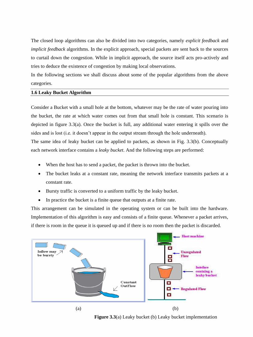
The closed loop algorithms can also be divided into two categories, namely explicit feedback and
implicit feedback algorithms. In the explicit approach, special packets are sent back to the sources
to curtail down the congestion. While in implicit approach, the source itself acts pro-actively and
tries to deduce the existence of congestion by making local observations.
In the following sections we shall discuss about some of the popular algorithms from the above
categories.
1.6 Leaky Bucket Algorithm
Consider a Bucket with a small hole at the bottom, whatever may be the rate of water pouring into
the bucket, the rate at which water comes out from that small hole is constant. This scenario is
depicted in figure 3.3(a). Once the bucket is full, any additional water entering it spills over the
sides and is lost (i.e. it doesn’t appear in the output stream through the hole underneath).
The same idea of leaky bucket can be applied to packets, as shown in Fig. 3.3(b). Conceptually
each network interface contains a leaky bucket. And the following steps are performed:
• When the host has to send a packet, the packet is thrown into the bucket.
• The bucket leaks at a constant rate, meaning the network interface transmits packets at a
constant rate.
• Bursty traffic is converted to a uniform traffic by the leaky bucket.
• In practice the bucket is a finite queue that outputs at a finite rate.
This arrangement can be simulated in the operating system or can be built into the hardware.
Implementation of this algorithm is easy and consists of a finite queue. Whenever a packet arrives,
if there is room in the queue it is queued up and if there is no room then the packet is discarded.
(a) (b)
Figure 3.3(a) Leaky bucket (b) Leaky bucket implementation
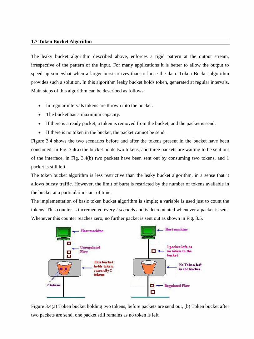
1.7 Token Bucket Algorithm
The leaky bucket algorithm described above, enforces a rigid pattern at the output stream,
irrespective of the pattern of the input. For many applications it is better to allow the output to
speed up somewhat when a larger burst arrives than to loose the data. Token Bucket algorithm
provides such a solution. In this algorithm leaky bucket holds token, generated at regular intervals.
Main steps of this algorithm can be described as follows:
• In regular intervals tokens are thrown into the bucket.
• The bucket has a maximum capacity.
• If there is a ready packet, a token is removed from the bucket, and the packet is send.
• If there is no token in the bucket, the packet cannot be send.
Figure 3.4 shows the two scenarios before and after the tokens present in the bucket have been
consumed. In Fig. 3.4(a) the bucket holds two tokens, and three packets are waiting to be sent out
of the interface, in Fig. 3.4(b) two packets have been sent out by consuming two tokens, and 1
packet is still left.
The token bucket algorithm is less restrictive than the leaky bucket algorithm, in a sense that it
allows bursty traffic. However, the limit of burst is restricted by the number of tokens available in
the bucket at a particular instant of time.
The implementation of basic token bucket algorithm is simple; a variable is used just to count the
tokens. This counter is incremented every t seconds and is decremented whenever a packet is sent.
Whenever this counter reaches zero, no further packet is sent out as shown in Fig. 3.5.
Figure 3.4(a) Token bucket holding two tokens, before packets are send out, (b) Token bucket after
two packets are send, one packet still remains as no token is left
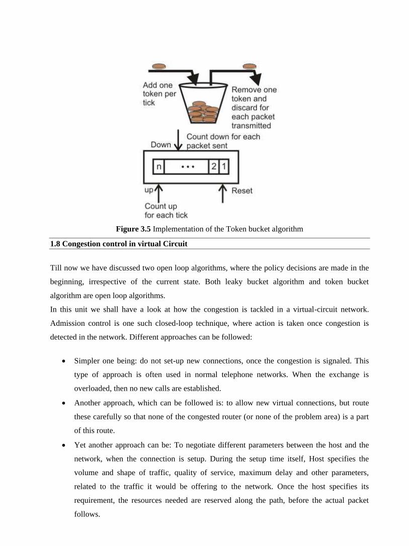
Figure 3.5 Implementation of the Token bucket algorithm
1.8 Congestion control in virtual Circuit
Till now we have discussed two open loop algorithms, where the policy decisions are made in the
beginning, irrespective of the current state. Both leaky bucket algorithm and token bucket
algorithm are open loop algorithms.
In this unit we shall have a look at how the congestion is tackled in a virtual-circuit network.
Admission control is one such closed-loop technique, where action is taken once congestion is
detected in the network. Different approaches can be followed:
• Simpler one being: do not set-up new connections, once the congestion is signaled. This
type of approach is often used in normal telephone networks. When the exchange is
overloaded, then no new calls are established.
• Another approach, which can be followed is: to allow new virtual connections, but route
these carefully so that none of the congested router (or none of the problem area) is a part
of this route.
• Yet another approach can be: To negotiate different parameters between the host and the
network, when the connection is setup. During the setup time itself, Host specifies the
volume and shape of traffic, quality of service, maximum delay and other parameters,
related to the traffic it would be offering to the network. Once the host specifies its
requirement, the resources needed are reserved along the path, before the actual packet
follows.

1.9 Choke Packet Technique
The choke packet technique, a closed loop control technique, can be applied in both virtual circuit
and datagram subnets. Each router monitors its resources and the utilization at each of its output
line. There is a threshold set by the administrator, and whenever any of the resource utilization
crosses this threshold and action is taken to curtail down this. Actually each output line has a
utilization associated with it, and whenever this utilization crosses the threshold, the output line
enters a “warning” state. If so, the router sends a choke packet back to the source, giving it a
feedback to reduce the traffic. And the original packet is tagged (a bit is manipulated in the header
field) so that it will not generate other choke packets by other intermediate router, which comes in
place and is forwarded in usual way. It means that the first router (along the way of a packet),
which detects any kind of congestion, is the only one that sends the choke packets.
When the source host gets the choke packet, it is required to reduce down the traffic send out to
that particular destination (choke packet contains the destination to which the original packet was
send out). After receiving the choke packet the source reduces the traffic by a particular fixed
percentage, and this percentage decreases as the subsequent choke packets are received. Figure 3.6
depicts the functioning of choke packets.
For Example, when source A receives a choke packet with destination B at first, it will curtail
down the traffic to destination B by 50%, and if again after affixed duration of time interval it
receives the choke packet again for the same destination, it will further curtail down the traffic by
25% more and so on. As stated above that a source will entertain another subsequent choke packet
only after a fixed interval of time, not before that. The reason for this is that when the first choke
packet arrives at that point of time other packets destined to the same destination would also be
there in the network and they will generate other choke packets too, the host should ignore these
choke packets which refer to the same destination for a fixed time interval.

Figure 3.6 Depicts the functioning of choke packets, (a) Heavy traffic between nodes P and Q, (b)
Node Q sends the Choke packet to P, (c) Choke packet reaches P, (d) P reduces the flow and send
a reduced flow out, (e) Reduced flow reaches node Q
1.10 Hop-by Hop Choke Packets
This technique is an advancement over Choked packet method. At high speed over long distances,
sending a packet all the way back to the source doesn’t help much, because by the time choke
packet reach the source, already a lot of packets destined to the same original destination would be
out from the source. So to help this, Hop-by-Hop Choke packets are used. In this approach, the
choke packet affects each and every intermediate router through which it passes by. Here, as soon
as choke packet reaches a router back to its path to the source, it curtails down the traffic between
those intermediate routers. In this scenario, intermediate nodes must dedicate few more buffers for
the incoming traffic as the outflow through that node will be curtailed down immediately as choke
packet arrives it, but the input traffic flow will only be curtailed down when choke packet reaches
the node which is before it in the original path. This method is illustrated in Fig. 3.7.
As compared to choke packet technique, hop-by-hop choke packet algorithm is able to restrict the
flow rapidly. As can been seen from Figures 3.6 and 3.7, one-step reduction is seen in controlling
the traffic, this single step advantage is because in our example there is only one intermediate
router. Hence, in a more complicated network, one can achieve a significant advantage by using
hop-by-hop choke packet method.
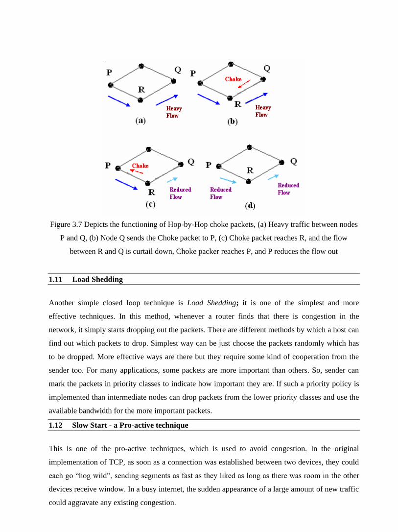
Figure 3.7 Depicts the functioning of Hop-by-Hop choke packets, (a) Heavy traffic between nodes
P and Q, (b) Node Q sends the Choke packet to P, (c) Choke packet reaches R, and the flow
between R and Q is curtail down, Choke packer reaches P, and P reduces the flow out
1.11 Load Shedding
Another simple closed loop technique is Load Shedding; it is one of the simplest and more
effective techniques. In this method, whenever a router finds that there is congestion in the
network, it simply starts dropping out the packets. There are different methods by which a host can
find out which packets to drop. Simplest way can be just choose the packets randomly which has
to be dropped. More effective ways are there but they require some kind of cooperation from the
sender too. For many applications, some packets are more important than others. So, sender can
mark the packets in priority classes to indicate how important they are. If such a priority policy is
implemented than intermediate nodes can drop packets from the lower priority classes and use the
available bandwidth for the more important packets.
1.12 Slow Start - a Pro-active technique
This is one of the pro-active techniques, which is used to avoid congestion. In the original
implementation of TCP, as soon as a connection was established between two devices, they could
each go “hog wild”, sending segments as fast as they liked as long as there was room in the other
devices receive window. In a busy internet, the sudden appearance of a large amount of new traffic
could aggravate any existing congestion.

To alleviate this, modern TCP devices are restrained in the rate at which they initially send
segments. Each sender is at first restricted to sending only an amount of data equal to one “full-
sized” segment—that is, equal to the MSS (maximum segment size) value for the connection. Each
time an acknowledgment is received, the amount of data the device can send is increased by the
size of another full-sized segment. Thus, the device “starts slow” in terms of how much data it can
send, with the amount it sends increasing until either the full window size is reached or congestion
is detected on the link. In the latter case, the congestion avoidance feature is used.
When potential congestion is detected on a TCP link, a device responds by throttling back the rate
at which it sends segments. A special algorithm is used that allows the device to drop the rate at
which segments are sent quickly when congestion occurs. The device then uses the Slow Start
algorithm just above to gradually increase the transmission rate back up again to try to maximize
throughput without congestion occurring again.
1.13 Flow Control Versus Congestion control
Let’s have a look at the difference between Flow Control and Congestion Control, which are
mixed up at times.
Flow control is a very important part of regulating the transmission of data between devices, but it
is limited in a way that it only considers what is going on within each of the devices on the
connection, and not what is happening in devices between them. It relates to the point-point traffic
between a given sender and a receiver. Flow control always involves some kind of feedback from
receiver to sender to tell sender how things are at other end of the network. Since we are dealing
with how TCP works between a typical server and client at layer four, we don't worry about how
data gets between them; that's the job of the Internet Protocol at layer three.
In practice, what is going on at layer three can be quite important. Considered from an abstract
point of view, our server and client may be connected “directly” using TCP, but all the packets we
transmit are carried across an internet and routers between different networks. These networks and
routers are also carrying data from many other connections and higher-layer protocols. If the
internet becomes very busy, the speed at which segments are carried between the endpoints of our
connection will be reduced, and they could even be dropped. This is called congestion control.
Congestion control has to do with making sure that subnet carry the offered traffic. It is the global
issue, involving the behavior of all the hosts, router, link, store and forward mechanism between
them in the entire subnet or internet.

1.14 Check Your Progress
1. What is congestion? Why congestion occurs?
2. What are the two basic mechanisms of congestion control?
3. How congestion control is performed by leaky bucket algorithm?
4. In what way token bucket algorithm is superior to leaky bucket algorithm?
1.15 Answer to Check Your Progress
1. In a packet switching network, packets are introduced in the nodes (i.e. offered load), and
the nodes in-turn forward the packets (i.e. throughput) into the network. When the “offered
load” crosses certain limit, then there is a sharp fall in the throughput. This phenomenon is
known as congestion.
In every node of a packet switching network, queues (or buffers) are maintained to receive
and transmit packets (store/forward network). Due to busty nature of the network traffic
there may be situations where there is overflow of the queues. As a result there will be re-
transmission of several packets, which further increases the network traffic. This finally
leads to congestion.
2 The two basic mechanisms of congestion control are:
• One is preventive, where precautions are taken so that congestion can not occur.
• Another is recovery from congestion, when congestion has already taken place.
3 In leaky bucket algorithm, a buffering mechanism is introduced between the host computer
and the network in order to regulate the flow of traffic. Busty traffic are generated by the host
computer and introduced in the network by leaky bucket mechanism in the following manner
• Packets are introduced in the network in one per tick
• In case of buffer overflow packets are discarded
4 The leaky bucket algorithm controls the rate at which the packets are introduced in the
network, but it is very conservative in nature. Some flexibility is introduced in token bucket
algorithm. In token bucket algorithm tokens are generated at each tick (up to certain limit). For
an incoming packet to be transmitted, it must capture a token and the transmission takes place
at the same rate. Hence some of the busty packets are transmitted at the same rate if tokens are

available and thus introduces some amount of flexibility in the system. This also improves the
performance.

Unit-04
Cryptography and Secured Communication
1.1 Learning Objectives
1.2 Introduction
1.3 Symmetric Key Cryptography
1.3.1 Monoalphabetic Substitution
1.3.2 Polyalphabetic Substitution
1.3.3 Transpositional Cipher
1.3.4 Block Ciphers
1.3.5 Data Encryption Standard(DES)
1.3.6 Encrypting a Larges Message
1.3.7 Triple DES
1.4 Public key Cryptography
1.4.1 RSA
1.4.2 Introduction to Secured Communication
1.4.3 Security Services
1.4.4 Privacy
1.4.5 Authentication, Integrity and Nonrepudiation using Digital Signature
1.4.6 User Authentication using symmetric key cryptography
1.4.7 User Authentication using Public Key Cryptography
1.4.8 Key Management
1.4.9 Application Layer Security
1.4.10 Virtual Private Network (VPN)
1.5 Check Your Progress
1.6 Answer to Check Your Progress
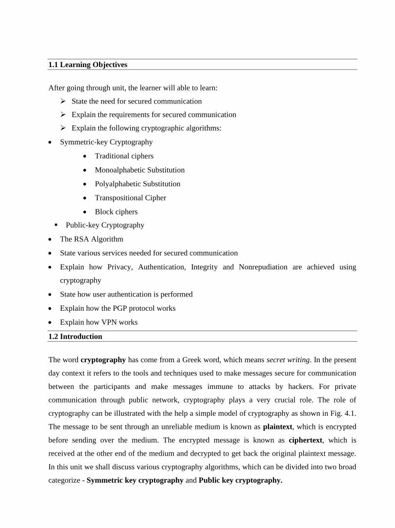
1.1 Learning Objectives
After going through unit, the learner will able to learn:
➢ State the need for secured communication
➢ Explain the requirements for secured communication
➢ Explain the following cryptographic algorithms:
• Symmetric-key Cryptography
• Traditional ciphers
• Monoalphabetic Substitution
• Polyalphabetic Substitution
• Transpositional Cipher
• Block ciphers
▪ Public-key Cryptography
• The RSA Algorithm
• State various services needed for secured communication
• Explain how Privacy, Authentication, Integrity and Nonrepudiation are achieved using
cryptography
• State how user authentication is performed
• Explain how the PGP protocol works
• Explain how VPN works
1.2 Introduction
The word cryptography has come from a Greek word, which means secret writing. In the present
day context it refers to the tools and techniques used to make messages secure for communication
between the participants and make messages immune to attacks by hackers. For private
communication through public network, cryptography plays a very crucial role. The role of
cryptography can be illustrated with the help a simple model of cryptography as shown in Fig. 4.1.
The message to be sent through an unreliable medium is known as plaintext, which is encrypted
before sending over the medium. The encrypted message is known as ciphertext, which is
received at the other end of the medium and decrypted to get back the original plaintext message.
In this unit we shall discuss various cryptography algorithms, which can be divided into two broad
categorize - Symmetric key cryptography and Public key cryptography.
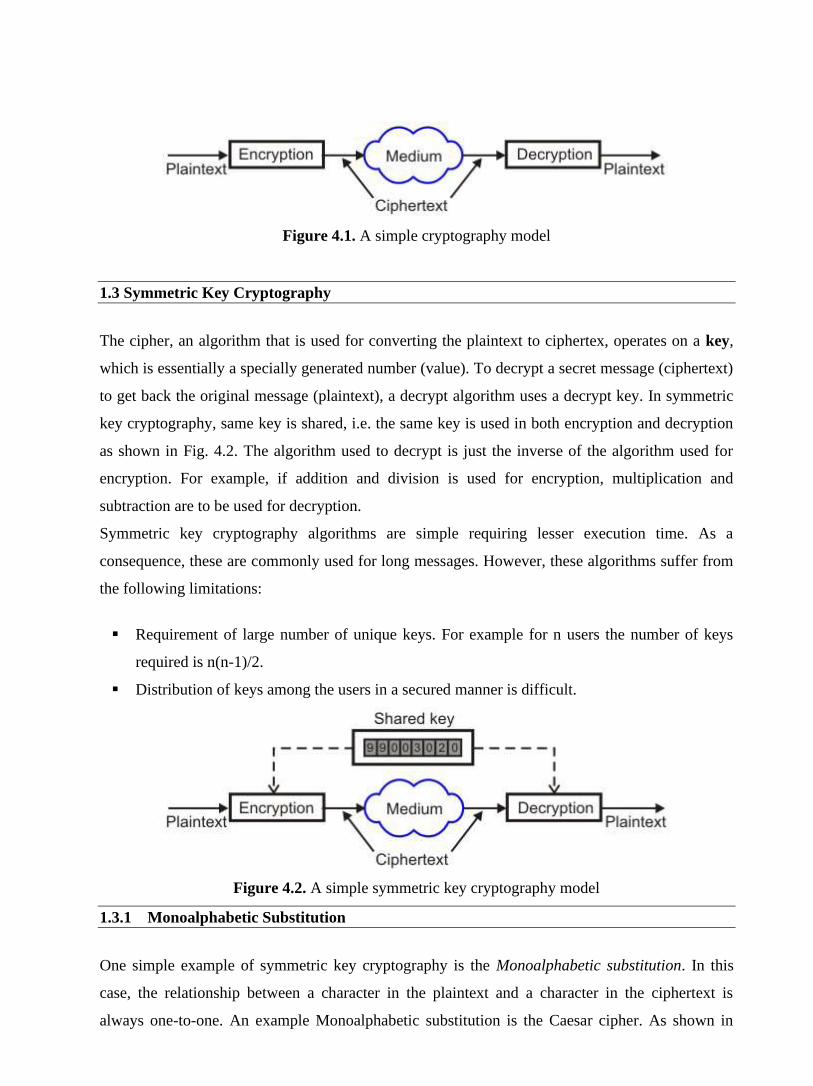
Figure 4.1. A simple cryptography model
1.3 Symmetric Key Cryptography
The cipher, an algorithm that is used for converting the plaintext to ciphertex, operates on a key,
which is essentially a specially generated number (value). To decrypt a secret message (ciphertext)
to get back the original message (plaintext), a decrypt algorithm uses a decrypt key. In symmetric
key cryptography, same key is shared, i.e. the same key is used in both encryption and decryption
as shown in Fig. 4.2. The algorithm used to decrypt is just the inverse of the algorithm used for
encryption. For example, if addition and division is used for encryption, multiplication and
subtraction are to be used for decryption.
Symmetric key cryptography algorithms are simple requiring lesser execution time. As a
consequence, these are commonly used for long messages. However, these algorithms suffer from
the following limitations:
▪ Requirement of large number of unique keys. For example for n users the number of keys
required is n(n-1)/2.
▪ Distribution of keys among the users in a secured manner is difficult.
Figure 4.2. A simple symmetric key cryptography model
1.3.1 Monoalphabetic Substitution
One simple example of symmetric key cryptography is the Monoalphabetic substitution. In this
case, the relationship between a character in the plaintext and a character in the ciphertext is
always one-to-one. An example Monoalphabetic substitution is the Caesar cipher. As shown in

Fig. 4.3, in this approach a character in the ciphertext is substituted by another character shifted by
three places, e.g. A is substituted by D. Key feature of this approach is that it is very simple but the
code can be attacked very easily.
Figure 4.3. The Caesar cipher
1.3.2 Polyalphabetic Substitution
This is an improvement over the Caesar cipher. Here the relationship between a character in the
plaintext and a character in the ciphertext is always one-to-many.
Example 8.1: Example of polyalphabetic substitution is the Vigenere cipher. In this case, a
particular character is substituted by different characters in the ciphertext depending on its position
in the plaintext. Figure 4.4 explains the polyalphabetic substitution. Here the top row shows
different characters in the plaintext and the characters in different bottom rows show the characters
by which a particular character is to be replaced depending upon its position in different rows from
row-0 to row-25.
• Key feature of this approach is that it is more complex and the code is harder to attack
successfully.
Figure 4.4. Polyalphabetric substitution

1.3.3 Transpositional Cipher
The transpositional cipher, the characters remain unchanged but their positions are changed to
create the ciphertext. Figure 4.5 illustrates how five lines of a text get modified using
transpositional cipher. The characters are arranged in two-dimensional matrix and columns are
interchanged according to a key is shown in the middle portion of the diagram. The key defines
which columns are to be swapped. As per the key shown in the figure, character of column is to be
swapped to column 3, character of column 2 is to be swapped to column 6, and so on. Decryption
can be done by swapping in the reverse order using the same key.
Transpositional cipher is also not a very secure approach. The attacker can find the plaintext by
trial and error utilizing the idea of the frequency of occurrence of characters.

Figure 4.5. Operation of a transpositional cipher
1.3.4 Block Ciphers
Block ciphers use a block of bits as the unit of encryption and decryption. To encrypt a 64-bit
block, one has to take each of the 264 input values and map it to one of the 264 output values. The
mapping should be one-to-one. Encryption and decryption operations of a block cipher are shown

in Fig. 4.6. Some operations, such as permutation and substitution, are performed on the block of
bits based on a key (a secret number) to produce another block of bits. The permutation and
substitution operations are shown in Figs 4.7 and 4.8, respectively. In the decryption process,
operations are performed in the reverse order based on the same key to get back the original block
of bits.
Figure 4.6. Transformations in Block Ciphers
Permutation: As shown in Fig. 4.7, the permutation is performed by a permutation box at the bit-
level, which keeps the number of 0s and 1s same at the input and output. Although it can be
implemented either by a hardware or a software, the hardware implementation is faster.
Figure 4.7. Permutation operation used in Block Ciphers
Substitution: As shown in Fig. 4.8, the substitution is implemented with the help of three building
blocks – a decoder, one p-box and an encoder. For an n-bit input, the decoder produces an 2n bit
output having only one 1, which is applied to the P-box. The P-box permutes the output of the
decoder and it is applied to the encoder. The encoder, in turn, produces an n-bit output. For
example, if the input to the decoder is 011, the output of the decoder is 00001000. Let the
permuted output is 01000000, the output of the encoder is 011.

Figure 4.8 Substitution operation used in Block Ciphers
A block Cipher: A block cipher realized by using substitution and permutation operations in shown
in Fig 4.9. It performs the following steps:
Step-1: Divide input into 8-bit pieces
Step-2: Substitute each 8-bit based on functions derived from the key
Step-3: Permute the bits based on the key
All of the above three steps re repeated for an optimal number of rounds

Figure 4.9 Encryption by using substitution and permutation
1.3.5 Data Encryption Standard(DES)
One example of the block cipher is the Data Encryption Standard (DES). Basic features of the
DES algorithm are given below:
• A monoalphabetic substitution cipher using a 64-bit character
• It has 19 distinct stages
• Although the input key for DES is 64 bits long, the actual key used by DES is only 56 bits in
length.
• The decryption can be done with the same password; the stages must then be carried out in
reverse order.
• DES has 16 round, meaning the main algorithm is repeated 16 times to produce the cipher text
• As the number of rounds increases, the security of the algorithm increases exponentially.
• Once the key scheduling and plaintext preparation have been completed, the actual encryption
or decryption is performed with help of the main DES algorithm as shown in Fig 4.10.
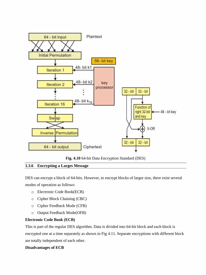
Fig. 4.10 64-bit Data Encryption Standard (DES)
1.3.6 Encrypting a Larges Message
DES can encrypt a block of 64-bits. However, to encrypt blocks of larger size, there exist several
modes of operation as follows:
o Electronic Code Book(ECB)
o Cipher Block Chaining (CBC)
o Cipher Feedback Mode (CFB)
o Output Feedback Mode(OFB)
Electronic Code Book (ECB)
This is part of the regular DES algorithm. Data is divided into 64-bit block and each block is
encrypted one at a time separately as shown in Fig 4.11. Separate encryptions with different block
are totally independent of each other.
Disadvantages of ECB
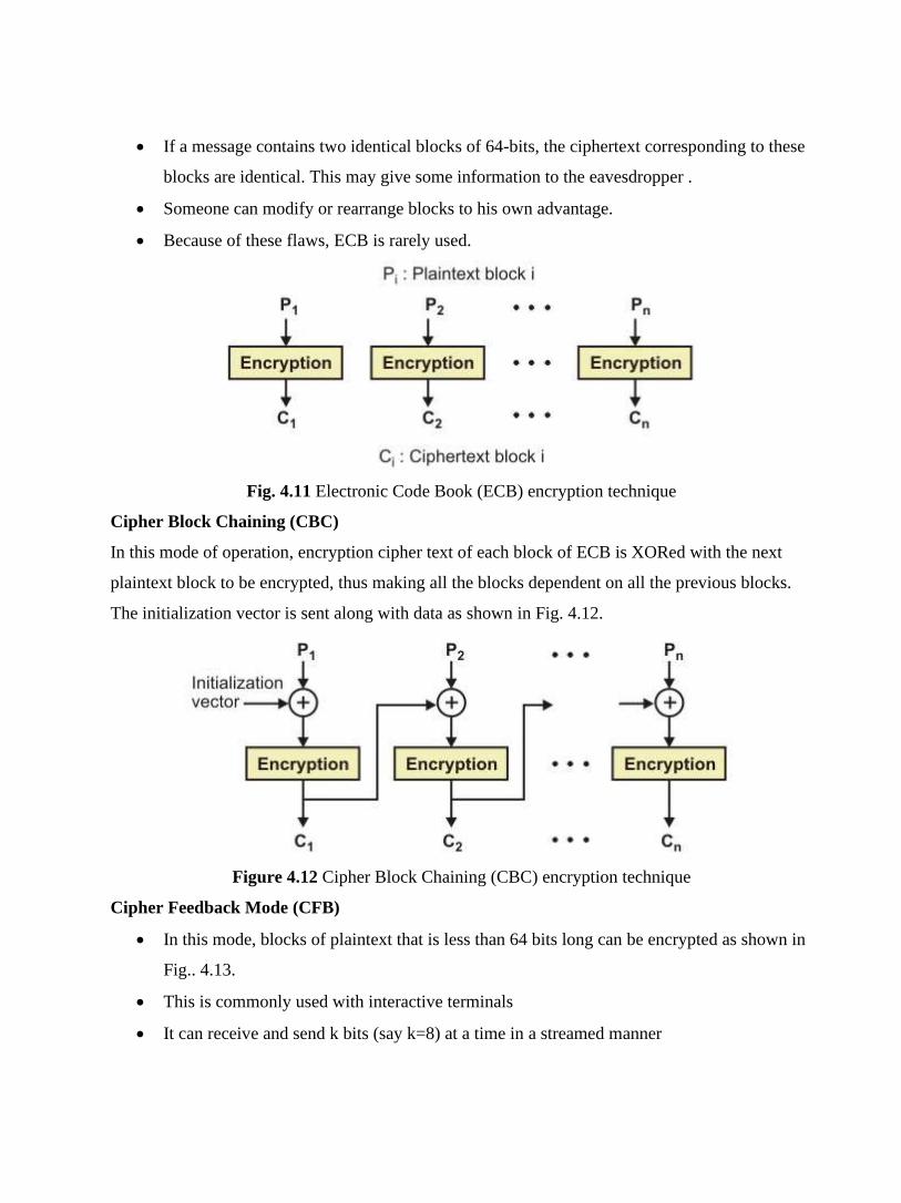
• If a message contains two identical blocks of 64-bits, the ciphertext corresponding to these
blocks are identical. This may give some information to the eavesdropper .
• Someone can modify or rearrange blocks to his own advantage.
• Because of these flaws, ECB is rarely used.
Fig. 4.11 Electronic Code Book (ECB) encryption technique
Cipher Block Chaining (CBC)
In this mode of operation, encryption cipher text of each block of ECB is XORed with the next
plaintext block to be encrypted, thus making all the blocks dependent on all the previous blocks.
The initialization vector is sent along with data as shown in Fig. 4.12.
Figure 4.12 Cipher Block Chaining (CBC) encryption technique
Cipher Feedback Mode (CFB)
• In this mode, blocks of plaintext that is less than 64 bits long can be encrypted as shown in
Fig.. 4.13.
• This is commonly used with interactive terminals
• It can receive and send k bits (say k=8) at a time in a streamed manner

Figure 4.13 Cipher Feedback Mode (CFB) encryption technique
Output Feedback Mode (OFB)
The encryption technique of Output Feedback Mode (OFB) is shown in Fig. 4.14. Key features of
this mode are mentioned below:
• OFB is also a stream cipher
• Encryption is performed by XORing the message with the one-time pad
• One-time pad can be generated in advance
• If some bits of the ciphertext get garbled, only those bits of plaintext get garbled
• The message can be of any arbitrary size • Less secure than other modes
Figure 4.14 Output Feedback Mode (OFB) encryption technique

1.3.7 Triple DES
Triple DES, popularly known as 3DES, is used to make DES more secure by effectively increasing
the key length. Its operation is explained below:
• Each block of plaintext is subjected to encryption by K1, decryption by K2 and again
encryption by K1 in a sequence as shown in Fig. 4.15.
• CBC is used to turn the block encryption scheme into a stream encryption scheme
Figure 4.15 Triple DES encryption techniques
1.4 Public key Cryptography
In public key cryptography, there are two keys: a private key and a public key. The public key is
announced to the public, whereas the private key is kept by the receiver. The sender uses the
public key of the receiver for encryption and the receiver uses his private key for decryption as
shown in Fig. 4.16.
Figure 4.16
• Advantages:
o The pair of keys can be used with any other entity
o The number of keys required is small

• Disadvantages:
o It is not efficient for long messages
o Association between an entity and its public key must be verified
1.4.1 RSA
The most popular public-key algorithm is the RSA (named after their inventors Rivest, Shamir and
Adleman ) as shown in Fig. 4.17. Key features of the RSA algorithm are given below:
• Public key algorithm that performs encryption as well as decryption based on number
theory
• Variable key length; long for enhanced security and short for efficiency (typical 512 bytes)
• Variable block size, smaller than the key length
• The Private key is a pair of number (d,n) and the public key is also a pair of number (e, n)
• Choose two large primes p and q (typically around 256 bits)
• Compute n=p x q and z= (p-1)x(q-1)
• Choose a number d relatively prime to z
• Find e such that e x d mod (p-1)x(q-1)=1
• For encryption: C= Pe(mod n)
For decryption: P= Cd(mod n)
Figure 4.17 The RSA public key encryption technique
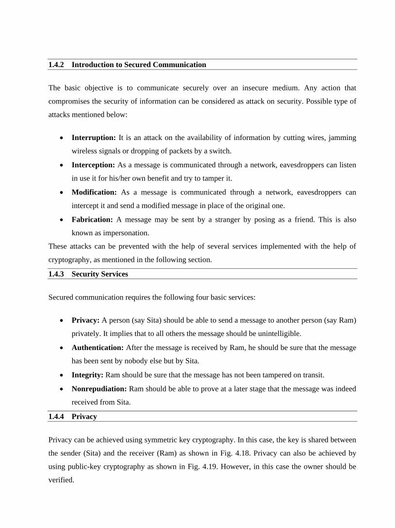
1.4.2 Introduction to Secured Communication
The basic objective is to communicate securely over an insecure medium. Any action that
compromises the security of information can be considered as attack on security. Possible type of
attacks mentioned below:
• Interruption: It is an attack on the availability of information by cutting wires, jamming
wireless signals or dropping of packets by a switch.
• Interception: As a message is communicated through a network, eavesdroppers can listen
in use it for his/her own benefit and try to tamper it.
• Modification: As a message is communicated through a network, eavesdroppers can
intercept it and send a modified message in place of the original one.
• Fabrication: A message may be sent by a stranger by posing as a friend. This is also
known as impersonation.
These attacks can be prevented with the help of several services implemented with the help of
cryptography, as mentioned in the following section.
1.4.3 Security Services
Secured communication requires the following four basic services:
• Privacy: A person (say Sita) should be able to send a message to another person (say Ram)
privately. It implies that to all others the message should be unintelligible.
• Authentication: After the message is received by Ram, he should be sure that the message
has been sent by nobody else but by Sita.
• Integrity: Ram should be sure that the message has not been tampered on transit.
• Nonrepudiation: Ram should be able to prove at a later stage that the message was indeed
received from Sita.
1.4.4 Privacy
Privacy can be achieved using symmetric key cryptography. In this case, the key is shared between
the sender (Sita) and the receiver (Ram) as shown in Fig. 4.18. Privacy can also be achieved by
using public-key cryptography as shown in Fig. 4.19. However, in this case the owner should be
verified.
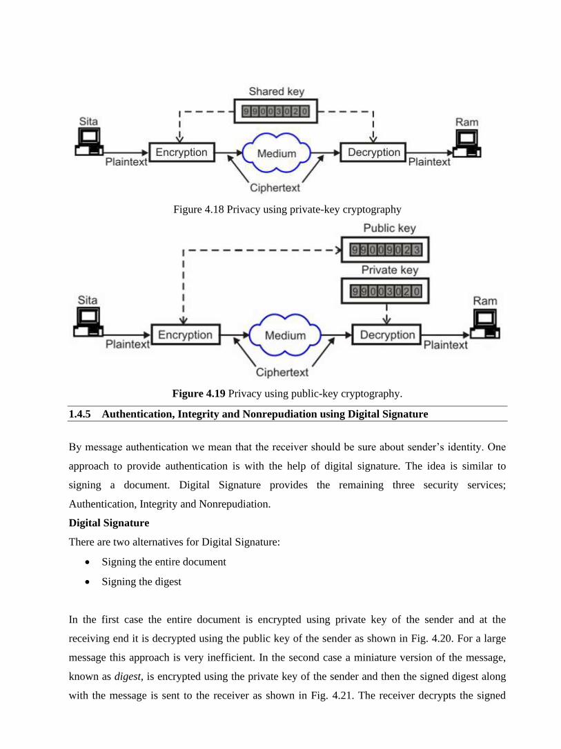
Figure 4.18 Privacy using private-key cryptography
Figure 4.19 Privacy using public-key cryptography.
1.4.5 Authentication, Integrity and Nonrepudiation using Digital Signature
By message authentication we mean that the receiver should be sure about sender’s identity. One
approach to provide authentication is with the help of digital signature. The idea is similar to
signing a document. Digital Signature provides the remaining three security services;
Authentication, Integrity and Nonrepudiation.
Digital Signature
There are two alternatives for Digital Signature:
• Signing the entire document
• Signing the digest
In the first case the entire document is encrypted using private key of the sender and at the
receiving end it is decrypted using the public key of the sender as shown in Fig. 4.20. For a large
message this approach is very inefficient. In the second case a miniature version of the message,
known as digest, is encrypted using the private key of the sender and then the signed digest along
with the message is sent to the receiver as shown in Fig. 4.21. The receiver decrypts the signed

digest using the public key of the sender and the digest created using the received message is
compared with decrypted digest as shown in Fig. 4.22. If the two are identical, it is assumed that
the sender is authenticated. This is somewhat similar to error detection using parity bit.
Figure 4.20 Authentication by signing the whole document
Figure 4.21 Sender site for authentication by signed digest
Figure 4.22 Receiver site for authentication by signed digest
Some key features of this approach are mentioned below:
• Digital signature does not provide privacy
• Hash function is used to create a message digest
• It creates a fixed-length digest from a variable-length message
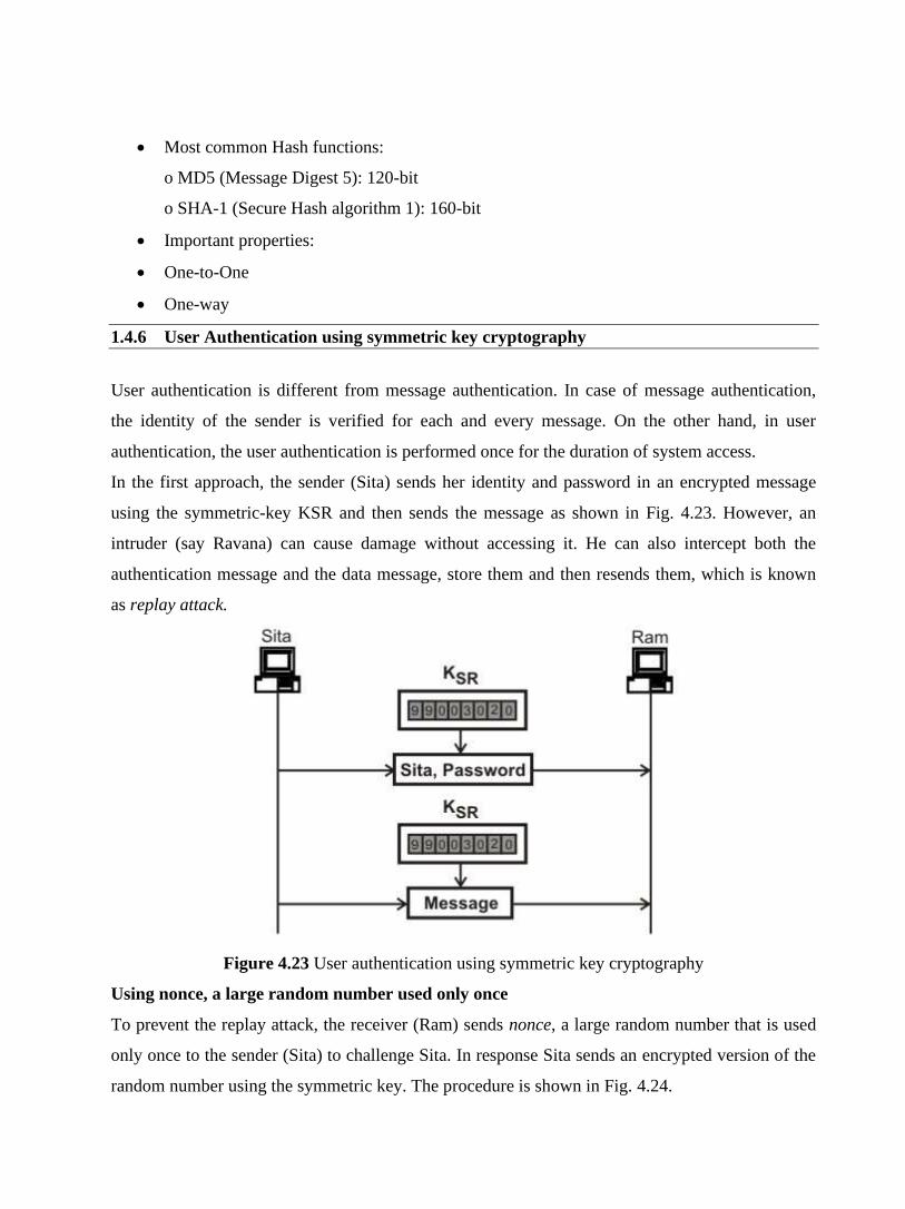
• Most common Hash functions:
o MD5 (Message Digest 5): 120-bit
o SHA-1 (Secure Hash algorithm 1): 160-bit
• Important properties:
• One-to-One
• One-way
1.4.6 User Authentication using symmetric key cryptography
User authentication is different from message authentication. In case of message authentication,
the identity of the sender is verified for each and every message. On the other hand, in user
authentication, the user authentication is performed once for the duration of system access.
In the first approach, the sender (Sita) sends her identity and password in an encrypted message
using the symmetric-key KSR and then sends the message as shown in Fig. 4.23. However, an
intruder (say Ravana) can cause damage without accessing it. He can also intercept both the
authentication message and the data message, store them and then resends them, which is known
as replay attack.
Figure 4.23 User authentication using symmetric key cryptography
Using nonce, a large random number used only once
To prevent the replay attack, the receiver (Ram) sends nonce, a large random number that is used
only once to the sender (Sita) to challenge Sita. In response Sita sends an encrypted version of the
random number using the symmetric key. The procedure is shown in Fig. 4.24.
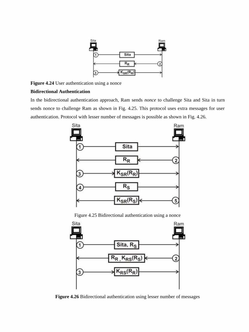
Figure 4.24 User authentication using a nonce
Bidirectional Authentication
In the bidirectional authentication approach, Ram sends nonce to challenge Sita and Sita in turn
sends nonce to challenge Ram as shown in Fig. 4.25. This protocol uses extra messages for user
authentication. Protocol with lesser number of messages is possible as shown in Fig. 4.26.
Figure 4.25 Bidirectional authentication using a nonce
Figure 4.26 Bidirectional authentication using lesser number of messages

1.4.7 User Authentication using Public Key Cryptography
Public key cryptography can also be used to authenticate a user. The procedure is shown in Fig.
4.27.
ER= Public key of Ram, ES= Public key of Sita
RS= nonce by Sita, RR= nonce by Ram
KS= Session key sent by Ram
Figure 4.27 User authentication using public key cryptography
1.4.8 Key Management
Although symmetric-key and public-key cryptography can be used for privacy and user
authentication, question arises about the techniques used for the distribution of keys. Particularly,
symmetric-key distribution involves the following three problems:
• For n people to communicate with each other requires n(n-1)/2 keys. The problem is
aggravated as n becomes very large.
• Each person needs to remember (n-1) keys to communicate with the the remaining (n-1)
persons.
• How the two parties will acquire the shared key in a secured manner?
In view of the above problems, the concept of session key has emerged. A session key is created
for each session and destroyed when the session is over. The Diffie-Hellman protocol is one of the
most popular approach for providing one-time session key for both the parties.
Diffie-Hellman Protocol
Key features of the Diffie-Hellman protocol are mentioned below and the procedure is given in
Fig. 4.28.
• Used to establish a shared secret key

• Prerequisite: N is a large prime number such that (N-1)/2 is also a prime number. G is also
a prime number. Both N and G are known to Ram and Sita.
• Sita chooses a large random number x and calculates R1 = Gxmod N and sends it to Ram
• Ram chooses another large random number y and calculates R2 = Gymod N and sends it to
Sita
• Ram calculates K = (R1)y mod N
• Sita calculates K = (R2)x mod N
Figure 4.28 Diffie-Hellman Protocol
Key Management using KDC
It may be noted that both R1 and R2 are sent as plaintext, which may be intercepted by an intruder.
This is a serious flaw of the Diffie-Hellman Protocol. Another approach is to use a trusted third
party to assign a symmetric key to both the parties. This is the basic idea behind the use of key
distribution center (KDC).
Key Management using Kerberos
Another popular authentication protocol known as Kerberos. It uses an authentication server (AS),
which performs the role of KDC and a ticket-granting server (TGS), which provides the session
key (KAB) between the sender and receiver parties. Apart from these servers, there is the real data
server say Ram that provides services to the user Sita. The operation of Kerberos is depicted with
the help of Fig.4.29. The client process (Sita) can get a service from a process running in the real
server Ram after six steps as shown in the figure. The steps are as follows:
Step 1. Sita uses her registered identity to send her message in plaintext.
Step 2. The AS server sends a message encrypted with Sita’s symmetric key KS. The message
contains a session key Kse, which is used by Sita to contact the TGS and a ticket for TGS that is
encrypted with the TGS symmetric key KTG.

Step3. Sita sends three items to the TGS; the ticket received from the AS, the name of the real
server, and a timestamp encrypted by Kse. The timestamp prevents replay by Ram.
Step 4. The TGS sends two tickets to Sita. The ticket for Sita encrypted with Kse and the ticket for
Ram encrypted with Ram’s key. Each of the tickets contains the session key KSR between Sita and
Ram.
Step 5. Sita sends Ram’s ticket encrypted by KSR.
Step 6. Ram sends a message to Sita by adding 1 to the timestamp confirming the receipt of the
message using KSR as the key for encryption.
Following this Sita can request and get services from Ram using KSR as the shared key.
Figure 4.29 The Kerberos Protocol
1.4.9 Application Layer Security
Based on the encryption techniques we have discussed so far, security measures can be applied to
different layers such as network, transport or application layers. However, implementation of
security features in the application layer is far simpler and feasible
compared to implementing at the other two lower layers. In this subsection, a protocol known as
Pretty Good Privacy (PGP), invented by Phil Zinmermann, that is used in the application layer to
provide all the four aspects of security for sending an email is briefly discussed. PGP uses a
combination of private-key and public key for privacy. For integrity, authentication and
nonrepudiation, it uses a combination of hashing to create digital signature and public-key
encryption as shown in Fig. 4.30.
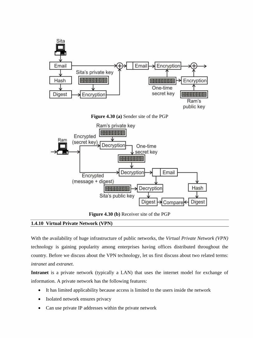
Figure 4.30 (a) Sender site of the PGP
Figure 4.30 (b) Receiver site of the PGP
1.4.10 Virtual Private Network (VPN)
With the availability of huge infrastructure of public networks, the Virtual Private Network (VPN)
technology is gaining popularity among enterprises having offices distributed throughout the
country. Before we discuss about the VPN technology, let us first discuss about two related terms:
intranet and extranet.
Intranet is a private network (typically a LAN) that uses the internet model for exchange of
information. A private network has the following features:
• It has limited applicability because access is limited to the users inside the network
• Isolated network ensures privacy
• Can use private IP addresses within the private network
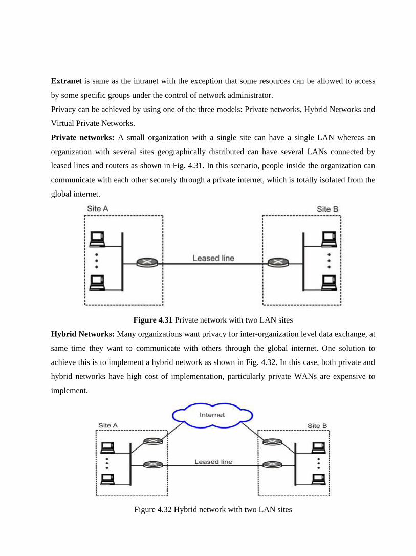
Extranet is same as the intranet with the exception that some resources can be allowed to access
by some specific groups under the control of network administrator.
Privacy can be achieved by using one of the three models: Private networks, Hybrid Networks and
Virtual Private Networks.
Private networks: A small organization with a single site can have a single LAN whereas an
organization with several sites geographically distributed can have several LANs connected by
leased lines and routers as shown in Fig. 4.31. In this scenario, people inside the organization can
communicate with each other securely through a private internet, which is totally isolated from the
global internet.
Figure 4.31 Private network with two LAN sites
Hybrid Networks: Many organizations want privacy for inter-organization level data exchange, at
same time they want to communicate with others through the global internet. One solution to
achieve this is to implement a hybrid network as shown in Fig. 4.32. In this case, both private and
hybrid networks have high cost of implementation, particularly private WANs are expensive to
implement.
Figure 4.32 Hybrid network with two LAN sites

Virtual Private Networks (VPN): VPN technology allows both private communication and
public communications through the global internet as shown in Fig. 4.33. VPN uses IPSec in the
tunnel mode to provide authentication, integrity and privacy. In the IPSec tunnel mode the
datagram to be sent is encapsulated in another datagram as payload. It requires two sets of
addressing as shown in Fig. 4.34.
Figure 4.33 VPN linking two LANs
Figure 4.34 VPN linking two LANs
1.5 Check Your Progress
1. What are the four services required for secured communication?
2. What is nonce?
3. Explain the function of Kerberos.

4. What is VPN?
1.6 Answer to Check Your Progress
1. The four services required for secured communication are: privacy, integrity,
authentication and nonrepudiation.
2. The nonce is a large random number that is used only once for the purpose of user
authentication.
3. Kerberos is a popular technique for key distribution. The kerberos is an authentication
protocol and at the same time acts as a Key Distribution Center. It requires an
authentication server and a ticket-granting server in addition to the real data server.
4. VPN allows private communication through public internet. It is essentially a logical
(virtual) network within a conventional network. It makes use of cryptography (IPSec in
tunnel mode) to perform private communication through insecure and public internet.

Unit-05
Firewalls
1.1 Learning Objectives
1.2 Introduction
1.3 Why a Firewall is needed?
1.4 Access Control Policies
1.5 Firewall Capabilities
1.6 Limitations of a Firewall
1.7 Types of Firewalls
1.8 Bastion Host
1.9 Network Address Translation
1.10 Firewall Configurations
1.11 Active Firewall Elements
1.12 Check Your Progress
1.13 Answer to Check Your Progress

1.1 Learning Objectives
After going through this unit, the learner will able to learn:
• What a firewall is?
• What are the design goals of Firewalls
• What are the capabilities and limitations of Firewalls
• What are the possible types of Firewalls
o Packet filters
o Application-level gateways
o Circuit-level gateways
• What are the possible configurations Firewalls
o Single-homed system
o Double-homed system
o Screened subnet firewall system
1.2 Introduction
Many organizations have confidential or proprietary information, such as trade secrets, product
development plans, marketing strategies, etc., which should be protected from unauthorized access
and modification. One possible approach is to use suitable encryption/decryption technique for
transfer of data between two secure sites, as we have discussed in the previous lesson. Although
these techniques can be used to protect data in transit, it does not protect data from digital pests
and hackers. To accomplish this it is necessary to perform user authentication and access control to
protect the networks from unauthorized traffic. This is known as firewalls. A firewall system is an
electronic security guard and electronic barrier at the same time. It protects and controls the
interface between a private network and an insecure public network as shown in the simplified
diagram of Fig. 5.1. It is responsible for partitioning a designated area such that any damage on
one side cannot spread to the other side. It prevents bad things from happening, i.e. loss of
information, without preventing good things from happening, that is controlled exchange of
information with the outside world. It essentially enforces an access control policy between two
networks. The manner in which this is implemented varies widely, but in principle, the firewall can
be considered as a pair of mechanisms: one that is used to block traffic, and the other that is used
to permit traffic. Some firewalls place more emphasis on blocking traffic, while others emphasize
on permitting traffic. Probably the most important issue to understand of a firewall is the access

control policy it implements. If a firewall administrator has no idea about what or whom he is
protecting his network, what should be allowed and what should be prohibited, a firewall really
won't help his organization. As firewall is a mechanism for enforcing policy, which affects all the
persons behind it, it imposes heavy responsibility on the administrator of the firewall. In this
lesson various issues related to Firewalls are discussed.
Figure 5.1 Schematic diagram of a firewall
1.3 Why a Firewall is needed?
There is no need for a firewall if each and every host of a private network is properly secured.
Unfortunately, in practice the situation is different. A private network may consist of different
platforms with diverse OS and applications running on them. Many of the applications were
designed and developed for an ideal environment, without considering the possibility of the
existence of bad guys. Moreover, most of the corporate networks are not designed for security.
Therefore, it is essential to deploy a firewall to protect the vulnerable infrastructure of an
enterprise.
1.4 Access Control Policies
Access control policies play an important role in the operation of a firewall. The policies can be
broadly categorized in to the following four types:
Service Control:
• Determines the types of internet services to be accessed
• Filters traffic based on IP addresses and TCP port numbers
• Provides Proxy servers that receives and interprets service requests before it is passed on
Direction Control:
Determines the direction in which a particular service request may be initiated and allowed to flow
through the firewall
User Control:
• Controls access to a service according to which user is attempting to access it
• Typically applied to the users inside the firewall perimeter
• Can be applied to the external users too by using secure authentication technique
Behavioral Control:
• Controls how a particular service is used
• For example, a firewall may filter email to eliminate spam
• Firewall may allow only a portion of the information on a local web server to an external
user
1.5 Firewall Capabilities
Important capabilities of a firewall system are listed below:
• It defines a single choke point to keep unauthorized users out of protected network
• It prohibits potentially vulnerable services from entering or leaving the network
• It provides protection from various kinds of IP spoofing
• It provides a location for monitoring security-related events
• Audits and alarms can be implemented on the firewall systems
• A firewall is a convenient platform for several internet functions that are not security
related
• A firewall can serve as the platform for IPSec using the tunnel mode capability and can be
used to implement VPNs
1.6 Limitations of a Firewall
Main limitations of a firewall system are given below:
• A firewall cannot protect against any attacks that bypass the firewall. Many organizations
buy expensive firewalls but neglect numerous other back-doors into their network
• A firewall does not protect against the internal threats from traitors. An attacker may be
able to break into network by completely bypassing the firewall, if he can find a ``helpful''
insider who can be fooled into giving access to a modem pool
• Firewalls can't protect against tunneling over most application protocols. For example,
firewall cannot protect against the transfer of virus-infected programs or files

1.7 Types of Firewalls
The firewalls can be broadly categorized into the following three types:
• Packet Filters
• Application-level Gateways
• Circuit-level Gateways
Packet Filters: Packet filtering router applies a set of rules to each incoming IP packet and then
forwards or discards it. Packet filter is typically set up as a list of rules based on matches of fields
in the IP or TCP header. An example table of telnet filter rules is given in Fig. 5.2. The packet
filter operates with positive filter rules. It is necessary to specify what should be permitted, and
everything that is explicitly not permitted is automatically forbidden.
Figure 5.2 A table of packet filter rules for telnet application
Application-level Gateway: Application level gateway, also called a Proxy Server acts as a relay
of application level traffic. Users contact gateways using an application and the request is
successful after authentication. The application gateway is service specific such as FTP, TELNET,
SMTP or HTTP.
Circuit Level Gateway: Circuit-level gateway can be a standalone or a specialized system. It does
not allow end-to-end TCP connection; the gateway sets up two TCP connections. Once the TCP
connections are established, the gateway relays TCP segments from one connection to the other
without examining the contents. The security function determines which connections will be
allowed and which are to be disallowed.
1.8 Bastion Host
An application level gateway is sometimes known as Bastion Host. It is a system identified by the
firewall administrator as a very critical point in the network’s security. It serves as a platform for
an application-level or circuit-level gateway. It executes a very secured version of OS and
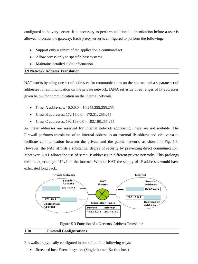
configured to be very secure. It is necessary to perform additional authentication before a user is
allowed to access the gateway. Each proxy server is configured to perform the following:
• Support only a subset of the application’s command set
• Allow access only to specific host systems
• Maintains detailed audit information
1.9 Network Address Translation
NAT works by using one set of addresses for communications on the internet and a separate set of
addresses for communication on the private network. IANA set aside three ranges of IP addresses
given below for communication on the internal network.
• Class A addresses: 10.0.0.0 – 10.255.255.255.255
• Class B addresses: 172.16.0.0 – 172.31. 255.255
• Class C addresses: 192.168.0.0 – 192.168.255.255
As these addresses are reserved for internal network addressing, these are not routable. The
Firewall performs translation of an internal address to an external IP address and vice versa to
facilitate communication between the private and the public network, as shown in Fig. 5.3.
However, the NAT affords a substantial degree of security by preventing direct communication.
Moreover, NAT allows the use of same IP addresses in different private networks. This prolongs
the life expectancy of IPv4 on the internet. Without NAT the supply of IP addresses would have
exhausted long back.
Figure 5.3 Function of a Network Address Translator
1.10 Firewall Configurations
Firewalls are typically configured in one of the four following ways:
• Screened host Firewall system (Single-homed Bastion host)
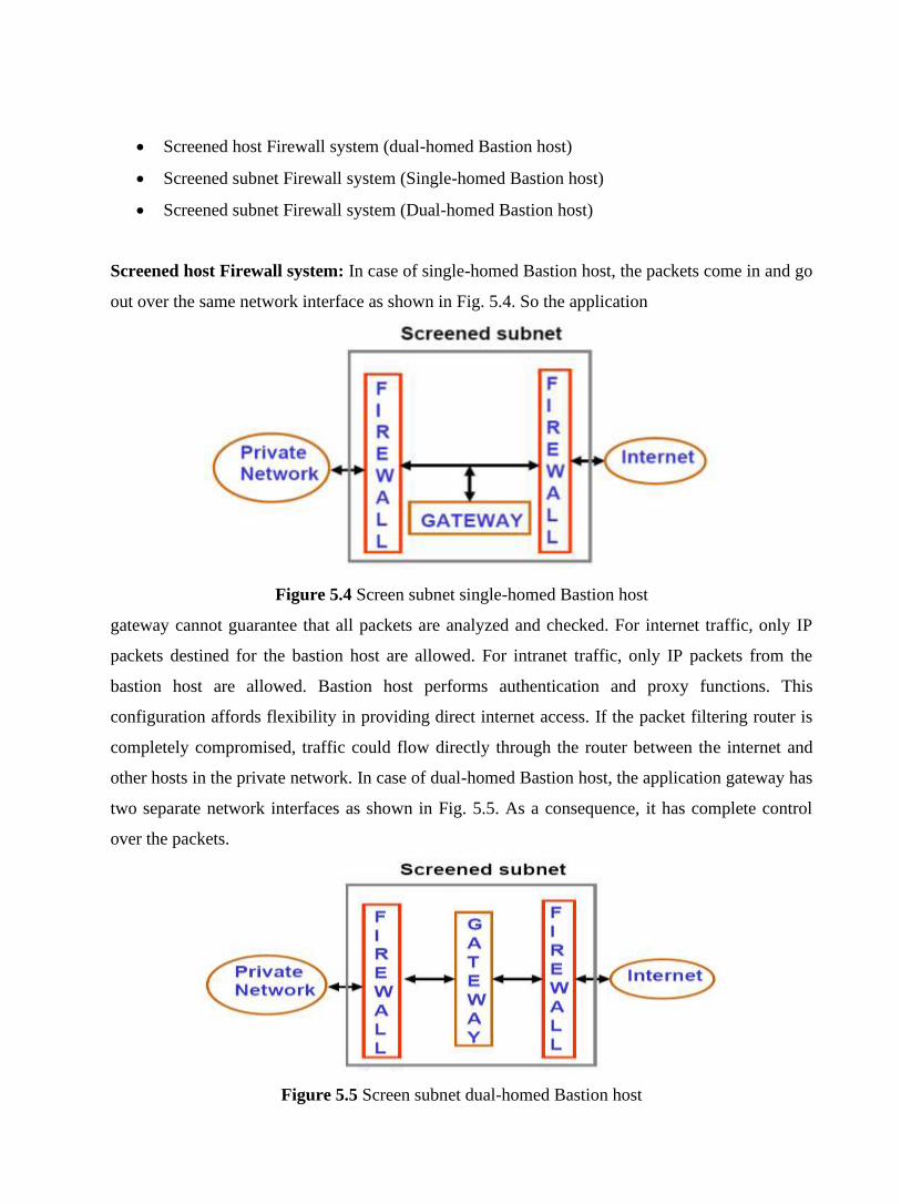
• Screened host Firewall system (dual-homed Bastion host)
• Screened subnet Firewall system (Single-homed Bastion host)
• Screened subnet Firewall system (Dual-homed Bastion host)
Screened host Firewall system: In case of single-homed Bastion host, the packets come in and go
out over the same network interface as shown in Fig. 5.4. So the application
Figure 5.4 Screen subnet single-homed Bastion host
gateway cannot guarantee that all packets are analyzed and checked. For internet traffic, only IP
packets destined for the bastion host are allowed. For intranet traffic, only IP packets from the
bastion host are allowed. Bastion host performs authentication and proxy functions. This
configuration affords flexibility in providing direct internet access. If the packet filtering router is
completely compromised, traffic could flow directly through the router between the internet and
other hosts in the private network. In case of dual-homed Bastion host, the application gateway has
two separate network interfaces as shown in Fig. 5.5. As a consequence, it has complete control
over the packets.
Figure 5.5 Screen subnet dual-homed Bastion host

1.11 Active Firewall Elements
The structure of an active firewall element, which is integrated in the communication interface
between the insecure public network and the private network is shown in Fig. 5.6. To provide
necessary security services, following components are required:
Integration Module: It integrates the active firewall element into the communication system with
the help of device drivers. In case of packet filters, the integration is above the Network Access
Layer, where as it is above the Transport layer ports in case of Application Gateway.
Analysis Module: Based on the capabilities of the firewall, the communication data is analysed in
the Analysis Module. The results of the analysis is passed on to the Decision Module.
Decision Module: The Decision Module evalutes and compares the results of the analysis with the
security policy definitions stored in the Ruleset and the communication data is allowed or
prevented based the outcome of the comparision.
Processing module for Securityrelated Events: Based on ruleset, configuration settings and the
message received from the decision module, it writes on the logbook and generates alarm message
to the Security Management System.
Authentication Module: This module is responsible for the identification and authentication of
the instances that are communicated through the firewall system.
Ruleset: It contains all the information necessary to make a decision for or against the
transmission of communication data through the Firewall and it also defines the security-releted
events to be logged.
Logbook: All security-related events that occur during operation are recorded in the loogbook
based on the existing ruleset.
Security Management System: It provides an interface where the administrator enter and
maintain the ruleset. It also analyses the data entered in the logbook.

Figure 5.6 Components of the active firewall system
1.12 Check Your Progress
1. What is the purpose of a Firewall?
2. What are the commonly used Firewall types?
3. Explain the operation of the packet-filter firewall.
4. Explain the operation of the Application Gateway Firewall.
5. What is NAT? How it improves network security?
1.13 Answer to Check Your Progress
1. The purpose of the Firewall is to protect a private network from the threats of hackers
coming from the Internet (a public network).
2. Firewalls can be of the following three types:
• Packet Filters
• Application-level Gateways
• Circuit-level Gateways.
3. A packet filter Firewall blocks or forwards packets based on the transport and network
layer addresses and protocols. It is typically set up as a list of rules based on matches of
fields in the IP or TCP header.
4. An Application Gateway blocks or forwards packets based on the information in the
application layers.

5. Network Address Translation (NAT) allows a private network to use a set of private
addresses and a set of global Internet Addresses for external communication. It uses a
translation table to route messages between the two networks and provides substantial
security.