Multimedia Fundamentals, Volume 1 - eopcw
291
-
Upload
khangminh22 -
Category
Documents
-
view
2 -
download
0
Transcript of Multimedia Fundamentals, Volume 1 - eopcw


MULTIMEDIA
FUNDAMENTALS
VOLUME 1:Media Coding and Content Processing

IMSC Press Multimedia Series
ANDREW TESCHER, Series Editor, Compression Science Corporation
Advisory EditorsLEONARDO CHIARIGLIONE, CSELT
TARIQ S. DURRANI, University of StrathclydeJEFF GRALNICK, E-splosion Consulting, LLC
CHRYSOSTOMOS L. “MAX” NIKIAS, University of Southern CaliforniaADAM C. POWELL III, The Freedom Forum
Desktop Digital Video Production
Frederic Jones
Touch in Virtual Environments: Haptics and the Design of Interactive Systems
Edited by Margaret L. McLaughlin, João P. Hespanha, and Gaurav S. Sukhatme
The MPEG-4 Book
Edited by Fernando M. B. Pereira and Touradj Ebrahimi
Multimedia Fundamentals, Volume 1: Media Coding and Content Processing
Ralf Steinmetz and Klara Nahrstedt
Intelligent Systems for Video Analysis and Access Over the Internet
Wensheng Zhou and C. C. Jay Kuo
▲▲
▲▲
▲

The Integrated Media Systems Center (IMSC), a National Science Foundation Engineering Research Center in the University of Southern California’s School of Engineering, is a preeminent multimedia and Internet research center. IMSC seeks to develop integrated media systems that dramatically transform the way we work, communicate, learn, teach, and entertain. In an integrated media system, advanced media technologies combine, deliver, and transform information in the form of images, video, audio, animation, graphics, text, and haptics (touch-related technologies). IMSC Press, in partnership with Prentice Hall, publishes cutting-edge research on multimedia and Internet topics. IMSC Press is part of IMSC’s educational outreach program.

PRENTICE HALL PTRUPPER SADDLE RIVER, NJ 07458WWW.PHPTR.COM
MULTIMEDIA
FUNDAMENTALS
VOLUME 1:Media Coding and Content Processing
Ralf SteinmetzKlara Nahrstedt

Library of Congress Cataloging-in-Publication Data
Steinmetz, Ralf. Multimedia fundamentals / Ralf Steinmetz, Klara Nahrstedt
p. cm. Includes bibliographical references and index.
Contents: v. 1. Media coding and content processing.ISBN 0-13-031399-8
1. Multimedia systems. I. Nahrstedt, Klara II. Title.
QA76.575 .S74 2002 006.7—dc21 2001056583
CIP Editorial/Production Supervision: Nick RadhuberAcquisitions Editor: Bernard GoodwinEditorial Assistant: Michelle VincenteMarketing Manager: Dan DePasqualeManufacturing Buyer: Alexis Heydt-LongCover Design: John ChristianaCover Design Director: Jerry Votta
© 2002 by Prentice Hall PTRPrentice-Hall, Inc.Upper Saddle River, NJ 07458
Prentice Hall books are widely used by corporations and government agencies for training, marketing, and resale.
The publisher offers discounts on this book when ordered in bulk quantities. For more information, contact Corporate Sales Department, phone: 800-382-3419; fax: 201-236-7141; email: [email protected] Or write: Corporate Sales Department, Prentice Hall PTR, One Lake Street, Upper Saddle River, NJ 07458.
Product and company names mentioned herein are the trademarks or registered trademarksof their respective owners.
All rights reserved. No part of this book may bereproduced, in any form or by any means, without permission in writing from the publisher.
Printed in the United States of America
10 9 8 7 6 5 4 3 2 1
ISBN 0-13-031399-8
Pearson Education LTD.Pearson Education Australia PTY, LimitedPearson Education Singapore, Pte. LtdPearson Education North Asia LtdPearson Education Canada, Ltd.Pearson Educación de Mexico, S.A. de C.V.Pearson Education—JapanPearson Education Malaysia, Pte. LtdPearson Education, Upper Saddle River, New Jersey

To our families:Jane, Catherine, and Rachel Horspool,
and Marie Clare Gormanfor their patience and support

vii
Contents
Preface xv
1 Introduction 11.1 Interdisciplinary Aspects of Multimedia .......................................................... 21.2 Contents of This Book...................................................................................... 31.3 Organization of This Book ............................................................................... 4
1.3.1 Media Characteristics and Coding ........................................................ 51.3.2 Media Compression............................................................................... 51.3.3 Optical Storage ...................................................................................... 61.3.4 Content Processing ................................................................................ 6
1.4 Further Reading About Multimedia.................................................................. 6
2 Media and Data Streams 72.1 The Term “Multimedia” ................................................................................... 72.2 The Term “Media”............................................................................................ 7
2.2.1 Perception Media................................................................................... 82.2.2 Representation Media............................................................................ 82.2.3 Presentation Media ................................................................................ 82.2.4 Storage Media ....................................................................................... 92.2.5 Transmission Media .............................................................................. 9

viii Contents
2.2.6 Information Exchange Media................................................................ 92.2.7 Presentation Spaces and Presentation Values ....................................... 92.2.8 Presentation Dimensions ..................................................................... 10
2.3 Key Properties of a Multimedia System......................................................... 112.3.1 Discrete and Continuous Media .......................................................... 122.3.2 Independent Media .............................................................................. 122.3.3 Computer-Controlled Systems ............................................................ 122.3.4 Integration ........................................................................................... 122.3.5 Summary ............................................................................................. 13
2.4 Characterizing Data Streams .......................................................................... 132.4.1 Asynchronous Transmission Mode ..................................................... 132.4.2 Synchronous Transmission Mode ....................................................... 142.4.3 Isochronous Transmission Mode ........................................................ 14
2.5 Characterizing Continuous Media Data Streams............................................ 152.5.1 Strongly and Weakly Periodic Data Streams ...................................... 152.5.2 Variation of the Data Volume of Consecutive Information Units ...... 162.5.3 Interrelationship of Consecutive Packets ............................................ 18
2.6 Information Units............................................................................................ 19
3 Audio Technology 213.1 What Is Sound?............................................................................................... 21
3.1.1 Frequency ............................................................................................ 223.1.2 Amplitude............................................................................................ 233.1.3 Sound Perception and Psychoacoustics............................................... 23
3.2 Audio Representation on Computers.............................................................. 263.2.1 Sampling Rate ..................................................................................... 273.2.2 Quantization ........................................................................................ 27
3.3 Three-Dimensional Sound Projection............................................................. 283.3.1 Spatial Sound....................................................................................... 283.3.2 Reflection Systems.............................................................................. 30
3.4 Music and the MIDI Standard ........................................................................ 303.4.1 Introduction to MIDI ........................................................................... 313.4.2 MIDI Devices ...................................................................................... 313.4.3 The MIDI and SMPTE Timing Standards .......................................... 32
3.5 Speech Signals ................................................................................................ 32

Contents ix
3.5.1 Human Speech..................................................................................... 323.5.2 Speech Synthesis ................................................................................. 33
3.6 Speech Output................................................................................................. 333.6.1 Reproducible Speech Playout.............................................................. 343.6.2 Sound Concatenation in the Time Range ............................................ 343.6.3 Sound Concatenation in the Frequency Range.................................... 363.6.4 Speech Synthesis ................................................................................. 36
3.7 Speech Input ................................................................................................... 373.7.1 Speech Recognition............................................................................. 38
3.8 Speech Transmission ...................................................................................... 403.8.1 Pulse Code Modulation ....................................................................... 403.8.2 Source Encoding ................................................................................. 413.8.3 Recognition-Synthesis Methods.......................................................... 423.8.4 Achievable Quality.............................................................................. 43
4 Graphics and Images 454.1 Introduction..................................................................................................... 454.2 Capturing Graphics and Images...................................................................... 46
4.2.1 Capturing Real-World Images............................................................. 464.2.2 Image Formats..................................................................................... 484.2.3 Creating Graphics................................................................................ 534.2.4 Storing Graphics.................................................................................. 54
4.3 Computer-Assisted Graphics and Image Processing...................................... 554.3.1 Image Analysis .................................................................................... 564.3.2 Image Synthesis................................................................................... 71
4.4 Reconstructing Images.................................................................................... 724.4.1 The Radon Transform ......................................................................... 734.4.2 Stereoscopy ......................................................................................... 74
4.5 Graphics and Image Output Options .............................................................. 754.5.1 Dithering.............................................................................................. 76
4.6 Summary and Outlook.................................................................................... 77
5 Video Technology 795.1 Basics.............................................................................................................. 79

x Contents
5.1.1 Representation of Video Signals ......................................................... 795.1.2 Signal Formats..................................................................................... 83
5.2 Television Systems ......................................................................................... 875.2.1 Conventional Systems ......................................................................... 875.2.2 High-Definition Television (HDTV)................................................... 88
5.3 Digitization of Video Signals ......................................................................... 905.3.1 Composite Coding............................................................................... 915.3.2 Component Coding ............................................................................. 91
5.4 Digital Television ........................................................................................... 93
6 Computer-Based Animation 956.1 Basic Concepts................................................................................................ 95
6.1.1 Input Process ....................................................................................... 956.1.2 Composition Stage .............................................................................. 966.1.3 Inbetween Process ............................................................................... 966.1.4 Changing Colors.................................................................................. 97
6.2 Specification of Animations ........................................................................... 976.3 Methods of Controlling Animation ................................................................ 98
6.3.1 Explicitly Declared Control ................................................................ 986.3.2 Procedural Control .............................................................................. 996.3.3 Constraint-Based Control .................................................................... 996.3.4 Control by Analyzing Live Action...................................................... 996.3.5 Kinematic and Dynamic Control....................................................... 100
6.4 Display of Animation ................................................................................... 1006.5 Transmission of Animation .......................................................................... 1016.6 Virtual Reality Modeling Language (VRML).............................................. 101
7 Data Compression 1057.1 Storage Space................................................................................................ 1057.2 Coding Requirements ................................................................................... 1067.3 Source, Entropy, and Hybrid Coding ........................................................... 110
7.3.1 Entropy Coding ................................................................................. 1107.3.2 Source Coding ................................................................................... 1117.3.3 Major Steps of Data Compression .................................................... 111

Contents xi
7.4 Basic Compression Techniques.................................................................... 1137.4.1 Run-Length Coding........................................................................... 1137.4.2 Zero Suppression............................................................................... 1137.4.3 Vector Quantization .......................................................................... 1147.4.4 Pattern Substitution ........................................................................... 1147.4.5 Diatomic Encoding............................................................................ 1147.4.6 Statistical Coding .............................................................................. 1147.4.7 Huffman Coding................................................................................ 1157.4.8 Arithmetic Coding............................................................................. 1167.4.9 Transformation Coding ..................................................................... 1177.4.10 Subband Coding ................................................................................ 1177.4.11 Prediction or Relative Coding ........................................................... 1177.4.12 Delta Modulation............................................................................... 1187.4.13 Adaptive Compression Techniques................................................... 1187.4.14 Other Basic Techniques..................................................................... 120
7.5 JPEG ............................................................................................................. 1207.5.1 Image Preparation.............................................................................. 1227.5.2 Lossy Sequential DCT-Based Mode ................................................. 1267.5.3 Expanded Lossy DCT-Based Mode .................................................. 1327.5.4 Lossless Mode ................................................................................... 1347.5.5 Hierarchical Mode............................................................................. 135
7.6 H.261 (p×64) and H.263 .............................................................................. 1357.6.1 Image Preparation.............................................................................. 1377.6.2 Coding Algorithms............................................................................ 1377.6.3 Data Stream ....................................................................................... 1397.6.4 H.263+ and H.263L........................................................................... 139
7.7 MPEG ........................................................................................................... 1397.7.1 Video Encoding................................................................................. 1407.7.2 Audio Coding .................................................................................... 1447.7.3 Data Stream ....................................................................................... 1467.7.4 MPEG-2 ............................................................................................ 1487.7.5 MPEG-4 ............................................................................................ 1527.7.6 MPEG-7 ............................................................................................ 165
7.8 Fractal Compression ..................................................................................... 1657.9 Conclusions................................................................................................... 166

xii Contents
8 Optical Storage Media 1698.1 History of Optical Storage ............................................................................ 1708.2 Basic Technology ......................................................................................... 1718.3 Video Discs and Other WORMs .................................................................. 1738.4 Compact Disc Digital Audio ........................................................................ 175
8.4.1 Technical Basics................................................................................ 1758.4.2 Eight-to-Fourteen Modulation........................................................... 1768.4.3 Error Handling................................................................................... 1778.4.4 Frames, Tracks, Areas, and Blocks of a CD-DA .............................. 1788.4.5 Advantages of Digital CD-DA Technology...................................... 180
8.5 Compact Disc Read Only Memory............................................................... 1808.5.1 Blocks................................................................................................ 1818.5.2 Modes ................................................................................................ 1828.5.3 Logical File Format ........................................................................... 1838.5.4 Limitations of CD-ROM Technology ............................................... 184
8.6 CD-ROM Extended Architecture ................................................................. 1858.6.1 Form 1 and Form 2............................................................................ 1868.6.2 Compressed Data of Different Media ............................................... 187
8.7 Further CD-ROM-Based Developments ...................................................... 1888.7.1 Compact Disc Interactive .................................................................. 1888.7.2 Compact Disc Interactive Ready Format .......................................... 1908.7.3 Compact Disc Bridge Disc ................................................................ 1918.7.4 Photo Compact Disc.......................................................................... 1928.7.5 Digital Video Interactive and Commodore Dynamic Total Vision ..193
8.8 Compact Disc Recordable ............................................................................ 1948.9 Compact Disc Magneto-Optical ................................................................... 1968.10 Compact Disc Read/Write ............................................................................ 1978.11 Digital Versatile Disc ................................................................................... 198
8.11.1 DVD Standards ................................................................................. 1988.11.2 DVD-Video: Decoder........................................................................ 2018.11.3 Eight-to-Fourteen+ Modulation (EFM+) .......................................... 2018.11.4 Logical File Format ........................................................................... 2028.11.5 DVD-CD Comparison....................................................................... 202
8.12 Closing Observations.................................................................................... 203
Contents xiii
9 Content Analysis 2059.1 Simple vs. Complex Features ....................................................................... 2069.2 Analysis of Individual Images ...................................................................... 207
9.2.1 Text Recognition ............................................................................... 2079.2.2 Similarity-Based Searches in Image Databases ................................ 209
9.3 Analysis of Image Sequences ....................................................................... 2109.3.1 Motion Vectors.................................................................................. 2109.3.2 Cut Detection..................................................................................... 2149.3.3 Analysis of Shots............................................................................... 2209.3.4 Similarity-Based Search at the Shot Level........................................ 2219.3.5 Similarity-Based Search at the Scene and Video Level .................... 224
9.4 Audio Analysis ............................................................................................. 2269.4.1 Syntactic Audio Indicators ................................................................ 2269.4.2 Semantic Audio Indicators ................................................................ 227
9.5 Applications.................................................................................................. 2299.5.1 Genre Recognition............................................................................. 2299.5.2 Text Recognition in Videos............................................................... 233
9.6 Closing Remarks........................................................................................... 234
Bibliography 235
Index 257

This page intentionally left blank

xv
Preface
Multimedia Systems are becoming an integralpart of our heterogeneous computing and communication environment. We have seenan explosive growth of multimedia computing, communication, and applications overthe last decade. The World Wide Web, conferencing, digital entertainment, and otherwidely used applications are using not only text and images but also video, audio, andother continuous media. In the future, all computers and networks will include multi-media devices. They will also require corresponding processing and communicationsupport to provide appropriate services for multimedia applications in a seamless andoften also ubiquitous way.
This book is the first of three volumes that will together present the fundamentalsof multimedia in a balanced way, particularly the areas of devices, systems, servicesand applications. In this book, we emphasize the field of multimedia devices. We alsodiscuss how media data affects content processing. In Chapter 2 we present genericmultimedia characteristics and basic requirements of multimedia systems. Chapters 3through 6 discuss basic concepts of individual media. Chapter 3 describes audio con-cepts, such as sound perception and psychoacoustic, audio representation on comput-ers; music and the MIDI standard; as well as speech signals with their input, output, andtransmission issues. Chapter 4 concentrates on graphics and image characteristics, pre-senting image formats, image analysis, image synthesis, reconstruction of images aswell as graphics and image output options. Chapter 5 goes into some detail about videosignals, television formats, and digitization of video signals. Chapter 6 completes thepresentation on individual media, addressing computer-based animation, its basic con-cepts, specification of animations, and methods of controlling them. Chapter 7 exten-sively describes compression concepts, such as run-length coding, Huffman coding,

xvi Preface
subband coding, and current compression standards such as JPEG, diverse MPEG for-mats, H.263 and others. Multimedia requires new considerations for storage devices,and we present in Chapter 8 basic optical storage technology as well as techniques thatrepresent the core of the Compact Disc-Digital Audio (CD-DA), Compact Disc-Read Only Memory (CD-ROM), and Digital Versatile Disc (DVD) technologies. InChapter 9, we summarize our conclusios utilizing the concepts in previous chapters andshowing our projections for future needs in content processing and analysis.
Volume 1 will be followed by Volume 2 and Volume 3 of Multimedia Fundamen-tals. Volume 2 will concentrate on the operating system and networking aspects of dis-tributed multimedia systems. Multimedia fundamentals in the System and Servicedomain will be covered, such as Quality of Service, soft-real-time scheduling, mediaservers and disk scheduling, streaming protocols, group communication, and synchro-nization. Volume 3 will emphasize some of the problems in the Service and Applicationdomains of a distributed multimedia system. Coverage will include fundamental algo-rithms, concepts and basic principles in multimedia databases, multimedia program-ming, multimedia security, hypermedia documents, multimedia design, user interfaces,multimedia education, and generic multimedia applications for multimedia preparation,integration, transmission, and usage.
Overall the book has the character of a reference book, covering a wide scope. Ithas evolved from the third edition of our multimedia technology book, published inGerman in 2000 [Ste00]. (Figures from this book were reused with the permission ofSpringer-Verlag). However, several sections in the three upcoming volumes havechanged from the corresponding material in the previous book. The results, presented inthis book, can serve as a groundwork for the development of fundamental componentsat the device and storage levels in a multimedia system. The book can be used by com-puter professionals who are interested in multimedia systems or as a textbook for intro-ductory multimedia courses in computer science and related disciplines. Throughoutwe emphasize how the handling of multimedia in the device domain will have clearimplications in content processing.
To help instructors using this book, additional material is available via our Website at http://www.kom.e-technik.tu-darmstadt.de/mm-book/. Please use mm_book andmm_docs for user name and password, respectively.
Many people have helped us with the preparation of this book. We would espe-cially like to thank I.Rimac as well as M.Farber and K.Schork-Jakobi.
Last but not least, we would like to thank our families for their support, love, andpatience.

1
C H A P T E R 1
Introduction
Multimedia is probably one of the most overusedterms of the 90s (for example, see [Sch97b]). The field is at the crossroads of severalmajor industries: computing, telecommunications, publishing, consumer audio-videoelectronics, and television/movie/broadcasting. Multimedia not only brings new indus-trial players to the game, but adds a new dimension to the potential market. For exam-ple, while computer networking was essentially targeting a professional market,multimedia embraces both the commercial and the consumer segments. Thus, the tele-communications market involved is not only that of professional or industrial net-works—such as medium- or high-speed leased circuits or corporate data networks—butalso includes standard telephony or low-speed ISDN. Similarly, not only the segment ofprofessional audio-video is concerned, but also the consumer audio-video market, andthe associated TV, movie, and broadcasting sectors.
As a result, it is no surprise when discussing and establishing multimedia as a dis-cipline to find difficulties in avoiding fuzziness in scope, multiplicity of definitions, andnon-stabilized terminology. When most people refer to multimedia, they generallymean the combination of two or more continuous media, that is, media that have to beplayed during some well-defined time interval, usually with some user interaction. Inpractice, the two media are normally audio and video, that is, sound plus movingpictures.
One of the first and best known institutes that studied multimedia was the Massa-chusetts Institute of Technology (MIT) Media Lab in Boston, Massachusetts. MIT hasbeen conducting research work in a wide variety of innovative applications, includingpersonalized newspapers, life-sized holograms, or telephones that chat with callers
2 Chapter 1 • Introduction
[Bra87]. Today, many universities, large-scale research institutes, and industrial organi-zations work on multimedia projects.
From the user’s perspective, “multimedia” means that information can be repre-sented in the form of audio signals or moving pictures. For example, movementsequences in sports events [Per97] or an ornithological lexicon can be illustrated muchbetter with multimedia compared to text and still images only, because it can representthe topics in a more natural way.
Integrating all of these media in a computer allows the use of existing computingpower to represent information interactively. Then this data can be transmitted overcomputer networks. The results have implications in the areas of information distribu-tion and cooperative work. Multimedia enables a wide range of new applications, manyof which are still in the experimental phase. Think for a moment that the World WideWeb (WWW) took its current form only at the beginning of the 90s. On the other hand,social implications inherent in global communication should not be overlooked. Whenanalyzing such a broad field as multimedia from a scientific angle, it is difficult to avoidreflections on the effects of these new technologies on society as a whole. However, thesociological implications of multimedia are not the subject of this book. We are essen-tially interested in the technical aspects of multimedia.
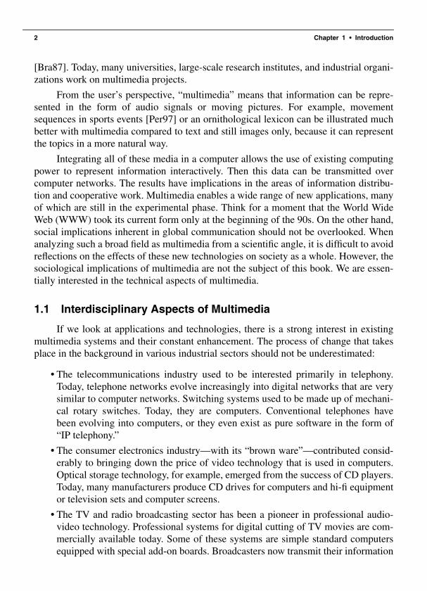
1.1 Interdisciplinary Aspects of Multimedia
If we look at applications and technologies, there is a strong interest in existingmultimedia systems and their constant enhancement. The process of change that takesplace in the background in various industrial sectors should not be underestimated:
• The telecommunications industry used to be interested primarily in telephony.Today, telephone networks evolve increasingly into digital networks that are verysimilar to computer networks. Switching systems used to be made up of mechani-cal rotary switches. Today, they are computers. Conventional telephones havebeen evolving into computers, or they even exist as pure software in the form of“IP telephony.”
• The consumer electronics industry—with its “brown ware”—contributed consid-erably to bringing down the price of video technology that is used in computers.Optical storage technology, for example, emerged from the success of CD players.Today, many manufacturers produce CD drives for computers and hi-fi equipmentor television sets and computer screens.
• The TV and radio broadcasting sector has been a pioneer in professional audio-video technology. Professional systems for digital cutting of TV movies are com-mercially available today. Some of these systems are simple standard computersequipped with special add-on boards. Broadcasters now transmit their information

Contents of This Book 3
over cables so it is only natural that they will continue to become information ven-dors over computer networks in the future.
• Most publishing companies offer publications in electronic form. In addition,many are closely related to movie companies. These two industries have becomeincreasingly active as vendors of multimedia information.
This short list shows that various industries merge to form interdisciplinary ven-dors of multimedia information.
Many hardware and software components in computers have to be properly modi-fied, expanded, or replaced to support multimedia applications. Considering that theperformance of processors increases constantly, storage media have sufficient capaci-ties, and communication systems offer increasingly better quality, the overall function-ality shifts more and more from hardware to software. From a technical viewpoint, thetime restrictions in data processing imposed on all components represent one of themost important challenges. Real-time systems are expected to work within well-definedtime limits to form fault-tolerant systems, while conventional data processing attemptsto do its job as fast as possible.
For multimedia applications, fault tolerance and speed are not the most criticalaspects because they use both conventional media and audio-video media. The data ofboth media classes needs to get from the source to the destination as fast as possible,i.e., within a well-defined time limit. However, in contrast to real-time systems and con-ventional data processing, the elements of a multimedia application are not independentfrom one another. In other words they do not only have to be integrated, they also haveto be synchronized. This means that in addition to being an integrated system, com-posed of various components from both data types, there has to be some form ofsynchronization between these media.
Our goal is to present the multimedia systems from an integrated and global per-spective. However, as outlined above, multimedia systems include many areas, hencewe have decided to split the content about multimedia system fundamentals into threevolumes. The first volume deals with media coding and content processing. The secondvolume describes media processing and communication. The third volume presents top-ics such as multimedia documents, security, and various applications.
1.2 Contents of This Book
If the word multimedia can have several meanings, there is a risk that the readermight not find what he or she is looking for. As mentioned above, this book is an inte-gral part of a three-volume work on “Multimedia Fundamentals.” Let us start by defin-ing the scope of this first volume.
The primary objective of the book is to provide a comprehensive panorama of top-ics in the area of multimedia coding and content processing. It is structured as a refer-

4 Chapter 1 • Introduction
ence book to provide fast familiarization with all the issues concerned. However, thisbook can also be used as a textbook for introductory multimedia courses. Many sec-tions of this book explain the close relationships of the wide range of components thatmake up multimedia coding, compression, optical storage, and content processing in amultimedia system.
1.3 Organization of This Book
The overall goal is to present a comprehensive and practical view of multimediatechnologies. Multimedia fundamentals can be divided as shown in Figure 1-1. We willpresent material about the most important multimedia fields in these volumes. Theoverall organization attempts to explain the largest dependencies between the compo-nents involved in terms of space and time. We distinguish between:
• Basics: In addition to the computer architecture for multimedia systems, one ofthe most important aspects is a media-specific consideration.
• Systems: This section covers system aspects relating to processing, storage, andcommunication and the relevant interfaces.
• Services: This section details single functions, which are normally implementedthrough individual system components.
• Usage: This section studies the type and design of applications and the interfacebetween users and computer systems.
In this volume, we will present the basics of multimedia, concentrating on media-specific considerations such as individual media characteristics and media compres-sion, and their dependencies on optical storage, content analysis, and processing.
Techniques like the sampling theorem or Pulse Code Modulation (PCM), dis-cussed in a later chapter, with their respective mathematical background and practicalimplementations form the basis for digital audio-video data processing. Several tech-niques have evolved from these basics, each specialized for a specific medium. Audiotechnology includes music and voice processing. The understanding of video technol-ogy is essentially based on the development of digital TV technology, involving singlepictures and animation. As demand on quality and availability of technologiesincreases, these media have high data rates, so that appropriate compression methodsare necessary. Such methods can be implemented both by hardware and software. Fur-thermore, the high demand on quality and availability of multimedia technology hasalso placed heavy demands on optical storage systems to satisfy their requirements. Asstorage capacity and availability of other resources increase, content analysis is becom-ing an integral part of our multimedia systems and applications.

Organization of This Book 5
Figure 1-1 The most important multimedia fields, as discussed in this book.
1.3.1 Media Characteristics and Coding
The section on media characteristics and coding will cover areas such as soundcharacteristics with discussion of music and the MIDI standard, speech recognition andtransmission, graphics and image coding characteristics. It will also include presenta-tion of image processing methods and a video technology overview with particularemphasis on new TV formats such as HDTV. In addition to the basic multimedia datasuch as audio, graphics, images, and video, we present basic concepts for animationdata and its handling within multimedia systems.
1.3.2 Media Compression
As the demand for high-quality multimedia systems increases, the amount ofmedia to be processed, stored, and communicated increases. To reduce the amount ofdata, compression techniques for multimedia data are necessary. We present basic con-cepts of entropy and source compression techniques such as Huffman Coding or DeltaModulation, as well as hybrid video compression techniques such as MPEG-4 orH.263. In addition to the basic concepts of video compression, we discuss image andaudio compression algorithms, which are of great importance to multimedia systems.
Usa
ge
Applications
Learning Design User Interface
Serv
ices Content
Analysis Documents Security ... Synchro-nization
GroupCommunication
Syst
ems
Databases Programming
Media Server Operating Systems Communication
Optical Storage Quality of Service Networks
Bas
ics
ComputerArchitecture
Compression
Graphics &Images Animation Video Audio

6 Chapter 1 • Introduction
1.3.3 Optical Storage
Optical storage media offer much higher storage density at lower cost than tradi-tional secondary storage media. We will describe various successful technologies thatare the successors of long-playing records, such as audio compact discs and digitalaudio tapes. Understanding the basic concepts such as pits and lands in the substratelayers, modulation and error handling on CD-DA, and modes on CD-ROM, is neces-sary in order to understand the needs of media servers, disk management, and othercomponents in multimedia systems.
1.3.4 Content Processing
Coding and storage directly or indirectly influence the processing and analysis ofmultimedia content in various documents. In recent years, due to the World Wide Web,we are experiencing wide distribution of multimedia documents and requests for multi-media information filtering tools using text recognition, image recognition, speech rec-ognition, and other multimedia analysis algorithms. This section presents basicconcepts of content analysis, such as similarity-based search algorithms, algorithmsbased on motion vectors and cut detection, and others. Hopefully this will clarify theeffects of content analysis in applications such as television, movies, newscasts, orsports broadcasts.
1.4 Further Reading About Multimedia
Several fields discussed in this book are covered by other books in more detail.For example, multimedia databases are covered in [Mey91], video coding in [Gha99]and in the Handbook of Multimedia Computing [Fur98]. Moreover, the basics of audiotechnology, video technology, image processing, and various network systems arediscussed in specialized papers and books, while this book describes all coding compo-nents involved in the context of integrated multimedia systems.
There is extensive literature on all aspects of multimedia. Some journals that fre-quently publish papers in this area are IEEE Multimedia, IEEE Transaction on Multi-media, Multimedia Systems (ACM Springer), and Multimedia Tools and Applications.Many other journals also publish papers on the subject.
In addition to a large number of national and international workshops in this field,there are several interdisciplinary, international conferences on multimedia systems, inparticular: the ACM Multimedia Conference (the first conference took place in Ana-heim, California, in August 1993), the IEEE Multimedia Conference (first conferenceheld in May 1994), and the European Workshop on Interactive Distributed MultimediaSystems and Telecommunication Services (IDMS).

7
C H A P T E R 2
Media and Data Streams
This chapter provides an introduction to theterminology used in the entire book. We begin with our definition of the term multime-dia as a basis for a discussion of media and key properties of multimedia systems. Next,we will explain data streams and information units used in such systems.
2.1 The Term "Multimedia"
The word multimedia is composed of two parts: the prefix multi and the rootmedia. The prefix multi does not pose any difficulty; it comes from the latin word mul-tus, which means “numerous.” The use of multi as a prefix is not recent and many Latinwords employ it.
The root media has a more complicated story. Media is the plural form of theLatin word medium. Medium is a noun and means “middle, center.”
Today, the term multimedia is often used as an attribute for many systems, compo-nents, products, and concepts that do not meet the key properties we will introduce later(see Section 2.3). This means that the definition introduced in this book is (intention-ally) restrictive in several aspects.
2.2 The Term "Media"
As with most generic words, the meaning of the word media varies with the con-text in which it is used. Our definition of medium is “a means to distribute and representinformation.” Media are, for example, text, graphics, pictures, voice, sound, and music.In this sense, we could just as well add water and the atmosphere to this definition.

8 Chapter 2 • Media and Data Streams
[MHE93] provides a subtle differentiation of various aspects of this term by use ofvarious criteria to distinguish between perception, representation, presentation, storage,transmission, and information exchange media. The following sections describe theseattributes.
2.2.1 Perception Media
Perception media refers to the nature of information perceived by humans, whichis not strictly identical to the sense that is stimulated. For example, a still image and amovie convey information of a different nature, though stimulating the same sense. Thequestion to ask here is: How do humans perceive information?
In this context, we distinguish primarily between what we see and what we hear.Auditory media include music, sound, and voice. Visual media include text, graphics,and still and moving pictures. This differentiation can be further refined. For example, avisual medium can consist of moving pictures, animation, and text. In turn, movingpictures normally consist of a series of scenes that, in turn, are composed of singlepictures.
2.2.2 Representation Media
The term representation media refers to how information is represented internallyto the computer. The encoding used is of essential importance. The question to ask hereis: How is information encoded in the computer? There are several options:
• Each character of a piece of text is encoded in ASCII.• A picture is encoded by the CEPT or CAPTAIN standard, or the GKS graphics
standard can serve as a basis.• An audio data stream is available in simple PCM encoding and a linear quantiza-
tion of 16 bits per sampling value.• A single image is encoded as Group-3 facsimile or in JPEG format.• A combined audio-video sequence is stored in the computer in various TV stan-
dards (e.g., PAL, SECAM, or NTSC), in the CCIR-601 standard, or in MPEGformat.
2.2.3 Presentation Media
The term presentation media refers to the physical means used by systems toreproduce information for humans. For example, a TV set uses a cathode-ray tube andloudspeaker. The question to ask here is: Which medium is used to output informationfrom the computer or input in the computer?
We distinguish primarily between output and input. Media such as paper, com-puter monitors, and loudspeakers are output media, while keyboards, cameras, andmicrophones are input media.

The Term "Media" 9
2.2.4 Storage Media
The term storage media is often used in computing to refer to various physicalmeans for storing computer data, such as magnetic tapes, magnetic disks, or digitaloptical disks. However, data storage is not limited to the components available in acomputer, which means that paper is also considered a storage medium. The question toask here is: Where is information stored?
2.2.5 Transmission Media
The term transmission media refers to the physical means—cables of varioustypes, radio tower, satellite, or ether (the medium that transmit radio waves)—thatallow the transmission of telecommunication signals. The question to ask here is:Which medium is used to transmit data?
2.2.6 Information Exchange Media
Information exchange media include all data media used to transport information,e.g., all storage and transmission media. The question to ask here is: Which datamedium is used to exchange information between different locations?
For example, information can be exchanged by storing it on a removable mediumand transporting the medium from one location to another. These storage media includemicrofilms, paper, and floppy disks. Information can also be exchanged directly, iftransmission media such as coaxial cables, optical fibers, or radio waves are used.
2.2.7 Presentation Spaces and Presentation Values
The terms described above serve as a basis to characterize the term medium in theinformation processing context. The description of perception media is closest to ourdefinition of media: those media concerned mainly with the human senses. Eachmedium defines presentation values in presentation spaces [HD90, SH91], whichaddress our five senses.
Paper or computer monitors are examples of visual presentation spaces. A com-puter-controlled slide show that projects a screen’s content over the entire projectionscreen is a visual presentation space. Stereophony and quadrophony define acousticpresentation spaces. Presentation spaces are part of the above-described presentationmedia used to output information.
Presentation values determine how information from various media is repre-sented. While text is a medium that represents a sentence visually as a sequence ofcharacters, voice is a medium that represents information acoustically in the form ofpressure waves. In some media, the presentation values cannot be interpreted correctlyby humans. Examples include temperature, taste, and smell. Other media require a
10 Chapter 2 • Media and Data Streams
predefined set of symbols we have to learn to be able to understand this information.This class includes text, voice, and gestures.
Presentation values can be available as a continuous sequence or as a sequence ofsingle values. Fluctuations in pressure waves do not occur as single values; they defineacoustic signals. Electromagnetic waves in the range perceived by the human eye arenot scanned with regard to time, which means that they form a continuum. The charac-ters of a piece of text and the sampling values of an audio signal are sequences com-posed of single values.
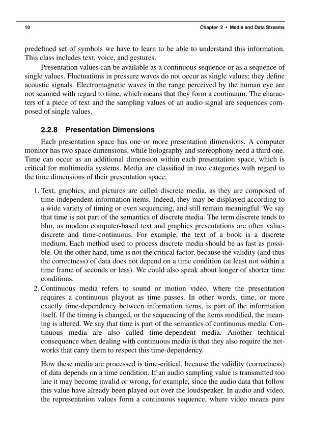
2.2.8 Presentation Dimensions
Each presentation space has one or more presentation dimensions. A computermonitor has two space dimensions, while holography and stereophony need a third one.Time can occur as an additional dimension within each presentation space, which iscritical for multimedia systems. Media are classified in two categories with regard tothe time dimensions of their presentation space:
1. Text, graphics, and pictures are called discrete media, as they are composed oftime-independent information items. Indeed, they may be displayed according toa wide variety of timing or even sequencing, and still remain meaningful. We saythat time is not part of the semantics of discrete media. The term discrete tends toblur, as modern computer-based text and graphics presentations are often value-discrete and time-continuous. For example, the text of a book is a discretemedium. Each method used to process discrete media should be as fast as possi-ble. On the other hand, time is not the critical factor, because the validity (and thusthe correctness) of data does not depend on a time condition (at least not within atime frame of seconds or less). We could also speak about longer of shorter timeconditions.
2. Continuous media refers to sound or motion video, where the presentationrequires a continuous playout as time passes. In other words, time, or moreexactly time-dependency between information items, is part of the informationitself. If the timing is changed, or the sequencing of the items modified, the mean-ing is altered. We say that time is part of the semantics of continuous media. Con-tinuous media are also called time-dependent media. Another technicalconsequence when dealing with continuous media is that they also require the net-works that carry them to respect this time-dependency.
How these media are processed is time-critical, because the validity (correctness)of data depends on a time condition. If an audio sampling value is transmitted toolate it may become invalid or wrong, for example, since the audio data that followthis value have already been played out over the loudspeaker. In audio and video,the representation values form a continuous sequence, where video means pure

Key Properties of a Multimedia System 11
moving images. A combination of audio and moving images, like in television ormovies, is not synonymous with the term video. For this reason, they are calledcontinuous media. When time-dependent representation values that occur aperi-odically are distinguished, they are often not put under the continuous media cate-gory. For a multimedia system, we also have to consider such non-continuoussequences of representation values. This type of representation-value sequenceoccurs when information is captured by use of a pointer (e.g., a mouse) and trans-mitted within cooperative applications using a common screen window. Here, thecontinuous medium and time-dependent medium are synonymous. By this defini-tion, continuous media are video (moving images) of natural or artificial origin,audio, which is normally stored as a sequence of digitized pressure-wave samples,and signals from various sensors, such as air pressure, temperature, humidity,pressure, or radioactivity sensors.
The terms that describe a temporally discrete or continuous medium do not referto the internal data representation, for example, in the way the term representationmedium has been introduced. They refer to the impression that the viewer or auditorgets. The example of a movie shows that continuous-media data often consist of asequence of discrete values, which follow one another within the representation spaceas a function of time. In this example, a sequence of at least 16 single images per sec-ond gives the impression of continuity, which is due to the perceptual mechanisms ofthe human eye.
Based on word components, we could call any system a multimedia system thatsupports more than one medium. However, this characterization falls short as it pro-vides only a quantitative evaluation. Each system could be classified as a multimediasystem that processes both text and graphics media. Such systems have been availablefor quite some time, so that they would not justify the newly coined term. The termmultimedia is more of a qualitative than a quantitative nature.
As defined in [SRR90, SH91], the number of supported media is less decisive thanthe type of supported media for a multimedia system to live up to its name. Note thatthere is controversy about this definition. Even standardization bodies normally use acoarser interpretation.
2.3 Key Properties of a Multimedia SystemMultimedia systems involve several fundamental notions. They must be
computer-controlled. Thus, a computer must be involved at least in the presentation ofthe information to the user. They are integrated, that is, they use a minimal number ofdifferent devices. An example is the use of a single computer screen to display all typesof visual information. They must support media independence. And lastly, they need tohandle discrete and continuous media. The following sections describe these keyproperties.
12 Chapter 2 • Media and Data Streams
2.3.1 Discrete and Continuous Media
Not just any arbitrary combination of media deserves the name multimedia. Manypeople call a simple word processor that handles embedded graphics a multimediaapplication because it uses two media. By our definition, we talk about multimedia ifthe application uses both discrete and continuous media. This means that a multimediaapplication should process at least one discrete and one continuous medium. A wordprocessor with embedded graphics is not a multimedia application by our definition.
2.3.2 Independent Media
An important aspect is that the media used in a multimedia system should be inde-pendent. Although a computer-controlled video recorder handles audio and movingimage information, there is a temporal dependence between the audio part and thevideo part. In contrast, a system that combines signals recorded on a DAT (DigitalAudio Tape) recorder with some text stored in a computer to create a presentation meetsthe independence criterion. Other examples are combined text and graphics blocks,which can be in an arbitrary space arrangement in relation to one another.
2.3.3 Computer-Controlled Systems
The independence of media creates a way to combine media in an arbitrary formfor presentation. For this purpose, the computer is the ideal tool. That is, we need a sys-tem capable of processing media in a computer-controlled way. The system can beoptionally programmed by a system programmer and/or by a user (within certain lim-its). The simple recording or playout of various media in a system, such as a videorecorder, is not sufficient to meet the computer-control criterion.
2.3.4 Integration
Computer-controlled independent media streams can be integrated to form a glo-bal system so that, together, they provide a certain function. To this end, synchronicrelationships of time, space, and content are created between them. A word processorthat supports text, spreadsheets, and graphics does not meet the integration criterionunless it allows program-supported references between the data. We achieve a highdegree of integration only if the application is capable of, for example, updating graph-ics and text elements automatically as soon as the contents of the related spreadsheetcell changes.
This kind of flexible media handling is not a matter to be taken for granted—evenin many products sold under the multimedia system label. This aspect is importantwhen talking of integrated multimedia systems. Simply speaking, such systems shouldallow us to do with moving images and sound what we can do with text and graphics[AGH90]. While conventional systems can send a text message to another user, a highly

Characterizing Data Streams 13
integrated multimedia system provides this function and support for voice messages ora voice-text combination.
2.3.5 Summary
Several properties that help define the term multimedia have been described,where the media are of central significance. This book describes networked multimediasystems. This is important as almost all modern computers are connected to communi-cation networks. If we study multimedia functions from a local computer’s perspective,we take a step backwards. Also, distributed environments offer the most interestingmultimedia applications as they enable us not only to create, process, represent, andstore multimedia information, but to exchange them beyond the limits of ourcomputers.
Finally, continuous media require a changing set of data in terms of time, that is, adata stream. The following section discusses data streams.
2.4 Characterizing Data Streams
Distributed networked multimedia systems transmit both discrete and continuousmedia streams, i.e., they exchange information. In a digital system, information is splitinto units (packets) before it is transmitted. These packets are sent by one system com-ponent (the source) and received by another one (the sink). Source and sink can resideon different computers. A data stream consists of a (temporal) sequence of packets.This means that it has a time component and a lifetime.
Packets can carry information from continuous and discrete media. The transmis-sion of voice in a telephone system is an example of a continuous medium. When wetransmit a text file, we create a data stream that represents a discrete medium.
When we transmit information originating from various media, we obtain datastreams that have very different characteristics. The attributes asynchronous, synchro-nous, and isochronous are traditionally used in the field of telecommunications todescribe the characteristics of a data transmission. For example, they are used in FDDIto describe the set of options available for an end-to-end delay in the transmission ofsingle packets.
2.4.1 Asynchronous Transmission Mode
In the broadest sense of the term, a communication is called asynchronous if asender and receiver do not need to coordinate before data can be transmitted. In asyn-chronous transmission, the transmission may start at any given instant. The bit synchro-nization that determines the start of each bit is provided by two independent clocks, oneat the sender, the other at the receiver. An example of asynchronous transmission is theway in which simple ASCII terminals are usually attached to host computers. Each time

14 Chapter 2 • Media and Data Streams
the character “A” is pressed, a sequence of bits is generated at a preset speed. To informthe computer interface that a character is arriving, a special signal called the start sig-nal—which is not necessarily a bit—precedes the information bits. Likewise, anotherspecial signal, the stop signal, follows the last information bit.
2.4.2 Synchronous Transmission Mode
The term synchronous refers to the relationship of two or more repetitive signalsthat have simultaneous occurrences of significant instants. In synchronous transmis-sion, the beginning of the transmission may only take place at well-defined times,matching a clocking signal that runs the synchronism with that of the receiver. To seewhy clocked transmission is important, consider what might happen to a digitized voicesignal when it is transferred across a nonsynchronized network. As more traffic entersthe network, the transmission of a given signal may experience increased delay. Thus, adata stream moving across a network might slow down temporarily when other trafficenters the network and then speed up again when the traffic subsides. If audio from adigitized phone call is delayed, however, the human listening to the call will hear thedelay as annoying interference or noise. Once a receiver starts to play digitized samplesthat arrive late, the receiver cannot speed up the playback to catch up with the rest of thestream.
2.4.3 Isochronous Transmission Mode
The term isochronous refers to a periodic signal, pertaining to transmission inwhich the time interval separating any two corresponding transitions is equal to the unitinterval or to a multiple of the unit interval. Secondly, it refers to data transmission inwhich corresponding significant instants of two or more sequential signals have a con-stant phase relationship. This mode is a form of data transmission in which individualcharacters are only separated by a whole number of bit-length intervals, in contrast toasynchronous transmission, in which the characters may be separated by random-lengthintervals. For example, an end-to-end network connection is said to be isochronous ifthe bit rate over the connection is guaranteed and if the value of the delay jitter is alsoguaranteed and small. The notion of isochronism serves to describe what the perfor-mance of a network should be in order to satisfactorily transport continuous mediastreams, such as real-time audio or motion video. What is required to transport audioand video in real time? If the source transmits bits at a certain rate, the network shouldbe able to meet that rate in a sustained way.
These three attributes are a simplified classification of different types of datastreams. The following sections describe other key properties.
Characterizing Continuous Media Data Streams 15
2.5 Characterizing Continuous Media Data Streams
This section provides a summary of the characteristics for data streams that occurin multimedia systems in relation to audio and video transmissions. The descriptionincludes effects of compression methods applied to the data streams before they aretransmitted. This classification applies to distributed and local environments.
2.5.1 Strongly and Weakly Periodic Data Streams
The first property of data streams relates to the time intervals between fully com-pleted transmissions of consecutive information units or packets. Based on the momentin which the packets become ready, we distinguish between the following variants:
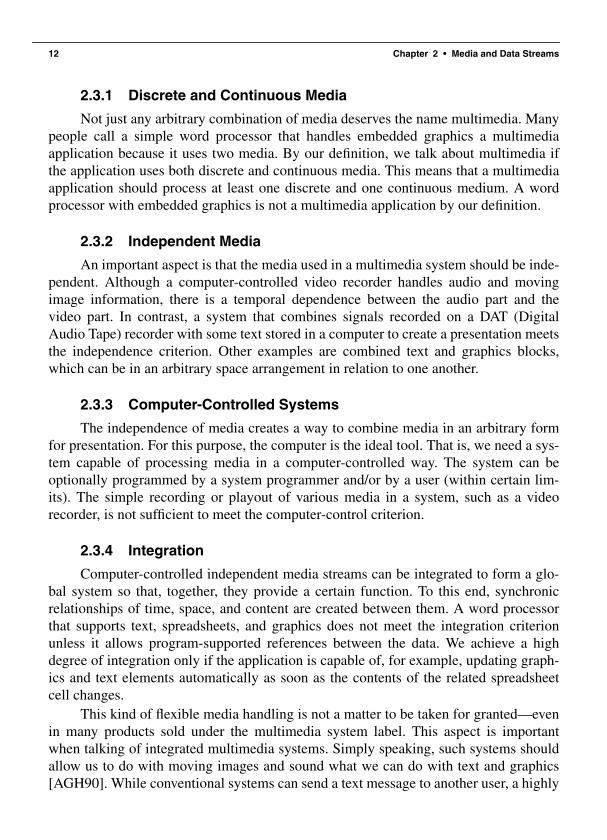
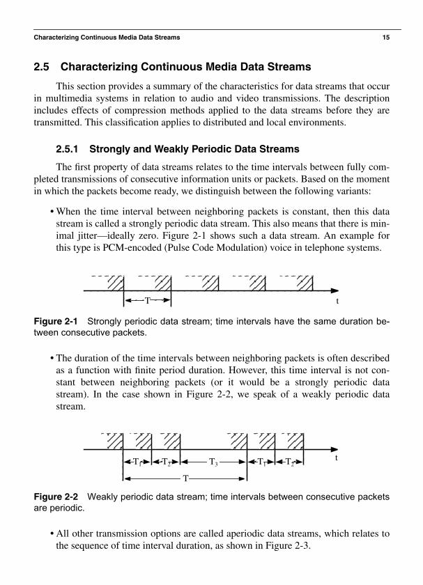
• When the time interval between neighboring packets is constant, then this datastream is called a strongly periodic data stream. This also means that there is min-imal jitter—ideally zero. Figure 2-1 shows such a data stream. An example forthis type is PCM-encoded (Pulse Code Modulation) voice in telephone systems.
Figure 2-1 Strongly periodic data stream; time intervals have the same duration be-tween consecutive packets.
• The duration of the time intervals between neighboring packets is often describedas a function with finite period duration. However, this time interval is not con-stant between neighboring packets (or it would be a strongly periodic datastream). In the case shown in Figure 2-2, we speak of a weakly periodic datastream.
Figure 2-2 Weakly periodic data stream; time intervals between consecutive packetsare periodic.
• All other transmission options are called aperiodic data streams, which relates tothe sequence of time interval duration, as shown in Figure 2-3.
T t
T
tT1 T2 T3 T1 T2

16 Chapter 2 • Media and Data Streams
Figure 2-3 Aperiodic data stream; the time interval sequence is neither constant norweakly periodic.
An example of an aperiodic data stream is a multimedia conference applicationwith a common screen window. Often, the status (left button pressed) and the currentcoordinates of the mouse moved by another user have to be transmitted to other partici-pants. If this information were transmitted periodically, it would cause a high data rateand an extremely high redundancy. The ideal system should transmit only data withinthe active session that reflect a change in either position or status.
2.5.2 Variation of the Data Volume of Consecutive Information Units
A second characteristic to qualify data streams concerns how the data quantity ofconsecutive information units or packets varies.
• If the quantity of data remains constant during the entire lifetime of a data stream,then we speak of a strongly regular data stream. Figure 2-4 shows such a datastream. This characteristic is typical for an uncompressed digital audio-videostream. Practical examples are a full-image encoded data stream delivered bycamera or an audio sequence originating from an audio CD.
Figure 2-4 Strongly regular data stream; the data quantity is constant in all packets.
• If the quantity of data varies periodically (over time), then this is a weakly regulardata stream. Figure 2-5 shows an example.
tT1 T2 Tn
t
D1
D1
T
Characterizing Continuous Media Data Streams 17
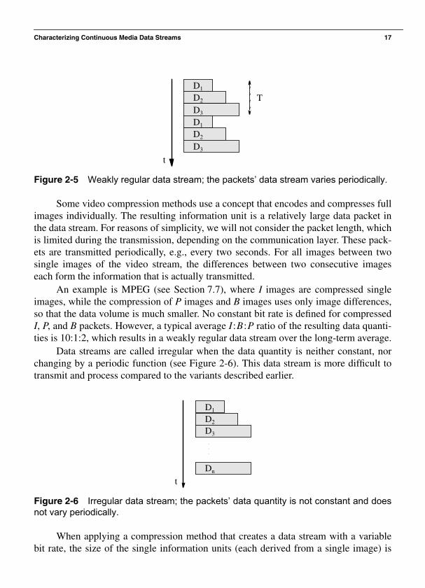
Figure 2-5 Weakly regular data stream; the packets’ data stream varies periodically.
Some video compression methods use a concept that encodes and compresses fullimages individually. The resulting information unit is a relatively large data packet inthe data stream. For reasons of simplicity, we will not consider the packet length, whichis limited during the transmission, depending on the communication layer. These pack-ets are transmitted periodically, e.g., every two seconds. For all images between twosingle images of the video stream, the differences between two consecutive imageseach form the information that is actually transmitted.
An example is MPEG (see Section 7.7), where I images are compressed singleimages, while the compression of P images and B images uses only image differences,so that the data volume is much smaller. No constant bit rate is defined for compressedI, P, and B packets. However, a typical average I:B:P ratio of the resulting data quanti-ties is 10:1:2, which results in a weakly regular data stream over the long-term average.
Data streams are called irregular when the data quantity is neither constant, norchanging by a periodic function (see Figure 2-6). This data stream is more difficult totransmit and process compared to the variants described earlier.
Figure 2-6 Irregular data stream; the packets’ data quantity is not constant and doesnot vary periodically.
When applying a compression method that creates a data stream with a variablebit rate, the size of the single information units (each derived from a single image) is
t
D1
TD2
D3
D1
D2
D3
t
D1
D2
D3
Dn

18 Chapter 2 • Media and Data Streams
determined from the image content that has changed in respect to the previous image.The size of the resulting information units normally depends on the video sequence andthe data stream is irregular.
2.5.3 Interrelationship of Consecutive Packets
The third qualification characteristic concerns the continuity or the relationshipbetween consecutive packets. Are packets transmitted progressively, or is there a gapbetween packets? We can describe this characteristic by looking at how the correspond-ing resource is utilized. One such resource is the network.
• Figure 2-7 shows an interrelated information transfer. All packets are transmittedone after the other without gaps in between. Additional or layer-independentinformation to identify user data is included, e.g., error detection codes. Thismeans that a specific resource is utilized at 100 percent. An interrelated datastream allows maximum throughput and achieves optimum utilization of aresource. An ISDN B channel that transmits audio data at 64Kbit/s is an example.
Figure 2-7 Interrelated data stream; packets are transmitted without gaps in between.
• The transmission of an interrelated data stream over a higher-capacity channelcauses gaps between packets. Each data stream that includes gaps between itsinformation units is called a non-interrelated data stream. Figure 2-8 shows anexample. In this case, it is not important whether or not there are gaps between allpackets or whether the duration of the gaps varies. An example of a non-interrelated data stream is the transmission of a data stream encoded by the DVI-PLV method over an FDDI network. An average bit rate of 1.2Mbit/s leads inher-ently to gaps between some packets in transit.
Figure 2-8 Non-interrelated data stream; there are gaps between packets.
To better understand the characteristics described above, consider the followingexample:
tD1 D2 D3 D4 Dn
D
tD1 D2 D3 Dn
D
Information Units 19
A PAL video signal is sampled by a camera and digitized in a computer. No com-pression is applied. The resulting data stream is strongly periodic, strongly regular, andinterrelated, as shown in Figure 2-4. There are no gaps between packets. If we use theMPEG method for compression, combined with the digitizing process, we obtain aweakly periodic and weakly regular data stream (referring to its longer duration). Andif we assume we use a 16-Mbit/s token-ring network for transmission, our data streamwill also be noninterrelated.
2.6 Information Units
Continuous (time-dependent) media consist of a (temporal) sequence of informa-tion units. Based on Protocol Data Units (PDUs), this section describes such an infor-mation unit, called a Logical Data Unit (LDU). An LDU’s information quantity anddata quantities can have different meanings:
1. Let’s use Joseph Haydn’s symphony, The Bear, as our first example. It consists ofthe four musical movements, vivace assai, allegretto, menuet, and finale vivace.Each movement is an independent, self-sufficient part of this composition. It con-tains a sequence of scores for the musical instruments used. In a digital system,these scores are a sequence of sampling values. We will not use any compressionin this example, but apply PCM encoding with a linear characteristic curve. ForCD-DA quality, this means 44,100 sampling values per second, which areencoded at 16bits per channel. On a CD, these sampling values are grouped intounits with a duration of 1/75 second. We could now look at the entire compositionand define single movements, single scores, the grouped 1/75-s sampling values,or even single sampling values as LDUs. Some operations can be applied to theplayback of the entire composition—as one single LDU. Other functions refer tothe smallest meaningful unit (in this case the scores). In digital signal processing,sampling values are LDUs.
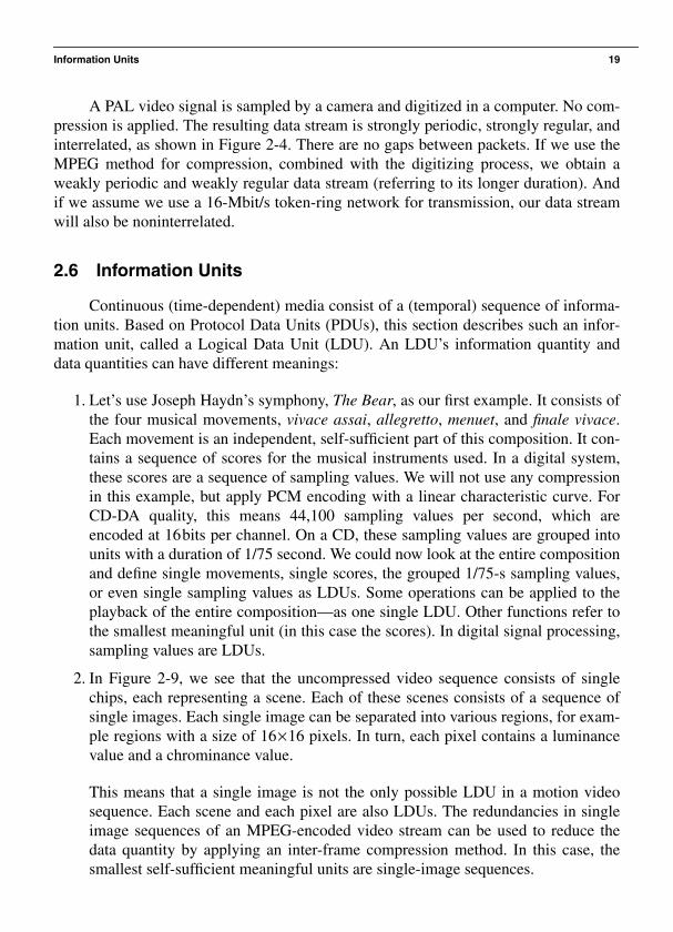
2. In Figure 2-9, we see that the uncompressed video sequence consists of singlechips, each representing a scene. Each of these scenes consists of a sequence ofsingle images. Each single image can be separated into various regions, for exam-ple regions with a size of 16×16 pixels. In turn, each pixel contains a luminancevalue and a chrominance value.
This means that a single image is not the only possible LDU in a motion videosequence. Each scene and each pixel are also LDUs. The redundancies in singleimage sequences of an MPEG-encoded video stream can be used to reduce thedata quantity by applying an inter-frame compression method. In this case, thesmallest self-sufficient meaningful units are single-image sequences.

20 Chapter 2 • Media and Data Streams
Figure 2-9 Granularity of a motion video sequence showing its logical data units(LDUs).
A phenomenon called granularity characterizes the hierarchical decomposition ofan audio or video stream in its components. This example uses a symphony and amotion video to generally describe extensive information units. We distinguish betweenclosed and open LDUs. Closed LDUs have a well-defined duration. They are normallystored sequences. In open LDUs, the data stream’s duration is not known in advance.Such a data stream is delivered to the computer by a camera, a microphone, or a similardevice.
The following chapter builds on these fundamental characteristics of a multimediasystem to describe audio data in more detail, primarily concentrating on voiceprocessing.
Movie
Clip
Frame
Pixel
Grid

21
C H A P T E R 3
Audio Technology
Audiology is the discipline interested in manipu-lating acoustic signals that can be perceived by humans. Important aspects are psychoa-coustics, music, the MIDI (Musical Instrument Digital Interface) standard, and speechsynthesis and analysis. Most multimedia applications use audio in the form of musicand/or speech, and voice communication is of particular significance in distributed mul-timedia applications.
In addition to providing an introduction to basic audio signal technologies and theMIDI standard, this chapter explains various enabling schemes, including speech syn-thesis, speech recognition, and speech transmission [Loy85, Fla72, FS92, Beg94,OS90', Fal85, Bri86, Ace93, Sch92]. In particular, it covers the use of sound, music,and speech in multimedia, for example, formats used in audio technology, and howaudio material is represented in computers [Boo87, Tec89].
Chapter 8 covers storage of audio data (and other media data) on optical disksbecause this technology is not limited to audio signals. The compression methods usedfor audio and video signals are described in Chapter 9 because many methods availablefor different media to encode information are similar.
3.1 What Is Sound?
Sound is a physical phenomenon caused by vibration of material, such as a violinstring or a wood log. This type of vibration triggers pressure wave fluctuations in the airaround the material. The pressure waves propagate in the air. The pattern of this oscilla-tion (see Figure 3-1) is called wave form [Tec89]. We hear a sound when such a wavereaches our ears.

22 Chapter 3 • Audio Technology
Figure 3-1 Pressure wave oscillation in the air.
This wave form occurs repeatedly at regular intervals or periods. Sound waveshave a natural origin, so they are never absolutely uniform or periodic. A sound that hasa recognizable periodicity is referred to as music rather than sound, which does nothave this behavior. Examples of periodic sounds are sounds generated by musicalinstruments, vocal sounds, wind sounds, or a bird’s twitter. Non-periodic sounds are,for example, drums, coughing, sneezing, or the brawl or murmur of water.
3.1.1 Frequency
A sound’s frequency is the reciprocal value of its period. Similarly, the frequencyrepresents the number of periods per second and is measured in hertz (Hz) or cycles persecond (cps). A common abbreviation is kilohertz (kHz), which describes 1,000 oscilla-tions per second, corresponding to 1,000Hz [Boo87].
Sound processes that occur in liquids, gases, and solids are classified by frequencyrange:
• Infrasonic: 0 to 20Hz• Audiosonic: 20Hz to 20kHz• Ultrasonic: 20kHz to 1GHz• Hypersonic: 1GHz to 10THz
Sound in the audiosonic frequency range is primarily important for multimediasystems. In this text, we use audio as a representative medium for all acoustic signals inthis frequency range. The waves in the audiosonic frequency range are also calledacoustic signals [Boo87]. Speech is the signal humans generate by use of their speechorgans. These signals can be reproduced by machines. For example, music signals havefrequencies in the 20Hz to 20kHz range. We could add noise to speech and music asanother type of audio signal. Noise is defined as a sound event without functional pur-pose, but this is not a dogmatic definition. For instance, we could add unintelligible lan-guage to our definition of noise.
+
-
One period
Amplitude
Time
Air
pre
ssur
e

What Is Sound? 23
3.1.2 Amplitude
A sound has a property called amplitude, which humans perceive subjectively asloudness or volume. The amplitude of a sound is a measuring unit used to deviate thepressure wave from its mean value (idle state).
3.1.3 Sound Perception and Psychoacoustics
The way humans perceive sound can be summarized as a sequence of events:Sound enters the ear canal. At the eardrum, sound energy (air pressure changes) aretransformed into mechanical energy of eardrum movement. The outer ear comprises thepinna, which is composed of cartilage and has a relatively poor blood supply. Its pres-ence on both sides of the head allows us to localize the source of sound from the frontversus the back. Our ability to localize from side to side depends on the relative inten-sity and relative phase of sound reaching each ear and the analysis of the phase/inten-sity differences within the brainstem. The cochlea is a snail-shaped structure that is thesensory organ of hearing. The vibrational patterns that are initiated by vibration set up atraveling wave pattern within the cochlea. This wavelike pattern causes a shearing ofthe cilia of the outer and inner hair cells. This shearing causes hair cell depolarizationresulting in on/off neural impulses that the brain interprets as sound.
Psychoacoustics is a discipline that studies the relationship between acousticwaves at the auditory ossicle and the spatial recognition of the auditor. We distinguishbetween two main perspectives, described briefly in the following sections.
3.1.3.1 The Physical Acoustic Perspective
Figure 3-2 is a simplified schematic representation of an auditor who perceivessound. Sound from a sound source diffuses in concentric pressures waves. The positionof the source can be described by the distance to the center of the auditor’s head and bytwo angles: one in the horizontal and one on the vertical level. It is obvious that soundwaves originating from a source arranged on the right side of the auditor reaches theright ear earlier than the left one. The time difference of sound waves reaching the earsis called interaural time difference (ITD). If a sound source prevails almost totally onone side, i.e., at an angle of 90 degrees from the auditor, then ITD reaches a maximumof approximately 0.7ms to 0.8ms. If the sound source is close, i.e., if the distancebetween the source and the auditor is very short, then the interaural intensity difference(IID) differs significantly from zero. These two characteristics of sound waves arrivingat the ear can be measured and described and represent the basis for spatial recognition[Ken95].

24 Chapter 3 • Audio Technology
Figure 3-2 The basics of sound perception.
An important property of the basic hearing process can be determined in the fre-quency range. When sound waves reach the auditor’s ear, they change due to the inter-action between the original wave and the auditor’s body. For example, in the 3-kHzrange, there is a strong resonance in the perception of size caused by the resonance inthe hearing canal. These properties can be measured and documented as a head-relatedtransfer function (HRTF) [Bla74, GM94]. Since the interaction between the soundwaves and the auditor’s body is complex, it generates a strong dependence on the hori-zontal and vertical angles, in which the sound source is arranged.
Another important aspect in spatial sound recognition is the physical acoustics ofnatural sounds. Similarly to all systems based on the wave model, the laws of reflection,refraction, and dispersion apply to the longitudinal diffusion of sound waves in air(these waves reach a speed of 344m/s). In a closed room, each surface reflects soundwaves. All waves will eventually reach the human ear, reflected many times on the wayfrom the sound source to the ear. Sound that reaches the ear directly includes informa-tion about the horizontal and vertical angles of the sound source. Other waves, derivedfrom direct waves, arrive later and provide additional information about the room’sproperties. The relationship between direct and derived waves can be used to get anidea about the distance between source and auditor. This allows us to expand and applybasic localization rules to moving sound sources or auditors. To achieve this expansion,we measure the sound speed, which is also called the doubling effect. The sound spec-trum of a sound source moving towards an auditor drifts upwards, while the sourcespectrum moving away from an auditor drifts downwards. It is not difficult to determinethis effect; an everyday example is when we are passed by a piercing ambulance siren.
Angle Sound source

What Is Sound? 25
3.1.3.2 The Psychoacoustic Perspective
One of the fundamental properties of humans’ spatial hearing perception is the so-called first wave-front law. This law says that an auditor’s judgment about the directionof an acoustic event is primarily influenced by the sound that takes the shortest andmost direct way. In a test environment [Bla71], a listener was seated in front of twoloudspeakers of identical make. Although both issued sound at the same amplitude, thelistener localized it stronger on the right side, because the left loudspeaker transmittedwith a delay of approximately 15 ms. When the delay exceeded 50ms, the listener per-ceived two different sound events from the left and right loudspeakers. To compensatefor the effect produced by this delay, we can increase the amplitude of the delayedchannel (Haas effect).
As with all human perception channels, the ear’s cochlea transforms stimulationlogarithmically. The size of a sound pressure level (SPL) is measured in decibels. Anaudibility threshold value of 20 microPascal is the limit value above which a sound canjust about be perceived. This value functions as a basis of the sound pressure, measuredin decibels. The dynamic range of the ear’s sound recognition is in the range of up to130dB.
Table 3-1 Various sound pressure examples.
The perception sensitivity we call loudness is not linear across all frequencies andintensities. The Fletcher-Munson graphics (of 1933) show the sound intensity requiredto enable the perception of constant loudness. Human sound perception is most sensi-tive in the mean frequency ranges between 700Hz and approximately 6,600Hz. Theequal loudness curves of Fletcher and Munson (see Figure 3-3) show that the humanhearing system responds much better to the mean frequency range than it does to lowand very high frequencies.
Sound example Sound pressure size
Rustling of paper 20 dB
Spoken language 60 dB
Heavy road traffic 80 dB
Rock band 120 dB
Pain sensitivity threshold 130 dB
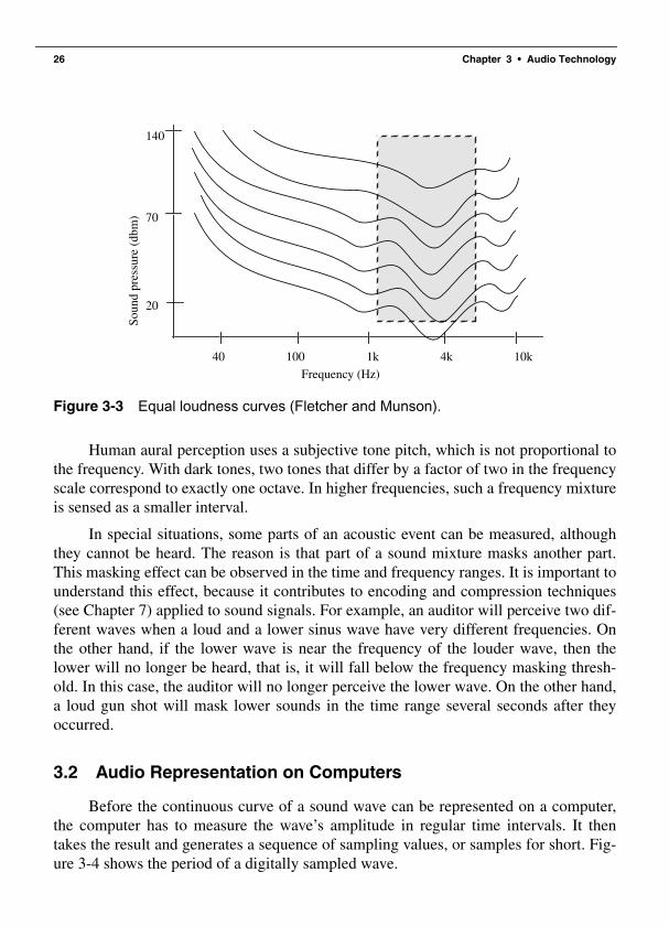
26 Chapter 3 • Audio Technology
Figure 3-3 Equal loudness curves (Fletcher and Munson).
Human aural perception uses a subjective tone pitch, which is not proportional tothe frequency. With dark tones, two tones that differ by a factor of two in the frequencyscale correspond to exactly one octave. In higher frequencies, such a frequency mixtureis sensed as a smaller interval.
In special situations, some parts of an acoustic event can be measured, althoughthey cannot be heard. The reason is that part of a sound mixture masks another part.This masking effect can be observed in the time and frequency ranges. It is important tounderstand this effect, because it contributes to encoding and compression techniques(see Chapter 7) applied to sound signals. For example, an auditor will perceive two dif-ferent waves when a loud and a lower sinus wave have very different frequencies. Onthe other hand, if the lower wave is near the frequency of the louder wave, then thelower will no longer be heard, that is, it will fall below the frequency masking thresh-old. In this case, the auditor will no longer perceive the lower wave. On the other hand,a loud gun shot will mask lower sounds in the time range several seconds after theyoccurred.
3.2 Audio Representation on Computers
Before the continuous curve of a sound wave can be represented on a computer,the computer has to measure the wave’s amplitude in regular time intervals. It thentakes the result and generates a sequence of sampling values, or samples for short. Fig-ure 3-4 shows the period of a digitally sampled wave.
40 100 1k 4k 10k
Frequency (Hz)
Soun
d pr
essu
re (
dbm
)
20
70
140

Audio Representation on Computers 27
Figure 3-4 Sampling a wave.
The mechanism that converts an audio signal into a sequence of digital samples iscalled an analog-to-digital converter (ADC) and a digital-to-analog converter (DAC) isused to achieve the opposite conversion.
3.2.1 Sampling RateThe rate at which a continuous wave form is sampled (see Figure 3-4) is called the
sampling rate. Like frequency, the sampling rate is measured in Hz. For example, CDsare sampled at a rate of 44,100 Hz, which may appear to be above the frequency rangeperceived by humans. However, the bandwidth—in this case, 20,000Hz–20Hz =19,980Hz—that can represent a digitally sampled audio signal is only about half as bigas a CD's sampling rate, because CDs use the Nyquist sampling theorem. This meansthat a sampling rate of 44,100Hz covers only frequencies in the range from 0Hz to22,050Hz. This limit is very close to the human hearing capability.
3.2.2 QuantizationThe digitization process requires two steps. First the analog signal must be sam-
pled. This means that only a discrete set of values is retained at (generally regular) timeor space intervals. The second step involves quantization. The quantization processconsists of converting a sampled signal into a signal that can take only a limited numberof values. An 8-bit quantization provides 256 possible values, while a 16-bit quantiza-tion in CD quality results in more than 65,536 possible values. Figure 3-5 shows a 3-bitquantization.
+
-
0
Sam
plin
g va
lue
Samples
Time

28 Chapter 3 • Audio Technology
Figure 3-5 3-bit quantization.
The values transformed by a 3-bit quantization process can accept eight differentcharacteristics: 0.75, 0.5, 0.25, 0, -0.25, -0.5, -0.75, and -1, so that we obtain an“angular-shape” wave. This means that the lower the quantization (in bits), the more theresulting sound quality deteriorates.
3.3 Three-Dimensional Sound Projection
The invention of loudspeakers in the 1920s had roughly the same effect on audioprocessing as the first light bulb did on everyday life. Suddenly, it was possible to playsounds in any kind of room. The first sound playback before an auditorium can be com-pared to the first movies. After some experimentation time with various sets of loud-speakers, it was found that the use of a two-channel sound (stereo) produces the besthearing effect for most people. Among the large number of home applications that havebeen developed over the years—for example, radio or music records—there were alsomovie systems and modern music components using a larger number of loudspeakers[Cho71] to better control spatial sound effects. Current multimedia and virtual-realityimplementations that include such components show a considerable concentration onspatial sound effects and three-dimensional sound projections [Beg94].
3.3.1 Spatial Sound
Figure 3-6 shows schematically how an auditor perceives three-dimensional spa-tial sound in a closed room. As an expansion of Figure 3-2, the walls and other objectsin a room absorb and reflect the sound’s dispersion paths.
0
0.75
0.5
0.25
-0.25
-0.5
-0.75
Sam
plin
g va
lue
Samples

Three-Dimensional Sound Projection 29
Figure 3-6 Sound dispersion in a closed room.
The shortest path between the sound source and the auditor is called the directsound path (bold line in Figure 3-6). This path carries the first sound waves towards theauditor’s head. All other sound paths are reflected, which means that they are tempo-rally delayed before they arrive at the auditor’s ear. These delays are related to the geo-metric length of the sound paths inside the room and they usually occur because thereflecting sound path is longer than the direct one [Ken95].
Figure 3-7 Pulse response in a closed room.
Figure 3-7 shows the energy of a sound wave arriving at an auditor’s ear as a func-tion over time. The source’s sound stimulus has a pulse form (e.g., like a gun shot), sothat the energy of the direct sound path appears as a large swing in the figure. Thisswing is called the pulse response. All subsequent parts of the pulse response refer toreflecting sound paths. Very early reflections belong to the group of paths that arereflected only once. This sound path group can occur in almost all natural environments
h(t)
t
Direct sound path
First and early reflections
Subsequent and dispersed echoes

30 Chapter 3 • Audio Technology
where echoes occur. Subsequent and dispersed echoes represent a bundle of soundpaths that have been reflected several times. These paths cannot be isolated in the pulseresponse because the pulse is diffuse and diverted both in the time and in the frequencyrange. All sound paths leading to the human ear are additionally influenced by the audi-tor’s individual HRTF (head-related transfer function). HRTF is a function of the path’sdirection (horizontal and vertical angles) to the auditor (see also Figure 3-2). A soundprojection that considers HRTF for each sound path, for example by use of headphones,is also called binaural stereophony [KDS95].
3.3.2 Reflection SystemsSpatial sound systems are used in many different applications, and each of them
has different requirements. A rough classification (see Table 3-2) groups these applica-tions into a scientific and a consumer-oriented approach. In general, the scientificapproach (simulation) is more common than consumer-oriented (imitation).
Table 3-2 Reflection system applications.
The scientific approach uses simulation options that enable professionals such asarchitects to predict the acoustics of a room when they plan a building on the basis ofCAD models [Vor89, KDS95]. The calculations required to generate a pulse responseof a hearing situation based on the database of a CAD model are complex, and normallyonly experts hear the results output by such systems. Consumer systems concentratemainly on applications that create a spatial or a virtual environment. In cinemas, forexample, a special multi-channel sound technique is used to create special soundeffects. In modern pop music, special echo processes based on signal feedback algo-rithms are used [Moo79] to perfect the sound of recorded clips. Modern multimediaenvironments use both approaches [JLW95]. Special interactive environments forimages and computer games, including sound or modern art projects, can be imple-mented, but in order to create a spatial sound, they require state-of-the-art technologies.
3.4 Music and the MIDI StandardWe know from previous sections that any sound can be represented as a digitized
sound signal that is a sequence of samples, each encoded with binary digits. Thissequence may be uncompressed as on audio compact disks, or compressed. We also
Approach Attribute Applications
scientific simulation, precise, complex,offline
research, architecture,computer music
consumer-oriented imitation, unprecise, impressive,real-time
cinema, music, home movies,computer games

Music and the MIDI Standard 31
know that any sound may be represented in that way, including music. A characteristicof this representation mode is that it does not preserve the sound’s semantic description.Unless complex recognition techniques are used, the computer does not know whethera bit sequence represents speech or music, for example, and if music what notes areused and by which instrument.
Music can be described in a symbolic way. On paper, we have the full scores.Computers and electronic musical instruments use a similar technique, and most ofthem employ the Musical Instrument Digital Interface (MIDI), a standard developed inthe early 1980s. The MIDI standard defines how to code all the elements of musicalscores, such as sequences of notes, timing conditions, and the instrument to play eachnote.
3.4.1 Introduction to MIDI
MIDI represents a set of specifications used in instrument development so thatinstruments from different manufacturers can easily exchange musical information[Loy85]. The MIDI protocol is an entire music description language in binary form.Each word describing an action of a musical performance is assigned a specific binarycode. A MIDI interface is composed of two different components:
• Hardware to connect the equipment. MIDI hardware specifies the physical con-nection of musical instruments. It adds a MIDI port to an instrument, it specifies aMIDI cable (that connects two instruments), and processes electrical signalsreceived over the cable.
• A data format that encodes information to be processed by the hardware. TheMIDI data format does not include the encoding of individual sampling values,such as audio data formats. Instead, MIDI uses a specific data format for eachinstrument, describing things like the start and end of scores, the basis frequency,and loudness, in addition to the instrument itself.
The MIDI data format is digital and data are grouped into MIDI messages. Whena musician plays a key, the MIDI interface generates a MIDI message that defines thestart of each score and its intensity. This message is transmitted to machines connectedto the system. As soon as the musician releases the key, another signal (MIDI message)is created and transmitted.
3.4.2 MIDI Devices
An instrument that complies with both components defined by the MIDI standardis a MIDI device (e.g., a synthesizer) able to communicate with other MIDI devicesover channels. The MIDI standard specifies 16 channels. A MIDI device is mappedonto a channel. Musical data transmitted over a channel are reproduced in the synthe-sizer at the receiver’s end. The MIDI standard identifies 128 instruments by means of

32 Chapter 3 • Audio Technology
numbers, including noise effects (e.g., a phone ringing or an airplane take-off). Forexample 0 specifies a piano, 12 a marimba, 40 a violin, and 73 a flute.
Some instruments enable a user to play one single score (e.g., a flute) exclusively,while other instruments allow concurrent playing of scores (e.g., an organ). The maxi-mum number of scores that can be played concurrently is an important property of syn-thesizers. This number can vary between 3 and 16 scores per channel.
A computer uses the MIDI interface to control instruments for playout. The com-puter can use the same interface to receive, store, and process encoded musical data. Inthe MIDI environment, these data are generated on a keyboard and played out by a syn-thesizer—the heart of each MIDI system. A typical synthesizer is similar to a regularpiano keyboard, but it has an additional operating element (for detailed information see[Boo87]). A sequencer is used to buffer or modify these data. In a multimedia applica-tion, the sequencer resides in the computer.
3.4.3 The MIDI and SMPTE Timing Standards
The MIDI clock is used by a receiver to synchronize itself to the sender’s clock.To allow synchronization, 24 identifiers for each quarter note are transmitted. Alterna-tively, the SMPTE (Society of Motion Picture and Television Engineers) timing codecan be sent to allow receiver-sender synchronization. SMPTE defines a frame format byhours:minutes:seconds:, for example 30 frames/s. This information is transmitted in arate that would exceed the bandwidth of existing MIDI connections. For this reason, theMIDI time code is normally used for synchronization because it does not transmit theentire time representation of each frame.
3.5 Speech Signals
Speech can be processed by humans or machines, although it is the dominant formof communication of human beings. The field of study of the handling of digitizedspeech is called digital speech processing.
3.5.1 Human Speech
Speech is based on spoken languages, which means that it has a semantic content.Human beings use their speech organs without the need to knowingly control the gener-ation of sounds. (Other species such as bats also use acoustic signals to transmit infor-mation, but we will not discuss this here.) Speech understanding means the efficientadaptation to speakers and their speaking habits. Despite the large number of differentdialects and emotional pronunciations, we can understand each other’s language. Thebrain is capable of achieving a very good separation between speech and interference,using the signals received by both ears. It is much more difficult for humans to filter

Speech Output 33
signals received in one ear only. The brain corrects speech recognition errors because itunderstands the content, the grammar rules, and the phonetic and lexical word forms.
Speech signals have two important characteristics that can be used by speechprocessing applications:
• Voiced speech signals (in contrast to unvoiced sounds) have an almost periodicstructure over a certain time interval, so that these signals remain quasi-stationaryfor about 30ms.
• The spectrum of some sounds have characteristic maxima that normally involveup to five frequencies. These frequency maxima, generated when speaking, arecalled formants. By definition, a formant is a characteristic component of thequality of an utterance.
[All85, BN93] describe and model human speech.
3.5.2 Speech Synthesis
Computers can translate an encoded description of a message into speech. Thisscheme is called speech synthesis. A particular type of synthesis is text-to-speech con-version. Fair-quality text-to-speech software has been commercially available for vari-ous computers and workstations, although the speech produced in some lacksnaturalness.
Speech recognition is normally achieved by drawing various comparisons. Withthe current technology, a speaker-dependent recognition of approximately 25,000words is possible. The problems in speech recognition affecting the recognition qualityinclude dialects, emotional pronunciations, and environmental noise. It will probablytake some time before the considerable performance discrepancy between the humanbrain and a powerful computer will be bridged in order to improve speech recognitionand speech generation [Ace93, Mam93].
3.6 Speech Output
Speech output deals with the machine generation of speech. Considerable work[End84, Fel85] has been achieved in this field. As early as in the middle of the 19th cen-tury, Helmholtz used several connected mechanical resonators to simulate the humanvocal tract and generate utterances. In 1940, Dudley introduced the first “speech syn-thesizer,” which simulated mechanical speech from electrical oscillating circles [Fal85].
A major challenge in speech output is how to generate these signals in real timefor a speech output system to be able, for instance, to convert text to speech automati-cally. Some applications (e.g., time announcements) handle this task with a limitedvocabulary, but most use an extensive if not unlimited vocabulary.

34 Chapter 3 • Audio Technology
The speech a machine outputs has to be understandable and should sound natural.In fact, understandability is compulsory and naturalness a nice thing to have to increaseuser acceptance.
It is important to understand the most important technical terms used in relation tospeech output, including:
• Speech basic frequency means the lowest periodic signal share in the speechsignal. It occurs in voiced sounds.
• A phoneme is a member of the set of the smallest units of speech that serve to dis-tinguish one utterance from another in a language or dialect. It is the smallestmeaningful linguistic unit but does not carry content.
• Allophones specify variants of a phoneme as a function of its phoneticenvironment.
• A morpheme is a meaningful linguistic unit whether in free form or bound formthat contains no smaller meaningful parts. For example, house is a morpheme,while housing is not.
• A voiced sound is generated by oscillations of the vocal cords. The characters M,W, and L are examples. Voiced sounds depend strongly on the speaker.
• Unvoiced sounds are generated with the vocal cords open, for example, F and S.These sounds are relatively independent of the speaker.
3.6.1 Reproducible Speech Playout
Reproducible speech playout is a straightforward method of speech output. Thespeech is spoken by a human and recorded. To output the information, the storedsequence is played out. The speaker can always be recognized. The method uses a lim-ited vocabulary or a limited set of sentences that produce an excellent output quality.The speech can be PCM-coded and stored (PCM will be described later), or one appliesother data reduction methods without utilizing properties typical for speech (compres-sion methods are described in Chapter 7).
3.6.2 Sound Concatenation in the Time Range
Speech can also be output by concatenating sounds in the time range [Ril89]. Thismethod puts together speech units like building blocks. Such a composition can occuron various levels. In the simplest case, individual phonemes are understood as speechunits. Figure 3-8 represents phonemes of the word “stairs.” It is possible to generate anunlimited vocabulary with few phonemes. The problem is that there are transitionsbetween the phonemes. Unfortunately, this problem cannot be solved entirely, but canbe ameliorated with a second approach that considers allophones, or phonemes in theirenvironment.

Speech Output 35
Figure 3-8 Sound concatenation of a phoneme in the time range.
If we group two phonemes we obtain a diphone. Figure 3-9 shows the word stairsagain, but this time consisting of an ordered quantity of diphones.
Figure 3-9 Sound concatenation of a diphone in the time range.
To further mitigate problematic transitions between speech units, we can formcarrier words. We see in Figure 3-9 that speech is composed of a set of such carrierwords.
Figure 3-10 Sound concatenation of a word in the time range.
The best pronunciation of a word is achieved by storing the entire word. By previ-ously storing a speech sequence as a whole entity, we use playout to move into thespeech synthesis area (see Figure 3-10).
All these cases have a common problem that is due to transitions between speech-sound units. This effect is called coarticulation. Coarticulation means mutual soundeffects across several sounds. This effect is caused by the influence of the relevantsound environment, or more specifically, by the idleness of our speech organs.
Another important factor in speech output is the so-called prosody, whichdescribes the accentuation and melody curves of a sentence. For example, we stresswords totally differently depending on whether we state something or we ask some-
s t e @ z
st te e@ @z
z--s
stairs
ste@zvowelconsonant consonant

36 Chapter 3 • Audio Technology
thing. This means that prosody depends on the semantics of a language, so that it has tobe considered in each sound concatenation in the time range [Wai88].
3.6.3 Sound Concatenation in the Frequency RangeAs an alternative to concatenating sound in the time range, we can affect sound
concatenation in the frequency range, for example, by formant synthesis [Ril89]. For-mants are energy concentrations in the speech signal’s spectrum. Formant synthesisuses filters to simulate the vocal tract. Characteristic values are the central filter fre-quencies and the central filter bandwidths. All voiced sounds are excited by a pulse sig-nal with a frequency corresponding to the speech basic frequency. In contrast, unvoicedsounds are generated by a noise generator.
The characteristic values of formants define individual speech elements, such asphonemes. However, the problems incurred here are similar to those of sound concate-nation in the time range. The transitions defined by a coarticulation represent a verycritical aspect. Moreover, prosody has to be determined. Sound-specific methods com-bine a synthesis in the time and frequency ranges [Fri92b]. The results show mainly inan improved quality of both fricative and explosive sounds.
We can use a multipolar lattice filter to simulate the human vocal tract. This filterallows us to correctly model the first four or five formants. A noise generator and aradio frequency oscillator are used to simulate the vocal cords. This linear predictivecoding method according to [Schr85a] is very similar to the formant synthesis.
Another approach uses tube models. The voice formation system is approximatedby a simplified mechanical tube model and simulated by a digital wave filter.
3.6.4 Speech SynthesisSpeech synthesis can be used to transform an existing text into an acoustic signal
[WSF92]. Figure 3-11 shows the components of such a system.
Figure 3-11 Components of a speech synthesis system, using sound concatenation inthe time range.
The first step involves a transcription, or translation of the text into the corre-sponding phonetic transcription. Most methods use a lexicon, containing a large quan-tity of words or only syllables or tone groups. The creation of such a library is
Dictionary Sound transfer
Transcription SynthesisText Sound script Speech

Speech Input 37
extremely complex and can be an individual implementation or a common lexicon usedby several people. The quality can be continually improved by interactive user interven-tion. This means that users recognize defects in such a transcription formula. Theyimprove their pronunciation manually and, gradually, their findings become an integralpart of the lexicon.
The second step converts the phonetic transcription into an acoustic speech signal,where concatenation can be in the time or frequency range. While the first step nor-mally has a software solution, the second step involves signal processors or dedicatedprocessors.
In addition to the problems posed by coarticulation and prosody, speech recogni-tion has to address pronunciation ambiguities to avoid generating misinterpretationslike “the grass is full” or “the glass is fool” instead of the phrase “the glass is full.” Theonly way to solve this problem is to provide additional information about the context.
3.7 Speech Input
Speech input deals with various applications, as shown in Figure 3-12.
Figure 3-12 Speech input applications.
In the speech input context, we need to ask three questions to obtain correctanswers: Who?, What?, and How?
• Who? Human speech has certain speaker-dependent characteristics, which meansthat speech input can serve to recognize a speaker [O'86]. The computer is used torecognize an acoustic fingerprint of the speaker. A typical application is personalidentification, for example, in police departments. A speech signal is input into thesystem to identify the correct speaker. Another application is verification, forexample, for access protection, where both the speech sample and the speaker areinput. The system has to determine whether or not the speech sample belongs tothe speaker.
• What? The central issue of speech input is to detect the speech contents them-selves. A speech sequence is normally input to generate a piece of text. Typical
Speech input
Speeker recognition Speech recognitionWhat?Who? How?
Verification Identification
…
(e.g. lie detector)

38 Chapter 3 • Audio Technology
applications are speech-controlled typewriters, language translation systems, oraccessibility options for users with special needs.
• How? Our third question relates to how a speech sample should be studied. Onetypical application is a lie detector.
3.7.1 Speech RecognitionSpeech recognition is a very interesting field for multimedia systems. In combina-
tion with speech synthesis, it enables us to implement media transformations.The primary quality characteristic of each speech recognition session is deter-
mined by a probability of ≤1 to recognize a word correctly. A word is always recog-nized only with a certain probability. Factors like environmental noise, room acoustics,and the physical and psychical state of the speaker play an important role. A poor rec-ognition rate is p=0.95, which corresponds to five percent wrongly recognized words.With a sentence of only three words, the probability that the system will recognize alltriples correctly drops to p=0.05×0.95× 0.95=0.86.
This small example shows that a speech recognition system should have a veryhigh single-word recognition rate. Figure 3-13 shows the conceptual components ofsuch a system.
Figure 3-13 The speech recognition principle: the tasks are distributed to system com-ponents by the basic principle “extract characteristics to reduce data.”
The speech recognition principle compares special characteristics of individualutterances with a sentence of previously extracted speech elements. This means thatthese characteristics are normally quantized for the speech sequence to be studied. Theresult is compared with existing references to allocate it to one of the existing speechelements. Identified utterances can be stored, transmitted, or processed as a parame-trized sequence of speech elements.
Pattern recognition:
Comparison withreference,decision
Speech analysis:
Parameters, response,property extraction
(Storage)
Reference storage:
Properties oflearned material
Speech
Recognizedspeech
(Special chip) (Main processor)

Speech Input 39
Practical implementations normally use dedicated components or a signal proces-sor to extract characteristic properties. The comparison and the decision are generallyhandled by the system’s main processor, while the lexicon with reference characteris-tics normally resides in the computer’s secondary storage unit.
Most practical methods differ in how they define characteristic properties. Theprinciple shown in Figure 3-13 can be applied several times, each time referring to dif-ferent characteristics. The application of the principle shown in Figure 3-13 can bedivided into the steps shown in Figure 3-14.
Figure 3-14 Speech recognition components.
The methods applied in the time and frequency ranges are:
1. Acoustic and phonetic analysis: Referring to the characteristic properties of thechosen method, the first step applies the principle shown in Figure 3-13 to soundpatterns and/or word models.
2. Syntactic analysis: The second step uses the speech units determined in the firststep to run a syntactic analysis on them. This process can detect errors in the firstrun. It serves as an additional decision tool because the first step does not nor-mally provide a final decision.
3. Semantic analysis: The third step analyzes the semantics of the speech sequencerecognized to this point. This step can detect errors from the previous decisionprocess and remove them by using another interplay with other analytical meth-ods. Note that even with current artificial intelligence and neural network technol-ogies, the implementation of this step is extremely difficult.
These methods often work with characteristics in the time and/or frequency range.They are based on the same criteria and speech units (e.g., formants or phonemes) as inspeech output.
A specific problem in speech input is the room acoustics, where environmentalnoise may prevail, so that frequency-dependent reflections overlay a sound wave alongwalls and objects with the primary sound wave. Also, word boundaries have to bedefined, which is not easy, because most speakers or most human languages do not
Syntacticalanalysis
Sound pattern,word models
Syntax Semantics
SpeechUnderstoodspeechAcoustic and
phoneticanalysis
Semanticanalysis

40 Chapter 3 • Audio Technology
emphasize the end of one and the beginning of the next word. A kind of time standard-ization is required to be able to compare a speech unit with existing samples. The sameword can be spoken fast or slow. However, we cannot simply clench or stretch the timeaxis, because elongation factors are not proportional to the total duration. There arelong and short unvoiced sounds.
3.7.1.1 Speaker-Dependent and Speaker-Independent Speech InputSystems
We know that speaker recognition is the term applied to the recognition of aspeaker based on his or her voice. Given equal reliability values, a speaker-dependentsystem can recognize many more words than a speaker-independent system, but at thecost of “training” the system in advance. To train a system to a speaker’s speech, thespeaker is normally requested to read specific speech sequences. Today, many speechrecognition systems have a training phase of less than half an hour. Most speaker-dependent systems can recognize 25,000 words and more. The “hit” rate of a speaker-independent system is approximately 1,000 words. Note that these values are onlyrough indicators. A real-world system evaluation should include environmental factors,for example, whether the measurement was taken in an anechoic room.
3.8 Speech Transmission
Speech transmission is a field relating to highly efficient encoding of speech sig-nals to enable low-rate data transmission, while minimizing noticeable quality losses.The following sections provide a short introduction to some important principles thatinterest us at the moment in connection with speech input and output. Encodingmethods and audio compression are described in Chapter 7.
3.8.1 Pulse Code Modulation
Signal form encoding does not consider speech-dependent properties or parame-ters. The technologies applied are merely expected to offer efficient encoding of audiosignals. A straightforward technique for digitizing an analog signal (waveform) is PulseCode Modulation (PCM). This method is simple, but it still meets the high qualitydemands stereo-audio signals in the data rate used for CDs:
As a side note, telephone quality requires only 64Kbit/s compared to176,400byte/s for the case studied here. Differential Pulse Code Modulation (DPCM)achieves 56Kbit/s in at least equal quality, while Adaptive Pulse Code Modulation(ADPCM) enables a further reduction to 32Kbit/s.
rate 244 100,
s----------------× 16 bits
8bits/byte-------------------------× 176 400 bytes/s,= =

Speech Transmission 41
3.8.2 Source EncodingAn alternative method is source encoding, where some transformations depend on
the original signal type. For example, an audio signal has certain characteristics that canbe exploited in compression. The suppression of silence in speech sequences is a typi-cal example of a transformation that depends entirely on the signal’s semantics.
Parametric systems use source encoding. They utilize speech-specific characteris-tics to reduce data, for example the channel vocoder shown in Figure 3-15.
Figure 3-15 Components of a speech transmission system using source encoding.
A vocoder is an electronic mechanism that reduces speech signals to slowly vary-ing signals that can be transmitted over communication systems of limited frequencybandwidth. A channel vocoder uses an enhanced subband encoding method. It analyzesspeech by dividing the signal into a set of frequency bands, assuming that certain fre-quency maxima are relevant for speech and others are not. Figure 3-16 shows such abandwidth division. In addition, the technique utilizes differences between voiced andunvoiced sounds. Unvoiced sounds are generated by means of a noise generator. Apulse sequence is selected to generate voiced sounds. These pulses have rates that cor-respond exactly to the basic frequency of the measured speech. However, the quality isnot always satisfactory.
A/D
Speech analysis
Reconstruction
D/A
Analogspeech signal
AnalogSpeech signal
Codedspeech signal

42 Chapter 3 • Audio Technology
Figure 3-16 The speech analysis components of a channel vocoder.
3.8.3 Recognition-Synthesis Methods
Current research work attempts to further reduce the data volume by approxi-mately 6Kbit/s. The quality should always correspond to an uncompressed 64-Kbit/ssignal. Experts also study ways to reduce the transmission rate of speech signals by useof pure recognition-synthesis methods (see Figure 3-17).
Figure 3-17 Components of a recognition-synthesis system for speech transmission.
This method conducts a speech analysis and a speech synthesis during reconstruc-tion, offering a reduction to approximately 50bit/s. Only the speech element character-istics are transmitted, for example formants containing data about the centerfrequencies and bandwidths for use by digital filters. However, the quality of the repro-duced speech and its recognition rate need to be further improved to be acceptable.
200 –300Hz
300 –450Hz
2,800 –3,400Hz
Speech fundamental
Rectifier+ LP
Rectifier+ LP
Rectifier+ LP
Modulator200 –300Hz
300 –450Hz
2,800 –3,400Hz
Pulsgenerator
Noisegenerator
Modulator
Modulator
Switch
… … ……
Ana
log
spee
ch s
igna
l
Cod
ed s
peec
h si
gnal
frequency analysis
Speech recognition
Speech synthesis
Analogspeech signal
Analogspeech signal
Codedspeech signal

Speech Transmission 43
3.8.4 Achievable QualityOne of the most important aspects of speech and audio transmission in multime-
dia systems is the minimal achievable data rate in a defined quality. An interesting dis-cussion of this aspect is given in [Fla92] and shown in Figure 3-18. A data rate of lessthan 8Kbit/s for telephone quality can be achieved.
Figure 3-18 Quality of compressed speech in relation to the compressed signal’s datarate.
Figure 3-18 relates the audio quality to the number of bits per sampling value.This ratio provides an excellent CD quality at a reduction of 16 bits per sampling valueto 2 bits per sampling value, which means that only one eighth of the actual data rate isrequired to achieve this quality.
excellent
good
satisfactory
sufficient
poorSpee
ch q
ualit
y
Data rate (Kbit/s)
1 2 4 8 16 32 64
1980
1990
2000

This page intentionally left blank

45
C H A P T E R 4
Graphics and Images
Graphics and images are both non-textual infor-mation that can be displayed and printed. They may appear on screens as well as onprinters but cannot be displayed with devices only capable of handling characters. Thischapter discusses computerized graphics and images, their respective properties, andhow they can be acquired, manipulated, and output on computers. This introductorydiscussion includes options to represent and process graphics and images on computers,some important formats, and automatic content analysis. (Chapter 9 describes how pic-ture and image contents are processed.) Building on this introduction, we explain meth-ods used to retransform two-dimensional images into three-dimensional space. Finally,the chapter presents particular techniques of how to output graphics and images on out-put devices (printers, display units). [EF94, FDFH92] provide a further discussion ofdigital image processing.
4.1 Introduction
Graphics are normally created in a graphics application and internally representedas an assemblage of objects such as lines, curves, or circles. Attributes such as style,width, and color define the appearance of graphics. We say that the representation isaware of the semantic contents. The objects graphics are composed of can be individu-ally deleted, added, moved, or modified later. In contrast, images can be from the realworld or virtual and are not editable in the sense given above. They ignore the semanticcontents. They are described as spatial arrays of values. The smallest addressable imageelement is called a pixel. The array, and thus the set of pixels, is called a bitmap.Object-based editing is not possible, but image editing tools exist for enhancing and

46 Chapter 4 • Graphics and Images
retouching bitmap images. The drawback of bitmaps is that they need much more stor-age capacity then graphics. Their advantage is that no processing is necessary beforedisplaying them, unlike graphics where the abstract definition must be processed first toproduce a bitmap. Of course, images captured from an analog signal, via scanners orvideo cameras, are represented as bitmaps, unless semantic recognition takes place suchas in optical character recognition.
4.2 Capturing Graphics and ImagesThe process of capturing digital images depends initially upon the image’s origin,
that is, real-world pictures or digital images. A digital image consists of N lines with Mpixels each.
4.2.1 Capturing Real-World ImagesA picture is a two-dimensional image captured from a real-world scene that repre-
sents a momentary event from the three-dimensional spatial world. Figure 4-1 showsthe camera obscura model of an image capturing system with focal length F, where thespatial Cartesian world coordinates [W1, W2, W3] specify the distance of a spatial pointfrom the camera lens (the coordinate system's origin). These points are mapped onto thecoordinates of the image level w=[r,s] by applying the central projection equation:
;
Figure 4-1 Projection of the real world onto the image plane.
An image capturing device, such as a CCD scanner or CCD camera for stillimages, or a frame grabber for moving images, converts the brightness signal into anelectrical signal. In contrast to conventional TV standards that use a line structure sys-tem (see Chapter 5), the line direction of the output signal that the capturing device gen-
r FW 1
W 3--------×= s F
W2
W3--------×=
s
r
W1
W2
W3
F

Capturing Graphics and Images 47
erates is normally continuous in the row direction, but discrete and analogous in thecolumn direction. The first step in processing real-world pictures is to sample and digi-tizes these signals. The second step normally involves quantization to achieve an aggre-gation of color regions to reduce the number of colors, depending on the hardware usedto output the images. Video technologies normally work with an 8-bit PCM quantiza-tion, which means they can represent 28=256 different colors or gray levels per pixel.This results in 28×28×28 or approximately 16 million different colors.
Next, the digitized picture is represented by a matrix composed of rows and col-umns to accommodate numerical values. Each matrix entry corresponds to a brightnessvalue. If I specifies a two-dimensional matrix, then I(r,c) is the brightness value at theposition corresponding to row r and column c of the matrix.
The spatial two-dimensional matrix representing an image is made up of pixels—the smallest image resolution elements. Each pixel has a numerical value, that is, thenumber of bits available to code a pixel—also called amplitude depth or pixel depth. Anumerical value may represent either a black (numerical value 0) or a white (numericalvalue 1) dot in bitonal (binary) images, or a level of gray in continuous-tone monochro-matic images, or the color attributes of the picture element in color pictures. Numericalvalues for gray levels range from 0 for black to FF for white. Figure 4-2 shows anexample with different tones.
Figure 4-2 Images with different numbers of gray levels.
A rectangular matrix is normally used to represent images. The pixels of an imageare equally distributed in the matrix, and the distance between the matrix dots is obvi-ously a measure of the original picture’s quality. It also determines the degree of detailand image’s resolution, but the resolution of an image also depends on the representa-tion system.
Digital images are normally very large. If we were to sample and quantize a stan-dard TV picture (525 lines) by use of a VGA (Video Graphics Array; see Chapter 5)video controller in a way to be able to represent it again without noticeable deteriora-tion, we would have to use a matrix of at least 640×480 pixels, where each pixel is rep-resented by an 8-bit integer, allowing a total of 256 discrete gray levels. This image
2 gray levels 4 gray levels 256 gray levels

48 Chapter 4 • Graphics and Images
specification results in a matrix containing 307,200 eight-bit numbers, that is, a total of2,457,600bits. In many cases, the sampling would be more complex. So the question ishow to store such high-volume pictures. The next section deals with image formatsbecause they influence storage requirements of images. Later we describe imagestorage options.
4.2.2 Image FormatsThe literature describes many different image formats and distinguishes normally
between image capturing and image storage formats, that is, the format in which theimage is created during the digitizing process and the format in which images are stored(and often transmitted).
4.2.2.1 Image Capturing Formats
The format of an image is defined by two parameters: the spatial resolution, indi-cated in pixels, and the color encoding, measured in bits per pixel. The values of bothparameters depend on the hardware and software used to input and output images.
4.2.2.2 Image Storage Formats
To store an image, the image is represented in a two-dimensional matrix, in whicheach value corresponds to the data associated with one image pixel. In bitmaps, thesevalues are binary numbers. In color images, the values can be one of the following:
• Three numbers that normally specify the intensity of the red, green, and bluecomponents.
• Three numbers representing references to a table that contains the red, green, andblue intensities.
• A single number that works as a reference to a table containing color triples.• An index pointing to another set of data structures, which represents colors.
Assuming that there is sufficient memory available, an image can be stored inuncompressed RGB triples. If storage space is scarce, images should be compressed ina suitable way (Chapter 7 describes compression methods). When storing an image,information about each pixel, i.e., the value of each color channel in each pixel, has tobe stored. Additional information may be associated to the image as a whole, such aswidth and height, depth, or the name of the person who created the image. The neces-sity to store such image properties led to a number of flexible formats, such as RIFF(Resource Interchange File Format), or BRIM (derived from RIFF) [Mei83], which areoften used in database systems. RIFF includes formats for bitmaps, vector drawings,animation, audio, and video. In BRIM, an image consists of width, height, authoringinformation, and a history field specifying the generation process or modifications.
The most popular image storing formats include PostScript, GIF (Graphics Inter-change Format), XBM (X11 Bitmap), JPEG, TIFF (Tagged Image File Format), PBM

Capturing Graphics and Images 49
(Portable Bitmap), and BMP (Bitmap). The following sections provide a brief introduc-tion to these formats; JPEG will be described in Chapter 7.
4.2.2.3 PostScript
PostScript is a fully fledged programming language optimized for printing graph-ics and text (whether on paper, film, or CRT). It was introduced by Adobe in 1985. Themain purpose of PostScript was to provide a convenient language in which to describeimages in a device-independent manner. This device independence means that theimage is described without reference to any specific device features (e.g., printer resolu-tion) so that the same description could be used on any PostScript printer without mod-ification. In practice, some PostScript files do make assumptions about the target device(such as its resolution or the number of paper trays it has), but this is bad practice andlimits portability. During its lifetime, PostScript has been developed in levels, the mostrecent being Level 3:
• Level 1 PostScript: The first generation was designed mainly as a page descriptionlanguage, introducing the concept of scalable fonts. A font was available in either10 or 12 points, but not in an arbitrary intermediate size. This format was the firstto allow high-quality font scaling. This so-called Adobe Type 1 font format isdescribed in [Inc90].
• Level 2 PostScript: In contrast to the first generation, Level 2 PostScript made ahuge step forward as it allowed filling of patterns and regions, though normallyunnoticed by the nonexpert user. The improvements of this generation includebetter control of free storage areas in the interpreter, larger number of graphicsprimitives, more efficient text processing, and a complete color concept for bothdevice-dependent and device-independent color management.
• Level 3 PostScript: Level 3 takes the PostScript standard beyond a page descrip-tion language into a fully optimized printing system that addresses the broadrange of new requirements in today’s increasingly complex and distributed print-ing environments. It expands the previous generation’s advanced features formodern digital document processing, as document creators draw on a variety ofsources and increasingly rely on color to convey their messages.
At some point, you may want to include some nice PostScript images into a docu-ment. There are a number of problems associated with this, but the main one is thatyour page layout program needs to know how big the image is and how to move it to thecorrect place on the page. Encapsulated PostScript (EPS) is that part of Adobe’s Docu-ment Structuring Convention (DSC) that provides this information. An EPS file is aPostScript file that follows the DSC and that follows a couple of other rules. In contrastto Postscript, the EPS format has some drawbacks:

50 Chapter 4 • Graphics and Images
• EPS files contain only one image.• EPS files always start with comment lines, e.g., specifying the author and
resources (e.g., fonts).
Detailed information on the EPS format is contained in [Sch97a]. The PostScriptlanguage and DSC specifications are available at www.adobe.com.
4.2.2.4 Graphics Interchange Format (GIF)
The Graphics Interchange Format (GIF) was developed by CompuServe Informa-tion Service in 1987. Three variations of the GIF format are in use. The original specifi-cation, GIF87a, became a de facto standard because of its many advantages over otherformats. Creators of drawing programs quickly discovered how easy it was to write aprogram that decodes and displays GIF images. GIF images are compressed to 20 to 25percent of their original size with no loss in image quality using a compression algo-rithm called LZW (see Chapter 7). The next update to the format was the GIF89a spec-ification. GIF89a added some useful features, including transparent GIFs.
Unlike the original GIF specifications, which support only 256 colors, the GIF24update supports true 24-bit colors, which enables you to use more than 16 million col-ors. One drawback to using 24-bit color is that, before a 24-bit image can be displayedon an 8-bit screen, it must be dithered, which requires processing time and may alsodistort the image. GIF24 uses a compression technique called PNG.
4.2.2.5 Tagged Image File Format (TIFF)
The Tagged Image File Format (TIFF) was designed by Aldus Corporation andMicrosoft [Cor92] in 1987 to allow portability and hardware independence for imageencoding. It has become a de facto standard format. It can save images in an almost infi-nite number of variations. As a result, no available image application can claim to sup-port all TIF/TIFF file variations, but most support a large number of variations.
TIFF documents consist of two components. The baseline part describes the prop-erties that should support display programs. The second part are extensions used todefine properties, that is, the use of the CMYK color model to represent print colors.
An important basis to be able to exchange images is whether or not a format sup-ports various color models. TIFF offers binary levels, gray levels, palettes, RGB, andCMYK colors. Whether or not an application supports the color system specified inTIFF extensions depends on the respective implementation.
TIFF supports a broad range of compression methods, including run-lengthencoding (which is called PackBits compression in TIFF jargon), LZW compression,FAX Groups 3 and 4, and JPEG (see Chapter 7). In addition, various encoding methods,including Huffman encoding, can be used to reduce the image size.
TIFF differs from other image formats in its generics. In general, the TIFF formatcan be used to encode graphical contents in different ways, for example, to provide

Capturing Graphics and Images 51
previews (thumbnails) for quick review of images in image archives without the need toopen the image file.
4.2.2.6 X11 Bitmap (XBM) and X11 Pixmap (XPM)
X11 Bitmap (XBM) and X11 Pixmap (XPM) are graphic formats frequently usedin the UNIX world to store program icons or background images. These formats allowthe definition of monochrome (XBM) or color (XPM) images inside a program code.The two formats use no compression for image storage.
In the monochrome XBM format, the pixels of an image are encoded and writtento a list of byte values (byte array) in the C programming language, grouping 8 pixelsinto a byte value. There are two additional definitions for the dimensions of an image(see Figure 4-3).
Figure 4-3 Example of an XBM image.
In XPM format, image data are encoded and written to a list of strings (stringarray), together with a header. The first line defines the image dimension and a hot spot,which is used as a cursor icon to identify the exact pixel that triggers a mouse selection.The next lines describe the colors used, replacing a text or an RGB color value by acharacter from the ASCII character set. The lines that follow these lines list the imagelines, including their replaced color values (see Figure 4-4). Note that unused pixels arerepresented by blanks.
#define xbm_image_width 8#define xbm_image_height 8static unsigned char xbm_image_bits [] = {
0x01,0x02,0x04,0x08,0x10,0x20,0x40,0x80
};

52 Chapter 4 • Graphics and Images
Figure 4-4 Example of an XPM image.
Neither XBM nor XPM images are compressed for storage. This means that theirrepresentation by 8-bit ASCII values generates always the same data volume. Both for-mats allow encoding of only 256 colors or gray levels.
4.2.2.7 Portable Bitmap plus (PBMplus)
PBMplus is a software package that allows conversion of images between variousimage formats and their script-based modification. PBMplus includes four differentimage formats, Portable Bitmap (PBM) for binary images, Portable Graymap (PGM)for gray-value images, Portable Pixmap (PPM) for true-color images, and PortableAnymap (PNM) for format-independent manipulation of images. These formats sup-port both text and binary encoding. The software package contains conversion tools forinternal graphic formats and other formats, so that it offers free and flexible conversionoptions.
The contents of PBMplus files are the following:
• A magic number identifying the file type (PBM, PGM, PPM, or PNM), that is,“P1” for PBM.
• Blanks, tabs, carriage returns, and line feeds.• Decimal ASCII characters that define the image width.• Decimal ASCII characters that define the image height.• ASCII numbers plus blanks that specify the maximum value of color components
and additional color information (for PPM, PNM, and PBM).
Filter tools are used to manipulate internal image formats. The functions offeredby these tools include color reduction; quantization and analysis of color values; modi-fication of contrast, brightness and chrominance; cutting, pasting and merging of sev-eral images; changing the size of images; or generating textures and fractalbackgrounds.
4.2.2.8 Bitmap (BMP)
BMP files are device-independent bitmap files most frequently used in Windowssystems. The BMP format is based on the RGB color model. BMP does not compress
static char *demo_xpm[] = {"8 8 1 4"," s None c None","X c black","X ", " X "," X ", " X "," X ", " X "," X ", " X",
};

Capturing Graphics and Images 53
the original image. The BMP format defines a header and a data region. The headerregion (BITMAPINFO) contains information about size, color depth, color table, andcompression method. The data region contains the value of each pixel in a line. Linesare flush-extended to a value divisible by 32 and padded with zero values.
Valid color depth values are 1, 4, 8, and 24. The BMP format uses the run-lengthencoding algorithm to compress images with a color depth of 4 or 8bits/pixel, wheretwo bytes each are handled as an information unit. If the first byte value contains zeroand the second value is greater than three, then the second value contains the number ofbytes that follow and contains the color of the next pixel as a reference to the color table(no compression). Otherwise, the first byte value specifies the number of pixels that fol-low, which are to be replaced by the color of the second byte value to point to the colortable. An image encoded with 4bits/pixel uses only four bits for this information. In theheader region, BMP defines an additional option to specify a color table to be used toselect colors when the image is displayed.
4.2.3 Creating Graphics
4.2.3.1 Input Devices
Modern graphical input devices include mice (with or without cables), tablets, andtransparent, highly sensitive screens, or input devices that allow three-dimensional orhigher-dimensional input values (degrees of freedom), in addition to the x and y posi-tions on the screen, such as trackballs, spaceballs, or data gloves.
Some trackball models available today rotate around the vertical axis in additionto the two horizontal axes, but there is no direct relationship between hand movementson the device and the corresponding movement in three-dimensional space.
A spaceball is a solid ball positioned on an elastic base. Pressing or pulling theball in any direction produces a 3D translation and a 3D orientation. The directions ofmovement correspond to the user’s attempts to move the solid ball although the handdoes not actually move.
A data glove is a device that senses the hand position and its orientation[ZLB+87]. It allows pointing to objects, exploring and navigating within scenes, or act-ing at a distance on the real world. Virtual objects may be manipulated, for examplerotated for further examination. With gloves, real objects may be moved at a distance,while the user only monitors their virtual representation. High-precision gloves aresophisticated and expensive instruments. Special gloves may feed back tactile sensa-tions by means of “tactile corpuscles,” which exert pressure on the finger tips. Shapes ofobjects may thus be simulated. Research is also going on in the simulation of objecttextures.

54 Chapter 4 • Graphics and Images
4.2.3.2 Graphics Software
Graphics are generated by use of interactive graphic systems. The conceptualenvironment of almost all interactive graphic systems is an aggregated view consistingof three software components—application model, application program, and graphicssystem—and one hardware component.
The application model represents data or objects to be displayed on the screen. Itis normally stored in an application database. The model acquires descriptions of prim-itives that describe the form of an object’s components, attributes, and relations thatexplain how the components relate to each other. The model is specific to an applicationand independent of a system used for display. This means that the application programhas to convert a description of parts of the model into procedure calls or commands thegraphic system can understand to create images. This conversion process is composedof two phases. First, the application program searches the application database for partsto be considered, applying certain selection or search criteria. Second, the extractedgeometry is brought into a format that can be passed on to the graphics system.
The application program processes user input and produces views by sending aseries of graphical output commands to the third component, the graphics system.These output commands include a detailed geometric description as to what is to beviewed and how the objects should appear.
The graphics system is responsible for image production involving detaileddescriptions and for passing user input on to the application program (for processingpurposes). Similar to an operating system, the graphics system represents an intermedi-ate component between the application program and the display hardware. It influencesthe output transformation of objects of the application model into the model’s view. In asymmetric way, it also influences the input transformation of user actions for applica-tion program inputs leading to changes in the model and/or image. A graphics systemnormally consists of a set of output routines corresponding to various primitives,attributes, and other elements. The application program passes geometric primitives andattributes on to these routines. Subroutines control specific output devices and causethem to represent an image.
Interactive graphics systems are an integral part of distributed multimedia sys-tems. The application model and the application program can represent applications aswell as user interfaces. The graphics system uses (and defines) programming abstrac-tions supported by the operating system to establish a connection to the graphicshardware.
4.2.4 Storing Graphics
Graphics primitives and their attributes are on a higher image representation levelbecause they are generally not specified by a pixel matrix. This higher level has to bemapped to a lower level at one point during image processing, for example, when

Computer-Assisted Graphics and Image Processing 55
representing an image. Having the primitives on a higher level is an advantage, becauseit reduces the data volume that has to be stored for each image and allows simplerimage manipulation. A drawback is that an additional step is required to convert graph-ics primitives and their attributes into a pixel representation. Some graphics packages,for example, the SRGP (Simple Raster Graphics Package), include this type of conver-sion. This means that such packages generate either a bitmap or a pixmap from graphicsprimitives and their attributes.
We have seen that a bitmap is a pixel list that can be mapped one-to-one to pixelscreens. Pixel information is stored in 1bit, resulting in a binary image that consistsexclusively of black and white. The term pixmap is a more general description of animage that uses several bits for each pixel. Many color systems use 8 bits per pixel (e.g.,GIF), so that 256 colors can be represented simultaneously. Other formats (includingJPEG) allow 24 bits per pixel, representing approximately 16 million colors.
Other packages—for example, PHIGS (Programmer's Hierarchical InteractiveGraphics System) and GKS (Graphical Kernel System)—use graphics specified byprimitives and attributes in pixmap form [FDFH92].
4.2.4.1 Graphics Storage Formats
File formats for vector graphics allow loading and storing of graphics in a vec-tored representation, such as files created in a vector graphics application. The mostimportant file formats include:
• IGES: The Initial Graphics Exchange Standard was developed by an industrycommittee to formulate a standard for the transfer of 2D and 3D CAD data.
• DXF: AutoDesk’s 2D and 3D format was initially developed for AutoCAD, acomputer-aided design application. It has become a de facto standard.
• HPGL: The Hewlett Packard Graphics Language has been designed to addressplotters, which is the reason why it only supports 2D representation.
The combination of vector and raster graphics is generally possible in modernvector graphics systems. With regard to representing data in files, the two graphicstypes are often totally separated from one another. Only a few so-called meta file for-mats—for example, CGM (Computer Graphics Metafile), PICT (Apple Macintosh Pic-ture Format), and WMF (Windows Metafile)—allow an arbitrary mixture of vector andraster graphics.
4.3 Computer-Assisted Graphics and Image Processing
Computer graphics deal with the graphical synthesis of real or imaginary imagesfrom computer-based models. In contrast to this technique, image processing involvesthe opposite process, that is, the analysis of scenes, or the reconstruction of modelsfrom images representing 2D or 3D objects. The following sections describe some

56 Chapter 4 • Graphics and Images
image analysis (image recognition) and image synthesis (image generation) basics. Fordetailed information, see [FDFH92, KR82, Nev82, HS92, GW93].
4.3.1 Image Analysis
Image analysis involves techniques to extract descriptions from images, which arerequired by methods used to analyze scenes on a higher level. Knowing the position andthe value of a particular pixel does not contribute enough information to recognize anobject, to describe the object form and its position or orientation, to measure the dis-tance to an object, or whether or not an object is defective. Techniques applied to ana-lyzing images include the calculation of perceived colors and brightness, a partial orfull reconstruction of three-dimensional data in a scene, and the characterization of theproperties of uniform image regions.
Image analysis is important in many different fields, for example, to evaluate pho-tos taken by an air contamination monitor, sampled TV pictures of the moon or otherplanets received from space probes, TV pictures generated by the visual sensor of anindustrial robot, X-ray pictures, or CAT (Computerized Axial Tomography) pictures.Some image processing fields include image improvement, pattern discovery and rec-ognition, scene analysis, and computer vision.
Image improvement is a technique to improve the image quality by eliminatingnoise (due to external effects or missing pixels), or by increasing the contrast.
Pattern discovery and pattern recognition involve the discovery and classificationof standard patterns and the identification of deviations from these patterns. An impor-tant example is OCR (Optical Character Recognition) technology, which allows effi-cient reading of print media, typed pages, or handwritten pages into a computer. Thedegree of accuracy depends on the source material and the input device, particularlywhen reading handwritten pages. Some implementations allow users to enter charactersby use of a steadily positioned device, normally a tablet pen, which are detected by thecomputer (online character recognition). This process is much easier compared to therecognition of scanned characters because the tablet acquires sequence, direction,and—in some cases—speed and pressure. Also, a pattern recognition algorithm canmatch these factors for each character against stored templates. The recognition processcan evaluate patterns without knowing how the patterns have been created (static pat-tern recognition). Alternatively, it can respond to pressure, character edges, or the draw-ing speed (dynamic pattern recognition). For example, a recognition process can betrained to recognize various block capital styles. In such a process, the parameters ofeach character are calculated from patterns provided by the user. [KW93] describes anarchitecture of an object-oriented character recognition engine (AQUIRE), which sup-ports online recognition with combined static and dynamic capabilities.

Computer-Assisted Graphics and Image Processing 57
Scene analysis and computer vision concern the recognition and reconstruction of3D models of a scene consisting of various 2D images. A practical example is an indus-trial robot that measures the relative sizes, shapes, positions, and colors of objects.
The following sections identify some properties that play an important role in rec-ognizing images. Information yielded by these methods is subsequently aggregated toallow recognition of image contents.
4.3.1.1 Image Properties
Most image recognition methods use color, texture, and edges to classify images.Once we have described an image based on these three properties, we can, for example,query an image database by telling the system, “Find an image with a texture similar tothat of the sample image.”
Color One of the most intuitive and important characteristics to describe imagesis color. Assume that the image we want to analyze is available in the usual RGB formatwith three 8-bit color channels. The basic approach is to use a color histogram toacquire the image, that is, how many pixels of the image take a specific color. To avoidworking with a indeterminable number of colors, we previously discretize the colorsoccurring in the image. We achieve this by using only the n leftmost bits of each chan-nel. With n=2, our histogram will have entries for 64 colors. Figure 4-5 shows an exam-ple of a gray-value histogram (because this book is printed in black on white paper) foran image with a palette of 256 possible gray values.
Figure 4-5 The gray-value histogram of an image.
For humans to recognize the colorfulness of an image, it is relevant whether or nota color tends to occur on large surfaces (in a coherent environment) or in many smallspots, in addition to the frequency in which a color occurs. This information will be lostif we were to count only the number of pixels in a specific color. For this reason,[PZM96] suggests a so-called color coherence vector (CCV). To calculate CCV, eachpixel is checked as to whether it is within a sufficiently large one-color environment
Numberof pixels
gray level

58 Chapter 4 • Graphics and Images
(i.e., in a region related by a path of pixels in the same color). If so, we call it coherent,otherwise it is incoherent. We prepare two separate histograms to count coherent andincoherent pixels for each color.
Assume we determined J colors after the discretization process, then αj or βj(j=1,...,J) describe the number of coherent or incoherent pixels of the color j. The colorcoherence vector is then given by ((α1,β1), ...,(αJ,βJ)), which we store to describe thecolorfulness of the image. When comparing two images, B and B', against CCVs((α1,β1), ...,(αJ,βJ)) or ((α1',β1'), ...,(αJ',βJ')), we use the expression
as a measure of distance.
An advantage of using color as our property to compare two images is that it isrobust and can represent slight changes in scaling or perspective and it allows fast cal-culation. However, we cannot normally use the Euclidean distance of two color vectorsto draw a direct conclusion on the difference in human color recognition. We can solvethis problem by transforming the RGB image before we transform the histogram into acolor space, which corresponds better to human recognition. One such color space isthe so-called L*a*b* space (see [Sch97a]).
Texture A texture is a small surface structure, either natural or artificial, regularor irregular. Examples of textures are wood barks or veining, knitting patterns, or thesurface of a sponge, as shown in Figure 4-6. When studying textures, we distinguishbetween two basic approaches. First, the structural analysis searches for small basiccomponents and an arrangement rule, by which to group these components to form atexture. Second, the statistical texture analysis describes the texture as a whole based onspecific attributes, for example, local gray-level variance, regularity, coarseness, orien-tation, and contrast. These attributes are measured in the spatial domain or in the spatialfrequency domain, without decoding the texture’s individual components. In practicalapplications, structural methods do not play an important role.
.
Figure 4-6 Some texture examples.
dist B B',( ) α j α j'–
α j α j' 1+ +----------------------------
β j β j'–
β j β j' 1+ +---------------------------+
j 1=J∑=

Computer-Assisted Graphics and Image Processing 59
To analyze textures, color images are first converted into a gray-level representa-tion. When studying natural images (e.g., landscape photographs), we have to deal withthe issue of what structures we want to call a texture (which depends on the scaling andother factors) and where in the image there may be textured regions. To solve this issue,we can use a significant and regular variation of the gray values in a small environment[KJB96] as a criterion for the occurrence of a texture in an image region. Once we haveopted for a texture measuring unit, we determine such homogeneous regions in theimage segmentation process. Finally, we calculate the texture measuring unit for eachtexture region.
To illustrate this process, we use a simplified statistical method to analyze a tex-ture in the local space. We calculate and interpret gray-level co-occurrence matrices[Zam89]. These matrices state how often two gray values, a and b, occur in an image ina specific arrangement. For an arrangement, [a][b] (i.e., gray-level b is immediatelyright of pixels with gray-level a), Figure 4-7 shows the gray-level co-occurrence matrixon the right for the sample represented on the left.
Figure 4-7 Example of a gray-level co-occurrence matrix.
We could form gray-level co-occurrence matrices for any other neighboringarrangement of two gray values. If we distinguish N gray values and call the entries inan N×N gray-level co-occurrence matrix g(a,b), then
can be used as a measurement unit for a texture’s contrast. Intuitively, we speak of highcontrast when there are very different gray values in a dense neighborhood. If the graylevels are very different, (a-b)2, and if they border each other frequently, then g(a,b)takes a high value [Zam89]. It is meaningful not to limit to one single neighboringarrangement. The expression
measures a texture’s homogeneity, because in a homogeneous and perfectly regular tex-ture, there are only very few different gray-level co-occurrence arrangements (i.e.,essentially only those that occur in the small basic component), but they occur
0
0 0
0
0 0
0 0
0
1
1
1 1
1 1
2
2 2
2
3 3
3
33
3 2
22
0
0
00
00
0
4
6
0
0
31
0
0 1
1
2
2
3
3a
b
K a b–( )2g a b,( )b 0=N 1–∑a 0=
N 1–∑=
H g a b,( )2b 0=N 1–∑a 0=
N 1–∑=

60 Chapter 4 • Graphics and Images
frequently.Powerful texture analysis methods are based on multiscale simultaneous autore-
gression, Markov random fields, and tree-structured wavelet transforms. These methodsgo beyond the scope of this book; they are described in detail in [PM95, Pic96].
Edges The use of edges to classify images provides a basic method for imageanalysis—the convolution of an image from a mask [Hab95]. This method uses a giveninput image, E, to gradually calculate a (zero-initialized) output image, A. A convolu-tion mask (also called convolution kernel), M, runs across E pixel by pixel and links theentries in the mask at each position that M occupies in E with the gray value of theunderlying image dots. The result of this linkage (and the subsequent sum across allproducts from the mask entry and the gray value of the underlying image pixel) is writ-ten to output image A. The terms
• e(x, y): gray value of the pixel at position (x, y) in input image E• a(x, y): entry at position (x, y) in output image A• m: size of mask M, that is, m×m, m uneven• m(u, v): entry at position (u, v); u, v = 0, ..., m-1 in mask M
are used to calculate k=(m-1)/2 from:
where marginal areas of width k remain initial in A. Figure 4-8 shows this method.
Figure 4-8 Using a filter.
This method is applied in the edge extraction process. A preliminary stepsmoothes the image available in gray-level representation, where the gray value of eachpixel is replaced by a suitably weighed mean value of the gray values of its neighboringpixels, at the cost of losing some sharpness. However, this loss is tolerable because themethod yields a less noisy image.
To locate pixels along the vertical edges (that is, pixels experiencing a strong hor-izontal gray-level transition), a mask, Mhoriz as shown in Figure 4-9, runs across thesmoothed image. The Sobel operators used in this example are particularly suitable tolocate gray-value transitions. In output image Ahoriz, a high-quantity entry means that
a x y,( ) e x k u– y k v–+,+( )m u v,( )u v, 0=
m 1–∑=
2
3 8
15 7
4 8
1 7
7 8
8
9 9
-1
-2
-10
0
0
2
1
1
-24 -13 -3
E A
M
6
66
7
... ... ............ ...
......
...
...
...... ...... ...
... ...
...
...
...
...
...
... ............
...
......
...
...... ...... ...
...
...
......
......... ... ...

Computer-Assisted Graphics and Image Processing 61
there is a significant change in gray-levels in the “left-right direction” at the relevantposition in E. The sign specifies the transition’s direction. The approach for the hori-zontal edges is similar; the convolution of E with Mvert results in Avert.
Figure 4-9 Using Sobel operators.
This concept provides partial derivations from E in the column and line directions.To determine the gradient amount that specifies the total strength of an “oblique” edgeat position (x,y), we determine
and finally binarize the result by use of a threshold value, E. This means that only thepixels in which a sufficient gray-value gradient was determined will flow into the finaloutput image. During binarization, 1s are entered for all pixels that exceed the thresholdvalue and 0s are entered for all remaining pixels in the output image.
Subsequent steps involve calculation of the gradient orientation and determinationof the quantities of pixels that are on the same edge.
4.3.1.2 Image Segmentation
Segmentation is an operation that assigns unique numbers (identifiers) to objectpixels based on different intensities or colors in the foreground and background regionsof an image. A zero is assigned to the background pixels. Segmentation is primarilyused to identify related pixel areas, so-called objects, while the recognition of theseobjects is not part of the segmentation process.
The following example uses gray-level images, but the methods can be easilyapplied to color images by studying the R, G, and B components separately.
Segmentation methods are classified as follows [Bow92, Jäh97, Jai89, RB93,KR82]:
• Pixel-oriented methods• Edge-oriented methods• Region-oriented methods
In addition to these methods, many other methods are known [GW93, Fis97b], forexample, methods working with neuronal networks.
-1 -2 -1
0 0 0
2 11
Mhoriz
-1
-2
-10
0
0
2
1
1
Mvert
agrad x y,( ) ahoriz x y,( )2avert x y,( )2
+=

62 Chapter 4 • Graphics and Images
Pixel-Oriented Segmentation Methods The segmentation criterion in pixel-oriented segmentation is the gray value of a pixel studied in isolation. This methodacquires the gray-level distribution of an image in a histogram and attempts to find oneor several thresholds in this histogram [Jäh97, LCP90]. If the object we search has onecolor but a different background, then the result is a bimodal histogram with spatiallyseparated maxima. Ideally, the histogram has a region without pixels. By setting athreshold at this position, we can divide the histogram into several regions.
Alternatively, we could segment on the basis of color values. In this case, wewould have to modify the method to the three-dimensional space we study so that pixelclouds can be separated. Of course, locating a threshold value in a one-dimensionalspace of gray values is much easier. In practical applications, this method has severaldrawbacks:
• Bimodal distribution hardly occurs in nature, and digitization errors preventsbimodal distribution in almost all cases [Jäh97].
• If the object and background histograms overlap, then the pixels of overlappingregions cannot be properly allocated.
• To function properly, these methods normally require that the images be editedmanually. This step involves marking the regions that can be segmented by use oflocal histograms.
Edge-Oriented Segmentation Methods Edge-oriented segmentation methodswork in two steps. First, the edges of an image are extracted, for example, by use of aCanny operator [Can86]. Second, the edges are connected so that they form closedcontours around the objects to be extracted.
The literature describes several methods to connect edge segments into closedcontours [GW93, KR82]. Many methods use the Hough transform to connect edges.This algorithm replaces a regression line by m predefined pixels, which means that theshare of straight lines contained in an image can be determined in the image region.
The Hough transform is a technique that can be used to isolate features of a partic-ular shape within an image. Because it requires that the desired features be specified insome parametric form, the classical Hough transform is most commonly used for thedetection of regular curves such as lines, circles, ellipses, and so on. A generalizedHough transform can be employed in applications where a simple analytic descriptionof features is not possible. Due to the computational complexity of the generalizedHough algorithm, we restrict the main focus of this discussion to the classical Houghtransform. Despite its domain restrictions, the classical Hough transform retains manyapplications, as most manufactured parts (and many anatomical parts investigated inmedical imagery) contain feature boundaries that can be described by regular curves.The main advantage of the Hough transform technique is that it is tolerant of gaps infeature boundary descriptions and is relatively unaffected by image noise.

Computer-Assisted Graphics and Image Processing 63
The Hough technique is particularly useful for computing a global description of afeature (where the number of solution classes need not be known a priori), given(possibly noisy) local measurements.
As a simple example, Figure 4-10 shows a straight line and the pertaining Houghtransform. We use the Hough transform to locate straight lines contained in the image.These lines provide hints as to how the edges we want to extract can be connected. Toachieve this goal, we take the straight lines starting at one edge end in the Hough trans-form to the next edge segment into the resulting image to obtain the contours we arelooking for.
Figure 4-10 Using the Hough transform to segment an image.
Once we have found the contours, we can use a simple region-growing method tonumber the objects. The region-growing method is described in the following section.
Region-Oriented Segmentation Methods Geometric proximity plays animportant role in object segmentation [CLP94]. Neighboring pixels normally have sim-ilar properties. This aspect is not taken into account in the pixel- and edge-orientedmethods. In contrast, region-growing methods consider this aspect by starting with a“seed” pixel. Successively, the pixel’s neighbors are included if they have some similar-ity to the seed pixel. The algorithm checks on each k level and for each region
of the image’s N regions whether or not there are unqualified pixels in theneighborhood of the marginal pixels. If an unqualified marginal pixel, x, is found, thenthe algorithm checks whether or not it is homogeneous to the region to be formed.
For this purpose, we use homogeneity condition . For exam-ple, to check homogeneity P, we can use the standard deviation of the gray levels of oneregion.
Ideally, one seed pixel should be defined for each region. To automate the seedpixel setting process, we could use the pixels that represent the maxima from the histo-grams of the gray-level distribution of the images [KR82].
m
-6 -4 -2 2 4 6
5
a
x
y
4321
-4
-2
02
4
6
8
a0
a1
Representation of straight linesin the original image
Image after the Hough transform
a1
yi
xi---- 1
xi----a0–=
Rik
1 i N≤ ≤( )
P Rik
x{ }∪( ) TRUE=

64 Chapter 4 • Graphics and Images
An efficient implementation of the required algorithm works recursively. Assumethat a function, ELEMENT, is defined. The function specifies whether or not the homoge-neity condition is met and one pixel has been marked. The steps involved in thisalgorithm are the following:
FUNCTION regionGrowing(x,y)if (ELEMENT(x,y))
mark pixel as pertaining to objectelse
if (ELEMENT(x-1,y-1)) regionGrowing(x-1,y-1)if (ELEMENT(x-1,y)) regionGrowing(x-1,y)if (ELEMENT(x-1,y+1)) regionGrowing(x-1,y+1)if (ELEMENT(x,y-1)) regionGrowing(x,y-1)if (ELEMENT(x,y+1)) regionGrowing(x,y+1)if (ELEMENT(x+1,y-1)) regionGrowing(x+1,y-1)if (ELEMENT(x+1,y)) regionGrowing(x+1,y)if (ELEMENT(x+1,y+1)) regionGrowing(x+1,y+1)
A drawback of this algorithm is that it requires a large stack region. If the imageconsists of one single object, we need a stack size corresponding to the image size.With a 100×100-pixel image, we would need a stack with a minimum depth of 10,000pixels. Note that the stack depth of modern workstations is much smaller. For thisreason, a less elegant iterative variant [FDFH92] is often used.
Region growing is based on a bottom-up approach, because smallest imageregions grow gradually into larger objects. A drawback of this method is its high com-puting requirement. This problem can be solved by the split-and-merge algorithm—anefficient top-down algorithm [BD97, CMVM86, CP79], however at the cost of losingcontour sharpness. The split step studies a square region as to homogeneity.
The gray-level mean value of a region is often used as a homogeneity criterion:
with standard deviation
where a region, k, is homogeneous with regard to a threshold, T, if .
Selecting threshold value T enables us to determine the granularity of the segmen-tation result. An inhomogeneous region is divided into four equally sized subregionsand the process is repeated. However, this process may produce neighboring and homo-geneous regions, which have to be merged in the subsequent merge step.
mk1
n2
----- P i j,( )j 1=
N
∑i 1=
N
∑=
σk1
n2
----- P i j,( ) mk–( )2
j 1=
N
∑i 1=
N
∑=
σk T<

Computer-Assisted Graphics and Image Processing 65
If ( ), we can merge two regions, where k serves as a factorspecifying the granularity of the segmented image. Figure 4-11 shows this algorithm.
Figure 4-11 Using the split-and-merge algorithm.
Edge-oriented segmentation does not take interrelationships between regions intoaccount during segmentation, that is, it utilizes only local information. The region-growing algorithm makes efficient use of pixel relationships, which means that it uti-lizes global information. On the other hand, it does not make efficient use of local edgeinformation.
Ongoing work attempts to solve the discrepancy problem between the twoapproaches [Fis97a, Hen95]. The following section describes an algorithm that com-bines both approaches.
Water-Inflow Segmentation The previous sections described local and globalsegmentation strategies. A more efficient segmentation can be achieved by combiningthe local and global approaches [HB90, Hen95, PL90, Fis97a]. The example given inthis section uses the so-called water-inflow algorithm [Fis97a].
The basic idea behind the water-inflow method is to fill a gray-level image gradu-ally with water. During this process, the gray levels of the pixels are taken as height.The higher the water rises as the algorithm iterates, the more pixels are flooded. Thismeans that land and water regions exist in each of the steps involved. The land regionscorrespond to objects. The second steps unifies the resulting segmented image partsinto a single image. This method is an expansion of the watershed method introducedby Vincent and Soille [VS91]. Figure 4-12 shows the segmentation result at waterlevel 30.
m1 m2– k σ× i i,< 1 2,=
R0
R2
R1
R3

66 Chapter 4 • Graphics and Images
Figure 4-12 Segmentation result at a specific water level.
One advantage of this approach is that depth information lost when matchingthree-dimensional real-world images with two-dimensional images can be recovered, atleast in part. Assume we look at a bent arm. Most segmentation strategies would findthree objects: the upper part of the body, the arm, and the lower part of the body (whichimplies that the arm has a different gray level than the rest of the body). The water-inflow algorithm can recognize that the arm is in front of the body, from a spatial view.For this view, we need to create a hierarchy graph.
Now let’s see how this algorithm works. First, it finds large objects, which aregradually split into smaller objects as the algorithm progresses. (The first object studiedis the complete image.) This progress can be represented in a hierarchical graph. Theroot of the graph is the entire image. During each step, while objects are cloned, morenew nodes are added to the graph. As new nodes are added, they become the sons of therespective object nodes. These nodes store the water level found for an object and aseed pixel for use in the region-growing process. This arrangement allows relocation ofan arbitrary subobject when needed. The different gray levels of the subobjects ensurethat the subobjects can be recognized as the water level rises and the algorithmprogresses.
This means that, by splitting objects into smaller objects, we obtain an importanttool to develop an efficient segmentation method. This aspect is also the main charac-teristic of this approach versus the methods described earlier.
4.3.1.3 Image Recognition
Previous sections described properties that can be used to classify the content ofan image. So far, we have left out how image contents can be recognized. This sectiondescribes the entire process required for object recognition.
The complete process of recognizing objects in an image implies that we recog-nize a match between the sensorial projection (e.g., by a camera) and the observed
Original image Segmented image

Computer-Assisted Graphics and Image Processing 67
image. How an object appears in an image depends on the spatial configuration of thepixel values. The following conditions have to be met for the observed spatial configu-ration and the expected projection to match:
• The position and the orientation of an object can be explicitly or implicitly derivedfrom the spatial configuration.
• There is a way to verify that the derivation is correct.
To derive the position, orientation, and category or class of an object (e.g., a cup)from the spatial configuration of gray levels, we need a way to determine the pixels thatare part of an object (as described in the segmentation section). Next, we need a way todistinguish various observed object characteristics from the pixels that are part of anobject, for example, special markings, lines, curves, surfaces, or object boundaries (e.g.,the rim of a cup). These characteristics are, in turn, organized in a spatial image-objectrelationship.
The analytical derivation of form, position, and orientation of an object dependson whether various object characteristics (a dot, line segment, or region in the two-dimensional space) match with corresponding object properties (a dot, line segment,circle segment, or a curved or plane surface).
The types of object, background, or sensor used to acquire the image, and the sen-sor's location determine whether a recognition problem is difficult or easy. Take, forexample, a digital image with an object in the form of a white plane square on an evenlyblack background (see Table 4-1).
Table 4-1 Numeric digital intensity image with a white square (gray level FF) on blackbackground (gray level 0) of a symbolic image.
A simple edge extraction method or a segmentation method could find the cornerpoints (see Table 4-2). In this case, there is a direct match between the characteristics ofthe corners in the image and those of the object corners.
0 0 0 0 0 0 0 0 0 0 0 0 0
0 0 0 0 0 0 0 0 0 0 0 0 0
0 0 0 0 FF FF FF FF FF 0 0 0 0
0 0 0 0 FF FF FF FF FF 0 0 0 0
0 0 0 0 FF FF FF FF FF 0 0 0 0
0 0 0 0 FF FF FF FF FF 0 0 0 0
0 0 0 0 FF FF FF FF FF 0 0 0 0
0 0 0 0 0 0 0 0 0 0 0 0 0
0 0 0 0 0 0 0 0 0 0 0 0 0

68 Chapter 4 • Graphics and Images
Table 4-2 Numeric digital intensity image of the corners of the image from Table 4-1(C = corner; N = no corner).
However, a transformation process may be difficult. It may involve the recognitionof a series of complex objects. Also, some objects could contain parts of other objects,there could be shadows, the light reflected by the object could vary, or the backgroundcould be restless.
The decision as to what type of transformation is suitable depends on the specificnature of the observation task, the image complexity, and the type of informationavailable at the beginning.
In general, computer-supported object recognition and inspection is a complextask. It involves a number of different steps to successively transform object data intorecognition information. To be suitable, a recognition method should include the fol-lowing six steps: image formatting, conditioning, marking, grouping, extraction, andmatching. These steps are shown schematically in Figure 4-13 and described briefly inthe following section.
N N N N N N N N N N N N N
N N N N N N N N N N N N N
N N N N C N N N C N N N N
N N N N N N N N N N N N N
N N N N N N N N N N N N N
N N N N N N N N N N N N N
N N N N C N N N C N N N N
N N N N N N N N N N N N N
N N N N N N N N N N N N N

Computer-Assisted Graphics and Image Processing 69
Figure 4-13 Steps involved in image recognition.
The Image-Recognition Procedure This section provides a brief introductionto the image recognition steps. A detailed analysis is given in [Nev82, HS92] and[GW93].
The formatting step shoots an image by use of a camera and transforms the imageinto digital form (i.e., pixels as described above). The conditioning, marking, grouping,extraction, and matching steps form a canonic division of the image recognition prob-lem, where each step prepares and transforms the data required for the next step.Depending on the application, it may be necessary to apply this sequence to more thanone level of recognition and description. These five steps are:
1. Conditioning: Conditioning is based on a model that assumes an image that can beobserved is composed of information patterns, which are disturbed by irrelevantvariations. Such variations are typically additive or multiplicative parts of such apattern. Conditioning estimates the information pattern based on the observedimage, so that noise (an unwanted disturbance that can be seen as a randomchange without recognizable pattern and that falsifies each measurement) can besuppressed. Also, conditioning can normalize the background by ignoring
Conditioning
Marking
Grouping
Extraction
Matching
Sourceimage
Target
image
Intermediate imagesFormatting
Log
ical
imag
e da
ta s
truc
ture
Log
ical
dat
a st
ruct
ure
Sym
bolic
rep
rese
ntat
ion
Observedimage
Conditionedimage
Markedimage
Groupedimage
Extractedimage

70 Chapter 4 • Graphics and Images
irrelevant systematic or patterned variations. The typical conditioning process isindependent from the context.
2. Marking: Marking is based on a model that assumes that information patternshave a structure in the form of spatial object arrangements, where each object is aset of interconnected pixels. Marking determines to which spatial objects eachpixel belongs.
An example of a marking operation is the edge recognition method describedabove. Edge recognition techniques find local discontinuities of some imageattributes, such as intensity or color (e.g., the rim of a cup). These discontinuitiesare particularly interesting because there is a high probability that they occuralong the boundaries of an object. Edge recognition finds a large quantity ofedges, but not all of them are significant. For this reason, an additional markingoperation has to be used after the edge recognition. This operation is called thresh-olding; it specifies the edges that should be accepted and those that can be dis-carded. This means that the operation filters and marks the significant edges of animage, while the remaining edges are removed. Additional marking operationscan find corner dots.
3. Grouping: The grouping operation identifies objects marked in the previous stepby grouping pixels that are part of the same object, or by identifying maximumquantities of interconnected pixels. Considering that intensity-based edge recogni-tion is actually a gradual modification, the grouping step includes the edge con-nection step. A grouping operation that groups edges into lines is also called linefitting, for which the above described Hough transform and other transformmethods can be used.
The grouping operation changes the logical data structure. The original images,the conditioned, and marked images are all available as digital image data struc-tures. Depending on the implementation, the grouping operation can produceeither an image data structure in which an index is assigned to each pixel and theindex is associated with this spatial occurrence, or a data structure that representsa quantity collection. Each quantity corresponds to a spatial occurrence and con-tains line/column pairs specifying the position, which are part of the occurrence.Both cases change the data structure. The relevant units are pixels before and pixelquantities after the grouping operation.
4. Extraction: The grouping operation defines a new set of units, but they are incom-plete because they have an identity but no semantic meaning. The extraction oper-ation calculates a list of properties for each pixel group. Such properties caninclude center (gravity), surface, orientation, spatial moments, spatial grayscalemoments, and circles. Other properties depend on whether the group is seen as aregion or as a circle sector. For a group in the form of a region, the number ofholes in the interconnected pixel group could be a meaningful property. On the
Computer-Assisted Graphics and Image Processing 71
other hand, the mean curvature could be a meaningful indicator for a circlesection.
In addition, the extraction operation can measure topological or spatial relation-ships between two or more groups. For example, it could reveal that two groupstouch each other, or that they are close spatial neighbors, or that one group hasoverlaid another one.
5. Matching: When the extraction operation is finished, the objects occurring in animage are identified and measured, but they have no content meaning. We obtain acontent meaning by attempting an observation-specific organization in such a waythat a unique set of spatial objects in the segmented image results in a uniqueimage instance of a known object, for example, a chair or the letter “A”. Once anobject or a set of object parts has been recognized, we can measure things like thesurface or distance between two object parts or the angles between two lines.These measurements can be adapted to a given tolerance, which may be the casein an inspection scenario. The matching operation determines how to interpret aset of related image objects, to which a given object of the three-dimensionalworld or a two-dimensional form is assigned.
While various matching operations are known, the classical method is templatematching, which compares a pattern against stored models (templates) withknown patterns and selects the best match.
4.3.2 Image Synthesis
Image synthesis is an integral part of all computer-supported user interfaces and anecessary process to visualize 2D, 3D, or higher-dimensional objects. A large numberof disciplines, including education, science, medicine, construction, advertising, andthe entertainment industry, rely heavily on graphical applications, for example:
• User interfaces: Applications based on the Microsoft Windows operating systemhave user interfaces to run several activities simultaneously and offer point-and-click options to select menu items, icons, and objects on the screen.
• Office automation and electronic publishing: The use of graphics in the produc-tion and distribution of information has increased dramatically since desktop pub-lishing was introduced on personal computers. Both office automation andelectronic publishing applications can produce printed and electronic documentscontaining text, tables, graphs, and other types of drawn or scanned graphic ele-ments. Hypermedia systems allow viewing of networked multimedia documentsand have experienced a particularly strong proliferation.
• Simulation and animation for scientific visualization and entertainment: Animatedmovies and presentations of temporally varying behavior of real and simulatedobjects on computers have been used increasingly for scientific visualization. For
72 Chapter 4 • Graphics and Images
example, they can be used to study mathematical models of phenomena, such asflow behavior of liquids, relativity theory, or nuclear and chemical reactions. Car-toon actors are increasingly modeled as three-dimensional computer-assisteddescriptions. Computers can control their movements more easily compared todrawing the figures manually. The trend is towards flying logos or other visualtricks in TV commercials or special effects in movies.
Interactive computer graphics are the most important tool in the image productionprocess since the invention of photography and television. With these tools, we cannotonly create images of real-world objects, but also abstract, synthetic objects, such asimages of mathematical four-dimensional surfaces.
4.3.2.1 Dynamic Versus Static Graphics
The use of graphics is not limited to static images. Images can also vary dynami-cally. For example, a user can control an animation by adjusting the speed or changingthe visible part of a scene or a detail. This means that dynamics are an integral part of(dynamic) graphics. Most modern interactive graphics technologies include hardwareand software allowing users to control and adapt the dynamics of a presentation:
• Movement dynamics: Movement dynamics means that objects can be moved oractivated relative to a static observer’s viewpoint. Objects may also be static whiletheir environment moves. A typical example is a flight simulator containing com-ponents that support a cockpit and an indicator panel. The computer controls themovement of the platform, the orientation of the aircraft, and the simulated envi-ronment of both stationary and moving objects through which the pilot navigates.
• Adaptation dynamics: Adaptation dynamics means the current change of form,color, or other properties of observed objects. For example, a system could repre-sent the structural deformation of an aircraft in the air as a response to many dif-ferent control mechanisms manipulated by the user. The more subtle and uniformthe change, the more realistic and meaningful is the result. Dynamic interactivegraphics offer a wide range of user-controllable modes. At the same time, thesemodes encode and convey information, for example, 2D or 3D forms of objects inan image, their gray levels or colors, and the temporal changes of their properties.
4.4 Reconstructing Images
We said at the beginning of this chapter that a two-dimensional image signal takenby a camera is built by projecting the spatial (three-dimensional) real world onto thetwo-dimensional plane. This section introduces methods used to reconstruct the origi-nal three-dimensional world based on projection data. To reconstruct an image, we nor-mally need a continuous series of projection images. The methods used to reconstruct

Reconstructing Images 73
images include the Radon transform and stereoscopy, which will be described brieflybelow.
4.4.1 The Radon Transform
Computer tomography uses pervious projections, regardless of whether or not animage is obtained from X-rays, ultrasound, magnetic resonance, or nuclear spin effects.The intensity of the captured image depends mainly on the “perviousness” of the vol-ume exposed to radiation. A popular method used in this field is the Radon transform[Jäh97].
To understand how this method works, assume that the equation of a straight lineacross A and B runs at a distance d1 and at an angle θ to the origin of .
We can form the integral of “brightness” along this beam by utilizing the fade-outproperty of the delta function, which is all zeros, except in the respective position, (r, s):
Figure 4-14 Using the Radon transform.
If we operate this transform on a variable instead of a fixed distance, d1, we obtainthe continuous two-dimensional Radon transform x(θ, d) from x(r, s). Two variants ofthe Radon transform are in use: parallel-beam projection and fan-beam projectionx(θ, t), which is based on a punctual radiation source, where angle β has to be definedfor each single beam.
In addition, the method shows that the 1D Fourier transform of a Radon transformis directly related to the 2D Fourier transform of the original image in all possibleangles θ (this is the projection disk theorem):
d1 r θcos s θsin+=
Rx θ d1,( ) x r s,( ) δ r θcos s θsin d1–+( )⋅ rd s 0 θ π≤ ≤( );d
∞–
∞
∫∞–
∞
∫=
x(r, s)
r
sd1Rx θ d1,( )

74 Chapter 4 • Graphics and Images
We can now clearly reconstruct the image signal from the projection:
However, reconstruction will be perfect only for the continuous case. In the dis-crete case, the integrals flow into sums. Also, only a limited number of projectionangles is normally available, and inter-pixel interpolations are necessary. As a generalrule, reconstruction improves (but gets more complex) as more information becomesavailable and the finer the sampling in d and θ (and the more beams available fromdifferent directions).
4.4.2 Stereoscopy
Objects in natural scenes observed by humans are normally not transparent;instead, we see only their surfaces. The Radon transform does not make sense in thiscase, because only the brightness of a single point will flow into the projection. Theprinciple of stereoscopy, which is necessary in order to be able to determine the spatialdistance, is based on the capture of two “retinal beams.” This process typically involvesa central projection equation and two cameras. Assume that one camera is positioned atW1=0, W2=0, W3=0 and the second at W1=A, W2=B, W3=0. Further assume that apoint, P, of the world coordinate [W1,W2,W3] is in the image level of the first camera atposition [r1,s1] and for the second camera at position [r2,s2]. Using the centralprojection equation, we obtain
Assuming that both cameras have the same focal length, F, we obtain the distanceof point P in W3:
The relative shift between the observation points on the image levels of a camerais called stereoscopic parallax:
F u v,( ) F x r s,( ){ } F θ w,( ); F Rx θ t,( ){ }= =
F u v,( ) F θ w,( ) for u w θ, vcos w θsin= = =
x r s,( ) F θ w,( )ej2πw r θcos s θsin+( )
w wd θd
0
∞
∫0
2π∫=
F θ w,( ) w ej2πwd
wd θd
∞–
∞
∫0
π∫=
W 1 r1
W 3
F1--------⋅ A r2
W 3
F2-------- W 2 s1
W 3
F1--------⋅=;⋅+ B s2
W 3
F2--------+ += = =
W 3 FA
r1 r2–( )--------------------⋅ F
Bs1 s2–( )
--------------------⋅= =

Graphics and Image Output Options 75
The stereoscopic parallax is proportionally inverse to the distance of the pointobserved by the cameras. We now obtain
This example shows that it is not difficult to produce an exact image of the three-dimensional space. However, the process is limited, for example with regard to the esti-mated height (W2), when B is very small (both eyes or cameras are at same height).Another problem is that we always have to produce an exact point-by-point correspon-dence between the image dots captured by the cameras, which is not possible along theobject boundaries, where the background may be obstructed for one camera but not forthe other one (see Figure 4-15). Yet another problem is that camera and reflection noisemay cause differences in the local brightness.
Figure 4-15 Stereovision.
4.5 Graphics and Image Output Options
Modern visual output technologies use raster display devices that display primi-tives in special buffers called refresh buffers in the form of pixel components. Figure 4-16 shows the architecture of a raster display device.
Some raster display devices have a display controller in hardware that receivesand interprets output command sequences. In low-end systems, for example, personalcomputers (as in Figure 4-16), the display controller is implemented in software andexists as a component of a graphics library. In this case, the refresh buffer is part of theCPU memory. The video controller can read this memory to output images.
r1 r2– FA
W 3-------- s1 s2–;⋅ F
BW 3--------⋅= =
W 1 r1A
r1 r2–---------------- W2;⋅ s1
Bs1 s2–---------------⋅= =
Visible for neither camera Visible forcamera 2 only
Visible forcamera 1 only
Camera 2Camera 1
Object
Background

76 Chapter 4 • Graphics and Images
The complete display of a raster display device is formed by the raster, consistingof horizontal raster lines that are each composed of pixels. The raster is stored in theform of a pixel matrix that represents the entire screen area. The video controllersamples the entire screen line by line.
Figure 4-16 Architecture of a raster display device.
Raster graphics can represent areas filled with colors or patterns, for example,realistic images of three-dimensional objects. The screen refresh process is totally inde-pendent of the image complexity (e.g., number of polygons), because modern hardwareworks fast enough to read each pixel from the buffer in every refresh cycle.
4.5.1 Dithering
Raster graphics technology has been developed at a fast pace, so that all moderncomputer graphics can represent color and gray-level images. The color depends prima-rily on the object, but also on light sources, environment colors, and human perception.On a black-and-white TV set or computer monitor, we perceive achromatic light, whichis determined by the light quality. Light quality is an attribute determined by brightnessand luminance parameters.
State-of-the-art technology uses the capabilities of the human eye to provide spa-tial integration. For example, if we perceive a very small area at a sufficiently long dis-tance, our eyes form a mean value of fine-granular details of that small area and acquireonly its overall intensity. This phenomenon is called continuous-tone approximation(dithering by means of grouped dots). This technique draws a black circle around eachsmallest resolution unit, where the circle’s surface is proportional to the blackness, 1-I(I stands for intensity), of the original picture surface. Image and graphics output
00000000000000000000000000000000000000
0000000000000000111000000000000000000000000000011111111111111111000000000000000001111111111111111111111111000000000000011111111111111111111111110000000000000111111100000000000111111100000000000001111111111111111111111111000000000000011111111100000111111111110000000000000111111111000001111111111100000000000001111111110000011111111111000000000000011111111111111111111111110000000000000000000000000000000000000000000000
(Display commands) (Interaction data)
Video controller
00000000000000000000000000000000000000000000000000000000000000000000000000000000000000000000000000000000000000000000000000000000000000000000000000000000
Computer-host interface
Display controller
Displayed image
Refresh buffer Mouse
Keyboard
Sampled image (raster-built)
(DC)

Summary and Outlook 77
devices can approximate variable surface circles for continuous-tone reproduction. Tounderstand how this works, imagine a 2×2-pixel surface displayed on a monitor thatsupports only two colors to create five different gray levels at the cost of splitting thespatial resolution along the axes into two halves. The patterns shown in Figure 4-17 canbe filled with 2×2 surfaces, where the number of enabled pixels is proportional to thedesired intensity. The patterns can be represented by a dithering matrix.
Figure 4-17 Using 2×2 dithering patterns to approximate five intensity levels.
This technique is used by devices that cannot represent individual dots (e.g., laserprinters). Such devices produce poor quality if they need to reproduce enabled isolatedpixels (the black dots in Figure 4-17). All pixels enabled for a specific intensity must beneighbors of other enabled pixels.
In contrast, a CRT display unit is capable of representing individual dots. To rep-resent images on a CRT display unit, the grouping requirement is less strict, whichmeans that any dithering method based on a finely distributed dot order can be used.Alternatively, monochrome dithering techniques can be used to increase the number ofavailable colors at the cost of resolution. For example, we could use 2×2 pattern sur-faces to represent 125 colors on a conventional color screen that uses three bits perpixel—one each for red, green, and blue. Each pattern can represent five intensities foreach color by using the continuous-tone pattern shown in Figure 4-17, so that we obtain5×5×5 = 125 color combinations.
4.6 Summary and Outlook
This chapter described a few characteristics of images and graphics. The qualityof these media depends on the quality of the underlying hardware, such as digitizationequipment, monitor, and other input and output devices. The development of input andoutput devices progresses quickly. Most recent innovations include new multimediadevices and improved versions of existing multimedia equipment. For example, themost recent generation of scanners for photographs supports high-quality digitalimages. Of course, such devices are quickly embraced by multimedia applications. Onthe other hand, the introduction of new multimedia devices (e.g., scanners) implies newmultimedia formats to ensure that a new medium (e.g., photographs) can be combinedwith other media. One example is Kodak’s introduction of their Photo Image Pac fileformat. This disk format combines high-resolution images with text, graphics, andsound. It allows the development of interactive photo-CD-based presentations[Ann94b]. (Optical storage media are covered in Chapter 8.)

78 Chapter 4 • Graphics and Images
Most existing multimedia devices are continually improved and new versions areintroduced to the market in regular intervals. For example, new 3D digitization cardsallow users to scan 3D objects in any form and size into the computer [Ann94a].

79
C H A P T E R 5
Video Technology
In addition to audio technology, television and videotechnology form the basis of the processing of continuous data in multimedia systems.In this chapter, we consider concepts and developments from this area that are signifi-cant for a basic understanding of the video medium. For further details, we make refer-ence to standard works in the area of television technology (see [Joh92]).
Video data can be generated in two different ways: by recording the real worldand through synthesis based on a description. We begin our discussion of video technol-ogy by covering current and future video standards (analog and digital) with respect toproperties of human perception.
5.1 Basics
The human eye is the human receptor for taking in still pictures and motion pic-tures. Its inherent properties determine, in conjunction with neuronal processing, someof the basic requirements underlying video systems.
5.1.1 Representation of Video Signals
In conventional black-and-white television sets, the video signal is usually gener-ated by means of a Cathode Ray Tube (CRT).
In order to lay the groundwork for a later understanding of the transmission ratesof films, we cover television signals in detail here, although we do not consider cameraor monitor technology. We begin by analyzing the video signal produced by a cameraand the resulting pictures [BF91].

80 Chapter 5 • Video Technology
The representation of a video signal comprises three aspects: visual representa-tion, transmission, and digitization.
5.1.1.1 Visual Representation
A key goal is to present the observer with as realistic as possible a representationof a scene. In order to achieve this goal, the television picture has to accurately conveythe spatial and temporal content of the scene. Important measures for this are:
• Vertical details and viewing distance
The geometry of a television image is based on the ratio of the picture width W tothe picture height H. This width-to-height ratio is also called the aspect ratio. Theconventional aspect ratio (for television) is 4/3=1.33. Figure 5-1 shows anexample of this ratio.
Figure 5-1 Decomposition of a motion picture. Width to height in ratio 4:3.
The viewing distance D determines the angular field of view. This angle is usuallycalculated as the ratio of the viewing distance to the picture height (D/H).
The smallest detail that can be reproduced in a picture is a pixel (picture element).Ideally every detail of a picture would be reproduced by a picture element. Inpractice, however, it is unavoidable that some details lie between scan lines. Forsuch picture elements, two scan lines are necessary. The result is loss of verticalresolution. Measurements of this effect show that only about 70 percent of the ver-tical details are present in the scan lines. This ratio, known as the Kell factor, isindependent of the sampling method, that is, whether the scan lines follow oneanother sequentially (progressive sampling) or alternately (interlaced sampling).
• Horizontal detail and picture width
The picture width normally used for television is 4/3 times the picture height. Thehorizontal field of view can be determined using the aspect ratio.
• Total detail content of a picture
The vertical resolution is equal to the number of picture elements of the pictureheight, while the number of horizontal picture elements is equal to the product of
833
625
...
...

Basics 81
the vertical resolution and the aspect ratio. The product of the picture’s elementsvertically and horizontally is the total number of picture elements in the image.However, in the case of television pictures, not all lines (and columns) are visibleto the observer. The invisible areas are often used to transmit additionalinformation.
• Depth perception
In nature, humans perceive the third dimension, depth, by comparing the imagesperceived by each eye, which view from different angles. In a flat television pic-ture, a considerable portion of depth perception is derived from the perspectiveappearance of the subject matter. Further, the choice of the focal length of thecamera lens and changes in depth of focus influence depth perception.
• Luminance
Color perception is achieved by three signals, proportional to the relative intensi-ties of red, green, and blue light (RGB) present in each portion of the scene. Theseare conveyed to the monitor separately and the tube reproduces them at each pointin time (unlike a camera). Often a different signal division is used for transmissionand storage: one brightness signal (luminance) and two color difference signals(chrominance). This division will be explained in more detail below.
• Temporal aspects of illumination
Another property of human visual perception is the limit of motion resolution. Incontrast to the continuous pressure waves of an acoustic signal, a discretesequence of individual still pictures is perceived as a continuous sequence. Thisproperty is used in television, in films, and for video data in computer systems.The impression of motion is created by presenting a rapid succession of barelydiffering still pictures (frames). Between frames, the light is cut off briefly. Twoconditions must be met in order to represent a visual reality through motion pic-tures. First, the rate of repetition of the images must be high enough to ensure con-tinuity of movements (smooth transition) from frame to frame. Second, the ratemust be high enough that the continuity of perception is not disrupted by the darkintervals between pictures.
• Continuity of motion
It is known that continuous motion is only perceived as such if the frame rate ishigher than 15 frames per second. To make motion appear smooth, at least 30frames per second must be used if the scene is filmed by a camera and not gener-ated synthetically. Films recorded using only 24 frames per second often appearstrange, especially when large objects move quickly and close to the viewer, as inpan shots. Showscan [Dep89] is a technology for producing and presenting filmsat 60 frames per second using 70-millimeter film. This scheme produces a large

82 Chapter 5 • Video Technology
image that occupies a greater portion of the field of view, resulting in smoothermotion.There are various standards for motion video signals that establish frame ratesensuring suitable continuity of motion. The standard used in the United States,NTSC (National Television Systems Committee), originally set the frame rate at30Hz. This was later changed to 29.97Hz in order to fix the separation betweenthe visual and audio carriers at precisely 4.5MHz. NTSC scanning equipment rep-resents frames using the 24Hz standard by translating them to the 29.97Hz scan-ning rate. A European standard for motion video, PAL (Phase Alternating Line),adopted a repetition rate of 25Hz, but uses a frame rate of 25Hz.
• FlickerIf the refresh rate is too low, a periodic fluctuation of the perceived brightness canresult. This is called the flicker effect. The minimum refresh rate to avoid flicker is50Hz. Achieving continuous, flicker-free motion would thus require a highrefresh rate. However, in both movies and television, there are technical measuresthat allow lower refresh rates to be used.The flicker effect would be very disturbing in films with, for example, 16 picturesper second without any additional technical measures. In order to reduce flicker,the light is interrupted an additional two times during the projection of a frame,yielding a picture refresh rate of 3×16Hz = 48Hz.In television, display refresh buffers—expensive until recently—can be used toalleviate the flicker effect. Picture data are written into the buffer at a rate higherthan needed for motion resolution (e.g., 25Hz). The monitor reads the display dataout at a rate that eliminates the flicker effect (e.g., 70Hz). This corresponds to the70Hz refresh rate of higher quality computer screens.In television, the full picture is divided into two half pictures consisting of inter-leaved scanning lines. One half of the picture is transmitted after the other usinginterlaced scanning. The transmission of full pictures takes place at around 30Hz(exactly 29.97Hz), or 25 Hz in Europe, whereas the transmission of half picturestakes place at 2×30Hz = 60Hz or 2×25Hz = 50Hz, respectively. Figure 5-2shows an example of this. Visual perception drops considerably more with arefresh rate of 25Hz (unbroken line) than 50Hz.

Basics 83
Figure 5-2 Flicker effect. Eye stimulation with refresh rates of 25 Hz and 50 Hz.
5.1.2 Signal Formats
Video signals are often transmitted to the receiver over a single television channel.In order to encode color, consider the decomposition of a video signal into three subsig-nals. For reasons of transmission, a video signal is comprised of a luminance signal andtwo chrominance (color) signals. In NTSC and PAL systems, the component transfer ofluminance and chrominance in a single channel is accomplished by specifying thechrominance carrier to be an odd multiple of half the line-scanning frequency. Thiscauses the component frequencies of chrominance to be interleaved with those of lumi-nance. The goal is to separate the sets of components in the receiver and avoid interfer-ence between them before the primary color signals are recovered for display. Inpractice, however, there are degradations in the picture quality, known as color crosstalkand luminance crosstalk. These effects have led the manufacturers of NTSC receivers toreduce the luminance bandwidth to less than 3MHz, under the carrier frequency of3.58MHz and far below the broadcast signal theoretical maximum limit of 4.2MHz.This limits the vertical resolution in such devices to about 25 lines. Chrominance andluminance signals are separated by using a simple notch filter tuned to the subcarrier’sfrequency. Today comb filters are also used for this purpose. The transmitter also uses acomb filter in the coding process.
Several approaches to color encoding are described below.
5.1.2.1 Color Encoding
• RGB signal
An RGB signal consists of separate signals for red, green, and blue. Every colorcan be encoded as a combination of these three primary colors using additive
Eye stimulation 25 Hz50 Hz
50 Hz
25 Hz
1/fv = 1/25 Hz = 40 ms
1/fv = 1/50 Hz = 20 mst
opticalstimulation

84 Chapter 5 • Video Technology
color mixing. The values R (for red), G (for green), and B (for blue), are normal-ized such that white results when R+G+B = 1 in the normalized representation.
• YUV signal
Since human vision is more sensitive to brightness than to color, a more suitableencoding separates the luminance from the chrominance (color information).Instead of separating colors, the brightness information (luminance Y) is separatedfrom the color information (two chrominance channels U and V). For reasons ofcompatibility with black-and-white receivers, the luminance must always betransmitted. For black-and-white reception, the utilization of the chrominancecomponents depends on the color capabilities of the television set.
The YUV signal can be calculated as follows:
Y = 0.30R + 0.59G + 0.11B
U = (B–Y)× 0.493
V = (R–Y)× 0.877
An error in the resolution of the luminance (Y) is more serious than one in thechrominance values (U,V). Thus the luminance values can be encoded usinghigher bandwidth than is used for the chrominance values.
Due to the different component bandwidths, the encoding is often characterizedby the ratio between the luminance component and the two chrominance compo-nents. For example, the YUV encoding can be specified as a (4:2:2) signal.Further, the YUV encoding is sometimes called the Y, B–Y, R–Y signal, from thedependencies among U, B–Y, V and R – Y in the equations above.
• YIQ signal
A similar encoding exists for NTSC’s YIQ signal:
Y = 0.30R + 0.59G + 0.11B
I = 0.60R – 0.28G – 0.32B
Q = 0.21R – 0.52G + 0.31B
A typical NTSC encoder is shown in Figure 5-3. It produces the I and Q signals,then performs a quadrature amplitude modulation on the suppressed chrominancesubcarrier and adds the modulated signal to the luminance Y. The signals are alsoblanked and synchronized.

Basics 85
Figure 5-3 YIQ encoding operations of an NTSC system.
5.1.2.2 Composite Signal
An alternative to component encoding is to combine all information in one signal.This implies that the individual components (RGB, YUV, or YIQ) must be combined ina single signal. The basic information consists of luminance information and chromi-nance difference signals. However, the luminance and chrominance signals can inter-fere since they are combined into one signal. For this reason, television technology usesappropriate modulation methods aimed at eliminating this interference.
The basic bandwidth needed to transmit the luminance and chrominance signalsfor the NTSC standard is 4.2MHz.
5.1.2.3 Computer Video Format
The video format processed by a computer depends on the video input and outputdevices. Current video digitalization hardware differs with respect to the resolution ofthe digital images (frames), quantization, and the frame rate (frames/second). Motionvideo output depends on the display hardware used, usually a raster display. The typicalarchitecture of such a device is shown in Figure 5-4.
MatrixQ
Matrix
MatrixI
Y
1.3 MHzLPF
0.6 MHzLPF
Adder4.2 MHz
LPF
CompositeNTSC Out
Subcarrier
R
G
B QuadratureModulation

86 Chapter 5 • Video Technology
Figure 5-4 Architecture of a raster display.
The video controller displays the image stored in the frame buffer, accessing thebuffer through a separate port as often as required by the video scanning rate. The mostimportant task is the constant refresh of the display. Due to the disturbing flicker effect,the video controller cycles through the frame buffer, one scan line at a time, typically 60times/second. To display different colors on the screen, the system works with a ColorLook-Up Table (CLUT or LUT). At any given time, a limited number of colors (n) areavailable for the whole picture. The set of the n most frequently used colors is chosenfrom a color palette consisting of m colors, whereby in general .
Some examples of well-known computer video formats are presented here. Eachsystem supports various resolutions and color presentations.
• The Color Graphics Adapter (CGA) has a resolution of 320× 200 pixels withsimultaneous display of four colors, among other modes. The necessary storagecapacity per frame is thus
• The Enhanced Graphics Adapter (EGA) supports display resolution of 640×350pixels with 16 simultaneous colors. The necessary storage capacity per frame is
• The Video Graphics Array (VGA) works mostly with a resolution of 640×480pixels with 256 simultaneous colors. The monitor is controlled via an analog RGBoutput. The necessary storage capacity per frame is
CPU Peripheral
Controller
Devices
MonitorSurface Frame BufferMemory
System Bus
Video
n m«
320 200 pixel× 2 bit/pixel8 bit/byte------------------------× 16 000 bytes,=
640 350 pixel× 4 bit/pixel8 bit/byte------------------------× 112 000 bytes,=
640 480 pixel× 8 bit/pixel8 bit/byte------------------------× 307 200 bytes,=

Television Systems 87
• The Super Video Graphics Array (SVGA) can present 256 colors at a resolutionof 1,024×768 pixels. The necessary storage capacity per frame is
Other SVGA modes include 1,280×1,024 pixels and 1,600×1,280 pixels.
SVGA video adapters are available with video accelerator chips that overcomereduced performance at higher resolution and/or higher numbers of colors [Lut94].Video accelerator chips can be used to improve playback of video, which would nor-mally appear in a window of at most 160×120 pixels. A video accelerator chip allowsfor playback of recorded video sequences at a significantly higher rate and quality[Ann94c].
5.2 Television Systems
Television is one of the most important applications driving the development ofmotion video. Since 1953, television has undergone many far-reaching changes. Thissection provides an overview of television systems, encompassing conventional black-and-white and color systems, enhanced resolution television systems intended as anintermediate solution, and digital interactive video systems and Digital VideoBroadcasting (DVB).
5.2.1 Conventional Systems
Black-and-white and current color television is based on the properties of videosignals as described in Section 5.1.1. Early on, different parts of the world adopteddifferent video standards. Conventional television systems use the following standards:
• NTSC stands for National Television Systems Committee and is the oldest andmost widely used television standard. The standard originated in the US and usescolor carriers of approximately 4.429MHz or approximately 3.57MHz. NTSCuses quadrature amplitude modulation with a suppressed color carrier and arefresh rate of about 30Hz. A picture consists of 525 rows.
NTSC can use 4.2MHz for the luminance and 1.5MHz for each of the twochrominance channels. Television sets and video recorders use only 0.5MHz forthe chrominance channels.
• SECAM stands for Sequential Couleur avec Memoire and is used primarily inFrance and Eastern Europe. In contrast to NTSC and PAL, it is based on fre-quency modulation. Like PAL, SECAM uses a refresh rate of 25Hz. Each pictureconsists of 625 rows.
1 024, 768 pixel× 8 bit/pixel8 bit/byte------------------------× 786 432 bytes,=

88 Chapter 5 • Video Technology
• PAL stands for Phase Alternating Line and was proposed in 1963 by W.Bruch ofTelefunken. It is used in parts of Western Europe. Figure 5-5 is a schematic of thepicture preparation process.
Figure 5-5 Color signal preparation in the PAL standard: converting RGB to CCVS.
The color carrier lies in the CCVS (Color Composite Video Signal) spectrumabout 4.43MHz from the picture carrier. The basic principle is quadrature ampli-tude modulation, whereby the color carrier and the chrominance signal U aredirectly multiplied. The color carrier, shifted by 90 degrees, is then multiplied bythe chrominance signal V. This product is then added to the shifted color carrier.This is a normal quadrature amplitude modulation. In every other row, in additionto the actual quadrature amplitude modulation, the phase of the modulated Vsignal is rotated in order to reduce phase errors.
5.2.2 High-Definition Television (HDTV)
Research in the area of High-Definition Television (HDTV) began in Japan in1968. This phase is considered to be the third technological change in television, afterblack-and-white and the introduction of color television. HDTV strives for picturequality at least as good as that of 35mm film.
Promoters of HDTV pursued the goal of approaching integrating the viewer withthe events taking place on the screen [Hat82]. Television systems, filming techniques,
TP1.5 MHz
TP1.5 MHz
Burst Modulator
V Modulator
Adder Step
90˚
R
G
B
Y
V
U
0˚
CCVS
synch.
T
Add
er
U Modulator
Chrominance Subcarrier4.43 Mhz
PAL
Impulse Former

Television Systems 89
and viewing requirements were chosen in order to give the viewer the impression ofbeing involved in the scene.
The parameters that had to be defined in order to achieve this goal were resolu-tion, frame rate, aspect ratio, interlaced and/or progressive scanning formats, andviewing conditions [Org96].
• ResolutionCompared to conventional systems, an HDTV picture has about twice as manyhorizontal and vertical columns and lines, respectively. The improved vertical res-olution is achieved by using more than 1,000 scanning lines. Improved luminancedetails in the picture can be accomplished with a higher video bandwidth, aboutfive times that used in conventional systems. Two resolution schemes are recom-mended for practical applications: the so-called “High 1440 Level” with1,440×1,152 pixels and the “High Level” containing 1,920×1,152 pixels.
• Frame rateThe number of frames per second was bitterly discussed in the ITU WorkingGroups. For practical reasons, namely compatibility with existing TV systems andwith movies, agreement on a single HDTV standard valid worldwide could not beachieved; options of 50 or 60 frames per second were established. Newly devel-oped, very efficient standard-conversion techniques, based in part on movementestimation and compensation, can mitigate this problem.
• Aspect ratioThe aspect ratio is defined as the ratio of picture width to picture height. Origi-nally, a ratio of 16:9 = 1.777 was adopted; the ratio in current televisions is 4:3.
• Interlaced and/or progressive scanning formatsConventional TV systems are based on alternation of scanning lines—each frameis composed of two consecutive fields, each containing half the scanning lines of apicture, which are scanned and presented in interlaced mode. In progressive scan-ning, used for example in computer displays, there is only one such field perpicture and the number of scanning lines per field is doubled.
• Viewing conditionsThe field of view and thus the screen size play an important role in visual effectsand thus also for the feeling of “reality.” Early studies found that the screen areamust be bigger than 8,000cm2. The line count per picture is about twice as largeas in conventional television, so the normal viewing distance can be halved com-pared to conventional systems and results in three times the picture height (3H).
In 1991, researchers at NTT Labs reported further progress in HDTV technology[OO91]. Their concept integrated various video media with their corresponding qualitylevels (communication, broadcast, and display) into one system. In order to achieve thisintegration, a minimum spatial resolution of 2k×2k pixels is needed, along with

90 Chapter 5 • Video Technology
temporal resolution of at least 60 frames per second and a signal resolution of at least256 steps (corresponding to 8bits). A resolution of 2k×2k corresponds to a high-resolution photo or a color A4 print.
Table 5-1 Properties of TV systems (p: progressive, i: interlaced).
5.3 Digitization of Video Signals
Before a motion picture can be processed by a computer or transmitted over anetwork, it must be converted from an analog to a digital representation.
This digitization process consists of the three steps of sampling, quantization, andcoding. In determining the sampling frequency, the Nyquist Theorem must be followed.This theorem states that the signal being sampled cannot contain any frequency compo-nents that exceed half the sampling frequency. In order to prevent the baseband fromoverlapping with repeating spectra and to allow for real hardware components notbehaving ideally, the sampling rate is normally chosen somewhat higher than the limitdictated by the Nyquist Theorem.
Since the gray value of a sampled spot can take on any value in a continuousrange, it must be quantized in order to be processed digitally. The gray-scale is subdi-vided into several ranges, and each pixel is assigned only one of these values. In orderto achieve acceptable quality in an image reconstructed from quantized pixels, it is agood idea to use at least 256 quantization steps.
The CCIR (Consultative Committee International Radio, currently ITU) hadalready passed an international standard for digital television in 1982. This standard(ITU 601) describes specific scanning resolutions and covers scanning and coding.There are two possible types of digital coding: composite coding and componentcoding.
System
Totalchannel
width(MHz)
Video basebands (MHz) Frame rate (Hz)
Y R - Y B - YRecording:
cameraPlayback:monitor
HDTV(USA)
9.0 10.0 5.0 5.0 59.94-p 59.94-i
NTSC 6.0 4.2 1.0 0.6 59.94-i 59.94-i
PAL 8.0 5.5 1.8 1.8 50-i 50-i
SECAM 8.0 6.0 2.0 2.0 50-i 50-i

Digitization of Video Signals 91
5.3.1 Composite Coding
The simplest way to digitize a video signal is to sample the entire analog signal(CCVS—Color Composite Video Signal). Here all signal components are convertedtogether to a digital representation. This “integrated coding” of an entire video signal isfundamentally simpler than digitizing separate signal components (luminance signaland two chrominance signals). However this approach also has numerous drawbacks:
• There is frequently disturbing crosstalk between the luminance and chrominanceinformation.
• The composite coding of a television signal depends on the television standardused. This would lead to a further difference among the various standards, in addi-tion to different numbers of scanning lines and motion frequencies. Even if multi-plexing methods were used for further signal transmission, the standardsdifference would be bothersome since different transmission techniques wouldhave to be used for different digital television standards.
• Because the luminance information is more important than the chrominance infor-mation, it should also take more bandwidth. When composite coding is used, thesampling frequency cannot be adapted to bandwidth requirements of differentcomponents. If component coding is used, it is possible to decouple the samplingfrequency from the color carrier frequency.
Having detailed the disadvantages of composite coding, we now consider theproperties of component coding.
5.3.2 Component Coding
Component coding is based on the principle of separate digitization of the compo-nents, that is, the luminance and color difference signals. These can then be transmittedtogether using a multiplexing method. The luminance signal (Y), which is more impor-tant than the chrominance signal, is sampled at 13.5MHz, while the chrominance sig-nals (R–Y, B–Y) are sampled at 6.75MHz. The digitized luminance and chrominancesignals are uniformly quantized using 8bits. Due to the different component band-widths in the ratio 4:2:2, this technique produces 864 sampling values per line forluminance (720 are visible) and 432 for each of the chrominance components (360 arevisible). In PAL, for example, a frame consists of 575 lines and there are 25 full framesper second. The high data rate and the fact that these signals do not fit in the PCM hier-archy (139.264Mbit/s, 34.368Mbit/s) are problematic. Thus several substandards withlower data rates have been defined. The data rates are easy to derive from the band-widths of the components (13.5MHz, 6.75MHz, 6.75MHz).
The standardized sampling frequency of 13.5MHz for R, G, B, or Y baseband sig-nals [CCI82] and the 8-bit quantization result in a data rate of 108Mbit/s for each indi-vidual signal. For the chrominance components Cr and Cb, the reduced sampling rate

92 Chapter 5 • Video Technology
of 6.75 MHz corresponds to 54 Mbit/s. The sampling frequency of 13.5 MHz is definedas an integral multiple in both the 625- and the 525-line TV standards.
Table 5-2 Comparison of component coding.
The resulting data rates for transmitting R, G, B (format 4:4:4) and Y, Cr, Cb (for-mat 4:2:2), are 324Mbit/s and 216Mbit/s, respectively. These relationships are listed inTable 5-2. In the 601 standard there is an option of using 10-bit signal resolution forbroadcast equipment and studio connections; the data rate increases accordingly. Forthe 16:9 aspect ratio, a sampling rate of 18MHz instead of 13.5MHz was proposed inorder to provide sufficient bandwidth for this new picture format [CCI82]. Thisincreases the data rate by a factor of 4/3.
Assuming a simple data reduction scheme is used, for example skipping theblanking intervals, the total data rate can be reduced from 216Mbit/s to 166Mbit/s, andfurther to 124.5Mbit/s using line-sequential Cr/Cb transmission (format 4:2:0). Reduc-ing sampling (subsampling) in the horizontal and vertical directions by a factor of twoyields a data rate of 31.1Mbit/s (so-called Source Input Format, SIF). SIF is a specialpicture format with progressive line scanning (no interlace) defined to work indepen-dently of the presentation. All of the values listed in Table 5-2 assume a frame rate of25Hz and 8-bit quantization.
Signals
Samplingfrequency
[MHz]Samples/
line LinesData rate[Mbit/s]
Total rate[Mbit/s] Format
R
G
B
13.5
13.5
13.5
864
864
864
625
625
625
108
108
108 324
4:4:4
ITU 601
Y
Cr
Cb
13.5
6.75
6.75
864
432
432
625
625
625
108
54
54 216
4:2:2
ITU 601
Y
Cr
Cb
13.5
6.75
6.75
720
360
360
576
576
576
83
41.5
41.5 166
4:2:2
Y
Cr/
Cb
13.5
6.75
720
360
576
576
83
41.5
124.5
4:2:0
Y
Cr/
Cb
6.75
3.375
360
180
288
288
20.7
10.4
31.1
4:2:0
SIF

Digital Television 93
5.4 Digital Television
When the topic of digital television was taken up by the relevant Working Groupsof the ITU, discussion centered around the digital representation of television signals,that is, composite coding or component coding. After considerable progress in com-pression technology (see Chapter 7) and an agreement to use exclusively componentcoding, at least in the TV studio, the work concentrated on the distribution of digitalsignals and consequently took on more of a system-oriented viewpoint.
In Europe, the development of digital television (Digital TeleVision Broadcasting,DTVB or—less precisely—Digital Video Broadcasting, DVB) started in the early 90s.At this time, universities, research facilities, and businesses were already intenselyworking on pushing a European HDTV system. Interested partners founded a Europeanconsortium—the European DVB Project—that made quick headway upon beginningwork and thus played a major role in the preliminary standardization work of all digitaltelevision system components. Excluded, however, are studio and display technologies[FKT96].
One of the first important decisions was the selection of MPEG-2 for the sourcecoding of audio and video data and of the MPEG-2 system technology for the creationof elementary program streams and transport streams (see Compression in Section 7.7).Although the original MPEG-2 standard [Org96] met practical requirements, it was toobroad to be implemented economically in its entirety. As a result, the syntax and possi-ble parameters were restricted; these DVB recommendations are contained in the“Guidelines Document” [Ins94].
Typical documents that describe the DVB system components are [Ins95] and[Eur94]. The former, also called DVB-TXT, specifies how to handle “analog” teletextin a DVB environment. A mechanism for transmitting all types of subtitles and graphi-cal elements as part of the DVB signal is described in [Eur96]. Program descriptionsand navigation tools are covered by the Service Information Document (SI) [Eur94].
Satellite connections, CATV networks, and (S)MATV ((Small) Master AntennaTV) systems are best suited for distributing digital television signals. Terrestrial broad-cast services, for example, data distribution to households over telephone connectionsor using “Multichannel Microwave Distribution Systems” (MMDS), are other technicalpossibilities. Suitable transmission systems had to be developed for all these optionsand standardized by the DVB Project. The standard for terrestrial broadcast (DVB-T) is[Eur96].
The European Telecommunications Standards Institute (ETSI) adopted the DVBsystem digital broadcast proposals for satellites (DVB-S) and for CATV systems (DVB-C) as official standards. These are ETS 300421 and ETS 300429. The standards docu-ments ETS 300472, ETS 300468, and ETS 300473 apply to (S)MATV.
If microwaves are used to transmit DVB signals, there are two specifications,depending on the frequency range used. ETSI standards also describe MMDS for use at

94 Chapter 5 • Video Technology
frequencies above 10GHz (DVB-MS). This transmission system is based on the use ofDVB-S technology. ETS 749 is applicable to frequencies below 10GHz. This specifica-tion is based on DVB-C technology and is thus also designated as DVB-MC.
Additionally, recommendations were published for conditional access, for estab-lishing backward channels in interactive video applications, and for the private use ofspecific networks.
In conclusion, the DVB solutions for digital television afford many advantages,the most important being the following:
• the increased number of programs that can be transmitted over a televisionchannel,
• the option of adapting video and audio quality to each application,• the availability of exceptionally secure encryption systems for pay-TV services,• the availability of tools to develop and implement new services such as data
broadcast, multimedia broadcast, and video-on-demand, and• the option of integrating new Internet services representing the “convergence” of
computers and TV.

95
C H A P T E R 6
Computer-Based Animation
To animate something is, literally, to bring it tolife. An animation covers all changes that have a visual effect. Visual effects can bevery different attributes: positions (motion dynamics), form, color, transparency, struc-ture, and texture of an object (update dynamics), as well as changes in lighting, cameraposition, orientation, and focus.
This chapter covers primarily computer-based animation, since this type of anima-tion constitutes a “medium” of integrated multimedia systems. Today, computer-basedanimations are produced, edited, and generated with the help of a computer usinggraphical tools to create visual effects. Naturally, the discipline of traditional,noncomputer-based animation continues to exist. Interestingly, many steps of conven-tional animation appear to be ideally suited for support by computer.
6.1 Basic Concepts
6.1.1 Input Process
Before the computer can be used, drawings must be digitized to create key frames,where the entities being animated are at extreme or characteristic positions. These digi-tized images can be produced by the computer using appropriate programs or createdby digitizing photos (pictures of real objects) or drawings. The drawings may need tobe carefully post-processed (e.g., filtering) in order to clean up any glitches arising fromthe input process.

96 Chapter 6 • Computer-Based Animation
6.1.2 Composition Stage
Individual frames in a completed animation are generated by using image compo-sition techniques to combine foreground and background elements [FDFH92]. By plac-ing low-resolution digitized frames of an animation in a grid, a trailer film (pencil test)can be generated using the pan-zoom feature available in some frame buffers. Theframe buffer can take a particular portion of such an image (pan) and enlarge it up to thesize of the whole screen (zoom). This process can be repeated with the various elementscontained in an animation’s frames. If this procedure is done fast enough, then theeffect of continuity results. Since each frame of an animation is reduced to a small por-tion of the total image (1/25 or 1/36) and then enlarged to the full image size, the reso-lution of the monitor can be effectively reduced.
6.1.3 Inbetween Process
The animation of movement from one position to another requires the composi-tion of frames with intermediate positions (intermediate frames) between key frames.In computer-based animation, this inbetween processing is done using interpolationmethods. In interpolation, the system obtains only the beginning and end positions. Lin-ear interpolation, sometimes called lerping, is the simplest method, but is subject tonumerous limitations. For example, if one uses lerping to calculate the intermediatepositions of a ball that has been thrown in the air and uses only three key frames, asshown in Figure 6-1(a), then the resulting motion of the ball, depicted in Figure 6-1(b),is totally unrealistic.
Figure 6-1 Linear interpolation of the motion of a ball: (a) key frames, (b) additional in-termediate frames.
Due to the disadvantages of lerping, splines are often used to smooth out the inter-polation between key frames. Splines can be used to smoothly vary different parametersas a function of time. With splines, individual points (or individual objects) can bemoved in a natural fashion through space and time. However, the entire inbetweenproblem is not solved.
(b)(a)

Specification of Animations 97
Inbetween processing also includes interpolation of the form of the objects in theintermediate frames. Some methods have been developed, including one by Burtnykand Wein [BW76]. The authors develop a skeleton for a motion by choosing a polygonthat describes the principal shape of a two-dimensional figure (or part of the figure) aswell as the vicinity of the shape. The figure is represented in a coordinate system basedon the skeleton. The intermediate processing proceeds by interpolating the characteris-tics of the skeleton between the key frames. A similar technique can also be transferredto the three-dimensional domain. In general, the process of interpolation between keyframes is a complex problem.
6.1.4 Changing ColorsTo process color changes, computer-based animation uses the Color Look-Up
Table (CLUT) or Look-Up Table (LUT) of the graphics memory and the doublebuffering method, whereby two parts of a frame are stored in different areas of graphicmemory. The graphic memory is divided into two fields, each having half as many bitsper pixel as the whole graphic memory.
The animation is generated by manipulating the LUT. The simplest method is tocyclically change the colors of the LUT, thereby changing the colors of different partsof an image. Performing LUT animation is relatively fast. If a frame buffer of size640×512 pixels uses eight bits per pixel for color, then an image contains 320Kbit ofdata. Transferring a new image into the frame buffer, which takes place every 1/30 of asecond, would require a bandwidth of over 9Mbit/s. On the other hand, new LUT val-ues can be sent very quickly since LUTs typically contain on the order of a few hundredto a thousand bytes.
6.2 Specification of AnimationsVarious languages exist to describe animations and new formal specification are
currently being researched and further developed.These specifications can be divided into the following three categories:
• Linear-List NotationsIn linear list notation each event in an animation is described by a beginning framenumber, an end frame number, and an action (event) that is to be performed.Actions typically accept input parameters in the form of an instruction such as thefollowing:42, 53, B, ROTATE “PALM”, 1, 30.This instruction means that between frames 42 and 53, the object denoted PALMshould be rotated 30 degrees around axis 1. A table determines the rotation in eachindividual frame, allowing for animations with either uniform or acceleratedmovement [FDFH92].
98 Chapter 6 • Computer-Based Animation
Many other linear list notations have been developed. Other notations are super-sets of linear lists, an example being Scefo (SCEne Format) [Str88], which alsoincludes the specification of groups and object hierarchies as well as transforma-tion abstractions (so-called actions) by using constructs from high-level program-ming languages.
• High-Level Programming Language Notations
Another way to describe animations is by embedding animation control in ageneral-purpose programming language. The values of variables in the languagecan then be used as parameters for animation routines.
ASAS is an example of such a language [Rei82] based on an extension of LISP.The language’s primitives include vectors, colors, polygons, surfaces, groups,points of view, subworlds, and aspects of lighting. ASAS also includes a large col-lection of geometric transformations that operate on objects. The following ASASprogram fragment describes an animated sequence in which an object called my-cube is rotated while the camera pans. This fragment is evaluated for each framein order to generate the entire sequence.
(grasp my-cube); Make the cube the current object(cw 0.05); Small clock-wise rotation(grasp camera); Make the camera the current object(right panning-speed); Move it to the right
• Graphical Languages
A problem with traditional, textual programming languages is that graphicalactions cannot be easily visualized by examining scripts. Graphical animation lan-guages describe animations in a more visual fashion. Such languages are used toname and edit the changes taking place simultaneously in an animation and tovisualize the effects created. The description of actions to be carried out is doneusing visual paradigms. GENESYS [Bae69], DIAL [FSB82] and the S-DynamicsSystem [Inc85] are examples of such systems.
6.3 Methods of Controlling Animation
Animation control is independent of the language used to describe animation.There are various techniques for controlling animation.
6.3.1 Explicitly Declared Control
Explicit control is the simplest type of animation control. In explicit control, theanimator provides a description of all events that could occur in an animation. This canbe done by specifying simple transformations—such as scalings, translations, androtations—or by specifying key frames and methods for interpolating between them.

Methods of Controlling Animation 99
Interpolation can be specified either explicitly or, in an interactive system, throughdirect manipulation with a mouse, joystick, data glove, or other input device. An exam-ple of this type of control is the BBOP system [Ste83].
6.3.2 Procedural Control
Procedural control is based on communication among different objects wherebyeach object obtains knowledge about the static or dynamic properties of other objects.This information can be used to verify that objects move in a consistent fashion. In par-ticular, in systems that represent physical processes, the position of an object can influ-ence the movement of other objects (for example, ensuring that balls cannot movethrough walls). In actor-based systems, individual actors can pass their positions alongto others in order to influence their behavior.
6.3.3 Constraint-Based Control
Although some objects in the real world move along straight lines, this is notalways the case. Many objects’ movements are determined by other objects with whichthey come in contact. It is thus much simpler to specify an animation sequence usingconstraints (usually determined by the environment) instead of explicit control. Suther-land’s Sketchpad [Sut63] and Borning’s ThingLab [Bor79] are examples of systemsusing constraints for control.
Currently much work is underway on support for hierarchies of conditions and ondetermination of motion. Many of these efforts allow for the specification of constraintsthat take into account the dynamics of real bodies and the structural properties of theirmaterials.
6.3.4 Control by Analyzing Live Action
By examining the motions of objects in the real world, one can animate the samemovement by creating corresponding sequences of objects. Traditional animation usesrotoscoping. A film is made in which people or animals act out the parts of the perform-ers in the animation. Afterwards, animators process the film, enhancing the backgroundand replacing the human actors with the animated equivalents they have created.
Another such technique is to attach indicators to key points on the body of ahuman actor. The coordinates of the corresponding key points in an animated modelcan be calculated by observing the position of these indicators. An example of this sortof interaction mechanism is the data glove, which measures the position and orientationof the wearer’s hand, as well as the flexion and hyperextension of each finger point.

100 Chapter 6 • Computer-Based Animation
6.3.5 Kinematic and Dynamic Control
Kinematics refers to the position and velocity of points. A kinematic descriptionof a scene, for example, might say, “The cube is at the origin at time t=0. Thereafter itmoves with constant acceleration in the direction (1 meter, 1 meter, 5 meters).”
In contrast, dynamics takes into account the physical laws that govern kinematics(for example, the Newtonian laws for the movement of large bodies, or the Euler-Lagrange equations for fluids). A particle moves with an acceleration proportional tothe forces acting on it; the proportionality constant is the mass of the particle. Adynamic description of a scene might be: “At time t=0, the cube is at position (0 meter,100 meter, 0 meter). The cube has a mass of 100 grams. The force of gravity acts on thecube.” The natural reaction in a dynamic simulation is that the cube would fall.
6.4 Display of Animation
To display animations with raster systems, the animated objects (which may con-sist of graphical primitives, such as lines or polygons) must be scan-converted andstored as a pixmap in the frame buffer. A rotating object can be shown by displayingsuccessive views from slightly different locations.
The scan-conversion must be done at least 10 (preferably 15 to 20) times per sec-ond in order to give a reasonably smooth visual effect; hence a new image must be gen-erated in at most 100ms. The actual scan-conversion of an object should take only asmall portion of this time. For example, if the scan-conversion took 75ms, only 25msremain to erase and redraw the complete object on the screen; this is not enough time,and the result is a distracting ghost effect.
“Double buffering” is used to avoid this problem. As an example, consider the dis-play of a rotation animation [FDFH92]. Assuming that the two halves of the pixmap areimage0 and image1, the process is as follows:
Load LUT to display values as background colorScan-convert object into image0Load LUT to display only image0Repeat
Scan-convert object into image1Load LUT to display only image1Rotate object data structure descriptionScan-convert object into image0Load LUT to display only image0Rotate object data structure description
Until (termination condition).
If rotating and scan-converting the object takes more than 100ms, the animation isquite slow, but the transition from one image to the next appears to be instantaneous.Loading the LUT typically takes less than 1ms [FDFH92].
Transmission of Animation 101
6.5 Transmission of Animation
Animated objects can be represented symbolically using graphical objects orscan-converted pixmap images. Hence, the transmission of an animation may be per-formed using one of two approaches:
• The symbolic representation (e.g., circle) of an animation’s objects (e.g., ball) istransmitted together with the operations performed on the object (e.g., roll theball). The receiver displays the animation as described earlier. Since the byte sizeof such a representation is much smaller than a pixmap representation, the trans-mission time is short. However, the display time is longer since the receiver mustgenerate the corresponding pixmaps.
In this approach, the bandwidth (e.g. bytes/second) required to transmit an anima-tion depends on (1) the size of the symbolic representation structure used toencode the animated object, (2) the size of the structure used to encode the opera-tion command, and (3) the number of animated objects and operation commandssent per second.
• The pixmap representations of the animated objects are transmitted and displayedby the receiver. The transmission time is longer compared to the previousapproach because of the size of the pixmap representation. However, the displaytime is shorter.
The necessary bandwidth is at least proportional to the size of a single pixmapimage and to the image repetition rate. These values are significantly higher thanin the case of a symbolic representation.
6.6 Virtual Reality Modeling Language (VRML)
The Virtual Reality Modeling Language (VRML) is a format for describing three-dimensional interactive worlds and objects that can be used together with the WorldWide Web. For example, VRML can be used to generate three-dimensional representa-tions of complex scenes such as illustrations, product definitions, or Virtual Reality pre-sentations.
The idea of a platform-independent standard for 3-D WWW applications origi-nated in May 1994 at the “First International Conference on the World-Wide Web.”Immediately afterwards, the Internet magazine Wired set up a mailing list to collect pro-posals and suggestions on the topic. Five months later, in October 1994, VRML 1.0 waspresented at the “Second International Conference on the World-Wide Web.” Twoweeks after SIGGRAPH 95 (in August 1995), the VRML Architecture Group (VAG)was established. As technical development of the language progressed, the VAGfocused increasingly on the standardization process. In January 1996, the VAG calledfor submission of proposals for VRML 2.0. Proposals submitted by Apple, the GermanNational Research Center for Information Technology (GMD), IBM Japan, Microsoft,

102 Chapter 6 • Computer-Based Animation
and Silicon Graphics, Inc. (SGI), were voted on in March 1996 over the Internet. The“Moving Worlds” proposal submitted by SGI was accepted by a majority and consid-ered to be the working basis for VRML 2.0. VRML 2.0 was publicly presented onAugust 6, 1996 at SIGGRAPH 96.
VRML was adopted as international standard ISO/IEC 14772, prepared by JointTechnical Committee ISO/IEC JTC 1, the Information Technology Sub-Committee 24(computer graphics and image processing) in cooperation with the VRML ArchitectureGroup (VAG) and the VRML mailing list ([email protected]). ISO/IEC 14772 isa single standard under the general title Information Technology—Computer Graphicsand Image Processing—Virtual Reality Modeling Language [Org97].
VRML is capable of representing static and animated objects as well as hyper-links to other media such as sound, motion pictures, and still pictures. Interpreters(browsers) for VRML are widely available for many different platforms, as are author-ing tools for generating VRML files.
VRML is a model that allows for the definition of new objects as well a registra-tion process that makes it possible for application developers to define common exten-sions to the base standard. Furthermore, there are mappings between VRML elementsand generally used features of 3-D Application Programmer Interfaces (API)[ANM96].
There are three ways of navigating through a virtual world:
• WALK: Movement over the ground at eye-level (the ground lies in the x-z plane).
• FLY: Movement at any height.
• EXAMINE: Rotating an object in order to examine it more closely during design.
The following color animation is an example of a VRML animation:
Color interpolatorThis example interpolates in a 10-second long cyclefrom red to green to blueDEF myColor ColorInterpolator{
key [ 0.0, 0.5, 1.0 ]keyValue [ 1 0 0, 0 1 0, 0 0 1 ] # red, green, blue
}DEF myClock TimeSensor{
cycleInterval 10.0 # 10 second animationloop TRUE # animation in endless loop
}ROUTE myClock.fraction_changed TO myColor.set_fraction
A more complex example demonstrates the capability of VRML to describe inter-active animations of 3-D objects as well as camera parameters:
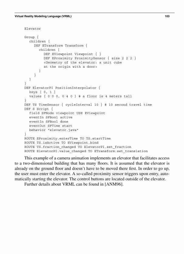
Virtual Reality Modeling Language (VRML) 103
Elevator
Group {children [
DEF ETransform Transform {children [
DEF EViewpoint Viewpoint { }DEF EProximity ProximitySensor { size 2 2 2 }<Geometry of the elevator: a unit cubeat the origin with a door>
]}
]}DEF ElevatorPI PositionInterpolator {
keys [ 0, 1 ]values [ 0 0 0, 0 4 0 ] # a floor is 4 meters tall
}DEF TS TimeSensor { cycleInterval 10 } # 10 second travel timeDEF S Script {
field SFNode viewpoint USE EViewpointeventIn SFBool activeeventIn SFBool doneeventOut SFTime startbehavior "elevator.java"
}ROUTE EProximity.enterTime TO TS.startTimeROUTE TS.isActive TO EViewpoint.bindROUTE TS.fraction_changed TO ElevatorPI.set_fractionROUTE ElevatorPI.value_changed TO ETransform.set_translation
This example of a camera animation implements an elevator that facilitates accessto a two-dimensional building that has many floors. It is assumed that the elevator isalready on the ground floor and doesn’t have to be moved there first. In order to go up,the user must enter the elevator. A so-called proximity sensor triggers upon entry, auto-matically starting the elevator. The control buttons are located outside of the elevator.
Further details about VRML can be found in [ANM96].

This page intentionally left blank
105
C H A P T E R 7
Data Compression
In comparison to the text medium, video frameshave high storage requirements. Audio and particularly video pose even greaterdemands in this regard. The data rates needed to process and send continuous media arealso considerable. This chapter thus covers the efficient compression of audio andvideo, which will be explained first in theory and subsequently in terms of compressionstandards.
7.1 Storage Space
Uncompressed graphics, audio, and video data require substantial storage capac-ity, which is not possible in the case of uncompressed video data, even given today’sCD and DVD technology. The same is true for multimedia communications. Data trans-fer of uncompressed video data over digital networks requires that very high bandwidthbe provided for a single point-to-point communication. To be cost-effective and feasi-ble, multimedia systems must use compressed video and audio streams.
Most compression methods address the same problems, one at a time or in combi-nation. Most are already available as products. Others are currently under developmentor are only partially completed (see also [SPI94]). While fractal image compression[BH93] may be important in the future, the most important compression techniques inuse today are JPEG [Org93, PM93, Wal91] for single pictures, H.263 (p×64) [Le 91,ISO93b] for video, MPEG [Lio91, ITUC90] for video and audio, as well as proprietarytechniques such as QuickTime from Apple and Video for Windows from Microsoft.
In their daily work, developers and multimedia experts often need a good under-standing of the most popular techniques. Most of today’s literature, however, is either

106 Chapter 7 • Data Compression
too comprehensive or is dedicated to just one of the above-mentioned compressiontechniques, which is then described from a very narrow point of view. In this chapter,we compare the most important techniques—JPEG, H.263, and MPEG—in order toshow their advantages, disadvantages, their similarities and differences, as well as theirsuitability for today’s multimedia systems (for further analysis, see [ES98]). First, themotivation for the use of compression techniques will be illustrated. Subsequently,requirements for compression techniques will be derived. Section 7.3 covers source,entropy, and hybrid coding. Sections 7.5 through 7.7 provide details about JPEG,H.263, and MPEG. Section 7.8 explains the basics of fractal compression.
7.2 Coding Requirements
Images have considerably higher storage requirements than text, and audio andvideo have still more demanding properties for data storage. Moreover, transmittingcontinuous media also requires substantial communication data rates. The figures citedbelow clarify the qualitative transition from simple text to full-motion video data anddemonstrate the need for compression. In order to be able to compare the different datastorage and bandwidth requirements of various visual media (text, graphics, images,and video), the following specifications are based on a small window of 640×480pixels on a display. The following holds always:
1kbit = 1000bit
1Kbit = 1024bit
1Mbit = 1024×1024bit
1. For the representation of the text medium, two bytes are used for every 8×8 pixelcharacter.
Character per screen page =
Storage required per screen page =
2. For the representation of vector images, we assume that a typical image consistsof 500 lines [BHS91]. Each line is defined by its coordinates in the x direction andthe y direction, and by an 8-bit attribute field. Coordinates in the x directionrequire 10 bits (log2(640)), while coordinates in the y direction require 9 bits(log2(480)).
Bits per line = 9bits + 10bits + 9bits + 10bits + 8bits = 46bits
Storage required per screen page
640 480×8 8×
------------------------ 4 800,=
4 800, 2 byte× 9 600 byte = 9.4, Kbyte=
500468------× 2 875 byte,== 2.8Kbyte=

Coding Requirements 107
3. Individual pixels of a bitmap can be coded using 256 different colors, requiring asingle byte per pixel.
Storage required per screen page = 640×480 ×1byte = 307,200 byte = 300Kbyte
The next examples specify continuous media and derive the storage required forone second of playback.
1. Uncompressed speech of telephone quality is sampled at 8kHz and quantizedusing 8bit per sample, yielding a data stream of 64Kbit/s.
Required storage space/s
2. An uncompressed stereo audio signal of CD quality is sampled at 44.1kHZ andquantized using 16 bits.
Data rate =
Required storage space/s
3. A video sequence consists of 25 full frames per second. The luminance andchrominance of each pixel are coded using a total of 3 bytes.According to the European PAL standard, each frame consists of 625 lines andhas a horizontal resolution of more than 833 pixels. The luminance and colordifference signals are encoded separately and transmitted together using a multi-plexing technique (4:2:2).According to CCIR 601 (studio standard for digital video), the luminance (Y) issampled at 13.5MHz, while chrominance (R–Y and B–Y) is sampled using6.75MHz. Samples are coded uniformly using 8bits.
Bandwidth = (13.5 MHz + 6.75 MHz + 6.75 MHz)×8bit = 216×106 bit/s.
Data rate =
Required storage sapce/s =
High-resolution television uses twice as many lines and an aspect ratio of 16:9,yielding a data rate 5.33 times that of current televisions.These examples briefly illustrate the increased demands on a computer system in
terms of required storage space and data throughput if still images and in particularcontinuous media are to be processed. Processing uncompressed video data streams inan integrated multimedia system requires storage space in the gigabyte range and buffer
64 Kbit/s8 bit/byte----------------------- 1 s
1 024 byte/Kbyte,------------------------------------------×= 8 Kbyte=
244 100,
s---------------- 16 bit
8 bit/byte-----------------------×× 176 400 byte/s,=
176 400 byte/s,1 s
1 024 byte/Kbyte,------------------------------------------×= 172 Kbyte=
640 480 25 3 byte/s××× 23 040 000 byte/s,,=
2 304, 104× byte/s1 s
1 024 byte/Kbyte,------------------------------------------× 22 500Kbyte,=

108 Chapter 7 • Data Compression
space in the megabyte range. The throughput in such a system can be as high as140Mbit/s, which must also be transmitted over networks connecting systems (per uni-directional connection). This kind of data transfer rate is not realizable with today’stechnology, or in the near future with reasonably priced hardware.
However, these rates can be considerably reduced using suitable compressiontechniques [NH88, RJ91], and research, development, and standardization in this areahave progressed rapidly in recent years [ACM89, GW93]. These techniques are thus anessential component of multimedia systems.
Several compression techniques for different media are often mentioned in theliterature and in product descriptions:
• JPEG (Joint Photographic Experts Group) is intended for still images.
• H.263 (H.261 p×64) addresses low-resolution video sequences. This can be com-plemented with audio coding techniques developed for ISDN and mobile commu-nications, which have also been standardized within CCITT.
• MPEG (Moving Picture Experts Group) is used for video and audio compression.
Compression techniques used in multimedia systems are subject to heavydemands. The quality of the compressed, and subsequently decompressed, data shouldbe as good as possible. To make a cost-effective implementation possible, the complex-ity of the technique used should be minimal. The processing time required for thedecompression algorithms, and sometimes also the compression algorithms, must notexceed certain time spans. Different techniques address requirements differently (see,for example, the requirements of [Org93]).
One can distinguish between requirements of “dialogue” mode applications (e.g.videoconferencing or picture transmission) and “retrieval” mode applications (e.g.audiovisual information systems, where a human user retrieves information from amultimedia database).
Compression techniques like p×64, with its symmetric processing expenditure forcompression and decompression and its strict delay limits, are better suited to dialogueapplications. Other techniques, such as MPEG-1, are optimized for use in retrievalapplications at the expense of considerable effort during compression.
The following requirement applies to compression techniques used for dialoguemode applications:
• The end-to-end delay for a technique used in a dialogue system should not exceed150ms for compression and decompression alone. To support an easy, natural dia-logue, ideally compression or decompression by itself should introduce an addi-tional delay of no more than 50ms. The overall end-to-end delay additionallycomprises delay in the network, communications protocol processing in the endsystem, and data transfer to and from the respective input and output devices.

Coding Requirements 109
The following requirements apply to compression techniques used for retrievalmode applications:
• Fast forward and fast rewind with simultaneous display (or playback) of the datashould be possible, so that individual passages can be sought and found quicker.
• Random access to single images or audio passages in a data stream should be pos-sible in less than half a second. This access should be faster than a CD-DA systemin order to maintain the interactive character of the retrieval application.
• Decompression of images, video, or audio passages should be possible withoutinterpreting all preceding data. This allows random access and editing.
The following requirements apply to compression techniques used for eitherdialogue or retrieval mode applications:
• To support display of the same data in different systems, it is necessary to define aformat that is independent of frame size and video frame rate.
• Audio and video compression should support different data rates (at differentquality) so that the data rate can be adjusted to specific system conditions.
• It should be possible to precisely synchronize audio and video. It should also bepossible for a system program to synchronize with other media.
• It should be possible to implement an economical solution today either in soft-ware or using at most a few VLSI chips.
• The technique should enable cooperation among different systems. It should bepossible for data generated on a local multimedia system to be reproduced onother systems. This is relevant, for example, in the case of course materials dis-tributed on CDs. This allows many participants to read the data on their own sys-tems, which may be made by different manufacturers. Also, since manyapplications exchange multimedia data between systems over communicationsnetworks, the compression techniques must be compatible. This can be assuredwith de jure (e.g. ITU, ISO, or ECMA) and/or de facto standards.
Different compression schemes take these requirements into account to a varyingextent.
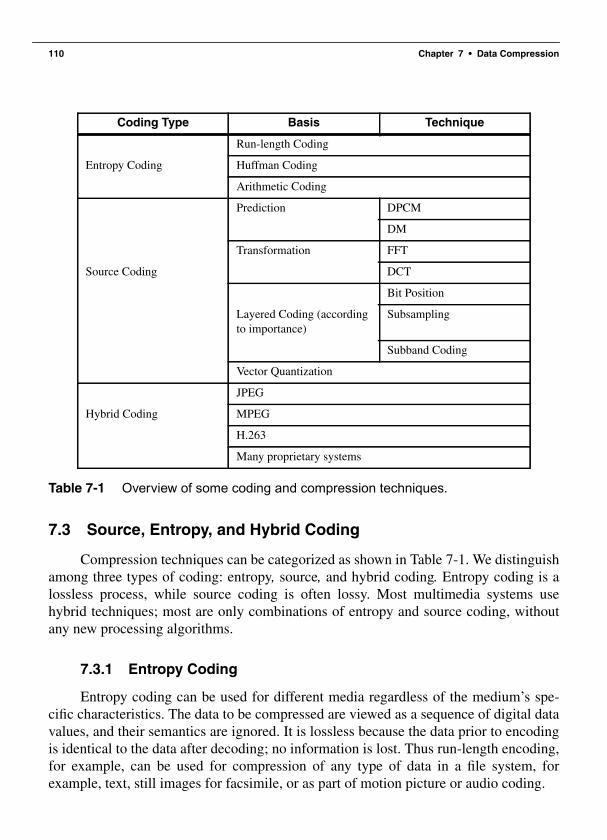
110 Chapter 7 • Data Compression
Table 7-1 Overview of some coding and compression techniques.
7.3 Source, Entropy, and Hybrid Coding
Compression techniques can be categorized as shown in Table 7-1. We distinguishamong three types of coding: entropy, source, and hybrid coding. Entropy coding is alossless process, while source coding is often lossy. Most multimedia systems usehybrid techniques; most are only combinations of entropy and source coding, withoutany new processing algorithms.
7.3.1 Entropy Coding
Entropy coding can be used for different media regardless of the medium’s spe-cific characteristics. The data to be compressed are viewed as a sequence of digital datavalues, and their semantics are ignored. It is lossless because the data prior to encodingis identical to the data after decoding; no information is lost. Thus run-length encoding,for example, can be used for compression of any type of data in a file system, forexample, text, still images for facsimile, or as part of motion picture or audio coding.
Coding Type Basis Technique
Run-length Coding
Entropy Coding Huffman Coding
Arithmetic Coding
Prediction DPCM
DM
Transformation FFT
Source Coding DCT
Bit Position
Layered Coding (accordingto importance)
Subsampling
Subband Coding
Vector Quantization
JPEG
Hybrid Coding MPEG
H.263
Many proprietary systems

Source, Entropy, and Hybrid Coding 111
7.3.2 Source Coding
Source coding takes into account the semantics of the information to be encoded[SGC90]. The degree of compression attainable with this often lossy technique dependson the medium. In the case of lossy compression, a relation exists between the uncodeddata and the decoded data; the data streams are similar but not identical. The character-istics of the medium can be exploited. In the case of speech, a considerable reduction ofthe amount of data can be achieved by transforming the time-dependent signal into thefrequency domain, followed by an encoding of the formants (see Chapter 3 regardingaudio).
Formants are defined as the maxima in the voice spectrum. Generally, five for-mants along with the voice fundamental frequency suffice for a very good reconstruc-tion of the original signal, although formant tracking has been shown to be a problemwith this form of speech analysis (see Chapter 3).
In the case of still images, spatial redundancies can be used for compressionthrough a content prediction technique. Other techniques perform a transformation ofthe spatial domain into the two-dimensional frequency domain by using the cosinetransform. Low frequencies define the average color, and the information of higher fre-quencies contains the sharp edges. Hence, low frequencies are much more importantthan the higher frequencies, a feature that can be used for compression.
Table 7-1 shows only a sampling of all coding and compression techniques. Theemphasis is on the algorithms that are most important for multimedia systems and ontheir properties. To better understand the hybrid schemes, we consider a set of typicalprocessing steps common to all techniques (entropy, source, and hybrid).
7.3.3 Major Steps of Data Compression
Figure 7-1 shows the typical sequence of operations performed in the compres-sion of still images and video and audio data streams. The following example describesthe compression of one image:
1. The preparation step (here picture preparation) generates an appropriate digitalrepresentation of the information in the medium being compressed. For example,a picture might be divided into blocks of 8×8 pixels with a fixed number of bitsper pixel.
2. The processing step (here picture processing) is the first step that makes use of thevarious compression algorithms. For example, a transformation from the timedomain to the frequency domain can be performed using the Discrete CosineTransform (DCT). In the case of interframe coding, motion vectors can be deter-mined here for each 8×8 pixel block.
3. Quantization takes place after the mathematically exact picture processing step.Values determined in the previous step cannot and should not be processed with

112 Chapter 7 • Data Compression
full exactness; instead they are quantized according to a specific resolution andcharacteristic curve. This can also be considered equivalent to the µ-law and A-law, which are used for audio data [JN84]. In the transformed domain, the resultscan be treated differently depending on their importance (e.g., quantized withdifferent numbers of bits).
4. Entropy coding starts with a sequential data stream of individual bits and bytes.Different techniques can be used here to perform a final, lossless compression. Forexample, frequently occurring long sequences of zeroes can be compressed byspecifying the number of occurrences followed by the zero itself.
Picture processing and quantization can be repeated iteratively, such as in the caseof Adaptive Differential Pulse Code Modulation (ADPCM). There can either be “feed-back” (as occurs during delta modulation), or multiple techniques can be applied to thedata one after the other (like interframe and intraframe coding in the case of MPEG).After these four compression steps, the digital data are placed in a data stream having adefined format, which may also integrate the image starting point and type of compres-sion. An error correction code can also be added at this point.
Figure 7-1 shows the compression process applied to a still image; the same prin-ciples can also be applied to video and audio data.
Figure 7-1 Major steps of data compression.
Decompression is the inverse process of compression. Specific coders and decod-ers can be implemented very differently. Symmetric coding is characterized by compa-rable costs for encoding and decoding, which is especially desirable for dialogueapplications. In an asymmetric technique, the decoding process is considerably lesscostly than the coding process. This is intended for applications where compression isperformed once and decompression takes place very frequently, or if the decompressionmust take place very quickly. For example, an audio-visual course module is producedonce, but subsequently decoded by the many students who use it. The main requirementis real-time decompression. An asymmetric technique can be used to increase thequality of the compressed images.
The following section discusses some basic compression techniques. Subsequentsections describe hybrid techniques frequently used in the multimedia field.
UncompressedPicture
CompressedPicture
PictureProcessing
Quanti-zation
EntropyCoding
PicturePreparation

Basic Compression Techniques 113
7.4 Basic Compression Techniques
The hybrid compression techniques often used on audio and video data in multi-media systems are themselves composed of several different techniques. For example,each technique listed in Table 7-1 employs entropy coding (in the form of variations ofrun-length coding and/or a statistical compression technique).
The simplest techniques are based on interpolation, whereby it is possible to makeuse of properties of the human eye or ear. For example, the eye is more sensitive tochanges in brightness than to color changes. Therefore, instead of dividing an imageinto RGB (red, green, blue) components, a YUV representation can be used (seeChapter 5). The U and V components can then be sampled with lower horizontal andvertical resolution, a technique called subsampling.
7.4.1 Run-Length Coding
Data often contains sequences of identical bytes. By replacing these repeated bytesequences with the number of occurrences, a substantial reduction of data can beachieved. This is known as run-length coding. A special marker M is needed in the datathat does not occur as part of the data stream itself. This M-byte can also be realized ifall 256 possible bytes can occur in the data stream by using byte stuffing. To illustratethis, we define the exclamation mark to be the M-byte. A single occurrence of an excla-mation mark is interpreted as the M-byte during decompression. Two consecutiveexclamation marks are interpreted as an exclamation mark occurring within the data.
The M-byte can thus be used to mark the beginning of a run-length coding. Thetechnique can be described precisely as follows: if a byte occurs at least four times in arow, then the number of occurrences is counted. The compressed data contain the byte,followed by the M-byte and the number of occurrences of the byte. Remembering thatwe are compressing at least four consecutive bytes, the number of occurrences can beoffset by –4. This allows the compression of between four and 258 bytes into only threebytes. (Depending on the algorithm, one or more bytes can be used to indicate thelength; the same convention must be used during coding and decoding.)
In the following example, the character C occurs eight times in a row and is com-pressed to the three characters C!4:
Uncompressed data: ABCCCCCCCCDEFGGGRun-length coded: ABC!4DEFGGG
7.4.2 Zero Suppression
Run-length coding is a generalization of zero suppression, which assumes that justone symbol appears particularly often in sequences. The blank (space) character in textis such a symbol; single blanks or pairs of blanks are ignored. Starting with sequencesof three bytes, they are replaced by an M-byte and a byte specifying the number of

114 Chapter 7 • Data Compression
blanks in the sequence. The number of occurrences can again be offset (by –3).Sequences of between three and 257 bytes can thus be reduced to two bytes. Furthervariations are tabulators used to replace a specific number of null bytes and the defini-tion of different M-bytes to specify different numbers of null bytes. For example, anM5-byte could replace 16 null bytes, while an M4-byte could replace 8 null bytes. AnM5-byte followed by an M4-byte would then represent 24 null bytes.
7.4.3 Vector Quantization
In the case of vector quantization, a data stream is divided into blocks of n byteseach (n>1). A predefined table contains a set of patterns. For each block, the table isconsulted to find the most similar pattern (according to a fixed criterion). Each patternin the table is associated with an index. Thus, each block can be assigned an index.Such a table can also be multidimensional, in which case the index will be a vector. Thecorresponding decoder has the same table and uses the vector to generate an approxi-mation of the original data stream. For further details see [Gra84] for example.
7.4.4 Pattern Substitution
A technique that can be used for text compression substitutes single bytes for pat-terns that occur frequently. This pattern substitution can be used to code, for example,the terminal symbols of high-level languages (begin, end, if). By using an M-byte, alarger number of words can be encoded–the M-byte indicates that the next byte is anindex representing one of 256 words. The same technique can be applied to still images,video, and audio. In these media, it is not easy to identify small sets of frequently occur-ring patterns. It is thus better to perform an approximation that looks for the most simi-lar (instead of the same) pattern. This is the above described vector quantization.
7.4.5 Diatomic Encoding
Diatomic encoding is a variation based on combinations of two data bytes. Thistechnique determines the most frequently occurring pairs of bytes. Studies have shownthat the eight most frequently occurring pairs in the English language are “E,” “T,”“TH,” “A,” “S,” “RE,” “IN,” and “HE.” Replacing these pairs by special single bytesthat otherwise do not occur in the text leads to a data reduction of more than tenpercent.
7.4.6 Statistical Coding
There is no fundamental reason that different characters need to be coded with afixed number of bits. Morse code is based on this: frequently occurring characters arecoded with short strings, while seldom-occurring characters are coded with longerstrings. Such statistical coding depends how frequently individual characters or

Basic Compression Techniques 115
sequences of data bytes occur. There are different techniques based on such statisticalcriteria, the most prominent of which are Huffman coding and arithmetic coding.
7.4.7 Huffman Coding
Given the characters that must be encoded, together with their probabilities ofoccurrence, the Huffman coding algorithm determines the optimal coding using theminimum number of bits [Huf52]. Hence, the length (number of bits) of the coded char-acters will differ. The most frequently occurring characters are assigned to the shortestcode words. A Huffman code can be determined by successively constructing a binarytree, whereby the leaves represent the characters that are to be encoded. Every nodecontains the relative probability of occurrence of the characters belonging to the subtreebeneath the node. The edges are labeled with the bits 0 and 1.
The following brief example illustrates this process:
1. The letters A, B, C, D, and E are to be encoded and have relative probabilities ofoccurrence as follows:
p(A)=0.16, p(B)=0.51, p(C)=0.09, p(D)=0.13, p(E)=0.11
2. The two characters with the lowest probabilities, C and E, are combined in thefirst binary tree, which has the characters as leaves. The combined probability oftheir root node CE is 0.20. The edge from node CE to C is assigned a 1 and theedge from CE to C is assigned a 0. This assignment is arbitrary; thus, differentHuffman codes can result from the same data.
3. Nodes with the following relative probabilities remain:
p(A)=0.16, p(B)=0.51, p(CE)=0.20, p(D)=0.13
The two nodes with the lowest probabilities are D and A. These nodes are com-bined to form the leaves of a new binary tree. The combined probability of theroot node AD is 0.29. The edge from AD to A is assigned a 1 and the edge fromAD to D is assigned a 0.
If root nodes of different trees have the same probability, then trees having theshortest maximal path between their root and their nodes should be combinedfirst. This keeps the length of the code words roughly constant.
4. Nodes with the following relative probabilities remain:
p(AD)=0.29, p(B)=0.51, p(CE)=0.20
The two nodes with the lowest probabilities are AD and CE. These are combinedinto a binary tree. The combined probability of their root node ADCE is 0.49. Theedge from ADCE to AD is assigned a 0 and the edge from ADCE to CE is assigneda 1.
5. Two nodes remain with the following relative probabilities:
p(ADCE)=0.49, p(B)=0.51
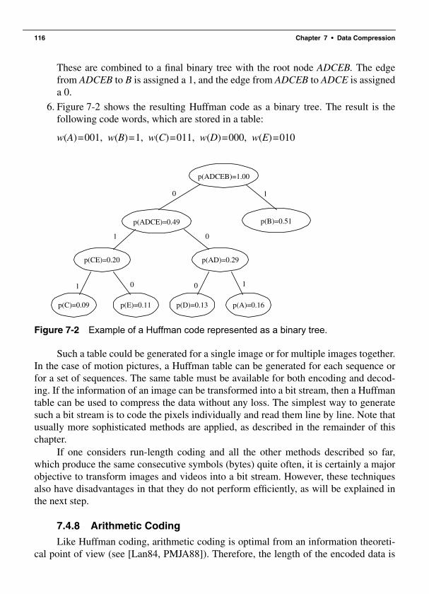
116 Chapter 7 • Data Compression
These are combined to a final binary tree with the root node ADCEB. The edgefrom ADCEB to B is assigned a 1, and the edge from ADCEB to ADCE is assigneda 0.
6. Figure 7-2 shows the resulting Huffman code as a binary tree. The result is thefollowing code words, which are stored in a table:
w(A)=001, w(B)=1, w(C)=011, w(D)=000, w(E)=010
Figure 7-2 Example of a Huffman code represented as a binary tree.
Such a table could be generated for a single image or for multiple images together.In the case of motion pictures, a Huffman table can be generated for each sequence orfor a set of sequences. The same table must be available for both encoding and decod-ing. If the information of an image can be transformed into a bit stream, then a Huffmantable can be used to compress the data without any loss. The simplest way to generatesuch a bit stream is to code the pixels individually and read them line by line. Note thatusually more sophisticated methods are applied, as described in the remainder of thischapter.
If one considers run-length coding and all the other methods described so far,which produce the same consecutive symbols (bytes) quite often, it is certainly a majorobjective to transform images and videos into a bit stream. However, these techniquesalso have disadvantages in that they do not perform efficiently, as will be explained inthe next step.
7.4.8 Arithmetic Coding
Like Huffman coding, arithmetic coding is optimal from an information theoreti-cal point of view (see [Lan84, PMJA88]). Therefore, the length of the encoded data is
p(ADCEB)=1.00
10
1 0
1 10 0
p(ADCE)=0.49 p(B)=0.51
p(AD)=0.29p(CE)=0.20
p(A)=0.16p(D)=0.13p(E)=0.11p(C)=0.09

Basic Compression Techniques 117
also minimal. Unlike Huffman coding, arithmetic coding does not code each symbolseparately. Each symbol is instead coded by considering all prior data. Thus a datastream encoded in this fashion must always be read from the beginning. Consequently,random access is not possible. In practice, the average compression rates achieved byarithmetic and Huffman coding are similar [Sto88].
Differences in compression efficiency arise in special cases, for example in digi-tized graphics consisting primarily of a single (background) color. Arithmetic coding isbetter suited than Huffman coding in this case. This is always the case if symbols occurin the input data stream with such a frequency that they have a very small informationcontent. These can be encoded using less than one bit, whereas in Huffman coding eachsymbol requires at least one bit.
7.4.9 Transformation Coding
Transformation coding pursues a different approach. Data is transformed intoanother mathematical domain that is more suitable for compression. An inverse trans-formation must exist. The simplest example is the Fourier transform, which transformsdata from the time domain into the frequency domain. Other examples include theWalsh, Hadamard, Haar, and Slant transforms. However, the transformed data have nomajor advantages with respect to a subsequent compression. The most effective trans-formations for data reduction are the Discrete Cosine Transform (DCT), described inSection 7.5.2, and the Fast Fourier Transform (FFT).
7.4.10 Subband Coding
Unlike transformation coding, which transforms all data into another domain,selective frequency transformation (subband coding) considers the signal only in pre-defined regions of the spectrum, such as frequency bands. The number of bands is acrucial quality criterion. This technique is well suited for the compression of speech.
7.4.11 Prediction or Relative Coding
Instead of compressing single bytes or sequences of bytes, differential encodingcan be used. This is also known as prediction or relative coding. For example, if charac-ters in a sequence are clearly different from zero, but do not differ much amongst them-selves, then calculating differences from the respective previous value could beprofitable for compression. The following examples explain this technique for differentmedia:
• For still images, edges yield large difference values, while areas with similar lumi-nance and chrominance yield small values. A homogeneous area is characterizedby a large number of zeroes, which could be further compressed using run-lengthcoding.

118 Chapter 7 • Data Compression
• For video, performing relative coding in the time domain leads to an encoding ofdifferences from the previous image only. In a newscast or a video telephonyapplication, there will be a large number of zero bytes, because the background ofsuccessive images does not change very often. Motion compensation can also beperformed here (see e.g. [PA91]). Blocks of, for example, 16×16 pixels are com-pared with each other in successive pictures. In the case of a car moving from leftto right, an area in the current image would be most similar to an area lying furtherto the left in the previous image. This motion can be coded as a vector.
• Audio techniques often apply Differential Pulse Code Modulation (DPCM) to asequence of PCM-coded samples (see e.g. [JN84]). This technique requires a lin-ear characteristic curve for quantization. It is thus not necessary to store the wholenumber of bits for each sample. It is sufficient to represent the first PCM-codedsample as a whole and all following samples as the difference from the previousone.
7.4.12 Delta Modulation
Delta Modulation is a modification of DPCM where difference values are encodedwith exactly one bit, which indicates whether the signal increases or decreases. Thisleads to an inaccurate coding of steep edges. This technique is particularly profitable ifthe coding does not depend on 8-bit grid units. If the differences are small, then a muchsmaller number of bits is sufficient. Difference encoding is an important feature of alltechniques used in multimedia systems. Section 7.5.2 describes other “delta” methodsthat can be applied to images.
7.4.13 Adaptive Compression Techniques
Most of the compression techniques described so far take advantage of alreadyknown characteristics of the data to be compressed (e.g., frequently occurringsequences of bytes or the probability of occurrence of individual bytes). An atypicalsequence of characters results in a poor compression. However, there are also adaptivecompression techniques, which can adjust themselves to the data being compressed.This adaptation can be implemented in different ways:
• We illustrate the first technique with the following example, which assumes a cod-ing table has been generated in advance (e.g., as per Huffman). For each symbolto be encoded, the table contains the corresponding code word and, in an addi-tional column, a counter. All entries’ counters are initialized to zero at the begin-ning. For the first symbol to be encoded, the coder determines the code wordaccording to the table. Additionally, the coder increments the counter by one. Thesymbols and their respective counters are then sorted in decreasing order bycounter value. The order of the code words is not changed. The most frequently

Basic Compression Techniques 119
occurring symbols are now at the beginning of the table, since they have the high-est counter values. Symbols with the highest frequency count are thus alwaysencoded with the shortest code words.
• Another adaptive compression technique is Adaptive DPCM (ADPCM), a gener-alization of DPCM. For simplicity, this is often called DPCM.
Here, difference values are encoded using only a small number of bits. WithDPCM, either coarse transitions would be coded correctly (the DPCM-encodedbits are used represent bits with a higher significance), or fine transitions arecoded exactly (if the bits are used to represent bits with less significance). In thefirst case, the resolution of low audio signals would not be sufficient, and in thesecond case a loss of high frequencies would occur.
ADPCM adapts to the significance of the data stream. The coder divides theDPCM sample values by an appropriate coefficient and the decoder multiplies thecompressed data by the same coefficient, thus changing the step size of the signal.The coder of the DPCM-encoded signal adjusts the value of the coefficient.
A signal with a large portion of high frequencies will result in frequent, very highDPCM values. The coder will select a high value for the coefficient. The result is avery rough quantization of the DPCM signal in passages with steep edges. Low-frequency portions of such passages are hardly considered at all.
In the case of a signal with steady, relatively low DPCM values, that is, with asmall portion of high frequencies, the coder will choose a small coefficient. Thisensures good resolution for the dominant, low frequency portion of the signal. Ifhigh frequencies suddenly occur in such a passage, a signal distortion in the formof a slope overload occurs. The greatest possible change that can be representedby an ADPCM value using the available number of bits and the current step size isnot enough to represent the new DPCM value. The jump in the PCM signal willbe faded.
Changes in the adaptively set coefficient can be explicitly inserted in the com-pressed data by the encoder. Alternatively, the decoder can calculate the coeffi-cients itself from an ADPCM-coded data stream. This predictor is rated so as tominimize errors in the data stream. Note that the definition of an error and theassociated predictor rating depends on the medium and is ideally trivial.
An audio signal with frequently changing portions of extreme low or high fre-quencies is generally not suited for ADPCM coding. For telephone applications,the ITU has standardized a version of the ADPCM technique using 32Kbit/s thatis based on four bits per difference value and a sampling frequency of 8kHz.

120 Chapter 7 • Data Compression
7.4.14 Other Basic Techniques
Apart from the compression techniques described earlier, some additional wellknown techniques are used today:
• Video compression techniques often use Color Look-Up Tables (seeSection 5.1.2). This technique is used in distributed multimedia systems, forexample in [LE91, LEM92].
• A simple technique for audio is silence suppression, whereby data is only encodedif the volume exceeds a certain threshold.
ITU incorporates some of the basic audio coding techniques in the G.700 series ofstandards: G.721 defines PCM coding for 3.4kHz quality over 64Kbit/s channels, andG.728 defines 3.4kHz quality over 16Kbit/s channels. See [ACG93] for a detaileddescription of various audio coding techniques.
The following sections describe the most important work in the standardizationbodies concerning image and video coding. In the framework of ISO/IECJTC1/SC2/WG8, four subgroups were established in May 1988: JPEG (Joint Photographic ExpertsGroup), working on coding of still images; JBIG (Joint Bi-Level Image ExpertsGroup), working on the progressive processing of bi-level coding algorithms; CGEG(Computer Graphics Experts Group), working on coding principles; and MPEG (Mov-ing Picture Experts Group), working on the coded representation of motion video. Thenext section presents the results of the JPEG activities.
7.5 JPEG
Since June 1982, Working Group 8 (WG8) of ISO has been working on standardsfor the compression and decompression of still images [HYS88]. In June 1987, ten dif-ferent techniques for coding color and gray-scaled still images were presented. Theseten were compared, and three were analyzed further. An adaptive transformation codingtechnique based on the Discrete Cosine Transform (DCT) achieved the best subjectiveresults [LMY88, WVP88]. This technique was then further developed with consider-ation paid to the other two methods. The coding known as JPEG (Joint PhotographicExperts Group) is a joint project of ISO/IECJTC1/SC2/WG10 and Commission Q.16of CCITT SGVIII. Hence the “J” (from “Joint”) in JPEG—ISO together with CCITT.In 1992, JPEG became an ISO International Standard (IS) [Org93].
JPEG applies to color and gray-scaled still images [LOW91, MP91, Wal91].Video sequences can also be handled through a fast coding and decoding of stillimages, a technique known as Motion JPEG. Today, implementations of parts of JPEGare already available, either as software-only packages or using special-purpose hard-ware support. It should be noted that as yet, most products support only the absolutelynecessary algorithms. The only part of JPEG currently commercially available is the

JPEG 121
base mode with certain processing restrictions (limited number of image componentsand color coding).
7.5.0.1 Requirements
In order to ensure the widespread distribution and application of JPEG, the fol-lowing requirements were established and fulfilled [Wal91]:
• The standard should be independent of image size.
• It should be applicable to any image aspect ratio and any pixel aspect ratio.
• The color space and the number of colors used should be independent of oneanother.
• Image content may be of any complexity, with any statistical characteristics.
• The JPEG standard should be start-of-the-art (or near) regarding the compressionfactor and image quality.
• The processing complexity should permit a software solution to run on a largenumber of available general-purpose processors, and should be drasticallyreduced with the use of special-purpose hardware.
• Sequential (line by line) and progressive (successive refinement of the wholeimage) decoding should both be possible. A lossless, hierarchical coding of thesame image with different resolutions should also be possible.
The user can select parameters to trade off the quality of the reproduced image,the compression processing time, and the size of the compressed image.
7.5.0.2 JPEG Overview
Applications do not have to include both an encoder and a decoder. In many appli-cations only one of them is needed. The encoded data stream has a fixed interchangeformat that includes encoded image data, as well as the chosen parameters and tables ofthe coding process, enabling decoding. If there is a common context between the coderand the decoder (e.g., if the coder and decoder are parts of the same application), thenthere can be an abbreviated interchange format. This format includes few if any of therequired tables (Appendix A in [Org93] describes this format in detail). The inter-change format includes all information required during decoding, if this information isnot available as part of the common context. In the regular, non-abbreviated mode, theinterchange format includes all information required to decode without prior knowl-edge of the coding process.
Figure 7-3 outlines the fundamental steps of JPEG compression in accordancewith the general scheme illustrated in Figure 7-1. JPEG defines several image compres-sion modes by selecting different combinations of these steps.
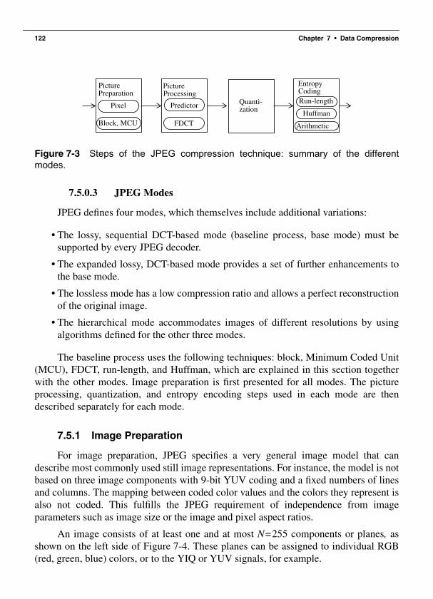
122 Chapter 7 • Data Compression
Figure 7-3 Steps of the JPEG compression technique: summary of the differentmodes.
7.5.0.3 JPEG Modes
JPEG defines four modes, which themselves include additional variations:
• The lossy, sequential DCT-based mode (baseline process, base mode) must besupported by every JPEG decoder.
• The expanded lossy, DCT-based mode provides a set of further enhancements tothe base mode.
• The lossless mode has a low compression ratio and allows a perfect reconstructionof the original image.
• The hierarchical mode accommodates images of different resolutions by usingalgorithms defined for the other three modes.
The baseline process uses the following techniques: block, Minimum Coded Unit(MCU), FDCT, run-length, and Huffman, which are explained in this section togetherwith the other modes. Image preparation is first presented for all modes. The pictureprocessing, quantization, and entropy encoding steps used in each mode are thendescribed separately for each mode.
7.5.1 Image Preparation
For image preparation, JPEG specifies a very general image model that candescribe most commonly used still image representations. For instance, the model is notbased on three image components with 9-bit YUV coding and a fixed numbers of linesand columns. The mapping between coded color values and the colors they represent isalso not coded. This fulfills the JPEG requirement of independence from imageparameters such as image size or the image and pixel aspect ratios.
An image consists of at least one and at most N=255 components or planes, asshown on the left side of Figure 7-4. These planes can be assigned to individual RGB(red, green, blue) colors, or to the YIQ or YUV signals, for example.
Quanti-zationPixel
Block, MCU
Predictor
FDCT
Run-length
Huffman
Arithmetic
PicturePreparation Coding
EntropyPictureProcessing

JPEG 123
Figure 7-4 Uncompressed digital image as per [Org93].
Each component is a rectangular array Xi×Yi of pixels (the samples). Figure 7-5shows an image with three planes, each with the same resolution.
Figure 7-5 Example of JPEG image preparation with three components having thesame resolution.
The resolution of the individual components may be different. Figure 7-6 showsan image with three planes where the second and third planes have half as many col-umns as the first plane. A gray-scale image will, in most cases, consist of a single com-ponent, while an RGB color image will have three components with the sameresolution (same number of lines Y1 = Y2 = Y3 and the same number of columnsX1 = X2 = X3). In JPEG image preparation, YUV color images with subsampling of thechrominance components use three planes with Y1 = 4Y2 = 4Y3 and X1 = 4X2 = 4X3.
Xi
Yi
line
rightleft
bottom
topsamples
C1
C2
CN
A1 A2
An
X
Y
B1 B2
Bn
X
Y
C1 C2
Cn
X
Y

124 Chapter 7 • Data Compression
Figure 7-6 Example of JPEG image preparation with three components havingdifferent resolutions.
Each pixel is represented by p bits with values in the range from 0 to 2p–1. Allpixels of all components of an image must have the same number of bits. The lossymodes of JPEG use a precision of either 8 or 12 bits per pixel. The lossless modes canuse between 2 and 12 bits per pixel. If a JPEG application uses any other number ofbits, the application itself must suitably transform the image to conform to the numberof bits defined by the JPEG standard.
Instead of the values Xi and Yi, the compressed data includes the values X (maxi-mum of all Xi) and Y (maximum of all Yi), as well as factors Hi and Vi for each plane. Hi
and Vi represent the relative horizontal and vertical resolutions with respect to theminimal horizontal and vertical resolutions.
Let us consider the following example from [Org93]. An image has a maximumresolution of 512 pixels in both the horizontal and vertical directions and consists ofthree planes. The following factors are given:
Plane 0: H0 = 4, V0 = 1Plane 1: H1 = 2, V1 = 2Plane 2: H2 = 1, V2 = 1
This leads to:
X = 512, Y = 512, Hmax = 4 and Vmax = 2Plane 0: X0 = 512, Y0 = 256Plane 1: X1 = 256, Y1 = 512Plane 2: X2 = 128, Y2 = 256
Hi and Vi must be integers between 1 and 4. This awkward-looking definition isneeded for the interleaving of components.
In the image preparation stage of compression, the image is divided into dataunits. The lossless mode uses one pixel as one data unit. The lossy mode uses blocks of8×8 pixels. This is a consequence of DCT, which always transforms connected blocks.
Up to now, the data units are usually prepared component by component andpassed on in order to the following image processing. Within each component, the data
A1 A2
An
X
Y
B1 B2
n
X/2
Y
C1 C2
X/2
Y
_2
B n_2
C

JPEG 125
units are processed from left to right, as shown in Figure 7-7. This is known as a non-interleaved data ordering.
Figure 7-7 Noninterleaved processing order of data units when processing a singlecomponent as per [Org93].
Due to the finite processing speed of the decoder, processing of data units of dif-ferent components may be interleaved. If the noninterleaved mode were used for a veryhigh-resolution, RGB-encoded image, during rendering the display would first showonly red, then red-green, and finally the correct colors.
Figure 7-8 Interleaved processing order of data units.
Figure 7-8 shows an example with four components from [Org93]. Above eachcomponent, the corresponding values for H and V are shown. The first component hasthe highest resolution in both dimensions and the fourth component has the lowest res-olution. The arrows within each component indicate the sampling order of individualdata units.
Minimum Coded Units (MCUs) are built in the following order:
rightleft
top
bottom
0 1 2 3 4 50123
0 1 2 3 4 501
0 1 20123
0 1 201
Cs1:H1=2, V1=2 Cs2:H2 = 2, V2=1 Cs3:H3=1, V3=2 Cs4:H4=1, V4=1
MCU1 d001
d011
d101
d111
d002
d012
d003
d103
d004
=
MCU2 d021
d031
d121
d131
d022
d032
d013
d113
d014
=
MCU3 d041
d051
d141
d151
d042
d052
d023
d123
d024
=
MCU4 d201
d211
d301
d311
d102
d112
d203
d303
d104
=
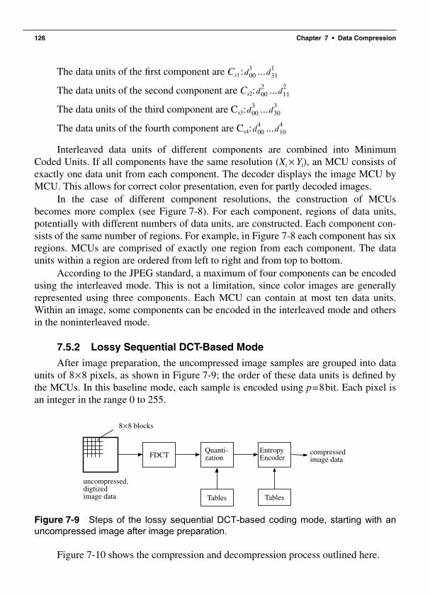
126 Chapter 7 • Data Compression
The data units of the first component are Cs1: ...
The data units of the second component are Cs2: ...
The data units of the third component are Cs3: ...
The data units of the fourth component are Cs4: ...
Interleaved data units of different components are combined into MinimumCoded Units. If all components have the same resolution (Xi × Yi), an MCU consists ofexactly one data unit from each component. The decoder displays the image MCU byMCU. This allows for correct color presentation, even for partly decoded images.
In the case of different component resolutions, the construction of MCUsbecomes more complex (see Figure 7-8). For each component, regions of data units,potentially with different numbers of data units, are constructed. Each component con-sists of the same number of regions. For example, in Figure 7-8 each component has sixregions. MCUs are comprised of exactly one region from each component. The dataunits within a region are ordered from left to right and from top to bottom.
According to the JPEG standard, a maximum of four components can be encodedusing the interleaved mode. This is not a limitation, since color images are generallyrepresented using three components. Each MCU can contain at most ten data units.Within an image, some components can be encoded in the interleaved mode and othersin the noninterleaved mode.
7.5.2 Lossy Sequential DCT-Based Mode
After image preparation, the uncompressed image samples are grouped into dataunits of 8×8 pixels, as shown in Figure 7-9; the order of these data units is defined bythe MCUs. In this baseline mode, each sample is encoded using p=8bit. Each pixel isan integer in the range 0 to 255.
Figure 7-9 Steps of the lossy sequential DCT-based coding mode, starting with anuncompressed image after image preparation.
Figure 7-10 shows the compression and decompression process outlined here.
d001
d311
d002
d112
d003
d303
d004
d104
FDCTQuanti-zation
EntropyEncoder
uncompressed,
compressedimage data
Tables Tables
*
8×8 blocks
digtizedimage data

JPEG 127
Figure 7-10 Example of DCT and IDCT.
7.5.2.1 Image Processing
The first step of image processing in the baseline mode (baseline process in[Org93]), as shown in Figure 7-9, is a transformation coding performed using the Dis-crete Cosine Transform (DCT) [ANR74, NP78]. The pixel values are shifted into thezero-centered interval (–128, 127). Data units of 8×8 shifted pixel values are definedby Syx, where x and y are in the range of zero to seven.
The following FDCT (Forward DCT) is then applied to each transformed pixelvalue:
where: for u, v = 0; otherwise cu, cv = 1
Altogether, this transformation must be carried out 64 times per data unit. Theresult is 64 coefficients Svu. Due to the dependence of DCT on the Discrete FourierTransform (DFT), which maps values from the time domain to the frequency domain,each coefficient can be regarded as a two-dimensional frequency.
Svu14---cucv Syx
2x 1+( )uπ16
--------------------------- 2y 1+( )vπ16
---------------------------coscosy 0=
7
∑x 0=
7
∑=
cu cv, 1
2-------=

128 Chapter 7 • Data Compression
Figure 7-11 Relationship between the two-dimensional space and frequencydomains.
The coefficient S00 corresponds to the portion where the frequency is zero in bothdimensions. It is also known as the DC-coefficient (DC voltage portion) and determinesthe fundamental color of all 64 pixels of the data unit. The other coefficients are calledAC-coefficients (analogous to the AC voltage portion). For instance, S70 represents thehighest frequency that occurs in the horizontal direction, that is, the closest possibleseparation of vertical lines in the 8×8 data unit. S07 represents the highest frequency inthe vertical dimension, that is, the closest possible separation of horizontal lines. S77
indicates the highest frequency appearing equally in both dimensions. Its absolute valueis greatest if the original data unit contains as many squares as possible, that is, if it con-sists solely of 1×1 squares. Accordingly, for example, S33 will be maximal if a blockconsists of 16 squares of 4×4 pixels. Taking a closer look at the above formula, we rec-ognize that the cosine expressions depend only upon x and u, or upon y and v, but not onSyx. Therefore, these expressions represent constants that do not need to be recalculatedover and over again. There are many effective DCT techniques and implementations[DG90, Fei90, Hou88, Lee84, LF91, SH86, VN84, Vet85].
For later reconstruction of the image, the decoder uses the Inverse DCT (IDCT).The coefficients Svu must be used for the calculation:
where for u, v = 0; otherwise cu, cv = 1
If the FDCT, as well as the IDCT, could be calculated with full precision, it wouldbe possible to reproduce the original 64 pixels exactly. From a theoretical point of view,DCT would be lossless in this case. In practice, precision is limited and DCT is thuslossy. The JPEG standard does not define any specific precision. It is thus possible that
# # # # # # # ## # # # # # # ## # # # # # # ## # # # # # # ## # # # # # # ## # # # # # # ## # # # # # # ## # # # # # # #
* * * * * * * ** * * * * * * ** * * * * * * ** * * * * * * ** * * * * * * ** * * * * * * ** * * * * * * ** * * * * * * *
…
…
Space domain:Image data
Frequency domain:
image datacompressed
sxy14--- cucvsvu
2x 1+( )uπ16
--------------------------- 2y 1+( )vπ16
---------------------------coscosv 0=
7
∑u 0=
7
∑=
cu cv, 1
2-------=

JPEG 129
two different JPEG decoder implementations could generate different images as outputof the same compressed data. JPEG merely defines the maximum allowable deviation.
Many images contain only a small portion of sharp edges; they consist mostly ofareas of a single color. After applying DCT, such areas are represented by a small por-tion of high frequencies. Sharp edges, on the other hand, are represented as high fre-quencies. Images of average complexity thus consist of many AC-coefficients with avalue of zero or almost zero. This means that subsequent entropy encoding can be usedto achieve considerable data reduction.
7.5.2.2 Quantization
Image processing is followed by the quantization of all DCT coefficients; this is alossy process. For this step, the JPEG application provides a table with 64 entries, onefor each of the 64 DCT coefficients. This allows each of the 64 coefficients to beadjusted separately. The application can thus influence the relative significance of thedifferent coefficients. Specific frequencies can be given more importance than othersdepending on the characteristics of the image material to be compressed. The possiblecompression is influenced at the expense of achievable image quality.
The table entries Qvu are integer values coded with 8 bits. Quantization isperformed according to the formula:
The greater the table entries, the coarser the quantization. Dequantization is per-formed prior to the IDCT according to the formula:
Quantization and dequantization must use the same tables.Figure 7-12 shows a greatly enlarged detail from Figure 7-16. The blocking and
the effects of quantization are clearly visible. In Figure 7-12(b) a coarser quantizationwas performed to highlight the edges of the 8×8 blocks.
sqvu roundSvu
Qvu--------=
Rvu Sqvu Qvu×=

130 Chapter 7 • Data Compression
Figure 7-12 Quantization effect.
7.5.2.3 Entropy Encoding
During the next step, either the initial step of entropy encoding or preparation forthe coding process, the quantized DC-coefficients are treated differently than the quan-tized AC-coefficients. The processing order of all coefficients is specified by the zig-zagsequence.
• The DC-coefficients determine the fundamental color of the data units. Since thischanges little between neighboring data units, the differences between successiveDC-coefficients are very small values. Thus each DC-coefficient is encoded bysubtracting the DC-coefficient of the previous data unit, as shown in Figure 7-13,and subsequently using only the difference.
Figure 7-13 Preparation of DCT DC-coefficients for entropy encoding. Calculation ofthe difference between neighboring values.
• The DCT processing order of the AC-coefficients using the zig-zag sequence asshown in Figure 7-14 illustrates that coefficients with lower frequencies (typicallywith higher values) are encoded first, followed by the higher frequencies (typi-cally zero or almost zero). The result is an extended sequence of similar databytes, permitting efficient entropy encoding.
(a) (b)
blocki-1
DCi-1
blocki
DCi
DIFF=DCi-DCi-1
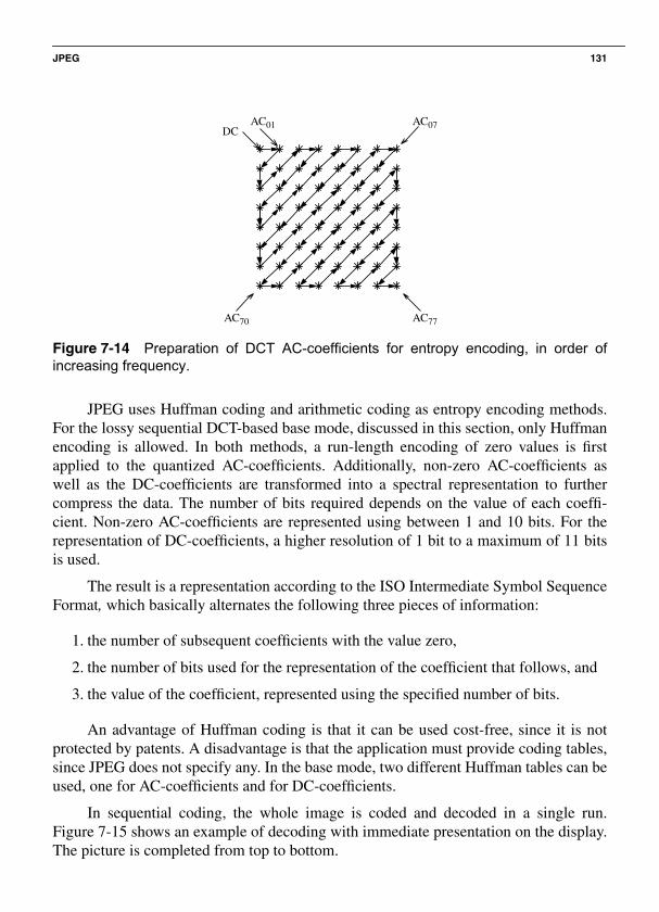
JPEG 131
Figure 7-14 Preparation of DCT AC-coefficients for entropy encoding, in order ofincreasing frequency.
JPEG uses Huffman coding and arithmetic coding as entropy encoding methods.For the lossy sequential DCT-based base mode, discussed in this section, only Huffmanencoding is allowed. In both methods, a run-length encoding of zero values is firstapplied to the quantized AC-coefficients. Additionally, non-zero AC-coefficients aswell as the DC-coefficients are transformed into a spectral representation to furthercompress the data. The number of bits required depends on the value of each coeffi-cient. Non-zero AC-coefficients are represented using between 1 and 10 bits. For therepresentation of DC-coefficients, a higher resolution of 1 bit to a maximum of 11 bitsis used.
The result is a representation according to the ISO Intermediate Symbol SequenceFormat, which basically alternates the following three pieces of information:
1. the number of subsequent coefficients with the value zero,
2. the number of bits used for the representation of the coefficient that follows, and
3. the value of the coefficient, represented using the specified number of bits.
An advantage of Huffman coding is that it can be used cost-free, since it is notprotected by patents. A disadvantage is that the application must provide coding tables,since JPEG does not specify any. In the base mode, two different Huffman tables can beused, one for AC-coefficients and for DC-coefficients.
In sequential coding, the whole image is coded and decoded in a single run.Figure 7-15 shows an example of decoding with immediate presentation on the display.The picture is completed from top to bottom.
DCAC01 AC07
AC77AC70

132 Chapter 7 • Data Compression
Figure 7-15 Example of sequential picture preparation, here using the lossy DCT-based mode.
7.5.3 Expanded Lossy DCT-Based Mode
Image preparation in this mode differs from the previously described mode interms of the number of bits per pixel. This mode supports 12 bits per sample value inaddition to 8 bits. The image processing is DCT-based and is performed analogously tothe baseline DCT mode. For the expanded lossy DCT-based mode, JPEG defines pro-gressive coding in addition to sequential coding. In the first decoding run, a very rough,unsharp image appears. This is refined during successive runs. An example of a veryunsharp image is shown in Figure 7-16(a). It is substantially sharper in Figure 7-16(b),and in its correct resolution in Figure 7-16(c).
Figure 7-16 Progressive picture presentation: (a) first phase, very unsharp image; (b)second phase, unsharp image; (c) third phase, sharp image.
(a) (b) (c)

JPEG 133
Progressive image presentation is achieved by expanding quantization. This isequivalent to layered coding. For this expansion, a buffer is added at the output of thequantizer that temporarily stores all coefficients of the quantized DCT. Progressivenessis achieved in two different ways:
• Using spectral selection, in the first run only the quantized DCT-coefficients ofeach data unit’s low frequencies are passed on to the entropy encoding. Successiveruns gradually process the coefficients of higher frequencies.
• In successive approximation, all of the quantized coefficients are transferred ineach run, but individual bits are differentiated according to their significance. Themost significant bits are encoded before the least significant bits.
Besides Huffman coding, arithmetic entropy coding can be used in the expandedmode. Arithmetic coding automatically adapts itself to the statistical characteristics ofan image and thus requires no tables from the application. According to several publica-tions, arithmetic encoding achieves around five to ten percent better compression thanHuffman encoding. Other authors presuppose a comparable compression rate. Arith-metic coding is slightly more complex and its protection by patents must be considered(Appendix L in [Org93]).
In the expanded mode, four coding tables are available for the transformation ofDC- and AC-coefficients. The simpler mode allows a choice of only two Huffmantables each for the DC- and AC-coefficients of an image. The expanded mode thusoffers 12 alternative types of processing, as listed in Table 7-2.
Table 7-2 Alternative types of processing in expanded lossy DCT-based mode.
Image Display Bits per Sample Value Entropy Coding
Sequential 8 Huffman coding
Sequential 8 Arithmetic coding
Sequential 12 Huffman coding
Sequential 12 Arithmetic coding
Progressive successive 8 Huffman coding
Progressive spectral 8 Huffman coding
Progressive successive 8 Arithmetic coding
Progressive spectral 8 Arithmetic coding
Progressive successive 12 Huffman coding
Progressive spectral 12 Huffman coding
Progressive successive 12 Arithmetic coding
Progressive spectral 12 Arithmetic coding

134 Chapter 7 • Data Compression
7.5.4 Lossless ModeThe lossless mode shown in Figure 7-17 uses single pixels as data units during
image preparation. Between 2 and 16 bits can be used per pixel. Although all pixels ofan image must use the same precision, one can also conceive of adaptive pixelprecision.
Figure 7-17 Lossless mode, based on prediction.
In this mode, image processing and quantization use a predictive techniqueinstead of transformation coding. For each pixel X as shown in Figure 7-18, one of eightpossible predictors is selected. The selection criterion is the best possible prediction ofthe value of X from the already known adjacent samples A, B, and C. Table 7-3 lists thespecified predictors.
Figure 7-18 Basis of prediction in lossless mode.
The number of the chosen predictor, as well as the difference between the predic-tion and the actual value, are passed to the subsequent entropy encoding, which can useeither Huffman or arithmetic coding.
In summary, this mode supports two types of processing, each with between 2 and16 bits per pixel. Each variant can use either Huffman coding or arithmetic coding.
Prediction EntropyEncoder
Uncompressed CompressedImage Data
TablesDigitizedImage Data
Technique
C B
A X

H.261 (p×64) and H.263 135
Table 7-3 Predictors in lossless mode.
7.5.5 Hierarchical Mode
The hierarchical mode can either use one of the lossy DCT-based algorithmsdescribed above or alternatively use the lossless compression technique, as the needarises. The main feature of this mode is the encoding of an image at different resolu-tions, that is, the compressed image contains images at several resolutions. To do this,the prepared digital image is first reduced by a factor of 2n and compressed. The origi-nal image is then reduced by a factor of 2n-1 vertically and horizontally. The previouslycompressed image is subtracted from this, and the result is once again compressed. Thisprocess is successively repeated until the full resolution of the image is compressed.
Hierarchical coding is computationally intensive and requires considerable stor-age space. The advantage is the compressed image is available at different resolutions.Applications working with lower resolutions thus do not need to first decode the wholeimage and then reduce the resolution. In other words, scaling becomes cheap. Accord-ing to the authors’ practical experience, it is often more efficient to display an image inits full resolution than to first scale it down and display a smaller image. Yet, in the caseof images encoded according to the hierarchical JPEG mode, the display of a reducedsize picture requires less time to process than one of higher resolution.
7.6 H.261 (p×64) and H.263The driving force behind the H.261 video standard was and is ISDN. One or both
B-channels of a narrowband ISDN connection can transfer video data, for example, inaddition to speech. This requires that both partners connected via the channel have touse the same coding of video data. In a narrowband ISDN connection, exactly two B-channels and one D-channel are available at the user interface. The European ISDNhierarchy also allows a connection with 30 B-channels, intended for PABX. In the fol-
Selection Value Prediction
0 No prediction
1 X=A
2 X=B
3 X=C
4 X=A+B+C
5 X=A+(B-C)/2
6 X=B+(A-C)/2
7 X=(A+B)/2

136 Chapter 7 • Data Compression
lowing, when we speak of the B-channel, this refers to one or more channels. Early on,the primary applications of ISDN were videophone and videoconferencing systems.These dialogue applications require that coding and decoding be carried out in realtime. In 1984, Study Group XV of CCITT established a committee of experts to drawup a standard for the compression of moving pictures [Lio91].
The resulting CCITT Recommendation H.261 Video CoDec for Audiovisual Ser-vices at p×64Kbit/s [ITUC90] was finalized after five years of work and accepted inDecember 1990. In this context, codec (Coder/Decoder) refers to encoding and decod-ing, or to compression and decompression. North America adopted the recommenda-tion with slight modifications. Since data rates of p×64Kbit/s are considered, therecommendation is also known as p×64.
The ITU Study Group XV Recommendation H.261 was developed for real-timeprocessing during encoding and decoding. The maximum combined signal delay forcompression and decompression must not exceed 150ms. If the end-to-end delay is toogreat, the subjective interactivity of a dialogue application using this standard suffersconsiderably.
H.263 is a provisional ITU-T Standard published in 1996 to replace H.261 formany applications. H.263 was designed for low bit rate transmission. Early designscalled for data rates under 64Kbit/s, though this was later revised. As part of the ITU-TH.320 family of standards (recommendation for real-time voice, data, and video overV.34 modems using a conventional GSTN telephone network), H.263 is used for a widerange of bit rates (not just low bit rate applications).
With respect to efficiency of video compression, H.263 is one of the best tech-niques available today. The H.263 coding algorithm is similar to that of H.261, withsome improvements and changes to further improve performance and add errorcorrection.
The following are the key differences between the H.261 and H.263 codingalgorithms:
• H.263 uses half pixel precision for motion compensation, while H.261 uses fullpixel precision with a “loop filter.”
• Some parts of the hierarchical structure of the data stream are optional in H.263,so that the codec can be configured for a lower bit rate or better error correction.
• H.263 includes four optional, negotiable parameters to improve performance:
• the unrestricted motion vector mode,• the syntax-based arithmetic coding mode,• the advanced prediction mode,• and forward and backward frame prediction (similar to the P and B frames in
MPEG).

H.261 (p×64) and H.263 137
• H.263 can often achieve the same quality as H.261 with less than half as many bitsby using the improved negotiable options.
• H.263 supports five resolutions. In addition to QCIF and CIF, which H.261 sup-ports, H.263 also supports SQCIF, 4CIF, and 16CIF. SQCIF has about half the res-olution of QCIF. 4CIF and 16CIF correspond to four and 16 times the resolutionof CIF, respectively. Support for 4CIF and 16CIF means that the codec canunquestionably vie with other high bit rate coding standards, such as MPEG.
7.6.1 Image Preparation
Unlike JPEG, H.261 defines a very precise image format. The image refresh fre-quency at the input must be 30000/1001 = 29.97frames/s. During encoding, it is possi-ble to generate a compressed image sequence with a lower frame rate of, for example,10 or 15 frames per second. Images cannot be presented at the input to the coder usinginterlaced scanning. The image is encoded as a luminance signal (Y) and chrominancedifference signals Cb , Cr, according to the CCIR 601 subsampling scheme (2:1:1),which was later adopted by MPEG.
Two resolution formats, each with an aspect ratio of 4:3 are defined. The so-calledCommon Intermediate Format (CIF) defines a luminance component of 352 lines, eachwith 288 pixels. As per the 2:1:1 requirement, the chrominance components are sub-sampled with 176 lines, each with 144 pixels.
Quarter CIF (QCIF) has exactly half the resolution in all components (i.e.,176×144 pixels for the luminance and 88×72 pixels for the other components). AllH.261 implementations must be able to encode and decode QCIF. CIF is optional.
The following example illustrates the compression ratio necessary to encode evenan image with the low resolution of QCIF for the bandwidth of an ISDN B-channel. At29.97 frames/s, the uncompressed QCIF data stream has a data rate of 9.115Mbit/s. Atthe same frame rate, CIF has an uncompressed data rate of 36.45Mbit/s. The image tobe processed should be compressed at a rate of ten frames per second. This leads to anecessary compression ratio for QCIF of about 1:47.5, which can be easily supportedby today’s technology.
For CIF, a corresponding reduction to about six ISDN B-channels is possible.H.261 divides the Y as well as the Cb and Cr components into blocks of 8×8 pixels. Amacro block is the result of combining four blocks of the Y matrix with one block eachfrom the Cb and Cr components. A group of blocks consists of 3×11 macro blocks. AQCIF image thus consists of three groups of blocks and a CIF image consists of twelvegroups of blocks.
7.6.2 Coding Algorithms
The H.261 standard uses two different methods of coding: intraframe and inter-frame. Intraframe coding under H.261 considers only the data from the image being

138 Chapter 7 • Data Compression
coded; this corresponds to intrapicture coding in MPEG (see Section 7.7.1). Interframecoding in H.261 uses data from other images and corresponds to P-frame coding inMPEG (see Section 7.7.1). The H.261 standard does not prescribe any criteria for usingone mode or the other depending on specific parameters. The decision must be madeduring encoding and thus depends on the specific implementation.
H.263, unlike H.261, recommends four negotiable modes of intraframe coding.These can be used separately or together. An exception is that the advanced predictionmode requires use of the unrestricted motion vector mode.
The new intraframe coding modes added to H.263 are briefly described below:
1. Syntax-based arithmetic coding modedefines the use of arithmetic coding instead of variable-length coding. This resultsin identical image recoverability with better compression efficiency.
2. PB-frame modecan increase the frame rate without changing the bit rate by coding two images asone unit. The images must be a predicted, or P frame, and a B frame (as definedby MPEG; see Section 7.7.1), which is predicted bidirectionally from the preced-ing P frame and the current P frame.
3. Unrestricted motion vector modemakes it possible for motion vectors to point outside image boundaries. This isparticularly useful for small images with movements in the direction of the edges.
4. Advanced prediction modeuses the Overlapped Block Motion Compensation (OBMC) technique for P-frameluminance. The coder can use one 16×16 vector or four 8×8 vectors for eachmacro block. Using smaller vectors requires more bits but yields better predic-tions, and in particular, fewer artifacts.
Like JPEG, for intraframe coding, each block of 8×8 pixels is transformed into 64coefficients using DCT. Here also, DC-coefficients are quantized differently than AC-coefficients. The next step is to perform entropy encoding using variable-length codewords.
In interframe coding, a prediction method is used to find the most similar macroblock in the preceding image. The motion vector is defined by the relative position ofthe previous macro block with respect to the current macro block. According to H.261,a coder does not need to be able to determine a motion vector. Thus a simple H.261implementation can always consider only differences between macro blocks located atthe same position of successive images. In this case, the motion vector is always thezero vector. Next, the motion vector and the DPCM-coded macro block are processed.The latter is transformed by the DCT if and only if its value exceeds a certain thresholdvalue. If the difference is less than the threshold, then the macro block is not encoded

MPEG 139
any further and only the motion vector is processed. The components of the motionvector are entropy encoded using variable-length coding. This is lossless.
Transformed coefficients are all quantized linearly and entropy encoded usingvariable-length code words.
Optionally, an optical low pass filter can be inserted between the DCT and theentropy encoding. This filter deletes any remaining high-frequency noise. H.261 imple-mentations need not incorporate this filter.
H.261 uses linear quantization. The step size is adjusted according to the amountof data in a transmission buffer, thereby enforcing a constant data rate at the output ofthe coder. This feedback also influences the image quality.
7.6.3 Data StreamAccording to H.261/H.263, a data stream is divided into several layers, the bottom
layer containing the compressed images. Some interesting properties of H.261 andH.263 are mentioned below (for further details, see [ITUC90]):
• The data stream contains information for error correction, although use of externalerror correction, e.g. H.223, is recommended.
• Each image in H.261 includes a five-bit number that can be used as a temporal ref-erence. H.263 uses eight-bit image numbers.
• During decoding, a command can be sent to the decoder to “freeze” the last videoframe displayed as a still frame. This allows the application to stop/freeze andstart/play a video scene without any additional effort.
• Using an additional command sent by the coder, it is possible to switch betweenstill images and moving images. Alternatively, instead of using explicit com-mands, a time out signal can be used.
7.6.4 H.263+ and H.263LH.263+ is a planned extension of the existing H.263 standard. Improvements will
probably be rather small, especially in the area of coding options. Examples of methodsthat will be incorporated in H.263+ are the 4×4 DCT, improved intra coding, and adeblocking filter in the prediction loop.
H.263L is further improvement on H.263 with a longer time horizon than H.263+.Here greater changes are expected. H.263L could coincide with the development ofMPEG-4.
7.7 MPEGMPEG was developed and defined by ISO/IEC JTC1/SC 29/WG 11 to cover
motion video as well as audio coding. In light of the state of the art in CD technology,the goal was a compressed stream data rate of about 1.2Mbit/s. MPEG specifies a

140 Chapter 7 • Data Compression
maximum data rate of 1,856,000 bit/s, which should not be exceeded [ISO93b]. Thedata rate for each audio channel can be chosen between 32 and 448 Kbit/s in incrementsof 16Kbit/s. This data rate enables video and audio compression of acceptable quality.Since 1993, MPEG has been an International Standard (IS) [ISO93b]. MPEG explicitlytakes into account developments in other standardization activities:
• JPEG: Since a video sequence can be regarded as a sequence of still images andthe JPEG standard development was always ahead of the MPEG standardization,the MPEG standard makes use of the results of the JPEG work.
• H.261: Since the H.261 standard already existed during the MPEG work, theMPEG group strived to achieve at least a certain compatibility between the twostandards in some areas. This should simplify implementations of MPEG that alsosupport H.261. In any case, technically MPEG is the more advanced technique.Conversely, H.263 borrowed techniques from MPEG.
Although mainly designed for asymmetric compression, a suitable MPEG imple-mentation can also meet symmetric compression requirements. Asymmetric codingrequires considerably more effort for encoding than for decoding. Compression is car-ried out once, whereas decompression is performed many times. A typical applicationarea is retrieval systems. Symmetric compression is characterized by a comparableeffort for the compression and decompression processing. This is a requirement forinteractive dialogue applications, as is a bounded processing delay for the processing.
Besides the specification of video coding [Le 91, VG91] and audio coding, theMPEG standard provides a system definition, which describes the combination ofindividual data streams into a common stream.
7.7.1 Video Encoding
In the image preparation phase (according to the reference scheme shown inFigure 7-1), MPEG, unlike JPEG but similar to H.263, defines the format of an imagevery precisely.
7.7.1.1 Image Preparation
An image must consist of three components. In addition to the luminance Y thereare two color difference signals Cr and Cb (similar to the YUV format). The luminancecomponent has twice as many samples in the horizontal and vertical axes as the othercomponents, that is, there is color subsampling. The resolution of the luminance com-ponent should not exceed 768×576 pixels. The pixel depth is eight bits in eachcomponent.
An MPEG data stream also contains information that is not part of a data streamcompressed according to the JPEG standard, for example the pixel aspect ratio. MPEGsupports 14 different pixel aspect ratios. The most important are:

MPEG 141
• A square pixel (1:1) is suitable for most computer graphics systems.• For a 625-line image, a ratio of 16:9 is defined (European HDTV).• For a 525-line image, a ratio of 16:9 is also defined (U.S. HDTV).• For 702×575 pixel images, an aspect ratio of 4:3 is defined.• For 711×487 pixel images, an aspect ratio of 4:3 is also defined.
The image refresh frequency is also encoded in the data stream. So far, eight fre-quencies have been defined (23.976Hz, 24Hz, 25Hz, 29.97Hz, 30Hz, 50Hz, 59.94Hz,and 60Hz), so no low image refresh frequencies are permitted.
Temporal prediction of still images usually yields a considerable data reduction.Areas within an image with strong, irregular motions can only be reduced by a ratiosimilar to that of intraframe coding. The use of temporal predictors requires the storageof a huge amount of previously determined information and image data. The extent towhich prediction is employed can be determined by balancing the required storagecapacity against the achievable compression rate.
In most cases, predictive coding only makes sense for parts of an image and notfor the whole image. The image is thus divided into areas called macro blocks. AnMPEG macro block is partitioned into 16×16 pixels for the luminance component and8×8 pixels for each of the two chrominance components. These sizes are well suited forcompression based on motion estimation. This is a compromise between the computa-tional effort required for estimation and the resulting data reduction. A macro block isformed of six blocks of 8×8 pixels, ordered as follows: first four blocks for the lumi-nance component then the two chrominance blocks. There are no user-defined MCUsas in JPEG since, given the defined frame rates, the maximum time to present an imageis 41.7ms. The three components are compressed and decompressed together. From theMPEG user’s perspective, there is no fundamental advantage to progressive imagedisplay over sequential display.
7.7.1.2 Image Processing
For the image processing stage, MPEG supports four types of image coding. Thereason for this is the contradictory demands of efficient coding and random access. Inorder to achieve a high compression ratio, temporal redundancies of successive imagesneed to be exploited. Fast random access requires that images be coded individually.Hence the following image types are distinguished:
• I frames (intra coded pictures) are coded without using information about otherframes (intraframe coding). An I frame is treated as a still image. Here MPEGfalls back on the results of JPEG. Unlike JPEG, real-time compression must bepossible. The compression rate is thus the lowest within MPEG. I frames form theanchors for random access.
• P frames (predictive coded pictures) require information about previous I and/or Pframes for encoding and decoding. Decoding a P frame requires decompression of

142 Chapter 7 • Data Compression
the last I frame and any intervening P frames. In return, the compression ratio isconsiderably higher than for I frames. A P frame allows the following P frame tobe accessed if there are no intervening I frames.
• B frames (bidirectionally predictive coded pictures) require information from pre-vious and following I and/or P frames. B frames yield the highest compressionratio attainable in MPEG. A B frame is defined as the difference from a predictionbased on a previous and a following I or P frame. It cannot, however, ever serve asa reference for prediction coding of other pictures.
• D frames (DC coded pictures) are intraframe-coded and can be used for efficientfast forward. During the DCT, only the DC-coefficients are coded; the AC-coefficients are ignored.
Figure 7-19 shows a sequence of I, P, and B frames. This example illustrates theprediction for the first P frame and the bidirectional prediction for a B frame. Note thatthe order in which the images are presented differs from the actual decoding order if Bframes are present in an MPEG-coded video stream.
Figure 7-19 Types of individual images in MPEG: I, B, and P frames.
The pattern of I, P, and B frames in a sequence is determined by the MPEG appli-cation. For random access, the ultimate resolution would be attained by encoding theentire stream using I frames. The highest compression rate can be achieved by using asmany B frames as possible. For practical applications, the sequence IBBPBBPBB
IBBPBBPBB... has proven to be useful. This permits random access with a resolution ofnine still images (i.e., about 330ms) and still provides a very good compression ratio.Every 15 images includes one I frame.
IB
B
PB
B
P
I
References
Time axis
t

MPEG 143
The following detailed description of image processing, quantization and entropyencoding distinguishes the four image types.
7.7.1.3 I Frames
I frames are encoded by performing a DCT on the 8×8 blocks defined within themacro blocks, as in JPEG. The DC-coefficients are then DPCM coded, and differencesbetween consecutive blocks of each component are calculated and transformed intovariable-length code words. AC-coefficients are run-length encoded and then trans-formed into variable-length code words. MPEG distinguishes two types of macroblocks: those that contain only coded data and those that additionally contain a parame-ter used for scaling the characteristic curve used for subsequent quantization.
7.7.1.4 P Frames
The coding of P frames exploits the fact that in consecutive images, some areas ofthe image often shift (move), but do not change. To encode a block, the most similarmacro block in the preceding image must be determined. This is done by calculating thedifferences between the absolute values of the luminance component for each macroblock in the preceding image. The macro block with the lowest sum of differences is themost similar. MPEG does not specify an algorithm for motion estimation, but ratherspecifies the coding of the result. Only the motion vector (the spatial difference betweenthe two macro blocks) and the small difference between the macro blocks need to beencoded. The search range, that is, the maximum length of the motion vector, is notdefined by the standard. As the search range is increased, the motion estimationbecomes better, although the computation becomes slower [ISO93b].
P frames can consist of macro blocks as in I frames, as well as six different predic-tive macro blocks. The coder essentially decides whether to code a macro block predic-tively or like an I frame and whether it should be coded with a motion vector. A P framecan thus also include macro blocks that are coded in the same way as I frames.
In coding P-frame-specific macro blocks, differences between macro blocks aswell as the motion vector need to be considered. The difference values between all six8×8 pixel blocks of a macro block being coded and the best matching macro block aretransformed using a two-dimensional DCT. Further data reduction is achieved by notfurther processing blocks where all DCT coefficients are zero. This is coded by insert-ing a six-bit value into the encoded data stream. Otherwise, the DC- and AC-coeffi-cients are then encoded using the same technique. This differs from JPEG and from thecoding of I frame macro blocks. Next, run-length encoding is applied and a variable-length coding is determined according to an algorithm similar to Huffman. Sincemotion vectors of adjacent macro blocks often differ only slightly, they are DPCMcoded. The result is again transformed using a table; a subsequent calculation performsa transformation into variable-length coded words.

144 Chapter 7 • Data Compression
7.7.1.5 B Frames
In addition to the previous P or I frame, B-frame prediction takes into account thefollowing P or I frame. The following example illustrates the advantages of bidirec-tional prediction:
In a video sequence, a ball moves from left to right in front of a static background.In the left area of the scene, parts of the image appear that in previous images were cov-ered by the moving ball. A prediction of these areas would ideally be derived from thefollowing, not from the previous, image. A macro block can be derived from macroblocks of previous and following P and/or I frames. Motion vectors can also point inorthogonal directions (i.e., in x direction and in y direction). Moreover, a prediction caninterpolate two similar macro blocks. In this case, two motion vectors are encoded andone difference block is determined between the macro block to be encoded and theinterpolated macro block. Subsequent quantization and entropy encoding are performedas for P-frame-specific macro blocks. Since B frames cannot serve as reference framesfor subsequent decoding, they need not be stored in the decoder.
7.7.1.6 D Frames
D frames contain only the low-frequency components of an image. A D-framealways consists of one type of macro block and only the DC-coefficients of the DCT arecoded. D frames are used for fast-forward display. This could also be realized by a suit-able placement of I frames. For fast-forward, I frames must appear periodically in thedata stream. In MPEG, slow-rewind playback requires considerable storage. All imagesin a so-called group of pictures must decoded forwards and stored before they can bedisplayed in reverse.
7.7.1.7 Quantization
Concerning quantization, it should be noted that AC-coefficients of B and Pframes are usually very large values, whereas those of I frames are very small. Thus,MPEG quantization quantization adjusts itself accordingly. If the data rate increases toomuch, quantization becomes more coarse. If the data rate falls, then quantization isperformed with finer granularity.
7.7.2 Audio Coding
MPEG audio coding is compatible with the coding of audio data used for Com-pact Disc Digital Audio (CD-DA) and Digital Audio Tape (DAT). The most importantcriterion is the choice of sample rate of 44.1kHz or 48kHz (additionally 32kHz) at16bits per sample value. Each audio signal is compressed to either 64, 96, 128, or192Kbit/s.

MPEG 145
Three quality levels (layers) are defined with different encoding and decodingcomplexity. An implementation of a higher layer must be able to decode the MPEGaudio signals of lower layers [Mus90].
Similar to two-dimensional DCT for video, a transformation into the frequencydomain is applied for audio. The Fast Fourier Transform (FFT) is a suitable technique.As shown in Figure 7-20, the relevant portion of the spectrum is divided into 32 non-overlapping subbands. The audio signal is thus split into 32 subbands. Different compo-nents of the spectrum can then be quantized differently. In parallel with the actual FFT,the noise level in each subband is determined using a psychoacoustic model. At ahigher noise level, a coarser quantization is performed. A lower noise level results infiner quantization. In the first and second layers, the appropriately quantized spectralcomponents are simply PCM-encoded. The third layer additionally performs Huffmancoding.
Figure 7-20 MPEG audio encoding.
Audio coding can be performed on stereo sound, a single channel, or two indepen-dent channels. MPEG provides for two types of stereo sound. In the first case, twochannels are processed completely independently. In the joint stereo mode, MPEG
UncompressedAudio Signal
Divisionin 32Frequency Bands
Quantization
(if applicable)Entropy Encoding
PsychoacousticModel
controls
Compressed
~~ 32 Bands
Audio Data

146 Chapter 7 • Data Compression
achieves a higher compression ratio by exploiting redundancies between the twochannels.
Each layer defines 14 fixed bit rates for the coded audio data stream, which inMPEG are addressed by a bit rate index. The minimal value is always 32Kbit/s. Thelayers support different maximal bit rates: layer 1 allows for a maximum of 448Kbit/s,layer 2 for 384Kbit/s, and layer 3 for 320Kbit/s. For layers 1 and 2, a decoder is notrequired to support a variable bit rate. In layer 3, a variable bit rate is specified by allow-ing the bit rate index to be switched. In layer 2, not all combinations of bit rate andmode are allowed:
• 32Kbit/s, 48Kbit/s, 56Kbit/s, and 80Kbit/s are only allowed for a single channel.• 64Kbit/s, 96Kbit/s, 112Kbit/s, 128Kbit/s, 160Kbit/s, and 192Kbit/s are allowed
for all modes.• 224Kbit/s, 256Kbit/s, 320Kbit/s, and 384Kbit/s are allowed for the stereo, joint
stereo and dual channel modes.
7.7.3 Data Stream
Like JPEG, MPEG specifies a precise syntax for the compressed audio and videodata streams.
7.7.3.1 Audio Stream
An audio stream is comprised of frames, which are made up of audio access units,which in turn are divided into slots. At the lowest coding complexity (layer 1), a slotconsists of 4 bytes; otherwise it is one byte. Frames consist of a fixed number of sam-ples. An audio access unit is the smallest compressed audio sequence that can be com-pletely decoded independently of all other data. At 48kHz, the audio access unitscontained in a frame have a play time of 8 ms; at 44.1kHz, the play time is 8.7ms; andat 32kHz, the play time is 12ms. In the case of stereo, data from both channels areincluded in one frame.
7.7.3.2 Video Stream
A video stream is comprised of 6 layers:
1. At the highest level, the sequence layer, data buffering is handled. For example, itdoes not make sense to generate a data stream that places excessive demands onstorage space in the decoder. Among other things, the beginning of the sequencelayer thus includes two entries: the constant bit rate of the sequence and theminimum storage capacity required during decoding.
A video buffer verifier is added after the quantizer that uses the bit rate resultingfrom decoding in order to monitor the decoding delay. The video buffer verifierinfluences the quantizer and forms a type of control loop. Successive sequences

MPEG 147
can have varying bit rates. During decoding of several consecutive sequences,often no data are output between the end of one sequence and the beginning of thenext sequence because the underlying decoder parameters need to be updated andan initialization performed.
2. The group of pictures layer is the next layer. This layer contains at least an Iframe, which must be one of the first images. Random access to this image isalways possible. At this layer, it is possible to distinguish between the order ofimages in the data stream and their display order. The data stream must alwaysbegin with an I frame so that the decoder can first decode and store the referenceimage. In order of presentation, however, B frames can precede the I frame. Thefollowing example illustrates the difference between decoding order and displayorder:
3. The picture layer contains a whole still image. The image’s temporal reference isdefined using an image number. This number is shown below each image in theexample above. There are also data fields defined in this layer that are not yet usedin MPEG. These fields are reserved for future extensions and may not be used bythe decoder.
4. The next layer is the slice layer. Each slice consists of macro blocks, the numberof which can vary from image to image. A slice also includes the scaling used forDCT quantization of all its macro blocks.
5. The next layer is the macro block layer. This contains a macro block with theproperties described above.
6. The lowest layer is the block layer, also described above.
7.7.3.3 System Definition
The MPEG system definition also specifies the combination of both data streamsinto a single stream. The most important task of this process is the actual multiplexing.It includes the coordination of input data streams with output data streams, clock
Decoding order
Type of Frame I P B B P B B P B B I B B
Frame number 1 4 2 3 7 5 6 10 8 9 13 11 12
Display order
Type of Frame I P B B P B B P B B I B B
Frame number 1 2 3 4 5 6 7 8 9 10 11 12 13

148 Chapter 7 • Data Compression
adjustment, and buffer management. Data streams as defined by ISO 11172 are dividedinto separate packs. The decoder gets the information it needs from the multiplexeddata stream. For example, the maximal data rate is included at the beginning of everyISO 11172 data stream in the first pack.
This definition of the data stream makes the implicit assumption that it is possibleto read such a header prior to the first (possibly random) data access from a secondarystorage medium. In dialogue services over communications networks, such as tele-phone or videophone, a participant will always get the header information first. On theother hand, this would be inconvenient in a conferencing application where a user canjoin at any time. The required header information would not then be immediately avail-able, since it transmitted only at the beginning of an ISO 11172 data stream. One could,however, define a protocol to supply the header upon request.
MPEG also supplies time stamps necessary for synchronization in ISO 11172 datastreams. These concern the relationship between multiplexed data streams within anISO 11172 data stream and not other ISO 11172 data streams that may exist.
It should be noted that MPEG does not prescribe compression in real-time.Moreover, MPEG defines the decoding process but not the decoder itself.
7.7.4 MPEG-2
Today one assumes that the quality of a video sequence compressed according tothe MPEG standard at the maximum data rate of about 1.5Mbit/s cannot be substan-tially improved. Here only the results (the compression ratio and the quality) shouldcount, not the required processing expenditure. Thus a video compression technique isbeing developed for rates up to 100Mbit/s. This is known as “MPEG-2” [ISO93a]. Thepreviously established technique is now known as “MPEG-1,” while MPEG-2 aims at ahigher image resolution, similar to the CCIR 601 digital video studio standard.
To ensure a harmonized solution that covered a wide range of applications, theISO/IEC Working Group ISO/IEC JTC1/SC29/WG11 developed MPEG-2 in closecooperation with the ITU-TS Study Group 15 Experts Group for ATM Video Coding.In addition to these two groups, other representatives of the ITU-TS, EBU, ITU-RS,SMPTE, and North American HDTV developers also worked on MPEG-2.
The MPEG group developed the MPEG-2 Video standard, which specifies thecoded bit stream for higher quality digital video. As a compatible extension, MPEG-2video builds on the MPEG-1 standard by supporting interlaced video formats and anumber of other advanced features, including support for HDTV.
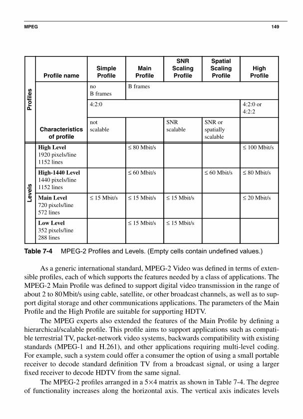
MPEG 149
Table 7-4 MPEG-2 Profiles and Levels. (Empty cells contain undefined values.)
As a generic international standard, MPEG-2 Video was defined in terms of exten-sible profiles, each of which supports the features needed by a class of applications. TheMPEG-2 Main Profile was defined to support digital video transmission in the range ofabout 2 to 80Mbit/s using cable, satellite, or other broadcast channels, as well as to sup-port digital storage and other communications applications. The parameters of the MainProfile and the High Profile are suitable for supporting HDTV.
The MPEG experts also extended the features of the Main Profile by defining ahierarchical/scalable profile. This profile aims to support applications such as compati-ble terrestrial TV, packet-network video systems, backwards compatibility with existingstandards (MPEG-1 and H.261), and other applications requiring multi-level coding.For example, such a system could offer a consumer the option of using a small portablereceiver to decode standard definition TV from a broadcast signal, or using a largerfixed receiver to decode HDTV from the same signal.
The MPEG-2 profiles arranged in a 5×4 matrix as shown in Table 7-4. The degreeof functionality increases along the horizontal axis. The vertical axis indicates levels
Pro
file
s
Profile nameSimpleProfile
MainProfile
SNRScalingProfile
SpatialScalingProfile
HighProfile
Characteristicsof profile
noB frames
B frames
4:2:0 4:2:0 or4:2:2
notscalable
SNRscalable
SNR orspatiallyscalable
Lev
els
High Level1920 pixels/line1152 lines
≤ 80 Mbit/s ≤ 100 Mbit/s
High-1440 Level1440 pixels/line1152 lines
≤ 60 Mbit/s ≤ 60 Mbit/s ≤ 80 Mbit/s
Main Level720 pixels/line572 lines
≤ 15 Mbit/s ≤ 15 Mbit/s ≤ 15 Mbit/s ≤ 20 Mbit/s
Low Level352 pixels/line288 lines
≤ 15 Mbit/s ≤ 15 Mbit/s

150 Chapter 7 • Data Compression
with increased parameters, such as smaller and larger frame sizes. For example, theMain Profile in the Low Level specifies 352pixels/line with 288 lines/frame and30 frames/s, without any B frames and a data rate not to exceed 4Mbit/s. The Main Pro-file in the High Level specifies 1920 pixels/line with 1152 lines/frame and 60 frames/swith a data rate not to exceed 80Mbit/s.
MPEG-2 incorporates, in a way similar to the hierarchical mode of JPEG, scalingof compressed video [GV92]. In particular, video is compressed at different qualitiesduring encoding, so that different alternatives are available during decompression[Lip91, GV92]. Scaling may act on various parameters:
• Spatial scaling facilitates decompression of image sequences with different hori-zontal and vertical resolutions. For example, a single data stream could includeimages with 352×288 pixels (H.261 CIF format), 360×240 pixels, 704×576 pix-els (a format according to CCIR 601) and, for example 1,250 lines at an aspectratio of 16:9. These resolutions refer to the luminance component; the chromi-nance component is subsampled by a factor of two. This can be implementedusing a pyramid for the level of the DCT-coefficients [GV92], that is, 8×8 DCT,7×7 DCT, 6×6 DCT, and other transformations can be formed. From a technicalstandpoint, only steps by a factor of two are useful.
• Scaling the data rate allows for playback at different frame rates. In MPEG-1, thisfunctionality is achieved by using D frames. This can be implemented in MPEG-2by using I frames, given a suitable distribution of I frames within the data stream.This condition must be met not only for a group of pictures, but also for the entirevideo sequence.
• Amplitude scaling can be interpreted as affecting either the pixel depth or the res-olution at which DCT-coefficients are quantized. This then leads to a layered cod-ing and to the possibility of progressive image presentation, which is not relevantfor video data. However, this can be of interest if certain images of an imagesequence can be extracted from the data stream as still images.
Scaling is one of the most important MPEG-2 extensions to MPEG-1. MPEG-2also, for example, minimizes the effects of the loss of individual ATM cells in anMPEG-2 coded data stream. Sequences of different frame types (I, P, B) should bedefined to minimize end-to-end delay at a given data rate.
The MPEG-2 group developed the MPEG-2 Audio Standard for low bit rate cod-ing of multichannel audio. MPEG-2 supplies up to five full bandwidth channels (left,right, center, and two surround channels), plus an additional low-frequency enhance-ment channel and/or up to seven commentary/multilingual channels. The MPEG-2Audio Standard also extends MPEG-1 coding of stereo and mono channels with halfsampling rates (16kHz, 22.05kHz, and 24kHz), which significantly improves quality at64Kbit/s or less per channel.

MPEG 151
The MPEG-2 Audio Multichannel Coding Standard is backwards compatible withthe existing MPEG-1 Audio Standard. The MPEG group carried out formal subjectivetesting of the proposed MPEG-2 Multichannel Audio codecs and up to threenonbackward-compatible codecs working at rates from 256 to 448Kbit/s.
7.7.4.1 MPEG-2 System
MPEG-2 addresses video together with associated audio. Note that in order toprovide a precise description, this section uses terminology from the original MPEG-2specification. MPEG-2 defines how an MPEG-2 system can combine audio, video, andother data in a single stream, or in multiple streams, suitable for storage and transmis-sion. MPEG-2 imposes syntactic and semantic rules that are necessary and sufficient tosynchronize the decoding and presentation of video and audio information, whileensuring that the decoder’s coded data buffers do not overflow or run out of data. Thestreams include time stamps used in the decoding, presentation, and delivery of thedata.
In the first step, the basic multiplexing approach adds system-level information toeach stream. Each stream is then divided into packets, forming a Packetized ElementaryStream (PES). Next, the PESs are combined into a Program Stream or a TransportStream. Both streams were developed to support a large number of known or antici-pated applications. They thus incorporate a significant degree of flexibility while ensur-ing interoperability between different device implementations.
• The Program Stream resembles the MPEG-1 stream, but should only be used in arelatively error-free environment. Program stream packets are of variable length.Timing information in this stream can be used to implement a constant end-to-enddelay (along the path from the input of the coder to the output of the decoder).
• The Transport Stream bundles the PESs and one or more independent time basesinto a single stream. This stream was developed for use with lossy or noisy media.Each packet has a length of 188 bytes, including a four-byte header. The TransportStream is well-suited for transmission of digital television and video telephonyover fiber, satellite, cable, ISDN, ATM, and other networks, as well as for storageon digital video tape and other devices.
A conversion between the Program Stream and the Transport Stream is possibleand sensible. Note that the MPEG-2 buffer management specification limits the end-to-end delay for audio and video data to under one second, a value unacceptably high forusers of dialogue mode applications.
A typical MPEG-2 video stream has a variable bit rate. By using a video buffer asspecified in the standard, a constant bit rate can be enforced, at the cost of varyingquality.
MPEG-2 reached the CD (Committee Draft) status in late 1993 and required threeadditional months to become a DIS (Draft International Standard). After a six-month

152 Chapter 7 • Data Compression
ballot period, the DIS became an IS (International Standard). Originally, there wereplans to specify an MPEG-3 standard covering HDTV. However, during the develop-ment of MPEG-2, it was found that scaling up could easily meet the requirements ofHDTV. Consequently, MPEG-3 was dropped.
7.7.5 MPEG-4
Work on another MPEG initiative for very low bit rate coding of audio visual pro-grams started in September 1993 in the ISO/IEC JTC1. Formally designated ISO/IEC14496, MPEG-4 was published in November 1998 and adopted as an internationalstandard in January 1999.
MPEG-4 incorporates new algorithmic techniques, such as model-based imagecoding of human interaction with multimedia environments and low bit-rate speechcoding for use in environments like the European Mobile Telephony System (GSM).The most important innovation is improved flexibility. Developers can use the compres-sion method in different ways and configure systems to support a multitude of applica-tions. MPEG-4 is thus not a fixed standard suitable only for a few applications.Moreover, MPEG-4 integrates a large number of audiovisual data types, for examplenatural and synthetic, aimed at a representation in which content-based interactivity issupported for all media types. MPEG-4 thus allows the design of audiovisual systemsthat are oriented around specific users yet are compatible with other systems.
Most currently available audiovisual services allow only playback functionality.In contrast, MPEG-4 places a strong emphasis on interactivity. Support for randomaccess to audio and video scenes as well as the ability to revise content are thus amongthe main objectives of the MPEG-4 standardization. MPEG-4 provides for a universalcoding of various forms of audiovisual data, called audiovisual objects. In other words,MPEG-4 seeks to represent the real world as a composition of audiovisual objects. Ascript then describes the spatial and temporal relationships among the objects. Usingthis form of representation, the user can interact with the various audiovisual objects ina scene in a manner that corresponds to the actions of everyday life.
Although this content-based approach to scene representation may seem obviousto the human user, it actually represents a revolution in video representation since itenables a quantum leap in the functionality that can be offered to the user. If a scene isrepresented as a collection of a few or many independent audiovisual objects, the userhas the opportunity to play with the contents of the scene, for example by changing theproperties of some objects (e.g., position, motion, texture, or form), accessing onlyselected parts of a scene, or even using cut and paste to insert objects from one sceneinto another scene. Interaction with contents is thus a central concept of MPEG-4.
Another major shortcoming of other audiovisual coding standards is the restrictednumber of audio and video data types used. MPEG-4 attempts to smoothly integratenatural and synthetic audiovisual objects, for example mono, stereo, and multiple

MPEG 153
channel audio. Moreover, MPEG-4 supports either 2-D or 3-D (mono or stereo, respec-tively) video modes, as well as these from additional camera perspectives (so-calledmultiview video). This integration should be extended with regard to audiovisual inter-relationships so that processing can incorporate the mutual influence and dependencebetween different types of information. Moreover, new and already available analysisand coding tools are being integrated into MPEG-4. In the future, MPEG-4 as a wholewill be further developed as new or better tools, data types, or functionality becomesavailable.
The quick pace of technological progress in recent years has accentuated theinflexibility of standards that do not allow for the continuous development of hardwareand methods. Such standards implement only specific solutions that very quickly nolonger reflect technological developments. Flexibility and extensibility are thus impor-tant objectives of MPEG-4. MPEG-4 provides flexibility and extensibility through the“MPEG-4 Syntactic Description Language (MSDL).” The MSDL approach to extend-ing audiovisual coding standards is revolutionary. Not only can new algorithms be inte-grated by selecting and integrating predefined tools (level 1), but they can be “learned”in that the coder can download new tools. At the same time, even MSDL is subject tofurther development since the MPEG-4 standard can always incorporate new tools,algorithms, and concepts in MSDL to support new or improved functionalities.
The areas of telecommunications, computers, and television/film are convergingand are in the position of being able to exchange elements that previously were typicalfor only one of the three areas. This convergence is more likely viewed as evolutionarybecause it is taking place through gradual transitions. Because qualitatively new multi-media services are emerging from this convergence, a logical consequence is that newrequirements will be placed on coding and transmission techniques. With its officialfocus on the three driving forces of content and interaction, integration and flexibilityand extensibility, MPEG-4 seems to be the appropriate answer to such requirements.
7.7.5.1 MPEG-4 Extensions Compared with MPEG-2
The vision of the MPEG-4 standard can be best explained using the eight new orimproved functionalities identified in the MPEG-4 Proposal Package Description.These were the result of a meeting held to determine which features could be of signifi-cance in the near future but that were not (or only partially) supported by present-daycoding standards.
MPEG-4 must additionally provide some other important so-called standard func-tions included in previously available standards, for example synchronization of audioand video, low-delay modes, and interoperability between networks. Unlike the new orimproved functions, the standard functions can be provided by standards that eitherexist or are under development.
MPEG-4 makes it possible to scale content, spatial and temporal resolution,quality, and complexity with finer granularity. This content-based scalability implies

154 Chapter 7 • Data Compression
the existence of a priority mechanism for a scene’s objects. The combination of variousscaling methods can lead to interesting scene representations, whereby more importantobjects are represented using higher spatial-temporal resolution. Content-based scalingis a key part of the MPEG-4 vision, since other features can easily be implemented oncea list of a scene’s important objects is available. In some cases, these and related fea-tures may require analyzing a scene to extract the audiovisual objects, depending on theapplication and on previous availability of composition information.
MPEG-4 incorporates a syntax and various coding methods to support content-based manipulation and bit stream editing, without requiring transcoding (conversionfrom one coding system to another). This means that the user should be able to access aspecific object within a scene or bit stream, thus making it possible to easily change theobject’s properties.
MPEG-4 offers efficient, content-based tools to access and organize multimediadata. These features include indexing, addition of hyperlinks, queries, viewing data,uploading or downloading data, and deleting data.
MPEG-4 supports efficient methods of combining synthetic and natural scenes(e.g., text and graphics overlays), the ability to code natural and synthetic audio andvideo data, as well as methods of mixing synthetic data with conventional video oraudio under decoder control. This feature of MPEG-4 enables extensive interaction fea-tures. The hybrid coding of natural and synthetic data allows, for the first time, asmooth integration of natural and synthetic audiovisual objects and thus represents afirst step towards the complete integration of all sorts of types of audiovisualinformation.
MPEG-4 supports scenes with different views/sound tracks and can efficientlycode them together with sufficient information to synchronize the resulting basicstreams. For video applications that use stereoscopic pictures or multiple views, thismeans that redundancy between multiple views of the same scene can be exploited.Furthermore, this permits solutions that are compatible with normal (mono) video.Coding multiple, simultaneous data streams should provide an efficient representationof natural 3-D objects if a sufficient number of views is available. On the other hand,this can necessitate a complex analysis process. This functionality should especiallybenefit applications that until now have used almost exclusively synthetic objects, forexample in the area of virtual reality applications.
The strong growth of mobile networks in particular has resulted in a need forimproved coding efficiency. MPEG-4 is thus needed in order to provide substantiallybetter audiovisual quality than either existing standards or standards under development(e.g. H.263), at comparably low bit rates. It should be noted that the simultaneous sup-port of other functionality does not necessarily further compression efficiency. How-ever, this is not problematic since different coder configurations can be used in differentsituations. Subjective tests carried out with MPEG-4 in November 1995 showed that, in

MPEG 155
terms of coding efficiency, the available coding standards performed very well incomparison to most other proposed techniques.
Universal accessibility implies access to applications over a wide range of net-works (both wireless and cable-based) and storage media. MPEG-4 must thereforework robustly in environments susceptible to errors. Especially for low bit rate applica-tions, the system must provide sufficient robustness against serious errors. Theapproach used is not to replace the error-control techniques that are implemented in thenetwork, but rather to offer elasticity against residual errors. This can be achieved with,for example, selective forward error correction, error containment, or errorconcealment.
MPEG-4 incorporates efficient methods to improve temporal random access toparts of an audiovisual sequence in a limited time interval with fine resolution. Theseinclude conventional techniques for achieving random access at very low bit rates.
7.7.5.2 Audiovisual Objects (AVOs) in MPEG-4
Audiovisual scenes in MPEG-4 are composed of audiovisual objects (AVOs),which are organized in a hierarchical fashion.
Primitive AVOs are found at the lowest level of the hierarchy. Examples are:
• a two-dimensional fixed background,• the image of a talking person (without background) or• the speech associated with the person.
MPEG-4 standardizes a number of these primitive AVOs that can be used to repre-sent natural as well as synthetic types of content, which can be either two- or three-dimensional.
MPEG-4 defines the coded representation of such objects, for example:
• text and graphics,• heads of speaking actors and associated text that the receiver can use to synthesize
corresponding speech and animate the head accordingly,• animated human bodies.
Figure 7-21 Example of an audiovisual scene in MPEG-4.
“Hello,
Audio
object 1 Video objects
12
3
Audio Audio
object 2
everyone”

156 Chapter 7 • Data Compression
AVOs are individually coded in order to achieve maximum efficiency. They can berepresented independently of other AVOs or of the background information.
MPEG is working with representatives of organizations that manage electronicmedia rights on defining a syntax for storing information about Intellectual PropertyRights (IPR) pertaining to MPEG-4 AVOs and on developing tools to support IPR iden-tification and IPR protection. The MPEG-4 standard thus incorporates support forunambiguous identification using attributes assigned by international naming authori-ties. These can be used to identify the current holder of the rights to an AVO. Protectionof the content will be part of a subsequent version of MPEG-4.
7.7.5.3 Combining AVOs into Scenes
AVOs are combined in a hierarchical fashion to make audiovisual scenes. Theresult is a dynamic, tree-like structure of AVOs that can be changed through user inter-action. Since each AVO possesses spatial and temporal components and can be locatedin relation to other AVOs, each AVO has coordinates that result from those of its parentAVO in the tree structure for the audiovisual scene.
7.7.5.4 Coding of Visual Objects
MPEG-4 uses a variety of methods to code visual objects. These are defined fornatural images and videos as a set of tools and algorithms for the efficient compressionof images, videos, textures, and 2-D and 3-D meshes, as well as geometry streams thatanimate these meshes in a time-varying manner. Tools to randomly access and manipu-late all types of visual objects are available. Furthermore, content-based coding as wellas content-based spatial, temporal, and qualitative scaling are supported. For naturalcontent, there are mechanisms that provide robustness against errors and elasticityagainst errors in environments susceptible to errors.
To code synthetic objects, MPEG-4 defines parametric description tools as well asanimated streams of human faces and bodies for static and dynamic mesh coding withtexture mapping and texture coding. MPEG-4 uses wavelet compression techniques toefficiently code textures. Integration of other standards for synthetic audiovisualcontent, such as VRML, is planned as a future extension to MPEG-4.
In efficiently coding multimedia content the greatest gains can be gotten fromvideo compression. Video coding is thus a particularly important aspect of the MPEG-4standard. Three fundamental video coding extensions, which are realized by MPEG-4,are described below in detail:
1. Object-based scene layering and separate coding and decoding of layers
In order to be able to support content-based functionalities, before processing avideo scene, the coder must be able to divide the scene into layers that representits physical objects. For example, one could divide a video scene into three layersO1, O2, and O3, whereby O1 represents the background, O2 represents the person

MPEG 157
in the foreground, and O3 represents the telephone (see Figure 7-22). Each objectis then coded separately and transmitted over its respective bit stream layer.
Figure 7-22 Example of division of a video sequence.
The layering approach has the major advantage that each bit stream layer can beindependently processed and separately coded and decoded. This achievesefficient coding and permits content-based functionalities.
If transmission takes place in environments susceptible to errors, different layerscan be treated differently. For example, better error protection could be used forthe foreground layer O2 than for the two other layers if the recipient is more inter-ested in the foreground object. Then at least the foreground layer can be decodedwith sufficient quality if there is significant noise in the transmission channel. Inother applications, the user could be interested in showing only the foregroundlayer when the video is being edited, manipulated, and mixed. The person in theforeground could then be placed in a scene coming from another video with a dif-ferent background (possibly even a synthetic scene that was created through com-puter graphics). The bit stream layer O3 can be accessed directly. This can also beinserted in the bit stream of another video scene without requiring that one of thetwo scenes be additionally segmented and transcoded.
2. Shape-adaptive DCT coding
After a scene has been successfully segmented, creating the different object lay-ers, each layer is coded separately. This is done using a DCT coding techniquethat adapts itself to the object’s shape. The fundamental structure of this techniquecan be considered an extension to conventional block-based hybrid DCT algo-rithms that use motion compensation and that code the different object layers. Incontrast to previous standards, images to be coded in each object layer are nolonger considered to be rectangular regions. Their shape and position can changebetween successive frames.
In order to model and optimize the performance of an algorithm for the functionalcoding of input sequences of arbitrarily shaped images at a bit rate of around1Mbit/s, the standard MPEG-1 coding system was extended with a shape codingalgorithm and a shape-adaptive DCT technique. Shape-adaptive DCT allowstransformation coding of image blocks of any shape.
“Hello,everyone”
primitive AVO
compound object
compound object

158 Chapter 7 • Data Compression
For each object layer, the object shape information is transmitted first. This is fol-lowed by the blocks’ motion vectors and the DCT coefficients corresponding tothe motion and to the object’s texture information as described by luminance andchrominance. In order to permit separate decoding of each object layer, the codinguses no information about shape, motion, or texture outside of the respective layer.As in previous MPEG definitions, input images to be encoded are split into gridsof macro blocks and blocks. A block motion vector is transmitted for each macroblock. For rectangular blocks, the SA-DCT algorithm reduces to the standardblock DCT algorithm.
3. Object-based tool box for motion prediction
The basic SA-DCT algorithm was developed in order to implement MPEG-4’sobject-based functionalities. The algorithm reduces temporal redundancy by usingblock-based motion compensation, comparable to that of the previous MPEG cod-ing algorithm. An important advantage of the SA-DCT object-based approach isthe significant increase in compression efficiency achieved by using appropriatetools for motion prediction in each object layer.
The alternative prediction tools Pred 1–Pred 3, for example, extend the basic SA-DCT motion compensation approach with object-based motion prediction tech-niques. After the initial scene segmentation and layered description of the videocontent, each object layer can be classified in view of specific object propertiesduring initial scene analysis (e.g., constant background with or without globalcamera movement motion, constant foreground objects with global motion orflexible foreground objects with related motion). This classification can be used toapply different tools for temporal prediction in layers with different properties.The set of motion prediction algorithms embedded in the basic SA-DCT codingsystem is also described as an object-based prediction tool box, in other words asa set of motion prediction tools that have been optimized for the motion statisticsof various object layers having different properties in the object model.
For flexible foreground objects with corresponding motion (e.g., the foregroundperson O2) or for constant objects with global motion (e.g., a car) it might be moresuitable to code and transmit fixed-motion vector fields or global motion parame-ters than block vectors. Moreover, a background with global camera motion canbe coded very efficiently by estimating and transmitting global camera parame-ters, such as zoom, rotation, and translation, that can be mapped to a stationarypanorama image of a constant background. This implies implementation withinthe coder and the decoder of a background memory that holds a complete (or ascomplete as possible) representation of the stationary background panorama.Based on these global parameters and on the panorama image stored in the back-ground memory, a prediction of the background layer image to be coded is gener-ated by the coder and by the decoder using efficient texturing algorithms.

MPEG 159
Correction images for the background prediction are generated using the SA-DCTalgorithm, similar to the hybrid DPCM/DCT standard coding method.
In the extended SA-DCT approach, conventional block-based motion compensa-tion (Pred 1) can be used for object layers that do not satisfy the special modelassumptions of the new prediction tools. In any case, intra-coded frames andregions where the model fails (for each of the prediction tools) are efficientlycoded using the SA-DCT algorithm.
The MPEG-4 decoder was specified with different complexity levels in order tosupport different types of applications. These are: Type 0 (not programmable,with a predetermined set of tools), Type 1 (flexible, with a set of configurabletools) and Type 2 (programmable, with the ability to download new tools from thecoder).
7.7.5.5 Streams in the MPEG-4 Standard
Just like MPEG-1 and MPEG-2, MPEG-4 also describes streams. Since MPEG-4divides content into multiple objects, the stream properties affect multiplexing,demultiplexing, and synchronization of multiple streams.
AVO data is bundled into one or more Elementary Streams. These are character-ized by the Quality of Service (QoS) needed for transmission (e.g., maximum bit rate orbit error rate) as well as other parameters, for example, stream type information, whichhelps determine the resources required in the decoder and the precision of time infor-mation in the coder. The manner in which such information about stream characteristicsis transported from the source to the sink in a synchronized fashion over networks hav-ing different QoS is specified in terms of an Access Unit Layer and a conceptual two-layer multiplexer.
The Access Unit Layer allows Access Units to be identified within ElementaryStreams, for example, video or audio frames, and scene description commands. Thislayer also permits the reestablishment of the time base of an AV-object or of a scenedescription as well as synchronization between them. The header of an Access Unit canbe configured in a variety of ways, permitting a wide range of systems.
The FlexMux Layer (Flexible Multiplex) is fully specified by MPEG-4. It com-prises a multiplexing tool that allows Elementary Streams (ESs) to be grouped withminimal multiplexing overhead. For example, Elementary Streams with similar QoSrequirements could be grouped.
The TransMux Layer (Transport Multiplexing) models the layer that provides thetransport services that match the required QoS. MPEG-4 specifies only the interface tothis layer. Thus any suitable transport protocol architecture, such as (RTP)/UDP/IP/(AAL5)/ATM or MPEG-2’s Transport Stream over a suitable link layer, may become aspecific TransMux instance. The choice is left to the end user/service provider, allowingMPEG-4 to be used in a multitude of operating environments.

160 Chapter 7 • Data Compression
Figure 7-23 MPEG-4 System Layer Model.
Usage of the FlexMux multiplexing tool is optional. As shown in Figure 7-23, thislayer can be skipped by the underlying TransMux instance since this provides equiva-lent functionality. The Access Unit Layer, however, is always present.
With this the following are possible:
1. Identification of Access Units, transport timestamps, clock reference information,and data loss.
2. Optional interleaving of data from different Elementary Streams into FlexMuxstreams.
3. Control information:
• to indicate the required QoS for each Elementary Stream and FlexMuxstream,
• to translate such QoS requirements into currently available networkresources,
• to transport the mapping of Elementary Streams associated with AVOs toFlexMux and TransMux channels.
Access Units
Adaptation Layer
FlexMux Layer
Elementary Streams
Multiplexed Streams
Network or local storage
e.g. video or audio framesor scene description commands
A/V object data, stream type information,synchronization information,
e.g. multiple Elementary Streams withsimilar QoS requirements
Flexible Multiplexing
Transport Multiplexing
- Only interface is specifiedTransMux Layer
- Layer can be any network
e.g. RTP/UDP/IP, AAL5/ATM
codeccodeccodeccodec
Display / Receipt
Media
Coder / Decoder
QoS requirement,...

MPEG 161
Individual Elementary Streams must be read from incoming data on a networkconnection or from a storage device. In the MPEG-4 system model, each network con-nection or file is homogeneously viewed as a TransMux Channel. Multiplexing is car-ried out partially or completely by layers that are not part of MPEG-4, depending on theapplication. The Stream Multiplex Interface is used as a reference point for integratingMPEG-4 in system environments. Streams packetized by the Adaptation Layer (AL)are accessed at this interface. The FlexMux layer specifies the optional FlexMux tool.The TransMux interface specifies how either streams packetized by the AL (noFlexMux used) or FlexMux streams are received from the TransMux layer. The Trans-Mux interface thus realizes the passage to transport functionality not defined by MPEG.The interface’s data part is considered here, while the control part is dealt with in thecontext of DMIF.
In the same way that MPEG-1 and MPEG-2 describe the behavior of an idealoperational decoding device together with the syntax and semantics of the bit stream,MPEG-4 defines a System Decoder Model. This allows the precise definition of a ter-minal’s operation without having to make unnecessary assumptions about implementa-tion details. This is essential in order to give developers the freedom to implementMPEG-4 terminals and decoding devices in a multitude of ways. Such devices rangefrom TV receivers, which cannot communicate with the sender, to computers, whichare fully capable of exchanging data bidirectionally. Some devices receive MPEG-4streams over isochronous networks, while others use nonisochronous means (e.g., theInternet) to exchange MPEG-4 information. The System Decoder Model represents acommon model that can serve as the basis for all MPEG-4 terminal implementations.
The MPEG-4 demultiplexing step is specified in terms of a conceptual two-layermultiplexer consisting of a TransMux layer and a FlexMux layer as well as the AccessUnit Layer, which conveys synchronization information.
The generic term TransMux Layer is used to abstract underlying multiplexingfunctionality (existing or future) that is suitable for transport of MPEG-4 streams. Itshould be noted that this layer is not defined in the context of MPEG-4. Examples arethe MPEG-2 Transport Stream, H.223, ATM AAL2, and IP/UDP. The TransMux Layeris modelled by means of a protection sublayer and a multiplexing sublayer, which makeit clear that this layer is responsible for offering a specific QoS. The functionality of theprotection sublayer includes error protection and error detection tools appropriate to thenetwork or storage medium. In some TransMux instances, it may not be possible toseparately identify the two sublayers.
Every concrete application scenario uses one or more specific TransMuxInstances. Each TransMux Demultiplexer provides access to the TransMux Channels.Requirements for access to the TransMux Channel at the data interface are the same forall TransMux Instances. They include reliable error detection, the delivery or erroneousdata with a suitable error indication (if possible), and the division of the payload into

162 Chapter 7 • Data Compression
frames. This division consists of either streams that have been packetized by the AL orof FlexMux streams. The requirements are summarized in an informal fashion in theTransMux interface, in the system part of the MPEG-4 standard.
On the other hand, MPEG fully describes the FlexMux Layer. It provides a flexi-ble tool for optional interleaving of data with minimal overhead and low delay and isparticularly useful if the underlying TransMux Instance has a large packet size or highoverhead. The FlexMux itself is not robust against errors. It can either be used on top ofTransMux Channels with high QoS or to bundle Elementary Streams, both of which areequivalent in terms of error tolerance. The FlexMux requires reliable error detectionand sufficient division of the FlexMux packets into frames (for random access and errorcorrection), which must be provided by the underlying layer. These requirements aresummarized in the Stream Multiplex Interface, which defines data access to individualtransport channels. The FlexMux demultiplexer receives AL-packetized streams fromFlexMux Streams.
The Access Unit Layer has a minimal set of tools for checking consistency, pad-ding headers, conveying time base information, and transporting time-stamped accessunits of an Elementary Stream. Each packet consists of an access unit or fragmentthereof. These time-stamped units represent the only semantic structure of ElementaryStreams that is visible in this layer. The AU Layer requires reliable error detection andframing of individual packets of the underlying layer, which can for example be per-formed by the FlexMux. The manner in which the compression layer accesses data issummarized in the informal Elementary Stream interface, also in the system part of theMPEG-4 standard. The AU layer retrieves Elementary Streams from the streamspacketized by the AL.
Depending on the degree of freedom allowed by the author of a scene, the usercan interact with the scene’s contents. The user could, for example, navigate throughthe scene, move objects to different positions, or trigger a sequence of events by click-ing on a specific object with the mouse (for example, starting or stopping a videostream or choosing the desired language if multiple language channels are available). Itwould also incorporate more complex behaviors. For example, a virtual telephone ringsand the user answers it, establishing a communications link.
Streams that come from the network (or from a storage device) as TransMuxStreams are demultiplexed into FlexMux Streams and passed on to appropriateFlexMux demultiplexers, which receive Elementary Streams (see Figure 7-24).

MPEG 163
Figure 7-24 Important components of an MPEG-4 terminal.
Parts of the control functionality are only available in conjunction with a transportcontrol unit, such as the DMIF environment, which MPEG-4 defines for precisely thispurpose. The Delivery Multimedia Integration Framework (DMIF) covers operations ofmultimedia applications over interactive networks, in broadcast environments or fromhard disks. The DMIF architecture is structured such that applications that use DMIFfor communication do not need to have any knowledge of the underlying communica-tions methods. The DMIF implementation takes care of the network details, presentingthe application with a simple interface. DMIF can be placed between an MPEG-4 appli-cation and the transport network (see Figure 7-25).
Elementary Streams
Audiovisual Objects
Network Layer
Demultiplexing
DecompressionScene Description(Script / Classes)
Composition and Rendering
Upstream(User Events,Class Events)
Audiovisual Scenes
Composition Information
Elementary Streams

164 Chapter 7 • Data Compression
Figure 7-25 DMIF architecture.
To predict the behavior of a decoder during decompression of the various elemen-tary data streams that make up an MPEG-4 session, the System Decoder Model makesit possible for the coder to specify and monitor the minimum buffer resources needed todecode the session. The required resources are conveyed to the decoder with objectdescriptors during establishment of the MPEG-4 session so that the decoder can decideif it is capable of proceeding with the session.
By managing the finite amount of buffer space, for example, the model allows thesender to transmit nonreal-time data too early, if sufficient space is available to store itat the receiver. The prestored data can be accessed at the appropriate moment, at whichtime real-time information can use a greater portion of the channel capacity, if required.
Real-time operation assumes a timing model where the end-to-end delay from thesignal output of the coder to the signal input of the decoder is constant. Furthermore,the transmitted data streams must carry either implicit or explicit time information.There are types of such information. The first is used to convey the clock speed, or theencoder time base, to the decoder. The second, which consists of time stamps attachedto parts of the coded AV data, contains desired decoding times for access units or thecomposition and expiration time for composition units. This information is conveyed inthe AL-PDU headers generated by the Access Unit Layer. This timing information canbe used to adapt the interval between pictures and the audio sampling rate at thedecoder to match the encoder’s values in order to achieve synchronized operation.
Different AV objects can be encoded by encoders with different time basestogether with the slightly different speeds that occur. At any time, it is possible to mapthese time bases to the receiving terminal’s time base. However, in this case no real
TransportNetworks(possiblyincluding
Client:DMIF Consumer Role
MPEG-4Application DMIF
Server:
DMIF Producer Role
MPEG-4ApplicationDMIF
(Broadcast or local storage)
Session andResourcemanagement(DSMCC IS)
called on demand
DVD devicedriver)

Fractal Compression 165
implementation of a receiving terminal can avoid the occasional repetition or loss of AVdata caused by temporal aliasing (relative reduction or extension of the time scale).
Although system operation without any timing information is allowed, it is notpossible to define a buffer model in this case.
7.7.6 MPEG-7After MPEG-3 did not materialize, it was decided not to allow MPEG-5 or
MPEG-6 either, in order to preserve the logic of the sequence MPEG-1 (+1) to MPEG-2 (+2) to MPEG-4 (+3) to MPEG-7 (+4) ...
MPEG-7 is not meant as another compression format, rather the intention of theMPEG-7 ISO Working Group was to establish a metadata standard to supplement con-tent coded in other formats (such as MPEG-4). The use of metadata aims at a new typeof extension to the coding of multimedia data: mainly improved searching techniquesand display strategies, but also consistency checking and, for example, scaling thatincorporates consistency and priority. MPEG-7 calls for the integration and extensionof other media content formats (especially MPEG-4) in this way.
In addition to the coding of metadata, MPEG-7 will define interfaces (and only theinterfaces) for working in tandem with tools for automatic content analysis and searchengines, but not these services themselves.
7.8 Fractal CompressionFractal image and video compression represents an entirely different coding
method. In this technique, no actual pixel information is transmitted, rather only atransformation function that contains an image similar to the target image as a fixedpoint. The decoding process then consists of an iterative application of this function toany beginning image.
Various specific attributes of this coding technique follow from this. First of all,the decoding process is progressive and the decoding efficiency is scalable, since thequality of the decoded image increases with each iteration step. Additionally, the pro-cess is independent of the resolution. The mapping function can be applied repeatedlyin order to get more detail. The third attribute is an asymmetry between the encodingand decoding processes.
This raises the question of how an image can be coded as a transformation func-tion. The algorithm makes use of a fractal attribute of images: their self-similarity.Images consist of regions that are similar to one another. A transformation functionthen consists of a mapping of each region of an image to the most similar part of theimage. The mapping consists of contracting, stretching, rotating, and skewing the formof the image regions and adjusting their contrast and brightness. This is a type of vectorquantization that does not use a fixed set of quantization vectors. The mapping willresult in an image if the existence of a fixed point can be guaranteed. The only

166 Chapter 7 • Data Compression
condition required by the theory for this is that of contractivity. The absolute value ofthe contraction factor must lie in the interval [0,1).
The mapping is achieved in current implementations [BH93] by dividing the orig-inal image into blocks (of 8×8 pixels) and, for each block, finding the most similarblock of image regions (i.e., overlapping 16×16 pixel blocks). The set of blocks com-pared with each (8×8) original block is increased by the possible geometric transforma-tions. The most similar block can be found by minimizing a distance measure. Usuallythe sum of the quadratic pixel differences is minimized.
For natural images, fractal compression can achieve high compression ratios (upto 1000:1) with very good image quality. The biggest disadvantage of this codingmethod is the complexity of calculation and its low efficacy when applied to graphicsimages. In order to keep the complexity within practicable limits, only a subset of alltransformations are considered, for example only rotation angles of 0o, 90o, 180o, and270o. Nevertheless each original block must be compared with a very large number ofblocks in order to find the mapping to the most similar block. In addition to the com-plexity of calculation, this coding technique is lossy since it uses only the similarity ofblocks, not their identity.
7.9 Conclusions
The important compression techniques used in multimedia systems all represent acombination of many well known algorithms:
7.9.0.1 JPEG
JPEG is the standard for still image coding that will have the most significance inthe future. Its far-reaching definition allows a large number of degrees of freedom. Forexample, an image can have up to 255 components, that is, levels. An image can consistof up to 65,535 lines, each of which can contain up to 65,535 pixels. Compression per-formance is measured in bits per pixel. This is an average value calculated as the quo-tient of the total number of bits contained in the coded picture and the number of pixelscontained in the picture. That said, the following statements can be made for DCT-coded still images [Wal91]:
• 0.25 to 0.50bit/pixel: moderate to good quality; sufficient for some applications.• 0.50 to 0.75bit/pixel: good to very good quality; sufficient for many applications.• 0.75 to 1.50bit/pixel: excellent quality; suitable for most applications.• 1.50 to 2.00bit/pixel: often barely distinguishable from the original; sufficient for
almost all applications, even those with the highest quality requirements.
In lossless mode, a compression ratio of 2:1 is achieved despite the remarkablesimplicity of the technique. Today JPEG is commercially available in software as wellas in hardware and is often used in multimedia applications that require high quality.

Conclusions 167
The primary goal of JPEG is compression of still images. However, in the form ofMotion JPEG, JPEG can also be used for video compression in applications such asmedical imaging.
7.9.0.2 H.261 and H.263
H.261 and H.263 are already established standards. These were mainly supportedby associations of telephone and wide area network operators. Due to the veryrestricted resolution of the QCIF format and reduced frame rates, implementing H.261and H.263 encoders and decoders does not cause any significant technical problemstoday. This is especially true if motion compensation and the optical low-pass filter arenot components of the implementation, although the quality is not always satisfactoryin this case. If the image is encoded in CIF format at 25 frames/s using motion compen-sation, the quality is acceptable. H.263 is mostly used for dialogue mode applications innetwork environments, for example video telephony and conferencing. The resultingcontinuous bit rate is eminently suitable for today’s wide area networks operating withISDN, leased lines, or even GSM connections.
7.9.0.3 MPEG
MPEG is the most promising standard for future audio and video compressionuse. Although the JPEG group has a system that can also be used for video, it is overlyfocussed on the animation of still images, instead of using the properties of motion pic-tures. The quality of MPEG video (without sound) at about 1.2Mbit/s, appropriate forCD-ROM drives, is comparable to that of VHS recordings [Le 91]. The compressionalgorithm works very well at a resolution of about 360×240 pixels. Obviously, higherresolutions can also be decoded. However, at a resolution of, for example 625 lines,quality is sacrificed. The future of MPEG points towards MPEG-2, which defines a datastream compatible with MPEG-1, but provides data rates up to 100Mbit/s. This signifi-cantly improves the currently available quality of MPEG-coded data.
MPEG also defines an audio stream with various sampling rates, ranging up toDAT quality, at 16bit/sample. Another important part of the MPEG group’s work is thedefinition of a data stream syntax.
Further, MPEG was optimized by making use of the retrieval model for applica-tion areas such as tutoring systems based on CD-ROMs and interactive TV. Embeddingthis optimization in MPEG-2 will allow TV and HDTV quality at the expense of ahigher data rate. MPEG-4 will provide high compression ratios for video and associatedaudio and is furthermore an appropriate tool for creating whole classes of new multime-dia applications. However, currently the complex and still very new MPEG-4 standardis little used in widespread commercial applications.
JPEG, H.263, MPEG, and other techniques should not be viewed as competingalternatives for data compression. Their goals are different and partly complementary.Most of the algorithms are very similar, but not identical. Technical quality, as well as

168 Chapter 7 • Data Compression
market availability, will determine which of these techniques will be used in future mul-timedia systems. This will lead to cooperation and convergence of the techniques. Forexample, a future multimedia computer could generate still images using JPEG, useH.263 or MPEG-4 for video conferencing, and need MPEG-2 to retrieve stored multi-media information. This is, however, a purely hypothetical conception and is not in anyway meant to prejudge future development or strategies for these systems.

169
C H A P T E R 8
Optical Storage Media
Conventional magnetic data carriers in the form ofhard disks or removable disks are traditionally used in computers as secondary storagemedia. These offer low average access time and provide enough capacity for generalcomputer data at an acceptable price. However, audio and video data, even in com-pressed form, place heavy demands on available storage capacity. The storage cost forcontinuous media is thus substantial unless other data carriers are used.
Optical storage media offer higher storage density at a lower cost. The audio com-pact disc (CD) has been commercially successful in the consumer electronics industryas the successor to long-playing records (LPs) and is now a mass-produced product.Due to the large storage capacity of this technology, the computer industry has bene-fited from its development, especially when audio and video data are stored digitally inthe computer. This technology is thus the main catalyst for the development of multi-media technology in computers. Other examples of external devices that can be used formultimedia systems include video recorders and DAT (Digital Audio Tape) recorders.
However, even the aforementioned mass storage media are not adequate to meetthe data rates and especially storage requirements implied by current quality standardsfor multiple applications and data. This has led to the development of new media withmany times the storage density of CDs or DAT tapes. The most important one, desig-nated Digital Versatile Disc (DVD), is based on CD-ROM technology and wasstandardized by an alliance of multimedia manufacturers.
Actually integrating multimedia into systems that do not offer random access (e.g.magnetic mass storage such as DATs) is possible in some cases, though not easy [HS91,RSSS90, SHRS90]. This chapter thus focuses primarily on optical storage. Other datacarriers are not considered here since most either do not have special properties with

170 Chapter 8 • Optical Storage Media
respect to integrated multimedia systems, or will be considered as components of amedia server.
In the following, we explain the basics of optical storage media, followed by abrief discussion of analog and Write Once Read Many (WORM) systems. CD-ROMand CD-ROM/XA are explained based on CD-DA. Various other developments thatpertain to multimedia include CD-I and the Photo CD, which are covered briefly. Inaddition to read only developments of the CD, the subsequently introduced CD-WOand CD-MO have been available for some time. This chapter concludes by comparingthese CD technologies with one another and mentioning possible further developments.
8.1 History of Optical StorageThe video disc was first described in 1973 in the form of the Video Long Play
(VLP). So far the video disc as a read-only medium has not been commercially success-ful although a large number of different write-once optical discs of different sizes andformats have been marketed. Most developments are based on analog technology,which can satisfy the highest quality standards at an acceptable cost.
About ten years later, at the end of 1982, the Compact Disc Digital Audio (CD-DA) was introduced. This optical disc digitally stores audio data in high-quality stereo.The CD-DA specification, drawn up by N.V. Philips and the Sony Corporation, wassummarized in the so-called Red Book [Phi82]. All subsequent CD formats are basedon this description. In the first five years after the introduction of the CD-DA, about 30million CD-DA players and more than 450 million CD-DA discs were sold [BW90b].
The extension of the Compact Disc to storage of computer data was announced byN.V. Phillips and Sony Corporation in 1983 and introduced to the public for the firsttime in November 1985. This Compact Disc Read Only Memory (CD-ROM) isdescribed in the Yellow Book [Phi85], which later led to the ECMA-119 standard[ECM88]. This standard specifies the physical format of a compact disc. The logicalformat is specified by the ISO 9660 standard, which is based on an industry proposal(High Sierra Proposal) and allows access using filenames and a directory.
In 1986, N.V. Philips and the Sony Corporation announced Compact Disc Interac-tive (CD-I). CD-I is described in the Green Book [Phi88], which includes, in addition tothe CD technology, a complete system description. In 1987, Digital Video Interactive(DVI) was presented publicly. The primary emphasis in DVI is on algorithms forcompression and decompression of audio and video data stored on a CD-ROM.
In 1988, the Compact Disc Read Only Memory Extended Architecture (CD-ROM/XA) was announced. N.V. Philips, Sony Corporation, and Microsoft produced aspecification of digital optical data carriers for multiple media, which was published in1989 at the CD-ROM conference in Anaheim, California [Phi89].
Since the beginning of 1990, we have seen the development of the Compact DiscWrite Once (CD-WO) and the rewritable Compact Disc Magneto Optical (CD-MO),

Basic Technology 171
both specified in the Orange Book [Phi91]. Additionally, since the beginning of 1995there has been the rewritable and erasable CD-RW (Compact Disc Read Write), alsospecified in the Orange Book [Phi91] (Part 3).
At the beginning of 1996, efforts to develop compact discs with higher storagedensities began. This was initially carried out in a proprietary fashion by individualfirms. At the end of 1996, the firms joined to form the DVD Consortium. The first DVDspecifications became available by the middle of 1997, and the first devices by the endof 1997.
8.2 Basic Technology
In optical storage media, the underlying principle is that information is repre-sented by using the intensity of laser light reflected during reading. A laser beam havinga wave length of about 780nm can be focused to a resolution of approximately 1µm. Ina polycarbonate substrate layer, there are depressions, called pits, corresponding to thedata to be encoded. The areas between the pits are called lands. Figure 8-1 shows a sec-tional view through an optical disc, running lengthwise along a data track. The pits andlands are represented schematically in the middle of the figure.
Figure 8-1 Sectional view of an optical disc along the data track. Schematic represen-tation of the layers (top), the “lands” and the “pits” (middle), and the signal waveform(bottom).
PitLand
Substrate Layer
Protective Layer
Pit Land
Inte
nsity
of
refle
cted
lase
r lig
ht
Laser
Label
Reflective Layer

172 Chapter 8 • Optical Storage Media
The substrate layer is smooth and coated with a thin, reflective layer. The laserbeam is focused at the height of the reflective layer from the substrate level. Thereflected beam thus has a strong intensity at the lands. The pits have a depth of 0.12µmfrom the substrate surface. Laser light hitting pits will be lightly scattered, that is, it willbe reflected with weaker intensity. The signal waveform shown schematically at thebottom of Figure 8-1 represents the intensity of the reflected laser light; the horizontalline represents a threshold value. The laser in the figure is currently sampling a land.
According to Figure 8-1, a Compact Disc (CD) consists of:
• the label,• the protective layer,• the reflective layer and• the substrate.
Figure 8-2 Data on a CD as an example of an optical disc. Track with “lands” and “pits.”
An optical disc consists of a sequential arrangement of pits and lands within atrack. The pits and lands represent data on the surface. Figure 8-2 shows a greatlyenlarged detail of such a structure.
In contrast to floppy disks and other conventional secondary storage media, all theinformation on an optical disc is placed on one track. The stored information can thusbe played back at a continuous data rate, which has particular advantages for continu-ous data streams such as audio and video data.
CD
1.6 µm
0.6 µm

Video Discs and Other WORMs 173
A track is in the form of a spiral. In the case of a CD, the spacing between adja-cent coils of the spiral—the track pitch—is 1.6µm. The track width of the pits is0.6µm, though their lengths can vary. The most important advantage of the CD overmagnetic storage media follows from these measurements. Along the length of the datatrack, 1.66 data bits/µm can be stored, resulting in a storage density of 1,000,000bit/mm2. With the given geometry, this corresponds to 16,000 tracks/inch. In comparison, afloppy disk has only 96 tracks/inch.
While magnetization can decrease over time and, for example in the case of tapes,crosstalk can occur, optical storage media are not subject to such effects. These mediaare thus very well suited for long-term storage. Only a decomposition or change of thematerial can cause irreparable damage. However, according to current knowledge, sucheffects will not occur in the foreseeable future.
The light source of the laser can be positioned at a distance of approximately1 mm from the disk surface and thus does not touch the disk directly, or float on an aircushion, as is the case with magnetic hard disks. This reduces wear and tear on thecomponents used and increases the life of the device.
8.3 Video Discs and Other WORMsVideo discs in the form of LaserVision are used for the reproduction of motion
picture and audio data. The data are stored on the disc in an analog-coded format, andthe sound and picture quality are excellent. LaserVision discs have a diameter ofapproximately 30cm and store approximately 2.6Gbytes.
Following the naming of the well known long play (LP) for audio information, thevideo disc was originally called Video Long Play. It was first described in 1973 in thePhilips Technical Review [Phi73].
Motion pictures are frequency-modulated on the video disc, and the audio signalis mixed with the modulated video signal. Figure 8-3 shows the principle used to recorddata. The important information of the mixed audio-video signal is the temporalsequence of the zero transitions. Each zero transition corresponds to a change betweena pit and a land on the disc. Such a change can occur at any time, and is written to thedisc in a nonquantized form, that is, the pit length is not quantized. This method is thustime-continuous and can be characterized as analog.

174 Chapter 8 • Optical Storage Media
Figure 8-3 Sectional view of a video disc. Time-continuous discrete value coding.
The video disc was conceived as a Read Only Memory. Since then, many differentwrite-once optical storage systems have come out, known as Write Once Read Many(WORM). An example is the Interactive Video Disc, which operates at Constant Angu-lar Velocity (CAV). On each side, up to 36 minutes of audio and video data at 30 framesper second can be stored and played back. Alternatively, approximately 54,000 studioquality still images can be stored per side.
In 1992, there were already many write-once storage media with capacitiesbetween 600 Mbytes and about 8 Gbytes. These discs have diameters between 3.5 and14 inches. The primary advantage of a WORM over rewritable mass storage is securityagainst alteration. In order to further increase capacity, there are so-called jukeboxes,which can yield capacities of more than 20 Gbytes by using multiple discs.
Besides the large number of incompatible formats, software support is lacking inmost systems. Computer integration is only available for a few selected systems.
WORMs have the following special properties:
• The term media overflow refers to problems that can occur when a WORM disc isalmost full. Firstly, a check must be performed to see if data to be stored can fit onthe WORM disc. Moreover, it must be determined if the data can or should bewritten on different physical discs, and if so, at what point in time to write to thenew disc. This is particularly important for continuous media, since these datastreams can only be interrupted at certain points.
• Packaging refers to problems stemming from the fixed block structure ofWORMs. It is only possible to write records of one given size. For example, if theblock size is 2,048 bytes and only one byte is written, then 2,047 bytes will berecorded without any information content.
PitLand Substrate Layer
Protective Layer
Label
Reflective Layer

Compact Disc Digital Audio 175
• Revision refers to the problem of subsequently marking areas as invalid. Forexample, if a document is changed, the areas that are no longer valid must bemarked as such, so that programs can always transparently access the current ver-sion. Such changes can result in a document being distributed over multipleWORM discs. Yet this must not disturb playback of continuous media streams.
8.4 Compact Disc Digital Audio
The Compact Disc Digital Audio (CD-DA) was developed jointly by N.V. Philipsand the Sony Corporation for storing audio data. The basic technology of the CD-DAwas developed by N.V. Philips [MGC82, DG82, HS82, HTV82].
8.4.1 Technical Basics
CDs have a diameter of 12cm and are played at a Constant Linear Velocity (CLV).The number of rotations per time unit thus depends on the radius of the data currentlybeing sampled. The spiral-shaped CD track has approximately 20,000 windings; incomparison, an LP has only approximately 850 windings.
Information is stored according to the principle depicted in Figure 8-1 andFigure 8-4, whereby the length of the pits is always a multiple of 0.3µm. A changefrom pit to land or from land to pit corresponds to the coding of a 1 in the data stream.If there is no change, a 0 is coded. In Figure 8-4, the data stream shown below corre-sponds to the coded data.
Figure 8-4 “Pits” and “lands.” Discrete time, discrete value storage.
8.4.1.1 Audio Data Rate
The audio data rate can easily be derived from the given sampling rate of44,100Hz and the 16-bit linear quantization. The stereo audio signal is pulse code mod-ulated, and the data rate is as follows:
Schutzschicht
CDLand
Pit
Substrate
10000000000 100000 1000000 100 100000 100000000 10000100
0.3µm
Protective Layer
Label
Reflective Layer

176 Chapter 8 • Optical Storage Media
Audio data rateCD-DA
Analog long-playing records and casette tapes have a signal-to-noise ratio ofapproximately 50 to 60dB. The quality of the CD-DA is substantially higher. As a ruleof thumb, one can assume 6dB per bit used during the sampling process. Given 16-bitlinear sampling:
The signal-to-noise ratio is exactly 98dB.
8.4.1.2 Capacity
The play time of a CD-DA is at least 74 minutes. Using this value, the capacity ofa CD-DA can easily be determined. The capacity given below applies only to storageused for audio data, without, for example, taking into account data used for errorcorrection:
8.4.2 Eight-to-Fourteen ModulationEach change from pit to land or land to pit corresponds to a channel bit of 1; if no
change takes place, the channel bit is a 0.Pits and lands may not follow each other too closely on a CD, since the resolution
of the laser would not suffice to read direct pit-land-pit-land-pit... sequences (i.e., 11111sequences) correctly. Therefore, it was agreed that at least two lands and two pits mustalways occur consecutively. Between every two 1s as channel bits, there will thus be atleast two 0s.
On the other hand, pits and longs cannot be too long, otherwise a phase-correctsynchronization signal (clock) cannot be derived. The maximum length of pits andlands was thus limited such that there can be at most ten consecutive 0s as channel bits.
For these reasons, the bits written on a CD-DA in the form of pits and lands do notcorrespond directly to the actual information. Before writing, Eight-to-Fourteen Modu-lation is applied [HS82]. This transformation ensures that the requirements regardingminimum and maximum lengths are met.
16bits
sample value------------------------------- 2 channels× 44 100
sample valuess channel×
---------------------------------,×= 1 411 200bits
s--------,,=
1 411 200,,bits/s
8 bits/byte-------------------------= 176.4
Kbytess
----------------- 172.3Kbytes
s-----------------≅=
S/NCD-DA 6dBbit------- 16 bits×≅ 96 dB=
CapacityCD-DA 74 min 1 411 200bits
s--------,,× 6 265 728 000 bits,,,= =
6 265 728 000 bits,,,1
8bitsbyte----------
-------------× 1
1 024bytesKbyte--------------,
-----------------------------× 1
1 024KbytesMbyte-----------------,
-------------------------------× 747 Mbytes≅=

Compact Disc Digital Audio 177
Eight-bit words are coded as 14-bit values. Given the minimum and maximumallowed distances, there are 267 valid values, of which 256 are used. The code tableincludes, for example, the entries shown in Table 8-1.
Table 8-1 Eight-to-Fourteen code table. Two sample entries.
With direct sequencing of modulated bits (14-bit values), it is still possible that theminimum distance of two bits would not be met, or that the maximum distance of tenbits would be exceeded. Three additional bits are inserted between successive modu-lated symbols to ensure that the required regularity is met. These filler bits are chosenbased on the neighboring modulated bits, as illustrated in Figure 8-5.
Figure 8-5 Integration of filler bits. p stands for pit, and l stands for land.
8.4.3 Error HandlingThe goal of error handling on a CD-DA is the detection and correction of typical
error patterns [HTV82]. An error is usually the result of scratches or dirt. These canusually be characterized as burst errors.
The first level of error handling implements two-stage error correction accordingto the Reed-Solomon algorithm. For every 24 audio bytes, there are two groups of cor-rection data bytes, each of four bytes. The first group corrects single-byte errors whilethe second group corrects double-byte errors. The correction bytes also allow detectionof additional errors in the sequence, although these cannot be corrected using thisapproach.
In the second level, real consecutive data bytes are distributed over multipleframes (a frame consists of 588 channel bits, corresponding to 24 audio bytes). Theaudio data are stored interleaved on the CD-DA. In this way, burst errors will alwaysdamage only parts of the data.
Using this technique, an error rate of 10-8 is achieved. Burst errors that span atmost seven frames can be detected and corrected exactly. This corresponds to a track
Audio Bits Modulated Bits
00000000 01001000100000
00000001 10000100000000
Audio Bits 0 0 0 0 0 0 0 0 0 0 0 0 0 0 0 1
Modulated Bits 0 1 0 0 1 0 0 0 1 0 0 0 0 0 1 0 0 0 0 1 0 0 0 0 0 0 0 0
Filler Bits 0 1 0 1 0 0
Channel Bits 0 1 0 0 1 0 0 1 0 0 0 1 0 0 0 0 0 1 0 0 1 0 0 0 0 1 0 0 0 0 0 0 0 0
On the CD-DA l p p p l l l p p p p l l l l l l p p p l l l l l p p p p p p p p p

178 Chapter 8 • Optical Storage Media
length of over 7.7mm. In this case, no additional errors can occur in this area. One can,for example, drill a hole with a diameter of 2mm in a CD-DA and still play the audiodata correctly. However, experiments have shown that CD players do not correct allerrors according to the given specifications.
The method described above for error correction is known as Cross InterleavedReed-Solomon Code.
8.4.4 Frames, Tracks, Areas, and Blocks of a CD-DAFrames consist of audio data, error correction, additional control and display
bytes, and a synchronization pattern.
• The audio data are divided into two groups of 12 bytes each. They contain thehigh and low bytes of the left and right channels.
• Additionally, the error detection and correction bytes as described above areappended to each frame in two groups of four bytes each.
• Each frame has a control and display byte, consisting of eight bits, designated P,Q, R, S, T, U, V, and W (subchannels). Subchannel bits from 98 frames are col-lected and used together, yielding eight subchannels of 98 bits each, of which 72bits are used for actual information. Every 98 frames form a block. Unfortunately,sometimes the blocks are also called frames. The P subchannel is used to distin-guish a CD-DA with audio data from a CD with other computer data. TheQ subchannel is used, for example:
• in the lead-in area to store the directory,• in the rest of the CD-DA to specify the relative time within a track and the
absolute time on the CD-DA.
• The synchronization pattern determines the beginning of each frame. It consists of12 1s followed by 12 0s as channel bits and three filler bits.
Table 8-2 shows an overview of the components of a frame and its correspondingbits.

Compact Disc Digital Audio 179
Table 8-2 Components of a frame.
Using these data, different data streams with corresponding data rates can bedistinguished [MGC82]:
• The audio bit stream (also called the audio data stream) carries 1.4112×106bit/s,counting only the 16-bit quantized sample values.
• The data bit stream includes the audio bit stream as well as the control and displaybytes and bytes needed for error handling. The data rate is 1.94×106bit/s.
• The channel bit stream contains the data bit stream with the Eight-to-FourteenModulation and filler and synchronization bits. The data rate is about4.32×106 bit/s.
Altogether, a CD-DA consists of the following three areas:
• The lead-in area contains the directory of the CD-DA. The beginning of the indi-vidual tracks are registered here.
• The program area includes all tracks of the CD-DA; the actual data are storedhere.
• At the end of each CD-DA, there is a lead-out area. This is used to help the CDplayer should it inadvertently read beyond the program area.
The program area of each CD-DA can consist of up to 99 tracks of differentlengths. A CD-DA consists of at least one track, whereby a track usually consists of, forexample, a song or a movement of a symphony. Random access to the beginning ofeach track is possible.
According to the Red Book specification, each track can have multiple indexpoints, allowing direct positioning at certain points. Usually only two pre-defined indexpoints (IP), IP0 and IP1, are used. IP0 marks the beginning of each track, and IP1 marksthe beginning of the audio data within the track. The area within a track between IP0
Audio BitsModulated
Bits Filler BitsChannel
Bits
Synchronization 3+ 24 = 27 bits
Control and Display (14+3) = 17 bits
12 Data 128 i.e. 12 (14+3) = 204 bits
4 Error Handling i.e. 4 (14+3) = 68 bits
12 Data 128 i.e. 12 (14+3) = 204 bits
4 Error Handling i.e. 4 (14+3) = 68 bits
Frame Total = 588 bits

180 Chapter 8 • Optical Storage Media
and IP1 is called the track pregap. CD-DA discs have a track pregap of two to threeseconds per piece.
Besides frames and tracks, another structure, called the block, was established(see Figure 8-6), though it does not have any significance for the CD-DA. In other CDtechnologies, it is used like a sector. A block contains 98 frames (see further details inSection 8.5.1).
Figure 8-6 Actual data of a CD audio block (sector). Layout according to the RedBook.
8.4.5 Advantages of Digital CD-DA Technology
Errors on a CD-DA can be caused by damage or dirt. For uncompressed audio, theCD-DA is very insensitive to read errors that usually occur. As far as the digital technol-ogy, all CD-DAs are identical. An additional advantage is that there is no mechanicalwear and tear.
The CD-DA specification as specified in the Red Book serves as the basis of alloptical CD storage media. For example, Eight-to-Fourteen Modulation and the CrossInterleaved Reed-Solomon Code are always used. Hence, a fundamental specificationwas developed that is used in many systems, providing compatibility across the sys-tems. However, the achievable error rate is too high for general computer data, necessi-tating an extension of the technology in the form of the CD-ROM.
8.5 Compact Disc Read Only Memory
The Compact Disc Read Only Memory (CD-ROM) was conceived as a storagemedium for general computer data, in addition to uncompressed audio data [PS86,FE88, Hol88, LR86, OC89]. Further, CD-ROM technology was intended to form thebasis for the storage of other media [KSN+87, Wil89]. It was specified by N.V. Philipsand the Sony Corporation in the Yellow Book [Phi85] and later accepted as an ECMAstandard [ECM88].
CD-ROM tracks are divided into audio (corresponding to CD-DA) and data types.Each track may contain exclusively data of one type. A CD-ROM can contain bothtypes of tracks. In such a mixed mode disc (see Figure 8-13), the data tracks are usuallylocated at the beginning of the CD-ROM, followed by the audio tracks.
2,352 bytes

Compact Disc Read Only Memory 181
8.5.1 Blocks
Since CD-ROMs store general computer data, they require better error correctionand higher resolution random access to data units than are specified for CD-DA. A CD-DA has an error rate of 10-8 and allows random access to individual tracks and indexpoints.
The CD-ROM data unit is called a block1 and has similar properties to the sectorsof other media and file systems. A CD-ROM block consists of the 2,352 bytes of a CD-DA block. Thus the de facto CD-DA standard can serve as the basis for the de factoCD-ROM standard.
Of the 2,352 bytes of a block, 2,048 bytes (computer data) or 2,336 bytes (audiodata) are available for user data. The remaining bytes are used for identification forrandom access and for another error correction layer that further reduces the error rate.
Figure 8-7 CD-ROM data hierarchy. Audio blocks as on a CD-DA.
Figure 8-7 shows the data hierarchy of a CD-ROM or CD-DA.
Seventy-five blocks per second are played back. Each block consists of 98 framesof 73.5 bytes (588 bits) each.
1. This refers to the physical block; in ISO 9660, there is also the concept of a logical block.
L L R R
Control&
Display CIRC
EFM+
Filler BitsSynchronization
CIRCPattern
CD 330,000 Blocks
Block2,352 Audio Bytes7,203 Channel Bytes
Frame, Channel Bytes588 bits, of which24 Audio Bytes = 4.32×106 bit/s
Data Bits = 1.94×106 bit/s
Audio Bits 1,411,200 bit/s
Block 1 411 200bits
s--------,,
175------s× 1
8 bits/byte-------------------------× 2 352 bytes,==

182 Chapter 8 • Optical Storage Media
8.5.2 Modes
The CD-ROM specification was defined with the goal of storing uncompressedCD-DA data and computer data, as well as serving as the basis for other media. This isachieved by using two CD-ROM modes. An additional mode 0, where all 2,336 userdata bytes are set to zero, serves to separate storage areas.
8.5.2.1 CD-ROM Mode 1
CD-ROM mode 1 is used to store computer data, as shown in Figure 8-8. Of the2,352 total bytes in each block, 2,048 bytes are available for storing information.
Figure 8-8 CD-ROM mode 1 block (sector) layout according to the Yellow Book.
To be more exact, the 2,352 bytes can be broken down into the following groups:
• 12 bytes for synchronization as the start-of-block indicator,• 4 bytes for the header. This contains an unambiguous block identifier. The first
two bytes contain minutes and seconds, respectively; the third byte contains theblock number, while the fourth byte identifies the mode,
• 2,048 bytes of user data,• 4 bytes for error detection,• 8 unused bytes, and• 276 bytes for error correction, whereby an error rate of 10-12 can be achieved.
Given a playing time of 74 minutes, a CD-ROM can store 330,000 blocks.The capacity of a CD-ROM with all blocks in mode 1 can be calculated as
follows:
The data rate in mode 1 is:
Sync Header User Data EDC Blanks ECC12 4 2,048 4 8 276
2,352 bytes
CapacityCD-ROMMode 1
333 000 blocks, 2 048bytesblock-------------,×= 681 984 000 bytes,,=
681 984 000 bytes,,1
1 024bytesKbyte--------------,
-----------------------------× 1
1 024KbytesMbyte-----------------,
-------------------------------× 650 Mbytes≅=
RateCD-ROMMode 12 048
bytesblock-------------, 75
blockss
---------------×= 153.6Kbytes
s----------------- 150
Kbytess
-----------------≅=

Compact Disc Read Only Memory 183
8.5.2.2 CD-ROM Mode 2
CD-ROM mode 2 serves as the basis for additional specifications for storage ofother media. A block in this mode is shown in Figure 8-9. Of the 2,352 total bytes ineach block, 2,336 bytes are available for storing information.
Figure 8-9 CD-ROM mode 2 block (sector) layout according to the Yellow Book.
The synchronization and header are dealt with as in mode 1. The additional errorcorrection is left out.
The capacity of a CD-ROM with all blocks in mode 2 can be calculated asfollows:
The data rate in mode 2 is:
8.5.3 Logical File Format
It was recognized early on that the specification of blocks in mode 1 as an equiva-lent to other data carriers’ sectors was not, by itself, sufficient to define a compatibledata carrier, since the logical file format and the directory were missing.
A group of industry representatives thus met in Del Webb’s High Sierra Hotel &Casino in Nevada and worked out a proposal that became known as the High SierraProposal. This proposal served as the basis for the ISO 9660 standard, which describesthe format exactly (see, for example, its application in [KGTM90]).
The ISO 9660 standard defines a directory tree, which includes information aboutall files. In addition, there is a table that lists all the directories in a compressed form.This so-called path table allows direct access to files at any level. The table is loadedinto the computer memory when a CD is mounted. Because a CD-ROM cannot bechanged (read only), this method can be performed statically in an efficient fashion.However, most implementations use the actual directory tree.
ISO 9660 reserves the first 16 blocks (sectors 0 through 15) in the first track forthe system area, which can be used in a vendor-specific manner. The volume descrip-tors start at sector 16 (for example, the primary volume descriptor or the supplementaryvolume descriptor). The most important descriptor is the primary volume descriptor,
Sync Header User Data12 4 2,336
2,352 bytes
CapacityCD-ROMMode 2333 000 blocks, 2 336
bytesblock-------------,×= 777 888 000 bytes 741.8518 Mbytes=,,=
RateCD-ROMMode 22 336
bytesblock-------------, 75
blockss
---------------×= 175.2Kbytes
s-----------------=

184 Chapter 8 • Optical Storage Media
which includes, among other things, the length of the file system it defines as well asthe length of the path table. Additional file systems can be defined using supplementaryvolume descriptors, which among other things offers flexibility with regard to thecharacter sets allowed for file names.
Each volume descriptor is stored in a 2,048-byte block, and a CD-ROM can con-tain an arbitrary number of volume descriptions. Repeated copies of individual volumedescriptors are usually stored in order to provide increased reliability in the case of adefective CD-ROM. The volume descriptor area ends with a volume descriptor termi-nator, which is implemented as a special block.
ISO 9660 established the logical block size as a power of two of at least 512 bytes.It may not exceed the size of the actual block (sector). The de facto maximum logicalblock size is 2,048 bytes, though this is not required by ISO 9660. If the underlyingtechnology supports another physical block size, ISO 9660 allows other logical blocksizes as well. Current block sizes are 512 bytes, 1,024 bytes, and 2,048 bytes. Thelogical block size is the same for the whole file system described by the volumedescriptor. Files always start at the beginning of a logical block. Thus, files can beginand end within a block (sector). Directories, however, always begin on sectorboundaries.
For some time there have been extensions to ISO 9660 explicitly supporting longfile names, extended access rights, bootability, and special features of system-specificfile systems. Among others, the following file system extensions have been introduced:
• Rockridge Extensions are used for specifying a version of the ISO 9660 formatsuitable for the Unix file system with long file names, links and access rights,
• The Joliet File System has been introduced by Microsoft, which implementsextensions to adapt to the Windows 95/NT file systems and
• The El Torito Extension of the ISO 9660 system, which allows PC systems to bootdirectly from a CD-ROM.
8.5.4 Limitations of CD-ROM Technology
CDs have a high storage capacity and a constant data transfer rate. A randomaccess time of about a second to an individual track can easily be tolerated for audioplayback. This is a major improvement over CD audio or tapes. On the other hand, for aCD-ROM as a data carrier, these access times represent a significant disadvantage com-pared to magnetic disks (which have a mean access time of under 6ms).
The following effects contribute to the time it takes to position to a desired blockon a CD:
• Synchronization time occurs because the internal clock frequency must beadjusted to be exactly in phase with the CD signal. Here, delays are in the range ofmilliseconds.

CD-ROM Extended Architecture 185
• Due to the Constant Linear Velocity (CLV) playback of a CD, the rotational veloc-ity at single speed is about 530 revolutions per second on the inside, but onlyabout 200 revolutions per second on the outside. The rotation delay describes thetime it takes to find the desired sector within a maximum of one rotation and tocorrectly set the rotation speed. Depending on the device, this time can be about300 ms. For a CD-ROM device with a real 40-time data transfer rate and about9,000 revolutions per minute, the maximum rotation delay is about 6.3ms.
• The seek time refers to the adjustment to the exact radius, whereby the laser mustfirst find the spiral track and adjust itself. The seek time frequently amounts toabout 100ms.
These partially overlapping effects cause a high maximum positioning time. How-ever, real times can be highly variable, depending on the current position and thedesired position. Using cache hierarchies, very good drives can reduce the access timeto under 100ms.
Outputting a steady audio data stream requires that audio blocks be stored sequen-tially on the CD. For example, an audio track cannot be played back at the same timedata are read from a CD-ROM mode 1 track. Although this simultaneous retrieval isoften very important for multimedia systems, it is not possible.
Today, there are already CD-ROM drives that sample the medium at speeds of upto 40 times that of a standard audio CD. This increases the data transfer rate achievedwhen reading large blocks. However, the access time during positioning, which is dom-inated by the seek time and does not depend directly on the rotational velocity, is notimproved substantially.
8.6 CD-ROM Extended Architecture
The Compact Disc Read Only Memory Extended Architecture (CD-ROM/XA),which is based on the CD-ROM specification, was established by N.V. Philips, theSony Corporation, and Microsoft [Fri92a, GC89, Phi89]. The main motivation was toaddress the inadequate consideration paid until then to concurrent output of multiplemedia. Prior to the CD-ROM/XA specification, this failing gave rise to other definitionsand systems that included this capability. For example, there are the historically inter-esting CD-I (Compact Disc Interactive) and DVI (Digital Video Interactive) systems.Experience that N.V. Philips and the Sony Corporation obtained from developing theCD-I was incorporated into the development of the CD-ROM/XA. Many features ofCD-ROM/XA and CD-I are thus identical.
The Red Book specifies a track for uncompressed audio data according toFigure 8-6. The Yellow Book specifies tracks for computer data using CD-ROM mode 1(Figure 8-8) and tracks for compressed media using CD-ROM mode 2 (see Figure 8-9).

186 Chapter 8 • Optical Storage Media
CD-ROM/XA uses CD-ROM mode 2 in order to define its own blocks and addi-tionally defines a subheader that describes each block (sector) as shown in Figure 8-10and Figure 8-11. This makes it possible to interleave different media using only mode 2blocks, since these can contain different media. The individual CD-ROM/XA datastreams are separated during playback.
Figure 8-10 Sector layout (1) for CD-ROM/XA according to the Green Book. Datalayout of a CD-ROM block in mode 2, form 1.
Figure 8-11 Sector layout (2) for CD-ROM/XA according to the Green Book. Datalayout of a CD-ROM block in mode 2, form 2.
8.6.1 Form 1 and Form 2
CD-ROM/XA differentiates blocks with form 1 and form 2 formats, similar to theCD-ROM modes:
1. The XA format form 1 in CD-ROM mode 2 provides improved error detectionand correction. Like CD-ROM mode 1, four bytes are needed for error detectionand 276 bytes for error correction. Unlike CD-ROM mode 1, the eight bytesunused in CD-ROM mode 1 are used for the subheader. Figure 8-10 shows ablock (sector), where 2,048 bytes are used for data.
2. The XA format form 2 in CD-ROM mode 2 allows a 13 percent increase in actualdata capacity, to 2,324 bytes per block, at the expense of error handling. Form 2blocks can be used to store compressed data of various media, including audio andvideo data.
On a CD-DA, CD-ROM, or mixed mode disc, a track always consists of homoge-neous data, meaning exclusively audio or computer data. It is thus not possible for thecomputer to, for example, concurrently read uncompressed audio data and computerdata. The main advantage of CD-ROM/XA is that blocks of different media can bestored in one track since they are all coded in CD-ROM mode 2, thus allowing inter-leaved storage and retrieval.
Sync Header User Data EDC ECC12 4 2,048 4 276
2,352 bytes
Sub-Header8
Sync Header User Data EDC12 4 2,324 4
2,352 bytes
Sub-Header8

CD-ROM Extended Architecture 187
8.6.2 Compressed Data of Different Media
Using interleaving, CD-ROM/XA allows the storage of different compressedmedia.
Audio can be compressed at different quality levels with ADPCM (Adaptive Dif-ferential Pulse Code Modulation). The total time of a CD-DA can be extended from 74minutes (without compression) to over 19 hours of lower quality audio by reducing theaudio signal to four bits per sample value. This compression is necessary in order tosimultaneously retrieve data of other media. The following variants are possible:
• Level B stereo achieves a compression factor of 4:1 compared to a CD-DA audiosignal. The level B sampling frequency is 37,800Hz, resulting in a capacity of4 hours and 48 minutes, based on a CD-DA playback time of 74 minutes. Thedata rate is about 43Kbyte/s.
• Level B mono achieves a compression factor of 8:1 compared to a CD-DA audiosignal. At this quality, 9 hours and 36 minutes of audio can be stored. The datarate is about 22Kbyte/s.
• Level C stereo also achieves a compression factor of 8:1 and thus yields results inthe same storage capacity and data rate as level B mono. The level C samplingfrequency is 18,900Hz.
• Level C mono works with a compression factor of 16:1, resulting in a maximumof 19 hours and 12 minutes with a data rate of about 11Kbyte/s.
MPEG audio does not use ADPCM coding (see Section 7.7.2 regarding compres-sion) and is thus still not compatible with the CD-ROM/XA specification. For othermedia, CD-ROM/XA is based on existing standards. Media-specific coding and decod-ing is not part of the CD technology. Thus, only references to other standards are givenhere.
When building applications using the CD-ROM/XA format, the maximum datarate must be considered when choosing the medium and the corresponding quality. Thesame applies to other CD-based formats, such as CD-I.
The logical format of CD-ROM/XA uses the ISO 9660 specification. ISO 9660provides for interleaved files, that is, multiple files that are interleaved with each other.However, ISO 9660 does not address channel interleaving, that is, alternating sectorswith audio, video, and other data within a file. ISO 9660 does not prescribe the contentof a file. Unfortunately, the term file interleaving is often used for interleaved files aswell as for channel interleaving.
An example of a system using this technology is a file system for PC systemsunder Unix described as early as 1992 [Kle92]. This file system is a component of theUnix kernel and is located under the Unix file system switch. All accesses that do notchange data, even to other file systems, are possible this way. The implementationdescribed uses CD-ROM/XA hardware with integrated chips for audio decompression.

188 Chapter 8 • Optical Storage Media
In this system, low-resolution video can be decoded in software at 15 frames persecond.
8.7 Further CD-ROM-Based Developments
The interaction of the different CD-ROM technologies is depicted in Figure 8-12.It should be stressed that the CD-DA, CD-ROM, and CD-ROM/XA specificationsshould be viewed like layers of a communications system.
Figure 8-12 CD-ROM technologies. Specification of multiple layers.
Fundamentally, the CD-DA specification applies to all layers. However, thesequential development of these layers does not cover all the basic facts in the RedBook. For example, the mixed mode disc is not defined.
Other CD-based developments building on these fundamental technologies haveappeared or are appearing to either handle multiple media or specific media and appli-cation areas. For the long term as well, it is expected that all further CD technologieswill be based on CD-DA, CD-ROM, and CD-ROM/XA.
8.7.1 Compact Disc Interactive
The Compact Disc Interactive (CD-I) was developed by N.V. Philips and the SonyCorporation [vZ89] prior to the specification of CD-ROM/XA. In 1986, CD-I wasannounced. In 1988 the Green Book [Phi88] was defined based on the Red Book and theYellow Book [Bas90, BW90a, B.V89, Sv91]. CD-I was originally designed for con-sumer electronics as an addition to the TV set, and the appropriate devices were avail-
CD-DA
CD-ROM
Mode 1 Mode 2
ISO 9660Form 1 Form 2
CD-ROM/XA
CD-Ie.g. DEC VMS
e.g. DVI CDTV

Further CD-ROM-Based Developments 189
able commercially in 1991. However, this system did not become widespread anddisappeared entirely from the market by the end of 1997.
CD-I specifies an entire system. It includes a CD-ROM based format (differentfrom CD-ROM/XA) with interleaving of various media and definition of compressionfor different media. Moreover CD-I defines system software based on the CD-RTOSoperating system and output hardware for multimedia data.
The CD-I hardware is called the decoder. It consists of a main processor from theMotorola 68000 family together with special video and audio chips. It also includes aCD player with a controller and a joystick or mouse interface, and there is provision fora connection to a RGB monitor or a television. CD-I devices, which are the same size asvideo recorders, were intended to replace and extend CD-DA devices in the consumerenvironment.
The CD-I system software consists of the CD-RTOS operating system, a deriva-tive of OS/9 with extensions for real-time processing.
8.7.1.1 Audio Coding
CD-I audio coding includes different quality levels with differing capacity anddata rate. The different modes (CD-DA audio, A, B, and C) are listed in Table 8-3. Theclose relationship between CD-I and CD-ROM/XA is easy to see. CD-I was the basisfor the CD-ROM/XA definition. The lower data rates can be used in combination withimages or motion pictures. Multiple channels of lower quality can also be used for play-back in different languages.
Table 8-3 CD-I audio coding
CD-DA ascomparison
CD-ILevel A
CD-ILevel B
CD-ILevel C
Sampling Frequency in kHz 44.1 37.8 37.8 18.9
Bandwidth in kHz 20 17 17 8.5
Coding 16 bit PCM 8 bit ADPCM 4 bit ADPCM 4 bit ADPCM
Maximum Recording Durationin Hours (Stereo/Mono)
74 minutes/- 2.4/4.8 4.8/9.6 9.6/19.2
Maximum Number of Concur-rent Channels (Stereo/Mono)
1/- 2/4 4/8 8/16
Portion (in %) of Total DataStream (Stereo/Mono)
100/- 50/25 25/12.5 12.5/6.25
Signal-to-Noise Ratio (S/N)in dB
98 96 60 60
Equivalent Quality Audio CD LP VHF Radio Medium WaveRadio

190 Chapter 8 • Optical Storage Media
8.7.1.2 Coding of Images
CD-I can be used to code images at different quality levels and resolutions. Thefollowing short overview shows that different data sizes and data rates are possible:
• The YUV mode is used for reproduction of natural images with many colors. Theimage resolution is 360×240 pixels, and the luminance component Y and thechrominance components U and V are coded using a total of 18 bits per pixel,allowing 262,144 colors per image. The resulting image size is:
• Using a Color Look-Up Table (CLUT), CD-I can work with four bits per pixel.Alternatively, three, seven, or eight bits per pixel are possible. This mode is suit-able for simple graphics with fast retrieval using a preloaded color table. Withfour bits per pixel, at most 16 colors can be simultaneously presented. At a resolu-tion of, for example, 720×240 pixels and four bits per pixel, the resulting imagesize is:
• The RGB mode is intended for very high-quality image output. Red, green, andblue components are each coded with five bits. Including an extra bit per pixel,colors are coded using a total of 16 bits per pixel, allowing up to 65,536 colors toper image to be displayed. With a resolution of 360×240 pixels, the data size foran image is:
8.7.1.3 Coding of Animations
Animations are run-length encoded using approximately 10,000 to 20,000 bytesper image. In the future, CD-I will use MPEG to code video. Although the CD-I fileformat was strongly influenced by the ISO 9660 standard, it is not completelycompatible.
The CD-I technology was originally intended for the consumer marketplace. It isinteresting in the context of the CD because it provided the basis for the CD-ROM/XA.
8.7.2 Compact Disc Interactive Ready Format
Although the different CD formats all stem from the CD-DA standard, it is notnecessarily possible to play a CD-I disc on a CD-DA device. Furthermore, one cannotassume that all CD-DA devices will, for example, be replaced by CD-I devices. There
Data SizeImage
----------------------- 360 240× 18× 1 bits8 bits/byte-------------------------× 194 400 bytes,= =
Data SizeImage
----------------------- 720 240× 4× 1 bits8 bits/byte-------------------------× 86 400 bytes,= =
Data SizeImage
----------------------- 360 240× 16× 1 bits8 bits/byte-------------------------× 172 800 bytes,= =

Further CD-ROM-Based Developments 191
was thus a need for a specification of an optical disc format that can be played on tradi-tional CD-DA devices as well as on CD-I devices. This format is called the CompactDisc Interactive Ready Format [Fri92a].
In the Compact Disc Interactive Ready Format, the track pregap area between theindex points IP0 and IP1 at the beginning of each track is increased from two to threeseconds to a minimum of 182 seconds. The CD-I-specific information is stored in thisarea. This could be, for example, details about individual pieces, images, or biographiesof the composer and the conductor.
A CD-I Ready Disc can be played in three different ways:
• With the usual CD-DA playback, the CD-I information in the track pregap isignored and only the audio will be played.
• The second mode uses only the CD-I data in the track pregap. This can containdata of any media, which can be read, presented, and interpreted, possibly inter-actively. The CD-DA audio data of the track are not played.
• In the third mode, during the audio playback, the CD-I data from the track pregapare presented concurrently. This method is similar to the mixed mode disc (seeSection 8.5). First, the CD-I data are read and stored. Then the audio informationis output together with the corresponding data from the track pregap (which wereread beforehand). In this way the data can be presented simultaneously.
8.7.3 Compact Disc Bridge DiscThe Compact Disc Bridge Disc (CD Bridge Disc)—like the CD-I Ready Disc—
has the goal of enabling a CD to be output on devices supporting different formats.While CD-I Ready Disc specifies a disc format to allow output on either a CD-DAdevice or on a CD-I device, CD Bridge Disc specifies a disc format to allow output oneither a CD-ROM/XA device or on a CD-I device [Fri92a].
Figure 8-13 shows the definitions of the aforementioned CD formats for output ondevices using different standards.

192 Chapter 8 • Optical Storage Media
Figure 8-13 Compact Discs for output on devices with multiple formats. Mixed modedisc, CD-I Ready Disc, and CD Bridge Disc.
A CD Bridge Disc must satisfy both the CD-I and the CD-ROM/XA specifica-tions, though it does not exploit all their capabilities. A common subset is defined thatholds for both formats. All tracks with computer data (as opposed to uncompressedaudio data as per CD-DA) must be recorded using CD-ROM mode 2. The disc may notcontain any CD-ROM mode 1 blocks. Audio tracks (CD-DA) may follow the computerdata tracks.
Another example of compatibility with both specifications is the track entry in thetable of contents at the beginning of the CD. References to CD-I tracks are neverincluded in this area. All tracks with data are thus marked as CD-ROM/XA tracks.
8.7.4 Photo Compact Disc
The Photo Compact Disc from Eastman Kodak and N.V. Philips is an example ofa CD Bridge Disc [Fri92a] used for storing high-quality photographs. The Photo CD isbased on CD-WO, so part of the Photo CD is delivered already written, and a secondpart can be written once. As a CD Bridge Disc, the Photo CD can be read by eitherCD-I or CD-ROM/XA devices. Additionally, it can be read and written by CD-WOdevices and by special Photo CD devices.
The Photo CD was announced at Photokina ‘90 as the Kodak Photo CD Systemand will be licensed by Agfa-Gevaert.
The Photo CD is based on the following process [Kle92]: photographs are createdusing using conventional cameras and film. After the film is developed, the pictures aredigitized using a resolution of eight bits for the luminance component and eight bits for
CD-ROM
Mixed
CD-DA
CD-I
ReadyDisc
CD-ROM/XACD-I
ModeDisc
CDBridge
Disc

Further CD-ROM-Based Developments 193
each of two chrominance components. Each pixel is thus coded in 24 bits. Each photo isthen coded in up to six resolutions as an ImagePac (see Table 8-4). This coding in mul-tiple resolutions is analogous to the idea of hierarchical coding of images in JPEG (seeSection 7.5.5 regarding compression). Each ImagePac usually requires 3–6 Mbytes ofstorage, depending on image complexity.
Table 8-4 Resolution of frames on a Photo CD.
The integration of photos with digital computer and television technology enablesmany new professional and consumer applications. For example, images can bedisplayed using a computer or TV. Using different resolutions, a digital zoom featurecan be easily implemented. Multiple images can be displayed in an overview presenta-tion by using a lower resolution. Using software, images can be modified after the factand/or inserted into documents.
8.7.5 Digital Video Interactive and Commodore Dynamic TotalVision
Digital Video Interactive (DVI) specifies—like CD-I—different components of asystem. DVI consists of compression and decompression algorithms; highly integrated,dedicated hardware components for compression and decompression of video in realtime; a user interface (the Audiovisual Kernel, AVK); and a fixed data format. In con-trast to CD-I, the emphasis is not on the CD technology, but on the compressionalgorithms [HKL+91, Lut91, Rip89].
DVI uses CD-ROM mode 1 with the block format depicted in Figure 8-8. In addi-tion, for the CD-ROM, DVI uses the ISO 9660 format as the basis for the AVSS(Audio/Video Support System) interleaved file format. Commodore’s CDTV (Commo-dore Dynamic Total Vision), for example, also uses CD-ROM mode 1 and theISO 9660 format. It should be noted that ISO 9660 distinguishes among different Inter-change Levels. DVI uses the basic mode (Interchange Level 1), where among otherrestrictions, filenames are limited to 8-point-3 characters from a predefined character
ImageVersion
Compressed/Uncompressed
Number ofRows
Number ofColumns
Base/16 uncompressed 128 192
Base/4 uncompressed 256 384
Base uncompressed 512 768
4 Base compressed 1,024 1,536
16 Base compressed 2,048 3,072
64 Base compressed 4,096 6,144

194 Chapter 8 • Optical Storage Media
set. CDTV uses the Interchange Level 2, which allows, among other things, file namesof up to 30 characters. Today neither system has any commercial significance.
8.8 Compact Disc Recordable
All of the CD technologies considered until now (except the Photo CD discussedin Section 8.7.4) do not allow users to write to discs, limiting the technologies’ applica-tion domain. Research laboratories thus have developed and are developing, in parallelwith read only storage media, compact discs that can be written once or multiple times.
The Compact Disc Recordable (CD-R), specified in the second part of the OrangeBook [Phi91], like WORM (Write Once Read Many) allows the user to write a CD onceand then read repeatedly [AFN90].
8.8.0.1 Principle of the CD-R
Figure 8-14 shows a sectional view through a CD-R vertically through the discsurface and the data track. The CD-R has a pre-engraved track. In all read-only CDs,the substrate (a polycarbonate) adjoins the reflective layer. In the CD-R, there is anabsorption layer between the substrate and the reflective layer. Strong heat has theeffect of irreversibly modifying this layer’s reflective properties for laser beams.
Figure 8-14 Sectional view of a CD-R disc, vertically through the data track. Schemat-ic representation.
In the original state, a CD reader sees a track consisting of lands. Using a laserwith an intensity of three to four times that of a read-only device’s, the absorption layerin the area of the pre-engraved track is heated to above 250˚C. This alters the materialsuch that the reflected laser light now corresponds to a pit. This gives rise to the mostnoteworthy property of the CD-R. The data on a CD-R can be read by traditionaldevices designed exclusively for read-only CDs.
8.8.0.2 Sessions
All of the CD systems described so far assume that a lead-in area precedes theactual data area, and that this is followed by a lead-out area (see Section 8.4.4). Thelead-in area holds a table of contents, which is needed by all playback devices in orderto ensure correct positioning. However, when writing a CD-R this area cannot be
PitLand
Protective Layer
Label
Reflective Layer
Absorption Layer(Pre-engraved Pits/Lands)

Compact Disc Recordable 195
written on the disc until after the write procedure has finished. Thus, all data on a CD-Rwould have to be copied to the disc in one atomic action. In the meantime, the discwould not be readable by other devices.
To solve this problem, the principle of multiple sessions, depicted in Figure 8-15,was introduced. Each session has its own lead-in and lead-out areas. In each write pro-cedure, all the data for a session with its table of contents is written. The disc can thenbe read by other devices.
Figure 8-15 Layout of a “hybrid disc.” Division into multiple sessions.
With this addition, the structure of a CD was extended to a maximum of 99 ses-sions. However, due to the space required for the lead-in and lead-out areas, at most 46sessions—even with empty data areas—can be stored. In turn, each session consists ofa lead-in area, a data area, and a lead-out area. Until 1992, all commercially availabledevices could read only one session. CD-R discs with only one session are called regu-lar CD-R; those with more than one session are called hybrid CD-R.
CD-R recorders operate at up to eight times the data rate of a player. This shortensthe write procedure, but also places requirements that cannot be ignored on thecomputer and additional software needed to produce a CD-R. This data rate must besustained throughout the write procedure. Simpler programs thus first create an imageof the CD-R on a hard disk. The data are then transferred to the CD-R in a second step.A storage-saving approach produces the data in the correct order and transfers them(without intermediate storage of the whole CD-R) at the necessary rate to the CD-R[Wep92].
Given the same price and features, the CD-R could, for example, be a substitutefor CD-DA discs. However, the CD-R production process is and will continue to bemore expensive than that of traditional CDs. Thus, it is used in other application areas.CD-Rs can be used whenever, for technical or legal reasons, large quantities of dataneed to be stored in an irreversible fashion. CD-R also finds application in the area ofCD publishing because the expensive and time-consuming process of creating a mastercan be omitted. It is thus possible to produce limited-circulation editions that are veryup to date.
Lead in Information Lead out InformationLead in Lead out
Session 1 Session 2
...

196 Chapter 8 • Optical Storage Media
8.9 Compact Disc Magneto-OpticalThe Compact Disc Magneto Optical (CD-MO), specified in the first part of the
Orange Book [Phi91], has a high storage capacity and allows the CD to be writtenmultiple times.
Figure 8-16 CD-WO and CD-MO in relation to other CD technologies: structure inmultiple layers.
The magneto-optical technique is based on the principle that at higher tempera-tures, a weak magnetic field is needed to polarize the dipoles in certain materials. Theblock (sector) to be written is heated to above 150˚C. At the same time, a magnetic fieldabout ten times the strength of the Earth’s magnetic field is applied. At this point, thematerial’s dipoles are polarized towards this magnetic field. A pit is coded with a down-wards-facing magnetic north pole. A land is coded using the opposite orientation.
In order to erase a block (sector), the area around the block is subjected to a con-stant magnetic field while it is heated.
If the CD is illuminated by a laser, the polarization of the light changes dependingon the magnetization of the CD. In this way, the information can be read.
8.9.0.3 Areas of a CD-MO
A CD-MO consists of an optional read-only area and the actual rewritable area.The read only area (premastered area in Figure 8-16) contains data written on the
disc in a format specified for this purpose. In Figure 8-16, this relationship is indicatedusing the arrows between the premastered area of a CD-MO and the read only technol-ogies. Thus, the read only area can be read using existing playback devices.
The rewritable area of a CD-MO cannot be read using existing CD-DA, CD-ROM, CD-ROM/XA, or CD-WO devices due to the fundamentally different technol-ogy used for reading and writing. Figure 8-16 shows the relationships between this
R/W MO- RO O- WO
CD-DA
CD-WO
Regular Hybrid
CD-MO
Recordable Premastered
O-
…
…
Area Area

Compact Disc Read/Write 197
recordable area and the underlying magneto-optical technology. This technology is thusincompatible with all the other CD technologies, although it was specified using thesame system parameters as the other techniques. For example, the dimensions and therotational speed are the same.
8.10 Compact Disc Read/WriteThe Compact Disc Read/Write (CD-RW) is a further development of the CD-WO
that, due to its physical makeup, can be repeatedly rewritten. This is achieved by usingthe reversible changeability of crystalline structures. The layers of a CD-RW aredepicted in Figure 8-17.
Figure 8-17 Layers of a CD-R/W. The upper/lower layers are protective layers that in-crease the stability of the CD-R/W.
Like the CD-R, phase changes are made by heating the crystal layer using thelaser. However, in this case the energy is emitted as a pulse waveform (see Figure 8-18).
Figure 8-18 In the “pit” phases, the recording beam varies between the write energyand the bias energy in order to prevent overheating in the crystal.
Label
Lacquer
Reflective
Upper
Recording
Lower
Substrate
amorphous crystalline amorphous
Write Energy
Erase Energy
Bias Energy

198 Chapter 8 • Optical Storage Media
However, using this technology it is no longer possible to read CD-RW discs onevery CD player on the market since the reflectivity is lower than that of a CD or CD-R(see Table 8-5). In order to compensate for these effects, newer CD systems automati-cally amplify the signal as necessary. The other technology and logical structure are thesame as the systems described earlier.
Table 8-5 Comparison of reflectivity of different CD variants.
8.11 Digital Versatile Disc
The Digital Versatile Disc (DVD) is, particularly in view of its larger storagespace, the logical refinement of the CD-ROM/CD-R/CD-RW technologies. In 1994,large electronics companies began work on a CD with higher storage capacity. In early1995, several companies joined to form the DVD Consortium and passed the firststandards in the framework of the DVD Forum in April 1996.
8.11.1 DVD Standards
The DVD Consortium set down the specifications for DVD in the publications“Book A-E.” Each Book defines a standard:
• DVD Read Only Specification (DVD-ROM, Book A): High capacity storagemedium, successor to the CD-ROM,
• DVD Video Specification (DVD-Video, Book B): Specific application of DVD todistributing “linear” video data streams,
• DVD Audio Specification (DVD-Audio, Book C): Specific application of DVD todistribute pure audio data, similar to the CD-DA,
• DVD Recordable Specification (DVD-R, Book D): Variation of DVD that allowsdata to be recorded once for later use, and
• DVD Rewritable Specification (DVD-RW, Book E): Type of DVD that, likeCD-RW, can be repeatedly written and erased; also known as DVD-RAM(Random Access Memory).
The storage capacity that can be achieved with DVD technology depends on theversion (see Table 8-6).
Type Reflectivity
CD-DA 70%
CD-R/CD-WO 65%
CD-RW 15-20%
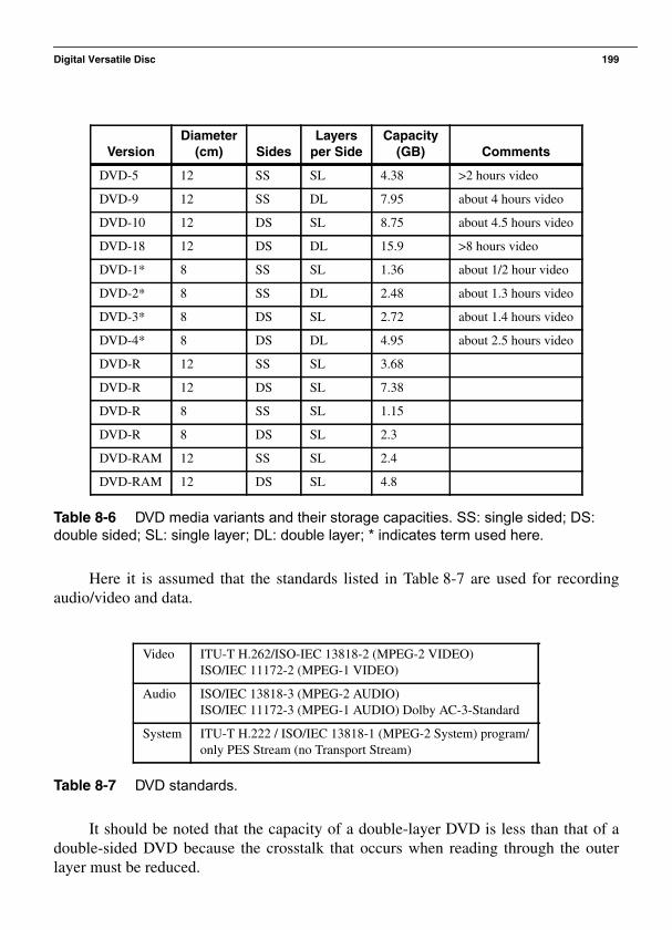
Digital Versatile Disc 199
Table 8-6 DVD media variants and their storage capacities. SS: single sided; DS:double sided; SL: single layer; DL: double layer; * indicates term used here.
Here it is assumed that the standards listed in Table 8-7 are used for recordingaudio/video and data.
Table 8-7 DVD standards.
It should be noted that the capacity of a double-layer DVD is less than that of adouble-sided DVD because the crosstalk that occurs when reading through the outerlayer must be reduced.
VersionDiameter
(cm) SidesLayers
per SideCapacity
(GB) Comments
DVD-5 12 SS SL 4.38 >2 hours video
DVD-9 12 SS DL 7.95 about 4 hours video
DVD-10 12 DS SL 8.75 about 4.5 hours video
DVD-18 12 DS DL 15.9 >8 hours video
DVD-1* 8 SS SL 1.36 about 1/2 hour video
DVD-2* 8 SS DL 2.48 about 1.3 hours video
DVD-3* 8 DS SL 2.72 about 1.4 hours video
DVD-4* 8 DS DL 4.95 about 2.5 hours video
DVD-R 12 SS SL 3.68
DVD-R 12 DS SL 7.38
DVD-R 8 SS SL 1.15
DVD-R 8 DS SL 2.3
DVD-RAM 12 SS SL 2.4
DVD-RAM 12 DS SL 4.8
Video ITU-T H.262/ISO-IEC 13818-2 (MPEG-2 VIDEO)ISO/IEC 11172-2 (MPEG-1 VIDEO)
Audio ISO/IEC 13818-3 (MPEG-2 AUDIO)ISO/IEC 11172-3 (MPEG-1 AUDIO) Dolby AC-3-Standard
System ITU-T H.222 / ISO/IEC 13818-1 (MPEG-2 System) program/only PES Stream (no Transport Stream)

200 Chapter 8 • Optical Storage Media
8.11.1.1 Technical Basics
DVDs achieve a higher capacity than CD-ROMs by using smaller pits (whichyields a higher track density), combined with a larger data area, more efficient codingof bits, more efficient error correction and lower sector overhead (see Figure 8-19).
Figure 8-19 Data on a DVD. The track pitch and the pit width are less than a CD’s.
From the standpoint of information technology, a DVD consists of a number ofblocks of 37,856 bytes each. Each block contains 16 sectors plus additional data forerror detection and correction. Individual sectors consist of 2,064 bytes divided into 12rows as shown in Table 8-8. The first 12 bytes in the first row contain the sector header(sector ID, sector ID error correction, and six reserved bytes). The rest of the block,except the last four bytes, which contain the error detection code, holds user data.
Table 8-8 Structure of a DVD sector.
Row Contents
0 12 byte sector header and 160 bytes of user data
1 172 bytes of user data
...10 172 byte of user data
11 168 bytes of user data and four byte error detection code
DVD
0.74 µm
0.24 µm

Digital Versatile Disc 201
In order to transfer parallel streams better, DVD interleaves 16 sectors together.This also provides better robustness against errors. The result of the interleaving is ablock of 192 rows (16 sectors × 12 rows per sector = 192 rows). At the end of each rowten bytes are added for further error correction, resulting in an additional 16 rows at theend of each block. Thus, only 33,024 bytes of each 37,856-byte block are available foruser data, yielding a payload of only 87 percent.
8.11.2 DVD-Video: Decoder
In the following, some principles of DVD technology are illustrated by examininga decoder in the context of the DVD video specification. The decoder provides for thefollowing six layers to transfer MPEG data:
• Layer 1: Synchronization, 8/16-demodulation, sector detectionAltogether eight synchronization elements are inserted into the 8/16-coded bitstreams. This layer recognizes and detects sector boundaries. At this step, thestarting channel bit rate is 26.16Mbit/s, while the ending user data rate amounts to13Mbit/s.
• Layer 2: Error detection (EDC) and correction (ECC)If the EDC check bits differ from the “fingerprint” generated from the data, thenthe inserted IEC data are used to help correct the error. After this layer, the userdata rate is reduced to about 11.08Mbit/s (about 2Mbit/s are used for errorcorrection, parity, and IEC data).
• Layer 3: Descrambling and decryptionThe data on the DVD are permuted in order to impede (or render impossible)unauthorized reading. Additional encryption is used for copy protection.
• Layer 4: EDC verificationThis is another error detection step.
• Layer 5: Track bufferThe track buffer makes it possible to deliver the data that are read from the DVDat a fixed rate (11.08Mbit/s) to an application at a variable data rate. Specificpackets included in the data stream to control the player are dropped, yielding amaximum data stream of 10.08Mbit/s.
• Layer 6: Transfer of data to MPEG System DecoderIn this step, the data stream is demultiplexed into substreams that are delivered totheir respective applications.
8.11.3 Eight-to-Fourteen+ Modulation (EFM+)
The lowest layer of the communication channel performs Eight-to-Fourteen+Modulation (EFM+), U.S. Patent #5,206,646, which is mainly intended to reduce theDC component of the data stream. Like Eight-to-Fourteen Modulation, EFM+

202 Chapter 8 • Optical Storage Media
eliminates certain sequences of bits (many zeroes). The main advantages of the 8/16modulation are that no filler bits are necessary and that simpler decoding mechanismsare possible.
8.11.4 Logical File FormatThe DVD file format (ISO 13490) is based on the ISO 9660 format. The ISO
13490 file format incorporates multisession capabilities specifically adapted to thefeatures of the DVD technology.
8.11.5 DVD-CD ComparisonTable 8-9 provides an overview of the most important parameters of DVD
technology compared with conventional CD technology.
Table 8-9 Comparison of DVD with conventional CD technology.
CD DVD
Media Diameter about 120 mm 120 mm
Media Thickness about 1.2 mm about 1.2 mm
Laser Wavelength 780 nm (infrared) 650 and 635 nm (red)
Track Pitch 1.6 µm 0.74 µm
Minimum Pit/Land Length 0.83 µm 0.4 µm
Data Layers 1 1 or 2
Sides 1 1 or 2
Capacity about 650 MB about 4.38 GB (SLSS)about 7.95 GB (DLSS)about 8.75 GB (SLDS)about 15.9 GB (DLDS)
Video Data Rate about 1.5 Mbit/s 1-10 Mbit/s (var.)
Video Compression Standard MPEG-1 MPEG-2
Video Capacity about 1 hour depending on format, between 2 and 8 hours
Sound Tracks 2-channel MPEG 2-channel PCM5.1-channel AC-3optional: up to 8 data streams
Subtitles - up to 32 languages

Closing Observations 203
8.12 Closing ObservationsIn the area of optical storage media, as far as can be seen today, Compact Disc
technology or its further development in the form of the DVD, will predominate for alltypes of storage. The interrelationships among the different, mostly de facto, standards(see Figure 8-20) allow a wide field of application. With the exception of the CD-MO,the technologies are all based on the CD-DA and its optical technology.
Figure 8-20 Important CD technologies and their relationships to one another.
A closer examination and comparison of the formats reveals the chronologicalsequence in which the CD technologies were specified. For example, CD-ROM inmode 1 defines improved error handling for computer data. CD-ROM/XA form 1,which is based on CD-ROM mode 2, provides the same service. It would thus be possi-ble to eliminate CD-ROM mode 1 if there weren’t already many applications that use it.The compression methods of CD-ROM/XA should permit use of the JPEG, MPEG,H.261, and CCITT ADPCM standards and not, for example, be limited to coding tech-niques supported by inexpensive chips already integrated on CD-ROM/XA controllerboards.
R/W MO- RO O WO
CD-DA
CD-WOCD-MO
O
CD-ROM
ISO9660
CD-ROM/XA

204 Chapter 8 • Optical Storage Media
Figure 8-21 Important DVD technologies and their relationships to one another.
A major disadvantage of this technology is the relatively high average access timeof at best about 200ms. Even in the future, this will probably not be improved uponconsiderably. The data rate can be further increased by simultaneously reading multipleparts of the track that run parallel to one another. However, by then cache techniquesmay buffer the entire CD, so that the access time will no longer be determined by theCD device. The incompatibility between the CD and the CD-MO is unavoidable, butwill become less important in the future due to CD-R/W and DVD-RAM technology.
The storage capacity achievable using CDs or DVDs is sufficient for many currentsystems. The storage density of up to 15.9 Gbytes obtainable today using DVDs isalready sufficient for complex multimedia applications. With the quick progress in stor-age density, it is possible to imagine there will be further improvements in this area. Assoon as stable robust semiconductor lasers with higher frequencies are available, a fur-ther jump in the storage density of optical media could follow.
The data rate of 10Mbit/s obtainable with DVDs generally suffices to achieve veryhigh quality audio and video playback with all currently used video and audio codings,such as MPEG-2 for video. However, this is not true for studio or movie theater quality.In this area, completely new developments are expected.
DVD Versions
DVD-RAM
DVD-R
DVD-ROM
DVD-Video
DVD-Audio
DVD-Data

205
C H A P T E R 9
Content Analysis
In recent years, multimedia documents have experi-enced wide distribution through the World Wide Web. In addition to the problems ofreceiving data over the network and storing it efficiently, users must now also cope withinformation overload. Search programs provide users looking for particular topics withso much information that they still must decide what is relevant. Information filteringtools, which provide the user with additional information about multimedia databesides just titles, are thus invaluable.
Most films currently available in digital form are uncommented and it is not to beexpected that the large mass of existing films will ever be marked up “by hand” with ametadata track providing information about the actors or the film content. However,modern information technology is in principle capable of automatically extractinginformation from digital films, generating metadata that can be used to support userssearching for specific content.
Pioneering works in this field include automatic cut detection in digital films[ADHC94, AHC93, ZKS93], automatic detection of newscasts [FLE95, ZGST94,ZS94], video indexing [GWJ92, RBE94, SC95, ZSW+95, ZWLS95] and the extractionof key scenes from films [Ror93, LPE97]. These works are based on various areas ofresearch in computer science [LWT94]: in addition to compression, pattern recognition,image recognition and signal processing make vital contributions to automatic contentrecognition of digital films.
This chapter begins with a discussion of currently available content analysis tech-niques inherent to various media. In this context, new types of applications have gainedin importance; several of these are presented subsequently.

206 Chapter 9 • Content Analysis
9.1 Simple vs. Complex Features
Features available for content analysis are called indicators and simple (syntactic)and complex (semantic) features are distinguished.
Syntactic indicators are features that can be extracted from a digital film throughdirect computation without any background knowledge regarding the content of thefilm. As a rule, it is not possible to directly make inferences about the content of thefilm by means of such indicators. Syntactic indicators are thus descriptive in nature.Only after they have been transformed into semantic indicators can a film be interpretedin such a way that, for example, its genre can be determined automatically.
Fundamentally two types of indicators can be defined:
• indicators that are valid at a fixed point in time t,• and indicators that are defined over an interval of time.
For example, video indicators such as RGB color or gray value can be extractedfrom an individual image, while motion vectors can only be computed from a sequenceof images.
Syntactic indicators thus represent both a transformation and an aggregation of aset of digital film material. Examples of syntactic video indicators include RGB colorinformation, gray value information, information about color differences betweenimages, edges in an image, similarity between images, motion vector information andsegmentation of individual images into unicolored regions. Examples of syntactic audioindicators include volume, speech fundamental frequency, or the frequencydistribution.
Semantic indicators allow film contents to be interpreted. Most of these featuresare obtained through a combined evaluation of previously considered syntactic indica-tors. In the video area, semantic indicators include zoom, cuts, fade-outs, dissolves,wipes, and the arrangement of segmented objects into logically related groups.
One differentiates between camera effects and editing effects. Camera effects arecarried out as the film is shot, by the camera operator according to stage directions;editing effects are carried out when the film is edited. Camera effects include cameramotion and zooms. A zoom is a camera operation whereby the camera operatorenlarges or reduces the image in the direction of the zoom center.
In a dissolve between two scenes, the earlier scene is faded out while the follow-ing scene is simultaneously faded in. During this operation, the complete individualimages of the superimposed scenes can always be identified.
In a wipe, the “fade to” (new) scene is superimposed over the currently visiblescene such that there is no pixel overlap between images of the new scene and those ofthe previous scene. In the case of a horizontal wipe from left to right, left edge regionsof images of the current scene are cut off and replaced with right edge regions ofimages of the new scene. The size of the region that is cut off is then successively

Analysis of Individual Images 207
enlarged until the new scene has completely replaced the old scene. Halfway throughthe time allotted for the wipe, the left half of the visible image is the right half of animage of the new scene, and the right half of the visible image is the left half of animage of the old scene.
In the audio domain, content-related features include, among many others, speechrecognition; segmentation of an audio stream into discrete parts; and recognition ofsilence, music, and noises.
9.2 Analysis of Individual Images
Many features are available for the analysis of individual images. Such featuresinclude color, texture, objects in the image, and similarity between images or betweenedge images. These indicators can be used to perform classification tasks such as textrecognition, which is described below. The analysis of individual images was alreadycovered in detail in Chapter 4 (Graphics and Images).
9.2.1 Text Recognition
Examples of the need for processing information that is only available in writtenform on paper include the automatic recognition of addressee information in mail sort-ing systems, reading forms (e.g., bank transfer forms), transferring “old” data into anelectronic form (e.g., converting a library’s card catalog system into an online data-base), or handwritten text input into a PDA (Personal Digital Assistant). This sectionexamines the automatization of these activities in greater detail.
In Optical Character Recognition (OCR) systems, text recognition takes placeafter an original document has been scanned in and is available as a bitmap [HHS96,SL95] (see Figure 9-1).
Figure 9-1 Text recognition in OCR systems.
Document analysis and character segmentation
Character recognition
Post-processing
Document (bitmap)
Characters (bitmaps)
Characters (symbols)
Text
“A” “B”
AB

208 Chapter 9 • Content Analysis
9.2.1.1 Document Analysis and Character Segmentation
In the first step, the image is coarsely segmented into text and nontext regions.Regions that have a low probability of containing any text, for example, because theyare made up of large unicolored areas, are discarded. In digital films, for example, sub-titles can be recognized easily if one assumes that such text always appears in the lowerfifth of the image and is oriented horizontally. Image enhancement is then performed onregions identified as containing text, for example, by removing underlining. In charac-ter segementation, the text regions are divided into a series of individual characters. Inthe case of printed Roman characters, connected component analysis is frequently usedsince once assumes that, with few exceptions, individual characters consist of con-nected strokes. In the case of handwriting or Japanese characters, other methods mustbe used. These are not covered here.
9.2.1.2 Character Recognition
In character recognition, patterns representing individual characters are classifiedas characters of the underlying alphabet. A set of character features is determined andforms the input to the classification process. Two classification methods can be used:template matching and structural classification.
In template matching, each individual pixel of a character is taken as a feature.The pattern is compared with a series of stored character templates (possibly multipletemplates per character, depending on the number of recognized fonts). A similaritymeasure is computed for each stored character template. Finally, the character is classi-fied according to the template that yielded the highest similarity.
The structural classification method works differently. Here, individual structureswithin a character and their arrangement are analyzed, for example, for the letter “B,”vertical or horizontal strokes, curves, or holes. The resulting structural features of acharacter to be classified are compared with known formation rules for each characterof the alphabet.
9.2.1.3 Post-Processing
Connected words are then formed from the recognized letters and context infor-mation is used to correct recognition errors. For example, spell checking can be used tocorrect a sequence of letters recognized as “multirnedia” into the word “multimedia.” Inthe case of recognizing destination addresses on letters, information about the postalcode can be used to restrict the set of valid place and street names.
Current OCR systems achieve recognition rates above 99 percent when analyzingprinted text.

Analysis of Individual Images 209
9.2.2 Similarity-Based Searches in Image DatabasesIn many traditional image databases, images are described through manually col-
lected text, for example, through a brief keyword content description or the name of thephotographer. To query the database, these annotations are searched for specific user-provided keywords. This procedure allows for image description and searches, but isnot always satisfactory since searches are limited to image features that appeared rele-vant to the annotator. Moreover, many image features are complicated if not impossibleto put into words, for example, textures represented in an image. Furthermore, manualannotation is very time consuming.
It thus makes sense to develop image databases that support searches based onfeatures that can be automatically extracted from the stored images, for example, colorand texture or the presence of faces. It then becomes possible to make queries such as“Find images that have coloring similar to my example image” or “Find images inwhich three faces are present near one another.” The output consists of a set of imagesfrom which the user must make a narrower selection. Currently available techniques arenot advanced enough to allow general semantic requests, although expert systems canbe used if the scope is limited to a specific type of images.
If a series of features has been computed for an image, these can be combined intoa feature vector that describes the image. When the database is searched, the differencebetween each image’s feature vector and the feature vector of the query image is deter-mined by means of a distance function. The output set includes only images from thedatabase that have a sufficiently small distance. If multiple features enter into the dis-tance calculation, then the distance functions of the individual features must first besuitably normalized. For this one determines, based on results of psychological percep-tion research, an interval [a1, a2] over which human observers can discern distance val-ues [LEJ98]. Distance values below a1 are insignificant to human perception. Above a2,saturation has been reached. Figure 9-2 shows an example of a normalization function.
Figure 9-2 Normalization function.
For some features, such as color perception, this interval can be determined inde-pendently of a concrete query. For other features, individual determinations must bemade, for example for the maximum permissible distance between human faces in theabove query.
Significance for
Distance values ofa1 a2
1
human perception
different features

210 Chapter 9 • Content Analysis
There are several ways to combine normalized feature distance functions into atotal distance function. For example, one can use the so-called L1 or L2 metrics as abasis and introduce weights for the features. For two arbitrary feature vectors
and , with weights (Σwi = 1) anddistance the metrics can be computed as follows:
If the covariance between the measures used is known, then the Mahalanobisdistance
can be used, which is recommended for strongly correlated measures (here C is thevariance-covariance matrix) [Rus94].
9.3 Analysis of Image Sequences
Analyzing image sequences requires, besides analysis of individual images (alsocalled frames), the analysis of their temporal structure. As a rule, the smallest logicaldata unit (LDU) above the frame level is the shot. A shot is a sequence of framesbetween two cuts that was recorded continuously by one camera. Multiple related shotsform a scene, for example, a dialog in which two interview partners are shownalternately.
The following sections explain how to analyze the temporal structure of a film.Besides time, the feature of motion is essential. The explanation thus begins withtechniques for computing motion vectors in films.
9.3.1 Motion Vectors
Motion is an important indicator for gleaning information from digital films. Withthe help of this indicator, for example, newscaster scenes can be separated from corre-spondents’ news segments in a newscast. Unlike correspondent news segments, news-caster scenes exhibit a minimal amount of motion. In the following, several approachesto computing motion vectors are presented. These can be divided into the followingcategories:
m m1 … mn,,( )= m' m'1 … m'n,,( )= w1 … wn,,di mi m'i–=
dL1m m',( ) widi
i 1=
n
∑=
dL2m m',( ) widi
2
i 1=
n
∑=
dM m m',( ) m1 … mnC 1– m'1 … m'n
T=
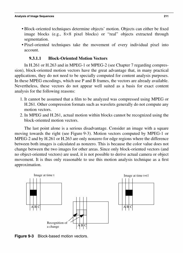
Analysis of Image Sequences 211
• Block-oriented techniques determine objects’ motion. Objects can either be fixedimage blocks (e.g., 8×8 pixel blocks) or “real” objects extracted throughsegmentation.
• Pixel-oriented techniques take the movement of every individual pixel intoaccount.
9.3.1.1 Block-Oriented Motion Vectors
In H.261 or H.263 and in MPEG-1 or MPEG-2 (see Chapter 7 regarding compres-sion), block-oriented motion vectors have the great advantage that, in many practicalapplications, they do not need to be specially computed for content analysis purposes.In these MPEG encodings, which use P and B frames, the vectors are already available.Nevertheless, these vectors do not appear well suited as a basis for exact contentanalysis for the following reasons:
1. It cannot be assumed that a film to be analyzed was compressed using MPEG orH.261. Other compression formats such as wavelets generally do not compute anymotion vectors.
2. In MPEG and H.261, actual motion within blocks cannot be recognized using theblock-oriented motion vectors.
The last point alone is a serious disadvantage. Consider an image with a squaremoving towards the right (see Figure 9-3). Motion vectors computed by MPEG-1 orMPEG-2 and by H.261 or H.263 are only nonzero for edge regions where the differencebetween both images is calculated as nonzero. This is because the color value does notchange between the two images for other areas. Since only block-oriented vectors (andno object-oriented vectors) are used, it is not possible to derive actual camera or objectmovement. It is thus only reasonable to use this motion analysis technique as a firstapproximation.
Figure 9-3 Block-based motion vectors.
Image at time t Image at time t+t1
Recognition of
A B CA B C
A B Ca change

212 Chapter 9 • Content Analysis
9.3.1.2 Pixel-Oriented Motion Vectors
Techniques for computing motion vectors on a pixel basis are called optical flowmethods.
Object movements in the real world appear in an image as color changes. In somecircumstances, color changes in two successive images can indicate movements (see[Jäh97]).
As already described in Chapter 4 (Graphics and Images), tristimulus color valuescan be transformed into gray values. The advantage of gray values is that they can bedifferentiated in one-dimensional space, whereas color values span a three-dimensionalspace. Thus operations are generally much simpler to perform using gray values. In thefollowing it is thus assumed that images for which motion vectors are to be computedare available as gray value images. The same technique can be used with color values,although it should be considered that in practice the computational time is significantlyhigher.
Optical flow refers to the movement of gray value patterns about the image area.First, the displacement vector is determined at each point for the respective gray value.Then a continuous vector field is computed, which should adequately reproduce theoptical flow. Implementing both steps requires certain limiting assumptions and theresults cannot be completely error-free [Jäh97].
Nevertheless, important spatio-temporal information can be obtained. It does notmatter whether changes are continuous, caused by a change in vantage point, or discon-tinuous, due to individual objects. In any case, it should be clear that it does not makesense to consider individual images in isolation. A sequence of at least two successiveimages must be examined [Jäh97].
The following are classes of methods for computing optical flow [BFB94]:
• Differential methods, which use derivatives of images’ gray values to determinemotion vectors [Luc84, LK81, Nag83, Nag89, UGVT88].
• Correlation-based methods, which determine vectors using correlation betweenregions of successive images [Ana87, Ana89, Sin90, Sin92].
• Energy-based methods, which use the energy resulting from the application ofvelocity-dependent filters [Hee87, Hee88].
• Phase-based methods, which define velocity as a phase dependence of theresponse of bandpass filters [FJ90, WWB88].
When three-dimensional reality is projected onto a two-dimensional image plane,it is no longer possible to easily distinguish objects and background from one anotherdue to the loss of the third dimension, particularly if there is no clear difference in thegray values. As described below, this has several interesting consequences for motiondetermination, which is based on recognizing and computing gray value differences insuccessive images in a sequence.

Analysis of Image Sequences 213
We start by assuming that gray value differences have been detected in an imagepair. These are not necessarily the result of object movements. For example, the differ-ences could have been caused by changing lighting conditions, by camera noise, as wellas by a change in the camera position. In the latter case, the entire image would move,which would likely lead to difficulties at edges of the image, which are no longer iden-tical. Here gray value changes occur without object movement. There is a physicalcorrespondence between the images, although it is no longer understandable visually[Jäh97].
On the other hand, even if one considers objects with a uniform surface structureand coloring that rotate about an axis perpendicular to the image plane, under some cir-cumstances gray value differences can occur that do not suffice to infer object move-ment. In this case, there is movement without (sufficient) gray value change [HS81].
Images always capture only a section of the real world, and the images themselvesare viewed as through an aperture. If the aperture is shifted, or if an observed objectmoves, it is possible that there will be difficulties in correctly analyzing the image con-tent. Gray value changes along an edge that extends across the entire image section canonly be discerned in directions perpendicular to the edge. Movements which are paral-lel to the edge direction are present in the real world, but do not manifest themselves ingray value changes. Examples of this are shown in Figure 9-4. In each case, lines arerecognized that were visible at times t0 and t1 in the respective images.
Figure 9-4 Optical flow problems.
In some cases, a nondeterminable motion component in the edge direction mustbe added to the computed displacement vector. This ambiguity is known as the apertureproblem. Figure 9-4 illustrates this situation.
The aperture problem can obviously be solved if the image section is moved farenough that both images being examined contain either the end of the gray value edgeor a corner of any angle [Jäh97]. It is then possible to unambiguously match the edgesbetween the two images.
Additional problems occur when deformable bodies are considered. Here, anoriginal point cannot be unambiguously mapped to its displaced point.
?
?
?
Aperture problem Solution toaperture problem
Deformablebodies
Periodicstructures
t0
t1
t0
t1
t1
t1
t0t0
?

214 Chapter 9 • Content Analysis
Even rigid bodies can lead to ambiguous computation results if they have periodicpatterns or structures. The displacement vector can then only be determined to an accu-racy of the order of a multiple of the width (length) of the repeated pattern or structure.
A third problem example is indistinguishable objects that move independently ofone another. If these occur in large numbers, noncorresponding pairs cannot beuniquely identified. Visual correspondence (indistinguishability) provides the illusionof physical correspondence [Jäh97] (Figure 9-5).
Figure 9-5 Physical correspondence.
With additional assumptions it is possible to find implementation approaches thatresolve the indistinguishability problem. For example, one can assume that images arerecorded at intervals short enough that movement by more than the structure or patternwidth is not possible.
By assuming that indistinguishable particles move at approximately the samespeed, it is possible to compute a solution with the smallest error by determining thevariance of all possible associated pairs [Jäh97].
In a theoretical and experimental comparison, Barron, Fleet, Beauchemin, andBurkitt [BFB94] show that differential methods, in particular those of Lucas andKanade [LK81] and Horn and Schunck [HS81] yielded the best results for processingdigital film sequences at the time of the study (1994). Even today these methods yieldoutstanding results. The authors further show that of the correlation methods, themethod ascribed to Singh [Sin90] yields the most reliable results.
9.3.2 Cut Detection
An important technique for dividing digital films into semantic units is the detec-tion of editing effects, such as cuts, fade-ins and fade-outs, or dissolves and wipes[AJ94]. A cut denotes the sudden change of the image content from one image to thenext. A scene consists of content-related shots, film segments demarcated by editingeffects (see also [BS83, DB81, HJW95, Kuc87]).
Commercial applications of automatic digital cut detection are particularly preva-lent in the area of video indexing systems [HJW94a, TATS94, ZKS93].
Well known methods for automatically recognizing editing effects are:
?
Analysis of Image Sequences 215
• methods that recognize editing effects based on histogram changes [NT91, OT93,RSK92, Ton91, ZKS93],
• methods that recognize editing effects with the aid of edge extraction [MMZ95],• methods that recognize editing effects by means of chromatic scaling [HJW95],
and• methods that infer cuts from changes in the distribution of DCT coefficients
[AHC93].
In the following, the term cut detection is used synonymously for the detection ofcuts and other editing effects.
9.3.2.1 Pixel-Based Cut Detection
Pixel-based methods compute a difference between two images based on theimages’ pixel differences (the pixels can be either separate color values or gray values).The computation can be performed either through a pair-wise comparison of pixels orimage blocks or through histogram comparison.
In the pair-wise comparison method, the pair-wise difference between two succes-sive images is calculated. Differences occur if the color value change or gray valuechange of a pixel exceeds a threshold value T. In a pair-wise comparison, the number ofpixels that change from one image to the next are counted. A cut is detected if a specificchange percentage Z is surpassed.
The problem with this approach is that it is very sensitive to camera motion orobject movement, causing these sorts of image change to be falsely recognized as cuts.
9.3.2.2 Likelihood Ratio
Here, instead of comparing individual pixels, image regions in consecutive imagesare compared using second order statistical methods [KJ91]. Cuts are automaticallydetected if an image has too many regions whose likelihood ratio exceeds a thresholdvalue T. If mi and mi+1 denote the mean intensity of a given region in two images and Siand Si+1 denote the corresponding variances, then the likelihood ratio is defined asfollows [KJ91]:
Compared to the method of pair-wise comparison, the likelihood ratio method hasthe advantage that small object movement or camera motion does not distort the resultsof the computation. Consequently, the total variance of the function is lower, whichmakes it easier to choose the threshold value. A potential problem is that two regionsthat have different distribution functions will be considered identical if they have thesame mean value and the same variance. This case, however, is very rare.
L
Si Si 1++
2---------------------
mi mi 1+–( )2
----------------------------2
+
Si Si 1+×-----------------------------------------------------------------=

216 Chapter 9 • Content Analysis
9.3.2.3 Histogram Comparisons
Instead of comparing individual pixels or regions, the statistical distributions oftwo images’ pixels can be compared. This is achieved by generating histograms thatcapture the distribution of gray values of an image. The idea here is that images inwhich objects and the background change only slightly will have similar gray value his-tograms. This technique can also be applied to RGB color images by using three-dimensional color histograms. However, this requires considerable computationalexpense, and the results are not improved substantially. Histogram-based algorithms arenot sensitive to camera motion or object movement.
A potential problem is that two completely different images can have identicalhistograms. Figure 9-6 shows four different images that have the same histogram. Theimages’ common histogram is shown in Figure 9-7. However, in practice this occurs sorarely between two adjacent frames in a film that this case need not be viewed asproblematic.
Figure 9-6 Images with identical histograms.
Figure 9-7 Histogram of images in Figure 9-6.
A cut is recognized if the histogram difference exceeds a specific thresholdvalue T.
2550Gray level
Am
plitu
de

Analysis of Image Sequences 217
Figure 9-8 and Figure 9-9 show three consecutive images and their histograms.While the first two images have almost identical histograms, the histogram of the thirdimage is markedly different. A cut is thus detected here.
Figure 9-8 Original images with cut after the second image.
Figure 9-9 Histograms of images from Figure 9-8.
A problem with all approaches is that sudden lighting changes or deformableobjects, which result in strong histogram changes, lead to false detections. Flashinglights or explosions, for example, are frequent error sources.
Nagasaka and Tanaka propose a technique to avoid these errors [NT91]. Theyobserve that at most half the image changes, if lighting changes are excluded. Theimage can thus be divided into 16 rectangular regions, which are examined separately.The cut detection is then computed using the eight lowest comparison values.
9.3.2.4 Detection of Fade-Ins/Fade-Outs and Dissolves
Figure 9-10 shows the histogram differences of frames in a film scene that con-tains a cut and a fade-out. Note that the difference measure increases markedly for thecut, which is easily recognized by choosing an appropriate threshold value. On theother hand, the fade-ins and fade-outs show relatively minor increases in the differencemeasure. They cannot be recognized by simply reducing the threshold value, sincemany transitions would be falsely identified as cuts. In this context, transitions that aredetected although none is present in the film material are called false positives.
0
0.02
0.04
0.06
0.08
0.1
0 50 100 150 200 250 300
Perc
ent
Histogram entries0
0.02
0.04
0.06
0.08
0.1
0 50 100 150 200 250 300
Perc
ent
Histogram entries
0
0.05
0.1
0.15
0.2
0 50 100 150 200 250 300
Perc
ent
Histogram entries

218 Chapter 9 • Content Analysis
Figure 9-10 Transition detection using pixel image differences.
Observing that the first and last images of a transition are usually very differentallows the problem to be reformulated as follows. Instead of searching for the transitioneffect, one can search for the beginning and ending of the transition. In order to accom-plish this, two threshold values T1 and T2 must be used. As before, T1 specifies thethreshold where a cut is recognized. T2 specifies a threshold value that marks the begin-ning of a potential transition. Then the difference between the marked image and thecurrent image is computed until either T1 is exceeded, meaning a gradual transition wasfound, or the difference again drops below T2, at which point the marking of the imageis ended. By selecting an appropriate tolerance value, it is possible to determine howoften the difference value may fall below T2 without the first image being unmarked[ZKS93].
A problem with this method is that the authors do not provide a way of differenti-ating a fade-in or fade-out from a dissolve or a wipe.
9.3.2.5 Cut Detection Based on Edge Extraction
Unlike histogram-based methods for cut detection, methods based on edge extrac-tion make use of local information. Here the number of edge pixels that disappear orappear from one image to the next is measured (for edge extraction see Chapter 4). Theindividual steps of this method are as follows:
1. Calculation of the binary edge images Ei and Ei+1 from two consecutive images Iiand Ii+1. In the edge images, a one represents an edge point and a zero representsany other image point.
2. Elimination of camera motion through motion compensation.3. Calculation of the number of edge points that disappear or appear from one image
to the next.4. Decision as to whether or not a transition as occurred, whereby the measure used
is the maximum of the number of edge pixels that disappeared or appeared.
0
0.1
0.2
0.3
0.4
0.5
0.6
0.7
0 5 10 15 20 25 30 35 40 45 50
Fram
e di
ffer
ence
in p
erce
nt
Frames
Cut
Fade-ins/fade-outs

Analysis of Image Sequences 219
Correlation-based methods are used for motion compensation between the imagesIi and Ii+1; these include the Hausdorff distance [HKR93] and the census transform[ZW94]. Using these methods it is possible to calculate the camera motion. The Haus-dorff distance is a displacement vector from which it is possible to derive the directionand length of the camera motion. If the image is simply moved by this vector, one findsthat at most points, the images are not congruent, even excluding points that have newlyappeared in the image due to object movement or camera motion. This process is alsocalled warping [Wol90].
It is easy to detect transitions by looking for local maxima of the function thatmeasures edge pixels that have newly appeared or disappeared from an image. If thisexceeds a threshold value T, a transition is recognized. One must then decide whetherthe transition is a cut, a fade-in or fade-out, a dissolve, or a wipe. This depends on thethreshold value used and on the time horizon over which the transition takes place.
A cut is easy to recognize, since in this case the time horizon is one image. Saidanother way, a cut causes a single deflection in the edge change function, whereas othertransitions take place over greater intervals.
Fade-ins or fade-outs and dissolves can be differentiated from one another by con-sidering the ratio of edge pixels that have come into the image to edge pixels that havedisappeared. In a fade-in, there will be a strictly monotonic increase in newly appearingedge pixels; the opposite holds for a fade-out. A dissolve is comprised of a fade-in anda fade-out and can thus be recognized as their combination.
Wipes can be recognized by examining the local edge distribution and edgechange. In a wipe, each image contains part of the preceding image and, at anotherlocation, part of the following image. Thus an isolated region of the image changes,while the other regions remain constant. During a horizontal wipe, there is a verticalstrip that passes through the image either from right to left or left to right. In this strip,the edge change ratio is higher than in the edge regions. The problem is thus one of dif-ferentiating the strip region from other regions. Zabih [MMZ95] proposes a simple, yetrobust method. The percentage of pixels that change is computed for the upper half ofthe image and for the left half of the image. During a horizontal wipe from left to right,most of the change will occur at the left at the beginning and at the right later. By com-puting change percentages for the four image quadrants at discrete times, it is possibleto accurately determine the type of wipe. Moreover, in a wipe one does not find a char-acteristic ratio of newly appearing or disappearing edge pixels, so it is unlikely to bemistaken for a fade-in, a fade-out, or a dissolve. This is due in particular to the fact thatthe differences between both pixel change ratios are small since the change occurs onlyin a small area of the image.

220 Chapter 9 • Content Analysis
9.3.2.6 Cut Detection through Chromatic Scaling
Hampapur et al. [Ham94, HJW94b, HJW95] describe an approach that identifiescut with the aid of the method described above, but uses a fundamentally differenttechnique, chromatic scaling, to identify fade-ins, fade-outs, and dissolves.
The authors’ cut detection method is based on cut boundaries and editing effectsof partial scenes. A partial scene denotes a sequence of images that does not contain acut. A scene can then be considered to be a set of partial scenes that belong togetherbased on their content, for example, a dialog scene where the speakers are shot by twofixed cameras.
Hampapur et al. observe that editing images are never inserted between twoimages that form a cut boundary, though presumably they may be in the case of fade-insor fade-outs and dissolves. They attempt to recognize these using chromatic scaling.
The basis of every video editing operation, with the exception of cuts, is the chro-matic scaling of two superimposed video tracks. In a fade-in or fade-out, a black videotrack is used and the video track is scaled. In a dissolve, the two video tracks beingmixed are both scaled [And88].
Commercial films primarily use two types of fades [Kuc87]: fade-in from blackand fade-out to black. These can be modelled as chromatic scaling with positive andnegative fade rates. A dissolve is the simultaneous scaling of two partial scenes and isthus the combination of a fade-in and a fade-out.
If one compares automatic transition detection methods, one finds that pixel-oriented methods recognize global features of the underlying images, whereas edge-oriented techniques tend to recognize local features. Local methods are more stronglyaffected by object movement than global methods, though they are more robust tobrightness variations. The objective is thus to combine different approaches so as toachieve optimal transition detection. This can be accomplished as follows: since algo-rithms for detecting fade-ins, fade-outs, dissolves, and wipes are only known for edge-based approaches and for those based on chromatic scaling, these approaches can beused for detecting these effects. Some tests have shown that edge-based detection yieldsbetter results than chromatic scaling methods [Fis97b]. Both approaches yield similarresults when recognizing fade-ins, fade-outs, and dissolves if a static image is scaled.Results with chromatic scaling are generally poorer for scenes in motion.
9.3.3 Analysis of Shots
In order to rapidly grasp the content of a shot, viewers often use the technique of“browsing.” For video data, a representation is needed that greatly reduces the temporalresolution of the images. The goal is thus to find a few representative images for eachshot. These so-called key frames are shown to stand in for the shot and give the viewera rough idea of the shot’s contents. When searching for specific shots in a database, this

Analysis of Image Sequences 221
technique substantially reduces the amount of data that must be transmitted, since onlythe selected shots need to be made available in full.
Ideally, expressive images would be selected by finding points where interestingobjects appear or interesting events occur. However, this requires semantic understand-ing, which until now is hardly ever possible except for special cases such as the detec-tion of faces [LEJ98]. Even the selection of key frames generally uses low-levelfeatures and proceeds as follows:
S denotes the shot being analyzed, consisting of images f1, ..., fn, and R denotesthe set of images selected as representative of S. R is initialized to R = {f1}. Further, atany time f* denotes for the last image added to R, and m denotes its index. Thus, ini-tially f* = f1 and m = 1. The distance function dfeature measures the distance betweentwo images; ε is the maximum tolerable difference. If exceeded, a new key frame istaken. In any case, brief periods of interference or fluctuation of up to k images are dis-regarded [YL95].
dol := min{l : l>m, l+k<=n, min{dfeature(f
*,fl),...,dfeature(f*,fl+k)}>ε}
f* := flm := lR :=
while m<n-k
Examples of features that can be used to compare images include color or texture,or motion from image to image, since content change is frequently associated withcamera motion or object movement [ZLSW95]. If multiple features are used, keyframes should be chosen on a per feature basis. There are techniques for extracting keyframes from sequences encoded in MPEG-1, MPEG-2, or motion JPEG that use fea-tures that can be computed directly from DCT coded images without requiring time-consuming decompression [DAM97].
9.3.4 Similarity-Based Search at the Shot Level
In the following it is assumed that a video is to be searched for shots that are sim-ilar to a given query shot. This problem arises, for example, if one is searching for thebroadcast of a known commercial [Fis97b, RLE97]. Further we assume that featurevectors at the image level has already been computed as described in Section 9.2.
The first question that presents itself is how to represent shots to be compared. Inpractice, there are three approaches:
• Representation as an (unordered) set of key frames, which are described by fea-ture vectors.
• Representation as an (ordered) sequence of key frames, which are likewisedescribed by feature vectors.
R f ∗∪

222 Chapter 9 • Content Analysis
• Representation as a disaggregated character string of feature vectors. For a shotwith n images, the character string has n characters; each character is a featurevector.
Representation as a disaggregated set of images is not common.
9.3.4.1 Representation as a Set of Key Frames
This method assumes two shots S1 and S2 are available for which sets of represen-tative key frames R1 and R2, respectively, have been chosen. The shot distance functionis defined as follows, where a distance function dfeature is used as a measure of thedifference between two images [LEJ98]:
The temporal ordering of the images is not considered here. A possible extensionwould be to compute mean values and deviation measures of some features as well asdominant colors across all images of the shot and to incorporate these into thecomparison [ZLSW95].
9.3.4.2 Representation as a Sequence of Key Frames
If similarity also depends on whether or not the temporal ordering of the keyframes in the shots being compared agrees, then the comparison algorithm presented in[DAM97] can be used. The sequence of key frames for shots S1 and S2 are denoted asR1 = {k1
1, ..., k1n} and R2 = {k2
1, ..., k2m}, respectively, with n < m.
In the first step, k11 is compared with k2
1 and the distance is determined. Then k12
is compared with the key frame(s) from R2 that come next after k12’s temporal position
(i.e., its offset from the beginning of the corresponding shot), whereby at most a maxi-mum difference is permitted. For example, if k1
2 is the third image in S1, then it will becompared with the second, third, and fourth images in S2, provided that these areincluded in R2. The distances (up to three) are added up and the number of addends isstored. If none of the images is contained in R2, then the comparison is skipped for k1
2.This process is repeated for all key frames in R1, until finally the distance sum has beenadded up (Step 1 in Figure 9-11). The average is then computed by dividing by thenumber of addends.
By processing R1 in this manner, R1 is displaced relative to the beginning of S2
such that the offset of k11 corresponds to the offset of k2
2 (Step 2 in Figure 9-11). R1 isdisplaced by the next offset difference in S2 a total (m-n-1) times (the j-loop in the algo-rithm below). In each displacement iteration, the computed average distance is com-pared to the minimum of the previously computed average distances. If the newdistance is smaller, it is stored as the new minimum and the current displacement isconsidered to be the optimal offset so far.
dshot S1 S2,( ) min d feature k1 k2,( ) k2 R2∈{ }k
1R
1∈∑=

Analysis of Image Sequences 223
Figure 9-11 Identification of key frames.
The algorithm can be specified more precisely as follows: the functionneighbor(R2,k1i)computes the set of offsets of the images in R2 whose respectiveoffsets differ by at most one position from the offset of k1
i; the number of elements inthis set is thus between zero and three:
min :=repeat for j := 1 to m-n
sumj := counterj := 0repeat for i := 1 to n
A := neighbor(R2, k1i)
sumj +=
counterj +=t := sumj / counterjif (t<min)
min := topt := j
increase the offset of all images in R1 by(offset of k2j+1 - offset of k
2j)
After the algorithm completes, min is checked to see if it less than a similaritythreshold value. If so, then shots S1 and S2 are considered to be similar, and opt repre-sents the offset of S1 from the beginning of S2 where the two shots best agree.
In order for the neighbor function to achieve an acceptable hit rate, the keyframes in R1 and R2 must be densely packed (ε small). However, satisfying this require-ment yields a smaller reduction in the amount of data, which was the goal of the key
Step 1:
Step 2:
S1
1 2 3 4 5 6 Images
R1
k k k Key frames
Table 0.1:
S1
1 2 3 4 5 6
R1
k k k
∞
d feature k1
i k2
a,( )a A∈∑
A

224 Chapter 9 • Content Analysis
frames concept. This leads to the representation of a shot as a character string of featurevectors of all images.
9.3.4.3 Representation as Character String of Feature Vectors
In this approach, a shot S2 is searched for a query shot S1. The two shots areassigned feature vector character strings V2 and V1, respectively. The comparison isperformed using an approximate string search for V1 in V2. The comparison is approxi-mate in two respects. Firstly, when comparing two individual characters (feature vec-tors), they are only required to match approximately in ordered to be considered“equal.” Secondly, V1 is considered to be contained in V2 even if a certain number ofinsertion, deletion, and character replacement operations are necessary in order to bringa substring of V2 into agreement with V1. Translated to the usual character alphabet, thismeans that “Muller” would be contained in “Hans_Müler-Schmidt,” since “ü” and “u”match approximately, and the addition of an “l” to form “Muller” from “Müler” isallowed.
The algorithm used to perform the approximate string search must work effi-ciently for large alphabets (value range of the feature vectors). Appropriate algorithmsare listed in [Ste94].
9.3.5 Similarity-Based Search at the Scene and Video Level
Analogous to the representation of a shot as a set or sequence of key frames or asa character string, one could represent a scene by using selected shots as well as byusing all shots. Two scenes are then compared using methods analogous to thosepresented in Section 9.3.3 that work at a higher level of aggregation [LEJ98].
If one considers scenes in a video film, one can frequently recognize characteristicshot patterns according to which individual shots are grouped. In a dialog, there is analternating series of shots from two classes (e.g., two interview partners shot in alterna-tion). It is possible to directly search for such shot patterns, thereby allowing queriessuch as “find a dialog.” In the following, shots that are similar to one another are indi-cated with the same letter of the alphabet, so that a dialog, for instance, can be visual-ized as “ABABABABA.” A dialog is recognized by first searching for multipleoccurrences of the same letter separated by short distances, whereby the distancebetween identical characters should be predominantly two. Once such a sequence isfound, a test is performed to see if in the same manner, characters of a second class arearranged between the characters of the sequence. If such an embedded sequence isfound, then the sequence represents a dialog. Note that the term “dialog” is used here ina broad sense—two parallel plot threads presented in alternation would also count as adialog. If one is searching specifically for a conversation between two people, thenadditional search criteria must be provided.

Analysis of Image Sequences 225
In video production, it is not unusual to fall back on existing material that wasused before either in a similar or in a completely different context. For example, onefinds edited versions of original films or reports that incorporate archive material.Through a new cut, film material is used in a context that was not originally intended.
Two measures for comparing entire videos are proposed in [LEJ98]: a measure ofthe correspondence of two videos and a measure of the modification of the ordering ofscenes within a single video (resequencing).
To compute these measures, video films are considered to be sequences of smallerunits, for example, scenes or shots. Let U1 = {u1
1, ..., u1n} denote the units that com-
prise video 1 and U2 = {u21, ..., u2
m} denote the units that comprise video 2. First theunits in U1 are compared with the units in U2. Then an undirected graph is generatedwhere the nodes represent the units and the edges connect units that are sufficientlysimilar to each other, as shown in Figure 9-12.
Figure 9-12 Similarity of videos.
If denotes the number of units in U1 for which there exists at least onesufficiently similar unit in U2, then the correspondence measure is computed as follows:
correspondence (video 1, video 2) = ,
that is, the portion of the units in video 1 that are similar to units in video 2.To test to what extent the common units in the videos occur in the same order, the
resequencing measure is computed as follows:
u11 u1
2 u13 u1
4 u15 u1
6 u17 u1
8
u21 u2
2 u23 u2
4 u25 u2
6
Video 1
Video 2
U1
U2∩
U1
U2∩
U1------------------------

226 Chapter 9 • Content Analysis
numReOrd := numOrdAgree := 0i1 := i2 := 1while (i2<m)
i2 := find the index of the first unit after i2 in video 2from which there is an edge to video 1
itemp := find the index of the first unit after i1 in video 1from which there is an edge to
if (itemp == 0)numReOrd++i1 := find the index of the first unit in video 1
from which there is an edge toelse
numOrdAgree++i1 := itemp + 1
ReSeq(video 1, video 2) :=
A low value indicates that material that is common to the two videos appears inessentially the same order, from which one can conclude that context and content havebeen preserved. On the other hand, with a high resequencing value there is reason tosuppose that due to reordering video material appears in a new context, and thus thatpossibly the content has been used in a way other than originally intended.
9.4 Audio Analysis
In the realm of digital audio, the syntactic indicators of volume and frequency dis-tribution are available [BC94]. An audio signal can be fully defined through both ofthese indicators.
Furthermore, the following semantic indicators are conceivable, among others:
• speech fundamental frequency,• fundamental frequency,• onset, offset, and frequency transitions, and• audio cut detection.
9.4.1 Syntactic Audio Indicators
The volume can be obtained from digital audio without any transformation if thedata is available uncompressed or is decompressed before further processing.
The frequency distribution of an audio file is obtained by performing the Fouriertransform. Although in the time domain there is a mixture of waves, their compositioncan be made visible in the frequency domain. Figure 9-13 shows a three-dimensionalrepresentation of the frequencies of a segment that contains silence followed by a shorthuman exclamation. Time is on the horizontal axis, energy is on the vertical axis, andthe frequency varies along the z-axis.
u2i2
u2i2
numReOrdnumReOrd + numOrdAgree--------------------------------------------

Audio Analysis 227
Figure 9-13 Frequency distribution of a sound mixture.
9.4.2 Semantic Audio Indicators
9.4.2.1 Fundamental Frequency
An important tool for analyzing the perception of complex sound mixtures isfundamental frequency or pitch. The fundamental frequency is the greatest commondenominator of the frequencies where local maxima were observed [Bul77, Hes83,RDS76, GLCS95]. The following methods, among others, can be used to determinefundamental frequency [Fel85, GLCS95, Haw93, RJ93]: the cepstrum technique, theautocorrelation method, the maximum likelihood estimation method, and centerclipping.
9.4.2.2 Audio Cut Detection
It is usually more difficult to implement cut detection in the audio domain than inthe video domain [Fis94, Köh84]. The reason is that a video cut is easy to define as aseries of two fundamentally different images. The audio domain, however, is differentsince a cut hierarchy can be specified. Examples of elements that can be used to definecuts in a digital audio include vowels in spoken language, words, sentences, and speechas opposed to other sound sources.
It is left to the user to set the decision threshold for recognizing a cut. This para-meter must thus be treated as variable.
If one wants to roughly distinguish between speech and other sounds, it is possibleto proceed according to the exclusion principle. Segments that have high energy valuesat frequencies above 7,000Hz cannot be speech segments, since the portion of speechabove 7,000Hz is usually negligible.
If a sound mixture ranges only up to 7,000Hz, it is not possible to make a determi-nation. Nevertheless, the following simple technique can be used to implement cutdetection in this case. Feature vectors consisting of volume, frequencies and speech
Time
Energy
Frequency

228 Chapter 9 • Content Analysis
fundamental frequency are computed for successive time windows i. The current valueis then tested to see whether it is similar to the preceding value. An audio cut is detectedif the distance measure between the vectors exceeds an established threshold value. Thethreshold can also be used to control the granularity of the cut detection. The techniquedescribed can also be used, for example to distinguish music from speech, even if bothlie in the range up to 7,000Hz. Among other things this is because the tone of music isnot similar to that of speech.
Furthermore it is possible to extract “silence.” However if noises occur after aquiet segment, the segment with the noises is much louder than the preceding segment.Thus to detect silence two conditions must be satisfied:
• The volume must be under a threshold value.
• The deviation between the segment and the preceding or following segment mustbe above a second threshold value.
9.4.2.3 Onset and Offset
Human auditory behavior is described as periodic increases or decreases in theresponse of auditory cells (measured via the cells’ “firing probability”). Thus eventsthat cause either a rise or drop in cell response are significant. These are measured usingthe two semantic indicators onset and offset. In the ear this mechanism is realized in thecase of onset by applying a strong excitatory input followed by a strong inhibitorystimulus [WC72]. The inhibitory stimulus prevents the stimulus that is still appliedfrom causing further cell reactions.
Both onset and offset can be set to more quickly identify signal changes that occurrelatively slowly. In this context, a rapidly rising (falling) stimulus is referred to as fastonset (fast offset).
Figure 9-14 Onset of a shout and of a shot.
0
0.1
0.2
0.3
0.4
0.5
0.6
0.7
0.8
0.9
1
0 5 10 15 20 25
Firi
ng p
roba
bilit
y
Time in ms
ShoutShot

Applications 229
Figure 9-14 shows the application of a fast onset filter, which is useful for detect-ing particularly fast signal changes. Here one sees the fast onset of a shout and a shot.Using the fast onset indicator, the shout and the shot can be clearly distinguished[PFE96].
The calculation of the offset is the opposite of the calculation of the onset.Excitatory and inhibitory stimuli thus occur in the opposite order.
9.5 Applications
While the previous sections presented methods for automatic content analysis(with emphasis on “moving pictures”), the following sections present example applica-tions of content analysis. These are based in part on directly derived syntactic indicatorsand in part on semantic indicators, such as scene length or fundamental frequency.
Content analysis can take place either through a classification or through a combi-nation of various methods, such as recognizing actors by recognizing their voices. Theapplications listed below can be classified according to this scheme [Fis97b].
9.5.1 Genre Recognition
The term film genre is used to refer to a category or group of films that are similarwith respect to the recording techniques used, subject, style, structure, or character.Genre categories are comprehensive enough that almost every film shot in a genre fallsinto a specific category. Nevertheless it is possible for some films to exist that havecharacteristics of several genres or that consist of several parts in different genres.Examples of genres are westerns, crime thrillers, soap operas or talk shows.
The basic principle behind automatic film genre recognition is to consider thecomputed indicators that form a feature vector to be like a fingerprint and to use a num-ber of such fingerprints to create a database that can be used to recognize fingerprints ofthe same genre. To generate such a profile the data must be classified.
The following aspects must be considered in solving the classification problem:
• Based on performance and correlation a subset of the indicators available must befound that optimally solves the classification problem (data analysis).
• Quantitative weights must be determined for the individual indicators in the sub-set (transformation of the analysis results).
• Methods must be found to determine genre based on the weighted indicators(training of the system).
• The efficiency of the developed application must be specified quantitatively(evaluation through tests).
Fundamentally, indicators can be distinguished based on whether multiple valuesor only one value is available per time unit (image or time window in the audio

230 Chapter 9 • Content Analysis
domain). For the RGB color indicator, values are available for each pixel. On the otherhand, for the image similarity indicator, there is a single value for each image pair.
9.5.1.1 Measuring the Performance of Indicators Used
First the performance of the indicators used must be analyzed and a subset needsto be determined that is always characteristic for the particular classification process. Inview of their complexity and their quality, the preferred performance measures for thisare nearest neighbor and inter- and intraclass distance.
The nearest neighbor performance measure ascertains the probability that thenearest neighbor of a point belongs to the feature space of the same class. The resultsthus lie in the range of zero to 100 percent.
The interclass distance performance measure specifies the average distance of theclusters of the feature vectors. A high interclass distance is desirable since the clusterfeatures are homogeneous and easily separable. Unlike the nearest neighbor criterion,here distances can only be specified as absolute numbers. The evaluation of the indica-tors is then performed through a qualitative comparison of the absolute values.
The inter- and intraclass distance performance measure specifies the average dis-tance of the clusters in combination with the average distance of the examples within aclass. By adding the inverse intraclass distance, a high distance measure is also desir-able in order to sufficiently separate the classes. As for the interclass distance, valuescan only be specified absolutely. The evaluation of the indicators is then performedthrough a qualitative comparison of the absolute values. Experiments have shown that a1:2 weighting of the inter- to the intraclass distance produces the best results [Fis97b].A higher weighting of the interclass distance results in features that have similar valuesfor many examples of the classes being weighted heavier than features that have highvalues for the other criteria.
After evaluating the indicators using the different performance measures, the nextstep is to investigate how many indicators are necessary to describe a genre class.
9.5.1.2 Selection of Suboptimal Feature Sets
In the scope of selecting suboptimal feature sets, the following arise as centralquestions:
• Which quantization of the data sets should be selected?• How many and which indicators should be selected in order to sufficiently
describe the classes?
These questions are of central importance since most content analysis methodsthat include classification currently are far from real-time computations. If it is possibleto specify a subset of the features that has performance criteria similar to the entire fea-ture set, then it should definitely be done.

Applications 231
In principle, the efficiency of the performance measures presented can becompared according to the following criteria:
• the quality obtained,
• the required CPU time,
• the convergence rate of the sequential forward selection, wherein one indicatorafter another is added until the classification results appear satisfactory.
The quality obtained by the different methods cannot be compared directly, sinceeach method has a different value range. The nearest neighbor performance measurespecifies the percentage of the examples that belong to the same class, while the inter-class distance and the inter- and intraclass distance performance gauges absolutedistances between and within classes. A comparison of the values is thus notmeaningful.
All the methods require approximately the same CPU time, so it is not possible todecide on a method based on this criterion.
The methods must therefore be judged according to the convergence of thesequential forward selection. One finds here that the nearest neighbor performancemeasure converges the fastest. A further advantage of this method is that the CPU timerequired is marginally less than for the other methods. Using this performance measureis thus advantageous.
9.5.1.3 Recognition Process
Classification for genre recognition can be performed in two steps:
• Computation of the indicators of a training set of films of different genres andbuilding profiles for each genre.
• Comparison of films to be tested with all profiles via a Euclidean distance mea-sure. The genre profile nearest to the test pattern is used to identify the recognizedgenre.
A profile represents a characterization of a class of examples. Thus to compute it anumber of training examples are necessary from which the profile can be derived.Figure 9-15 shows the brightness for the genres news, comics, and music clips. Onesees that these genres can be distinguished using the brightness indicator. A profile thusindicates the average distribution of the values of an indicator in a class of examples.

232 Chapter 9 • Content Analysis
Figure 9-15 Brightness for genres newscast, comics, and music clips.
A Euclidean similarity measure can be used to compare the test example with theprofiles. The profile that is most similar to the test example will be output as being rec-ognized. As per the aforementioned considerations, the nearest neighbor performancemeasure should be used to select a suboptimal indicator set.
A problem with this approach is that test examples for which no profile existscould nevertheless be assigned to one of the profiles. This problem can be avoided byclassifying examples as unknown unless the similarity measure exceeds a certain mini-mum value. Experiments have shown that requiring a similarity of at least 30 percent issufficient [Fis97b].
The different recognition rates of the various classes of examples can be explainedby the differing degrees of homogeneity of the classes. The music clip and commercialgenres are less homogeneous than the newscast genre, which manifests itself in a worserecognition rate.
Table 9-1 Recognition rates for the different genres.
Class of Examples Recognition Rate
Newscasts 91.3%
Music Clips 87.1%
Tennis 90.1%
Commercial 86.88%
Soccer 89.9%
00.010.020.030.040.050.060.070.080.090.1
0 5 10 15 20 25 30 35 40 45 50
Port
ion
in p
rofil
e
Increasing brightness normalized to 50 levels
NewsComicsMusic

Applications 233
9.5.2 Text Recognition in Videos
In television and movie theater films, newscasts or sports broadcasts, the superim-posed text often supplies valuable supplementary information about the content of thevideo. Film credits list the names of the director and the actors, the place of the eventsare superimposed in news reports, and the current score appears in sports broadcasts. Itthus stands to reason to search for such text occurrences when analyzing videosequences and to recognize them using the methods described in Section 9.3. A tech-nique for automatically recognizing text in videos is described in [LS96].
Characters that were artificially added to a video sequence using a title machine—as opposed to text that happens to appear on objects—are distinguishable in that,among other things, they are monochrome and rigid, contrast with the background,have a certain minimum size and maximum size in order to be readable, and appearrepeatedly in successive images while moving only linearly or not at all. These charac-teristics are taken as necessary prerequisites for extracting superimposed text in videos.This proceeds by incrementally identifying additional regions of an image as “nontext”and excluding them from subsequent processing until a suitable OCR algorithm can usethe remaining regions as candidate characters.
First the original image is segmented using the split-and-merge technique (seeChapter 4) based on its gray values into homogeneous regions, so that eventually allcharacters are contained in one such region. Based on assumptions about the minimumand maximum sizes of characters, some of these regions can already be rejected.
In the next step, subsequent images are included in the analysis and motion analy-sis is used to identify corresponding character regions in successive images. For this ablock matching method similar to the one used in MPEG-1 and MPEG-2 is used. Toconstruct the blocks, the image is binarized (background black, everything else white)and each white pixel is temporarily expanded into a circle so that tightly packed charac-ters are consolidated into a compact region. The delimiting rectangle of such a region isidentified as a block. Regions in blocks that either do not appear in subsequent imagesor that appear with very different gray values are not considered further.
Then regions that have too low a contrast to the background are discarded.The next step is to compute the ratio of the number of white pixels to the number
of black pixels for each remaining block and to discard regions in blocks that have toolow a fill factor.
The last segmentation step is to discard regions in blocks where the ratio of thewidth to the height does not lie within a preset interval.
For each image, one has kept only regions that have a high probability of beingcharacters. For the hand-over to suitable OCR software, a new video is created in whichfor each image only the regions identified as candidate characters retain their originalgray values and all other pixels are marked as background. The OCR procedure isapplied to each image separately. Since each character generally appears in multiple

234 Chapter 9 • Content Analysis
successive images, possibly in a slightly changed position, an adjustment of the OCRresults of these images is still necessary. The motion analysis described above is usedfor this, and it is possible to use the redundant information to simultaneously correctrecognition errors that creep into individual images.
9.6 Closing RemarksIt has been shown that already a multitude of features exist that can be used to
analyze video and audio. Reliable content analysis is thus not dependent on the devel-opment of new indicators, but on the skillful combination of these features to derive thesemantic characteristics of digital films.
In the scope of this chapter, emphasis was laid on features for content analysis aswell as on their possible combinations. It would also for example be conceivable tocouple the methods presented here with the results of pattern recognition analysis. Inthe process of genre recognition, for example, if a video is classified as a newscast, itwould be possible to additionally search for a logo or a newscaster if the analysis resultsdo not permit a unique demarcation to a further genre.
This chapter emphasized analysis of the contents of locally available data. Itwould also be possible to use the knowledge gained here for transmitting and storingdata, for example, to support content-oriented compression, such as MPEG-4, or forcontent-oriented scaling of data during network transmission.
For further literature, the reader is referred to [Jäh97] and to [AZP96] for a highlyreadable survey article.

235
Bibliography
[Ace93] A. Acero. Acoustical and Environmental Robustness in Automatic SpeechRecognition. Kluwer Academic Publishers, Boston, 1993.
[ACG93] B. S. Atal, V. Cuperman, and A. Gersho, editors. Speech and Audio Cod-ing for Wireless and Network Applications. Kluwer Academic Publisher,Dortrecht, 1993.
[ACM89] Communications of the ACM: Special Section on Interactive Technology,July 1989.
[ADHC94] F. Arman, R. Depommier, A. Hsu, and M.-Y. Chiu. “Content-basedbrowsing of video sequences.” In Proceedings of Second ACM Interna-tional Conference on Multimedia, pages 97–103, Anaheim, CA, October1994.
[AFN90] Y. Ashikaga, K. Fukuoka, and M. Naitoh. “CD-ROM Premastering Sys-tem Using CD-Write Once.” Fujitsu Scientific Technical Journal,26(3):214–223, October 1990.
[AGH90] D.P. Anderson, R. Govindan, and G. Homsy. “Abstractions for Continu-ous Media in a Network Window System.” Technical Report UCB/CSD90/596, Computer Science Division, UC Berkeley, Berkeley, CA, Sep-tember 1990.
[AHC93] F. Arman, A. Hsu, and M.-Y. Chiu. “Image processing on compresseddata for large video databases.” ACM Multimedia, pages 267–272, June1993.

236
[AJ94] P. Aigrain and P. Joly. “The automatic real-time analysis of film editingand transition effects and its applications.” Computers & Graphics,18(1):93–103, January–February 1994.
[All85] J. B. Allen. “Cochlear modelling.” IEEE ASSP Magazine, pages 3–29,1985.
[Ana87] P. Anandan. Measuring visual motion from image sequences. PhD thesis,Dept. of Computer Science, University of Massachussetts, Amherst, MA,1987.
[Ana89] P. Anandan. “A computational framework and an algorithm for the mea-surement of visual motion.” International Journal Computer Vision,2:283–310, 1989.
[And88] H.G. Anderson. Video Editing and Post Production: A ProfessionalGuide. Knowledge Industry Publications, 1988.
[ANM96] Ames, Nadeau, and Moreland. VRML 2.0 Sourcebook. Wiley and SonsInc., NY, 1996.
[Ann94a] Announcement. “3D Digitizing Systems.” Computer Graphics World,page 59, April 1994.
[Ann94b] Announcement. “Kodak Expands Photo CD System.” Computer GraphicsWorld, page 59, April 1994.
[Ann94c] Announcement. “Video Accelerator Boards.” Computer Graphics World,page 53, May 1994.
[ANR74] N. Ahmed, T. Natarajan, and K. R. Rao. “Discrete Cosine Transform.”IEEE Transactions on Computers, 23:90–93, January 1974.
[AZP96] P. Aigrain, H. Zhang, and D. Petkovic. “Content-based representation andretrieval of visual media: A state-of-the-art review.” Multimedia Tools andApplications, 3:179–202, 1996.
[Bae69] R. M. Baecker. “Picture Driven Animation.” In Proceedings of SpringJoint Computer Conference, pages 273–288, Montvale, NJ, 1969. AFIPSPress.
[Bas90] G. A. J. Bastiaens. “Compact Disc Interactive.” Computer Education,pages 2–5, February 1990.
[BC94] G.J. Brown and M. Cooke. “Computational auditory scene analysis.”Computer Speech and Language, 8:297–336, August 1994.
237
[BD97] L. Brun and J.P. Domenger. “A new split and merge algorithm based ondiscrete map.” In N.M. Thalmann and V. Skala, editors, The Fifth Interna-tional Conference in Central Europe on Computer Graphics and Visual-ization (WSCG ’97), pages 21–30, Plzen-Bory, Chech Republic, 1997.
[Beg94] D. R. Begault. 3-D Sound for Virtual Reality and Multimedia. AcademicPress, London, 1994.
[BF91] K. B. Benson and D. G. Fink. HDTV—Advanced Television for the 1990s.Intertext Publications, McGraw-Hill Publishing Company, Inc., 1991.
[BFB94] J.L. Barron, D.J. Fleet, and S.S. Beauchemin. “Performance of opticalflow techniques.” International Journal of Computer Vision, 12(1):43–77,January 1994.
[BH93] M. F. Barnsley and L. P. Hurd. Fractal Image Compression. AK Peters,Ltd., Wellesley, Massachusetts, 1993.
[BHS91] G. Blair, D. Hutchison, and D. Shepard. “Multimedia systems.” In Tuto-rial Proceedings of 3rd IFIP Conference on High-Speed Networking,Berlin, Germany, March 18–22, 1991.
[Bla71] J. Blauert. “Localization and the law of the first wavefront in the medianplane.” Journal of the Acoustical Society of America, 50:466–470, 1971.
[Bla74] J. Blauert. Räumliches Hören. S. Hirzel Verlag, Stuttgart, 1974.
[BN93] Ch. Baber and J. M. Noyes, editors. Interactive Speech Technology:Human Factors Issues in the Application of Speech Input/Output to Com-puters. Taylor & Francis, Bristol, PA, 1993.
[Boo87] M. Boom. Music Through MIDI. Microsoft Press, 1987.
[Bor79] A. Borning. “Thinglab—A Constraint-Oriented Simulation Laboratory.”Technical Report SSI-79-3, Xerox Palo Alto Research Center, Palo Alto,CA, July 1979.
[Bow92] Sing-Tze Bow. Pattern Recognition and Image Preprocessing. MarcelDekker, Inc., New York, NY, 1992.
[Bra87] S. Brand. The Media Lab, Inventing the Future at MIT. Viking Penguin,New York, 1987.
[Bri86] G. Bristow, editor. Electronic Speech Recognition: Techniques, Technol-ogy, and Applications. McGraw-Hill Publishing Company, Inc., NewYork, 1986.

238
[BS83] W. Becker and N. Schöll. Methoden und Praxis der Filmanalyse. Leskeund Budrich Verlag, Opladen, 1983.
[Bul77] T.H. Bullock, editor. Recognition of Complex Acoustic Signals, Volume 5of Life Sciences Research Report. Abakon Verlagsgesellschaft, Berlin,1977.
[B.V89] Philips International B.V. Compact Disc-Interactive—A DesignersOverview. Kluwen, Technische Boeken B.V., Deventer, Netherlands,1989.
[BW76] N. Burtnyk and M. Wein. “Interactive Skeleton Techniques for EnhancingMotion Dynamics in Key Frame Animation.” Communications of theACM, 19(10):564–569, October 1976.
[BW90a] C. Biaesch-Wiebke. Compact Disc Interactive. Vogel BuchverlagWürzburg, Vogelfachbuch: Kommunikationstechnik, 1990.
[BW90b] C. Biaschk-Wiebke. Compact Disc Interactive. Vogel-Verlag, Würzburg,1990.
[Can86] J. Canny. “A computational approach to edge detection.” In IEEE Trans-actions on Pattern Analysis and Machine Intelligence, Volume PAMI-VIII,No. 6, November 1986.
[CCI82] International Radio Consultative Committee (CCIR). Recommendation601: Encoding Parameters of Digital Television for Studios, vol. 11, Teil1, pp. 271-273. CCIR, Geneva, 1982.
[Cho71] J. Chowning. “The simulation of a moving sound source.” Journal of theAudio Engineering Society, 41(11), 1971.
[CLP94] T.-S. Chua, S.-K. Lim, and H.-K. Pung. “Content-based retrieval of seg-mented images.” In ACM Multimedia ‘94, pages 211–218, Anaheim, CA,October 1994.
[CMVM86] F. Cheevasuvut, H. Maitre, and D. Vidal-Madjar. “A robust method forpicture segmentation based on a split and merge procedure.” In ComputerVision, Graphics, and Image Processing, 34:268–281, 1986.
[Cor92] Aldus Corporation. TIFF—Tagged Image File Format—Revision 6.0Final. Aldus Corporation, Seattle, 1992.
[CP79] P. Chen and T. Pavlidis. “Segmentation by texture using a co-occurencematrix and a split and merge algorithm.” In Computer Graphics andImage Processing, pages 172–182, 1979.

239
[DAM97] N. Dimitrova and M. Abdel-Mottaleb. “Content-based video retrieval byexample video clip.” In Storage and Retrieval for Image and VideoDatabases (SPIE), SPIE Proceedings Vol. 3022, pages 59–70, San Jose,CA, 1997.
[DB81] U. Dehm and G. Bentele, editors. Thesen zum Vergleich elektronischerund konventioneller Inhaltsanalyse, chapter Semiotik und Massenmedien.Ölschläger Verlag, München, 1981.
[Dep89] Marketing Department. Brochure. Showscan Film Corporation, 1989.
[DG82] B.I. Slikvood, D. Goedhart, and R. J. van de Plassche. “Digital to analogconversion in playing a compact disc.” Philips Technical Review, 40(6),August 1982.
[DG90] P. Duhamel and C. Guillemot. “Polynomial transform computation of the2-D DCT.” In Proceedings of IEEE ICASSP-90, pages 1515–1518,Albuquerque, New Mexico, 1990.
[ECM88] ECMA. Data Interchange on Read-Only 120mm Optical Data Disks(CD-ROM). European Computer Manufacturers Association StandardECMA-130, 1988.
[EF94] J.J. Encarnacao and J.D. Foley. Multimedia. Springer-Verlag, Berlin,1994.
[End84] W. Endres. “Verfahren zur Sprachsynthese—Ein geschichtlicher Über-blick.” Der Fernmelde-Ingenieur, pages 2–40, September 1984.
[ES98] W. Effelsberg and R. Steinmetz. Video Compression Techniques. dpunkt-Verlag, Heidelberg, 1998.
[Eur94] European Telecommunications Standards Institute. Digital BroadcastingSystems for Television, Sound and Data Services: Specification forService Information (SI) in Digital Video Broadcasting Systems. ETSI,ETSI 300 468 edition, November 1994.
[Eur96] European Telecommunications Standards Institute. Digital BroadcastingSystems for Television, Sound and Data Services: Framing, Structure,Channel Coding and Modulation for Digital Terrestrial Television. ETSI,ETSI 300 744 edition, April 1996.
[Fal85] F. Fallside. Computer Speech Processing. Englewood Cliffs, NJ: Prentice-Hall International, 1985.

240
[FDFH92] J. D. Foley, A. van Dam, S. K. Feiner, and J. F. Hughes. ComputerGraphics—Principles and Practice. Addison-Wesley PublishingCompany, Inc., 2nd edition, 1992.
[FE88] E. A. Fox and M. E. Williams, editors. Optical disks and CD-ROM: Pub-lishing and Access. Elsevier Science Publishers, 1988.
[Fei90] E. Feig. “A fast scaled DCT algorithm.” In K. S. Pennington andR. J. Moorhead II, editors, Image Processing Algorithms and Techniques,volume 1244, pages 2–13, Santa Clara, CA, February 11–16, 1990.
[Fel85] K. Fellbaum. Sprachverarbeitung und Sprachsynthese. Springer-Verlag,Berlin, 1985.
[Fis94] Alon Fishbach. “Primary segmentation of auditory scenes.” In Interna-tional Conference on Pattern Recognition (ICPR), pages 113–117, Jerusa-lem, Israel, 1994.
[Fis97a] S. Fischer. “Image segmentation by water-inflow.” In Proceedings ofWSCG97,
The Fifth International Conference in Central Europe on Computer Graphics and Visu-alization, pages 134–143, Plzen-Bory, Czech Republic, 1997.
[Fis97b] S. Fischer. Indikatorenkombination zur Inhaltsanalyse digitaler Filme.PhD thesis, Universität Mannheim, 1997.
[FJ90] D.J. Fleet and A.D. Jepson. “Computation of component image velocityfrom local phase information.” International Journal of Computer Vision,5:77–104, 1990.
[FKT96] Fkt—Fachzeitschrift für Fernsehen, Film und Elektronische Medien.Schwerpunkt: Digital Video Broadcasting. April 1996.
[Fla72] J. L. Flanagan. Speech Analysis, Synthesis and Perception. Springer-Verlag, New York, 1972.
[Fla92] J. L. Flanagan. “Speech technology and computing: A unique partner-ship.” IEEE Communications Magazine, pages 84–89, May 1992.
[FLE95] S. Fischer, R. Lienhart, and W. Effelsberg. “Automatic recognition of filmgenres.” In Proceedings of Third ACM International Conference onMultimedia, pages 295–304, San Francisco, CA, November 1995.
[Fri92a] J. R. Frick. “Compact Disc Technology.” Internal Publication, 1992. DiscManufacturing, Inc.
241
[Fri92b] G. Fries. Lautspezifische Synthese von Sprache im Zeit- und imFrequenzbereich. VDI Fortschritts-Berichte, 10(213), 1992. VDI Verlag.
[FS92] S. Furui and M. M. Sondhi, editors. Advances in Speech Signal Process-ing. Marcel Dekker Inc., New York, Hong Kong, 1992.
[FSB82] S. Feiner, D. Salesin, and T. Banchoff. “DIAL: A diagrammaticanimation language.” In Computer Graphics and Applications, 2(7):43–54, September 1982.
[Fur98] Borko Furht, editor. Handbook of Multimedia Computing. CRC Press,Boca Raton, Florida, 1998.
[GC89] P. Ghislandi and A. Campana. “In Touch with XA. Some Considerationson Earlier Experiences of CD-ROM XA Production.” In Proceedings of13th International Online Information Meeting, pages 211–226, London,1989.
[Gha99] Mohammed Ghanbari. Video Coding: An Introduction to StandardCodecs. Number 42 in Telecommunications Series. IEE Press, London,UK, 1999.
[GLCS95] A. Ghias, J. Logan, D. Chamberlain, and B.C. Smith. “Query byhumming: Musical information retrieval in an audio database.” In Pro-ceedings of Third ACM International Conference on Multimedia, pages231–236, San Francisco, CA, November 1995.
[GM94] W. G. Gradner and K. Martin. “HRTF Measurements of a KEMARDummy.” Technical Report 280, MIT Media Lab Perceptual Computing,1994.
[Gra84] R. M. Gray. “Vector quantization.” IEEE Acoustics, Speech, and SignalProcessing Magazine, 1(2):4–29, April 1984.
[GV92] C. Gonzales and E. Viscito. Flexible Digital Video Coding. PersonalCommunication, 1992.
[GW93] R. C. Gonzales and R. E. Woods. Digital Image Processing. AddisonWesley Publishing Company, Inc., 1993.
[GWJ92] A. Gupta, T. Weymouth, and R. Jain. “Semantic queries in image data-bases.” In E. Knuth and L.M.Wegner, editors, IFIP Transactions A:Computer Science and Technologies, Volume A-7, pages 201–215,Amsterdam, Netherlands, 1992.
[Hab95] P. Haberäcker. Praxis der digitalen Bildverarbeitung und Mustererken-nung. Hanser Studienbücher, Carl Hanser Verlag, München, Wien, 1995.
242
[Ham94] A. Hampapur. Designing Video Data Management Systems. PhD thesis,University of Michigan, 1994.
[Hat82] Hatada. Psychophysical experiments on a widefield display. TechnicalReport 276, NHK, July 1982.
[Haw93] M.J. Hawley. Structure out of sound. PhD thesis, Massachussetts Instituteof Technology, MA, September 1993.
[HB90] J.F. Haddon and J.F. Boyce. “Image segmentation by unifying region andboundary information.” IEEE Transactions on Pattern Analysis andMachine Intelligence, PAMI-12(10):929–948, October 1990.
[HD90] R. G. Herrtwich and L. Delgrossi. “ODA-based data modeling in multi-media systems.” Technical Report 90-043, International ComputerScience Institute, Berkeley, 1990.
[Hee87] D.J. Heeger. “Model for the extraction of image flow.” Journal of theOptical Society of America, Am A4:1455–1471, 1987.
[Hee88] D.J. Heeger. “Optical flow using spatiotemporal filters.” InternationalJournal on Computer Vision, 1:279–302, 1988.
[Hen95] R.D. Henkel. “Segmentation in scale space.” In 6th International Confer-ence on Computer Analysis of Images and Pattern (CAIP), 1995.
[Hes83] W. Hess. Pitch determination of Speech Signals. Springer-Verlag, Berlin,Heidelberg, 1983.
[HHS96] T. Hong, J.J. Hull, and S. N. Srihari. “A unified approach towards textrecognition.” In IS&T/SPIE’s Symposium on Electronic Imaging: Science& Technology, San Jose, CA, January 1996.
[HJW94a] A. Hampapur, R. Jain, and T. Weymouth. “Digital video indexing in mul-timedia systems.” In Proceedings of the Workshop on Indexing and Reusein Multimedia Systems. American Association of Artificial Intelligence,Aug. 1994.
[HJW94b] A. Hampapur, R. Jain, and T. Weymouth. “Digital video segmentation.”In Proceedings of Second ACM International Conference on Multimedia,pages 357–364, San Francisco, CA, October 1994.
[HJW95] A. Hampapur, R. Jain, and T.E. Weymouth. “Production model baseddigital video segmentation.” Multimedia Tools and Applications, 1:9–46,March 1995.

243
[HKL+91] K. Harney, M. Keith, G. Lavelle, L. D. Ryan, and D. J. Stark. “The i750Video Processor: A total multimedia solution.” Communications of theACM, 34(4):64–78, April 1991.
[HKR93] D. Huttenlocher, G. Klanderman, and W. Rucklidge. “Comparing imagesusing the hausdorff distance.” IEEE Transactions PAMI, 15(9):850–863,1993.
[Hol88] F. Holtz. CD-ROM: Breakthrough in Information Storage. TAB Books,Inc., 1988. ISBN 0–8306–1426–5.
[Hou88] H. S. Hou. “A fast recursive algorithm for computing the discrete cosinetransform.” IEEE Transactions on Acoustics, Speech and Signal Process-ing, ASSP–35(10):1455–1461, 1988.
[HS81] B. Horn and B. Schunck. Determining optical flow. Artificial Intelligence,17:185–203, 1981.
[HS82] J. P. J. Heemskerk and K. A. Schouhamer Immink. “Compact disc:System aspects and modulation.” Philips Technical Review, 40(6), August1982.
[HS91] R. G. Herrtwich and R. Steinmetz. “Towards integrated multimediasystems: Why and how.” Informatik-Fachberichte, 293:327–342, 1991.Springer-Verlag.
[HS92] R. M. Haralick and L. G. Shapiro. Computer and Robot Vision, Volume 1.Addison-Wesley Publishing Company, Inc., 1992.
[HTV82] H. Hoeve, J. Timmermas, and L. B. Vries. “Error correction and conceal-ment in the compact disc system.” Philips Technical Review, 40(6),August 1982.
[Huf52] D. A. Huffman. “A method for the construction of minimum redundancycodes.” In Proceedings of IRE 40, pages 1098–1101, September 1952.
[HYS88] G. Hudson, H. Yasuda, and I. Sebestyen. “The international standardiza-tion of a still picture compression technique.” In Proceedings of IEEEGlobal Telecommunications Conference, pages 1016–1021, November1988.
[Inc85] Symbolics Inc. S-Dynamics. Symbolics, Inc., Cambridge, MA, 1985.
[Inc90] Philips International B.V. Adobe Systems Incorporated. Adobe Type 1Format. Adobe Systems Incorporated, 1990.

244
[Ins94] European Telecommunications Standards Institute. Digital BroadcastingSystems for Television; Implementation Guidelines for the Use of MPEG-2 Systems, Video and Audio in Satellite and Cable Broadcasting Applica-tions. ETSI, ETSI Technical Report 154 edition, November 1994.
[Ins95] European Telecommunications Standards Institute. Digital BroadcastingSystems for Television, Sound and Data Services; Framing, Structure,Channel Coding and Modulation for CATV Cable and SMATV Distribu-tion. ETSI, ETSI 300 473 edition, April 1995.
[ISO93a] ISO. Information Technology—Coding of Moving Pictures and Associ-ated Audio for Digital Storage Media, Test Model 4. Draft, MPEG 93/255b, February 1993. ISO IEC JTC 1.
[ISO93b] ISO. Information Technology—Coding of Moving Pictures and Associ-ated Audio for Digital Storage Media up to about 1.5 Mbit/s, 1993. ISOIEC JTC1/SC29.
[ITUC90] The International Telegraph International Telecommunication Union andTelephone Consultative Committee. Line Transmission on non-TelephoneSignals: Video Codec for Audiovisual Services at p×64 kbit/s. CCITTRecommendation H.261, 1990.
[Jäh97] B. Jähne. Digitale Bildverarbeitung. Springer-Verlag, Berlin, 4th edition,1997.
[Jai89] A. K. Jain. Fundamentals of Digital Image Processing. Prentice Hall,Inc., Englewood Cliffs, New Jersey, 1989.
[JLW95] J. M. Jot, V. Lachner, and O. Warusfel. Digital Signal Processing Issuesin the Context of Binaural and Transaural Stereophony. Audio Engineer-ing Society, 1995. Reprint 3980.
[JN84] N. S. Jayant and Peter Noll. Digital Coding of Waveforms. Prentice-Hall,1984.
[Joh92] J. Johann. Modulationsverfahren. Springer-Verlag, 1992. Reihe Nachrich-tentechnik.
[KDS95] M. Kleiner, B. Dalenbäck, and P. Svenson. “Auralization—an overview.”Journal of the Audio Engineering Society, 41(11), 1995.
[Ken95] G. S. Kendall. “A 3-D sound primer: Directional hearing and stereo repro-duction.” Computer Music, 19(4), 1995.

245
[KGTM90] P.H. Kao, W. A. Gates, B. A. Thompson, and D. K. McCluskey. “Supportfor the ISO 9669/HSG CD-ROM File System Standard in the HP-UXOperating System.” Hewlett-Packard Journal, pages 54–59, December1990.
[KJ91] R. Kasturi and R. Jain, editors. Dynamic vision. IEEE Computer SocietyPress, 1991.
[KJB96] K. Karu, A. K. Jain, and R. M. Bolle. “Is there any texture in the image?”Pattern Recognition, 29(9):1437–1446, 1996.
[Kle92] B. Klee. “CD-ROM/WO also Kompatibles Publishing Medium.” In Pro-ceedings of DGB-Online Tagung, Frankfurt, Germany, April 1992.
[Köh84] M. Köhlmann. Rhythmic Segmentation of Sound Signals and Their Appli-cation to the Analysis of Speech and Music (Rhythmische Segmentierungvon Schallsignalen und ihre Anwendung auf die Analyse von Sprache undMusik). PhD thesis, Technische Universität München, 1984. (in German).
[KR82] A. C. Kak and A. Rosenfeld. Digital Picture Processing, Volume 1.Academic Press, 2nd edition, 1982.
[KSN+87] S. Komatsu, T. Sampel, T. Nishihara, T. Furuuya, and Y. Yamada. “Themultimedia CD-ROM system for educational use.” IEEE Transactions onConsumer Electronics, 33(4):531–539, November 1987.
[Kuc87] T. Kuchenbuch. Filmanalyse. Prometh Verlag, Köln, 1987.
[KW93] B. Klauer and K. Waldschmidt. “An object-oriented character recognitionengine.” In Proceedings of European Informatik Congress, Euro-ARCH’93. Springer-Verlag, October 1993.
[Lan84] G. Langdon. “An Introduction to Arithmetic Coding.” IBM Journal ofResearch and Development, 28:135–149, March 1984.
[LCP90] S. Lee, S. Chung, and R. Park. “A comparative performance study of sev-eral global thresholding techniques for segmentation.” In ComputerVision, Graphics and Image Processing, 52:171–190, 1990.
[Le 91] D. Le Gall. “MPEG: A video compression standard for multimediaapplications.” Communications of the ACM, 34(4):46–58, April 1991.
[LE91] B. Lamparter and W. Effelsberg. “X-MOVIE: Transmission and presenta-tion of digital movies under X.” In Proceedings of 2nd InternationalWorkshop on Network and Operating System Support for Digital Audioand Video, pages 18–19, Heidelberg, Germany, November 1991.

246
[Lee84] B. G. Lee. “A new algorithm to compute the discrete cosine transform.”IEEE Transactions on Acoustic Speech and Signal Processing, ASSP–32(6):1243–1245, December 1984.
[LEJ98] R. Lienhart, W. Effelsberg, and R. Jain. “Towards a visual grep: A sys-tematic analysis of various methods to compare video sequences.” InK. Sethi and Ramesh C. Jain, editors, Storage and Retrieval for Imageand Video Databases VI, Proc. SPIE 3312, pages 271–282, 1998.
[LEM92] B. Lamparter, W. Effelsberg, and N. Michl. “MTP: A movie transmissionprotocol for multimedia applications.” In Proceedings of the 4th IEEEComSoc International Workshop on Multimedia Communications, pages260–270, Monterey, CA, April 1992.
[LF91] E. N. Linzer and E. Feig. “New DCT and scaled DCT algorithms forfused multiply/add architectures.” In Proceedings of IEEE InternationalConference on Acoustics, Speech, and Signal Processing (ICASSP), pages2201–2204, Toronto, Canada, May 1991.
[Lio91] M. Liou. “An overview of the p×64 kbit/s video coding standard.”Communications of the ACM, 34(4):59–63, April 1991.
[Lip91] A. Lippman. “Feature sets for interactive images.” Communications of theACM, 34(4):92–101, April 1991.
[LK81] B. Lucas and T. Kanade. “An iterative image registration technique withan application to stereo vision.” In Department of Defence AdvancedResearch Project Agency (DARPA) Image Understanding Workshop,pages 121–130, 1981.
[LMY88] A. Leger, J. Mitchell, and Y. Yamazaki. “Still picture compression algo-rithm evaluated for international standardization.” In Proceedings of IEEEGlobal Telecommunications Conference, pages 1028–1032, November1988.
[LOW91] A. Leger, T. Omachi, and G. K. Wallace. “JPEG still picture compressionalgorithm.” Optical Engineering, 30(7):947–954, July 1991.
[Loy85] C. Loy. “Musicians make a standard: The MIDI phenomenon.” ComputerMusic Journal, 9(4), 1985.
[LPE97] R. Lienhart, S. Pfeiffer, and W. Effelsberg. “Video abstracting.”Communications of the ACM, 40(12):55–62, 1997.
[LR86] S. Lambert and S. Roplequet. CD-ROM: The New Papyrus. MicrosoftPress, Redmond, WA, 1986.

247
[LS96] R. Lienhart and F. Stuber. “Automatic text recognition in digital videos.”In Image and Video Processing IV, Proc. SPIE 2666-20, 1996.
[Luc84] B.D. Lucas. Generalized Image Matching by the Method of Differences.PhD thesis, Dept. of Computer Science, Carnegie-Mellon University,Pittsburgh, 1984.
[Lut91] A. C. Luther. Digital Video in the PC Environment. Intertext PublicationsMcGraw-Hill Publishing Company, Inc., New York, 1991.
[Lut94] A. C. Luther. Authoring Interactive Multimedia. Academic Press, 1994.
[LWT94] C. J. Lindblad, D. J. Wetherall, and D. L. Tennenhouse. “The VuSystem:A programming system for visual processing of digital video.” InProceedings of Second ACM International Conference on Multimedia,pages 307–314, Anaheim, CA, October 1994.
[Mam93] R. J. Mammone, editor. Artificial Neural Networks for Speech and Vision.Chapman & Hall, London, New York, 1993.
[Mei83] B. Meier. BRIM. Technical report, Computer Graphics Group, ComputerScience Department, Brown University, Providence, RI, 1983.
[Mey91] K. Meyer-Wegener. Multimedia Datenbanken. B. G. Teubner, Stuttgart,1991.
[MGC82] J. P. Sinjou, M. G. Carasso, and J. B. H. Peek. “The compact disc audiosystem.” Philips Technical Review, 40(6), August 1982.
[MHE93] MHEG. Information Technology—Coded Representation of Multimediaand Hypermedia Information (MHEG), Part 1: Base Notation (ASN.1).Committee draft ISO/IEC CD 13522-1, June 1993. ISO/IEC JTC1/SC29/WG12.
[MMZ95] K. Mai, J. Miller, and R. Zabih. “A feature-based algorithm for detectingand classifying scene breaks.” In Proceedings of Third ACM InternationalConference on Multimedia, pages 189–200, San Francisco, CA, Novem-ber 1995.
[Moo79] James A. Moorer. “About this reverberation business.” Computer Music,3(2):13–28, 1979.
[MP91] J. L. Mitchell and W. B. Pennebaker. “Evolving JPEG color data com-pression standard.” In M. Nier and M. E. Courtot, editors, Standards forElectronic Imaging Systems, Volume CR37, pages 68–97. SPIE, 1991.

248
[Mus90] H. G. Musmann. “The ISO audio coding standard.” In IEEE Globecom90, pages 511–517, San Diego, CA, December 1990.
[Nag83] H.H. Nagel. “Displacement vectors derived from second-order intensityvariations in image sequences.” Computer Graphics and ImageProcessing, 21:85–117, 1983.
[Nag89] H.H. Nagel. “On a constraint equation for the estimation of displacementrates in image sequences.” IEEE Transactions on Pattern Analysis andMachine Intelligence, 11:13–30, 1989.
[Nev82] R. Nevatia. Machine Perception. Prentice-Hall, Inc., Englewood Cliffs,NJ, 1982.
[NH88] A. N. Netravali and B. G. Haskell. Digital Pictures: Representation andCompression. Plenum Press, New York, 1988.
[NP78] N. J. Narasinha and A. M. Peterson. “On the computation of the discretecosine transform.” IEEE Transactions on Communications,COM-26(6):966–968, October 1978.
[NT91] A. Nagasaka and Y. Tanaka. “Automatic video indexing and full-videosearch for object appearances.” In Proceedings of the Second WorkingConference Visual Database Systems, pages 119–133, 1991.
[O’86] D. O’Shaughnessy. “Speaker recognition.” IEEE Acoustics, Speech, andSignal Processing Magazine, 3(4):4–17, October 1986.
[OC89] S. Oberlin and J. Cox, editors. Microsoft CD-ROM Yearbook 1989–1990.Microsoft Press, Redmond, WA, 1989.
[OO91] M. Ohta and S. Ono. “Super high definition image communication—application and technologies.” In Fourth International Workshop onHDTV and Beyond, September 1991.
[Org93] International Standards Organization. Information Technology—DigitalCompression and Coding of Continuous-Tone Still Images. InternationalStandard ISO/IEC IS 10918, 1993. ISO IEC JTC 1.
[Org96] International Standards Organization. Information Technology—GenericCoding of Moving Pictures and Associated Audio Information(MPEG-2). International Standard ISO/IEC IS 13818, 1996. ISO IEC 1.
[Org97] International Standard Organization. Information Technology—Computer Graphics and Image Processing—Virtual Reality ModelingLanguage (VRML). ISO/IEC, Geneva, 1997. ISO 14772.

249
[O’S90] D. O’Shaughnessy. Speech Communication. Addison-Wesley PublishingCompany, Inc., Reading, Massachusetts, 1990.
[OT93] K. Otsuji and Y. Tonomura. “Projection detection filter for video cutdetection.” In Proceedings of ACM Multimedia 93 (Anaheim, CA, USA,August 1-6, 1993), pages 251–257. ACM, New York, 1993.
[PA91] A. Puri and R. Aravind. “Motion compensated video coding with adap-tive perceptual quantization.” IEEE Transactions on Circuits and Systemsfor Video Technology, 1:351, December 1991.
[Per97] J. Perl, editor. Informatik im Sport. Verlag Karl Hofmann, Schorndorf,1997.
[PFE96] S. Pfeiffer, S. Fischer, and W. Effelsberg. “Automatic audio contentanalysis.” In Proceedings of Fourth ACM International Conference onMultimedia, pages 21–30, November 1996.
[Phi73] Phillips. Laser vision. Phillips Technical Review, 33:187–193, 1973.
[Phi82] Phillips and Sony Corporation. System Description Compact Disc DigitalAudio, 1982. Red Book.
[Phi85] Phillips and Sony Corporation. System Description Compact Disc ReadOnly Memory, 1985. Yellow Book.
[Phi88] Phillips and Sony Corporation. CD-I Full Functional Specification, 1988.Green Book.
[Phi89] Phillips and Sony Corporation. System Description CD-ROM/XA, 1989.
[Phi91] Phillips and Sony Corporation. System Description Recordable CompactDisc Systems, 1991. Orange Book.
[Pic96] R. W. Picard. A Society of Models for Video and Image Libraries.Technical Report 360, MIT Media Lab Perceptual Computing Section,1996.
[PL90] T. Pavlidis and Y.-T. Liow. “Integrating region growing and edgedetection.” IEEE Transactions on Pattern Analysis and Machine Intelli-gence, PAMI-12(3):225–233, March 1990.
[PM93] W. B. Pennebaker and J. L. Mitchell. JPEG Still Image Data Compres-sion. Van Nostrand Reinhold, New York, 1993.
[PM95] R. W. Picard and T. P. Minka. “Vision texture for annotation.” MultimediaSystems, 3:3–14, 1995.

250
[PMJA88] W. B. Pennbaker, J. L. Mitchell, G. Langdon Jr., and R. B. Arps. “Anoverview of the basic principles of the Q-Coder binary arithmetic coder.”IBM Journal of Research Development, 32(6):717–726, November 1988.
[PS86] P. P-S. “The compact disc ROM: How it works.” IEEE Spectrum,23(4):44–49, Apr. 1986.
[PZM96] G. Pass, R. Zabih, and J. Miller. “Comparing images using color coher-ence vectors.” In ACM Conference on Multimedia, Boston, MA, 1996.ACM.
[RB93] T. R. Reed and J. M. H. Du Buf. “A review of recent texture segmentationand feature extraction techniques.” CVGIP: Image Understanding,57:359–372, May 1993.
[RBE94] L. A. Rowe, J. S. Boreczky, and C. A. Eads. “Indexes for user access tolarge video databases.” Symposium on Electronic Imaging: Science andTechnology, February 1994.
[RDS76] L.R. Rabiner, J.J. Dubnowski, and R.W. Schafer. “Realtime digital hard-ware pitch detector.” IEEE Transactions on Acoustics, Speech and SignalProcessing, 24(1):2–8, Feb. 1976.
[Rei82] C.W. Reinholds. “Computer animation with scripts and actors.” InSIGGRAPH 82, pages 289–296, 1982.
[Ril89] M. D. Riley. Speech Time-Frequency Representation. Kluwer AcademicPublishers, Boston, 1989.
[Rip89] G. D. Ripley. “DVI—A digital multimedia technology.” Communicationsof the ACM, 32(7):811–822, July 1989.
[RJ91] M. Rabbani and P. Jones. “Digital image compression techniques.” InTutorial Texts in Optical Engineering, Volume TT7. SPIE Press, 1991.
[RJ93] L. Rabiner and B.-H. Juang. Fundamentals of Speech Recognition. Signalprocessing. Prentice Hall, Englewood Cliffs, New Jersey, 1993.
[RLE97] Ch. Kuhmünch, R. Lienhart, and W. Effelsberg. “On the detection andrecognition of television commercials.” In Proc. IEEE Conference onMultimedia Computing and Systems, pages 509–516, Ottawa, Canada,June 1997.
[Ror93] M.E. Rorvig. “A method for automatically abstracting visual documents.”Journal of the American Society for Information Science, 44, 1993.

251
[RSK92] L.Q. Ruan, S.W. Smoliar, and A. Kankanhalli. “An analysis of low-reso-lution segmentation techniques for animate video.” In Proceedings ofInternational Conference on Control, Automation, Robotics, and Com-puter Vision (ICARCV), pages 16.3.1–16.3.5, Bordeaux France, 1992.
[RSSS90] J. Rückert, B. Schöner, R. Steinmetz, and H. Schmutz. “A distributedmultimedia environment for advanced CSCW applications.” In IEEEMultimedia ’90, Bordeaux, France, November 1990.
[Rus94] G. Ruske. Automatische Spracherkennung. Oldenburg Verlag, 1994.
[SC95] M.A. Smith and M. Christel. “Automating the creation of a digital videolibrary.” In Proceedings of Third ACM International Conference onMultimedia, pages 357–358, San Francisco, CA, November 1995.
[Sch92] M. E. H. Schouten, editor. The Auditory Processing of Speech: FromSounds to Words. Mounton de Gouyter, Berlin, New York, 1992.
[Sch97a] J. Schönhut. Document Imaging. Springer-Verlag, Heidelberg, 1997.
[Sch97b] R. Schulmeister. Grundlagen hypermedialer Lernsysteme. OldenbourgVerlag, München, Wien, 1997.
[SGC90] S. Singhal, D. Le Gall, and C.-T. Chen. “Source coding of speech andvideo signals.” Proceedings of the IEEE, 78(7), July 1990.
[SH86] N. Suehiro and M. Hatori. “Fast algorithms for the DFT and other sinuso-idal transforms.” IEEE Transactions on Acoustics, Speech and SignalProcessing, ASSP-34(3):642–644, June 1986.
[SH91] R. Steinmetz and R. G. Herrtwich. “Integrierte verteilte Multimedia-Systeme.” Informatik Spektrum, 14(5):280–282, October 1991.
[SHRS90] R. Steinmetz, R. Heite, J. Rückert, and B. Schöner. “Compoundmultimedia objects—Integration into network and operating systems.” InInternational Workshop on Network and Operating System Support forDigital Audio and Video, International Computer Science Institute,Berkeley, CA, USA, November 1990.
[Sin90] A. Singh. “An estimation-theoretic framework for image-flow computa-tion.” In Proceedings of the Third International Conference on ComputerVision (ICCV), pages 168–177, Osaka, Japan, 1990.
[Sin92] A. Singh. “Optic flow computation: A unified perspective.” IEEE Com-puter Society Press, 1992.

252
[SL95] S. N. Srihari and S. W. Lam. “Character Recognition.” Technical ReportCEDAR-TR-95-1, State University of New York at Buffalo CEDAR, Jan-uary 1995.
[SPI94] SPIE. Symposium on Electronic Imaging. In Conference on Digital VideoCompression on Personal Computers: Algorithms and Technologies,Volume 2187, February 1994. SPIE/IS&T.
[SRR90] R. Steinmetz, J. Rückert, and W. Racke. “Multimedia-Systeme.” Informa-tik Spektrum, 13(5):280–282, 1990.
[Ste83] G. Stern. “Bbop—A system for 3D keyframe figure animation.” InSIGGRAPH 83, pages 240 –243, New York, July 1983. Introduction toComputer Animation, Course Notes 7.
[Ste94] G. A. Stephen. String Search Algorithms. World Scientific Publishing Co.Pte. Ltd., 1994.
[Ste00] R. Steinmetz. Multimedia-Technologie: Grundlagen, Komponenten undSysteme. Springer-Verlag, Heidelberg, October 2000. 3.Auflage (erstma-lig mit CD).
[Sto88] J. A. Storer. Data Compression Methods and Theory. Computer SciencePress, 1988.
[Str88] P. Strauss. Bags: The Brown Animation Generation System. Ph.D. ThesisCS-88-22, Computer Science Department, Brown University, Providence,RI, May 1988.
[Sut63] I. E. Sutherland. “Sketchpad: A man-machine graphical communicationsystem.” In SJCC, Spartan Books, Baltimore, MD, 1963.
[Sv91] F. Sijstermans and J. van der Meer. “CD-I full-motion video encoding ona parallel computer.” Communications of the ACM, 34(4):81–91, April1991.
[TATS94] Y. Tonomura, A. Akutsu, Y. Taniguchi, and G. Suzuki. “Structured videocomputing.” IEEE Multimedia, 1(3):34–43, 1994.
[Tec89] Technical Manual, NeXT, Inc. NeXT 0.9 Technical Documentation: Con-cepts, 1989.
[Ton91] Y. Tonomura. “Video handling based on structured information for hyper-media systems.” In Proceedings of International Conference onMultimedia Information Systems, pages 333–344. Singapore, 1991.

253
[UGVT88] S. Uras, F. Girosi, F. Verri, and V. Torre. “A computational approach tomotion perception.” Biological Cybernetics, 60:79–97, 1988.
[Vet85] M. Vetterli. “Fast 2-D discrete cosine transform.” In Proceedings of IEEEICASSP-85, pages 1538–1541, Tampa, Florida, March 1985.
[VG91] E. Viscito and C. Gonzales. “A video compression algorithm with adap-tive bit allocation and quantization.” In Proceedings of SPIE Visual Com-munications and Image Processing, Volume 1605 205, Boston, MA,November 1991.
[VN84] M. Vetterli and H.J. Nussbaumer. “Simple FFT and DCT algorithms withreduced number of operations.” Signal Processing, August 1984.
[Vor89] M. Vorländer. “Simulation of transient and steady-state sound propaga-tion in rooms using a new combined ray-tracing/image-source algorithm.”Journal of the Acoustical Society of America, 86(7):172–178, 1989.
[VS91] L. Vincent and P. Soille. “Watersheds in digital spaces: An efficient algo-rithm based on immersion simulations.” IEEE Transactions on PatternAnalysis and Machine Intelligence, PAMI-13(6):583–598, June 1991.
[vZ89] B. A. G. van Luyt and L. E. Zegers. “The compact disc interactivesystem.” Phillips Technical review, 44(11/12):326–333, November 1989.
[Wai88] A. Waibel. Prosody and Speech Recognition. Pitman, London, and Mor-gan Kaufmann Publishers, San Mateo, CA, 1988.
[Wal91] G. K. Wallace. “The JPEG Still Picture Compression Standard.” Commu-nications of the ACM, 34(4):30–44, April 1991.
[WC72] H.R. Wilson and J.D. Cowan. “Excitatory and inhibitory interactions inlocalized populations of model neurons.” Biophysics Journal, pages 1–24,1972.
[Wep92] Artur Wepner. CD Software for the CD-WO Writer. Personal Communi-cation, 1992.
[Wil89] C. J. Williams. “Creating multimedia CD-ROM.” In Proceedings of 7thConference on Interactive Instructions Delivery, pages 88–92, March1989.
[Wol90] G. Wolberg. Digital Image Warping. IEEE Computer Society PressMonograph, 1990.

254
[WSF92] H. E. Wolf, F. Strecker, and G. Fries. Text-Sprache-Umsetzungen fürAnwendungen bei automatischen Informations- und Transaktionssyste-men. In H. Mangold, editor, Sprachliche Mensch-Maschine-Kommunika-tion. Oldenbourg, München, Wien, 1992.
[WVP88] G. Wallace, R. Vivian, and H. Poulsen. “Subjective testing results for stillpicture compression algorithms for international standardization.” InIEEE Global Telecommunications Conference, pages 1022–1027,November 1988.
[WWB88] A.M. Waxman, J. Wu, and F. Bergholm. “Contour evolution, neighbour-hood deformation, and global image flow.” In Proceedings of IEEE Con-ference on Computer Vision and Pattern Recognition, pages 717–723,Ann Arbor, 1988.
[YL95] M. Yeung and B. Liu. “Efficient matching and clustering of video shots.”In IEEE International Conference on Image Processing (ICIP), SpecialSession on Digital Libraries, Washingten, DC, October 1995.
[Zam89] P. Zamperoni. Methoden der digitalen Bildverarbeitung. Vieweg, Braun-schweig, Wiesbaden, 1989.
[ZGST94] H.-J. Zhang, Y. Gong, S. W. Smoliar, and S. Y. Tan. “Automatic parsingof news video.” In Proceedings of IEEE Conference on MultimediaComputing and Systems. IEEE, Boston, MA, May 1994.
[ZKS93] H.-J. Zhang, A. Kankanhalli, and S. W. Smoliar. “Automatic partitioningof full-motion video.” Multimedia Systems, 1(1):10–28, January 1993.
[ZLB+87] T. Zimmerman, J. Lanier, C. Blanchard, S. Bryson, and Y. Harvill. “Ahand gesture interface device.” In Proceedings of Computer Human Inter-action and Graphics Interface (CHI+GI), pages 189–192, New York, NY,1987. ACM.
[ZLSW95] H. J. Zhang, C. Y. Low, S. W. Smoliar, and J. H. Wu. “Video parsing,retrieval and browsing: An integrated and content-based solution.” InThird ACM Conference on Multimedia, pages 15–24, San Francisco,1995.
[ZS94] H.-J. Zhang and S. W. Smoliar. “Developing power tools for video index-ing and retrieval.” In Proceedings SPIE Conference on Storage andRetrieval for Image and Video Database, San Jose, CA, 1994. SPIE.
[ZSW+95] H. Zhang, S. W. Smoliar, J. H. Wu, C. Yong Low, and A. Kankanhalli. “Avideo database system for digital libraries.” Advance in Digital Libraries,Leisure Note in Computer Science, 1995.

255
[ZW94] R. Zabih and J. Woodfill. “Non-parametric local transforms for comput-ing visual correspondence.” In Jan-Olof Eklundh, editor, 3rd EuropeanConference on Computer Vision, Stockholm, Volume LNCS801, pages151–158. Springer-Verlag, 1994.
[ZWLS95] H. Zhang, J.H. Wu, C.Y. Low, and S. W. Smoliar. “A video parsing,indexing and retrieval system.” In Proceedings of Third ACM Interna-tional Conference on Multimedia, pages 359–360, San Francisco, CA,November 1995.

This page intentionally left blank

257
Numerics
16CIF, 1374CIF, 137
A
AALAAL 2, 161AAL5, 159
Absorption layer, 194Access Unit Layer, 159, 162, 164Access Units, 159AC-coefficient, 128, 129, 130Achromatic light, 76Acoustic analysis, 39Acoustic signals, 22Acoustics
doubling effect, 24frequency masking, 26Haas effect, 25masking effect, 26physical, 23, 24
Adaptation dynamics, 72
Adaptation Layer, 161Adaptive Differential Pulse Code
Modulation, 187Adaptive DPCM, 119Adaptive Pulse Code Modulation, 40ADC, 27Adobe
Type1 format, 49ADPCM, 40, 112, 119, 187, 203Aliasing, 165Allophones, 34Amplitude, 26
scaling, 150Analog-to-digital converter, 27Animation, 71, 95
control, 98conventional, 95
Annotation, 209Apple Macintosh Picture Format, 55AQUIRE, 56Area, 178Arithmetic coding, 116ASAS, 98ASCII, 8
Index

258 Index
Aspect ratio, 80ATM, 150, 151, 159, 161AU layer, 162Audio
access units, 146amplitude, 26coding, 40, 144
quality levels, 145compact disc, 169cut, 228cut detection, 226, 227data rate, 175indicators, 206samples, 26segmentation, 207signal, 107stream, 146technology, 21
Audio bit stream, 179Audio coding, 144Audio data stream, 179Audio/Video Support System, 193Audiovisual objects, 152Authoring tools, 102Autocorrelation method, 227AVO, 155AVSS, 193
B
B frame, 142, 144, 211Bandpass filters, 212BBOP system, 99Bidirectionally predictive-coded
pictures, 142Binarization, 61Bit rate
constant, 16variable, 17
Bitmap, 45, 52, 107Blanking interval, 92
Block, 181logical, 181physical, 181
Block layer, 147Block matching, 233Block vectors, 158Blocks, 137, 178, 181BMP, 52
color model, 52Book A-E, 198Brightness, 231
signal, 81BRIM, 48Burst error, 177Byte stuffing, 113
C
CAD, 30model, 30
Camera effects, 206Camera motion, 206, 215, 216, 218,
219Camera parameters, 158Canny operator, 62CAPTAIN, 8CAT, 56Cathode Ray Tube, 79CATV, 93CAV, 174CCD, 46
camera, 46scanner, 46
CCIR, 90CCIR 601, 107, 137, 148, 150CCITT, 136CCV, 57CCVS signal, 88CD, 172CD Bridge Disc, 191, 192CD publishing, 195

Index 259
CD quality, 107CD technology, 105CD track, 175CD-DA, 109, 144, 170, 176, 177, 181,
186capacity, 176
CD-I, 170, 185, 187, 188audio coding, 189
CD-MO, 170, 196, 204CD-R, 194CD-R/W, 204CD-ROM, 169, 170, 180, 186, 203CD-ROM mode 1, 182, 185, 186, 192,
193, 203capacity, 182data rate, 182
CD-ROM mode 2, 183, 186, 192, 203capacity, 183data rate, 183
CD-ROM technologies, 188CD-ROM/XA, 170, 185, 186, 189, 203CD-RTOS, 189CD-RW, 171, 197CDTV, 193CD-WO, 170, 192Census transform, 219Center clipping, 227Central projection equation, 46, 74Cepstrum technique, 227CEPT, 8CGA, 86CGEG, 120CGM, 55Channel bit stream, 179Channel bits, 176, 177Channel vocoder, 41Character recognition, 208Character segementation, 208Chromatic scaling, 215, 220Chrominance, 19, 81, 83, 84, 87, 107,
141, 158, 190, 193difference signal, 137signal, 88, 91
CIF, 137, 150Classification, 208, 229
structural, 208Classification problem, 229Clock, 176Clusters, 230CLUT, 86, 190CLV, 175CMYK, 50Coarticulation, 35Codec, 136Coding, 90, 141
arithmetic, 110, 115, 116, 131, 133as vector, 118asymmetric, 112, 165bi-level, 120component, 90, 91, 93composite, 90, 93diatomatic, 114DPCM, 143efficiency, 154entropy, 110hierarchical, 121Huffman, 110, 115, 131hybrid, 110, 154in MPEG-4, 156integrated, 91interframe, 111intraframe, 112, 141lossless, 110, 121lossy, 110of P frames, 143progressive, 132relative, 117requirements, 106run-length, 110, 113shape, 157

260 Index
source, 110, 111statistical, 114subband, 110, 117symmetric, 112table, 118transformation, 117with metadata, 165YUV, 122
Color, 57, 207channel, 48coherence vector, 57crosstalk, 83depth, 53encoding, 48histogram, 57information, 81, 83, 84look-up table, 86, 97, 120, 190model, 50perception, 209subsampling, 140table, 53values, 212
Color Graphics Adapter, 86Color Look-Up Table, 86, 97, 120, 190Comb filter, 83Commodore Dynamic Total Vision, 193Common Intermediate Format, 137Compact Disc, 172
Bridge Disc, 191Digital Audio, 144, 170, 175Interactive, 170, 185, 188Interactive Ready Format, 190, 191Magneto Optical, 170, 196Read Only Memory, 170, 180Read Only Memory Extended
Architecture, 170Recordable, 194Write Once, 170
Compressionadaptive, 118
asymmetric, 140fractal, 165symmetric, 108, 140wavelet, 156
Compression techniquesadaptive, 118
Computer graphics, 55Computer Graphics Metafile, 55Computer tomography, 73Computer vision, 57Computerized Axial Tomography, 56Connected component analysis, 208Constant Angular Velocity, 174Constant Linear Velocity, 175Content analysis, 229Continuous-tone approximation, 76Contraction factor, 166Contractivity condition, 166Control byte, 178Convolution, 60
kernel, 60mask, 60
Correspondence, 225Cosine transform, 111Cross Interleaved Reed-Solomon Code,
178, 180Crosstalk, 91, 173, 199CRT, 77, 79Cut, 206, 214, 217, 219Cut boundaries, 220Cut detection, 205, 215
audio, 227pixel-based, 215
Cuts, 214
D
D frame, 142, 144DAC, 27DAT, 144, 169Data bit stream, 179

Index 261
Data compression, 105Data glove, 53, 99Data stream, 16, 139, 146
constant bit rate, 16granularity, 20interrelated, 18irregular, 17non-interrelated, 18strongly regular, 16variable bit rate, 17weakly regular, 16
Data streams, 7, 13, 15aperiodic, 15strongly periodic, 15weakly periodic, 15
DC-coded pictures, 142DC-coefficient, 128, 130DCT, 110, 111, 117, 120, 122, 124,
127, 132, 143, 144, 145, 157, 166,221AC-coefficient, 128coefficients, 215DC-coefficient, 128inverse, 128shape adaptive, 157zig-zag sequence, 130
Deblocking filter, 139Decoder, 189Decryption, 201Delay
end-to-end, 108, 150Delay jitter, 14Delivery Multimedia Integration
Framework, 163Delta function, 73Delta modulation, 112, 118Demultiplexing, 159, 161Depth perception, 81Descrambling, 201DFT, 127
DIAL, 98Dialogue mode, 108, 109Diatomic encoding, 114Differential Pulse Code Modulation, 40,
118Digital Audio Tape, 144, 169Digital speech processing, 32Digital TeleVision, 93Digital Versatile Disc, 198Digital Video Broadcasting, 87Digital Video Interactive, 170, 185, 193Digital-to-analog converter, 27Digitization, 90Diphone, 35Directory tree, 183Discrete Cosine Transform, 117, 120,
127Display
controller, 75Display byte, 178Dissolve, 206, 214, 218, 219, 220Distance function, 222Distance measure, 231
Euclidean, 231Dithering, 76
matrix, 77monochrome, 77
DM, 110DMIF, 161, 163Double buffering, 97, 100Double-layer DVD, 199Doubling effect, 24DPCM, 40, 110, 118, 119, 138, 143,
159DTVB, 93Dual channel, 146DVB, 87, 93
Guidelines Document, 93DVB-TXT, 93DVD, 169

262 Index
Audio, 198Consortium, 171, 198ROM, 198standard, 198Video, 198
DVD technology, 105DVD-RAM, 204DVI, 170, 185, 193DXF, 55Dynamics, 100
E
Echo processes, 30ECMA, 109, 170ECMA standard, 180Edge
extraction, 60, 218image, 207, 218pixel, 218
Edges, 60, 206Editing effects, 206, 214, 220
chromatic scaling, 215edge extraction, 215histogram changes, 215
Editing images, 220EGA, 86Eight-to-Fourteen Modulation, 176,
180, 201Eight-to-Fourteen+ Modulation, 201El Torito Extension, 184Electronic publishing, 71Elementary Stream
interface, 162Encoding
diatomatic, 114differential, 117run-length, 53
Encryption systems, 94End-to-end delay, 13, 150, 151Enhanced Graphics Adapter, 86
Entropy coding, 110, 112, 133Entropy encoding, 130, 134, 143EPS, 49Error
correction code, 112handling, 177
Euclidean distance, 58Euler-Lagrange equations, 100Event, 97Eye
motion resolution, 81
F
Fade rate, 220Fade-in, 214, 219, 220
from black, 220Fade-out, 206, 214, 217, 218, 219, 220
to black, 220Fan-beam projection, 73Fast forward, 109Fast Fourier Transform, 145Fast offset, 228, 229Fast onset, 228, 229Fast onset filter, 229FDCT, 127Feature vector, 209, 224, 229FFT, 110, 117, 145Field of view
angular, 80File format
logical, 183Filler bit, 179Film, 82Film genre, 206, 229Filter
comb, 83deblocking, 139notch, 83
First wave-front law, 25FlexMux Layer, 159, 162

Index 263
Flicker effect, 82, 83, 86Focal length, 74Font
scalable, 49Form 1, 186Form 2, 186Formant synthesis, 36Formant tracking, 111Formants, 36, 111Forward DCT, 127Forward error correction, 155Fourier transform, 73, 117, 226
1D, 732D, 73fast, 117
Fractal, 52Frame, 81, 177, 178
buffer, 86, 96grabber, 46rate, 85, 109size, 109
Frames, 146, 210Frequency
bands, 117distribution, 206, 226domain, 111masking, 26transformation, 145transitions, 226
Full picture, 82Fundamental frequency, 226, 227, 229
G
G.700, 120G.721, 120G.728, 120GENESYS, 98GIF, 50GIF24, 50GIF87a, 50
GIF89a, 50GKS, 8, 55Gradient, 61
orientation, 61Graphic
application model, 54application program, 54interactive system, 54primitives, 54
Graphical Kernel System, 55Graphics, 45, 53
attributes, 45computer-assisted, 55dynamic, 72library, 75meta file format, 55output, 75static, 72storing, 54synthesis, 55system, 54
Graphics Interchange Format, 50Gray value, 206, 212Gray-level co-occurrence matrix, 59Green Book, 170, 188Group of pictures
layer, 147GSM, 152, 167
H
H.223, 139, 161H.261, 108, 135, 136, 140, 167, 203,
211group of blocks, 137interframe, 138intraframe, 137loop filter, 136macro block, 137motion vector, 138quantization, 139

264 Index
time out, 139H.263, 105, 108, 136, 167, 211
advanced prediction mode, 138arithmetic coding, 138Overlapped Block Motion
Compensation, 138H.263+, 139H.263L, 139H.320, 136Haar transform, 117Haas effect, 25Hadamard transform, 117Half picture, 82Hausdorff distance, 219HDTV, 88, 93, 141, 148, 152
High 1440 Level, 89High Level, 89standard, 89
Head-related transfer function, 24, 30Hewlett Packard Graphics Language, 55High Definition Television, 88High Sierra Proposal, 170Histogram, 62Homogeneity
condition, 63criterion, 64
Hough transform, 62HPGL, 55HRTF, 24, 30Huffman, 145
coding, 115, 131Hybrid
CD-R, 195coding, 110
Hyperlink, 102
I
I frame, 141, 143Icon
XBM, 51
XPM, 51IDCT, 128IGES, 55IID, 23Image, 45
analysis, 56conditioning, 69extraction, 70grouping, 70marking, 70matching, 71
binary, 47capturing, 48compression
fractal, 105enhancement, 208formats, 48generation, 56improvement, 56monochromatic, 47output, 75preparation, 134, 137, 140processing, 127, 134, 141, 143projecting, 72recognition, 56, 66, 69reconstructing, 72refresh frequency, 141segmentation, 61
edge-oriented, 62pixel-oriented, 62region-growing, 63region-oriented, 63split-and-merge, 64water-inflow, 65watershed method, 65
similarity, 230spatial resolution, 48stereoscopy, 73storage, 48synthesis, 71

Index 265
ImagePac, 193Imitation, 30Inbetween processing, 96Index point, 179, 181, 191Indicators, 206
semantic, 206, 227, 229syntactic, 206, 226, 229
Information filtering, 205Information unit, 7, 16, 19Initial Graphics Exchange Standard, 55Intellectual Property Rights, 156Inter- and intraclass distance, 230Interactive Video Disc, 174Interaural intensity difference, 23Interaural time difference, 23Interclass distance, 230Interference, 85
elimination, 85Interframe, 137Interlaced scanning, 137Interlaced video, 148Interleaving, 124, 187Inter-pixel interpolation, 74Interpolation, 99, 113
linear, 96Intra coded pictures, 141Intraframe, 137Inverse DCT, 128IP, 159, 161IPR, 156IS, 120ISDN, 135, 151, 167
B-channels, 135D-channel, 135
ISO, 109, 120ISO 11172, 148
data stream, 148ISO 9660, 183, 190
standard, 170ISO Intermediate Symbol Sequence, 131
ITD, 23ITU, 90, 109, 119
J
JBIG, 120Jitter, 14, 15Joint Photographic Experts Group, 120Joint stereo, 145, 146Joliet File System, 184Joystick, 189JPEG, 8, 105, 120, 140, 166, 203
abbreviated format, 121arithmetic coding, 131base mode, 121, 122baseline process, 122, 127common context, 121expanded lossy, DCT-based mode,
122expanded, lossy DCT-based mode,
132hierarchical mode, 122, 135Huffman coding, 131image preparation, 122lossless mode, 122, 134, 166lossy, sequential DCT-based mode,
122, 126Minimum Coded Unit, 122modes, 121, 122non-interleaved image processing,
125requirements, 121
K
Kell factor, 80Key frames, 95, 98, 220, 222Key scenes, 205Kinematics, 100

266 Index
L
Label, 172Land, 171, 175, 194, 196Lands
length, 176Language, 227LaserVision, 173Layer
reflective, 172Layered coding, 133, 150LDU, 19, 210Lead-in area, 179, 194Lead-out area, 179, 194Lerping, 96Light
achromatic, 76quality, 76
Likelihood ratio, 215Line fitting, 70Linear interpolation, 96Linear predictive coding, 36Logical data unit, 19Long-playing record, 169Look-Up Table, 97Low pass filter
optical, 139LP, 169Luminance, 19, 81, 83, 84, 87, 91, 107,
140, 141, 158, 190, 192crosstalk, 83signal, 91, 137
LUT, 86LZW, 50
M
Macro block, 137, 138, 141, 158Macro block layer, 147Mahalanobis distance, 210Main Profile, 149
Markov random fields, 60Masking effect
frequency range, 26time range, 26
Matrix, 47MATV, 93Maximum likelihood estimation method,
227MCU, 122, 125, 141Media, 7
computer-controlled, 12continuous, 10, 12, 107discrete, 10, 12independence, 11independent, 12information exchange, 9overflow, 174perception, 8presentation, 8
dimensions, 10spaces, 9values, 9
representation, 8, 11storage, 9time dependent, 10time-independent, 10transmission, 9
Medium, 7Mesh, 156Metadata, 165, 205
track, 205Metric
L1, 210L2, 210
Microwave, 93MIDI, 21, 30
cable, 31clock, 32data format, 31devices, 31

Index 267
interface, 32message, 31noise effects, 32port, 31sequencer, 32synthesizer, 31time code, 32
Minimum Coded Unit, 125, 126Mixed mode disc, 180, 186, 188, 191MMDS, 93Mode
hierarchical, 135Morpheme, 34Motion, 210
analysis, 233compensation, 118, 136, 157, 167,
218, 219continuity, 81resolution, 81vectors, 111, 138, 206, 210
block oriented, 211pixel oriented, 211, 212
Motion compensation, 167Motion dynamics, 95Motion JPEG, 167, 221Movement
compensation, 89Movement dynamics, 72Moving Worlds, 102MPEG, 105, 108, 120, 139, 167, 190,
201, 203audio, 187audio access unit, 146B frame, 142, 144channels, 145coding, 141D frame, 142, 144group of pictures, 144I frame, 141, 143image preparation, 140
image processing, 141image refresh frequency, 141layer, 145macro block, 141motion vector, 143multiplexing, 147P frame, 141, 143prediction, 141psychoacoustic model, 145quantization, 144quantization characteristic curve,
143search range, 143sequence layer, 146slot, 146stereo sound, 145subbands, 145System Decoder, 201system definition, 140, 147
MPEG-1, 108, 211, 221, 233MPEG-2, 148, 167, 211, 221, 233
audio coding, 150basic multiplexing, 151High Profile, 149Main Profile, 149Program Stream, 151scaling, 150system, 151Transport Stream, 151
MPEG-3, 152MPEG-4, 139, 152, 167
Access Unit, 159Access Unit Layer, 161, 162AL-PDU header, 164audiovisual objects, 152camera parameters, 158composition units, 164compression efficiency, 154content-based access, 154content-based scalability, 153

268 Index
Elementary Streams, 159error protection, 157error robustness, 155layers, 156macro blocks, 158multiplexing sublayer, 161Pred 1 - Pred 3, 158protection sublayer, 161real-time data, 164session, 164streams, 159time bases, 164TransMux, 159
MPEG-7, 165consistency checking, 165display strategies, 165searching techniques, 165
Multi-channel sound technique, 30Multilingual, 150Multimedia, 7
system, 11Multiplexing, 159
technique, 107Multi-scale simultaneous autoregression,
60Multiview video, 153Music, 30Musical Instrument Digital Interface, 21,
31
N
National Television Systems Committee,87
Nearest neighbor, 230, 232Noise, 22Notch filter, 83NTSC, 83, 87
standard, 82Nyquist Theorem, 27, 90
O
Objectcategory, 67class, 67extraction, 62movement, 216orientation, 67position, 67recognition, 56, 66segmentation, 63
Objects, 207OBMC, 138OCR, 56, 233
systems, 207Office automation, 71Offset, 226, 228Onset, 226, 228
fast onset, 229Optical Character Recognition, 46, 56,
207Optical flow, 212
aperture problem, 213correlation between regions, 212correlation-based methods, 212deformable bodies, 213differential methods, 212energy-based methods, 212methods, 212phase-based methods, 212physical correspondence, 213
Optical low pass filter, 139Orange Book, 171, 194, 196Overlapped Block Motion
Compensation, 138
P
P frame, 141, 143, 211coding, 143
Packaging, 174

Index 269
Packetized Elementary Stream (PES),151
Padding, 162PAL, 83, 88, 91
standard, 82, 107Pan, 96Parallel-beam projection, 73Parametric systems, 41Partial scene, 220Path table, 183Pattern
discovery, 56recognition, 56
dynamic, 56static, 56
substitution, 114Pay-TV
services, 94PBM, 52PBMplus, 52PCM, 8, 15, 40, 91, 118, 145, 175, 202
quantization, 47PDA, 207PDU, 19Pencil test, 96Performance measures, 230
efficiency, 231inter- and intraclass distance, 230nearest neighbor, 230
Personal Digital Assistant, 207PGM, 52Phase Alternating Line, 88Phase errors, 88PHIGS, 55Phoneme, 34, 35Phonetic analysis, 39Photo CD, 170, 192PICT, 55Picture
preparation, 111
processing, 111refresh rate, 82
Picture layer, 147Pit, 171, 175, 194, 196, 200Pitch, 227Pits
length, 176Pixel, 45, 47, 80, 111, 123
matrix, 76Pixmap, 55PNG, 50PNM, 52Portable Anymap, 52Portable Bitmap, 52Portable Bitmap plus, 52Portable Graymap, 52Portable Pixmap, 52PostScript, 49
encapsulated, 49Level 1, 49Level 2, 49Level 3, 49
PPM, 52Prediction, 117, 142
bidirectional, 144Predictive-coded pictures, 141Predictors, 134Premastered area, 196Preparation, 111Processing, 111Profile, 231Program area, 179Program stream, 93Programmer's Hierarchical Interactive
Graphics System, 55Projection, 212
disk theorem, 73fan-beam, 73parallel-beam, 73
Proportionality constant, 100
270 Index
Prosody, 35Protective layer, 172Protocol data unit, 19Proximity sensor, 103Psychoacoustics, 23
first wave-front law, 25Pulse Code Modulation, 15, 40Pulse response, 29
Q
QCIF, 137QoS, 161Quadrature Amplitude Modulation, 88Quadrophony, 9Quality of Service, 159Quantization, 27, 52, 85, 90, 111, 129,
134, 143, 23016-bit linear, 175characteristic curve, 118, 143steps, 90vector, 165
Quantizer, 133Quarter CIF, 137QuickTime, 105
R
Radon transform, 73Raster, 76
display, 75, 85graphics, 76lines, 76
Read Only Memory, 174Real-time
operation, 164Red Book, 170, 179, 180, 185, 188Reed-Solomon, 177Refresh buffer, 75Region-growing, 63Regular CD-R, 195
Relative coding, 117Resequencing, 225Resolution, 85Resource Interchange File Format, 48Retinal beam, 74Retrieval mode, 108, 109Revision, 175Rewind, 109RGB, 81, 113, 122
color, 206, 230mode, 190signal, 83triple, 48
RIFF, 48Rockridge Extensions, 184Rotation, 98, 158Rotation animation, 100Rotation delay, 185Rotoscoping, 99RTP, 159Run-length coding, 113Run-length encoding, 53, 131, 190
S
SA-DCT algorithm, 158Sampling, 90
frequency, 90interlaced, 80progressive, 80rate, 82
Sampling rate, 27Scalability, 153Scaling, 98Scefo, 98Scene, 210
analysis, 57length, 229segmentation, 158
Scientific visualization, 71S-Dynamics System, 98

Index 271
SECAM, 87Seed pixel, 63Seek time, 185Segmentation, 206
scene, 158Self-similarity, 165Semantic analysis, 39Semantics, 39Sequence layer, 146Sequential Couleur avec Memoire, 87Sequential forward selection, 231Session, 195Shape coding, 157Shot, 210, 214Showscan technology, 81SIF, 92Signal feedback algorithm, 30Signal-to-noise ratio, 176Silence suppression, 120Similarity
between images, 207Simple Raster Graphics Package, 55Simulation, 30, 71Sink, 13Sketchpad, 99Slant transform, 117Slice, 147Slope overload, 119Slots, 146SMPTE, 32, 148Sobel operator, 60Sound, 21
amplitude, 23basic frequency, 41concatenation
in frequency range, 36in time range, 34
decibel, 25direct path, 29dispersion, 28
path, 28doubling effect, 24effects, 28Fletcher-Munson graphics, 25frequency, 22Haas effect, 25loudness, 25noise, 22non-periodic, 22perception, 23periodic, 22periodicity, 22physical acoustic perspective, 23pressure level, 25psychoacoustic perspective, 25psychoacoustics, 23spatial, 28speech, 22stereo, 28stimulus, 29three-dimensional projection, 28two-channel, 28unvoiced, 41voiced, 41wave form, 21
Soundsexplosive, 36fricative, 36
Source, 13coding, 110, 111encoding, 41Input Format, 92
Spaceball, 53Spatial
domain, 58frequency domain, 58integration, 76
Spectral selection, 133Speech, 22, 32, 107
allophones, 34

272 Index
basic frequency, 34carrier words, 35coarticulation, 35, 36, 37digital processing, 32fundamental frequency, 206, 226,
227generation, 33input, 37
speaker-dependent, 40speaker-independent, 40
morpheme, 34output, 33phoneme, 34playout, 34pronunciation, 37prosody, 35, 36, 37recognition, 33, 38, 207semantics, 39signals, 32sound concatenation, 34synthesis, 33, 36transmission, 40tube models, 36unvoiced sound, 34, 36voiced signals, 33voiced sound, 34, 36
SPL, 25Spline, 96Split-and-merge, 64, 233SQCIF, 137SRGP, 55Standard
de facto, 109, 181, 203de jure, 109
Statistical coding, 114Stereo, 28, 146Stereo sound, 145Stereophony, 9
binaural, 30Stereoscopic parallax, 74
Stereoscopy, 73, 74Storage capacity, 105Stream Multiplex Interface, 161String search, 224Subband coding, 117Subband encoding, 41Subbands, 145Subchannel, 178
bit, 178Subheader, 186Subsampling, 92, 137Substrate, 172
layer, 171Subtitles, 208Successive approximation, 133Super Video Graphics Array, 87Surround, 150SVGA, 87Synchronization
audio and video, 109pattern, 178time, 184
Synchronization bit, 179Syntactic analysis, 39System
area, 183decoder, 161definition, 140, 147
T
Table of contents, 192, 194Tagged Image File Format, 50Teletext, 93Television
data rate, 107high-resolution, 107
Template matching, 71, 208Templates, 71Terminal symbols, 114Text
Index 273
recognition, 233representation, 106
Texture, 52, 58, 207analysis
statistical, 58structural, 58
coarseness, 58contrast, 58homogeneity, 59information, 158local gray-level variance, 58orientation, 58regularity, 58
Texturing algorithms, 158ThingLab, 99Thresholding, 70TIFF, 50
baseline, 50color model, 50extensions, 50PackBits compression, 50
Track, 173, 178, 179, 180, 181density, 200pregap, 180, 191
Trackball, 53Trailer film, 96Transcoding, 154Transcription, 36
phonetic, 36Transform
discrete cosine, 117, 120, 127fast Fourier, 117, 145forward DCT, 127Fourier, 117Haar, 117Hadamard, 117Slant, 117Walsh, 117
Transformation, 68coding, 117
Translation, 98, 158Transmission mode
asynchronous, 13isochronous, 14synchronous, 14
TransMuxChannel, 161Layer, 159, 161
Transport stream, 93Tree-structured wavelet transform, 60
U
UDP, 159, 161Update dynamics, 95
V
Variance-covariance matrix, 210Vector
field, 212images, 106quantization, 114, 165
VGA, 47, 86Video, 79
accelerator chips, 87buffer verifier, 146controller, 75, 86digitalization, 90disc, 173encoding, 140indexing systems, 214indicators, 206sequence, 107stream, 146telephony, 167track, 220
black, 220Video CoDec for Audiovisual Services at
px64 Kbits/s, 136Video for Windows, 105

274 Index
Video Graphics Array, 47, 86Video Long Play, 170, 173Videophone, 148Viewing distance, 80Virtual Reality, 101, 154
Modeling Language, 101VLP, 170Vocoder, 41Voice fundamental frequency, 111Volume, 206, 226Volume descriptor, 183, 184
primary, 183supplementary, 183
Vowels, 227VRML, 101, 156
W
Walsh transform, 117Warping, 219Water-inflow
hierarchy graph, 66Wavelet compression, 156Wavelets, 211Width-to-height ratio, 80Windows Metafile, 55Wipe, 206, 214, 218, 219WMF, 55Word models, 39World coordinate, 74
WORM, 170, 174, 194Write Once Read Many, 174
X
X11Bitmap, 51Pixmap, 51
XBM, 51XPM, 51
hot spot, 51
Y
Yellow Book, 170, 188YIQ
signal, 84, 122YUV, 113
coding, 122color images, 123format, 140mode, 190signal, 84, 122
Z
Zero suppression, 113Zig-zag sequence, 130Zoom, 96, 158, 193, 206
center, 206