CHAPTER ONE - eopcw

1

CHAPTER ONE 1. Introduction

Lesson objective

Explain the two classifications of statistics

List down and explain the stages of statistical investigation

Compare and explain the scopes of data collection.

1.1 Definition and classifications of Statistics

Some of these definitions are given below.

Statistics is a branch of mathematics that consists of a set of analytical techniques that can be applied

to data to help in making judgments and decisions in problems involving uncertainty.

Statistics is a scientific discipline consists of procedures for collecting, describing, analyzing and

interpreting numerical data.

Statistics is a body of principles and methods concerned with extracting useful information from a

set of numerical data.

In general, its meaning can be categories into two entirely different categories.

These are plural sense and singular sense.

Plural sense (statistical data): statistics is defined as aggregates of numerically expressed facts or figures

collected in a systematic manner for a pre-determined purpose.

Singular sense (statistical methods): statistics is defined as the science of collecting organizing,

presenting, analyzing and interpreting numerical data to make good decision on the basis of such analysis. Activity 1

Give a written response for the question below on the space provided.

1. What is statistics? Why the study of statistics is important in Engineering?

Classification (area) of statistics

Statistics have different distinct areas. Hence, the study of statistics is usually divided in to two areas of

statistics that can be described by two terms, Descriptive and Inferential statistics.

Descriptive statistics is a body of statistics that deals with methods and techniques of organizing, summering

and presenting data without making generalization beyond that data. It describes the important features of the

given data. This can be done in making tables, graphs and summary calculations (mean, model, median,

minimum, maximum, standard deviation etc.)

Inferential statistics: - is a body of statistics that deals with methods and techniques used to find out

something about the population based on a sample taken from the population.

2

Activity 2


What is descriptive and inferential statistics?

Food stuff, based in Dessie asked a sample of 500 football players in order to determine the acceptance level of a newly produced

food stuffs called Dessie delight. Of the sampled, 187 said that they would be willing to purchase the product if it is marketed.

What would the researcher reports to the manufacturer regarding the acceptance of the product in the population?

a. Is this an example of descriptive or inferential statistics?

1.2 Stages in Statistical Investigation In singular sense statistics defined procedural process performing data collection, data organization

(classification), data presentation, data analysis, and data interpretation. So we consider the following stages

of statistical investigation.

Data Collection: This is a stage where we gather information for our purpose

If data are needed and if not readily available, then we have to be collected.

Data may be collected by the investigator directly using methods like interview, questionnaire, and

observation or may be available from published or unpublished sources.

Data gathering is the basis (foundation) of any statistical work.

Valid conclusions can only result from properly collected data.

Data Organization: It is a stage where we edit our data. A large mass of figures that are collected from

surveys frequently need organization. The collected data involve irrelevant figures, incorrect facts, omission

and mistakes. Errors that may have been included during collection will have to be edited. After editing, we

may classify (arrange) according to their common characteristics. Classification or arrangement of data in

some suitable order makes the information easier for presentation.

Data Presentation: The organized data can now be presented in the form of tables and diagram. At this stage,

large data will be presented in tables in a very summarized and condensed manner. The main purpose of data

presentation is to facilitate statistical analysis. Graphs and diagrams may also be used to give the data a vivid

meaning and make the presentation attractive.

Data Analysis: This is the stage where we critically study the data to draw conclusions about the population

parameter. The purpose of data analysis is to dig out information useful for decision making. Analysis usually

involves highly complex and sophisticated mathematical techniques. However, in this material only the most

commonly used methods of statistical analysis are included. Such as the calculations of averages, the

computation of measures of dispersion, regression and correlation analysis are covered.

Data Interpretation: This is the stage where we draw valid conclusions from the results obtained through

data analysis. Interpretation means drawing conclusions from the data which form the basis for decision

making. The interpretation of data is a difficult task and necessitates a high degree of skill and experience. If

3

data that have been analyzed are not properly interpreted, the whole purpose of the investigation may be

defected and fallacious conclusion be drawn. So that great care is needed when making interpretation.

1.3 Definition of some Basic terms

1. Sampling is the selection of small number of elements from a large defined target group of elements

and expecting that the information gathered from the small group will allow judgment to be made

about the larger group.

2. Population is a totality of things, objects, people, etc about which information is being collected. It is

the totality of observations with which the researcher is concerned.

3. Sample is a limited number of items that describes or represent the characteristics of a large number

of items called population.

4. Census survey is the process of examining the entire population or is study that includes every

members of the target population.

5. Parameter is a measure used to describe the population characteristics. It is a value computed from

the population. Example: Populations mean, population standard deviation, etc.

6. Statistic is a measure used to describe the sample characteristics. It is a value computed from the

sample. Example: sample mean, sample standard deviation, sample proportion.

7. Sampling frame is a list of people, items or units from which the sample is taken.

8. Data: Data as a collection of related facts and figures from which conclusions can be drawn.

9. Variable is a characteristic under study that assumes different values for different elements. . Activity 3

Give a written response for the questions below on the space provided.

1. what is data? How do you relate data with elements, population, variable and values?

------------------------------------------------------------------------

1.4 Application, uses and limitations of statistics

Application of statistics

Research works.

Proving an important tool to the management of cost budgetary.

Estimating the relationship between dependent and one or more independent behaviors.

Estimating quality standards for industrial products, for maintaining their quested quality and for

assuring that the individual products sold are of a given standard of acceptance.

Uses of statistics

Today the field of statistics is recognized as a highly useful tool to making decision process by managers of

modern business, industry, frequently changing technology. It has a lot of functions in everyday activities.

The following are some of the most important ones.

Statistics condenses and summarizes complex data. The original set of data (raw data) is normally

voluminous and disorganized unless it is summarized and expressed in few numerical values.

Statistics facilitates comparison of data. Measures obtained from different set of data can be compared to

draw conclusion about those sets. Statistical values such as averages, percentages, ratios, etc, are the tools

that can be used for the purpose of comparing sets of data.

4

Statistics helps in predicting future trends. Statistics is extremely useful for analyzing the past and present

data and predicting some future trends.

Statistics influences the policies of government. Statistical study results in the areas of taxation, on

unemployment rate, on the performance of every sort of military equipment, etc, may convince a

government to review its policies and plans with the view to meet national needs and aspirations.

Statistical methods are very helpful in formulating and testing hypothesis and to develop new theories.

Limitations of statistics

Even though, statistics is widely used in various fields of natural and social sciences, which closely related

with human inhabitant. It has its own limitations as far as its application is concerned.

Some of these limitations are-

Statistics doesn’t deal with single (individual) values: Statistics deals only with aggregate values. But in

some cases single individual is highly important to consider in some situations. Example, the sun, a

deriver of bus, president, etc.

Statistics can’t deal with qualitative characteristics: It only deals with data which can be quantified.

Example, it does not deal with marital status (married, single, divorced, widowed) but it deals with

number of married, number of single, number of divorced.

Statistical conclusions are true in majority case: Statistical conclusions are true only under certain

condition or true only on average. The conclusions drawn from the analysis of the sample may, perhaps,

differ from the conclusions that would be drawn from the entire population. For this reason, statistics is

not an exact science.

Example: Assume that in your class there are 40 numbers of students. Take the result of mid-exam out of

30% for all 40 students and analysis mean of mid-exam result out of 30% is assumed 20. This value is on

average, because all individual has not get 20 out of 30%. There is a student who has scored above 20 and

below 20.

Statistical interpretations require a high degree of skill and understanding of the subject. It requires

extensive training to read and interpret statistics in its proper context. It may lead to wrong conclusions

if inexperienced people try to interpret statistical results.

Statistics can be misused by ignorant or wrongly motivated persons. Sometimes statistical figures can

be misleading unless they are carefully interpreted.

Example: From the 2003 E.C. graduates of sport science at MBC more than 80 percent of the females

graduated with the GPA above 2.50. Therefore, females are better in sport science than any other field. Here

the given information is not sufficient to make the conclusion stated because

1) It is a data taken from 2003 E.C only and does not also include the performance of females in the other

departments.

2) It does not tell the female to male proportion, where the fact may be there were only two female students

in the sport science department who graduated that year and all of them graduated with a GPA above 2.50.

5

1.5 Scales of Measurement

The various measurement scales result from the facts that measurement may be carried out under different

sets of rules. Generally, there are four types of measurements of scale.

a. Nominal Scale: Consists of ‘naming’ observations or classifying them into various mutually exclusive

categories. Sometimes the variable under study is classified by some quality it possesses rather than by an

amount or quantity. In such cases, the variable is called attribute.

Example: Sex: Male, Female

Eye color: brown, black, etc.

Blood type: A, B, AB and O

b. Ordinal Scale: Whenever observations are not only different from category to category, but also can be

ranked according to criterion. The variables deal with their relative difference rather than with quantitative

differences. Ordinal data are data which can have meaningful inequalities. The inequality signs < or >

may assume any meaning like ‘stronger, softer, weaker, better than’, etc.

Example:

Patients may be characterized as unimproved, improved & much improved.

Grade of contractors, level 1, level 2, etc.

Level of authority in a Region; kebele, district, zone, Regional offices

letter grading system, authority, career, etc

Individuals may be classified according to socio-economic as low, medium & high.

c. Interval Scale: With this scale it is not only possible to order measurements, but also the distance between

any two measurements is known but not meaningful quotients. There is no true zero point but arbitrary

zero point. Interval data are the types of information in which an increase from one level to the next always

reflects the same increase. Possible to add or subtract interval data but they may not be multiplied or

divided.

Example: Temperature of zero degrees does not indicate lack of heat. The two common temperature scales;

Celsius (C) and Fahrenheit (F). We can see that the same difference exists between 10oC (50oF) and 20oC

(68OF) as between 25oc (77oF) and 35oc (95oF) i.e. the measurement scale is composed of equal-sized interval.

But we cannot say that a temperature of 20oc is twice as hot as a temperature of 10oc. because the zero point

is arbitrary.

d. Ratio Scale: - Characterized by the fact that equality of ratios as well as equality of intervals may be

determined. Fundamental to ratio scales is a true zero point.

Example: Variables such as age, height, length, volume, rate, time, amount of rainfall, etc. are require

ratio scale.

6

Activity 4


1. What are the essential characteristics of nominal data? Give some more examples of nominal data? Do not use any of

the examples used in this material.

2. How do you distinguish between ordinal and interval data? Give appropriate example to illustrate.

3. Describe the difference between ratio data and the other data type by giving appropriate example to illustrate.

Exercise

1. Define statistics. How does it help for your profession?

2. Define the following terms by give examples.

a) Population and sample

b) Statistic and parameter

c) Sample survey and census survey

3. Mention some applications, uses and limitations of statistics.

4. Explain the difference between the following statistical terms by giving example?

. Qualitative and quantitative variables

. Nominal and ordinal

. Secondary and primary data

. Census and sample survey

5. Define the two types of statistics by giving an example

6. Classify the following data based on scale of measurement.

a. Months of the year June, July, August…

b. The net wages of a group of workers

c. Socioeconomic status of a family when classified as low, middle and upper classes.

d. The daily temperature of Axum town for 30 days.

References

Tukey, J. W. (1977) Exploratory Data Analysis. Addison-Wesley, Reading, MA.

Wilkinson, L., & the Task Force on Statistical Inference, APA Board of Scientific Affairs. (1999).

Statistical methods in psychology journals: Guidelines and explanations. American Psychologist, 54,

594–604.

7

CHAPTER TWO

2. Methods of Data Collection and Presentation Lesson objectives

Describe various data collection techniques and state their uses and limitations.

Explain the difference between discrete frequency distribution and continuous frequency

distribution.

Compare the diagrammatical and graphical presentation of data with frequency table

presentation.

2.1 Method of Data Collection

2.1.1 Source of Data

Broadly speaking, there are two sources of statistical data-internal and external. Internal source refers to the

information collected from within the organization. This information relates production, sales, purchases,

profits, wages, salaries etc. These internal data are compiled in basic records of the institutions. Compilation

of internal data ensures smooth management and fit policy formulation of the organization. On the other hand,

if data are collected from outside, are called external data. External data can be collected either from the

primary (original) so or from secondary sources. Such data are termed as primary and secondary data

respective.

Primary data:

Primary data are firsthand information. This information is collected directly from the source by means of

field studies. Primary data are original and are like raw materials. It is the crudest form of information. The

investigator himself collects primary data or supervises its collection. It may be collected on a sample or

census basis or from case studies.

Secondary data:

Secondary data are the second hand information. The data which have already been collected and processed

by some agency or persons and are not used for the first time are termed as secondary data. According to M.

M. Blair, “Secondary data are those already in existence and which have been collected for some other

purpose.” Secondary data may be abstracted from existing records, published sources or unpublished sources.

8

The distinction between primary and secondary data is a matter of degree only. The data which are primary

in the hands of one become secondary for all others. Generally, the data are primary to the source that collects

and processes them for the first time. It becomes secondary for all other sources, which use them later. For

example, the population census report is primary for the Registrar General of India and the information from

the report are secondary for all of us.

Both the primary and secondary data have their respective merits and demerits. Primary data are original as

they are collected from the source. So they are more accurate than the secondary data. But primary data

involves more money, time and energy than the secondary data. In an enquiry, a proper choice between the

two forms of information should be made. The choice to a large extent depends on the “preliminaries to data

collection”.

2.1.2 Types of Data

Definitions

Data is the result of taking measurements or making observations on variables.

Categorical data: Values that consist of non-numerical information -- the data values consist of classes,

categories, or presence/absence of a characteristic.

Numerical or Quantitative data: Values constitute numerical information --the data values are numbers.

Numerical variables can be further classified as:

Discrete Variable: If the possible data values of numerical data are isolated points, i.e., there are gaps between

the possible values, the data is discrete. (Example: counts; rate on a scale of 1 to 10)

Continuous Variable: If the possible data values of numerical data consist of all numbers within an interval,

i.e., there are no gaps between the possible values, the data is continuous (example: diameter of a pipe)

2.2 Methods of Data Presentation

2.2.1Introduction

So far you know how to collect data. Now you have to present the data that you have collected. Thus the

collected data also known as raw data are always in an unorganized form and need to be organized and

presented in a meaningful and readily comprehensible form in order to facilitate further statistical analysis.

We can present the collected data in the following ways:

1. Frequency distribution.

2. Diagrammatic and Graphical Presentation

2.2.2 Frequency Distribution

A frequency distribution: is a table that organizes data in classes; that is, into groups of values describing one

characteristic of data. It shows the number of observations from the data set that falls in to each of the classes.

If you can determine the frequency with which values occurs in each class of a data set, you can construct a

frequency distribution.

In general, a frequency distribution is a tabular summary of a set of data showing the frequency (or number)

of items in each of several non-overlapping classes. The distribution is typically condensed from data having

an interval or ratio level of measurement.

9

The objective in developing a frequency distribution is to provide insights about the data that cannot be

quickly obtained if we look only at the original data.

Frequency: - is the number of times a certain value or group of values or categories/qualities/ repeated in

a given set of data.

There are two types of frequency distributions. These are

Categorical frequency distributions

The categorical frequency distribution is used for data that can be placed in specific categories, such as

nominal or ordinal level data.

Example: 25 army inductees were given a blood test to determine their blood type. The data set is

A B B AB O

O O B AB B

B B O A O

A O O O AB

AB A O B A

Construct a frequency distribution for this data.

Solution:

Step1.

Make a table as shown.

Class tally frequency (f) percent (%)

A

B

O

AB

Step2. Tally the results and place the results in tally

column.

Step3. Count the tallies and place the result in the

frequency column.

Step4. Construct the frequency distribution.

Class tally frequency (f) percent (%)

A ///// 5 20

B //// /// 7 28

O //// //// / 9 36

AB //// 4 16

Total 25 100

Where percent (%) = 𝑓

𝑛 *100, n = total number of frequency and f = frequency of the class

2

Activity: 1

Construct frequency distribution for the marital status of 60 adults classified as single (25), married (20), divorced (8) and

widowed (7)

Marital status single married Divorced widowed total

Number of adults 25 20 8 7 60

Numerical (quantitative) frequency distribution: - Is a type of frequency distribution which is used to

display numerical data type. It can be either discrete or continuous according to whether the variable is discrete

or continuous.

A. Discrete frequency distribution

Is frequency distribution where we count the number of times each value of variable is repeated. It is the one

which involves a discrete variable like number of the students in a class, number of cars passing through a

traffic light, etc.

Example: The data shown here represents the number of miles per that 30 selected four wheel drive sports

utility vehicles obtained in city driving. Construct a frequency distribution.

12 17 12 14 16 18 16 18 12 16 17 15

15 16 12 15 16 16 12 14 15 12 15 15

19 13 16 18 16 14

Solution:

Step1. Determine the class. Since the range of the data set is small (19-12=7), classes consists of a

single data value can be used. They are 12, 13,14,15,16,17,18,19.

Step2. Tally the data.

Step3. Find the numerical frequency from tally.

Step4. Find the cumulative frequency.

The completed ungrouped frequency distributions,

Class limits 12 13 14 15 16 17 18 19

frequency 6 1 3 6 8 2 3 1

Cumulative frequency 6 7 10 16 24 26 29 30

If the number of possible values of a discrete variable is very large the discrete frequency distribution will not

more be condensed presentation, then the data handled as continuous variable and distributed in to classes.

B. Continuous Frequency distribution

3

Now we will see the formation of frequency table when the data are continuous like height, weight, income

of households in a certain city…etc. Unlike for a discrete frequency distribution, where one class is used for

each value of a variable, a class cannot be allocated to each value of a continuous variable. But before starting

it, we should have a clear idea of following terms:

Class Limits: These are the lowest and the highest values of a class. For example, take the class interval 30-

50. Here, we find that the lowest class limit is 30 and the highest class limit is 50. When we categories

individual observations within this class, the lowest limit is 30 and the highest limit is 50. When we categories

individual observation within this class, it is clear that none of the included observation is below 30 or above

50. Take another example; a class 60-79 indicates that no value below 60 can be included here and, likewise,

no value above 79 can be included.

Class Mid-point: When we add up the lower and the upper class limits of a class interval, we get a certain

value. This value is divided by two, which gives us the class mid-point. Thus, the mid-point of class interval

40-60 is (40+60)/2 = 50. The formula for obtaining class mid-point is as follows:

Midpoint (mi) = ,Where i = the ith class.

Class width: - is the difference between the upper class boundary and the lower class boundary of a class is

known as a class width (size).

Class width= upper class boundary - lower class boundary of a classor

Class width = mi+1 -mi, Where i = 1, 2, 3, - - -, k&miis the mid- point of ith class.

Note that:

When all the classes have the same (uniform) class width (size) then the class width

of the distribution is the difference between either the lower class limit or upper

class limit of the two consecutive classes.

Formation of a Grouped Frequency Table

The formation of a grouped frequency distribution table comprises the following steps:

1. Deciding the appropriate number of class groupings

2. Choosing a suitable size or width of a class interval

3. Establishing the boundaries of each class interval

4. Classifying the data into the appropriate classes

5. Counting the number of items (i.e. frequency) in each class.

It will be seen that steps 4 and 5 are purely mechanical. The first three steps assume considerable importance

and are discussed as follows.

Deciding the Appropriate Number of Class Groupings

The number of class intervals depends mainly on the number of observation as well as their range, as a general

rule, the number of classes should not be less than 4 nor should be more than 20. If the number of observations

22

iiii UCBLCBor

UCLLCL

4

is small, obviously the classes will be few as we cannot classify small data into 12 or 15 classes. If the classes

are too few, then the original data will be so compressed that only limited information will be available.

There is however, Struges’ formula available for guidance. The number of classes can be determined by

applying Struges’ formula, which is as follows:

k = 1 + 3.322 where k= number of classes (rounded to the next whole number), n = the total number

of observation. For example, if the total number of observation is 100, then the number of classes would be 1

+ 3.322 (2) = 7.644 or 8. In practice, the number of classes is determined keeping in mind the requirement in

a given problem. It would, therefore, vary from problem to problem and the satisfaction has to decide as to

how many classes should be formed in a particular problem.

Choosing the Width of a Class Interval.

Another major consideration while forming a frequency table is the size of the class width. It is desirable to

have each class grouping of equal width. In order to ascertain the width of each class, the difference

between the highest value and the lowest value, which is known as the range, should be divide by the

number of class groupings desired:

Width of class interval =

Establishing the Boundaries of the Classes

The next step in the formation of a frequency table is to decide class boundaries for each class-interval so that

observations can be placed into one class only. The point to note is that classes should not be overlapping, as

it would cause confusion and an observation could be included sometimes in one class and at other times in

another class.

The class boundaries, thus formed, are clear and there will not be any cause of confusion by placing individual

observations into different classes where they should belong. It’s therefore necessary to set exact limit or true

limits which are known as Class boundaries. Exact limits refer to values of continuous measurement.

A given class limit,

The LCB is obtained by subtracting half the unit of measurements (d) from the LCL of the class.

LCBi = LCLi - half the unit measurement

The LCB is obtained by adding half the unit of measurements (d) to the UCL of the class.

UCBi = UCLi +

, where i = the ith class.

The unit of measurement (d) is the gap between two UCL of the class and LCL to the next higher class (two

successive classes). Unit of measurement (d) = LCli +1 - UCLi

n

10log

groupings class ofNumber

uelowest val -lueHighest va

2

1 ii UCLLCL

2

1 ii UCLLCL

5

Activity: 2

Converts the following class limits into class boundaries

Class limit 100-104 105-109 110-114

Relative Frequency and Percentage Distributions

Our discussion so far was confined to absolute frequencies. We can transform the frequency distribution into

a relative frequency distribution. The relative frequency may be obtained from

Relative frequency of the ith class =

This relative frequency is the proportion to the total number of observation. By multiplying it by 100, we can

change it as a percentage to the total number of observations. It may be noted that at times the use of relative

frequencies is more appropriate than absolute frequencies. Whatever two or more sets of data contain different

number of observation, a comparison with absolute frequencies will be incorrect. In such cases, it is necessary

to use the relative frequency.

Cumulative Frequency Distribution

At this stage, we may introduce another concept relating to Frequency distribution. This is known as

cumulative frequency distribution or simply cumulative distribution. Cumulative frequency distribution of a

class is the sum of all frequencies preceding or succeeding that class including the frequency of that class.

There are two types of cumulative frequency distributions namely “less than “and “more than “cumulative

frequency distributions.

I. The “less than” cumulative frequency distribution (LCF) of a class is obtained by adding the

frequency of the preceding classes including the frequency of that class.

II. The “more than” cumulative frequency distribution (MCF)of a class is obtained by adding the

frequency of the succeeding classes including the frequency of that class.

Example:the number of calories per serving for selecting ready to eat cereals is listed here. Construct a

grouped frequency distribution for the data using seven classes.

112,100,127, 120, 134, 118, 105, 110, 109, 112, 110, 118, 117, 116, 118, 122, 114, 114, 105, 109, 107, 112,

114, 115, 118, 117, 118, 122, 106, 110, 116, 108, 110, 121, 113, 120, 119, 111, 104, 111, 120, 113, 120,

117, 105, 110, 118, 112, 114, 114.

Solution:Given number of observation (n) = 50 then, the number of class is,

K = 1 + 3.322 , where k is number of class.

Class width( w) = =5

Class limit class

boundaries

midpoint Frequency Relative

frequency

Percentage LCF MCF

nsobservatio ofnumber Total

class i of Frequency th

7log50

10

9.47

100134

k

elowestvaluuehighestval

6

100-104 99.5-104.5

102 2 0.04 4 2 50

105-109 104.5-109.5 107 8 0.16 16 10 48

110-114 109.5-114.5 112 18 0.36 36 28 40

115-119 114.5-119.5 117 13 0.26 26 41 22

120-124 119.5-124.5 122 7 0.14 14 48 9

125-129 124.5-129.5 127 1 0.02 2 49 2

130-134 129.5-134.5 132 1 0.02 2 50 1

2.2.3 Diagrammatic Presentation of Data

After the data have been organized in to a frequency distribution, they can be presented in diagrammatical

and graphical form. The purpose of graphs in statistics is to convey the data to the viewers in pictorial form.

It is easier for most people to comprehend the meaning of data presented graphically or diagrammatically than

data presented numerically in tables or frequency distributions. This is especially true if the users have little

or no statistical knowledge. Statistical graphs can be used to describe the data set or to analyze it. Graphs are

also useful in getting the audience’s attention in a publication or a speaking presentation. They can be used to

discuss an issue, reinforce a critical point, or summarize a data set. They can also be used to discover a trend

or pattern in a situation over a period of time.

Diagrammatic presentation of data

One of the most convincing and appealing ways in which data may be presented is through charts. As the

number and magnitude of figures increases, they become more confusing and their analysis tends to be more

tiring. A picture is said to be worth 10,000 words, i.e., through pictorial presentation data can be presented in

an interesting form. Not only this, charts have greater memorizing effect as the impressions created by them

last much longer than those created by the figures.

What are the Different Types of Bar Charts?

1. Bar charts

Activity: 3

Answer the following questions.

Describe each of the following briefly

Class interval

Frequency distribution

Class limit

1. Assume you want to construct a frequency distribution for the scores of students in a certain statistics course section.

Describe the steps you would follow.

2. A set of data contains 40 observations. How many classes would you recommend for the frequency distribution?

7

a. Simple Bar charts

Unlike the line diagram, a simple bar diagram shows a width or column. It is used to represent only one

variable. Suppose we are interested to draw diagrammatically the number of students for five departments in

a year. Thus we can show as in the following figure:

It will be seen that each bar has an equal width but unequal length. The length indicates the magnitude of

production. All the same, it suffers from a major limitation. Such a diagram can display only one classification

or one category of data.

b. Multiple Bar chart

When two or more interrelated series of data are depicted by a bar diagram, then such a diagram is known as

a multiple-bar diagram. Suppose we have export and import figures for a few years. We can display by two

bars close to each other, one representing exports while the other representing imports figure shows such a

diagram based on hypothetical data.

Multiple Bars

8

It should be noted that multiple bar diagrams are particularly suitable where some comparison is involved.

c. Component Bar chart

As the name of this diagram implies, it shows subdivisions of components in a single bar. For example, a bar

diagram may show the composition of revenue expenditure of the Government of Ethiopia. The components

of this bar could be defense expenditure, interest payments, major subsidies, grants to State and Union

Territories and others. Such bar diagrams are shown in Fig. for two years.

Subdivided or Component Bar Diagram

d. Pie chart

Another type of diagram, which is more commonly used than the square diagrams, is the circular or pie

diagram. In fact, circles can conveniently display the data on production of food grains presented in the

preceding square diagrams.

Example: - 25 army inductees were given a blood test to determine their blood type. The data set is

A B B AB O

O O B AB B

B B O A O

A O O O AB

AB A O B A

Construct a frequency distribution for the data

Solution:

9

Class frequency(f) percent(%)

A 5 20

B 7 28

O 9 36

AB 4 16

Where percent (%) = 𝑓

𝑛 *100, n = total number of frequency and

f = frequency of the class

We have first to calculate the degrees for each of the above mentioned items. These calculations are shown

below:

Blood type A = 5/25* 3600 = 720 Blood type AB = 4/25 * 3600 = 57.60

Blood type B =7/25 * 3600 = 100.80 blood type O = 9/25 * 3600 = 1290

The total of all these angles will be 3600.

The pie diagram is also known as an angular sector diagram though in common usage the term pie diagram

is used. It is advisable to adopt some logical arrangement, pattern or sequence while laying out the sectors of

a pie chart. Usually, the largest sector is given at the top and others in a clock-wise sequence. The pie chart

should also provide identification for each sector with some kind of explanatory or descriptive label.

2.2.4 Graphical Presentation of Data:

Like diagrammatic presentation, graphical presentation also gives a visual effect. Diagrammatic presentation

is used to present data classified according to categories and geographical aspects. On the other hand,

graphical presentation is used in situations when we observe some functional relationship between the values

of two variables. There are many forms of graphs; the most commonly used type graph is frequency graphs.

persent(%)

A

B

O

AB

10

Frequency Graphs:

a) Histogram: In histogram, we measure the size of the item in question, given in terms of class intervals,

on the axis of X while the corresponding frequencies are shown on the axis of Y. Unlike the line graph,

here the frequencies are shown in the form of rectangles the base of which is the class interval. Another

feature of this graph is that the rectangles are adjacent to each other without having any gap amongst

them. It may be recalled that this was not the case in the line graph where vertical frequency lines were

separate and unconnected with each other.

Note: the histogram is a graph that displays the data by using contiguous vertical bars (unless the

frequency of the class is 0) of various heights of represent the frequencies of the class.

b) Frequency polygon: the frequency polygon is a graph that displays the data by using the lines that

connect points plotted for the frequency at the mid-point of the classes. The frequencies are represented

by the heights of the points.

Examples:

Marks 0-20 20-40 40-60 60-80 80-100

Number of

Students

10 22 35 28 5

The preceding figure has been thus transformed into a frequency polygon as shown in the figure below

An Example of Frequency Polygon

It may be noted that instead of transforming a

histogram into a frequency polygon, one can draw straightaway a frequency polygon by taking the mid-point

of each class-interval and by joining the mid-points by the straight lines. Another point to note is that this can

be done only when we have a continuous series. In case of a discrete distribution, this is not possible.

c). Cumulative Frequency Curve or Ogive

So far we have discussed the graphic devices, that showed frequencies as are given to us or we may say non-

cumulative frequencies. We now take up another type of graph, which is based on cumulative frequencies. A

cumulative frequency distribution enables us to know how many observations are above or below a certain

value. A cumulative frequency curve is also known an ogive curve. First we have to transform the data

frequency into a cumulative freque4ncy. This can be done in two ways: ‘less than’ or ‘more than’ cumulative

frequency. We now plot the cumulative frequency on the graph, which is shown in figure given below.

11

‘Less than’ Ogive of the Distribution of Weekly Income of 110 Employees

It will be seen from figure that ‘less than’ Ogive is moving up and to the right. If we plot a ‘more than’ curve

then it would show a declining slope and to the right, as we shall see shortly. From the Ogive of figure, we

can find the number of employees earning weekly wages, say, between 625 birr and 725 birr. What we have

to do is to draw a perpendicular from the horizontal line at 625 meeting the Ogive at point A. From this point,

a straight line is to be drawn to meet the vertical line. This would give a certain number. Likewise, we have

to do with the upper amount of 725 birr. Thus, we would get two figures of number of employees. By

subtracting the smaller figure from the higher one, we can find the actual number employees earning between

625 birr and 725 birr. This has been shown in figure. The upper line which meets the vertical line shows the

figure of 76 employees, while the lower line which meets the vertical line shows the figure of 24 employees.

Accordingly, the number of employees whose weekly earnings are between 625 birr and 725 birr comes to

76 – 24 = 52

Similarly, we can find the weekly earnings of the middle 50percent of the employees. As we shall see later,

we can ascertain graphically the values of median, quartiles, percentiles and so on with the help of a

cumulative frequency graph.

An Example of ‘More than’ Ogive

Note: the ogive is the graph that represents the cumulative frequencies for the classes in a frequency

distribution.

12

Activities: 4

1. Explain the difference between histogram and frequency polygon.

2. What is the advantage of graphical presentation of data than numerical presentation?

3. Construct a histogram, frequency polygon and ogive using relative frequencies for the distribution of the miles that 20

randomly selected runners ran during a given week.

Class

boundaries

5.5-10.5 10.5-15.5 15.5-20.5 20.5-25.5 25.5-30.5 30.5-35.5 35.5-40.5

frequency 1 2 3 5 4 3 2

Exercise

1. What do you understand by a cumulative frequency distribution? Point out its special advantages and uses.

2. Name the various ways of presenting a frequency distribution graphically.

3. The data shown (in millions of dollars) are the values of the 30 national football league’s Ethiopia. construct a

frequency distribution for the data using 8 classes.

170 191 171 235 173 187 181 191 200 218 243 200 182 320 184 239 186 199 186 210 209

240 204 193 211 186 197 204 188 242

1. Construct a histogram, frequency polygon and ogive for the data in exercise 3 in this section and analyze the

result.

2. A sporting goods store kept records of sales of five items for one randomly selected hour during a recent sale.

Draw a pie graph for the data showing the sales of each item and analyze the result.

(B=baseball, G=golf ball, T=tennis ball, S=soccer ball, F=footballs)

F B B B G T F G G F S G

T F T T T S T F S S G S B

6. Change the following into continuous frequency distribution. Also find the less than and more than cumulative

frequencies:

Marks (Mid-values) 5 15 25 35 45 55

No. of students 8 12 15 9 4 2

7. If class mid-points in a frequency distribution of a group of persons are 25, 32, 39, 46, 53, 60, 67, 74 and 81, find

(a) size of the class interval, and (b) the class boundaries.

8. What are the advantages and limitations of diagrammatic presentation of data?

13

9. What factors would you take into consideration while deciding the type of diagram to be used for a given data

set?

10. “Charts are more effective in attracting attention than are any of the other methods of presenting data.” Do you

agree? Give reasons for your answer.

11. What are the different types of bar diagrams? Discuss their relative merits and demerits.

References

Tufte, E. R. (2001). The Visual Display of Quantitative Information (2nd ed.) (p.178).

Cheshire,CT:GraphicsPress.




594–604.

CHAPTER THREE

14

3. Measures of Central Tendency 3.1 Introduction

In the previous chapter, we discussed the techniques of classification and tabulation, which help in

summarizing the collected data and presenting them in the form of a frequency distribution. Now suppose the

students from two or more classes appeared in the examination and we wish to compare the performance of

the classes in the examination or wish to compare the performance of the same class after some coaching over

a period of time. When making such comparisons, it is not practicable to compare the full frequency

distributions of marks. However compactly these may be presented. Therefore, for such statistical analysis,

we need a single representative value that describes the entire mass of data given in the frequency distribution.

This single representative value is called the central value, measure of location or an average around which

individual values of a series cluster.

Lesson objective

Identify the different measure of central tendencies or averages.

Explain important characteristics of good average.

List down the main properties of measure of central averages.

Identify the measure methods used to compute central averages.

3.2 Objective of Measure of Central Tendency

The most important object of calculating and measuring central tendency is to determine a “ single figure “

which may be used to represent a whole series involving magnitudes of the same variable .In that sense it is

an even more compact description of the statistical data than the frequency distribution.

3.3 Summation Notation

1. )(sigma is used to facilitate the writing of sum

2.

n

i

ni xxxxx1

321 ....

3.

n

i

nnii yxyxyxyx1

2211 ..

4.

n

i

nnii yxyxyxyx1

2211 ...

= x1 + x2……… + xn + y1 + y2 + . . +yn =

n

i

n

i

ii yx1 1

5.

n

i

nCXCXCXCXCXi1

321 ...

= C ( x1 + x2 + x3 + . . . + xn) = C

n

i

xi1

6.

n

i

ncCCCCC1

....

7.

n

i

ni cxcxcxcx1

21 .

15

= x1 + x2 +. . . + xn + c + . . . + c

=

n

i

n

i

Cxi1 1

=

n

i

i ncx1

N.B

n

i

n

i

ii xx1

2

1

2 and iiii yxyx

3.4 Important characteristics of good average (Measures of Central Tendency)

1. It is easy to calculate and understand.

2. It is based on all the observations during computation.

3. It is rigidly defined, the definition should be clear and unambiguous so that it leads to one and only

one interpretation by different persons. So that the personal biases of the investigator don’t affect the

value of its usefulness.

4. It is the representative of the data, if it’s from sample. Then the sample should be random enough to

be accurate representative of the population.

5. It has sampling stability, it shouldn’t be affected by sampling fluctuations This means that if we pick

(take) two independent random samples of the same size from a given population and compute the

average for each of these samples then the value obtained from different samples should not vary

much from one another. (i.e. we should expect to get approximately the same result from these two

samples taken from one population).

6. It is not affected by the extreme value if a few very small and very large items is presented in the data,

they will influence the value of the average by shifting it to one side or of other side and hence, the

average chosen should be such that is not influenced by the extreme values.

Now we will discuss the various measures of central tendency.

3.5 Types of Measure of Central Tendency

In statistics, we have various types of measures of central tendencies. The most commonly used types of

measure of central tendency includes: -Mean, Median, Mode, Quartiles, Deciles and Percentiles. Now, we

will discuss these methods in detail one by one.

3.5.1 The Mean (Arithmetic, Weighted, Geometric and Harmonic)

The mean or average is intuitively familiar to you. This is because it is by far the most common statistical

measures of location. The mean is the representative of a collection of numbers, the single value which is

closest, in some senses, to all the number in the collection. The mean, often called the arithmetic average or

the arithmetic mean in non-statistical applications, is found by summing all the observations and dividing the

sum by the number of observations. There are four type of mean which is suitable for a particular type of data.

There are Arithmetic means, Geometric mean, Harmonic mean, and Weighted mean.

Arithmetic Mean (�̅�)

In classification and tabulation of data, we observed that the values of the variable or observations could be

put in the form of any of the following statistical series, namely:

I. Individual series or ungrouped (raw) data

II. Discrete (ungrouped) frequency distribution

16

III. Continuous (grouped) frequency distribution

Arithmetic mean for the above statistical series is calculated as follows:

Arithmetic Mean(AM) of Individual Series:

Let X be a variable which takes valuesx1 ,x2 ,x3 ,…………….,xn. In a sample size of n from a population of

size N for n < N then A.M. of a set of observations is the sum of all values in a series divided by the number

of items in the series. That is if x1, x2,x3 ---….xn be n random samples, their arithmetic mean is

𝒙𝟏+ 𝒙𝟐+ 𝒙𝟑+ 𝒙𝟒+𝒙𝟓+⋯+𝒙𝒏

𝒏=

∑ 𝑥𝑖𝑛𝑖=1

𝑛 For raw data

Example: Suppose the scores of a student on seven examinations were 5 ,10,20, 7,33, 60 and 68, find the

arithmetic mean of scores of students.

These are seven observations. Symbolically, the arithmetic mean, also called simply mean is

�̅� = ∑ 𝑥𝑖7

𝑖=1

7 = (5 + 10 + 20+ 7 + 33 + 60 + 68) / 7 = 203 / 7 = 29

Arithmetic mean of discrete frequency distribution:

In discrete frequency distribution we multiply the values of the variable (X) by their respective frequencies

(f) and get the sum of the products (∑ 𝑋𝑓). The sum of the products is then divided by the total of the

frequencies, i.e.,∑ 𝑓 = n. Thus according to this method, the formula for calculating arithmetic mean becomes:

�̅� = ∑ 𝑋𝑖𝑓𝑖

∑ 𝑓𝑖 Here, ∑ 𝑋𝑖𝑓𝑖= the sum of the products of observations with their respective frequencies.

∑ 𝑓𝑖= n = the sum of the frequencies.

That is Calculations of A. M for Simple /discrete/ frequency distributions.

Value Frequency Xi*Fi

X1 F1 X1*F1

X2 F2 X2*F2

Xn Fn Xn*Fn

�̅� = ∑ 𝑋𝑖∗𝑓𝑖

𝑛𝑖=1

∑ 𝑓𝑖𝑛𝑖=1

Example: Following table gives the wages paid to 125 workers in a factory. Calculate the arithmetic mean of

the wages.

Wages (in birr): 200 210 220 230 240 250 260

No. of workers: 5 15 32 42 15 12 4

17

Solution:

Wages(x) 200 210 220 Total

frequency 5 15 32 N = ∑ 𝑓𝑖 = 125

fX 1000 3150 7040 ∑ 𝑥𝑖 𝑓𝑖 = 28490

�̅� = ∑ 𝒙𝒊𝒇𝒊

∑ 𝒇𝒊 =

𝟐𝟖𝟒𝟗𝟎

𝟏𝟐𝟓 = 227.92birr

Arithmetic Mean of Grouped Data (Continuous frequency distribution

Simple arithmetic mean for continuous frequency distribution is given by,

�̅� = ∑ 𝑀𝑖𝑓𝑖

∑ 𝑓𝑖 , where Mi = mid- point of each class interval

Example: The following table gives the marks of 58 students in introduction to Statistics.

Calculate the average marks of this group.

Marks 0 -10 10 -20 20 - 30 30 – 40 40 – 50 50 -60 60 – 70

No. Students 4 8 11 15 12 6 2

Solution

Marks Mid-point (mi) No. of Students (fi) Mifi

0-10 5 4 20

10-20 15 8 120

20-30 25 11 275

30-40 35 15 525

40-50 45 12 540

50-60 55 6 330

60-70 65 2 130

Total ∑ 𝑓𝑖 = 58 ∑ 𝑀𝑖𝑓𝑖 = 1940

So, Arithmetic mean will be

�̅� = ∑ 𝑀𝑖𝑓𝑖

∑ 𝑓𝑖 = 1940/58 = 33.45 marks

18

It may be noted that the mid-point of each class is taken as a good approximation of the true mean of the

class. This is based on the assumption that the values are distributed fairy enough throughout the interval.

When large numbers of frequency occur, this assumption is usually accepted.

3.2.1 Properties of arithmetic mean 1. It is easy to calculate and understand

2. All observation involved in its calculation.

3. It cannot be computed for open end classes such as less than 10 (at first class), more than 90 (at last class)

and qualitative data (intelligence, honesty, beauty) which can’t be measured quantitatively

4. It may not be one of the values which the variable actually takes and termed as a fictitious(unreal)

average. E.g. The figure like on average 2.21 children per family, 3.4 accidents per day.

5. It is affected by extreme values.

Example: The data 5, 9, 13, 12 and 16 has mean 11 but, If we have 100 in steady of 5 i.e. 100, 9, 13,

12, 16 then the mean will be 30.

6. It is Unique: - a set of data has only one mean.

7. If a constant k is added or subtracted from each value of a distribution, then the new mean for the new

distribution will be the original mean plus or minus k, respectively

8. The sum of the deviation of various values from their mean is zero

i.e. ∑(𝑥𝑖 − �̅�) = 0

Proof. ∑(𝑥𝑖 − �̅�) = ∑ 𝑥𝑖𝑛𝑖=1 - ∑ �̅�𝑛

𝑖=1 = n�̅� - n�̅� = 0

= 0 xnxn

9. The sum of the squares of deviation of the given set of observations is minimum when taken from the

arithmetic mean

i.e. 2

Axi The value of the sum of the squares of deviation is smallest when taken

from mean than any arbitrary value from a give set of observation.

10. It can be used for further statistical treatment comparison of means, test of means, etc

Activity 1

Suppose a sample of 25 girl students of a primary school shows an average weight of 42kg.Assume further

that another sample of 15 boys of the same school gives an average weight of 46kg. Find the average weight

of all the 40 students, by pooling the data for the two samples.

Example: The average marks of 80 students were found to be 40. Later, it was discovered that a score of 54

was misread as 84. Find the corrected mean of the 80 students.

Solution: We are given N = 80, X = 40N

XX

, therefore XNX = 80´ 40 = 3200 But due to the

error discovered, X =3200 is not correct.

The correctX = incorrect X - misread observation + correct observation.

=3200 – 84 + 54=3170.

19

Therefore the corrected 80

3170

N

XcorrectedX = 39.625

Activity

The mean of a set of 100 observations were found to be 40. But my mistake a value 50 was taken in place

of 40 for one observation. Re-calculate the correct mean.

3.2.2 Advantage and disadvantage of arithmetic mean

Advantage

i. The calculation of arithmetic mean is simple and it is unique, that is, every data set has one and

only one mean.

ii. The calculation of arithmetic mean is based on all values given in the data set.

iii. The arithmetic mean is reliable single value that reflects all values in the data set.

Disadvantage

i. The value of A.M cannot be calculated accurately for unequal and open-ended class intervals at

the beginning or end of the given frequency distribution

ii. The calculation of A.M sometimes become difficult because every data element is used in the

calculation

iii. The mean cannot be calculated for qualitative characteristics such as intelligence, honesty,

beauty, or loyalty.

iv. The mean cannot be calculated for a data set that has open-ended class at either the high or low

end of the scale.

Weighted Mean One of the limitations of the arithmetic mean is that it gives equal importance (weight) to all the items in the

series. But there are cases where the relative importance of all the items is not equal. Weighted arithmetic

mean is the correct tool for measuring the central tendency of the given observations in such cases. Here, the

term weight stands for the relative importance of different items or observations. In other words, importance’s

assigned to different items with the help of figures according to priority are known as weights. For example,

it is wrong to give equal weight to different categories of employees in a firm viz., manager, clerks, laborers,

etc. for calculating mean Salary, as there may be only one manager, 30 clerks and 1000 laborers. In such

cases, salaries paid should be weighted according to relative importance, which may be number of different

categories of employees in the firm.

Calculation of Weighted Mean

The formula for calculating weighted arithmetic mean is as follow:

WX = ∑ 𝑥𝑖𝑤𝑖

∑ 𝑤𝑖 Here, WX = the weighted mean

Wi= the weights attached to values of the variable

Xi= the values of the variable.

Let us do the following example to further clarify the uses of weighted mean.

Example: Suppose a student has secured the following marks in three tests:

Mid-term test 30

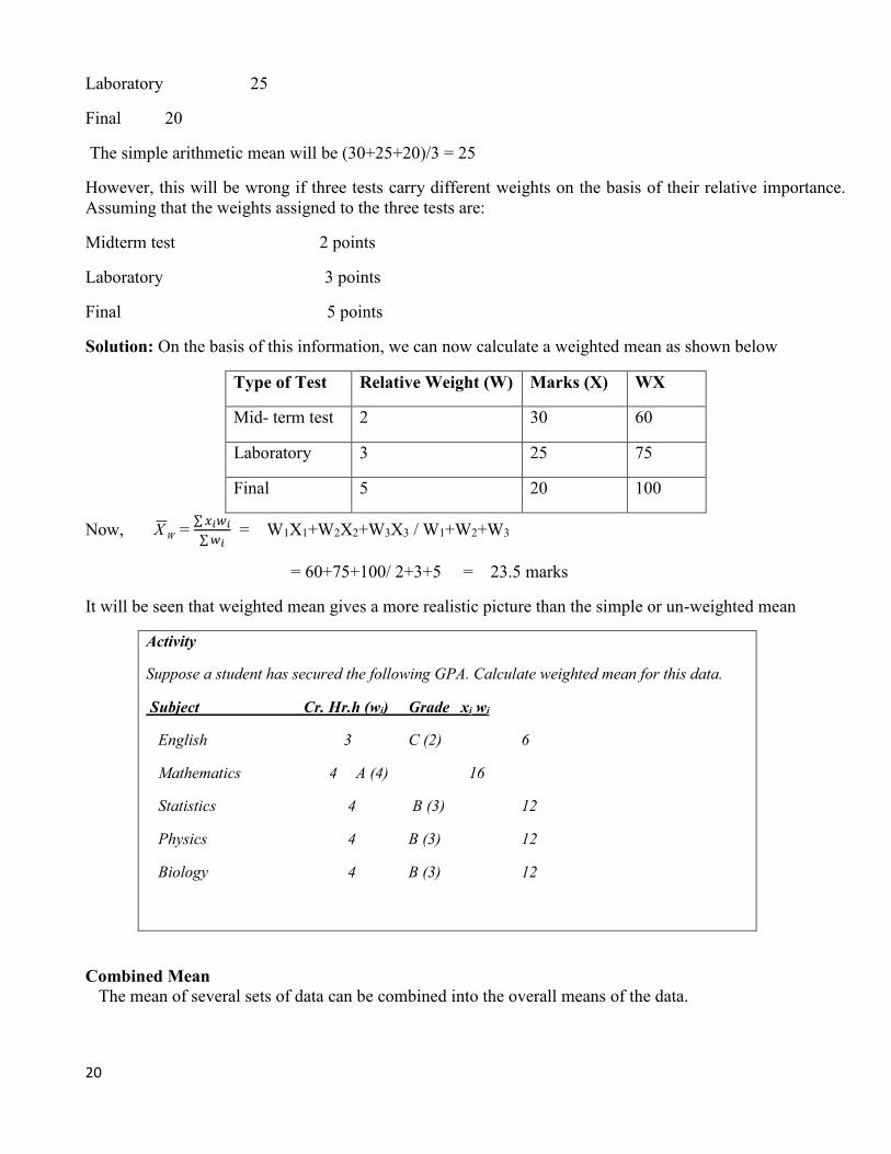
20

Laboratory 25

Final 20

The simple arithmetic mean will be (30+25+20)/3 = 25

However, this will be wrong if three tests carry different weights on the basis of their relative importance.

Assuming that the weights assigned to the three tests are:

Midterm test 2 points

Laboratory 3 points

Final 5 points

Solution: On the basis of this information, we can now calculate a weighted mean as shown below

Type of Test Relative Weight (W) Marks (X) WX

Mid- term test 2 30 60

Laboratory 3 25 75

Final 5 20 100

Now, WX = ∑ 𝑥𝑖𝑤𝑖

∑ 𝑤𝑖 = W1X1+W2X2+W3X3 / W1+W2+W3

= 60+75+100/ 2+3+5 = 23.5 marks

It will be seen that weighted mean gives a more realistic picture than the simple or un-weighted mean

Activity

Suppose a student has secured the following GPA. Calculate weighted mean for this data.

Subject Cr. Hr.h (wi) Grade xi wi

English 3 C (2) 6

Mathematics 4 A (4) 16

Statistics 4 B (3) 12

Physics 4 B (3) 12

Biology 4 B (3) 12

Combined Mean

The mean of several sets of data can be combined into the overall means of the data.

21

kxxx .....,, 21 The way the means obtained from different samples of size n1, n2 . . . nk

respectively then the overall (combined) mean is given as

k

i

i

k

i

ii

k

kkc

n

xn

nnn

xnxnxnx

1

1

21

2211

....

....

Example: Average monthly production of a certain factory in the first 9 months is 2584 units and for the

remaining 3 months it is 2416 units. Calculate average monthly production of for the year.

Solution: Combine mean production of a certain factory for year is computed by the formula k=2 given as

follows,

21

2211

nn

xnxncx

254212

2416*32584*9

cx

Geometric Mean (G.M) The geometric mean is the nth root of the product of n positive values. If X1, X2,…,,Xn are n positive values,

then their geometric mean is G.M =(X1X2…Xn)1/n .

The geometric mean is usually used in: Average rates of change , Ratio, Percentage distribution,

Logarithmical distribution and so on

In case of number of observation is more than two it may be tedious taking out from square root, in that case

calculation can be simplified by taking natural logarithm with base ten

G. M = nnxxx ...., 21 , G. M = n

nxx1

1 .... take log in both sides.

log ( G . M) = nxxn

....,log1

1

(we use common logarithm, base ten)

= nxxxn

log...loglog1

21 =

n

i

ixn 1

log1

G. M = Antilog

n

i

ixn 1

log1

This shows that the logarithms of G.M is the mean of the logarithms of individuals observations.

Example: The ratio of prices in 1999 to those in 2000 for 4 commodities were 0.9, 1.25,1.75 and 0.85. Find

the average price ratio by means of geometric mean.

22

Solution: G.M = antilogn

X i log= antilog

4

)85.0log75.1log25.1log92.0(log

= antilog4

)19294.02430.00969.01963.0( = antilog0.5829 = 1.14

Example2: The mangers three annual raises in his salary. At the end of the 1st year he gets an average 4 % at

the end of the 2nd year he gets an average 6 % and at the end of 3rd year he gets 9 % of his salary. What is

the average percentage of increase in the three periods?

Solution: Here the calculation G.M is as follows. We use reference values of (100 %) then consider the

increment.

Initial values Value after increment value

100 104 log (104) = 2.01 7037

100 106 log (106) = 2.025

100 109 log (109) = 2.0374

log (G. M ) = 0374.2025.2017033.23

1)log(1

ixn

= 2. 02647

Then G.M= antilog (2.026477) = 106. 286

Note that:

1.when the observed values x1,x2,……….,xn have the corresponding frequencies

f1,f2………,fn respectively then geometric mean is obtained by

G. M = nn

fffnxxx ...., 21

21

=

n

i

ii xfn 1

log1

where n=

n

i

if1

2. Whenever the frequency distributions are grouped (continuous), class marks of

the class interval are considered as Xi and the above formula can be used that is

G. M = n f

n

ff nmmm ...., 21

21

=

n

i

ii mfn 1

log1

where n=

n

i

if1

and mi is class mark if ith

class.

23

Therefore, the average percentage increase of salary is given by 106.286 - 100 = 6.286

Properties of geometric mean

a. Its calculations are not as such easy.

b. It involves all observations during computation

c. It may not be defined even it a single observation is negative.

d. If the value of one observation is zero its values becomes zero

Activity 4

1) Suppose the profits earned by the sure-construction company on five projects were 3, 4, 4, 6 and

5 percent, respectively. What is the geometric mean profit?

2) Find the geometric mean for the data given in the table below.

Xi fi

1 2

2 1

4 2

6 3

3) Suppose the prices of five different types of marbles have increased by 8%, 6%, 5%, 10% and

8% respectively, since 1987E.C. what is geometric mean percent increase in the price of the five

types of marbles.

Harmonic mean (H.M)

The Harmonic mean is the reciprocal of the arithmetic mean of the reciprocal of each single value. If X1,X2,

X3,…,Xn are n values, then their harmonic mean is

H.M =

nXXX

n

1...

11

21

=

iX

n

1

Example: Find the harmonic mean of the values 2,3 and 6.

H.M = 6/13/12/1

3

=

6

123

3

=

6

63= 3 ///

The harmonic mean is used to average rates rather than simple values. It is usually appropriate in averaging

kilometers per hour.

24

Example: A driver covers the 300km distance at an average speed of 60 km/hr makes the return trip at an

average speed of 50km/hr. What is his average speed for total distance?

Solution:

Average speed for the whole distance=takentimeTotal

cedisTotal tan=600km/11hrs=54.55km/hr.

Using harmonic formula

H.M=50/160/1

2

=600/110=54.55km/hr.

Note that A.M=2

5060=55km/hr

G.M= 5060 =54.7km/hr

Example: If man travels 200 KM, each on three days at speed of 60, 50 and 40 KM per hour respectively.

Find average speed traveled by a person.

H.M =

nxxx

n

1....1121

= KMperhour65.48

401

501

601

3

Note that

1. For simple frequency data harmonic mean is calculated by using the following

formula.

H. M = Reciprocal n

xf

i

i

Trip Distance Average speed Time taken

1st 300km 60km/hr 5hrs

2nd 300km 50km/hr 6hrs

Total 600km --------- 11hrs

25

=

i

i

x

f

n , Where n is the total number of observations

2. Whenever the frequency distributions are grouped (continuous), class marks of the

class interval are considered as Xi and the above formula can be used that is

H. M = Reciprocal n

mf

i

i

=

mi

f

n

i

, Where n is the total number of observations

Properties of harmonic mean

i. It is based on all observation in a distribution.

ii. Used when a situation where small weight is given for larger observation and larger weight

for smaller observation

iii. Difficult to calculate and understand

iv. Appropriate measure of central tendency in situations where data is in ratio, speed or rate. Activity 5:

Find the harmonic mean for the following discrete grouped data:

Xi 3 6 5 4

fi 2 3 1 4

5

Relationship among A.M, G.M, and H.M

For any set observation, its A.M, G.M, and H.M are related each other in the relationship

A.M ≥G.M≥H.M

The sign of ‘=’ holds if and only if all the observations are identical

If the observation on the data set takes the value a, ar, ar2, ar3 …arn-1,each with single frequencies

(G.M)2=A.M*H.M

3.5.2 The Mode

The mode is another measure of central tendency. It is the score or categories of the scores in a frequency

distribution that has greatest frequency. That means it is the value at the point around which the items are

most heavily concentrated.

A given set of data may have,

26

One mode – uni model e.g. A=3,3,7,6,2,1 �̂�=3

Two mode – Bi – modal e.g. 10,10,9,9,6,3,2,1 �̂�= 10 and 9

More than two mode- multi modal. eg. 5,5,5,6,6,6,8,8,8,2,3,2�̂�=5,6,8

May not exist at all e.g. 1,3,2,4,5,6,7,8 no modal value

How can you determine the mode for a given set of data?

Mode for ungrouped or raw data

Mode for ungrouped frequency distribution is the value that has greatest frequency. As an example, consider

the following series:

7, 8, 9, 8, 9, 11, 15, 16, 12, 15, 3, 7, 15, 11, 12, 15,

There are sixteen observations in the series, and observation 15 occurs four times. The mode is therefore 15.

Mode for discrete (ungrouped) frequency distribution

In case of discrete frequency distribution, mode is the value of the variable corresponding to the maximum

frequency. This method can be used conveniently if there is only one value with the highest concentration of

observation.

Example: Consider the following distribution, and then determine modal value of the distribution.

X 1 2 3 4 5 6 7 8 9

F 3 1 18 25 40 30 22 10 6

Solution: The maximum frequency is 40 and therefore the corresponding value of X=5 is the value of mode.

Mode for continuous or grouped frequency distribution

In the case of grouped data, mode is determined by the following formula:

Mode = �̂� =

wffff

fflo

2101

01

Where ol is the lower value of the class boundary in which the mode lie.

f1 is the frequency of modal class.

f0 is the frequency of the class preceding the modal class.

f2is the frequency of the class succeeding the modal class.

w is the class width.

While applying the above formula, we should ensure that the class-intervals are uniform throughout the class.

If the class-intervals are not uniform, then they should be made uniform on the assumption that the frequencies

are evenly distributed throughout the class.

27

Example: Let us take the following frequency distribution:

Class

intervals

30 _ 40 40 _ 50 50 _ 60 60 _ 70 70 _ 80 80 _ 90 90 _100

Frequency 4 6 8 12 9 7 4

Calculate the mode in respect of this series.

Solution: We can see from Column (2) of the table that the maximum frequency of 12 lies in the class-interval

of 60-70. This suggests that the mode lies in this class-interval. Applying the formula given earlier, we get:

10

912812

81260

Mode

= 1034

460

= 65.7

In several cases, just by inspection one can identify the class interval in which the mode lies. One should see

which the highest frequency is and then identify to which class-interval this frequency belongs. Having done

this, the formula given for calculating the mode in a grouped frequency distribution can be applied.

Properties of mode

It is not unique.

It is not affected by extreme value.

It is the only measurement of central tendency that can be used for qualitative data for example in

describing the opinion of people about a certain phenomenon. We may refer to the most frequent

opinion.

It can be calculated for distribution with open ended classes.

Advantage and disadvantage of mode

Advantage

1.The mode is not affected by the extreme value in the distribution.

2.The mode value can be calculated for open-ended frequency distribution.

3.The mode can be used to describe quantitative and qualitative data.

Disadvantage

1.Mode is not rigidly defined measure as there are several methods for calculating its value.

2.It is difficult to locate modal class in the case of multi-modal frequency distribution.

3.Mode is not suitable for algebraic manipulations.

4.When data set contains more than one mode, such values are difficult to interpret and compare.

3.5.3 The Median

Median is defined as the value of the middle item (or the mean of the values of the two middle items) when

the data are arranged in an ascending or descending order of magnitude. if there are an odd number of items

28

in the array, the median is the middle number. If there is an even number of items, the average of the two

middle numbers.

Median for ungrouped data

Thus, in an ungrouped frequency distribution if the n values are arranged in ascending or descending order of

magnitude, the median is the middle value if n is odd. When n is even, the median is the mean of the two

middle values.

Median =

thn

2

1 element, if n is odd.

= 2

122

ththnn

element, if n is even.

Suppose we have the following series: 15, 19, 21, 7, 33, 25, 18, 10 and 5

We have to first arrange it in either ascending or descending order. These figures are arranged in an ascending

order as follows:

5, 7, 10, 15, 18, 19, 21, 25, 33

Now as the series consists of odd number of items, to find out the value of the middle item, we use the formula

Median =

thn

2

1 element if n is odd. Then median=

th

2

19 = 5th

That is the size of the 5th item is the median. This happens to be 18.

Suppose the series consists of one more item, 23. We may, therefore, have to include 23 in the above series

at an appropriate place, that is, between 21 and 25. Thus, the series is now 5, 7, 10, 15, 18, 19, 21, 23, 25, and

33. Applying the above formula, the median is the size of 5.5th item. Here, we have to take the average of the

values of 5th and 6th item. This means an average of 18 and 19, which gives the median as 18.5.

Median for grouped frequency Distribution

In the case of a continuous frequency distribution, we first locate the median class by cumulating the

frequencies until

thN

2 point is reached. Finally, the median is calculated by with the help of the following

formula:

f

wCfN

LCbMedian

2

Where, Cf = less than cumulative frequency of the class preceding(one before) the median class ,

29

f is frequency of the median class, LCb is lower class boundary of median class and w is the size of the class

width and

k

i

ifN1

,

Example: find the median of the following continuous frequency distribution.

Monthly Wages

(in birr)

800-1,000 1,000-1,200 1,200-1,400 1,400-1,600 1,600-1,800 1,800-2,000

No. of Workers 18 25 30 34 26 10

Solution: In order to calculate median in this case, we have to first compute less than cumulative frequency.

Thus, the table with the less than cumulative frequency is written as:

Monthly

Wages

800--1,000 1,000--1,200 1,200--1,400 1,400--1,600 1,600--1,800 1,800--2,000

Frequency 18 25 30 34 26 10

LCF 18 43 73 107 133 143

Now, Median class is the value of

thN

2 =

th

2

43 =71.5thitem, which liesin the class (1,200-1,400). Thus

(1,200-1,400) is the medianclass. For determining the median in this class, we use interpolation formula as

follows:

wf

CfN

bCLMedianmc

2

=1200+ 20030

435.71

= 1390 birr

Properties of median

- Unlike mode it is unique that is likemean there is only one median for a given set of data.

- Easy to calculate and understand.

- It is not affected by extreme value.

- It’s especially used for open ended frequency distribution when median is not found in that class.

Activity 6:

A survey was conducted to determine the age (in year) of 120 automobiles. The result of such a survey is

as follows:

Age of automobile : 0-4 4-8 8-12 12-16 16-20

Number of automobiles : 13 29 48 22 8

What is the median age for the automobile?

30

Advantage and disadvantage of median

Advantage

i. The value of median is easy to understand and maybe calculated fro any type of data. The

median in many situations can be located simply by inspection.

ii. The sum of the absolute difference of all observations in the data set from median value is

minimum. In other word that absolute difference of observations from the median is less than

from any other value in the distribution.

iii. The extreme value in the data set does not affect the calculation of the median value.

iv. The median value may be calculated for an open-ended distribution of data set.

Disadvantage

i. The value of median is affected more by sampling variations, that is, it affected by the number

of observations rather than the values of the observations.

ii. Since median is an average of position, therefore arranging the data in ascending or descending

order of magnitude is time consuming in case of a large number of observation.

iii. The calculation of median in case of grouped data is based on the assumption that values of

observations are evenly spaced over the entire class-interval.

Which of the Three Measures is the Best?

At this stage, one may ask as to which of these three measure of central tendency is the best. There is no

simple answer to this question. It is because these three measures are based upon different concepts. The

arithmetic mean is the sum of the values divided by the total number of observations in the series. The median

is the value of the value of the middle observations tend to concentrate, As such; the use of a particular measure

will largely depend on the purpose of the study and the nature of the data.

For example, when we are interested in knowing the consumers’ preferences for different brands of television

sets or kinds of advertising, the choice should go in favor of mode. The use of mean and median would not

be proper. However, the median can sometimes be used in the case of qualitative data when such data can be

arranged in an ascending or descending order. Let us take another example. Suppose we invite applications

for a certain vacancy in our company. A large number of candidates apply for that post. We are now interested

to know as to which age or age group has the largest concentration of applicants. Her, obviously the mode

will be the most appropriate choice. The arithmetic mean may not be appropriate as it may be influenced by

some extreme values.

Example1: The following data give the savings bank accounts balances of nine sample households selected

in a survey. The figures are in birr

74, 2,000, 1,500, 68,000, 461, 549, 3,750, 1,800, 4,795

a) Find the mean and the median for these data.

b) Do these data contain an outlier? If so, exclude this value and recalculate the mean and median. Which of

these summary measures has a greater change when an outlier is dropped?

c) Which of these two summary measures is more appropriate for this series?

Solutions

a) 9

795,4800,1750,3549461000,68500,1000,2745 Mean

31

=9

600,83birr = 9,289 birr

Median = Size of

thn

2

1item =

th

2

19= th5 item

Arranging the data in an ascending order, we find that the median is 1,800 birr.

c) An item of 68,000 birr is excessively high. Such a figure is called an ‘outlier’ .We exclude this figure

and recalculate both the mean and the median.

8

000,68000,83 Mean =

8

600,15=1,950birr

Median = itemN

2

1

= th5.42

18

item 650,1

2

800,1500,1

birr

It will be seen that the mean shows a far greater change than the median when the outlier is dropped from the

calculations.

d) As far as these data are concerned, the median will be a more appropriate measure than the mean.

Example 2: Calculate the most suitable average for the following data:

Size of the Item Below 50 50-100 100-150 150-200 200 and above

Frequency 15 20 36 40 10

Solution: Since the data have two open-end classes- one in the beginning (below 50) and the other at the

end (200 and above), median should be the right choice as a measure of central tendency.

Table: Computation of Median

Size of Item Below 50 50-100 100-150 150-200 200 and above

Frequency 15 20 36 40 10

LCF 15 35 71 111 121

Median is size

thN

2item

= 121/2= 60.5th item

Now, 60.5th item lies in the 100-150 class

32

Now, wf

CfN

bCLMedianmc

2

50*

36

355.60100

= 136.1

Activity

The tableblow is the frequency distribution of ages to the nearest birthday for a random sample of 50

employees in a large company

age to nearest birthday 20-29 30-39 40-49 50-59 60-69

number of employees

Compute the mean median and mode for this data

Exercise

1. Define arithmetic mean. Discuss its merits and demerits.

2. Why the arithmetic mean is most commonly used measure of a central value?

3. List and explain at least three desirable properties of measure of central tendency.

4. Under what circumstances would it be appropriate to use mode or median?

5.. In a frequency distribution of 100 families given below the number of families corresponding to expenditure groups

20-40 and 60-80 are missing from the table. however, the median is known to be 50. find the missing frequencies

Expenditure group 0-20 20-40 40-60 60-80 80-100

No. of families 14 f2 27 f4 15

6. Determine appropriate average for the following income distribution.

Income Groups: below 100 100-200 200-300 300-400 400-500 above 500

No. of persons: 5 10 18 30 20 17

7 if x1 and x2 are two observed values, the geometric mean of their arithmetic mean and harmonic mean is equal to

the geometric mean of the number x1 and x2.show this.

8 The arithmetic mean of the two numbers is 13 and their geometric mean is 12.

33

a. find the two numbers b. find the harmonic mean

9. Complete the frequency for the distribution

Class limit 11-20 21-30 31-40 41-50 51-60 61-70 71-80 Total

frequency 12 30 F3 65 F5 25 18 229

If the median value is 46, then find

a. The missing frequency

b. Calculate the mean and quartile and interpret them

References

Maxwell, S. E., & Delaney, H. D. (2003) Designing Experiments and AnalyzingData: A Model

Comparison Perspective, Second Edition, Lawrence Erlbaum Associates, Mahwah, New Jersey.

Tukey, J. W. (1991) The philosophy of multiple comparisons, Statistical Science, 6,110-116.

Tufte, E. R. (2001). The Visual Display of Quantitative Information (2nd ed.) (p.178). Cheshire, CT:

Graphics Press.




594–604.

34

CHAPTER FOUR

4. Measure of Variation (Dispersion) 4.1 Introduction

In this unit we shall discus the most commonly used measure of dispersion like Range, Quartile Deviation,

Mean Deviation, Standard Deviation, coefficient of variation and standard score. We have seen that averages

are representatives of a frequency distribution. But they fail to give a complete picture of the distribution.

They do not tell anything about the slatterns of observations within the distribution.

Lesson objective

Identify the most commonly used measure of dispersion.

Explain the measure properties of measure of dispersion to have.

4.2 Objectives of Measures of Variation

The measures of central tendency or the “averages” described in the last chapter given a number which is the

typical value of the distribution. It is computed to see through the variability or dispersion of the individual

values .But the dispersion is itself a very important property of a distribution and needs to be measured by an

appropriate statistics.

Measure of dispersions is useful in:

1. Determining how representative the average is as a description of the data.

2. Comparing two or more series with regard to their scatter, and

3. Designing a production control system which is based on the premise that if a process is under control,

the variability it produces is same over a period of time. if the scatter produced by a process changes

over time ,it invariably means that something has gone wrong and needs to be corrected.

In addition to it we should have a measure of scatterings of observations. The scatterness or variation of

observations from their average is called dispersion.

Definition of Measures of Dispersion (Variation)

How can define measure of variation?

It measures the scatterness of observations around their averages. In other sense how the data are dispersed or

distributed from the mean.

A measure of dispersion should possess all those characteristics which are considered essential for a measure

of central tendency, viz.

It should be based on all observations.

It should be easy to compute and to understand.

It should not be affected much by extreme values.

It should not be affected by sampling fluctuation.

Be amenable to algebraic treatment.

35

4.3 Absolute and Relative Measures

For the study of dispersion, we need some measures which show whether the dispersion is small or large.

There are two types of measure of dispersion which are:

(a) Absolute Measure of Dispersion

(b) Relative Measure of Dispersion

Absolute Measures of Dispersion:

These measures give us an idea about the amount of dispersion in a set of observations. They give the

answers in the same units as the units of the original observations. When the observations are in kilograms,

the absolute measure is also in kilograms. If we have two sets of observations, we cannot always use the

absolute measures to compare their dispersion. We shall explain later as to when the absolute measures can

be used for comparison of dispersion in two or more than two sets of data. The absolute measures which are

commonly used are:

1. The Range

2. The Quartile Deviation

3. The Mean Deviation

4. The Standard deviation and Variance

Relative Measure of Dispersion: These measures are calculated for the comparison of dispersion in two or more than two sets of

observations. These measures are free of the units in which the original data is measured. If the original data

is in dollar or kilometers, we do not use these units with relative measure of dispersion. These measures are

a sort of ratio and are called coefficients. Each absolute measure of dispersion can be converted into its

relative measure. Thus the relative measures of dispersion are:

1. Coefficient of Range or Coefficient of Dispersion.

2. Coefficient of Quartile Deviation or Quartile Coefficient of Dispersion.

3. Coefficient of Mean Deviation or Mean Deviation of Dispersion.

4. Coefficient of Standard Deviation or Standard Coefficient of Dispersion.

5. Coefficient of Variation (a special case of Standard Coefficient of Dispersion)

4.4 Types of Measure of Dispersion

The following are some common measure of dispersion:

The range

The semi-interquartile range or the quartile deviation

The mean deviation and

The standard deviation.

Of these, the standard deviation is the best measure. We describe these measures in the following sections.

4.4.1 The Range and Relative Range

It is the simplest measure of dispersion. The range is the difference between the two extreme values (highest

and lowest value) of data. Range takes only maximum and minimum values into account and not all the

values. Hence it is a very unstable or unreliable indicator of the amount of deviation.

The major area in which range is applied is statistical quality control.

It is also applicable in the cases where extreme values are important like maximum rainfall,

temperature, etc. Properties of range

36

It’s easy to calculate and to understand.

It can be affected by extreme values.

It can’t be computed when the distribution has open ended classes.

It cannot take the entire data in to account.

It does not tell anything about the distribution of values in the series.

Range for ungrouped data

Range for ungrouped data is given by: Range = Xmax - Xmin

Example: Consider the following data on weight of 7 individuals and compute range for weight. 24, 25,

30, 15, 47, and 35.

Solution: Range = maximum value - minimum value = 47 - 15 = 32

Range for grouped frequency distribution

Range of a grouped frequency distribution is the difference between the upper class boundary of the last class

interval and lower class boundary of the first class interval.

Mathematical measure of dispersion

Mean Deviation

It is the mean of the deviations of individual values from their average. The average may be either mean or

median.

M.D=N

AX , for raw data. M.D =

f

AMif ,for grouped data.

A is either mean or median.

Calculation of mean deviations involves the following steps:

a) Calculate the median (or the mean)

b) Record the deviations |𝑑| = |𝑥 − 𝐴| of each of the items, ignoring the sign.

c) Find the average value of deviations

𝑀. 𝐷 =∑|𝑑|

𝑁

Example: Calculate the mean deviation from median of the following data giving marks obtained by 11

students in a class test. 14, 15, 23, 20, 10, 30, 19, 18, 16, 25, 12

Solution: 𝑀𝑒𝑑𝑖𝑎𝑛 = 𝑠𝑖𝑧𝑒𝑜𝑓(11+1

2)𝑡ℎ item =size of 6th item=18.

Serial No 1 2 3 4 5 6 7 8 9 10 11

37

Marks 10 12 14 15 16 18 19 20 23 25 30

|𝑥 − 𝑀𝑒𝑑𝑖𝑎𝑛| = |𝑑| 8 6 4 3 2 0 1 3 5 7 12

The Mean deviation from Median is,𝑀. 𝐷 =∑|𝑑|

𝑛=

50

11= 4.54 𝑚𝑎𝑟𝑘𝑠

Example 4.3.1.4: Calculate the mean deviation from mean and median

Xi 6 7 8 9 10 11 12

fi 3 6 9 13 8 5 4

Xi fi 18 42 72 117 80 55 48

Solution Mean = 948/432

i

ii

f

xf

Median = 92

99

2

2524

2

122

thth

ththnn

Xi 6 7 8 9 10 11 12 Total

fi 3 6 9 13 8 5 4 48

|𝑑𝑖| 3 2 1 0 1 2 3

𝑓𝑖|𝑑𝑖| 9 12 9 0 8 10 12 60

Where di = (Xi – median (or mean))

M. D from median = 25.148

60

i

ii

f

df

Property of Mean Deviation

- The mean deviation takes all values into consideration.

- It is fairly stable compared to range or quartile deviation. But it is not stable as standard deviation.

Since, it ignores signs of deviations.

- It is not possible to use for further statistical investigation. Activity 2.

The first quartile for the following data is 21.5

X 10-15 15-20 20-25 25-30 30-35 35-40 40-45 45-50 total

f 24 - 90 122 - 56 20 33 460

Find.

a. the missing value

b. quartile deviation

c. mean deviation from mean and median

38

4.4.2 The Variance(S2 or 2), Standard Deviation and Coefficient of Variation

Variance is the arithmetic mean of square deviation about the mean. When our data constitute a sample , the

variance averaging done by dividing the sum of squared deviation from mean by n-1 and it is denoted by

s2 .when our data constitute an entire population variance averaging done by dividing by N and denoted by

2 .The mathematical definition of variance is given by:

𝑆2 =∑ (𝑥𝑖−�̅�)2𝑛

𝑖=1

𝑛−1 ,(sample variance and is an unbiased estimator of the population variance)

𝜎2 =∑ (𝑥𝑖−𝜇)2𝑁

𝑖=1

𝑁(Population variance)

The easy computing formula for variance is S2=

1

2

2

n

n

xx

i

i

.This is Variance for ungrouped data or

raw data

How can determine variance of ungrouped frequency (discrete) distribution?

Variance for ungrouped frequency distribution

The determination of variance for ungrouped frequency distribution is,

S2 =

i

i

n

i

i

fnwheren

xxf

1

2

1

What about for grouped frequency distribution?

Variance for grouped frequency distribution The determination of variance for grouped frequency distribution is

)1(1

2

2

n

xmf

s

n

i

ii

, Where mi is mid value of class

Simplified formula used for computation is

𝑆2 =∑ 𝑓𝑖𝑚𝑖

2 −(∑ 𝑚𝑖𝑓𝑖)2

𝑛⁄

∑ 𝑓𝑖 − 1

Properties of Variance

1. The variance is always non – negative (S2 0 )

2. If every element in the distributions are multiplied by a constant C the new variance is 222

oldnew SCS

Old 1/.,...,,22

21 nxxSxxx ioldn

xi x1 x2 . . . xk

fi f1 f2 . . . fk

39

New

1,....,,

2

2

21

n

xccxScxcxcx

i

newn

=

1

2

n

xxc i

=

1

22

n

xxc i =

1

22

n

xxc i = 22

oldSC

3. When a constant c is added to all measurement of the distribution, the variance doesn’t change

i.e xi (old) = xi , x2 , . . . . , xn

xi (new) = x1 + c1, x2 + c , . . . . , xn + c

n

cx

n

cxX

ii

new

= n

nc

n

xi

= cX

old

iinew S

n

xx

n

cxcxS 2

2

2

11

4. The variance of constant measured n times is zero.

i.e. c, c , c , . . . . , c , .0, 2 Scx

Standard Deviation (S.D)

It is defined as the positive square root of the mean of the squared deviations of individual values from their

mean.

𝑆 = √∑(𝑥−�̅�)2

𝑛−1 , S is sample variance)

𝜎 = √∑ (𝑥𝑖−𝜇)2𝑁𝑖=1

𝑁 , (𝜎𝑖𝑠𝑝𝑜𝑝𝑢𝑙𝑎𝑡𝑖𝑜𝑛𝑣𝑎𝑟𝑖𝑎𝑛𝑐𝑒)

The simple formula for computation of standard deviation is

𝑆 = √∑ 𝑓𝑖𝑚𝑖2−

(∑ 𝑚𝑖𝑓𝑖)2

𝑛⁄

∑ 𝑓𝑖−1.

Merits of Standard Deviation

Its advantage over variance is that it is in the same unit as the variable under consideration.

40

It is a measure of average variation in the set of data.

Example: Compute the variance & S.D. for the data given below.

xi 32 36 40 44 48 Total

frequency 2 5 8 4 1 20

Solution: First we have to arrange the data into easy for computation.

xi 32 36 40 44 48 Total

fi 2 5 8 4 1 20

xifi 64 180 320 176 48 788

xi2fi 2048 6480 12800 7744 2304 31376

1

22

2

i

iiii

f

nfxxf

S =

19

20278831376

= 328.8

19= 17.31

Standard deviation (S.D) 2SS = 31.17 = 4.16

Example: Calculate the S.D for the following grouped frequency distribution.

Class intervals 1 - 3 3 - 5 5 -7 7 -9 9 -11 11 -13 13 -15

Frequency(fi) 1 9 25 35 17 10 3

Solution:

Class intervals 1 – 3 3 – 5 5 – 7 7 – 9 9 – 11 11 – 13 13 – 15

Frequency (fi ) 1 9 25 35 17 10 3

mi 2 4 6 8 10 12 14

mi2fi 4 144 900 2240 1700 1440 588

mi fi 2 36 150 280 170 120 42

1

22

2

i

iiii

f

nmfmf

S

=

99

10028007016

= 6.22

49.222.62 SS

41

Remark: Suppose that the two distributions to be compared are expressed in the same units and their means

are equal or nearly equal. Then their variability can be compared directly by using their standard deviations.

However, if their means are widely different or if they expressed indifferent units of measurement, we can

not use the standard deviation as such for comparing their variability. We have to use the relative measures

of dispersion which is known as coefficient of variation.

Activity 3.

1. Explain the advantage of standard deviation as a measure of variation over range and average

deviation. Under what circumstance will the variance of a variable be zero?

2. Consider the following distribution listed below

Class limit Frequency

10-14 5

15-19 6

20-24 3

25-29 4

30-34 2

Compute the variance and standard deviation for the distribution.

3. Compute the range, variance, and standard deviation for each of the following random samples.

a. 12 17 20 23 25 15 21 22 19 18 b. 5.2 6.5 5.6 4.1 6.7 7.3 5.8 6.1 5.5

Coefficient of variation (CV)

It is a unit free measure. It is always expressed as percentage.

CV = Mean

SD100% where, SD = Standard deviation

The CV will be small if the variation is small. Of the two groups, the one with less CV is said to be more consistent

less variation.

Example: The following are the scores of two batsmen A and B in a series of innings:

A 12 115 6 73 7 19 119 36 84 29

B 47 12 76 42 4 51 37 48 13 0

Who is the better run –getter? Who is more consistent?

Solution: in order to decide as to which of the two batsmen, A and B, is the better, we should find their batting

averages. The one whose average is higher will be considered as a better batsman.

42

To determine the consistency in batting we should determine, the coefficient of variation. The fewer

coefficients the more consistent will be the player.

A Scores(x) 12 115 6 73 7 19 119 .36 84 29 ∑ 𝑥=500

X2 1444 4225 1936 529 1849 961 4761 196 1156 441 ∑ 𝑥2 = 17498.

B Scores(x) 47 12 76 42 4 51 37 48 13 0 ∑ 𝑥 = 330.

X2 196 441 1849 81 841 324 16 225 400 1089 ∑ 𝑥2 = 5462.

Batsman A: Batsman B:

�̅� =500

10= 50. �̅� =

330

10= 33

𝜎 = √17498

10= 41.83. 𝜎 = √

5462

10= 23.37.

𝐶. 𝑣(𝐴) =41.83×100

50= 83.66% 𝐶. 𝑣(𝐴) =

23.37×100

33= 70.8%

A is better batsman since his average is 50 as compared to 33of B .But B is more consistent since the variation

in his case is 70.8 as compared to 83.66 of A.

Example: Consider the distribution of the yields (per plot) of two paddy varieties. For the first variety, the

mean and standard deviation are 60kg & 10kg, respectively. For the second variety, the mean and standard

deviation are 50kg & 9kg, respectively.

Then we have,

CV = (10/60)100%=16.7%, for first variety.

CV = (9/50)100%=18.0%, for second variety.

It is apparent that the variability in first variety is less as compared to that in the second variety. But in terms

of standard deviation the interpretation could be reverse.

Activity 4.

1. The following data related to the mean of score of a section of students in a statistics and language

Year 1990 1991 1992 1993 1994 1995 1996

Language 20.1 20.5 20.4 20.5 20.4 22.5 22.3

Statistics 19.5 19.3 1 9.2 19.2 19.1 21.9 22.0

Which portion of the test do you believe has a greater variability in its scores from year to year? Why?

2. Suppose that samples of polythene bags from two manufactures A and B are tested by a buyer for

bursting pressure, giving the following results:

a. Which set of bags has the highest bursting pressure?

b. Which has uniform pressure? if prices are the same, which manufacture’s bags would be preferred

by the buyer? Why?

43

4.5 The Standard Scores

Standard score measures the deviation of individual observation from the mean of the total observation in the

unit of standard deviation and termed as Z – Score.

The Z – scores of individuals in different groups are then added to give a true Measure of relative performance

The standard score is denoted by Z and defined as

S

xxZ i

Where S is Standard deviation of the distribution and Xi is value of each observation.

Example: Compare the performance of the following two students

Candidate Marks in anatomy Marks in introduction to statistics total

A 84 75 159

B 74 85 159

Average mark for Anatomy is 60 with standard deviation of 13.

Average mark for Introduction to statistics is 50 with standard deviation of 11.

Whose performance is better A’s or B’s?

Solution:

Z scores A: {𝐴𝑛𝑎𝑡𝑜𝑚𝑦

84−60

13= 1.85

𝑖𝑛𝑡𝑟𝑜𝑑𝑢𝑐𝑡𝑖𝑜𝑛 𝑡𝑜 𝑠𝑡𝑎𝑡 75−50

11= 2.27

Total Z score for A = 1.85 + 2.27 = 4.12

Z score B: {𝐴𝑛𝑎𝑡𝑜𝑚𝑦

74−60

13= 1.08

𝑖𝑛𝑡𝑟𝑜𝑑𝑢𝑐𝑡𝑖𝑜𝑛 𝑡𝑜 𝑠𝑡𝑎𝑡 85−50

11= 3.18

Total Z score for B = 1.08 + 3.18 = 4.26

Since B’s Z – score is higher; student B had good performance than student A.

Activity 5

A student scores 60 on anatomy test that has a mean of 54 and standard deviation of 3, and she scores

80 on introduction to statistics test with a mean of 75 and standard deviation of 4. On which test did

she perform better.

44

Exercises

1. What purpose does a measure of variation serve? In the light of this comment on some of the well-known

measure of variation.

2. Consider the marks of 20 students out of 20% in statistics test as follows

Marks of Students’ 0-5 5-10 10-15 15-20 Total

Number of students 2 6 8 4 20

Find

i. Range

ii. The first and third quartile

iii. Quartile deviation

iv. Mean and median deviation

v. Variance and standard deviation

3. The final exam of a course consists of two exams, mathematics and History. If a student scored 66 in

Mathematics and 80 in History. However, all students’ average score is 51 with a standard deviation 12 in

mathematics and 72 with the standard deviation 16 in history.

a. In which subject a student had better performance?

b. In which subject all students have similar (consistent) results?

4. From the analysis of months’ wages paid to workers in two organization X and Y, the following results were

obtained:

X Y

Number of wage- earners 550 600

Averages monthly wages (Rs) 1260 1348.5

Variance of distribution of wag s (Rs) 100 841

Obtain the average wages and the variability in individual wages of all the workers in the two organizations

taken together

5. A. describes the advantages and disadvantage of using either the range or the standard deviation as a

measure of variation.

a. What is the smallest value for the range or the standard deviation?

b. If the range or the standard deviation is equal to zero, what can you say about each value of the

sample?

6. The mean and the standard deviation of a sample of 100 observations were calculated as 40 and 5.1,

respectively by student who took mistake 50 instead of 40 for one observation. Find the correct mean and the

correct standard deviation.

References Box, G. E. P. and Cox, D. R. (1964). An analysis of transformations, Journal of the Royal Statistical

Society, Series B, 26, 211-252.

Kaiser, H. F. (1960) Directional statistical decisions. Psychological Review, 67,160-167

Kutner, M., Nachtsheim, C., Neter, J., and Li, W. (2004). Applied Linear Statistical Models,

McGraw-Hill/Irwin, Homewood, IL.

Maxwell, S. E., & Delaney, H. D. (2003) Designing Experiments and Analyzing Data: A Model




Graphics Press.

45

CHAPTER FIVE

5.Elementary Probability

5.1 Introduction

Before we can apply probability to the decision making process, we must first discuss just what is meant by

probability. The mathematical study of probability originated over 300 years ago. A Frenchman named

Antoine Gombauld (1607- 1684) began asking questions about the mathematical basis for success and failure

at the dice table. He was mostly interested in the probability of observing various out comes (probability 7s

and 11s) when a pair of dice was repeatedly rolled. He asked the French mathematician Blaise Pascal (1623-

1662) “what are the odd of rolling two sixes at least once in twenty-four rolls of pair of dice”?

Probability: can be defined as a measure of the likelihood or degree of predictability that a particular event

will occur. It is a numerical measure with a value between 0 and 1 of such likelihood. Where the probability

of zero indicates that the given event cannot occur and the Probability of one assures certainty of such an

occurrence.

Lesson objective

Explain the application of probability for the decision making process.

Compare the basic Principles of counting rules. Identify the different method of assigning probability.

5.2 Definitions and Some Concepts

1. Experiment: the activity that produces any outcome/events is referred to, in probability theory, as an

experiment.

For example, tossing of a fair coin is considered as a statistical experiment.

2. Outcome: - is the result of an experiment.

Example,

Experiment Outcomes Tossing of a fair coin Head, tail

Rolling a die 1, 2, 3, 4, 5, 6

Selecting an item from a production lot good, bad

Introducing a new product Success, failure

3. Sample space: A sample space is the collection of all possible outcomes of an experiment and denoted

by S.

For example, there are two possible outcomes of a tossing of a fair coin, which are a head and a tail.

Then the sample space S for this experiment would be: S = {H, T}. Each possible outcome in the sample

space is called sample point.

4. Event: -is a subset of the sample space or it is asset containing sample points of a certain sample space

under consideration.

For examples, getting two heads in the trial of tossing three fair coins simultaneously would be an event.

S ={HHH, HHT, HTT, THH, TTH, TTT, THT, HTH}, the events are {HHT, THH, HTH}

5. Elementary event (simple event): are those types of events that cannot be broken into other events. For

example, suppose that the experiment is to roll a die. The Elementary events for this experiment are to

roll a 1 or a 2, and so on, i.e., there are six elementary events (1, 2, 3, 4, 5, and 6).

6. Composite (compound) event: is an event having two or more elementary events in it. For example, in

rolling a die, the sample space is = {1,2,3,4,5,6) an event having {5} is simple event where as having

even number = {2,4,6} is compound (composite) event.

46

7. Mutually exclusive events: Two events are said to be mutually exclusive, if both events cannot occur

at the same time as outcome of a single experiment. In other word two events E and E are said to be

mutually exclusive events if there is no sample point in common to both events E and E .

For example, if we roll a fair dice, then the experiment is rolling the dice and Sample space (S) is;

S = {1, 2, 3, 4, 5, 6}

If we are interested the outcome of event E getting even numbers and E odd numbers

E = {2, 4, 6}

E = {1, 3, 5}

Clearly E E ={}. Thus E and E are called mutually exclusive events.

8. Independent Events: Two events A and B are said to be independent events if the occurrence of event

A has no influence on the occurrence of event B. For example, if two fair coins are tossed, then the result

of one toss is totally independent of the result of the other toss. The probability that a head will be the

outcome of any one toss will always be ½, irrespective of whatever the outcome is of the other toss.

Hence, these two events are independent.

9. Equally likely outcomes: In a certain experiment, if each outcome in the sample space has equal chance

to occur, then we say that the outcomes are equally likely outcomes.

5.3 Counting Rules

If the number of possible outcomes in an experiment is small, it is relatively easy to list and count all possible

events. When there are large numbers of possible outcomes an enumeration of cases is often difficult, tedious

or both. Therefore, to overcome such problems one can use various counting techniques or rules.

1. Addition rule

Suppose that a procedure designated by 1, can be performed in n ways. Assume that second procedure

designated by 2 can be performed in n ways. Suppose furthermore that it is not possible both procedures 1

and 2 are performed together. The number of ways in which we can perform 1 or 2 procedures is n + n

ways. This can be generalized as follows if there are k’s procedures and i procedure may be performed in n

ways, i = 1, 2… k, then the number of ways in which we perform procedure 1 or 2 or … or k is given by n

+n +…+ n = , assuming that no two procedures performed together.

Example: Suppose that we are planning a trip and are deciding between bus and train transportation. If

there are 3 bus routes and 2 train routes to go from A to B, find the available routes for the trip.

Solution: There are 3+2 = 5 possible routes for someone to go from A to B.

2. Multiplication Rule

Suppose that procedure 1 can be performed in n ways. Let us assume procedure 2 can be performed in n

ways. Suppose also that each way of doing procedure 2 may be followed by any way of doing procedure 1

, then the procedure consisting of n1 followed by n2 may be performed by n * n ways.

Example: An airline has 6 flights from A to B, and 7 flights from B to C per day. If the flights are to be

made on separate days, in how many different ways can the airline offer from A to C?

Solution: In operation 1 there are 6 flights from A to B, 7 flights are available to make flight from B to C.

Altogether there are 6*7 = 42 possible flights from A to C.

1 2

1 2

1 2

1

2

1 2 1 2

1

2

1 2

th

i

1 2 k

k

i

in1

1 2

1 2

47

Example2: suppose that in a medical study patients are classified according to their blood type as A, B, AB,

and O; according to their RH factors as + or - and according to their blood pressure as high, normal or low,

then in how many different ways can a patient be classified?

Solution: The1st classification has done in 4 ways; the 2nd in 2 ways, and the 3rd in 3 ways. Thus patient

can be classified in 4*2*3 = 24 different ways.

3. Permutation

Permutation is an arrangement of all or parts of a set of objects with regard to order.

Rule 1: The number of permutations of n distinct objects taken all together is n!

In particular, the number of permutations of n objects taken n at a time is:

nPn = = n!. Since 0! = 1! = 1.

Example: In how many ways 4 people are lined up to get on a bus (or to sit for photo graph)?

Solution: In 4! = 4*3*2*1 = 24 Ways.

Rule-2: A permutation of n different objects taken r at a time is an arrangement of r out of the n objects,

with attention given to the order of arrangement. The number of permutations of n objects taken r at a time

is denoted by nPr, and is given by:

nPr = n(n-1)(n-2)…(n-r+1) =

Example: An insect toxicologist would like to test the effectiveness of three new pyrethriod insecticides on

population of European corn borer moths, Ostrinia nubilalis, but she has 7different geographically isolated

strains available. If each strain could be used more than once, how many different tests could she perform?

Solution: a three-stage experiment with repetition permits 7*7*7 = 343

If each strain can be used once, how many ways could she perform?

7𝑃3 =7!

(7 − 3)!= 210

Rule-3: The number of permutation of n objects taken all at a time, when n1 objects are alike of one kind, n2

objects are alike of second kind, …, nk objects are alike of kth kind is given by:

Example: The total number of arrangement of the letters of the word STATISTICS taken all at a time is

given by = 50,400 since there are 3s’s, 3t’s, 1a, 2i’s and 1c.

!0

!

!

! n

nn

n

!!

rn

n

k

i

i

k

i

i

k n

n

nnnn

n

1

1

321 !

!

!!...!!

!

!1!2!1!3!3

!10

48

Note: When the method of selection or arrangement of r objects from n-objects is with repetition the

possible numbers of arrangements are nr.

4. Combinations

Combination is the selection of objects without regarding order of arrangement.

A combination of n different objects taken r at a time is a selection of r out of n objects, with no attention

given to the order of arrangement. The number of combinations of n objects taken r at a time is denoted by

the symbol (nr) or nCr is given by

(𝑛𝑟

) =

Example: suppose the geneticist decides to do a single experiment that will utilize 3 stocks of Drosophila

at once and, therefore, order is not important. How many experimental protocols are possible from his 5

available stocks?

5c3=5!

3!(5−3)!= 10, there are only 10 ways now to design this new experiment because order is not

important.

5.4 Approaches in Probability Definition

Probability definition can be viewed in to two categories:

Subjective probability: it can be defined as a person’s degrees of belief that an event will happen.

Objective probability: Estimates the likelihood of an event occurring in a repeatable experiment. It can be

categorized into two.

a. Classical or Mathematical Approach

If a random experiment results in N exhaustive, mutually exclusive and equally likely outcomes; out of

which M are favorable to the happening of an event A, then the probability of occurrence of A, usually

denoted by P (A) is given by:

Example: In a given basket there is 3 yellow, 4 black and 3 white balls. What is the probability of selectinga

black ball?

Solution: Let event A = event of selecting black ball.

P (A) = = = 0.4

b. Empirical or frequency approach

The classic definition of probability has a disadvantage in that of the words “equally likely” is vague. In fact,

since these words seem to be synonymous with “equally probable”, the definition is circular because we are

essentially defining probability in test of itself.

!!!

!

!

1...21

r

P

rnr

n

r

rnnnn rn

casesofNoexhaustive

AtocasesfavorableAP

.)(

casesofNoexhaustive

Atocasesfavorable

. 10

4

49

For this reason, a statistical definition of probability has been advocated by some people. According to this

the estimated probability, or empirical probability, of an event is taken to be the relative frequency of

occurrence of the event when the number of observations is very large. The probability itself is the limit of

the relative frequency as the number of observations increases indefinitely.

Example: If 1000 tosses of a coin result in 529 heads, the relative frequency of heads is 529/1000 = 0.529. If

another 1000 tosses results in 493 heads, the relative frequency in the total of 2000 tosses is,

=0.511.

According to the statistical definition, by counting in this manner we should ultimately get closer and closer

to a number that represents the probability of a head in a single toss of the coin. From the results so far

presented, this should be 0.5 to one significant figure.

From both definitions, it is obvious that 0 ≤ P (A) ≤ 1. If A is impossible events, P (A) = 0. Conversely if P

(A) = 0 then A can occur in a very small percentage of times in the long run. If A is a certain event, P (A) =1.

Conversely, if P (A) = 1, then A may fail to occur in a very small percentage of times in the long run.

Activity

Answer each of the following questions.

Find the number of distinct order groups of four that can be made from eight items.

Find the number of different grouping of 5, with order not being important, that can be made from eight

items.

Find the number of distinct permutations of engineers that can be made from a set of four civil, five

electrical and six mechanical engineers

A Forman has 6 workers on staff. The workers have agreed to work on Sundays but only 3 staff. The

Forman has decided to make up Sundays schedules in such a way that no set of three workers will be on

duty on particular day in order of usage. How many weeks can be covered by this schedule?

A firm would like to cut down commissions paid to salespersons and decided to reduce the sales force. How

many different sets of 5 salespersons can be selected from 25 salespersons if the firm decides to reduce the

sales force by 5?

,m,mnn

5.5 Some Probability Rules

The use of probability to quickly and efficiently to solve problems in biology is often a stumbling block for

many beginning students. The development of set theory along with some axioms of probability will lead to

several very useful methods to attack basic probability problems. Venn diagrams are ways of organizing

experimental situations in order to more easily solve probability problems.

2000

493529

50

Definition:

A set is a collection of definite distinct objects of interest.

The objects are called element or member of the set.

The set of all elements for which there is interest in a given discussion is called the universal set or

sample space and denoted by S.

Any subset A of the sample space or universal set or sample space, S, is called an event.

If every element of the set B is an element of the set A, then B is said to be a subset of A. this is

denoted by B⊂A.notice that we also have A⊂S and B⊂ 𝑺 here.

Two sets, A and B, are said to be conjoint when they have at least one element in common.

Two sets A and B are said to be disjoint when they have no elements in common. Disjoint sets are

sometimes said to be mutually exclusive.

Given a universal set, S, and a subset A⊂S then the complement of A (written A’ is the set of

elements of S that are not element of A).

The union of A and B written as AU B; is the set of elements that belong to either A or B or to both

A and B. see the shaded area of the next Venn diagram.

The intersection of A and B, written as A∩B, is the set of elements that belong to both A and B.

Axiomatic Approach

Given a sample space of a random experiment, the probability of the occurrence of any event A is defined as

a set function P (A) satisfying the following axioms:

P (A) is real and non-negative i.e. 0 ≤ P (A) ≤ 1.

P(S) = 1 where S is the sample space.

P , for impossible event.

If A1, A2 … An. . . . is any finite or infinite sequence of disjoint events of S, then,

If A and B are two independent events then the chance of occurrence of both events is, P (A B) =

P (A) P (B)

Two events A and B are mutually exclusive if A occurs and B does not occur and vice versa. i.e. P

(A n B) = 0

In the development of probability theory all results are derived directly or indirectly using only the

axioms of probability.

P (A) is real and non-negative i.e. 0 ≤ P (A) ≤ 1.

P(S) = 1 where S is the sample space.

P , for impossible event.

If A1, A2 … An. . . . is any finite or infinite sequence of disjoint events of S, then,

If A and B are two independent events then the chance of occurrence of both events is, P (A B) =

P (A) P (B)

Two events A and B are mutually exclusive if A occurs and B does not occur and vice versa. i.e. P

(A n B) = 0

0)(

k

i

ii

k

iAPAUP

11

)(

0)(

k

i

ii

k

iAPAUP

11

)(

51

In the development of probability theory all results are derived directly or indirectly using only the

axioms of probability.

Theorem1: probability of impossible event is zero.

Proof: certain events S and impossible events ∅ are mutually exclusive

P (S U ∅) = P(S) + P (∅), but S U ∅ = S

P(S) = P(S) + P (∅)

P (∅) = P(S) - P(S)

P (∅) = 0

Theorem2: if �̅� is the complementary event of A, P (�̅�) = 1- P (A)

Proof; A and �̅� are mutually exclusive events such that (A𝑈�̅�) = S

P (A𝑈�̅�) = P(S) = 1

P (A) + 𝑃(�̅�) = 1

𝑃(�̅�) = 1 – P (A)

Since P (A) ≥ 0 it follows that(�̅�) ≤ 1.

Theorem3: if A and B are any two events P (AUB) = P (A) + P (B) – P (A n B) ≤ P (A) + P (B)

Proof: A is the union of the mutually exclusive events A�̅� and AB. and B is the union of the mutually

exclusive events �̅�B and AB.

P (A) = P (A�̅�) + P (AB)

P (B) = 𝑃(�̅�B) + P (AB)

P (A) + P (B) = P (A�̅�) + P (AB) + 𝑃(�̅�B) + P (AB)

P (A) + P (B) = P (AUB) + P(A∩B)

P (A) + P (B) - P (A∩B) = P (AUB)

gghhhhhhhh

If A and B are two events then,

A∪ B: the happening of at least event A or B.

A∩ B: the simultaneously happening of both events A and B.

Al : A does not happen (complement of event A).

Al∪Bl: neither A nor B happens

A�̅� 𝐵�̅�

S

B A

52

Al∩ B: B occurs alone or exactly B occurs or only B occurs.

(A∩Bl) ∪ (Al∩ B): exactly one of the two events A and B happens

The general addition rule

The probability of occurrence of at least one of the two events A and B is given by:

𝑃(𝐴 ∪ 𝐵) = 𝑃(𝐴) + 𝑃(𝐵) − 𝑃(𝐴 ∩ 𝐵)

Example: The maidenhair tree, ginkgo biloba was thought to be extinct until early in the 20th

century when the population was found in the eastern china. Now this ornamental tree is cultivated

all over the world 35% of the specimens have variegated leaves, while the rest are normal green

leaves.70% of the trees have white flowers and the reminder have pink flower. Only 20% of the trees

have variegated leaves and white flowers. What is the probability that randomly collected specimens

will have variegated leaves or white flowers?

Solution: let v = variegated leaves tree, and w = white flower tree

P (v) = 0.35, P (w) = 0.70 P (v n w) = 0.20

P (v U w) = P (v) + P (w) - P (v n w) = 0.35 + 0.7 – 0.2 = 0.85

If A and B are mutually exclusive events, then, P (A

5.6 Conditional Probability and Independence

Let there be two events A and B. Then the probability of event A given that the outcome of event B is given

by: P [A/B] =

Where P [A /B] is interpreted as the probability of event A on the condition that event B has occurred. In this

case P [A n B] is the joint probability of event A and B, and P [B] is not equal to zero.

For the conditional probability distribution,

If A⊂ B, P (B/A) = 1, since A n B =A

If B⊂ A, P (B/A) ≥ P (B) since A n B =B, and 𝑃(𝐵)

𝑃(𝐴)≥ 𝑃(𝐵) as P (A) ≤ P(S) =1

If A and B are mutually exclusive events P (B/A) = 0 since P (A n B) = 0

If P (A) > P (B), P (A/B) > P (B/A)

If A1⊂ A2, P (A1/B) ≤ P (A2/B).

Example: suppose that on a field trip to Guatemala you decide to study handsome fungus beetle, steno tarsus

rotundas. The population you investigate is composed of 60% females and 40% males. In addition, it has two

colour morphs dull brown (70%) and bronze (30%) half of all the insects are dull brown females. what is the

probability that a randomly collected individual is either dull brown or female?

Let D = dull brown and F = female

P (F) = 0.6 P (D) = 0.7 P (F n D) = 0.5

If a beetle is female what is the probability that it is dull brown?

P (D/F) = 𝑃 (𝐹 𝑛 𝐷)

𝑃 (𝐹)=

0.50

0.60= 0.83

Theorem of total probability

)()() BPAPB

][

][

BP

AnBP

53

If B1, B2, B3,.......,Bn be a set of exhaustive and mutually exclusive events, and A is another event associat3ed

wit6h (or caused by ) Bi, then 𝑃(𝐴) = ∑ 𝑃(𝐵𝑖)𝑛𝑖=1 𝑃(𝐴/𝐵𝑖)

Baye’s theorem If B1, B2, B3,.......,Bn be a set of exhaustive and mutually exclusive events, and A is another event associated

with (or caused by ) Bi, then

P(Bi/A) =𝑷(𝑩𝒊)𝑷(𝑨/𝑩𝒊)

∑ 𝑷(𝑩𝒊)𝒏𝒊=𝟏 𝑷(𝑨/𝑩𝒊)

Example1: five men out of 100 and 25 women out of 1000 are colour-blind. A colour-blind person is chosen

at random. What is the probability that the person is a male? (Assume males and females are in equal

numbers).

Solution; let B1 be males and B2 be females who are exhaustive and mutually exclusive

Let A be a colour-blind person then,

Given; P (B1) = 1

2 and; P (B2) =

1

2

P (A/B1) = 5/100, P (A/B2) = 25/1000, P (A) = P (B1) P(A/B1) + P (B2) P(A/B2)

P (A/B1) = ½*1/20 + ½* 1/40

P (B1/A) = 𝑷(𝑩𝟏) 𝑷(𝑨/𝑩𝟏)

𝑷(𝑩𝟏)𝑷(𝑨

𝑩𝟏)+𝑷(𝑩𝟐)𝑷(𝑨/𝑩𝟐)

=½∗

𝟏

𝟐𝟎

½∗𝟏

𝟐𝟎+ ½∗

𝟏

𝟒𝟎

=𝟐

𝟑= 𝟎. 𝟔𝟔7

Example:The chance that a doctor A will diagnose a disease X correctly is 60%. The chance that a patient

will die by his treatment after correct diagnosis is 40% and the chance of death by wrong diagnosis is 70%.

A patient of doctor A who had disease X, died. What is the chance that his disease was diagnosed correctly?

Solution: Let B1 be diagnosing a disease X correctly by doctor A.

B2 be diagnosis the disease X wrongly by doctor A.

Activity

A survey made a firm revealed the following results about the willingness of senior employees to accept an early

retirement package. The number of years an employee has worked for the company is also indicated.

Total years employed by the company

<10 10 but <15 15 but<20 20 or more

Accept (A) 10 15 15 10

Reject (R) 80 55 45 20

What is the probability that an employee accepts the retirement package?

What is the probability of selecting an employee who have been employed for 20 years or more and rejected the

package?

What is the probability of selecting an employee who accepted the early retirement package or rejected the

package?

What is the probability of selecting an employee who accepted the early retirement package or who has been

employed by the company for less than 10 years?

What is the probability that an employee who rejected the early retirement package has been employed by the

company for 10 years or more?

54

P (B1) = 0.6, P (A/B1) = 0.4

P (B2) = 0.4 P (A/B2) = 0.7

P(B1/A)=P(B1)P(A/B1)/(P(B1)P(A/B1) + P(B2) P(A/B2)) = 0.6(04)

0.6(0.4)+0.7(0.4)= 0.462

Independent events

Two events A and B such that P (A) and P (B) ≠ 0 are independent events if,

P (B/A) = P (B) and P (A/B) = P (A)

Knowing that A has occurred does not affect the outcome or probability of B in any way.

P (B/A) = 𝑃(𝐴𝑛𝐵)

𝑃(𝐴) and P (A/B) =

𝑃(𝐴𝑛𝐵)

𝑃(𝐵)

Theorem: if the events A and B are independent, then events �̅� 𝑎𝑛𝑑 B, A and �̅� , �̅� 𝑎𝑛𝑑�̅� are also

independent.

Proof:

The event �̅�∩ �̅� and A∩B are mutually exclusive such that

(A∩B) U (�̅� ∩ 𝐵) = B

Therefore; P (A∩B) + P(�̅� ∩ 𝐵) = P (B),by addition theorem

P(�̅� ∩ 𝐵) = P (B) - P (A∩B)

= P (B) – P (A) P (B)

= P (B) (1- P (A))

= P (B) 𝑃(�̅�)

The events (A∩B) and A ∩ �̅� are mutually exclusive event such that

(A∩B) U (A ∩ �̅�) = A

P (A∩B) + P (A ∩ �̅�) = P (A)

P (A ∩ �̅�) = P (A) - P (A∩B)

= P (A) (1- P (B))

= P (A) P (�̅�)

If event A and B are independent then,

P (�̅� ∩ �̅�) = P (𝐴𝑈𝐵̅̅ ̅̅ ̅̅ ) = 1 − 𝑃(𝐴𝑈𝐵)

= 1 − [𝑃(𝐴) + 𝑃(𝐵) − 𝑃(𝐴 ∩ 𝐵)] , 𝑏𝑦 𝑎𝑑𝑑𝑖𝑡𝑖𝑜𝑛 𝑟𝑢𝑙𝑒. = 1- 𝑃(𝐴) − 𝑃(𝐵) + 𝑃(𝐴)𝑃(𝐵), since A and B are independent.

= [1-P (A)] – P(B) [1- P(A)]

= [1-P (A)][1-P(B)]

= 𝑃(�̅�) P (�̅�)

Example: copaiba memorials a widely studied species of land snail, exhibits several forms or morphs within

any given population. In one extensively studied population, 45% have pink back ground colouring while

55% have yellow background colouring. In addition 30% of this population are striped with 20% of the total

being pink and striped. Is the presence or absence of striping independent of background colour?

Solution: Let A be pink back ground colour and B be striped population.

P (A) = 0.45, P (B) = 0.3 P (A n B) = 0.2

What is the probability it will have stripes given that a snail is pink?

P (B/A) = 𝑃(𝐴𝑛𝐵)

𝑃(𝐴)=

0.2

0.45= 0.44 𝑤ℎ𝑖𝑐ℎ 𝑖𝑠 𝑑𝑖𝑓𝑓𝑒𝑟𝑒𝑛𝑡 𝑓𝑟𝑜𝑚 𝑡ℎ𝑒 𝑝𝑟𝑜𝑏𝑎𝑏𝑖𝑙𝑖𝑡𝑦 𝑜𝑓 𝐵. 𝑡ℎ𝑒𝑟𝑒𝑓𝑜𝑟𝑒

The presence or absence of striping is not independent of background colour. Activity

Put a tick (√) mark in front of the ideas you perform well. If you can’t, please, go back and refer the content you

passed through. Check yourself on the following:

I can:

a. Explain the major uses of probability theory in decision making. □

b. Explain the reasons behind and method of assessing probability. □

55

c. Define probability. □

d. Distinguish among event, experiment and sample. □

e. Identify the different method of assigning probability. □

f. Identify the basic rule of counting. □

g. Distinguish between permutation and combination. □

h. Apply the three methods of counting large number of possible outcomes. □

i. Explain the four main types of probabilities. □

j. Identify the basic rules of probability. □

k. Apply rule of probability to specific situations. □

l. Apply the Bayes’ rule appropriately to specific situations. □

m. If our response for any one of the tasks is negative, please, go back and refer to the relevant topic.

Exercise

Instruction: work out each of the following questions applying the necessary steps.

1. If there is any event A in the sample space(S), prove that

a. P(A/S) = P(A)

b. P(S/A) = 1

2. Let A and B be two events of the sample space with P(A/B) = 0.3 p(B/A) = 0.6 and P (A n B) = 0.3 then

find

a. P(A)

b. P(B)

3. From your class of 20 females and 30 male total students the department head wants to select 5 female and 7

male students for the purpose of specific meeting

a. What is the possible number of ways to select those required students without any restriction?

b. What is the probability that 6 male and 3 female students to be included in to the meeting?

4. Five biology, 2 statistics and 3 physics books are to be arranged in a row where books of the same subjects

are not distinguishable from each other, how many different ways of arrangement are possible?

5. All human blood can be typed as one of O, A, B, AB, but the distribution of the types varies a bit with race.

Here is the distribution of the blood type of a randomly chosen black American:

Blood type O A B AB

probability 0.49 0.27 0.2 ?

a. What is the probability of type AB blood? Why?

b. Helen has blood type B. she can safely receive blood transfusions from people with blood type O and

B. what is the probability that a randomly chosen black American can donate blood to Helen?

6. A firm has 100 laborers, 20 salespersons, and 10 executives. If an employee is chosen from each of these

categories, how many different sets of employees are possible?

7. A company is trying to encourage women to fill executive positions. For the latest batch of executive trainees,

it wishes to fill 7 vacancies with 5 women and 2 men. The company has 7 women and 8 men, making a total of

15 finalists for these seven vacancies.

a. In how many ways can be the 7 vacancies be filled if six is disregarded?

b. In how many ways can be the 7 vacancies be filled if the company insists on five women and two men

56

References

Box, G. E. P. and Cox, D. R. (1964). An analysis of transformations, Journal of the Royal Statistical


Kaiser, H. F. (1960) Directional statistical decisions. Psychological Review, 67,160-167

Kutner, M., Nachtsheim, C., Neter, J., and Li, W. (2004). Applied Linear Statistical Models, McGraw-

Hill/Irwin, Homewood, IL.





Graphics Press.

.

57

CHAPTER SIX

6. Probability Distributions

Introduction

We have seen that a frequency distribution is a use full way of transforming ungrouped data in to more

meaning full form and summarize the variations in the observed data. As you recall, frequency distribution

are constructed by listing all the possible outcomes of an experiment and then indicating the observed

frequency of each possible outcomes.

Probability distributions are related to frequency distributions. In fact, you can think of probability

distribution as a theoretical frequency distribution which describes how outcomes are expected to vary and

helps in making inferences and decisions under conditions of uncertainty.

Thus, because all learners can operate an uncertain environment, they must be able to make the connection

between descriptive statistics and probability. This connection is made by moving from frequency

distribution to probability distribution, which is the objective of decisions in this unit.

Lesson objective Explain the application of probability distribution for the decision making process.

Identify processes where the binomial, Poisson and normal probability distribution can apply.

Identify the different between discrete probability distribution and continuous probability

distribution.

Identify the relationship between frequency distribution and probability distribution.

Distinguish b/n the type of probability distribution and

Construct probability distribution for a given possible outcome.

6.1 Definition of Random Variable and Probability Distribution

Constructing and analyzing a frequency distribution for every decision-making situation would be time-

consuming. Just deciding on the correct data gathering procedures, the appropriate class intervals, and the

right methods of presenting the data is not a trivial problem. Fortunately, many physical events that appear

to be unrelated have the same underlying characteristics and can be described by the same probability

distribution. This characteristic shall be discussed in this section

Definitions of Random variables

Let E be an experiment and S is a sample space associated with the experiment. Let s indicates outcomes of a

sample space S.

Let X is a function that assigns a real number X (s) to every element s ∈ S ,and then X is called

Random Variable.

Random variable X also called function with domain sample space and range real numbers.

Remark:

Random variables are symbolized by Capital letter and their values are denoted by small letters.

Random variable X corresponds to every s ∈ 𝐒exactly one value x(s).

Different values of S i.e. s1, s2 ... may lead to same value of X.

𝐑𝐗 Is a set of all possible values of X and is called range space of X.

RX Also called reduced sample space.

58

Example: In the experiment of tossing a coin three times, let we define the random variables X as number of

heads. What are the possible values of the random variable X?

Solution: In the experiment of tossing a coin 3 times we have,

S = {HHH, HHT, HTH, THH, HTT, THT, TTH, TTT} (Original sample spaces which is non-numeric).

Since X is a random variable that represents number of heads, therefore it assigns a real number to each

possible outcome of S as follow,

X (HHH) = 3 = X (s1),

X (HHT) = X (THH) = X (THT) = 2 = X (s2) = X (s3) = X (s4).

X (HTT) = X (THT) = X (TTH) = 1 = X (s5) = X (s6 = X (s7).

X (TTT) = 0 = X (s8).

Therefore Rx = {0, 1, 2, 3} are the possible values of random variable X.

There are two types of random variables,

Discrete random variable

Definition of discrete random variable: Let X is a random variable.

If the number of possible values of X (i.e. Rx) is finite or countable infinite, we say X is a discrete

random variable.

Discrete random variables can only take isolated values.

The possible values of discrete random variable X may be listed as x1, x2 ,.., xn…..

Examples of discrete random variables are:

1. The number of defective transistors out of 100 inspected ones.

2. The number of bugs in a computer program.

3. The number of heads in tossing coin three times.

Continuous random variable:

Definition of continuous random variable: Let X is a random variable.

If the random variables X assumes all values in some interval say (c, d), where c and d are element of real

number then we say X is a continuous random variable.

A Continuous random variable has a continuous possible values.

Can take values in an interval.

Examples of continuous random variable includes the following

1. The decimal value between 1 and 2.

2. The time to assemble a product (e.g. a chair).

3. The market value of a publicly listed security on a given day.

The collection of all possible values of xi with their corresponding probability p (xi) is called probability

distribution of X.

59

Definition of a probability distribution

A probability distribution is similar to the frequency distribution of a quantitative population because both

provide a long –run frequency for outcomes

A probability distribution is the list of all the possible values that a random variable can take along with

their probabilities.

For instance, suppose you want to find out the probability distribution for the number of

heads on two tosses of a coin:

First toss = H H T T , Second toss= THHT

The probability distribution of the above experiment is as

Number of

heads(X)

Probability

p(X)

0 0.25

1 0.50

2 0.25

Probability distribution of discrete random variable

A discrete probability distribution of random variable is actually an extension of the relative frequency

distribution that is introduced in unit two. Here the only thing you focus on is transforming the relative

frequency distribution for a discrete variable to a discrete probability distribution. How to do so will then

concern of this section. In this section, we will also introduce you how to calculate the mean and standard

deviation for the discrete probability distribution.

Probability distribution of discrete random variable is known as probability function or probability mass

function (pmf) and is defined as a tabular arrangement of the values of the random variable and its probability.

Let X is a discrete random variable. For each possible value xi we associate a number p(xi) where p(xi) =P(X = xi) i = 1,2, …. is called of probability of xi satisfying the following two conditions.

i. p(xi) ≥ 0 for all i (Non negative probability). ii. ∑ p(xi

∞𝐢=0 ) = 1 (summed to “1”)

The function P is called probability function or probability mass function (Pmf) of the discrete random

variable X.

The probability function of random variable X is written as

Activity

Answer the following questions: Assume a coin is tossed three times

A. What are the possible outcomes of tossing the fair coin three times?

B. Find the probability of each possible result.

C. Construct the probability distribution

60

Values of the random variable (xi) X1 X2 X3 X4 . . .

Probability of xi P1 P2 P3 P4 . . .

Example: Consider a coin is tossed two times .Let X = number of heads.

a) Construct a probability distribution of X?

b) Is P legitimate probability function?

Solution:X is a discrete random variable with finite possible values of RX = {0, 1, 2}.

p (0) = P (X = 0) = P (TT) = ¼ = 0.25.

p (1) = P (X = 1) = P (HT or TH) = P (HT) + P (TH) = ¼ + ¼ = ½ = 0.5.

P (2) = P (X = 2) = P (HH) = ¼ = 0.25.

a) Therefore, the probability distribution of X is given by

xi 0 1 2

p(xi) 0.25 0.5 0.25

b) Is P legitimate probability function?

i. p(xi) ≥ 0 for all i (Non negative probability).

ii) ∑ p(xi∞𝐢= ) = 1 p(0) + p(1) +p(2) = 0.25 + 0.5 + 0.25 = 1

Therefore, p is legitimate probability function

Examples: A shipment of 8 similar computers to a retail outlet contains 3, that are defective. If a school

makes a random purchase 2 of these computers, find the probability distribution for the number of defectives.

Solution: Let X be the number of defective computers, RX= {0, 1, 2}

P(X = 0) =(3

0)(52)

(82)

= 0.357. P(X = 1) =(3

1)(51)

(82)

= 0.536.

P(X = 2) =(3

2)(50)

(82)

= 0.107.

Therefore, its probability distribution is given by,

xi 0 1 2

p(xi) 0.357 0.536 0.107

Activity

The sales manager of a given company is planning to select three of his four sales supervisors for

assignment in a remote geographical area. Two of the sales supervisors plan to resign next year.

The selection is made randomly.

If x represents the number of supervisors who plan to resign next year.

a. What are the lists of all possible outcomes for this experiment?

61

Probability distribution of a continuous random variable

It is known as probability density function (pdf).

Let X is a continuous random variable and there exists a function f called probability density function (Pdf)

of X if the following two conditions satisfy.

I. f (x) ≥ 0 for all x

II. ∫ f (x)dx = 1∞

−∞.

As third important property

For any a, b with −∞< a < b < +∞ we have P (a ≤ X ≤ b) = ∫ f (x)dxb

a.

Remark:

P (X = a) = P(a ≤ X ≤ a) = ∫ f (x)dx = 0a

a, So Probability at a point is zero for a continuous r.v.

P (a≤ X ≤b) = P (a< X ≤b) = P (a≤ X< b) = P (a< X <b).

For continuous case P (A) = 0 doesn’t imply A= Ø.

Example: Let X be a continuous random variable and its pdf be

f(X) = {2x 0 < 𝑥 < 10 otherwise

.

a) Verify that f is a probability density function(pdf)

b) Find P (1

2< 𝑋 <

3

4)

Solution:

a) To be a pdf

I. f(x) ≥ 0 for 0 < 𝑥 < 1

II. ∫ f(x)dx =∞

∞∫ f(x)dx + ∫ f(x)dx + ∫ f(x)dx

∞

1= 1

1

0

0

−∞

= 0 + ∫ 2xdx + 01

0= x2|0

1 = 1There for it is a pdf.

b) P (1

2 X <

3

4) = ∫ f(x)dx

3

41

2

=∫ 2xdx3

41

2

== x2|1

2

3

4 = (𝟑

𝟒)𝟐 − (

𝟏

𝟐)𝟐 =

𝟓

𝟏𝟔.

6.2 Introductions to Expectation: Mean and Variance of Random Variable Expectation of random variable.

The expected value (or population mean) of a random variable indicates its average or central value. It is a

useful summary value (a number) of the variable's distribution. Stating the expected value gives a general

b. What values can x assume?

c. Show the probability of the values x can take?

d. Construct a discrete probability distribution for the random variable x.

62

impression of the behavior of some random variable without giving full details of its probability distribution

(if it is discrete) or its probability density function (if it is continuous)

The expected value of a random variable X is symbolized by E(X) or µ.

Expectation of a discrete random variable

Definition: Let X is a discrete random variable with possible values x1, x2... xn,...

Let p (xi) = P (X=xi) is its probability function then the expected value of X is defined as,

E (X) = ∑ xi p (xi)∞i=1 , if the series ∑ xi p (xi)

∞i=1 converges otherwise does not exist.

Also called mean value of X.

Example: Find the expected number of heads in tossing a coin three times.

Solution: Let X = number of heads, this is a discrete random variable with finite possible values, i.e. Rx =

{0, 1, 2, 3}

The probability function of X is

Therefore, E (X) = ∑ xi p (xi)4i=1 = 0 (

1

8) + 1 (

3

8) + 2 (

3

8) + 3 (

1

8) =

3

2= 1.5

Remark:E (X) is not possible value of X.

Example: Consider the experiment of tossing two dice. Let X denote the sum of the two dice and Y their

absolute difference .Find E (X) and E (Y)

Solution: X and Y are discrete random variables with possible values

Rx = {2, 3, 4, 5, 6, 7, 8, 9, 10, 11, 12} And Ry = {0, 1, 2, 3, 4, 5} , then

E(Y) = ∑ yj p (yj)

∞

j=1

= ∑ yjp(yj)

6

j=1

= 0 (6

36) + 1 (

10

36) + 2 (

8

36) + 3 (

6

36) + 4 (

4

36) + 5 (

2

36) = 1.94

E (X) = ∑ xi p (xi)∞i=1 = ∑ xi p (xi)

11i=1 .

= 2 (1

36) + 3 (

2

36) + 4 (

3

36) + 5 (

4

36) + 6 (

5

36) + 7 (

6

26) + 8 (

5

36) + 9 (

4

36) + 10 (

3

36) + 11 (

2

36)

+ 12 (1

36) = 7

x i 0 1 2 3

p(xi) 1/8 3/8 3/8 1/8

63

Expectation of a continuous random variable

Definition: Let X be a continuous random variable with pdf of f. The expected value of X is defined as

E (X) = ∫ x f (x)dx+∞

−∞ , if the integral converges otherwise doesn’t exist.

Example: Let X be a continuous random variable with pdf

f (X) = {

1

(1500)2 x 0 ≤ x ≤ 1500

−1

(1500)2(x − 3000) 1500 ≤ x < 3000

0 else wher

.

Find expectation of X?

Solution: Since X is a continuous random variable. Hence,

E(X) = ∫ x f (x)dx ∞

−∞ by definition of expectation of a continuous random variable.

= 1

15002 ∫ x2dx + ∫ x−1

15002

3000

1500

1500

0 (X-3000) dx = 1500.

Properties of Expectation

Assume that the expected value of a random variable X exists

Property 1: If X=c where c is a constant, then E (X) = c.

Property 2: Suppose c is a constant and X is a random variable, then E (cX) = cE (X)

Property 3: If a and b are constants, then E (aX + b) = a E (X) + b .

Property 4: if c1, c2,.., c n are constants and gi(X) ,i=1,2,…n are functions of X, then

E (c1g1(X) + c2g2(X) + ⋯ + cngn(X)) = ∑ ci E (gi(X))ni=1 .

Property 5: If g1(x) ≤ g2(x) for all x, thenE (g1(X)) ≤ E (g2(X)).

Variance of random variable

Variance of a random variable is a non-negative number which gives an idea of how widely spread the values

of the random variable are likely to be; the larger the variance, the more scattered the observations on average.

Stating the variance gives an impression of how closely concentrated round the expected value the distribution

is; it is a measure of the 'spread' of a distribution about its average value.

Variance of random variable is symbolized by σx2or var(X) .

Mathematically we define variance of random variable as var(X) = E[X − E(X)]2.

Theorem:Var (X) = E (X2) – (E (X))2

Variance of discrete random variable

64

Definition: Let X be a discrete random variable with probability function p(x) and E(X) exists, and then

Variance of X is defined as

var(X) = ∑ [xi − E(xi)]2p(xi)∞i=1 .

Example: Let X be a sum of the two dice in the experiment of tossing two dice. Find variance of X?

Solution: Let X=sum of the two dice which is discrete random variable. Hence,

Rx= {2.3, 4... 12}

Var(X) = ∑ (xi − E(X))2p11i=1 (xi) , Where E(X) = ∑ xip

11i=1 (xi) = 7.

Var(X) = (2 − 7)2 136 ⁄ + (3 − 7)2 2

36 ⁄ + ⋯ + (12 − 7)2 136 ⁄ =

210

36.

Variance of continuous random variable

Definition: Let X is a continuous random variable with pdf f and its expected value exists. We define variance

of X as

var(X) = ∫ (x − E(x))2∞

−∞f(x)dx.

Example: Suppose X is a continuous random variable with pdf

f(x) = {1 + x − 1 ≤ x ≤ 01 − x 0 ≤ x ≤ 1

Find the expected value and variance of X.

Solution:E(X) = ∫ xf(x)dx = ∫ x(1 + x)dx + ∫ x(1 − x)dx = 01

0

0

−1

∞

−∞.

Var (X) = E (X2) – (E (X))2.

First we have to find E (X2) as follow

ACTIVITY 4:

The fire department of a town has recorded the number of emergency calls

received each day for the past 200 days. See below

calls(x) 0 1 2 3 4 5 6 7

number

of days

22 20 40 55 28 20 5 10

A. Determine the probability distribution based on the given frequency.

B. Find the mean and the standard deviation for the probability

distribution?

65

E (X2) = ∫ x2(1 + x)dx + ∫ x2(1 − x)dx1

0

0

−1=

1

6.

Var (X) = E (X2)– (E (X))2

=1

6.

Properties of variance of random variables

Property 1: If c is constant, Var (X ± c) = Var (X)

Property 2: var(cX) = c2var(X)

Property 3: Let X be a random variable with finite variance. Then for any real number α

Var (X) = E [(X − α)2] – [E (X) − α]2 .

Example: Let X be any random variable and Y = a + bX be any function defined on X. Find expected value

and variance of Y?

Solution: E (Y) = E (a + bX) = E (a) + E (bX).

= E (a) + bE (X) = a + bE (X).

Var (Y) = Var (a + bX) = E (a + bX – E (a + bX))2.

= E (a + bX – a – b E (X))2 = E ( bX – b E (X))2.

= b2 E (X – E (X))2 = b2 Var (X).

6.3 Common Discrete Probability Distributions: Binomial and Poisson

We will discuss briefly only about the two most important binomial and Poisson distributions.

Binomial Distribution

In this, section you will be introduced to the first of the two such distributions presented in this unit, the

binomial probability distribution.

What is binomial distribution?

Definition: A discrete random variable X is said to follow a Binomial distribution with parameters n and p,

written as X ~ Bi (n , p) or X ~ B(n , p), if its distribution is given by

P(X = x) = {(n

x)px(1 − p)n−x for x = 0,1,2, … , n

0 elsewhere.

Where, x = number of successes assumes values.

n = number of trails.

p = probability of success; 0 ≤ p ≤ 1.

The trials must meet the following requirements to say the random variable follows binomial distribution

I. The total number of trials is fixed in advance.

II. There are just two outcomes of each trial success and failure

III. the outcomes of all the trials are statistically independent

http://www.stats.gla.ac.uk/steps/glossary/probability_distributions.html#outcome

http://www.stats.gla.ac.uk/steps/glossary/probability_distributions.html#indepevents

66

IV. All the trials have the same probability of success.

Theorem 6.3.1: let X be a binomially distributed random variable with parameters p, based on n repetitions

of an experiment. Then, E(X) = np and Var(X) = npq.

Example: An experiment consists of flipping a fair coin 8 times and counting the number of tails.

a) Find the probability of seeing exactly 3 tails.

b) Find the probability of seeing exactly 6 or 7 tails.

SOLUTION: LET X=NUMBER OF TAILS (SUCCESSES)

P (SUCCESSES) =1/2, 𝐗~𝐁𝐢𝐧 (𝟏/𝟐, 𝟖)

A) 𝐏(𝐗 = 𝟑) = (𝟖𝟑)𝟎. 𝟓𝟑(𝟏 − 𝟎. 𝟓)𝟖−𝟑 = 𝟎. 𝟐𝟏𝟖𝟕𝟓.

B) 𝐏(𝐗 = 𝟔) = (𝟖𝟔)𝟎. 𝟓𝟔(𝟏 − 𝟎. 𝟓)𝟖−𝟔 = 𝟎. 𝟏𝟎𝟗𝟑𝟕𝟓.

𝐏(𝐗 = 𝟕) = (𝟖𝟕)𝟎. 𝟓𝟕(𝟏 − 𝟎. 𝟓)𝟖−𝟕 = 𝟎. 𝟎𝟑𝟏𝟐𝟓.

These are mutually exclusive events and thus,

P(X = 6 or X = 7) = 𝐏(𝐗 = 𝟔) + 𝐏(𝐗 = 𝟕) = 𝟎. 𝟏𝟎𝟗𝟑𝟕𝟓 + 𝟎. 𝟎𝟑𝟏𝟐𝟓 = 𝟎. 𝟏𝟒𝟎𝟔𝟐𝟓.

Activity

Develop the sample space for a situation where three products are tested for quality and can be good or

bad (detective). Assume that the probability that a product is defective is 0.10. Construct the probability

distribution of the number of defectives.

Poisson distribution.

Definition: A random variable X is said to have a Poisson distribution with parameter λ >0 if its distribution

is given by,

𝐏(𝐗 = 𝐱) = {𝐞−𝛌𝛌𝐱

𝐱!𝐟𝐨𝐫𝐱 = 𝟎, 𝟏, 𝟐, ….

𝟎𝐞𝐥𝐬𝐞𝐰𝐞𝐫𝐞.

Where x=count of the number of events that occur in a certain time interval or spatial area.

We write as 𝐗~𝐏𝐢𝐬(𝛌).

What are the assumptions to follow a random variable Poisson distribution?

The Poisson distribution is applicable to events occurring in some time interval, region, area, space etc.

For simplifying consider the event occurring in time interval [0, t] length of h as follow

0 t/h 2t/h (h-1)t/h t

Then we make the following assumptions.

67

I. The probability that exactly one event occurs in a time interval of length h is proportional to the length

of h.

II. The probability that two or more events occur in a time interval of length h is the same for all such

intervals and is negligible when compared to 1

III. The number of events in non-overlapping intervals is independent

If a random variable X is the number of events occurring in the time interval [0,t] then

P(X = x) =𝐞−𝛌𝛌𝐱

𝐱! x=0, 1, …

Where 𝛌=the mean rate of occurrence on [0, t].

Can you list some real situations that can be analyzed by Poisson distribution?

When an event occurs rarely, the number of occurrences of such an event may be assumed to follow a Poisson

distribution. The following are some of the examples, which can be analyzed using Poisson distribution:

i. The number of Bacteria in a given volume of water.

ii. The number of defective articles in a packet of 200.

iii. The number of road accidents reported in a city per day

Theorem: If X has a Poisson distribution with parameter λ , then E(X) = λ and Var(X) = λ .

Example: Assume that the number of accidents occurring on a high way follows a Poisson distribution with

an average of three accidents per day

a) Find the probability that three or more accidents occur on a given day.

b) Repeat a) under the assumption that at least one accident occurs a day.

Solution: Let X=number of accidents occur on a high way, hence X~Pis(3)

a) P(X ≥ 3) = ∑𝐞−𝟑𝟑𝐱

𝐱!∞x=3 = 1 − P(X < 3)

= 1 − P(X = 0) + P(X = 1) + P(X = 2) = 0.577.

b) P(X ≥ 3|X ≥ 1) =P(X≥3 and X≥1)

P(X≥1)=

0.577

1−P(X<1)=

0.577

1−P(X=0)= 0.607.

Example: Suppose the number of typographical errors on a single page of your book has a Poisson

distribution with parameter λ = 1/2. Calculate the probability that there is at least one error on this page.

Solution: Let X = number of errors on a single page, henceX~Pis(1

2).

P(X ≥ 1) = 1 − P(X = 0) = 1 −e−0.5 ≅0.395.

Example: Suppose that probability of an item produced by a certain machine will be defective is 0.1. Find

the probability that a sample of 10 items will contain at most 1 defective item.

Solution: Using the binomial distribution, the desired probability is

P(X ≤ 1) = p(0) + p(1) =(100

)(0.1)0(0.9)10 + (101

)(0.1)1(0.9)9 = 0.7361

Using Poisson approximation, we have λ = np = 1

68

P(X ≤ 1) = e−1 + e−1 ≈ 0.7358

Activity 5:

A manufacture who produces medicine bottles, finds that 0.1 percent of the bottles are defective. The bottles

are packed in boxes containing 50 bottles. a drug manufacturer buys 100 boxes from the producer of bottles.

Using Poisson distribution, find how many boxes will contain:

i. No defectives

ii. At least two defectives

6.4 Common Continuous Probability Distribution

Normal Distribution

The most important and widely used probability distribution is normal distribution. It is also known as

Gaussian distribution. Most of the distributions occurring in practice, for instance, binomial, Poisson, etc.,

can be approximated by normal distribution.

Further, many of the sampling distributions like Student’s t, F, & χ2 distributions tend to normality for large

samples. Therefore, the normal distribution finds an important place in statistical inference.

The normal distribution is used to represent the probability distribution of a continuous random variable like

life expectancies of some product, the volume of shipping container etc. Its probability density function is

expressed by the relation,

f(x) = 2

1e 2

12

X

In the above formula, = a constant equaling 22/7.

e = 2.7182…

= population mean.

= population standard deviation.

x= a given value of the rv in the range - . x

For a normal distribution the frequency curve will be symmetrical or bell shaped. However, not all

symmetrical curves are normal. The shape of the normal curve is completely determined by two parameters

& . For any given , there can be a number of normal curves each with a different . Likewise, for any

given , there can be a number of normal curves each with a different . In order to make such all

distributions readily comparable with each other, their individuality as expressed by their mean and standard

deviation has to be suppressed. This is done by transforming the normal variable into standard normal variable.

The standard normal variable is denoted by Z and is given by Z =

X. The distribution of the standard

normal variable is known as standard normal distribution. It is given by

F(x) = 2

1e 2

2

1z

in the range - z .

69

For standard normal distribution, .10 and Tables are readily available for different values of Z.

Because of the symmetrical nature of the normal distribution the tables are presented only for the positive

values of Z.

P (Z)

Note: Area under curve is equal to one.

But area above or below z = 0 is 0.5.

Example: If X is a normal random variable with parameters μ = 3 and σ2 = 9, find

i) P (2 < X <5)

ii) P(X >0)

iii) P(X >9).

Solution: First we have to standardize the random variance X.

i) P(2 < X <5) = P (2−3

3< 𝑍 <

5−3

3) =P(−0.33 < Z <0.67)

= 0.3779 (from table)

ii) P(X > 0) = P(Z > −1) = 1 − P(Z < 1)= 0 .8413.

iii) P(X > 9) = 𝑃(𝑍 > 2.0) = 0.5 − 0.4772 = 0 .0228

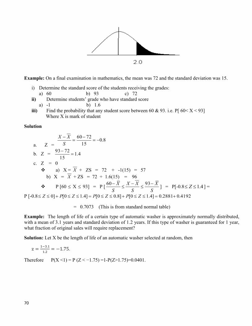
70

Example: On a final examination in mathematics, the mean was 72 and the standard deviation was 15.

i) Determine the standard score of the students receiving the grades:

a) 60 b) 93 c) 72

ii) Determine students’ grade who have standard score

a) -1 b) 1.6

iii) Find the probability that any student score between 60 & 93. i.e. P[ 60< X < 93]

Where X is mark of student

Solution

a. Z = 8.0

15

7260

S

XX

b. Z = 4.115

7293

c. Z = 0

a) X = X + ZS = 72 + -1(15) = 57

b) X = X + ZS = 72 + 1.6(15) = 96

P [60 X 93] = P [S

X

S

XX

S

X

9360] = P[-0.8 4.1 Z ] =

P [-0.8 4192.02881.0]4.10[]8.00[]4.10[]0 ZPZPZPZ

= 0.7073 (This is from standard normal table)

Example: The length of life of a certain type of automatic washer is approximately normally distributed,

with a mean of 3.1 years and standard deviation of 1.2 years. If this type of washer is guaranteed for 1 year,

what fraction of original sales will require replacement?

Solution: Let X be the length of life of an automatic washer selected at random, then

z =1−3.1

1.2= −1.75.

Therefore P(X <1) = P (Z < −1.75) =1-P(Z>1.75)=0.0401.

71

ACTIVITY

Assume that the daily wages for working in particular industry averages birr 11.90 per day and the

standard deviation is birr 0.40. if the wages are assumed to be normally distributed, determine what

percentage of workers receive wages

D. b/n birr 12,2 and birr 13.10

E. less than birr 11.00

F. more than birr 12.95

G. less than birr 11.00 and more than birr 12.95

Exercise

1. Suppose X has a binomial distribution with n = 10, p = .4. Find

a. P(X ≤ 4) c. P(X >4)

b. P(X <6) d. P(X = 5)

2. In a large population 40% votes for A and 60% for B. Suppose we select at random 10 people. What is the

probability that in this group exactly 4 people will vote for A?

3. We flip a fair coin 20 times.

a. What is the probability of exactly 10 Heads?

b. What is the probability of 15 or more Heads?

4. If the probability that an individual suffers a bad reaction from injection of a given serum is 0.001, determine

the probability that out of 2000 individual s

a. Exactly 3 individuals will suffer a bad reaction

b. More than 2 individuals will suffer a bad reaction

5. We draw at random 5 numbers from 1, . . . 100, with replacement (for example, drawing number 9 twice is

possible). What is the probability that exactly 3 numbers are even?

6. Let X be a random variable having a binomial distribution with parameters n=25 and P=0.2. Evaluate

P(X<𝜇 − 2𝜎)

7. Patients arrive randomly and independently at a doctor’s consulting room from 5 P.M.at an average rate of

one in 5. The minute waiting room can hold 12 persons. What is the probability that the room will be full,

when the doctor arrives at 6 P.M.?

8. The mean and variance of a binomial distribution are 4 and 4/3 respectively .Find P(X≥ 1) for n=6

9. The height of adult women in Ethiopia is normally distributed with mean 64.5 inches and standard deviation

2.4 inches

a) Find the probability that a randomly chosen woman is larger than 70 inches tall.

b) Feven is 71 inches tall. What percentages of women are shorter than Feven?

10. Suppose that your wife is pregnant and due in 100 days. Suppose that the probability density distribution function for having a child is approximately normal with mean 100 and standard deviation 8. You have a business trip and will return in 85 days and have to go on another business trip in 107 days.

d. What is the probability that the birth will occur before your second trip?

e. What is the probability that the birth will occur after you return from your first business trip?

c. What is the probability that you will be there for the birth?

72

References

Box, G. E. P. and Cox, D. R. (1964). An analysis of transformations, Journal of the

Royal Statistical Society, Series B, 26, 211-252.

Kaiser, H. F. (1960) Directional statistical decisions. Psychological Review, 67,

160-167

Kutner, M., Nachtsheim, C., Neter, J., and Li, W. (2004). Applied Linear Statistical Models,

McGraw-Hill/Irwin, Homewood, IL.

Maxwell, S. E., & Delaney, H. D. (2003) Designing Experiments and Analyzing

Data: A Model Comparison Perspective, Second Edition, Lawrence Erlbaum

Associates,Mahwah,NewJersey.


Tufte, E. R. (2001). The Visual Display of Quantitative Information (2nd ed.) (p.

178). Cheshire, CT: Graphics Press.

73

CHAPTER SEVEN

7. Sampling and Sampling Distribution of Sample Mean Introduction

When secondary data are not available for the problem under study, a decision may be taken to collect primary

data by using any of the methods discussed in the begging chapter. The required information may be obtained

by following either the census method or the sampling method.

Lesson objective: students are expected to be able to:

Identify the difference between census and sampling method of data collection.

Explain and list down the merit and demerit of census and sampling method of data

collection.

Identify the standard errors involved in sampling.

List down and elaborate probability sampling method and non-probability sampling method.

7.1 Basic Concepts

Population: the large pool of cases Example - All persons aged 18 or above living in the city of Dessie. All

business establishments employing more than 100 persons in AA that operated in Dec, 2000 E.C.

Sampling: is a process of systematically selecting cases to include them in a research project revision

commercials ared b/w 6:00-7:00 p.m. on three major networks

Sample: is a set of data collected and/or selected from a statistical population by a defined procedure.

Parameters:are numbers that summarize data for an entire population. Statistics are numbers that summarize

data from a sample, i.e. some subset of the entire population.

Statistic: is a characteristic of a sample. Generally, a statistic is used to estimate the value of a population parameter.

For instance, suppose we selected a random sample of 100 students from a school with 1000 students. The

average height of the sampled students would be an example of a statistic. So would the average grade point

average. In fact, any measurable characteristic of the sample would be an example of a statistic.

Sam`` --*9+pling Frame: an actual list that includes every case in the population.

7.2 Reasons for Sampling

When studying the characteristics of a population, there many reasons to study a sample (drawn from

population under study) instead of entire population such as:

1. Time: as it is difficult to contact each and every individual of the whole population

2. Cost: The cost or expenses of studying all the items (object or individual) in a population may be prohibitive

3. Physically Impossible: Some population are infinite, so it will be physically impossible to check the all

items in the population, such as populations of fish, birds, snakes, mosquitoes. Similarly, it is difficult to study

the populations that are constantly moving, being born, or dying.

4. Destructive Nature of items: Some items, objects etc are difficult to study as during testing (or checking)

they destroyed, for example a steel wire is stretched until it breaks and breaking point is recorded to have a

minimum tensile strength. Similarly, different electric and electronic components are check and they are

destroyed during testing, making impossible to study the entire population as time, cost and destructive nature

of different items prohibits studying the entire population.

5. Qualified and expert staff: For enumeration purposes, highly qualified and expert staff is required which

is some time impossible. National and International research organizations, agencies and staff is hired for

http://stattrek.com/statistics/Glossary.aspx?Target=Parameter

74

enumeration purposive which is some time costly, need more time (as rehearsal of activity is required), and

some time it is not easy to recruiter or hire a highly qualified staff.

6. Reliability: Using a scientific sampling technique the sampling error can be minimized and the non-

sampling error committed in the case of sample survey is also minimum, because qualified investigators are

included.

7.3 Types of Sampling Techniques

Sampling method can be categorizing into two

1. Non-Probability sampling (or non-random) sampling.

2. Probability (random sampling)

7.3.1 Non-probability Sampling

The difference between non-probability and probability sampling is that non-probability sampling does not

involve random selection and probability sampling does. Non-probability sampling methods are those,

which do not provide every item in the universe with a known chance of being included in the sample. The

selection process is, at least, partially subjective.

Judgment sampling

Quota sampling

Convenience sampling

Judgmental Sampling

In judgmental sampling, the person doing the sample uses his/her knowledge or experience to select the items

to be sampled.

For example, based on experience, an auditor may know which types of items are more apt tohave

nonconformance or which types of items have had problems in the past or which items area higher risk to the

organization. In another example, the acceptance tester might select test

Cases that exercise the most complex features, mission critical functions or most used sections ofthe software.

Quota Sampling

In quota sampling, you select people non-randomly according to some fixed quota. There are two types

of quota sampling: proportional and non-proportional.

Advantages

quick and cheap to organize

Disadvantages

not as representative of the population as a whole as other sampling methods

because the sample is non-random it is impossible to assess the possible sampling error

Snowball Sampling

In snowball sampling, you begin by identifying someone who meets the criteria for inclusion in your

study. You then ask them to recommend others who they may know who also meet the criteria.

Although this method would hardly lead to representative samples, there are times when it may be the

best method available. Snowball sampling is especially useful when you are trying to reach populations

75

that are inaccessible or hard to find. For instance, if you are studying the homeless, you are not likely to

be able to find good lists of homeless people within a specific geographical area. However, if you go to

that area and identify one or two, you may find that they know very well who the other homeless people

in their vicinity are and how you can find them.

Convenience sampling

Is used in exploratory research where the researcher is interested in getting an inexpensive approximation

of the truth. As the name implies, the sample is selected because they are convenient. This non-probability

method is often used during preliminary research efforts to get a gross estimate of the results, without

incurring the cost or time required to select a random sample.

7.3.2 Probability Sampling

Probability sampling methods are those in which every item in the universe has a known chance, or

probability, of being chosen for sample. This implies that the selection of sample items is independent of the

person making the study-that is, the sampling operation is controlled so objectively that the items will be

chosen strictly at random. It may be noted that the term random sample is not used to describe the data in the

sample but the process employed to select the sample. Randomness is thus a property of the sampling

procedure instead of an individual sample. As such, randomness can enter processed sampling in a number of

ways and hence random samples may be of kinds.

Advantages of Probability Sampling

The following are the basic advantages of probability sampling methods:

Probability sampling does not depend upon the existence of detailed information about the

universe for its effectiveness.

Probability sampling provides estimates which are essentially unbiased and have measurable

precision.

It is possible to evaluate the relative efficiency of various sample designs only when

probability sampling is used.

Limitations of Probability Sampling

Probability sampling requires a very high level of skill and experience for its use.

It requires a lot of time to plan and execute probability sampling.

The costs involved in probability sampling are generally large as compared to non-probability

sampling.

Probability Sampling can be classified as:

Simple random sampling

Stratified sampling

Systematic sampling

Cluster sampling

Simple Random Sampling

A simple random sampling is a type of Probability Sampling which gives each member of the population an

equal chance of being chosen. It is not a haphazard sample as some people think! One way of achieving a

simple random sample is to number each element in the sampling frame (e.g. give everyone on the Electoral

76

register a number) and then use random numbers to select the required sample.

Random numbers can be obtained using your calculator, a spreadsheet, printed tables of random numbers, or

by the more traditional methods of drawing slips of paper from a hat, tossing coins or rolling dice.

The optimum sample is the one which maximizes precision per unit cost, and by this criterion simple

random sampling can often be bettered by other methods.

Advantages

ideal for statistical purposes

Disadvantages

hard to achieve in practice

requires an accurate list of the whole population

expensive to conduct as those sampled may be scattered over a wide area

Random Numbers from a Calculator or Spreadsheet

Most electronic calculators have a RAN# function that produces a random decimal number between 0 and 1.

The formula =RAND ( ) in Excel achieves the same result, but to more decimal places. So how can you use

these to select a random sample?

Suppose you wanted to select a random lottery number between 1 and 49. There are two approaches.

Firstly, you could multiply the electronic random number by 49 to get a random number between 0 and 49,

and round this number up to the nearest whole number. For example, if the electronic random number is

0.497, when multiplied by 49 this gives 24.353, which you should round up to 25.

Secondly, you could treat the electronic random number as a series of random digits and use the first two as

your random number, ignoring any that are greater than 49. For example, the electronic random number

0.632 has first two digits 63 and you ignore it, whereas 0.317 gives the random number 31.

Random Number Tables

Random number tables consist of a randomly generated series of digits (0-9). To make them easy to read

there is typically a space between every 4th digit and between every 10th rows. When reading from random

number tables you can begin anywhere (choose a number at random) but having once started you should

continue to read across the line or down a column and NOT jump about.

Here is an extract from a table of random sampling numbers:

3680 2231 8846 5418 0498 5245 7071 2597

If we were doing market research and wanted to sample two houses from a street containing houses

numbered 1 to 48 we would read off the digits in pairs

36802231884654180498524570712597

and take the first two pairs that were less than 48, which gives house numbers 36 and 22.

If we wanted to sample two houses from a much longer road with 140 houses in it we would need to read

the digits off in groups of three:

368 022 318 846 541 804 985 245 707 1 25 97 and the numbers underlined would be the ones to visit: 22 and 125.

Houses in a road usually have numbers attached, which is convenient (except where there is no number 13).

In many cases, however, one has first to give each member of the population a number. For a group of 10

people we could number them as:

77

0 Apple yard 5 Francis

1 Ban yard 6 Gray

2 Croft 7 Hibbert

3 Duran 8 Jones

4 Entwhistle 9 Lilywhite

By numbering them from 0 to 9 you need only use single digits from the random number table.

36802231884654180498524570712597

In this case the first digit is 3 and so Durran is chosen.

Systematic Sampling

This is random sampling with a system! From the sampling frame, a starting point is chosen at random, and

thereafter at regular intervals. For example, suppose you want to sample 8 houses from a street of 120

houses.

120/8=15, so every 15th house is chosen after a random starting point between 1 and 15. If the random

starting point is 11, then the houses selected are 11, 26, 41, 56, 71, 86, 101, and 116.

If there were 125 houses, 125/8=15.625, so should you take every 15th house or every 16th house? If you

take every 16th house, 8*16=128 so there is a risk that the last house chosen does not exist. To overcome

this random starting point should be between 1 and 10. On the other hand if you take every 15th house,

8*15=120 so the last five houses will never be selected. The random starting point should now be between 1

and 20 to ensure that every house has some chance of being selected.

In a random sample every member of the population has an equal chance of being chosen, which clearly not

the case here is, but in practice a systematic sample is almost always acceptable as being random.

Advantages

Spreads the sample more evenly over the population

Easier to conduct than a simple random sample

Disadvantages

The system may interact with some hidden pattern in the population, e.g. every third house along

the street might always be the middle one of a terrace of three

Cluster Sampling

In cluster sampling the units sampled are chosen in clusters, close to each other.

Examples: households in the same street, or successive items off a production line.

The population is divided into clusters, and some of these are then chosen at random. Within each cluster

units are then chosen by simple random sampling or some other method. Ideally the clusters chosen

should be dissimilar so that the sample is as representative of the population as possible.

Advantages

saving of travelling time, and consequent reduction in cost

useful for surveying employees in a particular industry, where individual companies can form the

clusters

Disadvantages

78

units close to each other may be very similar and so less likely to represent the whole population

larger sampling error than simple random sampling

Stratified Sampling

In a stratified sampling the sampling frame is divided into non-overlapping groups or strata, e.g.

geographical areas, age-groups, genders. A sample is taken from each stratum, and when this sample is a

simple random sample it is referred to as stratified random sampling.

Advantages

Stratification will always achieve greater precision provided that the strata have been chosen so

that members of the same stratum are as similar as possible in respect of the characteristic of

interest. The bigger the differences between the strata, the greater the gain in precision. For

example, if you were interested in Internet usage you might stratify by age, whereas if you were

interested in smoking you might stratify by gender or social class.

It is often administratively convenient to stratify a sample. Interviewers can be specifically trained

to deal with a particular age-group or ethnic group, or employees in a particular industry. The

results from each stratum may be of intrinsic interest and can be analyzed separately.

It ensures better coverage of the population than simple random sampling.

Disadvantages

Difficulty in identifying appropriate strata.

More complex to organize and analyses results.

Choice of Sample Size for each Stratum

In general, the size of the sample in each stratum is taken in proportion to the size of the stratum. This is

called proportional allocation. Suppose that in a company there is the following staff:

male, full time 90

male, part time 18

female, full time 9

female, part time 63

and we are asked to take a sample of 40 staff, stratified according to the above categories.

The first step is to find the total number of staff (180) and calculate the percentage in each group.

% male, full time = (90 / 180) x 100 = 0.5 * 100

=50

% male, part time = (18 / 180) x100 = 0.1 x 100 =

10

% female, full time = (9 / 180) x 100 = 0.05 x 100

= 5

% female, part time = (63/180) x100 = 0.35 x 100

= 35

This tells us that of our sample of 40,

50%should be male, full time.

10% should be male, part time.

5% should be female, full time.

35% should be female, part time. 50%of 40 are

20.

10% of 40 is 4.5% of 40 is 2.35% of 40 is 14.

Sometimes there is greater variability in some strata compared with others. In this case, a larger sample

should be drawn from those strata with greater variability.

79

Determination of Sample Size

A number of formulas have been devised for determining the sample size depending upon the availability of

information. A few formulas are given below:

n=𝜹𝟐𝒁𝟐

𝑑2 ,Where n = Sample size

z= Value at a specified level of confidence or desired degree of precision.

𝜹𝟐 = variance of the population

d= Difference between population mean and sample mean.

The steps in computing the sample size from the above formula are:

Select the desired degrees of precision, i.e., specified level of confidence and designate it as

small ‘z’ (at 1% level of significance or 99% confidence level the value of ‘z’ is 2.58, and at

5% level of significance or 95% confidence level 1.96).

Multiply the ‘z’ selected in step 1 by the standard deviation of the universe, which may be

assumed.

Divide the product of the preceding step by the standard error of mean or difference between

population and sample mean. Square the resultant quotient. The result is the size of sample

required.

Example: Determine the sample size if 𝜹𝟐 =36, population mean = 25, sample mean = 23 and the desired

degree of precision is 99 per cent.

Solution n=

𝜹𝟐=36, d= 25-23 = 2

z = 2.576 (at 1% level the z value is 2.576)

Substituting the values:

Similarly, the sample size can be determined from the formula for determining the standard error of mean,

i.e. .𝜹�̅� = 𝜹�̅�

√𝒏=𝜹𝟐

�̅� =𝜹𝟐

𝒏 , If 𝜹 is 10 and 𝜹�̅�= 2.25, n shall be

Also from the formula for calculating standard error of proportion, the sample size can be determined:

2

d

ZS

6072.59728.72

6576.2 2

2

orn

16)4(25.2

10 2

2

n

n

pqs p

80

Merits of Sampling

The sampling technique has the following merits over the complete enumeration survey:

Less Time-consuming: Since the sample is a study of a part of the population, considerable time and labor

are saved when a sample survey is carried out.

Less Cost: Although the amount of effort and expense involved in collecting information is always greater

per unit of the sample than a complete census, the total financial burden of a sample survey is generally less

than that of a complete census. This is because of the fact that in sampling, we study only a part of population

and the total expense of collecting data is less than that required when the census method is adopted.

More Reliable Results: Although the sampling technique involves certain inaccuracies owing to sampling

errors, the result obtained is generally more reliable than that obtained from a complete count. There are

several reasons for it. First, it is always possible to determine the extent of sampling errors. Secondly, other

types of errors to which a survey is subject, such as inaccuracy of information, incompleteness of returns, etc.,

are likely to be more serious in a complete census than in a sample survey. Thirdly, it is possible to avail of

the services of experts and to impart thorough training to the investigators in a sample survey, which further

reduces the possibility of errors. Follow up work can also be undertaken much more effectively in the

sampling method. Indeed, even a complete census can only be tested for accuracy by some type of sampling

check.

More Detailed Information: Since the sampling technique saves time and money, it is possible to collect

more detailed information in a sample survey.

Sampling Method is the only Method that can be used in Certain Cases: There are some cases in which

the census method is inapplicable and the only practicable means is provided by the sample method. For

example, if one is interested in testing the breaking strength of chalks manufactured in a factory under the

census method all the chalks would be broken in the process of testing. Hence, census method is impracticable

and resort must be had to the sample method.

The Sample Method is often used to Judge the Accuracy of the Information Obtained on a Census

Basis: For example, in the population census, which is conducted very, often (10 years in our country) the

field officers employ the sample method to determine the accuracy of information obtained by the enumerators

on the census basis.

Demerits: Despite the various advantages of sampling, it is not completely free from limitations. Sample

survey must be carefully planned and executed the results obtained may be inaccurate and misleading.

Sampling generally requires the services of experts,

At times the sampling plan may be so complicated that it requires more time, labor and money

than a complete count.

If the information is required for each and every unit in the domain of study, complete

enumeration survey is necessary.

2

2

sp

pqnor

n

pqs p

000,10)005.0(

5.05.02

n

81

Types of Errors in Sampling Method

To appreciate the need for sample surveys, it is necessary to understand clearly the role of sampling and non-

sampling errors in complete enumeration and sample surveys. The error arising due to drawing inferences

about the population on the basis of few observations (sampling) is termed sampling error.

Clearly, the sampling error in this is non-existent in complete enumeration survey, since the whole population

is surveyed. However, the error mainly arising at the stage of ascertainment and processing of data, which are

termed non-sampling errors, are common both in complete enumeration and sample surveys.

Sampling Errors

Even if at most care has been taken in selecting a sample, the results derived from a sample study may not be

exactly equal to the true value of population. The reason is that estimate is based on a part and not on the

whole and samples are seldom, if ever, perfect miniature of the population. Hence sampling gives rise to

certain errors known as sampling errors (or sampling fluctuations). These errors would not be present in a

complete enumeration survey. However, the errors can be controlled. The modern sampling theory helps in

designing the survey in such a manner that the sampling errors can be made small.

Sampling errors are of two types: biased and unbiased.

Biased Errors: These errors arise from any bias in selection, estimation, etc. For example, if in place of

simple random sampling, deliberate sampling has been used in a particular case some bias is introduced in the

result and hence such errors are called biased sampling errors.

Unbiased Errors: These errors arise due to chance differences between the members of population included

in the sample and those included. An error in statistics is the difference between the value of a statistic and

that of the corresponding parameter.

Thus the total sampling error is made up of errors due to bias, if any, and the random sampling error. The

essence of bias is that it forms a constant component of error that does not decrease in a large population as

the number in the sample increases. Such error is, therefore known as cumulative or no compensating error.

The random sampling error, on the other hand, decreases on an average as the size sample increases. Such

error is, therefore, also known as non-cumulative or compensating error.

Causes of Bias error: Bias may arise due to:

Fault process of selection;

Fault work during the collection; and

Fault methods of analysis.

Faulty Selection Faulty selection of the sample may give rise to bias in a number of ways, such as:

a. Deliberate selection: of a ‘representative’ sample.

b. Conscious or unconscious bias in. the selection of a ‘random’ sample:

The randomness of selection may not really exist, even though the investigator claims that he had a random

sample if he allows his desire to obtain a certain result to influence his selection.

82

c. Substitution: Substitution of an item in place of one chosen in random sample sometimes leads to bias.

Thus, if it were decided to interview every 50th householder in the street, it would be inappropriate to interview

the 51st or any other number in his place as the characteristics possessed by them differ from those who were

originally to be included in the sample.

d. Non-response: If all the items to be included in the sample are not covered there will be bias even though

no substitution been attempted. This fault particularly occurs in mailed questionnaires, which are incompletely

returned. Moreover, the information supplied by the informants may also be biased.

e. An appeal to the vanity of the person, questioned may give rise to yet another kind of bias. For example,

the question ‘Are you a good student?’ is such that most of the students would succumb to vanity and answer

‘Yes’.

Bias due to Faulty Collection of Data: Any consistent error in measurement will give rise to bias whether

the measurements are carried out on a sample or on all the units of the population. The danger of is, however,

likely to be greater in sampling work, since the units measured are often Smaller. Bias may arise due to

improper formulation of the decision, securing an inadequate frame, and so on. Biased observations may result

from a poorly designed questionnaire, an ill-trained interviewer, failure of a respondent’s memory, etc. Bias

in the flow of the data may be due to unorganized collection procedure, faulty editing or coding of responses.

Bias in Analysis: In addition to bias which arises from faulty process of selection and faulty collection of

information, faulty methods of analysis may also introduce bias. Such bias can be avoided by adopting the

proper methods of analysis.

Avoidance of Bias: If possibilities of bias exist, fully objective conclusion cannot be drawn. The first essential

of any sampling or census procedure must, therefore, be the elimination of all sources of bias. The simplest

and the only certain way of avoiding bias in the selection process is for the sample to be drawn either entirely

at random, or at random subject to restrictions which, while improving the accuracy, are of such a nature that

they do not introduce bias in the results. In certain cases, systematic selection may also be permissible.

Method of Reducing Sampling Errors

Once the absence of bias has been ensured, attention should be given to the random sampling errors. Such

errors must be reduced to the minimum so as to attain the desired accuracy.

Apart from reducing errors of bias, the simplest way of increasing the accuracy of a sample is to increase its

size. The sampling error usually decreases with increase in sample size (number of units selected in the

sample) and in fact in many situations the decrease is inversely proportional to the square root of the sample

size.

It is clear that though the reduction in sampling error is substantial for initial increases in sample size, it

becomes marginal after a certain stage. In other words,

Considerably greater effort is needed after a certain stage to decrease the sampling error than in the initial

instance. Hence; after that stage sizable reduction in cost can be achieved by lowering even slightly the

precision required. From this point of view, there is a strong case for resorting to a sample survey to provide

estimates within permissible margins of error instead of a complete enumeration survey, as in the latter the

effort and the cost needed will be substantially higher due to the attempt to reduce the sampling error to zero.

As regards non-sampling errors they are likely to be more in case of complete enumeration survey than in

case of a sample survey, since it is possible to reduce the non-sampling errors to a great extent by using better

83

organization and suitably trained personnel at the field and tabulation stages. The behavior of the non-

sampling errors with increase in the sample size is likely to be the opposite of that of sampling error, that is ,

the non-sampling error is likely to increase with increase in sample size.

In many situations, it is quite possible that the non-sampling error in a complete enumeration survey is greater

than both the sampling and non-sampling errors taken together in a sample survey, and naturally in such

situations the latter is to be preferred to the former.

Non-sampling Errors

When a complete enumeration of units in the universe is made, one would expect that it would give rise to

data free from errors. However, in practice it is not so. For example, it is difficult to completely avoid errors

of observation or ascertainment. So also in the processing of data tabulation errors may be committed affecting

the final results. Errors arising in this manner are termed non-sampling errors, as they are due to factors other

than the inductive process of inferring about the population from a sample. Thus, the data obtained in an

investigation by complete enumeration, although free from sampling error, whereas the results of a sample

survey would be subject to sampling error as well as non-sampling error.

Data specification being inadequate and inconsistent with respect to the objective of the census or

survey.

Inappropriate statistical unit.

Inaccurate or inappropriate methods of interview, observation or measurement with inadequate or

ambiguous schedules, definitions or instructions.

Lack of trained and experienced investigators.

Lack of adequate inspection and supervision of primary staff.

Errors due to non-response, i.e., incomplete coverage in respect of units.

Errors in data processing operations such as coding, punching, verification, etc.

Errors committed during presentation and printing of tabulated results.

These sources are not exhaustive, but are given to indicate some of the possible sources of error. In a sample

survey, non-sampling errors may also arise due to defective frame and faulty selection of sampling units.

Control on Non-Sampling Errors

In some situations, the non-sampling errors may be large and deserve greater attention than sampling errors.

While, in general sampling errors decrease with increase in sample size, non-sampling errors tend to increase

with the sample size. In the case of complete enumeration non-sampling errors and in the case of sample

surveys both sampling and non-sampling errors require to controlled and reduced to a level at which their

presence does not vitiate the use of final results.

Reliability of Samples

The reliability of samples can be tested in the following ways:

84

More samples of the same size should be taken from the same universe and their results be compared.

If results are similar, the sample will be reliable.

If the measurements of the universe are known, then they should be compared with the measurements

of the sample.

In case of similarity of measurements, the sample will be reliable.

Sub-sample should be taken from the samples and studied. If the results of sample and sub sample study show

similarity, the sample should be considered reliable.

Exercises

1. Define sampling. Explain the different methods of sampling

2. State the advantages of adopting sampling procedure in carrying out large-scale surveys.

3. Point out the importance of sampling in solving business and economic problems.

4. What are the principles on which sampling methods rest?

5. What is random sampling? How can a random sample be selected? Is random sampling always better than

other forms of sampling in the context of socio-economic survey?

6. A sample may be large yet worthless because it is not random; or it may be random but unreliable because it

is small. “Comment upon this statement.”

1. (a) Define: (i) Random Sampling, (ii) Stratified Sampling, (iii) Multistage Sampling. (b) In a given sampling

enquiry, how will you determine the size of the sample? In what situations sampling method should be preferred

to complete enumeration?

85

References



Kaiser, H. F. (1960) Directional statistical decisions. Psychological Review, 67, 160-167





86

CHAPTER EIGHT

8. Estimation and Hypothesis Testing 8.1 Introduction

One aspect of inferential statistics is estimation, which is the process of estimating the value of the parameter

from information obtained from a sample.

An important question in estimation is that of sample size. How large should the sample be in order to make

an accurate estimate? This question is not easy to answer since the size of the sample depends on several

factors, such as the accuracy desired and the probability of making a correct estimate.

Lesson objective

Identify different application that requires statistical estimates.

Find the confidence interval for the mean when δ is known or n ≥ 30 and vice versa.

Identify and list down the quality of good estimator

Elaborate the application of chi-square test of homogeneity and test of independency.

8.2 Estimation

8.2.1 Point estimation

- Is a specific numerical value (single value) estimate of a parameter. The best point estimate of the

population means and proportion is the sample mean and the sample proportion respectively.

8.2.2 Interval estimation:

- is an interval range of values used to estimate the parameter. This estimate may or may not contain the

value of the parameter being estimated.

Thus instead of saying sample mean 𝑋 ̅is exactly equal to the population mean we obtain an interval by

subtracting a number from 𝑋 ̅ and by adding the same number to 𝑋 ̅, then we state that this interval contain

the population mean µ. To know the number, we should subtract or add firstly take two considerations.

a. The standard deviation 𝛿�̅� of the sample mean �̅�.

b. The level of confidence to be attached to the interval.

Estimator and Estimate

An estimator is a rule that tells you how to calculate an estimate based on information in the sample and

that is generally expressed as a formula.

An estimate is the value of estimator.

For instance, the sample mean is an estimator of population mean, from this sample mean is estimator and

the value of sample mean is estimate.

Qualities of Good Estimator

Goodness of an estimator is evaluated by observing its behavior in repeated sampling. A good estimator is

the one which provides an estimate with the following qualities.

87

Unbiasedness

An estimate is said to be unbiased estimate of a given parameter when the expected value of that estimator

can be shown to be equal to the parameter being estimated. An estimator of a parameter is said to be

unbiased if the mean of its distributions is equal to the true value of the parameter, otherwise, it is said to be

biased.

Consistency

The standard deviation of an estimate is called the standard error of the estimate. The large standard error

shows the more error in the estimate. The standard deviation of an estimate is a commonly used index of the

error entailed in estimating a population parameter based on the information in a random sample size n from

the entire population.

An estimator is said to be consistent if increasing the sample size produces an estimate with smaller

standard error.

Efficiency

An efficient estimate is one which has the smallest standard error among all unbiased estimators. If you

compare two statistics from a sample of the size and try to decide which one is more efficient estimate or

you should pick the statistic that has the smaller standard error or standard deviation of the sampling

distribution.

Sufficiency

This is another quality of a good estimator. An estimator is sufficient if it makes so much use of the

information in the sample that no other estimator could extract from the sample additional information about

the population parameter being estimated.

Activity

Answer the following question

Assume a symmetrically distributed population in which the values of the median and the mean

coincide. Which of this sample statistics (the mean or median) would be unbiased estimator of the

population median?

Confidence level and confidence interval

Each interval is constructed with regard to a given confidence level and are called confidence interval.

The confidence level isthe probability associated with the confidence interval, states how much confidence

we have that this interval contains the true population parameter and denoted by α.

Interval estimation of a population means

The (1-α) 100%confidence interval for µ is:

�̅� ± 𝑍𝛼

2𝛿�̅� if δ is known and for all sample size

88

�̅� ± 𝑍𝛼

2𝑆�̅� if δ is not known and sample size is large (n≥30)

�̅� ± t𝛼

2𝑆�̅�, if δ is not known and sample size is small (n<30), Where 𝛿�̅� =

𝛿

√𝑛 and 𝑆�̅� =

𝑆

√𝑛

The value of Z used here is read from the standard normal distribution table for the given confidence level

and the t- value is obtained from the t- distribution table for n-1 degrees of freedom and the given

confidence level.

Hence the width of confidence interval depends on value of z and sample size n. as confidence level

decrease and sample size increase, the confidence interval decrease.

Example1: - Suppose a particular species of under story plants is known to have a variance in heights of

16cm2. If this species is sampled with the heights of 25 plants averaging 15cm, find the 95% confidence

interval for the population mean.

Solution: Given, n =25, �̅� = 15cm, δ2 = 16cm2, δ = 4cm and 𝑍𝛼

2 = 𝑍0.05

2

= Z0.025 = 1.96

CI = �̅� ± 𝑍𝛼

2𝛿�̅�

CI = (15 ± 1.96(4

√25)

CI = (13.432, 16.568)

We are 95% confident that the values of population mean µ lie in between 13.432 and 16.568.

Example2: - an investigator wanted to estimate the mean nitration level for all plants living in Amazon

forest he took a sample of 25 plants and found that the mean nutrition levels for all plants are approximately

normally distributed. If sample mean and sample standard deviation of 25 plants are 186 and 12

respectively. Construct a 95% confidence interval for the population mean µ.

Solution: Given, n =25, �̅� = 186, S = 12, c. l. = 95%, 𝑆�̅� =

𝑆

√𝑛

= 12

√25 =2.40

Degrees of freedom (df) = n-1 = 25-1 =24 and 𝑡0.02524 = 2.064, (from t-table).

CI = �̅� ± t𝛼

2𝑆�̅�

CI =186 ± 2.064(2.4)

CI = 186 ± 4.95

CI = (181.05, 190.05)

We have 95% confident that the mean of nutrition level for all plants lies in between (181.05, 190.05)

Point and interval estimation of the population proportion

The population and sample proportions are denoted by P and�̂�, respectively and calculated as

P (population proportion) = 𝑋

𝑁and �̂�(sample proportion) =

𝑥

𝑛

89

For large sample

The sampling distribution of the sample proportion is approximately normal.

The mean µ𝑝 of the sampling distribution of �̂� is equal to the population proportion P.

The standard deviation, 𝛿�̂� is equal to √𝒑𝒒

𝒏, Where q =1-p

In the case of proportion, a sample is considered to be large if np and nq are both greater than 5. If p and

q are not known, then n�̂� and n�̂� should each be greater than 5 for the sample to be large. When

estimating the value of population proportion, we do not know the value of p and q. Consequently we

cannot compute𝛿�̂�. Therefore in the estimation of the population proportion, we use the value of 𝑆𝑝 as

an estimate of𝛿�̂�. The value of 𝑆𝑝 which gives a point estimate of 𝛿�̂� is calculated as

𝑆�̂� = √�̂��̂�

𝑛

�̂� Is the point estimator of the corresponding population proportion P.

The margin of error associated with this point estimation is calculated by

Margin of error = ±1.96𝑆�̂�

The (1-α) 100% confidence Interval for the population proportion P is �̂� ±Z𝑆�̂�

Example1: An epidemiologist wishes to determine the rate of breast cancer in women 60 to 65 years old in

Ireland. She surveys a random sample of 5000 women in this age group and determines that exactly 50 have

had this form of cancer sometime during their life time.

So �̂� =𝑥

𝑛=

50

5000 = 0.01

She now has an estimate of the population rate of breast cancer and needs a way of expressing her

confidence in this value.

Solution:

�̂� Is an unbiased estimator of P. since �̂�is actually a sample mean then the variance of �̂� is

𝑆�̂� = √𝑝�̂�

𝑛 = √

0.01(0.99)

500

CI = �̂� ±Z𝑆�̂� = (0.01±1.96√0.01(0.99)

500 ) = (0.01- 0.003, 0.01+0.003) = (0.007, 0.013)

We have 95% confident that the population proportion is lies between 0.007 and 0.013.

Example2: suppose you wanted to evaluate the number of jars of jelly that have less than the correct

amount of product and you randomly sampled 100 jars of the production line. Suppose that 23 jars were

found to have some type of fill problem. Now you want to estimate the proportion of jars of jelly that have

some type of fill problem. You will accept a 90% confidence level.

90

Solution:P = 23

100 , with 90% confidence level Z = 1.645

CI = �̂� ±Z𝑆�̂�

CI = (0.161, 0.299)

Activity

Answer the following questions

1. In certain locality, simple random samples of 800 farmers were asked what type of fertilizer they

make use of. 480 of them responded that they have been using DP fertilizer. Determine the

interval estimate of the total number of farmers who are using DP fertilizer with 94.44%

confidence level.

2. Assume that a simple random sample of 9 automobile tiers was drawn from a normal distributed

population of certain production run. The mean and standard deviation of the lifetime of the tiers

were 22010 miles and 2500 miles respectively determine the interval estimate of the mean lifetime

of all tiers in this production run with a 95% confidence interval.

Sample size determination

One reason why we usually conduct a sample survey and not a census is that almost always we have limited

resources at our disposal.

Determining the sample size for the estimation of µ

Given the confidence level and the standard deviation of the population, the sample size that will produce a

predetermined maximum error E of the confidence interval estimate of µ is

n = 𝒁𝟐𝜹𝟐

𝑬𝟐 if 𝛿2 is known unless use 𝑆2instead of 𝛿2

Determining the sample size for the estimation of P

Given the confidence level and the value of p and q the sample size that will produce a predetermined

maximum error of the confidence interval estimate of P is

n=𝒁𝟐𝑷𝒒

𝑬𝟐 , Where E =Z𝛿�̂� =Z√𝑃𝑞

𝑛

8.3Hypothesis testing

In a test of hypothesis, we test a certain given theory or belief about the population parameter. We may

want to find out using some sample information whether or not a given claim about a population parameter

is true by making tentative assumption about a population parameter.

The null and alternative hypothesis is competing statements about the population either the null hypothesis

is true or the alternative hypothesis is true, but not both.

91

8.3.1 Important Concepts in Testing Statistical Hypothesis

Null hypothesis:the hypothesis which is we are going to test for possible rejection under the assumption is

called null hypothesis and denoted by H0. For example,

H0: 𝜇= 𝜇0, H0: 𝜎 = 𝜎0

Alternative hypothesis: any hypothesis which is taken as complementary to the null hypothesis is called an

alternative hypothesis and is usually denoted byH1. For example,

H1: 𝜇>𝜇0, or H1 : 𝜇<𝜇0, or H1 : 𝜇 ≠ 𝜇0, etc.

Ideally the hypothesis testing procedure should lead to the acceptance of null hypothesis (H0) when H0 is

true and reject H0 when the alternative hypothesis (H1) is true. Unfortunately, this is not always possible.

Since hypothesis tests are based on sample information, we must allow for the possibility of errors. While

accepting or rejecting hypothesis we commit two types of errors.

Type I error: RejectH0when it is true.

Type II error: Accept H0 when it is false.

If we consider,

P [Type I error] = 𝜶

P [Type II error] = 𝜷

Where 𝛼 and 𝛽 referred to as produces risk (probability of type I error) and consumer risks (probability of

type two error) respectively.

Critical region: a region corresponding to a statistic which amounts to rejection of H0 is termed as critical

region or region of rejection.

Level of significance (𝜶): this is probability that a random value of the statistic belong to the critical region.

In other words, it is the size of the critical region. Usually, the level of significance is taken as 5% and 1%.

So, 𝜶 = P [type I error]

Critical value: the value which separates the critical region and the acceptance region is called critical

value which is set by seeing the alternative hypothesis.

Types of tests: it is determined based on the alternative hypothesis. For example,

If H1: 𝜇>𝜇0, it is called right tailed test.

If H1: 𝜇<𝜇0, it is called left tailed test.

If H1: 𝜇 ≠ 𝜇0, it is called two tailed test.

92

Two-tailed test left-tailed test right-tailed

Sign in the H0 = = or ≥ = or ≤

sign in the H1 ≠ < >

rejection region In both tails In the left tail In the right tail

Steps to perform a test of hypothesis:

a) Set up H0.

b) Set up H1.

c) Set up test statistic.

d) Set up the level of significance and critical value using statistical table.

e) Compute the value of statistic using sample drawn from sample.

f) Take decision. If the calculated values of test statistic lies in the critical region reject H0 i.e. the

assumption under null hypothesis cannot be accepted. If the calculated value of the test statistic lies

in the accepted region i.e. outside the critical region, accept H0 i.e. the assumption under H0 can be

true value of the parameter.

8.3.2 Hypothesis Testing About Single Population Mean

When sample size is large (n ≥ 30)

The normal distribution is used to test hypothesis about the population mean when the sample size is large.

In test of hypothesis about µ for large sample (n ≥ 30);

a. Set up H0: 𝜇= 𝜇0

b. Set up H1 : 𝜇>𝜇0, or 𝜇<𝜇0, or 𝜇 ≠ 𝜇0

c. Set up test statistic as,

Zcalc = �̅�−𝜇0

𝜎/√𝑛, if population standard deviation (𝜎) is known


𝑠/√𝑛, if population standard deviation (𝜎) is not known

d. Set up the level of significance ∝ and the critical value as 𝑍𝑡𝑎𝑏 from the normal table.

e. Compute the statistic, say 𝑍𝑐𝑎𝑙𝑐

f. Decisions;

H1 Reject H0 if

𝜇<𝜇0 𝑍𝑐𝑎𝑙𝑐< -𝑍𝑡𝑎𝑏

𝜇>𝜇0 𝑍𝑐𝑎𝑙𝑐>𝑍𝑡𝑎𝑏

𝜇 ≠ 𝜇0

𝑍𝑐𝑎𝑙𝑐< -𝑍𝑡𝑎𝑏 i.e. -𝒁∝

𝟐 or

𝑍𝑐𝑎𝑙𝑐>𝑍𝑡𝑎𝑏 i.e.𝒁∝

𝟐

93

Rejection and acceptance method by using normal curve:

Acceptance RegionRejection Region (𝛼) Rejection Region (𝛼)Acceptance Region

Z = 0𝑍∝ -𝑍∝ Z = 0

Fig. 8.1 Right tail test (: 𝜇>𝜇0) Fig. 8.2 Left tail test (: 𝜇<𝜇0)

Rejection Region (𝛼)Acceptance Rejection Region (𝛼)

Region

-𝒁∝

𝟐 0 𝒁∝

𝟐

Fig. 8.3 two tailed test (𝜇 ≠ 𝜇0)

Example1: the mean life time of 100 picture tubes produced by a manufacturing company is estimated to be 5795

hours with a standard deviation of 150 hours. If the population mean be the mean lifetime of all the picture tubes

produced by the company, test the hypothesis 𝜇= 6000 hours against 𝜇 ≠ 6000 hours at 5% level of

significance. Solution:

H0: 𝜇= 6000 hours

H1:𝜇 ≠ 6000 hours

Test statistic: here n = 100 i.e. large sample. Population standard deviation is not given but the

sample standard devastation is 150 hours.

Z = �̅�−𝜇0

𝑠/√𝑛

∝ = 0.05, ∝/2 = 0.025, since H1 shows, two tailed test.

𝑍∝/2 = 1.96 so the critical values (𝑍𝑡𝑎𝑏) are 1.96 and -1.96.

Compute 𝑍𝑐𝑎𝑙𝑐

𝑍𝑐𝑎𝑙𝑐= 5795−6000

150/√100 = -13.67

Decision:

Since 𝑍𝑐𝑎𝑙𝑐< -𝑍𝑡𝑎𝑏 (-13.67 < -1.96), H0 is rejected and the claim produced by Company is not true.

94

Activity

Answer the following questions.

a. A manufacture of detergent claims that the mean weight of a particular box of detergent is 3.25 kg. A

random sample of 64 boxes revealed a sample average of 3.238kg and a sample standard deviation is

0.117kg.

b. Using 1% level of significance, is there evidence that the average weight of the boxes is different from

3.25kg?

c. Find the lower and upper limit for the p value.

d. The personnel manager of a large company would like to buy health insurance policy for its employees. A

sample 100 employees were selected at random and the company leant that the sample has an average

annual medical cost of Birr 315.4 and standard deviation of Birr 43.2. At the 0.01 level of significance, is

there evidence that the population average is above 300Birr?

When sample size is small (n < 30)

In test of hypothesis about µ for small sample (n <30);

a. Set up H0: 𝜇= 𝜇0

b. Set up H1 : 𝜇>𝜇0, or 𝜇<𝜇0, or 𝜇 ≠ 𝜇0

c. Set up test statistic

tcalc = �̅�−𝜇0

𝑠/√𝑛, if population standard deviation (𝜎) is not known.


𝜎/√𝑛, if population standard deviation (𝜎) is known.

d. Set up the level of significance ∝ and the critical value as 𝑡𝑡𝑎𝑏 from the t- table.

e. Compute the statistic, say 𝑡𝑐𝑎𝑙𝑐

f. Decisions;

H1 Reject H0 if (for 𝑡𝑐𝑎𝑙𝑐) Reject H0 if (for 𝑧𝑐𝑎𝑙𝑐)

𝜇<𝜇0 𝑡𝑐𝑎𝑙𝑐< -𝑡𝑡𝑎𝑏,i.e. -tα 𝑧𝑐𝑎𝑙𝑐< -𝑧𝑡𝑎𝑏,i.e. -zα

𝜇>𝜇0 𝑡𝑐𝑎𝑙𝑐>𝑡𝑡𝑎𝑏,i.e. tα 𝑧𝑐𝑎𝑙𝑐>𝑧𝑡𝑎𝑏,i.e. zα

𝜇 ≠ 𝜇0

𝑡𝑐𝑎𝑙𝑐< -𝑡𝑡𝑎𝑏 i.e. -𝒕∝

𝟐 or

𝑡𝑐𝑎𝑙𝑐>𝑡𝑡𝑎𝑏 i.e.𝒕∝

𝟐

𝑧𝑐𝑎𝑙𝑐< -𝑧𝑡𝑎𝑏 i.e. -𝒛∝

𝟐 or

𝑧𝑐𝑎𝑙𝑐>𝑧𝑡𝑎𝑏 i.e.𝒛∝

𝟐

Example1: a forest ecologist studying regeneration of rainforest communities in gaps caused by large trees

falling during storms read that stinging tree, dendrocnide excels, and seeding will grow 1.5m/year indirect

sun light in such gaps. In the gaps in her study plot she identified nine specimens of this species and

measured them in 2009 and again 1 year later. Listed below are the changes in the height for the nine

specimens. Do her data support the polished contention that seedlings of this species will average grater

than1.5 m of growth per year in direct sunlight?

1.9, 2.5, 1.6, 2.0, 1.5, 2.7, 1.9, 1.0, 2.0

Solution: the ecologist is looking for deviations from 1.5m in the right side, so we have a right tailed test

here. Given: n = 9, �̅� = 1.90𝑚, S2 = 0.260m2, S = 0.51

95

a. H0:µ = 12.44m/year b. H1:µ> 1.5M/year

c. Test statistic: here n = 9, i.e. small sample. Population standard deviation is not given but the

sample standard devastation is 0.51. (use α = 0.05)


𝑠/√𝑛

d. ∝ = 0.05, since H1 shows, one tailed test.

Df = n-1 = 9-1 =8

t tab = tα, n =t0.05, 8 = 1.86

e. Compute 𝑡𝑐𝑎𝑙𝑐

𝑡𝑐𝑎𝑙𝑐= �̅�−µ

𝑆

√𝑛

=𝟏.𝟗𝟎−𝟏.𝟓𝟎

𝟎.𝟓𝟏

√𝟗

=𝟎.𝟒𝟎𝟎.𝟓𝟏

𝟑

= 2.35

f. Decision:

Since tcalc = 2.35 >ttab =1.86 we reject H0

We conclude that seedling of this species will not average 1.5m of growth per year in direct sun

light.

Example2: a random sample of size 20 from a normal population gives a sample mean of 42 and a sample

standard deviation of 6. Test the hypothesis that the population standard deviation is more than 9.

Solution:

g. H0: 𝜇= 9

h. H1:𝜇> 9

i. Test statistic: here n = 20 i.e. small sample. Population standard deviation is not given but the

sample standard devastation is 6 hours. (use α = 0.05)


𝑠/√𝑛

j. ∝ = 0.05, since H1 shows, one tailed test.

𝑡∝ = 1.729 at (n-1 = 19) df. So the critical values (𝑡𝑡𝑎𝑏) are 1.729 and -1.729.

k. Compute 𝑍𝑐𝑎𝑙𝑐

𝑡𝑐𝑎𝑙𝑐= 42−9

6/√20 = 24.59

l. Decision:

Since 𝑡𝑐𝑎𝑙𝑐>𝑡𝑡𝑎𝑏 (24.59 > 1.729), H0 is rejected and the population mean is more than 9.

Hypothesis testing about population proportion

The population proportion, denoted by P, is obtained by taking the ratio of the number of elements in a

population with specific characteristics to the total number of elements in the population. The sample

proportion denoted by �̂�, gives a similar ratio for a sample. Both are calculated as follows

𝑃 =𝑋

𝑁 𝑎𝑛𝑑 �̂� =

𝑥

𝑛

Where N = the number of elements in the population, n= the number of elements in the sample.

X = number of elements in the population that possess a specific characteristic, x = number of elements in

the sample that possess a specific characteristic.

The mean of sample proportion�̂�, is denoted by µ�̂� and is equal to the population proportion. Thus,µ�̂� = 𝑃

96

The sample proportion �̂� is called an estimator of the population proportion P.

The standard deviation of the sample proportion �̂� is denoted by 𝛿�̂� and is given by the formula,

𝛿�̂� = √𝑝𝑞

𝑛

Where �̂�is the sample proportion, p= 1 – q and n is sample size. This formula is used when n/N≤ 0.05.

However; if n/N ≥ 0.05,𝛿�̂� = √𝑝�̂�(𝑁−𝑛)

𝑛(𝑁−1),Where√

(𝑁−𝑛)

(𝑁−1) 𝑖𝑠 𝑐𝑎𝑙𝑙𝑒𝑑 𝑓𝑖𝑛𝑖𝑡𝑒 𝑝𝑜𝑝𝑢𝑙𝑎𝑡𝑖𝑜𝑛 𝑐𝑜𝑟𝑟𝑒𝑐𝑡𝑖𝑜𝑛 𝑓𝑎𝑐𝑡𝑜𝑟.

Steps of testing population proportion

a. Set up H0:p = p0

b. Set up H1 p>𝑝0, or p<𝑝0, or p≠ 𝑝0

c. Set up test statistic

Zcalc = 𝑝−𝑝0

√𝑝0𝑞0

𝑛

, which follow the standard normal distribution.

d. Set up the level of significance ∝ and the critical value as 𝑍𝑡𝑎𝑏 from the normal table.

e. Compute the statistic, say 𝑍𝑐𝑎𝑙𝑐

f. Decisions;

H1 Reject H0 if

𝑝 <𝑝0 𝑍𝑐𝑎𝑙𝑐< -𝑍𝑡𝑎𝑏

𝑝> p0 𝑍𝑐𝑎𝑙𝑐>𝑍𝑡𝑎𝑏

𝑝 ≠ 𝑝0

𝑍𝑐𝑎𝑙𝑐< -𝑍𝑡𝑎𝑏 i.e. -𝒁∝

𝟐 or

𝑍𝑐𝑎𝑙𝑐>𝑍𝑡𝑎𝑏 i.e.𝒁∝

𝟐

Example: - direct mailing company sells drugs by mail. The company claims that 90% of all orders are

mailed within 72 hours after they are received. The quality control department at the company often takes

samples to check, if this claim is valid a recently taken sample of 150 orders should that 129 of them were

mailed within 72 hour, do you think that the company’s claim is true? Use α = 2.5%.

Solution: Given n = 150, p0 = 0.9, q0 = 1- 0.9 = 0.1, 𝑎𝑛𝑑 �̂� =129

150= 0.86

Step1: state the null and alternative hypothesis

H0: P = 0.9

H1: P ≠ 0.9

Step2: Select the distribution to use

𝑛𝑝 = 150(0.9) = 135 > 5 𝑎𝑛𝑑 𝑛𝑞 = 150(0.1) = 15 > 5,

𝑐𝑜𝑛𝑠𝑒𝑞𝑢𝑒𝑛𝑡𝑙𝑦 𝑡ℎ𝑒 𝑠𝑎𝑚𝑝𝑙𝑒 𝑠𝑖𝑧𝑒 𝑖𝑠 𝑙𝑎𝑟𝑔𝑒. 𝑡ℎ𝑒𝑟𝑒𝑓𝑜𝑟𝑒 𝑤𝑒 𝑢𝑠𝑒 𝑡ℎ𝑒 𝑛𝑜𝑟𝑚𝑎𝑙 𝑑𝑖𝑠𝑡𝑟𝑖𝑏𝑢𝑡𝑖𝑜𝑛.

Step3: determine the critical value

97

𝛼 = 0.025, 𝑡ℎ𝑒 < 𝑠𝑖𝑔𝑛 𝑖𝑛𝑑𝑖𝑐𝑎𝑡𝑒𝑠 𝑡ℎ𝑒 𝑡𝑒𝑠𝑡 𝑖𝑠 𝑙𝑒𝑓𝑡 − 𝑡𝑎𝑖𝑙𝑒𝑑 𝑡𝑒𝑠𝑡

Ztab = -1.96 (approximately)

Step4: calculate the value of test statistic

𝛿�̂� = √𝑃𝑞

𝑛= √

0.90(0.10)

150= 0.02449490

𝑍 =�̂� − 𝑃𝑜

𝛿�̂�

=0.86 − 0.90

0.02449490= −1.63

Step5:make decision

-1.63 > -1.96 we fail to reject H0.

Activity2

Answer the following question

1. The personnel direct of a large insurance company is interested in reducing the rate of turnover of

salespersons n the first year of employment. Past records shows that 25% of all new hires in this area are no

longer employed at the end of the year. Extensive new training approaches are implemented for a sample of

150 new salespersons. At the end of one year period, of these 150 salespersons, 29 are no longer employed.

a. At the 5% level of significance, is there evidence that the proportion of salespersons who have gone

through the new training and are no longer employed is less than 0.25

b. Compute the p value and interpret your results

Central limit theorem for sample proportion

The sampling distribution of �̂� is approximately normally distributed for a sufficiently large size. In the case

of proportion, the sample size is considered to be sufficiently large if nP and nq are both greater than 5.

Therefore, we can use the normal distribution to perform a test of hypothesis about the population

proportion, P, for a large sample.

Exercises

1. A supermarket wants to determine the average amount of time a customer must wait to be served. A simple

random sample of 100 customers was taken and it was found that the mean waiting time was 7.2 minutes. From

past experience the standard deviation is known to be 15 minutes. Find the 95% confidence interval estimate of

the mean waiting time for all the supermarket’s customers.

2. A survey claims that the average cost of hotel room in Atlanta is $69.21. To test the claim, a researcher selects a

sample of 30 hotel rooms and finds the average cost is $68.43. The standard deviation of the population is $3.72.

At =0.05, is there enough evidence to reject the claim?

3. The production manager of a company that manufactures footballs would like to estimate the diameter of the balls.

One of his biggest customers specified that the footballs are supposed to have a population mean diameter of 7.3

98

inches and a standard deviation of 0.04inches. Suppose a random sample of 25 foot balls were selected from a

delivery and indicate a sample average of 7.31inches.

a. Set up a 95% confidence interval estimate of the true average diameter of the footballs in this delivery.

b. Does the population of footballs need to have a diameter that normally distributed here?

4. An auditor of the government insurance company would like to determine the proportion of claims that are paid

by a health insurance company within two months of receipt of the claim. A random sample of 200 claims are

selected, and it is determined that 80 were paid out within two months of the receipt of the claim. Set up a 95 %

confidence interval estimate of the true proportion of the claims paid within two months.

5. An educator claims that the average salary of substitute teachers in school district in Allegheny country,

Pennsylvania, is less than $60 per day. A random sample of 8 school districts selected, and the daily salary (in

dollars) are shown. At =0.05, is there enough evidence to support the educators claim?

5560557055605660

6. A recent survey found the 64.7% of the population own their homes. In a random sample of 150 heads of

households, 92 responded that they owned their homes. At = 0.01, dose that indicated a difference from the

national proportion?

7. A clothes manufacturer wants to know whether customer prefer any specific color over other color in shirts. She

selects a random sample of 100 shirts sold and notes the colors. Then data are shown here. At α = 0.10, is there

color preference for the shirts?

Color white blue black red yellow green

No. sold 43 22 16 10 5 4

References








99

CHAPTER NINE

9. Simple Linear Regression and Correlation

9.1 Introduction

Regression analysis, in the general sense, means the estimation of or prediction of the Unknown values of

one variable from known values of the other variable. In Regression analysis there are two types of variables.

The variable whose value is influenced or to be predicted is called dependent (regressed or explained)

variable and the variable which influences the values or is used for prediction, is called independent variable

(regressor or Predictor or explanatory). If the Regression curve is a straight line, we say that there is linear

relationship between the variables under study, non-linear elsewhere.

When only two variables are involved, the functional relationship is known as simple regression. If the

relationship between the two variables is a straight line, it is known as simple linear regression; otherwise it

is called as simple non-linear regression. When there are more than two variables and one of them is assumed

dependent upon the other, the functional relationship between the variables is known as multiple regressions.

Moreover, correlation analysis is concerned with mathematical measure of the extent or degree of

relationship between two variables.

Unit objective

At the end of this Unit, the leaner should be able to:

Define what a simple linear regression and correlation

Know Significance of regression and correlation analysis

Use least square method to fit regression line of the dependent variable Y on an independent

variable X

Compute and interpret the simple, rank correlation coefficient between two variables and

coefficient of determination.

Understand the difference between simple and rank correlation coefficient

Lesson objective

Explain the difference between simple linear regression and correlation analysis.

Identify the dependent and independent variable in order to fit the linear regression equation.

Identify the properties of simple correlation coefficient.

9.2 Fitting Simple Linear Regression

It is better to define the terms dependent and independent variable. Dependent variable is a variable that

changes its value when the other variable (independent variable) changes.

Example: An instructor wants to see how the number of absences a student in her class has affects the

student’s final grade.

So, if we take number of absence and final grade, Final grade is dependent variable and number of absence

is independent variable.

How can we define regression?

Regression is used to study the relationship between dependent variable and independent variables. the

relationship may be linear, quadratic, polynomial and soon.

The simple linear regression of Y on X in the population is given by

100

𝑌 = 𝛼 + 𝛽𝑋 + 휀, Where,Y=dependent variable

X=independent variable

𝛼 = y- intercept

𝛽= regression coefficient or slope of the line (the amount of changing in the dependent

variable(Y) when the independent variable(X) changes one unit)

휀 =Error term

Assumptions of simple linear regression

1. There is linear relationship between dependent variable y and explanatory variable x

2. Expected value of error term is zero and its variance is constant (δ2 ) Hence error term is approximately

normally distributed with mean zero and constant variance (𝜎2).

Based on the sample data we estimate the values of the population parameter of 𝛼 𝑎𝑛𝑑 𝛽 .The estimator of

𝛼 𝑎𝑛𝑑 𝛽 are denoted by a and b, respectively.

Thus the fitted regression line is (the equation used to estimate the relationship based on the sample data or

after finding the values of 𝛼 = 𝑎 and 𝛽 = 𝑏 ) is given by �̂� = 𝑎 + 𝑏𝑥.

The values of a and b are obtained using the method of least squares. According to the principle of least

squares, one should select a and b such that ∑ 𝑒2will be as small as possible, that is, we minimize

𝑆𝑆𝐸 = ∑ 𝑒2 = 𝑆 = ∑[𝑦 − (𝑎 + 𝑏𝑥)]2

To minimize this function, first we take the partial derivatives of SSE with respect to a and b. Then the partial

derivatives are equal to zero separately. These will result in the equations known as normal equations.

For the straight line, y= a+ bx the normal equations are

∑ 𝑦 = 𝑛𝑎 + 𝑏𝑥 ……………. Appling summation notation on both sides.

⟹ 𝑎 =∑ 𝑦−𝑏 ∑ 𝑥

𝑛……………………………………………………. (1)

∑ 𝑥𝑦 = 𝑎 ∑ 𝑥 + 𝑏 ∑ 𝑥2 …………. multiplying both sides by x.

∑ 𝑥𝑦 =∑ 𝑦 − 𝑏𝑥

𝑛∑ 𝑥 + 𝑏 ∑ 𝑥2

⟹

222

2xxn

yxxyn

n

xx

n

yxxy

b

timator

of

β………….(2)

And when we substitute equation (2) in equation (1) we get the best estimator of 𝛼 which is given by

𝑎 = �̅� − 𝑏�̅�

Example: given the data on age and blood pressure of 6 persons.

101

Age (X) 43 48 56 61 67 70

Blood pressure (Y) 128 120 135 143 141 152

Fit a regression line of y on x and hence predict Y ifx=50.

Solution:

x345

y=819

2x

=20399

2y=112443

xy=47634

Regression equation of y on x is, 𝑌 = 𝑎 + 𝑏𝑥

The values of a and b are given by normal equations as,

∑ 𝑦 = 𝑛𝑎 + 𝑏 ∑ 𝑥

∑ 𝑥𝑦 = 𝑎 ∑ 𝑥 + 𝑏 ∑ 𝑥2

Substituting the values from the table, we have

819 = 6𝑎 + 345𝑏…….. (i)

47634 = 345𝑎 + 20399𝑏…….. (ii)

Solving (i) and (ii), we get

a =81.048

b=-0.964

∴�̂� = 81.048 + 0.964𝑥 is the regression equation of y on x when x=50, Y is given by

𝑌 = 81.048 + 0.964 × 50 = 129.248 This implies the systolic blood pressure for a 50 years old person is 129.

Example: From the following data obtain the regression equation of Y on X

Sales(X) : 91 97 108 121 67 124 51 73 111 57

Purchase(Y):75 75 69 97 70 91 39 61 80 47

𝐒𝐨𝐥𝐮𝐭𝐢𝐨𝐧: 𝑛 = 10, 900x

, 700y , 66900xy , 873602x

𝑏 =𝑛 ∑ 𝑥𝑦 − ∑ 𝑥 ∑ 𝑦

𝑛 ∑ 𝑥2 − (∑ 𝑥)2 =

10 × 66900 − 900 × 700

10 × 87360 − (900)2= 0.61

1.15)90061.0700(10

1)(

1

1

n

i

i

n

i

i xbyn

xbya

xy 61.01.15

102

Activities: 1

1. What are the assumptions for regression analysis?

2. What is the general form of the regression line used in statistics?

3. Wins and strikeout for hall of fame pitchers

Wins 329 150 236 300 284 207 247 314 273 324

strikeout 4136 1155 1956 2266 3192 1277 1068 3534 1987 3574

Fit the equation of the regression line and find the values of Y when X =260 wins.

9.3 The Covariance and Correlation Coefficient

Correlation analysis is concerned with measuring the strength (degree) of the relationship between two or

more variables. It is used if we are interested in knowing the extent of interdependence between two or more

variables.

Karl Pearson’s coefficient of (simple) correlation

The Karl Pearson correlation coefficient denoted by ),( yxr or xyr or simply r, is defined as the ratio of

the covariance between X and Y to the product of their standard deviations:

𝑟 =∑(𝑋𝑌) − 𝑛�̅��̅�

√[∑ 𝑋2 − 𝑛�̅�2][∑ 𝑌2 − 𝑛�̅�2]

The simplified formula used for computational purpose is

𝑟 =𝑛 ∑ 𝑥𝑦−∑ 𝑥 ∑ 𝑦

√[𝑛 ∑ 𝑥2−(∑ 𝑥)2

][𝑛 ∑ 𝑦2−(∑ 𝑦)2

]

An increase in one variable may cause an increase in the other variable, or a decrease in one variable may

cause decrease in the other variable. When the variables move in the same direction like this they are said to

be positively correlated. The positive correlation may be termed as direct correlation. If a decrease in one

variable causes an increase in the other variable or vice versa, the variables are said to be negatively correlated.

The negative correlation may be termed as inverse correlation. In case the two variables are not at all related

they are said to be independent or uncorrelated.

Example

1. There is a direct cause and effect relationship between the variable.

Example: water cause plant to grow, poison causes death and heat causes ice to melt.

2. There is a reverse (indirect) cause and effect relationship between the variables.

Example: suppose a researcher believes excessive coffee consumption causes nervousness, but the

researcher fails to consider that the reverse situation may occur. That is, it may be that an extremely

nervous person craves coffee to calm his or her nervous.

Properties of simple correlation coefficient

Coefficient of correlation lies between –1≤ r ≤1

If r =0 indicate that there is no linear relationship between two variables.

103

If r = -1 or +1 indicate that there is perfect negative (inverse) or positive (direct) linear relationship

between two variables respectively.

A coefficient of correlation(r) that is closes to zero shows the relationship is quite weak, whereas r

is closest to +1 or -1, shows that the relationship is strong.

Note that:

The strength of correlation does not depend on the positiveness and negativeness of 𝑟.

The slope of simple linear regression (coefficient of regression) and correlation coefficient should be

the same in sign.

The correlation between two variables is linear if a unit changes in one variable result in a constant change in

the other variable.

Example: Compute the values of the correlation coefficient for the data obtained in the study of the number

of absences and the final grades of the seven students in the sport science class.

r = (7)(3745)−(57)(511)

√[(7)(579)−(572)][(7)(38993)−(5112) = -0.944

The value of r indicates a strong negative linear relationship between a student’s final grade and the number

of absences a student has. That is, the more absence a student has, the lower is his or her grade.

Example: calculate the values of the correlation coefficient for the data given for the number of hours a person

exercises and the amount of milk a person consumes per week.

Subject Hours x Amount y xy x2 y2

A 3 48 144 9 2304

B 0 8 0 0 64

C 2 32 64 4 1024

D 5 64 320 25 4096

E 8 10 80 64 100

F 5 32 160 25 1024

G 10 56 560 100 3136

H 2 72 144 4 5184

I 1 48 48 1 2304

∑x=36 ∑y=370 ∑xy=1520 ∑x2=232 ∑y2=19236

Substituting in the formula and obtain r,

r = (9)(1520)−(36)(370)

√[(9)(232)−(362)][(9)(19236)−(3702) = 0.067

The value of r indicates there is a very week positive relationship between the variables.

104

Activities: 2

1. What statistical test is used to test the significance of the correlation coefficient?

2. A football fans wishes to see how the number of pass attempts (not completion) relates to the number of yards gained

for quarter backs in past NFL season playoff games. The data are shown for five quarter backs. Describes the

relationship.

Pass attempts x 116 90 82 108 92

Yards gained y 1001 823 851 873 839

Coefficient of determination

It is defined as the proportion of the variation in the dependent variable Y that is explained, or accounted for,

by the variation of the independent variable X. Its value is the square of the coefficient of correlation, thus we

denote it by r2 and it is usually expressed in the form of percentage.

Note: it is usually easier to find the coefficient of determination by squaring r and converting it to percentages.

9.4 The Rank Correlation Coefficient

Sometimes we come across statistical series in which the variables under consideration are not capable of

quantitative measurement, but can be arranged in serial order. This happens when we dealing with qualitative

characteristics (attributes) such as beauty, efficient, honest, intelligence, etc., in such case one may rank the

different items and apply the spearman method of rank difference for finding out the degree of relationship.

The greatest use of this method (rank correlation) lies in the fact that one could use it to find correlation of

qualitative variables, but since the method reduces the amount of labor of calculation, it is sometimes used

also where quantitative data is available. It is used when statistical series are ranked according to their

magnitude and the exact size of individual item is not known. Spearman’s correlation coefficient is denoted

by rs. If the ranks are given, denote the difference R1i - R2i by di and obtain the total of di. Then the following

formula is applied

1

61

2

2

nn

drs

If the actual data is given, rank it in ascending or descending order and follow the above procedures.

Note: that the values of rank correlation (rs) always lies between -1 and +1 inclusive.

Example: Ten competitors in a beauty contest are ranked by two judges in the following order. Compute and

interpret opinion of two judges with regard to beauty out looking.

1st judge(x) 1 6 5 10 3 2 4 9 7 7

2nd judge(y) 3 5 8 4 7 10 2 1 6 9

Solution

d=(x-y) -2 1 -3 6 -4 -8 2 8 1 -2

d2 4 1 9 36 16 64 4 64 1 4

2032d

105

2303.0

11010

203*61

1

61

22

2

nn

drs

Hence the pair of judges has opposite (divergent) tastes for beauty since rank correlation coefficient

is negative.

Exercise

1. Determine whether each statement is true or false. If the statement is false explaining why.

A. A negative relationship between two variables means that for the most part, as the x variable increases,

the y variable increases.

B. A correlation coefficient of -1 implies a perfect linear relationship between the variables.

2. Explain the meaning and significance of the concept of simple linear regression and correlation analysis.

3. How do you interpret a calculated value of Karl person’s correlation coefficient? Discuss in particular the

values of r= 0, r=-1 and +1.

4. A study is conducted with a group of dieters to see if the number of grams of fat each consumes per day is

related to cholesterol level. The data are shown here. if there is a significance relationship ,predict the

cholesterol level of a dieter who consumes 8.5 grams of fat per day.

Fat gram x 6.8 5.5 8.2 10 8.6 9.1 8.6 10.4

Cholesterol

level y

183 201 193 283 222 250 190 218

5. Obtain the regression equation for costs related to age of cars for the following data on the ages of cars of

a certain make and annual maintenance costs. Estimate the maintenance cost of cars when age of cars is

12 years

Age of cars(in years)(x) 2 4 6 8

Maintenance cost(in 100 birr)(y) 10 20 25 30

6. Based on the data on problem 4 and 5 find the correlation coefficient and coefficient of determination and

interpret the result.

106

References










GraphicsPress.


Wilkinson, L., & the Task Force on Statistical Inference, APA Board of Scientific

Affairs. (1999). Statistical methods in psychology journals: Guidelines and

explanations. American Psychologist, 54, 594–604.

CHAPTER ONE - eopcw

Documents

Transcript of CHAPTER ONE - eopcw