Biophysical correlates of relative abundances of marine megafauna at Ningaloo Reef, Western...
16
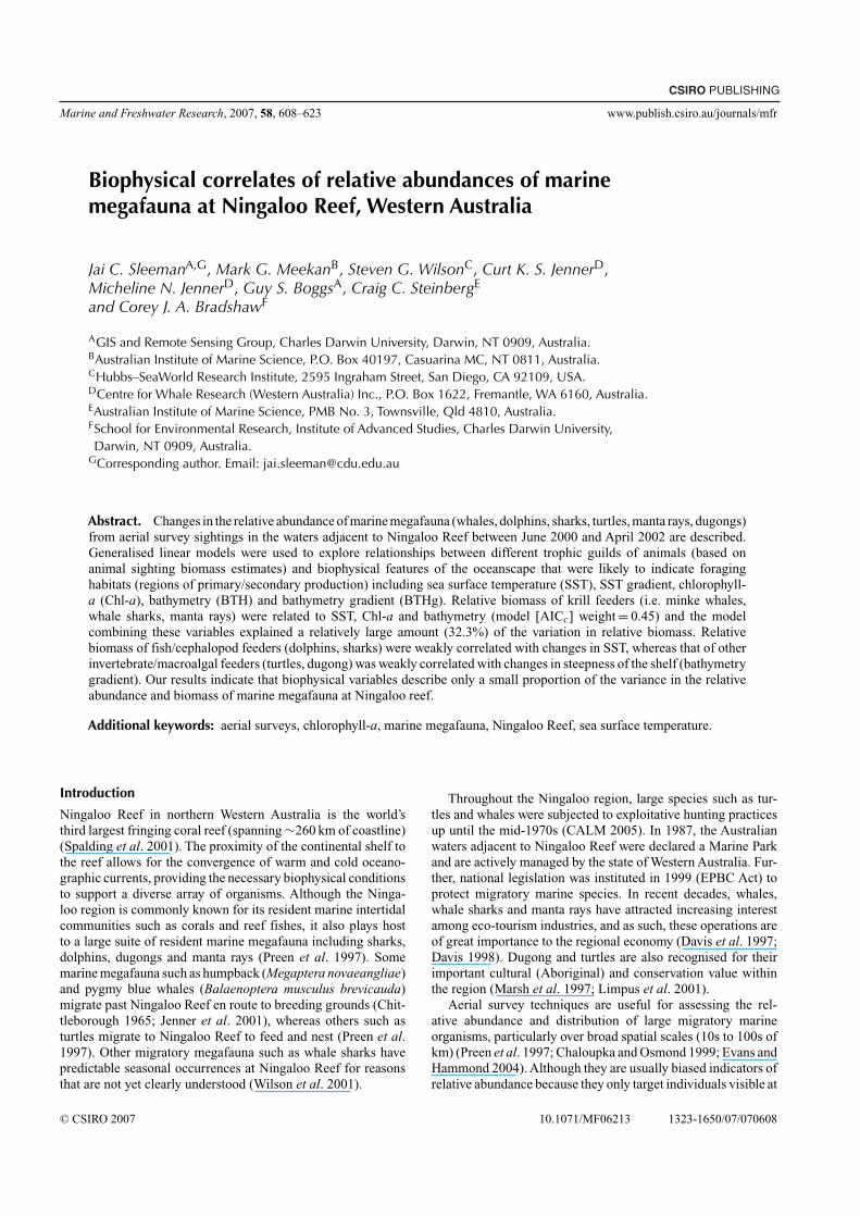
CSIRO PUBLISHING Marine and Freshwater Research, 2007, 58, 608–623 www.publish.csiro.au/journals/mfr Biophysical correlates of relative abundances of marine megafauna at Ningaloo Reef, Western Australia Jai C. Sleeman A,G , Mark G. Meekan B , Steven G. Wilson C , Curt K. S. Jenner D , Micheline N. Jenner D , Guy S. Boggs A , Craig C. Steinberg E and Corey J. A. Bradshaw F A GIS and Remote Sensing Group, Charles Darwin University, Darwin, NT 0909, Australia. B Australian Institute of Marine Science, P.O. Box 40197, Casuarina MC, NT 0811, Australia. C Hubbs–SeaWorld Research Institute, 2595 Ingraham Street, San Diego, CA 92109, USA. D Centre for Whale Research (Western Australia) Inc., P.O. Box 1622, Fremantle, WA 6160, Australia. E Australian Institute of Marine Science, PMB No. 3,Townsville, Qld 4810, Australia. F School for Environmental Research, Institute ofAdvanced Studies, Charles Darwin University, Darwin, NT 0909, Australia. G Corresponding author. Email: [email protected] Abstract. Changes in the relative abundance of marine megafauna (whales, dolphins, sharks, turtles, manta rays, dugongs) from aerial survey sightings in the waters adjacent to Ningaloo Reef between June 2000 and April 2002 are described. Generalised linear models were used to explore relationships between different trophic guilds of animals (based on animal sighting biomass estimates) and biophysical features of the oceanscape that were likely to indicate foraging habitats (regions of primary/secondary production) including sea surface temperature (SST), SST gradient, chlorophyll- a (Chl-a), bathymetry (BTH) and bathymetry gradient (BTHg). Relative biomass of krill feeders (i.e. minke whales, whale sharks, manta rays) were related to SST, Chl-a and bathymetry (model [AIC c ] weight = 0.45) and the model combining these variables explained a relatively large amount (32.3%) of the variation in relative biomass. Relative biomass of fish/cephalopod feeders (dolphins, sharks) were weakly correlated with changes in SST, whereas that of other invertebrate/macroalgal feeders (turtles, dugong) was weakly correlated with changes in steepness of the shelf (bathymetry gradient). Our results indicate that biophysical variables describe only a small proportion of the variance in the relative abundance and biomass of marine megafauna at Ningaloo reef. Additional keywords: aerial surveys, chlorophyll-a, marine megafauna, Ningaloo Reef, sea surface temperature. Introduction Ningaloo Reef in northern Western Australia is the world’s third largest fringing coral reef (spanning ∼260 km of coastline) (Spalding et al. 2001). The proximity of the continental shelf to the reef allows for the convergence of warm and cold oceano- graphic currents, providing the necessary biophysical conditions to support a diverse array of organisms. Although the Ninga- loo region is commonly known for its resident marine intertidal communities such as corals and reef fishes, it also plays host to a large suite of resident marine megafauna including sharks, dolphins, dugongs and manta rays (Preen et al. 1997). Some marine megafauna such as humpback (Megaptera novaeangliae) and pygmy blue whales (Balaenoptera musculus brevicauda) migrate past Ningaloo Reef en route to breeding grounds (Chit- tleborough 1965; Jenner et al. 2001), whereas others such as turtles migrate to Ningaloo Reef to feed and nest (Preen et al. 1997). Other migratory megafauna such as whale sharks have predictable seasonal occurrences at Ningaloo Reef for reasons that are not yet clearly understood (Wilson et al. 2001). Throughout the Ningaloo region, large species such as tur- tles and whales were subjected to exploitative hunting practices up until the mid-1970s (CALM 2005). In 1987, the Australian waters adjacent to Ningaloo Reef were declared a Marine Park and are actively managed by the state of Western Australia. Fur- ther, national legislation was instituted in 1999 (EPBC Act) to protect migratory marine species. In recent decades, whales, whale sharks and manta rays have attracted increasing interest among eco-tourism industries, and as such, these operations are of great importance to the regional economy (Davis et al. 1997; Davis 1998). Dugong and turtles are also recognised for their important cultural (Aboriginal) and conservation value within the region (Marsh et al. 1997; Limpus et al. 2001). Aerial survey techniques are useful for assessing the rel- ative abundance and distribution of large migratory marine organisms, particularly over broad spatial scales (10s to 100s of km) (Preen et al. 1997; Chaloupka and Osmond 1999; Evans and Hammond 2004). Although they are usually biased indicators of relative abundance because they only target individuals visible at © CSIRO 2007 10.1071/MF06213 1323-1650/07/070608
Transcript of Biophysical correlates of relative abundances of marine megafauna at Ningaloo Reef, Western...
CSIRO PUBLISHING
Marine and Freshwater Research, 2007, 58, 608–623 www.publish.csiro.au/journals/mfr
Biophysical correlates of relative abundances of marinemegafauna at Ningaloo Reef, Western Australia
Jai C. SleemanA,G, Mark G. MeekanB, Steven G. WilsonC, Curt K. S. JennerD,Micheline N. JennerD, Guy S. BoggsA, Craig C. SteinbergE
and Corey J. A. BradshawF
AGIS and Remote Sensing Group, Charles Darwin University, Darwin, NT 0909, Australia.BAustralian Institute of Marine Science, P.O. Box 40197, Casuarina MC, NT 0811, Australia.CHubbs–SeaWorld Research Institute, 2595 Ingraham Street, San Diego, CA 92109, USA.DCentre for Whale Research (Western Australia) Inc., P.O. Box 1622, Fremantle, WA 6160, Australia.EAustralian Institute of Marine Science, PMB No. 3, Townsville, Qld 4810, Australia.FSchool for Environmental Research, Institute of Advanced Studies, Charles Darwin University,Darwin, NT 0909, Australia.
GCorresponding author. Email: [email protected]
Abstract. Changes in the relative abundance of marine megafauna (whales, dolphins, sharks, turtles, manta rays, dugongs)from aerial survey sightings in the waters adjacent to Ningaloo Reef between June 2000 and April 2002 are described.Generalised linear models were used to explore relationships between different trophic guilds of animals (based onanimal sighting biomass estimates) and biophysical features of the oceanscape that were likely to indicate foraginghabitats (regions of primary/secondary production) including sea surface temperature (SST), SST gradient, chlorophyll-a (Chl-a), bathymetry (BTH) and bathymetry gradient (BTHg). Relative biomass of krill feeders (i.e. minke whales,whale sharks, manta rays) were related to SST, Chl-a and bathymetry (model [AICc] weight = 0.45) and the modelcombining these variables explained a relatively large amount (32.3%) of the variation in relative biomass. Relativebiomass of fish/cephalopod feeders (dolphins, sharks) were weakly correlated with changes in SST, whereas that of otherinvertebrate/macroalgal feeders (turtles, dugong) was weakly correlated with changes in steepness of the shelf (bathymetrygradient). Our results indicate that biophysical variables describe only a small proportion of the variance in the relativeabundance and biomass of marine megafauna at Ningaloo reef.
Additional keywords: aerial surveys, chlorophyll-a, marine megafauna, Ningaloo Reef, sea surface temperature.
Introduction
Ningaloo Reef in northern Western Australia is the world’sthird largest fringing coral reef (spanning ∼260 km of coastline)(Spalding et al. 2001). The proximity of the continental shelf tothe reef allows for the convergence of warm and cold oceano-graphic currents, providing the necessary biophysical conditionsto support a diverse array of organisms. Although the Ninga-loo region is commonly known for its resident marine intertidalcommunities such as corals and reef fishes, it also plays hostto a large suite of resident marine megafauna including sharks,dolphins, dugongs and manta rays (Preen et al. 1997). Somemarine megafauna such as humpback (Megaptera novaeangliae)and pygmy blue whales (Balaenoptera musculus brevicauda)migrate past Ningaloo Reef en route to breeding grounds (Chit-tleborough 1965; Jenner et al. 2001), whereas others such asturtles migrate to Ningaloo Reef to feed and nest (Preen et al.1997). Other migratory megafauna such as whale sharks havepredictable seasonal occurrences at Ningaloo Reef for reasonsthat are not yet clearly understood (Wilson et al. 2001).
Throughout the Ningaloo region, large species such as tur-tles and whales were subjected to exploitative hunting practicesup until the mid-1970s (CALM 2005). In 1987, the Australianwaters adjacent to Ningaloo Reef were declared a Marine Parkand are actively managed by the state of Western Australia. Fur-ther, national legislation was instituted in 1999 (EPBC Act) toprotect migratory marine species. In recent decades, whales,whale sharks and manta rays have attracted increasing interestamong eco-tourism industries, and as such, these operations areof great importance to the regional economy (Davis et al. 1997;Davis 1998). Dugong and turtles are also recognised for theirimportant cultural (Aboriginal) and conservation value withinthe region (Marsh et al. 1997; Limpus et al. 2001).
Aerial survey techniques are useful for assessing the rel-ative abundance and distribution of large migratory marineorganisms, particularly over broad spatial scales (10s to 100s ofkm) (Preen et al. 1997; Chaloupka and Osmond 1999; Evans andHammond 2004). Although they are usually biased indicators ofrelative abundance because they only target individuals visible at
© CSIRO 2007 10.1071/MF06213 1323-1650/07/070608
Marine megafauna and oceanography at Ningaloo Reef Marine and Freshwater Research 609
or near the surface, when repeated at regular intervals and correc-tion factors for observer bias (perception and availability bias)are applied (Marsh and Sinclair 1989), aerial surveys can pro-vide improved estimates of relative abundance and distributionof megafauna without the use of expensive and logistically chal-lenging techniques such as satellite telemetry (Mate et al. 1997;Hays et al. 2004; Wilson et al. 2006). Furthermore, broad-scalesurvey data can be compared with surrogates of the physical andbiological properties of ocean surface waters to provide heuristicinterpretations of the environmental conditions influencing rela-tive abundance patterns (Jaquet andWhitehead 1996; Kasamatsuet al. 2000; Schick et al. 2004).
Fluctuations in the relative abundance and distribution ofmarine megafauna at broad spatial scales have been attributed tooceanographic processes that operate in a ‘bottom-up’ fashionby influencing the availability of food. For example, sea surfacetemperature (SST), SST gradient (SSTg), chlorophyll-a (Chl-a)concentration and bathymetry can be used as surrogate vari-ables for primary production. Many studies have demonstratedcorrelations of these variables to the relative abundance and dis-tribution of zooplankton (Myers and Hick 1990; Sugimoto andTadokoro 1998; Kideys et al. 2000; Wilson et al. 2002). In turn,zooplankton can structure the relative abundance and distribu-tion of fish (Agenbag et al. 2003; Schick et al. 2004), and forthis reason, surrogate measures of zooplankton biomass havebeen used to model marine mammal (Bradshaw et al. 2004;Littaye et al. 2004) and reptile (Polovina et al. 2004) distribu-tions and behaviour. However, plankton distributions may bealtered by factors that are not responsible for their production andgrowth (Guinet et al. 2001; Bradshaw et al. 2004). Forcing fac-tors are also susceptible to dilution effects through the food web(El-Sayed 1988; Guinet et al. 2001). For these reasons, it seemslikely that distributions of species feeding on lower trophic-levelprey species will be more closely correlated with variables suchas SST and Chl-a than the distributions of higher trophic-levelspecies (Gende and Sigler 2006).
In this paper we examine spatial and temporal patterns inthe distribution, relative sighting occurrence and biomass ofmarine megafauna species observed at Ningaloo Reef, WesternAustralia. Occurrence of megafauna and fish/krill schools wasestimated using aerial surveys flown at roughly weekly intervalsbetween June 2000 and April 2002. These estimates of occur-rence were compared with the physical and biological oceanog-raphy of the region characterised by satellite remote-sensingdata. We aimed to identify important spatial and temporal pat-terns of habitat use by this suite of marine fauna and determinewhether there were useful physical and biological correlates toexplain some of the variation in their relative abundance. Weexamined the hypothesis that the strength of any correlationsfound varies depending on trophic level, with stronger correla-tions expected for those species feeding on lower trophic-levelorganisms such as invertebrates and algae.
Materials and methodsOceanographic settingThe oceanography of the Ningaloo region of northern West-ern Australia is dominated by the Leeuwin Current that driveswarm, low-nutrient surface waters south along the continental
shelf and influences the production and recruitment of inverte-brate and fish communities depending on its strength (Caputiet al. 1996). The Current is strongest during autumn and winter(April–September) (Godfrey and Ridgeway 1985), and weakensduring the summer (September–April) as a result of southerlywinds that drive the Ningaloo Current (Taylor and Pearce 1999).As a wind-driven current, the Ningaloo Current is limited to thesurface (<50 m) (Gersbach 1999; Woo et al. 2006a), but is suf-ficient to influence cold water upwelling (Woo et al. 2006b) thatgenerates high primary production and phytoplankton biomass(Hanson et al. 2005).
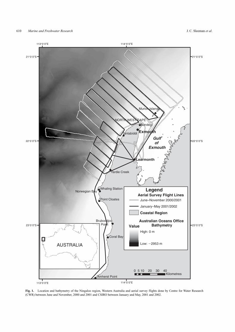
Aerial censusesBetween June 2000 and April 2002, Woodside Energy Ltd com-missioned the Centre for Whale Research (CWR) and CSIROMarine Research to conduct a series of aerial surveys of marinemegafauna in the waters adjacent to Ningaloo Reef, from NorthWest Cape (21◦47′S, 114◦09′E) to south Amherst Point, south ofCoral Bay (23◦37′S, 113◦36′E) to establish a baseline descrip-tion of the region as part of an environmental impact assessment(Woodside 2003). A total of 26 surveys were carried out byCWR at roughly 8-day intervals (weekly) depending on weatherand aircraft availability between June and November in 2000and 2001. CSIRO Marine Research did a total of 12 surveysbetween January and May in 2001 and January and April 2002.Between January and March, surveys were carried out monthlyby CSIRO and between April and May, surveys were carried outfortnightly.All surveys used a twin engine over-head wing Parte-navia P68B aircraft fitted with bubble windows to maximise thefield of view beneath the plane. The survey teams comprisedtwo observers positioned on opposite sides of the aircraft whologged sighting occurrence and positions of animals using a GPSor a palm-top computer synchronised with a GPS logger at reg-ular 1-s intervals. Survey routes used by CWR consisted of 16NW–SE oriented transects running perpendicular to the coast-line, spaced ∼5 nm (9.3 km) apart and averaging a total distanceof 1041.45 km (Fig. 1a). A standardised flight path consistingof 12 inshore–offshore transects spanning a total distance of637.87 km was flown on each of the CSIRO surveys (Fig. 1b).One month following the commencement of the CSIRO sur-veys (February–May 2001 and January–April 2002), a singleobserver recorded positions and sighting occurrence of animalswith a GPS when transiting between Learmonth and Carnarvon(24◦53′S, 113◦38′E). Unlike the standardised survey route, thisdeviated flight path ran adjacent to the coast at a distance of 300–400 m seaward of the front of Ningaloo Reef and covered a totaldistance of ∼403 km (Fig. 1b). The inclusion of this additionalsurvey dataset during the period of the CSIRO surveys providedbetter control of survey effort, with the approximate distance sur-veyed at each transect interval being around 1040 km (Table 1).No estimates were made of transect width on any of the surveyflights because the overhead position of the wings preventedthe attachment of reference streamers needed for defining tran-sect width. As such, no estimates of animal densities could bemade.
For the aerial surveys conducted by CSIRO, observers usedclinometers (Suunto PM-5/360PC) and compass boards to reportthe relative vertical and horizontal position of sighting to the
610 Marine and Freshwater Research J. C. Sleeman et al.
113°0�0�E
113°0�0�E
114°0�0�E
114°0�0�E
23°0�0�S 23°0�0�S
22°0�0�S 22°0�0�S
21°0�0�S 21°0�0�S
0 10 20 30 405
Kilometres
Whaling Station
Amherst Point
Bruboodjoo Point
Yardie Creek
Point Cloates
Tantabiddi
Gulfof
Exmouth
Coral Bay
Learmonth
AUSTRALIA
Exmouth
NORTH WEST CAPE
Bundegi
Aerial Survey Flight LinesJune–November 2000/2001
January–May 2001/2002
ValueHigh: 0 m
Low: �2953 m
Legend
Coastal Region
Australian Oceans Office Bathymetry
Norwegian Bay
Murion Islands
Fig. 1. Location and bathymetry of the Ningaloo region, Western Australia and aerial survey flights done by Centre for Water Research(CWR) between June and November, 2000 and 2001 and CSIRO between January and May, 2001 and 2002.

Marine megafauna and oceanography at Ningaloo Reef Marine and Freshwater Research 611
Table 1. The number of aerial surveys per year/month and the monthly total transect length (km) andranges of Beaufort Sea States during the aerial surveys
Year Month Survey effort Total transect Beaufort Sea(no. of transects) lengths (km) State (range)
2000 June 4 ∼4165.8 1–5July 4 ∼4165.8 1–4August 3 ∼3124.35 1–4September 2 ∼2082.9 1–5October 3 ∼3124.35 1–4November 2 ∼2082.9 2–4
2001 January 1 ∼637.87 2–3February 1 ∼1040.87 2–3March 1 ∼1040.87 1April 2 ∼2081.74 1–3May 2 ∼2081.74 1–4June 4 ∼4165.8 1–3July 3 ∼3124.35 2–4August 2 ∼2082.9 2–3September 2 ∼2082.9 2–4October 1 ∼1041.45 2–4November 1 ∼1041.45 2–3
2002 January 1 ∼1040.87 2–3February 1 ∼1040.87 2–3March 1 ∼1040.87 1–2April 2 ∼2081.74 1–3
Table 2. The trophic guilds, the broad taxonomic groups contained within guilds and the specific taxonomic ‘species’ classes that also constitutedguilds
Estimates of the approximate proportion (0–1) of taxa that were positively identified to a species level from aerial surveys are provided along with estimatesof the approximate proportion (0–1) of each species that comprised a trophic guild
Trophic guilds Broad taxonomic Specific taxonomic classes Proportion animals positively Proportion animals ingroups identified to species trophic guild
Krill feeders Whales Humpback whales (Megaptera novaeangliae) 1.0 ∼0.67Pygmy blue whales (Balaenoptera musculus brevicauda) ∼1.0 ∼0.02Minke whales (B. acutorostrata) ∼1.0 ∼0.01
Whale sharks Whale sharks (Rhincodon typus) ∼1.0 ∼0.01Rays Manta rays (Manta birostris) <0.13 ∼0.29
Mobulid rays (Mobula eregoodootenkee) ?Fish/cephalopod Dolphins Bottlenose dolphins (Tursiops truncatus) <0.02 ∼0.89feeders Indo-Pacific humpback dolphins (Sousa chinensis) <0.01
Clymene dolphin (Stenella clymene) ?Risso’s dolphins (Grampus griseus) ?
Sharks Hammerhead shark (Sphyrna spp.) <0.18 ∼0.11Requiem sharks (Carcharhinus spp.) <0.03
Invertebrate/ Turtles Green turtles (Chelonia mydas) ? ∼0.99macro-algae Flatback turtles (Natator depressus) ?feeders Hawksbill turtles (Eretmochelys imbricata) ?
Loggerhead turtles (Caretta caretta) ?Olive ridley turtles (Lepidochelys olivacea) ?Leatherback turtles (Dermochelys coriacea) ?
Dugong Dugongs (Dugong dugon) 1.0 ∼0.01
aircraft. Angle of drift for each transect was corrected so thathorizontal angles reported from the compass boards could bemade relative to direction of the flight path. Using trigonometryto calculate the approximate location of animals, most sightingsoccurred within a 500 m radius of the aircraft. In all surveys,
a mean altitude of 305 m and a speed of 120 knots were main-tained. Of the animals identified, only large cetaceans, whalesharks, dugongs and some sharks were discernable to specieslevel; thus, taxa were generally grouped as turtles, dolphins,sharks, etc. (Table 2). Although attempts were made to avoid
612 Marine and Freshwater Research J. C. Sleeman et al.
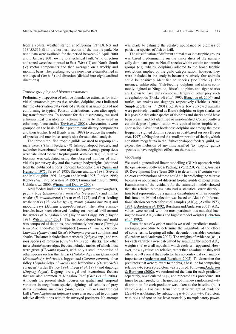
Table 3. The types of biophysical variables analysed, the spatial scale of analysesBroad, averaged across Ningaloo region; fine, spatially explicit or equal to the spatial resolution of satellite data; data sources, temporal coverage and spatial
resolution of data. AVHRR, Advanced Very High Resolution Radiometer; MODIS, Moderate Resolution Imaging Spectroradiometer
Biophysical variable Scale of analysis Data source Temporal coverage Spatial resolution (km)
Sea surface temperature Broad AVHRR Pathfinder (Version 5) Weekly Composites 4Fine MODIS Terra level 2 (Collection 4) Daily 1
Sea surface temperature Broad AVHRR Pathfinder (Version 5) Weekly Composites 4gradient Fine MODIS Terra level 2 (Collection 4) Daily 1
Chlorophyll-a Broad SeaWiFS level 3 (Version 5.1) Weekly Composites 9Fine SeaWiFS level 2 (Version 5.1) Daily ∼1
Bathymetry Fine National Oceans Office of Australia ? 0.250Bathymetry gradient Fine National Oceans Office of Australia ? 0.250
surveying in sea surface conditions greater than Beaufort SeaState 3, this was not always possible. In preliminary analyses ofthe data, negative correlations between Beaufort Sea State andsighting occurrence of all taxonomic categories were found, indi-cating that marine fauna sighting were subject to observationalbiases related to poor sea-state conditions. Approximately 34%of the surveys were carried out in conditions with greater thanBeaufort Sea State 3 (see Table 1). Although inclusion of thesedata for analysis was likely to increase perception bias relat-ing to omission of animals owing to turbidity, it was necessaryfor increasing the statistical robustness by maximising the sam-ple size of animal sighting of the relatively poorly representedspecies such as sharks, dugongs and some whales.
Remotely sensed dataBiophysical variables of SST, SSTg and Chl-a concentrationwere derived from satellite imagery and were used to describe(i) broad-scale (i.e. across the entire region) and (ii) fine-scale(spatially-explicit positions where animals were sighted) physi-cal and biological surface oceanography at Ningaloo during theaerial survey transects. The variables (SST, SSTg and Chl-a)were selected for analysis because they were: (i) likely to actas surrogates for processes that influence primary productionand food availability, (ii) could be classified accurately, with-out bias and classification methods could be easily replicated,(iii) could be resolved at fine spatial (kilometres) and temporal(daily) scales appropriate to the survey data, and (iv) relativelyeasy to access at little or no cost. Additionally, bathymetry andbathymetry gradient (see below) were also included in the analy-sis.A variety of data were used to derive the different biophysicalvariables in a form (spatial and temporal scale) appropriate forcomparison and analysis with the aerial survey data (Table 3).
For the broad-scale analysis, we used remote-sensing data ofSST and Chl-a that were generalised (averaged spatially) acrossthe entire region and averaged temporally (from daily compos-ites) on a monthly basis. Biophysical data used for the fine-scaleanalysis such as SST imagery were collected at approximately4-day intervals (two images per 8-day period). This eliminatedproblems associated with atmospheric effects, which can rendersatellite imagery less useful and ensured that at least one imagecorresponded (approximately) with the dates and intervals ofthe aerial surveys. In every 8-day period only one image was
retained for analysis following a screening and removal of theimage with the most incomplete data coverage (missing data asa result of clouds and/or sensor malfunctions). In spite of this,priority of selection was given to images that closely matchedthe dates of aerial surveys, thus temporal differences betweendatasets likely influenced the results negligibly.
HDF-EOS to GeoTIFF Conversion (HEG)Tool software pro-vided by NASA’s Earth Observing System (EOS) was usedto geo-locate and convert files from Hierarchical data format(HDF) to GeoTIFF files usable within Environmental SystemsResearch Institute (ESRI) ArcGIS 9.1. The resulting data wereconverted into grids with a geographic projection (WGS84) anda spatial resolution of ∼1 km. Cloud masks were used to remove(reclassify) erroneous data. SSTg was derived by reprojectingSST images into standard Mercator grids with equal intervalx, y coordinates (m). A 3 × 3 neighbourhood function (Menniset al. 2005) was used to evaluate the rate of change in the temper-ature values of adjacent cells and these values were subsequentlyoutputted as a geo-referenced grid of temperature gradients.
NASA’s SeaDAS 4.8 software (running on Linux FedoraCore 2) was used to geo-reference and subset Chl-a imagery forthe Ningaloo region, which were then exported as ASCII files,uploaded and interpolated (inverse distance weighted) into rastercoverages with ESRIArcINFO. High-resolution bathymetry griddata with a spatial resolution (x, y) of 250 m were acquired fromthe National Oceans Office of Australia for the entire Ninga-loo region. A map of bathymetric gradient was constructed byreprojecting the data as Mercator and applying a similar neigh-bourhood function as that used to generate the SSTg data. Weused a macro inArcGIS 9.1 to extract the values for each oceano-graphic variable (raster dataset) that corresponded to each animalobservation from the aerial surveys (point dataset). Density dis-tribution maps generated in ArcGIS 9.1 using a 5 km focalfunction were derived from the GPS point data of taxonomicgroups that were recorded in large numbers during the surveys.
Weather station dataWind data were used in a preliminary analysis to investigatehow this variable influenced sightings given that southerly windsare known to influence the Ningaloo Current, which enhancesnutrient upwelling and productivity in the region (Woo et al.2006a). Wind speed and direction data were collected hourly
Marine megafauna and oceanography at Ningaloo Reef Marine and Freshwater Research 613
from a coastal weather station at Milyering (21◦1.816′S and113◦55.316′E) in the northern section of the marine park. Nowind data were available for the period between 26 April 2000and 5 January 2001 owing to a technical fault. Wind directionand speed were decomposed to East–West (U) and North–South(V) vector components and then averaged on a weekly andmonthly basis.The resulting vectors were then re-transformed aswind speed (km h−1) and direction (divided into eight cardinaldirections).
Trophic grouping and biomass estimatesPreliminary inspection of relative abundance estimates for indi-vidual taxonomic groups (i.e. whales, dolphins, etc.) indicatedthat the observation data violated statistical assumptions of notconforming to typical Poisson distributions, even after apply-ing transformations. To account for this discrepancy, we useda hierarchical classification scheme similar to those used inother megafauna studies (Davis et al. 2002), where animals weregrouped on the basis of their predominant dietary componentsand their trophic level (Pauly et al. 1998) to reduce the numberof species and maximise sample size for statistical analysis.
The three simplified trophic guilds we used to regroup ani-mals were: (i) krill feeders, (ii) fish/cephalopod feeders, and(iii) other invertebrate/macro-algae feeders. Average group sizeswere calculated for each trophic guild. Within each guild, relativebiomass was calculated using the observed number of indi-viduals per survey day and the average bodyweights (obtainedfrom the published reports) for each taxonomic class (Spain andHeinsohn 1975; Pai et al. 1983; Stevens and Lyle 1989; Stevensand McLoughlin 1991; Lanyon and Marsh 1995; Plotkin 1995;Kohler et al. 1996; Marsh et al. 1997; Tamura and Ohsumi 2000;Uchida et al. 2000; Wintner and Dudley 2000).
Krill feeders included humpback (Megaptera novaeangliae),pygmy blue (Balaenoptera musculus brevicauda) and minkewhales (B. acutorostrata) (Preen et al. 1997) and filter-feedingwhale sharks (Rhincodon typus), manta (Manta birostris) andmobulid rays (Mobula eregoodootenkee). The latter elasmo-branchs have been observed feeding on tropical krill aroundthe waters of Ningaloo Reef (Taylor and Grigg 1991; Taylor1994; Wilson et al. 2001). The fish/cephalopod feeders’ guildwas composed of dolphins, predominantly bottlenose (Tursiopstruncatus), Indo–Pacific humpback (Sousa chinensis), clymene(Stenella clymene) and Risso’s (Grampus griseus) dolphins, andsharks.The latter included hammerheads (Sphyrna spp.) and var-ious species of requiem (Carcharhinus spp.) sharks. The otherinvertebrate/macro-algae feeders included turtles, of which mostwere green (Chelonia mydas), with only a small proportion ofother species such as the flatback (Natator depressus), hawksbill(Eretmochelys imbricata), loggerhead (Caretta caretta), oliveridley (Lepidochelys olivacea) and leatherback (Dermochelyscoriacea) turtles (Prince 1994; Preen et al. 1997) and dugongs(Dugong dugon). Dugongs are algal and invertebrate feedersthat are also common at Ningaloo Reef (Gales et al. 2004).Although the present study focuses on spatial and temporalvariation in megafauna species, sightings of schools of preyitems including anchovies (Stolephorus indicus) and tropicalkrill (Pseudeuphausia latifrons) were also recorded to comparerelative distributions with their surveyed predators. No attempt
was made to estimate the relative abundance or biomass ofparticular species of fish or krill.
The classification of different animal taxa into trophic groupswas based predominantly on the major diets of the numeri-cally dominant species. Not all species within certain taxonomicgroups (e.g. whales, dolphins) adhered to the broad trophicrestrictions implied by the guild categorisation; however, theywere included in the analysis because relatively few animalscould be positively identified to species (see Table 2). Forinstance, unlike other ‘fish-feeding’ dolphins and sharks com-monly sighted at Ningaloo, Risso’s dolphins and tiger sharksare known to have diets composed largely of other prey suchas cephalopods (Cockcroft et al. 1993; Blanco et al. 2006), andturtles, sea snakes and dugongs, respectively (Heithaus 2001;Simpfendorfer et al. 2001). Relatively few surveyed animalswere positively identified as Risso’s dolphins or tiger sharks, soit is possible that other species of dolphins and sharks could havebeen present and not identified or misidentified. Consequently, acertain degree of generalisation was required in the ‘trophic’cat-egorisation. Given that bottlenose dolphins are among the mostfrequently sighted dolphin species in boat-based surveys (Preenet al. 1997) at Ningaloo and the small proportion of sharks, whichconstitute megafauna in the ‘fish/cephalopod feeders’ guild, weexpect the inclusion of any misclassified (to ‘trophic’ guild)species to have negligible effects on the results.
ModellingWe used a generalised linear modelling (GLM) approach withthe open-source software R Package (Ver.2.2.0, Vienna, Austria)(R Development Core Team 2004) to determine if certain vari-ables or combinations of these could aid in predicting the relativebiomass or abundance of different trophic guilds of megafauna.Examination of the residuals for the saturated models showedthat the relative biomass data had a statistical error distribu-tion best represented by a gamma distribution with an identitylink function. Model selection was based on Akaike’s Informa-tion Criterion corrected for small samples (AICc), (Akaike 1973,1974; Lebreton et al. 1992; Burnham and Anderson 2001). AICc
values were ranked, with the most parsimonious model(s) hav-ing the lowest AICc values and highest model weights (Lebretonet al. 1992).
From the set of a priori models we used a predictive model-averaging procedure to determine the magnitude of the effectof some terms, keeping all other dependent variables constant(Burnham and Anderson 2002). The weights of evidence (w+i)for each variable i were calculated by summing the model AICc
weights (wi) over all models in which each term appeared. How-ever, the w+i values are relative, rather than absolute, so they willoften be >0 even if the predictor has no contextual explanatoryimportance (Anderson and Burnham 2002). To determine thepredictors that were relevant to the data, a baseline for comparingrelative w+i across predictors was required. FollowingAnderson& Burnham (2002), we randomised the data for each predictorseparately, re-calculated w+i, and repeated this procedure 100times for each predictor.The median of this new randomised w+i
distribution for each predictor was taken as the baseline (null)value (w + 0). For each term the relative weight of evidence(�w+) was obtained by subtracting w + 0 from w+i. Predictorswith �w+ of zero or less have essentially no explanatory power.
614 Marine and Freshwater Research J. C. Sleeman et al.
We considered five oceanographic variables within the all-subsets model set: SST, SSTg, Chl-a, bathymetry (BTH) andbathymetric gradient (BTHg) where the saturated model was:
Guild relative biomass/25 km2 grid cell ∼SST+SSTg+Chl-a+BTH+BTHg+ε
where ε represents the error term. All variables were log-transformed before analysis to account for their large range invalues. We did not use the complete set of variables availableto prevent the loss of too many degrees of freedom that couldlead to poor model convergence. In addition, exclusion of vari-ables such as geostrophic currents was necessary owing to theircoarse spatial scale (relative to aerial data) and poor coverage(i.e. missing data at coastal boundary zones). We also parame-terised the models with a 50% random sub-selection of the datato reduce autocorrelation problems associated with the fact thatthe count and oceanographic measurements were not temporallyor spatially independent (e.g. Bradshaw et al. 2004). The rela-tive biomass of humpback whales was large compared with allthe other animals (making the distribution of krill-feeder relativebiomass bimodal and too skewed to correct with transformation),so these animals were considered in two modelling scenar-ios: one where humpback counts rather than relative biomass(with single-species models, the ‘relative biomass’ response wasessentially a scalar of the count data, so counts were used instead)were considered alone,
Humpback relative abundance per 25 km2 grid cell
∼SST+SSTg+Chl − a+BTH+BTHg+ε
and one where humpbacks were excluded from the krill feederguild altogether.
The latter model was likely to hold greater support partic-ularly given that humpback whales are known to be migratingthrough the region and are unlikely to be feeding (Chittleborough1965; Jenner et al. 2001).
A Poisson error distribution with a log link function was usedin the humpback count model. A Spearman’s correlation wascalculated for each set of variables in each model set. Highly cor-related (r2 > 0.8) variables were not included in the same modelset. The percentage of deviance explained (%DE) was also cal-culated for each model as a functional goodness-of-fit measure.
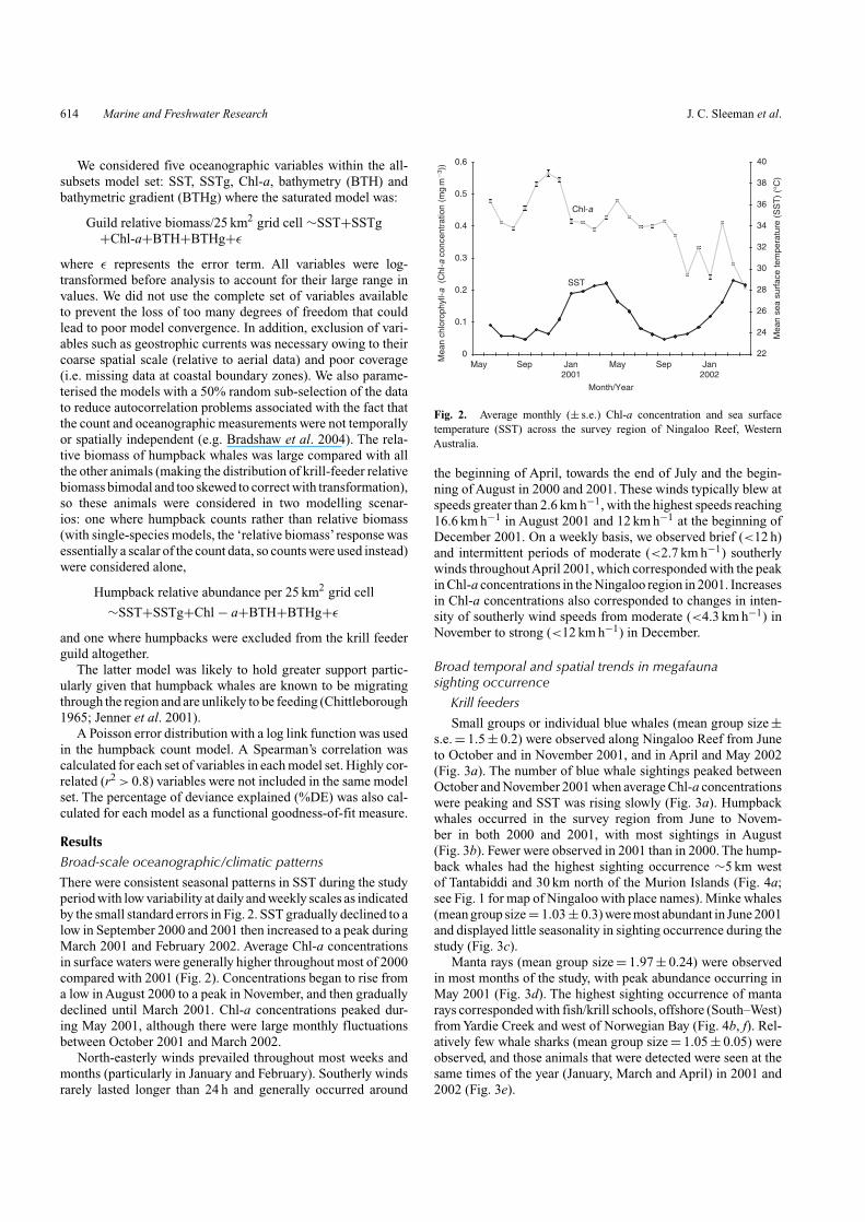
ResultsBroad-scale oceanographic/climatic patternsThere were consistent seasonal patterns in SST during the studyperiod with low variability at daily and weekly scales as indicatedby the small standard errors in Fig. 2. SST gradually declined to alow in September 2000 and 2001 then increased to a peak duringMarch 2001 and February 2002. Average Chl-a concentrationsin surface waters were generally higher throughout most of 2000compared with 2001 (Fig. 2). Concentrations began to rise froma low in August 2000 to a peak in November, and then graduallydeclined until March 2001. Chl-a concentrations peaked dur-ing May 2001, although there were large monthly fluctuationsbetween October 2001 and March 2002.
North-easterly winds prevailed throughout most weeks andmonths (particularly in January and February). Southerly windsrarely lasted longer than 24 h and generally occurred around
0
0.1
0.2
0.3
0.4
0.5
0.6
May Sep Jan2001
May Sep Jan2002
Month/Year
Mea
n ch
loro
phyl
l-a (
Chl
-a c
once
ntra
tion
(mg
m�
3 ))
22
24
26
28
30
32
34
36
38
40
Mea
n se
a su
rfac
e te
mpe
ratu
re (
SS
T)
(°C
)
SST
Chl-a
Fig. 2. Average monthly (± s.e.) Chl-a concentration and sea surfacetemperature (SST) across the survey region of Ningaloo Reef, WesternAustralia.
the beginning of April, towards the end of July and the begin-ning of August in 2000 and 2001. These winds typically blew atspeeds greater than 2.6 km h−1, with the highest speeds reaching16.6 km h−1 in August 2001 and 12 km h−1 at the beginning ofDecember 2001. On a weekly basis, we observed brief (<12 h)and intermittent periods of moderate (<2.7 km h−1) southerlywinds throughout April 2001, which corresponded with the peakin Chl-a concentrations in the Ningaloo region in 2001. Increasesin Chl-a concentrations also corresponded to changes in inten-sity of southerly wind speeds from moderate (<4.3 km h−1) inNovember to strong (<12 km h−1) in December.
Broad temporal and spatial trends in megafaunasighting occurrence
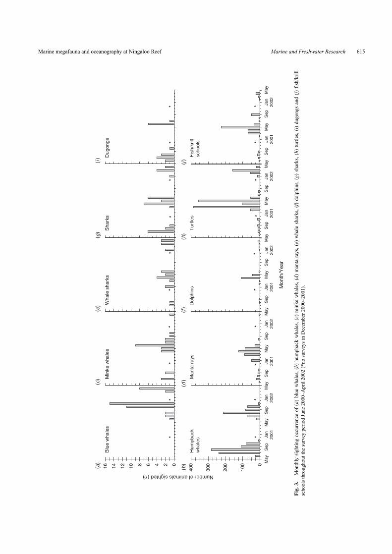
Krill feedersSmall groups or individual blue whales (mean group size ±
s.e. = 1.5 ± 0.2) were observed along Ningaloo Reef from Juneto October and in November 2001, and in April and May 2002(Fig. 3a). The number of blue whale sightings peaked betweenOctober and November 2001 when average Chl-a concentrationswere peaking and SST was rising slowly (Fig. 3a). Humpbackwhales occurred in the survey region from June to Novem-ber in both 2000 and 2001, with most sightings in August(Fig. 3b). Fewer were observed in 2001 than in 2000. The hump-back whales had the highest sighting occurrence ∼5 km westof Tantabiddi and 30 km north of the Murion Islands (Fig. 4a;see Fig. 1 for map of Ningaloo with place names). Minke whales(mean group size = 1.03 ± 0.3) were most abundant in June 2001and displayed little seasonality in sighting occurrence during thestudy (Fig. 3c).
Manta rays (mean group size = 1.97 ± 0.24) were observedin most months of the study, with peak abundance occurring inMay 2001 (Fig. 3d). The highest sighting occurrence of mantarays corresponded with fish/krill schools, offshore (South–West)from Yardie Creek and west of Norwegian Bay (Fig. 4b, f). Rel-atively few whale sharks (mean group size = 1.05 ± 0.05) wereobserved, and those animals that were detected were seen at thesame times of the year (January, March and April) in 2001 and2002 (Fig. 3e).
Marine megafauna and oceanography at Ningaloo Reef Marine and Freshwater Research 615
May
Sep
Jan
2001
May
Sep
Jan
2002
May
Sep
Jan
2001
May
Sep
Jan
2002
May
Mon
th/Y
ear
May
Sep
Jan
2001
May
Sep
Jan
2002
0246810121416
May
Sep
Jan
2001
May
Sep
Jan
2002
May
Sep
Jan
2001
May
Sep
Jan
2002
Number of animals sighted (n)
0
100
200
300
400
Dol
phin
s
Sha
rks
Tur
tles
Dug
ongs
Fis
h/kr
illsc
hool
s
**
**
**
**
Blu
e w
hale
s
Hum
pbac
kw
hale
s
Min
ke w
hale
s
Man
ta r
ays
Wha
le s
hark
s
**
**
**
**
**
**
(a)
(b)
(c)
(d)
(e)
(f)
(g)
(h)
(i)
(j)
Fig
.3.
Mon
thly
sigh
ting
occu
rren
ceof
(a)
blue
wha
les,
(b)
hum
pbac
kw
hale
s,(c
)m
inke
wha
les,
(d)
man
tara
ys,
(e)
wha
lesh
arks
,(f
)do
lphi
ns,
(g)
shar
ks,
(h)
turt
les,
(i)
dugo
ngs
and
(j)
fish
/kri
llsc
hool
sth
roug
hout
the
surv
eype
riod
June
2000
–Apr
il20
02(*
nosu
rvey
sin
Dec
embe
r20
00–2
001)
.

616 Marine and Freshwater Research J. C. Sleeman et al.
113°0�0�E 114°0�0�E
23°0�0�S
22°0�0�S
21°0�0�S
LegendAnimal density probability
0 – 0.060.06 – 0.200.20 – 0.340.34 – 0.510.51 – 0.720.72 – 1.00100 m Isobath200 m IsobathBenthic HabitatCoastal region
21°0�0�S
22°0�0�S
23°0�0�S
0 40 2 0 60 8010Kilometres
N
(c) Dolphins(a) Humpback whales
(b) Manta rays (d ) Sharks
(e) Turtles
(f ) Fish/krill schools
Fig. 4. Sighting distribution maps (5 km neighbourhood kernel) for truncated aerial survey observations of (a) humpback whales, (b) manta rays, (c) dolphins,(d) sharks, (e) and turtles and (f) krill/fish schools.
Fish/cephalopod feedersDolphins (mean group size = 2.9 ± 0.5) were observed
throughout most of the year, with the largest number sightedbetween March and May 2001 (Fig. 3f). Dolphin sightings wererelatively well distributed in the Ningaloo region, with mostsighted in the Gulf of Exmouth (10 km east of Bundegi) and5 km west fromYardie Creek on Ningaloo Reef (Fig. 4c). Sharks(mean group size = 1.06 ± 0.04) were observed in greatest num-bers in July in 2000 and inApril–June 2001 (Fig. 3g).The highestsightings of sharks occurred 10 km south-west of Yardie Creek,directly off Bundegi and 15 km north of the tip of North WestCape (Fig. 4d).
Other invertebrate/macroalgae feedersTurtles (mean group size = 1.31 ± 0.03) occurred in almost
every month of the study (with the exception of January and
September–November 2001) and sightings peaked in March andMay 2001, corresponding to a peak in SST and Chl-a concentra-tions (Fig. 3h). The greatest density of turtles occurred adjacentto Point Cloates and 10 km west of Bruboodjoo Point (Fig. 4e).Dugongs (mean group size = 1) were observed in June and Julyin both 2000 and 2001, with largest numbers sighted in June 2001(Fig. 3i). Fish/krill schools were sighted in greatest numbers dur-ing April and May 2001 (Fig. 3j) and sighting occurrence tendedto correspond in distribution with that of manta rays (Fig. 4f).
Fine-scale trends in megafauna sighting occurrenceand biophysical variables
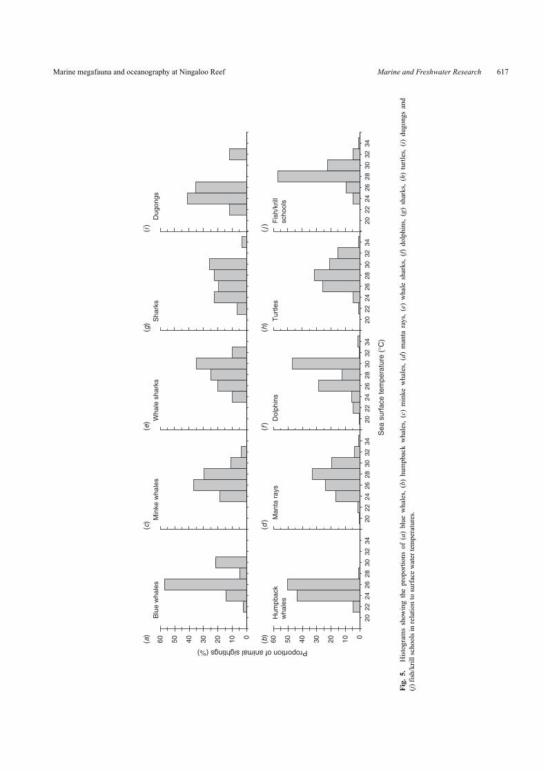
Krill feedersOverall, more than 55% of blue whales observed were
seen in water between 25◦C and 27◦C (Fig. 5a). Blue whales
Marine megafauna and oceanography at Ningaloo Reef Marine and Freshwater Research 617
2022
2426
2830
3234
Sea
sur
face
tem
pera
ture
(°C
)
2022
2426
2830
3234
0102030405060
2022
2426
2830
3234
2022
2426
2830
3234
2022
2426
2830
3234
0102030405060D
olph
ins
Sha
rks
Tur
tles
Dug
ongs
Fis
h/kr
illsc
hool
s
Blu
e w
hale
s
Hum
pbac
kw
hale
s
Min
ke w
hale
s
Man
ta r
ays
Wha
le s
hark
s
Proportion of animal sightings (%)
(a)
(b)
(c)
(d)
(e)
(f)
(g)
(h)
(i)
(j)
Fig
.5.
His
togr
ams
show
ing
the
prop
orti
ons
of(a
)bl
uew
hale
s,(b
)hu
mpb
ack
wha
les,
(c)
min
kew
hale
s,(d
)m
anta
rays
,(e
)w
hale
shar
ks,
(f)
dolp
hins
,(g
)sh
arks
,(h
)tu
rtle
s,(i
)du
gong
san
d(j
)fi
sh/k
rill
scho
ols
inre
lati
onto
surf
ace
wat
erte
mpe
ratu
res.
618 Marine and Freshwater Research J. C. Sleeman et al.
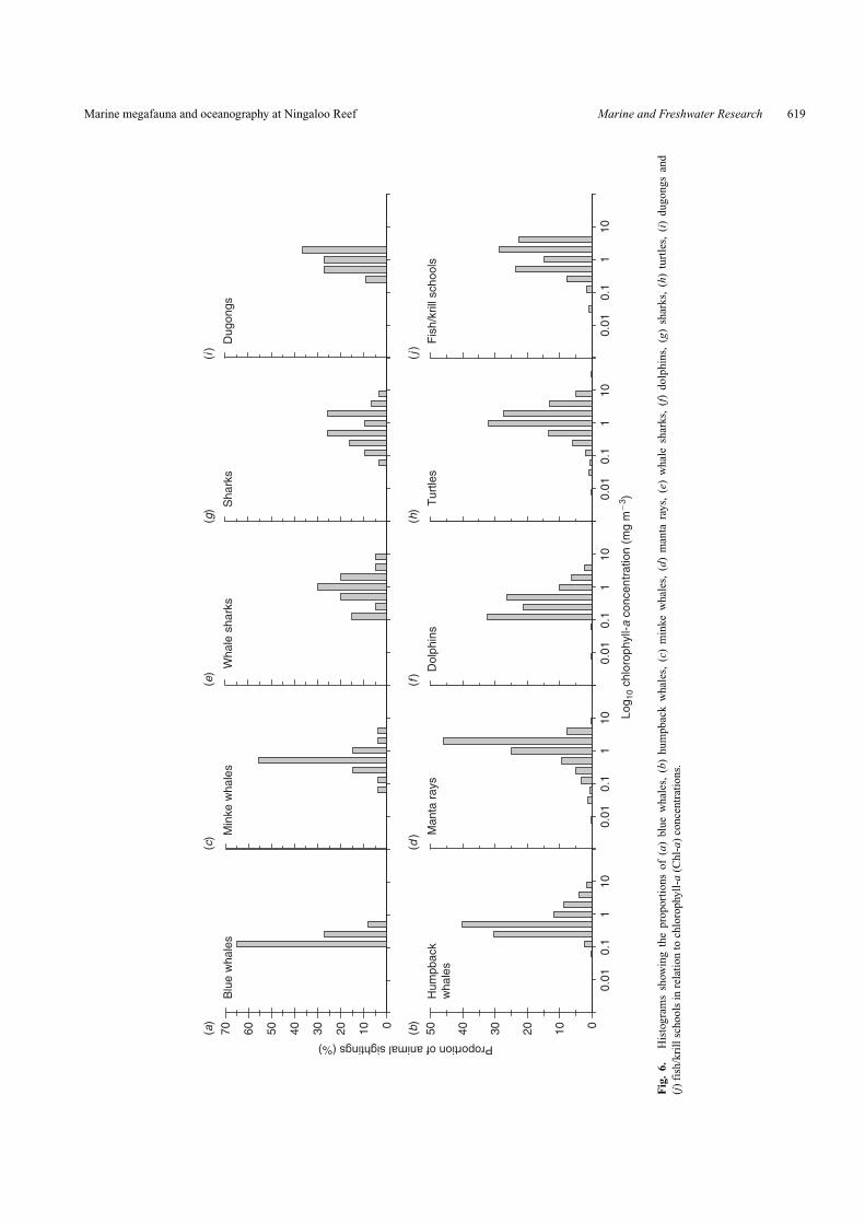
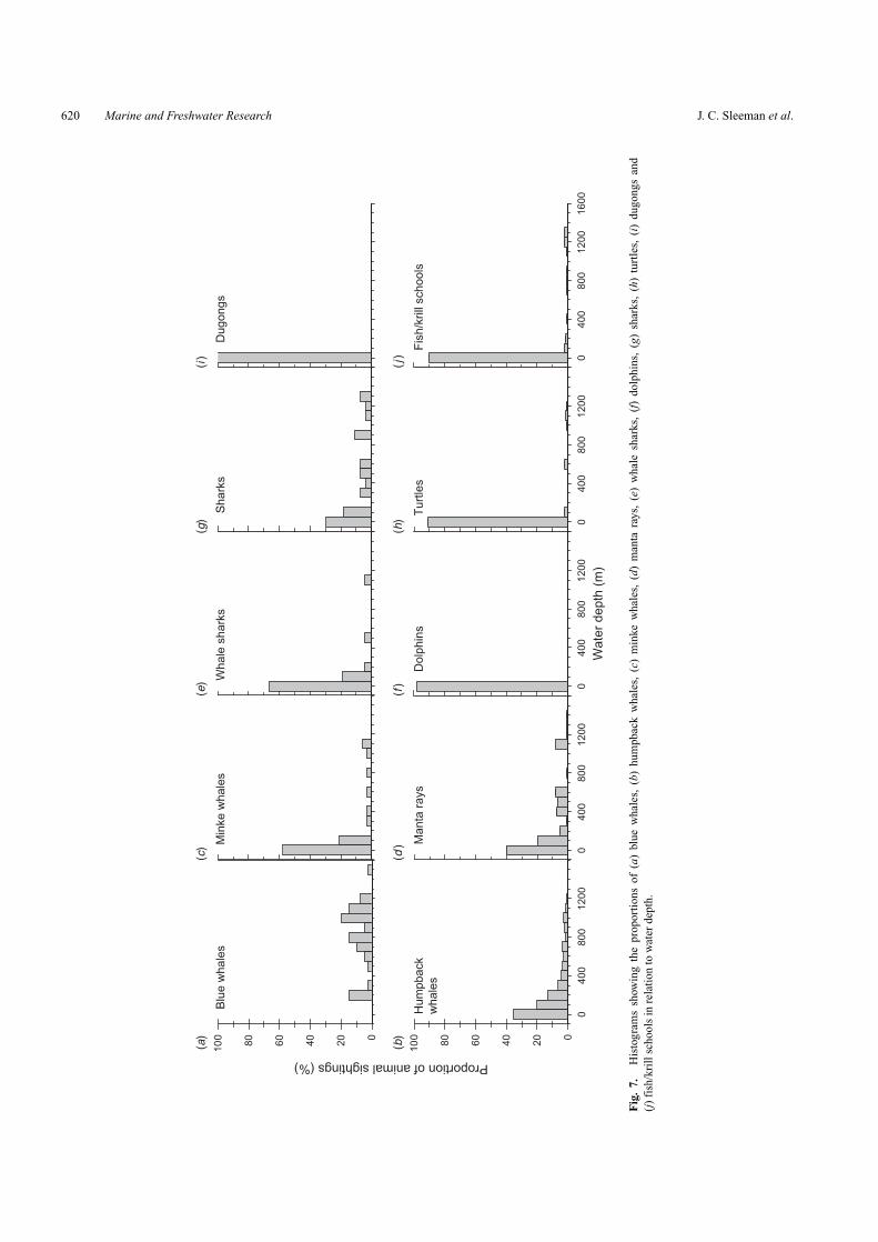
occurred in a restricted range of relatively low surface Chl-aconcentrations, with 65% found in concentrations of 0.125–0.25 mg m−3 (Fig. 6a). Blue whales were recorded in a largerange of depths (Fig. 7a). Compared with other taxa, hump-backs generally occurred in the narrowest temperature range(Fig. 5b). Approximately 70% of humpbacks were recorded inwaters with moderate to high surface Chl-a concentrations of0.25–1.00 mg m−3 (Fig. 6b) and tended to be spotted in waterswith depths >200 m (Fig. 7b). Almost 70% of minke whalesoccurred in warm SST between 25◦C and 29◦C (Fig. 5c) and over55% occurred in waters with medium to high 0.25–0.50 mg m−3
Chl-a (Fig. 6c).Most of the manta rays and whale sharks (>60%) occurred in
relatively warm waters between 27◦C and 31◦C (Fig. 5d, e). Mostof the manta rays observed during the surveys were in Chl-a-richwaters, with concentrations of 1.0–4.0 mg m−3 (Fig. 6d).
Although the average Chl-a concentration is low in theNingaloo region during the period when whale sharks wereobserved, ∼70% of whale sharks were found in high Chl-a of0.5–2.0 mg m−3 (Fig. 6e).
Manta rays (Fig. 7d) and whale sharks (Fig. 7e) were foundin a range of water depths, but were mainly sighted in shallowwaters (<100 m).
Fish/cephalopod feedersDolphins occurred in a wide range of SSTs, although >55%
were found in warm waters (27–31◦C, Fig. 5d). More than75% of dolphins occurred in moderate Chl-a concentrations of0.125–0.50 mg m−3 (Fig. 6f). Dolphins were spotted in watersof varying depths, with around 40% of those sighted occurringin shallow inshore areas (<100 m, Fig. 7f). Sharks occurredin a large range of SSTs (Fig. 5g) with over 75% of sharkssighted being found in high surface Chl-a of 0.50–2.00 mg m−3
(Fig. 6g). Sharks were observed in a broad range of depths, butmost were in shallower waters (<100 m, Fig. 7g).
Other invertebrate/macroalgae feedersTurtles were observed in the widest range of SSTs, with
more than 70% of individuals sighted in waters at 25–33◦C(Fig. 5h). Although turtles occurred in a range of Chl-a con-centrations, more than 70% were found in areas of high Chl-a(0.5–2.0 mg m−3, Fig. 6h). Most turtles were also found in shal-low waters (<100 m, Fig. 7h). Dugongs were generally found inwater with intermediate to low temperature ranges (21–27◦C)(Fig. 5i). Most dugongs were also found in areas of high surfaceChl-a (Fig. 6i). All dugongs were only sighted in shallow waters(<100 m, Fig. 7i). Over 57% of fish/krill schools were found inmoderate to high SSTs between 27◦C and 29◦C (Fig. 5j). Mostfish/krill schools were observed in high surface Chl-a waters(Fig. 6j). Fish/krill schools occurred in a range of water depths,with most in shallow waters (<100 m, Fig. 7j).
Generalised linear modelsKrill feedersThe best-supported model for the krill feeding guild (exclud-
ing humpback whales) included SST, Chl-a and BTH (AICc
weight = 0.45) and explained a relatively high proportion ofthe variation in relative biomass (%DE = 32.3%). Models
including SSTg and BTHg also had moderate levels of sup-port (AICc weights = 0.16). However, the weights of evidenceanalysis demonstrated model-averaged support only for BTH(�w+ = 0.70), indicating that most of the %DE in the bestmodel was explained by variation in BTH alone (all other termshad �w+ < 0) so that there was a greater relative biomass ofkrill-feeding species observed in deeper water. The Poisson-distributed count model failed to explain much of the variationin sighting occurrence of humpback whales (top model withAICc weight = 0.17 and %DE = 1.8%), and none of the explana-tory variables had any model-averaged support according to theweights of evidence analysis (all �w+ ∼= 0).
Fish/cephalopod feedersFor the fish/cephalopod feeders, the best model (AICc
weight = 0.32) included SST and Chl-a and explained 9.4%of the deviance (%DE) in relative biomass. Although the less-supported models had other terms including BTH, SSTg andBTHg (AICc weights = 0.14, 0.12 and 0.10, respectively), theweights of evidence analysis indicated that only SST hadreasonable model-averaged support (�w+ = 0.44). The modelsuggested that larger relative biomasses of fish/cephalopodfeeders were found in warmer compared with cooler surfacewaters.
Other invertebrate/macroalgae feedersModels of relative biomass distributions of invertebrate/
macroalgae feeders included all oceanographic variables exceptSSTg (AICc weight = 0.50), and explained 8.4% of the deviance(%DE). However, the weights of evidence analysis only demon-strated support for BTHg (�w+ = 0.46), indicating that largerrelative biomasses of species within this guild were observed inwaters over steeper bathymetric slopes.
Discussion
The foraging and distribution patterns of many predatory marinespecies such as whales, seals and seabirds are often correlatedwith the physical and biological properties of surface waters(Bradshaw et al. 2004; Littaye et al. 2004; Polovina et al. 2004;Ainley et al. 2005). Although the relationship between marineanimal distributions and oceanographic conditions can be strongin some circumstances, it is often difficult to establish the rela-tive contribution of different variables (e.g. SST, Chl-a, etc.) tovariation in distribution patterns (Polovina et al. 2004; Piatt et al.2006). These problems arise because models cannot accommo-date the complexity of predator behaviour when coupled withfactors that can influence primary or first-order secondary pro-duction (Horne and Schneider 1994;Agenbag et al. 2003; Gendeand Sigler 2006).
We found that the distributions of krill-feeding animals (notincluding humpback whales) were largely predicted by vari-ation in bathymetry. This outcome suggests that krill feedersmay experience greater foraging success when in deeper waters(assuming krill feeders were mainly observed when foraging)and that they may target increased abundances of krill in areaswith greater variation in depth (i.e. for vertical migration orwider resource use) (Wilson et al. 2002; Wilson et al. 2003).Alternatively, this pattern may relate to the potential distributionof predators (i.e. killer whales) in shallow waters. Killer whales
Marine megafauna and oceanography at Ningaloo Reef Marine and Freshwater Research 619
0.01
0.1
10
Log 1
0 ch
loro
phyl
l-a c
once
ntra
tion
(mg
m�
3 )
0.01
0.1
10
010203040506070
0.01
0.1
100.
010.
110
0.01
0.1
10
Proportion of animal sightings (%)
01020304050D
olph
ins
Sha
rks
Tur
tles
Dug
ongs
Fis
h/kr
ill s
choo
ls
Blu
e w
hale
s
Hum
pbac
kw
hale
s
Min
ke w
hale
s
Man
ta r
ays
Wha
le s
hark
s
(a)
(b)
(c)
(d)
(e)
(f)
(g)
(h)
(i)
(j)
11
11
1
Fig
.6.
His
togr
ams
show
ing
the
prop
orti
ons
of(a
)bl
uew
hale
s,(b
)hu
mpb
ack
wha
les,
(c)
min
kew
hale
s,(d
)m
anta
rays
,(e
)w
hale
shar
ks,
(f)
dolp
hins
,(g
)sh
arks
,(h
)tu
rtle
s,(i
)du
gong
san
d(j
)fi
sh/k
rill
scho
ols
inre
lati
onto
chlo
roph
yll-
a(C
hl-a
)co
ncen
trat
ions
.
620 Marine and Freshwater Research J. C. Sleeman et al.
Wate
r depth
(m
)
0400
800
1200
0400
800
1200
0
20
40
60
80
10
0
04
00
80
01
20
01
60
00
400
80
01
20
00
400
800
1200
0
20
40
60
80
10
0D
olp
hin
s
Shark
s
Turt
les
Dugongs
Fis
h/k
rill
schools
Blu
e w
hale
s
Hum
pback
whale
s
Min
ke w
hale
s
Manta
rays
Whale
shark
s
Proportion of animal sightings (%)
(a)
(b)
(c)
(d)
(e)
(f)
(g)
(h)
(i)
(j)
Fig
.7.
His
togr
ams
show
ing
the
prop
orti
ons
of(a
)bl
uew
hale
s,(b
)hu
mpb
ack
wha
les,
(c)
min
kew
hale
s,(d
)m
anta
rays
,(e
)w
hale
shar
ks,
(f)
dolp
hins
,(g
)sh
arks
,(h
)tu
rtle
s,(i
)du
gong
san
d(j
)fi
sh/k
rill
scho
ols
inre
lati
onto
wat
erde
pth.
Marine megafauna and oceanography at Ningaloo Reef Marine and Freshwater Research 621
(Orcinus orca) have been known to target krill feeders such asbaleen whales as calves or juveniles, when in their high latitudebreeding grounds (rather than in their feeding grounds), as evi-denced by flesh wounds that resemble the teeth marks of killerwhales (Chittleborough 1965; Mehta et al. submitted).
If the patterns we observed in the distribution of krill feedersare related to increased abundance of prey, we might expect to seea greater incidence of krill schools in areas with deeper water, yetmost of the schools observed in the aerial surveys were sightedin shallow areas (Fig. 4e). Consequently, we can assume thateither krill feeders have a foraging advantage in deeper water, orthat insufficient data were collected to understand the underly-ing mechanism. For instance, the observed patterns in krill/fishschool distributions may be an artefact of clumping fish/krillinto the same taxonomic category or may relate to observer biasissues of omission (i.e. not seeing krill schools in deeper watersas a result of reduced visibility).
The primary and secondary sources of productivityexploited by feeding guilds such as fish/cephalopod andinvertebrate/macroalgae feeders were likely to have been influ-enced by a complex suite of other factors, given that we founda general pattern of weak correspondence between their dis-tributions and the surrounding oceanography and bathymetry.Bathymetry gradient was weakly related to the relative biomassof invertebrate/macroalgae feeders, with these species beingmore abundant where there was a steep change in depth contours.Such slopes may provide a more suitable habitat for macroal-gae and associated benthic fauna with appropriate light, nutrientand dispersal enhancement mechanisms (Kendrick et al. 1998).Thus, our results provide little evidence to reject the hypothesis ofGende and Sigler (2006) that the distribution of species feedingon lower trophic-level prey species were not more closely corre-lated with variables such as SST and Chl-a than the distributionsof higher trophic-level species (Gende and Sigler 2006).
The patterns in relative biomass of fish/cephalopod feederswere explained to some extent by SST, possibly indicating thatwarmer currents provide the conditions necessary for the preyspecies of sharks and dolphins. Similar patterns in distributionsof predatory fishes such as tuna have been observed with increas-ing SST or higher SST ranges (Myers and Hick 1990; Schicket al. 2004). We observed peaks in SST in the Ningaloo regionaround April 2001 and March 2002. This reflects the gradualwater surface heating as a result of high summer temperaturesfrom November through to March and an absence or diminishedflow of the Ningaloo Current as a result of changes in seasonalwind and weather patterns (Woo et al. 2006a).
Krill feeders such as humpback whales were present at Ninga-loo during the peaks in Chl-a in both 2000 and 2001, yet despitetheir high sighting occurrence, it is likely that little foragingwas occurring during their migration north to warmer watersfor calving around July–August and the subsequent return southto the Antarctic in September–October (Chittleborough 1965;Jenner et al. 2001; Jenner and Jenner 2002). As such, the lack ofassociation with any oceanographic variables we examined wasexpected. Other krill feeders such as whale sharks were observedin low numbers, but appeared consistently towards the end ofsummer (April–May) when ocean productivity was highest. Thisperiodicity likely reflects the availability of major prey itemssuch as the tropical krill, Pseudeuphausia latifrons, although
krill distributions may have little direct association with oceansurface properties (Wilson et al. 2002, 2003).
Conclusion
Our study illustrates some of the difficulties involved in pre-dicting habitat associations or trophic distributions of marinemegafauna from aerial counts and remotely sensed data alone.The prediction of spatio-temporal animal distributions relieson information on the behaviour of individuals in relation totheir surrounding environment at the time of the survey, inaddition to information on migration patterns, diet and rela-tive habitat selection (e.g. dugongs and seagrass beds; sharksand reefs). Resolving issues associated with food web inter-actions between taxa and environmental limitations of preyitems is important when attempting to understand the expecteddegree of correlation between trophic groups and biophysicalprocesses. To help further identify mechanisms dictating spatialand temporal patterns in marine megafauna distributions, werequire: (1) oceanographic data with higher spatial and tempo-ral resolution, and (2) longer-term sampling of specific speciesincorporating behavioural information about their habitat useand feeding habits.
AcknowledgementsWe are grateful to Woodside Energy Ltd, for authorising the use of theaerial survey data originally collected for the WA-271-P Field Develop-ment Environmental Impact Statement. We thank the Australian Instituteof Marine Science for providing the Milyering weather station data, NASAGoddard Space Flight Center for the remotely sensed ocean colour and SSTdata, AVISO for altimetry data and National Oceans Office of Australia forbathymetry data. We thank three anonymous reviewers for helpful commentsto improve the manuscript.
ReferencesAgenbag, J. J., Richardson, A. J., Demarcq, H., Freon, P., Weeks, S., and
Shillington, F. A. (2003). Estimating environmental preferences ofSouth African pelagic fish species using catch size and remotesensing data. Progress in Oceanography 59, 275–300. doi:10.1016/J.POCEAN.2003.07.004
Ainley, D. G., Speara, L. B., Tynanb, C. T., Barthc, J. A., Piercec, S. D.,Fordd, R. G., and Cowles, T. J. (2005). Physical and biological variablesaffecting seabird distributions during the upwelling season of the north-ern California Current. Deep-Sea Research. Part II, Topical Studies inOceanography 52, 123–143. doi:10.1016/J.DSR2.2004.08.016
Akaike, H. (1973). Information theory as an extension of the maximumlikelihood principle. In ‘Second International Symposium on Informa-tion Theory’. (Eds B. N. Petrov and F. Csaki.) pp. 267–281. (AkademiaiKiado: Budapest.)
Akaike, H. (1974). A new look at the statistical model identification.IEEE Transactions on Automatic Control 19, 716–723. doi:10.1109/TAC.1974.1100705
Anderson, D. R., and Burnham, K. P. (2002). Avoiding pitfalls when usingInformation–Theoretic methods. The Journal of Wildlife Management66, 912–918. doi:10.2307/3803155
Blanco, C., Raduan, M. A., and Raga, J. A. (2006). Diet of Risso’s dolphin(Grampus griseus) in the western Mediterranean Sea. Scientia Marina70, 407–411.
Bradshaw, J. A., Higgins, J., Michael, K., Wotherspoon, S. J., andHindell, M. A. (2004). At-sea distribution of female southern elephantseals relative to variation in ocean surface properties. ICES Journal ofMarine Science 61, 1014–1027. doi:10.1016/J.ICESJMS.2004.07.012

622 Marine and Freshwater Research J. C. Sleeman et al.
Burnham, K. P., and Anderson, D. R. (2001). Kullback–Leibler informationas a basis for strong inference in ecological studies. Wildlife Research28, 111–119. doi:10.1071/WR99107
CALM (2005) Management plan for the Ningaloo Marine Park and MuironIslands marine management area 2005–2015. Department of Conser-vation and Land Management, Management Plan Number 52, Perth,Western Australia.
Caputi, N., Fletcher, W. J., Pearce, A. F., and Chubb, L. J. V. (1996). Effectsof the Leeuwin Current on the recruitment of fish and invertebratesalong the Western Australian coast. Marine and Freshwater Research47, 147–155. doi:10.1071/MF9960147
Chaloupka, M., and Osmond, M. (1999). Spatial and seasonal distribution ofHumpback whales in the Great Barrier Reef region. American FisheriesSociety Symposium 23, 89–106.
Chittleborough, R. G. (1965). Dynamics of two populations of the hump-back whale, Megaptera novageangliae (Borowski).Australian Journal ofMarine and Freshwater Research 16, 33–128. doi:10.1071/MF9650033
Cockcroft, V. G., Haschick, S. L., and Klages, N. T. W. (1993). The diet ofRisso’s dolphin Grampus griseus (Cuvier, 1812), from the east coast ofSouth Africa. Zeitschrift fuer Saeugetierkunde 58, 286–293.
Davis, D. (1998). Whale shark tourism in Ningaloo marine park, Australia.Anthrozoos 11, 5–11.
Davis, D., Banks, S., Birtles, A., Valentine, P., and Cuthill, M. (1997).Whale sharks in Ningaloo marine park – managing tourism in anAustralian marine protected area. Tourism Management 18, 259–271.doi:10.1016/S0261-5177(97)00015-0
Davis, R. W., Ortega-Ortiz, J. G., Ribic, C. A., Evans, W. E., Biggs, D. C.,Ressler, P. H., Cady, R. B., Leben, R. R., Mullin, K. D., and Würsig,B. (2002). Cetacean habitat in the northern oceanic Gulf of Mexico.Deep-sea Research. Part I, Oceanographic Research Papers 49, 121–142. doi:10.1016/S0967-0637(01)00035-8
El-Sayed, S. Z. (1988). Productivity of the Southern Ocean: a closer look.Comparative Biochemistry and Physiology 90B, 489–498.
Evans, P. G. H., and Hammond, P. S. (2004). Monitoring cetaceans inEuropean waters. Mammal Review 34, 131–156. doi:10.1046/J.0305-1838.2003.00027.X
Gales, N., McCauley, R. D., Lanyon, J., and Holley, D. (2004). Change inabundance of dugongs in Shark Bay, Ningaloo and Exmouth Gulf, West-ern Australia: evidence for large-scale migration. Wildlife Research 31,283–290. doi:10.1071/WR02073
Gende, S. M., and Sigler, M. F. (2006). Persistence of forage fish ‘hotspots’ and its association with foraging Steller sea lions (Eumetopiasjubatus) in southeast Alaska. Deep-Sea Research. Part II, Topi-cal Studies in Oceanography 53, 432–441. doi:10.1016/J.DSR2.2006.01.005
Gersbach, G. H. (1999). Coastal upwelling off Western Australia. PhDThesis, University of Western Australia, Crawley.
Godfrey, J. S., and Ridgeway, K. R. (1985). The large-scale environ-ment of the poleward-flowing Leeuwin Current, Western Australia:longshore steric height gradients, wind stresses and geostrophic flow.Journal of Physical Oceanography 15, 481–495. doi:10.1175/1520-0485(1985)015<0481:TLSEOT>2.0.CO;2
Guinet, C., Dubroca, L., Lea, M. A., Goldsworthy, S., Cherel, Y.,Duhamel, G., Bonadonna, F., and Donnay, J. P. (2001). Spatial distribu-tion of the foraging activity of Antarctic fur seal Arctocephalus gazellafemales in relation to oceanographic factors: a scale-dependent approachusing geographic information systems. Marine Ecology Progress Series219, 251–264.
Hanson, C. E., Pattiaratchi, C., and Waite, A. M. (2005). Continental shelfdynamics off the Gascoyne region, Western Australia: Physical andchemical controls on phytoplankton biomass and productivity. Conti-nental Shelf Research 25, 1561–1582. doi:10.1016/J.CSR.2005.04.003
Hays, G. C., Houghton, J. D. R., and Myers, E. H. (2004). Endangeredspecies: pan-Atlantic leatherback turtle movements. Nature 429, 522.doi:10.1038/429522A
Heithaus, M. R. (2001). The biology of tiger sharks, Galeocerdo cuvier,in Shark Bay, Western Australia: sex ratio, size distribution, diet, andseasonal changes in catch rates. Environmental Biology of Fishes 61,25–36. doi:10.1023/A:1011021210685
Horne, J. K., and Schneider, D. C. (1994). Lack of spatial coherence ofpredators with prey – a bioenergetic explanation for Atlantic cod feedingon capelin. Journal of Fish Biology 45, 191–207.
Jaquet, N., and Whitehead, H. (1996). Scale-dependent correlation of spermwhale distribution with environmental features and productivity in theSouth Pacific. Marine Ecology Progress Series 135, 1–9.
Jenner, C., and Jenner, M. (2002). ‘Humpback Whale and Mega Fauna Sur-vey 2000/2001 Report North West Cape Western Australia.’ (Centre forWhale Research (Western Australia) Inc.: Fremantle.)
Jenner, K. C. S., Jenner, M.-N. M., and McCabe, K. A. (2001). Geographicand temporal movements of humpback whales in Western Australianwaters. Australian Petroleum Production and Exploration Association(APPEA) Journal 41, 749–765.
Kasamatsu, F., Ensor, P., Joyce, G. G., and Kimura, N. (2000). Dis-tribution of minke whales in the Bellingshausen and AmundsenSeas (60 degrees W–120 degrees W), with special reference toenvironmental/physiographic variables. Fisheries Oceanography 9, 214–223. doi:10.1046/J.1365-2419.2000.00137.X
Kendrick, G. A., Langtry, S., Fitzpatrick, J., Griffiths, R., and Jacoby, C. A.(1998). Benthic microalgae and nutrient dynamics in wave-disturbedenvironments in Marmion Lagoon, Western Australia, compared withless disturbed mesocosms. Journal of Experimental Marine Biology andEcology 228, 83–105. doi:10.1016/S0022-0981(98)00011-2
Kideys,A. E., Kovalev,A.V., Shulman, G., Gordina,A., and Bingel, F. (2000).A review of zooplankton investigations of the Black Sea over the lastdecade. Journal of Marine Systems 24, 355–371. doi:10.1016/S0924-7963(99)00095-0
Kohler, N., Casey, J. G., and Turner, P. A. (1996). ‘Length–Length andLength–Weight Relationships for 13 Shark Species from the West-ern North Atlantic.’ National Oceanic and Atmospheric Administration(NOAA) Technical Memorandum NMFS-NE-110. (NOAA: Washing-ton, DC.)
Lanyon, J. M., and Marsh, H. (1995). Digesta passage times in thedugong. Australian Journal of Zoology 43, 119–127. doi:10.1071/ZO9950119
Lebreton, J. D., Burnham, K. P., Clobert, J., and Anderson, D. R. (1992).Modeling survival and testing biological hypotheses using marked ani-mals: a unified approach with case studies. Ecological Monographs 62,67–118. doi:10.2307/2937171
Limpus, C. J., Carter, D., and Hamann, M. (2001).The GreenTurtle, Cheloniamydas, in Queensland, Australia: the Bramble Cay Rookery in the 1979–1980 Breeding Season. Chelonian Conservation and Biology 4, 34–46.
Littaye, A., Gannier, A., Laran, S., and Wilson, J. P. F. (2004). The relation-ship between summer aggregation of fin whales and satellite-derivedenvironmental conditions in the northwestern Mediterranean Sea.Remote Sensing of Environment 90, 44–52. doi:10.1016/J.RSE.2003.11.017
Marsh, H., Harris, A. N. M., and Lawler, I. R. (1997). The Sustainabil-ity of Indigenous Dugong Fishery in Torres Strait, Australia/PapuaNew Guinea. Conservation Biology 11, 1375–1387. doi:10.1046/J.1523-1739.1997.95309.X
Marsh, H., and Sinclair, F. (1989). An experimental evaluation of dugongand sea turtle aerial survey techniques. Australian Wildlife Research 16,639–650. doi:10.1071/WR9890639
Mate, B. R., Nieukirk, S. L., and Kraus, S. D. (1997). Satellite-monitoredmovements of the northern right whale. Journal of Wildlife Management61, 1393–1405. doi:10.2307/3802143
Mehta, A. V., Allen, J., Constantine, R., Garrigue, C., Gill, P., Jann, B.,Jenner, C., Marx, M., Matkin, C., Mattila, D. K., Minton, G.,Mizroch, S. A., Olavarría, C., Robbins, J., Russel, K. G., Seton, R. E.,Steiger, G. H., Víkingsson, G. A., Wade, P. R., Witteveen, B. H., and
Marine megafauna and oceanography at Ningaloo Reef Marine and Freshwater Research 623
Clapham, P. J. (in press). Baleen whales are not important as prey forkiller whales Orcinus orca in high latitudes. Marine Ecology ProgressSeries.
Mennis, J., Tomlin, C. D., and Viger, R. (2005). Cubic map algebra functionsfor spatio-temporal analysis. Cartography and Geographic InformationScience 32, 17–32. doi:10.1559/1523040053270765
Myers, D. G., and Hick, P. T. (1990). An application of satellite-derivedsea-surface temperature data to the Australian fishing industry in nearreal-time. International Journal of Remote Sensing 11, 2103–2112.
Pai, M. V., Nandakumar, G., and Telang, K. Y. (1983). On a whale shark,Rhincodon typus Smith landed off Karwar, Karnataka. Indian Journal ofFisheries 30, 157–160.
Pauly, D., Trites, A. W., Capuli, E., and Christensen, V. (1998). Diet com-postion and trophic levels of marine mammals. ICES Journal of MarineScience 55, 467–481. doi:10.1006/JMSC.1997.0280
Piatt, J. F., Wetzel, J., Bell, K., DeGange, A. R., Balogh, G. R., Drew, G. S.,Geernaert, T., Ladd, C., and Byrd, G. V. (2006). Predictable hotspots andforaging habitat of the endangered short-tailed albatross (Phoebastriaalbatrus) in the North Pacific: Implications for conservation. Deep-Sea Research. Part II, Topical Studies in Oceanography 53, 387–398.doi:10.1016/J.DSR2.2006.01.008
Plotkin, P. T. (1995). ‘National Marine Fisheries Service and U.S. Fish andWildlife Service Status Reviews for Turtles Listed under the EndangeredSpecies Act of 1973.’ (National Marine Fisheries Service: Silver Spring,MA.)
Polovina, J. J., Balazs, G. H., Howell, E. A., Parker, D. M., Seki, M. P.,and Dutton, P. H. (2004). Forage and migration habitat of loggerhead(Caretta caretta) and olive ridley (Lepidochelys olivacea) sea turtles inthe central North Pacific Ocean. Fisheries Oceanography 13, 36–51.doi:10.1046/J.1365-2419.2003.00270.X
Preen, A. R., Marsh, H., Lawler, I. R., Prince, R. I. T., and Shepherd, R.(1997). Distribution and abundance of dugongs, turtles, dolphins andother megafauna in Shark Bay, Ningaloo Reef and Exmouth Gulf, West-ern Australia. Wildlife Research 24, 185–208. doi:10.1071/WR95078
Prince, R. I.T. (1994). Update: sea turtles in WesternAustralia. MarineTurtleNewsletter 67, 5–6.
R Development Core Team (2004). ‘R: A Language and Environment forStatistical Computing.’(R Foundation for Statistical Computing:Vienna,Austria.)
Schick, R. S., Goldstein, J., and Lutcavage, M. E. (2004). Bluefin tuna(Thunnus thynnus) distribution in relation to sea surface temperaturefronts in the Gulf of Maine (1994–96). Fisheries Oceanography 13,225–238. doi:10.1111/J.1365-2419.2004.00290.X
Simpfendorfer, C. A., Goodreid, A. B., and McAuley, R. B. (2001). Size,sex and geographic variation in the diet of the tiger shark, Galeocerdocuvier, from WesternAustralian waters. Environmental Biology of Fishes61, 37–46. doi:10.1023/A:1011021710183
Spain, A. V., and Heinsohn, G. E. (1975). Size and weight allometry in anorth Queensland population of Dugong dugon (Muller) (Mammalia:Sirenia). Australian Journal of Zoology 23, 159–168. doi:10.1071/ZO9750159
Spalding, M. D., Ravilious, C., and Green, E. P. (2001). ‘WorldAtlas of CoralReefs.’ (University of California Press: Berkeley.)
Stevens, J. D., and Lyle, J. M. (1989). Biology of three Hammerhead sharks(Eusphyra blochii, Sphyrna mokarran and S. lewini) from NorthernAustralia. Australian Journal of Marine and Freshwater Research 40,129–146. doi:10.1071/MF9890129
http://www.publish.csiro.au/journals/mfr
Stevens, J. D., and McLoughlin, K. J. (1991). Distribution, size and sex com-postion, reproductive biology and diet of sharks from NorthernAustralia.Australian Journal of Marine and Freshwater Research 42, 151–199.doi:10.1071/MF9910151
Sugimoto, T., and Tadokoro, K. (1998). Interdecadal variations of plank-ton biomass and physical environment in the North Pacific. FisheriesOceanography 7, 289–299. doi:10.1046/J.1365-2419.1998.00070.X
Tamura, T., and Ohsumi, S. (2000). ‘Regional Assessments of Prey Con-sumption by Marine Cetaceans in the World.’ International WhalingCommission document SC/52/E6. (International Whaling Commission:Cambridge, UK.)
Taylor, G. (1994). ‘Whale Sharks: the Giants of Ningaloo Reef.’ (Angus andRobertson: Sydney.)
Taylor, G., and Grigg, G. (1991). ‘Whale Sharks of Ningaloo Reef.’(Australian National Parks and Wildlife Service: Canberra.)
Taylor, J. G., and Pearce, A. F. (1999). Ningaloo Reef currents: implica-tions for coral spawn dispersal, zooplankton and whale shark abundance.Journal of the Royal Society of Western Australia 82, 57–65.
Uchida, S., Toda, M., Kamei,Y., and Teruya, H. (2000). The husbandry of 16whale sharks Rhincodon typus, from 1980 to 1998 at the Okinawa expoaquarium. In ‘American Elasmobranch Society 16th Annual Meeting,June 14–20, 2000’. La Paz, B.C.S., México.
Wilson, S. G., Meekan, M. G., Carleton, J. H., Stewart, T. C., and Knott, B.(2003). Distribution, abundance and reproductive biology of Pseude-uphausia latifrons and other euphausiids on the southern North WestShelf, Western Australia. Marine Biology 142, 369–379.
Wilson, S. G., Pauly, T., and Meekan, M. G. (2002). Distribution of zoo-plankton inferred from hydroacoustic backscatter data in coastal watersoff Ningaloo Reef, Western Australia. Marine and Freshwater Research53, 1005–1015. doi:10.1071/MF01229
Wilson, S. G., Polovina, J. J., Stewart, B. S., and Meekan, M. G. (2006). Move-ments of whale sharks (Rhincodon typus) tagged at Ningaloo Reef, West-ern Australia. Marine Biology 148, 1157–1166. doi:10.1007/S00227-005-0153-8
Wilson, S. G.,Taylor, J. G., and Pearce,A. F. (2001).The seasonal aggregationof whale sharks at Ningaloo Reef, Western Australia: currents, migra-tions and the El Nino/Southern Oscillation. Environmental Biology ofFishes 61, 1–11. doi:10.1023/A:1011069914753
Wintner, S. P., and Dudley, S. F. J. (2000). Age and growth estimatesfor the tiger shark, Galeocerdo cuvier, from the east coast of SouthAfrica. Marine and Freshwater Research 51, 43–53. doi:10.1071/MF99077
Woo, M., Pattiaratchi, C., and Schroeder,W. (2006a). Dynamics of the Ninga-loo Current off Point Cloates Western Australia. Marine and FreshwaterResearch 57, 291–301. doi:10.1071/MF05106
Woo, M., Pattiaratchi, C., and Schroeder, W. (2006b). Summer surfacecirculation along the Gascoyne continental shelf,WesternAustralia. Con-tinental Shelf Research 26, 132–152. doi:10.1016/J.CSR.2005.07.007
Woodside (2003). ‘WA-271-P Field Development, Draft Environmen-tal Impact Statement and WA-271-P Field Development, FinalEnvironmental Impact Statement, July 2003.’ Summary availableat http://www.woodside.com.au/NR/rdonlyres/B05E20B7-6D17-449F-B643-2DCA8E0296A2/3663/ExecutiveSummary.pdf [accessed 18 June2007].
Manuscript received 8 November 2006, accepted 22 May 2007