1

Bimodal atomic force microscopy imaging of isolated antibodies

in air and liquids

N. F. Martínez1, J.R. Lozano

1, E.T. Herruzo

1, F. Garcia

1,

C. Richter2, T. Sulzbach

2 and R.Garcia

1,a

1 Instituto de Microelectrónica de Madrid, CSIC, Isaac Newton 8, 28760 Tres Cantos,

Madrid, Spain 2 NanoWorld Services GmbH, Schottkystraße 10, 91058 Erlangen, Germany

a Corresponding author, email: rgarcia@imm.cnm.csic.es

We develop a dynamic atomic force microscopy (AFM) method based on the

simultaneous excitation of the first two flexural modes of the cantilever. The

instrument, called bimodal AFM, allows us to resolve the structural components of

antibodies in both monomer and pentameric forms. The instrument operates in both

high and low quality factor environments, i.e., air an liquids. We show that under the

same experimental conditions, bimodal AFM is more sensitive to compositional

changes than amplitude modulation AFM. By using theoretical and numerical methods,

we study the material contrast sensitivity as well as the forces applied on the sample

during bimodal AFM operation.

2

1. Introduction.

Atomic or molecular resolution images by atomic force microscopy (AFM)

imply the application of forces of about 0.5 nN on top of a few atoms. Individual

covalent bonds within a crystal lattice readily sustain those forces by experiencing very

small displacements in the sub-angstrom range. However, the individual noncovalent

bonds that hold together the tertiary structure of proteins (50-100 pN) may be broken

by the AFM probe. This fact has prevented the observation of isolated biomolecules at

molecular level.

Many attempts have been performed to render high resolution images of isolated

proteins [1-8]. Cryogenic AFM has hinted the intramolecular structure of Y-shaped IgG

antibodies [5]. There, the low temperatures enhanced the attachment of the molecules to

the flat support and increased the molecular rigidity by suppressing the thermal motion.

Ultra sharp single-walled carbon nanotube tips ( 3 nm) have also been applied to study

antibodies and DNA [2]. Operating an amplitude modulation AFM (AM-AFM) in the

attractive regime has also showed the Y-shape structure of antibodies in air [4, 6].

However, either the intrinsic limitations of cryo-AFM, the difficulties to fabricate ultra

sharp nanotube probes [9] or the narrow instrumental window to access the attractive

regime have severely limited the evolution and impact of the above approaches.

On the other hand, molecular resolution images have been achieved by imaging

crystalline or semicrystalline two dimensional protein or lipid bilayer domains in liquid

[10-13]. There, the close packing provided a mechanism to release the force exerted by

the tip into vertical and lateral elastic deformations, so the molecular shape remains

unchanged during imaging. Additionally, periodic structures enables the use of

averaging procedures to improve resolution [14].

In conventional AM-AFM experiments (Figure 1(a)), the applied forces are

usually reduced by using small free amplitudes (in order to maximize the amplitude

range where cantilever oscillates in the attractive regime) and by working at relatively

high average distances (set-point amplitude close to the free amplitude) [15]. Those

conditions usually suppress compositional contrast in phase contrast images. Under the

above conditions the tip-surface forces involve conservative or quasi-conservative

processes which do not give rise to phase contrast in AM-AFM [16-18]. Thus, other

AFM methods are needed to enhance compositional contrast while imaging soft

biological samples at low forces.

Recently, several studies have proposed the use of either higher harmonics [18-

21] or modes [22-25] to enhance the sensitivity to tip-surface interactions. In particular,

theoretical modelling by Rodriguez and Garcia has shown that, in the presence of mode

coupling [26], the second mode of the cantilever is able to detect long range attractive

force variations of 10 pN. Those simulations prompted the development of a new

technique called bimodal AFM which consists on the simultaneous excitation of the

two flexural modes of the cantilever, usually the first and the second (Figure 1(b)). This

method opens two additional information channels (second mode amplitude and phase)

with respect to conventional AM-AFM operation (monomodal excitation).

Experiments performed on conjugated molecular materials and proteins have

showed a substantial compositional contrast with respect to AM-AFM and phase

3

imaging [27-28]. Proksch has used the same method to image graphite sub-surface

structures in air and desoxyrribonucleic acids in water [29]. Bimodal AFM imaging is

also compatible with nanotomography techniques applied to polymers [30]. Stark et al.

have used this method to minimize the cross-talk between mechanical and electrical

interactions while imaging charge patterns in electrets [31]. Other recent applications

include the imaging of absorbed protein monolayers [32]. A theoretical model shows

[33] that both conservative and dissipative interactions are responsible for the material

contrast observed in bimodal AFM imaging. The phase shift of the first mode is

constrained by the feedback in the first mode amplitude while several parameters of the

second mode are free to map compositional changes on the surface. However, many

aspects of bimodal AFM operation must be addressed. Specifically in this contribution

we analyze the potential of bimodal AFM for high resolution imaging of biomolecules

in either liquids or air. we perform a comparison between tapping mode and bimodal

AFM imaging of antibodies under the same applied forces. We also study which

parameters of the microscope are more sensitive to detect material contrast in bimodal

AFM.

2. Experimental set-up.

The experiments were carried out in both ambient and liquids with a hybrid

AFM that includes commercial components (Nanoscope IV AFM controller and a

multimode base from Veeco and a home-built bimodal excitation/detection unit

(bimodal unit) [27]. The bimodal unit allow us to perform both the multifrequency

excitation and the analysis of the cantilever oscillation signal. The unit provides four

DC signals as outputs. These are the amplitudes and phase shifts of the first and second

flexural modes, A1, A2, 1, 2. These signals can be introduced as external inputs to the

AFM imaging software (Figure 1(c)). The photodiode signal of the amplitude of the

first mode is fed back to the control unit to perform the distance control similarly as in

AM-AFM. The flexural frequencies are determined by the standard method of recording

the amplitude as a function of the excitation frequency and finding the peaks. The

experiments in liquids were performed in a conventional fluid cell.

3. Materials and methods.

We have used both commercial and specially tailored cantilevers (NanoWorld,

Germany) for bimodal AFM operation in air. The commercial cantilevers have force

constant values of k = 6-10 N/m and first and second mode flexural frequencies f1 =

110-120 KHz and f2 = 650-700 KHz. The tailored cantilevers have been designed to

enhance the response of the second eigenmode (Figure 2a). For imaging in liquids, we

have used Olympus OMCL-RC800PSA cantilevers with nominal spring constant of

0.39 N/m. The cantilever spring constant for the commercial cantilevers was determined

by using Sader’s formula [34], while the bimodal cantilevers were calibrated by the

thermal noise spectrum method [35, 36]. The cantilever was mechanically excited by a

piezo-actuator attached to the cantilever chip holder.

The photodiode sensitivity was first calibrated for contact mode and then

recalibrated for first and second modes by considering the angle at the cantilever end

with a continuous model [37]. This procedure is not valid for the tailored cantilevers

because those cantilevers have not an uniform geometry as it is assumed in the model

4

(rectangular cantilevers). We obtained calibration values of 95 nm/V and 28 nm/V for

first and second modes.

Antibodies were deposited over a freshly cleaved piece of mica. They were

prepared from a concentrated solution and diluted 1:100-1:1000 times until an

homogenous deposition of antibodies over the mica was achieved. The antibodies were

purchased from Sigma Aldrich (I8260 or A6029 for IgG or IgM respectively)

Antibodies are proteins that have well defined structures and binding sites. Those

properties makes them good candidates to test the sensitivity and resolution of AFM

methods [1-5]. We have imaged antibodies in monomer and pentameric forms. IgG is

a Y-shaped protein that consists of four polypeptide chains arranged in three fragments,

one Fc receptor and two identical Fab antigen-binding sites. The van der Waals length

of each fragment is about 6 nm. IgM has five Y-shaped monomers (inset of figure 4(b)),

each of them having one Fc and two Fab fragments. Additionally, there is a small

polypeptide chain (J-chain) that joins two consecutive Fc fragments.

4. Theoretical model.

Theoretical simulations have contributed to the understanding of cantilever-tip

dynamics under the presence of tip-surface forces [4, 19, 26, 38, 39, 40]. Here we

simulate the bimodal AFM by solving the Euler-Bernouilli equation for a one

dimensional beam that interacts with a surface and is externally excited at its first two

eigenfrequencies [26, 41]

)()()(),(),(),(

),( 02

2

14dFtFLx

t

txwa

t

txwbh

t

txwatxw

xEI stexc

(1)

where x is the spatial coordinate along the beam, E the cantilever Young modulus, I the

area moment of inertia, a1 the internal damping coefficient, the mass density, b the

width, h the height and L is the length of the rectangular cantilever; a0 is the

hydrodynamic damping. Finally, w(x,t) is the time dependent transverse displacement of

the cantilever. The excitation force under bimodal operation is Fexc(t)=F1cos 1t +

F2cos 2t, with 1 and 2 the normal bending frequencies and F1 and F2 the

corresponding driving forces. The model considers long-range attractive conservative

forces between tip and surface, modelled by the van der Waals expression [42]

26)(

d

HRdFts (2)

where H is the Hamaker constant related to the sample free surface energy and R the

effective tip radius. The instantaneous tip-sample distance is defined as d(t) = zc +

w(L,t) with zc the cantilever base position and w(L,t) the tip displacement.

The solution of the Euler-Bernouilli equation can be Fourier-transformed in

order to extract the amplitude and phase at first and second mode frequencies, according

to

5

)cos()cos(),( 222111 tAtAtLw (3)

5. Experimental results.

5.1. Tailored cantilevers for bimodal AFM operation in air

We have designed several cantilevers to enhance the response of the second

flexural mode (Figure 2(a)). The amplitude ratio of the different flexural modes can be

modified by redistributing the mass along the cantilever length. Figure 2(b) shows a

comparison of the frequency spectra of rectangular and tailored cantilevers. We

compare the average values of the driving force (monomodal excitation) required to

obtain a given value of the oscillation amplitude of the second flexural mode oscillation,

here we set the target in of 1 V (table 1). For cantilevers of II, III and IV, the driving

force required to reach the target output was 30-40 mV. For cantilevers I and V, a

driving force 10 mV was required to reach the target. In fact, cantilevers I and V were

so sensitive that it was very hard to take images with them, because a change of 1 mV

in the driving force produced amplitude changes of 100 mV. This would make almost

impossible to control the amplitude of the second mode in the required range of 0.2-1.4

nm. On the other hand, the response of cantilevers II, III and IV did not show any

appreciable differences with respect to those available commercially. This could be due

to the fact that the quality factor of the second flexural mode is very high for both of

them (800-1000).

5.2. Comparison between amplitude modulation and bimodal AFM phase images

To compare amplitude modulation and bimodal AFM phase images under the

same conditions we have taken images of the same IgG antibodies deposited on mica

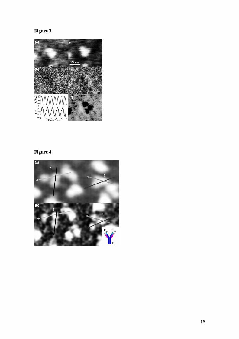
and with the same cantilever. Figures 3(a) and 3(b) shows the tapping mode AFM

images (AM-AFM) and Figures 3(d), 3(e), 3(f) the bimodal AFM images. In the

comparison, we used identical values for the free amplitude of the first mode A01 and for

the same set-point amplitude, those values were respectively A01=22 nm and Asp=21.2.

For bimodal AFM operation we added a second mode free amplitude of A02=0.7 nm.

Figure 3(c) shows AM-AFM and bimodal AFM amplitude oscillations.

The topography images given by both AM-AFM and bimodal AFM reveal

featureless objects on the mica surface (Figures 3(a) and 3(d)). Furthermore, the phase

image corresponding to the first mode does not reveal any kind of contrast between the

protein and the mica surface (Figures 3(b) and 3(e)). The lack of contrast in the above

phase images is due to the imaging conditions that were chosen to minimize tip-

antibody forces. This was achieved by using set-point values very close to the free

amplitude. Consequently, the imaging was dominated by conservative tip-molecule

forces. As it was stated previously, conservative forces do not give rise to material

contrast in the phase images of the 1st mode.

On the other hand, the phase image of the second mode does reveal three

structures that could be easily linked to the three fragments of the IgG antibody (Fig.

3(f)). The phase image resolves the three lobes of the structure with a separation

between peak lobes of 7.1 and 7.8 nm.

6

5.3. Bimodal AFM imaging of antibodies in air

Figure 4 shows topography and phase images (2nd

mode) of IgG antibodies

acquired with a Bimodal AFM. Two of the objects resemble the Y-shape of IgG

antibodies (termed as antibody 1 and antibody 2). The topography (Figure 4(a)) of

antibody 1 shows the characteristic three lobes of IgG (see inset for an scheme of IgG),

while antibody 2 just shows a triangular shape. On the contrary, the bimodal AFM

phase image (Figure 4(b)) resolves the three fragments of the molecule for both

antibodies. In order to make a detailed comparison, topographic and bimodal AFM

phase cross-sections are plotted for each antibody (Figures 5(a), 5(b), 5(c) and 5(d)).

The comparison shows that for both antibodies the bimodal AFM phase image gives

better lateral resolution than the corresponding topographic image.

The four Fab fragments (two per antibody) give very similar phase values (3.8º-

4.2º). However, we obtain a noticeable difference between the phase shift values of the

Fc fragments (~1.2 º). The difference could be attributed to small differences between

the morphologies of the Fc fragments upon deposition. This interpretation is consistent

with the differences observed in the apparent lengths of antibodies 1 and 2. So that,

differences in topographic lateral dimensions could be explained.

Bimodal AFM phase images reveal the monomer components of individual IgM

antibodies deposited on mica (Figure 6). We observe that the lateral size of the

antibodies as measured the AFM image is slightly larger than the nominal values (35

nm vs. 25 nm). This broadening could be a convolution effect originated by the tip’s

finite size.

The above images have been obtained with a cantilever spring constant of 8.7

N/m, free amplitude values for first and second modes of A01 = 21.4 nm and A02 = 0.4

nm respectively. The set-point amplitude was Asp = 20.1 nm.

5.4 Bimodal AFM imaging of antibodies in liquids

In conventional AFM fluid cells the mechanical excitation drives the cantilever ,

the fluid and the fluid cell. The resulting frequency spectrum shows many peaks that

bury the genuine cantilever resonances. This forest of peaks phenomenon [43] is shown

in the inset of Figure 7(a). It is difficult to conclude which of these peaks is closer to the

true resonances of the cantilever. To determine the cantilever’s eigenmodes in fluids we

measured the thermal noise spectrum. In this way, the first and second flexural modes

(arrows in the inset of Figure 7(a)) are found at 22.49 kHz and 146.98 kHz respectively.

For imaging IgM antibodies we have used a first mode free amplitude of A01 =

9.1 nm and a second mode free amplitude of A02 = 1.9 nm. The set-point amplitude was

6.0 nm. Figure 7(a) shows the bimodal AFM phase image of IgM antibodies in water.

We can see some individual antibodies (marked by circles) as well as multiple

aggregates and smaller objects that could be single separate monomers. Figures 7(b),

7(c) and 7(d) show a comparison among topography, first mode phase and second

mode phase images of another individual IgM. Topography and first mode phase

images do not resolve the inner structure of the protein, however, the phase image of the

second mode do distinguish the different monomers and the overall pentameric shape of

7

the antibody. The apparent lateral size of the pentamers as given by the AFM image is

37 nm.

6. Simulations of bimodal AFM dynamics

The numerical simulations have been performed for a cantilever with length L,

width b and thickness h of 225 m, 40 m, 1.8 m, respectively. The Young modulus

and mass density were respectively 170 GPa and 2320 kg/m3. The force constants,

resonance frequencies and quality factors of the first two flexural modes were

respectively 0.9 N/m, 35.2 N/m, 48.913 kHz, 306.194 kHz, 255 and 1000. The tip

radius R was 20 nm. The simulations have been calculated for two different materials,

SiO2-air-water-mica (H=4.7x10-20

J) and SiO2-air-mica (H=9.03x10-20

J) respectively.

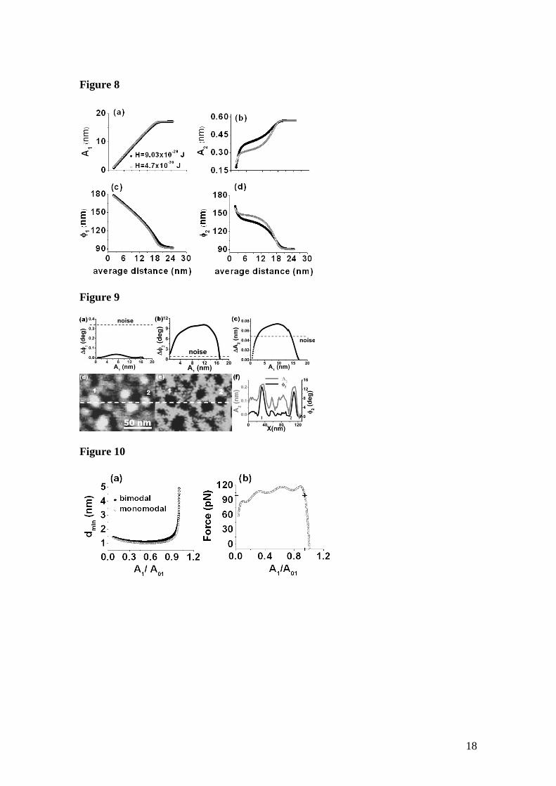
Figure 8 shows the dependence of A1, A2, 1, 2 on the average tip-surface

distance. The behaviour of the amplitude and phase shift of the first mode does not

seem to depend on the sample’s Hamaker values (Figures 8(a) and 8(c)). In particular,

A1 varies rather linearly with the tip-surface distance. This property makes the

amplitude of the first mode a suitable feedback parameter to track topography in

bimodal AFM. In addition, the curves do not show any noticeable dependence on the

sample’s Hamaker constant. On the other hand, the amplitude and phase shift curves of

the second flexural mode (Figures 8(b) and 8(d)) show a marked difference with the

Hamaker values. This property supports the use of the second mode parameters in

bimodal AFM to extract information on material properties.

6.1. Material contrast sensitivity in bimodal AFM operation

To analyze the sensitivity of bimodal AFM operation to detect compositional

changes we represent the differences in the microscope parameters (A2, 1, 2) (see Fig.

8) against the set-point amplitude A1 (Figure 9). The material contrast is defined as the

difference observed in any of the microscope parameters for two Hamaker constant

values at a given set-point amplitude. The dashed lines are the experimental noise

measured in our experimental set-up. As it was predicted [26], 1 shows no material

contrast above the noise level because of the absence of dissipation in the tip-surface

forces (Figure 9(a)). The small contrast is attributed to numerical errors in the

simulations. On the other hand, the parameters of the second mode do show material

contrast well above the noise level [26, 33]. Figures 9(b) and 9(c) show a maximum in

the contrast at intermediate set-point amplitudes. Consequently, those set-point values

define the optimal conditions for material contrast imaging. The value of that Signal to

Noise Ratio (SNR) is about 200 for 2 and 3.6 for A2.

The origin of the material contrast observed in bimodal AFM operation is due to

the ability to detect conservative and nonconservative interactions. In contrast,

conservative forces in AM-AFM do not give material contrast in the phase shift signal

because the restrictions imposed by the feedback mechanism [33].

8

As in regular tapping-mode AFM operation, the non-linear nature of the

interaction makes hard the determination of the sample’s Young modulus or Hamaker

constant from the experimental parameters. That is the reason why numerical

calculations are widely used to simulate the tip-surface dynamics in theoretical AFM

analyses [44].

To compare the material contrast obtained in amplitude and phase shifts A2 and

2, we have normalized the maximum contrast obtained in Figures 9(b) and 9(c) to their

respective ranges of variation (A02 = 0.6 nm for A2 and 90º for 2) resulting A2,max /0.6

nm = 0.14 and 2,max / 90º = 0.11. The comparison reveals a similar sensitivity for

both parameters. However, the changes observed in the amplitude 0.08 nm are very

close to the noise level ( 0.04 nm). The above does not occur for the phase shift

variations.

Figures 9(d) and 9(e) show A2 and 2 images of a silicon sample covered by

sexythiophene molecules. We can distinguish the same features in both images, thus

revealing that compositional sensitivity is similar in both channels. In order to check the

contrast of the two images, a profile (dashed line in Figures 9(d) and 9(e)) is depicted.

In Figure 9(f) the A2 image gives a positive contrast of 0.2 nm, while 2 image gives a

negative contrast of 9.1 º. Experimental conditions were: k = 8.5 N/m, A01 = 18.1 nm,

A02 = 1.8 nm with Asp/A01 = 95 %.

6.2. Estimation of the force applied on the sample surface

Unlike in static AFM, direct measurements of the forces applied on the sample

surface are not possible in dynamic AFM. However, there are several methods to

reconstruct the value of the interaction from dynamic force curves, i.e., amplitude and

phase shift versus distance curves in AM-AFM and frequency shift versus distance in

FM-AFM [45-52]. The rationale for most of the above methods relies on inverting the

integral equation deduced from 2nd

Newton law by averaging over one period of

oscillation. In the integral equations the interaction force appears multiplied by the

instantaneous tip deflection or its higher derivatives. This makes hard to extract the

force as a function of the experimental parameters. We remark that the above methods

have assumed a point-mass model for the cantilever, as a consequence all the higher

modes of the cantilever but the fundamental have been neglected. This seems to be a

reasonable approximation in bimodal AFM because A02/A01 << 1.

Here, we apply the method developed by Hölscher in Ref. [49]. This method

extracts the force at the minimum tip-surface distance from both amplitude and phase

shift curves. In this case we choose A1 and 1 as the tapping amplitude and phase values,

respectively, since we neglect the second mode tip-surface dynamics. According to

Hölscher’s formula, the maximum force calculated at resonance as the force at the

minimum distance, dmin, is

)(2

1

min

1

min

1min

min1min

min

)(cos)(

2)(

dAd

dts z

dz

zAdz

d

FdF (4)

9

where F1=k1A01/Q1 is the first mode driving force (k1 and Q1 are the spring

constant and quality factor for the first mode, respectively). The values for z in the

numerical integration of Eq. 4 have to be taken from the corresponding amplitude and

phase shift dynamic force curves, at the minimum distance, dmin=zc - A1.

Figure 10(a) shows the minimum tip-surface distance as calculated by numerical

simulations for both bimodal and monomodal (conventional) excitation methods. The

tip-surface distance hardly changes by the introduction of the bimodal excitation.

Consequently, the maximum force per oscillation will hardly change by introducing the

second mode excitation. This in turns supports the use of algorithms based on point-

mass models to reconstruct the force in bimodal AFM operation. The reconstructed

force lies below 120 pN (Fig. 10(b)). The force varies from 0 (no interaction) to a

maximum of 120 pN. Most of the experimental data shown here were acquired at an

amplitude ratio A1/A01 = 0.95 (black cross) which gives a maximum forces below 100

pN.

7. Summary

We have presented a dynamic force microscopy method based on the

simultaneous excitation of the first two flexural modes of the cantilever. The

performance and the potential of the instrument for biology applications has been

characterized by imaging isolated antibodies in air and water. The instrument resolves

the Fc and Fab fragments in single antibodies as well as the individual monomers in

pentameric antibodies.

We have also compared the compositional sensitivity and spatial resolution of

amplitude modulation and bimodal AFM methods. Under experimental conditions

aimed to minimize tip-surface forces, bimodal AFM phase images show higher

compositional contrast and spatial resolution than amplitude modulation AFM

topography and phase images.

One of the advantages of bimodal AFM is that makes compatible high resolution

imaging of isolated biomolecules at very low forces. Routine bimodal AFM imaging

can be performed by applying maximum forces below 100 pN. The force exerted by the

tip on the biomolecule has been estimated by using theoretical methods.

We have also characterized the sensitivity of the different bimodal AFM

parameters to detect material contrast. The phase shift of the second flexural mode is

the parameter that gives the highest material contrast.

Acknowledgements. This work was financially supported by the European

Commission (FORCETOOL, NMP4-CT-2004-013684), Ministerio de Educación y

Ciencia (MAT2006-03833) and Comunidad de Madrid (S-0505/MAT/0283).

10

Table 1. Resonance frequencies and driving forces to obtain a second mode oscillation

amplitude of 1V.

Cant. Type <f2 (kHz)> <driving force (mV)>

I 491.6 8

II 375.2 32

III 484.1 32

IV 388.2 42

V 413.1 9

Commercial 703.5 48

11

References

[1] Fritz M, Radmacher M, Cleveland J P, Allersma M W, Stewart R J, Gieselmann

R, Janmey P, Schmidt C F and Hansma P K 1995 Langmuir 11 3529-35

[2] Hafner J H, Cheung C L and Lieber C M 1999 Nature 398 761-2

[3] Hinterdorfer P and Dufrene Y F 2006 Nat. Meth. 3 347-55

[4] San Paulo A and Garcia R 2000 Biophys. J. 78 1599-605

[5] Shao Z F and Zhang Y Y 1996 Ultramicroscopy 66 141-52

[6] Thomson N H 2005 Ultramicroscopy 105 103-10

[7] Horber J K H and Miles M J 2003 Science 302 1002-5

[8] Muller D J and Engel A 2007 Nat. Protocol. 2 2191-7

[9] Martinez J, Yuzvinsky T D, Fennimore A M, Zettl A, Garcia R and Bustamante

C 2005 Nanotechnology 16 2493-6

[10] Ando T, Kodera N, Takai E, Maruyama D, Saito K and Toda A 2001 Proc. Natl.

Acad. Sci 98 12468-72

[11] Higgins M J, Polcik M, Fukuma T, Sader J E, Nakayama Y and Jarvis S P 2006

Biophys. J. 91 2532-42

[12] Hoogenboom B W, Hug H J, Pellmont Y, Martin S, Frederix P L T M, Fotiadis

D and Engel A 2006 Appl. Phys. Lett. 88 193109-3

[13] Scheuring S, Seguin J, Marco S, Levy D, Robert B and Rigaud J-L 2003 Proc.

Natl. Acad. Sci 100 1690-3

[14] Engel A and Muller D J 2000 Nat Struct Mol Biol 7 715-8

[15] García R and San Paulo A 1999 Phys. Rev. B 60 4961

[16] Garcia R, Gomez C J, Martinez N F, Patil S, Dietz C and Magerle R 2006 Phys.

Rev. Lett. 97 016103-4

[17] Martinez N F and Garcia R 2006 Nanotechnology 17 S167-S72

[18] Legleiter J and Kowalewski T 2005 Appl. Phys. Lett. 87 163120-3

[19] Preiner J, Tang J, Pastushenko V and Hinterdorfer P 2007 Phys. Rev. Lett. 99

046102-4

[20] Sahin O, Quate C F, Solgaard O and Atalar A 2004 Phys. Rev. B 69

[21] Stark M, Stark R W, Heckl W M and Guckenberger R 2000 Appl. Phys. Lett. 77

3293-5

[22] Crittenden S, Raman A and Reifenberger R 2005 Phys. Rev. B 72 235422-13

[23] Dareing D W, Thundat T, Jeon S and Nicholson M 2005 J. Appl. Phys. 97

084902-6

[24] Minne S C, Manalis S R, Atalar A and Quate C F 1996 Appl. Phys. Lett. 68

1427-9

[25] Sugimoto Y, Innami S, Abe M, Custance O and Morita S 2007 Appl. Phys. Lett.

91 093120-3

[26] Rodriguez T R and Garcia R 2004 Appl. Phys. Lett. 84 449-51

[27] Martinez N F, Patil S, Lozano J R and Garcia R 2006 Appl. Phys. Lett. 89

153115-3

[28] Patil S, Martinez N F, Lozano J R and Garcia R 2007 J. Molec. Recognit. 20

516-23

[29] Proksch R 2006 Appl. Phys. Lett. 89 113121-3

[30] Dietz C, Zerson M, Riesch C, Gigler A M, Stark R W, Rehse N and Magerle R

2008 Appl. Phys. Lett. 92 143107-3

12

[31] Stark R W, Naujoks N and Stemmer A 2007 Nanotechnology 18 065502

[32] Platz D, Tholen E A, Pesen D and Haviland D B 2008 Appl. Phys. Lett. 92

153106-3

[33] Lozano J R and Garcia R 2008 Phys. Rev. Lett. 100 076102-4

[34] Sader J E, Chon J W M and Mulvaney P 1999 Rev. Sci. Instrum. 70 3967-9

[35] Butt H J and Jaschke M 1995 Nanotechnology 6 1-7

[36] Levy R and Maaloum M 2002 Nanotechnology 13 33-7

[37] Schaffer T E 2005 Nanotechnology 16 664-70

[38] Melcher J, Hu S and Raman A 2007 Appl. Phys. Lett. 91 053101-3

[39] Stark R W, Schitter G, Stark M, Guckenberger R and Stemmer A 2004 Phys.

Rev. B 69 085412

[40] Solares S D 2007 J. Phys. Chem. B 111 2125-9

[41] Stark R W and Heckl W M 2000 Surf. Sci. 457 219-28

[42] Israelachvili J 2005 Intermol. and Surf. Forces (London: Elsevier Academic

Press)

[43] Schaffer T E, Cleveland J P, Ohnesorge F, Walters D A and Hansma P K 1996

J. Appl. Phys. 80 3622-7

[44] Raman A, Melcher J and Tung R 2008 Nano Today 3 20-7

[45] Giessibl F J 1997 Phys. Rev. B 56 16010

[46] Durig U 1999 Appl. Phys. Lett. 75 433-5

[47] Stark M, Stark R W, Heckl W M and Guckenberger R 2002 Proc. Natl. Acad.

Sci 99 8473-8

[48] Sader J E and Jarvis S P 2004 Appl. Phys. Lett. 84 1801-3

[49] Holscher H 2006 Appl. Phys. Lett. 89 123109-3

[50] Holscher H and Schwarz U D 2007 Intern. J. Non-Linear Mechs. 42 608-25

[51] Hu S and Raman A 2007 Appl. Phys. Lett. 91 123106-3

[52] Lee M H and Jhe W H 2006 Phys. Rev. Lett. 97 036104-4

13

Figure Captions

Figure 1. Comparison between amplitude modulation and bimodal AFM. (a) AM-AFM

(monomodal excitation). (b) Bimodal AFM. (c) Schematics of the bimodal AFM

instrument. The bimodal excitation/detection unit performs the multifrequency

excitation and the multicomponent signal processing while the control unit runs the

feedback.

Figure 2. (a) Cantilevers designed for enhancing the second flexural mode response. (b)

Comparison of the frequency response between commercial and tailored cantilevers.

Figure 3. Comparison between AM-AFM and bimodal AFM images of IgG antibodies.

(a) Topography and (b) phase images of an IgG obtained in AM-AFM. (c) Tip

oscillation in AM-AFM (top) and bimodal AFM (bottom). (d) Topography in bimodal

AFM. (e) Phase shift image of the first mode in bimodal AFM. (f) Bimodal AFM phase

image (2nd

mode) of the same antibody. The image shows a Y shaped object.

Figure 4. Bimodal imaging of IgG antibodies. (a) Topography. (b) Second mode phase

image (b). Two objects are identified as IgG proteins (termed as 1 and 2). The inset

shows a scheme of the IgG antibody structure.

Figure 5. Cross-sections along the arrows shown in Figure 4(a) and 4(b) for antibodies

1 and 2. (a) is the topography and (b) the phase shift (2nd

mode) cross-sections

corresponding to antibody 1. (c) is the topography and (d) the phase shift (2nd

mode)

cross-sections corresponding to antibody 2. The darker cross-sections correspond to the

darker line in Fig. 4.

Figure 6. (a) Topography image of a region with a homogenous deposition of the

antibodies. (b) Topography image of an isolated antibody. The antibody shows an

overall pentagonal shape but there is no hint on the monomer positions. (c) Scheme of

the IgM antibody. (d), (e) and (f) Bimodal AFM phase images (2nd

mode) of three

different antibodies. The above images reveal the monomer components, they also hint

the position of the J-chain.

Figure 7. (a) Bimodal AFM phase images (2nd

mode) of IgM antibodies in water. The

objects that show a pentagonal shape are marked by circles. The inset shows the

frequency spectrum of a commercial cantilever in water. The dashed lines indicate the

frequencies of first and second flexural modes of the cantilever. They were determined

by measuring the thermal noise spectrum. (b) Topography of an isolated antibody. (c)

First mode phase image and (d) Bimodal AFM phase image (2nd

mode) of the same

antibody.

Figure 8. Amplitude and phase shift curves for two different materials (Hamaker values

of 4.7x10-20

J, open dots; 9.03x10-20

J, dark dots). (a) Amplitude curve of the first mode.

(b) Amplitude curve of the second mode. (c) Phase shift curve of the first flexural mode.

(d) Phase shift curve of the second flexural mode.

14

Figure 9. Material contrast sensitivity in bimodal AFM. (a) Dependence of the 1st mode

phase shift contrast on the set-point amplitude. (b) Dependence of the bimodal AFM

phase shift (2nd

mode) contrast on the set-point amplitude. (c) Dependence of the

bimodal AFM amplitude (2nd

mode) contrast on the set-point amplitude. The materials

have been simulated by using two Hamaker values (H=4.7x10-20

J and 9.03x10-20

J).

The dashed lines represent the experimental noise. Experimental A2 (d) and 2 (e)

images of sexythiophene molecules on silicon. (f) Cross section along the dashed lines

of Fig. 9d.

Figure 10. (a) Minimum tip-surface distance for bimodal (dark dots) and monomodal

(open dots) excitations as a function of the amplitude ratio. (b) Reconstructed tip-

surface forces as a function of the amplitude ratio. The simulations were performed with

H=9.03x10-20

J and R = 20 nm.

15

Figure 1

Figure 2

16

Figure 3

Figure 4

17

Figure 5

Figure 6

Figure 7

18

Figure 8

Figure 9

Figure 10