Bifurcations in an autoparametric system in 1 : 1 internal resonance with parametric excitation

BIFURCATIONS IN AN AUTOPARAMETRIC SYSTEM IN

�� INTERNAL RESONANCE WITH PARAMETRIC

EXCITATION

�revised preprint nr� ��

S� Fatimah�� and M� Ruijgrok

Mathematisch Instituut� University of Utrecht� PO Box �� TA Utrecht�

The Netherlands

Abstract� We consider an autoparametric system which consists of anoscillator� coupled with a parametrically�excited subsystem� The oscil�lator and the subsystem are in � � � internal resonance� The excitedsubsystem is in � � � parametric resonance with the external forcing�The system contains the most general type of cubic nonlinearities� Us�ing the method of averaging and numerical bifurcation continuation� westudy the dynamics of this system� In particular� we consider the sta�bility of the semi�trivial solutions� where the oscillator is at rest and theexcited subsystem performs a periodic motion� We �nd various typesof bifurcations� leading to non�trivial periodic or quasi�periodic solu�tions� We also �nd numerically sequences of period�doublings� leadingto chaotic solutions�

�� Introduction

An autoparametric system is a vibrating system which consists of at leasttwo subsystems� the oscillator and the excited subsystem� This system isgoverned by dierential equations where the equations representing the oscillator are coupled to those representing the excited subsystem in a nonlinearway and such that the excited subsystem can be at rest while the oscillatoris vibrating� We call this solution the semitrivial solution� When this semitrivial solution becomes unstable� nontrivial solutions can be initiated� Formore backgrounds and references see Svoboda� Tondl� and Verhulst �� andTondl� Ruijgrok� Verhulst� and Nabergoj ��We shall consider an autoparametric system where the oscillator is ex

cited parametrically� of the form�

x�� k�x� q��x ap��x f�x� y� � �

y�� k�y� q��y g�x� y� � �

��

The �rst equation represents the oscillator and the second one is theexcited subsystem� An accent� as in x�� will indicate dierentiation with

�corresponding author

�

� Bifurcations in an Autoparametric System in �� Internal Resonance

respect to time � and x� y � R� k� and k� are the damping coe�cients�q� and q� are the natural frequencies of the undamped� linearized oscillatorand excited subsystem� respectively� The functions f�x� y� and g�x� y�� thecoupling terms� are C� and g�x� �� for all x � R� The damping coe�cients and the amplitude of forcing a are assumed to be small positivenumbers� We will consider the situation that the oscillator and the externalparametric excitation are in primary � � � resonance and that there existsan internal � � � resonance�There exist a large number of studies of similar autoparametric systems�

The case of a � � � internal resonance has been studied by Ruijgrok �� andOueini� Chin� and Nayfeh �� in the case of parametric excitation� In Ruijgrok �� the averaged system is analyzed mathematically� and an applicationto a rotor system is given� In Oueni� Chin� and Nayfeh �� theoretical results are compared with the outcomes of a mechanical experiment� Tien�Namachchivaya� and Bajaj �� also consider the situation that there existsa � � � internal resonance� now however with external excitation�In Tien� Namachchivaya� and Bajaj �� and in Bajaj� Chang and John

son �� the bifurcations of the averaged system are studied� and the authorsshow the existence of chaotic solutions� numerically in Bajaj� Chang� andJohnson �� and by using an extension of the Melnikov method in Tien�Namachchivaya� and Bajaj �� for the case with no damping� In Banerjee and Bajaj �� similar methods as in Tien� Namachchivaya� and Bajaj�� are used� but now for general types of excitation� including parametricexcitation�The case of a � � � internal resonance has received less attention� In

Tien� Namachchivaya� and Malhotra �� this resonance case is studied� incombination with external excitation� The author shows analytically thatfor certain values of the parameters� a �Silnikov bifurcation can occur� leading to chaotic solutions� In Feng and Sethna �� parametric excitation wasconsidered� and also here a generalization of the Melnikov method was usedto show the existence of chaos in the undamped case�In this paper we study the behavior of the semitrivial solution of system

�� This is done by using the method of averaging� It is found that severalsemitrivial solutions can coexist� These semitrivial solutions come in pairs�connected by a mirrorsymmetry� However� only one of these �pairs of� semitrivial solutions is potentially stable� In section � we study the stability ofthis particular solution� the results of which are summarized in �dimensionalstability diagrams� In section � the bifurcations of the semitrivial solutionare analyzed� These bifurcations lead to nontrivial solutions� such as stableperiodic and quasiperiodic orbits� In section � we show that one of thenontrivial solutions undergoes a series of perioddoublings� leading to astrange attractor� The chaotic nature of this attractor is demonstrated bycalculating the associated Lyapunov exponents�Finally� we mention that in the averaged system we encounter a codi

mension � bifurcation� The study of this rather complicated bifurcation will

S� Fatimah and M� Ruijgrok �

be described in a separate paper� where we also use a method similar tothe one used in Tien� Namachchivaya� Malhotra �� to show analytically theexistence of �Silnikov bifurcations in this system�

�� The averaged system

We will take f�x� y� � c�xy� �

�x�� g�x� y� � �

�y� c�x

�y� and p�� cos �� Let q�� and q�� where �� and �� are the detunings

from exact resonance� After rescaling k� � � �k�� k� � � �k�� a � ��a� x �p��x�

and y �p��y� then dropping the tildes� we have the system�

x�� x ��k�x� ��x a cos ��x

�

�x� c�y

�x� � �

y�� y ��k�y� ��y c�x

�y �

�y��

��

It is possible to start with a more general expression for f�x� y� and g�x� y��for instance including quadratic terms� We have limited ourselves to thelowestorder resonant terms� which in this case are of third order� and whichcan be put in this particular form by a suitable scaling of the x� y� and � coordinates� This is not a restriction� as a more general form for the couplingterms leads to the same averaged system and normal forms�The system �� is invariant under �x� y�� x��y�� x� y�� x� y�� and

�x� y�� x��y�� In particular the �rst symmetry will be important in theanalysis of this system� We emphasize that these symmetries do not dependon our particular choice for f�x� y� and g�x� y�� but are a consequence of the�� and �� resonances and the restriction that we have an autoparametricsystem� i�e� that g�x� �� for all x � R�We will use the method of averaging �see Sanders and Verhulst �� for

appropriate theorems � to investigate the stability of solutions of system�� by introducing the transformation�

x � u� cos � v� sin � � x� � �u� sin � v� cos ��

y � u� cos � v� sin � � y� � �u� sin � v� cos ��

After substituting �� and �� into �� averaging over � � and rescaling� � �

� �� we have the following averaged system�


u�� k�u� ��

�a�v� v��u

�� v��

�

�c�u

��v�

�

�c�v

��v�

�

�c�u�v�u�

v�� k�v� � ��

�a�u� � u��u

�� v��

�

�c�u

��u� �

�

�c�v

��u� �

�

�c�u�v�v�

u�� k�u� ��v� v��u�� v��

�

�c�u

��v�

�

�c�v

��v�

�

�c�u�v�u�

v�� k�v� � ��u� � u��u�� v��

�

�c�u

��u� �

�

�c�v

��u� �

�

�c�u�v�v�

��

�� The semi�trivial solution

In this section we investigate the semitrivial solutions of system ��and determine their stability� From section �� the semitrivial solutions correspond to u� � v� � �� so that we have�

u�� k�u� ��

�a�v� v��u

�� v��

v�� k�v� � ��

�a�u� � u��u

�� v��

��

Apart from �� the �xed points of system �� correspond with periodicsolutions of system �� The nontrivial �xed points are

��u��v�� R�k

��

�� a R�

��q��

�a R�

�� k��

�� R�k�q��

�a R�

�� k��

�A

��

where

R��

r�

�a� � k��

Assuming R� �� there are three cases� depending on the value of a and ��

�� If a � �p�� k�� there is one solution for R�

�

�� If �� and �k� � a � �p�� k�� there are two solutions for R

��

�� For a � �k�� there is no solution for R��

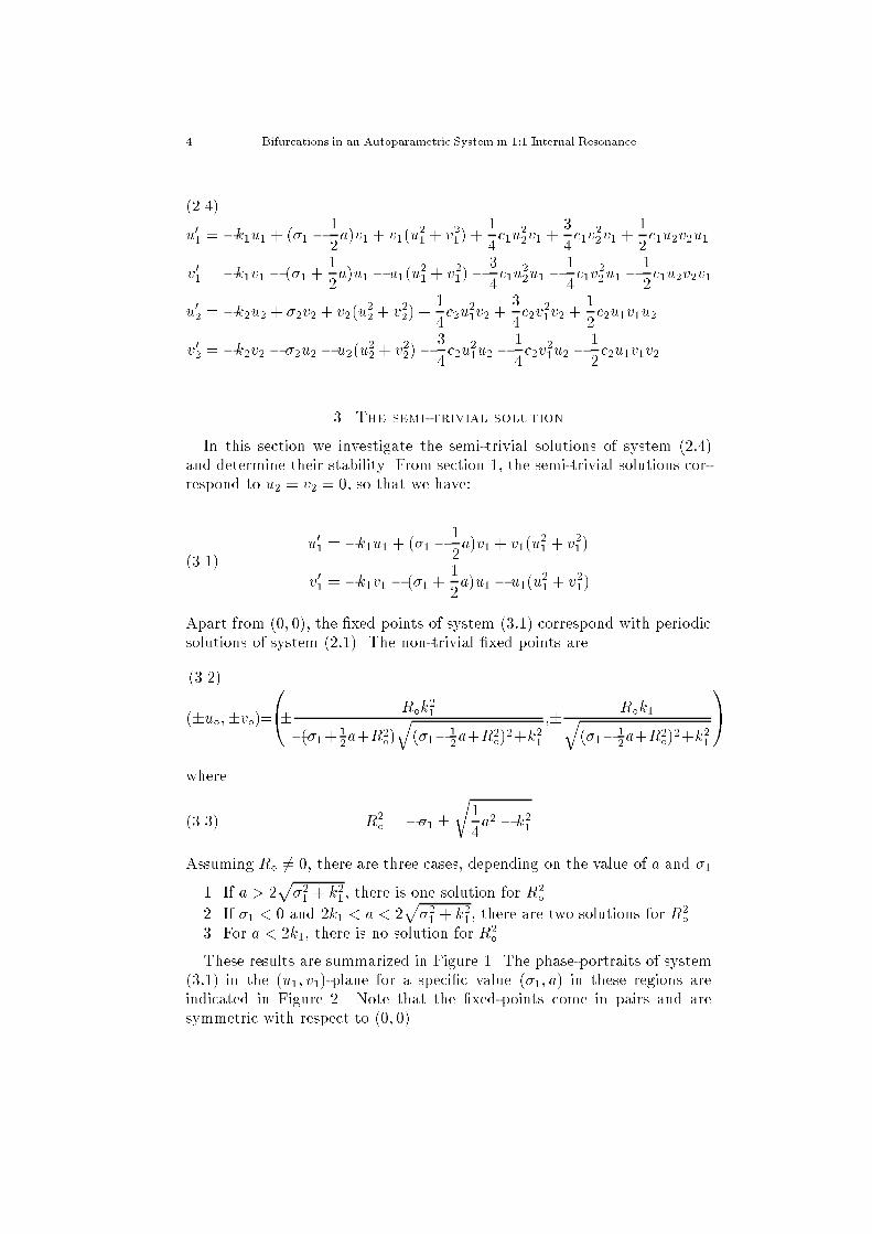
These results are summarized in Figure �� The phaseportraits of system�� in the �u�� v��plane for a speci�c value �� a� in these regions areindicated in Figure �� Note that the �xedpoints come in pairs and aresymmetric with respect to ��


0σ

Region I

Region II

Region III2k1

a

1

Figure �� The parameter diagram of system �� in the�� a�plane

u

v

1

1

u

v

1

1

u

v

1

1

Figure �� The phaseportraits of system �� in the�u�� v��plane for speci�c values �� a� in region I� II� andIII� respectively�

�� Stability of the semi�trivial solution

In this section we will study the stability of the semitrivial solution depending on the values of the forcing amplitude a and the detunings �� in system �� From section �� we �nd that the semitrivial solution corresponding to R�

�with the plus sign is always stable �as a solution of ��

therefore we will only study this semitrivial solution and ignore the unstablesemitrivial solutions�


Write the averaged system �� in the form�

X� � F �X��

where X �

�BB�

u�v�u�v�

�CCA and

�F

�X�

�A�� A��

A�� A��

��

where A�� A�� A�� and A�� are � � � matrices depending on u�� v�� u�and v�� At the solution ��u��v�� corresponding to the semitrivialsolution of system �� we have �F

�X� AX with

A�

�BB�

�k��u�v� ��

�a��v�

��R�

��

��

�a��u�

��R�

��k��u�v� � �

� � �k��

�c�u�v� ��

�

�c�u

�

��

�c�v

�

�

� � ��

�c�v

�

��

�

�c�v

�

��k��

�

�c�u�v�

�CCA

��

u� and v� satisfy �� and R��satis�es �� Let

A �

�A�� A��

�

To get the stability boundary of system �� we solve detA � detA��detA�� From the equation detA�� we �nd

��q

��a

� � k��q

��a

� � k��

or

a � �k� or a � �q�� k��

and from detA�� we have�

�� c�R

��r

�

��c��R

�� k�� where R�

��

k�

c��

Because R��is a function of �� and a� equation �� now gives a relation

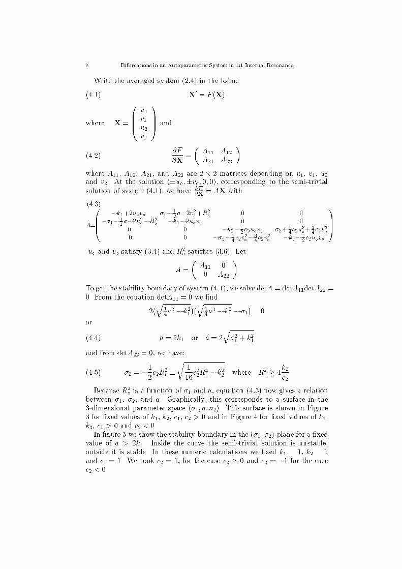
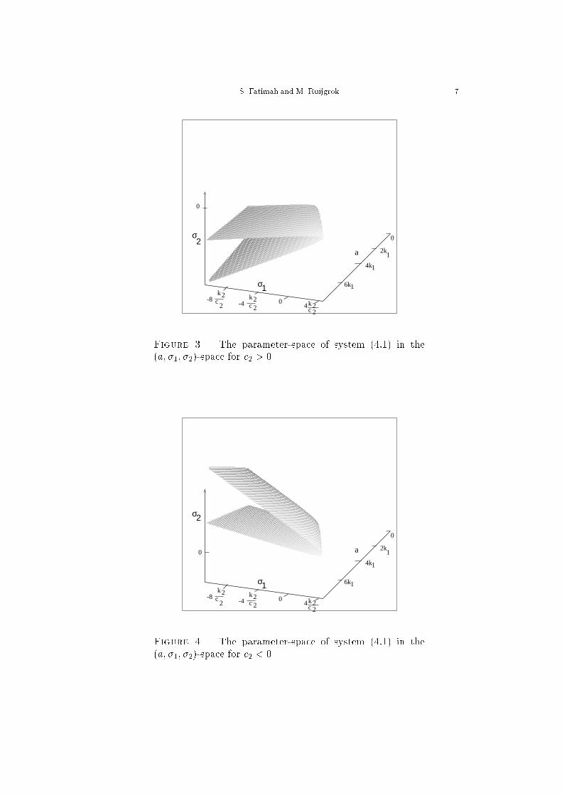
between �� and a� Graphically� this corresponds to a surface in the�dimensional parameter space �� a� �� This surface is shown in Figure� for �xed values of k�� k�� c�� c� � � and in Figure � for �xed values of k��k�� c� � � and c� � ��In �gure � we show the stability boundary in the �� plane for a �xed

value of a � �k�� Inside the curve the semitrivial solution is unstable�outside it is stable� In these numeric calculations we �xed k� � �� k� � �and c� � �� We took c� � �� for the case c� � � and c� � �� for the casec� � ��

S� Fatimah and M� Ruijgrok

0

σ1 6k1

4k1

a 2k1

0

kc

2

2 k2c 2

-4-8 0

4k2c 2

σ2

Figure �� The parameterspace of system �� in the�a� �� space for c� � ��

σ1 6k1

4k1

a 2k1

0

kc

2

2 k2c 2

-4-8 0

4k2c 2

0

σ2

Figure �� The parameterspace of system �� in the�a� �� space for c� � ��

Bifurcations in an Autoparametric System in �� Internal Resonance

-20

-15

-10

-5

0

5

sigma2

-10 -8 -6 -4 -2 0 2 4sigma1

σ 2

σ 1

-5

0

5

10

15

20

sigma2

-10 -8 -6 -4 -2 0 2 4sigma1 σ

σ 2

1

�a �b

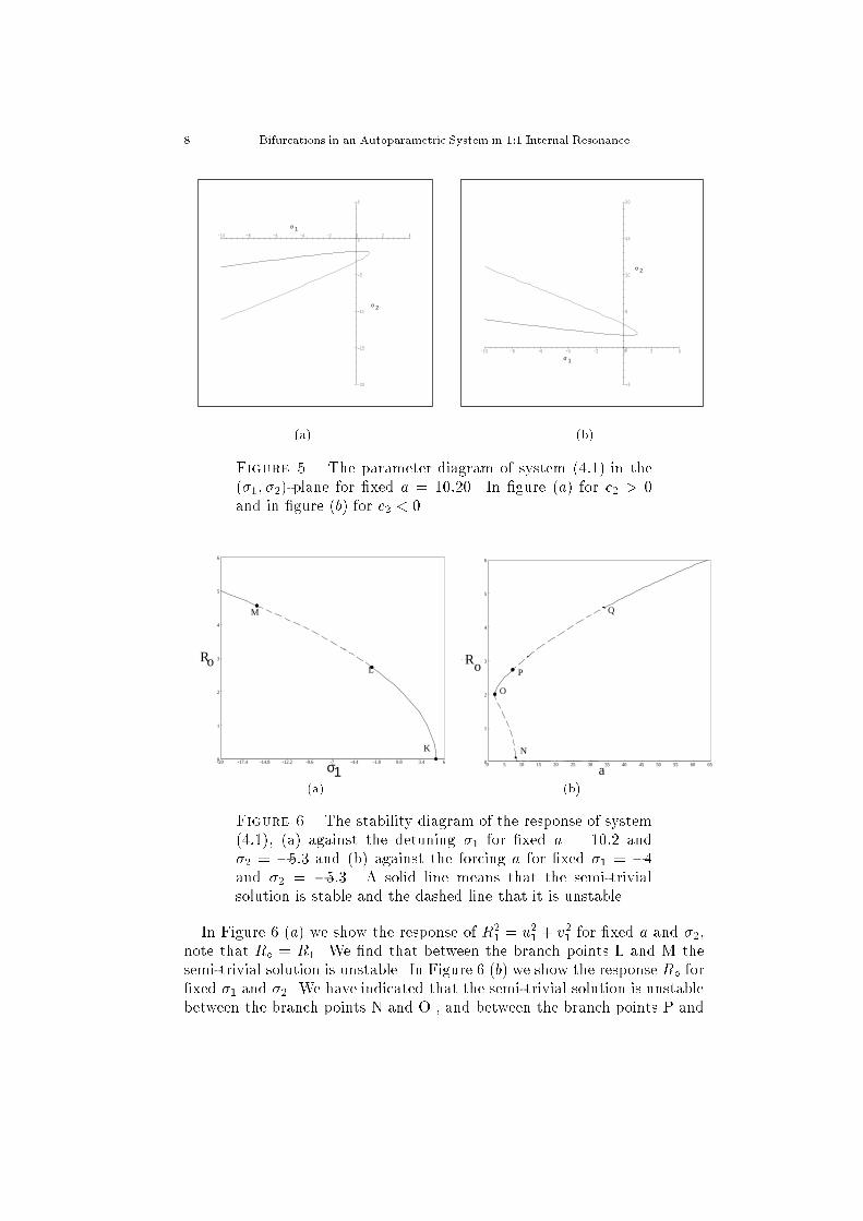
Figure �� The parameter diagram of system �� in the�� plane for �xed a � �� In �gure �a� for c� � �and in �gure �b� for c� � ��

0

1

2

3

4

5

6

-20 -17.4 -14.8 -12.2 -9.6 -7 -4.4 -1.8 0.8 3.4 6sigma1

L2_NormRo

K

L

M

σ10

1

2

3

4

5

6

0 5 10 15 20 25 30 35 40 45 50 55 60 65a

L2_NormRo

N

O

P

Q

.a

�a �b

Figure �� The stability diagram of the response of system�� a� against the detuning �� for �xed a � �� and�� and �b� against the forcing a for �xed �� and �� A solid line means that the semitrivialsolution is stable and the dashed line that it is unstable�

In Figure � �a� we show the response of R�� u�� v�� for �xed a and ��

note that R� � R�� We �nd that between the branch points L and M thesemitrivial solution is unstable� In Figure � �b� we show the response R� for�xed �� and �� We have indicated that the semitrivial solution is unstablebetween the branch points N and O � and between the branch points P and


Q� Figure � does not depend on the sign of c�� We have similar �gures forthe case c� � �� and for the case c� � ��

�� Bifurcations of the semi�trivial solution

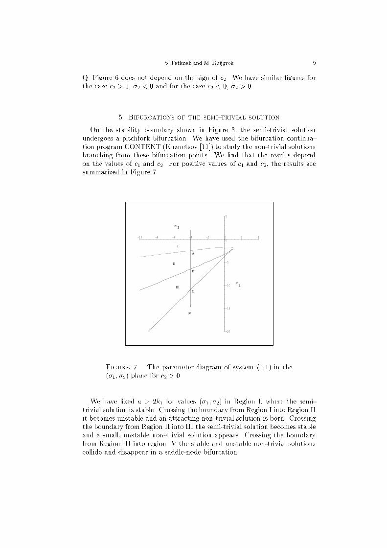
On the stability boundary shown in Figure �� the semitrivial solutionundergoes a pitchfork bifurcation� We have used the bifurcation continuation program CONTENT �Kuznetsov �� to study the nontrivial solutionsbranching from these bifurcation points� We �nd that the results dependon the values of c� and c�� For positive values of c� and c�� the results aresummarized in Figure ��

-20

-15

-10

-5

0

5

sigma2

-10 -8 -6 -4 -2 0 2 4sigma1

I

II

III

IV

A

B

C

σ2

σ 1

Figure � The parameter diagram of system �� in the�� plane for c� � ��

We have �xed a � �k� for values �� in Region I� where the semitrivial solution is stable� Crossing the boundary from Region I into Region IIit becomes unstable and an attracting nontrivial solution is born� Crossingthe boundary from Region II into III the semitrivial solution becomes stableand a small� unstable nontrivial solution appears� Crossing the boundaryfrom Region III into region IV the stable and unstable nontrivial solutionscollide and disappear in a saddlenode bifurcation�

�� Bifurcations in an Autoparametric System in �� Internal Resonance

-4

-2.4

-0.8

0.8

2.4

4

-15 -13.3 -11.6 -9.9 -8.2 -6.5 -4.8 -3.1 -1.4 0.3 2sigma2

u2

σ2

u2AB

C

C

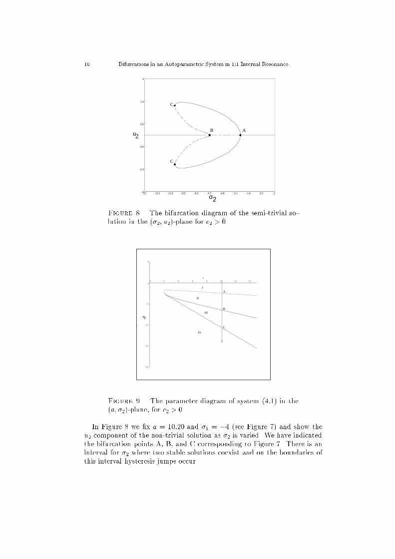
Figure � The bifurcation diagram of the semitrivial solution in the �� u��plane for c� � ��

-20

-15

-10

-5

0

5

sigma2

0 2 4 6 8 10 12 14a

σ2

A

B

C

I

II

III

IV

Figure �� The parameter diagram of system �� in the�a� ��plane� for c� � ��

In Figure � we �x a � �� and �� see Figure �� and show theu� component of the nontrivial solution as �� is varied� We have indicatedthe bifurcation points A� B� and C corresponding to Figure �� There is aninterval for �� where two stable solutions coexist and on the boundaries ofthis interval hysteresis jumps occur�

S� Fatimah and M� Ruijgrok ��

It is possible to make similar diagrams in the �a� ��plane� keeping ��xed� Again we �nd similar bifurcations� see Figure �� Note that the pointsA� B correspond to the branching points in Figure �� and C corresponds toa saddlenode bifurcation�

0

1

2

3

4

5

6

-20 -17.4 -14.8 -12.2 -9.6 -7 -4.4 -1.8 0.8 3.4 6sigma1

L2_Norm

K

L

M

L’

Ro

R

σ10

1

2

3

4

5

6

0 5 10 15 20 25 30 35 40 45 50 55 60 65a

L2_NormR

a

Ro

N

O

P

Q

P’

.

�a �b

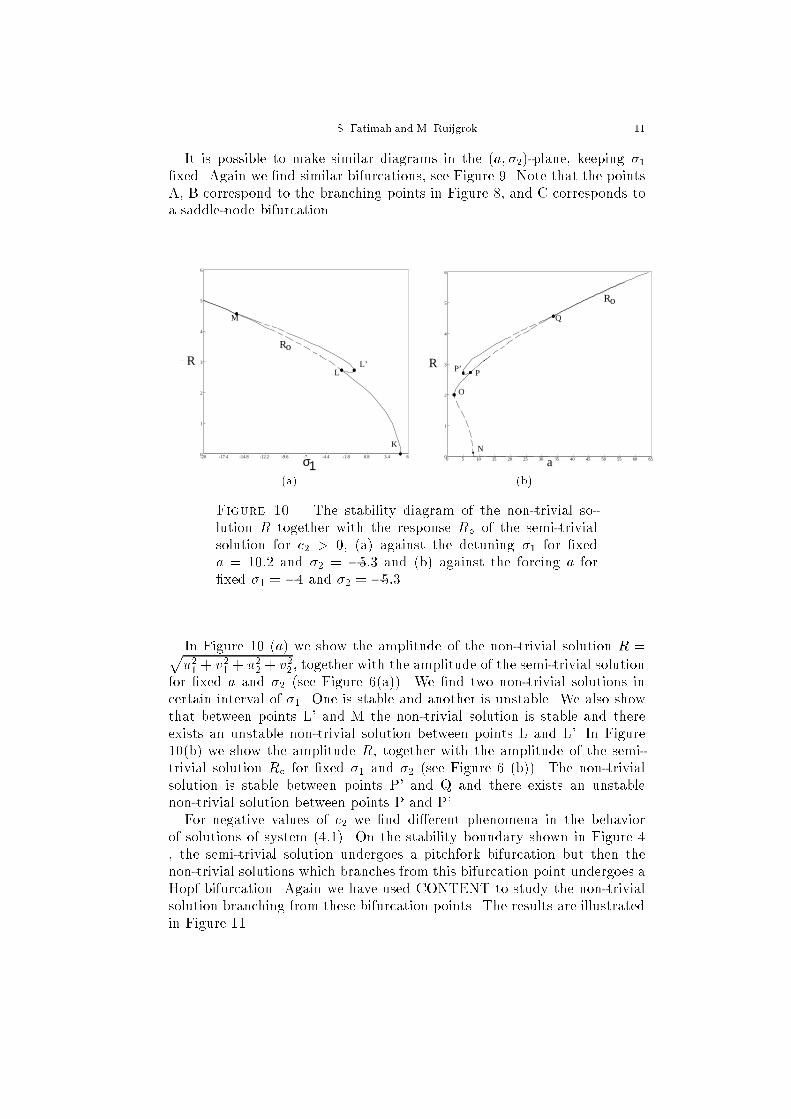
Figure �� The stability diagram of the nontrivial solution R together with the response R� of the semitrivialsolution for c� � �� a� against the detuning �� for �xeda � �� and �� and �b� against the forcing a for�xed �� and ��

In Figure �� a� we show the amplitude of the nontrivial solution R �pu�� v�� u�� v�� together with the amplitude of the semitrivial solution

for �xed a and �� see Figure ��a�� We �nd two nontrivial solutions incertain interval of �� One is stable and another is unstable� We also showthat between points L� and M the nontrivial solution is stable and thereexists an unstable nontrivial solution between points L and L�� In Figure��b� we show the amplitude R� together with the amplitude of the semitrivial solution R� for �xed �� and �� see Figure � �b�� The nontrivialsolution is stable between points P� and Q and there exists an unstablenontrivial solution between points P and P��For negative values of c� we �nd dierent phenomena in the behavior

of solutions of system �� On the stability boundary shown in Figure �� the semitrivial solution undergoes a pitchfork bifurcation but then thenontrivial solutions which branches from this bifurcation point undergoes aHopf bifurcation� Again we have used CONTENT to study the nontrivialsolution branching from these bifurcation points� The results are illustratedin Figure ��


-20

-10

0

10

20

sigma2

-10 -8 -6 -4 -2 0 2 4sigma1

A

BC

D

E

I

II

III

IV

VVI

σ2

σ1

VI

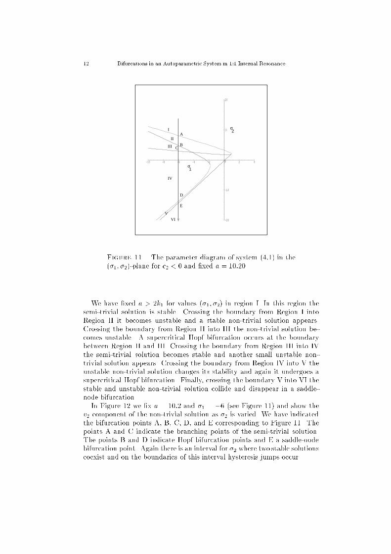
Figure �� The parameter diagram of system �� in the�� plane for c� � � and �xed a � ��

We have �xed a � �k� for values �� in region I� In this region thesemitrivial solution is stable� Crossing the boundary from Region I intoRegion II it becomes unstable and a stable nontrivial solution appears�Crossing the boundary from Region II into III the nontrivial solution becomes unstable� A supercritical Hopf bifurcation occurs at the boundarybetween Region II and III� Crossing the boundary from Region III into IVthe semitrivial solution becomes stable and another small unstable nontrivial solution appears� Crossing the boundary from Region IV into V theunstable nontrivial solution changes its stability and again it undergoes asupercritical Hopf bifurcation� Finally� crossing the boundary V into VI thestable and unstable nontrivial solution collide and disappear in a saddlenode bifurcation�In Figure �� we �x a � �� and �� see Figure �� and show the

v� component of the nontrivial solution as �� is varied� We have indicatedthe bifurcation points A� B� C� D� and E corresponding to Figure �� Thepoints A and C indicate the branching points of the semitrivial solution�The points B and D indicate Hopf bifurcation points and E a saddlenodebifurcation point� Again there is an interval for �� where two stable solutionscoexist and on the boundaries of this interval hysteresis jumps occur�


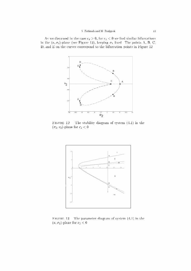
As we discussed in the case c� � �� for c� � � we �nd similar bifurcationsin the �a� ��plane �see Figure �� keeping �� xed� The points A� B� C�D� and E on the curves correspond to the bifurcation points in Figure ��

-4

-2.4

-0.8

0.8

2.4

4

-20 -16.5 -13 -9.5 -6 -2.5 1 4.5 8 11.5 15sigma2

v2

A

B

B

C

D

D

E

E

σ2

v2

Figure �� The stability diagram of system �� in the�� v��plane for c� � ��

-20

-15

-10

-5

0

5

10

sigma2

0 2 4 6 8 10 12 14a

σ 2

A

B

C

D

E

I

II

III

IV

V

VI

Figure �� The parameter diagram of system �� in the�a� ��plane for c� � �


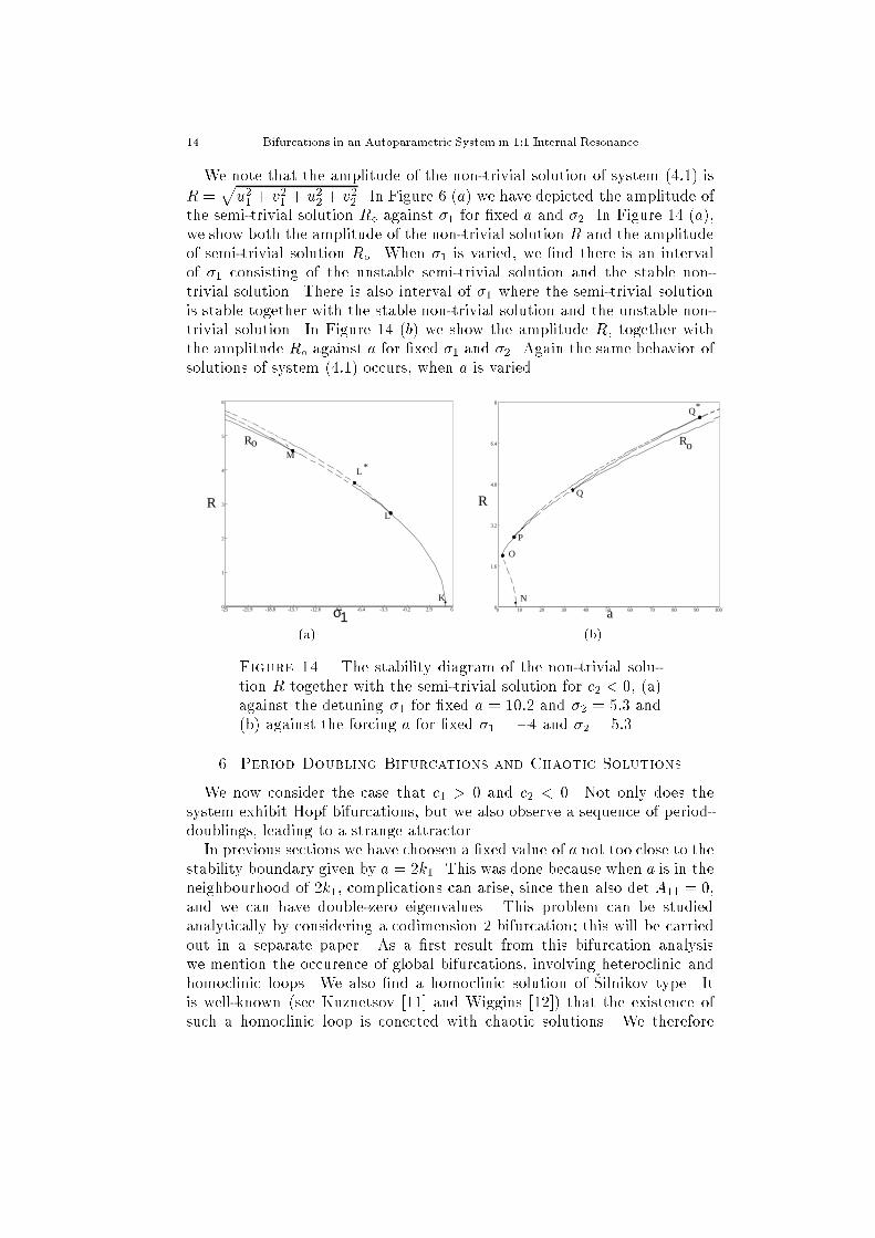
We note that the amplitude of the nontrivial solution of system �� is

R �pu�� v�� u�� v�� In Figure � �a� we have depicted the amplitude of

the semitrivial solution R� against �� for �xed a and �� In Figure �� a��we show both the amplitude of the nontrivial solution R and the amplitudeof semitrivial solution R�� When �� is varied� we �nd there is an intervalof �� consisting of the unstable semitrivial solution and the stable nontrivial solution� There is also interval of �� where the semitrivial solutionis stable together with the stable nontrivial solution and the unstable nontrivial solution� In Figure �� b� we show the amplitude R� together withthe amplitude R� against a for �xed �� and �� Again the same behavior ofsolutions of system �� occurs� when a is varied�

0

1

2

3

4

5

6

-25 -21.9 -18.8 -15.7 -12.6 -9.5 -6.4 -3.3 -0.2 2.9 6sigma1

L2_Norm

.

R

K

L

M

Ro

L *

σ10

1.6

3.2

4.8

6.4

8

0 10 20 30 40 50 60 70 80 90 100a

L2_Norm

.a

Ro

N

O

P

Q

Q*

R

�a �b

Figure �� The stability diagram of the nontrivial solution R together with the semitrivial solution for c� � �� a�against the detuning �� for �xed a � �� and �� and�b� against the forcing a for �xed �� and ��

�� Period Doubling Bifurcations and Chaotic Solutions

We now consider the case that c� � � and c� � �� Not only does thesystem exhibit Hopf bifurcations� but we also observe a sequence of perioddoublings� leading to a strange attractor�In previous sections we have choosen a �xed value of a not too close to the

stability boundary given by a � �k�� This was done because when a is in theneighbourhood of �k�� complications can arise� since then also det A�� and we can have doublezero eigenvalues� This problem can be studiedanalytically by considering a codimension � bifurcation� this will be carriedout in a separate paper� As a �rst result from this bifurcation analysiswe mention the occurence of global bifurcations� involving heteroclinic andhomoclinic loops� We also �nd a homoclinic solution of �Silnikov type� Itis wellknown �see Kuznetsov �� and Wiggins �� that the existence ofsuch a homoclinic loop is conected with chaotic solutions� We therefore


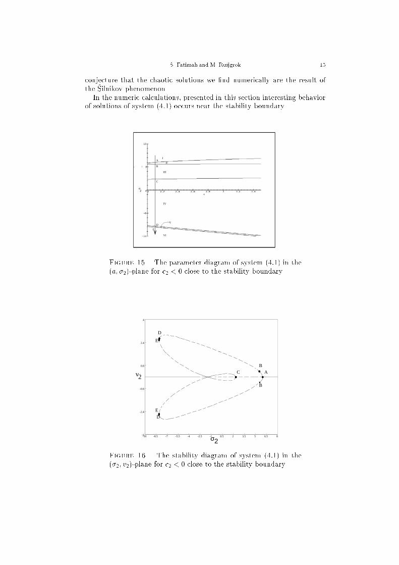
conjecture that the chaotic solutions we �nd numerically are the result ofthe �Silnikov phenomenon�In the numeric calculations� presented in this section interesting behavior

of solutions of system �� occurs near the stability boundary�

A

B

C

D

E

I

σ2

II

III

IV

V

VI

Figure �� The parameter diagram of system �� in the�a� ��plane for c� � � close to the stability boundary�

-4

-2.4

-0.8

0.8

2.4

4

-10 -8.5 -7 -5.5 -4 -2.5 -1 0.5 2 3.5 5 6.5 8sigma2

v2

σ2

v2A

B

B

C

D

E

ED

Figure �� The stability diagram of system �� in the�� v��plane for c� � � close to the stability boundary�


u1

v1

u2

v2

�a

u1

v1

u2

v2

�b

u1

v1

u2

v2

�c

u1

v1

u2

v2

�d

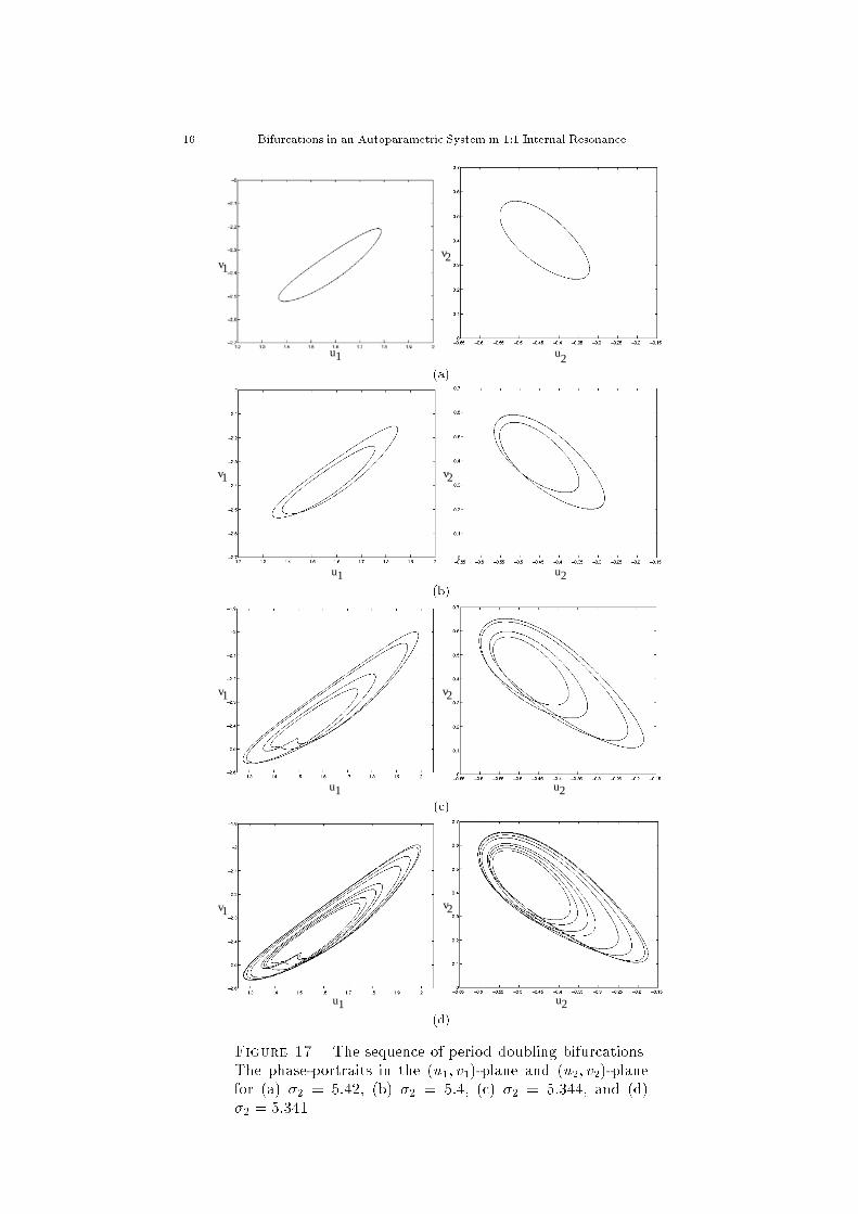
Figure �� The sequence of period doubling bifurcations�The phaseportraits in the �u�� v��plane and �u�� v��planefor �a� �� b� �� c� �� and �d��


In Figure �� we �xed �� k�c�� a close to �k� and c� � � �a � ��

�� and c� � �� The bifurcations of the semitrivial solution aresimilar to the case where a is taken far away from the stability boundary�compare Figure �� and Figure ��In Figure �� the semitrivial solution branches at point A� and then

at point C� When the semitrivial solution branches at point A� a stablenontrivial solution bifurcates and then this nontrivial solution undergoes aHopf bifurcation at point B� We point out that a �xed point and a periodicsolution in the averaged system correspond to a periodic and quasiperiodicsolution� respectively� in the original� time dependent system� A supercritical Hopf bifurcation occurs at point B for �� and at point Dfor �� Again� a saddlenode bifurcation occurs at point E for�� We �nd a stable periodic orbit for all values of �� in the interval �� As �� is decreased� period doubling of the stableperiodic solution is observed� see Figure�� There is an in�nite number ofsuch period doubling bifurcations� until the value �� is reached�The values of �� with �� produce a strange attractor�

v2

u2

u1

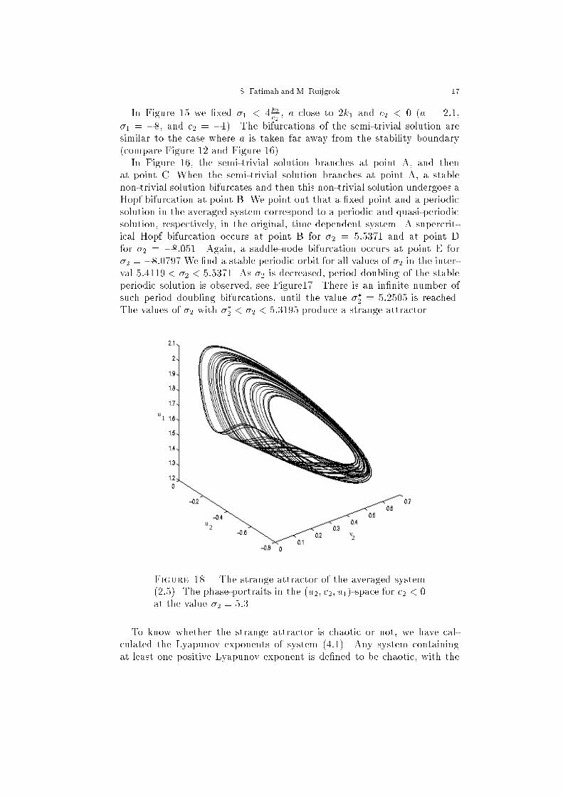
Figure �� The strange attractor of the averaged system�� The phaseportraits in the �u�� v�� u��space for c� � �at the value ��

To know whether the strange attractor is chaotic or not� we have calculated the Lyapunov exponents of system �� Any system containingat least one positive Lyapunov exponent is de�ned to be chaotic� with the


magnitude of the exponent re�ecting the time scale on which system becomeunpredictable �Wolf� Swift� Swinney� and Vastano ��We �nd that the Lyapunov spectra of system �� corresponding to pa

rameter values above are � � �� and� � �� so that the orbits displayed in Figure �� are chaotic� We havefound that for other values of c� � �� c� � �� k� and k� the same type of scenario occurs i�e� periodic solutions which after a series of periodicdoublingslead to a strange attractor with one positive and three negative Lyapunovexponents�The Lyapunov spectrum is closely related to the fractal dimension of the

associated strange attractor� We �nd that the KaplanYorke dimension ofthe strange attractor for �� is ��

�� Conclusion

An autoparametric system of the form �� with the conditions stated inequation �� has at most �ve semitrivial solutions� which come in pairsand are symmetric with respect to �� We have studied one semitrivialsolution� which is stable as a solution of �� and considered its stabilityin the full system� The dependence of the stability of this solution on theforcing and the detunings is pictured in Figure � and �� We �nd that therecan exist at most one stable nontrivial periodic solution� By studying thebifurcations from the semitrivial solution� we also �nd in some cases Hopfbifurcations� leading to quasiperiodic solutions� Also� we have observedcascades of perioddoublings� leading to chaotic solutions� The fact thatthese chaotic solutions arise in the averaged system implies that chaoticdynamics is a prominent feature in the original system�

�� Acknowledgements

The authors wish to thank Prof� A� Tondl for formulating the problem� Thanks also to Prof� F� Verhulst for many suggestions and discussionsduring the execution of the research and for reading the manuscript� Wethank L� van Veen for numerically calculating Lyapunov exponents and J�M�Tuwankotta for assistance in using the program� The research was conductedin the department of Mathematics of the University of Utrecht�

References

�� R� Svoboda� A� Tondl� and F� Verhulst� Autoparametric Resonance by Coupling ofLinear and Nonlinear Systems� J� Non�linear Mechanics� ��

�� A� Tondl� M� Ruijgrok� F� Verhulst� and R� Nabergoj� Autoparametric Resonance inMechanical Systems� Cambridge University Press� New York� ��

�� M� Ruijgrok� Studies in Parametric and Autoparametric Resonance� Ph�D� Thesis�Universiteit Utrecht� ��

� S�S� Oueini� C� Chin� and A�H� Nayfeh� Response of Two Quadratically Coupled Os�cillators to a Principal Parametric Excitation� to Appear J� of Vibration and Control�


�� W� Tien� N�S Namachchivaya� and A�K� Bajaj� Non�Linear Dynamics of a ShallowArch under Periodic Excitation�I� �� Internal Resonance� Int� J� Non�Linear Me�

chanics� �� A�K� Bajaj� S�I� Chang� and J�M Johnson� Amplitude Modulated Dynamics of a

Resonantly Excited Autoparametric Two Degree�of�Freedom System� Nonlinear Dy�namics� � ��

�� B� Banerjee� and A�K� Bajaj� Amplitude Modulated Chaos in Two Degree�of�FredoomSystems with Quadratic Nonlinearities� Acta Mechanica� ��

�� W� Tien� N�S� Namachchivaya� and N� Malhotra� Non�Linear Dynamics of a Shal�low Arch under Periodic Excitation�II� �� Internal Resonance� Int� J� Non�LinearMechanics� ��

�� Z� Feng� and P� Sethna� Global Bifurcation and Chaos in Parametrically Forced Sys�tems with one�one Resonance� Dyn�Stability Syst��

�� J�A� Sanders� and F� Verhulst� Averaging Methods in Nonlinear Dynamical System�Appl�math� Sciences �� Springer�Verlag� New York� ��

�� Y�A� Kuznetsov� Elements of Applied Bifurcation Theory� Second Edition� Springer�New York� ��

�� S� Wiggins� Global Bifurcation and Chaos� Applied Mathematical Science ��Springer�Verlag� New York� ��

�� A� Wolf� J�B� Swift� H�L� Swinney� and J�A� Vastano� Determining Lyapunov Expo�nent from a Time Series� Physica� ��D ��

Bifurcations in an autoparametric system in 1 : 1 internal resonance with parametric excitation

Documents

Transcript of Bifurcations in an autoparametric system in 1 : 1 internal resonance with parametric excitation