Seediscussions,stats,andauthorprofilesforthispublicationat:https://www.researchgate.net/publication/281909981

Between-taxonmatchingofcommonandrarespeciesrichnesspatterns

ARTICLE·DECEMBER2015

DOI:10.1111/geb.12372

READS

62

3AUTHORS,INCLUDING:

CarlReddin

UniversityofNantes

4PUBLICATIONS1CITATION

SEEPROFILE

Allin-textreferencesunderlinedinbluearelinkedtopublicationsonResearchGate,

lettingyouaccessandreadthemimmediately.

Availablefrom:CarlReddin

Retrievedon:04April2016

1

Between taxa matching of common and rare species richness patterns 1

Reddin C.J.1*, J.H. Bothwell2, J.J. Lennon1 2

Addresses: 1School of Biological Sciences, Queen's University Belfast, 97 Lisburn Road, Belfast BT9 3

7BL; 2School of Biological and Biomedical Sciences, Durham University, South Road, Durham, DH1 4

3LE. 5

Email: Carl Reddin, creddin01@qub.ac.uk; John Bothwell, j.h.bothwell@durham.ac.uk; Jack Lennon, 6

j.lennon@qub.ac.uk 7

Key words: Species richness, rarity, surrogacy, indicator, marine, spatial, intertidal ecology 8

Running-title: Common and rare species distributions between taxa 9

*Corresponding author: creddin01@qub.ac.uk 10

Word count: Abstract, 295; Main text, approx. 4310 words (excluding figure legends). 11

Six figures, one table, Supporting Information: Appendix S1, S2 12

Number of references: 50 13

This is the pre-peer reviewed version of the following article: Reddin, C. 14

J., Bothwell, J. H., & Lennon, J. J. (2015). Between‐taxon matching of 15

common and rare species richness patterns. Global Ecology and 16

Biogeography, which has been published in final form here. 17

18

2

ABSTRACT 19

Aim. The contribution of rare and common species to overall species richness patterns within taxa 20

typically shows that common species explain most of the variation, but rare species sometimes 21

contribute more than expected for their range sizes. Given their importance within taxa, we might 22

hypothesise common species to drive richness pattern similarity between taxa, albeit for different 23

reasons. We studied three marine assemblages focusing on how common and rare species, arranged 24

along a continuous spectrum of range size, match each other. We expected two consumer taxa 25

(molluscs and crustaceans) to match most and additionally, a general signal of stronger common-26

common matches relative to rare-rare or rare-common matches between taxa. 27

Location. UK intertidal zone. 28

Methods. We used high resolution marine datasets for UK intertidal macroalgae, molluscs and 29

crustaceans each with > 400 species. We adapted current methods for within-taxon analyses where 30

rarity and commonness are treated as a continuous spectrum. Pattern-matching was determined by 31

spatial cross-correlation; strength and significance was estimated within and between taxa. 32

Results. Within taxa, common species drove richness patterns as expected, but information-scaled 33

patterns favoured rare species. Between-taxa, our hypothesis that the consumer pair would match 34

most was not supported. Small sub-assemblages (< 60 species) of common species produced the 35

maximum correlation, regardless of taxa pairing, as expected. Pattern-matching between rare 36

species was more idiosyncratic, with maximum correlation occurring between small sub-37

assemblages in only one case. Cross-correlations between common and rare species of different taxa 38

were consistently weak or absent. 39

Main conclusions. Internal structure of richness patterns of these marine taxa does not differ from 40

typical patterns observed in terrestrial taxa. Between taxa, the stronger correlations among common 41

species contrasted with the weak or absent correlation of rare species hints at a coordinated 42

decoupling of processes driving common and rare species richness patterns. 43

3

INTRODUCTION 44

Species richness is distributed non-randomly at multiple spatial (and temporal) scales but different 45

taxa usually do not show strong agreements over the location of richness hotspots (Prendergast et 46

al., 1993a; Reid, 1998; Myers et al., 2000). More generally, studies of similarity among the spatial 47

patterns of richness from different sympatric taxa typically document weak to moderate positive 48

correlations (Wolters et al. 2006; Rodrigues & Brooks, 2007). Such pattern matches are important 49

from the practical standpoint of using more easily recorded taxa as indicators for the more difficult 50

(e.g. Hess et al., 2006). They are also of considerable interest in that the degree to which one taxon’s 51

richness pattern matches another is potentially informative about the ecological and ultimate 52

evolutionary processes producing variation in species richness, a major feature of biodiversity (e.g. 53

Faith, 1992; Cairns et al., 2008). In this paper we present an analysis of richness patterns of three 54

major marine taxa, focusing on how the commonness and rarity of their constituent species 55

contributes to the matching of richness patterns between taxa. 56

It has been known for a long time that ecological communities are typically characterised by few 57

common (widespread) species and many rare (restricted range) species (Grinnell, 1922; Preston, 58

1948; Gaston, 1994; Pachepsky et al., 2001). Species richness analyses usually ignore information on 59

which species are contributing to richness variation (but see Jetz & Rahbek, 2002; Lennon et al., 60

2004). Common species have been found to drive richness patterns within several taxa (Machair 61

grassland vegetation: Lennon et al., 2011; neotropical palms: Kreft et al., 2006; Mexican mammal 62

species: Vásquez & Gaston, 2004; South African and British bird species: Jetz & Rahbek, 2002, 63

Lennon et al., 2004, Evans et al., 2005; and Swiss birds, butterflies and vascular plants: Pearman & 64

Weber, 2007). Much of this might arguably be thought of as obvious: most distribution records are 65

from common species, so species richness patterns are inclined to reflect patterns of common 66

species primarily (Jetz & Rahbek, 2002; Lennon et al., 2004). However, this is apparently obvious 67

only in light of the observation that common species have range sizes that are farther away from 68

complete coverage than the rare species are close to complete absence; the closer a species’ 69

4

distribution is to 50% coverage the greater its potential contribution to species richness patterns. For 70

within-taxon analyses of richness, this effect can be taken into account by weighting species for their 71

information content, or more loosely, as it is used here, the binomial variance (Lennon et al., 2004; 72

also Šizling et al., 2009). Once thus rescaled, in within-taxon analyses rare species typically tend to 73

have a stronger association with full richness patterns than do the commoner species (perhaps 74

excepting the rarest few species; Lennon et al., 2011; Heegaard et al., 2013; but see Vasquez & 75

Gaston, 2004). These studies support the notion that rare species may generally help identify species 76

richness hotspots. 77

Richness pattern structural analyses have hitherto been almost entirely limited to within rather than 78

between taxa. An exception is Pearman & Weber (2007) where species richness patterns of plants, 79

butterflies and birds were split into quartiles of common and rare species, ‘most common’ and ‘red-80

listed’ groups. Spatially explicit correlations within the groups between different taxa pairs showed 81

that only the most common group was significantly correlated among all three taxa. These results 82

suggest that common species may dominate between-taxa relationships; however, caution is 83

needed in that quartiles of ranked species (Gaston, 1994) or other groups may not fit natural 84

transitions from common to rare species, if indeed they exist (e.g. see Siqueira et al., 2012). This lack 85

of a universally applicable cut-off method follows inevitably from the lack of a universally useful way 86

of defining rare species (Gaston, 1994). 87

There is some evidence that common and rare species, either defined by their abundance or range 88

size, differ in their ecology (e.g. Cornwell & Ackerly, 2010). Lennon et al. (2011) used a spatial 89

regression model on subsets of grassland plants and found that common species richness patterns 90

were better explained by simple environmental variables. Similarly, Evans et al. (2005) found that 91

common species contribute more to the species-energy relationship in British birds. We might 92

therefore hypothesise that common species, having apparently stronger relationships with simple 93

environmental variables, might lean towards being environmental generalists, supported 94

5

additionally by their very commonness. These and other studies (Beville & Louda, 1999; Kunin & 95

Gaston, 2007; Matias et al., 2012), have suggested that the environmental requirements of rare 96

species may be more idiosyncratic, and therefore harder to predict. 97

There is a bias towards the terrestrial realm in this field and macroecology in general (Field et al., 98

2009; Tittensor et al., 2010). Studies of richness pattern relationships among taxa were found by 99

Wolters et al. (2006) to be concentrated on forests and grasslands (70% of all), and none on marine 100

systems. Marine and terrestrial systems have traditionally been described as fundamentally 101

different, but recent discussions propose that there may be as much difference within realms as 102

between them in many ways (Dawson & Hamner, 2008; Webb, 2012). More recently, global species 103

richness patterns of coastal taxa have been described as “remarkably congruent” (Tittensor et al., 104

2010). Here we focus on the UK intertidal, which is well sampled and covers a large array of 105

environmental variation (e.g. substrate, wave exposure; Blight et al., 2009). We used three 106

taxonomic assemblages: (1) macroalgae, a speciose group of primary producers defined mainly by 107

size, but typically containing the phyla Chlorophyta, Rhodophyta and Ochrophyta; (2) molluscs (the 108

consumer phylum Mollusca; see, for example, Gladstone, 2002 for indicator relationships with 109

macroalgae and molluscs); and (3) crustaceans (consumer subphylum Crustacea). 110

The most obvious null hypothesis is that all taxa are either equally correlated or uncorrelated with 111

each other. If this null hypothesis is rejected, as perhaps seems likely given previous studies, we can 112

proceed with predictions concerning the degree to which particular taxa are expected to show 113

stronger or weaker associations. For the three taxa considered here, taking a broad trophic 114

perspective we might expect associations between the two consumers groups (molluscs and 115

crustaceans) to be stronger than each is with the primary producers (macroalgae), because of shared 116

heterotrophic requirements of the former two phyla in contrast with the autotrophic requirements 117

of the latter (e.g. Wright et al., 1993). Furthermore, we expected the two producer-consumer pairs 118

to differ: crustaceans v. macroalgae to be strongest and molluscs v. macroalgae to be weakest. This 119

6

is what we would expect if we accept that crustaceans might be, on average, more dependent on 120

the habitat structure provided by macroalgae (Bégin et al., 2004), due to the smaller adult sizes and 121

softer and more permeable exoskeletons of most species, although there are many exceptions for 122

both points. 123

Superimposed on this expected pattern of between-taxa associations is the signal from different 124

parts of the common-rare spectrum within each taxon. For reasons discussed above, we expect the 125

within-taxon associations to favour a match of the common species to the full assemblage, all else 126

being equal and for purely statistical rather than ecological reasons. But when it comes to cross-127

taxon associations, this statistical tendency no longer holds. However, we expect richness patterns 128

from common species to match better between taxa, too. This is because, we suggest, that common 129

species distribution patterns and their associated richness patterns are defined more by where these 130

species are absent than by where they are present. We also suggest that the absences are subject to 131

relatively simple and more consistent causes across species; they are caused by common 132

environmental conditions inimical to species presence such as harsh environments hostile to life in 133

general. In contrast we expect the rare species patterns to match less well because these are 134

defined more by presence than absence (at least compared to the common species) and the reasons 135

for rare species presence we expect to be more environmentally idiosyncratic (Lennon et al., 2011). 136

METHODS 137

Dataset compilation 138

The database was collated in 2007 from the National Biodiversity Network (NBN) Gateway 139

(http://data.nbn.org.uk/) for intertidal macroalgae, molluscs and crustaceans (UK only; Shetlands 140

and other localities excluded due to data inconsistencies; See Fig. 1 and Appendix S1 in Supporting 141

Information). Several procedures were employed to maximise methodological, temporal and 142

identification quality, including objectively removing the oldest tail in the temporal distribution of 143

records, merging records of synonymous taxa (including removing subspecies and species 144

7

morphotypes), and checking that species lists agreed with accepted taxonomic names using the 145

online tool “Match Taxa” (WoRMS Editorial Board, 2013), and objectively removing records 146

suspected to be inaccurate (full details in Appendix S1). The regional species pool was n = 500, n = 147

428 and n = 427 for macroalgae, molluscs and crustaceans, respectively (listed in Appendix S2). 148

Correlations among rare and common species: within- and between-taxa 149

The first part of our analyses focused on within-taxon structure in macroalgae, molluscs and 150

crustaceans. We adopted the method of Lennon et al. (2004; 2011) whereby the full spectrum of 151

range sizes is used, treating rarity and commonness as a continuum. In this approach, a sequence of 152

patterns arises as each species is added in turn. The species are added in order of range size defined 153

as the number of 10 km cells occupied, either from common to rare, beginning with the most 154

widespread species e.g. Fucus vesiculosus for macroalgae, or rare to common, beginning with the 155

most range-restricted species. This approach created two sets of richness patterns (with one set 156

beginning with the most common, the other with the rarest) each pattern of which was then 157

correlated with the pattern for total species richness for the taxon. 158

The second and main part of our analyses focused on between-taxa structure. The sets of richness 159

patterns created for the within-taxon analysis were used to estimate cross-correlations of the spatial 160

distributions of pairs of sub-assemblages of the macroalgae, molluscs and crustaceans. We 161

represented the correlations on orthogonal axes in a 2D space, with coordinates given by the sub-162

assemblage sizes in the two series of richness patterns. Four combinations of these sub-assemblage 163

series were possible for each pair of taxa compared. Where range size ranks were tied, most 164

frequently among rare species, ties were randomised, ranked and correlation values taken as the 165

median value of many repetitions (103 for within-taxon analyses, and 2000 for cross-correlations 166

between taxa). Statistical significance of within-taxon richness correlation coefficients could not be 167

assessed conventionally because the sub-assemblages are subsets of the full assemblage. Instead 168

8

significance was estimated by plotting the median and 95 % confidence intervals of a randomisation 169

null model, given by a random accumulation of species permuted 105 times. 170

The within-taxon richness structure is presented as in Lennon et al. (2004), where the correlations 171

were plotted against sub-assemblage size for the unscaled case, and for the scaled case against the 172

sub-assemblage sum of species’ expected binomial variance p (1 – p), where p is range size as a 173

proportion of total study area. The between-taxa richness composition correlation matrices were 174

plotted similarly, both unscaled and scaled. The scaled plots included a correction to account for 175

different taxa full assemblage sizes, defined by their total binomial variance. In total eight plots were 176

produced per pairwise comparison of taxa (four unscaled, four scaled). Regions of the correlation 177

matrices where values were not statistically significant were highlighted (p > 0.05; 102 iterations, 178

number limited by computational constraints), with their degrees of freedom adjusted to account 179

for spatial autocorrelation (Dutilleul et al., 1993, available in R package ‘SpatialPack’, Vallejos et al., 180

2013). All analyses were performed in the R statistics package (R Development Core Team, 2008). 181

RESULTS 182

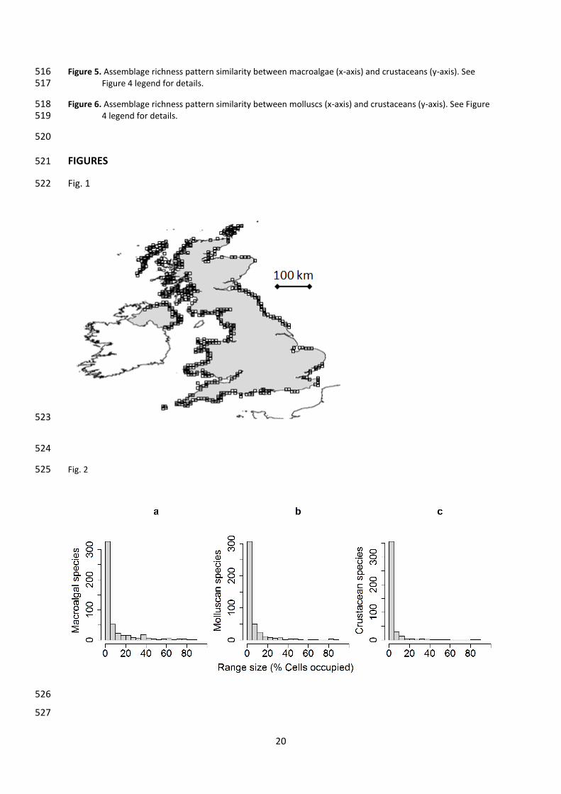
The majority of species from all three taxa were rare (Fig. 2) although some species from each were 183

present across the majority of the study extent (e.g. Fucus vesiculosus Linnaeus, 1753, Mytilus edulis 184

Linnaeus, 1758, and Semibalanus balanoides (Linnaeus, 1767); the most widespread species for 185

macroalgae, molluscs and crustaceans, respectively). Full assemblage correlations were highest 186

between macroalgae and crustaceans (r = 0.679, d.f. = 180.6, p < 0.0001), followed by molluscs and 187

crustaceans (r = 0.579, d.f. = 211.8, p < 0.0001), and finally macroalgae and molluscs (r = 0.514, d.f. = 188

225.3, p < 0.0001). 189

Within-taxon structure 190

Within-taxa species richness was found to be strongly determined by common species for all three 191

groups (Fig. 3a-c). When the contribution of individual species was adjusted for their binomial 192

9

variance (Fig. 3d-f), rare species were more strongly associated with the full species richness than 193

common species for all three taxa. 194

Between-taxa structure 195

We classified the correlation surface plots into three general patterns to aid discussion of the results 196

(Table 1). A peak in correlation strength situated closer to the origin (few species used, e.g. Fig. 4a) 197

than to the complete assemblages point (top right corner) is a Small Assemblage Peak (SAP). The 198

opposite trend to a SAP, with a peak in correlation strength situated closer to the full assemblages 199

point (top right, e.g. Fig. 5d), is a Large Assemblage Peak (LAP). We observed a third major pattern of 200

a gradient sloping from one side to the other or top to bottom (e.g. Fig. 4f), indicating that the value 201

of the cross-correlation coefficient is relatively unaffected by one of the two compared assemblages. 202

Because this pattern was consistently observed for rare v. common comparisons (i.e. rare to 203

common series v. common to rare series), we called this the Rare-Common Trend (RCT). 204

Cross-correlations between common sub-assemblages consistently displayed a SAP (panel (a) in 205

Figures 4 - 6), where a peak in correlation strength was reached, not immediately, but with fewer 206

than 60 species. When species’ cumulative contribution to the sub-assemblage was scaled for range 207

size (panel (e) in Figures 4 - 6) the effect was an emphasis of the SAP. Maximum correlations 208

between taxa sub-assemblage pairs were the strongest between common sub-assemblages, where 209

values approached r = 0.8 (all p < 0.0001). Although these were consistently stronger than the 210

correlations between the full taxonomic assemblages, maximum strength between common sub-211

assemblages of taxa pairs was not always proportional to the respective full assemblage correlation 212

strength between taxa pairs (Table 1). The SAP generally did not fall on the y = x line but was 213

displaced towards macroalgae in both comparisons involving them (e.g. Fig. 4a), demonstrating that 214

common consumer sub-assemblages (molluscs or crustaceans) tend to be present alongside 215

relatively larger sub-assemblages of common macroalgae (rather than common sub-assemblages of 216

both being similar sized). This effect held after scaling for range size and taxon assemblage size. 217

10

In no cases were common sub-assemblages strongly correlated with rare sub-assemblages (i.e. no 218

SAP patterns, panels (b) and (c) in Fig. 4 - 6), or vice versa. Instead, RCT patterns showed that rare 219

sub-assemblage distributions matched the distribution patterns of full assemblages between taxa. 220

Peak correlation strength varied idiosyncratically relative to the full assemblage correlation between 221

taxa, with the strongest peak between macroalgal full assemblages and rare molluscan sub-222

assemblages (> 10 composite singleton species, r > 0.6, p < 0.0001). However, caution is warranted 223

for the interpretation of correlations including small sub-assemblages, which are likely to have non-224

Gaussian richness distributions. In any case, scaling for range size (panels (f) and (g) in Fig. 4 - 6) 225

clarified the RCT pattern and emphasised the relationship between full assemblages and rare sub-226

assemblages. 227

Zero or very weak correlations (r < 0.2) were found between rare sub-assemblages in two out of 228

three cases (panels (d) in Fig. 4 – 5, consumer taxa against macroalgae) following a LAP pattern. 229

Molluscs and crustaceans (Fig. 6d) demonstrated the only case of a SAP pattern for the rare v. rare 230

case, with small sub-assemblages of rare species being moderately correlated (> 14 singleton 231

species, r > 0.4, maximum r = 0.64, p < 0.0001, between sub-assemblages of 150 molluscan species, 232

range sizes 1 – 4 cells, and 270 crustacean species, range sizes 1 – 5 cells). However, scaling for range 233

size reduced the difference between taxa pairs, de-emphasising the peak between molluscs and 234

crustaceans, and amplifying the LAP patterns (panels (h) in Fig 4 – 6). Correlation strengths were 235

consistently stronger between rare v. rare sub-assemblage pairs than between common v. rare sub-236

assemblage pairs (range size scaled panels (h) v. (f-g) in Fig 4 – 6). 237

DISCUSSION 238

We found that common species drive richness pattern similarity between taxa. This shows a parallel 239

with common species driving richness patterns within taxa, although the underlying reasons for this 240

parallel may not be the same. From comparison of the three taxa we found strongly matching 241

distributions (SAP type) between common species sub-assemblages and weakly matching 242

11

distributions (LAP type) between rare species sub-assemblages. This conclusion was further 243

emphasised by scaling species by their range size. This scaling also reduced the prominence of the 244

single observation of a SAP pattern between rare sub-assemblages of molluscs and crustaceans, 245

suggesting this feature may be of minor significance. 246

Our specific hypotheses of relative correlation strength between taxa full assemblage patterns were 247

not supported, with the strongest correlation observed between crustaceans and macroalgae, rather 248

than crustaceans and molluscs as predicted. Instead of trophic similarities (autotrophy v. 249

heterotrophy) underlying taxa species richness associations (Wolters et al., 2006), a stronger 250

dependence of crustaceans upon the habitat structure provided by macroalgae may be responsible 251

for the strong association between crustacean and macroalgal richness. Habitat structure provided 252

by macroalgae, especially canopy formers, can provide shelter from predation and desiccation stress 253

(Bégin et al., 2004), potentially facilitating populations of many crustacean species which might 254

benefit more from this cover than molluscs. 255

The observed SAP patterns showed maximum cross-correlations to be much stronger than the full-256

assemblage correlations. This demonstrates that, at least in the cases studied here, common species 257

reinforce, and are central to, the congruency between full assemblage richness patterns of different 258

taxa, allowing the use of taxonomic ‘surrogates’ or ‘indicators’ (e.g. Hess et al., 2006). Maximum SAP 259

cross-correlations were not proportional to, and therefore not predictable by, the correlation 260

strengths between full assemblages of the taxa pairs. Instead, the addition of rarer species, reducing 261

the cross-correlation strength, was still important in determining the extent of full assemblage 262

similarity. We found correlations between full assemblages that were substantially higher (e.g. rmin = 263

0.51, rmax = 0.68) than those reported in meta-analyses (e.g. r = 0.37 from Wolters et al. 2006, and a 264

‘Species Accumulation Index’ = 0.41, interpretable similarly to an r value, from Rodrigues & Brooks, 265

2007). Pearman & Weber (2007), despite a negative correlation (r = -0.19, p = 0.25) between bird 266

and butterfly full assemblages, also found that their most common species sub-assemblage was the 267

12

only one that was significantly correlated among all three of their taxa, with correlation strengths 268

exceeding those of full assemblages. Coastal marine taxa may show relatively strong congruency 269

(Tittensor et al., 2010) and our study’s constraint to the intertidal habitat may have increased the 270

likelihood of environmental drivers similarly affecting the distributions of species from the different 271

taxa. After splitting their datasets into high and low altitude subsets, Pearman & Weber (2007) 272

concluded that (within-taxa) correlation strength could be affected by the range of habitat 273

heterogeneity covered by the data (hence also scale and extent; Hess et al., 2006). For instance, if 274

our study extended offshore, where waters increased in depth (increasing habitat heterogeneity), 275

we might have observed a decrease in between-taxa correlation between macroalgae and the 276

consumer taxa as macroalgal species distributions are limited to the photic zone while many 277

consumer species distributions do not directly need light to survive. These examples illustrate the 278

potential effect of environment on the observed between-taxa relationships, which vary between 279

studies (Hess et al., 2006; Wolters et al. 2006; Rodrigues & Brooks, 2007). 280

The displacement in the precise location of the SAP relative to the line y = x towards larger 281

macroalgal common sub-assemblages suggests that between-taxa sub-assemblage associations need 282

not be balanced by numbers of species, nor sub-assemblage relative commonness. Depending on 283

the degree of skewness of the taxon species occupancy distributions, between-taxa associations may 284

peak upon inclusion of less common species from one taxon, such as the ‘frequent’ and ‘occasional’ 285

species we observed for macroalgae. 286

Rare sub-assemblages were not completely uncorrelated between taxa, and generally showed 287

stronger cross-correlations than those between rare and common sub-assemblages. These weak 288

correlations suggest that rare species of different taxa do have a slight tendency to be found 289

together. Traditional means of defining species ‘hotspots’ often indicate little overlap between taxa 290

(Prendergast et al., 1993a; Reid, 1998; Orme et al., 2005), most likely because reasons for 291

occurrence of different rare species from different taxa are inconsistent. The within-taxon analyses 292

13

show that rare species distributions tend to more strongly associate with full assemblage 293

distributions after taking into account binomial variance (Fig. 3; Lennon et al., 2004; 2011; Šizling et 294

al., 2009). This pattern may arise due to the nestedness of species distributions (characteristic of 295

metacommunities and mutualistic networks; Almeida-Neto et al., 2008), where rare species’ 296

occurrences typically tend to fall on top of those of common species (Šizling et al., 2009; Heegaard et 297

al., 2013). A parallel observation in our study saw relatively high cross-correlations between the 298

distributions of rare sub-assemblages and full assemblages of different taxa (RCT patterns), although 299

these cross-correlations did not achieve the strength of within-taxon correlations between 300

distributions of similarly sized rare sub-assemblages and full assemblages. 301

We observed only one instance of a strong cross-correlation (SAP) between rare sub-assemblages, 302

for molluscs and crustaceans. We first explored the possibility that this might emerge because of 303

sampling effort. Working with NBN data on intertidal macroalgae and molluscs, Blight et al. (2009) 304

detected that cells occupied by university marine stations topped the ranks of raw species richness 305

for both. However we observed rare macroalgal sub-assemblages to be distributed dissimilarly to 306

molluscan sub-assemblages (either rare or common). It is possible that experts in the consumer taxa 307

and experts in macroalgae may not frequent the same areas. Upon examination of the geographical 308

distribution of molluscan and crustacean sub-assemblages at this peak of cross-correlation, some of 309

the peaks of co-occurrence fell close to marine stations (possibly well-frequented study sites), but 310

this did not account for all large peaks, nor the numerous minor sites of co-occurrence that were 311

spread across the country. Therefore the cross-correlation peak between molluscan and crustacean 312

rare sub-assemblages does not appear to be solely due to proximity to marine stations. Potential 313

ecological explanations include rare habitat types important for both consumer taxa, but not for 314

macroalgae (intertidal caves for example). Macroalgae require sunlight, mostly inorganic chemicals, 315

and are essentially bound to solid substrate, whilst the consumer taxa are generally not restricted by 316

these conditions (though there are exceptions, such as sessile barnacles in Crustacea). Molluscs and 317

crustaceans can be diverse in sedimentary habitats (e.g. Ellingsen, 2002), whilst macroalgae are 318

14

more restricted to solid substrata (again, there are exceptions). In our case this between-taxa 319

clustering of rare species was likely to be partly attributable to some sites of high sampling effort. 320

Overlap and clustering of UK rare benthic species’ distributions (10 km grain) has been found 321

previously by Sanderson (1996), using a small sample of rare species with reliable distributions (data-322

deficient species were removed). In south-east Australia, although from a small sample size (15 323

sites), Gladstone (2002) recorded a strong correlation (r = 0.93, non-spatial p < 0.01) between 324

molluscan species and species of all taxa, both richnesses weighted to emphasise rare species. Rare 325

species will always be sensitive to sampling effort (e.g. difficult to detect species; Boulinier et al., 326

1998), and are frequently regarded as ‘noise’ and recommended for removal prior to analysis (e.g. 327

Clarke & Green, 1988; Cottenie & De Meester 2003), despite their potential functional importance 328

(Emmerson et al., 2001; Lyons et al., 2005). 329

While our common-to-rare sequences always began with the same commonest (few) species, the 330

rare-to-common sequences did not start with any particular rarest species because there were many 331

such candidates, and so each cross-correlation resulted from a bootstrap over many permutations of 332

randomly ranking the tied ranks (singletons, doubletons, and so forth). This is important because the 333

identity of the commonest species is likely to be ecologically significant (e.g. in species interactions 334

and ecosystem functioning; O’Connor & Crowe, 2005; Gaston, 2010), but the identity of singleton 335

species may not always be important (notwithstanding chance or transient occurrences; Novotný & 336

Basset, 2000; Magurran & Henderson, 2003). 337

Common species have been suggested as responsible for the majority of certain ecosystem functions 338

and services (Walker, 1992; Gaston, 2010) and indeed it would be surprising if this were not the 339

case. Our conclusions suggest that the processes that limit the range of common species may be 340

generally consistent across taxa, provided that certain conditions are maintained (for example, that 341

taxa share the same broadly defined habitat). Studies that have associated patterns of common sub-342

assemblages with environmental variables have suggested that common species are environmental 343

15

generalists (Evans et al., 2005; Lennon et al., 2011) that share an aversion to particularly hostile 344

habitats (e.g. low energy habitats; Evans et al., 2005). 345

Most studies of the contribution of common and rare species to full richness patterns have been 346

from birds (e.g. Lennon et al., 2004; Evans et al., 2005; Pearman & Weber, 2007), which are usually 347

well sampled and have large accessible datasets (e.g. Boulinier et al., 1998). Our study from a marine 348

perspective covering both primary producers (macroalgae) and consumers (molluscs and 349

crustaceans) widens the potential generality of these patterns across realms (Dawson & Hamner, 350

2008; Webb, 2012). In our analysis all three marine intertidal taxa supported the emerging general 351

trend that, typically (i.e. with right-skewed species’ occupancy distributions, Heegaard et al., 2013), 352

common species drive species richness patterns (Jetz & Rahbek 2002, Lennon et al., 2004), but when 353

species’ contributions are corrected for their range size it is typically the rare species that are most 354

associated with overall richness patterns (Lennon et al., 2004; Šizling et al., 2009). Atypical datasets 355

(in which species occupancy distributions are not right-skewed) may still present complications 356

(Šizling et al., 2009; Heegaard et al., 2013), which is an important potential limit to generalisation. 357

358

ACKNOWLEDGEMENTS. CJR was funded by the Department of Employment and Learning 359

Northern Ireland as part of his PhD thesis. We thank dataset providers British Phycological Society, 360

Natural Resources Wales, Conchological Society of Great Britain & Ireland, English Nature, Joint 361

Nature Conservation Committee, Marine Biological Association, Centre for Environmental Data and 362

Recording, Marine Conservation Society, and Scottish Natural Heritage. 363

364

REFERENCES 365

Almeida‐Neto, M., Guimaraes, P., Guimarães, P.R., Loyola, R.D. & Ulrich, W. (2008) A consistent metric for 366 nestedness analysis in ecological systems: reconciling concept and measurement. Oikos, 117, 1227-367 1239. 368

16

Bégin, C., Johnson, L.E. & Himmelman, J.H. (2004) Macroalgal canopies: distribution and diversity of associated 369 invertebrates and effects on the recruitment and growth of mussels. Marine Ecology Progress Series, 370 271, 121-32. 371

Blight, A.J., Allcock, L.A., Maggs, C.A. & Johnson, M.P. (2009) Intertidal molluscan and algal species richness 372 around the UK coast. Marine Ecology Progress Series, 396, 235-243. 373

Boulinier, T., Nichols, J.D., Sauer, J.R., Hines, J.E. & Pollock, K.H. (1998) Estimating species richness: The 374 importance of heterogeneity in species detectability. Ecology, 79, 1018–1028. 375

Cairns, D.K., Gaston, A.J. & Huettmann, F. (2008) Endothermy, ectothermy and the global structure of marine 376 vertebrate communities. Marine Ecology Progress Series, 356, 239-250. 377

Clarke, K.R. & Green, R.H. (1988) Statistical design and analysis for a" biological effects" study. Marine Ecology 378 Progress Series, 46, 213-226. 379

Cornwell, W.K. & Ackerly, D.D. (2010) A link between plant traits and abundance: evidence from coastal 380 California woody plants. Journal of Ecology, 98, 814-821. 381

Cottenie, K. & De Meester, L. (2003) Connectivity and cladoceran species richness in a metacommunity of 382 shallow lakes. Freshwater Biology, 48, 823-832. 383

Dawson, M.N. & Hamner, W.M. (2008) A biophysical perspective on dispersal and the geography of evolution 384 in marine and terrestrial systems. Journal of the Royal Society Interface, 5, 135-150. 385

Dutilleul, P., Clifford, P., Richardson, S. & Hemon, D. (1993) Modifying the t test for assessing the correlation 386 between two spatial processes. Biometrics, 49, 305-314. 387

Ellingsen, K.E. (2002) Soft-sediment benthic biodiversity on the continental shelf in relation to environmental 388 variability. Marine Ecology Progress Series, 232, 15-27. 389

Emmerson, M.C., Solan, M., Emes, C., Paterson, D.M. & Raffaelli, D. (2001) Consistent patterns and the 390 idiosyncratic effects of biodiversity in marine ecosystems. Nature, 411, 73-77. 391

Evans, K.L., Greenwood, J.J. & Gaston, K.J. (2005) Relative contribution of abundant and rare species to 392 species–energy relationships. Biology letters, 1, 87-90. 393

Faith, D. P. (1992) Conservation evaluation and phylogenetic diversity. Biological Conservation, 61, 1-10. 394

Field, R., Hawkins, B.A., Cornell, H.V., Currie, D.J., Diniz‐Filho, J.A. F., Guégan, J.F., Kaufman, D.M., Kerr, J.T., 395 Mittelbach, G.G., Oberdorff, T., O’Brien, E.M. & Turner, J.R. (2009) Spatial species‐richness gradients 396 across scales: a meta‐analysis. Journal of Biogeography, 36, 132-147. 397

Gaston, K.J. (2010) Valuing common species. Science, 327, 154-155. 398

Gaston, K.J. (1994) Rarity, pp. 2. Chapman & Hall, London. 399

Gladstone, W. (2002) The potential value of indicator groups in the selection of marine reserves. Biological 400 Conservation, 104, 211-220. 401

Grinnell, J. (1922) The role of the" accidental". The Auk, 39, 373-380. 402

Heegaard, E., Gjerde, I. & Sætersdal, M. (2013) Contribution of rare and common species to richness patterns 403 at local scales. Ecography, 36, 937–946, 404

Hess, G.R., Bartel, R.A., Leidner, A.K., Rosenfeld, K.M., Rubino, M.J., Snider, S.B. & Ricketts, T.H. (2006). 405 Effectiveness of biodiversity indicators varies with extent, grain, and region. Biological Conservation, 406 132, 448-457. 407

17

Hourigan, T.F., Timothy, C.T. & Reese, E.S. (1988) Coral reef fishes as indicators of environmental stress in coral 408 reefs. In Marine Organisms as Indicators, pp. 107-135. Springer, New York. 409

Jetz, W. & Rahbek, C. (2002) Geographic range size and determinants of avian species richness. Science, 297, 410 1548-1551. 411

Kreft, H., Sommer, J.H. & Barthlott, W. (2006) The significance of geographic range size for spatial diversity 412 patterns in Neotropical palms. Ecography, 29, 21-30. 413

Lennon, J.J., Koleff, P., Greenwood, J.J. & Gaston, K.J. (2004) Contribution of rarity and commonness to 414 patterns of species richness. Ecology Letters, 7, 81-87. 415

Lennon, J.J., Beale, C.M., Reid, C.L., Kent, M. & Pakeman, R.J. (2011) Are richness patterns of common and rare 416 species equally well explained by environmental variables? Ecography, 34, 529-539. 417

Lyons, K.G., Brigham, C.A., Traut, B.H. & Schwartz, M.W. (2005) Rare species and ecosystem functioning. 418 Conservation Biology, 19, 1019-1024. 419

Magurran, A.E. & Henderson, P.A. (2003) Explaining the excess of rare species in natural species abundance 420 distributions. Nature, 422, 714-716. 421

Matias, M.G., Chapman, M.G., Underwood, A.J. & O'Connor, N.E. (2012) Increasing density of rare species of 422 intertidal gastropods: tests of competitive ability compared with common species. Marine Ecology 423 Progress Series, 453, 107-116. 424

Myers, N., Mittermeier, R.A., Mittermeier, C.G., Da Fonseca, G.A. & Kent, J. (2000) Biodiversity hotspots for 425 conservation priorities. Nature, 403, 853-858. 426

Novotný, V. & Basset, Y. (2000) Rare species in communities of tropical insect herbivores: pondering the 427 mystery of singletons. Oikos, 89, 564-572. 428

O'Connor, N.E. & Crowe, T.P. (2005) Biodiversity loss and ecosystem functioning: distinguishing between 429 number and identity of species. Ecology, 86, 1783-1796. 430

Orme, C.D.L., Davies, R.G., Burgess, M., Eigenbrod, F., Pickup, N., Olson, V.A., Webster, A.J., Ding, T., 431 Rasmussen, P.C., Ridgely, R.S., Stattersfield, A.J., Bennett, P.M., Blackburn, T.M., Gaston, K.J. & 432 Owens, I.P. (2005) Global hotspots of species richness are not congruent with endemism or threat. 433 Nature, 436, 1016-1019. 434

Pachepsky, E., Crawford, J.W., Bown, J.L. & Squire, G. (2001) Towards a general theory of biodiversity. Nature, 435 410, 923-926. 436

Pearman, P.B. & Weber, D. (2007) Common species determine richness patterns in biodiversity indicator taxa. 437 Biological Conservation, 138, 109-119. 438

Prendergast, J.R., Quinn, R.M., Lawton, J.H., Eversham, B. C. & Gibbons, D. W. (1993a) Rare species, the 439 coincidence of diversity hotspots and conservation strategies. Nature, 365, 335-337. 440

Prendergast, J., Wood, S., Lawton, J. & Eversham, B. (1993b) Correcting for variation in recording effort in 441 analyses of diversity hotspots. Biodiversity Letters, 1, 39-53. 442

Preston, F.W. (1948) The commonness, and rarity, of species. Ecology, 29, 254-283. 443

R Development Core Team (2008) R: A language and environment for statistical computing. R Foundation for 444 Statistical Computing, Vienna, Austria. http://www.R-project.org 445

Reid, W.V. (1998) Biodiversity hotspots. Trends in Ecology & Evolution, 13, 275-280. 446

Rodrigues, A.S.L. & Brooks, T.M. (2007) Shortcuts for Biodiversity Conservation Planning: The Effectiveness of 447 Surrogates. Annual Review of Ecology, Evolution, and Systematics, 38, 713–37. 448

18

Siqueira, T., Bini, L.M., Roque, F.O., Marques Couceiro, S.R., Trivinho‐Strixino, S. & Cottenie, K. (2012) Common 449 and rare species respond to similar niche processes in macroinvertebrate metacommunities. 450 Ecography, 35, 183-192. 451

Šizling, A.L., Šizlingová, E., Storch, D., Reif, J. & Gaston, K.J. (2009) Rarity, commonness, and the contribution of 452 individual species to species richness patterns. The American Naturalist, 174, 82-93. 453

Tittensor, D.P., Mora, C., Jetz, W., Lotze, H.K., Ricard, D., Berghe, E.V. & Worm, B. (2010) Global patterns and 454 predictors of marine biodiversity across taxa. Nature, 466, 1098-1101. 455

Vallejos, R., Osorio, F., & Cuevas, F. (2013) SpatialPack - An R package for computing spatial association 456 between two stochastic processes defined on the plane. Submitted. 457

Vázquez, L.B. & Gaston, K.J. (2004) Rarity, commonness, and patterns of species richness: the mammals of 458 Mexico. Global Ecology and Biogeography, 13, 535-542. 459

Walker, B.H. (1992) Biodiversity and ecological redundancy. Conservation Biology, 6, 18-23. 460

Webb, T.J. (2012). Marine and terrestrial ecology: unifying concepts, revealing differences. Trends in ecology & 461 evolution, 27, 535-541. 462

Wolters, V., Bengtsson, J. & Zaitsev, A.S. (2006) Relationship among the species richness of different taxa. 463 Ecology, 87, 1886-1895. 464

WoRMS Editorial Board (2013) World Register of Marine Species. Available from 465 http://www.marinespecies.org at VLIZ. Accessed 2013-11-28 466

Wright, D.H., Currie, D.J. & Maurer, B.A. (1993) Energy supply and patterns of species richness on local and 467 regional scales. In: Species diversity in ecological communities: historical and geographical 468 perspectives. (ed. by R.E. Ricklefs & D. Schluter), pp. 66-74. Chicago University Press, Chicago. 469

470

BIOSKETCH 471

Carl Reddin is quantitative marine ecologist with an interest in macroecological methods and their 472

use to extend our understanding of biodiversity patterns across realms. 473

John Bothwell works on seaweed, primarily on their evolution and systematics, but also on their 474

bioenergy potential and ecological importance along the UK’s coastlines. 475

Jack Lennon's main research interests include understanding how environmental constraints and 476

processes act on the spatial and temporal distribution of species to create and maintain emergent 477

diversity patterns. 478

479

19

TABLES 480

Table 1. Maximum correlation between taxa (of any sub-assemblage comparison i.e. the peak value 481 in the correlation surfaces shown in Figure 4-6) and its coordinates on the unscaled correlation 482 surfaces, given as the proportion of each full assemblage represented by the sub-assemblages 483 correlated (Common, C; Rare, R). Also given is a classification of the cross-correlation plots according 484 to major surface trends (Small Assemblage Peak, SAP; Rare Common Trend, RCT; Large Assemblage 485 Peak, LAP). The correlation for the full taxon comparisons, in bold, is given as rtotal. Figure numbers 486 for the correlation surfaces are indicated. 487

Sub-assemblage pair C v. C C v. R R v. C R v. R

Figure a,e b,f c,g d,h

Type Type Type Type

Macroalgae v. molluscs 4 SAP RCT RCT LAP

Macroalgae v. crustaceans 5 SAP RCT RCT LAP

Molluscs v. crustaceans 6 SAP RCT RCT SAP

rtotal rmax rmax rmax rmax

Macroalgae v. molluscs 0.51 0.79 (.05, .02) 0.63 (1.0, .04) 0.53 (.21, 1.0) 0.51 (1.0, 1.0)

Macroalgae v. crustaceans 0.68 0.76 (.09, .04) 0.72 (.93, .27) 0.69 (.53, 1.0) 0.69 (.96, 1.0)

Molluscs v. crustaceans 0.58 0.74 (.05, .05) 0.60 (1.0, .09) 0.61 (.10, 1.0) 0.64 (.35, .63)

488

489

FIGURE LEGENDS 490

Figure 1. Coastline map of the UK showing the 10 km cells (n = 522) occupied by at least one record for each 491 taxon. Latitude min = 50°N, max = 59°N, approximately. 492

Figure 2. The range size of intertidal species, (a) macroalgae, (b) molluscs and (c) crustaceans, showing that 493 most species were rare (small range size). Total cell numbers were 522 for all taxa. 494

Figure 3. The correlation of sub-assemblages built from common to rare (thin solid line), or rare to common 495 (dashed line), with the full species richness for macroalgae (a & d), molluscs (b & e) or crustaceans (c 496 & f). The top row (a-c) shows sub-assemblages built species-by-species, from a single species to the 497 full species richness, while the bottom row (d-f) shows sub-assemblages built from cumulative 498 binomial variance (species contribute varying amounts depending upon their occupancy). The grey 499 region shows the null hypothesis of correlation with the full assemblage (95% confidence intervals of 500 the mean, while the thick solid line is the median, derived from 104 randomly permuted 501 accumulations of species from the species pool). 502

Figure 4. Assemblage richness pattern similarity between macroalgae (x-axis) and molluscs (y-axis). Axes 503 represent sub-assemblages, built species-by-species from the origin of the plot, beginning with: 504 commonest ‘x’ against commonest ‘y’ (panels a,e); commonest ‘x’ against rarest ‘y’ (panels b,f); rarest 505 ‘x’ against commonest ‘y’ (panels c,g); rarest ‘x’ against rarest ‘y’ (panels d,h); the diagonal line is y = 506 x, equal assemblage growth. Top row (panels a,b,c,d) represents unscaled sub-assemblages, 507 increasing by species number (i.e. each species contributes ‘1’ to the sub-assemblage), while bottom 508 row (panels e,f,g,h) represents scaled sub-assemblages, by increasing species binomial variance (i.e. 509 weighting by information content) scaled in proportion to the largest assemblage size; the smaller 510 assemblage was multiplied by the size difference between the two taxonomic assemblages, putting 511

the smaller assemblage on equal footing with the larger, 𝑝𝑎 (1 − 𝑝𝑎) (∑ 𝑝𝑏 (1−𝑝𝑏)

∑ 𝑝𝑎(1−𝑝𝑎)) , where pa and pb 512

were range sizes, as proportions of total study area, for the taxon of smallest and largest full 513 assemblage size, respectively. Delineated grey regions are regions where the correlations were not 514 significant (p > 95, corrected for spatial autocorrelation). 515

20

Figure 5. Assemblage richness pattern similarity between macroalgae (x-axis) and crustaceans (y-axis). See 516 Figure 4 legend for details. 517

Figure 6. Assemblage richness pattern similarity between molluscs (x-axis) and crustaceans (y-axis). See Figure 518 4 legend for details. 519

520

FIGURES 521

Fig. 1 522

523

524

Fig. 2 525

526

527

21

Fig. 3 528

529

530

Fig. 4 531

532

533

22

Fig. 5 534

535

Fig. 6 536

537