VIEMORANDUM

IM-4697-PR)CTOBER 1966

AN ANALYSIS OFMAJOR SCHEDULING TECHNIQUES

IN THE DEFENSE SYSTEMS ENVIRONMENT

J. N. Holtz°""• _ .• C L,, ,.E A R I 14GHO0U S E

Lg INYMORSDDC

SJAN 12 1967

REPARED FOR: CWNITED STATES AIR FORCE PROJECT RAND

SANTA MONICA * CALIFORNIA

Best Available Copy 00

DISCLAER NOTICI

THIS DOCUMENT IS BESTQUALITY AVAILABLE. THE COPYFURNISHED TO DTIC CONTAINEDA SIGNIFICANT NUMBER OFPAGES WHICH DO NOTR-PRODUCE LEGIBLY.

REPRODUCED FROMBEST AVAILABLE COPY

MEMORANDUM

RM-4697-PROCTOBER 1966

AN ANALYSIS OFMAJOR SCHEDULING TECHNIQUES

IN THE DEFENSE SYSTEMS ENVIRONMENTJ. N. Holtz

This research is stupJportd by the United States Air Forc-e 'under Project RAND-Con-tract No. AF 19(638) 17(K)-monitored hy the Directorate of Operational Requirementsand Development Plansz, Deputy Chief of Staff. Research and I)evevopment. Hq USAF.Views or conMlusons contained in this Memorandu<m should not be interprgted, asrepres.enting the official opinion or po*ly jthe Unite-dyStates Air Force. ...

DISTRIBUTION STATEMENTDistribution of this document is unlimited.

f700 MAIN ST SANTA MONICA * CAtI0OINI& tA 4*4

?dA%4) + +4+jX

PREFACE

The acquisition of a major new weapon system is a complex process

involving numerous technologies, agencies, firms, and personnel. If

the delivery schedule for a priority military program is to be attained,

these diverse factors must be coordinated. Although formal scheduling

techniques were in use over a half century ago, the shifting technolog-

ical environment has made it necessary to adapt old techniques and de-

velop new ones to manage the many factors involved in current weapon

system development. Recently, defense requirements have stimulated the

generation of numerous scheduling systems, each offering some promise

for improving ptject management. This proliferation of techniques has

in turn created pressures for their standardization.

This Memorandum surveys, compares, and evaluates the major sched-

uling techniques currently available to project management, and suggests

areas for improvement. A comparison of existing techniques indicates

that although some are relatively advanced, various aspects still re-

quire addieional development and refinement.

The study should be of interest to scheduling departments ranging

from first-line supervision in contractor organizations through system

project offices and headquarters groups. It should also be useful in

schools or training organizations that instruct personnel in the use of

scheduling techniques. Hopefully, it will stimulate efforts to advance

the state of the art in scheduling techniques, either by incremental

improvements on existing techniques, or through development of substan-

tially new systems.

i/

SmeMARY

This Memorandum has three main objectives: (1) to describe simply

and clearly the major characteristics and operating features of each

of the more important scheduling techniques currently available to mil-

itary management; (2) to compare and evaluate the techniques in terms

of their applicability to the acquisition of weapon systems; and (3)

to define areas for further research leading to improvement in the sched-

uling state of the art.

The nature of the systems acquisition environment, with its inher-

ent complexities, is first examined in some detail, and criteria are

established for comparing the various scheduling techniques. In de-

scribing each system, attention is paid to its appropriateness in the

scheduling of both development and production activities. Since the

newr -nd more unique scheduling requirements are generated in the de-

velopment phase, they are illustrated by applying the essential features

of each technique to a common hypothetical missile system development program.

Among the basic scheduling techniques are the

Gantt Chart,

Milestone Chart,

Line of Balance Technique,

Critical Path Method, and the

Program Evaluation and Review Technique (PERT).

In addition, variations of these have frequently been used by individ-

ual organizations for specific applications. The features of each of

the basic techniques are described and compared in this Memorandum.

A discussion of the extent to which these techniques satisfy sched-

uling demands suggests certain areas where additional study is needed

to develop a comprehensive and reasonably uniform system covering the

total life cycle of a project. As might be expected, each of the tech-

niques has its own most appropriate areas of application. Limitations

in alternative applications range from minor to serious, depending on

the application. Among the broader observations are the following:

(a) The network is particularly significant as a planning device because

-vii-

ACKNOLEDGEMNT

The author would like to express his appreciation to F. S. Pardee

of The RAND Corporation, who proposed this study, offered many sugges-

tions for its organization, and coimiented extensively on its various

draft versions.

"-ix-

CONTENTS

PREFACE ..... *.. **** * *... .. **.. . .. ..... .... . iiiSUMMARY ........................... ............................ l

AC KN DGMENT ................................................ vii

FIGURES ........................... . xi

TABLES ........................................................ xiii

SectionI. INTRODUCTION ................................

The Weapon System Acquisition Environment .............. 1Criteria for Comparison of Alternative Scheduling

Techniques ............................................ 5Missile System Development Example ...... .............. 7

II. GANTT AND MILESTONE CHARTS ............................... 10Gantt Technique ........................................ 10Milestone Technique .................................... 17

III. THE LINE OF BALANCE TECHN•IQUE (LOB) ...................... 22Application to Production Operations ............ 22Application to Development Operations .................. 26Evaluation of LOB Technique ............................. 33

IV. THE CRITICAL PATH METHOD (CPM) ........................... 35Application of CPM .................................. ... 35Application to the Model ............................... 43Evaluation of CPM ...................................... 47

V. PROGRAM EVALUATION AND REVIEW TECHNIQUE (PERT) ............ 50PERT Methodology ....................................... 50Application of PERT to Hypothetical Missile System ..... 59Evaluation of PERT ..................................... 64

VI. AREAS FOR FURTHER RESEARCH ............................... 67Greater Use of Data Available in Existing Scheduling

Systems .............................................. 67Use of Networks in the Selection of Alternativec ....... 68Integration of Cost-Performance Parameters with

Scheduling Techniques ................................ 69Development of a Technique for Identifying and

Processing Interfaces ................................. 70Simplification of Scheduling Techniques ................ 73Extension of Network Concepts to Top-level Management .. 76Need for New Scheduling Concepts and Techniques ........ 77

BIBLIOG;RAPHY ................................................... 79

.xi-

FIGURES

1. Gantt Man-Loading Chart .. . . . . .. . . ............. .... 12

2. Gantt Chart Showing Plan for Missile System Development 14

3. Gantt Chart Showing Progress against Plan ................. 16

4. Milestone Chart Applied to Missile Project ......... 20

5. The Line of Balance Technique ...... 23

6. LOB Prototype Development Objectives Chart ........ 27

LOB Prototype Development Plan Chart ............. 29

8. LOB Prototype Development Phase Progress Chart ............ 32

9. CPM Time-Cost Trade-off ................ .......... 42

10. CPM Network Applied to Hypothetical Missile System ........ 44

11. PERT: Planning and Operating Phases ..................... 54

12. PERT: Relationships among Networks ......... 60

13. PERT Network Applied to Hypothetical Missile System ....... 62

14. Network Integration and Condensation ..................... 72

15. Typical Use of Scheduling Techniques over a Project LifeCycle ................................................... 73

16. PERT/LOB Repetitive Activity Input/Output Plan ............ 75

-xiii-

TABLES

1. Data for the Missile System Development Examuple............. 8

2. Gantt Technique--Strengths and Weaknesses .................. 18

3. Supporting Data for Fig. 6 ....................... 27

4. Data for Overall Project Objectives Curve .................. 28

5. Supporting Computations for Fig. 8 ......................... 31

6. LOB Technique--Strengths and Weaknesses .................... 34

7. CPM Matrix Showing Earliest Start (ES) and Latest Com-pletion (LC) Times for Illustrative Example ............. 46

8. CPM Technique--Strengths and Weaknesses .................... 49

9. Computations Required for Probability of Positive Slack .... 63

10, PERT Technique--Strengths and Weaknesses ................... 66

1. INTRODUCTION

THE WEAPON SYSTEM ACQUISITION ENVIRONMENT

The aerospace industry, faced with time deadlines and using sophis-

ticated technology, requires scheduling techniques that are frequently

more advanced than those of the more traditional commercially oriented

finms. Consequently, the industry has devoted considerable effort in

the past decade to advancing the scheduling state of the art. The de-

vices discussed in this Memorandum, however, are not applicable solely

to defense-oriented systems. Several are used by industrial firms on

various commercial products, and these firms are increasingly adopting

the more aJvanced techniques.

This Memorandum attempts to survey, compare, and evaluate the major

scheduling techniques currently available to project management, and

to suggest areis for further research that may lead to improving these

techniques. To provide a framework for this analysis, the nature of

the weapon system acquisition environment must be clearly understood.

The following discussion describes several critical dimensions of this

environment: the life cycle of a weapon system--its built-in uncertain-

ties and dynamic character--the numerous firms involved in a given proj-

ect, and the hierarchies of project management existing in corporations

and agencies.

The Life Cycle of a Weapon System

Most, if not all, conmnercial products have a life cycle. Fad items--

hula hoops, for example--have a very short l'fe cycle. Other items--

such as stoves or refrigerators--have a longer cycle. Each new product

must be conceived, researched, designed, tested, produced, sold, and

serve itq function before it becomes obsolete.

Defense systems likewise have a life cycle, but their period of

usefulness is limited by changing operational requirements and advances

Readers already familiar with this environment may prefer to turndirectly to the subsequtnt material.

-2-

in technology. This life cycle usually consists of several phases:

(a) conceptual, (b) definition, (c) acquisition (including development

and production), and (d) operation.

From a scheduling standpoint, perhaps the most significant charac-

teristic of the life cycle is the change in the type of work performed

in each phase. In the conceptual and definition phases, emphasis is

on specifying the performance characteristics and hardware configura-

tions that will eventually result for the system. Here the effort is

primarily analytical, and activities are usually unique and varied.

In the development phase, the design, fabrication, and testing of

a limited number of prototypes are usually the primary functions. Fre-

quently, the vehicles used to test individual performance characteris-

tics may be quite dissimilar. The activities in the development phase,

although not highly repetitive, have reached the stage where enough in-

formation is available to permit the scheduling of resources to specific

functions. In a large weapon system development, interactions among

the activities are likely to be numerous, complex, and consequently,

formidable to manage. A comprehensive scheduling system is therefore

required to permit efficient management of the project.

When performance has been demonstrated by the prototypes, produc-

tion operations usually follow. Contractors are required to produce

quantities of the same item on a scale that on occasion approaches mass

production. By this time, most of the design uncertainty has been over-

come, and reasonably final production drawings exist for the components.

It is thus possible to make detailed subdivision of production opera-

tions and to control the use of resources on these operations.

Eventually the completed systems, and spares, are turned over to

the using commands--Strategic Air Command (SAC), Tactical Air Command

(TAC), etc.--which are responsible for their deployment and operation

until the systems become obsolete.

Managerial decisions affecting the project must be made throughout

all phases of the life cycle. The diverse nature of the activities in

each phase requires a variety of scheduling information. This Memoran-

dum will attempt to determine whether any single scheduling technique

is sufficiently versatile to be used throughout the entire life cycle

of a project.

-3-

Numerous Industrial Suppliers

The development of a new product frequently requires diverse tech-

nologies. An example is the recent coummercial development of petro-

chemicals, which was accomplished by forming joint subsidiaries combin-

ing technologies adapted to petroleum and chemical firms. Yet the de-

velopment of defense systems is substantially more complex than the

development of most commercial products. The technologies required

generally exceed the feasibly attainable capabilities of any one firm.

Consequently, defense firms frequently form arrangements similar to a

Joint venture. The simplest arrangement involves the designation of

one firm as a weapon system prime contractor, the other firms being

affiliated with it as subcontractors.

Another common arrangement is where several large firms become

associate contractors, each being responsible for developing a major

segment of the weapon system. For example, one associate contractor

is responsible for guidance, another for airframe, 4nother for propulsion,

etc. Frequently each associate contractor subcontracts a portion of

his project to another firm; the subcontractor may sub-subcontract a

smaller portion to yet another firm, etc. Such subcontracting fre-

quently involves thousands of industrial firms in the system develop-

ment effort.

A third arrangement is one similar to the associate contractor sys-

tem but with the addition of an integrating contractor whose function

is primarily to coordinate systems engineering and checkout for the

entire weapon system.

Many governmental agencies often furnish personnel, facilities,

or material to develop a system. Each industrial firm and governmental

agept cy, in turn, has more than one level of internal management. The

levels vary in number from firm to firm but range in scope from first-

line supervision to top management. Consequently, for a significant

weapon system there evolve a substantial number of managerial interre-

lationships. Each managerial group must be informed of plans and prog-

ress relating to its sphere of responsibility.

-4-

Program Monitors

It is obvious that in this environment some group or agency should

be responsitle for management of the entire project. In the Air Force

a System Project Office (SPO) is established in the appropriate division

of the Air Force Systems Conmand (AFSC) to provide this function. The

SPO is responsible for the project throughout the weaporn acquisition

phase. Upon completion and delivery of the hardware, the remaining re-

sponsibilities of the SPO are transferred to a weapon system manager

in the Air Force Logistics Command (AFLC). Responsibility for opration

of the weapon system in the field rests with one of the using cormtands

(i.e., SAC, TAC, ADC, etc.). The SPO, in conjunction with AFLC and the

training command (ATC), coordinates the planning for training and for

the maintenance and supply which will be required in the operational

phase of the system.

If many firms are to make portions of the system, some mechanism

should exist to ensure that all components will mate (interface) and

function properly in the completed system. The SPO has this responsi-

bility and accomplishes it with technical support either from in-house

systems engineering laboratories (those at Wright Field, for example)

or from nonprofit engineering concerns.

In defense contracting, the industrial firms deal with only one

consumer, the Government, and more specifically with the program man-

ager designated by the Department of Defense. The importance of

national defense, coupled with this monopsony (one buyer) situation,

naturally leads the Government to take a very active interest in the

progress of the system. The SPO is primarily responsible for directing

the program, while AFSC, Headquarters USAF, and the Office of the Sec-

retary of Defense (OSD) are also involved in reviewing its progress.

In addition, the Bureau of the Budget, Congressional comnmittees, and

even the President may become involved in a particular program from

time to time.

Again, it is essential that the information systems used for analy-"

zing program status be capable of directing pertinent information to

each of the appropriate agencies and individuals concerned.

The MITRE Corporation, Aerospace Corporation, etc.

SDynamic Nature of the Environment

To be useful in this environment a scheduling system also must be

responsive to extensive changes in the projects. The project life

cycle generally lasts a period of several years; frequently, develop-

ment effort alone will require four or five years. A mix of various

weapon systems is necessary to accomplish the objectives of national

defense. From time to time the assessment of the threat to our national

security may be modified, which in turn may alter the relative priority

of a given project in this mix or affect the amount of funds allocated

over time to the project. These factors often rcsult in either an ac-

celerated schedule or a program "stretchout."

Likewise, general technological advances and experience on a spe-

cific project frequently lead to design changes that affect the project

schedule. The scheduling system must respond to these changes if it

is to be useful to management.

CRITERIA FOR COMPARISON OF ALTERNATIVE

SCHEDULING TECHNIQUE S

It is difficult, if not impossible, to prepare a quantitative as-

sessment of the utility of a particular scheduling technique. It is

possible, however, to isolate features that are desirable and then to

assess the extent to which these features are satisfied. Although,

conceptually, it is possible to assign weights to each feature and

thereby construct an index of relative usefulness, thl 2dditional step,

being inherently subjective, will be left to the reader.

The following criteria are not intended to be comprehensive but

are sufficiently ba3ic to be helpful in estimating the strengths and

weaknesses of each technique. The discussion in the subsequent sections

should indicate the usefulness of these criteria in assessing various

systems.

1. Validity. The in'ormation contained in the system and pre-

sented to the appropriate levels of management should reflect genuine

progress. For example, suppose a guidance system is required to keep

a missile on course, and a gyroscope is an integral component of this

.6-

guidance system. If the gyroscope is improperly designed, a bias will

be introduced into the measurement of spatial relationships. Measure-

ments used in the guidance system will be invalid, that is, they will

not reflect the true state of affairs.

2. Reliability. The data contained in the system should be con-

sistent regardless of who obtains them or when they are obtained. In

the above example, suppose that the gyroscope were properly designed.

and thus capable of providing a valid measurement of attitude, but that

electrical pulses, external to the gyroscope, frequently altered its

motion and generated inconsistent readings. Readings used by the guid-

ance system would then be unreliable. Relating this example to sched-

uling techniques, the system may be well designed, and consequently

valid, yet subject to error because of weanesses in data collection,

and therefore unreliable. Or the reverse, that is, reliable yet invalid

results also are possible.

3. Implementation. A large number of personnel are likely to be

involved in furnishing inputs to and using outputs from a scheduling

system. Thus the technique should be easy to explain and understand,

and simple to operate.

4. Universality of Project Coverage. Ideally, one scheduling

system should be sufficient from beginning to end of a project life

cycle. All levels of maragement should be able to use the information

in the system, and all relevant factors to be controlled should be en-

compassed by the one system.

5. Sensitivity Testing (Simulation). Since management decision-

making involves selecting one course of action out of alternative pos-

sible courses, it is desirable to assess the scheduling implications

of these alternatives. A system that enables management to simulate

the impacts of alternative courses of action can facilitate the selec-

tion process and lead to better decisions concerning the project.

6. Forecnstlnq. One purpose of collecting data is to assess the

probability oi accomplishing future tasks. Some scheduling systems are

oriented tnore cx21l4 citly toward longer term operations than others.

7. L-iaatinS. Program decisions in a dynamic environment must be

based on curre:-. data. The scheduling system should be capable of in-

corporating rap.diy. and with ease, information on project progress.

-7-

8. Flexibility. A desirable feature in a scheduling technique

is its ability to adapt easily to changes in the project. This feature

is closely related to a simulation capability. The system must be flex-

ible if simulation of alternatives is to be possible, but a system may

be flexible without emphasizing simulation potential.

9. Cost., The scheduling system should provide the required in-

formation at the lowest cost. Cost is a difficult factor to measure

for several reasons. First, scheduling costs are not usually uniformly

recorded by industry and government, probably because the functions

attributable to collection of data in support of the system vary among

contractors. Also, total scheduling costs are needed to compare tech-

niques. In a Gantt system, for example, time standards are as much a

part of the cost as is chart preparation, yet this factor frequently

is not included in estimates of schedule cost.

Second, systems that are the most useful in terms of the above

criteria generally involve greater cost. Consequently, the appropriate

cost statistic is not total dollar cost, but rather cost per unit of

utility, or benefit. This cannot as yet be precisely measured.

Finally, cost is largely a function of the size of the program,

and implementation of each system involves both fixed and variable

costs. Thus, techniques with high fixed costs tend to be relatively

less expensive in large-scale applications and relatively more expen-

sive in small projects.

MISSILE SYSTEM DEVELOPMENT EXAMPLE

A hypothetical missile system has been selected to facilitate a

comparison of alternative scheduling techniques for the development

phiase of a project. Although the example is greatly abbreviated, it

will suffice to demonstrate the major characteristics of each technique.

Various nonstandard illustrations are used in describing applications

to production processes.

Table 1 contains all the basic data--events, activities, and time

estimates--needed to compare the scheduling techniques for the missile

system development example. The discussion in the various sections

throughout the Memorandum will draw upon this table.

ýoO' O - oa t ge o 4 ao-a-0 0-8-0 .3c

1.0 0 O 0 ~ 0 0 0 0 0 B 0 0 N 4

34, -8. C,41 0 VS

g B 0-'

? I Z- 00a- 4 5 " c-

c* t C* - c ,-0 P

1w, !. 0 0.M

CC 05 a c a- 0 a

0 0- t) 0 0d~ a

v C

0 E 5CC1A

VC ,V"CdO 0 E C

0 00g 0

C ~ ~ l -C s.w 1 ~ S V~ 0o ~ 'S ~C ~ SBS CCB - - - A V~BC CAV ~ * A

S SC U.A -. SC CCC SUU .A C ~ dS -a~S SBB ~ Ad BVV ~ S0 ~ - C B

CaC~ t~ n d~ aaC 5 050. CB UUSC.00 dB~d~d~ 1 Ad d 5 0 j d AAd10 S*C S S Ad~. -. A EB 3 C .. A BC dIB CSS CACC AS B

-9-

Project status is measured by the accomplishment of events repre-

senting significant points of partial completion of a project. Activ-

ities, on the other hand, occur over a time horizon. Each activity is

defined by a starting and an ending event. Resources are consumed by

activities rather than events. Decisions made by project management

may alter the levels and qualities of resources applied to activities.

Estimates of the time required to accomplish each activity are given

in Table 1. These estimates are indicated as "optimistic,' "most likely,"

and "pessimistic," and serve as the schedule data for the example.

Generally, the events and activities required to complete a compo-

Dnent or subsystem are dependent upon the results of the preceding ac-

tivities in that subsystem. Frequently, information generated through

performance on an activity in one subsystem also is essential to the

definition and performance of activities in a different subsystem.

For example, information concerning the size, weight, etc., of a mis-

sile must be obtained from the missile design before the launching

equipment can be designed and fabricated. In general, fabrication of

launching equipment is separate from fabrication of the missile except

for this information requirement. This relationship makes the activi-

ties interdependent. Such interdependencies must be considered in

scheduling projects. The relevant interdependencies are identified in

footnotes to Table I.

The meaning of optimistic, most likely, and pessimistic times isexplained in Section V.

.10-

L1. GANTT AND MILESTONE CHARTS

GANTT TECHNIQUE

The Gantt technique was the first formal scheduling system to be

used by management. The cornerstone of the technique is the Gantt

chart, which is basically a bar chart showing planned and actual per.

formance for those resources that management desires to control. In

addition, major factors that create variance (i.e., overproduction or

underproduction) are coded and depicted on the chart.

Application to Production Operations

The Gantt chart was designed for, and is most successfully applied

to, highly repetitive production operations. Normally, it assumes that

time standards are available for each operation and that the objective

of management is to obtain "normal" output from each major resource

employed, especially labor and machinery. If, for example, it has been

established that an average of 60 seconds (including personal time)

is required for a "typical" worker to assemble a cigarette lighter,

Developed by Henry L. Gantt in the late 1800s, the technique wasbased on the scientific management approach of Frederick W. Taylor.Prior to the twentieth century, management of productive operations wasloosely organized. Few standards existed by which performance couldbe gauged. In the 1880s, Taylor altered the process of management byattempting to substitute "scientific management" for "opinions" and"hunches" based on little factual data.

This "scientific method" involved identifying tasks and subtasksto be performed in the productive operations of the plant. The sub-tasks were refined into elementary work movements, which were "timed"to determine how much time each movement should require under normalworking conditions if performed by a "typical" operator. The elementaryoperations were then assigned to an operatir and their accumulatedtimes became a standard by which the operator's performance was measured.The variance, if any, between work planned for the day, week, etc., andwork completed for the period was analyzed to determine the factorsresponsible for underperformance (or overperformance), so that correc-tive action could be prescribed.

Gantt met Taylor in 1887 and became actively involved in the scien-tific management movement. Gantt made numerous contributions to man-agement philosophy, but he is remembered primarily for his graphic tech-nique, which he devised to display data required for scheduling purposes.

An allowance for coffee breaks, wash room, etc.

then each man assigned to that task should be scheduled to assemble

60 per hour and he should meet this quota. Reasons for underperform-

ance should be established.

A similar example can be given for machinery. If a drilling ma-

chine is rated as requiring 30 seconds to drill six holes in a two-

barrel carburetor, then that machine should be scheduled to perform

this function on 120 carburetors per hour. Again, reasons for any vari-

ation In rerformance should be established.

The Gantt charts applicable to these two types of production op-

eration are called "man-loading" and "machine-loading," respectively.

An example of a man-loading chart is given in Fig. 1. The machine-

loading chart is similar, except that machine time rather than man time

is scheduled. The chart shown in Fig. 1 provides the following information:

o The "4" indicatcs that the chart was based on actual produc-

tion through Friday, July 10.

o The space shown for each day represents the output scheduled

for that day. The thin line indicates the output actually produced

by the worker for the day. In the example, Mr. Braden failed to pro-

duce his scheduled output on Monday, Tuesday, and Wednesday. His under-

production on Monday and Tuesday was Aue to material troubles (M) and

Wednesday's underproduction was traced to tool troubles (T). On Thurs-

day, Braden met his scheduled output, and on Friday he exceeded it.

The overproduction on Friday is indicated by a second thin line.

o Braden's performance for the entire week is shown as a heavy,

solid line immediately beneath the thin lines representing his daily

performance. It can be readily seen that his cumulative output for the

week was less than scheduled. Each worker's performance is analyzed

in a similar way.

o Because the foreman is responsible for the output of those work-

ing under him, the chart records the scheduled output of his combined

work force. In the example, the shaded line opposite his name indi-

cates that Mr. Allen did not meet the scheduled output for the week.

The reasons for this underperformance can be traced to specific employees

on specific days.

-12-

JULY

Mon 6 Tues 7 Wed 8 Thurs 9 Fri 10

GRAESSLEY (General Foremani) F ___....... ,_.. ._____

ALLEN (Foreman) ___. . ..___ _ _ _ _ _-__ _ _ _ __ . . . .._

PADEN M M 1T

SCHNEIDER -. -.-

HENDERSHOTT . ....

WRIGHT Foreman) _ __

DUVALL R IR R

NEWLAND L L M

BFLLOW - N N N N - N

LEGEND

A. The ordinate (y axis) comprises a discrete listing of the names of employeesin a department. The abscissa ( x axis) represents a time horizon.

B. Other characteristics

1. I I Width of daily space represents amount of work that should bedone in a day.

2. - Amount of work actually done in a day.

3. ------- Time taken on work on which no es-imate is availoble.

4. Weekly total of operator. Solid line for estimated work;broken line for time spent on work not estimated.

5. Weekly total for group of operators.

6. J ýVeekly total for department.

7. Reasons for falling behind-A z AbsentN = New operatorL = Slow operatorR = Repairs neededT r Tool troubleM = Material trouble

Y = Lot smaller• than estimated

Fig.1-Gantt mcn-loading chart

-13-

o The general foreman is responsible for the overall production

of the department and thus the row opposite his name represents the

scheduled output for the entire department. In the example the solid

bar indicates that the output of the department did not meet the week's

scheduled production. Consequently, the factors responsible for the

poor performance and the areas in which they occurred will need to be

determined.

In a simi: : manner, the work performance of several departments

can be combined on a single chart to show aggregative accomplishment.

Charts can also be prepared for various managerial levels so that per-

formance citn be depicted and responsibility traced throughout the or-

ganization. The graphs are normally maintained on a daily basis to

provide up-to-date control.

Frequently, even in production operations, workers perform tasks

for which there are no tni'. standards, such as tool repair, housekeep-

ing, etc. The amount of time spent on such tasks is usually repre-

sented by a dashed line. This type of effort is not indicated in Fig. 1,

but the line is identified in the legend.

Gantt charts need not be organized along departmental lines only.

For example, instead of showing quantity of output for one department,

the chart could depict the progress of various departments striving

simultaneously toward completion of a component or some other appropri-

ate unit. This latter type of chart is more appropriate for prototype

development and testing. Its application is discussed below.

Application to Developmentt Uperatins

To demonstrate the application of a Gantt chart to nonrepetitive

operations we will use the hypothetical missile system development ex-

ample presented on page 7. A schedule of planned activities (taken

from Table I) is shown in Fig. 2.

In constructing such a schedule, it is important to keep in mind

that when activities must be performed in series, they cannot be

Activities with a most likely time of less than 1.0 week addlittle to the illustration at this point and are omitted, reducing thenumber of activities listed from 43 to 22.

"0-

0__ _ _ - . - - - - "

30 0

CC.0 c

r .2

0 00.

C - 2

_ K 0

e 4) 0u~ 0 r U 2 -

.2=v c cr -M-- o t

c 4)U 0 2 - U.

00 vt -E )-~~ Mc c

.c c C U 0 e -o40- 1 a 0 Ge OGe cc z, - ~

_ o- 0 0

C0 en I0. LM P, 0 0 0 0 0o 0 V Ge

V4 m N) a, - I~' N 0 ~ 0 ~ - '

Z - - - -n' N coa N 'n - " m -C-

-15-

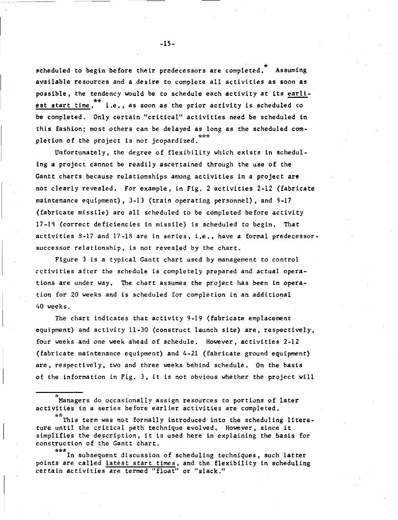
scheduled to begin before their predecessors are completed. Assuming

available resources and a desire to complete all activities as soon as

possible, the tendency would be to schedule each activity at its earli-

est start time, i.e., as soon as the prior activity is scheduled co

be completed. Only certain "critical" activities need be scheduled in

this fashion; most others can be delayed as long as the scheduled com-

pletion of the project is not jeopardized.

Unfortunately, the degree of flexibility which exists in schedul-

ing a project cannot be readily ascertained through the use of the

Gantt charts because relationships among activities in a project are

not clearly revealed. For example, in Fig. 2 activities 2-12 (fabricate

maintenance equipment), 3-13 (train operating personnel), and 3-17

(fabricate missile) are all scheduled to be completed before activity

17-13 (correct deficiencies in missile) is scheduled to begin. That

activities 8-17 and 17-18 are in series, i.e., have a formal predecessor-

successor relationship, is not revealed by the chart.

Figure 3 is a typical Gantt chart used by management to control

cctivities after the schedule is completely prepared and actual opera-

tions are under way. The chart assumes the project has been in opera-

tion for 20 weeks and is scheduled for completion in an additional

40 weeks.

The chart indicates that activity 9-19 (fabricate emplacement

equipment) and activity 11-30 (construct launch site) are, respectively,

four weeks and one week ahead of schedule. However, activities 2-12

(fabricate maintenance equipment) and 4-21 (fabricate ground equipment)

are, respectively, two and three weeks behind schedule. On the basis

of the information in Fig. 3, it is not obvious whether the project will

Managers do occasionally assign resources to portions of lateractivities in a series before earlier activities are completed.

This term was not formally introduced into the scheduling litera-ture until the critical path technique evolved. However, since itsimplifies the description, it is used here in explaining the basis forconstruction of the Gantt chart.

In subsequent discussion of scheduling techniques, such latterpoints are called latest start times, and the flexibility in schedulingcertain activities are termed "float" or "slack."

-16

4-0

v 2 -0 0r

C0.0

c .- w 0 - 4

-Oj -) UU - 0

C o o C -

Cn ýo o 2 2

'a 'a A

17-

be completed on schedule. Actually it is possible to complete the fab-

rication of maintenance equipment and the fabrication of ground equip-

ment as late as the 60th and 64th week, respectively, and still complete

the project on schedule. Since the chart does not provide this in-

formation, it is necessary to use other techniques to establish interre-

lationships and to compute the earliest start and latest completion

dates for each activity. A Gantt chart incorporating all of this in-

formation would be too cluttered to be easily read and understood.

A Gantt chart based on earliest start times combined with a trans-

parent overlay based on latest completion times would provide more of

the information useful for scheduling but would still not depict the

interrelationships existing among activities.

The Gantt technique was devised originally for use by first-line

supervision on repetitive production operations. It is an excellent

tool for this type of operation because (1) good estimates of normal

production times can be obtained when work is performed repetitively;

and (2) produiction responsibility of. first-line supervision is normally

limited to a few operations. Thus, significant interrelationships, if any,

are obvious at this level. The complex interrelationships evolve when

information on many facets of an overall pr-ject must be presented to

higher levels of management. The large amount of detailed information

accumulated at the foreman level must then be compiled and summarized

into fewer activities.

The more important strengths and weaknesses of the Gantt technique

are surrmarized in Table 2.

MILESTONE TECHNIQUE

The milestone scheduling system is based largely on the same prin-

ciples as the Gantt system but the technique of displaying project

status differs. The milestone system is usually applied to development

The method for computation of latest completion dates is given inTable 7 in Sec. IV.

.18 -

Table 2

GANTT TECHNIQUE--STRENGTHS AND WEAKNESSES

Criteria Strengths Weaknesses

1. Validity Good in production operations. No explicit technique for depict.Because of short time duration ing interrelationships, which artof each measured operation, especially important in develop.only small errors in measure- ment.ment are likely to occur.

2. Reliability Simplicity of system affords Frequently unreliable, especiallysome reliability, in development stage, because

judgment of estimator may changeover timd. Numerous estimates ina large project, each with some ureliability, may lead to errors ijudging status.

3. Implementation Easiest of all systems in some Quite difficult to implement forrespects because it is well the control of operations in de-understood. (System implies velopment phase, where time standexistence of time standards.) ards do not ordinarily exist and

must be developed.

4. Universality of Can comprehensively cover a Less useful in definition andproject coverage given phase of a life cycle, development phases of life cycle.

Effective at the resource orinput level of control.

5. Sensitivity test- No significant capability.ing (simulation)

6. Forecasting In production operations, good Weak in forecasting ability to me(technique to assess ability to schedule when interrelationshipsmeet schedule on a given activ- among activities are involved.ity if based on good timestandards.

7. Updating Easy to update graphs weekly,etc., if no major programchanges.

3.' Flexibility If significant program changesoccur frequently, numerous chartsmust be completely reconstructed.

9. Cost Data gathering and processing The graph tends to be inflexible.relatively inexpen.'ive. Display Program changes require new graphscan be inexpensive if existing which are time consuming and costlcharts can be updated and if Frequently expensive display devicinexpensive materials are used. are used.

NOTE: Recall that this table is intended only as a sunmmary of certain qualitative infortion on the relative usefulness of the scheduling technique. As indicated previously, amore formal quantitative evaluation of the extent to which the criteria are met was considered infeasible in this study.

-19-

projects and is frequently used at several of the higher-management

levels, for example, corporate, SPO, AFSC, and Hq USAF.

A milestone represents an important event along the path to proj-

ect completion. All milestones are not equally significant. The most

significant are termed "major milestones" usually representing the com-

pletion of an important group of activities. (Also, events of lesser

significance are often called "footstones" and "inch stones" at least

in conversation if not in the formal literature.) In reality, of course,

there are many gradations of importance.

Events that are designated as milestones vary from system to sys-

tem. Attempts are currently being made to establish milestones common

to all programs, especially within major systems. For example, events

such as "Contractor Selected," "Equipment Delivered," and "Final

Acceptance Inspection Completed" are common to all systems, while "Air-

craft Flyaway" is common to all aircraft systems, but not to missile

systems. It is anticipated that milestone standardization, if success-

ful, will be of significant help to program monitors in comprehending

the status of the program, as well as in comparing progress on various

programs.

Milestone Chart

Systems management requirements currently specify that schedule

data be furnished in milestone form by the System Project Office (SPO)

and various contractors. In the planning phase, milestones are estab-

lished for the total life cycle of the program. Major milestones are

included in a comprehensive development plan, i.e., the System Package

Prigram. Progress in accordance with the plan usually is reported for

two time periods: (1) milestones scheduled to occur in the current

fiscal year and (2)'milestones scheduled to be completed during the

current month.

*

Described in System Program Documentation, Air Force Regulation375-4, Department of the Air Force, Washington, D.C., Nov. 25, 1963.Progress information is reported in accordance with a procedure some-times referred to as the Rainbow Reporting System. When initiated theRainbow System required status information on cost, manpower, facilities,and technical performance, as well as schedule information. The systemwas called Rainbow because each type of information required was describedon a card of a designated color, the assembled package being not unlikea rainbow.

-20-

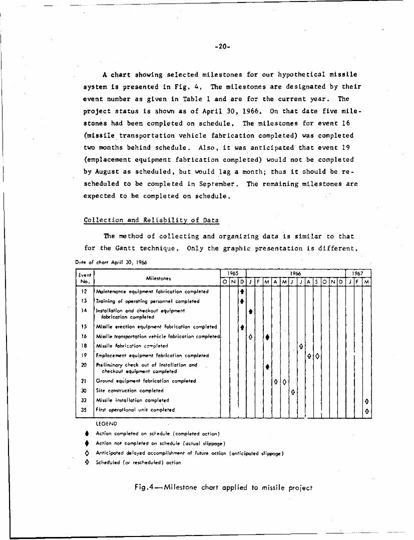
A chart showing selected milestones for our hypothetical missile

system is presented in Fig. 4. The milestones are designated by their

event number as given in Table I and are for the current year. The

project status is shown as of April 30, 1966. On that date five mile-

stones had been completed on schedule. The milestones for event 16

(missile transportation vehicle fabrication completed) was completed

two months behind schedule. Also, it was anticipated that event 19

(emplacement equipment fabrication completed) would not be completed

by August as scheduled, but would lag a month; thus it should be re-

scheduled to be completed in Seprember. The remaining milestones are

expected to be completed on schedule.

Collection and Reliability of Data

The method of collecting and organizing data is similar to that

for the Gantt technique. Only the graphic presentation is different.

Doite of chart April 30, 1966

Event Milestones 1965 1966 1967No. ON D J IF M A MIJ J A S O NID J F M

12 Maintenance equipment fabrication completed

13 Training of operating personnel completed

14 Installation and checkout equipmentfabrication completed

15 Missile erection equipment fabrication completed

16 Missile transportation vehicle fabrication completed 0

18 Missile fobri:alion completed

19 Emplacement equipment fabrication completed 0 0

20 Preliminary check out of installation andcheckout equipment completed

21 Ground equipment fabrication completed 0 0

30 Site construction completed 0K3 Missile installation completed

3 First operational unit completed I0

LEGEND

SAction completed on scl-edule (completed action)

*Action not completed on schedule (actual slippage)

0. Anticipated delayed accomplishment nf future action (anticipated slippage)

0 Scheduled (or rescheduled) action

Fig.4-Milestone chart applied to missile project

-21 -

Accordingly, the strengths and weaknesses of the milestone technique

are very similar to those summarized in Table 2 for the Gantt tech-

nique. The milestone reporting system can be automated with relative

ease. Data on changes in status can be read into a computer, which

prints the required format depicting progress on the appropriate mile-

stones. This innovation tends to reduce the costs of the system and

also to irrprove the timeliness of the data.

-22-

III. THE LINE OF BALANCE TECHNIQUE (LOB)

APPLICATION TO PRODUCTION OPERATIONS

The line of balance technique (LOB) was developed to improve

scheduling and status reporting in an ongoing production process. Es-

sentially the technique consists of four elements:

1. The objective,

2. The program or production plan,

3. Measurement of progress, and

4. The line of balance.

The Objective

The first step in scheduling production is to obtain the contract

delivery schedule. The obj,..tive of the production operation is to

meet a schedule based on cumulative deliveries. Figure 5(a) illustrates

this objective as used in LOB. The chart shows the cumulative number

of units scheduled to be delivered and the dates of delivery. The con-

tract schedule line represents the cumulative quantity of units sched-

uled to be delivered over time.

The Program

The second step is to chart the program. The program, also called

the production plan, comprises the stages in the producer's planned

production process and consists, essentially, of key manufacturing and

assembly operations sequenced in a logical production scheme over the

time period required to complete. A sample program is presented in

Fig. 5(b). Time is shown in working days remaining urtil each unit

can be completed. Symbols and color schemes can be used to depict dif-

ferent types of activity, such as assembly, machining, purchasing of

materials, etc.

(a) The Objective (cumulative delivery schedule)

50 -- - 1 1 504,5W45 ---.--..- 45

40 - -- I-- -

40

35 35

Contract Schedule Line

30 ------ -

/c"E 25 25

20 ,20

10 /10

Ac~tual Delivery

Jul Aug Sep Oct Nov Dec -ion Feb Mar Apr May Jun 123456

Scheduled delivery 10 30 50

Actual Delivery 5

; : (b) The Program or PrDote of study a' 29 Oct 1965

co; I wIm n-"

Jw rlolsw

0*of INIF vh weo w" ,~ ýWo

Co i •.;tmt In wbly IAi• i~12 m1

I16

"M' f.o 4wg 15

hiq

4 42 f 34 36 34 32 30 20 26 24

Fig.5--The Line of

(c Program Progress Data and Line of Balance (showing progress through major control points)

X.

Line of balance

7 1 l 3 4151 1 S 9202 2 3 4252 2 8 9303 3 3 4353 3 3 3 0 ? 3444 4 7 8495 5 2X35

~V_ - s*

I~~~ Conr9 pon s ubcnrc at

m 0 or PoutoPln(hwnmaor, oprtin nd controlpoints

bake, 4e b0-Wrpi

Stet.-*ft w-4bl Qoo Sit-b

20~ W;ý atere Itotat Ra.tto ma rteria$Mt. hake, 9-dt eo. d.reptenr

.ke oft Balance Techequ

ovl2t1 eNVXSPE51 pU1,92 lt o5

-24-

Measurement of Progress

To illustrate the control function, let us assume that production

has been in progress for a month. We are then able to measure the

status of the components (units) in the variouz stages of completion.

Program progress data are obtained by taking a physical inventory

of the quantities of marerial.w:, parts, or sub-assemblies that have

passed through a series of control points in the production plan. The

data are then plotted on a bar chart illustrated by Fig. 5(c). For

example, if control point 15 in chart (b) were selected, the inventory

might reveal that 29 units were completed on that date and hence 29

would be shown on the bar chart, which thus represents actual produc.

tion progress.

Line of Balance

The last step is to construct the line of balance, which represents

the number of units that should pass through each control point at a

given date if management can reasonably expect the objective, i.e.,

the delivery schedule, to be met.

The line of balance is constructed in the following manner:

I. Select a particular control point, for example, 15.

2. From the production plan (Fig. 5(b)) determine the number of

days required to complete a unit from the control point to

the end of the production plan (i.e., 27 days).

3. Using this number determine the date the units should be com-

pleted. (October 29 plus 27 working days is December 3.)

4. Find the point corresponding to this completion date (December 3)

on the contract schedule line and ascertain the number of

units (35) that should be completed on that date if the deliv-

ery schedule is to be met.

The legend also utilizes shading in parts (b) and (c) to indicatethe type of material or function involved. This assists in identify-ing general areas of responsibility.

Actually one would probably start with the last control point(42) and work back through the project. For our purposes here controlpoint 15 is of special interest in illustrating the usefulness of thetechnique.

-25-

5. Draw a line on the production progress chart (Fig. 5(c)) at

that level (35 units) and over the control point (15).

6. Repeat this procedure for each control point and connect the

horizontal lines over the control points. The resulting line

is the line of balance. It indicates the quantities of units

that should have passed through each control point on the

date of the study (October 30) if the delivery schedule is to

be met.

The production progress chart shows the status of a program at a

given point in time. Thus management can determine at a glance how

actual progress compares with planned progress. Where actual progress

lags planned progress, the variance can be traced to the individual

control point(s).

In the example described above, it is evident that without manage-

ment action the delivery schedule will not be met because several con-

trol points, including the last one, are behind schedule. By using

both the production plan and the program progress chart, one can begin

at the end control point (42) and trace back through the series to find

the source of the delay. Working backward, we see that control point

37 is a critical point of delay, If 37 were on schedule, then it is

quite likely that all the succeeding control points would be on sched-

ule. In trying to determine why 37 is behind schedule, we see that

control points 35, 31, and 30 are also behind schedule. Control point

35, however, is in series with 31 and is presumably held up because 31

is not on schedule, which in turn is held up because control point 30

is not on schedule. We note that the control points preceding opera-

tion 30 are on schedule and therefore assume that the difficulty prob-

ably lies within operation 30 itself. The initial difficulty, however,

lies in the sequence of activities preceding operation 31, so that 31

is behind schedule because 15 is behind schedule. Thus control point

15 is the bottleneck. It is reasonable to assume that with more man-

agement surveillance, and perhaps with more resources devoted to oper-

ations 15 and 30, operation 31 will be on schedule, and as a result so

will 35, 37, 38, 39, 40, 41, and 42.

-26-

APPLICATION TO DEVELOPMENT OPERATIONS

Although LOB has been widely applied to production operations at

the prime and associate contractor level, a variant of this technique

can be used in the development stage of a weapon system where only one

complete system, or a small number of complete systems, is to be pro-

duced. In this case, control of the quantity of items through a given

point is not relevant as it is in production operations. Instead,

monitoring of progress is directed toward major events, that is, the

completion of significant activities in the development process. In

our discussion, we assume the development of a single unit using the

hypothetical missile system described in Sec. I,

As applied to the development phase, the four elements of the

technique are essentially the same as those for production scheduling

and control, but their composition is altered.

The Objective

Instead of scheduling many units, the delivery schedule is based

on the production of a single unit or on a limited number of units.

The objectives chart will thus show the required percent completion

of individual activities, rather than number of systems through each

control point. Figure 6 illustrates this possible adaptation of LOB

to the hypothetical development project. Supporting data are given

in Tables 3 and 4.

The scheduled starting date of the component begins in the appro-

priate week at a point on the abscissa representing zero percent com-

pletion. The scheduled completion date of each activity is represented

in the appropriate week at a point on the abscissa which represents 100

percent completion. A straight line is drawn between these two points.

This straight line assumes that the same rate of progress will occur

throughout the activity period. If the scheduler has reason to doubt

that progress will proceed at a constant rate, the line can be drawn

in any shape that management feels will correctly depict the expected

progress.

The list of activities has been condensed for purposes ofillustration.

-27-

Date of stdy

Events-----. • t 15 16 21 13 12 17 29 30 18 19 20 34

60.-

40- /0

_AA

84 3 5 7 2 6 9 11 10 17 33 14 -* EvntsI /I I I ,I I -

0o 20 30 40 60 70

Tiý* { *eks

Fig.6--lO0 prototype development objectives chart

Table 3

SUPPORTING DATA FOR FIG. 6

EstimatedActivity Scheduled Dates

Activity TimeNo. Activities (weeks) Start Complete

2-12 Fabricate maintenance equipment 19 10 293-13 Train operating personnel 19 4 234-21 Fabricate ground equipment 19 2 215-14 rabricate installation and checkout equipment 6 6 126-15 Fabricate missile erection equipment 3 12 157-16 Fabricate missile transportation vehicle 9 8 178-17 Fabricate missile 30 0.2 30.29-19 Fabricate emplacement equipment 28 16 44

10-29 Train maintenance personnel 9 25 3411-30 Construct launch site 21 18 3514-20 Test installation and checkout equipment 7 45 5217-18 Correct deficiencies in missile 10 30.2 40.233-34 Check out missile installation 24 40.6 64.6

Total ........................... 204

-28-

Table 4

DATA FOR OVERALL PROJECT OBJECTIVES CURVE

Time Period Estimated Cumulative Percent of Planned(Identified by Activity-Weeks Activity-Weeks Completiona

Final Week) Required to DateDuring Period

0 0 0 05 9 9 4.4

10 21 30 14.715 30 60 29.420 28 88 43.125 24 112 54.930 24 136 66.635 19 155 76.040 14 169 82.845 9 178 87.250 10 188 92.155 7 195 95.660 5 200 98.065 4 204 100.0

aInformation in this column is basis for dotted line in Fig. 6.

Using the data in Table 4, an overall project objLc'ives curve

can be constructed as follows:

1. Sunmmarize the weeks estimated to complete each activity and

thus obtain the total activity-weeks of effort to be involved

during each incremental time period. (Computations were made

for five-week intervals in the example.)

2. Compute the cumulative activity-weeks of planned effort

through the end of each time period.

3. Compute the ratio of (1) over (2) for each time period. This

ratio is the percent of the project planned to be completed

at the respective points. The line connecting these points

is the overall project objectives curve. The completion date

of the last activity should coincide with the completion date

of the overall project.

-29-

The Development Plan

A flow chart showing the development plan of the hypothetical mis-

sile system is given in Fig. 7. Procedurally, the development plan

514

10* 29

70 50 30 20 to 0Tim* (.w*tk)

Fig.7-LOB prototype development plan chart

chart is taken as a control point for the progress chart (see Fig. 8

on page 31). The development plan chart in our example daes not show

connections between the activities because only 13 activities out of

the 34 given in Table 1 are included. If all 34 were shown, the activ-

ities would follow in sequence to the completed missile system.

Determination of Progress

There is no technique available to determine true overall program

status where considerable uncertainty exists concerning completion

dates. The original estimated titwc ':o complete an activity, the length

of time devoted to it to date and the current physical state of comple-

tion all may be known. However, the actual time required to complete

-30-

tt is not known and must be estimated by the responsible project en-

gineer. The LOB technique for approximating the status of the nrogram

is as follows:

Percent completion a I - d

where d - the number of weeks required to complete

a particular activity,

A = the gross number of weeks originally es-

timated for the entire project.

As an example, suppose that the time originally required to complete

the development phase was 10 weeks, that 8 weeks have already elapsed,

and that the current estimate of the time to completion is 4 weeks.

According to the LOB formula, the development phase is 100(1 - (4/10)) 60

percent complete.

Two alternative techniques could also be used to estimate percent

completion. For example, if it now appears that the total time re-

quired for the development phase is 12 weeks, when 4 weeks remain to

completion one can consider that the development is actually 8/12 or

67 percent complete, and not 60 percent complete as revealed by the

LOB formula.

A second alternative would be to place the 8 actual weeks of ef-

fort over the original time estimate (10 weeks); this would indicate

that the phase was 80 percent complete.

While the major reference material on LOB discusses the second

alternative, it selects the basic LOB technique as the preferable onebecause "while the prescribed method requires one additional mathemati-

cal step, it helps compensate for inaccuracies in the initial estimate

of time required for the entire phase."* However, in some respects the

first alternative appears to be the most realistic because it is based

on current information rather than on the original estimate.

Line of Balance Technology, op. cit., p. 19.

-31-

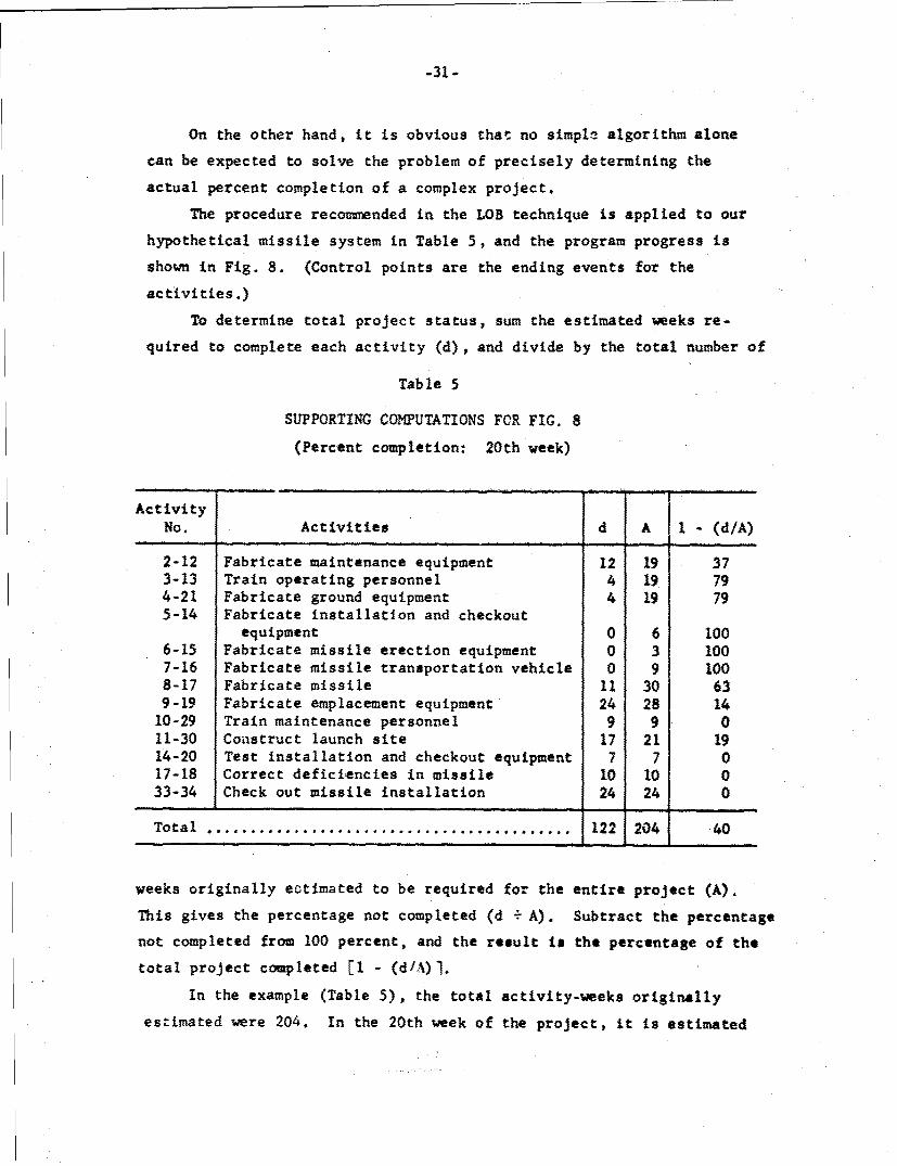
On the other hand, it is obvious that no simpl algorithm alone

can be expected to solve the problem of precisely determining the

actual percent completion of a complex project.

The procedure recoumended in the LOB technique is applied to our

hypothetical missile system in Table 5, and the program progress is

shown in Fig. 8. (Control points are the ending events for the

activities.)

To determine total project status, sum the estimated weeks re-

quired to complete each activity (d), and divide by the total number of

Table 5

SUPPORTING COMPUTATIONS FOR FIG. 8

(Percent completion: 20th week)

ActivityNo. Activities d A 1 -(d/A)

2-12 Fabricate maintenance equipment 12 19 373-13 Train operating personnel 4 19 794-21 Fabricate ground equipment 4 19 795-14 Fabricate installation and checkout

equipment 0 6 1006-15 Fabricate missile erection equipment 0 3 1007-16 Fabricate missile transportation vehicle 0 9 1008-17 Fabricate missile 11 30 639-19 Fabricate emplacement equipment 24 28 14

10-29 Train maintenance personnel 9 9 011-30 Construct launch site 17 21 1914-20 Test installation and checkout equipment 7 7 017-18 Correct deficiencies in missile 10 10 033-34 Check out missile installation 24 24 0

Total .............................................122 204 40

weeks originally ectimated to be required for the entire project (A).

This gives the percentage not completed (d + A). Subtract the percentage

not completed from 100 percent, and the result is the percentage of the

total project completed fI - (d/A)1.

In the example (Table 5), the total activity-weeks originally

estimated were 204. In the 20th week of the project, it is estimated

.32-

100

90

80

o70

0 50/

I 40 4 / 40 /ecet

30 /

20 //

10' IN /

12 13 21 It 15 16 17 1 9 291 0. 20 18 34

Con~trol points

Fig.8-LOB prototype development phase progress chart

that 122 activity-weeks will, be needed to complete the project. Ac-

.cordingly, the estimated percentage of the overall project completed

is 1 - (122/204) - 40 percent.

Although the LOB technique does not provide any sophisticated way

of guiding personnel in the process of estimating time remaining to

complete a project, one method frequently used by schedulers is to di-

vide a major phase into a number of individual technical tasks and then

relate the number completed to the total. However, such a method has

the limitation of assuming that all tasks are of equal difficulty.

An alternative, of course, is for the estimator to draw more generally

on his own experience in determining estimated time to completion.

The Line of Balance

An additional step is necessary to complete the analysis of pro-

gram progress. That step is "striking the LOB." On the objectives

chart (Fig. 6), construct a vertical line perpendicular to the abscissa

at the date of the study. This vertical line will intersect several,

if not all, of the percent completion lines for the individual events

-33-

at a point representing their currently scheduled completion status.

Then draw a horizontal line at the percent completion point on the prog-

ress chart (Fig. 8), above the respective events. Thus, both the

scheduled status and the actual status of the events and of the overall

project are shown for the date of the study. Notice that in the de-

velopment phase, the line of balance does not necessarily descend con-

tinuiously in a stepwise fashion as it must in the production plan.

EVALUATION OF LOB TECHNIQRUE

The LOB technique, like the Gantt technique, was originally de-

signed for production operations. The Gantt technique focused on pro-

viding management with information relating to the efficient utiliza-

tion of resources. Machine and manpower inputs to the production

process were emphasized. On the other hand, the LOB technique is prod-

uct oriented. Its information centers on the extent to which the

planned production of a quantity of items is actually being realized.

It is not directly concerned with the efficient utilization of re-

sources. Its key usefulness is that bottlenecks in the production

process are emphasized. Maaagement must then take appropriate action,

generally increasing the level of resources at these bottlenecks. Con-

sequently, Gantt and LOB are complementary techniqjes.

The LOB technique has some applicability in prototype development

when a limited number of components, or operations, are to be controlled.

The LOB development plan chart is capable of depicting interrelationships.

although seldom is the effort made to include all such relationships.

The LOB technique has several limitations. The inability to pre-

cisely state the percent completion of components is one area that can

lead to weakened managerial control of the project.

In addition, if management wishes to examine the impact of alterna-

tive approaches to overcoming a bottleneck, the LOB affords no simula-

tion capability for this purpose. The determination of the time to

complete a component is left up to the judgment of an engineer, and

LOB is silent as to how this estimate should be made. Consequently,

inconsistencies occur and reliability is impaired. Finally, the tech-

nique is rather inflexible. If there is a change in the development

-34-

plan, the entire chart system may need to be reconstructed; the up-

dating of program progress requires extensive chart changes. Table 6

further identifies the strengths and weaknesses of the LOB technique.

Table 6

LOB TECHNIQUE.-STRENGTHS AND WEAKNESSES

Criteria Strengths Weaknesses

1. Validity Uncertainties surrounding Uncertainties encountered incompletion times in production the development phase impairoperations are minimal; con- judgment on actual projectsequently LOB affords manage- status. The techniques for es-ment a sound technique for timation of percent completionjudging status of operations, can lead to erroneous decisions

concerning project development.

2. Reliability Compares favorably with Gantttechnique.

3. Implementation Only slightly more difficultto comprehend and to implementthan Gantt technique.

4. Universality of Capable of covering a system Does not emphasize resourceproject coverage life cycle, allocation directly.

5. Sensitivity test- No significant capability foring (simulation) simulating alternative courses

of action.

6. Forecasting Depicts status of project well Offers no technique to handlein production stage and can uncertainty in development phase.forcast whether or not sched-ule will be met.

7. Updating Considerable clerical effort re-quired to update graphs.

8. Flexibility Inflexible. When major programchanges occur, the entire set ofgraphs must be redrawn.

9. Cost Data gathering and computa- Charts require frequent recon-tions can be handled routinely. struction, which is time-consum-Expense is moderate and largely ing.for clerical personnel andchart materials.

NOTE: Recall that this table is intended only as a summary of certain qualita, .ve informa-tion on the relative usefulness of the scheduling technique. As indicated previously,a more formal quantitative evaluation of the extent to which the criteria are met wasconsidered infeasible in this study.

-35-

IV. THE CRITICAL PATH METHOD L(CPM)

APPLICATION OF CPM

The critical path method (CPM) was the first technique designed

specifically for complex, one-of-a-kind operations. Although initially

used to plan and control the construction of facilities, it applies

equally well to development of new weapon systems and is designed to

interrelate diverse activities and explicitly depict important inter-

dependencies. The construction of a chemical plant, for example, re-

quires coordination of numerous functions and activities. A well-

coordinated construction schedule can shorten the project by months

and thereby significantly reduce project costs. The CPM technique

utilizes a network approach and a limited time-cost trade-off capabil-

ity for organizing data on these types of interactions. Accordingly,

the basic elements in CPM are:

1. The flow diagram or network,

2. Critical time paths ,

3. Float (scheduling leeway), and

4. The time-cost function.

Network

The development of a network or flow diagram that embraces all

events and activities and explicitly recognizes major known interde-

pendencies among activities is an important element in the CPM. It

is based on the following simple concepts:

1. An activity (or job) is depicted by an arrow:

The basic development is attributable to M. R. Walker who waswith the Engineering Service Division of E. I. DuPont De Nemours &Company Inc., and J. E. Kelley, Jr., Remington Rand Univac (nowSperry Rand Corporation).

-36-

2. Each arrow is identified by an activity description:

develop engine

3. A sequence of activities is indicated by linking arrows:

.. .A B.. •'" '

4. Events link activities: E

An event occurs at a point in time and signifies either the start or

completion of an activity.

5. A grouping of activities and events forms a network. Net-

works may be either activity- or event-oriented. In activity-oriented

networks, the activities (arrows) are labeled; in event-oriented net-

works, the events (circles, or other symbols) are labeled:

I4

-37-

There are certain rules to follow in constructing a network; e.g., no

looping is allowed:

Looping indicates not only that event 1 must be completed before event

2, and event 2 before event 3, but also that event 3 must be completed

before event 1. It is logically not possible to require the start of

a preceding event that depends on completion of a succeeding event.

6. The length of an arrow has no significance; it merely identi-

fies the direction of work flow. Also, time estimates which are

secured for activities represent elapsed or flow time and are not iden-

tified--at least initially--with calendar dates.

The Critical Time Paths

In a complex project, involving multiple activities and events,

sequences or paths of activities can be identified. These paths vary

in length according to the time required to accomplish the component

activities. The path or paths requiring the longest time are called the

critical paths. When a critical path has been determined, management

is advised to devote resources to those activities along this path in

an effort to reduce the time requircment and thus shorten the overall

program. Of course, as one critical path is shortened, another eventu-

ally becomes critical.

Float

Some leeway exists in scheduling activities not on a critical path.

This leeway is called float. The technique for determining float is

as followq:

The distinction between flow time and calendar (or scheduled) time

will be clarified further under the subsequent section on the PERT system.

-38-

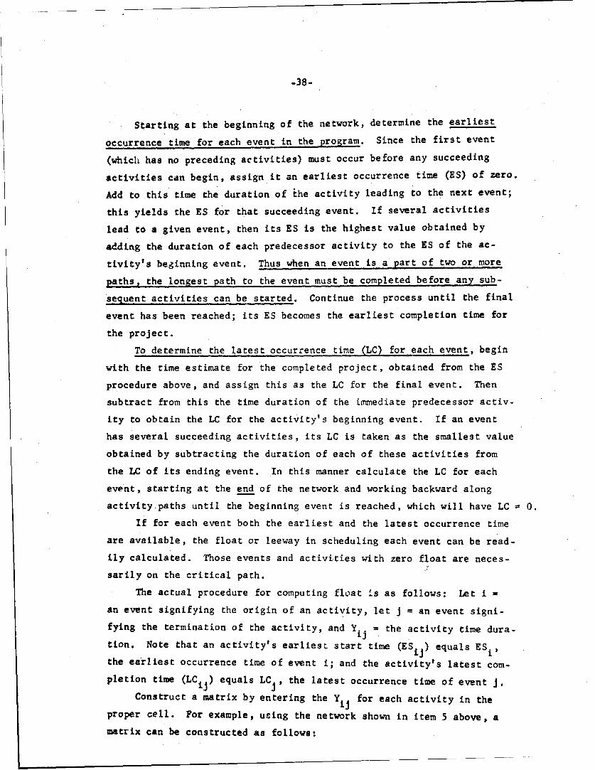
Starting at the beginning of the network, determine the earliest

occurrence time for each event in the program. Since the first event

(which has no preceding activities) must occur before any succeeding

activities can begin, assign it an earliest occurrence time (ES) of zero.

Add to this time the duration of ihe activity leading to the next event;

this yields the ES for that succeeding event. If several activities

lead to a given event, then its ES is the highest value obtained by

adding the duration of each predecessor activity to the ES of the ac-

tivity's beginning event. Thus when an event is a part of two or more

paths, the longest path to the event must be completed before any sub-

sequent activities can be started. Continue the process until the final

event has been reached; its ES becomes the earliest completion time for

the project.

To determine the latest occurrence time (LC) for each event, begin

with the time estimate for the completed project, obtained from the ES

procedure above, and assign this as the LC for the final event. Then

subtract from this the time duration of the immediate predecessor activ-

ity to obtain the LC for the activity's beginning event. If an event

has several succeeding activities, its LC is taken as the smallest value

obtained by subtracting the duration of each of these activities from

the LC of its ending event. In this manner calculate the LC for each

event, starting at the end of the network and working backward along

activity paths until the beginning event is reached, which will have LC = 0.

If for each event both the earliest and the latest occurrence time

are available, the float or leeway in scheduling each event can be read-

ily calculated. Those events and activities with zero float are neces-

sarily on the critical path.

The actual procedure for computing float is as follows: Let i =

an event signifying the origin of an activity, let j = an event signi-

fying the termination of the activity, and Yij = the activity time dura-

tion. Note that an activity's earliesL start time (ESij) equals ESi,

the earliest occurrence time of event i; and the activity's latest com-

pletion time (LCij) equals LCJ, the latest occurrence time of event J.

Construct a matrix by entering the Y for each activity in the

proper cell. For example, using the network shown in item 5 above, a

matrix can be constructed as follows:

-39-

ES"i 1 2 3 4 5

0 0 2 6 - -

2 1 - 4 8 -

6 2 - - 5 2 13

11 3 - - - 5 9

16 4 . . . . 3

S~20

t0 21 6 11 17 I2O LC

Computing Earliest Occurrence Time. The procedure for computing

earliest occurrence time (ES) is as follows:

1. Enter a zero in the first cell of the ES column, which repre-

sents the starting time of the project.

2. Add the corresponding values of Yij to the ES values column by

column. In our example, ES 0 = 0 and YO 0 2; hence 0 + 2 - 2, and we

enter 2 in the ES column below the zero, indicating that 2 weeks are

required before the activities immediately after event I can be started.

3. Continue this procedure for each column. For example, the

values in column 2 of the matrix are 6 weeks and 4 weeks. The corres-

ponding values in the ES column are 0 and 2 weeks. Adding 6 + 0 - 6 and

4 + 2 - 6, we see that by either path it will be 6 weeks before event 2

can occur. Consequently, we enter 6 in the ES column opposite event 2.

4. Where different times result from this summation process,

select the longest time (path) and enter that number in the ES column.

For example, column 3 of the matrix has Y values of 8 and 5; the cor-

responding ES values are 2 and 6. By adding 8 + 2 - 10 and 5 + 6 - ii,

we see that 11 is the longest time path and place it in the ES column.

Computing Latest Occurrence Time. The procedure for computing

latest occurrence time (LC) is as follows:

-40-

1. Enter the longest time path in the project (i.e., 20 weeks,

taken from the last cell in the ES column) in the last cell of the LC row.

2. Subtract the corresponding values of Y from the LC values

row by row. In our example, LC05 20, and Y45 - 3; hencd 2.0 - 3 - 17,

and we enter 17 in the LC row to the left of the 20 weeks. This means

that event 4 must occur by the seventeenth week if the project is to be

completed in 20 weeks. Continue this procedure for each row.

3. Where different times result from the subtraction process, se-

lect the shortest time (path) and enter that number in the LS row. For

example, row 3 of the matrix has Y values of 5 and 9; the corresponding

LC values are 17 and 20. By subtracting 17 - 5 - 12 and 20 - 9 - 11, we

i4:ee that the shortest time path is 11 and enter that number in the LC row.

.4. The last entry in the LC row should be a zero, corresponding to

the zero in the first cell of the ES column.

Identifying Events on the Critical Path. Every event that has an

equal ES and LC time is on the critical path. In our example, event 1

has an ES of 2 and an LC of 2; hence it is on the critical path. Event 4

has an ES of 16 and an LC of 17; hence it is not on the critical path.

Accordingly, the critical path includes events 0, 1, 2, 3, and 5.

Identifying Total Float. Total float for an activity is the amount

of time available for an activity less the amount of estimated time re-

quired to complete the activity. In our example, total float for an

activity equals (LCd - ESi) - Yij. Thus, for event 3, LC 3 = 11; ES1 1 2;

Y = 8; hence (11 - 2) 8 1 week of float.

Y6 - Toto I float

ESi LCi

Other Types of Float: Free, Interfering, and Independent. It may

be desirable to know how much a preceding activity may be delayed (if

at all) without interfering with the earliest start of the succeeding

activity. This is called free float. At this point, it is necessary

-41-

to introduce data on an activity's completion time (EC 1 j). EC j is de-

rived by adding the estimated time required for an activity (Yij) to

the activity's earliest start time (ESij). To compute free float: Let

ES 1 2 , EC1 2 , LC1 2 , and Y1 2 apply to the preceding activity and let ES 2 3 ,EC23' LC23' and Y23 apply to the succeeding activity. Then ES23

(EC 1 2 + Y1 2 ) = free float for activity 1-2.

EC, 2

l. . ... -j-Free ES2 3float_=.! y. .

ES12 LC2 3

Interfering float is total float minus free float. The concept

also can be presented in a diagram. For example, any delay in activity

1-2 beyond the ES date of activity 2-3 will delay or interfere with

activity 2-3. Hence, part of the total float for activity 1-2 is free

float ($23 - EC1 2) and the remainder is interfering float (LC 1 2 - ES2 3 ).

LC12

ES12 --2 ----- Total floatEQl2

Free

SI. float InterferingY 12 -j - ,*--flo at - 1 1

423ES2 3 EC23

Independent float is computed as ES 3 4 - LC1 2 - Y2 3 " For example,

if all activities prior to activity 2-3 are completed by the LC12 date,

and all activities succeeding activity 2-3 are started at the ES34 date,

then ES3, - LC12 is the amount of time available to perform activity 2-3.

Subtracting the actual time required to perform the activity from the

available time gives the independent float; i.e., the activity can be

displaced forward or backward within this time interval without inter-

fering with any other event.

tC12 ES34

Zm 2 Inndeendent -23 Ifndependoent . .

f loat f loat

-42-

Time-Cost Function

The contribution to system management embodied in the CPM does not

end with the time parameter. It also provides a technique to aid man-

agement in making time-cost trade-off decisions.

The technique is quite simple, requiring only four estimates: (1)

normal activity time, (2) normal activity costs, (3) activity times on

a "crash" basis, and (4) cost on a "crash" basis. These estimates are

based on the principle of the time-cost curve, as illustrated in Fig. 9.

o 20Crash~

'•AS I

10 --------- ---- Normal S.'at

0

0 1 2 3 4 5 6 7 8 9 10

Time (weeks)

Fig.9-CPM time-cost trade-off

In this example, the normal activity time estimate would be six

weeks and the cost estimate would be $10,000. On a crash basis, the

activity time would be four weeks and the cost $20,000. A simple as-

sumption would be that cost and time are related inversely and linearly

(i.e., for each reduction in time there will be a corresponding incre-

ment of added cost). For example, according to Fig. 9, shortening the

time by one week (from six to five) would cost $5,000. The decision-

maker can compare the costs of shortening the schedule by allocating

additional resources to an activity (or activities) on the critical

path for which marginal cost is less than for any other activity. Thus

the time required or any path can be shortened at least cost. Assump-

tions other than an inverse linear relationship can also be introduced

by properly reflecting them in the shape of the time-cost curve.

The task of calculating these time-cost trade-of's can be quite

formidable to accomplish manually if the project becomes even moderately

complex. A computer program assuming linear time-cost relationships

-43-

has been developed that will automatically schedule the project for the

least cost activities. This computer routine requires at least the two

time-cost data points--i.e., assuming normal and crash programs for

each activity. Non-linear assumptions are more difficult to treat in

large projects.

It is not the purpose of this Memorandum to explore time-cost re-

lationships; however, this mechanism is usually considered a component

of CPM and should be mentioned when comparing CPM with PERT.

APPLICATION TO THE MODEL

The CPM can be applied to the hypothetical missile system described

in Sec. II. Figure 10 represents the planned sequence of activities in

in network form. The numbered circles correspond to the events in

Table i. Note that interdependencies are depicted in the network. For

example, event 3 must occur before event 20 can be completed. Such

interdependencies can be readily ascertained from the CPM network but

would not be clearly evident in a tree diagram or in a Gantt or mile-

stone chart.

It could be argued that engineers responsible for development are

usually aware of these interrelationships when the Gantt chart is used,

and nothing is gained by the network presentation. This may indeed be

the case in simple or small-scale projects. However, when a number of

managers are involved in planning and measuring the progress of a com-

plex system, they may not be aware of the effect of interdependencies

beyond their inmediate sphere of interest. It is possible that a sub-

contractor may be well aware of those relationships within his control,

and yet not realize that his schedule is in jeopardy because another

department will not be able to deliver its portion of the project on

time, or, conversely, that a component he is developing may, if not

Several scheduling techniques have since been expanded to incor-porate cost considerations, e.g., PERT-Cost, RAMPS, SPAR, etc. Seeespecially PERT-Cost System Description Manual, Vol. 3, U.S. Air Force,December 1963; Jack Moshman, Jacob Johnson, and Madalyn Larsen, RAMPS--A Technique for Reseurce Allocation and Multi-Project Scheduling, Pro-ceedings- 1963 Spring Joint Computer Conference; and J. D. Wiest, TheScheduling of Large Projects with Limited Resources, Research MemorandumNo. 113, Graduate School of Industrial Administration, Carnegie Instituteof Technology, Pittsburgh, 1963.

-44-

209.2 5 2

LV

199

28 0 2t2 24

F; 9 . 1O--CPM network applied to hypothetical missile s/stem

completed on time, retard another subcontractor and hence the entireproject. In making the relationships explicit, the network serves as acormmunications device to ensure that all parties concerned are awareof the overall plan and their responsibilities in view of the plan.

The problem of keeping the planning and control information sys-tern attuned to actual development operations is conmmon to all mana-gerial techniques. A major advanLage of the network-type presentation

is that it enables the manager to cumulate the ac2.ivity times along a

given path to determine the total estimated time per path. The long-est time path is the critical path. In Fig. 10, for example, thelongest time path is 64.8 weeks and is cemposed of events 1, 8, 17, 18,27, 33, 34, and 35. All other paths are estimated r) be completed in

-45-

less time. If the tasks are scheduled to take the estimated time,

then all paths other than this critical path contain float. Any path

on which estimated completion time is greater than, or equal to, the

time remaining before a scheduled project completion date is called

critical. Hence, there may exist the most critical path, the second

most critical, etc. In Fig. 10, events 1, 9, 19, 28, 33, 34, and 35

would comprise the second most critical path (58.6 weeks).

Table 7 presents the matrix of task times needed to compute the

ES and LC times for each activity in our hypothetical missile system.

For example, activity 14-20 has an earliest start time of 6.2 weeks

from the beginning vf the project. It must be completed in the 64th

week or the activity will "float" the succeeding activity beyond the

project completion date. Thus we can compute the various float con-

cepts for activity 14-20:

1. Total float = (LC 2 0 - ES1 4) "Y 1 4 - 20

= (64 - 6.2) - 7 = 50.8

2. Free float = ES 20 _2 2 - (ES 14 . 20 + Y14-20)

= 13.2 - (6.2 + 7) = 0.

3. Independent float = (ES 20 _2 2 - LC5 . 14) - Y14-20

= (13.2 - 57) - 7 = -50.8

1. Total float. Assuming that there are no project changes, and

that activity 14-20 is started at the earliest possible date and com-

pleted at the earliest possible time, 50.8 weeks will elapse before

activity 20-22 will have to be started. Consequently, freedom exists

to allocate resources to other more critical tasks up to a maximum of

50.3 weeks before the scheduled completion of activity 14-20 is jeopardized.

2. Free float. If activity 20-22 were to start on the earliest

possible date, no freedom would exist to allocate resources to other

For clarity, and to be consistent with the explanation on pages40-41, LC and ES values are identified by the appropriate activitydesignator which in turn is composed of both t,e starting and endingevent numbers. Technically, however, ES can be fully defined by thestarting event and LC by the ending event number.

-46-U

I ~i 'I19,V

I - - - - - - - - - -V,9

' I

--6- - - - - -I I

96E

SZ •Z.-- --. - --

N'03 - - - - - -

umZ -- _

-J

>

Niui Z':: P9~iw -L -- ---- - -- F9

< /I I I I

- -l -�oZ --

-~ - xu - ---- ---- - - -Ii: - - -t

e-- --- - - - - - - - - - - - - - - ---- I

- 8

CL- --

_I T- _-------- --- _I'N U.I~.. cDj~c

7 J J J flrjJyN .

'0.0 ~1'0 44-

I ' l l -1

"R I

-47 -

tasks. In other words, there would be no free float in the scheduling

of activity 14-20. As mentioned previously, total float can be sub-

divided into free float and interfering float. Interfering float would

delay (interfere with) the start of the subsequent activity (20-22)

beyond the earliest start date. In the above example, all of the float

for activity 14-20 is interfering.

3. Independent float. In the illustration a negative value

(-50.8) was obtained and therefore there is no independent float.

This negative statistic does indicate that there would be no time avail-

able to perform activity 14-20 if the prior activity (5-14) were de-

layed until its latest completion date and if scheduling the subsequent

activity (20-22) on its earliest start date •as contemplated. in fact,

the latest completion date for activity 5-14 significantly postdates

the earliest start date for activity 20-22. This, of course, is of

no real concern here because thc earliest start date of activity 20-22

(also identified by LC 2 0 ) can be delayed substantially without jeopar-

dizing project completion. In other words, total float exists, but

independent float, being a very restrictive concept, does not in this case.

EVALUATION OF CPM

The network concept of CPM is an excellent device for explicitly

depicting significant interrelationships among events. The flow of

all activi:ies is on paper so that those concerned can analyze the work

plan and approve or disapprove it. Coimmunication of planned activity

is thus facilitated.

Since time estimates lead to the determination of a critical path,

the attention of management is focused on the activities along the path

so that resources can be applied to them, perhaps by reallocatian from

other activities where float exists.

,If these resources were allocated, it would be at the cost of

delaying the start of task 20-22. This may, nevertheless, be a wisedecision since activity 20-22 may be delayed a maximum of 50.8 weeksand the project can still be on schedule.

-48-

One criticism of CPM is that emphasis on critical path activities

may obscure the fact that some activities on a second path may be very

close to being critical and would become so with slight changes in

values. However, this possibility can be alleviated by determining the

first most critical path, the second most critical path, etc., and then

determining the critical activities within this broader context.

The time-cost function, although not fully implemented in actual

systems, can provide trade-off information on the relative cost of re-

ducing scheduled time in various activities. This trade-off feature

linking cost and schedule is beyond the scope of this study but never-

theless is an important element of the CPM method.

CPM does not provide a capability for handling schedule uncertainty.

For example, the development of a component may involve a major engi-

neering improvement, and there may be considerable uncertainty regard-

ing the time required for its accomplishment. In CPM, the responsible

individual must provide management with his single best estimate -f the

time requirement. He may not reflect his uncertainty in terms of a

range of estimates. The single value is incorporated into the network

and the critical path determined. If the estimate is in error, then

the critical, path may be incorrectly drawn.

The strengths and weaknesses of CPM are sulimarized in Table 8.

-49-

Table 8

CMH TECHNIQUES--STRENGTHS AND WEAKNESSES

Criteria Strengths Weaknesses

I. Validity No formula is provided to esti-mate time to completion; con-sequently, the technique is asvalid as the estimator. Themargin of error is generallyless in construction than indevelopment.

2. Reliability Numierous estimates 4n a largeproject, each with $ome unreli-ability may lead to Isignificanterrors in judging project status

3. Implementation Relatively difficu~t to explain,especially if the various con-cepts of float are utilized.

4. Universality of Very good for single-shot Weak in the production phase ofproject coverage activities, such as construc- a weapon life cycle. The tech-

tion or development projects. nique is not well adapted toscheduling production quantities

5. Sensitivity test- Excellent for simulatinging (simulation) alternative plans, especially

when coupled with the time-cost aspect.

6. Forecasting Strongly oriented to forecast-ing ability to accomplishfuture events un schedule.

7. Updating Good capability. Activitiesare clearly identified and timeestimates can be obtained asneeded.

8. Flexibility Portions of the network can beeasily changed to reflect pro-gram changes.

9. Cost Considerable data are requiredto use CPM as both a planningand status reporting tool and acomputer is almost invariablyrequired. Therefore, the costoutlay can be fairly extensive.

NOTE: Recall that this table is intended only as a simnary of certain qualitative infor-mation on the relative usefulness of the scheduling technique. As indicated pre-viously, a more formal quantitative evaluation of the extent to which the criteriaare met was considered infeasible in this study.

-50-

V. PROGRAM EVALUATION AND REVIEW TECHNIQUE (PERT)

PERT METHODOLOGY

The program evaluation and review technique (PERT) was formulated

at approximately the same time as the critical path method (CPM). Like

CPM, PERT is designed for scheduling activities in the development

phase and is not directly suitable for application to repetitive pro-

duction operations. Both CPM and PERT are based on the network concept;

both identify a critical path; both isolate float or slack. CPM, how-

ever, pioneered simple time-cost trade-off relationships. PERT, on the

other hand, used a more sophisticated approach to the problem of treat-

ing schedule uncertainties.

Since the events, activities, and network concepts embodied in

PERT are the same as those described for CPM, our discussion of PERT

will cover only the major differences between the two techniques.

The PERT Planning Phase: Estimated Time

It is essential in the PERT planning process to secure estimates

of the amount of time required to complete each activity. PERT recom-

mends that three estimates be obtained rather than a single point

estimate:

1. Optimistic time, a, (only I percent of the time would the

activity be completed more quickly),

2. Most likely time, m, (mode),

3. Pessimistic time, b, (only 1. percent of the time'would more

time be required).

This estimating method has the following advantages. First, es-

timators usually make more valid estimates if they can express the

extent of their uncertainty. Range-of-time estimates are more realistic

PERT was developed by C. E. Clark, W. Fazar, D. G. Malcolm, andJ. H. Roseboom, working with the management consulting firm of Booz,Allen and Hamilton, the Navy Bureau of Ordnance, and Lockheed Corporation.

TfThis 1 percent requirement is frequently relaxed in practice.

-51-

and informative than a single point estimate. They are particularly

worthwhile assuming that the burden of preparation does not become excessive.

Second, a single point ectimate is likely to be the mode. In es-

timating activity time, the mean is generally considered a more repre-

sentative statistic than the mode. It more nearly represents all

possible values in the time distribution because it is based on all

the information relative to the distribution, rather than being merely

the most frequent single estimate.

The beta (B) distribution is used in the PERT estimation process.

A formula approximating the mean of the distribution, called the ex-

pected time (t e), can be derived based on the three time estimates and

the beta distribution. For example:

=a+4m+b

•6 "

Letting a 5 months, m 7 months, and b 15 months, we obtain

a + 4m + b 5 + 47) + 15 4 8 8months.6 6 6

Note that the midpoint of the range is (15 + 5) + 2 1 10 months.

The mode is 7 months. The mean (t ) is 8 months. The mean lies one-

third of the distance from the mode to the midpoint of the range.

The Critical Path

After the expected time has been determined for each activity in

the network, it is possible to compute the critical path, which is

simply the longest path of expected times in the network. When more

than one time path leads into an event, the longest time path leading

into that event establishes the expected time for the event.

The beta distribution has two interesting characteristics: (1)The range precisely equals six standard deviations (i.e., the "tails"of the distribution do not approach infinity), and (2) using the PERTapproximation, the mean of the distribution lies one-third of the dis-tance from the mode to the midpoint of the range. Also, in practicethe skewness of activities tends to be toward the right.

-52-

Calendar Time

The scheduler is now ready to schedule the start and the comple-

tion of each activity, based on the expected time estimates. Several

concepts have been developed to aid management in monitoring progress

and allocating resources to the activities. The first is that of the

earliest expected occurrence date of an event (TE). Normally, the start

of a project is associated with a specific calendar date, and then the

elapsed time for an activity is added to that date to determine the

calendar date of the next event. This procedure is followed for every

event on the PERT network. In working from the start to the end of the

project--i.e., the forward pass--the expected earliest occurrence dates

for each event can be determined.

After the earliest completion date has been established for the

end item in the project, the latest allowable occurrence date (TL) for

each event can be determined by proceeding backward--the backward pass--,

from the earliest completion date, or from a promised due date, and

subtracting expected times. The TL represents the latest date that anevent can occur and not jeopardize the project completion date.

It is now possible to determine the amount of slack in the proj-

ect. Slack is the time flexibility available to management in schedul-

ing resources to a given activity and is defined as TL - TE. If TL is

later than TE, then positive slack exists and management has some free-

dom in scheduling the event If TL is earlier than TE, negative slack

exists and completion o : project is in jeopardy. The path with the

most negative slack, or tie least positive slack if there is no nega-

tive slack, is necessari the longest time path--the critical path.

Negative slack should not exist in the planning phase of a proj-

ect. If the TE and TL were computed as described above, n'gative slack

could not exist, and the critical path would contain, at a minimum,

If the earliest completion date is used as the project completiondate (due date) in performing the backward pass, earliest and latestcompletion dates will be identical for events on the critical path.

TE and T, correspond to the ES and LC measures for events in Chap-ter IV. A different symbol has been selected to emphasize that theevent occurrence times in the PERT model are probabilistic measures--the sum of expected activity duration times.

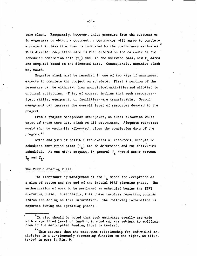
-53 -

zero slack. Frequently, however, under pressure from the customer or

in eagerness to obtain a contract, a contractor will agree to complete

a project in less time than is indicated by the preliminary estimates.

This directed completion date is then entered on the calendar as the

scheduled completion date (Ts) and, in the backward pass, new TL dates

are computed based on the directed date. Consequently, negative slack

may exist.

Negative slack must be remedied in one of two ways if management

expects to complete the project on schedule. First a portion of the

resources can be withdrawn from noncritical activities and allotted to

critical activities. This, of course, implies that such resources--

i.e., skills, equipment, or facilities--are transferable. Second,

management can increase the overall level of resources devoted to the

project.

From a project management standpoint, an ideal situation would

exist if there were zero slack on all activities. Adequate resources

would then be optimally allocated, given the completion date of the

,program.**

After analysis of possible trade-offs of resources, acceptable

scheduled completion dates (TS) can be determined and the activities

scheduled. As one might suspect, in general TS should occur between

TE and TL'

The PERT Operating Phase

The acceptance by management of the TS means the .cceptance of

a plan of action and the end of the initial PERT planning phase. The

authorization of work to be performed as scheduled begins the PERT

operating phase. Essentially, this phase involves reporting program

status and acting on this information. The following information is

reported during the operating phase:

It also should be noted that such estimates usually are madewith a specified level of funding in mind and are subject to modifica-tion if the anticipated funding level is revised.

**This assumes that the cost-time relationship for individual ac-

tivities is a continuously decreasing function to the right, as illus-trated in part in Fig. 9.

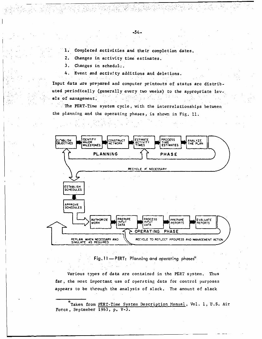
-54-

1. Completed activities and their completion dates.

2. Changes in activity time estimates.

3. Changes in schedul.

4. Event and activity additions and deletions.

Input data are prepared and computer printouts of status are distrib-

uted periodically (generally every two weeks) to the appropriate lev-

els of management.

The PERT-Time system cycle, with the interrelationships between

the planning and the operating phases, is shown in Fig. 11.

ESALS IDENTIFY R ESTIMATE PROCESS•)

MAJORIS HCONSTRuCT ATVY TIEANALYZEOBJETIVE MILESTONES NETWORK TIMES ESTIMATES THE.....

RECYCLE IF NECESSARY

ESTABLISHSCHEOULES

APPROVESCHEDULE S

REPLAN WHEN NECESSARY AND ' RECYCLE TO REFLECT PROGRESS AND MANAGEMENT ACTIONSIMULATE AS REQUIRED

Fig. I1 -PERT: Planning and operating phase?

Various types of data are contained in the PERT system. Thus

far, the most important use of operating data for control purposes

appears to be through the analysis of slack. The amount of slack

Taken from PERT-Time System Description Manual, Vol. 1, U.S. AirForce, September 1963, p. V-3.

-155e°

(often negative) is charted periodically so that management can follow

the trend from week to week. Normally, with good control the amount

of negative slack on a path should decrease over time. This decrease

is generally attributable either to greater management attention to ac-

tivities on that path or, as described below, to the lessening of un-

certainty concerning completion times.

The Standard Deviation (a) of an Activity

By using three time estimates for each activity, the scheduler

can apply probability theory in determining uncertainty in scheduling

activities. Assuming that the beta distribution is a valid representa-

tion of the distribution of the estimates, the standard deviation for

an activity can be approximated by the following equation:

b - a6'

thus the range (b - a) is six times the standard deviation.

To illustrate the standard deviation of an activity, let a = 10

months, m = 13 months, and b = 16 months. Then

t e 0 + 4(13) + 16= 13; (16 - 10) = 1.e . 6 6

A common interpretation of this statistic is that a 67 percent

chance (67 out of 100 times) exists that the activity will be completed

within one standard deviation (12th and 14thmonths);a 95 percent chance

between 2c of the mean (l1th and 15th months); and a 99 percent chance

between 3cr of the mean (10th and 16th months). This interpretation is

misleading because the above applies to a normal, and not to a beta

distribution. Depending on the skewness of the beta distribution one a

from the mean may contain considetably more or less than 67 percent of

the observations. The c has no inherent meaning in quantifying uncer-

tainty for an individual activity; however it is used to compute the a

of an eVent which is described in the following subsection.

-56-

Probability of Meeting Scheduled Date

or of Having Positive Slack

The probability of meeting the scheduled date or, alternatively,

of having positive slack can be determined by using the concepts of

slack and standard deviation of an activity. While this probability

statistic can be computed for any event in the project, the ending

event is used in the following example.

First, compute the length of the longest path leading into any

specific event (TE), and then compute the standard deviation of that

event's earliest occurrence time (arTE). The aTE is defined as the

square root of the sum of the activity standard deviations squared (a),

i.e., the variances of the activities lying on the longest time path

leading into that event. Here the event time (path length) is generally

assumed to be normally distributed, not beta distributed. The proba-

bility of meeting the scheduled date can then be determined by using

tables of the areas under the normal curve. The formula for this

normalized statistic is

T - TE

S E

If we assume that an event is scheduled to be completed in I0

n.onths, but the earliest expected date is 12 months from now, and the

standard deviation of that event.is 1 month, then

E " 10 12 -2 2.

"From tables of the area under a normal curve we find thaL a Z of minus

two (-2) is associated with 0.0228 of the total area under the curve;

Through invoking the central limit theorem. Also, the assumptionmust be made that the activities are independent. This assumption hasbeen challenged on numerous occasions, since many activities are inter-connected and also frequently appear on more than one path in a network.

Tables of areas under the normal curve can be found in virtuallyevery basic statistics textbook. They are also included in the PERT-Time System Description Manual, Appendix B.

-57 -

in other words, only two times out of 100 would management expect to

complete that event on schedule. Since this represents a small prmo-

ability, it is clear that the program schedule is in difficulty.

Unfortunately, management usually does not employ this probatility

measure because of a feeling that too much uncertainty exists in the

entire estimation and planning process for this statistical calculation

to have meaning. It also appears that management in general is"not

familiar with probability theory.

Actually, similar information can be presented to management with-

out using formal probability theory. The scheduling section in the

Dynasoar (X-20) Program Office derived an interesting surrogate for such

probability statistics. A "recovery ratio" was computed that was simply

a ratio of the negative slack to the length of the critical path. For

example, path A in a project may require 23 weeks to perform and con-

tain 5 weeks of negative slack. Path B may require 3 weeks and have I

week of negative slack. Slack calculations alone would indicate that

Path A was most critical (i.e., 5 > I). The recovery ratios for path A

would be (5 + 20), 1/4, or 0.25; for path B they would be (1 & 3), 1/3,

or 0.33. This would indicate that in reality path B is more critical

than path A, since only 3 weeks would remain to pick up I week of nega-

tive slack, whereas on A, 20 weeks are available to pick p 5 weeks of

negative slack. The recovery ratio is easier to compute and to under-

stand than the probability distribution, and is worth serious consider-

ation by management.

Types oE PERT Networks

The fact that various levels of management and numerous interre-

lationships among firms, agencies, and military offices that are in-

volved in weapon system acquisition was brought out in Sec. I of this

Memorandum. In such an environment, with its variety of demands, a

single network often will not suffice. Accordingly, variations have

been evolved to handle various aspects of the planning and control

process.

-58-

1. Detailed and Operating Level Networks

Generally, each prime or associate contractor constructs and uses

a network that covers his individual sphere of program responsibility.

If a portion of the project is subcontracted to another firm that sub-

contractor in turn may be required to construct #nd use a network for

his portion of the project. These networks are constructed in consider-

able detail and frequently comprehend even relatively minor activities

and events. Such networks are utilized by operating managements and

are termed operating networks, or detailed networks. In addition,

since they often cover only a fragment of a project, NASA has referred

to them as fragnets (fa.mentary networks).

2. integrated Project Networks

.The detailed operating networks prepared by the separate firms and

agencies may be combined or integrated, generally at the SPO level,

into one comprehensive network encompassing all events in the entire

project. Although perhaps not directly involved in detailed operations,

,the SPO can exercise management surveillance over the progress of the

entire project through use of this integrated network.

3. Condensed or Summary Networks

Generally, detailed networks contain too much operating data for

top project management or other interested parties (i.e., DOD, Head-

quarters USAF, etc.) monitoring the progress of the program on a more

aggregative basis. To accomplish this, a summary, or condensed network

is constructed which eliminates much of the detail, yet retains the

events of major significance. Such networks frequently are displayed

in project control offices.

Accurate translations of activity time estimates must be made when

the operating networks are either integrated or condensed. The inte-

gration and condensation processes involve identifying, recording, co-

ordinating and storing interface events. Various computer routines

It is evident that the level of detail may vary among ccntractors.

An interface event signals the transfer of responsibility, enditems, or information from one part of the project effort to another.

-59-

are being developed to accomplish this complex and vital task. The

relationship among these various forms of networks is indicated in

Fig. 12. This diagram depicts condensation of networks prior to net-

work integration. Either condensation or integration can occur first

depending on the requirements of the levels of program management.

Information usually is abstracted from the condensed network and

forwarded to agencies above the SPO in milestone form. The current

procedure of selecting information from the networks and listing this

information in line item or narrative form appears to have limitations.

One relatfvely simple improvement would utilize the network concept

and its relevant information on interrelationships at top project lev-

els. Perhaps this could be accomplished by including a requirement that

summary networks be incorporated in the System Package Program and that

project progress be reported against these networks.

APPLICATION OF PERT TO HYPOTHETICAL MISSILE SYSTEM

The PERT network shown in Fig. 13 for our hypothetical missile

system is a summary network. The events and activities are identical

to those used in the network illustrating the critical path technique

in Sec. IV, and the same "rules" are followed. In each case the work

flow envisioned at the time is the same, and thus the networks are the

same. However, in the PERT network, three time estimates are used for

each activity: optimistic, most likely, and pessimistic. These esti-

mates (taken from Table 1) are displayed in red on Fig. 13 to emphasize

the major difference between CPM and PERT.

The expected times as derived from the three time estimates in

PERT freqtently will differ somewhat from the single time estimates

recorded in CPM. As descrtbed above, the mean is conceptually a more

comprehensive measure incorporating the extreme (optimistic and pessi-

mistic) values and in this sense reflects the range of uncertainty re-

vealed by the three time estimates. The mean used in PERT will vary

As mentioned previously, the System Package Program is the basicmanagement document for major weapon systems programs. (See alsop. 19.)

-60.

1 4A

a II-

In

ce C

1-- I-0U'

00

o79 0) 0

0 0'

0 0. 0- u

El o Al

z 0 oww m

-61.

oio;

0 2 '470 0 20230

t IS 0 "

00

0.ý

0 -

9 79

Fig.13-PERT network applied to hypothetical missile system

from the mode used in CW in those instances when the time interval be-

tween the mode and the optimistic time differs from the interval be-

tween the mode and the pessimistic time estimates. The mean and mode

will coincide where there is equal uncertainty in positive and negative

directions, since the mode will bisect the range between the optimis-

tic and pessimistic times.

Once the expected time for each event has been computed, the tech-

niques are identical in their method of identifying the critical path.

In our missile system'example, the critical path for PERT is identical

with that for CPM (i.e., events 1, 8, 17, 18, 27, 33, 34, and 35).

However, the time to complete the project has been lengthened from 64.8

weeks to 68.6 weeks. This difference is the result of the fact that

-62-

in the estimates for individual activities prepared using the PERT tech-

nique, the range between the optimistic and expected times was less

than the range between the pessimistic and expected times.

In this simple example, the diffurence of 3.8 weeks in.a project

of 69 weeks' duration is only moderately important. It would be dif-

ficult to state clearly which estimate (PERT or CPM) was the more ac-

curate. The PERT technique is more sophisticated in that it does at-

tempt to deal with uncertainty. However, various mathematicians have

questioned certain of the simplifying assumptions used in the PERT

estimation process.

If, in scheduling the activities for our hypothetical missile sys-

tem, we assume a directed date of 65 weeks from now, that becomes the

scheduled date for completion of the project. If the length of the

critical path is 68.6 weeks, we have negative slack of 3.6 weeks. Be-

cause of the uncertainty inherent in the activities as shown by the

estimation intervals, management may require some "feeling" for the

likelihood of the project's being completed on schedule. Using the

concept of zero slack, this likelihood can be ascertained by computing

(1) the standard deviations of the activities on the critical path (c),

(2) the standard deviation of the final event (aE), (3) the Z statis-

tic, and, finally, (4) the probability of positive slack. These com-

putations are given in I Tle 9.

Note that the probability is only 0.25. A gambling management

might be content to proceed and see what develops, but most managements

would probably require at the very least a 50 percent chance of meeting

schedule. This would then call either for shifting resources from non-

critical events to critical events or for employing a higher level of

resources. If positive slack exists, management frequently is content

to assume that the project will be completed on schedule.

An analysis of the significance of these arguments is found inK.R. MacCrimmon and C. A. Ryavec, An Analytical Study of the PERTAssumptions, The RAND Corporation, RM-3408, December 1962.

-63-

Table 9

COMPUTATIONS REQUIRED FOR PROBABILITY OF POSITIVE SLACK

(I) Standard deviation and variance of critical path activities:

Event Number on Standard Deviation of Variance of anCritical Path an Activity E(b - a)/6] Activity (a 2)

8 0.5 - 0.1 0.07 0.00496

17 54 - 27 4.5 20.25006

18 1 0.5 0.25006

27 0.5 - 0.1 0.07 0.00496

33 0.5 - 0.1 0.07 0.00496

34 34" 1 3.0 9.00006

35 ~0.5 - 0.1 00

Total variance along the critical path .... 29.5196 or 29.52

(2) Standard deviation for the final event - ,'29.52 or 5.43.

(3) Z = T E 65 - 68.6 -3.6_ -0.662.'r"E 5.43 5.43

(4) Probability of positive slack. Referring to tables of the area underthe normal curve, the Z statistic corresponding to the number -0.662is approximately 0.25. This means that only 25 times out of 100could vanagement expect to complete the project on schedule.

EVALUATION OF PERT

Since its forrmilation, PERT has been received both favorably and

unfavorably. Those who favor it recognize it as a good planning tool.

Others feel that it has been offered as a panacea for all scheduling

problems. Still others think that the technique is "basically nothing

-64-

new." PERT, however, does offer several concepts not previously in-

corporatei in scheduling techniques.

Unfortunately, PERT, as conceived by its developers, has never

been applied in total to any major system. In particular, the three

time estimates and the probability computations have never had a thorough

test throughout a full project cycle. Perhaps the most complete at-

tempt was the use of the three time estimates on the Dynasoar program,

but that program was cancelled before compleLion.

Obviously, it is difficult to make a satisfactory comparison be-

tween CPM and PERT if the factors unique to PERT--its three time esti-

mates and use of probability theory--are not implemented. Since use

of the beta distribution in the PERT technique has been attacked by

mathematicians, and engineers have been reluctant to make the three time

estimates because they believe them to be too time-consuming, the prob-

ability calculations have usually been abandoned, perhaps justifiably.

However, any new system that is to be used by numerous firms requires

time to implement. Perhaps PERT should be implemented a portion at a

time. Further study might indicate that in most cases expected time

estimates do not vary significantly from single point estimates and

therefore multiple estimates are not justified in view of the added in-

convenience and cost. On the other hand, the problem of dealing with

uncertainties in estim-ates remains. This issue is as yet unresolved.

At first, PERT had no cost-estimating capability. Now the network

and critical path features of PERT-Time have proved their worth, and

attempts are being made to extend the concept to the cost and reliabil-

ity aspects of project management. The first full-scale application

of the PERT-Cost technique was made on the TFX program. It is important

to note that the PERT-type network provides a cormmon framework for in-

corporating these other factors, and thus PERT provides the basis for a

a more completely integrated management system.

PERT has earned widespread acceptance in industry and government.

and undoubtedly will be the dominant scheduling system for major devel-

opment programs for some time to come, especially rince attempts are

being made to integrate it with companion techniques for planning and

control of cost. In addition, it appears likely that a related

-65-

effort will be made to utilize it in the planning and control of tech-

nical performance.

Some of the strengths and weaknesses of PERT are suumarized in

Table 10.

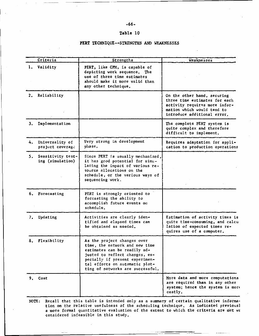
-66-

Table 10

PERT TECHNIQUE--STRENGTHS AND WEAKNESSES

Criteria Strengths Weaknesses

1. Validity PERT, like CPM, is capable ofdepicting work sequence. Theuse of three time estimatesshould make it more valid thanany other technique.

2. Reliability On the other hand, securingthree time estimates for eachactivity requires more infor-mation which would tend tointroduce additional error.

3. Implementation The complete PERT system isquite complex and thereforedifficult to implement.

4. Universality of Very strong in development Requires adaptation for appli-projuct coverage phase, cation to production operations

5. Sensitivity test- Since PERT is usually mechanized,ing (simulation) it has good potential for simu-

lating the impact of various re-source allocations on theschedule, or the various ways ofsequencing work.

6. Forecasting PERT is strongly oriented toforcasting the ability toaccomplish future events ouschedule.

7. Updating Activities are clearly iden- Estimation of activity times istified and elapsed times can quite time-consuming, and calcube obtained as needed. lation of expected times re-

quires use of a computer.

8. Flexibility As the project changes overtime, the network and new timeestimates can be readily ad-justed to reflect changes, es-pecially if present experimen-tal efforts on automatic plot-ting of networks are successful.

9. Cost More data and more computationsare required than in any othersystem; hence the system is mortcostly.

NOTE: Recall that this table is intended only as a summary of certain qualitative informa-tion on the relative usefulness of the scheduling technique. As indicated previous]a more formal quantitative evaluation of the extent to which the criteria are met weconsidered infeasible in this study.

-67-

VI. AREAS FOR FURTHER RESEARCH

Immediately following the development of CPM and PERT, many sched-

uling systems, often identified by ingenious acronyms, were developed

by industrial firms and governmental agencies. Most were attempts to

link time and cost information by relating both types of data to the

same network events. Several of the systems were developed by indi-

vidual corporations to conform to their special planning and control

requirements and were documented for use by other interested firms.

This recent stimulus to innovate in the area of planning and con-

trol techniques is largely attributable to the development of PERT and

CPM and to the availability of high-speed computers. The importance

of these variations should not be minimized, for they contribute toward

improvements in existing scheduling systems.

The following are some aspects of schedule planning and control

that oifer potential for further development or implementation in meet-

ing management requirements for information:

I. Greater use of data available in existing scheduling systems.

2. Use of networks in the selection of alternatives.

3. Integration of cost and performance elements with scheduling

techniques.

4. Development of a technique for identifying and processing

interfaces.

5. Simplification of scheduling techniques.

6. Extension of network concept to top-level management.

GREATER USE OF DATA AVAILABLE IN

EXISTING SCHEDULING SYSTEMS

Management has, in general, made substantial use of the informa-

tion in the available scheduling techniques. In several instances, how-

ever, these techniques could be made even more useful. For example,

at present no use is made of the concept of slack in the Gantt or mile-

stone techniques when planning developmental activity. It would be very

simple to compute the latest start date for an activity in addition to

-68-

its earliest start date. This simple extension of the data, perhaps

presented on a transparent overlay over the control chart of a given

date, would enable management to assess how critical schedule slippage

is on each milestone.

Likewise, the data contained in the PERT system really never have

been fully utilized. Aa indicated previously, the three time estimates

have never been consistently collected throughout any major weapon sys-

tem program, with the result that the use of probAbility applications

have been entirely lost to management. This is indeed unfortunate

since probabilistic approaches represent the best formal techniques

available to quantify the uncertainty inherent in forecasting the future

completion times for a project, PERT, without probability, in essence"Idegenerates" into the critical path method.

If three time estimates were obtained for a major system, statis-

tics similar to the recovery ratio described in Sec. V could be com-

puted. Although not as refined and sophisticated as the probability

computations, the recovery ratio would provide a better measure of un-

certainty than is presently obtainable and thus should lead to more

appropriate decisionmaking.

A well-documented case history of the application of the complete

PERT technique to a major system would provide a basis for evaluating

certain features of the PERT technique, such as the applicability of

the beta distribution. Modifications resulting from such an evaluation

would probably improve PERT and lead to more complete implementation

on projects where this technique is applicable.

USE OF NETWORKS IN THE SELECTION OF ALTERNATIVES

Management is continually faced with alternative courses of action

in system development. At least two major types of decisions recur

throughout the life cycle of a major system: (1) the selection of a

component design from alternative designs; and (2) the proper mix of

resources to develop a component at minimum cost. The network is a

very valuable aid in this decisionmaking process.

-69-

When more than one design is feasible, preparation of networks

depicting the development paths for each alternative can be of consid-

erable assistance in choosing the most suitable course of action.

Given a network of the activities involved in developing a certain

component, management can secure estimates of time required to

complete the component, assuming varying amounts and qualities of re-

sources for individual events. The least cost allocation can be selec-

ted, based on an acceptable level of quality and a time constraint.

Alternatively, given quality and cost limitations, the approach requir-

ing the shortest period of time can be selected.

These are examples of sensitivity analysis, i. e., of testing

the sensitivity of time to various component designs or resource

mixes. It is difficult for management to make these decisions by in-

tuition alone. Simulation of alternatives provides a quantitative

basis for selecting a preferred approach. In general, increased empha-

sis should be devoted to this process of identifying and analyzing

feasible alternatives.

The PERT technique permits simulation of alternatives if manage-

ment takes time to develop the networks and obtain the estimates. Fur-

ther research is desirable in scheduling for operations with limited

resources. For example, a forecast of activities based on presently

available resources may indicate that certain schedulea dates are unat-

tainable. Two or more activities may require a limuted resource--for

example, unique engineering skills--concurrently. Since the impact of

this resource limitation may not have been prope:ly identified initially,

these activities will be completed later than originally estimated.

INTEGRATION OF COST AND PERFORMANCE PARAMETERS

WITH SCHEDULING TECHNIQUES

Scheduling of resources to activities has cost and performance as

well as schedule implications. Frequently, the more resources applied

the shorter the time to completion, but also the greater the total

cost. Or, the higher the caliber of resource the shorter the time to

design technically complex projects and perhaps the higher the perform-

ance of the resulting system. It follows, then, that decisionmaking

-70-

would be improved if information were interrelated on the quantity and

quality of resources and the probability of attaining or surpassing the

desired performance specifications.

The critical path method offers a limited capability for time-cost

trade-offs. Recently, PERT/Cost has been developed establishing work

packages, comprehending groups of activities the completion of which

usually are identified by major events. Estimation can then be made on

the cost to complete a work package as well as on the time required to

attain the event. Thus, time and cost can be interrelated.

Some r search is being directed toward delineation of performance

specificati, ns for c'.iponents and subsystems based on an overall config-

uration index directly relatable with cost work packages and scheduled

events. Estimates of the probability of attaining the performance

specifications also can be made as the project progresses.

Each of these techniques has merit and when appropriately inte-

grated into a comprehensive information system, a much improved basis

for planning and controlling projects should evolve. The network con-

cept appears to provide a useful framework for such a system. As

familiarity is gained with the operational aspects of PERT/Cost, any

weak features should be overcome and suitable cost-estimating techniques

should evolve. Considerable research remains before the technical per-

formance fehtures become operational at a detailed level and additional

effort will be required to develop and integrate these techniques into

a single system.

DEVELOPMENT OF A TECHNIQUE FOR IDENTIFYING

AND PROCESSING INTERFACES

The interface problem has always plagued schedulers in constructing

networks. A technical interface occurs where one item in a project

mates with another item; or when information on the project is exchanged

between engineers or managers; or when responsibility is transferred

from one organization to another. There are countless such interfaces

in a large program, varying in level of importance in their effect on

project control. The most significant interfaces are placed on a net-

work and become interface events--i.e., events that signal the transfer

-71-

of responsibility, end items, or information from one part of the pro-

gram to another.

Several thousand network interfaces may occur during the acquisi-

tion of a large program. Failure to recognize significant interfaces

will result in loss of information and can distort schedule information

considerably. This distortion and loss of information is illustrated

in Fig. 14. Starting at the top of the figure, panel A depicts a simple

network for firms 1 and 2. The critical path for events under the con-

trol of firm I is A-B-C and is 12 weeks long. For the events under

firm 2's control, the critical path is D-E-F and is 16 weeks long.

Panel B shows the two networks integrated into one network. Note

the dependency of event B in firm i upon completion of event D in firm 2.

This dependency, plus the addition of starting event (I) and ending

event (J), lengthens the critical path to 28 weeks and has events in

both firms lying on the critical path.

Panel C is a sunmmary network for the integrated network in panel B.

Failure to recognize the interface between event D and event B resulted

in a critical path of 21 weeks; in addition, all events on the critical

path are within firm 2.

Panel D is a condensed network with the interrelationships properly

sunmmarizad. Note that the critical path is 28 weeks, the sane as in

the integrated network in panel B.

Interface events permit separate networks to be integrated into

one, complete network, and detailed networks to be summiarized into dis-

play networks. If interfaces are properly selected and coordinated,

loss of schedule information at the various levels of project control

will be minimized.

Most firms that use networks to schedule large projects have

evolved their own summarization and integration techniques, and each

firm has its preferred technique for handling interfaces. However,

there seems to be no complete documentation that describes a technique

for the proper identification and processing of all significant inter-

faces. A process, including a computer routine, must be established to

select, record, coordinate, and store information on these interfaces.

-72-

Panel A: Networks for individual firms

Firm No.1 Firm No.2

Panel B: Integrated network

66

2 15 3•

6 E Critical path 28 weeks

Panel C: Condensed network distorted because ignored inter-firm interface D-B

13 C5

18 3

F Critical path=21 weeks

Panel D: Properly condensed network

D Critical path =28 weeks

Fig.14-Network integration and condensation

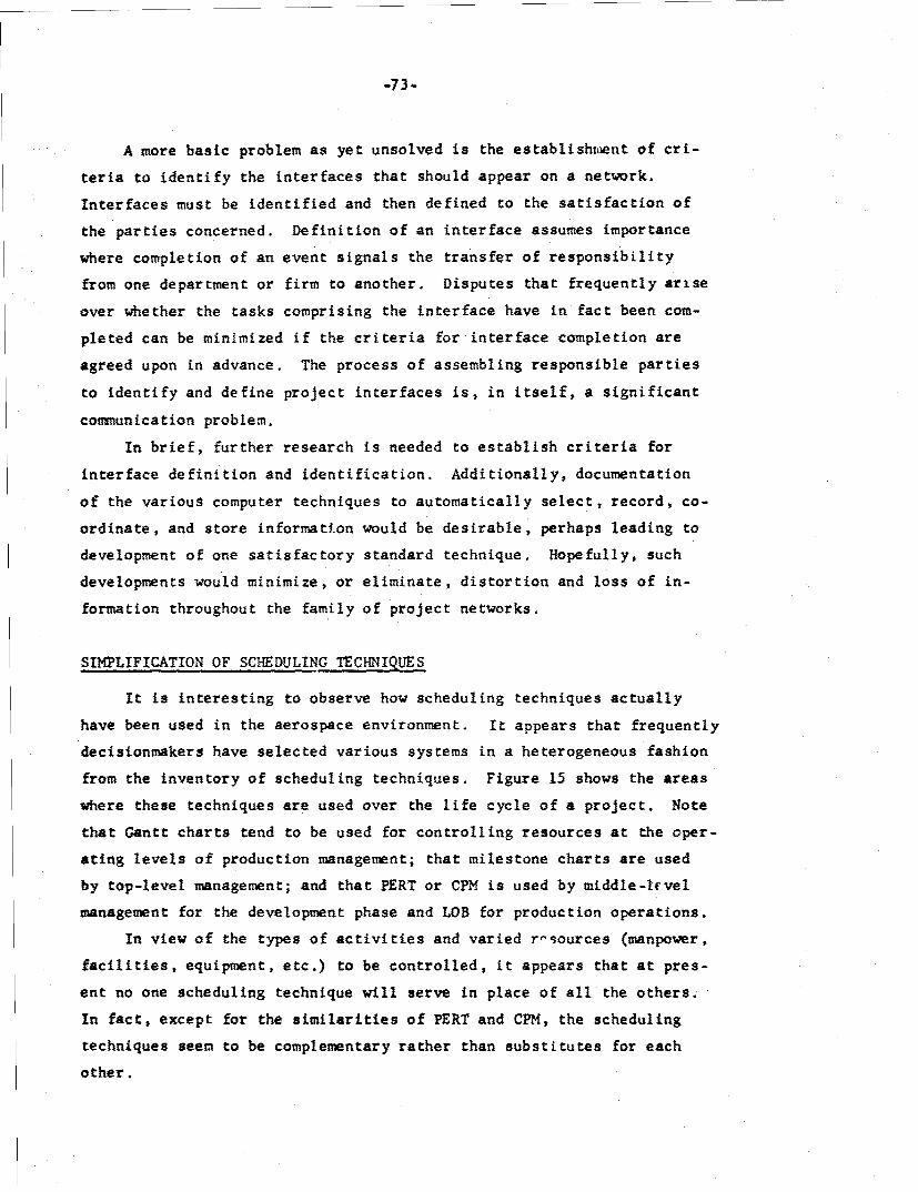
-73-

A more basic problem as yet unsolved is the establishment of cri-

teria to identify the interfaces that should appear on a network.

Interfaces must be identified and then defined to the satisfaction of

the parties concerned. Definition of an interface assumes importance

where completion of an event signals the transfer of responsibility

from one department or firm to another. Disputes that frequently arise

over whether the tasks comprising the interface have in fact been com-

pleted can be minimized if the criteria for interface completion are

agreed upon in advance. The process of assembling responsible parties

to identify and define project interfaces is, in itself, a significant

communication problem.

In brief, further research is needed to establish criteria for

interface definition and identification. Additionally, documentation

of the various computer techniques to automatically select, record, co-

ordinate, and store information would be desirable, perhaps leading to

development of one satisfactory standard technique. Hopefully, such

developments would minimize, or eliminate, distortion and loss of in-

formation throughout the family of project networks.

SIMPLIFICATION OF SCHEDULING TECHNIQUES

It is interesting to observe how scheduling techniques actually

have been used in the aerospace environment. It appears that frequently

decisionmakers have selected various systems in a heterogeneous fashion

from the inventory of scheduling techniques. Figure 15 shows the areas

where these techniques are used over the life cycle of a project. Note

that Gantt charts tend to be used for controlling resources at the aper-

sting levels of production management; that milestone charts are used

by top-level management; and that PERT or CPM is used by middle-lcvel

management for the development phase and LOB for production operations.

In view of the types of activities and varied r-sources (manpower,

facilities, equipment, etc.) to be controlled, it appears that at pres-

ent no one scheduling technique will serve in place of all the others.

In fact, except for the similarities of PERT and CPM, the scheduling

techniques seem to be complementary rather than substitutes for each

other.

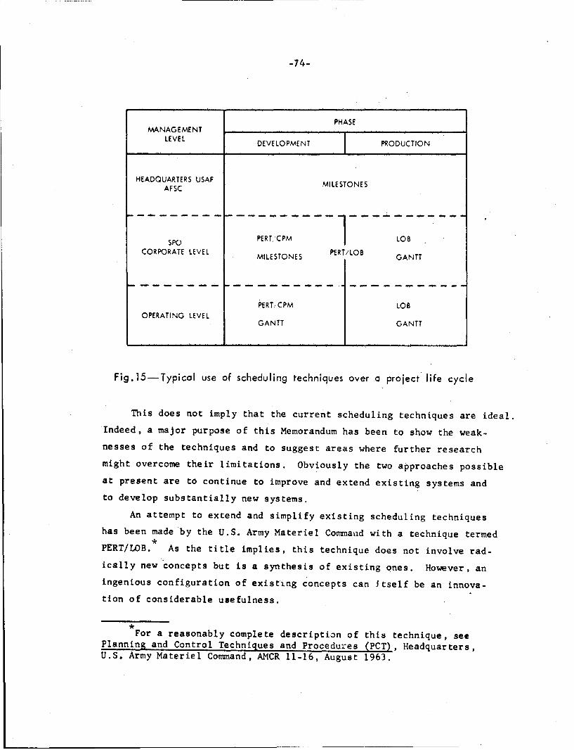
-74-

PHASEMANAG EMENT .. .. .. . ... . . . . . . . .LVLDEVE LO PME NT PR ODUCTIO N

HEADQUARTERS USAF MILESTONESAF SC ILSTNS

SKo PERT, 'CPM LOB

CORPORATE LEVEL MILESTONES PERT/LOB GANTT

PERT CPM LOBOPERATING LEVEL

GANTT GANTT

Fig.15-Typicol use of scheduling techniques over a project life cycle

This does not imply that the current scheduling techniques are ideal.Indeed, a major purpose of this Memorandum has been to show the weak-nesses of the techniques and to suggest areas where further researchmight overcome their limitations. Obviously the two approaches possibleat present are to continue to improve and extend existing systems and

to develop substantially new systems.

An attempt to extend and simplify existing scheduling techniqueshas been made by the U.S. Army Materiel Command with a technique termedPERT/LOB. As the title implies, this technique does not involve rad-ically new concepts but is a synthesis of existing ones. However, an

ingenious configuration of existing concepts can Itself be an innova-

tion of considerable usefulness.

For a reasonably complete description of this technique, seePlanning and Control Techniques and Procedures (PCT), Headquarters,U.S. Army Materiel Command, AMCR 11-16, August 1963.

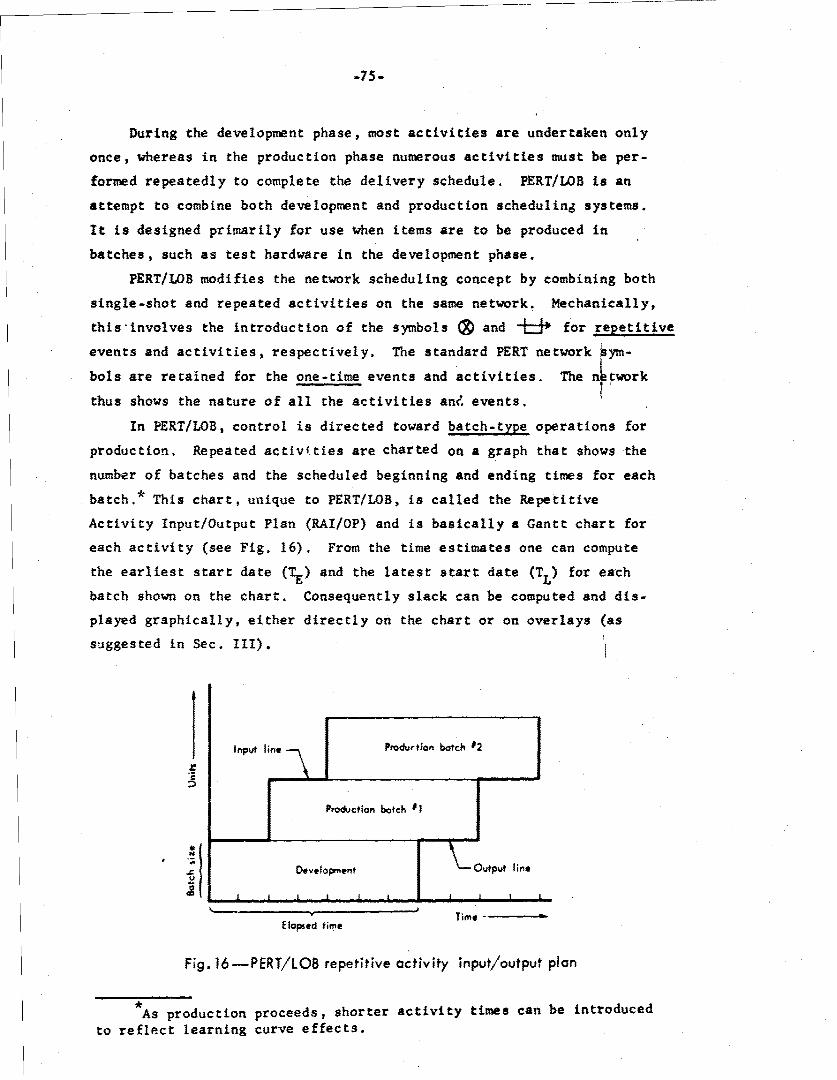
-75-

During the development phase, most activities are undertaken only

once, whereas in the production phase numerous activities must be per-

formed repeatedly to complete the delivery schedule. PERT/LOB is an

attempt to combine both development and production scheduling systems.

It is designed primarily for use when items are to be produced in

batches, such as test hardware in the development phase.

PERT/LOB modifies the network scheduling concept by combining both

single-shot and repeated activities on the same network. Mechanically,

this'involves the introduction of the symbols ® and &9* for repetitive

events and activities, respectively. The standard PERT network Sym-

bols are retained for the one-time events and activities. The n.work

thus shows the nature of all the activities anC events.

In PERT/LOB, control is directed toward batch-type operations for

production. Repeated activities are charted on a graph that shows the

number of batches and the scheduled beginning and ending times for each

batch.* This chart, unique to PERT/LOB, is called the Repetitive

Activity Input/Output Plan (RAI/OP) and is basically a Gantt chart for

each activity (see Fig. 16). From the time estimates one can compute

the earliest start date (TE) and the latest start date (TL) for each

batch shown on the chart. Consequently slack can be computed and dis-

played graphically, either directly on the chart or on overlays (as

suggested in Sec. III).

Input line Production botch 02

Production batch F1

tDevelopment \ Output line

TimeElapsed time

Fig. 16-PERT/LOB repetitive activity input/output plan

* As production proceeds, shorter activity times can be introduced

to reflect learning curve effects.

.76-

A further minor modification in scheduling technique involves the

construction of the line of balance on the program progres; chart. In

the traditional LOB technique for continuous production ui individual

units, the line of balance indicates the quantity of units that should

have passed through various control points if the delivery schedule is

to be met. In PERT/LOB, the line of balance is constructed to indicate

the number of batches that should be completed. Since a batch generally

contains more than one unit, this trethod results in a more conservative

line of balance than the traditional method. In PERT/LOB the entire

batch must be past the control point to be on schedule. For example,

if there were 10 units in the batch and 7 units had been completed, the

batch~would be behind schedule, whereas if only units were being con-

trolled, the completion of 7 units might indicate that the schedule

would be met without undue difficulty.

Finally, since PERT/LOB is based on a work breakdown structure,

work packages can be costed; and where batches are produced, cost esti-

mates for each batch can be employed.

In brief, PERT/LOB is a conglomerate technique embodying numerous

concepts entirely within the state of the art in scheduling. It pro-

vides a framework for planning and control of the development and pro-

duction phases of a major system, and also permits the combining of

schedule and cost considerations. Although not representing a real ad-

vance in the state of the art, it is a step in the proper direction.

Further experimentation along these lines should be encouraged.

EXTENSION OF NETWORK CONCEPT TO TOP-LEVEL MANAGEMENT

Networks are not currently employed at the lowest levels of activ-

ity nor at the highest levels of project monitoring. There are valid

reasons for not using them at the lower levels since the Gantt chart is

more applicable to the control of resource inputs (machines, labor, etc.).

However, assuming that the networks can be adequately summarized, there

is no valid reason for not extending the network concept to top-level

management, who presently rely on milestone charts. In the System

Package Program (SPP) in particular the milestones could be related to

-77-

each other in network form and could, with little effort, be made to

depict major interdependencies in the project. It would also be pos-

sible to show slack for each milestone, and perhaps the probability of

zero slack. If networks were not feasible for certain projects at the

SPP level, at least the analysis of slack and other pertinent informa-

tion could be integrated into the milestone chart system.

NEED FOR NEW SCHEDULING CONCEPTS AND TECHNIQUES

Each of the scheduling techniques discussed in this Memorandum

contained new concepts that were evolved to meet a perceived need. A

need now exists for a reasonably standardized technique capable of en-

compassing the entire weapon system. There is every reason to be op-

timistic that new concepts and applications--perhaps beyond networks--will

continue to evolve to meet this need.

This Memorandum has been directed toward defining the multi-faceted

environment of weapon systems acquisition and explaining the major

scheduling systems developed to date. Analysis of these scheduling

techniques has highlighted their strengths and weaknesses, which, in

turn, has led to suggested areas where further research is needed. Ad-

mittedly, a bias exists for preferring theoretically superior informa-

tion systems, in spite of the fact that formidable problems frequently

exist in their wide-scale implementation. In the future, advanced sched-

uling techniques will undoubtedly evolve. Currently, the wise selection

and adaption of techniques, with full knowledge of their strengths and

limitations, should lead to improved scheduling and, consequently, to

increased effectiveness in meeting delivery dates and in the efficient

use of resources.

-79-

BIBLIOGRAPHY

Badin, John, Jr., Application of Management Alternatives UtilizingNetwork Techniques, American Society of Mechanical Engineers, PaperNo. 63-WA357, New York, 1963.

Clark, Wallace, The Gantt Chart, 3d ed., Sir Isaac Pitman & Sons, Ltd.,London, 1957.

Cosinuke, Walter, Critical Path Technique, Catalytic ConstructionCompany, Philadelphia, November 1961.

Critical Path Method, General Electric Company, Computer Department,1961.

Fondahl, John W., A Non-Computer Approach to the Critical Path Methodfor the Construction Industry, 2d ed., Department of Civil Engineering,Stanford, California, 1962.

Glossary of Management Systems Terms (with Acronyms), Headquarters,U.S. Air Force Systems Command, AFSCP 11-2, November 9, 1962.

Kelley, J. E., Jr., and M. R. Walker, "Critical Path Planning andScheduling," Proceedings, Eastern Joint Computer Conference, Boston,Massachusetts, December 1959.

Line of Balance Technology, U.S. Department of the Navy, Office ofNaval Materiel, NAVEXOS P1851, April 17, 1952.

MacCrimmon, K. R., and C. A. Ryavec, An Analytical Study of the PERTAssumptions, The RAND Corporation, RM-3403, December 1962.

Moshman, Jack, Jacob Johnson and Madalyn Larsen, RAMPS--A Technique forResource Allocation and Multi-Project Scheduling, Proceedings 1963Spring Joint Computer Conference.

PERT Implementation Manual, Vol. 5, U.S. Air Force, April 1964.

PERT: An integrated Management Information and Control System, Opera-tion Research Inc., Silver Spring, Maryland, 1961.

PERT, Program Evaluation Research Task, Phase I, Summary Report, U.S.Department of the Navy, Bureau of Ordnance, Special Projects Office,Washington, D.C., July 1958.

PERT-Cost System Description Manual, Vol. 3, U.S. Air Force, December1963.

PERT-Time System Description Manual, Vol. 1, U.S. Air Force, !september1963.

Planning and Control Techniques and Procedures(PCT), Headquarters, U.S.Army Materiel Command, AMC Regulation 11-16, Vol. 2, August 1963.

Rathe, A. W. (ed.), Gantt on Management, American Management Associationand the American Association of Mechanical Engineers, The RiversidePress, Cambridge, Massachusetts, 1961.

-80-

Sadow, R. M., How PERT is Used in Managing the X-20 (DYNA-SOAR) Program,U.S. Air Force Systems Command, Aerospace Systems Division, TechnicalDocumentary Report No. ASD-TDR-63-698, Wright-Patterson Air Force Base,Ohio, September 1963.

Sperling, J. A., Functional Analysis of Several Project Control Techniques,Master's Thesis, Columbia University, New York, 1961.

Systems Data Presentation and Reporting Procedures (Rainbow Report),Headquarters, U.S. Air Force Systems Command, Andrews Air Force Base,Washington, D.C., November 1, 1961.

System Program Documentation, Air Force Regulation No. 375-4, Departmentof the Air Force, Washington, D.C., November 25, 1963.

Systems Program Management Manual, U.S. Air Force Systems Command, AFSCM375-4, March 16, 1964.

Wiest, J. D., The Scheduling of Large Projects with Limited Resources,Doctoral Dissertation, Office of Naval Research, Research MemorandumNo. 113, Graduate School of Industrial Administration, CarnegieInstitute of Technology, Pittsburgh, 1963.

UMENT CONTROL DATAIGINATING ACTIVITY 2o REPORT SECURITY CLASSIFICATION

UNCLASSIFIE0)THE RAND CORPORATION 2b. GROUP

.PORT TITLE

AN ANALYSIS OF MAJOR SCHEDULING TECHNIQUES IN THE DEFENSESYSTEMS ENVI RONMENT

JTHOR(S) (Lost name, ti ,st nom., initial)

Holtz, J. N.

PORT DATE October 1966 6o TOTAL Nn OF PAGES . 6b.NNo. OF REFS.

NTRACT OR GRANT No. 8. ORIGINATOR'S REPORT No.

AF 49(638)-1700 RM-4697-PR

,AILABILITY/ LIMITATION NOTICES 9b. SPONSORING AGENCY

DDC-1 United States Air ForceProject RAND

BSTRACT II. KEY WORDS

A z;rvey ' f the mat'or . u , "':.'- riter e e ;'.;t..*;ZufPz curre-ntly~ .availi:• le t p, rc,le-.:' L,:•,•.,,e u.'i n ,"aýe men.nt. 'hf nat ure o t h w af1-c s,'y;- ii tarv p.anrr,

Saziulstiori e2Viron:.ent With its in-

ernt r-r n'. r , s cxa. i n e in 1 i, 1.•r a s :e•u %i-; devices (the "..u,

r't, m'i z ,•e chart, line-ofl-b'ii.:1•i'eirnique, criti --al-path metnod, %n! "IrIPT)evaluated and contraste'l throuh , a1tein• 'ITd wea,,on synt, em. he it-zte t

-ýX•.• i s "t" i :r ;na-r • i• :' i n:ualso " i rd- r't.r,ý;. r

Q om--ifi. Aq oq