This article was published in an Elsevier journal. The attached copyis furnished to the author for non-commercial research and

education use, including for instruction at the author’s institution,sharing with colleagues and providing to institution administration.

Other uses, including reproduction and distribution, or selling orlicensing copies, or posting to personal, institutional or third party

websites are prohibited.

In most cases authors are permitted to post their version of thearticle (e.g. in Word or Tex form) to their personal website orinstitutional repository. Authors requiring further information

regarding Elsevier’s archiving and manuscript policies areencouraged to visit:

http://www.elsevier.com/copyright

Author's personal copy

Benzene exposure in a sample of population residing in adistrict of Florence, Italy

M. Cristina Fondellia,⁎, Paolo Bavazzanob, Daniele Grechic, Giuseppe Gorinia,Lucia Miligia, Gaetano Marchesed, Isabella Cennib, Danila Scalac,Elisabetta Chellinia, Adele Seniori Costantinia

aOccupational–Environmental Epidemiology Unit, Centre for the Study and Oncology Prevention (CSPO), Florence, ItalybLocal Health Authority 10 (ASL 10), Prevention Department — Public Health Laboratory, Florence, ItalycTuscan Environment Protection Agency (ARPAT) — Local Department of Florence, ItalydLocal Health Authority 10 (ASL 10), Prevention Department — Unit Hygiene and Public Health, Florence, Italy

A R T I C L E I N F O A B S T R A C T

Article history:Received 17 July 2007Received in revised form18 October 2007Accepted 24 October 2007Available online 21 December 2007

Objective: Personal exposure to airborne benzene is influenced by various outdoor andindoor sources. The first aim of this studywas to assess the benzene exposure of a sample ofurban inhabitants living in an inner-city neighborhood of Florence, Italy, excludingexposure from active smoking. The secondary objective was to differentiate the personalexposures according to personal usage patterns of the vehicles.Methods: A sample of 67 healthy non-smokers was monitored by passive samplers duringtwo 4-weekday campaigns in winter and late spring. Simultaneously, benzenemeasurements were also taken for a subset of participants, inside and outside theirhouses. A 4-day time microenvironment activity diary was completed by each subjectduring each sampling period. Other relevant exposure data were collected by aquestionnaire before the sampling. Additional data on urban ambient air benzene levelswere also available from the public air quality network. The passive samplers, afterautomated thermal desorption, were analyzed by GC-FID.Results: Benzene personal exposure levels averaged 6.9 (SD=2.1) and 2.3 (SD=0.7) μg/m3 inwinter and spring, respectively. Outdoor and indoor levels showed high correlation inwinterand poor in spring. In winter the highest benzene personal exposure levels were for peopletraveling by more public transport, followed by users of only car and by users of only busrespectively.Conclusions: The time spent in-transport for work or leisure makes a major contribution tobenzeneexposureamongFlorentinenon-smokingcitizens. Indoorpollutionandtransportationmeans contribute significantly to individual exposure levels especially in winter season.

© 2007 Elsevier B.V. All rights reserved.

Keywords:BenzeneCommuting exposurePersonal exposurePersonal monitoringUrinary cotinineEnvironmental tobacco smoke

1. Introduction

Benzene is an ubiquitous un-reactive primary pollutant of theambient air, mainly due to anthropogenic mobile (vehicular)

sources: about 86% in Italy (De Lauretis et al., 2003), withbackground ambient levels in the pristine European conti-nental air ranging from 0.6 to 1.9 μg/m3, and in heavilytrafficked urban areas frequently up to 10 μg/m3 (EC, 2005). In

S C I E N C E O F T H E T O T A L E N V I R O N M E N T 3 9 2 ( 2 0 0 8 ) 4 1 – 4 9

⁎ Corresponding author. Occupational–Environmental Epidemiology Unit, Centre for the Study and Oncology Prevention (CSPO), S. Salvistreet, 12; 50135 — Florence, Italy. Tel.: +39 055 6268346; fax: +39 055 679954.

E-mail address: mc.fondelli@cspo.it (M.C. Fondelli).

0048-9697/$ – see front matter © 2007 Elsevier B.V. All rights reserved.doi:10.1016/j.scitotenv.2007.10.060

ava i l ab l e a t www.sc i enced i rec t . com

www.e l sev i e r. com/ loca te / sc i to tenv

Author's personal copy

metropolitan areas, benzene is commonly known as a vehicleexhaust gas-phase emission marker (Jo and Park, 1999).

People are exposed to benzene mainly through inhalationof polluted air, particularly in outdoor areas of heavy traffic(from both vehicular exhaust emission and evaporative lossesof petroleum-related fuels) (Crosignani et al., 2004; Raaschou-Nielsen et al., 2001; Pearson et al., 2000), around oil refineries,industrial production and processing of benzene, repairgarages, and gasoline service stations (Harrison et al., 1999;Steffen et al., 2004; Karakitsios et al., 2007). Similarly, living inthe vicinity of hazardous landfills and industrial facilities mayincrease residential benzene exposure (Jo et al., 2004). Whenindoors, the principal emission sources are EnvironmentalTobacco Smoke (ETS), usage of petroleum-related fuels forcooking/heating, and benzene emitting cleaning/consumerproducts. Among the personal lifestyle sources: active smok-ing and automobile-related activities (e.g., driving, riding, self-service refueling (Egeghy et al., 2000), and vehicle exhaustemissions from attached garages) may increase the individualexposure.

Benzene is an air toxin of the greatest concern to publichealth because is a well-known human carcinogen since 1981,causing leukemia (Rinsky et al., 1981; IARC, 1982): hence nosafe exposure level could be recommended.

Before the 1980s, benzene was widely used as industrialintermediate and solvent (e.g., for waxes, resins, paints,glues, degreasing agents etc.). Progressive elimination,replacements, and use restrictions, when possible, or theintroduction of closed cycles to protect worker health inindustrial and manufacturing workplaces, and the banningfrom the commercial products, have ensured that healtheffects due to high concentration levels do not occur nowa-days. Currently, benzene exposures in working and livingenvironments are quite similar, so the focus is made on thelong-term effects of low levels occurring both occupationallyand environmentally.

In Florence, a negative trend in the annual mean ambientbenzene level has been registered at the end of the 1990s dueto the increasing number of catalyst-equipped vehicles (DeLauretis et al., 2003) and to the Italian lawn 413/1997 (Italian OJn 282, 1997) that fixed to less than 1% and 40% by volume themaximum quantity of benzene and of total aromatic hydro-carbons in gasoline, respectively, and required vapor recoverysystems at all gasoline pumps starting from July, 2000.

A Florentine public air quality monitoring network of fixedstations routinely provides time integrated measurements ofambient benzene, in accordancewith the European and Italianrules, to establish compliance with the yearly average LimitValue (LV) of 5 μg/m3 set by Directive 2000/69/EC (ECOJ L 313,2000). These data, collected in order to determine long-termair quality, are not good proxy for the citizen exposuresbecause people living in urban areas habitually spend morethan 90% of their time inside (Klepeis et al., 1996) andwhen areoutdoors at roadside locations are exposed to higher motorvehicle emission levels (Violante et al., 2006).

The present study was conducted with the aims ofestimating the inhalation benzene exposure of healthy, non-occupationally exposed, and non-smoking citizens during ausual weekday, concurrently comparing concentration levelsinside and outside of participants' residences, and evaluating

how different personal behaviors and lifestyles might changepersonal benzene exposure.

2. Materials and methods

2.1. Study area description, participant recruitment, andsample collection

Florence is located in the centre of the Italian peninsula andhas about 352,000 inhabitants. Florence's largest residentialdistrict is Rifredi (population density: 3715 people/km2; area:28 km2), located in the northern part of city. Approximately104,000 people live here and have a diverse ethnic makeup:95.3% Italian citizens, 4.7% Immigrants. The Rifredi's mainambient sources of benzene are dispersed mobile and sta-tionary sources (e.g., filling stations, domestic heatings, repairshops, and small manufacturing facilities etc.). Rifredi wasselected because it is considered representative of whole city:it is highly populated, has streets having different trafficintensities, and the local public administrators gave greatsupport and agreement to our project to arrange meetingswith the Residents.

Sixty-seven Italian adults, who self-reported to be occupa-tionally unexposed to benzene and non-smokers or ex-smokers, participated in this study. Forty-seven subjectswere randomly selected from the municipal demographicalregister (acceptance rate 60%) and twenty were volunteers.

They were invited to wear a radial diffusive integratedsampler in their breathing zone, Radiello® (Cocheo et al.,1996), to assess 4-day-Time-Weighted-Average personal inha-lation exposures during the first four weekdays in winter (onDecember 10–13, 2001, from Monday to Thursday) and in latespring (on June 3–6, 2002, the same weekdays as in winter).During showering, bathing, and while sleeping, the partici-pants placed their samplers in locations that could practicallyrepresent the breathing zone (e.g., night table while sleeping).The study's participants were trained in the use of Radiello®samplers and provided with written instructions.

Outdoor and indoor residential airborne benzene wassimultaneously collected using the Radiello® devices in thesub-group of volunteers' dwellings.

Two indoor samplers were installed: the first one (insidehome I) in the room located near the street with high-trafficdensity, the second (inside home II) characterized by theopposite situation (possibly near an inner courtyard). Theoutdoor sampler was placed in a location corresponding to thefirst indoor sampler, in a protected but not obstructed locationjust outside the facade of the building (facing the road). Thesamplers, if possible without shelter, were usually positionedapproximately 2mvertically from the apartment floor and 1maway any obstacle with a free solid angle of 180°.

After the first sampling day, a daily sample of the partici-pant's urine from 5 to 8 p.m. was collected for each campaignand subject: urinary-cotinine (U-cotinine) concentration wasmeasured to validate the non-smoking status and to assess theETS exposure.

Each participant was also invited to fill out a 4-day TimeMicroenvironmental Activity Diary (TMAD) to determine thedaily time spent indoors, outdoors, and in-traffic and possible

42 S C I E N C E O F T H E T O T A L E N V I R O N M E N T 3 9 2 ( 2 0 0 8 ) 4 1 – 4 9

Author's personal copy

benzene sources during the monitoring period. Additionalquestions also considered the occupation, the number ofsmokers among their relatives, transportation mode andhouse characteristics (e.g., floor, heating mode, and proximityto high-traffic road). Before undertaking personal exposuresampling, each participant was provided with backgroundinformation on the study and was asked to complete aninformed consent form according to the Italian privacyprotection law n 675/1996. All participants gave their writteninformed consent.

2.2. Sample analysis

After the sampling, all the exposed cartridges were trans-ported and stored at less than 4 °C until analysis and wereprocessed within a week after their arrival in the laboratory.

The benzene sampling rate at 25 °C, equal to 28 mL/min,was supplied by the Radiello® manufacturer. Temperatureand relative humidity are not significant for indoor andpersonal samples. For outdoor samples, extreme temperatureconditions did not occur during the survey periods (seeTable 1), so the sampling rate was not adjusted by tempera-ture. The mean concentration C (μg/m3) was calculated by:

C ¼ 106Ms�Mb

Kt

� �:

Where: Ms = benzene mass in μg which is desorbed fromsample;Mb = benzenemass in μgwhich is desorbed fromblank;K = sampling rate in mL/min; t = sampling time in minutes.

The collected benzene was thermally desorbed using aPerkinElmer® Turbomatrix ATD and analyzed with a gas-chromatograph GC-FID, equipped with PerkinElmer® Turbo-chromWorkstation Software. The benzenewas desorbed withhelium (40 mL/min) at 300 °C for 15 min in a cold trap (−30 °C)filled with 60–80 mesh Tenax TA. Other desorption conditionsincluded: the split inlet at 5 mL/min, the valve transfer linetemperature at 180 °C, and an injection time of 1 min.

The GC column was a capillary Supelco Petrocol DH(0.25 μm I.D., 100 m long, 0.5 μm film thickness). Helium wasused as a carrier at the flow rate of 36 mL/min. The GCtemperature programme started at 70 °C for 20 min, thenrising 10 °C/min to 120 °C, and was held for 16 min, afterwardrising 15 °C/min to 180 °C, and was held for 10 min. Thedetector temperature was at 250 °C. The analysis time was

55 min. The 5 point calibration curve was created by usingdifferent standards (from 50 to 250 μg/mL) and determined bylinear least-squares regression. The peak identification of thechromatogram was done on the basis of retention time ofstandard referencematerial (high purity), if the retention timeof the sample was within ±2 s compared to the standard, thepeak could be determined. Following IUPAC guidance andusing 10 blanks, the benzene Detection Limit (DL) was 10 ng,while the Quantitation Limit (LOQ) was 20 ng. This self-developed analytical method was validated following theStandard UNI CEI EN ISO/IEC 17025/2000. By vapor benzeneaddiction to the sampler, the recovery was estimated to beabout 98%. Within-run and run-to-run repeatability wasevaluated on 10 replicates at two levels (100, 200 ng/sample)and was found to be below 5 and 10.7%, respectively.Measurement uncertainty was estimated by combination ofstandard uncertainty coming from repeatability, trueness, andcalibration acceptability, with a coverage factor K=2 and 95%confidence level. The interval of extended uncertainty socalculated was 26%. A control sample (100 ng/mL) was twinceanalyzed at the beginning and the end of each analytical run.

Determination of U-cotinine was carried out by highperformance gas chromatography/mass spectrometric analy-sis with Positive Chemical Ionization and with Tri-deuteratedcotinine as the internal standard according to a publishedprocedure by Skarping et al. (1988; http://www.ao-meyer.toscana.it/oggetti/1328.pdf). The LOQ was about 0.2 ng/mL.

2.3. Meteorological and ambient benzene data

For characterizing the ambient conditions during each of thedays on which monitoring was performed, we used themeteorological data (e.g., temperature, wind speed, etc.)obtained from the TuscanMeteorological Centre “OsservatorioXimeniano”, located at the city centre, while the Florentinemonitoring network provided the corresponding daily ambi-ent benzene data.

2.4. Statistical analysis

The obtained data were processed using Microsoft OfficeEXCEL. All statistics and the linear regressionswere performedwith Intercooled STATA program (version 9 for Windows,STATA Corp, College Station, TX).

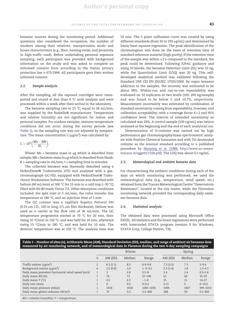
Table 1 – Number of sites (n), Arithmetic Mean (AM), Standard Deviation (SD), median, and range of ambient air benzene datameasured by air monitoring network, and of meteorological data in Florence during the two 4-day sampling campaigns

Winter Spring

n AM (SD) Median Range AM (SD) Median Range

Traffic station (μg/m3) 2 8.3 (2.1) 8.3 6.9–9.8 7.3 (3.2) 7.3 5–9.6Background station (μg/m3) 4 2.5 (0.6) 2.6 1. 9–3.2 2.3 (1.4) 1.8 1.2–4.3Daily mean prevalent horizontal wind speed (m/s) 1 3 2.8 0.5–8 2.4 2.4 0.5–5.6Daily mean RH (%) 1 70 73 27–100 61 60 35–97Daily mean T (°C) 1 4.5 4.3 −1–9 21 21 14–27Daily rain (mm) 1 0 0.0 0–0.2 0.15 0 0–14.6Daily mean pressure (mbar) 1 1018 1018 1005–1030 1005 1007 995–1013Daily mean global radiation (W/m2) 1 75 0.3 0.2–400 208 59 0.1–903

RH = relative humidity; T = temperature.

43S C I E N C E O F T H E T O T A L E N V I R O N M E N T 3 9 2 ( 2 0 0 8 ) 4 1 – 4 9

Author's personal copy

3. Results

Table 1 describes the ambient air benzene levels and themeteorological data by sampling campaigns. The maindifferences were, of course, between rainfall levels andtemperature and global radiation levels that were respectivelylower and higher on winter sampling days than those inspring. December was chosen to represent winter conditionsand May to represent spring/early summer.

Only 54 subjects of first 67 have joined the springcampaign. The study group consisted predominantly of men(54%). The mean age was 44±17 years (range between 16 and75 years). Thirty subjects resided in a low-traffic street (TrafficDensity (TD) b2000 vehicles/day), 15 in amedium-traffic street(TD 2000–10,000 vehicles/day), and 22 on a high-traffic street(TD N10,000 vehicles/day). Other participants' features are inTable 2.

Based on information provided by Haufroid and Lison (1998),the subjects with mean U-cotinine levels above 100 ng/mg ofcreatinine were classified as “active smokers” and elimi-nated from the statistics. The threshold mean U-cotinine levelof 5ng/mgof creatininewasused to classify the subjects asnon-exposedor exposed to ETS. Fifty-four (81%) and41 (76%) subjectswere non-ETS exposed, non-smoking in winter and spring,respectively.

Before the data analysis, we used the subjects' 4-dayTMADs to classify the study participants according to theirusual time spent daily commuting to work or for other taskslike school, shopping, leisure etc., and U-cotinine data usingthe following categories:

Active smokers: persons who self-reported to be non-smokers, but had mean U-cotinine levels above 100 ng/mg ofcreatinine. These persons: 5 people in winter (3 in spring) wereeliminated from the data set.

Non-ETS and non-traffic-related pollutant exposed per-sons (reference group): non-smokers who spent more than17 h/day (1020 min) inside their homes (more than 71% of theday) and were not exposed to ETS (mean U-cotinineb5 ng/mgof creatinine). They rarely traveled by motor vehicles and onlyoccasionally walked around. This group is composed of 6people in winter (3 in spring).

Car users: they spent more than 60 min/day traveling bypersonal cars (median value: 85 (91)min inwinter (spring)) anddid not use municipal public bus service. They might beexposed to ETS (U-cotinine range: 0.6–80.0 ng/mg of creati-nine). The group has 18 people in winter (9 in spring).

Bus users: they spent about 60 min/day traveling by publicbus (median value: 69 (54) min in winter (spring)). Theymay beexposed to ETS (U-cotinine range: 1.3–4.5 ng/mg of creatinine).The group has 6 people in winter (2 in spring).

Mixed users: each day used more than one type of motorvehicle (e.g., public bus, private car, motorbike, and all thesetypes of vehicle in combination), bicycling and walkingwithout any specific pattern in transportation mode andtraffic-related activities (e.g., traveling to and from work/school, shopping, etc.). They might be exposed to ETS (U-cotinine range: 0.4–90.3 ng/mg creatinine). This group has 32people in winter (37 in spring).

The results of personal measurements are shown in Fig. 1.A statistical summary of personal and residential measure-ments is given in Table 3. None of the obtained datawas belowthe detection limit.

In wintertime the mean personal level was equal to 6.9±2.1 μg/m3 (n=62) and equal to 2.3±0.7 μg/m3 (n=52) in spring,givingapproximately three timeshigherexposure inwinter thaninspring. TheShapiro–WilkW test fornormalitywithagraphicalmethod (e. g., histogram, box-and-whisker, symmetry, andnormal probability graph), showed that the personal exposuredata were quite normally distributed. The winter personalexposures are significantly different from late spring exposure(t-test: t=15.07, pb0.000; ANOVA: F=227.25, R2-adj=0.67).

The mean personal exposures in the sub-group, for whomindoor and outdoor benzene concentrations were also mea-sured, were 7.1±1.4 and 1.9±1.4 μg/m3 in winter and spring,respectively (Table 3).

Three sampled apartments were located on the first floor,three on the second floor (∼3 m from land), three on the thirdfloor (∼6m from land), and two on the fourth floor (∼9m fromland). The average benzene concentrations in the volunteers'apartments did not differ substantially from personal mea-surements and were equal to 5.9, 5.1, and 7.1 μg/m3 (3.0, 2.7and 5.2 μg/m3) inside home I, inside home II, and outdoorfront-side in winter (spring), respectively. Fig. 2 presents asummary of the personal exposure, and the dwelling mea-surements during the two seasons. The correlations between

Table 2 – Some personal, job, and dwelling characteristicsamong the people studied (n=67)

Characteristics n (%)

GenderMale 36 (53.7)Female 31 (46.3)

Job, business, activityManager 16 (23.9)Office worker 19 (28.4)Retired person 9 (13.4)Housewife 5 (7.5)Student 18 (26.9)

Live with smokersYes 22 (32.8)No 45 (67.2)

Level of traffic near participant's houseLow 30 (44.8)Medium 15 (22.4)High 22 (32.8)

Floor of house1st–2nd floor 21 (31.3)3rd–4th floor 30 (44.8)5th and upper floors 12 (17.4)Missing 4 (6)

Use of vehicle during workYes 1 (1.5)No 66 (98.5)

Transportation meansBy foot 7 (10.4)By motor vehicles 60 (89.5)

U-cotinine (ng/mg)N100 ng/mg 5 (7.5)≥5 ng/mg and ≤100 ng/mg 8 (11.9)b5 ng/mg 54 (80.6)

44 S C I E N C E O F T H E T O T A L E N V I R O N M E N T 3 9 2 ( 2 0 0 8 ) 4 1 – 4 9

Author's personal copy

outdoor and the two indoor levels were very good with aPearson's correlation coefficient (R) equal to 0.98 (0.96) foroutside and inside house I (II), and R=0.97 for inside house Iand inside house II in winter. The correlation betweenresidential outdoor versus inside house I (II) was equal toR=0.69 (0.32) and between inside house I and inside house IIwas R=0.84 in spring.

A linear relationship was obtained between personalbenzene and the ambient residential outside house levels bythe model (n=20, Y=5.44+0. 23X; R2-adj=0.27, F1,18=8.04,p=0.01). The regression had a poor fit, describing only 27% inthe variance of the personal exposure, but the overall relation-ship was significant in winter, indicating that outsideresidence benzene concentrations may play a significant rolefor the personal exposure in this season. In spring time, thelinear relationship between the personal monitoring andoutdoor data was unacceptable (R2-adj=−0.014).

The ratio of Inside home I to Outside air benzene con-centrations (I/O) reveals the relationship between outdoor andindoor sources, which is an even better indicator than theabsolute concentrations. If I/ON1 and the correlation betweenindoor and outdoor is low, this indicates the existence of indoorsources. Inside houses, the benzene levels are less thanoutdoors in almost all cases in both seasons. In winter the I/Oratio ranged from 0.67 to 1.12, with a median I/O=0.81, while inspring it ranged from 0.31 to 1.33, with a median I/O=0.64.In spring, even if the median I/O ratio was less than 1, the

correlation of indoor vs. outdoor concentration levelswas lowerthan in winter.

Fig. 2 displays the box-plots of the control and the transportgroup personal exposure levels for winter and spring, andTable 4 summarizes the descriptive statistics by commutinggroup. The mean benzene (SD) concentration value for thecontrol groupwas equal to 5.2 (1.7) in winter and 2.7 (0.2) μg/m3

in spring. Among the groups of commuting people, those whouse a lot of transportation vehicles had the highest exposurelevels with an average value of 7.5 (2.3) μg/m3, followed by bususers and car users with amean exposure value of 6.8 (0.8) andof 6.6 (1.9) μg/m3 in winter. In the spring campaign there wereno significant differences in the exposure levels to benzeneamong the groups. Themedian times spent traveling on boardvehicles were 67, 85, and 23 min for bus, car, and mixed users,respectively, in winter. Table 5 shows the summary statisticsfor time that subjects spent in-vehicles and out-of-vehiclemicro-environments (e.g., in busy streets) by sampling period.

To determine and quantify the main factors whichinfluence the personal exposure, regression was applied. Themost relevant questionnaire data and subject characteristicswere considered for entry as independent variables into theregression model. In Table 6, univariate and multivariate

Table 3 – Personal and dwelling benzene concentration levels (μg/m3) (number of subjects or residential flats (n), arithmeticmean (AM), standard deviation (SD), median, and range), by sampling period

Winter Spring

n AM(SD) Median Range n AM(SD) Median Range

Personal 62a 6.9 (2.1) 6.9 2.7–12.8 52a 2.3 (0.7) 2.2 1–4.220 subject sub-group, personal 20 7.1 (1.4) 6.9 4.8–11.9 18 1.9 (1.2) 2.1 1.4–4.2Inside house I 11 5.9 (2.4) 5.7 3.3–9.6 10 3.3 (1.3) 3.1 1.7–6.0Inside house II 11 5.1 (2.0) 4.7 2.9–8.7 10 2.7 (1.3) 2.5 1.6–6.2Out house 11 7.1 (3.4) 6.1 3.4–12.3 10 5.2 (2.5) 5.5 2.1–8.8

a Five subjects were eliminated as active smokers (U-cotinine more than 100 ng/mg creatinine) in winter, and two in spring.

Fig. 2 –Box plots of personal, sub-group personal, outdoor,inside I, inside II benzene concentration levels (μg/m3)measured in the Rifredi study in winter and spring. Eachplot shows the 50th percentile and the interquartile range(25th–75th percentile; box), lower range, upper range, andthe outside values (dot) of distribution.

Fig. 1 –Scatter plot of benzene personal exposure levels bysampling campaigns.

45S C I E N C E O F T H E T O T A L E N V I R O N M E N T 3 9 2 ( 2 0 0 8 ) 4 1 – 4 9

Author's personal copy

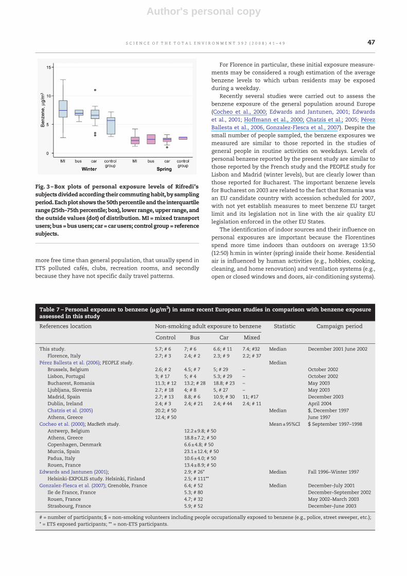
analyses of well-know prognostic factors in winter, besidesseasonal variation, are presented. Commuting habits are animportant determinant of personal exposure (Fig. 3).

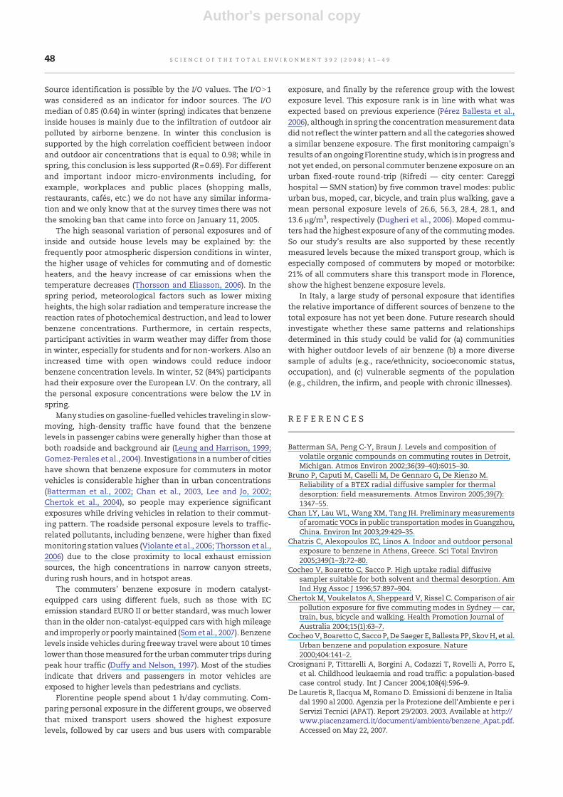
Table 7 presents a summary of data compiled from thepresent study and from some recently published populationexposure studies in European cities to evaluate the benzenepersonal exposures and also during commuting.

4. Discussion and conclusion

Indoor or outdoor benzene data alone have distinct limitationsfor extrapolating personal exposure. A subject's exposure isdetermined by his daily routine and benzene levels associatedwith his activities and related micro-environments. Personalmonitoring is consequently the preferred method for deter-mining exposures.

People's exposures to benzene occur mainly throughbreathing air (Duarte-Davidson et al., 2001), so the study'sdata should give good approximate estimations for the totalbenzene exposure. The Radiello® sampler used in this study isan appropriate device because it allowed us to measuresimultaneously the personal exposure of 67 people withoutgreat cost. It was previously validated in laboratory to controlfactors (i.e., relative humidity, temperature, wind speed, andstandard concentrations) (Cocheo et al., 1996; 2000), and otherimportant studies on benzene exposurewere carried out usingthis device (Cocheo et al., 2000; Chatzis et al., 2005; PérezBallesta et al., 2006; Gonzalez-Flesca et al., 2007). Thissampling method is equivalent to the reference method ofthe directive 2000/69/EC (Bruno et al., 2005). Moreover,personal benzene concentrations were integrated over thefour sampling days, making the exposure data obtained freefrom accidental variation due to unusual personal behaviors.An important factor that must be taken into account whenpersonal exposure is directly measured by personal monitors

is to evaluate the degree to which the investigation may alterthe normal behavior of participants and therefore bias theresults: this study design planned that the subjects couldcommute using their usual vehicles, routes and daily travelpatterns, and because the passive sampler used is very small,in this context, the obtained results necessarily reflect theusual travel patterns of all people.

Although the study sample cannot be seen as representa-tive of the general Florentine population because the samplingdesign really excluded smokers, children, and the peopleoccupationally exposed to benzene, and some participantswere volunteers; it may be representative about the commut-ing exposure. We carried out the residential measures amongvolunteer group because they were more willing and sociable,so gave us the permission to control their homes for selectingappropriate sampling locations and then to perform theresidential sampling. Among the composition of test subjects,a bias may be related to the higher number of non-workers(i.e., students and healthy retirees) firstly, because they have

Table 4 – Descriptive statistics for personal commuting group's benzene exposures (μg/m3), by sampling period

Groups Winter Spring

n AM (SD) Median Range n AM (SD) Median Range

Reference group 6 5.2 (1.7) 5.7 2.9–7.2 3 2.7 (0.2) 2.8 2.4–2.8Bus users 6 6.8 (0.8) 7 5.5–7.5 2 2.4 (1.1) 2.4 1.6–3.2Car users 11 6.6 (1.9) 6.6 3.1–11 9 2.3 (0.7) 2.4 1–3.2Mixed user 32 7.5 (2.3) 7.4 2.7–12.8 37 2.3 (0.7) 2.2 1.2–4.2

Table 5 – Summary of the medians of personal group'stimes (minutes) spent in-vehicles and out-of vehicle atroadside in streets, by sampling period

Groups Winter Spring

Car Bus Street Total Car Bus Street Total

Referencegroup

14 14 38 66 30 0 70 107

Bus users 10 69 51 133 13 54 80 119Car users 85 0 19 110 91 0 35 142Mixed user 11 0 84 111 11 3 61 95

Table 6 - Univariate association between benzenepersonal levels (μg/m3) and characteristics of study'sparticipants in winter season

β (95% CI) p

Univariate analysesGenderFemale RCMale 0.43 (−0.65 to 1.52) 0.43

JobHousewife RCManager 0.44 (−1.84 to 2.72) 0.7Office worker −0.086 (−2.32 to 2.14) 0.93Retired person 2.25 (−0.19 to 4.69) 0.07Student 0.78 (−1.5 to 3.07) 0.49

U-cotinine≤5 ng/mg RCN5 ng/mg 0.17 (−1.43 to 1.78) 0.83

Live with smokersYes RCNo − .31 (−1.48 to 0.85) 0.59

SeasonWinter RCSpring −4.66 (−5.3 to 4.05) 0.000

Level of traffic near participant's houseHigh RCMedium 0.59 (−0.84 to 2.02) 0.41Low −0.73 (−1.94 to 0.47) 0.22

Multivariate associations among personal exposure, commutinghabits, and season (β: regression coefficient; 95% CI: 95% confidenceinterval; RC: reference category).

46 S C I E N C E O F T H E T O T A L E N V I R O N M E N T 3 9 2 ( 2 0 0 8 ) 4 1 – 4 9

Author's personal copy

more free time than general population, that usually spend inETS polluted cafés, clubs, recreation rooms, and secondlybecause they have not specific daily travel patterns.

For Florence in particular, these initial exposure measure-ments may be considered a rough estimation of the averagebenzene levels to which urban residents may be exposedduring a weekday.

Recently several studies were carried out to assess thebenzene exposure of the general population around Europe(Cocheo et al., 2000; Edwards and Jantunen, 2001; Edwardset al., 2001; Hoffmann et al., 2000; Chatzis et al.; 2005; PérezBallesta et al., 2006, Gonzalez-Flesca et al., 2007). Despite thesmall number of people sampled, the benzene exposures wemeasured are similar to those reported in the studies ofgeneral people in routine activities on weekdays. Levels ofpersonal benzene reported by the present study are similar tothose reported by the French study and the PEOPLE study forLisbon and Madrid (winter levels), but are clearly lower thanthose reported for Bucharest. The important benzene levelsfor Bucharest on 2003 are related to the fact that Romania wasan EU candidate country with accession scheduled for 2007,with not yet establish measures to meet benzene EU targetlimit and its legislation not in line with the air quality EUlegislation enforced in the other EU States.

The identification of indoor sources and their influence onpersonal exposures are important because the Florentinesspend more time indoors than outdoors on average 13:50(12:50) h:min in winter (spring) inside their home. Residentialair is influenced by human activities (e.g., hobbies, cooking,cleaning, and home renovation) and ventilation systems (e.g.,open or closed windows and doors, air-conditioning systems).

Fig. 3 –Box plots of personal exposure levels of Rifredi'ssubjectsdividedaccording their commutinghabit, bysamplingperiod.Eachplot shows the50thpercentileand the interquartilerange (25th–75thpercentile; box), lower range, upper range, andthe outside values (dot) of distribution. MI =mixed transportusers; bus=bususers; car = car users; control group= referencesubjects.

Table 7 – Personal exposure to benzene (μg/m3) in same recent European studies in comparison with benzene exposureassessed in this study

References location Non-smoking adult exposure to benzene Statistic Campaign period

Control Bus Car Mixed

This study.Florence, Italy

5.7; # 6 7; # 6 6.6; # 11 7.4; #32 Median December 2001 June 20022.7; # 3 2.4; # 2 2.3; # 9 2.2; # 37

Pérez Ballesta et al. (2006); PEOPLE study. MedianBrussels, Belgium 2.6; # 2 4.5; # 7 5; # 29 – October 2002Lisbon, Portugal 3; # 17 5; # 4 5.3; # 29 – October 2002Bucharest, Romania 11.3; # 12 13.2; # 28 18.8; # 23 – May 2003Ljubljana, Slovenia 2.7; # 18 4; # 8 5, # 27 – May 2003Madrid, Spain 2.7; # 13 8.8; # 6 10.9; # 30 11; #17 December 2003Dublin, Ireland 2.4; # 3 2.4; # 21 2.4; # 44 2.4; # 11 April 2004Chatzis et al. (2005) 20.2; # 50 Median $, December 1997Athens, Greece 12.4; # 50 June 1997

Cocheo et al. (2000); MacBeth study. Mean±95%CI $ September 1997–1998Antwerp, Belgium 12.2±9.8; # 50Athens, Greece 18.8±7.2; # 50Copenhagen, Denmark 6.6±4.8; # 50Murcia, Spain 23.1±12.4; # 50Padua, Italy 10.6±4.0; # 50Rouen, France 13.4±8.9; # 50

Edwards and Jantunen (2001);Helsinki-EXPOLIS study. Helsinki, Finland

2.9; # 26⁎ Median Fall 1996–Winter 19972.5; # 111⁎⁎

Gonzalez-Flesca et al. (2007); Grenoble, France 6.4; # 52 Median December–July 2001Ile de France, France 5.3; # 80 December–September 2002Rouen, France 4.7; # 32 May 2002–March 2003Strasbourg, France 5.9; # 52 December–June 2003

# = number of participants; $ = non-smoking volunteers including people occupationally exposed to benzene (e.g., police, street sweeper, etc.);⁎ = ETS exposed participants; ⁎⁎ = non-ETS participants.

47S C I E N C E O F T H E T O T A L E N V I R O N M E N T 3 9 2 ( 2 0 0 8 ) 4 1 – 4 9

Author's personal copy

Source identification is possible by the I/O values. The I/ON1was considered as an indicator for indoor sources. The I/Omedian of 0.85 (0.64) in winter (spring) indicates that benzeneinside houses is mainly due to the infiltration of outdoor airpolluted by airborne benzene. In winter this conclusion issupported by the high correlation coefficient between indoorand outdoor air concentrations that is equal to 0.98; while inspring, this conclusion is less supported (R=0.69). For differentand important indoor micro-environments including, forexample, workplaces and public places (shopping malls,restaurants, cafés, etc.) we do not have any similar informa-tion and we only know that at the survey times there was notthe smoking ban that came into force on January 11, 2005.

The high seasonal variation of personal exposures and ofinside and outside house levels may be explained by: thefrequently poor atmospheric dispersion conditions in winter,the higher usage of vehicles for commuting and of domesticheaters, and the heavy increase of car emissions when thetemperature decreases (Thorsson and Eliasson, 2006). In thespring period, meteorological factors such as lower mixingheights, the high solar radiation and temperature increase thereaction rates of photochemical destruction, and lead to lowerbenzene concentrations. Furthermore, in certain respects,participant activities in warm weather may differ from thosein winter, especially for students and for non-workers. Also anincreased time with open windows could reduce indoorbenzene concentration levels. In winter, 52 (84%) participantshad their exposure over the European LV. On the contrary, allthe personal exposure concentrations were below the LV inspring.

Many studies on gasoline-fuelled vehicles traveling in slow-moving, high-density traffic have found that the benzenelevels in passenger cabins were generally higher than those atboth roadside and background air (Leung and Harrison, 1999;Gomez-Perales et al., 2004). Investigations in a number of citieshave shown that benzene exposure for commuters in motorvehicles is considerable higher than in urban concentrations(Batterman et al., 2002; Chan et al., 2003, Lee and Jo, 2002;Chertok et al., 2004), so people may experience significantexposures while driving vehicles in relation to their commut-ing pattern. The roadside personal exposure levels to traffic-related pollutants, including benzene, were higher than fixedmonitoring station values (Violante et al., 2006; Thorsson et al.,2006) due to the close proximity to local exhaust emissionsources, the high concentrations in narrow canyon streets,during rush hours, and in hotspot areas.

The commuters' benzene exposure in modern catalyst-equipped cars using different fuels, such as those with ECemission standard EURO II or better standard, was much lowerthan in the older non-catalyst-equipped cars with highmileageand improperly or poorlymaintained (Somet al., 2007). Benzenelevels inside vehicles during freeway travel were about 10 timeslower than thosemeasured for theurbancommuter trips duringpeak hour traffic (Duffy and Nelson, 1997). Most of the studiesindicate that drivers and passengers in motor vehicles areexposed to higher levels than pedestrians and cyclists.

Florentine people spend about 1 h/day commuting. Com-paring personal exposure in the different groups, we observedthat mixed transport users showed the highest exposurelevels, followed by car users and bus users with comparable

exposure, and finally by the reference group with the lowestexposure level. This exposure rank is in line with what wasexpected based on previous experience (Pérez Ballesta et al.,2006), although in spring the concentrationmeasurement datadid not reflect thewinter pattern and all the categories showeda similar benzene exposure. The first monitoring campaign'sresults of an ongoing Florentine study,which is in progress andnot yet ended, on personal commuter benzene exposure on anurban fixed-route round-trip (Rifredi — city center: Careggihospital — SMN station) by five common travel modes: publicurban bus, moped, car, bicycle, and train plus walking, gave amean personal exposure levels of 26.6, 56.3, 28.4, 28.1, and13.6 μg/m3, respectively (Dugheri et al., 2006). Moped commu-ters had the highest exposure of any of the commutingmodes.So our study's results are also supported by these recentlymeasured levels because the mixed transport group, which isespecially composed of commuters by moped or motorbike:21% of all commuters share this transport mode in Florence,show the highest benzene exposure levels.

In Italy, a large study of personal exposure that identifiesthe relative importance of different sources of benzene to thetotal exposure has not yet been done. Future research shouldinvestigate whether these same patterns and relationshipsdetermined in this study could be valid for (a) communitieswith higher outdoor levels of air benzene (b) a more diversesample of adults (e.g., race/ethnicity, socioeconomic status,occupation), and (c) vulnerable segments of the population(e.g., children, the infirm, and people with chronic illnesses).

R E F E R E N C E S

Batterman SA, Peng C-Y, Braun J. Levels and composition ofvolatile organic compounds on commuting routes in Detroit,Michigan. Atmos Environ 2002;36(39–40):6015–30.

Bruno P, Caputi M, Caselli M, De Gennaro G, De Rienzo M.Reliability of a BTEX radial diffusive sampler for thermaldesorption: field measurements. Atmos Environ 2005;39(7):1347–55.

Chan LY, Lau WL, Wang XM, Tang JH. Preliminary measurementsof aromatic VOCs in public transportationmodes in Guangzhou,China. Environ Int 2003;29:429–35.

Chatzis C, Alexopoulos EC, Linos A. Indoor and outdoor personalexposure to benzene in Athens, Greece. Sci Total Environ2005;349(1–3):72–80.

Cocheo V, Boaretto C, Sacco P. High uptake radial diffusivesampler suitable for both solvent and thermal desorption. AmInd Hyg Assoc J 1996;57:897–904.

Chertok M, Voukelatos A, Sheppeard V, Rissel C. Comparison of airpollution exposure for five commuting modes in Sydney — car,train, bus, bicycle and walking. Health Promotion Journal ofAustralia 2004;15(1):63–7.

CocheoV, Boaretto C, Sacco P, De Saeger E, Ballesta PP, SkovH, et al.Urban benzene and population exposure. Nature2000;404:141–2.

Crosignani P, Tittarelli A, Borgini A, Codazzi T, Rovelli A, Porro E,et al. Childhood leukaemia and road traffic: a population-basedcase control study. Int J Cancer 2004;108(4):596–9.

De Lauretis R, Ilacqua M, Romano D. Emissioni di benzene in Italiadal 1990 al 2000. Agenzia per la Protezione dell'Ambiente e per iServizi Tecnici (APAT). Report 29/2003. 2003. Available at http://www.piacenzamerci.it/documenti/ambiente/benzene_Apat.pdf.Accessed on May 22, 2007.

48 S C I E N C E O F T H E T O T A L E N V I R O N M E N T 3 9 2 ( 2 0 0 8 ) 4 1 – 4 9

Author's personal copy

Dugheri S, Dolara P, Pecchioli M, Piacenti M, Cupelli V.Determinazione del benzene aerodisperso a Firenze in relazioneai mezzi di trasporto mediante tecnica di microestrazione infase solida (SPME). La Spettrometria di Massa e le sue più recentiapplicazioni. Meeting; 2006 Florence, 10 March. Available athttp://www.cism.unifi.it/pdf/dugheri.pdf. Accessed on May 10,2007.

Duarte-Davidson R, Courage C, Rushton L, Levy L. Benzene in theenvironment: an assessment of the potential risks to thehealth of the population. Occup Environ Med 2001;58:2–13.

Duffy BL, Nelson PF. Exposure to emissions of 1,3-butadiene andbenzene in the cabins of moving motor vehicles and buses inSydney, Australia. Atmos Environ 1997;31(23):3877–85.

Edwards RD, Jantunen MJ. Benzene exposure in Helsinki, Finland.Atmos Environ 2001;35(8):1411–20.

Edwards RD, Jurvelin J, Koistinen K, Saarela K, Jantunen M. VOCssource identification from personal and residential indoor,outdoor, and workplace microenvironmental samples inEXPOLIS-Helsinki, Finland. Atmos Environ 2001;35:4829–41.

Egeghy PP, Tornero-Velez R, Rappaport SM. Environmental andbiological monitoring of benzene during self-service automobilerefueling. Environ Health Perspect 2000;108(12):1195–202.

European Commission, Joint Centre Reaserch, Institute for HealthandConsumerProtection, KotziasD,KoistinenK,KephalopoulosS, Schlitt C, Carrer P, et al. Final Report. The INDEX project.Critical appraisal of the setting and implementation of indoorexposure limits in the EU; 2005. EUR 21590 EN.

European Community Official Journal L 313. Directive 2000/69/ECof the European Parliament and of the Council of 16 November2000 relating to limit values for benzene and carbon monoxidein ambient air. OJEC 2000; L 313, 13/12/2000: 12–21.

Gonzalez-Flesca N, Nerriere E, Leclerc C, Le Meur S, Marfaing H,Hautemaniere A, et al. Personal exposure of children andadults to airborne benzene in four French cities. Atmos Environ2007;41(12):2549–58.

Gomez-Perales JE, Colvile RN, Nieuwenhuijsen MJ, Fernandez-Bremauntz A, Gutierrez-Avedoy VJ, Paramo-Figueroa VH, et al.Commuters' exposure to PM2.5, CO, and benzene in publictransport in the metropolitan area of Mexico City. AtmosEnviron 2004;38(8):1219–29.

Harrison RM, Leung PL, Sommervaille L, Smith R, Gilman E.Analysis of incidence of childhood cancer in theWestMidlandsof United Kingdom in relation to proximity to main roads andpetrol stations. Occup Environ Med 1999;56:774–80.

Haufroid V, Lison D. Urinary cotinine as a tobacco-smoke exposureindex: a minireview. Int Arch Occup Environ Health 1998;71(3):162–8.

Hoffmann K, Krause C, Seifert B, Ullrich D. The GermanEnvironmental Survey 1990/92 (GerES II): sources of personalexposure to volatile organic compounds. J Expo Anal EnvironEpidemiol 2000;10(2):115–25.

International Agency for Research on Cancer (IARC) Monographs.Some industrial chemicals and dyestuffs. Monogr Eval CarcinogRisk Hum 1982;29:95–148.

Italian Official Journal n 282, 3/12/1997. Legge 4 Novembre 1997,n. 413. Misure urgenti per la prevenzione dell'inquinamentoatmosferico da benzene. Available at www.parlamento.it/parlam/leggi/97413l.htm.

JoWK, Lee JW, Shin DC. Exposure to volatile organic compounds inresidences adjacent to dyeing industrial complex. Int ArchOccup Environ Health 2004;77:113–20.

JoWK, Park KH. Commuter exposure to volatile organic compoundsunder different driving conditions. Atmos Environ1999;33:409–17.

Karakitsios SP, Delis VK, Kassomenos PA, Pilidis GA. Contributionto ambient benzene concentrations in the vicinity of petrolstations: Estimation of the associated health risk. AtmosEnviron 2007;41(9):1889–902.

Klepeis NE, Tsang AM, Beahr JV. Analysis of the National HumanActivity Pattern Survey (NHAPS) respondents from astandpoint of exposure assessment. US-EPA report.EPA/600/R-96/074; 1996.

Lee JW, JoWK. Actual commuter exposure tomethyl-tertiary butylether, benzene and toluene while traveling in Korean urbanareas. Sci Total Environ 2002;291:219–28.

Leung PL, Harrison RM. Roadside and in-vehicle concentrations ofmonoaromatic hydrocarbons. Atmos Environ 1999;33(2):191–204.

Pearson RL, Wachtel H, Ebi L. Distance-weighted traffic density inproximity to a home is a risk factor for leukemia and otherchildhood cancers. J Air Waste Manage Assoc 2000;50:175–80.

Pérez Ballesta P, Field RA, Connolly R, Cao N, Caracena Baeza A, DeSaegerE. Populationexposure tobenzene:oneday cross-sectionsin six European cities. Atmos Environ 2006;40(18):3355–66.

Raaschou-Nielsen O, Hertel O, Thomsen BL, Olsen JH. Air pollutionfrom traffic at the residence of children with cancer. Am JEpidemiol 2001;153:433–43.

Rinsky RA, Young RJ, Smith AB. Leukemia in benzene workers.Am J Ind Med 1981;2(3):217–45.

Skarping G, Willers S, Dalene M. Determination of cotinine inurine using glass capillary gas chromatography and selectivedetection, with special reference to the biological monitoringof passive smoking. J Chromatogr 1988;454:293–301.

Som D, Dutta C, Chatterjee A, Mallick D, Jana TK, Sen S. Studies oncommuters'exposure to BTEX in passenger car in Kalkata,India. Sci Total Environ 2007;372:426–32.

Steffen C, Auclerc MF, Auvrignon A, Baruchel A, Kebaili K,Lambilliotte A, et al. Acute childhood leukaemia andenvironmental exposure to potential sources of benzene andother hydrocarbons; a case–control study. Occup EnvironMed 2004;61:773–8.

Thorsson S, Eliasson I. Passive and active sampling of benzene indifferent urban environments in Gothenburg, Sweden. WaterAir Soil Pollut 2006;173:39–56.

Violante FS, Barbieri A, Curti S, Sanguinetti G, Graziosi F, Mattioli S.Urban atmospheric pollution: personal exposure versus fixedmonitoring station measurements. Chemosphere 2006;64(10):1722–9.

49S C I E N C E O F T H E T O T A L E N V I R O N M E N T 3 9 2 ( 2 0 0 8 ) 4 1 – 4 9