Chairperson Florence D. DiGennaro Reed, Ph.D., BCBA-D ...

TRANSLATING REINFORCER DIMENSIONS AND BEHAVIORAL ECONOMIC DEMAND TO

INFORM INCENTIVE DELIVERY IN ORGANIZATIONAL BEHAVIOR MANAGEMENT

BY

©2017 Amy Jessica Henley

Submitted to the graduate degree program in the Department of Applied Behavioral Science and the Graduate Faculty of the University of Kansas in partial fulfillment of the requirements for the degree of

Doctor of Philosophy

___________________________________

Chairperson Florence D. DiGennaro Reed, Ph.D., BCBA-D

___________________________________

Derek D. Reed, Ph.D., BCBA-D

___________________________________

Peter G. Roma, Ph.D.

___________________________________

Jacob T. Fowles, Ph.D.

___________________________________

Edward K. Morris, Ph.D.

Date Defended: April 21, 2017

ii

The Dissertation Committee for Amy Jessica Henley

certifies that this is the approved version of the following Dissertation:

TRANSLATING REINFORCER DIMENSIONS AND BEHAVIORAL ECONOMIC DEMAND TO

INFORM INCENTIVE DELIVERY IN ORGANIZATIONAL BEHAVIOR MANAGEMENT

___________________________________

Florence D. DiGennaro Reed, Ph.D., BCBA-D

Date Approved: April 21, 2017

iii

Abstract

Recent research has effectively translated behavioral economic demand curve analyses

for use with work-related behavior and workplace incentives (e.g., Henley, DiGennaro Reed,

Reed, & Kaplan, 2016). The present experiments integrated a hypothetical and experiential

demand preparation into a computerized task for use with Amazon Mechanical Turk Workers to

evaluate the effects of parametric manipulations of reinforcer dimensions on performance using a

behavioral economic demand framework. The first experiment examined the effects of three

incentive magnitudes ($0.05, $0.10, and $0.20) on performance assessed with a progressive ratio

schedule. Results indicate responding on the hypothetical and experiential demand assessments

was sensitive to incentive magnitude, with higher responding in the higher incentive magnitude

conditions. Participant responses on the hypothetical assessment were in general agreement with

observed responding in the experiential assessment. The second experiment extended the

methods of Experiment 1 to evaluate the effects of three parametric values of reinforcer

probability (10%, 50%, and 90% probability of earning incentives). Responding was generally

comparable for all three probability conditions. Experiment 3 evaluated the effects of three

delays to incentive receipt (1, 14, and 28 days). Responding was higher in the condition in which

incentives were delayed by 1 as compared to 28 days. Results of the current studies may inform

the development of novel methods for measuring reinforcer efficacy in organizations.

iv

Acknowledgements

I would like to extend my sincere gratitude to all the wonderful members of the KU Performance

Management and Applied Behavioral Economics laboratories, both past and present. I very much

appreciate all your encouragement, feedback, and support over the last five years!

Special thanks to Sarah Jenkins for patiently listening and selflessly providing her time,

guidance, and friendship.

A big thank you also goes out to Matt Novak for asking the tough questions and always being

willing to hash out the answers over the office whiteboard in the middle of the night or at a good

happy hour.

I would like to thank my committee—Drs. Peter Roma, Edward Morris, and Jacob Fowles—for

their expert guidance and mentorship. Your thoughtful suggestions and insight were invaluable

to this project. A special thank you to Dr. Derek Reed, this project would not have been possible

if not for your willingness to share your time and expertise to help support my professional

goals.

Thank you to my family and friends who provided encouragement to press on and reassurance

that “I’ve got this.”

Finally, I cannot express how thankful I am to have had such an incredible mentor, Dr. Florence

DiGennaro Reed. There seems to be no bounds to your passion, generosity, and support, all of

v

which helped me get here today. In addition to so many professional opportunities you made

available to me over the years, I cannot thank you enough for your enormous support and

flexibility in helping me pursue my research interests.

vi

Table of Contents

Introduction 1

Organizational Behavior Management 1

Behavioral Systems Analysis 2

Behavior-Based Safety 3

Performance Management 4

Performance Feedback 6

Incentives 7

Reinforcement Schedules 8

Percentage of Incentive Pay 9

Preference Assessments 13

Prevalence of Incentive Use 14

Reinforcer Dimensions 16

Reinforcer Delay 17

Response Effort 17

Reinforcer Magnitude 18

Reinforcer Probability 19

Reinforcer Quality 19

Rate of Reinforcement 20

Reinforcer Dimensions and OBM 21

Quantitative Analyses 25

Behavioral Economics 26

Discounting 26

vii

Discounting and OBM 27

Demand 28

Factors Influencing Elasticity 29

Linear Elasticity Model 31

Exponential Demand Equation 32

Application of Demand Curve Analyses 34

Hypothetical Purchase Tasks 36

Demand and OBM 40

Purpose 46

Experiment 1 47

Methods 47

Results and Discussion 61

Experiment 2 74

Methods 74


Experiment 3 95

Method 95


General Discussion 108

Dimensions of Reinforcement 108

Accuracy 110

HWT Predictive Validity 112

Alternative Predictive Measures of Performance 113

viii

Contributions to the Literature 114

Experimental Preparation Influences on Predictive Validity 116

Limitations and Future Research 120

AtD Model Fits 122

References 125

Tables 149

Figures 163

Appendices 195

ix

List of Illustrative Materials

Table 1. Experiment 1 Participant Demographic Information 149

Table 2. Experiment 1 HWT and EWT Analog to Demand Indices and Model Fits 151


Table 4. Experiment 2 Amazon Mechanical Turk Employment 153

Table 5. Experiment 2 Employment and Incentive Information at Most Recent Paid Position

154



Table 8. Experiment 3 Amazon Mechanical Turk Employment 158

Table 9. Experiment 3 Employment and Incentive Information at Most Recent Paid Position

159


Table 11. Percentage of Accurate Responding at Each Ratio Requirement for All Conditions and Experiments

162

Figure 1. Prototypical Demand Curve 163

Figure 2. Experiment 1 HWT and EWT Breakpoint 164

Figure 3. Experiment 1 HWT and EWT Unit Price Breakpoint 165

Figure 4. Experiment 1 Percentage of Accurate Work Units Completed 166

Figure 5. Experiment 1 Analog to Demand Curves Plotted Using Ratio Value for the HWT and EWT

167

Figure 6. Experiment 1 HWT Work Function

168

Figure 7. Experiment 1 Cost-Benefit Analysis

169

Figure 8. Residual Plots for Experiment 1 170

Figure 9. Experiment 1 Analog to Demand Curves Separated by Condition 171

x

Figure 10. Experiment 1 Analog to Demand Curves Plotted Using Unit Price for the HWT and EWT

172

Figure 11. Experiment 1 Predictive Validity of the HWT 173

Figure 12. Experiment 1 Percentage Change in Predicted Work and Cost

174

Figure 13. Experiment 2 Programmed versus Experienced Probabilities 175



Figure 16. Experiment 2 Analog to Demand Curves for the HWT and EWT

178

Figure 17. Experiment 2 HWT Work Function 179

Figure 18. Experiment 2 Cost-Benefit Analysis 180

Figure 19. Residual Plots for Experiment 2 181



Figure 22. Experiment 2 Percentage Change in Predicted Work 184

Figure 23. Experiment 2 Percentage Change in Predicted Cost 185



Figure 26. Experiment 3 Analog to Demand Curves for the HWT and EWT

188

Figure 27. Experiment 3 HWT Work Function 189

Figure 28. Experiment 3 Cost-Benefit Analysis 190

Figure 29. Experiment 3 Residual Plots 191



Figure 32. Experiment 3 Percentage Change in Predicted Work and Cost 194

xi

Appendix Index

A) Literature Search Procedures 195

B) Experiment 1 Amazon Mechanical Turk HIT 196

C) Sample Work Unit 197

D) Monetary Choice Questionnaire 198

E) Behavioral Inhibition System/Behavioral Activation System Scale 199

F) Experiment 1 Demographic Questionnaire 201

G) Experiment 1 Practice Trial, HWT, and EWT Instructions and Ratio Wording 203

H) Scoring for the Monetary Choice Questionnaire 204

I) Experiments 2 and 3 Amazon Mechanical Turk HIT 205

J) Experiments 2 and 3 Practice Trial, HWT, and EWT Instructions and Ratio Wording

206

K) Experiments 2 and 3 Demographic, Employment, and Incentive Survey 207

1

Translating Reinforcer Dimensions and Behavioral Economic Demand to Inform Incentive

Delivery in Organizational Behavior Management

Applied behavior analysis is a scientific discipline that uses the principles of behavior to

identify practical strategies for improving socially significant behavior (Baer, Wolf, & Risley,

1968). Behavior analysts have made impressive advancements in numerous areas including

autism treatment, addiction, educational practices, public health, parent training, and others. A

sub-discipline of applied behavior analysis, known as organizational behavior management

(OBM), has a rich history of changing behavior of individuals and groups in the workplace

(Wilder, Austin, & Casella, 2009). The importance of targeting efforts in the workplace may not

be immediately obvious until one considers that work is the single activity to which Americans

allocate the most time and the workforce accounts for 60% of Americans over the age of 16

(Bureau of Labor Statistics, 2014, 2016a). The workplace is also affected by a host of pressing

issues including job dissatisfaction among more than half of U.S. workers (Ray, Rizzacasa, &

Levanon, 2013) and employee turnover rates that are often highest in human service and

education settings where skilled employees delivering quality services are essential for consumer

and learner outcomes (Dib & Sturmey, 2007; Gresham, Gansle, Noell, Cohen, & Rosenblum,

1993; Ingersoll, Merrill, & Stuckey, 2014; Strouse, Carroll-Hernandez, Sherman, & Sheldon,

2003). Moreover, nearly 5,000 work-related fatalities and 3 million injuries and illnesses occur

annually (Bureau of Labor Statistics, 2016b) and over a quarter of Americans have been bullied

at work (Workplace Bullying Institute, 2014). The workplace is paramount to our daily lives,

increasing the need for strategies to alleviate the many issues faced by organizations, employees,

and consumers of the goods and services they produce.

When one considers the central role work plays in our lives and the many workplace

issues, it is not surprising that a specialized sub-discipline of applied behavior analysis was

2

established to address behavior in the workplace. The burgeoning of OBM since its beginning in

the 1960s may be attributable, at least in part, to the robust results the field has achieved in

diverse industries, with organizations of all sizes, and in addressing issues of varying complexity

(Dickinson, 2001). The expansion of OBM has resulted in the development of three sub-

disciplines within the field: behavioral systems analysis, behavior-based safety, and performance

management.

Behavioral Systems Analysis

Behavioral systems analysis is an approach to evaluating organizational performance that

integrates traditional behavior analytic principles with general systems theory (Diener, McGee,

& Miguel, 2009; Von Bertalanffy, 1950). Behavioral systems analysis views the organization as

a whole and evaluates the interaction between the components (e.g., departments) and processes

within the system (e.g., hiring practices, product development) and between the organization and

external environment (e.g., consumers and competition; Johnson, Casella, McGee, & Lee, 2014).

The overarching goal of behavioral systems analysis is to increase an organization’s ability to

adapt to and meet the needs and pressures of a dynamic and an ever-changing environmental

context in which the organization exists (Diener et al., 2009; Johnson et al., 2014). Behavioral

systems analysis focuses on changing organizational systems, processes, and individual

employee performance to accomplish this goal. Typical procedures in behavioral systems

analysis include, but are not limited to, process design, policy changes, organizational

restructuring, and re-allocation of resources and individual employee performance. The

substantial resources needed to carry out behavioral systems analysis is a noted disadvantage. In

fact, it can take several weeks or even months to pinpoint organizational issues and identify a

change strategy (Johnson et al., 2014). Although advocates of behavioral systems analysis report

3

numerous successful applications in practice, to date there is limited published empirical or

experimental evidence evaluating and consequently supporting its use (Johnson et al., 2014;

Sigurdsson & McGee, 2015). Clearly more research is needed; however, the molar approach to

improving organizations taken by behavioral systems analysis may ultimately prove propitious.

Behavior-Based Safety

As previously noted, work-related injuries and illnesses are a pervasive problem (e.g.,

Bureau of Labor Statistics, 2016b). In addition to personal and emotional harm, work-related

injuries have tremendous financial ramifications. The National Safety Council (2015) estimates

that medical costs, administrative expenses, and losses in wages and productivity totaled over

$206 billion in 2013. In fact, Loafman (1996) argues the costs of work-related injuries and

illnesses is one of the nation’s largest avoidable expenditures. Although some instances may be

unavoidable, many injuries result from unsafe behavior of staff. Traditional approaches to

decreasing injuries involve reducing or eliminating physical hazards in the environment by

developing equipment or mechanical safety devices that physically block contact with dangerous

machines or to unsafe spaces (e.g., hard hat, safety goggles, railings). Unfortunately, preventable

injuries continue to occur at unacceptable rates despite impressive advances in safety equipment.

In many cases, safety equipment is not permanently affixed and requires behavior for safe use—

this fact necessarily requires behavioral approaches to ameliorate workplace injuries.

Thus, behavior-based safety involves the application of behavioral principles and

environmental manipulations to reduce the occurrence of preventable work-related injuries and

illnesses (Sulzer-Azaroff & Austin, 2000). Grindle, Dickinson, and Boettcher (2000) suggest that

close consideration of the consequences for safe and unsafe behavior may provide insight into

the causes of work-related injuries. Specifically, they note:

4

… natural consequences may support and encourage unsafe behaviors because: (a)

performing in a safe manner results in immediate, probable, negative consequences such

as discomfort and increased effort or time; while (b) performing in an unsafe manner

rarely results in an injury but does result in immediate, probable positive consequences

such as savings in time and effort and avoidance of discomfort. (p. 34)

The inadequacy of natural consequences operating in the workplace to evoke and maintain safe

behavior is supported by the findings of Grindle and colleagues. In their review of behavioral

safety interventions, Grindle et al. found that consequent interventions proved more effective

than antecedent interventions for safety behavior. In this context, antecedent interventions

include environmental modifications and other strategies (e.g., altering motivating operations) to

change working conditions before workers emit behavior (Cooper, Heron, & Heward, 2006).

Whereas consequent interventions involve contingent manipulations of stimuli that follow a

behavior (i.e., modifying consequences). The findings of Grindle et al. suggest delay to

reinforcement, probability of reinforcement, and effort required for safe behavior are important

considerations to supplement inadequate natural contingencies when designing behavior change

procedures for safety and potentially other behavior in the workplace.

Performance Management

The third OBM sub-discipline—performance management—involves the analysis and

direct manipulation of antecedents and consequences to improve individual or group

performance within an organization (Daniels & Daniels, 2006). In contrast with the relatively

specific nature of behavior-based safety, performance management targets a wide variety of

employee behavior including absenteeism (e.g., Camden & Ludwig, 2013), cleaning (e.g.,

Clayton & Blaskewicz, 2012; Doll, Livesey, McHaffie, & Ludwig, 2007), implementation of

5

behavior support plans or teaching procedures (e.g., Miller, Carlson, & Sigurdsson, 2014),

customer service (e.g., So, Lee, & Oah, 2013), identification-checking (e.g., Downing & Geller,

2012), and numerous others. Performance management procedures are a necessary component of

behavioral systems analysis and behavior-based safety, rendering continued efforts to evaluate

and maximize the effectiveness of performance management interventions of particular

importance to OBM.

Within performance management, employee performance problems are frequently

classified as either a skill or motivational deficit (Mager & Pipe, 1970). A skill deficit refers to

performance problems that are a function of insufficient knowledge or practice necessary for

correct performance to occur. In contrast, when an individual can correctly demonstrate a

behavior but does not, the problem is likely attributable to a motivational deficit, wherein the

consequences for correct performance are inadequate to maintain behavior. Accordingly,

performance management interventions are often classified as antecedent- or consequent-based

to address skill and motivational deficits, respectively (Mager & Pipe, 1970; Wilder et al., 2009).

Common antecedent interventions in OBM include staff training, goal setting, instruction, and

task clarification. Consequent-based interventions in OBM consist of performance feedback,

incentives (monetary and non-monetary), and—although they are infrequently evaluated in the

literature—other types of consequences including promotion and progressive discipline.

VanStelle et al. (2012) conducted a review of empirical research articles published in the

Journal of Organizational Behavior Management (JOBM) between 1998 and 2009 to evaluate

the types of performance issues researchers targeted for change as well as intervention strategies

used. VanStelle et al. found that 78% of performance problems were due to a motivational

deficit. The frequency of performance problems that are a function of motivational deficits

6

underscores the importance of continued research examining consequent interventions.

Performance feedback and incentives were the most frequently employed consequent

interventions VanStelle and colleagues reported, used in 68% and 26% of studies, respectively.

The importance of high-quality staff training and appropriate antecedents cannot be discounted;

these components are necessary for correct performance. However, as evidenced by the greater

relative frequency with which performance problems are a function of motivational deficits,

antecedent-based interventions are not sufficient to maintain performance over time.

Examination of consequences may shed light on specific consequence properties that support

desirable and undesirable employee behavior, similar to the explanation proposed by Grindle and

colleagues (2000) with respect to safety behavior. Thus, continued evaluation of consequent-

based interventions that OBM researchers use most frequently (i.e., performance feedback and

incentives) is a worthwhile endeavor.

Performance Feedback

Performance feedback—hereafter referred to in short as feedback—is the provision of

information about performance that allows an individual to adjust his or her behavior (Daniels &

Daniels, 2006; Prue & Fairbank, 1981). Feedback is the most frequently used of any

performance management technique, including antecedent interventions (VanStelle et al., 2012).

Although it is classified here and elsewhere as a consequent-based intervention (e.g., Wilder et

al., 2009), feedback may also function as an antecedent for correct performance the next time an

employee performs a task (Daniels, 2000). Numerous literature reviews and component analyses

have evaluated various feedback characteristics in an effort to identify the method of delivery

and content that maximizes feedback effectiveness (e.g., group vs. individual, weekly vs. daily,

objective vs. evaluative; Alvero, Bucklin, & Austin, 2001; Balcazar, Hopkins, & Suarez, 1985;

7

Henley & DiGennaro Reed, 2015; Johnson, 2013, 2015; Pampino, MacDonald, Mullin, &

Wilder, 2004; Prue & Fairbank, 1981; Reid & Parsons, 1996). The cumulative research

examining feedback characteristics has provided valuable insight regarding effective delivery

methods. In a review of the feedback literature published between 1985 and 1998, Alvero and

colleagues found that only 47% of studies resulted in consistent performance improvements

when feedback was the sole behavior change procedure. The inconsistency with which feedback

interventions result in performance improvements is a noted disadvantage. However, feedback

remains a valuable method because it is a flexible and cost-effective means for changing

employee behavior that can be adapted for use in most organizational settings. Organizational

behavior management would benefit from continued research on the characteristics and function

of feedback to improve its effectiveness and consistency.

Incentives

Incentives are rewards delivered to an individual or group contingent on the occurrence

of a desired behavior or reaching a performance criterion (e.g., fire drill completion, number of

hours billed). Incentives may include money or other tangible or intangible items (i.e., non-

monetary incentives) such as time off from work (Austin, Kessler, Riccobono, & Bailey, 1996),

food (Kortick & O’Brien, 1996), gift certificates (Miller et al., 2014), and numerous others. The

use of incentives to improve employee performance in OBM dates back to the early 1970s (for a

review of the history of OBM see Dickinson, 2001). Incentives have documented advantages

including reliable increases in net profits as well as improvements in performance, however

measured (Bucklin & Dickinson, 2001). Furthermore, monetary and non-monetary incentives

have been shown to be effective in both laboratory (e.g., Oah & Dickinson, 1992) and applied

settings (e.g., Luiselli et al., 2009), when delivered alone (e.g., Lee & Oah, 2015) or in

8

combination with other performance management procedures (e.g., Goomas & Ludwig, 2007),

with lottery or probabilistic arrangements (e.g., Alavosius, Getting, Dagen, Newson, & Hopkins,

2009; Orpen, 1974), and with varied behaviors in diverse industries (for a review see Bucklin &

Dickinson, 2001). The robust findings have resulted in sustained interest in incentives as an

attractive and viable performance management procedure.

Like feedback, numerous methodological variations in the delivery of incentives exist.

Empirical evaluations of incentive variations are important because effectiveness may depend, at

least in part, on the method with which they are delivered. Unfortunately, experimental

evaluations of methodological variations are relatively infrequent. Of the extant literature

comparing individual incentive arrangements, several lines of inquiry have emerged (Bucklin &

Dickinson, 2001).

Reinforcement schedules. One area of investigation popular in the 1970s and 1980s

concerned experimental evaluations of reinforcement schedules for incentive delivery. Roughly

half of these studies were conducted in the laboratory (Berger, Cummings, & Heneman, 1975;

Lee & Oah, 2015; Pritchard, DeLeo, & Von Bergen, 1976; Pritchard, Hollenback, & DeLeo,

1980; Yukl, Wexley, & Seymore, 1972) and the remaining were conducted in the workplace

(Latham & Dossett, 1978; Saari & Latham, 1982; Yukl & Latham, 1975; Yukl, Latham, &

Pursell, 1976). Eight of the nine studies involved comparisons of continuous and variable ratio

(VR) schedules of reinforcement on performance. For example, in an early applied investigation,

Yukl and Latham evaluated the effects of three schedules of monetary incentives on bags of

seedlings planted by 38 tree planters using a between groups design. In addition to a fixed $2

hourly wage, incentive amounts were $2, $4, and $8 for the groups that received incentives on a

continuous reinforcement, VR2, and VR4 schedule, respectively. The authors also included a

9

control condition in which planters earned fixed pay only in the amount of $3 per hour. Relative

to baseline, performance in the continuous reinforcement condition increased by 33%, decreased

by 8% in the VR2 condition, and increased by 18% in the VR4 condition. Performance in the

control condition was unchanged. Although Yukl and Latham’s results demonstrate

differentiated performance in the incentive conditions with the highest performance in the

condition with the highest rate of reinforcement (i.e., continuous reinforcement), their results

should be interpreted with caution because of at least two limitations. Several participants in the

VR2 condition had difficulty understanding the procedures and objected to the method for

determining incentive receipt (i.e., correctly guessing a coin toss), potentially accounting for

performance decreases. Relatedly, because incentive receipt was based on a coin toss, Dickinson

and Poling (1996) estimate that the reinforcement schedule participants actually experienced was

a VR1.75 rather than a VR2. The collective findings of research evaluating reinforcement

schedules indicate performance was generally higher when participants earned incentives as

compared to hourly pay. However, results comparing different schedules of incentive delivery

were idiosyncratic.

Percentage of incentive pay. A second line of inquiry involves evaluations of varying

percentages of incentive pay (Dickinson & Gillette, 1994; LaMere, Dickinson, Henry, Henry, &

Poling, 1996; Matthews & Dickinson, 2000; Oah & Lee, 2011; Riedel, Nebeker, & Cooper,

1988). To examine percentage of incentive pay, researchers constrained total compensation and

manipulated the proportion of pay available through incentives relative to base pay (i.e.,

guaranteed wages). Incentive pay ranged between 0% (i.e., no incentives) and 100% (i.e., piece-

rate pay only) with higher percentages constituting a higher proportion of pay dependent on

measureable performance. Although arrangements in which pay is primarily earned through

10

incentives provide the strongest contingent relation, performance compensation is subject to vary

across pay periods and may increase the unpredictability of pay. The potential outcome includes

difficulty budgeting individual income and aggregate labor costs for employees and employers,

respectively, which may be perceived as riskier and less preferred relative to fixed wages for

both parties. In light of the large body of research revealing superior performance when

individuals earn incentives, research examining the percentage of incentive pay sought to

evaluate whether there was an optimal percentage that balances the advantages (performance

improvements) with the disadvantages (risk) of incentive systems.

Despite what one might predict given contingent relations, all but one study evaluating

the percentage of incentive pay found performance to be comparable across varying percentages

of incentive pay. One criticism of this body of literature is the limited ecological validity of

laboratory settings. Specifically, many of the contingencies for engaging in on- and off-task

behavior, motivating operations, and competing response alternatives present in the workplace

are often lacking from laboratory-based studies despite researchers’ best efforts. To increase

ecological validity, Oah and Lee (2011) used a modified experimental preparation by recruiting

individuals with a three-year history of socializing with one another to jointly participate and

increasing the number and length of sessions to better approximate the workplace (30 sessions

each lasting 6 hr conducted 5 days a week). The authors found consistently higher productivity

and duration of time working when participants earned 100% of their pay from incentives

relative to conditions in which participants earned 10% and 0% of their pay from contingent

incentives. Productivity and work duration did not differ between the 10% and 0% conditions.

Although more research is needed, these initial findings suggest that higher percentages of

incentive pay may result in higher levels of performance and that percentages at or below 10%

11

incentive pay may not be sufficient to generate meaningful performance increases. Additionally,

the findings suggest OBM researchers can modify the laboratory setting to better approximate a

workplace.

A possible explanation for the inconsistent findings across studies evaluating

reinforcement schedules for incentive delivery and the percentage of incentive pay may involve

the difficulty simulating complex and competing contingencies operating in the workplace.

Results of studies evaluating reinforcement schedules appear initially to be idiosyncratic

(Bucklin & Dickinson, 2001; Dickinson & Poling, 1996). Upon further inspection, an interesting

pattern emerges. Performance was generally equivalent under fixed and variable schedules for

studies conducted in a simulated work setting but differentiated in studies conducted in a real

workplace. With respect to the line of research evaluating the percentage of incentive pay,

LaMere and colleagues (1996) were the only researchers to evaluate this topic in an applied

setting. Although LaMere and colleagues did not find differences in performance among

percentages, the authors evaluated percentages of incentive pay below 10%, which may not be

sufficiently high to result in performance differences revealed by Oah and Lee (2011). The

inconsistent findings between laboratory and applied studies highlights a common and prominent

limitation of laboratory-based OBM research; namely, the limited ecological validity associated

with many simulated workplaces.

Based on findings from the basic literature, Bucklin and Dickinson (2001) argue, “the

work environment can be viewed as analogous to a behavioral choice situation where multiple

concurrent schedules of reinforcement exist” (p. 65) and individuals in this situation will

maximize reinforcement. For that reason, even when the percentage of incentive pay is small or

the reinforcement schedule is lean, performance may be undifferentiated across conditions when

12

no alternative sources of reinforcement are available or when the reinforcing efficacy of

concurrently available alternatives is low relative to the experimental task. For example, to

simulate the presence of alternative activities present in real work settings, Matthews and

Dickinson (2000) provided participants with the opportunity to engage in off-task behavior.

During a single 70-min experimental session, a computer program provided either two or four

prompted opportunities to play one of three computer games for a maximum of 5 min. The

ecological validity of these procedures are questionable because the session duration, prompts to

engage in off-task behavior for a finite duration, and limited available alternatives are not

representative of the workplace. Oah and Lee (2011) evaluated the same percentages of incentive

pay as Matthews and Dickinson (i.e., 0%, 10%, and 100% incentive pay), but Oah and Lee’s

experimental preparation produced performance differences. In addition to the features noted

previously, participants in Oah and Lee were allowed to take breaks within or outside of the

laboratory at any time and had unrestricted access to all computer features including high-speed

internet. The presence of known peers with whom to socialize likely served as an additional

alternative source of reinforcement (perhaps with high relative reinforcing efficacy) and the

quantity and duration of sessions may have functioned as a motivating operation for engaging in

off-task behavior over time. The features Oah and Lee included to increase simulation fidelity

may better approximate the workplace and enhance the external validity of the findings. Despite

the advantages, the financial resources needed to adopt Oah and Lee’s preparation limit

widespread use of this method. Researchers who wish to study variables relevant to the

organization may need to identify an alternative analog setting that is sensitive to resources, but

better approximates the workplace than the laboratory.

13

Preference assessments. Although not a variation of delivery, methods for selecting

stimuli for use in an incentive arrangement is a related and imperative research area for incentive

effectiveness. Preference assessments include a variety of methods for identifying stimuli likely

to function as a reinforcer. Monetary incentives may obviate the need for organizational leaders

to conduct preference assessments because money functions as a generalized conditioned

reinforcer and is relatively independent of motivating operations. However, the financial and

human resources needed to implement an incentive system may preclude the use of monetary

incentives. Non-monetary incentives are a popular method to help mediate budgetary

restrictions. The myriad types of non-monetary incentives are an advantage of their use, but can

make it challenging for organizational leaders or managers to accurately select preferred

incentives for employees; a supposition supported by recent empirical work (Wilder, Harris,

Casella, Wine, & Postma, 2011; Wilder, Rost, McMahon, 2007). The inadequacy of manager

selection underscores the need for the development and evaluation of methods to identify

preferred incentives in organizations. Fortunately, interest in employee preference assessments is

emerging.

Several studies have compared various preference assessment methods for use in the

workplace (Waldvogel & Dixon, 2008; Wilder, Therrien, & Wine, 2006; Wine, Reis, & Hantula,

2014). In the most recent example, Wine and colleagues evaluated three preference assessment

methods. For the multiple stimulus without replacement, Wine et al. asked participants to select

the most preferred stimulus from an array after which the experimenter removed the selected

item and presented the remaining stimuli. The experimenter repeated this process of elimination

until all the stimuli were assessed. The survey method asked participants to rate each item on a

scale of how much work they would be willing to complete for an item. Response options for the

14

survey method included: (1) none at all, (2) a little, (3) a fair amount, (4) much, and (5) very

much. Lastly, the stimulus ranking procedure asked participants to order the items (provided

textually on index cards) from most to least preferred. After completing the preference

assessments, Wine and colleagues conducted a reinforcer assessment to evaluate whether high-

preferred stimuli functioned as reinforcers and low-preference stimuli did not function as

reinforcers (i.e., accuracy). Reinforcer assessment results indicate the survey method consistently

classified reinforcing stimuli as high-preferred whereas the multiple stimulus without

replacement and ranking methods identified some but not all reinforcers as high-preferred.

Wilder et al. obtained similar findings when comparing the survey method to a paired stimulus

assessment in which each item assessed was paired with every other stimulus and participants

selected the more preferred item of the two. Wilder and colleagues found the survey method to

be more accurate than the paired stimulus procedure. Incorporating the amount of work an

individual is willing to complete to earn an incentive is a distinguishing feature of the survey

method from the other methods Wine et al. and Wilder et al. assessed. Although the survey

method uses a subjective (e.g., “a fair amount” of work) rather than objective (e.g., reporting a

quantity) measure of work output, the survey method is nonetheless an improvement over

methods in which reinforcers are identified at low work requirements or without consideration of

the work requirement, which is not representative of conditions employees will actually

experience in the workplace to earn incentives. The results of Wine et al. and Wilder et al.

suggest preference assessment methods for use in organizations may benefit from incorporating

the work requirement needed to earn an incentive.

Prevalence of incentive use. DiGennaro Reed and Henley (2015) evaluated staff training

and performance management practices offered to individuals certified by or seeking

15

certification from the Behavior Analyst Certified Board® and working in applied settings.

DiGennaro Reed and Henley found that just 8% of respondents reported receiving incentives

contingent on performance more than twice per year. When considering the effectiveness of

incentives and the frequency with which they are evaluated in the OBM literature, incentives

appear to be used with relative paucity in applied settings employing board-certified staff.

The infrequent use of incentives observed by DiGennaro Reed and Henley (2015)

suggests there may be a gap in the literature that serves as a barrier to incentive use in practice.

Conceivably, the numerous possible incentive delivery methods may pose a challenge to their

use. The literature comparing delivery methods only covers a modest portion of possibilities. It

may be difficult for organizational leaders to draw clear conclusions from the extant literature

comparing incentive delivery variations needed to guide the design of an empirically supported

incentive system, particularly when one considers the conflicting findings noted previously. As a

result, incentives may be delivered in ineffective and/or cost-prohibitive ways. For example,

leaders must select an appropriate incentive amount for use in a system. Erring on the side of

providing larger incentives may not be financially sustainable and organizational leaders could

be forced to discontinue the program before obtaining the desired behavior change. Incentives

that are too small may not be sufficient to motivate employees to change their behavior and

leaders risk expending valuable resources on an ineffective system. Leaders must also select the

work requirement needed to earn an incentive, the frequency of delivery, delay to delivery, and

incentive type, as well as make decisions about many other variables. Decisions such as these

can be detrimental if made arbitrarily. The numerous logistical questions that remain unanswered

suggests that, although incentive effectiveness was established over 40 years ago, since then

research has generated limited information to guide their use in the workplace. A general lack of

16

helpful information to guide effective incentive delivery likely contributes to their lack of use or

short half-life when used (DiGennaro Reed & Henley, 2015; Huselid, 1995).

In the present context incentives are, generally speaking, reinforcers delivered in the

workplace. Comparisons or parametric analyses of basic reinforcer dimensions to effectively

improve and maintain desired performance in a way that is appealing for employees and

sustainable for the organization—factors that ultimately dictate whether an incentive system is

used in the short- and long-term—are largely absent from the literature. Therefore, an

understanding of how reinforcer dimensions influence incentive efficacy is important to guide

their efficient and effective delivery in practice.

Reinforcer Dimensions

Reinforcers may vary along a number of dimensions that influence their efficacy

including delay, response effort, magnitude, probability, quality, and rate of reinforcement. The

experimental analysis of reinforcer dimensions has a long and rich history of study culminating

in an extensive empirical literature. The findings of both laboratory (e.g., Chung & Herrnstein,

1967) and applied (e.g., Neef, Mace, & Shade, 1993) studies consistently demonstrate systematic

changes in responding with changes in reinforcer dimensions. These findings have led to the

successful application of numerous interventions that manipulate reinforcer dimensions of

response alternatives to increase the frequency of desired behavior (e.g., Horner & Day, 1991).

Reinforcer dimensions are therefore an important consideration that warrant attention in the

OBM literature. Experimental investigations evaluating how reinforcer dimensions differentially

affect performance may provide a better understanding of the variables that influence employee

behavior in the workplace and help inform the development of behavior change procedures for

promoting desired performance.

17

Reinforcer delay. Delay of reinforcement refers to the duration between behavior

producing a reinforcer and subsequent reinforcer delivery (Mazur, 1993). A large literature base

has shown that reinforcer efficacy systematically decreases as a function the delay to its receipt

(Mazur, 1993). An understanding of how delayed reinforcement affects behavior may be of

particular relevance to OBM because of practical restrictions that constrain the immediacy with

which reinforcers may be delivered in the workplace (e.g., payroll processing). Such constraints

render many delays in the workplace of greater duration than those observed in non-human

animal studies of reinforcement. Malott (1993) suggests delay to reinforcement in the workplace

is too great to directly control behavior. As a result, Malott makes an important distinction

between direct- and indirect-acting contingencies. A direct-acting contingency is “a contingency

for which the outcome of the response reinforces or punishes that response” (p. 46) and an

indirect-acting contingency is “a contingency that controls behavior indirectly rather than

through the direct action of reinforcement or punishment by the outcome of that contingency” (p.

46). Malott suggests most behavior in the workplace is controlled by indirect-acting

contingencies and mediated by rules describing those contingencies, whereas non-human operant

studies rely on direct-acting contingencies to control behavior. An understanding of how

reinforcer dimensions, including delay, influence behavior governed by indirect-acting

contingencies is less understood and represents a valuable area for future research. Although

several OBM researchers have evaluated the effects of delayed feedback (Krumhus & Malott,

1980; Mason & Redmon, 1992; Reid & Parsons, 1996), this analysis has not been sufficiently

extended to incentives.

Response effort. Response effort (referred to hereafter as effort) involves the type or

amount of behavior required to access reinforcement. Effort encompasses various facets of a

18

response including difficulty, physical exertion (e.g., weight, force required, distance traveled),

or time necessary to successfully perform a behavior. Research manipulating response effort

reliably demonstrates an inverse relation between effort and response rate, with higher rates

associated with lower effort responses (Friman & Poling, 1995). Therefore, careful consideration

and evaluation of response effort is warranted (DiGennaro Reed, Henley, Hirst, Doucette, &

Jenkins, 2015). With respect to the workplace, employees have multiple job responsibilities that

differ in the amount of effort required by an employee. The effort needed may influence the tasks

to which employees allocate their time, and could result in allocation to irrelevant, inappropriate,

or unsafe tasks or behaviors. A strategically delivered incentive contingent on completion of

high-effort responses could help ameliorate this issue. Effort may also influence whether

employees engage in a desired behavior. In one of the only published experimental accounts of

an effort manipulation in JOBM, Shook, Johnson, and Uhlman (1978) slightly improved the

frequency direct care staff graph client behavior by moving the necessary materials closer to the

location in which graphing was to take place, thereby reducing the effort required to perform this

job responsibility. Unfortunately, further evaluations of response effort in OBM are well

overdue.

Reinforcer magnitude. Also commonly referred to as amount, reinforcer magnitude is

the quantity of a reinforcer and can be measured in terms of number or duration of access.

Research has consistently documented that magnitude influences reinforcer efficacy with

reinforcers of greater magnitude being relatively more efficacious (Fantino, 1977). Although

money is generally assumed to be an effective reinforcer for humans, Daniels (2000) suggests

the reinforcing efficacy of money may still depend on amount. The reinforcer magnitude

necessary to evoke behavior change is important to organizations because it must be financially

19

feasible to implement any incentive system involving reinforcers that cost money, directly or

indirectly (i.e., personnel time to implement the system). Identifying the lowest-magnitude

reinforcer that can effectively maintain behavior may be especially important for human service,

educational, or nonprofit organizations where finances are often limited.

Reinforcer probability. Probability of reinforcement is the likelihood, on a given

schedule, a reinforcer will be delivered (Ferster & Skinner, 1957). Numerous studies have

demonstrated incentive effectiveness when delivered in a probabilistic or lottery arrangement

(e.g., Alavosius et al., 2009; Orpen, 1974; Reed, DiGennaro Reed, Campisano, LaCourse, &

Azulay, 2012). However, many of these studies do not specify the programmed and/or

experienced probability. For example, Cook and Dixon (2006) evaluated the effects of a $50

probabilistic incentive on the percentage of completed forms for three supervisors working with

individuals with intellectual and developmental disabilities. All participants had the opportunity

to earn the incentive each week regardless of performance; however, the experienced probability

varied weekly because it was determined based on performance of all three participants. The

highest performer had a 50% chance of earning the incentive, the second and third highest

performers had a 33% and 17% chance, respectively. If two participants completed an equal

percentage of forms for a given week, both participants had a 40% probability, whereas the

lowest performer had a 20% probability of earning the incentive. Although performance was

highest for all participants during the lottery incentive system, the probability associated with

performance gains remains unclear. Research evaluating incentive probability may help mediate

budgetary restrictions associated with delivering higher magnitude or more frequent incentives.

Reinforcer quality. Reinforcer effectiveness depends in part on the relative preference

for a reinforcing stimulus, referred to as quality (DiGennaro Reed et al., 2015). As previously

20

discussed, OBM researchers are beginning to develop preference assessment methods that will

provide useful information about reinforcer quality (e.g., Wine et al., 2014). Research has also

demonstrated that quality is influenced by other reinforcer dimensions such as magnitude

(Trosclaire-Lasserre, Lerman, Call, Addison, & Kodak, 2008). Because reinforcer dimensions

may interact and influence quality in unpredictable ways, leaders would benefit from having

reliable and efficient methods to assess reinforcer preference in OBM. Despite a robust literature

examining methods for identifying preferred reinforcers with individuals with intellectual and

developmental disabilities (see Cannella, O’Reilly, & Lancioni, 2005 for a review), research in

OBM has only just started to evaluate methods for identifying reinforcers in the workplace.

Rate of reinforcement. Lastly, rate of reinforcement refers to the number of reinforcers

per unit of time (DiGennaro Reed et al., 2015). Because rate of reinforcement is influenced by

the schedule of reinforcement, investigations of reinforcement schedules involving incentives

may provide insight to the effects of reinforcement rate on work-related behavior. Features of the

organizational setting make it challenging to experimentally investigate this dimension despite

its relevance to leaders and employees. For example, restrictions associated with how often

reinforcement can be delivered in an organization—payroll processing, duration of job

responsibilities for which reinforcement is contingent—constrain the strategic use of

reinforcement schedules. Unfortunately, response alternatives unrelated to job responsibilities

may provide higher rates of reinforcement for off-task behavior (e.g., engaging social media

several times during a work day). These and other variables emphasize the importance of

identifying ways to maximize the effects of other reinforcer dimensions (e.g., probability, delay)

to combat challenges associated with addressing concurrently available reinforcers in the

workplace.

21

The wealth of basic behavioral research demonstrates that variations in reinforcer

dimensions modulate reinforcer efficacy. Much of the research, however, has been conducted

with non-human animals in highly controlled settings using choice procedures in which an

animal responds to two concurrent alternatives. The workplace is replete with innumerable

contingencies associated with consequences that vary asymmetrically in terms of the dimensions

reviewed in the preceding discussion. Moreover, reinforcer efficacy is modulated by the context

and concurrent response options. Therefore, it is important for incentive efficacy that reinforcers

are delivered in a way that effectively competes with alternative sources of reinforcement

available in the workplace. The translation of basic literature to inform an understanding of

dimensions influencing reinforcer efficacy and performance in organizations is vital for the

effective use of incentives.

Reinforcer Dimensions and OBM

As part of a comprehensive review of the literature (Appendix A), I identified 75

experimental studies that evaluated the effects of incentives on work behavior.1 Seven studies,

discussed previously, compared the effects of different schedules of reinforcement (i.e., rate;

Berger et al., 1975; Latham & Dossett, 1978; Pritchard et al., 1976; Saari & Latham, 1982; Yukl

& Latham, 1975; Yukl et al., 1976; Yukl et al., 1972). One study evaluated the effects of two

probabilistic arrangements (Evans, Kienast, & Mitchell, 1988). No studies examined reinforcer

magnitude, reinforcer quality, or response effort. Therefore, outside of evaluations of

reinforcement schedules, only one published study has systematically manipulated and directly

evaluated the effects of varied features of reinforcer dimensions on work performance (i.e.,

1 Although researchers in the field of industrial-organizational psychology frequently study incentives, much of this research is correlational in nature and—despite being identified in the early stages of the literature review—did not meet the inclusionary criterion outlined in Appendix A requiring that researchers manipulate a reinforcer dimension.

22

Evans et al., 1988). Evans and colleagues evaluated the effects of two probabilistic incentive

arrangements on performance of 18 automobile service mechanics across two dealerships. For

each service repair, the experimenters measured the difference between standard repair duration

indicated in the automobiles’ service manual and observed participant repair time, referred to as

time saved. Following a baseline period in which service mechanics earned hourly pay only, the

experimenters implemented one of two incentive arrangements for eight weeks. In both incentive

arrangements, participants could draw a token for every hour of time saved during the previous

workday. Drawings occurred every morning. Tokens were worth zero, one, two, or five

Washington State Lottery Tickets. In the first arrangement, 100% of tokens were worth at least

one lottery ticket delivered immediately. In the second arrangement, only 10% of tokens resulted

in the receipt of at least one lottery ticket. In the second arrangement only, all tokens were

entered into a weekly drawing for the chance to win $150 regardless of whether the participant

received any lottery tickets. Winners of the weekly drawing were then entered into a second

drawing for $350, conducted every four weeks in lieu of the weekly drawing. Participants could

collect monetary earnings in the form of a check immediately after the weekly and four-week

drawings. The authors found that both incentive systems increased performance above baseline

(hourly pay), however, there were no differences between the two incentive arrangements.

Despite empirically evaluating two incentive probabilities, several features of Evans et

al.’s (1988) experiment preclude any conclusions about the influence of probability level on

performance. First, participants in the second arrangement were entered into two additional

drawings for which the probability of reinforcement was unknown. The additional drawings also

differed in magnitude and delay making it difficult to isolate the effects of probability on

performance. Moreover, the authors found that both incentive arrangements were less effective

23

as compared to seven comparison dealerships with “traditional” incentive programs and there

were no significant differences in cost-effectiveness from baseline to intervention for either

group or between groups. The authors failed to specify what “traditional” incentive programs

were; thus, this comparison provides little if any new information about the effects of incentives

on work behavior. Because Evans et al. did not provide a rationale for the reinforcer magnitude

selected, perhaps the amount was selected arbitrarily and may have been too expensive to offset

the savings resulting from performance improvements. If this was the case, the program may

have been cost-effective if the authors had made decisions about the incentive system

arrangement based on empirical evidence. Unfortunately, as previously noted, such empirical

evidence is lacking.

The paucity of OBM research evaluating reinforcer dimensions is concerning.

Additionally, of the research that has manipulated and compared reinforcer dimensions, the most

recent was conducted nearly 30 years ago (Evans et al., 1988). Although reinforcer dimensions

received some limited interest early in OBM’s history, manipulations of reinforcer dimensions

based on extrapolations from laboratory findings with non-humans have dwindled.

Consequently, incentive applications arguably stand decades behind basic behavior analytic

developments (Poling & Braatz, 2001).

A possible explanation for the disconnect between OBM and basic behavior analytic

research may be, broadly speaking, a function of the reinforcement history of OBM applications.

After all, scientific behavior is subject to operant contingencies (Skinner, 1956). Poling and

Braatz (2001) argue OBM interventions are often “without fine-grained analysis of the variables

controlling behavior… or of the behavioral mechanism through which an intervention works”

(pp. 44-45). Despite this observation, OBM interventions have produced desired changes in

24

performance on an assortment of socially important behaviors, irrespective of the procedure

used. Poling and Braatz further submit that the effectiveness of such “crude” applications was

likely possible because many procedures and contingencies operating in organizations were

arranged by organizational leaders who have limited knowledge of controlling variables. As a

result, it is “not terribly difficult for a behavioral technician to make reasonable suggestions for

improvement” (p. 45) based on a knowledge of operant behavior and contingencies—even

without an understanding of the function of target behavior or a proposed intervention. It is

therefore conceivable that the disconnect between basic research findings and OBM is partly

attributable to early researchers having contacted punishment when extrapolating from basic

non-human animal findings (as evidenced by the incongruous findings of evaluations of

reinforcement schedules) but contacted reinforcement for implementing interventions not

directly derived from the basic behavioral literature. Poling and Braatz caution that the

challenges associated with keeping up with competition and managing expenses in a tough

economic climate will in turn demand a higher level of analysis for understanding, predicting,

and managing employee behavior.

Considering the incentive literature is insufficient to guide data-based decisions when

organizational leaders are tasked with designing a system, perhaps the contingencies operating in

many workplaces no longer support haphazardly selecting the reinforcer type, magnitude, rate, or

probability, providing a possible explanation for the lack of incentive use in organizations.

Incentives may be more popular—and possibly more effective—if the extant literature better

guided leaders on the successful application of incentives. To remain relevant and advance the

field, OBM researchers must identify and apply techniques that allow for greater precision in the

25

prediction and control of employee behavior. Fortunately, such a method may already exist in the

basic behavioral literature.

Quantitative Analyses

Over the last several decades, basic behavioral research has developed and popularized

techniques that use mathematical and statistical modeling (i.e., quantitative analyses; Nevin,

2008). Quantitative analyses in the basic literature frequently include matching (e.g., Baum,

1979), discounting (e.g., Bickel, Jarmolowicz, Mueller, Koffarnus, & Gatchalian, 2012),

behavioral momentum (e.g., Nevin, 1988), and demand (e.g., Hursh & Silberberg, 2008). One

important advantage of quantitative analyses is that they measure higher-order dependent

variables that capture changes in behavior among varied situations; a feature that may be

advantageous in applied settings in which numerous variables may differ between any two

instances of a given behavior (Critchfield & Reed, 2009). Quantitative analyses also allow for

more nuanced measurement and prediction of the direction and degree of behavior change. This

advantage is particularly relevant because organizational viability depends on employee

performance and the careful and appropriate allocation of resources. Therefore, a priori

understanding of the costs and benefits of an intervention is critical to organizational success.

Researchers have successfully applied quantitative analyses in organizations (e.g., Manevska-

Tasevsk, Hansson, & Labajova, 2016; Moncrief, Hoverstad, & Lucas, 1989), however, they are

relatively underexplored in OBM. Behavior analytic researchers have investigated the utility of

quantitative models in other applied areas such as with individuals with intellectual and

developmental disabilities (e.g., Neef, Shade, & Miller, 1994; Waltz & Follette, 2009) and

athletic performance (e.g., Reed, Critchfield, & Martens, 2006). The translation of novel

quantitative analyses for evaluating staff performance and reinforcer efficacy in organizational

26

settings may serve to facilitate scientific progress and stimulate research to improve application

technology ultimately advancing the field of OBM.

Behavioral economics. Behavioral economics is a specialized sub-field within behavior

analysis that seeks to understand and improve the human condition by blending and applying

principles from microeconomics with behavioral science (Hursh, 1980). Behavioral economics

consists largely of two major quantitative models, discounting and demand, both of which have

been suggested for use in OBM.

Discounting. Discounting describes a pattern of responding in which contextual factors

associated with a reinforcer reduce its value (Reed, Niileksela, & Kaplan, 2013). Research has

most commonly assessed discounting within the context of reinforcer delay (see Madden &

Bickel, 2010 for a comprehensive review). Although less common, researchers have also focused

on discounting of other contextual factors and behaviors such as probabilistic outcomes and

sexual behavior (Johnson & Bruner, 2012; Rachlin, Raineri, & Cross, 1991). Higher rates of

delay discounting have been associated with numerous maladaptive behaviors of social

significance including obesity, drug abuse, gambling, and risky sexual behavior (Bickel et al.,

2012). Although researchers have evaluated discounting with non-human animals using actual

reinforcers, most preparations for evaluating discounting with humans rely on hypothetical

procedures (Odum, 2011). In a typical delay discounting experimental preparation with humans,

participants are presented with a series of choices between two alternatives that vary along the

contextual feature of interest (e.g., delay). For example, participants may be asked to choose

between the receipt of $100 now or $200 in one year. Over successive presentations the amount

and/or delay are manipulated until researchers identify the point at which the two alternatives are

subjectively equivalent, referred to as an indifference point. Indifference points can then be used

27

to obtain the rate at which an individual subjectively discounts the value of a delayed outcome.

Despite a reliance on hypothetical questionnaires, research evaluating the correspondence

between responding to procedures using hypothetical and real reinforcers suggests the degree of

discounting is similar across methods (Odum, 2011).

Discounting and OBM. Many of the contextual variables assessed in discounting, such as

delay and probability, may influence behavior in the workplace. Although discounting has

implications for OBM, research in this area is sparse. In one interesting application to work

behavior, Sigurdsson, Taylor, and Wirth (2013) evaluated the relation between discounting of

risk and effort in occupational settings to understand safety-related decision-making using a

hypothetical task with undergraduate participants. The hypothetical scenario described a job in

which participants were working on the roof of a building. Across a series of questions,

participants selected in which of two situations they would be more likely to wear safety

equipment. Based on participant selections, the distance from the roof to the ground and the time

needed to put on a safety harness was adjusted. The authors found that increased effort

associated with engaging in safety behavior contributes to riskier decision-making. Specifically,

participants discounted the risk associated with working at a given height as the effort to engage

in safe behavior increased. Research has also begun to evaluate discounting of the availability of

alternative off-task activities in the workplace such as cell phone use (e.g., Hirst & DiGennaro

Reed, 2016). Findings of initial discounting investigations make a compelling case for continued

scholarly attention in this area. Choice, as assessed via discounting, undoubtedly plays an

important role in work behavior and it is possible that measures of delay discounting correlate

with other behaviors of interest to the organization.

28

Demand. Although others had suggested the utility of economic demand theory for

behavior analysis (e.g., Lea, 1978), the use of demand curve analyses in behavioral economics

was more formally introduced by Hursh in the early 1980s (1980, 1984). Demand curve analyses

are predicated on one of the most fundamental economic concepts, the law of demand, which

states that as the price of a commodity increases consumption of that commodity decreases

(Samuelson & Nordhaus, 1985). A demand curve graphically depicts the relation between

consumption and price by plotting changes in consumption across a range of increasing prices—

on the y- and x-axes, respectively (Figure 1). Demand curve analyses then, quantify the

sensitivity of consumption to increases in price for a given commodity. Hursh noted overlap

between economic and behavior analytic concepts and subsequently operationalized economic

terminology for use within a behavior analytic framework. In the case of behavior analysis, a

commodity refers to a reinforcer. Because reinforcers encompass edible (e.g., food), inedible

(e.g., stickers, fuel), and even intangible goods (e.g., attention), consumption can refer to the

amount (in terms of quantity or duration of access) of the commodity obtained or consumed for a

given unit of time (i.e., rate of reinforcement). Price is the combined cost and benefit of a

commodity wherein cost is an environmental constraint imposed on obtaining a commodity and

benefit is the amount of commodity available at a given cost. Price can refer to a variety of

environmental constraints such as effort, time, or money required to produce a reinforcer, delay

to reinforcement, and others. Price is often used interchangeably with unit price which is a cost-

benefit ratio. Demand curve analyses have received considerable attention in the literature and

behavior analysts have successfully used them to evaluate a wide range of commodities with

diverse populations (for a review see Reed, Kaplan, & Becirevic, 2015).

29

Several features of demand curves—illustrated in Figure 1—are worthy of note. First,

demand intensity is equal to the level of consumption when the commodity is available for free

or at a near-free price. Intensity is the maximum level of demand, or the level of consumption the

organism behaves to defend as price increases. Breakpoint is the highest price the organism will

tolerate to access the commodity. In accordance with the law of demand, consumption decreases

as price increases along the x-axis such that demand curves necessarily slope downward; the

slope is therefore always negative. Elasticity is an index describing the degree to which

consumption is sensitive to increases in price (Hursh, 1984). When the curve is inelastic,

consumption declines slowly with increases in price, meaning the organism increases

expenditure to access an equal or similar rate of consumption. Specifically, when demand is

inelastic, a 1% increase in price results in a less than 1% decrease in consumption, resulting in a

slope greater than -1. However, because (according to the law of demand) consumption does not

increase with price increases, the slope of the inelastic portion of the curve, although greater than

-1, should theoretically also be less than zero. Unit elasticity is the point at which the curve shifts

from inelastic to elastic. At this point, a 1% increase in price is met with exactly a 1% decrease

in consumption, resulting in a slope equal to -1. At prices higher than the point of unit elasticity,

the curve becomes elastic wherein price increases result in a greater than 1% decrease in

consumption with a 1% increase in price and the slope is less than -1. Lastly, demand curves are

plotted in log-log coordinates to facilitate visual inspection of the proportional changes in

consumption and price (Hursh, Madden, Spiga, DeLeon, & Francisco, 2013).

Factors influencing elasticity. Several variables have been found to modulate demand

elasticity, including economy type, the availability of substitutes and complements, the species

of the consumer, and the type of commodity (Hursh, 1984). Economy type ranges along a

30

continuum from open to closed (Hursh, 1984). In an open economy, an organism has some

degree of access to the target commodity outside of the experimental or target environment.

Access may be concurrent or delayed, such as post-session feeding to maintain the organism at

80% of free-feeding weight. In a closed economy, access to the commodity is restricted to the

environment being studied and all reinforcers in the experimental setting are earned (i.e.,

contingent on behavior). All else being equal, research generally suggests demand is more elastic

in an open economy than in a closed economy. Manipulations of economy type may have

important applications outside of the laboratory (e.g., animal training, treatment of problem

behavior). Johnson, Mawhinney, and Redmon (2001) suggest the effects of economy type may

be an important variable of interest for future OBM research. For example, piece-rate pay

systems in which employees earn a fixed monetary incentive for each pre-specified unit of work

completed may closely approximate a closed economy. However, the economy type may not be

exclusively closed as employees could still have access to outside sources of income such as that

of a spouse or from a second job. A pay system in which compensation is relatively less

dependent on actual work output (e.g., hourly or salaried pay) may be more analogous to an open

economy. A reasonable postulation is that pay arrangements in which employees earn a

proportion of pay through contingent incentives are effective because they shift the economy

type towards the closed end of the continuum. Presently, however, the influence of economy

type on behavior in organizations remains to be explored.

Another variable influencing demand elasticity that has implications for the workplace is

the availability of other reinforcers. The relation between two reinforcers varies along a

continuum between perfect substitutes and complementary reinforcers, with partial substitutes

and independent reinforcers falling intermediary. Substitutable reinforcers are functionally

31

similar stimuli that individuals will readily consume interchangeably. For example, a gift card

may function as a partial substitute for a cash incentive of equal value. When substitutable

reinforcers are available concurrently or delayed, consumption decreases and elasticity increases

regardless of whether the alternative reinforcer is a perfect or partial substitute; although perfect

substitutes influence consumption and elasticity of the target commodity to a greater extent than

partial substitutes (Hursh, 1980). Independent reinforcers are functionally unrelated and do not

influence elasticity. Complementary reinforcers are those that are typically consumed together.

In contrast with substitutes, concurrently available complementary reinforcers increase demand.

That is, the efficacy of a reinforcer decreases when the complement is unavailable or price is too

high (e.g., music and headphones in a shared office space).

Linear elasticity model. Since the introduction of demand curve analyses to operant

behavior, several equations have been proposed to quantify elasticity. In 1989, Hursh, Raslear,

Bauman, and Black introduced the first widely used equation, the linear elasticity model of

demand:

ln ln ln Equation 1

where Q is the quantity consumed, L is the level of consumption when the commodity is free or a

near-zero price (i.e., intensity), b is the slope of the demand curve after an imperceptibly small

increase in price from a zero level price, P is price, and a is a coefficient. Though providing an

indispensable first step towards a quantitative analysis of reinforcer efficacy, the linear equation

relies on two parameters to model demand (i.e., a and b). If, as Hursh (1980) proposes, reinforcer

efficacy is captured in the rate of change in elasticity as price increases, a model that

incorporates multiple parameters obviates a single molar metric of reinforcer effectiveness.

32

Instead, Hursh et al. (1989) provided an equation to solve for elasticity at specific price points, a

relatively more molecular measure of efficacy:

Equation 2

Equation 2 could also be used to derive the price at which consumption shifts from inelastic to

elastic, by setting elasticity to the point of unit elasticity (i.e., -1), which Hursh et al. refer to as

Pmax. Although Pmax is not a measure of overall elasticity, its identification allows researchers to

classify demand at prices lower and higher than Pmax as inelastic and elastic, respectively, which

has value.

Exponential demand equation. In 2008, Hursh and Silberberg modified the demand

equation to include a single quantitative measure of an organism’s defense of consumption. The

exponential model is as follows:

log log e ⋅ 1 Equation 3

where Q is consumption and C is cost. Similar to the L parameter in the linear elasticity model,

Q0 is equal to consumption when the price is free or near-free (i.e., intensity), and k is the scaling

constant equal to the range of consumption in log units. Hursh and Silberberg recommend setting

k to a common constant value to facilitate comparisons between or among commodities. Lastly,

alpha (α) is a rate constant equal to the rate in change in elasticity across the entire range in

prices. Alpha is inversely related to reinforcer efficacy; larger α values reflect steeper (i.e., more

elastic) demand curves. Therefore, the equation allows for an evaluation of reinforcer efficacy

using a single parameter. Additionally, by placing Q0 and C in the exponent, the exponential

equation controls for scalar differences of a reinforcer by standardizing the cost of obtaining

baseline levels of reinforcer consumption (Q0). Although other models have been suggested (e.g.,

33

Koffarnus, Franck, Stein, & Bickel, 2015), the exponential equation is generally accepted as the

contemporary standard model of demand.

Several other indices of demand may be derived from α including essential value (EV),

Pmax, and Omax. Essential value is a quantitative index of the relative reinforcing efficacy of the

commodity calculated using the following equation (Hursh, 2014):

⋅ ⋅ . Equation 4

Essential value may be a more intuitive metric because, unlike α, EV is directly related to

reinforcer efficacy. That is, larger EVs indicate relatively greater reinforcing efficacy. Pmax is

also directly proportional to reinforcer efficacy and represents the point of unit elasticity, or the

highest price participants will tolerate before the curve becomes elastic and consumption

declines markedly. When derived using α, Pmax is calculated using the following equation

introduced by Hursh in 2014:

⋅ ⋅ . , where = 0.083k + 0.65. Equation 5

Pmax is also the point at which expenditure or responding is greatest, referred to as Omax, which is

equal to the product of Pmax and predicted consumption at Pmax. Omax is plotted on the work

function (also referred to as an expenditure curve); a graphic depiction of how expenditure,

rather than consumption, changes as a function of price. Expenditure is calculated by deriving

the product of consumption and price. The general shape of the work function is that of an

inverted U with expenditure increasing along the left limb until peak expenditure at Omax,

followed by a decline along the right limb of the curve. Regardless of the equation used, research

has consistently demonstrated a robust relation between consumption and price with a wide

range of commodities and populations (Reed et al., 2015).

34

It is important to note that, in addition to the derived measures just described, Pmax and

Omax can be determined empirically (i.e., observed). This can be accomplished by creating an

expenditure curve and finding the maximum output value (Omax) and its associated price (Pmax).

Obtaining these parameters empirically may have particular value because they can be

determined without the need for nonlinear regression. Individuals wishing to use demand

analyses for applied purposes in real world settings may not have the resources to purchase

software or employ an individual capable of performing complex nonlinear regression

techniques. Murphy and MacKillop (2006) have found a high correlation between empirical and

derived measures for Omax and Pmax. However, they suggest the empirical parameters are more

reliable than their derived counterparts (MacKillop & Murphy, 2007). The latter statement was

unfortunately based on unpublished data and it is not clear what factors may be compromising

the reliability of derived metrics. Given the applied value of obtaining these measures without

the need for nonlinear regression, continued evaluation of the relation between observed and

derived demand parameters is a worthwhile endeavor.

Application of demand curve analyses. Although much of the behavioral economic

demand research has been conducted in highly controlled laboratory settings (Hursh &

Silberberg, 2008), demand analyses may have important practical utility in applied settings. For

example, determining the degree to which responding is sensitive to price increases for a range

of commodities may help practitioners select the reinforcer that is likely to produce persistent

responding. In fact, researchers have effectively used demand curve analyses to inform complex

issues of societal concern including assessments of the abuse liability of drugs (e.g., Hursh,

Galuska, Winger, & Woods, 2005), responsiveness to treatment for addiction (Bickel, Johnson,

Koffarnus, MacKillop, & Murphy, 2014), and the relative efficacy of therapeutic reinforcers

35

(Roane, Lerman, & Vorndran, 2001). The benefit of demand curve analyses to inform applied

issues of social significance is rarely disputed. However, there have been noted concerns

regarding the viability of assessing demand in applied settings (e.g., Hursh et al., 2013).

Generating the data needed for a full demand curve requires exposing an organism to long

sessions at several prices in which an organism may consume large quantities of a commodity.

This experimental arrangement may have negative outcomes depending on the applied context,

target problem, and commodity. For example, when working with individuals with intellectual or

developmental disabilities, time spent assessing consumption may delay treatment or reduce time

spent engaging in educational activities. Additionally, the extensive financial (e.g., cost of

commodity or equipment) and time (e.g., staff to conduct sessions) resources necessary to carry

out such a study further limits the feasibility. Researchers examining the effects of addictive and

illicit substances have raised similar concerns (Jacobs & Bickel, 1999). Providing long-duration

access to an illegal drug at a nominal price to individuals who abuse substances raises obvious

ethical concerns.

Though the possible outcomes may not be as grave, similar logistical and ethical

restrictions in the workplace may preclude a researcher’s ability to generate demand curves in a

real organization. First, as it is, OBM researchers often battle financial pressures from

organizations. Researchers may experience considerable difficulty convincing organizational

leaders that the information gained from a demand analysis justifies the needed resources to

conduct the analysis. In addition, common workplace reinforcers may complicate demand curve

analyses. For example, employees are unlikely to satiate even over long duration sessions (an

important feature for analysis; Hursh et al., 2013) when the commodity of interest is a monetary

incentive. It may also be difficult to measure repeated instances of consumption for a number of

36

non-monetary incentives (e.g., access to a preferred parking spot). Importantly, to measure

changes in consumption, researchers would need to systematically increase the work requirement

necessary to access an incentive. Even if a researcher identified an organization in which labor

laws, unions, or employee contracts permitted such manipulations of compensation, it is easy to

imagine the employee reprisal this analysis might cause. Clearly, it is ethically questionable to

impose such conditions on employees. The difficulty assessing demand in applied contexts—

despite undeniable utility—does not obviate the need for demand analyses but instead raises

methodological questions about effective, practical, and resource-efficient methods for making

use of a model with wide-reaching benefits (Jacobs & Bickel, 1999).

Hypothetical purchase tasks. In light of the aforementioned ethical and practical

constraints associated with experiential preparations, hypothetical purchase tasks (HPT) were

proposed to efficiently assess reinforcer demand without the need for individuals to experience

the outcomes (Jacobs & Bickel, 1999). Hypothetical purchase tasks are a simulation procedure

for assessing demand in which researchers provide individuals with a vignette describing the

commodity of interest and the context under which purchases and consumption are to take place.

Participants then report an estimation of the amount of the commodity they would consume

across increasing prices. Prices commonly range from free or near-free prices (demand intensity;

Q0) to prices that are sufficiently high to suppress an individual’s demand for the commodity to

zero, thus allowing for evaluation of changes in consumption across a broad array of prices.

Additionally, the information described in the vignette can be used to control for extraneous

factors (e.g., deprivation, income, economy type) providing researchers access to variables that

are often difficult to manipulate or control in applied contexts.

37

In a seminal HPT study, Jacobs and Bickel (1999) evaluated self-report consumption

patterns of heroin and cigarettes with 17 opioid-dependent participants. The contextual features

in the vignette indicated that (a) there were no legal consequences for using heroin, (b)

participants were not currently in treatment, (c) participants had no access to other drugs, and (d)

any purchases had to be used by participants alone within a 24-hour period. The purchase tasks

asked participants to report the number of bags of heroin or cigarettes they would hypothetically

purchase across 15 prices ranging from $0.01 to $1,120. The authors found demand for heroin

was more inelastic than demand for cigarettes. Consistent with previous human operant studies

using real consequences, the demand curves were a positively decelerating function of price and

were well accounted for by the linear elasticity model and later the exponential model of demand

when Hursh and Silberberg (2008) reanalyzed the data. The method Jacobs and Bickel used

provided valuable insight to purchasing and consumption patterns in a time- and cost-efficient

manner. The finding that elasticity varied in expected ways—with higher demand for heroin

given its greater abuse liability as compared to cigarettes—provides some initial, albeit limited,

evidence of the validity of the HPT despite the hypothetical nature of the data. Similar results

with HPTs have been obtained with other drug reinforcers including alcohol (e.g., Murphy &

MacKillop, 2006), cocaine (e.g., Bruner & Johnson, 2014), and marijuana (e.g., Collins, Vincent,

Yu, Liu, & Epstein, 2014). Hypothetical purchase tasks therefore provide insight to questions

that may be difficult or even unanswerable using traditional operant techniques.

Although much of the research has focused on illicit and addictive substances,

researchers are beginning to examine the utility of HPTs with non-drug reinforcers including

snack foods (Epstein, Dearing, & Roba, 2010), chocolate (Chase, MacKillop, & Hogarth, 2013),

fuel (Reed, Partington, Kaplan, Roma, & Hursh, 2014), and luxury goods/activities (Roma,

38

Hursh, & Hudja, 2016). The numerous commodities and experimental questions that can been

evaluated make HPTs a versatile methodology worthy of continued research interest. In addition

to mediating the above-referenced restrictions, purchase task methodology has allowed for

extensions and adaptations of demand preparations, thereby allowing researchers to assess a

wider range of reinforcers and contextual factors. For example, Roma et al. evaluated

commodities, such as refrigerators, that are typically only consumed in small and/or infrequent

quantities. Rather than asking participants to report the number of refrigerators they would

purchase across a range of prices, as had been done in previous purchase task preparations,

Roma and colleagues asked participants to report probability of purchase, which extends the

literature by providing a measure that may be more representative of a typical purchasing

situation for certain commodities.

Critics have argued that HPT responses are self-reports of consumption and may not

reflect behavior that would be observed in an actual situation. A growing body of literature has

sought to evaluate the reliability and validity of purchase task methodology as a result of this

criticism. In one example, Madden and Kalman (2010) asked 60 smokers to complete two

purchase tasks, one during intake and one completed after one week of treatment. Treatment

consisted of one counseling session and one week of taking either Bupropion or a placebo. The

HPT asked participants to report the number of cigarettes they would purchase for themselves

alone and smoke each day at 26 prices that ranged from $0 to $1,120 per cigarette. Participants

returned after 10 weeks of treatment to evaluate their smoking status. Despite no significant

differences in elasticity at intake between those who did and did not quit smoking, Madden and

Kalman found that changes in elasticity between intake and one week of treatment predicted

treatment success, regardless of whether participants received Bupropion or the placebo. That is,

39

individuals with a greater increase in elasticity (i.e., less demand) from intake to one week of

treatment were significantly more likely to successfully quit smoking at a 10-week follow-up.

The results of Madden and Kalman demonstrate the predictive validity of purchase tasks.

Researchers have demonstrated other psychometric properties of HPTs including construct

validity (e.g., MacKillop et al., 2010), concurrent validity (e.g., Murphy & MacKillop, 2006),

convergent validity (e.g., MacKillop et al. 2008), divergent validity (e.g., Murphy, MacKillop,

Tidey, Brazil, & Colby, 2011), test-retest reliability (e.g., Murphy, MacKillop, Skidmore, &

Pederson, 2009), and inter-method reliability (Reed, Kaplan, Roma, & Hursh, 2014).

Other procedures for evaluating HPTs have examined the correspondence between

responding on a purchase task and observed behavior (e.g., Amlung, Acker, Stojek, Murphy, &

MacKillop, 2012). In one of the most comprehensive measures of HPT validity to date, Amlung

and MacKillop (2015) evaluated the correspondence between self-report responses on a purchase

task with actual consumption of alcohol during a laboratory self-administration period with 19

heavy drinkers. The alcohol purchase task indicated participants (1) had $15 to purchase “mini”

alcoholic beverages that were approximately half the volume of a standard drink, (2) could

purchase a maximum of eight mini-drinks of their typical alcoholic beverage, and (3) could keep

any money not spent on alcohol. Participants then reported their estimated consumption across

22 prices ranging from $0.01 to $15 per drink presented in a random order. Participants

completed two versions of the alcohol purchase task, hypothetical and incentivized. In the

hypothetical condition, the instructions indicated participants would not receive any alcohol or

money from their choices. The incentivized purchase task informed participants that the

experimenter would randomly select one of their choices and provide participants with the

quantity indicated on the purchase task during a self-administration period. Amlung and

40

MacKillop found a significant positive correlation between participant responses on the

hypothetical and incentivized purchase tasks. Additionally, participants who received alcohol

during the self-administration period consumed an average of 89% of provided alcohol—a

significant positive correlation—suggesting self-report responses on the purchase task have

strong correspondence with observed consumption.

However, the $15 budget and maximum of eight mini-drinks is a noted limitation of

Amlung and MacKillop (2015). For the $2, $3, $4 to $5, and $6 to $7 price points, the maximum

possible drinks participants could purchase were seven, five, three, and two, respectively. At the

eight prices lower than $2 and higher than $7, participants could purchase a maximum of eight

and one drink(s), respectively. Providing a budget and capping consumption effectively

restricted the range of drinks participants could purchase and consume at each price, thereby

artificially forcing decreases in consumption with increases in price. Forced decreases in

consumption resulted in elastic demand that may not represent participants’ actual demand for

alcohol if purchases were not restricted. This limitation underscores the practical and ethical

constraints researchers face when examining demand for addictive substances, which highlights

the need for purchase tasks to facilitate continued experimental investigation of this important

area of study. Regardless, the collective literature suggests HPT methodology is a promising

method for evaluating demand. The increased feasibility of assessing demand afforded by

purchase task methodology has opened the possibility for evaluating the utility of demand curve

analyses in other settings, including organizations.

Demand and OBM. Demand curve analyses applied to the organization may help identify

the extent to which employees will work to obtain a given incentive as well as the highest price

(or work requirement) employees are willing to complete to access that incentive. This

41

application of demand would help inform durable resource-efficient interventions capable of

maintaining high levels of responding. Purchase task methodology may be especially well suited

for examining reinforcer demand in the workplace to circumvent issues that may arise when

assessing demand in applied contexts or undifferentiated responding in contrived laboratory

workplaces. Despite recent calls from researchers in both OBM and behavioral economics

(Hursh & Roma, 2016; Roma, Reed, DiGennaro Reed, & Hursh, 2017; Jarmolowicz, Reed,

DiGennaro Reed, & Bickel, 2015; Johnson et al., 2001; Roma et al., 2016; Sigurdsson et al.,

2013; Wine, Gilroy, & Hantula, 2012), the generality of behavioral economic methodology and

demand curve analyses to the organizational setting remains largely unexamined. This translation

can lead to a greater understanding of behavior and motivation in the workplace and offer a

unique approach for evaluating the dimensions of reinforcement to inform incentive delivery and

ultimately address workplace challenges experienced by many organizations. Although a

relatively new line of inquiry, several studies have begun to examine evaluations of reinforcer

dimensions by investigating the applicability of demand curve analyses to work-related behavior.

One of the first experiments to apply behavioral economic demand curve analyses to

OBM evaluated the applicability of purchase task methodology to work-related behavior and

workplace reinforcers. In a two-part study, Henley, DiGennaro Reed, Kaplan, and Reed (2016)

used a hypothetical work task (HWT) with undergraduate participants to assess the effects of

experience on responding and the effects of delay of monetary compensation on demand. The

HWT, a variation of the hypothetical purchase task adapted for work behavior, described a job in

which students were hired to pass out flyers on campus for 1 hr in exchange for $10. Similar to

Roma and colleagues (2016), participants reported the likelihood they would distribute a given

number of flyers across an increasing work requirement (i.e., number of flyers passed out to earn

42

pay). The first study compared responding of individuals with and without actual work

experience distributing flyers to evaluate the influence of a pre-experimental history of engaging

in the behavior-for-hire on responding. Henley, DiGennaro Reed, Kaplan et al. found no

difference in demand at the group or the individual level suggesting individuals without formal

experience completing the work task responded comparably despite not having directly

contacted the contingencies under investigation.

In the second study, participants completed two variations of the HWT that differed only

in the duration to payment. The short delay condition indicated participants would receive

payment immediately after working and the long delay condition indicated payment would be

delayed by four weeks. Henley, DiGennaro Reed, Kaplan et al. (2016) found a statistically

significant difference in demand at the group and individual levels, with higher demand for the

short delay condition. At the group level, the difference in the amount of work completed at Pmax

was equal to a 45% increase in the number of flyers participants would be willing to distribute

when compensation was delayed by 1 hr as compared to 4 weeks. In both studies, distribution

likelihood was a positively decelerating function of the work requirement and the exponential

demand equation provided an excellent fit to the data (minimum R2 values of .94). Adequacy of

the model fit in combination with the finding that contextual variables in the HWT vignette (i.e.,

delay) modulated participant responding in ways that are consistent with previous research on

delay of reinforcement (e.g., Grace, Schwendiman, & Nevin, 1998; Hursh & Fantino, 1973;

Woolverton & Anderson, 2006) suggests that demand analyses using hypothetical procedures

have merit in evaluations of reinforcer efficacy in the workplace.

Henley, DiGennaro Reed, Kaplan et al. (2016) discuss several areas in which demand

analyses may have utility in OBM. For example, they note that the HWT could serve as a novel

43

method for assessing employee preference for incentives. Moreover, Pmax may help

organizational leaders identify appropriate employee goals and work requirements because it

specifies the highest work requirement that employees will tolerate before performance rapidly

declines. The external validity of these findings is limited, however, because participants were

not employees and did not experience the outcomes of the study. Therefore, questions regarding

the correspondence of responding on the HWT to actual behavior remain unanswered. Because

of the difficulties assessing demand for workplace reinforcers in applied contexts and arranging

laboratory settings that simulate complexities of the workplace (Oah & Lee, 2011), it may be

necessary to identify an alternative setting that allows for the manipulation of reinforcers and

better simulates the organizational environment to examine the predictive validity of the HWT.

In an attempt to identify a novel solution for conducting OBM research, Henley,

DiGennaro Reed, Reed, and Kaplan (2016) used Amazon Mechanical Turk (www.mTurk.com)

to extend their evaluation of demand curve analyses to work-related behavior. Amazon

Mechanical Turk (mTurk) is an online crowdsourcing site in which requesters post brief

computer-mediated tasks (referred to as Human Intelligence Tasks or HITs) to the online

platform for individuals (referred to as Workers) to complete in exchange for monetary

compensation. Several features render mTurk propitious for OBM research. First, because

“employers” are requesters posting HITs, the requester (i.e., researcher) functionally serves as

the employer. Therefore, researchers do not need to compromise experimental control as a result

of financial pressures from an organization to improve performance or concerns about how

manipulations may influence productivity and profit. Amazon Mechanical Turk has fewer

restrictions with respect to manipulating pay that may allow researchers to answer questions that

may be unethical in the workplace when adopting a demand assay. This flexibility is possible in

44

part because participant’s livelihood is not dependent on a single work task, Workers choose

which HITs to complete and can discontinue at any time to begin another paid HIT in a matter of

seconds; in the workplace employees cannot easily change jobs without considerable burden

(e.g., searching and interviewing). Next, Workers complete HITs in the “natural” environment.

Regardless of location—mTurk Workers can complete HITs while sitting in a coffee shop, in a

home office, or in an airport terminal—there are undoubtedly alternative sources of

reinforcement that compete with performance on the work task similar to traditional work

environments. Finally, the several hundred thousand mTurk Workers boast unprecedented

geographic and demographic diversity when compared to typical university-based populations

used in laboratory OBM research (Paolacci & Chandler, 2014). Presumably, mTurk Workers

have longer and more varied work histories and may be more representative of the American

workforce. These collective attributes may provide a beneficial balance between the pros and

cons of applied and laboratory OBM research settings and render mTurk well-suited for OBM

research, a hypothesis Henley, DiGennaro Reed, Reed et al. (2016) explored.

To this end, Henley, DiGennaro Reed, Reed, et al. (2016) used a novel experiential

procedure to evaluate the effects of two incentive magnitudes on performance using a between

groups design. To accomplish this aim, the authors integrated a human operant preparation, in

which participants expended effort in exchange for monetary incentives, into a computerized

format for use with mTurk Workers. The simulated work consisted of a match to sample task.

Participants were asked if they would like to complete a given work requirement in exchange for

a monetary incentive across a progressively increasing response requirement ranging from one to

256 work tasks. Participants then completed the ratio if they selected yes, or exited the survey if

they selected no. Completion of each ratio resulted in a fixed monetary incentive in which half of

45

the participants had the opportunity to earn $0.05 per ratio requirement completed and the other

half could earn $0.10 for each ratio completed. This method differed from traditional demand

analyses in several ways. First, responding at each price was dichotomous. Participants either did

or did not complete the ratio, as compared to measuring the quantity consumed or probability of

consumption at each price. Additionally, participants experienced each ratio requirement just

once. Third, because these experimental features precluded demand curve analyses of individual

performance, the authors translated a market percent consumption approach (Greenwald &

Hursh, 2006) and the Kaplan-Meier estimate of survival (Kaplan & Meier, 1958) to convert

individual dichotomous choices at each price into a group level demand curve. Henley,

DiGennaro Reed, Reed et al. found a significant difference in elasticity with greater inelasticity

in the smaller magnitude. Although participants completed slightly more work in the $0.10

condition, participants in the $0.05 condition completed more work per penny, suggesting the

smaller magnitude was a more efficient use of resources.

The results of Henley, DiGennaro Reed, Reed et al. (2016) demonstrate responding is

sensitive to incentive amount, revealing that magnitude is an important reinforcer dimension

deserving of consideration for effective incentive delivery for which no guidelines currently

exist. Additionally, mTurk proved to be a promising platform for OBM research. Henley,

DiGennaro Reed, Reed et al.’s experimental preparation provides a possible method for

evaluating the correspondence between self-report responses on a HWT and actual behavior, an

important research area noted in previous work by these authors (Henley, DiGennaro Reed,

Kaplan et al., 2016). Two limitations are worthy of note. First, the authors examined a limited

range of incentive magnitudes. Next, Henley, DiGennaro Reed, Reed et al. only evaluated the

quantity of work participants completed. Many work settings rely on several important

46

performance indices, such as accuracy. Because the simulated work task required participants to

respond correctly to progress through the ratio requirements the extent to which reinforcer

magnitude influences other performance indices is unknown.

Purpose

A greater understanding of the relative efficacy of reinforcer dimensions and how

parametric manipulations of their values differentially influence performance could lead to

effective strategies for predicting and managing employee behavior. Moreover, a method for

quantifying the relation between reinforcer dimensions and performance may provide greater

precision to guide behavior change strategies. Therefore, the present studies served to extend the

prevailing literature applying behavioral economic demand curve analyses in two ways. First,

these studies evaluated the effects of parametric manipulations of reinforcer dimensions on

performance. Second, they evaluated the predictive validity of the HWT. These aims were

investigated using a crowdsourced human operant procedure adapted from Henley, DiGennaro

Reed, Reed et al. (2016). Experiment 1 replicated and extended Henley, DiGennaro Reed, Reed

et al.’s findings by examining the effects of three incentive magnitudes ($0.05, $0.10, and $0.20)

and incorporating a HWT to evaluate the correspondence between self-report responses on the

HWT and observed responding on the experiential procedure. Using a similar experimental

preparation, Experiments 2 and 3 examined the effects of three parametric values of reinforcer

probability (90%, 50%, and 10% probability of earning incentives) and delay (incentive receipt

following 1, 14, and 28 days). Additionally, all three experiments employed an adapted version

of the simulated work task to allow for evaluations of the accuracy with which participants

completed the task.

47

Experiment 1: Reinforcer Magnitude

Method

Participants. To recruit participants, I posted three HITs to the mTurk platform

containing inclusion criteria, a brief description of the study, compensation amount, instructions

for receiving compensation, and a link to the study. The HITs, featured in Appendix B, contained

identical study descriptions but each HIT presented a unique survey URL corresponding to one

of three conditions assessed. I required Workers to meet four criteria for inclusion: (1) reside in

the United States, (2) have greater than 1,000 previously approved HITs, (3) have a 95% or

above approval rate on completed HITs, and (4) submit a unique access code within 3 hr of

selecting the survey link. The HIT informed Workers they would receive $0.25 for participation

and involved an academic survey about monetary rewards, which was created using Qualtrics

Research Suite® (http://www.qualtrics.com). Note “survey” in this context refers to the various

activities comprising the experimental preparation hosted by an online survey software program.

Lastly, the HIT instructed Workers to enter a unique access code into the textbox below the

survey link following survey completion to receive compensation. The survey generated and

displayed the unique 17-character alpha-numeric access code. After selecting the link, the survey

presented Workers with an information statement. Workers who agreed to participate and

submitted an access code to the HIT within 3 hr served as participants.

A total of 324 unique access codes were submitted. For Workers who completed the

study more than once, I retained the first attempt completed by a participant. As a result, I

excluded 35 responses ($0.05 condition = 6; $0.10 condition = 8; $0.20 condition = 21); 289

participants remained and served as participants. Participant ages ranged between 20 and 72 (M

= 36, SD = 11.6) and were primarily Caucasian (n = 243, 84.1%). Participants indicated living in

48

43 of the 52 states and territories with the highest concentration of participants residing in

California (n = 26, 9.0%), Pennsylvania (n = 25, 8.7%), and Texas (n = 23, 8.0%). Half of the

participant sample was female (n = 146, 50.5%). Participants reported a wide range of education

and income levels; a four-year college degree (n = 115, 38.9%) and an annual household income

of less than $30,000 (n = 90, 31.1%) had the highest frequency. For participants who indicated

having a disability, a physical disability was reported with the highest frequency (n = 18, 6.2%).

When asked to indicate if they are currently or have ever been a smoker, more than half of

participants reported “No – Never” (n = 158, 54.7%) and 25% of participants indicated “Yes –

Previously.” Table 1 summarizes participant demographic variables, separated by condition, in

more detail.

Simulated work task. The present study adapted the simulated work task used by

Henley, DiGennaro Reed, Reed et al. (2016), illustrated in Appendix C. Specifically, the work

task contained a visual analog scale that displayed a number line ranging from -100 to 100. The

scale contained 11 evenly spaced labels designating the numerical values along the scale. The

manipulandum default start position was always zero (i.e., centered on the scale). For each work

task, the survey displayed a target value on the far-left side of the scale. As participants moved

the manipulandum, the survey displayed a second value located to the far right of the scale,

opposite the target value. This second value represented the integer at which the manipulandum

was located on the scale. Participants were instructed to move a manipulandum along the scale to

match the value on the right side of the visual analog scale with the target value on the left. The

work task was referred to as a “slider question” in the instructions to participants. A single slider

question is hereafter referred to as a work unit.

49

The work task also included a progressive ratio (PR) schedule in which the ratio

requirement increased after the delivery of each reinforcer (Hodos, 1961). The PR schedule

contained the following 15 ratio requirements: 1, 2, 4, 8, 10, 12, 15, 20, 25, 32, 48, 64, 96, 128,

and 256 work units presented in an ascending order. To select target values, I first generated a

list of random values for each ratio requirement using Microsoft Excel’s (2013) random between

function, which populates selected cells with random integers between a specified upper and

lower boundary, in this case between -100 and 100. Next, I removed target values equal to the

manipulandum start point (i.e., zero). The remaining target values were adjusted such that for

each ratio requirement, the target values equaled zero when summed to equate effort across

ratios. This summation was not possible for the first ratio requirement or the practice trial, each

of which contained only one work unit. As a result, the first ratio requirement and practice trial

values equaled zero when summed. Therefore, target values were selected in a pseudorandom

fashion.

The survey required participants to provide a response for each work unit in the ratio. If

participants selected the “next” button without moving the manipulandum from the start point,

the survey displayed the error message, “Please answer this question” in red text above the

unanswered work unit. However, the survey did not require responses to be accurate. That is,

participants could continue to the next work unit as long as they provided a response, regardless

of the correspondence between the response and target value.

Experimental conditions. Using a between-groups design, I evaluated the effects of

three incentive magnitudes on performance. The incentive magnitude conditions included $0.05

(M05, n = 99), $0.10 (M10, n = 95), and $0.20 (M20, n = 95).

50

Procedure. The survey contained six sections presented in the following order: (1) 27-

item monetary choice questionnaire (MCQ; Kirby, Petry, & Bickel, 1999), (2) behavioral

inhibition system/behavioral activation system scales (BIS/BAS; Carver & White, 1994), (3)

demographic questionnaire, (4) practice trial, (5) hypothetical work task (HWT), and (6)

experiential work task (EWT).

Monetary choice questionnaire. After reviewing an information statement, participants

completed the 27-item MCQ (Kirby et al., 1999; Appendix D). The MCQ is a method for

assessing rates of delay discounting with demonstrated test-retest reliability (Intraclass

correlation coefficient [ICC] = .56) and internal consistency scores (Kuder Richardson 20 [KR-

20] = .94 to .96) in previous research (Black & Rosen, 2011). The purpose of the MCQ was to

provide preliminary information evaluating the relation between discounting and more traditional

performance measures (work output). For each question, participants were asked which of two

outcomes they would rather have: a smaller immediate reward or a larger delayed reward. For

example, “Would you rather have $11 tonight or $30 in 7 days?” All 27 questions were

displayed on a single screen.

Behavioral inhibition system/behavioral activation system. The BIS/BAS scale

evaluates the extent to which behavior is motivated by achieving positive consequences or by

avoidance of loss (Carver & White, 1994). Carver and White demonstrate acceptable test-retest

reliability and validity of the BIS/BAS. Alpha reliabilities range from .73 to .76 for the BIS,

BAS-RR, and BAS-D. Reliability for the BAS-FS is lower (α = .66). The BIS/BAS was included

to evaluate its relation to objective performance measures. The BIS/BAS contains 24 items and

is comprised of four subscales listed in Appendix E. The BIS scale asks participants to rate the

degree to which they perceive their behavior as being governed by or sensitive to punishment

51

(seven items). The BAS comprises the remaining three subscales. The drive (BAS-D; four

items), fun seeking (BAS-FS; four items), and reward responsiveness (BAS-RR; five items)

subscales assess the extent to which participants report (1) they engage in behavior to access a

reinforcer, (2) their behavior is influenced by novel reinforcing stimuli and events, and (3) their

behavior is sensitive to reinforcement, respectively. The survey also includes four filler

questions. For each item, participants read a statement describing behavior and indicated the

degree to which the statement is representative of their behavior on a four-point Likert scale

(strongly disagree, disagree, agree, strongly agree).

Demographic questionnaire. Next, participants completed an eight-item demographic

questionnaire (Appendix F). The demographic information included: (1) age, (2) gender, (3)

ethnicity, (4), state or territory of residence, (5) highest level of education completed, (6)

combined annual household income, (7) disability status, and (8) smoking status.

Practice trial. During the practice trial, participants read instructions describing how to

perform the simulated work task (Appendix G). The survey then provided participants with the

opportunity to complete one work unit. The practice trial was included so all participants had an

understanding of and experience with the simulated work before completing the HWT and EWT.

Hypothetical work task. After completing the practice trial, the survey presented

participants with instructions for the HWT (Appendix G). The purpose of the HWT was to assess

the amount of work participants reported they would hypothetically complete in exchange for

monetary incentives. The HWT was also used to evaluate the correspondence between self-

reported and observed performance on the EWT. The instructions informed participants that on

the following page they would be asked to indicate their willingness to complete a given number

of work units to receive an incentive if provided the opportunity. The term “bonus” rather than

52

incentive was used throughout the survey to remain consistent with mTurk terminology when

communicating with participants. However, I will use the term incentive here to remain

consistent with the OBM literature. The instructions also asked participants to answer honestly

and thoughtfully as if they were in the situation. After selecting the next button, the survey

presented the first ratio requirement (i.e., one work unit). For each ratio in the progression,

participants were asked, “Would you complete XX slider question(s) in exchange for a YY cent

bonus?” with XX corresponding to each of the ratio requirements in the PR schedule. The value

of YY varied and was equal to the incentive magnitude condition to which the participant was

assigned ($0.05, $0.10, or $0.20). Each question contained a dichotomous yes/no response

option. Participants could select yes, indicating they would be willing to complete the ratio, or

no, they would not complete the ratio if given the opportunity. Participants were unable to

continue until they selected a response option. The survey displayed the following error message,

“please answer this question” above any question for which a participant failed to provide a

response. If the participant selected yes, the survey presented the same question for the

subsequent ratio. The survey continued to present increasing ratio requirements in accordance

with the PR schedule until the participant selected no, at which point the HWT ended. Each ratio

requirement was presented on a separate page. Upon completion of the HWT, the survey

informed participants they would have the opportunity to earn real incentives in the following

section.

Experiential work task. Next, participants completed the EWT. The purpose of the EWT

was to assess the highest ratio requirement participants complete when given the opportunity to

earn real incentives. After reviewing the instructions (Appendix G), the survey presented the first

ratio requirement in the PR progression. Each ratio began with a question reading, “You can earn

53

a bonus of XX cents by completing YY question(s) in this section. Would you like to continue?”

with the value of XX corresponding to the incentive magnitude condition and YY the ratio

requirement. If the participant selected yes, the survey displayed the corresponding number of

work units, with each work unit presented on a separate page. Each work unit was labeled with

the number in the progression. For example, in a ratio containing 20 work units the fifth unit was

labeled, “Question 5 of 20.” After completing a ratio, the survey presented the same question for

the subsequent ratio in the progression. This sequence continued until the participant selected no,

at which point the survey ended.

Payment. Participants earned a base pay of $0.25 for completing the MCQ, BIS/BAS,

practice trial, demographic survey, and HWT. On average, participants required 5 min to

complete these tasks. Average completion time for the entire battery, including the EWT, was 14

min and 32 s. Participants in the M05, M10, and M20 conditions earned an average of $0.47 (SD =

0.13), $0.74 (SD = 0.28), $1.38 (SD = 0.65), respectively. Incentives were delivered 1 to 3 days

following participation.

Data analyses. Before performing subsequent analyses, I first examined whether

participant demographic variables (with the exception of state of residence), BIS/BAS subscale

scores, and delay discounting rates were evenly distributed among the three incentive magnitude

conditions using a series of Chi-Square and one-way Analysis of Variance (ANOVA) tests. To

evaluate the influence of incentive magnitude on participant responding, I examined several

performance parameters including: highest ratio requirement completed (i.e., breakpoint),

accuracy of work unit completion, and group-level elasticity. Additionally, I evaluated the

predictive validity of the HWT. Unless otherwise indicated, all statistical analyses were two-

tailed.

54

Breakpoint. I first obtained a breakpoint for all participants in the HWT and EWT for use

in subsequent analyses. Breakpoint was defined as the highest ratio requirement participants

indicated willingness to complete in the HWT or completed in the EWT. Any participant whose

responding did not break during the HWT or EWT was assigned a value of 256, the highest ratio

requirement assessed. Responding for one participant in the HWT for both the M05 and M10

conditions and for one participant in the EWT for the M20 condition did not reach a breakpoint;

all three were assigned a breakpoint value of 256.

Based on results of a D’Agostino and Pearson omnibus normality test, the distribution of

breakpoint deviated from normality for all conditions in the HWT and EWT. Therefore, I used a

Kruskal-Wallis one-way ANOVA to examine the effects of incentive magnitude on breakpoint

for the HWT and EWT. To determine for which conditions breakpoint differed significantly, I

used a Dunn’s multiple comparison test. Additionally, to evaluate within-subject differences in

breakpoint between the HWT and EWT, I conducted a Wilcoxon matched pairs signed-rank test

for each incentive magnitude.

Unit price breakpoint. I also performed similar analyses as those listed above using a

transformation of breakpoint—referred to as unit price breakpoint—to equate the costs and

benefits across conditions. Specifically, for analyses involving comparisons of HWT or EWT

breakpoint among incentive magnitudes, I divided participants’ breakpoint by the incentive

magnitude to facilitate evaluations of the amount of work performed per unit of compensation

earned. Unit price breakpoint therefore represents the number of work units completed per

penny. For example, a participant with a breakpoint of 25 in the M10 condition would have a unit

price breakpoint of 2.5 work units to earn $0.01. Based on results of a D’Agostino and Pearson

omnibus normality test, none of the conditions were normally distributed for the HWT or EWT.

55

Therefore, I used a Kruskal-Wallis one-way ANOVA to examine the effects of incentive

magnitude on unit price breakpoint for the HWT and EWT with a Dunn’s multiple comparison

test was used to evaluate which conditions differed significantly.

Monetary choice questionnaire. For all conditions, participants’ rates of delay

discounting (i.e., k) were derived from their responses on the MCQ by entering their selections

into a freely available Microsoft Excel-based tool (Kaplan, Lemley, Reed, & Jarmolowicz,

2014). This tool follows the standard calculation procedures outlined by Kirby et al. (1999;

presented in Appendix H). Specifically, the 27 MCQ items are assigned one of nine possible k

values and re-arranged in an ascending order based on k, thereby creating nine groups of three

questions. The three questions in each group include a small, medium, and large magnitude

reward. The k value assigned to each group is equal to the discounting rate that would be derived

given indifference between the smaller-sooner and larger-later options presented in the question.

That is, an individual with a k of .25 would select to receive $20 tonight and $55 in 7 days with

equal frequency. Therefore, k can be estimated based on an individual's response pattern such

that for a given question, selecting the smaller-sooner reward suggests a k greater than the value

associated with that question, and selecting the larger-later reward suggests a smaller k value.

Although participants' exact indifference points are not obtained with the MCQ, we can presume

the value of k is somewhere between the values at which participants switch from selecting the

larger-later response to the smaller-sooner response. This value is estimated by calculating the

geometric mean of the k values associated with the two responses at which the switch occurred.

To identify unsystematic responding, I evaluated the consistency score provided by Kaplan et

al.’s tool for all participants. The consistency score is a relative measure of the overall

percentage of an individual’s selections that are consistent with his or her k value. Consistency is

56

calculated by summing the number of larger-later responses before and smaller-sooner responses

after the switch, and dividing by 27. I selected a minimum consistency score of 75%.

Consistency scores for two participants in the M05 condition and two participants in the M20

condition fell below this criterion and were excluded from MCQ analyses. To evaluate the

relation between rates of delay discounting and quantity of work completion, I conducted a

Spearman rank-order correlation between k values and EWT breakpoint. A non-parametric test

was selected because a D’Agostino and Pearson omnibus normality test indicated EWT

breakpoint was non-normally distributed.

Behavioral inhibition system/behavioral activation system. For each item on the

BIS/BAS, apart from two items that were reverse-scored, responses were assigned a value of

one, two, three, or four, for strongly disagree, disagree, agree, and strongly agree, respectively. I

then summed participant responses for each item related to the four subscales. I conducted

separate Spearman rank-order correlations to evaluate the relation between participant scores on

the four BIS/BAS subscales (BIS, BAS-D, BAS-FS, and BAS-RR) and EWT breakpoint.

Accuracy. Next, I evaluated differences in accuracy of work completion among

conditions in the EWT. An inaccurate response was defined as any response value that did not

match the target value. Because ratio requirements differed in the number of opportunities for

inaccurate responses, I calculated percentage accuracy to compare relative differences in

accuracy across ratio requirements. To calculate percentage accuracy, I multiplied the ratio value

by the number of participants who completed the ratio to obtain the total number of

opportunities. I then summed the number of inaccurate responses for a given ratio and subtracted

this value by total opportunities to derive the number of correctly completed work units. Lastly, I

divided correctly completed work units by total opportunities and multiplied by 100 to obtain a

57

percentage [(Ratio value × Number of participants) – Inaccurate responses ÷ (Ratio Value ×

Number of participants) × 100]. Differences in accuracy among incentive magnitude conditions

were determined using visual inspection of percentage accuracy across ratio requirements.

Analog to Demand. The present experimental preparation differs from those typically

used in behavioral economic demand analyses. Specifically, responding at each price was binary

(i.e., participants indicated either yes or no) as compared to measuring the quantity consumed, or

more recently the likelihood of consumption, an element that may be a fundamental feature of

demand (Henley, DiGennaro Reed, Reed et al., 2016). Additionally, participants in the present

study only experienced the price sequence once. Although not frequently used, researchers have

measured the percentage of participants that consume a commodity when presented with a

dichotomous choice, referred to as market-percent consumption (e.g., Greenwald & Hursh,

2006). Experiencing a dichotomous choice once at each PR value renders individual data across

ratio requirements more closely analogous to data used in survival curve analyses than demand,

and thereby preclude an analysis of elasticity at the individual level. Survival curve analyses

have been used successfully in the workplace (e.g., Lane & Andrew, 1955; Moncrief et al.,

1989); however, they lack the benefits and application utility afforded by the quantitative metrics

derived from measures of elasticity (e.g., EV).

Henley, DiGennaro Reed, Reed et al. (2016) used a novel adaptation of the Kaplan and

Meier (1958) estimate of survival and the exponential equation to derive a group-level demand

curve. Given the noted deviations from traditional demand curve analyses, Henley, DiGennaro

Reed, Reed et al. refer to this measure as an analog to demand (AtD), which is similarly

appropriate in the present study. Therefore, to compare differences in elasticity among incentive

magnitude conditions and between the hypothetical and experiential work tasks, I adopted the

58

methods used by Henley, DiGennaro Reed, Reed et al. to convert participant’s binary choices at

each price into a group-level demand curve, thus yielding an analysis of the elasticity of

workforce responding across successive ratio requirements.

To obtain values for use in fitting the exponential demand equation, I first calculated the

percentage of participants indicating willingness to complete (HWT) or for whom I observed

completion (EWT) at each ratio requirement (i.e., market-percent consumption). I used two

methods in fitting the percentage of participants to the data. First, I fit Hursh and Silberberg’s

(2008) exponential model of demand (Equation 3) to the percentage of participants using the

ratio requirement as price. Additionally, given the differences in incentive size, I divided the

ratio requirement by the incentive amount associated with each condition (i.e., $0.05, $0.10, or

$0.20) to establish a common price across conditions (i.e., unit price). I then used the unit price

values in fitting the percentage of participants to the exponential demand model. For all demand

analyses, k was set to a shared constant value of 2, Q0 was set to 100 (i.e., maximum possible

consumption, 100% of participants), and α was left unconstrained when fitting Equation 3 to the

data for all conditions. A freely available tool (Exponential Model of Demand template;

www.ibrinc.org) was used with GraphPad Prism version 7.01 for Windows (GraphPad Software,

La Jolla, California, USA; www.graphpad.com) to fit the demand equation to the data. Three

separate Extra sum-of-squares F-tests were used to evaluate whether differences in α differed

significantly between each condition when compared with every other condition. Additionally,

an Extra sum-of-squares F-test was used to compare elasticity between the HWT and EWT for

all three conditions.

I used Kaplan and Reed’s (2014) Microsoft Excel-based tool to obtain derived

calculations of EV (Equation 4) and Pmax (Equation 5). However, because consumption was

59

measured in units that differed from traditional demand analyses in the present experimental

preparation—percentage of participants responding rather than quantity—Omax must be

interpreted with caution. When consumption is measured as the percentage of individuals, the

traditional equation for Omax (consumption at Pmax Pmax) represents peak response output per

100 individuals because percentage is a relative measure that standardizes quantity out of 100

and is therefore unaffected by sample size. In other words, Omax is equal to the derived value for

a sample of 100 individuals even if, for example, the actual sample size is 10 or even 200

individuals. There are undoubtedly situations in which standardized Omax is a desired and useful

metric, for instance, when comparing reinforcer efficacy in terms of peak response output with

groups of unequal size. Nevertheless, because the traditional calculation for Omax reflects

response output when the sample size is 100, with less than 100 participants per condition in the

present study, Omax is not an accurate reflection of peak responding.

Therefore, I used a modified equation to calculate derived Omax. Like the traditional

method, I first obtained consumption at Pmax by inputting the derived Pmax value into the

exponent (C) of Equation 3 and solving for Q. After transforming consumption at Pmax into a

proportion by dividing by 100, I multiplied this value by the sample size to obtain the number of

participants responding at Pmax. To avoid irrational numbers, I then rounded the number of

participants responding at Pmax down to the nearest integer. Lastly, I multiplied the number of

individuals responding by Pmax. Although deviating from the traditional calculation, this

modified Omax equation quantifies the number of work units completed at Pmax.

In addition to the derived measures, I generated empirical values for Pmax and Omax using

observed responding on the HWT and EWT as opposed to estimates of consumption generated

via nonlinear regression. Therefore, to obtain empirical Omax, I plotted a work function and

60

identified the point at which response output was the greatest. I then obtained empirical Pmax by

identifying the ratio requirement (price) at which peak responding occurred.

Researchers often report R2 when conducting demand curve analyses as a measure of how

well the best-fit curve generated by the exponential demand equation account for the data (i.e.,

goodness of fit; Motulsky, 2013). Although researchers have speculated about the adequacy of

R2 for a given model (e.g., Shull, 1991)—including its validity with nonlinear models (Johnson

& Bickel, 2008)—this metric provides some initial indication of how well the model describes

the data. However, R2 does not provide information on whether the model is appropriate.

Motulsky and Cristopoulos (2006) suggest a better indication of a model’s appropriateness is

whether the data are randomly distributed around the best-fit curve. It is possible for a curve to

deviate in small but systematic ways from the data that are not captured by R2. For example, data

points could be consistently further from the curve at low prices than at high prices or clustered

above or below the best-fit line. Careful inspection of residual plots of the AtD curves may be

especially important for the current experiment given the novelty of this research and the ways in

which the preparation deviate from more traditional demand curve analyses mentioned

previously. Therefore, in addition to reporting R2, I also used visual inspection of residual plots

for AtD curves in the HWT and EWT to examine the distribution and trends present in the

residuals. This analysis will provide information about whether best-fit curves systematically

deviate from the data.

Predictive validity. Two measures were used to evaluate the predictive validity of the

HWT. First, I conducted a series of Spearman rank-order correlations to assess the relation

between responding on the HWT and EWT for each incentive magnitude condition. Second, I

calculated the percentage change in predicted work output (and corresponding cost) based on

61

HWT responses to observed output and cost in the EWT. This analysis was done by subtracting

the number of participants who indicated willingness to complete a given ratio requirement from

the number of participants who completed the requirement in the EWT, dividing by the number

of participants indicating willingness in the HWT, and multiplying by 100 to obtain a percentage

for each ratio requirement. For example, suppose seven participants completed a ratio of 20 in

the EWT but 10 participants indicated willingness to complete the same ratio in the HWT [(7-10)

÷ 10 × 100]. The calculation reveals a 30% decrease in the amount of work (and cost) completed

from what was predicted based on the HWT.

Cost-benefit analysis. To compare expected aggregate costs and benefits for the three

incentive magnitudes, I overlaid the amount paid at each ratio requirement onto the work

function for the EWT. This depiction allows for visual inspection of the relative changes in cost

and output between successive ratio requirements and how these changes differ among

conditions.

Results and Discussion

A series of Chi-Square analyses revealed that magnitude conditions did not significantly

differ for gender, χ2(2) = 1.33, p = .52, ethnicity, χ2(10) = 8.63, p = .57, highest level of

education, χ2(14) = 19.44, p = .15, smoking status, χ2(4) = 3.75, p = .44, and disability status,

χ2(2) = 1.08, p = .58. One-way ANOVA results indicate the conditions did not differ in age, F(2,

286) = 0.78, p = .46, or for scores on the BAS-D, F(2, 286) = 0.70, p = .50, BAS-FS, F(2, 286) =

1.38, p = .25, BAS-RR, F(2, 286) = 1.19, p = .31, and BIS, F(2, 286) = 0.11, p = .90. Because

income was broken into nine ranges, when separated by condition several of the categories

contained too few participants to accurately perform a Chi-Square test. Therefore, to evaluate

whether conditions differed on income bracket, I combined several income ranges to create five

62

categories (< $30,000; $30,000 - $49,999; $50,000 - $69,999; $70,000 - $89,999; > $90,000).

Based on this analysis, income did not differ significantly among conditions, χ2(8) = 6.54, p =

.59. Additionally, results of two Kruskal-Wallis one-way ANOVAs also indicated the conditions

did not differ in k, H(2) = .25, p = .88.

Breakpoint. Figure 2 presents breakpoint for all conditions in the HWT and EWT. I

observed a positive relation between incentive amount and median breakpoint in the HWT with

systematic increases in breakpoint with increases in incentive magnitude. Specifically, median

breakpoint in the M05, M10, and M20 conditions was 4, 8, and 10 work units, respectively. A

Kruskal-Wallis one-way ANOVA indicated a significant difference in breakpoint, H(2) = 23.09,

p < .0001. Results of a Dunn’s multiple comparison test revealed breakpoint was significantly

lower in M05 condition than either the M10 (p = .0031) or M20 conditions (p < .0001). Differences

between the M10 and M20 conditions were not significant (p = .51). In the EWT, differences in

median breakpoint were less orderly than the HWT, with values of 8, 8, and 10 for the M05, M10,

and M20 conditions. Nonetheless, I observed a significant main effect in EWT breakpoint, H(2) =

7.01, p = .03. However, the only conditions in which breakpoint differed significantly was

between M05 and M20 (p = .025) with higher breakpoints in the M20 condition.

Results of the Wilcoxon matched pairs signed-rank tests indicated differences in

breakpoint between the HWT and EWT were significant for the M05 condition, W = 1045, p =

.0011. Participants in the M05 condition completed higher ratio requirements in the EWT than

they indicated in the HWT. I did not observe significant differences in breakpoint between the

HWT and EWT for the M10, W = 207, p = .49, or M20 conditions, W = 366, p = .31.

Unit price breakpoint. Figure 3 portrays HWT and EWT unit price breakpoints for the

three incentive magnitudes to compare the number of work units completed per penny earned.

63

For the HWT, median unit price breakpoints were 0.80, 0.80, and 0.50, for the M05, M10, and M20

conditions, respectively. Results of the HWT Kruskal-Wallis one-way ANOVA showed a

significant main effect of incentive magnitude on unit price breakpoint, H(2) = 9.8, p = .0074.

Unit price breakpoint was significantly lower in the M20 condition than the M05 (p = .012) and

M10 conditions (p = .037). There was no significant difference between the M05 and M10

conditions.

Median unit price breakpoints for the EWT were 1.60 (M05), 0.80 (M10), and 0.50 (M20).

Results of a Kruskal-Wallis one-way ANOVA revealed differences in unit price breakpoint were

also significant for the EWT, H(2) = 33.59, p < .0001. Based on a Dunn’s multiple comparison

test, differences in unit price breakpoint were significant among all conditions in the EWT.

Specifically, unit price breakpoint for the M05 condition was significantly higher than the M10 (p

= .0075) and M20 conditions (p < .0001). Results demonstrate the M10 condition was also

significantly higher than the M20 condition (p = .019). These results stand in contrast with the

results of the traditional breakpoint analyses in that, when controlling for incentive amount, I

observed a negative relation between incentive magnitude and unit price breakpoint with

individuals in the lower incentive magnitude conditions completing more work per penny

earned.

Monetary choice questionnaire. Results of a Spearman rank-order correlation revealed

a nonsignificant negative correlation of -.04 (p = .51) between overall k and EWT breakpoint.

These results suggest the rate at which participants discount delayed monetary rewards is not

predictive of sensitivity to price in the current experimental preparation.

Behavioral inhibition system/behavioral activation system. Of the four BIS/BAS

subscales assessed, the BAS-RR (reward responsiveness) was the only measure found to be

64

significantly correlated with EWT breakpoint, rs(289) = -.13, p = .034. Correlations between

EWT and BAS-D, rs(289) = .01, p = .87, BAS-FS, rs(289) = .07, p = .21, and BIS, rs(289) = -.06,

p = .34, subscales were not significant.

Accuracy. Figure 4 illustrates the percentage of accurately completed work units across

the 15 ratio requirements for the M05, M10, and M20 conditions. Overall, accuracy was high for

the three magnitude conditions across all ratio requirements assessed. Relative to other

conditions, accuracy in the M05 condition was slightly lower for the first ratio with an increasing

trend for the next three ratio requirements (two, four, and eight). Accuracy stabilized around

99% for the remaining requirements in the M05 condition. Median accuracy for the M05 condition

was 99.4% (range: 90.4 to 100.0%). Accuracy in the M10 condition was variable and ranged from

90.6 to 100.0% with a median of 96.7%. More than half of the errors in the M10 condition were

committed by one participant, whose highest ratio requirement was 25. When this participant

stopped responding and exited the study, M10 accuracy improved and stabilized near 99%. I

observed an increase in accuracy in the M20 condition for the first three ratio requirements, which

stabilized between ratios four and 15. Variability in accuracy for the M20 condition increased at

ratio values greater than 15. Median accuracy in the M20 condition was 98.3% (range: 91.4 to

99.2%).

Analog to demand. When plotted using the untransformed ratio requirement displayed in

Figure 5, elasticity increased systematically with decreases in incentive magnitude in the HWT

(top panel) and EWT (bottom panel). That is, responding was more inelastic in the larger

incentive magnitude conditions. Similar to the results of the traditional breakpoint analyses for

the HWT, Extra sum-of-squares F-tests revealed that the M05 (α = 2.9 × 104) condition was

significantly more elastic than the M10, α = 1.9 × 104, F(1, 28) = 7.6, p = .01, or M20, α = 1.8 ×

65

104, F(1, 27) = 16.0, p = .0005. However, there was no significant difference in elasticity

between the M10 and M20 conditions in the HWT, F(1, 27) = 1.4, p = .25. In the bottom panel of

Figure 5, the percentage of participants who completed the ratio requirement in the EWT is

shown for all three incentive magnitudes. I observed a similar pattern in the EWT as the HWT,

with systematic increases in elasticity with decreases in incentive magnitude. Extra sum-of-

squares F-test results indicated that elasticity differed among all incentive magnitude conditions,

F(2, 38) = 22, p = < .0001.

Work functions for the HWT and EWT used to determine empirical demand indices are

shown in Figures 6 and 7, respectively. Additionally, all derived and empirical metrics, including

model fits, are listed in Table 2. Except for empirical Pmax in the HWT which was highest in the

M05 condition, empirical and derived demand indices—EV, Pmax, and Omax—for both the HWT

and EWT were lowest in the M05 condition and highest in the M20 condition. It is likely that

empirical Pmax was inflated in the M05 condition as a result of participants who did not reach a

breakpoint in the HWT. Given the additive nature of the ratio progression, continued responding

of just a few participants at the highest ratio requirement may cause the tail end of the work

function to increase—and in some cases, to increase above the output observed at lower prices.

To illustrate, three individuals indicating willingness to complete the highest ratio requirement

(256) would result in a total output of 768, which is higher than if an entire sample of 95

participants completed ratio 8, totaling 760 work units. This increase along the right tail end of

the expenditure curve may prove especially problematic in practice because discrepant empirical

measures could alter important intervention decisions and compromise outcomes. Quite possibly,

in these instances, inflated empirical measures may be a function of the method with which they

were obtained (i.e., determining Pmax by identifying peak output) rather than an accurate

66

reflection of the facet of demand they are meant to capture (e.g., unit elasticity). As for the M05

condition in the HWT, the increase in output at higher ratio requirements resulted in an empirical

Pmax of 128, which is markedly higher than the derived value of 9.95. Because relatively few

participants did not reach a breakpoint in the study, the M05 condition was the only condition in

which the data appear to be affected by this pattern of persistent responding.

Figure 8 displays residual plots for all conditions in the HWT and EWT when data were

plotted as a function of the ratio requirement. For the HWT, data points were consistently above

but close to the best fit line at low ratio requirements. At higher ratio requirements, I observed

clusters of data points above the best fit line in the HWT for the M05 and M10 conditions. For the

EWT, data points at low ratio requirements were clustered above the best-fit curve and generally

demonstrate an increasing trend. The trend of increasing distance from the best-fit line at lower

prices for the M05 and M20 conditions peaked closely to derived Pmax. At prices above Pmax, data

points in the EWT were more evenly distributed above and below the curve fit.

Figure 9 depicts a comparison of the HWT and EWT AtD curves for each incentive

magnitude separately. Responding in the hypothetical and experiential work tasks decreased at

almost imperceptibly similar rates for all magnitude conditions. This is supported by the results

of the Extra sum-of-squares F-tests which were not significant for any of the conditions, M05,

F(1, 26) = 0.43, p = .52, M10, F(1, 26) = 2.4, p = .13, M20, F(1, 27) = 0.3, p = .59. The

overlapping AtD curves suggest a high degree of correspondence in responding between the

hypothetical and experiential AtD preparations. For the remaining AtD indices, I observed a

systematic pattern in which derived indices for each condition were similar but slightly lower in

the EWT than the HWT (Table 2). For example, in the M05 condition derived Pmax was 9.95 and

9.02 in the HWT and EWT, respectively. However, I observed some inconsistencies when

67

comparing empirical measures between the HWT and EWT. To illustrate, despite empirical Pmax

being markedly higher in the HWT for the M05 condition, Omax was lower. Empirical Pmax, and

Omax values were nonetheless similar in the HWT and EWT for the M10 and M20 conditions.

Figure 10 displays AtD curves for the three magnitude conditions in the HWT (top panel)

and EWT (bottom panel) with the percentage of participants completing the requirement plotted

as a function of unit price. Responding on the HWT was relatively more inelastic in the M05

condition (α = 1.5 × 103) than the M10 (α = 1.9 × 103) and M20 conditions (α = 3.4 × 103). Three

separate Extra sum-of-squares F-tests were conducted to evaluate whether the differences in

elasticity were statistically significant. Results indicate responding was significantly more

inelastic in the M05 condition than the M20 condition, F(1, 27) = 37, p < .0001. I also found

statistically significant differences in elasticity between the M10 and M20 conditions with greater

elasticity in the M20 condition, F(1, 27) = 35, p < .0001. However, differences in between the

M05 and M10 conditions did not reach significance, F(1, 28) = 2.9, p = .099. Accordingly, the

associated empirical and derived demand indices were highest in the M05 condition and lowest in

the M20 condition. Essential value was 2.36 in the M05 condition, 1.86 in the M10 condition, and

1.04 in the M20 condition. Derived Pmax, expressed as the number of work units per $0.01, was

1.92, 1.52, and 0.85 for the M05, M10, and M20 conditions, respectively. Derived Omax was 55.78

in the M05 condition, 44.03 in the M10 condition, and 24.61 in the M20 condition. Similar to when

the data were fitted using the ratio requirement, empirical values for Pmax were somewhat lower

and Omax values were higher than the derived values for all conditions.

I observed a similar pattern for the EWT. Responding in the M05 condition was the most

inelastic relative to the other conditions (α = 1.6 × 103) followed by the M10 condition (α = 2.3 ×

103). The M20 condition was the most elastic (α = 3.6 × 103). Extra sum-of-squares F-tests

68

revealed statistically significant differences in elasticity among all conditions; M05 and M10, F(1,

24) = 14, p = .0011; M05 and M20, F(1, 26) = 69, p < .0001; M10 and M20, F(1, 26) = 26, p <

.0001. Like the HWT, derived demand indices were highest in the M05 condition, (EV = 2.21;

Pmax = 1.80; Omax = 55.90) followed by the M10 condition (EV = 1.54; Pmax = 1.25; Omax = 36.38),

and lowest in the M20 condition (EV = 0.98; Pmax = 0.80; Omax = 23.24). Similarly, empirical

Omax values were highest in the M05 condition and lowest in the M20 condition, however,

empirical Pmax was lowest in the M10 condition.

Predictive validity. The experiential work task breakpoint plotted as a function of HWT

breakpoint is shown in Figure 11 for each incentive magnitude. For the predictive validity

graphs, data points falling within the gray shaded area indicate the participants had a higher

breakpoint on the HWT than the EWT; that is, they completed less work when given the

opportunity than they originally indicated. Data points falling in the white portion indicate a

higher breakpoint on the EWT task; these participants completed more work than they indicated

they would on the HWT. Data points located along the intersection of the white and gray regions

indicate perfect correspondence between breakpoint on the HWT and EWT. The size of the data

point symbols reflects the number of participants whose data are represented by that value

(smallest points represent a single participant, largest points equal to 10 participants). Results of

Spearman rank-order correlations indicated a significant positive correlation between responding

on the HWT and EWT for all three conditions; M05, rs(99) = .47, p < .0001; M10, rs(95) = .59, p <

.0001; M20, rs(95) = .57, p < .0001.

I observed a slightly lower correlation in the M05 condition that may be a function of the

relatively greater proportion of participants completing more work in the EWT than the HWT.

Fifty-one percent of participants in the M05 condition (n = 51) completed more work in the EWT

69

than they indicated on the HWT as compared with 38% (n = 36) and 40% (n = 38) of participants

for the M10 and M20 conditions, respectively. The M10 condition had the highest percentage of

participants with perfect correspondence on the HWT and EWT with 33.7% (n = 32). This value

was followed by the M05 condition (n = 29, 29.3%). The M20 condition had the fewest

participants with perfect correspondence (n = 23, 24.2%).

To evaluate predictive validity at the aggregate (or organizational) level, I calculated the

percentage change in work completed, and corresponding cost, from the HWT to the EWT

(Figure 12). I observed more variability at ratio requirements above 25, possibly as a result of the

lower number of participants continuing to respond at these higher ratios. At requirements below

25, I observed a higher percentage change in the M05 condition relative to the other conditions

with the M10 and M20 conditions generally remaining stable near zero. These data reveal that the

predictive validity of the HWT at the aggregate level was sufficient for the M10 and M20

conditions up to and including a work requirement of 25 units.

Cost-benefit analysis. Lastly, Figure 7 displays the amount of money paid and work

units completed to assess the relative costs and benefits at each ratio requirement among

conditions in the EWT. Work completion was nearly identical through ratio 4, but costs differed

substantially. Thus, in instances where Pmax is equal to or less than 4, it would be wise to select

the M05 condition for use (similar productivity at a relatively lower cost). Beginning at ratio 8,

the expenditure curves diverge with participants in the M20 condition completing more work at

each ratio than the M05 or M10 conditions. Participants in the M05 and M10 conditions completed

roughly an equal number of work units at all prices; however, cost in the M05 condition was

always lower except for two ratio requirements (32 and 48) wherein cost was equivalent.

Mirroring decisions made in an organization from a cost-benefit perspective, it would not be

70

ideal to select the M10 condition for use in an incentive program. Although participants in the

M20 condition completed the most work units for 11 of the 15 ratio requirements, the cost was

also substantially higher for all ratios. Opting to use the largest incentive magnitude may

therefore depend on whether the organizational goals are more in line with maximizing output or

minimizing cost, in which case the largest and smallest incentive magnitudes would be preferred,

respectively.

Overall, the results of Experiment 1 indicate responding on the HWT and EWT was

sensitive to incentive magnitude and participant responses on the HWT were in general

agreement with observed responding on the EWT. Rates of delay discounting derived from the

MCQ were not significantly correlated with responding on the EWT. However, the absence of a

significant relation between delay discounting and breakpoint does not indicate that discounting

does not influence work-related behavior. As evidenced by the findings of Sigurdsson et al.

(2013), discounting measures may yield valuable insight to decision-making in the workplace.

Instead, findings of Experiment 1 provide support for the notion that elasticity derived from the

exponential demand equation may provide a more useful quantitative model than discounting for

researchers interested in the amount of behavior maintained by a reinforcer. Although BAS-RR

scores were significantly correlated with EWT breakpoint, the effect was minimal at best and it

is unlikely BAS-RR alone would provide sufficient information of value to organizational

leaders designing incentive systems to justify its use.

The traditional breakpoint analyses generally revealed a linear relation in the direction

expected based on the reinforcer magnitude literature, with higher breakpoints in the larger

incentive magnitude conditions. However, differences in breakpoint among magnitude

conditions were often small (particularly when compared to the increase in incentive amount)

71

and failed to reach significance in several instances (i.e., between the M10 and M20 conditions in

the HWT and EWT and between the M05 and M10 conditions in the EWT). When using unit price

to equate the benefit across conditions, the relation between breakpoint and magnitude was

reversed. Consistent with the results of Henley, DiGennaro Reed, Reed et al. (2016), I observed

systematic decreases in unit price breakpoint with increasing incentive magnitudes. The finding

that unit price breakpoint was lower in the higher incentive magnitude conditions does not

suggest higher magnitude incentives produce less work output. As observed in the cost-benefit

analysis (Figure 7), larger incentives resulted in the completion of more work units. However, by

equating costs and benefits, unit price reveals important information; namely, increases in

responding were not proportional to increases in incentive magnitude. Therefore, the M05

condition resulted in a more efficient use of resources.

Although there were slight differences among conditions, accuracy was high for all

incentive magnitudes. It is possible, however, that high levels of accuracy observed in all

conditions were a result of the contingencies for completing the practice trial. That is, unlike the

work units in the EWT, the practice trial required participants to provide an accurate response to

continue to the next section. Therefore, participants who initially provided an inaccurate practice

trial response experienced an error message presented in red text that delayed survey progression

and required additional effort to correct the response before proceeding to the HWT. If the

consequences for inaccurate responding on the practice trial functioned as punishment and

decreased the frequency of inaccurate responses in the EWT, a punishment contingency could

account for high levels of accuracy observed. It is unclear if removing the contingency for

accurate responding on the practice trial would influence accuracy in the EWT.

72

For the AtD analyses, I observed a similar pattern of responding for the HWT and EWT.

Overall, the percentage of participants completing the ratio requirement decreased systematically

as a function of the number of work units required to earn the incentive for both the HWT and

EWT. The data were well accounted for by the exponential model of demand with R2 values of

.87 or above for all conditions (range: .87 to .98). Although this finding is promising, as

mentioned previously, careful inspection of residuals may provide insight into AtD analyses not

captured by R2. Residual plots for the present experiment suggest the empirical data differ in

small but relatively systematic ways from derived estimates of consumption (percentage of

participants working) represented by the best-fit curve.

Depending on whether price was expressed as the ratio requirement needed to earn the

incentive or the ratio requirement divided by incentive size (i.e., unit price) the order of

conditions differed. When using the ratio requirement, elasticity was greatest in the M05

condition and lowest in the M20 condition for both the hypothetical and experiential tasks, with

the opposite relation observed when using unit price to fit the exponential demand equation.

Though I observed general correspondence between empirical and derived demand measures

supporting previous research reporting strong correlations between the two metrics (e.g., Murphy

& MacKillop, 2006), the inconsistency obtained with Pmax in the M05 HWT condition raises

some concern regarding the utility of empirical measures for informing real-world interventions.

Therefore, the future of translational applications of demand curve analyses would benefit from

the identification and evaluation of a simple and consistent method for improving the accuracy of

empirical measures.

Regardless, AtD findings replicate similar analyses completed by Henley, DiGennaro

Reed, Reed et al. (2016) and provide further support for the importance of evaluating reinforcer

73

dimensions to improve incentive delivery and continued investigation of the HWT. Additionally,

the similarity in measures of elasticity and AtD indices (derived and observed; e.g., EV, Omax)

between the HWT and EWT for all incentive magnitudes supports previous research evaluating

the correspondence between hypothetical and experiential demand preparations (e.g., Amlung &

MacKillop, 2015) and extends this literature to work-related behavior and workplace reinforcers.

Responding on the HWT was generally a good predictor of actual work performance,

particularly at the aggregate level. However, responding on the EWT may have been influenced

by responses on the HWT completed minutes prior and separated only by a single screen

containing instructions for the EWT. As such, sequence effects may have influenced responding

and would benefit from explicit empirical investigation in future research. The influence of

sequence may be mitigated to a degree by separating the HWT and EWT by a distractor task.

Given the demographic diversity of mTurk Workers, information regarding participants’

employment history and experience receiving incentives in paid positions outside of mTurk may

provide insight to observed response patterns. Previous employment information and history

with incentive receipt information may also serve to provide a more complete understanding of

the frequency with which incentives are delivered outside of behavior analytic service delivery

organizations documented by DiGennaro Reed and Henley (2015). Relatedly, HIT completion

serves various functions for mTurk Workers. Ipeirotis (2010) reported nearly 70% of mTurk

Workers in the United States complete HITs as a “fruitful way to spend free time” whereas

approximately 15% use mTurk as a source of primary income and just over 60% use mTurk as a

secondary source of income. Quite possibly, the degree to which participant responding persists

despite increasing ratio requirements may vary systematically with the function of HIT

completion.

74

Experiment 2: Incentive Probability

The purpose of Experiment 2 was to examine parametric effects of varying levels of

probabilistic incentives on performance of mTurk Workers engaged in a simulated work task

within a behavioral economic demand framework. Experiment 2 extends the findings of

Experiment 1 by examining a second reinforcer dimension and is one of the first OBM studies to

conduct a parametric evaluation of incentive probability. Conditions included a 90%, 50%, and

10% probability of earning incentives in the EWT.

Method

Participants. To recruit participants, I posted a HIT to the mTurk platform containing

inclusionary criteria, a brief study description, compensation amount, and a link to the survey.

Sample size was determined by conducting a power analysis using an effect size of .25, an alpha

error probability of .05, and power of .95. The analysis indicated I would need a total sample size

of 252 participants (84 per group) to detect differences in performance if they exist (G*Power

version 3.1). Because the data were likely to deviate from normality based on Experiment 1, I

increased the sample size by approximately 15% informed by recommendations for conducting

power analyses with nonparametric methods (Motulsky, 2017). Workers were required to meet

four criteria for inclusion: (1) reside in the United States, (2) have greater than 1,000 previously

approved HITs, (3) have a 95% or above approval rate on previously completed HITs, and (4)

submit a unique access code within 4 hr of selecting the survey link. Rather than post three

identical HITs with unique survey links (as was done in Experiment 1), I posted one HIT and

programmed the Qualtrics® hosted survey (www.qualtrics.com) to randomly assign participants

to a condition. The information contained in the HIT (Appendix I) differed slightly from

Experiment 1 to: (1) adjust the HIT description from evaluating “attitudes about life events and

75

monetary rewards” to “monetary reinforcement in the workplace,” (2) the statement indicating

participants will have the opportunity to earn bonuses was removed to decrease the likelihood of

selection bias, (3) include a statement indicating the project is personally funded based on

correspondence with and online information from mTurk Workers regarding best practices for

posting a HIT, and (4) extend HIT completion time from 3 hr to 4 hr to ensure participants with a

high breakpoint had sufficient time to complete the task. To make certain I would not need to

exclude data for participants who completed the study multiple times, the HIT was also

programmed to ensure Workers could not participate more than once. Workers who agreed to

participate and submitted a unique access code—provided following study completion—served

as participants.

Simulated work task. The work task (Appendix C) and PR schedule (1, 2, 4, 8, 10, 12,

15, 20, 25, 32, 48, 64, 96, 128, 256) were identical to Experiment 1. However, I adjusted the

target values from Experiment 1 to exclude values equal to -100 and 100, the highest and lowest

values on the visual analog scale range. Excluding target values of -100 and 100 prevented

participants from providing an accurate response when quickly sliding the manipulandum to the

end of the scale, a relatively low effort response compared to target values for which this was not

possible. Therefore, target values ranged from -99 to 99 with the exception of zero but the visual

analog scale ranged from -100 to 100.

Experimental conditions. I used a between-groups design to evaluate the effects of

incentive probability. Participants were randomly assigned to one of three conditions that

differed in the probability of receiving incentives in the EWT. Conditions included a 90%

probability (P90), 50% probability (P50), and 10% probability (P10) of earning incentives.

Incentive magnitude for each condition was yoked to equal $0.20 if the probability of incentive

76

receipt was 100%, thereby equating amount of compensation across conditions and isolating the

effects of probability. Thus, the incentive equaled $0.22, $0.40, and $2.00 for the P90, P50, and

P10 conditions, respectively. I yoked the incentive amount to a $0.20 incentive to increase total

compensation based on Worker feedback in Experiment 1.

Procedures. The study contained four sections presented in the following order: (1)

practice trial, (2) HWT, (3) demographic, employment, and incentive survey, and (4) EWT.

Practice trial. After selecting the study link from the mTurk HIT and reviewing an

information statement, participants completed the practice trial. The practice trial included

instructions for completing the simulated work task (Appendix J) and provided participants with

three opportunities to perform the simulated work task. The practice trial was increased from one

work task in Experiment 1 to three work tasks in the present experiment to give participants

experience with the repetitive nature of the work—similar to what participants experience at

ratio requirements above one—prior to completing the HWT and EWT. Unlike Experiment 1,

participants were not required to provide accurate responses to the practice opportunities.

Although a lack of feedback regarding inaccurate responding may also influence the likelihood

of inaccurate responding, the contingency for correct responding in Experiment 1 was removed

to avoid inflating response accuracy on the EWT.

Hypothetical work task. Instructions for the HWT were adjusted to include a statement

indicating that there are no right or wrong responses. This information is frequently included in

hypothetical demand assays—including the HWT evaluated by Henley, DiGennaro Reed,

Kaplan et al. (2016). The question phrasing at each ratio requirement for the HWT was adjusted

slightly from Experiment 1 to reflect changes in the independent variable. For example, the P50

condition at a ratio value of 20 read, “Would you complete 20 slider questions in exchange for a

77

5 in 10 (50%) chance of receiving a 40 cent bonus paid in 1 day?” Information about the duration

to incentive receipt (i.e., one day) was included to control for delay to reinforcement, assessed in

Experiment 3. Additionally, I phrased the delay as the number of days to minimize changes in

wording between Experiment 2 and 3. For each of the 15 ratios in the PR schedule, participants

either selected yes or no indicating whether they would or would not complete the ratio

requirement if provided the opportunity. The survey presented the HWT on a single page with

the instructions positioned at the top of the page and questions for each ratio requirement

presented in an ascending order. An important difference from Experiment 1 is that the survey

required participants to provide a response to all 15 ratio requirements rather than ending after

the first ratio at which a participant select no. This change was implemented to evaluate the

consistency of responding as price increases. Observed inconsistencies could suggest a problem

with the HWT. Appendix J provides instructions and question phrasing for the HWT.

Demographic, employment, and incentive survey. To better understand participants’

experience in the workplace, self-reported motivation for completing mTurk tasks, and history

receiving incentives, participants completed a demographic, employment, and incentive survey

following the HWT (Appendix K). The demographic, employment, and incentive survey also

functioned as a distractor task before participants proceeded to the EWT. The survey items

pertaining to participant demographic information were: (1) age, (2) gender, (3) ethnicity, (4),

state of residence, (5) highest level of education completed, and (6) combined annual household

income. Several demographic items unrelated to the independent variable included in

Experiment 1 were removed from the current study to minimize HIT completion time (i.e.,

disability and smoking status). One participant in the P90 condition reported an age of three.

Because this value is likely not possible, this participant was excluded from analyses containing

78

age. I also included three questions specific to mTurk employment, including: (1) hours per week

spent on mTurk, (2) reason for completing mTurk tasks, and (3) amount of money earned per

week on mTurk. When asked about the average amount of income earned per week on mTurk,

three participants (P90 = 1; P10 = 2) provided a range rather than a single value. In these instances,

I recoded their reported weekly mTurk income to equal the average of the range (e.g., 150-200

was recoded as 175). Questions regarding employment at their most recent paid position outside

of mTurk included: (1) tenure, (2) number of promotions received, (3) occupation category, and

(4) reason for leaving last paid position. Participants who reported that they have not held a paid

position in the last 10 years when asked about tenure, were redirected to the next section (i.e.,

EWT directions). Finally, participants indicated whether monetary and/or non-monetary

incentives (referred to as “other gifts”) were available at their most recent paid position and, if

so, how often these incentives were made available.

Experiential work task. After the demographic, employment, and incentive survey,

participants reviewed the EWT instructions and began the task. Similar to the HWT, I adjusted

the phrasing for each ratio requirement in the EWT to reflect changes in the independent

variable. For example, the P50 condition read, “Would you like to complete 20 slider questions in

exchange for a 5 in 10 (50%) chance of earning a 40 cent bonus paid in 1 day?” Unlike

Experiment 1, the study did not end when participants select no for a ratio requirement. This

change was made for the same reason as stated in the HWT. As a result, if participants selected

yes for a given ratio, the survey displayed the corresponding number of work units, with each

work unit presented on a separate page and numbered in the same manner as Experiment 1 (i.e.,

Question X of Y). After completing the ratio, or if the participant selected no for the previous

ratio requirement, the survey presented the same question for the subsequent ratio in the

79

sequence. This format continued until participants responded to all 15 ratio requirements at

which point the survey displayed a unique access code and a free response text box for

participants to provide feedback, as desired.

Each ratio requirement completed in the EWT had an equal probability of being selected

to receive the incentive and varied according to the probability condition to which the participant

was assigned (90%, 50%, or 10%). For example, a participant assigned to the P50 condition who

completed the first four ratios had four separate opportunities each with a 50% probability of

receiving a $0.40 incentive.

Payment. Participants received a base pay of $0.25 for completing the practice trial,

HWT, demographic, employment, and incentive survey, and providing yes/no responses to the

15 questions that preceded each ratio requirement in the EWT (i.e., “Would you like to

complete…?”). All participants received base pay and total incentives accrued 1 day following

study completion. Average completion time for the entire study, including the EWT, was 11 min

and 41 s (range: 2 min 45 s to 2 hr 18 min 39 s). Participants in the P90, P50, and P10 conditions

earned an average of $1.08 (SD = 0.42), $1.21 (SD = 0.66), $1.26 (SD = 1.48), respectively.

To randomly determine whether participants received the incentive for each ratio

completed, I used Microsoft Excel’s random between function (described in Experiment 1). For

each ratio requirement a participant completed in the EWT, I generated a random number

between 1 and 100. Participants received an incentive if the random value was less than or equal

to the value of the probability for the condition to which the participant was assigned. Said

another way, to receive an incentive for a completed ratio the random value was required to be

less than or equal to 90, 50, and 10 for the P90, P50, and P10 conditions, respectively. For example,

a P10 participant who completed the first four ratio requirements in the EWT had four

80

opportunities to receive $2.00 (each with a 10% probability). If the random numbers were 10, 9,

88, and 53, the participant received $4.00 in incentives because the first two values are less than

or equal to 10.

Data analyses. Like Experiment 1, I examined whether participant demographic

variables were evenly distributed among the conditions using a series of Chi-Square and one-

way ANOVAs. For all data analyses, nonparametric tests were used for data that deviated

significantly from normality assessed using a D’Agostino and Pearson omnibus normality test.

Unless otherwise indicated, all statistical analyses were two-tailed.

Experienced probabilities. Because probability was determined by random values, it was

possible for the experienced probability to deviate from the programmed value across ratios.

Therefore, I also calculated the observed probabilities for the three conditions by dividing the

number of participants in each condition who received the incentive by the total number of

participants who completed the response requirement and multiplying by 100 to obtain a

percentage for each ratio value. I then used a one sample t-test for each condition to compare

whether experienced probabilities differed significantly from the programmed value.

Breakpoint. I identified the highest ratio requirement participants indicated willingness to

complete in the HWT or completed in the EWT (i.e., breakpoint). Any participant whose

responding did not break during the HWT or EWT was assigned a value of 256, the highest ratio

requirement assessed. Responding for three participants in the HWT for both the P90 and P50

conditions and five participants in the P10 condition did not reach a breakpoint and were assigned

a breakpoint value of 256. I did not use unit price breakpoint for any analyses. For the HWT and

EWT, a Kruskal-Wallis one-way ANOVA was used to examine breakpoint among the P90, P50,

and P10 conditions with post-hoc comparisons when warranted. To evaluate within-subject

81

differences in breakpoint between the HWT and EWT, I used a Wilcoxon matched pairs signed-

rank test for each probability condition.

Spearman rank order correlation analyses were conducted to evaluate the relation

between EWT breakpoint and education, income, employment tenure, and number of promotions

received. Additionally, point biserial correlations were used to evaluate the relation between

EWT breakpoint and reasons for completing mTurk tasks.

Accuracy. Accuracy was defined and calculated in the same manner as Experiment 1. I

also evaluated the percentage of accurately completed work units during the practice trial.

Analog to demand. To calculate elasticity, I used the same procedures and parameter

values for Q0 and k as Experiment 1. I also used the same methods for calculating empirical and

derived AtD measures. However, I only used ratio requirement values as opposed to unit price in

fitting the percentage of participants to the exponential demand equation. Extra sum-of-squares

F-tests were used to compare elasticity among probability conditions and between the HWT and

EWT within each probability condition.

Predictive validity. Correlation analyses were identical to Experiment 1. However,

because the number of participants who received the incentive at each ratio was probabilistic, the

number of incentives delivered in the EWT (i.e., cost) was no longer a direct function of the

number of participants who completed the ratio requirement. Thus, although percentage change

for work output was calculated identically to Experiment 1, I also calculated percentage change

from projected cost in the HWT to observed cost in the EWT. Percentage change in cost was

obtained by multiplying the incentive amount (P90, $0.22; P50, $0.40; P10, $2.00) by the product

of the number of participants who indicated willingness to complete the ratio in the HWT and the

probability associated with that condition (P90, .90; P50, .20; P10, .10). After obtaining the

82

difference between amount paid at each ratio in the HWT and EWT, I divided the resulting value

by the cost in the HWT and multiplied by 100.

Cost-benefit analysis. To compare expected aggregate costs and benefits for the three

incentive probabilities, I plotted the total number of work units completed (i.e., a work function)

against the amount paid at each ratio requirement for the EWT as well as the percentage of

maximum possible output.


A total of 304 Workers completed all study procedures and submitted access codes to the

mTurk HIT. Participants were excluded from analyses if responding was inconsistent in the

HWT or EWT. Inconsistent responding was defined as having at least one instance in which a

participant reached a breakpoint and subsequently indicated willingness to complete (HWT) or

completed (EWT) a higher ratio requirement. Because it is unclear which price should signify

the breakpoint, participants were excluded from analyses rather than assigned a breakpoint value.

This criterion for identifying and excluding inconsistent responding differs from the method

employed in more recent behavioral economic demand research as outlined by Stein, Koffarnus,

Snider, Quisenberry, and Bickel (2015). At the individual level, the present experimental

preparation generated binary data that effectively restricted any change in consumption to 100%.

Binary measures of consumption are not sensitive enough to be amenable to much of Stein and

colleagues’ recommendations that are primarily based on the degree to which consumption

changes.

Fourteen participants were excluded based on inconsistent responding on the HWT (P90 =

4; P50 = 3; P10 = 7), two were excluded due to inconsistent responding on the EWT (P50 = 1; P10

= 1), and three participants displayed inconsistent responding on both the HWT and EWT and

83

were subsequently excluded (P90 = 2; P50 = 1). A total of 19 participants were excluded (6.25%)

and data for 285 participants were retained for analysis (P90 = 95; P50 = 95; P10 = 95).

Demographic, employment, and incentive survey. Participant information separated by

condition are reported in Tables 3, 4, and 5, for demographic information, mTurk employment

characteristics, and non-mTurk employment and incentive history, respectively. Participants

ranged from 19 to 72 years with a mean age of 36 years (SD = 11.05) with males accounting for

a slightly greater percentage of participants than females (nmale = 154, 54.0%; nfemale = 131,

46.0%). Similar to Experiment 1, participants were primarily Caucasian (n = 236, 82.8%) and

reported living in 43 of the 52 states and territories in the United States with the highest

concentration of participants living in California (n = 34, 11.9%), Pennsylvania (n = 18, 6.3%),

and Texas (n = 18, 6.3%). Education ranged from less than a high school diploma (n = 2, 0.7%)

to doctoral (n = 3, 1.1%) and professional degrees (n = 3, 1.1%) with a four-year college degree

reported with the highest frequency (n = 100, 35.1%). A combined annual household income of

less than $30,000 per year was reported with the highest frequency (n = 62, 21.8%) followed by

an income in the $30,000 to $39,999 range (n = 50, 17.5%). A series of Chi-Square analyses

revealed that conditions did not differ significantly for gender, χ2(2) = 0.54, p = .77, ethnicity,

χ2(12) = 7.28, p = .84, education, χ2(14) = 18.72, p = .18, or income, χ2(8) = 9.06, p = .34 (using

the same aggregating procedure as Experiment 1). Additionally, a one-way ANOVA indicated

the conditions did not differ significantly in participant age, F(2, 282) = 0.20, p = .82.

On average, participants reported spending 16.69 hr per week completing HITs on

Amazon Mechanical Turk (range: 1 to 100 hr, SD = 13.5). Average weekly income earned on

mTurk ranged from $1.50 to $1000 with a mean of $91.19 per week (SD = 13.49). To

standardize mTurk income, I divided the reported average income by the average number of

84

hours spent on mTurk per week to obtain participants average hourly mTurk wage, which

equaled $6.39 (range: $0.15 to $50.00, SD = 5.61). The survey also asked participants to indicate

their reason(s) for completing mTurk tasks. Because participants were asked to indicate all the

applicable reasons, the sum of percentages is greater than 100. The most frequently endorsed

reason for completing mTurk HITs was as a secondary source of income (n = 208, 73.0%)

followed by a fruitful way to spend free time (n = 157, 55.1%). Besides one participant who

indicated “other” (i.e., “to pay for insurance required by the ACA [obamacare]”), participants

reported completing HITs because they are currently unemployed or only employed part-time

with the lowest frequency (n = 35, 12.3%).

With respect to current or previous employment outside of mTurk, nearly one quarter (n

= 67, 23.5%) indicated being employed between 1 and 3 years at their most recent paid position.

Participants also frequently reported tenure durations of 3 to 5 years (n = 54, 18.9%) and 5 to 10

years (n = 56, 19.6%). Participants who reported not having held a paid position outside of

mTurk in the last 10 years (n = 11, 3.9%) were redirected to the end of the demographic,

employment, and incentive survey and not asked any further questions related to employment

outside of mTurk. Thus, their responses are not included in the data presented below or in the

data for the corresponding questions presented in Table 5. Even though three quarters of

participants have held their position for 1 year or longer, nearly half of the sample reported never

having received a promotion at their current place of employment (n = 123, 44.9%) and another

28.5% have only received one promotion (n = 78). Participants reported a wide range of

occupations with office/administrative support (n = 42, 15.3%), sales (n = 34, 12.4%), and

computer/mathematical (n = 32, 11.7%) positions reported with the highest frequency. Accepting

a new job at a different company was the most endorsed reason for leaving their last paid

85

position (n = 95, 34.7%). Participants selected the remaining reasons for leaving their last paid

position with a similar frequency (range: 10.9 to 14.6%).

Approximately half of the participants indicated they did not receive monetary and/or

non-monetary incentives at their most recent paid position (n = 152, 53.3%). Of the participants

who received incentives, monetary and non-monetary goods were used with a similar frequency

(monetary, n = 78, 27.4%; non-monetary, n = 74, 26.0%). With respect to how often incentives

were available to employees—regardless of incentive type—twice yearly was reported with the

highest frequency (n = 40, 32.8%).

Experienced probabilities. Although the experienced probabilities were generally

similar to the programmed values at the aggregate level, I observed some deviations in

experienced probabilities from the programmed levels (Figure 13). However, one sample t-tests

indicated the experienced probabilities did not differ significantly from 90% for the P90

condition, t(11) = 0.44, p = .67, from 50% in the P50 condition, t(10) = 1.58, p = .15, or from

10% for the P10 condition, t(12) = 0.22, p = .83. Probabilities in the P90 condition ranged from

66.7% at a ratio requirement of 48 to 100% at ratio values 25, 32, and 64 with a mean probability

of 88.53% likelihood of receiving the incentive. Experienced probabilities for the P50 condition

were generally higher than 50%, ranging from 41.7% at ratio 20 to 100% at ratio 48 (M =

57.54%). Experienced probabilities for the P10 condition were, on average, slightly less than 10

(M = 9.35%, range: 0 to 33.3%). Differences from the programmed probabilities were slightly

more pronounced at higher ratio requirements during which fewer participants continued to

respond.

Breakpoint. Figure 14 displays breakpoints in the HWT and EWT for all three

probability conditions. For the HWT, median breakpoint was 12 for the P90 and P50 conditions

86

and 15 for the P10 condition. Breakpoint for all conditions in the HWT ranged from 0 to 256

work units. Results of a Kruskal-Wallis one-way ANOVA indicated breakpoint did not differ

significantly among probability conditions, H(2) = 1.14, p = .57. Median breakpoint in the EWT

was 8 for the P90 (range: 0 to 64) and P10 (range: 1 to 96) conditions and 4 for the P50 condition

(range: 0 to 48). There was no significant difference in breakpoint among any of the conditions

in the EWT, H(2) = 0.21, p = .90. A Wilcoxon matched pairs signed-rank test indicated

significant differences in breakpoint between the HWT and EWT for all three conditions (P90: W

= -2382, p < .0001; P50: W = -2077, p < .0001; P10: W = -2758, p < .0001), with higher

breakpoints observed in the HWT than the EWT in all cases. Of the variables assessed in the

demographic, employment, and incentive survey, only one question was significantly correlated

with EWT breakpoint, rpb = .19, p < .001 (i.e., completing mTurk HITs because participants find

the tasks to be fun).

Accuracy. Accuracy was high and stable for all three conditions through a ratio

requirement of 15 after which I observed a decrease for the P90 and P10 conditions (Figure 15).

Decreases in accuracy at ratios greater than 15 also coincided with increases in variability in

participant accuracy. Increased variability is likely a function of the relatively fewer number of

participants continuing to respond at higher requirements; with fewer opportunities, inaccurate

responses have a disproportionately large effect on percentage accuracy as compared to lower

response requirements with greater proportions of the participant sample responding. Median

accuracy for the P90 condition was 90.22% (range: 66.67 to 100%) and 91.84% for the P50

condition (range: 85.27 to 100%). Accuracy was lowest in the P10 condition with a median of

84.88% (range: 0.00 to 95.45%), which was likely due to the pronounced decreases at higher

ratio requirements.

87

Of the 95 participants in each condition, 27, 29, and 27 participants inaccurately

completed at least one work unit in the P90, P50, and P10 conditions, respectively. Of those, just 7

(P90), 7 (P50), and 6 (P10) participants accurately completed less than 50% of work units as

compared to the 82, 83, and 82 participants who accurately completed at least 90% of work units

in the P90, P50, and P10 conditions, respectively. Closer inspection of inaccurate responses

revealed they were typically due to participants matching the inverse of the target number (e.g.,

65 for the target -65) or missing the target value by a few integers rather than sliding the

manipulandum without attempting to match the target number.

Analog to demand. Figure 16 shows AtD curves for the three probability conditions in

the HWT and EWT with the percentage of participants plotted as a function of the ratio

requirement (i.e., price). Overall, the percentage of participants completing the ratio requirement

decreased systematically as a function of the number of work units required to earn the incentive

for both the HWT and EWT.

Hypothetical work task. The top panel of Figure 16 portrays the percentage of

participants indicating willingness to complete the ratio requirement on the HWT for all three

probability conditions. Aggregate responding was idiosyncratic in terms of incentive probability.

Specifically, the P10 condition was the most inelastic, followed by the P90 condition, with the P50

condition being the most elastic. The observed difference in elasticity between the P90 and P50

conditions was less pronounced, F(1, 28) = 2.0, p = .17, than the difference between the P10

condition and either the P90, F(1, 28) = 13 p = .0011, or P50 conditions, F(1, 22) = 28, p < .0001.

Elasticity, R2, and all values for Pmax and Omax are listed in Table 6. Except for empirical

Pmax, the remaining derived and empirical demand indices for the HWT followed the same

pattern as elasticity noted above. That is, all metrics were highest in the P10 condition (derived

88

Pmax, 40.21; derived Omax, 1195.21; empirical Omax, 1280.00), followed by the P90 condition

(derived Pmax, 24.04; derived Omax, 697.21; empirical Omax, 800.00), with the lowest values in the

P50 condition (derived Pmax, 20.61; derived Omax, 597.61; empirical Omax, 768.00).

Empirical Pmax, however, was equal in the P50 and P10 conditions with a value of 256 and

lowest in the P90 condition (empirical Pmax, 20.00). Examination of the work functions for the

HWT plotted in Figure 17 suggests empirical metrics may be influenced by the number of

participants who did not reach a breakpoint. I observed a pronounced increase in the number of

participants who exhibited this pattern of persistent responding in the HWT in the present

experiment, particularly in the P10 condition, which may explain the discrepancies between

derived and empirical Pmax. One solution to addressing instances in which empirical metrics are

inflated because of persistent responding may be to disregard the tail end of the expenditure

curve (e.g., the last three prices). In doing so, empirical Pmax would equal 20, 20, and 48, in the

P90, P50, and P10 conditions, respectively, which more closely approximate the derived Pmax

values for each condition. Although certainly not without its limitations, this adjustment may be

one approach worth considering for addressing such discrepancies when attempting to make

decisions in applied settings.

Experiential work task. Analog to demand curves for the EWT are shown in the bottom

panel of Figure 16. Responding in the EWT was largely undifferentiated among probability

conditions. An Extra sum-of-squares F-test revealed elasticity did not significantly differ among

any of the conditions, F(2, 33) = 1.2, p = .31, and thus is plotted with a simpler model in which a

single global curve is fit to all the data. Although I observed differences in derived demand

indices among conditions with the largest values in the P50 condition (derived Pmax, 9.62; derived

Omax, 278.88) followed by the P10 condition (derived Pmax, 8.24; derived Omax, 239.04), and

89

lowest in the P90 condition (derived Pmax, 7.80; derived Omax, 226.12), these differences were

small (Table 6).

Figure 18 illustrates work functions for the probability conditions in the EWT. The

ordering of the values of the empirical indices differed from that observed with the derived

indices. Relative to the other conditions, empirical Pmax was still highest in the P50 condition but I

observed equal values for the P90 and P10 conditions. Although empirical Pmax was highest in the

P50 condition, empirical Omax was lowest in this condition.

Residual plots for all conditions in the HWT and EWT are shown in Figure 19. Residuals

for the P90 and P50 conditions in the HWT followed a similar trend. The data were slightly above

the best-fit curve with a modest increase up to a ratio requirement of 10, which was followed by

a subtle decrease and subsequent increase at derived Pmax. Residuals at prices near Pmax were

generally close to the best-fit line for these conditions. At higher ratio requirements, data for the

P90 and P50 conditions fell below the best fit line and rapidly increased along the right tail of the

figures. Data for the P10 condition generally followed a similar trend. However, derived Pmax was

more closely aligned with the point at which the residuals were negative and furthest from the

best-fit curve.

For all conditions in the EWT, residuals at low prices demonstrate a positive increase in

distance from the best-fit curve as price increases. This trend was observed until the price

denoted by derived Pmax. After Pmax, the pattern of residuals for each probability condition in the

EWT differs. Residuals at prices above Pmax were somewhat clustered below the best-fit curve in

the P90 condition, but generally well scattered, particularly when compared to the data for the

lower half of the prices. Apart from the highest price, data in the P50 condition largely remained

90

above the best-fit curve. After Pmax, data for the P10 condition decreased steeply and

subsequently increased to levels observed at Pmax.

Figure 20 separates AtD curves by probability condition to facilitate comparisons of

elasticity between the HWT and EWT. Inspection of the curves reveals that differences between

the HWT and EWT were pronounced, with higher demand in the HWT than the EWT in all

cases. Results of three separate Extra sum-of-squares F-tests revealed differences in elasticity

were significant for all conditions, P90, F(1, 25) = 95, p < .0001, P50, F(1, 24) = 32, p < .0001,

P10, F(1, 26) = 118, p < .0001.

Predictive validity. Figure 21 displays the results of correlation analyses between the

HWT and EWT breakpoint using the same graphing conventions as Experiment 1. Results of

Spearman rank-order correlations showed a significant positive correlation between responding

on the HWT and EWT for all three probability conditions; P90, rs(95) = .48, p < .0001; P50, rs(95)

= .49, p < .0001; P10, rs(95) = .51, p < .0001.

Figures 22 and 23 depict the percentage change in work output and cost from the HWT to

the EWT, respectively. Overall, predictive validity in terms of percentage change for work

output and cost was low and followed a similar pattern across probability conditions. For all

three groups, percentage change in work output was close to 0% during the first two ratio

requirements after which I observed marked decreases in the predictive validity of the HWT as

the ratio requirement increased. That is, participants largely overestimated the amount of work

they would be willing to complete in the HWT, but it does not appear the probability level

systematically influenced predictive validity. Similarly, percentage change in cost was at or

slightly above 0% for the first two ratio requirements. After the second ratio, percentage change

for all conditions markedly decreased to -100% at ratio requirements above 64 for all conditions.

91

Variability in the data appear to be a direct function of the probability level, with the highest

variability observed in the lowest probability condition.

Cost-benefit analysis. A graphic depiction of the relation between cost and work output

(i.e., organizational benefit) is presented in Figure 18. Although more variable in the P10

condition than the P90 and P50 conditions, cost showed a decreasing trend as the ratio requirement

increased for all three conditions. Work output generally followed an inverted U shape. Work

output peaked at ratio 8 for the P90 and P10 conditions with the highest output occurring at ratio

10 for the P50 condition. Although the price at which responding in the P50 condition peaked was

higher than the other conditions, peak output at ratio 10 was 380 work units, which is lower than

440 work units completed in the other conditions at ratio 8. Organizational leaders wishing to

inform an incentive arrangement based on the cost-benefit analysis results might wish to select a

50% probability of receiving an incentive. Although peak work output is not as high compared to

the other conditions, responding persists at higher ratio requirements in which the costs are

substantially lower than that observed at the ratio requirement associated with peak output for the

P90 and P10 conditions. Relative to the P10 condition, the P50 condition was less influenced by

momentary fluctuations in the amount paid, making it easier for organizational leaders to

accurately budget incentives.

In sum, unlike the effects of incentive magnitude observed in Experiment 1, responding

in the present experiment did not appear to differ systematically as a function of the probability

of incentive receipt for most response measures. Specifically, the highest median breakpoint in

the HWT was obtained in the lowest probability condition, and in the EWT the highest median

breakpoint was identical in both the highest and lowest probability conditions. Comparisons of

breakpoint among probability conditions were not statistically significant in the hypothetical or

92

experiential work tasks. Although not in the direction one might expect given programmed

probabilities, the only conditions to yield significant differences when individual breakpoints

were used to generate a group-level measure of elasticity (i.e., AtD) were between the P10 and

both the P90 and P50 conditions in the HWT, with greater inelasticity in the P10 condition. This

apparent effect was not replicated in the EWT in which did not differ significantly among any

of the conditions.

Previous research in OBM has demonstrated that incentives are consistently effective

when the probability of incentive receipt is less than 100% (e.g., Alavosius et al., 2009; Orpen,

1974; Reed et al., 2012). Researchers have shown that incentive probabilities as low as 17% may

still be effective at maintaining work-related behavior (e.g., Cook & Dixon, 2006). However,

research has often failed to hold the probability constant or even report the probability

participants experienced.

Surprisingly, the current experiment is the first in nearly three decades to directly

manipulate and compare the effects of varying levels of incentive probability (Evans et al.,

1988). Evans and colleagues’ experimental preparation included multiple interlocking

probabilistic incentive arrangements in which probability and magnitude varied. Such features of

the experimental preparation make it difficult to draw conclusions about the effects of

probability alone on performance. Although Evans and colleagues failed to find differences in

performance between the two probability conditions—which is consistent with the results of the

present experiment—the disparate methodologies used to evaluate probability make it

challenging to compare across studies.

One consistent finding in the present study was that individual breakpoints in the

hypothetical task were significantly higher than their experiential counterparts for all conditions.

93

These findings, though observed for all probability conditions, also stand in contrast to much of

the research evaluating hypothetical and experiential demand assessments (e.g., Amlung &

MacKillop, 2015; Amlung et al., 2012). Although significant, correlation coefficients between

breakpoint in the HWT and EWT were generally lower than Experiment 1. This decline is likely

attributable to the relatively greater proportion of participants who overestimated the amount of

work they would be willing to complete in the HWT. The percentage of participants in

Experiment 1 who completed more work in the EWT than they indicated on the HWT ranged

from 38% to 51%. This is contrasted with the current experiment in which the percentage of

participants completing more work was 9%, 12%, and 7% in the P90, P50, and P10 conditions,

respectively. This effect was consistently observed in comparisons between responding on the

HWT and EWT regardless of the analysis method. That is, not only was breakpoint significantly

lower in the EWT than the HWT in all conditions, responding was also strikingly more elastic

and therefore more sensitive to increases in price in the EWT and percentage change from

predicted output and cost rapidly declined as the ratio requirement increased. Similar to the lack

of orderly changes in responding with changes in probability level, the difference in responding

between hypothetical and experiential assessment methods stands in contrast with the findings

from similar analyses in Experiment 1.

One possible explanation for the lack of differentiation among incentive probabilities

involves the procedure for equating the conditions. It is imperative to manipulate only the

dimension of reinforcement under investigation to isolate the effect of that dimension. Because

lower probabilities would also decrease compensation, the magnitude of reinforcement was

increased with decreases in probability. That is, incentive amount was yoked across conditions to

equate compensation when only 90%, 50%, or 10% of completed ratio requirements resulted in

94

incentive receipt. Controlling for magnitude can be seen by inspecting the cost-benefit analysis

and noting the similarity in cost curves among conditions despite large differences in

programmed probabilities. It is possible, however, that this control measure may have rendered

the conditions functionally equivalent in the present experimental preparation and contributed to

the lack of differentiation among conditions.

The yoking procedure may also be considered a limitation with respect to external

validity. That is, an important reason for using probabilistic incentive systems is to mediate

budgetary restrictions. Organizations may not always use a higher magnitude incentive when

implementing a probabilistic incentive system. Consequently, an important area of investigation

may be to evaluate the extent to which responding persists at a similar level despite decreases in

probability while holding magnitude constant.

An interesting finding pertinent to organizational incentive systems is that the standard

deviation in participant compensation increased with decreases in probability. Greater variability

in compensation amounts may produce wide fluctuations in expenses and compromise the ability

of organizational leaders to accurately predict and budget incentives. Because responding was

similar across conditions, organizational leaders may wish to select an incentive arrangement

with a higher probability of incentive receipt.

It is also possible that withholding information from participants about their receipt of an

incentive after completing each EWT ratio may have inadvertently increased the uncertainty of

compensation (beyond the manipulated probabilities) and influenced responding in unknown

ways. This uncertainty may have also been influenced by participants’ individual histories

contacting reinforcement under probabilistic schedules. For example, an individual with a dense

or recent history receiving probabilistic outcomes may have created a self-generated rule about

95

the likelihood of his or her behavior contacting reinforcement that was higher than the

programmed probability. Perhaps providing participants with information about whether they

received the incentive following each ratio requirement may mitigate the effects of individual

histories over successive requirements. Though generally versatile, the constraints associated

with using a survey software for the present study prevented this feature from being incorporated

into the current experimental arrangement. Future research could address this issue.

Experiment 3: Incentive Delay

An extensive literature base has documented the impact of delay on reinforcer value.

However, delay remains largely unexplored in the OBM incentive literature. The purpose of

Experiment 3 is to examine the effects of delayed incentives on performance of mTurk Workers.

I evaluated three incentive delays using a behavioral economic demand framework. To facilitate

comparisons of the influence of reinforcer dimensions across experiments, the experimental

preparation and data analyses for Experiment 3 were identical to Experiment 2 with several

noted exceptions.

Method

Participants. Two hundred and ninety-six participants were recruited from mTurk using

the same procedures as Experiment 2.

Simulated work task. The work task, PR schedule, and target values were identical to

Experiment 2.

Experimental conditions. To evaluate the effects of incentive delay, participants were

randomly assigned to one of three conditions. Incentives were delivered after 1, 14, or 28 days

following participation for the D01, D14, and D28 conditions, respectively

96

Procedures. The survey contained four sections presented in the following order: (1)

practice trial, (2) HWT, (3) demographic, employment, and incentive survey, and (4) EWT.

Practice trial. The practice trial was identical to Experiment 2.

Hypothetical work task. The question phrasing at each ratio requirement for the HWT

was adjusted slightly from Experiment 2 to reflect changes in the independent variable

(Appendix J). For example, the D14 condition at a ratio value of 20 read, “Would you complete

20 slider questions in exchange for a 20 cent bonus paid for certain in 14 days?” Information

about the probability of receiving the incentive (i.e., for certain) was included to control for

probability of reinforcement, assessed in Experiment 2. The remaining features of the HWT were

identical.

Demographic, employment, and incentive survey. After the HWT, participants

completed the demographic, employment, and incentive survey, identical to Experiment 2. When

asked about the average amount of income earned per week on mTurk two participants in the D14

condition provided a range rather than a single value, which were recoded to equal the average of

the range. One participant in the D01 condition failed to provide an average income and instead

wrote “Not enough.” Data for this participant were excluded from analyses containing weekly

mTurk income because I was unable to generate a usable value based on this individual’s

response.

Experiential work task. After the demographic, employment, and incentive survey,

participants completed the EWT. The only change to the EWT from the previous experiment was

that the phrasing for each ratio differed slightly to reflect changes in the independent variable.

For example, the D28 condition read, “Would you like to complete 20 slider questions in

exchange for a 20 cent bonus paid for certain in 28 days?”

97

Payment. Participants received a base pay of $0.25 for completing the practice trial,

HWT, demographic, employment, and incentive survey, and providing yes/no responses to the

15 questions that preceded each ratio requirement in the EWT (i.e., “Would you like to

complete…?”). Participants received the $0.25 base pay 24 hr following participation regardless

of the delay condition to which they were assigned. Therefore, participants in the D01 condition

received base pay and incentive pay the same day. However, receipt of the incentive was delayed

by 14 days for the D14 and 28 days for the D28 condition. Average completion time for the entire

study, including the EWT, was 11 min and 39 s. Participants in the D01, D14, and D28 conditions

earned an average of $1.28 (SD = 0.57), $1.15 (SD = 0.52), $1.06 (SD = .49), respectively.

Data analyses. I completed identical analyses for breakpoint, accuracy, AtD, predictive

validity, and a cost-benefit analysis as Experiment 2.


Of the 296 Workers who submitted access codes, eight were excluded for inconsistent

responding on the HWT (D01 = 4; D14 = 3; D28 = 1), one participant in the D28 condition for

inconsistent responding on the EWT, and two participants were excluded for inconsistent

responding in both the HWT and EWT (D01 = 1; D28 = 1). After excluding the 11 participants

with inconsistent responding from analyses (3.27%), 95 participants remained in each of the

three delay conditions.

Demographic, employment, and incentive survey. Demographic information, mTurk

employment characteristics, and non-mTurk employment and incentive history for the remaining

285 participants are listed by condition in Tables 7, 8, and 9, respectively. Participants ranged

from 18 to 75 years of age (M = 32.56). Males accounted for 58.6% of the sample (n = 167) and

females accounted for 41.4% of the sample (n = 118). The sample was predominantly Caucasian

98

(n = 238, 82.8%) and reported living in 43 of the 52 states and territories in the United States

with the highest concentration of participants living in California (n = 33, 11.6%), Florida (n =

22, 7.7%), and Texas (n = 19, 6.7%). All participants held a least a high school diploma or

equivalent certification with the largest percentage of participants having received a four-year

college degree (n = 102, 35.8%). With respect to income, more than one quarter of participants

reported earning an average annual household income of less than $30,000 per year (n = 78,

27.4%). A series of Chi-Square analyses revealed that conditions did not differ significantly for

gender, χ2(2) = 1.24, p = .54, ethnicity, χ2(12) = 13.18, p = .36, education, χ2(14) = 8.67, p = .56,

or income, χ2(8) = 6.01, p = .65. A one-way ANOVA also indicated the conditions did not differ

significantly in age, F(2, 282) = 1.37, p = .26.

Participants spent an average of 1 to 100 hours engaged in mTurk HITs per week (M =

19.6, SD = 14.13) with earnings averaging $98.25 per week (range: $0.00 to $680, SD = 92.34).

Thus, hourly wages calculated based on average weekly time and compensation ranged between

$0.00 and $25.00 an hour with an average $5.96 per hour. The most commonly reported reasons

for completing mTurk HITs was as a source of secondary income (n = 175, 61.4%) and as a

fruitful way to spend free time (n = 146, 51.2%).

Similar to Experiment 2, participants most frequently reported having held their most

recent paid position for 1 to 3 years (n = 80, 28.1%) followed by tenure durations of 3 to 5 years

(n = 62, 21.8%) and 5 to 10 years (n = 46, 16.1%). Five participants reported not having held a

paid position in the previous 10 years and were excluded from subsequent data summaries

involving employment outside of mTurk. Half of the participants reported never having received

a promotion at their current or most recent place of employment (n = 142, 50.7%). The most

frequently reported occupations included sales (n = 42, 15.0%), office/administrative support (n

99

= 31, 11.1%), and food preparation/serving (n = 30, 10.7%). Approximately one quarter of the

participants reported leaving their last paid position because they accepted a new job at a

different company (n = 74, 26.4%). None of the demographic variables assessed were

significantly correlated with EWT breakpoint.

Sixty-three percent of participants reported monetary and/or non-monetary incentives

were not available at their most recent paid position (n = 180). A quarter of the participants

indicated monetary incentives were available (n = 78) and 16% reported the availability of non-

monetary incentives (n = 46). Incentives delivered weekly (n = 26, 26.0%), monthly (n = 26,

26.0%), and twice yearly (n = 28, 28.0%), were the most common and reported with a similar

frequency.

Breakpoint. Any participant whose responding did not break during the HWT or EWT

was assigned a value of 256, the highest ratio requirement assessed. Responding for 12

participants did not reach a breakpoint during the HWT (D01 = 4; D14 = 2; D28 = 6) and one

participant in both the D01 and D14 conditions did not reach a breakpoint in the EWT. Figure 24

displays breakpoint for the HWT and EWT for each delay condition separately. With a median

of 15, breakpoint in the HWT was highest in the D01 condition (range: 1 to 256). Median HWT

breakpoint was 10 and ranged from 0 to 256 work units for the D14 and D28 conditions. Despite a

higher median breakpoint in the D01 condition, results of a Kruskal-Wallis one-way ANOVA

suggest this difference was not statistically significant, H(2) = 5.92, p = .052. In contrast, median

EWT breakpoint was 8 for all of the delay conditions, but results of a Kruskal-Wallis one-way

ANOVA revealed a significant main effect of condition, H(2) = 7.42, p = .024. Based on a

Dunn’s multiple comparison test, differences in breakpoint were significant between the D01 and

D28 conditions, p = .02, with higher breakpoints in the D01 condition. Results of the Wilcoxon

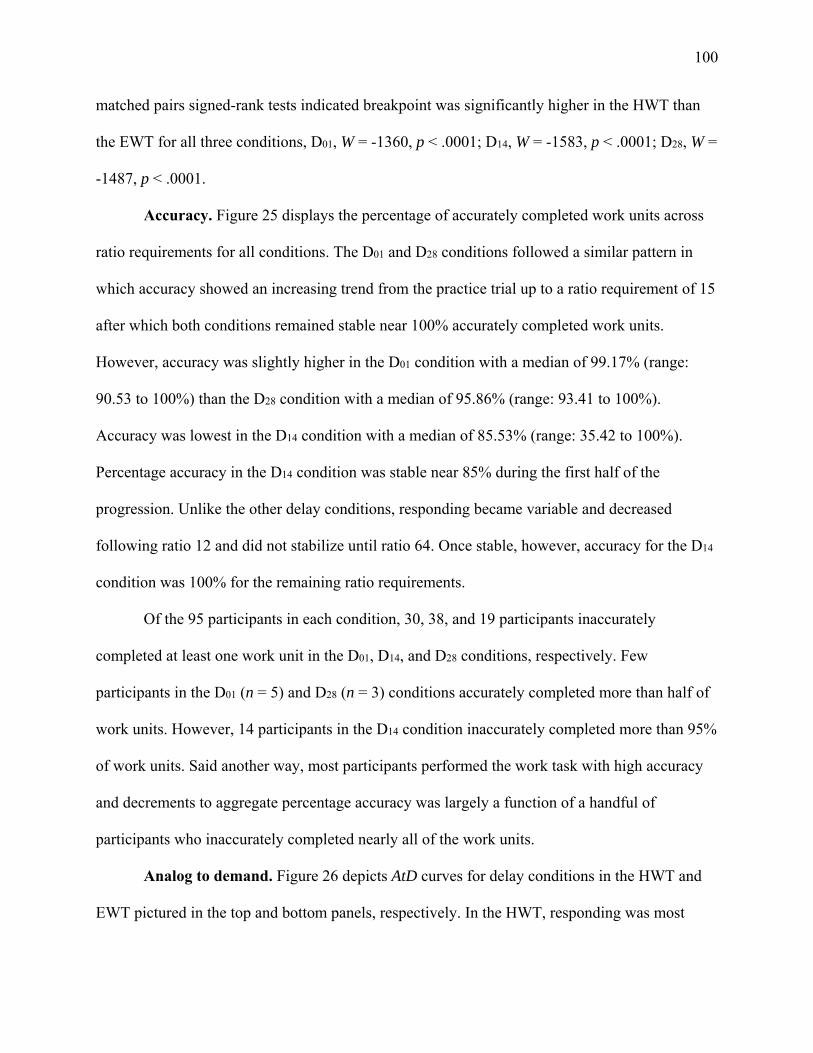
100

matched pairs signed-rank tests indicated breakpoint was significantly higher in the HWT than

the EWT for all three conditions, D01, W = -1360, p < .0001; D14, W = -1583, p < .0001; D28, W =

-1487, p < .0001.

Accuracy. Figure 25 displays the percentage of accurately completed work units across

ratio requirements for all conditions. The D01 and D28 conditions followed a similar pattern in

which accuracy showed an increasing trend from the practice trial up to a ratio requirement of 15

after which both conditions remained stable near 100% accurately completed work units.

However, accuracy was slightly higher in the D01 condition with a median of 99.17% (range:

90.53 to 100%) than the D28 condition with a median of 95.86% (range: 93.41 to 100%).

Accuracy was lowest in the D14 condition with a median of 85.53% (range: 35.42 to 100%).

Percentage accuracy in the D14 condition was stable near 85% during the first half of the

progression. Unlike the other delay conditions, responding became variable and decreased

following ratio 12 and did not stabilize until ratio 64. Once stable, however, accuracy for the D14

condition was 100% for the remaining ratio requirements.

Of the 95 participants in each condition, 30, 38, and 19 participants inaccurately

completed at least one work unit in the D01, D14, and D28 conditions, respectively. Few

participants in the D01 (n = 5) and D28 (n = 3) conditions accurately completed more than half of

work units. However, 14 participants in the D14 condition inaccurately completed more than 95%

of work units. Said another way, most participants performed the work task with high accuracy

and decrements to aggregate percentage accuracy was largely a function of a handful of

participants who inaccurately completed nearly all of the work units.

Analog to demand. Figure 26 depicts AtD curves for delay conditions in the HWT and

EWT pictured in the top and bottom panels, respectively. In the HWT, responding was most

101

elastic in the D14 condition (α = 1.4 × 10-4). Elasticity was equal in the D01 and D28 conditions (α

= 1.1 × 10-4) and did not differ significantly, F(1, 28) = 0.02, p = .88. Despite identical α values,

I observed a significant difference in elasticity between the D14 and D01 conditions, F(1, 28) =

4.4, p = .046, but not between the D14 and D28 conditions, F(1, 28) = 1.8, p = .19.

Consistent with the α values from which they were derived, EV, Pmax, and Omax were

identical in the D01 and D28 conditions and lowest in the D14 condition. Based on the work

function for the HWT pictured in Figure 27, I observed an equal response output at more than

one ratio requirement in the D14 condition (ratio 10 and 20). In this case, the higher price (i.e.,

higher ratio requirement) was selected for empirical Pmax. Although there may be reasons that

favor using the lower ratio for empirical Pmax (e.g., retaining a greater portion of the workforce),

I used the higher ratio because the purpose of this line of research is to inform organizational

incentive systems. From an organizational perspective, both ratio requirements will produce

equal output. However, expenses would be lower in the higher ratio requirement. The higher

ratio would better maximize the relative costs and benefits and would likely be viewed more

favorably by an organization. As such, the selected method serves to frame my results in a

manner consistent with which they are likely to be used in applied settings. Therefore, empirical

Pmax was equal to 20 in the D14 condition, this value was lower than the D01 and D28 conditions

that were both equal to 256. Similarly, empirical Omax was lowest in the D14 condition and

highest in the D28 condition. Although both measures generally followed a similar pattern, like

the previous experiments, increases in the right tail of the expenditure curve led to empirical

values that were often noticeably higher than the derived values. These increases were more

pronounced in the conditions with a higher number of participants who did not reach a

breakpoint (i.e., D28 and D01). Elasticity and related indices are summarized in Table 10.

102

Within the EWT, I observed a significant main effect of delay on elasticity, F(2, 37) = 11,

p = .0002. The main effect was attributable to significant pairwise comparisons between the D01

and D14 conditions, F(1, 28) = 17, p = .0003, and between the D01 and D28 conditions, F(1, 23) =

17, p = .0004, with responding being the most inelastic in the D01 condition in both cases.

However elasticity was equivalent in the D14 and D28 conditions, F(1, 23) = 0.009, p = .93.

Figure 28 displays the work functions for the three delay conditions in the EWT. In all three

conditions, empirical Pmax was lower than the derived values summarized in Table 10 whereas

empirical Omax was higher than the derived value.

As highlighted in Figure 29, residual plots follow a systematic pattern in which data

points in the HWT and EWT were consistently clustered above the best-fit curve and slightly

increasing at low ratio requirements. At higher ratio requirements (above derived Pmax), residuals

in the EWT varied among conditions. Data in the D01 condition were generally well scattered

above and below the best-fit curve line with clusters of no more than three data points above or

below zero. Following derived Pmax, residuals decreased in the D28 condition. The D14 condition

followed the same pattern as the D28 condition, but I observed a subsequent increase back to zero

at the higher end of the ratio requirements. For all conditions in the HWT, residuals for ratio

requirements higher than derived Pmax demonstrate a decreasing trend that was followed by a

rapid increase during the highest ratios.

Similar to Experiment 2, I observed appreciable differences in elasticity between the

HWT and EWT with responding being significantly more elastic in the EWT for all delay

conditions, D01, F(1, 28) = 42, p < .0001, D14, F(1, 28) = 74, p < .0001, D28, F(1, 23) = 32, p <

.0001. These differences are shown in Figure 30. Empirical and derived demand indices were

markedly lower in the EWT than the HWT within each delay condition.

103

Predictive validity. To examine the relation between breakpoint on the hypothetical and

experiential work tasks, Figure 31 plots EWT breakpoint as a function of HWT breakpoint,

separated by delay condition. Results of three separate Spearman rank-order correlations

revealed a significant positive relation between responding on the HWT and the EWT for all

three conditions, D01, rs(95) = .45, p < .0001; D14, rs(95) = .62, p < .0001; D28, rs(95) = .42, p <

.0001. Despite significant correlations in all three delay conditions, participants frequently

overestimated the amount of work they would complete (i.e., higher breakpoint in the HWT than

EWT). At the aggregate level, frequent overestimations of work output resulted in marked

decreases in percentage change in all conditions (Figure 32). Similar to Experiment 2, more than

half of the participants in each condition overestimated how much they would complete in the

EWT (range: D28, 51.58% to D01, 55.79%). I observed perfect correspondence in breakpoint

between the HWT and EWT in approximately one quarter of participants in each condition (D01,

25.26%; D14, 24.21%; D28, 24.21%).

Cost-benefit analysis. Figure 28 displays the relation between the work function on the

left y-axis and cost on the right y-axis at each ratio requirement for all three conditions. Because

work output was generally higher in the D01 condition, cost was also higher. However, work

output and cost in the D14 and D28 conditions were generally equivalent through ratio 32.

Between ratio requirements of 8 and 25, work output in D01 condition decreased slightly but

remained relatively stable while cost decreased drastically. Thus, if it is feasible to deliver the

incentive following a 1 day delay, selecting the D01 condition at a ratio requirement of 25 would

appear to maximize benefits while minimizing cost. Several constraints in the workplace (e.g.,

payroll processing) may limit the feasibility of delivering monetary reinforcement after only one

day. Perhaps—because of the wide range of possibilities—non-monetary incentives such as

104

access to a preferred parking spot or allowing an employee to bring his or her dog to work may

be amenable to relatively immediate delivery. It remains to be seen, however, if delayed non-

monetary reinforcers result in response patterns similar to that found with monetary incentives in

the present experiment. I observed numerous points of overlap between the D14 and D28

conditions for curves depicting both work output and cost despite the delay between the

conditions. Two points of Figure 28 suggest the D14 condition may yield favorable results for an

organization. First, at ratio values of 10 and 12, work functions for the D14 and D28 conditions

diverge with greater output in the D14 condition. Second, by ratio 48, all participants in the D28

condition reached a breakpoint, whereas several participants in the D14 condition continued to

respond at ratio 256.

In contrast with Experiment 2, I observed some differences in responding among

incentive delay conditions. Responding was highest and more inelastic in the condition

associated with the most immediate incentive delivery (i.e., D01). Despite being consistent with

previous research on the effects of reinforcer delay previously discussed, this effect was often

small and not always significantly different than responding in the other conditions. For

example, median HWT breakpoint was highest in the D01 condition, but the differences between

the D01 condition and the other conditions was not significant. Median EWT breakpoint was

equal among all conditions, but significantly higher in the D01 condition than the D28 condition.

The significant differences, despite equal median breakpoint values, may be a result of the spread

of the data, which are difficult to ascertain based on Figure 24. In fact, the highest breakpoint

values were 96, 48, and 32, in the D01, D14, and D28 conditions, respectively. The effects of

delays greater than one day were more variable, but never differed significantly from one another

105

for the breakpoint or AtD analyses. The present data are tentative and more research is needed to

support the findings. Nonetheless, two findings warrant additional discussion.

First, accuracy in the D14 condition was consistently lower than the D01 and D28

conditions, though typically remaining above 80%. This finding differs from Experiments 1 and

2 in which percentage accuracy was largely undifferentiated among conditions. Upon closer

inspection of the data, the lower levels of accuracy observed in the D14 condition were likely due

to a greater percentage of participants in that group who inaccurately completed nearly all work

units. Unfortunately, based on the present data, it is not clear if the decreased accuracy in the D14

condition is related to the incentive delay.

Importantly, the determination that delays greater than one day did not drastically change

participant responding might indicate a relative insensitivity to delay beyond a certain threshold.

This result, if it holds in future research, may be viewed as a success from a business standpoint.

Delays of 14 and 28 days are especially relevant to organizational incentive arrangements

because organizational payroll systems commonly occur on a bi-weekly or monthly cycle. When

distributed with fixed earnings, monetary incentive payouts follow similar delays. At least two

interpretations may provide insight regarding the variables controlling such an insensitivity to

increases in delay and suggest areas for future research.

First, Malott (2003) argues that employee responding is not controlled by direct-acting

contingencies because the delay to reinforcement is simply too long. Instead, indirect-acting

contingencies control behavior. Indirect-acting contingencies mediated by rules describing those

contingencies may moderate the effects of longer delays to reinforcement in the workplace and

account for the data observed in the present study. It might be that participants generated rules

that functionally equated the value of the incentive despite the delays. A function-altering effect

106

of rules in this way would likely lead to the present findings. Further research is needed to

provide support for this interpretation.

Second, research in delay discounting commonly finds that money is discounted less

steeply than other commodities (e.g., Charlton & Fantino, 2008). Results of a recent study by

Holt, Glodowski, Smits-Seemann, and Tiry (2016) suggest this may be partially due to the fact

that money is low in terms of perishability and high in terms of fungibility. Said another way,

money can be used over long durations (i.e., in the future) and exchanged for a wide variety of

goods or services (i.e., generalized conditioned reinforcer). It is possible that the same relative

insensitivity to delay may not be observed when using other incentive types. For instance, a visa

gift-card that expires in six months may not maintain the same levels of responding as cash.

Although a gift-card can be used to purchase many other goods and services (highly fungible), it

is also more perishable because it expires. This can further be contrasted with other non-

monetary incentives. Providing an employee with access to a preferred parking spot for six

months is perishable and not fungible and may result in marked decreases in responding at

longer delays. Researchers in OBM may benefit from considering the delay discounting

literature when making decisions about items used in an incentive arrangement.

The findings are in general agreement with previous research evaluating the effects of

delay on work-related behavior within a behavioral economic demand framework. Although I

did not observe significant differences in elasticity between the D01 and D28 conditions in the

HWT, this effect was obtained in the EWT. Henley, DiGennaro Reed, Kaplan, et al. (2016) used

a HWT to assess delays of 1 hr and 4 weeks with undergraduate participants. They found

significant differences in elasticity with greater inelasticity in the 1-hr delay condition. An

107

interesting feature of the present experiment that differs from Henley et al. was the use of mTurk

workers, which may contribute to the differences in findings of the HWT.

As previously discussed, OBM research evaluating the effects of delayed incentives is

largely lacking. Several researchers have evaluated the effects of delay on feedback (Krumhus &

Malott, 1980; Mason & Redmon, 1992; Reid & Parsons, 1996), the findings of which may have

implications for the use of delayed incentives. Research on delayed feedback suggests, when

provided the option, 100% of participants chose to receive feedback delivered immediately

rather than delayed (Reid & Parsons, 1996). Although the present study showed similarities in

responding among delay conditions for a brief research session, different findings may emerge if

participant preference impacted responding over longer periods (i.e., stronger preference for

shorter delays may be correlated with or functionally related to responding). Quite possibly,

employee acceptability with intervention procedures may effect intervention effectiveness and

should be considered when evaluating the relative pros and cons of an incentive arrangement. If

the difficulties of arranging incentive delivery every other week versus every four weeks are

roughly equivalent in a given situation, Reid and Parsons’ findings suggest that a relatively

shorter delay should be selected. Evaluations of interactions between incentive delay and

preference remain to be explored in future research.

One limitation of the present experiment involves the influence of the analog preparation

on the accuracy of the cost-benefit analyses. Specifically, procedures for processing and

delivering incentives to participants differed from real work settings. Paying participants in the

present study required a few minutes per participant, and in fact, required slightly less work on

the part of the experimenter in the D01 condition because there was no need to track the passage

of time. Delivering monetary incentives in real world settings likely requires additional resources

108

to expedite their delivery. The analog nature of the present experiment prevented me from

quantifying and including such costs in the cost-benefit analysis. The significant increase in

responding in the D01 condition may not be sufficient to offset the costs an organization would

need to allocate to carry out such an arrangement.

General Discussion

The current experiments examined the relative efficacy of reinforcer dimensions within a

behavioral economic demand framework and how parametric manipulations of their values

differentially influence performance. The goal was to provide insight into potentially effective

strategies for predicting and managing behavior in the workplace. The present studies also

sought to evaluate the predictive validity of a hypothetical assessment. Experiment 1 tested the

effects of three incentive magnitudes and found an orderly relation between magnitude and

responding as well as high correspondence between responding using hypothetical and

experiential demand assessment procedures. Experiments 2 and 3 evaluated the effects of

parametric values of incentive probability and delay, respectively. When the magnitude of

reinforcement was yoked, responding was comparable across multiple response measures (e.g.,

breakpoint, accuracy) regardless of probability. Results of Experiment 3 revealed small effects of

incentive delay in favor of the more immediate incentive delivery. Observed responding for

delays greater than one day were roughly equivalent.

Dimensions of Reinforcement

Although there are certainly exceptions, the results of these collective studies suggest

reinforcer dimensions influence responding and their values should not be haphazardly selected.

The most consistent effects of these parametric manipulations within each reinforcer dimension

were observed between the highest and lowest values. In Experiment 1, breakpoint was

109

consistently higher and elasticity consistently lower in the M20 condition relative to responding

in the M05 condition in both the HWT and EWT. Although few comparisons between any of the

conditions reached significance in Experiment 2, a significant difference in elasticity between the

P90 and P10 conditions was observed in the HWT. Lastly, EWT breakpoint in Experiment 3 was

significantly higher in the D01 condition compared to the D28 condition. The same effect of delay

was observed in comparisons of elasticity in the EWT.

When comparing among dimensions assessed, the effects of incentive magnitude had the

most consistent and discernable effect on responding with higher magnitude incentives being

relatively more efficacious. Results of the incentive magnitude manipulations are in general

agreement with the larger literature evaluating reinforcer amount (Fantino, 1977). Probability,

however, yielded no significant differences between any conditions despite comparisons of

widely disparate probability values (i.e., 10% and 90%). As briefly mentioned, yoking the

incentive magnitude to equate the amount earned after the probabilistic contingency was applied

may have rendered the conditions functionally equivalent. Magnitude then, may have exerted a

relatively greater influence on responding compared to probability when associated with the

same consequence. Although I observed some mixed effects of incentive delay, the present

findings are in general agreement with the literature on delayed reinforcement (e.g., Chung &

Herrnstein, 1967).

One goal of this line of research is to identify the reinforcer dimension that competes

most effectively with concurrent sources of reinforcement in the workplace. A greater

understanding of the relative efficacy of reinforcer dimensions and how parametric

manipulations of their values differentially influence performance could lead to effective

strategies for predicting and managing employee behavior. This information can then be used to

110

maximize the effectiveness of incentive interventions. Neef and Noone Lutz (2001) provide a

possible definition of what constitutes the most effective dimension which states, “[the]

dimension that consistently produced the highest proportion of time allocation in relation to any

of the other three dimensions with which it competed” (p. 58). Considering the differences in

relative consistency and differentiation noted above, an extension of Neef and Noone Lutz’s

definition to the current research supports an interpretation that work-related behavior may be

more sensitive to manipulations of magnitude and delay than probability. Other researchers have

made similar arguments (Catania, 1979; Kimble, 1961; Lattal, 2010). For example, Lattal

suggests, “along with rate, quality, and magnitude, delay has been considered a primary

determinant of the effectiveness of a reinforcer” (p. 129). Further research is needed to

investigate relative contributions of these reinforcer dimensions on responding in the work

environment.

Accuracy

The accuracy with which employees perform their job is of great importance to

organizational leaders in a diverse range of fields, in part because of the tremendous impact

inaccurate performance can have on the consumers of the goods or services organizations

produce. For example, Makary and Daniel (2016) recently estimated more than 250,000

Americans die each year from preventable medical errors (e.g., inaccuracies during medical

procedures or drug administration). This finding ranks medical mistakes as the third leading

cause of death in the U.S. and underscores the importance of identifying interventions that

support high levels of this socially significant organizational metric.

One important finding across all three experiments is the consistently high levels of

accurate work completion. As evidenced by the data presented in Table 11, overall median

111

accuracy never dropped below 85% for any condition. High levels of accuracy were maintained

despite removing the contingency for correct responding in the practice trial in Experiments 2

and 3. This finding suggests that the contingency for accurate responding in the practice trial was

not responsible for the high levels of accuracy in Experiment 1. The finding that accuracy

remained high irrespective of magnitude, probability, or delay is potentially promising for

organizations (recognizing the translational nature of the present study, of course). Additionally,

findings of all three studies suggest that decrements in accuracy could primarily be attributed to a

relatively small percentage of participants. From an organizational perspective, this is good news

because it may allow for organizations to focus behavior change efforts (e.g., feedback) on a low

number of workers. This approach would likely require fewer resources than if the entire

workforce consistently made errors that required intervention.

However promising, it is possible that the contingencies in place for mTurk Workers

contributed to the high levels of accuracy observed. Requesters may reject a HIT if Workers’

performance is not considered acceptable. In addition to not receiving compensation for their

work in these cases, Amazon tracks Workers’ approval rate (i.e., the percentage of completed

HITs accepted by requesters) and allows requesters to set a minimum acceptable level when

posting a HIT; in the present experiments, Workers were required to have at least a 95%

approval rate. Thus, having a low approval rate results in decreased opportunities to complete

HITs. Workers may have responded accurately to avoid rejection of their work. Future research

may wish to evaluate whether the percentage of accurately completed work varies as a function

of Worker approval rates. It is also possible that decreases in accuracy would emerge if measured

over longer periods of time. Thus, the effects of reinforcer dimensions on accuracy must be

interpreted with some degree of caution.

112

HWT Predictive Validity

I also observed significant positive correlations between breakpoint on the HWT and

EWT for every condition in all three experiments. The consistent correlations suggest the HWT

is a promising method for future research evaluating the effects of reinforcer dimension and the

application of demand curve analyses to work-related behavior. However, comparisons of

changes in the predictive validity of the HWT across studies suggested several features of the

experimental arrangement and methodology may have influenced the correspondence between

the HWT and EWT. Each of these experimental features are discussed in detail below (see the

section with a heading labeled “Experimental Preparation Influences on Predictive Validity”).

An important point regarding the HWT is the conceptualization of this measure as having

predictive validity. Predictive validity assesses the degree to which a measure predicts

performance assessed at some point in the future (Crocker & Algina, 1986). Arguably, in the

current preparation, the HWT may not be assessing predictive validity because the EWT was

completed only a few minutes following the HWT. Unfortunately, it is unclear how long the

duration between an initial assessment and performance measurement must be for the original

assessment to be accurately conceptualized as having predictive validity. Because the purpose of

the HWT is to draw inferences to behavior in the workplace, the HWT likely falls under the

general umbrella of criterion-related validity (Crocker & Algina, 1986), but may also be

conceptualized as concurrent validity. According to Crocker and Algina, concurrent validity is

another type of criterion-related validity that:

“refers to the relationship between test scores and criterion measurements made at the

same time the test was given…a sufficient correlation between the two would justify the

use of the test in place of the less efficient and more costly observation system” (p. 224).

113

The HWT, if proven useful, would likely function in place of less efficient methods (i.e.,

experiential demand assessments) but will be used to predict a certain level of performance in the

future when the contingencies described in the HWT are implemented in the organization. Thus,

both predictive and concurrent validity may be appropriate. However, only predictive validity is

used throughout the present document for consistency.

Alternative Predictive Measures of Performance

One goal of the present experiments was to identify behavioral scales, demographic

characteristics, or employment-related variables that have predictive validity for how individuals

will respond on the EWT. In the first experiment, rates of delay discounting assessed via the

monetary choice questionnaire were not significantly correlated with work output, and only one

measure from the behavioral inhibition/behavioral activation scale (BIS/BAS) was significantly

related to breakpoint. Given the limited findings from Experiment 1, the monetary choice

questionnaire and the BIS/BAS were replaced with the demographic, employment, and incentive

survey in Experiments 2 and 3. Unfortunately, the only variable significantly related to EWT

breakpoint was completing mTurk HITs because participants find the tasks to be fun

(Experiment 2 only). This finding could be interpreted as an indication that a possible relation

exists between enjoyment of work responsibilities and output, which certainly has some face

validity. Nonetheless, the question was specific to the completion of mTurk HITs and in its

current form would likely not prove probative in traditional work settings. Moreover, this

relation was not observed in Experiment 3. Identifying a measure predictive of work output

through additional research could have implications for a number of organizational practices,

such as personnel selection and hiring practices.

114

The paucity of research on personnel selection and hiring practices in OBM stands in

contrast to the substantial extant literature on the topic in industrial and organizational

psychology (DiGennaro Reed, Hirst, & Howard, 2013). Personnel selection represents a major

responsibility that organizational leaders must effectively navigate, for which the OBM literature

offers little guidance. The relative skill of employees can substantially impact the effectiveness

of an organization. In fact, highly successful organizations like Google frequently allocate six-

figure salaries to employ individuals whose primary role is to identify and recruit skilled staff.

Quite possibly, increased scholarly attention to personnel selection in OBM could generate

methods that, when implemented in practice, reduce the frequency or intensity of initial and

ongoing training or interventions needed to address skill and performance deficits. Identification

of such personnel selection methods would allow organizations to re-allocate valuable resources

from recruitment efforts to empirically supported staff training and support programs. If this

supposition holds, higher quality staff supports could lead to improvements in a host of socially

significant issues that plague organizations, their employees, and consumers (e.g., turnover,

workplace injuries, compromised treatment integrity). Such endeavors, if successful, may also

serve to increase the exposure of OBM outside of behavior analysis given the premium

businesses place on staff selection previously noted.

Contributions to the Literature

In spite of several noted inconsistencies between the current findings and previous

research, these studies contribute to the literature in a number of ways. First, these studies are

some of the only studies in OBM to systematically manipulate reinforcer dimensions in a way

that allows for direct comparisons among parametric values. Second, the inclusion of the HWT

to evaluate the correspondence between hypothetical and experiential demand preparations

115

supports and extends previous research by allowing for a direct comparison of responding at

every price. Research using experiential methods to validate hypothetical purchase tasks have

typically only provided participants with one real outcome based on their responding on the

hypothetical task—including Amlung and MacKillop’s (2015) study on alcohol purchases

described previously.

A third contribution of the present experiments was the inclusion of cost-benefit analyses.

Cost is a major factor for organizations that influences intervention acceptability and

implementation. Cost-benefit analyses provide organizational leaders with an efficient means of

evaluating the economic feasibility of an intervention (Wells, Reimer, & Houmanfar, 2013).

Despite numerous calls urging the use of such analyses (e.g., Andrasik, 1979; Balcazar, Shupert,

Daniels, Mawhinney, & Hopkins, 1989; Poling, Smith, & Braatz, 1993), Wells and colleagues

recently reported that just 10% of experimental OBM research published between 1977 and 2011

include cost-benefit analyses. Higher rates of reporting cost-benefit analyses may also hold OBM

researchers accountable for developing interventions in a cost-sensitive manner, selecting only

those interventions indicated by the function of the problem behavior.

A fourth contribution relates to the use of demand curve analyses. Consistent with the

law of demand, the percentage of participants who completed the work requirement was inelastic

and highest at a price of 1 and steadily decreased and became elastic with increases in the

number of work units required to earn the incentive. I observed similar positively accelerating

response patterns in the HWT and EWT across all conditions and experiments. Thus, despite

parametric manipulations of reinforcer dimensions, responding in all cases was consistent with

behavioral economic demand theory (Hursh, 1980). This finding extends previous research

applying behavioral economic demand curve analyses to work-related behavior and monetary

116

incentives in at least three ways. First, it evaluated a wider range of reinforcer magnitudes than

Henley, DiGennaro Reed, Reed, et al. (2016) with the inclusion of a $0.20 incentive in

Experiment 1. Second, Experiment 2 evaluated parametric values of incentive probability

previously unexplored in this novel line of research. Third, these studies also included

evaluations of incentive delay using a different work task and participant pool using an

experiential arrangement in addition to examinations of delay using a HWT performed by

Henley, DiGennaro Reed, Kaplan, et al. (2016).

Experimental Preparation Influences on Predictive Validity

As noted previously, an interesting finding across studies was the marked decrease in

several measures of predictive validity from Experiment 1 to Experiments 2 and 3. For all

conditions in Experiments 2 and 3, I observed significant differences in breakpoint between the

HWT and EWT; striking differences in the AtD curves between the HWT and EWT; and

pronounced decreases in percentage change. Results for all three analyses stand in contrast to the

findings of Experiment 1. Despite high correlations between breakpoints, the consistent and

pronounced differences in responding between the HWT and EWT call into question the utility

of the HWT for use in an organization. Interestingly though, decreases in predictive validity

measures across studies were even observed between the M20 and D01 conditions. Both

conditions had a 100% likelihood of earning a $0.20 incentive at a relatively short delay; one day

in the D01 condition and between one and three days in the M20 condition. The finding that

predictive validity was high for all measures, but the same measures resulted in highly discrepant

response patterns on the HWT despite experiencing very similar contingencies suggests this

difference may not be a function of the reinforcer dimensions assessed in Experiments 2 and 3.

Rather, several features of the experimental arrangement and methodology were changed after

117

Experiment 1 and may have influenced the correspondence between the HWT and EWT in

Experiments 2 and 3. If the source of this discrepancy cannot be identified through additional

research, and the same general level of overestimation is consistently observed, it may be

possible to quantify the extent to which individuals overestimate work completion using

hypothetical tasks. Organizational leaders may then account for this difference when using the

HWT to predict work output and cost or researchers may be able to identify a method handling

data for participants without a breakpoint to ameliorate some of the effects on predictive validity.

Even so, the implications of this finding for research and application warrants additional

attention.

Decreases in predictive validity in Experiments 2 and 3 co-occurred with increases in the

numbers of participants who did not reach a breakpoint in the HWT. The percentage of

participants who did not reach a breakpoint in the HWT was 0.69%, 4.9%, and 4.2% in

Experiments 1, 2, and 3, respectively. Because several of the dependent measures were based on

aggregate group performance, retaining data for these participants resulted in pronounced

increases in projected performance and contributed to the disparity between the HWT and EWT.

Two features of the HWT presentation might have influenced responding on the HWT. First, the

HWT ratio requirements in Experiments 2 and 3 were presented simultaneously on a single page

rather than presenting a single ratio requirement per page in a sequential manner. Skidmore and

Murphy (2011), although evaluating alcohol consumption with a purchase task, used a similar

arrangement in that the prices were presented in an ascending order and shown all at once. When

Skidmore and Murphy presented the prices in this fashion, nearly a quarter of their sample (n =

47; 22.7%) were excluded from analyses because their R2 values when fit to the demand equation

fell below 0.3. In 2012, Gentile, Librizzi, and Martinetti sought to address the limitations of

118

Skidmore and Murphy, including how prices were presented to participants. In their extension,

only one price was shown at a time. No participants were excluded due to unsystematic

responding on the purchase task or low R2 values. Although a seemingly minor variation, HPT

research has consistently demonstrated changes in responding with minor procedural

manipulations (e.g., Skidmore & Murphy, 2011). Thus, it is possible that presenting the HWT on

a single page resulted in a higher number of participants who did not reach a breakpoint. It would

be informative for future research to examine whether this difference systematically affects

HWT responding. The fact that responding is highly sensitive to minor manipulations could be

used as evidence against the use of hypothetical tasks as it may result in inconsistent or variable

results. However, basic research on instructional control has also consistently demonstrated

robust effects of minor variations on response patterns (e.g., Henley, Hirst, DiGennaro Reed,

Becirevic, & Reed, 2016).

It may also be the case that requiring participants to respond to every ratio requirement in

the HWT may have influenced predictive validity. This contingency increased the number of

overall required responses and several participants noted frustration with this experimental

feature when given the opportunity to provide feedback following study completion. For

example, one participant commented, “I'm not sure why you asked me at the end the same

questions you asked at the beginning, but if you had some good reason to ask them all again, and

all on different pages, at least you could have stopped asking me once I said no - why would

anyone possibly be uninterested in answering 10, but be *interested* in doing *more* than 10?

That part was just totally a waste of time.” Responses such as these—though unclear if related to

changes in predictive validity among experiments—may have implications for the social validity

of HWT methodology and could inform any procedures recommended for use in practice.

119

Third, decreases in predictive validity may be due to the increased time between

completion of the HWT and EWT as a result of requiring participants to complete the

demographic, employment, and incentive survey between the tasks. Separating the work tasks

was intended to mitigate sequence effects of completing the HWT prior to the EWT, but may

have inadvertently decreased predictive validity. In real work environments, however,

assessments intended to predict subsequent job performance would likely be separated in time by

days, weeks, months, or even years. It is important to note that psychometric studies of

predictive validity involve varying time differences suggesting this issue is likely not responsible

for the low predictive validity I observed. Systematic manipulation and evaluation of how delay

between assessment and performance influences predictive validity represents a logical and

important area for future research on this topic. In addition, the aforementioned features may also

have contributed to the increase in the number of participants who overestimated their work

completion and contributed to the striking differences in breakpoint and elasticity between the

HWT and EWT for all probability and delay conditions.

One possible feature contributing to the number of individuals who overestimated their

responding involves the use of a PR schedule. A notable limitation of the use of the PR schedule

in the present study involves the cumulative number of responses emitted as the ratio

requirement increased within the session. Responding at each ratio requirement was not

necessarily reflective of that reinforcement schedule as it may also have been influenced by each

prior ratio presented in the session; a limitation tacted by several participants in the present

studies. For example, when given the opportunity to provide feedback one participant noted,

“Doing 25 sliders is not the same as doing the amount of each number up to 25.” Such responses

raise the possibility that some participants may have been responding as if the requirement would

120

be presented in isolation when prompted to indicate their willingness to complete increasing

requirements in the HWT. When presented consecutively in the EWT, however, the

experimental preparation may have led to lower breakpoints than might otherwise be observed if

the ratio requirements were not presented in a progressive fashion within session. Future research

could assess the predictive validity of the HWT using a derivation of the PR arrangement

wherein participants complete progressively increasing ratio requirements during different

sessions separated in time (Jarmolowicz & Lattal, 2010). Researchers have successfully used

modified PR schedules wherein the response requirement is increased between rather than within

session in human operant drug self-administration studies (e.g., Bickel & Madden, 1999). The

effects of using a PR schedule, however relevant, does not explain why overestimations

increased in Experiments 2 and 3 when the schedule remained unchanged from Experiment 1.

Limitations and Future Research

In addition to those already identified, several other limitations inform areas for future

research. As mentioned previously, nonmonetary reinforcers are a flexible means for mediating

budgetary restrictions associated with implementing an incentive system. Recall also that

response effort may affect the allocation of employee responding among concurrently available

work tasks that require varying levels of effort. A logical extension, therefore, would be to

examine parametric effects of effort and quality.

Second, the current experimental preparation was designed to address the limitations of

typical laboratory-based analog OBM research employing undergraduate participants in which

limited concurrent response options capable of effectively competing with the simulated work

task exist. Despite improvements, the preparation nonetheless differed form a real work

environment in several potentially important ways. Additionally, because a similar preparation

121

was used, all three experiments are subject to the same limitations regarding external validity

some of which include the duration and complexity of the work task, relative immediacy of base

pay (24 hr), and incentive amounts. It is also likely that progressive reinforcement contingencies

are uncommon in the workplace. As a result, the analog arrangement limits conclusions about

how the effects may generalize to real workplaces. However, this line of research is still in the

early stages and transitioning to an applied setting at this point may result in unintended

consequences. A related limitation of this arrangement is that I did not have control over the

environment in which participants completed the experimental procedures. The variability in

environmental conditions may have obscured differences that would otherwise emerged if

participants completed study procedures under similar settings.

Third, despite observing consistent differences among magnitude conditions, increases in

responding in the larger magnitude conditions were relatively modest in comparison to the

relatively large differences in incentive amount. As illustrated by the reversed relation between

response output and magnitude observed when using unit price, a one-unit increase in magnitude

was met with a less than one-unit increase in response output. Small changes in behavior despite

relatively large differences in reinforcer magnitude have been consistently documented in the

literature since the early 1960s (Catania, 1963; Fantino & Logan, 1979), but this relation is

typically observed in single operant arrangements. When researchers manipulate magnitude in a

concurrent operant arrangement, however, large differences in responding emerge. Researchers

have long commented on the advantages of concurrent operant arrangements as compared to

single operant arrangements for examining the effects of manipulating reinforcer dimensions on

behavior (e.g., Fisher & Mazur, 1997). Therefore, future investigations may wish to extend the

current experimental paradigm to a concurrent operant arrangement. Extending choice

122

procedures used to evaluate reinforcer dimensions and preference in other applied settings (e.g.,

Neef et al., 1994) to evaluations of incentive arrangements in the workplace may also provide

valuable information on the social validity of such arrangements (Schwartz & Baer, 1991).

Results of several studies evaluating reinforcer dimensions in applied settings suggest the

most efficacious dimension often differs for each participant (Neef et al., 1994; Neef & Noone

Lutz, 2001). Based on these results, comparing the current findings to those obtained using

within-subject methods may be an important contribution to the literature evaluating the effects

of reinforcer dimensions on work-related responding. A within-subject approach may provide

insight into how varying parametric levels within a reinforcer dimension as well as between

dimensions may influence responding within-subject as compared to group responding. Because

performance management interventions frequently target the behavior of individuals and groups

any differences may help improve application technology.

AtD Model Fits

One final observation that warrants some discussion is the AtD model fits. Across the

three experiments, R2 values for AtD curves were consistently high, ranging from .74 to .98 (M =

.93). As previously mentioned, R2 may not be the most informative measure for evaluating the

applicability and appropriateness of the exponential model of demand. Consistent with Motulsky

and Cristopoulos’ (2006) suggestion, I carefully inspected residual plots for all AtD model fits to

evaluate whether residuals are randomly distributed around the best-fit curve.

Visual inspection of the residual plots for systematic deviations from the best-fit curves

revealed an interesting pattern. In the EWT, residuals at lower prices demonstrate an increasing

trend away from the curve fit, the peak of which closely aligns with derived Pmax. Thus, the point

at which consumption values derived from the exponential model deviate the most in the EWT

123

occurs at the point of unit elasticity. This is also the point at which one would expect peak

response output and has been suggested in research as the point with the greatest potential for

applied utility.

This discrepancy may explain some of the inconsistencies with empirical and derived

Omax in the EWT. Because consumption at Pmax is used to quantify derived Omax, if the curve is

consistently under-fitting the data at this point, derived Omax is calculated based on deflated

consumption values that are not reflective of observed responding. For example, derived Omax for

the P90 condition in the EWT was 226 work units at a price of 7.8. Despite similar derived and

empirical Pmax values, the number of work units completed at empirical Omax is approximately

double.

The same extended sequence of increasing data points above the best fit line at low prices

can also be seen in the HWT, however, the residuals at these values are more closely aligned

with the best fit curve. This increase is followed by a stretch of negative residuals and

subsequently a considerable positive deviation from the best fit at the highest prices. The pattern

observed in the HWT was partially influenced by the number of individuals who did not reach a

breakpoint. The presence of extreme values could also influence empirical and derived parameter

estimates.

Cursory examination of previous research using the exponential model suggests this trend

may not be unique to the current data (e.g., Hursh, 2014; Reed et al., 2014). If MacKillop and

Murphy (2007) experienced a similar issue, it may explain their statement “data from our

laboratory suggest that the observed parameters are more reliable than the derived values” (p.

229). Similar fitting issues have been noted in the delay discounting literature. For example,

Odum (2011) suggests Mazur’s (1987) discounting equation tends to overpredict indifference

124

points at shorter delays and underpredict indifference points at longer delays. Ultimately,

questions remain about how systematic deviations from the best fit line—particularly at Pmax—

may influence the applied utility of the exponential model and how it may be addressed in future

research.

125

References

Alavosius, M., Getting, J., Dagen, J., Newson, W., & Hopkins, B. (2009). Use of a cooperative

to interlock contingencies and balance the commonwealth. Journal of Organizational

Behavior Management, 29, 193-211. doi: 10.1080/01608060902874575

Alvero, A. M., Bucklin, B. R., & Austin, J. (2001). An objective review of the effectiveness and

essential characteristics of performance feedback in organizational settings. Journal of

Organizational Behavior Management, 21(1), 3-29. doi: 10.1300/J075v21n01_02

Amlung, M. T., Acker, J., Stojek, M. K., Murphy, J. G., & MacKillop, J., (2012). Is talk

‘cheap’?: An initial investigation of the equivalence of alcohol purchase task

performance for hypothetical and actual rewards. Alcoholism: Clinical and Experimental

Research, 36, 716–724. doi: 10.1111/j.1530-0277.2011.01656.x

Amlung, M. T., & MacKillop, J. (2015). Further evidence of close correspondence for alcohol

demand decision making for hypothetical and incentivized rewards. Behavioral

Processes, 113, 187-191. doi: 10.1016/j.beproc.2015.02.012

Andrasik, F. (1979). Organizational behavior modification in business settings: A

methodological and content review. Journal of Organizational Behavior Management,

2(2), 85–102.

Austin, J., Kessler, M. L., Riccobono, J. E., & Bailey, J. S. (1996). Using feedback and

reinforcement to improve the performance and safety of a roofing crew. Journal of

Organizational Behavior Management, 16, 49-75. doi: 10.1300/J075v16n02_04

Baer, D. M., Wolf, M, M., & Risley, T. R. (1968). Some current dimensions of applied behavior

analysis. Journal of Applied Behavior Analysis, 1, 91–97. doi: 10.1901/jaba.1968.1-91

126

Balcazar, F., Hopkins, B. L., & Suarez, Y. (1985). A critical, objective review of performance

feedback. Journal of Organizational Behavior Management, 7, 65-89. doi:

10.1300/J075v07n03_05

Balcazar, F., Shupert, M., Daniels, A., Mawhinney, T., & Hopkins, B. (1989). An objective

review and analysis of ten years of publication in the Journal of Organizational Behavior

Management. Journal of Organizational Behavior Management, 10(1), 7–37.

Baum, W. M. (1979). Matching, undermatching, and overmatching in studies of choice. Journal

of the Experimental Analysis of Behavior, 32, 269-281. doi: 10.1901/jeab.1979.32-269

Berger, C. J., Cummings, L. L., & Heneman, H. G. (1975). Expectancy theory and operant

conditioning predictions of performance under variable ratio and continuous schedules of

reinforcement. Organizational Behavior and Human Performance, 14, 227-243. doi:

10.1016/0030-5073(75)90026-4

Bickel, W. K., Jarmolowicz, D. P., Mueller, E. T., Koffarnus, M. N., & Gatchalian, K. M.

(2012). Excessive discounting of delayed reinforcers as a trans-disease process

contributing to addiction and other disease-related vulnerabilities: Emerging evidence.

Pharmacology & Therapeutics, 134, 287-297. doi: 10.1016/j.pharmthera.2012.02.004

Bickel, W. K., Johnson, M. W., Koffarnus, M. N., MacKillop, J., & Murphy, J. G. (2014). The

behavioral economics of substance use disorders: Reinforcement pathologies and their

repair. Annual Review of Clinical Psychology, 10(1), 641–677. doi: 10.1146/annurev-

clinpsy-032813-153724

Bickel, W. K., & Madden, G. J. (1999). A comparison of measures of relative reinforcing

efficacy and behavioral economics: cigarettes and money in smokers. Behavioural

Pharmacology, 10(6), 627–638. doi:10.1097/00008877-199911000-00009

127

Black, A. C., & Rosen, M. I. (2011). A money management-based substance use treatment

increases valuation of future rewards. Addictive Behaviors, 36, 125-128. doi:

10.1016/j.addbeh.2010.08.014

Bruner, N. R., & Johnson, M. W. (2014). Demand curves for hypothetical cocaine in cocaine-

dependent individuals. Psychopharmacology, 231, 889-897. doi: 10.1007/s00213-013-

3312-5

Bucklin, B. R., & Dickinson, A. M. (2001). Individual monetary incentives. Journal of

Organizational Behavior Management, 21 (3), 45-137. doi: 10.1300/J075v21n03_03

Bureau of Labor Statistics (2014). American time use survey. Retrieved from

http://www.bls.gov/tus/charts/#work

Bureau of Labor Statistics (2016a). Labor force statistics from the current population survey.

Retrieved from http://data.bls.gov/timeseries/LNS11300000

Bureau of Labor Statistics (2016b). Occupational injuries and illnesses industry data. Retrieved

from http://data.bls.gov/timeseries/ISU00000000061100

Camden, M. C., & Ludwig, T. D. (2013). Absenteeism in health care: Using interlocking

behavioral contingency feedback to increase attendance with certified nursing assistants.

Journal of Organizational Behavior Management, 33, 165-184. doi:

10.1080/01608061.2013.814521

Cannella, H. I., O’Reilly, M. F., & Lancioni, G. E. (2005). Choice and preference assessment

research with people with severe to profound disabilities: A review of the literature.

Research in Developmental Disabilities, 26, 1-5. doi: 10.1016/j.ridd.2004.01.006

128

Carver, C. S., & White, T. L. (1994). Behavioral inhibition, behavioral activation, and affective

responses to impending reward and punishment: The BIS/BAS scales. Journal of

Personality and Social Psychology, 67, 319-333. doi: 10.1037/0022-3514.67.2.319

Catania, A. C. (1963). Concurrent performances: A baseline for the study of reinforcement

magnitude. Journal of the Experimental Analysis of Behavior, 6, 299-300.

Catania, A. C. (1979). Learning. Englewood Cliffs, NJ: Prentice Hall.

Charlton, S. R., & Fantino, E. (2008). Commodity specific rates of temporal discounting: does

metabolic function underlie differences in rates of discounting? Behavioural Processes,

77, 334–342.

Chase, H. W., MacKillop, J., & Hogarth, L. (2013). Isolating behavioral economic indices of

demand in relation to nicotine dependence. Psychopharmacology, 226, 371-380. doi:

10.1007/s00213-012-2911-x

Chung, S., & Herrnstein, R. J. (1967). Choice and delayed reinforcement. Journal of the

Experimental Analysis of Behavior, 10, 67-74.

Clayton, M. C., & Blaskewicz, J. (2012). The use of visual prompts to increase the cleanliness of

restrooms on a college campus. Journal of Organizational Behavior Management, 32,

329-337. doi. 10.1080/01608061.2012.729393

Collins, R. L., Vincent, P. C., Yu, J., Liu, L., & Epstein, L. H. (2014). A behavioral economic

approach to assessing demand for marijuana. Experimental and Clinical

Psychopharmacology, 22, 211-221. doi: 10.1037/a0035318

Cook, T., & Dixon, M. R. (2006). Performance feedback and probabilistic bonus contingencies

among employees in a human service organization. Journal of Organizational Behavior

Management, 25, 45-63. doi: 10.1300/J075v25n03_04

129

Cooper, J. O., Heron, T. E., & Heward, W. L. (2006). Applied behavior analysis. Upper Saddle

River, NJ: Merrill Prentice Hall.

Critchfield, T. S., & Reed, D. D. (2009). What are we doing when we translate from quantitative

models? The Behavior Analyst, 32, 339-362.

Crocker, L., & Algina, J. (1986). Introduction to classical and modern test theory. Toronto:

Holt, RineHart, and Winston, Inc.

Daniels, A. C. (2000). Bringing out the best in people: How to apply the astonishing power of

positive reinforcement. New York, NY: McGraw-Hill.

Daniels, A. C., & Daniels, J. E. (2006) Performance management. Atlanta: Performance

Management Publications.

Dib, N., & Sturmey, P. (2007). Reducing student stereotypy by improving teachers’

implementation of discrete trial teaching. Journal of Applied Behavior Analysis, 40, 339–

343. doi:10.1901/jaba.2007.52-06

Dickinson, A. M. (2001). The historical roots of organizational behavior management in the

private sector. Journal of Organizational Behavior Management, 20, 9-58. doi:

10.1300/J075v20n03_02

Dickinson, A. M., & Gillette, K. L. (1994). A comparison of the effects of two individual

monetary incentive systems on productivity: Piece rate pay versus base pay plus

incentives. Journal of Organizational Behavior Management, 14 (1), 3-82. doi:

10.1300/J075v14n01_02

Dickinson, A. M., & Poling, A. D. (1996). Schedules of monetary reinforcement in

organizational behavior management: Latham and Huber (1992) revisited. Journal of


130

Diener, L. H., McGee, H. M., & Miguel, C. F. (2009). An integrated approach for conducting a

behavioral systems analysis. Journal of Organizational Behavior Management, 29, 108–

135. doi:10.1080/01608060902874534

DiGennaro Reed, F. D., & Henley, A. J. (2015). A survey of staff training and performance

management practices: The good, the bad, and the ugly. Behavior Analysis in Practice, 8,

16-26. doi: 10.1007/s40617-015-0044-5

DiGennaro Reed, F. D., Henley, A. J., Hirst, J. M., Doucette, J. L., & Jenkins, S. R. (2015).

Basic research considerations for performance management of staff. In F.D. DiGennaro

Reed & D.D. Reed (Eds.), Bridging the gap between science and practice in autism

service delivery. New York: Springer.

DiGennaro Reed, F. D., Hirst, J. M., & Howard, V. J. (2013). Empirically supported staff

selection, training, and management strategies. In D. D. Reed, F. D. DiGennaro Reed, &

J. K. Luiselli (Eds.), Handbook of crisis intervention for individuals with developmental

disabilities. New York: Springer.

Doll, J., Livesey, J., McHaffie, E., & Ludwig, T. D. (2007). Keeping an uphill edge. Journal of


Downing, C. O., & Geller, E. S. (2012). A goal-setting and feedback intervention to increase ID-

checking behavior: An assessment of social validity and behavioral impact. Journal of

Applied Behavior Analysis, 32, 297-306. doi: 10.1080/01608061.2012.729383

Epstein, L. H., Dearing, K. K., & Roba, L. G. (2010). A questionnaire approach to measuring the

relative reinforcing efficacy of snack foods. Eating Behaviors, 11, 67-73. doi:

10.1016/j.eatbeh.2009.09.006

131

Evans, K. M., Kienast, P., & Mitchell, T. R., (1988). The effects of lottery incentive programs on

performance. Journal of Organizational Behavior Management, 9, 113-135. doi:

10.1300/J075v09n02_08

Fantino, E. (1977). Conditioned reinforcement: Choice and information. In W. Honig & J.

Staddon (Eds.), Handbook of Operant Behavior (pp. 313-339). Englewood Cliffs, NJ:

Prentice-Hall.

Fantino, E., & Logan, C. L. (1979). Choice behavior. In E. Fantino, & C. Logan (Eds.), The

experimental analysis of behavior: A biological perspective (208-241). San Francisco:

Freeman.

Ferster, C. B., & Skinner, B. F. (1957). Schedules of reinforcement. New York: Appleton-

Century-Crofts.

Fisher, W. W., & Mazur, J. E. (1997). Basic and applied research on choice responding. Journal

of Applied Behavior Analysis, 30, 387-410.

Friman, P. C., & Poling, A. (1995). Making life easier with effort: Basic findings and applied

research on response effort. Journal of Applied Behavior Analysis, 28, 583-590. doi:

10.1901/jaba.1995.28-583

Gentile, N. D., Librizzi, E. H., & Martinetti, M. P. (2012). Academic constraints on alcohol

consumption in college students: A behavioral economic analysis. Experimental and

Clinical Psychopharmacology, 20(5), 390–399. doi:10.1037/a0029665

Goomas, D. T., & Ludwig, T. D. (2007). Enhancing incentive programs with proximal goals and

immediate feedback. Journal of Organizational Behavior Management, 27, 33-68. doi:

10.1300/J075v27n01_02

132

Grace, R. C., Schwendiman, J. W., & Nevin, J. A. (1998). Effects of unsignaled delay of

reinforcement on preference and resistance to change. Journal of the Experimental

Analysis of Behavior, 69 (3), 247-261. doi: 10.1901/jeab.1998.69-247

Greenwald, M. K., & Hursh, S. R. (2006). Behavioral economic analysis of opioid consumption

in heroin-dependent individuals: Effects of unit price and pre-session drug supply. Drug

and Alcohol Dependence, 85 (1), 35-48. doi: 10.1016/j.drugalcdep.2006.03.007

Gresham, F. M., Gansle, K. A., Noell, G. H., Cohen, S., & Rosenblum, S. (1993). Treatment

integrity of school-based behavioral intervention studies: 1980–1990. School Psychology

Review, 22, 254–272.

Grindle, A. C., Dickinson, A. M., & Boettcher, W. (2000). Behavioral safety research in

manufacturing settings. Journal of Organizational Behavior Management, 20, 29-68. doi:

10.1300/J075v20n01_03

Henley, A. J., & DiGennaro Reed, F. D. (2015). Should you order the feedback sandwich?

Efficacy of feedback sequence and timing. Journal of Organizational Behavior

Management, 35, 321-335. doi: 10.1080/01608061.2015.1093057

Henley, A. J., DiGennaro Reed, F. D., Kaplan, B. A., & Reed, D. D. (2016). Quantifying

efficacy of workplace reinforcers: An application of behavioral economic demand to

evaluate hypothetical work performance. Translational Issues in Psychological Science,

2, 174-183. doi: 10.1037/tps0000068

Henley, A. J., DiGennaro Reed, F. D., Reed, D. D., & Kaplan, B. A. (2016). A crowdsourced

nickel-and-dime approach to Analog OBM research: A behavioral economic framework

for understanding workforce attrition. Journal of the Experimental Analysis of Behavior.

106, 134-144. doi: 10.1002/jeab.220

133

Henley, A. J., Hirst, J. M., DiGennaro Reed, F. D., Becirevic, A., & Reed, D. D. (2016).

Function-altering effects of rule phrasing in the modulation of instructional control. The

Analysis of Verbal Behavior. Advance online publication. doi: 10.1007/s40616-016-

0063-5

Hirst, J. M., & DiGennaro Reed, F. D. (2016). Cross-commodity discounting of monetary

outcomes and access to leisure activities. The Psychological Record, 66, 515-526. doi:

10.1007/s40732-016-0201-4

Hodos, W. (1961, September 29). Progressive ratio as a measure of reward strength. Science,

134, 943-944. doi: 10.1126/science.134.3483.943

Holt, D. D., Glodowski, K., Smits-Seemann, R. R., & Tiry, A. M. (2016). The domain effect in

delay discounting: The roles of fungibility and perishability. Behavioural Processes, 131,

47-52.

Horner, R. H., & Day, H. M. (1991). The effects of response efficiency on functionally

equivalent competing behaviors. Journal of Applied Behavior Analysis, 24, 719-732. doi:

10.1901/jaba.1991.24-719

Hursh, S. R. (1980). Economic concepts for the analysis of behavior. Journal of the

Experimental Analysis of Behavior, 34, 219-238. doi: 10.1901/jeab.1980.34-219

Hursh, S. R. (1984). Behavioral economics. Journal of the Experimental Analysis of Behavior,

42, 435-452. doi: 10.1901/jeab.1984.42-435

Hursh, S. R. (2014). Behavioral economics and the analysis of consumption and choice. In F. K.

McSweeney & E. S. Murphy (Eds.), The Wiley Blackwell handbook of operant and

classical conditioning (pp. 275–305). Hoboken, NJ: Wiley.

134

Hursh, S. R., & Fantino, E. (1973). Relative delay of reinforcement and choice. Journal of the


Hursh, S. R., Galuska, C. M., Winger, G., & Woods, J. H. (2005). The economics of drug abuse:

A quantitative assessment of drug demand. Molecular Interventions, 5, 20-28. doi:

10.1124/mi.5.1.6

Hursh, S. R., Madden, G. J., Spiga, R., DeLeon, I. G., & Francisco, M. T. (2013). The

translational utility of behavioral economics: Experimental analysis of consumption and

choice. In G. Madden, W. Dube, T. Hackenberg, G. Hanley, & K. Lattal (Eds). APA

handbook of behavior analysis, Vol. 2: Translating principles into practice (pp. 191-

224). Washington, DC: American Psychological Association.

Hursh, S. R., Raslear, T. G., Bauman, R., & Black, H. (1989). The quantitative analysis of

economic behavior with laboratory animals. In K. Grunert & F. Olander (Eds.),

Understanding economic behaviour (pp. 117-1657). New York, NY, US: Kluwer

Academic Publishers, Theory and Decision Library. doi: 10.1007/978-94-009-2470-3_22

Hursh, S. R., & Roma, P. G. (2016). Behavioral economics and the analysis of consumption and

choice. Managerial and Decision Economics, 37(4-5), 224-238. doi: 10.1002/mde.2724

Hursh, S. R., & Silberberg, A. (2008). Economic demand and essential value. Psychological

Review, 115 (1), 186-198. doi: 10.1037/0033-295X.115.1.186

Huselid, M. A. (1995). The impact of human resource management practices on turnover,

productivity, and corporate financial performance. Academy of Management Journal¸ 38

(3), 635-672. doi: 10.2307/256741

135

Ingersoll, R., Merrill, L., & Stuckey, D. (2014). Seven trends: The transformation of the teaching

force (April 2014 ed). Retrieved from

http://www.cpre.org/sites/default/files/workingpapers/1506_7trendsapril2014.pdf

Ipeirotis, P. (2010). Demographics of Mechanical Turk. (CeDER Working Paper-10-01). New

York University. Retrieved from: http://hdl.handle.net/2451/29585.

Jacobs, E. A., & Bickel, W. K. (1999). Modeling drug consumption in the clinic using simulation

procedures: Demand for heroin and cigarettes in opioid-dependent outpatients.

Experimental and Clinical Psychopharmacology, 7, 412-426. doi: 10.1037//1064-

1297.7.4.412

Jarmolowicz, D. P., & Lattal, K. A. (2010). On distinguishing progressively increasing response

requirements for reinforcement. The Behavior Analyst, 33(1), 119–125.

Jarmolowicz, D. P., Reed, D. D., DiGennaro Reed, F. D., & Bickel, W. K. (2015). The

behavioral and neuroeconomics of reinforcer pathologies: Implications for managerial

and health decision making. Managerial and Decision Economics, 37, 274-293. doi:

10.1002/mde/2716

Johnson, C. M., Mawhinney, T. C., & Redmon, W. K. (2001). Introduction to organizational

performance: Behavior analysis and management. In C. Johnson, W. Redmon, & T.

Mawhinney (Eds.), Handbook of organizational performance: Behavior analysis and

management (pp. 3-22). New York, NY: The Hawthorn Press, Inc.

Johnson, D. A. (2013). A component analysis of the impact of evaluative and objective feedback

on performance. Journal of Organizational Behavior Management, 33, 89-103. doi:

10.1080/01608061.2013.785879

136

Johnson, D. A. (2015). Considerations in feedback delivery: The role of accuracy and type of

evaluation. Journal of Organizational Behavior Management, 35, 240-258. doi:

10.1080/01608061.2015.1093055

Johnson, D. A., Casella, S. E., McGee, H., & Lee, S. C. (2014). The use and validation of

preintervention diagnostic tools in organizational behavior management. Journal of

Organizational Behavior Management, 34 (2), 104-121. doi:

10.1080/01608061.2014.914009

Johnson, M. W., & Bickel, W. K. (2008). An algorithm for identifying nonsystematic delay-

discounting data. Experimental Clinical Psychopharmacology, 16, 264-274. doi:

10.1037/1064-1297.16.3.264

Johnson, M. W., & Bruner, N. R. (2012). The sexual discounting task: HIV risk behavior and the

discounting of delayed sexual rewards in cocaine dependence. Drug Alcohol Depend,

123, 15-21. doi: 10.1016/j.drugalcdep.2011.09.032

Kaplan, B. A., Lemley, S. M., Reed, D. D., & Jarmolowicz, D. P. (2014). 2-1 and 27-item

monetary choice questionnaire automated scorers [spreadsheet application]. Retrieved

from: http://hdl.handle.net/1808/15424.

Kaplan, B. A., & Reed, D. D. (2014). Essential value, Pmax, and Omax automated calculator

[spreadsheet application]. Retrieved from: http://hdl.handle.net/1808/14934.

Kaplan, E. L., & Meier, P. (1958). Nonparametric estimation for incomplete observations.

Journal of the American Statistical Association, 53, 457–481. doi:

10.1080/01621459.1958.10501452

Kimble, G. A. (1961). Hilgard and Marquis’ Conditioning and Learning. New York: Appleton

Century Crofts.

137

Kirby, K. N., Petry, N. M., & Bickel, W. K. (1999). Heroin addicts have higher discount rates for

delayed rewards than non-drug-using controls. Journal of Experimental Psychology:

General, 128, 78-87. doi: 10.1037/0096-3445.128.1.78

Koffarnus, M. N., Franck, C. T., Stein, J. S., & Bickel, W. K. (2015). A modified exponential

behavioral economic demand model to better describe consumption data. Experimental

and Clinical Psychopharmacology, 23, 504-512. doi: 10.1037/pha0000045

Kortick, S. A., & O’Brien, R. M. (1996). The world series of quality control: A case study in the

package delivery industry. Journal of Organizational Behavior Management, 16, 77-93.

doi: 10.1300/J075v16n02_05

Krumhus, K. M., & Malott, R. W. (1980). The effects of modeling and immediate and delayed

feedback in staff training. Journal of Organizational Behavior Management, 2, 279-293.

doi: 10.1300/J075v02n04_05

LaMere, J. M., Dickinson, A. M., Henry, M., Henry, G., & Poling, A. (1996). Effects of

multicomponent monetary incentive program on the performance of truck drivers.

Behavior Modification, 4, 385-405.

Lane, K. F., & Andrew, J. E. (1955). A method of labour turnover analysis. Journal of the Royal

Statistical Society. Series A (General), 118 (3), 296-323. doi: 10.2307/2342495

Latham, G. P., & Dossett, D. L. (1978). Designing incentive plans for unionized employees: A

comparison of continuous and variable ratio reinforcement schedules. Personnel

Psychology, 31, 47-61. doi: 10.1111/j.1744-6570.1978.tb02108.x

Lattal, K. A. (2010). Delayed reinforcement of operant behavior. Journal of the Experimental

Analysis of Behavior, 93, 129-139.

138

Lea, S. E. G. (1978). The psychology and economics of demand. Psychological Bulletin, 85,

441-466. doi: 10.1037/0033-2909.85.3.441

Lee, J., & Oah. S. (2015). A comparison of the effects of incentive and penalty procedures on

work performance: A simulation. Journal of Organizational Behavior Management, 35,

336-345. doi: 10.1080/01608061.2015.1093056

Loafman, B. (1996). Rescue from the safety plateau. Performance Management Magazine,

14(3), 3-10.

Luiselli, J. K., DiGennaro Reed, F. D., Christian, W. P., Markowski, A., Rue, H. C., St. Amand,

C., & Ryan, C. J. (2009). Effects of an informational brochure, lottery-based financial

incentive, and public posting on absenteeism of direct-care human services employees.

Behavior Modification, 33, 175–181. doi: 10.1177/0145445508320624

MacKillop J., & Murphy, J. G. (2007). A behavioral economic measure of demand for alcohol

predicts brief intervention outcomes. Drug and Alcohol Dependence, 89, 227-233. doi:

10.1016/j.drugalcdep.2007.01.002

MacKillop, J., Murphy, J. G., Ray, L. A., Eisenberg, D. T., Lisman, S. A., Lum, J. K., & Wilson,

D. S. (2008). Further validation of a cigarette purchase task for assessing the relative

reinforcing efficacy of nicotine in college smokers. Experimental and Clinical

Psychopharmacology, 16, 57-65. doi: 10.1037/1064-1297.16.1.57

MacKillop, J., O’Hagen, S., Lisman, S. A., Murphy, J. G., Ray, L. A., Tidey, J. W., & Monti, P.

M. (2010). Behavioral economic analysis of cue-elicited craving for alcohol. Addiction,

105, 1599–1607. doi:10.1111/j.1360-0443.2010.03004.x

Madden, G. J., & Bickel, W. K. (2010). Impulsivity: The behavioral and neurological science of

discounting. Washington, DC: American Psychological Association.

139

Madden, G. J., & Kalman, D. (2010). Effects of bupropion on simulated demand for cigarettes

and the subjective effects of smoking. Nicotine & Tobacco Research, 12(4), 416-422.

doi: 10.1093/ntr/ntq018

Makary, M. A., & Daniel, M. (2016). Medical error—the third leading cause of death in the US.

BMJ, 353, 1-5. doi: 10.1136/bmj.i2139

Mager, R. F., & Pipe, P. (1970). Analyzing performance problems or ‘You really oughta wanna’.

Belmont, CA: Fearon.

Malott, M. (2003). The paradox of organizational change: Engineering organizations with

behavioral systems analysis. Context Press: Reno, NV. Malott, R. W. (1993). A theory of

rule-governed behavior and organizational behavior management. Journal of


Malott, R. W. (1993). A theory of rule-governed behavior and organizational behavior

management. Journal of Organizational Behavior Management, 12, 45-65.

Manevska-Tasevska, G., Hansson, H., & Labajova, K. (2016). Impact of management practices

on persistent and residual technical efficiency-a study of Swedish pig farming.

Managerial and Decision Economics. Advanced online publication. doi:

10.1002/mde.2823

Mason, M. A., & Redmon, W. K. (1992). Effects of immediate versus delayed feedback on error

detection accuracy in a quality control simulation. Journal of Organizational Behavior


Matthews, G. A., & Dickinson, A. M. (2000). Effects of alternative activities on time allocated to

task performance under different percentages of incentive pay. Journal of Organizational

Behavior Management, 20 (1), 3-27. doi: 10.1300/J075v20n01_02

140

Mazur, J. E. (1987). An adjusting procedure for studying delayed reinforcement. In M.L.

Commons, J.E. Mazur, J.A. Nevin, & H. Rachlin (Eds.), Quantitative analysis of

behavior: Vol. 5. The effect of delay and of intervening events of reinforcement value (pp.

55–73). Hillsdale, NJ: Erlbaum.

Mazur, J. E. (1993). Predicting the strength of a conditioned reinforcer: Effects of delay and

uncertainty. Current Directions in Psychological Science, 2, 70-74.

Miller, M. V., Carlson, J., & Sigurdsson, S. O. (2014). Improving treatment integrity in a human

service setting using lottery-based incentives. Journal of Organizational Behavior

Management, 34 (1), 29-38. doi: 10.1080/01608061.2013.873381

Moncrief III, W. C., Hoverstad, R., & Lucas Jr, G. H. (1989). Survival analysis: A new approach

to analyzing sales force retention. Journal of Personal Selling & Sales Management, 9

(2), 19-30. doi: 10.1080/08853134.1989.10754521

Motulksy, H. J. (2013). Intuitive biostatistics: A nonmathematical guide to statistical thinking

(3rd ed.). Oxford University Press.

Motulsky, H. J. (2017). Sample size for nonparametric tests, GraphPad Statistics Guide.

Retrieved from:

http://www.graphpad.com/guides/prism/7/statistics/index.htm?stat_sample_size_for_non

parametric_.htm

Motulsky, H. J., & Christopoulis, A. (2006). Fitting models to biological data using linear and

nonlinear regression: A practical guide to curve fitting. San Diego, CA: GraphPad

Software.

141

Murphy, J. G., & MacKillop, J. (2006). Relative reinforcing efficacy of alcohol among college

student drinkers. Experimental and Clinical Psychopharmacology, 14, 219-227. doi:

10.1037/1064-1297.14.2.219

Murphy, J. G., MacKillop, J., Skidmore, J. R., & Pederson, A. A. (2009). Reliability and validity

of demand curve measure of alcohol reinforcement. Experimental and Clinical

Psychopharmacology, 14, 394-404. doi: 10.1037/a0017684

Murphy, J. G., MacKillop, J., Tidey, J. W., Brazil, L. A., & Colby, S. M. (2011). Validity of a

demand curve measure of nicotine reinforcement with adolescent smokers. Drug and

Alcohol Dependence, 113, 207-214. doi: 10.1016/j.drugalcdep.2010.08.004

National Safety Council (2015). Injury facts, 2015 edition. Itasca, IL: Author.

Neef, N. A., Mace, F. C., & Shade, D. (1993). Impulsivity in students with serious emotional

disturbance: The interactive effects of reinforcer rate, delay, and quality. Journal of

Applied Behavior Analysis, 26, 37-52. doi: 10.1901/jaba.1993.26-37

Neef, N. A., & Noone Lutz, M. (2001). A brief computer-based assessment of reinforcer

dimensions affecting choice. Journal of Applied Behavior Analysis, 34, 57-60.

Neef, N. A., Shade, D., & Miller, M. S. (1994). Assessing influential dimensions of reinforcers

on choice in students with serious emotional disturbance. Journal of Applied Behavior

Analysis, 27, 575-583. doi: 10.1901/jaba.1994.27-575

Nevin, J. A. (1988). Behavioral momentum and the partial reinforcement effect. Psychological

Bulletin, 103, 44–56. doi: 10.1037/0033-2909.103.1.44

Nevin, J. A. (2008). Control, prediction, order, and the joys of research. Journal of the


142

Oah, S., & Dickinson, A. M. (1992). A comparison of the effects of a linear and an exponential

performance pay function on work productivity. Journal of Organizational Behavior


Oah, S., & Lee, J. H. (2011). Effects of hourly, low-incentive, and high-incentive pay on

simulated work productivity: Initial findings with a new laboratory method. Journal of

Organizational Behavior Management, 31 (1), 21-42. doi:

10.1080/01608061.2011.541820

Odum, A. L. (2011). Delay discounting: I’m a k, you’re a k. Journal of the Experimental

Analysis of Behavior, 96, 427-439. doi: 10.1901/jeab.2011.96-423

Orpen, C. (1974). The effect of reward contingencies on the job satisfaction-task performance

relationship: An industrial Experiment. Psychology: A Journal of Human Behavior.

Pampino, R. N. Jr., MacDonald, J. E., Mullin, J. E., & Wilder, D. A. (2004). Weekly feedback

vs. daily feedback. Journal of Organizational Behavior Management, 23, 21-43. doi:

10.1300/J075v23n02_03

Paolacci, G., & Chandler, J. (2014). Inside the Turk: Understanding Mechanical Turk as a

participant pool. Current Directions in Psychological Science, 23 (3), 184-188. doi:

10.1177/0963721414531598

Poling, A., Smith, J., & Braatz, D. (1993). Data sets in organizational behavior management: Do

we measure enough? Journal of Organizational Behavior Management, 14(1), 99–116

Poling, A., & Braatz, D. (2001). Principles of learning: Respondent and operant conditioning and

human behavior. In C. Johnson, W. Redmon, & T. Mawhinney (Eds.), Handbook of

organizational performance: Behavior analysis and management (pp. 23-49). New York,

NY: The Hawthorn Press, Inc.

143

Pritchard, R. D., DeLeo, P. J., & Von Bergen, C. W. (1976). A field experimental text of

expectancy-valence incentive motivation techniques. Organizational Behavior and

Human Performance, 15, 355-406.

Pritchard, R. D., Hollenback, J., & DeLeo, P. J. (1980). The effects of continuous and partial

schedules of reinforcement on effort, performance, and satisfaction. Organizational

Behavior and Human Performance, 25, 336-353. doi: 10.1016/0030-5073(80)90032-X

Prue, D. M., & Fairbank, J. A. (1981). Performance feedback in organizational behavior

management: A review. Journal of Organizational Behavior Management, 3, 1-16.

doi: 10.1300/J075v03n01_01

Rachlin, H., Raineri, A., & Cross, D. (1991). Subjective probability and delay. Journal of the

Experimental Analysis of Behavior, 55, 233–244. doi:10.1901/jeab.1991.55-233

Ray, R. L., Rizzacasa, T., & Levanon, G. (2013). Job satisfaction: 2013 edition (Report No.

TCB_R-1524-33-RR). Retrieved from

http://www.conferenceboard.org/publications/publicationdetail.cfm?publicationid=2522

Reed, D. D., Critchfield, T. S., & Martens, B. K. (2006). The generalized matching law in elite

sport competition: Football play calling as operant choice. Journal of Applied Behavior

Analysis, 39, 281-297. doi: 10.1901/jaba.2006.146-05

Reed, D. D., DiGennaro Reed, F. D., Campisano, N., LaCourse, K., & Azulay, R. L. (2012).

Assessing and increasing staff preference for job tasks using concurrent-chains schedules

and probabilistic outcomes. Journal of Organizational Behavior Management, 32, 253-

262. doi: 10.1080/01608061.2012.698121

144

Reed, D. D., Kaplan, B. A., & Becirevic, A. (2015). Basic research on preference and reinforcer

demand functions. In F. D. DiGennaro Reed & D. D. Reed (Eds.), Bridging the gap

between science and practice in autism service delivery. New York, NY: Springer.

Reed, D. D., Kaplan, B. A., Roma, P. G., & Hursh, S. R. (2014). Inter-method reliability of

progression sizes in a hypothetical purchase task: Implications for empirical public

policy. The Psychological Record, 65(4), 671-679. doi: 10.1007/s40732-014-0076-1

Reed, D. D., Niileksela, C., & Kaplan, B. A. (2013). Behavioral economics: A tutorial for

behavior analysts in practice. Behavior Analysis in Practice, 6, 34-54.

Reed, D. D., Partington, S. W., Kaplan, B. A., Roma, P. G., & Hursh, S. R. (2013). Behavioral

economic analysis of demand for fuel in North America. Journal of Applied Behavior

Analysis, 46, 1-5. doi: 10.1002/jaba.64

Reid, D. H., & Parsons, M. B. (1996). A comparison of staff acceptability of immediate versus

delayed verbal feedback in staff training. Journal of Organizational Behavior


Riedel, J. A., Nebecker, D. M., & Cooper, B. L. (1988). The influence of monetary incentives on

goal choice, goal commitment, and task performance. Organizational Behavior and

Human Decision Processes, 42, 155-180. doi: 10.1016/0749-5978(88)90010-6

Roane, H. S., Lerman, D. C., & Vorndran, C. M. (2001). Assessing reinforcers under progressive

schedule requirements. Journal of Applied Behavior Analysis, 18, 249-255. doi:

10.1901/jaba.2001.34-145

Roma, P. G., Hursh, S. R., & Hudja, S. (2016). Hypothetical purchase task questionnaires for

behavioral economic assessments of value and motivation. Managerial and Decision

Economics, 37, 306-323. doi: 10.1002/mde.2718

145

Roma, P. G., Reed, D. D., DiGennaro Reed, F. D., & Hursh, S. R. (2017). Progress of and

prospects for hypothetical purchase task questionnaires in consumer behavior analysis

and public policy. The Behavior Analyst. Advanced online publication. doi:

10.1007/s40614-017-0100-2.

Saari, L. M., & Latham, G. P. (1982). Employee reactions to continuous and variable ratio

reinforcement schedules involving a monetary incentive. Journal of Applied Psychology,

67, 506-508. doi: 10.1037/0021-9010.67.4.506

Samuelson, P. A., & Nordhaus, W. D. (1985). Economics. New York, NY: McGraw-Hill.

Schwartz, I. S., & Baer, D. M. (1991). Social validity assessments: Is current practice state of the

art? Journal of Applied Behavior Analysis, 24, 189–204.

Shook, G. L., Johnson, M., & Uhlman, W. F. (1978). The effect of response effort reduction,

instructions, group and individual feedback, and reinforcement on staff performance.

Journal of Organizational Behavior Management, 1, 206-215. doi:

10.1300/J075v01n03_05

Shull, R. L. (1991). Mathematical description of operant behavior: An introduction. In I. H.

Iversen & K. A. Lattal (Eds.), Experimental analysis of behavior (Part 2, pp. 243–282).

Amsterdam: Elsevier.

Sigurdsson, S. O., & McGee, H. M. (2015). Organizational behavior management: Systems

analysis. In H. Roane, J. Ringdahl, & T. Falcomata (Eds.), Clinical and organizational

applications of applied behavior analysis (627-647). San Diego, CA: Academic Press.

Sigurdsson, S. O., Taylor, M. A., & Wirth, O. (2013). Discounting the value of safety: Effects of

perceived risk and effort. Journal of Safety Research, 46, 127-134. doi:

10.1016/j.jsr.2013.04.006

146

Skidmore, J. R., & Murphy, J. G. (2011). The effects of drink price and next day responsibilities

on college drinking: A behavioral economic analysis. Psychology of Addictive Behaviors,

25(1), 57-68. doi: 10.1037/a0021118

Skidmore, J. R., & Murphy, J. G. (2011). The effect of drink price and next-day responsibilities

on college student drinking: A behavioral economic analysis. Psychology of Addictive

Behaviors, 25(1), 57–68. doi:10.1037/a0021118

Skinner, B. F. (1956). A case history in scientific method. American Psychologist, 11, 221–233.

doi: 10.1037/h0047662

So, Y., Lee, K., & Oah, S. (2013). Relative effects of daily feedback and weekly feedback on

customer service behavior at a gas station. Journal of Organizational Behavior

Management, 33, 137-151. doi: 10.1080/01608061.2013.785898

Stein, J. S., Koffarnus, M. N., Snider, S. E., Quisenberry, A. J., & Bickel, W. K. (2015).

Identification and management of nonsystematic purchase task data: Toward best

practice. Experimental and Clinical Psychopharmacology, 23(5), 377–386.

doi:10.1037/pha0000020

Strouse, M. C., Carroll-Hernandez, T. A., Sherman, J. A., & Sheldon, J. B. (2003). Turning over

turnover. Journal of Organizational Behavior Management, 23, 45–63. doi:10.1300/

J075v23n02_04.

Sulzer-Azaroff, B., & Austin, J. (2000). Does BBS work? Behavior-based safety & injury

reduction: A survey of the evidence. Professional Safety, 45, 19–24.

Trosclaire-Lasserre, N. M., Lerman, D. C., Call, N. A., Addison, L. R., & Kodak, T. (2008).

Reinforcement magnitude: An evaluation of preference and reinforcer efficacy. Journal of

Applied Behavior Analysis, 41, 203-220. doi: 10.1901/jaba.2008.41-203

147

VanStelle, S. E., Vicars, S. M., Harr, V., Miguel, C. F., Koerber, J. L., Kazbour, R., & Austin, J.

(2012). The publication history of Journal of Organizational Behavior Management: An

objective review and analysis: 1998-2009. Journal of Organizational Behavior

Management, 32(2), 93-123. doi: 10.1080/01608061.2012.675864

Von Bertalanffy, L. (1950). An outline of general systems theory. The British Journal for the

Philosophy of Science, 1, 134-165. doi: 10.1093/bjps/I.2.134

Waldvogel, J. M., & Dixon, M. R. (2008). Exploring the utility of preference assessments in

organizational behavior management. Journal of Organizational Behavior Management,

28, 76-87. doi: 10.1080/01608060802006831

Waltz, T. J., & Follette, W. C. (2009). Molar functional relations and clinical behavior analysis:

Implications for assessment and treatment. The Behavior Analyst, 32, 51-68.

Wells, J., Reimer, D., & Houmanfar, R. (2013). Money and the Journal of Organizational

Behavior Management interventions: A review. Journal of Organizational Behavior

Management, 33, 276-289.

Wilder, D. A., Austin, J., Casella, S. (2009). Applying behavior analysis in organizations:

Organizational behavior management. Psychological Services, 6(3), 202-211. doi:

10.1037/a0015393

Wilder, D. A., Harris, C., Casella, S., Wine, B., & Postma, N. (2011). Further evaluation of the

accuracy of managerial prediction of employee preference. Journal of Organizational

Behavior Management, 31, 130–139. doi: 10.1080/01608061.2011.569202

Wilder, D. A., Rost, K., & McMahon, M. (2007). The accuracy of managerial prediction of

employee preference: A brief report. Journal of Organizational Behavior Management,

27, 1-14. doi: 10.1300/J075v27n02_01

148

Wilder, D. A., Therrien, K., & Wine, B. (2006). A comparison between survey and verbal choice

methods of identifying potential reinforcers among employees. Journal of Organizational

Behavior Management, 25, 1-13. doi: 10.1300/J075v25n04_01

Wine, B., Gilroy, S., & Hantula, D. A. (2012). Temporal (in)stability of employee preference for

rewards. Journal of Organizational Behavior Management, 32, 58-64. doi:

10.1080/01608061.2012.646854

Wine, B., Reis, M., & Hantula, D. A. (2014). An evaluation of stimulus preference assessment

methodology in organizational behavior management. Journal of Organizational

Behavior Management, 34, 7-15. doi: 10.1080/01608061.2013.873379

Woolverton, W. L., & Anderson, K. G. (2006). Effects of delay to reinforcement on the choice

between cocaine and food in rhesus monkeys. Psychopharmacology, 186 (1), 99-106.

doi: 10.1007/s00213-006-0355-x

Workplace Bullying Institute (2014). 2014 WBI U.S. workplace bullying survey. Retrieved from

http://workplacebullying.org/multi/pdf/WBI-2014-US-Survey.pdf

Yukl, G. A., & Latham, G. P. (1975). Consequences of reinforcement schedules and incentive

magnitudes for employee performance: Problems encountered in an industrial setting.

Journal of Applied Psychology, 60, 294-298. doi: 10.1037/h0076755

Yukl, G. A., Latham, G. P., & Pursell, E. D. (1976). The effectiveness of performance incentives

under continuous and variable ratio schedules of reinforcement. Personnel Psychology,

29, 221-231. doi: 10.1111/j.1744-6570.1976.tb00410.x

Yukl, G. A., Wexley, K. N., & Seymore, J. D. (1972). Effectiveness of pay incentives under

variable ratio and continuous reinforcement schedules. Journal of Applied Psychology,

56, 19-23. doi: 10.1037/h0032137

149

Table 1 Experiment 1 Participant Demographic Information

Demographic M05 M10 M20 Age (years) Min 20.0 20.0 21.0 Max 72.0 66.0 63.0 M 36.4 36.6 34.7 SD 12.0 11.8 10.8

n % n % n % Gender Female 46 46.5 52 54.7 48 50.5 Male 53 53.5 43 45.3 47 49.5 Ethnicity Asian 3 3.0 4 4.2 6 6.3 Black/African American 9 9.1 4 4.2 5 5.3 Hispanic/Latino 2 2.0 4 4.2 3 3.2 Mixed 2 2.0 1 1.1 1 1.1 Other 0 0.0 0 0.0 2 2.1 White/Caucasian 83 83.8 82 86.3 78 82.1 Education Less than high school 1 1 2 2.1 1 1.1 High school/GED 13 13.1 8 8.4 12 12.6 Some college 18 18.2 22 23.2 33 34.7 2-year college degree 10 10.1 9 9.5 14 14.7 4-year college degree 47 47.5 39 41.1 29 30.5 Master’s degree 7 7.1 11 11.6 6 6.3 Doctoral degree 2 2.0 1 1.1 0 0.0 Professional degree (JD, MD) 1 1.0 3 3.2 0 0.0 Income Less than 30,000 37 37.4 22 23.2 31 32.6 30,000 – 39,999 18 18.2 13 13.7 17 17.9 40,000 – 49,999 6 6.1 12 12.6 11 11.6 50,000 – 59,999 9 9.1 18 18.9 10 10.5 60,000 – 69,999 7 7.1 5 5.3 7 7.4 70,000 – 79,999 5 5.1 4 4.2 4 4.2 80,000 – 89,999 5 5.1 6 6.3 4 4.2 90,000 – 99,999 1 1.0 3 3.2 2 2.1 100,000 or more 11 11.1 12 12.6 9 9.5

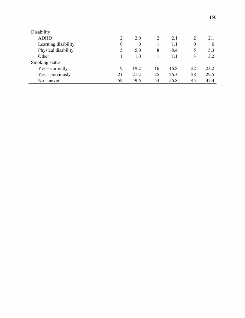
150

Disability ADHD 2 2.0 2 2.1 2 2.1 Learning disability 0 0 1 1.1 0 0 Physical disability 5 5.0 8 8.4 5 5.3 Other 1 1.0 1 1.1 3 3.2 Smoking status Yes – currently 19 19.2 16 16.8 22 23.2 Yes – previously 21 21.2 25 26.3 28 29.5 No – never 59 59.6 54 56.8 45 47.4

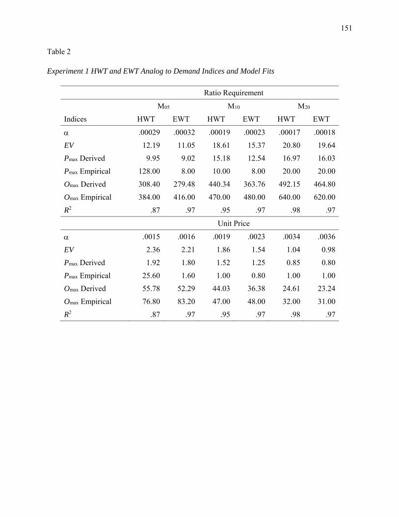
151

Table 2 Experiment 1 HWT and EWT Analog to Demand Indices and Model Fits

Ratio Requirement

M05 M10 M20

Indices HWT EWT HWT EWT HWT EWT

.00029 .00032 .00019 .00023 .00017 .00018

EV 12.19 11.05 18.61 15.37 20.80 19.64

Pmax Derived 9.95 9.02 15.18 12.54 16.97 16.03

Pmax Empirical 128.00 8.00 10.00 8.00 20.00 20.00

Omax Derived 308.40 279.48 440.34 363.76 492.15 464.80

Omax Empirical 384.00 416.00 470.00 480.00 640.00 620.00

R2 .87 .97 .95 .97 .98 .97

Unit Price

.0015 .0016 .0019 .0023 .0034 .0036

EV 2.36 2.21 1.86 1.54 1.04 0.98

Pmax Derived 1.92 1.80 1.52 1.25 0.85 0.80

Pmax Empirical 25.60 1.60 1.00 0.80 1.00 1.00

Omax Derived 55.78 52.29 44.03 36.38 24.61 23.24

Omax Empirical 76.80 83.20 47.00 48.00 32.00 31.00

R2 .87 .97 .95 .97 .98 .97

152


Demographic P90 P50 P10 Age (years) Min 19.0 19.0 22.0 Max 64.0 65.0 72.0 M 36.0 36.0 35.0 SD 10.8 11.0 11.4

n % n % n % Gender Female 46 48.4 44 6.3 41 43.2 Male 49 51.6 51 53.7 54 56.8 Ethnicity Asian 5 5.3 8 8.4 8 8.4 Black/African American 6 6.3 2 2.1 3 3.2 Hispanic/Latino 3 3.2 3 3.2 3 3.2 Mixed 2 2.1 2 2.1 2 2.1 Other 0 0.0 0 0.0 2 2.1 White/Caucasian 79 83.2 80 84.2 77 81.1 Education Less than high school 0 0.0 2 2.1 0 0.0 High school/GED 10 10.5 15 15.8 5 5.3 Some college 29 30.5 28 29.5 25 26.3 2-year college degree 8 8.4 15 15.8 16 16.8 4-year college degree 35 36.8 27 28.4 38 40.0 Master’s degree 9 9.5 7 7.4 10 10.5 Doctoral degree 2 2.1 0 0.0 1 1.1 Professional degree (JD, MD) 2 2.1 1 1.1 0 0.0 Income Less than 30,000 21 22.1 27 28.4 14 14.7 30,000 – 39,999 14 14.7 16 16.8 12 21.1 40,000 – 49,999 12 12.6 11 11.6 13 13.7 50,000 – 59,999 13 13.7 8 8.4 11 11.6 60,000 – 69,999 11 11.6 11 11.6 5 5.3 70,000 – 79,999 4 4.2 6 6.3 7 7.4 80,000 – 89,999 6 6.3 2 2.1 5 5.3 90,000 – 99,999 5 5.3 2 2.1 4 4.2 100,000 or more 9 9.5 12 12.6 16 16.8

153

Table 4 Experiment 2 Amazon Mechanical Turk Employment

Variable P90 P50 P10

Average hours per week on mTurk

Min 2.0 1.0 1.0

Max 100.0 80.0 72.0

M 15.6 19.2 15.2

SD 14.0 14.2 12.0

Average weekly mTurk income

Min 1.5 5.0 5.0

Max 1000.0 700.0 500.0

M 79.9 114.4 79.3

SD 109.8 103.3 78.8

Hourly wage (hours/income)

Min .15 .75 1.0

Max 25.0 50.0 40.0

M 5.6 6.8 6.7

SD 4.2 6.7 6.0

n % n % n %

Reason for completing mTurk tasks

Unemployed or employed part-time 10 10.5 12 12.6 13 13.7

Fruitful way to spend free time 59 62.1 46 48.4 52 54.7

Like to participate in research 33 34.7 28 29.5 28 29.5

Primary income 12 12.6 23 24.2 15 15.8

Secondary income 73 76.8 68 71.6 67 70.5

Tasks are fun 29 30.5 27 28.4 22 23.2

To kill time 17 17.9 15 15.8 21 22.1

Other 0 0.0 0 0.0 1 1.1

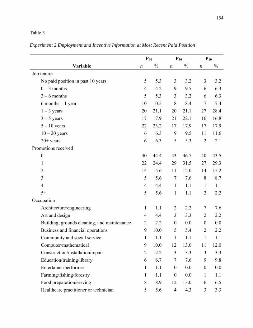
154

Table 5 Experiment 2 Employment and Incentive Information at Most Recent Paid Position

P90 P50 P10

Variable n % n % n %

Job tenure

No paid position in past 10 years 5 5.3 3 3.2 3 3.2

0 – 3 months 4 4.2 9 9.5 6 6.3

3 – 6 months 5 5.3 3 3.2 6 6.3

6 months – 1 year 10 10.5 8 8.4 7 7.4

1 – 3 years 20 21.1 20 21.1 27 28.4

3 – 5 years 17 17.9 21 22.1 16 16.8

5 – 10 years 22 23.2 17 17.9 17 17.9

10 – 20 years 6 6.3 9 9.5 11 11.6

20+ years 6 6.3 5 5.3 2 2.1

Promotions received

0 40 44.4 43 46.7 40 43.5

1 22 24.4 29 31.5 27 29.3

2 14 15.6 11 12.0 14 15.2

3 5 5.6 7 7.6 8 8.7

4 4 4.4 1 1.1 1 1.1

5+ 5 5.6 1 1.1 2 2.2

Occupation

Architecture/engineering 1 1.1 2 2.2 7 7.6

Art and design 4 4.4 3 3.3 2 2.2

Building, grounds cleaning, and maintenance 2 2.2 0 0.0 0 0.0

Business and financial operations 9 10.0 5 5.4 2 2.2

Community and social service 1 1.1 1 1.1 1 1.1

Computer/mathematical 9 10.0 12 13.0 11 12.0

Construction/installation/repair 2 2.2 3 3.3 3 3.3

Education/training/library 6 6.7 7 7.6 9 9.8

Entertainer/performer 1 1.1 0 0.0 0 0.0

Farming/fishing/forestry 1 1.1 0 0.0 1 1.1

Food preparation/serving 8 8.9 12 13.0 6 6.5

Healthcare practitioner or technician 5 5.6 4 4.3 3 3.3

155

Healthcare support 3 3.3 4 4.3 7 7.6

Legal occupations 1 1.1 3 3.3 1 1.1

Life science 0 0.0 2 2.2 3 3.3

Management 3 3.3 5 5.4 5 5.4

Media and communications 3 3.3 1 1.1 2 2.2

Military and protective service 1 1.1 0 0.0 2 2.2

Office/administrative support 18 20.0 11 12.0 13 14.1

Personal care and service 0 0.0 1 1.1 0 0.0

Physical science 0 0.0 0 0.0 0 0.0

Production/manufacturing 1 1.1 2 2.2 0 0.0

Sales 11 12.2 11 12.0 12 13.0

Social science 0 0.0 0 0.0 0 0.0

Transportation 0 0.0 3 3.3 2 2.2

Reason for leaving last paid position

Accepted a new job at a different company 41 45.6 28 30.4 26 28.3

Internal promotion 11 12.2 14 15.2 10 10.9

Decided not to work outside of the home 3 3.3 16 17.4 11 12.0

Laid off or otherwise terminated 13 14.4 9 9.8 14 15.2

Prefer not to answer 12 13.3 14 15.2 14 15.2

Other 10 11.1 11 12.0 17 18.5

Incentive availability

Yes – monetary incentives 28 29.5 29 30.5 21 22.1

Yes – other gifts 24 25.3 24 25.3 26 27.4

No 51 53.7 49 51.6 52 54.7

Incentive frequency

Daily 3 7.7 4 9.3 1 2.5

Weekly 7 17.9 2 4.7 12 30.0

Monthly 10 25.6 10 23.3 7 17.5

Quarterly 3 7.7 6 14.0 4 10.0

Twice yearly 14 35.9 15 34.9 11 27.5

Annually 0 0.0 3 7.0 1 2.5

Other 2 5.1 3 7.0 4 10.0

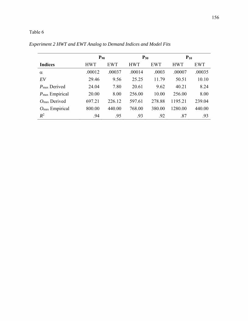
156


P90 P50 P10


.00012 .00037 .00014 .0003 .00007 .00035

EV 29.46 9.56 25.25 11.79 50.51 10.10

Pmax Derived 24.04 7.80 20.61 9.62 40.21 8.24

Pmax Empirical 20.00 8.00 256.00 10.00 256.00 8.00

Omax Derived 697.21 226.12 597.61 278.88 1195.21 239.04

Omax Empirical 800.00 440.00 768.00 380.00 1280.00 440.00

R2 .94 .95 .93 .92 .87 .93

157


Demographic D01 D14 D28 Age (years) Min 19.0 19.0 18.0

Max 75.0 67.0 64.0

M 33.6 32.9 31.2

SD 10.3 11.4 8.0

n % n % n % Gender Female 35 36.8 41 43.2 42 44.2 Male 60 63.2 54 56.8 53 55.8 Ethnicity Asian 6 6.3 14 14.7 7 7.4 Black/African American 7 7.4 8 8.4 10 10.5 Hispanic/Latino 6 6.3 2 2.1 6 6.3 Mixed 2 2.1 2 2.1 0 0.0 Other 1 1.1 0 0.0 1 1.1 White/Caucasian 73 76.8 69 72.6 71 74.7 Education Less than high school 0 0.0 0 0.0 0 0.0 High school/GED 15 15.8 18 18.9 11 11.6 Some college 26 27.4 31 32.6 26 27.4 2-year college degree 15 15.8 8 8.4 11 11.6 4-year college degree 34 35.8 29 30.5 39 41.1 Master’s degree 5 5.3 8 8.4 6 6.3 Doctoral degree 0 0.0 0 0.0 0 0.0 Professional degree (JD, MD) 0 0.0 1 1.1 2 2.1 Income Less than 30,000 27 28.4 27 28.4 24 25.3 30,000 – 39,999 17 17.9 15 15.8 21 22.1 40,000 – 49,999 11 11.6 8 8.4 12 12.6 50,000 – 59,999 14 14.7 14 14.7 7 7.4 60,000 – 69,999 6 6.3 4 4.2 6 6.3 70,000 – 79,999 3 3.2 7 7.4 6 6.3 80,000 – 89,999 3 3.2 4 4.2 6 6.3 90,000 – 99,999 8 8.4 5 5.3 4 4.2 100,000 or more 6 6.3 11 11.6 9 9.5

158

Table 8 Experiment 3 Amazon Mechanical Turk Employment

Variable D01 D14 D28

Average hours per week on mTurk

Min 2.0 1.0 2.0

Max 70.0 80.0 100.0

M 19.1 19.0 20.7

SD 13.6 14.7 14.1

Average weekly mTurk income

Min 0.00 5.0 2.0

Max 500.0 680.0 500.0

M 83.1 92.4 119.3

SD 76.8 97.5 98.3

Hourly wage (hours/income)

Min .5 .7 .0

Max 25.0 20.0 25.0

M 6.5 5.8 5.8

SD 4.7 4.3 5.4

n % n % n %

Reason for completing mTurk tasks

Unemployed or employed part-time 11 11.6 16 16.8 16 16.8

Fruitful way to spend free time 48 50.5 47 49.5 51 53.7

Like to participate in research 26 27.4 19 20.0 28 29.5

Primary income 22 23.2 21 22.1 25 26.3

Secondary income 61 64.2 62 65.3 52 54.7

Tasks are fun 29 30.5 21 22.1 26 27.4

To kill time 17 17.9 14 14.7 15 15.8

Other 2 2.1 1 1.1 2 2.1

159

Table 9 Experiment 3 Employment and Incentive Information at Most Recent Paid Position

D01 D14 D28

Variable n % n % n %

Job tenure

No paid position in past 10 years 1 1.1 2 2.1 2 2.1

0 – 3 months 4 4.2 4 4.2 6 6.3

3 – 6 months 6 6.3 4 4.2 6 6.3

6 months – 1 year 12 12.6 16 16.8 9 9.5

1 – 3 years 21 22.1 30 31.6 29 30.5

3 – 5 years 28 29.5 13 13.7 21 22.1

5 – 10 years 17 17.9 14 14.7 15 15.8

10 – 20 years 4 4.2 5 5.3 5 5.3

20+ years 2 2.1 7 7.4 2 2.1

Promotions received

0 48 51.1 52 55.9 42 45.2

1 25 26.6 24 25.8 32 34.4

2 15 16.0 10 10.8 12 12.9

3 5 5.3 3 3.2 4 4.3

4 1 1.1 1 1.1 2 2.2

5+ 0 0.0 3 3.2 1 1.1

Occupation

Architecture/engineering 1 1.1 1 1.1 0 0.0

Art and design 2 2.1 3 3.2 2 2.2

Building, grounds cleaning, and maintenance 0 0.0 0 0.0 1 1.1

Business and financial operations 9 9.6 11 11.8 9 9.7

Community and social service 3 3.2 0 0.0 2 2.2

Computer/mathematical 7 7.4 8 8.6 10 10.8

Construction/installation/repair 4 4.3 6 6.5 1 1.1

Education/training/library 10 10.6 9 9.7 7 7.5

Entertainer/performer 1 1.1 1 1.1 0 0.0

Farming/fishing/forestry 0 0.0 1 1.1 2 2.2

Food preparation/serving 13 13.8 8 8.6 9 9.7

Healthcare practitioner or technician 3 3.2 9 9.7 3 3.2

160

Healthcare support 1 1.1 5 5.4 6 6.5

Legal occupations 0 0.0 0 0.0 2 2.2

Life science 1 1.1 1 1.1 1 1.1

Management 3 3.2 3 3.2 3 3.2

Media and communications 2 2.1 1 1.1 2 2.2

Military and protective service 2 2.1 1 1.1 0 0.0

Office/administrative support 13 13.8 7 7.5 11 11.8

Personal care and service 1 1.1 0 0.0 2 2.2

Physical science 1 1.1 0 0.0 0 0.0

Production/manufacturing 1 1.1 2 2.2 1 1.1

Sales 16 17.0 11 11.8 15 16.1

Social science 0 0.0 1 1.1 1 1.1

Transportation 0 0.0 4 4.3 3 3.2

Reason for leaving last paid position

Accepted a new job at a different company 23 24.5 26 28.0 25 26.9

Internal promotion 19 20.2 9 9.7 18 19.4

Decided not to work outside of the home 9 9.6 13 14.0 10 10.8

Laid off or otherwise terminated 16 17.0 8 8.6 13 14.0

Prefer not to answer 13 13.8 18 19.4 18 19.4

Other 14 14.9 19 20.4 9 9.7

Incentive availability

Yes – monetary incentives 20 21.1 25 26.3 33 34.7

Yes – other gifts 15 15.8 13 13.7 18 18.9

No 66 69.5 60 63.2 54 56.8

Incentive frequency

Daily 1 3.6 2 6.1 2 5.1

Weekly 11 39.3 7 21.2 8 20.5

Monthly 8 28.6 4 12.1 14 35.9

Quarterly 2 7.1 4 12.1 3 7.7

Twice yearly 6 21.4 12 36.4 10 25.6

Annually 0 0.0 3 9.1 0 0.0

Other 0 0.0 1 3.0 2 5.1

161


D01 D14 D28


.00011 .00023 .00014 .00032 .00011 .00032

EV 32.14 15.37 25.25 11.05 32.14 11.05

Pmax Derived 26.23 12.54 20.61 9.02 26.23 9.02

Pmax Empirical 256.00 8.00 10/20.00 8.00 256.00 8.00

Omax Derived 760.59 363.76 597.61 261.45 760.59 261.45

Omax Empirical 1024.00 496.00 600.00 416.00 1536.00 408.00

R2 .90 .98 .96 .97 .74 .95

162

Table 11 Percentage of Accurate Responding at Each Ratio Requirement for All Conditions and Experiments

Ratio M05 M10 M20 P90 P50 P10 D01 D14 D28

PT 88.07 89.82 92.63 90.53 77.89 94.39

1 90.43 92.47 91.40 91.40 94.57 93.68 92.55 86.67 93.41

2 96.74 94.38 94.44 90.22 91.21 93.48 94.94 85.16 95.68

4 97.53 96.91 98.40 93.75 94.33 95.33 97.59 87.34 93.93

8 99.28 96.46 98.63 91.59 92.02 95.45 98.99 85.82 97.06

10 99.76 97.33 98.27 89.09 94.74 91.71 98.89 85.64 95.86

12 99.36 96.15 98.67 93.23 91.67 83.97 99.34 85.42 95.08

15 99.63 94.55 98.95 90.77 93.70 85.78 99.51 80.33 99.65

20 99.23 93.89 95.65 85.00 91.67 71.22 99.13 77.50 99.58

25 99.50 90.55 98.29 75.00 87.56 0.00 98.29 68.50 98.67

32 100.00 98.44 99.15 66.67 85.27 33.33 100.00 35.42 100.00

48 100.00 100.00 98.21 66.67 100.00 50.00 100.00 50.00

64 100.00 100.00 96.35 100.00 50.00 99.22 100.00

96 98.96 98.96 94.79 49.48 100.00 100.00

128 98.44 100.00 100.00

256 94.14 100.00 99.61

Median 99.36 96.46 98.27 90.22 91.84 84.88 99.17 85.53 95.86 Note. Experiment 1 did not have the opportunity to provide inaccurate responses in the practice trial. PT = practice trial.

163

Figure 1. Prototypical demand curve.

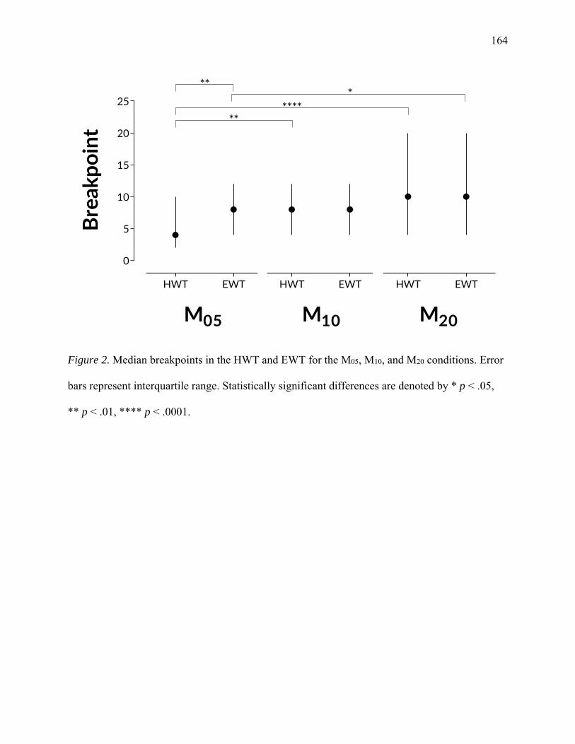
164

HWT EWT HWT EWT HWT EWT

0

5

10

15

20

25Breakpo

int

M05 M10 M20

***

******

Figure 2. Median breakpoints in the HWT and EWT for the M05, M10, and M20 conditions. Error

bars represent interquartile range. Statistically significant differences are denoted by * p < .05,

** p < .01, **** p < .0001.

165


0

1

2

3

Unit Price Breakpo

int

M05 M10 M20

******

*

**

Figure 3. Median unit price breakpoints (work units per $0.01) in the HWT and EWT for the

M05, M10, and M20 conditions. Error bars denote interquartile range. Statistically significant

differences are denoted by * p < .05, ** p < .01, **** p < .0001.

166

1 2 4 8 10 12 15 20 25 32 48 64 96 128 25690

92

94

96

98

100

Ratio Requirement

Percentage Accuracy M05

M10

M20

Figure 4. Experiment 1 percentage of accurately completed work units. Horizontal lines

represent group medians across all ratio requirements and correspond to the data paths denoting

the condition to which it belongs.

167

1 10 100 1000

1

10

100

HWT

M10

M20

M05

1 10 100 1000

1

10

100

EWT

M05

M10

M20

Ratio Requirement

Percentage of Participants

Figure 5. Analog to demand curves for the M05, M10, and M20 conditions in the HWT (top panel)

and EWT (bottom panel). The y-axis depicts the percentage of participants in each incentive

magnitude condition who indicated willingness to complete (HWT) or completed (EWT) the

ratio requirement. The x-axis depicts the ratio requirement needed to earn the incentive. Vertical

lines correspond to derived Pmax.

168

Figure 6. Work functions for the M05, M10, and M20 conditions in the HWT for Experiment 1.

1 2 4 8 10 12 15 20 25 32 48 64 96 128 256

0

100

200

300

400

500

600

700Work Units

M20

Ratio Requirement

M05

M10

HWT

169

Figure 7. Cost-benefit analysis of the EWT for Experiment 1. The number of work units

completed is depicted by the grey data points and scaled to the left y-axis. Cost in dollars per

ratio requirement is depicted by the open data points and plotted on the right y-axes.

1 2 4 8 10 12 15 20 25 32 48 64 96 128 256

0

200

400

600

0

5

10

15

20

Work Units C

ost ($)

EWT M05 Cost

M10 Cost

M20 Cost

M05Work

M10 Work

M20 Work

Ratio Requirement

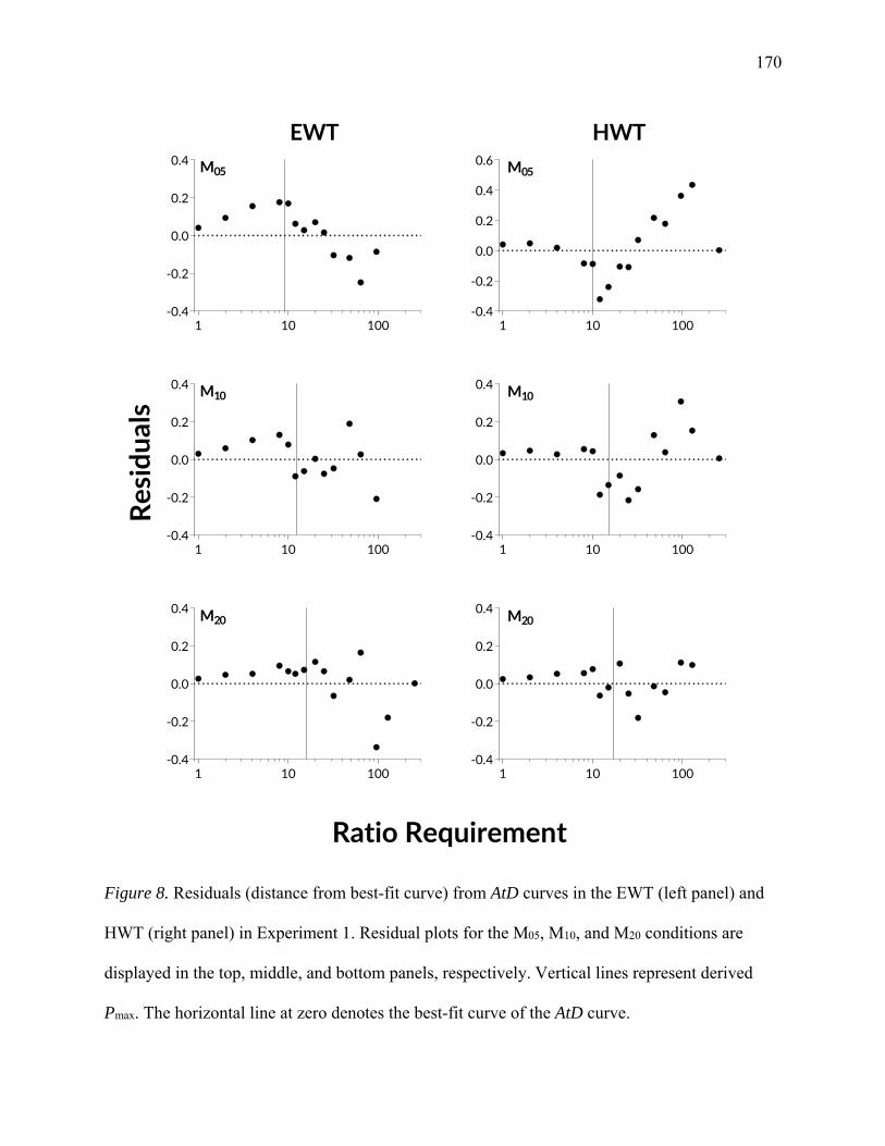
170

Figure 8. Residuals (distance from best-fit curve) from AtD curves in the EWT (left panel) and

HWT (right panel) in Experiment 1. Residual plots for the M05, M10, and M20 conditions are

displayed in the top, middle, and bottom panels, respectively. Vertical lines represent derived

Pmax. The horizontal line at zero denotes the best-fit curve of the AtD curve.

1 10 100‐0.4

‐0.2

0.0

0.2

0.4

1 10 100‐0.4

‐0.2

0.0

0.2

0.4

1 10 100‐0.4

‐0.2

0.0

0.2

0.4

1 10 100‐0.4

‐0.2

0.0

0.2

0.4

0.6

1 10 100‐0.4

‐0.2

0.0

0.2

0.4

1 10 100‐0.4

‐0.2

0.0

0.2

0.4

Ratio Requirement

Residuals

HWTEWTM05

M10

M20

M05

M10

M20

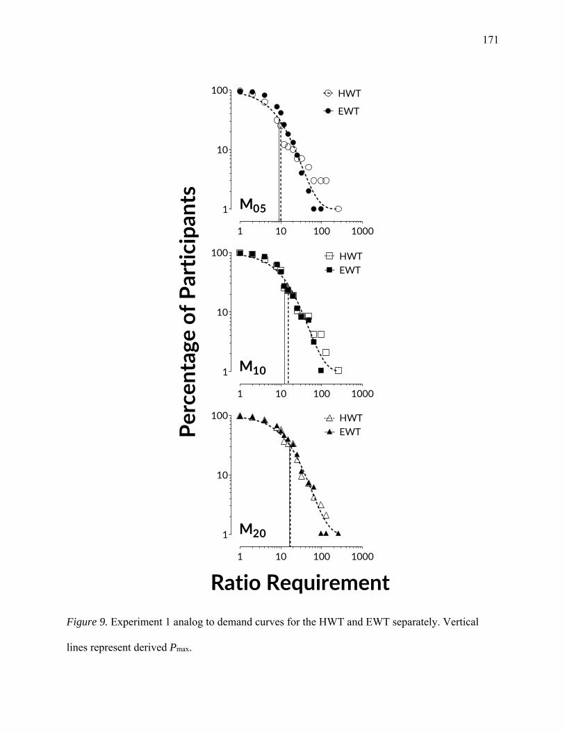
171

Figure 9. Experiment 1 analog to demand curves for the HWT and EWT separately. Vertical

lines represent derived Pmax.

1 10 100 1000

1

10

100

M05

HWT

EWT

1 10 100 1000

1

10

100

M10

HWTEWT

1 10 100 1000

1

10

100 HWTEWT

M20


Ratio Requirement

172

0.1 1 10 100

1

10

100

HWT

M05

M10

M20

0.1 1 10 100

1

10

100

EWT


Unit Price

Figure 10. Analog to demand curves for the M05, M10, and M20 conditions in the HWT (top

panel) and EWT (bottom panel). The y-axis depicts the percentage of participants in each

incentive magnitude condition who indicated willingness to complete (HWT) or completed

(EWT) the ratio requirement. The x-axis depicts unit price (ratio requirement/incentive amount).

Vertical lines correspond to derived Pmax.

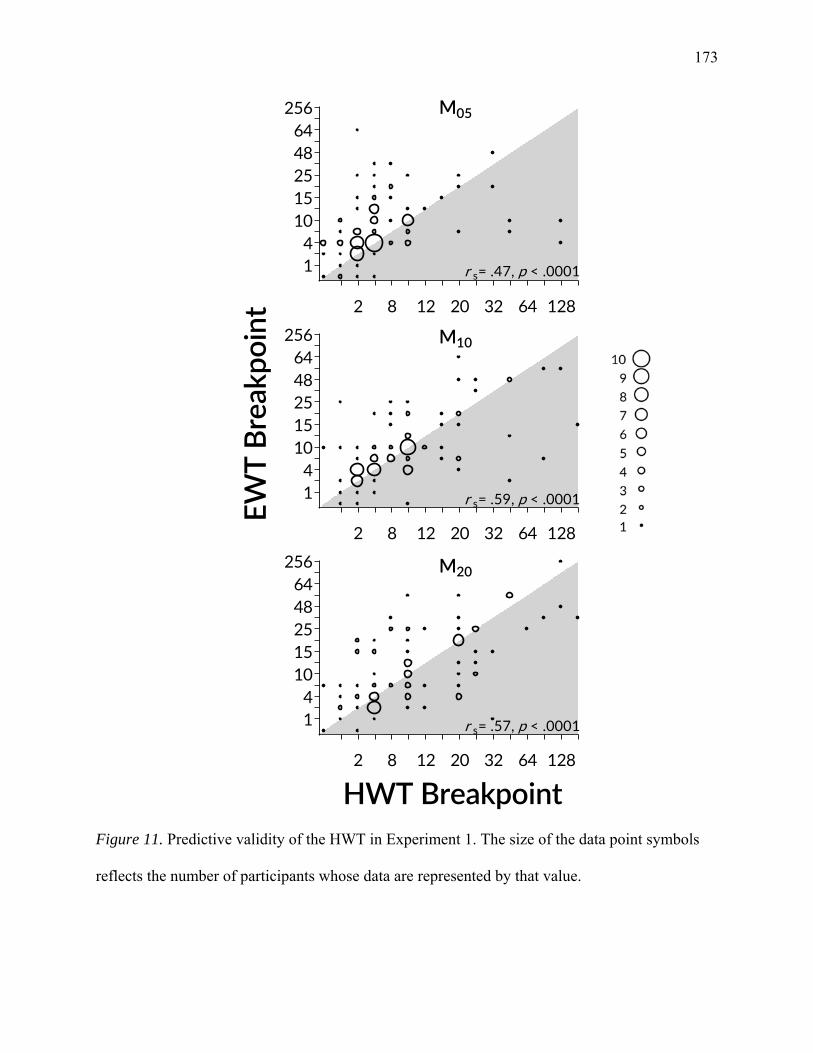
173

14

1015254864

256

2 8 12 20 32 64 128

r s= .59, p < .0001

M10

EWT Breakpo

int

HWT Breakpoint

2 8 12 20 32 64 128

14

1015254864

256

r s= .47, p < .0001

M05

2 8 12 20 32 64 128

14

1015254864

256

r s= .57, p < .0001

M20

Figure 11. Predictive validity of the HWT in Experiment 1. The size of the data point symbols

reflects the number of participants whose data are represented by that value.

174

1 2 4 8 10 12 15 20 25 32 48 64 96 128 256‐150

‐100

‐50

0

50

100

150

Ratio Requirement

Percentage Change M05 M20

M10

Figure 12. Experiment 1 percentage change in predicted work output and corresponding cost

from the HWT to observed output and cost in the EWT. The gray horizontal line indicates a 0%

change, or perfect aggregate correspondence. Data above the gray horizontal line indicate an

increase in the amount of work completed and higher costs associated with the EWT than were

predicted. Data points below the line indicate less work completed and a lower cost observed in

the EWT than predicted by the HWT.

175

1 2 4 8 10 12 15 20 25 32 48 64 960

25

50

75

100

Ratio Requirement

Expe

rien

ced Probability P90

P50P10*

*

*

Figure 13. Experienced probabilities across ratio requirements for Experiment 2. Grey horizontal

lines indicate the programmed probabilities for the P90, P50, and P10 conditions (from top to

bottom), respectively. Asterisks denote the first ratio requirement at which fewer than ten

participants continued responding.

176

0

5

10

15

20

25Breakpo

int

P90 P50 P10


**** **** ****

Figure 14. Median breakpoints in the P90, P50, and P10 conditions. Error bars denote interquartile

range. Statistically significant differences are denoted by **** p < .0001.

177

PT 1 2 4 8 10 12 15 20 25 32 48 64 960

20

40

60

80

100

Ratio Requirement

% Accuracy

P90P50P10



the condition to which it belongs. PT = Practice trial.

178

1 10 100

1

10

100 P90P50

HWT

P10

1 10 100

1

10

100 P90P50

EWT

P10


Ratio Requirement

Figure 16. Experiment 2 analog to demand curves for the P90, P50, and P10 conditions in the

HWT (top panel) and EWT (bottom panel). The y-axis depicts the percentage of participants in

each incentive probability condition who indicated willingness to complete (HWT) or completed

(EWT) the ratio requirement. The x-axis depicts the ratio requirement needed to earn the

incentive. Vertical lines correspond to derived Pmax.

179

1 2 4 8 10 12 15 20 25 32 48 64 96 128 256

0

250

500

750

1000

1250

1500Work Units

Ratio Requirement

HWTP90

P10

P50

Figure 17. Work functions for the P90, P50, and P10 conditions in the HWT for Experiment 2.

180

1 2 4 8 10 12 15 20 25 32 48 64 96 128 256

0

50

100

150

200

250

300

350

400

450

500

0

5

10

15

20

25

Ratio Requirement

Work Units C

ost ($)

P90Work P90 Cost

P10 Cost

P50 CostEWT

P50Work

P10Work

Figure 18. Cost-benefit analysis of the EWT in Experiment 2. Number of work units completed

is denoted by the grey data points and scaled to the left y-axis. Cost in dollars per ratio

requirement is depicted by the open data points and plotted on the right y-axes.

181


HWT (right panel) in Experiment 2. Residual plots for the P90, P50, and P10 conditions are



1 10 100‐0.4

‐0.2

0.0

0.2

0.4

1 10 100‐0.4

‐0.2

0.0

0.2

0.4

1 10 100‐0.4

‐0.2

0.0

0.2

0.4

1 10 100‐0.4

‐0.2

0.0

0.2

0.4

1 10 100‐0.4

‐0.2

0.0

0.2

0.4

0.6

1 10 100‐0.4

‐0.2

0.0

0.2

0.4

P90

P50

P10

Ratio Requirement

Residuals

HWTEWTP90

P50

P10

182

1 10 100

1

10

100

EWTHWT

P90

1 10 100

1

10

100

EWTHWT

P50

1 10 100

1

10

100

EWTHWT

P10


Ratio Requirement



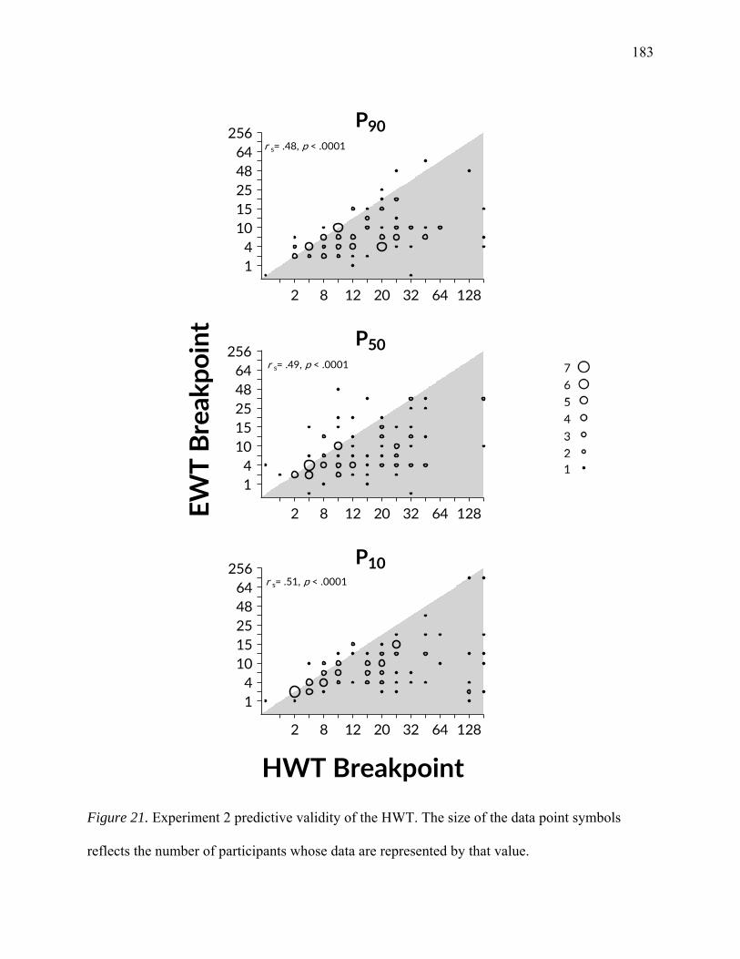
183

2 8 12 20 32 64 128

14

1015254864

256r s= .48, p < .0001

P90

2 8 12 20 32 64 128

14

1015254864

256r s= .49, p < .0001

P50

2 8 12 20 32 64 128

14

1015254864

256r s= .51, p < .0001

P10

HWT Breakpoint

EWT Breakpo

int

Figure 21. Experiment 2 predictive validity of the HWT. The size of the data point symbols


184

1 2 4 8 10 12 15 20 25 32 48 64 96 128 256

‐100

‐80

‐60

‐40

‐20

0

20

Ratio Requirement

% Change in W

ork

P50

P10

P90

Figure 22. Percentage change in predicted work output from the HWT to observed output in the

EWT for Experiment 2. The gray horizontal line indicates a 0% change, or perfect aggregate

correspondence. Data points below the line indicate less work completed in the EWT than

predicted by the HWT.

185

Figure 23. Percentage change in predicted cost from the HWT to observed cost in the EWT for

Experiment 2. The gray horizontal line indicates a 0% change, or perfect aggregate

correspondence. Data points below the line indicate the cost of incentive payments was less in

the EWT than predicted by the HWT.

1 2 4 8 10 12 15 20 25 32 48 64 96 128 256

‐100

‐75

‐50

‐25

0

25

50

75

100

Ratio Requirement

% Change in Cost

P50

P10

P90

186

0

5

10

15

20

25

Breakpo

int

D01


D14 D28

**** **** ****

*

Figure 24. Median breakpoints in the D01, D14, and D28 conditions. Error bars denote

interquartile range. Statistically significant differences are denoted by * p < .05, **** p < .0001.

187

PT 1 2 4 8 10 12 15 20 25 32 48 64 96 128 25620

40

60

80

100

Ratio Requirement

% Accuracy

D01

D14

D28



the condition to which it belongs. PT = Practice trial.

188

1 10 100

1

10

100 D01

D14

HWT

D28

1 10 100

1

10

100 D01

D14

EWT

D28


Ratio Requirement

Figure 26. Analog to demand curves for the D01, D14, and D28 conditions in the HWT (top panel)

and EWT (bottom panel). The y-axis depicts the percentage of participants in each incentive

magnitude condition who indicated willingness to complete (HWT) or completed (EWT) the

ratio requirement. The x-axis depicts the ratio requirement needed to earn the incentive. Vertical

lines correspond to derived Pmax.

189

1 2 4 8 10 12 15 20 25 32 48 64 96 128 256

0

250

500

750

1000

1250

1500

1750

Work Units

D01

D14

D28

Ratio Requirement

HWT

Figure 27. Work functions for the D01, D14, and D28 conditions in the HWT for Experiment 3.

190

1 2 4 8 10 12 15 20 25 32 48 64 96 128 256

0

100

200

300

400

500

0

5

10

15

20

Work Units C

ost ($)

D01 Cost

D14 Cost

D28 Cost

D01Work

D14Work

D28Work

Ratio Requirement

EWT

Figure 28. Cost-benefit analysis of the EWT in Experiment 3. Number of work units completed

are denoted by the grey data points and scaled to the left y-axis. Cost in dollars per ratio

requirement are depicted by the open data points and plotted on the right y-axes.

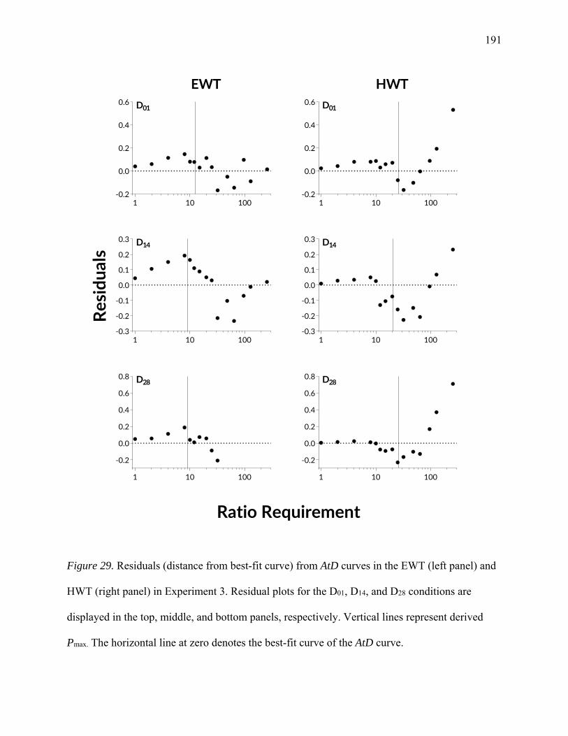
191


HWT (right panel) in Experiment 3. Residual plots for the D01, D14, and D28 conditions are



1 10 100‐0.2

0.0

0.2

0.4

0.6

1 10 100‐0.3

‐0.2

‐0.1

0.0

0.1

0.2

0.3

1 10 100

‐0.2

0.0

0.2

0.4

0.6

0.8

1 10 100‐0.2

0.0

0.2

0.4

0.6

1 10 100‐0.3

‐0.2

‐0.1

0.0

0.1

0.2

0.3

1 10 100

‐0.2

0.0

0.2

0.4

0.6

0.8

Ratio Requirement

Residuals

HWTEWTD01

D14

D28

D01

D14

D28

192

1 10 100

1

10

100

EWTHWT

D01

1 10 100

1

10

100

EWTHWT

D14

1 10 100

1

10

100

EWTHWT

D28

Percentage of Participa

nts

Ratio Requirement



193

2 8 12 20 32 64 128

14

1015254864

256r s= .45, p < .0001

D01

2 8 12 20 32 64 128

14

1015254864

256r s= .62, p < .0001

D14

2 8 12 20 32 64 128

14

1015254864

256r s= .42, p < .0001

D28

HWT Breakpoint

EWT Breakpo

int

Figure 31. Predictive validity of the HWT in Experiment 3. The size of the data point symbols


194

Figure 32. Percentage change in predicted work output and corresponding cost from the HWT to

observed output and cost in the EWT for Experiment 3. The gray horizontal line indicates a 0%

change, or perfect aggregate correspondence. Data points below the line indicate less work

completed and a lower cost observed in the EWT than predicted by the HWT.

1 2 4 8 10 12 15 20 25 32 48 64 96 128 256

‐100

‐80

‐60

‐40

‐20

0

20

Ratio Requirement

% Change D01

D14

D28

195

Appendix A

Literature search procedures, conducted on November 5, 2015.

n =• Keyword Anywhere: Employee OR Staff

136,120• Keyword Anywhere: Reinforcer OR Incentive

73,193• Keyword Anywhere: Performance OR Behavior

1,162• Published in Scholarly Journal

806• Written in English

784

• Abstract search: excluding correlational studies, editorials, literature reviews, commentaries, staff or simulated staff not participants, incentives not IV, DV not measurable behavior

75

• Method search:comparison of a dimension under study (i.e., probability, delay, effort, magnitude, rate, quality)

6• Hand search of reference sections

8• Final

196

Appendix B Experiment 1 Amazon Mechanical Turk HIT. Highlighted content indicates information removed in Experiments 2 and 3.

197

Appendix C

Sample work unit.

ScaleTarget

Manipulandum

198

Appendix D Monetary choice questionnaire. For each question below, please select the option that you would prefer.

Which would you rather have:

$54 tonight $55 in 117 days



























199

Appendix E

Behavioral inhibition system/behavioral activation system scale.

Please respond to the following statements by indicating the degree to which you either Agree or Disagree.

A person's family is the most important thing in life.e

Strongly Disagree Disagree Agree Strongly Agree

Even if something bad is about to happen to me, I rarely experience fear or nervousness.a,f


I go out of my way to get things I want.b


When I'm doing well at something I love to keep at it.d


I'm always willing to try something new if I think it will be fun.c


How I dress is important to me.e


When I get something I want, I feel excited and energized.d


Criticism or scolding hurts me quite a bit.a


When I want something I usually go all-out to get it.b


I will often do things for no other reason than that they might be fun.c


It's hard for me to find time to do things such as get a haircut.e


If I see a chance to get something I want I move on it right away.b


200

I feel pretty worried or upset when I think or know somebody is angry at me.a


When I see an opportunity for something I like I get excited right away.d


I often act on the spur of the moment.c


If I think something unpleasant is going to happen I usually get pretty "worked up."a


I often wonder why people act the way they do.e


When good things happen to me, it affects me strongly.d


I feel worried when I think I have done poorly at something important.a


I crave excitement and new sensations.c


When I go after something I use a "no holds barred" approach.b


I have very few fears compared to my friends.a,f


It would excite me to win a contest.d


I worry about making mistakes.a


aBehavioral inhibition scale. bBehavioral activation scale – drive. cBehavioral activation scale – fun seeking. dBehavioral activation scale – reward responsiveness. eFiller question. fReverse scored item

201

Appendix F Experiment 1 demographic questionnaire. What is your current age? What is your gender? Male Female Race/ethnic background: White/Caucasian Black/African American Hispanic/Latino Asian Native American Pacific Islander Mixed Other In what state do you currently reside? [drop down list] What is the highest level of education you have completed? Less than High School High School / GED Some College 2-year College Degree 4-year College Degree Masters Degree Doctoral Degree Professional Degree (JD, MD) What is your combined annual household income? Less than 30,000 30,000 – 39,999 40,000 – 49,999 50,000 – 59,999 60,000 – 69,999 70,000 – 79,999 80,000 – 89,999 90,000 – 99,999

202

100,000 or more Do you have a DOCUMENTED disability? Yes No If yes, please specify: Learning disability Attention deficit/hyperactivity disorder Physical disability Other Are you currently, or have you ever been a smoker? Yes - Currently Yes - Previously No - Never

203

Appendix G Experiment 1 practice trial, HWT, and EWT instructions and ratio wording.

INSTRUCTIONS AT START OF EACH SECTION:

PRACTICE TRIAL In the following section you will be asked whether or not you would be willing to complete a given number of "slider questions" to earn a 5/10/20 cent bonus if given the opportunity. To continue please complete the practice slider question according to the instructions below: Please move the slider to match the number indicated to the left. Once the numbers match, press the next button to continue

HWT For each question below, please indicate whether you would complete the number of slider questions indicated to receive the bonus. Please answer honestly, thoughtfully, and as if you were actually in this situation.

EWT Next, you will have the opportunity to complete slider questions to earn real bonuses paid after you complete the study. Each section will begin with a statement indicating the amount of the bonus and the number of questions that must be completed to earn the bonus. You will then be asked if you would like to complete the section. If you select "no" the survey will end. If you would no longer like to continue after beginning a section, you may exit the survey by closing your browser or returning to the mTurk website. If you exit the survey before finishing the section you will not receive the bonus for the section. Thank you for taking the time to complete the survey.

If you wish to receive bonuses, you must wait to submit your unique access code until you are finished. Be sure to write the code down.

If you no longer wish to continue, copy your unique access code found below and submit it through the Amazon Mechanical Turk survey page.

WORDING FOR EACH RATIO:

HWT Would you complete 1 slider question in exchange for a 5/10/20 cent bonus?

EWT You can earn a bonus of 5/10/20 cents by completing 1 question in this section. Would you like to continue?

204

Appendix H

Scoring for the Monetary Choice Questionnaire.

Response Option

Smaller-sooner Larger-later k Magnitude

$34 tonight $35 in 186 days 0.00016 Small

$54 tonight $55 in 117 days 0.00016 Medium

$78 tonight $80 in 162 days 0.00016 Large

























205

Appendix I Experiments 2 and 3 Amazon Mechanical Turk HIT. Highlighted content denotes modifications from Experiment 1.

206

Appendix J

Experiments 2 and 3 practice trial, HWT, and EWT instructions and ratio wording. INSTRUCTIONS AT START OF EACH SECTION:

PRACTICE TRIAL The task in this HIT involves matching numbers on a slider scale. Below you have three opportunities to practice before you begin. Please move the slider to match the number indicated on the left of the slider scale. Then press the “next” button to continue.

HWT For each question below, please indicate whether you would complete the indicated number of slider questions to receive the bonus if given the opportunity. There are no right or wrong responses. Please answer honestly, thoughtfully, and as if you were actually in this situation.

EWT Next, you will have the opportunity to complete slider questions to earn real bonuses paid after you complete the study. Each section will begin with a statement indicating the amount of the bonus and the number of slider questions that must be completed to earn the bonus. You will then be asked if you would like to complete the section. If you exit the survey before finishing the section, you will not receive the bonus for that section. WORDING FOR EACH RATIO:

HWT

Experiment 2 - Probability: Would you complete 1 slider question in exchange for a 9 in 10 (90%) / 5 in 10 (50%) / 1 in 10 (10%) chance of receiving a 22 cent / 40 cent / 2 dollar bonus paid in 1 day? Experiment 3 - Delay: Would you complete 1 slider question in exchange for a 20 cent bonus paid for certain in 1/14/28 day(s)?

EWT Experiment 2 - Probability: Would you like to complete 1 slider question in exchange for a 9 in 10 (90%) / 5 in 10 (50%) / 1 in 10 (10%) chance of earning a 22 cent / 40 cent / 2 dollar bonus paid in 1 day? Experiment 3 - Delay: Would you like to complete 1 slider question in exchange for a 20 cent bonus paid for certain in 1/14/28 day(s)?

207

Appendix K Experiments 2 and 3 demographic, employment, and incentive survey. What is your current age?

What is your gender? Male Female Race/ethnic background: White/Caucasian Black/African American Hispanic/Latino Asian Native American Pacific Islander Mixed Other In what state do you currently reside? [drop down list]

208

What is the highest level of education you have completed? Less than High School High School / GED Some College 2-year College Degree 4-year College Degree Master’s Degree Doctoral Degree Professional Degree (JD, MD) What is your combined annual household income? Less than 30,000 30,000 – 39,999 40,000 – 49,999 50,000 – 59,999 60,000 – 69,999 70,000 – 79,999 80,000 – 89,999 90,000 – 99,999 100,000 or more Approximately how many hours do you spend on Mechanical Turk a week? Why do you complete tasks in Mechanical Turk? Please check all that apply: Fruitful way to spend free time and get some cash (e.g., instead of watching TV) For "primary" income purposes (e.g., gas, bills, groceries, credit cards) For "secondary" income purposes, pocket change (e.g., for hobbies, gadgets, going out) To kill time I find the tasks to be fun I am currently unemployed, or have only a part time job I like to participate in research Other: ____________________ Approximately how much money do you earn a week on Mechanical Turk?

209

How long were you employed at your most recent paid position outside of Mechanical Turk in the past 10 years? I have not had a paid position in the past 10 years 0-3 months 3-6 months 6 months - 1 year 1 - 3 years 3 - 5 years 5 - 10 years 10 - 20 years 20+ years How many promotions did you receive at your most recent paid position? 0 1 2 3 4 5+

210

Which occupational category best describes your employment? Architecture/Engineering (e.g. architect, landscape architect, surveyor, cartographer,

engineer, drafter) Art and Design (e.g. fine artist, animator, graphic/floral/interior designer, multimedia artist,

set/exhibit designer, art director) Building and Grounds Cleaning and Maintenance (e.g. landscaper, tree-trimmer, building

cleaner, janitor, pest control) Business and Financial Operations (e.g. financial specialist, budget analyst, event planner,

agent, buyer, claims adjuster, real estate assessor, human resources specialist, accountant) Community and Social Service (e.g. mental health counselor, social worker, guidance

counselor, clergy, health educator, probation officer) Computer/Mathematical (e.g. computer programmer, network/database administrator,

mathematician, statistician, software/web developer, user support) Construction/Installation/Repair (e.g. mason, carpenter, electrician, pipefitter, building

inspector, equipment repair, electronics installer, mechanic) Education/Training/Library (e.g. teacher, adult educator, teaching assistant, librarian, curator,

archivist) Entertainer/Performer (e.g. actor, producer, director, musician, dancer, athlete, coach) Farming/Fishing/Forestry Worker (e.g. farm/greenhouse/fishing/forestry worker, agricultural

inspector) Food Preparation/Serving (e.g. cook, bartender, food server, caterer, dishwasher, host) Healthcare Practitioner or Technician (e.g. physician, nurse, veterinarian,

physical/occupational/recreational therapist, nutritionist, EMT, laboratory technician) Healthcare Support (e.g. medical/dental/veterinary assistant, massage therapist, home health

aide) Legal Occupations (e.g. lawyer, legal assistant, paralegal, title examiner) Life Science (e.g. biologist, ecologist, zoologist, biochemist, conservation/plant/soil scientist,

forester) Management (e.g. managers of: operations, marketing, public relations, human resources,

advertising, finance, hotels, restaurants, etc.) Media and Communications (e.g. writer, editor, reporter, announcer, interpreter, media

equipment technician, photographer, film/video/TV operator, public relations specialist) Military and Protective Service (e.g. military officer, infantry, police officer, firefighter,

security guard, lifeguard, ski patrol, animal control, game warden) Office/Administrative Support (e.g. financial/billing/file/mail clerk, bookkeeper, teller,

receptionist, administrative assistant, data entry processor, library assistant, legal secretary) Personal Care and Service (e.g. hairstylist, fitness trainer, usher, childcare worker/nanny,

recreation worker, travel/wilderness/river raft/kayak guide, nonfarm animal caretaker/trainer) Physical Science (e.g. physicist, chemist, astronomer, hydrologist, geoscientist) Production/Manufacturing (e.g. assembler, machinist, textile worker, woodworker, plant

operator, photo processor, welder, printing worker, baker, butcher)

211

Sales (e.g. retail management, cashier, sales/advertising representative, travel agent, real estate broker, telemarketer)

Social Science (e.g. clinical/counseling/school psychologist, economist, survey researcher, anthropologist, sociologist, historian, political scientist, regional planner)

Transportation (e.g. truck/bus/taxi/ambulance driver, material mover, sailor, pilot, flight attendant, railway worker)

What was the reason for leaving your last paid position? I accepted a new job at a different company I was promoted in the same company I decided not to work outside of the home I was laid off or otherwise terminated (seasonal work, employer downsizing, dismissed) I prefer not to answer Other (please specify): Excluding an annual pay increase or holiday bonus, did you receive incentives or rewards in the form of money or other gifts (preferred parking spaces, time off, lunch, water bottles, etc) at your most recent paid position? Mark all that apply. Yes, I received monetary incentives Yes, I received other gifts No How often were these incentives delivered? Daily Weekly Monthly Quarterly Twice yearly Annually Other (please specify) ____________________

Chairperson Florence D. DiGennaro Reed, Ph.D., BCBA-D ...

Documents

Transcript of Chairperson Florence D. DiGennaro Reed, Ph.D., BCBA-D ...