Behavioral Analysis of Network Traffic for Detecting - GETD

Behavioral Analysis of Network Traffic for Detecting

Advanced Cyber-threats

by

Babak Rahbarinia

(Under the Direction of Roberto Perdisci)

Abstract

Internet miscreants continue to spread malware on thousands of users’ machines and they

have become stealthier than ever before. Current prevention and detection technologies to

protect users and networks from the threat of cyber attacks are lagging behind and becoming

frustratingly useless. In this research, we tackle the problem of dealing with cyber criminals

by introducing advanced and novel detection technologies. We present detailed measurement

analysis of real-world malicious ecosystems that are utilized to distribute malware nowadays.

In addition, we propose various state-of-the-art systems to fight against the spread of malice

on the Internet, deploy our systems in real-world operative environments, and show the

effectiveness and advantages of our design. We cover numerous aspects of today’s security

concerns ranging from P2P applications to malware downloads and Command and Control

domains.

Index words: Network security and intelligence, Machine Learning, Large-scale dataanalysis, Malware, Botnet, P2P applications



by

Babak Rahbarinia

B.S., University of Science and Culture, Iran, 2007

M.S., Azad University, Iran, 2010

A Dissertation Submitted to the Graduate Faculty of The University of Georgia in Partial

Fulfillment of the Requirements for the Degree

Doctor of Philosophy

Athens, Georgia

2015

c©2015

Babak Rahbarinia

All Rights Reserved



by

Babak Rahbarinia

Approved:

Major Professor: Roberto Perdisci

Committee: Kang LiKhaled Rasheed

Electronic Version Approved:

Julie CoffieldInterim Dean of the Graduate SchoolThe University of GeorgiaMay 2015

ACKNOWLEDGMENTS

I would like to thank Dr. Perdisci for his support, his patience, and his inspiration with this

research. I am also grateful to Dr. Li and Dr. Rasheed for all their help and guidance.

iv

TABLE OF CONTENTS

ACKNOWLEDGMENTS iv

LIST OF TABLES viii

LIST OF FIGURES x

1 INTRODUCTION AND LITERATURE REVIEW 1

1.1 Introduction . . . . . . . . . . . . . . . . . . . . . . . . . . . . . . . . . . . . 1

1.2 Literature Review . . . . . . . . . . . . . . . . . . . . . . . . . . . . . . . . . 5

2 PEERRUSH: MINING FOR UNWANTED P2P TRAFFIC 23

2.1 Introduction . . . . . . . . . . . . . . . . . . . . . . . . . . . . . . . . . . . . 25

2.2 System Overview . . . . . . . . . . . . . . . . . . . . . . . . . . . . . . . . . 27

2.3 Evaluation . . . . . . . . . . . . . . . . . . . . . . . . . . . . . . . . . . . . . 40

2.4 Discussion . . . . . . . . . . . . . . . . . . . . . . . . . . . . . . . . . . . . . 56

2.5 Related Work . . . . . . . . . . . . . . . . . . . . . . . . . . . . . . . . . . . 58

2.6 Conclusion . . . . . . . . . . . . . . . . . . . . . . . . . . . . . . . . . . . . . 60

3 MEASURING THE PROPERTIES OF C&C DOMAINS 61

3.1 Introduction . . . . . . . . . . . . . . . . . . . . . . . . . . . . . . . . . . . . 63

3.2 Related Work . . . . . . . . . . . . . . . . . . . . . . . . . . . . . . . . . . . 64

3.3 The Approach and Goals . . . . . . . . . . . . . . . . . . . . . . . . . . . . . 64

v

3.4 Evaluation . . . . . . . . . . . . . . . . . . . . . . . . . . . . . . . . . . . . . 70

3.5 Conclusion . . . . . . . . . . . . . . . . . . . . . . . . . . . . . . . . . . . . . 79

4 SINKMINER: MINING BOTNET SINKHOLES FOR FUN AND PROFIT 80

4.1 Introduction . . . . . . . . . . . . . . . . . . . . . . . . . . . . . . . . . . . . 82

4.2 System Overview . . . . . . . . . . . . . . . . . . . . . . . . . . . . . . . . . 84

4.3 Preliminary Evaluation . . . . . . . . . . . . . . . . . . . . . . . . . . . . . . 88

4.4 Discussion . . . . . . . . . . . . . . . . . . . . . . . . . . . . . . . . . . . . . 90

4.5 Conclusion . . . . . . . . . . . . . . . . . . . . . . . . . . . . . . . . . . . . . 91

5 SEGUGIO: EFFICIENT BEHAVIOR-BASED TRACKING OF MALWARE-

CONTROL DOMAINS IN LARGE ISP NETWORKS 92

5.1 Introduction . . . . . . . . . . . . . . . . . . . . . . . . . . . . . . . . . . . . 94

5.2 Segugio System Description . . . . . . . . . . . . . . . . . . . . . . . . . . . 98

5.3 Summary of Results . . . . . . . . . . . . . . . . . . . . . . . . . . . . . . . 106

5.4 Experimental Setup . . . . . . . . . . . . . . . . . . . . . . . . . . . . . . . . 107

5.5 Experimental Results . . . . . . . . . . . . . . . . . . . . . . . . . . . . . . . 110

5.6 Comparison with Notos . . . . . . . . . . . . . . . . . . . . . . . . . . . . . . 127

5.7 Limitations and Discussion . . . . . . . . . . . . . . . . . . . . . . . . . . . . 130

5.8 Related Work . . . . . . . . . . . . . . . . . . . . . . . . . . . . . . . . . . . 132

5.9 Conclusion . . . . . . . . . . . . . . . . . . . . . . . . . . . . . . . . . . . . . 135

6 BEHAVIORAL GRAPH-BASED DETECTION OF MALICIOUS FILES

AND URLS IN LARGE SCALE 136

6.1 Introduction . . . . . . . . . . . . . . . . . . . . . . . . . . . . . . . . . . . . 136

6.2 System Overview . . . . . . . . . . . . . . . . . . . . . . . . . . . . . . . . . 138

6.3 Experimental Setup . . . . . . . . . . . . . . . . . . . . . . . . . . . . . . . . 149

vi

6.4 Evaluation . . . . . . . . . . . . . . . . . . . . . . . . . . . . . . . . . . . . . 154

6.5 Conclusion . . . . . . . . . . . . . . . . . . . . . . . . . . . . . . . . . . . . . 157

7 CONCLUSION 162

REFERENCES 164

vii

LIST OF TABLES

2.1 P2P traffic dataset summary . . . . . . . . . . . . . . . . . . . . . . . . . . . 43

2.2 P2P Host Detection: results of 10-fold cross-validation using J48+AdaBoost 44

2.3 P2P Host Detection: classification of P2P botnet traffic instances . . . . . . 45

2.4 P2P Host Detection: “leave one application out” test . . . . . . . . . . . . . 46

2.5 P2P Host Detection: test of non-P2P traffic instances excluded from the train-

ing set (data collected across ∼ 5 days) . . . . . . . . . . . . . . . . . . . . . 47

2.6 One-Class Classification Results . . . . . . . . . . . . . . . . . . . . . . . . . 50

2.7 P2P Traffic Disambiguation: Results of 10-fold cross-validation . . . . . . . . 51

2.8 80/20 experiments . . . . . . . . . . . . . . . . . . . . . . . . . . . . . . . . 54

2.9 80/20 with extra noise . . . . . . . . . . . . . . . . . . . . . . . . . . . . . . 54

2.10 Encrypted µTorrent 80/20 Experiments Results . . . . . . . . . . . . . . . . 55

3.1 Experiment data: details of the dataset . . . . . . . . . . . . . . . . . . . . . 71

4.1 Examples of known sinkhole locations . . . . . . . . . . . . . . . . . . . . . . 89

4.2 Examples of newly found sinkhole IPs . . . . . . . . . . . . . . . . . . . . . . 90

5.1 Experiment data (before graph pruning). . . . . . . . . . . . . . . . . . . . . 109

5.2 Cross-day and cross-network test set sizes (includes the total size and the size

of the test subsets). . . . . . . . . . . . . . . . . . . . . . . . . . . . . . . . . 118

5.3 Cross-day and cross-network test set sizes. . . . . . . . . . . . . . . . . . . . 119

viii

5.4 Analysis of Segugio’s FPs . . . . . . . . . . . . . . . . . . . . . . . . . . . . 123

5.5 Break-down of Notos’s FPs . . . . . . . . . . . . . . . . . . . . . . . . . . . . 130

6.1 Sample Statistics of Experiment Data - Nodes Info . . . . . . . . . . . . . . 153

6.2 Sample Statistics of Experiment Data - Graph Info . . . . . . . . . . . . . . 154

ix

LIST OF FIGURES

1.1 Architecture of the classifier system in [19] . . . . . . . . . . . . . . . . . . . 10

1.2 Threat model in [10] . . . . . . . . . . . . . . . . . . . . . . . . . . . . . . . 17

1.3 Defense mechanisms for the threat model in [10] . . . . . . . . . . . . . . . . 18

2.1 PeerRush system overview. . . . . . . . . . . . . . . . . . . . . . . . . . . . 28

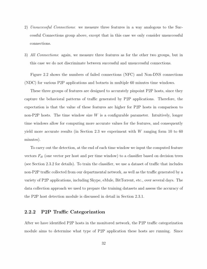
2.2 An example of number of failed connections (NFC) and non-DNS connections

(NDC) in ten 60-minute time windows . . . . . . . . . . . . . . . . . . . . . 33

2.3 Distribution of bytes per packets for management flows of different P2P apps. 38

3.1 DNS data collected at authoritative level VS. RDNS level ([8]) . . . . . . . . 71

3.2 A sample C&C domain lifetime . . . . . . . . . . . . . . . . . . . . . . . . . 73

3.3 A sample C&C domain lifetime with incorporated IP resolution history . . . 74

3.4 Categorization of C&C domains based on their infection population size . . . 75

3.5 C&C domains life VS. Size . . . . . . . . . . . . . . . . . . . . . . . . . . . . 77

3.6 Hierarchical clustering results using various configurations . . . . . . . . . . 78

4.1 IP transitions from/to known sinkholes to/from an unknown IP . . . . . . . 88

5.1 Machine-domain annotated graph. By observing who is querying what, we

can infer that d3 is likely a malware-related domain, and consequently that

MD is likely infected. . . . . . . . . . . . . . . . . . . . . . . . . . . . . . . . 95

5.2 Segugio system overview. . . . . . . . . . . . . . . . . . . . . . . . . . . . . . 98

x

5.3 Distribution of the number of malware-control domains queried by infected

machines. About 70% of known malware-infected machines query more than

one malware domain. . . . . . . . . . . . . . . . . . . . . . . . . . . . . . . . 99

5.4 Overview of Segugio’s feature measurement and classification phase. First

domain d’s features are measured, and then the feature vector is assigned a

“malware score” by the previously trained classifier. . . . . . . . . . . . . . . 105

5.5 Training set preparation: extracting the feature vector for a known malware-

control domain. Notice that “hiding” d’s label causes machine M1 to also be

labeled as unknown, because in this example d was the only known malware-

control domain queried by M1. Machines M2, M3, M4 queried some other

known malware domains, and therefore keep their original labels. . . . . . . 105

5.6 Graph-based 10-fold Cross-Validation Algorithm . . . . . . . . . . . . . . . . 111

5.7 Cross-validation results for three different ISP networks (with one day of traffic

observation; FPs in [0, 0.01]) . . . . . . . . . . . . . . . . . . . . . . . . . . . 113

5.8 Feature analysis: results obtained by excluding one group of features at a

time, and comparison to using all features (FPs in [0, 0.01]) . . . . . . . . . . 115

5.9 Feature analysis: results obtained by using only one group of features at a

time, and comparison with results obtained using all features (FPs in [0, 0.01]).116

5.10 Cross-day and cross-network test results for three different ISP networks (FPs

in [0, 0.01]) . . . . . . . . . . . . . . . . . . . . . . . . . . . . . . . . . . . . . 119

5.11 Cross-malware family results for three different ISP networks (with one day

of traffic observation; FPs in [0, 0.01]) . . . . . . . . . . . . . . . . . . . . . . 121

5.12 Example set of domains that were counted as false positives. The effective

2LDs are highlighted in bold. . . . . . . . . . . . . . . . . . . . . . . . . . . 122

5.13 Cross-validation results using only public blacklists . . . . . . . . . . . . . . 125

xi

5.14 Early detection results: histogram of the time gap between Segugio’s discovery

of new malware-control domains and the time when they first appeared on the

blacklist. . . . . . . . . . . . . . . . . . . . . . . . . . . . . . . . . . . . . . . 126

5.15 Comparison between Notos and Segugio (notice that the range of FPs for

Notos is [0, 1.0], while for Segugio FPs are in [0, 0.03]) . . . . . . . . . . . . . 127

6.1 System Overview . . . . . . . . . . . . . . . . . . . . . . . . . . . . . . . . . 139

6.2 An example download behavior graph and components of URLs . . . . . . . 143

6.3 Computation of SHA1 and GUID behavior-based features for a URL, u . . . 147

6.4 An example of behavior-based feature computation for a URL, u . . . . . . . 148

6.5 System Operation . . . . . . . . . . . . . . . . . . . . . . . . . . . . . . . . . 152

6.6 Cross-validation results for SHA1s and URLs layer on Feb 26 . . . . . . . . . 155

6.7 Train and test experiment on Feb 26 for SHA1s and URLs using Itst . . . . . 158

6.8 Train and test experiment on Feb 26 for SHA1s and URLs using Etst . . . . 159

6.9 Train and test experiment on Feb 26 for SHA1s and URLs using UEtst . . . 160

6.10 Early Detection of Malwares . . . . . . . . . . . . . . . . . . . . . . . . . . . 161

xii

CHAPTER 1

INTRODUCTION AND LITERATURE REVIEW

1.1 Introduction

Despite extensive research efforts, malicious software (or malware) is still at large. In fact,

numbers clearly show that malware infections continue to be on the rise. Because malware

is at the root of most of today’s cyber-crime, it is of utmost importance to persist in our

battle to defeat it. Unfortunately, existing defense technologies (e.g., antivirus softwares

or domain blacklists) have not been able to deal with new and sophisticated techniques

utilized by the Internet miscreants to distribute and deploy their malware on thousands of

users’ machines. Nowadays, it is safe to say that we have reached a point where antivirus

softwares simply don’t work anymore. This is mostly due to the fact that the traditional

antivirus systems rely on signature matching or static URL blacklisting, approaches that

have long been counteracted by the criminals. In this research, we focus on studying and

designing state-of-the-art prevention and detection models that are completely different from

the ineffective, routine techniques to fight this uphill battle. The main theme of this work

is, therefore, network security and machine learning with an emphasis on large-scale data

analysis.

This study focuses on the behavior of malicious infrastructures as a whole, rather than

having an individualistic approach on analysis of bad files or domains. It is next to impossible

1

to detect zero-day malwares installing and running themselves on victims’ machines due to

extreme obfuscation and code polymorphism techniques utilized by the malwares that conceal

their existence. Nonetheless, a global understanding of distribution or control infrastructures

of malwares hold promise, because it enables us to see the interaction patterns among the

involved entities and to leverage these patterns in defusing the cyber threats. This idea forms

the basis of this research and serves as the building block of this dissertation’s chapters. More

specifically, we researched behavioral models and graph-based learning algorithms that use a

belief propagation strategy to enable detection. This work constitutes the design of distinct

detection systems and measurement studies, each looking at the problem from a unique

standpoint while carrying the core ideology, behavioral analysis. What follows is a summary

of the chapters in this dissertation.

1.1.1 Behavior-based Classification of P2P Traffic

Peer2Peer (P2P) networks have been utilized greatly by criminals to facilitate their malware

distribution efforts. A malicious P2P botnet is a network of infected machines, called bots,

that are under the full control of an adversary, called a botmaster. The botmaster controls

its army of bots through Command & Control (C&C) channels. Since in P2P networks

there is no centralized and dedicated C&C servers to manage the bots, the P2P botnets are

very hard to detect. In a novel research project, we studied P2P networks and designed

a system for detection and categorization of P2P traffic [58]. The core idea behind this

system is P2P behavioral analysis which involves investigation of different P2P networks’

characteristics to be able to build profiles of their network activities. To generate the models,

the traffic of numerous benign and malicious P2P applications were collected, and their key

behavioral characteristics were extracted in terms of statistical feature vectors. These feature

vectors were used to train an accurate classification system comprising a group of One-Class

classifiers. Each One-Class classifier is basically an expert in classification of a specific P2P

2

application. When united, these distinct P2P profiles act in a collaborative fashion to reveal

the true nature of P2P traffic crossing the boundaries of the network under surveillance.

Chapter 2 provides a detailed discussion about this work.

1.1.2 Measuring the Properties of C&C Domains

While Chapter 2 focus is on P2P botnets, in Chapter 3 we study the properties of cen-

tralized botnets. So in a measurement study, we turn our attention to researching the

malware-control domains (C&C servers) to obtain a better understanding of their life cycle.

This work is a multiyear study of botnets that concerns the birth, growth, and death of their

malicious infrastructure where we analyzed four years of DNS traffic related to known C&C

servers. This project is based on a massive DNS traffic dataset that is unique in a sense that

it is collected at upper DNS hierarchy that provides a global visibility into all domain resolu-

tions from a few providers and their respective requesters. The C&C servers’ lifetimes were

modeled and their DNS resolutions were analyzed. The results help the security community

to obtain an accurate understanding of how Internet miscreants manage their infrastructure

and how agile they are in relocating their C&C servers. Chapter 3 contains details of this

research study. Moreover, an interesting outcome of the study in Chapter 3 that involves

further investigating the DNS resolution characteristics of inactive C&C servers is presented

in Chapter 4.

1.1.3 Behavioral Graph-based Detection System Using Belief Prop-

agation Strategy

Graph Learning is a novel approach that is introduced in two of our projects to detect

malicious cyber contents. By building a behavioral graph, this method allows us to obtain

3

a global awareness related to the interaction among entities in a system, such as an ISP

network or download patterns of users from various URLs.

Chapter 5 proposes a novel approach to detect malware-control (C&C) domains and

Chapter 6 focuses on detecting the malware downloads from malicious domains.

Large-scale Detection of C&C servers

In this research project, we designed a novel detection system based on behavioral-graphs

to identify new and previously unknown malware-control domains in live network traffic. A

malware-control domain hosts malicious software with the sole purpose of distributing and

installing it on users’ machines. This system has been fully tested and deployed in real-world

large ISP networks that serve millions of users in major cities in the United States where

users visit hundreds of millions of domains daily. The system automatically learns how

to discover new malware-control domain names by monitoring the DNS query behavior of

both known malware-infected machines as well as benign, meaning non-infected, machines.

Specifically, we build a machine-domain bipartite graph representing who is querying what.

Based on the machine-domain bipartite graph, it is noticeable that unknown domains that

are consistently queried only (or mostly) by known malware-infected machines are likely to

be malware-related. In essence, we combine the machines’ query behavior in terms of who is

querying what with a number of other domain name features, such as IP resolution history

and age, to compute the probability that a domain name is used for malware control or that

a machine is infected. Refer to Chapter 5 for full details.

Detection of Malicious Files, URLs, and Vulnerable Users

In another novel research project, we use the same overall strategy to perform behavioral

graph-based detection of malicious files, URLs, and vulnerable machines on a large scale.

This study is based on a unique dataset containing download events of customers of a famous

4

antivirus company. The download events are 3-tuple of files, URLs, and user machines.

Using this dataset, we build a tripartite graph which reveals the associations among the

aforementioned three entities. Similar to the previous study, we propagate either goodness

or badness information in the graph from labeled nodes towards unknown ones. The devised

classification system measures the amount of information push from the neighbors of an

unknown node towards making it either good or bad. The novelty and great advantage of

this study is that, firstly, it takes into account only the relationships and associations among

files, URLs, and machines and deduces based upon adjacencies (either direct or indirect) in

the tripartite graph. It doesn’t need to perform any deep file analysis, traffic monitoring,

DNS query inspection, etc.. Secondly, the detection occurs in a unified manner. In other

words, the system acts as a central defense and protection system that could detect malware

downloads, identify infected machines, and automatically block malicious URLs at the same

time. In fact, the detection result at each level in the graph assists in detection at other

levels. In summary, we show that the system can detect malicious files and URLs days or

even weeks before they are detected by antivirus softwares. This work is also partially similar

to another URL reputation system which is published in [70]. This system explained fully

in Chapter 6.

1.2 Literature Review

This section presents the state-of-the-art in network security and machine learning. The

section is divided into two parts. The first part provides a clear picture of usage of various

machine learning techniques in network security topics, including malware detection, intru-

sion detection systems, and spam detection. Machine learning is an integral part of this

research and provides a framework to build and evaluate statistical models. The second part

5

of the literature review is designated to the review of some of the most recent studies that

are closely related to each chapter of this dissertation.

1.2.1 Machine Learning and Security

One of the important applications of machine learning techniques is in security, where deal-

ing with large datasets, for example, network or DNS traffic, and extracting the hidden

knowledge in them is a challenge. In this section, we explore three major research areas of

security, namely malware detection, intrusion detection systems, and spam detection. The

papers discussed here are directly related to the research topics mentioned earlier, they also

have great emphasis on machine learning. Moreover, a diverse group of different machine

learning algorithms is discussed in the papers.

Malware Detection

Malicious code is “any code added, changed, or removed from a software system to inten-

tionally cause harm or subvert the system’s intended function” [44]. Anti-viruses alone are

proved to be ineffective [61], and new techniques are required to fight against them [16]. Due

to the sheer number of unknown files to be analyzed, manual methods cannot keep up, and,

instead, machine learning methods hold promise to enable automatic detection and classifi-

cation of malicious files [19]. Nonetheless, they come with their own unique challenges [10].

Malware distributors employ various techniques to install their malicious binaries into users’

machines. In early days, the main distribution mean was the malicious email attachments. In

this scenario, inexperienced or careless users were encouraged to open and run an attachment

by utilizing social engineering methods. Once the attachment was run, the user’s computer

was infected. However, this method requires user’s cooperation, which in turn makes the

attacks less effective. Recently, a stealthier and more effective distribution attack vector has

been used: Drive-by Downloads [37]. In this method, no user interaction is needed and,

6

in fact, merely visiting a malicious web site is enough to compromise the users’ machines.

Usually, upon visiting a page with drive-by download exploit code, an executable will run

on the browser and forces it to download the malware automatically. The malware then will

be installed and infects the host. After infection, the malware tries to communicate with

a Command and Control channel (C&C) to update itself, download new binaries, upload

stolen information, receive new orders, and etc.

Learning to Detect and Classify Malicious Executables in the Wild Kolter

and Maloof [44] focus on detection of malware executables. Also they train models that

are able to classify malwares based on their main operations (spamming, back door, etc.).

A collection of 1,971 benign and 1,651 malicious executables were used. Then n-grams are

extracted from the hex representation of these samples. Each n-gram represents a binary

feature (same as text classification methods). The most informative ones were chosen by

computing the information gain for each.

Multiple classification algorithms were used to train models to tell malware files apart

from the legitimate ones. These algorithms are: 1) Instance-based Learner (including IBk,

or k nearest neighbors), 2) Naive Bayes, 3) Support Vector Machines, 4) Decision Trees.

Moreover, they also tried and evaluated classifier combination methods. Boosting is the

used algorithm and it was performed on SVM, decision tress, and Naive Bayes.

The aforementioned classifiers are then trained using 10-fold cross validation, and their

performance is evaluated by computing their ROC curve and the area under the ROC curve.

There are a few variables that need to be determined before classifier evaluation. These

variables are, the value of n in the n-grams, the number of n-grams to be used, and the

size of the words. By performing some pilot experiments, they determine the optimal values

for these variables. The evaluation results show that Boosting decision trees yields the best

result, while Naive Bayes produces the worst performance.

7

Second part of the paper focuses on classifying the malwares based on what they do on

the system. The approach used here is one-versus-all classifiers. In this method, instead of

having one multi-class classifier, multiple binary classifiers are trained. Each binary classifier

tells if the unknown input sample belongs to the class that is being represented by the

classifier. For example, one classifier tells keyloggers apart from the rest, while another one

separates backdoors from the rest. Since a single malware could perform multiple actions

corresponding to different binary classifiers, multiples classifiers could produce a “hit” as

output. A similar approach is also taken in [58]. The experimental evaluation suggests that

the task of classifying malwares is a more difficult task than detecting malwares.

Automatic Analysis of Malware Behavior using Machine Learning The classifi-

cation step presented in [44] works directly with the content of the binary files. Unfortunately,

malware distributors utilize variety of techniques, such as code obfuscation, re-packing the

files, self generating codes, and etc., to evade this method. Having this in mind, Reick et

al. [61] employ another method for malware behavior classification. To analyze malwares

behavior, they are run in controlled environment, sandbox, and the chain of operations per-

formed, such as system calls, are logged. Instructions are then transformed into hex codes,

and similar to [44], n-grams of them are considered. Finally, for the sake of using machine

learning techniques, a malware’s set of instruction n-grams is converted into a feature vector,

where each element denotes the existence of a specific instruction. Now it would be possible

to measure similarity of two sequences using simple means, for example, Euclidean distance.

Both clustering, for identification of similar and new behaviors among malwares, and

classification, to assign a particular malware based on its operational characteristics to a

known class, are studied in the paper. Hierarchical clustering algorithm is used to partition

the feature vectors. The distance between the clusters is computed based on the complete

linkage method that considers the distance of two farthest members of each cluster as the

clusters distance. To perform classification, labeled data is required. To obtain the labeled

8

data, they use the clusters that are formed using their clustering method, and adopt k nearest

neighbors algorithm to assign the closest cluster’s label to instances.

Finally, the system is meant to be used in an incremental fashion, i.e. it gets updated

when new instances become available through numerous feeds. A novel approach is taken

here to incorporate new comers into the clusters. Upon receiving a new instance, the system

checks if it matches one of the existing classes. In this case the new objects is absorbed. If

it is not sufficiently close to one of the pre-established classes, it enters a clustering phase

with other left out instances. If they bond well (i.e. could form a new cluster), then system

has found a new cluster of malware behaviors that could correspond to a new operation, for

example.

Large-scale Malware Classification Using Random Projections and Neural

Networks The work presented in [19] also concerns with the detection and classification

of malware. However, one interesting problem the authors try to tackle is to deal with a

very large dataset of labeled instances where samples are represented with enormous num-

ber of features (179,000 features). In addition, one of their requirement is to produce an

infinitesimal false positives rate, with reasonably low false negatives. In this large-scale setup

it is very expensive to apply more sophisticated and effective classification algorithms. So

another challenge is to properly get rid of the “curse of dimensionality”.

The dataset used to train the models contains 1,843,359 labeled malware samples and

817,485 benign files. They also associated with each malware sample, a malware family. If

malware family is not known for a malware sample, it is assigned a generic family class.

The feature vectors in the labeled dataset, contain information from dynamic behavior of

malwares. This information are captured via the system calls, and the 3-gram of them are

considered as features (n-grams of system calls as features are also used in other studies,

such as [61] and [44]). A simple feature selection technique is used to reduce the 50 million

features generated by the tri-grams. This method reduces the dimensionality of the search

9

Figure 1.1: Architecture of the classifier system in [19]

space to 179 thousand. To train a Neural Network, however, the number of features are

too many, and this makes the training too expensive. As a result, another feature selection

method, called Random Projections, is used.

The classifier architecture is shown in Figure 1.1. It is composed of multiple steps and a

combine classifier that comprises Neural Networks and multinomial logistic regression. The

first step, as it was discussed above, is to reduce the dimensionality. The number of features

in Neural Network input is 4,000. The output of the Neural Network layers is fed into the

logistic regression classifier (the “softmax” layer), which in turn maps it to either of the

malware family outputs or benign output (136 classes). Note that in this case, simple linear

regression cannot be used, since it is a linear classifier, capable of only handling binary cases.

The proposed method is evaluated, and it is shown it can perform well. Specifically, mul-

tiple different configurations of the systems are tested. For example, different classification

accuracies are reported for different number of hidden layers in the Neural Networks.

Polonium: Tera-Scale Graph Mining for Malware Detection A new malware

detection approach is introduced by Polo et al. [16], called Polonium. It leverages a few

simple intuitions about goodness and badness of the binary executables and utilizes statistical

graphical models to build a reputation system. Having access to anonymous reports of

10

Symantec anti-virus about the users and the files on their computers, the system, first,

builds a very large bipartite graph of machines and files, representing who is running what.

The edges in this graph are drawn between a user’s machine and a file, if the file exists on

the machine. Belief Propagation algorithm is used to circulate information in this graph,

to eventually compute the marginal probability of the files belonging to either good or bad

classes. Machines reputation affects the reputation of the files associated with them, and

similarly, files reputation impacts the machines’ reputation. For example, a file is more

likely good, if it appears on many machines, whereas a file that only exists on a very few

machines is more likely malicious. Or an unknown file that mostly exists on infected hosts,

and no other clean hosts, could be a malware. By using some ground truth about the files,

machines and files are first labeled in the graph. Based on this labeling, an initial belief is

associated with each node, denoting our prior knowledge about the true nature of the nodes.

Then a repetitive message passing algorithm propagate the believes in the graph through

weighted edges. Each incoming message to a node, carries the opinion of its neighbors about

the nature of the node. For example, a malicious file’s outgoing message to its machine

neighbors pushes them toward badness. The aggregate of incoming messages to a node is

used to update node’s belief. The algorithm converges, if the changes of nodes’ believes

remain constant between iterations.

Large-Scale Malware Indexing Using Function-Call Graphs The goal of [33] is to

have a mean to identify similar malwares. Since malwares often employ heavy polymorphism

their contents in terms of bytes are different. But they are semantically the same. So the

authors propose a malware database that provides an indexing mechanism that given a

new graph of malware system calls, it finds most similar graphs in the database to the

new sample. This method, first, generates the function call graph. A metric is defined to

compare two graphs. This metric assigns a cost (an edit distance) to a series of operations

required to convert one graph to another. Since computing the edit distance is expensive,

11

an optimization step is designed to give a close approximation of the real edit distance with

less computational overhead. Having the more efficient edit distance, the next step is to

build an index that can find a close neighbor to an input query. The indexing mechanism

employs a multi-resolution search method. In a coarse-grained search, a B+-Tree is used

to efficiently and quickly find groups of malware entities that are close enough to the input

query. The leaves of the B+-Tree point to fine-grained VPT (Vantage Point Tree) indices.

A VPT index is a tree where each node is an item in the database. Each node’s children are

groups of items that are within a specific range from their parent. For example, all nodes

that have distance between x and y, where x < y, are grouped together in a child node.

Given an input query and a distance threshold, the distance between the query and the root

is computed and k nearest neighbors according to the computed distance and the distance

threshold are explored recursively.

Nazca Nazca [37] is a malware distribution network detection system. That is, it

does not analyze the malware binaries to extract signatures nor does take into account the

provenance features of the source, such as the server host, network, etc. In contrast, Nazca

takes a “zoomed out” approach where it considers the traits of malware distribution networks

as a whole rather than single downloads or executables by monitoring the HTTP requests

made by hosts in a network. The observation should have enough visibility to network traffic,

e.g. at large ISP networks, universities, or large enterprise networks. One of the advantages

of Nazca is that it can detect zero-day malware (new and previously unseen malware from

unknown sources) better, because the origin of the file, and the file itself are not relevant to

the system’s operation.

In the first step, all HTTP communications that are related to fetching binaries are

detected in the monitored network, and some relevant information (IPs, URIs, file hash, etc)

are extracted from them. Next, from the set of all collected HTTP meta data, they select

the ones that are likely related to malicious downloads using a few intuitive heuristics and

12

classifiers. One classifier designed to capture rapid file mutations (to avoid anti-viruses).

Another classifier identifies malicious content providers and distinguishes them from benign

ones. A decision tree with six features is trained and evaluated using leave-one-out cross

validation. The third classifier detects dedicated malware hosts. Finally, the fourth classifier

identifies exploit domains that infect users. Then a graph with heterogeneous nodes (host

IPs, domains, files, etc) is generated over the suspicious events from the previous step that

captures the correlated entities in a large scale. The goal here is to identify malicious

candidates in this graph by a classifier that uses a specific metric. The metric is the strength

and distance of candidates to other malicious entities. The evaluation on this part shows

the classifier has low false positives, however, it also suffers from low detection rate.

Intrusion Detection Systems

Intrusion detection systems refer to a general class of security systems that identify malicious

activities in a network under surveillance. They could be divided into anomaly detection

systems that capture behaviors that deviate from normal and expected ones, and misuse

detection systems that identifies predefined malicious activities [64]. From another view

point, intrusion detection systems could be categorized into network-based and host-based

intrusion detection systems, where the former considers network as a whole while looking for

malicious traits, while the latter considers each individual host in the network as an entity,

like [58].

Trust-Based Classifier Combination for Network Anomaly Detection This

paper, [60], combines several intrusion detection methods and improve the quality of their

decisions. It creates a model of the traffic in the network from the past observations, predicts

the properties of current traffic, and identifies the potentially malicious actions. In another

word, Net flows are aggregated over an observation period, relevant feature are extracted,

and a conclusion (malicious flows, legitimate flows) is made. The paper defines Flow identity

13

(srcIP, srcPort, dstIP, dstPort, numPackets, ...) and Flow context (Features observed on the

other flows in the same dataset. For example, number of similar flows from same srcIP). The

flow identity and flow context collectively create the feature space. Several agents monitor

the network flows and each one has a built in system to identify flows as legitimate or

malicious. Each agent utilizes a different model, different detection method, and different

flow context, i.e. different feature space, but all agents are given the same data which are

the network flows in intervals. The detection process contains three stages. During the

first stage each agent outputs a predicted anomaly value for each flow. Then the average of

outputted values is taken. The aggregated anomaly then is fed into the agents feature space

in the second stage. Each agent updates its model of the flows, and particularly updates its

centroids, which are trustees of the model and are used to deduce the trustfulness of feature

vectors in its vicinity. Finally, in stage three to determine the trustfulness of an individual

flow, they aggregate the trustfulness associated with the centroids in the vicinity of flows

feature vector.

In the experimental results of the paper a nice discussion is presented about why and how

the proposed method helps to improve the results by decomposing the problem and letting

each agent have a distinct insight into the problem, and, also how this method reduces the

False Positives.

Outside the Closed World: On Using Machine Learning For Network Intru-

sion Detection Differences between usage of machine learning techniques in intrusion

detection systems and other domains is studies in [64]. The authors discuss the unique chal-

lenges and difficulties that researches face when using machine learning methods in intrusion

detection systems. These challenges are:

• Outlier Detection: In general machine learning algorithms and specially classification

techniques require sufficient representatives of all classes in the training data. However,

14

one major challenge in intrusion detection systems is to identify new and previously

unseen attacks.

• High Cost of Errors: False positives and false negatives in network intrusion detection

systems are very costly compared to other areas (such as similar product recommenda-

tion of online merchants). For example, a system with even a very small false positive

rate, could produce errors in its real deployment, and a security specialist should man-

ually vet the output to make sure of its accuracy.

• Semantic Gap: A real-world deployment of intrusion detection systems poses the chal-

lenge of how to interpret the results. Does an anomaly mean an activity that is

malicious, or does it simply mean that there is a new activity that was never seen

before, but potentially legitimate?

• Diversity of Network Traffic: Intrusion detection systems have hard time dealing with

the diverse types of traffic that could be observed in a network. Many variables play a

part to make the same activity look different in distinct networks (such as bandwidth).

Another issue is finding a stable definition of what is considered as “normal”, because

traffic in networks usually happens in burst intervals, i.e. for some periods of time a

host’s traffic might seem very heavy while in the next interval the traffic could be just a

fraction of the previous interval. These all are normal, but how it could be represented

to the algorithm?

• Difficulties with Evaluation: Evaluating intrusion detection systems poses another chal-

lenge. This challenge is two-fold: First, acquiring a valid, large enough, labeled dataset

of network traffic is not easy. One problem here is how to find data for some anomaly

that has not happened yet? Because the goal of the system is to identify new attacks.

Is it a valid dataset if one synthetically simulate a few attacks? Second, how the output

15

of the classifier could be evaluated? Is telling what is normal from what is abnormal

apart sufficient? (Please see the “Semantic Gap” challenge above)

Spam Detection

Spam Email Filtering The focus of [79] is on spam filtering. Many spam filtering

techniques have been proposed. Many of them rely solely on blacklisting spammers, and

others are content based filters which require constant maintenance. This paper proposes

a filtering based approach using various machine learning techniques to distinguish spam

emails from non-spam ones. The first step is to extract the message features. The words in

the messages are features in this work which are extracted by, first, using word stemming to

automatically remove suffixes. Then valuable features are extracted from the document by

using a method called Mutual Information (MI), and features with highest MI are selected.

Also two types of feature vectors that are used are Boolean and term frequency. One of

the main contributions of the paper is introducing three information theoretic measures for

evaluating the performance of spam categorization techniques in terms of False Positives and

Negatives. These are, as they stated in[79]: “the remaining uncertainty after classifying a

received message as non-spam or spam by a particular spam categorization technique, the

uncertainty remaining after a message is classified as non-spam by the spam categorization

technique under consideration, and the uncertainty remaining after a message is classified as

spam, by the spam categorization technique under consideration”.

The paper proposes a way to integrate two trained classification methods for spam classi-

fication, which one of them is expert with regards to False Positives while the other presents

high accuracy with respect to False Negatives. Several classification methods have been

used for this purpose which includes: Nave Bayes, AdaBoostM1, Classification Via Re-

gression, MultiBoostAB, Random Committee, ADTree (Alternate Decision Tree), ID3-Tree,

RandomTree.

16

Figure 1.2: Threat model in [10]

Machine Learning and Security

Can Machine Learning Be Secure? Barreno et al. [10] try to answer the question

in the title of the paper. More specifically, the authors explore the answers behind a few

fundamental questions, such as how machine learning based classifiers could be evaded by

attackers?, the degree of difficulty and effort required by the attackers to introduce noise in

such a way that it makes the system unreliable?, can the learning algorithm be attacked?,

and etc.

Usually, in security papers, a “threat model” is defined that enlists the abilities of the

attacker. This model makes some assumptions about what an attacker could or could not do.

The threat model discussed in this paper is given in Figure 1.2. Based on the threat model,

possible defense mechanisms are discussed. Figure 1.3 shows a summary of techniques to

prevent each attack from happening (The figures were directly copied from [10]).

The following provides a brief overview of the defense mechanisms. Regularization is one

of the techniques that is beneficial against causative attacks, since it penalizes complexity,

hence prevents overfitting. So it strengthens the robustness of the models. Detecting attacks

from each of the categories is another defense strategy. For example, an exploratory attack

is detectable by observing the classifier’s output, and identify a cluster(s) of inputs that

cause the system to output a decision near the decision boundary. This signals an attack on

17

Figure 1.3: Defense mechanisms for the threat model in [10]

the classifier itself. Interestingly, the classifier could actually benefit from the exploratory

attacks, by hiding information about its boundary decision, and therefore, confuse the at-

tacker, the same way the attacker tried to confuse the classifier by probing the area near

the classes boundary line. Randomization prevents the targeted attacks, because the ran-

domization process affects the placement of the decision boundary, and therefore, it makes it

harder for the attacker to predict a good few points to target one class of the model. Finally,

the quality and quantity of the training data plays an important role. As more information

become available for training, less open space will remain for the attacker to exploit. On

the other hand, it could adversely damage the classifier’s flexibility to generalize beyond the

training set.

1.2.2 State-of-the-art in Analysis and Detection of Cyber-threats

For each chapter of this dissertation a few closely related research papers are discussed. The

discussion of all the related work to each chapter is deferred to the respective chapters.

18

Detection and Classification of P2P Traffic (Chapter 2)

Except than port and application-layer signature based methods, which their ineffectiveness

is known nowadays, the effectiveness of transport-layer heuristics on P2P traffic identification

is shown by Madhukar et al. [49]. These methods are based on concurrent use of TCP and

UDP and connection patterns for IP, Port pairs. This method could be useful in only

determination of presence of P2P traffic, and not categorization of it. There are various

limitations associated with transport-layer heuristics, and, moreover, identification of Skype

and botnets are missing in this work.

Hu et al. [34] use flow statistics to build traffic behavior profiles for P2P applications.

However, [34] does not attempt to separate P2P control and data transfer traffic. Because

data transfer patterns are highly dependent on user behavior, the approach proposed [34] may

not generalize well to P2P traffic generated by different users. Furthermore, [34] is limited

to modeling and categorizing only two benign non-encrypted P2P applications (BitTorrent

and PPLive), and does not consider at all malicious P2P applications.

A “zoomed-out” approach to identify P2P communities, rather than individual P2P

hosts, is introduced by Li et al. [47]. Participating hosts in a P2P community use the

same P2P application to communicate with each other. An unsupervised learning algorithm

analyzes the graph of who-talks-to-whom and identifies the strongly connected parts of the

graph as P2P communities. Although it is shown in [47] that P2P communities use the same

P2P application, this method cannot determine the underlying P2P application, whereas

PeerRush labels the P2P hosts.

In [30], Haq et al. discuss the importance of detecting and categorizing P2P traffic to

improve the accuracy of intrusion detection systems. However, they propose to classify P2P

traffic using deep packet inspection, which does not work well in case of encrypted P2P

traffic. More recently, a number of studies have addressed the problem of detecting P2P

19

botnets [25, 76, 77]. However, all these works focus on P2P botnet detection, and cannot

categorize the detected malicious traffic and attribute them to a specific botnet family.

Please see Section 2.5 for more related work and a detailed discussion of main differences

of each work presented here from PeerRush. In summary, the differences of our work from

the aforementioned studies are:

• Our analysis are based on traffic statistics without considering any information from

packet payloads. This enables PeerRush to deal with encrypted traffic, too.

• PeerRush detects and categorizes P2P traffic, unlike the majority of the studies which

only focus on detection.

• PeerRush not only detects and categorizes botnets, but also labels other legitimate

P2P traffic. To the best of our knowledge all previous works only focused on either

botnets or legitimate P2Ps, and not both.

• We evaluated our system using five legitimate P2P applications (including Skype), and

three P2P botnets, unlike previous studies which used a few P2P applications.

Analysis and Measurement of Botnets and C&C Domains (Chapters 3 and 4)

One of the outstanding researches in studying botnets has been done by Dagon et al. [18]. In

this paper, they have studied and described different topological structures of botnets. The

main goal of this paper is to provide a taxonomy of botnets spotted in the wild to better

understand the threat. By assigning a new botnet to a predefined taxonomy, defenders could

better analyze the botnet, identify its characteristics, and adjust their remedial efforts to

take down the botnet. Measuring the effectiveness of responses to each category of botnets

is another contribution of this paper. To measure the robustness of botnets against the

possible responses, they identify four network models for botnets including: Erdos-Renyi

20

random graph, Watts-Strogatz small world, barabasi-Albert scale free, and P2P models. For

each model they also describe a specific response model. After analyzing the various response

techniques, they provide some ideas and approaches for removing the attacks. For example,

they show that botnets that are based on random models are usually harder to deal with,

or targeted removals of C&C nodes on scale free botnets usually is the best response.

Detection of Malicious Domains (Chapter 5)

Recently, researchers have proposed domain name reputation systems [7, 12] as a way to

detect malicious domains, by modeling historic domain-IP mappings, using features of the

domain name strings, and leveraging past evidence of malicious content hosted at those do-

mains. These systems mainly aim to detect malicious domains in general, including phishing,

spam domains, etc. Notice that while both Notos [7] and Exposure [12] leverage informa-

tion derived from domain-to-IP mappings, they do not leverage the query behavior of the

machines “below” a local DNS server. As an example, domain reputation systems tend to

classify as malicious those domains that resolve into IPs located in “dirty” networks (e.g.,

bullet proof networks), which may host spam URLs, phishing attacks, social engineering

attacks, etc.

Kopis [8] has a goal more similar to ours: detect malware-related domains. However,

Kopis’s features (e.g., requester diversity and requester profile) are engineered specifically

for modeling traffic collected at authoritative name servers, or at top-level-domain (TLD)

servers, thus requiring access to authority-level DNS traffic [8]. This type of global access to

DNS traffic is extremely difficult to obtain, and can only be achieved in close collaboration

with large DNS zone operators. Furthermore, due to the target deployment location, Kopis

may allow for detecting only malware domains that end with a specific TLD (e.g., .ca).

More recently, Antonakakis et al. have proposed Pleiades [9], which aims to detect

machines infected with malware that makes use of domain generation algorithms (DGAs).

21

While Pleiades monitors the DNS traffic between the network users and their local DNS

resolver, as we do, it focuses on monitoring non-existent (NX) domains, which are a side-

effect of DGA-based malware.

For further discussion of the differences between the system presented in Chapter 5 and

other related work see Section 5.8.

Detection of Malware Downloads (Chapter 6)

A few studies address the problem of detecting malicious files or URLs using the behav-

ioral associations. [50] uses graphical models to detect malicious domains via loopy belief

propagation [43]. However, the approach in [50] does not scale well to very large network

log datasets that is the target of our work. The loopy belief propagation algorithm is quite

expensive and takes very long time to run. Our goal in Chapter 6, however, is to provide

online classification of files and URLs without long delays. Moreover, the work in [50] can

only detect malicious binary files. In contrast, the system introduced in Chapter 6 enables

the automatic and simultaneous detection of malicious files and URLs. Another work related

to ours is Polonium [16], which similarly to [50], aims to detect malware files using graphical

models.

A similar system called Amico [70] leverages a provenance based classifier to detect

malware binary downloads in a monitored network. The classifier is trained based on the

history of downloads by users in a network and takes into account the origin of the file

downloads, such as the URL, domain, IP space, and etc. Google CAMP [59] is a system

similar to [70] that detect malware files based on their origin reputation. However, this

system only works with Google’s web browser, and therefore, can only be used to monitor

the users of the browser.

22

CHAPTER 2

PEERRUSH: MINING FOR UNWANTED P2P TRAFFIC1

1B. Rahbarinia, R. Perdisci, A. Lanzi, K. Li, Journal of Information Security and Applications, Volume19, Issue 3, July 2014, Pages 194-208, DOI: 10.1016/j.jisa.2014.03.002.Reprinted here with permission of the publisher.

23

Abstract

In this paper we present PeerRush, a novel system for the identification of unwanted

P2P traffic. Unlike most previous work, PeerRush goes beyond P2P traffic detection,

and can accurately categorize the detected P2P traffic and attribute it to specific P2P

applications, including malicious applications such as P2P botnets. PeerRush achieves

these results without the need of deep packet inspection, and can accurately identify

applications that use encrypted P2P traffic.

We implemented a prototype version of PeerRush and performed an extensive eval-

uation of the system over a variety of P2P traffic datasets. Our results show that we

can detect all the considered types of P2P traffic with up to 99.5% true positives and

0.1% false positives. Furthermore, PeerRush can attribute the P2P traffic to a specific

P2P application with a misclassification rate of 0.68% or less.

24

2.1 Introduction

Peer-to-peer (P2P) traffic represents a significant portion of today’s global Internet traf-

fic [49]. Therefore, it is important for network administrators to be able to identify and

categorize P2P traffic crossing their network boundaries, so that appropriate fine-grained

network management and security policies can be implemented. In addition, the ability to

categorize P2P traffic can help to increase the accuracy of network-based intrusion detection

systems [30].

While there exist a vast body of work dedicated to P2P traffic detection [24], a large

portion of previous work focuses on signature-based approaches that require deep packet

inspection (DPI), or on port-number-based identification [63, 31]. Because modern P2P

applications avoid using fixed port numbers and implement encryption to prevent DPI-

based detection [49], more recent work has addressed the problem of identifying P2P traffic

based on statistical traffic analysis [40, 41]. However, very few of these studies address the

problem of P2P traffic categorization [34], and they are limited to studying only few types

of non-encrypted P2P communications. Also, a number of previous studies have focused

on detecting P2P botnets [25, 76, 52, 17, 77], but with little or no attention to accurately

distinguishing between different types of P2P botnet families based on their P2P traffic

patterns.

In this paper, we propose a novel P2P traffic categorization system called PeerRush.

Our system is based on a generic classification approach that leverages high-level statistical

traffic features, and is able to accurately detect and categorize the traffic generated by a

variety of P2P applications, including common file-sharing applications such as µTorrent,

eMule, etc., P2P-based communication applications such as Skype, and P2P-botnets such

as Storm [32], Waledac [55], and a new variant of Zeus [46] that uses encrypted P2P traffic.

We would like to emphasize that, unlike previous work on P2P-botnet detection, PeerRush

25

focuses on accurately detecting and categorizing different types of legitimate and

malicious P2P traffic, with the goal of identifying unwanted P2P applications within the

monitored network. Depending on the network’s traffic management and security policies,

the unwanted applications may include P2P-botnets as well as certain specific legitimate P2P

applications (e.g. some file-sharing applications). Moreover, unlike most previous work on

P2P-botnet detection, PeerRush can reveal if a host is compromised with a specific

P2P botnet type among a set of previously observed and modeled botnet families. To

the best of our knowledge, no previous study has proposed a generic classification approach

to accurately detect and categorize network traffic related to both legitimate and malicious

P2P applications, including popular applications that use encrypted P2P traffic, and different

types of P2P-botnet traffic (encrypted and non-encrypted).

Figure 2.1 provides an overview of PeerRush, which we discuss in detail in Section 2.2.

The first step involves the identifications of P2P hosts within the monitored network. Then,

the P2P traffic categorization module analyzes the network traffic generated by these hosts,

and attempts to attribute it to a given P2P application by matching an application profile

previously learned from samples of traffic generated by known P2P applications. If the P2P

traffic does not match any of the available profiles, the traffic is classified as belonging to

an “unknown” P2P application (e.g., this may represent a new P2P application release or

a previously unknown P2P botnet), and should be further analyzed by the network admin-

istrator. On the other hand, if the P2P traffic matches more than one profile, an auxiliary

disambiguation module is used to “break the tie”, and the traffic is labeled as belonging to

the closest P2P application profile.

The application profiles can model the traffic characteristics of legitimate P2P applica-

tions as well as different P2P-botnets. It is common for security researchers to run botnet

samples in a controlled environment to study their system and network activities [20]. The

traffic collected during this process can then be used as a sample for training a specific P2P-

26

botnet application profile, which can be plugged into our P2P traffic categorization module.

In summary this paper makes the following contributions:

• We present PeerRush, a system for P2P traffic categorization that enables the

accurate identification of unwanted P2P traffic, including encrypted P2P traffic

and different types of P2P botnet traffic. To achieve these goals, we engineer a

set of novel statistical features and classification approaches that provide both accuracy

and robustness to noise.

• We collected a variety of P2P traffic datasets comprising of P2P traffic generated by

five different legitimate P2P applications used in different configurations, and three

different P2P botnets including a P2P botnet that employs encrypted P2P traffic. We

are making these datasets publicly available.

• We performed an extensive evaluation of PeerRush’s classification accuracy and noise

resistance. Our results show that we can detect all the considered types of P2P traffic

with up to 99.5% true positives and 0.1% false positives. Furthermore, PeerRush can

correctly categorize the P2P traffic of a specific P2P application with a misclassification

rate of 0.68% or less.

2.2 System Overview

PeerRush’s main goal is to enable the discovery of unwanted P2P traffic in a monitored

computer network. Because the exact definition of what traffic is unwanted depends on the

management and security policies of each network, we take a generic P2P traffic categoriza-

tion approach, and leave the final decision on what traffic is in violation of the policies to

the network administrator.

27

P2P trafficsamples

P2P hostdetection

Non-P2Psamples

Live networktraffic

P2P trafficcategorization

AuxiliaryP2P traffic

disambiguation

training

training

trainingapplication

profile 1

applicationprofile 2

applicationprofile 3

applicationprofile N

P2P trafficcategorization

reports

Figure 2.1: PeerRush system overview.

To achieve accurate P2P traffic categorization, PeerRush implements a two-stage classifi-

cation system that consists of a P2P host detection module, and a P2P traffic categorization

module, as shown in Figure 2.1. PeerRush partitions the stream of live network traffic into

time windows of constant size W (e.g., W = 10 minutes). At the end of each time win-

dow, PeerRush extracts a number of statistical features from the observed network traffic,

and translates the traffic generated by each host H in the network into a separate feature

vector FH (see Section 2.2.1 for details). Each feature vector FH can then be fed to a pre-

viously trained statistical classifier that specializes in detecting whether H may be running

a P2P application, as indicated by its traffic features within the considered time window.

Splitting the traffic analysis in time windows allows to generate periodic reports and leads

to more accurate results by aggregating outputs obtained in consecutive time windows (see

Section 2.3.3).

The classifier used in the P2P host detection is trained using samples of network traffic

generated by hosts that are known to be running a variety of P2P applications, as well as

samples of traffic from hosts that are believed not to be running any known P2P application

28

(see Section 2.3.1). Once a host H is classified as a P2P host within a given time window W

by the first module, its current network traffic (i.e., the traffic collected during the current

analysis time window W ) is sent to the P2P traffic categorization module. This module

consists of a number of one-class classifiers [69], referred to as “application profiles” in

Figure 2.1, whereby each classifier specializes in detecting whether H may be running a

specific P2P application or not. Each one-class classifier is trained using only previously

collected traffic samples related to a known P2P application. For example, we train a one-

class classifier to detect Skype traffic, one for eMule, one for the P2P-botnet Storm, and

etc. This allows us to build a new application profile independently from previously learned

traffic models. Therefore, we can train and deploy a different optimal classifier configuration

for each target P2P application and analysis time window W .

Given the traffic from H, we first translate it into a vector of categorization features,

or traffic profile, PH (notice that these features are different from the detection features

FH used in the previous module). Then, we feed PH to each of the available one-class

classifiers, and each classifier outputs a score that indicates how close the profile PH is to

the application profile that the classifier is trained to recognize. For example, if the Skype

one-class classifier outputs a high score, this means that PH closely resembles the P2P traffic

generated by Skype. If none of the one-class classifiers outputs a high enough score for PH ,

PeerRush cannot attribute the P2P traffic of H to a known P2P application, and the P2P

traffic profile PH is labeled as “unknown”. This decision may be due to different reasons.

For example, the detected P2P host may be running a new P2P application for which no

traffic sample was available during the training of the application profiles, or may be infected

with a previously unknown P2P-botnet.

Because of the nature of statistical classifiers, while a host H is running a single P2P

application more than one classifier may declare that PH is close to their application profile.

In other words, it is possible that the P2P traffic categorization module may conclude that

29

H is running either Skype or eMule, for example. In these cases, to try to break the tie

PeerRush sends the profile PH to a disambiguation module, which consists of a multi-class

classifier that specializes in deciding what application profile is actually the closest to an

input profile PH . Essentially, the output of the disambiguation module can be used by the

network administrator in combination with the output of the single application profiles that

“matched” the traffic to help in further investigating and deciding if the host is in violation

of the policies.

In the following, we detail the internals of the P2P traffic detection and categorization

modules. It is worth noting that while some of the ideas we use for the detection module

are borrowed from previous work on P2P traffic detection (e.g., [77]) and are blended into

our own P2P host detection approach, the design and evaluation of the P2P traffic

categorization component include many novel P2P traffic categorization features

and traffic classification approaches, which constitute our main contributions.

2.2.1 P2P Host Detection

Due to the nature of P2P networks, the traffic generated by hosts engaged in P2P commu-

nications shows distinct characteristics, which can be harnessed for detection purposes. For

example, peer churn is an always-present attribute of P2P networks [65], causing P2P hosts

to generate a noticeably high number of failed connections. Also, P2P applications typically

discover and contact the IP address of other peers without leveraging DNS queries [73].

Furthermore, the peer IPs are usually scattered across many different networks. This makes

P2P traffic noticeably different from most other types of Internet traffic (e.g, web browsing

traffic). To capture the characteristics of P2P traffic and enable P2P host detection, Peer-

Rush measures a number of statistical features extracted from a traffic time window. First,

given the traffic observed during a time window of length W (e.g., 10 minutes), the net-

work packets are aggregated into flows, where each flow is identified by a 5-tuple (protocol,

30

srcip, srcport, dstip, dstport). Then, to extract the features related to a host H, we

consider all flows whose srcip is equal to the IP address of H, and compute a vector FH

that includes the following features:

Failed Connections: we measure the number of failed TCP and (virtual) UDP connections.

Specifically, we consider as failed all TCP or UDP flows for which we observed an outgoing

packet but no response, and all TCP flows that had a reset packet. We use two versions

of the failed connection feature: (1) the number of failed connections as described above,

and (2) the number of failed connections per host, where the failed connections to a same

destination host are counted as one (i.e., we count the number of distinct dstip related to

failed connections).

Non-DNS Connections: we consider the flows for which the destination IP address dstip

was not resolved from a previous DNS query, and we measure two features: (1) the number

of non-DNS connections, namely the number of network flows for which dstip was not

resolved from a DNS query, and (2) non-DNS connections per host, in which all flows to a

same destination host are counted as one (i.e., we count the number of distinct dstip related

to non-DNS connections).

Destination Diversity: given all the dstip related to non-DNS connections, for each dstip

we compute its /16 IP prefix, and then compute the ratio between the number of distinct

/16 prefixes in which the different dstips reside, divided by the total number of distinct

dstips. This gives us an approximate indication of the diversity of the dstips contacted

by a host H. We consider /16 IP prefixes because they provide a good approximation of

network boundaries. In other words, it is likely that two IP addresses with different /16

IP prefixes actually reside in different networks owned by different organizations. We define

nine features divided in three groups:

1) Successful Connections: we measure the destination diversity of all successful connections,

the number of distinct dstips, and number of distinct /16 networks.

31

2) Unsuccessful Connections: we measure three features in a way analogous to the Suc-

cessful Connections group above, except that in this case we only consider unsuccessful

connections.

3) All Connections: again, we measure three features as for the other two groups, but in

this case we do not discriminate between successful and unsuccessful connections.

Figure 2.2 shows the numbers of failed connections (NFC) and Non-DNS connections

(NDC) for various P2P applications and botnets in multiple 60 minutes time windows.

These three groups of features are designed to accurately pinpoint P2P hosts, since they

capture the behavioral patterns of traffic generated by P2P applications. Therefore, the

expectation is that the value of these features are higher for P2P hosts in comparison to

non-P2P hosts. The time window size W is a configurable parameter. Intuitively, longer

time windows allow for computing more accurate values for the features, and consequently

yield more accurate results (in Section 2.3 we experiment with W ranging form 10 to 60

minutes).

To carry out the detection, at the end of each time window we input the computed feature

vectors FH (one vector per host and per time window) to a classifier based on decision trees

(see Section 2.3.2 for details). To train the classifier, we use a dataset of traffic that includes

non-P2P traffic collected from our departmental network, as well as the traffic generated by a

variety of P2P applications, including Skype, eMule, BitTorrent, etc., over several days. The

data collection approach we used to prepare the training datasets and assess the accuracy of

the P2P host detection module is discussed in detail in Section 2.3.1.

2.2.2 P2P Traffic Categorization

After we have identified P2P hosts in the monitored network, the P2P traffic categorization

module aims to determine what type of P2P application these hosts are running. Since

32

1 2 3 4 5 6 7 8 9 1010

0

101

102

103

104

time window

NF

CNFC in 60−minute time window

eMule

uTorrent

Frostwire

Vuze

Skype

Storm

Zeus

Waledac

(a)

1 2 3 4 5 6 7 8 9 1010

1

102

103

104

time window

ND

C

NDC in 60−minute time window

eMuleuTorrentFrostwireVuzeSkypeStormZeusWaledac

(b)

Figure 2.2: An example of number of failed connections (NFC) and non-DNS connections(NDC) in ten 60-minute time windows

different P2P applications (including P2P-botnets) use different P2P protocols and networks

(i.e., they connect to different sets of peers), they show distinguishable behaviors in terms

of their network communication patterns. Therefore, we construct a classification system

that is able to learn different P2P application profiles from past traffic samples, and that

can accurately categorize new P2P traffic instances.

As shown in Figure 2.1, the categorization module consists of a number of one-class

classifiers [69] that specialize in recognizing a specific application profile. For example,

we train a one-class classifier to recognize P2P traffic generated by Skype, one that can

recognize eMule, etc. Also, we build a number of one-class classifiers that aim to recognize

different P2P-botnets, such as Storm, Waledac, and a P2P-based version of Zeus. Overall,

in our experiments we build eight different one-class classifiers, with five models dedicated

to recognizing five different legitimate P2P applications, and three models dedicated to

categorizing different P2P-botnets (see Section 2.3.3). PeerRush can be easily extended to

33

new P2P applications by training a specialized one-class classifier on the new P2P traffic,

and plugging the obtained application profile into the categorization module.

Given the traffic generated by a previously detected P2P hostH, we first extract a number

of statistical features (described below) that constitute the traffic profile PH of H within a

given time window. Then, we feed PH to each of the previously trained one-class classifiers,

and for each of them we obtain a detection score. For example, let sk be the score output by

the classifier dedicated to recognizing Skype. If sk is greater than a predefined threshold θk,

which is automatically learned during training, there is a high likelihood that H is running

Skype. If no classifier outputs a score si (where the subscript i indicates the i-th classifier)

greater than the respective application detection threshold θi, we label the P2P traffic from

H as “unknown”. That is, PeerRush detected the fact that H is running a P2P application,

but the traffic profile does not fit any of the previously trained models. This may happen in

particular if H is running a new P2P applications or an unknown P2P-botnet for which we

could not capture any traffic samples to learn its application profile (other possible scenarios

are discussed in Section 2.4).

Notice that the threshold θi is set during the training phase to cap the false positive rate

to ≤ 1%. Specifically, the false positives produced by the i-th classifier over the traffic from

P2P applications other than the one targeted by the classifier is ≤ 1%. Because of the nature

of statistical classifiers, it is possible that more than one one-class classifier may output a

score si greater than the respective detection threshold θi, thus declaring that PH matches

their application profile. In this case, to break the tie we use a P2P traffic disambiguation

module that consists of a multi-class classifier trained to distinguish among the eight different

P2P applications that we consider in our experiments. In this case, the multi-class classifier

will definitely assign one application among the available ones, and the output of the multi-

class classifier can then be interpreted as the most likely P2P application that is running

on H. This information, along with the output of each single one-class classifier, can then

34

be used by the network administrator to help decide if H is in violation of the network

management and security policies.

The main reason for building the application profiles using one-class classifiers, rather

than directly using multi-class classification algorithms, is that they enable a modular clas-

sification approach. For example, given a new P2P application and some related traffic

samples, we can separately train a new one-class classifier even with very few or no coun-

terexamples (i.e., traffic samples from other P2P applications), and we can then directly

plug it into the P2P traffic categorization module. Learning with few or no counterexamples

cannot be easily done with multi-class classifiers. In addition, differently from multi-class

classifiers, which will definitely assign exactly one class label among the possible classes, by

using one-class classifiers we can more intuitively arrive to the conclusion that a given traffic

profile PH does not really match any previously learned P2P traffic and should therefore be

considered as belonging to an “unknown” P2P application, for example.

Feature Engineering To distinguish between different P2P applications, we focus on

their management (or control) traffic, namely network traffic dedicated to maintaining up-

dated information about the overlay P2P network at each peer node [15]. The reason for

focusing on management flows and discarding data-transfer flows is that management flows

mainly depend on the P2P protocol design and the P2P application itself, whereas data

flows are more user-dependent, because they are typically driven by the P2P application

user’s actions. Because the usage patterns of a P2P application may vary greatly from user

to user, focusing on management flows allows for a more generic, user-independent P2P

categorization approach. These observations apply to both legitimate P2P applications and

P2P-botnets.

Management flows consist of management packets, such as keep-alive messages, period-

ically exchanged by the peers to maintain an accurate view of the P2P network to which

they belong. In a way, the characteristics of management flows serve as a fingerprint for a

35

given P2P protocol, and can be used to build accurate application profiles. The first ques-

tion, therefore, is how to identify management flows and separate them from the data flows.

The answer to this question is complicated by the fact that management packets may be

exchanged over management flows that are separate from the data flows, or may be embed-

ded within the data flows themselves, depending on the specific P2P protocol specifications.

Instead of making strong assumptions about how managements packets are exchanged, we

aim to detect management flows by applying a few intuitive heuristics as described below.

We consider the outgoing flows of each P2P hosts (as detected by the P2P host detection

module), and we use the following filters to identify the management packets and discard

any other type of traffic:

1) Inter-packet delays : given a flow, we only consider packets that have at least a time gap

δ > θδ between their previous and following packets, where θδ is a predefined threshold

(set to one second, in our experiments). More precisely, let pi be the packet under

consideration within a flow f , and pi−1 and pi+1 be the packets in f that immediately

precede and follow pi, respectively. Also, let δ− and δ+ be the inter-packet delay (IPD)

between pi−1 and pi and between pi and pi+1, respectively. We label pi as a management

packet if both δ− and δ+ are greater than θδ. The intuition behind this heuristic is that

management packets are exchanged periodically, while data packets are typically sent

back-to-back. Therefore, the IPDs of data packets are typically very small, and therefore

data packets will be discarded. On the other hand, management packets are typically

characterized by much larger IPDs (in fact, a θδ = 1s IPD is quite conservative, because

the IPDs between management packets are often much larger).

2) Duration of the connection: P2P applications often open long-lived connections through

which they exchange management packets, instead of exchanging each management mes-

sage in a new connection (notice that UDP packets that share the same source and

36

destinations IPs and ports are considered as belonging to the same virtual UDP connec-

tion). Therefore, we only consider flows that appear as long-lived relative to the size W

of the traffic analysis time windows, and we discard all other flows. Specifically, flows

that are shorter than W3

are effectively excluded from further analysis.

3) Bi-directionality : this filter simply considers bi-directional flows only. The assumption

here is that management messages are exchanged both ways between two hosts, and

for a given management message (e.g., keep-alive) we will typically see a response or

acknowledgment.

Notice that these rules are only applied to connections whose destination IP address did not

resolve from DNS queries. This allows us to focus only the network traffic that has a higher

chance of being related to the P2P application running on the identified P2P host. While

a few non-P2P flows may still survive this pre-filtering (i.e., flows whose destination IP was

not resolved from DNS queries, and that are related to some non-P2P application running on

the same P2P host), thus potentially constituting noise w.r.t. the feature extraction process,

they will be excluded (with very high probability) by the management flow identification

rules outlined above.

After we have identified the management (or control) flows and packets, we extract a

number of features that summarize the “management behavior” of a P2P host. We consider

two groups of features: features based on the distribution of bytes-per-packet (BPP) in the

management flows, and feature based on the distribution of the inter-packet delays (IPD)

between the management packets. Specifically, given a P2P host and its P2P management

flows, we measure eight features computed based on the distribution of BPPs of all incoming

and outgoing TCP and UDP flows and the distribution of IPDs for all incoming and outgoing

TCP and UDP packets within each management flow.

37

The intuition behind these features is that different P2P applications and protocols use

different formats for the management messages (e.g., keep-alive), and therefore the distribu-

tion of BPP will tend to be different. Similarly, different P2P applications typically behave

differently in terms of the timing between when management messages are exchanged be-

tween peers. As an example, Figure 2.3 reports the distribution of BPP for four different P2P

applications. As can be seen from the figure, different applications have different profiles,

which we leverage to perform P2P traffic categorization.

0 75 150 225 300 3750

100

200

300

400

outgoing UDP byte/pkt

Fre

quency

Skype

(a) Skype

0 75 150 225 300 3750

200

400

600

800

1000

1200

1400


Fre

quency

eMule

(b) eMule

0 75 150 225 300 3750

2000

4000

6000

8000

10000

12000


Fre

quency

uTorrent

(c) µTorrent

0 75 150 225 300 3750

100

200

300

400


Fre

quency

Zeus

(d) Zeus

Figure 2.3: Distribution of bytes per packets for management flows of different P2P apps.

To translate the distribution of the features discussed above into a pattern vector, which

is a more suitable input for statistical classifiers, we proceed as follows. First, given a host H

38

and its set of management flows, we build a histogram for each of the eight features. Then,

given a histogram, we sort its “peaks” according to their height in descending order and

select the top ten peaks (i.e., the highest ten). By choosing only the top ten peaks, we aim

to isolate possible noise in the distribution, focusing only on the most distinguishing patterns.

For each of these peaks we record two values: the location (in the original histogram) of the

peak on the x axis, and the its relative height compared to the remaining top ten peaks. For

example, the relative height hk of the k-th peak is computed as hk = hk/∑10

j=1 hj, where hj

is the height of the j-th peak. This gives us a vector of twenty values for each feature, and

therefore the overall feature vector contains 160 features.

This format of the feature vectors is used both as input to the application-specific one-

class classifiers and the P2P traffic disambiguation multi-class classifier (see Figure 2.1). The

learning and classification algorithms with which we experimented and the datasets used for

training the P2P traffic categorization module are discussed in Section 2.3.3.

Although some of the features require fine grained information about the network packets,

such as packet timings, we do not need to compute these features for the majority of the

hosts in the network, because the traffic categorization module only deals with the P2P hosts

identified by the first module. Moreover, we only focus on the management packets of the

P2P hosts, and will not consider all the traffic generated by these hosts. This in turn hugely

reduces the amount of network traffic for which traffic categorization module features should

be computed.

39

2.3 Evaluation

2.3.1 Data Collection

PeerRush relies on three main datasets for the training of the P2P host detection and traffic

categorization modules: a dataset of P2P traffic generated by a variety of P2P applications,

a dataset of traffic from three modern P2P botnets, and a dataset of non-P2P traffic. In the

next Sections, we will refer back to these datasets when presenting our evaluation results,

which include cross-validation experiments. We plan to make our P2P traffic datasets openly

available to facilitate further research and to make our results easier to reproduce2.

(D1) Ordinary P2P Traffic To collect the P2P traffic dataset, we built an experimental

network in our lab consisting of 11 distinct hosts which we used to run 5 different popular

P2P applications for several weeks. Specifically, we dedicated 9 hosts to running Skype, and

the two remaining hosts to run, at different times, eMule, µTorrent, Frostwire, and Vuze.

This choice of P2P applications provided diversity in both P2P protocols and networks (see

Table 2.1). The 9 hosts dedicated to Skype were divided into two groups: we configured

two hosts with high-end hardware, public IP addresses, and no firewall filtering. This was

done so that these hosts had a chance to be elected as Skype super-nodes (indeed, a manual

analysis of the volume of traffic generated by these machines gives us reasons to believe

that one of the two was actually elected to become a super-node). The remaining 7 hosts

were configured using filtered IP addresses, and resided in distinct sub-networks. Using

both filtered and unfiltered hosts allowed us to collect samples of Skype traffic that may be

witnessed in different real-world scenarios. For each host, we created one separate Skype

account and we made some of these accounts be “friends” with each other and with Skype

instances running on machines external to our lab. In addition, using AutoIt [1], we created

2Please contact the authors to obtain a copy of the datasets.

40

a number of scripts to simulate user activities on the host, including periodic chat messages

and phone calls to friends located both inside and outside of our campus network. Overall,

we collected 83 days of a variety of Skype traffic, as shown in Table 2.1.

We used other two distinct unfiltered hosts to run each of the remaining legitimate P2P

applications. For example, we first used these two hosts to run two instances of eMule

for about 9 consecutive days. During this period, we initiated a variety of file searches

and downloads. Whenever possible, we used AutoIt [1] to automate user interactions with

the client applications. The files to be downloaded were selected among popular open-

source software. However, because of a possible mismatch between file names and actual

file contents, to avoid potential copyright issues we made sure to never store the downloads

permanently. Furthermore, we set our packet capture tool to only capture part of the

payloads, so to make it impossible to reconstruct the downloaded files from the collected

traffic traces (notice that in this paper we do not use deep packet inspection for detection,

only flow statistics). We replicated this process to collect approximately the same amount

of traffic from FrostWire, µTorrent, and Vuze.

(D2) P2P Botnet Traffic In addition to popular P2P applications, we were able to

obtain (mainly from third parties) several days of traffic from three different P2P-botnets:

Storm [32], Waledac [55], and Zeus [46]. It is worth noting that the Waledac traces were

collected before the botnet takedown enacted by Microsoft, while the Zeus traces are from

a very recent version of a likely still active Zeus botnet that relies entirely on P2P-based

command-and-control (C&C) communications. Table 2.1 indicates the number of hosts and

days of traffic we were able to obtain, along with information about the underlying transport

protocol used to carry P2P management traffic.

(D3) Non-P2P Traffic To collect the dataset of non-P2P traffic, we proceeded as follows.

We monitored the traffic crossing our departmental network over about 5 days, and collected

each packet in an anonymized form. Specifically, we wrote a sniffing tool based on libpcap

41

that can anonymize the packets “on the fly” by mapping the department IPs to randomly

selected 10.x.x.x addresses using a keyed hash function, and truncating the packets pay-

loads. We leave all other packet information intact. Also, we do not truncate the payload

of DNS response packets, because we need domain name resolution information to extract a

number of statistical features (see Section 2.2). Because users in our departmental network

may use Skype or (sporadically) some P2P file-sharing applications, we used a number of

conservative heuristics to filter out potential P2P hosts from the non-P2P traffic dataset.

To identify possible Skype nodes within our network, we leverage the fact that whenever

a Skype client is started, it will query domain names ending in skype.com [31]. Therefore,

we use the DNS traffic collected from our department to identify all hosts that query any

Skype-related domain names, and we exclude them from the traces. Obviously, this is a

very conservative approach, because it may cause a non-negligible number of false positives,

excluding nodes that visit the www.skype.com website, for example, but that are not running

Skype. However, we chose this approach because it is difficult to devise reliable heuristics

that can identify with high precision what hosts are running Skype and for how long (that’s

why systems such as PeerRush needed in the first place), and using a conservative approach

gives us confidence on the fact that the non-P2P dataset contains a very low amount of

noise. Using this approach, we excluded 14 out of 931 hosts in our network.

To filter out other possible P2P traffic, we used Snort [6] with a large set of publicly

available P2P detection rules based on payload content inspection. We ran Snort in parallel to

our traffic collection tool, and excluded from our dataset all traffic from hosts that triggered

a Snort P2P detection rule. Again, we use a very conservative approach of eliminating all

traffic from suspected P2P hosts to obtain a clean non-P2P dataset. The reason is that it is

very hard to exactly identify for how long certain hosts ran a P2P application simply based

on the Snort alerts. From a manual analysis of the Snort alerts, we suspect that some of the

users of our network may only run P2P file-sharing applications (e.g., eMule or BitTorrent)

42

Table 2.1: P2P traffic dataset summary

Application Protocol Hosts Capture Days TransportSkype Skype 9 83 TCP/UDPeMule eDonkey 2 9 TCP/UDPFrostWire Gnutella 2 9 TCP/UDPµTorrent BitTorrent 2 9 TCP/UDPVuze BitTorrent 2 9 TCP/UDP

Storm - 13 7 UDPZeus - 1 34 UDPWaledac - 3 3 TCP

for a short amount of time, perhaps because P2P traffic is not seen favorably by the network

administrators, and users may not want to be reprimanded. Even using this conservative

approach, we only filtered out 7 out of 931 IP addresses from our department traffic traces.

The heuristics-based traffic filtering approach discussed above aims to produce a dataset

for which we have reliable ground truth. While our heuristics are quite conservative, and

may erroneously eliminate hosts that are not actually engaging in P2P traffic, we ended up

eliminating only a small fraction of hosts within our network. Therefore, we believe the

remaining traffic is representative of non-P2P traffic in our department. Naturally, it is also

possible that the non-P2P dataset may contain some P2P traffic (e.g., encrypted or botnet

traffic) that we were not able to label using Snort or our heuristics, thus potentially inflating

the estimated false positives generated by PeerRush. However, since this would in the worst

case underestimate the accuracy of our system, not overestimate it, we can still use the

dataset for a fair evaluation.

2.3.2 Evaluation of P2P Host Detection

Balanced Dataset To evaluate the P2P host detection module, we proceed as follows. We

perform cross-validation tests using the datasets D1, D2, and D3 described in Section 2.3.1.

We then applied the process described in Section 2.2.1 to extract statistical features and

translate the traffic into feature vectors (one vector per host and per observation time win-

43

Table 2.2: P2P Host Detection: results of 10-fold cross-validation using J48+AdaBoost

time window TP FP AUC60 min 99.5% 0.1% 140 min 99.1% 0.8% 0.99920 min 98.4% 1.1% 0.99910 min 97.9% 1.2% 0.997

dow). Because the volume of Skype-related traffic in D1 was much larger than the traffic we

collected from the remaining popular P2P applications, we under-sampled (at random) the

Skype-related traffic to obtain a smaller, balanced dataset. Also, we under-sampled from

D3 to obtain approximately the same number of labeled instances derived from P2P and

non-P2P traffic. Consequently, our training set for this module contains roughly the same

number of samples from legitimate P2P applications and from the non-P2P traffic.

Cross-validation To perform cross-validation, we initially excluded D2, and only consid-

ered a balanced version of D1 and D3. As a classifier for the P2P host detection module we

used boosted decision trees. Specifically, we employ Weka [72] to run 10-fold cross-validation

using the J48 decision tree and the AdaBoost meta-classifier (we set AdaBoost to combine

50 decision trees). We repeated the same experiment by measuring the features for different

values for the time window length W ranging from 10 to 60 minutes. For W = 60 minutes,

we had 1,885 P2P and 3,779 non-P2P training instances, while for 10 minutes we had 10,856

P2P and 19,437 non-P2P instances. The results in terms of true positive rate (TP), false

positive rate (FP), and area under the ROC curve (AUC) are summarized in Table 2.2. As

can be seen, the best results are obtained for the 60 minutes time window, with a 99.5%

true positives and a 0.1% false positives. This was expected, because the more time we wait,

the more evidence we can collect on whether a host is engaging in P2P communications.

However, even at a 10 minutes time window, the classifier perform fairly well, with a true

positive rate close to 98%, a false positive rate of 1.2%, and an AUC of 99.7%.

44

Table 2.3: P2P Host Detection: classification of P2P botnet traffic instances

Time Win. Botnet Instances TPs IPs detected

60 minStorm 306 100% 13 out of 13Zeus 825 92.48% 1 out 1

Waledac 75 100% 3 out 3

40 minStorm 306 100% 13 out of 13Zeus 1,229 91.05% 1 out of 1

Waledac 111 100% 3 out of 3

20 minStorm 918 100% 13 out of 13Zeus 2,448 58.99% 1 out of 1


10 minStorm 1,834 100% 13 out of 13Zeus 4,877 33.46% 1 out of 1


Botnets Besides cross-validation, we performed two additional sets of experiments. First,

we train the P2P host detection classifier (we use J48+AdaBoost) using D1 and D3, but

not D2. Then, given the obtained trained classifier, we test against the P2P botnet traffic

D2. The results of this experiments are summarized in Table 2.3 . As we can see, the P2P

host detection classifier can perfectly classify all the instances of Storm and Waledac traffic.

Zeus traffic is somewhat harder to detect, although when we set the time window for feature

extraction to 40 minutes or higher we can correctly classify more than 90% of all Zeus traffic

instances. We believe this is due to the fact that in our Zeus dataset the host infected by

the Zeus botnet sometimes enters a “dormant phase” in which the number of established

connections decreases significantly. Also, by considering traffic over different time windows,

all the IP addresses related to the P2P botnets are correctly classified as P2P hosts. That is,

if we consider the Zeus-infected host over a number of consecutive time windows, the Zeus

P2P traffic is correctly identified in at least one time window, allowing us to identify the

P2P host. Therefore, the 33.46% detection rate using 10-minute time windows is not as low

as it may seem, in that the host was labeled as a P2P host at least once in every three time

windows.

45

Table 2.4: P2P Host Detection: “leave one application out” test

time window: 60 minutes time window: 40 minutesLeft out Test on left out app. Test on left out app.

app. Instances TPs IPs detected Instances TPs IPs detectedSkype 16,534 95.11% 9 out of 9 24,795 94.64% 9 out of 9eMule 386 100% 2 out of 2 386 100% 2 out of 2

Frostwire 386 100% 2 out of 2 386 100% 2 out of 2µTorrent 339 100% 2 out of 2 339 100% 2 out of 2

Vuze 339 100% 2 out of 2 339 100% 2 out of 2

time window: 20 minutes time window: 10 minutesLeft out Test on left out app. Test on left out app.

app. Instances TPs IPs detected Instances TPs IPs detectedSkype 49,596 92.17% 9 out of 9 99,165 90.26% 9 out of 9eMule 1,158 100% 2 out of 2 2,316 100% 2 out of 2

Frostwire 1,158 100% 2 out of 2 2,316 100% 2 out of 2µTorrent 1,018 100% 2 out of 2 2,035 100% 2 out of 2

Vuze 1,018 100% 2 out of 2 2,035 100% 2 out of 2

Leave-one-out In addition, we performed a number of experiments to assess the general-

ization ability of our P2P host classifier. To this end, we again trained the classifier on D1

and D3. This time, though, we train the classifier multiple times, and every time we leave

out one specific type of P2P traffic from D1. For example, first we train the classifier while

leaving out all Skype traffic from the training dataset, and then we test the obtained trained

classifier on the Skype traffic that we left out. We repeat this leaving out from D1 one P2P

application at a time (as before, we did not include the P2P botnet traffic from the training

dataset). The results of this set of experiments are reported in Table 2.4 . The results show

that we can detect most of the left out applications perfectly in all time windows. In case

of Skype, the classifier can still generalize remarkably well and correctly classifies more than

90% of the Skype instances using W = 10. Using larger time windows improves the results

further, because the statistical features can be measured more accurately. Also, the IPs

detected column shows that all IP addresses engaged in P2P communications are correctly

classified as P2P hosts.

Other non-P2P instances Besides the cross-validation experiments, to further asses

the false positives generated by our system we tested the P2P host detection classifier over

46

Table 2.5: P2P Host Detection: test of non-P2P traffic instances excluded from the trainingset (data collected across ∼ 5 days)

Time window Instances FP rate FP IPs60 18,892 0.29% 21 out of 52740 18,449 1.08% 44 out of 50220 51,875 0.45% 25 out of 53710 97,185 1.14% 78 out of 559

the portion of the non-P2P traffic dataset that was left out from training (due to under-

sampling). The results are reported in Table 2.5. Notice that the “FP IPs” column shows the

number of distinct IP addresses for which at least one traffic instance (i.e., a small snapshot

of its traffic) was at some point labeled as P2P traffic. The non-P2P traffic used for testing

was collected over about 5 days, and therefore the average number of false positive IPs is

approximately 2 per day. These false positives can be further reduced by flagging a host as

P2P only if its traffic instances are classified as P2P by the P2P host detection module for

more than one consecutive time window.

2.3.3 Evaluation of P2P Traffic Categorization

In this Section, we evaluate the P2P traffic categorization module. First, we separately eval-

uate the one-class classifiers used to learn single application profiles (E1) and the auxiliary

P2P traffic disambiguation module (E2). Then, we evaluate the entire P2P traffic catego-

rization module in a scenario that replicates the intended use of PeerRush after deployment

(E3). Finally, given a separate new dataset of encrypted µTorrent traffic that we recently

collected, we show that this new P2P traffic can be accurately detected by the P2P host

detection module, and a new application profile can be readily built and plugged into the

P2P traffic categorization module for accurate traffic labeling (E4).

In all our experiments, we translate a host’s traffic into statistical features using the

process described in Section 2.2.2. Similar to the evaluation of the P2P host detection module

47

presented in Section 2.3.2, we experiment with values of the time windows W ranging from

10 to 60 minutes.

(E1) P2P Application Profiles As mentioned in Section 2.2.2, each application profile

is modeled using a one-class classifier. Specifically, we experiment with the Parzen, KNN,

and Gaussian data description classifiers detailed in [69] and implemented in [68]. To build

a one-class classifier (i.e., an application profile) for Skype traffic, for example, we use part

of the Skype traffic from D1 as a target training dataset, and a subset of non-Skype traffic

from the other legitimate P2P applications (again from D1) as an outlier validation dataset.

This validation dataset is used for setting the classifier’s detection threshold so to obtain

≤ 1% false positives (i.e., non-Skype traffic instances erroneously classified as Skype). Then

we use the remaining portion of the Skype and non-Skype traffic from D1 that we did not

use for training and threshold setting to estimate the FP, TP, and AUC. We repeat the same

process for each P2P application in D1 and P2P botnets in D2. Each experiment is run

with a 10-fold cross-validation setting for each of the considered one-class classifiers. The

results of these experiments are summarized in Table 2.6. The “#Inst.” column shows the

overall number of target instances available for each traffic class.

Besides experimenting with different one-class classifiers, we also evaluated different com-

binations of features and different feature transformation algorithms, namely principal com-

ponent analysis (PCA) and feature scaling (Scal.). The “Configuration” column in Table 2.6

shows, for each different time window, the best classifier and feature configuration. For ex-

ample, the first row of results related to Skype reports the following configuration: “60min;

KNN; 32 feat.; PCA”. This means that the best application profile for Skype when consid-

ering a 60 minutes traffic time window was obtained using the KNN algorithm, 32 features

(out of all possible 160 features we extract from the traffic characteristics), and by applying

the PCA feature transformation. In the remaining rows, “Scal.” indicates features scaling,

while “-” indicates no feature transformation.

48

Notice that because we use one-class classifiers, each application profile can be built

independently from other profiles. Therefore, we can train and deploy different optimal

classifier configurations depending on the target P2P application and desired time window

W for traffic analysis. For example, for a time window of 60 minutes, we can use a KNN

classifier with 32 features transformed using PCA for Skype, and a Parzen classifier with

16 scaled features for eMule. This gives us a remarkable degree of flexibility in building

the application profiles, compared to multi-class classifiers, because in the latter case we

would be limited to using the same algorithm and set of features for all application profiles.

Furthermore, using multi-class classifiers makes identifying P2P traffic that does not match

any of the profiles (i.e., “unknown” P2P traffic) more straightforward.

Table 2.6 shows that for most applications we can achieve a TP rate of more than 90%

with an FP rate close to or below 1%. In particular, all traffic related to P2P botnets can

be accurately categorized with very high true positive rates and low false positives. These

results hold in most cases even for time windows of W = 10 minutes, with the exception

of Waledac, for which we were not able to build a comparably accurate application profile

using a 10 minutes time window, since we did not have enough target instances to train a

classifier (this unsatisfactory result is omitted from Table 2.6).

(E2) P2P Traffic Disambiguation When a traffic instance (i.e., the feature vector

extracted from the traffic generated by a host within a given time window) is classified as

target by more than one application profile, we can use the traffic disambiguation module

to try to break the tie. while it is possible for a host to run more than one P2P application

at the same time within a given time window, we can still apply the disambiguation module

and send the output of the disambiguation results along with the output of each application

profile to the network administrator for further analysis. Essentially, we want to provide

the network administrator with two pieces of information: the fact that more than one

49

Table 2.6: One-Class Classification Results

App. #Inst. Configuration TP FP AUC

Skype

526 60min; KNN; 32 feat.; PCA 96.54% 0.74% 0.998541 40min; Parzen; 8 feat.; PCA 100% 0.85% 1.000559 20min; KNN; 24 feat.; PCA 98.18% 0.88% 0.999579 10min; Parzen; 16 feat.; - 91.27% 1.00% 0.978

eMule

387 60min; Parzen; 16 feat; Scal. 90.64% 0.92% 0.989421 40min; Parzen; 16 feat.; Scal. 92.79% 0.90% 0.995448 20min; Parzen; 12 feat.; PCA 95.56% 0.90% 0.985483 10min; KNN; 8 feat.; PCA 88.40% 1.16% 0.961

Frostwire

382 60min; KNN; 12 feat.; PCA 85.58% 0.96% 0.966402 40min; Parzen; 8 feat.; - 90.81% 1.04% 0.975436 20min; Parzen; 8 feat.; PCA 87.12% 0.59% 0.963467 10min; KNN; 8 feat.; PCA 92.68% 1.25% 0.989

µTorrent

370 60min; KNN; 8 feat.; - 92.94% 1.30% 0.948431 40min; KNN; 4 feat.; Scal.+PCA 91.89% 1.14% 0.985509 20min; KNN; 8 feat.; - 93.25% 1.11% 0.962609 10min; Parzen; 4 feat.; Scal. 94.55% 1.24% 0.992

Vuze

376 60min; KNN; 8 feat.; - 91.92% 0.95% 0.979421 40min; KNN; 8 feat.; - 91.79% 1.06% 0.966462 20min; KNN; 12 feat.; PCA 95.44% 1.24% 0.992514 10min; KNN; 8 feat.; PCA 84.18% 1.17% 0.964

Storm

162 60min; Parzen; 16 feat.; - 100% 0% 1.000240 40min; Parzen; 16 feat.; - 99.29% 0% 0.993305 20min; Parzen; 16 feat.; - 99.62% 0.03% 0.996391 10min; Parzen; 12 feat.; PCA 100% 0% 1.000

Zeus

375 60min; KNN; 4 feat.; - 97.29% 0.99% 0.996426 40min; KNN; 4 feat.; PCA 94.80% 0.91% 0.991160 20min; Parzen; 8 feat.; PCA 98.71% 0.73% 0.987188 10min; KNN;12 feat.; - 94.53% 0.79% 0.976

Waledac37 60min; Gaussian; 12 feat.; PCA 99.99% 0.90% 0.99842 40min; Gaussian; 12 feat.; PCA 95.00% 1.13% 0.99934 20min; Kmeans; 28 feat.; PCA 90.00% 1.07% 0.993

application profile “matched” the traffic instance, and the most likely (or “prevalent”) P2P

application according to the disambiguation module.

The disambiguation module (see Section 2.2) consists of a multi-class classifier based

on the Random Forest algorithm combining 100 decision trees. In this case, we use all

160 features computed as described in Section 2.2.2 without any feature transformation,

because even without applying any feature selection process we obtained high accuracy. We

independently tested the disambiguation module using 10-fold cross-validation. On average,

we obtained an accuracy (percentage of correctly classified instances) of 98.6% for a time

window of 60 minutes, 98.3% for 40 minutes, 97.5% for 20 minutes, and 96.7% for 10 minutes.

50

Table 2.7: P2P Traffic Disambiguation: Results of 10-fold cross-validation

time window: 60min time window: 40minApplication TP FP AUC TP FP AUC

Skype 99.8% 0.4% 1 99% 0.1% 1eMule 99.5% 0.2% 1 100% 0.6% 1

Frostwire 96.1% 0.6% 0.998 95.5% 0.6% 0.998µTorrent 99.7% 0% 1 99.5% 0% 1

Vuze 96% 0.3% 0.999 95.8% 0.3% 0.999Storm 100% 0% 1 100% 0% 1Zeus 99.5% 0% 1 100% 0.3% 1

Waledac 97.2% 0.1% 0.988 92.7% 0% 0.99

time window: 20min time window: 10minApplication TP FP AUC TP FP AUC

Skype 99.6% 0.6% 1 99.3% 0.2% 1eMule 96.7% 0.5% 0.999 98.1% 1.1% 0.997

Frostwire 96.1% 1.1% 0.997 94.8% 1.7% 0.99µTorrent 99.2% 0.3% 1 98.7% 0.2% 0.999

Vuze 95.6% 0.4% 0.999 90.6% 0.6% 0.996Storm 100% 0% 1 100% 0.1% 1Zeus 96.9% 0.1% 1 96.3% 0% 0.998

Waledac 85.7% 1% 0.986 46.7% 0% 0.974

The detailed classification results obtained using 10-fold cross validation are reported in

Table 2.7.

Note that the disambiguation module could be employed as the primary classification

system for categorizing P2P flows, and it could eliminate the use of one-class classifiers. In

fact, the accuracy of the categorization step will be enhanced by doing so (compare Tables 2.6

and 2.7). Nonetheless, we will loose the flexibility of PeerRush, and the advantage of having

“unknown” as the classifier output, because the multi-class classifier should always output

one of its classes as the answer, even in the case that an unknown input instance is fed to it.

The advantage of using one-class classifiers is that each could use a certain group of

features that is more effective in detecting a certain P2P protocol. As a result, there is no

general rule on which features are more or less useful. A certain group of features might be

quite effective on categorizing Skype, while they might not do well on Zeus (see Table 2.6,

column “Configuration”).

51

(E3) Overall Module Evaluation In this section we aim to show how the P2P catego-

rization module performs overall, and how robust it is to noise. To this end, we first split

the D1 dataset into two parts: (i) a training set consisting of 80% of the traffic instances

(randomly selected) that we use for training the single application profiles, automatically

learn their categorization thresholds, and to train the disambiguation module; (ii) a test set

consisting of the remaining 20% of the traffic instances.

To test both the accuracy and robustness of PeerRush’s categorization module, we also

perform experiments by artificially adding noise to the traffic instances in the test dataset.

In doing so, we consider the case in which non-P2P traffic is misclassified by the P2P host

detection module and not completely filtered out through the management flow identification

process described in Section 2.2.2. To obtain noisy traffic we processed the entire D3 dataset

(about 5 days of traffic from 910 distinct source IP addresses) to identify all flows that

resemble P2P management flows. To simulate a worst case scenario, we took all the noisy

management-like flows we could obtain, and randomly added these flows to all the P2P traffic

instances in the 20% test dataset described above. Effectively, we simulated the scenario in

which the traffic generated by a known P2P host is overlapped with non-P2P traffic from

one or more randomly selected hosts from our departmental network.

For each test instance fed to the categorization module, we have the following possible

outcomes: (1) the instance is assigned the correct P2P application label; (2) no application

profile “matches”, and the P2P traffic instance is therefore labeled as “unknown”; (3) more

than one profile “matches”, and the instance is sent to the disambiguation module. Table 2.8

and Table 2.9 report a summary of the obtained results related to the 20% test dataset

with and without extra added noise, considering W = 60 minutes. For example, Table 2.9

shows that over 90% of the Skype-related traffic instances can be correctly labeled as being

generated by Skype with 1.29% FP, even in the presence of added noise.

52

Overall, 45 out of 732 (6.15%) of the noisy test traffic instances were classified as “un-

known”, 32 instances were passed to the disambiguation module and all of them were classi-

fied perfectly. Finally, only 5 out of 732 instances were eventually misclassified as belonging

to the wrong P2P application. It is worth noting that an administrator could handle the

“unknown” and misclassified instances by relying on the categorization results for a given

P2P host across more than one time window. For example, a P2P host that is running eMule

may be categorized as “unknown” in one given time window, but has a very high chance

of being correctly labeled as eMule in subsequent windows, because the true positive rate

for eMule traffic is above 93%. In fact, in our experiments, by considering the output of

the categorization module over more than one single time window we were always able to

attribute the P2P traffic in our test to the correct application.

As we can see by comparing Table 2.8 and Table 2.9, the extra noise added to the P2P

traffic instances causes a decrease in the accuracy of the P2P traffic categorization module.

However, in most cases the degradation is fairly limited. The noise has a more negative

impact on the categorization of Storm and Waledac, in particular. Notice, though, that

the results reported in Table 2.9 are again related to single traffic instances (i.e., a single

time window). This means that if a Storm- or Waledac-infected host connects to its botnet

for longer than one time window, which is most likely the case since malware often makes

itself permanent into the compromised systems, the probability of correct categorization

would increase. Therefore, even in the scenario in which each P2P host is also running

other network applications that may introduce noise in the management flow identification

and feature extraction process, we can accurately detect the P2P traffic, and still achieve

satisfactory categorization results.

We also wanted to determine how PeerRush’s categorization module would deal with noise

due to detection errors in the P2P host detection module. To this end, we further tested the

classifier using traffic from the non-P2P traffic dataset that were misclassified as P2P by the

53

P2P host detection module. We found that considering a time window of 60 minutes, only

35 traffic instances misclassified by the P2P host detection module passed the management

flow discovery filter. Of these, 33 were classified as “unknown” by the categorization module,

one was misclassified as both Skype and µTorrent, and one was misclassified as Zeus.

Table 2.8: 80/20 experiments

time window: 60 minutesApplication TP FP AUC

Skype 100% 0.86% 1eMule 93.59% 1.44% 0.9968

Frostwire 88.31% 0.97% 0.9873µTorrent 96.97% 1% 0.9789

Vuze 93.1% 0.7% 0.9938Storm 100% 0% 1Zeus 96.69% 1.26% 0.9964

Waledac 57.14% 0.83% 0.9420

Classified as “unknown”: 3.96% (29 out of 732)Misclassified as other P2P: 0% (0 out of 732)Disambiguation needed: 4.64% (34 out of 732)· Correctly disambiguated: 33, Incorrectly disambiguated: 1

Total misclassified as other P2P: 0.14% (1 out of 732)

Table 2.9: 80/20 with extra noise

time window: 60 minutesApplication TP FP AUC

Skype 90.4% 1.29% 0.9891eMule 94.87% 2.39% 0.9935

Frostwire 94.73% 0.48% 0.9927µTorrent 98.99% 0.66% 0.9997

Vuze 93.22% 3.02% 0.9873Storm 45.45% 0% 0.7273Zeus 97.32% 0.72% 0.9991

Waledac 40% 0.8% 0.8610

Classified as “unknown”: 6.15% (45 out of 732)Misclassified as other P2P: 0.68% (5 out of 732)Disambiguation needed: 4.37% (32 out of 732)· Correctly disambiguated: 32, Incorrectly disambiguated: 0

Total misclassified as other P2P: 0.68% (5 out of 732)

(E4) Encrypted µTorrent Recently, we collected a separate trace of encrypted µTorrent

traffic. First we tested the P2P host detection module on instances of encrypted µTorrent

traffic where all instances were correctly classified as P2P traffic. So our focus in this section

is to show how the new traffic profile of encrypted µTorrent could be easily added to the

system as a plugin and how the proposed classification system could accurately label the

new encrypted traffic. Note that encrypted µTorrent traffic statistical behavior is different

54

Table 2.10: Encrypted µTorrent 80/20 Experiments Results

Time Window: 60 minutesApplication Target Outlier TP FP AUCEnc. µTorrent 9 732 9 (100 %) 0 (0 %) 1

Classified as Unknown 0 out of 741 (0 %)

Mixed Enc. µTorrent 9 732 9 (100 %) 0 (0 %) 1Classified as Unknown 0 out of 741 (0 %)

from µTorrent even though they both are based on a same P2P protocol (perhaps due to

changes in packet sizes as a result of encryption), so a new one-class classifier is required for

the encrypted version.

To evaluate the P2P categorization module, we use a similar approach as E3 experiments,

and divide encrypted µTorrent traffic into training and testing sets consisting of 80% and

20% of all instances respectively. The training set is used to build a traffic profile for

encrypted µTorrent, and the test set is used to evaluate the classifier. We also amalgamate

the encrypted µTorrent test instances with noise from non-P2P traffic (as discussed in E3

experiments section). The results of these experiments for time window W = 60 minutes are

shown in Table 2.10. The 20% test set contains 9 instances (targets), and 732 outliers are

the test instances from other P2P applications used in E3 experiments. It is clear that newly

introduced P2P application profile works perfectly and categorizes the encrypted µTorrent

instances with 100% accuracy and without FPs, even in the presence of noise. The modular

design of PeerRush enabled us to perform this addition without making any changes to other

modules, especially the other traffic profiles. Had we used multi-class classifiers for P2P traffic

categorization instead of one-class classifiers, we should have trained a new classifier with

the newly added class. However, the disambiguation module still needs to be re-trained, in

order to be able to break the tie in case of the new class. In this experiment, none of the

other one-class classifiers identified encrypted µTorrent as their targets, so we did not need

to utilize the disambiguation module.

55

2.4 Discussion

PeerRush is intentionally built using a modular approach, which allows for more flexibility.

For example, as shown in Section 2.3, it may be best to use a different number of features

and different classification algorithms to learn the traffic profile of different P2P applications.

To build the profile for a new P2P application we can apply a model selection process, which

is commonly used for other machine learning tasks, to find the best classifier configuration

for the job, and then we can plug it directly into PeerRush.

One parameter that has direct influence on all the system modules is the observation time

window used to split and translate the network traffic into instances (or feature vectors).

It is important to notice that while different modules need to extract different statistical

features from the same time window, all features can be extracted incrementally, and each

given module can simply use the appropriate subset of all the extracted features for its own

classification purposes. Also, while all modules perform quite well in most cases by setting

the time window length to 10 minutes, the results tend to improve for larger time windows,

because this allows the feature extraction process to collect more evidence. Therefore, fixing

the observation time window at 60 minutes for all modules may be a good choice. However,

this choice depends on the desired trade-off between the detection time and the categorization

accuracy.

Classification systems, in general, always require a good number of labeled instances to

build reliable models. This means if they encounter a new instance for which they did not

have prior knowledge, they cannot reason about it by any means. One important advantage

of PeerRush is the ability to provide the “unknown” answer, when is fed with a truly unknown

traffic sample that does not have a designated one-class classifier. This by itself is enough

to raise an alarm for network administrator to take a closer look at the traffic and analyze

it further. So the new sample could be considered as “unwanted” right away, until further

56

information become available. Neither PeerRush, nor any other classification system could

assign a label to an unknown sample it never have encountered. So in case there are one or

more botnets appear at the same time they more likely will be detected as unknown P2P

traffic, and according to the network policies, the network administrator might want to block

them until their true nature is revealed.

It is possible that a host may be running more than one P2P application at the same

time (or there may be a NAT device that effectively aggregates multiple single hosts), in

which case the traffic patterns of these applications may overlap and prevent a match of the

profiles. Therefore, PeerRush may categorize these cases as unknown P2P traffic. However,

in many practical cases not all P2P applications will be active at the same time. Therefore,

the analysis of traffic across different time windows applied by PeerRush may still allow for

effectively distinguishing among P2P applications. However, notice that even in the cases

when a host continuously runs more than one active P2P application at the same time, the

host will be detected as a P2P host, although its P2P traffic may be classified as “unknown”

and may therefore require further analysis by the network administrator.

Botnet developers could try to introduce noise (e.g., dummy packets or random padding)

into the management flows to alter the distribution of BPP and IPDs. This may cause

a “mismatch” with a previously learned application profile for the botnet. In this case,

PeerRush would still very likely detect the P2P botnet hosts as running a P2P application,

because the features used by the P2P host detection module are intrinsic to P2P traffic in

general (see Section 2.2.1 and the results in Table 2.4) and are harder to evade. However, the

P2P traffic categorization module may classify the P2P botnet traffic as “unknown”, thus

requiring further analysis to differentiate the botnet traffic from other possible types of P2P

traffic. Because P2P botnet hosts may for example engage in sending large volumes of spam

emails, be involved in a distributed denial-of-service (DDoS) attack, or download executable

binaries to update the botnet software, one possible way to distinguish P2P traffic related

57

to botnets is to monitor for other suspicious network activities originating from the detected

P2P hosts [25].

The developer of a new P2P application, including P2P botnets, may attempt to model

its P2P traffic following the behavior of other legitimate P2P applications. Because some

networks may consider most P2P applications (legitimate or not) as unwanted, the developer

may be restricted to mimic a specific type of P2P traffic that is likely to be allowed in most

networks (e.g., Skype traffic). However, while possible, morphing the traffic to mimic other

protocols may require significant effort [51].

In order to deploy PeerRush, the classifiers could be trained at the vendors lab rather

than the customers network, since the features are intrinsic to P2P applications and how

they behave, and they are not dependent on specific network behaviors. The P2P host

detection module binary classifier takes into account peer churn, non-DNS connection, and

diversity of connected IPs of P2P applications. These are signatures of P2P applications

regardless of the network they are used in. The P2P categorization module classifiers make

their decisions based on the management flows of P2P applications as well, which are also

protocol-dependent. As a result, PeerRush could easily be trained outside of the customers

network, which facilitates the real deployment of the system.

2.5 Related Work

While P2P traffic detection has been a topic of much research, P2P traffic categorization has

received very little attention. Because of space limitations, we cannot mention all related

work here and we therefore refer the reader to a recent survey by Gomes et al. [24]. In the

following, we limit our discussion to the most relevant work on P2P traffic categorization,

and on P2P botnet detection.

58

Hu et al. [34] use flow statistics to build traffic behavior profiles for P2P applications.

However, [34] does not attempt to separate P2P control and data transfer traffic. Because

data transfer patterns are highly dependent on user behavior, the approach proposed [34] may

not generalize well to P2P traffic generated by different users. Furthermore, [34] is limited

to modeling and categorizing only two benign non-encrypted P2P applications (BitTorrent

and PPLive), and does not consider at all malicious P2P applications. Unlike [34], Peer-

Rush categorizes P2P applications based on an analysis of their P2P control traffic, which

captures fundamental properties of the P2P protocol in use and is therefore less susceptible

to different application usage patterns. Furthermore, we show that PeerRush can accurately

categorize many different P2P applications, including encrypted traffic and different modern

P2P botnets.

A “zoomed-out” approach to identify P2P communities, rather than individual P2P

hosts, is introduced by Li et al. [47]. Participating hosts in a P2P community use the

same P2P application to communicate with each other. An unsupervised learning algorithm

analyzes the graph of who-talks-to-whom and identifies the strongly connected parts of the

graph as P2P communities. Although it is shown in [47] that P2P communities use the same

P2P application, this method cannot determine the underlying P2P application, whereas

PeerRush labels the P2P hosts.

In [30], Haq et al. discuss the importance of detecting and categorizing P2P traffic to

improve the accuracy of intrusion detection systems. However, they propose to classify P2P

traffic using deep packet inspection, which does not work well in case of encrypted P2P

traffic. More recently, a number of studies have addressed the problem of detecting P2P

botnets [25, 76, 77]. However, all these works focus on P2P botnet detection, and cannot

categorize the detected malicious traffic and attribute them to a specific botnet family.

PeerRush is different because it focuses on detecting and categorizing unwanted P2P traffic

in general, including a large variety of legitimate P2P applications and botnets.

59

Coskun et al. [17] proposed to discover hosts belonging to a P2P botnet from a seed of

compromised hosts. Similarly, [52] analyzes communication graphs to identify P2P botnet

nodes. Detecting botnets before they start their attacks (waiting stage), when bots maintain

infrequent yet long-lived flows, is studied in [29]. These works focus solely on P2P botnets

detection.

2.6 Conclusion

We presented PeerRush, a novel system for the identification of unwanted P2P traffic. We

showed that PeerRush can accurately categorize P2P traffic and attribute it to specific P2P

applications, including malicious applications such as P2P botnets. PeerRush achieves these

results without the need of deep packet inspection, and can accurately identify applications

that use encrypted P2P traffic. We implemented a prototype version of PeerRush and

performed an extensive evaluation of the system over a variety of P2P traffic datasets. Our

results show that PeerRush can detect all the considered types of P2P traffic with up to

99.5% true positives and 0.1% false positives. Furthermore, PeerRush can attribute the P2P

traffic to a specific P2P application with a misclassification rate of 0.68% or less.

Acknowledgments

We would like to thank Brett Mayers for his contribution to collecting the P2P traffic

datasets, and the anonymous reviewers for their constructive comments. This material is

based in part upon work supported by the National Science Foundation under Grant No.

CNS-1149051. Any opinions, findings, and conclusions or recommendations expressed in this

material are those of the authors and do not necessarily reflect the views of the National

Science Foundation.

60

CHAPTER 3

MEASURING THE PROPERTIES OF C&C DOMAINS1

1B. Rahbarinia, prepared for publication but not submitted.

61

Abstract

Botnets utilize Command & Control channels (C&C) to manage their malicious

infrastructure. In centralized botnets, botmasters usually maintain one or more C&C

servers and abuse Domain Name System (DNS). In order to better understand botnets

activities and find efficient approaches to hinder their network, it is important to study

the characteristics and life-time trends of these C&C servers. In this project, by har-

nessing a unique dataset of DNS query and responses that is collected from upper DNS

hierarchy, we aim to measure the life-time traits of C&C servers. Our measurement

results demonstrate some key behaviors of botnets life cycle.

62

3.1 Introduction

Every day, ISPs are facing with millions of cyber-attacks all around the world with different

purposes including Botnets using Command and Control (C&C) domains. In the botnet

attacks, criminals typically use bots to infect large numbers of computers which in result

will form a network or botnet. In this type of attacks, criminals distribute the malwares

through the network to infect machines and turn them into a bot or robot for sending out

spam emails, spreading viruses, attacking computers and servers and stealing personal and

private information [2].

In the past years, Domain Name System (DNS) has played an important role in propa-

gating the malicious aim requests on Internet especially via C&C mechanism of botnets. In

this mechanism the infected machines are a set of infected hosts which communicate with

one or several C&C servers. The criminals use domains for C&C mechanism and to evade

the countermeasure of blocking domains, create hundreds of domains every day.

In this paper we utilize a massive and unique dataset of historic DNS query and response

which has been collected at an authoritative name server level during 4.5 years in which

many malicious C&C domains reside. We aim to summarize C&C domains life cycle in

terms of their requesters and their resolved IPs. That is, for domains’ requesters, we form a

time-series of their requesters (volume of queries) with epochs equal to one day. On each day

of these domains’ lives, we also extract their resolved IPs. We envision to plot C&C domains

life cycles with respect to the volume of the queries. This presents an opportunity to study

C&C domains in terms of botnets life cycle trends and shows how a malware started its

malicious activity, how it reached its peak, and finally how it gradually died. The results of

this study will help us devise more effective detection technologies, such as the one presented

in Chapter 5.

63

In order to analyze this huge dataset, we employ Hadoop in a cluster with capacity of

472 mappers and 219 reducers. After processing the raw data, we study the resultant time-

series of each C&C domain. More specifically, we do a clustering step to compare and group

different C&C domains according to their life cycle trends, so we research possible techniques

to cluster time-series data.

3.2 Related Work

One of the outstanding researches in studying botnets has been done by Dagon et al. [18]. In

this paper, they have studied and described different topological structures of botnets. The

main goal of this paper is to provide a taxonomy of botnets spotted in the wild to better

understand the threat. By assigning a new botnet to a predefined taxonomy, defenders could

better analyze the botnet, identify its characteristics, and adjust their remedial efforts to

take down the botnet. Measuring the effectiveness of responses to each category of botnets

is another contribution of this paper. To measure the robustness of botnets against the

possible responses, they identify four network models for botnets including: Erdos-Renyi

random graph, Watts-Strogatz small world, barabasi-Albert scale free, and P2P models. For

each model they also describe a specific response model. After analyzing the various response

techniques, they provide some ideas and approaches for removing the attacks. For example,

they show that botnets that are based on random models are usually harder to deal with,

or targeted removals of C&C nodes on scale free botnets usually is the best response.

3.3 The Approach and Goals

Studying botnets and analyzing their evolution during the years could reveal a lot about how

attackers tend to organize their malicious infrastructure and how they launch their attacks.

64

This benefits large ISP network administrators as well as security researchers to be well

prepared on their efforts to take down botnets or at least cripple their fundamental activities.

This type of study, however, requires having access to a large historic botnet dataset that

could be mined to extract useful information. In this paper, we utilize a massive and unique

dataset that contains historic DNS query and responses collected on the authoritative DNS

level during a period of 4.5 years (see section 3.4.1 for more details about the dataset). We

use this dataset to acquire knowledge about hundreds of C&C domains from a dynamic DNS

provider and their infection campaigns.

We perform a number of measurements on the botnets and their respective C&C domains.

Each measurement aims to demonstrate some interesting observations about various aspects

of C&C domains. We define two groups of measurements: i) individual C&C domains study,

and ii) collective C&C studies. In the former, we present lifetime analysis of each individual

C&C domain, while in the latter, we aim to study C&C domains trends in general, compare

them, and discover methods to effectively group them.

3.3.1 Individual C&C Domains Study

In this group of measurements, we show how each individual C&C domain appears in the

wild (the birth), how it extends its infection campaign (the growth), and how it eventually

and gradually is ceased from existence (the death). To this end, we split each C&C domains’

life into epochs. In our experiments we consider a day as our epoch. For each epoch, we

record the domains requesters. Each requester is in fact a compromised host on the Internet

that is infected with the same malware as to the domain under investigation. Each requester

is identified by its IP address, and hence, could be mapped into distinct BGP prefixes (IP

networks), Autonomous System numbers (ASN), and Country Codes (C&C). As a result, for

each day of C&C domain’s life, we can measure how many requester contacted the domain,

and where these requester came from. The location of the requesters represents the type

65

of the botnet in general, in a sense that we could identify whether the C&C domain has a

domestic or global infection breadth. More specifically, the requesters IP, BGP, ASN, and

CC provide different levels of granularity for analyzing the infection campaign. In addition,

for each epoch of C&C domain’s life, we also extract its IP resolution to help identify how its

malicious infrastructure moves. This kind of information manifests the C&C domains agility

levels to avoid being trivially blacklisted. It also shows the mechanism that is common

among C&C domains in changing their IPs, and the frequency of doing so. The results of

this experiment and some implementation details are reported in section 3.4.2.

3.3.2 Collective C&C Domains Study

While the measurement explained in section 3.3.1 is useful in measuring single C&C domains

lives in general, we also want to study the C&C domains trends in general. To do so we

perform three different experiments as follows.

1. Study C&C domains with respect to their infection population (section 3.3.2).

2. Analyze the relationship between the C&C domains infection population and their

lifetime duration (section 3.3.2).

3. Clustering C&C domains according to their lifetime patterns (section 3.3.2).

C&C Domains Sizes

Botnets come in different shapes and sizes according to their targets or based on their

success. Botnets are the financial sources of their operators. So each botmaster endeavors

to expand its botnet via recruiting more and more compromised machines, also known as

bots. Recruiting happens through drive-by downloads in majority of the cases. Studying

the various botnet sizes that appeared in the network in the past could provide crucial

66

information about the success rates of the botmasters in the respective network as well as

prevalent trends in terms of infected population. Furthermore, it could give a good estimate

of the number of current infected machines in the network. To perform this experiment, we

estimated the size of each C&C domain in terms of its requesters. To do so, we considered

the whole window in which we had full visibility of the C&C domain, and counted the unique

number of requesters that ever contacted the domain during that window. The results of

this experiment are reported in section 3.4.3.

C&C Domains Lifetime VS. Size

Security community have always speculated that smaller botnets tend to live longer than

larger botnets. The reason behind this speculation is that they think larger botnets attract

lots of attention and get noticed faster, and thus, are the targets of extensive take down

efforts. On the other hand, smaller botnets could go unnoticed for a while before they are

remediated. We put this thought into evaluation to confirm whether it is true or it is a

myth. We chose those botnets that we had full visibility of their lifetime from birth to death

phases. Then we estimated their population using the approach described in section 3.3.2.

Our result that is presented in section 3.4.4, reveals a mixed phenomenon. We observed

smaller botnets with both short and long lifetimes, and also larger botnets with varying

lifetimes. This observation could be due to many reasons. For example, C&C domains could

be used for a while and then before they give away the whole botnet, the attackers might

decide to abandon them for another domain. As a result, it might appear that smaller C&C

domains live shorter, even though the whole botnet’s life might be longer simply because

they used multiple C&C domains in their malicious campaign. Another reason for this mixed

behavior could be C&C domains sinkholing that might fool us into believing that a large

C&C domain is still alive and active while in fact it could be dead and sinkholed. These

67

and many other reasons that could be behind this phenomenon are beyond the scope of this

paper and will not be discussed further.

C&C Domains Lifetime Trends

It is of great importance to be able to group C&C domains related to the same botnet family

or same malware family, because it provides the following advantages:

• Often botnets constitute multiple C&C domains that attackers use either in order to

avoid blacklisting or simultaneously to provide load balancing capabilities for their

botnets. It is quite difficult to detect all these domains, since researchers run bot-

nets’ malware samples in sandboxes for a limited amount of time that does not allow

the malware binary to contact all of the C&C domains. As a result, only a small

number of C&C domains could be discovered using this method. By enabling C&C

domain grouping, we can infer what other domains are part of the same botnet, and

consequently could improve take down efforts.

• Attackers often use the same set of tools to come up with different variants of malware.

Although these malwares are completely independent and are used by different attack-

ers, they are semantically similar and show similar network behaviors. Now if security

researchers already know how to deal with one specific botnet, they can extrapolate

their methods to cope with other variants of the botnet developed using the same tool

set given the domains from these botnets are grouped together using our technique.

• Different types of botnets may demonstrate the same lifetime patterns. For example,

spamming botnets could show distinguishing patterns during their lifetime. Now if

unknown domains show the same patterns, one could deduce that they are spamming

botnets’ C&C domains.

68

To enable the aforementioned advantages, we introduce a clustering technique for C&C

domains according to their lifetime patterns. An overview of the clustering steps are sum-

marized in Algorithm 1.

Algorithm 1: Clustering Algorithminput : C&C domains time seriesoutput: Clustered C&C domains

beginfor d in C&C domains time series do

Smooth-out d time series using EWMA;Build a multi-dimensional time-series, in which each point is a feature vectorcontaining the value of different ”views” (requesters, BGPs, CCs, etc);

endMdist ← Apply distributed DTW to obtain a distance matrix;Apply hierarchical clustering given Mdist;

end

We start by converting each domain’s lifetime into a time series vector, in which each

element of the time series is the count of unique requesters for each epoch (e.g. day) in the

C&C’s life. In order to reduce noise in the requesters counts we apply a smoothing filter

namely exponentially-weighted moving average (EWMA) [35]. EWMA filters out sudden

jumps and deviations from the norm in the time series vectors. Then for each C&C domain

we build a multi-dimensional time series by combining different values of different view

granularities, namely requesters, BGP prefixes, ASNs, and CCs. As a result, each element

of the multi-dimensional time series will contain the different counts for each epoch. Then

we employ Dynamic Time Warping (DTW) [11] to compute the similarity between the pairs

of C&C domains (a brief description of DTW is provided at the end of this section). The

output of this step is a distance matrix. This matrix finally could be fed into the hierarchical

clustering method [39] to generate clusters of similar C&C domain with different tunable

distances between them. The details of clustering results as well as some implementation

considerations are reported in section 3.4.5.

69

Dynamic Time Warping DTW is an algorithm for measuring similarity between

two time series which may vary in length and time. It finds an optimal match between two

given sequences, and outputs the best alignment between the two. Depending on how well

the given time series are aligned, DTW also outputs a number representing the degree of

similarity between the two time series.

3.4 Evaluation

This section is organized as follows: the details of our dataset is explained in section 3.4.1,

measurement results corresponding to sections 3.3.1, 3.3.2, 3.3.2, and 3.3.2 are next, and

finally, we perform some benchmarks on the Hadoop cluster that was available and utilized

for the course of this project.

3.4.1 The Dataset

Our data is 4.5 years of DNS query responses from a dynamic DNS providers at the authorita-

tive DNS level. To be more specific, for every domain that belongs to the this dynamic DNS

provider our dataset contains the following: <date, domain, requester IP, resolved

IP>. This dataset is unique in a sense that is collected at upper DNS hierarchy that provides

a full visibility into all domain resolutions from the provider and their respective requesters.

Figure 3.1 shows the difference between collecting data at the authoritative level and at the

recursive DNS (RDNS) level. Table 3.1 shows more details about the dataset.

3.4.2 C&C Domains Lifetime Results

To parse the dataset, we employed Hadoop and used Python streaming [54]. For this project

we had access to a large Hadoop cluster with hundreds of mapper and reducer nodes. In the

Hadoop script, the mappers at first, parsed the data and while removing possible noise and

70

Completevisibility

Only partialvisibility

(not useful)

Figure 3.1: DNS data collected at authoritative level VS. RDNS level ([8])

Table 3.1: Experiment data: details of the dataset

Data Size (GB)2007 345.42008 240.02009 531.62010 664.52011 307.0

71

malformed records, output the following: <date, domain, requester IP, resolved IP>.

We like this data to be partitioned based on domains while be sorted based on domain and

date fields. To achieve that we set our partitioner key to be domain, and the secondary key

(for the purpose of sorting to be domain and date combined) [4].

Figure 3.2 shows a sample of C&C domains lifetime plots. The X axis is the date in

which we observed the domain, and the Y access is the volume of the requesters. For each

domain we report different lifetime plots, each corresponds to volume of requesters from

different views, namely unique IPs, BGP prefixes, ASNs, and CCs. We also incorporated

the resolved IPs into the lifetime plots. Figure 3.3 is an example C&C domain. The Y axis

in the right hand side of the lifetime plots reports different IP addresses that the domain

resolved to during its lifetime.

3.4.3 C&C Domains Sizes Results

We combined the estimated population of all the C&C domains we observed in our dataset

to cluster them accordingly. We plotted the histogram of C&C sizes for each distinct view

point. Figure 3.4 reports the results. As it can be seen from the results, smaller C&Cs are

more prevalent in our dataset, suggesting by and large C&C domains cannot grow extremely

large.

3.4.4 C&C Domains Size VS. Life

To properly study the relationship between C&C domains size and lifetime we utilized the

results of section 3.4.3, and used the same histograms reported in Figure 3.4, but this time,

we replaced each bin of the histogram with min and max lifetime of domains that belong to

that bin. As a result, each bar in Figure 3.5 reports the min and max of lifetime of domains

that are grouped in that bin. We also augment each bar with mean and median of all C&C

72

2008

-06

2008

-08

2008

-10

2008

-12

2009

-02

2009

-04

2009

-06

2009

-08

2009

-10

2009

-12

2010

-02

2010

-04

2010

-06

2010

-08

2010

-10

2010

-12

2011

-02

2011

-04

2011

-06

0

100

200

300

400

500

600

requester IP

2008

-06

2008

-08

2008

-10

2008

-12

2009

-02

2009

-04

2009

-06

2009

-08

2009

-10

2009

-12

2010

-02

2010

-04

2010

-06

2010

-08

2010

-10

2010

-12

2011

-02

2011

-04

2011

-06

0

10

20

30

40

50

60

70

80

90

requester BGP

2008

-06

2008

-08

2008

-10

2008

-12

2009

-02

2009

-04

2009

-06

2009

-08

2009

-10

2009

-12

2010

-02

2010

-04

2010

-06

2010

-08

2010

-10

2010

-12

2011

-02

2011

-04

2011

-06

0

10

20

30

40

50

60

requester ASN

2008

-06

2008

-08

2008

-10

2008

-12

2009

-02

2009

-04

2009

-06

2009

-08

2009

-10

2009

-12

2010

-02

2010

-04

2010

-06

2010

-08

2010

-10

2010

-12

2011

-02

2011

-04

2011

-06

0

5

10

15

20

25

requester CC

Figure 3.2: A sample C&C domain lifetime

73

2009

-0720

09-08

2009

-0920

09-10

2009

-1120

09-12

2010

-0120

10-02

2010

-0320

10-04

2010

-0520

10-06

2010

-0720

10-08

2010

-0920

10-10

2010

-1120

10-12

2011

-0120

11-02

2011

-0320

11-04

2011

-0520

11-06

0

100

200

300

400

500

600

700

800

dist

inct

requ

este

r vol

ume

N/A

8.23.224.0/24

24.188.0.0/14

58.160.0.0/12

68.105.56.0/21

69.65.0.0/18

70.68.0.0/14

82.0.0.0/13

rdat

a ip

p

2009

-0720

09-08

2009

-0920

09-10

2009

-1120

09-12

2010

-0120

10-02

2010

-0320

10-04

2010

-0520

10-06

2010

-0720

10-08

2010

-0920

10-10

2010

-1120

10-12

2011

-0120

11-02

2011

-0320

11-04

2011

-0520

11-06

0

100

200

300

400

500

600

700

800

dist

inct

requ

este

r vol

ume

N/A

14627

6128

1221

22773

32181

6327

5089

rdat

a as

n

Figure 3.3: A sample C&C domain lifetime with incorporated IP resolution history

74

1-493

532-1028

1039-1523

1581-2081

2100-2600

2604-3101

3125-3576

3638-4132

4143-4630

4652-5113

5235-5730

5737-6206

6248-6739

6750-7151

7300-7761

7812-8288

8357-8852

8868-9363

9461-9894

9992-10414

10521-11002

11089-11577

11610-12079

12115-12592

12673-13098

13220-13613

13737-14120

14246-14586

15052-15494

15650-16000

16277-16739

16785

17384-17850

17933-18368

18547-18708

19093-19586

19870-20208

20436-20672

21154-21499

21877-22292

22633

23729

24317-24717

25307-25694

26269-26419

28448-28649

29270-29483

31077-31161

34774

41512

46898

47411-47882

51615

65339

69599

91367

301342

319187

368152

403599

8459780

20

40

60

80

100

120requester size (bin width: 500)

1-250

252-502

504-754

755-1005

1007-1256

1262-1511

1516-1764

1767-2013

2045-2263

2302-2543

2557-2791

2817-3067

3110-3357

3426-3659

3679-3860

3934-4142

4200-4411

4452-4519

4742-4956

5053

5495-5713

5761-6002

6096-6232

7522

7882-8015

9572

11329

14194

14834

15574

20809

41789-42001

64391

66786

811410

20

40

60

80

100

120

140

160

180bgp prefix size (bin width: 250)

1-125

127-251

253-377

379-504

507-632

633-757

761-877

895-1019

1022-1142

1152-1274

1284-1393

1415-1529

1546-1669

1682-1805

1822-1930

1954-2051

2096-2214

2230-2297

2384-2404

2541-2609

2693-2746

2889-2954

30413244

35273913

44175028

54697313

10517-10561

13140

13893

143370

20

40

60

80

100

120

140

160asn size (bin width: 125)

1-67-1

1

13-18

19-24

25-30

31-36

37-42

43-48

49-54

55-60

61-66

67-72

73-78

79-84

85-90

91-96

97-102

103-108

109-114

115-120

121-126

127-132

133-138

139-144

145-150

151-156

157-162

163-168

170-171

176

182-184

190

203-206

0

10

20

30

40

50

60cc size (bin width: 5)

Figure 3.4: Categorization of C&C domains based on their infection population size

75

lifetimes present in that bin. The mean values in Figure 3.5 suggests a steady size to life

relationship. These results that are backed up by 4.5 years of real DNS information shows

that there is no apparent relationship between size and life of C&C domains.

3.4.5 C&C Domains Lifetime Trends Results

We implemented our version of EWMA and DTW using Python, however, DTW compu-

tation is quite time consuming. To speed things up, we implemented a distributed version

of DTW. In this version, we again employed Hadoop in a map only fashion. Each mapper

was responsible for computing a few DTW pairs, since each pair computation is completely

independent of others, so it could be efficiently parallelized. This noticeably reduced the

overall execution time. In our DTW implementation we experimented with various distance

metrics, including Euclidean, Squared Euclidean, and Manhattan.

To perform the hierarchical clustering step, we used hcluster [5], a Python module. Fig-

ure 3.6 reports some of the clustering outputs that are computed based on 90 sample C&C

domains. We performed numerous experiments using different hierarchical clustering config-

urations, however, the combination of Squared Euclidean metric with “complete” method to

merge clusters almost always produced the best results, given its good intra-cluster similarity

and inter-cluster dissimilarity measures. This is also visible by comparing different methods

reported in Figure 3.6 (Figure 3.6(a) is the best result).

We further investigated the results of the clustering manually to confirm the similarity

of domains in the same clusters, and was able to verify the C&C domains that are placed in

the same cluster are indeed quite similar in majority of the cases.

76

1-493

532-1028

1039-1523

1581-2081

2100-2600

2604-3101

3125-3576

3638-4132

4143-4630

4652-5113

5235-5730

5737-6206

6248-6739

6750-7151

7300-7761

7812-8288

8357-8852

8868-9363

9461-9894

9992-10414

10521-11002

11089-11577

11610-12079

12115-12592

12673-13098

13220-13613

13737-14120

14246-14586

15052-15494

15650-16000

16277-16739

16785

17384-17850

17933-18368

18547-18708

19093-19586

19870-20208

20436-20672

21154-21499

21877-22292

22633

23729

24317-24717

25307-25694

26269-26419

28448-28649

29270-29483

31077-31161

34774

41512

46898

47411-47882

51615

65339

69599

91367

301342

319187

368152

403599

8459780

500

1000

1500

2000

2500lifetime against requester size (bin width: 500)

1-250

252-502

504-754

755-1005

1007-1256

1262-1511

1516-1764

1767-2013

2045-2263

2302-2543

2557-2791

2817-3067

3110-3357

3426-3659

3679-3860

3934-4142

4200-4411

4452-4519

4742-4956

5053

5495-5713

5761-6002

6096-6232

7522

7882-8015

9572

11329

14194

14834

15574

20809

41789-42001

64391

66786

811410

500

1000

1500

2000

2500lifetime against ip prefix size (bin width: 250)

1-125

127-251

253-377

379-504

507-632

633-757

761-877

895-1019

1022-1142

1152-1274

1284-1393

1415-1529

1546-1669

1682-1805

1822-1930

1954-2051

2096-2214

2230-2297

2384-2404

2541-2609

2693-2746

2889-2954

30413244

35273913

44175028

54697313

10517-10561

13140

13893

143370

500

1000

1500

2000

2500lifetime against asn size (bin width: 125)

1-67-1

1

13-18

19-24

25-30

31-36

37-42

43-48

49-54

55-60

61-66

67-72

73-78

79-84

85-90

91-96

97-102

103-108

109-114

115-120

121-126

127-132

133-138

139-144

145-150

151-156

157-162

163-168

170-171

176

182-184

190

203-206

0

500

1000

1500

2000

2500lifetime against cc size (bin width: 5)

Figure 3.5: C&C domains life VS. Size

77

71

76

48

61

83

55 6

43

84

44

80

28

23

68

53

13

16

20

33

66

21

26

81

11

38 9

59

18

57

64

29

36

74

47

14

60

67

15

56

87

24

79

78

82

88

69 12

40

34

19

51

30

22

73

42

72

49 3

27

46 77

58

85

17

65 8

63

37

10

70

54 1

35

89 0

45 7

31 2 4 62

32

75

25

50

41

86 5

39

520

100

200

300

400

Dis

tance

metric: squared euclidean, method: complete, criterion: distancecophenet: 0.338, thresh: 92.819

(a)

17

77

71

76

65

19 5

39

52

34

78

24

79

58

85

69 12

40 15

56

87

51 7

31

30

72

42

22

73

82

88 3

27

46 18

37

10

70

47

14

60

67

81

57

64

20 8

63

53

13

16

84 11

38 9

59

80

83

44 55 6

43

28

23

68

48

29

36

74

21

26

33

66

89 0

45

54 1

35

61

50

62

32

75

25 2 4

49

41

860

20

40

60

80

Dis

tance

metric: squared euclidean, method: average, criterion: distancecophenet: 0.444, thresh: 18.457

(b)

17

65 8

63

20

33

10

70

66

71

76 0

37

49

61

41

86

62 4 32

75 1

50

25

73

35

54 2

30 7

31

72

22

42

34

21

89

81

53

13

16

84 11

26

80 9

38

59

68

23

28

45

83

55 6

43

44

47

14

60

67

57

64 19

48

29

36

74

18

58

77

78

24

79

69 12

40

51 5

39

52

85

56

87

15

82

88 3

27

460

50

100

150

200

Dis

tance

metric: euclidean, method: weighted, criterion: distancecophenet: 0.564, thresh: 38.582

(c)

56

87

15

82

42

88

85

58

77

34

78

24

79

49 3

27

46 5

39

52

69 12

40 19

51

17

65

10

70

71

76

72 7

31

25

22

73 2

30

62 4 32

75

35

54

61 1

50

41

86 0

37

18

57

64 13

48

29

36

74

33 9

38

66

53

45

23

84

89

21

11

26

20 8

63

47

14

60

67 6

28

80

43

44 55

83

81

16

59

680

200

400

600

800

1000

Dis

tance

metric: manhattan, method: complete, criterion: distancecophenet: 0.516, thresh: 198.861

(d)

Figure 3.6: Hierarchical clustering results using various configurations

78

3.5 Conclusion

In this paper we studied botnet C&Cs in terms of their individual life cycles as well as

analyzing their overall lifetime trends by considering groups of C&C domains. Using our

historic DNS data and by employing Hadoop, we showed the type of botnets that existed

in the wild. A clustering scheme, based on DTW for aligning C&C domains time series

and hierarchical clustering, was discussed that provides a mean for grouping C&C domains

together based on the similarity of their lifetime trends.

79

CHAPTER 4

SINKMINER: MINING BOTNET SINKHOLES FOR FUN AND

PROFIT1

1B. Rahbarinia, R. Perdisci, M. Antonakakis, D. Dagon. 6th USENIX Workshop on Large-Scale Exploitsand Emergent Threats, 2013.Reprinted here with permission of the publisher.

80

Abstract

Contrary to what security researcher have believed so far, C&C domains still have

a mysterious journey after they die. Often their afterlife is filled with riddles that

make it quite difficult to reason what really happens to them then. In this paper, we

demystify the life of C&C domains after their death. Specifically, we turn our attention

to sinkholed C&C domains which are malicious domains that are made inactive and

their traffic is redirected to another IP address. We follow the chain of IP relocations to

detect new sinkhole IPs. These IPs are of quite interest since their discovery could have

benign and not-so-benign consequences. SinkMiner is a novel graph-based sinkhole IP

discovery system that leverages a behavioral detection technology to enable the security

community to better understand the afterlife of C&C domains.

81

4.1 Introduction

Botnets continue to pose a significant threat to Internet security, and their detection remains

a focus of academic and industry research. Some of the most successful botnet measurement

and remediation efforts rely heavily on sinkholing the botnet’s command and control (C&C)

domains [14]. Essentially, sinkholing consists of re-writing the DNS resource records of

C&C domains to point to one or more sinkhole IP addresses, thus directing victim C&C

communications to the sinkhole operator (e.g., law enforcement).

Sinkholes are typically managed in collaboration with domain registrars and/or registries,

and the owner of the network range where the botnet C&C is sinkholed. Registrars often

play a critical role in remediating abusive domains (e.g., by invoking rapid take-down terms

commonly found in domain registration contracts, such as the “Uniform Rapid Suspension

System” [36]). Collaboration with the sinkhole network range owners is needed to endure the

possible IP reputation damage to their IP space, since sinkholes may appear as real C&Cs

to others.

While some sinkhole IPs are publicly known or can be easily discovered (see Section 4.2.1),

most are jealously kept as trade secrets by their operators, to protect proprietary black lists

of remediated domains. Therefore, third-party researchers are often unable to distinguish

between malicious C&C sites and remediated domains pointed to sinkholes.

In some cases, this stove-piping of sinkhole information can cause “friendly fire”, whereby

security operators or law enforcement may take down an already sinkholed C&C. This results

in disrupting remediation efforts, and may in some cases bring more harm to the botnet

victims (whose infected clients may turn to secondary or backup C&C domains not being

remediated). It is therefore useful to build technologies capable of identifying whether or

not a C&C domain and/or IP are part of a sinkholing effort.

82

In this paper, we present SinkMiner, a novel forensics system that enables the discovery

of previously unknown sinkhole IPs and the related sinkholed domains by efficiently mining

large passive DNS databases. Being able to discover “secretive” sinkhole operations has

both benign and not-so-benign implications. On a purely benign side, labeling previously

unknown sinkhole IPs may prevent “friendly fire,” as mentioned above. Also, the discovery

of sinkhole IPs may enable a much more precise measurement of the effective lifetime of

C&C domains. On the other hand, the ability to identify sinkhole IPs may allow less-than-

honest researchers to collect all related sinkholed domains, which could then be re-sold to

third-parties as part of a domain blacklist, thus unfairly taking advantage of the often very

meticulous and costly work done by the sinkhole operator.

Our system’s ability to detect previously unknown sinkhole IPs is based on a somewhat

surprising empirical observation: sinkhole operators often relocate C&C domains from a

sinkhole IP to another (see Section 4.2.2). Therefore, given a small seed of known sinkhole

IPs, we can leverage passive DNS databases to monitor the “behavior” or their sinkholed

domains to track where they relocate — effectively discovering “by association” previously

unknown sinkholes. This is in stark contrast with what common knowledge may suggest,

namely that once a C&C domain falls into a sinkhole it will never escape until it expires or

is “retired” by the sinkhole operator, making it “unresolvable”.

In summary, we make the following contributions:

• We present SinkMiner, a novel forensics system for the identification of previously

unknown C&C domain sinkholes.

• We provide insight and measurements on the “behavior” of sinkhole operators.

• We report preliminary results of our SinkMiner prototype, and show how our system

can be used in practice to greatly expand on an initial list of known sinkhole IPs.

83

4.2 System Overview

The main goal of our system is to find new and previously unknown sinkhole IPs. We start

with a list of few known sinkhole IPs, S, which may be derived through manual investigation

and/or personal communications with some sinkhole operators. Using a large passive DNS

database (PDNS), we travel back in time and gather all the sinkholed domains SD histor-

ically related to IPs in S. In other words, SD contains all domains that resolved to any

of the IPs in S at least once during their lifetime (see Section 4.3 for more details). Next,

we extract the full IP resolution history of the domains in SD. One may expect that after

a domain is sinkholed, it will continue to resolve to that sinkhole IP for the rest of its life.

Nonetheless, we found numerous counterexamples. In practice, there exist many sinkholed

domains that after pointing to an initial sinkhole IP later start to resolve to some other IPs,

some of which are different known sinkholes whereas others are “unknown”. Our goal is to

properly label this set of unknown IPs, which we call Spot (potential sinkholes).

We empirically found that the IPs in the set Spot fall in one of the following categories:

1. New Sinkhole: These are IP addresses owned by security operators and used for the

purposes of taking over and/or studying botnets. A previously sinkholed domain name

may move to a new sinkhole IP due to a deliberate relocation decision performed by

the sinkhole operator.

2. Parking : Parking IPs are typically used as a “traffic vacuum” [23]. Often, when a

domain name registration expires, a registrar (or third-party) may take ownership of the

expired domain, and point it to a parking IP. Machines (e.g., infected machines) that

still query the now expired domain are redirected to websites that serve advertisement,

thus generating revenue. Therefore, as a sinkholed C&C domain registration expires,

the domain may later start resolving to one or more parking IPs.

84

3. NX-Domain Rewriting : Some ISPs generate revenue from advertisement by redirecting

machines that query for non-existent (NX) domains, including some expired C&C

domains, to an ad-populated web page [71]. To this end, the DNS resolver owned by

the ISP performs an on-the-fly rewriting of the DNS response, injecting a valid resource

record into the answer section.

Note that we do not make any claims about the IPs that the C&C domains resolved

to before they were sinkholed. That is, the set Spot only includes IP addresses resolved by

domains that previously pointed to a known sinkhole. In the following sections, we address

the problem of distinguishing new sinkhole IPs from parking and NX-domain rewriting IPs.

4.2.1 Preliminary Labeling

In this section, we describe two methods we use to perform a preliminary labeling of the

potential sinkhole IPs (Spot).

Popularity-based labeling One thing that we observed while studying the characteristics

of known sinkholes, is that sinkhole IPs are pointed to (in time) by relatively large numbers

of domains (e.g., several thousands). Therefore, given the set Spot, we query the PDNS

database, and rank the IPs by “popularity”, and only consider IPs that in time were pointed

to by more than θpop previously sinkholed domains.

Clearly, this subset of “popular” IPs may still include parking and NX-rewriting IPs.

Therefore, we map the IPs to their autonomous system (AS) and consider as (highly likely)

new sinkhole IPs only those addresses that are located within an IP space owned by well-

known organization that are known to operate botnet sinkholes (e.g., Microsoft, Verisign,

Google, ISC, etc.).

Name server-based labeling In addition, we consider the name server name associated

with the remaining potential sinkhole IPs in Spot. This allows us to find additional sinkhole

85

IPs, and to also label a large number of known parking IPs. For example, we label as sinkhole

IPs those that are resolved by name servers such as torpig-sinkhole.org, ns1.sinkhole.

ch, dns3.sinkdns.net, sinkhole-00.shadowserver.org, etc. In general, we search the

PDNS database for name server names that contain the keyword “sink”, and then perform

a quick manual analysis to only select names that are clearly related to botnet sinkhole

operations.

Similarly, we label as parking those IPs resolved by name servers such as dns1.ns-park.

net, park1.dns.ws, nx1.dnspark.net, one.parkingservice.com, etc. Again, we leverage

the PDNS database to find name server names containing the word “park”, and then perform

a quick manual analysis to only select the most likely parking name servers.

Labeling popular NX-rewriting IPs is also feasible. For example, some ISP are very

aggressive, and return an IP even for queries to invalid domain names, which should clearly

return an NXDOMAIN error. Based on this and other empirical observations, we built a

number of simple heuristics to automatically label the most likely NX-rewriting IP addresses.

4.2.2 Graph-based Labeling

While studying the “behavior” of botnet sinkholes, we noticed that in some cases sinkholed

domains would be “relocated” from a known sinkhole IP to an uncategorized IP, and then

back to another known sinkhole IP (not necessarily the original one). Other, more com-

plicated patterns were also observed: some malware domains would relocate from a known

sinkhole to an uncategorized IP, then to a different uncategorized IP, and so on, before

moving back to a (possibly different) known sinkhole. While we are not entirely sure what

drives this behavior, we believe sinkholes are sometimes relocated to enable some form of

load balancing, or to isolate some botnets from each other, for the purpose of more precise

measurements.

86

In other cases, sinkholed domains may “naturally” relocate to one or more parking or NX-

rewriting IPs, as they expire without being reclaimed by the sinkhole operators. To efficiently

distinguish among such behavioral patterns, we leverage the PDNS database to build a graph

database around the set of known and potential sinkhole IPs, S ∪Spot. Specifically, we build

a weighted directed graph in which a node represents an IP address p ∈ S ∪ Spot. Given

two nodes pi and pj, we draw an edge if there exists any domain name that, according to

the PDNS database, first resolved to pi and later started to resolve to pj. The weight of the

edge is equal to the number of such domains that transitioned from pi to pj during a given

time window of interest.

Once the graph database is built, to discover new sinkholes we perform the following

queries:

(1) S → px → S: We look for any node px “in between” known sinkhole IPs. In other

words, we look for all cases in which there exist some domains that first pointed to

a known sinkhole, then moved to px, and then relocated to another known sinkhole.

Notice that as shown in Figure 4.1, there may be cases in which there are multiple

domains that resolve to px, and these domains previously pointed to different sinkhole

IPs. Similarly, domains that point to px may then relocate to different known sinkhole

IPs.

In the context of the query, we also set some constraints on the edge weights: we only

consider an IP address px as a new sinkhole IP if the edge weights (represented as

occk, for “occurrences”, in Fig.4.1) exceed a (tunable) threshold θw. We also require

that the number of distinct “opening” and “terminal” S IPs that transit to/from px

be above an adjustable threshold θn.

(2) S → px → py → S: Similarly, we look for any pair of consecutive nodes px and py “in

between” known sinkhole IPs. As for the previous query, we only consider px and py

87

as new sinkhole IPs if the edge weights and the number of opening and terminal IPs

exceed the mentioned thresholds.

Essentially, we currently use the graph database as a forensic analysis tool, to make

investigating the behavior of sinkhole IPs easier, and to discover previously unknown sinkhole

operations. In our future work, we plan to explore other types of queries and to fully

automate the sinkhole detection process.

So1

So2

Son

.

.

.

px

occo1occ

o2

occ on

St1

St2

Stm

.

.

.

occ t1

occ t2

occtm

Ope

ning

kno

wn

sink

hole

IPs Term

inal known sinkhole IP

s

Figure 4.1: IP transitions from/to known sinkholes to/from an unknown IP

4.3 Preliminary Evaluation

To evaluate SinkMiner, we started from an initial list of 22 known sinkholes (S) from 19

different Autonomous Systems (AS). Table 4.1 lists some of the ASes (we refrain from dis-

closing the initial sinkhole IPs, because they were provided to us by collaborators and are not

part of our new discoveries). By querying our PDNS database, which contains historic DNS

information that dates back to the start of 2011, overall we extracted 2,945,483 sinkholed

domains. However, many of these domains appeared to be related to DGA-based botnets2.

To eliminate this “DGA noise”, we filtered out domain names that appeared in the PDNS

2DGA = domain generation algorithm.

88

Table 4.1: Examples of known sinkhole locations

ASN Organization Popularity ASN Organization Popularity14618 AMAZON-AES 46,959 1280 ISC 16,9878069 MICROSOFT 16,522 2637 GEORGIATECH 15,39030060 VERISIGN 11,168 15169 GOOGLE 630

database for less than three days. This reduced our set of sinkholed domains to 130,901.

The “popularity” column of Table 4.1 shows the number of domains pointing to sinkholes in

the listed ASes. As mentioned before, many C&C domains change resolved IPs after being

sinkholed. We observed such behavior in 51,371 domains (39%). Overall, we collected 5,576

distinct IPs that appear after a known sinkhole, which represent our set Spot.

Among the Spot IPs, using the approach described in Section 4.2.1, we were able to identify

23 new (highly likely) sinkhole IPs based on popularity, and 15 based on name server names,

thus expanding our initial set of sinkholes from 22 to 60. In the process, we were also able

to label 475 IPs as related to parking services, and 7 IPs related to NX-rewriting.

Our graph database (Section 4.2.2) is built over the set of both known and potential

sinkholes (S ∪ Spot). As mentioned above, using the preliminary labeling approach we were

able to label some of the graph nodes in Spot as either “popular” sinkhole, parking or NX-

rewriting. Overall, the graph consisted of 5,613 nodes and 164,344 edges.

To set the detection thresholds θw and θn described in Section 4.2.2, we fine-tuned them

so to obtain no false positives (FP). Here, we consider an IP px classified as sinkhole through

our graph as a FP if it was previously labeled as either parking or NX-rewiring. By leveraging

the graph database queries defined in Section 4.2.2, we were able to label 49 highly likely

new sinkhole IPs. In particular, by manual inspection we verified that query (1) yielded 12

highly likely new sinkhole IPs, whereas query (2) yielded 37 new potential sinkholes. In our

future work we plan to seek further confirmation through a more direct collaboration with

sinkhole operators.

89

Table 4.2: Examples of newly found sinkhole IPs

IP ASN Organization Popularity93.170.52.30 44557 DRAGONARA 817,563216.239.32.21 15169 GOOGLE 535,63869.25.27.173 10913 INTERNAP 347,902

208.91.197.101 40034 CONFLUENCE 337,539174.129.212.2 14618 AMAZON 110,381199.2.137.141 3598 MICROSOFT 1,367

To summarize, SinkMiner allowed us to find 87 new (highly likely) sinkholes, thus ex-

panding our initial list of 22 known sinkhole IPs to 109. Overall, these 109 IPs were resolved

by 3,443,344 distinct domains. This demonstrates the potential impact of discovering new

sinkhole IPs using C&C domain intelligence.

4.4 Discussion

One of the limitations of our method is the lack of available labeled training dataset; we do

not have any ground truth about the true nature of the IPs we found. Even though we are

overly conservative in every step of our approach and tried to mark as sinkhole only the IPs

that we are very confident about, there is no way for us to evaluate them against a known

labeled test dataset. Moreover, in this paper we only executed two queries in our graph

dataset that are intuitive and easy to understand. However, not only we could try many

other queries (for instance, with more than two intermediate unknown IPs), we could also

learn the queries themselves and evaluate them based on their performance in terms of true

and false positives. A future work is required to explore these ideas further.

90

4.5 Conclusion

In this paper we presented SinkMiner, a novel system for the identification of previously un-

known and secretive sinkhole IPs that utilizes a large dataset of historic DNS information.

We also discussed the advantages and disadvantages that finding sinkholes could present.

While some of the use cases we discussed are beneficial, some are malicious. Numerous ap-

proaches were also introduced to detect sinkholes IPs. To evaluate the system, we generated

a large graph database of IP transitions associated with malicious domains, and showed

SinkMiner could mark sinkhole IPs with high confidence and no false positives.

Acknowledgments

We thank the anonymous reviewers for their helpful comments. This material is based in

part upon work supported by the National Science Foundation under Grant No. CNS-

1149051. Any opinions, findings, and conclusions or recommendations expressed in this

material are those of the authors and do not necessarily reflect the views of the National

Science Foundation.

91

CHAPTER 5

SEGUGIO: EFFICIENT BEHAVIOR-BASED TRACKING OF

MALWARE-CONTROL DOMAINS IN LARGE ISP

NETWORKS1

1B. Rahbarinia, R. Perdisci, M. Antonakakis. IEEE/IFIP International Conference on Dependable Sys-tems and Networks, DSN 2015 (June).

92

Abstract

In this paper, we propose Segugio, a novel defense system that allows for efficiently

tracking the occurrence of new malware-control domain names in very large ISP net-

works. Segugio passively monitors the DNS traffic to build a machine-domain bipartite

graph representing who is querying what. After labeling nodes in this query behavior

graph that are known to be either benign or malware-related, we propose a novel be-

lief propagation strategy that allows us to accurately detect new, previously unknown,

malware-control domains.

We implemented a proof-of-concept version of Segugio, and deployed it in three

large ISP networks each serving millions of users. Our experimental results show that

Segugio can track the occurrence of new malware-control domains with up to 94% true

positives (TPs) at less than 0.1% false positives (FPs). In addition, we provide the

following results: (1) we show that Segugio can also detect control domains related to

new, previously unseen malware families, with 85% TPs at 0.1% FPs; (2) Segugio’s

detection models learned on traffic from a given ISP network can be deployed into

different ISP networks and still achieve very high detection accuracy; (3) new malware-

control domains can be detected days or even weeks before they appear in a large

commercial domain name blacklist; and (4) we show that Segugio clearly outperforms

Notos, a previously proposed domain name reputation system.

93

5.1 Introduction

Despite extensive research efforts, malicious software (or malware) is still at large. In fact,

numbers clearly show that malware infections continue to be on the rise [67, 66]. Because

malware is at the root of most of today’s cyber-crime, it is of utmost importance to persist

in our battle to defeat it, or at the very least to severely cripple its ability to cause harm by

tracking and blocking its command-and-control (C&C) communications.

Our Research. In this paper, we propose Segugio2, a novel defense system that allows

for efficiently tracking the occurrence of new malware-control domain names in very large

ISP networks. Segugio automatically learns how to discover new malware-control domain

names by monitoring the DNS query behavior of both known malware-infected machines as

well as benign (i.e., “non-infected”) machines. Our work is based on the following simple

but fundamental intuitions: (1) in time, as the infections evolve, infected machines tend

to query new malware-control domains; (2) machines infected with the same malware, or

more precisely malware family, tend to query the same (or a partially overlapping) set of

malware-control domains; and (3) benign machines have no reason to query malware-control

domains that exist for the sole purpose of providing malware C&C capabilities or other

“malware-only” functionalities.

Segugio’s main goal is to track current malware infections to discover where (i.e. to what

new names) malware-control domains relocate. In addition, we will show that Segugio can

also discover malware-control domains related to new malware families previously unseen in

the monitored networks.

To put the above observations and goals into practice, we propose an efficient belief

propagation strategy. First, Segugio passively observes the DNS traffic between the users’

machines and the ISP’s local DNS resolver to build an annotated bipartite graph representing

2The name Segugio refers to a hound dog breed.

94

??

??d1 d2 d3

MA MB MC

?

?

MD

Annotations- IP addresses- Domain activity- other info...

Figure 5.1: Machine-domain annotated graph. By observing who is querying what, we caninfer that d3 is likely a malware-related domain, and consequently that MD is likely infected.

who is querying what, as shown in Figure 5.1. In this graph, nodes represent either machines

or domain names, and an edge connects a machine to a domain if that machine queried

the domain during the considered traffic observation time window. The domain nodes are

augmented with a number of annotations, such as the set of IPs a domain resolved to,

its domain activity (e.g., how long ago a domain was first queried), etc. Then, we label as

malware those nodes that are already known to be related to malware control functionalities.

For example, we can first label known malware C&C domains, and as a consequence also

propagate that label to the machines, by marking any machine that queries a C&C domain as

malware-infected. Similarly, we can label as benign those domains that belong to a whitelist

of popular domains (e.g., according to alexa.com), and consequently propagate the benign

label to machines that query exclusively known benign domains. All remaining machine

nodes are labeled as unknown, because they do not query any known malware domain and

query at least one unknown domain, whose true nature is not yet known. Segugio aims to

efficiently classify these unknown graph nodes.

Approach. Based on the machine-domain bipartite graph (Figure 5.1), we can notice that

unknown domains that are consistently queried only (or mostly) by known malware-infected

machines are likely themselves malware-related, especially if they have been active only for a

95

very short time or point to previously abused IP space. In essence, we combine the machines’

query behavior (i.e., who is querying what) with a number of other domain name features

(annotated in the graph) to compute the probability that a domain name is used for malware

control or that a machine is infected.

Main Differences w.r.t. Previous Work. Recently, researchers have proposed domain

name reputation systems [7, 12] as a way to detect malicious domains, by modeling historic

domain-IP mappings, using features of the domain name strings, and leveraging past evidence

of malicious content hosted at those domains. These systems mainly aim to detect malicious

domains in general, including phishing, spam domains, etc.

Notice that while both Notos [7] and Exposure [12] leverage information derived from

domain-to-IP mappings, they do not leverage the query behavior of the machines “below”

a local DNS server. Unlike [7, 12], our work focuses specifically on accurately tracking new

“malware-only” domains by monitoring the DNS query behavior of ISP network users. In

Section 5.6, we show that our approach yields both a lower false positive rate and much

higher true positives, compared to Notos [7] (we perform a direct comparison to a version of

Notos provided by the original authors of that system).

Kopis [8] has a goal more similar to ours: detect malware-related domains. However,

Kopis’s features (e.g., requester diversity and requester profile) are engineered specifically

for modeling traffic collected at authoritative name servers, or at top-level-domain (TLD)

servers, thus requiring access to authority-level DNS traffic [8]. This type of global access to

DNS traffic is extremely difficult to obtain, and can only be achieved in close collaboration

with large DNS zone operators. Furthermore, due to the target deployment location, Kopis

may allow for detecting only malware domains that end with a specific TLD (e.g., .ca).

Unlike Kopis, Segugio allows for efficiently detecting new malware-control domains regardless

of their TLD, by monitoring local ISP traffic (namely, DNS traffic between ISP users and

96

their local DNS resolver). Therefore, Segugio can be independently deployed by ISP network

administrators, without the need of a collaboration with external DNS operators.

More recently, Antonakakis et al. have proposed Pleiades [9], which aims to detect

machines infected with malware that makes use of domain generation algorithms (DGAs).

While Pleiades monitors the DNS traffic between the network users and their local DNS

resolver, as we do, it focuses on monitoring non-existent (NX) domains, which are a side-

effect of DGA-based malware. Our work is different, because we do not focus on DGA-based

malware. In fact, Segugio only monitors “active” domain names, and aims to detect malware-

control domains in general, rather than being limited to detecting only DGA-generated

domains.

We further discuss the differences between Segugio and other related work in Section 5.8.

Summary of Our Contributions. In summary, with Segugio we make the following

contributions:

• We propose a novel behavior-based system that can efficiently detect the occurrence

of new malware-control domains by tracking the DNS query behavior of malware in-

fections in large ISP networks.

• We implemented a proof-of-concept version of Segugio, and deployed it in three large

ISP networks each serving millions of users. Our experimental results show that Segu-

gio in average can classify an entire day worth of ISP-level DNS traffic in just a few

minutes, achieving a true positive (TP) rate above 94% at less than 0.1% false positives

(FPs).

• We provide the following additional results: (1) we show that Segugio can also detect

malware-control domains related to previously unseen malware families, with 85% TPs

at 0.1% FPs; (2) Segugio’s detection models learned on traffic from an ISP network can

be deployed into different ISP networks and still achieve very high detection accuracy;

97

Local DNS Resolver

Active DomainsLarge ISPNetwork

PassiveDNS DB

Build Machine-DomainBehavior Graph

Reports:

- New Malware Domains- List of Infections

Behavior-BasedDomain Classifier

Graph Pruning(de-noising)

Annotateand Label Nodes

- Blacklists- Whitelists

Figure 5.2: Segugio system overview.

(3) new malware-control domains can be detected days or even weeks before they

appear in a large commercial domain name blacklist; and (4) we show that Segugio

clearly outperforms Notos [7].

5.2 Segugio System Description

Segugio’s main goal is to track the DNS query behavior of current malware infected machines

to discover their new malware-control domains. In addition, in Section 5.5.4 we show that

Segugio is also capable of discovering domains related to malware families previously unseen

in the monitored networks. In this section, we first motivate the intuitions on which our

system is based, and then describe Segugio’s components.

Intuitions. As mentioned in Section 5.1, Segugio is based on the following main intuitions:

(1) in time, infected machines tend to query new malware-related domains; (2) machines

infected with the same malware family tend to query partially overlapping sets of malware-

control domains; and (3) benign machines have no reason to query domains that exist for

the sole purpose of providing “malware-only” functionalities.

We motivate the above three intuitions as follows (in reverse order), deferring a discussion

of possible limitations and corner cases to Section 5.7. Intuition (3) is motivated by the fact

98

0 5 10 15 20 25 30 35 40 45malware domains queried

0

5

10

15

20

25

30

35

perc

en

tag

e o

f in

fecte

d m

ach

ines

Figure 5.3: Distribution of the number of malware-control domains queried by infectedmachines. About 70% of known malware-infected machines query more than one malwaredomain.

that most malware-control domains host no benign content whatsoever, because they are

often registered exclusively for supporting malware operations. This is particularly true for

“recently activated” domains. Therefore, non-infected machines would have no reason to

reach out to such domains. Intuition (2) relates to the fact that different variants of a same

original malware are semantically similar, and will therefore exhibit similar network behavior.

Finally, intuition (1) is motivated by the fact that malware needs to employ some level of

network agility, to avoid being trivially blacklisted. To this end, malware-control servers will

periodically relocate to new domain names and/or IP addresses. This intuition is further

supported by the measurements on real-world ISP-level DNS traffic reported in Figure 5.3.

During one day of traffic observation, roughly 70% of the malware-infected machines queried

more than one malware-control domain name (Figure 5.3 also shows that it is extremely

unlikely that an infected machine queries more than twenty malware-control domains in one

day). We also verified that these results are consistent across different observation days and

different large ISP networks.

99

5.2.1 System Components

We now describe the components of our Segugio system, which are also shown in Figure 5.2.

Machine-Domain Behavior Graph

As a first step, Segugio monitors the DNS traffic between the machines in a large ISP

network and their local DNS server, for a given observation time window T (e.g., one day).

Accordingly, it constructs a machine-domain graph that describes who is querying what.

Notice that we are only interested in authoritative DNS responses that map a domain to a

set of valid IP addresses.

Based on the monitored traffic, Segugio builds an undirected bipartite graph G = (M,D,E)

that captures the DNS query behavior of machines in the ISP network. Nodes in the set M

represent machines, whereas nodes in D represent domain names. A machine mi ∈ M is

connected to a domain dj ∈ D by an edge eij ∈ E, if mi queried dj during the observation

window T .

Node Annotations and Labeling. We augment each domain node dj ∈ D by recording

the set of IP addresses that the domain pointed to during the observation window T (as

collected from the live DNS traffic). In addition, we estimate how long ago (w.r.t. to T ) the

domain was first queried.

We then label machine and domain nodes as either malware, benign, or unknown. Specif-

ically, by leveraging a small number of public and private malware C&C domain blacklists,

we can first label known malware-control domains as malware. To label benign domains,

we leverage the top one-million most popular second-level domains according to alexa.com.

Specifically, we label as benign those domains whose effective second-level domain3 consis-

tently appeared in the top one-million alexa.com list for about one year (see Section 5.4 for

3We compute the effective second-level domain by leveraging the Mozilla Public Suffix List (publicsuf-fix.org) augmented with a large custom list of DNS zones owned by dynamic DNS providers.

100

details). These domains are unlikely to be used for malware control. Notice also that we

take great care to exclude certain “free registration” second-level domains from our whitelist,

such as dynamic DNS domains, blog domains, etc., because subdomains of these second-level

domains can be freely registered and are very often abused. At the same time, we acknowl-

edge that perfectly filtering the whitelist is difficult, and that some amount of noise (i.e., a

few malicious domains) may still be present. In Section 5.5.5 we discuss the potential impact

of such whitelist noise, which may cause us to somewhat overestimate our false positives.

All remaining domains are labeled as unknown, since we don’t have enough information

about their true nature. These unknown domains are the ones we ultimately want to classify,

to discover previously unknown malware-control domains. Finally, we label machines as

malware, if they query malware-control domains, in that they are highly likely infected. We

can also label as benign those machines that query only known benign domains. All other

machines are labeled as unknown.

Graph Pruning

Because we aim to monitor all DNS traffic in large ISP networks, our machine-domain graph

G may contain several million machine nodes, hundreds of millions of distinct domain nodes,

and potentially billions of edges. To boost performance and reduce noise, we prune the graph

using the following conservative rules:

(R1) We identify and discard machines that are essentially “inactive”, because it is unlikely

that they can help our detection system. To be conservative, we only filter out machines

that query 6 5 domains.

(R2) In our ISP test networks, we observed a number of machine nodes that likely represent

large proxies or DNS forwarders serving an entire enterprise network. Such devices ap-

pear as nodes with very high degree, and tend to introduce substantial levels of “noise”.

101

We therefore filter them by discarding all machines that query > θd domains. Empir-

ically setting θd to be the 99.99-percentile of the distribution of number of domains

queried by a machine was sufficient to remove these outlier machines.

(R3) The graph G may contain a number of domain nodes that are queried by only one or

very few machines. Because we are primarily interested in detecting malware domains

that affect a meaningful number of victim machines, we discard all domain names that

are queried by only one machine.

(R4) Very popular domains, i.e., domains that are queried by a very large fraction of all

machines in the monitored network, are unlikely to be malware-control domains. For

example, assume we monitor an ISP network serving three million users, in which a

domain d is queried by one million of them. If d was a malware-control domain, this

would mean that 1/3 of the ISP population is infected with the same malware (or

malware family). By extrapolation, this would probably also mean that hundreds of

millions of machines around the Internet may be infected with the same malware. While

this scenario cannot be completely ruled out, such successful malwares are quite rare.

In addition, due to the high number of victims, the malware would draw immediate

attention from the security community, likely initiating extensive remediation and take

down efforts. Therefore, we discard all domain names whose effective second-level

domain is queried by > θm machines, where θm is conservatively set to 1/3 of all

machines in the network, in our experiments.

To make our pruning even more conservative, we apply two small exceptions to the

above rules. Machines that are labeled as malware are not pruned away by rule (R1), even

if they query very few domains. The reason is that a machine may appear to be basically

“inactive”, but the malware running on the machine may periodically query a very small

list (e.g., two or three) malware-control domains. We therefore keep those machine nodes,

102

as they may (slightly) help to detect currently unknown malware domains. Similarly, known

malware-control domains are kept in the graph, even if they are queried by only one machine

(exception to R3).

Behavior-Based Classifier

We now describe how we measure the features that describe unknown (i.e., to-be-classified)

domains, which aim to capture the intuitions we outlined at the beginning of Section 5.2.

Then, we explain how the behavior-based classifier is trained and deployed. We divide the

domain features in three groups:

(F1) Machine Behavior (3 features):

Consider Figure 5.4. Let S be the set of machines that query domain d, I ⊆ S be the

subset of these machines that are known to be infected (i.e., are labeled as malware),

and U ⊆ S be the subset of machine labeled as unknown. We measure three features:

the fraction of known infected machines, m = |I|/|S|; the fraction of “unknown”

machines, u = |U |/|S|; and the total number of machines, t = |S|, that query d. These

features try to capture the fact that the larger the total number t and fraction m of

infected machines that query d, the higher the probability that d is a malware-control

domain.

(F2) Domain Activity (4 features):

Intuitively, newly seen domains are more likely to be malware-related, if they are

queried mostly by known malware-infected machines. Registration information may

be of help, but some malware domains may have a long registration period and remain

“dormant” for some time, waiting to be used by the attackers. Instead of measuring

the “age” of a domain, we aim to capture its domain activity. Let tnow be the day in

which the graph G was built, and tpast be n days in the past, w.r.t. tnow (e.g., we use

103

n = 14 in our experiments). We measure the total number of days in which d was

actively queried within the time window [tnow − tpast], and the number of consecutive

days ending with tnow in which d was queried. We similarly measure these two features

for the effective second-level domain of d.

(F3) IP Abuse (4 features):

Let A be the set of IPs to which d resolved during our observation window T . We would

like to know how many of these IPs have been pointed to in the past by already known

malware-control domains. To this end, we leverage a large passive DNS database.

We consider a time period W preceding tnow (e.g., we set W = 5 months, in our

experiments). We then measure the fraction of IPs in A that were associated to known

malware domains during W . Also, for each IP in A we consider its /24 prefix, and

measure the fraction of such prefixes that match an IP that was pointed to by known

malware domains during W . Similarly, we measure the number of IPs and /24’s that

were used by unknown domains during W .

Past Feature Use. It is worth noting that while information similar to our IP abuse

features (F3) has been used in previous work, e.g., in Notos [7] and Exposure [12], we show

in Section 5.5.2 that those features are indeed helpful but not critical for Segugio to achieve

high accuracy. In fact, the combination of our feature groups (F1) and (F2) by themselves

already allows us to obtain quite accurate classification results. In addition, in Section 5.6 we

show that by combining the IP abuse features with our machine behavior features, Segugio

outperforms Notos.

Classifier Operation. To put Segugio in operation, we proceed as follows. Let C be Segu-

gio’s domain classifier trained during a traffic observation window T1 (the training process

is explained later in this section). Our main objective is to use C to classify unknown do-

mains observed in DNS traffic from a different time window T2. To this end, we first build a

104

??

? ? ??

labeled domains (malware or benign) to-be-classified (unknown)

unknown machineslabeled machines (malware or benign)

d

measure d'sfeatures

V1V2,,,Vn

Behavior-BasedClassifier Score(d)

feature vector

Figure 5.4: Overview of Segugio’s feature measurement and classification phase. First do-main d’s features are measured, and then the feature vector is assigned a “malware score”by the previously trained classifier.

d

M2 M3

?

M1 M4

?

?

d

M2 M3

?

M1 M4

hide d's ground truth measure d's features V1V2,,,Vn

label feature vector

labe

led

train

ing

sam

ple

Figure 5.5: Training set preparation: extracting the feature vector for a known malware-control domain. Notice that “hiding” d’s label causes machine M1 to also be labeled asunknown, because in this example d was the only known malware-control domain queried byM1. Machines M2, M3, M4 queried some other known malware domains, and therefore keeptheir original labels.

machine-domain graph GT2 on traffic from T2. Then, for each unknown (i.e., to be classified)

domain d ∈ GT2 , we measure the statistical features defined earlier, as shown in Figure 5.4.

Then, we input d’s feature vector into the previously trained classifier C, which computes

a malware score for d. If this score is above a (tunable) detection threshold, we label d as

malware. The detection threshold can be chosen to obtain the desired trade-off between true

and false positives, which we evaluate in Section 5.5.

Training Dataset. To obtain the dataset used to train the classifier C, we proceed as follows

(see Figure 5.5). Let T1 be the “training time” (e.g., one day). For each benign or malware

domain d observed during T1, we first temporarily “hide” its true label, and then measure

its features as defined earlier. The reason why we need to temporarily hide the ground truth

105

related to d is precisely to enable feature measurement. In fact, our definition of features

(see above) applies to unknown domains only, because if a domain is already known to be

malware, its first two machine behavior features, for example, would be by definition always

one and zero, respectively.

Notice that hiding d’s true label may have an impact on the label assigned to the machines

that query it. For example, if d is a malware domain and there exists a machine that was

labeled as malware only because it queried d, once we hide d’s ground truth that machine

should also be relabeled as unknown, as shown for machine M1 in the example in Figure 5.5.

After measuring the features, we label the obtained feature vector with d’s original label (see

Figure 5.5). By repeating this process for every malware and benign domain, we obtain a

dataset that can be used to train the statistical classifier C (e.g., using Random Forest [13],

Logistic Regression [21], etc.).

5.3 Summary of Results

To help the reader follow our evaluation, here we briefly summarize the most important

results and refer to the related sections for details:

• Cross-validation tests (§5.5.1): We performed extensive 10-fold cross-validation tests

in three separate large ISP networks and on multiple different days of traffic. Segugio

can consistently achieve a true positive rate around 95% at 0.1% false positives.

• Feature analysis (§5.5.2): We show that each of the three groups of features we describe

in Section 5.2.1 contributes meaningfully to Segugio’s detection abilities, and at the

same time that none of the feature groups by itself is absolutely critical to achieve high

accuracy.

106

• Cross-day and cross-network tests (§5.5.3): Segugio can be trained on a given day

of traffic from a given network, and can then be deployed in a separate network to

accurately detect new malware-control domains on traffic observed even several days

later.

• Cross-malware family tests (§5.5.4): We show that Segugio can also discover domains

related to machines infected with malware families previously unseen in the monitored

networks, achieving 85% true positives at a false positive rate of 0.1%.

• Segugio’s FP analysis (§5.5.5): An analysis of possible causes of Segugio’s false posi-

tives.

• Additional results : We provide the following additional results: (§5.5.6) by relying

on public blacklist information, we can still accurately detect new malware-control

domains; (§5.5.7) Segugio can detect new malware-control domains several days before

they appear in malware C&C blacklists; and (§5.5.8) our system can classify one entire

day worth of ISP-level DNS traffic in a few minutes.

• Comparison with Notos (§5.6): We show that, on the task of detecting malware-control

domains, Segugio clearly outperforms Notos [7].

5.4 Experimental Setup

We deployed Segugio into three large regional ISP networks, one located in the South East,

one in the North West Coast, and one in the West United States. We refer to these ISP

networks simply as ISP1, ISP2, and ISP3. Notice that this paper is part of an IRB-approved

study; appropriate steps have been taken by our data provider to minimize privacy risks for

the network users.

107

By inspecting the DNS traffic between the ISPs’ customers and their local resolvers, we

observed between roughly one to four million distinct machine identifiers per day (notice

that the identifiers we were provided were stable, and did not appreciably suffer from DHCP

effects, for example). Most of our experiments with Segugio were conducted in the month

of April, 2013. In particular, we randomly sampled four days of traffic from that month,

per each of the ISP networks. Table 5.1 summarizes the number of distinct machines and

domains observed in the traffic, and the (randomly) sampled days used in our evaluation.

Domain and Machine Labeling. To label the known malware domain names, we check

if its entire domain name string matches a domain in our C&C blacklist. We made use of a

large commercial C&C domain blacklist containing tens of thousands of recently discovered

malware-control domains (in Section 5.5.6 we also report on experiments using public black-

lists). The advantage of using a commercial blacklist, is that domains are carefully vetted

by expert threat analysts, to minimize noise (i.e., mislabeled benign domains). All machines

that query a known C&C domain are also labeled as malware, because we assume benign

machines would have no reason to query “malware-only” C&C domains (see Section 5.7 for

possible limitations).

To label known benign domains, we collected a one-year archive of popular effective

second-level domain (e2LD) rankings according to alexa.com. Specifically, every day for

one year, we collected the list of top one million (1M, for short) popular domain names.

Then, we searched this large archive for domain names that consistently appeared in the top

1M list for the entire year. This produced a list of 458,564 popular e2LDs, which we used

to label benign domains. Accordingly, we label a domains d as benign if its e2LD matches

the whitelist. For example, we would label www.bbc.co.uk as benign, because its e2LD is

bbc.co.uk, which is whitelisted.

The reason why we only add “consistently top” e2LDs to our whitelist, is that sometimes

malicious domains may become “popular” (due to a high number of victims) and enter the

108

top 1M list for a brief period of time. The vast majority of such domains can be filtered out

by the filtering strategy described above. In addition, we filter out e2LDs that allow for the

“free registration” of subdomains, such as popular blog-publishing services or dynamic DNS

domains (e.g., wordpress.com and dyndns.com), as their subdomains are often abused by

attackers. At the same time, as mentioned in Section 5.2.1, we acknowledge that perfectly

filtering all such “special” e2LDs may be difficult, and some small amount of noise may

remain in the whitelist. In Section 5.5.5 we discuss how the possible remaining noise may

potentially inflate the number of false positives we measure. Notice that such whitelist noise

may cause us to underestimate Segugio’s true accuracy (i.e., the accuracy we could otherwise

achieve with a perfectly “clean” whitelist), and we therefore believe this is acceptable because

it would not artificially favor our evaluation.

Table 5.1 summarizes the number of benign and malware domains and machines we

observed.

Table 5.1: Experiment data (before graph pruning).

Traffic SourceNum. of Domains Num. of Machines

EdgesTotal Benign Malware Total Malware

ISP1, Day 1 (Apr.01) ∼ 5.4M ∼ 1.2M 12,120 ∼ 0.9M 32,327 ∼ 157.9MISP1, Day 2 (Apr.12) ∼ 8.7M ∼ 1.8M 28,158 ∼ 2M 72,583 ∼ 345.9MISP1, Day 3 (Apr.21) ∼ 4.9M ∼ 1.2M 13,005 ∼ 0.81M 27,907 ∼ 138MISP1, Day 4 (Apr.30) ∼ 6M ∼ 1.3M 14,385 ∼ 0.84M 29,803 ∼ 157.5MISP2, Day 1 (Apr.02) ∼ 9M ∼ 1.8M 13,239 ∼ 1.6M 50,339 ∼ 319.9MISP2, Day 2 (Apr.15) ∼ 9M ∼ 1.9M 20,277 ∼ 1.6M 49,944 ∼ 324.2MISP2, Day 3 (Apr.23) ∼ 8.2M ∼ 1.8M 18,020 ∼ 1.6M 47,506 ∼ 310.7MISP2, Day 4 (Apr.28) ∼ 10M ∼ 1.9M 11,597 ∼ 1.6M 44,299 ∼ 312.3MISP3, Day 1 (Apr.08) ∼ 10.2M ∼ 2M 15,706 ∼ 4M 78,990 ∼ 352.6MISP3, Day 2 (Apr.20) ∼ 9.8M ∼ 2M 14,279 ∼ 3.9M 74,098 ∼ 347.1MISP3, Day 3 (Apr.26) ∼ 9.6M ∼ 2M 36,758 ∼ 3.9M 69,773 ∼ 333.7MISP3, Day 4 (Apr.30) ∼ 10.6M ∼ 2.2M 13,467 ∼ 4M 72,519 ∼ 355.6M

Domain Node Annotations. For each day of traffic monitoring, we build a machine-

domain bipartite graph, as discussed in Section 5.2.1. Each domain node is augmented with

information about the IP addresses the domain resolved to during the observation day, and

its estimated activity. Given a machine-domain graph built on a day ti, to estimate the

109

domain activity features (see Section 5.2.1) for a domain d we consider DNS queries about

d within two weeks preceding ti. For estimating the resolved IP abuse features, we leverage

a large passive DNS (pDNS) database, and consider pDNS data stored within five months

before ti.

Graph Pruning. Following the process described in Section 5.2.1, we prune the graph by

applying our set of conservative filtering rules (R1 to R4). In average, the pruning process

reduced the number of domain nodes by 26.55%, and the machine nodes by 13.85%. Also,

we obtained a 26.59% reduction of the total number of edges.

5.5 Experimental Results

5.5.1 Cross-Validation Tests

To evaluate Segugio’s accuracy, we performed extensive 10-fold cross-validation experiments.

Our main goal in setting up the experiments was to guarantee that no ground truth infor-

mation about the domains to be classified is ever used to measure the features or derive

the training dataset. Namely, all training and test instances are derived from a machine-

behavior graph whose nodes (both domains and machines) are labeled by pretending that all

the domains to be used for testing are unknown. To achieve this goal, we devised a rigorous

procedure to build the training and test folds, as explained below.

Preparing the “10 folds”. We now provide full details on the procedure we use to setup

the cross-validation experiments over a machine-domain bipartite graph. A summary of

what we discuss below is given as an algorithm in Figure 5.6.

Let G = (M,D,E) be the pruned machine-domain graph derived from a given ISP

network based on one day of traffic observation. Also, let Dm, Db, and Du be the subsets of

domain nodes in D that are either known malware, benign, or unknown, respectively.

110

Algorithm: Graph-based 10-fold Cross-ValidationG = (M,D,E)Dm: known malware domainsDb: known benign domainsDu: unknown domainsResult: 10-fold cross-validation resultsk = 10split Dm into k disjoint sets {D(1)

m , . . . , D(k)m } s.t. Dm =

⋃ki=1D

(i)m

split Db into k disjoint sets {D(1)b , . . . , D

(k)b } s.t. Db =

⋃ki=1D

(i)b

for i← 1 to k do

build Gi = (Mi, Di, Ei) by hiding the ground truth for D(i)m and D

(i)b

relabel Mi according to the new (partial) domain ground truth

V(i)m = {set of feature vectors ∀d ∈ D(i)

m }V

(i)b = {set of feature vectors ∀d ∈ D(i)

b }V (i) = V

(i)m ∪ V (i)

b (i-th fold test data)

W(i)m = {set of feature vectors ∀d ∈ D(¬i)

m =⋃

j 6=iD(j)m

computed by temporarily hiding d’s true label}W

(i)b = {set of feature vectors ∀d ∈ D(¬i)

b =⋃

j 6=iD(j)b

computed by temporarily hiding d’s true label}W (i) = W

(i)m ∪W (i)

b (i-th fold training data)

C(i) ← train a classifier on W (i)

P (i) ← classify feature vectors in the test set V (i) using C(i)store their malware scores

end for(TPs, FPs) ← set the detection threshold based on all scores in P =

⋃ki=1 P

(i) to obtained the desired trade-off betweentrue and false positivesreturn P and (TPs, FPs)

Figure 5.6: Graph-based 10-fold Cross-Validation Algorithm

First, we take the labeled domain sets Dm and Db, and randomly partition them into

k = 10 different disjoint subsets. For example, we split the set of known malware-control

domains Dm into k subsets {D(1)m , . . . , D

(k)m }. We do the same for the set of known benign

domains, Db. Then, we build k new machine-domain graphs {G1, . . . ,Gk}, where domain

nodes of Gi that belong to the sets D(i)m and D

(i)b are labeled as unknown. All other remaining

domain nodes in D(j)m and D

(j)b , ∀j 6= i, are labeled according to their true labels, i.e., as

malware and benign, respectively. Finally, all domains in Du remain labeled as unknown. In

other words, graph Gi is built by “hiding” our ground truth about domains in D(i)m and D

(i)b ,

and labeling all domain nodes according to this new “partial” ground truth. Afterwards, we

also label the machine nodes according to the new ground truth. For example, all machines

111

that query any domain in D(j)m , ∀j 6= i, are labeled as malware, because, as mentioned earlier,

we assume that machines that query known malware-control domains are infected. On the

other hand, machines that queried one or more domains in D(i)m but never queried any

domain in D(j)m , ∀j 6= i, are labeled as unknown, because the ground truth associated to D

(i)m

is “hidden” (it will be used only to compute the true positives during the test phase).

Feature measurement and test set preparation. Now, let us consider one of these k

graphs, say Gi. Our test data is represented by all nodes (i.e., all domains) in D(i)m and D

(i)b ,

whose true labels we want to recover by using our behavior-based classifier (remember that

nodes in Gi are labeled after “hiding” the ground truth in D(i)m and D

(i)b ).

To this end, for each domain node in D(i)m and D

(i)b , we measure the statistical features

as defined in Section 5.2.1 (see also Figure 5.4). Let V(i)m and V

(i)b be the set of all feature

vectors derived from the domains in D(i)m and D

(i)b , respectively. While for the purpose of

feature measurement we pretend the domains are unknown, we do know their true labels,

and therefore we can eventually label their vectors, thus obtaining the desired labeled test

set V (i) = V(i)m ∪V (i)

b . By applying this process for each i = 1, . . . , k, we obtained the required

k = 10 different test datasets, one per each fold.

Training set preparation. To prepare the training dataset for the i-th cross-validation fold,

we proceed as follow. We consider the pruned graph Gi, and the set of its labeled domain

nodes D(¬i)m =

⋃j 6=iD

(j)m and D

(¬i)b =

⋃j 6=iD

(j)b , namely all malware and benign domains

excluding the “test domains” in D(i)m and D

(i)b (which, as explained earlier, we pretend are

labeled as unknown). Then, we apply the training dataset preparation procedure explained

in Section 5.2.1 (see also Figure 5.5), thus obtaining the i-th fold’s training dataset.

10-fold cross validation results. Given one day of traffic from an ISP network, we prepare

the training and test sets as explained above, and then applied the standard cross-validation

procedure to evaluate our classifier. For each fold, we compute the ROC curve by varying

the detection threshold on the classifier’s output scores, the area under the curve (AUC), and

112

the partial AUC (PAUC). Notice that the PAUC is computed by measuring the area under

the ROC curve in a range of false positive between 0% and 1%, and by normalizing this

measure to obtain a value in [0, 1]. In essence, the PAUC highlights the classifier’s trade-off

between true positives (TP) and false positives (FP) at very low FP rates. We then average

these results across all folds.

0.000 0.002 0.004 0.006 0.008 0.010FP

0.0

0.2

0.4

0.6

0.8

1.0

TP

AUC=1.000, PAUC=0.975TP% | FP%

--------------------60.34 - 0.0184.83 - 0.0392.51 - 0.0594.66 - 0.0795.86 - 0.1097.97 - 0.3099.36 - 0.5099.73 - 0.7099.92 - 1.00

Baggingj48rRandomForestLibLinear

(a) ISP1

0.000 0.002 0.004 0.006 0.008 0.010FP

0.0

0.2

0.4

0.6

0.8

1.0

TP

AUC=0.999, PAUC=0.975TP% | FP%

--------------------64.01 - 0.0188.21 - 0.0393.56 - 0.0594.62 - 0.0795.59 - 0.1097.95 - 0.3099.26 - 0.5099.58 - 0.7099.72 - 1.00


(b) ISP2

0.000 0.002 0.004 0.006 0.008 0.010FP

0.0

0.2

0.4

0.6

0.8

1.0

TP

AUC=0.999, PAUC=0.973TP% | FP%

--------------------78.66 - 0.0188.96 - 0.0393.01 - 0.0594.15 - 0.0794.95 - 0.1097.64 - 0.3098.84 - 0.5099.29 - 0.7099.53 - 1.00


(c) ISP3

Figure 5.7: Cross-validation results for three different ISP networks (with one day of trafficobservation; FPs in [0, 0.01])

Figure 5.7 shows results obtained for each of the three ISP networks available to us.

We conducted our experiments by building the machine-domain graphs based on one day

of DNS traffic, and by comparing three different learning algorithms: a multiple-classifier

system built using bagged decision trees [45] (BaggingJ48), the Random Forest algorithm by

Breiman [13] (RandomForest), and an efficient implementation of Logistic Regression with

113

L1 regularization [21] (LibLinear). As shown in Figure 5.7, we consistently obtained the

best results with BaggingJ48, achieving an AUC close to 100% and a PAUC above 97.5%.

Also, the TP-FP trade-off tables embedded in the graphs show that we can achieve above

95% true positives at a false positive rate of 0.1%. These results are consistent across all

ISP networks and days of traffic we had available.

5.5.2 Feature Analysis

We repeated the cross-validation experiments described in Section 5.5.1 (using BaggingJ48)

to perform a detailed analysis of our statistical features. To this end, we first trained our

classifier by completely removing one of the three feature groups described in Section 5.2.1

at a time. For example, in Figure 5.8 the “No IP” ROC curves (dashed black line) refer to

a statistical classifier learned without making use of the IP abuse features (F3). As we can

see, even without the IP abuse features, Segugio can consistently achieve more than 80%

TPs at less than 0.2% FPs. Also, we can see from the “No machine” line that removing

our machine behavior (F1) features (i.e., using only domain activity and IP abuse features)

would cause a noticeable drop in the TP rate, for most FP rates below 0.5%. This shows

that our machine behavior features are needed to achieve high detection rates at low false

positives. Overall, the combination of all three feature groups yields the best results.

Figure 5.9 shows the ROC curves obtained by using only one group of features at a time.

The figure shows that at low FPs the IP abuse features by themselves yield a worse TP rate

than using the machine behavior or domain activity features. (see the “IP” ROCs, which

refer to cross-validation results obtained with a classifier trained using only the IP abuse

features).

114

0.000 0.002 0.004 0.006 0.008 0.010FP

0.0

0.2

0.4

0.6

0.8

1.0

TP

All_features

No_machine

No_activity

No_IP

(a) ISP1

0.000 0.002 0.004 0.006 0.008 0.010FP

0.0

0.2

0.4

0.6

0.8

1.0

TP

All_features

No_machine

No_activity

No_IP

(b) ISP2

0.000 0.002 0.004 0.006 0.008 0.010FP

0.0

0.2

0.4

0.6

0.8

1.0

TP

All_features

No_machine

No_activity

No_IP

(c) ISP3

Figure 5.8: Feature analysis: results obtained by excluding one group of features at a time,and comparison to using all features (FPs in [0, 0.01])

5.5.3 Cross-Day and Cross-Network Tests

In this section we aim to show that Segugio’s classifier learned on a given day can be success-

fully deployed in a different ISP network, and can accurately classify new malware-control

domains observed several days after the training was completed.

Training and Test set preparation. To prepare the training and test sets, we consider

two days of traffic observed at two different networks. We use the DNS traffic from the first

day for training purposes, and then test our Segugio classifier on the second day of traffic

115

0.000 0.002 0.004 0.006 0.008 0.010FP

0.0

0.2

0.4

0.6

0.8

1.0

TP

All_features

MachineActivityIP

(a) ISP1

0.000 0.002 0.004 0.006 0.008 0.010FP

0.0

0.2

0.4

0.6

0.8

1.0

TP

All_features

MachineActivityIP

(b) ISP2

0.000 0.002 0.004 0.006 0.008 0.010FP

0.0

0.2

0.4

0.6

0.8

1.0

TP

All_features

MachineActivityIP

(c) ISP3

Figure 5.9: Feature analysis: results obtained by using only one group of features at a time,and comparison with results obtained using all features (FPs in [0, 0.01]).

(observed at a different network). We devised a rigorous procedure to make sure that no

ground truth information about the test domains is ever used during training and feature

measurement.

Training set preparation. To prepare the training and test sets, we first built the machine-

domain graphs Gt1 and Gt2 according to the DNS traffic observed at two different ISP networks

on two different days, t1 and t2, respectively. These two days of traffic do not need to be

consecutive, and in fact in our experiments they are separated by a gap of several days. Our

main goal in preparing the training set was to make sure that a large subset of the known

116

malware and benign domains that appear in day t1 and day t2 are excluded from training,

and are used only for testing. This allows us to evaluate the classifier’s generalization ability,

and how accurately we can detect previously unknown malware and benign domains.

To achieve this goal, we proceeded as follows. Let Dt1m and Dt2

m be the sets of known

malware-control domains that were “visible” in the traffic (i.e., that were queried at least

once) on day one and day two, respectively. Similarly, let Dt1b and Dt2

b be the sets of

known benign domains observed in the traffic on the two different days. First, we computed

the set intersections Dt12m = Dt1

m ∩ Dt2m, and Dt12

b = Dt1b ∩ D

t2b . In other words, we find

all known malware and benign domains that were queried both in day one and day two.

Then, we randomly “hide” the ground truth for half of the malware-control domains in Dt12m ,

effectively re-labeling them as unknown. We do the same for the benign domains in Dt12b ,

and call Dt12;50%m and D

t12;50%b the resulting sets of domains whose ground truth was “hidden”.

The reason why we “hide” the true label of domains in these two sets is that we will later use

them for testing. Therefore, we need to effectively remove them from the labeled training

set.

Let Gt1;50% be the graph Gt1 relabeled by excluding the ground truth for domains in

Dt12;50%m and D

t12;50%b (i.e., those domain nodes are re-labeled as unknown, and the machines

that query them are re-labeled accordingly). For each remaining labeled domain node in

this new graph, we measure its features as explained in Section 5.2.1 (see also Figure 5.5) to

obtain the training dataset.

Test set preparation. To prepare the test set we consider graph Gt2 , which was built on

day two. Let Nm = Dt2m−Dt12

m be the set of “new” known malware domains that we observed

in the traffic of day t2, but not in t1 (i.e., those domains that where queried on day two but

not on day one). Similarly, let Nb = Dt2b − D

t12b be the set of “new” benign domains. We

first randomly split Nm and Nb in half, obtaining two sets N50%m and N50%

b by picking one of

117

the halves per set. Then, we “hide” the true labels of domains in these two sets, effectively

pretending they are labeled as unknown.

Now, we form our test dataset of malware domains as Tm = N50%m ∪ Dt12;50%

m , and Tb =

N50%b ∪Dt12;50%

b for the benign domains. Namely, we obtain a large set of domain names for

which we know the ground truth, but whose ground truth is never used to train Segugio or

to measure the features. Then, given graph Gt2 , we relabel it according to all the available

ground truth excluding all domains in Tm and Tb, thus obtaining a new labeled graph that

we can use for testing purposes. We use this new (partially labeled) graph to measure the

features for and classify each test domain in Tm and Tb, following the process described in

Section 5.2.1 (see also Figure 5.4). This allows us to estimate the true and false positive

rates.

Ultimately, the experimental approach outlined above allows us to obtain a large labeled

test dataset of domains that were never used for training and whose true labels are never

used during the feature measurement process. The number of test samples we obtained this

way are reported in Table 5.2. The experimental results are discussed in Section 5.5.3.

Table 5.2: Cross-day and cross-network test set sizes (includes the total size and the size ofthe test subsets).

Experiment Tm Tb Dt12;50%m D

t12;50%b N50%

m N50%b

ISP1,ISP2 6,390 748,093 2,021 322,982 4,369 425,111ISP1,ISP3 6,490 820,219 2,234 372,803 4,256 447,416ISP2,ISP3 6,477 879,328 2,165 406,558 4,312 472,770

Cross-day and cross-network test results. We used multiple training and test sets to

evaluate our behavior-based classifier on all three ISP networks, and on several combinations

of different networks and dates for traffic days t1 and t2. Table 5.3 reports the number of

malicious and benign test domains for three representative experiments. For example, in the

first experiment we train Segugio on traffic from ISP1 and test it on domains seen in ISP2.

118

The classification results for these three experiments are reported in Figure 5.10. Segugio

was able to consistently achieve above 92% TPs at 0.1% FPs.

Table 5.3: Cross-day and cross-network test set sizes.

Test Experiment malicious domains benign domainsISP1,ISP2 (1 day gap) 6,390 748,093ISP1,ISP3 (14 days gap) 6,490 820,219ISP2,ISP3 (15 days gap) 6,477 879,328

0.000 0.002 0.004 0.006 0.008 0.010FP

0.0

0.2

0.4

0.6

0.8

1.0

TP

AUC=0.993, PAUC=0.960TP% | FP%

--------------------54.56 - 0.0167.89 - 0.0391.05 - 0.0591.40 - 0.0792.52 - 0.1096.69 - 0.3098.16 - 0.5099.01 - 0.7099.33 - 1.00

BaggingJ48RandomForestLibLinear

(a) Train on ISP1, test on ISP2, 1 day gap

0.000 0.002 0.004 0.006 0.008 0.010FP

0.0

0.2

0.4

0.6

0.8

1.0

TP

AUC=0.999, PAUC=0.963TP% | FP%

--------------------76.46 - 0.0187.33 - 0.0391.03 - 0.0591.89 - 0.0792.58 - 0.1095.82 - 0.3098.21 - 0.5099.10 - 0.7099.44 - 1.00


(b) Train on ISP1, test on ISP3, 14 days gap

0.000 0.002 0.004 0.006 0.008 0.010FP

0.0

0.2

0.4

0.6

0.8

1.0

TP

AUC=0.998, PAUC=0.964TP% | FP%

--------------------75.81 - 0.0187.16 - 0.0390.97 - 0.0592.20 - 0.0793.28 - 0.1096.33 - 0.3097.99 - 0.5099.02 - 0.7099.51 - 1.00


(c) Train on ISP2, test on ISP3, 15 days gap

Figure 5.10: Cross-day and cross-network test results for three different ISP networks (FPsin [0, 0.01])

119

5.5.4 Cross-Malware Family Tests

While Segugio’s main goal is to discover the occurrence of new malware-control domains by

tracking known infections, in this section we show that Segugio can also detect domains re-

lated to malware families previously unseen in the monitored networks. Namely, no infection

related to those families was previously known to have occurred in the monitored networks.

To this end, we performed a set of cross-validation experiments by splitting our dataset of

known blacklisted C&C domains according to their malware family, rather than at random as

in Section 5.5.1. The source of our commercial blacklist was able to provide us with malware

family labels4 for the vast majority of blacklisted domains (less than 0.1% of blacklisted

domains were excluded form these experiments). Overall, the blacklist consisted of tens of

thousands of C&C domains divided in more than one thousand different malware families.

To prepare our new tests, we partitioned the blacklisted domains into balanced sets of

malware families. Namely, each fold contained roughly the same number of malware families.

The net result is that the domains used for test always belonged to malware families never

used for training. Said another way, none of the known malware-control domains used for

training belonged to any of the malware families represented in the test set.

The results are reported in Figure 5.11. As we can see, Segugio is able to discover

domains related to new malware families with more than 85% TPs at 0.1% FPs. To explain

this result, we performed a set of feature analysis experiments (similar to Section 5.5.2) using

the new experiment settings. We found that if we remove the (F1) group of machine behavior

features, the detection rate drops significantly. In other words, our machine behavior features

are important, because using only feature groups (F2) and (F3) yields significantly lower

detection results for low FP rates.

4Often, the labels were more fine-grained than generic malware families, and associated domains to aspecific cyber-criminal group.

120

One reason for the contribution of our machine behavior features (F1) is the existence of

multiple infections. Some machines appear to be infected with multiple malware belonging

to different families, possibly due to the same vulnerabilities being exploited by different

attackers, to the presence of malware droppers that sell their infection services to more than

one criminal group, or because of multiple infections behind a NAT device (e.g., in case of

home networks). Also, the domain activity features (F2) may help because the new domains

were only recently used. Finally, the IP abuse features (F3) may help when new malware

families point their control domains to IP space that was previously abused by different

malware operators (e.g., in case of the same bulletproof hosting services used by multiple

malware owners).

0.000 0.002 0.004 0.006 0.008 0.010FP

0.0

0.2

0.4

0.6

0.8

1.0

TP

AUC=0.999, PAUC=0.932TP% | FP%

--------------------30.83 - 0.0130.83 - 0.0375.06 - 0.0581.63 - 0.0785.80 - 0.1092.59 - 0.3097.40 - 0.5099.31 - 0.7099.92 - 1.00


(a) ISP1

0.000 0.002 0.004 0.006 0.008 0.010FP

0.0

0.2

0.4

0.6

0.8

1.0

TP

AUC=0.996, PAUC=0.924TP% | FP%

--------------------0.97 - 0.01

57.26 - 0.0372.34 - 0.0581.78 - 0.0785.21 - 0.1092.83 - 0.3096.55 - 0.5097.98 - 0.7098.95 - 1.00


(b) ISP2

0.000 0.002 0.004 0.006 0.008 0.010FP

0.0

0.2

0.4

0.6

0.8

1.0

TP

AUC=0.995, PAUC=0.933TP% | FP%

--------------------51.51 - 0.0161.36 - 0.0375.52 - 0.0577.90 - 0.0785.15 - 0.1094.49 - 0.3096.77 - 0.5098.28 - 0.7099.07 - 1.00


(c) ISP3

Figure 5.11: Cross-malware family results for three different ISP networks (with one day oftraffic observation; FPs in [0, 0.01])

121

5.5.5 Analysis of Segugio’s False Positives

We now provide an analysis of domains in our top Alexa whitelist that were classified as

malware by Segugio. It is worth remembering that the whitelist we use contains only effective

second-level domains (e2LDs) that have been in the top one million list for an entire year (see

Section 5.4 for more details). During testing, we count as false positive any fully qualified

domain (FQD) classified by Segugio as malware whose e2LD is in our whitelist.

By analyzing Segugio’s output, we found that most of the false positives are due to

domains related to personal websites or blogs with names under an e2LD that we failed

to identify as offering “free registration” of subdomains. As discussed in Section 5.4, such

e2LDs may introduce noise in our whitelist, and should have been filtered out. For example,

most of Segugio’s false positives were related to domain names under e2LDs such as egloos

.com, freehostia .com, uol.com.br, interfree.it, etc. Unfortunately, these types of

services are easily abused by attackers. Consequently, many of the domains that we counted

as false positives may very well be actual malware-control domains. Figure 5.12 shows an

example subset of such domains.

thaisqz.sites.uol.com.brjkishii.sites.uol.com.brsjhsjh333.egloos.comivoryzwei.egloos.comdat007.xtgem.comvk144.narod.rujhooli10.freehostia.com7171.freehostia.comcr0s.interfree.itcr0k.interfree.itid11870.luxup.ruid23166.luxup.ru...

Figure 5.12: Example set of domains that were counted as false positives. The effective 2LDsare highlighted in bold.

122

We now provide a breakdown of the false positives generated by Segugio during the three

different cross-day and cross-network tests reported in Section 5.5.3 and in Figure 5.10 (a),

(b), and (c). Table 5.4 summarizes the results. For example, experiment (a) produced 724

distinct false positive FQDs, using a detection threshold set to produce at most 0.05% FPs

and > 90% TPs. Many of these FP domains shared the same e2LD. In fact, we had only

401 distinct e2LDs. Of these, the top 10 e2LDs that contributed the most FQDs under their

domain name caused 32% of all FPs.

Table 5.4: Analysis of Segugio’s FPs

Test Experiment (a) ISP1-ISP2 (b) ISP1-ISP3 (c) ISP2-ISP3

Absolute number of false positives for overall 0.05% FPs and > 90% TPsFully qualified domains (FQDs) 724 807 786Effective second-level domains (e2LDs) 401 410 451Contribution of top 10 e2LDs 230 (32%) 308 (38%) 247 (31%)Feature Contributions> 90% infected machines 73% 71% 55%Past abused IPs 86% 85% 80%Active for ≤ 3 days 26% 20% 27%Evidence of Malware Communications (sandbox traces)Domains queried by malware 21% 23% 19%

Table 5.4 also shows that 73% of all false positive domains were queried by a group of

machines of which more than 90% were known to be infected. Also, 86% of the FP domains

resolved to a previously abused IP addressed, and 26% of them were active for only less than

three days. Finally, using a separate large database of malware network traces obtained by

executing malware samples in a sandbox, we found that 26% of the domains that we counted

towards the false positives had been contacted by known malware samples.

To summarize, our experiments show that Segugio’s false positive rate is low (e.g., ≤

0.05% FPs at a TP rate ≥ 90%) and FPs may also be somewhat overestimated. In general,

Segugio yields much lower FPs than previously proposed systems for detecting malicious

domains (see Section 5.6 for a comparison to Notos [7]). Even so, we acknowledge that some

false positives are essentially inevitable for statistical detection systems such as Segugio.

123

Therefore, care should be taken (e.g., via an additional vetting process) before the discovered

domains are deployed to block malware-control communications.

5.5.6 Experiments with Public Blacklists

To show that Segugio’s results are not critically dependent on the specific commercial mal-

ware C&C blacklist we used as our ground truth, we also performed a number of experiments

using public blacklist information.

Cross-Validation Tests. We repeated the cross-validation experiments on machine-domain

graphs labeled using exclusively known malware-control domains collected from public black-

lists. More specifically, we collected domains labeled as malware C&C (we excluded other

types of non-C&C malicious domains) from the following sources: spyeyetracker.abuse.

ch, zeustracker.abuse.ch, malwaredomains.com, and malwaredomainlist.com. Overall,

our public C&C domain blacklist consisted of 4,125 distinct domain names. We then used

this blacklist to label the malware nodes in the machine-domain graph, and then performed

all other steps to conduct cross-validation experiments using the same procedure described

in Section 5.5.1 (the only change was the blacklist).

Figure 5.13 reports the results on traffic from ISP3 (results for other ISP networks and

day of traffic are very similar). Segugio was able to achieve over 94% true positives at a false

positive rate of 0.1%.

Cross-Blacklist Tests. To further demonstrate Segugio’s ability to discover new malware-

control domains, we conducted another experiment by using our commercial C&C blacklist

(described in Section 5.4) for training purposes, and then testing Segugio to see if it would

be able to detect new malware-control domains that appeared in the public blacklists but

were not in our commercial blacklist (and therefore were not used during training). By

inspecting a day of traffic from ISP3, we observed 260 malware control domains that matched

our public blacklist. However, of these 260 domains, 207 domains already existed in our

124

0.000 0.002 0.004 0.006 0.008 0.010FP

0.0

0.2

0.4

0.6

0.8

1.0

TP

AUC=0.988, PAUC=0.962TP% | FP%

--------------------78.39 - 0.0185.34 - 0.0390.68 - 0.0592.59 - 0.0794.43 - 0.1097.13 - 0.3097.61 - 0.5097.96 - 0.7098.06 - 1.00


Figure 5.13: Cross-validation results using only public blacklists

commercial blacklist as well. Therefore, we used only the remaining 53 new domains that

matched the public blacklist (but not the commercial blacklist) to compute Segugio’s true

positives. We found that Segugio could achieve the following trade-offs between true and false

positives: (TPs=57%, FPs=0.1%), (TPs=74%, FPs=0.5%), and (TPs=77%, FPs=0.9%).

While the TP rate looks somewhat lower than what obtained in other tests (though still

fairly good, considering the low FP rates), we believe this is mainly due to the limited test

set size (only 53 domains) and noise. In fact, we manually found that the public blacklists

we used contained a number of domains labeled as C&C that were highly likely benign

(e.g., recsports.uga.edu and www.hdblog.it), and others that were likely not related to

malware-control activities (though possibly used for different malicious activities), which

would not be labeled as malware by Segugio.

125

5.5.7 Early Detection of Malware-Control Domains

We also performed experiments to measure how early Segugio can detect malware-control

domains, compared to malware domain blacklists. To this end, we selected four consecutive

days of data from each of the three ISP networks (12 days of traffic, overall). For each day,

we trained Segugio and set the detection threshold to obtain ≤ 0.1% false positives. We then

tested the classifier on all domains that on that day were still labeled as unknown. Finally,

we checked if the new malware-control domains we detected appeared in our blacklists in

the following 35 days. During the four days of monitoring, we found 38 domains that later

appeared in the blacklist. A large fraction of these newly discovered domains were added to

the blacklist many days after they were detected by Segugio, as shown in Figure 5.14.

0 5 10 15 20 25 30 35detection gap (days)

0

5

10

15

20

25

perc

en

tag

e o

f d

ete

cte

d d

om

ain

s

Figure 5.14: Early detection results: histogram of the time gap between Segugio’s discoveryof new malware-control domains and the time when they first appeared on the blacklist.

126

5.5.8 Segugio’s Performance (Efficiency)

Segugio is able to efficiently learn the behavior-based classifier from an entire day of ISP-level

DNS traffic, and can classify all (yet unknown) domains seen in a network in a matter of a few

minutes. To show this, we computed the average training and test time for Segugio across the

12 days of traffic used to perform the early detection experiments discussed in Section 5.5.7.

In average the learning phase took about 60 minutes, for building the machine-domain

graph, annotating and labeling the nodes, pruning the graph, and training the behavior-

based classifier. The feature measurement and testing of all unknown domains required only

about 3 minutes.

5.6 Comparison with Notos

0.0 0.2 0.4 0.6 0.8 1.0FP

0.0

0.2

0.4

0.6

0.8

1.0

TP

ISP1ISP2ISP3

(a) Notos

0.000 0.005 0.010 0.015 0.020 0.025 0.030FP

0.0

0.2

0.4

0.6

0.8

1.0

TP

ISP1ISP2ISP3

(b) Segugio

Figure 5.15: Comparison between Notos and Segugio (notice that the range of FPs for Notosis [0, 1.0], while for Segugio FPs are in [0, 0.03])

In this section, we aim to compare our Segugio system to Notos [7], a recently proposed

domain reputation system. As mentioned in Section 5.1, Notos’ goal is somewhat different

from ours, because domain reputation systems aim to detect malicious domains in general,

which include phishing and spam domains, for example. On the other hand, we focus

127

on a behavior-based approach for accurately detecting malware-control domains, namely

“malware-only” domains through which attackers provide control functionalities to already

infected machines. Nonetheless, Notos could be also used to detect malware-control domains,

and therefore here we aim to compare the two systems.

Experimental setup. We have obtained access to a version of Notos built by the original

authors of that system. The version of Notos available to us was trained using a very large

blacklist of malicious domains, and a whitelist consisting of the top 100,000 most popular

domains according to Alexa. We were able to verify that the blacklist they used to train Notos

was a proper superset of the blacklist of malware-control domains we used to train Segugio.

In addition, we made sure to train Segugio using only the top 100,000 Alexa domains, as

done by Notos, thus allowing for a balanced comparison between the two systems.

To compute the false positives, we used the whitelist detailed in Section 5.4 (domains

that were consistently very popular for at least one year), from which we removed the top

100,000 Alexa domains used during the training of Notos and Segugio. As mentioned earlier,

we acknowledge that our whitelist may contain some small amount of noise. Later in this

section we discuss how we further aggressively reduce such noise to obtain a more precise

estimate of the false positives.

The version of Notos to which we were given access was trained on October 8, 2013,

which we refer to as ttrain. Therefore, we trained Segugio on traffic from the very same day

ttrain, and labeled malware domains using our blacklist updated until that same day. In

other words, both Notos and Segugio were trained using only ground truth gathered before

ttrain. Then, we tested both Notos and Segugio on each of the three ISP networks, using one

entire day of traffic from November 1, 2013, which we refer to as ttest. To compute the true

positives, we considered as ground truth only those new confirmed malware-control domains

that were added to our blacklist between days (ttrain + 1) and ttest. Overall, during that

128

period we had 43, 44, and 36 new blacklisted malware-control domains that appeared (i.e.,

were queried) in ISP1, ISP2, and ISP3, respectively.

Results. Figure 5.15 shows the detection results for the two systems. In particular, Fig-

ure 5.15(a) shows that the detection threshold on Notos’s output score needs to be increased

significantly, before the new malware-control domains (i.e., the ones blacklisted after ttrain)

are detected. Unfortunately, this causes a fairly high false positive rate (16%, 16.23%, and

21.11%, respectively, for the three ISP networks). In addition, only less than 58% of the

newly blacklisted domains are detected in the best case (ISP1 in Figure 5.15(a)). Notice

that the version of Notos given to us employed a “reject option” whereby the system may

avoid classifying an input domain, if not enough historic evidence about its reputation could

be collected. This explains why Notos is not able to detect all malware-control domains even

at the highest FP rates.

According to Figure 5.15(b) (where FPs are in [0, 0.03]), Segugio was able to detect

respectively 81.39%, 90.9%, and 75% of new malware-control domains with less than 0.7%

of false positives. This shows that Segugio outperforms Notos, even considering that we had

24 days of gap between the training and test phases.

Braking down the FPs. To better understand why Notos produced a high false positive

rate, we investigated the possible reasons why many of our whitelisted domains were assigned

a low reputation (see Table 5.5). After adjusting the detection threshold so that Notos could

detect the blacklisted domains (i.e., produce the true positives), Notos classified as malicious

13,432 of the whitelisted domains that were “visible” in the ISP1 traffic on day ttest (see

Figure 5.15(a)). Among these, 1,826 domain names (or 13.6% of the FPs) were related to

adult content, and probably hosted in what we could consider as “dirty” networks. For other

234 domain names (1.7% of the FPs), we have evidence that they were queried at least once

by malware samples executed in a sandboxed environment. We know that malware samples

often query also popular benign domains. However, a domain queried by malware may be

129

considered as “suspicious”, and that is probably why Notos assigns them a low reputation,

though it does not necessarily mean that these domains are malware-related. Another 2,011

domain names (or 15% of the FPs) resolved to IP addresses that were contacted directly

by malware samples in the past. Overall 7,341 domains (54.7% of FPs) resolved into a /24

network which hosted IPs contacted by at least one malware sample in the past. Finally, we

are left with 2,020 domains (or 15% of the FPs) for which no evidence is available to infer

why Notos classified them as malicious.

To summarize, this means that potentially the actual number of “reputation-based” false

positives could be less than 15% of the 13,432 domains that Notos classified as malicious,

which correspond to 2.94% of all whitelisted test domains. In other words, even considering

these filtered results, Notos would still generate 2.94% FPs. Therefore, overall our experi-

ments show that, on the task of discovering new malware-control domains, Segugio clearly

outperforms Notos.

Table 5.5: Break-down of Notos’s FPs

All Notos’s FPs 13,432

Explicit evidenceSuspicious content 1,826 (13.6%)Domains queried by malware 234 (1.7%)Domains with IPs previously contacted by malware 2,011 (15%)

Implicit evidenceDomain names in /24 networks used by malware 7,341 (54.7%)

No evidencePotential reputation FPs 2,020 (15%)

5.7 Limitations and Discussion

Segugio requires preliminary ground truth to label known malware and benign nodes. This

is fundamental to apply our belief propagation strategy. Fortunately, some level of ground

truth is often openly available, like in the case of public C&C blacklists and popular domain

130

whitelists, or can be obtained for a fee from current security providers (in the case of com-

mercial blacklists). In Section 5.5.6 we show that even using only ground truth collected

from public sources, Segugio can still detect new malware-control domains. Notice also that

while the ground truth may contain some level of noise, it is possible to apply some filtering

steps to reduce its impact (see discussion in Section 5.4, for example).

Because Segugio focuses on detecting “malware-only” domains, an attacker may attempt

to evade Segugio by somehow operating a malware-control channel under a legitimate and

popular domain name. For example, the malware owner may build a C&C channel within

some social network profile or by posting apparently legitimate blog comments on a popular

blog site. While this is possible, popular sites are often patrolled for security flaws, which

exposes the C&C channel to a potentially more prompt takedown. This is one of the reasons

why attackers often prefer to point their C&C domains to servers within “bullet proof”

hosting providers.

A possible limitation of Segugio is that a malware-control domain that is never queried

by any of the previously known malware-infected machines is more difficult to detect, using

a belief propagation strategy. However, in Section 5.5.4 we showed that by combining the

machine behavior features (defined in Section 5.2.1) to the domain activity and IP abuse

features, Segugio is still able to detect many such new domains.

Another possible challenge is represented by networks that have a high DHCP churn,

if source IP addresses are used as the machine identifiers. High DHCP churn may cause

some inflation in the number of machines that query a given (potentially malware-related)

domain. However, we should consider that Segugio can independently be deployed by each

ISP. Therefore, for deployments similar to ours, the ISP’s network administrators may be

able to correlate the DHCP logs with the DNS traffic, to obtain unique machine identifiers

that can be used for building the machine-domain graphs.

131

Segugio’s detection reports are generated after a given observation time window (one day,

in our experiments). Therefore, malware operators may try to change their malware C&C

domains more frequently than the observation window, so that if the discovered domains are

deployed into a blacklist, they may be of less help for enumerating the infected machines

in a network. However, it is worth noting that Segugio can detect both malware-control

domains and the infected machines that query them at the same time. Therefore, infections

can still be enumerated, thus allowing network administrators to track and remediate the

compromised machines.

Some ISP networks may host clients that run security tools that attempt to continu-

ously “probe” a large list of malware-related domains, for example to actively keep track

of their activities (e.g., whether they are locally blacklisted, what is their list of resolved

IPs, their name server names, etc.). Such clients may introduce noise into our bipartite

machine-domain graph, potentially degrading Segugio’s accuracy and performance. During

our experiments, we used a set of heuristics to verify that our filtered graphs (obtained after

pruning, as explained in Section 5.2) did not seem to contain such “anomalous” clients.

5.8 Related Work

In Section 5.1 we have discussed the main differences with recent previous work on detecting

malicious domains, such as [7, 12, 8, 9]. In this section, we discuss the differences between

Segugio and other related works.

Botnet/Malware detection: Studies such as [27, 28, 26, 76, 78] focus on detecting bot-

compromised machines. For example, BotSniffer [28] and BotMiner [26] look for similar

network behavior across network hosts. The intuitions is that compromised hosts belonging

to the same botnet share common C&C communication patterns. These systems typically

require to monitor all network traffic (possibly at different granularities) and are therefore

132

unlikely to scale well to very large ISP networks. Our work is different, because we focus

on a more lightweight approach to detecting malware-control domains by monitoring DNS

traffic in large ISP networks.

A large body of work has focused on detecting malware files. One work related to ours

is Polonium [16], which aims to detect malware files using graphical models. Our work

is different from Polonium in many respects. We focus on detecting new malware-control

domains, rather than malware files. In addition, Polonium employes a very expensive loopy

belief propagation algorithm on a graph with no annotations. Furthermore, through pilot

experiments using GraphLab [48] we found that the inference approach used in Polonium

would result in a significantly lower accuracy for Segugio with a huge negative impact on

performance.

Malware C&C modeling and tracking. Wurzinger et al. [74] propose to first detect ma-

licious network activities (e.g., scanning, spamming, etc.) generated by malware executed in

a controlled environment (see [20]), and then to analyze the network traffic “backwards” to

find what communication could have carried the command that initiated the malicious activ-

ities. Jackstraws [38], executes malware in an instrumented sandbox to generate “behavior

graphs” for system calls related to network communications. These system-level behavior

graphs are then compared to C&C graph templates to find new C&C communications. Our

work is different, because we don’t rely on performing detailed malware dynamic analysis in

a controlled environment. Rather, we focus on detecting new malware-control domains via

passive DNS traffic analysis in live ISP networks.

In [62], Sato et al. performed a preliminary study of unknown domains that frequently

co-occur with DNS queries to known C&C domains. While the co-occurrence used in [62] has

some resemblance to Segugio’s machine behavior features, our work if different from [62]. For

example the system presented in [62] suffers from a large number of false positives, even at a

fairly low true positive rate. Furthermore, unlike Segugio, [62] is not able to detect new C&C

133

domains that have low or no co-occurrence with known malicious domains. Importantly,

[62] has been evaluated only at a very small scale. In contracts, we performed a thorough

evaluation of Segugio in many different settings, including cross-validation, cross-day and

cross-network tests, feature analysis, performance evaluation, and direct comparison with

Notos [7]. All our experiments were conducted at large scale, via a deployment in multiple

real-world ISP networks hosting millions of users.

Signature-based C&C detection. Researchers have recently proposed a number of stud-

ies that focus on a signature-based approach to detect malware C&C communications, and

the related malware C&C domains. For example, Perdisci et al. [56] proposed a system for

clustering malware that request similar sets of URLs, and to extract token-subsequences sig-

natures that may be used to detect infected hosts. ExecScent [53] is a new signature-based

C&C detection system that builds control protocol templates (CPT) of known C&C com-

munications, which are later used to detect new C&C domains. Another recent signature

generation system, called FIRMA [57], can be used to detect C&C communications and the

related malware-control domains.

The signature-based approaches outlined above typically require access to all TCP traffic

crossing a network, to enable the detection of C&C communications. Instead, our system is

based on a much more lightweight monitoring of DNS traffic only.

Other related work. Karagiannis et al. consider who is talking to whom to discover

communities among hosts for flow classification purposes [42]. In a related study [75], Xu

et al. use a bipartite graph of machine-to-machine communications. They use spectral

clustering to identify groups of hosts with similar network behaviors. Coskun et al. [17]

use a graph-based approach to discover peer nodes in peer-to-peer botnets. While we also

leverage bipartite graphs, our work is very different from [42, 75, 17] in both the goals and

approach. Felegyhazi et al. [22] take a proactive blacklisting approach to detect likely new

malicious domains by leveraging domain registration information. Our work is different in

134

that Segugio mainly focuses on detecting new malware-control domains based on who is

querying what. While we use information such as domain activity, Segugio does not rely on

domain registration records.

5.9 Conclusion

In this paper, we presented Segugio, a novel defense system that is able of efficiently discover

new malware-control domain names by passively monitoring the DNS traffic of large ISP

networks.

We deployed Segugio in three large ISP networks, and we showed that Segugio can achieve

a true positive rate above 94% at less than 0.1% false positives. In addition, we showed that

Segugio can detect control domains related to previously unseen malware families, and that

it outperforms Notos [7], a recently proposed domain reputation systems.

135

CHAPTER 6

BEHAVIORAL GRAPH-BASED DETECTION OF MALICIOUS

FILES AND URLS IN LARGE SCALE

6.1 Introduction

Today drive-by downloads are one of the most effective ways for malware distributors to

infect thousands of users’ machines. Unfortunately, the infection can occur by merely visit-

ing malicious URLs, in which case malwares automatically install themselves on vulnerable

machines. Current defense technologies, such as antivirus softwares or URL blacklisting,

are quite ineffective in preventing the infection. Antivirus softwares cannot deal with so-

phisticated, polymorphic malwares due to the fact that antivirus softwares employ signature

based methods. Moreover, URL blacklists struggle to keep up with the agility of the Internet

miscreants.

While in Chapter 5 we focused on the detection of malware-control domains, in this

Chapter we study how do malwares infect the machines and introduce a novel protection

system that enables the simultaneous detection of malware file downloads and malicious

URLs. This system uses the same overall strategy of Segugio, introduced in Chapter 5, to

perform behavioral graph-based detection of malicious files, URLs, and vulnerable machines

on a large scale. This study is based on a unique dataset containing download events of

customers of a famous antivirus company. The download events are 3-tuple of files, URLs,

136

and user machines. Using this dataset, we build a tripartite behavioral graph which reveals

the associations among the aforementioned three entities. then we propagate either goodness

or badness information in the graph from labeled nodes towards unknown ones. The devised

classification system measures the amount of information push from the neighbors of an

unknown node towards making it either good or bad. The novelty and great advantage of

this study is that, firstly, it takes into account only the relationships and associations among

files, URLs, and machines and deduces based upon adjacencies (either direct or indirect) in

the tripartite graph. It does not need to perform any deep file analysis, traffic monitoring,

DNS query inspection, etc.. Secondly, the detection occurs in a unified manner. In other

words, the system acts as a central defense and protection system that could detect malware

downloads, identify infected machines, and automatically block malicious URLs at the same

time. In fact, the detection result at each level in the graph assists in detection at other

levels.

Summary of our contributions follows.

• We propose a novel detection system that leverages behavioral graphs for identification

of malicious files and URLs.

• Our system enables simultaneous detection of files and URLs and generates online

classification reports.

• By implementing a prototype of our system, we show that it can detect malicious files

and URLs with very high true positive rate even at extremely low false positive rates.

137

6.2 System Overview

6.2.1 Approach Outline

The main goal of this system is to automatically detect malware files and malicious URLs.

This goal is achieved by passively monitoring download events that are triggered by users

(machines). A download event occurs when a machine downloads a file from a URL and is

denoted as a 3-tuple of <SHA1, URL, GUID>, where SHA1 is the hash of the binary file

downloaded and GUID is the unique ID of monitored machines.

The detection is based on the associations and behavioral patterns of the download events.

That is, we reason about an unknown item in a download event by analyzing the behavior

of other entities in other download events that are somehow related and interact with the

unknown item in question. Our belief about the interacting entities with an unknown node

as well as their true nature, if known, lead the system to a conclusion regarding the unknown

item. In general, to reason about an unknown file, the system performs an analysis of where

this file is downloaded from and who is downloading the file. If the origin source of this file

is historically associated with malicious file downloads or if the machine that downloaded

the file is known to be a vulnerable machine the system could detect the file as a malware.

On the other hand, a known legitimate source or a secure and clean machine will less likely

cause a malicious file download. Similarly, an unknown URL could be labeled by our system

by monitoring what files have been downloaded from the unknown URL in the past and

who has accessed this URL previously. If a URL is hosted in a domain or network that was

the source of many malware downloads, and numerous queries were made to this URL from

susceptible machines, the system will likely label the URL as malicious. In our analysis we

don’t limit ourselves to association related to URLs only, instead, the association analysis is

138

Download evens

<Files, URLs, Machines>

DataCollection

DownloadBehavior Graph

Node Labeling &Reputations

BehavioralClassifiers

URL classifier

SHA1 classifier

Files &URLs

Classification Results

Figure 6.1: System Overview

expanded to relationships among files, machines, URLs’ domains, paths, query strings, IPs,

and etc.

An overview of the system is given in Figure 6.1. First, download events are monitored

and are used to generate a large tripartite graph. Then, by using our ground truth, the

graph nodes are partially labeled as either malicious, benign, or unknown. Next, based on

the labeled graph, behavioral classifiers are trained to build detection models. Finally, these

classifiers are used to provide classification of unknown nodes in the graph.

6.2.2 Download Behavior Graph

We first build a tripartite graph that reveals the associations among the three entities of all

download events, namely SHA1s, URLs, and GUIDs, in an observation time window, T . The

graph is denoted as G = (V,E) where V is the nodes and E the edges. The nodes include

139

the items of download events V = {S, U,G}, where S, U , and G are the set of all SHA1s,

URLs, and GUIDs, respectively. A relationship between two nodes in V , such as a SHA1

downloaded from a URL, or a GUID downloads a SHA1s, is represented by an edge in E.

Each node in G is augmented with other information. The nodes in S have file name,

size, prevalence (number of times this SHA1 was seen during T ), first seen and last seen,

and etc. The nodes in G have information of the operating system running on the machine.

The nodes in U have the resolved IP addresses and prevalence. In addition, each node in

U is annotated by the information about the URL itself which include the fully qualified

domain name (FQD) and effective second level domain name (e2LD) of the domain portion

of the URL, and the path and query string components of the URL. As a result, the graph

not only shows the relationship between URLs and SHA1s or GUIDs, but it also shows the

relationships between different URL components and SHA1s or GUIDs.

Furthermore, each download event is also augmented with additional information which

include the timestamp of the event and details related to the process on the machine that

triggered the event, such as the SHA1 of the downloading process.

6.2.3 Graph Node Labeling and Reputations

Using our partial ground truth about some of the nodes in the graph, we label G and assign

reputation scores to nodes. A badness reputation score, R, is in range [0, 1] where 1 means

maximum badness, 0 means maximum goodness, and 0.5 means unknown node. If a node’s

R is above a badness threshold, the node will be labeled as known bad, while if the reputation

is below a certain threshold, the node will be labeled as known good. In all other cases the

node will be labeled as unknown. The badness reputation scores for nodes in each layer of

the graph are assigned as follows.

SHA1s Ground truth could be collected for some of the SHA1s in G using various sources,

such as VirusTotal. If available, we use the assigned labels of reputable and well-known

140

antivirus companies to compute reputation scores for SHA1s. We also use a proprietary list

of known benign files to further enhance the SHA1 reputation computation.

Our list of ten well-known antivirus softwares include Trend Micro, Microsoft, Symantec,

McAfee, Kaspersky, AVG, Avast, ESET Nod32, BitDefender, and Sophos, and we refer to

this list as trusted AVs. Our confidence a of SHA1 being bad depends on the number of AVs

from the trusted AVs list that label the SHA1 as malicious, and, therefore, it determines the

R for the SHA1. The more trusted AVs have a bad label for a SHA1 the higher the badness

score will become. On the other hand, if no AV (either trusted or not) have a bad label for

a SHA1, a low R and consequently a good label will be given to the SHA1. In addition, we

utilize a proprietary list of known benign files to refine R.

URLs We leverage black and whitelists of URLs and domains to gather ground truth

regarding URLs. While some of the sources that we use are private, the majority are publicly

available, such as list of popular domains according to Alexa and a blacklist of malicious

domains according to Google Safe Browsing (GSB) [3]. To assign a good label to URLs, we

maintain a list of domains that consistently appeared in top 1 million Alexa list for about

a year. These domains are very unlikely to be malicious. Nonetheless, we acknowledge that

there might be not-so-benign domains in this list. Thus, we consult multiple whitelists to

eliminate noise from the Alexa list and to adjust the reputation of URLs as follows. If the

e2LD of a URL appears in our Alexa list and the URL itself also belongs to a proprietary

list of known benign URLs, the URL will receive a low R, i.e. a score close to 0, indicating

the URL is likely benign and, therefore, a good label. A URL will be assigned an R close to

1 (maximum badness), if GSB and our private blacklist have that URL as a malicious URL,

and so a bad label will be assigned. In all other cases, R will be a number close to 0.5, and

an unknown label will be assigned.

GUIDs The reputation computation of machines in G is somewhat different in terms of

meaning from SHA1s and URLs, as benign and malicious labels for these group of nodes

141

don’t necessarily denote a good or a bad machine per se. Instead, a malicious label for a

machine signifies a vulnerable machine that historically is known to download malwares and

contact malicious URLs and a benign label represents a machine that seemed not associated

with malicious content when looking at its activities in the past.

To compute a machine’s R, we consider the history of this machine’s activities in a time

window. We average the three highest R of SHA1s, the three highest R of URLs, and the

three highest R of processes that are associated with the download events of the GUID.

Then we take the max of these three averages and use it as R of the GUID. The intuition

is if a GUID during a time period does not download bad SHA1s, contact bad URLs, or

run bad processes, it is likely that the GUID is a clean machine. In contrast, a GUID will

be assigned a high R if in the past downloaded enough bad SHA1s, contacted some bad

URLs, or had malware processes running. In this case, it is likely that this GUID will access

malicious content again in the future.

An example of a download behavior graph is shown in Figure 6.2(a) where some of the

nodes are labeled (colored nodes indicating good and bad items). In addition, Figure 6.2(b)

depicts a URL example in the download behavior graph and two of its components (FQDs

and e2LDs). Each of the URL components are also connected to SHA1s and GUIDs.

6.2.4 Behavioral Graph-based Classifier

We use statistical classifiers that harness behavioral patterns among the nodes in the graph

as well as the partially available ground truth from known nodes to detect malware file

downloads and malicious URLs. More specifically, each layer in the graph (SHA1s and

URLs) have their own behavioral classifiers. The classifiers in each layer receive a statistical

feature vector as input for an unknown node, n, and output a badness score. The badness

score is checked against an automatically learned detection threshold to label n. Each layer’s

classifier uses a set of statistical features to enable the detection. The classifier features in

142

URLs

SHA1s GUIDs

(a) A download behavior graph with labeled nodes

?

?

URLs

SHA1s

GUIDs

FQD

e2LD

(b) A URL example and two of its components

Figure 6.2: An example download behavior graph and components of URLs

143

each layer could be divided into two groups. A set of behavioral-based features and a set

of intrinsic features. Behavioral-based features in each layer are the ones that describe the

goodness or badness of related nodes connected to an unknown node. These features can

only be computed by using the graph nodes and edges. The intrinsic features, on the other

hand, are the features that could be computed without the graph, such as a SHA1’s file size.

First, we describe the intrinsic features of nodes for each layer in the download behavior

graph.

Intrinsic Features

SHA1s

• Size: The file size of the SHA1.

• Extension: This feature tries to capture malware binary downloads that have an un-

usual extension, such as jpg, to deceive users.

• Lifetime: The time difference between the last time and first time of seen date for a

file.

• Prevalence: The number of downloads of a file by unique machines.

• Packed: This feature identifies whether files are packed by a packer or not.

• Signed: This feature identifies whether files are signed or not.

• Number of countries: The number of unique countries that downloaded the file.

• Java or Acrobat Reader downloading process: If the downloading process of a SHA1

is Java (java.exe) or Acrobat Reader (acrord32.exe) and the download URL is not

oracle.com or acrobat.com, then this feature will be set to true. The reason is

144

usually the downloads that are triggered by the Java or Acrobat Reader processes are

malicious.

URLs

• URL age: This feature determines how long ago the URL was first seen in a time

window.

• FQD age: Same as URL age, but for FQD of URLs.

• e2LD age: Same as URL age, but for e2LD of URLs.

Note that we don’t have a classifier for GUID layer, however, we use GUIDs as a support

layer in our graph to compute the behavioral-based features for the other two layers as it is

described in the following section.

Behavior-based Features

The behavior-based features for nodes in a layer of the download behavior graph, e.g. URLs,

are computed based on the badness reputation, R, of nodes in the other two layers.

URLs To compute the behavior-based features for a URL, u, we first find the set of all

SHA1s and GUIDs in the graph that are connected to u. Assume the set of connected SHA1s

to u is Su with m members and the set of connected GUIDs to u is Gu with n members.

Then we compute min, max, average, median, and standard deviation of the following and

use these numbers as features of u.

• Badness reputation, R, of all SHA1s for each si ∈ Su where i = 1 · · ·m.

• Badness reputation, R, of all GUIDs for each gi ∈ Gu where i = 1 · · ·n.

• Number of trusted AVs that labeled each si ∈ Su where i = 1 · · ·m.

• Number of all AVs that labeled each si ∈ Su where i = 1 · · ·m.

145

Figure 6.3 shows how the mentioned behavior-based features are computed for a sample

URL u that is connected to three files and four GUIDs. Each file and GUID in Figure 6.3

sends its R to u for feature computations. R of files and GUIDs are shown on the edges.

It is important to note that as mentioned in Section 6.2.2, we can also find the set of

all SHA1s and GUIDs in the graph that are connected to different components of u, such

as FQD, e2LD, path, etc. For each of these components we also repeat the computation of

features. That is we gather R and AV labels of all SHA1s that are connected to FQD of u,

R of all GUIDs that are connected to FQD of u, and so forth for other components. For a

given URL, u, these components are:

• FQD

• e2LD

• Path

• Path pattern: This is an advanced regular expression for u’s path. To generate it,

we identify sequences of letters, digits, and hexadecimal numbers in a path, and gen-

eralize them while keeping non-alphanumeric characters. For example, if a path is

/sample/123/DA10/install.exe, then the generated path pattern would be /S6/D3/H4/S7.S3,

which represents a path that contains a sequence of letters of length 6, a sequence of

digits of length 3, a sequence of hexadecimal digits of length 4, a sequence of 7 letters,

and a sequence of 3 letters.

• Query string

• Query string pattern: This is defined and generated in a similar fashion as path pat-

terns.

• IP: This is the set of IP addresses that u resolved to during the observation time

window.

146

u

File1 File2 File3

GUID1 GUID2 GUID3 GUID4

F1-R F2-R F3-R

G1-RG2-R G3-R

G4-R

(a) An example URL, u, connected to three SHA1s and four GUIDs

u

File1 File2 File3


F1-R F2-R F3-R

G1-RG2-R G3-R

G4-R

u-Features = {Files stats}

(b) SHA1 behavior-based features of u

u

File1 File2 File3


F1-R F2-R F3-R

G1-RG2-R G3-R

G4-R

u-Features = {Files stats, GUID stats}

(c) GUID behavior-based features of u

Figure 6.3: Computation of SHA1 and GUID behavior-based features for a URL, u

147

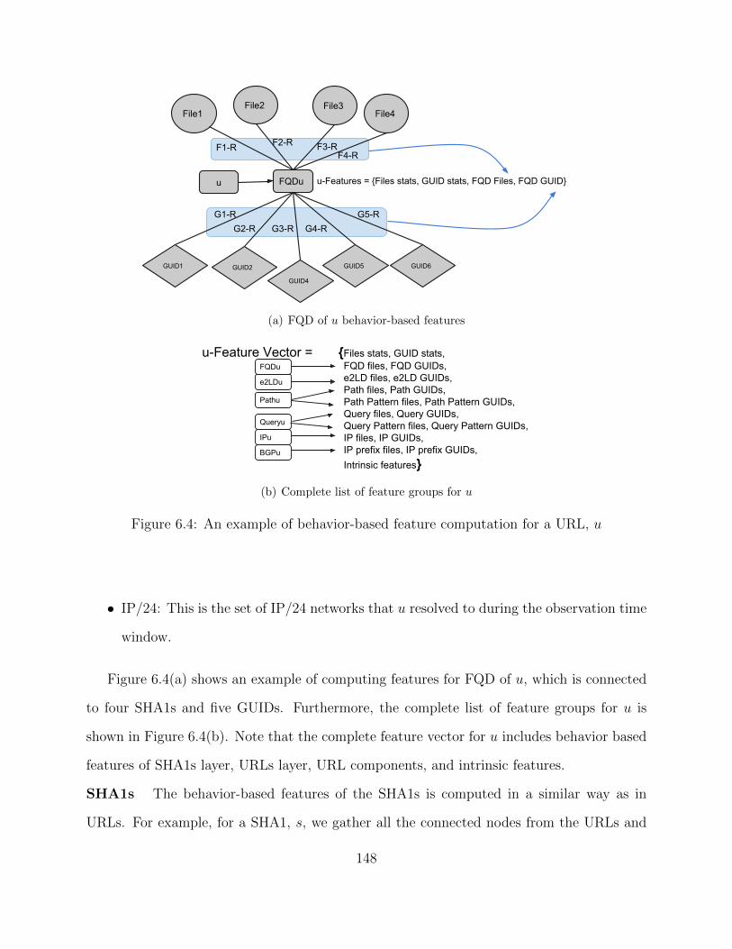
FQDu

File1File2

File4


F1-R F2-RF4-R

G1-RG2-R G4-R

G5-R

u-Features = {Files stats, GUID stats, FQD Files, FQD GUID}u

File3

F3-R

GUID4

G3-R

(a) FQD of u behavior-based features

u-Feature Vector = {Files stats, GUID stats, FQD files, FQD GUIDs, e2LD files, e2LD GUIDs,

Path files, Path GUIDs, Path Pattern files, Path Pattern GUIDs,

Query files, Query GUIDs, Query Pattern files, Query Pattern GUIDs, IP files, IP GUIDs, IP prefix files, IP prefix GUIDs,

Intrinsic features}

Queryu

e2LDu

Pathu

FQDu

IPu

BGPu

(b) Complete list of feature groups for u

Figure 6.4: An example of behavior-based feature computation for a URL, u

• IP/24: This is the set of IP/24 networks that u resolved to during the observation time

window.

Figure 6.4(a) shows an example of computing features for FQD of u, which is connected

to four SHA1s and five GUIDs. Furthermore, the complete list of feature groups for u is

shown in Figure 6.4(b). Note that the complete feature vector for u includes behavior based

features of SHA1s layer, URLs layer, URL components, and intrinsic features.

SHA1s The behavior-based features of the SHA1s is computed in a similar way as in

URLs. For example, for a SHA1, s, we gather all the connected nodes from the URLs and

148

GUID layers to compute the features. Note that the connected nodes from the URLs layer

also include FQDs, e2LDs, paths, path patterns, etc. So part of a SHA1’s, s, behavior-based

features are actually statistics of connected URL components to s. Thus, the components of

the URLs should also have R values, since these reputations will be used to compute SHA1s

behavior-based features. For a given component of a URL, such as path pattern, we average

R of all URLs that share the same component, i.e. the path pattern. Moreover, for those

FQDs and e2LDs that are extremely popular, we override the averaged R with a badness

reputation score of 0.5, indicating that these URL components are most likely not malicious,

but might not be completely benign either. To be conservative with this rule, we sort the

FQDs and e2LDs based on their popularity (the number of unique machines that contact

them) and apply the rule to 99-percentile of the sorted list. That is only 0.01% of FQDs’

and e2LDs’ R will be overridden by a value of 0.5.

6.3 Experimental Setup

6.3.1 The Data

As discussed in Section 6.2.1, our approach is based on download events which are 3-tuples

of <SHA1, URL, GUID>. This data is provided to us through Trend Micro and is collected

by monitoring the download events of customers of Trend Micro. This work is based the

data that is collected from Dec 18, 2013 through Apr 5, 2014. Note that each record in the

data (3-tuples) is also associated with other useful information. The following reports the

details of data for each layer of the download behavior graph which are used to compute the

features:

SHA1 This layer includes the following information.

• SHA1

149

• SHA1 location (this filed is anonymized in our dataset)

• SHA1 name

• SHA1 size

• downloading process SHA1

• downloading process location (this filed is anonymized in our dataset)

• downloading process name

• downloading process size

• prevalence

• first seen

• last seen

• list of countries

• packers

• signers

• first submission

• last submission

• known benign (true/false based on a private whitelist of SHA1s)

• AV labels

• last scan time

URL This layer includes the following information.

• URL

• resolved IP

• prevalence

150

GUID This layer includes the following information.

• GUID

• operating system

each download events also has a timestamp that indicates the time and date of the record.

6.3.2 System Operation

In this section we describe how the behavioral classifiers are trained and how the system

operates. This system is intended to provide real-time classification results for SHA1s and

URLs observed on daily basis. In other words the system automatically classifies any new

items (SHA1 and URL) on the current day harnessing historical knowledge gathered from

the previous days in a time window T . The historical knowledge is, in fact, the augmented

download behavior graph that associates the items of download events together where all

nodes are assigned an R value. We keep a sliding window over all the download events

and set T = 1 −month. That is, the beginning of T is set to a month before the start of

current day, dc, for which we are interested to classify any unknown items using the download

behavior graph that is generated by considering all download events during T .

For any unknown node in dc, we compute its feature vector by following the procedure

described in Section 6.2.4, and feed the feature vector of the unknown item to the related

behavioral classifier, i.e. an unknown SHA1 will be fed to the SHA1s classifier and an un-

known URL will be fed to the URLs classifier. The classifier in return produces a score which

will be compared against a previously learned detection threshold. If the produced score is

above the detection threshold the unknown item will be labeled as malicious. Figure 6.5

shows how does the system operate by keeping a sliding window over all the 3-tuples during

T and using them to generate a download behavior graph and train behavioral classifiers.

151

TimeDay 1 Day 2 Current day (dc)

...Day 30

T (time window)

Trained classifiersURL classifier

SHA1 classifier

Real-timeclassificationofURLs &SHA1

Figure 6.5: System Operation

6.3.3 Training the Classifiers

We train the SHA1 and URL behavioral classifiers using a training dataset of known bad

and good SHA1s and URLs. In order to properly train classifiers to be used for detection

in current day, dc, we use the knowledge from previous days during T in the graph. To this

end, we identify all known bad and good SHA1s and URLs during T and use them to obtain

a labeled training dataset. More specifically, we take every labeled node in the graph, and

compute a feature vector for them. For a labeled node n, we consider all of its download

events during a training time window, Ttr, which starts a month before the last time n was

seen. As a result, for every labeled node in the download behavior graph of time window T ,

a training time window Ttr is considered to compute the features.

152

Computing Behavior-based Features During Training

We need to compute the behavior-based features for SHA1s and URLs fairly that resembles

the real-world operation of the system. Especially, part of the behavior-based features for

SHA1s and URLs are based on R of GUIDs connected to them. However, the R of GUIDs

was computed originally according to the SHA1s and URLs that are connected to GUIDs. As

a result, if we simply use the assigned R of GUIDs to compute the behavior-based features

for the SHA1s and URLs layer during training, we actually unfairly give the classifier an

advantage. To resolve this issue and in order to compute behavior-based features for a labeled

node, n, to be included in the training dataset, we recompute R of the GUIDs connected to

n while pretending we don’t know the true R (hence the label) of n temporarily and replace

the true value of R with 0.5. In this way, the true nature of n will not have any effect on

R of the GUIDs. This replicates the real-world operation of the system when an unknown

node’s R = 0.5 is used to compute reputation of the connected GUIDs. Conservatively, to

compute behavior-based features of a URL, u, we actually hide R of any URLs that share

the same e2LD with u from the connected GUIDs.

6.3.4 Statistics of Download Behavior Graphs

Tables 6.1 and 6.2 summarize some simple statistics related to the download behavior graphs

generated during different Ttr (the last day of Ttr is shown in column “Date”).

Table 6.1: Sample Statistics of Experiment Data - Nodes Info

DateSHA1s URLs GUIDs

Total Benign Malware Total Benign Malware Total Vulnerable CleanFeb 24 355,011 5,637 2,513 308,736 101,777 33,498 288,970 901 66,201Feb 26 352,325 5,732 2,438 306,474 100,495 34,213 287,787 852 63,766Mar 12 310,729 4,775 1,784 271,422 90,050 31,697 252,192 822 64,393

153

Table 6.2: Sample Statistics of Experiment Data - Graph Info

Date Download events EdgesFeb 24 491,761 5,835,537Feb 26 473,344 5,788,903Mar 12 410,703 5,063,351

6.4 Evaluation

We performed numerous experiments to fully evaluate the system. In this section, first we

explain our cross-validation experiment (CV), then we discuss the details of various other

testing scenarios, and finally we report the result of analyzing our features.

6.4.1 Cross-Validation

To perform cross-validation, we pick a date, dtr from the data that marks the end of the

training time window, Ttr. Then we generate a download behavior graph from all the events

with timestamps during Ttr. Finally, we generate a training dataset using all the known nodes

in the graph by following the procedure detailed in Section 6.3.3. The training dataset is

used to perform standard 10-fold CV experiments.

Figure 6.6 shows the result of CV for SHA1s and URLs layer during Ttr ending on Feb

26. We compute the ROC curve by varying the detection threshold on the classifier’s output

scores, the area under the curve (AUC), and the partial AUC (PAUC). Notice that the

PAUC is computed by measuring the area under the ROC curve in a range of false positive

between 0% and 1%, and by normalizing this measure to obtain a value in [0, 1]. In essence,

the PAUC highlights the classifier’s trade-off between true positives (TP) and false positives

(FP) at very low FP rates. In practice, if PAUC is close to 1, it means that the classifier

154

yields close to 100% true positives at low false positive rates. The small table embedded in

the figures reports various points on the ROCs.

0.0 0.2 0.4 0.6 0.8 1.0FP (percentage)

0

20

40

60

80

100

TP (

perc

enta

ge)

POS=7314, NEG=5732AUC=1.000, PAUC=0.969

TP% | FP%--------------------72.09 - 0.0076.26 - 0.0176.26 - 0.0378.86 - 0.0579.68 - 0.0790.85 - 0.1099.26 - 0.5099.63 - 0.7099.95 - 1.00

SHA1 CV 2014-02-26

RandomForest

(a) SHA1s CV

0.0 0.2 0.4 0.6 0.8 1.0FP (percentage)

0

20

40

60

80

100

TP (

perc

enta

ge)

POS=11290, NEG=8039AUC=0.997, PAUC=0.962

TP% | FP%--------------------84.87 - 0.0090.39 - 0.0192.81 - 0.0393.35 - 0.0593.95 - 0.0794.69 - 0.1096.76 - 0.5097.06 - 0.7097.50 - 1.00

URL CV 2014-02-26

RandomForest

(b) URL CV

Figure 6.6: Cross-validation results for SHA1s and URLs layer on Feb 26

155

6.4.2 Train and Test Experiments

In this section we show the evaluation result of system operation as it was discussed in

Section 6.3.2. To this end we have defined a sliding time window, T , which keeps track of all

download events that happened during T . We are interested to use trained classifiers based

on labeled nodes in the download behavior graph during T to enable detection of new and

unknown items on the current day, dc. First, we discuss how do we prepare our training and

test datasets and then present the results.

Training and Test Datasets

The training dataset is generated in a same manner as the training dataset that is used in

Section 6.4.1, in which all known nodes during T in the graph will be used for training the

behavioral classifiers. To prepare the test datasets and to replicate the real-world operation

of the system we proceed as follows. We consider the labeled nodes on dc that were not

present during T for evaluating the classifiers. This ensures that no information regarding

the test samples were ever used during training and properly simulates the operative mode

of the system where we are only interested to label new and unknown nodes on dc. We

prepare three different test datasets using the labeled nodes on dc as follows:

New items (Itst) These are labeled nodes that only appear on dc and not during T .

New events (Etst) These are labeled nodes that are subset of Itst and are part of download

events where none of the three entities of the download events were seen during T .

New unknown events (UEtst) These are labeled nodes that are subset of Etst and are

part of download events where all the entities of the download event are unknown,

except, of course, the labeled node that is used for testing purposes.

156

Train and Test Evaluation Results

We perform train and test experiments to evaluate the generalization capabilities of our

behavioral classifiers. First, we create the three test datasets, Itst, Etst, UEtst, for SHA1s

and URLs in the download behavior graph. Then we evaluate the performance of our trained

classifiers on the test datasets.

Figures 6.7, 6.8, and 6.9 show the result of train and test on Feb 25 (one day after the

CV experiments) for SHA1s and URLs using Itst, Etst, and UEtst datasets.

6.4.3 Early Detection of Malwares

We also performed experiments to measure how early the system can detect malware binaries,

compared to antivirus softwares. To this end, we trained a SHA1 classifier and used it to

label all files that were unknown to antivirus companies on Feb 27 but later on received a

label. Finally, we evaluated the performance of our system on these files. Figure 6.10 shows

the result of this experiment.

6.5 Conclusion

In this paper, we presented a novel system that is able of efficiently detecting new malware

files and malicious URLs by passively monitoring the download events of users of a famous

antivirus company. We developed a proof-of-concept prototype of the system and evaluated

it using real-world data. Our evaluation results show that the system can detect malware

files and malicious URLs while only incurring less than 1% false positives, respectively. In

addition, we showed that the system can detect unknown files many days before they are

labeled by antivirus companies.

157

0.0 0.2 0.4 0.6 0.8 1.0FP (percentage)

0

20

40

60

80

100

TP (

perc

enta

ge)

POS=30, NEG=114AUC=0.997, PAUC=0.823

TP% | FP%--------------------76.67 - 0.0076.67 - 0.0176.67 - 0.0376.67 - 0.0576.67 - 0.0776.67 - 0.1086.67 - 0.5086.67 - 0.7086.67 - 1.00

SHA1s

RandomForest

(a) SHA1s

0.0 0.2 0.4 0.6 0.8 1.0FP (percentage)

0

20

40

60

80

100

TP (

perc

enta

ge)

POS=1988, NEG=2894AUC=0.993, PAUC=0.940

TP% | FP%--------------------79.12 - 0.0079.12 - 0.0179.83 - 0.0379.83 - 0.0581.09 - 0.0787.63 - 0.1096.53 - 0.5096.68 - 0.7096.98 - 1.00

URLs

RandomForest

(b) URL

Figure 6.7: Train and test experiment on Feb 26 for SHA1s and URLs using Itst

158

0.0 0.2 0.4 0.6 0.8 1.0FP (percentage)

0

20

40

60

80

100

TP (

perc

enta

ge)

POS=20, NEG=88AUC=1.000, PAUC=1.000

TP% | FP%--------------------100.00 - 0.00100.00 - 0.01100.00 - 0.03100.00 - 0.05100.00 - 0.07100.00 - 0.10100.00 - 0.50100.00 - 0.70100.00 - 1.00

SHA1s

RandomForest

(a) SHA1s

0.0 0.2 0.4 0.6 0.8 1.0FP (percentage)

0

20

40

60

80

100

TP (

perc

enta

ge)

POS=1325, NEG=1420AUC=0.994, PAUC=0.947

TP% | FP%--------------------82.49 - 0.0082.49 - 0.0182.49 - 0.0383.70 - 0.0583.70 - 0.0783.70 - 0.1097.74 - 0.5098.04 - 0.7098.11 - 1.00

URLs

RandomForest

(b) URL

Figure 6.8: Train and test experiment on Feb 26 for SHA1s and URLs using Etst

159

0.0 0.2 0.4 0.6 0.8 1.0FP (percentage)

0

20

40

60

80

100

TP (

perc

enta

ge)

POS=1, NEG=56AUC=1.000, PAUC=1.000

TP% | FP%--------------------100.00 - 0.00100.00 - 0.01100.00 - 0.03100.00 - 0.05100.00 - 0.07100.00 - 0.10100.00 - 0.50100.00 - 0.70100.00 - 1.00

SHA1s

RandomForest

(a) SHA1s

0.0 0.2 0.4 0.6 0.8 1.0FP (percentage)

0

20

40

60

80

100

TP (

perc

enta

ge)

POS=33, NEG=1356AUC=0.984, PAUC=0.884

TP% | FP%--------------------54.55 - 0.0054.55 - 0.0154.55 - 0.0357.58 - 0.0557.58 - 0.0757.58 - 0.1093.94 - 0.5093.94 - 0.7093.94 - 1.00

URLs

RandomForest

(b) URL

Figure 6.9: Train and test experiment on Feb 26 for SHA1s and URLs using UEtst

160

0.0 0.2 0.4 0.6 0.8 1.0FP (percentage)

0

20

40

60

80

100

TP (

perc

enta

ge)

POS=14, NEG=21AUC=1.000, PAUC=1.000

TP% | FP%--------------------100.00 - 0.00100.00 - 0.01100.00 - 0.03100.00 - 0.05100.00 - 0.07100.00 - 0.10100.00 - 0.50100.00 - 0.70100.00 - 1.00

Unknown SHA1s to AVs on 2014-02-27

RandomForest

Figure 6.10: Early Detection of Malwares

161

CHAPTER 7

CONCLUSION

In this dissertation we focused on detection and analysis of advanced cyber threats. Various

novel research studies were conducted to help us better understand how Internet miscreants

manage their malicious infrastructures. These projects also provide us with state-of-the-art

detection technologies to protect our networks against the cyber attacks. Behavioral analysis

and detection of these threats was the main focus of our work. More specifically, PeerRush

was presented in Chapter 2 where we introduced a novel system for the identification of

unwanted P2P traffic. We showed that PeerRush can accurately categorize P2P traffic

and attribute it to specific P2P applications, including malicious applications such as P2P

botnets. PeerRush achieves these results without the need of deep packet inspection, and can

accurately identify applications that use encrypted P2P traffic. We implemented a prototype

version of PeerRush and performed an extensive evaluation of the system over a variety of

P2P traffic datasets. Our results show that PeerRush can detect all the considered types of

P2P traffic with up to 99.5% true positives and 0.1% false positives. Furthermore, PeerRush

can attribute the P2P traffic to a specific P2P application with a misclassification rate of

0.68% or less.

In an attempt to understand how botmasters manage their botnets, in Chapter 3, we

studied the lifetime traits of C&C servers in terms of their individual life cycles as well as

analyzing their overall lifetime trends by considering groups of C&C domains. Using our

162

historic DNS data and by employing Hadoop, we showed the type of botnets that existed

in the wild. A clustering scheme, based on DTW for aligning C&C domains time series

and hierarchical clustering, was discussed that provides a mean for grouping C&C domains

together based on the similarity of their lifetime trends.

Our findings and new results in Chapter 3 led to another project which aims to demys-

tify the afterlife of C&C servers, i.e. when they die. As a result, in Chapter 4 we presented

SinkMiner, a novel system for the identification of previously unknown and secretive sinkhole

IPs that utilizes a large dataset of historic DNS information. We also discussed the advan-

tages and disadvantages that finding sinkholes could present. While some of the use cases

we discussed are beneficial, some are malicious. Numerous approaches were also introduced

to detect sinkholes IPs. To evaluate the system, we generated a large graph database of IP

transitions associated with malicious domains, and showed SinkMiner could mark sinkhole

IPs with high confidence and no false positives.

After analyzing the C&C domains characteristics in the previous two chapters, we turned

our attention towards detecting C&C servers while they are active to be able to track the

relocations of these domains and identify the ones that were unknown previously. So we

introduced Segugio, a novel defense system that is able of efficiently discover new malware-

control domain names by passively monitoring the DNS traffic of large ISP networks. Segugio

monitors who is querying what to build a machine-domain bipartite graph. First, we label

some of the nodes in the graph using prior knowledge of benign and malware-control do-

mains names (e.g., domain whitelists and C&C domain blacklists). Then, Segugio applies a

novel belief propagation strategy to accurately detect previously unknown malware-control

domains. We deployed Segugio in three large ISP networks, and we showed that Segugio

can achieve a true positive rate above 94% at less than 0.1% false positives. In addition,

we showed that Segugio can detect control domains related to previously unseen malware

families, and that it outperforms Notos [7], a recently proposed domain reputation systems.

163

REFERENCES

[1] AutoIt. http://www.autoitscript.com/site/autoit/.

[2] Botnets. http://www.microsoft.com/security/resources/botnet-whatis.aspx.

[3] Google Safe Browsing API. https://developers.google.com/safe-browsing/.

[4] Hadoop streaming. http://hadoop.apache.org/docs/r1.1.2/streaming.html.

[5] hcluster. https://pypi.python.org/pypi/hcluster.

[6] Snort. http://www.snort.org.

[7] M. Antonakakis, R. Perdisci, D. Dagon, W. Lee, and N. Feamster. Building a dynamic

reputation system for dns. In Proceedings of the 19th USENIX conference on Security,

USENIX Security’10, 2010.

[8] M. Antonakakis, R. Perdisci, W. Lee, N. Vasiloglou, II, and D. Dagon. Detecting

malware domains at the upper dns hierarchy. In Proceedings of the 20th USENIX

conference on Security, SEC’11, 2011.

[9] M. Antonakakis, R. Perdisci, Y. Nadji, N. Vasiloglou, S. Abu-Nimeh, W. Lee, and

D. Dagon. From throw-away traffic to bots: detecting the rise of dga-based malware. In

Proceedings of the 21st USENIX conference on Security symposium, Security’12, pages

24–24, Berkeley, CA, USA, 2012. USENIX Association.

164

[10] M. Barreno, B. Nelson, R. Sears, A. D. Joseph, and J. D. Tygar. Can machine learning

be secure? In Proceedings of the 2006 ACM Symposium on Information, Computer

and Communications Security, ASIACCS ’06, pages 16–25, New York, NY, USA, 2006.

ACM.

[11] D. J. Berndt and J. Clifford. Using dynamic time warping to find patterns in time

series. In KDD workshop, volume 10, pages 359–370. Seattle, WA, 1994.

[12] L. Bilge, E. Kirda, C. Kruegel, and M. Balduzzi. Exposure: Finding malicious domains

using passive dns analysis. In NDSS. The Internet Society, 2011.

[13] L. Breiman. Random forests. Machine learning, 45(1):5–32, 2001.

[14] G. Bruneau. DNS sinkhole, 2010. http://www.sans.org/reading_room/

whitepapers/dns/dns-sinkhole_33523.

[15] J. Buford, H. Yu, and E. K. Lua. P2P Networking and Applications. Morgan Kaufmann

Publishers Inc., 2008.

[16] D. Chau, C. Nachenberg, J. Willhelm, A. Wright, and C. Faloutsos. Polonium: Tera-

scale graph mining and inference for malware detection. Proccedings of SIAM Interna-

tional Conference on Data Mining (SDM), pages 131–142, 2011.

[17] B. Coskun, S. Dietrich, and N. Memon. Friends of an enemy: identifying local mem-

bers of peer-to-peer botnets using mutual contacts. In Proceedings of the 26th Annual

Computer Security Applications Conference, pages 131–140. ACM, 2010.

[18] D. Dagon, G. Gu, and C. P. Lee. A taxonomy of botnet structures. In Botnet detection,

pages 143–164. Springer, 2008.

[19] G. E. Dahl, J. W. Stokes, L. Deng, and D. Yu. Large-scale malware classification using

random projections and neural networks. In ICASSP, pages 3422–3426. IEEE, 2013.

165

[20] M. Egele, T. Scholte, E. Kirda, and C. Kruegel. A survey on automated dynamic

malware-analysis techniques and tools. ACM Comput. Surv., 44(2):6:1–6:42, Mar. 2008.

[21] R.-E. Fan, K.-W. Chang, C.-J. Hsieh, X.-R. Wang, and C.-J. Lin. Liblinear: A library

for large linear classification. The Journal of Machine Learning Research, 9:1871–1874,

2008.

[22] M. Felegyhazi, C. Kreibich, and V. Paxson. On the potential of proactive domain

blacklisting. In In Proceedings of the Third USENIX Workshop on Large-scale Exploits

and Emergent Threats (LEET), 2010.

[23] E. M. Flanagan. No free parking: Obtaining relief from trademark-infringing domain

name parking. Minn. L. Rev., 92:498–1966, 2007.

[24] J. V. Gomes, P. R. M. Inacio, M. Pereira, M. M. Freire, and P. P. Monteiro. Detection

and classification of peer-to-peer traffic: A survey. ACM Computing Surveys, 2012.

[25] G. Gu, R. Perdisci, J. Zhang, and W. Lee. Botminer: Clustering analysis of network

traffic for protocol- and structure-independent botnet detection. In Proceedings of the

17th conference on Usenix Security Symposium, SS’08, 2008.

[26] G. Gu, R. Perdisci, J. Zhang, W. Lee, et al. Botminer: Clustering analysis of network

traffic for protocol-and structure-independent botnet detection. In Proceedings of the

17th conference on Security symposium, pages 139–154, 2008.

[27] G. Gu, P. Porras, V. Yegneswaran, M. Fong, and W. Lee. Bothunter: detecting malware

infection through ids-driven dialog correlation. In Proceedings of 16th USENIX Security

Symposium on USENIX Security Symposium, SS’07, pages 12:1–12:16, Berkeley, CA,

USA, 2007. USENIX Association.

166

[28] G. Gu, J. Zhang, and W. Lee. BotSniffer: Detecting botnet command and control

channels in network traffic. In Proceedings of the 15th Annual Network and Distributed

System Security Symposium (NDSS’08), February 2008.

[29] H. Hang, X. Wei, M. Faloutsos, and T. Eliassi-Rad. Entelecheia: Detecting p2p botnets

in their waiting stage. In IFIP Networking Conference, 2013, pages 1–9. IEEE, 2013.

[30] I. U. Haq, S. Ali, H. Khan, and S. A. Khayam. What is the impact of P2P traffic on

anomaly detection? In 13th International Conference on Recent Advances in Intrusion

Detection, RAID’10, 2010.

[31] B. Hayes. Skype: A practical security analysis. http://www.sans.org/reading_room/

whitepapers/voip/skype-practical-security-analysis_32918.

[32] T. Holz, M. Steiner, F. Dahl, E. Biersack, and F. Freiling. Measurements and mitigation

of peer-to-peer-based botnets: a case study on storm worm. In Proceedings of the 1st

Usenix Workshop on Large-Scale Exploits and Emergent Threats, LEET’08, 2008.

[33] X. Hu, T.-c. Chiueh, and K. G. Shin. Large-scale malware indexing using function-call

graphs. In Proceedings of the 16th ACM Conference on Computer and Communications

Security, CCS ’09, pages 611–620, New York, NY, USA, 2009. ACM.

[34] Y. Hu, D.-M. Chiu, and J. C. S. Lui. Profiling and identification of P2P traffic. Comput.

Netw., 53(6):849–863, Apr. 2009.

[35] J. S. Hunter. The exponentially weighted moving average. J. QUALITY TECHNOL.,

18(4):203–210, 1986.

[36] ICANN. Request for Information - Uniform Rapid Suspension System. https://www.

icann.org/en/news/rfps/urs-24sep12-en.pdf, September 2012.

167

[37] L. Invernizzi, S. Miskovic, R. Torres, S. Saha, S.-J. Lee, C. Kruegel, and G. Vigna.

Nazca: Detecting Malware Distribution in Large-Scale Networks. In Proceedings of the

ISOC Network and Distributed System Security Symposium (NDSS ’14), Feb 2014.

[38] G. Jacob, R. Hund, C. Kruegel, and T. Holz. Jackstraws: picking command and control

connections from bot traffic. In Proceedings of the 20th USENIX conference on Security,

Berkeley, CA, USA, 2011.

[39] S. C. Johnson. Hierarchical clustering schemes. Psychometrika, 32(3):241–254, 1967.

[40] T. Karagiannis, A. Broido, M. Faloutsos, and K. Claffy. Transport layer identifica-

tion of p2p traffic. In Proceedings of the 4th ACM SIGCOMM conference on Internet

measurement, IMC ’04, 2004.

[41] T. Karagiannis, K. Papagiannaki, and M. Faloutsos. Blinc: multilevel traffic classifica-

tion in the dark. SIGCOMM Comput. Commun. Rev., 35(4), aug 2005.

[42] T. Karagiannis, K. Papagiannaki, and M. Faloutsos. Blinc: Multilevel traffic classifica-

tion in the dark. In Proceedings of the 2005 Conference on Applications, Technologies,

Architectures, and Protocols for Computer Communications, SIGCOMM ’05, pages 229–

240, New York, NY, USA, 2005. ACM.

[43] D. Kollar and N. Friedman. Probabilistic graphical models: principles and techniques.

The MIT Press, 2009.

[44] J. Z. Kolter and M. A. Maloof. Learning to detect and classify malicious executables in

the wild. J. Mach. Learn. Res., 7:2721–2744, Dec. 2006.

[45] L. I. Kuncheva. Combining Pattern Classifiers: Methods and Algorithms. Wiley-

Interscience, 2004.

168

[46] A. Lelli. Zeusbot/spyeye p2p updated, fortifying the botnet. http://www.symantec.

com/connect/blogs/zeusbotspyeye-p2p-updated-fortifying-botnet.

[47] L. Li, S. Mathur, and B. Coskun. Gangs of the internet: Towards automatic discovery

of peer-to-peer communities. In Communications and Network Security (CNS), 2013

IEEE Conference on, pages 64–72. IEEE, 2013.

[48] Y. Low, J. Gonzalez, A. Kyrola, D. Bickson, C. Guestrin, and J. M. Hellerstein.

Graphlab: A new parallel framework for machine learning. In Conference on Uncer-

tainty in Artificial Intelligence (UAI), Catalina Island, California, July 2010.

[49] A. Madhukar and C. Williamson. A longitudinal study of p2p traffic classification.

In Proceedings of the 14th IEEE International Symposium on Modeling, Analysis, and

Simulation, MASCOTS ’06, 2006.

[50] P. Manadhata, S. Yadav, P. Rao, and W. Horne. Detecting malicious domains via graph

inference. In M. Kutylowski and J. Vaidya, editors, Computer Security - ESORICS 2014,

volume 8712 of Lecture Notes in Computer Science, pages 1–18. Springer International

Publishing, 2014.

[51] H. M. Moghaddam, M. D. B. Li, and I. Goldberg. SkypeMorph: Protocol obfuscation

for tor bridges. Tech. Report CACR 2012-08.

[52] S. Nagaraja, P. Mittal, C.-Y. Hong, M. Caesar, and N. Borisov. Botgrep: finding p2p

bots with structured graph analysis. In Proceedings of the 19th USENIX conference on

Security, USENIX Security’10, 2010.

[53] T. Nelms, R. Perdisci, and M. Ahamad. Execscent: mining for new c&c domains in live

networks with adaptive control protocol templates. In Proceedings of the 22nd USENIX

conference on Security, pages 589–604. USENIX Association, 2013.

169

[54] M. G. Noll. Writing an hadoop mapreduce pro-

gram in python. http://www.michael-noll.com/tutorials/

writing-an-hadoop-mapreduce-program-in-python/.

[55] C. Nunnery, G. Sinclair, and B. B. Kang. Tumbling down the rabbit hole: exploring the

idiosyncrasies of botmaster systems in a multi-tier botnet infrastructure. In Proceedings

of the 3rd USENIX conference on Large-scale exploits and emergent threats: botnets,

spyware, worms, and more, LEET’10, 2010.

[56] R. Perdisci, W. Lee, and N. Feamster. Behavioral clustering of http-based malware and

signature generation using malicious network traces. In Proceedings of the 7th USENIX

conference on Networked systems design and implementation, NSDI’10, 2010.

[57] M. Z. Rafique and J. Caballero. FIRMA: Malware Clustering and Network Signature

Generation with Mixed Network Behaviors. In Proceedings of the 16th International

Symposium on Research in Attacks, Intrusions and Defenses, St. Lucia, October 2013.

[58] B. Rahbarinia, R. Perdisci, A. Lanzi, and K. Li. PeerRush: mining for unwanted P2P

traffic. In DIMVA 2013, 10th International Conference on Detection of Intrusions and

Malware, and Vulnerability Assessment, July 17-19, 2013, Berlin, Germany / Also

published in LNCS 7967/2013, Berlin, GERMANY, 07 2013.

[59] M. A. Rajab, L. Ballard, N. Lutz, P. Mavrommatis, and N. Provos. CAMP: content-

agnostic malware protection. In 20th Annual Network and Distributed System Security

Symposium, NDSS 2013, San Diego, California, USA, February 24-27, 2013, 2013.

[60] M. Rehak, M. Pechoucek, M. Grill, and K. Bartos. Trust-based classifier combination

for network anomaly detection. In Proceedings of the 12th International Workshop on

Cooperative Information Agents XII, CIA ’08, pages 116–130, Berlin, Heidelberg, 2008.

Springer-Verlag.

170

[61] K. Rieck, P. Trinius, C. Willems, and T. Holz. Automatic analysis of malware behavior

using machine learning. J. Comput. Secur., 19(4):639–668, Dec. 2011.

[62] K. Sato, K. Ishibashi, T. Toyono, and N. Miyake. Extending black domain name list

by using co-occurrence relation between dns queries. In LEET, 2010.

[63] S. Sen, O. Spatscheck, and D. Wang. Accurate, scalable in-network identification of p2p

traffic using application signatures. In Proceedings of the 13th international conference

on World Wide Web, WWW ’04, 2004.

[64] R. Sommer and V. Paxson. Outside the closed world: On using machine learning for

network intrusion detection. In In Proceedings of the IEEE Symposium on Security and

Privacy, 2010.

[65] D. Stutzbach and R. Rejaie. Understanding churn in peer-to-peer networks. In Pro-

ceedings of the 6th ACM SIGCOMM conference on Internet measurement, IMC ’06,

2006.

[66] Symantec. 2013 internet security threat report, volume 18.

[67] Symantec. India sees 280 percent increase in bot infections, 2013. http://www.

symantec.com/en/in/about/news/release/article.jsp?prid=20130428_01.

[68] D. Tax. DDtools, the data description toolbox for Matlab. v1.9.1 http://prlab.

tudelft.nl/david-tax/dd_tools.html.

[69] D. Tax. One-class classification. 2001. Ph.D. Thesis, TU Delft.

[70] P. Vadrevu, B. Rahbarinia, R. Perdisci, K. Li, and M. Antonakakis. Measuring and

detecting malware downloads in live network traffic. In J. Crampton, S. Jajodia, and

K. Mayes, editors, Computer Security ESORICS 2013, volume 8134 of Lecture Notes in

Computer Science, pages 556–573. Springer Berlin Heidelberg, 2013.

171

[71] N. Weaver, C. Kreibich, and V. Paxson. Redirecting dns for ads and profit. In USENIX

Workshop on Free and Open Communications on the Internet (FOCI), San Francisco,

CA, USA (August 2011), 2011.

[72] Weka. Weka 3: Data mining software in java. http://www.cs.waikato.ac.nz/ml/

weka/.

[73] H.-S. Wu, N.-F. Huang, and G.-H. Lin. Identifying the use of data/voice/video-based

p2p traffic by dns-query behavior. In Proceedings of the 2009 IEEE international con-

ference on Communications, ICC’09, 2009.

[74] P. Wurzinger, L. Bilge, T. Holz, J. Goebel, C. Kruegel, and E. Kirda. Automatically

generating models for botnet detection. In Proceedings of the 14th European conference

on Research in computer security, ESORICS’09, 2009.

[75] K. Xu, F. Wang, and L. Gu. Network-aware behavior clustering of internet end hosts.

In in Proceedings of IEEE INFOCOM, 2011.

[76] T.-F. Yen and M. K. Reiter. Are your hosts trading or plotting? telling p2p file-sharing

and bots apart. In Proceedings of the 2010 IEEE 30th International Conference on

Distributed Computing Systems, ICDCS ’10, 2010.

[77] J. Zhang, R. Perdisci, W. Lee, U. Sarfraz, and X. Luo. Detecting stealthy P2P bot-

nets using statistical traffic fingerprints. In Proceedings of the 2011 IEEE/IFIP 41st

International Conference on Dependable Systems&Networks, DSN ’11, 2011.

[78] J. Zhang, R. Perdisci, W. Lee, U. Sarfraz, and X. Luo. Detecting stealthy p2p bot-

nets using statistical traffic fingerprints. In Proceedings of the 2011 IEEE/IFIP 41st

International Conference on Dependable Systems&Networks, DSN ’11, 2011.

172

[79] V. Zorkadis, D. A. Karras, and M. Panayotou. 2005 special issue: Efficient information

theoretic strategies for classifier combination, feature extraction and performance eval-

uation in improving false positives and false negatives for spam e-mail filtering. Neural

Netw., 18(5-6):799–807, June 2005.

173

Behavioral Analysis of Network Traffic for Detecting - GETD

Documents

Transcript of Behavioral Analysis of Network Traffic for Detecting - GETD