BEAM SEARCH ALGORITHMS FOR THE MIXED-MODEL ...

BEAM SEARCH ALGORITHMS FOR THE MIXED-MODEL

ASSEMBLY LINE SEQUENCING PROBLEM

A THESIS

SUBMITTED TO THE DEPARTMENT OF INDUSTRIAL ENGINEERING

AND THE INSTITUTE OF ENGINEERING AND SCIENCE

OF BILKENT UNIVERSITY

IN PARTIAL FULFILLMENT OF THE REQUIREMENTS

FOR THE DEGREE OF

MASTER OF SCIENCE

By

Yasin Göçgün

July, 2005

ii

I certify that I have read this thesis and that in my opinion it is fully adequate, in scope

and in quality, as a thesis for the degree of Master of Science.

Prof. İhsan Sabuncuoğlu (Principal Advisor)



Prof. Erdal Erel



Asst. Prof. Ayşegül Toptal

Approved for the Institute of Engineering and Science:

Prof. Mehmet Baray

Director of Institute of Engineering and Science

iii

Abstract

BEAM SEARCH ALGORITHMS FOR THE MIXED-MODEL ASSEMBLY LINE SEQUENCING PROBLEM

Yasin Göçgün

M.S. in Industrial Engineering

Supervisor: Prof. İhsan Sabuncuoğlu

July 2005

In this thesis, we study the mixed-model assembly line sequencing problem that

considers the following objectives: 1) leveling the part usage, and 2) leveling

workload on the final assembly line. We propose Beam Search algorithms for this

problem. Unlike the traditional Beam Search, the proposed algorithms have

information exchange and backtracking capabilities. The performances of the

proposed algorithms are compared with those of the heuristics in the literature. The

results indicate that the proposed methods generally outperform the existing

heuristics. A comprehensive bibliography is also provided in this study.

Keywords: Mixed-model assembly line sequencing, Beam Search

iv

Özet

KARIŞIK MODELLİ MONTAJ HATTI SIRALAMA PROBLEMİ İÇİN IŞIN

TARAMASI ALGORİTMALARI

Yasin Göçgün

Endüstri Mühendisliği Yüksek Lisans

Tez Yöneticisi: Prof. İhsan Sabuncuoğlu

Temmuz 2005

Bu tezde, şu belirtilen amaçları göz önüne alan karışık modelli montaj hattı

sıralama problemini incelemekteyiz: son montaj hattı üzerinde 1) parça kullanımı

ve 2) iş yükü dengelenmesi. Bu problem için Işın Taraması algoritmaları

önermekteyiz. Geleneksel Işın Tarama yönteminden farklı olarak, önerilen

algoritmalar bilgi değiştirme ve geri izleme yeteneğine sahiptir. Önerilen

algoritmaların performansları literatürdeki sezgisel yöntemlerinki ile

karşılaştırılmıştır. Sonuçlar, önerilen yöntemlerin halihazırdaki yöntemlerden

genelde üstün olduğunu göstermektedir. Bu çalışmada ayrıca ayrıntılı bir kaynakça

verilmektedir.

Anahtar Kelimeler: Karışık modelli montaj hattı sıralama, Işın Taraması

v

To my family,

vi

Acknowledgement

I would like to express my sincere gratitude to Prof. İhsan Sabuncuoğlu and Prof. Erdal Erel for their instructive comments and encouragements in this thesis work. I believe that their valuable suggestions in the supervision of the thesis will guide me throughout all my academic life.

I am also indebted to Asst. Prof. Ayşegül Toptal for accepting to review this thesis, and her useful comments and suggestions.

I would like to express my special thanks to Sefa Erenay for his encouragements, friendship, and for sharing his technical knowledge with me.

I would also like to thank to Evren Körpeoğlu, Murat Kalaycılar, Utku Koç, Oğuz Şöhret, Çağrı Latifoğlu, İ. Esra Büyüktahtakın, Önder Bulut, Kaya Sevindik, Zümbül Bulut, M. Mustafa Tanrıkulu, Fazıl Paç, and all my friends for their morale support during my graduate study.

Finally, I would like to express my deepest gratitude to my family for their understanding and patience during my graduate life.

vii

CONTENTS

CHAPTER 1 ........................................................................................…………. … 1

INTRODUCTION ...................................................................................….….. … 1

1.1.Background ...................................................................................…………. 2

1.2. Statement of the problem ………………………………………………… 4

1.3. Contribution ……………………………………………………………… 5

1.4. Thesis outline ………………………………………………….…………. 6

CHAPTER 2 …………………………………………………………………….. 7

LITERATURE REVIEW …………………………………………….………… 7

2.1. MMAL sequencing problem ……………………………………………... 7

2.1.1. The MMAL problem with single objective ............................................ 8

2.1.2. The MMAL problem with multiple objectives ...................................... 13

2.2. Beam search techniques ................................................................................ 21

2.3. Summary of the literature and research motivation ..................................... 24

CHAPTER 3 ............................................................................................................ 26

PROBLEM FORMULATION AND EXISTING HEURISTICS ..................... 26

3.1. Problem formulation ..................................................................................... 26

3.1.1. The parts usage problem ......................................................................... 26

3.1.2. The load leveling problem ...................................................................... 28

3.2. Heuristics ....................................................................................................... 31

3.2.1. Goal Chasing Method ............................................................................. 31

viii

3.2.2. 2-step Heuristic ...................................................................................... 32

3.2.3. Variance Method ................................................................................... 32

3.2.4. 2-step-variance Method ......................................................................... 34

3.2.5. Beam Search Method ............................................................................. 34

3.2.6. Performance of the heuristics .................................................................. 35

CHAPTER 4 .............................................................................................................. 36

PROPOSED ALGORITHM ................................................................................... 36

4.1. Structure of beam search .............................................................................. 36

4.2. Proposed Beam search Method ................................................................... 37

4.2.1. Backtracking procedure ............................................................................. 40

4.2.1.1. Equivalency Theorem ......................................................................... 41

4.2.2. Exchange of Information (EOI) procedure ............................................... 44

4.2.3. Global evaluation ....................................................................................... 47

4.2.4. Different versions of the proposed method ............................................... 50

CHAPTER 5 .............................................................................................................. 57

COMPUTATIONAL RESULTS ............................................................................ 57

5.1. The evaluation of the proposed algorithm .................................................... 57

5.1.1. Computational results for the parts usage measure ................................ 58

5.1.1.1. Experimental conditions .................................................................. 58

5.1.1.2. Results of the comparison study .................................................... .. 60

5.1.1.2.1. Comparison of the CPU time requirements ............................... 60

ix

5.1.1.2.2. Comparison ............................................................................ 61

5.1.2. The computational results for the loading problem ........................... 62

5.1.2.1. Experimental conditions ............................................................... 62

5.1.2.2. Results ........................................................................................... 69

5.2. The effect of backtracking and EOI on solution quality ........................... 69

5.2.1. The effect of backtracking .................................................................... 69

5.2.2. The effect of EOI .................................................................................. 71

5.3. The effect of EOI at different positions ...................................................... 72

CHAPTER 6 ............................................................................................................. 78

CONCLUSION ......................................................................................................... 78

BIBLIOGRAPHY ..................................................................................................... 80

APPENDIX .............................................................................................................. 87

x

LIST OF FIGURES

FIGURE 1: MIXED-MODEL MULTI-LEVEL PRODUCTION SYSTEM ......... 3

FIGURE 2: THE FLOW OF PRODUCTION IN MIXED-MODEL ASSEMBLY

LINES ...................................................................................................................... 3

FIGURE 3: REPRESENTATION OF A BS TREE .............................................. 37

FIGURE 4: THE SCHEMATIC VIEW OF BACKTRACKING PROCEDURE ... 43

FIGURE 5: THE SCHEMATIC VIEW OF EOI ................................................... 46

FIGURE 6: THE ILLUSTRATION OF SEVERAL STEPS OF THE HEURISTIC

USED IN GLOBAL EVALUATION .................................................................. 49

FIGURE 7: DIFFERENT VERSIONS OF THE PROPOSED ALGORITHM .... 51

FIGURE 8: THE BS TREE OBTAINED BY IMPLEMENTING BS-1 .............. 54

FIGURE 9: THE BACKTRACKING PROCEDURE INVOKED IN THE

IMPLEMENTATION OF BS-4 .......................................................................... 55

FIGURE 10: THE EOI PROCEDURE IN THE IMPLEMENTATION OF BS-4 ... 56

FIGURE 11: THE EFFECT OF EOI ON THE PERFORMANCE MEASURE

WHEN NUMBER OF LEVELS IS 20 ………………………………………… 74

FIGURE 12: THE EFFECT OF INFORMATION EXCHANGE ON THE

PERFORMANCE MEASURE WHEN NUMBER OF LEVELS IS INCREASED

TO 260 ................................................................................................................... 76

xi

LIST OF TABLES

Table 1: The summary of research on MMAL sequencing problem ....................... 19

Table 2: The part structure used for the example problem ....................................... 52

Table 3: Experimental factors and their levels used in the comparison ………. 59

Table 4: Demand pattern for the newly generated problems …………………. 59

Table 5: Demand pattern for the example problem …………………………… 60

Table 6: The comparison of the algorithms in terms of computational effort …. 61

Table 7: The computational results obtained by the data sets in given in the

literature …………………………………………………………………… 63

Table 8: The computational results obtained by the newly generated data sets … 66

Table 9: Experimental factors and their levels for the loading problem ……… 68

Table 10: Demand pattern for the newly generated problems ……………….. 68

Table 11: The computational results for the loading problem ……………….. 70

Table 12: The effect of backtracking on the solution quality ………………… 71

Table 13: The effect of exchange of information on the solution quality ……. 72

Table A.1: Number of each part required for each product ………………….. 87

Table A2: Demand vector for products ………………………………………. 90

1

Chap t e r 1

INTRODUCTION

An assembly line consists of a sequence of stations performing a specified set

of tasks repeatedly on consecutive items moving along the line (Erel et al. 2005).

The development of the first assembly line is credited to Henry Ford in 1913.

Since the early times of Henry Ford, several advancements took place that

changed assembly lines from single-model lines to more flexible systems such as

lines with parallel stations, and customer-oriented mixed-model lines.

In today’s business environment, many industries have to cope with the trend

of diversification of customer demand which requires an increasing variety of

products. Many repetitive manufacturers that used to produce single items via

mass production now have to produce more variety of products on a single

assembly line. Hence, many companies have been using mixed-model assembly

lines (MMALs). This is because, mixed-model lines can assemble a variety of

related products in very small quantities without a changeover delay. In this way,

the companies can respond quickly to changes in market demand and avoid large

inventories of specific product models.

Below, background for the mixed-model lines, statement of the problem,

contribution of this study, and thesis outline are given.

2

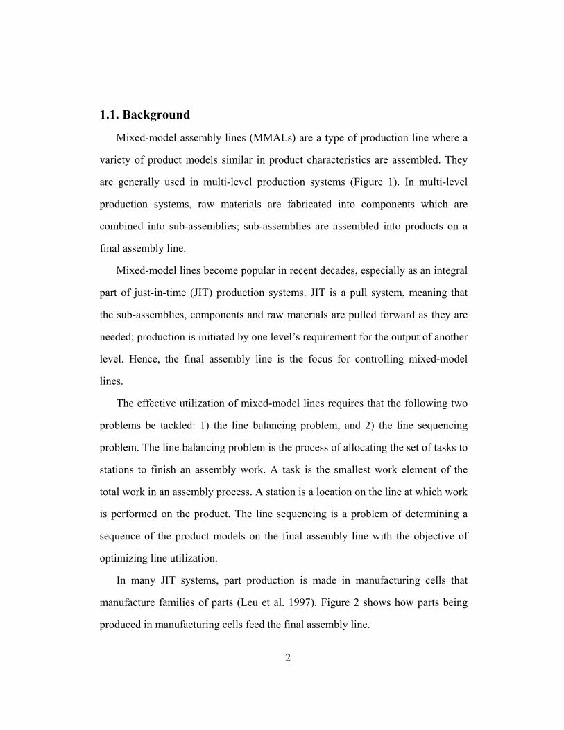
1.1. Background

Mixed-model assembly lines (MMALs) are a type of production line where a

variety of product models similar in product characteristics are assembled. They

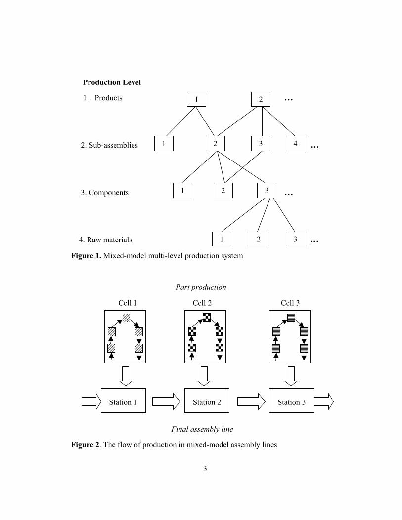
are generally used in multi-level production systems (Figure 1). In multi-level

production systems, raw materials are fabricated into components which are

combined into sub-assemblies; sub-assemblies are assembled into products on a

final assembly line.

Mixed-model lines become popular in recent decades, especially as an integral

part of just-in-time (JIT) production systems. JIT is a pull system, meaning that

the sub-assemblies, components and raw materials are pulled forward as they are

needed; production is initiated by one level’s requirement for the output of another

level. Hence, the final assembly line is the focus for controlling mixed-model

lines.

The effective utilization of mixed-model lines requires that the following two

problems be tackled: 1) the line balancing problem, and 2) the line sequencing

problem. The line balancing problem is the process of allocating the set of tasks to

stations to finish an assembly work. A task is the smallest work element of the

total work in an assembly process. A station is a location on the line at which work

is performed on the product. The line sequencing is a problem of determining a

sequence of the product models on the final assembly line with the objective of

optimizing line utilization.

In many JIT systems, part production is made in manufacturing cells that

manufacture families of parts (Leu et al. 1997). Figure 2 shows how parts being

produced in manufacturing cells feed the final assembly line.

3

Production Level

1. Products …

2. Sub-assemblies … …

3. Components …

4. Raw materials …

Figure 1. Mixed-model multi-level production system

Part production

Cell 1 Cell 2 Cell 3

Final assembly line

Figure 2. The flow of production in mixed-model assembly lines

1 2

1 2 3 4

1 2 3

1 2 3

Station 1 Station 2 Station 3

4

1.2. Statement of the problem

In this thesis, we study the MMAL sequencing problem assuming that the line

balancing is accomplished, and setup times between the different product models

are negligible. In determining the sequence of models produced on the line, we

consider the following common goals separately:

1) Leveling parts usage: maintain a constant rate of usage of all parts that

feed the final assembly line

2) Leveling workload: Smooth the workload on the final assembly line to

reduce the chance of production delays and stoppages

The first goal, also known as leveling the parts usage, requires that products

(level 1) be assembled at rates proportional to their volume requirements, and parts

(levels 2, 3, and so on) be pulled through the system at constant rates (Miltenburg

and Sinnamon 1992). In other words, there should be very little variability in the

parts usage from one time period to the next.

The second goal, balancing the workload, recognizes that not all products have

the same operation time at each station on the line. Products requiring relatively

longer operation times at any station are difficult to assemble unless they are

balanced off with products having shorter operation times. The load leveling goal

aims to level the work load on the final assembly line to reduce the chance of

production delays and line stoppages. Products are sequenced so that production

requirements for the outputs required to support the production of the products are

balanced.

Since the parts usage goal is generally considered to be more important for JIT

production systems, we mainly focus on the parts usage goal. We also consider the

5

variability only at the sub-assembly level (level 2), as suggested by Monden

(1983). Small versions of this problem are optimally solved by exact procedures.

However, heuristics should be developed to handle large-size problems. The

existing heuristics are computationally efficient but their performances are not

sufficient enough in terms of solution quality. Hence, in this study we aim to

propose an efficient heuristic procedure for the parts usage problem that

outperforms the existing heuristics in terms of solution quality.

In order to solve the MMAL sequencing problem, we propose several beam

search methods which include some enhancement tools, and compare their

performances against the well-known heuristics from the literature.

1.3. Contribution

First, this research is the first to use enhanced Beam Search methods for the

MMAL sequencing problem. Second, our proposed algorithms are generally

superior to the state-of-the-art heuristics in terms of solution quality. We also draw

conclusions about the algorithmic performances of the existing heuristics, which

have not been performed completely in the literature.

Our contribution to beam search literature is two-fold: First we incorporate a

novel enhancement tool, the exchange of information (EOI) procedure, into

traditional beam search applications and show that it generally improves the

solution quality. Second we draw inferences about where EOI should be invoked

during the search procedure.

6

1.4. Thesis outline

The rest of the thesis is organized as follows. We briefly discuss the existing

studies in Chapter 2. We give the formulation of the problem, and the explanation

of the heuristics developed for the problem in Chapter 3. In Chapter 4, we discuss

the proposed Beam Search algorithms in detail. We explain the computational

results in Chapter 5. Finally, in Chapter 6 we give concluding remarks and further

research directions.

7

Chap t e r 2

LITERATURE REVIEW

This chapter is organized in two sections: 1) brief discussion of the research

conducted on the MMAL sequencing problem, and 2) summary of the studies on the

beam search.

2.1. MMAL sequencing problem

After first investigated by Kilbridge and Webster (1963), a large number of

research have been conducted on the MMAL sequencing problem, the pioneers of

which are Thomopoulos (1967), Dar-el and Cother (1975), and Dar-el and Cucuy

(1977), and Yamashita and Okamura (1979). A common property of all these studies

is that, they consider the final assembly line, by ignoring the effects on other levels

in the multi-level production system, with different objectives such as minimizing

line length, and line stoppages. The first analysis of mixed-model, multi-level

production systems have been made by Monden (1983), and Miltenburg and

Sinnamon (1989). The detailed explanation of research carried out on the MMAL

sequencing problem is given below.

8

2.1.1. The MMAL problem with single objective

Miltenburg (1989) studies the mixed-model sequencing problem by considering

the variation in production rates of the finished products. Under the assumption that

all models require the same number and mix of parts, he emphasizes that minimizing

the variation in production rates of the finished products achieves minimizing the

variation in parts usage rates. The author formulates the problem as a nonlinear

integer programming model with the aim of minimizing the total deviation of actual

production rates from the desired production rates. The author develops an exact

algorithm to solve the program which has a worst case complexity that grows

exponentially with the number of products. Hence, he proposes two heuristics,

called Miltenburg’s Algorithm 3 Using Heuristic 1 (MA3H1), and Miltenburg’s

Algorithm 3 Using Heuristic 2 (MA3H2) for the problem.

In another study, Miltenburg and Sinnamon (1989) consider multi-level model

production systems to solve mixed-model sequencing problem with the objective of

keeping a constant rate of every part used by the system. They develop a

mathematical model for the problem, and extend the heuristics proposed by

Miltenburg (1989) to include all levels in the multi-level system. In a follow up

study, Miltenburg and Sinnamon (1992) consider the same problem and propose

heuristic procedures for finding good solutions, and solving large problems.

Sumichrast and Russell (1990) consider the MMAL sequencing problem with

the objective of leveling the parts usage. They review five sequencing methods

which are Goal Chasing 1 (GC1), Goal Chasing 2 (GC2), and Miltenburg’s three

heuristics (M-A1, MA3H1, and M-A3H2). The performance of the heuristics is

evaluated for the special case in which all models use the same parts. The evaluation

9

is based on the ability to minimize the mean absolute deviation from uniform

production of each model. The results of their experimental study indicate that M-

A3H2 outperforms other methods under all conditions tested. They also observe that

the relative performance of the method is not related to the number of models,

demand type, or the length of production sequence. As for the case of different

models requiring different components, only goal chasing methods are tested since

Miltenburg’s algorithms are not appropriate for this problem. It is shown that the

performance of the two goal chasing methods is good when the products have

simple product structures. However, when more than one component or many

different components are used for models, the performance of GC2 worsens

significantly.

Miltenburg and Goldstein (1991) address the mixed-model multi-level

sequencing problem that considers both the usage and loading goal. They propose a

single-stage and a double-stage heuristic to solve the joint problem. The single-stage

(double-stage) heuristic myopically minimizes the one-stage (two-stage) variation

each time a model is added to the sequence.

Kubiak and Sethi (1991) study the MMAL sequencing problem with the

objective of minimizing the product usage variation. They formulate an assignment

problem to obtain optimal level schedules for MMALs. They show that their

assignment formulation can be extended to more general objective functions than the

one used by Miltenburg (1989).

Inman and Bulfin (1991) propose Earliest Due Date (EDD) algorithm to

determine the optimal sequence with the objective of leveling product usage rate.

They demonstrate that model sequencing can be reduced to a single machine

10

sequencing problem if processing times are identical for all items. They compare the

EDD approach with others reported in the literature. The computational study shows

that the proposed algorithm is as good as other algorithms in terms of solution

quality when evaluated with respect to traditional objectives, but its sequences are

found extremely faster.

Yano and Rachamadugu (1991) study the problem of MMAL sequencing to

minimize work overload. They first consider the sequencing problem for a single

station, and propose an optimal procedure for this problem. For multiple stations,

they develop a heuristic procedure which is shown to reduce work overload

significantly.

For the MMAL sequencing problem, Ding and Cheng (1993) propose a simple

heuristic procedure that aims to smooth product usage rate. They compare the

proposed algorithm with M-A3H2 in problem sets conducted by Russell and

Sumichrast. The experimental results indicate that the proposed method is as good as

M-A3H2 in solution quality regarding the mean squared and absolute deviations and

much more efficient in terms of computational effort. It is also shown that as the

number of products increases, the computation time required by M-A3H2 increases

much faster than the proposed method.

Kubiak (1993) reviews the results of research conducted on the problem of

MMAL sequencing with the goal of smoothing the parts usage rate. In his paper, he

considers research efforts made on both product usage rate and component usage

rate variation with various objective functions such as maximum and total deviaiton

between actual usage and the expected usage. The author relates the results of this

research to the due date based scheduling problems and reviews a mathematical

11

programming model of the problem. The author further discusses another primary

concern in JIT systems, which is smoothing the workload on each workstation on

the line to reduce the chance of production delays and stoppages.

Ng and Mak (1994) study the sequencing problem of mixed-model assembly

lines that produce products with similar part requirements in a just-in-time

production environment. The objective used in their study is to minimize the total

variation of the actual production quantities of products from desired amount. They

propose an efficient Branch and Bound algorithm for determining the optimal

sequence. The computational results reveal that the algorithm is very efficient for the

MMAL sequencing problem.

Bautista et al. (1996) develop an exact algorithm that considers leveling parts

usage rate to solve MMAL sequencing problem. Their algorithm is based on

bounded dynamic programming (BDP). BDP combines features of dynamic

programming with features of branch and bound algorithms. The authors show that

the problem is equivalent to searching for a minimum path in an associated graph.

They also emphasize the myopic behavior of goal chasing method, and propose

several heuristics that are modification of GC method.

Cheng and Ding (1996) study the MMAL sequencing problem with the objective

of maintaining nearly constant rates of model usage on the line. They generalize the

problem to consider the weights for different models in evaluating their influence on

the model usage rate. They demonstrate that the existing sequencing heuristics (i.e.,

Miltenburg’s Algorithm 3 using heuristic 2, two-stage algorithm, and EDD method)

for equal-weight MMALs can be extended to this problem. They also compare these

modified heuristics and an optimal procedure in terms of solution quality and CPU

12

time requirements. The results indicate that the modified EDD, the modified two-

stage, and the modified MA3-H2 methods are quite efficient for this problem.

Duplaga et al. (1996) describe and illustrate the mixed-model sequencing

approach used by Hyundai Motor Company that minimizes the parts usage variation.

Hyundai’s methodology is developed to provide a reasonable solution that

approximates the result found by GCM1 while reducing CPU time considerations.

In their paper, Kim et al. (1996) propose a genetic algorithm for the MMAL

sequencing problem to minimize the overall length of a line. The computational

results indicate that the proposed algorithm is very efficient in terms of CPU time

considerations as well as solution quality.

Duplaga and Bragg (1998) compare the performance of six sequencing heuristics

developed for smoothing parts usage in MMALs. The heuristics evaluated in their

study are Goal-Chasing Method 1, Goal-Chasing Method 2, Hyundai’s heuristic,

Miltenburg and Sinnamon’s heuristic 1, Miltenburg and Sinnamon’s heuristic 2, and

Extended Goal-Chasing method. Performance comparison is made considering

products that may require different components that are common among products.

The results of their computational experiments show that Extended Goal-chasing

Method and Miltenburg and Sinnamon’s heuristic 2 have statistically better

performance than the others.

In another study, Zhu and Ding (2000) transform the minimization of the two-

stage variation in the mixed-model sequencing problem of reducing the part-level

variation to product-level terms. The two-stage transformation is based on a

simplification of the two-stage approach and a relationship matrix that evaluates the

relevance of product structures of a variety of models. Computational comparisons

13

indicate that the proposed method generally outperforms the one-stage method in

terms of solution quality, and is much faster than direct enumeration in computation.

The authors also present a general sufficient condition for the equivalence of the

sequencing problems of the product and part levels.

In another study, Celano et al. (2005) investigate the sequencing of MMAL

assuming the parts usage smoothing as the goal of the sequence selection. They

study this problem considering not only the traditional goal chasing approaches,

which assume zero-length assembly lines, but also models which take into account

the effective length of the assembly line. This implies that the number of

workstations and their extensions become important parameters for the optimal

sequence of the models. They propose a simulated annealing (SA) algorithm for this

problem and compare it with Goal Chasing algorithms. The experimental results

indicate that in the most cases the SA outperforms other heuristics. It is also shown

that the differences in the algorithm performances are affected by workstations and

parts number. As line length and mix to be assembled grows, satisfying the

component usage constraint becomes very difficult.

2.1.2. The MMAL problem with multiple objectives

Dar-El (1978) develops a broad classification of mixed-model assembly lines

(MMAL) from which four categories of model sequencing are derived. In each

category, satisfying one or both of two objective criteria, the one minimizing the

overall line length, and the other minimizing the throughput time is aimed.

Methodologies for solving the sequencing problem in each category are also

14

presented. The author also proposes a design strategy that can be followed by

designers of mixed-model assembly lines.

Bard et al. (1994) study MMAL sequencing problem with the objective of

minimizing the line length of the line (i.e., minimizing the risk of stopping the

conveyor and the station lengths are fixed) and maintaining constant product usage

rate. They present a bicriteria formulation of the problem that is suitable to examine

the tradeoffs between line length and product usage. The resulting model is solved

with a combination of Branch and Bound and heuristics such as Tabu Search and

adjacent pairwise interchange heuristic. The evaluation of the methods is performed

with a wide range of problems sizes defined by the number of stations on the line,

the number of different model types, and the total number of units to be assembled.

The results reveal that as problem size increases, computation times grow

exponentially for Branch and Bound algorithm, which necessitates the use of

heuristics for large problems. It is also shown that in the majority of cases at least

one of the heuristics finds either the optimal or near-optimal solution.

Hyun et al. (1998) propose a new genetic algorithm (GA) to solve multiple

objective sequencing problems in MMALs. They consider three objectives:

minimizing total utility work, minimizing total setup cost, and keeping model

production constant. The algorithm searches for a set of diverse non-dominated

solutions and give importance to the diversity of solutions and the Pareto optimality.

The results of the performance comparison of the proposed GA with three existing

GAs in terms of solution quality and diversity reveal that the proposed GA is better,

especially for problems that are large, and involve great variation in setup cost.

15

Merengo et al. (1999) develop new balancing and sequencing methods for the

MMAL problem with the following objectives: minimizing the rate of incomplete

jobs (in paced lines and in moving lines) or the probability of blocking/starvation

events, and reducing WIP. Minimizing the product usage variation is also considered

by their sequencing methodology. Regarding the sequencing problems, they

highlight the similarities between the need to minimize incomplete units and the

need to level product usage. They demonstrate that one single sequencing method

can meet both objectives.

Sumichrast et al. (2000) develop a new sequencing method, Evolutionary

Production Sequencer (EPS) to maximize production on MMAL’s. They evaluate

the performance of EPS using three measures: minimum cycle time necessary to

attain 100% completion without rework, percent of items completed without rework

for a given cycle time, and maintaining nearly constant rates of parts usage.

Sequence smoothness is measured by the mean absolute deviation (MAD) between

actual part usage and the expected part usage at each level in the production

sequence. They compare the performance of EPS with well-known sequencing

methods developed by Miltenburg (1989), Okamura and Yamashina (1979), and

Yano and Rachamadugu (1991). Their experimental study indicates that, when

MAD is the criterion of success, EPS is inferior to the Miltenburg heuristic, but

better than the other two methods.

In another study, McMullen and Frazier (2000) propose a Simulated Annealing

(SA) based heuristic that simultaneously considers both setups and the stability of

product usage rates to solve MMAL sequencing problem. The performance of the

SA algorithm is compared with that of Tabu Search approach from the literature.

16

The results indicate that the SA approach generally outperforms Tabu Search. It is

also shown that the SA approach achieves near-optimal solutions for smaller

problems.

In another study, Zeramdini (2000) et al. consider bicriteria sequencing problem

for mixed-model assembly lines with the following goals: 1) keeping a constant rate

of parts usage, and 2) leveling the workload at work stations to avoid line stoppages.

They develop a two-step approach, where in the first step they consider only goal 1

by applying Extended Goal Chasing Method (EGCM). In the second step they place

emphasis on goal 2, by investigating the efficiency of a spacing-constraint based

approach, in comparison with a more general time-based one. They show that the

EGCM is an appropriate choice for step 1 with a new performance measure that

represents a lower bound on variation in parts usage. As for the workload

smoothing, it is shown that the spacing-constraint based method outperforms the

time-based approach.

Drexl and Kimms (2001) propose a new integer-programming model that

considers both of the following objectives: smoothing the usage rate of all parts fed

into the final assembly line, and keeping the line’s workstation loads as constant as

possible. Unlike the algorithms reported in the literature, their model allows one to

control the risk of conveyor stoppage or enables one to control the cost for utility

work while producing smooth JIT schedules. They solve the problem by specifying

a set-partitioning/ column-generation approach. They demonstrate that solving the

LP-relaxation of this model by column generation provides tight lower bounds for

the optimal value of objective function.

17

Korkmazel and Meral (2001) study MMAL sequencing problem considering two

major goals: 1) smoothing the workload on each workstation on the assembly line,

2) keeping a constant rate of usage of products on the assembly line. They develop

the modified Ding and Cheng algorithm to minimize the sum of deviations of actual

production from the desired amount. The proposed algorithm is compared with M-

A3H2 and Ding and Cheng (D&C) Algorithm. The results of evaluation reveal that

the modified D&C algorithm outperforms the other methodologies in all problem

instances handled. Furthermore, the approaches that perform better than the others

are extended for the bicriteria problem considering goals 1 and 2, simultaneously. In

their study, it is also demonstrated that the bicriteria problem with the sum-of-

deviations type objective function can also be formulated as an assignment problem;

and hence, the optimal solution to the small-sized problems can be obtained by

solving the assignment problem.

Ponnambalam (2003) et al. propose a genetic algorithm (GA) for the MMAL

sequencing problem considering both a single objective and multiple objectives.

They compare genetic algorithm with the algorithm of Miltenburg and Sinnamon

(MS1992) to get the constant usage of every part considering variation at four levels:

1) product, 2) subassembly, 3) component, and 4) raw material. The results of

evaluation show that GA outperforms MS1992 in the majority of the problems

investigated. As for the multiple-objective genetic algorithm for sequencing

MMALs, the minimization of total utility work, leveling parts usage, and

minimization of total setup cost are considered. The genetic algorithm used to solve

this problem employs the selection mechanism of Pareto stratum-niche cubicle.

Pareto stratum-niche cubicle is compared with the selection based on scalar fitness

18

function value. The results show that GA using Pareto stratum-niche cubicle

performs better than the GA with other selection mechanisms.

McMullen and Tarasewich (2005) consider the problem of mixed-model

sequencing with setups. The problem has two objectives: minimizing the product

usage variation and number of setups. Since the objectives are frequently in

opposition with one another, they present an efficient frontier approach for this

problem. To effectively generate efficient frontiers necessary to solve the problem,

they develop a beam-search heuristic. The experimental results reveal that the

proposed approach performs well in terms of solution quality as well as

computational effort.

In a recent study, Mansouri (2005) develops a multi-objective genetic algorithm

for MMAL sequencing problem to optimize the variation of product usage rates and

number of steps simultaneously. Since the two objectives are inversely correlated

with each other, simultaneously optimizing both of them is difficult. Hence, the

proposed method searches for locally Pareto-optimal or locally non-dominated

frontier where simultaneous minimization of the product usage rate variation and the

number of setups is desired. Performance of the algorithm is compared against a

total enumeration (TE) scheme in small problems and also against several heuristics

in small, medium and large problems. The results of evaluation show that the

proposed method is better in CPU time considerations and it outperforms the

comparator algorithms in solution quality as well as computational effort.

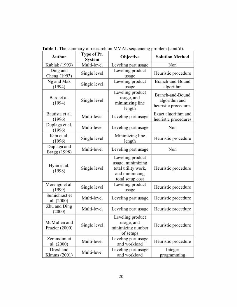
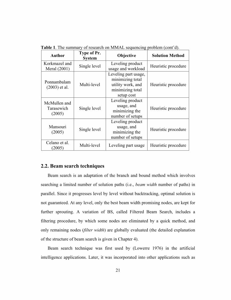
It is worth concluding this section with the summary of research on the MMAL

sequencing problem. Table 1 presents the related research with their objectives.

19

Table 1. The summary of research on the MMAL sequencing problem.

Author Type of the Prod. System

Objective Solution Method

Thomopoulos (1967)

Single level Optimally utilizing

line operators Heuristic procedure

Dar-el and Cother (1975)

Single level Minimizing line

length Heuristic procedure

Dar-el and Cucuy (1977)


length Integer

programming

Dar-el (1978) Single level Minimizing line

length, and throughput time

Heuristic procedures

Yamashita and Okamura (1979)


stoppages Heuristic procedure

Monden (1983) Multi-level Leveling part usage Heuristic procedure Miltenburg

(1989) Single level

Leveling product usage

Heuristic procedure

Miltenburg and Sinnamon (1989)

Multi-level Leveling product and part usage

Heuristic procedure

Sumichrast and Russell (1990)

Multi-level Leveling part usage Non

Kubiak and Sethi (1991)

Single level Leveling product

usage Optimization algorithm

Miltenburg and Goldstein (1991)


Heuristic procedure

Inman and Bulfin (1991)


usage EDD algorithm

Yano and Rachamadugu

(1991) Single-level

Minimizing work overload

Heuristic procedure

Miltenburg and Sinnamon (1992)


Heuristic procedure

20

Table 1. The summary of research on MMAL sequencing problem (cont’d).

Author Type of Pr. System


Kubiak (1993) Multi-level Leveling part usage Non Ding and

Cheng (1993) Single level

Leveling product usage

Heuristic procedure

Ng and Mak (1994)


usage Branch-and-Bound

algorithm

Bard et al. (1994)

Single level

Leveling product usage, and

minimizing line length

Branch-and-Bound algorithm and

heuristic procedures

Bautista et al. (1996)

Multi-level Leveling part usage Exact algorithm and heuristic procedures

Duplaga et al. (1996)


Kim et al. (1996)


length Heuristic procedure

Duplaga and Bragg (1998)


Hyun et al. (1998)

Single level

Leveling product usage, minimizing total utility work, and minimizing total setup cost

Heuristic procedure

Merengo et al. (1999)


usage Heuristic procedure

Sumichrast et al. (2000)

Multi-level Leveling part usage Heuristic procedure

Zhu and Ding (2000)


McMullen and Frazier (2000)

Single level


minimizing number of setups

Heuristic procedure

Zeramdini et al. (2000)

Multi-level Leveling part usage

and workload Heuristic procedure

Drexl and Kimms (2001)

Multi-level Leveling part usage

and workload Integer

programming

21

Table 1. The summary of research on MMAL sequencing problem (cont’d).

Author Type of Pr. System


Korkmazel and Meral (2001)


usage and workload Heuristic procedure

Ponnambalam (2003) et al.

Multi-level

Leveling part usage, minimizing total utility work, and minimizing total

setup cost

Heuristic procedure

McMullen and Tarasewich

(2005) Single level


minimizing the number of setups

Heuristic procedure

Mansouri (2005)

Single level


minimizing the number of setups

Heuristic procedure

Celano et al. (2005)


2.2. Beam search techniques

Beam search is an adaptation of the branch and bound method which involves

searching a limited number of solution paths (i.e., beam width number of paths) in

parallel. Since it progresses level by level without backtracking, optimal solution is

not guaranteed. At any level, only the best beam width promising nodes, are kept for

further sprouting. A variation of BS, called Filtered Beam Search, includes a

filtering procedure, by which some nodes are eliminated by a quick method, and

only remaining nodes (filter width) are globally evaluated (the detailed explanation

of the structure of beam search is given in Chapter 4).

Beam search technique was first used by (Lowerre 1976) in the artificial

intelligence applications. Later, it was incorporated into other applications such as

22

FMS and job shop scheduling problems (see Ow and Morton 1988, Sabuncuoglu

and Karabuk 1998, Sabuncuoglu and Bayiz 2000). More recently, some

enhancement tools have been used with beam search techniques which are

mentioned below.

Honda et al. (2003) propose backtracking beam search algorithm for multi-

objective flowshop problem to minimize both objectives. As there may not be a

schedule that can optimize both criteria, the authors seek non-dominated schedules

(i.e., feasible schedules that are not dominated by any other feasible schedules). In

the proposed method, the traditional beam search is performed. Then, backtracking

is invoked to some nodes and the re-search is performed many times so that

widespread non-dominated solutions can be obtained. During the searching, the

pruned nodes are preserved. The lower bound of each pruned node is compared with

the tentative solution, and the bounded operation is applied, as done in branch-and-

bound method. The computational study indicates that the proposed algorithm can

find more balanced solutions than does the beam search method.

In another study, Croce and Tadei (2004) develop a Recovering Beam Search

(RBS) method for the two combinatorial optimization problems: the two-machine

total completion time flow shop scheduling problem and the uncapacitated p-median

location problem. The recovering phase of the algorithm aims at recovering from

previous wrong decisions. This step is invoked to each of the beam width number of

best child nodes generated. For a given node, the recovering phase, by means of

interchange operators applied to the current partial schedule, checks whether the

current solution is dominated by another partial solution sharing the same search tree

level. If so, the current solution is replaced by the better solution. The results of

23

evaluation show that RBS procedure outperforms basic beam search approach in

solution quality, and is competitive with the state-of-the-art heuristics.

Valente and Alves (2005) develop filtered and recovering beam search

algorithms for the single machine earliness/tardiness scheduling problem with no

idle time. The RBS algorithm differs from filtered beam search in three ways: First,

its beam width is equal to 1; second, the global evaluation is employed by a

weighted sum of both lower and upper bounds for the solution that can be obtained

from the partial schedule represented by the node. Third, once the best node and the

corresponding best partial solution are retained, a recovering step is applied. The

computational results show that the RBS algorithms outperform the filtered beam

search algorithm in terms of solution quality as well as computational effort.

Ghirardi and Potts (2005) propose a RBS method for minimizing makespan on

unrelated parallel machine. In order to test its effectiveness, they compare it with a

procedure reported in the literature. The computational study reveals that the RBS

algorithm generally outperforms the other in both solution quality as well as

computational time. In addition, it is shown that the RBS method is able to

generate approximate solutions for instances with large size using reasonable

computation time.

Esteve et al. (2005) propose RBS algorithm and several heuristic algorithms for

the single machine JIT scheduling problem. The recovering step is invoked to each

of the beam width number of best child nodes generated. For a given node, a local

search is applied to the current partial schedule. If the obtained partial schedule is

superior and has a lower makespan than the current one, the current schedule is

replaced by the better schedule. The authors state that although this condition is not

24

an exact dominance condition, it improves the behavior of RBS algorithm. The

computational experiments indicate that the RBS algorithm outperforms other

heuristics in solution quality.

2.3. Summary of the literature and research motivation

Over years, a large number of research have been conducted on the MMAL

sequencing problem with the aim of minimizing the parts usage variation and the

workload variation. Since the parts usage problem is considered to be more

important for JIT production systems, the majority of research deals with the parts

usage problem.

Although small versions of this problem are optimally solved by exact

procedures, heuristic methods are needed to solve large-size problems in a

reasonable time frame. Hence, several heuristic procedures are developed for the

problem in the literature. Although they are efficient in terms of CPU time

considerations, they are not competent in solution quality. In addition to this, there

is not a sufficient study on the performance comparison of the state-of-the-art

heuristics in the literature. Hence, in this study we propose Beam Search

algorithms to minimize the parts usage variation that generally outperform the

existing heuristics. We also implement these algorithms to solve the load leveling

problem. We draw conclusions about the algorithmic performances of the state-of-

the-art heuristics in the literature, as well.

Beam search applications have also been used in various research areas such

as scheduling, artificial intelligence, and assembly lines. In recent studies, the

structure of beam search techniques has been improved with several enhancement

25

tools. The algorithms we propose are one type of enhanced beam search

techniques, which have never been used for the MMAL sequencing problem.

Unlike the traditional beam search applications, the proposed algorithms have the

following capabilities: 1) backtracking, and 2) exchange of information (EOI).

Among the enhancement procedures, exchange of information is a novel

enhancement tool for the beam search literature. We further address the research

question of where to invoke EOI in the search procedure.

26

Chap t e r 3

PROBLEM FORMULATION AND

EXISTING HEURISTICS

First, the formulation of the MMAL sequencing problem is given by considering

the part usage and load leveling goals separately. Then, the solution procedures

reported in the literature are explained in Section 3.2.

3.1. Problem formulation

3.1. 1. The parts usage problem

The formulation of the MMAL sequencing problem to minimize the parts usage

variation was developed by Jin and Wu (2002), which is presented below.

We assume that there are N different models to be produced on the final

assembly line, and C different parts that can be used by a model. The following

notation is used in formulating the problem.

di : the demand for model i, i = 1,…, N

cj,i : the number of part j required for one model i, i = 1,…, N, j = 1,…, C

DT: the total demand for models, ∑=

=N

i

iT dD1

27

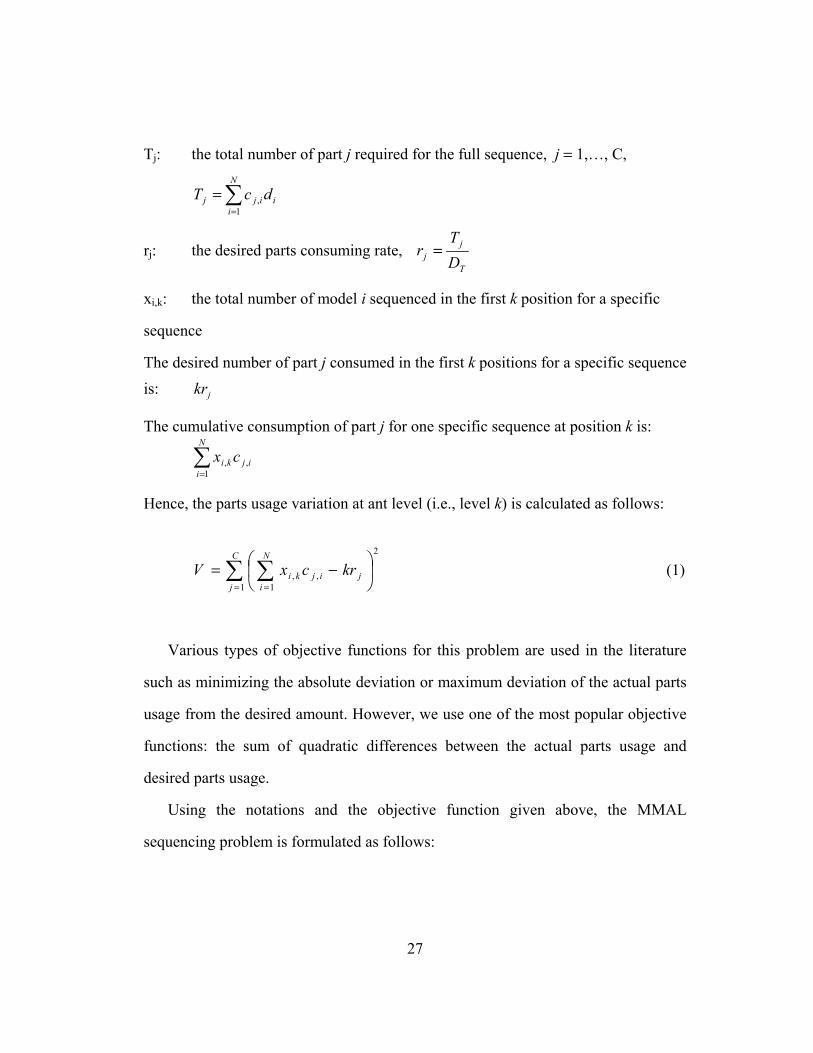
Tj: the total number of part j required for the full sequence, j = 1,…, C,

∑=

=N

i

iijj dcT1

,

rj: the desired parts consuming rate, T

j

jD

Tr =

xi,k: the total number of model i sequenced in the first k position for a specific

sequence

The desired number of part j consumed in the first k positions for a specific sequence

is: jkr

The cumulative consumption of part j for one specific sequence at position k is:

∑=

N

i

ijki cx1

,,

Hence, the parts usage variation at ant level (i.e., level k) is calculated as follows:

2

1 1,,∑ ∑

= =

−=

C

j

j

N

i

ijki krcxV (1)

Various types of objective functions for this problem are used in the literature

such as minimizing the absolute deviation or maximum deviation of the actual parts

usage from the desired amount. However, we use one of the most popular objective

functions: the sum of quadratic differences between the actual parts usage and

desired parts usage.

Using the notations and the objective function given above, the MMAL

sequencing problem is formulated as follows:

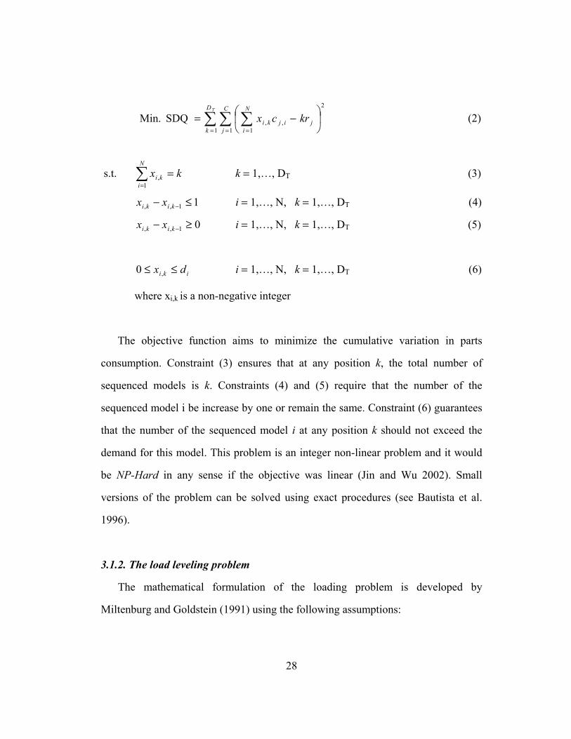
28

2

1 1 1,, SDQ Min. ∑∑ ∑

= = =

−=

TD

k

C

j

j

N

i

ijki krcx (2)

s.t. ∑=

=N

i

ki kx1

, k = 1,…, DT (3)

11,, ≤− −kiki xx i = 1,…, N, k = 1,…, DT (4)

01,, ≥− −kiki xx i = 1,…, N, k = 1,…, DT (5)

iki dx ≤≤ ,0 i = 1,…, N, k = 1,…, DT (6)

where xi,k is a non-negative integer

The objective function aims to minimize the cumulative variation in parts

consumption. Constraint (3) ensures that at any position k, the total number of

sequenced models is k. Constraints (4) and (5) require that the number of the

sequenced model i be increase by one or remain the same. Constraint (6) guarantees

that the number of the sequenced model i at any position k should not exceed the

demand for this model. This problem is an integer non-linear problem and it would

be NP-Hard in any sense if the objective was linear (Jin and Wu 2002). Small

versions of the problem can be solved using exact procedures (see Bautista et al.

1996).

3.1.2. The load leveling problem

The mathematical formulation of the loading problem is developed by

Miltenburg and Goldstein (1991) using the following assumptions:

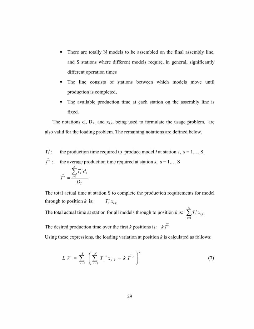
29

• There are totally N models to be assembled on the final assembly line,

and S stations where different models require, in general, significantly

different operation times

• The line consists of stations between which models move until

production is completed,

• The available production time at each station on the assembly line is

fixed.

The notations di, DT, and xi,k, being used to formulate the usage problem, are

also valid for the loading problem. The remaining notations are defined below.

Tis : the production time required to produce model i at station s, s = 1,… S

_sT : the average production time required at station s, s = 1,… S

T

N

i

i

s

i

s

D

dT

T

∑== 1

_

The total actual time at station S to complete the production requirements for model

through to position k is: ki

s

i xT ,

The total actual time at station for all models through to position k is: ∑=

N

i

ki

s

i xT1

,

The desired production time over the first k positions is: __sTk

Using these expressions, the loading variation at position k is calculated as follows:

2

1

_

1, ∑ ∑

= =

−=

S

s

sN

i

ki

s

i TkxTVL (7)

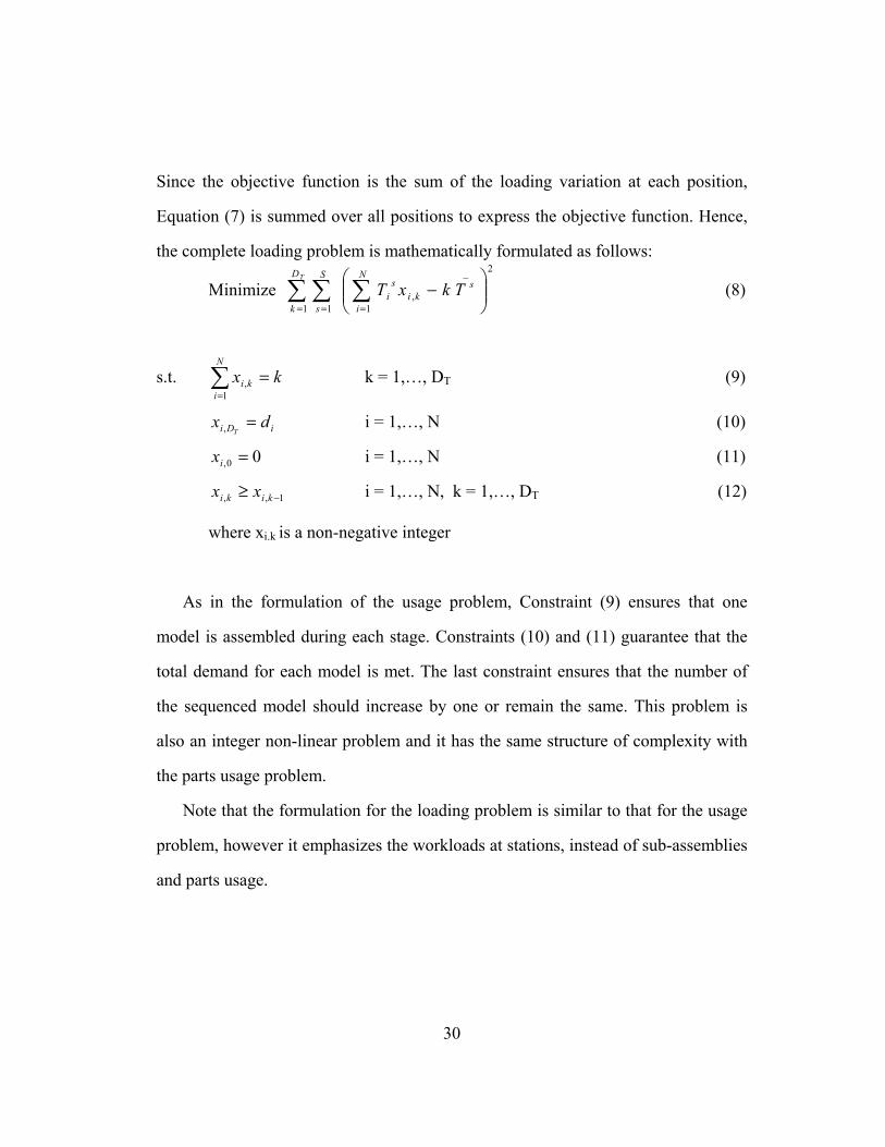
30

Since the objective function is the sum of the loading variation at each position,

Equation (7) is summed over all positions to express the objective function. Hence,

the complete loading problem is mathematically formulated as follows:

Minimize ∑ ∑ ∑= = =

−

TD

k

S

s

sN

i

ki

s

i TkxT1

2

1

_

1, (8)

s.t. ∑=

=N

i

ki kx1

, k = 1,…, DT (9)

iDi dxT

=, i = 1,…, N (10)

00, =ix i = 1,…, N (11)

1,, −≥ kiki xx i = 1,…, N, k = 1,…, DT (12)

where xi.k is a non-negative integer

As in the formulation of the usage problem, Constraint (9) ensures that one

model is assembled during each stage. Constraints (10) and (11) guarantee that the

total demand for each model is met. The last constraint ensures that the number of

the sequenced model should increase by one or remain the same. This problem is

also an integer non-linear problem and it has the same structure of complexity with

the parts usage problem.

Note that the formulation for the loading problem is similar to that for the usage

problem, however it emphasizes the workloads at stations, instead of sub-assemblies

and parts usage.

31

3.2. Heuristics

In this section, we present the algorithms developed for minimizing parts usage

on MMALs since we mainly focus on the usage problem. Since the structure of the

load leveling problem is similar to that of the usage problem, the algorithms can also

be used for the latter case.

Over years, a large number of solution procedures have been proposed for the

MMAL sequencing problem with the objective of minimizing parts usage. Among

them, we consider the well-known algorithms developed for the Monden problem,

which considers the variability at the sub-assembly level, and ignores the variability

at the final assembly. The explanation of these algorithms is given next.

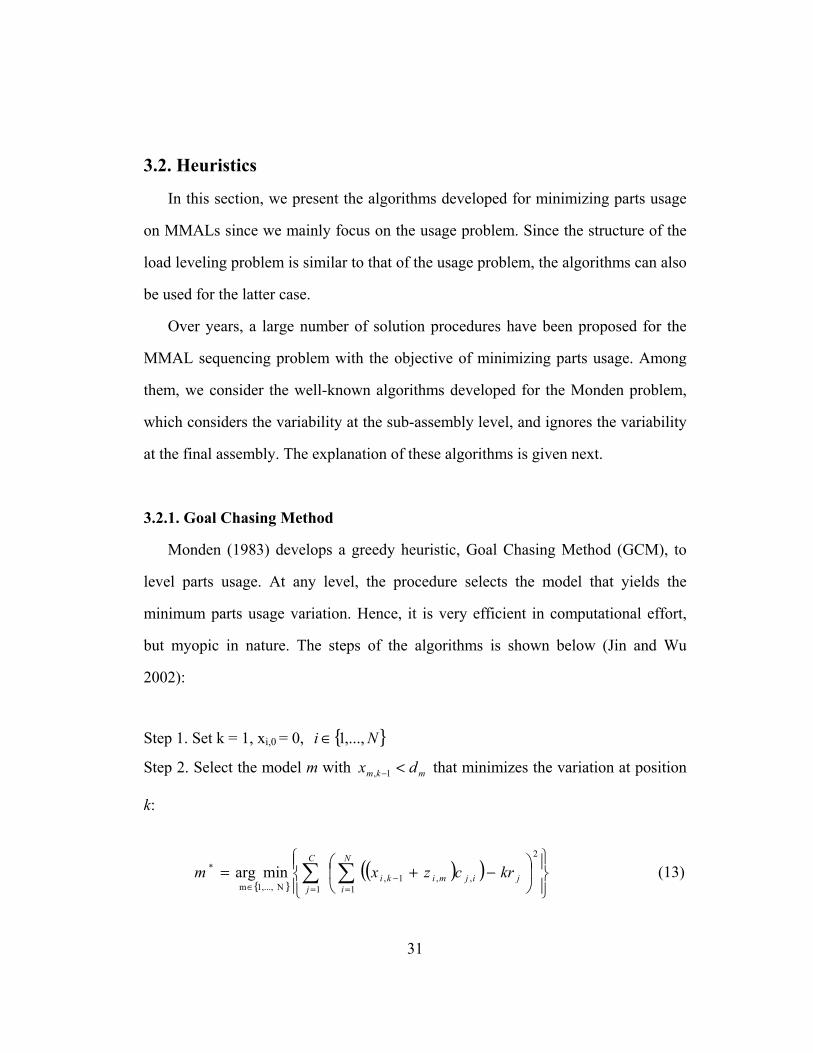
3.2.1. Goal Chasing Method

Monden (1983) develops a greedy heuristic, Goal Chasing Method (GCM), to

level parts usage. At any level, the procedure selects the model that yields the

minimum parts usage variation. Hence, it is very efficient in computational effort,

but myopic in nature. The steps of the algorithms is shown below (Jin and Wu

2002):

Step 1. Set k = 1, xi,0 = 0, { }Ni ,...,1∈

Step 2. Select the model m with mkm dx <−1, that minimizes the variation at position

k:

{ }

( )( )

−+= ∑ ∑

= =

−∈

2

1 1,,1,

N1,...,m

* min argC

j

N

i

jijmiki krczxm (13)

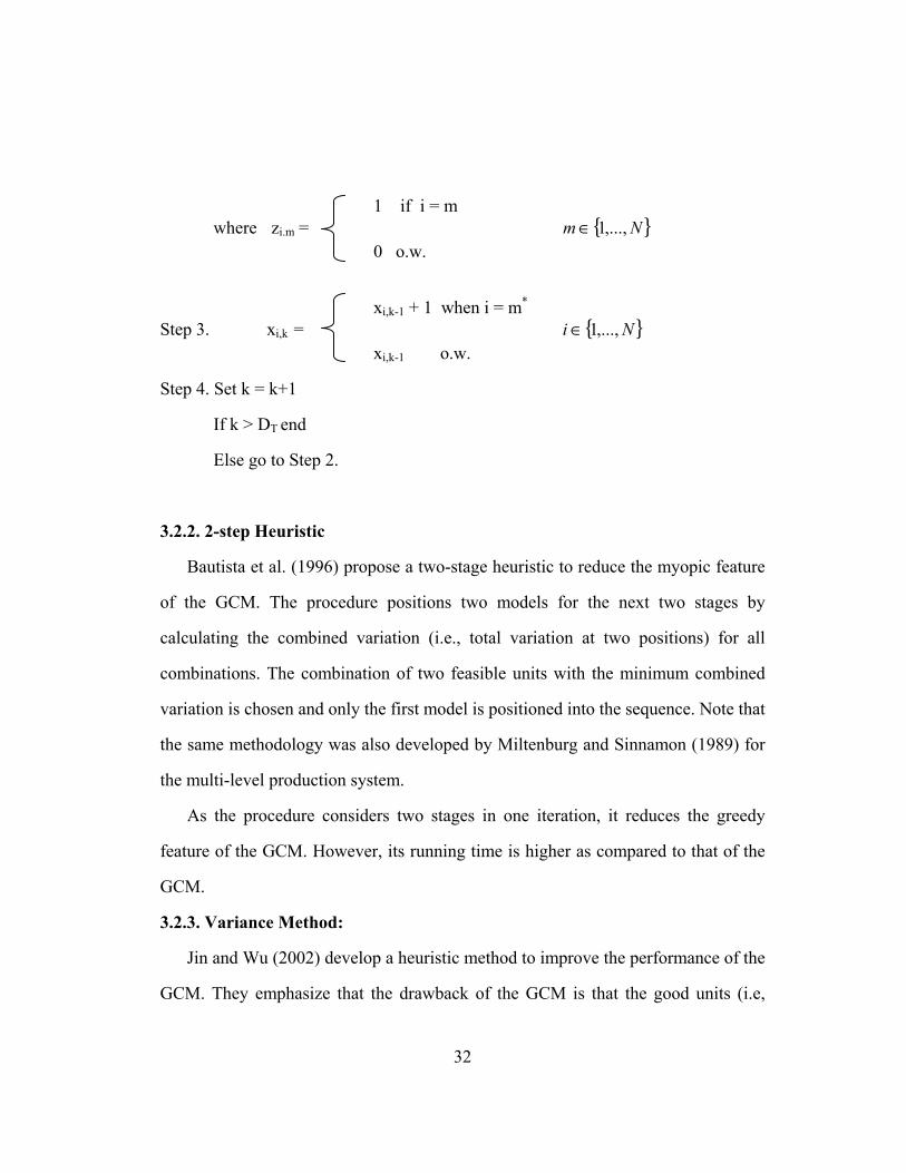
32

1 if i = m

where zi.m = { }Nm ,...,1∈

0 o.w.

xi,k-1 + 1 when i = m*

Step 3. xi,k = { }Ni ,...,1∈

xi,k-1 o.w.

Step 4. Set k = k+1

If k > DT end

Else go to Step 2.

3.2.2. 2-step Heuristic

Bautista et al. (1996) propose a two-stage heuristic to reduce the myopic feature

of the GCM. The procedure positions two models for the next two stages by

calculating the combined variation (i.e., total variation at two positions) for all

combinations. The combination of two feasible units with the minimum combined

variation is chosen and only the first model is positioned into the sequence. Note that

the same methodology was also developed by Miltenburg and Sinnamon (1989) for

the multi-level production system.

As the procedure considers two stages in one iteration, it reduces the greedy

feature of the GCM. However, its running time is higher as compared to that of the

GCM.

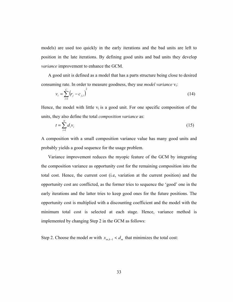
3.2.3. Variance Method:

Jin and Wu (2002) develop a heuristic method to improve the performance of the

GCM. They emphasize that the drawback of the GCM is that the good units (i.e,

33

models) are used too quickly in the early iterations and the bad units are left to

position in the late iterations. By defining good units and bad units they develop

variance improvement to enhance the GCM.

A good unit is defined as a model that has a parts structure being close to desired

consuming rate. In order to measure goodness, they use model variance vi:

( )2

1,∑

=

−=C

i

ijji crv (14)

Hence, the model with little vi is a good unit. For one specific composition of the

units, they also define the total composition variance as:

∑=

=N

i

iivdt1

(15)

A composition with a small composition variance value has many good units and

probably yields a good sequence for the usage problem.

Variance improvement reduces the myopic feature of the GCM by integrating

the composition variance as opportunity cost for the remaining composition into the

total cost. Hence, the current cost (i.e, variation at the current position) and the

opportunity cost are conflicted, as the former tries to sequence the ‘good’ one in the

early iterations and the latter tries to keep good ones for the future positions. The

opportunity cost is multiplied with a discounting coefficient and the model with the

minimum total cost is selected at each stage. Hence, variance method is

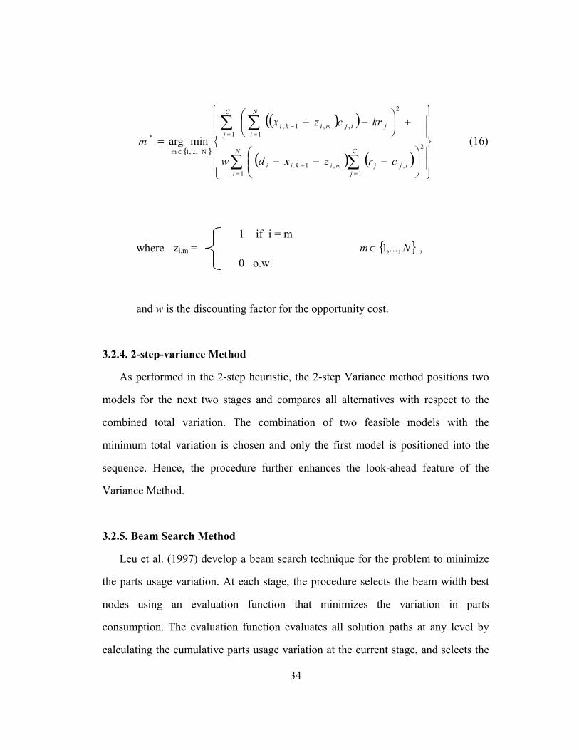
implemented by changing Step 2 in the GCM as follows:

Step 2. Choose the model m with mkm dx <−1, that minimizes the total cost:

34

{ }

( )( )

( ) ( )

−−−

+

−+

=

∑ ∑

∑ ∑

= =

−

= =

−

∈ N

i

C

j

ijjmikii

C

j

N

i

jijmiki

crzxdw

krczx

m

1

2

1,,1.

2

1 1,,1,

N1,...,m

*

min arg (16)

1 if i = m

where zi.m = { }Nm ,...,1∈ ,

0 o.w.

and w is the discounting factor for the opportunity cost.

3.2.4. 2-step-variance Method

As performed in the 2-step heuristic, the 2-step Variance method positions two

models for the next two stages and compares all alternatives with respect to the

combined total variation. The combination of two feasible models with the

minimum total variation is chosen and only the first model is positioned into the

sequence. Hence, the procedure further enhances the look-ahead feature of the

Variance Method.

3.2.5. Beam Search Method

Leu et al. (1997) develop a beam search technique for the problem to minimize

the parts usage variation. At each stage, the procedure selects the beam width best

nodes using an evaluation function that minimizes the variation in parts

consumption. The evaluation function evaluates all solution paths at any level by

calculating the cumulative parts usage variation at the current stage, and selects the

35

beam width nodes that yield the minimum cumulative variation. In the same manner,

the search procedure continues until the last stage at which the best solution path can

be determined. The sequence is determined by tracing back up the best solution path.

3.2.6. Performance of the heuristics

The performances of the existing heuristics are tested in several studies. Leu et

al. (1997) test the performance of the BS method against the GC method and the 2-

step method. They consider over 400 test problems that vary in terms of number of

number of product models, quantity of assembly, and degree of part commonality.

The results reveal that the BS method outperforms the GC method and the 2-step

method in solution quality. It is also shown that the BS method offers a substantial

improvement over the 2-step method when the problem size increases. Besides, Jin

and Wu (2002) demonstrate that the Variance method is superior to the GC method

in solution quality. They also show that the Variance method is superior to the 2-

step method in terms of computational effort. However, their study does not contain

the extensive comparison of the Variance and 2-step Variance methods against the

BS Method.

36

Chap t e r 4

PROPOSED ALGORITHM

4.1. Structure of beam search

Beam search (BS) is an adaptation of the branch and bound method in which

only some nodes are evaluated in the search tree. It is similar to a breadth-first

search as it progresses level by level without backtracking. However, unlike breadth-

first, only the best β promising nodes, called beam width, are kept for further

sprouting at any level (Sabuncuoglu and Bayiz 1999). The potential promise of each

node is determined by global evaluation function, to select the best β nodes. Global

evaluation function typically estimates the minimum total cost of the best solution

obtained from the partial schedule represented by the node. In order to reduce

computational burden, filtering mechanism can also be used, by which some nodes

are eliminated by a computationally fast method (i.e., local evaluation function), and

only remaining nodes (filter width) are globally evaluated.

The representation of BS tree is shown in Figure 3. We select the promising

nodes (beam nodes) by invoking local and global evaluations and proceed with the

search through these selected nodes. After determining the first beam nodes at level

1, we apply the algorithm to these nodes independently and generate one partial tree

(i.e., beam) from each of them. After filtering procedure, for each beam, one node

(beam node for the next level) is chosen among the descendants of its beam node,

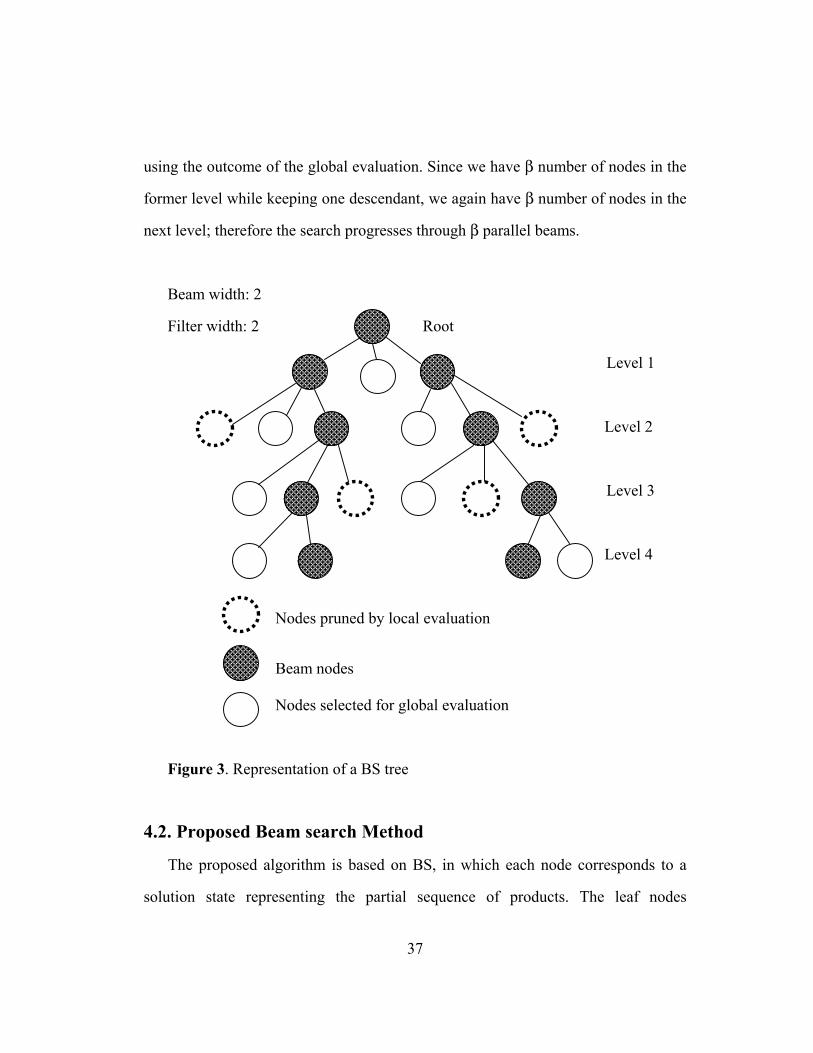
37

using the outcome of the global evaluation. Since we have β number of nodes in the

former level while keeping one descendant, we again have β number of nodes in the

next level; therefore the search progresses through β parallel beams.

Beam width: 2

Filter width: 2 Root

Level 1

Level 2

Level 3

Level 4

Nodes pruned by local evaluation

Beam nodes Nodes selected for global evaluation

Figure 3. Representation of a BS tree

4.2. Proposed Beam search Method

The proposed algorithm is based on BS, in which each node corresponds to a

solution state representing the partial sequence of products. The leaf nodes

38

correspond to the full sequence of products. The value of local evaluation function is

the parts usage variation, which is shown in Equation (1) on page 27. Global

evaluation function is defined as the total parts usage variation, which is the sum of

the parts usage variation at the current level (i.e., one level ahead of the beam node)

and some subsequent levels. Hence, it estimates the solution quality of a partial

solution, instead of full solution, which allows us to globally evaluate the candidate

nodes quickly. It first selects the product (i.e., descendant of the evaluated node)

with the minimum variation at the next level. Thus, for each of the subsequent

levels, it schedules products so that the variability is kept as small as possible (this

procedure is explained in Section 4.2.3.).

Differing from the traditional (BS) applications, the proposed algorithm

incorporates various enhancement tools such as backtracking and information

exchange (i.e, sharing). Backtracking is the process of going back to the previous

solution states in the search tree with the expectation of obtaining better solutions.

The motivation to implement this procedure stems from the fact that whenever two

or more beams are equivalent in some sense, as explained below, some of the beams

are further explored by going back to their previous solution states.

The other enhancement tool is the exchange of information (EOI) by which we

take the part of the solution from one beam and transfer it to another beam, hoping

that the resulting beam with this additional information will lead to better solutions.

EOI is performed at certain predetermined levels, considering the possibility that the

part of a beam that precedes and follows the same product will lead to better

solutions if it is located just after the same product in another beam.

39

Before explaining these enhancement tools and other features of the proposed

algorithm, the steps of the algorithm and related notation are introduced next.

Notation:

BL: beginning level for EOI

I: interval for EOI

k: indicator for EOI

DT : total demand

l: current level in the search tree

Steps of the Proposed Algorithm:

Step 0. (Initialization)

Set k = 0 and l = 0.

Step 1. Generate descendant nodes.

Step 2. (Determining beam nodes)

Select the best β beam nodes using global evaluation function, and set 1+= ll .

Step 3. (Search in the beam nodes)

Step 3.1. For each beam:

Step 3.1.1. Keep at most α nodes emanating from the current beam node,

using the local evaluation function.

Step 3.1.2. Select the best node among w of them, using the global

evaluation function.

Step 3.2. Set 1+= ll .

Step 4. (Exchange of information)

Step 4.1. If kIBLl *+= and TDl ≤ , then

40

Step 4.1.1. For each beam:

Step 4.1.1.1. Select the best beam among the alternative solutions

generated by EOI procedure.

Step 4.1.2. Set 1+= kk .

Step 5. (Backtracking)

Step 5.1. If TDl = , then stop the algorithm.

Step 5.2. If equivalency is observed, then create an alternative beam for each

inferior beam with backtracking procedure.

Step 5.3 Go to Step 1.

4.2.1. Backtracking procedure

The backtracking procedure is applied whenever the equivalency is observed

after the selection of beam nodes at any level. Beams are considered equivalent at a

level whenever the number of each product sequenced up to that level at each beam

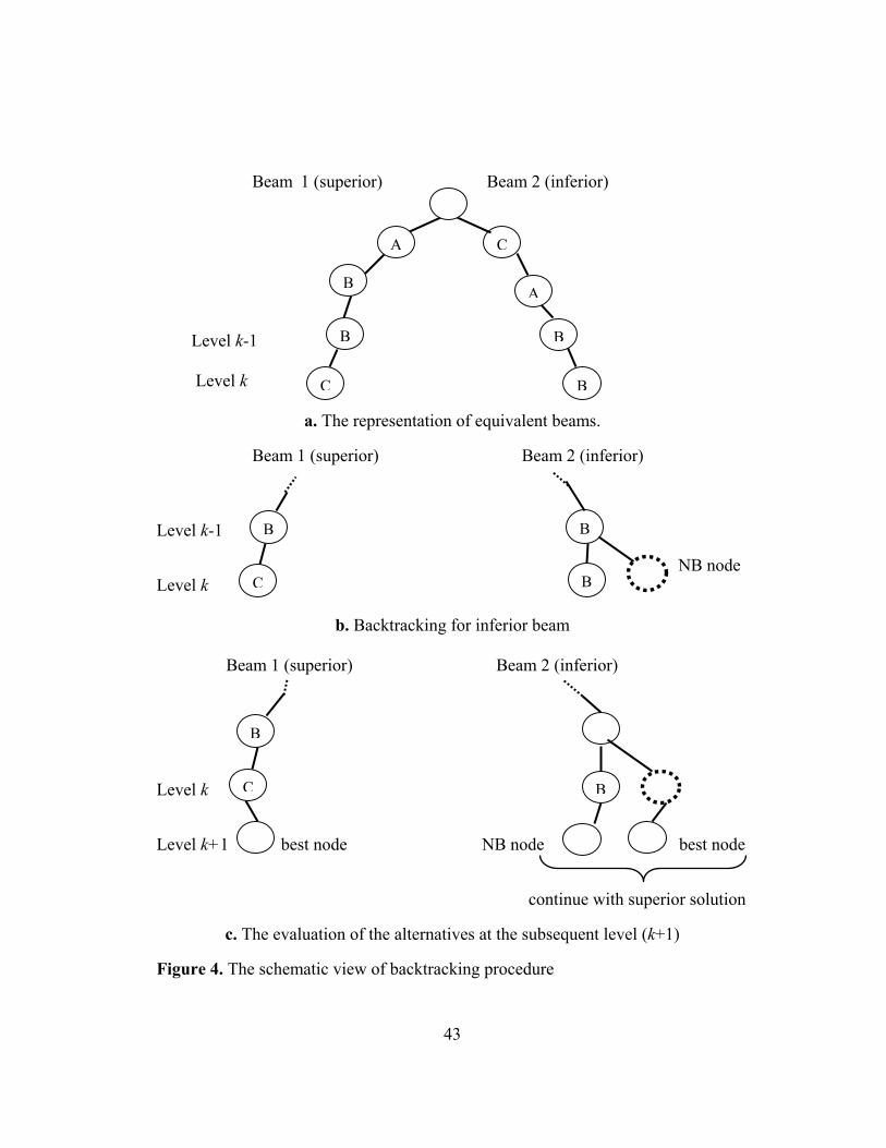
are equal to each other. As an illustration, consider the following two beams in

Figure 4: The products A, B, B, C are sequenced in Beam 1 and the products C, A,

B, B are sequenced in Beam 2 (see Figure 4a). Since both of the beams have one A,

two B’s, and one C, they are considered equivalent.

The cumulative variation of equivalent beams at the current level (i.e., level k <

DT) is calculated and each of the inferior beams is backtracked by moving one level

up, and generating the next best (NB) child node. Hence, β+1 nodes are usually

investigated. NB node is further sprouted by selecting the best node, using global

evaluation function. The original node, however, is further sprouted by selecting the

NB node, due to equivalency theorem. Finally, these two newly generated nodes are

41

evaluated in the sense that the one having the minimum value of global evaluation

function plus the variation at the current level is selected.

The backtracking procedure is shown by considering two equivalent beams

represented in Figure 4a. After comparing the cumulative variation values of the two

beams at level k, Beam 2 is found to be inferior. Then, NB child node of Beam 2 at

level k is further branched by choosing the best node at level k+1; whereas the

original node (i.e., product B) at level k is further branched by selecting the NB node

at level k+1. Hence, at level k+1 we have two alternative beam nodes; after

evaluating these nodes, we continue the search procedure by selecting the superior

one.

4.2.1.1. Equivalency Theorem:

The notation is introduced before the detailed explanation and proof of the

theorem.

Notation: i

kσ : partial sequence at level k on beam i, k = 1,…,DT-1

V ( i

kσ ) : parts usage variation for i

kσ at level k

CV ( i

kσ ) : cumulative parts usage variation for i

kσ ( ∑=

=k

j

i

j

i

k VCV1

)()( σσ )

GE j (i

kσ ) : the value of global estimation obtained by completing i

kσ up to

level j, j= k+1,…, DT

Theorem: Let i

kσ and j

kσ be two equivalent sequences belonging to beam i and

beam j, respectively. If the result of global and local evaluation functions only

depend on remaining products at level k-1, and )()( j

k

i

k CVCV σσ < , then the

42

following inequality holds (as long as the same BS parameters are used in the

remaining levels of search tree):

)()( j

D

i

D TTCVCV σσ <

This theorem implies that since beam j is inefficient under these circumstances,

it is backtracked with the expectation of leading to a better solution than beam i.

Proof: First consider the case in which only the global evaluation function is

invoked. Since the remaining products to be scheduled for beam i and beam j are

identical, during global evaluation the same nodes are considered at level k+1 for

each beam. Let the products chosen for beam i and beam j at level k+1 be m and n,

respectively such that m≠n ; hence:

( ){ } : , minarg ksk

i

kts

dxssGEm <= Uσ (17)

where xsk : number of product s sequenced up to level k

ds : demand for product s

The following inequality is drawn by Expression 1:

)( )( nGEmGE i

kt

i

kt UU σσ < (18)

After applying the same steps for beam j, the following inequality is obtained:

)( )( mGEnGE j

kt

j

kt UU σσ < (19)

Since the values of global estimations are equal for the equivalent sequences

(i.e., li

k Uσ and lj

k Uσ ), the following equality holds:

( ) ( )lGElGE j

kt

i

kt UU σσ = , l = m, n (20)

43

Beam 1 (superior) Beam 2 (inferior)

Level k-1 Level k

a. The representation of equivalent beams.

Beam 1 (superior) Beam 2 (inferior)

Level k-1

NB node Level k

b. Backtracking for inferior beam Beam 1 (superior) Beam 2 (inferior)

Level k

Level k+1 best node NB node best node

continue with superior solution

c. The evaluation of the alternatives at the subsequent level (k+1)

Figure 4. The schematic view of backtracking procedure

B

C

B

B

B

C

B

B

B

C

A

B

B

A C

44

Hence, the inequalities (18) and (19) contradict with each other, implying m = n. As

a result, the same product is chosen for each beam at level k+1. The selection of the

same product at further levels for each beam is pursued since the beams are also

equivalent at each of the remaining levels.

Since variation at any level only depends on the number of each product

sequenced up to that level, and the sequences of beam i and beam j are also

equivalent at level k+1; the following equality is obtained:

( ) ( )mVmV j

k

i

k UU σσ = (21)

It is inferred from Equality (21) that cumulative variation for each beam is equally

incremented at subsequent levels. Accordingly, if beam i is superior than beam j at

level k, it is also superior at the last level (i.e, level DT), which means that the

following inequality holds:

)()( j

D

i

D TTCVCV σσ < .

The theorem is also valid if a filtering procedure is also applied in the BS

implementation. This is because of the fact that, the same candidate nodes are

filtered for beam i and beam j since the local evaluation function depends only on

the remaining products at level k-1. As a result, the same nodes are considered at

further levels for each beam during the global evaluation, which also implies that

cumulative variation for each beam is equally incremented at further levels.

4.2.2. Exchange of Information (EOI) Procedure

EOI is invoked at certain levels, with the expectation of finding better solutions

in the search tree. At these levels, EOI between the beams is performed in the

following way: First, the last product (i.e., product i for Beam 2 in Figure 5a) of a

45

beam is chosen. Then, a partial solution consisting of the product sequence between

the first and the last appearance of that product (i.e., product i) is transferred to all

other beams (see Figure 5b). This transfer is carried out as follows:

First we try to insert the partial solution to a new beam at the level where

product i appears first in the sequence. If the length of the new beam is smaller than

the current level, then we try to repeat this insertion operation at the next level where

i appears the second, third, etc. If the length of the beam is greater than the current

level, we truncate the partial solution so that its length becomes equal to the current

level. Note that in either case, we repeat the insertion operation until the feasible

solution is achieved.

After constructing the new beams, each original beam is compared against its

new beams; the beam with the smallest value of global evaluation function plus the

cumulative variation at the previous level (i.e., one level before the current level) is

chosen to continue the search procedure (see Figure 5b). The same method is

repeated at subsequent predetermined levels.

Note that if EOI and backtracking procedures are both used at the same level,

EOI is applied before backtracking. Moreover, during the comparison of an original

beam and its new beams, consider the case where a new beam is chosen. If the

equivalency is observed between the new beam and another beam, and the new

beam is found to be an equivalent inferior beam, it is not backtracked. Instead, it

progresses by selecting the NB node for the next level.

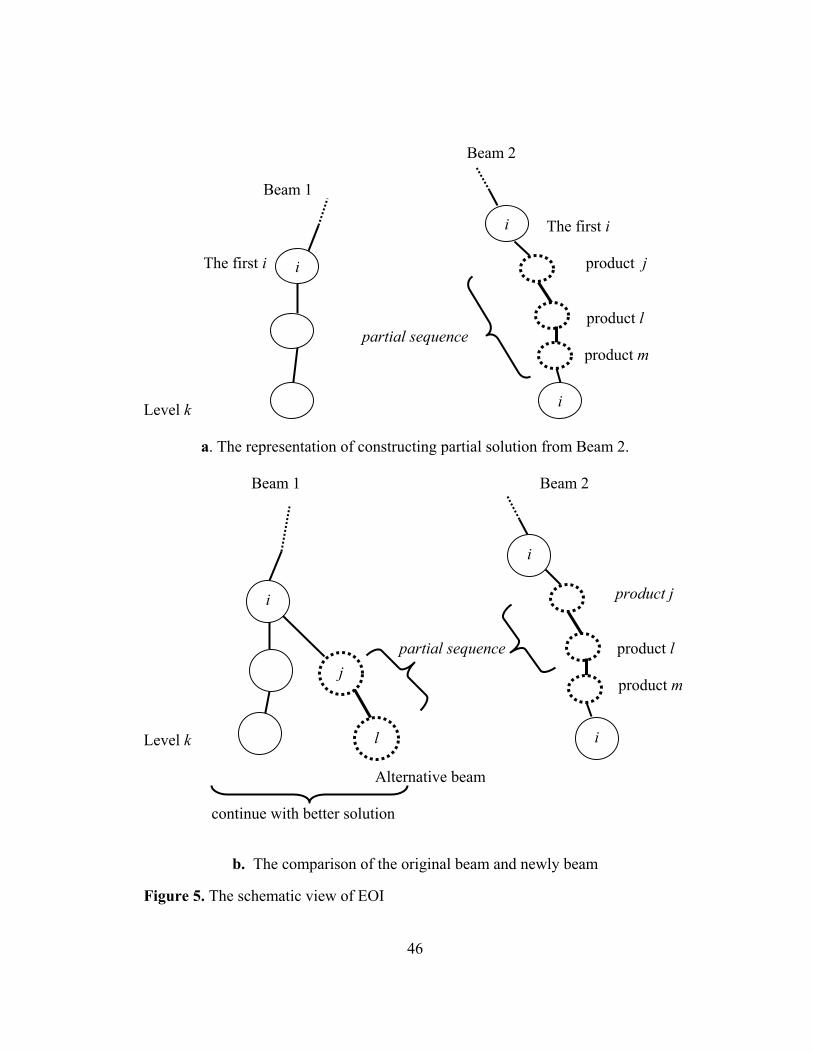
46

Beam 2

Beam 1 The first i The first i product j

product l partial sequence

product m Level k

a. The representation of constructing partial solution from Beam 2.

Beam 1 Beam 2 product j

partial sequence product l

product m

Level k Alternative beam continue with better solution

b. The comparison of the original beam and newly beam

Figure 5. The schematic view of EOI

i

i

i

j

i

l

i

i

47

4.2.3. Global evaluation

Global evaluation function used in our algorithm calculates the sum of variation

at the current level (i.e., level k) and subsequent three levels. It is expressed

mathematically as follows: 23

1 1,, ∑∑ ∑

+

= = =

−=

k

kl

C

j

j

N

i

ijli lrcxGF (22)

Global evaluation function uses a heuristic procedure to determine the products

for each of the further three levels of a partial solution. The procedure first selects

the product with the minimum variation at the next level (i.e., level k+1 for a

sequence at level k). For each of the last two levels, it calculates the combined

variations (i.e, the variations at levels k+1 and k+2) with each of the alternative

product pairs (see Figure 6c). Then, it selects the first product of the pair with the

minimum combined variation, as done in 2-step Monden heuristic. However, unlike

2-step heuristic, some of the alternative pairs are eliminated.

Since the minimization of the sum of the variation at each level is the objective

function of the sequencing problem, it is intuitive that an optimal/near-optimal

sequence yields relatively small variation at each level. This implies that the amount

of actual usage is very close to that of desired usage for each part at a particular

level. As an example, if the variation at level k+1 would be equal to 0, the products

for the next 2 levels could be determined without considering the sequence at level

k+1. Hence, if the variation at level k+1 is ignored, some of the alternative pairs can

be eliminated without considering the sequence at level k+1. The detailed

explanation of the methodology to select the last two products is given below:

48

First, all of the feasible 3-level sequences starting with the product at level k+1

are created (see Figure 6b). Then, the total variation for each of them is calculated

by summing the variations at level 2 and 3, and the variation at level 2 for a

sequence with the last two products. As an example, for a sequence of A (the last

product of the sequence at level k+1), B, and D, the total variation is calculated as

follows:

( ) ( ) ),(,,,),,( DBVDBAVBAVDBATV ++=

The equation shown above implies that if the TV(A,B,D) is small enough, the

products B and D are suitable to be sequenced after A, and D is suitable to be chosen

after B. If TV (A,B,D) is significantly large, products B and D should not be added

respectively to any partial solution that ends with A. This is because of the fact that

the total variation at the last three levels of any near-optimal solution that ends with

A, B, and D most probably increases dramatically.

After calculating the value of total variation for each 3-level sequence, the best w

solutions (i.e., the ones that have the minimum total variation) of at most n2

alternatives is considered for global estimation. Then, w solutions are created by

adding the last two products of the filtered 3-level sequences to the current solution

(i.e., the sequence at level k+1) and the pair that yields the minimum combined

variation is selected. Then, the first product of the best pair is chosen for level k+2.

The product for level k+3 is selected using the same procedure.

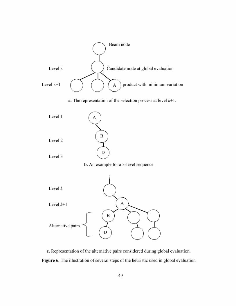
49

Beam node

Level k Candidate node at global evaluation

Level k+1 product with minimum variation

a. The representation of the selection process at level k+1.

Level 1

Level 2

Level 3

b. An example for a 3-level sequence

Level k

Level k+1

Alternative pairs

c. Representation of the alternative pairs considered during global evaluation.

Figure 6. The illustration of several steps of the heuristic used in global evaluation

A

A

B

D

A

B

D

50

4.2.4. Different versions of the proposed method

In the earlier implementation of the proposed method, we thus far considered

the BS technique in which beams progress independently. However, contrary is

also possible in the sense that the BS technique can be implemented with

dependent beams, i.e., all descendant nodes are evaluated at any level and the best

β nodes are chosen among them as the beam nodes. Thus, we also consider this

version of the BS method, with the expectation of obtaining better solutions. Note

that the filtering procedure is invoked for each beam independently in this version,

as performed in the first version.

In order to observe the effect of the backtracking and EOI on the objective

function, we also design several versions of the algorithm with backtracking or

EOI, or neither of them. Note that we do not apply the backtracking procedure for

the BS method with dependent beams as this procedure requires that beams

progress independently.

The versions of the proposed method used in this study are:

BS-1: A BS technique in which beams progress independently.

BS-2: A BS technique in which beams progress independently, and

backtracking procedure is invoked.

BS-3: A BS technique in which beams progress independently, and EOI

procedure is invoked.

BS-4: A BS technique in which beams progress independently, and

backtracking and EOI procedures are invoked.

BS-5: A BS technique with dependent beams.

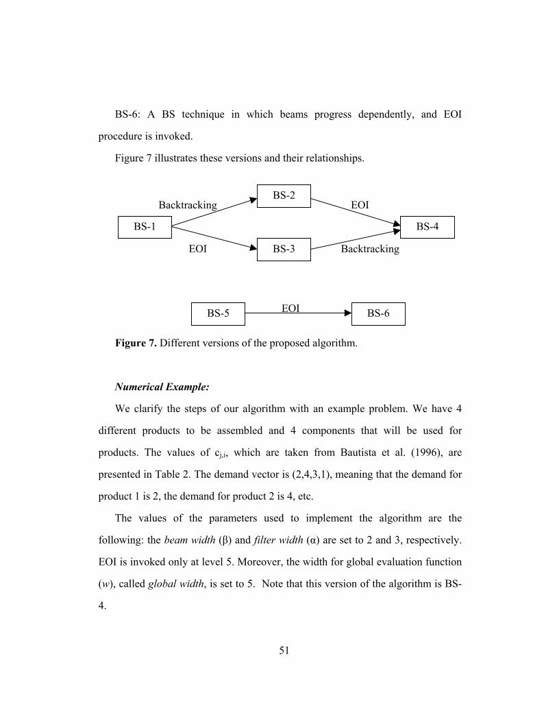
51

BS-6: A BS technique in which beams progress dependently, and EOI

procedure is invoked.

Figure 7 illustrates these versions and their relationships.

Backtracking EOI

EOI Backtracking

EOI

Figure 7. Different versions of the proposed algorithm.

Numerical Example:

We clarify the steps of our algorithm with an example problem. We have 4

different products to be assembled and 4 components that will be used for

products. The values of cj,i, which are taken from Bautista et al. (1996), are

presented in Table 2. The demand vector is (2,4,3,1), meaning that the demand for

product 1 is 2, the demand for product 2 is 4, etc.

The values of the parameters used to implement the algorithm are the

following: the beam width (β) and filter width (α) are set to 2 and 3, respectively.

EOI is invoked only at level 5. Moreover, the width for global evaluation function

(w), called global width, is set to 5. Note that this version of the algorithm is BS-

4.

BS-1

BS-2

BS-3

BS-4

BS-5 BS-6

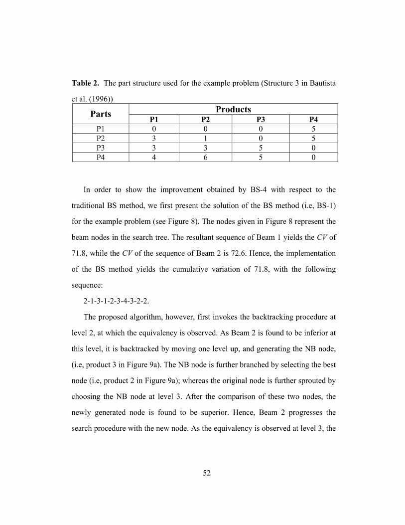
52

Table 2. The part structure used for the example problem (Structure 3 in Bautista

et al. (1996))

Products Parts P1 P2 P3 P4

P1 0 0 0 5 P2 3 1 0 5 P3 3 3 5 0 P4 4 6 5 0

In order to show the improvement obtained by BS-4 with respect to the

traditional BS method, we first present the solution of the BS method (i.e, BS-1)

for the example problem (see Figure 8). The nodes given in Figure 8 represent the

beam nodes in the search tree. The resultant sequence of Beam 1 yields the CV of

71.8, while the CV of the sequence of Beam 2 is 72.6. Hence, the implementation

of the BS method yields the cumulative variation of 71.8, with the following

sequence:

2-1-3-1-2-3-4-3-2-2.

The proposed algorithm, however, first invokes the backtracking procedure at

level 2, at which the equivalency is observed. As Beam 2 is found to be inferior at

this level, it is backtracked by moving one level up, and generating the NB node,

(i.e, product 3 in Figure 9a). The NB node is further branched by selecting the best

node (i.e, product 2 in Figure 9a); whereas the original node is further sprouted by

choosing the NB node at level 3. After the comparison of these two nodes, the

newly generated node is found to be superior. Hence, Beam 2 progresses the

search procedure with the new node. As the equivalency is observed at level 3, the

53

same procedure is invoked for the inferior beam (i.e., Beam 2 in Figure 9b) at this

level.

In addition to the backtracking method, we apply the EOI procedure at a

certain level which is level 5. We first choose the last products of Beam1 and

Beam 2, which are product 2 and product 3, respectively. Then we exchange the

information between each beam in the following way:

First we transfer the sequence of 2-2 from Beam 2 to Beam 1 since it is

between the first and the last appearance of the last product (i.e., product 3) of

Beam 2. This partial sequence is inserted to Beam 1 at level 3, at which the first

appearance of product 3 is observed. Hence, a new solution with the sequence of

2-1-3-2-2 is obtained at level 5. This solution is compared with the original

solution of Beam 1 that has the sequence of 2-1-3-1-2. Similarly, the sequence of

1-3-1 is transferred from Beam 1 to Beam 2, leading a new beam with a sequence

of 1-3-2-1-3-1. Since the length of the new beam is greater than the current level,

it is truncated, by which we obtain the sequence of 1-3-2-1-3. The result of the

evaluation of the original beams and the newly generated beams reveals that the

new beams are inferior. Hence, the procedure progresses with the original beams

at level 5.

During the implementation of the algorithm, the equivalency is observed again

at level 9. However it does not change the structure of the inferior beam (i.e.,

Beam 1) at this level. The resulting sequence is 1-3-2-2-3-4-2-3-1-2, with a CV

value of 66.2. Hence, the CV is improved by 8.4 percent.

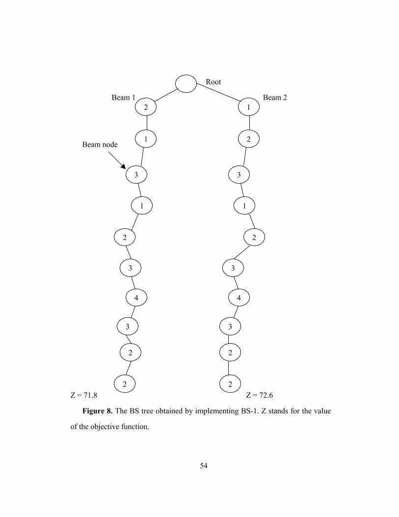
54

Root

Beam 1 Beam 2

Beam node

Z = 71.8 Z = 72.6

Figure 8. The BS tree obtained by implementing BS-1. Z stands for the value

of the objective function.

3

4

3

2

2

3

4

3

2

2

2

3

2

1

3

1

2

1

1

2

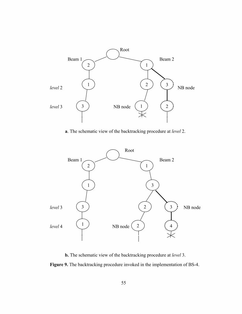
55

Root

Beam 1 Beam 2

level 2 NB node

level 3 NB node

a. The schematic view of the backtracking procedure at level 2.

Root

Beam 1 Beam 2

level 3 NB node

level 4 NB node

b. The schematic view of the backtracking procedure at level 3.

Figure 9. The backtracking procedure invoked in the implementation of BS-4.

2

1

3

1

3

2

1 2

3

4

2

1

3

1

2

1

3

2

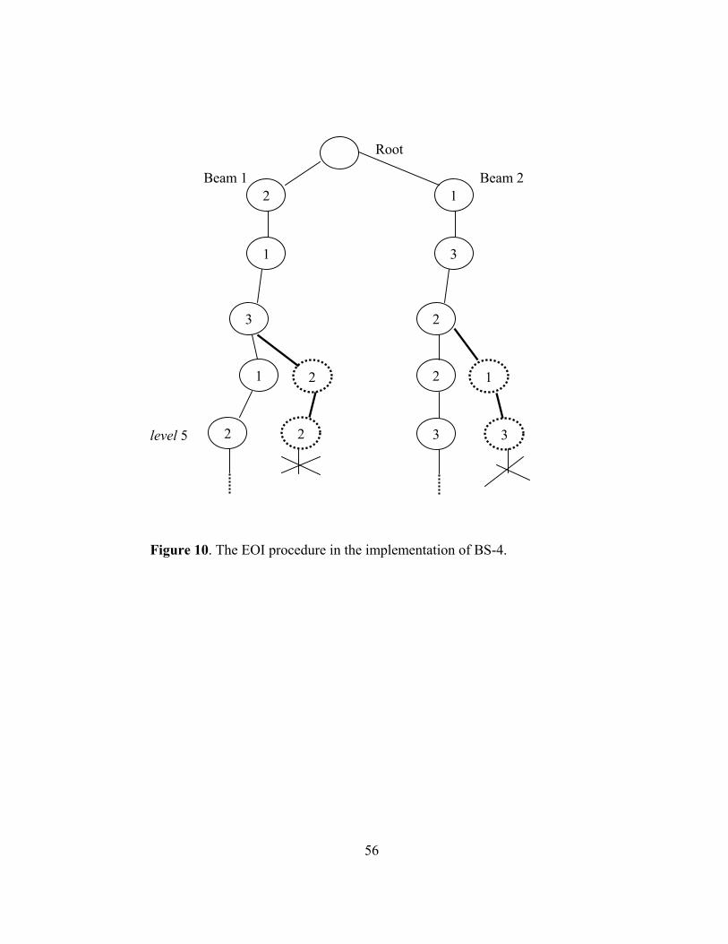
56

Root

Beam 1 Beam 2

level 5

Figure 10. The EOI procedure in the implementation of BS-4.

2

1

3

1

2

1

3

2

2

3

2

2

1

3

57

Chap t e r 5

COMPUTATIONAL RESULTS

In this chapter, we first give the comparison of the proposed method with the

existing heuristics reported in the literature. Then, we analyze the case if the solution

quality is improved by the backtracking and EOI procedures in Section 5.2. We

investigate the effect of the EOI procedure at different positions. The results are

presented in Section 5.3.

5.1. The evaluation of the proposed algorithm

The proposed methods (i.e, BS-1,…, BS-6) are compared with the five

heuristics, which are GC Method, 2-step Method, Variance Method, 2-step Variance

Method, and Beam Search Heuristic. In the implementation of the Variance and 2-

step Variance algorithms, we optimize the discounting coefficient of the opportunity

cost which is added to the objective function. The following parameters of the beam

search algorithms are also optimized: filter width, global width, the beginning level

for EOI, and the interval for EOI. Note that, we use a clever search mechanism in

the implementation of the parameter optimization, rather than the total enumeration.

In addition, we perform the parameter optimization for each problem instance.

58

5.1.1. Computational results for the parts usage measure

5.1.1.1. Experimental conditions

For the parts usage problem, the heuristics are first tested with the problem data

set given in Bautista et al. (1996) and Jin and Wu (2002). In order to statistically

compare the best of the proposed methods and the best of the five existing heuristics,

the p-value is calculated via the paired-t test. In the statistical analysis, the 95%

confidence interval is used. Hence the p-value being less than 0.05 implies the

statistical significance.

The part-product relationship (i.e., number of each part required for each

product) represents a structure in the literature. For Structure 6, we generate totally

45 demand patterns using the demand data in Ding and Chen (1993). This is

because, only one demand pattern is used for this structure in the literature.

The algorithms are further tested by generating various additional data sets. In

order to generate the appropriate data, the following factors given in Leu et al.

(1997) are used: 1) number of products, 2) quantity per assembly, and 3) degree of

commonality. The explanations of these factors are given next.

Quantity per assembly indicates the number of units of a part required for a final

product. The value of 1-10 for this factor implies that the ceiling of a uniform

random number between 1 and 10 is set to quantity per assembly of a part for a

product. Degree of commonality shows the approximate percentage of common

parts used by the products. As an example, if a part has 0% commonality, it is used

by only one product, whereas an 80% commonality means that a part is used by

approximately 80% of the product. Number of parts is set to two times the number

of products.

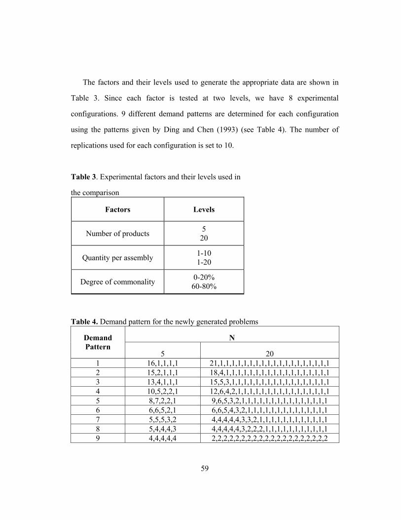
59

The factors and their levels used to generate the appropriate data are shown in

Table 3. Since each factor is tested at two levels, we have 8 experimental

configurations. 9 different demand patterns are determined for each configuration

using the patterns given by Ding and Chen (1993) (see Table 4). The number of

replications used for each configuration is set to 10.

Table 3. Experimental factors and their levels used in

the comparison

Factors Levels

Number of products 5 20

Quantity per assembly 1-10 1-20

Degree of commonality 0-20% 60-80%

Table 4. Demand pattern for the newly generated problems

N Demand Pattern

5 20 1 16,1,1,1,1 21,1,1,1,1,1,1,1,1,1,1,1,1,1,1,1,1,1,1,1 2 15,2,1,1,1 18,4,1,1,1,1,1,1,1,1,1,1,1,1,1,1,1,1,1,1 3 13,4,1,1,1 15,5,3,1,1,1,1,1,1,1,1,1,1,1,1,1,1,1,1,1 4 10,5,2,2,1 12,6,4,2,1,1,1,1,1,1,1,1,1,1,1,1,1,1,1,1 5 8,7,2,2,1 9,6,5,3,2,1,1,1,1,1,1,1,1,1,1,1,1,1,1,1 6 6,6,5,2,1 6,6,5,4,3,2,1,1,1,1,1,1,1,1,1,1,1,1,1,1 7 5,5,5,3,2 4,4,4,4,4,3,3,2,1,1,1,1,1,1,1,1,1,1,1,1 8 5,4,4,4,3 4,4,4,4,4,3,2,2,2,1,1,1,1,1,1,1,1,1,1,1 9 4,4,4,4,4 2,2,2,2,2,2,2,2,2,2,2,2,2,2,2,2,2,2,2,2

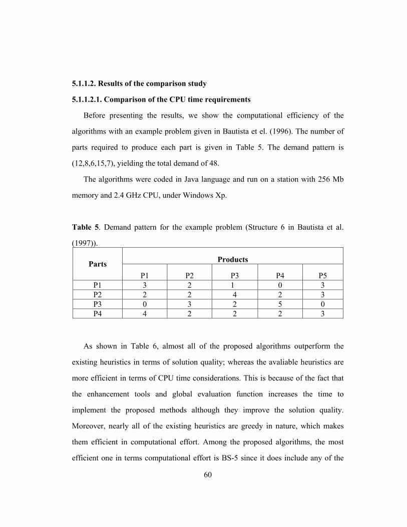
60

5.1.1.2. Results of the comparison study

5.1.1.2.1. Comparison of the CPU time requirements

Before presenting the results, we show the computational efficiency of the

algorithms with an example problem given in Bautista et el. (1996). The number of

parts required to produce each part is given in Table 5. The demand pattern is

(12,8,6,15,7), yielding the total demand of 48.

The algorithms were coded in Java language and run on a station with 256 Mb

memory and 2.4 GHz CPU, under Windows Xp.

Table 5. Demand pattern for the example problem (Structure 6 in Bautista et al.

(1997)).

Products Parts

P1 P2 P3 P4 P5 P1 3 2 1 0 3 P2 2 2 4 2 3 P3 0 3 2 5 0 P4 4 2 2 2 3

As shown in Table 6, almost all of the proposed algorithms outperform the

existing heuristics in terms of solution quality; whereas the avaliable heuristics are

more efficient in terms of CPU time considerations. This is because of the fact that

the enhancement tools and global evaluation function increases the time to

implement the proposed methods although they improve the solution quality.

Moreover, nearly all of the existing heuristics are greedy in nature, which makes

them efficient in computational effort. Among the proposed algorithms, the most

efficient one in terms computational effort is BS-5 since it does include any of the

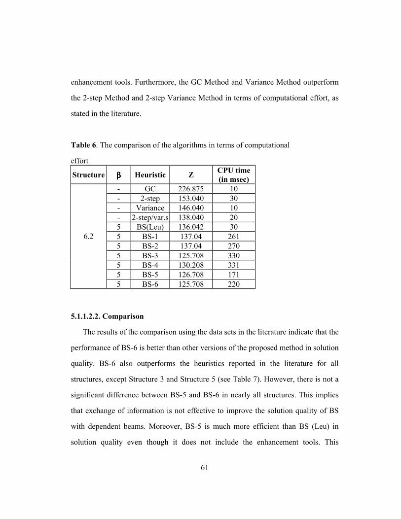
61

enhancement tools. Furthermore, the GC Method and Variance Method outperform

the 2-step Method and 2-step Variance Method in terms of computational effort, as

stated in the literature.

Table 6. The comparison of the algorithms in terms of computational

effort

Structure ββββ Heuristic Z CPU time (in msec)

- GC 226.875 10 - 2-step 153.040 30 - Variance 146.040 10 - 2-step/var.s 138.040 20 5 BS(Leu) 136.042 30 5 BS-1 137.04 261 5 BS-2 137.04 270 5 BS-3 125.708 330 5 BS-4 130.208 331 5 BS-5 126.708 171

6.2

5 BS-6 125.708 220

5.1.1.2.2. Comparison

The results of the comparison using the data sets in the literature indicate that the

performance of BS-6 is better than other versions of the proposed method in solution

quality. BS-6 also outperforms the heuristics reported in the literature for all

structures, except Structure 3 and Structure 5 (see Table 7). However, there is not a

significant difference between BS-5 and BS-6 in nearly all structures. This implies

that exchange of information is not effective to improve the solution quality of BS

with dependent beams. Moreover, BS-5 is much more efficient than BS (Leu) in

solution quality even though it does not include the enhancement tools. This

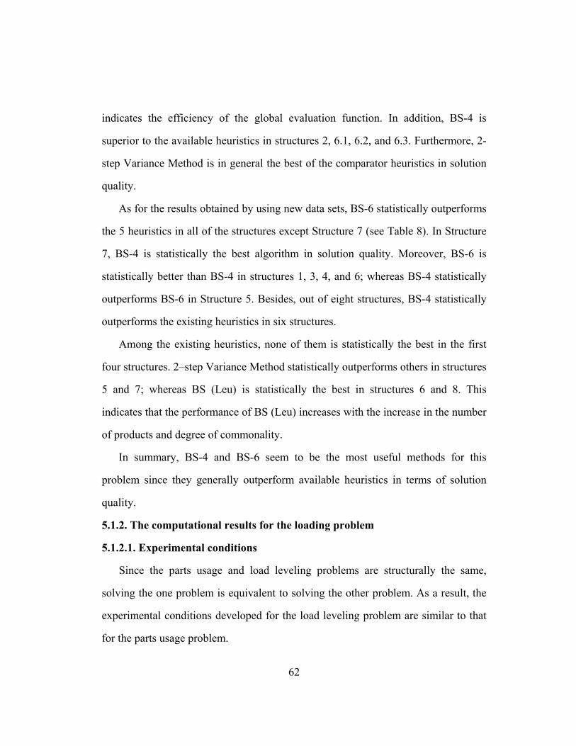
62

indicates the efficiency of the global evaluation function. In addition, BS-4 is

superior to the available heuristics in structures 2, 6.1, 6.2, and 6.3. Furthermore, 2-

step Variance Method is in general the best of the comparator heuristics in solution

quality.

As for the results obtained by using new data sets, BS-6 statistically outperforms

the 5 heuristics in all of the structures except Structure 7 (see Table 8). In Structure

7, BS-4 is statistically the best algorithm in solution quality. Moreover, BS-6 is

statistically better than BS-4 in structures 1, 3, 4, and 6; whereas BS-4 statistically

outperforms BS-6 in Structure 5. Besides, out of eight structures, BS-4 statistically

outperforms the existing heuristics in six structures.

Among the existing heuristics, none of them is statistically the best in the first

four structures. 2–step Variance Method statistically outperforms others in structures

5 and 7; whereas BS (Leu) is statistically the best in structures 6 and 8. This

indicates that the performance of BS (Leu) increases with the increase in the number

of products and degree of commonality.

In summary, BS-4 and BS-6 seem to be the most useful methods for this

problem since they generally outperform available heuristics in terms of solution

quality.

5.1.2. The computational results for the loading problem

5.1.2.1. Experimental conditions

Since the parts usage and load leveling problems are structurally the same,

solving the one problem is equivalent to solving the other problem. As a result, the

experimental conditions developed for the load leveling problem are similar to that

for the parts usage problem.

63

Table 7. The computational results obtained by the data sets in given in the literature

Structure N D # of demand pattern

ββββ Heuristic Zavg p-value

- GC 93.333 - 2-step 64.711 - Variance 66.116 - 2-step/var. 61.973 4 BS(Leu) 72.124 4 BS-1 62.24 4 BS-2 61.742 4 BS-3 61.795 4 BS-4 60.818 4 BS-5 60.356

1 4 20 45

4 BS-6 60.124

0.003 *


2 4 20 45

4 BS-6 133.529

0.0005 *


3 4 20 45

4 BS-6 137.309

0.478

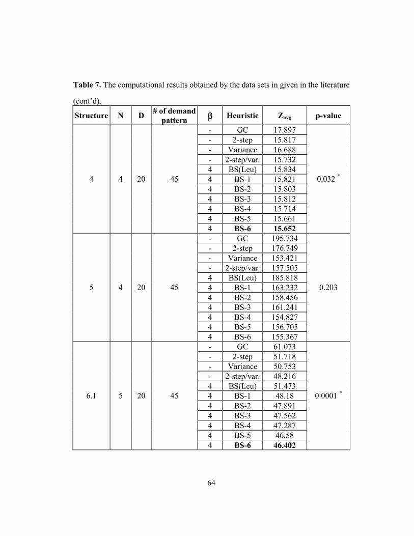
64


(cont’d).




4 4 20 45

4 BS-6 15.652

0.032 *


5 4 20 45

4 BS-6 155.367

0.203


6.1 5 20 45

4 BS-6 46.402

0.0001 *

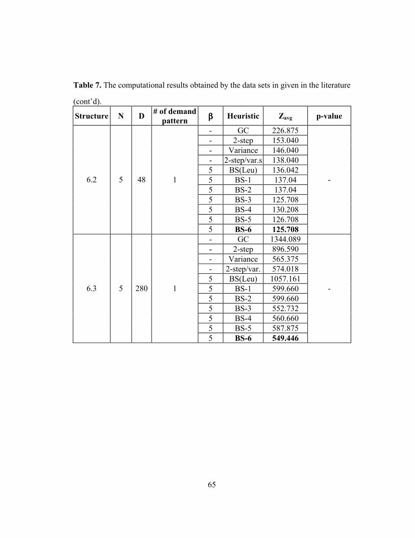
65


(cont’d).



- GC 226.875 - 2-step 153.040 - Variance 146.040 - 2-step/var.s 138.040 5 BS(Leu) 136.042 5 BS-1 137.04 5 BS-2 137.04 5 BS-3 125.708 5 BS-4 130.208 5 BS-5 126.708

6.2 5 48 1

5 BS-6 125.708

-


6.3 5 280 1

5 BS-6 549.446

-

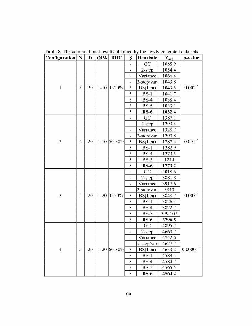
66

Table 8. The computational results obtained by the newly generated data sets Configuration N D QPA DOC ββββ Heuristic Zavg p-value

- GC 1088.9 - 2-step 1054.4 - Variance 1066.4 - 2-step/var. 1043.8 3 BS(Leu) 1043.5 3 BS-1 1041.7 3 BS-4 1038.4 3 BS-5 1033.1

1 5 20 1-10 0-20%

3 BS-6 1032.4

0.002 *

- GC 1387.1 - 2-step 1299.4 - Variance 1328.7 - 2-step/var. 1290.8 3 BS(Leu) 1287.4 3 BS-1 1282.9 3 BS-4 1279.5 3 BS-5 1274

2 5 20 1-10 60-80%

3 BS-6 1273.2

0.001 *

- GC 4018.6 - 2-step 3881.8 - Variance 3917.6 - 2-step/var. 3840 3 BS(Leu) 3848.7 3 BS-1 3826.3 3 BS-4 3822.7 3 BS-5 3797.07

3 5 20 1-20 0-20%

3 BS-6 3796.5

0.003 *

- GC 4895.7 - 2-step 4660.7 - Variance 4742.6 - 2-step/var 4627.7 3 BS(Leu) 4653.2 3 BS-1 4589.4 3 BS-4 4584.7 3 BS-5 4565.5

4 5 20 1-20 60-80%

3 BS-6 4564.2

0.00001 *

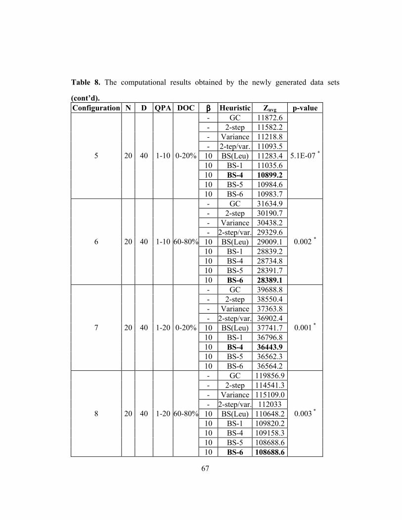
67

Table 8. The computational results obtained by the newly generated data sets

(cont’d). Configuration N D QPA DOC ββββ Heuristic Zavg p-value

- GC 11872.6 - 2-step 11582.2 - Variance 11218.8 - 2-tep/var. 11093.5 10 BS(Leu) 11283.4 10 BS-1 11035.6 10 BS-4 10899.2 10 BS-5 10984.6

5 20 40 1-10 0-20%

10 BS-6 10983.7

5.1E-07 *


6 20 40 1-10 60-80%

10 BS-6 28389.1

0.002 *


7 20 40 1-20 0-20%

10 BS-6 36564.2

0.001 *

- GC 119856.9 - 2-step 114541.3 - Variance 115109.0 - 2-step/var. 112033 10 BS(Leu) 110648.2 10 BS-1 109820.2 10 BS-4 109158.3 10 BS-5 108688.6

8 20 40 1-20 60-80%

10 BS-6 108688.6

0.003 *

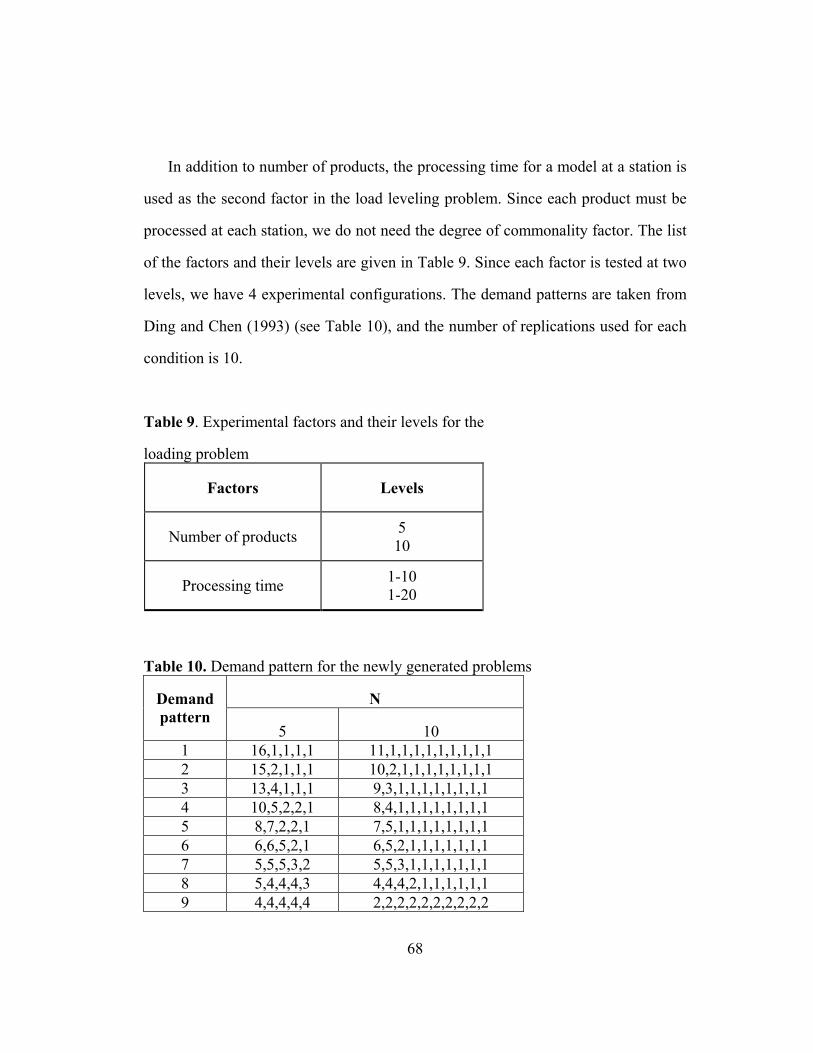
68

In addition to number of products, the processing time for a model at a station is

used as the second factor in the load leveling problem. Since each product must be

processed at each station, we do not need the degree of commonality factor. The list

of the factors and their levels are given in Table 9. Since each factor is tested at two

levels, we have 4 experimental configurations. The demand patterns are taken from

Ding and Chen (1993) (see Table 10), and the number of replications used for each

condition is 10.

Table 9. Experimental factors and their levels for the

loading problem

Factors Levels

Number of products 5 10

Processing time 1-10 1-20

Table 10. Demand pattern for the newly generated problems

N Demand pattern

5 10 1 16,1,1,1,1 11,1,1,1,1,1,1,1,1,1 2 15,2,1,1,1 10,2,1,1,1,1,1,1,1,1 3 13,4,1,1,1 9,3,1,1,1,1,1,1,1,1 4 10,5,2,2,1 8,4,1,1,1,1,1,1,1,1 5 8,7,2,2,1 7,5,1,1,1,1,1,1,1,1 6 6,6,5,2,1 6,5,2,1,1,1,1,1,1,1 7 5,5,5,3,2 5,5,3,1,1,1,1,1,1,1 8 5,4,4,4,3 4,4,4,2,1,1,1,1,1,1 9 4,4,4,4,4 2,2,2,2,2,2,2,2,2,2

69

5.1.2.2. Results

The results of the comparison study for the loading problem indicate that BS-6

statistically outperforms other algorithms in terms of solution quality (see Table 11).

This verifies the structural equivalency of the load leveling and parts usage problem.

Moreover, the performances of BS-5 and BS-6 are statistically the same, implying

that information sharing between dependent beams does not improve the solution

quality.

5.2. The effect of backtracking and EOI on solution quality

In this section, we show that the enhancement tools incorporated into classical

beam search technique with independent beams improve the solution quality. First,

we consider the improvement obtained by the backtracking procedure. Then, we

focus on the effect of the EOI procedure on the objective function in Section 5.2.2.

5.2.1. The effect of backtracking

In order to test the efficiency of the backtracking procedure, we compare the

performances of BS-1 and BS-2. As explained in previous chapter, in BS-1 beams

progress independently and none of the enhancement tools are invoked. In BS-2,

beams progress independently and only the backtracking procedure is performed.

The performance of the algorithms for the data sets in Bautista et al. (1996) and

Jin and Wu (2002) are shown in Table 12. The results reveal that the backtracking

procedure generally improves the solution quality. However, if the quantity per

assembly for each part shows considerably slight variations (i.e., in Structure 5), the

backtracking method does not statistically increase the solution quality.

70

Table 11. The computational results for the loading problem

Configuration N Processing times



1 5 1-10

3 BS-6 269.876

0.0001 *


2 5 1-20

3 BS-6 1179.8

2.5E-07 *


3 10 1-10

5 BS-6 815.685

6.2E-05 *

- GC 4084.1 - 2-step 3777.9 - Variance 3812.8 - 2-step/var. 3634.8 5 BS(Leu) 3672.7 5 BS-1 3646 5 BS-4 3607.9 5 BS-5 3572.7

4 10 1-20

5 BS-6 3572.7

0.0004 *

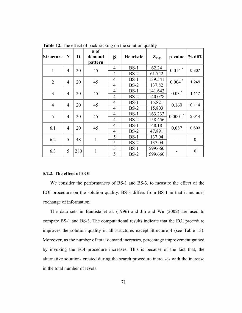
71

Table 12. The effect of backtracking on the solution quality

Structure N D # of

demand pattern

ββββ Heuristic Zavg p-value % diff.

4 BS-1 62.24 1 4 20 45

4 BS-2 61.742 0.014 * 0.807

4 BS-1 139.541 2 4 20 45

4 BS-2 137.82 0.004 * 1.249

4 BS-1 141.642 3 4 20 45

4 BS-2 140.078 0.03 *

1.117

4 BS-1 15.821 4 4 20 45

4 BS-2 15.803 0.160 0.114

4 BS-1 163.232 5 4 20 45

4 BS-2 158.456 0.0001 *

3.014

4 BS-1 48.18 6.1 4 20 45

4 BS-2 47.891 0.087 0.603

5 BS-1 137.04 6.2 5 48 1

5 BS-2 137.04 - 0

5 BS-1 599.660 6.3 5 280 1

5 BS-2 599.660 - 0

5.2.2. The effect of EOI

We consider the performances of BS-1 and BS-3, to measure the effect of the

EOI procedure on the solution quality. BS-3 differs from BS-1 in that it includes

exchange of information.

The data sets in Bautista et al. (1996) and Jin and Wu (2002) are used to

compare BS-1 and BS-3. The computational results indicate that the EOI procedure

improves the solution quality in all structures except Structure 4 (see Table 13).

Moreover, as the number of total demand increases, percentage improvement gained

by invoking the EOI procedure increases. This is because of the fact that, the

alternative solutions created during the search procedure increases with the increase

in the total number of levels.

72

Table 13. The effect of exchange of information on the solution quality

Structure N D # of

demand pattern

ββββ Heuristic Zavg p-value % diff.

4 BS-1 62.24 1 4 20 45

4 BS-3 61.795 0.046 * 0.720

4 BS-1 139.541 2 4 20 45

4 BS-3 137.545 0.0003 * 1.451

4 BS-1 141.642 3 4 20 45

4 BS-3 140.82 0.018 * 0.584

4 BS-1 15.821 4 4 20 45

4 BS-3 15.812 0.323 0.057

4 BS-1 163.232 5 4 20 45

4 BS-3 161.241 0.0005 * 1.235

4 BS-1 48.18 6.1 4 20 45

4 BS-3 47.562 0.006 * 1.299

5 BS-1 137.04 6.2 5 48 1

5 BS-3 125.708 - 9.015

5 BS-1 599.660 6.3 5 280 1

5 BS-3 552.732 - 8.490

5.3. The effect of EOI at different positions

The performance of the proposed algorithm shows that the EOI procedure

generally improves the solution quality. However, further analysis is necessary to

determine the interval for which the EOI is more effective. Hence, the EOI

procedure is invoked at predetermined intervals to observe its effect on the

performance measure (see Figure 11 and Figure 12). As an example, for a design

with 20 levels, EOI is only performed at the following intervals: 1-4, 5-8, 9-12, 13-

16, 17-2. Note that the analysis is performed by using BS-3, in which beams

progress independently and exchange of information is invoked. In addition, we

consider the data sets given in Bautista et al. (1996). The experimental analysis is

73

first performed on small problems in which the number of total demand is 20. Then,

the total demand is increased to higher levels such as 260.

The analysis on the exchange of information indicates that if the number of

levels (i.e., total demand) is small, invoking the EOI procedure between certain

intervals generally does not improve the objective function (see Figure 11). Only

in Structure 2, the EOI procedure statistically improves the solution quality if it

invoked at the middle levels. If we increase the number of levels, the EOI

procedure statistically improves the solution quality in Structures 1, 2, and 5. It is

inferred from the Figure 12 that the interval at which EOI is the most effective

seems to be the middle of the search procedure. However, as shown in Figure 12b,

in some cases the most effective interval for EOI may shift toward the end of the

search procedure.

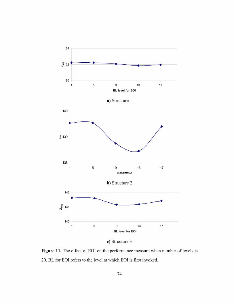
74

60

62

64

1 5 9 13 17

BL level for EOI

Zavg

a) Structure 1

138

139

140

1 5 9 13 17

BL level for EOI

Zavg

b) Structure 2

140

141

142

1 5 9 13 17

BL level for EOI

Zavg

c) Structure 3

Figure 11. The effect of EOI on the performance measure when number of levels is

20. BL for EOI refers to the level at which EOI is first invoked.

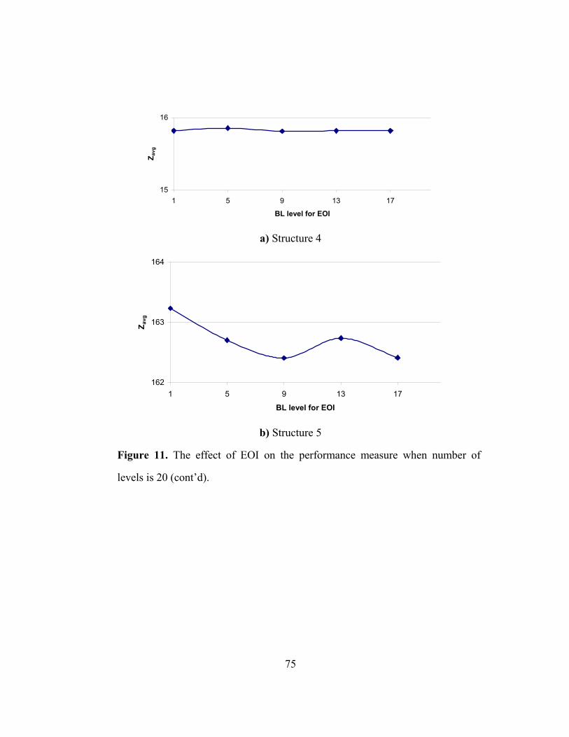
75

15

16

1 5 9 13 17

BL level for EOI

Zavg

a) Structure 4

162

163

164

1 5 9 13 17

BL level for EOI

Zavg

b) Structure 5

Figure 11. The effect of EOI on the performance measure when number of

levels is 20 (cont’d).

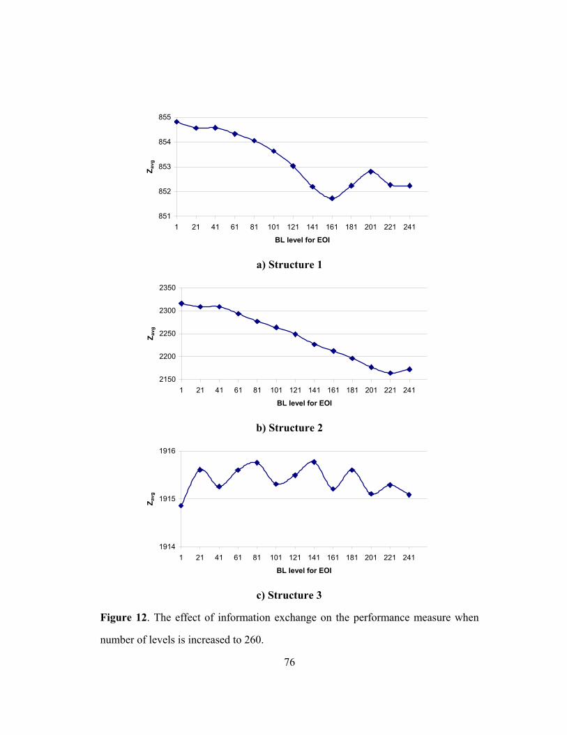
76

851

852

853

854

855

1 21 41 61 81 101 121 141 161 181 201 221 241

BL level for EOI

Zavg

a) Structure 1

2150

2200

2250

2300

2350

1 21 41 61 81 101 121 141 161 181 201 221 241

BL level for EOI

Zavg

b) Structure 2

1914

1915

1916

1 21 41 61 81 101 121 141 161 181 201 221 241

BL level for EOI

Zavg

c) Structure 3

Figure 12. The effect of information exchange on the performance measure when

number of levels is increased to 260.

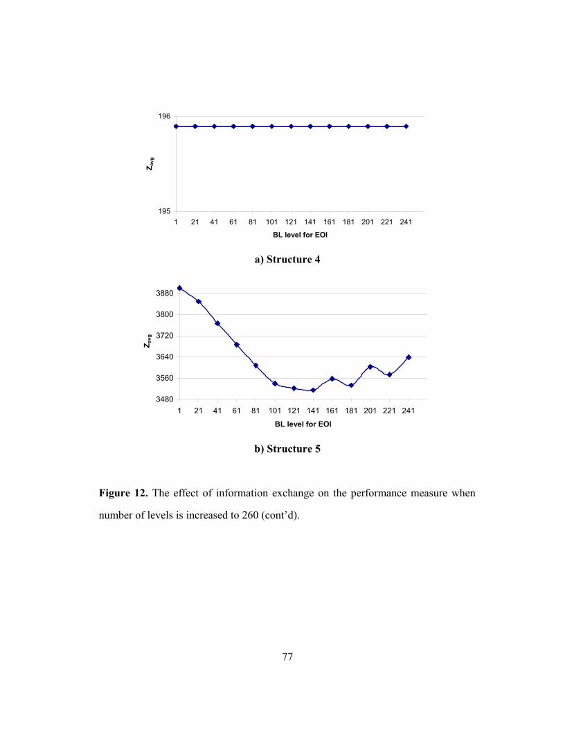
77

195

196

1 21 41 61 81 101 121 141 161 181 201 221 241

BL level for EOI

Zavg

a) Structure 4

3480

3560

3640

3720

3800

3880

1 21 41 61 81 101 121 141 161 181 201 221 241

BL level for EOI

Zavg

b) Structure 5

Figure 12. The effect of information exchange on the performance measure when

number of levels is increased to 260 (cont’d).

78

Chap t e r 6

CONCLUSION

In this thesis, we study the mixed-model assembly line sequencing problem,

with the assumptions of balanced lines with fix processing times, and negligible

setup times between the different product models. We aim to optimize the

following objectives separately:

1) Maintaining a constant rate of usage of all parts that feed the final

assembly line

2) Smoothing the workload on the final assembly line to reduce the chance of

production delays and stoppages

We propose Beam Search algorithms to solve the problem. Unlike the classical

beam search techniques, the proposed algorithms have some enhancement tools

that improve the solution quality. These tools are the backtracking and EOI

procedures. The backtracking method enables to return to some previous solution

states in the search tree with the expectation of obtaining better solutions. The EOI

procedure takes the part of the solution from one beam and transfers it to another

beam. Hence, the resulting beam with this additional information may lead to

better solutions.

We compare the beam search algorithms with the existing heuristics reported

in the literature, using various problem data sets. The computational results

79

indicate that the proposed algorithms generally outperform the available heuristics

for the parts usage and loading problems. Besides, we demonstrate that the

backtracking and EOI procedures generally improve the solution quality.

We also analyze the effect of the EOI when it is invoked at different positions

in the search tree. The results lead us to the following conjecture: the exchange of

information is the most effective when it is invoked at the middle levels in the

search tree.

We can list the following further research directions: First, the proposed

algorithms can be implemented for the same problem with different objectives

such as minimizing the utility work (i.e, the amount of work that cannot be

completed within the given length of the station), and line stoppages. Second, the

EOI procedure can be incorporated into beam search algorithms that are used in

other research areas such as scheduling, assembly line balancing, etc. Third,

different versions of the EOI and backtracking methods can be developed for the

MMAL sequencing problem to further improve their efficiency. Fourth, a further

analysis on the EOI should be performed to draw inferences about where it is the

most effective during the search procedure. Furthermore, the MMAL sequencing

problem can be studied by considering asynchronous lines as well as hybrid

systems. It may also be useful to observe whether the line balancing and the line

sequencing problems can be solved simultaneously in some real-life conditions.

80

BIBLIOGRAPHY

[1] Bard, J. F., Shtub, A., Joshi S.B., 1994, “Sequencing Mixed-model

Assembly Lines to Level Parts Usage and Minimize Line Length”,

International Journal of Production Research, 32, 2431-2454.

[2] Bautista, J., Companys, R., Corominas, A., 1996, “Heuristics and Exact

Algorithms for Solving The Monden Problem”, European Journal of

Operational Research, 88, 101-113.

[3] Celano, G., Costa, A., Fichera, S., “A Comparative Analysis of Sequencing

Heuristics for Solving The Toyota Goal Chasing Problem”, Robotics and

Computer-integrated Manufacturing (to appear).

[4] Cheng, L., Ding, F., Y., 1996, “Modifying Mixed-model Assembly Line

Sequencing Methods to Consider Weighted Variations for Just-in-time

Production Systems” IIE Transactions, 28, 919-927.

[5] Croce, F., D., T’kindt, V., 2002, “A Recovering Beam Search Algorithm for

The One-machine Dynamic Total Completion Time Scheduling Problem”,

Journal of The Operational Research Society, 53, 1275-1280.

[6] Croce, F. D., Ghirardi, M., Tadei, R., 2004, “Recovering Beam Search:

Enhancing The Beam Search Approach for Combinatorial Optimization

Problems”, Journal of Heuristics, 10, 89-104.

[7] Dar-el, E., M., Cother, R.F., 1975, “Assembly Line Sequencing for Model

Mix”, International Journal of Production Research, 13, 463-477.

81

[8] Dar-el, E., M., Cucuy, S., 1977, “Optimal Mixed-model Sequencing for

Balanced Assembly Lines”, Omega, 5, 333-342

[9] Dar-el, E., M., 1978, “Mixed-model Assembly Line Sequencing Problems“,

The International Journal of Management Science, 6, 343-323.

[10] Ding, F., Y., Cheng, L., 1993, “An Effective Mixed-model Assembly Line

Sequencing Heuristic for Just-in-time Production Systems”, Journal of

Operations Management, 11, 45-50.

[11] Drexl, A., Kimms, 2001, “Sequencing JIT Mixed-model Assembly Lines

Under Station-Load and Part-usage Constraints”, Management Science, 47,

480-491.

[12] Duplaga, E., A., Hahn, C. K., Hur, D., 1996, “Mixed-Model Assembly Line

Sequencing at Hyundai Motor Company”, “Production and Inventory

Management Journal”, 37, 20-26.

[13] Duplaga, E., A., Bragg, D., J., 1998, “Mixed-model Assembly Line

Sequencing Heuristics for Component Parts Usage: A Comparative

Analysis”, International Journal of Production Research, 36, 2209-2224.

[14] Esteve, B., Aubijoux, C., Chartier, A., T’kindt, V., “A Recovering Beam

Search Algorithm for The Single Machine Just-in-time Scheduling Problem,

European Journal of Operational Research (to appear).

[15] Erel, E., Sabuncuoglu, I., Sekerci, H., 2005, “Stochastic Assembly Line

Balancing Using Beam Search”, International Journal of Production

Research, 43, 1411-1426.

82

[16] Ghirardi, M., Potts, C., N., 2005, “Makespan Minimization for Scheduling

Unrelated Parallel Machines: A recovering Beam Search Approach”,

European Journal of Operational Research, 165, 457-467.

[17] Honda, N., Mohri, S., Ishii, H., 2003, “Backtracking Beam Search Applied

to Multi-objective Scheduling Problem”, The Fifth Metaheuristics

International Conference, Kyoto, 1-6.

[18] Hyun, C., J., Kim, Y., Kim, Y., K., 1998, “A Genetic Algorithm for Multiple

Objective Sequencing Problems in Mixed Model Assembly Lines”,

Computers Operations Research, 25, 675-690.

[19] Inman, R. R., Bulfin, R. L., 1991, “Sequencing JIT Mixed-Model Assembly

Lines”, Management Science, 37, 901-904.

[20] Kilbridge, M., Webster, L., 1963, “The Assembly Line Model Mix

Sequencing Problem”, Proceedings of The Third International Conference

on Operations Research, Oslo, 247.

[21] Kim, Y., K., Hyun, C., J., Kim, Y., 1996, “Sequencing in Mixed Model

Assembly Lines: A Genetic Algorithm Approach”, Computers Ops Res., 23,

1131-1145.

[22] “Korkmazel, T., Meral S., 2001, “Bicriteria Sequencing Methods for The

Mixed-model Assembly Line in Just-in-time Production Systems”, 131, 188-

207.

[23] Kubiak, W., Sethi, S.P., 1991, “A Note on Level Schedules for Mixed-model

Assembly Lines in Just-in-time Production Systems”, Management Science,

37, 121-122.

83

[24] Kubiak, W., 1993, “Minimizing Variation of Production Rates in Just-in-

time Systems: A Survey”, European Journal of Operations Management, 66,

259-271.

[25] Leu, Y., Huang, P. Y., Russell, R., S., 1997, “Using Beam Search

Techniques for Sequencing Mixed-model Assembly Lines”, Annals of

Operations Research, 70, 379-397.

[26] Lowerre, B., T., 1976, “The HARPY Speech Recognition System”, Ph.D.

Thesis, Carnegie Mellon University, Pittsburgh, PA.

[27] Mansouri, S., A., 2005, “A Multi-objective Genetic Algorithm for Mixed-

model Sequencing on JIT Assembly Lines”, European Journal of

Operational Research, 167, 696-716.

[28] McMullen, P. R., Frazier, G. V., 2000, “A Simulated Annealing Approach to

Mixed-Model Sequencing with Multiple Objectives on a Just-in-time Line,

32, 679-686.

[29] McMullen, P.R., Tarasewich, 2005, “A Beam Search Heuristic Method for

Mixed-Model Scheduling with Setups”, International Journal of Production

Economics, 96, 273-383.

[30] Merengo, C., F. Nava, Pozzetti, A., 1999, “Balancing and Sequencing

Manual Mixed-model Assembly Lines”, International Journal of Production

Research, 37, 2835-2860.

[31] Miltenburg, J., 1989, “Level Schedules for Mixed-model Assembly Lines in

Just-in-time Production Systems”, Management Science, 35, 192-207.

84

[32] Miltenburg, J., Sinnamon, G., 1989, “Scheduling Mixed-model Multi-level

Just-in-time Production Systems”, International Journal of Production

Research, 27, 1487-1509.

[33] Miltenburg, G.J., Goldstein, T., 1991, “Developing Production Schedules

which Balance Part Usage and Smooth Production Loads for Just-in-time

Production Systems, Naval Research Logistics, 38, 893-910.

[34] Mıltenburg, J., Sinnamon, G., 1992, Algorithms for Scheduling Multi-level

Just-in-time Production Systems, 24, 121-130.

[35] Monden, Y., 1983, “Toyota Production System”, Institute of Industrial

Engineers, Norcross, Georgia, USA.

[36] Ng., W.C., Mak, K.L., 1994, “A Branch and Bound Algorithm for

Scheduling Just-in-time Mixed-Model Assembly Lines”, International

Journal of Production Economics, 33, 169-183.

[37] Ow, S., P., Morton, T., E., 1988, “Filtered Beam Search in Scheduling”,

International Journal of Production Research, 26, 35-62.

[38] Ponnambalam, S.G., Aravindan, P., Rao, M. S., 2003, “Genetic Algorithms

for Sequencing Problems in Mixed Model Assembly Lines”, Computers and

Industrial Engineering, 45, 669-690.

[39] Sabuncuoglu, I., Karabuk, S., 1998, “A Beam Search-based Algorithm and

Evaluation of Scheduling Approaches for Flexible Manufacturing Systems,

IIE Transactions, 30, 179-191.

[40] Sabuncuoglu, I., Bayiz, M., 1999, “Job Shop Scheduling with Beam Search”,

European Journal of Operational Research, 118, 390-412.

85

[41] Sabuncuoglu, I., Bayiz, M., 2000, “Analysis of Reactive Scheduling

Problems in a Job Shop Environment”, European Journal of Operational

Research, 126, 567-586.

[42] Sumichrast, R., T., Russell, R., S., 1990, “Evaluating Mixed-Model

Assembly Line Sequencing Heuristics for Just-in-Time Production Systems”,

Journals of Operations Management, 9, 371-390.

[43] Sumichrast, R., T., Oxenrider, K., A., Clayton E. R., 2000, “An Evolutionary

Algorithm for Sequencing Production on a Paced Assembly line”, Decision

Sciences, 31, 149-172.

[44] Thomopoulos, N., T., 1967, “Line Balancing-sequencing for Mixed-model

Assembly “, Management Science, 14, 59-75.

[45] Valente, J., M., S., Alves, R., A., F., S., 2005, “Filtered and Recovering

Beam Search Algorithms for The Early/tardy Scheduling Problem with No

Idle Time”, Computers and Industrial Engineering, 48, 363-375.

[46] Jin, M., Wu, S.D., 2002, “A New Heuristic Method for Mixed Model

Assembly Line Balancing Problem”, 44, 159-169.

[47] Yamashita, H., Okamura, K., 1979, “A Heuristic Algorithm for The

Assembly Line Model-mix Sequencing Problem to Minimize the Risk os

Stopping the Conveyor”, International Journal of Production Research, 17,

233-246.

[48] Yano, C., A., Rachamadugu, R., 1991, “Sequencing to Minimize Work

Overload in Assembly Lines with Product Options”, Management Science,

37, 572-586.

86

[49] Zeramdini, W., Aigbedo, H., Monden, Y., 2000, “Bicriteria Sequencing for

Just-in-Time Mixed-model Assembly Lines”, International Journal of

Production Research, 38, 3451-3470.

[50] Zhu, J., Ding, F., Y., 2000, “A Transformed Two-stage Method for Reducing

The Part-usage Variation and A Comparison of The Product-level and Part-

level Solutions in Sequencing Mixed-model Assembly Lines”, European

Journal of Operational Research, 127, 203-216.

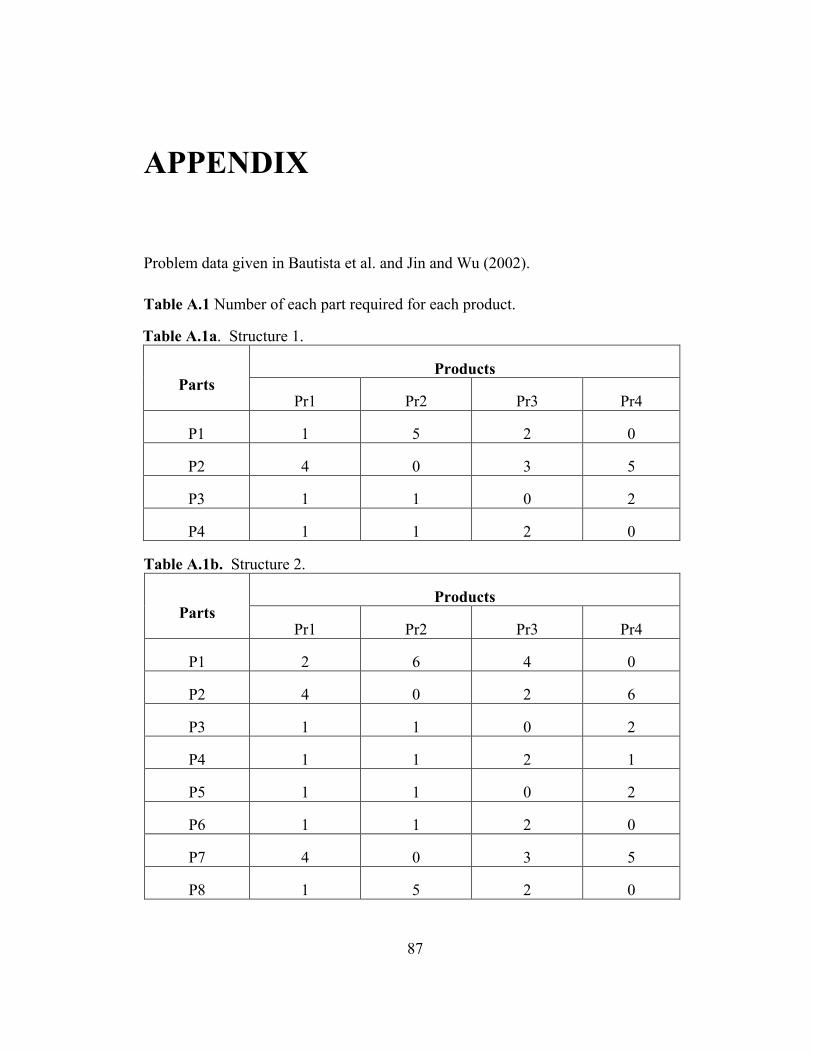
87

APPENDIX

Problem data given in Bautista et al. and Jin and Wu (2002).

Table A.1 Number of each part required for each product.

Table A.1a. Structure 1.

Products Parts

Pr1 Pr2 Pr3 Pr4

P1 1 5 2 0

P2 4 0 3 5

P3 1 1 0 2

P4 1 1 2 0

Table A.1b. Structure 2.

Products Parts

Pr1 Pr2 Pr3 Pr4

P1 2 6 4 0

P2 4 0 2 6

P3 1 1 0 2

P4 1 1 2 1

P5 1 1 0 2

P6 1 1 2 0

P7 4 0 3 5

P8 1 5 2 0

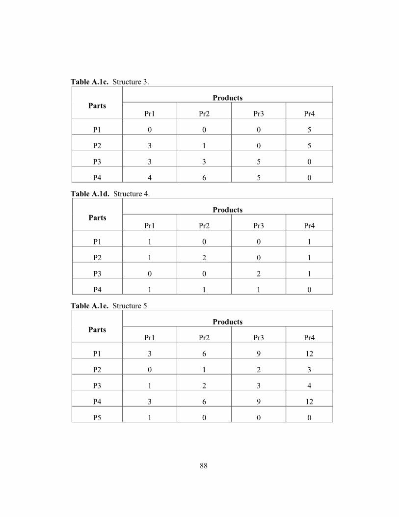
88

Table A.1c. Structure 3.

Products Parts

Pr1 Pr2 Pr3 Pr4

P1 0 0 0 5

P2 3 1 0 5

P3 3 3 5 0

P4 4 6 5 0

Table A.1d. Structure 4.

Products Parts

Pr1 Pr2 Pr3 Pr4

P1 1 0 0 1

P2 1 2 0 1

P3 0 0 2 1

P4 1 1 1 0

Table A.1e. Structure 5

Products Parts

Pr1 Pr2 Pr3 Pr4

P1 3 6 9 12

P2 0 1 2 3

P3 1 2 3 4

P4 3 6 9 12

P5 1 0 0 0

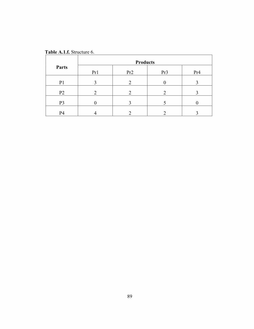
89

Table A.1.f. Structure 6.

Products Parts

Pr1 Pr2 Pr3 Pr4

P1 3 2 0 3

P2 2 2 2 3

P3 0 3 5 0

P4 4 2 2 3

90

Table A.2. Demand vector for products.

Table A.2a. Demand vector for Structure 1..5

Pr. 1-9 Pr. 10-18 Pr. 19-27 Pr. 28-36 Pr. 37-45

17,1,1,1 1,1,9,9 6,6,2,6 4,2,6,8 6,4,8,2

1,17,1,1 6,6,4,4 6,2,6,6 4,2,8,6 6,8,2,4

1,1,17,1 6,4,6,4 2,6,6,6 4,6,2,8 6,8,4,2

1,1,1,17 6,4,4,6 2,4,6,8 4,6,8,2 8,2,4,6

9,9,1,1 4,6,6,4 2,4,8,6 4,8,2,6 8,2,6,4

9,1,9,1 4,6,4,6 2,6,4,8 4,8,6,2 8,4,2,6

9,1,1,9 4,4,6,6 2,6,8,4 6,2,4,8 8,4,6,2

1,9,9,1 5,5,5,5 2,8,4,6 6,2,8,4 8,6,2,4

1,9,1,9 6,6,6,2 2,8,6,4 6,4,2,8 8,6,4,2

Table A.2b. Demand vector for Structure 6.1

Pr. 1-9 Pr. 10-18 Pr. 19-27 Pr. 28-36 Pr. 37-45

16,1,1,1,1 4,13,1,1,1 1,4,1,1,13 5,5,3,5,2 5,2,5,5,3

1,16,1,1,1 4,1,13,1,1 1,1,13,4,1 5,5,3,2,5 3,5,2,5,5

1,1,16,1,1 4,1,1,13,1 1,1,13,1,4 5,5,2,3,5 3,5,5,2,5

1,1,1,16,1 4,1,1,1,13 1,1,4,13,1 5,5,2,5,3 3,5,5,5,2

1,1,1,1,16 1,13,4,1,1 1,1,4,1,13 5,3,5,5,2 3,2,5,5,5

13,4,1,1,1 1,13,1,4,1 1,1,1,13,4 5,3,5,2,5 2,5,3,5,5

13,1,4,1,1 1,13,1,1,4 1,1,1,4,13 5,3,2,5,5 2,5,5,3,5

13,1,1,4,1 1,4,13,1,1 5,5,5,3,2 5,2,3,5,5 2,5,5,5,3

13,1,1,1,4 1,4,1,13,1 5,5,5,2,3 5,2,5,3,5 2,3,5,5,5

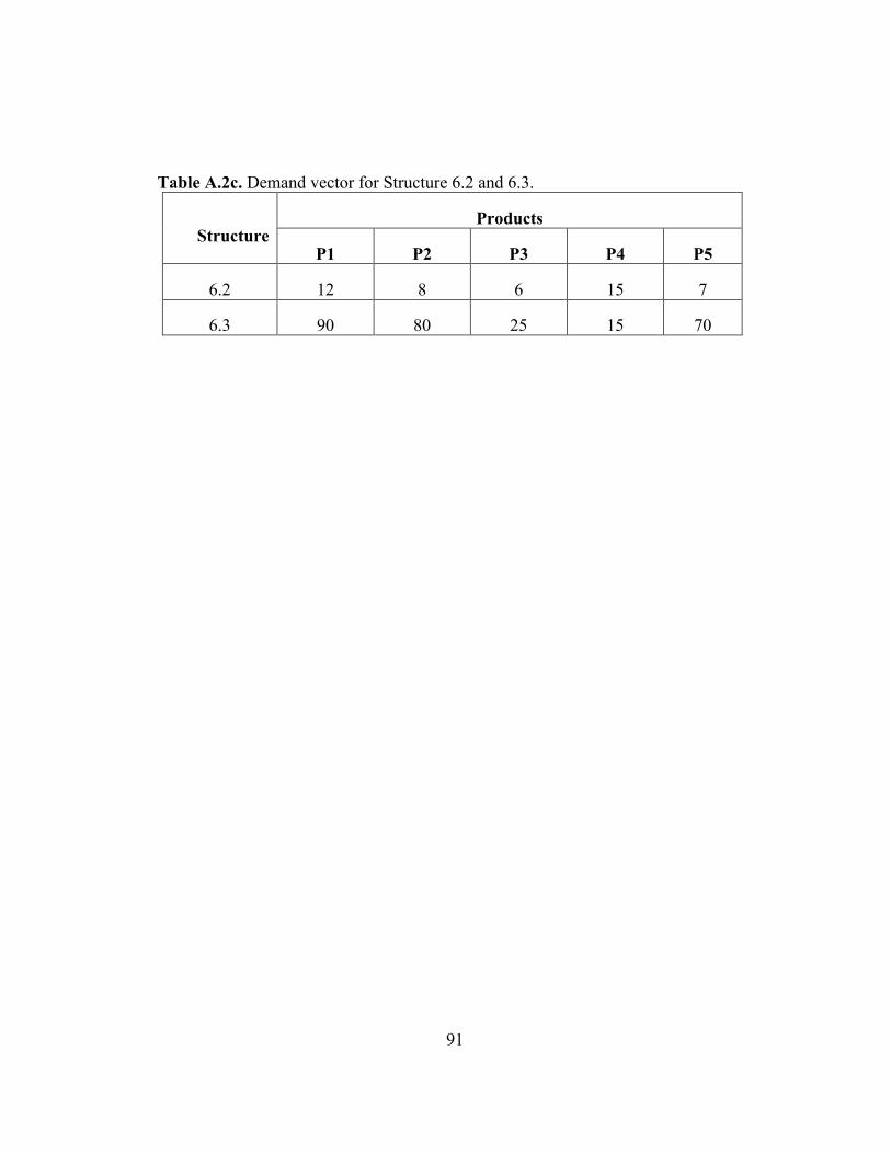
91

Table A.2c. Demand vector for Structure 6.2 and 6.3.

Products Structure

P1 P2 P3 P4 P5

6.2 12 8 6 15 7

6.3 90 80 25 15 70

BEAM SEARCH ALGORITHMS FOR THE MIXED-MODEL ...

Documents

Transcript of BEAM SEARCH ALGORITHMS FOR THE MIXED-MODEL ...