Beam Loss Reduction by Barrier Bucketsin the CERN Accelerator Complex

Mihaly Vadai

Submitted in partial fulfillment of the requirementsof the Degree of Doctor of Philosophy

Antennas and Electromagnetics Research GroupSchool of Electronic Engineering and Computer Science

Queen Mary University of LondonSystems Department - Radiofrequency Group

CERN, Geneva

2021

Statement of originality

I, Mihaly Vadai, confirm that the research included within this thesis is my ownwork or that where it has been carried out in collaboration with, or supportedby others, that this is duly acknowledged below and my contribution indicated.Previously published material is also acknowledged below.

I attest that I have exercised reasonable care to ensure that the work isoriginal, and does not to the best of my knowledge break any UK law, infringeany third party’s copyright or other Intellectual Property Right, or contain anyconfidential material.

I accept that the College has the right to use plagiarism detection softwareto check the electronic version of the thesis.

I confirm that this thesis has not been previously submitted for the awardof a degree by this or any other university.

The copyright of this thesis rests with the author. Content from the thesismay only be used under the Creative Commons Attribution 3.0 licence (CC-BY-3.0), https://creativecommons.org/licenses/by/3.0/. The copyrightterms above do not apply to previously published material, which may be usedunder the licence applicable to the specific content as indicated in the thesis.

Signature: Mihaly VadaiDate: 29-01-2021

Details of collaboration and publications

The initial beam tests reported in Section 4.3 were conducted by H. Damerauand myself. My contribution was the control of the new barrier bucket drivethat I developed for the studies. Tests carried out later, especially the testsoptimising the flatness of the profiles and the tests with moving barriers areonly my work.

The beam tests reported in Section 4.4 were conducted in a team due totheir complexity by H. Damerau, M. Giovannozzi, A. Huschauer and myself.My main contribution to the practical tests was the expert control of the newlyinstalled barrier bucket RF system.

For section 4.4.5, the logging and initial analysis of the beam loss monitordata was provided by A. Huschauer for our joint publication [1].

1

Abstract

For a future intensity increase of the fixed-target beam in the accelerator com-plex at CERN, new techniques to reduce beam loss are required. A majorfraction of the losses during extraction of the coasting beam from the PS to-wards the SPS originate from poorly kicked particles during the Multi-TurnExtraction.

A line density depletion, synchronised with the extraction kickers, decreasesthese losses significantly when successfully combined with the present extractionscheme involving the transverse splitting of the beam. The Finemet® wide-bandcavity recently installed in the PS as a longitudinal feedback kicker was used togenerate a so-called barrier bucket, which is utilised to deplete the line densityand reduce the losses.

The drive to generate the barrier bucket waveform synchronously with thebeam was developed and installed by the radiofrequency cavity as part of thesestudies. The effectiveness of the combination of the Multi-Turn Extraction andthe barrier bucket was evaluated with beam. This manipulation was performedfor the first time in a particle accelerator.

The measured data with beam in the CERN PS shows a substantial, up toan order of magnitude beam loss reduction at extraction, even well beyond thestandard operational beam intensity. This means that the combination of theMulti-Turn Extraction with the barrier buckets achieves a practically loss-lessextraction for the fixed target beam from the PS.

Based on the results of the measurements and simulations with beam, aconcept for the synchronisation between the CERN PS and SPS accelerators isalso presented to realise the beam loss reduction in future operation.

Author’s publications

Portions of the work detailed in this thesis have been presented in internationalscholarly publications with the author of this report listed as main author, asfollows:

• Parts of Chapters 1, 4 and 6 are published in the journal article [1] titledBarrier bucket and transversely split beams for loss-free multi-turn extrac-tion in synchrotrons. Authors: M. Vadai, A. Alomainy, H. Damerau, S.Gilardoni, M. Giovannozzi and A. Huschauer

• Parts related to the low and high energy beam tests without the MTEin Chapters 4 and 6 were published in the peer-reviewed 2019 Journal ofPhysics Conference Series [2]. Title: Beam manipulations with barrierbuckets in the CERN PS. Authors: M. Vadai, A. Alomainy, H. Damerau,S. Gilardoni, M. Giovannozzi and A. Huschauer.

• Parts related to the hardware implementation of Chapters 3 and 6 werepresented at the International Particle Accelerator Conference 2019. Title:Barrier Bucket Studies in the CERN PS [3]. Authors as it appears on thepaper: M. Vadai, A. Alomainy, H. Damerau.

4

Acknowledgements

I would like to thank for the opportunity and financial support provided by theCERN Doctoral Student Programme that allowed me to work on this projectat CERN.

I would like to thank Queen Mary University of London for the flexibility inthe administration of this unusual project and the financial support provided inform of a fee waiver.

I would like to thank both of my supervisors, A. Alomainy and H. Dameraufor creating an efficient structure and supporting atmosphere that allowed meto work on the PhD.

I would like to thank the CERN PS Operations team for going the extra milein fulfilling the requests during the machine development sessions on weekdaysand weekends. Special thanks to the colleagues in the SPS island in the CCCto having allowed the preliminary SPS beam tests on the very last day of theproton run before LS2.

I would like to thank M. Giovannozzi and A. Huschauer for the discussionsand active participation in the setup and measurements sessions during the highenergy beam tests.

This thesis could only be a reality, because while I was working on it I wassurrounded by a positive environment of building 864 and the inspiring peopleworking in the ATS sector of CERN. Thanks to all of you for the feedbackprovided during my presentations and informal chats.

Relocations are exciting, but hardly ever convenient. They are definitelyeasier with help, so I would like to thank my wife and my family for the supportthey provided in this and for the continuing support and enthusiasm for theproject ever since.

5

Contents

Contents 6

List of Tables 9

List of Figures 10

1 Introduction 191.1 Review of the extraction of fixed target beams from the PS . . . 201.2 Motivation . . . . . . . . . . . . . . . . . . . . . . . . . . . . . . 22

1.2.1 RF barrier buckets for loss reduction . . . . . . . . . . . . 221.3 Overview of barrier buckets in synchrotrons . . . . . . . . . . . . 24

1.3.1 Use cases of barrier buckets . . . . . . . . . . . . . . . . . 241.3.2 Brief overview of barrier bucket implementations . . . . . 25

1.4 Main contributions . . . . . . . . . . . . . . . . . . . . . . . . . . 261.5 Structure of the thesis . . . . . . . . . . . . . . . . . . . . . . . . 27

2 Longitudinal beam dynamics 282.1 Introduction . . . . . . . . . . . . . . . . . . . . . . . . . . . . . . 282.2 Continuous time approach . . . . . . . . . . . . . . . . . . . . . . 28

2.2.1 Longitudinal phase space . . . . . . . . . . . . . . . . . . 292.2.2 Synchrotron frequency spread . . . . . . . . . . . . . . . . 34

2.3 Barrier buckets . . . . . . . . . . . . . . . . . . . . . . . . . . . . 352.3.1 Bucket height and area for sine based barrier buckets . . 352.3.2 Estimation of phase-space area growth due to barrier bucket

compression and expansion . . . . . . . . . . . . . . . . . 382.4 Discrete time approach . . . . . . . . . . . . . . . . . . . . . . . . 41

2.4.1 Normalised tracking . . . . . . . . . . . . . . . . . . . . . 422.4.2 Energy- and time-offset based tracking . . . . . . . . . . . 422.4.3 Phase and relative momentum offset based tracking . . . 43

2.5 Beam-accelerator interaction, impedance . . . . . . . . . . . . . . 432.6 Summary . . . . . . . . . . . . . . . . . . . . . . . . . . . . . . . 44

6

3 Requirements and implementation of the barrier bucket wave-form generator 453.1 Introduction . . . . . . . . . . . . . . . . . . . . . . . . . . . . . . 453.2 Requirements . . . . . . . . . . . . . . . . . . . . . . . . . . . . . 46

3.2.1 Amplitude requirement . . . . . . . . . . . . . . . . . . . 463.2.2 Frequency range and waveform control . . . . . . . . . . . 483.2.3 Bandwidth requirement . . . . . . . . . . . . . . . . . . . 49

3.3 Low-level RF system . . . . . . . . . . . . . . . . . . . . . . . . . 543.3.1 Beam synchronous, arbitrary waveform generation . . . . 543.3.2 Implementation . . . . . . . . . . . . . . . . . . . . . . . . 55

3.4 High-level RF system . . . . . . . . . . . . . . . . . . . . . . . . . 603.4.1 Transfer function - linear pre-distortion . . . . . . . . . . 603.4.2 Limitations . . . . . . . . . . . . . . . . . . . . . . . . . . 61

3.5 The barrier bucket RF system in BLonD . . . . . . . . . . . . . . 633.6 Summary . . . . . . . . . . . . . . . . . . . . . . . . . . . . . . . 65

4 Beam tests and comparison with simulations 664.1 Introduction . . . . . . . . . . . . . . . . . . . . . . . . . . . . . . 664.2 Measurement signals . . . . . . . . . . . . . . . . . . . . . . . . . 67

4.2.1 Wall current monitor . . . . . . . . . . . . . . . . . . . . . 674.2.2 Wide-band, electrostatic pick-up . . . . . . . . . . . . . . 684.2.3 Beam Loss Monitors . . . . . . . . . . . . . . . . . . . . . 71

4.3 Low energy and low intensity studies . . . . . . . . . . . . . . . . 714.3.1 Reflection at barrier during debunching . . . . . . . . . . 724.3.2 Bunch length manipulation using moving barriers . . . . . 72

4.4 Studies at high energy . . . . . . . . . . . . . . . . . . . . . . . . 794.4.1 The acceleration cycle for the fixed-target beam in the PS 804.4.2 Re-bucketing and debunching into a barrier bucket . . . . 814.4.3 Beam in the PS and in the transfer line . . . . . . . . . . 914.4.4 Intensity dependent effects . . . . . . . . . . . . . . . . . 964.4.5 Beam loss reduction . . . . . . . . . . . . . . . . . . . . . 102

4.5 Summary . . . . . . . . . . . . . . . . . . . . . . . . . . . . . . . 107

5 A concept of synchronisation for barrier buckets 1095.1 Introduction . . . . . . . . . . . . . . . . . . . . . . . . . . . . . . 1095.2 Requirements and constraints . . . . . . . . . . . . . . . . . . . . 111

5.2.1 Minimum duration of the phase slip . . . . . . . . . . . . 1125.2.2 Smooth phase bump . . . . . . . . . . . . . . . . . . . . . 1135.2.3 Adiabaticity of re-phasing . . . . . . . . . . . . . . . . . . 115

5.3 Simulations and benchmarking . . . . . . . . . . . . . . . . . . . 117

7

5.3.1 Benchmarking with past measurements . . . . . . . . . . 1185.3.2 Simulation results . . . . . . . . . . . . . . . . . . . . . . 120

5.4 Implementation . . . . . . . . . . . . . . . . . . . . . . . . . . . . 1235.5 Summary . . . . . . . . . . . . . . . . . . . . . . . . . . . . . . . 126

6 Conclusions 1276.1 Summary of contributions . . . . . . . . . . . . . . . . . . . . . . 127

6.1.1 Implementation . . . . . . . . . . . . . . . . . . . . . . . . 1276.1.2 Beam test and loss reduction . . . . . . . . . . . . . . . . 1286.1.3 Synchronisation . . . . . . . . . . . . . . . . . . . . . . . . 129

6.2 Future work . . . . . . . . . . . . . . . . . . . . . . . . . . . . . . 129

References 131

A Synthesis using half revolution frequency harmonics 153

B Location of firmware and software 157

8

List of Tables

2.1 Types of tracking used in the thesis . . . . . . . . . . . . . . . . . 41

3.1 The comparison of the bucket heights and bucket areas for differ-ent barrier bucket generating waveform shapes for the same hr.Calculating the cosine sections bucket area involves a numericalintegration. . . . . . . . . . . . . . . . . . . . . . . . . . . . . . . 51

4.1 Parameters used for the low energy simulations and beam tests. . 724.2 Parameters used for the high energy simulations and beam tests

with one barrier pulse per turn. . . . . . . . . . . . . . . . . . . . 814.3 RF cavities installed in the PS ring and the status of their gaps

after the re-bucketing into the barrier bucket took place. . . . . . 101

5.1 Requirements for the synchronisation. . . . . . . . . . . . . . . . 1125.2 Overview of the proposed synchronisation steps when including

a short flat-top in the cycle after acceleration and before thetransverse splitting. . . . . . . . . . . . . . . . . . . . . . . . . . . 112

5.3 Parameter comparison of the measurements in 2016 and the pro-posed and simulated parameters for barrier bucket synchronisa-tion. Note the adiabaticity parameter is based on the change ofthe bucket area, see Eq. 5.7 and [37]. . . . . . . . . . . . . . . . . 118

5.4 Steps of the proposed synchronisation. . . . . . . . . . . . . . . . 1245.5 An example of the timings needed for the synchronisation. . . . . 124

9

List of Figures

1.1 The CERN Accelerator Complex. The original image by E.Mobs [12] was simplified and the path of the fixed target beamassociated with in these studies was highlighted using thick lines.Copyright CERN. . . . . . . . . . . . . . . . . . . . . . . . . . . . 20

1.2 The beam loss along the circumference of the PS. The goal ofthis study is to eliminate the residual losses represented with thered area to improve the performance of the extraction after theimplementation of MTE. As a short summary of the results ofthe present studies, this figure is to be compared with Fig. 4.37,which shows the significantly reduced losses in straight sections14-18, when the barrier bucket manipulation is added. Presentfigure taken from [16], Figure 9. Copyright CERN, 2016 CC-BYlicence. . . . . . . . . . . . . . . . . . . . . . . . . . . . . . . . . . 21

1.3 The extraction region behind the barrier and the preceding sec-tions seen from the direction of the beam with the last kicker inthe foreground. BFA9 is one of the kickers used in the Multi-TurnExtraction. The main PS dipole magnets, two beam loss moni-tors (BLM) are also indicated. The data from the BLM systemwas used to evaluate the loss reduction in Chapter 4. . . . . . . . 22

1.4 Illustration of the beam loss reduction scheme. Gaps are gener-ated in the coasting beam in the PS with upstream and down-stream accelerator connections. The diagram only shows parts ofthe CERN injector chain and it is not to scale. . . . . . . . . . . 23

2.1 Illustration of the azimuth θ, radius R, momentum p and phaseφ variables. The phase is to be interpreted with respect to theRF voltage for two harmonics: h = 1 and h = 2 in this example.Note that the phase and azimuth angles are the opposite signfollowing the usual convention E.g. [123, 124]. . . . . . . . . . . . 29

10

2.2 Illustration of sinusoidal RF voltage (top), corresponding poten-tial (middle) and a conventional, stationary RF bucket (bottom). 32

2.3 Synchrotron frequency spread in a conventional, stationary bucketas a function of phase. . . . . . . . . . . . . . . . . . . . . . . . . 34

2.4 Normalised RF voltage (top) of the pulsed RF system generatinga barrier bucket, together with an illustration of correspondingtrajectories (bottom) in the longitudinal phase space, includingthe separatrix (dashed). Barrier bucket parameters in barrier RFphase. φd corresponds to the drift space, where the particles donot experience any RF voltage. φr corresponds to the reflectionregion on one side of the barrier. . . . . . . . . . . . . . . . . . . 36

2.5 Synchrotron frequency spread as the function of the relative phasevelocity in barrier buckets made by the same sinusoidal pulseswith different drift space ratios. φd/φr = 0 corresponds to aconventional bucket, see also Fig. 2.3. . . . . . . . . . . . . . . . 37

2.6 Illustration of the normalised amplitude g(φ) and the gap har-monic hr parameters for a barrier bucket waveform. The [−π, π)

interval represents the whole circumference of the accelerator. . . 372.7 Diagram of the quarter areas of the phase space before and after

a particle reflection off a moving barrier. The two phase spacesare shifted such that the main parameters used in the calculationare visible. . . . . . . . . . . . . . . . . . . . . . . . . . . . . . . . 40

2.8 Left: Emittance growth estimate for low relative barrier speeds.Right: limiting case of the relative barrier speed at half of thephase velocity of an outer particle in the bunch. . . . . . . . . . . 41

3.1 Peak voltage requirement for the ideal case of emittance preser-vation during re-bucketing. . . . . . . . . . . . . . . . . . . . . . 47

3.2 Peak voltage requirement taking the simulated longitudinal emit-tance blow-up during re-bucketing into account, too. . . . . . . . 48

3.3 Comparison of different waveforms generated for the same gapwidth using 20 Fourier harmonics. . . . . . . . . . . . . . . . . . 51

3.4 Comparison of the Fourier harmonics of different waveforms. Inthis example hr = 5. . . . . . . . . . . . . . . . . . . . . . . . . . 52

3.5 σ3 modulated spectra. In this example hr = 5. The transpar-ent dots and lines are the Fourier coefficients without window-ing (m = 0) corresponding to Fig. 3.4. . . . . . . . . . . . . . . . 52

3.6 Comparison of different waveforms generated for the same gapwidth using 20 Fourier harmonics using σ3 modulation. . . . . . 53

11

3.7 The diagram shows the functional elements of the beam syn-chronous RF source firmware generating barrier buckets. . . . . . 54

3.8 The PS one turn delay feedback board with the illustration of thebarrier bucket firmware. The board inputs and outputs are alsomarked in our implementation. The coaxial leads are to routethe test points to the front panel. . . . . . . . . . . . . . . . . . . 56

3.9 The result of a Modelsim simulation of the MHS phase rampoutput (bottom) and two barriers generated per turn (top), wherethe distance between them can be set. Note that a distancecloser than the width of the pulse can produce higher potentialas the second pulse from the left shows. Such operation is notforeseen for this drive. Either one barrier is to be made per turnat extraction or multiple barriers at low energy commissioning,but not the two at the same time, hence this is not a true limitation. 58

3.10 The prototype barrier bucket system as it is installed in the PS. . 603.11 Measured S21 parameters from the RF input to the summed out-

put of all the cavity cells corrected for the attenuation in the pathto the VNA and the electrical delay from the input to the cavityinstalled in the ring. . . . . . . . . . . . . . . . . . . . . . . . . . 61

3.12 Pre-distorted input waveforms (blue) and cavity gap return wave-forms (red) for the bucket stretching exercise with low intensitybeam in barrier buckets. Note, the delay was added to the redwaveforms to display it on the same plot. . . . . . . . . . . . . . 62

3.13 The first 25 sigma modulated harmonics used in the simulationsfor different gap sizes at the peak voltage of 4 kV. . . . . . . . . 62

4.1 Sketch of the longitudinal cut of the Wall Current Monitor in-stalled in the PS illustrating its principle of operation. . . . . . . 68

4.2 Illustration of the plots from a WCM. Two time axis are used,the x time axis is during a fraction of the turn and the y timeaxis is showing repeated acquisitions along a cycle on a longertime scale. Left: acquisitions as a mountain range plot. Right:the same acquisitions as on the right displayed as an image withthe signal amplitude colour-coded. . . . . . . . . . . . . . . . . . 69

4.3 An example of the raw acquisition from the oscilloscope and thecorrected beam profile. . . . . . . . . . . . . . . . . . . . . . . . . 69

12

4.4 Frequency responses of the compensation used for the pick-upsignal. The droop was compensated for by a high pass filter (left).Then it was replaced by an integrator (right) for compensatingfor the losses on the low end of the spectrum due to the lowfrequency cut-off of the acquisition. The sample spacing is 0.5 ns,which explains the 1 GHz length of the full Nyquist range. . . . . 70

4.5 Protons reflecting off the right hand side and left hand side ofthe potential barrier in a barrier bucket. Two longitudinal profileevolutions were combined in this plot. Injecting the beam on theleft hand side of the barrier at about 320 ns and injecting on theright hand side of the barrier at about 700 ns. The top of theimage shows the RF voltage and the corresponding potential. . . 73

4.6 Illustration of the RF program during a decompression and com-pression operation. The blue traces generate a conventional, iso-lated bucket. The other traces generate barrier buckets with in-creasing drift space from purple to yellow. . . . . . . . . . . . . . 74

4.7 Measured longitudinal line density profile evolution of a decom-pression operation with moving barriers. . . . . . . . . . . . . . . 74

4.8 Evolution of the bunch profile during fast compression and ex-pansion at φb/φf ≈ 0.25. The oscillations after 60 ms are a clearindication of a non-adiabatic manipulation. Simulated (left) andmeasured (right) profiles are shown. The plot in the middle showthe bunch lengths, highlighting the oscillations at the end. . . . . 76

4.9 Evolution of the bunch profile during slow compression and ex-pansion at a normalised speed of φb/φf ≈ 0.01. The smoothtransitions indicate an adiabatic manipulation. Simulated (left)and measured (right) profiles are shown. . . . . . . . . . . . . . . 76

4.10 Evolution of the bunch profile during fast compression and ex-pansion at φb/φf ≈ 0.25. The increased bunch length at the endof the manipulation shows a non-adiabatic manipulation. Simu-lated (left) and measured (right) profiles are shown. . . . . . . . 77

4.11 Evolution of the profile during slow compression and expansionat φb/φf ≈ 0.01. Bunch profiles at the end are restored indicatingan adiabatic manipulation. Simulated (left) and measured (right)profiles are shown. . . . . . . . . . . . . . . . . . . . . . . . . . . 77

13

4.12 Difference of initial (200 ns) and final bunch length versus com-pression and expansion. Each marker on the time axis havingcategorical labels has two associated boxes for the two schemeswith the marker in the middle, except for 30ms and 50ms. Oncethe compression speed is near the theoretical limit, the bunchesare perturbed after compression resulting in a not well defined orlarge bunch length due to the fast manipulations. Plot uses thesame data as Figure 4. in [2] (CC-BY), but the improved speedlimit from Chapter 2 is also shown. . . . . . . . . . . . . . . . . . 78

4.13 The current of the different magnetic elements taking part in thetransverse splitting, the magnetic flux density along the cycleand the RF voltages peaking at 200 kV are shown. Figure takenfrom [16], Figure 3 (top). Copyright CERN, 2016 CC-BY licence. 80

4.14 Total RF voltage evolution during re-bucketing with peak ampli-tudes (top) and waveform (bottom). . . . . . . . . . . . . . . . . 82

4.15 Re-bucketing into a barrier bucket at total beam intensity of1.87 × 1013 ppp. . . . . . . . . . . . . . . . . . . . . . . . . . . . 83

4.16 Comparison of line-density modulations during the handover fromthe conventional to the barrier bucket RF system. Left: re-bucketing to an isolated bucket. Centre: modulation due to driftof particles. Right: modulation due to both potential-well dis-tortion and particle drift. . . . . . . . . . . . . . . . . . . . . . . 84

4.17 Tomographic reconstruction of the longitudinal phase space basedon measured data. The reference profiles were available at theend of the intermediate flat top. . . . . . . . . . . . . . . . . . . . 86

4.18 Tomographic reconstruction of the simulated longitudinal phasespace matching the parameters of Fig. 4.17. . . . . . . . . . . . . 87

4.19 Simulated profile evolution for the same principal RF voltageevolution as for the measurements shown in Fig.4.15. The initiallongitudinal emittance corresponds to the one measured duringacceleration. . . . . . . . . . . . . . . . . . . . . . . . . . . . . . . 88

4.20 Simulated longitudinal phase space at extraction with the matchedemittance corresponding to Fig. 4.15, 4.19 and without the 200 MHzmodulation. The partial filamentation mechanism in the barrierbucket is illustrated. The projection of the beam distribution isalso shown. . . . . . . . . . . . . . . . . . . . . . . . . . . . . . . 88

14

4.21 Beam reflecting off a potential barrier, shown over half a PS turn.The amplitude of the h = 16 system was lowered and then sub-sequently turned off at 70 ms and the amplitude of the barrierbucket RF system was increased to reach the maximum at thesame time. The transverse beam splitting was disabled duringthese measurements. Simulated (left) and measured (right) pro-files are shown. . . . . . . . . . . . . . . . . . . . . . . . . . . . . 89

4.22 Oscillations in barrier buckets with a pulse duration of 300 ns.Beam profile evolution (right) and corresponding 90% area emit-tance (left). Peaks in 90% emittance correspond to shoulder form-ing in the barrier bucket. . . . . . . . . . . . . . . . . . . . . . . 90

4.23 Examples of the longitudinal beam structure measured in thetransfer line without barrier bucket (top), with barrier bucketasynchronous with the rise of the PS extraction kicker (middle)and with barrier bucket synchronous with the rise of the PS ex-traction kickers (bottom). The 200 MHz modulation is clearlyvisible in all cases. . . . . . . . . . . . . . . . . . . . . . . . . . . 92

4.24 Single pass response of the low-pass filter. The forward-backwardfiltering technique squares the frequency response and cancels thephase response. . . . . . . . . . . . . . . . . . . . . . . . . . . . . 93

4.25 The cross-correlation sequence of the signals compared in Fig. 4.26,with the maximum at 0.97 for this example. . . . . . . . . . . . . 94

4.26 The summed profiles from the WBP in the TT2 transfer line com-pared with the WCM trace before extraction aligned accordingto the maximum of Rxy. . . . . . . . . . . . . . . . . . . . . . . . 95

4.27 The maximums of the cross-correlation sequences of the last ac-quisitions before extraction from the PS and the summed five-turn profiles normalised to the same power. Each thin, horizontalline represents a pair of acquisitions. The length of the horizon-tal line shows the relative frequency of the values falling in thecorresponding bin [194]. . . . . . . . . . . . . . . . . . . . . . . . 96

4.28 The measured and profiles calculated from local elliptical beamdistribution scaled for shoulder height detection. . . . . . . . . . 96

4.29 The cross-correlation sequence of the measured and calculatedprofiles with the detected peaks. . . . . . . . . . . . . . . . . . . 97

4.30 Comparison of the low-pass filtered, normalised longitudinal linedensity profiles at extraction at the same time in the re-bucketingprocess for acquisitions with 180 ns gap size setting. The effectof the beam intensity can be seen. . . . . . . . . . . . . . . . . . 98

15

4.31 Normalised line density change along the bunch, showing a de-creasing trend towards improved flatness of the bunch with in-creasing intensity. The colours refer to the different gap durationsettings as indicated in the legend. Independent of the gap dura-tion, the line density change improves with increasing intensity.63 and 76 acquisitions for 180 ns and 250 ns are shown. Theleast-squares linear fits are displayed to highlight the downwardtrend. . . . . . . . . . . . . . . . . . . . . . . . . . . . . . . . . . 99

4.32 The results of the analysis without low-pass filtering. The detec-tion routine is less efficient at the highest intensities in this caseand there is an overall increase in the line density peak whenthe 200 MHz system is active with the 180 ns gap setting. . . . . 100

4.33 Simulated voltage seen by the beam at extraction at differentbeam intensities with reference. The impedance of the Finemet®,40 MHz and 80 MHz cavities with higher order modes was takeninto account. . . . . . . . . . . . . . . . . . . . . . . . . . . . . . 102

4.34 The relative contributions to beam loading at the lowest andhighest beam intensities of the different cavities. The voltageinduced in the Finemet® cavity is an order of magnitude morethan voltage induced in the 40 MHz and 80 MHz cavities. . . . . 103

4.35 Simulated effect of beam loading in the Finemet® cavity on theprofiles at extraction with different beam intensities and withoutintensity effects at a 180 ns gap setting. . . . . . . . . . . . . . . 103

4.36 The measurements with the old (left) and new (right) BLM sys-tems show the effectiveness of the barrier bucket system in reduc-ing the losses across all intensities, which is obvious by comparingthe orange box and whiskers indicating much higher losses withthe barrier off to the purple ones indicating much lower losseswhen the barrier bucket system was operational. . . . . . . . . . 104

4.37 An example logarithmic plot of the losses as the function of the lo-cation in the PS ring with different gap sizes. Left: the total beamloss as a function of location along the PS ring. Right: zoom ofthe BLM readings in the extraction region. Plot shows the samedata as [1] Fig. 9 using different colours and aspect ratios. Theintensity corresponding to these measurements is 1870 × 1010 ppp.105

4.38 Integrated beam loss in the extraction region with three inten-sities, indicated on the top of the plot. The losses decrease asthe gap size increases. Figure re-plotted from [1] Fig. 10 usingdifferent colours. . . . . . . . . . . . . . . . . . . . . . . . . . . . 106

16

5.1 Chain of phase relationships between the systems of the PS andSPS involved in the extraction and injection. The fixed phaserelationships mean that the position of the beam has to be alignedin the PS. . . . . . . . . . . . . . . . . . . . . . . . . . . . . . . . 110

5.2 The minimum time needed for the beam to spend on off-orbitversus the radial displacement. . . . . . . . . . . . . . . . . . . . 113

5.3 The following parameters are shown during a 10, 20 and 30 mslong manipulation: the pre-defined phase program (top), the rel-ative change of the RF frequency (middle) and the change of theradial position (bottom). . . . . . . . . . . . . . . . . . . . . . . . 114

5.4 The following parameters are shown during a 10, 20 and 30 mslong manipulation with the same parameters as Fig. 5.3 from topto bottom: synchronous phase, momentum change, synchrotronfrequency in the middle of the bucket and relative bucket area. . 115

5.5 Comparison of the general adiabaticity parameter (top), the ap-proximation valid for the phase slip operation (middle) and theconventional (bottom) one. It is clear that the main contributioncomes from the change of the bucket area factor. . . . . . . . . . 117

5.6 Longitudinal profile evolution during a 30 ms phase slip opera-tion. Data from the 2016 measurements. The colours indicatethe longitudinal line density from yellow (high) to blue (low). . . 118

5.7 Profile evolution aligned in the coordinate system of the bunchwith αAb

= 0.2%. The plot shows that with a slow manipulationthe beam can follow both in the simulated (left) and in the mea-sured (right) case, because the profile evolution is preserved. Thecolours indicate the longitudinal line density from yellow (high)to blue (low). . . . . . . . . . . . . . . . . . . . . . . . . . . . . . 119

5.8 Profile evolution aligned in the coordinate system of the bunchwith αAb

= 1.9%. The simulations on the left show oscillationafter the manipulation. The measurements on the right show athat the beam is practically lost. This was attributed to technicalproblems found in the phase program. The colours indicate thelongitudinal line density from yellow (high) to blue (low). . . . . 119

5.9 Simulated longitudinal profile evolution during a fast, 12 ms h =

16 displacement. This time is too short for the manipulation asshown by the oscillations. The colours indicate the longitudinalline density from yellow (high) to blue (low). . . . . . . . . . . . 120

17

5.10 The simulated longitudinal profile evolution during a slower, 30 ms h = 16 dis-placement. This time is sufficient for the manipulation as shownby the lack of oscillations. The colours indicate the longitudinalline density from yellow (high) to blue (low). . . . . . . . . . . . 121

5.11 The time difference between the average bunch position and theprogrammed position for various durations of the phase shift ma-nipulation. The initial oscillations are an artefact of the imperfectmatching in the simulations. . . . . . . . . . . . . . . . . . . . . . 121

5.12 The dependence of the position on the voltage and time avail-able. The higher the peak amplitude, the lower the amplitudeof the oscillations and, in general, the longer the time, the lowerthe oscillations. Due to the non-linearity of the synchrotron os-cillations bunch oscillations are very sensitive to the length of themanipulation. . . . . . . . . . . . . . . . . . . . . . . . . . . . . . 122

5.13 Step 1: Switch from B-train reference to external RF referenceof the revolution frequency. . . . . . . . . . . . . . . . . . . . . . 125

5.14 Step 2: Reduce phase and radial loop gain to zero. . . . . . . . . 1255.15 Step 3: measure phase difference and perform phase bump by

acting on the frequency of the master clock. . . . . . . . . . . . . 1255.16 Step 4. Perform transverse splitting and generate barrier bucket

by increasing the amplitude of the wide-band RF connected tothe Finemet® cavity. . . . . . . . . . . . . . . . . . . . . . . . . . 125

A.1 si - start of the pulse, fi - end of the pulse, ri - the magnitude ofthe pulse . . . . . . . . . . . . . . . . . . . . . . . . . . . . . . . . 153

A.2 The illustration of equation A.5. The sum is performed at eachstep to highlight the mechanism. The top left graph shows thedifference of the two frequency components at half of the revolu-tion frequency summed up on their own when there is no phaseshift between them. The sum has only graphical significance, thecomponents cancel individually and the result is zero. Then aphase shift in the half frequency components is introduced (topright) which makes a pair of pulses when the components areadded. Then these components are squared and summed withthe standard Fourier method (bottom left) and the modified orfiltered version (bottom right) using the σ factors. It is clear fromthe formula and the images that the magnitude of the phase shiftis the main factor in determining the width of the potential barriers.156

18

Chapter 1

Introduction

The CERN hadron accelerator complex consisting of two linear accelerators,seven rings and connecting transfer lines at multiple sites serves a considerablenumber of physics experiments, as Fig. 1.1 illustrates. Among these are fixedtarget experiments [4–9] served by the Super Proton Synchrotron (SPS) in theNorth Area [10]. The beams for these experiments are passing though severalaccelerators before arriving at their targets. The figure of merit for most ex-periments is the total number of protons on target, which can be improved byincreasing the intensity of the beam. However, such increase is limited by beamlosses in the upstream accelerator chain, which the present study intends toreduce.

Section 1.1 summarises the path of the beam to fixed target experiments ofthe North Area of the SPS and Section 1.2 outlines the proposed method of theloss reduction motivating the studies.

Since the beam loss reduction is to be achieved using a radiofrequency ma-nipulation called the barrier bucket, Section 1.3 gives a brief overview of barrierbucket use cases and implementations in particle accelerators.

The main contributions of the work are listed in Section 1.4 and the structureof the thesis is outlined in Section 1.5.

19

1.1 Review of the extraction of fixed target beamsfrom the PS

The protons for fixed target experiments served by the SPS follow the pathas indicated by the thick lines in Fig. 1.1. The particles start their journeyin Linac 2, (Linac 4 from 2020 [11]) accelerated from rest to 50 MeV kineticenergy (160 MeV in Linac 4), being again accelerated in the PS Booster to1.4 GeV kinetic energy (2.0 GeV from 2021), then extracted to the PS. A furtheracceleration takes place in the PS up to 14 GeV/c momentum for fixed targetbeams in the present study.

The CERN Accelerator Complex

LINAC 2

North Area

LINAC 3Ions

East Area

TI2TI8

TT41TT40

CLEAR

TT10

TT66

e-

TT20

n

p

p

RIBsp

1976 (7 km)

ISOLDE1992

2016

REX/HIE2001/2015

BOOSTER1972 (157 m)

AD1999 (182 m)

LEIR2005 (78 m)

2001

LHC2008 (27 km)

PS1959 (628 m)

2011

p (protons) ions RIBs (radioactive ion beams) n (neutrons) – - (electrons)

2016 (31 m)

ELENA

2017

ALICE

CMS

ATLAS

LHCb

SPS

TT2

HiRadMat

n-ToF

p (antiprotons) e

AWAKE

LINAC 4 (from 2020)

Figure 1.1: The CERN Accelerator Complex. The original image by E.Mobs [12] was simplified and the path of the fixed target beam associated within these studies was highlighted using thick lines. Copyright CERN.

The main fraction of beam loss happens at the extraction of the fixed targetbeams from the PS to the SPS. This extraction process occurs in five turnsdue to the circumference ratio of 1/11 between the synchrotrons, thus two PScycles are needed to fill the SPS. Extracting the beam in five turns in the PSmeans that the beam must be cut transversely along the cross-section of theaccelerator.

This was first implemented by the Continuous Transfer (CT) [13–15] ex-traction method, which utilised a physical septum blade to slice the beam and

20

extract it during five turns. This method, while effective and operated for manyyears, induced beam losses in several parts of the PS as the beam loss moni-tor (BLM) readings show in Fig. 1.2. This lead to high activation and reducedlifetime of equipment in the ring.

Figure 1.2: The beam loss along the circumference of the PS. The goal of thisstudy is to eliminate the residual losses represented with the red area to improvethe performance of the extraction after the implementation of MTE. As a shortsummary of the results of the present studies, this figure is to be compared withFig. 4.37, which shows the significantly reduced losses in straight sections 14-18,when the barrier bucket manipulation is added. Present figure taken from [16],Figure 9. Copyright CERN, 2016 CC-BY licence.

To lower these losses, the Multi-Turn Extraction (MTE) method was de-veloped [17]. This operates on the principle of splitting the beam transverselybased on a magnetic resonance induced by sextupoles and octopoles [18–20]thereby avoiding the direct contact of the beam with the mechanical septumblade. Thus, the beam loss in the ring has been significantly reduced [16, 18,21–23] as shown by Fig. 1.2 with the exceptions of straight sections 14-18. Thispart of the accelerator is what the photo in Fig. 1.3 shows from the fast bumpermagnet towards the ejection region in the direction of the beam. During theinitial operation of the MTE important localised losses occurred at the extrac-tion septum in SS16 [24]. A dummy septum, a movable absorber [25–29] wastherefore installed to protect the blade of the magnetic extraction septum byphysically intercepting the particles during the rise time of the kicker dipoles.This interception results in a beam loss in straight sections 14-18, and as aresult, the dummy septum becomes highly radioactive.

21

Bending magnets

Beam loss monitors

BFA9 kicker magnet

Extraction region behind barrier

Figure 1.3: The extraction region behind the barrier and the preceding sectionsseen from the direction of the beam with the last kicker in the foreground. BFA9is one of the kickers used in the Multi-Turn Extraction. The main PS dipolemagnets, two beam loss monitors (BLM) are also indicated. The data from theBLM system was used to evaluate the loss reduction in Chapter 4.

1.2 Motivation

The motivation of the present studies is to significantly reduce this residualbeam loss, while maintaining the beneficial properties of the MTE. This goalwas achieved at the end of the studies as Fig. 4.37 shows at the end of Chapter 4.

In the spirit of reducing beam losses by avoiding beam interception, a ra-diofrequency manipulation is proposed to remove particles during the rise timeof the kickers from the extraction region by creating a gap in the longitudinalprofile. If the length of this gap in time matches this rise time, the extractionlosses are reduced virtually to zero. Such a gap can be generated by the meansof a so-called barrier bucket. Figure 1.4 illustrates the longitudinal gaps in thebeams as a result of the RF manipulation.

1.2.1 RF barrier buckets for loss reduction

Since the beam consists of charged particles, the potential created by RF fieldsis suitable to confine and accelerate it. These containers for the beam of charged

22

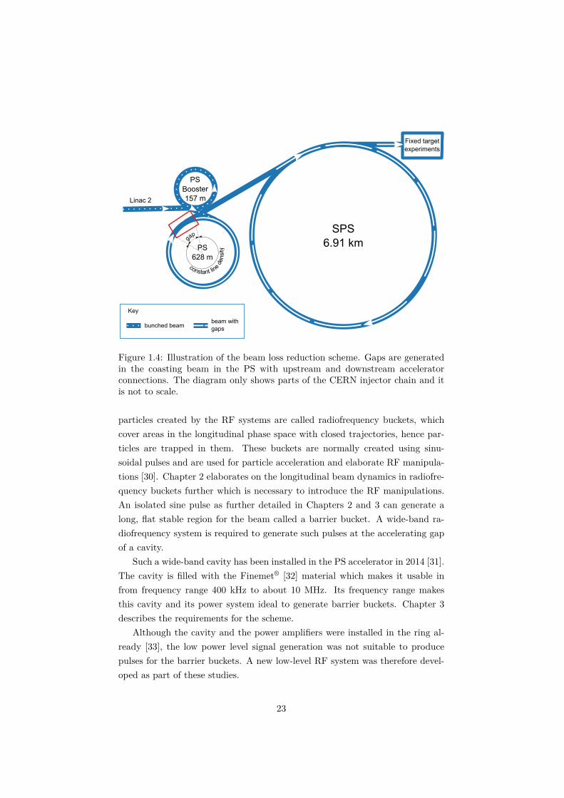
Figure 1.4: Illustration of the beam loss reduction scheme. Gaps are generatedin the coasting beam in the PS with upstream and downstream acceleratorconnections. The diagram only shows parts of the CERN injector chain and itis not to scale.

particles created by the RF systems are called radiofrequency buckets, whichcover areas in the longitudinal phase space with closed trajectories, hence par-ticles are trapped in them. These buckets are normally created using sinu-soidal pulses and are used for particle acceleration and elaborate RF manipula-tions [30]. Chapter 2 elaborates on the longitudinal beam dynamics in radiofre-quency buckets further which is necessary to introduce the RF manipulations.An isolated sine pulse as further detailed in Chapters 2 and 3 can generate along, flat stable region for the beam called a barrier bucket. A wide-band ra-diofrequency system is required to generate such pulses at the accelerating gapof a cavity.

Such a wide-band cavity has been installed in the PS accelerator in 2014 [31].The cavity is filled with the Finemet® [32] material which makes it usable infrom frequency range 400 kHz to about 10 MHz. Its frequency range makesthis cavity and its power system ideal to generate barrier buckets. Chapter 3describes the requirements for the scheme.

Although the cavity and the power amplifiers were installed in the ring al-ready [33], the low power level signal generation was not suitable to producepulses for the barrier buckets. A new low-level RF system was therefore devel-oped as part of these studies.

23

1.3 Overview of barrier buckets in synchrotrons

Lengthening the stable phase region of ordinary buckets employing multi-harmonic RF systems has been studied since the early 1960s [34]. The suggestionwas to extend the phase stable region in a radiofrequency bucket by using multi-harmonic RF systems to nearly a full accelerator turn to reduce space chargeeffects, which limit the beam intensity in low energy accelerators. The extremecase of a long bucket, formed by a potential barrier was called barrier bucket inthe early 1980s [35].

1.3.1 Use cases of barrier buckets

With the increased availability of wide-band RF systems, barrier buckets [36] be-came a routine operation at many facilities, first at Fermilab [35, 36] where mul-tiple injection schemes [37, 38] involving moving barriers were studied and usedfor the accumulation of intense beams [39, 40]. The creation of flat bunches wasimproved with the development of RF systems [41–43] reaching even longitudinalprofiles [44]. Early barrier bucket studies were also performed in the BrookhavenAGS in collaboration with KEK to accumulate a debunched beam [45–49]. Inthe framework of the AGS studies the use of both, conventional ferrite-loadedcavities and Finemet® cavities was validated [50–55] providing an importantmilestone to enable the present studies.

Low emittance beamlets at a well defined momentum can be extracted in aprocess called longitudinal momentum mining [39, 56, 57]. Associated with thisoperation a unique feature of the beam dynamics in square wave barriers [58]was explored, which highlights the importance of smooth waveforms in barrierbucket generation.

To overcome the limitation of low synchrotron frequencies, which makes anadiabatic bunch length changes slow, shock compression benefiting from spacecharge was also proposed [59, 60].

Barrier buckets found one of their main use case in low energy storage rings,where high intensity beams need to be kept for longer durations. In particularheavy ion facilities, where space charge effects are dominant have become relianton this RF structure, see for example [61–64] and references therein. Barrierbuckets are often combined with stochastic cooling to compensate for the meanenergy loss [65] after the interaction with the target [66–78] and mitigate againstelectron cloud build up [79]. Preparatory studies for the FAIR accelerator com-plex for barrier buckets with stochastic cooling were performed at COSY [80–84]. In the ESR at GSI barrier buckets were also experimentally tested to ac-

24

cumulate multiple injections. The NICA collider, currently in its final phase ofits construction [85–92] will also accumulate beam in barrier buckets.

Accelerating beam in barrier buckets is a challenging task. It was proposedand studied in detail at the KEK PS [93–103].

The feasibility of a super-bunch hadron collider [104, 105] was also explored.The super-bunch collider is an induction synchrotron concept [106], where wide-band induction devices for acceleration and beam confinement separately wouldbe used. Such a device, the Finemet® cavity generates barrier buckets in thepresent studies, too.

Thick barrier buckets using narrow band RF systems were studied in theCERN SPS [107, 108].

1.3.2 Brief overview of barrier bucket implementations

Two main strategies can be employed to generate barrier bucket waveforms,which depend on the shape of the pulse they generate. The waveforms arefurther compared in Chapter 3 in detail.

The frequency domain approach is to use multiple harmonics [35]. This iswell suited to isolated sinusoidal shaped pulses, since these have lower band-width requirement compared to isolated square waves. Arbitrary waveformgenerators [41, 109–111] are also typically employed to generate barrier buck-ets. Custom waveform generators in programmable logic [44, 112, 113] are also atypical approach, especially when great flexibility is needed. The present studyuses the latter for reasons detailed in Chapter 3.

Isolated square pulses generate a higher bucket area for the same pulse du-ration and peak voltage compared to the sine, at the expense of a higher band-width. These can be generated either via the arbitrary waveform generationmethod, but via a pulsed power modulator [93, 114–118] as a waveform gener-ator.

A common problem in barrier bucket systems is the distortion of the wideband pulse as it is transmitted through the high power system [119] to thecavity gap. Therefore an important part of the implementation of the waveformgenerator is a compensation method for the non-linear transfer characteristics,such that the desired shape appears at the cavity gap. For this, the modelling ofthe high power level RF system is essential. Linear models can compensate [109,119] around a well defined working point reasonably well. If the working pointor the system behaviour changes more significantly, adding a feedback systemcould improve the quality of the waveforms at the cavity gap [44]. Non-linearmodels [110, 120, 121] are needed if the cavity behaviour is time and powerdependent to a larger degree. In addition, in the case of an integrated analogue

25

solution, the transfer characteristics have to be sufficiently linearised [114]. Sincethe behaviour of the cavity in the CERN PS does not change with time or beamintensity in a significant way, a linear approach was sufficient for the presentimplementation as shown in Chapter 3.

1.4 Main contributions

The barrier bucket manipulation is daily routine in many accelerators as de-scribed in the previous section. The MTE is a standard operational techniqueof extracting beams from the PS. However, the combination of both sophisti-cated beam manipulations, the barrier bucket with transversely split beams wasperformed for the first time as the part of these studies [1].

The combination showed that the barrier bucket preserved the transversebeam quality, which is not trivial since the transverse and longitudinal beamdynamics are not necessarily decoupled in all cases. This result has an importantpractical consequence, since the combined beam manipulation can achieve avirtually loss-less extraction of fixed target beams from the PS.

In order to achieve these results, an electronic design for the barrier bucketdrive was conceived, implemented and commissioned in the lab and with beamfirst as part of these studies. This included the development of the concept andwriting the firmware for a field programmable gate array (FPGA). Developing awaveform generation method with a smoothing scheme was important to avoidthe consequences of a discontinuous waveform on the beam dynamics in narrowbarrier buckets [58], produce a flatter waveform and limit the bandwidth.

The studies in this thesis show that a significant beam loss reduction in thePS can be achieved by using barrier buckets at extraction.

For the fixed target experiments to benefit from this, the barrier bucketgeneration has to be synchronous with the circulating beam in the SPS. Aconcept is developed in Chapter 5 supported by analytical calculations andbenchmarked macroparticle simulations. It is also shown that the conventionaladiabaticity criterion based on the change of the synchrotron frequency can notbe applied in all cases to the re-phasing operation, which is a central part of thesynchronisation, instead, a different criterion is developed.

26

1.5 Structure of the thesis

Chapter 1 The present chapter. Briefly summarises the state of the art inbarrier bucket apparatus in particle accelerators. Details the motivationsand highlights the contributions of the thesis to this.

Chapter 2 A study of longitudinal beam dynamics was carried out to introducebarrier buckets used in these studies in an analytical way.

Chapter 3 Contains the analysis of the requirements, the development of theconcept, the implementation, validation, installation and commissioning ofa beam synchronous arbitrary waveform generator for the barrier buckets.Includes details from the publication [3]. The chapter summarises thetechnical contribution of the work.

Chapter 4 Contains the main contribution of the work. The combination ofthe barrier buckets with transversely split beams, a first in the field, leadto a proven, significant beam loss reduction at extraction from the PS.Several steps were needed to reach this conclusion, hence this chapter alsopresents the initial results of the tests with beam. Additionally, it containslongitudinal beam dynamics simulations to explain the main features ofthe observed beam profiles at extraction. The chapter presents the ex-perimental evidence of the beam loss reduction and includes details fromthe publications [1, 2].

Chapter 5 In order to put the barrier bucket scheme into operation the gen-eration of the barrier buckets has to be synchronised with the injection ofthe beam into the SPS. This chapter presents a conceptual design for thissynchronisation.

Chapter 6 Summarises the main contributions and outlines the future workrelated to the barrier bucket studies in the PS.

Appendix A Presents an alternative synthesis method for the barrier wave-form from a series of two harmonics at half of the revolution frequency.

Appendix B Contains the location of the firmware and software developedduring this project.

27

Chapter 2

Longitudinal beamdynamics

2.1 Introduction

This chapter provides a brief theoretical background for the contributions of thesubsequent chapters. The main purpose is to introduce the basic parametersto describe the motion of charged particles under the influence of a periodiclongitudinal electric field. This is needed to understand the fundamental beamdynamics in barrier buckets. Section 2.2 introduces a continuous time approachto solve the non-linear equations of motion of particles in a synchrotron in thelongitudinal direction. Section 2.3 applies the concepts outlined in section 2.2to the case of stationary barrier buckets, which are of central importance in thebeam loss reduction. An estimation of emittance growth when the potentialbarriers are moved is found in Section 2.3.2 which is confirmed by beam testsin Chapter 4.

The particle motion can also be described in discrete time using differenceequations. This approach is called (macro-)particle tracking. The techniquesused in thesis are summarised in Section 2.4.

Finally, section 2.5 briefly describes different sources of the longitudinalimpedance to provide a background to the results of simulations in Chapter 4.

2.2 Continuous time approach

Subsections 2.2.1 and 2.2.2 deal with the description of the mechanical system ofclassical, relativistic particles circulating in a synchrotron [122]. The treatmentis restricted to the longitudinal aspect of the dynamics of particles approximated

28

as circular motion in the accelerator illustrated by Fig. 2.1 (top). It is assumedthat the particles are not interacting with each other or the environment otherthan with an ideal, arbitrary, radiofrequency (RF) source. Fig. 2.1 (bottom)illustrates two harmonics of the RF voltage. This voltage generates a potentialwhich confines the charged particles of the beam.

2.2.1 Longitudinal phase space

Figure 2.1: Illustration of the azimuthθ, radius R, momentum p and phase φvariables. The phase is to be interpretedwith respect to the RF voltage for twoharmonics: h = 1 and h = 2 in thisexample. Note that the phase and az-imuth angles are the opposite sign fol-lowing the usual convention E.g. [123,124].

The momentum and/or the distribution of the particles along a synchrotronring is manipulated by RF systems [30, 123, 125] in the longitudinal direction.Since these studies require a wide-band RF waveform, an arbitrary amplitudefunction g(φ) is defined following [125]. ω0 is the angular frequency of theparticle moving along a circle with R0 radius. The multiples of the revolutionfrequency, hω0 are called its harmonics, with h denoting the harmonic number.Figure 2.1 (bottom) illustrates two RF waveforms for h = 1 and h = 2, withthe associated azimuthal position, θ, RF phase, φ, with the sign conventions.

The energy change of a particle in a synchrotron is largely due to RF systems.For the particle having E energy, p momentum and q charge, revolving with R

radius, the change of energy, ∆E, during one interaction with the RF system is

∆E = qV g(φ) . (2.1)

For a more complete derivation which takes the details of this interaction intoaccount see [124, 125]. To link the energy change, ∆E, to the momentumchange, ∆p, it is useful to express ∆p in the form of the rest energy, m0c

2,

29

which is invariant:

∆p = m0c∆(βγ) → m0c2 =

c∆p

∆(βγ), (2.2)

where 1/γ2 + β2 = 1, m0 is the rest mass of the particle and c is the speed oflight in vacuum. The differential change of the relativistic parameters, ∆(βγ),with respect to ∆γ, see Eqs. 2.2 and 2.4 for the motivation, can be written as

∆(βγ)

∆γ=

∆βγ

∆γ+

β∆γ

∆γwith ∆β

∆γ=

1

βγ3→ ∆(βγ)

∆γ=

1

β

(1

γ2+ β2

)=

1

β.

(2.3)The energy change per revolution becomes using Eq. 2.2 and 2.3:

∆E = ∆γm0c2 =

∆γ

∆(βγ)c∆p = cβ∆p = ωR∆p , (2.4)

with βc = v = ωR from the circular motion of the particles in the synchrotron.The average rate of momentum change in time using Eq. 2.1 and 2.4 with theapproximation that the change of momentum is small over a revolution period,T , is the following:

∆p

T= ∆p

ω

2π≈ dp

dt=

qV

2πRg(φ) . (2.5)

One can write 2.5 twice, for two particles, one having parameters with theindex 0, called the synchronous particle and another particle with parametershaving no index. Multiplying these equations by R and subtracting the equationwith 0 index expressions from the other

∆(Rp) =qV

2π[g(φ)− g(φ0)] (2.6)

is obtained. To the first order ∆(Rp) = d(R0∆p)/dt [123]. Then using Eq. 2.4and 2.6 the first equation of synchrotron motion is obtained:

d

dt

(∆E

ω0

)=

qV

2π[g(φ)− g(φ0)] . (2.7)

The particles that have different energies to the synchronous particle arrive atdifferent times from turn to turn. The relative time and angular frequencydifferences are linked to the relative momentum difference through the phaseslip factor, η, which is approximated to the first order as [124, p. 129]:

∆ω

ω0= −∆T

T= −

(αc −

1

γ2

)∆p

p= −ηδ. (2.8)

30

Using the following definitions η = αc − 1/γ2, αc = 1/γ2tr, δ = ∆p/p. The

momentum compaction factor, αc, and subsequently γtr is derived from theoptics of the ring. The transverse aspects of the particle motion in a synchrotronare out of the scope of this thesis, for further details on αc see [124, pp. 122–30].The singularity, when αc = 1/γ2, called transition, is not treated in this thesis,either.

The change of the revolution angular frequency is ∆ω = dθ/dt = −1/h dφ/dt.The negative sign comes from the definition [123] of the phase with respect tothe measurement of azimuth, see Fig. 2.1. Note that this is also in agreementwith the definition of the time difference in Eq. 2.8. When the RF waveform isdefined for the whole ring, a simplification of h = 1 in the equations below canbe made. In this case g(φ) = g(−θ) as per Fig. 2.1. The equation expressingthe change of the phase in time is the following

dφ

dt=

hω0η

pR0

(∆E

ω0

), (2.9)

which is the second equation of the synchrotron motion. Equations 2.9 and 2.7can be combined to a single second order differential equation involving φ as thesingle variable assuming a small change for the parameters of the synchronousparticle.

d2φ

dt2=

hω0ηqV

2πpR0[g(φ)− g(φ0)] (2.10)

The slowly varying machine parameters can be lumped in one term:

ζ = −hω0ηqV

2πpR0. (2.11)

Since Eq. 2.10 usually does not have a solution in closed form, it is useful toinvestigate the types of solutions in two dimensional phase space [126]. Thisallows to study the stability of the motion even if the exact analytical solutionis not known.

An example solution of the two, first order equations 2.7 and 2.9 for the caseof g(φ) = sinφ is shown in Fig. 2.2 (bottom) in the φ, φ phase space. The setof closed trajectories corresponding to a bounded, stable motion is called theradiofrequency bucket. The points making up the trajectories revolve arounda centre in phase space following the evolution of the motion in time. Theparticle, whose parameters are in the centre of this revolution is the synchronousparticle, since it has the phase φ0. It is worth noting that φ0 does not necessarilycorrespond to a single value, see Section 2.3, but g(φ0) obviously does.

Depending on the value of g(φ0), three kinds of buckets are defined. In caseg(φ0) corresponds to an energy increase over a turn for the synchronous particle,

31

g(φ)

W(φ

)

−π −π/2 0 π/2 πφ [rad]

φ(φ

)

Figure 2.2: Illustration of sinusoidal RF voltage (top), corresponding poten-tial (middle) and a conventional, stationary RF bucket (bottom).

as per Eq. 2.1, then the resulting RF bucket is an accelerating bucket. Wheng(φ0) = 0, as seen in Fig 2.2 (bottom), the resulting RF bucket is a stationarybucket. Finally, when g(φ0) contributes to an energy decrease over a turn, theRF bucket is a decelerating bucket.

If g(φ) = sinφ, then the angular frequency of oscillations of the particles inthe centre of the bucket, called the synchrotron frequency, ωs, can be expressedas:

ω2s = ζ cosφ0 = −hω0ηqV cosφ0

2πpR0. (2.12)

One can also describe the system using Hamilton’s method with two vari-ables [127, pp. 172–92], which allows an analytical calculation of the revolutionperiods for all particles in RF buckets. Hamilton’s equations for two coordinatesare the following [127, p. 167]:

q =∂H

∂p, p = −∂H

∂q, (2.13)

where the function H(p, q) is called the Hamiltonian. Using the variables φ andφ one can define the following Hamiltonian:

H(φ, φ) =1

2φ2 + ζW (φ) . (2.14)

32

Where the W (φ) potential is defined as the following:

W (φ) =

∫g(φ)dφ− g(φ0)φ (2.15)

Using Eqs. 2.13 with p = φ and q = φ one obtains Eq. 2.7 and Eq. 2.9. Figure 2.2shows g(φ) on the top, a corresponding W (φ) in the middle and trajectories inphase space associated with Eq. 2.14 at the bottom. These are obtained fromthe Hamiltonian formulation by picking a few pairs of values of the coordinatesand substituting them to Eq. 2.14. This gives a constant H, corresponding toa constant energy. Then for all values of φ, the solution for φ according to

φ(φ) = ±√2 [H − ζW (φ)] , (2.16)

can be found, with the condition H−ζW (φ) > 0. Note that the same trajectoriescan be obtained from the Eqs. 2.7 and 2.9. The equation of the separatrix canbe obtained from Eq. 2.14 by finding the phase corresponding to the unstablefixed point [126, pp. 168–170], φU. The phase velocity should be zero at thispoint. Therefore a value H0 = H(φU , 0) = ζW (φU) can be calculated. Thenusing this value the separatrix is obtained by

φ(φ) = ±√2ζ [W (φU)−W (φ)] . (2.17)

The bucket half height is the maximum of this value at the stable phase φs:

φ(φs) =√2ζ [W (φU)−W (φs)] . (2.18)

The bucket area is the area enclosed by the separatrix and is calculated bythe following integral:

AB = 2

∫ φmax

φmin

√2ζ [W (φU)−W (φ)]dφ , (2.19)

where φmin and φmax are defined by W (φU)−W (φ) = 0.For sinusoidal RF voltages, the Hamiltonian becomes:

H(φ, φ) =1

2φ2 + ω2

sWs(φ) . (2.20)

This formalism is useful, because the Hamiltonian contains the synchrotronfrequency corresponding to the stable phase in the bucket, but Ws(φ) is required

33

to have a scaling factor 1/ cosφ0 compared to W (φ):

Ws(φ) =1

cosφ0W (φ) . (2.21)

2.2.2 Synchrotron frequency spread

The function describing the revolution frequencies for particles in phase space asa function of one of the variables is called the synchrotron frequency distributionor synchrotron frequency spread. In the Hamiltonian formalism this can becalculated based on a method first introduced in astronomy [127, pp. 243–57].The technique involves a transformation of the Hamiltonian to action-anglevariables. This transformation reveals the periodicity of the trajectories in phasespace [127, pp. 249–50]. The action, J , is introduced as one of the variables ofthe transformed Hamiltonian H ′.

Following the general procedure of [127, p. 247], J becomes

J =

∮pdq → J =

∮φ(φ)dφ . (2.22)

The value of the line integral is equal to the area enclosed by the trajectoryover a period of oscillation in phase space [127, p. 247]. The frequency, fs, orangular frequency, ωs, of the oscillation belonging to one trajectory is directlygiven [127, p. 251] by

fs =∂H ′

∂Jor J ′ =

1

2πJ → ωs =

∂H ′

∂J ′ . (2.23)

The value of the Hamiltonian during the transformation is constant H ′ = H,since it is assumed that this value is not explicitly dependent on time. Thereforeby calculating the values of H ′ = H and J and forming the derivative, thesynchrotron frequencies for each trajectory can be calculated. The result ofsuch calculation is Fig. 2.3, calculated for a conventional, stationary bucket.

0 π/4 π/2 3π/4 πφ

0.0

0.5

1.0

f s/f

sl

Figure 2.3: Synchrotron frequencyspread in a conventional, stationarybucket as a function of phase.

A different reasoning can be found in [124, pp. 247–8], which calculates therevolution period, T , and derives a specific J for conventional buckets usingg(φ) = sinφ. Similar calculations in different variables are found for example

34

in [128, pp. 115–6] or [124, pp. 256–8] with analytical estimations for the caseof the conventional, stationary bucket.

An equivalent method of finding the synchrotron frequency spread is toFourier transform the time evolution of one of the variables, which can be per-formed based on the discrete, tracking method as mentioned in Section 2.4.

2.3 Barrier buckets

A gap in the otherwise constant longitudinal line density can be made by twoisolated pulses as illustrated by Fig. 2.4 (top). This generates two distinctregions based on the value of g(φ). When g(φ) 6= 0, the trajectory of the particleschanges direction. If their phase velocity is sufficiently low, they reflect off thepotential barriers, hence this is called the reflection region, with its length inphase being φr. If their phase velocity is too high, they are not trapped by thepotential barriers as shown by the outer trajectories of Fig. 2.4 (bottom), whichin our application would cause beam loss. When g(φ) = 0, the particles driftalong straight trajectories in phase space called the drift space. φd is the lengthof the drift space in phase.

Comparing the fundamental behaviour of the beam in stationary barrierbuckets with conventional stationary buckets can be done by comparing theirsynchrotron frequency distributions as calculated from the action J according toEq. 2.23. Figure 2.5 shows the synchrotron frequency spread in barrier bucketshaving different φd/φr aspect ratios, but the same bucket height versus thephase velocity. The synchrotron frequency spread was normalised to the oneof the conventional bucket, denoted fsl and calculated from Eq. 2.12. Themaximum of the synchrotron frequency becomes significantly lower comparedto a conventional bucket as the drift space increases for the same bucket height.The consequences of this with respect to the barrier bucket manipulations willbe explored in Section 2.3.2 and Chapter 4.

2.3.1 Bucket height and area for sine based barrier buckets

An isolated sine pulse as illustrated by Fig. 2.6 is a good approximation of therealistic pulses shown in Fig 2.4 (top) with the advantage, that it allows for theanalytical calculation of the bucket parameters. These are given in the variablesenergy and voltage, such that they can be used to estimate the requirements ofthe barrier bucket RF system in Chapter 3.

The normalised RF voltage is defined as the following using the notations of

35

Figure 2.4: Normalised RF voltage (top) of the pulsed RF system generating abarrier bucket, together with an illustration of corresponding trajectories (bot-tom) in the longitudinal phase space, including the separatrix (dashed). Barrierbucket parameters in barrier RF phase. φd corresponds to the drift space, wherethe particles do not experience any RF voltage. φr corresponds to the reflectionregion on one side of the barrier.

Fig. 2.6:

g(φ) =

{sgn(η) sin

(φ 2π

φr

), if − φr/2 ≤ φ < φr/2

0, otherwise.(2.24)

This is scaled with the peak voltage, V .It is convenient to define the harmonic number corresponding to the reflec-

tion region generating the gap, because the form of the bucket height and areaexpressions become similar to ones of the conventional buckets:

hr =π

φr. (2.25)

Note that this is not the same as the conventional harmonic number, h, of thewide-band RF system. The latter is fixed at h = 1 for the barrier bucket wave-forms used in these studies, meaning that the wide-band waveform is definedfor one revolution of the accelerator.

36

0.0 0.2 0.4 0.6 0.8 1.0φ/φmax

0.0

0.2

0.4

0.6

0.8

1.0f s/f

slφd/φr = 0

φd/φr = 1/10

φd/φr = 1

φd/φr = 10

Figure 2.5: Synchrotron frequency spread as the function of the relative phasevelocity in barrier buckets made by the same sinusoidal pulses with differentdrift space ratios. φd/φr = 0 corresponds to a conventional bucket, see alsoFig. 2.3.

−π −π/hr 0 π/hr πφ [rad]

1

0

1

g(φ)

φr−φr

Figure 2.6: Illustration of thenormalised amplitude g(φ)and the gap harmonic hr pa-rameters for a barrier bucketwaveform. The [−π, π) inter-val represents the whole cir-cumference of the accelera-tor.

The frequency associated with isolated sine is defined as:

fr = hrfrev . (2.26)

The drift region, where the RF amplitude is zero covers the remaining part ofthe circumference:

td =1

frev

(1− 1

hr

)and tg =

1

frevhr. (2.27)

This also means that 1/frev = Trev = tr + td.Following the definitions above, the bucket half height of the barrier bucket

can be expressed as the bucket height of the conventional sinusoidal bucket

37

obtained from Eq. 2.18:

∆Emax = β

√2eV E

πhr|η|. (2.28)

The barrier bucket area consists of the area of the reflection region and thedrift region. According to Eq. 2.19, the total area of the reflection region is thearea of a single, conventional, stationary bucket:

Ag =16β

(2π)2/3

fr

√eV E

hr|η|. (2.29)

The area of the drift space is the bucket height times the duration of the driftspace in time:

Ad = 2β

√2eV E

πhr|η|td . (2.30)

The barrier bucket area is the sum of the reflection regions and the drift spaceand it is obtained by adding Eqs. 2.29 and 2.30:

AB = Ag +Ad . (2.31)

It is also useful to express the peak RF voltage needed for a given bucket area.Expressing V from Eqs. 2.29, 2.30 and 2.31 results in

V =A2

B

4e

|η|f2rev

β2E

h3r[

8(2π)2/3

+√

2π (hr − 1)

]2 , (2.32)

where the first group of terms on the right-hand-side are constants, the secondgroup are dependent on the energy of the beam and the third only on the widthof the gap.

2.3.2 Estimation of phase-space area growth due to barrierbucket compression and expansion

To estimate the emittance growth during the barrier bucket compression andexpansion, the trajectory of a particle encircling the entire bunch is studied.The surface inside this trajectory represents the initial value of its invariant.The following derivation has two parts corresponding to the two regions of thestationary barrier bucket. The first part describes the changes in the drift spaceby looking at the nature of reflection of particles off a moving potential barrier.The second part describes the changes in the reflection region. Together theseprovide a basis for the estimates of the emittance growth and barrier speedlimits.

38

The drift speed of the particle outside of the reflection region in phase spaceis the phase velocity φ. The phase velocity of the barrier is denoted as φb, whichalso moves along the φ axis. The barrier speed is taken to be constant, as itwas the case in the tests reported in further parts of this section.

Looking at the dynamics of a single reflection, it is evident that the phasevelocities before and after a reflection are equal and have the opposite sign forthe case of a stationary barrier. This motion is mathematically identical toan elastic collision of a point particle with a stationary wall of infinite massin a non-relativistic approximation. However, when the wall is moving with aconstant, non-zero velocity vwall in the observer’s reference frame, the velocitiesbefore, vi, and after, vf , according to the classical Galileo transformation arethe following:

vi + vf = 2 vwall . (2.33)

These speeds do not depend on the details of the reflection, they only assumethat the interaction happens and energy and momentum are conserved. This isalso the assumption that is made for the phase velocity of a particle in phasespace, where the wall becomes the moving barrier:

φi + φf = 2 φb . (2.34)

This relationship holds for an arbitrary voltage shape, as long as its amplitudeguarantees that the particle is reflected.

During the reflection, the drift space gets shorter in case of compressionor gets longer in case of expansion. The time it takes for a particle to bereflected can be approximated by half of a synchrotron period Tsl/2 = π/ωs of aconventional, stationary RF bucket corresponding to the reflection region of thebarrier bucket. The phase of the barrier moves half of the synchrotron periodby φbTsl/2 = φbπ/ωs.

To estimate the change of emittance in the reflection region, a linear voltageis assumed for a stationary bucket. This is justified, since the essential particledynamics in a barrier bucket does not depend on the shape of the voltage used,but only on the integral of the voltage [36]. Therefore the Hamiltonian for themoving half bucket representing the reflection region becomes

H(φ, φ) =1

2φ2 +

1

2ω2sφ

2 . (2.35)

The following geometrical argument can be used to estimate the emittancegrowth during the time the particle reflects off the barrier while the barrieris moving at the same time. Let us assume an initial half drift space length,see also Fig. 2.4, of φd/2 compared to the edge of the reflection region. Then

39

using E.q. 2.34 and the notations of Fig. 2.7, the ratio of the two coloured areas

Figure 2.7: Diagram of the quarter areas of the phase space before and after aparticle reflection off a moving barrier. The two phase spaces are shifted suchthat the main parameters used in the calculation are visible.

representing the change in emittance is evaluated:

Af

Ai=

|φf |(|φf |π + 2φdωs

)|φi|

(|φi|π + 4|φb|π + 2φdωs

) . (2.36)

It is worth noting that the phase change due to the change of a trajec-tory 2|φb|/ωs in the reflection region is not the same as the change of phasein the drift region due to the displacement of the barrier |φb|π/ωs. The sin-gularity when φf = 2φb is the case when the beam in a very thin barrierbucket turns into a beam in a conventional RF bucket in Ts/2 time or viceversa. This provides a hard limit on the barrier speed for an adiabatic manipu-lation, see Fig. 2.8 (right). If the area occupied by the particles in phase spacechanges too fast, the manipulation will become non-adiabatic, therefore the bar-rier speed should correspond to a very small area change during one reflection,see Fig. 2.8 (left). Using the notations of Fig. 2.4, φr = φf/ωs. The estimatedemittance growth corresponding to different φd/φr barrier bucket drift spaceratios can also be seen on Fig. 2.8 (left).

The speed of the barrier should be much smaller than the drift speed of aparticle with a maximum energy offset [36, 45], which means φb/φf � 1. This isthe limiting case of a particle, which is not interacting with the potential barrierat all, as it never enters the reflection region. However, the speed of the barriermust be much less than even the half of this [37], which the present estimationalso shows.

40

0.00 0.05 0.10 0.15 0.20φb/φf

0.0

0.1

0.2

0.3

0.4

0.5

0.6

0.7Af/A

i−

1

φd/φr = 0

φd/φr = 3

φd/φr = 6

φd/φr = 9

φd/φr = 12

φd/φr =∞

0.2 0.3 0.4 0.5φb/φf

0

50

100

150

200

250

300

Af/A

i−

1

φd/φr = 0

φd/φr = 3

φd/φr = 6

φd/φr = 9

φd/φr = 12

φd/φr =∞

Figure 2.8: Left: Emittance growth estimate for low relative barrier speeds.Right: limiting case of the relative barrier speed at half of the phase velocity ofan outer particle in the bunch.

2.4 Discrete time approach

The longitudinal dynamics of the particles in a synchrotron can be described on aturn by turn basis using a set of two non-linear difference equations, sometimescalled mappings [124, p. 235]. Longitudinal particle tracking is a method ofsolving the difference equations of the synchrotron motion numerically. Thismethod is different from the analytical calculations in phase space, since it doesnot involve an averaging step. Three sets of variables were used in thesis basedon the same turn-by-turn tracking principle. Table 2.1 shows the variables usedby the different methods. Certain choice of variables makes a problem easier

VariablesNormalised tracking φ, φ

Time- and energy offset based ∆t,∆E

Phase and relative momentum offset based φ, δ = ∆p/p

Table 2.1: Types of tracking used in the thesis

to handle, the reason for choosing each method is highlighted in this section. Aconvention applied to all cases is that the indices n and n + 1 are referring tothe n and n+ 1 iteration of the difference equation performed from some set ofinitial conditions.

41

2.4.1 Normalised tracking

First, normalised longitudinal tracking is outlined. Using the same notations asin section 2.2.1, the mapping equations to calculate the φ and φ coordinates ofa particle are the following

φn+1 = φn +2π

ω0φn , (2.37)

φn+1 = φn − 2π

ω0ωsg(φn+1) . (2.38)

Equation 2.38 assumes that the particle drifts with the phase velocity of the pre-vious turn, φn, over a turn of the duration 2π/ω0. Following from Eqs. 2.7, 2.9and 2.12, the second term on the right-hand-side of Eq. 2.38 represents thephase velocity change integrated over one turn in the stationary bucket case.This formulation is useful, since the slowly-varying accelerator parameters areall lumped in one term, ωs, therefore the comparison of the two phase spacevariables is transparent, which makes validating analytical considerations men-tioned in section 2.3.2 easier.

2.4.2 Energy- and time-offset based tracking

The energy and time offset based tracking is an efficient way of tracking physi-cal variables, which is implemented in the CERN Beam Longitudinal Dynamicscode BLonD [129]. Since the change of the variables compared to their mag-nitude is small, it is more memory efficient and also more precise to track thedifferences only [130, p. 19]. The units and the derivations of these equationscan be found at the following reference [129]. Since the energy unit is eV, thevoltage V has the same unit as the energy. The tracking equations used in thisthesis are the following:

∆En+1 = ∆En +

nrf−1∑k=0

V nk sinϕrf,k(∆tn)− (En+1

0 − En0 ) , (2.39)

∆tn+1 = ∆tn +2π

ωn+1− 2π

ωn+10

. (2.40)

The constant nrf is the number of RF systems, Vk and φrf,k is the peak voltageand phase of these, respectively.

Note that the sum of the voltages in equation 2.40 resembles a classicalFourier sum of an odd waveform. This simple notion was utilised to model thewide-band waveform used in beam tests in BLonD as shown in the results inChapter 4. This was accompanied with the appropriate amplitude modulationof the harmonics, as it will be seen in Chapter 3 to use identical methods of the

42

hardware implementation also developed during this study.

2.4.3 Phase and relative momentum offset based tracking

To cross-check the BLonD simulations for the re-phasing operation in conven-tional buckets for the proposed synchronisation in Chapter 5, a third set ofequations [124, p. 235] were used in a custom made tracker.

δ =∆p

p(2.41)

δn+1 = δn +qV

β2E(sinφn − sinφ0) , (2.42)

φn+1 = φn + 2πhη(δn+1)δn+1 . (2.43)

These equations are the direct consequence of Eqs. 2.7, 2.9 for the case of g(φ) =sinφ.

2.5 Beam-accelerator interaction, impedance

The goal of this brief section is the introduce the beam and accelerator interac-tion restricted to longitudinal impedance.

The beam generates a potential by passing through a structure in the ac-celerator. This is called the wake function WL(t) and it essentially acts as anextra wide-band RF system on the beam. In the frequency domain, this pulsecorresponds to an impedance, called the longitudinal impedance. [124, p. 355]

Z(ω) =

∫ ∞

−∞WL(t)e

−jωtdt , WL =1

2π

∫ ∞

−∞Z(ω)ejωtdω . (2.44)

The complex valued and frequency dependent longitudinal impedance dependson many parameters. The following types are distinguished: the longitudinalspace charge impedance, resistive wall impedance and narrow- and broad-bandimpedances [131].

The longitudinal space charge impedance depends on the vacuum impedance,Z0 the geometrical factor of the beam pipe, g0, and the speed of the particles,β, γ [124, pp. 365–6] and [132, 133]:

ZSC

n= −j

g0Z0

2βγ2. (2.45)

The resistive wall impedance follows from the fact that the beam pipe isnot perfectly conducting [124, pp. 357–8]. Therefore predominantly the highfrequency components of the wake can penetrate the beam pipe causing losses.

43

This depends on the skin depth δskin =√2/σcµω, where σc and µ are the

conductivity and the permeability of the beam pipe and ω is the frequencycomponent in question. The impedance contribution can be approximated as:

Z(ω) ≈ R

bσcδskin(ω). (2.46)

Where b is the average radius of the beam pipe. Further geometries can befound at [134].

In general, the narrow-band impedances in an accelerator are present dueto the resonant RF cavities. Broad-band impedances are due to broad-bandcavities and in general discontinuities of the beam pipe.

2.6 Summary

This chapter describes the two main tools to investigate longitudinal beam dy-namics in a synchrotron, the continuous time, analytical approach based onHamiltonian mechanics and the discrete time approach as it is used in this the-sis work. The continuous time approach was applied to describe the propertiesof barrier buckets and to calculate the phase space area change in barrier buck-ets in a simple way. Finally, concepts related to longitudinal impedance wereintroduced briefly.

44

Chapter 3

Requirements andimplementation of thebarrier bucket waveformgenerator

3.1 Introduction

To generate a barrier bucket waveform, a wide-band RF system is needed. Thiscan be introduced with a short comparison with a single harmonic RF systemin the context of synchrotrons. A single RF system, as its name suggests, canproduce a sine wave of a given frequency [124, pp. 330–347] [135]. This singlefrequency can be changed to a smaller or larger degree by tuning the system ac-commodating the need of the acceleration of beams. A wide band or pulsed RFsystem [106, pp. 263–283], on the other hand, is capable of generating more har-monics across the spectrum at the same time. Hence a typical multi-harmonicRF system can interact with several parts of the beam spectrum at once mak-ing beam manipulations that require wide-band waveforms possible. However,a wide band system couples to more harmonic components of the spectrum,too, making the control of such systems more complex if their impedance or thebeam intensities are higher.

In the case of the PS, as introduced in Chapter 1, the Finemet® system cannot provide enough power to change the mean energy of the beam in a shorttime, therefore acceleration is not achievable in a realistic time frame with it.On the other hand, it is ideal for barrier bucket generation.

45

In order to interact with the beam, the barrier bucket waveform has to besynchronous with it as explained in the previous chapter. To achieve this, abeam synchronous, arbitrary waveform generator was devised and implementedin programmable logic. It uses the direct digital synthesis (DDS) principle [136,137] extended to arbitrary waveforms as opposed to the conventional sine-basedDDS. To implement the generation of the drive signal for the power RF sys-tem before the end of 2018, as many parts of the existing low power level RFinfrastructure of the CERN PS was reused as possible. The details of thisimplementation are found in Section 3.3.

The electronic board with the new barrier bucket firmware on a field pro-grammable gate array (FPGA) working in the lab was an important milestonefor the PhD, but the integration into the accelerator high power level RF andcontrol system was just as crucial. In particular, the distortion that the highpower signal chain adds to the wide-band waveform had to be compensated forto achieve the desired waveform shape at the cavity gap. Section 3.4 describesthe measurements and the model used to achieve this.

In order to investigate the behaviour of the beam in barrier buckets, lon-gitudinal beam dynamics simulations are an indispensable tool as described inChapter 2. The barrier bucket waveform generator system was added to thealready existing simulator framework: BLonD to provide an accurate represen-tation of the real RF system for numerical studies as described by Section 3.5.

3.2 Requirements

The pulse generating the gap must have two main properties. Firstly, the du-ration should be in the range of the rise time of the kickers, which is in theorder of 300 ns [138]. Secondly, the amplitude should be high enough efficientlyremove particles from the gap region during this time. In addition, the beamsynchronous requirement mentioned in the introduction means that the fre-quency range of the system has to be compatible with the revolution frequencyrange of the PS. This, together with the wide band waveform defines the fre-quency range and the bandwidth of the installation. Furthermore, the systemneeds to be compatible with the CERN control system for remote control. Theserequirements are detailed below.

3.2.1 Amplitude requirement

Measurements with beam along the cycle detailed in Section 4.4 were used toestablish total longitudinal emittance of the beam of 16 bunches. At least thetotal longitudinal emittance of 24 eVs of these bunches will have to be contained

46

by the barrier buckets, which provides a lower estimate for the amplitude. Themaximum voltage available from the Finemet® cavity is about 5 kV [31]. Theachievable bucket filling factors were compared to this value across a range of gapsizes using Eq. 2.32. The filling factor is the ratio of the longitudinal emittanceof the beam divided by the bucket area.

Figure 3.1 shows the voltage requirement calculated for different filling fac-

Figure 3.1: Peak voltage requirement for the ideal case of emittance preservationduring re-bucketing.

tors based on Eq. 2.32 as a function of the gap size for the total emittance ofthe 16 bunches. The gap size is taken to be the length of the non-zero part ofthe waveform, which approximates the completely particle free region with lowfilling factors well in the first order. However, even if there are some particles inthe gap region with higher filling factors, the line density can still be significantlyreduced by the potential barriers as illustrated in Fig. 2.4 (bottom).

The re-bucketing without longitudinal blow up can not be expected in thepresent configuration, because of the limited time available. Longitudinal track-ing simulations using BLonD were performed to estimate the longitudinal emit-tance of the coasting beam at extraction. This was found to be 30 eVs. Hencethe voltage requirements are somewhat higher assuming a blow up during de-bunching. The study of the de-bunching process in detail is foreseen as futurework detailed in Chapter 6.

Fig 3.2 shows that with the present RF system, a filling factor of approxi-mately 80% can be achieved with the peak voltage of 5 kV for all gap sizes. Itis clear that the voltage requirement increases with narrower gaps for the same

47

350 325 300 275 250 225 200 175 150Gap size [ns]

0

2

4

6

8

10

Volta

ge r

equi

rem

ent [

kV]

Approx. available voltage

Filling factor: 50 %Filling factor: 60 %Filling factor: 70 %Filling factor: 80 %Filling factor: 90 %

Figure 3.2: Peak voltage requirement taking the simulated longitudinal emit-tance blow-up during re-bucketing into account, too.

filling factor. Nevertheless, the amplitude of the Finemet® system based onthese estimations is sufficient to make a particle free region in the beam, whichcan reduce the losses at extraction.

3.2.2 Frequency range and waveform control

This system should be able to validate the behaviour of the beam in an RFbarrier bucket in the PS. This means that it should be able to operate in therevolution frequency range, 437 kHz – 476 kHz, synchronously with the beam.Furthermore, it should be compatible with the existing RF installations.

In order to generate azimuthally moving barriers, the phase of the barrierpulses have to be controlled remotely from the CERN Control System [139, 140].To facilitate the re-bucketing process from the h = 16 bunches to the barrierbucket, the amplitude of the barrier bucket system is required to be controlledin real-time, too.

As it was explained in Section 2.3 if one inverts an RF waveform generat-ing a barrier bucket, a conventional, isolated bucket is generated. Therefore awaveform inverter is useful to test the behaviour of the beam in a conventionalbucket and a barrier bucket generated at the same azimuthal position. Thisfunction is useful to change between below and above transition operation, too.In addition, the ability to program a constant RF offset makes the system more

48

flexible in calibrating azimuthal reference points.

3.2.3 Bandwidth requirement

The barrier bucket waveform consists of a zero and non-zero part, which meansthat it is a wide-band waveform as described in 2.3. However, the shape ofthe waveform is a free parameter, provided it satisfies the general requirements.Hence the trade-offs involved in choosing a waveform shape are investigated inthis section.

Firstly, the bandwidth requirement for two commonly used waveforms forbarrier buckets, the sine and the square based barriers is evaluated analytically.Then a cosine section waveform is analysed that can be advantageous in cer-tain respects compared to the other two. Finally, regardless of the waveformof choice, a windowing technique is presented that limits the bandwidth re-quirement for all pulses while keeping the correctness of their phase, which isimportant in synchrotron applications.

3.2.3.1 Waveform shape, bucket height and roll-off

Since the pulses have a fixed period determined by the revolution frequency ofthe synchrotron, it is sufficient to calculate components of the Fourier series:

g(φ) =

∞∑n=0

an cosnφ+

∞∑n=1

bn sinnφ , (3.1)

where an and bn are the Fourier coefficients. Waveforms that generate barrierbuckets to be used in the present studies are odd as detailed in Section 2.3,hence an = 0. Eq. 3.1 simplifies to:

g(φ) =

∞∑n=1

bn sinnφ . (3.2)

The bandwidth requirement depends on the shape of the waveform. Threeexample waveforms are analysed in this section based on their discontinuities.Square and sine barriers are introduced first, which have been widely used ingenerating barrier buckets [35, 45, 106, 110, 141]. An additional waveform basedon cosine sections is introduced which combines desirable spectral properties ofboth, the square and sine waveforms.

The square wave is a discontinuous waveform, therefore its bandwidth re-quirements are the most demanding. This can be analytically seen from thediminishing of its Fourier coefficients. The normalised amplitude function, g(φ),as introduced in Section 2.2.1 is defined for the square wave barrier first:

49

g(φ) =

−sgn(η), if − π/hr ≤ φ ≤ 0

sgn(η), if 0 < φ ≤ π/hr

0, otherwise .

(3.3)

The waveform changes sign at transition energy, this is incorporated in thesgn(η) term.

Its Fourier coefficients evaluate to:

bn = sgn(η)2

nπ

[1− cos

(n

hrπ

)], (3.4)

decreasing proportional to 1/n. Technically, this barrier is easier to realise whenone uses, for instance, the switched signals of a power converter as demonstratedin [106]. However, due to its discontinuity, it is not the best candidate to beimplemented using a wide-band RF system. On the other hand, the advantageof using a square barrier is that it achieves the largest bucket area for a givenreflection region width as shown by Table 3.1.

As a generalisation of the square wave, an arbitrary pulse train synthesismethod is presented in Appendix A. That approach uses two phase shifted har-monics of an equal frequency at half of the harmonic frequencies of the classicalFourier sum to generate a pulse train. This could potentially be beneficial inimplementations with wide band feedback as it is referred to in Section 3.4.

The normalised amplitude of the single sine barrier waveform is defined asfollows.

g(φ) =

sgn(η) sin (hrφ), if − π/hr ≤ φ ≤ π/hr

0, otherwise .(3.5)

The first derivative of this waveform is discontinuous. Its Fourier coefficientswere published in [35]. The calculation leads to two different formulas, sincethere is a discontinuity depending on the value of n and hr. When n 6= hr:

bn = sgn(η)2hr

π (h2r − n2)

sin

(n

hrπ

). (3.6)

When n = hr,

bn =sgn(η)

hr. (3.7)

The coefficients decrease with 1/n2, meaning that the isolated sine wave isless demanding in terms of the required bandwidth compared to the square wave,since its Fourier coefficients diminish faster with the number of terms requiredto synthesise the waveform as depicted in Fig. 3.4. However, the bucket heightshrinks for the same hr compared to the square wave representing the maximum

50

Waveform Relative bucket height Relative bucket areaSquare 1 1

Sine√2/π ≈ 80% 3

√2(π(hr−1)+2)

π32 (3hr−1)

Cosine sections√2/2 ≈ 71% ≈ 2.1213 2

√2√hr+π

32 (hr−1)

π32 (3hr−1)

Table 3.1: The comparison of the bucket heights and bucket areas for differentbarrier bucket generating waveform shapes for the same hr. Calculating thecosine sections bucket area involves a numerical integration.

−π −π/hg 0 π/hg π

Square waveSingle sineCosine sections Figure 3.3:

Comparison ofdifferent wave-forms generatedfor the samegap width us-ing 20 Fourierharmonics.

for a given hr as seen in Table 3.1.The following example is made out of cosine sections. The waveform has a

discontinuity in its second derivative but not in the zeroth or in the first:

g(φ) =

sgn(η)

[12 cos (2hrφ)− 1

2

], if − π

hr≤ φ ≤ 0

−sgn(η)[12 cos (2hrφ)− 1

2

], if 0 < φ ≤ π

hr

0, otherwise .

(3.8)

The waveform is illustrated in Fig. 3.3. Its Fourier coefficients when 2hr 6= n

arebn = sgn(η)

4h2r

πn (4h2r − n2)

[1− cos

(n

hrπ

)], (3.9)

which decrease as 1/n3. When n = 2hr, bn = 0.It can be observed from Eq. 3.9, that the ∼ 1/n3 roll-off begins at n = 2hr

contrary to the previous cases, whose coefficients start to diminish from n = hr.An example is shown for h = 5, in Fig. 3.4. Suppose that the available band-width for this example is set at 4hr = 20, only to illustrate the significance of thelimit being at twice of hr. The cosine sections waveform has higher amplitudescompared with the sine in the second lobe, for the same hr. These are harmonics10-20 in the example of Fig. 3.4. This results in an improved waveform fidelitycompared to the sine, because the higher harmonics fill the pass-band better.However, unlike the square waveform, the cosine sections pulse has a sine like

51

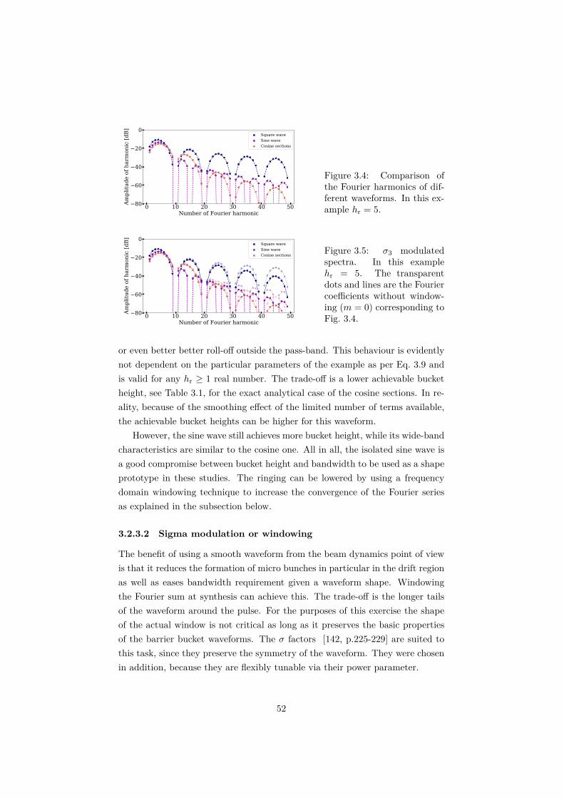
0 10 20 30 40 50Number of Fourier harmonic

80

60

40

20

0Am

plitu

de o

f har

mon

ic [d

B]

Square waveSine waveCosine sections

Figure 3.4: Comparison ofthe Fourier harmonics of dif-ferent waveforms. In this ex-ample hr = 5.

0 10 20 30 40 50Number of Fourier harmonic

80

60

40

20

0

Ampl

itude

of h

arm

onic

[dB

]

Square waveSine waveCosine sections

Figure 3.5: σ3 modulatedspectra. In this examplehr = 5. The transparentdots and lines are the Fouriercoefficients without window-ing (m = 0) corresponding toFig. 3.4.

or even better better roll-off outside the pass-band. This behaviour is evidentlynot dependent on the particular parameters of the example as per Eq. 3.9 andis valid for any hr ≥ 1 real number. The trade-off is a lower achievable bucketheight, see Table 3.1, for the exact analytical case of the cosine sections. In re-ality, because of the smoothing effect of the limited number of terms available,the achievable bucket heights can be higher for this waveform.

However, the sine wave still achieves more bucket height, while its wide-bandcharacteristics are similar to the cosine one. All in all, the isolated sine wave isa good compromise between bucket height and bandwidth to be used as a shapeprototype in these studies. The ringing can be lowered by using a frequencydomain windowing technique to increase the convergence of the Fourier seriesas explained in the subsection below.

3.2.3.2 Sigma modulation or windowing

The benefit of using a smooth waveform from the beam dynamics point of viewis that it reduces the formation of micro bunches in particular in the drift regionas well as eases bandwidth requirement given a waveform shape. Windowingthe Fourier sum at synthesis can achieve this. The trade-off is the longer tailsof the waveform around the pulse. For the purposes of this exercise the shapeof the actual window is not critical as long as it preserves the basic propertiesof the barrier bucket waveforms. The σ factors [142, p.225-229] are suited tothis task, since they preserve the symmetry of the waveform. They were chosenin addition, because they are flexibly tunable via their power parameter.

52

−π −π/hg 0 π/hg π

Square waveSingle sineCosine sections

Figure 3.6: Comparison ofdifferent waveforms gener-ated for the same gap widthusing 20 Fourier harmonicsusing σ3 modulation.

The definition of the factors to multiply the Fourier coefficients with are

σm(n) = sincm nπ

2(N + 1), (3.10)

where N is the total number of Fourier coefficients in the finite sum. Thegeneral shape is half of the main lobe of the sinc function. The larger m, thefaster the roll-off and the narrower the main lobe. This results in larger the tailof the waveform in the time domain, but less ripple. m = 0 corresponds to therectangular window.

The waveform synthesis with the sigma factors included is the following:

g(φ) =

N∑n=1

σm(n)bn(h) sinnφ . (3.11)

It is clear from Eq. 3.11 that the phase of the components is not changed.The consequence in practice is that the smoothing does not affect the azimuthalposition of the generated barrier bucket, which is convenient in the presentimplementation.

53

3.3 Low-level RF system

As explained in Section 3.2.3, the barrier bucket waveform has to be generatedsynchronously with the circulating beam. A conventional LLRF system [143]generates sinusoidal voltages, but for a barrier bucket, a special wide-band wave-form is needed. In addition, the waveform has to be pre-distorted at the inputof the high power amplifier chain, such that the voltage seen at the cavity gapis close to the expected, isolated, approximately sinusoidal pulses as describedin earlier sections of this chapter.

3.3.1 Beam synchronous, arbitrary waveform generation

Waveform generation for a conventional digital RF system [135] in the frequencyrange up a few 100 MHz is typically achieved by using a direct digital synthe-sizer (DDS) [136, 137]. The basic structure of a DDS consists of a phase accumu-lator, a waveform look-up table and a digital to analogue converter (DAC). Mostimplementations have a sine look-up table (e.g. [144–150]) in different configura-tions or, alternatively use a CORDIC algorithm [151], such as [152]. Generatinga barrier bucket requires a wide band waveform with many harmonics, in whichcase the previous solutions do not scale well. However, changing the sine onlylook-up table of a conventional DDS to a programmable look-up table achievesa compact arbitrary waveform generator based on the DDS principle.

Fig. 3.7 shows the block diagram of the beam synchronous, arbitrary wave-

Figure 3.7: The diagram shows the functional elements of the beam synchronousRF source firmware generating barrier buckets.

form generator. The DDS core, or a special numerically controlled oscilla-tor (NCO), provides the beam synchronous azimuth information, Θ, based onthe reference clock at 256 times the revolution frequency, frev [152]. A pro-grammable offset, Θoffset, to change the centre of the generated barrier bucketwas added. Two look-up tables were used to generate two symmetrically moving

54

barriers with respect to the fixed azimuth position, the phase shifts, Θbarrier,were implemented. The waveform in the look-up tables is calculated outside thehardware allowing flexibility of choosing pre-distortion methods.

In addition, an alternate waveform generator concept was also conceivedand is outlined in Appendix A. This combined with a complex multiplicationbased harmonic synthesis can potentially be more frugal on the same hardwareplatform with the added benefit of perhaps easier feedback option. However,the latter possibility was not realised, because that would have required consid-erably more time investment with some existing functionality re-implementedin a different form and, more importantly, the original plan with a shorter timespan allowing for a longer experimental program with beam succeeded.

3.3.2 Implementation

The concept of the beam synchronous arbitrary waveform generator using pro-grammable memory was implemented on existing electronics, the PS one turndelay feedback board [153], hosting an Altera Stratix II FPGA. This board waschosen, since its analogue and digital specifications met the requirements of bar-rier bucket waveform generation as outlined in Section 3.2. The advantage anFPGA is that it can be reprogrammed for a different purpose. In the presentimplementation, the rewiring of the device was described in virtual hardwaredefinition language (VHDL) partially using Visual Elite and text based VHDLwith the test benches simulated with Modelsim. The Altera toolchain was usedfor constraints definition, routing, bitstream generation and flashing.

3.3.2.1 FPGA utilisation

The challenge of the implementation was that the utilisation of the FPGA wasquite high, around 70% without the barrier functionality, with the potentiallyre-usable firmware blocks: the NCO and the blocks necessary to connect theboard to the RF signal chain and the accelerator control system including aCORDIC for validation purposes. Therefore the barrier bucket implementationhad to be economical if it was to benefit from earlier development. This meantthat several optimisations were performed to fit the barrier bucket firmwareon the FPGA while trying not to re-develop existing functionality as detailedbelow.

3.3.2.2 Beam synchronous NCO

Thus, an existing numerically controlled oscillator (NCO) capable of providingbeam synchronous phase information serving as a phase accumulator was the

55

Real-time functions:amplitude and phasevia CVORB serial link

Waveform,offset parametersvia VME

DAC

Vout

t

RF clock

Sync

MEMMEM

NCO

FPGA

WaveformRF clock

Sync Phase

Amplitude

PS one turn delay feedback board

Figure 3.8: The PS one turn delay feedback board with the illustration of thebarrier bucket firmware. The board inputs and outputs are also marked in ourimplementation. The coaxial leads are to route the test points to the frontpanel.

starting point of the implementation. This firmware block was analysed to seewhere the wide-band waveform generator could be added.

The NCO’s multiplied phase output represents a fixed azimuthal or phaseposition, Θm. This position is a reference for the imaginary centre of the twobarrier waveforms:

Θm(n) = Θ + n · 2N mod 2M . (3.12)

Here, n is the output of the phase accumulator, an N bit overflow counterdriven by the RF clock outputting 2N samples per turn. 2M represents theavailable phase resolution with M > N in a typical implementation. The con-ventional harmonic number is h = 1 for barrier buckets as detailed in Chapter 2,therefore not shown in the equations, and Θ is a fixed azimuthal angle. Theramp of the phase accumulator is implemented as a counter. This, togetherwith the output of the RAM is illustrated by Fig 3.9.

In order to dynamically align the centre position of the barriers along theazimuth of the accelerator, a programmable offset, Θoffset, was added to themarker, Θm:

Θout(n) = Θm(n) + Θoffset mod 2M . (3.13)

56

If only one waveform is used, Θoffset sets the azimuthal position of the waveformused to generate the longitudinal gap in the beam distribution.

3.3.2.3 Waveform merging and splitting

The task of this part is to generate two distinct sinusoidal waveforms and movethem without overlap. This corresponds to capturing a bunch in a conventionalbucket when the two waveforms are next to each other. To generate two, mov-able barriers to confirm the adiabaticity limits of the barrier manipulation, twoRAMs with identical content were used as illustrated by Fig. 3.9.

The azimuthal angle between the two barriers was set by adding or subtract-ing an angle value to or from Θout, which sets the correct look-up addresses ofthe RAMs to offset the waveforms by the correct number of samples. Then thesamples are merged and sent to the output as illustrated by by Fig. 3.12.

At the end of the waveform lookup stage of the DDS, a final amplitudescaling was added by using one multiplier only to facilitate the handover froma conventional RF system to the barrier bucket RF.

3.3.2.4 Mitigation of the latency of the address look-up

SRAM blocks were still available on the FPGA. However, the look-up duringone clock cycle of the RF clock was not fast enough for a stable output usingonly one block of the SRAM at the highest clock speeds of 128 MHz RF clockcorresponding to a speed 5% higher than the speed of light in vacuum in thering to provide a margin for the implementation. Two of the RAM blocks wereused with a clock at half speed each. Then the stable output was connected tothe DAC at the original RF clock rate providing a stable output at the desiredclock rate.

57

Figure 3.9: The result of a Modelsim simulation of the MHS phase ramp output (bottom) and two barriers generated per turn (top),where the distance between them can be set. Note that a distance closer than the width of the pulse can produce higher potential as thesecond pulse from the left shows. Such operation is not foreseen for this drive. Either one barrier is to be made per turn at extraction ormultiple barriers at low energy commissioning, but not the two at the same time, hence this is not a true limitation.

58

3.3.2.5 Optional linear interpolator

If only a smaller amount of RAM is available with a higher resolution of phaseinformation, interpolating the output of the RAM makes the output smoother.To do so, the lower phase bits not utilised for address look-up can be used tocalculate intermediate values between two RAM output values, bb1 and bb2.

The linear interpolation formula is the following between two points of thewaveform: bb1 and bb2 with l interval length at a point bb1 ≤ φ ≤ bb2.

y(φ) =(l − φ)bb1 + φ bb2

l(3.14)

The calculation is done every RF clock cycle. I is the intermediate value forthe interpolation and Iout is the digital to analogue converter (DAC) output.The interval used for the interpolation is [0, 2N − 1]. The equation for a genericimplementation is the following, where w is the output bitwidth, n is the numberof bits used for the RAM address.

I[w+n−1 : 0] = bb1[w−1 : 0]·(2n−1−φLSB [n−1 : 0])+bb2[w−1 : 0]·φLSB [n−1 : 0]

(3.15)It can be see that 2n − 1−φLSB [n− 1 : 0] is the one’s complement of φLSB ,

therefore it can be substituted in the equation with just a bitwise inversion andthe pseudo code simplifies to the following.

I[w+n−1 : 0] = bb1[w−1 : 0] ·(∼ φLSB [n−1 : 0])+bb2[w−1 : 0] ·φLSB [n−1 : 0]

(3.16)Then the division becomes the following:

Iout = I[w + n− 1 : n] (3.17)

3.3.2.6 System integration

With a significant firmware version ready, the frequency and stability of theoutput was tested in the lab from 100 MHz to 128 MHz, which is beyond therequired swept clock range. To integrate the drive with the cavity high powerlevel amplifier chain, the board was installed by the accelerator ring.

For the LLRF drive to be usable with the beam, connections to the controlsystem were established, which were at the present level of implementationso called low-level, expert settings. As illustrated by Fig. 3.8, the memorycontaining the waveform was exposed via a communication bus to a Pythonscript that could write to it, running on a virtual machine on CERN’s technicalnetwork. This has the advantage of changing the waveform properties, including

59

the pre-distortion model without changing the firmware implementation. Thereal-time, remote amplitude control was necessary to implement a smooth hand-over from the main RF system to the barrier RF system.

3.4 High-level RF system

A beam synchronous direct digital synthesizer drives the six pairs of solid stateamplifiers. The outputs of these are directly connected to the cavity gap asillustrated by Fig. 3.10. The broad-band cavity is loaded with the magneticalloy called Finemet® [33, 154, 155] which couples to the beam similarly to a 1:1autotransformer [106, pp. 28–32]. The high power level signal chain alters thephase and the magnitude of the harmonic components of the input waveform,therefore a pre-distortion scheme was devised and applied to the input to counterthis effect.

Figure 3.10: The prototype barrier bucket system as it is installed in the PS.

3.4.1 Transfer function - linear pre-distortion

In the first order of approximation, the high power level system is considered asa combination of linear elements. Therefore in order to establish the magnitudeand phase adjustments this makes to the components of the input waveform, anS21 parameter measurement was performed from the input of the pre amplifierof the high power signal chain to the cavity return sum, which represents the

60

sum of the voltage of the six gaps of the cavity, see Fig. 3.10. The correspondingtransfer function in the 0− 20 MHz range is shown on Fig. 3.11.

0.0 2.5 5.0 7.5 10.0 12.5 15.0 17.5 20.0Frequency [MHz]

0

20

40

60

80

Ampl

itude

[dB

]O

ut2

/ RFi

n +

66

dB

0.0 2.5 5.0 7.5 10.0 12.5 15.0 17.5 20.0Frequency [MHz]

15

10

5

0

Phas

e c

orre

cted

with

604

ns d

elay

[rad

]

Figure 3.11: Measured S21 parameters from the RF input to the summed outputof all the cavity cells corrected for the attenuation in the path to the VNA andthe electrical delay from the input to the cavity installed in the ring.

Knowing the magnitude and phase shifts the system adds from the driveinput to the cavity gap, the inverse of these are calculated. Then the harmoniccomponents of the input waveform are modified accordingly: the magnitudesare pre-scaled and the phases are shifted. Examples of linearly pre-distortedwaveforms can be seen in Fig. 3.12.

3.4.2 Limitations

At highest power outputs harmonic distortion is detectable. The third harmonicof the component having the highest amplitude in the wide band waveform wasthe most pronounced. The deviation compared to the expected linear behaviour

61

Time [μs]0.0 0.5 1.0 1.5 2.0

Time [μs]0.0 0.5 1.0 1.5 2.0

Cavity gap returnLLRF drive

Cavity gap returnLLRF drive 4

2

0

−2

−4

V [k

V]

4

2

0

−2

−4

V [k

V]

0.20.10.0

−0.1

−0.2

−0.3

V [V

]

0.20.1

0.0−0.1

−0.2

−0.3

V [V

]

Added delay to red outputto show details of blue input on same plot.

Figure 3.12: Pre-distorted input waveforms (blue) and cavity gap return wave-forms (red) for the bucket stretching exercise with low intensity beam in barrierbuckets. Note, the delay was added to the red waveforms to display it on thesame plot.

was the highest, where these harmonics have a relatively higher amplitude, asillustrated by the yellow-orange curves of Fig. 3.13. The figure shows the ampli-

0 2 4 6 8 10 12Frequency [MHz]

0

250

500

750

1000

1250

Ampl

itude

[V]

Gap size = 100 nsGap size = 200 nsGap size = 300 nsGap size = 400 nsGap size = 500 nsGap size = 600 ns

Figure 3.13: The first 25 sigma modulated harmonics used in the simulationsfor different gap sizes at the peak voltage of 4 kV.

tudes required for a 4 kV peak RF voltage. This means in practice that longergaps than 300− 400 ns will have a ripple higher or equal than the few percentof the peak amplitude, since the present scheme does not have a compensationmechanism for this. This would make a significant distortion in the drift space.

62

However, gaps of this width are too long for the presently foreseen operationalconditions, therefore this does not limit the effectiveness of the gap generationand were not investigated further.

The technical limitation of generating very narrow barriers is the availablecavity bandwidth, as illustrated by the blue curves of Fig. 3.13 when comparedwith Fig. 3.11. However, the amplification in this domain is lower resultingin a lower waveform amplitude. Furthermore, to generate a shorter waveformcombined with a low amplitude means a significantly lower integrated pulsestrength as explained in Section 3.2.1, therefore the achievable bucket height issignificantly less, too. This means in practice that much lower than 150 ns widegaps are not feasible to achieve if a full depletion of the line density in the gapregion is required.

Problems with the accuracy of the simple transfer function model were notobserved during the approximately 6 months of tests with beam and measure-ments after the proton run stopped at the end of 2018. Nevertheless, it isimportant to point out that the accuracy of this pre-distortion depends on theaccuracy of the transfer function measurements, since there is no feedback orcorrection mechanism applied. Note that Fig. 3.11 represents the latest stateafter the LS2 updates, measured in October 2020.

3.4.2.1 Potential improvements

Appendix A outlines a different way of synthesising the barrier bucket waveformutilising its basic symmetries in the complex plane, that could potentially bepaired with a feedback system better than the current DDS-based version. Thiswas not implemented for the beam tests, since the open loop configuration witha remote waveform update and linear pre-distortion was sufficient.

3.5 The barrier bucket RF system in BLonD

In order to simulate the longitudinal dynamics of the beam in barrier buckets,the barrier bucket system had to be modelled in BLonD. The pulsed RF voltagegenerating the barrier bucket has been modelled by the Fourier sum of 25 RFharmonics with sinusoidal amplitudes.

The simulation uses the same Python code base as the remote waveformgeneration, therefore there is no difference in the generation method betweenthe simulated and physical waveforms. Naturally, in a floating point arithmetic,the fixed point limitations are not present, but the effects of these on the phys-ical system are not pronounced given the sufficient resolution of the digital toanalogue converters [153].

63

The starting point of the implementation is a so-called a single BLonD RFsystem with the output:

Vn(t) = Mn sin (nωt+ φ) . (3.18)

The magnitude Mn of one barrier harmonic for a given gap harmonic h is:

Mn = σ(n)b(n, h) . (3.19)

The energy kick is calculated in electron volts in BLonD, therefore the volt-ages can simply be added to the energy term. Therefore the waveform synthesishappens at the energy kick calculation. This means that the waveform synthe-sis itself does not take added computational effort other than adding extra RFsystems to the simulation.

∆E′i = ∆Ei +

nrf−1∑j=0

Vj sin(ωj∆ti + φj) (3.20)

The harmonics of the RF voltage program are illustrated in Fig. 3.13 addingup to a peak voltage of 4 kV. The results of the simulations are presented inChapter 4.

64

3.6 Summary

The voltage and the bandwidth requirements for a barrier bucket RF systemfor beam loss reduction were analysed and were found to be compatible withthe capabilities of the Finemet® cavity and amplifier system already installedin the PS.

Different waveform shapes were investigated comparing their bandwidth andthe barrier bucket parameters they provide. The bandwidth requirement andconsequently the ringing of the waveforms can be limited by increasing theconvergence of the Fourier series by the application of sigma factors resulting insmoother time domain waveforms. A sigma modulated, isolated sine pulse wasselected for the beam tests conducted in this study as a compromise betweenbandwidth usage and achievable bucket area.

In order to realise the barrier bucket manipulation with beam, a beam syn-chronous, arbitrary waveform generator concept was developed based on swap-ping the sine look-up table of a conventional DDS with a remotely programmablewaveform memory. The concept was implemented on a field programmable gatearray and the drive successfully tested in the laboratory.

The LLRF drive was installed by the PS ring and integrated into the con-trol system to perform beam tests. Since the signal chain from the waveformgenerator to the cavity gap alters the magnitudes and phases of the harmoniccomponents of the input waveform, a linear pre-distortion scheme was devisedand implemented. The linear model performs adequately within the foreseenoperational parameters, but the limits of the scheme were also explored.

Finally, the barrier bucket system was implemented in a similar way to theactual drive in the longitudinal beam dynamics simulator, BLonD for numericalsimulations.

65

Chapter 4

Beam tests and comparisonwith simulations

4.1 Introduction

The full validation of the low-level RF and power hardware completed, thestrategy was to confirm the beam synchronous operation first at PS injectionenergy. The demonstration of this synchronisation was the objective of theinitial tests. As shown in Sec. 4.3, more evolved manipulation schemes, likechanging the azimuth of the barrier to shorten and stretch the bunch in thebarrier bucket have been exercised at low energy to illustrate the behaviour ofthe beam in barrier buckets. Following the success at low energy, high energybeam tests were prepared by modifying the cycle for fixed target beams toinclude the barrier bucket operation alone, and later, the combination of theMTE with barrier buckets. Section 4.4 presents an analysis on the details of thelongitudinal profile evolution at extraction and reports on the substantial beamloss reduction achieved in the PS.

In order to test the barrier bucket scheme with beam at the foreseen oper-ational conditions to reduce losses, the acceleration cycle for the fixed targetbeams with MTE had to be modified as described in Section 4.4.1. The barrierbucket manipulation was added to the cycle after the acceleration in h = 16

buckets took place. This re-bucketing from the h = 16 buckets to the barrierbucket and the debunching are detailed in Section 4.4.2 which reports on a seriesof measurements with and without MTE. Simulations confirmed the observedbehaviour of the beam before extraction.

Extraction of the beam from the PS to the TT2 transfer line with MTEwas carried out. The results of the comparison of the longitudinal beam profiles

66

before and after extraction to highlight the contribution of the extraction kickersis summarised in Section 4.4.3. To check the effects of beam intensity on thequality of the longitudinal profiles at extraction an intensity scan is described inSection 4.4.4. The results were analysed and the effects of the impedance of thecavities on the shape of the longitudinal profiles at extraction was evaluated.

Following the analysis of the beam loss at extraction, it is concluded thatthe barrier bucket scheme reduces the losses at extraction significantly acrossthe probed intensity range. As expected, the magnitude of the loss reductiondepends on the size of the gap made by the barrier bucket system: a shorter gapresults in a smaller loss reduction. As the length of the gap in time approachesthe duration corresponding to the rise time of the extraction kickers, more thanan order of magnitude loss reduction is achieved in the extraction region at highbeam intensity as described in Section 4.4.5.

The results presented in this chapter are based on signals from beam obser-vation equipment, namely a wall current monitor (WCM) installed in the PSring, a wide-band electrostatic pick-up (WBP) in the TT2 transfer line and twoPS beam loss monitor (BLM) systems. The working principles of these devicesare introduced int the following Sections.

4.2 Measurement signals

The devices measuring the longitudinal line density in the PS ring and in theTT2 transfer line are introduced in Sections 4.2.1 and 4.2.2. The integratedbeam loss was measured by two beam loss monitor systems in the PS brieflypresented in Section 4.2.3.

4.2.1 Wall current monitor

Most of the measurement data reported in this chapter was acquired by a de-vice called Wall Current Monitor (WCM). Such a device installed in straightsection 03 of the PS ring [156].

The device acts as a current to voltage transformer similar to a simple re-sistor [157–159]. The passing beam induces an equal and opposite local imagecurrent indicated in Figure 4.1. This image current generates a voltage when itreaches a gap in the beam pipe. More precisely, the voltage is an electromag-netic pulse and is confined in a cylindrical geometry surrounded by a conductorlabelled detector cavity in Fig. 4.1. To increase the inductance and thereby de-crease the lower cut-off frequency of the device, the cavity is loaded with Ferritetoroids. Absorbers damp the detector cavity resonances to improve the qualityof the signal towards the upper end of the device’s bandwidth.

67

GapFerrite toroids

Output:

Beam pipe

Induced voltage

Absorbers

Detector cavity

Local image current

Beam current

Figure 4.1: Sketch of the longitudinal cut of the Wall Current Monitor installedin the PS illustrating its principle of operation.

The lower cut-off frequency is about 100 kHz, which is less than the quarterof the PS revolution frequency, therefore it contains the relevant parts of thespectrum of the longitudinal profiles. This device can not measure DC currentssince the cavity material is conducting providing a shunt. The upper frequencycut-off is limited by the gap capacitance and it is about 4 GHz [160, 161].However, despite the presence of the absorbers, the higher end of the spectrumis dominated by cavity resonances [161]. The bandwidth used in these studieswas from 100 kHz to 500 MHz. The upper end was limited by the 1 ns samplingrate of the acquisition system.

To observe the profile evolution, which happens on a longer scale than oneturn, the WCM acquisition is typically repeated with a given interval along onepart of the cycle, as illustrated in Figure 4.2. Assuming adiabatic manipulations,the profiles of consecutive turns in a synchrotron are very similar. Therefore foreconomical data logging, depending on the beam manipulation, several turns oflogging can be skipped without the loss of information on the profile evolution.

4.2.2 Wide-band, electrostatic pick-up

In order to compare the longitudinal beam profile before and after extractionfrom the PS, it was measured before extraction in the PS and after in the TT2transfer line. The device providing the transfer line profiles is introduced in thissection.

The wide-band pick-up (WBP) currently named BPMW208 [162], previouslyUES208, with 4 tetrahedron-shaped electrodes forming a cube [163] is installed

68

RepeatedWCMacquisitions

. . .

Figure 4.2: Illustration of the plots from a WCM. Two time axis are used, thex time axis is during a fraction of the turn and the y time axis is showingrepeated acquisitions along a cycle on a longer time scale. Left: acquisitions asa mountain range plot. Right: the same acquisitions as on the right displayedas an image with the signal amplitude colour-coded.

0 5000 10000 15000 20000 25000 30000 35000 40000Samples

2

1

0

1

2

3

Sign

al a

mpl

itude

[10

4 c

ount

s]

Oscilloscope signalCorrected signal

Figure 4.3: An example of the raw acquisition from the oscilloscope and thecorrected beam profile.

69

in the TT2 transfer line in the beam pipe. The signal from the capacitivepick-up is impedance transformed using high input impedance and low outputimpedance buffer amplifiers [164] to also preserve the low frequency part ofthe beam signal. The acquisitions are five times longer in time, therefore theirlower frequency components are more relevant than in the case of the WCM.The electrode signals are summed via an RF hybrid [165] and then connectedto an oscilloscope. The −3 dB bandwidth of the device installed in the transferline is about 5 kHz−400 MHz.

A slight correction in post processing was needed to compensate for thebaseline and still, the low-frequency cut-off of the system. Figure 4.3 showsan example of the acquisition from the oscilloscope and the filtered waveform.To compensate for the baseline of the acquired signal, a custom discrete-time

0 250 500 750 1000Frequency [MHz]

80

60

40

20

0

Mag

nitu

de [d

B]

0 250 500 750 1000Frequency [kHz]

0

2

4

Mag

nitu

de [d

B]

0 250 500 750 1000Frequency [MHz]

0.0

0.5

1.0

1.5

Phas

e [r

ad]

0 250 500 750 1000Frequency [kHz]

6

4

2

0

Phas

e [r

ad]

Figure 4.4: Frequency responses of the compensation used for the pick-up signal.The droop was compensated for by a high pass filter (left). Then it was replacedby an integrator (right) for compensating for the losses on the low end of thespectrum due to the low frequency cut-off of the acquisition. The sample spacingis 0.5 ns, which explains the 1 GHz length of the full Nyquist range.

infinite impulse response filter was applied in post processing, as a part of astandard collection of routines [166] developed for data analysis. The filter hastwo operational modes. It is a high-pass filter when the beam is absent, actingas a baseline corrector as shown in Fig. 4.4 at the beginning and the end ofthe blue trace. In the second mode, it is operated as a compensator for the

70

low frequency cut-off of the acquisition system when the beam is present. Thefrequency response of the two modes is shown in Fig. 4.4, the baseline correctoron the left-hand-side and the low frequency cut-off compensator on the right-hand-side. See Figure 4.3 for an example input and output. The analysis of thediscrete time filter was performed as part of these studies.

4.2.3 Beam Loss Monitors

When the particles of a beam hit parts of the accelerator, usually the beampipe, they generate a shower of secondary particles that can be detected usinga range of methods [167, 168]. A state-of-the-art beam loss monitor (BLM) iscapable of measuring the energy deposited by these particles over time, whichis dependent on the type of the radiation at a given site in the accelerator. Therelationship is usually established using Monte Carlo simulations [169–173].

The BLMs in the PS are ionisation chambers attached [174] to all 100 mainmagnets [175, pp. 71–158], signalling the location of the integrated beam lossalong the ring. The current measured from the BLM [176, pp. 593–5] is inte-grated over a cycle, representing the deposited charge relating to the beam loss.The signal from both, the old measurement system in the PS [177, 178], whichis only capable of a relative measurement, and the new, high dynamic range andcalibrated BLM system [179–181] was used in the analysis in Section 4.4.5. Theparticularly interesting region for our studies over straight sections 14-17, whichcontain the dummy and extraction septa. This is where the beam is expectedto hit the accelerator first as explained in Section 1. The barrier bucket schemeis expected to reduce the integrated beam loss, as mentioned in Section 1.

4.3 Low energy and low intensity studies

When the barrier bucket RF system was used with beam for the first time,simple tests were performed to see the interaction of the beam with a single po-tential barrier produced per turn at injection, this is detailed in Section 4.3.1.Producing two barriers per turn allows to check the adiabaticity of the manip-ulations with moving barriers. Section 4.3.2 presents the results of simulationsand beam tests performed with azimuthally moving barriers. The barrier speedlimits predicted by Section 2.3.2 confirmed by both simulations and measure-ments. The key beam parameters used in the low energy and low intensitystudies are in Table 4.1.

71

Parameter name Symbol ValueKinetic energy of the beam E 1.4 GeVMaximum energy offset ∆E 2.1 MeVIntensity N 1011 pppAverage beam current Ib 6.4 mAPeak RF voltage V 3− 4 kVRevolution period T 2.29 µsOne-sided barrier excursion in time td/2 300 nsOne-sided barrier excursion in azimuth φd/2 7.5◦

Time range of the manipulation tm 20 ms – 1 sThe range of the relative phase velocity |φb/φf | 0.01 – 0.25

Table 4.1: Parameters used for the low energy simulations and beam tests.

4.3.1 Reflection at barrier during debunching

One bunch from the PSB was injected in the PS and solely the barrier RF systemwas turned on. The first goal was to find the azimuthal position of the barriercreated each turn. By scanning the azimuthal position of the injected bunch,the newly created barrier was found. Figure 4.5 (top) shows the RF voltage andthe potential barrier made during half of a PS turn. Fig. 4.5 (bottom) shows theprofile evolution of two separate acquisitions with the same azimuthal barrierposition, but different bunch injection positions on two sides of the barrier. Thephase of the barrier was found by the protons reflecting off both sides of thebarrier. The barrier waveform was also inverted to check that the expectedbunching is observed instead of reflection. Although not shown here with lowenergy beam, the bunching with high energy beam can be seen in Fig. 4.16 (left).

4.3.2 Bunch length manipulation using moving barriers

While the strategy to inject the beam directly into a barrier bucket was sufficientfor the phase calibration of the system, it is not sufficient for more elaboratebeam tests. This is because the barrier bucket system can not provide sufficientvoltage for a matched capture of the beam at injection from the PSB. Nonethe-less, it is possible to create a matched initial condition for beam manipulationswith the barrier bucket system alone. To begin with, one needs an isolatedbucket, which can be made by placing two isolated sinusoidal pulses next toeach other as shown in the bottom of Fig. 4.6. To match the beam distributionto the isolated bucket created by these two isolated pulses, a blow-up with the200 MHz system was performed. As a result, some particles were not capturedin the bucket between the two barriers, which need removal not to interfere withthe subsequent moving barrier tests. In order to achieve this, a transverse kickersufficiently fast to remove the uncaptured beam in one turn was chosen, because

72

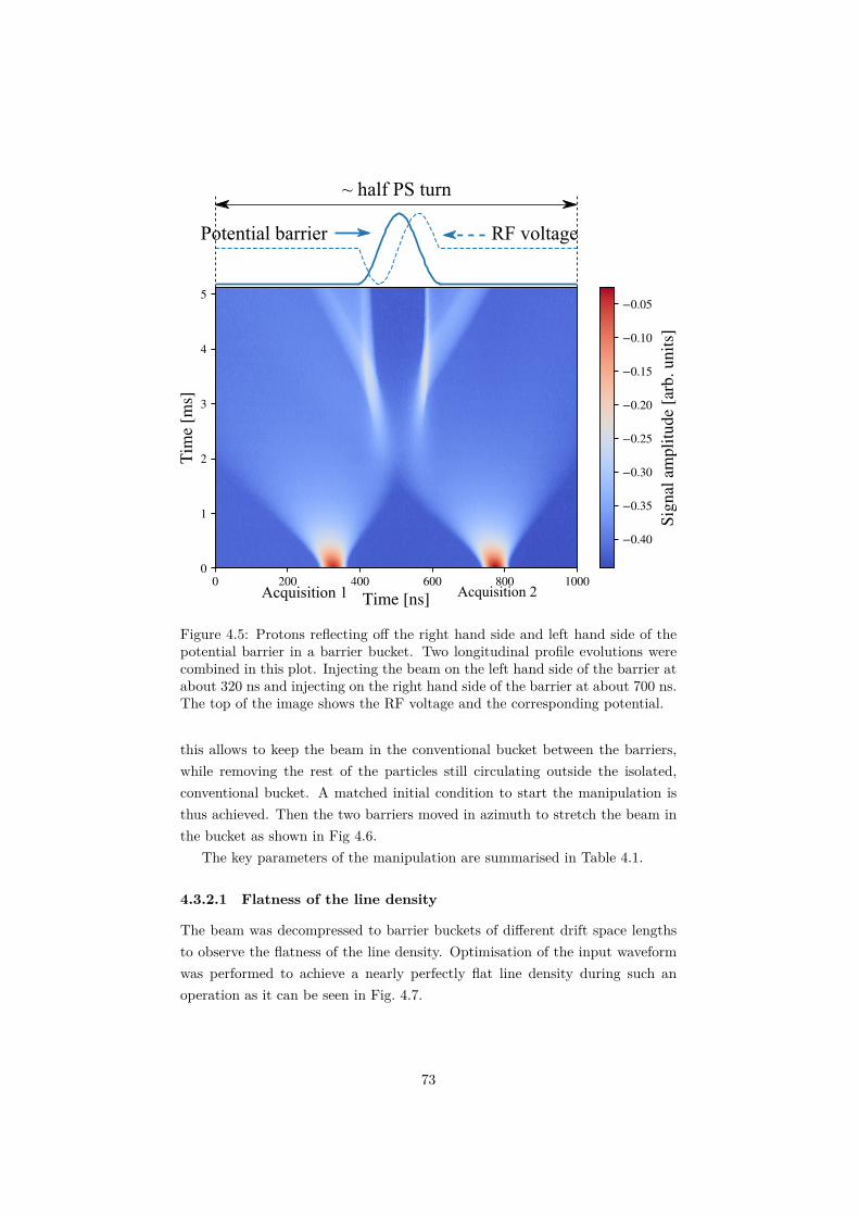
Acquisition 1 Acquisition 2

Figure 4.5: Protons reflecting off the right hand side and left hand side of thepotential barrier in a barrier bucket. Two longitudinal profile evolutions werecombined in this plot. Injecting the beam on the left hand side of the barrier atabout 320 ns and injecting on the right hand side of the barrier at about 700 ns.The top of the image shows the RF voltage and the corresponding potential.

this allows to keep the beam in the conventional bucket between the barriers,while removing the rest of the particles still circulating outside the isolated,conventional bucket. A matched initial condition to start the manipulation isthus achieved. Then the two barriers moved in azimuth to stretch the beam inthe bucket as shown in Fig 4.6.

The key parameters of the manipulation are summarised in Table 4.1.

4.3.2.1 Flatness of the line density

The beam was decompressed to barrier buckets of different drift space lengthsto observe the flatness of the line density. Optimisation of the input waveformwas performed to achieve a nearly perfectly flat line density during such anoperation as it can be seen in Fig. 4.7.

73

Figure 4.6: Illustration of theRF program during a decom-pression and compression op-eration. The blue traces gen-erate a conventional, isolatedbucket. The other traces gen-erate barrier buckets with in-creasing drift space from pur-ple to yellow.

Figure 4.7: Measured longitudinal line density profile evolution of a decompres-sion operation with moving barriers.

4.3.2.2 Simulations

Before moving onto tests to check the effect of different barrier speeds on theprofile evolution, simulations with moving barriers are discussed in order tocompare the results of the measurements with the results of these. Figure 4.6illustrates a voltage program of the simulations.

As in the real tests, the beam was matched to a conventional RF bucketcreated by two barrier RF pulses right next to each other at the beginning ofthe simulations. The initial conditions of this bunch in the isolated bucket werematched using tomography [182] based on measured reference profiles similarlyto the method used in the high energy case, see Fig. 4.17. Then the two,isolated pulses were moved apart to expand the isolated bunch into a bunchin a barrier bucket and compress to a bunch in a conventional bucket again as

74

shown in Fig. 4.6.The main challenge of the simulations using BLonD [129] was to model the

wide-band RF system, as it is outlined in Section 3.5. To compress and expandthe beam, only the phase of the individual harmonic components was linearlyincreased and decreased again. The main accelerator and beam parameters usedin these simulations are summarised in Table 4.1.

Since the intensity of the beam is very low, the beam induced voltage wasneglected in these simulations. The results of these simulations are directlycompared with measurements in the next section.

4.3.2.3 Comparison of measurements with simulations

The result of the estimation performed based on Section 2.3.2 is that the barrierpulse speed should be such that the ratio of the barrier phase velocity to themaximum phase velocity is |φb/φf | � 0.5. The duration of compression andexpansion, tc, was varied in a range of 10ms to 300ms. In all cases the bucketwas stretched to a maximum drift space of 600 ns and compressed back again.Although the upper speed is still well below the optimistically defined limit, itbecame clear during the tests that approaching even a fifth of this value resultsin a significant perturbation of the bunch profile. Similar observations havebeen reported in [45].

In the first tests, the barriers were receding and approaching only, thereforethe total time of the manipulation was 2tc. When tc = 10 ms, corresponding toφb/φf ≈ 0.25, the decompression and compression results in a highly perturbedprofile after the manipulation as it is shown in Fig. 4.8, which shows the bunchlength measured as a Gaussian fit. The barrier bucket part can not be approx-imated this way, thus it was removed from the middle plot. Therefore thesetests are suitable to calculate the perturbation or oscillation of the resultinglongitudinal line density profiles. However, when the speed of the barriers weremuch slower corresponding to about φb/φf ≈ 0.01, the original bunch profilewas restored after the manipulation as it can be seen in Fig. 4.9.

In the subsequent tests a different timing was used aiming to measure thefilamented bunch length at the end of the manipulation rather than the oscilla-tions as in the previously mentioned tests. This means that the total time waskept as long as it was possible in the cycle, and an intermediate filamentationphase in the created barrier bucket was added. The probed barrier speed rangewas kept the same. Figure 4.10 shows the results of a fast, non-adiabatic ma-nipulation, whereas Fig. 4.11 presents an adiabatic manipulation with a slowbarrier movement. It is clear from the simulated and measured profile evolu-tion, that the measurements agree with the simulations to a high degree in all

75

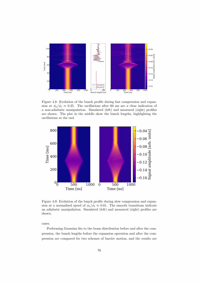
0 200 400 600 800 1000Time [ns]

0

20

40

60

80

100

Tim

e [m

s]

0 500Bunch length [ns]

SimulatedMeasured

0 200 400 600 800 1000Time [ns]

0.16

0.14

0.12

0.10

0.08

0.06

0.04

Sign

al a

mpl

itude

[arb

. uni

ts]

Figure 4.8: Evolution of the bunch profile during fast compression and expan-sion at φb/φf ≈ 0.25. The oscillations after 60 ms are a clear indication ofa non-adiabatic manipulation. Simulated (left) and measured (right) profilesare shown. The plot in the middle show the bunch lengths, highlighting theoscillations at the end.

0 500 1000Time [ns]

0

200

400

600

800

Tim

e [m

s]

0 500 1000Time [ns]

0.16

0.14

0.12

0.10

0.08

0.06

0.04

Sign

al a

mpl

itude

[arb

. uni

ts]

Figure 4.9: Evolution of the bunch profile during slow compression and expan-sion at a normalised speed of φb/φf ≈ 0.01. The smooth transitions indicatean adiabatic manipulation. Simulated (left) and measured (right) profiles areshown.

cases.Performing Gaussian fits to the beam distribution before and after the com-

pression, the bunch lengths before the expansion operation and after the com-pression are compared for two schemes of barrier motion, and the results are

76

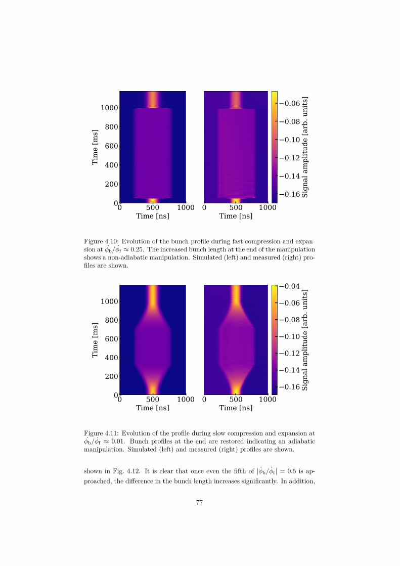
0 500 1000Time [ns]

0

200

400

600

800

1000

Tim

e [m

s]

0 500 1000Time [ns]

0.16

0.14

0.12

0.10

0.08

0.06

Sign

al a

mpl

itude

[arb

. uni

ts]

Figure 4.10: Evolution of the bunch profile during fast compression and expan-sion at φb/φf ≈ 0.25. The increased bunch length at the end of the manipulationshows a non-adiabatic manipulation. Simulated (left) and measured (right) pro-files are shown.

0 500 1000Time [ns]

0

200

400

600

800

1000

Tim

e [m

s]

0 500 1000Time [ns]

0.16

0.14

0.12

0.10

0.08

0.06

0.04

Sign

al a

mpl

itude

[arb

. uni

ts]

Figure 4.11: Evolution of the profile during slow compression and expansion atφb/φf ≈ 0.01. Bunch profiles at the end are restored indicating an adiabaticmanipulation. Simulated (left) and measured (right) profiles are shown.

shown in Fig. 4.12. It is clear that once even the fifth of |φb/φf | = 0.5 is ap-proached, the difference in the bunch length increases significantly. In addition,

77

Figure 4.12: Difference of initial (200 ns) and final bunch length versus compres-sion and expansion. Each marker on the time axis having categorical labels hastwo associated boxes for the two schemes with the marker in the middle, exceptfor 30ms and 50ms. Once the compression speed is near the theoretical limit,the bunches are perturbed after compression resulting in a not well defined orlarge bunch length due to the fast manipulations. Plot uses the same data asFigure 4. in [2] (CC-BY), but the improved speed limit from Chapter 2 is alsoshown.

the data taken for the shorter beam manipulations show that the bunch lengthspread increases for larger barrier speeds as a result of quadrupolar oscillationsof the final bunch. This view of the experimental data in Fig. 4.12 supports theexpected conclusion that approaching the optimistically-defined barrier speedlimit results in a non-adiabatic compression.

78

4.4 Studies at high energy

As outlined in Chapter 1, the aim of the studies is to reduce beam losses for fixedtarget beams at the transfer from the PS to the SPS. The PS injection duringthese studies was at 1.4 GeV kinetic energy and extraction happens at 14 GeV/cmomentum. The barrier bucket RF system can not accelerate the beam with therequired ramp rate, since the maximum voltage it achieves is not sufficient [31].Therefore the main RF system [183, 184] operated at h = 16 is used to reachthe beam momentum of 14 GeV/c. Then, at flat-top, the beam is re-bucketedin a barrier bucket.

Although sufficient for the acceleration of the beam, a single harmonic RFsystem is unsuited to create a barrier bucket required for the beam loss reduc-tion, because it can not generate a wide-band waveform. Hence re-bucketingfrom the main RF system to the barrier bucket system is needed before extrac-tion.

Given these requirements, beam tests at extraction energy were performed [1,2]. A convenient choice to start was to modify the operational acceleration cyclefor the beam for fixed target experiments [185] as summarised in Section 4.4.1.The challenge was to find a way to accommodate the barrier bucket manipula-tion in a highly optimised cycle [16, 21, 22], while keeping the benefits of MTE.Adding a re-bucketing operation from the h = 16 buckets to a barrier bucketat 14 GeV/c momentum near extraction is compatible with the requirements ofthe RF acceleration and handover and the limitations imposed by the maximumduration of the existing cycle.

The description of the re-bucketing from the h = 16 buckets to a barrierbucket is presented in Section 4.4.2 accompanied by simulations and measure-ments with beam. To understand the longitudinal profile modulation due tothe drift of the particles around the barrier, a beam test and simulations witha longer debunching time were also performed in addition to the operational,shorter debunching duration. During this longer operation, the transverse split-ting was disabled.

To observe the efficiency of the barrier bucket operation with the transversesplitting, the latter was activated. The beam was extracted during five turns.Section 4.4.3 compares the longitudinal profiles in the accelerator and the un-folded longitudinal structure in the TT2 transfer line spanning five turns in time.Variation of the longitudinal profiles depending on the intensity of the beam isanalysed in Section 4.4.4. Finally, Section 4.4.5 presents the main achievementof the study, the significant beam loss reduction at extraction.

79

4.4.1 The acceleration cycle for the fixed-target beam inthe PS

As illustrated in Chapter 1, the beam is injected into the PS from rings 3, 4,2 and 1 of the PS Booster (PSB), in this order, with the principal harmonicnumber being h = 2. The injection takes place at 1.4 GeV kinetic energy,upgraded [176, pp. 285–90] to 2 GeV [186, 187] of the accelerators. Since thecircumference of the PS is four times longer than the one of the PSB, the bunch-to-bucket transfer requires an RF capture at h = 8 in the PS. The RF voltageprograms for h = 8 and h = 16, as well as the current programs for the magneticelements involved in the transverse splitting are shown in Figure 4.13 for thewhole acceleration cycle.

Figure 4.13: The current ofthe different magnetic ele-ments taking part in thetransverse splitting, the mag-netic flux density along thecycle and the RF voltagespeaking at 200 kV are shown.Figure taken from [16], Fig-ure 3 (top). CopyrightCERN, 2016 CC-BY licence.

To suppress longitudinal instabilities during the PS cycle, a controlled lon-gitudinal emittance blow-up with a phase-modulated 200 MHz system is per-formed. After accelerating to an intermediate magnetic plateau at 3.5 GeV/c,an additional longitudinal emittance blow-up is applied, to mitigate instabilitieswhen crossing transition.

At the same time a splitting from 8 to 16 bunches is accomplished by chang-ing the main harmonic to h = 16. The beam is then accelerated throughtransition energy to the magnetic flat top at 14 GeV/c momentum. At thispoint the beam is transversely split into four islands and a core. Then a de-bunching process is realised by decreasing the amplitude of the main RF systemat 7.6 MHz (h = 16) down to zero. At the very end of the cycle, just beforeextraction, the 200 MHz system is pulsed for 1 ms to modulate the longitudinalbeam structure and ease the injection capture in the SPS with its main RFsystem at 200 MHz.

The operational cycle was modified for beam the tests to include the han-dover to the barrier bucket RF system [1, 2]. One barrier per waveform wasgenerated to cover the rise time of the extraction kicker. These modificationstake place a the end of the cycle, after the main RF amplitude is dropped

80

from 200 kV to about 12 kV and the transverse splitting to took place. An ex-ception to this was the tests without the transverse splitting. In this case about50 ms time was gained in some of the tests to study the re-bucketing processlonger.

The key beam parameters used in the high energy studies are summarisedin Table 4.2.

Parameter name Symbol ValueRevolution period of the PS T 2.1 µsMomentum p 14 GeV/cIntensity N 4× 1012 ppp – 2.2× 1013 pppAverage beam current Ib 0.3 A – 1.7 ATotal initial longitudinal emittance ε 25 eVsPeak RF voltage V 3− 4 kVLength of the gap in time tgap 150 ns – 300 nsDuration of the manipulation tm ≈ 20 ms

Table 4.2: Parameters used for the high energy simulations and beam tests withone barrier pulse per turn.

4.4.2 Re-bucketing and debunching into a barrier bucket

As described in the previous section, the beam is accelerated to 14 GeV/c usingh = 16 buckets, since the main RF system has sufficient peak amplitude toachieve this opposed to the barrier RF system. Therefore to achieve a gap inthe debunched beam at extraction a re-bucketing from the h = 16 buckets tothe barrier buckets must take place driven by an RF handover from the main,single harmonic RF system to the barrier bucket wide-band system. The detailson how to perform this handover were first tried experimentally at the end ofrun 2 of the LHC operation.

4.4.2.1 RF handover and observations with beam

One barrier waveform generating a gap was programmed per turn by loweringthe amplitude of the main RF system at h = 16 and, at the same time, in-creasing the amplitude of the wide-band system. The voltage program and thecorresponding RF waveform evolution is shown in Figure 4.14 top. During thetests, the azimuthal position of the barrier was varied and the longitudinal pro-file evolution was observed. The symmetry of the profiles at extraction aroundthe gap depend on the azimuthal position of the barrier bucket with respect tothe position of the conventional buckets. If the RF phase corresponding to theunstable fixed point of both buckets is not aligned, the resulting longitudinal

81

Figure 4.14: Total RF voltage evolution during re-bucketing with peak ampli-tudes (top) and waveform (bottom).

profiles become asymmetric around the gap region. Simulations presented laterin this section provide an explanation for this observation.

This observation then defined the relative phase of the barrier RF systemand that of the conventional RF system during the re-bucketing. It can beobserved in Fig. 4.14 that the zero crossing and the sign of the slope of the halfpulses generating a conventional and a barrier bucket are the same resulting inthe alignment of the unstable fixed points of the buckets.

Using an aligned RF program, profile evolution that is symmetrical aroundthe gap was observed see Fig. 4.15.

Apart from the positioning of the gap with respect to the bunches, RF wave-form imperfections can cause uneven profiles at extraction, too. A few numberof tests were performed to investigate the effects of RF waveform distortions.

82

Figure 4.15: Re-bucketing into a barrier bucket at total beam intensity of1.87 × 1013 ppp.

83

4.4.2.2 RF waveform imperfections and drift

Inverted and distorted barrier waveforms were generated to trap the beam insub-buckets near the gap region. Figure 4.16 shows three measurements withdifferent RF waveforms. Fig. 4.16 (left) illustrates the measured longitudinal

2000 2500Time [ns]

0

10

20

30

40

50

Tim

e [m

s]

2000 2500Time [ns]

2000 2500Time [ns]

0.2

0.0

0.2

0.4

0.6

0.8

Sign

al a

mpl

itude

[arb

. uni

ts]

Figure 4.16: Comparison of line-density modulations during the handover fromthe conventional to the barrier bucket RF system. Left: re-bucketing to anisolated bucket. Centre: modulation due to drift of particles. Right: modulationdue to both potential-well distortion and particle drift.

profile evolution corresponding to an isolated bucket made by an inverted bar-rier bucket waveform. The merging of two bunches can be observed from 20 ms.The measurement in the centre plot highlights the reflection around the gapregion with a conventional barrier RF waveform as reported earlier in this sec-tion. During the measurement shown in the right figure, an inverted RF pulseright next to the barrier generating the pulse was made. This plot shows bothphenomenon on two sides of the gap. The bunching can be observed on theleft-hand-side of the gap, where the sub-bucket was made by generating an RFripple. On the right-hand-side of the gap, the longitudinal profile evolutionconsistent with particles reflecting off the potential barrier can be seen.

84

4.4.2.3 Simulations

To analyse the bunch distribution at extraction, numerical simulations withthe longitudinal tracking code BLonD [129] have been performed. Appendix Bcontains further details on the simulation framework and the code developedfor the barrier bucket simulations.

4.4.2.4 Matching of the initial conditions

Most tests were performed with the time frame corresponding to the voltageevolution shown in Fig. 4.14. Hence the same RF program was used in theinitial simulations.

Apart from the RF voltage, the distributions were also matched. The parti-cle distribution in the longitudinal phase space and its corresponding emittanceduring acceleration can be reconstructed based on a set of bunch profiles us-ing tomography [182]. To observe the fundamental beam dynamics during re-bucketing, a matching of the measured distribution based on a parabolic beamdistribution was performed. Although a more sophisticated method exists [188],this simple approximation was sufficient to simulate the fundamental behaviourof the beam without intensity effects.

A set of longitudinal profile evolutions having different emittances were gen-erated using BLonD. The reference profiles were available at the end of theintermediate flat top, hence the RF parameters were matched to those earlierin the cycle. These profiles were exported from the simulation and the same to-mography algorithm was run on them as on the measured profiles. Figure 4.18illustrates the reconstructed profiles from simulations and the reconstructionfrom the measurements see Fig. 4.17. The emittance corresponding to the low-est error in the RMS emittance, the 90% emittance, the matched area and dp/p

was chosen. Approximately 1% agreement was achieved for all four parameters.A minor longitudinal blow-up, 10% was added, since levels below this can

be expected from the moment of the emittance measurement, around C350 inthe cycle, and the start of the re-bucketing process to the barrier bucket aroundC800. This is because the reference profiles were only available after transitioncrossing at the end of the intermediate flat top, but before the acceleration inthe h = 16 buckets.

85

Figure 4.17: Tomographic reconstruction of the longitudinal phase space basedon measured data. The reference profiles were available at the end of the inter-mediate flat top.

86

Figure 4.18: Tomographic reconstruction of the simulated longitudinal phasespace matching the parameters of Fig. 4.17.

87

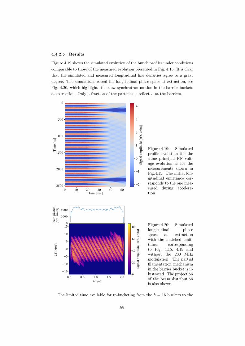
4.4.2.5 Results

Figure 4.19 shows the simulated evolution of the bunch profiles under conditionscomparable to those of the measured evolution presented in Fig. 4.15. It is clearthat the simulated and measured longitudinal line densities agree to a greatdegree. The simulations reveal the longitudinal phase space at extraction, seeFig. 4.20, which highlights the slow synchrotron motion in the barrier bucketsat extraction. Only a fraction of the particles is reflected at the barriers.

0

1000

500

1500

2000

2500

Tim

e [n

s]

Sig

nal a

mpl

itude

[ar

b. u

nits

]

Time [ms]10 20 30 40 500

4

3

2

1

0

−1

−2

Figure 4.19: Simulatedprofile evolution for thesame principal RF volt-age evolution as for themeasurements shown inFig.4.15. The initial lon-gitudinal emittance cor-responds to the one mea-sured during accelera-tion.

Figure 4.20: Simulatedlongitudinal phasespace at extractionwith the matched emit-tance correspondingto Fig. 4.15, 4.19 andwithout the 200 MHzmodulation. The partialfilamentation mechanismin the barrier bucket is il-lustrated. The projectionof the beam distributionis also shown.

The limited time available for re-bucketing from the h = 16 buckets to the

88

barrier bucket, combined with the low synchrotron frequency, means that thereis no time for the beam to filament into the barrier bucket. Since the duration ofa reflection at the barrier is significantly shorter than the drift time in betweenthe barriers, more particles are accumulated at the barriers near the reflectionregion. This results in the formation of shoulders on the bunch profile, i.e.regions with larger line density close to the barriers. This was also confirmedby simulations, which are in good agreement with the measured data [1].

4.4.2.6 Debunching on a longer time scale

The slow drift of particles between the barriers being the reason for the for-mation of shoulders near the gaps on a shorter time scale is also supported bymeasurements taken on a longer time scale. Here the longitudinal profile evo-lution corresponding to the drift of the particles can be observed. In order togain time for these measurements, the nominal MTE cycle was modified not toinclude the transverse splitting. This made advancing the re-bucketing possi-ble, see Fig. 4.21 (right). Simulations on a longer time scale were performed

0 500 1000Time [ns]

0

20

40

60

80

100

120

140

Tim

e [m

s]

500 1000Time [ns]

0.2

0.0

0.2

0.4

0.6

0.8

Sign

al a

mpl

itude

[arb

. uni

ts]

Figure 4.21: Beam reflecting off a potential barrier, shown over half a PS turn.The amplitude of the h = 16 system was lowered and then subsequently turnedoff at 70 ms and the amplitude of the barrier bucket RF system was increasedto reach the maximum at the same time. The transverse beam splitting wasdisabled during these measurements. Simulated (left) and measured (right)profiles are shown.

to confirm the slow filamentation process compared to the time of the beammanipulation in barrier buckets at extraction. Figure 4.21 (left) shows the sim-

89

ulated longitudinal profile evolution on the same time scale as the measureddata.

No more than 80 ms in total were available in the experimental cycle toobserve a full filamentation in the barrier bucket. However, simulations on aneven longer time scale were performed to confirm the slow speed of the fila-mentation in the barrier buckets made at extraction. Figure 4.22 (right) shows

Figure 4.22: Oscillations in barrier buckets with a pulse duration of 300 ns.Beam profile evolution (right) and corresponding 90% area emittance (left).Peaks in 90% emittance correspond to shoulder forming in the barrier bucket.

three consecutive turns logged in one acquisition. This acquisition was repeatedduring the simulation and at the same time the corresponding 90% most densearea occupied by the particles (left figure) was calculated as a measure of thelongitudinal emittance. The corresponding area in phase space occupied bythe beam increases only slowly. This provides further evidence that during thetime of the manipulation there is no significant macroscopic emittance growth,this only happens on a longer time scale. However, tests with beam are stillrequired to confirm this result of the simulation at extraction energy given theunusual initial conditions of the re-bucketing process. The emittance in thiscase is measured with a numerical area calculation routine.

90

4.4.3 Beam in the PS and in the transfer line

As explained in Chapter 1, the extraction of the beam from the PS happensduring five turns, each turn extracting a beamlet of the length of the acceleratorcircumference. The first four turns are extracting the islands of the distributionusing kickers KFA31 and KFA21 with a correction from KFA9. The rise timeof these kickers is 350 ns and their pulse is 10.5 µs long. The core is extractedwith KFA4, KFA71 and KFA79, which have a much faster rise time of 56 ns,but can not sustain the pulse longer than one PS turn [138].

4.4.3.1 Longitudinal profiles in the transfer line

In order to investigate the beam removed by the kickers in the longitudinalstructure and compare it with the gap made by the barrier, the longitudinalprofiles recorded with the WCM, e.g. Fig. 4.15, and the WBP, e.g. Fig. 4.23,were compared.

During the joint beam tests in PS and SPS, the synchronisation of the po-sition of the gap made by the barrier with the rise of the PS extraction andSPS injection kickers was not yet possible for technical reasons. A scheme forsynchronising the phase of the barriers with the kicker rise times is proposed inChapter 5. This means that the trigger of the PS extraction and SPS injectionkickers, which are fixed with respect to each other in time, and the gap made bythe barrier was fluctuating randomly from cycle to cycle. Examples of the mea-sured longitudinal beam profiles in the transfer line for three different scenariosare shown in Fig. 4.23.

A typical longitudinal beam profile without barrier bucket is shown in thetop plot. Two features are worth mentioning. Firstly, the increased line densityfluctuations during the first four extracted turns and, secondly, a short longitu-dinal gap corresponding to the rise time of the kickers used to extract the firstisland and at the end of the profile, the central beamlet during the fifth turn.A profile corresponding to the barrier bucket position being asynchronous withthe rise of the extraction kickers is visible in the middle plot. The gap regionof the barrier bucket can be seen in the unfolded beam structure. In this case,five additional gaps are added for the longitudinal beam profile. Their positionvaries within the time corresponding to a single PS turn at the momentum of14 GeV/c, i.e. 2.1 µs, as the transfer trigger jitters with respect to the gap posi-tion due to the lack of synchronisation. The bottom plot shows a case when thebarrier bucket is approximately synchronous with the kicker rise times, whichoccurred only accidentally during these measurements.

91

0 2 4 6 8 10Time [ s]

0

1

2

3

0

1

2

3

0

1

2

3

Sign

al a

mpl

itude

[arb

. uni

ts]

Figure 4.23: Examples of the longitudinal beam structure measured in the trans-fer line without barrier bucket (top), with barrier bucket asynchronous with therise of the PS extraction kicker (middle) and with barrier bucket synchronouswith the rise of the PS extraction kickers (bottom). The 200 MHz modulationis clearly visible in all cases.

4.4.3.2 Longitudinal profiles in the PS and in the transfer line

Comparing the line density measured in the TT2 transfer line and in the PSring indicates parts of the beam lost due to kicker rise times. In the case of anideal, loss-less extraction, it is expected that the longitudinal line density signalmeasured in the transfer line, during the five turns of extraction, is identicalto the longitudinal line density profile before extraction. Clearly, the totallongitudinal beam distribution is ideally the same before and after extraction.To demonstrate this, the following analysis using [189–194] and code developedfor this study was performed.

As both instruments, the WBP and the WCM are operated at differentsampling rates, have different bandwidths and their triggers were also different,the acquired profiles from the two instruments were pre-processed. The WCM

92

106 107 108100

50

0M

agni

tude

[dB

]

106 107 108

Frequency [Hz]

10

5

0

Phas

e [r

ad]

Figure 4.24: Single pass re-sponse of the low-pass filter.The forward-backward filter-ing technique squares the fre-quency response and cancelsthe phase response.

signal has high lower cut-off frequency, meaning that the comparison with theWBP is usable only when the barrier bucket is present. Furthermore, the WCMand the WBP have different amplitude scaling and DC offsets. Therefore, nor-malisation of the longitudinal line density and the current were also performed.Simply scaling by the minimums and maximums is more sensitive to outliersthan the proposed method. A different normalisation was chosen based on thebasic statistical properties of the signals. The steps of the analysis are detailedbelow.

The measured voltage from the WBP was downsampled using polyphase de-composition [195, pp. 179–184], [196] in combination with an anti-aliasing filterto match the sampling rate of the WCM without noticeable artefacts. Sincethe high frequency components of the signal are not responsible for the fluc-tuations in the longitudinal line density of the beam removed by the kickers,an additional low-pass filter was applied to remove, in particular, the 200 MHzcomponent. The response of a single pass of the filter is shown in Fig. 4.24.The filter was applied forward-backward, which squares frequency response andcancels the phase response [197]. Since the signal to be filtered has potentiallylarge swings at the beginning and at the ends of the intervals, the initial con-ditions for the filter were chosen using Gustaffson’s method [198, 199]. As aresult, filter artefacts related to the transient response of the filter around theseregions are minimised.

The resampled WBP signal was then sliced up into five segments of equallengths in time, corresponding to one PS turn each. The falling edge of theinstantaneous beam current at the tail of the batch was chosen as a referenceposition for the slicing. The slices were then summed giving a sequence ofsamples corresponding to one PS turn.

It is assumed that the WCM, x, and WBP, y, signals are generated bylargely the same beam, but measured by the two different devices. Hence thevariance, the estimate of the normalised power of the signal [195, p. 816] in theoverlapping bandwidth, is the same apart from a constant scaling factor. The

93

mean value, 〈x〉 differs only by a constant offset. The following normalisation

x[n] =x[n]− 〈x〉√

1N

∑Ni=1(x[i]− 〈x〉)2

(4.1)

cancels the DC offsets and the differences of the amplitude scaling at the sametime for the signal of length N . To align x and y in time, the sample offset of themaximum of their cross-correlation sequence [200], [195, p. 815] was used. Thenon-overlapping parts were padded with zeros. The m-th term of the sequenceis:

Rxy[m] =1

N

N∑n=1

x[n+m]y[n] . (4.2)

It follows from the property of the cross-correlation sequence [195, p. 818], that

|Rxy| ≤ Rxx[0] = Ryy[0] = 1 , (4.3)

where the normalisation was performed according to Eq. 4.1. Figure 4.25 il-lustrates the normalised cross correlation sequence for a pair of acquisitions.

0 1000 2000 3000 4000Samples

0.0

0.5

1.0

Rxy

Figure 4.25: The cross-correlation sequence of thesignals compared in Fig. 4.26,with the maximum at 0.97for this example.

In the ideal case when the signals are identical, the maximum of their nor-malised cross-correlation sequence is equal to 1, which is the starting value oftheir normalised autocorrelation sequence. Otherwise, max

{Rxy

}falls in the

[−1, 1) interval, with a positive value signalling some degree of similarity.Figure 4.26 shows an example comparison between x and y. As expected, the

match between the normalised WCM and the normalised and summed 5-turnsignal of the WBP is nearly perfect.

There is a small, but relevant difference between these profiles during thefirst few tens of nanoseconds. This short longitudinal gap can be attributedto the rise time of the kickers required to extract the beam from the PS. Thedifference is systematically present in all the summed profiles when comparedto the WCM acquisition before extraction. It only disappears when the barrierbucket position is synchronised with the kicker rise time as it coincides with the

94

Figure 4.26: The summed profiles from the WBP in the TT2 transfer line com-pared with the WCM trace before extraction aligned according to the maximumof Rxy.

gap position (Fig. 4.23, bottom). Hence, the deviation between the traces ofFig. 4.26 during the first few hundred nanoseconds demonstrates a difference inthe line density attributed to the kickers.

Figure 4.27 summarises how well the sums of five-turn acquisitions correlatewith the last-turn PS profile, taking into account in total 234 measurementsfrom the PS with different gap size settings. The higher correlation scores forlarger barrier bucket gap are due to the better signal-to-noise ratio. The lower,but still positive, correlations with small gap sizes are due to the higher relativenoise in the profiles when the gaps made by the barrier bucket system are narrow.Although the high lower cut-off frequency of the WCM means that it can notmeasure DC levels of a coasting beam line density, an attempt of comparingthe WCM and WBP signals without barriers was made. This is possible bydetecting similarities outside the kicker gap regions in the longitudinal profiles,for example based on the residual h = 16 structure that both signals still contain.The downside is that the noise is higher once the profile comparison is restrictedto these regions. Therefore, the result is a wide variation from a low, but stillpositive correlation to a relatively high correlation as illustrated by Fig. 4.27with a zero gap setting.

It is clear from the systematic analysis that the beam structure before andafter extraction when the barrier is present essentially only differs in a relativelysmall detail. This underlines that the beam loss mitigation can be adequately

95

Figure 4.27: The maximums of the cross-correlation sequences of the last ac-quisitions before extraction from the PS and the summed five-turn profiles nor-malised to the same power. Each thin, horizontal line represents a pair ofacquisitions. The length of the horizontal line shows the relative frequency ofthe values falling in the corresponding bin [194].

addressed by the barrier bucket system once it is synchronised with the extrac-tion kickers. A sufficiently large gap can be made to leave time for the field ofthe kickers to rise.

4.4.4 Intensity dependent effects

The measured variation of the line density at the edge of the drift space decreaseswith increasing intensity. The difference of a profile calculated using local ellip-tic [201] beam distribution and a measured profile can be seen in Fig. 4.28. As

0 500 1000 1500 2000Samples

0.0

0.5

1.0

1.5

Nor

mal

ised

am

plitu

de[a

rb. u

nits

]

Measured profileScaled, ideal profilefor shoulder detection

Figure 4.28: The measuredand profiles calculated fromlocal elliptical beam distri-bution scaled for shoulderheight detection.

the intensity increases, the measured line density gets closer to the calculated.

96

In order to confirm this observation systematically, the acquisitions during theintensity scan were analysed.

The measured profiles were low-pass filtered to remove the 200 MHz compo-nent as described in Section 4.4.3 using the same filter, see Fig. 4.24. In orderto establish the position of the gaps, calculated profiles were cross-correlatedwith the measured profiles.

A correction for the DC level based on the mean of the signal as in Sec-tion 4.4.3. It was not necessary to normalise for the power of the rest of thespectral components in this case, because the signal amplitude of the calculatedand measured profiles were in the same range, hence the correlation producesaccurate results. Figure 4.29 shows an example of the result.

Since one gap per PS turn was made, the criterion for successful gap de-tection was that the single, isolated maximums, see Fig. 4.29, of the cross-

Trev Trev Trev Trev

Figure 4.29: The cross-correlation sequence of themeasured and calculatedprofiles with the detectedpeaks.

correlation sequence corresponding to the gaps are one revolution period apartwith a ± 1% error corresponding to the uncertainty of the peak detection. Theminimums of Fig. 4.29 represent the shoulders that are in anti-phase with thegaps. The reliability of the detection was improved by using a series of ideal pro-files spanning three turns not just a single one. This value was established basedon practical considerations of the calculation, representing a trade-off betweenaccuracy and running time. The full cross correlation series spans almost 5 PSturns in time, because the original data was spanning almost two PS turns, con-taining two gaps, plus the calculated profiles were three turns long. Establishingthe position of the gaps made it possible to align the profiles automatically.

Once the azimuthal position of the gaps were known, the height of the peaksof the longitudinal profiles near the gap region could be established by comparingthe flat region of the profiles with the peaks around the gaps as illustrated byFig. 4.28. Technically, the profiles were normalised such that the height of theline density between the gaps in the middle and the minimum of the line densityis equal to one, see Fig. 4.28 for an example. This way, the middle point betweenthe gaps, the mean of the centre of the profiles calculated for 200 ns, becomes

97

Figure 4.30: Comparison of the low-pass filtered, normalised longitudinal linedensity profiles at extraction at the same time in the re-bucketing process foracquisitions with 180 ns gap size setting. The effect of the beam intensity canbe seen.

the reference for the height of the shoulders. This is a reasonable referencesince, as already said in Section 4.4.2, the particles that reflect off the barriers,can not reach the middle of the barrier during the manipulation. Therefore bymeasuring the height of the excess peak, the deviation of the low-pass-filteredprofiles from the calculated can be compared.

Figure 4.30 shows all the traces acquired by the WCM at extraction duringdifferent cycles for the case of 180 ns gap setting, ordered by beam intensity.The traces were sorted into three intensity categories based on the number ofavailable measurements: the beam intensity is less than 6 × 1012 ppp in thebottom plot, greater or equal than 6 × 1012 ppp and less than 1.6 × 1013 ppp inthe middle plot and greater or equal than 1.6 × 1013 ppp in the top plot. Thecolour of the traces is mapped to the intensity scale on the right of the figure.

98

Figure 4.31: Normalised line density change along the bunch, showing a de-creasing trend towards improved flatness of the bunch with increasing intensity.The colours refer to the different gap duration settings as indicated in the leg-end. Independent of the gap duration, the line density change improves withincreasing intensity. 63 and 76 acquisitions for 180 ns and 250 ns are shown.The least-squares linear fits are displayed to highlight the downward trend.

Firstly, the observation is clear that longitudinal line density gets flatter asthe intensity increases.

Secondly, the asymmetry around the generated gap increases as the intensityincreases. Comparing the left-hand-side and right-hand-side of the gap regionsof the middle and top plots shows greater asymmetry than the same features inthe bottom plot. The observations seem to indicate that the asymmetry aroundthe gap: a sharper peak on the right-hand-side of the gap compared to theleft-hand-side is preserved as the intensity increases.

When extending the analysis to the longitudinal profiles corresponding toa 250 ns gap setting, too, the observations indicate that as the intensity increasesthe profiles become flatter irrespective of the size of the gap. Figure 4.31 showsthe peak value of the line density profiles around the gap with respect to thereference in the middle of the profiles. The normalisation described earlier inthis section means that the middle of the profiles correspond to the value 1,meaning that an ideal profile without an increase in the line density around thegap would have a line density peak of 1. Larger than 1 values indicate thatthe line density around the gap is higher than the ideal, filamented profile’s linedensity. The clear downward trend shows that the line density profiles nearextraction get flatter as the intensity increases.

99

4.4.4.1 200 MHz modulation and flatness

The analysis was performed with several low pass filter settings with a cut-offset at 20 MHz–500 MHz to establish the robustness of the cross-correlationtechnique. When a low pass filter is used, the results are very similar to the onereported in the previous section largely independent of the cut-off frequency ofthe low pass filter.

Although the results without filter also support the same trend as the filteredprofiles, an additional effect of the short, 200 MHz modulation can be seen inthis case. Figure 4.32 shows that the trend is still visible with the high frequency

Figure 4.32: The results of the analysis without low-pass filtering. The detectionroutine is less efficient at the highest intensities in this case and there is anoverall increase in the line density peak when the 200 MHz system is activewith the 180 ns gap setting.

noise not filtered. However, a difference in the overall offset is clearly visible.This is because almost all of the 180 ns profiles were acquired with the 200 MHzsystem activated. Unfortunately, the detection was not successful for more ofthe high intensity profiles with 180 ns due to high noise content without theapplication of a low-pass filter.

As mentioned before, the reference level, corresponding to the line densitypeak value 1 in Fig. 4.32, is taken in the opposite azimuthal position comparedto the position of the gap as an average calculated for 200 ns of the longitudinalprofile. Therefore the reason for the offset in the trend of the 180 ns, 200 MHzmodulated profiles is that the averaging provides the same reference value as in

100

the previous analysis, but the line density peak is calculated as the maximumof the line density in the detected gap region without smoothing.

Therefore, as it is clear from Fig. 4.32, the 200 MHz modulation adds anoverall offset and changes slope of the trendline with the 180 ns setting comparedto its low-pass filtered counterpart in Fig. 4.31. However, the limited amountof data available seems to indicate that the 200 MHz modulation does notchange the overall trend of improving flatness with increasing intensity, whichis expected because of the short duration of the manipulation.

4.4.4.2 Effects of cavity impedances

In order to investigate intensity effects, particle tracking simulations includingcavity longitudinal impedance models [202] were performed. Table 4.3 lists ofall the RF cavities and their gap status after the re-bucketing has taken place.

Cavity Number installed Gap status after re-bucketingFinemet® 1 Open10 MHz 11 Closed20 MHz 2 Closed40 MHz 2 Open80 MHz 4 Open200 MHz 6 Open during last 1 ms, only.

Table 4.3: RF cavities installed in the PS ring and the status of their gaps afterthe re-bucketing into the barrier bucket took place.

The beam spectrum overlaps with the Finemet® cavity band, therefore themost beam loading is expected in the frequency range of this cavity. Thisexpectation is confirmed with simulations. The parameters used were the sameas detailed at the beginning of Section 4.4. The longitudinal impedance of thecavities with their gaps open were included in the simulations. Figure 4.4.4.2shows the simulated effective RF waveforms changing with beam intensity. Thedistortion of the profiles near the peak of the pulses is visible as the intensityincreases.

In order to evaluate the relative contributions of the different cavities, thetotal voltage for different configurations of cavities was calculated: VALL repre-sents all open gap cavities; VFC denotes the total voltage with only the Finemet®

cavity included; VPROG is the ideal, programmed voltage without any inten-sity effects. Then simulations with these configurations were performed usingBLonD. The difference VALL−VFC represents the additional voltage contributionoriginating in the 40 MHz and 80 MHz cavities. The difference VALL − VPROG

is the induced voltage contribution of all the cavities, including the Finemet®

cavity. Figure 4.4.4.2 compares these voltage differences. As expected, there is

101

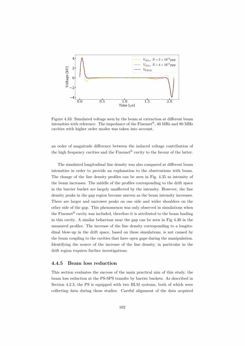
0.0 0.5 1.0 1.5 2.0Time [µs]

4

2

0

2

4

Volta

ge [k

V]

VALL, N= 2× 1013ppp

VALL, N= 4× 1012ppp

VPROG

Figure 4.33: Simulated voltage seen by the beam at extraction at different beamintensities with reference. The impedance of the Finemet®, 40 MHz and 80 MHzcavities with higher order modes was taken into account.

an order of magnitude difference between the induced voltage contribution ofthe high frequency cavities and the Finemet® cavity to the favour of the latter.

The simulated longitudinal line density was also compared at different beamintensities in order to provide an explanation to the observations with beam.The change of the line density profiles can be seen in Fig. 4.35 as intensity ofthe beam increases. The middle of the profiles corresponding to the drift spacein the barrier bucket are largely unaffected by the intensity. However, the linedensity peaks in the gap region become uneven as the beam intensity increases.There are larger and narrower peaks on one side and wider shoulders on theother side of the gap. This phenomenon was only observed in simulations whenthe Finemet® cavity was included, therefore it is attributed to the beam loadingin this cavity. A similar behaviour near the gap can be seen in Fig 4.30 in themeasured profiles. The increase of the line density corresponding to a longitu-dinal blow-up in the drift space, based on these simulations, is not caused bythe beam coupling to the cavities that have open gaps during the manipulation.Identifying the source of the increase of the line density, in particular in thedrift region requires further investigations.

4.4.5 Beam loss reduction

This section evaluates the success of the main practical aim of this study, thebeam loss reduction at the PS-SPS transfer by barrier buckets. As described inSection 4.2.3, the PS is equipped with two BLM systems, both of which werecollecting data during these studies. Careful alignment of the data acquired

102

0.0 0.5 1.0 1.5 2.0Time [µs]

100

50

0

50

100Vo

ltage

diff

eren

ce[s

calin

g: s

ee le

gend

]

VALL − VFC, N= 2× 1013 ppp, [V]

VALL − VFC, N= 4× 1012 ppp, [V]

VALL − VPROG, N= 2× 1013 ppp, [10 V]

VALL − VPROG, N= 4× 1012 ppp, [10 V]

Figure 4.34: The relative contributions to beam loading at the lowest andhighest beam intensities of the different cavities. The voltage induced inthe Finemet® cavity is an order of magnitude more than voltage induced inthe 40 MHz and 80 MHz cavities.

0.0 0.5 1.0 1.5 2.0Time [µs]

0

1

2

Mac

ropa

rtic

les

per

bin ×

103

N= 2× 1013 pppN= 4× 1012 pppNo intensity effects

Figure 4.35: Simulated effect of beam loading in the Finemet® cavity on theprofiles at extraction with different beam intensities and without intensity effectsat a 180 ns gap setting.

103

1.48 1.87 2.20Intensity [1013 ppp]

2

4

6

8

10

12

14E

xtra

ctio

n be

am lo

ss[a

rb. u

nits

]barrier OFFbarrier ON

1.48 1.87 2.20Intensity [1013 ppp]

2468

10121416

Rad

iatio

n do

se[m

Gy/

s]

barrier OFFbarrier ON

Figure 4.36: The measurements with the old (left) and new (right) BLM systemsshow the effectiveness of the barrier bucket system in reducing the losses acrossall intensities, which is obvious by comparing the orange box and whiskersindicating much higher losses with the barrier off to the purple ones indicatingmuch lower losses when the barrier bucket system was operational.

by the BLM and WCM systems made the comparison of beam losses with andwithout the barrier buckets possible. The results of the subsequent analysis arepresented below.

4.4.5.1 Reduction of losses

The following section assesses the magnitude of the beam loss reduction providedby the new scheme. The integrated radiation dose along the cycle reported byall the new BLMs were summed and compared when the barrier bucket systemwas operational and when switched off. The losses at the moment of extractionas provided by the old BLM system were also summed for all detectors andcompared with respect to the new RF system being active or not. The twodifferent BLM systems provide conclusive evidence on the effectiveness of thebeam loss reduction provided by the new barrier bucket RF. All cases with thebarrier on, irrespective of the size of the gap, were lumped together in Fig. 4.36.Both the left and right plots in Fig. 4.36 indicate a beam loss reduction acrossall gap sizes and intensities when the barrier bucket system is operational. Thebarrier bucket scheme effectively reduces losses at extraction.

The difference in the spread of the measurements across the two plots ofFig. 4.36 with the barrier bucket system operational is the result of varyingbeam loss reduction with different sized gaps. Shorter gaps were also triedwith 1.87 × 1013 ppp beam intensity, but not with other intensities, hence thewhiskers are consistently longer in these cases representing a larger spread ofbeam loss corresponding to a larger range of gap settings. This is presented indetail in the next subsection. The small spread with the highest, 2.20 × 1013 ppp

104

0 5 10 15 20 25 30 35 40 45 50 55 60 65 70 75 80 85 90 95BLM location

10-2

10-1

100

101

Rad

iatio

n do

se [m

Gy/

s] barrier OFFbarrier ON, gap size = 150 nsbarrier ON, gap size = 300 ns

1415161718

dummy

Figure 4.37: An example logarithmic plot of the losses as the function of thelocation in the PS ring with different gap sizes. Left: the total beam loss as afunction of location along the PS ring. Right: zoom of the BLM readings inthe extraction region. Plot shows the same data as [1] Fig. 9 using differentcolours and aspect ratios. The intensity corresponding to these measurementsis 1870 × 1010 ppp.

intensity of the control measurement, when the barrier is off, is because of thelow number of data points available. Furthermore, measurement data was notavailable for the new system from straight sections 83-90 for technical reasons.This is also seen in Fig. 4.37. The losses in this section add to the extractionloss shown in the left figure, but are missing from the radiation dose reported bythe right figure. Nevertheless, these details do not alter the overall conclusion,that the new barrier bucket system is highly effective in reducing the losses inthe fixed target cycle.

4.4.5.2 Dependence of the losses on the gap size

The distribution of the integrated radiation dose during the cycle along thewhole PS circumference is illustrated with three examples in Fig. 4.37 (left)together with a zoom (right) of the extraction region. The measurement datashown as a logarithmic plot by Fig. 4.37 was acquired by the new BLM system.The more than an order of magnitude loss reduction is visible in straight section15 with a 300 ns long gap. Even a shorter gap reduces the losses significantlythroughout the extraction region. The more particles are displaced by the widerbarrier in the septum region, the lower the losses, as expected. In practice,wider than 300 ns gaps are becoming difficult to reach with the required qualitywith the hardware as mentioned in Chapter 3 due to bandwidth limitations.Making a much wider gap would not serve a practical purpose, either, sinceeven the slowest kickers involved in MTE have a 360 ns rise time as explainedin Section 4.4.3.

105

0 250 0 120 150 200 250 300 0 250Barrier gap length, tg [ns]

0

2

4

6

8

10

12

14

Rad

iatio

n do

se in

the

extr

actio

n re

gion

[mG

y/s]

barrier OFF barrier ON

1.48×1013 ppp 1.87×1013 ppp 2.20×1013 ppp

Figure 4.38: Integrated beam loss in the extraction region with three intensities,indicated on the top of the plot. The losses decrease as the gap size increases.Figure re-plotted from [1] Fig. 10 using different colours.

Barriers with various gap sizes were generated at different beam intensitiesas part of the studies. Figure 4.38 summarises the low, medium and high in-tensity measurements with varying gap sizes in the left, middle and right plots,respectively. In all three cases the losses in the extraction region decrease withincreasing gap size as the barrier bucket covers a bigger fraction of the kickerrise times. This demonstrates that the barrier bucket system is capable of sig-nificant beam loss reduction when extracting fixed target beams from the PSusing MTE.

106

4.5 Summary

Following the essential commissioning of the basic features of the new firmwaredeveloped to generate barrier buckets with beam, barrier buckets with flat linedensities were produced from matched initial conditions. Progressing with morecomplex tests, barriers moving in azimuth confirmed the theoretically predictedbehaviour of the beam in decompressed and compressed buckets.

The conditions for the re-bucketing at flat top from h = 16 conventionalbuckets to a barrier bucket were studied with beam and analysed using particletracking simulations. These studies highlight that during the time available inthe cycle only partial filamentation in the barrier bucket can take place. For thisreason, to achieve a quasi-symmetrical longitudinal distribution at extractionfrom the PS, the gaps generated by the barriers have to be aligned with thegaps already existing before debunching between the conventional h = 16 RFbuckets.

Application of the cross-correlation sequence of the longitudinal profiles ac-quired in the transfer line and the ones acquired in the PS also confirms thatthe 5-turn-length profiles, when added together, after the multi-turn extractionand the one-turn-length profiles before extraction are very similar. This wasexpected, but never explicitly shown before. However, a relevant and system-atic difference in the line density of these profiles also confirm that the lossesoccurring at extraction are consistent with the extraction kicker rise times.

Using an adaptive barrier detection algorithm based on the cross-correlationof calculated and measured profiles show that as the intensity increases theflatness of the profiles also increases. A measure of the flatness was also de-veloped. Comparing the profiles with varying intensity lead to the conclusionthat the improvement of the longitudinal line density at larger beam intensitiesis likely to be independent of the size of the gap. The measured longitudinalline density profiles show an asymmetry around the gap region with increasingintensity. BLonD particle tracking simulations performed with the longitudi-nal impedance models of the Finemet®, 40 MHz and 80 MHz cavities identifybeam loading from the Finemet® cavity as a likely source for the asymmetry ofthe profiles. The reason behind the flatness of the profiles at high intensity issubject of further studies.

Analysis of the carefully merged datasets acquired by the BLM and WCMsystems allowed to assess the beam loss reduction attributed to the new barrierbucket system. Data from the old and new BLM systems was analysed focusingon the total integrated loss along the whole ring and in the extraction region.The clear conclusion can be drawn that the barrier bucket system reduces thebeam loss up to an order of magnitude in the extraction region. Scans with

107

different sized gaps demonstrate that the longer the gap, the lower the losses.When the system was operated with a gap setting of 300 ns, a practically loss-free extraction from the PS was achieved.

In order to benefit from this scheme, a synchronisation between the SPSinjection and the PS extraction processes has to be taken place. The nextChapter presents a proposal for this.

108

Chapter 5

A concept ofsynchronisation for barrierbuckets

As explained in detail in the previous chapter, in order to benefit from thebeam loss reduction in both the PS and SPS, the gaps in the beam covering therise times of the PS extraction and SPS injection kickers have to be synchro-nised. This chapter outlines a conceptual synchronisation scenario and presentsa proposed sequence.

The manipulation requires to move the bunches in azimuth in the PS withrespect to the beam already circulating in the SPS, which is investigated usinganalytical calculations and particle tracking simulations.

5.1 Introduction

The SPS is presently able to receive the fixed target beam without barrier buck-ets from the PS, therefore the fundamental criteria for synchronisation [143,203], such as the energy matching of the beam at transfer and the aperturerequirements are met. However, since essentially a coasting beam is transferredwith a modest 200 MHz modulation, the means of a conventional RF synchroni-sation are not necessary and therefore not available for this cycle. This presentsa challenge for beam in barrier buckets as opposed to a coasting beam, becausethe gap needs to be generated synchronously with respect to the SPS referenceposition as detailed below.

As introduced in Chapter 1, the fixed target beam in the PS is extractedin 5 turns, hence one extraction fills 5/11 of the circumference of the SPS. There-

109

fore two PS cycles are needed in order to fill 10/11 of the SPS circumference.The remaining 1/11 of the SPS circumference remains empty in order to avoidlosses at extraction due to the rise time of the kickers of the SPS.

The two transfers from the PS to the SPS, including the trigger for theextraction and SPS injection systems are presently controlled entirely from theSPS. This is possible since the coasting beam structure allows to extract at anyazimuthal position. However, the presence of the gap means that this can notbe the case. The synchronisation process must be able to trigger the generationof the barrier bucket in the PS such, that once the beam arrives in the SPS,the gap initiated in the PS overlaps with the gap needed by the SPS. Figure 5.1presents a diagram of the chain of the fixed phase relationships between thesystems involved in the synchronisation process to ultimately align the beamsin both accelerators.

PS extraction

Barrier RF

h = 16 RF

fixed phase

fixed phase

fixed phase

fixed time of flightSPS injection

Beam in SPS

SPS RF

fixed phase

fixed phase

Beam in PSGoal:beamssynchronised

Figure 5.1: Chain of phaserelationships between thesystems of the PS and SPSinvolved in the extractionand injection. The fixedphase relationships meanthat the position of the beamhas to be aligned in the PS.

Moving the azimuth to achieve the fixed phase relationship means that thesynchronisation requires to slightly accelerate and decelerate the beam in thePS. Such an azimuthal beam alignment is also referred to as cogging [204–212]or re-phasing [213]. This operation can be used for example as injection phasesynchronisation, see for instance [214] and references therein, or for a collisionpoint alignment [215–220]. In all cases the success of the synchronisation de-pends on whether the beam can follow the desired energy change associatedwith the cogging.

There are four main constraints in the PS to change the mean energy of theparticles of the beam. All of these stem from the fact that only a few tens ofmilliseconds are available for the synchronisation.

Firstly, the main 10 MHz RF system can not be set to a sufficiently highvoltage at flat-top once the transverse splitting is initiated, because the MTErequires a low momentum spread, which can only be provided by a low RF

110

voltage. Therefore to accelerate or decelerate the beam within the short timeframe is not possible with this system. Hence a strategy such as the one appliedfor a conventional bunch to bucket transfer [214], is not directly applicable, onlyas a part of the synchronisation.

Secondly, the synchrotron frequency is too low in barrier buckets to movethe beam azimuthally without significant perturbation of the longitudinal linedensity as shown in Section 4.4. In addition, the barrier bucket RF system doesnot have sufficient voltage to change the mean energy of the beam sufficientlyfast for the synchronisation.

Thirdly, the experimental studies and simulations of the re-bucketing inthe previous chapter have shown that the barrier bucket, and consequently thegap in the longitudinal line density, can not be made at an arbitrary azimuthalposition as discussed in detail in Section 4.4.2. In fact, the gap has to be locatedbetween two conventional h = 16 buckets.

Fourthly, the radial displacement has to be kept small during the manipu-lation, because of the aperture limitation of the PS.

Introducing a short, few tens of milliseconds long flat-top, just before theh = 16 RF voltage is decreased for the transverse splitting, could in principlemeet these requirements.

The initial idea is to profit from the already existing h = 16 structure of thebeam to accommodate the gap to be made by the barrier bucket, as there aregaps between the bunches already. Then the barrier bucket azimuth is locked toone of these gaps, closest to the known extraction position. Moving the bunchesand the gaps between the h = 16 bunches using the main RF system can be aviable strategy, when its voltage is sufficient before the transverse splitting isinitiated. The position, where the gap should be is determined by the time ofthe extraction, which is known well before the operation takes place from theSPS. The advantage of such a manipulation is that it would only require a 1/16azimuthal movement at maximum, conservatively assuming a one directionalazimuthal motion.

5.2 Requirements and constraints

As explained in the introduction, it is sufficient to move the beam by only oneh = 16 bucket and generate the barrier with respect to the nearest possible gapposition, assuming one directional movement only. Such an operation could beachieved by using the main RF system before its voltage is lowered for transversesplitting.

The radial displacement should additionally be small to respect the aperture

111

limitation. On the other hand, the precision of the synchronisation can berelaxed to the few ns compared to a conventional case, when this alignmentmust be even an order of magnitude better to transfer a bunch into a veryshort 200 MHz bucket in the SPS. The gap needs to only occur during thekicker rise time, which is a few hundred ns long, therefore the centre position ofthe gap can vary a few nanoseconds without the loss of the effectiveness of thebeam loss reduction scheme. The requirements are summarised in Table 5.1.

Beam momentum 14 GeV/cPrecision < 5 nsManipulation time tens of millisecondsMax. phase change 2π/16 corresponding to 1 bucket at h = 16Max. radial excursion < few mm

Table 5.1: Requirements for the synchronisation.

The main steps of a synchronisation sequence requiring only a 1/16 az-imuthal displacement are shown in Table 5.2.

No. Manipulation1 Set PS revolution frequency is synchronous with the

on of the SPS at an exact ratio of 1/11.2 Move the beam to the nearest h=16 gap synchronous

with the extraction azimuth.3 Create barrier at the right position for re-bucketing

and extraction.4 Trigger ejection system based on SPS signals.

Table 5.2: Overview of the proposed synchronisation steps when including ashort flat-top in the cycle after acceleration and before the transverse splitting.

After aligning the frequency reference of the PS to the SPS, the beam needsto be accelerated and decelerated to move its azimuth. This is achieved bychanging the RF frequency at a constant magnetic field. The required durationfor such a manipulation is calculated in the following.

5.2.1 Minimum duration of the phase slip

Since one of the limitations is the radial displacement, the frequency requirementis calculated from this, despite the fact that the radial position in practicedefined by the frequency. If the beam is displaced by ∆R at a constant magneticfield [213], the required frequency change can be calculated according to [221,p. 9] as:

df

f=

γ2

γ2tr − γ2

dR

R. (5.1)

112

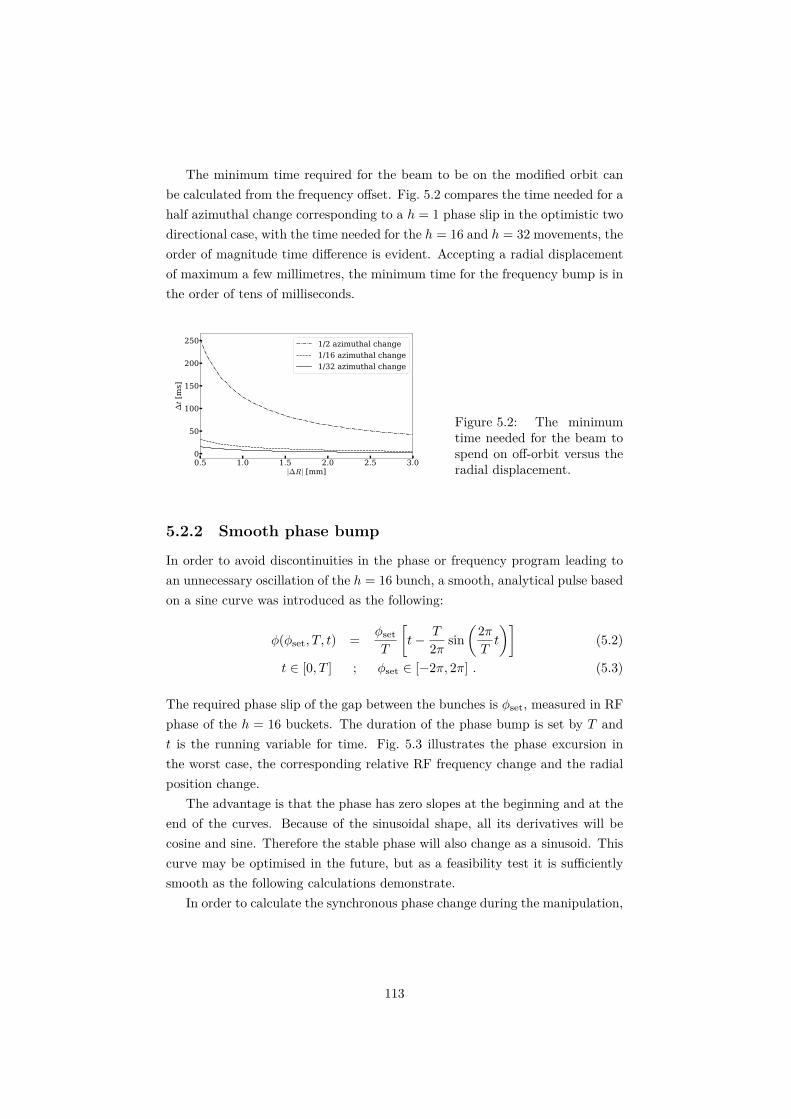
The minimum time required for the beam to be on the modified orbit canbe calculated from the frequency offset. Fig. 5.2 compares the time needed for ahalf azimuthal change corresponding to a h = 1 phase slip in the optimistic twodirectional case, with the time needed for the h = 16 and h = 32 movements, theorder of magnitude time difference is evident. Accepting a radial displacementof maximum a few millimetres, the minimum time for the frequency bump is inthe order of tens of milliseconds.

0.5 1.0 1.5 2.0 2.5 3.0|∆R| [mm]

0

50

100

150

200

250

∆t [

ms]

1/2 azimuthal change1/16 azimuthal change1/32 azimuthal change

Figure 5.2: The minimumtime needed for the beam tospend on off-orbit versus theradial displacement.

5.2.2 Smooth phase bump

In order to avoid discontinuities in the phase or frequency program leading toan unnecessary oscillation of the h = 16 bunch, a smooth, analytical pulse basedon a sine curve was introduced as the following:

φ(φset, T, t) =φset

T

[t− T

2πsin

(2π

Tt

)](5.2)

t ∈ [0, T ] ; φset ∈ [−2π, 2π] . (5.3)

The required phase slip of the gap between the bunches is φset, measured in RFphase of the h = 16 buckets. The duration of the phase bump is set by T andt is the running variable for time. Fig. 5.3 illustrates the phase excursion inthe worst case, the corresponding relative RF frequency change and the radialposition change.

The advantage is that the phase has zero slopes at the beginning and at theend of the curves. Because of the sinusoidal shape, all its derivatives will becosine and sine. Therefore the stable phase will also change as a sinusoid. Thiscurve may be optimised in the future, but as a feasibility test it is sufficientlysmooth as the following calculations demonstrate.

In order to calculate the synchronous phase change during the manipulation,

113

5

0φ [r

ad]

φset = − 2π

10 ms20 ms30 ms

2

0

df R

F

f RF×

10−

6

0 10 20 30 40 50Time [ms]

0

2

∆R

[mm

]

Figure 5.3: The following parameters are shown during a 10, 20 and 30 ms longmanipulation: the pre-defined phase program (top), the relative change of theRF frequency (middle) and the change of the radial position (bottom).

the frequency and momentum differential relation is used [221, p. 9]:

dp

p=

γ2trγ

2

γ2tr − γ2

df

f. (5.4)

The relation above is combined with Eqs. 2.5 and 5.1 to obtain:

sinφs =df

dt

p

f

γ2trγ

2

γ2tr − γ2

2πR

qV=

dR

dtp2πγ2

tr

qV. (5.5)

The estimates of the most relevant parameters during the manipulation,the synchronous phase, the momentum change and the synchrotron frequencyaccording to Eq. 2.12 are shown in Fig. 5.4.

The bucket filling factor is in the order of 20%. The bucket area shrinks inthe case of the shortest, 10 ms manipulation by approximately 20% as illustratedby Fig. 5.4 bottom. Therefore the beam will still only occupy approximately aquarter of the accelerating and decelerating buckets meeting this requirement.However, a 10 ms short duration causes oscillations of the bunch as shown bysimulations, therefore this is already a limiting case of the operation. The actualchange of the bucket area is expected to be well below one fifth. The small stablephase change with a small radial change compared to the aperture are promisingparameters showing that the beam could possibly follow a change in the orderof 30 ms during a short flat top.

114

5

0

5φ

s [de

g]

10

0

10

dp [k

eV/c

]

1907.5

1910.0

ωs [

Hz]

0 10 20 30 40 50Time [ms]

0.8

1.0

Ab/A

b0 10 ms

20 ms30 ms

Figure 5.4: The following parameters are shown during a 10, 20 and 30 mslong manipulation with the same parameters as Fig. 5.3 from top to bottom:synchronous phase, momentum change, synchrotron frequency in the middle ofthe bucket and relative bucket area.

5.2.3 Adiabaticity of re-phasing

To evaluate the adiabaticity of the RF manipulation, a general adiabaticitycriterion based on the bucket area change was applied, see [37] and [124, p. 303].The conventional one based on the synchrotron frequency change [124, p. 241]does not take into account the consequences of the change of the shape of thebucket as shown below.

The relative bucket area change can be written as

dA

A= αABωsdt . (5.6)

For the manipulation to be adiabatic the change of the area has to be smallcompared to the synchrotron period as also explained for barrier buckets earlierin Chapter 2, which means:

αAB=

∣∣∣∣ 1

ωsAB

dAB

dt

∣∣∣∣� 1 . (5.7)

115

The following calculation was performed with the conventions of [124, pp. 241–4] and separately using the variables of Eq. 2.19 leading to the same result asexpected. The calculation using the former convention is presented.

Using the conventional αb(φs), the bucket area factor [124, p. 243] for accel-erated sinusoidal buckets and Eq. 5.7 the following is true of the change of thebucket area:

dAB

dt∼ d

dt

(ωsαb(φs)√| cosφs|

)=

αb(φs)√| cosφs|

dωs

dt+ ωs

d

dt

(αb(φs)√| cosφs|

). (5.8)

The change in αb is much larger than the contribution of√| cosφs|, around the

zero stable phase where we operate, therefore:

dAB

dt∼ αb

dωs

dt+ ωs

dαb

dt. (5.9)

According to Eqs. 5.7 and 5.9:

αAB =

∣∣∣∣ 1

ω2sαb

(ωs

dαb

dt+ αb

dωs

dt

)∣∣∣∣ = ∣∣∣∣ 1

ωsαb

dαb

dt+

1

ω2s

dωs

dt

∣∣∣∣ . (5.10)

Neglecting the contribution of the first term in the sum Eq. 5.10 leads to theconventional adiabaticity criterion based on the change of the synchrotron fre-quency:

αad =

∣∣∣∣ 1ω2s

dωs

dt

∣∣∣∣ . (5.11)

However, in our case, the contribution of the first term in the sum in Eq. 5.10is two orders of magnitude higher than the second, therefore it can not be ne-glected. Hence the classical adiabaticity criterion (Eq. 5.11) can not be applied.

On the other hand, neglecting the first term in 5.10 leads to an approximatedadiabaticity criterion that is applicable to the phase slip:

αp =

∣∣∣∣ 1

αbωs

dαb

dt

∣∣∣∣� 1 . (5.12)

This result highlights that the main contribution to the change in the lon-gitudinal beam dynamics during a phase slip is not the synchrotron frequencychange, but the change of the bucket area factor, which means trajectory shapeand bucket area change. In other words, αp measures the adiabaticity due tosqueezing the beam into an accelerating and decelerating bucket, whereas it isinsensitive to the change of the synchrotron frequency. The three adiabaticityparameters are compared in Fig. 5.5 for the proposed phase slip. The rela-tion between the adiabaticity parameters according to the triangle inequalitytheorem is:

116

0.00

0.05αA

b

0.00

0.05

αp

0.000

0.001

αad

10 ms20 ms30 ms

Figure 5.5: Comparison of the general adiabaticity parameter (top), the approx-imation valid for the phase slip operation (middle) and the conventional (bot-tom) one. It is clear that the main contribution comes from the change of thebucket area factor.

αAB≤ αad + αp . (5.13)

A 10 ms long process is expected to be too short because the value of therelevant adiabaticity parameters is higher than 0.05, which usually indicates anon-adiabatic manipulation [124, p. 303], whereas in the other cases this valueis much lower. Furthermore, the αAb

and αp curve suggests that by optimisingthe shape of the phase program, a faster manipulation can possibly be achievedby smoothing the discontinuity in the higher derivatives of the phase curve.This could achieve a somewhat lower peak adiabaticity.

With the analytical estimations being favourable when compared to the re-quirements mentioned in Table 5.1, macroparticle simulations were performedto investigate the operation further in the next section.

5.3 Simulations and benchmarking

Macroparticle simulations using the longitudinal beam dynamics code BLonDhave been performed to investigate the phase slip after the beam is acceleratedto 14 GeV/c flat top momentum. In addition, benchmarking with past mea-surements [222, 223] is also performed, since the accelerator complex was notavailable to test the proposed scheme with beam.

117

5.3.1 Benchmarking with past measurements

Validating the simulation code with previously conducted beam tests under verysimilar conditions in the PS in 2016 [222, 223] was possible. Although the energyof the beam and the RF frequency were different, the adiabaticity parameterrange of the measurement and the current proposal is almost exactly the sameas indicated in Table 5.3, hence a fair comparison can be made.

Measurement Proposedparameter (2016) parameter

Energy 26 GeV 14 GeVRF frequency 40 MHz 7.6 MHzMax. RF amplitude 100 kV 100 kVAzimuthal change range 0–360◦ 0–22.5◦Time range of the manipulation 20–60 ms 10–30 msPeak synchrotron frequency 512 Hz 305 HzAdiabaticity parameter range 0.2 % – 6.4 % 0.3 % – 7.1 %

Table 5.3: Parameter comparison of the measurements in 2016 and the pro-posed and simulated parameters for barrier bucket synchronisation. Note theadiabaticity parameter is based on the change of the bucket area, see Eq. 5.7and [37].

0 250 500 750 1000 1250 1500 1750 2000Time [ns]

0

10

20

30

Tim

e [m

s]

Figure 5.6: Longitudinal profile evolution during a 30 ms phase slip operation.Data from the 2016 measurements. The colours indicate the longitudinal linedensity from yellow (high) to blue (low).

The longitudinal line density evolution was available from the beam studiesin 2016. Figures 5.7 and 5.8 provide a typical example of the longitudinal profileevolution in the simulated and measured case, for an adiabatic and non-adiabaticmanipulation respectively. As Fig. 5.6 indicates, due to the high h = 84 har-monic number in the PS, the bunch is barely visible when looking at a whole

118

0 10 20Time [ns]

0

20

40

60

Tim

e [m

s]

0 10 20Time [ns]

0

20

40

60

Tim

e [m

s]

Figure 5.7: Profile evolution aligned in the coordinate system of the bunch withαAb

= 0.2%. The plot shows that with a slow manipulation the beam can followboth in the simulated (left) and in the measured (right) case, because the profileevolution is preserved. The colours indicate the longitudinal line density fromyellow (high) to blue (low).

0 10 20Time [ns]

0

10

20

30

40

Tim

e [m

s]

0 10 20 30Time [ns]

0

10

20

30

Tim

e [m

s]

Figure 5.8: Profile evolution aligned in the coordinate system of the bunch withαAb

= 1.9%. The simulations on the left show oscillation after the manipulation.The measurements on the right show a that the beam is practically lost. Thiswas attributed to technical problems found in the phase program. The coloursindicate the longitudinal line density from yellow (high) to blue (low).

119

turn longitudinal profile evolution data of the phase slip. Therefore the com-parison was achieved by detecting the bunch position in the whole turn profilesand aligning it along a straight line, effectively observing the manipulation inthe coordinate system of the bunch.

In the case of the slow manipulations as shown in Fig. 5.7 the bunch evolutionmatches the measured one. This operation clearly preserves the shape of thebunch and does not excite any oscillations, which is also confirmed by the lowadiabaticity parameter. The non adiabatic case of a short manipulation does notreproduce the simulation exactly as shown in Fig. 5.8. Problems with the phaseprogram function for the measurement were found for faster manipulations. Theazimuthal change was programmed as a phase change in RF harmonic numberh = 84. During the already fast azimuthal change h = 84 cycles were skippedin the program according to the reconstruction, possibly causing an abruptphase change leading to an even less adiabatic manipulation. Nevertheless, theadiabaticity parameter and the presence of the oscillations in the simulated caseshows that this manipulation is unacceptably fast, anyway. Further beam testsare planned after the accelerator shutdown to test the operation.

5.3.2 Simulation results

With the 2016 measurement data analysed and the simulation code bench-marked, the proposed phase slip operation was programmed in BLonD as indi-cated by Table 5.3.

Figure 5.9: Simulated longitudinal profile evolution during a fast, 12 ms h = 16displacement. This time is too short for the manipulation as shown by theoscillations. The colours indicate the longitudinal line density from yellow (high)to blue (low).

120

Figure 5.10: The simulated longitudinal profile evolution during aslower, 30 ms h = 16 displacement. This time is sufficient for the manipulationas shown by the lack of oscillations. The colours indicate the longitudinal linedensity from yellow (high) to blue (low).

A scan was performed for a manipulation in 10− 36 ms with an RF voltageof 100 kV, which already underestimates the current value in the fixed targetcycle at flat top by 15%. However, the RF system in the PS can output amaximum of 200 kV providing a substantial margin.

Two example cases are shown for the simulated longitudinal profile evolutionduring an azimuthal displacement of a bunch by 2π/16 (h = 16). Fig. 5.9illustrates a worst, 12 ms case showing the highest oscillations in the probedrange due to the fast bump coupling to the synchrotron oscillations of the beam.

0 5000 10000 15000 20000Turns

4

2

0

2

4

∆t -

∆t p

rog [n

s]

V= 100 kV

∆tchange = 131 ns

T = 10 msT = 12 msT = 14 msT = 16 msT = 18 msT = 20 msT = 22 msT = 24 msT = 26 msT = 28 msT = 30 msT = 32 msT = 34 msT = 36 ms

Figure 5.11: The time difference between the average bunch position and theprogrammed position for various durations of the phase shift manipulation. Theinitial oscillations are an artefact of the imperfect matching in the simulations.

121

0 2000 4000 6000 8000 10000 12000 14000Turns

5.0

2.5

0.0

2.5

∆t -

∆t p

rog [n

s]

80 kV V 90 kV∆tchange = 131 ns

T = 10 msT = 11 msT = 12 ms

Figure 5.12: The dependence of the position on the voltage and time available.The higher the peak amplitude, the lower the amplitude of the oscillations and,in general, the longer the time, the lower the oscillations. Due to the non-linearity of the synchrotron oscillations bunch oscillations are very sensitive tothe length of the manipulation.

For an almost three times longer manipulation with a duration of 30 ms, asdepicted in Fig. 5.10, the situation is much improved. There are no noticeabledipole oscillations visible at the resolution of the plot.

To provide a more systematic picture on the time scale of the operation, thedifference between the simulated and the expected mean position in time wascalculated and the results shown in Fig. 5.11. Lower RF voltages and shortertimes lead to stronger oscillations in general, but not always. For examplea 12 ms manipulation causes slightly higher amplitude oscillations than theone executed in 10 ms, due to a resonance with the synchrotron frequency asmentioned earlier. However, beyond approximately 20 ms the bunch oscillationsdecrease for a longer manipulation. When reaching 30 ms in duration, themanipulation does not induce any noticeable degradation of the longitudinalbeam quality. The initial oscillation is a result of an imperfect matching of theparticles at the beginning of the simulation as it can be seen in Fig. 5.11. Thesame random seed was used to generate the initial conditions in this case suchthat the initial oscillations are the same.

A scan of the voltage shows (Fig. 5.12), as expected, that the lower voltagesresult in higher oscillations, because the bunch in this case occupies a larger areain the bucket and as the duration of the operation gets longer, non-linearity ofthe synchrotron oscillations, but it still degrades the longitudinal beam qualityby causing an emittance increase. Following this campaign of simulations, aduration of 30 ms for the azimuthal alignment as part of the synchronisationseems adequate. Beam studies will be conducted to confirm this.

122

5.4 Implementation

The steps of the implementation are illustrated in Figs. 5.13 – 5.16 and sum-marised Table 5.4.

Upon arrival at the flat-top in the PS, the open loop revolution frequencyof the PS is set to the one obtained from the measured bending field during theacceleration phase. Since the PS phase loop is initially closed, see Fig. 5.13, theeffect of this synchronisation on the beam is not visible.

Once this is achieved, the radial phase loop gains are reduced to zero,see Fig. 5.14, thereby a fixed frequency is achieved. Because the phase loopis off, the resolution (LSB) of the phase program will cause a drift. Therefore,the resolution of the master clock [224] needs to be taken into account not tocause a larger than a few ns displacement in the gap position at extraction.

Assuming re-using the present hardware the LSB of the master clock is0.23 Hz. This integrated over 200 ms amounts to less than 500 ps time differenceof the expected and actual gap position in the worst case. Before performingthe phase slip operation, the RF phase versus the extraction phase is measuredin harmonic number 16, then an appropriate phase bump is applied to movethe gap by the difference in phase, see Fig. 5.15. As a result, the beam is atthe correct azimuthal position for barrier bucket generation modulo 2π/16. Theposition of the gap is ideally the same as the setpoint of the phase bump, sincethe gap is to be generated between two bunches. Therefore this is known and canbe controlled in the present firmware for the barrier bucket drive. The accuracydepends on the accuracy of the phase slip, which based on the simulations thebeam can follow.

Since the azimuthal position of the beam does not have to be changed anymore, the main RF voltage can be lowered and the transverse splitting can takeplace. At the end of this process, the barrier voltage is increased as the mainRF voltage goes from a low value to zero and the re-bucketing is performed withthe gap made at the correct azimuthal position.

The new manipulation would require only a little more time to be availablein the cycle. Table 5.5 shows the estimated durations needed for the individualsteps of the synchronisation process.

123

No. Main sequence Detailed steps1 Establish pre-conditions for syn-

chronisation• Smooth switch from B-train fre-

quency reference to SPS RF refer-ence, see also Fig. 5.13.

• Reduce phase loop gain to zero, seealso Fig. 5.14.

• Reduce radial loop gain to zero.Result PS RF open-loop frequency is syn-

chronous with SPS RF.2 Move the bunch to the nearest • Perform phase measurement.

gap position, see also Fig. 5.15. • Program and perform phase bumpby acting on the master clock fre-quency.

Result Gap between h = 16 buckets is inthe correct position to be replacedby gap made by the barrier bucket.

3 Barrier bucket and transversesplitting, see also Fig. 5.16.

• Reduce main RF voltage fromabout 100 kV to about 12 kV.

• Perform transverse splitting.• Set barrier bucket azimuth to gap

position, which is automaticallysynchronous with the PS extractionkickers.

• Re-bucketing: reduce main RF volt-age from 12 kV to zero. Simulta-neously increase barrier voltage to2− 4 kV depending on gap size.

Result Gap in beam made synchronouslywith PS extraction kickers and SPSinjection kickers.

4 Beam transfer • Trigger beam transfer elementsbased on signals derived from SPSRF

Result PS extraction and SPS injectionkickers switch simultaneously withgap in line density.

Table 5.4: Steps of the proposed synchronisation.

Manipulation t0 Duration (ms)Match PS-SPS frequency at flat-top t0 5

Perform phase measurement t0 + 5 5Phase bump t0 + 10 30

Barrier manipulation no added time

Table 5.5: An example of the timings needed for the synchronisation.

124

Figure 5.13: Step 1: Switch from B-train reference to external RF reference ofthe revolution frequency.

Figure 5.14: Step 2: Reduce phase and radial loop gain to zero.

Figure 5.15: Step 3: measure phase difference and perform phase bump byacting on the frequency of the master clock.

Figure 5.16: Step 4. Perform transverse splitting and generate barrier bucketby increasing the amplitude of the wide-band RF connected to the Finemet®

cavity.

125

5.5 Summary

The proposed synchronisation scenario for the gaps generated by the barrierbucket system with azimuthal positions required for the beam in the SPS isdifferent from a conventional bunch to bucket transfer. In order to align thegap in the PS, the mean energy of the beam has to be temporarily changedduring unfavourable conditions such as: a relatively short time available forthe manipulation; the low RF voltage available from all RF systems duringthe transverse splitting; the low synchrotron frequencies in barrier buckets andpotentially small radial displacement allowed by the MTE on top of the usualaperture limitation. Short time and small radial displacement, in addition,are conflicting requirements. On the other hand, compared to a conventionalbunch to bucket transfer, the accuracy of the synchronisation can be an orderof magnitude lower.

A fast synchronisation by placing the barrier between two bunches is pos-sible with the gaps generated between the h = 16 bunches. This allows for ashort 2π/16 azimuthal phase slip while achieving effectively a harmonic one syn-chronisation. Furthermore, the synchronisation is performed with the main RFsystem before the transverse splitting takes place, when sufficient RF voltage isstill available to rapidly change the mean energy of the beam.

Analytical calculations of the bucket parameters during the phase bumpshowed that the operation is feasible within a few tens of milliseconds. Thesewere complemented by macroparticle simulations of the manipulation, whichconfirmed the analytical estimates. The simulation code was successfully bench-marked against previous beam measurements in the PS.

The parameters used in the analytical calculations and in the simulationswere conservative. An ideal manipulation would only require a maximum of2π/32 azimuthal change when two directional movement is applied around thecircumference of the PS. Yet, the twice, 2π/16 has been included with theassumption that the phase slip is only performed in one direction. Furthermore,the increased injection energy of the PS after LS2 should be able to providefurther margin to accommodate the manipulations in this cycle.

Machine development studies to validate the steps of this synchronisationscheme are foreseen during the upcoming run of the accelerators at CERN.

126

Chapter 6

Conclusions

6.1 Summary of contributions

The three main contributions of this thesis are summarised in the following threesections: the implementation of the LLRF drive signal for barrier buckets inthe PS, the subsequent commissioning and beam tests including the significantbeam loss reduction at extraction and the proposal for synchronisation of barrierbuckets between the PS and SPS.

6.1.1 Implementation

The requirements of the barrier parameters were analysed which confirmed thecompatibility with the existing PS Finemet® cavity and its high power levelRF installation. In order effectively reduce the losses, the duration of the pulsehas to cover the kicker rise times, defining the bandwidth requirement. Theamplitude has to be sufficiently high to contain the beam in the barrier bucketfor a given pulse length. The emittance was measured during the cycle and cross-checked with simulations after de-bunching, form this the amplitude requirementwas calculated.

The waveform shape to generate a stationary barrier bucket is essentiallya free parameter as long as it has a flat part and has no DC component asdetailed in Chapters 2 and 3. Following a comparison of a few typical waveformshapes, the isolated sine wave based implementation was chosen as a compromisebetween bandwidth and bucket height. A general smoothing scheme was alsointroduced to limit the bandwidth of any kind of waveform.

The concept of the waveform generator was developed and implemented inprogrammable logic. A beam synchronous, swept clock digital synthesizer witha remotely programmable arbitrary waveform look-up table [3] was selected,

127

because it is synchronous with conventional RF signals, flexible and it is easyto implement evolved manipulations such as moving barriers. It has the addedbenefit of compatibility with the existing low-level RF infrastructure in the PS.The hardware was installed and commissioned successfully.

A linear pre-distortion scheme was developed based on the transfer functionmeasurement of the cavity and amplifier system. Since the behaviour of thecavity does not drift significantly with time nor with beam intensity, no furtheradjustments were necessary to this data-based model during the beam tests.

To simulate the behaviour of the beam in barrier buckets, all barrier testswere compared to extensive tracking simulations in BLonD with the same fea-tures as the hardware implementation, which allowed accurate simulations ofthe beam dynamics with beam loading.

6.1.2 Beam test and loss reduction

First beam tests with a single barrier were performed to validate the proof-of-principle and to calibrate its phase with respect to the beam. This initialcommissioning was successful. Special cycles were set up at injection energy,which allowed to control the initial conditions of the beam in isolated and barrierbuckets. This, in turn, allowed to conduct more sophisticated tests to comparethe adiabaticity of the barrier compression and decompression against literature.The results were in agreement with predictions and beam tests performed inother laboratories as detailed in [2] and Chapter 4.

Following the low intensity and low energy beam tests, the energy and theintensity of the beam was increased to test the barrier bucket extraction schemeclose to its foreseen operational conditions. The fixed target cycle was modi-fied to remove the transverse splitting. This allowed to check the re-bucketingprocess from the h = 16 bunches to the barrier bucket at flat top in the PSwith 14 GeV/c momentum. It was established that for symmetry reasons thegap made by the barrier has to be between two h = 16 bunches to obtain asymmetric bunch profile at extraction.

The barrier buckets were combined with the transversely split beam in thePS with great success, which is the main original result [1] of the present studies.Subsequently, the longitudinal beam profiles were analysed in detail and it wasestablished that the extraction scheme scales works very well up to the highestbeam intensity.

The analysis of the beam loss monitor data confirmed the significant lossreduction at extraction form the PS across all beam intensities.

128

6.1.3 Synchronisation

To benefit from the beam loss reduction scheme, the barrier bucket generation inthe PS has to be synchronised with the injection in the SPS. For this to happenthe beam has to be moved in azimuth, which requires slight acceleration anddeceleration in the PS. The main constraint for acceleration is that very nearto the extraction there is no sufficient RF voltage to accelerate or deceleratethe beam with any of the RF systems available, because of the low momentumspread required for the Multi-turn Extraction.

Introducing additional time just before the transverse splitting takes place,where there is still sufficient voltage from the main, h = 16 RF system to movethe bunches was explored. If the position of the barrier is locked to the gapsbetween the h = 16 bunches, then maximum only a 2π/16 azimuthal movementof the beam is sufficient in the worst case to synchronise the gap with the SPS.

Analytical calculations were performed to investigate the adiabaticity of theoperation. A phase slip in the order of few tens of milliseconds could move thebeam adiabatically for the gap to be at the right position at extraction. Particletracking simulations confirmed this, which were benchmarked with previousmeasurements in the PS as the accelerator complex was not available for beammeasurements during LS2.

6.2 Future work

The feasibility of the barrier bucket operation for beam loss reduction in the PSwas established and the natural next step is to put the scheme in operation.

Approximately 50 ms time seems to be reasonable for the complete synchro-nisation process. The time for this must be found within the fixed target cycle.Therefore, the post LS2 fixed target cycle in the PS has to be analysed andoptimised to accommodate the synchronisation. This is foreseen to include anoptimisation of the de-bunching process at the end of the fixed target cycle. Theshape of the phase curve could be also tuned with respect to the adiabaticitycriterion shown in Chapter 6, which could possibly shorten the time for theoperation or improve the adiabaticity for the same duration.

Although the main steps of the synchronisation have been proposed in Chap-ter 5, further technical details remain to be elaborated. The steps of the smoothhandover from the PS to the SPS frequency have to be established. The mea-surement of the phase after arrival on the flat top in the PS needs to be developedan implemented in detail. The question whether one phase measurement be-fore the phase bump is sufficient or not has to be investigated also with beam.The technical details of the beam control of the frequency bump have to be

129

ascertained. Further integration of the barrier bucket drive in the sequence ofsynchronisation has to be established.

Following the path of the fixed target beam in the accelerator chain, after asuccessful synchronisation, the next step is acceleration in the SPS. The conse-quences of the gaps in the beam in the SPS and the impact on the experimentshave to be analysed and studied with beam especially with respect to transientbeam loading, since empty gaps have to be compensated by a larger line densityto keep the total intensity equally high. In addition, the detailed analysis of theSPS ring performance for MTE beams in combination with the barrier bucketis needed with the goal of quantitatively assessing the overall performance ofthis new beam process.

130

Bibliography

1. M. Vadai, A. Alomainy, H. Damerau, S. Gilardoni, M. Giovannozzi, A.Huschauer. Barrier bucket and transversely split beams for loss-free multi-turn extraction in synchrotrons. EPL 128, 14002. 7 p (2019).

2. M. Vadai, A. Alomainy, H. Damerau, Heiko, S. Gilardoni, M. Giovannozzi,A. Huschauer. Beam manipulations with barrier buckets in the CERN PS.2019 J. Phys.: Conf. Ser. 1350 012088.

3. M. Vadai, A. Alomainy, H. Damerau. Barrier bucket studies in the CERNPS. Proc. 10th Int. Particle Accelerator Conf. (IPAC’19), Melbourne,Australia, May 2019, pp. 1128–1131. MOPTS106.

4. CERN. NA58/COMPASS, COmmon Muon and Proton Apparatus forStructure and Spectroscopy, The CERN Experimental Programme, GreyBook database Accessed: 07-01-2020. https : / / greybook . cern . ch /greybook/experiment/detail?id=NA58.

5. CERN. NA61/SHINE, Study of Hadron Production in Hadron-Nucleusand Nucleus-Nucleus Collisions at the CERN SPS, The CERN Exper-imental Programme, Grey Book database Accessed: 07-01-2020. https://greybook.cern.ch/greybook/experiment/detail?id=NA61.

6. CERN. NA62, Proposal to Measure the Rare Decay K+ -> pi+ nunu at the Cern SPS, The CERN Experimental Programme, Grey Bookdatabase Accessed: 07-01-2020. https://greybook.cern.ch/greybook/experiment/detail?id=NA62.

7. CERN. NA63, Electromagnetic Processes in strong Crystalline Fields,The CERN Experimental Programme, Grey Book database Accessed: 07-01-2020. https://greybook.cern.ch/greybook/experiment/detail?id=NA63.

8. CERN. NA64, Search for dark sectors in missing energy events, TheCERN Experimental Programme, Grey Book database Accessed: 07-01-2020. https://greybook.cern.ch/greybook/experiment/detail?id=NA64.

131

9. CERN. NA65/DsTau, Study of tau neutrino production, The CERN Ex-perimental Programme, Grey Book database Accessed: 07-01-2020. https://greybook.cern.ch/greybook/experiment/detail?id=NA65.

10. A. Ceccucci, G. Mallot, L. Gatignon. Fixed target, striking physics. Ac-cessed: 07-01-2020. https : / / cerncourier . com / a / fixed - target -striking-physics/.

11. Vretenar, M. et al. Linac4 design report (CERN Yellow Reports: Mono-graphs 6/2020, CERN, Geneva).

12. E. Mobs. The CERN accelerator complex - 8ust 2018. Complexe desaccélérateurs du CERN - Août 2018. 8 2018, Image ID: OPEN-PHO-ACCEL-2018-005, accessed: 07/01/2020. https://cds.cern.ch/record/2636343.

13. C. Bovet, D. Fiander, L. Henny, A. Krusche, G. Plass. The Fast ShavingEjection for Beam Transfer from the CPS to the CERN 300 GeV Machine.IEEE Transactions on Nuclear Science 20, 438 (June 1973).

14. D. C. Fiander, D. Grier, K. D. Metzmacher, P. Pearce. A modulated fastbump for the CPS continuous transfer. IEEE Trans. Nucl. Sci. 24, 1340–2(1977).

15. G. Arduini, G. Crockford, M. Giovannozzi, K. Hanke, D. Manglunki, M.Martini, G. Métral, C. Niquille. TT2/TT10 Transfer Line Studies for the14 GeV/C Continuous Transfer. SL-Note-99-013-MD (Mar. 1999).

16. J. Borburgh, S. Dam1ovic, S. Gilardoni, M. Giovannozzi, C. Hernalsteens,M. Hourican, A. Huschauer, K. Kahle, G. Le Godec, O. Michels, G.Sterbini. First implementation of transversely split proton beams in theCERN Proton Synchrotron for the fixed-target physics programme. Euro-phys. Lett. 113, 34001. 6 p (2016).

17. M. Giovannozzi et. al. The CERN PS multi-turn extraction based on beamsplitting in stable islands of transverse phase space: Design Report CERN-2006-011 (CERN, Geneva, 2006).

18. R. Cappi, M. Giovannozzi. Novel Method for Multiturn Extraction: Trap-ping Charged Particles in Islands of Phase Space. Phys. Rev. Lett. 88,104801 (10 Feb. 2002).

19. Y. Suetsugu, K. Shibata, A. Morishige, Y. Suzuki, M. Tsuchiya. Designstudy of a movable mask with low beam impedance. Phys. Rev. ST Accel.Beams 9, 103501 (10 Oct. 2006).

20. A. Franchi, S. Gilardoni, M. Giovannozzi. Progresses in the studies of adi-abatic splitting of charged particle beams by crossing nonlinear resonances.Phys. Rev. ST Accel. Beams 12, 014001 (1 Jan. 2009).

132

21. S. Abernethy, A. Akroh, H. Bartosik, A. Blas, T. Bohl, S. Cettour-Cave,K. Cornelis, H. Damerau, S. Gilardoni, M. Giovannozzi, C. Hernalsteens,A. Huschauer, V. Kain, D. Manglunki, G. Métral, B. Mikulec, B. Salvant,J.-L. Sanchez Alvarez, R. Steerenberg, G. Sterbini, Y. Wu. Operationalperformance of the CERN injector complex with transversely split beams.Phys. Rev. Accel. Beams 20, 014001. 21 p (2017).

22. A. Huschauer, A. Blas, J. Borburgh, S. Dam1ovic, S. Gilardoni, M. Gio-vannozzi, M. Hourican, K. Kahle, G. Le Godec, O. Michels, G. Sterbini.Transverse beam splitting made operational: Key features of the multiturnextraction at the CERN Proton Synchrotron. Phys. Rev. Accel. Beams20, 061001. 15 p (2017).

23. A. Huschauer, M. Giovannozzi, O. Michels, A. Nicoletti, G. Sterbini. Anal-ysis of performance fluctuations for the CERN Proton Synchrotron multi-turn extraction. Journal of Physics: Conference Series 874, 012072 (July2017).

24. M. Giovannozzi et al. Results from the 2009 Beam Commissioning of theCERN Multi-turn Extraction. Proc. 1st Int. Particle Accelerator Conf.(IPAC’10), Kyoto, Japan, May 2010, paper THOBMH02, pp. 3619–3621.

25. M. Giovannozzi, J. Borburgh, S. S. Gilardoni, H. Bartosik, D. Bodart, R.J. Brown, S. Dam1ovic, C. Hernalsteens, M. Hourican, M. Widorski, B.Goddard. Proposal of a Dummy Septum to Mitigate Ring Irradiation forthe CERN PS Multi-Turn Extraction. Proc. 3rd Int. Particle AcceleratorConf. (IPAC’12), New Orleans, LA, USA, May 2012, paper MOPPD059,pp. 499–501.

26. M. Giovannozzi, S. S. Gilardoni, C. Hernalsteens, A. Lachaize, G. Metral.Modified Extraction Scheme for the CERN PS Multi-Turn Extraction.Proc. 3rd Int. Particle Accelerator Conf. (IPAC’12), New Orleans, LA,USA, May 2012, paper MOPPD060, pp. 502–504.

27. L. N. Drosdal, A. Ulsroed, M. Giovannozzi, S. S. Gilardoni, H. Bartosik,C. Hernalsteens, A. Lachaize, Y. Papaphilippou. Design and Beam Mea-surements of Modified Fast Extraction Schemes in the CERN PS forInstalling a Dummy Septum to Mitigate Ring Irradiation. Proc. 4th Int.Particle Accelerator Conf. (IPAC’13), Shanghai, China, May 2013, paperWEPEA056, pp. 2633–2635.

28. C. Hernalsteens, S. Dam1ovic, S. S. Gilardoni, M. Giovannozzi. Numeri-cal Simulations to Evaluate the Performance of CERN PS Dummy Sep-tum to Reduce Irradiation for the Multi-Turn Extraction. Proc. 4th Int.

133

Particle Accelerator Conf. (IPAC’13), Shanghai, China, May 2013, paperWEPEA057, pp. 2636–2638.

29. C. Bertone, J. Borburgh, D. Bodart, R. Brown, S. Burger, S. Dam1ovic,P. Demarest, R. Fernandez Ortega, J. A Ferreira Somoza, D. Gerard, S.Gibson, S. Gilardoni, M. Giovannozzi ( ed.), G. Le Godec, C. Hernal-steens, M. Hourican, N. J urado, J.-M. Lacroix, S. Mataguez, G. Métral,C. Pasquino, E. Perez-Duenas, S. Persichelli, B. Salvant, R. Steerenberg,P. van Trappen. Studies and implementation of the PS dummy septumto mitigate irradiation of magnetic septum in straight section 16 CERN-ACC-2014-0043 (Apr. 2014).

30. R. Garoby. RF gymnastics in synchrotrons. CAS - CERN AcceleratorSchool: Specialised Course on RF for Accelerators; 8 - 17 Jun 2010,Ebeltoft, Denmark, 16 p (Dec. 2011).

31. S. Persichelli, M. Migliorati, M. M. Paoluzzi, B. Salvant. Impedance Stud-ies for the PS Finemet® Loaded Longitudinal Damper. Proc. 5th Int. Par-ticle Accelerator Conf. (IPAC’14), Paper TUPRI060, Dresden, Germany,Jun. 2014.

32. Hitachi Metals Ltd. Nanocrystalline Soft Magnetic Material FINEMET®Accessed: 07-01-2020. https://www.hitachi-metals.co.jp/e/products/elec/tel/p02_21.html.

33. M. Paoluzzi, H. Damerau. Design of the PS longitudinal damper. CERN-ACC-NOTE-2013-0019 (2013).

34. L. L. Foldy. A method for expanding the phase-stable regime in syn-chronous accelerators. Il Nuovo Cimento (1955-1965) 19, 1116–1120.issn: 1827-6121 (Mar. 1961).

35. J. E. Griffin, C. Ankenbrandt, J. A. MacLachlan, A. Moretti. IsolatedBucket RF Systems in the Fermilab Antiproton Facility. Proc. 10th Par-ticle Accelerator Conf. (PAC’83), Santa Fe, NM, USA, Mar. 1983, pp.3502–3505.

36. S. Y. Lee, K. Y. Ng. Particle dynamics in storage rings with barrier rfsystems. Phys. Rev. E 55, 5992–6001 (5 May 1997).

37. K. Y. Ng. Continuous multiple injections at the Fermilab Main Injector.Phys. Rev. ST Accel. Beams 5, 061002 (6 June 2002).

38. C. M. Bhat. Barrier RF Systems in Synchrotrons. Proc. 9th EuropeanParticle Accelerator Conf. (EPAC’04), Lucerne, Switzerland, Jul. 2004,paper THOBCH03.

39. C. M. Bhat. Longitudinal momentum mining of beam particles in a storagering. Physics Letters A 330, 481–486. issn: 0375-9601 (2004).

134

40. W. Chou, D. Capista, E. Griffin, K. Y. Ng, D. Wildman. Fast BeamStacking using RF Barriers. Proc. 22nd Particle Accelerator Conf., Al-buquerque, NM, USA, Jun. 2007, paper TUPAS014, pp. 1682–1684.

41. G. Jackson. Operational Experience with the Permanent Magnet Recy-cler Ring at Fermilab. Proc. 7th European Particle Accelerator Conf.(EPAC’00), Vienna, Austria, Jun. 2000, paper MOP5B01.

42. M. Hu. The Fermilab Recycler Ring. Proc. 19th Particle Accelerator Conf.(PAC’01), Chicago, IL, USA, Jun. 2001, paper MOPA006.

43. S. Mishra. Status of the Fermilab Recycler Ring. Proc. 8th EuropeanParticle Accelerator Conf. (EPAC’02), Paris, France, Jun. 2002, paperMOPLE035.

44. M. Hu, D. R. Broemmelsiek, B. Chase, J. L. Crisp, N. Eddy, P. W. Joire-man, K. Y. Ng. Uniform Longitudinal Beam Profiles in the FermilabRecycler Using Adaptive RF Correction. Proc. 22nd Particle AcceleratorConf. (PAC’07), Albuquerque, NM, USA, Jun. 2007, paper MOPAS011,pp. 458–460.

45. M. Fujieda, Y. Iwashita, A. Noda, Y. Mori, C. Ohmori, Y. Sato, M.Yoshii, M. Blaskiewicz, J. M. Brennan, T. Roser, K. S. Smith, R. Spitz,A. Zaltsmann. Barrier bucket experiment at the AGS. Phys. Rev. STAccel. Beams 2, 122001 (12 Dec. 1999).

46. M. Brennan, T. Roser. High Intensity Performance of the BrookhavenAGS. Proc. 5th European Particle Accelerator Conf. (EPAC’96), Sitges,Spain, Jun. 1996, paper TUP011G.

47. M. Blaskiewicz, J. M. Brennan. A Barrier Bucket Experiment for Ac-cumulating De-bunched Beam in the AGS. Proc. 5th European ParticleAccelerator Conf. (EPAC’96), Sitges, Spain, Jun. 1996, paper MOP002G.

48. M. Fujieda, Y. Iwashita,Y. Mori, H. Nakayama, C. Ohmori, K. Saito,Y. Sato, S. Sawada, A. Takagi, Y. Tanabe, M. Toda, T. Uesugi, M. Ya-mamoto, T. Yan, M. Yoshii. An RF Cavity for Barrier Bucket Experi-ment in the AGS. Proc. 1st Asian Particle Accelerator Conf. (APAC’98),Tsukuba, Japan, Mar. 1998, paper 5D012.

49. L. A. Ahrens, J. G. Alessi, M. M. Blaskiewicz, J. M. Brennan, K. A.Brown, C. J. Gardner, J. W. Glenn, T. Roser, K. S. Smith, W. K. vanAsselt, S. Y. Zhang. High Intensity Performance of the Brookhaven AGS.Proc. 18th Particle Accelerator Conf. (PAC’99), New York, NY, USA,Mar. 1999, paper FRAR3.

135

50. C. Ohmori, M. Fujieda, S. Machida, Y. Mori, H. Nakayama, K. Saito,S. Sawada, Y. Tanabe, M. Yamamoto, E. Ezura, A. Takagi, M. Toda,M. Yoshii, T. Tanabe, T. Uesugi. A Wideband RF Cavity for JHF Syn-chrotrons. Proc. 17th Particle Accelerator Conf. (PAC’97), Vancouver,Canada, May 1997, paper 8P041.

51. M. Fujieda, S. Machida, Y. Mori, H. Nakayama, C. Ohmori, Y. Sato,A. Takagi, Y. Tanabe, M. Toda, T. Uesugi, M. Yamamoto, M. Yoshii,Y. Iwashita. MA-Loaded Cavities For Barrier Bucket Experiment. Proc.6th European Particle Accelerator Conf. (EPAC’98), Stockholm, Sweden,Jun. 1998, paper TUP14G.

52. M. Fujieda, Y. Iwashita, A. Noda, Y. Mori, C. Ohmori, Y. Sato, M.Yoshii, M. M. Blaskiewicz, J. M. Brennan, T. Roser, K. S. Smith, R.Spitz, A. Zaltsman. Magnetic Alloy Loaded RF Cavity for Barrier BucketExperiment at the AGS. Proc. 18th Particle Accelerator Conf. (PAC’99),New York, NY, USA, Mar. 1999, paper MOP81.

53. J.M. Brennan, J. Brodowski, M. Meth, K.A. Rogers, R. Spitz, M. Yoshii,A. Zaltsman. Design of Ferrite Loaded High Voltage Barrier Cavity. Proc.6th European Particle Accelerator Conf. (EPAC’98), Stockholm, Sweden,Jun. 1998, paper TUP22G.

54. E. Ezura, M. Fujieda, Y. Mori, R. Muramatsu, H. Nakayama, C. Ohmori,Y. Sato, A. Takagi, M. Toda, T. Uesugi, M. Yamamoto, M. Yoshii, M.Kanazawa, K. Noda. High Field-Gradient Cavities Loaded with MagneticAlloys for Synchrotrons. Proc. 18th Particle Accelerator Conf. (PAC’99),New York, NY, USA, Mar. 1999, paper THAL1.

55. K. Torikai, Y. Arakida, S. Inagaki, K. Ishibashi, J. Kishiro, K. Koseki, E.Nakamura, K. Takayama, T. Toyama, M. Wake. Design Study of 1 MHzInduction Cavity for Induction Synchrotron. Proc. 20th Particle Acceler-ator Conf. (PAC’03), Portland, OR, USA, May 2003, paper TPPB079.

56. C. M. Bhat. A New Technique for Making Bright Proton Bunches us-ing Barrier RF Systems. Proc. 21st Particle Accelerator Conf. (PAC’05),Knoxville, TN, USA, May 2005, paper TPAP021.

57. C. M. Bhat, B. Chase, C. Gattuso, P. W. Joireman. Longitudinal Momen-tum Mining of Antiprotons at the Fermilab Recycler: Past, Present, andFuture. Proc. 22nd Particle Accelerator Conf. (PAC’07), Albuquerque,NM, USA, Jun. 2007, paper WEOCKI04, pp. 1941–1943.

58. K. Y. Ng. Stability of Barrier Buckets with Short or Zero Barrier Sepa-rations. Proc. 21st Particle Accelerator Conf. (PAC’05), Knoxville, TN,USA, May 2005, paper TPAT018.

136

59. O. Boine-Frankenheim. rf barrier compression with space charge. Phys.Rev. ST Accel. Beams 13, 034202 (3 Mar. 2010).

60. B. Beaudoin, I. Haber, R. A. Kishek. Barrier Shock Compression withLongitudinal Space Charge. Proc. 6th Int. Particle Accelerator Conf.,Richmond, VA, USA, May 2015, pp. 646–648.

61. O. Boine-Frankenheim, V. Kornilov. Implementation and validation ofspace charge and impedance kicks in the code PATRIC for studies oftransverse coherent instabilities in the FAIR rings. Proc. 9th Int. Com-putational Accelerator Physics Conf. (ICAP’06), Chamonix, Switzerland,Oct. 2006, paper WEA3MP04, pp. 267–270.

62. T. Kikuchi, J. Dietrich, T. Katayama, R. Maier, D. Prasuhn, H. Stock-horst. Simulation Study of Simultaneous Use of Stochastic Cooling andElectron Cooling with Internal Target at COSY and HESR. Proc. 7thWorkshop on Beam Cooling and Related Topics (COOL’09), Lanzhou,China, 8.-Sep. 2009, paper THPMCP005, pp. 138–141.

63. O. Boine-Frankenheim, V. Kornilov. 3D Simulation of Coherent Instabili-ties in Long Bunches Induced by the Kicker Impedances in the FAIR Syn-chrotrons. Proc. 22nd Particle Accelerator Conf. (PAC’07), Albuquerque,NM, USA, Jun. 2007, paper FRPMN014, pp. 3919–3921.

64. O. Boine-Frankenheim, O. Chorniy. RF Barrier Compression with SpaceCharge for the FAIR Synchrotrons. Proc. 23rd Particle Accelerator Conf.,Vancouver, Canada, May 2009, paper TH5PFP021, pp. 3236–3238.

65. T. Katayama, M. Steck, R. Maier, D. Prasuhn, H. Stockhorst. ElectronCooling of Heavy Ions Interacting with Internal Target at HESR of FAIR.Proc. 4th Int. Particle Accelerator Conf. (IPAC’13), Shanghai, China,May 2013, paper MOPEA017, pp. 103–105.

66. H. Stockhorst, R. Maier, D. Prasuhn, R. Stassen, T. Katayama. Status ofStochastic Cooling Predictions at the HESR. Proc. 2nd Int. Particle Accel-erator Conf. (IPAC’11), San Sebastian, Spain, Sep. 2011, paper THPS003,pp. 3430–3432.

67. H. Stockhorst, B. Lorentz, R. Maier, D. Prasuhn, R. Stassen, T. Katayama.Simulation Study of Heavy Ion Beam Injection and Acceleration in theHESR for Internal Target Experiments with Cooling. Proc. 5th Int. Par-ticle Accelerator Conf. (IPAC’14), Dresden, Germany, Jun. 2014, pp.768–770.

137

68. V.B. Reva, M.I. Bryzgunov, V.V. Parkhomchuk, V. Kamerdzhiev, T.Katayama, R. Stassen, H. Stockhorst. Experimental Observation of Longi-tudinal Electron Cooling of DC and Bunched Proton Beam at 2425 MeV/cat COSY. Proc. 10th Workshop on Beam Cooling and Related Top-ics (COOL’15), Newport News, VA, USA, Sep.-Oct. 2015, paper MOX-AUD02, pp. 10–14.

69. C. Dimopoulou, B. Franzke, T. Katayama, D. Möhl, F. Nolden, G. Schreiber,M. Steck. Experimental Demonstration of Longitudinal Ion Beam Ac-cumulation with Electron Cooling. Proc. 11th European Particle Accel-erator Conf. (EPAC’08), Genoa, Italy, Jun. 2008, paper THPP048, pp.3470–3472.

70. M. Frey, P. HÃ, H. Klingbeil, D. Domont-Yankulova, K. Gross, J. Harzheim.Prototype Results of the ESR Barrier-Bucket System. Proc. 8th Int. Par-ticle Accelerator Conf. (IPAC’17), Copenhagen, Denmark, May 2017, pp.4133–4135.

71. P. Spiller, K. Blasche, O. Boine-Frankenheim, B. Franczak, P. Hülsmann,G. Moritz, H. Reich-Sprenger, P. Schütt. Double Synchrotron ComplexSIS100/200 for a New Research Facility at GSI. Proc. 8th EuropeanParticle Accelerator Conf. (EPAC’02), Paris, France, Jun. 2002, paperTHPLE078.

72. M. Frey, R. Balß, C. Christoph, O. Disser, G. Fleischmann, U. Hartel, P.Hülsmann, S. Jatta, A. Klaus, H. Klingbeil, H.G. König, U. Laier, D.E.M.Lens, D. Mondry, K.-P. Ningel, H. Richter, S. Schäfer, C. Thielmann, T.Winnefeld, B. Zipfel, K. Groß, H. Klingbeil. Status of the Ring RF Systemsfor FAIR. Proc. 6th Int. Particle Accelerator Conf. (IPAC’15), Richmond,VA, USA, May 2015, pp. 2789–2791.

73. A. Lehrach, F. Hinterberger, B. Lorentz, G. Hansen, R. Greven, F. M.Esser, F. Klehr, K. Bongardt, R. Tolle, T. Bergmark, S. Johnson, T. John-son, G. Norman, A. Raccanelli, E. Senicheva, K. Rathsman, O. Felden, R.Maier, B. Gålnander, T. Lofnes, M. Steck, R. Stassen, H. Stockhorst, D.Prasuhn, J. Dietrich, M. Schmitt, D. Reistad, T. Peterson, Y. Senichev.HESR at FAIR: Status of Technical Planning. Proc. 22nd Particle Accel-erator Conf. (PAC’07), Albuquerque, NM, USA, Jun. 2007, paper TU-PAN024, pp. 1442–1444.

74. B. Lorentz, A. Lehrach, R. Maier, D. Prasuhn, H. Stockhorst, R. Tölle.HESR Linear Lattice Design. Proc. 11th European Particle AcceleratorConf. (EPAC’08), Genoa, Italy, Jun. 2008, paper MOPC112, pp. 325–327.

138

75. R. Maier. The High-Energy Storage Ring (HESR). Proc. 24th ParticleAccelerator Conf. (PAC’11), New York, NY, USA, Mar.-Apr. 2011, paperTHOCN2, pp. 2104–2106.

76. R. Stassen, F. J. Etzkorn, G. Schug, H. Stockhorst, T. Katayama, L.Thorndahl. RF and Stochastic Cooling System of the HESR. Proc. 3rdInt. Particle Accelerator Conf. (IPAC’12), New Orleans, LA, USA, May2012, paper MOPPD008, pp. 385–387.

77. H. Stockhorst, R. Maier, D. Prasuhn, R. Stassen, T. Katayama. FeasibilityStudy of Heavy Ion Storage and Acceleration in the HESR with StochasticCooling and Internal Targets. Proc. 4th Int. Particle Accelerator Conf.(IPAC’13), Shanghai, China, May 2013, paper MOPEA018, pp. 106–108.

78. P. Beller, K. Beckert, C. Dimopoulou, A. Dolinskii, F. Nolden, M. Steck,J. Yang. Layout of an Accumulator and Decelerator Ring for FAIR. Proc.10th European Particle Accelerator Conf. (EPAC’06), Edinburgh, UK,Jun. 2006, paper MOPCH074.

79. F. B. Petrov, T. Weiland, O. Boine-Frankenheim. Electron Cloud Ef-fects in Coasting Heavy-ion Beams. Proc. 2nd Int. Particle AcceleratorConf. (IPAC’11), San Sebastian, Spain, Sep. 2011, paper MOPS053, pp.724–726.

80. R. Stassen, F. J. Etzkorn, R. Maier, D. Prasuhn, H. Stockhorst, L. Thorn-dahl. COSY as Ideal Test Facility for HESR RF and Stochastic CoolingHardware. Proc. 23rd Particle Accelerator Conf. (PAC’09), Vancouver,Canada, May 2009, paper TU5PFP022, pp. 861–863.

81. H. Stockhorst, T. Katayama, R. Maier, D. Prasuhn, R. Stassen. StochasticMomentum Cooling Experiments with a Barrier Bucket Cavity and In-ternal Targets at COSY-Jülich in Preparation for HESR at FAIR. Proc.1st Int. Particle Accelerator Conf. (IPAC’10), Kyoto, Japan, May 2010,paper MOPD068, pp. 846–848.

82. R. Stassen et al. Recent Results of the HESR RF System. Proc. 5th Int.Particle Accelerator Conf. (IPAC’14), Dresden, Germany, Jun. 2014, pp.2094–2096.

83. R. Gebel, R. Brings, O. Felden, R. Maier. Activities at the COSY/JülichInjector Cyclotron JULIC. Proc. 19th Int. Conf. on Cyclotrons and theirApplications, Lanzhou, China, Sep. 2010, paper MOPCP010, pp. 63–65.

84. T. Katayama, T. Kikuchi, R. Maier, I.N. Meshkov, D. Prasuhn, R. Stassen,H. Stockhorst. Bunched Beam Stochastic Cooling at COSY. Proc. 1st Int.Particle Accelerator Conf. (IPAC’10), Kyoto, Japan, May 2010, paperMOPD064, pp. 834–836.

139

85. A. O. Sidorin, A. D. Kovalenko, I. N. Meshkov, G. V. Trubnikov. Projectof the Nuclotron-Based Ion Collider Facility (Nica) at JINR. Proc. 1stInt. Particle Accelerator Conf. (IPAC’10), Kyoto, Japan, May 2010, paperMOPD011, pp. 693–695.

86. T. Katayama, I. N. Meshkov, G. V. Trubnikov. Numerical Investigationof Stochastic Cooling at NICA Collider. Proc. 8th Workshop on BeamCooling and Related Topics (COOL’11), Alushta, Ukraine, Sep. 2011,paper TUIOB01, pp. 52–57.

87. A. Smirnov, A. Sidorin, D. Krestnikov, R. Pivin, D. Prasuhn, M. Wolke.Simulation of Pellet Target Experiments with Betacool Code. Proc. 21stRussian Particle Accelerator Conf. (RuPAC’08), Zvenigorod, Russia, Sep.-Oct. 2008, paper MOAPH04.

88. O. S. Kozlov, A. V. Smirnov, V. Volkov, T. Katayama, A. O. Sidorin,G. V. Trubnikov, I. N. Meshkov, E. Kenzhbulatov, G. Y. Kurkin, A. V.Eliseev, V. M. Petrov. Storage, Acceleration and Short Bunched BeamFormation of 197Au+79 Ions in the NICA Collider. Proc. 23rd RussianParticle Accelerator Conf. (RuPAC’12), Saint Petersburg, Russia, Sep.2012, paper MOBCH01, pp. 30–32.

89. A. V. Smirnov, I. N. Meshkov, A. O. Sidorin, G. V. Trubnikov, A. V.Eliseev, T. Katayama. Stacking Modes with Barrier Buckets Method inNICA Collider. Proc. 9th Workshop on Beam Cooling and Related Top-ics (COOL’13), Mürren, Switzerland, Jun. 2013, paper WEPPO02, pp.97–99.

90. E. Syresin,A. V. Eliseev,N. V. Mityanina,V. M. Petrov,E. Rotov,A. V.Smirnov,A. G. Tribendis. Longitudinal Particle Dynamics in NICA Col-lider. Proc. 10th Int. Particle Accelerator Conf. (IPAC’19), Melbourne,Australia, May 2019, pp. 455–457.

91. T. Katayama, I. N. Meshkov, G. V. Trubnikov. Beam Cooling at NICACollider. Proc. 23rd Russian Particle Accelerator Conf. (RuPAC’12), SaintPetersburg, Russia, Sep. 2012, paper TUYCH02, pp. 53–57.

92. N. V. Mityanina, I. N. Meshkov, V. M. Petrov,E. Rotov, A. O. Sidorin,E. Syresin, A. G. Tribendis. Longitudinal Particle Dynamics and Coolingin NICA Collider. Proc. 12th Workshop on Beam Cooling and RelatedTopics (COOL’19), Novosibirsk, Russia, Sep. 2019, pp. 64–67.

93. K. Takayama et al. Induction Synchrotron (3): Rapid Cycle Synchrotronand Slow Cycle Synchrotron (Hardware Components for the Upgradeof KEK 12 GeV-PS). Proc. 19th Particle Accelerator Conf. (PAC’01),Chicago, IL, USA, Jun. 2001, paper RPPH028.

140

94. Y. Shimosaki, K. Horioka, K. Koseki, M. Nakajima, E. Nakamura, K.Takayama, K. Torikai, T. Toyama, M. Watanabe. Specific Beam Dynam-ics in Super-bunch Acceleration. Proc. 9th European Particle AcceleratorConf. (EPAC’04), Lucerne, Switzerland, Jul. 2004, paper WEPLT110.

95. K. Takayama, K. Koseki, K. Torikai, A. Tokuchi, E. Nakamura, Y. Arakida,Y. Shimosaki, M. Wake, T. Kouno, K. Horioka, S. Igarashi, T. Iwashita,A. Kawasaki, J. Kishiro, M. Sakuda, H. Sato, M. Shiho, M. Shirakata,T. Sueno, T. Toyama, M. Watanabe, I. Yamane. Observation of the Ac-celeration of a Single Bunch by Using the Induction Device in the KEKProton Synchrotron. Phys. Rev. Lett. 94, 144801 (14 Apr. 2005).

96. K. Takayama, Y. Arakida, T. Dixit, T. Iwashita, T. Kono, E. Nakamura,K. Otsuka, Y. Shimosaki, K. Torikai, M. Wake. Experimental Demonstra-tion of the Induction Synchrotron. Phys. Rev. Lett. 98, 054801 (5 Jan.2007).

97. K. Takayama, D.A. Arakawa, Y.A. Arakida, K. Horioka, S. Igarashi, T.Iwashita, A.K. Kawasaki, J. Kishiro, T. Kono, K. Koseki, E. Nakamura,M. Sakuda, H. Sato, M.S. Shiho, Y. Shimosaki, M.J. Shirakata, T. Sueno,A. Tokuchi, K. Torikai, T. Toyama, M. Wake, M. Watanabe, I. Yamane.Induction Acceleration of a Single RF Bunch in the KEK PS. Proc. 21stParticle Accelerator Conf. (PAC’05), Knoxville, TN, USA, May 2005,paper FPAE020.

98. K. Takayama et al. Present Status of the Induction Synchrotron Exper-iment in the KEK PS. Proc. 10th European Particle Accelerator Conf.(EPAC’06), Edinburgh, UK, Jun. 2006, paper MOPCH119.

99. T. S. Dixit, Y. Shimosaki, K. Takayama. Adiabatic Damping During Ac-celeration in the Induction Synchrotron. Proc. 22nd Particle AcceleratorConf. (PAC’07), Albuquerque, NM, USA, Jun. 2007, paper FRPMN033,pp. 4009–4011.

100. K. Takayama. Induction Synchrotron Experiment in the KEK PS. Proc.22nd Particle Accelerator Conf. (PAC’07), Albuquerque, NM, USA, Jun.2007, paper TUXC02, pp. 836–840.

101. A. V. Smirnov, C. Dimopoulou, D.A. Krestnikov, I.N. Meshkov, R. Pivin,G. Schreiber, A.O. Sidorin, M. Steck. Particle Accumulation with a Bar-rier Bucket RF System. Proc. 7th Workshop on Beam Cooling and Re-lated Topics (COOL’09), Lanzhou, China, 8.-Sep. 2009, TUM2MCIO02,pp. 67–70.

141

102. K. Torikai, Y. Arakida, Y. Shimosaki, K. Takayama. Fully Digitized Syn-chronizing and Orbit Feed-back Control System in the KEK InductionSynchrotron. Proc. 10th European Particle Accelerator Conf. (EPAC’06),Edinburgh, UK, Jun. 2006, paper THPCH094.

103. T. Iwashita, T. Adachi, K. Takayama, K. W. Leo, T. Arai, Y. Arakida,M. Hashimoto, E. Kadokura, M. Kawai, T. Kawakubo, T. Kubo, K.Koyama, H. Nakanishi, K. Okazaki, K. Okamura, H. Someya, A. Tak-agi, A. Tokuchi, M. Wake. KEK digital accelerator. Phys. Rev. ST Accel.Beams 14, 071301 (7 July 2011).

104. R. Yamada, J. Kishiro, Y. Shimosaki, K. Takayama, T. Toyama, M.Wake. 62-TeV Center of Mass Hadron Collider with Capability for SuperBunch Beams. Proc. 19th Particle Accelerator Conf. (PAC’01), Chicago,IL, USA, Jun. 2001, paper RPAH138.

105. K. Takayama, J. Kishiro, E. Nakamura, T. Toyama, S. Arakawa, K.Koseki, T. Hatano, K. Iida, Y. Imanishi, T. Sakuma, N. Shimizu, S.Naitoh, A. Tokuchi, K. Horioka, M. Nakajima, M. Watanabe, Induc-tion Accelerating Devices for Induction Synchrotrons and the SuperbunchVLHC. Proc. 8th European Particle Accelerator Conf. (EPAC’02), Paris,France, Jun. 2002, paper MOPRI075.

106. K. Takayama, R. J. Briggs. Induction accelerators (Springer, Berlin, 2011).

107. T. Bohl, T. Linnecar, E. Shaposhnikova. Barrier Buckets in the CERNSPS. Proc. 7th European Particle Accelerator Conf. (EPAC’00), Vienna,Austria, Jun. 2000, paper THP2A10.

108. Bohl, T and Linnecar, Trevor Paul R and Shaposhnikova, Elena. Thickbarrier buckets using the SPS travelling wave structures. CERN, Geneva,SL-Note-2000-032-HRF, May, 2000.

109. R. Stassen, K. Bongardt, F. J. Etzkorn, A. Schnase, H. Stockhorst. TheHESR RF-system and Tests in COSY. Proc. 11th European Particle Ac-celerator Conf. (EPAC’08), Genoa, Italy, Jun. 2008, paper MOPC125, pp.361–363.

110. J. Harzheim, D. Domont-Yankulova, K. Gross, H. Klingbeil, M. Frey.Input Signal Generation for Barrier Bucket RF Systems at GSI. Proc.8th Int. Particle Accelerator Conf. (IPAC’17), Copenhagen, Denmark,May 2017, pp. 3359–3362.

111. K. Gross, D. Domont-Yankulova, J. Harzheim, H. Klingbeil, M. Frey.Test Setup for Automated Barrier Bucket Signal Generation. Proc. 8thInt. Particle Accelerator Conf. (IPAC’17), Copenhagen, Denmark, May2017, pp. 3948–3950.

142

112. B. Ashmanskas, S. U. Hansen, T. Kiper, D. W. Peterson. FPGA-BasedInstrumentation for the Fermilab Antiproton Source. Proc. 21st Parti-cle Accelerator Conf. (PAC’05), Knoxville, TN, USA, May 2005, paperRPAT009.

113. E. Bayer, P. Zipf, A. Klaus, H. Klingbeil, G. Schreiber. Fast FPGA BasedLow-Trigger-Jitter Waveform Generator Method for Barrier-Bucket Elec-tronics at FAIR. Proc. North American Particle Accelerator Conf. (NA-PAC’13), Pasadena, CA, USA, Sep.-Oct. 2013, paper THPMA01, pp.1352–1354.

114. K. Koseki, M. Wake, K. Takayama. Significance of isolation impedancein a solid-state power modulator. Nuclear Instruments and Methods inPhysics Research Section A: Accelerators, Spectrometers, Detectors andAssociated Equipment 554, 64–74. issn: 0168-9002 (2005).

115. M. Wake et al. Switching Power Supply for Induction Accelerators. Proc.22nd Particle Accelerator Conf. (PAC’07), Albuquerque, NM, USA, Jun.2007, paper MOPAN042, pp. 251–253.

116. K. Horioka et al. Rapidly Switched Accelerating Devices for InductionSynchrotrons. Proc. 7th European Particle Accelerator Conf. (EPAC’00),Vienna, Austria, Jun. 2000, paper TUP4A14.

117. W. Chou, J. Griffin, K. Y. Ng, A. Takagi, D. Wildman, H. Zheng. BarrierRF Stacking at Fermilab. Proc. 20th Particle Accelerator Conf. (PAC’03),Portland, OR, USA, May 2003, paper RPAG016.

118. W. Chou, A. Takagi, D. Wildman, H. Zheng. Barrier RF System and Ap-plications in Main Injector. Proc. 21st Particle Accelerator Conf. (PAC’05),Knoxville, TN, USA, May 2005, paper FPAE010.

119. J. Dey, S. Dris, T. Kubicki, J. Reid. Linearization of the Fermilab RecyclerHigh Level RF. Proc. 20th Particle Accelerator Conf. (PAC’03), Portland,OR, USA, May 2003, paper TPAB011.

120. J. Harzheim, D. Domont-Yankulova, K. Gross, H. Klingbeil, M. Frey, D.E. M. Lens. The ESR Barrier-Bucket LLRF System - Design and FirstResults. Proc. 9th Int. Particle Accelerator Conf. (IPAC’18), Vancouver,Canada, Apr.-May 2018, pp. 4964–4966.

121. J. Harzheim, D. Domont-Yankulova, H. Klingbeil, R. Königstein, M. Frey.Modeling and Simulation of Broadband RF Cavities in PSpice. Proc. 7thInt. Particle Accelerator Conf. (IPAC’16), Busan, Korea, May 2016, pp.392–395.

122. V. I. Veksler. A new method of acceleration of relativistic particles. J.Phys. 9, 153–158 (1945).

143

123. B. W. S. L. Montague. Single-particle dynamics-RF acceleration. CERN-1977-013.63 (1977).

124. S. Y. Lee. Accelerator physics; 4th ed. (World Scientific, Singapore, 2019).

125. G. Dôme. Theory of RF acceleration and RF noise. CAS - CERN Accel-erator School : Antiprotons for Colliding-beam Facilities, CERN, Geneva,Switzerland, 11 - 21 Oct 1983, pp.215-253 (CERN-1984-015) (1984).

126. S. H. Strogatz. Nonlinear dynamics and chaos: With applications to physics,biology, chemistry, and engineering (Westview Press, Boulder, Colorado,2015).

127. C. Lanczos. The variational principles of mechanics; 4th ed. (Dover, NewYork, NY, 1986).

128. H. Wiedemann. Particle accelerator physics; 4th ed. (Springer, Berlin,2015).

129. CERN. CERN Beam Longitudinal Dynamics code BLonD Accessed: 07-07-2018. http://blond.web.cern.ch.

130. IEEE Standard for Floating-Point Arithmetic. IEEE Std 754-2019 (Revi-sion of IEEE 754-2008) (2019).

131. J. L. Laclare. Coasting beam longitudinal coherent instabilities. https://cds.cern.ch/record/398299 (1994).

132. M. Migliorati, S. Persichelli, H. Damerau, S. Gilardoni, S. Hancock, L.Palumbo. Beam-wall interaction in the CERN Proton Synchrotron for theLHC upgrade. Phys. Rev. ST Accel. Beams 16, 031001 (3 Mar. 2013).

133. O. Boine-Frankenheim, I. Hofmann. Space charge effects and coherentstability limits in barrier buckets. Phys. Rev. ST Accel. Beams 6, 034207(3 Mar. 2003).

134. L. Wang, Y. Li. Analysis of the longitudinal space charge impedance ofa round uniform beam inside parallel plates and rectangular chambers.Phys. Rev. ST Accel. Beams 18, 024201 (2 Feb. 2015).

135. T. Schilcher. RF applications in digital signal processing. Accessed: 01-08-2019. https://cds.cern.ch/record/1100538 (2008).

136. J. Tierney, C. M. Rader, B. Gold. A Direct Digital Synthesizer. IEEETransactions on Audio and Electroacoustics, Vol. AU-19, NO.1., March1971.

137. V. F. Kroupa (ed.) Direct digital frequency synthesizers (IEEE Press,1999).

144

138. L. Sermeus, M. J. Barnes, T. Fowler. The Kicker Systems for the PS Multi-turn Extraction. Proc. 1st Int. Particle Accelerator Conf. (IPAC’10), Ky-oto, Japan, May 2010, paper WEPD091, 3311–3313.

139. H. Schmickler. Accelerator Controls Part 1: CERN Accelerator ControlsAccessed: 11/01/2020. http://cas.web.cern.ch/sites/cas.web.cern.ch/files/lectures/divonne-2009/schmickler-1.pdf.

140. S. Deghaye, E. Fortescue-Beck. Introduction to the BE-CO Control Sys-tem. CERN-ACC-NOTE-2020-0069 (Dec. 2020).

141. T. Kikuchi, R. Maier, M. Steck, R. Stassen, H. Stockhorst, T. Katayama,D. Prasuhn, I. N. Meshkov. Beam Accumulation with Barrier Voltage andStochastic Cooling. Proc. 1st Int. Particle Accelerator Conf. (IPAC’10),Kyoto, Japan, May 2010, paper MOPD065, pp. 837–839.

142. C. Lanczos. Applied analysis (Prentice-Hall, Englewood Cliffs, NJ, 1956).

143. R. Garoby. Low level rf building blocks. CERN-PS-91-44-RF, 31 p (1991).

144. B. E. Chase, B. Barnes, K. Meisner. Digital Low Level RF Systems forFermilab Main Ring and Tevatron. 17th Particle Accelerator Conference,Vancouver, Canada, 12 - 16 May 1997, pp.2326.

145. T. Hayes, M. Harvey, G. Narayan, F. Severino, K.S. Smith, S. Yuan.A High Performance DAC / DDS D8hter Module for the RHIC LLRFPlatform. Proc. 24th Particle Accelerator Conf. (PAC’11), New York, NY,USA, Mar.-Apr. 2011, paper MOP284, pp. 648–650.

146. M. Bousonville, J. Rausch. Reference Signal Generation with Direct Dig-ital Synthesis for FAIR. Proc. 11th Int. Conf. on Heavy Ion AcceleratorTechnology (HIAT’09), Venice, Italy, Jun. 2009, paper A–01, pp. 218–222.

147. A. Caruso, L. Calabretta, G. Cosentino, A. Spartà, F. Speziale. DDS-based Control Loops for the RF System at INFN - LNS. Proc. 17th Int.Conf. on Cyclotrons and Their Applications, Tokyo, Japan, Oct. 2004,paper 20P23.

148. J. DeLong, J. M. Brennan, W. Fischer, T. Hayes, K. S. Smith, S. Valentino.Synthesizer Controlled Beam Transfer from the AGS to RHIC. Proc. 19thParticle Accelerator Conf. (PAC’01), Chicago, IL, USA, Jun. 2001, paperTPAH133.

149. X. Pei. Longitudinal Rf Matching During AGS-RHIC Beam Transfer.Proc. 15th Particle Accelerator Conf. (PAC’93), Washington D.C., USA,Mar. 1993, pp. 1424–1427.

145

150. T. Hayes, M. Harvey, G. Narayan, F. Severino, K. S. Smith, S. Yuan.A High Performance DAC / DDS D8hter Module for the RHIC LLRFPlatform. Proc. 24th Particle Accelerator Conf. (PAC’11), New York, NY,USA, Mar.-Apr. 2011, paper MOP284, pp. 648–650.

151. J. Volder. The CORDIC Computing Technique in Managing RequirementsKnowledge, International Workshop on 1 (IEEE Computer Society, LosAlamitos, CA, USA, 1959), 257.

152. H. Damerau, D. Perrelet. Upgrade of the Beam-synchronous RF SourceSystem in the CERN PS Accessed: 19-07-2019. https://public.cells.es/workshops/www.llrf2017.org/pdf/Posters/P-66.pdf.

153. D. Perrelet, H. Damerau. New CERN PS 10 MHz Cavity One-turn Feed-back Hardware and Beam Tests Accessed: 19-07-2019. https://conferences.lbl.gov/event/27/session/23/contribution/21/material/poster/0.pdf.

154. S. Persichelli, M. Migliorati, M. M. Paoluzzi, B. Salvant. Impedance Stud-ies for the PS Finemet® Loaded Longitudinal Damper. Proc. 5th Int.Particle Accelerator Conf. (IPAC’14), Dresden, Germany, Jun. 2014, pp.1708–1710.

155. S. Persichelli, M. Migliorati, M. M. Paoluzzi, B. Salvant. Finemet cavityimpedance studies. CERN-ACC-NOTE-2013-0033.

156. J. Belleman. WCM03 Installation Accessed: 2017-09-11. https://psring.web.cern.ch/psring/misc/wcm03.shtml.

157. D. Belohrad. Beam Charge Measurements. Conf. Proc. C11-05-16.4.CERN-BE-2011-019, WEOC01. 5 p (May 2011).

158. T. P. R. Linnecar. The high frequency longitudinal and transverse pick-upsin the CERN SPS accelerator. IEEE Trans. Nucl. Sci. 26. CERN-SPS-ARF-78-17, 3409–3411. 99 p (Aug. 1978).

159. R. Cappi, G. Cyvoct, J. Durant, M. Ruette, E. C. Schulte. Single shotlongitudinal shape measurements of nanosecond particle bunches. CERN-PS-87-31-PSR, 4 p (Mar. 1987).

160. R. J. Steinhagen, S. Bart-Pedersen, J. Belleman, T. Bohl, H. Damerau.Wall-Current-Monitor based Ghost and Satellite Bunch Detection in theCERN PS and the LHC Accelerators. Conf. Proc. C1204151. CERN-ATS-2012-249, WEDP01. 4 p (Apr. 2012).

161. J. Belleman, W. Andreazza, A. Nosych. A New Wall Current Monitorfor the CERN Proton Synchrotron. Proc. 5th Int. Beam InstrumentationConf. (IBIC’16), Barcelona, Spain, Sep. 2016, pp. 143–146.

146

162. J. M. Belleman. FT16.UES208 Accessed: 2020-09-26. http://jeroen.web.cern.ch/jeroen/tt2wbespu/ues208.shtml.

163. J. M. Belleman. The TT2 Wideband Electrostatic Pick-Ups Accessed:2020-09-26. http://jeroen.web.cern.ch/jeroen/tt2wbespu/.

164. J. M. Belleman. Pre-amplifier schematic diagram Accessed: 2020-09-26.http://jeroen.web.cern.ch/jeroen/tt2wbespu/preampschematics.shtml.

165. J. M. Belleman. A Four-Decade Bandwidth Hybrid Coupler. AB-Note-2006-005. CERN-AB-Note-2006-005. CERN-PS-BD-Note-99-09 (Feb. 2006).

166. G. Sterbini. LIU Toolbox. Version 0.3. unpublished.

167. K. Wittenburg. Beam loss monitors Accessed: 2020-09-07. https://cds.cern.ch/record/1213279.

168. R.E. Shafer. A tutorial on beam loss monitoring https://ab-div-bdi-bl-blm.web.cern.ch/Beam_loss_detectors/Literature/schaefer_biw02_tutorial.pdf.

169. CERN. Geant 4 Accessed: 2020-09-07. https://geant4.web.cern.ch/.

170. J. Allison et al. Geant4—a simulation toolkit. Nuclear Instruments andMethods in Physics Research Section A: Accelerators, Spectrometers, De-tectors and Associated Equipment 506, 250–303. issn: 0168-9002 (2003).

171. J. Allison et al. Geant4 developments and applications. IEEE Transactionson Nuclear Science 53, 270–278 (2006).

172. J. Allison et al. Recent developments in Geant4. Nuclear Instruments andMethods in Physics Research Section A: Accelerators, Spectrometers, De-tectors and Associated Equipment 835, 186–225. issn: 0168-9002 (2016).

173. CERN. FLUKA Accessed: 2020-09-07. https://fluka.cern/about.

174. C. Zamantzas et al. Injectors’ BLM system: PS ring installation at EYETSAccessed: 2020-09-08. https : / / indico . cern . ch / event / 648710 /contributions/2637394/attachments/1483809/2302429/20170627_LIU-PS_BLMINJ_EYETS.pdf.

175. E. Regenstreif. The CERN Proton Synchrotron doi:10.5170/CERN-1959-029 (CERN, Geneva, 1959).

176. H. Damerau et al. LHC Injectors Upgrade, Technical Design Report, Vol.I: Protons CERN-ACC-2014-0337. CERN-ACC-2014-0337 (Dec. 2014).

177. S. S. Gilardoni, S. Aumon, E. Effinger, J. Gil Flores, U. Wienands. BeamLoss Monitors Comparison at the CERN Proton Synchrotron. Proc. 2ndInt. Particle Accelerator Conf. (IPAC’11), San Sebastian, Spain, Sep.2011, paper TUPC135, pp. 1341–1343.

147

178. V. Agoritsas, F. Beck, G.P. Benincasa, J. P. Bovigny. A microprocessor-based system for continuous monitoring of radiation levels around theCERN PS and PSB accelerators. Nuclear Instruments and Methods inPhysics Research Section A: Accelerators, Spectrometers, Detectors andAssociated Equipment 247, 44–49. issn: 0168-9002 (1986).

179. W. Vigano, M. Alsdorf, B. Dehning, M. Kwiatkowski, G. G. Venturini, C.Zamantzas. 10 orders of magnitude current measurement digitisers for theCERN beam loss systems. Journal of Instrumentation 9, C02011–C02011(Feb. 2014).

180. C. Zamantzas, M. Alsdorf, B. Dehning, S. Jackson, M. Kwiatkowski, W.Vigano. System Architecture for measuring and monitoring Beam Lossesin the Injector Complex at CERN. Proc. 1st Int. Beam InstrumentationConf. (IBIC’12), Tsukuba, Japan, Oct. 2012, paper TUPA09, pp. 347–350.

181. W. Vigano, B. Dehning, E. Effinger, G. G. Venturini, C. Zamantzas.Comparison of Three Different Concepts of High Dynamic Range andDependability Optimised Current Measurement Digitisers for Beam LossSystems. Proc. 1st Int. Beam Instrumentation Conf. (IBIC’12), Tsukuba,Japan, Oct. 2012, paper MOPA09, pp. 66–70.

182. S. Hancock, P. Knaus, M. Lindroos. Tomographic Measurements of Lon-gitudinal Phase Space Density; 1998 ed. CERN-PS-98-030-RF, 4 p (July1998).

183. G. Favia, H. Damerau, V.D. Desquiens, S. Energico, M. Morvillo, D.Perrelet, C. Rossi. The PS 10 MHz High Level RF System Upgrade. Proc.7th Int. Particle Accelerator Conf. (IPAC’16), Busan, Korea, May 2016,pp. 622–625.

184. H. C. Grassmann, R. 1kovsky, W. Pirkl. New RF system for the 28 GeVproton synchrotron at CERN. Siemens Rev. 44, 164–70 (1977).

185. CERN. The CERN Experimental Programme https://greybook.cern.ch/greybook/ (2020).

186. W. Bartmann, J. Borburgh, S.S. Gilardoni, B. Goddard, A. Newborough,S. Pittet, R. Steerenberg, C.H. Yu. CERN PSB-to-PS Transfer Modifi-cations for the 2 GeV Upgrade. Proc. 3rd Int. Particle Accelerator Conf.(IPAC’12), New Orleans, LA, USA, May 2012, paper MOPPD057, pp.493–495.

187. W. Bartmann, J. Borburgh, J.R.T. Cole, S.S. Gilardoni, B. Goddard, O.Hans, M. Hourican, L. Sermeus, R. Steerenberg, C.H. Yu. Upgrades forthe CERN PSB-TO-PS Transfer at 2 GeV. Proc. 4th Int. Particle Accel-

148

erator Conf. (IPAC’13), Shanghai, China, May 2013, paper MOPFI054,pp. 404–406.

188. L. Michelotti. Integral for longitudinal phase space tomography on equilib-rium distributions. Phys. Rev. ST Accel. Beams 6, 024001 (2 Feb. 2003).

189. G. Van Rossum, F. L. Drake. Python 3 Reference Manual isbn: 1441412697(CreateSpace, Scotts Valley, CA, 2009).

190. T. E. Oliphant. A guide to NumPy (Trelgol Publishing USA, 2006).

191. P. Virtanen et. al. SciPy 1.0: Fundamental Algorithms for Scientific Com-puting in Python. Nature Methods 17, 261–272. https://rdcu.be/b08Wh(2020).

192. The pandas development team. pandas-dev/pandas: Pandas Feb. 2020.https://doi.org/10.5281/zenodo.3509134.

193. J. D. Hunter. Matplotlib: A 2D graphics environment. Computing in Sci-ence & Engineering 9, 90–95 (2007).

194. M. Waskom and the seaborn development team. mwaskom/seaborn seaborn.vi-olinplot Sept. 2020. https://doi.org/10.5281/zenodo.592845.

195. A. V. Oppenheim, R. W. Schaefer, J. R. Buck. Discrete-time signal pro-cessing (Upper Saddler River, NJ: Prentice Hall., 1999).

196. The SciPy community. scipy.signal.resample_poly Accessed: 2020-09-08.https://docs.scipy.org/doc/scipy/reference/generated/scipy.signal.resample_poly.html.

197. Julius O. Smith III. Introduction to Digital Filters with Audio Applica-tions Accessed: 2020-09-08. https://ccrma.stanford.edu/~jos/fp/Forward_Backward_Filtering.html (Sept. 2007).

198. F. Gustafsson. Determining the initial states in forward-backward filtering.IEEE Transactions on Signal Processing 44, 988–992 (1996).

199. The SciPy community. scipy.signal.filtfilt Accessed: 2020-09-08. https://docs.scipy.org/doc/scipy/reference/generated/scipy.signal.filtfilt.html.

200. The SciPy community. numpy.correlate Accessed: 2020-09-08. https://numpy.org/doc/stable/reference/generated/numpy.correlate.html.

201. A. Hofmann, F. Pedersen. Bunches with Local Elliptic Energy Distribu-tion. Accessed: 01/08/2019. https://cds.cern.ch/record/890555(1979).

149

202. A. Lasheen. PS Longitudinal Impedance Model (2020). DOI:10.5281/zen-odo.4420903 (Jan. 2021).

203. R. Garoby. Timing aspect of bunch transfer between circular machines:State of the art in the PS complex. CERN-PS-RF-Note-84-6 (1984).

204. W. A. Pellico, R. C. Webber. RF Cogging in the FNAL Booster Accel-erator. Proc. 18th Particle Accelerator Conf. (PAC’99), New York, NY,USA, Mar. 1999, paper TUA13.

205. D. A. Herrup. Cogging in the Fermilab Booster. Proc. 18th Particle Accel-erator Conf. (PAC’99), New York, NY, USA, Mar. 1999, paper TUA11.

206. R. M. Zwaska, S. E. Kopp, W. Pellico, R. C. Webber. Synchronizationof the Fermilab Booster and Main Injector for Multiple Batch Injec-tion. Proc. 9th European Particle Accelerator Conf. (EPAC’04), Lucerne,Switzerland, Jul. 2004, paper THPLT130.

207. R. M. Zwaska, S. E. Kopp, W. Pellico. Cycle-to-Cycle Extraction Syn-chronization of the Fermilab Booster for Multiple Batch Injection to theMain Injector. Proc. 21st Particle Accelerator Conf. (PAC’05), Knoxville,TN, USA, May 2005, paper FPAE022.

208. K. Seiya, C. C. Drennan, W. Pellico, A. K. Triplett, A. M. Waller. Momen-tum Cogging at the Fermilab Booster. Proc. 3rd Int. Particle AcceleratorConf. (IPAC’12), New Orleans, LA, USA, May 2012, paper THPPP023,pp. 3782–3784.

209. F. G. G. Garcia, W. Pellico. Current and Planned High Proton FluxOperations at the FNAL Booster. Proc. 52nd ICFA Advanced Beam Dy-namics Workshop on High-Intensity and High-Brightness Hadron Beams(HB’12), Beijing, China, Sep. 2012, paper WEO3A04, pp. 378–380.

210. K. Seiya, S. Chaurize, C. C. Drennan, W. Pellico, A. K. Triplett, A. M.Waller. Development of Cogging at the Fermilab Booster. Proc. 5th Int.Particle Accelerator Conf. (IPAC’14), Dresden, Germany, Jun. 2014, pp.2109–2111.

211. K. Seiya et al. Beam Studies for the Proton Improvement Plan (PIP)- Reducing Beam Loss at the Fermilab Booster. Proc. 6th Int. Parti-cle Accelerator Conf. (IPAC’15), Richmond, VA, USA, May 2015, pp.4027–4029.

212. K. Seiya, S. Chaurize, C. C. Drennan, W. Pellico. Injection Bucket JitterCompensation Using Phase Lock System at Fermilab Booster. Proc. 8thInt. Particle Accelerator Conf. (IPAC’17), Copenhagen, Denmark, May2017, pp. 1999–2001.

150

213. P. Baudrenghien, T. P. R. Linnecar, D. Stellfeld, U. Wehrle. SPS Beamsfor LHC: RF Beam Control to Minimize Rephasing in the SPS. CERN-SL-98-027-RF, 3 p (1998).

214. J. N. Bai, R. Baer, D. Beck, O.K. Kester, D. Ondreka, C. Prados, W.W.Terpstra, T. Ferrand. Bunch to Bucket Transfer System for FAIR. Proc.15th Int. Conf. on Accelerator and Large Experimental Physics ControlSystems (ICALEPCS’15), Melbourne, Australia, Oct. 2015, pp. 980–983.

215. P. Martin, J. Dinkel, R. J. Ducar, C. R. Kerns, Q. A. Kerns, K. G.Meisner, H. W. Miller, J. Reid, S. R. Tawzer, D. Wildman. Antiprotonacceleration in the Fermilab main ring and Tevatron. 12th IEEE ParticleAccelerator Conference, Washington, DC, USA, 16 - 19 Mar 1987, pp.47-49.

216. K. G. Meisner, H. Edwards, J. Fitzgerald, Q. A. Kerns. A low level rfsystem for the Fermilab Tevatron. 11th IEEE Particle Accelerator Con-ference, pt.1, Vancouver, Canada, 13 - 16 May 1985, pp.1687.

217. D. Trbojevic, L.A. Ahrens, M. Bai, M. Blaskiewicz, M. Brennan, P. Cameron,J. Cardona, R. Connolly, A. Drees, W. Fischer, R.P. Fliller, G. Ganetis,J.W. Glenn, H. Hahn, T. Hayes, J. Kewisch, A. Lehrach, W.W. MacKay,S. Peggs, V.I. Ptitsyn, T. Roser, T. Sa. Commissioning of the Relativis-tic Heavy Ion Collider. Proc. 19th Particle Accelerator Conf. (PAC’01),Chicago, IL, USA, Jun. 2001, paper RPAH124.

218. M. Meisner. RF Synchronous Transfer Into Specific Buckets Between Fer-milab Main Ring And Tevatron Accelerators. 15th IEEE Particle Accel-erator Conference, Washington, DC, USA, 17 - 20 May 1993, pp.2522.

219. J.M. Jowett, R. Alemany-Fernandez, P. Baudrenghien, D. Jacquet, M.Lamont, D. Manglunki, S. Redaelli, M. Sapinski, M. Schaumann, M.Solfaroli Camillocci, R. Tomas, J.A. Uythoven, D. Valuch, R. Verstee-gen, J. Wenninger. Proton-nucleus Collisions in the LHC. Proc. 4th Int.Particle Accelerator Conf. (IPAC’13), Shanghai, China, May 2013, paperMOODB201, pp. 49–51.

220. J.M. Jowett, R. Alemany-Fernandez, G. Baud, P. Baudrenghien, R. DeMaria, R. De Maria, D. Jacquet, M.A. Jebramcik, A. Mereghetti, T.Mertens, M. Schaumann, H. Timko, M. Wendt, J. Wenninger. The 2016Proton-Nucleus Run of the LHC. Proc. 8th Int. Particle Accelerator Conf.(IPAC’17), Copenhagen, Denmark, May 2017, pp. 2071–2074.

221. C. Bovet, R. Gouiran, I. Gumowski, K. H. Reich. A selection of formulaeand data useful for the design of A.G. synchrotrons; rev. version (CERN,Geneva, 1970).

151

222. T. Ferrand, H. Klingbeil, H. Damerau. Synchronization of Synchrotronsfor bunch-to-bucket Transfers. Sep. 2015, CERN-ACC-NOTE-2015-0025.

223. T. Ferrand, H. Klingbeil, O. Bachmann, J. N. Bai, H. Damerau. Progressin the Bunch-to-Bucket Transfer Implementation for FAIR. Proc. 8th Int.Particle Accelerator Conf. (IPAC’17), Copenhagen, Denmark, May 2017,paper THPVA041, pp. 4525–4527.

224. J. P. H., Sladen. High Frequency Direct Digital Synthesizer and ClockGenerator Modules. CERN, Geneva, 2004, CERN-AB-Note-2004-046.

152

Appendix A

Synthesis using halfrevolution frequencyharmonics

An alternative synthesis method using the basic symmetries of the barrier bucketpulses is presented. A property of such a pulse is a difference of two, phaseshifted harmonic components at the half of the original harmonic frequency,which can be used to generate the pulses in the frequency domain.

s1 f1 s2 f2 s3 f3s4 f5s5f4 s6 f6

r1

r2

r3r4

r5

r6

Figure A.1: si - start of the pulse, fi - end of the pulse, ri - the magnitude ofthe pulse

To derive the synthesis method, the notations of Fig. A.1 are going to beused. The Fourier coefficients for the i-th pulse in the pulse train can be foundby direct integration:

c0 =r

π(fi − si) cn,i =

rj

nπ

(e−jnfi − e−jnsi

)(A.1)

153

To limit the amplitude of the higher harmonics, if this is needed, a low pass filtercan be added, which in this case is the σ factor as also introduced in Chapter 3.The synthesizer formula for M pulses and N Fourier terms becomes:

V (t) =

M∑i=1

riπ

{fi − si + j

N−1∑n=1

σn,m

n

[ejn(ωt−fi) − ejn(ωt−si)

]}(A.2)

The σ is defined as the following:

σn,m = sincm n π

2 (N + 1)(A.3)

A symmetric barrier consists of two bumps of equal height and equal width.Given s0, f0 and r0 and the symmetry, s1, f1, r1 are all uniquely determined.

s1 = f0 f1 = 2f0 − s0 r1 = −r0 (A.4)

To express the symmetry in the formula, introducing b = f0 for the barriercentre and the barrier width as w = 2(f0 − s0). Applying eq. A.2 the offsetcancels.

V (t) =r

πj

N−1∑n=1

σ

n

[ejn

(ωt−b−w

2

)+ ejn

(ωt−b+w

2

)− 2ejn(ωt−b)

](A.5)

This is the same as:

V (t) =r

πj

N−1∑n=1

σ

n

[ejn

(ω2 t− 2b−w

4

)− e

jn(

ω2 t− 2b+w

4

)]2. (A.6)

Where w corresponds to the width of the barrier bucket generating waveform.The b corresponds to the azimuthal position. σ acts as a low-pass filter andω is the revolution angular frequency, t the time, N the number of harmoniccomponents.

The merit of this formula is that the Fourier coefficients do not have tobe calculated, since the waveform is generated from two, clean complex ex-ponentials. At the core of the waveform generator formula is a difference oftwo harmonics at the half of the Fourier harmonic frequencies. The Fourierharmonics correspond to the revolution frequency harmonics in a synchrotron.Therefore the fundamental, phase shifted barrier components are at the half ofthe revolution frequency. The revolution frequency harmonics are ”restored” bysquaring the components or mixing them with themselves. Then a smoothingwindow is applied. The process is illustrated in Fig. A.2.

154

An alternative implementation using whole revolution frequency harmonicscan be achieved by grouping the terms in the bracket:

V (t) = =

{r

π

N−1∑n=1

σ

n

[ejn(ωt−b) − ejn

(ωt−b−w

2

)+ ejn(ωt−b) − ejn

(ωt−b+w

2

)]}.

(A.7)The multiplication by 1/j and taking the negative of the imaginary part areinterchangeable, hence the slightly different formalism in Eqs. A.7 and A.5.

155

Phase shifted difference summedDifference of two components summed

FilteringMixing

Figure A.2: The illustration of equation A.5. The sum is performed at each stepto highlight the mechanism. The top left graph shows the difference of the twofrequency components at half of the revolution frequency summed up on theirown when there is no phase shift between them. The sum has only graphicalsignificance, the components cancel individually and the result is zero. Thena phase shift in the half frequency components is introduced (top right) whichmakes a pair of pulses when the components are added. Then these componentsare squared and summed with the standard Fourier method (bottom left) andthe modified or filtered version (bottom right) using the σ factors. It is clearfrom the formula and the images that the magnitude of the phase shift is themain factor in determining the width of the potential barriers.

156

Appendix B

Location of firmware andsoftware

The GitLab repositories related to the PhD work are listed below for reference.

• Firmware for the FPGA: https://gitlab.cern.ch/BE-RF-PLDesign/PS/EDA-02175-V2-BarrierBuckets.

• Additional routines for barrier bucket generaion in Python: https://gitlab.cern.ch/mivadai/barrierbucket.

• Initial re-bucketing simulations: https://gitlab.cern.ch/mivadai/BLonD.

• The analytical calculations and simulations related to the synchronisation:https://gitlab.cern.ch/mivadai/PSBBSynchronisation.

• Accelerator related re-usable calculations, general helper routines: https://gitlab.cern.ch/mivadai/mkit.

• Versioned .svg diagrams: https://gitlab.cern.ch/mivadai/diagrams.

157