Bayesian Near-Boundary Analysis in Basic

Macroeconomic Time Series Models∗

Michiel De Pooter1 Francesco Ravazzolo2 Rene Segers3 Herman K. Van Dijk3,†

1Federal Reserve Board2Norges Bank

3Tinbergen Institute and Econometric Institute

Erasmus University Rotterdam

Econometric Institute Report EI 2008-13

August 21, 2008

Abstract

Several lessons learnt from a Bayesian analysis of basic macroeconomic time seriesmodels are presented for the situation where some model parameters have substantialposterior probability near the boundary of the parameter region. This feature refers tonear-instability within dynamic models, to forecasting with near-random walk modelsand to clustering of several economic series in a small number of groups within a datapanel. Two canonical models are used: a linear regression model with autocorrelationand a simple variance components model. Several well-known time series models likeunit root and error correction models and further state space and panel data modelsare shown to be simple generalizations of these two canonical models for the purposeof posterior inference. A Bayesian model averaging procedure is presented in order todeal with models with substantial probability both near and at the boundary of theparameter region. Analytical, graphical and empirical results using U.S. macroeco-nomic data, in particular on GDP growth, are presented.

Keywords: Gibbs sampler, MCMC, autocorrelation, nonstationarity, reduced rankmodels, state space models, error correction models, random effects panel data models,Bayesian model averaging

JEL Classification Codes: C11, C15, C22, C23, C30

∗This paper is a substantial revision and extension of De Pooter et al. (2006). We are very grateful toparticipants of the 3rd World Conference on Computational Statistics & Data Analysis (Cyprus, 2005), theInternational Conference on Computing in Economics and Finance (Geneva, 2007), and the Advances inEconometrics Conference (Louisiana, 2007), for their helpful comments on earlier versions of the paper andwe are in particular indebted to William Griffiths, Lennart Hoogerheide and Arnold Zellner for many usefulcomments. Herman Van Dijk gratefully acknowledges financial support from the Netherlands Organizationfor Scientific Research (NWO). The views expressed in this paper are solely the responsibility of the authorsand should not be interpreted as reflecting the views of the Board of Governors of the Federal ReserveSystem or of any other employee of the Federal Reserve System nor the views of Norges Bank (the CentralBank of Norway).

This paper contains a number of references to Appendices. These appendices contain sampling schemes,conditional and marginal density results, probability density functions and an overview of models used inthe paper. They are available on http://people.few.eur.nl/hkvandijk/research.htm. Also given onthis website is the computer code and data which was used in the empirical applications in the paper.

†Corresponding author. Tinbergen Institute, Erasmus University Rotterdam, P.O. Box 1738, NL-3000 DR Rotterdam, The Netherlands. Tel.: +31-10-4088900, fax: +31-10-4089031. E-mail addresses:michiel.d.depooter@frb.gov (M. De Pooter), francesco.ravazzolo@norges-bank.no (F. Ravazzolo),rsegers@few.eur.nl (R. Segers), hkvandijk@few.eur.nl (H.K. Van Dijk).

1 Introduction

Stable economic growth with possibly temporary periodic deviations - better known asbusiness cycles - is one of the most important economic issues for any country. A widelyused macroeconomic time series to measure these characteristics of growth and cyclesis real Gross Domestic Product. A commonly used model in this context is the linearautoregressive model with deterministic trend terms. Using such time series and modelclasses, econometric analysis -Bayesian and Non-Bayesian- leads for most industrializednations to substantial evidence that economic growth evolves according to a trend processthat is largely determined by stochastic shocks. Otherwise stated, in the autoregressivemodels one finds substantial empirical evidence of a characteristic root that is near theboundary of unity or at this boundary in the parameter region. There exists an enormousliterature on this topic; here we only mention the well-known study of Nelson and Plosser(1982) and for empirical evidence on industrialized nations over the past century we referto Van Dijk (2004).

There are several other examples in macro economics of the existence of substantialposterior probability near the boundary of a parameter region. In business cycle analysisone may be interested to know how much of the variation in an economic time series isdue to the cycle and how much is due to the trend. This issue is relevant in the contextof an adequate policy mix for stimulating long term economic growth and short termbusiness cycle control. Using a structural time series model one may find substantialposterior probability of the cyclical component near zero and the relative weights of thetrend and cyclical components are then very uncertain. Another example occurs withtypical characteristics of financial time series in stock markets. These series behave closeto a random walk model or, otherwise stated, close to a model with a characteristic rootclose to the boundary of unity. The economic issue of such a process is whether financialmarkets are efficient in the sense that the optimal forecast for future stock market prices isthe current price. A fourth example is the club or cluster behavior in panel data models foreconomic growth in industrialized nations. In this context, convergence of economic growthis studied and the number of clusters may be relatively small. Substantial probabilitymay occur at the boundary of the parameter region of the number of clubs and, as aconsequence, large uncertainty exists with respect to the correct number of clubs.

To explore the issue of Bayesian near-boundary analysis in basic economic time se-ries models, one derives their likelihoods and specifies prior information. Our approachwith respect to specifying prior information is to start with uniform priors on a largeregion. The use of such noninformative priors means that we concentrate on the infor-mation content in and the shape of the likelihood function. Given our diffuse priors, theposterior distributions of parameters of interest may or may not exist. The latter occurs,in particular, at the boundary of the parameter region, due to nonidentifiability of someparameters of interest. We discuss how Information matrix priors or training sample priorsmay regularize or smooth the shape of irregular posterior distributions. In our analysis wemake use of an interplay of analytical techniques, simulation methods and graphics. Asa simulation technique we use the Gibbs sampling method. A brief introduction is givenin Section 2. We note that graphs in the context of Bayesian analysis are becoming moreand more important see, for example, Murrell (2005). In our analysis we therefore alsoplace emphasis on presenting results in a graphical way.

In this paper we make use of two classes of canonical models. The first class of modelsis known as the class of single equation dynamic regression models. A first contribution

1

of this paper is to show that, for our purpose of a Bayesian near-boundary analysis in theparameter region, basic members of this class of models like unit root models, distributedlag models and error correction models are special cases of the well-known linear regressionmodel with first-order autocorrelation in the disturbances. We also indicate that an errorcorrection model with near unit root behavior is - for posterior analysis - equivalent to aninstrumental variable regression model with possibly weak instruments; see also Hooger-heide and Van Dijk (2001) and Hoogerheide and Van Dijk (2008). Interpretation of themodels, their posteriors and the effect of smoothness priors like the Information matrixand training sample priors is one aim. A second aim is to illustrate a Bayesian analysis ofeconomic growth in U.S. Gross Domestic Product using different model specifications.

The second class of models deals with variance parameters as parameters of interest.We discuss how the simple regression model with heteroscedasticity can be used as anintroduction to the class of Hierarchical Linear Mixed Models (HLMM). As a secondcontribution, we show that the latter model serves as a parent class for time-varyingparameter models such as state space models and panel data models. We investigate whathappens when the density of one of the variance parameters is located near the zero boundand what happens when the number of components/groups in a panel is very small. Weshow that the latter case also leads to a boundary issue. We note that a combinationof the first and second class of basic models has recently become important in empiricalanalysis.

A third contribution of this paper is to show how Bayesian model averaging over modelswith substantial posterior probability near and at the boundary leads to better forecasting.That is to say, we do not consider the case where substantial posterior probability is nearand/or at the boundary as an econometric inferential problem where model selection isappropriate in order to determine or test whether the economic process is stationary ornonstationary but as a case where model averaging is to be preferred. This may lead toimproved forecasting.

The results of our analysis may be summarized as ‘lessons learnt from models used’and the start of a road map for learning Bayesian near-boundary analysis. A summaryis presented in Section 7. Some key lessons are: investigate the shape of the likelihoodof the parameters of interest; investigate the influence of smoothness priors in case ofsubstantial near-boundary posterior probability; learn which simulation technique maybe used efficiently in which situation; apply Bayesian model averaging over models withposterior probability near a boundary and models with substantial probability at theboundary. The topic of this paper should be of interest to Bayesians who make use of basicregression models for economic time series when the focus is on the information contentof the likelihood. The topic should interest non-Bayesians who are very knowledgeableabout basic econometric models and want to learn how the information in the likelihoodfunction of such models is summarized according to Bayes’ rule.

There exists an excellent literature of Bayesian analysis of regression models with auto-correlation, unit root models, distributed lag models, unobserved component models andpanel data models. An incomplete list of references is given as Chib (1991), Chib andGreenberg (1994, 1995) and Chib and Carlin (1999), Schotman and Van Dijk (1991a,b)and Harvey (1989). The purpose of the present paper is to extend this analysis to situa-tions where substantial posterior probability is near or at the boundary of the parameterregion. We emphasize that this paper does not result and is not intended to result in asimple message with respect to using one model, one particular prior and one simulationtechniques. We do not believe in such simplistic claims but rather in a situation where

2

different priors, different models and simulation algorithms are suitable depending on theproblem studied, the data, and the shape of the posterior of the model considered. Ourpurpose is to investigate a set of models and, next, to explore Bayesian model averaging.

The content of this paper is structured as follows. In Section 2 we briefly review some(artificial) examples of shapes of posterior densities that the researcher may encounter ineconometric practice. We also give an introduction to Gibbs sampling. This method isvery natural given our derivations of joint, conditional and marginal posteriors for thelinear regression model and this model with possibly autocorrelated disturbances. InSection 3 we present some basic results for the linear regression model that will be usedin subsequent sections. In Sections 4 and 5 we present our empirical analysis and presentsome theoretical results of near-boundary posterior probability for a number of modelsfor economic time series. Section 6 deals with forecasting U.S. Gross Domestic Product(GDP) using Bayesian model averaging. Section 7 contains a summary of models used andlessons learnt. The Appendices contain some technical details. We note that the technicallevel of the paper is like that of an introductory graduate econometrics course. Matrixnotation is used in order to indicate the common, linear (sub-)structure of several models.

2 Preliminaries I: Basics of Gibbs Sampling and Typical

Shapes of Posterior Densities

2.1 Basics of Gibbs sampling

As discussed in, for instance, Van Dijk (1999) and Hamilton (2006), the ‘simulation revolu-tion in Bayesian econometric inference’ is to a large extent due to the advent of computerswith ever-increasing computational power. This allows researchers to apply alternativeBayesian simulation techniques for estimation in which extensive use is made of pseudo-random number generators. One of the most important and widely used simulation meth-ods is Gibbs sampling, developed by Geman and Geman (1984), Tanner and Wong (1987)and Gelfand and Smith (1990). This method has become a popular tool in economet-rics for analyzing a wide variety of problems; see for instance Chib and Greenberg (1996)and Geweke (1999). Judging from numerous recent articles in the literature, Gibbs sam-pling is still gaining more and more momentum. Recent textbooks such as Bauwens et al.(1999), Koop (2003), Lancaster (2004), and Geweke (2005) discuss how Gibbs sampling isused in a wide range of econometric models, in particular in models with latent variables.Mixture processes are an important class of latent variable models in econometrics; themost well-known due to Hamilton (1989). In recent papers by, for instance, Celeux et al.(2000), Fruhwirth-Schnatter (2001), Jasra et al. (2005) and Geweke (2007), the issue ofconvergence of the Gibbs sampler in this class of models is discussed. The posterior dis-tribution in mixture processes may be multimodal and may exhibit ridges often due tonear nonidentification of parameters. A detailed analysis of this topic is beyond the scopeof the present paper but we note and will make use of the distinction by Geweke (2007)between the interpretation of a model and its posterior densities on the one hand and thenumerical efficiency and convergence of a simulation algorithm on the other hand.

One may characterize the Gibbs sampling algorithm as an application of the divide-and-conquer principle1. First, a K-dimensional parameter vector θ is divided into m

1We are necessarily brief in our explanation of the Gibbs sampler. See e.g. Casella and George (1992),or Hoogerheide et al. (2008), for a more elaborate discussion.

3

components θ1, θ2, ..., θm, where m ≤ K. Second, for many posterior distributions whichare intractable in terms of simulation the lower-dimensional conditional distributions turnout to be remarkably simple and tractable. The Gibbs sampler exploits this feature, asit samples precisely from these conditional distributions. Its usefulness is, for example,demonstrated by Chib and Greenberg (1996) and Smith and Roberts (1993).

Since Gibbs sampling is based on the characterization of the joint posterior distributionby means of the complete set of conditional distributions, it follows that a requirementfor application of the Gibbs sampler is that the conditional distributions, described by thedensities

p(θi|θ−i), for i = 1, ...,m (1)

where θ−i denotes the parameter component vector θ without the ith component, can allbe sampled from. The Gibbs sampling algorithm starts with the specification of an initial

set of values: (θ(0)1 , ..., θ

(0)m ) and then generates a sequence

(θ(1)1 , ..., θ(1)

m ), (θ(2)1 , ..., θ(2)

m ), ......, (θ(J)1 , ..., θ(J)

m ) (2)

following a process such that θ(j)i is obtained from p(θi|θ(j−1)

−i ). Thus, θ(j)i is obtained

conditional on the most recent values of the other components. We may summarize theGibbs sampling algorithm as follows:

1 : Specify starting values θ(0) = (θ(0)1 , . . . , θ

(0)m )

and set j = 1.2 : Generate (the jth Gibbs step) :

θ(j)1 from p(θ1|θ(j−1)

2 , . . . , θ(j−1)m )

θ(j)2 from p(θ2|θ(j)

1 , θ(j−1)3 , . . . , θ

(j−1)m )

θ(j)3 from p(θ3|θ(j)

1 , θ(j)2 , θ

(j−1)4 , . . . , θ

(j−1)m )

...

θ(j)m from p(θm|θ(j)

1 , . . . , θ(j)m−1)

3 : If j < J , set j = j + 1, and go back to Step 2.

The above algorithm yields a sequence of J realizations θ(j) = (θ(j)1 , ..., θ

(j)m ), for j =

1, 2, ..., J , from a Markov chain, converging to the target distribution. We will refer toStep 2 of the algorithm as ‘the Gibbs step’ and for each of the models that we discuss inthe subsequent sections we will always indicate what the Gibbs step looks like. Note thatthe components of θ do not necessarily need to be one-dimensional. Generating draws forblocks of parameters where some of the θi components denote a block of parameters is alsopossible.

The Gibbs algorithm is illustrated in Figure 1 where we show an example path of Gibbssampled points, when the conditional densities of θ1|θ2 and θ2|θ1 are both standard Normaland assuming a correlation coefficient of 0.75. The sample path is shown at different stagesof the algorithm.

4

The key feature of Gibbs sampling is:

For large enough J the sequence of Gibbs draws, generated from the conditional distri-butions, is distributed according to the joint and marginal posterior distributions.2

Figure 1: Gibbs sampling: Example steps

(a) 1 substep (b) 1 step (c) 2 steps

(d) 10 steps (e) 100 steps (f) 1000 steps

Notes: Panels (a) through (f) show consecutive steps of the Gibbs sampler using two conditional posteriordensities, p(θ1|θ2) and p(θ2|θ1) which are both standard normal with a correlation coefficient of 0.75. The

open circles in Panels (a)-(f) indicate the starting vector (θ(0)1 , θ

(0)2 ).

A simple argument for the general case is as follows. Suppose θi and θ−i have a jointposterior distribution with density p(θi,θ−i). Thus this posterior should exist, which mustbe carefully verified, compare also Sections 3 and 4. Then θ−i has the marginal posteriordistribution with density p(θ−i). Denote by θ−i and θj−1 the drawing generated in the(j−1)th step from the marginal posterior with density p(θ−i). In the jth step of the Gibbs

sampling algorithm, θ(j)i is drawn from p(θi|θ(j−1)

−i ), which is the density of the conditional

distribution of θi given θ(j−1)−i . The joint density of θ

(j)i and θ

(j−1)−i is

p(θ(j)i |θ(j−1)

−i )p(θ(j−1)−i ) = p(θ

(j)i ,θ

(j−1)−i ). (3)

2Strictly speaking, sensitivity to initial conditions persists, but it becomes negligible if the sequence ofGibbs draws mixes sufficiently well.

5

Therefore, (θ(j)i ,θ

(j−1)−i ) is distributed according to the joint posterior distribution. So the

posterior is an invariant distribution of the Gibbs Markov chain, which is the invariantlimiting distribution under the standard assumption of ergodicity. For a more detailedanalysis on theoretical properties of the Gibbs sampler we refer to Smith and Roberts(1993), Tierney (1994) and Geweke (1999).

Because in practice it may take some time for the Markov chain to converge, it iscommon to discard the first B draws, where typically B << J . These draws are referredto as the burn-in draws. Consequently, posterior results will be based only on drawsθ(B+1), . . . ,θ(J) of the generated chain. Furthermore, the sequence of draws sometimesdisplays some degree of autocorrelation. When autocorrelations are significant up to the(h − 1)th lag, one can consider using only every hth draw and to discard the intermediatedraws (h is known as the thinning value)3. An altogether different approach is to generatemultiple Markov chains instead of just one chain and to use only the final draw from eachsequence. Doing so implies that the Gibbs algorithm has to be executed a substantialnumber of times. When opting for this approach the researcher does not have to worryabout which value to choose for h. Although the drawback of this method is that itcan be very computationally intensive, it can alternatively help prevent posterior resultsfrom being (partially) determined by a particular set of starting values. We show in thenext section that randomizing over θ(0) can be a worthwhile endeavor when the likelihooddisplays signs of multimodality.

2.2 Three typical shapes of posterior densities

To illustrate the kinds of shapes that may occur in posterior densities we work through anumber of examples which are based on the model in Gelman and Meng (1991). Supposethat we have a joint posterior density of (θ1, θ2), which has the following form

p(θ1, θ2) ∝ exp

[− 1

2

(aθ2

1θ22 + θ2

1 + θ22 − 2bθ1θ2 − 2c1θ1 − 2c2θ2

) ](4)

where a, b, c1 and c2 are constants under the restrictions that a ≥ 0 and if a = 0 then|b| < 1 4. This Gelman and Meng (1991) class of bivariate distributions has the featurethat the random variables θ1 and θ2 are conditionally Normally distributed. In fact, theconditional densities p(θ1|θ2) and p(θ2|θ1) can be derived (picked) directly from the righthand side of (4) and can be recognized as Normal densities:

p(θ1|θ2, a, b, c1, c2) ∼ N(

bθ2 + c1

aθ22 + 1

,1

aθ22 + 1

)(5)

p(θ2|θ1, a, b, c1, c2) ∼ N(

bθ1 + c2

aθ21 + 1

,1

aθ21 + 1

)(6)

Note that, typically, the joint density of (θ1, θ2) is not Normal. By choosing differentparameter configurations for a, b, c1 and c2 we can construct joint posterior densities withrather different shapes, while the conditional densities remain Normal. In the remainderof this section we consider three types of shapes and we apply the Gibbs sampler to each

3The current consensus in the literature, however, seems to be to always include the information of alldraws, even when these are correlated.

4These restrictions are to insure that the joint density in (4) is integrable and therefore a properprobability density function.

6

of these. Although the shapes are all in a way artificial since they are not based directly ona model and data, doing so will give us some early insights into different shapes of (joint)posterior densities and boundary issues which we discuss in detail in the remainder of thispaper.

For each of the examples below the jth Gibbs step consists of sequentially drawing from(5) and (6):

jth Gibbs step for the Gelman-Meng model:

- generate θ(j)1 |θ(j−1)

2 from p(θ1|θ2, a, b, c1, c2) ∼ N(

bθ(j−1)2 +c1

a�

θ(j−1)2

�2+1

, 1

a�

θ(j−1)2

�2+1

)

- generate θ(j)2 |θ(j)

1 from p(θ2|θ1, a, b, c1, c2) ∼ N(

bθ(j)1 +c2

a�

θ(j)1

�2+1

, 1

a�

θ(j)1

�2+1

)

(i) Bell-shape

The first parameter configuration that we consider for the joint density in (4) is the fol-lowing; [a = b = c1 = c2 = 0] in which case the joint density is given by

p(θ1, θ2) ∝ exp[−1

2(θ21 + θ2

2)]

(7)

Both the conditional densities and the joint density are standard Normal. The latteris depicted in Figure 2(a). Gibbs sampling simply comes down to obtaining draws byiteratively drawing from standard Normal densities5. A scatterplot of one thousand ofsuch draws is shown in Figure 2(b).

The estimated conditional means and variances are equal to 0 and 1 for both para-meters. These are exactly the parameters of the marginal densities which, in this case,we know to be standard Normal. In fact, for the chosen parameter configuration, theconditional and marginal densities coincide since the conditional density for θ1 does notdepend on θ2 and vice versa. In this particular example it would therefore obviously notbe necessary to use Gibbs sampling.

(ii) Ridges

The second parameter configuration that we examine is [a = c1 = c2 = 0]6. The jointdensity is now given by

p(θ1, θ2) ∝ exp[−1

2(θ21 − 2bθ1θ2 + θ2

2)]

(8)

∝ exp

[−1

2

[θ1 θ2

] [ 1 bb 1

] [θ1

θ2

]]

It is apparent from Figure 3 that the shape of this density depends on the value of b.When b tends to 1 a ridge along the line θ1 = θ2 appears in the shape of the posterior.The scatterplots of Gibbs draws for this example in Figure 3 reveal that Gibbs samplingtends to become less efficient in such a case. Ridges may occur in econometric modelswhere the Information matrix tends to become singular, that is when b → 1; see the nextsection for examples. We emphasize that the posterior in Figures 3(e) and 3(f) is defined ona bounded region with bounds -75 and +75. This posterior is constant along the diagonaland it is a continuous function defined on a bounded region and thus a proper density.

5For all three examples in this section we used a burn-in period of B = 10, 000 draws and we set thethinning value h equal to 10.

6Note that this parameter vector violates the earlier stated parameter restrictions when b ≥ 1.

7

Figure 2: Gelman-Meng: Bell-shape

(a) Joint posterior density (b) Gibbs draws

Notes: Panel (a) shows the Gelman-Meng joint posterior density for θ1 and θ2 given in (4) for parametervalues [a = b = c1 = c2 = 0] whereas Panel (b) shows the scatterplot of 1,000 draws from the Gibbssampler together with the 99% highest probability density region.

(iii) Bimodality

The third and final configuration we consider is [a = 1, b = 0] and large, but not necessarilyequal, values for c1 and c2.

7 Here we select c1 = c2 = 10 which gives

p(θ1, θ2) ∝ exp

[− 1

2 [θ21θ

22 + θ2

1 + θ22 − 20θ1 − 20θ2]

](9)

∝ exp

[−1

2

[θ1−10 θ2−10

] [ 1 00 1

] [θ1−10θ2−10

]+ θ2

1θ22

]

At first sight the scatterplot of one thousand Gibbs draws, shown in Figure 4(b), seemsperfectly reasonable and posterior means and variances can easily be computed. However,when inspecting the joint density as depicted in Figure 4(a) we immediately see thatthe joint density p(θ1, θ2) is bimodal and that the Gibbs sampler has sampled from onemode but not from the other. Apparently it tends to get stuck in one of the two modes8.This is because the modes are too far apart with an insufficient amount of probabilitymass in between the two modes for the sampler to regularly jump from one to the other.Admittedly, substantially increasing the number of draws substantially will eventually leadto a switch. However, one cannot be certain when this will occur. The scatterplot showsthat with a single run, one thousand draws is clearly not enough. However, althoughnot shown here, also one million draws is still an insufficient number to witness a switch.Therefore, the Gibbs output only provides the researcher with information about a subsetof the full domain of p(θ1, θ2) and posterior results are thus incomplete. One option to tryand at least signal the bimodality of the likelihood is to execute the Gibbs sampler severaltimes with widely dispersed initial values. However, we do note that even when doingso the issue of determining how much probability mass is located in each of the modesremains nontrivial. Although the example we discuss here is a rather extreme case, it

7See also Hoogerheide et al. (2007) for a further analysis of the three types of shapes (elliptical shapes,bimodality, ridges) for posterior densities in the IV model.

8Which of the two modes the Gibbs sampler gets stuck in depends on the initial values (θ(0)1 , θ

(0)2 ).

8

Figure 3: Gelman-Meng: Ridges

(a) Joint posterior density, b = 0.95 (b) Gibbs draws, b = 0.95

(c) Joint posterior density, b = 0.995 (d) Gibbs draws, b = 0.995

(e) Joint posterior density, b = 1.0 (f) Gibbs draws, b = 1.0

Notes: Panel (a) shows the Gelman-Meng joint posterior density for θ1 and θ2 given in (4) for parametervalues [a = c1 = c2 = 0 and b = 0.95] whereas panel (b) shows the scatterplot of 1,000 draws from theGibbs sampler together with the 99% highest probability density region. Panels (c) and (d) show the samefigures for b = 0.995 and (e) and (f) for b = 1.0.

should be clear that multimodality can result in very slow converge for the Gibbs sampler.Multimodality may occur in reduced rank models when one is close to the boundary ofthe parameter region.

Summarizing, the above examples of a bell-shaped, a ridge-shaped, and a bimodal-

9

Figure 4: Gelman-Meng: Bimodality

(a) Joint posterior density (b) Gibbs draws

Notes: Panel (a) shows the Gelman-Meng joint posterior density for θ1 and θ2 given in (4) with parametervalues [a = 1, b = 0 and c1 = c2 = 10] whereas panel (b) shows the scatterplot of 1,000 draws from theGibbs sampler together with the 99% highest probability density region.

shaped density, indicate that it is essential to scrutinize a proposed model and the shape ofits posterior distribution before moving on to drawing posterior inference on its parametersthrough a simulation method. Doing so may not always be straightforward, however,especially in large dimensional spaces.

3 Preliminaries II: Joint, Conditional and Marginal Poste-

rior and Predictive Densities for the Linear Regression

Model

3.1 Linear regression model

We start our model analysis by considering the basic linear regression model where thevariation of a dependent variable yt is explained by a set of explanatory variables, assummarized in the (1 × K) (row-)vector xt where K is the number of variables in xt

(including a constant):

yt = xtβ + εt, t = 1, ..., T with εt ∼ i.i.d N (0, σ2ε ) (10)

The goal is to draw inference on the (K×1) vector of regression parameters β = (β1 β2 . . . βK)′9

and the scalar variance parameter σ2ε . In matrix notation, this model is given by

y = Xβ + ε with ε ∼ N (0, σ2ε I

T) (11)

where y denotes the vector of T time-series observations or cross-sectional observationson the dependent variable, y = (y1 y2 . . . y

T)′. X = (x′

1 x′2 . . . x′

T )′ denotes the matrixof observations on the explanatory variables and I

Tis an identity matrix of dimension

(T × T ).In the following we provide basic results for the joint, conditional and marginal posterior

densities of the linear regression model in (11) which are useful for simulation purposes.

9A simple case is when xt ≡ 1 and β = µ in which case one only estimates the mean and variance of y.

10

More details can be found in, e.g., Zellner (1971), Koop (2003) and Geweke (2005). For anexpert reader we suggest to consider only the summary tables and diagrams in AppendixB.

Joint density

We start by specifying the likelihood for the linear regression model in (11) as:

p(y|X,β, σ2ε ) = (2πσ2

ε)−T

2 exp

[− 1

2σ2ε

(y − Xβ)′(y − Xβ)

](12)

Combining the likelihood with a noninformative or Jeffreys’ prior10

p(β, σ2ε) ∝ (σ2

ε)−1 (13)

gives the joint posterior density

p(β, σ2ε |D) ∝ (σ2

ε)− (T+2)

2 exp

[− 1

2σ2ε

(y − Xβ)′(y − Xβ)

](14)

where we define D as the data information set, i.e. D ≡ (y,X).A useful result to facilitate the derivation of the conditional and marginal posterior

densities is to rewrite (14) by completing the squares on β as

(y − Xβ)′(y − Xβ) = (y − Xβ)′(y − Xβ) + (β − β)′X ′X(β − β) (15)

with β = (X ′X)−1X ′y, the OLS estimator of β. One can now rewrite (14) as

p(β, σ2ε |D) ∝ (σ2

ε)−

(T+2)2 exp

[− 1

2σ2ε

[(y − Xβ)′(y − Xβ) + (β − β)′X ′X(β − β)

]](16)

The density (16) is known as the Normal Inverted-Gamma density of (β, σ2ε ), see Raiffa

and Schlaifer (1961, p. 310) and Zellner (1971, Chapter 3).

Conditional densities

The only part of the posterior in (16) which is relevant for determining the posteriordensity of β conditional on a value for σ2

ε is the part that depends on β. The first part,(y−Xβ)′(y−Xβ), only depends on the data D and does therefore not enter the conditionaldensity of β. From the probability density functions given in Appendix C, we can recognize,for a given value of σ2

ε , a multivariate Normal density for β which has mean vector M = βand variance matrix S = σ2

ε [X′X]−1, see equation (C-4). Similarly, the conditional density

of σ2ε , for a given parameter vector β, follows from equation (C-3) and is Inverted Gamma

10A noninformative prior for the regression parameters can simply be specified as p(β) ∝ 1. For avariance parameter a noninformative prior comes down to p(σ2) ∝ (σ2)−1 which follows from specifyinga uniform prior for the logarithm of σ2, see Box and Tiao (1973), Chapter 1 for more details. If one hasprior information it is strictly advisable to include this in the analysis (see the discussion in Lancaster,2004 and Geweke, 2005). Specifying conjugate priors is, however, not always an easy task, especially whenone is faced with a large dimensional parameter region. Here we focus on noninformative priors since weare concerned with what we can learn about the model parameters through the data likelihood.

11

with location parameter m = 12(y − Xβ)′(y − Xβ) and ν = 1

2T degrees of freedom.Summarizing, the conditional posterior densities are

p(β|D,σ2ε) ∼ N

(β, σ2

ε [X′X]−1

)(17)

p(σ2ε |D,β) ∼ IG

(1

2(y − Xβ)′(y − Xβ),

1

2T

)(18)

Gibbs sampling for the basic linear regression model consists of iteratively drawingfrom the conditional densities p(β|D,σ2

ε) and p(σ2ε |D,β). A scheme of derivations for

Gibbs sampler results is presented in the top part of Figure 5. The jth Gibbs step consistsof

jth Gibbs step for the linear regression model:

- generate β(j)|σ2ε

(j−1)from p(β|D, σ2

ε) ∼ N(β, σ2

ε

(j−1)[X ′X ]−1

)

- generate σ2ε

(j)|β(j) from p(σ2ε |D, β) ∼ IG

(12 (y − Xβ(j))′(y − Xβ(j)), 1

2T)

Marginal densities

Ultimately, we are interested in learning about the properties of the marginal densities ofβ and σ2

ε . In this model it is straightforward to derive these. Using the results of AppendixC, the marginal posterior densities are given as

p(β|D) ∼ t(β, s2[X ′X]−1, T − K

)(19)

p(σ2ε |D) ∼ IG

(1

2(y − Xβ)′(y − Xβ),

1

2(T − K)

)(20)

where s2 = (y − Xβ)′(y − Xβ)/(T − K). A scheme for the derivations for the joint andmarginal posterior densities of the linear regression model is given in Appendix B, FigureB-1. Since in this case one can directly simulate from the marginal densities withouthaving to rely on the Gibbs sampler to obtain posterior results, we present direct samplingresults in Appendix B, Figure B-2.

We emphasize that the derivation of conditional and marginal densities does not changeif we were to replace xtβ by ρyt−1 in (10) using a uniform prior. That is, within anoninformative Bayesian analysis one can go from a static analysis with xtβ to a dynamicmodel: the posterior of regression parameters remains Student-t while in the frequentistworld one cannot go from a static analysis to a simple dynamic analysis without a changein the properties of the OLS estimators. The same argument also hold for predictivedensities which we discuss next.

Predictive densities

Suppose one is interested in constructing forecasts of future values of yt in the linearregression model. A vector of Q future values, y = [y

T+1y

T+2... y

T+Q]′, is then assumed

to be generated by the following model:

y = Xβ + ε (21)

where X is a Q × K matrix of given values for the independent variables in the Q futureperiods and ε is a Q× 1 vector of future errors which are assumed to be i.i.d. Normal with

12

zero mean and variance-covariance matrix σ2ε IQ. The marginal predictive density for y can

be derived by integrating the joint density p(y, β, σ2ε |X,D) with respect to β and σ2

ε :

p(y|X,D) =

∫

σ2ε

∫

β

p(y, β, σ2ε |X,D)dβ dσ2

ε (22)

The joint density is specified as follows:

p(y, β, σ2ε |X,D) = p(y|β, σ2

ε , X)p(β, σ2ε |D) (23)

where p(β, σ2ε |D) is the posterior density in (14) and p(y|β, σ2

ε , X) is the conditional pre-dictive density of y in (21) which is given as:

p(y|β, σ2ε , X) ∝ (σ2

ε)− 1

2Q exp

[− 1

2σ2ε

(y − Xβ)′(y − Xβ)

](24)

which is a kernel of a multivariate Normal variable with mean Xβ and covariance matrixσ2

ε IQ. Scheme 1 shows a Gibbs sampling scheme for predictive analysis.For each draw of (β, σ2

ε ) one can draw y from (24). The draws that are obtained inthis way are draws from the predictive density in (22). The joint density in (23) is acombination of (14) and (24) and becomes:

p(y, β, σ2ε |X,D)∝(σ2

ε)−1

2(T+Q+2)exp

[− 1

2σ2ε

((y−Xβ)′(y−Xβ)+(y−Xβ)′(y−Xβ)

)]

(25)The first step to analytically obtain the marginal predictive density follows from integratingwith respect to σ2

ε which results in:

p(y, β|X,D) ∝ [(y − Xβ)′(y − Xβ) + (y − Xβ)′(y − Xβ)]−12(T+Q)

The second step is to complete the squares on β and to integrate with respect to the Kelements of β which gives:

p(y|X,D) ∝ [(T − K) + (y − Xβ)′H(y − Xβ)]−12(T+Q−K) (26)

where H = (I + X(X ′X)−1X ′)/s2. Equation (26) indicates that y has a multivariateStudent-t distribution with mean Xβ, scale matrix H−1 and (T −K) degrees of freedom.By means of (26) one can draw directly from the predictive density. Schemes 2 and 3,both listed in Appendix B, summarize the derivations of distributions that are needed ina direct sampling and Gibbs sampling scheme.

We emphasize again that in a Bayesian noninformative framework all these derivationscarry over directly to a dynamic model with lagged endogenous variables.

4 Single Equation Dynamic Regression Models

For this class of models the near-boundary issue refers to near-instability of dynamic mod-els. This is an important boundary issue in the sense that it has substantial implicationsfor efficient forecasting. The purpose of this section is three-fold. We start with deriva-tions of posteriors of parameters of interest for different dynamic model specifications (andthe construction of corresponding Gibbs samplers). We show here the uniformity of the

13

Figure 5: Sampling scheme: posterior and predictive results for Gibbs sampling

Posterior densities

prior density likelihoodp(β, σ2

ε ) L(β, σ2ε |D)

ց ւ

posterior densityp(β, σ2

ε |D)

ւ ց

conditional posterior of β conditional posterior of σ2ε

p(β|σ2ε ,D) ∼ N

(β, σ2

ε(X′X)−1

)p(σ2

ε |β,D) ∼ IG(

12(y − Xβ)′(y − Xβ), 1

2T)

- - - - - - - - - - - - - - - - - - - - - - - - - - - - - -

Predictive densities

conditional posteriors of β and σ2ε

p(β|σ2ε ,D) p(σ2

ε |β,D)

↓ (Normal - Inverted Gamma simulation)

conditional predictive density of y

p(y|β, σ2ε , X,D) ∼ N (Xβ, σ2

ε IQ)

↓ (Normal simulation)

marginal predictive density of y

p(y|X,D)

Notes: The figure presents results for Gibbs sampling schemes to obtain posterior and predictive results.

derivations for different model structures. We also discuss interpretation of the determinis-tic terms in autoregressive models with a focus on the issue of near-boundary analysis. Thekey feature in this context is: under what conditions do the dynamic economic processesunder consideration return to a deterministic mean or trend and/or when does there exista random walk or stochastic trend? Is there a substantial probability mass in the station-ary region and/or on the boundary of a random walk or stochastic trend model? Theseare boundary issues which have important implications for forecasting. Finally, we presentempirical illustrations using some major U.S. macroeconomic and financial series.

14

4.1 Posterior analysis and Gibbs samplers

4.1.1 Linear regression with autocorrelation

We are now ready to analyze the extension of the model in (10) by allowing the error termsto have first-order autocorrelation11. That is:

yt = xtβ + νt, t = 1, ..., T (27)

νt = ρνt−1 + εt, with εt ∼ i.i.d N (0, σ2ε ) (28)

where ρ is the parameter that determines the strength of the autocorrelation. For ex-pository purposes with respect to the derivation of the conditional and marginal posteriordensities we distinguish between two cases: one where the domain of ρ is not restricted andone where it is. We emphasize that for economic purposes the domain of this parameter isin most cases restricted to the interval −1 ≤ ρ ≤ 1. We note that later we will distinguishbetween the cases where ρ is 1 and where ρ is in the bounded interval of (0, 1). The domainfor the remaining parameters is given by −∞ < β < ∞ and 0 < σ2

ε < ∞. When ρ = 0, theautocorrelation model coincides with the basic linear regression model since νt reduces to awhite noise series. As we will see later, difficulties occur when there is a constant term andρ has substantial posterior probability mass at the edges of its domain. By substituting(28) in (27) and rewriting the resulting expression in matrix notation, we obtain

y − ρy−1 = Xβ − X−1βρ + ε, with ε ∼ i.i.d N (0, σ2ε I

T) (29)

where y−1 and X−1 denote the one-period lagged values of y and X. This reformulationshows that the autocorrelation model is nonlinear in its parameters β and ρ. This problemof inference on a product (or ratio) of parameters is a classic issue. A detailed analysis is,however, beyond the scope of the present paper. For an early example see Press (1969)and we refer to Fieller (1954) and Van Dijk (2003) for more references. Although thisissue of nonlinearity hampers parameter estimation and inference when using frequentistestimation approaches, obtaining posterior results using Gibbs sampling is straightforwardas we will show below, in the case where ρ is unrestricted and no such deterministic termsas a constant or trend occur in the equation. We first turn to deriving the joint, conditionaland marginal densities. It will become apparent that the autocorrelation model serves asa template for several other well-known econometric models.

Joint, posterior and marginal densities

The combination of the likelihood of the autocorrelation model with the noninformativeprior in (13) and a uniform prior on ρ on a large region, and, further, assuming thatthe initial observations are fixed nonrandom quantities, gives the following joint posteriordensity,

p(β, ρ, σ2ε |D) ∝ (σ2

ε)− 1

2(T+2) exp

[− 1

2σ2ε

(y− ρy−1 −Xβ +X−1βρ

)′(y− ρy−1 −Xβ +X−1βρ

)]

(30)where D once again represents the known data (y,X). In case the domain of the parameterρ is bounded, we make use of an indicator function I(β, ρ) which is 1 on the domain

11For a more general discussion on Bayesian inference in dynamic econometric models, we refer to Chib(1993) and Chib and Greenberg (1994).

15

specified (which is usually (−∞ < β < ∞), (−1 ≤ ρ ≤ 1) and 0 elsewhere). Thus, weobtain a truncated posterior density defined on the region indicated. We now derive theexpression for the conditional densities p(β|ρ, σ2

ε ,D), p(ρ|β, σ2ε ,D) and p(σ2

ε |β, ρ,D) andthe marginal densities p(β|D) and p(ρ|D). For analytical convenience, we start with thederivations for the case where ρ is not restricted.

To facilitate the derivation of the conditional densities it is useful to rewrite the modelin (29) in two different ways. In each case we condition on one of the two types of regressioncoefficients. First, we rewrite (29) conditional on values of ρ,

y∗ = X∗β + ε where

{y∗ = y∗(ρ) ≡ y − ρy−1

X∗ = X∗(ρ) ≡ X − ρX−1(31)

Second, we rewrite (29) conditional on values of β which then becomes

y = ρy−1 + ε where

{y = y(β) ≡ y − Xβy−1 = y−1(β) ≡ y−1 − X−1β

(32)

To derive the conditional density for β we use (31) to rewrite the joint posterior density.Doing so gives us the joint density of the basic linear regression model again so we can re-use all our earlier derivations. It therefore follows immediately that the conditional densityfor β is multivariate Normal with mean m = β∗ ≡ (X∗′X∗)−1X∗′y∗ and variance matrixS = Sβ ≡ σ2

ε(X∗′X∗)−1. Similarly, using (32) we obtain the result that the conditional

density for the unrestricted parameter ρ is Normal with mean m = ρ ≡ (y−1′y−1)

−1y−1′y

and variance s2 = σ2ρ ≡ σ2

ε(y−1′y−1)

−1. The conditional density for σ2ε is again Inverted

Gamma with parameter m = 12ε′ε ≡ 1

2

(y − ρy−1 −Xβ + X−1βρ

)′(y − ρy−1 −Xβ + X−1βρ

)

and ν = 12T degrees of freedom. Summarizing, we have

p(β|ρ, σ2ε ,D) ∼ N

(β, Sβ

)

p(ρ|β, σ2ε ,D) ∼ N

(ρ, σ2

ρ

)

p(σ2ε |β, ρ,D) ∼ IG

(1

2ε′ε,

1

2T

)

Whereas in the basic regression model Gibbs sampling was unnecessary because themarginal densities could be derived analytically, here we do not have analytical results andtherefore we need Gibbs sampling. This is due to the fact that the marginal densities ofβ, ρ and σ2

ε are not a member of any known class of densities. We show this as follows.After integrating out σ2

ε from the joint density we get

p(β, ρ|D) ∝[(

y − ρy−1 − Xβ + X−1βρ)′(

y − ρy−1 − Xβ + X−1βρ)]−T

2(33)

We can rewrite this joint density in two different ways

p(β, ρ|D) ∝[y′My−1 y + (ρ − ρ)′y−1

′y−1(ρ − ρ)]−T

2 (34)

p(β, ρ|D) ∝[y∗′M

X∗y∗ + (β − β∗)′X∗′X∗(β − β∗)

]−T2 (35)

where My−1 and MX∗ are idempotent residual maker matrices of y−1 and X∗ respectively12.

12The general residual maker matrix is given as MA = IT − A(A′A)−1A′.

16

Integrating out ρ from (34) and β from (35) gives the marginal densities

p(β|D) ∝[(y − Xβ)′M

y−1−X−1β(y − Xβ)

]−T−12 [

(y−1 − X−1β)′(y−1 − X−1β)]− 1

2 (36)

p(ρ|D) ∝[(y − ρy−1)

′MX−ρX−1

(y − ρy−1)]−T−K

2 [(X − ρX−1)

′(X − ρX−1)]− 1

2 (37)

In case the parameter ρ is restricted to the interval [−1, 1] we proceed as follows.Equations (30), (34) and (35) are now changed with inclusion of the indicator functionI(β, ρ). The right hand side of equation (36) now contains the function c(β) given as

c(β) = Φ(

1−ρσρ

)−Φ

(−1−ρ

σρ

)where Φ stands for the standard Normal distribution function.

The conditional normal density of ρ given β, σ2ε and D is in this case a truncated normal

density and the right hand side of equation (37) is now changed with the inclusion of theindicator function I(ρ) which is defined as 1 on the interval [−1, 1] and 0 elsewhere.

Both densities in (36) and (37) - and their truncated variants - do not belong to aknown class of density functions which means that we need Gibbs sampling to obtainposterior results. Despite the fact that the marginal densities of β and ρ can not be de-termined analytically, applying the Gibbs sampler is, however, a straightforward exercise,conditional upon the fact that all variables in the data matrix X have some nontrivialdata variability.

Fisher Information matrix

The Fisher Information matrix can provide information as to whether problems are likelyto occur when ρ approaches the edges of its domain, in the sense that the joint poste-rior density becomes improper. The Fisher Information matrix is defined as minus theexpectation of the matrix of second order derivatives of the log likelihood with respect to

the parameter vector θ = (β, ρ, σ2ε ), i.e. I = −E[ δ

2 lnL(θ|D)

δθδθ′ ]. For the linear model with

autocorrelation the Information matrix is given by13

I = −E

δ2 ln Lδρ2

δ2 lnLδρδβ′

δ2 ln Lδρδσ2

εδ2 ln Lδβδρ

δ2 lnLδβδβ′

δ2 ln Lδβδσ2

εδ2 ln Lσ2

εδρδ2 lnLδσ2

εδβ′δ2 ln Lδσ4

ε

=

T1−ρ2 0 0

0 (X−ρX−1)′(X−ρX−1)σ2

ε0

0 0 T2σ4

ε

(38)

The inverse of the Information matrix shows that even when |ρ| = 1 none of the variances‘explode’. In the next sections we will see that this not always needs to be the case. Moregeneral, under the condition that all variables in X have some variability, there are noissues in terms of impropriety of the joint posterior density when ρ reaches the edges ofits domain.

13We note here that we focus on long term expectations which implies that E[y] = E[y−l] = Xβ forl > 0. In reality, T is finite and therefore (small) sample means should be considered. For expositionalpurposes, however, we focus solely on long term expectations; see Kleibergen and Van Dijk (1994) for afinite sample analysis.

17

Gibbs sampling for the unrestricted case of ρ

jth Gibbs step for the linear regression model with autocorrelation:

- generate β(j)|ρ(j−1), σ2ε(j−1)

from p(β|ρ, σ2ε ,D) ∼ N

(β∗

(j−1), S

(j−1)β

)

- generate ρ(j)|β(j), σ2ε(j−1)

from p(ρ|β, σ2ε ,D) ∼ N

(ρ(j), σ2

ρ(j−1)

)

- generate σ2ε(j)|β(j), ρ(j) from p(σ2

ε |β, ρ,D) ∼ IG(

12ε(j)′ε(j), 1

2T)

We can see from the conditional densities given earlier that the Gibbs sampler has no dif-ficulties with the nonlinearities in the likelihood. This is due to the fact that conditionallyon one regression parameter, the model for the other regression parameter is the basiclinear regression model as shown in (31) and (32). In fact, the joint posterior density ofρ and any element of β, or the other way around, resembles the density shown in Figure2(a). Therefore, the Gibbs sampler is a very convenient tool for drawing inference on theparameters in these types of models.

We distinguish between a Gibbs step when there is no truncation for ρ (then all drawsare accepted) and the case of a truncated domain for ρ. In the latter case, a simple solutionfor the Gibbs step is to ignore drawings outside the bounded region (−1 < ρ < 1). A moreefficient algorithm has been developed by Geweke (1991, 1996).

4.1.2 Distributed lag models: Koyck model

A further extension of the basic linear regression model is the univariate distributed lagmodel14. This model has proven to be one of the workhorses of econometric modellingpractice since it offers the econometrician a straightforward tool to investigate the depen-dence of a variable on its own history or on the history of exogenous explanatory variables.Here we focus in particular on the well-known Koyck model which is popular in for examplemarketing econometrics to investigate the dynamic link between sales and advertising. Thegeneral distributed lag model has, in principle, an infinite number of parameters. Koyck(1954) proposed a model specification in which the lag parameters are a geometric series,governed by a single unknown parameter. The resulting model is known as the geometricdistributed lag model or simply as the Koyck model. Below, we discuss the boundary issuethat can occur in this model which results in a parameter (near) nonidentification issue.

The Koyck model is given by

yt = βwt + νt, t = 1, ..., T (39)

wt = (1 − ρ)

∞∑

i=0

ρixt−i (40)

νt = ρνt−1 + εt, with εt ∼ i.i.d N (0, σ2ε ) (41)

where we allow for first-order autocorrelation in the error term. It is assumed that 0 ≤ρ ≤ 1, −∞ < β < ∞ and 0 < σ2

ε < ∞. Note that the effect of lagged values of the (heresingle) explanatory variable xt is determined solely by ρ and that this parameter is assumedto be equal to the first-order autocorrelation parameter. In marketing econometrics theparameter ρ is usually referred to as the ‘retention’ parameter.

14For an extensive overview of distributed lag models, see Griliches (1967).

18

We assume that νt is serially correlated. One may also assume that νt is i.i.d. Thenthe transformed model has an MA(1) error. Another closely related model that also givesa boundary problem is the so called partial adjustment model15. This model is given as

y∗t = βwt + νt (42)

yt − yt−1 = (1 − ρ)(y∗t − yt−1) + εt (43)

where yt is observed but y∗t unobserved.For the Koyck model, substituting (41) in (39) gives a similar type of expression as we

found for the linear model with autocorrelation. In particular, with matrix notation oneobtains

y − ρy−1 = β(w − ρw−1) + ε

Equation (40) puts additional structure on the term w − ρw−1. More specifically, it holdsthat w − ρw−1 = (1 − ρ)x which gives

y = ρy−1 + β(1 − ρ)x + ε, with ε ∼ N (0, σ2ε I

T) (44)

The result in (44) shows that the Koyck model is nested in the autocorrelation model andthat therefore all earlier derivations hold here as well. The main difference, however, isthat contrary to the autocorrelation model, the specific structure that is placed on theexogenous variable will result in a boundary issue when ρ is near 1. We can understandwhy this is the case by realizing that β will be near nonidentification for values of ρ closeto 1. This means that y effectively becomes a random walk and that exogenous variablesno longer have any influence on y. When ρ = 1, then β is not identified and the modelreduces to a random walk. We will analyze the joint, conditional and marginal densitiesto give insights in the consequences of the nonidentification of β when applying the Gibbssampler.

Joint, posterior and marginal densities

Derivations for the joint and conditional densities are very similar to before. Therefore weonly report the joint and conditional densities for the case of the bounded domain of ρ.The joint density, after integrating out σ2

ε , is specified as

p(β, ρ|D) ∝[(

y − ρy−1 − β(1 − ρ)x)′(

y − ρy−1 − β(1 − ρ)x)]−T

2I(β, ρ)

where I(β, ρ) is an indicator function which is 1 on the region bounded by 0 ≤ ρ ≤1,−∞ < β < ∞ and 0 elsewhere. The conditional densities - given that ρ is an element ofthe interval (0,1) - are given as

p(β|ρ, σ2ε ,D) ∼ N

(β∗, σ2

β

)

p(ρ|β, σ2ε ,D) ∼ T N

(ρ, σ2

ρ

)

p(σ2ε |β, ρ,D) ∼ IG

(1

2ε′ε,

1

2T

)

15We are indebted to William Griffiths for pointing this out.

19

where T N indicates a Truncated Normal density. The parameters in the conditionaldensities are specified as

β∗ = (x∗′x∗)−1x∗′y∗=[(1 − ρ)2x′x

]−1x′(y − ρy−1) (45)

σ2β = σ2

ε(x∗′x∗)−1 =σ2

ε

[(1 − ρ)2x′x

]−1(46)

and

ρ = (y−1′y−1)

−1y−1′y=

[(y−1−βx)′(y−1−βx)

]−1(y−1−βx)′(y−βx) (47)

σ2ρ = σ2

ε(y−1′y−1)

−1 =σ2ε

[(y−1−βx)′(y−1−βx)

]−1(48)

and ε′ε =(y − ρy−1 − β(1− ρ)x

)′(y − ρy−1 − β(1− ρ)x

). The density for ρ is truncated to

the unit interval which is indicated by the density notation T N .At first sight, it may seem straightforward to apply the Gibbs sampler to the Koyck

model. However, upon closer inspection of the conditional density parameters it becomesclear that a problem can occur for values of ρ close to 1. Suppose that a value near 1 isdrawn for ρ. The conditional variance of β given this draw will be close to infinity, see(46), which means that any large value is likely to be drawn for β. If the next draw for β isindeed large then the conditional variance of ρ goes to zero, see (48). As a result the nextdraw for ρ is again going to be close to 1, see (47). This means that the Gibbs Markovchain will converge very slowly. Convergence is not achieved for the case ρ = 1 since thisis an absorbing state of the Markov chain. The extent of this problem depends on howmuch probability mass there actually exists close to ρ = 1 and at ρ = 1.

When ρ = 1, it follows directly from the joint posterior p(β, ρ|D) that p(β|ρ = 1,D)is constant. Thus when ρ = 1 the conditional density of β is uniform on the interval(−∞ < β < ∞) and as a consequence it is improper. The conditional density of ρ is justthe value of the truncated normal in the point ρ = 1. The economic issue is that we cannotlearn (draw inference) on the parameter when ρ = 1, which is basically very natural for arandom walk model.

To understand the behavior of the Gibbs sampler further we examine the marginaldensities in detail. Given 0 < ρ < 1, the marginal densities for β and ρ are as follows:

p(β|D) ∝[(y − βx)′M

y−1−βx(y − βx)

]−T−12 [

(y−1 − βx)′(y−1 − βx)]− 1

2 c(β) (49)

p(ρ|D) ∝[(y − ρy−1)

′M(1−ρ)x

(y − ρy−1)]−T−1

2 [x′x]− 1

2 (1 − ρ)−1 (50)

where c(β) is similar as in the previous section but now such that ρ is defined on thebounded interval (0,1).

Focusing on the density for ρ, we can recognize it to be a Student-t type density, butwith an additional factor (1 − ρ)−1. It is exactly this factor that is causing the behaviorof the Gibbs sampler. The reason is that the joint density p(β, ρ|D) is improper at ρ = 1for −∞ < β < ∞. Graphically, this means that the joint density has a ‘wall’, similar tothe ridge that was depicted in Figure 3(e). The marginal density for ρ will tend to infinitywhen ρ tends to 1.

To reiterate what we said before, the extent of the problem - given the specification ofthe model - depends on the data at hand. If the likelihood assigns virtually no probabilitymass to the region close to ρ = 1 then the marginal for β will be virtually indistinguishablefrom a Student-t density. Furthermore, the marginal density for ρ will still tend to infinitelyclose to ρ = 1, but if this event happens to be far out in the tail of the distribution then

20

this should not pose a serious problem. We shall show an example of this data feature inthe empirical analysis relating to U.S. inflation and growth of real GDP. If, on the otherhand, substantial probability mass is near ρ = 1 then measures should be taken to preventthe Gibbs sampler from reaching that part of the domain of ρ or, alternatively, to try andregularize the likelihood. Choosing an appropriate prior density can do the trick.

Fisher Information matrix

Analyzing the Information matrix gives similar insights in the irregularity in the jointdensity close to and equal to ρ = 1 and furthermore, it provides us with a direction for apossible solution to tackle this irregularity. The Information matrix follows directly from(38) by substituting in X − ρX−1 = (1 − ρ)x. Therefore

I =

T1−ρ2 0 0

0 (1−ρ)2x′x

σ2ε

0

0 0 T2σ4

ε

(51)

The Information matrix again shows that when ρ is close to 1, the variance of ρ is zero(the inverse of the first diagonal element) whereas the variance of β goes to infinity (theinverse of the second diagonal element). When ρ = 1, then the determinant of Informationmatrix is zero.

Gibbs sampling when 0 < ρ < 1

The Gibbs jth step is given by

jth Gibbs step for the distributed lag model:

- generate β(j)|ρ(j−1), σ2ε(j−1)

from p(β|y, x, ρ, σ2ε ) ∼ N

(β∗(j−1), σ2

β(j−1)

)

- generate ρ(j)|β(j), σ2ε(j−1)

from p(ρ|y, x, β, σ2ε ) ∼ T N

(ρ(j), σ2

ρ(j−1)

)

- generate σ2ε(j)|β(j), ρ(j) from p(σ2

ε |y, x, β, ρ) ∼ IG(

12ε(j)′ε(j), 1

2T)

When ρ is 1 it follows that Gibbs sampling is inappropriate.

Potential solutions: truncation of parameter region, Information matrix prioror training sample prior

In order to apply the Gibbs sampler without serious converge problems something shouldbe done about the irregularity in the joint density close to ρ = 1. A number of potentialsolutions have been proposed in the literature to circumvent this problem, see e.g. Schot-man and Van Dijk (1991a) and Kleibergen and Van Dijk (1994, 1998). Here we only brieflytouch upon the several options in order to just give a flavor of how to tackle the impropri-ety of the likelihood. One can distinguish three solution approaches: (i) truncation of theparameter space, (ii) regularization by choosing a prior that sufficiently smoothes out theposterior, (iii) use of a training sample to specify a weakly informative prior for β.

In terms of applying the first solution, one can truncate the domain of ρ and checkwhether there is probability mass near 1. Imposing an upper bound can be achieved byselecting for example a local uniform prior. The goal would be to only allow draws for ρthat are at least η away from 1 with η > 0 to prevent a wall in the joint posterior density.

21

Choosing a specific value for η would necessarily be a subjective choice. However, once avalue for η is agreed upon one can apply the Gibbs sampler. Alternatively, one can use aMetropolis-Hastings type step in which only draws that fall below 1− η are accepted. Foran example of this method, see e.g. Geman and Reynolds (1992).

As for the second solution, one can try and regularize the likelihood in the neighborhoodof ρ = 1 such that it becomes a proper density. This can be achieved by using a prior thatis chosen in such the way that it eliminates the factor (1 − ρ)−1. From the Informationmatrix in (51) we can construct the following Jeffreys’ type prior for β given ρ and σ2

ε ,16

p(β|ρ, σ2ε ) ∝ (1 − ρ)2

σ2ε

for 0 < ρ < 1 (52)

Deriving the joint and marginal densities with this prior will show that it eliminates thefactor (1−ρ)−1 from the marginal density of ρ. What happens is that the marginal densityfor ρ is now integrable everywhere except for ρ = 1 which in turn has a zero probabilityof occurring.

The third solution is an alternative way of regularizing the posterior density. One canuse a training sample17 to specify a weakly informative prior for β. Schotman and VanDijk (1991a) specify the following prior

p(β|ρ, σ2ε) ∝ N

(y0,

σ2ε

(1−ρ)2

)for 0 < ρ < 1 (53)

where y0 is the initial value of the time-series for y. The intuition behind this prior is thatas ρ approaches 1 it becomes increasingly difficult to learn about β from the data since theunconditional mean of y, given as (1− ρ)β, does not exist for ρ at 1. The prior is strongerfor smaller values of ρ but approaches an uninformative prior for ρ → 1. It is derivedfrom the unconditional distribution of y0 under the assumption of normality. The effect ofthis Normal prior on the joint posterior density is that it eliminates the pronounced wallfeature in the joint density. We will see an example of this approach when we discuss theUnit Root model.

We conclude that for solutions (ii) and (iii) one has to - in most cases - replace thesimple Gibbs procedures by other Monte Carlo integration methods. This is a topic outsidethe scope of the present paper. Further solutions, which we do not discuss here in thedetail, are to reparameterize the model in such a way that the Gibbs sampler can be usedwithout any problems for the reformulated model. However, one still has to translatethe posterior results back to the original model. Without imposing some sort of prior,similar problems will still occur only now at a different stage in the analysis. For examplesof reparametrization see for instance Gilks et al. (2000). Finally, modified versions of theGibbs sampler such as the Collapsed Gibbs sampler (see Liu, 1994), where some parameterscan be temporarily ignored when running the Gibbs sampler (in this case ρ) can be usefulin this context as well. In the empirical application in Section 5 we only use the truncationprior approach.

16In general the Jeffreys’ Information matrix prior is proportional to the square root of the determinantof the Information matrix of the considered model. For our purposes, however, we use a somewhat strongerprior because we need (1 − ρ)2 instead of (1 − ρ)1 to regularize the likelihood. For more details and anadvanced analysis on similar Jeffreys’ priors we refer to Kleibergen and Van Dijk (1994, 1998).

17For details on training samples we refer to O’Hagan (1994).

22

4.1.3 Autoregressive models and error correction models with deterministiccomponents

We present the issue of near-boundary analysis in the context of an autoregressive modelwith deterministic components. The simplest example is a first-order autoregressive modelwith an additive constant, given as

yt = c + ρyt−1 + εt (54)

This model can be respecified as an error correction model (ECM) around a constant meanusing a restriction on c. We start with rewriting (54) as

yt = µ(1 − ρ) + ρyt−1 + εt (55)

where c is now restricted as c = µ(1 − ρ). We can rewrite the latter equation as a meanreversion model, see Schotman and Van Dijk (1991a,b),

∆yt = (ρ − 1)(yt−1 − µ) + εt (56)

Here one can see the expected ‘return to the long-term unconditional mean (µ) of theseries’ when 0 < ρ < 1. That is, when yt−1 is greater than µ and 0 < ρ < 1, then theconditional expected change in yt, given previous observations, is negative while in theopposite case the expected change in positive. Furthermore, when ρ tends to 1 then in theECM specification (55) one has a smooth transition from stationarity to a random walkmodel. In other words one approaches the boundary in a continuous way. On the contraryin equation (54) one has a transition from stationarity to a random walk with drift: onehits the boundary with a ‘jump’. The models are much farther apart then the ones in theECM setup. Note that the constant term c in (54) does not have a direct interpretationin terms of being the mean of the process while in (55) the constant µ is the long termunconditional mean of the series given 0 < ρ < 1.

Similar as for the Koyck model, imposing this particular ECM structure introduces aboundary issue when there is substantial posterior probability near ρ = 1. In the ECMmodel for yt, the interpretation of µ depends on whether the series y is stationary (ρ < 1)or whether it has a unit root (i.e. ρ = 1). In the latter case, the mean of y does not existand µ is thus nonidentified. Therefore, even when y is a weakly stationary process, anyvalue for µ along the real line is likely to be drawn in the Gibbs sampler when ρ is sampledclose to 1. This will not only make it very difficult to pinpoint the posterior mean of µbut it also causes the sequence of draws for ρ to have difficulties moving away from ρ = 1.Of course, ρ close to 1 can be an indication that one should model first differences of yinstead of y itself which will circumvent the entire issue altogether. However, for seriessuch as interest rate levels there is no clear economic interpretation why these should beI(1) processes and one is left with dealing with the boundary issue nonetheless.

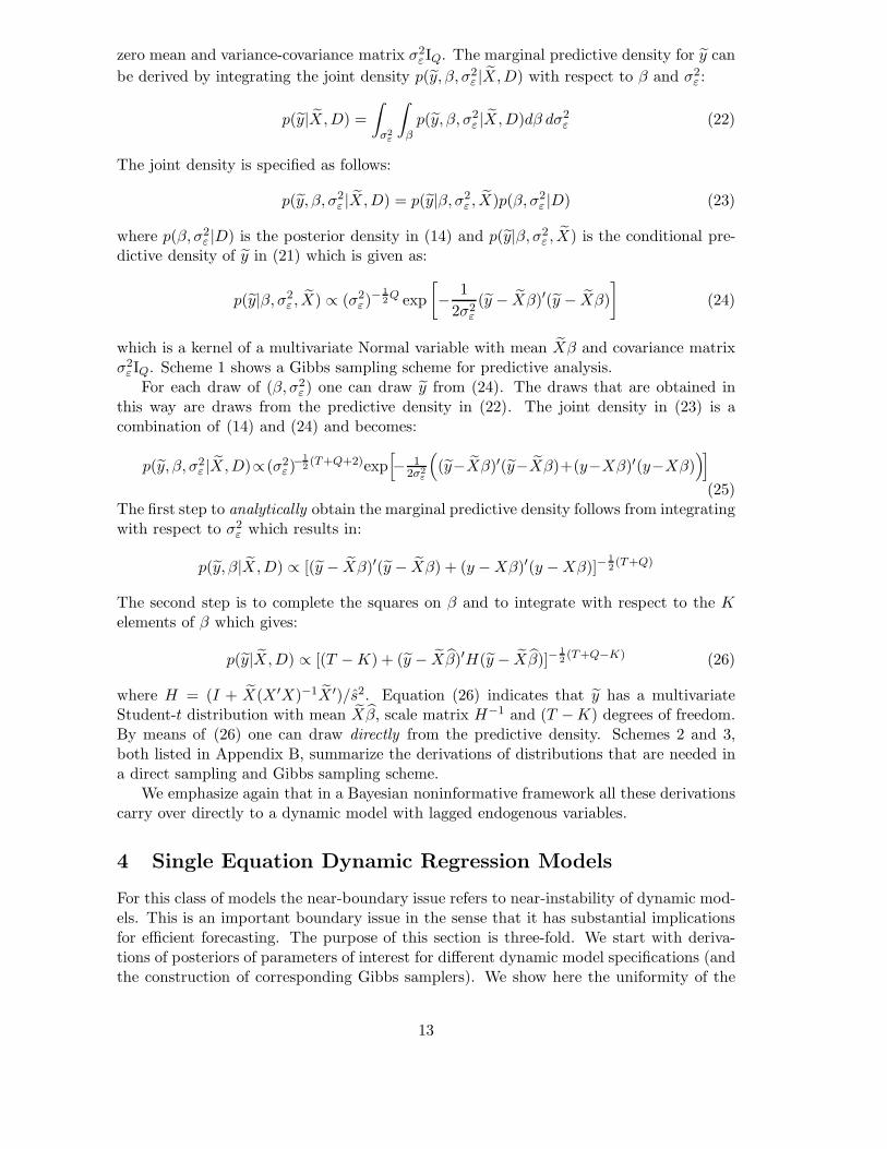
For series that are near unit root, substantial probability mass will lie close to ρ = 1and at ρ = 1 so that the impropriety of the joint posterior poses a serious issue. As anexample we depicted the joint density for the unit root model for a series of monthly dataon the 10-year U.S. Treasury Bond yield in Figure 6(a). A time-series plot of this series isgiven in Figure 7(b). Figure 6(a) clearly shows the pronounced wall feature close to andat ρ = 1. In order to resolve the impropriety of the joint density a local uniform prioror truncation of the domain for ρ could be used. Another possibility would be to use aregularizing prior like the Schotman and Van Dijk (1991a) prior. The joint density thatresults from

23

Figure 6: Joint posterior density in the unit root model

(a) Uniform prior (b) Schotman and Van Dijk (1991a) prior

Notes: Panel (a) shows the joint posterior density p(ρ, µ|y) when we use a uniform prior as in (13)whereas panel (b) shows the same posterior density however now with the prior proposed by Schotmanand Van Dijk (1991a) as given in (53). In both panels we use the end-of-month 10-year U.S. TreasuryBond constant maturity yield for the period January 1960-July 2007 as the data vector y.

combining the data likelihood with this particular prior is shown in Figure 6(b). The jointdensity no longer has a wall feature close to ρ = 1 although it still flattens out somewhatnear the edge of the domain. We note that this posterior may also be interpreted as theexact likelihood including the initial observation. For details see Schotman and Van Dijk(1991a).

We emphasize that the autoregressive model with an additive constant, equation (54),can be treated like the linear regression model of Section 3. Direct sampling or a simpleGibbs procedure is possible. The model with the ECM interpretation can be written as inthe autoregressive form of Sections 4.1.1 and 4.1.2 and deriving the corresponding Gibbssampling formulas is left to the interested reader. We also refer to that subsection for theconvergence issues of the Gibbs sampler.

Next, we treat the autoregressive model with additive linear trend. We start with adistributed lag model of order two,

yt = c + βt + ρ1yt−1 + ρ2yt−2 + εt with εt ∼ i.i.d N (0, σ2ε ) (57)

where t captures a linear increasing trend. We can rewrite this model as an error correctionmodel as follows. Consider

(1 − ρ1L − ρ2L

2)(yt − µ − δt) = εt with εt ∼ i.i.d N (0, σ2

ε ) (58)

using c = µ(1 − ρ1 − ρ2) + δ(ρ1 + 2ρ2) and β = (1 − ρ1 − ρ2)δ and where L is the lagoperator; Lyt = yt−1. Applying this operator to equation (58) we obtain

yt = (1 − ρ1 − ρ2)µ + δ (t − ρ1(t − 1) − ρ2(t − 2)) + ρ1yt−1 + ρ2yt−2 + εt (59)

This equation can be rewritten further as

∆yt = δ + (ρ1 + ρ2 − 1) (yt−1 − µ − δ(t − 1)) − ρ2 (∆yt−1 − δ) + εt (60)

24

which shows that yt is mean-reverting towards a linear trend when ρ1 + ρ2 < 1, otherwisewe have a random walk with drift (if ρ1+ρ2 = 1). This is our ECM model with linear trend.Similar as in Section 4.1.1, the derivation of the conditional densities can be simplified ifwe rewrite (60) by conditioning on one of the two types of regression coefficients. Like forthe linear model with autocorrelation, the idea is that given ρ = [ρ1, ρ2]

′ one has a linearmodel in β = [µ, δ]′ whereas given β one has a linear model in ρ. First, we rewrite (58)conditional on values for ρ:

y∗t = X∗t β + εt where

{y∗t = y∗t (ρ) ≡ yt − ρ1yt−1 − ρ2yt−2

X∗t = X∗

t (ρ) ≡ [1 − ρ1 − ρ2, t − ρ1(t − 1) − ρ2(t − 2)](61)

yt = ρyt− + εt where

{yt = yt(β) ≡ y − µ − δtyt− = yt−(β) ≡ [yt−1 − µ − δ(t − 1), yt−2 − µ − δ(t − 2)]

(62)

Posterior densities and predictive densities can now be derived in the same fashion as forthe linear and autoregressive models from Section 3 and 4.1.2. We note that we use therestriction ρ1 + ρ2 < 1 in the Gibbs sampling scheme, since in the unrestricted case theposterior is improper.

We can summarize this section by stating that what we did was to make a distinctionbetween additive deterministic terms in autoregressive models and ‘interpretable’ deter-ministic terms in error correction models. The interpretation of mean or trend reversionis important in economics. In addition, the resulting forecasts from these models can bequite different. Given our interest in near-boundary analysis, the smooth transition tothe boundary (from stationarity to unit roots) is relevant for model comparison, modelaveraging and forecasting. This is a well-known topic in the literature, see Sims and Uhlig(1991) and Schotman and Van Dijk (1991a,b, 1993) among others. In this paper we do,however, not focus on computing posterior model probabilities for model selection for thechoice or test for stationarity and unit root cases. Our interest in these models is primarilyfrom a forecasting perspective.

4.2 Illustrative empirical analysis using macroeconomic series

4.2.1 Possible unit root models in inflation, interest rates and dividend yield

Before we apply the models discussed in this section to analyze our main macroeconomicseries of interest, U.S. GDP growth, we apply the autoregressive model of the previousparagraph to three time series which are of important economic relevance: U.S. inflation,the 10-year U.S. Treasury Bond yield and the Standard & Poor’s 500 Index DividendYield. Figure 7 shows time series plots of each of the series. We note that this section isby no means meant to be a full attempt at modelling these series empirically, it is purelyfor illustrative purposes. We aim at analyzing the posterior mean, a unit root and, next,how to deal with the latter in a model averaging procedure for forecasting purposes.

The first series we analyze is inflation. We collected quarterly U.S. CPI figures from theFederal Reserve of Philadelphia database. We then construct inflation, πt, as the quarterlydifferences in log price levels, πt = ln(CPIt) − ln(CPIt−1). The data sample runs from1984:Q1 to 2006:Q3, for a total of 91 observations. The model we estimate is specified asin (55):

πt − µ = ρ(πt−1 − µ) + εt, with εt ∼ i.i.dN (0, σ2ε ) (63)

25

Figure 7: Macroeconomic and financial series

(a) inflation (b) 10-year Treasury Bond yield

(c) Dividend Yield

Notes: Shown in this figure are in Panel a) quarterly changes in log U.S. price levels (CPI), Panel (b)end-of-month levels of the U.S. 10-year Treasury Bond constant maturity yield and Panel (c) monthlydividend yield on the Standard & Poor’s 500 Index.

This specification allows us to analyze first-order autocorrelation in inflation growth. Fig-ure 8 and Table 1 show posterior results based on 10,000 draws from the Gibbs sampler18.The first column of Table 1 shows that first-order autocorrelation seems to be an importantfeature of inflation as it cannot be rejected at any reasonable level of credibility. We noteagain that the posterior is improper but that the Gibbs sampler does not detect this (i.e.it does not reach the absorbing state in our finite set of random drawings) since we areso far away from the boundary. A simple truncation of the region for ρ seems a practicalsolution in this case. Figure 8(b) confirms that the value of ρ = 1 will only occur withextremely low probability.

The second series we consider is the U.S. 10-year Treasury Bond constant maturity

18The Gibbs sampler is applied with a burn-in period of 4,000 draws and a thinning value of two.

26

yield. Data for this series was collected from the FRED database and the sample spansthe period January 1960 to July 2007 for a total of 571 monthly observations. The model

Table 1: Posterior results for inflation, Treasury Bond and dividend yield series

parameters CPI TBU TBR TBRW DYU DYR DYRW

c − − − 0.0005 − − −0.0002− − − [0.0122] − − [0.0006]

µ 0.7706 ±∞ 6.9739 − ±∞ 0.2480 −[0.0675] − [1.1956] − − [0.0586] −

ρ 0.4487 0.9992 0.9895 1 0.9993 0.9893 1[0.0994] [0.0025] [0.0014] − [0.0025] [0.0019] −

σ2ε 0.1083 0.0856 0.0854 0.0855 0.0177∗ 0.0176∗ 0.0177∗

[0.0166] [0.0051] [0.0051] [0.0050] [0.0012] [0.0011] [0.0011]

predictions

RMSPE - 3m 0.3031 − 0.6922 0.7015 − 0.0213 0.0211RMSPE - 6m 0.3184 − 0.9569 0.9844 − 0.0307 0.0303RMSPE - 12m 0.3441 − 1.4099 1.4914 − 0.0454 0.0443

Notes: The table presents posterior means, posterior standard deviations (in between brackets), and the RootMean Square Prediction Error (RMSPE) for models on U.S. quarterly inflation growth [CPI], U.S. 10-year TreasuryBond constant maturity yield [TB] and Standard & Poor’s 500 Index dividend yield [DY]. The subscripts for TBand DY distinguish between using an unconstrained parameter space (TBU , DYU), imposing stationarity withρ < 1 (TBR, DYR) and imposing a random walk with drift (TBRW , DYRW ). A star (*) indicates that the numberhas been multiplied by a factor 100. The RMSPE results are for 3, 6 and 12 months ahead predictions for thesample 1985:Q1 - 2007:Q2.

we apply to analyze unit root behavior in the 10-year yield yt is again the ECM model in(55). Learning about the value of ρ is crucial for several reasons. For example, ρ determineswhether long run forecasts will converge to a long-term mean (ρ < 1) or whether they willdisplay explosive behavior (ρ > 1). We analyze three specifications of the ECM model.In the first application we use a noninformative prior on ρ and we refer to this approachas TBU . We note that with this case of a flat prior on a large region it can be shown,using the results of sections 4.1.1 and 4.1.2, that the posterior of (µ, ρ) is improper. Yeta naive application of the Gibbs sampler will produce results. We emphasize that this isnot a limitation/fault of the Gibbs sampler. It is simply the consequence of a poor searchof the shape of the posterior and it is simply a wrong application of Gibbs. However, thismay occur and has occurred in practice. We use TBR to indicate the second approachfor which we estimate the model under stationarity by truncating the parameter spaceto ρ < 1. Finally, in the third approach we consider model (54) and impose a unit root(ρ = 1) and analyze a random walk with drift model, TBRW .

Figure 9 and Table 1 show that the improper posterior density of ρ, which has anasymptote at 1, has substantial probability mass close to 1 and even some mass beyond1. These results suggest that the 10-year Treasury yield may be nonstationary whichis difficult to interpret economically, however. The second application therefore uses atruncation prior to restrict ρ to be lower than 1. Panel (b) in Figure 9 shows the posteriordensity of ρ. Posterior densities for the other model parameters look similar in both cases.

To assess the restrictiveness or importance of restricting ρ to be smaller than 1 weperform a small forecasting exercise19. In particular, we make 3, 6 and 12 month aheadforecasts (with the forecast taken to be the mean of the predictive density) starting in

19Because of the posterior being improper we do not report forecast results for TBU and DYU in Table1.

27

Figure 8: Posterior density histograms for CPI

(a) µ (b) ρ

(c) σ2ε

Notes: Shown in this figure are posterior density histograms for the model in (63). Panel (a) shows thedensity for µ, (b) for ρ and (c) for σ2

ε . The densities are based on 10,000 draws from the Gibbs sampler.

January 1985. We construct forecasts using an expanding window approach. In particular,we use the sample from January 1960 to December 1984 to construct the forecast forJanuary 1985. We then expand the estimation sample to include the realized January 1985yield value in order to construct the forecast for February 1985 and we keep expanding thesample in the same way until the final forecast, July 2007, which is based on the estimationsample January 1960 to June 2007. The bottom rows of Table 1 report results. We assessforecasting accuracy by means of the Root Mean Squared Prediction Error (RMSPE).The results seem to indicate that imposing the truncation is relevant since the RMSPE isreduced for all horizons.

The third and final series that we examine is the dividend yield on the Standard andPoor’s 500 Index which is a commonly used predictor variable for forecasting stock returns,see e.g. Keim and Stambaugh (1986), Campbell and Shiller (1988) and Fama and French(1988). We use monthly data from January 1966 to December 2006 (492 observations).Figure 7(c) shows that the dividend yield has a quite different pattern in the initial 20years compared to the 1990s and beyond. Whether or not the dividend yield displays unitroot-type behavior is a widely discussed topic in the literature, see e.g. Cochrane (2006).

28

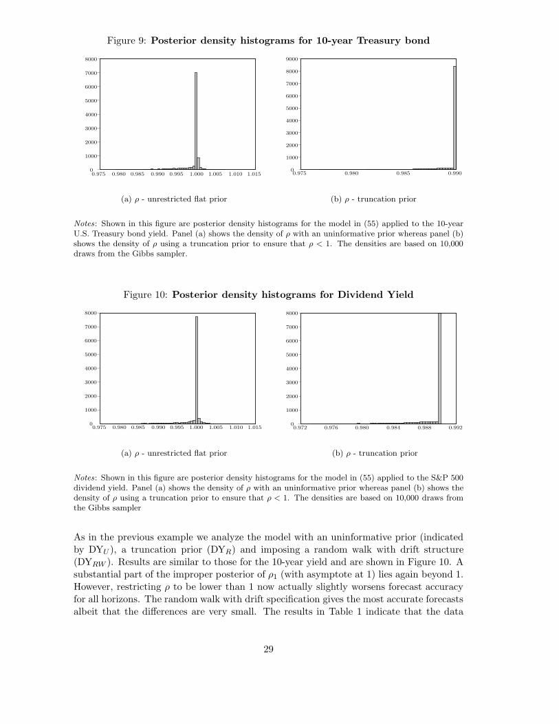
Figure 9: Posterior density histograms for 10-year Treasury bond

(a) ρ - unrestricted flat prior (b) ρ - truncation prior

Notes: Shown in this figure are posterior density histograms for the model in (55) applied to the 10-yearU.S. Treasury bond yield. Panel (a) shows the density of ρ with an uninformative prior whereas panel (b)shows the density of ρ using a truncation prior to ensure that ρ < 1. The densities are based on 10,000draws from the Gibbs sampler.

Figure 10: Posterior density histograms for Dividend Yield

(a) ρ - unrestricted flat prior (b) ρ - truncation prior

Notes: Shown in this figure are posterior density histograms for the model in (55) applied to the S&P 500dividend yield. Panel (a) shows the density of ρ with an uninformative prior whereas panel (b) shows thedensity of ρ using a truncation prior to ensure that ρ < 1. The densities are based on 10,000 draws fromthe Gibbs sampler

As in the previous example we analyze the model with an uninformative prior (indicatedby DYU ), a truncation prior (DYR) and imposing a random walk with drift structure(DYRW ). Results are similar to those for the 10-year yield and are shown in Figure 10. Asubstantial part of the improper posterior of ρ1 (with asymptote at 1) lies again beyond 1.However, restricting ρ to be lower than 1 now actually slightly worsens forecast accuracyfor all horizons. The random walk with drift specification gives the most accurate forecastsalbeit that the differences are very small. The results in Table 1 indicate that the data

29

does not provide a clear answer as to whether the dividend yield series is stationary ornonstationary.

As mentioned earlier the results of this section are for illustrative purposes only. Amore detailed analysis for the Treasury bond and dividend yield series should involveBayesian diagnostic checking on the (mis-)appropriateness of using Gibbs sampling resultsfrom improper posteriors and using a misspecified model like the autoregressive modelwith a possible unit root in a forecasting exercise. Further, Figures 7(b) and 7(c) suggesta time varying trend and this data feature should be modelled. However, a detailedBayesian misspecification and/or empirical analysis for these series is beyond the scope ofthe present paper and is therefore left to the interested reader.

4.2.2 U.S. real GDP growth

We develop our empirical analysis mainly on one key macroeconomic series: U.S. GrossDomestic Product (GDP) growth. We apply the models from the previous paragraphs (aswell as those in Section 5.1.2) to model this series to illustrate boundary issues and toshow how to approach these. We collected real GDP (seasonally adjusted) figures fromthe U.S. Department of Commerce, Bureau of Economic Analysis. Figure 11(a) plots thelog quarterly GDP level for our sample 1960:Q1 to 2007:Q2 (190 observations) and showsthat GDP

Figure 11: U.S. GDP

Notes: Shown in this figure are in Panel (a) quarterly log levels of real U.S. GDP whereas Panel (b) showsthe quarterly GDP growth rate (in % terms). The sample is 1960:Q1 - 2007:Q2.

has followed an upward sloping pattern but with fluctuations around this trend. The quar-terly growth rate of log GDP, gt = ln GDPt−lnGDPt−1, shown in Figure 11(b), underlinesthese fluctuations with periods of positive changes followed by periods of negative changes,clearly indicating business cycles. The sample average growth rate is positive but with ahigh level of variation which is mainly due to different cycles (for more details we refer toHarvey et al., 2007). We apply the various linear models we discussed earlier to model andassess empirical facts on stochastic shocks over the full sample so as to assess these models’suitability in a out-of-sample forecasting exercise. In the forecast exercise we use an initialin-sample period from 1960:Q1 to 1992:Q2 to obtain initial parameter estimates and weforecast the GDP growth figure for 1992:Q3. We then expand the estimation sample with

30

the value in 1992:Q3, re-estimating the parameters, and we forecast the next value for1992:Q4. We continue this procedure up to the last value and we end up with a total of60 forecasts. Also here we remark that this section is not meant as a full-fledged empiricalanalysis of U.S. GDP. We mainly want to analyze and compare the various linear modelsfor illustrative purposes. It is also for this reason that we ignore the ‘great moderation’that occurred in fluctuations of real GDP since 1985 in our analysis, see Stock and Watson(2002).

Random walk with drift for GDP growth

The first model that we put forth to describe U.S. GDP growth is the univariate constantmodel in equation (10):

gt = c + εt with εt ∼ i.i.d. N (0, σ2ε ) (64)

Figure 12: Joint and conditional posterior densities

(a) p(c, σ2ε |D)

(b) p(c|σ2ε , D)

0.9

0.8

0.7

0.6

1.1

1.0

0.80.9

1.11.2

0.7

0.50.4

0.6

1.0

(c) p(σ2ε |c, D)

Notes: Panel (a) shows the joint posterior of c and σ2ε whereas panels (b) and (c) show the conditional

posterior density of c for given values of σ2ε and the data D; p(c|σ2

ε , D) and the conditional density of σ2ε

for given values of c and the data; p(σ2ε |c, D) respectively. We apply the linear regression model (64) to

quarterly U.S. GDP growth.

We refer to this model by the label ‘random walk with drift’ in tables and graphs.This model allows us to infer the average growth rate of GDP although with the drawback

31

that other fluctuations cannot be explained. Section 3 provides details on how to computeposterior densities and predictive densities using the Gibbs sampler. We note that in thiscase direct sampling is also a good strategy for efficient computation.

Figure 12 shows the posterior densities p(c|σ2ε ,D) and p(σ2

ε |c,D) and clearly revealsthe conditional Normal and conditional Inverted Gamma densities. Also shown is the jointposterior density.

Table 2 and Figure 13, which summarize posterior results, show that the growth rate ison average positive, well distributed around the mean value of 3.25% (in annual terms) witha small variance. However, the model explains relatively little as the residual variance isquite close to the unconditional variance of GDP growth which equals 0.71%. In addition,the posterior standard deviation of σ2

ε is quite substantial as well.

Table 2: Posterior results for U.S. GDP

growth levels

parameters RW+drift simple ECM ECM trendµ - 3.2516∗ 16.8940 −

- [0.3308]∗ [3.8574] −c 3.2500* − − 1.5417∗

[0.2460]* − − [0.5512]∗δ - − −0.0087 −

- − [0.0157] −β - − − 0.0004

- − − [0.0001]ρ1 - 0.2719 1.1624 1.2246

- [0.0715] [0.0901] [0.0706]ρ2 - − −0.2596 −0.2727

- − [0.0715] [0.0701]σ2

ε 0.7214 0.6750 0.6711 0.6490∗∗[0.0749] [0.0712] [0.0704] [0.0682]

Notes: The table presents posterior means and posterior standard deviations (in betweenbrackets) for models for log real U.S. GDP level/growth. The considered models are (i)the random walk with drift model (for GDP growth), (ii) the simple ECM model in (55)(for GDP growth), (iii) the ECM model in (60) (for GDP growth) and (iv) the trend modelin (57) (for GDP level). Note that the interpretation of the parameter µ is different in (55)and (60). In the simple ECM µ represents the unconditional mean of the series whereasfor the ECM in (60) it represents the constant of the linear trend line. The difference ininterpretation also applies to c. For the random walk with drift model it represents thedrift whereas for the trend model it is the constant of the trend line. One star (*) indicatesthat the number has been annualized (multiplied by a factor of 4), two stars (**) is for amultiplication factor of 104.

Moving to Table 3 which contains the MSPE results of our forecast exercise, we dofind that the model has higher forecasting power than the benchmark random walk (RW)model. The RMSPE of the constant mean model is lower for all horizons compared to therandom walk.

32

Figure 13: GDP: random walk with drift

(a) c (b) σ2ε

Notes: Shown in this figure are posterior density histograms for the model in (64). The left hand sidepanel shows the density for c whereas the right hand side panel is for σ2

ε . The densities are based on 10,000draws from the Gibbs sampler. Note that the left hand side panel shows the density of quarterly growthwhereas the results in Table 2 are stated in terms of annualized growth.

Table 3: Forecast accuracy results for U.S. GDP growth

RW RW+drift simple ECM trend ECM TVP BMA BMA BMA[1] [2] [3] [4] [5] [6] [2],[3] [4],[5],[6] [2]-[6]

RMSPE - 1Q 0.6198 0.4738 0.4761 0.4713 0.4724 0.4726 0.4700 0.4802 0.4865RMSPE - 2Q 0.5462 0.5299 0.5178 0.5050 0.5220 0.5318 0.4742 0.4991 0.4991RMSPE - 4Q 0.6118 0.5257 0.5251 0.5054 0.5202 0.5223 0.4888 0.5131 0.5474

Notes: The table presents Root Mean Squared Prediction Error (RMSPE) results for U.S. GDP growth for variousmodels. The models used are [1] the random walk model, [2] the random walk with drift model, [3] the ECM modelin (55), [4] the model with additive trend (57), [5] the error correction model in (60), [6] the time-varying parametermodel (91)-(92) and three Bayesian model averaging (BMA) schemes: (i) averaging over the random walk with driftand simple ECM model, (ii) averaging over the trend, ECM and time-varying parameter model and (iii) averaging overall models. The out-of-sample period is 1992:Q3-2007:Q2 (60 forecasts) and an expanding window approach is usedfor each model. For the BMA models we use the initial 30 forecasts from 1985:Q1-1992:Q2 as training period.

Simple error correction model for GDP growth

The second specification that we propose is the error correction model in (55). Allowingfor autocorrelation in GDP growth may be beneficial. The model is given by

gt − µ = ρ(gt−1 − µ) + εt, with εt ∼ i.i.d N (0, σ2ε ) (65)

and we refer to it as ‘simple ECM’. Section 4 gives estimation details for this model.Posterior results are shown in the second column of Table 2. It can be seen for µ thatwhereas its posterior mean is again positive and very close to the posterior mean of c in theprevious model, the explanatory power of the model increases. The posterior mean of ρ is0.27 and Figure 14 shows that nearly all probability mass is to the right of 0. The latterobservation provides evidence of the presence of autocorrelation in growth. Here we seeagain an example where the posterior is improper. However, the data keep the parameter

33

ρ away from 1. We use as potential solution a truncated density where the truncationis a binding constraint in practice. Finally, the density of σ2

ε has both a lower posteriormean and posterior variance which suggests that this model explains more variation inGDP growth than the random walk with drift model. Similarly, allowing for first-orderautocorrelation in growth improves forecast accuracy as shown in Table 3 although theimprovement is only marginal (and only for longer horizons). A possible explanation isthat both models have a nearly identical posterior mean for µ.

Figure 14: GDP: simple ECM for growth

(a) ρ (b) σ2ε

Notes: Shown in this figure are posterior density histograms for the model in (65). Panel (a) shows thedensity for ρ and (b) for σ2

ε . The densities are based on 10,000 draws from the Gibbs sampler.

Autoregressive model with additive linear trend for GDP level

In addition to using models for GDP growth we also analyze models that draw inferenceon the level of GDP. In particular we consider an autoregressive distributed lag model forGDP level. Within these types of models one attempts to explain the level of GDP byusing the information in lagged GDP levels and a linearly increasing variable. The modelwe consider here is that of (57) and is given as:

ln GDPt = c + βt + ρ1 ln GDPt−1 + ρ2 ln GDPt−2 + εt with εt ∼ i.i.d. N (0, σ2ε ) (66)

which we refer to as ‘trend’. The results in Section 3 can be used to draw inference on theparameters in this model.

Table 2 shows that the constant (or long term growth rate) is positive. However, itsvalue is substantially lower than when we model the growth rate directly and cannot bedirectly interpreted as being the average growth rate. Part of the long term growth rate isnow being explained by the trend (long term trend) which, as we may expect, has a positiveposterior mean and a small standard deviation. The behavior of the lag parameters of pastGDP levels is also interesting to examine. The first lag has a distribution which lies almostentirely beyond 1, implying compounding GDP growth. However, the parameter of thesecond lag is always negative, which captures the cycles in GDP. The residual variance isvery small compared to the previous two models.

Panel (a) of Figure 15 shows the posterior density histogram of the persistence inln GDP , as measured by ρ1 + ρ2. We note that we do not truncate the parameter space

34

Figure 15: GDP: autoregressive model with linear trend and ECM

(a) ρ1 + ρ2 (b) ρ1 + ρ2

Notes: Shown in this figure is the posterior density histograms of the persistence parameter ρ1 + ρ2 for thetrend model (66) in Panel (a) and the error correction model (60) in Panel (b). The densities are based on10,000 draws from the Gibbs sampler.

of ρ1 and/or ρ2 here. We emphasize that even with a flat prior on a large region, theposteriors of the parameters in (63) are proper. Whereas this unrestricted model doeswell in terms of in-sample fit, the fact that there is some probability mass for ρ1 + ρ2 > 1(as shown in Figure 15) implies that the model can potentially display explosive behaviorwhen forecasting future values. In fact, Table 3 shows that the forecast accuracy of thismodel is high, but not superior to that of the random walk with drift model.

Error correction model for GDP level

As a final model for GDP levels we analyze the error correction model given in (60). Panel(b) in Figure 15 shows the persistence in GDP. Here we do truncate the parameter spacesuch that ρ1 + ρ2 < 0.95. Not doing so results in ρ1 and ρ2 often adding up to values closeto 1 in the Gibbs sampling algorithm which makes inference on the remaining parametersµ and δ difficult. The ECM with truncation provides accurate forecasts, even though theseare marginally worse than the forecasts of the simple ECM and the trend models.

Because the forecast performance of all models is very similar it is unclear whetherone should decide to model the level of GDP or its growth rate directly to forecast GDPgrowth. In Section 6 we propose a simple procedure, that of model averaging, to alleviatethis decision problem. As we show in Table 3, the model averaging of a random walk withdrift and a simple error correction model gives the most accurate forecasts.

4.3 Remark on equivalence between boundary problems in dynamic re-

gression models and instrumental variable models

The final class of models that we discuss in the current section is the class of multivariatemodels. The issues involved here are similar to those surrounding univariate unit rootmodels, i.e. nonidentifiability of parameters. This results in the Information matrix beingsingular, or alternatively, in the Hessian having a reduced rank. This reduced rank problem

35

can occur in several well-known models, such as for example cointegration models, VectorAutoregressive (VAR) and Simultaneous Equation Models (SEM) which in turn are closelylinked to Instrumental Variables (IV) models.

To show which role nonidentifiability plays in these models we give an example bymeans of a just identified IV model and in particular we focus on the Incomplete Simul-taneous Equation Model (INSEM). Our analysis, which is necessarily brief, is based onVan Dijk (2003) and Hoogerheide et al. (2007) and we refer to these studies for a morein-depth analysis. Consider the INSEM model as it is specified in Zellner et al. (1988)20

y = xβ + ε (67)

x = zπ + ν (68)

[ε ν]′ ∼ N([0 0]′ ,Σ

)with Σ =

[σ2

ε σε,ν

σε,ν σ2ν

](69)

with y, x and z all having dimensions (T × 1) and β and π being scalar parameters. Inthis model, (67) is to be interpreted as the structural relation of interest, x is an endoge-nous variable and z is the (weakly exogenous) instrument. Similarly, β is the structuralparameter of interest and |π| measures the quality of the instrument. Furthermore, thecorrelation parameter ρ =

σε,ν√σ2

εσ2ν

measures the degree of endogeneity of x in the equation

for y. Equations (67)-(69) comprise the structural form of the INSEM. By substituting(68) in (67) we can derive the reduced form which is given by

y = zπβ + ξ (70)

x = zπ + ν (71)

with ξ = ε + νβ and [ε ν]′ as in (69). We can interpret the reduced form model as amultivariate regression model which is nonlinear in the parameters β and ρ as in (44).As was the case in the unit root model this nonlinearity can lead to a nonidentifiabilityproblem. In particular, when we assume a flat prior on the parameters β and π, thenwhen π = 0 (this is usually labeled as the case of no identification or case of irrelevantinstruments) the joint posterior density is improper because it is flat and nonzero in thedirection of β. In fact, the joint density looks very similar to that in Figure 6(a) in thesense that it has a wall at π = 0. Therefore, β is not identified when π = 0 whereas itis for any π 6= 0. In a multivariate setting where y, x and z are all matrices and β and πare matrices as well, the identification problem of (part of the elements) of β occurs whenπ = 0 or when π is of reduced rank. The above problem is known as local nonidentificationand is discussed in detail in Kleibergen and Van Dijk (1998).

As a result of the local nonidentification problem, the marginal density of π is non-integrable because of infinite probability mass near π = 0 (see Kleibergen and Van Dijk,1998). Whether or not the impropriety of the joint density will be revealed in the outputfrom the Gibbs sampler is unclear. Slow convergence of the Gibbs sampler due to the factthat π = 0 is acting as an absorbing state could be an indication. Examples of bimodalposterior densities on bounded intervals are given in Hoogerheide et al. (2007). A possiblesolution to circumvent the local nonidentification problem in INSEM models would againbe the specification of sensible prior densities. However, it can be an arduous task to findconjugate priors, mainly since these will have to curtail multiple parameters all at thesame time.

20The reason this model is called just identified is because there is only a single instrument, z.

36

5 Variance Components and State Space Models

We now switch our attention to drawing inference on variance parameters instead of regres-sion parameters. In particular, we focus on situations when a variance component tendstowards the zero bound or when a degrees of freedom restriction may be violated or anidentification problem arises. We do so by again analyzing a canonical type of model, theso-called Hierarchical Linear Mixed Model (HLMM). This model is a variance componentsmodel, that is, the relative importance of several variances is the object of study. A secondfeature of this canonical model is the presence of unobserved components. The startingpoint of our analysis will be a basic specification of the HLMM. This model serves as aparent model for extensions such as a state space model and a panel data model, whichwe discuss subsequently.

5.1 Heteroscedasticity and Hierarchical Linear Mixed Models

Before we specify the basic setup of the HLMM we first discuss two preliminary models,focusing on variances of disturbances. The models serve to identify the following twoissues: (i) a degrees of freedom bound which refers to a sufficient number of observationsor a sufficient number of cross-sectional groups, and (ii) an identification issue or labelingissue with respect to the different variance components.

5.1.1 Linear regression model with a small number of observations or naiveheteroscedasticity

T = small, degrees of freedom bound

In Section 3 we analyzed the basic linear regression model. Now we revisit this modelwhich we simplify using xt = 1 and β = µ

yt = µ + εt, t = 1, ..., T, with εt ∼ N (0, σ2ε ) (72)

We emphasize that the number of observations T may refer to the number of observation ina time-series and to individuals or groups of individuals in a cross-section. For notationalconvenience, we use the same symbol T here for time series and cross-section observations.If we use a uniform prior on both µ and σ2

ε ,

p(µ, σ2ε) ∝ 1 (73)

then, from the results of Table B-1 in Appendix B we can derive the marginal densitiesof µ and σ2

ε . Note, however, that because the prior is now that of (73) instead of (13), wehave two degrees of freedom less. The marginal densities are given by

p(µ|y) ∼ t

(µ,

(T − 3)T

s2, T − 3

)

p(σ2ε |y) ∼ IG

(1

2(y − ι

Tµ)′(y − ι

Tµ),

1

2(T − 3)

)

with y the full vector of observations; y = [y1 . . . yT ]′, µ = 1T

ι′Ty and s2 = y′Mι

Ty. The

degrees of freedom for the general linear regression model with the prior in (73) is T−K−2.For the model in (72) we have K = 1 . From the parameters of the marginal densities and

37

the conditions given in Appendix C it is clear that in order for these Student-t and InvertedGamma densities to exist one needs more than 3 observations, i.e. T > 3. Analogousresults can be derived for the existence of higher order moments. For illustration, Figure16 shows that the right tail of an Inverted Gamma density tends to zero at a rate that istoo small when the number of degrees of freedom is too small. For instance, for T = 4 thezeroth moment exists but the higher moments do not21.

Figure 16: Inverted Gamma density

Notes: The graph shows the Inverted Gamma density function, as specified in (C-3), for m = 10 and for avarying number of degrees of freedom, ν.

The conditional densities, using a uniform prior, are given by

p(µ|y, σ2ε) ∼ N

(µ,

σ2ε

T

)

p(σ2ε |y, µ) ∼ IG

(1

2(y − ι

Tµ)′(y − ι

Tµ),

1

2(T − 2)

)

Only focusing on these conditional densities shows that T = 3 is a already sufficient forthe Gibbs sampler to function properly. However, it follows from our analysis that themarginal densities for µ and σ2

ε do not exist. Thus, we have a simple case where the Gibbssampler can be applied as a simulation method, whereas the joint and marginal densitiesdo not exist (similar as the ridge example in Section 2.2) , see also the discussion in forexample Koop (2003). Therefore, the generated Gibbs sequences cannot be interpreted.We emphasize that for the usual number of time series observations this degrees of freedomrestriction is obviously of no significance. However, for the case of the number of groupsin a panel it may become restrictive. In Section 5.5 we give an example using a panel datamodel.

Naive heteroscedasticity and a degrees of freedom bound

Consider model (72) in which each observation yt, for t = 1, . . . , T , is allowed to have itsown variance parameter σ2

t . When we use a uniform prior on µ as well as on each of the

21A Jeffreys’ type prior, p(σ2ε) ∝ 1/σ2

ε , increases the number of degrees of freedom with 1. As a result,densities now exist for T > 1.

38

σ2t components then the posterior of (µ, σ2

1 , . . . , σ2T ) is given as:

p(µ, σ21 , . . . , σ

2T |y) ∝

T∏

t=1

(σ2

t

)− 12 exp

[− 1

2σ2t

(yt − µ)2]

(74)

The posterior is unbounded since for some t, one may have yt = µ and/or σ2t = 0,

then p(µ, σ21 , . . . , σ

2T |y) → ∞. One solution would be to partition the observations into

groups, assuming that per group the variance is constant whereas it is allowed to bedifferent across groups. Each partition needs to be chosen in such a way that it containsa sufficient number of observations. Our main point, although trivial as it may seem, isthat the degrees of freedom restriction implies that one needs multiple observations todraw inference on variance components. This becomes particularly relevant in dynamicpanels with groups of observations, see Section 5.5. We note that Geweke (1993) uses aweakly informative Inverted Gamma density which makes the posterior more regular. Thelinear regression model with naive heteroscedasticity serves as introduction to the class ofHierarchical Linear Mixed Models, since the latter class is not so well-known in economics.

5.1.2 Hierarchical Linear Mixed Model

An example of a canonical model with multiple variance components is the class of Hi-erarchical Linear Mixed Models (HLMM). Instead of T variances, one has two variancecomponents with the additional issue of two stochastic processes. We introduce this classthrough the following hierarchical model with two variance components

yt = µt + εt, with εt ∼ N (0, σ2ε ) for t = 1, . . . , T (75)

µt = θ + ηt, with ηt ∼ N (0, σ2η) and E[εtηs] = 0 (76)

with µ = (µ1, . . . , µT )′ a vector containing the time-varying mean of y and θ the mean ofthe distribution of µt which, for any t, is Normal with variance σ2

η.This model serves as a parent model for more elaborate models such as state space

models or panel data models. Before moving on to introducing and discussing these models,we analyze the base model by distinguishing between two cases. The first case assumesthat σ2

ε is known with T being small whereas the second case is the opposite: σ2ε is assumed

unknown and T is large. Each case helps to gain a better understanding of the existenceconditions for joint, conditional and marginal posterior distributions of the HLMM classof models. Note that unless stated otherwise, we assume a uniform prior for each of thevariance components.

(i) σ2ε = 1 and T small: a degrees of freedom bound

Because σ2ε is given and equal to 1, the only unknown variance component is σ2

η . Therequirement on a minimum number of degrees of freedom as discussed in the previousparagraph is of importance here. Sensible posterior results can only be obtained whenthere is a sufficient number of observations. The conditional densities p(θ|σ2

η) and p(σ2η |θ)

can be derived by substituting (76) in (75)

yt = θ + εt + ηt with εt ∼ N (0, σ2ε ), ηt ∼ N (0, σ2

η) (77)

The joint posterior density is

p(θ, σ2η |σ2

ε = 1, y) ∝ (σ2η + 1)−

12(T−1) exp

[− 1

2(σ2η + 1)

(y − ιTθ)′(y − ι

Tθ)

](78)

39

By using the transformation of random variables: σ2η∗ ≡ σ2

η +1, one is back in the situationof the beginning of Section 5.1. A degrees of freedom bound is necessary for obtainingexistence of posterior moments. Gibbs sampling is possible but not sensible when thenumber of observations (or the number of groups) is less than or equal to 3. This isessentially the same result as is more formally derived by Hobert and Casella (1996).We refer the interested reader to that reference for details but we emphasize here thatsubstitution of (76) in (75) yields a simplified derivation of the Hobert and Casella resulton the degrees of freedom restriction. As before, the Gibbs sampler may seem to workin this model even when the marginal posterior densities for θ and σ2

η do not exist, seeHobert and Casella (1996) for an example and discussion22.

(ii) σ2ε unknown and T large: an identification or labeling issue

By taking T large enough, one no longer needs to worry about the marginal posteriordensities possibly being nonexistent. However, making the first variance component, σ2

ε ,unknown as well introduces a new issue. More specifically, one now has to deal with anidentification or labeling issue in the sense that it is not possible to distinguish the twovariance components from each other. Why this is the case can be made clear as follows.Note first that since T is assumed to be large enough, the marginal densities of σ2

ε and σ2η

will exist. However, respecifying the model in (77) to

y = ιTθ + ε + η with ε ∼ N (0, σ2

ε IT) and η ∼ N (0, σ2

ηIT) (79)

yields that the unconditional mean and variance of y are given by E [y] = ιTθ and V[y] =

(σ2ε + σ2

η)IT. Also, the joint posterior density which, after integrating out θ, is given by

p(σ2η, σ

2ε |y) ∝ (σ2

η + σ2ε)

− 12(T−1) exp

(− 1

2

(y − ιTθ)′(y − ι

Tθ)

σ2η + σ2

ε

)(80)

with θ = y being the average of y. Clearly, only the total variance is identified, not theindividual components. Furthermore, the roles of σ2

ε and σ2η are interchangeable (this

explains the use of the term labeling issue). This holds true for any value of the signal-to-noise ratio which is defined as SN = σ2

η/σ2ε . Figure 17 shows the joint density for

signal-to-noise ratios of 1 and 0.5.Panels (a) and (b) show that irrespective of the signal-to-noise ratio the joint density

is perfectly symmetrical. It is also clear from the figure that the joint density will alwayshave a ridge. Note that everywhere along this ridge the sum of the variance componentsis the same. This becomes evident by first defining ξ = ε + η and σ2

ξ = σ2ε + σ2

η and thenrecognizing the resulting model as the basic linear regression model which only has a singlevariance component. The model in (75)-(76) basically splits up this single component intotwo components which explains the ridge. However, because this ridge is on a boundeddomain the joint density is nevertheless integrable23. The Gibbs sampler can therefore beused to obtain posterior results.

22Note that Hobert and Casella (1996) assume an independent Jeffreys’ prior as a result of whichthe Inverted Gamma density of σ2

η has one degree of freedom since their sample consists of T = 2groups/observations.

23The density shown in Figure 3(e) on the other hand has a ridge on the domain [0,∞) × [0,∞) whichmakes it nonintegrable on this domain. For expository purposes we restricted the domain in this figureand therefore for the figure the posterior is a proper density.

40

Figure 17: Joint posterior density of σ2ε and σ2

η with a uniform prior

(a) SN = 1 (b) SN = 0.5

Notes: Panel (a) and (b) show the joint density in (80) with a signal-to-noise (SN) ratio of 1 and 0.5respectively. For both panels y was simulated from (75)-(76) with θ = 1 and for panel (a) σ2

ε = σ2η = 1

whereas for panel (b) σ2ε = 2, σ2

η = 1 was used.

The joint posterior density of (σ2ε , σ

2η) is given in (80). The conditional density of σ2

ε ,given some draw or value for σ2

η is given by

p(σ2ε |σ2

η = σ2η , y) ∝ (σ2

η + σ2ε)

− 12(T−1) exp

[−1

2

(y − ιθ)′(y − ιθ)

σ2η + σ2

ε

](81)

and in a similar way one obtains p(σ2η |σ2

ε = σ2ε , y). Thus we are back in the situation of

Section 5.1.1. However, now these conditional posterior densities are identical and the roleof the two variance components is interchangeable. The dynamic processes in (75) and(76) have an identical structure. The result is an identification or labeling issue since it ispossible to relabel σ2

ε as σ2η and everything remains the same.

A further problem arises when instead of a uniform prior, an independent Jeffreys’prior for σ2

ε and σ2η is used, p(θ, σ2

ε , σ2η) ∝ 1

σ2ε

1σ2

η, in which case the joint density becomes

p(σ2η, σ

2ε |y) ∝ 1

σ2ε

1

σ2η

(1

σ2η + σ2

ε

) 12(T−1)

exp

(− 1

2

(y − ιTθ)′(y − ι

Tθ)

σ2η + σ2

ε

)(82)

Figure 18 shows that the Jeffreys’-type prior causes the joint density to shoot off toinfinity for either σ2

ε → 0 or σ2η → 0 24. Therefore, the joint posterior is now improper and

the Gibbs sampler will not converge25. The Jeffreys’ Information matrix prior in this caseis given as

p(σ2η, σ

2ε) ∝

√c(σ2

η , σ2ε , T )

∣∣∣∣[

1 11 1

]∣∣∣∣

12

(83)

24Although Figure 18 is similar in shape as Figure 4 the two figures have a very different interpretation.Whereas Figure 4 shows a density that has two well-defined modes (albeit far apart) the density in Figure18 is only well behaved in the domain (δ,∞) × (δ,∞) for a δ that is sufficiently far away from zero. Thelatter density goes to infinity when either of the variance components tends to zero.

25For an early Bayesian paper in this field we refer to Griffiths et al. (1979).

41

Figure 18: Joint posterior density of σ2ε and σ2

η with a Jeffreys’-type prior

(a) SN = 1 (b) SN = 0.5

Notes: Panels (a) and (b) show the joint density in (82) with a signal-to-noise (SN) ratio of 1 and 0.5respectively. For both panels y was simulated from (75)-(76) with θ = 1 and for panel (a) σ2

ε = σ2η = 1

whereas for panel (b) σ2ε = 2 and σ2

η = 1 was used.

where c(σ2η , σ

2ε , T ) = 1

2(T + 3)(σ2η + σ2

ε)−2. Clearly the determinant in the right hand side

of (83) is zero. This is in a certain sense obvious since the gradients of the log likelihoodare the same for σ2

ε and σ2η and the ridge in Figure 17 shows the constancy of the likelihood

function. We note that in our evaluation of the likelihood we marginalized in an analyticalway (by substituting the state equation (76) into the measurement equation (75)) withrespect to the unobserved component µt and thus we make use of the EM method toevaluate the Information matrix. In Hobert and Casella (1996), Theorem 1, a number ofconditions are stated that ensure propriety of the posterior density in HLMM models. Ourderivation is a simplified version which we achieve by substituting the state equation intothe measurement equation.

Summarizing, our analysis indicates the following. A uniform prior yields a properposterior on a bounded region for (σ2

η , σ2ε), compare also Gelman (2006). However, there

exists an identification or labelling issue for σ2η and σ2

ε , see Fruhwirth-Schnatter (2001).A weakly informative prior like an (independent) Jeffreys’-type prior is not appropriateand leads to improper posteriors. A natural conjugate informative prior has the possibledisadvantage of cutting away posterior probability mass observed near zero.

Solutions: structural time series or cross sectional information

A number of solutions exist to prevent the problems presented in cases (i) and (ii). For case(i) increasing the number of observations or groups beyond three and assuming constantvariance for the observations or groups will prevent the degrees of freedom problem. Tosolve the identification issue of case (ii) one can proceed in a number of ways. Onepossibility of dealing with this problem is to impose an identifiability constraint on thevariance components, for example, σ2

ε > σ2η . Imposing this constraint in the Gibbs sampler

aids in classifying the Gibbs draws to either of the variance components. However, itshould be noted that ‘identification’ is only coming from the constraint and not in anyway from the data. We note that a smoothness prior like the Jeffreys’-type prior is alsonot a solution.

42

Another possibility is to extend the basic HLMM in such a way that one can distinguishσ2

ε from σ2η . Two possible directions can be taken here. The first direction is to change the

dynamics of µ by changing the specification of the model in (75)-(76) to that of a statespace model. The variance components can then be identified from the imposed additionalmodel structure. The second direction is to use a second source of information. Includingadditional information via more dependent variables in a panel data model enables one toidentify σ2

η from the cross-sectional observations. We discuss both types of models in thefollowing sections.

5.2 State space model: a random walk for µt

Starting from the HLMM in the previous paragraph we can specify a state space model(SSM) by introducing time series dynamics for the latent variable. Specifying a randomwalk process for the state variable µt gives

yt = µt + εt, with εt ∼ N (0, σ2ε ) and t = 1, . . . , T (84)

µt = µt−1 + ηt, with ηt ∼ N (0, σ2η) and E[εtηs] = 0 (85)

This model, which is generally known as the local level model or time-varying parametermodel, see Harvey (1989), is a basic specification of a state-space model and has beenstudied extensively in the literature, see e.g. Koop and Van Dijk (2000).

More elaborate state space models are easily obtained by including explanatory vari-ables in the measurement equation (84) and state equation (85), see Hamilton (1994) orKim and Nelson (1999) for an overview.

The main tool for drawing inference in state space models is the Kalman Filter. Thisrecursive procedure computes the optimal estimate of the unobserved state vector µ giventhe data y and given values for the remaining parameters, see Kim and Nelson (1999) formore details. Popular algorithms for drawing Bayesian inference in state space modelsare given in Carter and Kohn (1994), Fruhwirth-Schnatter (1994), De Jong and Shephard(1995) and Durbin and Koopman (2001).

The specification in (85) implies that µt is a random walk process which follows fromrecursively substituting µt−1, µt−2 etc. Due to the additional structure of the state spacemodel one can now distinguish σ2

ε from σ2η and therefore identify both variance components.

We explain the Gibbs sampler by solving (85) in a recursive way which yields

yt = µ0 +

t∑

i=1

ηi + εt (86)

For simplicity, we assume that the initial value µ0 equals zero so that we can obtain theposterior density of (σ2

η , σ2ε) as

p(σ2η , σ

2ε |y, µ0 = 0) ∝ |σ2

ηV + σ2ε IT |−

12 exp

[−1

2y′(σ2

ηV + σ2ε IT )−1y

](87)

where V = CC ′ and C is the so-called random walk generating matrix which is defined as

C =

1 0 · · · 0

1 1...

......

. . . 01 1 . . . 1

43

Figure 19 depicts the joint posterior density of σ2ε and σ2

η for 100 data points generatedfor the case where the “true” σ2

ε is chosen as 4 and the “true” σ2η is chosen as 1.

Figure 19: Joint posterior density of σ2ε and σ2

η

Notes: The graph shows the joint density (87) for 100 data points generated for the case where the “true”σ2

ε is chosen as 4 and the “true” σ2η is chosen as 1.

In a similar way as indicated before, we can derive the conditional posterior densitiesof σ2

η|σ2ε = σ2

ε and σ2ε |σ2

η = σ2η . Both conditional densities are again Inverted Gamma-

type which are translated by a constant. It follows that Gibbs sampling is now properbecause the variance components are distinguishable. Details are omitted in order to savespace. Figures 20 and 21 show the conditional densities for some draws of the varianceparameters.

Figure 20: Conditional posterior densities of σ2ε and σ2

η

(a) σ2ε (b) σ2

η

Notes: Panels (a) and (b) show the conditional posterior densities for σ2ε and σ2

η for 100 data pointsgenerated for the case where the “true” σ2

ε is chosen as 4 and the “true” σ2η is chosen as 1.

44

Figure 21: Marginal densities of σ2ε and σ2

η

0.0

0.2

0.4

0.6

0.8

1.0

(a) σ2ε (b) σ2

η

Notes: Panels (a) and (b) show the marginal densities for σ2ε and σ2

η for 100 data points generated for thecase where the “true” σ2

ε is chosen as 4 and the “true” σ2η is chosen as 1.

5.3 State space model: Gibbs sampling with explanatory variables

We explain the Gibbs step in a state space model by means of a model that is slightlymore complicated than the above local level model:

yt = xtβt + εt, with εt ∼ N (0, σ2ε ) and t = 1, . . . , T (88)

βt = βt−1 + ηt, with ηt ∼ N (0,Ση) and E[εsηk,t] = 0 (89)

with xt a (1×K) vector of explanatory variables, βt the (K×1) state vector with individualelements βk,t for k = 1, . . . ,K and Ση is a (K×K) diagonal covariance matrix with diagonalelements σ2

η,k for k = 1, . . . ,K. We use this model in an empirical illustration below. It isconvenient to first factorize the likelihood when deriving the Gibbs conditional densities.From the hierarchical structure of the model it follows that

p(y|β, σ2ε ,Ση) = p(y|β, σ2

ε)p(β|Ση) (90)

where β is the T × K matrix of latent states. Furthermore, we use βk to denote the kth

column of β and βt to denote the tth row of β. p(β|σ2η) has to be factorized further down

to its individual elements p(βk,t|βk,t−1). It is straightforward to show that the Gibbs stepin this case is given by26

jth Gibbs step for the state space model with explanatory variables:

- generate β(j)|σ2ε

(j−1), Ση

(j−1) from p(β|y, σ2

ε , Ση

)∼ KFS

- generate σ2ε

(j)|β(j), Ση(j−1) from p

(σ2

ε |y, β, Ση

)∼ IG

(12 (y − Xβ

(j)′)′(y − Xβ(j)′), 1

2 (T − 2))

- generate σ2η,k

(j)|β(j), σ2ε

(j)from p

(σ2

η,k|y, β, σ2ε

)∼ IG

(12 (β

(j)k − β

(j)−1,k)′(β(j)

k − β(j)−1,k), 1

2 (T − 2))

where KFS represents the Kalman filter sampler using one of the above mentioned algo-rithms.

26If one allows for correlation between the errors in the transition equation one would have to generatedraws for Ση from an Inverted Wishart density which is given in for example Poirier (1995).

45

5.4 Empirical application: U.S. GDP growth

In our empirical analysis to infer and forecast U.S. GDP growth we also use the locallevel/time-varying parameter (TVP) model given in (84) and (85). Specifying a randomwalk for the state variable µt gives the TVP model27

gt = ct + εt, with εt ∼ N (0, σ2ε ) and t = 1, . . . , T (91)

ct = ct−1 + ηt, with ηt ∼ N (0, σ2η) and E[εtηs] = 0 (92)

This model can be interpreted as capturing time varying growth. As a special case of thismodel we have the random walk with drift model when there is no time-variation in ct.

When we apply the TVP model to our U.S. GDP growth series we obtain that theposterior mean of σ2

ε equals 0.7030 compared to 0.7214 for the random walk model withdrift. This suggests that allowing for GDP growth to vary over time does indeed improvein-sample fit. However, the increased in-sample explanatory power of the TVP model doesnot help in out-of-sample forecasting as shown in Table 3.

5.5 Panel data model

The attractive feature of panel data models is that by using time series observations inaddition to cross-sectional information, one can control for time-varying and cross-sectionspecific variables as well as account for unobserved heterogeneity. The cross-sectionalinformation results from including multiple dependent variables in the model. By groupingdependent variables that are hypothesized to have similar characteristics one can thenproceed to identify the parameters for each group. Extensive discussions on panel datamodels can be found in recent textbooks by Baltagi (2001), Arellano (2002) and Hsiao(2003), among others. As an example of panel data models we discuss the followingrandom effects model in which we allow for only a single group

yi,t = µi + εit, with εi,t ∼ N (0, σ2ε ) and t = 1, . . . , T, i = 1, . . . , N, (93)

µi = θ + ηi, with ηi ∼ N (0, σ2η) (94)

where µ = (µ1 µ2 . . . µN )′. The double subscript on y reflects that one now has observationsacross time as well as across groups. The model allows for differences in mean, µi, acrossindividuals by modelling these as random draws for a Normal distribution with mean θand variance σ2

η. As before, the vector µ, which contrary to the state space model isnow constant over time but varies across groups, consists of latent variables and can besampled alongside the other parameters in the Gibbs sampler. Note that inference on σ2

η isbased on the cross-sectional observations whereas for σ2

ε variation across the cross-sectionas well as over time is utilized. Therefore, by including data on multiple individuals,the identification issues for the variance components do not exist. However, inference isonly possible if a group consists of a sufficient number of individuals otherwise a degreesof freedom issue emerges. Throughout this section we assume a uniform prior on theparameters.

27We also analyzed a more general formulation of the state equation by estimating ct = α0 +α1ct−1 + ηt

but this resulted in posterior densities which were very tightly centered around 0 (for α0) and 1 (for α1)so we settled for the random walk specification.

46

Gibbs sampling

As for the state space model, the likelihood for a Random Effects panel model can befactorized as

p(Y |µ, θ, σ2ε , σ

2η) ∝ p(Y |µ, σ2

ε)p(µ|θ, σ2η)

The matrix Y contains the observations on all individuals for all time periods. We denotethe time-series observations on the ith individual by yi (column i of Y ) and the observationson all individuals at time t by the vector yt (the tth row of Y ). Furthermore, define theoverall sum of squares as

E′E = [vec(Y ) − (IN ⊗ ιT)µ]′ [vec(Y ) − (I

N⊗ ι

T)µ]

where vec() is the operator that stacks the columns of Y into a single vector of dimensionsTN × 1, ⊗ is the Kronecker product and I

Nis a (N × N) identity matrix. Given these

definitions, the Gibbs step can be shown to be,

jth Gibbs step for the panel data model:

- generate µ(j)i |θ(j−1), σ2

ε

(j−1), σ2

η

(j−1)from p

(µi|Y, θ, σ2

ε , σ2η

)∼N

(Mi,

σ2ε

(j−1)σ2

η

(j−1)

σ2ε(j−1)+Tσ2

η(j−1)

)

- generate θ(j)|µ(j), σ2ε

(j−1), σ2

η

(j−1)from p

(θ|Y, µ, σ2

ε , σ2η

)∼N

(1N

ιN

µ(j), 1N

σ2η

(j−1))

- generate σ2ε

(j)|µ(j), θ(j), σ2η

(j−1)from p

(σ2

ε |Y, µ, θ, σ2η

)∼IG

(12E(j)′E(j), 1

2 (TN−2))

- generate σ2η

(j)|µ(j), θ(j), σ2ε

(j)from p

(σ2

η|Y, µ, θ, σ2ε

)∼IG

(12 (µ(j)−ι

Nθ(j))′(µ(j)−ι

Nθ(j)), 1

2 (N−2))

where Mi, for i = 1, . . . , N , is defined as

Mi =σ2

η(j−1)

σ2η(j−1) + (1/T )σ2

ε(j−1)

ι′Tyt +

σ2ε(j−1)

Tσ2η(j−1) + σ2

ε(j−1)

θ(j)i (95)

The expression in (95) shows that draws for µi are based on a weighted average of the

information in the cross section (through θ(j)i ) and the information in the time-series

(through zt) and that the weights are determined by the two variance components. Seealso Gelfand et al. (1990) for more details.

Empirical application: cross-country GDP growth

We use the Gibbs sampler to analyze the random effects model for a panel of OECDannual real per capita GDP growth rates (in %). The dataset consists of 17 industrializedcountries which include Australia, Canada, New Zealand, Japan, the USA and 12 WesternEuropean countries, for the period 1900-2000. It should be noted that the setup of thepanel model that we consider here is very limited. For example, we assume that growthrates are independent across countries and that there is no autocorrelation in growth rates.Nevertheless, it may serve as a good starting-point from which to consider more elaboratemodels.

Table 4 shows posterior results for the full panel (final column) that includes all in-dividual countries (as a single group). In the table we only report posterior standarddeviations for Australia since those for the other countries are qualitatively similar. Themean growth rate θ of the 17 countries is estimated at 1.90%. Interestingly, some part ofthe variation in the data is due to cross-country differences in growth, which is reflected

47

Table 4: Posterior results for the random effects panel data model

Country N = 3 N = 4 N = 5 N = 6 N = 10 N = 17

θ 1.292** 1.426*** 1.542*** 1.667*** 1.882*** 1.903***[0.562] [0.506] [0.449] [0.407] [0.311] [0.208]

σ2ε 50.716 45.286 39.833 37.138 47.215 38.042

[4.251] [3.246] [2.568] [2.182] [2.146] [1.321]σ2

η 4.279 2.219 1.444 1.154 0.697 0.415[35.062] [7.272] [2.215] [1.420] [0.532] [0.215]

Australia µ1 1.525** 1.563*** 1.589*** 1.629*** 1.731*** 1.752***[0.633] [0.587] [0.543] [0.522] [0.533] [0.448]

Austria µ2 1.765*** 1.785*** 1.811*** 1.842*** 1.907*** 1.908***Belgium µ3 1.610** 1.642*** 1.669*** 1.706*** 1.795*** 1.808***Canada µ4 1.883*** 1.906*** 1.938*** 1.980*** 1.976***Denmark µ5 1.922*** 1.953*** 1.989*** 1.987***Finland µ6 2.224*** 2.210*** 2.185***France µ7 1.932*** 1.937***Germany µ8 1.831*** 1.841***Italy µ9 2.151*** 2.133***Japan µ10 2.464*** 2.417***Netherlands µ11 1.846***New Zealand µ12 1.588***Norway µ13 2.271***Sweden µ14 1.966***Switzerland µ15 1.873***UK µ16 1.677***USA µ17 1.923***

Notes: The table shows posterior means and posterior standard deviations (in between brackets) forthe random effects panel model (93)-(94) when applied to the full panel (N = 17), and several subsets(N = 3, 4, 5, 6, 10) of annual real per capita percentage GDP growth rates for OECD countries. Thesample period is 1900-2000 with GDP levels for 1900-1949 obtained from Maddison (1995) whereasthose for 1950-1998 were obtained from Maddison (2001). For 1999 and 2000, the data were obtainedfrom the GGDC Total Economy Database, http://www.ggdc.net. All the levels are measured in1990 U.S. dollars converted at Geary-Khamis purchasing power parities, see Maddison (1995) for afull description. We applied a log transformation to remove the exponential trend in GDP levelsacross time. Posterior results are based on 100,000 draws after a burn-in of B = 10, 000 draws andselecting every h = 10th draw. *** indicates that zero is not contained in the 99% highest posteriordensity (HPD) region, ** indicates that zero is contained in the 99% but not in the 90% and 95%HPD region and * that zero is contained in the 99% and 95% but not in the 90% HPD region. Onlyposterior standard deviations for Australia are given as those for the other countries are all verysimilar.

by the estimate of σ2η . The Scandinavian countries seem to have experienced the highest

average growth rates over the twentieth century, as well as Italy and Japan, due to theirpostwar growth spurt. The Australian, New Zealand, and the UK economies witnessedcomparatively low growth.

Apart from including all the countries we also estimated the model with fewer coun-tries28. These results, which are shown in the first five columns of Table 4 corroboratethe analytical result from Section 5.1 which for a panel model translates to a minimumrequired number of individuals in a group. The results for N = 3 show that, compared to

28We selected countries according to their alphabetical ordering in the full panel. Although this issomewhat arbitrary we expect results using a random selection of countries to be similar.

48

the results for larger N , the posterior mean and standard deviation for σ2η are very large.

Especially the standard deviation of 35.602 seems to indicate that the second moment doesnot exist. In fact, we know that with N = 3 neither posterior mean nor posterior standarddeviation indeed exists. Including at least one additional country helps to identify themean but still not the variance of σ2

η . From N = 6 onwards the variance seems to be morereasonable, although the values are still comparatively large.

We re-emphasize that this panel data model is used for illustrative purposes only. Fora more detailed analysis of cross-country growth analysis over a long period we refer to,e.g. Barro (1991), Sala-i-Martin (1994), Quah (1997) and Zellner and Palm (2004).

6 Forecasting U.S. GDP growth using model averaging

Since the seminal article of Bates and Granger (1969) several papers have shown thatcombinations of forecasts can outperform individual forecasts in terms of symmetric lossfunctions. For example, Stock and Watson (2004) find that using forecast combinations topredict output growth in seven countries generally perform better than forecasts based onsingle models. Marcellino (2004) has extended this analysis to a large European data setand reaches broadly the same conclusion. Bayesian approaches have been widely used toconstruct forecast combinations, see for example Leamer (1978), Hodges (1987), Draper(1995), Min and Zellner (1993), and Strachan and Van Dijk (2007). In general one derivesthe posterior probability for any individual model and combines these. The predictivedensity accounts then for model uncertainty by averaging over the probabilities of individ-ual models. Sala-i-Martin et al. (2004) propose a Bayesian model averaging method basedon frequentist estimates of individual models and apply their method to long term GDPgrowth. Ravazzolo et al. (2007) extend this approach to a complete Bayesian estimationof a linear regression framework to combine individual models.

Suppose we are considering J predictive models to forecast GDP growth with. Thepredictive density of gT+1 = ln GDPT+1 − ln GDPT given the data up to time T , D =(yT ,XT ), is computed by inferring the following linear regression

gT+1 = c +

j∑

j=1

βj gj,T+1 + εT+1 εT+1 ∼ i.i.d.N (0, σ2ε ) (96)

where gi,T+1 is the forecast given by model j = 1, .., J , which can be chosen as the meanof the conditional predictive density for model mj given D; p(gT+1|D,mj), for j = 1, ..., J .We use this Bayesian averaging scheme to combine the growth forecasts from the modelsanalyzed in Section 4.2.2 and Section 5.4. We estimate the model in (96) and computeforecasts by applying uninformative priors and using the derivations in Section 3. Forpoint estimates and forecasts we use the posterior mean29.

The set of models we discussed earlier can be grouped in two classes: (i) specificationsthat model GDP growth with a constant intercept as the random walk plus drift and thesimple error correction model and (ii) specifications that model GDP growth with trendsas the additive linear trend model for levels, the error correction model and the local levelmodel. We showed in Table 3 that the five models provide similar out-of-sample results anda practitioner may therefore find it difficult to choose which individual model to use. As

29An alternative approach, often associated with the general definition of Bayesian model averaging, isto restrict c = 0 and to approximate βj with the posterior probability based on the marginal likelihood formodel j. We refer to Ravazzolo et al. (2007) for a comparison of these and alternative methods.

49

an alternative, we propose applying the Bayesian averaging approach using three schemes.In the first scheme we average models which only have constant terms (µ,c), in the secondscheme we average models with trends and as third and final scheme we average over all thefive models. In the empirical application we compute additional forecasts from individualmodels for the period 1985Q1-1992:Q2, for a total of 30 observations, and we use theseto compute the first forecast for 1992:Q3 for the averaging schemes in (96). We use anexpanding window to update the model averaging coefficients.

The results of the three schemes as presented in the final columns of Table 3. The tableprovides evidence that model averaging is an appealing strategy for forecasting. All thethree schemes produce MSPEs which are similar to the best individual model. The firstscheme in fact even outperforms the best individual model which is the additive lineartrend model for levels. The combination of models with only constant terms gives themost accurate forecasts even if the two individual models used in this strategy are lessprecise than the other models. A possible explanation is that having to determine onlytwo averaging weights results in smaller estimation error than in the other two schemes,where three and five weights need to be derived respectively. For the first scheme we findthat the estimated weights of the random walk with drift and the simple ECM model doshow quite some variation over time. A promising extension over the averaging scheme in(96) would therefore be to make the weights time varying but we consider this to be beyondthe scope of this paper. To summarize, Table 3 indicates that model averaging is a safeand accurate strategy, but that its success is likely to depend on how it is implemented.

7 Final Remarks: Models used and Lessons Learnt

Using a set of basic economic time series models, focusing on dynamic processes and timevarying structures, we presented the results of a Bayesian analysis for the case wheresubstantial posterior probability is near and/or at the boundary of the parameter region.As canonical models we considered the dynamic regression model with autocorrelation inthe disturbances and the Hierarchical Linear Mixed Model in a variance components setup.We have indicated how several empirically relevant model structures are simple extensionsof these two canonical ones. A summary of models used and their key features is shownin Table A-1. The results of our Bayesian analysis may be summarized as ’lessons learnt’.We describe these as follows:

Single equation dynamic regression models and no boundary issues

When the model and data information are such that boundary issues do not occur evenunder diffuse priors, then posteriors are - at least - locally proper and basic simulation tech-niques like Gibbs sampling can successfully be used for computing posterior and predictiveresults. The role of deterministic trend terms should be carefully evaluated.

Single equation dynamic regression models and the presence of boundary issues

In many macroeconomic processes, the information in the data is weak and the mass of thelikelihood function may be close to the boundary of the parameter region. Examples arenearly nonstationary processes or nearly nonidentified processes as exhibited by inflation,interest rates, dividend yield and GDP processes. The single equation dynamic regressionmodel serves in this case as a workhorse for unit root models, distributed lag models,

50

and error correction models. A flat prior leads to improper posteriors. Regularizationor smoothness priors like the Information matrix prior may be fruitfully used to obtainproper posteriors. Gibbs sampling may fail and the use of more indirect sampling methodslike Importance Sampling and/or Metropolis Hastings is to be recommended.

Time varying parameters models and the presence of boundary issues

A simple regression model with a time varying variance explains the structure of Hierar-chical Linear Mixed Models (HLMM). The latter class serves as workhorse for state spacemodels and panel data models. Boundary issues occur due to a lack of degrees of freedomor nonidentification of the variance component. The degrees of freedom problem may occurin panel data problems when a small number of groups is considered. Here we concentrateon right tail behavior of the posterior density. When there exists a substantial probabil-ity near the zero variance bound, uniform priors are still recommended, since conditionalconjugate priors will cut off relevant data mass near zero, see also the recommendation byGelman (2006). Informative dynamic structure in time series is used in state space modelsand a sufficient number of units are used in the cross-sectional models to regularize theshape of the posterior. This is shown theoretically and empirically.

Given these ‘lessons’, a practical path for an empirical economic researcher is to inves-tigate the shape of the posterior distribution of the parameters of interest and to classifythis shape in two categories. As long as this shape is approximately elliptical and muchprobability mass is in the interior of the parameter region, then applying Gibbs samplingis straightforward and yields accurate results. When the posterior distribution has strongnonelliptical contours and substantial mass is at the boundary of the parameter regionthen warning signals for the researcher should appear. It depends on the specification ofthe model and the information in the data in which situation a researcher is located. Asecond advice for the empirical researcher is to apply Bayesian model averaging in caseswhere substantial posterior probability is at the boundary of the parameter region, com-pare Section 6.

Some directions on how to continue further in nonstandard cases are left for futureresearch. One could think of a reparameterization of the model, the use of subjectiveinformative priors, and the use of predictive priors, see, for example, Geweke (2005).

51

References

Arellano, M. (2002), Panel Data Econometrics, Oxford University Press, New York.

Baltagi, B. H. (2001), Econometric Analysis of Panel Data, second edn., John Wiley &Sons, New York.

Barro, R. J. (1991), Economic growth in a cross section of countries, Quarterly Journal ofEconomics, 106, 407–443.

Bates, J. M. and C. W. J. Granger (1969), Combination of Forecasts, Operational ResearchQuarterly , 20, 451–468.

Bauwens, L., M. Lubrano, and J. F. Richard (1999), Bayesian Inference in DynamicEconometric Models, Oxford University Press.

Box, G. and G. Tiao (1973), Bayesian Inference in Statistical Analysis, Addison-Wesley.

Campbell, J. and R. Shiller (1988), Stock Prices, Earnings, and Expected Dividends,Journal of Finance, 43, 661–676.

Carter, C. K. and R. Kohn (1994), On Gibbs Sampling for State Space Models, Biometrika,81, 541–553.

Casella, G. and E. George (1992), Explaining the Gibbs Sampler, The American Statisti-cian, 46, 167–174.

Celeux, G., M. Hurn, and C. Robert (2000), Computational and Inferential Difficultieswith Mixture Posterior Distributions, Journal of the American Statistical Association,95, 957–970.

Chib, S. (1991), Bayes Regression With Autocorrelated Errors: A Gibbs Sampling Ap-proach, Journal of Econometrics, 58, 275–294.

Chib, S. (1993), Bayes Estimation of Regressions with Autoregressive Errors: A GibbsSampling Approach, Journal of Econometrics, 58, 275–294.

Chib, S. and B. P. Carlin (1999), On MCMC Sampling in Hierarchical Longitudinal Mod-els, Statistics and Computing , 9, 17–26.

Chib, S. and E. Greenberg (1994), Bayes Inference in Regression Models with ARMA (p,q)Errors, Journal of Econometrics, 64, 183–206.

Chib, S. and E. Greenberg (1995), Understanding the Metropolis-Hasting Algorithm, TheAmerican Statistician, 49, 327–335.

Chib, S. and E. Greenberg (1996), Markov Chain Monte Carlo Simulation Methods inEconometrics, Econometric Theory , 12, 409–431.

Cochrane, J. H. (2006), The Dog That Did Not Bark: A Defense of Return Predictability,forthcoming in Review of Financial Studies.

Draper, D. (1995), Assessment and Propagation of Model Uncertainty, Journal of theRoyal Statistical Society Series B , 56, 45–98.

52

De Jong, P. and N. Shephard (1995), The Simulation Smoother for Time Series Models,Biometrika, 82, 339–350.

De Pooter, M., R. Segers, and H. van Dijk (2006), Gibbs Sampling in Econometric Practice,Econometric Institute Report 2006-13 .

Durbin, J. and S. J. Koopman (2001), Time Series Analysis by State Space Models, OxfordStatistical Science Series, Oxford.

Fama, E. and K. French (1988), Dividend Yields and Expected Stock Returns, Journal ofFinancial Economics, 22, 3–25.

Fieller, E. C. (1954), Some Problems in Interval Estimation, Journal of the Royal StatisticalSociety. Series B , 16, 175–185.

Fruhwirth-Schnatter, S. (1994), Applied State Space Modelling of Non-Gaussian TimeSeries Using Integration-based Kalman Filtering, Statistics and Computing , 4, 259–269.

Fruhwirth-Schnatter, S. (2001), Markov Chain Monte Carlo Estimation of Classical andDynamic Switching and Mixture Models, Journal of American Statistical Association,96, 194–209.

Gelfand, A., S. Hills, A. Racine-Poon, and A. Smith (1990), Illustration of Bayesian Infer-ence in Normal Data Models Using Gibbs Sampling, Journal of the American StatisticalAssociation, 85, 398–409.

Gelfand, A. E. and A. F. M. Smith (1990), Sampling-Based Approaches to CalculatingMarginal Densities, Journal of the American Statistical Association, 85, 398–409.

Gelman, A. (2006), Prior distributions for variance parameters in hierarchical models,Bayesian Analysis, 1, 515–533.

Gelman, A. and X.-L. Meng (1991), A Note on Bivariate Distributions That Are Condi-tionally Normal, The American Statistician, 45, 125–126.

Geman, D. and G. Reynolds (1992), Constrained Restoration and the Recovery of Discon-tinuities, IEEE Transactions of Pattern Analysis and Machine Intelligence, 14, 367–383.

Geman, S. and D. Geman (1984), Stochastic Relaxations, Gibbs Distributions and theBayesian Restoration of Images, IEEE Transactions on Pattern Analysis and MachineIntelligence, 6, 721–741.

Geweke, J. (1991), Efficient Simulation from the Multivariate Normal and Student-t Distri-butions Subject to Linear Constraints, in Computing Science and Statistics: Proceedingsof the Twenty-Third Symposium on the Interface, Fairfax: Iterface Foundation of NorthAmerican, Inc., 571-578.

Geweke, J. (1993), Bayesian Treatment of the Independent Student-t Linear Model, Jour-nal of Applied Econometrics, 8, S19–S40.

Geweke, J. (1996), Bayesian Inference for Linear Models Subject to Linear InequalityConstraints, in W. Johnson, J. Lee, and A. Zellner (eds.), Modeling and Prediction:Honoring Seymour Geisser , New York: Springer-Verlag, 248-263.

53

Geweke, J. (1999), Using Simulation Methods for Bayesian Econometric Models: Inference,Development, and Communication, Econometric Reviews, 18, 1–126.

Geweke, J. (2005), Contemporary Bayesian Econometrics and Statistics, Wiley, New Jer-sey.

Geweke, J. (2007), Interpretation and Inference in Mixture Models: Simple MCMC works,Computational Statistics and Data Analysis, 51, 3529–3550.

Gilks, W. R., S. Richardson, and D. J. Spiegelhalter (2000), Markov Chain Monte Carloin Practice, Chapman & Hall/CRC.

Griffiths, W. E., R. G. Drynan, and S. Prakash (1979), Bayesian Estimation of a RandomCoefficients Model, Journal of Econometrics, 10, 201–220.

Griliches, Z. (1967), Distributed Lags: A Survey, Econometrica, 35, 16–49.

Hamilton, J. D. (1989), A New Approach to the Economic Analysis of NonstationaryTime-Series Subject to Changes in Regime, Econometrica, 57, 357–384.

Hamilton, J. D. (1994), Time Series Analysis, Princeton University Press, Princeton, NewJersey.

Hamilton, J. D. (2006), Computing Power and the Power of Econometrics, MediumEconometrische Toepassingen, 14, 32–38.

Harvey, A. (1989), Forecasting, Structurak Time Series Models and the Kalman Filter ,Cambridge University Press.

Harvey, A. C., T. M. Trimbur, and H. K. Van Dijk (2007), Bayes Estimates of the CyclicalComponent in Twentieth Century U.S. Gross Domestic Product, in G. L. Mazzi andG. Savio (eds.), Growth and Cycle in the Eurozone, Palgrave MacMillan, New York, pp.76–89.

Hobert, J. P. and G. Casella (1996), The Effect of Improper Priors on Gibbs Sampling inHierarchical Linear Mixed Models, Journal of the American Statistical Association, 91,1461–1473.

Hodges, J. (1987), Uncertainty, Policy Analysis and Statistics, Statistical Science, 2, 259–291.

Hoogerheide, L. F., J. F. Kaashoek, and H. K. Van Dijk (2007), On the Shape of PosteriorDensities and Credible Sets in Instrumental Variable Regression Models with ReducedRank: An Application of Flexible Sampling Methods using Neural Networks, Journalof Econometrics, 139, 154–180.

Hoogerheide, L. F. and H. K. Van Dijk (2001), Comparison of the Anderson-Rubin Testfor Overidentification and the Johansen Test for Cointegration, Econometric InstituteReport 2001-4 .

Hoogerheide, L. F. and H. K. Van Dijk (2008), Possible Ill-behaved Posteriors in Econo-metric Models, Tinbergen Institute Discussion Paper 08-36/4 .

54

Hoogerheide, L. F., H. K. Van Dijk, and R. D. Van Oest (2008), Simulation Methods forBayesian Econometric Inference, in Handbook of Computational Economics and Statis-tics, Elsevier (forthcoming).

Hsiao, C. (2003), Analysis of panel data, second edn., Cambridge University Press.

Jasra, A., C. Holmes, and D. Stephens (2005), Markov Chain Monte Carlo Methods andthe Label Switching Problem in Bayesian Mixture Modeling, Statistical Science, 20,50–67.

Keim, D. and R. Stambaugh (1986), Predicting Returns in the Stock and Bond Markets,Journal of Financial Economics, 17, 357–424.

Kim, C.-J. and C. R. Nelson (1999), State-Space Models with Regime Switching , MITPress, Cambridge, Massachusetts.

Kleibergen, F. R. and H. K. Van Dijk (1994), On the Shape of the Likelihood/Posteriorin Cointegration Models, Econometric Theory , 10, 514–551.

Kleibergen, F. R. and H. K. Van Dijk (1998), Bayesian Simultaneous Equations AnalysisUsing Reduced Rank Structures, Econometric Theory , 701–743.

Koop, G. (2003), Bayesian Econometrics, Wiley-Interscience.

Koop, G. and H. Van Dijk (2000), Testing for Integration using Evolving Trend andSeasonals Models:. A Bayesian Approach, Journal of Econometrics, 97, 261–291.

Koyck, L. M. (1954), Distributed Lags and Investment Analysis, North Holland PublishingCo, Amsterdam.

Lancaster, T. (2004), An Introduction to Modern Bayesian Econometrics, Blackwell Pub-lishing.

Leamer, E. (1978), Specification Searches, New York: Wiley.

Liu, J. S. (1994), The Collapsed Gibbs Sampler in Bayesian Computations with Applica-tions to a Gene Regulation Problem, Journal of the American Statistical Association,89, 958–966.

Maddison, A. (1995), Monitoring the World Economy 1820-1992 , OECD DevelopmentCentre, Paris.

Maddison, A. (2001), The World Economy - A Millenial Perspective, OECD DevelopmentCentre, Paris.

Marcellino, M. (2004), Forecasting Pooling for Short Time Series of Macroeconomic Vari-ables, Oxford Bulletin of Economic and Statistics, 66, 91–112.

Min, C. and A. Zellner (1993), Bayesian and Non-Bayesian Methods for Combining Modelsand Forecasts with Applications to Forecasting International Growth Rates, Journal ofEconometrics, 56, 89–118.

Murrell, P. (2005), R Graphics, CRC Computer Science & Data Analysis, Chapman &Hall.

55

Nelson, C. and C. Plosser (1982), Trends and Random Walks in Macroeconomic TimeSeries: Some Evidence and Implications, Journal of Monetary Economics, 10, 139–162.

O’Hagan, A. (1994), Kendall’s Advanced Theory of Statistics, Volume 2B, Bayesian Infer-ence, London: Edward Arnold.

Poirier, D. J. (1995), Intermediate Statistics and Econometrics, MIT Press, London, Eng-land.

Press, S. J. (1969), The t-Ratio Distribution, Journal of American Statistical Association,64, 242–252.

Quah, D. T. (1997), Empirics for Growth and Distribution: Stratification, Polarization,and Convergence Clubs, Journal of Economic Growth, 2, 27–59.

Raiffa, H. and R. Schlaifer (1961), Applied Statistical Decision Theory , Harvard BusinessSchool, Boston.

Ravazzolo, F., H. K. van Dijk, and M. Verbeek (2007), Predictive Gains from ForecastCombination Using Time-varying Model Weight, Econometric Institute Report 2007-26 .

Sala-i-Martin, X. (1994), Cross-sectional Regression and the Empirics of EconomicGrowth, European Economic Review , 38, 739–747.

Schotman, P. and H. K. Van Dijk (1991a), A Bayesian Analysis of the Unit Root in RealExchange Rates, Journal of Econometrics, 49, 195–238.

Schotman, P. and H. K. Van Dijk (1991b), On Bayesian Roots to Unit Roots, Journal ofApplied Econometrics, 6, 387–401.

Schotman, P. and H. K. Van Dijk (1993), Posterior Analysis of Possibly Integrated TimeSeries with an Application to Real GNP, in P. Caines, J. Geweke, and M. Taqqu (eds.),New Directions in Time Series Analysis part II , Springer Verlag, Heidelberg, pp. 341–361.

Sims, C. A. and H. Uhlig (1991), Understanding Unit Rooters: A Helicopter Tour, Econo-metrica, 59, 1591–1599.

Smith, A. F. M. and G. O. Roberts (1993), Bayesian Computation via the Gibbs Sam-pler and Related Markov Chain Monte-Carlo Methods, Journal of the Royal StatisticalSociety B , 55, 3–23.

Stock, J. H. and M. W. Watson (2002), Has the Business Cycle Changed and Why?, NBERMacroeconomics Annual .

Stock, J. H. and M. W. Watson (2004), Combination Forecasts of Output Growth in aSeven-country Data Set, Journal of Forecasting , 23, 405–430.

Strachan, R. and H. K. Van Dijk (2007), Bayesian Model Averaging in Vector Autoregres-sive Processes with an Investigation of Stability of the US Great Ratios and Risk of aLiquidity Trap in the USA, UK and Japan, Econometric Institute Report 2007-09 .

56

Tanner, M. A. and W. H. Wong (1987), The Calculation of Posterior Distributions byData Augmentation, Journal of the American Statistical Association, 82, 528–550.

Sala-i-Martin, X., G. Doppelhoffer, and R. Miller (2004), Determinants of long-termgrowth: A Bayesian averaging of classical estimates (BACE) approach, American Eco-nomic Review , 94, 813–835.

Tierney, L. (1994), Markov Chains For Exploring Posterior Distributions, Annals of Sta-tistics, 22, 1701–1762.

Van Dijk, H. (1999), Some Remarks on the Simulation Revolution in Bayesian Economet-rics, Econometric Reviews, 18.

Van Dijk, H. K. (2003), On Bayesian Structural Inference in a Simultaneous EquationModel, in B. P. Stigum (ed.), Econometrics and the Philosophy of Economics, Princeton,New Jersey: Princeton University Press, 642-682.

Van Dijk, H. K. (2004), Twentieth Century Shocks, Trends and Cycles in IndustrializedNations, De Economist , 152, 211–232.

Zellner, A. (1971), An Introduction to Bayesian Inference in Econometrics, Wiley, NewYork.

Zellner, A., L. Bauwens, and H. K. van Dijk (1988), Bayesian Specification Analysis andEstimation of Simultaneous Equations Models Using Monte-Carlo Integration, Journalof Econometrics, 38, 39–72.

Zellner, A. and F. C. Palm (2004), The Structural Econometric Time Series AnalysisApproach, Cambridge University Press.

57

Table

A-1

:Sum

mary

ofm

odels

and

their

key

featu

res

model

specifi

cati

on

key

featu

res

1.

Auto

corr

elati

on

yt=

xtβ

+ε t

Fla

tpri

or

on

(∞<

β<

∞,−

1<

ρ<

1)

giv

esfinit

esa

mple

post

erio

ranaly

sis

ε t=

ρε t

−1

+η

ton

auto

corr

elati

on

whic

his

easy

usi

ng

the

Gib

bs

sam

ple

r

2.

Koy

ckR

epla

cex

tin

Model

1.

Fla

tpri

or

giv

esim

pro

per

post

erio

rnea

rρ

=1.

Gib

bs

sam

pling

issl

ownea

rth

isby

(1−

ρ)∑

∞ i=0ρ

ix

t−

iboundary

.Jeff

reys’

pri

or

and

train

ing

sam

ple

pri

or

regula

rize

post

erio

r.

3.

Unit

root

Rep

lace

xt

inM

odel

1.

Sam

efe

atu

reas

for

Model

2.

by

the

const

ant

1

4.

Wea

kin

stru

men

tsy

t=

xtβ

+ε t

Sam

efe

atu

reas

for

Model

2.

but

now

at

π=

0.

xt=

z tπ

+ν

t

5.

Naiv

ehet

erosc

edast

icity

yt=

xtβ

+ε t

Fla

tpri

or

on

σ2 t

giv

esim

pro

per

post

erio

r.D

egre

esoffr

eedom

rest

rict

ion

implies

ε t∼

N(0

,σ2 t)

aco

nst

ant

σ2

for

at

least

thre

eobse

rvati

ons.

6.

Hie

rarc

hic

al

yt=

µt+

ε tM

odel

ispare

nt

model

for

Sta

teSpace

model

and

Random

Effec

tsPanel

Data

model

.µ

t=

θ+

ηt

Para

met

ers

σ2 ε

and

σ2 η

are

not

iden

tified

wit

huniform

pri

ors

.

7.

Sta

teSpace

model

Rep

lace

µt

inM

odel

6.

Addit

ionalst

ruct

ure

inth

est

ate

equati

on

iden

tifies

the

vari

ance

para

met

ers

σ2 ε

and

σ2 η.

µt=

µt−

1+

ηt

Aflat

pri

or

may

giv

ein

form

ati

on

on

pro

bability

mass

nea

rboundary

.

8.

Random

Effec

tsy

it=

µi+

ε it

Usi

ng

aflat

pri

or

and

suffi

cien

tnum

ber

ofgro

ups

or

indiv

iduals

(N≥

3)

yie

lds

Panel

Data

model

µi=

θ+

ηi

that

Gib

bs

sam

pling

may

work

wel

l.

A Summary of models used and lessons learnt

B Summary results for linear regressions models

The diagrams below trace the main steps to derive the posterior and the predictive den-sities of a linear model by direct sampling and by the Gibbs algorithm. Results of themultivariate linear regression model are reported, but the scheme can be adapted to otherlinear forms. The tables list the probability density functions of the posteriors for theparameters and of the predictive density for different linear models.

Figure B-1: Sampling scheme: joint and marginal posterior density results

prior density likelihoodp(β, σ2

ε) L(β, σ2ε |D)

ց ւ

posterior densityp(β, σ2

ε |D)

↓

completing the squares on β

↓

Normal Inverted -Gamma density of (β, σ2ε)

ւ ց

Inverted Gamma integration step on σ2ε Normal integration step on β

↓ ↓

marginal posterior of β marginal posterior of σ2ε

p(β|D) ∼ t(β, s2(X ′X)−1, T − K

)p(σ2

ε |D) ∼ IG(

12(y − Xβ)′(y − Xβ), 1

2(T − K))

Notes: The figure presents joint and marginal density results for direct sampling.

Figure B-2: Sampling scheme: marginal and predictive density results

Posterior densities

prior density likelihood densityp(β, σ2

ε ) L(β, σ2ε |D)

ց ւ

posterior densityp(β, σ2

ε |D)

↓

completing the square on β − Inverted Gamma step

ւ ց

marginal posterior of β marginal posterior of σ2ε

p(β|D) ∼ t(β, s2(X ′X)−1, T − k) p(σ2ε |D) ∼ IG

(12(y − Xβ)′(y − Xβ), 1

2(T − K))

- - - - - - - - - - - - - - - - - - - - - - - - - - - - - -

Predictive densities

conditional predictive density marginal posterior density

p(y|β, σ2ε , X) p(β|D)p(σ2

ε |D)

ց ւ

marginal predictive density

p(y|X) ∼ t(Xβ,H−1, T − K)

with H = (IQ + X(X ′X)−1X ′)/s2

Notes: The figure presents marginal and predictive density results for direct sampling.

Table B-1: Overview of distributions for direct sampling

model marginal density marginal density predictive densityregression parameters residual variance

constant univariate Student-t Inverted Gamma multivariate Student-t

t(µ, s2/T, T − 1

)IG(

12 (y − ιµ)′(y − ιµ), 1

2 (T − 1))

t(µ, s2(IQ + Q/T ), T − 1

)

multiple multivariate Student-t Inverted Gamma Multivariate Student-tregression

t(β, s2(X ′X)−1, T − K

)IG(

12 (y − Xβ)′(y − Xβ), 1

2 (T − K))

t(Xβ, H−1, T − K

)

Table B-2: Overview of distributions for Gibbs sampling

model posterior density posterior density predictive densityregression parameters residual variance

constant univariate normal Inverted Gamma multivariate normal

N(µ, σ2

ε/T)

IG(

12 (y − ιµ)′(y − ιµ), 1

2T)

N(µ, σ2

εIQ)

multiple multivariate normal Inverted Gamma multivariate normalregression

N(β, σ2

ε(X ′X)−1)

IG(

12 (y − Xβ)′(y − Xβ), 1

2T)

N (Xβ, σ2ε IQ)

C Probability Density Functions

In this appendix we specify several univariate and multivariate probability density functions whichare used throughout this paper. For univariate densities, we indicate the kth moment aroundthe mean by µk whereas for multivariate densities these are indicated by µk. Upper case symbolstypically indicate vectors or matrices. More properties of the below densities and concise derivationsof moments and moment conditions can be found in for example Raiffa and Schlaifer (1961) orPoirier (1995).

C.1 Univariate densities

Normal density:If Z is univariate Normally distributed with parameters m and s2, i.e. Z ∼ N (m, s2), then thedensity of Z and its first two moments about the mean are given by

fN (z|m, s2) ≡ 1√2πs2

exp[− 1

2

(z−m

s

)2]for −∞ < z < ∞

−∞ < m < ∞0 < s2 < ∞

(C-1)

µ1 = mµ2 = s2

Student-t density:If Z is univariate Student-t distributed with parameters m, s2 and ν, i.e. Z ∼ t(m, s2, ν), then thedensity of Z and its first two moments about the mean are given by

fz(z|m, s2, ν) ≡ ν12

ν

B( 12 , 12 ν)

√s2[ν +

(z−m

s

)2]−

12 (ν+1) for −∞ < z < ∞

−∞ < m < ∞0 < s2 < ∞

ν > 0

(C-2)

µ1 = m for ν > 1

µ2 = νs2

ν−2 for ν > 2

with B(12 , 1

2ν) the Beta function defined as B(p, q) ≡ (p−1)!(q−1)!(p+q−1)! .

Inverted Gamma density:If Z is univariate Inverted Gamma distributed with parameters m and ν, i.e. Z ∼ IG(m, ν), thenthe density of Z and its first two moments are given by

fIG(z|m, ν) ≡ mν

Γ(ν)z−(ν+1) exp

[−m

z

]for z ≥ 0

m, ν > 0(C-3)

µ1 = mν−1 for ν > 1

µ2 = m2

(ν−1)2(ν−2) for ν > 2

with Γ(ν) the Gamma function defined as Γ(ν) ≡∫∞0 zν−1 exp(−z)dz.

C.2 Multivariate densities

Multivariate Normal density:If Z is multivariate Normally distributed with parameters M and S, i.e. Z ∼ N (M, S), where Zand M are (N × 1) and S is (N × N), then the density of Z and its first two moments about themean are given by

f(N)N (z|M, S) ≡ (2π)−

12N |S|− 1

2 exp[− 1

2 (z − M)′S−1(z − M)]

for −∞ < z < ∞−∞ < M(i) < ∞ [i = 1, . . . , N ]z′Sz > 0 ∀ z 6= 0

(C-4)µ1 = Mµ2 = S

Multivariate Student-t density:If Z is multivariate Student-t distributed with parameters M , S and ν, i.e. Z ∼ t(m, S, ν), whereZ and M are (N × 1) and S is (N × N), then the density of Z and its first two moments aboutthe mean are given by

f(N)t (z|M, S, ν) ≡ ν

12

νΓ( 12 ν+ 1

2N)

π12

N Γ( 12ν)

|S|− 12 [ν + (z − M)′S−1(z − M)]−

12 (ν+N) for −∞ < z < ∞

−∞ < M(i) < ∞ [i = 1, . . . , N ]z′Sz > 0 ∀ z 6= 0ν > 0

(C-5)µ1 = M for ν > 1µ2 = S ν

ν−2 for ν > 2