Bayesian methods for sparse and low-rank matrix ... - DIVA
214
Bayesian methods for sparse and low-rank matrix problems MARTIN SUNDIN Doctoral Thesis in Electrical Engineering Stockholm, Sweden 2016
-
Upload
khangminh22 -
Category
Documents
-
view
4 -
download
0
Transcript of Bayesian methods for sparse and low-rank matrix ... - DIVA

Bayesian methods for sparse and low-rank matrixproblems
MARTIN SUNDIN
Doctoral Thesis in Electrical EngineeringStockholm, Sweden 2016

TRITA-EE 2016:087ISSN 1653-5146ISBN 978-91-7729-044-5
KTH, School of Electrical EngineeringDepartment of Signal Processing
SE-100 44 StockholmSWEDEN
Akademisk avhandling som med tillstand av Kungl Tekniska hogskolan framlaggestill offentlig granskning for avlaggande av teknologie doktorsexamen i elektro- ochsystemteknik onsdagen den 14 september 2016 klockan 10.15 i horsal F3, Lindsted-tsvagen 26, Stockholm.
© 2016 Martin Sundin, unless otherwise noted.
Tryck: Universitetsservice US AB
AbstractMany scientific and engineering problems require us to process measurements
and data in order to extract information. Since we base decisions on information,it is important to design accurate and efficient processing algorithms. This is oftendone by modeling the signal of interest and the noise in the problem. One type ofmodeling is Compressed Sensing, where the signal has a sparse or low-rank repre-sentation. In this thesis we study different approaches to designing algorithms forsparse and low-rank problems.
Greedy methods are fast methods for sparse problems which iteratively detectsand estimates the non-zero components. By modeling the detection problem as anarray processing problem and a Bayesian filtering problem, we improve the detectionaccuracy. Bayesian methods approximate the sparsity by probability distributionswhich are iteratively modified. We show one approach to making the Bayesianmethod the Relevance Vector Machine robust against sparse noise.
Bayesian methods for low-rank matrix estimation typically use probability dis-tributions which only depends on the singular values or a factorization approach.Here we introduce a new method, the Relevance Singular Vector Machine, whichuses precision matrices with prior distributions to promote low-rank. The methodis also applied to the robust Principal Component Analysis (PCA) problem, wherea low-rank matrix is contaminated by sparse noise.
In many estimation problems, there exists theoretical lower bounds on how wellan algorithm can perform. When the performance of an algorithm matches a lowerbound, we know that the algorithm has optimal performance and that the lowerbound is tight. When no algorithm matches a lower bound, there exists room forbetter algorithms and/or tighter bounds. In this thesis we derive lower bounds forthree different Bayesian low-rank matrix models.
In some problems, only the amplitudes of the measurements are recorded. De-spite being non-linear, some problems can be transformed to linear problems. Earlierworks have shown how sparsity can be utilized in the problem, here we show howthe low-rank can be used.
In some situations, the number of measurements and/or the number of parame-ters is very large. Such Big Data problems require us to design new algorithms. Weshow how the Basis Pursuit algorithm can be modified for problems with a verylarge number of parameters.


SammanfattningManga vetenskapliga och ingenjorsproblem kraver att vi behandlar matningar
och data for att finna information. Eftersom vi grundar beslut pa information ardet viktigt att designa noggranna och effektiva behandlingsalgoritmer. Detta gorsofta genom att modellera signalen vi soker och bruset i problemet. En typ av model-lering ar Compressed Sensing dar signalen har en gles eller lagrangs-representation.I denna avhandling studerar vi olika satt att designa algoritmer for glesa ochlagrangsproblem.
Giriga metoder ar snabba metoder for glesa problem som iterativt detekteraroch skattar de nollskilda komponenterna. Genom att modellera detektionsproblemetsom ett gruppantennproblem och ett Bayesianskt filtreringsproblem forbattrar viprestandan hos algoritmerna. Bayesianska metoder approximerar glesheten medsannolikhetsfordelningar som iterativt modifieras. Vi visar ett satt att gora denBayesianska metoden Relevance Vector Machine robust mot glest brus.
Bayesianska metoder for skattning av lagrangsmatriser anvander typiskt sanno-likhetsfordelningar som endast beror pa matrisens singularvarden eller en faktoris-eringsmetod. Vi introducerar en ny metod, Relevance Singular Vector Machine,som anvander precisionsmatriser med a-priori fordelningar for att infora lag rang.Metoden anvands ocksa for robust Principal Komponent Analys (PCA), dar enlagrangsmatris har storts av glest brus.
I manga skattningsproblem existerar det teoretiska undre granser for hur val enalgoritm kan prestera. Nar en algoritm moter en undre grans vet vi att algoritmen aroptimal och att den undre gransen ar den basta mojliga. Nar ingen algoritm moteren undre grans vet vi att det existerar utrymme for battre algoritmer och/ellerbattre undre granser. I denna avhandling harleder vi undre granser for tre olikaBayesianska lagrangsmodeller.
I vissa problem registreras endast amplituderna hos matningarna. Nagra prob-lem kan transformeras till linjara problem, trots att de ar olinjara. Tidigare ar-beten har visat hur gleshet kan anvandas i problemet, har visar vi hur lag rang kananvandas.
I vissa situationer ar antalet matningar och/eller antalet parametrar mycketstort. Sadana Big Data-problem kraver att vi designar nya algoritmer. Vi visar huralgoritmen Basis Pursuit kan modifieras nar antalet parametrar ar mycket stort.

AcknowledgmentsEven though this thesis bears the name of one, it would not have been possible
without the contribution of many. Many members of the signal processing lab atKTH, past and present, have contributed to the research of this thesis.
First and foremost I wish to thank my supervisor Professor Magnus Janssonfor accepting me as a PhD student and introducing me to the fascinating field ofCompressed Sensing. Magnus has always been available for technical discussions,new projects and have always provided good feedback and suggestions. Magnus eyefor quality has been very helpful, greatly improving the quality of the work fromthe first draft to the final product. Many thanks to Magnus for proofreading thethesis during his vacation and providing valuable feedback.
I am also greatly thankful to my co-supervisor Dr. Saikat Chatterjee. WithoutSaikat, this thesis would have been a lot sparser. As a newer ending source of newideas and suggestions, Saikat has helped me to see new directions and ask newquestions about all things.
I want to express my gratitude to my highly skilled team of co-authors: Dr. DaveZachariah for many discussions on a wide range of topics ranging from economy tocosmology, Dennis Sundman for his extensive computer skills and optimism, AdriaCasamitjama for his insights on Spanish and Catalan culture, Dr. Kezhi Li for ourlow-rank matrix and review discussions and Cristian Rojas for many interestingthoughts on research and academia.
The members of the signal processing has made my stay fun, interesting andchallenging. Thanks to the Professors Magnus Jansson, Peter Handel, Mats Bengts-son and Joakim Jaldén for keeping a well organized and friendly department, teach-ing interesting courses and good seminars. I am grateful to my fellow PhD students,past and present, for many interesting discussions, lunches and conferences. Greatthanks to all of you. Fortunately, you are so many that I, unfortunately, cannot giveeach one of you the proper credit you deserve. I am also thankful of Tove Schwartzfor help with the administrative details and Niclas and Pontus for the IT support.
I want to thank Professor Yoram Bresler of the University of Illinois, Urbana-Champaign for serving as opponent in my PhD dissertation. I am also thankful ofProfessor Maria Sandsten of Lund University, Professor Mats Viberg of ChalmersUniversity of Technology and Professor Subhrakanti Dey of Uppsala University forserving in the thesis grading committee. Great thanks also to Dr. Johan Karlssonof KTH for our restaurant visits and for serving as replacement in the gradingcommittee.
Finally, I am grateful for the support, inspiration and motivation I have receivedfrom my dear family, my dear parents and my dear brothers in all stages of my PhDstudies, life and work.
Martin SundinStockholm, August 2016

Contents
Contents viii
1 Introduction 11.1 Thesis scope and contributions . . . . . . . . . . . . . . . . . . . 21.2 Copyright notice . . . . . . . . . . . . . . . . . . . . . . . . . . . 6
2 Background 72.1 Bayesian modeling . . . . . . . . . . . . . . . . . . . . . . . . . . 72.2 Sparsity . . . . . . . . . . . . . . . . . . . . . . . . . . . . . . . . 92.3 Robust methods . . . . . . . . . . . . . . . . . . . . . . . . . . . 132.4 Low rank matrices . . . . . . . . . . . . . . . . . . . . . . . . . . 142.5 Robust principal component analysis . . . . . . . . . . . . . . . . 172.6 Bayesian Cramér-Rao bounds . . . . . . . . . . . . . . . . . . . . 182.7 Phase retrieval . . . . . . . . . . . . . . . . . . . . . . . . . . . . 19
3 Improving greedy pursuit methods 213.1 Beamforming for sparse recovery . . . . . . . . . . . . . . . . . . 253.2 Beamforming in the presence of noise . . . . . . . . . . . . . . . . 303.3 Bayesian filtering for greedy pursuits . . . . . . . . . . . . . . . . 323.4 Conditional prior based OMP . . . . . . . . . . . . . . . . . . . . 373.5 Computational complexity . . . . . . . . . . . . . . . . . . . . . . 393.6 Numerical evaluation . . . . . . . . . . . . . . . . . . . . . . . . . 403.7 Conclusion . . . . . . . . . . . . . . . . . . . . . . . . . . . . . . 47
4 Outlier robust relevance vector machine 494.1 RVM for combined sparse and dense noise (SD-RVM) . . . . . . 514.2 SD-RVM for block sparse signals . . . . . . . . . . . . . . . . . . 554.3 Simulation experiments . . . . . . . . . . . . . . . . . . . . . . . 564.4 Derivation of update equations . . . . . . . . . . . . . . . . . . . 664.5 Conclusion . . . . . . . . . . . . . . . . . . . . . . . . . . . . . . 72
5 Relevance singular vector machine for low-rank matrix recon-struction 73
viii

Contents ix
5.1 Low-rank matrix estimation . . . . . . . . . . . . . . . . . . . . . 745.2 The one-sided precision based model . . . . . . . . . . . . . . . . 765.3 Two-sided precision based model . . . . . . . . . . . . . . . . . . 795.4 Practical algorithms . . . . . . . . . . . . . . . . . . . . . . . . . 825.5 Simulation experiments . . . . . . . . . . . . . . . . . . . . . . . 855.6 Conclusion . . . . . . . . . . . . . . . . . . . . . . . . . . . . . . 100
6 Bayesian learning for robust PCA 1016.1 Robust principal component analysis . . . . . . . . . . . . . . . . 1016.2 Robust RSVM . . . . . . . . . . . . . . . . . . . . . . . . . . . . 1026.3 Numerical experiments . . . . . . . . . . . . . . . . . . . . . . . . 1056.4 Conclusion . . . . . . . . . . . . . . . . . . . . . . . . . . . . . . 108
7 Bayesian Cramér-Rao bounds for low-rank matrix estimation 1097.1 Introduction . . . . . . . . . . . . . . . . . . . . . . . . . . . . . . 1097.2 Priors for low-rank matrices . . . . . . . . . . . . . . . . . . . . . 1127.3 Bayesian Cramér-Rao bounds for low-rank matrix reconstruction 1157.4 Numerical experiments . . . . . . . . . . . . . . . . . . . . . . . . 1257.5 Conclusion . . . . . . . . . . . . . . . . . . . . . . . . . . . . . . 145
8 Low-rank phase retrieval 1478.1 Introduction . . . . . . . . . . . . . . . . . . . . . . . . . . . . . . 1478.2 The low-rank phase retrieval problem . . . . . . . . . . . . . . . 1498.3 Low-rank PhaseLift . . . . . . . . . . . . . . . . . . . . . . . . . . 1508.4 Extensions of low-rank phase retrieval . . . . . . . . . . . . . . . 1538.5 Experiments with random measurement matrices . . . . . . . . . 1578.6 Conclusion . . . . . . . . . . . . . . . . . . . . . . . . . . . . . . 1598.7 Derivations and proofs . . . . . . . . . . . . . . . . . . . . . . . . 160
9 Fast solution of the `1-norm 1739.1 Introduction . . . . . . . . . . . . . . . . . . . . . . . . . . . . . . 1739.2 The geometry of basis pursuit . . . . . . . . . . . . . . . . . . . . 1779.3 Greedy l1-minimization . . . . . . . . . . . . . . . . . . . . . . . 1789.4 Numerical comparison . . . . . . . . . . . . . . . . . . . . . . . . 1809.5 Derivations and proofs . . . . . . . . . . . . . . . . . . . . . . . . 1859.6 Conclusion . . . . . . . . . . . . . . . . . . . . . . . . . . . . . . 188
10 Conclusion 189
Bibliography 191


Chapter 1
Introduction
Measurements and experience are important parts of all scientific activities.Even more important is the information and conclusions we extract fromthem. This importance is illustrated in several historical examples. For
example, in 1901, a discouraged Wilbur Wright stated that “man would not flyin a thousand years” after their second design of a glider plane crashed in severaltrials [WKW02]. Even though the theory of flight was well understood, it was notknown if the force would ever be enough to lift an airplane and cargo. One parameterin the lift equation which describes the mechanics of flight is the Smeaton coefficient,which relates speed and lifting force. In 1901, it was widely believed that the value ofthe Smeaton coefficient was 0.0054. With this value of the coefficient, the brother’sglider should be able to carry one man. After several crashes, the Wright brothersbegan to question the value of the Smeaton coefficient. They therefore began tobuild their own wind tunnel to estimate the coefficient. After several measurements,the Wright brothers determined the Smeaton coefficient to be closer to 0.0033. Withthis new value, they were able to construct a glider with better wings in 1902 andperform the first ever powered controlled flight in 1903. Without a better estimateof the Smeaton coefficient, the Wright brothers would probably never have madetheir flight and the development of aviation would have been delayed.
In earlier times, a main difficulty was to perform the actual experiments andmeasurements in order to obtain data. As “it is a capital mistake to theorize beforeone has data” [Doy94], data collection was often the main obstacle for many engi-neering and scientific problems. Today, experiments are becoming easier to performwith more and more ubiquitous (and cheaper) sensors. With easier data collection,the main problems today are instead the communication, storage and processingof data. To efficiently process data and measurements, it is necessary to constructnumerical procedures, algorithms, which combine the data to give us the estimatesand information we seek. The theory of such algorithms is commonly called esti-mation theory in signal processing, regression in machine learning and quantitivefinance and inference in statistics. In this thesis, we consider the problem of design-ing algorithms for a certain classes of estimation problems.
1
2 Introduction
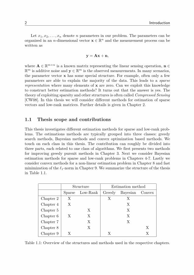
Let x1, x2, . . . , xn denote n parameters in our problem. The parameters can beorganized in an n-dimensional vector x ∈ Rn and the measurement process can bewritten as
y = Ax + n,
where A ∈ Rm×n is a known matrix representing the linear sensing operation, n ∈Rm is additive noise and y ∈ Rm is the observed measurements. In many scenarios,the parameter vector x has some special structure. For example, often only a fewparameters are able to explain the majority of the data. This leads to a sparserepresentation where many elements of x are zero. Can we exploit this knowledgeto construct better estimation methods? It turns out that the answer is yes. Thetheory of exploiting sparsity and other structures is often called Compressed Sensing[CW08]. In this thesis we will consider different methods for estimation of sparsevectors and low-rank matrices. Further details is given in Chapter 2.
1.1 Thesis scope and contributions
This thesis investigates different estimation methods for sparse and low-rank prob-lems. The estimations methods are typically grouped into three classes: greedysearch methods, Bayesian methods and convex optimization based methods. Wetouch on each class in this thesis. The contribution can roughly be divided intothree parts, each related to one class of algorithms. We first presents two methodsfor improving greedy pursuit methods in Chapter 3. Next we consider Bayesianestimation methods for sparse and low-rank problems in Chapters 4-7. Lastly weconsider convex methods for a non-linear estimation problem in Chapter 8 and fastminimization of the `1-norm in Chapter 9. We summarize the structure of the thesisin Table 1.1.
Structure Estimation methodSparse Low-Rank Greedy Bayesian Convex
Chapter 2 X X XChapter 4 X XChapter 5 X XChapter 6 X X XChapter 7 X XChapter 8 X XChapter 9 X X X
Table 1.1: Overview of the structures and methods used in the respective chapters.
1.1. Thesis scope and contributions 3
Some of the results presented in the thesis have already been published in journalsand conferences, and some are under review. Parts of the thesis are adopted fromthe corresponding research papers nearly verbatim.
Chapter 2In Chapter 2 we give the background of the work. We present some modern engi-neering problems and show how they are related to the work of the thesis. We havetried to do so by including a minimal amount of mathematics and concentrate onthe main concepts and ideas. If you merely wish to understand the context of thework and how it relates to other problems, this is the chapter for you.
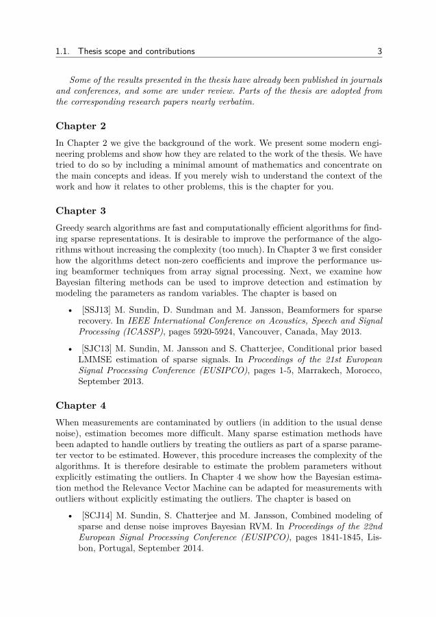
Chapter 3Greedy search algorithms are fast and computationally efficient algorithms for find-ing sparse representations. It is desirable to improve the performance of the algo-rithms without increasing the complexity (too much). In Chapter 3 we first considerhow the algorithms detect non-zero coefficients and improve the performance us-ing beamformer techniques from array signal processing. Next, we examine howBayesian filtering methods can be used to improve detection and estimation bymodeling the parameters as random variables. The chapter is based on
• [SSJ13] M. Sundin, D. Sundman and M. Jansson, Beamformers for sparserecovery. In IEEE International Conference on Acoustics, Speech and SignalProcessing (ICASSP), pages 5920-5924, Vancouver, Canada, May 2013.
• [SJC13] M. Sundin, M. Jansson and S. Chatterjee, Conditional prior basedLMMSE estimation of sparse signals. In Proceedings of the 21st EuropeanSignal Processing Conference (EUSIPCO), pages 1-5, Marrakech, Morocco,September 2013.
Chapter 4When measurements are contaminated by outliers (in addition to the usual densenoise), estimation becomes more difficult. Many sparse estimation methods havebeen adapted to handle outliers by treating the outliers as part of a sparse parame-ter vector to be estimated. However, this procedure increases the complexity of thealgorithms. It is therefore desirable to estimate the problem parameters withoutexplicitly estimating the outliers. In Chapter 4 we show how the Bayesian estima-tion method the Relevance Vector Machine can be adapted for measurements withoutliers without explicitly estimating the outliers. The chapter is based on
• [SCJ14] M. Sundin, S. Chatterjee and M. Jansson, Combined modeling ofsparse and dense noise improves Bayesian RVM. In Proceedings of the 22ndEuropean Signal Processing Conference (EUSIPCO), pages 1841-1845, Lis-bon, Portugal, September 2014.
4 Introduction
• [SCJ15b] M. Sundin, M. Jansson and S. Chatterjee, Combined modeling ofsparse and dense noise for improvement of Relevance Vector Machine. Sub-mitted journal paper.
We note that [SCJ15b] is an extended journal version of [SCJ14].
Chapter 5The low-rank reconstruction problem is closely related to the sparse recovery prob-lem. However, a hierarchical Bayesian method, like the Relevance Vector Machine,has not been developed for the low-rank reconstruction problem. In Chapter 5 wedevelop such a method by introducing left and right precision matrices. We showhow the prior distribution of the precision matrices is related to the prior distri-bution of the matrix to be estimated and compare the performance with existingalgorithms through numerical simulations. The chapter is based on
• [SCJR14] M. Sundin, S. Chatterjee, M. Jansson, C.R. Rojas, Relevance Singu-lar Vector Machine for low-rank matrix sensing. In 2014 International Confer-ence on Signal Processing and Communications (SPCOM), Bangalore, India,July 2014.
• [SRJC] M. Sundin, S. Chatterjee, M. Jansson, C.R. Rojas, Relevance SingularVector Machine for low-rank matrix reconstruction. Accepted for publicationin IEEE Transactions of Signal Processing.
We note that [SRJC] is an extended journal version of [SCJR14].
Chapter 6Principal Component Analysis (PCA) is an important method for finding under-lying patterns in data and measurements. However, PCA is not robust to outliernoise in the data. To design estimation methods for robust PCA problem requirescombining methods for sparse and low-rank problems. In Chapter 6 we combine therobust estimation technique from Chapter 4 and the low-rank estimation methodfrom Chapter 5 to construct a Bayesian learning algorithm for robust PCA. Thechapter is based on
• [SCJ15a] M. Sundin, S. Chatterjee and M. Jansson, Bayesian learning forrobust principal component analysis. In Proceedings of the 23rd EuropeanSignal Processing Conference (EUSIPCO), pages 2361 - 2365, Nice, France,September 2015.
Chapter 7A fundamental tool in evaluating the performance of estimation algorithms is the-oretical lower bounds. The Cramér-Rao Bound (CRB) is a theoretical lower bound
1.1. Thesis scope and contributions 5
for unbiased estimators of deterministic parameters. When the parameters to beestimated are random, the CRB does not hold in general since the prior distributionbrings more information about the parameters. The Bayesian CRB (also called thevan Trees inequality) is a lower bound for random parameters. In Chapter 7 weconsider the Bayesian CRB for different low-rank matrix reconstruction problems.We show that the extension of the CRB to the Bayesian setting with random pa-rameters is not unambiguous and that several different bounds can be derived. Thechapter is based on
• [SCJa] M. Sundin, M. Jansson and S. Chatterjee, Bayesian Cramér-Raobounds for factorized model based low rank matrix reconstruction. Acceptedto the European Signal Processing Conference (EUSIPCO) 2016.
• [SCJb] M. Sundin, M. Jansson and S. Chatterjee, Bayesian Cramér-Raobounds for low-rank matrix reconstruction. In preparation.
We note that [SCJb] is an extended journal version of [SCJa].
Chapter 8In many scenarios, such as X-ray crystallography, the problem contains non-linearmeasurements. However, some problems can be transfered into non-linear problemsin another variable. One such problem is the phase retrieval problem. The phaseretrieval problem can be lifted to a positive semidefinite problem, by relaxing theproblem one then obtains the convex optimization problem PhaseLift, which canreadily be solved. The PhaseLift algorithm has been developed to sparse phaseretrieval problems, but lacks a low-rank matrix analogue. In Chapter 8 we showhow the low-rank phase retrieval problem can be lifted to a semidefinite programusing the theory of Kronecker product approximations. The chapter is based on
• [SCJc] M. Sundin, M. Jansson and S. Chatterjee, Convex recovery for low-rank phase retrieval. In preparation.
Chapter 9The power of convex relaxation techniques for sparse problems is that efficient off-the-shelf algorithms exist that can solve almost any convex optimization problem.It is thus not difficult to implement sparse estimation methods based on convexoptimization. While the general methods are efficient, they can sometimes be beatenin performance by specialized methods that solve the problem in another way. InChapter 9 we present such a method for the basis-pursuit problem. By consideringthe geometry of the basis pursuit method we are able to derive conditions foroptimality of the solution. We then develop an algorithm based on these conditions.The method has the advantage of exploiting the sparsity of the solution and doestherefore not need to keep all variables in memory. This makes the method suited
6 Introduction
for problems with large number of variables. We illustrate this point by using thealgorithm to find a wavelet decomposition of an image over all wavelet families inMatlab. The chapter is based on
• [SCJ15c] M. Sundin, M. Jansson and S. Chatterjee, Greedy minimizationof the L1-norm with high empirical success. In IEEE International Confer-ence on Acoustics, Speech and Signal Processing (ICASSP), pages 3816-3820,Brisbane, Australia, April 2015.
Chapter 10In the last chapter, we summarize the work presented in the thesis.
Contributions Outside the Scope of the ThesisBesides the listed contributions, the author of this thesis has also contributed toother related works listed below.
• [ZSJC12] D. Zachariah, M. Sundin, M. Jansson and S. Chatterjee, Alternat-ing least-squares for low-rank matrix reconstruction. In IEEE Signal Process-ing Letters, vol. 19, no. 4, pages 231-234, April 2012.
• [LSR+16] K. Li, M. Sundin, C.R. Rojas, S. Chatterjee and M. Jansson, Al-ternating strategies with internal ADMM for low-rank matrix reconstruction.In Signal Processing, vol. 121, pages 153-159, April 2016.
• [CSGC15] A. Casamitjana, M. Sundin, P. Ghosh, S. Chatterjee, Bayesianlearning for time-varying linear prediction of speech. In Proceedings of the23rd European Signal Processing Conference (EUSIPCO), pages 325 - 329,Nice, France, September 2015.
• [SVJC] M. Sundin, A. Venkitaraman, M. Jansson, S. Chatterjee, A convexconstraint for graph connectedness. Conference paper. In preparation.
1.2 Copyright notice
Parts of the material presented in this thesis are partly verbatim based on the thesisauthor’s joint works which are previously published or submitted to conferencesand journals held by or sponsored by the Institute of Electrical and ElectronicsEngineer (IEEE). IEEE holds the copyright of the published papers and will holdthe copyright of the submitted papers if they are accepted. Materials (e.g., figure,graph, table, or textual material) are reused in this thesis with permission.
Chapter 2
Background
In signal processing, one important task is to extract a signal from from noisymeasurements. This is usually done by 1) modeling the noise, 2) modeling thesignal and 3) using the models to construct an algorithm (an estimator) to
extract the information from the data. How accurate we manage to extract theinformation naturally depends on how accurate and flexible our models are. A veryprecise model can be very efficient if it is correct and very poor if it is incorrect,while a very flexible model can account for many different models but may not beas accurate. In this thesis we will mainly discuss a combination of two differentmodels, Bayesian models and parsimonious models. Bayesian modeling is a way tomodel prior knowledge and uncertainty using probability theory. Using Bayesianmethods, it is possible both to extract information and quantify the uncertainty ofthe information. Parsimonious models are models where the information contentis a fraction of the signal content, i.e. the signal is strongly redundant and can becompressed a lot without losing any information. Many natural signals are parsimo-nious, something which makes them easier to extract. Here we especially considersparse and low-rank models. We will show how Bayesian methods can be used tohandle different parsimonious models.
2.1 Bayesian modeling
Probability theory allows us to calculate the probability of an event and it alsoallows us to calculate the probability of a second event given that a first event hasoccurred. This is commonly known as conditional probability. Bayes rule allows usto reverse conditional probabilities, allowing us to compute the probability thatthe first event happened given that we observed the second event. Let P (A) bethe probability of an event A, P (B) be the probability of an event B and P (B|A)be the probability of event B given that A has occurred. Bayes rule allows us tocompute the reverse probability P (B|A), i.e. the probability that A did occur given
7

8 Background
0 0.1 0.2 0.3 0.4 0.5 0.6 0.7 0.8 0.9 10
1
2
3
4
5
6
Figure 2.1: The prior (in blue) and the posterior (in red) probability of getting headswhen flipping a coin. The prior suggests that the coin most probably is balancedwhile the posterior (given after observing Nh = 5 heads and Nt = 15 tails) suggeststhat the coin is biased.
that we observed the event B, as
P (B|A) = P (A|B)P (B)P (A) .
Bayes rule is useful since it allows us to find the most probable cause of an event.Consider the problem of deciding whether a coin is balanced or not. Assume
that the probability of heads is q, then the probability of tails is 1− q. We have ahigh degree of confidence that the coin is balanced (p = 1
2 ). We model this priorknowledge by assigning a prior distribution p(q) to the probability q. After weobserve Nh heads and Nt tails in Nh + Nt independent trials, Bayes rule gives usthat the posterior distribution of q is
p(q|Nh, Nt) = p(heads|q)Nhp(tails|q)Ntp(q)∫ 10 p(heads|q)Nhp(tails|q)Ntp(q)dq
= qNh(1− q)Ntp(q)∫ 10 q
Nh(1− q)Ntp(q)dq.
In the coin-flipping example, it is common to use a Beta-distribution as a priordistribution. An example of a prior and posterior distribution is shown in Figure 2.1.
Bayesian methods are useful even when the prior knowledge is weak. In thatcase, the prior is often chosen to be as non-informative as possible. This can be doneby selecting the prior to be approximately flat or by using the Jeffries prior whichis invariant under change of variables. Prior distribution for which the posterior isof the same type as the prior distribution are called conjugate priors. Conjugatepriors are useful since statistical inference can be performed more easily than fornon-conjugate priors.
Sometimes we want to chose a prior distribution in which the parameters of theprior distribution are themselves random variables. Such priors are called hierarchi-

2.2. Sparsity 9
0 2000 4000 6000 8000 10000 120000
500
1000
1500
2000
2500
Frequency in Hz
Ma
gn
itu
de
Figure 2.2: The energy in each frequency of a violin tone.
cal priors since the model consists of several layers of random variables. Hierarchicalpriors are often very flexible and can thus model several different distributions. Todo inference in hierarchical priors often requires approximate inference methods.
2.2 Sparsity
Many tones of musical instruments have their energy concentrated to just a fewfrequencies, for example, a violin tone has it energy concentrated to one main fre-quency with residual energy in several smaller overtones, see Figure 2.2. The violintone thus has an approximately sparse representation in the frequency domain.Other instruments also have sparse representations, for example the beats of adrum can be sparsely represented in the time domain. Most natural signals havesparse representations in some domain.
The fact that sparse signals contain less information than an arbitrary signalcan be exploited to reconstruct the signals also when the number of measurementsis not sufficient for standard reconstruction techniques. One example of this is fromMagnetic Resonance Imaging (MRI). In MRI, a sample (e.g. a part of the body)is exposed to a magnetic field which varies in space. The magnetic field causes themagnetic moments of the hydrogen atoms to align with the magnetic field. Theatoms are then exposed to a magnetic pulse which excites the magnetic moments.When the atoms relax back into equilibrium they emit radiation with frequencyproportional to the strength of the magnetic field. This produces a signal whoseamplitude is proportional to the density of hydrogen atoms. By computing theFourier transform of the signal we can find the average concentration of hydrogenatoms in the area which has the same magnetic field strength. The measurementprocess thus gives a sub-sampled Fourier transform of the image. Each measurementtakes about a half second, making MRI imaging a time consuming process (imagingthe brain takes about 20-45 minutes). The many measurements needed for MRImakes it hard to apply to sensitive parts of the body. It is therefore desirable toreduce the number of measurements needed.
An often used toy-model for MRI is the Shepp-Logan phantom [SL74] shown in
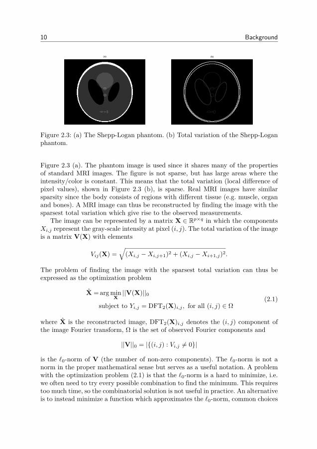
10 Background
(a) (b)
Figure 2.3: (a) The Shepp-Logan phantom. (b) Total variation of the Shepp-Loganphantom.
Figure 2.3 (a). The phantom image is used since it shares many of the propertiesof standard MRI images. The figure is not sparse, but has large areas where theintensity/color is constant. This means that the total variation (local difference ofpixel values), shown in Figure 2.3 (b), is sparse. Real MRI images have similarsparsity since the body consists of regions with different tissue (e.g. muscle, organand bones). A MRI image can thus be reconstructed by finding the image with thesparsest total variation which give rise to the observed measurements.
The image can be represented by a matrix X ∈ Rp×q in which the componentsXi,j represent the gray-scale intensity at pixel (i, j). The total variation of the imageis a matrix V(X) with elements
Vij(X) =√
(Xi,j −Xi,j+1)2 + (Xi,j −Xi+1,j)2.
The problem of finding the image with the sparsest total variation can thus beexpressed as the optimization problem
X = arg minX||V(X)||0
subject to Yi,j = DFT2(X)i,j , for all (i, j) ∈ Ω(2.1)
where X is the reconstructed image, DFT2(X)i,j denotes the (i, j) component ofthe image Fourier transform, Ω is the set of observed Fourier components and
||V||0 = |(i, j) : Vi,j 6= 0|
is the `0-norm of V (the number of non-zero components). The `0-norm is not anorm in the proper mathematical sense but serves as a useful notation. A problemwith the optimization problem (2.1) is that the `0-norm is a hard to minimize, i.e.we often need to try every possible combination to find the minimum. This requirestoo much time, so the combinatorial solution is not useful in practice. An alternativeis to instead minimize a function which approximates the `0-norm, common choices

2.2. Sparsity 11
l2 reconstruction l
1 reconstruction
Figure 2.4: Reconstruction of the Shepp-Logan phantom from MRI measurementsusing the `2-norm and `1-norm.
are the `1-norm and `2-norm
||V||1 =∑i,j
|Vi,j |, ||V||2 =√∑
i,j
|Vi,j |2.
The advantage of using the `1 and `2-norm is that the problem becomes convexand can thus be solved using standard methods from convex optimization. In Fig-ure 2.4 we show the reconstructed image using the `2 and `1-norm. We find thatwhile both images resemble the original, the image reconstructed using the `2-normhas several artifacts and the image reconstructed using the `1-norm is very close tothe original. The difference is because the total variation is sparse and the `1-normbetter promotes sparsity than the `2-norm.
The general sparse reconstruction problem can be described as follows. Letx ∈ Rn be a sparse parameter vector and assume that we linearly measure x as
y = Ax + n, (2.2)
where A ∈ Rm×n is a known measurement matrix and n is additive noise. It istypically assumed that the noise is i.i.d. Gaussian. The problem is to recover x fromy. When x is not sparse, we in general need more measurements than parameters,i.e. m ≥ n, to reconstruct x while sparse x can be reconstructed also when m < n.
To find the sparsest solution, we need to minimize the `0-norm of x, i.e. thenumber of non-zero components. The solution of trying every combination, an ex-haustive search, is often infeasible since it takes too long time. For this reason,several other methods have been developed for finding sparse solutions. The meth-ods are often classified as convex optimization based, greedy search based methodsand Bayesian methods.
Convex optimization based methods formulates the estimation problem as anoptimization problem. This is done by making the residual ||y−Ax||22 small whilesimultaneously minimizing a function g(x) which is “small” when x is sparse. Acommon choice is to use the `1-norm where g(x) = ||x||1 =
∑ni=1 |xi|, the estimator
12 Background
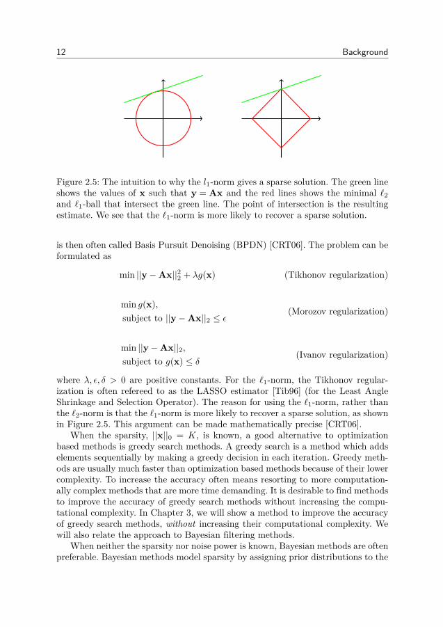
Figure 2.5: The intuition to why the l1-norm gives a sparse solution. The green lineshows the values of x such that y = Ax and the red lines shows the minimal `2and `1-ball that intersect the green line. The point of intersection is the resultingestimate. We see that the `1-norm is more likely to recover a sparse solution.
is then often called Basis Pursuit Denoising (BPDN) [CRT06]. The problem can beformulated as
min ||y−Ax||22 + λg(x) (Tikhonov regularization)
min g(x),subject to ||y−Ax||2 ≤ ε
(Morozov regularization)
min ||y−Ax||2,subject to g(x) ≤ δ
(Ivanov regularization)
where λ, ε, δ > 0 are positive constants. For the `1-norm, the Tikhonov regular-ization is often refereed to as the LASSO estimator [Tib96] (for the Least AngleShrinkage and Selection Operator). The reason for using the `1-norm, rather thanthe `2-norm is that the `1-norm is more likely to recover a sparse solution, as shownin Figure 2.5. This argument can be made mathematically precise [CRT06].
When the sparsity, ||x||0 = K, is known, a good alternative to optimizationbased methods is greedy search methods. A greedy search is a method which addselements sequentially by making a greedy decision in each iteration. Greedy meth-ods are usually much faster than optimization based methods because of their lowercomplexity. To increase the accuracy often means resorting to more computation-ally complex methods that are more time demanding. It is desirable to find methodsto improve the accuracy of greedy search methods without increasing the compu-tational complexity. In Chapter 3, we will show a method to improve the accuracyof greedy search methods, without increasing their computational complexity. Wewill also relate the approach to Bayesian filtering methods.
When neither the sparsity nor noise power is known, Bayesian methods are oftenpreferable. Bayesian methods model sparsity by assigning prior distributions to the

2.3. Robust methods 13
parameters and the noise and then iteratively updating the distributions to obtaina good estimate. Bayesian methods are often able to learn both the sparsity andnoise power from data alone.
2.3 Robust methods
Sparse reconstruction is closely related to robust estimation methods. In the mea-surement model (2.2), it was assumed that the noise components have the samevariance, i.e. the noise is the same in all measurements. However, in many sce-narios, some noise components are very large (outliers). This can severely perturbthe final estimate. To perform estimation from measurements with outliers requiresrobust estimation methods.
Outliers often occur when some datapoints are not well described by the model.Consider, for example, the problem of predicting house prices. It is plausible toassume that the house price increase with the number of rooms. In Figure 2.6 weshow the house prices versus the average number of rooms from the Boston housingdataset [AN07]. The presence of outliers show that other factors also influence thehouse price. Using normal regression methods (least squares) we obtain the red linein the figure while removing many outliers gives the green line. Since the lines differwe find that the outliers affect our prediction and that a better prediction can bemade when taking the outliers into account. By removing the outliers, the trendonly models the majority of house prices and not the outliers.
3 4 5 6 7 8 90
5
10
15
20
25
30
35
40
45
50
55
Average number of rooms
Me
dia
n p
rice
in
$1
00
0
Figure 2.6: Predicting the trend of house prices from the Boston housing dataset.Not taking outliers into account gives the red line of regression, while taking outliersinto account gives the green line of regression. The green line better shows the trendin house prices.
14 Background
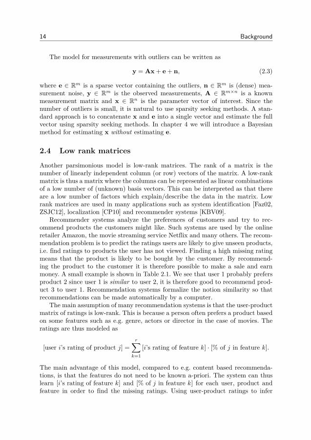
The model for measurements with outliers can be written as
y = Ax + e + n, (2.3)
where e ∈ Rm is a sparse vector containing the outliers, n ∈ Rm is (dense) mea-surement noise, y ∈ Rm is the observed measurements, A ∈ Rm×n is a knownmeasurement matrix and x ∈ Rn is the parameter vector of interest. Since thenumber of outliers is small, it is natural to use sparsity seeking methods. A stan-dard approach is to concatenate x and e into a single vector and estimate the fullvector using sparsity seeking methods. In chapter 4 we will introduce a Bayesianmethod for estimating x without estimating e.
2.4 Low rank matrices
Another parsimonious model is low-rank matrices. The rank of a matrix is thenumber of linearly independent column (or row) vectors of the matrix. A low-rankmatrix is thus a matrix where the columns can be represented as linear combinationsof a low number of (unknown) basis vectors. This can be interpreted as that thereare a low number of factors which explain/describe the data in the matrix. Lowrank matrices are used in many applications such as system identification [Faz02,ZSJC12], localization [CP10] and recommender systems [KBV09].
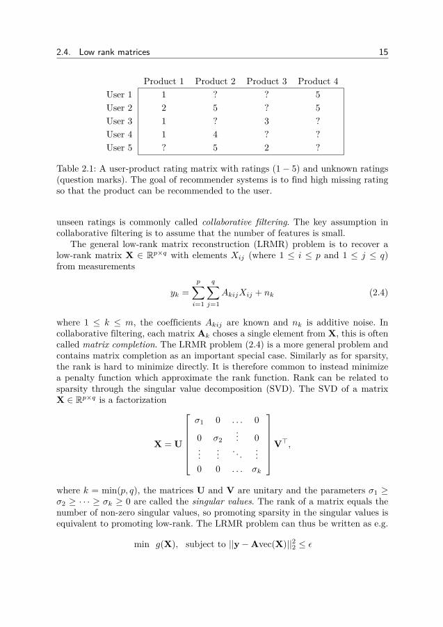
Recommender systems analyze the preferences of customers and try to rec-ommend products the customers might like. Such systems are used by the onlineretailer Amazon, the movie streaming service Netflix and many others. The recom-mendation problem is to predict the ratings users are likely to give unseen products,i.e. find ratings to products the user has not viewed. Finding a high missing ratingmeans that the product is likely to be bought by the customer. By recommend-ing the product to the customer it is therefore possible to make a sale and earnmoney. A small example is shown in Table 2.1. We see that user 1 probably prefersproduct 2 since user 1 is similar to user 2, it is therefore good to recommend prod-uct 3 to user 1. Recommendation systems formalize the notion similarity so thatrecommendations can be made automatically by a computer.
The main assumption of many recommendation systems is that the user-productmatrix of ratings is low-rank. This is because a person often prefers a product basedon some features such as e.g. genre, actors or director in the case of movies. Theratings are thus modeled as
[user i’s rating of product j] =r∑
k=1[i’s rating of feature k] · [% of j in feature k].
The main advantage of this model, compared to e.g. content based recommenda-tions, is that the features do not need to be known a-priori. The system can thuslearn [i’s rating of feature k] and [% of j in feature k] for each user, product andfeature in order to find the missing ratings. Using user-product ratings to infer
2.4. Low rank matrices 15
Product 1 Product 2 Product 3 Product 4User 1 1 ? ? 5User 2 2 5 ? 5User 3 1 ? 3 ?User 4 1 4 ? ?User 5 ? 5 2 ?
Table 2.1: A user-product rating matrix with ratings (1− 5) and unknown ratings(question marks). The goal of recommender systems is to find high missing ratingso that the product can be recommended to the user.
unseen ratings is commonly called collaborative filtering. The key assumption incollaborative filtering is to assume that the number of features is small.
The general low-rank matrix reconstruction (LRMR) problem is to recover alow-rank matrix X ∈ Rp×q with elements Xij (where 1 ≤ i ≤ p and 1 ≤ j ≤ q)from measurements
yk =p∑i=1
q∑j=1
AkijXij + nk (2.4)
where 1 ≤ k ≤ m, the coefficients Akij are known and nk is additive noise. Incollaborative filtering, each matrix Ak choses a single element from X, this is oftencalled matrix completion. The LRMR problem (2.4) is a more general problem andcontains matrix completion as an important special case. Similarly as for sparsity,the rank is hard to minimize directly. It is therefore common to instead minimizea penalty function which approximate the rank function. Rank can be related tosparsity through the singular value decomposition (SVD). The SVD of a matrixX ∈ Rp×q is a factorization
X = U
σ1 0 . . . 0
0 σ2... 0
......
. . ....
0 0 . . . σk
V>,
where k = min(p, q), the matrices U and V are unitary and the parameters σ1 ≥σ2 ≥ · · · ≥ σk ≥ 0 are called the singular values. The rank of a matrix equals thenumber of non-zero singular values, so promoting sparsity in the singular values isequivalent to promoting low-rank. The LRMR problem can thus be written as e.g.
min g(X), subject to ||y−Avec(X)||22 ≤ ε
16 Background
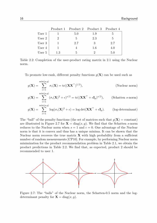
Product 1 Product 2 Product 3 Product 4User 1 1 5.0 1.9 5User 2 2 5 2.3 5User 3 1 2.7 3 2.7User 4 1 4 1.6 4.0User 5 1.3 5 2 5.0
Table 2.2: Completion of the user-product rating matrix in 2.1 using the Nuclearnorm.
To promote low-rank, different penalty functions g(X) can be used such as
g(X) =min(p,q)∑i=1
σi(X) = tr((XX>)1/2), (Nuclear norm)
g(X) =min(p,q)∑i=1
(σi(X)2 + ε)s/2 = tr((XX> + εIp)s/2), (Schatten s-norm)
g(X) =min(p,q)∑i=1
log(σi(X)2 + ε) = log det(XX> + εIp). (log-determinant)
The “ball” of the penalty functions (the set of matrices such that g(X) = constant)are illustrated in Figure 2.7 for X = diag(x, y). We find that the Schatten s-normreduces to the Nuclear norm when s = 1 and ε = 0. One advantage of the Nuclearnorm is that it is convex and thus has a unique minima. It can be shown that theNuclear norm recovers the true matrix X with high probability from a sufficientnumber of random measurements [CP10]. For example, by performing Nuclear normminimization for the product recommendation problem in Table 2.1, we obtain theproduct predictions in Table 2.2. We find that, as expected, product 2 should berecommended to user 1.
Figure 2.7: The “balls” of the Nuclear norm, the Schatten-0.5 norm and the log-determinant penalty for X = diag(x, y).
2.5. Robust principal component analysis 17
One disadvantage of the Nuclear norm is that the noise power needs to be knowna-priori. When the noise power is unknown, Bayesian methods are preferable sincethey can learn the noise power from the data. In Chapter 5 we will present oneBayesian method for LRMR where the distributions of the hyper-parameters canbe related to certain penalty functions.
2.5 Robust principal component analysis
An important special case of low-rank matrix reconstruction is robust PrincipalComponent Analysis (PCA). In regular PCA, we measure all elements of a low-rank matrix as
Y = X + N,
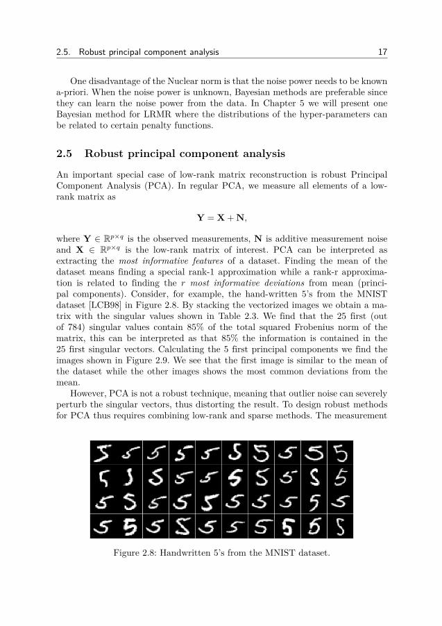
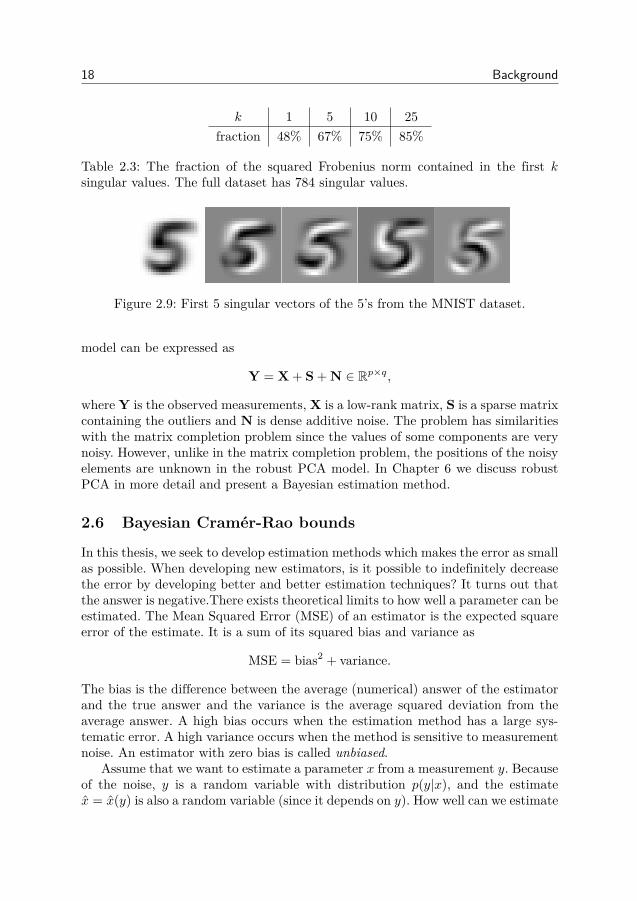
where Y ∈ Rp×q is the observed measurements, N is additive measurement noiseand X ∈ Rp×q is the low-rank matrix of interest. PCA can be interpreted asextracting the most informative features of a dataset. Finding the mean of thedataset means finding a special rank-1 approximation while a rank-r approxima-tion is related to finding the r most informative deviations from mean (princi-pal components). Consider, for example, the hand-written 5’s from the MNISTdataset [LCB98] in Figure 2.8. By stacking the vectorized images we obtain a ma-trix with the singular values shown in Table 2.3. We find that the 25 first (outof 784) singular values contain 85% of the total squared Frobenius norm of thematrix, this can be interpreted as that 85% the information is contained in the25 first singular vectors. Calculating the 5 first principal components we find theimages shown in Figure 2.9. We see that the first image is similar to the mean ofthe dataset while the other images shows the most common deviations from themean.
However, PCA is not a robust technique, meaning that outlier noise can severelyperturb the singular vectors, thus distorting the result. To design robust methodsfor PCA thus requires combining low-rank and sparse methods. The measurement
Figure 2.8: Handwritten 5’s from the MNIST dataset.
18 Background
k 1 5 10 25fraction 48% 67% 75% 85%
Table 2.3: The fraction of the squared Frobenius norm contained in the first ksingular values. The full dataset has 784 singular values.
Figure 2.9: First 5 singular vectors of the 5’s from the MNIST dataset.
model can be expressed as
Y = X + S + N ∈ Rp×q,
where Y is the observed measurements, X is a low-rank matrix, S is a sparse matrixcontaining the outliers and N is dense additive noise. The problem has similaritieswith the matrix completion problem since the values of some components are verynoisy. However, unlike in the matrix completion problem, the positions of the noisyelements are unknown in the robust PCA model. In Chapter 6 we discuss robustPCA in more detail and present a Bayesian estimation method.
2.6 Bayesian Cramér-Rao bounds
In this thesis, we seek to develop estimation methods which makes the error as smallas possible. When developing new estimators, is it possible to indefinitely decreasethe error by developing better and better estimation techniques? It turns out thatthe answer is negative.There exists theoretical limits to how well a parameter can beestimated. The Mean Squared Error (MSE) of an estimator is the expected squareerror of the estimate. It is a sum of its squared bias and variance as
MSE = bias2 + variance.
The bias is the difference between the average (numerical) answer of the estimatorand the true answer and the variance is the average squared deviation from theaverage answer. A high bias occurs when the estimation method has a large sys-tematic error. A high variance occurs when the method is sensitive to measurementnoise. An estimator with zero bias is called unbiased.
Assume that we want to estimate a parameter x from a measurement y. Becauseof the noise, y is a random variable with distribution p(y|x), and the estimatex = x(y) is also a random variable (since it depends on y). How well can we estimate
2.7. Phase retrieval 19
x? If the estimator x(y) is unbiased, the Cramér-Rao bound (CRB) [Kay98] givesthe following lower bound on the MSE,
MSE = variance ≥ CRB = 1Jy, (2.5)
where Jy is the Fisher information
Jy = E[(
∂ log p(y|x)∂x
)2].
When the parameters are random, the CRB is no longer a valid bound since theprior distribution p(x) give additional information about x. A bound for randomparameters is given by the Bayesian Cramér-Rao bound (BCRB) which takes theprior distribution into account. The BCRB is given by
MSE = variance ≥ BCRB = 1Jy + Jx
, (2.6)
where Jx is given by
Jx = E[(
∂ log p(x)∂x
)2],
where the expected value is taken with respect to the distribution p(y, x) = p(y|x)p(x).The BCRB is also known as the van-Trees inequality and the Borovkov-Sakhanenkoinequality. The CRB (2.5) and BCRB (2.6) have multivariate counterparts for theestimation of several variables. In Chapter 7, we compute Bayesian Cramér-Raobounds for different models of random low-rank matrices.
2.7 Phase retrieval
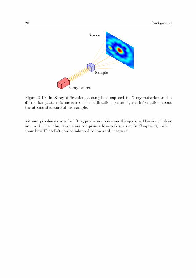
In many scenarios the measurements are non-linear. Non-linear problems are of-ten harder to solve and require different estimation techniques. One example ofnon-linear measurements is X-ray crystallography where a molecule or crystal is il-luminated by X-rays and a diffraction pattern is measured as shown in Figure 2.10.In the process, the amplitude of the measurement is recorded, but the phase infor-mation is lost. Since finding the true parameters is related to finding the phase ofthe measurements, this estimation problem is often called phase retrieval.
Phase retrieval is traditionally solved by iteratively estimating the parametersand the phases. The disadvantage of the traditional methods is that they requiremany measurements to perform well. A more modern method is to lift the non-linearproblem to a linear problem with rank constraints. As before, we can approximatethe constraints by penalty functions to give a problem we can solve numerically. Thissolution method is called PhaseLift. PhaseLift can be adapted to sparse parameters
20 Background
Screen
Sample
X-ray source
Figure 2.10: In X-ray diffraction, a sample is exposed to X-ray radiation and adiffraction pattern is measured. The diffraction pattern gives information aboutthe atomic structure of the sample.
without problems since the lifting procedure preserves the sparsity. However, it doesnot work when the parameters comprise a low-rank matrix. In Chapter 8, we willshow how PhaseLift can be adapted to low-rank matrices.

Chapter 3
Improving greedy pursuit methods
Greedy pursuits are fast and effective methods for finding sparse representa-tions. Even though the methods are sometimes less accurate than convexoptimization based methods, their simplicity and speed often make them
preferable for many problems. Greedy method finds a solution by iteratively make achoice that gives the largest gain in the present iteration. Because of their lower ac-curacy, it is desirable to improve the performance of greedy pursuit methods whilenot decreasing the speed (too much).
In this chapter we present two methods for improving the performance of greedysearch methods. Both methods modify how the algorithm detects non-zero entries.The first method is deterministic and models the problem as an array processingproblem while the second method uses a Bayesian approach and models the problemas a stochastic filtering problem. The methods are shown to be equivalent in acertain limit.
The goal of sparse reconstruction algorithms is to recover a sparse vector x ∈ Rnfrom measurements
y = Ax + n, (3.1)
where A = [a1, a2, . . . , an] ∈ Rm×n is the sensing matrix, n ∈ Rm is additive noiseand x ∈ Rn is a sparse vector. We here assume that the sparsity
||x||0 = |i|xi 6= 0| = K.
is known a-priori. This assumption is necessary for many greedy search algorithmsin order to know when to stop the algorithm.
3.0.1 Exhaustive searchWhen the sparsity is known, the sparse reconstruction problem can be written asthe optimization problem
minx||y−Ax||2
s.t. ||x||0 ≤ K(3.2)
21
22 Improving greedy pursuit methods
When the support set I is known, the solution is given by the least squares estimate
xI = A+I y,
xIc = 0,
where Ic = [n]\I is the complement set of I. The problem (3.2) can be solved bytrying all possible support sets I such that |I| = K and chose the solution whichgives the smallest residual. This strategy is commonly called the exhaustive searchand requires solving
(nK
)systems of equations. The exhaustive search is typically
too slow to be useful in practice. Faster methods, such as greedy search methods,are therefore often used to solve the sparse approximation problem in reasonabletime.
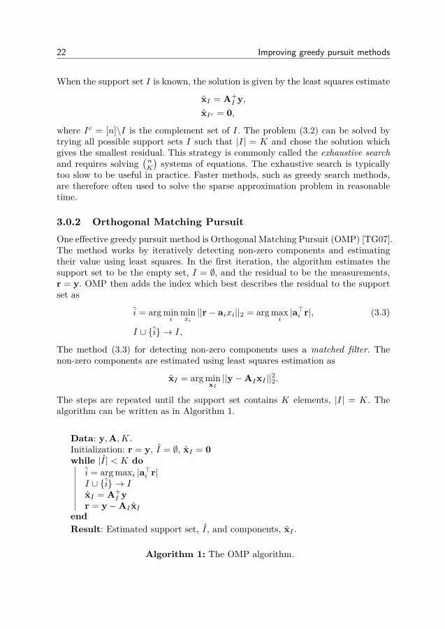
3.0.2 Orthogonal Matching PursuitOne effective greedy pursuit method is Orthogonal Matching Pursuit (OMP) [TG07].The method works by iteratively detecting non-zero components and estimatingtheir value using least squares. In the first iteration, the algorithm estimates thesupport set to be the empty set, I = ∅, and the residual to be the measurements,r = y. OMP then adds the index which best describes the residual to the supportset as
i = arg mini
minxi||r− aixi||2 = arg max
i|a>i r|, (3.3)
I ∪ i → I,
The method (3.3) for detecting non-zero components uses a matched filter. Thenon-zero components are estimated using least squares estimation as
xI = arg minxI||y−AIxI ||22.
The steps are repeated until the support set contains K elements, |I| = K. Thealgorithm can be written as in Algorithm 1.
Data: y,A,K.Initialization: r = y, I = ∅, xI = 0while |I| < K do
i = arg maxi |a>i r|I ∪ i → IxI = A+
I yr = y−AI xI
endResult: Estimated support set, I, and components, xI .
Algorithm 1: The OMP algorithm.
Improving greedy pursuit methods 23
OMP is an extension of the Matching Pursuit algorithm [MZ93] which, unlikeOMP, does not use least square estimation. Because in each iteration, the residual,r, becomes orthogonal to the prediction, AI xI , OMP is an orthogonal version ofmatching pursuit (hence the name). Several improvements to the OMP algorithmhas been proposed, see e.g. [WS12, SM15,CSS11, SCS12,CSVS12,CSVS11,BD08,YdH15,RG09,SGIH13,SACH14,WS11,GAH98,RNL02].
How well OMP is able to recover a sparse vector depends on the sensing matrixA. If the column vectors are close together, it is harder to find which vector isactive. How close the column vectors are can be measured by the mutual coherence.
Definition 3.1. The mutual coherence, µ(A), of a sensing matrix A (with columnvectors of unit `2-norm) is the maximum absolute inner product of two columnvectors of A, i.e.
µ(A) = maxi6=j|a>i aj |.
We see that when the mutual coherence is small, the column vectors of A arenearly orthogonal. It then becomes easier to decompose y as a linear combinationsof atoms in A. When the mutual coherence is large, some column vectors are closetogether and it becomes harder to distinguish which vector is active. This can beformulated through the following theorem.
Theorem 3.0.1. Let µ(A) be the mutual coherence of the sensing matrix A. If
K <12
(1 + 1
µ(A)
), (3.4)
then OMP recovers all K-sparse vectors exactly from measurements y = Ax.
Proof. We can assume that the non-zero components of x are x1, x2, . . . , xK andthat the first component has the largest absolute value. We write the measurements,y, as
y = Ax =K∑k=1
akxk.
The OMP algorithm recovers a component in the support set, I, if
max1≤i≤K
∣∣∣∣∣a>i(
K∑k=1
akxk
)∣∣∣∣∣ > maxK+1≤j≤n
∣∣∣∣∣a>j(
K∑k=1
akxk
)∣∣∣∣∣ , (3.5)
Using the triangle inequality, we can bound the left-hand side of (3.5) from belowas
max1≤i≤K
∣∣∣a>i (∑Kk=1 akxk
)∣∣∣≥ max1≤i≤K |a>i a1| · |x1| −
∑Kk=2 |xk| · |a>i ak|
≥ |x1| − |x1|µ(A)K.(3.6)
24 Improving greedy pursuit methods
Similarly, we can bound the right-hand side of (3.5) from above as
maxK+1≤j≤n
∣∣∣a>j (∑Kk=1 akxk
)∣∣∣≤ maxK+1≤j≤n
∑Kk=1 |xk| · |a>j ak|
≤ |x1|µ(A)K(3.7)
We find that if (3.7) is smaller than (3.6), then (3.5) holds, i.e. when
|x1|µ(A)K < |x1| − |x1|µ(A)(K − 1).
Rearranging the terms gives us that
K <12
(1 + 1
µ(A)
). (3.8)
So, when (3.8) holds, OMP recovers a component in the support set. Since (3.8)does not depend on y or x, OMP also recovers the other components in subsequentiterations and thus the full vector. This proves the theorem.
Borrowing terminology from array signal processing, we can interpret the the-orem as saying that we can resolve more sources when the sidelobes |a>i aj | aresmall. We also see that the theorem gives the worst case scenario where all side-lobes are large. Often a few sidelobes are large and the remaining small. This is notcaptured by the mutual coherence which overestimates the sidelobes. Another wayto measure sidelobes is the cumulative coherence, or Babel function, of A definedas [Ela,T+04]
µ1(p) = maxJ,|J|≤p
maxl/∈J
∑k∈J
|a>l ak|.
The cumulative coherence is the maximum sum of coherences rather than the maxi-mum coherence. Clearly µ1(1) = µ(A). The cumulative coherence can be calculatedby computing |A>A|, summing the largest p+ 1 components in each column, find-ing the maximum and subtracting 1. The cumulative coherence provides tighterbounds on the performance of OMP as follows.
Theorem 3.0.2. If A is a matrix with cumulative coherence µ1(s) andµ1(K) + µ1(K − 1) < 1, (3.9)
then OMP recovers all K-sparse vectors from measurements y = Ax.
Proof. As in the proof of theorem 3.0.1, OMP recovers an atom in the support setif (3.5) holds. Using the cumulative coherence, we can bound the left-hand side of(3.5) from below as
max1≤j≤K
∣∣∣∣∣a>i(
K∑k=1
akxk
)∣∣∣∣∣ ≥ max1≤i≤K
|x1||a>i a1| − |x1|K∑k=2|a>i ak|
≥ |x1| − |x1|µ1(K − 1).
3.1. Beamforming for sparse recovery 25
1 2 3 4 5 6 7 8 9 10 11 12 13 14 150
0.2
0.4
0.6
0.8
1
|b*a
|
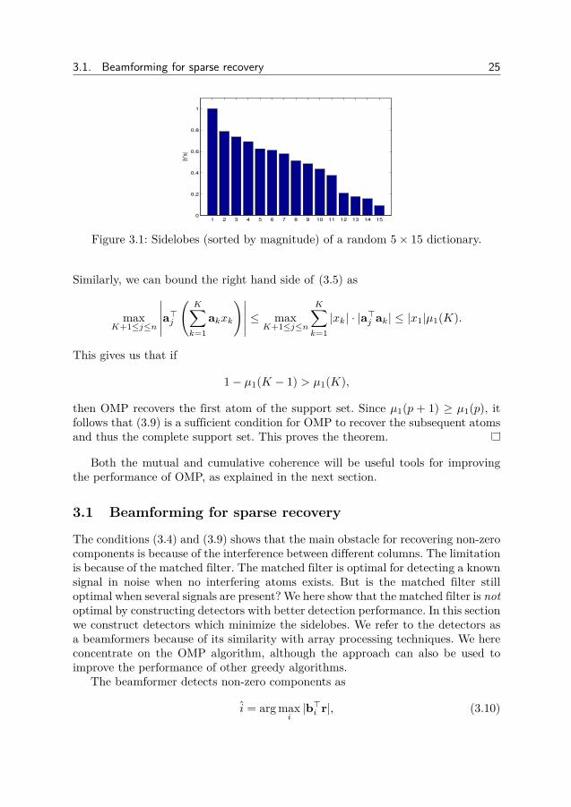
Figure 3.1: Sidelobes (sorted by magnitude) of a random 5× 15 dictionary.
Similarly, we can bound the right hand side of (3.5) as
maxK+1≤j≤n
∣∣∣∣∣a>j(
K∑k=1
akxk
)∣∣∣∣∣ ≤ maxK+1≤j≤n
K∑k=1|xk| · |a>j ak| ≤ |x1|µ1(K).
This gives us that if
1− µ1(K − 1) > µ1(K),
then OMP recovers the first atom of the support set. Since µ1(p + 1) ≥ µ1(p), itfollows that (3.9) is a sufficient condition for OMP to recover the subsequent atomsand thus the complete support set. This proves the theorem.
Both the mutual and cumulative coherence will be useful tools for improvingthe performance of OMP, as explained in the next section.
3.1 Beamforming for sparse recovery
The conditions (3.4) and (3.9) shows that the main obstacle for recovering non-zerocomponents is because of the interference between different columns. The limitationis because of the matched filter. The matched filter is optimal for detecting a knownsignal in noise when no interfering atoms exists. But is the matched filter stilloptimal when several signals are present? We here show that the matched filter is notoptimal by constructing detectors with better detection performance. In this sectionwe construct detectors which minimize the sidelobes. We refer to the detectors asa beamformers because of its similarity with array processing techniques. We hereconcentrate on the OMP algorithm, although the approach can also be used toimprove the performance of other greedy algorithms.
The beamformer detects non-zero components as
i = arg maxi|b>i r|, (3.10)
26 Improving greedy pursuit methods
1 2 3 4 5 6 7 8 9 10 11 12 13 14 150
0.2
0.4
0.6
0.8
1
|b*a
|
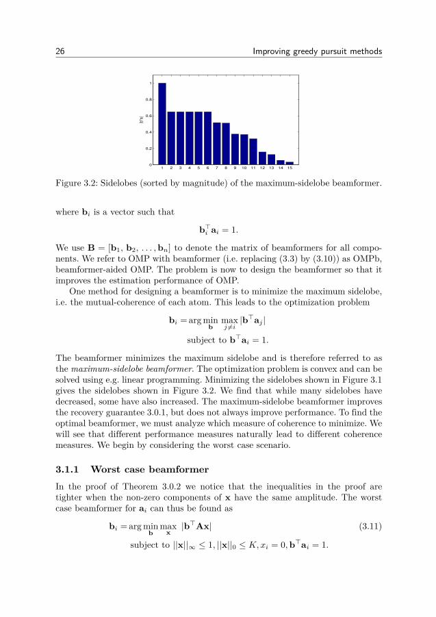
Figure 3.2: Sidelobes (sorted by magnitude) of the maximum-sidelobe beamformer.
where bi is a vector such that
b>i ai = 1.
We use B = [b1, b2, . . . ,bn] to denote the matrix of beamformers for all compo-nents. We refer to OMP with beamformer (i.e. replacing (3.3) by (3.10)) as OMPb,beamformer-aided OMP. The problem is now to design the beamformer so that itimproves the estimation performance of OMP.
One method for designing a beamformer is to minimize the maximum sidelobe,i.e. the mutual-coherence of each atom. This leads to the optimization problem
bi = arg minb
maxj 6=i|b>aj |
subject to b>ai = 1.
The beamformer minimizes the maximum sidelobe and is therefore referred to asthe maximum-sidelobe beamformer. The optimization problem is convex and can besolved using e.g. linear programming. Minimizing the sidelobes shown in Figure 3.1gives the sidelobes shown in Figure 3.2. We find that while many sidelobes havedecreased, some have also increased. The maximum-sidelobe beamformer improvesthe recovery guarantee 3.0.1, but does not always improve performance. To find theoptimal beamformer, we must analyze which measure of coherence to minimize. Wewill see that different performance measures naturally lead to different coherencemeasures. We begin by considering the worst case scenario.
3.1.1 Worst case beamformerIn the proof of Theorem 3.0.2 we notice that the inequalities in the proof aretighter when the non-zero components of x have the same amplitude. The worstcase beamformer for ai can thus be found as
bi = arg minb
maxx|b>Ax| (3.11)
subject to ||x||∞ ≤ 1, ||x||0 ≤ K,xi = 0,b>ai = 1.
3.1. Beamforming for sparse recovery 27
1 2 3 4 5 6 7 8 9 10 11 12 13 14 150
0.2
0.4
0.6
0.8
1
|b*a
|
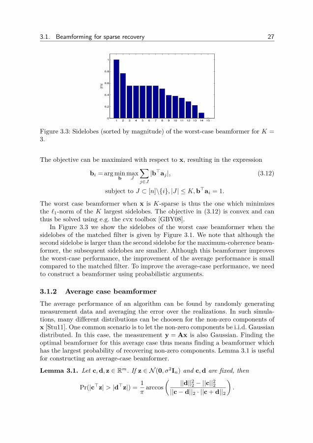
Figure 3.3: Sidelobes (sorted by magnitude) of the worst-case beamformer for K =3.
The objective can be maximized with respect to x, resulting in the expression
bi = arg minb
maxJ
∑j∈J|b>aj |, (3.12)
subject to J ⊂ [n]\i, |J | ≤ K,b>ai = 1.
The worst case beamformer when x is K-sparse is thus the one which minimizesthe `1-norm of the K largest sidelobes. The objective in (3.12) is convex and canthus be solved using e.g. the cvx toolbox [GBY08].
In Figure 3.3 we show the sidelobes of the worst case beamformer when thesidelobes of the matched filter is given by Figure 3.1. We note that although thesecond sidelobe is larger than the second sidelobe for the maximum-coherence beam-former, the subsequent sidelobes are smaller. Although this beamformer improvesthe worst-case performance, the improvement of the average performance is smallcompared to the matched filter. To improve the average-case performance, we needto construct a beamformer using probabilistic arguments.
3.1.2 Average case beamformerThe average performance of an algorithm can be found by randomly generatingmeasurement data and averaging the error over the realizations. In such simula-tions, many different distributions can be choosen for the non-zero components ofx [Stu11]. One common scenario is to let the non-zero components be i.i.d. Gaussiandistributed. In this case, the measurement y = Ax is also Gaussian. Finding theoptimal beamformer for this average case thus means finding a beamformer whichhas the largest probability of recovering non-zero components. Lemma 3.1 is usefulfor constructing an average-case beamformer.
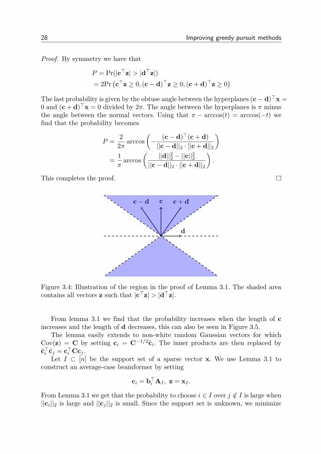
Lemma 3.1. Let c,d, z ∈ Rm. If z ∈ N (0, σ2In) and c,d are fixed, then
Pr(|c>z| > |d>z|) = 1π
arccos(
||d||22 − ||c||22||c− d||2 · ||c + d||2
).
28 Improving greedy pursuit methods
Proof. By symmetry we have that
P = Pr(|c>z| > |d>z|)= 2Pr
(c>z ≥ 0, (c− d)>z ≥ 0, (c + d)>z ≥ 0
)The last probability is given by the obtuse angle between the hyperplanes (c− d)>x =0 and (c + d)>x = 0 divided by 2π. The angle between the hyperplanes is π minusthe angle between the normal vectors. Using that π − arccos(t) = arccos(−t) wefind that the probability becomes
P = 22π arccos
(− (c− d)>(c + d)||c− d||2 · ||c + d||2
)= 1π
arccos(
||d||22 − ||c||22||c− d||2 · ||c + d||2
).
This completes the proof.
c
d
c + dc− d
Figure 3.4: Illustration of the region in the proof of Lemma 3.1. The shaded areacontains all vectors z such that |c>z| > |d>z|.
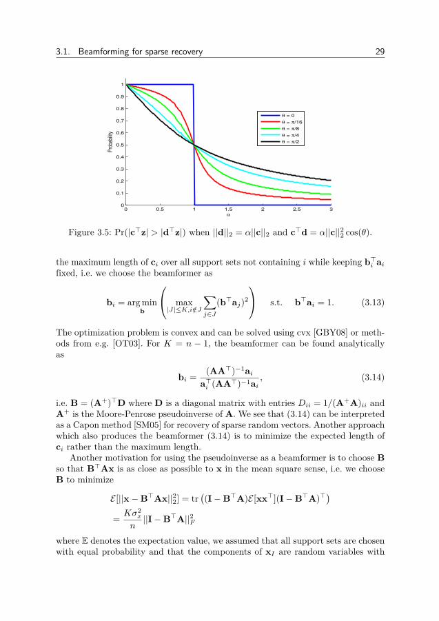
From lemma 3.1 we find that the probability increases when the length of cincreases and the length of d decreases, this can also be seen in Figure 3.5.
The lemma easily extends to non-white random Gaussian vectors for whichCov(z) = C by setting ci = C−1/2ci. The inner products are then replaced byc>i cj = c>i Ccj .
Let I ⊂ [n] be the support set of a sparse vector x. We use Lemma 3.1 toconstruct an average-case beamformer by setting
ci = b>i AI , z = xI .
From Lemma 3.1 we get that the probability to choose i ∈ I over j /∈ I is large when||ci||2 is large and ||cj ||2 is small. Since the support set is unknown, we minimize
3.1. Beamforming for sparse recovery 29
0 0.5 1 1.5 2 2.5 30
0.1
0.2
0.3
0.4
0.5
0.6
0.7
0.8
0.9
1
α
Pro
babi
lity
θ = 0
θ = π/16
θ = π/8
θ = π/4
θ = π/2
Figure 3.5: Pr(|c>z| > |d>z|) when ||d||2 = α||c||2 and c>d = α||c||22 cos(θ).
the maximum length of ci over all support sets not containing i while keeping b>i aifixed, i.e. we choose the beamformer as
bi = arg minb
max|J|≤K,i/∈J
∑j∈J
(b>aj)2
s.t. b>ai = 1. (3.13)
The optimization problem is convex and can be solved using cvx [GBY08] or meth-ods from e.g. [OT03]. For K = n − 1, the beamformer can be found analyticallyas
bi = (AA>)−1aia>i (AA>)−1ai
, (3.14)
i.e. B = (A+)>D where D is a diagonal matrix with entries Dii = 1/(A+A)ii andA+ is the Moore-Penrose pseudoinverse of A. We see that (3.14) can be interpretedas a Capon method [SM05] for recovery of sparse random vectors. Another approachwhich also produces the beamformer (3.14) is to minimize the expected length ofci rather than the maximum length.
Another motivation for using the pseudoinverse as a beamformer is to choose Bso that B>Ax is as close as possible to x in the mean square sense, i.e. we chooseB to minimize
E [||x−B>Ax||22] = tr((I−B>A)E [xx>](I−B>A)>
)= Kσ2
x
n||I−B>A||2F
where E denotes the expectation value, we assumed that all support sets are chosenwith equal probability and that the components of xI are random variables with
30 Improving greedy pursuit methods
1 2 3 4 5 6 7 8 9 10 11 12 13 14 150
0.2
0.4
0.6
0.8
1
|b*a
|
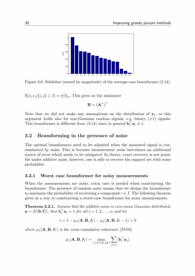
Figure 3.6: Sidelobes (sorted by magnitude) of the average-case beamformer (3.14).
E[xixj |i, j ⊂ I] = σ2xδij . This gives us the minimizer
B = (A+)>
Note that we did not make any assumptions on the distribution of xI , so thisargument holds also for non-Gaussian random signals, e.g. binary (±1) signals.This beamformer is different from (3.14) since in general b>i ai 6= 1.
3.2 Beamforming in the presence of noise
The optimal beamformers need to be adjusted when the measured signal is con-taminated by noise. This is because measurement noise introduces an additionalsource of error which needs to be mitigated. In theory, exact recovery is not possi-ble under additive noise, however, one is able to recover the support set with someprobability.
3.2.1 Worst case beamformer for noisy measurementsWhen the measurements are noisy, extra care is needed when constructing thebeamformer. The presence of random noise means that we design the beamformerto maximize the probability of recovering a component i ∈ I. The following theoremgives us a way to constructing a worst-case beamformer for noisy measurements.
Theorem 3.2.1. Assume that the additive noise is zero-mean Gaussian distributed,n ∼ N (0,C), that b>i ai = 1 for all i = 1, 2, . . . , n and let
c = 1− µ1(A,B,K)− µ1(A,B,K − 1) > 0
where µ1(A,B,K) is the cross cumulative coherence [SV08]
µ1(A,B,K) = maxi,|J|≤K,i/∈J
∑j∈J|b>i aj |.

3.2. Beamforming in the presence of noise 31
Then the probability P that OMPb recovers the component xi of x with maximummodulus in the first iteration obeys
P ≥ 1− 2Q(
c|xi|√b>i Cbi
)(3.15)
where Q(x) = 1√2π
∫∞xe−t
2/2dt is the tail probability of the normal distribution.
Proof. A sufficient condition for OMPb to recover i ∈ I is
2|xi||b>i n| < 1−
∑j∈I\i
|b>i aj | −maxl/∈I
∑j∈I|b>l aj | (3.16)
Using that ∑j∈I\i
|b>i aj | ≤ µ1(A,B,K − 1)
maxl/∈I
∑j∈I|b>l aj | ≤ µ1(A,B,K)
we find that (3.16) holds provided that |b>i n| < c|xi|/2. Using this we find that
P ≥ Pr(|b>i n| < c|xi|
2
)(3.17)
When the noise is N (0,C) distributed, then zi = b>i n is N (0,b>i Cbi) distributed.Using that P (|zi| < ε) = 1− 2Q (2ε/σi) we arrive at the result.
Note that (3.17) also holds for non-Gaussian noise distributions, but for suchcases it is harder to obtain an expression similar to (3.15). Theorem 3.2.1 givesthat the probability of recovering the largest component increases with increasingSignal-to-Noise Ratio (SNR), as can be expected. One way to maximize P is tomaximize the argument of the Q-function. The argument is, however, a non-convexfunction of B and is therefore difficult to maximize. A more accesible approach isto find the beamformer as
bi = arg minb
max|J|=K,i/∈J
∑j∈J|b>aj |+ λb>Cb
(3.18)
s.t. b>ai = 1
where λ ≥ 0 is a design parameter.

32 Improving greedy pursuit methods
3.2.2 Average case beamformer for noisy measurementsTo find the average case beamformer for the noisy setting, we can still utilizeLemma 3.1 by redefining the vectors involved. For measurements (3.1) with supp(x) =I, xI ∼ N (0, σ2
xI) and n ∼ N (0,C) we set
b>i y = b>i (AIxI + n) = (c>i , b>i )(
xIn
),
where ci = A>I bi. The probability to choose the index i over the index j thenbecomes
P (|b>i (Ax + n)| > |b>j (Ax + n)|) =
1π
arccos
σ2x(||cj ||22 − ||ci||22) + (b>j Cbj − b>i Cbi)√
(σ2x||cj ||22 + σ2
x||ci||22 + b>i Cbi + bjCbj)2 − 4(σ2xc>i cj + b>i Cbj)2
To maximize the probability of recovery, we need to minimize the length of bj
while maximizing the length of ci relative to the length of cj . One approach is, asbefore, to penalize the length of bi by setting
bi = arg minb
max|J|≤K,i/∈J
∑j∈J|b>aj |2 + λb>Cb
(3.19)
s.t. b>ai = 1,
where λ is a design parameter. Again, setting K = n−1, we obtain the beamformer
bi = (AA> + λC)−1aia>i (AA> + λC)−1ai
. (3.20)
When considering the expected cumulative-cross-coherence rather than the maxi-mum cross-coherence for K sparse vectors, one obtains a similar beamformer withλaverage = nλ/K in (3.20). We see that both (3.18) and (3.20) converge to ai inthe limit λ → ∞. Next we investigate how the detection problem can be modeledas a Bayesian filtering problem.
3.3 Bayesian filtering for greedy pursuits
A basic problem in signal processing is to extract a signal from noisy observations.Since the signal is unknown, but has known properties such as first and secondorder statistics, the signal and noise are often modeled as random processes. Byusing the statistics of the signal it is possible to construct a filter which minimizesthe error in a probabilistic sense, e.g. the mean square error. Two common filters
3.3. Bayesian filtering for greedy pursuits 33
are the Wiener and Kalman filters [Kay98,KSH00]. The standard linear filteringtheory is not directly applicable to the sparse signals. Rather, the sparse signalreconstruction problem is both a detection (finding which components are non-zero) and estimation (finding the values of the non-zero components) problem. Toconstruct filters for sparse signals, we first need to model the random signals.
To model the support set of a sparse signal we assign a prior probability to thepossible support sets
p(I) = probability that supp(x) = I.
Further we choose a distribution for the components. The distribution of the com-ponents of a sparse random vector are conditioned on whether the index of thecomponent is in the support set or not as follows
p(xi|i ∈ I) = p(xi),p(xi|i /∈ I) = δ(xi).
Assuming that all support sets contains K elements and are equally probable weget that
p(I) =(n
K
)−1.
We find that the probability of an index i belonging to the support set is
p(i ∈ I) =(n
K
)−1(n− 1K − 1
)= K
n.
From now on we assume that the non-zero components are Gaussian distributedas p(xi) = N (xi|0, σ2
x) and that the noise is Gaussian distributed as p(n) =N (n|0, σ2
nIm). When the support set is fixed, the measurements y is Gaussiandistributed with
p(y|I) = N (y|0,CI) = 1(2π)m/2|CI |1/2
e−12 y>C−1
Iy
where the covariance of y is given by
CI = σ2xAIA>I + σ2
nIn.
For a known support set, the Minimum Mean Square Error (MMSE) estimatorof x is given by
xMMSE(I,y)I = E [xI |y, I] = σ2xA>I C−1
I y,xMMSE(I,y)Ic = E [xIc |y, I] = 0.

34 Improving greedy pursuit methods
When the support set is random, the MMSE estimator becomes
xMMSE = E [x|y] =∑⊂[n]
p(I|y)xMMSE(I,y), (3.21)
where the a-posteriori probability p(I|y) of a support set I is given by Bayes rule
p(I|y) = p(y|I)p(I)p(y) = e−
12 y>C−1
Iy
Z|CI |1/2,
where Z is a normalization constant.The MMSE estimator is optimal with respect to the mean square error (MSE).
A disadvantage of the MMSE estimator is that it requires computing(nK
)matrix
inverses. The computational complexity is thus of the order of the exhaustive search,making the estimator intractable for many problems. Even for small problems, theestimator is computationally demanding. For example, when n = 100 and K = 5the estimator requires about 75 million 5 × 5 matrix inverses. This means that ittakes a standard laptop computer about 11 days to compute the estimate.
The intractability of the MMSE estimator for sparse Bayesian reconstructionhas given rise to several approximate estimators. One such estimator is the approx-imate MMSE estimator by Selen and Larsson [LS07] which approximates the sumby a partial sum over more significant support sets and finds these subsets using agreedy search method. However, the search strategy employed by the approximateMMSE estimator requires subsets of all cardinalities to have non-zero probabil-ity. This makes the estimator unable to handle problems where the cardinality isknown. Another method which can handle support sets of fixed cardinality is therandOMP algorithm by Elad and Yavneh [EY09]. The randOMP algorithm com-putes several estimates using an OMP algorithm which selects the atoms at randomby a probabilistic rule. The final estimate is the average of the random estimates.Both the approximate MMSE estimator and randOMP uses the standard matchedfilter to detect non-zero components.
The Wiener filter exploits first and second order statistics, i.e. expectation valuesand correlations, to construct a linear estimator which minimizes the MMSE. Givenmeasurements y, the Wiener filter is the linear estimator
x = b>y + c,
where b and c are choosen to minimize the Mean Square Error (MSE)
MSE = E [(x− x)2].
Minimizing the MSE gives the estimator
x = E [x] + C(x,y)C(y)−1(y− E [y]),
3.3. Bayesian filtering for greedy pursuits 35
where
C(y) = Cov(y,y) = E [(y− E [y])(y− E [y])>],C(x,y) = Cov(x,y) = E [(x− E [x])(y− E [y])>],
are a-priori covariance and cross-correlation matrices.
3.3.1 Detecting active componentsDirectly applying the Wiener filter to the sparse reconstruction problem leads tothe MMSE estimator (3.21). To avoid the high complexity of the MMSE estima-tor we construct a Wiener filter conditioned on the support set. We do this bydeveloping a Bayesian detector and estimator by conditioning the prior distribu-tion on hypotheses about the support, i.e. the prior distribution is p(x|Hi) whereHi is a hypothesis. We then chose the hypothesis which best describes the data.One extreme is the exhaustive search which corresponds to testing the hypothe-sizes Hi = Ii = I for i = 1, 2, 3, . . . ,
(nK
). Another extreme is the least restrictive
hypothesis Hi = i ∈ I for i = 1, 2, . . . , n.We first consider the noise-free case. Under the hypothesis i /∈ I, the LMMSE
estimator is the trivial estimator
xi|(i /∈ I) = 0.
For the hypothesis Hi = i ∈ I, the LMMSE estimator is x|(i ∈ I) = b>y, whereb minimizes the conditional MSE
E [(xi − b>y)2|i ∈ I] = EI
(1− b>ai)2σ2x +
∑j∈I\i
(b>aj)2σ2x
∣∣∣∣∣∣ i ∈ I (3.22)
= (1− b>ai)2σ2x + σ2
x
∑j 6=i
(b>aj)2P (j ∈ I|i ∈ I).
When all support sets are equally probable, we get that for j 6= i
P (j ∈ I|i ∈ I) =(n−2K−2
)(n−1K−1
) = K − 1n− 1 = ρ1.
Using this, we find that
b =((1− ρ1)aia>i + ρ1AA>
)−1 ai.
The conditional LMMSE estimator thus becomes
xi|(i ∈ I) = a>i((1− ρ1)aia>i + ρiAA>
)−1 y
= a>i (AA>)−1yρ1 + (1− ρ1)a>i (AA>)−1ai
,
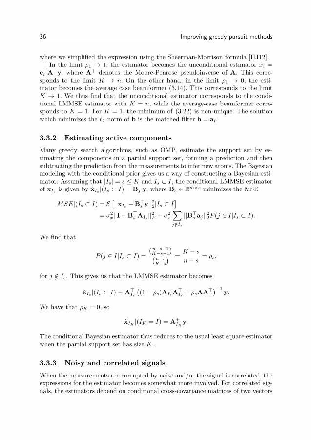
36 Improving greedy pursuit methods
where we simplified the expression using the Sheerman-Morrison formula [HJ12].In the limit ρ1 → 1, the estimator becomes the unconditional estimator xi =
e>i A+y, where A+ denotes the Moore-Penrose pseudoinverse of A. This corre-sponds to the limit K → n. On the other hand, in the limit ρ1 → 0, the esti-mator becomes the average case beamformer (3.14). This corresponds to the limitK → 1. We thus find that the unconditional estimator corresponds to the condi-tional LMMSE estimator with K = n, while the average-case beamformer corre-sponds to K = 1. For K = 1, the minimum of (3.22) is non-unique. The solutionwhich minimizes the `2 norm of b is the matched filter b = ai.
3.3.2 Estimating active components
Many greedy search algorithms, such as OMP, estimate the support set by es-timating the components in a partial support set, forming a prediction and thensubtracting the prediction from the measurements to infer new atoms. The Bayesianmodeling with the conditional prior gives us a way of constructing a Bayesian esti-mator. Assuming that |Is| = s ≤ K and Is ⊂ I, the conditional LMMSE estimatorof xIs is given by xIs |(Is ⊂ I) = B>s y, where Bs ∈ Rm×s minimizes the MSE
MSE|(Is ⊂ I) = E[||xIs −B>s y||22|Is ⊂ I
]= σ2
x||I−B>s AIs ||2F + σ2x
∑j /∈Is
||B>s aj ||22P (j ∈ I|Is ⊂ I).
We find that
P (j ∈ I|Is ⊂ I) =(n−s−1K−s−1
)(n−sK−s
) = K − sn− s
= ρs,
for j /∈ Is. This gives us that the LMMSE estimator becomes
xIs |(Is ⊂ I) = A>Is((1− ρs)AIsA>Is + ρsAA>
)−1 y.
We have that ρK = 0, so
xIK |(IK = I) = A+IK
y.
The conditional Bayesian estimator thus reduces to the usual least square estimatorwhen the partial support set has size K.
3.3.3 Noisy and correlated signals
When the measurements are corrupted by noise and/or the signal is correlated, theexpressions for the estimator becomes somewhat more involved. For correlated sig-nals, the estimators depend on conditional cross-covariance matrices of two vectors
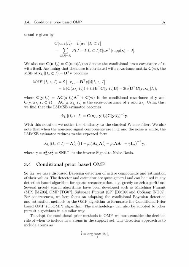
3.4. Conditional prior based OMP 37
u and v given by
C(u,v|Is) = E [uv>|Is ⊂ I]
=∑
J,|J|=K
P (J = I|Is ⊂ I)E [uv>|supp(x) = J ].
We also use C(u|Is) = C(u,u|Is) to denote the conditional cross-covariance of uwith itself. Assuming that the noise is correlated with covariance matrix C(w), theMSE of xIs |(Is ⊂ I) = B>y becomes
MSE|(Is ⊂ I) = E[||xIs −B>y||22|Is ⊂ I
]= tr(C(xIs |Is)) + tr(B>C(y|Is)B)− 2tr(B>C(y,xIs |Is),
where C(y|Is) = AC(x|Is)A> + C(w) is the conditional covariance of y andC(y,xIs |Is ⊂ I) = AC(x,xIs |Is) is the cross-covariance of y and xIs . Using this,we find that the LMMSE estimator becomes
xIs |(Is ⊂ I) = C(xIs ,y|Is)C(y|Is)−1y.
With this notation we notice the similarity to the classical Wiener filter. We alsonote that when the non-zero signal components are i.i.d. and the noise is white, theLMMSE estimator reduces to the expected form
xIs |(Is ⊂ I) = A>Is((1− ρs)AIsA>Is + ρsAA> + γIm
)−1 y,
where γ = σ2n/σ
2x = SNR−1 is the inverse Signal-to-Noise-Ratio.
3.4 Conditional prior based OMP
So far, we have discussed Bayesian detection of active components and estimationof their values. The detector and estimator are quite general and can be used in anydetection based algorithm for sparse reconstruction, e.g. greedy search algorithms.Several greedy search algorithms have been developed such as Matching Pursuit(MP) [MZ93], OMP [TG07], Subspace Pursuit (SP) [DM09] and CoSamp [NT09].For concreteness, we here focus on adopting the conditional Bayesian detectionand estimation methods to the OMP algorithm to formulate the Conditional Priorbased OMP (CpOMP) algorithm. The methodology can also be adopted to otherpursuit algorithms in a similar way.
To adapt the conditional prior methods to OMP, we must consider the decisionrule of when to include new atoms in the support set. The detection approach is toinclude atoms as
i = arg maxj|xj |,
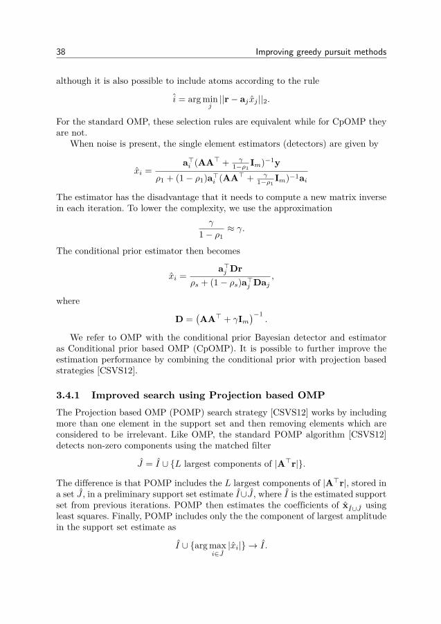
38 Improving greedy pursuit methods
although it is also possible to include atoms according to the rule
i = arg minj||r− aj xj ||2.
For the standard OMP, these selection rules are equivalent while for CpOMP theyare not.
When noise is present, the single element estimators (detectors) are given by
xi =a>i (AA> + γ
1−ρ1Im)−1y
ρ1 + (1− ρ1)a>i (AA> + γ1−ρ1
Im)−1ai
The estimator has the disadvantage that it needs to compute a new matrix inversein each iteration. To lower the complexity, we use the approximation
γ
1− ρ1≈ γ.
The conditional prior estimator then becomes
xi =a>j Dr
ρs + (1− ρs)a>j Daj,
where
D =(AA> + γIm
)−1.
We refer to OMP with the conditional prior Bayesian detector and estimatoras Conditional prior based OMP (CpOMP). It is possible to further improve theestimation performance by combining the conditional prior with projection basedstrategies [CSVS12].
3.4.1 Improved search using Projection based OMPThe Projection based OMP (POMP) search strategy [CSVS12] works by includingmore than one element in the support set and then removing elements which areconsidered to be irrelevant. Like OMP, the standard POMP algorithm [CSVS12]detects non-zero components using the matched filter
J = I ∪ L largest components of |A>r|.
The difference is that POMP includes the L largest components of |A>r|, stored ina set J , in a preliminary support set estimate I∪J , where I is the estimated supportset from previous iterations. POMP then estimates the coefficients of xI∪J usingleast squares. Finally, POMP includes only the the component of largest amplitudein the support set estimate as
I ∪ arg maxi∈J|xi| → I .
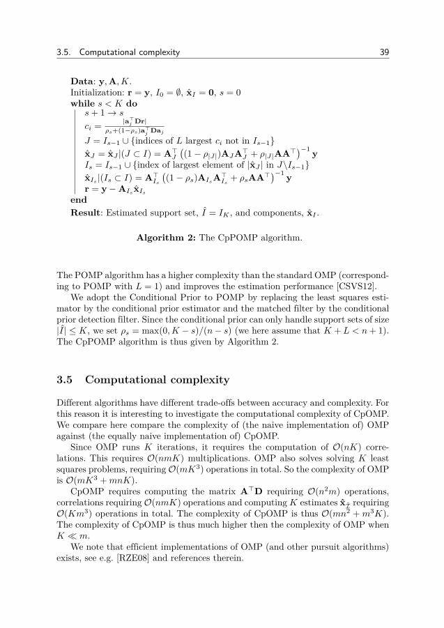
3.5. Computational complexity 39
Data: y,A,K.Initialization: r = y, I0 = ∅, xI = 0, s = 0while s < K do
s+ 1→ s
ci = |a>j Dr|ρs+(1−ρs)a>j Daj
J = Is−1 ∪ indices of L largest ci not in Is−1xJ = xJ |(J ⊂ I) = A>J
((1− ρ|J|)AJA>J + ρ|J|AA>
)−1 yIs = Is−1 ∪ index of largest element of |xJ | in J\Is−1xIs |(Is ⊂ I) = A>Is
((1− ρs)AIsA>Is + ρsAA>
)−1 yr = y−AIs xIs
endResult: Estimated support set, I = IK , and components, xI .
Algorithm 2: The CpPOMP algorithm.
The POMP algorithm has a higher complexity than the standard OMP (correspond-ing to POMP with L = 1) and improves the estimation performance [CSVS12].
We adopt the Conditional Prior to POMP by replacing the least squares esti-mator by the conditional prior estimator and the matched filter by the conditionalprior detection filter. Since the conditional prior can only handle support sets of size|I| ≤ K, we set ρs = max(0,K − s)/(n− s) (we here assume that K + L < n+ 1).The CpPOMP algorithm is thus given by Algorithm 2.
3.5 Computational complexity
Different algorithms have different trade-offs between accuracy and complexity. Forthis reason it is interesting to investigate the computational complexity of CpOMP.We compare here compare the complexity of (the naive implementation of) OMPagainst (the equally naive implementation of) CpOMP.
Since OMP runs K iterations, it requires the computation of O(nK) corre-lations. This requires O(nmK) multiplications. OMP also solves solving K leastsquares problems, requiring O(mK3) operations in total. So the complexity of OMPis O(mK3 +mnK).
CpOMP requires computing the matrix A>D requiring O(n2m) operations,correlations requiring O(nmK) operations and computingK estimates xI requiringO(Km3) operations in total. The complexity of CpOMP is thus O(mn2 + m3K).The complexity of CpOMP is thus much higher then the complexity of OMP whenK m.
We note that efficient implementations of OMP (and other pursuit algorithms)exists, see e.g. [RZE08] and references therein.
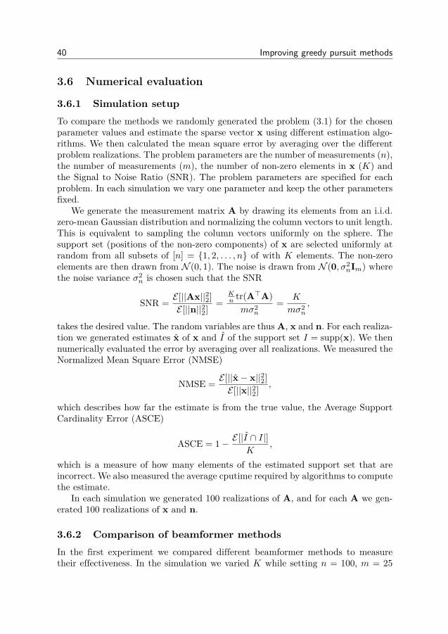
40 Improving greedy pursuit methods
3.6 Numerical evaluation
3.6.1 Simulation setupTo compare the methods we randomly generated the problem (3.1) for the chosenparameter values and estimate the sparse vector x using different estimation algo-rithms. We then calculated the mean square error by averaging over the differentproblem realizations. The problem parameters are the number of measurements (n),the number of measurements (m), the number of non-zero elements in x (K) andthe Signal to Noise Ratio (SNR). The problem parameters are specified for eachproblem. In each simulation we vary one parameter and keep the other parametersfixed.
We generate the measurement matrix A by drawing its elements from an i.i.d.zero-mean Gaussian distribution and normalizing the column vectors to unit length.This is equivalent to sampling the column vectors uniformly on the sphere. Thesupport set (positions of the non-zero components) of x are selected uniformly atrandom from all subsets of [n] = 1, 2, . . . , n of with K elements. The non-zeroelements are then drawn from N (0, 1). The noise is drawn from N (0, σ2
nIm) wherethe noise variance σ2
n is chosen such that the SNR
SNR = E [||Ax||22]E [||n||22] =
Kn tr(A>A)mσ2
n
= K
mσ2n
,
takes the desired value. The random variables are thus A, x and n. For each realiza-tion we generated estimates x of x and I of the support set I = supp(x). We thennumerically evaluated the error by averaging over all realizations. We measured theNormalized Mean Square Error (NMSE)
NMSE = E [||x− x||22]E [||x||22] ,
which describes how far the estimate is from the true value, the Average SupportCardinality Error (ASCE)
ASCE = 1− E [|I ∩ I|]K
,
which is a measure of how many elements of the estimated support set that areincorrect. We also measured the average cputime required by algorithms to computethe estimate.
In each simulation we generated 100 realizations of A, and for each A we gen-erated 100 realizations of x and n.
3.6.2 Comparison of beamformer methodsIn the first experiment we compared different beamformer methods to measuretheir effectiveness. In the simulation we varied K while setting n = 100, m = 25
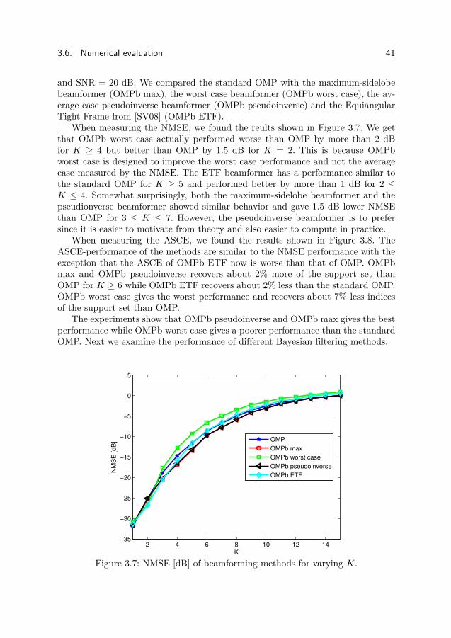
3.6. Numerical evaluation 41
and SNR = 20 dB. We compared the standard OMP with the maximum-sidelobebeamformer (OMPb max), the worst case beamformer (OMPb worst case), the av-erage case pseudoinverse beamformer (OMPb pseudoinverse) and the EquiangularTight Frame from [SV08] (OMPb ETF).
When measuring the NMSE, we found the reults shown in Figure 3.7. We getthat OMPb worst case actually performed worse than OMP by more than 2 dBfor K ≥ 4 but better than OMP by 1.5 dB for K = 2. This is because OMPbworst case is designed to improve the worst case performance and not the averagecase measured by the NMSE. The ETF beamformer has a performance similar tothe standard OMP for K ≥ 5 and performed better by more than 1 dB for 2 ≤K ≤ 4. Somewhat surprisingly, both the maximum-sidelobe beamformer and thepseudionverse beamformer showed similar behavior and gave 1.5 dB lower NMSEthan OMP for 3 ≤ K ≤ 7. However, the pseudoinverse beamformer is to prefersince it is easier to motivate from theory and also easier to compute in practice.
When measuring the ASCE, we found the results shown in Figure 3.8. TheASCE-performance of the methods are similar to the NMSE performance with theexception that the ASCE of OMPb ETF now is worse than that of OMP. OMPbmax and OMPb pseudoinverse recovers about 2% more of the support set thanOMP for K ≥ 6 while OMPb ETF recovers about 2% less than the standard OMP.OMPb worst case gives the worst performance and recovers about 7% less indicesof the support set than OMP.
The experiments show that OMPb pseudoinverse and OMPb max gives the bestperformance while OMPb worst case gives a poorer performance than the standardOMP. Next we examine the performance of different Bayesian filtering methods.
2 4 6 8 10 12 14−35
−30
−25
−20
−15
−10
−5
0
5
K
NM
SE
[dB
]
OMP
OMPb max
OMPb worst case
OMPb pseudoinverse
OMPb ETF
Figure 3.7: NMSE [dB] of beamforming methods for varying K.

42 Improving greedy pursuit methods
2 4 6 8 10 12 140
0.1
0.2
0.3
0.4
0.5
0.6
0.7
0.8
K
AS
CE
OMP
OMPb max
OMPb worst case
OMPb pseudoinverse
OMPb ETF
Figure 3.8: ASCE of beamforming methods for varying K.
3.6.3 Comparison of Bayesian filtering methods
In the second experiment we measured the performance of different Bayesian filter-ing methods for greedy pursuits when varying the number of non-zero elements, K.We compared the standard Orthogonal Matching Pursuit (OMP), the Projectionbased OMP (POMP), the Conditional prior OMP (CpOMP) and the Projectionbased CpOMP (CpPOMP). The algorithms POMP and CpPOMP both use L = Kin the simulation. In the simulation we set n = 100, m = 25 and SNR = 20 dB.
When measuring the NMSE we found the results shown in Figure 3.9. We seethat CpPOMP and CpOMP gave the smallest error while POMP gave a smallererror than the standard OMP. The NMSE of CpOMP and CpPOMP was about 2dB lower than the NMSE of OMP for K ≥ 2 while the NMSE of POMP was 1.5dB lower than the NMSE of OMP for K ≥ 3.
When measuring the ASCE we found the results shown in Figure 3.10. We seethat CpPOMP and CpOMP gave the smallest error while POMP gave a smallererror than the standard OMP. The ASCE of CpOMP and CpPOMP was about 4%lower than the ASCE of OMP for K ≥ 7 while the ASCE of POMP was about 3%lower than the ASCE of OMP for K ≥ 7.
From the experiments we get that CpOMP and CpPOMP give better perfor-mance than the standard OMP and POMP. In the next section we examine howthe methods compare with OMPb and other methods.
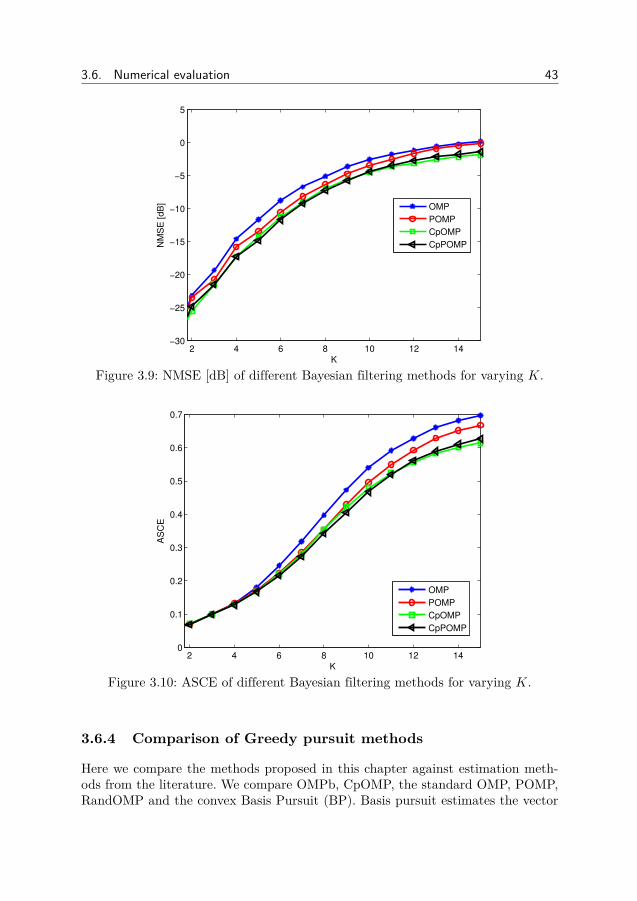
3.6. Numerical evaluation 43
2 4 6 8 10 12 14−30
−25
−20
−15
−10
−5
0
5
K
NM
SE
[dB
]
OMP
POMP
CpOMP
CpPOMP
Figure 3.9: NMSE [dB] of different Bayesian filtering methods for varying K.
2 4 6 8 10 12 140
0.1
0.2
0.3
0.4
0.5
0.6
0.7
K
AS
CE
OMP
POMP
CpOMP
CpPOMP
Figure 3.10: ASCE of different Bayesian filtering methods for varying K.
3.6.4 Comparison of Greedy pursuit methods
Here we compare the methods proposed in this chapter against estimation meth-ods from the literature. We compare OMPb, CpOMP, the standard OMP, POMP,RandOMP and the convex Basis Pursuit (BP). Basis pursuit estimates the vector
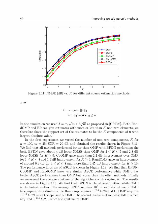
44 Improving greedy pursuit methods
2 4 6 8 10 12 14−30
−25
−20
−15
−10
−5
0
5
K
NM
SE
[dB
]
OMP
OMPb
CpOMP
RandOMP
BPDN
Figure 3.11: NMSE [dB] vs. K for different sparse estimation methods.
x as
x = arg min ||x||1s.t. ||y−Ax||2 ≤ δ
In the simulation we used δ = σn√m+ 8
√m as proposed in [CRT06]. Both Ran-
dOMP and BP can give estimates with more or less than K non-zero elements, wetherefore chose the support set of the estimates to be the K components of x withlargest absolute value.
In the first experiment we varied the number of non-zero components, K forn = 100, m = 25, SNR = 20 dB and obtained the results shown in Figure 3.11.We find that all methods performed better than OMP with BPDN performing thebest. BPDN gave about 4 dB lower NMSE than OMP for 2 ≤ K ≤ 5 and 2.8 dBlower NMSE for K ≥ 9. CpOMP gave more than 2.2 dB improvement over OMPfor 3 ≤ K ≤ 8 and 1.9 dB improvement for K ≥ 9. RandOMP gave an improvementof around 0.3 dB for 4 ≤ K ≤ 8 and more than 0.45 dB improvement for K ≥ 10.The performance in terms of ASCE is shown in Figure 3.12. We find that BPDN,CpOMP and RandOMP have very similar ASCE performance while OMPb hasbetter ASCE performance than OMP but worse than the other methods. Finallywe measured the average cputime of the algorithms with varying K. The resultsare shown in Figure 3.13. We find that BPDN is the slowest method while OMPis the fastest method. On average BPDN requires 106 times the cputime of OMPto compute the estimate while Randomp requires 102.4 ≈ 25 and CpOMP requires101.9 ≈ 79 times the cputime of OMP. The second fastest method was OMPb whichrequired 100.4 ≈ 2.5 times the cputime of OMP.
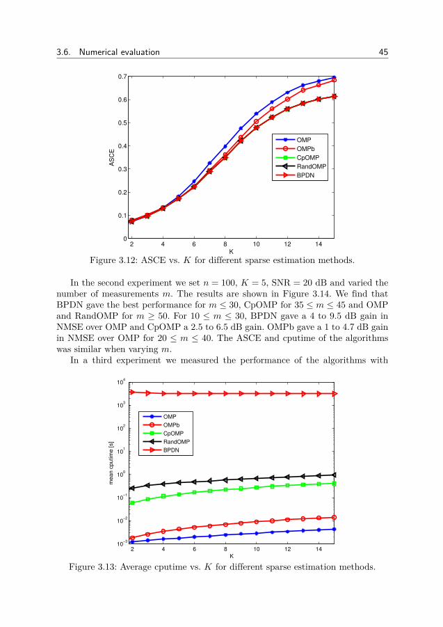
3.6. Numerical evaluation 45
2 4 6 8 10 12 140
0.1
0.2
0.3
0.4
0.5
0.6
0.7
K
AS
CE
OMP
OMPb
CpOMP
RandOMP
BPDN
Figure 3.12: ASCE vs. K for different sparse estimation methods.
In the second experiment we set n = 100, K = 5, SNR = 20 dB and varied thenumber of measurements m. The results are shown in Figure 3.14. We find thatBPDN gave the best performance for m ≤ 30, CpOMP for 35 ≤ m ≤ 45 and OMPand RandOMP for m ≥ 50. For 10 ≤ m ≤ 30, BPDN gave a 4 to 9.5 dB gain inNMSE over OMP and CpOMP a 2.5 to 6.5 dB gain. OMPb gave a 1 to 4.7 dB gainin NMSE over OMP for 20 ≤ m ≤ 40. The ASCE and cputime of the algorithmswas similar when varying m.
In a third experiment we measured the performance of the algorithms with
2 4 6 8 10 12 1410
−3
10−2
10−1
100
101
102
103
104
K
mean c
putim
e [s]
OMP
OMPb
CpOMP
RandOMP
BPDN
Figure 3.13: Average cputime vs. K for different sparse estimation methods.
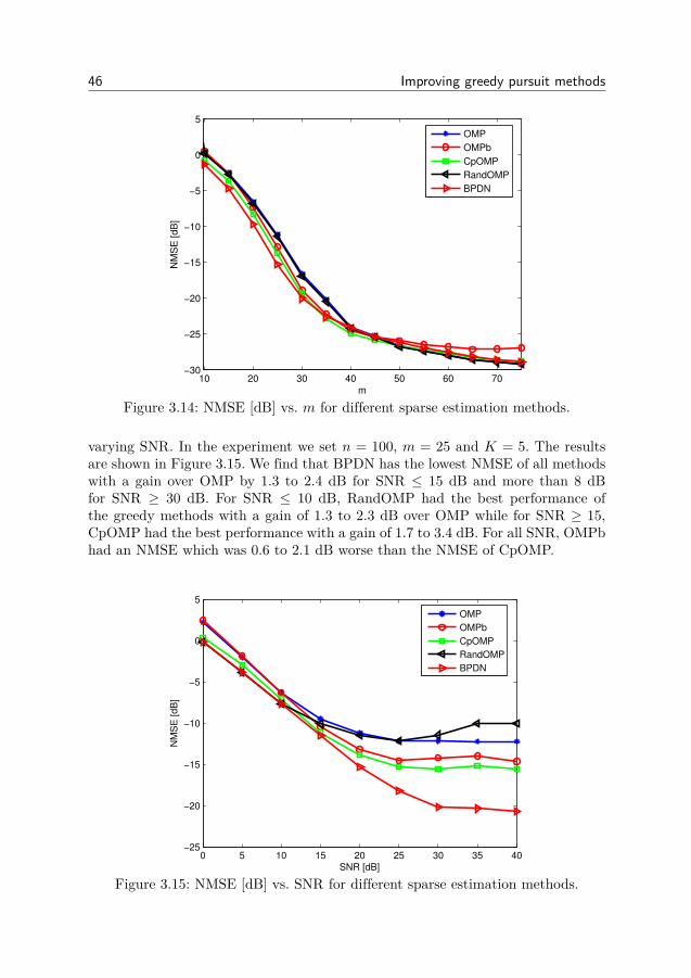
46 Improving greedy pursuit methods
10 20 30 40 50 60 70−30
−25
−20
−15
−10
−5
0
5
m
NM
SE
[dB
]
OMP
OMPb
CpOMP
RandOMP
BPDN
Figure 3.14: NMSE [dB] vs. m for different sparse estimation methods.
varying SNR. In the experiment we set n = 100, m = 25 and K = 5. The resultsare shown in Figure 3.15. We find that BPDN has the lowest NMSE of all methodswith a gain over OMP by 1.3 to 2.4 dB for SNR ≤ 15 dB and more than 8 dBfor SNR ≥ 30 dB. For SNR ≤ 10 dB, RandOMP had the best performance ofthe greedy methods with a gain of 1.3 to 2.3 dB over OMP while for SNR ≥ 15,CpOMP had the best performance with a gain of 1.7 to 3.4 dB. For all SNR, OMPbhad an NMSE which was 0.6 to 2.1 dB worse than the NMSE of CpOMP.
0 5 10 15 20 25 30 35 40−25
−20
−15
−10
−5
0
5
SNR [dB]
NM
SE
[d
B]
OMP
OMPb
CpOMP
RandOMP
BPDN
Figure 3.15: NMSE [dB] vs. SNR for different sparse estimation methods.

3.7. Conclusion 47
3.7 Conclusion
In this chapter we examined how greedy search algorithms such as OMP can beimproved by improving the step in which new atoms are detected. We first consid-ered the deterministic construction of beamformers and thereafter Bayesian filteringmethods which can be described as conditional Wiener filters for sparse estimation.The Bayesian filtering method improves both the detection and estimation of com-ponents in the support set. The Bayesian filtering method has the advantage ofcapturing the random nature of the non-zero elements. For simplicity we here onlyconsidered the scenario of uniformly distributed support sets, but the conditionalprior method can be extended to non-uniform scenarios. The experiments showthat while the improved greedy search methods OMPb and CpOMP are not aseffective as BPDN, they are much faster and outperform the standard OMP. Thegain in performance comes at the price of higher complexity. CpOMP has a highercomplexity than OMP, but lower than RandOMP and OMPb has a complexitywhich is closer to OMP. This shows that the OMP algorithm can be improved byimproving the detection and estimation steps of the algorithm.


Chapter 4
Outlier robust relevance vector machine
Measurements are typically assumed to be perturbed by noise. The noiseaccounts for measurement errors and model imperfections. Often, somemeasurements are corrupted by extra strong noise. This sparse noise ac-
counts for saturation of sensors, missing values, quantizing errors or impulse burstsas well as datapoints which deviate from the model. In images, for example, thepixels can become saturated by salt and pepper noise which turns the pixels blackor white. Since the sparse noise can strongly perturb the final estimate (as for theBoston housing dataset in Figure 2.6), it is important to make estimation methodsrobust against sparse noise. Because of its sparsity, the noise can be removed usingsparse estimation techniques.
Most sparse estimation methods can be made robust by treating the sparsenoise as additional parameters to be estimated. This approach is often successful,but leads to higher complexity since the parameter vector becomes larger. The Rel-evance Vector Machine (RVM) [Tip01] is a Bayesian method for sparse estimation.Bayesian methods are often preferable since they can estimate both the parametervector and noise power from the measurements alone. We here show how the RVMcan be made robust to sparse noise without explicitly estimating the componentsof the outliers.
4.0.1 System modelWe consider the linear system model
y = Ax + e + n, (4.1)
where y ∈ Rm is the observed measurements, x ∈ Rn is a sparse vector (for exampleweights in regression or sparse signal to estimate in compressed sensing) we wish toestimate, A ∈ Rm×n is a known system matrix (for example, regressors or samplingsystem) representing the measurement process. Further, e ∈ Rm and n ∈ Rm aresparse and dense noise respectively. We assume that ||x||0 n and ||e||0 mare small and unknown, where || · ||0 denotes the number of non-zero components
49

50 Outlier robust relevance vector machine
of a vector. The random vectors x, e and n are independent. The model (4.1) isused in e.g. face recognition [WYG+09], image denoising [MVC10] and compressedsensing [JXC08].
4.0.2 Prior workAlmost all prior works [MVC10, LDB+09, JR10, VKC13] translate (4.1) into theequivalent setup
y =[
A Im] [ x
e
]+ n, (4.2)
where Im is the m×m identity matrix,[
A Im]acts as the effective system ma-
trix and[x> e>
]> acts as the effective parameter vector. The RB-RVM of [MVC10]uses the standard RVM approach for (4.2) directly. Hence RB-RVM learns modelparameters for all three signals x = [x1, x2, . . . , xn]>, e = [e1, e2, . . . , em]> and n,and thus estimates both x and e jointly.
RVM has high similarity with Sparse Bayesian Learning (SBL) [ZR11, ZR13,WR04,WPR04]. Sparse Bayesian learning has been used for structured sparse sig-nals, for example block sparse signals [ZR11], where the problem of unknown signalblock structure was treated using overlapping blocks. The model extension of RB-RVM shown in (4.2) for handling block sparse noise with unknown block structureis straight-forward to derive. However, in our formulation, as we are not estimatingthe noise explicitly, the use of block sparse noise with unknown block structure isnon-trivial.
Further, convex optimization based methods have been used for sparse esti-mation problems [LDB+09,CDS01,CSVS12, ZCJ12]. For example, justice pursuit(JP) [LDB+09] uses the optimization technique of the standard basis pursuit de-noising method [CDS01], as follows
x, e = arg minx,e||x||1 + ||e||1 (4.3)
s.t. ||y−Ax− e||2 ≤ ε, (4.4)
where ε > 0 is a model parameter. For unknown noise power, it is impossible toknow ε a-priori. We mention that a fully Bayesian setup like the RVM does notrequire parameters set by a-priori.
4.0.3 Our contributionOur main contribution is developing a robust RVM using a combined noise model.The method uses fewer parameters than the robust RVM of [MVC10], since thesparse noise is not estimated explicitly. This means that the method has lowercomputational complexity and also better performance in some instances. As an
4.1. RVM for combined sparse and dense noise (SD-RVM) 51
extension we also consider the scenario where the signal x and noise e are blocksparse. By using techniques from [ZR11] we generalize the methods to signals wherethe position of the blocks are unknown. The main technical contribution is to deriveupdate equations that are used iteratively for estimation of parameters in the newRVM. We refer to the new RVM as the RVM for combined sparse and dense noise(SD-RVM). By an approximate analysis, the SD-RVM algorithm is shown to beequivalent to the minimization of a sparsity inducing cost function. Finally, theperformance of SD-RVM is evaluated numerically using examples from compressedsensing, block sparse signal recovery, house price prediction and image denoising.Throughout the paper, we take an approach of comparing SD-RVM vis-a-vis theexisting Robust Bayesian RVM (RB-RVM) of [MVC10].
4.1 RVM for combined sparse and dense noise (SD-RVM)
4.1.1 SD-RVM MethodFor (4.1), we propose to use a combined model for the noise terms, as follows
e + n ∼ N (0,B−1), (4.5)
where B = diag(β), β = [β1, β2, . . . , βm] and βj > 0 for j ∈ [m] = 1, 2, . . . ,m.The two noise terms are treated as a single combined noise where each noise com-ponent has its own precision. The rationale is that we do not need to seperate thetwo noises. Although our model promotes sparsity in the noise we empirically findthat it is able to model both sparse and non-sparse noise.
We model the components of the parameter vector x as
xi ∼ N (0, γ−1i ), (4.6)
where γi > 0 and i ∈ [n] = 1, 2, . . . , n. From (4.5) and (4.6) we find that themaximum a posteriori (MAP) estimate of x is
x = ΣA>By,Σ = (Γ + A>BA)−1,
where Γ = diag(γ) and γ = [γ1, γ2, . . . , γn].To promote sparsity in x, the RVM assigns prior probabilities to the precisions
[Tip01]. A common choice is to assign Gamma distributions
p(γi) =Gamma(γi|a, b) = baγa−1i e−bγi
Γ(a) , (4.7)
p(βj) =Gamma(βi|c, d) = dcγc−1i e−dβj
Γ(c) , (4.8)
where a, b, c, d > 0 are parameters. We will consider parameters for which thedistributions are “nearly flat”, i.e. a, c are slightly larger than one and b, d are
52 Outlier robust relevance vector machine
slight larger than zero. Through expectation-maximization (EM) we find that theprecisions are updated as
γnewi = 1 + 2(a− 1)x2i + Σii + 2b , (4.9)
βnewj = 1 + 2(c− 1)[y−Ax]2j + [AΣA>]jj + 2d , (4.10)
where we use [·]ij to denote the i, j element of a matrix. The derivations of (4.9)and (4.10) are given in Section 4.4.1. Next we show that the model is equivalent toMAP estimation with a sparsity promoting penalty function.
4.1.2 Relation to sparsity promoting penalty functionA common approach to sparse estimation is to estimate x as
x = arg minx
β
2 h(n) + g(x),
subject to y = Ax + n(4.11)
where g(·) is a penalty function which promotes sparsity in x, e.g. the `1-norm,and typically h(n) = ||n||22. Here we show that SD-RVM corresponds to (4.11) for acertain sparsity promoting penalty function. Since several approximations are madein the derivation of the iterative update equations. It is interesting to see how theapproximations affect the sparsit promoting penalty function.
To motivate that the standard RVM is sparsity promoting, one can note thatthe marginal distribution of xi is a student-t distribution. For a fixed β (and e = 0),the standard RVM is therefore an iterative method for minimizing [Tip01]
β
2 h(n) +(
12 + a
) n∑i=1
log(x2i + 2b),
subject to the constraint y = Ax + n. The log-sum penalty function can be usedas a sparsity promoting cost function, making it plausible that the RVM promotessparsity.
For the SD-RVM, the precisions are updated by maximizing the log-likelihoodL = log p(y,γ,β) = constant
− 12 log det(B−1 + AΓ−1A>)
− 12y>(B−1 + AΓ−1A>)−1y
+n∑i=1
(a log γi − bγi)
+m∑j=1
(c log βj − dβj).
(4.12)

4.1. RVM for combined sparse and dense noise (SD-RVM) 53
By the matrix determinant lemma [Har97],
det(B−1 + AΓ−1A>) = det(Σ−1)det(Γ−1)det(B−1).
We can approximate (4.12) using that
log det(Σ−1) ≈ log det((Σold)−1)
+n∑i=1
Σoldii (γi − γoldi )
+m∑j=1
[AΣoldA>]jj(βj − βoldj ),
(4.13)
where the approximation is to first order in γ and β. We also introduce variablesx and e through the relation [RKH13]
y>(AΓ−1A> + B−1)−1y = minx,e
n∑i=1
γix2i +
m∑j=1
βj e2j ,
such that Ax + e = y
(4.14)
where now e = e + n as in (4.5). The minimization problem then becomes
minx,e,γ,β
n∑i=1
[(x2i + Σoldii + 2b)γi + (2a− 1) log(γi)
]+
m∑j=1
[(e2j + [AΣoldA>]jj + 2d)βj + (2c− 1) log(βj)
].
such that Ax + e = y
(4.15)
By minimizing (4.15) with respect to γi and βj , the problem reduces to
minx,e
(2a− 1)n∑i=1
log(x2i + Σoldii + 2b) (4.16)
+ (2c− 1)m∑j=1
log(e2j + [AΣoldA>]jj + 2d),
such that Ax + e = y
where we have ignored additive constants. Because of the approximations, the con-stants Σoldii and [AΣoldA>]jj make the penalty function penalize different com-ponents of x and e differently. In a similar fashion it can be shown that thestandard RVM and RB-RVM are also equivalent to similar penalty functions. Atwo-dimensional illustration of the penalty function is shown in Figure 4.1.
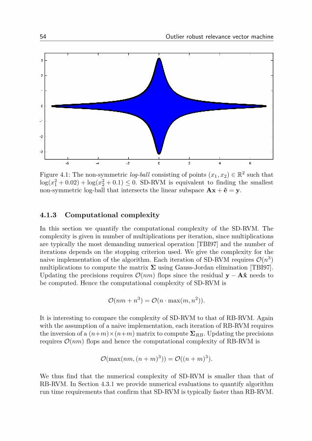
54 Outlier robust relevance vector machine
Figure 4.1: The non-symmetric log-ball consisting of points (x1, x2) ∈ R2 such thatlog(x2
1 + 0.02) + log(x22 + 0.1) ≤ 0. SD-RVM is equivalent to finding the smallest
non-symmetric log-ball that intersects the linear subspace Ax + e = y.
4.1.3 Computational complexity
In this section we quantify the computational complexity of the SD-RVM. Thecomplexity is given in number of multiplications per iteration, since multiplicationsare typically the most demanding numerical operation [TBI97] and the number ofiterations depends on the stopping criterion used. We give the complexity for thenaive implementation of the algorithm. Each iteration of SD-RVM requires O(n3)multiplications to compute the matrix Σ using Gauss-Jordan elimination [TBI97].Updating the precisions requires O(nm) flops since the residual y−Ax needs tobe computed. Hence the computational complexity of SD-RVM is
O(nm+ n3) = O(n ·max(m,n2)).
It is interesting to compare the complexity of SD-RVM to that of RB-RVM. Againwith the assumption of a naive implementation, each iteration of RB-RVM requiresthe inversion of a (n+m)×(n+m) matrix to compute ΣRB . Updating the precisionsrequires O(nm) flops and hence the computational complexity of RB-RVM is
O(max(nm, (n+m)3)) = O((n+m)3).
We thus find that the numerical complexity of SD-RVM is smaller than that ofRB-RVM. In Section 4.3.1 we provide numerical evaluations to quantify algorithmrun time requirements that confirm that SD-RVM is typically faster than RB-RVM.
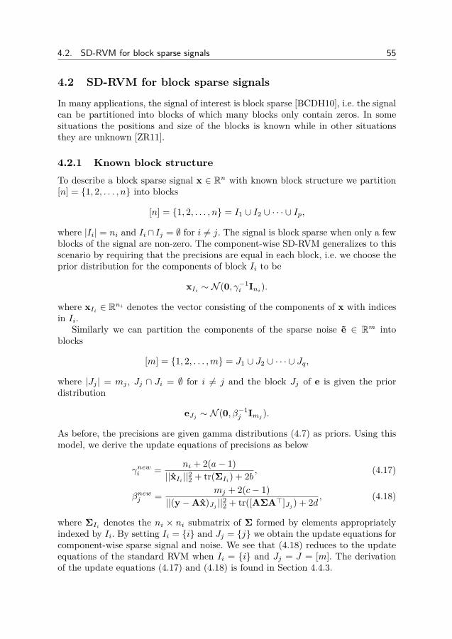
4.2. SD-RVM for block sparse signals 55
4.2 SD-RVM for block sparse signals
In many applications, the signal of interest is block sparse [BCDH10], i.e. the signalcan be partitioned into blocks of which many blocks only contain zeros. In somesituations the positions and size of the blocks is known while in other situationsthey are unknown [ZR11].
4.2.1 Known block structureTo describe a block sparse signal x ∈ Rn with known block structure we partition[n] = 1, 2, . . . , n into blocks
[n] = 1, 2, . . . , n = I1 ∪ I2 ∪ · · · ∪ Ip,
where |Ii| = ni and Ii ∩ Ij = ∅ for i 6= j. The signal is block sparse when only a fewblocks of the signal are non-zero. The component-wise SD-RVM generalizes to thisscenario by requiring that the precisions are equal in each block, i.e. we choose theprior distribution for the components of block Ii to be
xIi ∼ N (0, γ−1i Ini).
where xIi ∈ Rni denotes the vector consisting of the components of x with indicesin Ii.
Similarly we can partition the components of the sparse noise e ∈ Rm intoblocks
[m] = 1, 2, . . . ,m = J1 ∪ J2 ∪ · · · ∪ Jq,
where |Jj | = mj , Jj ∩ Ji = ∅ for i 6= j and the block Jj of e is given the priordistribution
eJj ∼ N (0, β−1j Imj ).
As before, the precisions are given gamma distributions (4.7) as priors. Using thismodel, we derive the update equations of precisions as below
γnewi = ni + 2(a− 1)||xIi ||22 + tr(ΣIi) + 2b , (4.17)
βnewj = mj + 2(c− 1)||(y−Ax)Jj ||22 + tr([AΣA>]Jj ) + 2d , (4.18)
where ΣIi denotes the ni × ni submatrix of Σ formed by elements appropriatelyindexed by Ii. By setting Ii = i and Jj = j we obtain the update equations forcomponent-wise sparse signal and noise. We see that (4.18) reduces to the updateequations of the standard RVM when Ii = i and Jj = J = [m]. The derivationof the update equations (4.17) and (4.18) is found in Section 4.4.3.

56 Outlier robust relevance vector machine
4.2.2 Unknown block structure
In some situations the signal can have an unknown block structure, i.e. the signalis block sparse, but the dimensions and positions of the blocks are unknown. Thisscenario can be handled by treating the signal as a superposition of block sparsesignals [ZR11] (see illustration in Figure 4.2). This approach also describes thescenario (4.1) when e is component wise sparse and n is dense (e.g. Gaussian). Theprecision of each component is then a combination of the precisions of the blocksto which the component belongs. Let γi be the precision of the component xi andγk be the precision of block Ik. We model the signal as
xi ∼ N (0, γ−1i ),
γ−1i =
∑k,i∈Ik
γ−1k . (4.19)
We model the noise in a similar way with precisions βj for component j and pre-cisions βl for the block with support Jl. To promote sparsity, the precisions of theunderlying blocks are given gamma distributions as priors. In each iteration we up-date the underlying precisions γk. The component-wise precisions are then updatedusing (4.19). With this model, the update equations for the precisions become
γnewk =1γk
tr(Γk) + 2(a− 1)1γ2k
||Γix||22 + 1γ2k
tr(ΓkΣΓk) + 2b, (4.20)
βnewl =1βl
tr(Bl) + 2(c− 1)1β2l
||Bl(y−Ax)||22 + 1β2l
tr(BlA>ΣABl) + 2d, (4.21)
where Γk is the diagonal matrix with [Γk]ii = γi if i ∈ Ik and [Γk]ii = 0 otherwise.We denote the corresponding matrix for βl by Bl. The component-wise precisionsare updated using (4.19) and similar for βj .
We see that when the underlying blocks are disjoint, then γi = γk for all i ∈ Ikand βj = βl for all j ∈ Jl. The update equations then reduce to the update equations(4.18) for the block sparse model with known block structure.
4.3 Simulation experiments
In this section we evaluate the performance of SD-RVM compared to other methodsusing several scenarios – for simulated and real signals. For simulated signals, weconsidered the sparse and block sparse recovery problem in compressed sensing.For real signals, we considered prediction of house prices using the Boston housingdataset [AN07] and denoising of images contaminated by salt and pepper noise. Weused the cvx toolbox [GBY08] to implement JP.
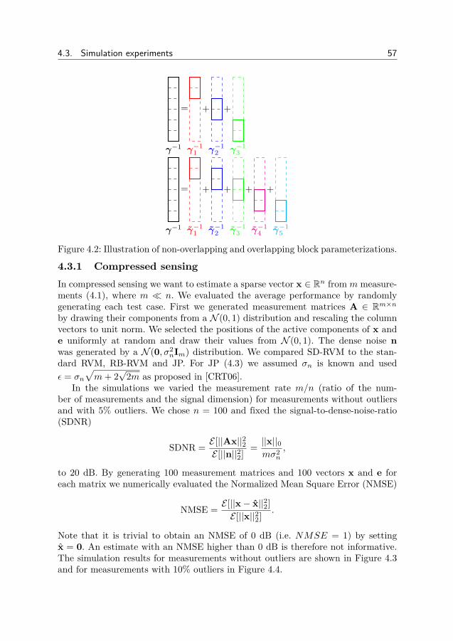
4.3. Simulation experiments 57
γ−1
=
γ−11
+
γ−12
+
γ−13
γ−1
=
γ−11
+
γ−12
+
γ−13
+
γ−14
+
γ−15
Figure 4.2: Illustration of non-overlapping and overlapping block parameterizations.
4.3.1 Compressed sensingIn compressed sensing we want to estimate a sparse vector x ∈ Rn from m measure-ments (4.1), where m n. We evaluated the average performance by randomlygenerating each test case. First we generated measurement matrices A ∈ Rm×nby drawing their components from a N (0, 1) distribution and rescaling the columnvectors to unit norm. We selected the positions of the active components of x ande uniformly at random and draw their values from N (0, 1). The dense noise nwas generated by a N (0, σ2
nIm) distribution. We compared SD-RVM to the stan-dard RVM, RB-RVM and JP. For JP (4.3) we assumed σn is known and usedε = σn
√m+ 2
√2m as proposed in [CRT06].
In the simulations we varied the measurement rate m/n (ratio of the num-ber of measurements and the signal dimension) for measurements without outliersand with 5% outliers. We chose n = 100 and fixed the signal-to-dense-noise-ratio(SDNR)
SDNR = E [||Ax||22E [||n||22] = ||x||0
mσ2n
,
to 20 dB. By generating 100 measurement matrices and 100 vectors x and e foreach matrix we numerically evaluated the Normalized Mean Square Error (NMSE)
NMSE = E [||x− x||22]E [||x||22] .
Note that it is trivial to obtain an NMSE of 0 dB (i.e. NMSE = 1) by settingx = 0. An estimate with an NMSE higher than 0 dB is therefore not informative.The simulation results for measurements without outliers are shown in Figure 4.3and for measurements with 10% outliers in Figure 4.4.
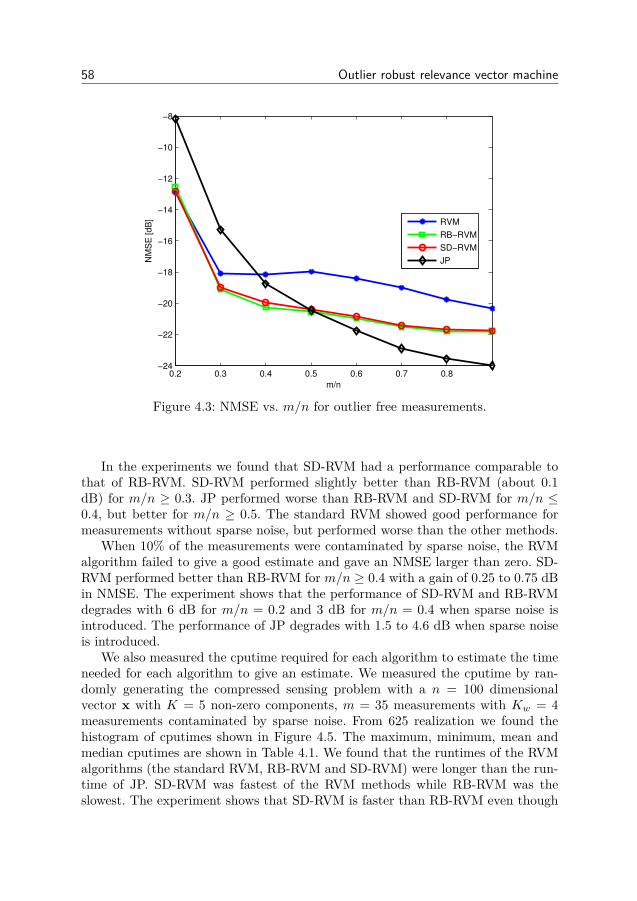
58 Outlier robust relevance vector machine
0.2 0.3 0.4 0.5 0.6 0.7 0.8−24
−22
−20
−18
−16
−14
−12
−10
−8
m/n
NM
SE
[dB
]
RVM
RB−RVM
SD−RVM
JP
Figure 4.3: NMSE vs. m/n for outlier free measurements.
In the experiments we found that SD-RVM had a performance comparable tothat of RB-RVM. SD-RVM performed slightly better than RB-RVM (about 0.1dB) for m/n ≥ 0.3. JP performed worse than RB-RVM and SD-RVM for m/n ≤0.4, but better for m/n ≥ 0.5. The standard RVM showed good performance formeasurements without sparse noise, but performed worse than the other methods.
When 10% of the measurements were contaminated by sparse noise, the RVMalgorithm failed to give a good estimate and gave an NMSE larger than zero. SD-RVM performed better than RB-RVM for m/n ≥ 0.4 with a gain of 0.25 to 0.75 dBin NMSE. The experiment shows that the performance of SD-RVM and RB-RVMdegrades with 6 dB for m/n = 0.2 and 3 dB for m/n = 0.4 when sparse noise isintroduced. The performance of JP degrades with 1.5 to 4.6 dB when sparse noiseis introduced.
We also measured the cputime required for each algorithm to estimate the timeneeded for each algorithm to give an estimate. We measured the cputime by ran-domly generating the compressed sensing problem with a n = 100 dimensionalvector x with K = 5 non-zero components, m = 35 measurements with Kw = 4measurements contaminated by sparse noise. From 625 realization we found thehistogram of cputimes shown in Figure 4.5. The maximum, minimum, mean andmedian cputimes are shown in Table 4.1. We found that the runtimes of the RVMalgorithms (the standard RVM, RB-RVM and SD-RVM) were longer than the run-time of JP. SD-RVM was fastest of the RVM methods while RB-RVM was theslowest. The experiment shows that SD-RVM is faster than RB-RVM even though
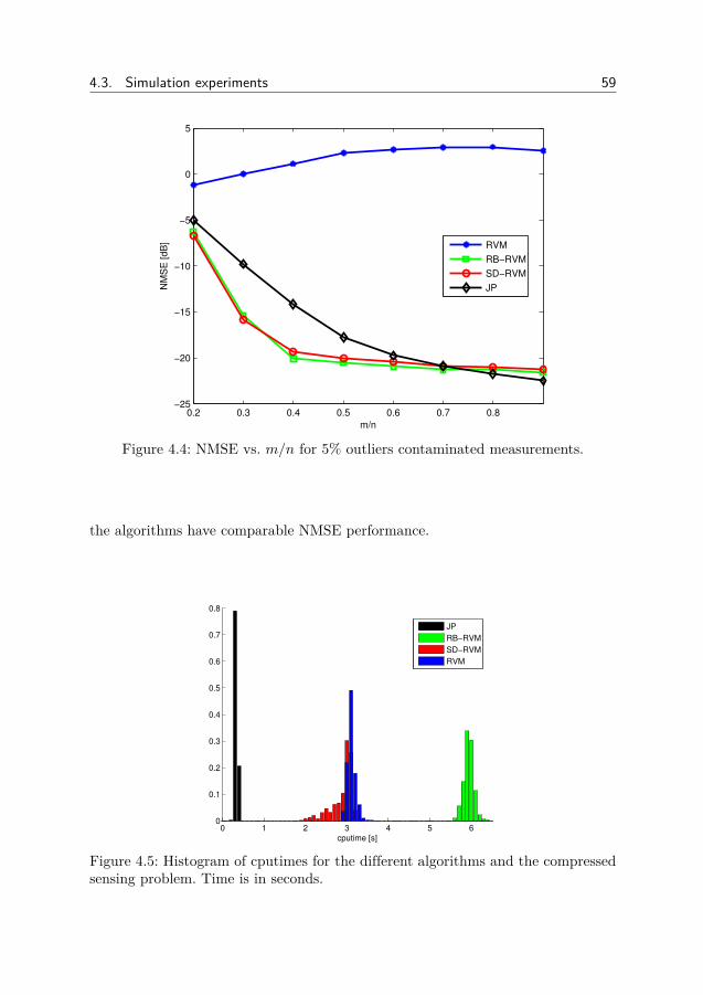
4.3. Simulation experiments 59
0.2 0.3 0.4 0.5 0.6 0.7 0.8−25
−20
−15
−10
−5
0
5
m/n
NM
SE
[dB
]
RVM
RB−RVM
SD−RVM
JP
Figure 4.4: NMSE vs. m/n for 5% outliers contaminated measurements.
the algorithms have comparable NMSE performance.
0 1 2 3 4 5 60
0.1
0.2
0.3
0.4
0.5
0.6
0.7
0.8
cputime [s]
JP
RB−RVM
SD−RVM
RVM
Figure 4.5: Histogram of cputimes for the different algorithms and the compressedsensing problem. Time is in seconds.
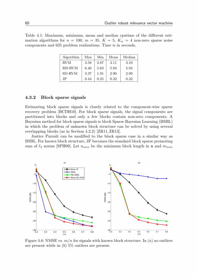
60 Outlier robust relevance vector machine
Table 4.1: Maximum, minimum, mean and median cputime of the different esti-mation algorithms for n = 100, m = 35, K = 5, Kw = 4 non-zero sparse noisecomponents and 625 problem realizations. Time is in seconds.
Algorithm Max Min Mean MedianRVM 3.58 2.87 3.11 3.10RB-RVM 6.40 5.63 5.94 5.94SD-RVM 3.37 1.91 2.90 2.99JP 0.44 0.25 0.32 0.32
4.3.2 Block sparse signals
Estimating block sparse signals is closely related to the component-wise sparserecovery problem [BCDH10]. For block sparse signals, the signal components arepartitioned into blocks and only a few blocks contain non-zero components. ABayesian method for block sparse signals is block Sparse Bayesian Learning (BSBL)in which the problem of unknown block structure can be solved by using severaloverlapping blocks (as in Section 4.2.2) [ZR11,ZR13].
Justice Pursuit can be modified to the block sparse case in a similar way asBSBL. For known block structure, JP becomes the standard block sparse promotingsum of `2 norms [SPH09]. Let nmin be the minimum block length in x and mmin
0.2 0.3 0.4 0.5 0.6 0.7 0.8−35
−30
−25
−20
−15
−10
−5
0
m/n
NM
SE
[dB
]
(a)
Block JP
BSBL
RB−BSBL
Block SD−RVM
0.2 0.3 0.4 0.5 0.6 0.7 0.8−35
−30
−25
−20
−15
−10
−5
0
NM
SE
[dB
]
m/n
(b)
Figure 4.6: NMSE vs.m/n for signals with known block structure. In (a) no outliersare present while in (b) 5% outliers are present.

4.3. Simulation experiments 61
be the minimum block length in e. By defining matrices
Z = [z1, z2, . . . , zn−nmin+1] ∈ Rnmin×(n−nmin+1),
W = [w1, w2, . . . ,wm−mmin+1] ∈ Rmmin×(m−mmin+1),
the block-JP algorithm for unknown block structure can be written as
minx,e
n−nmin+1∑l=1
||zl||2 +m−mmin+1∑
a=1||wa||2,
subject to xi =min(i,n−nmin+1)∑l=1+(i−nmin)+
Zi+1−l,l, 1 ≤ i ≤ n,
ej =min(j,m−mmin+1)∑a=1+(j−mmin)+
Wj+1−a,a, 1 ≤ j ≤ m,
||y−Ax− e||2 ≤ ε
(4.22)
where (x)+ = max(x, 0) and we set ε = σn√m+
√8m as before.
To numerically evaluate the performance of the block sparse algorithms wevaried the measurement rate m/n for measurements with 5% sparse noise. We setthe signal dimension to n = 100 and fixed the SDNR to 20 dB. We divided thesignal x into 20 blocks of equal size of which 3 blocks were non-zero. The sparsenoise consisted of blocks with 5 components in each block. In the sparse noise, 5% ofthe blocks were active. For known block structure, the blocks were chosen uniformlyat random from a set of predefined and non-overlapping blocks while for unknownblock structure, the first component of each block was chosen uniformly at random,making it possible for the blocks to overlap. The active components of the signal andthe sparse noise were drawn from N (0, 1). By generating 50 measurement matricesA and 50 signals x and sparse noises e for each matrix we numerically evaluatedthe NMSE.
For known block structure we found that block SD-RVM gave 1.1 to 2.2 improve-ment in NMSE versus RB-BSBL and 4.5 to 12.6 dB improvement versus block JPfor m/n ≥ 0.4 when no outliers are present. The non-robust BSBL method gave alower NMSE than the other methods for m/n < 0.4 and a performance betweenSD-RVM and RB-RVM for m/n ≥ 0.4. For measurements with outliers, the im-provement of SD-RVM was 1.6 to 2.2 dB versus RB-RVM and 6 to 14.7 dB versusblock JP for m/n ≥ 0.5. The BSBL method performed worse when outliers werepresent with an NMSE of about −4.5 to −7.4 dB. The NMSE of the block sparseSD-RVM was lower than the NMSE of block JP by more than 4.7 dB form/n ≥ 0.3.The results are shown in Figure 4.6.
For unknown block structure we found that BSBL gave the best performancewhen no outliers where present. Block SD-RVM and block JP had similar per-formance with block SD-RVM performing better for m/n < 0.4 and block JP
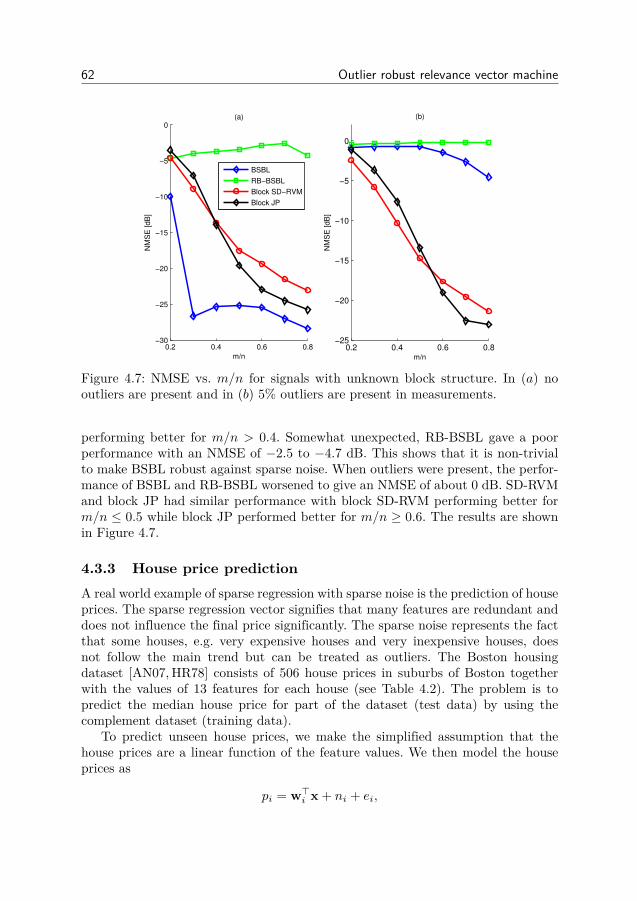
62 Outlier robust relevance vector machine
0.2 0.4 0.6 0.8−25
−20
−15
−10
−5
0
NM
SE
[d
B]
m/n
(b)
0.2 0.4 0.6 0.8−30
−25
−20
−15
−10
−5
0
m/n
NM
SE
[d
B]
(a)
BSBL
RB−BSBL
Block SD−RVM
Block JP
Figure 4.7: NMSE vs. m/n for signals with unknown block structure. In (a) nooutliers are present and in (b) 5% outliers are present in measurements.
performing better for m/n > 0.4. Somewhat unexpected, RB-BSBL gave a poorperformance with an NMSE of −2.5 to −4.7 dB. This shows that it is non-trivialto make BSBL robust against sparse noise. When outliers were present, the perfor-mance of BSBL and RB-BSBL worsened to give an NMSE of about 0 dB. SD-RVMand block JP had similar performance with block SD-RVM performing better form/n ≤ 0.5 while block JP performed better for m/n ≥ 0.6. The results are shownin Figure 4.7.
4.3.3 House price predictionA real world example of sparse regression with sparse noise is the prediction of houseprices. The sparse regression vector signifies that many features are redundant anddoes not influence the final price significantly. The sparse noise represents the factthat some houses, e.g. very expensive houses and very inexpensive houses, doesnot follow the main trend but can be treated as outliers. The Boston housingdataset [AN07, HR78] consists of 506 house prices in suburbs of Boston togetherwith the values of 13 features for each house (see Table 4.2). The problem is topredict the median house price for part of the dataset (test data) by using thecomplement dataset (training data).
To predict unseen house prices, we make the simplified assumption that thehouse prices are a linear function of the feature values. We then model the houseprices as
pi = w>i x + ni + ei,
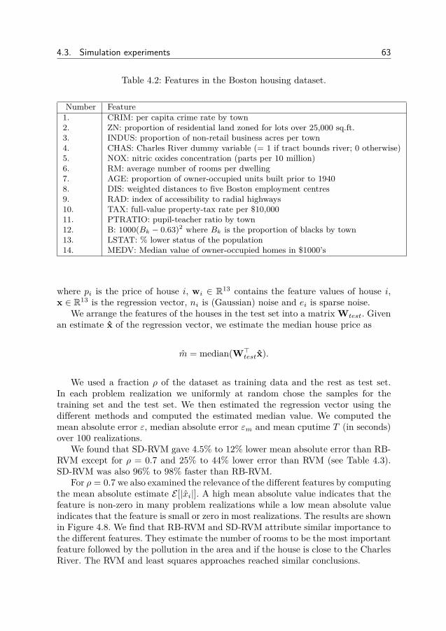
4.3. Simulation experiments 63
Table 4.2: Features in the Boston housing dataset.
Number Feature1. CRIM: per capita crime rate by town2. ZN: proportion of residential land zoned for lots over 25,000 sq.ft.3. INDUS: proportion of non-retail business acres per town4. CHAS: Charles River dummy variable (= 1 if tract bounds river; 0 otherwise)5. NOX: nitric oxides concentration (parts per 10 million)6. RM: average number of rooms per dwelling7. AGE: proportion of owner-occupied units built prior to 19408. DIS: weighted distances to five Boston employment centres9. RAD: index of accessibility to radial highways10. TAX: full-value property-tax rate per $10,00011. PTRATIO: pupil-teacher ratio by town12. B: 1000(Bk − 0.63)2 where Bk is the proportion of blacks by town13. LSTAT: % lower status of the population14. MEDV: Median value of owner-occupied homes in $1000’s
where pi is the price of house i, wi ∈ R13 contains the feature values of house i,x ∈ R13 is the regression vector, ni is (Gaussian) noise and ei is sparse noise.
We arrange the features of the houses in the test set into a matrix Wtest. Givenan estimate x of the regression vector, we estimate the median house price as
m = median(W>testx).
We used a fraction ρ of the dataset as training data and the rest as test set.In each problem realization we uniformly at random chose the samples for thetraining set and the test set. We then estimated the regression vector using thedifferent methods and computed the estimated median value. We computed themean absolute error ε, median absolute error εm and mean cputime T (in seconds)over 100 realizations.
We found that SD-RVM gave 4.5% to 12% lower mean absolute error than RB-RVM except for ρ = 0.7 and 25% to 44% lower error than RVM (see Table 4.3).SD-RVM was also 96% to 98% faster than RB-RVM.
For ρ = 0.7 we also examined the relevance of the different features by computingthe mean absolute estimate E [|xi|]. A high mean absolute value indicates that thefeature is non-zero in many problem realizations while a low mean absolute valueindicates that the feature is small or zero in most realizations. The results are shownin Figure 4.8. We find that RB-RVM and SD-RVM attribute similar importance tothe different features. They estimate the number of rooms to be the most importantfeature followed by the pollution in the area and if the house is close to the CharlesRiver. The RVM and least squares approaches reached similar conclusions.
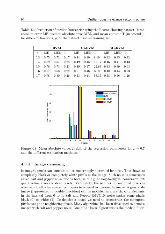
64 Outlier robust relevance vector machine
Table 4.3: Prediction of median houseprice using the Boston Housing dataset. Meanabsolute error ME, median absolute error MED and mean cputime T (in seconds),for different fractions, ρ, of the dataset used as training set.
RVM RB-RVM SD-RVMρ ME MED T ME MED T ME MED T
0.3 0.75 0.71 0.17 0.44 0.40 8.10 0.42 0.35 0.320.4 0.69 0.67 0.23 0.49 0.43 15.17 0.46 0.41 0.430.5 0.76 0.73 0.23 0.49 0.47 22.63 0.43 0.39 0.630.6 0.67 0.63 0.22 0.51 0.46 30.80 0.48 0.44 0.730.7 0.78 0.80 0.26 0.51 0.44 57.37 0.58 0.56 1.26
1 2 3 4 5 6 7 8 9 10 11 12 130
1
2
3
4
5
6
Feature
Mean a
bsolu
te v
alu
e
Least squares
RVM
RB−RVM
SD−RVM
Figure 4.8: Mean absolute value, E [|xi|], of the regression parameters for ρ = 0.7and the different estimation methods.
4.3.4 Image denoisingIn images, pixels can sometimes become strongly disturbed by noise. This shows ascompletely black or completely white pixels in the image. Such noise is sometimescalled salt and pepper noise and is because of e.g. analog-to-digital conversion, bitquantization errors or dead pixels. Fortunately, the number of corrupted pixels isoften small, allowing sparse techniques to be used to denoise the image. A gray scaleimage (represented in double-precision) can be modeled as a matrix with elementsin the interval from 0 to 1. Salt and Pepper [MVC10] noise makes some pixelsblack (0) or white (1). To denoise a image we need to reconstruct the corruptedpixels using the neighboring pixels. Many algorithms has been developed to denoiseimages with salt and pepper noise. One of the basic algorithms is the median filter.
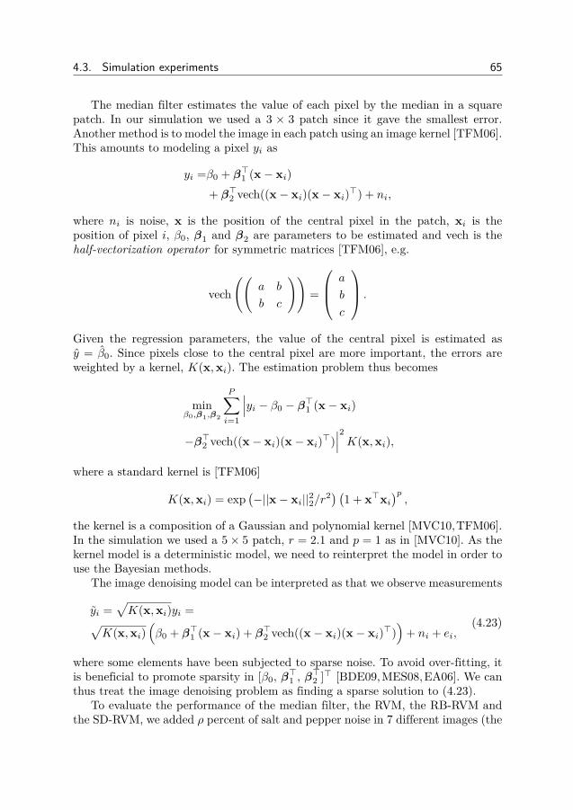
4.3. Simulation experiments 65
The median filter estimates the value of each pixel by the median in a squarepatch. In our simulation we used a 3 × 3 patch since it gave the smallest error.Another method is to model the image in each patch using an image kernel [TFM06].This amounts to modeling a pixel yi as
yi =β0 + β>1 (x− xi)+ β>2 vech((x− xi)(x− xi)>) + ni,
where ni is noise, x is the position of the central pixel in the patch, xi is theposition of pixel i, β0, β1 and β2 are parameters to be estimated and vech is thehalf-vectorization operator for symmetric matrices [TFM06], e.g.
vech((
a b
b c
))=
a
b
c
.
Given the regression parameters, the value of the central pixel is estimated asy = β0. Since pixels close to the central pixel are more important, the errors areweighted by a kernel, K(x,xi). The estimation problem thus becomes
minβ0,β1,β2
P∑i=1
∣∣∣yi − β0 − β>1 (x− xi)
−β>2 vech((x− xi)(x− xi)>)∣∣∣2K(x,xi),
where a standard kernel is [TFM06]
K(x,xi) = exp(−||x− xi||22/r2) (1 + x>xi
)p,
the kernel is a composition of a Gaussian and polynomial kernel [MVC10,TFM06].In the simulation we used a 5× 5 patch, r = 2.1 and p = 1 as in [MVC10]. As thekernel model is a deterministic model, we need to reinterpret the model in order touse the Bayesian methods.
The image denoising model can be interpreted as that we observe measurements
yi =√K(x,xi)yi =√
K(x,xi)(β0 + β>1 (x− xi) + β>2 vech((x− xi)(x− xi)>)
)+ ni + ei,
(4.23)
where some elements have been subjected to sparse noise. To avoid over-fitting, itis beneficial to promote sparsity in [β0, β
>1 , β
>2 ]> [BDE09,MES08,EA06]. We can
thus treat the image denoising problem as finding a sparse solution to (4.23).To evaluate the performance of the median filter, the RVM, the RB-RVM and
the SD-RVM, we added ρ percent of salt and pepper noise in 7 different images (the
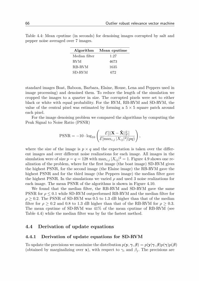
66 Outlier robust relevance vector machine
Table 4.4: Mean cputime (in seconds) for denoising images corrupted by salt andpepper noise averaged over 7 images.
Algorithm Mean cputimeMedian filter 1.27RVM 4673RB-RVM 1635SD-RVM 672
standard images Boat, Baboon, Barbara, Elaine, House, Lena and Peppers used inimage processing) and denoised them. To reduce the length of the simulation wecropped the images to a quarter in size. The corrupted pixels were set to eitherblack or white with equal probability. For the RVM, RB-RVM and SD-RVM, thevalue of the central pixel was estimated by forming a 5 × 5 square patch aroundeach pixel.
For the image denoising problem we compared the algorithms by computing thePeak Signal to Noise Ratio (PSNR)
PSNR = −10 · log10
(E [||X− X||2F ]
E [maxi,j |Xij |2](pq)
),
where the size of the image is p × q and the expectation is taken over the differ-ent images and over different noise realizations for each image. All images in thesimulation were of size p = q = 128 with maxi,j |Xij |2 = 1. Figure 4.9 shows one re-alization of the problem, where for the first image (the boat image) SD-RVM givesthe highest PSNR, for the second image (the Elaine image) the RB-RVM gave thehighest PSNR and for the third image (the Peppers image) the median filter gavethe highest PSNR. In the simulations we varied ρ and used 3 noise realizations foreach image. The mean PSNR of the algorithms is shown in Figure 4.10.
We found that the median filter, the RB-RVM and SD-RVM gave the samePSNR for ρ ≤ 0.1 while SD-RVM outperformed RB-RVM and the median filter forρ ≥ 0.2. The PSNR of SD-RVM was 0.5 to 1.3 dB higher than that of the medianfilter for ρ ≥ 0.2 and 0.8 to 1.3 dB higher than that of the RB-RVM for ρ ≥ 0.3.The mean cputime of SD-RVM was 41% of the mean cputime of RB-RVM (seeTable 4.4) while the median filter was by far the fastest method.
4.4 Derivation of update equations
4.4.1 Derivation of update equations for SD-RVM
To update the precisions we maximize the distribution p(y,γ,β) = p(y|γ,β)p(γ)p(β)(obtained by marginalizing over x), with respect to γi and βj . The precisions are
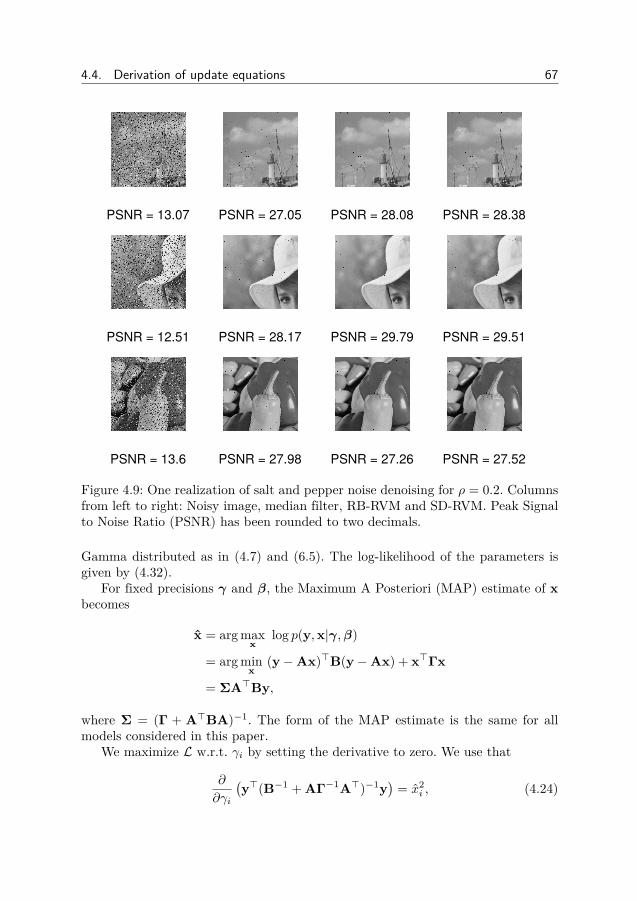
4.4. Derivation of update equations 67
PSNR = 13.07 PSNR = 27.05 PSNR = 28.08 PSNR = 28.38
PSNR = 12.51 PSNR = 28.17 PSNR = 29.79 PSNR = 29.51
PSNR = 13.6 PSNR = 27.98 PSNR = 27.26 PSNR = 27.52
Figure 4.9: One realization of salt and pepper noise denoising for ρ = 0.2. Columnsfrom left to right: Noisy image, median filter, RB-RVM and SD-RVM. Peak Signalto Noise Ratio (PSNR) has been rounded to two decimals.
Gamma distributed as in (4.7) and (6.5). The log-likelihood of the parameters isgiven by (4.32).
For fixed precisions γ and β, the Maximum A Posteriori (MAP) estimate of xbecomes
x = arg maxx
log p(y,x|γ,β)
= arg minx
(y−Ax)>B(y−Ax) + x>Γx
= ΣA>By,
where Σ = (Γ + A>BA)−1. The form of the MAP estimate is the same for allmodels considered in this paper.
We maximize L w.r.t. γi by setting the derivative to zero. We use that
∂
∂γi
(y>(B−1 + AΓ−1A>)−1y
)= x2
i , (4.24)
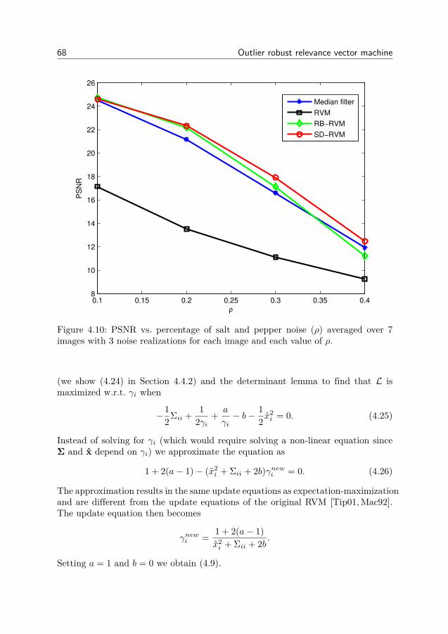
68 Outlier robust relevance vector machine
0.1 0.15 0.2 0.25 0.3 0.35 0.48
10
12
14
16
18
20
22
24
26
ρ
PS
NR
Median filter
RVM
RB−RVM
SD−RVM
Figure 4.10: PSNR vs. percentage of salt and pepper noise (ρ) averaged over 7images with 3 noise realizations for each image and each value of ρ.
(we show (4.24) in Section 4.4.2) and the determinant lemma to find that L ismaximized w.r.t. γi when
−12Σii + 1
2γi+ a
γi− b− 1
2 x2i = 0. (4.25)
Instead of solving for γi (which would require solving a non-linear equation sinceΣ and x depend on γi) we approximate the equation as
1 + 2(a− 1)− (x2i + Σii + 2b)γnewi = 0. (4.26)
The approximation results in the same update equations as expectation-maximizationand are different from the update equations of the original RVM [Tip01,Mac92].The update equation then becomes
γnewi = 1 + 2(a− 1)x2i + Σii + 2b .
Setting a = 1 and b = 0 we obtain (4.9).

4.4. Derivation of update equations 69
For the noise precisions we use that
∂
∂βj
[y>(B−1 + AΓ−1A>)−1y
]= [y−Ax]2j . (4.27)
We show the identity (4.27) in 4.4.2. We find that L is maximized w.r.t. βj when
−12tr(ΣA>j,:Aj,:) + 1
2βj− 1
2 [y−Ax]2j + c
βj− d = 0,
where Aj,: denotes the j’th row vector of A. Rewriting the equation as
1 + 2(c− 1)− ([y−Ax]2j + Aj,:ΣA>j,: + 2d)βnewj = 0,
and using that Aj,:ΣA>j,: = [AΣA>]jj , we find that
βnewj = 1 + 2(c− 1)[y−Ax]2j + [AΣA>]jj + 2d .
Setting c = 1 and d = 0 we obtain (4.10).
4.4.2 Derivation of (4.24) and (4.27)Proof of (4.24). Since
B−1 + AΓ−1A> = B−1 +n∑i=1
γ−1i aia>i ,
where ai is the i’th column vector of A we find that
∂
∂γi
(y>(B−1 + AΓ−1A>)−1y
)= γ−2
i
(a>i (B−1 + AΓ−1A>)−1y
)2.
Using that
Γ−1A>(B−1 + AΓ−1A>)−1y (4.28)= Γ−1A>
(B−BA(Γ + A>BA)−1A>B
)y
= Γ−1A>By− Γ−1 A>BA︸ ︷︷ ︸=Σ−1−Γ
(Γ + A>BA)−1︸ ︷︷ ︸=Σ
A>By
= ΣA>By = x,
we find that∂
∂γi
(y>(B−1 + AΓ−1A>)−1y
)= γ−2
i (γixi)2 = x2i .
70 Outlier robust relevance vector machine
Proof of (4.27). Since
y>(B−1 + AΓ−1A>)−1y = y>By− yBA (Γ + A>BA)−1︸ ︷︷ ︸=Σ
A>By,
we get that
∂
∂βj
(y>(B−1 + AΓ−1A>)−1y
)= y2
j − 2yjAj,:ΣA>By + y>BAΣA>j,:Aj,:ΣA>By= y2
j − 2yjAj,:x + (Aj,:x)2 = [y−Ax]2j .
4.4.3 Update equations for known block structureLet Γ and B be diagonal matrices with
[Γ]kk = γi, if k ∈ Ii, [B]ll = βj , if l ∈ Jj ,
and zero otherwise.To update the precisions we maximize the marginal distribution
p(y,γ,B) = p(y|γ,β)p(γ)p(β),
with respect to γ and β, where p(γ) and p(β) are as in (4.7) and (6.5). The log-likelihood of the parameters is
L = const.− 12 log det(B−1 + AΓ−1A>)− 1
2y>(B−1 + AΓ−1A>)−1y
+p∑i=1
((a− 1) log γi − bγi) +q∑j=1
((c− 1) log βj − dβj).
We get that L is maximized when
∂L∂γi
= −12tr(ΣIi) + ni
2γi+ a− 1
γi− b− 1
2γ2i
||A>Ii(B−1 + AΓ−1A>)−1y||22 = 0,
(4.29)
where ΣIi ∈ Rni×ni is the submatrix of Σ consisting of the columns and rows inIi. Further, using (4.28) we get that
A>Ii(B−1 + AΓ−1A>)−1y = γixIi . (4.30)
Thus, (4.29) is fulfilled when
−12tr(ΣIi) + ni
2γi+ a− 1
γi− b− 1
2 ||xIi ||22 = 0.
4.4. Derivation of update equations 71
As before, we rewrite the equation as
ni + 2(a− 1)− (||xIi ||22 + tr(ΣIi) + 2b)γnewi = 0. (4.31)
Solving (4.31) for γnewi gives us the update equation (4.17).To find the update equation for βj we use that
∂
∂βj
[y>(B−1 + AΓ−1A>)−1y
]= ||yJj ||22 − 2y>JjAJj ,:ΣA>By + y>BAΣA>Jj ,:AJj ,:ΣA>By= ||(y−Ax)Jj ||22,
where AJj ,: consists of the row vectors with row indexes in Jj . We find that
∂L∂βj
= −12tr(ΣA>Jj ,:AJj ,:) + mj
2βj− 1
2 ||(y−Ax)Jj ||22 + c− 1βj− d = 0.
Rewriting the equation as
1 + 2(c− 1) = (||(y−Ax)Jj ||22 + tr(AJj ,:ΣA>Jj ,:) + 2d)βnewj ,
and using that tr(AJj ,:ΣA>Jj ,:) = tr([AΣA>]Jj ) gives us the update equation(4.18).
4.4.4 Update equations for unknown block structureWhen the block structure is unknown, we use the overparametrized model in section4.2.2. The log-likelihood of the parameters is
L = log p(y|γ,β)p(γ)p(β) (4.32)
= const.− 12 log det(B−1 + AΓ−1A>)− 1
2y>(B−1 + AΓ−1A>)−1y
+p∑i=1
((a− 1) log γi − bγi) +q∑j=1
((c− 1) log βj − dβj).
We search to maximize (4.32) with respect to the underlying variables γk andβl. Using that ∂γ−1
i
∂γk= −γ−2
k , ∂γi∂γk
= γ2i γ−2k , when i ∈ Ik and zero otherwise and
(4.28) we find that L is maximized when
∂L∂γk
= − 12γ2k
tr(ΣΓ2k) + 1
2γ2k
tr(Γk)− 12γ2k
x>Γ2kx + a− 1
γk− b = 0, (4.33)
By rewriting (4.33) as
1γk
tr(Γk) + 2(a− 1) =(
1γ2k
||Γkx||22 + 1γ2k
tr(ΓkΣΓk) + 2b)γnewk . (4.34)
72 Outlier robust relevance vector machine
Solving (4.34) for γnewk gives us the update equation (4.20).For the noise precisions, we similarly find that
∂L∂βl
= − 12β2
l
tr(BlA>ΣABl) + 12β2
l
tr(Bl)
− 12β2
l
||Bl(y−Ax)||22 + c− 1βl− d = 0.
By rewriting the expression as
1βl
tr(Bl) + 2(c− 1) =(
1β2l
||Bl(y−Ax)||22 + 1β2l
tr(BlA>ΣABl) + 2d)βnewl ,
we find the update equation (4.21).We see that the form of update equations depends on how the equations are
rewritten. The form used here has the advantage of reducing to (4.18) when theunderlying blocks are disjoint.
4.5 Conclusion
We proposed a modification of the Relevance Vector Machine (RVM) which is ro-bust against sparse noise while not needing to estimate the sparse noise explicitly.We denote the proposed method by SD-RVM for Sparse and Dense noise combinedRVM. The method is faster than the robust RVM (RB-RVM) of [MVC10] wherethe sparse noise is treated as an additional estimation variable. Simulations showthat the method is faster than the RB-RVM for compressed sensing and has sim-ilar performance. We also show how the method can be modified to block-sparsesignals and noise and simulate the method for housing price prediction and imagedenoising.
Chapter 5
Relevance singular vector machine forlow-rank matrix reconstruction
Low-rank matrices is a parsimonious model which, like the sparse model, canbe used to improve estimation performance. However, unlike sparsity, which isa property of the individual components, low-rank is a property of the entire
matrix. While sparsity gives a parsimonious representation of data in a knownbasis, low-rank matrices can be interpreted as representing data in an unknownbasis. One prominent low-rank model is collaborative filtering where a recommendersystem attempts to find if you will like a product you have not yet seen. The basicassumption of low-rank models is that the problem has a high degree of inherent(linear) structure.
The recommendation problem can be modeled as follows: what you prefer de-pends on what persons you are similar to and what those persons prefer. Despitethe simplistic nature of the model, it has been shown to be a good model for therecommendation problem [KBV09,CP10]. Other applications of low-rank modelingis clustering documents by topic and system identification [CP10,LSR+16].
Several approaches have been developed to solve the low-rank estimation prob-lem. A prominent class of methods are convex optimization based techniques whichgeneralizes the `1-norm for sparse problems to low-rank problems. The low-rankpenalty corresponding to the `1-norm is the nuclear norm which is the sum of thesingular values of a matrix [CP10,CR09, Faz02]. In the same way as the `1-normcan be shown to be the tightest convex approximation of the `0-norm, the nuclearnorm can be shown to be the tightest convex approximation of the rank (undercertain conditions, see [LO15] for a counterexample).
The low-rank estimation problem also allows for factorization based techniques.Factorization based techniques are used a lot [KBV09, ZSJC12, TN11, RFGST09,CWZY15,YC11,LBA11,Alq13,MS07,SM08,LT07,RIK07,BLMK12] since they al-low one to specify a strict upper bound on the rank of the estimate. Factorizationbased methods are fast, but they require an upper bound on the rank to be knowna-priori. It is also difficult to relate the factorization based approach to the opti-
73

74 Relevance singular vector machine for low-rank matrix reconstruction
mization based approach. A third approach is the greedy search method ADMIRA[LB10] which is a low-rank matrix generalization of the CoSamp method [NT09]for sparse vectors.
Bayesian methods have also been developed for low-rank matrix reconstruction.Most such methods rely on the factorized model and promotes low-rank throughblock sparsity promoting priors [CWZY15,YC11,Alq13,MS07,SM08,LT07,RIK07,BLMK12]. The question arises if it is possible to construct a low-rank analogueof the Relevance Vector Machine where the low-rank matrix is not modeled as aproduct of two matrices? Here we show one approach to generalize the RVM to thelow-rank problem using precision matrices to induce low-rank. We call the resultingmethod the Relevance Singular Vector Machine.
5.1 Low-rank matrix estimation
In low-rank matrix estimation, a low-rank matrix X ∈ Rp×q is measured throughlinear measurements of the matrix components as
y = A(X) + n, (5.1)
where y ∈ Rm is the observed measurements, n ∈ Rm is additive noise and A :Rp×q → Rm is a linear operator representing the measurement process. The sensingoperator can be expressed as
A(X) =
tr(A>1 X)tr(A>2 X)
...tr(A>mX)
, (5.2)
where
tr(A>k X) =∑
1≤i≤p,1≤j≤q[Ak]ij [X]ij
gives a linear combination of the elements in X with coefficients from Ak ∈ Rp×q.The sensing operation can also be expressed as A(X) = Avec(X) using the vec-torization operator. The vectorization representation shows the similarity betweenthe LRMR problem and the sparse vector reconstruction problem.
A standard approach to promoting structure (such as sparsity or low-rank) isto minimize a penalty function in addition to the norm of the error. This leads tothe optimization problem
X = arg minX
β
2 ||y−Avec(X)||22 + g(X), (5.3)
where β > 0 is a regularization parameter and g(·) is a penalty function. Whenthe penalty function g(X) is convex (and β is fixed), the problem is a convex
5.1. Low-rank matrix estimation 75
optimization problem and can be solved using standard optimization tools such ascvx [GBY08]. For non-convex penalty functions the optimization problem can beapproximately solved through e.g. gradient descent. Common penalty functions forpromoting low-rank are
g(X) =min(p,q)∑i=1
σi(X) = tr((XX>)1/2), (Nuclear norm)
g(X) = tr((XX>)s/2), (Schatten s-norm)g(X) = ν log |XX> + εIp|. (Log-determinant penalty)
The nuclear norm is a convex penalty function while the log-determinant and Schat-ten s-norm (for 0 < s < 1) are non-convex. In the Bayesian framework, the mini-mization in (5.3) correspond to finding the maximum-a-posteriori (MAP) estimateof X when the noise is Gaussian and the matrix X is assigned a prior distributionp(X) ∝ e− 1
2 g(X). An alternative approach is to set
X = argX min ||X||∗, such that ||y−Avec(X)||2 ≤ δ, (5.4)
where δ > 0 is related to the (known) noise power. The choice δ = β−1√m+
√8m
suggested in [CRT06] often provides good performance.In the factorization based approach, the matrix X is modeled as a product of
two matrices as [KBV09,ZSJC12,TN11,RFGST09,CWZY15,YC11,LBA11,Alq13,MS07,SM08,LT07,RIK07,BLMK12]
X = FB>,
where F ∈ Rp×r, B ∈ Rq×r and 0 < r ≤ min(p, q) is a parameter. The fac-tor matrices can be found in a deterministic manner by minimizing the resid-ual ||y−Avec(FB>)||22 iteratively for F and B while keeping the other matrixfixed [TN11,ZSJC12], this is sometimes called alternating least squares (ALS). Sincethe residual is non-convex in F and B, it is not guaranteed to converge to a globaloptima. One approach to improving the performance of ALS is to incorporate dualvariables and ADMM iterations [LSR+16].
The estimates produced by ALS are mostly full rank, i.e. rank(FB>) = r. Whenthe rank is unknown, the method can be modified so that the final estimate hasrank less than r. This can be achieved by assigning appropriate priors to the factormatrices. One approach is to minimize
||y−Avec(FB>)||22 + λ(||F||2F + ||B||2F
),
where λ > 0 is a regularization parameter. The penalty function is expected topromote low-rank through the relation [MS07]
||X||∗ = 12 min
F,B:FB>=X
(||F||2F + ||B||2F
).

76 Relevance singular vector machine for low-rank matrix reconstruction
Another method is to use priors which promote column sparsity in the factor ma-trices [LT07,BLMK12], i.e. a prior which makes many of the column vectors in Fand B zero. This approach promotes low-rank since if F has rF non-zero columnsand B has rB non-zero columns, then rank(X) ≤ min(rL, rB) ≤ r. We describe thismodel in more detail in Chapter 7.
5.2 The one-sided precision based model
The difficulty of assigning priors to low-rank matrices is that the set of low-rankmatrices is a strictly lower dimensional submanifold of the set of all matrices. Itis thus difficult to assign a “hard” prior which has non-zero probability (in thesense of an induced measure) only for matrices of low-rank. We therefore want tofind priors which approximately promotes low-rank, i.e. it has non-zero probabilityfor all matrices, but is concentrated around the set of low-rank matrices. We dothis by characterizing a random low-rank matrix as a matrix with strongly cor-related column and row vectors rather than the standard notion of few non-zerosingular values. We thus need a prior which makes the column vectors lie in alow-dimensional subspace (similarly for the row vectors).
The Relevance Vector Machine models the components xi of the parametervector x ∈ Rn are modeled as
xi = γ−1/2i ui, (5.5)
where γi > 0 is the precision of xi and ui ∼ N (0, 1) is a Gaussian variable. Whenthe inverse precision, γ−1 is small, xi is small with a high probability and whenthe inverse precision is large, xi is large with a high probability. In the extremecase where γ−1
i = 0, we have that xi = 0. However, the extreme case has zero priorprobability and does therefore not occur in practice. In analogue with the sparsecase, we model the low-rank matrix X as a Gaussian variable with a precisionmatrix α as
X = α−1/2U, (5.6)
whereα ∈ Rp×p is positive definite,α−1/2 denotes a symmetric such that (α−1/2)2 =α−1 and the elements of U are i.i.d. N (0, 1) distributed. We notice the similaritybetween (5.5) and (5.6). When the inverse precision matrix, α−1, has a few largesingular values and otherwise small singular values, the random matrix X has low-rank with high proability. In the extreme case where α−1 has low-rank, the matrixX also has low-rank. The approach (5.6) is equivalent to letting X to be a matrixvariate Gaussian variable with distribution [GN99,NSB13]
p(X|α) = |α|q/2
(2π)pq/2exp
(−1
2tr(X>αX)). (5.7)
In order to promote low-rank, we need to assign a prior to the precision matrix α.In Section 5.2.1 we will show one approach to selecting the prior distribution.
5.2. The one-sided precision based model 77
5.2.1 Relation between priors and the MAP estimationHere we show how the distribution p(α) is related to the penalty function g(X).We see that the prior distribution (5.7) depends on X only through Z = XX>. Letthe prior distribution of α be p(α), we find that the marginal distribution p(X)becomes
p(X) = Ce−12 g(X) =
∫α0
p(X|α) p(α) dα
=∫α0
e−12 tr(αZ) |α|q/2
(2π)pq/2p(α)dα = C ′e−
12 g(Z), (5.8)
where we used that tr(X>αX) = tr(αXX>) = tr(αZ), g(·) and g(·) are some func-tions and C and C ′ are normalization constants. To relate g(Z) and p(α), we notethat p(X) is the matrix Laplace transform of |α|q/2p(α)/(2π)pq/2 at Z/2 [Ter12](we give a short introduction to the matrix Laplace transform in Section 5.5.6).This gives us that we can calculate p(α) from p(X) = C ′e−
12 g(Z) by the inverse
Laplace transform [Ter12] as
p(α) ∝ |α|−q/2∫
Re Z=α∗
e12 tr(αZ)e−
12 g(Z)dZ, (5.9)
where the integral is taken over all symmetric matrices Z ∈ Cp×p such that Re Z =α∗ and α∗ is a real matrix such that the contour path of integration is in the regionof convergence of the integrand. While the Laplace transform characterizes theexact relation between priors, the computation is non-trivial and often analyticallyintractable. In practice, a standard approach to evaluating integrals like (5.8) isto use the Laplace approximation [Mac03,Bis06] where typically the mode of thedistribution under approximation is found first and then a Gaussian distribution ismodeled around that mode. Let us write p(α) as p(α) ∝ e− 1
2K(α); then the Laplaceapproximation becomes
g(Z) = minα0tr(αZ)− q log |α|+K(α)
− log |H|+ constant,
where H is the Hessian of tr(αZ)− q log |α|+K(α) evaluated at the minima. Thederivation of the Laplace approximation is shown in Section 5.5.7.
Denoting K(α) = q log |α| −K(α) and neglecting the Hessian we get that
g(Z) = minα0
tr(αZ)− K(α)
,
where we absorbed the constants into the normalization factor of p(X). We findthat g(Z) is the concave conjugate of K(α) [BV04]. Hence, for a given g(Z) wecan recover K(α) as
K(α) = minZ0tr(αZ)− g(Z) (5.10)
78 Relevance singular vector machine for low-rank matrix reconstruction
if K(α) is concave (which holds under the assumption that K(α) is convex). Fur-ther, we can find K(α) from K(α) and solve for the prior p(α) ∝ e−
12K(α). Using
the concave conjugate relation (5.10), we now find priors (functions K(α)) corre-sponding to the Schatten-s norm and the log-determinant penalty.
1. The Schatten s-norm: The regularized Schatten s-norm based penalty func-tion is
g(X) =tr((XX> + εIp)s/2), (5.11)
where the constant ε > 0 is used to bring numerical stability. For the penaltyfunction (5.11), we find that
K(α) = Cs tr(α−s
2−s ) + q log |α|+ ε tr(α), (5.12)
where Cs = 2−ss
( 2s
)− s2−s . The derivation of (5.12) is given in Section 5.5.10.
Let σi(X) denote the i’th singular value of X, for s = 1 and ε = 0 we see thatg(X) becomes the nuclear norm of X as tr((XX>) 1
2 ) =∑min(p,q)i=1 σi(X).
2. The Log-determinant penalty: The log-determinant based penalty function is
g(X) = ν log∣∣XX> + εIp
∣∣ , (5.13)
where ν > q − 2 is a positive number. We find that
K(α) = ε tr(α) + (q − ν) log |α|. (5.14)
The derivation of (5.14) is shown in Section 5.5.11. As p(α) ∝ e−12K(α), we
find that the precision matrix α is Wishart distributed [GN99,Bis06]. We alsofind that p(X) ∝ e− 1
2 g(XX>) is a matrix t-distribution [GN99].
5.2.2 Left and right-sided precision based models
For a low-rank matrix, the components of each column vector are correlated as wellas the components of each row vector. In (5.6), the precision matrix α−1/2 is usedin the left side of U, we refer to this as the left-sided precision based model. Themodel helps to make the components of each column of X correlated. We can alsomake the row-vectors correlated by setting
X = Uα−1/2. (5.15)
We refer to this model as the right-sided precision based model.
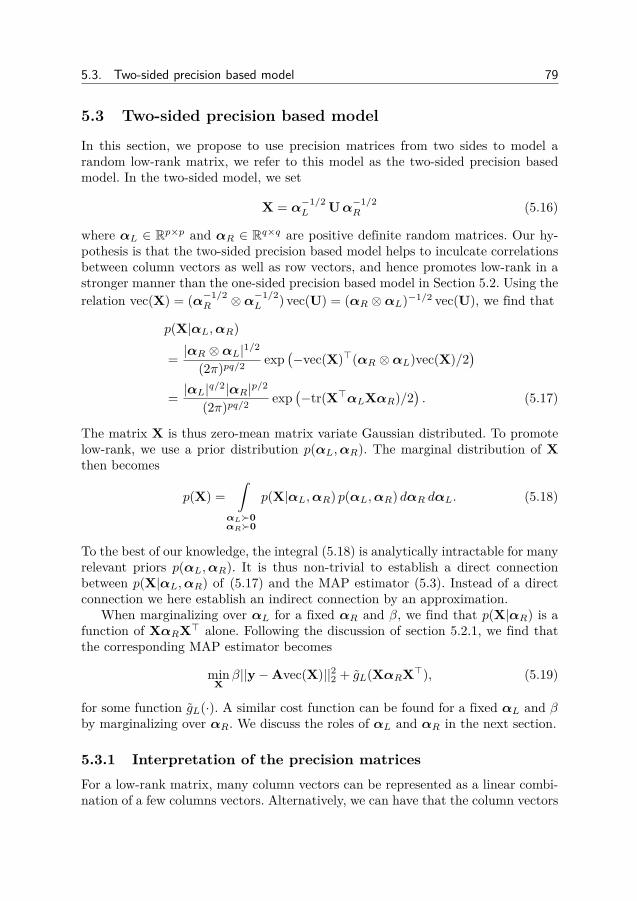
5.3. Two-sided precision based model 79
5.3 Two-sided precision based model
In this section, we propose to use precision matrices from two sides to model arandom low-rank matrix, we refer to this model as the two-sided precision basedmodel. In the two-sided model, we set
X = α−1/2L Uα
−1/2R (5.16)
where αL ∈ Rp×p and αR ∈ Rq×q are positive definite random matrices. Our hy-pothesis is that the two-sided precision based model helps to inculcate correlationsbetween column vectors as well as row vectors, and hence promotes low-rank in astronger manner than the one-sided precision based model in Section 5.2. Using therelation vec(X) = (α−1/2
R ⊗α−1/2L ) vec(U) = (αR ⊗αL)−1/2 vec(U), we find that
p(X|αL,αR)
= |αR ⊗αL|1/2
(2π)pq/2exp
(−vec(X)>(αR ⊗αL)vec(X)/2
)= |αL|
q/2|αR|p/2
(2π)pq/2exp
(−tr(X>αLXαR)/2
). (5.17)
The matrix X is thus zero-mean matrix variate Gaussian distributed. To promotelow-rank, we use a prior distribution p(αL,αR). The marginal distribution of Xthen becomes
p(X) =∫
αL0αR0
p(X|αL,αR) p(αL,αR) dαR dαL. (5.18)
To the best of our knowledge, the integral (5.18) is analytically intractable for manyrelevant priors p(αL,αR). It is thus non-trivial to establish a direct connectionbetween p(X|αL,αR) of (5.17) and the MAP estimator (5.3). Instead of a directconnection we here establish an indirect connection by an approximation.
When marginalizing over αL for a fixed αR and β, we find that p(X|αR) is afunction of XαRX> alone. Following the discussion of section 5.2.1, we find thatthe corresponding MAP estimator becomes
minX
β||y−Avec(X)||22 + gL(XαRX>), (5.19)
for some function gL(·). A similar cost function can be found for a fixed αL and βby marginalizing over αR. We discuss the roles of αL and αR in the next section.
5.3.1 Interpretation of the precision matricesFor a low-rank matrix, many column vectors can be represented as a linear combi-nation of a few columns vectors. Alternatively, we can have that the column vectors
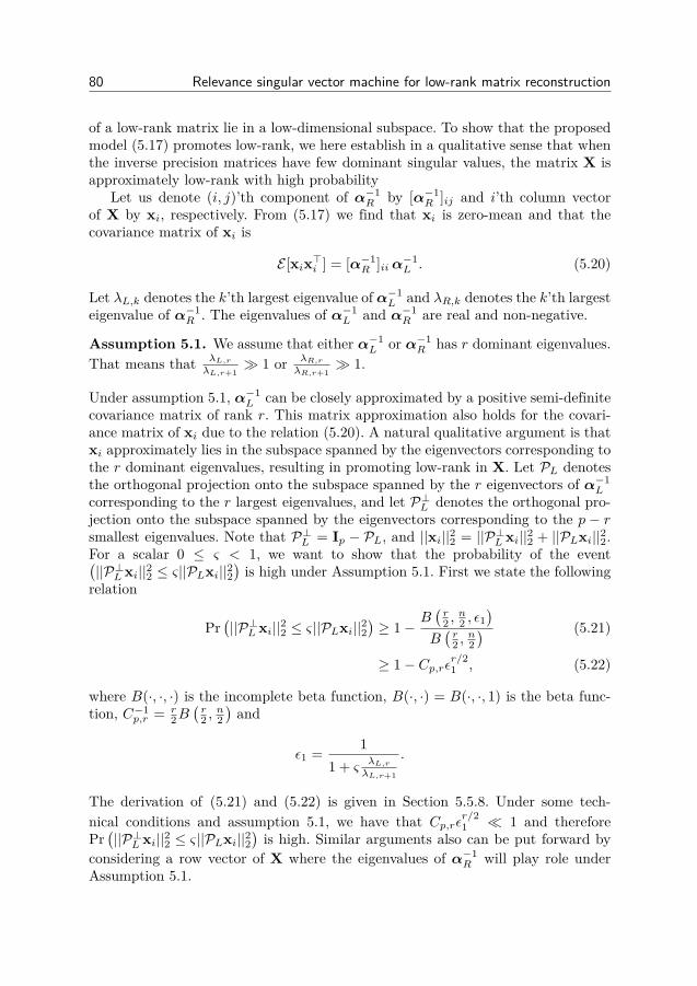
80 Relevance singular vector machine for low-rank matrix reconstruction
of a low-rank matrix lie in a low-dimensional subspace. To show that the proposedmodel (5.17) promotes low-rank, we here establish in a qualitative sense that whenthe inverse precision matrices have few dominant singular values, the matrix X isapproximately low-rank with high probability
Let us denote (i, j)’th component of α−1R by [α−1
R ]ij and i’th column vectorof X by xi, respectively. From (5.17) we find that xi is zero-mean and that thecovariance matrix of xi is
E [xix>i ] = [α−1R ]iiα−1
L . (5.20)
Let λL,k denotes the k’th largest eigenvalue of α−1L and λR,k denotes the k’th largest
eigenvalue of α−1R . The eigenvalues of α−1
L and α−1R are real and non-negative.
Assumption 5.1. We assume that either α−1L or α−1
R has r dominant eigenvalues.That means that λL,r
λL,r+1 1 or λR,r
λR,r+1 1.
Under assumption 5.1, α−1L can be closely approximated by a positive semi-definite
covariance matrix of rank r. This matrix approximation also holds for the covari-ance matrix of xi due to the relation (5.20). A natural qualitative argument is thatxi approximately lies in the subspace spanned by the eigenvectors corresponding tothe r dominant eigenvalues, resulting in promoting low-rank in X. Let PL denotesthe orthogonal projection onto the subspace spanned by the r eigenvectors of α−1
L
corresponding to the r largest eigenvalues, and let P⊥L denotes the orthogonal pro-jection onto the subspace spanned by the eigenvectors corresponding to the p − rsmallest eigenvalues. Note that P⊥L = Ip − PL, and ||xi||22 = ||P⊥L xi||22 + ||PLxi||22.For a scalar 0 ≤ ς < 1, we want to show that the probability of the event(||P⊥L xi||22 ≤ ς||PLxi||22
)is high under Assumption 5.1. First we state the following
relation
Pr(||P⊥L xi||22 ≤ ς||PLxi||22
)≥ 1−
B(r2 ,
n2 , ε1
)B(r2 ,
n2) (5.21)
≥ 1− Cp,rεr/21 , (5.22)
where B(·, ·, ·) is the incomplete beta function, B(·, ·) = B(·, ·, 1) is the beta func-tion, C−1
p,r = r2B(r2 ,
n2)and
ε1 = 11 + ς
λL,rλL,r+1
.
The derivation of (5.21) and (5.22) is given in Section 5.5.8. Under some tech-nical conditions and assumption 5.1, we have that Cp,rεr/21 1 and thereforePr(||P⊥L xi||22 ≤ ς||PLxi||22
)is high. Similar arguments also can be put forward by
considering a row vector of X where the eigenvalues of α−1R will play role under
Assumption 5.1.
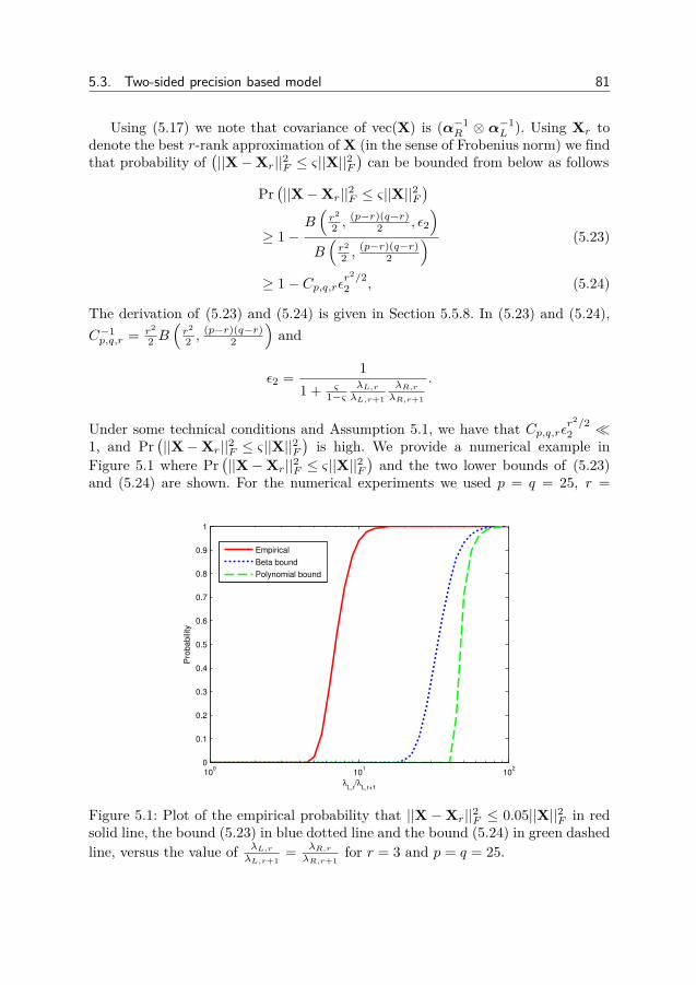
5.3. Two-sided precision based model 81
Using (5.17) we note that covariance of vec(X) is (α−1R ⊗ α
−1L ). Using Xr to
denote the best r-rank approximation of X (in the sense of Frobenius norm) we findthat probability of
(||X−Xr||2F ≤ ς||X||2F
)can be bounded from below as follows
Pr(||X−Xr||2F ≤ ς||X||2F
)≥ 1−
B(r2
2 ,(p−r)(q−r)
2 , ε2
)B(r2
2 ,(p−r)(q−r)
2
) (5.23)
≥ 1− Cp,q,rεr2/2
2 , (5.24)
The derivation of (5.23) and (5.24) is given in Section 5.5.8. In (5.23) and (5.24),C−1p,q,r = r2
2 B(r2
2 ,(p−r)(q−r)
2
)and
ε2 = 11 + ς
1−ςλL,rλL,r+1
λR,rλR,r+1
.
Under some technical conditions and Assumption 5.1, we have that Cp,q,rεr2/2
2 1, and Pr
(||X−Xr||2F ≤ ς||X||2F
)is high. We provide a numerical example in
Figure 5.1 where Pr(||X−Xr||2F ≤ ς||X||2F
)and the two lower bounds of (5.23)
and (5.24) are shown. For the numerical experiments we used p = q = 25, r =
100
101
102
0
0.1
0.2
0.3
0.4
0.5
0.6
0.7
0.8
0.9
1
λL,r
/λL,r+1
Pro
ba
bili
ty
Empirical
Beta bound
Polynomial bound
Figure 5.1: Plot of the empirical probability that ||X −Xr||2F ≤ 0.05||X||2F in redsolid line, the bound (5.23) in blue dotted line and the bound (5.24) in green dashedline, versus the value of λL,r
λL,r+1= λR,r
λR,r+1for r = 3 and p = q = 25.
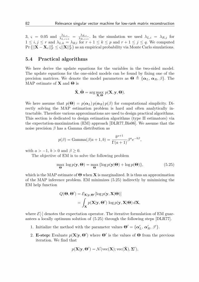
82 Relevance singular vector machine for low-rank matrix reconstruction
3, ς = 0.05 and λL,rλL,r+1
= λR,rλR,r+1
. In the simulation we used λL,i = λR,j for1 ≤ i, j ≤ r and λL,k = λR,l for r + 1 ≤ k ≤ p and r + 1 ≤ j ≤ q. We computedPr(||X−Xr||2F ≤ ς||X||2F
)as an empirical probability via Monte Carlo simulations.
5.4 Practical algorithms
We here derive the update equations for the variables in the two-sided model.The update equations for the one-sided models can be found by fixing one of theprecision matrices. We denote the model parameters as Θ , αL, αR, β. TheMAP estimate of X and Θ is
X, Θ = arg maxX,Θ
p(X,y,Θ).
We here assume that p(Θ) = p(αL) p(αR) p(β) for computational simplicity. Di-rectly solving the MAP estimation problem is hard and often analytically in-tractable. Therefore various approximations are used to design practical algorithms.This section is dedicated to design estimation algorithms (type II estimators) viathe expectation-maximization (EM) approach [DLR77,Bis06]. We assume that thenoise precision β has a Gamma distribution as
p(β) = Gamma(β|a+ 1, b) = ba+1
Γ(a+ 1)βae−bβ ,
with a > −1, b > 0 and β ≥ 0.The objective of EM is to solve the following problem
maxΘ
log p(y,Θ) = maxΘlog p(y|Θ) + log p(Θ), (5.25)
which is the MAP estimate of Θ when X is marginalized. It is thus an approximationof the MAP inference problem. EM minimizes (5.25) indirectly by minimizing theEM help function
Q(Θ,Θ′) = EX|y,Θ′ [log p(y,X|Θ)]
=∫
Xp(X|y,Θ′) log p(y,X|Θ) dX,
where E [·] denotes the expectation operator. The iterative formulation of EM guar-antees a locally optimum solution of (5.25) through the following steps [DLR77].
1. Initialize the method with the parameter values Θ′ = α′L, α′R, β′.
2. E-step: Evaluate p(X|y,Θ′) where Θ′ is the values of Θ from the previousiteration. We find that
p(X|y,Θ′) = N (vec(X); vec(X),Σ′),
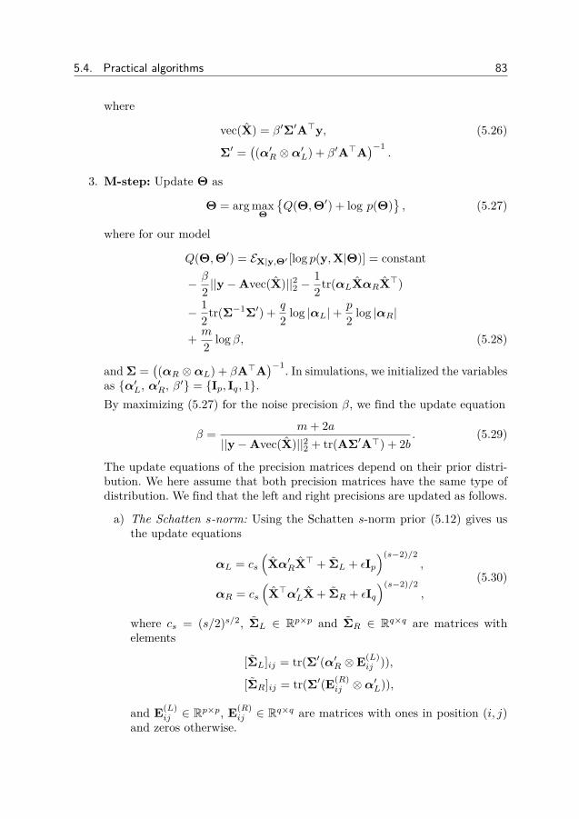
5.4. Practical algorithms 83
where
vec(X) = β′Σ′A>y, (5.26)
Σ′ =((α′R ⊗α′L) + β′A>A
)−1.
3. M-step: Update Θ as
Θ = arg maxΘ
Q(Θ,Θ′) + log p(Θ)
, (5.27)
where for our model
Q(Θ,Θ′) = EX|y,Θ′ [log p(y,X|Θ)] = constant
− β
2 ||y−Avec(X)||22 −12tr(αLXαRX>)
− 12tr(Σ−1Σ′) + q
2 log |αL|+p
2 log |αR|
+ m
2 log β, (5.28)
and Σ =((αR ⊗αL) + βA>A
)−1. In simulations, we initialized the variablesas α′L, α′R, β′ = Ip, Iq, 1.By maximizing (5.27) for the noise precision β, we find the update equation
β = m+ 2a||y−Avec(X)||22 + tr(AΣ′A>) + 2b
. (5.29)
The update equations of the precision matrices depend on their prior distri-bution. We here assume that both precision matrices have the same type ofdistribution. We find that the left and right precisions are updated as follows.
a) The Schatten s-norm: Using the Schatten s-norm prior (5.12) gives usthe update equations
αL = cs
(Xα′RX> + ΣL + εIp
)(s−2)/2,
αR = cs
(X>α′LX + ΣR + εIq
)(s−2)/2,
(5.30)
where cs = (s/2)s/2, ΣL ∈ Rp×p and ΣR ∈ Rq×q are matrices withelements
[ΣL]ij = tr(Σ′(α′R ⊗E(L)ij )),
[ΣR]ij = tr(Σ′(E(R)ij ⊗α
′L)),
and E(L)ij ∈ Rp×p, E(R)
ij ∈ Rq×q are matrices with ones in position (i, j)and zeros otherwise.

84 Relevance singular vector machine for low-rank matrix reconstruction
b) The log-determinant penalty: For the log-determinant prior (5.14) theupdate equations become
αL = ν(Xα′RX> + ΣL + εIp
)−1,
αR = ν(X>α′LX + ΣR + εIq
)−1.
(5.31)
The derivations of (5.28) and (5.31) are given in Section 5.5.9.
4. Stop iterating if X does not change significantly. Otherwise go to step 2.
5.4.1 Balancing the precisionsWe have found that in practical algorithms, there is a chance that one of the twoprecisions becomes large and the other becomes small. A small precision resultsin numerical instability in the Kronecker covariance structure (5.17). To preventthe imbalance we rescale the matrix precisions in each iteration such that 1) thea-priori and a-posteriori squared Frobenius norm of X are equal, i.e.
E [||X||2F |αL,αR] = tr(α−1L )tr(α−1
R )= E [||X||2F |αL,αR, β,y] = ||X||2F + tr(Σ),
and 2) the contribution of each precision to the norm is equal, i.e.
tr(α−1L ) = tr(α−1
R ).
The rescaling makes the algorithm more stable and often improves estimation per-formance.
5.4.2 NomenclatureHere we explain the nomenclature used for the RSVM algorithms. We use the nameleft-sided RSVM for the left-sided model where αL is random and αR = Iq andright-sided RSVM for the right-sided model where αR is random and αL = Ip. Werefer to the model where both αL and αR are random as the two-sided RSVM orsimply as RSVM. We assume that αL and αR are independent with distributionsp(α) ∝ e−
12K(α). We refer to the RSVM method with priors related to the log-
determinant penalty function (5.14) as RSVM-LD and to the RSVM method priorsrelated to the Schatten s-norm penalty function (5.12) as RSVM-SN. For example,left-sided RSVM-LD is RSVM with log-determinant prior (5.14) and a left-sidedprecision.
5.4.3 Complexity analysisOne motivation for the RSVM algorithm is that it can infer low-rank directly with-out factorizing the matrix X. However, one disadvantage of this is that for given
5.5. Simulation experiments 85
precision matrices, the estimation of X is a Gaussian inference problem with pqvariables, requiring computationally demanding matrix inverses. To study how theproblem size affects the runtime, we here study the computational complexity ofthe algorithm.
The most computationally demanding operation of the RSVM algorithm is thecomputation of Σ. A direct approach to computing Σ is to invert a pq× pq matrix,this requires O((pq)3) multiplications. However, this does not use the fact thatrank(A>A) ≤ m pq. By using the Woodbury matrix inversion formula [Bis06]we get that
Σ = (α−1R ⊗α
−1L )− (α−1
R ⊗α−1L )A>C−1
y A(α−1R ⊗α
−1L )
where
Cy = β−1Im + A(α−1R ⊗α
−1L )A>.
The computation of Σ thus reduces to computing (α−1R ⊗α
−1L ) (requiringO(p3+q3+
p2q2) multiplications), A(α−1R ⊗α
−1L ) and A(α−1
R ⊗α−1L )A> (requiring O(mp2q2)
multiplications) and C−1y (requiring O(m3) multiplications). The total complexity
is therefore
O(p3 + q3 + p2q2 +m3 +mp2q2) ≈ O(mp2q2),
where we used that O(mp2q2) dominates over the other terms when m pq.The use of the Woodbury matrix inversion thus helps to reduce computationalcomplexity per iteration from O((pq)3) to O(m(pq)2). Further we note that thecomplexity does not depend on the rank of X. This is because RSVM, in contrastto factorization based methods [BLMK12], does not use rank information as ana-priori information.
5.5 Simulation experiments
5.5.1 Simulations setupHere we describe datasets, performance measure, experimental setup, competingalgorithms and computational resources. In the experiments we used syntheticdata for low-rank matrix reconstruction (LRMR) and low-rank matrix completion(LRMC). We used the MovieLens dataset [HKBR99] as a real dataset for matrixcompletion. To compare the algorithms for synthetic data, we use the normalized-mean-square-error
NMSE = E [||X−X||2F ]E [||X||2F ]
as the performance measure. The NMSE was evaluated by averaging over manyinstances of n, A and X using Monte-Carlo simulations. For experiments withsynthetic data, we evaluated the NMSE as follows:

86 Relevance singular vector machine for low-rank matrix reconstruction
1. For LRMR, the random measurement matrix A ∈ Rm×pq was generated byindependently drawing the elements from N (0, 1) and normalizing the columnvectors to unit norm. For LRMC, we chose m elements uniformly at randomfrom [p]× [q]. We then chose A such that it selected the elements from vec(X)by letting one element in each row be one and the other elements zero.
2. Matrices F ∈ Rp×r and B ∈ Rq×r with elements drawn from N (0, 1) wererandomly generated and the matrix X was formed as X = FB>. Note thatX has rank r (with probability one).
3. Generate the measurement y = Avec(X)+n, where n is drawn fromN (0, β−1Im)and β−1 is chosen such that the signal-to-measurement-noise ratio (SNR) isfixed. The SNR is given by
SNR = E [||Avec(X)||22]E [||n||22] = β
rpq
m,
for LRMR and SNR = βr for LRMC.
4. Estimate X using competing algorithms and calculate the error ||X−X||2F .
5. Repeat steps 2− 4 for T1 times.
6. Repeat steps 1− 5 for T2 times.
7. Then compute the NMSE by averaging.
In the simulations we chose T1 = T2 = 10, which means that the averaging wasdone over 100 realizations. Further, we evaluated the performance of RSVM vis-a-vis other methods for LRMR and LRMC. For LRMR, we compared with NNand the variational Bayes method of [BLMK12] (referred henceforth as VB-1). Theuse of VB-1 for LRMR was not addressed in [BLMK12] and hence we derive thealgorithm in Section 5.5.12. Further, following (5.3), we also compare with theperformance of
minX
tr((XX>)s/2) s.t. ||y−Avec(X)||2 ≤ δ, (5.32)
with s = 0.5 and δ = β−1√m+
√8m as in (5.4), where β denotes the true noise
precision. Both NN and SNA thus require knowledge of the noise power. The SNAproblem is non-convex and we use a gradient search method to find the solution; toinitialize the method, we used vec(X) = A>(AA>)−1y. For LRMC, we comparedwith NN, VB-1, Probabilistic Matrix Factorization (PMF) [MS07], the WeightedTrace Norm (WTN) [SS10] and the variational Bayes method of [LT07] (referred toas VB-2). Finally, we mention our computational resources. For the experiments,we used a Dell Latitude E6400 laptop computer with a 3GHz processor and 8GBmemory.
5.5. Simulation experiments 87
5.5.2 Experiments using synthetic data for LRMR
The objective of our first experiment is to compare the performance of the two-sided precision based model the one-sided precision based models. For the one-sidedmodel, we also have two choices – left-sided and right-sided – and hence it interestingto know which choice is better for a particular setup. In this experiment, we fixedrank(X) = r = 3, p = 15, q = 30, SNR = 20 dB and varied m. The resultsare shown in Figure 5.2 where NMSE is plotted against the normalized number ofmeasurements m/(pq). We note that for RSVM-LD, the right-sided model performsbest for m/pq < 0.6, the left-sided model performs best for m/pq > 0.6 and thatthe two-sided RSVM-LD gives a good compromise between the left- and right-sided RSVM-LD. For RSVM-SN we find that the left-sided model performs betterthan both the right- and two-sided model for m/pq 6= 0.7. However, the two-sidedmodel has a more consistent performance improvement with increasing m/pq whilethe left and right-sided models show performance degradation for m/pq = 0.7and m/pq = 0.8, respectively. Henceforth we use the two-sided models because oftheir reasonable good performance. It is possible that the one-sided models arepreferable in other scenarios. We mention that, for RSVM-SN, it was empiricallyfound that s = 0.5 provides good performance. The same trend also repeats forLRMC, reported in section 5.5.3. Henceforth RSVM-SN with s = 0.5 is used unlessstated otherwise.
In the second experiment we report the LRMR performance of RSVM-LD andRSVM-SN vis-a-vis NN, VB-1 and SNA. We mention that NN and SNA know themeasurement noise power (see (5.4) and (5.32)), and VB-1 knows the rank of X.The results are shown in Figure 5.3. With the parameters of the first experiment(rank(X) = r = 3, p = 15, q = 30, SNR = 20 dB), we show NMSE vs. m/(pq)in Figure 5.3 (a). We observe that RSVM-LD provides the best performance form/pq < 0.9, whereas NN, SNA and RSVM-SN are close to each other with NN per-forming better than SNA and RSVM-SN. In Figure 5.3 (b), we report performanceNMSE vs. SNR while rank r = 3 and m/(pq) = 0.7 are fixed. We find that RSVM-LD shows best performance in the middle SNR region (15 < SNR < 35), while NNand SNA perform best in the low and high SNR regions. Next, in Figure 5.3 (c),we report the NMSE vs. rank for m/(pq) = 0.7 and SNR = 20 dB. We find thatRSVM-LD is the best, and RSVM-SN and NN are comparable. At this point it isinteresting to investigate the performance at higher SNR, shown in Figure 5.4 forSNR = 40 dB. While NN performs better for the case of NMSE versus m/(pq) inFigure 5.4 (a) where r = 3, we notice that RSVM-LD is promising when rank ishigher as reported in Figure 5.4 (b). Finally, in Figure 5.5 we show the cpu execu-tion times of all competing algorithms for the setup reported in Figure 5.3 (c). FromFigure 5.5, we conclude that NN, implemented using the cvx toolbox [GBY08], isthe fastest algorithm followed by the RSVM algorithms (implemented in Matlab).
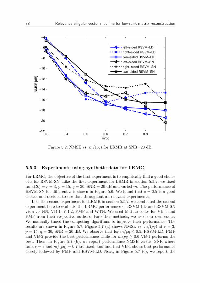
88 Relevance singular vector machine for low-rank matrix reconstruction
0.3 0.4 0.5 0.6 0.7 0.8−22
−20
−18
−16
−14
−12
−10
−8
−6
−4
m/pq
NM
SE
[d
B]
left−sided RSVM−LD
right−sided RSVM−LD
two−sided RSVM−LD
left−sided RSVM−SN
right−sided RSVM−SN
two−sided RSVM−SN
Figure 5.2: NMSE vs. m/(pq) for LRMR at SNR=20 dB.
5.5.3 Experiments using synthetic data for LRMC
For LRMC, the objective of the first experiment is to empirically find a good choiceof s for RSVM-SN. Like the first experiment for LRMR in section 5.5.2, we fixedrank(X) = r = 3, p = 15, q = 30, SNR = 20 dB and varied m. The performance ofRSVM-SN for different s is shown in Figure 5.6. We found that s = 0.5 is a goodchoice, and decided to use that throughout all relevant experiments.
Like the second experiment for LRMR in section 5.5.2, we conducted the secondexperiment here to evaluate the LRMC performance of RSVM-LD and RSVM-SNvis-a-vis NN, VB-1, VB-2, PMF and WTN. We used Matlab codes for VB-1 andPMF from their respective authors. For other methods, we used our own codes.We manually tuned the competing algorithms to improve their performance. Theresults are shown in Figure 5.7. Figure 5.7 (a) shows NMSE vs. m/(pq) at r = 3,p = 15, q = 30, SNR = 20 dB. We observe that for m/pq ≤ 0.5, RSVM-LD, PMFand VB-2 provide the best performance while for m/pq ≥ 0.6 VB-1 performs thebest. Then, in Figure 5.7 (b), we report performance NMSE versus. SNR whererank r = 3 and m/(pq) = 0.7 are fixed, and find that VB-1 shows best performanceclosely followed by PMF and RSVM-LD. Next, in Figure 5.7 (c), we report the
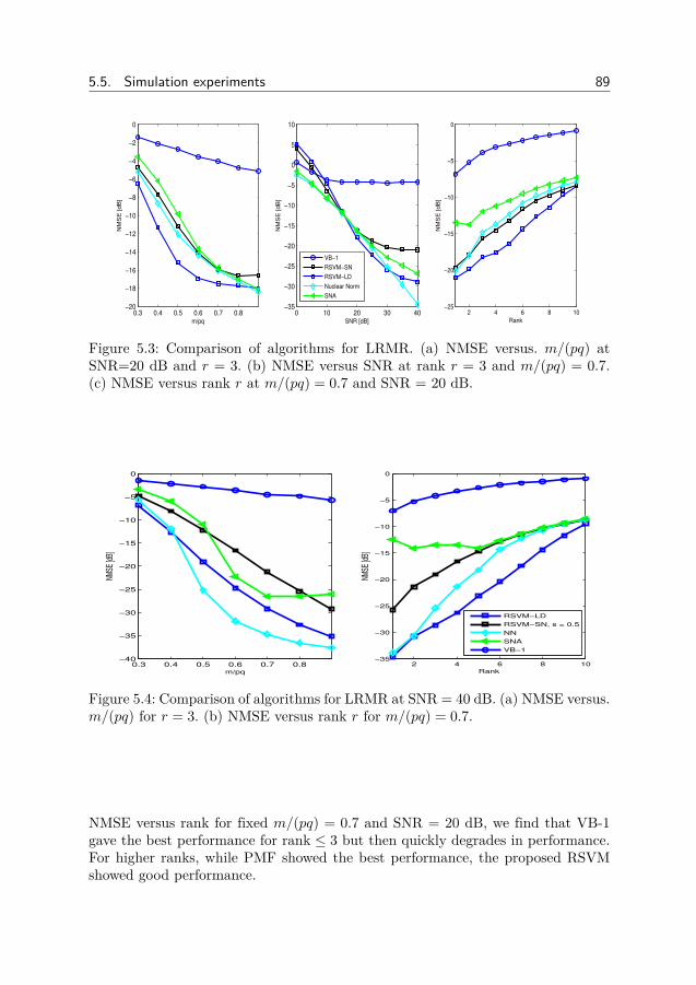
5.5. Simulation experiments 89
0.3 0.4 0.5 0.6 0.7 0.8−20
−18
−16
−14
−12
−10
−8
−6
−4
−2
0N
MS
E [
dB
]
m/pq
0 10 20 30 40−35
−30
−25
−20
−15
−10
−5
0
5
10
SNR [dB]
NM
SE
[d
B]
VB−1
RSVM−SN
RSVM−LD
Nuclear Norm
SNA
2 4 6 8 10−25
−20
−15
−10
−5
0
Rank
NM
SE
[d
B]
Figure 5.3: Comparison of algorithms for LRMR. (a) NMSE versus. m/(pq) atSNR=20 dB and r = 3. (b) NMSE versus SNR at rank r = 3 and m/(pq) = 0.7.(c) NMSE versus rank r at m/(pq) = 0.7 and SNR = 20 dB.
0.3 0.4 0.5 0.6 0.7 0.8−40
−35
−30
−25
−20
−15
−10
−5
0
NMSE
[dB]
m/pq
2 4 6 8 10−35
−30
−25
−20
−15
−10
−5
0
Rank
NMSE
[dB]
RSVM−LD
RSVM−SN, s = 0.5
NN
SNA
VB−1
Figure 5.4: Comparison of algorithms for LRMR at SNR = 40 dB. (a) NMSE versus.m/(pq) for r = 3. (b) NMSE versus rank r for m/(pq) = 0.7.
NMSE versus rank for fixed m/(pq) = 0.7 and SNR = 20 dB, we find that VB-1gave the best performance for rank ≤ 3 but then quickly degrades in performance.For higher ranks, while PMF showed the best performance, the proposed RSVMshowed good performance.

90 Relevance singular vector machine for low-rank matrix reconstruction
1 2 3 4 5 6 7 8 9 10
100
101
102
103
Rank
cp
utim
e
RSVM−LD
RSVM−SN, s = 0.5
NN
SNA
VB−1
Figure 5.5: Mean cputime versus rank r for the setup in Figure 5.3 (c).
5.5.4 Experiments using MovieLens data for LRMC - Movierating prediction
To evaluate the performance on real data we used the MovieLens 100K dataset[HKBR99]. The dataset contains user-movie pairs where in each pair, a user providesan integer rating between 1− 5 to a movie. Each user has only rated a few moviesaccording to the features of movies, and the underlying assumption is that the ratingmatrix has a factorized representation, leading to low-rank. Now let us assume thatwe observe few ratings of the large rating matrix randomly. The goal is to inferthe missing ratings from the observed ratings and hence the problem is an LRMCproblem.
In our experimental study, we used the u1 datasets (both training and test-ing) from the MovieLens dataset. Then we used a portion of the u1 datasets asX. The dimensions of X are p = q = 100. According to the MovieLens datasetinstructions, we used m = 307 measurements. The measurements are collected viaa pre-determined element picking matrix A. Using the measurements and X fromthe u1 training data, we learn the model parameters for all competing algorithms.Then, using the learned parameters we perform LRMC for the u1 test data. For
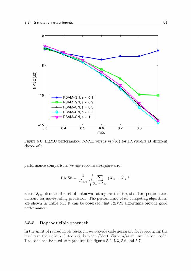
5.5. Simulation experiments 91
0.3 0.4 0.5 0.6 0.7 0.8−15
−10
−5
0
m/pq
NM
SE
[dB
]
RSVM−SN, s = 0.1
RSVM−SN, s = 0.3
RSVM−SN, s = 0.5
RSVM−SN, s = 0.7
RSVM−SN, s = 1
Figure 5.6: LRMC performance: NMSE versus m/(pq) for RSVM-SN at differentchoice of s.
performance comparison, we use root-mean-square-error
RMSE = 1|Jtest|
√ ∑(i,j)∈Jtest
(Xij − Xij)2,
where Jtest denotes the set of unknown ratings, as this is a standard performancemeasure for movie rating prediction. The performance of all competing algorithmsare shown in Table 5.1. It can be observed that RSVM algorithms provide goodperformance.
5.5.5 Reproducible research
In the spirit of reproducible research, we provide code necessary for reproducing theresults in the website: https://github.com/MartinSundin/rsvm_simulation_code.The code can be used to reproduce the figures 5.2, 5.3, 5.6 and 5.7.
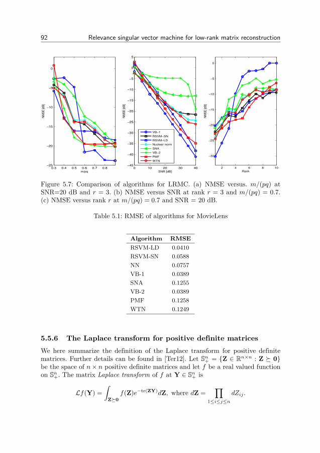
92 Relevance singular vector machine for low-rank matrix reconstruction
0.3 0.4 0.5 0.6 0.7 0.8−25
−20
−15
−10
−5
0
NM
SE
[dB
]
m/pq
0 10 20 30 40−45
−40
−35
−30
−25
−20
−15
−10
−5
0
5
SNR [dB]
NM
SE
[dB
]
VB−1
RSVM−SN
RSVM−LD
Nuclear norm
SNA
VB−2
PMF
WTN
2 4 6 8 10
−30
−25
−20
−15
−10
−5
0
NM
SE
[dB
]
Rank
Figure 5.7: Comparison of algorithms for LRMC. (a) NMSE versus. m/(pq) atSNR=20 dB and r = 3. (b) NMSE versus SNR at rank r = 3 and m/(pq) = 0.7.(c) NMSE versus rank r at m/(pq) = 0.7 and SNR = 20 dB.
Table 5.1: RMSE of algorithms for MovieLens
Algorithm RMSERSVM-LD 0.0410RSVM-SN 0.0588NN 0.0757VB-1 0.0389SNA 0.1255VB-2 0.0389PMF 0.1258WTN 0.1249
5.5.6 The Laplace transform for positive definite matricesWe here summarize the definition of the Laplace transform for positive definitematrices. Further details can be found in [Ter12]. Let Sn+ = Z ∈ Rn×n : Z 0be the space of n× n positive definite matrices and let f be a real valued functionon Sn+. The matrix Laplace transform of f at Y ∈ Sn+ is
Lf(Y) =∫
Z0f(Z)e−tr(ZY)dZ, where dZ =
∏1≤i≤j≤n
dZij .
5.5. Simulation experiments 93
The transform is defined for sufficiently nice functions [Ter12] for which it convergeswhen Re Y Z∗ for some Z∗. The inverse Laplace transform can be expressedas [Ter12]
1(2πi)n(n+1)/2
∫Re Y=Z∗
Lf(Y)etr(YZ)dY
=
f(Z) , if Z ∈ Sn+,0, , otherwise
.
5.5.7 Derivation of the Laplace ApproximationThe Laplace approximation is an approximation of the integral
I =∫e−
12 f(a)da,
where the integral is over a ∈ Rn. When the function e−12 f(a) is sufficiently well
behaved, the integral can be well approximated by the Laplace approximation. Inthe approximation, the function f(a) is approximated by a second order polynomialaround its minima a0 as
f(a) ≈ f(a0) + 12(a − a0)>H(a − a0),
where H = ∇2f(a)|a=a0 is the Hessian of f(a) at a0. The term linear in a vanishesand H 0 at a0 since we expand around a minima. With this approximation, theintegral becomes
I ≈∫e−
12 f(a0)− 1
4 (a−a0)>H(a−a0)da =
√(4π)n|H| e
− 12 f(a0).
In (5.8), the integral is given by
I = 1(2π)pq/2
∫α0
e−12 [tr(αZ)−q log |α|+K(α)]dα.
Set f(a) = tr(αZ) − q log |α| + K(α), where a = vech(α) and vech(·) is the half-vectorization operator for symmetric matrices, e.g.
vech(a b
b c
)=
a
b
c
.
Let α0 0 denote the minima of f(a) and H the Hessian at α0. Assuming that α0and H are “large” in the sense that the integral over α 0 can be approximated
94 Relevance singular vector machine for low-rank matrix reconstruction
by the integral over α ∈ Rp×p we find that
I ≈ 1(2π)pq/2
∫e−
12 f(a0)− 1
4 (a−a0)>H(a−a0)da
= (4π)p2/2
(2π)pq/2|H|1/2e−
12 f(a0),
where a0 = vech(α0).
5.5.8 Derivation of (5.21), (5.22), (5.23) and (5.24)Let P1 , Pr
(||P⊥L xi||22 ≤ ς||PLxi||22
)and assume that 1 ≤ r < p and let n =
p− r. The random variables PLxi and P⊥L xi are independent zero-mean Gaussianvariables. Let w1, w2, . . . , wr, z1, z2, . . . , zn be i.i.d. N (0, 1) variables. For the proofsof (5.21), (5.22), we find that
P1 = Pr(λL,r+1z
21+λL,r+2z
22+...λL,pz2
n
λL,1w21+λL,2w2
2+···+λL,rw2r≤ ς)
(a)≥ Pr
(λL,r+1(z2
1+z22+···+z2
n)λL,r(w2
1+w22+···+w2
r) ≤ ς)
= 1− Pr(λL,r+1(z2
1+z22+···+z2
n)λL,r(w2
1+w22+···+w2
r) ≥ ς)
= 1− Pr(
(w21+w2
2+···+w2r)/r
(z21+z2
2+···+z2n)/n ≤
nλL,r+1ςrλL,r
)(b)≥ 1− B( r2 ,n2 ,ε1)
B( r2 ,n2 )(c)≥ 1− Cp,rεr/21 ,
(5.33)
where B(·, ·, ·) is the incomplete beta function, B(·, ·) = B(·, ·, 1) is the beta functionand
C−1p,r = r
2B(r
2 ,n
2
), and ε1 = 1
1 + ςλL,rλL,r+1
.
In (a), λL,r+1z21+λL,r+2z
22+...λL,pz2
n
λL,1w21+λL,2w2
2+···+λL,rw2r≤ λL,r+1(z2
1+z22+···+z2
n)λL,r(w2
1+w22+···+w2
r) is used. In (b) we note that(w2
1+w22+···+w2
r)/r(z2
1+z22+···+z2
n)/n is F-distributed. Then, in (c), we use the following relation
B(r2 ,
n2 , ε1
)=∫ ε1
0 tr/2−1(1− t)n/2−1dt
= εr/21∫ 1
0 ur/2−1(1− ε1u)n/2−1du
≤ 2r εr/21 .
(5.34)
This shows (5.22).Suppose P2 , Pr
(||X−Xr||2F ≤ ς||X||2F
). To show (5.24) we introduce the pro-
jection PR onto the subspace spanned by the r eigenvectors of α−1R corresponding
5.5. Simulation experiments 95
to the r largest eigenvalues and P⊥R = Iq − PR. Using the projection operators PLand PR, we have the following relation
||X||2F = ||PLXPR||2F + ||PLXP⊥R ||2F+||P⊥LXPR||2F + ||P⊥LXP⊥R ||2F .
If P1 and P2 are two projection operators with properties rank(P1) = p − r andrank(P2) = q − r, then we have the following relation
||X−Xr||2F = minP1,P2
||P1XP2||2F
≤ ||P⊥LXP⊥R ||2F .
We now find the following relation
P2 , Pr(||X−Xr||2F ≤ ς||X||2F
)≥ Pr
(||P⊥LXP⊥R ||2F ≤ ς||X||2F
)≥ Pr
(||P⊥LXP⊥R ||2F ≤ ς
(||PLXPR||2F + ||P⊥LXP⊥R ||2F
))= Pr
(||P⊥LXP⊥R ||2F ≤ ς
1−ς ||PLXPR||2F), P3
The random variables PLXPR and P⊥LXP⊥R are independent zero-mean Gaussianvariables. Let wi,j, and zk,l be i.i.d. N (0, 1) variables, where 1 ≤ i, j ≤ r,1 ≤ k ≤ p− r and 1 ≤ l ≤ q − r. This gives us that [GN99]
P3 = Pr(∑p−r
k=1∑q−rl=1 λL,r+kλL,r+lw
2k,l∑
1≤i,j≤r λL,iλR,jz2i,j
≤ ς
1− ς
).
Using that ∑1≤i,j≤r
λL,iλR,jz2i,j ≥ λL,rλR,r
∑1≤i,j≤r
z2i,j ,
p−r∑k=1
q−r∑l=1
λL,r+kλR,r+lw2k,l ≤ λL,r+1λR,r+1
p−r∑k=1
q−r∑l=1
w2k,l,
we find that
P3 ≥ Pr(∑p−r
k=1∑q−rl=1 w
2k,l∑
1≤i,j≤r z2i,j
≤ ς
1− ςλL,rλR,r
λL,r+1λR,r+1
).
Since1
(p−r)(q−r)∑p−rk=1
∑q−rl=1 w
2k,l
1r2
∑1≤i,j≤r z
2i,j
96 Relevance singular vector machine for low-rank matrix reconstruction
is F-distributed, we find that
P2 ≥ P3 ≥ 1−B(r2
2 ,(p−r)(q−r)
2 , ε2
)B(r2
2 ,(p−r)(q−r)
2
) ≥ 1− Cr,p,qεr22
2 ,
where
C−1r,p,q = r2
2 B(r2
2 ,(p−r)(q−r)
2
),
ε2 = 11+ ς
1−ςλL,rλL,r+1
λR,rλR,r+1
.
5.5.9 The EM help function
The EM help function Q(Θ,Θ′) is given by
Q(Θ,Θ′) = EX|y,Θ′ [log p(X|y,Θ)] = c+ m
2 log β
− β
2 E [||y−Avec(X)||22 −12E [tr(αLXαRX>)]
+ q
2 log |αL|+p
2 log |αR|,
where c is a constant. Using that
E [||y−Avec(X)||22] = ||y||22 − 2y>Avec(X)+ tr(A>A(vec(X)vec(X)> + Σ′))= ||y−Avec(X)||22 + tr(A>AΣ′),
and
E [tr(αLXαRX>)]= tr((αR ⊗αL)(vec(X)vec(X)> + Σ′))= tr(αLXαRX>) + tr((αR ⊗αL)Σ′),
we recover the expression (5.28) for the EM help function.
5.5.10 Details for the RSVM with the Schatten s-norm penalty
We here set S = εIq to keep the derivation more general. The regularized Schattens-norm penalty is given by
g(Z) = tr((X>X + S)s/2).
5.5. Simulation experiments 97
For the concave conjugate formula (5.10) we find that the minimum over Z occurswhen
α− s
2(Z + S)s/2−1 = 0.
Solving for Z gives us that
K(α) = −tr(αS)− 2− ss
(2s
)−2/(2−s)tr(α−2/(2−s)),
which results in (5.12).Using (5.28), we find that the minimum of (5.27) for the Schatten s-norm occurs
when
XαRX> + ΣR −(
2s
)−s/(2−s)α−2/(2−s)L = 0
Solving for αL gives us (5.30). The update equation for αR is derived in a similarmanner.
5.5.11 Details for RSVM-LD
The log-determinant penalty is given by
g(X) = ν log |Z + S|.
For the concave conjugate formula (5.10) we find that the minimum over Z occurswhen
α− ν(Z + S)−1 = 0.
Solving for Z gives that
K(α) = −tr(αS) + ν log |α|+ νp− ν log ν.
By removing the constants we recover (5.14).Using (5.28), we find that the minimum of (5.27) with respect to αL for the
log-determinant penalty occurs when
XαRX> + ΣR + SL − να−1L = 0
Solving for αL gives us (5.31). The derivation of the update equation for αR isfound in a similar way.
98 Relevance singular vector machine for low-rank matrix reconstruction
5.5.12 Update equations of VB-1 for LRMRHere we generalize the update equations of the Variational Bayes method from[BLMK12] to LRMR, referred to as VB-1 in section 5.5.1. Similar methods wereused in [MS07, SM08,NSB13,LT07]. The VB-1 method factorizes the matrix X ∈Rp×q as
X = FB>,
were the column vectors of F = [f1 f2 . . . fr] ∈ Rp×r, B = [b1 b2 . . . br] ∈ Rq×r(r ≤ min(p, q) is a user parameter) are given Gaussian priors as
p(F|γ) =r∏i=1N (fi|0, γ−1
i Ip),
p(B|γ) =r∏j=1N (bj |0, γ−1
j Iq),
where γi > 0 is the precisions of fi and bi. We usually set r = rank(X) when therank is known, otherwise r can be used to upper bound the rank of X = FB>. Theadditive noise in (5.1) is modeled as a zero-mean white Gaussian with the unknownprecision β > 0. The precisions are given Gamma and Jeffreys priors as
p(γi) ∝ γa−1i exp(−bγi),
p(β) ∝ β−1.
In the variational Bayes framework, blocks of variables are assumed to haveindependent posterior distributions allowing to approximate the posterior. Assumethat we want to approximate a distribution p(z) using variational Bayes. Let zIdenote the variables with indices’s in a set I, the variational Bayes approximatesthe distribution p(zI) by q(zI) as [Bis06]
log q(zI) = EzIc |zI [log p(zI , zIc)] + constant.
Different choices of blocks of parameters can be made, we here chose to use indepen-dent rows in F and B (as in [BLMK12]) since it gives good (empirical) performance.We here use Ak to denote the k’th sensing matrix in (5.2), [Ak].i to denote thei’th column vector of Ak, [Ak]i. to denote the i’th row vector of Ak and [Ak]ij todenote the (i, j)’th component of Ak. We also set Γ = diag(γ1, γ2, . . . , γr).
Given means γ, β of γ and β, that bk ∼ N (bk,Σ(B)k ) for all k and fj ∼
N (fj ,Σ(F )j ) for all j 6= i, we find that
log q(fi) = − β2
(m∑k=1
y2k − 2f>i B>[Ak]i.yk

5.5. Simulation experiments 99
+2∑j 6=i
f>i E[B>[Ak]i.[Ak]>j.B
]fj
+f>i E[B>[Ak]i.[Ak]>i.B
]fi)− 1
2 f>i Γfi + constant.
where
E[B>[Ak]i.[Ak]>j.B
]=B>[Ak]i.[Ak]>j.B
+∑c
[Ak]ic[Ak]jcΣ(B)d .
This gives us that fi ∼ N (fi,Σ(F )i ) with
fi = βΣ(F )i
(B>
∑k
yk[Ak]i.
−∑j 6=i,k
E[B>[Ak]i.Ak]>j.B
]fj
,
Σ(F )i =
(β∑k
E[B>[Ak]i.[Ak]>i.B
]+ Γ
)−1
.
Similarly, when the distributions of the other variables are fixed, we get thatbi ∼ N (bi,Σ(B)
i ) with
bi = βΣ(B)i
(F>∑k
yk[Ak].i
−∑j 6=i,k
E[F>[Ak].i[Ak]>.jF
]bj
,
Σ(B)i =
(β∑k
E[F>[Ak].i[Ak]>.iF
]+ Γ
)−1
,
where now
E[F>[Ak].i[Ak]>.jF
]=F>[Ak].i[Ak].jF
+∑d
[Ak]di[Ak]djΣ(F )d .
We also find that the precisions γi are Gamma distributed with posterior pa-rameters
ai = p+ q + 2a2 ,
bi = 12
(||fi||22 + ||bi||22 + tr(Σ(F )
i ) + tr(Σ(B)i ) + 2b
).

100 Relevance singular vector machine for low-rank matrix reconstruction
This gives us that the posterior mean of γi is γi = ai/bi. Similary we find that theposterior distribution of β is Gamma(c, d) with
c = m/2,
d = 12
||y− vec(FB>)||22 +∑i,k
(f>i AkΣ(B)
i A>k fi
+b>i A>k Σ(F )i Akbi + tr(Σ(F )
i AkΣ(B)i A>k )
)].
The posterior mean of β is thus β = c/d.
5.6 Conclusion
We derived a low-rank analogue of the Relevance Vector Machine, called the Rel-evance Singular Vector Machine (RSVM). The RSVM uses precision matrices anda hierarchical prior to promote low-rank in X. For the one-sided model, the priorof the precision matrix is related to the marginal prior on X through the Laplacetransform and through the concave conjugate formula. However, for the MAP es-timation problem, the concave conjugate formula gives an exact relation. For thetwo-sided model, an relation is more difficult to establish because of the prior onX depends non-linearly on the precision matrices. Simulations show that the per-formance of the RSVM methods is similar to the performance of the nuclear normestimator for SNR = 20 dB and slightly worse than the performance of the nuclearnorm for SNR = 40 dB. The RSVM method suffers from high complexity but showsgood performance. To develop the method for larger scale problems is therefore aninteresting problem.
Chapter 6
Bayesian learning for robust PCA
One of the main tasks in signal processing and machine learning is to describedata in as simple a manner as possible. This is usually done by describingthe data with fewer parameters than the number of data points. In the linear
model, this is done by writing the data points as linear combinations of a fixed setof atoms. Often, the atoms themselves are not known. It is then required to learn allparameters from data alone. One method for finding a simple linear description isPrincipal Component Analysis (PCA) which attempts to find a lower-dimensionalsubspace which best describes the data best. The mismatch between the data andthe PCA description is often treated as noise.
PCA is a kind of least square estimator and works well when the noise is dense.However, similarly to the standard least squares, PCA is sensitive to sparse outliernoise. Since the outliers are sparse and the PCA estimate is low-rank, the robustPCA problem is a combination of the sparse and low-rank estimation problems.Many methods for sparse and low-rank problems have been adapted to the robustPCA problem. Here we construct a Bayesian method for robust PCA by combiningthe robust SD-RVM from Chapter 4 and the RSVM from Chapter 5.
6.1 Robust principal component analysis
Robust Principal Component Analysis (RPCA) is the problem of estimating a low-rank matrix X from measurements
Y = X + S + N ∈ Rp×q, (6.1)
where Y is the observed matrix, N is additive dense noise (typically isotropic Gaus-sian) and S is a sparse matrix modeling outliers. The RPCA model (6.1) has beenused in e.g. [CLMW11,WLZ13,ZT11,BLMK12,Wip12,DHC11,WYG+09,CSPW11,OCS14,SW12,MMG13] to model different phenomena and has applications in e.g.image processing, collaborative filtering, face recognition [CLMW11] and machinelearning [WLZ13]. The system model (6.1) can also be used in a matrix completion
101
102 Bayesian learning for robust PCA
setup, where only some components of Y are observed, by modeling the unobservedentries as outliers.
In the literature, three classes of estimation methods are typically used: greedy,convex optimization based and Bayesian. The greedy method in [ZT11] uses alter-nating optimization to estimate X and S via a least-squares principle. The greedymethod is highly effective but requires rank and sparsity level to be known a-priori.The method may therefore be infeasible in many applications. The convex opti-mization based method in [CLMW11] is called principal component pursuit (PCP)and uses nuclear-norm and `1-norm penalty functions to estimate X and S. Onelimitation of PCP is that it requires the power of the dense noise to be known. Inabsence of a-priori knowledge, Bayesian methods are a suitable choice since theycan learn all necessary parameters from data. Formulating a Bayesian method for(6.1) requires low-rank and sparsity promoting priors for X and S, respectively. Themethod of [BLMK12] uses a variational Bayes (VB) approach where the low-rankprior is induced using block sparsity in a matrix factorization model. The empiricalBayes (EB) method of [Wip12] promotes low-rank by modeling the column vectorsof X as correlated Gaussian vectors. Further, in [Wip12] S is given a sparsity pro-moting prior by the usual approach where the elements are Gaussian variables withgamma distributed precisions.
In this chapter we develop a new Bayesian method for RPCA. To promote low-rank, we use a model that induces correlations among the column and row vectorsof X. The new method is called robust RSVM (rRSVM) and the parameters areestimated using the expectation-maximization (EM) framework. Through numer-ical simulations, we investigate the performance for synthetic data as well as realdata from the MovieLens 100K dataset [HKBR99]. The performance of rRSVM isfound to be better than that of the competing algorithms PCP, EB and VB forboth synthetic and real data.
6.2 Robust RSVM
To formulate a Bayesian learning method for the RPCA model (6.1), we needappropriate priors for X, S and N. Here we use the prior for outliers from Chapter 4to promote sparsity and the two-sided precision with log-determinant prior fromChapter 5 to promote low-rank. We first discuss the priors in Section 6.2.1 and thendesign the learning algorithm rRSVM in Section 6.2.2 using the EM framework.
6.2.1 Priors for low-rank and sparsity
Low-rank promoting prior
As in Chapter 5 we set the prior on X to be
vec(X) ∼ N (0,α−1R ⊗α
−1L ), (6.2)
6.2. Robust RSVM 103
and the prior on the precision matrices to be
p(αL) ∝ |αL|(ν−q)/2e−ε2 tr(αL),
p(αR) ∝ |αR|(ν−p)/2e−ε2 tr(αR),
(6.3)
Prior for combined noise
As in Chapter 4 we model the combined noise as
Sij +Nij ∼ N (0, β−1ij ), (6.4)
where βij > 0 is the total noise precision of the combined noise component Sij+Nij .The motivation of using a combined model instead of an independent treatmentstems from the fact that S and N need not be separated individually for estima-tion of X. This approach also reduces the number of model parameters and oftenimproves estimation performance [SCJ15b]. The combined noise is only approxi-mately sparse and is well modeled using a sparsity promoting prior. We here usethe Gamma prior
p(βij) = Gamma(βij |a+ 1, b) = ba+1
Γ(a+ 1)βaije−bβij , (6.5)
for the noise precisions βij , where Γ(·) denotes the Gamma function [Bis06], topromote sparsity in the noise [Wip12,MVC10].
6.2.2 Bayesian learning algorithm for rRSVMA common method for estimating the model parameters is the maximum a-posteriorimethod
X, θ = arg maxX,θ
p(X, θ|Y), (6.6)
where θ = αL,αR,β. The maximization of (6.6) is often hard to perform in prac-tice and therefore needs to be approximated through e.g. evidence approximationor expectation maximization (EM) [Bis06]. To initialize EM, we make an initialchoice of θ. Next, in the expectation step, EM computes the posterior distributionp(X|Y, θ′) of X given the measurements Y and the latent variables θ′ from theprevious iteration. In the second step (the maximization step), the latent variablesθ are updated by maximizing the EM help function
Q(θ, θ′) = E [log p(Y,X|θ)|Y, θ′] + log p(θ),
with respect to θ. The expectation and maximization step is repeated until con-vergence. An advantage of EM over e.g. evidence approximation is that it hasestablished monotone convergence properties [Bis06], i.e. in each iteration the costin (6.6) does not increase.
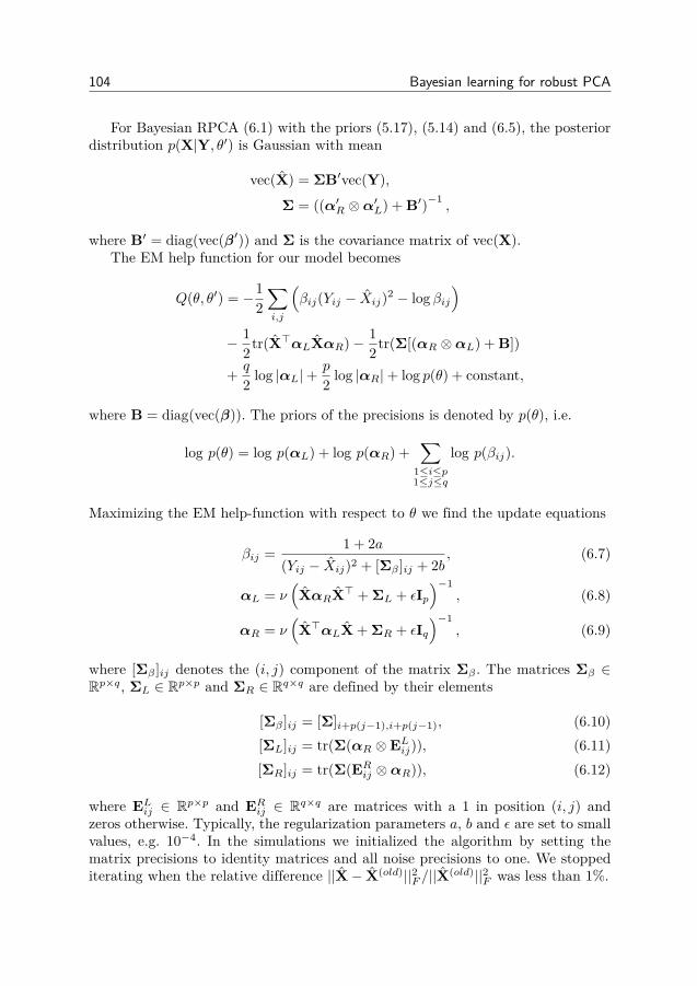
104 Bayesian learning for robust PCA
For Bayesian RPCA (6.1) with the priors (5.17), (5.14) and (6.5), the posteriordistribution p(X|Y, θ′) is Gaussian with mean
vec(X) = ΣB′vec(Y),
Σ = ((α′R ⊗α′L) + B′)−1,
where B′ = diag(vec(β′)) and Σ is the covariance matrix of vec(X).The EM help function for our model becomes
Q(θ, θ′) = −12∑i,j
(βij(Yij − Xij)2 − log βij
)− 1
2tr(X>αLXαR)− 12tr(Σ[(αR ⊗αL) + B])
+ q
2 log |αL|+p
2 log |αR|+ log p(θ) + constant,
where B = diag(vec(β)). The priors of the precisions is denoted by p(θ), i.e.
log p(θ) = log p(αL) + log p(αR) +∑
1≤i≤p1≤j≤q
log p(βij).
Maximizing the EM help-function with respect to θ we find the update equations
βij = 1 + 2a(Yij − Xij)2 + [Σβ ]ij + 2b
, (6.7)
αL = ν(XαRX> + ΣL + εIp
)−1, (6.8)
αR = ν(X>αLX + ΣR + εIq
)−1, (6.9)
where [Σβ ]ij denotes the (i, j) component of the matrix Σβ . The matrices Σβ ∈Rp×q, ΣL ∈ Rp×p and ΣR ∈ Rq×q are defined by their elements
[Σβ ]ij = [Σ]i+p(j−1),i+p(j−1), (6.10)[ΣL]ij = tr(Σ(αR ⊗EL
ij)), (6.11)[ΣR]ij = tr(Σ(ER
ij ⊗αR)), (6.12)
where ELij ∈ Rp×p and ER
ij ∈ Rq×q are matrices with a 1 in position (i, j) andzeros otherwise. Typically, the regularization parameters a, b and ε are set to smallvalues, e.g. 10−4. In the simulations we initialized the algorithm by setting thematrix precisions to identity matrices and all noise precisions to one. We stoppediterating when the relative difference ||X− X(old)||2F /||X(old)||2F was less than 1%.
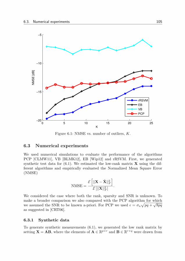
6.3. Numerical experiments 105
0 5 10 15 20 25−20
−15
−10
−5
K
NM
SE
[dB
]
rRSVM
EB
VB
PCP
Figure 6.1: NMSE vs. number of outliers, K.
6.3 Numerical experiments
We used numerical simulations to evaluate the performance of the algorithmsPCP [CLMW11], VB [BLMK12], EB [Wip12] and rRSVM. First, we generatedsynthetic test data for (6.1). We estimated the low-rank matrix X using the dif-ferent algorithms and empirically evaluated the Normalized Mean Square Error(NMSE)
NMSE =E[||X− X||2F
]E [||X||2F ] .
We considered the case where both the rank, sparsity and SNR is unknown. Tomake a broader comparison we also compared with the PCP algorithm for whichwe assumed the SNR to be known a-priori. For PCP we used ε = σn
√pq +
√8pq
as suggested in [CRT06].
6.3.1 Synthetic dataTo generate synthetic measurements (6.1), we generated the low rank matrix bysetting X = AB, where the elements of A ∈ Rp×r and B ∈ Rr×q were drawn from
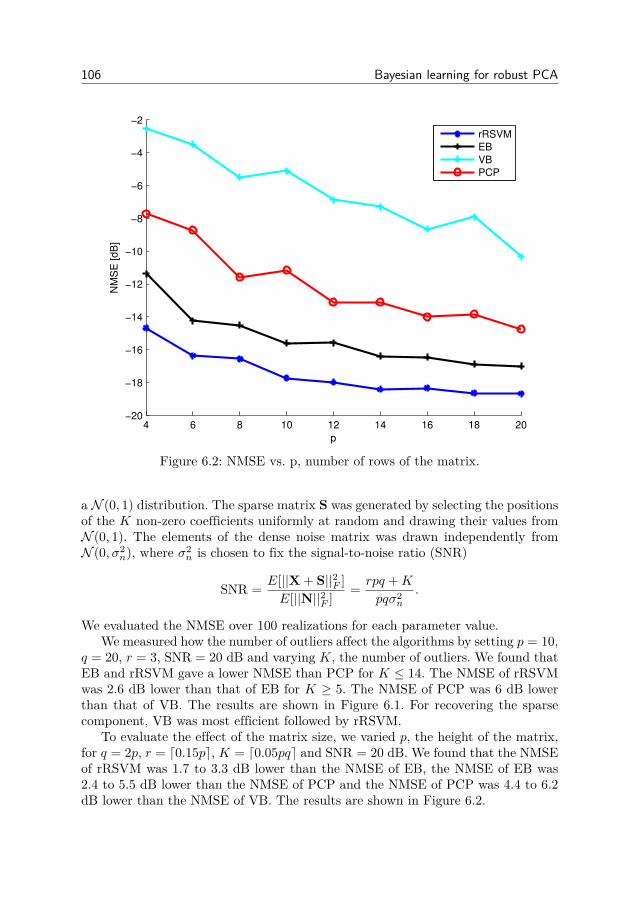
106 Bayesian learning for robust PCA
4 6 8 10 12 14 16 18 20−20
−18
−16
−14
−12
−10
−8
−6
−4
−2
p
NM
SE
[dB
]
rRSVM
EB
VB
PCP
Figure 6.2: NMSE vs. p, number of rows of the matrix.
a N (0, 1) distribution. The sparse matrix S was generated by selecting the positionsof the K non-zero coefficients uniformly at random and drawing their values fromN (0, 1). The elements of the dense noise matrix was drawn independently fromN (0, σ2
n), where σ2n is chosen to fix the signal-to-noise ratio (SNR)
SNR = E[||X + S||2F ]E[||N||2F ] = rpq +K
pqσ2n
.
We evaluated the NMSE over 100 realizations for each parameter value.We measured how the number of outliers affect the algorithms by setting p = 10,
q = 20, r = 3, SNR = 20 dB and varying K, the number of outliers. We found thatEB and rRSVM gave a lower NMSE than PCP for K ≤ 14. The NMSE of rRSVMwas 2.6 dB lower than that of EB for K ≥ 5. The NMSE of PCP was 6 dB lowerthan that of VB. The results are shown in Figure 6.1. For recovering the sparsecomponent, VB was most efficient followed by rRSVM.
To evaluate the effect of the matrix size, we varied p, the height of the matrix,for q = 2p, r = d0.15pe, K = d0.05pqe and SNR = 20 dB. We found that the NMSEof rRSVM was 1.7 to 3.3 dB lower than the NMSE of EB, the NMSE of EB was2.4 to 5.5 dB lower than the NMSE of PCP and the NMSE of PCP was 4.4 to 6.2dB lower than the NMSE of VB. The results are shown in Figure 6.2.

6.3. Numerical experiments 107
0 5 10 15 20 25 30 35 40−40
−35
−30
−25
−20
−15
−10
−5
0
5
SNR [dB]
NM
SE
[dB
]
rRSVM
EB
VB
PCP
Figure 6.3: NMSE vs. SNR.
Finally, we measured the sensitivity to noise by setting p = q = 10, r = 2,K = 5 and varied the SNR. We found that rRSVM performed best for SNR ≥ 10dB. For SNR = 30 dB, the NMSE of rRSVM was 9.7 dB lower than the NMSE ofEB while the NMSE of PCP was 9.5 dB lower than the NMSE of VB. The resultsare shown in Figure 6.3.
6.3.2 MovieLens dataset
The MovieLens 100K dataset [HKBR99] consists of 100 000 ratings of 1682 moviesby 943 users collected in the years 1997 and 1998. Each rating is given by an integerfrom 1 to 5. In collaborative filtering, the movies are modeled by certain features,e.g. genre, and each user has preferences based on these features. The preferencesof a user can thus be modeled as a linear combination of preferences for certain(unknown) features. For a low number of relevant features, the matrix of ratings isa low-rank matrix.
Some users may have unique preferences for which the low-rank model is ill-suited. There are also examples of so called schilling attacks in which users gener-ate ratings in order to manipulate recommendations [CNZ05]. Ratings which arenot modeled well by a low-rank matrix are often few and can thus be modeledby a sparse matrix, the recommendation problem then becomes a robust matrix
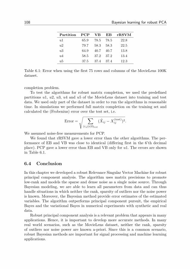
108 Bayesian learning for robust PCA
Partition PCP VB EB rRSVMu1 65.9 78.5 78.5 22.8u2 79.7 58.3 58.3 22.5u3 64.9 40.7 40.7 13.8u4 58.5 37.2 37.2 13.4u5 37.5 37.4 37.4 12.3
Table 6.1: Error when using the first 75 rows and columns of the MovieLens 100Kdataset.
completion problem.To test the algorithms for robust matrix completion, we used the predefined
partitions u1, u2, u3, u4 and u5 of the MovieLens dataset into training and testdata. We used only part of the dataset in order to run the algorithms in reasonabletime. In simulations we performed full matrix completion on the training set andcalculated the (Frobenius) error over the test set, i.e.
Error =√ ∑
(i,j)∈Ωtest
(Xij −X(test)ij )2.
We assumed noise-free measurements for PCP.We found that rRSVM gave a lower error than the other algorithms. The per-
formance of EB and VB was close to identical (differing first in the 6’th decimalplace). PCP gave a lower error than EB and VB only for u1. The errors are shownin Table 6.1.
6.4 Conclusion
In this chapter we developed a robust Relevance Singular Vector Machine for robustprincipal component analysis. The algorithm uses matrix precisions to promotelow-rank and models the sparse and dense noise as a single noise source. ThroughBayesian modeling, we are able to learn all parameters from data and can thushandle situations in which neither the rank, sparsity of outliers nor the noise poweris known. Moreover, the Bayesian method provide error estimates of the estimatedvariables. The algorithm outperforms principal component pursuit, the empiricalBayes and the variational Bayes in numerical experiments with synthetic and realdata.
Robust principal component analysis is a relevant problem that appears in manyapplications. Hence, it is important to develop more accurate methods. In manyreal world scenarios, such as the MovieLens dataset, neither the rank, sparsityof outliers nor noise power are known a-priori. Since this is a common scenario,robust Bayesian methods are important for signal processing and machine learningapplications.
Chapter 7
Bayesian Cramér-Rao bounds for low-rankmatrix estimation
In the work of designing more accurate estimation algorithms, it is useful toknow how close (or far) the algorithms are from being optimal. Theoreticallower bounds provide limits on the Mean-Square Error (MSE) of estimators.
When the performance of an estimator reaches the lower bound, we know that theestimator is optimal and that the bound is the best possible. When the performanceof the best estimator and best lower bounds does not meet, it shows that there ispossible to design better estimators and/or better bounds.
The Cramér-Rao bound [Cra47, Kay93] provides a lower bound on the MSEfor unbiased estimators of deterministic parameters. When the parameters to beestimated are random, the prior distributions need to be taken into account whenderiving lower bounds. This is because the prior distribution brings additional in-formation about the parameters. A strong prior gives much information about thevariable while a weak prior gives less information about the parameters. For the ran-dom variables, a lower bound is given by the Bayesian Cramér-Rao Bound (BCRB)[VT04,VTB07,GL95,BS80]. In this chapter we investigate Bayesian Cramér-Raobounds for certain Bayesian low-rank reconstruction models.
7.1 Introduction
In low-rank matrix reconstruction (LRMR), we seek to estimate a low-rank matrixX ∈ Rp×q from linear measurements
y = A(X) + n = Avec(X) + n = Ax + n, (7.1)
where y ∈ Rm is the observed measurements, n ∈ Rm is additive measurement noiseand the sensing operator A : Rp×q → Rm and the sensing matrix A ∈ Rm×pq aretwo equivalent representations of the linear sensing process. For brevity we intro-duce x , vec(X) where vec(·) is the standard vectorization operator. The sensing
109
110 Bayesian Cramér-Rao bounds for low-rank matrix estimation
operator A and sensing matrix A are linear operators which can be represented as
Avec(X) = A(X) =
tr(A>1 X)tr(A>2 X)
...tr(A>mX)
,
where the i’th row of A is vec(Ai)> with Ai ∈ Rp×q and i = 1, 2, . . . ,m. Thesensing matrix A (and therefore also A) is assumed to be known. An importantspecial case of LRMR is matrix completion where we observe individual elementsof X.
The LRMR problem occurs in several applications, such as system identification[CP10,Faz02,ZSJC12] and recommendation systems [CP10,CR09,CP11,RFGST09,CWZY15,YC11,KBV09,LBA11,Alq13,Suz15,HKBR99,SS10,SM08,LT07,RIK07,FRW11,MS07, LB10,BLMK12,Wip12, SRJC,TN11,CT10]. In many applications,the LRMR problem setup (7.1) is under-determined, i.e. m < pq.
There exists several reconstruction algorithms for LRMR, see e.g. [CR09,RFGST09,CWZY15, YC11, KBV09, LBA11, SS10, SM08, LT07, RIK07, FRW11, MS07, LB10,BLMK12,Wip12,SRJC,TN11]. In the Bayesian strategy, the low-rank property ofthe matrix X is modeled by a prior distribution. Prominent models of prior distribu-tions are the factorized model of [KBV09,SS10,SM08,LT07,RIK07,BLMK12] andthe hierarchical model of our previous work [SRJC]. Our contribution is the theo-retical derivation of Bayesian Cramer-Rao bounds (BCRB) for the mentioned priormodels. We also evaluate BCRB for a direct low-rank promoting prior distributionthat was not used in practical algorithms, but that is interesting for theoretical un-derpinning. Finally, we perform numerical simulations to compare the performanceof practical Bayesian LRMR algorithms against the derived BCRB bounds.
BCRB’s for sparse Bayesian models was considered in [PM13]. On the topicof deriving BCRB for LRMR, there exists no work in literature except the work[YC11] that only considered a restricted case of low-rank matrix completion and afactorized model for X. Our work goes much beyond the work of [YC11]. At thispoint we mention that there exists bounds for deterministic scenario of LRMR, suchas Cramer-Rao bounds for unstructured [TN11] and structured [ZSJC12] low-rankmatrices. In the following subsections, we explain notations used in this article andprovide preliminaries of BCRB.
7.1.1 NotationWe use Eq[·] to denote the expectation value with respect to random variablesq. The element-wise (Khatri-Rao) product of two matrices is denoted by andthe Kronecker product by ⊗. The `2-norm and Frobenius norm are denoted by‖.‖F . We denote the k × k identity matrix by Ik and the i’th unit vector by ei,i.e. ei = [0, 0, . . . , 0, 1, 0, . . . , 0]>. We also use the matrices EL
ij ∈ Rp×p and
7.1. Introduction 111
ERij ∈ Rq×q defined as
[Eij ]kl =
1 if (k, l) = (i, j) or (k, l) = (j, i),0 otherwise
.
The commutation matrix is the matrix representation of the transpose operation,i.e. Kp,qvec(Z) = vec(Z>) for all Z ∈ Rp×q and can be expressed as
Kp,q =∑
1≤i≤q,1≤j≤peie>j ⊗ eje>i .
We introduce the linear operators T1 and T2 such that T1(C⊗D) = (C> ⊗D) andT2(C⊗D) = (C⊗D>) for all matrices C ∈ Rq×q and D ∈ Rp×p. The operatorsare defined for any matrix W ∈ Rpq×pq through linearity.
We also introduce the matrix Dp such that
Dpvec(Z) = vec(Z + Z> − (Z Ip)
),
where Z ∈ Rp×p. We find that D>p = Dp. The matrix is useful when taking deriva-tive with respect to a symmetric matrix. If Z is symmetrix, then e.g. [KvR06]
∂ log |Z|∂vec(Z) = vec(2Z−1 − (Z−1 Ip)) = Dpvec(Z−1),
∂vec(Z−1)∂vec(Z) = −Dp(Z−1 ⊗ Z−1),
∂tr(AZ)∂vec(Z) = Dpvec(A).
7.1.2 Preliminaries on BCRBWithout loss of generality, we assume that the matrix X is a function of someparameters w ∈ Rn. We write this dependence as x = h(w) where h(·) is a knownfunction. We model random matrices X by letting w be a random variable witha prior distribution p(w|θ) that depends on some hyper-parameters θ ∈ RK . Thehyper-parameters θ can be either deterministic or random. When the prior is on Xdirectly, we set x = w. Throughout the chapter, we assume the noise is zero-meanwhite Gaussian distributed as
n ∼ N (0, β−1Im).
where β > 0 is the noise precision. When β is random, we assume that it is Gammadistributed with a prior Gamma distribution
p(β) = Gamma(β|c, d) = 1Γ(c)d
cβc−1e−dβ , (7.2)
112 Bayesian Cramér-Rao bounds for low-rank matrix estimation
where Γ(·) is the standard Gamma function and c, d > 0 are model parameters.The joint distribution of all variables is
p(y,w,θ, β) = p(y|w, β)p(w|θ)p(θ)p(β).
For brevity of notation, we denote the model variables by
z , [w> θ> β]>. (7.3)
We are often interested in estimating a variable η , g(z) where g(·) is a knownfunction. The BCRB provides a lower bound on the mean-square-error (MSE) of anunbiased estimator η. In the literature, the BCRB is also known as the van-Treesinequality [VT04,VTB07] and the Borovkov-Sakhanenko inequality [VTB07,BS80].To derive the BCRB, we need to compute the Fisher information matrix F of z
[F]ij = Ey[∂ log p(y, z)
∂zi
∂ log p(y, z)∂zj
],
where zi denotes the i’th element of z. We denote the covariance matrix of theestimation error ε , η − η by
Cε , Ey,z[εε>
]= Ey,z
[(η − η)(η − η)>
].
Proposition 7.1.1 (BCRB). Assume that g(z) does not depend on A. For anunbiased estimator η, the covariance Cε of the estimation error ε is bounded as
Cε Ez[∂g∂z
](Ez[F])−1 Ez
[∂g∂z
]>. (7.4)
It also holds that
Cε Ez
[∂g∂z
∂g∂z
>](Ez
[∂g∂zF∂g
∂z
>])−1
Ez
[∂g∂z
∂g∂z
>]. (7.5)
When g(z) = z, both bounds reduce to the bound Cε (Ez[F])−1. Proof ofProposition 7.1.1 is given in Section 7.4.3. While (7.4) is easier to evaluate, theBCRB (7.5) can sometimes be more informative, for example when Ez
[∂g∂z
]= 0.
We obtain a lower bound on the MSE by taking the trace of the inequalities.Table 7.1 shows a nomenclature of various BCRBs and their associated variables.
7.2 Priors for low-rank matrices
In this section, we show three prior models for random low-rank matrices. Later weevaluate the BCRB for these priors.
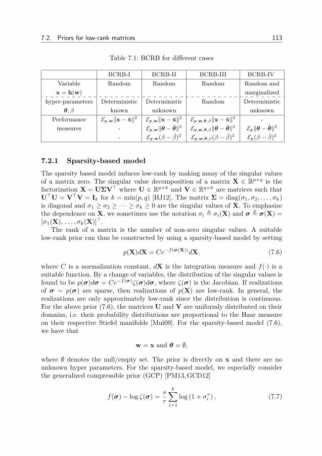
7.2. Priors for low-rank matrices 113
Table 7.1: BCRB for different cases
BCRB-I BCRB-II BCRB-III BCRB-IVVariable Random Random Random Random and
x = h(w) marginalizedhyper-parameters Deterministic Deterministic Random Deterministic
θ, β known unknown unknownPerformance Ey,w‖x− x‖2 Ey,w‖x− x‖2 Ey,w,θ,β‖x− x‖2 -
measures - Ey,w‖θ − θ‖2 Ey,w,θ,β‖θ − θ‖2 Ey‖θ − θ‖2
- Ey,w(β − β)2 Ey,w,θ,β(β − β)2 Ey(β − β)2
7.2.1 Sparsity-based modelThe sparsity based model induces low-rank by making many of the singular valuesof a matrix zero. The singular value decomposition of a matrix X ∈ Rp×q is thefactorization X = UΣV> where U ∈ Rp×k and V ∈ Rq×k are matrices such thatU>U = V>V = Ik for k = min(p, q) [HJ12]. The matrix Σ = diag(σ1, σ2, . . . , σk)is diagonal and σ1 ≥ σ2 ≥ · · · ≥ σk ≥ 0 are the singular values of X. To emphasizethe dependence on X, we sometimes use the notation σi , σi(X) and σ , σ(X) =[σ1(X), . . . , σk(X)]>.
The rank of a matrix is the number of non-zero singular values. A suitablelow-rank prior can thus be constructed by using a sparsity-based model by setting
p(X)dX = Ce−f(σ(X))dX, (7.6)
where C is a normalization constant, dX is the integration measure and f(·) is asuitable function. By a change of variables, the distribution of the singular values isfound to be p(σ)dσ = Ce−f(σ)ζ(σ)dσ, where ζ(σ) is the Jacobian. If realizationsof σ ∼ p(σ) are sparse, then realizations of p(X) are low-rank. In general, therealizations are only approximately low-rank since the distribution is continuous.For the above prior (7.6), the matrices U and V are uniformly distributed on theirdomains, i.e. their probability distributions are proportional to the Haar measureon their respective Stiefel manifolds [Mui09]. For the sparsity-based model (7.6),we have that
w = x and θ = ∅,
where ∅ denotes the null/empty set. The prior is directly on x and there are nounknown hyper parameters. For the sparsity-based model, we especially considerthe generalized compressible prior (GCP) [PM13,GCD12]
f(σ)− log ζ(σ) = s
τ
k∑i=1
log (1 + στi ) , (7.7)
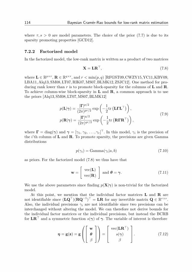
114 Bayesian Cramér-Rao bounds for low-rank matrix estimation
where τ, s > 0 are model parameters. The choice of the prior (7.7) is due to itssparsity promoting properties [GCD12].
7.2.2 Factorized modelIn the factorized model, the low-rank matrix is written as a product of two matrices
X = LR>, (7.8)
where L ∈ Rp×r, R ∈ Rq×r, and r < min(p, q) [RFGST09,CWZY15,YC11,KBV09,LBA11,Alq13,SM08,LT07,RIK07,MS07,BLMK12,ZSJC12]. One method for pro-ducing rank lower than r is to promote block-sparsity for the columns of L and R.To achieve column-wise block-sparsity in L and R, a common approach is to usethe priors [Alq13,SM08,LT07,MS07,BLMK12]
p(L|γ) = |Γ|p/2
(2π)pr/2exp
(−1
2tr(LΓL>
)),
p(R|γ) = |Γ|q/2
(2π)qr/2exp
(−1
2tr(RΓR>
)),
(7.9)
where Γ = diag(γ) and γ = [γ1, γ2, . . . , γr]>. In this model, γi is the precision ofthe i’th column of L and R. To promote sparsity, the precisions are given Gammadistributions
p(γi) = Gamma(γi|a, b) (7.10)
as priors. For the factorized model (7.8) we thus have that
w =[
vec(L)vec(R)
]and θ = γ. (7.11)
We use the above parameters since finding p(X|γ) is non-trivial for the factorizedmodel.
At this point, we mention that the individual factor matrices L and R arenot identifiable since (LQ>)(RQ−1)> = LR for any invertible matrix Q ∈ Rr×r.Also, the individual precisions γi are not identifiable since two precisions can beinterchanged without altering the model. We can therefore not derive bounds forthe individual factor matrices or the individual precisions, but instead the BCRBfor LR> and a symmetric function s(γ) of γ. The variable of interest is therefore
η = g(z) = g
wθ
β
=
vec(LR>)s(γ)β
. (7.12)
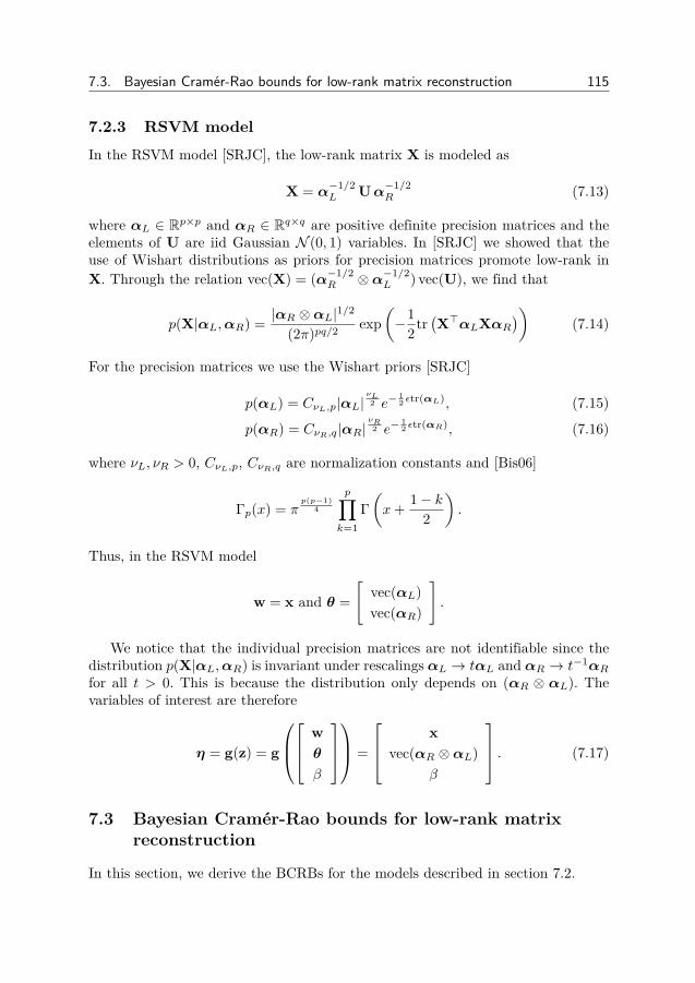
7.3. Bayesian Cramér-Rao bounds for low-rank matrix reconstruction 115
7.2.3 RSVM model
In the RSVM model [SRJC], the low-rank matrix X is modeled as
X = α−1/2L Uα
−1/2R (7.13)
where αL ∈ Rp×p and αR ∈ Rq×q are positive definite precision matrices and theelements of U are iid Gaussian N (0, 1) variables. In [SRJC] we showed that theuse of Wishart distributions as priors for precision matrices promote low-rank inX. Through the relation vec(X) = (α−1/2
R ⊗α−1/2L ) vec(U), we find that
p(X|αL,αR) = |αR ⊗αL|1/2
(2π)pq/2exp
(−1
2tr(X>αLXαR
))(7.14)
For the precision matrices we use the Wishart priors [SRJC]
p(αL) = CνL,p|αL|νL2 e−
12 εtr(αL), (7.15)
p(αR) = CνR,q|αR|νR
2 e−12 εtr(αR), (7.16)
where νL, νR > 0, CνL,p, CνR,q are normalization constants and [Bis06]
Γp(x) = πp(p−1)
4
p∏k=1
Γ(x+ 1− k
2
).
Thus, in the RSVM model
w = x and θ =[
vec(αL)vec(αR)
].
We notice that the individual precision matrices are not identifiable since thedistribution p(X|αL,αR) is invariant under rescalings αL → tαL and αR → t−1αRfor all t > 0. This is because the distribution only depends on (αR ⊗ αL). Thevariables of interest are therefore
η = g(z) = g
wθ
β
=
xvec(αR ⊗αL)
β
. (7.17)
7.3 Bayesian Cramér-Rao bounds for low-rank matrixreconstruction
In this section, we derive the BCRBs for the models described in section 7.2.
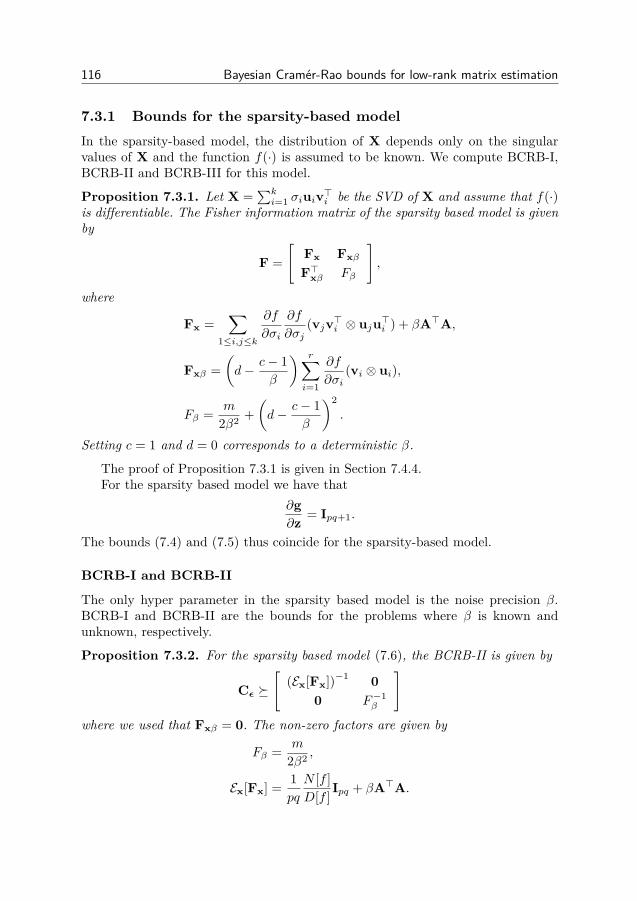
116 Bayesian Cramér-Rao bounds for low-rank matrix estimation
7.3.1 Bounds for the sparsity-based modelIn the sparsity-based model, the distribution of X depends only on the singularvalues of X and the function f(·) is assumed to be known. We compute BCRB-I,BCRB-II and BCRB-III for this model.
Proposition 7.3.1. Let X =∑ki=1 σiuiv>i be the SVD of X and assume that f(·)
is differentiable. The Fisher information matrix of the sparsity based model is givenby
F =[
Fx Fxβ
F>xβ Fβ
],
where
Fx =∑
1≤i,j≤k
∂f
∂σi
∂f
∂σj(vjv>i ⊗ uju>i ) + βA>A,
Fxβ =(d− c− 1
β
) r∑i=1
∂f
∂σi(vi ⊗ ui),
Fβ = m
2β2 +(d− c− 1
β
)2.
Setting c = 1 and d = 0 corresponds to a deterministic β.
The proof of Proposition 7.3.1 is given in Section 7.4.4.For the sparsity based model we have that
∂g∂z = Ipq+1.
The bounds (7.4) and (7.5) thus coincide for the sparsity-based model.
BCRB-I and BCRB-II
The only hyper parameter in the sparsity based model is the noise precision β.BCRB-I and BCRB-II are the bounds for the problems where β is known andunknown, respectively.
Proposition 7.3.2. For the sparsity based model (7.6), the BCRB-II is given by
Cε [
(Ex[Fx])−1 00 F−1
β
]where we used that Fxβ = 0. The non-zero factors are given by
Fβ = m
2β2 ,
Ex[Fx] = 1pq
N [f ]D[f ] Ipq + βA>A.

7.3. Bayesian Cramér-Rao bounds for low-rank matrix reconstruction 117
with
N [f ] =∫
Ωh(σ)g(σ)e−f(σ)dσ, (7.18)
D[f ] =∫
Ωg(σ)e−f(σ)dσ, (7.19)
for Ω = (σ1, σ2, . . . , σk) : σ1 ≥ σ2 ≥ · · · ≥ σk ≥ 0 and
g(σ) =∏
1≤i<j≤k(σ2i − σ2
j )∏
1≤i≤kσ|p−q|i ,
h(σ) =k∑i=1
(∂f
∂σi
)2.
The bound exists provided that the function f(·) is such that the integrals converge.We also find that BCRB-I of x with known β is given by
Ey,x[(x− x) (x− x)>
] (Ex[Fx])−1
.
The proof of Proposition 7.3.2 is given in Section 7.4.5. We find that the integralsare non-trivial to evaluate analytically. We therefore use Monte-Carlo integration[BGJM11] to numerically compute (7.24) and (7.25).
BCRB-III
To compute BCRB-III we also need to compute expectation values with respect toβ, which is now a random variable. We state the bound as a proposition.
Proposition 7.3.3. The bound BCRB-III for the sparsity based model is given by
Cε [
(Ez[Fx])−1 00 (Eβ [Fβ ])−1
].
where we used that Ez [Fxβ ] = 0 and
Ez[Fx] = 1pq
N [f ]D[f ] Ipq + c
dA>A,
Ez[Fβ ] = (m+ 2(c− 1))d2
2(c− 1)(c− 2) .
Proof. The proposition follows from parts of Proposition 7.3.2 and the fact that
Eβ [β] = c
d,
Eβ
[m
2β2 +(d− c− 1
β
)2]
= md2
2(c− 1)(c− 2) + d2
− 2d(c− 1)dc− 1 + (c− 1)2d2
(c− 1)(c− 2) = (m+ 2(c− 1))d2
2(c− 1)(c− 2)
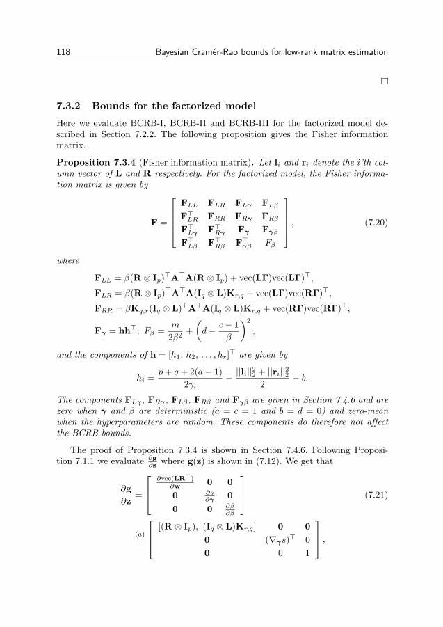
118 Bayesian Cramér-Rao bounds for low-rank matrix estimation
7.3.2 Bounds for the factorized modelHere we evaluate BCRB-I, BCRB-II and BCRB-III for the factorized model de-scribed in Section 7.2.2. The following proposition gives the Fisher informationmatrix.
Proposition 7.3.4 (Fisher information matrix). Let li and ri denote the i’th col-umn vector of L and R respectively. For the factorized model, the Fisher informa-tion matrix is given by
F =
FLL FLR FLγ FLβF>LR FRR FRγ FRβF>Lγ F>Rγ Fγ FγβF>Lβ F>Rβ F>γβ Fβ
, (7.20)
where
FLL = β(R ⊗ Ip)>A>A(R ⊗ Ip) + vec(LΓ)vec(LΓ)>,FLR = β(R ⊗ Ip)>A>A(Iq ⊗ L)Kr,q + vec(LΓ)vec(RΓ)>,FRR = βKq,r(Iq ⊗ L)>A>A(Iq ⊗ L)Kr,q + vec(RΓ)vec(RΓ)>,
Fγ = hh>, Fβ = m
2β2 +(d− c− 1
β
)2,
and the components of h = [h1, h2, . . . , hr]> are given by
hi = p+ q + 2(a− 1)2γi
− ||li||22 + ||ri||22
2 − b.
The components FLγ , FRγ , FLβ, FRβ and Fγβ are given in Section 7.4.6 and arezero when γ and β are deterministic (a = c = 1 and b = d = 0) and zero-meanwhen the hyperparameters are random. These components do therefore not affectthe BCRB bounds.
The proof of Proposition 7.3.4 is shown in Section 7.4.6. Following Proposi-tion 7.1.1 we evaluate ∂g
∂z where g(z) is shown in (7.12). We get that
∂g∂z =
∂vec(LR>)
∂w 0 00 ∂s
∂γ 00 0 ∂β
∂β
(7.21)
(a)=
[(R ⊗ Ip), (Iq ⊗ L)Kr,q] 0 00 (∇γs)> 00 0 1
,
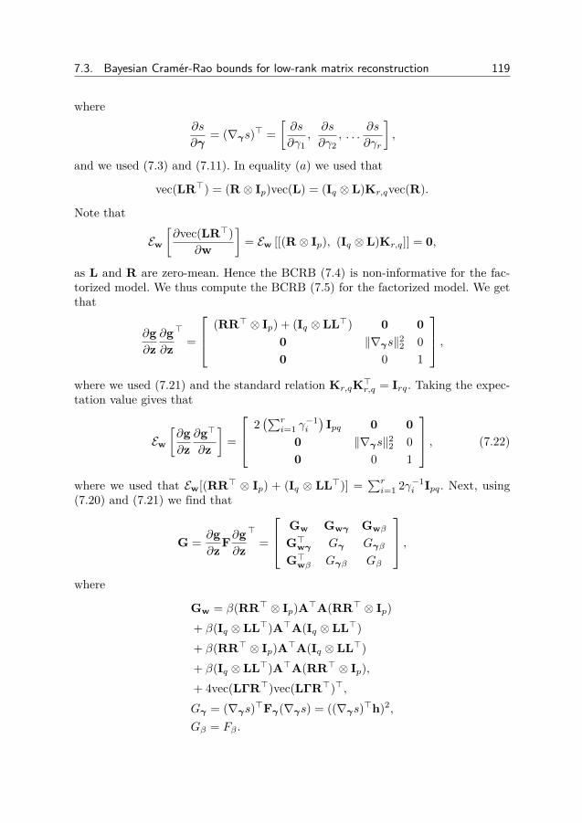
7.3. Bayesian Cramér-Rao bounds for low-rank matrix reconstruction 119
where∂s
∂γ= (∇γs)> =
[∂s
∂γ1,∂s
∂γ2, . . .
∂s
∂γr
],
and we used (7.3) and (7.11). In equality (a) we used that
vec(LR>) = (R ⊗ Ip)vec(L) = (Iq ⊗ L)Kr,qvec(R).
Note that
Ew[∂vec(LR>)
∂w
]= Ew [[(R ⊗ Ip), (Iq ⊗ L)Kr,q]] = 0,
as L and R are zero-mean. Hence the BCRB (7.4) is non-informative for the fac-torized model. We thus compute the BCRB (7.5) for the factorized model. We getthat
∂g∂z
∂g∂z
>=
(RR> ⊗ Ip) + (Iq ⊗ LL>) 0 00 ‖∇γs‖22 00 0 1
,where we used (7.21) and the standard relation Kr,qK>r,q = Irq. Taking the expec-tation value gives that
Ew[∂g∂z
∂g>
∂z
]=
2(∑r
i=1 γ−1i
)Ipq 0 0
0 ‖∇γs‖22 00 0 1
, (7.22)
where we used that Ew[(RR> ⊗ Ip) + (Iq ⊗ LL>)] =∑ri=1 2γ−1
i Ipq. Next, using(7.20) and (7.21) we find that
G = ∂g∂zF∂g
∂z
>=
Gw Gwγ Gwβ
G>wγ Gγ Gγβ
G>wβ Gγβ Gβ
,where
Gw = β(RR> ⊗ Ip)A>A(RR> ⊗ Ip)+ β(Iq ⊗ LL>)A>A(Iq ⊗ LL>)+ β(RR> ⊗ Ip)A>A(Iq ⊗ LL>)+ β(Iq ⊗ LL>)A>A(RR> ⊗ Ip),+ 4vec(LΓR>)vec(LΓR>)>,Gγ = (∇γs)>Fγ(∇γs) = ((∇γs)>h)2,
Gβ = Fβ .
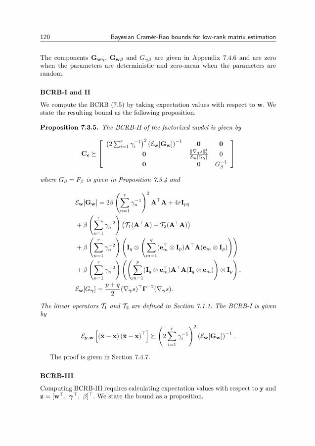
120 Bayesian Cramér-Rao bounds for low-rank matrix estimation
The components Gwγ , Gwβ and Gγβ are given in Appendix 7.4.6 and are zerowhen the parameters are deterministic and zero-mean when the parameters arerandom.
BCRB-I and II
We compute the BCRB (7.5) by taking expectation values with respect to w. Westate the resulting bound as the following proposition.
Proposition 7.3.5. The BCRB-II of the factorized model is given by
Cε
(2∑ri=1 γ
−1i
)2 (Ew[Gw])−1 0 00 ‖∇γs‖4
2Ew[Gγ ] 0
0 0 G−1β
where Gβ = Fβ is given in Proposition 7.3.4 and
Ew[Gw] = 2β(
r∑n=1
γ−1n
)2
A>A + 4rIpq
+ β
(r∑
n=1γ−2n
)(T1(A>A) + T2(A>A)
)+ β
(r∑
n=1γ−2n
)(Iq ⊗
(q∑
m=1(e>m ⊗ Ip)A>A(em ⊗ Ip)
))
+ β
(r∑
n=1γ−2n
)((p∑
m=1(Iq ⊗ e>m)A>A(Iq ⊗ em)
)⊗ Ip
),
Ew[Gγ ] = p+ q
2 (∇γs)>Γ−2(∇γs).
The linear operators T1 and T2 are defined in Section 7.1.1. The BCRB-I is givenby
Ey,w[(x− x) (x− x)>
]
(2
r∑i=1
γ−1i
)2
(Ew[Gw])−1.
The proof is given in Section 7.4.7.
BCRB-III
Computing BCRB-III requires calculating expectation values with respect to y andz = [w>, γ>, β]>. We state the bound as a proposition.
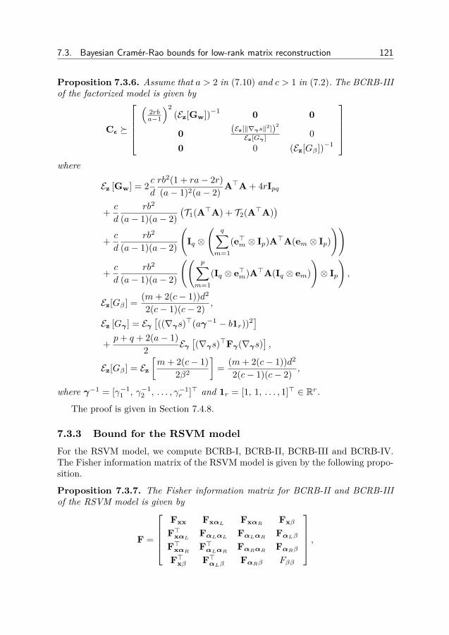
7.3. Bayesian Cramér-Rao bounds for low-rank matrix reconstruction 121
Proposition 7.3.6. Assume that a > 2 in (7.10) and c > 1 in (7.2). The BCRB-IIIof the factorized model is given by
Cε
(
2rba−1
)2(Ez[Gw])−1 0 0
0 (Ez[‖∇γs‖2])2
Ez[Gγ ] 00 0 (Ez[Gβ ])−1
where
Ez [Gw] = 2 cd
rb2(1 + ra− 2r)(a− 1)2(a− 2) A>A + 4rIpq
+ c
d
rb2
(a− 1)(a− 2)(T1(A>A) + T2(A>A)
)+ c
d
rb2
(a− 1)(a− 2)
(Iq ⊗
(q∑
m=1(e>m ⊗ Ip)A>A(em ⊗ Ip)
))
+ c
d
rb2
(a− 1)(a− 2)
((p∑
m=1(Iq ⊗ e>m)A>A(Iq ⊗ em)
)⊗ Ip
),
Ez[Gβ ] = (m+ 2(c− 1))d2
2(c− 1)(c− 2) ,
Ez [Gγ ] = Eγ[((∇γs)>(aγ−1 − b1r))2]
+ p+ q + 2(a− 1)2 Eγ
[(∇γs)>Fγ(∇γs)
],
Ez[Gβ ] = Ez[m+ 2(c− 1)
2β2
]= (m+ 2(c− 1))d2
2(c− 1)(c− 2) ,
where γ−1 = [γ−11 , γ−1
2 , . . . , γ−1r ]> and 1r = [1, 1, . . . , 1]> ∈ Rr.
The proof is given in Section 7.4.8.
7.3.3 Bound for the RSVM modelFor the RSVM model, we compute BCRB-I, BCRB-II, BCRB-III and BCRB-IV.The Fisher information matrix of the RSVM model is given by the following propo-sition.
Proposition 7.3.7. The Fisher information matrix for BCRB-II and BCRB-IIIof the RSVM model is given by
F =
Fxx FxαL FxαR Fxβ
F>xαL FαLαL FαLαR FαLβF>xαR F>αLαR FαRαR FαRβF>xβ F>αLβ FαRβ Fββ
,

122 Bayesian Cramér-Rao bounds for low-rank matrix estimation
where
Fxx = βA>A + vec(αLXαR)vec(αLXαR)>,FαLαL = vLv>L , FαLαR = vLv>R, FαRαR = vRv>R,
Fββ = m
2β2 +(d− c− 1
β
)2,
and
vL = 12Dpvec
(XαRX> + εIp − (q + νL)α−1
L
),
vR = 12Dqvec
(X>αLX + εIq − (p+ νR)α−1
R
).
For deterministic hyper parameters νL = νR = ε = 0, c = 1 and d = 0. The termsFxαL and FxαR are zero mean with respect to x and that the terms Fxβ, FαLβand FαRβ are zero when β is deterministic and zero-mean when β is random. Theterms do therefore not contribute to the bounds. For completeness we give the termsin Section 7.4.9.
The proof of Proposition 7.3.7 is given in Section 7.4.9. The submatrix
Fαα =[
FαLαL FαLαRF>αLαR FαRαR
]=[
vLvR
] [v>L v>R
],
is singular for a fixed x. However, Ex [Fα] is not singular. For the RSVM model,we find that
∂g∂z =
Ipq 0 00 Uα 00 0 1
,where the column vectors of Uα = [UαL UαR ] are given by
[UαL ]:,i+(j−1)p = vec(αR ⊗ELij),
[UαR ]:,k+(l−1)q = vec(ERkl ⊗αL).
BCRB-I and BCRB-II
We compute the BCRB-II by calculating expectation values with respect to x =vec(X). We state the BCRB bound in the following proposition.
Proposition 7.3.8. The BCRB-II of the RSVM model is given by
Cε
(Ex[Fxx])−1 0 00 Uα(Ex[Fαα])−1U>α 00 0 F−1
ββ
,

7.3. Bayesian Cramér-Rao bounds for low-rank matrix reconstruction 123
where
Ex [Fx] = (αR ⊗αL) + βA>A,
Ex [Fα] =[Ex[vLv>L
]Ex[vLv>R
]Ex [vRvL] Ex
[vRv>R
] ] ,Ex[vLv>L
]= 1
4Dpvec(εIp − νLα−1L )vec(εIp − νLα−1
L )>D>p
+ q
4Dp(Ip2 + Kp,p)(α−1L ⊗α
−1L )D>p ,
Ex[vRv>R
]= 1
4Dqvec(εIq − νRα−1R )vec(εIq − νRα−1
R )>D>q
+ p
4Dq(Iq2 + Kq,q)(α−1R ⊗α
−1R )D>q ,
Ex[vLv>R
]= 1
4Dpvec(εIp − νLα−1L )vec(εIq − νRα−1
R )>D>q
+ 12Dpvec(α−1
L )vec(α−1R )>Dq,
Fββ = m
2β2 .
Also, the BCRB-I of the RSVM model is given by
Ey,x[(x− x) (x− x)>
] (Ex[Fxx])−1 =
((αR ⊗αL) + βA>A
)−1
The proof of Proposition 7.3.8 is given in Section 7.4.10.
7.3.4 BCRB-IIIComputation of BCRB-III requires taking expectation values with respect to theprecision matrices αL, αR and the noise precision β. We state the BCRB boundas a proposition.
Proposition 7.3.9. The BCRB-III of the RSVM model is given by
Cε
(Ez[Fxx])−1 0 00 Ez[Uα](Ez[Fαα])−1Ez[Uα]> 00 0 (Ez[Fββ ])−1
,
where
Ez [Fxx] = (νL + p+ 1)(νR + q + 1)ε−2Ipq + 1 + c
dA>A,
Ez[vLv>L
]= ε2
4 (ν2LcL − 1 + 2qdL)vec(Ip)vec(Ip)>
+ ε2
4 (ν2LdL + cL + dL)D2
p
124 Bayesian Cramér-Rao bounds for low-rank matrix estimation
+ ε2q
4 (cL + dL)DpKp,pDp + ε2ν2LdL4 DpKp,pDp,
Ez[vLv>R
]= ε2
2νLνRvec(Ip)vec(Iq)>,
Ez[vRv>R
]= ε2
4 (ν2RcR − 1 + 2pdR)vec(Iq)vec(Iq)>
+ ε2
4 (ν2RdR + cR + dR)D2
q
+ ε2p
4 (cR + dR)DqKq,qDq + ε2ν2RdR4 DqKq,qDq,
Ez [Fββ ] = (m2 + 2c)d2
2c(c− 1) ,
Ez[[UαL ]:,i+(j−1)p
]= (νR + q + 1)ε−1vec(Ip ⊗EL
ij),Ez[[UαR ]:,k+(l−1)q
]= (νL + p+ 1)ε−1vec(ER
kl ⊗ Iq).
The proof of Proposition 7.3.9 is given in Section 7.4.11.
7.3.5 BCRB-IVIn the BCRB-IV, we are only interested in estimating the precisions, i.e. (deter-ministic and unknown) precisions matrices and the noise precision. The variable Xis marginalized and the measurements have the distribution
p(y|αL,αR, β) = N (y|0,C),
where
C = A(α−1R ⊗α
−1L )A> + β−1Im.
We want to find bounds for estimators of
η = g(z) =[
vec(αR ⊗αL)β
],
where now
∂g∂z =
[UαL UαR 0
0 0 1
].
The Fisher information for BCRB-IV becomes different from that of Proposi-tion 7.3.7. We state the Fisher information matrix and the bound BCRB-IV in thefollowing proposition.
7.4. Numerical experiments 125
Proposition 7.3.10. Let
A = A(α−1R ⊗α
−1L ),
P = A>C−1A.
The BCRB-IV of the RSVM model is given by
Cη ∂g∂zF−1 ∂g
∂z
>
where the Fisher information is
F =
FLL FLR FLβFRL FRR FRβF>Lβ F>Rβ Fββ
and the components of the block matrices are given by
[FLL]i+(j−1)p,k+(l−1)p
= 14tr(P(αR ⊗EL
ij)P(αR ⊗ELkl)),
[FLR]i+(j−1)p,k+(l−1)q
= 14tr(P(αR ⊗EL
ij)P(ERkl ⊗αL)
),
[FRR]i+(j−1)q,k+(l−1)q
= 14tr(P(ER
ij ⊗αL)P(ERkl ⊗αL)
),
[FLβ ]i+(j−1)p = 14β2 tr
(A>C−2A(αR ⊗EL
ij)),
[FRβ ]k+(l−1)q = 14β2 tr
(A>C−2A(ER
kl ⊗αL)),
Fββ = 14β4 tr
(C−2) .
The proof of Proposition 7.3.10 is given in Section 7.4.12.
7.4 Numerical experiments
In this section we perform numerical experiments to evaluate how low-rank realiza-tions of the random matrix models are and also compare the BCRB bounds withexisting methods.
7.4.1 Numerical rank of the random matrix modelsThe sparsity-based model, the factorized model and the RSVM model were outlinedin Section 7.2 where we argued that the models could be used as priors to promote
126 Bayesian Cramér-Rao bounds for low-rank matrix estimation
low-rank. Here we show that for appropriate values of the hyperparameters, themodels give realizations that are approximately low-rank. We notice that since thedistributions are continuous, the probability of a matrix being exactly low-rankis zero. However, the realizations can be effectively low-rank, meaning that thematrices have few large singular values and the remaining singular values are small.This can be quantified through the numerical rank. We here use two versions of thenumerical rank.
The first measure of numerical rank we use, for X ∈ Rp×q, is
nrank1(X) = ||X||2∗
||X||2F,
where ||X||∗ =∑ki=1 σi(X) is the nuclear norm of X and ||X||2F =
∑ki=1 σi(X)2 is
the Frobenius norm. By the Cauchy-Schwarz inequality we get that the numericalrank is a lower bound for the true rank as nrank1(X) ≤ rank(X). The secondmeasure of numerical rank is
nrank2(X) = |i : σi(X) > ε||X||F | ,
where we set ε = 0.9/√
min(p, q). We see that nrank2(·) also is a lower bound onthe actual rank. We will find in simulations that both measures of numerical rankshow the same qualitative behavior.
Numerical rank of the sparsity-based model
We saw in Section 7.2.1 that the effective distribution of the singular values in thesparsity based model is
e−f(σ) = ζ(σ)e−f(σ),
where f(σ) = f(σ)− log ζ(σ).To evaluate the numerical rank, we generate samples from the effective and naive
GCP prior using the Metropolis-Hastings algorithm [ADFDJ03]. For p = q = 100and τ = 1 we randomly chose s uniformly in the interval [0, 10]. Using the value of swe compute a realization of σ and compute the numerical rank of σ. We obtainedthe results shown in Figure 7.1. We find that the majority of realizations of theGCP prior satisfy nrank1(X) ≤ 30 and nrank2(X) ≈ 20 for 1 ≤ s ≤ 2. We thus seethat the GCP prior gives realizations of low numerical rank.
Numerical rank of the factorized model
In the factorized model, the low rank matrix X ∈ Rp×q is written as the prod-uct X = LR> where L ∈ Rp×r and R ∈ Rq×r. Clearly rank(X) ≤ r. However,the effective rank can be made lower by setting the parameter a in (7.10) to anappropriate value. We find that the parameter b > 0 only affects the magnitude

7.4. Numerical experiments 127
0 0.5 1 1.5 2 2.5 3 3.5 40
5
10
15
20
25
30
35
40
45
s
nrank1
nrank2
Figure 7.1: Numerical rank for realizations of the sparsity based model with gener-alized compressible priors for p = q = 100 and τ = 1.
of the precisions since if γi ∼ Gamma(1 + a, 1), then bγi ∼ Gamma(1 + a, b). Toevaluate how the choice of a affects the numerical rank we drew log(a) uniformlyfrom the interval [−10, 5] and for the corresponding value of a we generated L andR and computed the numerical rank of X. In the experiment we used p = q = 100,r = 50 and b = 1. The results are shown in Figure 7.2 where the green line showsa local average value of the numerical rank. We find that for 10−10 ≤ a ≤ 1, rank1has mean 7.8 and rank2 has mean 6.2. Both measures of numerical rank have highvariance in this region. For a > 1, rank1 has mean 38 and rank2 has mean 30.We thus see that the factorized model promotes sparsity less than r when a ≤ 1.Unfortunately, this is also the region where the BCRB-III does not exist.
Numerical rank of the RSVM model
The parameters νL and νR control the numerical rank in the RSVM model sincethe parameter ε only controls the magnitude of the precision matrices. Here weset νL = νR = ν for simplicity. In the experiment we drew ν uniformly from[max(p, q), 2(p+ q)]. For each value of ν we drew the precision matrices αL and αRfrom the Wishart distributions and generated X as in (7.13). We then computednrank1 and nrank2 for the matrix. The results are shown in Figure 7.9. We findthat nrank1(X) ≤ 20 when ν ≤ 115 while nrank2(X) ≤ 20 when ν ≤ 150. For largerν, the numerical rank nrank1(X) increases towards 72 while nrank2(X) increasestowards 45.
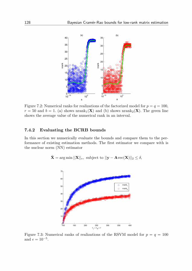
128 Bayesian Cramér-Rao bounds for low-rank matrix estimation
10−10
100
0
5
10
15
20
25
30
35
40
nra
nk
a
(a)
10−10
100
0
5
10
15
20
25
30
35
nra
nk
a
(b)
Figure 7.2: Numerical ranks for realizations of the factorized model for p = q = 100,r = 50 and b = 1. (a) shows nrank1(X) and (b) shows nrank2(X). The green lineshows the average value of the numerical rank in an interval.
7.4.2 Evaluating the BCRB bounds
In this section we numerically evaluate the bounds and compare them to the per-formance of existing estimation methods. The first estimator we compare with isthe nuclear norm (NN) estimator
X = arg min ||X||∗, subject to ||y−Avec(X)||2 ≤ δ,
100 150 200 250 300 350 4000
10
20
30
40
50
60
70
νL = ν
R = ν
nrank1
nrank2
Figure 7.3: Numerical ranks of realizations of the RSVM model for p = q = 100and ε = 10−5.
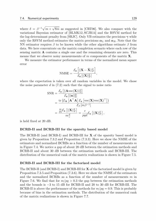
7.4. Numerical experiments 129
where δ = β−1√m+
√8m as suggested in [CRT06]. We also compare with the
variational Bayesian estimator of [BLMK12, SCJR14] and the RSVM method forthe log-determinant penalty from [SRJC]. Only VB estimates the precisions γ whileonly the RSVM method estimates the matrix precisions αL and αR. Note that theNN estimator requires β to be known while the other algorithms estimate β fromdata. We here concentrate on the matrix completion scenario where each row of thesensing matrix A contains a single one and the remaining elements are zero. Thismeans that we observe noisy measurements of m components of the matrix X.
We measure the estimator performance in terms of the normalized mean squareerror
NMSE =Ez[||X− X||2F
]Ez [||X||2F ] ,
where the expectation is taken over all random variables in the model. We chosethe noise parameter d in (7.2) such that the signal to noise ratio
SNR =Ez[||Avec(X)||22
]Ez [||n||22]
=tr(EA[A>A
]Ex[vec(X)vec(X)>
])Eβ [mβ−1]
=mpqEx
[||X||2F
]mdc
= c
pqdEx[||X||2F
],
is held fixed at 20 dB.
BCRB-II and BCRB-III for the sparsity based model
The BCRB-II (and BCRB-I) and BCRB-III for X of the sparsity based model isgiven by Proposition 7.3.2 and Proposition (7.3.3). Here we show the NMSE of theestimators and normalized BCRBs as a function of the number of measurements min Figure 7.4. We notice a gap of about 20 dB between the estimation methods andBCRB-II and about 30 dB between the estimation methods and BCRB-III. Thedistribution of the numerical rank of the matrix realizations is shown in Figure 7.5.
BCRB-II and BCRB-III for the factorized model
The BCRB-II (and BCRB-I) and BCRB-III for X of the factorized model is given byProposition 7.3.5 and Proposition (7.3.6). Here we show the NMSE of the estimatorsand the normalized BCRBs as a function of the number of measurements m inFigure 7.6. We find that for m/pq > 0.3 the gap between the estimation methodsand the bounds is −3 to 15 dB for BCRB-II and 20 to 30 dB for BCRB-III. TheBCRB-II is above the performance of the methods for m/pq = 0.9. This is probablybecause of bias in the estimation methods. The distribution of the numerical rankof the matrix realizations is shown in Figure 7.7.
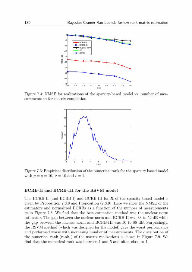
130 Bayesian Cramér-Rao bounds for low-rank matrix estimation
0.1 0.2 0.3 0.4 0.5 0.6 0.7 0.8 0.9−45
−40
−35
−30
−25
−20
−15
−10
−5
0
m/pq
NM
SE
[dB
]
BCRB−II
BCRB−III
Nuclear norm
VB
RSVM
Figure 7.4: NMSE for realizations of the sparsity-based model vs. number of mea-surements m for matrix completion.
1 2 3 4 5 6 7 8 90
5
10
15
20
25
30
nrank1
Pro
babili
ty
Figure 7.5: Empirical distribution of the numerical rank for the sparsity based modelwith p = q = 10, ν = 10 and ε = 1.
BCRB-II and BCRB-III for the RSVM model
The BCRB-II (and BCRB-I) and BCRB-III for X of the sparsity based model isgiven by Proposition 7.3.8 and Proposition (7.3.9). Here we show the NMSE of theestimators and normalized BCRBs as a function of the number of measurementsm in Figure 7.8. We find that the best estimation method was the nuclear normestimator. The gap between the nuclear norm and BCRB-II was 33 to 52 dB whilethe gap between the nuclear norm and BCRB-III was 50 to 88 dB. Surprisingly,the RSVM method (which was designed for the model) gave the worst performanceand performed worse with increasing number of measurements. The distribution ofthe numerical rank (rank1) of the matrix realizations is shown in Figure 7.9. Wefind that the numerical rank was between 1 and 5 and often close to 1.
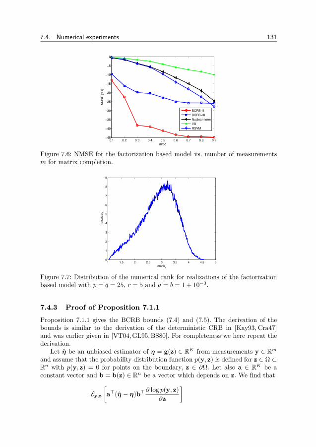
7.4. Numerical experiments 131
0.1 0.2 0.3 0.4 0.5 0.6 0.7 0.8 0.9−45
−40
−35
−30
−25
−20
−15
−10
−5
0
m/pq
NM
SE
[dB
]
BCRB−II
BCRB−III
Nuclear norm
VB
RSVM
Figure 7.6: NMSE for the factorization based model vs. number of measurementsm for matrix completion.
1 1.5 2 2.5 3 3.5 4 4.5 50
1
2
3
4
5
6
7
8
9
nrank1
Pro
ba
bili
ty
Figure 7.7: Distribution of the numerical rank for realizations of the factorizationbased model with p = q = 25, r = 5 and a = b = 1 + 10−3.
7.4.3 Proof of Proposition 7.1.1
Proposition 7.1.1 gives the BCRB bounds (7.4) and (7.5). The derivation of thebounds is similar to the derivation of the deterministic CRB in [Kay93, Cra47]and was earlier given in [VT04,GL95,BS80]. For completeness we here repeat thederivation.
Let η be an unbiased estimator of η = g(z) ∈ RK from measurements y ∈ Rmand assume that the probability distribution function p(y, z) is defined for z ∈ Ω ⊂Rn with p(y, z) = 0 for points on the boundary, z ∈ ∂Ω. Let also a ∈ RK be aconstant vector and b = b(z) ∈ Rn be a vector which depends on z. We find that
Ey,z[a>(η − η)b> ∂ log p(y, z)
∂z
]
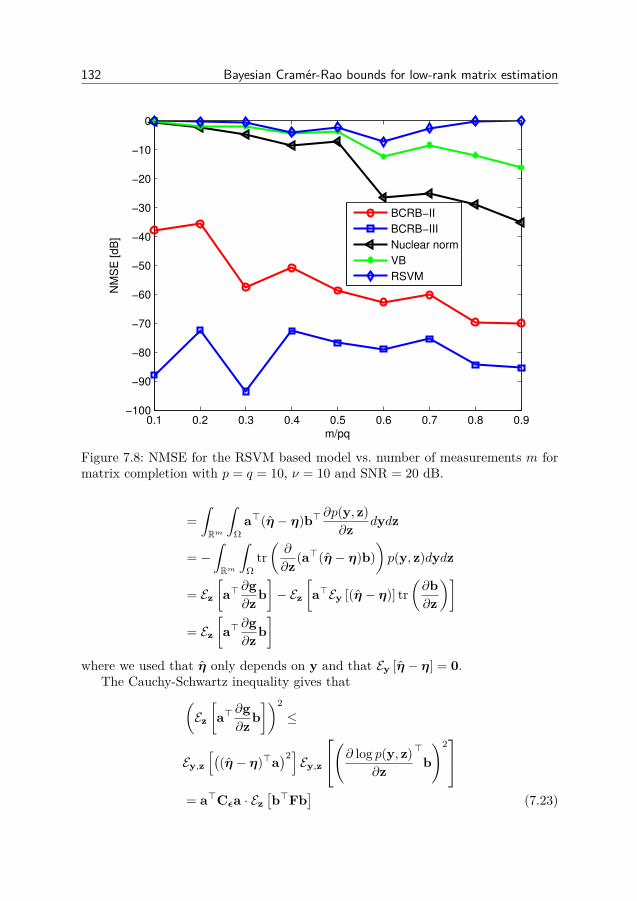
132 Bayesian Cramér-Rao bounds for low-rank matrix estimation
0.1 0.2 0.3 0.4 0.5 0.6 0.7 0.8 0.9−100
−90
−80
−70
−60
−50
−40
−30
−20
−10
0
m/pq
NM
SE
[dB
]
BCRB−II
BCRB−III
Nuclear norm
VB
RSVM
Figure 7.8: NMSE for the RSVM based model vs. number of measurements m formatrix completion with p = q = 10, ν = 10 and SNR = 20 dB.
=∫Rm
∫Ω
a>(η − η)b> ∂p(y, z)∂z dydz
= −∫Rm
∫Ω
tr(∂
∂z (a>(η − η)b))p(y, z)dydz
= Ez[a> ∂g
∂zb]− Ez
[a>Ey [(η − η)] tr
(∂b∂z
)]= Ez
[a> ∂g
∂zb]
where we used that η only depends on y and that Ey [η − η] = 0.The Cauchy-Schwartz inequality gives that(
Ez[a> ∂g
∂zb])2≤
Ey,z[(
(η − η)>a)2] Ey,z
(∂ log p(y, z)∂z
>b)2
= a>Cεa · Ez[b>Fb
](7.23)
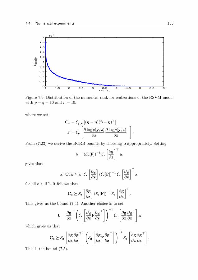
7.4. Numerical experiments 133
1 1.5 2 2.5 3 3.5 4 4.5 5 5.5 60
0.2
0.4
0.6
0.8
1
1.2
1.4
1.6
1.8
2x 10
4
nrank1
Prob
abilit
y
Figure 7.9: Distribution of the numerical rank for realizations of the RSVM modelwith p = q = 10 and ν = 10.
where we set
Cε = Ey,z[(η − η)(η − η)>
],
F = Ey
[∂ log p(y, z)
∂z∂ log p(y, z)
∂z
>].
From (7.23) we derive the BCRB bounds by choosing b appropriately. Setting
b = (Ez[F])−1 Ez[∂g∂z
]>a,
gives that
a>Cεa ≥ a>Ez[∂g∂z
](Ez[F])−1 Ez
[∂g∂z
]>a,
for all a ∈ Rn. It follows that
Cε Ez[∂g∂z
](Ez[F])−1 Ez
[∂g∂z
]>.
This gives us the bound (7.4). Another choice is to set
b = ∂g∂z
>(Ez
[∂g∂zF∂g
∂z
>])−1
Ez
[∂g∂z
∂g∂z
>]
a
which gives us that
Cε Ez
[∂g∂z
∂g∂z
>](Ez
[∂g∂zF∂g
∂z
>])−1
Ez
[∂g∂z
∂g∂z
>].
This is the bound (7.5).

134 Bayesian Cramér-Rao bounds for low-rank matrix estimation
7.4.4 Proof of Proposition 7.3.1Here we compute the Fisher information matrix for the sparsity based model. Inthe sparsity based model, p(y, z) = p(y|x, β)p(x)p(β). To compute the Fisher in-formation we need to compute the derivatives of log p(y, z) with respect to x andβ. We have that
log p(y, z) = −β2 ||y−Ax||22 + m
2 log β
− f(σ(X)) + (c− 1) log β − dβ + const
By varying with respect to x, we get that
d log p(y, z) = β(y−Ax)>Adx−k∑i=1
∂f
∂σiu>i dXvi
= β(y−Ax)>Adx−k∑i=1
∂f
∂σi(v>i ⊗ u>i )dx,
where k = min(p, q). This gives us that
∂ log p(y, z)∂x = βA>(y−Ax)−
k∑i=1
∂f
∂σi(vi ⊗ ui).
We also find that∂ log p(y, z)
∂β= −1
2 ||y−Ax||22 + m+ 2(c− 1)2β − d.
This gives us that
Fxx =∑i,j
∂f
∂σj
∂f
∂σi(vjv>i ⊗ uju>i )
+ β2A>Ey[(y−Ax)(y−Ax)>]A,
=∑i,j
∂f
∂σj
∂f
∂σi(vjv>i ⊗ uju>i ) + βA>A,
Fxβ =(d− c
β
) k∑i=1
∂f
∂σi(vi ⊗ ui),
Fββ = m
2β2 +(d− c− 1
β
)2.
where we used that
Ey[(y−Ax)] = 0,Ey[(y−Ax)(y−Ax)>] = β−1Im,Ey[(y−Ax)||y−Ax||22] = 0.

7.4. Numerical experiments 135
We note that the term Fxβ is zero when β is deterministic (c = 1 and d = 0) andzero mean when β is random. This proves Proposition 7.3.1.
7.4.5 Proof of Proposition 7.3.2To show Proposition 7.3.2 we need to compute the expectation value of Fxx and Fxβwith respect to x. When the distribution p(X) only depends on the singular valuesof X, the singular values and the left and right singular vectors are independent(provided that the matrix is not symmetric). So the singular vectors have zeromean, Ex[ui] = 0. This gives us that Ex[Fxβ ] = 0. Moreover, conditioned on asingular vector ui, another singular vector uj (with j 6= i) is marginally uniformlydistributed on the set u ∈ Rp : ||u||2 = 1,u>ui = 0. This gives us that wheni 6= j
Ex[uju>i ] = 0.
Also, if h ∼ χ2(p), then√hui is Gaussian N (0, I) and
Ip = Eh,x[huiu>i ] = Eh[h]Ex[uiu>i ] = pEx[uiu>i ],
so
Ex[uiu>i ] = 1pIp.
Similarly we find that
Ex[viv>j ] = δij1qIq.
We thus get that
Ex[Fx] = 1pq
Ipqk∑i=1Ex
[(∂f
∂σi
)2].
To compute the remaining expectation we make a change of variables corre-sponding to the singular value decomposition. Without loss of generality, we hereassume that p ≤ q. Under the variable transformation, the integration measure dXtransforms as [Mui09]
dX =∏
1≤i<j≤k(σ2i − σ2
j )∏
1≤l≤kσ|p−q|l dσ[U>dU][V>dV],
where σ ∈ Ω and the extended orthogonal matrix V = [V V′] is such that V′>V′ =Iq−k and V′>V = 0. By performing the integration over the singular vectors, weget that
Ex
[(∂f
∂σi
)2]
= N [f ]D[f ] ,
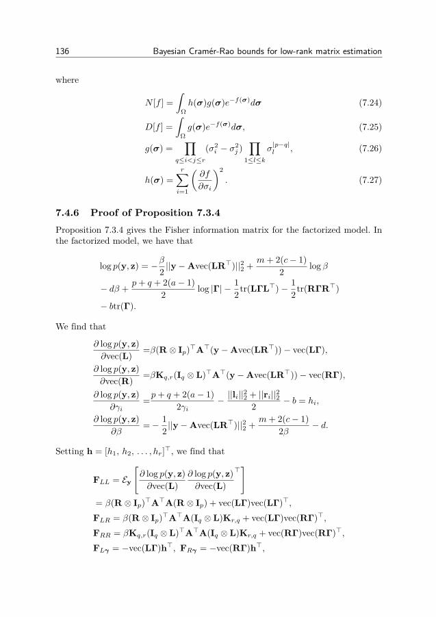
136 Bayesian Cramér-Rao bounds for low-rank matrix estimation
where
N [f ] =∫
Ωh(σ)g(σ)e−f(σ)dσ (7.24)
D[f ] =∫
Ωg(σ)e−f(σ)dσ, (7.25)
g(σ) =∏
q≤i<j≤r
(σ2i − σ2
j )∏
1≤l≤kσ|p−q|l , (7.26)
h(σ) =r∑i=1
(∂f
∂σi
)2. (7.27)
7.4.6 Proof of Proposition 7.3.4Proposition 7.3.4 gives the Fisher information matrix for the factorized model. Inthe factorized model, we have that
log p(y, z) = −β2 ||y−Avec(LR>)||22 + m+ 2(c− 1)2 log β
− dβ + p+ q + 2(a− 1)2 log |Γ| − 1
2tr(LΓL>)− 12tr(RΓR>)
− btr(Γ).
We find that
∂ log p(y, z)∂vec(L) =β(R ⊗ Ip)>A>(y−Avec(LR>))− vec(LΓ),
∂ log p(y, z)∂vec(R) =βKq,r(Iq ⊗ L)>A>(y−Avec(LR>))− vec(RΓ),
∂ log p(y, z)∂γi
=p+ q + 2(a− 1)2γi
− ||li||22 + ||ri||22
2 − b = hi,
∂ log p(y, z)∂β
=− 12 ||y−Avec(LR>)||22 + m+ 2(c− 1)
2β − d.
Setting h = [h1, h2, . . . , hr]>, we find that
FLL = Ey
[∂ log p(y, z)∂vec(L)
∂ log p(y, z)∂vec(L)
>]
= β(R ⊗ Ip)>A>A(R ⊗ Ip) + vec(LΓ)vec(LΓ)>,FLR = β(R ⊗ Ip)>A>A(Iq ⊗ L)Kr,q + vec(LΓ)vec(RΓ)>,FRR = βKq,r(Iq ⊗ L)>A>A(Iq ⊗ L)Kr,q + vec(RΓ)vec(RΓ)>,FLγ = −vec(LΓ)h>, FRγ = −vec(RΓ)h>,
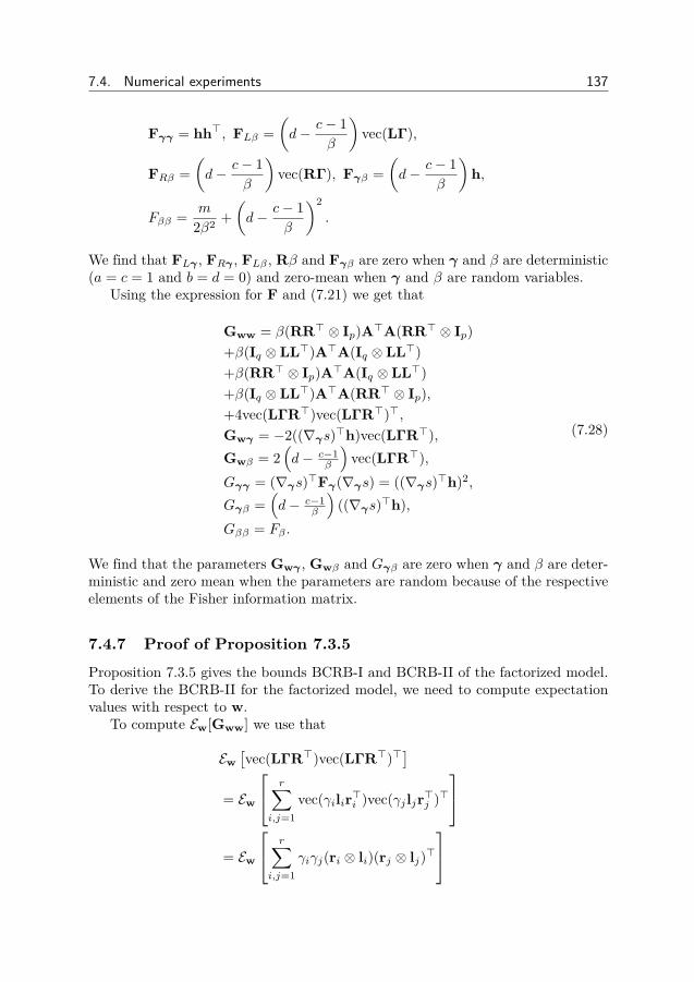
7.4. Numerical experiments 137
Fγγ = hh>, FLβ =(d− c− 1
β
)vec(LΓ),
FRβ =(d− c− 1
β
)vec(RΓ), Fγβ =
(d− c− 1
β
)h,
Fββ = m
2β2 +(d− c− 1
β
)2.
We find that FLγ , FRγ , FLβ , Rβ and Fγβ are zero when γ and β are deterministic(a = c = 1 and b = d = 0) and zero-mean when γ and β are random variables.
Using the expression for F and (7.21) we get that
Gww = β(RR> ⊗ Ip)A>A(RR> ⊗ Ip)+β(Iq ⊗ LL>)A>A(Iq ⊗ LL>)+β(RR> ⊗ Ip)A>A(Iq ⊗ LL>)+β(Iq ⊗ LL>)A>A(RR> ⊗ Ip),+4vec(LΓR>)vec(LΓR>)>,Gwγ = −2((∇γs)>h)vec(LΓR>),Gwβ = 2
(d− c−1
β
)vec(LΓR>),
Gγγ = (∇γs)>Fγ(∇γs) = ((∇γs)>h)2,
Gγβ =(d− c−1
β
)((∇γs)>h),
Gββ = Fβ .
(7.28)
We find that the parameters Gwγ , Gwβ and Gγβ are zero when γ and β are deter-ministic and zero mean when the parameters are random because of the respectiveelements of the Fisher information matrix.
7.4.7 Proof of Proposition 7.3.5
Proposition 7.3.5 gives the bounds BCRB-I and BCRB-II of the factorized model.To derive the BCRB-II for the factorized model, we need to compute expectationvalues with respect to w.
To compute Ew[Gww] we use that
Ew[vec(LΓR>)vec(LΓR>)>
]= Ew
r∑i,j=1
vec(γilir>i )vec(γjljr>j )>
= Ew
r∑i,j=1
γiγj(ri ⊗ li)(rj ⊗ lj)>
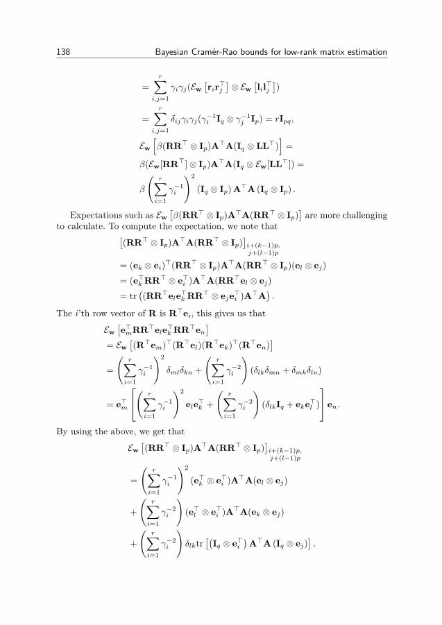
138 Bayesian Cramér-Rao bounds for low-rank matrix estimation
=r∑
i,j=1γiγj(Ew
[rir>j
]⊗ Ew
[lil>j
])
=r∑
i,j=1δijγiγj(γ−1
i Iq ⊗ γ−1j Ip) = rIpq,
Ew[β(RR> ⊗ Ip)A>A(Iq ⊗ LL>)
]=
β(Ew[RR>]⊗ Ip)A>A(Iq ⊗ Ew[LL>]) =
β
(r∑i=1
γ−1i
)2
(Iq ⊗ Ip) A>A (Iq ⊗ Ip) .
Expectations such as Ew[β(RR> ⊗ Ip)A>A(RR> ⊗ Ip)
]are more challenging
to calculate. To compute the expectation, we note that[(RR> ⊗ Ip)A>A(RR> ⊗ Ip)
]i+(k−1)p,j+(l−1)p
= (ek ⊗ ei)>(RR> ⊗ Ip)A>A(RR> ⊗ Ip)(el ⊗ ej)= (e>k RR> ⊗ e>i )A>A(RR>el ⊗ ej)= tr
((RR>ele>k RR> ⊗ eje>i )A>A
).
The i’th row vector of R is R>ei, this gives us that
Ew[e>mRR>ele>k RR>en
]= Ew
[(R>em)>(R>el)(R>ek)>(R>en)
]=(
r∑i=1
γ−1i
)2
δmlδkn +(
r∑i=1
γ−2i
)(δlkδmn + δmkδln)
= e>m
( r∑i=1
γ−1i
)2
ele>k +(
r∑i=1
γ−2i
)(δlkIq + eke>l )
en.
By using the above, we get that
Ew[(RR> ⊗ Ip)A>A(RR> ⊗ Ip)
]i+(k−1)p,j+(l−1)p
=(
r∑i=1
γ−1i
)2
(e>k ⊗ e>i )A>A(el ⊗ ej)
+(
r∑i=1
γ−2i
)(e>l ⊗ e>i )A>A(ek ⊗ ej)
+(
r∑i=1
γ−2i
)δlktr
[(Iq ⊗ e>i
)A>A (Iq ⊗ ej)
].
7.4. Numerical experiments 139
Let T1 be the operator defined in section 7.1.1, we find that
(e>k ⊗ e>i )A>A(el ⊗ ej) = [A>A]i+(k−1)p,j+(l−1)p,
(e>l ⊗ e>i )A>A(ek ⊗ ej) = [T1(A>A)]i+(k−1)p,j+(l−1)p,
Using that (en ⊗ Ip)ej = (en ⊗ Ip)(1⊗ ej) = (en ⊗ ej), we get that
δlktr[(
Iq ⊗ e>i)A>A (Iq ⊗ ej)
]= e>l ektr
[(Iq ⊗ eje>i
)A>A
]= e>l ek
r∑n=1
(e>n ⊗ e>i
)A>A (en ⊗ ej)
=[(
Iq ⊗(
r∑n=1
(e>n ⊗ Ip
)A>A (en ⊗ Ip)
))]i+(k−1)p,j+(l−1)p
.
A similar computation can be made for L.To compute
Gγγ = Ew[((∇γs)>h)2] = (∇γs)>Ew[hh>](∇γs)
we use that
Ew[hh>] = Ew[h]Ew[h]> + Cov(h),
where the covariance is diagonal since the precisions are independent. We find (aftera somewhat lengthy calculation) that
Ew[hi] = a− 1γi− b,
Ew[(hi − Ez[hi])2] = p+ q
2γ2i
.
We see that Ew[hi] = 0 when γ is deterministic. So
Gγ = ((∇γs)>(aγ−1 − b1r))2 + p+ q + 2(a− 1)2 (∇γs)>Γ−2(∇γs)
= p+ q
2 (∇γs)>Γ−2(∇γs).
7.4.8 Proof of Proposition 7.3.6The bound BCRB-III can be computed from BCRB-II by taking the appropriateexpectation values with respect to γ and β. Using that
Eβ [β] = cd , Eβ [β−2] = d2
(c−1)(c−2) ,
Eγ [γ−ki ] = bkΓ(a− k)
Γ(a) = bk
a...(a− k) , for k ≥ 1,
we are able to compute the respective expectation values.
140 Bayesian Cramér-Rao bounds for low-rank matrix estimation
7.4.9 Proof of Proposition 7.3.7Proposition 7.3.7 gives the Fisher information matrix for the RSVM model. Wehave that
log p(y, z) = −β2 ||y−Ax||22 + m+ 2(c− 1)2 log β
− dβ − 12tr(αLXαRX>) + q + νL
2 log |αL|
+ p+ νR2 log |αR| −
ε
2tr(αL)− ε
2tr(αR) + const,
where x = vec(X). We find that∂ log p(y, z)
∂x = βA>(y−Ax)− vec(αLXαR),
∂ log p(y, z)∂vec(αL) = −1
2Dpvec(XαRX>)+
q + νL2 Dpvec(α−1
L )− ε
2Dpvec(Ip) = −vL,
∂ log p(y, z)∂vec(αR) = −1
2Dqvec(X>αLX)+
p+ νR2 Dqvec(α−1
R )− ε
2Dqvec(Iq) = −vR,
∂ log p(y, z)∂β
= −12 ||y−Ax||22 + m+ 2(c− 1)
2β − d.
This gives us that the Fisher information is
F =
Fxx FxαL FxαR Fxβ
F>xαL FαLαL FαLαR FαLβF>xαR F>αLαR FαRαR FαRβF>xβ F>αLβ FαRβ Fββ
,where
Fxx = βA>A + vec(αLXαR)vec(αLXαR)>,FxαL = vec(αLXαR)v>L , FxαR = vec(αLXαR)v>R,FαLαL = vLv>L , FαLαR = vLv>R, FαRαR = vRv>R,
Fxβ =(d− c− 1
β
)vec(αLXαR),
FαLβ =(d− c− 1
β
)vL, FαRβ =
(d− c− 1
β
)vR,
Fββ = m
2β2 +(d− c− 1
β
)2.
7.4. Numerical experiments 141
We find that the terms FxαL and FxαR zero mean with respect to x and that theterms Fxβ , FαLβ and FαRβ are zero when β is deterministic and zero-mean whenβ is random. The terms do therefore not contribute to the bounds.
7.4.10 Proof of Proposition 7.3.8Proposition 7.3.8 gives the BCRB-I and BCRB-II for the RSVM model.
We get that
Ex[vec(αLXαR)vec(αLXαR)>
]=
(αR ⊗αL)(αR ⊗αL)−1(αR ⊗αL) = (αR ⊗αL).
Using the Einstein summation convention (repeated indices are summed over) anddenoting αR,ab = [αR]ab, α−1
R,ab = [α−1R ]ab for brevity (similarly for αL) we find
that
Ex[XαRX>
]= eie>j αR,abEx [XiaXjb]
= eie>j αR,abα−1L,ijα
−1R,ab = eie>j δaaα−1
L,ij = qα−1L ,
and similarly Ex[X>αLX
]= pα−1
R . We also find that
Ex[vec(XαRX>)vec(XαRX>)>
]=
(ei ⊗ ej)(ek ⊗ el)>αR,abαR,cdEx [XiaXjbXkcXld] =
(ei ⊗ ej)(ek ⊗ el)>αR,abαR,cd(α−1L,ijα
−1R,abα
−1L,klα
−1R,cd
+α−1L,ikα
−1R,acα
−1L,jlα
−1R,bd +α−1
L,ilα−1R,adα
−1L,jkα
−1R,bc
)=
(ei ⊗ ej)(ek ⊗ el)>(q2α−1
L,ijα−1L,kl + qα−1
L,ikα−1L,jl
+qα−1L,ilα
−1L,jk
)= q2vec(α−1
L )vec(α−1L )>
+ q(α−1L ⊗α
−1L ) + qKp,p(α−1
L ⊗α−1L ),
In the same fashion one can show that
Ex[vec(XαRX>)vec(X>αLX)>
]=
(pq + 2)vec(α−1L )vec(α−1
R ),Ex[vec(X>αLX)vec(X>αLX)>
]= p2vec(α−1
R )vec(α−1R )>
+ p(α−1R ⊗α
−1R ) + pKq,q(α−1
R ⊗α−1R )
We thus get that
Ex [Fxx] = (αR ⊗αL) + βA>A,
142 Bayesian Cramér-Rao bounds for low-rank matrix estimation
and
Ex[vLv>L
]= 1
4Dpvec(εIp − νLα−1L )vec(εIp − νLα−1
L )>Dp
+ q
4Dp(Ip2 + Kp,p)(α−1L ⊗α
−1L )Dp,
Ex[vRv>R
]= 1
4Dqvec(εIq − νRα−1R )vec(εIq − νRα−1
R )>D>q
+ p
4Dq(Iq2 + Kq,q)(α−1R ⊗α
−1R )Dq,
Ex[vLv>R
]= 1
4Dpvec(εIp − νLα−1L )vec(εIq − νRα−1
R )>Dq
+ 12Dpvec(α−1
L )vec(α−1R )>Dq.
We also find that Ex [FxαL ] = 0 and Ex [FxαR ] = 0 since x has zero mean. Theterms Fxβ , FαLβ and FαRβ are zero since β is deterministic.
7.4.11 Proof of Proposition 7.3.9We have that
Ez[αL] = (νL + p+ 1)ε−1Iq,Ez[α−1
L ] = ν−1L εIq.
From [vR88,KvR06] we get that
Ez[(α−1
L ⊗α−1L )]
= cLε2Ip2
+ dLε2vec(Ip)vec(Ip)> + dLε
2Kp,p,
Ez[vec(α−1
L )vec(α−1L )>
]= cLε
2vec(Ip)vec(Ip)>
+ dLε2Ip2 + dLε
2Kp,p
where cL = (νL− 1)dL, dL = 1/((νL + 1)νL(νL− 2)). Similar expressions can easilybe found for αR.
This gives us that
Ez [Fxx] = (νL + p+ 1)(νR + q + 1)ε−2Ipq + 1 + c
dA>A,
and
Ez[vLv>L
]= 1
4Dp
((ν2LcL − 1)vec(Ip)vec(Ip)>
+ν2Lε
2dLIp2 + ν2Lε
2Kp,p
)Dp+
q
4Dp(Ip2 + Kp,p)(cLε
2Ip2 + dLε2vec(Ip)vec(Ip)>
7.4. Numerical experiments 143
+dLε2Kp,p
)Dp = ε2
4 (ν2LcL − 1 + 2qdL)vec(Ip)vec(Ip)>
+ ε2
4 (ν2LdL + cL + dL)D2
p
+ ε2q
4 (cL + dL)DpKp,pDp + ε2ν2LdL4 DpKp,pDp,
Ez[vLv>R
]= ε2
2νLνRvec(Ip)vec(Iq)>,
and similarly for E[vRv>R
].
7.4.12 Proof of Proposition 7.3.10
In the BCRB-IV bound, the variable X is marginalized and the precisions αL, αRand β are deterministic. The only random variable is thus y. We find that
log p = log p(y|αL,αR, β)
= −12 log |C| − 1
2y>C−1y + const,
where
C = A(α−1R ⊗α
−1L )A> + β−1Im.
Recalling the definition of ELij and ER
kl from Section 7.1.1 and setting A = A(α−1R ⊗
α−1L ), we get that
∂ log p∂[αL]ij
= 12tr(C−1A(αR ⊗EL
ij)A>)
− 12y>C−1A(αR ⊗EL
ij)A>C−1y,
∂ log p∂[αR]kl
= 12tr(C−1A(ER
kl ⊗αL)A>)
− 12y>C−1A(ER
kl ⊗αL)A>C−1y,
∂ log p∂β
= 12β2 tr(C−1)− 1
2β2 y>C−2y.
A useful identity when computing the Fisher information matrix is that if y ∼N (0,C) and A and B are symmetric matrices, then
Ey[y>Ay
]= tr
(AEy
[yy>
])= tr(AC),
Ey[y>Ayy>By
]= tr(AC)tr(BC) + 2tr(ACBC).
144 Bayesian Cramér-Rao bounds for low-rank matrix estimation
Setting and P = A>C−1A, we find that the Fisher information matrix becomes
F =
FαLαL FαLαR FαLβF>αLαR FαRαR FαRβF>αLβ F>αRβ Fββ
,where
[FαLαL ]i+(j−1)p,k+(l−1)p
= Ey[∂ log p∂[αL]ij
∂ log p∂[αL]kl
]= −1
4tr(P(αR ⊗ELij))tr(P(αR ⊗EL
kl))
+ 14Ey
[y>C−1A(αR ⊗EL
ij)A>C−1y·
y>C−1A(αR ⊗ELkl)A>C−1y
]= 1
4tr(P(αR ⊗EL
ij)P(αR ⊗ELkl)).
In a similar way we find that
[FαLαR ]i+(j−1)p,k+(l−1)q
= Ey[∂ log p∂[αL]ij
∂ log p∂[αR]kl
]= 1
4tr(P(αR ⊗EL
ij)P(ERkl ⊗αL)
),
[FαRαR ]i+(j−1)q,k+(l−1)q
= Ey[∂ log p∂[αR]ij
∂ log p∂[αR]kl
]= 1
4tr(P(ER
ij ⊗αL)P(ERkl ⊗αL)
),
[FLβ ]i+(j−1)p = Ey[∂ log p∂[αL]ij
∂ log p∂β
]= 1
4β2 tr(A>C−2A(αR ⊗EL
ij)),
[FαRβ ]k+(l−1)q = Ey[∂ log p∂[αR]kl
∂ log p∂β
]= 1
4β2 tr(A>C−2A(ER
kl ⊗αL)),
Fββ = Ey[∂ log p∂β
∂ log p∂β
]= 1
4β4 tr(C−2) .
These terms gives us the BCRB-IV for the RSVM model.

7.5. Conclusion 145
7.5 Conclusion
In this chapter we derived Bayesian Cramér-Rao bounds for low-rank matrix com-pletion. We considered a sparsity-based model, a factorized model and the hierar-chical RSVM model. We compute the BCRB bounds for all models and simulatedthem numerically. We found that the random low-rank matrix models does giverealizations of low numerical rank for appropriate parameter values. We also foundthat there exists a considerable gap between the lower bounds of the BCRB’s andthe performance of existing algorithms. This indicates that there is room for de-signing better estimation algorithms and/or tighter theoretical bounds.

Chapter 8
Low-rank phase retrieval
When measurements are non-linear, it is often much more difficult to esti-mate parameters. There are, however, some problems which are almostlinear. This means that the non-linear problem can be transformed into
a linear problem. Phase retrieval is one problem which can be transformed to a lin-ear problem, the transformation of the problem is often called PhaseLift. In phaseretrieval we seek to estimate the parameters of a vector by only measuring theamplitudes of measurements. PhaseLift has been modified to exploit sparsity inthe parameter vector. However, it is unknown how to exploit low-rank propertiesof the parameters. In this chapter we show how the phase retrieval problem canbe adapted to non-linear measurements of low-rank matrices and how the low-rankmatrices can be recovered using convex optimization techniques.
8.1 Introduction
In the phase retrieval model, a vector x ∈ Cn (or x ∈ Rn) is measured as
yi = |a>i x|2 + ni (8.1)
where ai ∈ Cn (or ai ∈ Rn) represents the measurement process, ni ∈ R is ad-ditive noise and i = 1, 2, . . . ,m. The process (8.1) only register the amplitude ofthe measurements and not the phase. Recovering x is equivalent to recovering thephase’s of the measurements, the problem is therefore often called phase retrieval.As the problem with complex coefficients can be expressed using real variables,we will from now on only consider the real scenario where x ∈ Rn. The problemcan be found in many applications, e.g. X-ray crystallography [Fie78,Har93,Mil90],speckle imaging [RCLV13] and blind channel estimation [RCLV13] where the phaseis lost during the measurement process.
147
148 Low-rank phase retrieval
8.1.1 Prior workOne of the origins of phase retrieval is X-ray crystallography [Har93]. In X-ray crys-tallography, a crystal sample is exposed to X-ray radiation. When the radiation hitsthe sample, the radiation is split up in different directions after hitting the crystal.By measuring the intensity of the resulting beams (and not the phase), one canregister the diffraction pattern. From the diffraction pattern one can then recon-struct the electron density map of the sample and thus the crystal structure. Theclassical methods for reconstructing the crystal are the Gerchberg-Saxton [Ger72]and the Fienup methods [Fie78] which iteratively estimates the amplitudes and thephases.
Recently much work has been done on reformulating the phase retrieval prob-lem as a rank minimization problem [CESV15,RCLV13,EM14,OE14,CCG15]. Themethod lifts the non-linearity in the problem by noting that
|a>i x|2 = tr(aia∗i xx∗) = tr(aia∗iZ) = A(Z)i,
where Z = xx∗, A : Cn×n → Rm is a known linear operator and A(Z)i is the i’thelement of A(Z) ∈ Rm. Changing variable from x to Z transforms the problem froma non-linear problem of finding an n-dimensional vector to finding an n×n positivedefinite matrix Z of rank one. Given that the noise is bounded as ||n||1 ≤ η, thephase retrieval problem can be written as
min rank(Z),subject to ||y−A(Z)||1 ≤ η, Z 0,
. (8.2)
A correct estimate is then such that rank(Z) = 1. Since the rank function is hardto minimize, a common approach is to make a convex relaxation of the problem,the rank is replaced by the trace [CESV15,CCG15]. The PhaseLift program is thus
min tr(Z),subject to ||y−A(Z)||1 ≤ η, Z 0
(PhaseLift)
Another method based on convex relaxation is PhaseCut [WdM15] for which theunknown phases transforms into a new optimization variable. PhaseLift has theadvantage over PhaseCut that it is easily modified to sparse vectors. This canbe done by using `1-norm regularization [OYDS11] to make Z more sparse. Theapproach uses the fact that
||xx∗||0 = ||x||20, ||xx∗||1 = ||x||21.
Uniqueness conditions for the phase retrieval problem have been investigated in[LV11,RCLV13,EM14,OE14,BCMN14,CESV15] while recovery conditions for the`1-penalized PhaseLift have been established in e.g. [CCG15,OE14].
To construct PhaseLift for low-rank matrices, the rank and the nuclear normneed to be lifted in a similar way as sparsity and the `1-norm. However, unlike
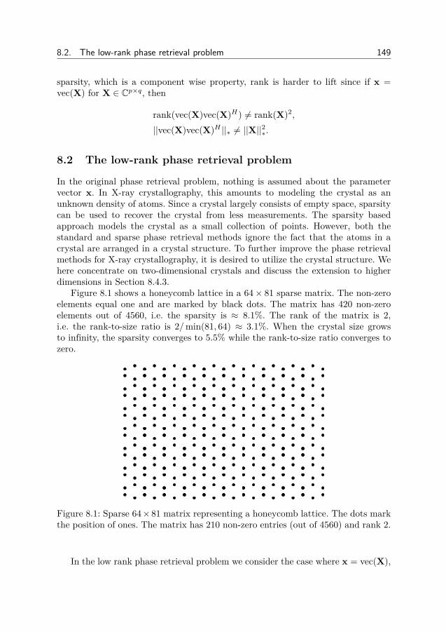
8.2. The low-rank phase retrieval problem 149
sparsity, which is a component wise property, rank is harder to lift since if x =vec(X) for X ∈ Cp×q, then
rank(vec(X)vec(X)H) 6= rank(X)2,
||vec(X)vec(X)H ||∗ 6= ||X||2∗.
8.2 The low-rank phase retrieval problem
In the original phase retrieval problem, nothing is assumed about the parametervector x. In X-ray crystallography, this amounts to modeling the crystal as anunknown density of atoms. Since a crystal largely consists of empty space, sparsitycan be used to recover the crystal from less measurements. The sparsity basedapproach models the crystal as a small collection of points. However, both thestandard and sparse phase retrieval methods ignore the fact that the atoms in acrystal are arranged in a crystal structure. To further improve the phase retrievalmethods for X-ray crystallography, it is desired to utilize the crystal structure. Wehere concentrate on two-dimensional crystals and discuss the extension to higherdimensions in Section 8.4.3.
Figure 8.1 shows a honeycomb lattice in a 64× 81 sparse matrix. The non-zeroelements equal one and are marked by black dots. The matrix has 420 non-zeroelements out of 4560, i.e. the sparsity is ≈ 8.1%. The rank of the matrix is 2,i.e. the rank-to-size ratio is 2/min(81, 64) ≈ 3.1%. When the crystal size growsto infinity, the sparsity converges to 5.5% while the rank-to-size ratio converges tozero.
Figure 8.1: Sparse 64×81 matrix representing a honeycomb lattice. The dots markthe position of ones. The matrix has 210 non-zero entries (out of 4560) and rank 2.
In the low rank phase retrieval problem we consider the case where x = vec(X),
150 Low-rank phase retrieval
X ∈ Rp×q and rank(X) min(p, q). The low-rank phase retrieval problem is thus
min rank(X)subject to ||y− |Avec(X)|2||1 ≤ η
(8.3)
We notice the similarity between (8.3) and (8.2). However, in (8.2) the measure-ments are linear in Z while in (8.3) they are non-linear in X. The question arisesof when the solution to (8.3) is unique. By extending the results of [EM14] we findthe following probabilistic uniqueness condition.
Proposition 8.2.1. Assume that the measurements are noise free (η = 0), thatthe components of A ∈ Rm×pq are i.i.d. zero-mean Gaussian distributed and thatrank(X) = r ≤ min(p, q)/2. Then the solution to the low-rank phase retrieval prob-lem (8.3) is unique (and equals ±X) with probability at least 1 − 2 exp(−cu2r(p +q − 2r)), if
m ≥ Cu3/2r(p+ q − 2r),
where c, C and u are positive constants.
The proof of Proposition 8.2.1 is given in Section 8.7.1. The proposition givesus that uniqueness can be guaranteed with high probability when the number ofmeasurements is approximately proportional to the number of degrees of freedom
degrees of freedom = r(p+ q − r).
We now turn to extending PhaseLift to use the low-rank property in (8.3).
8.3 Low-rank PhaseLift
To promote low-rank we need to construct a penalty which acts on the lifted variableZ while promoting low-rank in X. It turns out that one approach can be found usingthe theory of Kronecker product approximation.
8.3.1 Lifting the rankIn the Kronecker approximation problem we search to approximate a matrix B ∈Rp1p2×q1q2 by the Kronecker product (C ⊗ D) of two matrices, C ∈ Rp1×q1 andD ∈ Rp2×q2 . The least square approximation problem is
min(C⊗D)
||B− (C⊗D)||F . (8.4)
The problem has an algebraic solution which uses a linear transformation [VLP93]R : Rp1p2×q1q2 → Rp1q1×p2q2 such that
R(C⊗D) = vec(C)vec(D)>.

8.3. Low-rank PhaseLift 151
The linear transformation R is invertible, giving us that if B is the best rank-1approximation of R (B) then the solution to (8.4) is
(C⊗ D) = R−1 (B) .The inverse transformation, R−1, is the key to lifting the rank property. If
Z = vec(X)vec(X)>, then R−1(Z) = (X⊗X) and
rank(R−1(Z)) = rank(X)2, ||R−1(Z)||∗ = ||X||2∗.
By using the transformation R−1(·), we can write the low rank phase retrievalproblem (8.3) in the variable Z = vec(X)vec(X)> as
min rank(R−1Z)),subject to ||y−A(Z)||1 ≤ η, Z ≥ 0, rank(Z) = 1.
By relaxing the rank functions, the Low-Rank PhaseLift program becomes
Z = arg min tr(Z) + λ||R−1(Z)||∗,subject to ||y−A(Z)||1 ≤ η, Z 0,
(8.5)
where λ > 0 is a regularization parameter. We notice that in order to give goodrecovery, the regularization parameter needs to be chosen such that rank(Z) = 1. InSection 8.3.3 we will discuss a method for selecting λ. We now turn to establishingerror bounds for (8.5).
8.3.2 Error bounds for low-rank phase liftWe here establish probabilistic error bounds for (8.5) when the entries of ai arerandom variables. For simplicity we here concentrate on Gaussian measurementsalthough the extension to sub-Gaussian variables is straight forward. We state themain results in this section and give the proofs in Section 9.5. We consider twocases: (a) λ ∈
[1√r, ||X||F√
r||Xr||∗
](Theorem 8.1) and (b) λ → ∞ (Theorem 8.2). The
case λ = 0 corresponds to the standard PhaseLift method. The theorems upperbound the error ||Z− Z||2F . The inequality
||x− x||22 · ||x + x||22 ≤ 2||xx> − xx>||2F = 2||Z− Z||2F , (8.6)
can be used to give the corresponding error bounds in x. The inequality (8.6) holdswhen x and x are real. For completeness we give a proof of (8.6) in Section 8.7.2.We now give the error bound for λ in a closed interval.
Theorem 8.1. Assume that the entries of ai are i.i.d. Gaussian distributed, ||n||1 ≤η and Z = vec(X)vec(X)> = xx>. Let Xr denote the best rank-r approximation ofX and xr = vec(Xr). If
m > C ′min
(p2 + q2 + 1)r2, 2pq + 1,

152 Low-rank phase retrieval
then the solution Z of (8.5) with λ ∈[
1√r, ||Xr||F√
r||Xr||∗
]satisfies
||Z− Z||F ≤C(||xx> − xrx>r ||∗ + λ||R−1(xx> − xrx>r )||∗ + η
m
),
with probability at least 1− C0 exp(−c0m) for some positive constants C,C ′, C0, c0which only depend on r.
Next we give the error bound for λ → ∞, i.e. for the estimator which onlypenalize the nuclear norm of X (through Z) and not the trace of Z.
Theorem 8.2. Assume that the entries of ai are i.i.d. zero-mean Gaussian, ||n||1 ≤η and let R−1(Z)s denote the best rank-s approximation of R−1(Z). If
m > C(p2 + q2 + 1)s,
then the solution Z of (8.5) in the limit λ→∞ satisfies
||Z− Z||F ≤ C1||R−1(Z)−R−1(Z)s||∗√
s+ C2
η
m,
with probability at least 1−C0 exp(−c0m) for some positive constants C0, c0, C1, C2, Cwhich only depends on s.
For our scenario rank(R−1(Z)) = r2, so the sufficient number of measurementsare m > C(p2 + q2 + 1)r2 to obtain a “noise-only” error bound. For p = q, thetheorems therefore imply that the estimators with finite λ and λ → ∞ requiresless measurements in order to obtain a noise-only error bound. The bounds are,however, expected to be quite loose compared to the actual performance of theestimators. In Section 8.5, we compare the empirical performance of the estimatorsthrough numerical simulations.
8.3.3 Regularization path for λ
As “the world is full of obvious things which nobody by any chance ever ob-serves” [DF02] we note that the Low-Rank PhaseLift estimate (8.5) depends onthe parameter λ. Selecting a proper value of λ is important for finding a good esti-mate. We therefore write the estimate (8.5) as Z(λ) to emphasize the dependence onλ. The value of λ should be such that rank(Z(λ)) = 1 and rank(R−1(Z(λ))) is min-imized. This means that λ should be small enough to ensure that rank(Z(λ)) = 1while still maximally penalizing the rank of R−1(Z(λ)). By this argument we hy-pothesize that the optimal value of λ is
λoptimal = max λ, subject to rank(Z(λ)) = 1.
8.4. Extensions of low-rank phase retrieval 153
One problem with the parameter λ is that we possibly need to search over arbitrarilylarge λ ∈ [0,∞). For this reason we instead consider the equivalent estimator
Z∗(t) = arg min ||R−1(Z)||∗subject to ||y−A(Z)||1 ≤ η, Z 0,
tr(Z) ≤ t.(8.7)
The advantage of the estimator (8.7) is that the parameter t lies in the boundedinterval
tr(Z(0)) = t0 ≤ t ≤ t1 = tr(Z(∞)). (8.8)
The goal is thus to find the maximal value of t that minimize rank(Z∗(t)) for tin the interval (8.8). As minimizing the rank is numerically difficult, we insteadminimize the continuous function
f(t) = tr(Z∗(t))− ||Z∗(t)||F . (8.9)
Using that tr(Z∗(t)) ≥ ||Z∗(t)||F and the Cauchy-Schwarz inequality, we get that
0 ≤ f(t) ≤(√
rank(Z∗(t))− 1)||Z∗(t)||F .
So for t such that Z∗(t) 6= 0, f(t) = 0 if and only if rank(Z∗(t)) = 1.Several methods can be used to minimize (8.9). Here we use the secant method
which updates t based on earlier values tn and tn−1 as
tn+1 = tn−1f(tn)− tnf(tn−1)f(tn)− f(tn−1) ,
tn+1 = min(tmax,max(tmin, tn+1), ),
where we use the min-max operation to ensure that t lies in the interval. Oneexample of how f(t) and the NMSE of Z depend on t is shown in Figure 8.2. Wenow discuss possible extensions of the Low-Rank Phase Retrieval problem.
8.4 Extensions of low-rank phase retrieval
In this section we discuss the extension of low-rank phase retrieval to other com-monly discussed scenarios.
8.4.1 Robust low-rank phase retrievalAs in robust PCA, the low-rank matrix is in some scenarios corrupted by sparsenoise. To separate the low-rank and sparse component, low-rank and sparse penal-ties are used.
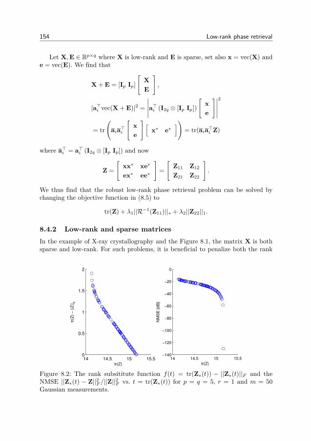
154 Low-rank phase retrieval
Let X,E ∈ Rp×q where X is low-rank and E is sparse, set also x = vec(X) ande = vec(E). We find that
X + E = [Ip Ip][
XE
],
|a>i vec(X + E)|2 =
∣∣∣∣∣a>i (I2q ⊗ [Ip Ip])[
xe
]∣∣∣∣∣2
= tr(
aia>i
[xe
] [x∗ e∗
])= tr(aia>i Z)
where a>i = a>i (I2q ⊗ [Ip Ip]) and now
Z =[
xx∗ xe∗
ex∗ ee∗
]=[
Z11 Z12
Z21 Z22
].
We thus find that the robust low-rank phase retrieval problem can be solved bychanging the objective function in (8.5) to
tr(Z) + λ1||R−1(Z11)||∗ + λ2||Z22||1.
8.4.2 Low-rank and sparse matricesIn the example of X-ray crystallography and the Figure 8.1, the matrix X is bothsparse and low-rank. For such problems, it is beneficial to penalize both the rank
14 14.5 15 15.50
0.5
1
1.5
2
tr(Z)
tr(Z
) −
||Z
||F
14 14.5 15 15.5−140
−120
−100
−80
−60
−40
−20
0
NM
SE
[d
B]
tr(Z)
Figure 8.2: The rank subsititute function f(t) = tr(Z∗(t)) − ||Z∗(t)||F and theNMSE ||Z∗(t) − Z||2F /||Z||2F vs. t = tr(Z∗(t)) for p = q = 5, r = 1 and m = 50Gaussian measurements.

8.4. Extensions of low-rank phase retrieval 155
and the sparsity of the solution. The natural modification to the estimator (8.5) istherefore
Z = arg min tr(Z) + λ1||R−1(Z)||∗ + λ2||Z||1,subject to ||y−A(Z)||1 ≤ η, Z 0
(8.10)
where λ1, λ2 ≥ 0 are regularization parameters. For the estimator (8.10) we findthe following error bounds.
Theorem 8.3. Assume that the entries of ai are i.i.d. Gaussian distributed, ||n||1 ≤η and Z = vec(X)vec(X)> = xx>. Let
Xr,k = arg minrank(X′)≤r||X′||1≤k
||X′ −X||F
denote the best k-sparse and rank-r approximation of X and xr,k = vec(Xr,k). If
m > C ′k2r2 log(pq/k2),
then the solution Z of (8.10) with λ1 ∈[
1√r,||Xr,k||F√r||Xr,k||∗
]and λ2 ∈
[1√k,||Xr,k||F√k||Xr,k||1
]satisfies
||Z− Z||F ≤ C(||xx> − xr,kx>r,k||∗ + λ1||R−1(xx> − xr,kx>r,k)||∗
+λ2||xx> − xr,kx>r,k||1 + η
m
),
with probability at least 1− C0 exp(−c0m) for some positive constants C,C ′, C0, c0which only depends on k and r.
The proof of Theorem 8.3 is similar to the proof of Theorem 8.1 and is thereforeomitted.
8.4.3 Recovery of low-rank tensorsSo far we have only discussed the recovery of matrices, i.e. two-dimensional struc-tures which describe e.g. two dimensional crystals. As most crystals are three di-mensional, it is interesting to consider how the low-rank phase retrieval becomesmodified for higher order structures. The higher order generalization of a matrixis the tensor [KB09]. As the components of a vector is written with one indexxi (a first order tensor), the component of a matrix with two indices Xij (a sec-ond order tensor), the components of a k’th order tensor is written with k indicesXi1i2...ik . Since we considered X-ray crystallography as an important applicationwe, for simplicity, focus on rank minimization for third order tensors.
Unlike matrices, several low-rank decompositions exist for third order tensors[BL10,KB09]. The two most common decompositions are the Tucker or higher order
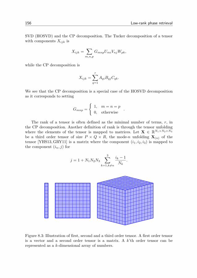
156 Low-rank phase retrieval
SVD (HOSVD) and the CP decomposition. The Tucker decomposition of a tensorwith components Xijk is
Xijk =∑m,n,p
GmnpUmiVnjWpk,
while the CP decomposition is
Xijk =r∑q=1
AqiBqjCqk.
We see that the CP decomposition is a special case of the HOSVD decompositionas it corresponds to setting
Gmnp =
1, m = n = p
0, otherwise.
The rank of a tensor is often defined as the minimal number of terms, r, inthe CP decomposition. Another definition of rank is through the tensor unfoldingwhere the elements of the tensor is mapped to matrices. Let X ∈ RN1×N2×N3
be a third order tensor of size P × Q × R, the mode-n unfolding X(n) of thetensor [YHS13,GRY11] is a matrix where the component (i1, i2, i3) is mapped tothe component (in, j) for
j = 1 +N1N2N3
3∑k=1,k 6=n
ik − 1Nk
.
Figure 8.3: Illustration of first, second and a third order tensor. A first order tensoris a vector and a second order tensor is a matrix. A k’th order tensor can berepresented as a k-dimensional array of numbers.
8.5. Experiments with random measurement matrices 157
The unfolding of a tensor is sometimes called matricization. It is also possible todefine the vectorization of a tensor in the same way as for matrices. The 3-rank ofa third order tensor is the tuple
(r1, r2, r3) =(rank(X(1)), rank(X(2)), rank(X(3))
).
A common approach to tensor rank minimization is to minimize the sum of the3-ranks [YHS13]. The corresponding convex penalty is then to replace the matrixranks by the nuclear norm.
In the phase retrieval problem, the lifted variable is Z = vec(X)vec(X)>. Topromote low tensor rank in X we note that vec(X) is related to the tensor unfoldingsby a linear transformation. Thus we can write
vec(X) = vec1(X(1)) = P1vec(X(1)),vec(X) = vec2(X(2)) = P2vec(X(2)),vec(X) = vec3(X(1)) = P3vec(X(3)),
where veck(·) is the vectorization operators related to the k’th tensor unfolding andP1,P2,P3 are permutation matrices. By using the permutation matrices, we findthat the nuclear norm tensor rank penalty becomes
||R−1(P−11 Z(P>1 )−1)||∗ + ||R−1(P−1
2 Z(P>2 )−1)||∗ + ||R−1(P−13 Z(P>3 )−1)||∗.
This formulation is easily extended to higher order tensors.
8.5 Experiments with random measurement matrices
Here we perform numerical experiments to investigate the empirical performanceof low-rank matrix phase retrieval (LRPR). We compare the performance of Low-Rank PhaseLift (LR-PhaseLift) (8.7), with the parameter t set by the proceduredescribed in 8.3.3, with the standard PhaseLift. The methods where implementedusing the cvx toolbox [GBY08]. Since the solution is only unique up to a globalphase, we use the error measure
minθ||X− eiθX||2F = ||X||2F + ||X||2F − 2|tr(X>X)|.
We consider the scenario where the elements of the sensing matrix in (8.1)A are drawn from an N (0, 1) distribution. We generated the low-rank matrix bysetting X = LR> where L ∈ Rp×r, R ∈ Rq×r and the elements from L and R areindependently drawn from a N (0, 1) distribution.
8.5.1 Noise-free measurementsIn the first experiment we considered noise free measurements. We used p = 7,q = 7, r = 2 and varied the number of measurements m. The results are shown

158 Low-rank phase retrieval
70 80 90 100 110 120 130 140 150−140
−120
−100
−80
−60
−40
−20
0
m
NM
SE
[d
B]
PhaseLift
LR−PhaseLift
Figure 8.4: NMSE for reconstruction from Gaussian measurements for p = q = 5and rank(X) = 1. (Change to other figure when simulation is done)
in Figure 8.4. We find that LR-PhaseLift is able to reconstruct the matrix (up tonumerical precision) for m ≥ 105 measurements while PhaseLift requires m ≥ 125measurements to reconstruct the matrix.
8.5.2 Noisy measurements
In the second experiment we examined how noise affects the final estimates. Inthe experiments, we generated the noise from a N (0, σ2
nIm) distribution. The noisevariance, σ2
n was chosen so that the Signal-to-Noise-Ratio (SNR)
SNR =E [∣∣∣∣|Ax|2
∣∣∣∣22]
E [||n||22] = r2m(pq)2 + 2r2mpq
mσ2n
,
was equal to 20 dB.To estimate X we used the standard PhaseLift and LR-PhaseLift with
η = σnm,
as in [CCG15].

8.6. Conclusion 159
80 90 100 110 120 130 140 150−50
−45
−40
−35
−30
−25
−20
−15
−10
−5
0
m
NM
SE
[dB
]
PhaseLift
LR−PhaseLift
Figure 8.5: NMSE for reconstruction from noisy Gaussian measurements for p =q = 7, r = 2 and SNR = 20 dB.
The results are shown in Figure 8.5. We find that the estimation methods gavelarger errors when noise was present. This is to be expected since the use of η > 0makes the estimates biased towards zero. LR-PhaseLift gave an NMSE which was10 to 7 dB lower than the NMSE of PhaseLift for the values of m shown in theFigure.
8.6 Conclusion
In this chapter we showed how the PhaseLift method for phase retrieval can beadapted to promote low-rank in the estimate. In phase retrieval we only mea-sure the magnitudes of measurements, the sign or phase of the measurements aretherefore lost. This occurs in e.g. X-ray crystallography where X-rays are scatteredagainst a crystal. The approach uses the theory of approximation with Kroneckerproducts and leads to a convex penalty in the lifted variable. Using methods for con-vex optimization bounds, we derived error bounds for the estimation methods. Thelow-rank phase retrieval method was also extended to robust low-rank matrix re-construction, low-rank and sparse matrix reconstruction and the recovery of higherorder tensors. Lastly we evaluated the empirical performance of the algorithms us-
160 Low-rank phase retrieval
ing numerical experiments. We found that the proposed method could reconstruct alow-rank matrix from fewer number of measurements than the standard PhaseLiftalgorithm.
8.7 Derivations and proofs
8.7.1 Details for uniqueness boundThe proof of Proposition 8.2.1 relies on Theorem 2.4. in [EM14].
A random variable a ∈ Rn is isotropic if
E [|a>t|2] = ||t||22
for all t ∈ Rn and L-subgaussian if
Pr(|a>t| ≥ Lu(E [|a>t|2])1/2) ≤ 2 exp(−u2/2),
for all t ∈ Rn. Let T ⊂ Rn be a set and let
T− =
t− s||t− s||2
, t, s ∈ T, t 6= s,
T+ =
t + s||t + s||2
, t, s ∈ T, t 6= s
.
Denote
E = maxEg
[sup
v∈T−
n∑i=1
givi
], Eg
[sup
v∈T+
n∑i=1
givi
],
ρT,m = E√m
+ E2
m
and
κ(v,w) = E[a>v/||v||2a>w/||w||2
].
Theorem 8.4 (Theorem 2.4 from [EM14]). Let A ∈ Rm×n be a matrix with i.i.d.random isotropic L-subgaussian row vectors. For every L ≥ 1 there exists constantsc1, c2 and c3 that depends only on L such that for u ≥ c1∣∣∣∣|As|2 − |At|2
∣∣∣∣1 ≥ D||s− t||2||s + t||2,
D = κ(s− t, s + t)− c3u3ρT,m
holds for all s, t ∈ T with probability at least
1− 2 exp(−c2u2 minm,E2).

8.7. Derivations and proofs 161
The quantity κ(v,w) can be shown to be bounded from below as κ(v,w) ≥ c1under some conditions (e.g. small-ball or Paley Sygmund arguments) [EM14]. Wefind that it is necessary for m to be large enough such that
c1 − c3u3ρT,m > 0
to ensure a unique solution.
Proof of Proposition 8.2.1. For simplicity we only consider Gaussian measurementmatrices. The extension to sub-Gaussian measurement matrices is straightforward.Let Tr = X ∈ Rp×q : rank(X) ≤ r. Each row vector of A can be represented bya p× q matrix. Let G denote a reshaped row vector of A and let Ur = X ∈ Rp×q :rank(X) ≤ r, ||X||F = 1, we find that [CRPW12]
E = EG
[sup
W∈U2r
tr(G>W)]
= EG
( 2r∑i=1
σi(G)2
)1/2≤√
6r(p+ q − 2r) = E′
Provided that infv,w κ(v, w) ≥ c1, Theorem 8.4 now gives that the solution to
y = |Avec(X)|2, rank(X) ≤ r
is unique with probability at least
1− 2 exp(−c2u2E′2) = 1− 2 exp(−6c2u2r(p+ q − 2r)),
when r ≤ min(p, q)/2 and
c1 − c3u3ρT,m ≥ c1 − c3u3(E′√m
+ E′2
m
)≥ c1 − c3u3
[E′√m
+(E′√m
)2]> 0
⇐ m >E′√
c1c3u3 + 1
4 −12
⇐ m >
√c3u3
c1
√6r(p+ q − 2r).
162 Low-rank phase retrieval
8.7.2 Proof of (8.6)We find that
2||xx> − xx>||2F − ||x− x||22 · ||x + x||22= 2tr(xx>xx>) + 2tr(xx>xx>)− 4tr(xx>xx>)− (||x||22 + ||x||22 − 2x>x)(||x||22 + ||x||22 + 2x>x)= 2||x||42 + 2||x||42 − 4(x>x)2 − ||x||42 − ||x||42 − 2||x||22||x||22 + 4(x>x)2
= ||x||42 + ||x||42 − 2||x||22||x||22= (||x||22 − ||x||22)2 ≥ 0.
This proves (8.6).
8.7.3 Recovery bounds under RIP-conditionsTheorem 8.1 and 8.2 require the bounds on the RIP constants given in Corol-lary 8.7.1. The proof of Theorem 8.2 is similar to the proof of Theorem 1 in [CCG15]when Corollary 8.7.1 is given, the proofs are therefore not repeated here. Here wefirst show the proof of Theorem 8.1 since it differs from the proof in [CCG15] andlater also prove Corollary 8.7.1.
The lifted random sensing operatorA(·) = Φvec(·) does not satisfy the RIP sincethe individual components have non zero-means. However, in Proposition 8.7.2 andCorollary 8.7.1 in Section 8.7.5 we show that the operator B defined as
B(Z)i = Φ(Z)2i−1 − Φ(Z)2i,
does satisfy the following RIP with high probability.
Definition 8.1. A linear operator B satisfies theMK1,K2 `2/`1-RIP property if
(1− γlbK1,K2)||W||F ≤
1m||B(W)||1 ≤ (1 + γubK1,K2
)||W||F ,
for all matrices W ∈MK1,K2 where
Mk,r =
W ∈ Rp2×q2
: rank(W) ≤ r2, rank(R(W)) ≤ k,R−1(W) 0.
Assuming that the RIP condition holds, we prove Theorem 8.1 with the help ofthe following proposition.
Proposition 8.7.1. Assume that Z = vec(X)vec(X)> = xx> and let Xr be thebest rank-r approximation of X and xr = vec(Xr). If there exists K1,K2 such thatB satisfies the MK1,K2 `2/`1-RIP property, with
(1 + δubK1,K2)√
3(1− δlb2K1,2K2
)√K1
+1 + δubK1,K2
(1− δlbK1,K2)√K1
<1
1 +√
2

8.7. Derivations and proofs 163
then for√
K1K2≤ λ ≤ ||X||F√
r||Xr||∗there exists a constant C such that
||Z− Z||F ≤C(||xx> − xrx>r ||∗ + λ||R−1(xx> − xrx>r )||∗ + η
m
).
Proof. Let Z be the minimizer of (8.5) and let Z = xx>, then Z = xx> + H. SetZr = xrx>r and Zc = Z − xrx>r . Let Xr = UrΣrV>r be the SVD of Xr and setu = vec(Xr/||Xr||F ). A subdifferential of || · ||∗ + λ||R−1(·)||∗ at Zr is
uu> + Y + λ(R−1)∗(VrV>r ⊗UrU>r ) + λW= uu> + Y + λvec(UrV>r )vec(UrV>r )> + λW,
where ||Y|| ≤ 1, u>Y = 0 and W is such that U>r W = 0, WVr = 0 and ||W|| ≤ 1.Define the tangent spaces T and S by
T = TZrZ : rank(Z) ≤ 1 = urz> + zu>r , z ∈ RpqS = TZrZ : rank(R−1(Z)) ≤ r2,=
(Iq ⊗Ur)B(Iq ⊗Ur)> + (Vr ⊗ Ip)A(V>r ⊗ Ip) : A ∈ Rrp×rp,B ∈ Rrq×rq.
We find that the projections onto the tangent spaces are given by
PT (Z) = uu>Z + (I− uu>)Zuu>,PS(Z) = (VrV>r ⊗UrU>r )Z + (Ipq − (VrV>r ⊗UrU>r ))Z(VrV>r ⊗UrU>r ).
This gives us that PSPT = PTPS = PT , so T ⊂ S.We can chose Y and W such that 〈Y,H〉 = ||HT⊥∩S ||∗ and 〈W,H〉 = ||R−1(HS⊥)||∗.
We also set v = vec(UrV>r ) for brevity.We find that
0 ≥ tr(Z + H) + λ||R−1(Z + H)||∗ − tr(Z)− λ||R−1(Z)||∗ = ||Z + H||∗ + λ||R−1(Z + H)||∗− ||Z||∗ − λ||R−1(Z)||∗≥ ||Zr + H||∗ + λ||R−1(Zr + H)||∗ − 2||Zc||∗− ||Zr||∗ − λ||R−1(Zr)||∗ − 2λ||R−1(Zc)||∗≥⟨uu> + Y + λvv> + λW,H
⟩− 2λ||R−1(Zc)||∗
− 2||Zc||∗ =⟨uu> + λPT
(vv>
),HT
⟩+ ||HT⊥∩S ||∗
+ λ⟨PT⊥(vv>),HT⊥
⟩+ λ||R−1(HS⊥)||∗
− 2λ||R−1(Zc)||∗ − 2||Zc||∗.
We further have that HT⊥ 0 because Z + H 0. This gives us that⟨PT⊥(vv>),HT⊥
⟩=⟨vv>,HT⊥
⟩= v>HT⊥v> ≥ 0.

164 Low-rank phase retrieval
Putting this together we find that
||HT⊥∩S ||∗ + λ||R−1(HS⊥)||∗≤ −
⟨uu> + λPT (vv>),HT
⟩+ 2||Zc||∗ + 2λ||R−1(Zc)||∗
≤ ||HT ||+ λ||PT (vv>)||∗||HT ||+ 2||Zc||∗ + 2λ||R−1(Zc)||∗
Also, since λ ≤ ||Xr||F√r||Xr||∗
we get that
||PT (vv>)||2∗ ≤ 2||PT (vv>)||2F= 4(u>v)2||v||22||u||22 − 2(u>v)4
= 4r ||Xr||2∗||Xr||2F
− 2 ||Xr||4∗||Xr||4F
≤ 2r ||Xr||2∗||Xr||2F
≤ 2λ2 .
This gives us that
||HT⊥∩S ||∗ + λ||R−1(HS⊥)||∗≤ (1 +
√2)||HT ||+ 2||Zc||∗ + 2λ||R−1(Zc)||∗.
Next, decompose HS⊥∩T and HS⊥ into mutually orthogonal matrices
HT⊥∩S =M1∑i=1
H(i)T⊥∩S ,
HS⊥ =M2∑i=1
H(i)S⊥,
such that
σmin(H(i)T⊥∩S) ≥ σmax(H(i+1)
T⊥∩S),
σmin(R−1(H(i)S⊥
)) ≥ σmax(R−1(H(i+1)S⊥
)),
rank(H(i)T⊥∩S) = K1, 1 ≤ i ≤M1 − 1
||HT⊥∩S ||∗ =M1∑i=1||H(i)
T⊥∩S ||∗,
rank(R−1(H(i)S⊥
)) = K2, 1 ≤ i ≤M2 − 1,
rank(H(i)S⊥
) = K1, 1 ≤ i ≤M2 − 1,
||R−1(HS⊥)||∗ =M1∑i=1||R−1(H(i)
S⊥)||∗,
where σmin(·) denotes the smallest non-zero singular value.
8.7. Derivations and proofs 165
Combined with the RIP-property, this gives us that
M1∑i=2
1m||B(H(i)
T⊥∩S)||1 ≤ (1 + δubK1,K2)M1∑i=2||H(i)
T⊥∩S ||F
≤(1 + δubK1,K2
)√K1
||HT⊥∩S ||∗,
M2∑i=2
1m||B(H(i)
S⊥)||1 ≤ (1 + δubK1,K2
)M2∑i=2||H(i)
S⊥||F
= (1 + δubK1,K2)M2∑i=2||R−1(H(i)
S⊥)||F
≤(1 + δubK1,K2
)√K2
||R−1(HS⊥)||∗.
Because of the constraint, we get that
1m||B(H)||1 ≤
1m||Φ(H)||1 ≤
1m
(||y− Φ(Z)||1 + ||y− Φ(Z)||1
)≤ 2ηm. (8.11)
We now take K1 and K2 such that√
K1K2≤ λ. Using this, we find that
2ηm≥ 1m||B(H)||1 ≥
1m
∣∣∣∣∣∣B (HT + H(1)T⊥∩S + H(1)
S⊥
)∣∣∣∣∣∣1
−M1∑i=2
1m||B(H(i)
T⊥∩S)||1 −M2∑i=2
1m||B(H(i)
S⊥)||1
≥ (1− δlb2K1,2K2)||HT + H(1)
T⊥∩S + H(1)S⊥||F
−(1 + δubK1,K2
)√K1
||HT⊥∩S ||∗ −(1 + δubK1,K2
)√K2
||R−1(HS⊥)||∗
≥1− δlb2K1,2K2√
3
(||HT ||F + ||H(1)
T⊥∩S ||F + ||H(1)S⊥||F)
−(1 + δubK1,K2
)√K1
(||HT⊥∩S ||∗ + λ||R−1(HS⊥)||∗
)≥
1− δlb2K1,2K2√3
(||HT ||F + ||H(1)
T⊥∩S ||F + ||H(1)S⊥||F)−
(1 + δubK1,K2)
√K1
((1 +
√2)||HT ||+ 2λ||R−1(Zc)||∗ + 2||Zc||∗
).

166 Low-rank phase retrieval
This gives us that
||HT ||F + ||H(1)T⊥∩S ||F + ||H(1)
S⊥||F
≤ C1
((1 +
√2)||HT ||+ 2||Zc||∗ + 2λ||R−1(Zc)||∗
)+
√3
(1− δlb2K1,2K2)
2ηm,
where
C1 =(1 + δubK1,K2
)√
3(1− δlb2K1,2K2
)√K1
.
For the remaining terms we find thatM1∑i=2||H(i)
T⊥∩S ||F +M2∑i=2||H(i)
S⊥||F
≤ 11− δlbK1,K2
(M1∑i=2
1m||B(H(i)
T⊥∩S)||1 +M2∑i=2
1m||B(H(i)
S⊥)||1
)
≤1 + δubK1,K2
(1− δlbK1,K2)√K1||HT⊥∩S ||∗ +
1 + δubK1,K2
(1− δlbK1,K2)√K2||R−1(HS⊥)||∗
≤1 + δubK1,K2
(1− δlbK1,K2)√K1
(||HT⊥∩S ||∗ + λ||R−1(HS⊥)||∗
)≤
1 + δubK1,K2
(1− δlbK1,K2)√K1
((1 +
√2)||HT ||+ 2||Zc||∗ + 2λ||R−1(Zc)||∗
)Putting this together gives us that
||H||F = ||HT + HT⊥∩S + HS⊥ ||F
≤ ||HT ||F + ||H(1)T⊥∩S ||F + ||H(1)
S⊥||F +
M1∑i=2||H(i)
T⊥∩S ||F +M2∑i=2||H(i)
S⊥||F
≤ γ(
(1 +√
2)||HT ||+ 2||Zc||∗ + 2λ||R−1(Zc)||∗)
+√
3(1− δlb2K1,2K2
)2ηm,
where
γ =(1 + δubK1,K2
)√
3(1− δlb2K1,2K2
)√K1
+1 + δubK1,K2
(1− δlbK1,K2)√K1
.
We thus have that
||H||F ≤2γ
1− (1 +√
2)γ(||Zc||∗ + λ||R−1(Zc)||∗
)+ 1
1− (1 +√
2)γ
√3
(1− δlb2K1,2K2)
2ηm
≤ C(||Zc||∗ + λ||R−1(Zc)||∗ + η
m
)
8.7. Derivations and proofs 167
provided that γ < 1/(1 +√
2).
We notice that the proof provides loose recovery bounds since the proof impliesthat λ should be chosen as small as possible. Theorem 8.2 follows directly from 8.7.1using e.g. the techniques in the proof of Theorem 1 in [CCG15] and is thereforeomitted.
8.7.4 Proof of Theorem 8.2Proof: We note that
tr(aia>i R−1(Z)) = tr((Ai ⊗Ai)>W),
where W = R−1(Z). We can thus express the measurements as y = AK(W) + n.The program (8.1) in the limit λ→∞ can be written as
min||W||∗,such that ||y−AK(W)||1 ≤ η, R(W) 0,
(8.12)
where AK(W)i = tr((Ai ⊗Ai)>W). Let W = W + H ∈ Rp2×q2 be the minimizerof (8.12). Let Ws be the best rank-s approximation of W and set Wc = W−Ws.Let Ws = UsΣsV>s be the SVD decomposition of Ws. We find that
||WT ||∗ + ||WT⊥ ||∗ ≥ ||W||∗ ≥ ||W + H||∗ ≥ ||WT + H||∗ − ||WT⊥ ||∗≥ ||WT ||∗ − ||HT ||∗ + ||HT⊥ ||∗ − ||WT⊥ ||∗.
This gives that
||HT⊥ ||∗ ≤ 2||WT⊥ ||∗ + ||HT ||∗. (8.13)
Decompose HT⊥ into orthogonal matrices
HT⊥ =M∑i=1
H(i)T⊥,
such that
σmin(H(i)T⊥
) ≥ σmax(H(i+1)T⊥
),
rank(H(i)T⊥
) = K1, for i = 1, 2, . . . ,M − 1.
We find that∑i≥2||H(i)
T⊥||F ≤
1√K1
∑i≥1||H(i)
T⊥||∗ = 1√
K1||HT⊥ ||∗ (8.14)
≤ 1√K1
(2||Wc||∗ + ||HT ||∗) ≤1√K1
(2||Wc||∗ +
√s||HT ||F
). (8.15)
168 Low-rank phase retrieval
This gives us that
M∑i=2
1m||BK(H(i)
T⊥)||1 ≤ (1 + δ
(ub)K1
)M∑i=2
1m||H(i)
T⊥||F
≤1 + δ
(ub)K1√K1
||HT⊥ ||∗.
Similar to (8.11), we find that
1m||BK(H)||1 ≤
2ηm.
This gives us that
2ηm≥ 1m||BK(HT + H(1)
T⊥)||1 −
M∑i=2
1m||BK(H(i)
T⊥)||1 ≥
(1− δ(lb)2K1
)||HT + H(1)T⊥||F −
1 + δ(ub)K1√K1
||HT⊥ ||∗ ≥
1− δ(lb)2K1√2
(||HT ||F + ||H(1)
T⊥||F)−
1 + δ(ub)K1√K1
||HT⊥ ||∗
≥1− δ(lb)
2K1√2
(||HT ||F + ||H(1)
T⊥||F)
−1 + δ
(ub)K1√K1
(2||Wc||∗ +
√s||HT ||F
).
Rearranging the terms we get that
(1− δ(lb)
2K1√2
−√s
1 + δ(ub)K1√K1
)||HT ||F +
1− δ(lb)2K1√2||H(1)
T⊥||F
≤ 21 + δ
(ub)K1√K1
||Wc||∗ + 2ηm.
We thus find that
||HT ||F + ||H(1)T⊥||F ≤
2β
(1 + δ
(ub)K1√K1
||Wc||∗ + η
m
). (8.16)

8.7. Derivations and proofs 169
Combining (8.14), (8.13) and (8.16) we finally get that
||H||F ≤ ||HT ||F + ||H(1)T⊥||F +
∑i≥2||H(i)
T⊥||F
≤ ||HT ||F + ||H(1)T⊥||F + 1√
K1
(2||Wc||∗ +
√s||HT ||F
)≤(C1
β+ C2
)||Wc||∗√
K2+ C3
β
η
m.
This establishes the bound.
8.7.5 Bounds for RIP conditionsHere we establish the probabilities and required number of measurements for theRIP to hold for the different cases. We first show the following proposition.
Proposition 8.7.2. Let B be the linear operator with components
B(W)i = tr(B>i W
)where W is a p2 × q2 matrix,
Bi = (A2i ⊗A2i)− (A2i−1 ⊗A2i−1)
and the elements of Ak are i.i.d. sub-Gaussian variables. Then for every W thereexists positive constants c1, c2, c3 such that
c1||W||F ≤1m||B(W)||1 ≤ c2||W||F ,
holds with probability at least 1− exp(−c3m).
Proof. To prove the proposition, we introduce the commutation matrices Kp whichare matrices such that, Kpvec(X) = vec(X>) for all X ∈ Rp×p. It follows thatKp(X⊗Y)Kq = (Y⊗X) when X,Y ∈ Rp×q [MN95]. Another useful operator is
T (W) = R−1(diag(R(W))),
which projects out certain components of the p2×q2 matrix W. Here diag(·) denotesprojection onto the closest diagonal matrix. The operator T (·) can also be expressedusing index-notation as
T (W)i+(k−1)p,j+(l−1)q = δi,kδj,lWi+(k−1)p,j+(l−1)q,
for 1 ≤ i, k ≤ p and 1 ≤ j, l ≤ q.

170 Low-rank phase retrieval
From Lemma 7 (the Hanson-Wright Inequality) of [CCG15] it follows thatB(W)i is a sub-exponential random variable with
E [|B(W)i|] ≤ c′1||W||2F . (8.17)
To establish a lower bound on E [|B(W)i|] we use that [CCG15]
E [|B(W)i|] ≥
√(E [|B(W)i|2])3
c′3||W||2F.
We have that
E [Ai ⊗Ai] = T (11>),E [(Ai ⊗Ai)tr((Ai ⊗Ai)>W)] = W + Kp2WKq2
+ (1>T (W)1) · T (11>) + (µ4 − 3)T (W).
We thereby find that for all 1 ≤ i ≤ m
E [Bitr(B>i W)] = 4W + 2(µ4 − 3)T (W).
From which it follows that
E [|B(W)i|2] = E[tr(W>Bitr(B>i W))] (8.18)= 4||W||2F + 2(µ4 − 3)||T (W)||2F≥ min(4, 2(µ4 − 1))||W||2F = c4||W||2F (8.19)
So
E [|B(W)i|2] ≥
√c34c′3||W||F = c′2||W||F . (8.20)
Lemma 8 of [CCG15] (see also [Ver12]) gives us that with probability at least1− 2 exp(−cmε) ∣∣∣∣ 1
m||B(W)||1 −
1mE [||B(W)||1]
∣∣∣∣ ≤ ε||W||F .Together with (8.17), we get that
1m||B(W)||1 ≤
1mE [||B(W)||1] + ε||W||F
≤ (c′1 + ε)||W||F = c1||W||Fand together with (8.20), we have that
1m||B(W)||1 ≥
1mE [||B(W)||1]− ε||W||F
≥ (c′2 − ε)||W||F = c2||W||F ,
with probability at least 1− 2 exp(−c3m) for c3 = cε.
8.7. Derivations and proofs 171
We want to derive the number of necessary measurements for the RIP to holdfor matrices in the set
Mk,r =
W ∈ Rp2×q2
: rank(W) ≤ r2,
rank(R(W)) ≤ k,R−1(W) 0.
By using standard covering arguments as in [CP11], we find the following corol-lary.
Corollary 8.7.1. For the sub-Gaussian sensing model, there exists positive con-stants C, c1, c2, c3 such that
1− δlbk,r ≥ c1/2, 1 + δubk,r ≤ 2c2,
with probability at least 1− exp(−c3m) provided that
m > C min
(p2 + q2 + 1)r2, (2pq + 1)k.

Chapter 9
Fast solution of the `1-norm
Traditionally, the biggest problem to making informed decisions was to ob-tain data through observations and experiments. Now, with more inexpen-sive sensors and hardware, data can be collected at a much lower cost. The
main problem now is instead to transmit, store and process the large amounts ofdata. The problem of handling and analyzing large amounts of data is often re-ferred to as the data deluge and Big Data [Bar11]. In Big Data problems, machinelearning methods are used to process large amounts of data to extract useful in-formation. The large amounts of data requires that the algorithms are fast andmemory efficient to be useful in practice. Sparse representations are useful for BigData problems since they allow us to describe data in an economical way. To findsparse representations requires that our dictionary contains many atoms. For thestandard sparse representation problem, the big data problem occurs when: (1) thenumber of atoms is very large, (2) the number of measurements is very large or (3)both the number of measurements and number of atoms is very large. Typically(2) can be solved using e.g. batched gradient descent methods while (1) and (3) re-quire new approaches. In this chapter we will consider case (1) where the number ofatoms is so large that the entire dictionary cannot be stored in the RAM memory ofa computer. This means that the dictionary needs to be stored in the hard drive ofthe computer and only be accessed parts at the time. It is possible to adapt greedyalgorithms such as OMP to the Big Data scenario using distributed computationalmethods [Sun14]. Here we show how the convex method Basis Pursuit (BP) can beapplied to the Big Data problem by designing an algorithm which is fast and onlyneeds to access parts of the dictionary in each iteration.
9.1 Introduction
A sparse representation is a special solution to a set of linear equations. Let x ∈ Rnbe a vector which solves the linear system of equations
y = Ax, (9.1)
173
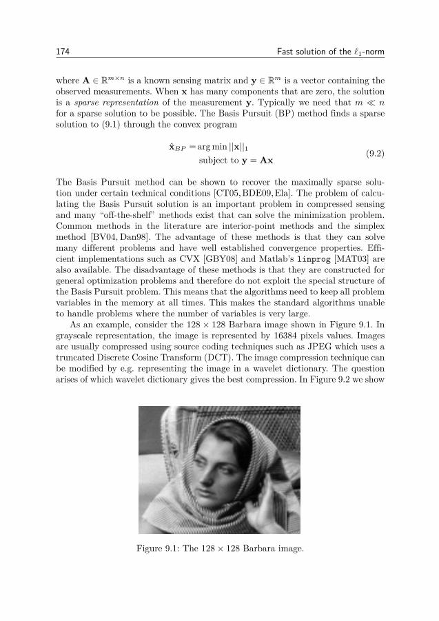
174 Fast solution of the `1-norm
where A ∈ Rm×n is a known sensing matrix and y ∈ Rm is a vector containing theobserved measurements. When x has many components that are zero, the solutionis a sparse representation of the measurement y. Typically we need that m nfor a sparse solution to be possible. The Basis Pursuit (BP) method finds a sparsesolution to (9.1) through the convex program
xBP = arg min ||x||1subject to y = Ax
(9.2)
The Basis Pursuit method can be shown to recover the maximally sparse solu-tion under certain technical conditions [CT05,BDE09,Ela]. The problem of calcu-lating the Basis Pursuit solution is an important problem in compressed sensingand many “off-the-shelf” methods exist that can solve the minimization problem.Common methods in the literature are interior-point methods and the simplexmethod [BV04, Dan98]. The advantage of these methods is that they can solvemany different problems and have well established convergence properties. Effi-cient implementations such as CVX [GBY08] and Matlab’s linprog [MAT03] arealso available. The disadvantage of these methods is that they are constructed forgeneral optimization problems and therefore do not exploit the special structure ofthe Basis Pursuit problem. This means that the algorithms need to keep all problemvariables in the memory at all times. This makes the standard algorithms unableto handle problems where the number of variables is very large.
As an example, consider the 128 × 128 Barbara image shown in Figure 9.1. Ingrayscale representation, the image is represented by 16384 pixels values. Imagesare usually compressed using source coding techniques such as JPEG which uses atruncated Discrete Cosine Transform (DCT). The image compression technique canbe modified by e.g. representing the image in a wavelet dictionary. The questionarises of which wavelet dictionary gives the best compression. In Figure 9.2 we show
Figure 9.1: The 128× 128 Barbara image.
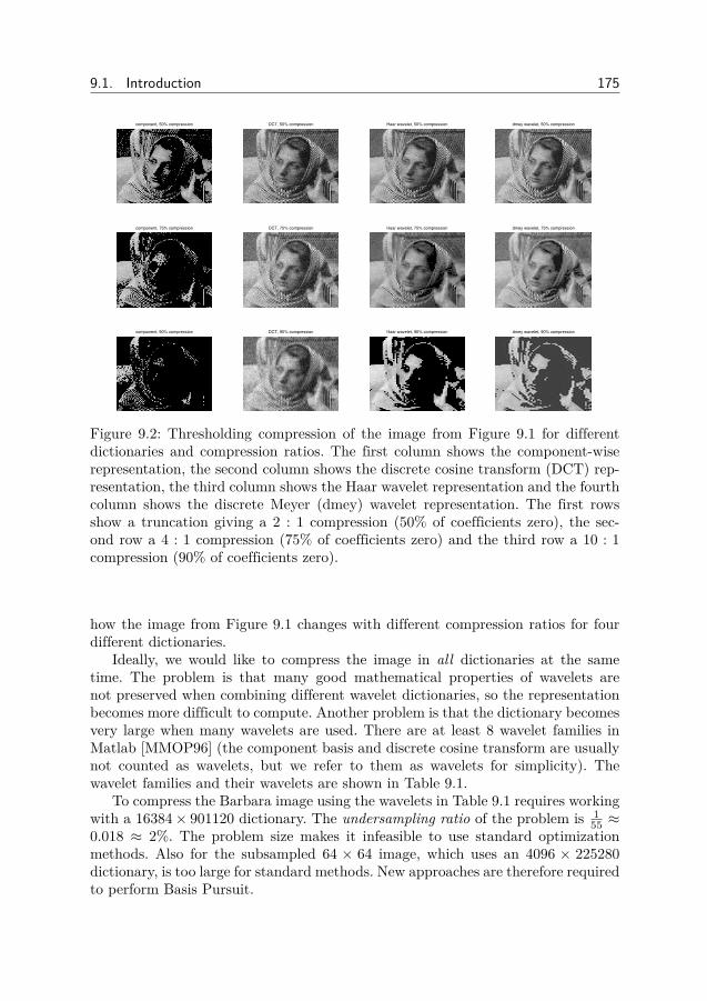
9.1. Introduction 175
component, 50% compression DCT, 50% compression Haar wavelet, 50% compression dmey wavelet, 50% compression
component, 75% compression DCT, 75% compression Haar wavelet, 75% compression dmey wavelet, 75% compression
component, 90% compression DCT, 90% compression Haar wavelet, 90% compression dmey wavelet, 90% compression
Figure 9.2: Thresholding compression of the image from Figure 9.1 for differentdictionaries and compression ratios. The first column shows the component-wiserepresentation, the second column shows the discrete cosine transform (DCT) rep-resentation, the third column shows the Haar wavelet representation and the fourthcolumn shows the discrete Meyer (dmey) wavelet representation. The first rowsshow a truncation giving a 2 : 1 compression (50% of coefficients zero), the sec-ond row a 4 : 1 compression (75% of coefficients zero) and the third row a 10 : 1compression (90% of coefficients zero).
how the image from Figure 9.1 changes with different compression ratios for fourdifferent dictionaries.
Ideally, we would like to compress the image in all dictionaries at the sametime. The problem is that many good mathematical properties of wavelets arenot preserved when combining different wavelet dictionaries, so the representationbecomes more difficult to compute. Another problem is that the dictionary becomesvery large when many wavelets are used. There are at least 8 wavelet families inMatlab [MMOP96] (the component basis and discrete cosine transform are usuallynot counted as wavelets, but we refer to them as wavelets for simplicity). Thewavelet families and their wavelets are shown in Table 9.1.
To compress the Barbara image using the wavelets in Table 9.1 requires workingwith a 16384× 901120 dictionary. The undersampling ratio of the problem is 1
55 ≈0.018 ≈ 2%. The problem size makes it infeasible to use standard optimizationmethods. Also for the subsampled 64 × 64 image, which uses an 4096 × 225280dictionary, is too large for standard methods. New approaches are therefore requiredto perform Basis Pursuit.
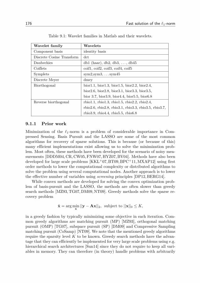
176 Fast solution of the `1-norm
Table 9.1: Wavelet families in Matlab and their wavelets.
Wavelet family WaveletsComponent basis identity basisDiscrete Cosine Transform dctDaubechies db1 (haar), db2, db3, . . . , db45Coiflets coif1, coif2, coif3, coif4, coif5Symplets sym2,sym3, . . . sym45Discrete Meyer dmeyBiorthogonal bior1.1, bior1.3, bior1.5, bior2.2, bior2.4,
bior2.6, bior2.8, bior3.1, bior3.3, bior3.5,bior 3.7, bior3.9, bior4.4, bior5.5, bior6.8
Reverse biorthogonal rbio1.1, rbio1.3, rbio1.5, rbio2.2, rbio2.4,rbio2.6, rbio2.8, rbio3.1, rbio3.3, rbio3.5, rbio3.7,rbio3.9, rbio4.4, rbio5.5, rbio6.8
9.1.1 Prior workMinimization of the `1-norm is a problem of considerable importance in Com-pressed Sensing. Basis Pursuit and the LASSO are some of the most commonalgorithms for recovery of sparse solutions. This is because (or because of this)many efficient implementations exist allowing us to solve the minimization prob-lem. Most often, these methods have been developed for the scenario of noisy mea-surements [DDDM04,CR,CW05,FNW07,HYZ07,BV04]. Methods have also beendeveloped for large scale problems [KKL+07,BT09,BPC+11,MXAP12] using firstorder methods to lower the computational complexity or distributed algorithms tosolve the problem using several computational nodes. Another approach is to lowerthe effective number of variables using screening principles [DP12,BERG14].
While convex methods are developed for solving the convex optimization prob-lem of basis-pursuit and the LASSO, the methods are often slower than greedysearch methods [MZ93,TG07,DM09,NT09]. Greedy methods solve the sparse re-covery problem
x = arg minx||y−Ax||2, subject to ||x||0 ≤ K,
in a greedy fashion by typically minimizing some objective in each iteration. Com-mon greedy algorithms are matching pursuit (MP) [MZ93], orthogonal matchingpursuit (OMP) [TG07], subspace pursuit (SP) [DM09] and Compressive Samplingmatching pursuit (CoSamp) [NT09]. We note that the mentioned greedy algorithmsrequire the sparsity level K to be known. Greedy search methods have the advan-tage that they can efficiently be implemented for very large scale problems using e.g.hierarchical search architectures [Sun14] since they do not require to keep all vari-ables in memory. They can therefore (in theory) handle problems with arbitrarily
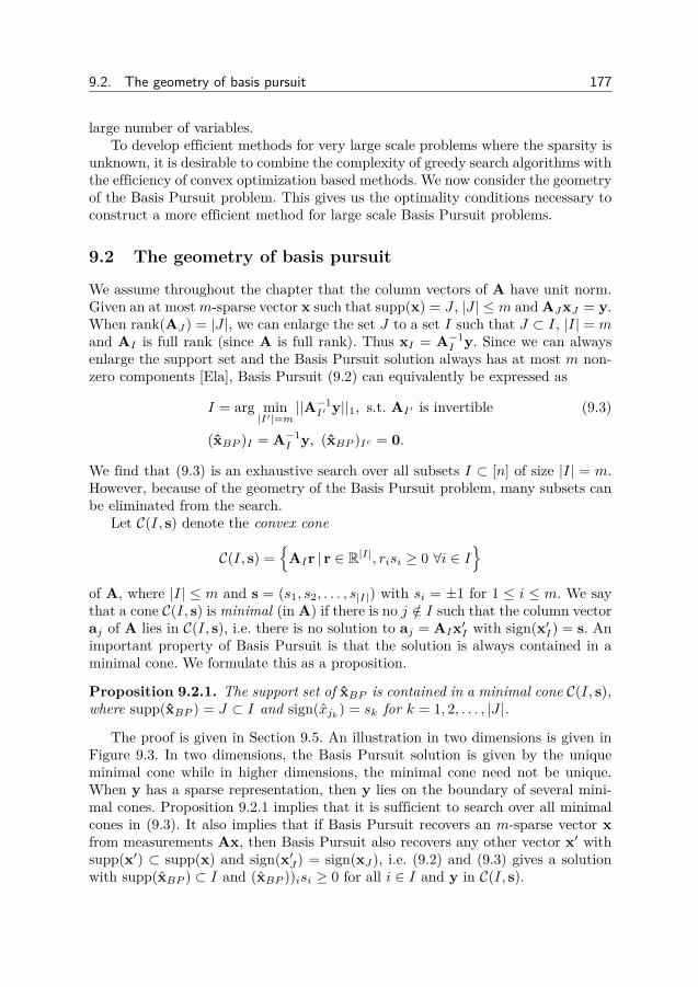
9.2. The geometry of basis pursuit 177
large number of variables.To develop efficient methods for very large scale problems where the sparsity is
unknown, it is desirable to combine the complexity of greedy search algorithms withthe efficiency of convex optimization based methods. We now consider the geometryof the Basis Pursuit problem. This gives us the optimality conditions necessary toconstruct a more efficient method for large scale Basis Pursuit problems.
9.2 The geometry of basis pursuit
We assume throughout the chapter that the column vectors of A have unit norm.Given an at mostm-sparse vector x such that supp(x) = J , |J | ≤ m and AJxJ = y.When rank(AJ) = |J |, we can enlarge the set J to a set I such that J ⊂ I, |I| = mand AI is full rank (since A is full rank). Thus xI = A−1
I y. Since we can alwaysenlarge the support set and the Basis Pursuit solution always has at most m non-zero components [Ela], Basis Pursuit (9.2) can equivalently be expressed as
I = arg min|I′|=m
||A−1I′ y||1, s.t. AI′ is invertible (9.3)
(xBP )I = A−1I y, (xBP )Ic = 0.
We find that (9.3) is an exhaustive search over all subsets I ⊂ [n] of size |I| = m.However, because of the geometry of the Basis Pursuit problem, many subsets canbe eliminated from the search.
Let C(I, s) denote the convex cone
C(I, s) =
AIr | r ∈ R|I|, risi ≥ 0 ∀i ∈ I
of A, where |I| ≤ m and s = (s1, s2, . . . , s|I|) with si = ±1 for 1 ≤ i ≤ m. We saythat a cone C(I, s) is minimal (in A) if there is no j /∈ I such that the column vectoraj of A lies in C(I, s), i.e. there is no solution to aj = AIx′I with sign(x′I) = s. Animportant property of Basis Pursuit is that the solution is always contained in aminimal cone. We formulate this as a proposition.
Proposition 9.2.1. The support set of xBP is contained in a minimal cone C(I, s),where supp(xBP ) = J ⊂ I and sign(xjk) = sk for k = 1, 2, . . . , |J |.
The proof is given in Section 9.5. An illustration in two dimensions is given inFigure 9.3. In two dimensions, the Basis Pursuit solution is given by the uniqueminimal cone while in higher dimensions, the minimal cone need not be unique.When y has a sparse representation, then y lies on the boundary of several mini-mal cones. Proposition 9.2.1 implies that it is sufficient to search over all minimalcones in (9.3). It also implies that if Basis Pursuit recovers an m-sparse vector xfrom measurements Ax, then Basis Pursuit also recovers any other vector x′ withsupp(x′) ⊂ supp(x) and sign(x′J) = sign(xJ), i.e. (9.2) and (9.3) gives a solutionwith supp(xBP ) ⊂ I and (xBP ))isi ≥ 0 for all i ∈ I and y in C(I, s).
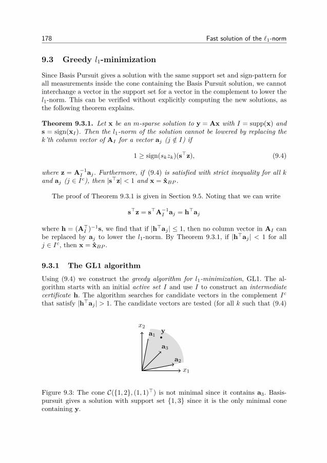
178 Fast solution of the `1-norm
9.3 Greedy l1-minimization
Since Basis Pursuit gives a solution with the same support set and sign-pattern forall measurements inside the cone containing the Basis Pursuit solution, we cannotinterchange a vector in the support set for a vector in the complement to lower thel1-norm. This can be verified without explicitly computing the new solutions, asthe following theorem explains.
Theorem 9.3.1. Let x be an m-sparse solution to y = Ax with I = supp(x) ands = sign(xI). Then the l1-norm of the solution cannot be lowered by replacing thek’th column vector of AI for a vector aj (j /∈ I) if
1 ≥ sign(skzk)(s>z), (9.4)
where z = A−1I aj. Furthermore, if (9.4) is satisfied with strict inequality for all k
and aj (j ∈ Ic), then |s>z| < 1 and x = xBP .
The proof of Theorem 9.3.1 is given in Section 9.5. Noting that we can write
s>z = s>A−1I aj = h>aj
where h = (A>I )−1s, we find that if |h>aj | ≤ 1, then no column vector in AI canbe replaced by aj to lower the l1-norm. By Theorem 9.3.1, if |h>aj | < 1 for allj ∈ Ic, then x = xBP .
9.3.1 The GL1 algorithm
Using (9.4) we construct the greedy algorithm for l1-minimization, GL1. The al-gorithm starts with an initial active set I and use I to construct an intermediatecertificate h. The algorithm searches for candidate vectors in the complement Icthat satisfy |h>aj | > 1. The candidate vectors are tested (for all k such that (9.4)
x1
x2a1
a2
a3
•y
Figure 9.3: The cone C(1, 2, (1, 1)>) is not minimal since it contains a3. Basis-pursuit gives a solution with support set 1, 3 since it is the only minimal conecontaining y.
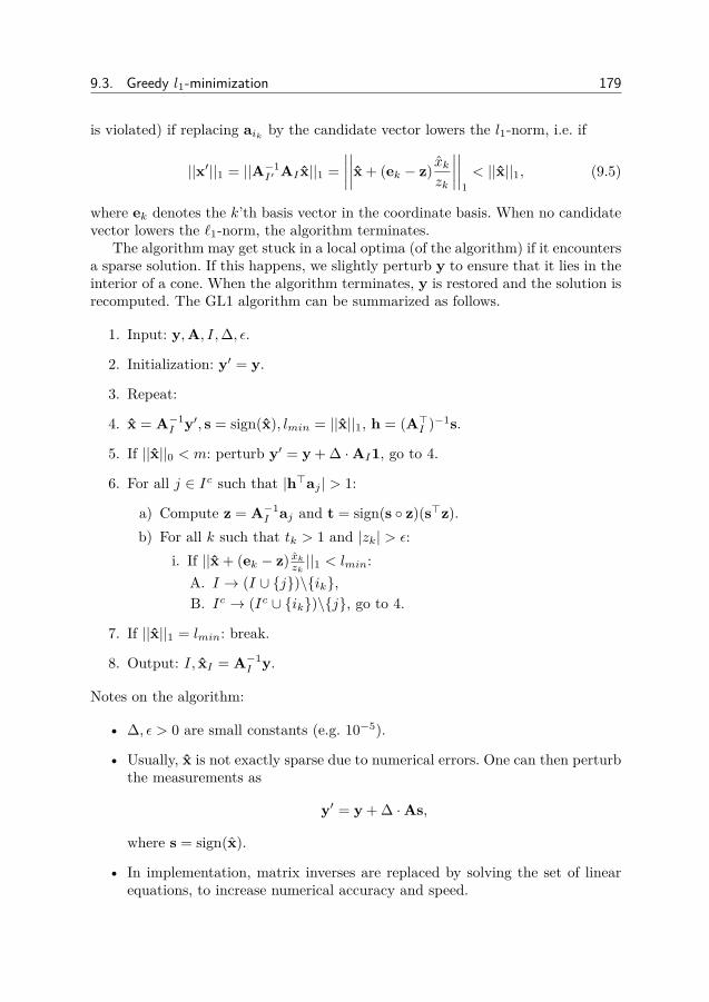
9.3. Greedy l1-minimization 179
is violated) if replacing aik by the candidate vector lowers the l1-norm, i.e. if
||x′||1 = ||A−1I′ AI x||1 =
∣∣∣∣∣∣∣∣x + (ek − z) xkzk
∣∣∣∣∣∣∣∣1< ||x||1, (9.5)
where ek denotes the k’th basis vector in the coordinate basis. When no candidatevector lowers the `1-norm, the algorithm terminates.
The algorithm may get stuck in a local optima (of the algorithm) if it encountersa sparse solution. If this happens, we slightly perturb y to ensure that it lies in theinterior of a cone. When the algorithm terminates, y is restored and the solution isrecomputed. The GL1 algorithm can be summarized as follows.
1. Input: y,A, I,∆, ε.
2. Initialization: y′ = y.
3. Repeat:
4. x = A−1I y′, s = sign(x), lmin = ||x||1, h = (A>I )−1s.
5. If ||x||0 < m: perturb y′ = y + ∆ ·AI1, go to 4.
6. For all j ∈ Ic such that |h>aj | > 1:
a) Compute z = A−1I aj and t = sign(s z)(s>z).
b) For all k such that tk > 1 and |zk| > ε:i. If ||x + (ek − z) xkzk ||1 < lmin:
A. I → (I ∪ j)\ik,B. Ic → (Ic ∪ ik)\j, go to 4.
7. If ||x||1 = lmin: break.
8. Output: I, xI = A−1I y.
Notes on the algorithm:
• ∆, ε > 0 are small constants (e.g. 10−5).
• Usually, x is not exactly sparse due to numerical errors. One can then perturbthe measurements as
y′ = y + ∆ ·As,
where s = sign(x).
• In implementation, matrix inverses are replaced by solving the set of linearequations, to increase numerical accuracy and speed.
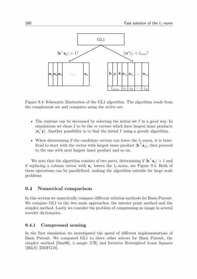
180 Fast solution of the `1-norm
a1 a2 a3 . . . an
GL1
|h>aj | > 1? ||x′||1 < lmin?
h y x ai1 ai2 . . . aim
lmin i1 i2 . . . im
Figure 9.4: Schematic illustration of the GL1 algorithm. The algorithm reads fromthe complement set and computes using the active set.
• The runtime can be decreased by selecting the initial set I in a good way. Insimulations we chose I to be the m vectors which have largest inner products|a>i y|. Another possibility is to find the initial I using a greedy algorithm.
• When determining if the candidate vectors can lower the l1-norm, it is bene-ficial to start with the vector with largest inner product |h>aj |, then proceedto the one with next largest inner product and so on.
We note that the algorithm consists of two parts, determining if |h>aj | > 1 andif replacing a column vector with aj lowers the l1-norm, see Figure 9.4. Both ofthese operations can be parallelized, making the algorithm suitable for large scaleproblems.
9.4 Numerical comparison
In this section we numerically compare different solution methods for Basis Pursuit.We compare GL1 to the two main approaches, the interior point method and thesimplex method. Lastly we consider the problem of compressing an image in severalwavelet dictionaries.
9.4.1 Compressed sensing
In the first simulation we investigated the speed of different implementations ofBasis Pursuit. We compared GL1 to three other solvers for Basis Pursuit, thesimplex method [Dan98], l1-magic [CR] and Iterative Reweighted Least Squares(IRLS) [DDFG10].

9.4. Numerical comparison 181
0 5 10 15 20 25
10
15
20
25
cputime [seconds]
l 1-norm
SimplexGL1
l1-magicIRLS
Figure 9.5: l1-norm vs. cputime for one problem realization for the different methodswhen n = 8000 and m = 50.
The Simplex method formulates (9.2) as
min 1>(x+ + x−),s.t. y = A(x+ − x−)
x+,x− ≥ 0
where 1 ∈ Rn is a vector of ones and we used Matlab’s linprog to run the simplexalgorithm. The method l1-magic formulates (9.2) as
min 1>ts.t. y = Ax
− ti ≤ xi ≤ ti, for i = 1, 2, . . . , n
and solves the optimization problem using a primal-dual interior point method [CR].The IRLS algorithm approximates the l1-norm by a weighted l2-norm which isupdated iteratively [DDFG10].
In the simulation we used n = 8000 and varied the number of measurements m.The measurements were generated by drawing the elements of A from a N (0, 1)distribution and normalizing the column vectors, the vector x was generated as ad0.25me-sparse vector with its non-zero elements drawn from a N (0, 1) distribu-tion. Finally we computed y = Ax and compute the solution using the differentalgorithms. Because A is Gaussian, xBP in (9.2) is unique with probability 1.
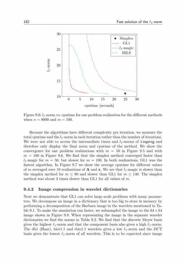
182 Fast solution of the `1-norm
0 5 10 15 20 25 3010
15
20
25
30
cputime [seconds]
l 1-norm
SimplexGL1
l1-magicIRLS
Figure 9.6: l1-norm vs. cputime for one problem realization for the different methodswhen n = 8000 and m = 100.
Because the algorithms have different complexity per iteration, we measure thetotal cputime and the l1-norm in each iteration rather than the number of iterations.We were not able to access the intermediate times and l1-norms of linprog andtherefore only display the final norm and cputime of the method. We show theconvergence for one problem realizations with m = 50 in Figure 9.5 and withm = 100 in Figure 9.6. We find that the simplex method converged faster thanl1-magic for m = 50, but slower for m = 100. In both realizations, GL1 was thefastest algorithm. In Figure 9.7 we show the average cputime for different valuesof m averaged over 10 realizations of A and x. We see that l1-magic is slower thanthe simplex method for m ≤ 80 and slower than GL1 for m ≤ 140. The simplexmethod was about 3 times slower than GL1 for all values of m.
9.4.2 Image compression in wavelet dictionariesNext we demonstrate that GL1 can solve large scale problems with many parame-ters. We decompose an image in a dictionary that is too big to store in memory byperforming a decomposition of the Barbara image in the wavelets mentioned in Ta-ble 9.1. To make the simulation run faster, we subsampled the image to the 64×64image shown in Figure 9.8. When representing the image in the separate waveletdictionaries we find the norms in Table 9.2. We find that the discrete Meyer basisgives the highest `1-norm and that the component basis also gives a high `1-norm.The db1 (Haar), bior1.1 and rbio1.1 wavelets gives a low `1-norm and the DCTbasis gives the lowest `1-norm of all wavelets. This is to be expected since image
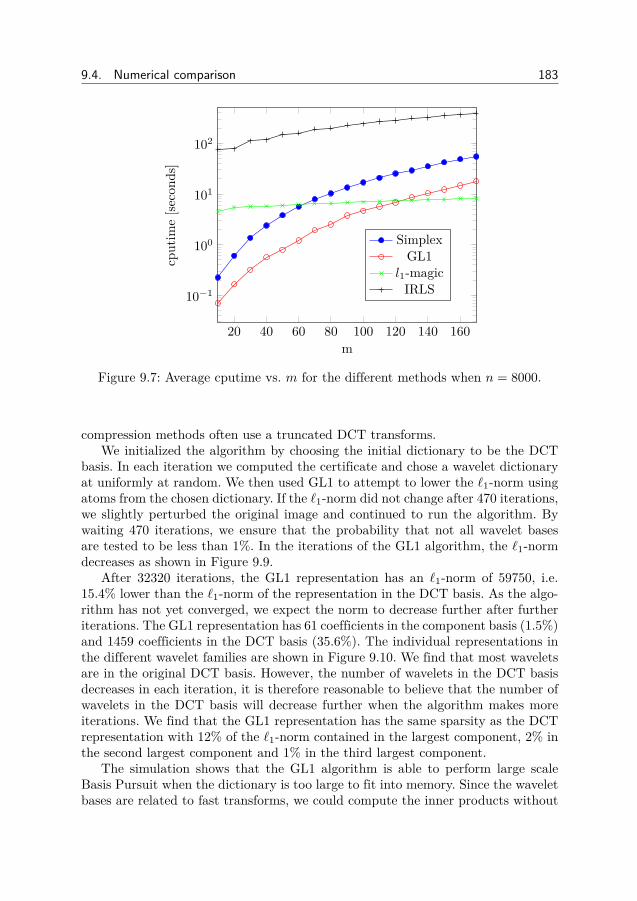
9.4. Numerical comparison 183
20 40 60 80 100 120 140 160
10−1
100
101
102
m
cputim
e[se
cond
s]
SimplexGL1
l1-magicIRLS
Figure 9.7: Average cputime vs. m for the different methods when n = 8000.
compression methods often use a truncated DCT transforms.We initialized the algorithm by choosing the initial dictionary to be the DCT
basis. In each iteration we computed the certificate and chose a wavelet dictionaryat uniformly at random. We then used GL1 to attempt to lower the `1-norm usingatoms from the chosen dictionary. If the `1-norm did not change after 470 iterations,we slightly perturbed the original image and continued to run the algorithm. Bywaiting 470 iterations, we ensure that the probability that not all wavelet basesare tested to be less than 1%. In the iterations of the GL1 algorithm, the `1-normdecreases as shown in Figure 9.9.
After 32320 iterations, the GL1 representation has an `1-norm of 59750, i.e.15.4% lower than the `1-norm of the representation in the DCT basis. As the algo-rithm has not yet converged, we expect the norm to decrease further after furtheriterations. The GL1 representation has 61 coefficients in the component basis (1.5%)and 1459 coefficients in the DCT basis (35.6%). The individual representations inthe different wavelet families are shown in Figure 9.10. We find that most waveletsare in the original DCT basis. However, the number of wavelets in the DCT basisdecreases in each iteration, it is therefore reasonable to believe that the number ofwavelets in the DCT basis will decrease further when the algorithm makes moreiterations. We find that the GL1 representation has the same sparsity as the DCTrepresentation with 12% of the `1-norm contained in the largest component, 2% inthe second largest component and 1% in the third largest component.
The simulation shows that the GL1 algorithm is able to perform large scaleBasis Pursuit when the dictionary is too large to fit into memory. Since the waveletbases are related to fast transforms, we could compute the inner products without
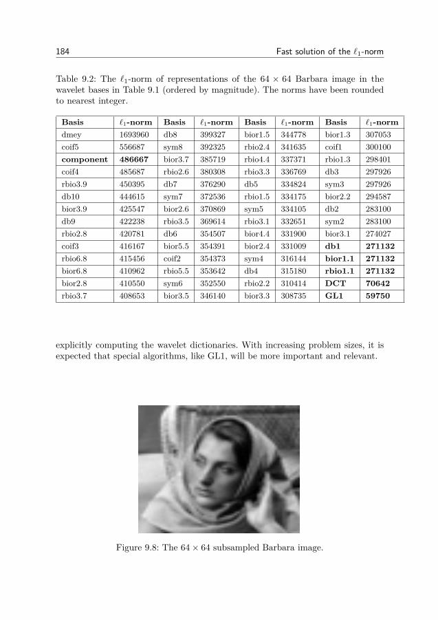
184 Fast solution of the `1-norm
Table 9.2: The `1-norm of representations of the 64 × 64 Barbara image in thewavelet bases in Table 9.1 (ordered by magnitude). The norms have been roundedto nearest integer.
Basis `1-norm Basis `1-norm Basis `1-norm Basis `1-normdmey 1693960 db8 399327 bior1.5 344778 bior1.3 307053coif5 556687 sym8 392325 rbio2.4 341635 coif1 300100component 486667 bior3.7 385719 rbio4.4 337371 rbio1.3 298401coif4 485687 rbio2.6 380308 rbio3.3 336769 db3 297926rbio3.9 450395 db7 376290 db5 334824 sym3 297926db10 444615 sym7 372536 rbio1.5 334175 bior2.2 294587bior3.9 425547 bior2.6 370869 sym5 334105 db2 283100db9 422238 rbio3.5 369614 rbio3.1 332651 sym2 283100rbio2.8 420781 db6 354507 bior4.4 331900 bior3.1 274027coif3 416167 bior5.5 354391 bior2.4 331009 db1 271132rbio6.8 415456 coif2 354373 sym4 316144 bior1.1 271132bior6.8 410962 rbio5.5 353642 db4 315180 rbio1.1 271132bior2.8 410550 sym6 352550 rbio2.2 310414 DCT 70642rbio3.7 408653 bior3.5 346140 bior3.3 308735 GL1 59750
explicitly computing the wavelet dictionaries. With increasing problem sizes, it isexpected that special algorithms, like GL1, will be more important and relevant.
Figure 9.8: The 64× 64 subsampled Barbara image.

9.5. Derivations and proofs 185
0 0.5 1 1.5 2 2.5 3
x 104
5.8
6
6.2
6.4
6.6
6.8
7
7.2x 10
4
Iteration
l1−
norm
GL1
DCT
Figure 9.9: The `1-norm of the GL1 representation of the 64× 64 Barbara image indifferent iterations. The `1-norm of the representation in the DCT basis is shownas a dashed line.
9.5 Derivations and proofs
Proof of proposition 1. Let I be a set with m elements and let I ′ = (I\k) ∪ j.We need to show that if y ∈ C(I ′, s′) ⊂ C(I, s), then ||xI′ ||1 < ||xI ||1. Set
y =∑i∈I
xiai, (9.6)
aj =∑i∈I
ziai, (9.7)
y = x′jaj +∑
i∈I,i6=kx′iai. (9.8)
Without loss of generality we can assume that xi, zi, x′i ≥ 0 for all i ∈ I ∪ j . Byinserting (9.7) into (9.8) we find that
x′jaj +∑
i∈I,i6=kx′iai = x′jzkak +
∑i∈I,i6=k
(x′i + x′jzi)ai =∑i∈I
xiai.

186 Fast solution of the `1-norm
Component DCT db coif
sym dmey bior rbio
Figure 9.10: The GL1 representation of the 64 × 64 Barbara image after 32320iterations in the wavelet families from Table 9.1.
We find that when AI is full rank, then xk = x′jzk and xi = x′i + x′jzi for i 6= k.Using that
1 = ||aj ||2 <∑i∈I|zi| · ||ai||2 = ||z||1,
where we have strict inequality because the column vectors in AI are not parallel,we find that
||x||1 =∑i∈I
xi = x′jzk +∑
i∈I,i6=k(x′i + x′jzi)
= x′j∑i∈I
zi +∑
i∈I,i6=kx′i
= x′j(||z||1 − 1) + ||x′||1 > ||x′||1,
provided that x′j > 0.
Proof of Theorem 1. Assume that we cannot interchange the k’th column vectorof AI for a vector aj to get a solution with lower l1-norm. Then all y in C(I, s)give Basis Pursuit solutions with the same support set and sign-pattern, i.e. for allw ∈ Rm, w ≥ 0
||w||1 ≤ ||A−1I′ AISw||1, (9.9)
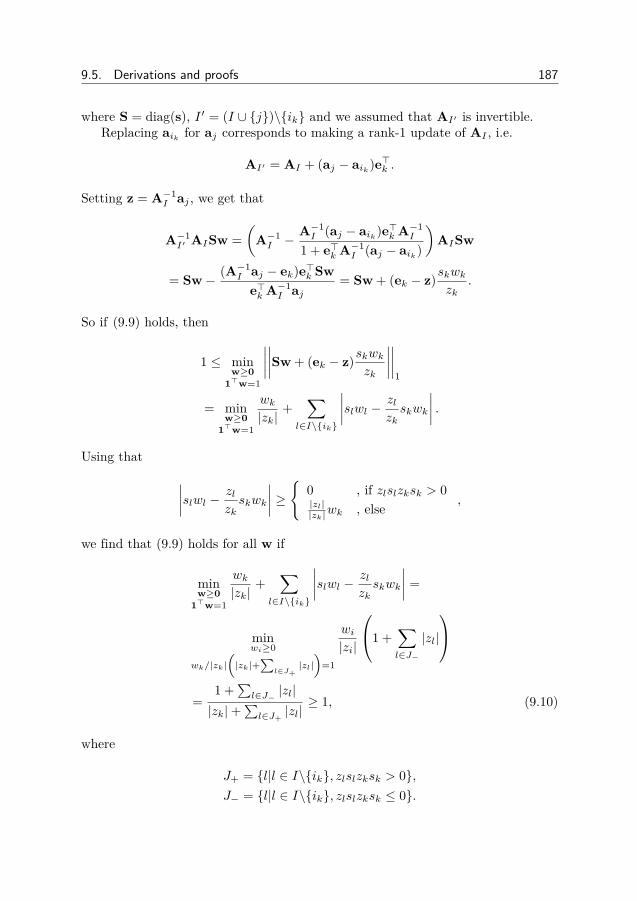
9.5. Derivations and proofs 187
where S = diag(s), I ′ = (I ∪ j)\ik and we assumed that AI′ is invertible.Replacing aik for aj corresponds to making a rank-1 update of AI , i.e.
AI′ = AI + (aj − aik)e>k .
Setting z = A−1I aj , we get that
A−1I′ AISw =
(A−1I −
A−1I (aj − aik)e>k A−1
I
1 + e>k A−1I (aj − aik)
)AISw
= Sw− (A−1I aj − ek)e>k Sw
e>k A−1I aj
= Sw + (ek − z)skwkzk
.
So if (9.9) holds, then
1 ≤ minw≥0
1>w=1
∣∣∣∣∣∣∣∣Sw + (ek − z)skwkzk
∣∣∣∣∣∣∣∣1
= minw≥0
1>w=1
wk|zk|
+∑
l∈I\ik
∣∣∣∣slwl − zlzkskwk
∣∣∣∣ .Using that ∣∣∣∣slwl − zl
zkskwk
∣∣∣∣ ≥
0 , if zlslzksk > 0|zl||zk|wk , else
,
we find that (9.9) holds for all w if
minw≥0
1>w=1
wk|zk|
+∑
l∈I\ik
∣∣∣∣slwl − zlzkskwk
∣∣∣∣ =
minwi≥0
wk/|zk|(|zk|+
∑l∈J+
|zl|)
=1
wi|zi|
1 +∑l∈J−
|zl|
=1 +
∑l∈J− |zl|
|zk|+∑l∈J+
|zl|≥ 1, (9.10)
where
J+ = l|l ∈ I\ik, zlslzksk > 0,J− = l|l ∈ I\ik, zlslzksk ≤ 0.

188 Fast solution of the `1-norm
Rewriting (9.10) as ∑l:zlslzksk>0
|zl| ≤ 1 +∑
l:zlslzksk≤0|zl|
⇔ 1 ≥∑l
sign(zlslzksk)|zl|
= sign(zksk)∑l
slzl = sign(zksk)(s>I z),
we recover the optimality condition (9.4).To show that strict inequality in (9.4) implies that |s>z| < 1, assume that
|s>z| ≥ 1, but sign(skzk)(s>z) < 1 for all k. This implies that sign(skzk) =−sign(s>z) for all k. However, if all terms skzk have the same sign, then sign(skzk) =sign(s>z), giving a contradiction. Thus, strict inequality in (9.4) implies that |s>z| <1.
We find that
s>z = s>A−1I aj = h>aj
where h = (A>I )−1s. This gives that if |h>aj | < 1 for all j ∈ Ic, then A>I h = sand ||A>Ich||∞ < 1. The vector h is thus the dual certificate of the Basis Pursuitsolution [ZYC15], giving us that x = xBP .
9.6 Conclusion
In this chapter we considered the problem of solving the Basis Pursuit problemwhen the number of parameters is very large. Standard methods are efficient forsolving the Basis Pursuit problem, but do not scale well when the number of pa-rameters becomes very large. By considering the geometry of the problem we wereable to derive optimality conditions for the Basis Pursuit solution. The optimalityconditions were then used to construct the greedy minimization method GL1. Thealgorithm has the advantage that it does not need to keep all variables in memory,but only works with a subset of the parameters in each iteration. Through numer-ical simulations we showed that the algorithm is faster than the standard methodswhen the number of parameters is large. We also showed that the algorithm isable to perform the wavelet decomposition of an 64 × 64 image in several waveletdictionaries.
Chapter 10
Conclusion
As the amount of data and measurements increases, so does also the assistancewe can receive from it to make well informed decisions. To make good use of thedata we need good algorithms to help us process the data to provide us with theinformation we seek. Such algorithms needs to be fast, efficient and accurate. Tomeet such standards it is useful to exploit the internal structures of the problem toincrease the performance and usability of the algorithms. Two of the most studiedstructures in compressed sensing is sparse vectors and low-rank matrices. Theseare the structures we have studied in this thesis. We used three approaches todesigning estimation algorithms, greedy search algorithms, Bayesian methods andconvex optimization based methods.
In Chapter 3 we considered greedy pursuit algorithms and how the way thealgorithms detect non-zero components can be improved. We used two approaches,array processing and Bayesian filtering. In array processing, it is customary tocancel the contributions from sidelobes occurring in the problem to increase theresolution of the system. This is done using a beamformer, i.e. a linear filter whichfilters out the contribution of the sidelobes. With this methodology we were ableto construct beamformers for the worst-case and average case detection scenario.Bayesian filtering often rely on linear filters to decrease the interference and noise.The Wiener filter is the optimal filter in the mean square sense and is heavilyused in signal processing. By designing a Wiener filter for random sparse vectorsconditioned on if a component is zero or not, we developed the Conditional priorOMP algorithm.
In Chapters 4, 5 and 6 we investigated Bayesian methods based on the Rele-vance Vector Machine (RVM). Bayesian methods use prior distributions to modelthe structure of the parameters. The difficulty is to model the structure in an appro-priate way as the distribution should be continuous to give a tractable model whilethe structure often is non-continuous in nature. In Chapter 4 we showed how theRVM can be adapted to measurements with sparse noise without treating the noiseas an additional estimation parameter. We showed that this increase the speed andaccuracy of the algorithm. In Chapter 5 we used precision matrices to construct a
189
190 Conclusion
low-rank analogue of the RVM and related the prior distribution of the precisionmatrices to low-rank promoting penalty functions. In Chapter 6 we combined themethods of Chapter 4 and 5 to construct a Bayesian method for robust principalcomponent analysis. We showed that the method can outperform standard methodsbut that this comes at the price of higher complexity.
In Chapter 8 we considered how low-rank can be incorporated in the phaseretrieval problem. We showed that by using the theory of Kronecker product ap-proximation, it is possible to promote rank in the underlying variable. Throughnumerical simulations we showed that by properly selecting the regularization pa-rameter, it is possible to recover low-rank at fewer measurements than the with thestandard method.
Lastly, in Chapter 9 we considered the big data problem of constructing a sparserepresentation when the number of parameters is very large. As standard optimiza-tion methods require all parameters to be kept in memory, the large number ofparameters in the problems we consider make such methods infeasible. By derivingoptimality conditions for the solution, we construct a greedy method for solvingthe `1-norm minimization problem. The proposed method is faster than standardmethods when the number of measurements is not too large and is able to performwavelet decomposition on a 128× 128 image in all wavelets in Matlab.
The methods used for compressed sensing are often divided into their respec-tive classes, greedy, Bayesian and convex methods. In this thesis we have combinedapproaches to construct new methods. Chapter 3 combined greedy and Bayesianmethods while Chapter 9 combines greedy and convex methods. The multitude ofmethods show that sparse and low-rank problems is a fascinating research areawhere methods from computer science, signal processing, machine learning and re-gression can be combined to give new insights into structured estimation problems.As every new solution gives rise to new problems to be explored. It is quite certainthat different approaches can be further connected and that one method can solvethe challenges presented by another method. As estimation methods and signal pro-cessing algorithms continue to improve, we have new possibilities to further developnew technology and new science for the future.
Bibliography
[ADFDJ03] C. Andrieu, N. De Freitas, A. Doucet, and M. I. Jordan, “An intro-duction to mcmc for machine learning,” Machine learning, vol. 50, no.1-2, pp. 5–43, 2003.
[Alq13] P. Alquier, “Bayesian methods for low-rank matrix estimation: Shortsurvey and theoretical study,” in Algorithmic Learning Theory.Springer, 2013, pp. 309–323.
[AN07] A. Asuncion and D. Newman, “UCI machine learning repository,”2007.
[Bar11] R. G. Baraniuk, “More is less: signal processing and the data deluge,”Science, vol. 331, no. 6018, pp. 717–719, 2011.
[BCDH10] R. G. Baraniuk, V. Cevher, M. F. Duarte, and C. Hegde, “Model-based compressive sensing,” Information Theory, IEEE Transactionson, vol. 56, no. 4, pp. 1982–2001, 2010.
[BCMN14] A. S. Bandeira, J. Cahill, D. G. Mixon, and A. A. Nelson, “Savingphase: Injectivity and stability for phase retrieval,” Applied and Com-putational Harmonic Analysis, vol. 37, no. 1, pp. 106–125, 2014.
[BD08] T. Blumensath and M. E. Davies, “In greedy pursuit of new direc-tions:(nearly) orthogonal matching pursuit by directional optimisa-tion,” in Proc. European Signal Processing Conference (EUSIPCO),2008.
[BDE09] A. M. Bruckstein, D. L. Donoho, and M. Elad, “From sparse solutionsof systems of equations to sparse modeling of signals and images,”SIAM review, vol. 51, no. 1, pp. 34–81, 2009.
[BERG14] A. Bonnefoy, V. Emiya, L. Ralaivola, and R. Gribonval, “A dynamicscreening principle for the lasso,” in Signal Processing Conference (EU-SIPCO), 2014 Proceedings of the 22nd European. IEEE, 2014, pp.6–10.
[BGJM11] S. Brooks, A. Gelman, G. Jones, and X.-L. Meng, Handbook of MarkovChain Monte Carlo. CRC press, 2011.
191

192 Bibliography
[Bis06] C. M. Bishop, Pattern recognition and machine learning. SpringerNew York, 2006, vol. 4, no. 4.
[BL10] G. Bergqvist and E. G. Larsson, “The higher-order singular value de-composition: theory and an application [lecture notes],” IEEE SignalProcessing Magazine, vol. 27, no. 3, pp. 151–154, 2010.
[BLMK12] S. D. Babacan, M. Luessi, R. Molina, and A. K. Katsaggelos, “Sparsebayesian methods for low-rank matrix estimation,” Signal Processing,IEEE Transactions on, vol. 60, no. 8, pp. 3964–3977, 2012.
[BPC+11] S. Boyd, N. Parikh, E. Chu, B. Peleato, and J. Eckstein, “Dis-tributed optimization and statistical learning via the alternating di-rection method of multipliers,” Foundations and Trends® in MachineLearning, vol. 3, no. 1, pp. 1–122, 2011.
[BS80] A. Borovkov and A. Sakhanienko, “On estimates of the expectedquadratic risk,” Probab. Math. Statist, vol. 1, pp. 185–195, 1980.
[BT09] A. Beck and M. Teboulle, “A fast iterative shrinkage-thresholding algo-rithm for linear inverse problems,” SIAM journal on imaging sciences,vol. 2, no. 1, pp. 183–202, 2009.
[BV04] S. Boyd and L. Vandenberghe, Convex optimization. Cambridge uni-versity press, 2004.
[CCG15] Y. Chen, Y. Chi, and A. J. Goldsmith, “Exact and stable covarianceestimation from quadratic sampling via convex programming,” IEEETransactions on Information Theory, vol. 61, no. 7, pp. 4034–4059,2015.
[CDS01] S. S. Chen, D. L. Donoho, and M. A. Saunders, “Atomic decompositionby basis pursuit,” SIAM review, vol. 43, no. 1, pp. 129–159, 2001.
[CESV15] E. J. Candès, Y. C. Eldar, T. Strohmer, and V. Voroninski, “Phaseretrieval via matrix completion,” SIAM Review, vol. 57, no. 2, pp.225–251, 2015.
[CLMW11] E. J. Candès, X. Li, Y. Ma, and J. Wright, “Robust principal compo-nent analysis?” Journal of the ACM, vol. 58, no. 3, p. 11, 2011.
[CNZ05] P.-A. Chirita, W. Nejdl, and C. Zamfir, “Preventing shilling attacks inonline recommender systems,” in Proceedings of the 7th annual ACMinternational workshop on Web information and data management.ACM, 2005, pp. 67–74.
[CP10] E. J. Candès and Y. Plan, “Matrix completion with noise,” Proceedingsof the IEEE, vol. 98, no. 6, pp. 925–936, 2010.
Bibliography 193
[CP11] ——, “Tight oracle inequalities for low-rank matrix recovery from aminimal number of noisy random measurements,” Information Theory,IEEE Transactions on, vol. 57, no. 4, pp. 2342–2359, 2011.
[CR] E. Candès and J. Romberg, “l1-magic: Recovery of sparsesignals via convex programming,” URL: www. acm. caltech.edu/l1magic/downloads/l1magic. pdf.
[CR09] E. J. Candès and B. Recht, “Exact matrix completion via convex op-timization,” Foundations of Computational mathematics, vol. 9, no. 6,pp. 717–772, 2009.
[Cra47] H. Cramér, “Mathematical methods of statistics,” 1947.
[CRPW12] V. Chandrasekaran, B. Recht, P. A. Parrilo, and A. S. Willsky, “Theconvex geometry of linear inverse problems,” Foundations of Compu-tational mathematics, vol. 12, no. 6, pp. 805–849, 2012.
[CRT06] E. J. Candès, J. K. Romberg, and T. Tao, “Stable signal recovery fromincomplete and inaccurate measurements,” Communications on pureand applied mathematics, vol. 59, no. 8, pp. 1207–1223, 2006.
[CSGC15] A. Casamitjana, M. Sundin, P. Ghosh, and S. Chatterjee, “Bayesianlearning for time-varying linear prediction of speech,” in Signal Pro-cessing Conference (EUSIPCO), 2015 23rd European. IEEE, 2015,pp. 325–329.
[CSPW11] V. Chandrasekaran, S. Sanghavi, P. A. Parrilo, and A. S. Willsky,“Rank-sparsity incoherence for matrix decomposition,” SIAM Journalon Optimization, vol. 21, no. 2, pp. 572–596, 2011.
[CSS11] S. Chatterjee, D. Sundman, and M. Skoglund, “Robust matching pur-suit for recovery of gaussian sparse signal,” in Digital Signal Pro-cessing Workshop and IEEE Signal Processing Education Workshop(DSP/SPE), 2011 IEEE. IEEE, 2011, pp. 420–424.
[CSVS11] S. Chatterjee, D. Sundman, M. Vehkapera, and M. Skoglund, “Hybridgreedy pursuit,” in Signal Processing Conference, 2011 19th European.IEEE, 2011, pp. 343–347.
[CSVS12] S. Chatterjee, D. Sundman, M. Vehkapera, and M. Skoglund,“Projection-based and look-ahead strategies for atom selection,” SignalProcessing, IEEE Transactions on, vol. 60, no. 2, pp. 634–647, 2012.
[CT05] E. J. Candès and T. Tao, “Decoding by linear programming,” IEEEtransactions on information theory, vol. 51, no. 12, pp. 4203–4215,2005.
194 Bibliography
[CT10] ——, “The power of convex relaxation: Near-optimal matrix comple-tion,” Information Theory, IEEE Transactions on, vol. 56, no. 5, pp.2053–2080, 2010.
[CW05] P. L. Combettes and V. R. Wajs, “Signal recovery by proximal forward-backward splitting,” Multiscale Modeling & Simulation, vol. 4, no. 4,pp. 1168–1200, 2005.
[CW08] E. J. Candès and M. B. Wakin, “An introduction to compressive sam-pling,” Signal Processing Magazine, IEEE, vol. 25, no. 2, pp. 21–30,2008.
[CWZY15] P. Chen, N. Wang, N. L. Zhang, and D.-Y. Yeung, “Bayesian adaptivematrix factorization with automatic model selection,” in Proceedingsof the IEEE Conference on Computer Vision and Pattern Recognition,2015, pp. 1284–1292.
[Dan98] G. B. Dantzig, Linear programming and extensions. Princeton uni-versity press, 1998.
[DDDM04] I. Daubechies, M. Defrise, and C. De Mol, “An iterative threshold-ing algorithm for linear inverse problems with a sparsity constraint,”Communications on pure and applied mathematics, vol. 57, no. 11, pp.1413–1457, 2004.
[DDFG10] I. Daubechies, R. DeVore, M. Fornasier, and C. S. Gunturk, “Iterativelyreweighted least squares minimization for sparse recovery,” Communi-cations on Pure and Applied Mathematics, vol. 63, no. 1, pp. 1–38,2010.
[DF02] A. C. Doyle and C. Frayling, The hound of the Baskervilles. PenguinUK, 1902.
[DHC11] X. Ding, L. He, and L. Carin, “Bayesian robust principal componentanalysis,” IEEE Transactions on Image Processing, vol. 20, no. 12, pp.3419–3430, 2011.
[DLR77] A. P. Dempster, N. M. Laird, and D. B. Rubin, “Maximum likelihoodfrom incomplete data via the em algorithm,” Journal of the royal sta-tistical society. Series B (methodological), pp. 1–38, 1977.
[DM09] W. Dai and O. Milenkovic, “Subspace pursuit for compressive sens-ing signal reconstruction,” Information Theory, IEEE Transactions on,vol. 55, no. 5, pp. 2230–2249, 2009.
[Doy94] A. C. Doyle, A scandal in Bohemia. Springer, 1994.

Bibliography 195
[DP12] L. Dai and K. Pelckmans, “An ellipsoid based, two-stage screening testfor bpdn,” in Signal Processing Conference (EUSIPCO), 2012 Proceed-ings of the 20th European. IEEE, 2012, pp. 654–658.
[EA06] M. Elad and M. Aharon, “Image denoising via sparse and redundantrepresentations over learned dictionaries,” Image Processing, IEEETransactions on, vol. 15, no. 12, pp. 3736–3745, 2006.
[Ela] M. Elad, Sparse and Redundant Representations: From Theory to Ap-plications in Signal and Image Processing.
[EM14] Y. C. Eldar and S. Mendelson, “Phase retrieval: Stability and recoveryguarantees,” Applied and Computational Harmonic Analysis, vol. 36,no. 3, pp. 473–494, 2014.
[EY09] M. Elad and I. Yavneh, “A plurality of sparse representations is betterthan the sparsest one alone,” Information Theory, IEEE Transactionson, vol. 55, no. 10, pp. 4701–4714, 2009.
[Faz02] M. Fazel, “Matrix rank minimization with applications,” Ph.D. disser-tation, PhD thesis, Stanford University, 2002.
[Fie78] J. R. Fienup, “Reconstruction of an object from the modulus of itsfourier transform,” Optics letters, vol. 3, no. 1, pp. 27–29, 1978.
[FNW07] M. A. Figueiredo, R. D. Nowak, and S. J. Wright, “Gradient projectionfor sparse reconstruction: Application to compressed sensing and otherinverse problems,” Selected Topics in Signal Processing, IEEE Journalof, vol. 1, no. 4, pp. 586–597, 2007.
[FRW11] M. Fornasier, H. Rauhut, and R. Ward, “Low-rank matrix recovery viaiteratively reweighted least squares minimization,” SIAM Journal onOptimization, vol. 21, no. 4, pp. 1614–1640, 2011.
[GAH98] M. Gharavi-Alkhansari and T. S. Huang, “A fast orthogonal matchingpursuit algorithm,” in Acoustics, Speech and Signal Processing, 1998.Proceedings of the 1998 IEEE International Conference on, vol. 3.IEEE, 1998, pp. 1389–1392.
[GBY08] M. Grant, S. Boyd, and Y. Ye, “CVX: Matlab software for disciplinedconvex programming,” 2008.
[GCD12] R. Gribonval, V. Cevher, and M. E. Davies, “Compressible distri-butions for high-dimensional statistics,” Information Theory, IEEETransactions on, vol. 58, no. 8, pp. 5016–5034, 2012.
[Ger72] R. W. Gerchberg, “A practical algorithm for the determination of phasefrom image and diffraction plane pictures,” Optik, vol. 35, p. 237, 1972.
196 Bibliography
[GL95] R. D. Gill and B. Y. Levit, “Applications of the van Trees inequality:a Bayesian Cramér-Rao bound,” Bernoulli, pp. 59–79, 1995.
[GN99] A. K. Gupta and D. K. Nagar, Matrix variate distributions. CRCPress, 1999, vol. 104.
[GRY11] S. Gandy, B. Recht, and I. Yamada, “Tensor completion and low-n-ranktensor recovery via convex optimization,” Inverse Problems, vol. 27,no. 2, p. 025010, 2011.
[Har93] R. W. Harrison, “Phase problem in crystallography,” JOSA A, vol. 10,no. 5, pp. 1046–1055, 1993.
[Har97] D. A. Harville, Matrix algebra from a statistician’s perspective.Springer, 1997, vol. 1.
[HJ12] R. A. Horn and C. R. Johnson, Matrix analysis. Cambridge universitypress, 2012.
[HKBR99] J. L. Herlocker, J. A. Konstan, A. Borchers, and J. Riedl, “An algorith-mic framework for performing collaborative filtering,” in Proceedingsof the 22nd annual international ACM SIGIR conference on Researchand development in information retrieval. ACM, 1999, pp. 230–237.
[HR78] D. Harrison and D. L. Rubinfeld, “Hedonic housing prices and thedemand for clean air,” Journal of environmental economics and man-agement, vol. 5, no. 1, pp. 81–102, 1978.
[HYZ07] E. T. Hale, W. Yin, and Y. Zhang, “A fixed-point continuation methodfor l1-regularized minimization with applications to compressed sens-ing,” CAAM TR07-07, Rice University, vol. 43, p. 44, 2007.
[JR10] Y. Jin and B. D. Rao, “Algorithms for robust linear regression byexploiting the connection to sparse signal recovery,” in Acoustics Speechand Signal Processing (ICASSP), 2010 IEEE International Conferenceon. IEEE, 2010, pp. 3830–3833.
[JXC08] S. Ji, Y. Xue, and L. Carin, “Bayesian compressive sensing,” SignalProcessing, IEEE Transactions on, vol. 56, no. 6, pp. 2346–2356, 2008.
[Kay93] S. M. Kay, “Fundamentals of statistical signal processing, volume I:Estimation theory,” 1993.
[Kay98] ——, “Fundamentals of statistical signal processing, volume II: De-tection theory,” Signal Processing. Upper Saddle River, NJ: PrenticeHall, 1998.
[KB09] T. G. Kolda and B. W. Bader, “Tensor decompositions and applica-tions,” SIAM review, vol. 51, no. 3, pp. 455–500, 2009.
Bibliography 197
[KBV09] Y. Koren, R. Bell, and C. Volinsky, “Matrix factorization techniquesfor recommender systems,” Computer, no. 8, pp. 30–37, 2009.
[KKL+07] S.-J. Kim, K. Koh, M. Lustig, S. Boyd, and D. Gorinevsky, “Aninterior-point method for large-scale l 1-regularized least squares,” Se-lected Topics in Signal Processing, IEEE Journal of, vol. 1, no. 4, pp.606–617, 2007.
[KSH00] T. Kailath, A. H. Sayed, and B. Hassibi, Linear estimation. PrenticeHall Upper Saddle River, NJ, 2000, vol. 1.
[KvR06] T. Kollo and D. von Rosen, Advanced multivariate statistics with ma-trices. Springer Science & Business Media, 2006, vol. 579.
[LB10] K. Lee and Y. Bresler, “Admira: Atomic decomposition for mini-mum rank approximation,” Information Theory, IEEE Transactionson, vol. 56, no. 9, pp. 4402–4416, 2010.
[LBA11] B. Lakshminarayanan, G. Bouchard, and C. Archambeau, “Robustbayesian matrix factorisation,” in International Conference on Artifi-cial Intelligence and Statistics, 2011, pp. 425–433.
[LCB98] Y. LeCun, C. Cortes, and C. J. Burges, “The mnist database of hand-written digits,” 1998.
[LDB+09] J. N. Laska, M. Davenport, R. G. Baraniuk et al., “Exact signal re-covery from sparsely corrupted measurements through the pursuit ofjustice,” in Signals, Systems and Computers, 2009 Conference Recordof the Forty-Third Asilomar Conference on. IEEE, 2009, pp. 1556–1560.
[LO15] V. Larsson and C. Olsson, “Convex envelopes for low rank approx-imation,” in Energy Minimization Methods in Computer Vision andPattern Recognition. Springer, 2015, pp. 1–14.
[LS07] E. G. Larsson and Y. Selen, “Linear regression with a sparse parametervector,” Signal Processing, IEEE Transactions on, vol. 55, no. 2, pp.451–460, 2007.
[LSR+16] K. Li, M. Sundin, C. R. Rojas, S. Chatterjee, and M. Jansson, “Alter-nating strategies with internal admm for low-rank matrix reconstruc-tion,” Signal Processing, vol. 121, pp. 153–159, 2016.
[LT07] Y. J. Lim and Y. W. Teh, “Variational bayesian approach to movierating prediction,” in Proceedings of KDD Cup and Workshop, vol. 7.Citeseer, 2007, pp. 15–21.

198 Bibliography
[LV11] Y. M. Lu and M. Vetterli, “Sparse spectral factorization: Unicity andreconstruction algorithms,” in Acoustics, Speech and Signal Processing(ICASSP), 2011 IEEE International Conference on. IEEE, 2011, pp.5976–5979.
[Mac92] D. J. MacKay, “Bayesian interpolation,” Neural computation, vol. 4,no. 3, pp. 415–447, 1992.
[Mac03] ——, Information theory, inference and learning algorithms. Cam-bridge university press, 2003.
[MAT03] D. MATLAB, “Optimization toolbox user’s guide,” 2003.
[MES08] J. Mairal, M. Elad, and G. Sapiro, “Sparse representation for colorimage restoration,” Image Processing, IEEE Transactions on, vol. 17,no. 1, pp. 53–69, 2008.
[Mil90] R. P. Millane, “Phase retrieval in crystallography and optics,” JOSAA, vol. 7, no. 3, pp. 394–411, 1990.
[MMG13] M. Mardani, G. Mateos, and G. B. Giannakis, “Recovery of low-rankplus compressed sparse matrices with application to unveiling trafficanomalies,” IEEE Transactions on Information Theory, vol. 59, no. 8,pp. 5186–5205, 2013.
[MMOP96] M. Misiti, Y. Misiti, G. Oppenheim, and J.-M. Poggi, “Wavelet tool-box,” The MathWorks Inc., Natick, MA, 1996.
[MN95] J. R. Magnus and H. Neudecker, “Matrix differential calculus withapplications in statistics and econometrics,” 1995.
[MS07] A. Mnih and R. Salakhutdinov, “Probabilistic matrix factorization,”in Advances in neural information processing systems, 2007, pp. 1257–1264.
[Mui09] R. J. Muirhead, Aspects of multivariate statistical theory. John Wiley& Sons, 2009, vol. 197.
[MVC10] K. Mitra, A. Veeraraghavan, and R. Chellappa, “Robust rvm regressionusing sparse outlier model,” in 2010 IEEE Conference on ComputerVision and Pattern Recognition (CVPR). IEEE, 2010, pp. 1887–1894.
[MXAP12] J. F. Mota, J. M. Xavier, P. M. Aguiar, and M. Puschel, “Distributedbasis pursuit,” Signal Processing, IEEE Transactions on, vol. 60, no. 4,pp. 1942–1956, 2012.
[MZ93] S. G. Mallat and Z. Zhang, “Matching pursuits with time-frequencydictionaries,” Signal Processing, IEEE Transactions on, vol. 41, no. 12,pp. 3397–3415, 1993.
Bibliography 199
[NSB13] S. Nakajima, M. Sugiyama, and S. D. Babacan, “Variational bayesiansparse additive matrix factorization,” Machine learning, vol. 92, no.2-3, pp. 319–347, 2013.
[NT09] D. Needell and J. A. Tropp, “Cosamp: Iterative signal recovery fromincomplete and inaccurate samples,” Applied and Computational Har-monic Analysis, vol. 26, no. 3, pp. 301–321, 2009.
[OCS14] R. Otazo, E. Candès, and D. K. Sodickson, “Low-rank plus sparsematrix decomposition for accelerated dynamic mri with separationof background and dynamic components,” Magnetic Resonance inMedicine, 2014.
[OE14] H. Ohlsson and Y. C. Eldar, “On conditions for uniqueness in sparsephase retrieval,” in Acoustics, Speech and Signal Processing (ICASSP),2014 IEEE International Conference on. IEEE, 2014, pp. 1841–1845.
[OT03] W. Ogryczak and A. Tamir, “Minimizing the sum of the k largestfunctions in linear time,” Information Processing Letters, vol. 85, no. 3,pp. 117–122, 2003.
[OYDS11] H. Ohlsson, A. Y. Yang, R. Dong, and S. S. Sastry, “Compressivephase retrieval from squared output measurements via semidefiniteprogramming,” arXiv preprint arXiv, vol. 1111, 2011.
[PM13] R. Prasad and C. R. Murthy, “Cramér-rao-type bounds for sparsebayesian learning,” Signal Processing, IEEE Transactions on, vol. 61,no. 3, pp. 622–632, 2013.
[RCLV13] J. Ranieri, A. Chebira, Y. M. Lu, and M. Vetterli, “Phase re-trieval for sparse signals: Uniqueness conditions,” arXiv preprintarXiv:1308.3058, 2013.
[RFGST09] S. Rendle, C. Freudenthaler, Z. Gantner, and L. Schmidt-Thieme,“Bpr: Bayesian personalized ranking from implicit feedback,” in Pro-ceedings of the Twenty-Fifth Conference on Uncertainty in ArtificialIntelligence. AUAI Press, 2009, pp. 452–461.
[RG09] G. Rath and C. Guillemot, “Sparse approximation with an orthogonalcomplementary matching pursuit algorithm,” in Acoustics, Speech andSignal Processing, 2009. ICASSP 2009. IEEE International Confer-ence on. IEEE, 2009, pp. 3325–3328.
[RIK07] T. Raiko, A. Ilin, and J. Karhunen, “Principal component analysis forlarge scale problems with lots of missing values,” in Machine Learning:ECML 2007. Springer, 2007, pp. 691–698.
200 Bibliography
[RKH13] C. R. Rojas, D. Katselis, and H. Hjalmarsson, “A note on the spicemethod,” Signal Processing, IEEE Transactions on, vol. 61, no. 18, pp.4545–4551, 2013.
[RNL02] L. Rebollo-Neira and D. Lowe, “Optimized orthogonal matching pur-suit approach,” Signal Processing Letters, IEEE, vol. 9, no. 4, pp. 137–140, 2002.
[RZE08] R. Rubinstein, M. Zibulevsky, and M. Elad, “Efficient implementationof the k-svd algorithm using batch orthogonal matching pursuit,” CSTechnion, vol. 40, no. 8, pp. 1–15, 2008.
[SACH14] P. B. Swamy, S. K. Ambat, S. Chatterjee, and K. Hari, “Reduced lookahead orthogonal matching pursuit,” in Communications (NCC), 2014Twentieth National Conference on. IEEE, 2014, pp. 1–6.
[SCJa] M. Sundin, S. Chatterjee, and M. Jansson, “Bayesian Cramér-Raobounds for factorized model based low rank matrix reconstruction,”in Signal Processing Conference (EUSIPCO), 2016 Proceedings of the23rd European.
[SCJb] ——, “Bayesian Cramér-Rao bounds for low-rank matrix reconstruc-tion,” In preparation.
[SCJc] ——, “Convex recovery for low-rank phase retrieval,” In preparation.
[SCJ14] ——, “Combined modeling of sparse and dense noise improvesbayesian rvm,” in European Signal Processing Conference (EUSIPCO).Eurasip, 2014.
[SCJ15a] ——, “Bayesian learning for robust principal component analysis,” inSignal Processing Conference (EUSIPCO), 2015 23rd European, 2015,pp. 2361–2365.
[SCJ15b] ——, “Combined modeling of sparse and dense noise for improve-ment of relevance vector machine,” Submitted paper. arXiv preprintarXiv:1501.02579, 2015.
[SCJ15c] ——, “Greedy minimization of l1-norm with high empirical success,” in40th IEEE International Conference on Acoustics, Speech and SignalProcessing (ICASSP), 2015.
[SCJR14] M. Sundin, S. Chatterjee, M. Jansson, and C. Rojas, “Relevance singu-lar vector machine for low-rank matrix sensing,” in 2014 InternationalConference on Signal Processing and Communications (SPCOM), July2014, pp. 1–5.
Bibliography 201
[SCS12] D. Sundman, S. Chatterjee, and M. Skoglund, “A greedy pursuit algo-rithm for distributed compressed sensing,” in 2012 IEEE InternationalConference on Acoustics, Speech, and Signal Processing (ICASSP).IEEE, 2012, pp. 2729–2732.
[SGIH13] C. Soussen, R. Gribonval, J. Idier, and C. Herzet, “Joint k-step analysisof orthogonal matching pursuit and orthogonal least squares,” Infor-mation Theory, IEEE Transactions on, vol. 59, no. 5, pp. 3158–3174,2013.
[SJC13] M. Sundin, M. Jansson, and S. Chatterjee, “Conditional prior basedlmmse estimation of sparse signals,” in Proceedings of the 21st Euro-pean Signal Processing Conference, EUSIPCO 2013, 2013, pp. 1–5.
[SL74] L. A. Shepp and B. F. Logan, “The fourier reconstruction of a headsection,” Nuclear Science, IEEE Transactions on, vol. 21, no. 3, pp.21–43, 1974.
[SM05] P. Stoica and R. L. Moses, Spectral analysis of signals. Pear-son/Prentice Hall Upper Saddle River, NJ, 2005.
[SM08] R. Salakhutdinov and A. Mnih, “Bayesian probabilistic matrix factor-ization using markov chain monte carlo,” in Proceedings of the 25thinternational conference on Machine learning. ACM, 2008, pp. 880–887.
[SM15] S. K. Sahoo and A. Makur, “Signal recovery from random measure-ments via extended orthogonal matching pursuit,” Signal Processing,IEEE Transactions on, vol. 63, no. 10, pp. 2572–2581, 2015.
[SPH09] M. Stojnic, F. Parvaresh, and B. Hassibi, “On the reconstruction ofblock-sparse signals with an optimal number of measurements,” IEEETransactions on Signal Processing, vol. 57, no. 8, pp. 3075–3085, Aug2009.
[SRJC] M. Sundin, C. R. Rojas, M. Jansson, and S. Chatterjee, “Relevancesingular vector machine for low-rank matrix reconstruction,” Acceptedfor publication in IEEE Transactions on Signal Processing.
[SS10] N. Srebro and R. R. Salakhutdinov, “Collaborative filtering in a non-uniform world: Learning with the weighted trace norm,” in Advancesin Neural Information Processing Systems, 2010, pp. 2056–2064.
[SSJ13] M. Sundin, D. Sundman, and M. Jansson, “Beamformers for sparserecovery,” in Acoustics, Speech and Signal Processing (ICASSP), 2013IEEE International Conference on. IEEE, 2013, pp. 5920–5924.

202 Bibliography
[Stu11] B. L. Sturm, “Sparse vector distributions and recovery from com-pressed sensing,” arXiv preprint arXiv:1103.6246, 2011.
[Sun14] D. Sundman, “Greedy algorithms for distributed compressed sensing,”PhD Thesis, 2014.
[Suz15] T. Suzuki, “Convergence rate of bayesian tensor estimator and its min-imax optimality,” in Proceedings of the 32nd International Conferenceon Machine Learning (Lille, 2015), 2015, pp. 1273–1282.
[SV08] K. Schnass and P. Vandergheynst, “Dictionary preconditioning forgreedy algorithms,” Signal Processing, IEEE Transactions on, vol. 56,no. 5, pp. 1994–2002, 2008.
[SVJC] M. Sundin, A. Venkitaraman, M. Jansson, and S. Chatterjee, “A con-vex constraint for graph connectedness,” in preparation.
[SW12] X. Shen and Y. Wu, “A unified approach to salient object detectionvia low rank matrix recovery,” in 2012 IEEE Conference on ComputerVision and Pattern Recognition (CVPR). IEEE, 2012, pp. 853–860.
[T+04] J. Tropp et al., “Greed is good: Algorithmic results for sparse approx-imation,” Information Theory, IEEE Transactions on, vol. 50, no. 10,pp. 2231–2242, 2004.
[TBI97] L. N. Trefethen and D. Bau III, Numerical linear algebra. Siam, 1997,vol. 50.
[Ter12] A. Terras, Harmonic analysis on symmetric spaces and applications II.Springer Science & Business Media, 2012.
[TFM06] H. Takeda, S. Farsiu, and P. Milanfar, “Robust kernel regression forrestoration and reconstruction of images from sparse noisy data,” inImage Processing, 2006 IEEE International Conference on. IEEE,2006, pp. 1257–1260.
[TG07] J. A. Tropp and A. C. Gilbert, “Signal recovery from random measure-ments via orthogonal matching pursuit,” Information Theory, IEEETransactions on, vol. 53, no. 12, pp. 4655–4666, 2007.
[Tib96] R. Tibshirani, “Regression shrinkage and selection via the lasso,” Jour-nal of the Royal Statistical Society. Series B (Methodological), pp. 267–288, 1996.
[Tip01] M. E. Tipping, “Sparse bayesian learning and the relevance vectormachine,” Journal of Machine Learning Research, vol. 1, pp. 211–244,2001.

Bibliography 203
[TN11] G. Tang and A. Nehorai, “Lower bounds on the mean-squared errorof low-rank matrix reconstruction,” Signal Processing, IEEE Transac-tions on, vol. 59, no. 10, pp. 4559–4571, 2011.
[Ver12] R. Vershynin, “Introduction to the non-asymptotic analysis ofrandom matrices,” in Compressed Sensing, Y. C. Eldar andG. Kutyniok, Eds. Cambridge University Press, 2012, pp. 210–268,cambridge Books Online. [Online]. Available: http://dx.doi.org/10.1017/CBO9780511794308.006
[VKC13] M. Vehkapera, Y. Kabashima, and S. Chatterjee, “Statistical mechan-ics approach to sparse noise denoising,” in Signal Processing Confer-ence (EUSIPCO), 2013 Proceedings of the 21st European. IEEE, 2013,pp. 1–5.
[VLP93] C. F. Van Loan and N. Pitsianis, Approximation with Kronecker prod-ucts. Springer, 1993.
[vR88] D. von Rosen, “Moments for the inverted wishart distribution,” Scan-dinavian Journal of Statistics, pp. 97–109, 1988.
[VT04] H. L. Van Trees, Detection, estimation, and modulation theory. JohnWiley & Sons, 2004.
[VTB07] H. L. Van Trees and K. L. Bell, “Bayesian bounds for parameter esti-mation and nonlinear filtering/tracking,” AMC, vol. 10, p. 12, 2007.
[WdM15] I. Waldspurger, A. d’Aspremont, and S. Mallat, “Phase recovery, max-cut and complex semidefinite programming,” Mathematical Program-ming, vol. 149, no. 1-2, pp. 47–81, 2015.
[Wip12] D. Wipf, “Non-convex rank minimization via an empirical bayesianapproach,” arXiv preprint arXiv:1207.2440, 2012.
[WKW02] W. Wright, F. C. Kelly, and O. Wright, Miracle at Kitty Hawk: TheLetters of Wilbur and Orville Wright. Da Capo Press, 2002.
[WLZ13] S. Wang, D. Liu, and Z. Zhang, “Nonconvex relaxation approaches torobust matrix recovery,” in Proceedings of the Twenty-Third interna-tional joint conference on Artificial Intelligence. AAAI Press, 2013,pp. 1764–1770.
[WPR04] D. Wipf, J. Palmer, and B. Rao, “Perspectives on sparse bayesianlearning,” Computer Engineering, vol. 16, no. 1, p. 249, 2004.
[WR04] D. P. Wipf and B. D. Rao, “Sparse bayesian learning for basis se-lection,” IEEE Transactions on Signal Processing, vol. 52, no. 8, pp.2153–2164, 2004.
204 Bibliography
[WS11] J. Wang and B. Shim, “Exact reconstruction of sparse signals via gener-alized orthogonal matching pursuit,” in Signals, Systems and Comput-ers (ASILOMAR), 2011 Conference Record of the Forty Fifth AsilomarConference on. IEEE, 2011, pp. 1139–1142.
[WS12] ——, “On the recovery limit of sparse signals using orthogonal match-ing pursuit,” Signal Processing, IEEE Transactions on, vol. 60, no. 9,pp. 4973–4976, 2012.
[WYG+09] J. Wright, A. Y. Yang, A. Ganesh, S. S. Sastry, and Y. Ma, “Robustface recognition via sparse representation,” Pattern Analysis and Ma-chine Intelligence, IEEE Transactions on, vol. 31, no. 2, pp. 210–227,2009.
[YC11] J. Yoo and S. Choi, “Bayesian matrix co-factorization: Variational al-gorithm and cramér-rao bound,” in Machine Learning and KnowledgeDiscovery in Databases. Springer, 2011, pp. 537–552.
[YdH15] M. Yang and F. de Hoog, “Orthogonal matching pursuit with thresh-olding and its application in compressive sensing,” 2015.
[YHS13] L. Yang, Z. H. Huang, and X. Shi, “A fixed point iterative method forlow n-rank tensor pursuit,” IEEE Transactions on Signal Processing,vol. 61, no. 11, pp. 2952–2962, June 2013.
[ZCJ12] D. Zachariah, S. Chatterjee, and M. Jansson, “Dynamic iterative pur-suit,” Signal Processing, IEEE Transactions on, vol. 60, no. 9, pp.4967–4972, 2012.
[ZR11] Z. Zhang and B. D. Rao, “Sparse signal recovery with temporally cor-related source vectors using sparse bayesian learning,” Selected Topicsin Signal Processing, IEEE Journal of, vol. 5, no. 5, pp. 912–926, 2011.
[ZR13] Z. Zhang and B. Rao, “Extension of sbl algorithms for the recovery ofblock sparse signals with intra-block correlation,” Signal Processing,IEEE Transactions on, vol. 61, no. 8, pp. 2009–2015, 2013.
[ZSJC12] D. Zachariah, M. Sundin, M. Jansson, and S. Chatterjee, “Alternatingleast-squares for low-rank matrix reconstruction,” Signal ProcessingLetters, IEEE, vol. 19, no. 4, pp. 231–234, 2012.
[ZT11] T. Zhou and D. Tao, “Godec: Randomized low-rank & sparse matrixdecomposition in noisy case,” in Proceedings of the 28th InternationalConference on Machine Learning (ICML-11), 2011, pp. 33–40.
[ZYC15] H. Zhang, W. Yin, and L. Cheng, “Necessary and sufficient conditionsof solution uniqueness in 1-norm minimization,” Journal of Optimiza-tion Theory and Applications, vol. 164, no. 1, pp. 109–122, 2015.