Analyrica Orimica Acta, 281(1993) 207-218 Elsevier Science Publishers B.V., Amsterdam

207

Background bilinearization by the use of generalized standard addition method on two-dimensional data

Yulong Xie, Jihong Wang, Yizeng Liang, Kai Ge and Ruqin Yu

Lkparrment of Chemimy and Chemical Engineering, Hunan University, Changsha 410012 (China)

(Received 38th September 1992; revised manuscript received 3rd March 1993)

AbstTact

The capability of the standard addition method to correct the matrix effects and the advantage of two-dimensional bilinear analytical data were utilized in a hybrid method combining the generaliid standard addition method (GSAM) and constrained background bilinearixation. The proposed method can effectively compensate for both matrix effects and the influence of unexpected interferents in multivariate calibration. First, GSAM was extended to twodimensional bilinear data. In the process of standard additions, the background is fixed and the standard responses of the sought-for components in actual samples could be thus acquired even with the existence of unexpected interfere& in the sample. The quantitkation of the sought-for analytes was then completed by use of background bilinearixation. In the optimization process of background bilinearixation, a global optimization tech- nique, generalized simulated annealing (GSA), was adopted to guarantee the global minimum. The characteristic performance of the proposed method was tested by a series of simulations and experimental fluorescence excitation- emission data with organic dye mixtures.

Keywords: Multivariate calibration; Background bilinearixation; Background correction; Generalized standard addi- tion method, Generalized simulated annealing; Two-dimensional bilinear data

With the widespread availability of various modem analytical instruments, it is more and more challenging to handle the huge amounts of experimental data efficiently in order to solve complicated analytical problems. A commonly en- countered problem in the calibration of modem analytical instruments is the diffkulty of access to the actual standard responses for the sought-for analytes and the correction of the matrix effect for a complicated multi-component sample. The actual standard response for a given analyte in a real sample might be radically different from that measured in pure solutions owing to matrix ef- fects and other factors. The generalized standard addition method (GUM) provided a useful tool

Correspondence to: Ruqin Yu, Department of Chemistry and Chemical Engineering, Hunan University, Changsha 410012 (China).

for compensating for both the matrix effect and the influence caused by the interaction between co-existing components in the sample [l]. Very often, unfortunately, the sample also contained some unexpected interferents (background con- stituents), and GSAM could not eliminate their influence. Search methods for obtaining quantita- tive results from samples with background con- stituents without time-consuming separation is of considerable interest. Osten and Kowalski [2] proposed a method based on curve resolution and calibration techniques for solving this hind of problems. A hybrid method combining GSAM and iterative target factor analysis was developed in this laboratory [3]. These methods, unfortu- nately, cannot provide a unique solution, because they are applied to one-dimensional analytical signals (the data for each sample will be a vector) which have the intrinsic limitation of lacking

0003-2670/93/$06.00 Q 1993 - Elsevier Science Publishers B.V. All rights reserved

208 Y. Xi et al. /Anal Chh. Acta 281 (1993) 207-218

enough information necessary for the data inter- pretation. The situation changed dramatically when two-dimensional analytical data were adopted to attack this kind of problem. Rank annihilation factor analysis (RAFA), proposed by Ho et al. 141, was the first chemometric procedure treating two-dimensional bilinear data. The itera- tive RAFA method was later modified to a direct approach by Lorber [51 and extended by Sanchez and Kowalski [6] to a more universal procedure called generalized rank annihilation factor analy- sis (GRAFA). More recently, the residual back- ground bilinerization (RBL) method was pre- sented by Ohman et al. [7,8], and the constrained background bilinearization (CBBL) method by Liang et al. [9]. These methods were claimed to be able to provide better results than GRAFA. These methods, based on two-dimensional bilin- ear data, tried to remove the influence of unmod- elled background constituents in the quantifica- tion of the sought-for analytes, but still required the actual standard response of the pure sought- for analytes or a set of their standard mixtures, which might not be available for samples with a complicated matrix. Therefore, for the quantifica- tion of the sought-for analytes in a sample con- taining some unexpected interferents with a com- plicated matrix, neither the GSAM- nor RBL-type methods used individually would be successful. In this paper, an algorithm is proposed for tackling this extremely complex problem. First, GSAM is extended to two-dimensional bilinear data and the actual standard response of the sought-for analytes in the actual sample environment is ob- tained by the use of GSAM with the background fixed in the process of standard additions. The sought-for analytes are then quantified in the presence of unexpected interferents with the bi- linearization of the background under certain constraints. A global optimum search algorithm, generalized simulated annealing (GSA), was used for the bilinearization.

THEORY AND COMPUTATION STRATEGY

Throughout the text, normal letters signify scalars, bold lower-case letters represent column

vectors and bold capital letters denote matrices. Italic bold capital letters refer to third-order ten- sors. For the sake of clarification, a list of sym- bols is given in the Appendix.

One-dimensional GSAM The standard addition method (SAM) is a well

known procedure for correcting for so-called ma- trix effects. Saxberg and Kowalski [l] extended SAM to multi-component systems by using stan- dard additions of more than one analyte and called it generalized SAM (GSAM), which is able to detect and correct for the matrix effects and spectral interferences among components simul- taneously. The details of GSAM have been exten- sively studied and described elsewhere [l,lO,lll and only a brief discussion is presented here for the purpose of clarification of the proposed pro- cedure. For one-dimensional data obtained by techniques such as UV-visible spectrophotome- try or a sensor array with which each sample yields a data vector in a single measurement, GSAM can be formulated as

L

zT = nTB + eT = c n,bT + eT I=1

(la)

Z=(SN+InT)B+E (lb)

where z is the response vector of the original sample measured with J sensors; II is the sought- for concentration vector of all the L analytes in the original sample; 1 is a column vector of I elements, all of them are ones; and B is an L X .Z sensitivity matrix which also remains unknown because of the matrix effects. Equation la re- flects the relationship among these three quanti- ties. In order to obtain the sensitivity matrix B in a certain sample matrix, Z (I r L) standard addi- tions for all the L analytes are made, and one will obtain an Z XJ response matrix Z and an Z x L concentration increment matrix SN. A simi- lar linear relationship between concentration and response will be hold for the sample after stan- dard additions (Bqn. lb); e and E refer to mea- surement noise and the superscript T signifies the transpose of a matrix or a vector. All the re- sponses and concentrations are assumed to be volume-corrected.

Y Xii et al. /Arm! Chh. Acta 281 (1993) 207-218 209

Subtracting Eqn. la from each row of matrix Z in Eqn. lb, one obtains

62 = (6N)B + E (2) where SZ is an Z X J response increment matrix obtained after standard additions. The estimate of B is thus obtained:

B = (IN)+ = [(sN)~(sN)]-I(sN)=(Gz)

(3)

and consequently the sought-for concentrations n is

n= 3 x=B+, x=B=(BB=) -I (4) where the superscript - 1 represents the inverse of a matrix and the superscript + denotes the generalized inverse, and the least-squares inverse is adopted in this context.

Two-dimensionul GUM A certain type of instrument, including chro-

matography with a multi-channel detector (e.g., liquid chromatography with ultraviolet diode ar- ray detection (LC-UV), gas chromatography- mass spectrometry (GC-MS)) and excitation- emission spectrofluorimetry (EX-EM), possesses the important characteristics that (i) each sample yields a response data matrix (as opposed to a single scalar or a data vector); in the case of LC-W, for instance, the signal from each sam- ple is a chromatographic profile times a W spectrum; and (ii) the rank of a response matrix for a pure chemical component is unity in the absence of noise. The bilinear response can be expressed as a product of two independent re- sponses. In X-W, the elution profile and the W spectrum are independent of each other. Instruments and the data thereby generated meeting these two requirements are called two- dimensional bilinear [4]. These characteristics are very useful for data interpretation. For a pure component, its response data matrix Q produced by a two-dimensional bilinear instrument can be expressed as the product of two vectors:

Q = dg= (5) where d may represent, for example, an excita- tion spectrum in two-dimensional spectrofluo-

rimetry or the chromatographic profile in coupled chromatography (e.g., LC-WI, and g may be the corresponding emission spectra or standard spec- trum, respectively.

For a mixture sample, the number of compo- nents, L, can be determined from the rank of the corresponding two-dimensional bilinear data ma- trix Q, which is not possible in one-dimensional data interpretation. Also, Q can be expressed as the summation of the products of vector pairs as follows:

Q= i d,gT (6) I=1

GSAM can be applied to the two-dimensional bilinear data in a similar way as in the one-di- mensional case:

Q=n=S+E= &,+E (7a) I=1

Q=(SN+ln=)S+E P) where Q refers to the .Z X K response matrix of the original sample, .Z and K denoting the num- bers of the measurement points in both directions of the two-dimensional bilinear instrument, e.g., 3 excitation wavelengths and K emission wave- lengths in EX-EM fluorimetry, S refers to the unknown L X J X K response sensitivity 1 tensor consisting of L response sensitivity matrices S, (1 = 1, 2,. . . , L) of L components, Q is also a third-order response tensor constructed by ZJ x K

data matrices after Z standard additions on the original sample, and the concentration vector, II, and the concentration increment matrix, 6N, re- main the same as before. Following the method of treatment in one-dimensional GSAM, one can therefore write

8Q=6NS+E (8)

s=(a~)+(s~) =[(~N)=(~N)]-~(SN)=(~Q)

(9)

and

II= = QS+= QST(SST)-1 (IO) An inverse operation of the third-order tensor

S is included in Eqn. 10. Equivalently, the inverse

210 Y: Xii et al. /Anal. Chim. Acta 281 (1993) 207-218

of the third-order tensor can be transferred into the inverse of a large matrix. For doing this, the cube S can be broken up into L (J x K) planes (matrices) and an L X (.I X K) large plane (ma- trix) will be formed by putting the L planes of S end to end. Correspondingly, the J X K matrix Q should be changed into an 1 x (.I x K) vector by linking rows of Q into a large row (vector).

GSAiU with a fired background in the presence of unexpected interferents

Up to now, we have only discussed the direct extension of GSAM to a two-dimensional bilinear data version without considering the presence of unexpected background interferents. If some un- expected background interferents exist in the sample, the corresponding response models of the original sample for one- and two-dimensional data (Eqns. la and 7a, respectively) should be changed to

zT = i n,bT + E n,rz + eT = nTB + rT l-1 m-l

(lla)

Q = 5 n,S, + E nmRm + E = nTS + R (llb) I=1 m-l

where M is the number of the unexpected inter- ferents and R, (or rm) is the corresponding re- sponse sensitivity matrix (or vector). The overall contribution of A4 unmodelled interferents to- gether with the random noise E (or e) can be expressed by an overall background response ma- trix R (or vector r).

If one conducts standard additions of L sought-for analytes under the constraint of a fixed overall background (this can easily be done by fixing the volume of the original sample taken and the ultimate volume after addition), the over- all background response R (or r) will remain constant in the responses of both the original sample and samples after standard additions. It will be subtracted in the computation of the re- sponse increment and Eqn. 8 (or Eqn. 2) will still hold on this occasion. Hence the response sensi- tivity tensor S (or matrix B) of L sought-for analytes can also be obtained from the response

and concentration increment tensors (or matri- ces) from Eqn. 9 (or Eqn. 3). However, the quan- tification of the L sought-for components in the original sample is still impossible because the term R (or r) in Eqn. llb (or Eqn. lla) is not known. Obviously, in order to estimate II in Eqn. 11, the term R (or r) should be estimated in advance or during the computation process.

For the one-dimensional case, we tried to search for an approximate estimate of r by use of iterative target factor analysis, partially alleviating the aforementioned difficulty [3].

For two-dimensional bilinear data, the situa- tion changed dramatically. The total number of chemical species (including the sought-for ana- lytes and the unexpected interferents) of the orig- inal sample can be determined by the use of a factor-analytical technique treating the response matrix, Q, of the original sample. Consequently, the number of unexpected interfere&, M, can be obtained by simply subtracting the number of sought-for analytes, L, from the rank of matrix Q. The information about the number of unmod- elled background interferents is crucial. In spite of the lack of the knowledge of the response features of these M background constituents, one does know that the overall background con- cerns with M independent factors. Therefore, according to the. bilinear structure of the re- sponse, one can factor analyse the overall back- ground and reconstructed it with the M leading principal components. This process is called the bilinearization of background and can be formu- lated as follows:

M

R= c t,uT,+E=TU=+E (12) m-l

where t, is the mth orthonormal factor score vector and u, is the corresponding orthogonal factor loading vector. T is a J X A4 matrix consist- ing of the M leading score vectors and U is a K X A4 matrix consisting of the M leading loading vectors. The product TUT represents the bilinear part in R and E is the residual. In this way, Eqn. llb can be rewritten as

Q=nTS+R= in,&+ 5 t,uz+E (13a) I-1 m-1

Y Xii et al. /Anal Chim. Acta 281 (1993) 207-218 211

or

(13b) l-1 m-l

Through the bilinearization of overall back- ground, the concentration vector of the sought-for analytes can be obtained by an optimization pro- cedure according to following reasoning.

Given an estimate of II, an estimate of overall background matrix R could be obtained from the difference of Q and Zn,S,. If the estimate of n is a correct one, the difference matrix Q - Cn~S, should be a good estimate of R and could be expressed in the form of Eqn. 12. Hence, with the constraint of rank (R) being equal to M, the leading M principal components of the differ- ence matrix should reconstruct the background matrix fairly well and the residual part of the background matrix, E = Q - Cn~““S, - &,,u~, should be at the same level as the measurement noise. Here the first summation taking from 1 to L and the second summation from 1 to M. On the other hand, if n is misestimated, the informa- tion about the sought-for analytes would be sub- tracted incorrectly, and consequently the differ- ence matrix Q - Cn,S, is not a suitable estimate of the background matrix R and could not be regenerated accurately with M leading principal components of the current difference matrix dur- ing the computation process. Hence the residual matrix E = Q - Cn,S, - Et,u’, would be signifi- cantly different from the measurement noise. Ob- viously, the sum of the squares of the elements of the residual matrix E could be used as a suitable objective function 9 for the optimization prob- lem of searching n:

j-1 k-l

j= l,...,.!

k= l,...,K

Therefore, the best estimate of II should corre- spond to the minimum of the response surface of 9.

Computation strategy According to the discussion above, the follow-

ing computation strategy is proposed:

Solving the sensitivity tensor S. The response matrix Q (Eqn. 7a) is subtracted form each of Z planes (matrices) in the response tensor Q (Eqn. 7b) obtained after Z (Zr L) standard additions for L sought-for analytes with fixed amount of unexpected interferents (see above), the incre- ment response tensor SQ is computed. The esti- mate of the sensitivity tensor S is calculated from Eqn. 9 by the use of SQ and the real concentra- tion increment matrix SN.

Estimating the number of unexpected interfer- ents. The number of the unexpected interferents, M, is obtained by subtracting L from the rank of the original sample response matrix Q:

M-Rank(Q)-L (15)

The rank of matrix Q may be estimated by using a factor-analytical method. If M equals zero, complete the quantification of L sought-for ana- lytes directly by using Rqn. 10; otherwise, turn to the next step.

ZX$ning the search region. In order to improve the efficiency of optimization, a relatively small search region is defined with some constraints [9].

The reasonable requirement of non-negative spectral intensity can be expressed as follows with consideration of the experimental error:

R, = Qik - i n,Sljk 2 - E 1 = 1,. . . , L I-l

(164

or

4: ntstjk 5 Qjk + E (16b) l-l

where E is an error bound associated with the instruments adopted.

This constraint can be used to define the up- per limits of the sought-for concentrations [9]:

L

s, C nlsljk I’k< I-1

nl(max) = nt(max) s

I (Qjk+e) W &jk stjk

sMin (Qjk+e)

[ 1 S

I=1 ,...,L (17) ljk

212 Y. Xie et al. /Ad Chim. Acta 281 (1993) 207-218

Together with another reasonable requirement of non-negative concentration, the sought-for concentrations could be limited in a relatively small region as follows:

0 5 n1 s hl(rnax) I = 1, 2,. . . , L (18)

Calculating n. One can calculate II by the use of the background bilinearization with general- ized simulated annealing (GSA) as a global opti- mization procedure.

(a) GSA is started by selecting a random initial guess n as the current state and the objective function is computed:

j=l k=l

A

1 10 20 30 40 so

Retention time

(19)

(b) A new random state n’ is generated in the neighbourhood of the current state according to following equation:

n’=n+Arv (20)

where Ar is the step size, which should be preset in advance together with other parameters men- tioned below; v is a random direction with ele- ments u1 determined by L random numbers uI (I=1 , . . . , L) from MO, 1) according to

UI VI =

( I i

‘/2

4 l-l

(21)

Cc) The perturbed state n’ is checked to see whether it satisfies the constraints formulated in

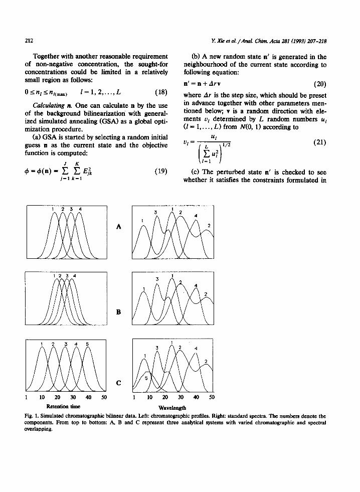
Fig. 1. Simulated chromatographic bilinear data. Left: chromatographic profiles. Right: standard spectra. The numbers denote the components. From top to bottom: A, B and C represent three analytical systems with varied chromatographic and spectral overlapping.

Y. Xl et al./AnaL Chim. Acta 281 (1993) 207-218 213

Eqn. 18. If not, the process is returned to step (b) and a new random state is generated again with Eqn. 20. Otherwise, the objective function of the perturbed state, 4 = &I’), is calculated together with its difference from 4, S4 = C#J - 4’. If 84 s 0, the perturbed state is accepted as the next current state unconditionally. If SC# > 0, an ac- ceptance probability p is defined:

P==P[-BW/(~-~~)] (22)

where /3 is a controlling parameter and &, is the value of the objective function in the global opti- mum (see below).

The calculated probability p is compared with a random number, P, drawn from a uniform distribution at the interval [O,l]. If p r P, the detrimental perturbed new state is accepted as the current state; otherwise, the process is re- turned to step (b) and another random perturba- tion on the current state n is executed for com- puting another new state. The process is repeated

until some termination criteria defined by the analytical precision are satisfied. The result satis- fying the stopping criterion is taken as the best estimate of the sought-for concentrations.

EXPERIMENTAL

Apparatus Spectrofluorimetric measurements were done

with a Hitachi 850 spectrofluorimeter. All com- putations were carried out on a Macintosh II microcomputer and an IBM 386 compatible mi- crocomputer.

Numerical simulation Three 50 X 50 two-dimensional bilinear cou-

pled chromatographic systems with various spec- tra and chromatographic profiles were simulated by use of Gaussian bands and their combinations

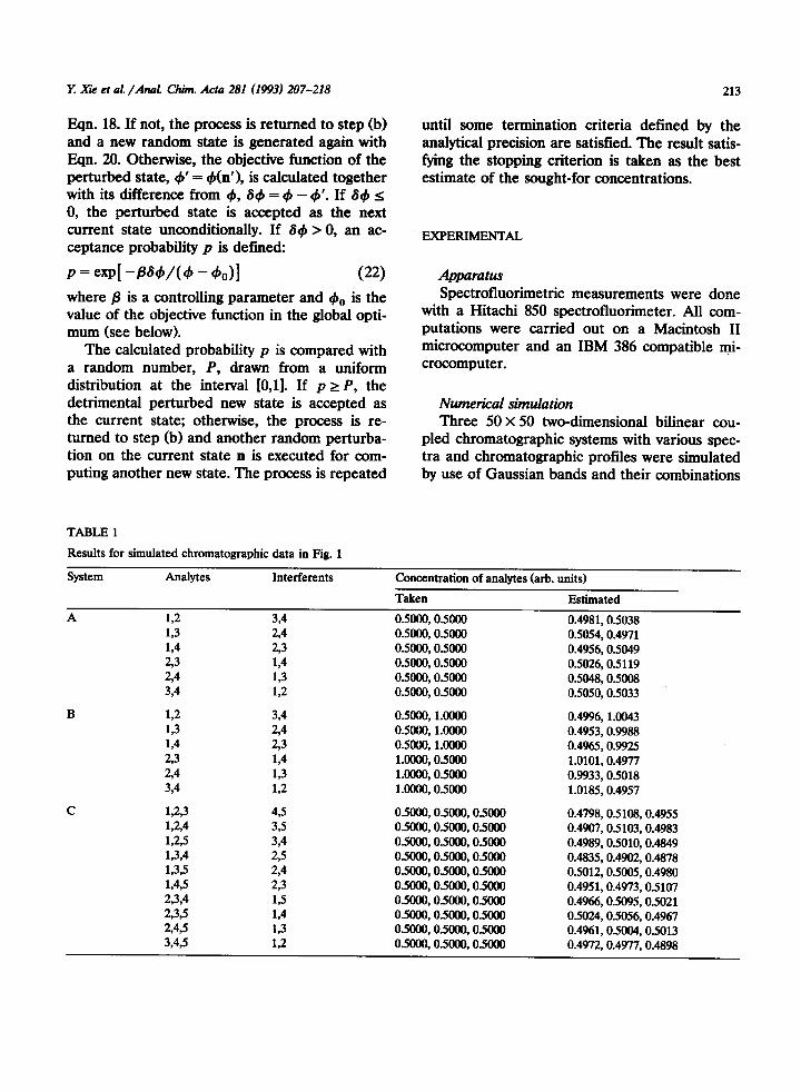
TABLE 1

Results for simulated chromatographic data in Fig. 1

System

A

Analytes Interferents

192 394

193 24 t: 2,3 194

54 193 394 192

192 394 133 2,4

194 2,3 2,3 194 2,4 193

394 192

1,53 475 1,54 395

1,295 394 1,394 2,5 1,3,5 2,4 1,495 2,3 2,394 195

2,3,5 l-4 2,495 193

3,4J 192

Concentration of analytes (arb. units)

Taken Estimated

0.5000,0.5Ocm 0.4981, 0.5038

0.5000,0.5000 0.5054,0.4971

0.5000,0.5Oal 0.5000,0.5Ow 0.4956,0.5049 0.5026,0.5119

0.5000,0.5Oal 0.5048,0.5008

0.5000,0.5Oal 0.5050,0.5033

0.5000, 1.0000 0.4996, 1.0043 0.5000, 1.OOcm 0.4953,0.9988

0.5000, 1.0000 0.4965,0.9925 1.0000,0.5ooo 1.0101,0.4977 10000,0.5000 0.9933,0.5018 1.0000,0.5000 1.0185,0.4957

0.5000,0.5000,0.5000 0.4798,0.5108,0.4955 0.5000,0.5000,0.5fmO 0.4907,0.5103,0.4983 0.5000,0.5000,0.5000 0.4989,0.5010,0.4849 0.5000,0.5000,0.5000 0.4835,0.4902,0.4878 0.5000,0.5000,0.5ooo 0.5012,0.5005,0.4980 0.5000,0.5000,0.5000 0.4951,0.4973,0.5107 0.5000,0.5000,0.5am 0.4966,0.5095,0.5021 0.5000,0.5000,0.5000 0.5024,0.5056,0.4967 0.5000,0.5000,0.5ooo 0.4961,0.5004,0.5013 0.5000,0.5000,0.5000 0.4972,0.4977, 0.4898

214 Y. Xii et al. /Ad Chim. Acta 281(1993) 207-218

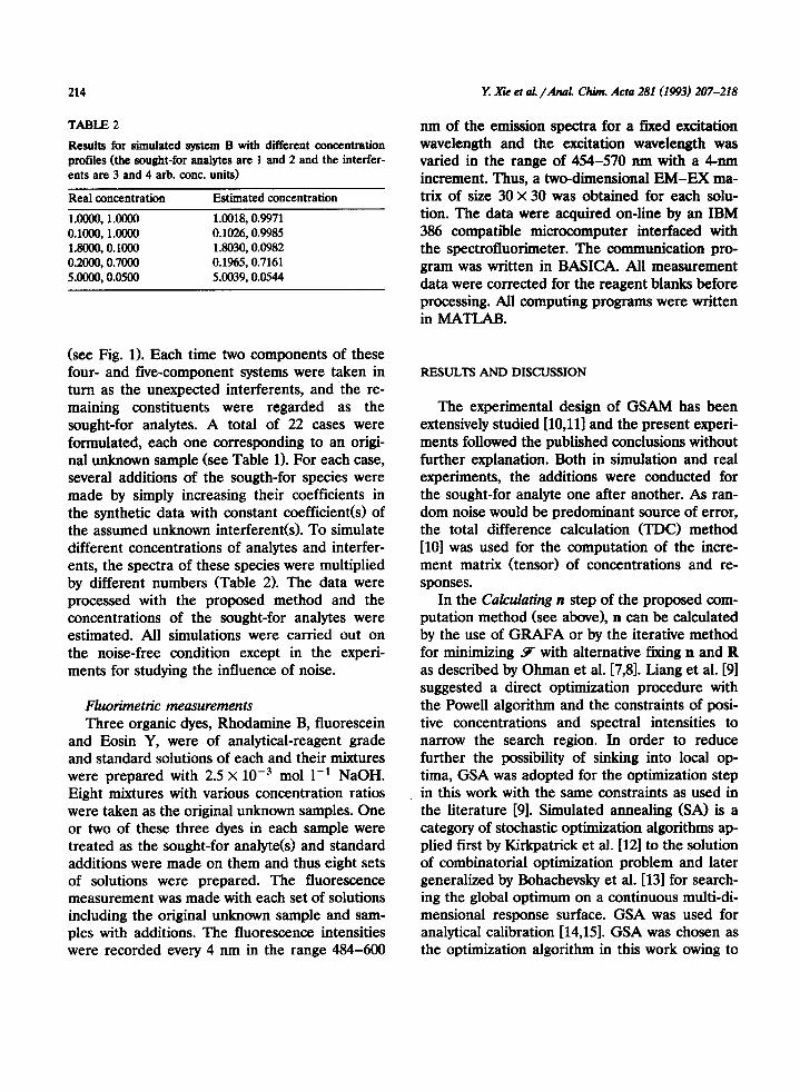
TABLE 2

Results for simulated system B with different concentration profiles (the sought-for anaiytes are 1 and 2 and the interfer- ents are 3 and 4 arb. cont. units)

Real concentration Estimated concentration

1.OooO, l.Ol.MM 1.0018,0.9971 O.lOaI, l.OcmO 0.1026,0.9985 1.8000,0.1000 1.8030,0.0982 0.2000,0.7cKM 0.1965,0.7161 5.oOOO, 0.0500 5.0039,0.0544

(see Fig. 1). Each time two components of these four- and five-component systems were taken in turn as the unexpected interferents, and ‘the re- maining constituents were regarded as the sought-for analytes. A total of 22 cases were formulated, each one corresponding to an origi- nal unknown sample (see Table 1). For each case, several additions of the sougth-for species were made by simply increasing their coefficients in the synthetic data with constant coefficient(s) of the assumed unknown interferentcs). To simulate different concentrations of analytes and interfer- ents, the spectra of these species were multiplied by different numbers (Table 2). The data were processed with the proposed method and the concentrations of the sought-for analytes were estimated. All simulations were carried out on the noise-free condition except in the experi- ments for studying the influence of noise.

Fhorimetric measurements Three organic dyes, Rhodamine B, fluorescein

and Eosin Y, were of analytical-reagent grade and standard solutions of each and their mixtures were prepared with 2.5 x 10m3 mol 1-l NaOH. Eight mixtures with various concentration ratios were taken as the original unknown samples. One or two of these three dyes in each sample were treated as the sought-for analyte(s) and standard additions were made on them and thus eight sets of solutions were prepared. The fluorescence measurement was made with each set of solutions including the original unknown sample and sam- ples with additions. The fluorescence intensities were recorded every 4 nm in the range 484-600

MI of the emission spectra for a fmed excitation wavelength and the excitation wavelength was varied in the range of 454-570 nm with a 4-nm increment. Thus, a two-dimensional EM-EX ma- trix of size 30 x 30 was obtained for each solu- tion. The data were acquired on-line by an IBM 386 compatible microcomputer interfaced with the spectrofluorimeter. The communication pro- gram was written in BASICA. All measurement data were corrected for the reagent blanks before processing. All computing programs were written in MATLAB.

RESULTS AND DISCUSSION

The experimental design of GSAM has been extensively studied [ 10,111 and the present experi- ments followed the published conclusions without further explanation. Both in simulation and real experiments, the additions were conducted for the sought-for analyte one after another. As ran- dom noise would be predominant source of error, the total difference calculation (TDC) method [lo] was used for the computation of the incre- ment matrix (tensor) of concentrations and re- sponses.

In the Calculating A step of the proposed com- putation method (see above), n can be calculated by the use of GRAFA or by the iterative method for minimizing 9 with alternative fixing n and R as described by Ohman et al. [7,8]. Liang et al. [9] suggested a direct optimization procedure with the Powell algorithm and the constraints of posi- tive concentrations and spectral intensities to narrow the search region. In order to reduce further the possibility of sinking into local op- tima, GSA was adopted for the optimization step in this work with the same constraints as used in the literature [9]. Simulated annealing @A) is a category of stochastic optimization algorithms ap- plied first by Kirkpatrick et al. 1121 to the solution of combinatorial optimization problem and later generalized by Bohachevsky et al. [131 for search- ing the global optimum on a continuous multi-di- mensional response surface. GSA was used for analytical calibration [14,15]. GSA was chosen as the optimization algorithm in this work owing to

Y: Xie et al/Anal. Chim. Acta 281 (1993) 207-218 215

TABLE 3 TABLE 4

Results for simulated system B with different initial values (the sought-for anaiytes are 1 and 2 and the interferents are 3 and 4 arb. cent. units)

Results for simulated system B with different noise levels (the sought-for analytes are. 1 and 2 and the interferents are 3 and 4 arb. cont. units)

Initial state Real Estimated concentration concentration

o.oollo, o.oocm 0.5ooo, l.oooo 0.4996,1.0043 1.0000, 1.0009 0.5000,1.0009 0.4978,1.0139 l.OOoO, 0.0009 0.5000, 1.0000 0.5032,0.9903 0.0000, l.Owo 0.5000, 1.0000 0.5067,1.0963 0.5000,0.5090 0.5000, 1.0009 0.4975,0.9955 0.2000,2.cKKm 0.5090, l.MmO 0.5063,0.9946

its excellent mechanism of walking across local optima.

The influences of the parameters of GSA have been extensively discussed [12-151. According to Bohachevsky et al. [13], B was chosen and ad- justed automatically in the process of computa- tion so that the inequality 0.5 <p < 0.9 is satis- fied. In order to search the whole space of states, a relatively large initial step size, say 10% of the size of the constrained region, is adopted. The objective function of the global optimum, &,, is not always known a priori. A reasonable initial value of zero was used in this paper.

Standard deviation Real Estimated of noise (u) concentration concentration

0.001 0.5000, l.MKKl 0.5035,0.9879 0.005 0.5000, 1.0090 0.4999,0.9963 0.010 0.5090, 1.cumO 0.5057,0.9841 0.030 0.5090, l.OcmO 0.5097,0.9878

Some modifications of GSA were adopted [16]. First, the step size Ar is a constant in the GSA, which limits the precision of the optimixation results. Therefore, an additional cycle for reduo ing Ar is introduced in this algorithm. Second, as GSA accepted detrimental states with non-zero probability, which makes GSA not sink into local optima, the ultimate state in one cycle of GSA is usually not the best state produced in this cycle. In order to improve the efficiency of the algo- rithm, the best state appearing in the cycle of the computation is stored and taken as the initial state of the successive cycle or the ultimate result if the algorithm is terminated. In this way, GSA can operate more efficiently.

TABLE 5

Interpretation of two-dimensional fluorescence data

No. Concentration of Concentration Concentration of ana- anaiytes (taken) B of interferent(s) a lytes (estimated) a

1 A(O.2080) CiO.2052) A(O.2254) IMO.2088) B(O.2134)

2 A(O.2080) B(O.2088) A(O.2162) C(O.2052)

3 A(O.3130) CtO.2052) A(O.3426) M0.2088) B(O.2217)

4 A(O.4160) CXO.2052) A(O.4560) B(o.29w B(O.2023)

5 B(O.2088) A(O.5200) B(O.uyI7l cx0.2052)

6 B(0.3132) A(O.5200) B(0.2945) c(O.2052)

7 A(O.2006) B(O.4320) A(0.1966) (X0.4372) Cio.46w

8 B(0.5400~ A(O.1003) MO.53111 cxO.21S7) c(O.2303)

* A = Rluorescein, B = Rosin Y, C = Rhodamine B, concentrations in ppm.

Relative error (%I

8.4 2.2 3.9

9.5 6.2 9.6

-3.1 -0.5

-6.0

-2.0 7.2

-1.6 5.3

216 Y Xii et al. /Am! Chim. Acta 281 (1993) 207-218

Table 1 shows the quantification results for the sought-for species of the simulation systems. It is clear that for all 22 cases the global optima have been found. As GSA played the central role in this procedure, its performance was tested in some detail. Table 2 presents the results for the first case of simulated system B of Table 1 with different concentration profiles. Although the es- timates were less precise for the minor compo- nents when the difference in concentrations be- tween species was large, they were still accept- able. Table 3 lists the results for the same case of simulated system B of Table 1 with different initial values. It demonstrates that the positions of initial states had no influence on the perfor- mance of,GSA owing to its intrinsic randomness. The influence of noise was also investigated. Nor- mal random numbers with zero-mean and four different standard deviations, u = 0.001, 0.005, 0.010 and 0.030, were generated and added to the mixture response matrices after multiplying the absolute value of the largest element in each mixture response matrix to simulate the experi- mental error. The results in Table 4 show that a moderate level of noise did not degrade the ana- lytical results very much.

Two-dimensional jluorescence data Eight mixtures of three dyes were prepared

according to the GSAM experimental design and the measured fluorescence excitation-emission data sets were treated by using the proposed method. The error bound, E, was taken as ten times the fluorescence intensity unit of the Hi- tachi 850 instrument. One or two of these three components were taken as unknown interferents and the concentration of the remaining compo- nents was estimated. The initial estimates of con- centrations were set to zero. The true concentra- tions and their estimates are given in Table 5. If one remembers that the proposed method did not require the standard spectra of analytes in the environment of real samples or any a priori information concerning the background interfer- ents, the estimated results should be considered to be reasonably acceptable.

It must be pointed out that the computation of GSA is generally more time consuming than that

of generally used local optimization algorithms such as the Powell algorithm [9] owing to its intrinsic randomness. However, there are two ad- vantages with the adoption of GSA. First, the response surface of background bilinearixation would be complicated owing to its complex rela- tionship with II and R. Some local optima may exist. GSA has the ability to walk across them. Also, GSA is only slightly influenced by the initial values owing to its intrinsic randomness. This may not be the case with the Powell algorithm and algorithms of this type. Second, the concen- tration constraints (Eqn. 18) can be exerted more easily in the process of computation of GSA just by checking directly the availability of the per- turbed state, but in the algorithms associated with a one-dimensional search, as in the Powell algorithm, the troublesome transfer of the multi- dimensional constraints to the one-dimensional search boundary is inevitable.

From the results of simulation and processing of real EX-EM data, it seems that the proposed method can work satisfactority.

This work was supported by Natural Science Foundation of China and partially by the Labora- tory of Electroanalytical Chemistry, Changchun Institute of Applied Chemistry, Chinese Academy of Science.

APPENDIX

List of symboL!Y bT a row vector of response sensitivity for the

Zth analyte (size 1 x.0 B the matrix of response sensitivity (size L X J) d a cohmm vector of one direction variable in

a two-dimensional instrument (size .Z X 1) eT a row vector of experimental error for the

original sample (size 1 X .I) Ejk the (i,k)th element of experimental error

matrix E a matrix of experimental error after addi-

tions in the one-dimensional case (size Z X J) or a matrix of experimental error for the original sample in the two-dimensional case (size JXK)

Y. Xie et al. /Anal. Gim. Acta 281 (1993) 207-218

E

9-

g=

i

I

j

J k

K 1

L m

M

n1 nrn

UT P P

Q jk

Q

Q

IT m

rT

Rjk

%

R

the third-order tensor of experimental error after additions in the two-dimensional case (size ZXJXK) the objective function a row vector of another direction variable in a two-dimensional instrument (size 1 X K)

a dummy index for counting standard addi- tions the number of standard additions a dummy index for counting variable of a one-dimensional instrument or for counting one direction variable of a two-dimensional instrument the number of measurement variable a dummy index for counting another direc- tion variable of a two-dimensional instru- ment the number of measurement variable

a dummy index for counting sought-for ana- lytes the number of sought-for-analytes a dummy index for counting unexpected in- terferents or principal components the number of unexpected interferents or the number of principal components the concentration of the Zth analyte the concentration of the mth unexpected interferent a row vector of concentration (size 1 X L) the calculated acceptance probability a random number drawn from uniform dis- tribution at the interval [O,l]. the (j,k)th element of original response ma- trix a matrix of response yielded in the original sample (size J x K)

the third-order tensor of response after stan- dard additions (size Z x J x K)

a row vector of response sensitivity for the mth unexpected interferent (size 1 x J) a row vector of overall response for M unex- pected interferents (size 1 X J) the (j, k)th element of overall response ma- trix a matrix of response sensitivity for the mth unexpected interferent (size J x K)

a matrix of overall response for M unex- pected interferents (size J X K)

sljk

Sl

s

trn T

UI UT m

UT

*I V

Ar E

217

the (I, j, k)th element of response sensitivity tensor a matrix of response sensitivity for the Ith analyte (size J x K)

the third-order tensor of response sensitivity (size L xJxK)

a column vector of factor score for R, factor m&e Jxl) the matrix of R scores (size J X MI

a random number for N(0, 1) a row vector of factor loading for R, factor m (size 1 X K)

the matrix of R loadings (size M X K)

the Ith element in v a column vector representing a random di- rection in GSA optimization (size L X 1) a row vector of response yielded in the origi- nal sample (size 1 x J)

the matrix of response after standard addi- tions (size Z x J)

controlling parameter in GSA the matrix of concentration increment (size IXL)

the third-order tensor of response increment (size ZxJxK)

the matrix of response increment (size I x J)

the difference of objective function between the current state n and the perturbed state n’ step size error bound the value of objective function the value of objective function at the global optimum

REFERENCES

1 D.E. Saxberg and B.R. Kowalski, Anal. Chem., 57 (1985) 908.

2 D.W. Osten and B.R. Kowalski, Anal. Chem., 57 (1985) 908.

3 Y.-Z. Liang, Y.-L. Xie and R.-Q. Yu, Chin. Sci. Bull. (Engl. Ed.), 34 (1989) 1533.

4 C.N. Ho, G.D. Christian and E.R. Davidson, Anal. Chem., 50 (1978) 1108.

5 A. Lorber, Anal. Chim. Acta, 164 (1984) 293. 6 E. Sanchez and B.R. Kowalski, Anal. Chem., 58 (1986)

4%.

218

7 J. Ohman, P. Geladi and S. Wold, J. Chemometr., 4 (1990) 79.

8 J. Ohman, P. Geladi and S. Wold, J. Chemometr., 4 (1990) 135.

9 Y. Liang, R. Manne and O.M. KvaIheim, Chemometr. InteIl. Lab. Syst., 14 (1992) 175.

10 M.G. Moran and B.R. Kowalski, Anal. Chem., 56 (1984) 562.

11 C. Jochum, P. Jochum and B.R. Kowalski, Anal. Chem., 53 (1981) 85.

Y Xii et aL /AnaL Chim. Acta 281(1993) 207-218

12 S. Kirkpatrick, C.D. Gelatt and M.P. Vecchi, Jr., Science, 220 (1983) 671.

13 1.0. Bohachevsky, M.E. Johnson and M.L. Stein, Techno- metrics, 28 (1986) 209.

14 J.H. Kalivas, N. Roberts and J.M. Sutter, Anal. Chem., 61 (1989) 2824.

15 J.H. Kalivas, J. Chemometr., 5 (1991) 37. 16 X.-L. Xie, J.-H. Wang, Y.-Z. Liang, K. Ge and R.-Q. Yu,

J. Chemometr., in press.