Axisymmetric spherical shell models of mantle convection with variable properties and free and rigid...

JOURNAL OF GEOPHYSICAL RESEARCH, VOL. 97, NO. El2, PAGES 20,899-20,923, DECEMBER 25, 1992

Axisymmetric Spherical Shell Models of Mantle Convection With Variable Properties and Free and Rigid Lids

A.M. LEITCIt, 1 D. A. YUEN, AND C. L. LAUSTEN

Department of Geology and Geophysics and Minnesota Supercomputer Institute University of Minnesota, Minneapolis

Axisymmetric spherical shell numerical simulations of mantle convection were carried out to investigate the influence of two end-member surface stress conditions: stress-free and rigid. These correspond approximately to a subducting or a rigid lithosphere and can be seen as end-member models of the surface of Venus. Our model assumed an effective Rayleigh number of 3x106, similar to that for Earth, and included uniform internal heating and depth-dependent thermal expansivity ot and thermal conductivity k. The simulations utilized a Newtonian viscosity which was constant or varied with depth and/or temperature. We show how the temperature, speed and vorticity fiel&q change qualitatively and quantitatively with surface temperature, surface stress condition, internal heating and viscosity distribution. Among the significant results, we find that a rigid lid and viscosity which increases with depth both promote steady large-scale circulation with smaller-scale circulation in the upper mantle.

1. INTRODUCTION

With the recent acquisition of radar images by the Magellan spacecraft, the dynamics of Venus ha• become' the focus of some attention. Although a detailed surface map has now been assembled, interpretation of this map will be going on for many years, and without seismological data or dating of surface features, there is difficulty in making inferences about the present and past conditions in the mantle. It is therefore timely to study a general model of mantle convection to see how some important properties of the surface and interior of Venus will affect the heat flow and style of convection. Although model parameters were chosen with Venus in mind, since there is little overlap in the geophysical observations of Venus and the ob- servables of our models, most of the results are more of general interest in the study of mantle convection.

Leitch and Yuen, [1991] considered the influence of the top stress condition, top temperature and internal heating on mantle convection at a Rayleigh number of 3x105, which implies a viscosity of about 1023 Pa s, or 10 times that typically assumed for the averaged Earth. Such a high viscosity might arise on Venus due to lack of recycling of volatiles [Kaula, 1990a ] and is suggested by the high apparent depths of compensation [Kau- la, 1990b; Phillips, 1990]; however, there is still much uncertainty about the viscosity of Venus, and Kiefer et al. [1986] argue that high apparent depths of compensation may be due to the lack of a low-viscosity asthenosphere. In this paper, we extend our investigation to a Rayleigh number of 3x106, assming an Earth-like average viscosity, and include the effects of temperature- and depth-dependent viscosity.

Studies of whole mantle convection can be roughly divided up into those which investigate the influence of surface boundary conditions and those which look at the (possibly depth-

I Now at Research School of Earth Sciences, Australian National University, Canberra.

Copyright 1992 by the American Geophysical Union.

Paper number 92JE02368. 0148-0227/92/92JE-02368 $05.00

and temperature-dependent) properties of the mantle. This study is of the second type, though it looks at two very simple end-member surface boundary conditions, stress-free and rigid.

Venus has a size, density, and composition similar to Earth. The surface conditions, however, are markedly different and make it an ideal subject for our study. On Earth there is a bi- modal distribution of topography corresponding to the oceanic and continental plates, and it is likely that the distribution of oceans and continents has a significant influence on the style of mantle convection [e.g., Davies, 1986; Gurnis, 1988].

On Venus, on the other hand, there is a unimodal distribution of topography and the surface is uniformly hot. Higher surface temperatures together with an assumption of approximately chondritic amounts of radiogenic heat-producing elements in the mantle suggest that the brittle crust is thin, while the deep apparent depths of compensation indicate a significant amount of dynamic support to the topography from the mantle and the lack of a deep low-viscosity zone in the upper mantle [Kiefer, 1990]. There is no evidence of plate tectonics as it is known on Earth, where stresses are transmitted over large distances and deformation takes place in narrow margins [Solomon et al., 1991]. Venus apparently has a more uniform near-surface structure that might realistically be modelled with a free-slip or rigid boundary condition at the top of the convecting mantle. We use the term "top" rather than "surface" in the following to allow for the fact that the surface may not take part in convection.

A free-slip condition at the top means that the surface layers (crust and/or lithosphere) exert no retarding force on the convection: either the surface layers subduct freely with the convection or there is a lubricating layer underneath the buoyant surface layers which decouples them from the underlying flow. A rigid (no-slip) condition means that the surface layers are immobile. For free-slip the surface is in motion and there is no shear; for no-slip there is shear but no motion. A rigid lid im- poses zero velocities at the top and so slows and changes the pattern of flow in the interior and impedes heat transfer at the surface.

Which of these two top stress conditions is more accurate has not been resolved. While the relatively old, deformed surface suggests that the recycling rate of crust into the mantle cannot

20,899

20,900 LEITCH œT AL.: MAN'II.E CONVECTION WITH FREE AND RIGID LIPs

be high, it is uncertain whether the' mantle beneath the crust takes part in mantle convection [Phillips, 1990; Lenafdic et a/., 1991] or forms a nonsubducting lithosphere. The surface deformation implies of course that the lithosphere is not completely rigid: the true situation probably lies between the two extreme end-members that our simulations consider. Numeri-

cally, they are the easiest conditions to impose. Another surface boundary condition that is simple to impose is that of a high-viscosity lid. Such a surface condition arises in our models with temperature-dependent viscosity (see Figure 12); it is more thoroughly investigated by Steinbach and Yuen [1992].

In the following work, in addition to the effect of the top stress condition, we look at the influence of the temperature at the top To, the amount of internal heating R, and the viscosity distribution. We present our findings on the pattern of convection, average temperature, and heat transfer at the boundaries.

If the surface layers take part in the convection, then To is the (dimensionless) surface temperature (see Tables 1 and 2); but if there is a buoyant insulating crust, then To may be significantly higher. The adiabatic temperature gradient in the mantle is proportional to the absolute temperature T + To, so high values of To imply steep adiabatic gradients, more sluggish flow, and, in the extreme, the disappearance of hot plumes from the core-mantle boundary (CMB).

We use two values of the internal heating parameter R, which is proportional to the concentration of heat-producing elements (HPEs) in the mantle. We ran simulations for R = 0 and R = 10, which corresponds to approximately chondritic quantities of HPEs [Leitch and Yuen, 1989]. R affects the average temperature of the mantle and hence the adiabatic temperature gradient and the temperature changes across the boundary layers. At higher temperatures there are more convection cells, weaker hot plumes, and greater time dependence in the flow.

We also look at convection when the viscosity decreases with increasing temperature, increases with increasing depth, or a

TABLE 1. Dimensionless Variables

Symbol Name Definition

A surface area r' 2/d' 2

D dissipation number o[ ',g'a r/c'• eij rate of strain component see equation (3) k thermal conductivity Id/k', p dynamic pressure fid' 2/q'K', q heat flux per unit area If' i}7,12' ' d'/k',A7, Q total heat flux qA r radial coordinate r'/a r

flux ratio [Q 0,,Q,c• l/Qo R internal heating parameter p',H d Z/k',A7, Ra Rayleigh number p', g' •t', A7,d' 3/q,• ß t time f •,ld '2 T temperature 7'-7' o/AT' T O normalized T at top 7, 0/A7, u i velocity component u i ' a r/•, u horizontal velocity (u0) u' a r/•, v radial velocity (Ur) ¾' d'/K•,

•t thermal expansivity •t'/0t', ¾ Griineisen parameter 0t'K's / p'c'• q dynamic viscosity q'/q', 0 co-latitudinal angle

1A2) • viscous dissipation q(eijeij - gij deviatoric stress component 2q(eij - 1.•.Afij ) p density p'/p', to vorticity to'at 2/•,

TABLE 2. Dimensional Quantities

Symbol Name Mantle Value

c t, specific heat d' depth of the mantle g' acceleration of gravity H' internal heat generation k', average thermal conductivity K' s adiabatic bulk modulus

• CMB core radius 7,o temperature at top boundary •t', average thermal expansivity A7' temperature drop across a K', thermal diffusivity k',/@', q', average viscosity @', average density

Subscripts 0 value at top

CMB value at core-mantle boundary * depth-integrated average S constant entropy p constant pressure

1250 J kg -1 2.7xl 0 6 m 8.9 m s -2 0-5x10 -12 Wkg -• 6 Wm-•K -l 120-•660 GPa

3.26x 106 m 750-1500 K

2x10-5 K-l 1.5-3.75x103 K 10 -6 m 2 s -l 1022 Pas 4500 kg m -3

combination of both. Purely temperature-dependent viscosity results in a hot mantle with weak hot plumes and highly time- dependent flow. Purely depth-dependent viscosity conversely results in relatively steady flow patterns and a colder mantle. The combination of depth- and temperature-dependent viscosity produces a viscosity which increases with depth with boundary layers of high and low viscosity, at the top and the core-mantle boundary, (CMB) respectively. Flow is similar to purely depth-dependent viscosity, but there are fewer cells.

In this paper we have used some innovations in presentation which we believe are useful in building up a comprehensive view of the mantle. We present contour plots of speed (Figures 6 and 13-16), which provide information on the velocity field that is easier to understand intuitively than stream function plots. Changes in flow speed along the direction of flow, for instance, are more easily recognized.

We use the vorticity field to find the position of plumes (Fig- ures 11 and 23). Similar "plume position" graphs were developed earlier and independently by Goldhirsh et al. [1989] and Hansen et al. [1990], but an advantage of using vorticity is that the gradient of vorticity at the center of a plume can be used as a measure of the strength of the plume.

Finally, we have used the statistical technique of factorial design (section 4.7) to measure and compare the effects of the three important parameters R, To, and the stress condition on global properties of the system.

Previous work on modelling mantle convection on Venus in- cludes recent papers by Kiefer and Hager [1991a,b] and the three-dimensional models of Schubert et al. [1990]. Axisym- metric models have been utilized, for example, by Machetel and Yuen [1989] and Solheirn and Peltier [1990].

The paper is divided into seven sections. Sections 2 and 3 describe the equations and method. Section 4 gives the results of the constant viscosity calculations, and section 5 is concerned with the variable viscosity simulations. Section 6 is a review of interesting fluid dynamical results. Section 7 is a discussion of particular implications of the results for convection on Venus.

2. EQUATIONS

The equations solved were the time-dependent, anelastic- liquid compressible equations of motion [Jarvis and McKenzie,

L.vxrc• •'r a•.: MAN'II• CONVECTION WITH FREE AND RIOID Lms 20,901

1980] with constant Newtonian rheology and an even distribution of internal heating. The primitive variable formulation was used. The dimensionless variables in which the equations are written are explained in Table 1. In axisymmetric spherical shell geometry, the conservation of momentum is written [e.g., Lapwood and Usami, 1981]

1 •p q' k •00 •}'lJr0 3XrO TOO--X** r i}0 r'-•- + '•r + + = 0 (1) r rtan0

__• •rr 1 3XrO XrO 2Xrr•-- X** •r +•+-- + + +Ra•pT = 0 r • r tan0 r

where xii •e the com•nents of •e deviatoric s•ess tensor, which for a fluid has •e general form [e.g., Batc•lor, 1967]

x•i = 2•(e•i - •ASij ) (2)

where e•d is •e rate of s•ain •nsor, A is •e rate of exposion e• = V.u, •d • is •e •n•ker del•. For a •mpressible liquid • axis•me•c spherical geome• the •m•nen• of the ra• of s•n tensor c• be written [Bmc•lor, 1967],

Ou•

1 3u0 Ur + • (3) eøø= r •0 r

Ur UO e** = • + r r tan0

r •._•_(Uo) 1 OUr er ø = '•- • r r + •r •-• thus

V'U • 1 3Uo 3Ur 2Ur Uo r i}0 +'-•-r + + (4) r rtan0

and we obtain

2 3Ur 10Uo 2Ur Uo qJrr = '•'Tl[2 Or r 30 r rtan0 ]

• 3Ur 2 •}ue Ur UO x0o= q[-•+- + - •] (5) r '• r rtan0

2 3Ur 1 •}ue Ur 2Uo . %* = •q[ Or r 30 +•+ ] r r•n0'

XrO = q[• •Ur •Uo UO ] r• + •r r

energy equation is'

•r • • • .,•r k 3T r:O Ot • (•r: ) + ) + = m0 OT Uo OT r:D

- pr2[Ur •+• Ra •+Dura(T+To)]+ •+Rpr 2 (6) where the viscous dissipation per unit mass • is given by

I 2 ß = 2q(eue o-•A )

OUr 2 (! OuO Ur = 2q [•-r • + + Ur•: + • + Y-• Y Y UO

rtanO )21

1 3Ur 3Uo UO ]2 + q [7('• -) + Or r

2 •}Ur + 1__ •}Uo 2Ur UO -- • -11[ •} r r '•- + ' + r rtan0 (7)

The problem was closed using the penalty formulation for the dynamical pressure p'

• •U e •U r 2Ur Ue )q'_•_F Ur] (8) p = -)bV'pu = -)b[p( '•-+'•-r +'• '-+ rtan0 where the penalty parameter )b was 106.

Controlling parameters in these equations are the Rayleigh number Ra, the thermal expansivity or, the thermal conductivity k, the nondimensional temperature at the top of the convecting region To, and the internal heating R.

In these simulations we used a Rayleigh number of 3x106, which implies an average viscosity similar to what is thought to be appropriate for Earth.

As set out by Leitch and Yuen [1991], we assumed a thermal expansivity ot which decreased with depth [Chopelas and Boehler, 1989] according to

ot = {Xo• p-• for (r - rc•te)/(ro- rc•te) > 0.65 (9)

ot = •to2 p-2 for (r - rc•ts)/(ro- rc•ts) < 0.65

a thermal conductivity k which increased with depth [Ander- son, 1987]

k = kop 3, (10)

and an equation of state based on the Adams-Williamson rela- tion

p = p0[l+2Dø(1-z)] • (11) 70

We used a value of Do/To of 0.45, which gives a density contrast across the mantle of 1.38.

Three values of the nondimensional temperature at the top of the convecting region To were chosen, 0.2, 0.6, and 1.0, covering the range of possibilities considered reasonable for the Venusian mantle (see Table 3). To is most sensitive to the dimensional temperature 7'0, which is likely to be either close to the surface temperature of Venus (733 K) if ductile near- surface layers take part in the convection or near the mantle liquidus (1500 K) if there is a thick buoyant crust. Any higher 7'0 would give melting at the top, and for any lower value of 7'CMS, we would expect Venus to have a solidifying inner core and a much stronger magnetic field than it actually possesses.

A constant concentration of heat producing elements per unit mass was assumed. The internal heating parameter R is defined in Table 1. A chondritic heat production rate of 5x10-12W/kg corresponds to R of about 10, depending on the temperature drop across the mantle (see example values in Table 3). Another measure of the importance of internal heating is the proportion r of the total heat flux that is due to internal heating. Values of r for all the internally heated cases are given in the figure captions.

All the cases presented here were run to a quasi-steady state, that is, until the average temperature, time-integrated over one overturn, was not changing; thus there was no secular cooling.

TABLE 3. Mantle Boundary Temperatures and T O

•' o(K ) •'cMs (K ) A•' (K ) T O Rcn 750 4500 3750 0.2 7.3 750 3250 2500 0.3 10.9

1500 4000 2500 0.6 10.9 1500 3000 1500 1.0 18.2

Rch is the value of R corresponding to chondritic internal heating.

20,902 Lerrc•i ET AL.: MANTLE CONVECTION WITH From AND RIGID LIDS

It should be noted (see equation (6)) that as far as the relative heat fluxes across the CMB and the top are concerned, a steady secular cooling term can be modelled by an additional quantity of internal heating. It is thought that on Earth the secular cooling and internal heating contributions to surface heat flow are roughly similar. Thus from the point of view of modelling the thermal structure and relative heat fluxes across the boundaries, it makes sense to consider cases where R is greater than the chondritic amount.

In the quasi-steady state there were temperature oscillations of the order of 1% on the time scale of instabilities in the boun-

dary layers. For the first part of our project the viscosity •1 was constant.

In the second part we employed a nondimensional viscosity which varied with depth and temperature according to the simple relationship:

•1 = exp[-A (T-T)+ C (r-r•a)] (12)

We considered temperature-dependent viscosity (with A = ln30, C = 0) depth-dependent viscosity (with A = 0 and C = ln20) and viscosity dependent on both temperature and depth (with A = ln30 and ½ = ln80).

The boundary conditions for all runs were constant temperature, free slip at the CMB (appropriate for a low-viscosity, highly conductive molten core) and constant temperature at the top. For some models the top was free slip, and for others, no-slip (rigid) conditions were used.

Approximate dimensional equivalents to dimensionless values of temperature, speed, and vorticity are given in the figure captions. Note that the temperature scale AT' is different for different To (see Table 3 and Figure 2 caption).

Errata in Momentum Equation

The stress tensor components 'cii as written by Leitch and Yuen [1991] are erroneous, as they were calculated using V.u for cylindrical rather than spherical co-ordinates, so that they were off by an amount 2/3•1 [(2Ur/r)+(uo/rtanO)]. This quantity is small compared to the other terms in the 'cii except near the boundaries within a few degrees of the poles and, to a lesser extent, along upwelling and downwelling sheets.

Comparisons of simulations run using the correct and incorrect momentum equation showed that the error had little effect. The change in the time-averaged heat fluxes at the boundaries was less than 2%, within the temporal variation of the fluxes, which was typically 5-10%. The convection patterns (that is, the number of cells and the steadiness of plumes) did not change. Thus none of the conclusions of the paper were affected, and values given for heat fluxes and temperatures changed by only insignificant amounts.

Although the averaged and broad-scale features of the flow were not affected by the error, there were differences in the details of the time history. This is illustrated in Figure 1, which compares the total heat flux at the upper and lower boundaries as a function of time using the incorrect and correct momentum equations.

3. COMPuTATIONS

The simulations were carried out using the finite-element code TWODEPEP [Sewell, 1985]. The code was run on a Cray 2. We used 3000 triangular elements with cubic interpola- tion, refined by a factor of 5 or 10 in the boundary layers and polar regions and a time step of 5x10 -5 to lx10 -4 thenhal

diffusion time scales. This is equivalent resolution to that used for the lower Rayleigh number cases by Leitch and Yuen [1991]. After reaching thermal equilibrium, the cases were run for between 80 and 200 time steps, which corresponds to 2 to 10 overturns and thermal diffusion times of 0.008 to 0.02.

Initial conditions for some cases were a constant internal

temperature adjusted to the amount of internal heating and error function boundary layers at surface and CMB. A perturbation with a wavelength of/=1 was applied to the bottom boundary layer. Other runs were started from solutions to different cases.

4. CONSTANT VISCOSITY RESULTS

In characterizing convection for the constant viscosity simulations with varying R (0 and 10), To (0.2, 0.6, and 1.0), and surface condition (rigid or free), the issues we are interested in are the size and stability of the convection cells, any radial variations in strength and speed of the plumes due to variation of the physical properties (• and k) or surface boundary condition, and the resulting influence on the temperature and boundary heat fluxes.

We present the results of the simulations in four different forms: a table of globally averaged properties; contour plots of temperature, speed, and vorticity at representative time instances; profiles of horizontally averaged properties as func- tions of depth; and "plume position" diagrams, showing the location of upwellings and downwellings as a function of latitude and time.

The table of results (Table 4) gives the number of large scale cells n, the globally averaged temperature T, the volume averaged speed (U2+V2) v•, and the total heat fluxes at the boundaries QcMs and Q o for all the simulations that we carried out. An overbar indicates a volume average taken over the entire

(36.8)

(35.9)

(6.6)

(6.5)

I I I I I I I I

0 10 20 30 40 50 60 70 80

time step

Fig. 1. Total heat fluxes Q0 (triangles) and QcMs (circles) for incorrect (upper line) and corrected momentum equations. Numbers in parentheses give average values for Q. Vertical scale: distance between dashed lines is five units. Ra = 3x105, T O = 0.2, R = 10, free slip lid (see Figure 4d of Leitch and Yuen [ 1991 ]).

LerrcH •r AL: MAm'• CONVECnON wrm FR• AND Rm• L•s 20,903

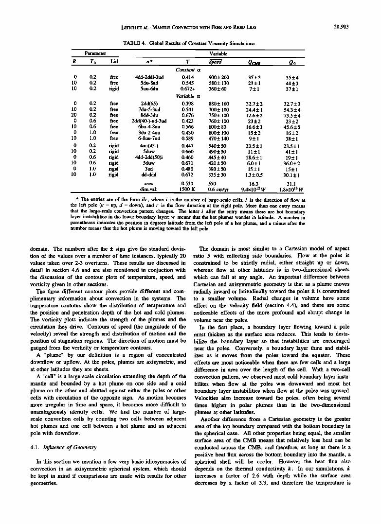
TABLE 4. Global Results of Constant Viscosity Simulations

Parameter Variable

R T O Lid n * • Speed QcMs Q o Constant ix

0 0.2 free 4dd-2ddi-3ud 0.414 900+200 35+3 35+4 10 0.2 free 5du-8ud 0.545 580+ 130 23 + 1 48 + 3 10 0.2 rigid 5uu-6du 0.672+ 360+ 60 7 + 1 37 + 1

Variable ix

0 0.2 free 2dd(65) 0.398 880+ 160 32.7 + 2 32.7 + 3 10 0.2 free 7du-5-3ud 0.541 700+ 100 24.4+ 1 54.3+ 4 20 0.2 free 8dd-3du 0.676 750+ 100 12.6+2 73.5+ 4 0 0.6 free 2dd(40-)-ud-3ud 0.423 760+ 100 23 + 2 23 + 2

10 0.6 free 6bu-4-8uu 0.566 600+ 80 16.6+ 1 45.6+5 0 1.0 free 3du-2-4uu 0.430 600+ 100 15+2 16+2

10 1.0 free 6-8uu-7ud 0.589 470+ 140 9+ 1 38+ 1

0 0.2 rigid 4uu(45-) 0.447 540+ 50 23.5 + 1 23.5 + 1 10 0.2 rigid 5duw 0.660 490+50 11+1 41+1 0 0.6 rigid 4dd-2dd(50)i 0.460 445+ 40 18.6+ 1 19+ 1

10 0.6 rigid 5duw 0.671 420+50 6.0+ 1 36.0+2 0 1.0 rigid 3ud 0.480 390+ 50 15 + 1 15 + 1

10 1.0 rigid dd-ddd 0.672 335+30 1.3+0.5 30.1+ 1

ave: 0.530 550 16.3 31.1 dim.val: 1500 K 0.6 cm/yr 9.4x10 •2 W 1.8x10 •3 W

* The entries are of the form ilr, where i is the number of large-scale cells, l is the direction of flow at the left pole (u = up, d = down), and r is the flow direction at the right pole. More than one entry means that the large-scale convection pattern changes. The letter i after the entry means there are hot boundary layer instabilities in the lower boundary layer; w means that the hot plumes wander in latitude. A number in parentheses indicates the position in degrees latitude from the left pole of a hot plume, and a minus after the number means that the hot plume is moving toward the left pole.

domain. The numbers after the _+ sign give the standard deviation of the values over a number of time instances, typically 20 values taken over 2-3 overturns. These results are discussed in

detail in section 4.6 and are also mentioned in conjuction with the discussion of the contour plots of temperature, speed, and vorticity given in other sections.

The three different contour plots provide different and com- plimentary information about convection in the systems. The temperature contours show the distribution of temperature and the position and penetration depth of the hot and cold plumes. The vorticity plots indicate the strength of the plumes and the circulation they drive. Contours of speed (the magnitude of the velocity) reveal the strength and distribution of motion and the position of stagnation regions. The direction of motion must be gauged from the vorticity or temperature contours.

A "plume" by our definition is a region of concentrated downflow or upflow. At the poles, plumes are axisymetric, and at other latitudes they are sheets.

A "cell" is a large-scale circulation extending the depth of the mantle and bounded by a hot plume on one side and a cold plume on the other and abutted against either the poles or other cells with circulation of the opposite sign. As motion becomes more irregular in time and space, it becomes more difficult to unambiguously identify cells. We find the number of large- scale convection cells by counting two cells between adjacent hot plumes and one cell between a hot plume and an adjacent pole with downflow.

4.1. Influence of Geometry

In this section we mention a few very basic idiosyncracies of convection in an axisymmetric spherical system, which should be kept in mind if comparisons are made with results for other geometries.

The domain is most similar to a Cartesian model of aspect ratio 5 with reflecting side boundaries. Flow at the poles is constrained to be strictly radial, either straight up or down, whereas flow at other latitudes is in two-dimensional sheets

which can fall at any angle. An important difference between Cartesian and axisymmetric geometry is that as a plume moves radially inward or latitudinally toward the poles it is constrained to a smaller volume. Radial changes in volume have some effect on the velocity field (section 4.4), and there are some noticeable effects of the more profound and abrupt change in volume near the poles.

In the first place, a boundary layer flowing toward a pole must thicken as the surface area reduces. This tends to desta-

bilize the boundary layer so that instabilities are encouraged near the poles. Conversely, a boundary layer thins and stabil- izes as it moves from the poles toward the equator. These effects are most noticeable when there are few cells and a large difference in area over the length of the cell. With a two-cell convection pattern, we observed most cold boundary layer insta- bilites when flow at the poles was downward and most hot boundary layer instabilities when flow at the poles was upward. Velocities also increase toward the poles, often being several times higher in polar plumes than in the two-dimensional plumes at other latitudes.

Another difference from a Cartesian geometry is the greater area of the top boundary compared with the bottom boundary in the spherical case. All other properties being equal, the smaller surface area of the CMB means that relatively less heat can be conducted across the CMB, and therefore, as long as there is a positive heat flux across the bottom boundary into the mantle, a spherical shell will be cooler. However the heat flux also depends on the thermal conductivity k. In our simulations, k increases a factor of 2.6 with depth while the surface area decreases by a factor of 3.3, and therefore the temperature is

20,904 LErrc• ET AL.: MANTL• CONVECnON wrm FR• AND RIO•D DDS

a b

g h

i j

I

Fig. 2. Typical contour plots of temperature for the 12 cases studied. Ra = 3x106. (a)-(f) Free slip lid: (a) R = 0, To= 0.2; (b) R = 10, To = 0.2, r =0.55; (c) R =0, To= 0.6; (d) R = 10, To= 0.6, r =0.64; (e) R =0, To= 1.0; (f) R = 10, T O = 1.0, r = 0.75. (g)-(l) Rigid (no-slip) lid: (g) R = O, To= 0.2; (h) R = 10, T O = 0.2, r = 0.75; (i) R = 0, T O = 0.6; (j) R = 10, T O = 0.6, r = 0.84; (k)R = 0, T O = 1.0; (l)R = 10, T O = 1.0, r = 0.96. Contour interval 0.1 (350 K, 250 K, 150 K for T O of 0.2, 0.6, and 1.0, respectively) from 0 to 1.0. Bold dashed contour line is T = 0.5.

LœrrcH ET AL.: MANTLE CONVECTION wrrH FRE• A•D RIGID LIDs 20,905

not far different from a Cartesian simulation with constant k.

A fully three-dimensional spherical geometry has another degree of freedom which allows additional forms of instability and more efficient heat transfer. There are no "poles" and plumes are free to assume sheetlike or axisymetric forms independent of latitude. Three-dimensional simulations show that flow leaving a boundary layer tends to be sheetlike to start with and then concentrates into axisymetric structures as it rises or sinks. The axisymetric plumes are not obliged to move strictly radially, and so the connectedness of the boundaries may be less, particularly at high Rayleigh number. Such information on plume structure cannot be obtained in our two- dimensional simulations. However, a comparison of two- and three-dimensional simulations at moderate Rayleigh number [Leitch and Yuen, 1991] showed that two-dimensional simulations can capture many important features of convection.

4.2. Temperature Fields

Temperature contours are most familiar and easily inter- preted, and we show representative frames for all the 12 constant viscosity cases. Figures 2a-2f have a free slip surface condition, and Figures 2g-2l have a rigid lid. For each surface condition, the left-hand panels show no internal heating (R =0), the right-hand panels have R =10 (approximately chondritic quantities of internal heating) and To increases from 0.2 to 0.6 to 1.0 from the top of Figure 2 downward.

These 12 simulations have the same range of R, To, and surface condition as the simulations at lower Rayleigh number discussed by Leitch and Yuen [1991]. The increase in Ra of an order of magnitude has the well-known consequence of thinner boundary layers and plumes, faster velocities, and, for positive R, cooler temperatures. The cooler temperatures arise because at higher Ra, the internal heat produced is transferred more efficiently out of the top boundary layer.

Another expected consequence of higher Ra is the destabili- zation of both the bottom and the top boundary layers. For Ra = 3x105, we found that while the top boundary was characterized by unsteady collections of travelling boundary layer instabilities and downflowing plumes, upflow was in the form of a few very steady hot plumes. It was thus easy to find representative contour plots of the temperature fields and to define the number n of large-scale convection cells.

For Ra = 3x106, for a free-slip surface, there are moving instabilities in the lower boundary layer and the position and number of hot plumes varies; thus it is not as easy to produce characteristic temperature or flow fields. With this caution, we have chosen typical frames to illustrate our observations of the time-dependent flow. The ranges of n observed are listed in Table 4, and the time-dependent behavior of selected cases is illustrated by plume position diagrams (Figure 11) (section 4.6).

Figure 2 shows that as To is increased the adiabatic temperature gradient in the interior steepens. This comes about because the compressional heating term in energy equation (6),

- pr2Dur(x(T + To) (13)

is proportional to the absolute temperature T + To. Increased To has a similar effect to an increase in the dissipation number D. This is also seen in the temperature profiles in Figure 3. The average temperature does not vary greatly with To as the lower heat flux across the top boundary is compensated by a lower flux across the CMB. Note the overshoots in the boundary layers in Figure 3a for R = 0, To = 0.2: these are due to the

impingement of plumes from the opposite boundaries and the spreading out of fluid from the plumes in tongues on the out- side of the boundary layer. The warm and cold tongues can also be seen in the contour plots.

The addition of internal heating of R = 10 raises the temperature of the mantle by about 0.15 (0.2 for a rigid lid, see section 4.7), which corresponds to about 500 K. For R = 0 or lower Rayleigh number [Leitch and Yuen, 1991], strong outflow from the few hot plumes kept cold downflow away from the roots of the hot plumes. For R = 10 at Ra = 3x106, there are more hot plumes, and the cold boundary layer instabilities and plumes can be much closer to the hot plumes, in some cases directly above them. For the internally heated systems, the position and number of plumes vary much more with time, as will be shown below.

A rigid lid increases the temperature and therefore (equation (13)) steepens the adiabatic gradient. For R = 10, To = 1.0, the bottom boundary layer disappears (Figures 2l and 3b), and so

1.00

0.75

I

•.o 0.50

• 0.25 0.00

0.0 0.2. 0.4 0.6 0.8 '1.0

<T>

1.00

0.75 ,b ,

,__o 0.50

'o,

0.0 0.2 0.4 0.6 0.8 1.0

<T>

Fig. 3. Profiles of horizontally averaged temperature <T>, for the 12 cases shown in Figure 2. (a) Free slip lid, R = 0 and 10; (b) rigid lid, R--0 and 10. Solid lines, T O = 0.2; dashed lines, T O = 0.6; dotted lines, To -- 1.0.

20,906 LEITCH ET AL.: MAN'n.E CON•'ECrlON wrm FREE AND RIGID LIPs

there are no hot plumes. Because horizontal motion near the upper boundary is retarded by the no-slip condition, there are more cold boundary layer instabilities. Inflow of cold boundary layer material into plumes is slower, and thus downflow is weaker and has less ability to disturb flow in the lower boundary. The hot plumes are therefore much more steady with time.

There is a tendency for the number of cells to increase with To. This is most marked for To-- 1.0. There is little qualita- tive difference between the convection patterns for To = 0.2 and 0.6. In the following, we will concentrate on describing major differences in behavior in the cases where they exist.

4.3. Residual Temperature

Profiles of the horizontally averaged magnitude of the rms residual temperature [Honda, 1987] are given in Figure 4.

<•T>(r,t) = [l(T(r,O,t)-•(r,t))2dO]V2 (14)

<•ST> is a measure of the inhomogeneity of the temperature field as a function of depth and can be compared at least qualitatively with profiles of seismic residuals [Tanirnoto, 1990].

The profiles in Figure 4 are "typical", in that they were picked for having as close as possible to the time-averaged properties for each case. At any given radius, thermal anomalies due to the hot and cold plumes will contribute to <•ST>. There are two peaks, one just underneath the top and one just above the CMB due to the fact that the thermal anomalies of the plumes are greatest just as they break away from the boundary layers. Table 5 shows averages and standard deviations for the magnitudes of the peaks.

There are systematic variations with To and R of the magnitudes of the peaks and the value of <•ST> at midmantle levels. These are simply related to changes in the thermal contrast across the boundary layers. A higher adiabatic gradient leads to a reduced thermal contrast across the boundary layer and hence to reduced thermal anomalies in the plumes. Therefore as To

1.00 '

0.75

0.50

0.25 -

0.00 0.0

.iX -"• To = 0.6 '.•,,, • e---o To: 'i.0

'X

", -.-::,,,, 0.02 0.04 0.06 0.08 0.1

1.00

0.75

0.50

0.25 -

0.00 0.0

.o • , , To=0. 2 *---• To = 0.6

• ,, o .... • To: 1.0

0.02 0.04 0.06 0.08

<6T> <6T>

1.00

0.75

0.50

0.25

0.00 0.0

d"' "•, ( , , To=0.2 ! ,:1 ---• To=0'6 • t/ e ..... • To:I.0

0.02 0.04 0.06 0.08

1.00

0.75

o.$o

0.25 -

0.00 0.0

f , , To=O.Z ; ,' • a,---• T O = 0.6

\ .....

0.02 0.04 0.06 0.08

<6T> <6T>

Fig. 4. Profiles of <fiT> (equation (14)) for the 12 cases shown in Figure 2. (a) Free slip lid, R = 0; (b) free slip lid, R = 10; (c) rigid lid, R = 0; (d) rigid lid, R = 10. Solid lines, T O = 0.2; dashed lines, T O = 0.6; dotted lines, T O = 1.0.

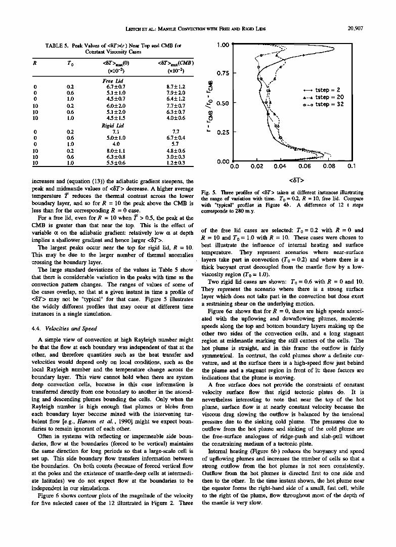
LFxrC• ET AL.: MnNTLE CONVECTION WITH FREE AND RIGID LIDs 20,907

TABLE 5. Peak Values of <$T>(r) Near Top and CMB for Constant Viscosity Cases

T O <ST >max(O) <ST >max(CMB ) (x10 -2) (x10 -2)

Free Lid 0 0.2 6.7 +0.7 8.7+ 1.2 0 0.6 5.1 + 1.0 7.9+2.0 0 1.0 4.5 +0.7 6.4 + 1.2

10 0.2 6.0+2.0 7.7+0.7 10 0.6 5.1+2.0 6.3+0.7 • 0 •.0 4.5 + •.5 4.0 + 0.6

Rigid Lid 0 0.2 7.1 7.7

0 0.6 5.0+ 1.0 6.7+0.4 0 1.0 4.0 5.7

10 0.2 8.0+ 1.1 4.8+0.6 10 0.6 6.3 +0.8 3.0+0.3 10 1.0 5.5 +0.6 1.2+0.3

1.00 '

0.75

0.50

0.25

0.00 0.0 0.1

k•'""i½ "a , , tstep = 2 \ ,"::\ .-..• tstep = 20

••i .x,,: o...o tstep = 32

0.02 0.04 0.06 0.08

increases and (equation (13)) the adiabatic gradient steepens, the peak and midmantle values of <fiT> decrease. A higher average temperature T reduces the thermal contrast across the lower boundary layer, and so for R = 10 the peak above the CMB is less than for the corresponding R = 0 case.

For a free lid, even for R = 10 when T > 0.5, the peak at the CMB is greater than that near the top. This is the effect of variable ct on the adiabatic gradient: relatively low ct at depth implies a shallower gradient and hence larger <fiT>.

The largest peaks occur near the top for rigid lid, R = 10. This may be due to the larger number of thermal anomalies crossing the boundary layer.

The large standard deviations of the values in Table 5 show that there is considerable variation in the peaks with time as the convection pattern changes. The ranges of values of some of the cases overlap, so that at a given instant in time a profile of <fiT> may not be "typical" for that case. Figure 5 illustrates the widely different profiles that may occur at different time instances in a single simulation.

4.4. Velocities and Speed

A simple view of convection at high Rayleigh number might be that the flow at each boundary was independent of that at the other, and therefore quantities such as the heat transfer and velocities would depend only on local conditions, such as the local Rayleigh number and the temperature change across the boundary layer. This view cannot hold when there are system deep convection cells, because in this case information is transferred directly from one boundary to another in the ascending and descending plumes bounding the cells. Only when the Rayleigh number is high enough that plumes or blobs from each boundary layer become mixed with the intervening tur- bulent flow [e.g., Hansen et al., 1990] might we expect boundaries to remain ignorant of each other.

Often in systems with reflecting or impermeable side boundaries, flow at the boundaries (forced to be vertical) maintains the same direction for long periods so that a large-scale cell is set up. This side boundary flow transfers information between the boundaries. On both counts (because of forced vertical flow at the poles and the existence of mantle-deep cells at intermedi- ate latitudes) we do not expect flow at the boundaries to be independent in our simulations.

Figure 6 shows contour plots of the magnitude of the velocity for five selected cases of the 12 illustrated in Figure 2. Three

<•T>

Fig. 5. Three profiles of <fiT> taken at different instances illustrating the range of variation with time. T o = 0.2, R = 10, free lid. Compare with "typical" profiles in Figure 4b. A difference of 12 t steps corresponds to 280 m.y.

of the free lid cases are selected: To = 0.2 with R = 0 and R = 10 and To = 1.0 with R = 10. These cases were chosen to best illustrate the influence of internal heating and surface temperature. They represent scenarios where near-surface layers take part in convection (To = 0.2) and where there is a thick buoyant crust decoupled from the mantle flow by a low- viscosity region (To = 1.0).

Two rigid lid cases are shown: To = 0.6 with R = 0 and 10. They represent the scenario where there is a strong surface layer which does not take part in the convection but does exert a restraining shear on the underlying motion.

Figure 6a shows that for R = 0, there are high speeds associated with the upflowing and downflowing plumes, moderate speeds along the top and bottom boundary layers making up the other two sides of the convection cells, and a long stagnant region at midmantle marking the still centers of the cells. The hot plume is straight, and in this frame the outflow is fairly symmetrical. In contrast, the cold plumes show a definite cur- vature, and at the surface there is a high-speed flow just behind the plume and a stagnant region in front of it: these factors are indications that the plume is moving.

A free surface does not provide the constraints of constant velocity surface flow that rigid tectonic plates do. It is nevertheless interesting to note that near the top of the hot plume, surface flow is at nearly constant velocity because the viscous drag slowing the outflow is balanced by the tensional pressure due to the sinking cold plume. The pressures due to outflow from the hot plume and sinking of the cold plume are the free-surface analogues of ridge-push and slab-pull without the constraining medium of a tectonic plate.

Internal heating (Figure 6b ) reduces the buoyancy and speed of upfiowing plumes and increases the number of cells so that a strong outflow from the hot plumes is not seen consistently. Outflow from the hot plumes is directed first to one side and then to the other. In the time instant shown, the hot plume near the equator forms the right-hand side of a small, fast cell, while to the fight of the plume, flow throughout most of the depth of the mantle is very slow.

20,908 LEITC•I ET AL.: MAmLE CONVEC'rlON WITH F•EE AND RIGID La)s

Fig. 6. Contour plots of speed (•Ur2+Uo 2 ) for five selected cases of the 12 shown in Figure 2. (a)-(c) Free slip lid: (a) R =0, T0 = 0.2 (cf. Figure 2a); (b) R = 10, T0 = 0.2 (cf. Figure 2b); (c) R = 10, To= 1.0 (cf. Figure 2f). (d)-(e) Rigid (no-slip) lid: (d) R =0, T o = 0.6 (cf. Figure 2i); (e) R = 10, T O = 0.6 (cf. Figure 2j). Contour interval is 250 (0.3 cm/yr), lowest contour line (250) dotted; bold contour is 1500 (1.75 cm/yr).

For high To (Figure 6c ) the hot plumes are still weaker and fast speeds are almost exclusively associated with cold downflow. The downflowing plume on the left pulls material from both sides as it sinks, implying that it is relatively stationary whereas the strong cold plume in the right hemisphere has the characteristic shape of a plume moving toward the right pole.

The speed fields for a rigid lid (Figures 6d and 6e ) have a very different shape than those for a free lid. The speed is constrained to be zero at the top, so that outflow from the hot plumes is concentrated just below the top and is deflected into a wavy stream by frequent cold boundary layer instabilities (bli's). This hot outflow in turn bends the cold bli's (Figure 2). The fastest speeds in the meandering stream occur just below and parallel to the thermal signatures of the bli's. The shape of the hot plume reveals that it is moving toward the left pole.

For R = 10 there are more cells and upflow is weaker, but the same basic features of the speed field are observed.

Figures 7a and 7b show profiles of horizontally averaged speed for the five cases and emphasize some of the points made about the contour plots. Figure 7a shows <speed> for the free lid cases, where the angle brackets represent an average taken over 0 and weighted according to area:

I ,0)sin(0)sin( d_• <X>(r)= X(r )

For R = 0 the strong horizontal flow at the top and CMB and the extensive stagnant region between plumes lead to a <speed>

profile with peaks at the boundaries. For R = 10, there are more plumes and outflow is less vigorous so that <speed> is almost uniform with depth. For To = 1.0 (dotted line) there is a similar uniform distribution but at a lower speed, demonstrating that flow is more sluggish.

For a rigid lid (Figure 7b ) the profiles are of course modified by the fact that the speed is constrained to be zero at the surface. With this proviso the same features are observed as for a free lid: for R = 0 there are two peaks associated with the horizontal outflow from the plumes, and for R = 10 the globally averaged speed is less and <speed> is more uniform with depth.

4.4.1. Influence of geometry and ct. We ran simulations in a Cartesian geometry and for constant ot in an axisymmetric spherical geometry to investigate the influence of geometry and variable ot on the velocity fields. The results are summarized in Figure 8 and Table 6. All cases had R = 0 and Ra = 3xlO 6.

For flow in a Cartesian geometry with R = 0 and ot constant, we expect the flow, on average, to be nearly symmetrical, so that the horizontal velocity at the top boundary is the same as that at the bottom boundary. Introducing depth-varying ot reduces the buoyancy at the bottom and makes flow more sluggish. The Rayleigh number based on local properties is a factor of 4.5 lower at the bottom. If flow was determined only by local properties we would then expect to be a factor (Racus/Rao) 2/3 = 2.7 lower. In fact, we find it 25-30% lower (solid line in Figure 8a ).

Gurnis and Davies [1986] studied the effect of depth varying viscosity in an aspect ratio 1 Cartesian box. They plotted

Lœrrc• m' nC.: Mam-• Com'•C•ON wrm From n•a) PdG• LBs 20,909

1.00

0.75

,- 0.50

I

0.25 -

0.00 0

"• o--• To =0.2, R =0 _ • -- --To=0.6, R=10

t ... To =1.0, R=I 0

I

25O 500 750 1000 1250

<speed>

1.00

0.75

ß - 0.50

I

0.25

0.00

s

.._...•.•..•' a'"' : : Cart.esi.an /if;:'"" • ...... A constant a -••.. e---.o variable (x

••:';;"JZ. -... '-• .•.

,

*'-•,.

o 5oo 1 ooo 1500

1.00

0.75 -

o.so-

0.25 -

0.00 0

---• R=O

ß --. R=10

I

200 1000 _ --

400 600 800

< speed >

Fig. 7. Profiles of horizontally averaged speed (<•]Ur2+U0 2 >) for (a) free slip lid, R = 0, T O =0.2 (solid line, open symbols), R = 10, T O = 0.2 (solid line, crosses), R = 10, T O = 1.0 (dotted line, crosses); (b) rigid lid, R = O, T O = 0.6 (dashed line, open symbols), R = 10, T O = 0.6 (dashed line, crosses). Ra = 3x106. In Figures 7-9, 1000 on x axis corresponds to 1.2 cm/yr.

1.00

0.75

,- 0.50

I

0.25

0.00

: : Cartesian *- .... , constant • ", "'...

-e----o variable (x • a.. /

.e'" z,"

,,." ..•s. A '''

0 200 400 600

<v>

Fig. 8. Profiles of horizontally averaged (a) horizontal velocity () and (b) radial velocity <Ur> (<v>), for Cartesian geometry, aspect ratio = 5, constant k, variable • (solid line); axisymetric spherical geometry with variable o• (dashed line); axisymetric spherical geometry with constant {z (dotted line). Ra = 3xlO 6, R = O, T O = 0.2, free slip lid.

<Ucsts>l<uo> as a function of 1og[Rao/Racsts] (their Figure 8) and their observations are entirely consistent with ours. A factor of 4.5 decrease in Rayleigh number with depth (due to a corresponding increase in viscosity) leads to a 30% decrease in <UCMt; >/.

The peak value of <v > also occurs above the centerline of the mantle because of the greater buoyancy forces in the upper part of the mantle.

The dashed lines in Figures 8a and 8b show typical profiles of <u0> (= ) and <Ur> (= <v>) for variable ot in an axisymmetric spherical geometry. With the change in geometry, is symmetrical about the middepth in the mantle and <v> is reduced. For these conditions, the effect of geometry counteracts that of variable

The <Uc•t;> is higher and <u0> is lower than in the Carte- sian geometry because of the way the geometry constrains the

plume. As a cold plume sinks, the surface area available for it decreases. Horizontal outflow from the plume must therefore be faster. Conversely, outflow from a rising plume will be slower, though the effect is less because as the radius of curva- ture increases the relative change in area is less. <v> may be reduced because of the greater resistance encountered by sinking plumes.

The dotted lines in Figure 8 illustrate results for constant •t in an axisymmetric spherical geometry. is about 15% greater at the CMB than it is at the surface, due to the geometry. <v > is also greater than it is when •t is variable, and the peak occurs at a greater depth.

4.4.2. Influence of R. Figure 9 shows <speed> profiles for three different values of R: O, 10 and 20. From Table 4 we see

that the volume-averaged speed for R = 10 is significantly less than that for R = 0, and from Figure 9 that it has a completely

20,910 LErrcH ET AL.: M/u'½mE CONVECHO•4 wrrH FREE AND RIGID LIDS

TABLE 6. Velocities for Differing Geometry and 0t

Geometry ot R n u ,u o(CMB) u ,us(O ) u (CMB)/u (0) v ,ur (max) r (max)

Cartesian vat 0 4dd 890+ 225 1235 + 345 0.72 555 + 165 0.57

Spherical const 0 2-4dd-3udi 1370+280 1187+225 1.15 545+ 100 0.40 Spherical vat 0 2dd 1160+320 1175+270 0.99 400+90 0.44 Spherical vat 10 3-7du 738 862 0.86 530+ 70 0.58 Spherical vat 20 8dd-3du 812 1022 0.79 595 + 35 0.64

different shape. We explained above that large cells with strong outflow at top and bottom and large stagnant regions in the middle of cells led to the profile seen for R = 0.

As R is increased to 10, there are more cells, and inflow into

the cold plumes is less extensive and outflow from the hot plumes is weaker at the top. The average and <v > velocities are more nearly equal and since the maxima occur at com- plementary depths (see Figure 7), the <speed> profile is almost straight.

The profile for R = 20, however, has more in common with the profile for R = 0: the average speed is higher than for R = 10 and once more there are peaks at top and bottom. This is despite the fact that, as we can see from the n column in Table 4, there are a large number of cells for R = 20. The answer to this observation lies in the changing buoyancy of the boundary layers as R changes. As R increases from 0 to 10, the buoyancy loss across the lower boundary layer is greater than the buoyancy gain across the top boundary, whereas when R increases again to 20, there is a net buoyancy gain. At this point the lower boundary layer is not providing much buoyancy, and the system is driven mainly from above.

For R = 20 there is fast inflow into the strong cold plumes at the top and it is ejected above the CMB in fast cold tongues. A comparison with the R = 0 profile shows that for R = 20, <speed> is faster at the top and slower at the CMB, suggesting that inflow into the departing plumes at each boundary layer is more important than the spreading tongues from the arriving plumes in determining the strength of the local horizontal flow.

4.5. Vorticity

Figure 10 shows the vorticity fields for the same selected cases for which the speed is given in Figure 6, that is,

1.00

0.75

I

•o o.5o

I

0.25

I

0.00 0 250

•--o R= 0

o--e R=10

=--R=20

500 750 1000 1250

< speed > Fig. 9. Profiles of horizontally averaged speed for R = 0 (dotted line), 10 (dashed line), 20 (solid line). Ra = 3xlO 6, T o = 0.2, free slip lid.

corresponding to the temperature frames in Figures 2a, 2b, 2f, 2i and 2j.

Vorticity is the local rotation in the system. In an axisymmetric spherical geometry it is given by

, •}u o u o 1 •)Ur to = 'A (--•-r + ) (15) r r•

For free slip boundaries, it is generated only by horizontal gradients in buoyancy. An approximate formula is [Jarvis and McKenzie, 1980]

•)T V2to = Rao• (16)

•x

and regions of high vorticity are associated only with the rising and sinking plumes (Figures 10a- 10c ). For a rigid lid (Fig- ures 10d and 10e ) it is also generated by the shear associated with horizontal flow at the upper boundary. The sign of the vorticity indicates the direction of flow in the convection cell (clockwise or counterclockwise).

There is a peak in vorticity near the base of a plume, and it tends to reduce along the plume as the temperature anomaly diffuses. In Figure 10a, for which internal heating R = 0 and To = 0.2, this trend is enhanced in the case of cold, sinking plumes and reversed in the case of the rising hot plume, so that there is a second maximum in voriticity in the upper mantle. This is because vorticity generation is proportional to •x which increases steeply in the upper mantle [Leitch et al., 1991].

The existence of large regions in Figure 10a where the sign of the vorficity is constant confirms the large cell size observed in Figure 2a. The cold boundary layer instabilities cause a local circulation and thus have a change in the sign of to associated with them, but the circulation does not extend the full

depth of the mantle. Note, comparing Figures 6 and 10, that the vorficity gives little indication of the strength of the horizontal flows.

Figure 10b (R = 10) shows the existence of several more cells than does Figure 10a. The hot plumes are weaker, gen- erating less vorticity both at their bases and near the surface, though the strongest hot plumes, near the equator and at the left pole, do show the second maximum near the top.

The vorticity fields for To = 0.6 are very similar to those for To = 0.2. Figure 10c shows the vorticity field for To = 1.0, R = 10 (cf. Figure 2f). The flow is weaker, with less pro- nounced vorticity maxima associated with the plumes. In particular, the vorticity signals of the hot plumes are scarcely visi- ble using the contour interval given. The sign of to between the plumes is constant throughout the depth of the mantle, indicating that the plumes are associated with deep narrow cells rather than than being boundary layer instabilities which generate only local circulation.

Figures 10d and 10e show vorticity for a rigid lid with To = 0.6 and R of 0 and 10, respectively. The most noteable features of these fields is the presence of vorticity maxima at the upper boundary. The vorticity associated with the horizon-

LœrrcH ET AL.: MAN'I• CONVECTION WITH FREE AND RIGID Ln•s 20,911

a b

Fig. 10. Contour plots of vorficity (equation (15)) for the same five selected cases shown in Figure 6. (a)-(c) Free slip lid: (a) R =0, T 0=0.2; (b) R = 10, T 0=0.2; (c) R =10, T 0=l.0. (d)-(e) Rigid (no-slip) lid: (d) R =0, T 0=0.6; (e) R = 10, T o = 0.6. Contour interval 2500 (3.4x10 -16 s-l). Negative contours dashed.

tal shear flow is a little greater in magnitude than that associated with the sinking cold plumes. It is interesting to observe that the shape of the vorticity maxima near the top is similar to the shape of the speed near travelling boundary layer instabilities for a free lid (see Figures 6a-6c): that is, it increases rapidly until the point at which the plume detaches.

The sign of the vorticity in the lower part of the mantle shows that the large-scale circulation comprises few cells (n = 2 for R = 0 and n = 4 for R = 10), but there is local circulation in the upper part of the mantle associated with the sloping cold boundary layer instabilities. This reinforces the picture of the circulation given by the speed contours in Figures 6c and 6d. This division of scales for the circulation due to

the rigid lid condition is a form of incompletely layered mantle convection.

4.6. Plume Wandering

It is difficult to obtain much insight into the time dependence of convecting systems by studying representative contour plots at single instances, such as those shown in Figures 2, 6, and 10. To represent the time dependence of the system, we have plotted the latitude of plumes near the upper boundary as a function of time in Figures 11a-lle, which correspond to the selected cases shown in Figures 6 and 10. The plumes were identified by seeking zeros of the vorticity at a distance of 5% of the mantle depth below the top. We could also have plotted plume wandering near the CMB; however, we are most interested in the signals of hot plumes which have penetrated the mantle.

The concept of displaying time dependence by tracking

plume wandering was first used by Goldhirsch et al. [1989] and later by Hansen et al. [1990], who identified the plumes from changes in the sign of the horizontal velocity.

Using the vorticity field, the direction of the plume can be found from the sign, and the strength of the plume from the magnitude of the gradient •)ol/•)x I•0. •ro/•x I•-0 < 0 implies a downflowing plume and •ro/•x I•0 > 0 signifies outflow from a rising hot plume. In Figure 11, solid triangles indicate a hot plume.

The plume strength is indicated in Figure 11 by the size of the symbols according to

Size log [•ro/•x I•0] = (•7)

minimum Size log [•Ol/•Xmin]

The largest symbol is 10 times the size of the smallest. The values of the vorticity gradient corresponding to the maximum and minimum symbol sizes are given in the Figure 11 caption.

Figure 1 la shows several striking features of time-dependent flow for R = 0, To = 0.2 and a free slip lid (cf. Figures 2a, 6a, and 10a). There is strong, steady outflow from a hot plume left of the equator. Downflow first appears some distance from the hot plume and is in the form of boundary layer instabilities (bli's) which are swept toward the poles. There is almost always downflow at the poles though it varies in strength as it is periodically augmented by collisions from the bli's.

A bli is distinguishable from a plume by two features: (1) it is part of a large-scale circulation so it is moving toward the strong stationary (or at least more slowly moving) downflow marking the boundary of the cell; and (2) it generates only local

20,912 LErrCH ET nl..: MnnTLE Com, ECnOS wrm FREE Am• Rm•D DDS

(x10 -$)

4

C

t

(x10 -$)

.i.

&

ß

ß

&

ß

ß

ß

ß

ß ß

ß

ß

I I

/1;/2

ß - v , VA

ß • VA VA• z

.. •Y

ß

'A

rA

•A

•A

?A

7

7

o

t

2

(x10 -•)

4•

,v

ß

ß

ß

ß

ß

ß

&

ß

ß

ß

ß

ß

ß

•7 & ' A V & V A

v .V-v,V V ' V' •7' V V--' V V'"•'V'V

t

2

(x10 -$)

z o

Fig. 11. Plume positions at the top boundary as a function of 0 and t for the five selected cases shown in Figures 6 and 10. Solid triangles represent upflow; open, inverted triangles represent downflow. Size of symbols is related to gradient B•)x (equation (17)), and therefore to strength of plume. (a)-(c) Free slip lid: •o•/•Xmin = 10 4, •0•Xmax = 5x10 5. (a) R =0, T O = 0.2; (b) R = 10, T O = 0.2; (c) R = 10, To = 1.0. (d)-(e) Rigid (no-slip) lid: B•)Xmi n = 10 4, •}O•/•)Xma x = 3x10 5. (d) R =0, T 0=0.6;(e)R =10, T 0=0.6.

rather than mantle-deep return flow, so it is trailed closely by a weak vorticity reverse (small solid triangles). Near the poles the moving, cold "bli's" are strong and penetrate deeply (Figure 2a) so definitions become rather cloudy.

Figure l lb (R = 10) shows a system with more cells and much greater time dependence of the large-scale flow. Flow at the poles varies much more in magnitude than in Figure 11a and periodically flips in direction. There is still relatively steady hot outflow near the equator, but it is weak in comparison with the surrounding downflow and wanders more in latitude. Downflow occurs quite close to the hot outflow.

Note the way downflow occurs and strengthens first on one side of the equatorial hot plume and then on the other as the first downflow moves away. This is the signal of the outflow flipping from one side to the other. Near the right pole is a second quasi-steady hot plume which has a similar limited influence on the downflow around it as the equatorial plume. Cold plumes collide between these two hot plumes.

In the left hemisphere there are two or three strong downflows with only weak return flow signals between them. This case illustrates the waning but still positive influence of hot plumes in organizing the flow field.

Lœrrc• •r •a•.: M•rt• CotYledoN wrm FR• Am R[am Lms 20,913

4

e

t

(x10 -•)

Fig. 11.

• VAV• V

•/2

o

(continued)

Figure 11c (To= 1.0, R = 10) demonstrates yet another scenario. The hot outflows are still weaker relative to the cold

downflow and flow at the poles is variable, but the plumes, with the exception of the strong downflow in the right hemisphere, are fairly stationary, moving and merging only slowly. From Figure 10c we know that the cells extend the depth of the mantle.

The last two plume-wandering graphs, Figures lid and 1 le are for the rigid lid cases with To = 0.6 and R = 0 and 10. For these graphs the vorticity was measured at the surface rather than just below it. These patterns are dominated by the signals of the cold boundary layer instabilities (bli's), which move slowly toward the poles, and their accompanying weak return flows. For Figure lid there is only one hot plume, which starts at 0 = •r/3 and whose signal fluctuates in strength and position and at one point moves abruptly several degrees to the left. A plot of the vorticity zeros near the CMB would show much less activity.

Figure 11e (R = 10) shows even more signals from the cold bli's. The steady hot plumes mark a straight path through ave- nues of slowly moving cold bli's.

4.7. Effects of R, To, and Lid

Our simulations yielded values of such variables of interest as the globally averaged temperature T, the globally averaged speed (u2+ v2) v2, and the temporally and spatially averaged heat fluxes at the boundaries QcMa and Q0 (Table 4). From these results, it is possible to quantify the "effect" that each of the

parameters we varied in our simulations (R, To, and the surface stress condition) has on these global values using a statistical technique called factorial design [Box et al., 1978]. The results are given in Table 7.

The "effect" of a parameter x•, on a result y is the average change in y as xk is varied over a given range. The average is taken for all possible values of the other parameters. The effect of the interaction of two parameters xj and xk indicates whether or not there is a systematic change in the effect of xk on y as xj varies. The way in which the effects are calculated by fac- toffal design is explained in the appendix.

The changes in the dimensionless quantities can be roughly translated into dimensional numbers with the help of the last two rows in Table 4, which give typical values of the dimensionless quantities and their dimensional equivalents. Thus a change in T of 0.18 corresponds to roughly 0.18x1500/0.53 = 510 K. This is only an approximate value because cases may be nondimensionalized with, for instance, different values of

A glance at the results in Table 7 shows that as the parameters change over the given ranges, R from 0 to 10, the "lid" from a free to a rigid surface stress condition, and To from 0.2 to 1.0, the temperature always increases, the speed decreases, and, with the exception of the effect of R on Q0, the fluxes always decrease. R has the greatest effect on T, the lid has the greatest effect on the speed, and To and R have the greatest effects on the fluxes.

The effects of the interactions R and lid and To and lid are considerable, in many cases of similar size to the effects of the parameters themselves, showing that the parameters cannot be considered as affecting the system independently of one another. Only R and To do not produce a systematic variation in any of the values x when they are varied together and may thus be considered to affect the system independently.

From column 3 in Table 7, we see that R, the lid, and To all lead to an increase in T. This is as expected: greater internal heating will always lead to an increase in temperature; a rigid lid inhibits heat loss from the surface; and higher To steepens the adiabatic temperature gradient leading to more sluggish flow and less efficient loss of internal heat at the surface.

Changing R from 0 to 10 has the largest effect, 0.18, more than twice that of the lid. The effect of To is relatively minor though still statistically significant, since it is greater than the effects of the interactions of To with the other parameters.

The interaction of R and the lid is positive. This means that the effect of R is greater for a rigid lid than for a free lid and the effect of the lid is greater for R = 10 than for R = 0. The number 0.06 says that the effect of R is 0.06 greater for a rigid than for a free lid. Inspection of Table A1 confirms this: for a free lid, internal heating of R = 10 increases the temperature by about 0.15, and for a rigid lid it increases it by about 0.21.

The number after the + sign in the effect of an interaction is

Parameter

R

Lid

To

R and Lid

R and T O T O and Lid

TABLE 7. Effects of R, Lid and T O by Factorial Design

Variation Effect on •ff Effect on Speed Effect on QCMB Effect on Q 0

o-•1o

free -• rigid 0.2 -• 1.0

+0.18 -100 -9.9 +19.3 +0.075 -235 -7.5 -7.5 +0.032 -200 -12.8 -13.2

0.06 + 0.02 + 115 + 30 -6.0+ 1.8 -5.5 + 1.4 -0.004 + 0.03 +20+ 60 +0.6 + 2.6 - 1.0+ 2.4 -0.02+0.03 +100+60 +7.6+2.0 +7.2 +3.0

20,914 LErrCH ET AL.: MANTLE CO8VECHO8 wrrH FREE AND Rm•D L•Ds

TABLE 8. Global Results of Variable Viscosity Simulations

Case Lid T O A C n T Speed QCMB Qo

1 free 0.2 ln30 0

2 free 0.2 0 ln20 3 free 0.2 ln30 ln80

4 rigid 0.6 ln30 ln80

9du-6uu-3-5ud 0.61 640_+ 140 19_+2 47_+ 4 3du-i 0.44 850_+200 24_+2 54_+ 4 2dd-i 0.45 900_+200 23_+2 53_+4 2dd 0.65 580_+ 30 5.8 _+ .3 35_+ 1

A and C are from equation (12).

the standard deviation of the numbers which made up the average. It gives the range of the interaction effect over the third parameter (the lid in the case of R and To) and so indicates the significance of the interaction. R and To and To and lid are less than their ranges, meaning that there is no consistent trend in T as the two parameters are varied together.

From column 4 in Table 7, the given changes in R, the lid, and To all lead to a reduction in the average speed. The greatest effect is due to the lid. The high shear stress at the rigid surface reduces the average speed by about one third, as inspection of the values in Table 4 shows. The next greatest effect is that of To; as mentioned above, at higher To flow is more sluggish.

Increased R also reduces the average speed. As discussed in section 4.6, the greater negative buoyancy of the upper boundary layer does not compensate for the loss of buoyancy of the lower boundary layer in driving convection.

The effects of the interactions R and lid and To and lid on

the speed are large and positive. This means that the effects of R and To in reducing speed is less for a rigid lid, and conversely that the effect of the rigid lid in reducing speed is less for R = 10 and To = 1.0.

Columns 5 and 6 of Table 7 show that a rigid lid and higher To reduce the fluxes Qcsta and Q0 significantly. The fluxes are reduced by the same amount because of the heat balance requirement. It is noteworthy that the change in To has a greater effect on the fluxes than a rigid lid. Again, for heat balance we require that Q o-Qcsta = RM, where

m •

o

c•P r2 dr is the mass of the mantle. For our equation of state, M = 2.92 and so for R = 10, Q o-Qcsts = 29.2. The first row of Table 7 shows that as R increases from 0 to 10, two thirds of this

difference is accommodated by an increase in the surface heat flux and one third by a reduction of the core flux.

The interaction R and lid is negative so for a rigid lid the reduction in Qcsts is greater and the increase in Q0 not as great. To and lid is positive, indicating that the effect of the lid was less when To was greater.

We note that these results are only accurate over the parameter range given. It would be a mistake, for instance, to assume that because the effect of R changing from 0 to 10 is to reduce the volume averaged speed, that the speed always decreases with R. As mentioned in section 4.4.2, increasing R from 10 to 20 increases the speed.

4.8. Summary of Constant Viscosity Results

Increasing the internal heating R from 0 to 10 increases the temperature of the mantle (Figure 3). Table 7 shows that the increase is 0.15 for a free lid and 0.21 for a rigid lid, in dimen-

sionless units, independent of To. Increasing R also increases the number and time dependence of hot plumes, changing the convection pattern from one of few steady cells with strong horizontal flow at the boundaries for R = 0, to one where there

are smaller, shorter-lived cells with strong downflow. The volume averaged speed is reduced as R increases from 0

to 10, and speed is uniformly distributed throughout the mantle instead of being concentrated at the boundaries. However, when R is increased further to 20, speed increases again and a speed profile similar to that for R = 0 is recovered (Figure 9).

To plays a similar role as the Dissipation number D in its effect on the dynamics of the mantle, as can be deduced from looking at the term of the the energy equation given in equation (13). Higher To implies steeper adiabatic gradients and smaller superadiabatic temperature jumps across the boundary layers. Flow is more sluggish and thermal anomalies dissipate more quickly.

There was little difference observed between To = 0.2 and

0.6 in the number and stability of cells, and salient features of the speed and vorticity fields. For To = 1.0, flow was notice- ably slower, there tended to be a greater number of cells, and the plumes wandered less so that the cells were more stable.

The rigid lid leads to an increase in temperature of about 0.045 for R = 0 and 0.105 for R = 10 (Table 7), that is, it has one third to one half as much effect on T as the internal heat-

ing under these conditions. Horizontal motion near the top is impeded, and speeds are lower than for free lid convection by about 30%. The weakening of flow at the top boundary layer allows the bottom boundary layer and hot plumes to be much steadier.

1.00 [ [] ' '0 ..... 0.75

I

e? o.so

I

•- 0.25

0.00 -1.0 -0.5 0.0 0.5 1.0

< log q > Fig. 12. Pr6files of horizontally averaged log of viscosity (<1og10(rl)>) for the four variable viscosity cases. Dashed line, rl = rl(T); dotted line, rl = rl(r); solid lines, rl = rl(T,r). Pluses, rigid lid; all others, free lid.

LEITCH ET AL.: MANTLE CONVECTION WITH FREE AND RIGID L•DS 20,915

a a

Fig. 13. Contour plots for •1 = •I(T). A = ln30. (a) Temperature. Contour interval 0.1 (350 K). Bold dashed contour is T=0.5. (b) Speed. Contour interval 250 (0.3 cndyr); maximum value = 2900 (3.4 cndyr). (c) Vorticity. Contour interval 2500 (3.4x10 -16 s-i); maximum value = +11,000 (1.5xlO

Fig. 14. Contour plots for •1 = •l(r). C = ln20. (a) Temperature. Con- tour interval 0.1 (350 K). (b) Speed. Contour interval 500 (0.6 c•n/yr); maximum value = 13,500 (16 cndyr). (c) Vorticity. Contour interval 5000 (6.9x10 -16 s-l); maximum value = +_54,600 (7.5x10

A rigid lid can also lead to a division of scales in the circulation. A large-scale circulation is driven from below, the upper boundary layer of which meanders around local circulations associated with cold boundary layer instabilities (Figures 6d and 6e ). The vorticity field for rigid lid convection is thus very different from that for a free lid (Figure 10), with regions of high vorticity associated with shear at the top and the many local circulations.

The global convection pattern is set up by a cooperation of flows from each boundary and at least while there is whole mantle convection, the flow near the boundary cannot be determined by the properties at the boundary alone. A boundary layer becomes unstable when it reaches a certain critical buoyancy which is determined by local properties ggkT and z:, and also the length of time flow is attached to the boundary.

For our variable • simulations, flow at the CMB is faster and

flow at the top is slower than it would be if local conditions existed throughout the mantle, and thus fluid in the lower boundary layer can travel farther and fluid in the top boundary less far before it becomes unstable. There is a battle between the

boundary layer flows to decide which will determine the aspect ratio of the large-scale circulation, and its outcome depends on the relative strengths of plumes which reach the opposite boundary. A significant decrease in • with depth favors the lower boundary layer and long cells, since outflow from the hot

plumes is strong near the top and the cold plumes lose buoyancy as they sink.

As our simulations illustrate, weakening the bottom boundary layer by decreasing AT (CMB) (increasing R or To) allows the top boundary layer more influence and the cells become shorter. Conversely, weakening the top boundary layer with the imposi- tion of a rigid lid condition favours long cells.

5. RESULTS FOR VARIABLE VISCOSITY

Up until now we have been concemed only with constant viscosity flows. It is well known that variable viscosity can exert a strong influence on mantle convection. We ran four cases to investigate the effect of variable Newtonian viscosity on mantle convection, using the viscosity law given in equation (12). With a free lid surface conditi6n, internal heating R = !0, and top temperature To = 0.2, we looked at purely temperature- dependent viscosity (C = 0), purely depth-dependent viscosity (A = 0), and depth- and temperature-dependent viscosity. We also ran one simulation with a rigid lid, using R = 10 and To = 0.6. All cases were for a Rayleigh number of 3x10 6 based on the average viscosity in the mantle. The conditions of the simulations are summarized in Table 8 together with results for some globally averaged quantities. We label the cases 1 to 4 for convenience.

20,916 LEITCH ET AL.: Mnh•n.• CONVEC'HON WITH FREE AND RIGID LIPS

Profiles with depth of the horizontally averaged log of the viscosity <1og•0•l> (r) are given in Figure 12. From the equation for the viscosity (equation (12)), the log viscosity for case 1 mirrors the temperature profile (cf. Figure 18), for case 2 it increases linearly with depth, and for cases 3 and 4 it also increases with depth but with strong and weak boundary layers at the top and CMB respectively.

For case 1 the viscosity decreases by a factor of 30 from the top to the CMB, with most of the change occurring over the boundary layers. There is about a factor of 2 decrease in viscosity with depth between the boundary layers. For case 2, viscosity increases with depth by a factor of 20. The values of A and C for the other cases was chosen to result in approximately the same viscosity increase with depth as case 2. For cases 3 and 4 there is an increase in viscosity of about a factor of 3 across the upper boundary layer. For case 3 (free lid) there is a decrease in viscosity of a similar magnitude across the lower boundary layer, whereas for case 4 (rigid lid), because the temperature contrast is much less (see Figures 16 and 18), the viscosity decrease across the lower boundary layer is only about 10%.

Figures 13 to 16 show contour plots of temperature, speed and vorticity at representative time instances for the four cases, respectively, and Figure 17 shows a contour plot of log•0(•l) for cases 3 and 4. For case 1, the log viscosity is simply the inverse of the temperature field in Figure 13a, and for case 2 it does not vary with latitude; thus we have not bothered to show contour plots of log viscosity for these cases.

\

Fig. 15. Contour plots for •1 = •l(T,r). A = ln30, C = ln80. Contour intervals as in Figure 14. (a) Temperature. (b) Speed. Maximum value = 5700 (6.7 cm/yr). (c) Vorticity. Maximum value = ñ32,000 (4.4x10-•s s-•).

Fig. 16. Contour plots for B = B(T,r). A = ln30, C = ln80. Rigid lid. Contour intervals as in Figure 13. (a) Temperature. Contour interval 0.1 (250 K). (b) Speed. Maximum value = 3100 (3.6 cm/yr). (c) Vorticity. Maximum value = ñ15,000 (2.1x10

The convecting systems revealed in Figures 13 to 16 illustrate four rather different behavior. Briefly, case 1 (•l(T)) is hot and the convection pattern very time-dependent. There are several weak hot plumes which wander in latitude with time. Case 2 (•l(r)) is significantly cooler and forms a fairly steady three-cell convection pattern. The boundary layer is thicker and does contain hot bli's. Downflow is localized in narrow, fast

cold plumes. Case 3 (•(T,r)) is close to the same temperature as case 2

but has a two-cell pattern. Bli's were also observed in the hot boundary layer, but the hot plume was generally steadier. Case 4 (rigid lid) is hotter (similar temperature as case 1) and has a very steady tWo-cell pattern with the slowly moving cold bli's that were found in section 4 to be characteristic of rigid lid convection. We look in more detail at each of the fields below.

5.1. Temperature and Heat Flux

The temperature. profiles in Figure 18 reinforce the information in Figures 13-16a and Table 8. Cases 2 and 3 have very similar, cool temperatures, whereas cases 1 and 4 are hotter. Case 4 has a steeper adiabatic gradient in the interior because it was run at higher To (see equation (13)).

The average nondimensional temperature T for case 1 is 0.61, compared with a value of 0.54 for the equivalent constant viscosity case. The average viscosity is the same in both cases, so this implies that for the variable viscosity case, the viscosity

LErrc• ET AL.: M,•rrL• Co•wE•os wrrn FREE A•D Rm•D L•DS 20,917

Fig. 17. Contour plots of 1og10(q) for q = q(T,r). Contour interval 0.125. Negative contours dashed. (a) Free lid. (b) Rigid lid.

0.00

0.0 0.2 0.4 0.6 0.8 1.0

<T>

Fig. 18. Profiles of horizontally averaged temperature for the four variable viscosity cases. Case I q(T), dashed line; case 2 q(r), dotted line; cases 3 and 4 q(T,r), solid lines. Pluses, rigid lid (case 4).

is higher at the top and lower at the bottom. Since the mantle is stiffer near the top, heat transfer is impeded and the temperature rises. Additionally, more fluid conditions near the CMB facilli- tate heat transfer from the core.

Actually, the heat flux Qctas is less in case 1 than for constant viscosity, because the temperature rises until the drop across the lower boundary layer is sufficiently reduced. Qctas must be less than it is for the constant viscosity case because Q0 is less and R is the same. Heat balance requires that Q o- Qctas = RM, where M is the mass of the mantle.

If the viscosity increases rather than decreases with depth (case 2), then the converse situation exists and the mantle is cooler with T = 0.45. The heat fluxes Q are similar to the constant viscosity case, but in case 2 there are fewer cells, which, other things being equal, reduces the expected heat flux.

Despite the differences in the viscosity in the boundary layers in cases 2 and 3, the temperature is very similar, indicating that the viscosity boundary layers have not greatly affected the heat transfer.

Case 4 has very similar global thermal properties to its constant viscosity equivalent. This presumeably comes about because the high viscosity boundary layer occurs directly next to a rigid lid, where its impact would not be expected to be very great. The high viscosity region just under the lid and the low viscosity region underneath that counteract each other to give similar heat transfer as constant viscosity.

5.2. fit

Figure 19 shows typical profiles of the residual temperature <fiT> (equation (14)) and Table 9 gives the average and standard deviation for the magnitude of the peaks near the surface and the CMB for each case.

The magnitudes of the peaks near the CMB correlate well with the temperature change across the upper boundary layer (cf. Figure 18), as they did for the constant viscosity cases described in section 4.3, and as for the constant viscosity cases, the time variations in the peak magnitudes are quite significant.

The peaks above the CMB also follow the temperature drops

across the boundary layer with one important exception: case 2 has a significantly stronger peak than case 3. This is due to the fact that there is a larger number of hot plumes in case 2, and the plumes are thicker. Profiles of <ST> are the only profiles we have looked at that clearly distinguish between cases 2 and 3.

5.3. Speed

The contour plots of speed for the four cases shown in Fig- ures 13-16b are quite different in the magnitude and distribution of high-velocity regions. The contour interval in Figures 13b and 16b is the same, and that in Figures 14b and 15b is twice as great.

Horizontally averaged profiles of , <v> and <speed> are shown in Figures 20, 21, and 22, respectively. The horizontally averaged speed at midmantle levels is very similar for all

1.00 '

0.75

0.50

0.25

0.00

0.0

I I:' • 2: ,• iii•..... ' 3: q (T,r) • 4: rigid lid

0.025 0.05 0.075 0.10 0.125

<bT>

Fig. 19. Profiles of horizontally averaged fit (equation (14)) for the four variable viscosity cases. Lines as for Figure 18. '

20,918 L•.rrc• ST •L.: M/a•rn.s Cohwsc'no• wrm FR• •a•D RIom Lms

TABLE 9. Peak Values of <iST>(r) Near Top and CMB for Variable Viscosity Cases

Case A C <fiT>max(O) <iST>max(CMB) (x10 -2 ) (x10 -2 )

Free Lid I 30 0 7.8 + 0.8 5.5 + 0.8 2 0 20 4.8_+ 1.0 11.1 _+ 1.2

3 30 80 5.0+ 1.1 8.3_+ 1.5

Rigid Lid 4 30 80 6.3 +0.9 3.7 +0.5

models and is therefore probably dependent only on the average Rayleigh number, which is the same for all cases. The volume averaged speeds for cases 2 and 3 are about 50% higher than for the other cases (Table 8) largely due to higher speeds in the upper mantle.

Although the horizontally averaged velocities , <v> for cases 2 and 3 are very similar, the downflowing plumes in case 2 are faster and more concentrated. The maximum u and v

velocities in case 2 are about twice that of those in case 3

because the maxima occur near the top, where the viscosity is up to a factor of 3 lower in case 2.

The velocities for the free lid cases show the expected peaks at the boundaries. For case 1 the minimum is at midmantle, but the maximum velocity at the CMB is about 20% higher than it is at the top. This compares with the constant viscosity result that <Uc•ts> is about 15% lower.

For cases 2 and 3, the minimum is higher in the mantle, <Uo> is much higher, and <Uc•ts > is lower, so that the horizontal velocity is concentrated toward the lower viscosities in the upper mantle. The ratio <Ucsts >/ is about 0.40. This is very similar to the results of Gumis and Davies [1986] for an increase in viscosity of a factor of 20 in a Cartesian box of aspect ratio 1. We might not expect such an exact correspon- dence bearing in mind differences in geometry and mantle properties; however, we noted in section 4.4.1 that it is possible for the influences of spherical geometry and variable ix to cancel.

The maximum <v > for case 1 occurs in the lower part of the mantle, while <v >max for case 2 occurs in the upper part. Each favors the region where the resistance to flow is least. The magnitudes of the maxima are similar: the individual plumes in case 2 are faster, but there are more plumes in case 1.

Case 3 is similar to case 2, but case 4 shows a stronger peak in <v> in the upper mantle. This peak owes its existence to cold bli's and the downward jags in the meandering hot outflow (see Figure 16b ).

Profiles of <speed> (Figure 22) mirror the features of the profiles of (Figure 20), except that for case 4, the peak in <v> is close to the upper mantle peak in and so that the highest <speed>, unlike the highest , occurs in the upper mantle.

5.4. Vorticity

The vorticity signals of the hot plumes in case 1 (Figure 13c ) are quite distinct; however, this does not mean that the plumes are strong. Vorticity is a measure of how rapidly fluid elements are rotating (equation (15)), and for lower viscosity the rotation occurs more easily. The hot plumes lose their signal, as they rise in the mantle and encounter increasingly stiff resistance to rotation.

This fate also overtakes cold plumes descending into a stiffening mantle in cases 2 and 3. In Figures 14c and 15c,

1.00

0.75

o.$o

0.25

0.00

ß • ß ß

ß

,". •--o 1' •1 (T) • " o .... o 2' •1 (r)

ß .0 ß

500 1000 1500 2000



1.00

0.75

0.50

0.25

0.00 i i 0 1000 1500 2000

f.--"

½ , 3' •1 (T,r) - , , 4: rigid lid

I .

5OO



Fig. 20. Profiles of horizontally averaged u e. (a) Cages I and 2; (b) cases 3 and 4. In Figures 20-22, 1000 on x axis corresponds to 1.2 cm/yr.

vorticity, generated by both ascending and descending plumes, is concentrated in the upper part of the mantle. The vorticity maxima are stronger and closer to the top in case 2 because of the lack of a stiff upper boundary layer.

It is interesting to compare the vorticity field in Figure 16c with the corresponding case at constant viscosity (Figure 10e ). For constant viscosity, weak vortices, generated as the hot outflow meanders around the cold bli's, extend deep into the manfie. In contrast, in case 4 the hot outflow is restricted to the

weaker upper regions of the mantle and there is a more orderly progression of shallower vortices.

5.5. Viscosity Fields

Figure 17 shows contour plots of log]0T I for cases 3 and 4. The depth dependence of viscosity illustrated in Figure 12 (solid lines) is also evident in the contours. There is a trend of increasing viscosity with depth with strong and weak boundary layers at the top and CMB, respectively.

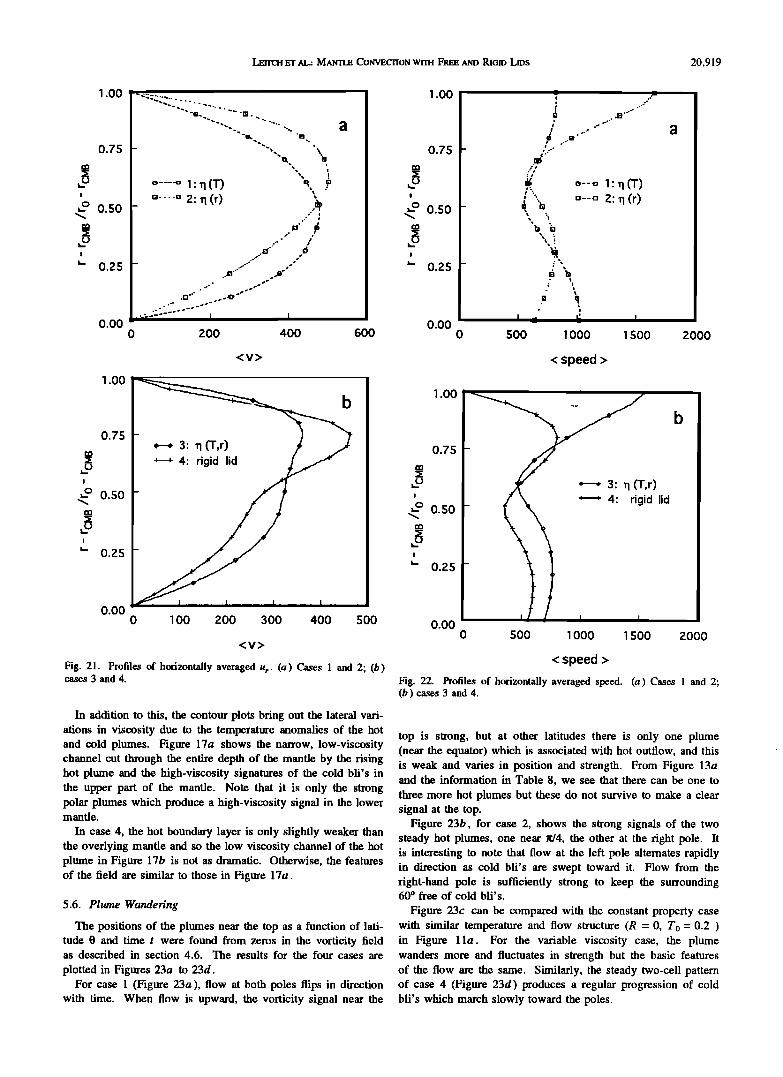
LErrc• EW AL.: MamLg CONVECTION WITH FREE AND RIGID LIDs 20,919

1.00

0.75

o.so

0.25

0.00 0 200 400 600

1.00

0.75

i

•_o 0.50

i

0.25

I

0.00 0 500 1000 1500 2OOO

<v>

1.00

0.75

0.50

0.25

0.00 0 1 O0 200 300 400 500

<v>

Fig. 21. Profiles of horizontally averaged u r . (a) Cases 1 and 2; (b) cases 3 and 4.

In addition to this, the contour plots bring out the lateral variations in viscosity due to the temperature anomalies of the hot and cold plumes. Figure 17a shows the narrow, low-viscosity channel cut through the entire depth of the mantle by the rising hot plume and the high-viscosity signatures of the cold bli's in the upper part of the mantle. Note that it is only the strong polar plumes which produce a high-viscosity signal in the lower mantle.

In case 4, the hot boundary layer is only slightly weaker than the overlying mantle and so the low viscosity channel of the hot plume in Figure 17b is not as dramatic. Otherwise, the features of the field are similar to those in Figure 17a.

5.6. Plume Wandering

The positions of the plumes near the top as a function of latitude 0 and time t were found from zeros in the vorticity field as described in section 4.6. The results for the four cases are

plotted in Figures 23a to 23d. For case 1 (Figure 23a), flow at both poles flips in direction

with time. When flow is upward, the vorticity signal near the

< speed >

1.00 •.•,.,

0.75

.•,ø 0.50

0.25

0.00

' j

- / ; ; 3: q(T,r)

0 500 1000 1500 2000

< speed >

Fig. 22. Profiles of horizontally averaged speed. (a) Cases 1 and 2; (b) cases 3 and 4.

top is strong, but at other latitudes there is only one plume (near the equator) which is associated with hot outflow, and this is weak and varies in position and strength. From Figure 13a and the information in Table 8, we see that there can be one to

three more hot plumes but these do not survive to make a clear signal at the top.

Figure 23b, for case 2, shows the strong signals of the two steady hot plumes, one near g/4, the other at the right pole. It is interesting to note that flow at the left pole alternates rapidly in direction as cold bli's are swept toward it. Flow from the right-hand pole is sufficiently strong to keep the surrounding 60 ø free of coM bli' s.

Figure 23c can be compared with the constant property case with similar temperature and flow structure (R = 0, To = 0.2 ) in Figure 11a. For the variable viscosity case, the plume wanders more and fluctuates in strength but the basic features of the flow are the same. Similarly, the steady two-cell pattern of case 4 (Figure 23d) produces a regular progression of cold bli's which march slowly toward the poles.

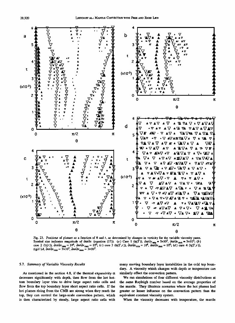
20,920 LEITCI-I ET AL.: MAhqLE CONVECTION WITH FREE AND RIGID LIPs

6

a

5

3•A

(xlO -3) • •& 7A X7 •

7•

o

o

ß . V V,

V• V

•L

•L

•k

t

(xl 0 -3) 1

•7 ß V V ß

v iv

7& v

V

ß V

ß V

ß V i a•7 A

A ß

ß

A A A A & A &

A A A A

I

t

2

(x10 -3)

(x10 -3)

ß

- V 0 •

0

7 7 x

o 0 ;t/2

0

Fig. 23. Positions of plumes as a function of 0 and t, as determined by changes in vorticity for the variable viscosity cases. Symbol size indicates magnitude of •)(o/•)x (equation (17)). (a)Case I (q(T)), •)m/•)Xmin = 3xlO 3, •)0)/•)Xma x = 3x105; (b) case 2 (q(r)), •)fiX/•}Xmi n = 10 4, •)OY•}Xmax = 106; (c) case 3 (q(T,r)), •)Ol/•}Xmin = 104, Dm//)Xmax = 106; (d) case 4 (q(T,r)), rigid lid, Dm/DXmi n = 3x103, Dm/DXma x = 3x105.

5.7. Summary of Variable Viscosity Results

As mentioned in the section 4.8, if the thermal expansivity a decreases significantly with depth, then flow from the hot bottom boundary layer tries to drive large aspect ratio cells and flow from the top boundary layer short aspect ratio cells. If the hot plumes rising from the CMB are strong when they reach the top, they can control the large-scale convection pattern, which is then characterized by steady, large aspect ratio cells with

many moving boundary layer instabilities in the cold top boundary. A viscosity which changes with depth or temperature can similarly effect the convection pattern.

We ran simulations of four different viscosity distributions at the same Rayleigh number based on the average properties of the mantle. They illustrate scenarios where the hot plumes had greater or lesser influence on the convection pattern than the equivalent constant viscosity system.

When the viscosity decreases with temperature, the manfie

LœrrcH ET AL.: MANTLE CONVECTION WITH FR,• AND RmID LIDS 20,921

temperature increases and flow in the hot, weak lower mantle is very time-dependent. The lower viscosity counteracts the lower 0t near the CMB so there is a tendency for shorter aspect ratio cells. Hot plumes are many and weak and do not dominate the behavior of the cold plumes.

For a mantle viscosity which increases with depth the opposite situation occurs. The mantle is cooler than a constant

viscosity mantle with the same globally averaged properties, and for the large-scale convection, there are larger cells and the convection pattern is steady. The local Rayleigh number at the CMB is lowered by increased viscosity in a similar way as it is by decreased 0t, and we recover the interesting feature we observed at lower average mantle Rayleigh number: that of a few, steady hot plumes rising from the CMB [Leitch and Yue n , 1991].

The superimposition of temperature-dependent viscosity on a depth-increasing viscosity leads to the existence of strong and weak boundary layers at the top and CMB respectively. This makes litfie difference to globally averaged quantities such as T and speed and the total heat fluxes at the boundaries •0 and •CMB (Table 8) or to profiles of horizontally averaged temperature and velocity (Figures 12, 18, and 20-22). It does, however, make a difference to the two-dimensional flow structure (see Figures 13 and 14). For q(T,r) there are fewer cells and the speeds of the individual cold plmnes are slower and the plumes broader.

The combination of depth- and temperature-dependent viscosity with a rigid lid produced a very steady hot plume and large aspect ratio cells. The stiff lower mantle prevented fluctuations in the upper mantle flow, due to the presence of cold bli's, from disturbing the lower boundary layer.

The viscosity contrasts in this study were not very great, only about an order of magnitude, but they were sufficient to generate important differences in the patterns of mantle flow and to illustrate physical principles which we would expect to hold for greater viscosity contrasts.

6. GENERAL IMPLICATIONS

We have carried out numerical simulations of mantle convec-

tion in an axisymmetric spherical geometry to study the effects of free and rigid lids, internal heating, the temperature To at the top of the convecting region, and variable Newtonian viscosity. Details of the study axe given in sections 4 and 5, and sum- maries axe given at the end of each section. Here we review implications that this work has for mantle convection in general.

The most important result is a deepening appreciation of the way differing conditions at the top and bottom boundaries, due to temperature- and depth-dependent physical properties, effect the overall circulation. If there is communication between the

boundaries (that is, if there axe cells extending the whole depth of the mantle) the global convection pattern arises from cooperation and competition between flows from the opposing boundary layers.

We showed (section 4.4) that flow speeds near a boundary are not determined solely by local properties but can be greatly influenced by high-buoyancy flow from the opposite boundary layer. Flow speeds vary relatively little between the top and the bottom.

A thermal expansivity 0t which decreases with depth increase the stability of the bottom boundary layer relative to the top. Flow from the bottom boundary layer fayours steadier, larger

aspect ratio cells, flow from the top, shorter, more time-varying cells. Which of the boundary flows determines the mantle-deep circulation pattern depends on their relative strengths. A cooler mantle, for instance, has a stronger lower boundary layer, and for purely bottom heated cases we see a few large aspect ratio mantle-deep cells bounded by steady hot plumes and time- dependent cold boundary layer instabilities driving local circulation in the upper part of the mantle.

For Ra = 3x105, we found steady two- or three-cell solutions for convection with chondritic abundances of HPEs [Leitch and Yuen, 1991]. When we raised the Rayleigh number an order of magnitude, flow in the lower boundary became more unstable, and, for a free lid, the pattern broke down to one of shorter, more time-dependent cells.

Temperature-dependent viscosity increases the trend toward chaos, but a depth-dependent viscosity reverses it. The effect of variable viscosity is roughly equivalent to the effect of variable 0t in changing the velocity field. A factor of 20 increase in viscosity Xl with depth restored the steady, long-aspect ratio large-scale circulation that we had observed at lower global Rayleigh number.

A rigid lid reduces the strength of upper boundary layer flow so that steady large-cell convection is favoured. This is particularly interesting to note since it is conventional to think that a rigid boundary reduces the aspect ratio of convection cells.

Other interesting results axe as follows: 1. Thermal residuals in the boundary layers (such as may be

responsible for the seismic anomalies in the D" of Earth) show a systematic change with To and R when time-averaged (section 4.3), but can have dramatic variations over time (Figure 5). Thus, the presently observed seismic residuals may not be representative of Earth's thermal state.

2. Horizontal velocities in the deep mantle are higher in a spherical geometry than they are in a Cartesian geometry, con- trary to what is sometimes thought (section 4.4.1).

3. Differing amounts of internal heating can effect the profile of speed in the mantle, concentrating it to a greater or lesser degree near the boundaries, depending on how they change the buoyancy in the boundary layers (section 4.4.2).

7. IMPLICATIONS FOR VENUS

7.1. Temperature

We can apply the results of our calculations to find (1) the range of mantle temperatures implied by possible ranges of boundary temperatures 7'0 and 7'cstB and concentrations of heat-producing elements (HPEs); and (2) constraints on HPE concentrations placed by the condition that the core is not heated (Qcsts >0) and there is no large-scale melting in the mantle. A heat flux from the mantle into the core (Qcsts <0) could not be maintained, because the core would quickly heat up to eliminate it. Although the surface of Venus shows abun- dant volcanism, the volumes are not such that would require large-scale melting in the deep mantle: moreover, such large- scale melting is not consistent with the moderate Rayleigh number of 3x106 that we have assumed.

The results in Tables 4 and 7 show how the volume averaged temperature T changes with internal heating R, a rigid lid, and a change in top temperature To. It is straightforward to convert these results to dimensional units by making use of the scaling in Tables 1 and 2, but we must bear in mind that AT', the tern-

20,922 LEITCH ET AL.: MANTLE CONVECTION WITH FRE• AND RIam Lms

perature drop across the mantle, is used in the scaling for Ra, R, and To.

In Table 10, we have assembled four cases covering the possible range of boundary temperatures that we consider reasonable for Venus. We have tabulated the resulting average temperatures for zero and chondritic quantities of HPEs and for a free and rigid lid. Note that this is all for a Rayleigh number of 3x106 where Ra still scales with A•.

There is a wide range of temperatures • but little variation in the temperature change d• that results from adding chondritic quantities of HPEs. The range in • reflects the range of boundary temperatures chosen, from about 1800 K if there is no internal heating and the boundary temperatures are low, to 3200 K for chondritic concentrations of HPEs, high boundary temperatures, and a rigid lid. Since our simulations did not take into account secular cooling, so the theoretical upper bound is still higher.

Here d• is about 410+25 K for a free lid and 570+30 K for

a rigid lid. For a free lid, d•' increases slightly with To, while for a rigid lid it decreases with To.

The lowest •c•ta and the highest •0 that we consider reasonable give To = 1.0. From Tables 4 and 7, the maximum R that can be reached before QcMa < 0 is 24 for a free lid and 11 for a rigid lid. Rchona = 18.2; thus the mantle may contain chondritic HPE concentrations for a free lid and 60% of chon-

dritic abundances for a rigid lid. To = 1.0 is an extreme case, so for Ra >_ 3x106, chondritic or close to chondritic abundances of HPEs are not ruled out by the condition that Qc•n• >- 0.

The other constraint, that there is no large-scale melting, is met if the temperature at midmantle does not exceed the melting temperature •m. The slightly different uncompressed density of Venus may be explained by different concentrations of FeO and H20 [Phillips and Malin, 1983] which may imply a different •m for Venus than for Earth, however, lacking better information, we assume that •m is similar to that on Earth at similar pressures. Experiments by Heinz and Jeanloz [1987] and Knittle and Jeanloz [1989] on the melting of perovskite at lower mantle conditions predict that /'m = 3000_+300 K to a pressure of 60GPa (about 60% mantle depth on Venus) and increases to 3900_+300K at 96GPa (about 90% mantle depth). With our adiabatic temperature gradients (Figure 3), melting would first occur near the boundaries or at 60% of mantle

depth. The average nondimensional temperature T corresponds to

the temperature at about 30% of mantle depth. The temperature at 60% mantle depth allowing for an increase due to the adiabatic gradient is

T,o• = T3o• +D•x(T3o•+To)0.3 = 1.076T+0.076T0 (18)

and

/'•0• = 1.076 (/'0+ TA7') (19)

Within our ranges of /'o and 7'csta, midmantle melting never

occurs for R = 0 and only occurs for R < Rcnona when when /'c•ts > 3500 K and/'0> 1000 K.

Melting near the top is harder to comment on because our models do not include phase transition boundaries. In Earth, melting temperatures in the upper mantle are predicted to be lower than those in the lower mantle [e.g., see Leitch and Yuen, 1989, Figure 4], but it is possible there is a decrease in mantle temperatures due to latent heat absorption in the transition region. To avoid melting at the CMB, the data of Knittle and Jeanloz [1989] constrain/'csta < 4200_+300 K.

7.2. Temperature and Variable Viscosity

The remarks in section 6.1 apply to a constant viscosity mantle with Ra = 3x10 •. However, mantle temperatures can change greatly with relatively mild variations in viscosity with temperature and depth. Although the viscosity of Earth's mantle is subject to uncertainty, evidence from geoid studies points to an increase of a factor of 10-50 with depth as a result of a trade-off between the effect of pressure, which increases viscosity and the effect of temperature, which decreases viscosity. Temperature and composition differences on Venus may lead to an entirely different viscosity distribution.

Our results show that at Ra = 3x10 • (based on average mantle properties), a viscosity decrease of a factor of 30 with depth can lead to a temperature increase of 150-200 K and a viscosity increase with depth of a factor of 20 can decrease temperature by a similar amount.

7.3. Convection Pattern

The variable viscosity runs show that depth-increasing viscosity could stabilize and increase the size of the largest-scale flow. This is an important result: it suggests that even if there is low viscosity in the upper part of the mantle, flow capable of main- taining a large-scale, global stress field on Venus may be set up from a high-viscosity lower mantle. Moderately strong and weak boundary layers at the top and CMB due to the superposi- tion of temperature-dependent x I have been shown to assist in the formation of large-scale flow.

Surface features on Venus suggest stress fields of various scales. While very large-scale flows may be set up due to high x I and/or low •x at depth, we observed smaller-scale local flows in the upper part of the mantle due to moving cold boundary layer instabilities.

In particular, even at this moderate Rayleigh number, a rigid lid led to a form of partially layered convection, in which there were many local return flows in the upper part of the mantle. A depth-increasing viscosity helped to restrict the effect of the return flows closer to the top.

APPENDIX: FACTORIAL DESIGN

If we have an experimental system with various input parameters xi, then we can quantify the effect of a variation in each

TABLE 10. Dimensional Te•nperatures T' Covering a Range of Possible Conditions on Venus

Free Rigid

T' o T'CM a AT' T O Rcn • (R--O) • (R=Rcn) d• •(R--O) • (R=Rcn) d• 750 4500 3750 0.2 7.3 2250 2634 384 2419 3007 588 750 3250 2500 0.3 10.9 1763 2158 395 1875 2461 586

1500 4000 2500 0.6 10.9 2558 2966 408 2650 3225 575 1500 3000 1500 1.0 18.2 2145 2579 434 2220 2744 524

T' is in degrees Kelvin. Rcn is the value of R corresponding to chondritic quantities of HPEs. d• is the change in T' with the addition of d•ondritic quantities of HPF•.

LErrCH ET AL.: MnmLE CONVECTION WITH FREE AND RIGID LIPs 20,923

TABLE A1. Calculating the Effect of R on • by Factorial Design

X 1 X 2 x 3 Y "Effect" Effect of Interaction R Lid T O T of R of R and Lid 0 free 0.2 0.398

10 free 0.2 0.541 0.541-0.398 = 0.143

0 rigid 0.2 0.447 10 rigid 0.2 0.660 0.660-0.447 = 0.213 0 free 0.6 0.423

10 free 0.6 0.566 0.566-0.423 = 0.143

0 rigid 0.6 0.460 10 rigid 0.6 0.671 0.671-0.460 = 0.211 0 free 1.0 0.430

10 free 1.0 0.589 0.589-0.430 = 0.159

0 rigid 1.0 0.480 10 rigid 1.0 0.672 0.672-0.480 = 0.192

Average: 0.177

0.213-0.143 = 0.070

0.211-0.143 = 0.068

0.192-0.159 = 0.033

Average: 0.057 s.d.: 0.021

individual xk on a result y of the experiment using a statistical technique called "factorial design".

We must first identify the influential parameters and the range over which they vary. In our simulations the parameters are the internal heating R which varies from 0 to 10, the surface stress condition (free or rigid lid), and the nondimensional temperature at the top To which has three values' 0.2, 0.6, and 1.0. The result y may be, for instance, the volume-averaged temperature T or the total heat flux at the surface Q 0.

We draw up a table of y for the 12 possible combinations of the three parameters xi (e.g., Table A1). There are a number of pairs of values for which only one of the xi (say x l) varies while the other two remain the same. For each of these pairs, we find the difference in y caused by the change in X l and average the differences. The resultant average is called the "effect" of x• on y. Table A1 illustrates how we determine the effect of R on T to be 0.177.

To find the effect of the interaction of two parameters (say x• and x2), we start with the differences in y due to changes in x l, find the differences of these differences when x2 is varied, and take the average. Column 5 in Table A1 shows how we calcu- late the effect of the interaction of R and the lid on T to be

0.053.

Acknowledgments. We thank A.F. Zebib for pointing out the error in the momentum equations. C.L.L. would like to thank K. Dooley for his course on "Design of Experiments" and for proofreading the sections on factorial design. This research was supported by NSF grant EAR- 8817039 and NASA and was partially carried out while A.M.L. was a recipient of a Minnesota Supercomputer Institute Fellowship. C.L.L. was supported partially by an MSI undergraduate graphics intership pro- gram.

REFERENCES

Anderson, D.L., A seismic equation of state, II, Shear properties and thermodynamics of the lower mantle, Phys. Earth Planet. Inter., 45, 307-323, 1987.

Batchelor, G.K., An Introduction to Fluid Dynamics, 615pp., Cambridge University Press, New York, 1967.

Box, G.E.P., W.G. Hunter, and J.S. Hunter, Statistics for Experimenters, 651 pp., John Wiley, New York, 1978.

Chopelas, A., and R. Boehler, Thermal expansion measurements at very high pressure, systematics and a case for a chemically homogeneous mantle, Geophys. Res. Lett., 16, 1347-1350, 1989.

Davies, G.F., Mantle convection under simulated plates: Effects of heating modes and ridge and trench migration, and implications for the core-mantle boundary, bathymetry, the geoid and Benioff zones, Geo- phys. J. R. Astron. Soc., 84, 153-183, 1986.

Goldhirsch, I., R.B. Pelz, and S.A. Orszag, Numerical simulations of thermal convection in a finite box, J. Fluid Mech., 199, 1-28, 1989.

Gurnis, M., Large-scale mantle convection and the aggregation and dispersal of supercontinents, Nature, 332, 695-699, 1988.

Gurnis, M.C., and G.F. Davies, Numerical study of high Rayleigh number convection in a medium with depth-dependent viscosity, Geo- phys. J. R. Astron. $oc., 85, 523-541, 1986.

Hansen, U., D.A. Yuen, and S.E. Kroening, Transition to hard tur- bulence in thermal convection at infinite Prandtl number, Phys. Fluids A 2(12), 2157-2163, 1990.

Heinz, D.L. and R. Jeanloz, Measurement of the melting curve of Mg0.9Fe0.1SiO 3 at lower mantle conditions and its geophysical implications, J. Geophys. Res., 92, 11,437-11,444, 1987.

Honda, S., The RMS residual temperature in the convecting mantle and seismic heterogeneilies, J. Phys. Earth, 35, 195-207, 1987.

Jarvis, G.T., and D.P. McKenzie, Convection in a compressible fluid with infinite Prandtl number, J. Fluid Mech., 96, 515-583, 1980.

Kaula, W.M., Venus: A contrast in evolution to the Earth, Science, 247, 1191-1196, 1990a.

Kaula, W.M., Mantle convection and crustal evolution on Venus, Geo- phys. Res. Lett., 17, 1401-1403, 1990b.

Kiefer, W.S., Models for the formation of highland regions on Venus, Ph.D. thesis, Calif. Inst. of Technol., Pasadena, 1990.

Kiefer, W.S., and B.H. Hager, A mantle plume model for the Equatorial Highlands of Venus, J. Geophys. Res., 96, 20,947-20,966, 1991a.

Kiefer, W.S., and B.H. Hager, Mantle downwelling and crustal conver- gence: A model for Ishtar Terra, Venus, J. Geophys. Res., 96, 20,967-20,980, 1991b.

Kiefer, W.S., M.A. Richards, and B.H. Hager, A dynamic model of Venus's gravity field, Geophys. Res. Lett., 13, 14-17, 1986.

Knittie, E., and R. Jeanloz, Melting curve of (Mg,Fe)SiO 3 perovskite to 96GPa, evidence for a structural transition in lower mantle melts, Geophys. Res. Lett., 16, 421-424, 1989.

Lapwood, E.R., and T. Usami, Free Oscillations of the Earth, 243 pp., Cambridge University Press, New York, 1981.

Leitch, A.M., and D.A. Yuen, Internal heating and thermal constraints on the mantle, Geophys. Res. Lett., 16, 1407-1410, 1989.

Leitch, A.M., and D.A. Yuen, Compressible convection in a viscous Venusian mantle, J. Geophys. Res., 96, 15,551-15,562, 1991.

Leitch, A.M., D.A. Yuen, and G. Sewell, Mantle convection with internal heating and pressure-dependent thermal expansivity, Earth Planet. Sci. Lett., 102, 213-232, 1991.

Lenardic, A., W.M. Kaula, and D.L. Bindschadler, The tectonic evolution of western Ishtar Terra, Venus, Geophys. Res. Lett., 18, 2209- 2212, 1991.

Machetel, P., and D.A. Yuen, Penetrative convective flows induced by internal heating and mantle compressibility, J. Geophys. Res., 94, 10,609-10,626, 1989.

Phillips, R.J., Convection-driven tectonics on Venus, J. Geophys. Res., 95, 1301-1316, 1990.

Phillips, R.J., and C. Malin, The interior of Venus and tectonic implications, in Venus, edited by D.M. Hunten et al., pp. 159-214, Univer- sity of Arizona Press, Tucson, 1983.

Schubert, G., D. Bercovici, and G.A. Glatzmaier, Mantle dynamics in Mars and Venus: Influence of an immobile lithosphere on three- dimensional mantle convection, J. Geophys. Res., 95, 14,105-14,129, 1990.

Sewell, G., Analysis of a Finite-Element Method, 154 pp., Springer- Verlag, New York, 1985.

Solheim, L.P. and W. R. Peltier, Heat-transfer and the onset of chaos in a spherical, axisymmetric anelastic model of whole mantle convection, Geophys. Astrophys. Fluid Dyn. 53, 205-255, 1990.

Solomon, S.C., J.W. Head, W.M. Kaula, D. McKenzie, B.E. Parsons, R.J. Phillips, G. Schubert, S.W. Squyres, and M. Talwani, Venus tectonics: The perspective from Magellan at the half-way point (abstract), Lunar Planet. Sci. Conf., 22nd, 1299-1300, 1991.

Steinbach, V., and D.A. Yuen, The effects of multiple phase transitions on Venusian mantle convection, Geophys. Res. Lett., in press, 1992.

Tanimoto, T., Long wavelength S-wave velocity structure throughout the mantle, Geophys. J. Int., 100, 327-336, 1990.

C.L. Lausten and D.A. Yuen, Minnesota Supercomputer Institute, 1200 Washington Avenue South, Minneapolis, MN 55415.

A.M. Leitch, Research School of Earth Sciences, Australian National University, G.P.O. Box 4, Canberra, 2601, Australia.

(Received January 10, 1992; revised Septe•nber 24, 1992; accepted October 7, 1992.)

Axisymmetric spherical shell models of mantle convection with variable properties and free and rigid...

Documents

Transcript of Axisymmetric spherical shell models of mantle convection with variable properties and free and rigid...