AVITY STAB_ZATION SYSTEM APPLICATIONS SATELLITE ...

AVITYSTAB_ZATION SYSTEM

APPLICATIONS

SATELLITE

for the

. i:i(_++

10 JANUARY 196S

GPO pRiCE $

CFSTt pR|CE(S) S

P

SECOND QUARTERLY

PROGRESS REPORT

NASA CONTRACT NAS 5--9042

GENERAL Q ELECTRIC8pAGEGRAFT DEPARTMENT

DOCUMENT No. 65SD4201

10 JANUARY 1965

GRAVITY GRADIENT STABILIZATION SYSTEM

FOR THE

APPLICATIONS TECHNOLOGY SATELLITE

SECOND QUARTERLY PROGRESS REPORT

1 October through 31 December 1964

CONTRACT No. NAS 5-9042

FOR THE

National Aeronautics and Space Administration

John M. Thole

ATS TECHNICAL OFFICER

tLJ. KATUCKI, MANAGERPASSIVE ATTITUDE CONTROL PROGRAMS

4

GENERAL 0 ELECTRICSPACECRAFT DEPARTMENT

A Department of the Missile and Space Ditision

Valley Forge lploo Teohnology Center

P.O. Box 8555 " Philadelphia, Penn=,. 19101

i/ii

I

I

I!

II

I

!II

I

!

II

I

Ii

I

Section

1

2

CONTENTS

Page

_TRODUC_ON ................................................ I-I

TECHNICAL DISCUSSION ........................................

2.1 System Analysis and Integration ..............................

2.1.1

2.1.2

2.1.3

2.1.4

2.1.5

2.1.6

2.1.7

2.1.8

2.1.9

2.1.10

2-1

2-1

Description of Mathematical Model ..................... 2-1

Preliminary Performance Predictions .................. 2-I

Attitude Sensor System Error Analysis .................. 2-49

Data Correlation Procedures ........................... 2-50

Analytical Studies and Results ......................... 2-50

2.1.5.1 Isolated Effectof Boom Thermal Bending ........ 2-50

2.1.5.2 Capture Studies ............................... 2-51

2.i.5.3 Inversion Studies ............................. 2-52

2.1.5.4 Orbital Equations for Eccentricity Maneuvers .... 2-61

2.i.5.5 Variation of Damper with Boom Position ........ 2-75

2.1.5.6 Effect of Spring Constant on DampingPerformance of MAGGE ....................... 2-76

2.2 Boom

2.2.1

2.2.2

2.2.3

2.2.4

2.2.5

2.2.6

2.2.7

2.2.8

2.2.9

2.2.10

System Requirements for TV .......................... 2-77

Boom Thermal Bending Studies ........................ 2-88

Gravity Correction for Thermal Bending Tests .......... 2-90

Boom Dynamics Studies ............................... 2-94

Testing ............................................. 2-95

2.i.10. i Thermal Test Requirements .................. 2-95

2.i.10.2 Vibration Test Requirements .................. 2-97

Subsystem ........................................... 2-100

150-Foot Rod Configuration ............................ 2-102

Lubrication Requirements .............................. 2-103

Motor Selection ...................................... 2-107

Potentiometer Boom Length Indicator ................... 2-110

100-Foot Stop ......................................... 2-110Microswitch Functions ................................ 2-110

Boom Electrical Isolation .............................. 2-111

Tip Target Configuration .............................. 2-111

Clutch Design ........................................ 2-112

Damper Boom Release Monitor ........................ 2-112

.o°

111

CONTENTS (Continued)

Section Page

2.3 Combination Passive Damper ................................ 2-113

2.3.1 Introduction .......................................... 2-113

2.3.1.1 Basic CPD Functional Description ............. 2-113

2.3.1.2 Chronological Summary of Major Events

During Reporting Period 2-114e e e e e e e oe e e e e • • • • ee • e,

2.3.2 Design Effort ........................................ 2-115

2 3 2 1 General 2-115• • • e • o • • e o e o e • • e e o e• o o • • • • • • • • • • • • • • • e,

2.3.2.2 Damper Configuration Currently Proposed ...... 2-118

2.3.2.3 Diaphragm Analysis ......................... 2-125

2.3.3 Development Engineering Activities .................... 2-132

2.3.3.1 Diamagnetic Torsional Restraint for Eddy-

Current Damper 2-132ee o e • e• • e• e • e e • e o • • • • • • • i• • • •

2 3 3 2 Diamagnetic Suspension 2-137• • • e e • • o • • e • e • • • • • o • e• • • •

2.3.3.3 Eddy-Current Damper ........................ 2-142

2.3.3.4 Hysteresis Damper ........................... 2-142

2.3.3.5 Caging ...................................... 2-1522 3 3 6 Instrumentation 2-153• • • e e• e e o •• o e o o• • e. • • • • e• • • • • • • • •

2 3 3 7 Magnetic Dipole 2-153• • • o• e e e •e * e e •• • • • • • • • •• • • • • • • • •

2.3.4 Sub-Contract Activities ................................ 2-155

2.3.4.1 Hysteresis Damper (STL) ..................... 2-155

2.3.4.2 Angle Detector (DPC) ......................... 2-155

2 3 4 3 Solenoid (DRC) 2-155• • • • e • •o , e • e • e e e • • • • i • • e• • • • o • • • •

2 3 5 Test Equipment Progress 2-156• , •oooeoeoeooooooooo eoooooooooe

2 4 Attitude Sensor Subsystem 2-159• • • e e • • o • • •o e • e • • • e • e e • , • • •* • • • • • • • • •

2.4.1 Subsystem Description ................................ 2-1592.4.2 Power Control Unit ................................... 2-161

2-1612.4.2.1 Summary ..................................2.4.2.2 General Discription .......................... 2-161

2.4.2.3 Electrical Design ............................ 2-161

2.4.2.4 Mechanical Design ..................... ... ... 2-171

2-177Solar Aspect Sensor ..................................

TV Camera Subsystem 2-185ee e • • ee o • e e • • o • • e • • •• • • • e • • e o • • •

iv

I

I

I

I

I

I

I

I

Section

3

4

5

CONTENTS (Continued)

2.4.4.1 Summary ..................................

2.4.4.2 Standby Filament Power ....................

2.4.4.3 A Slow Scan Version of the TV Camera

Subsystem .................................

2.4.4.4 Available Readout Accuracy of TV

Camera Subsystem .........................

2.4.4.5 Testing, TV Camera .......................

2.4.5 Infrared Earth Sensor ................................

2.4.6 RF Attitude Sensor ..................................

2.4.6.1 Introduction ...............................

2.4.6.2 Electrical Design ..........................

2.4.6.3 Mechanical Design .........................

2.5 Reliability ................................................

2.5.1 Parts, Materials and Standards .......................

2.5. I.1 Documentation .............................

2.5.1.2 Part Tasks ...............................

2.5.2 Parts Program ......................................

2.6 Quality Control ............................................

2.6.1 Primary and Secondary Boom Subsystems .............

2.6.2 Combination Passive Damper .........................

2.6.3 RF Attitude Sensor ..................................

2.6.4 Solar Aspect Sensor .................................

2.7 Manufacturing .............................................

2.7.1 Power Control Units .................................

2.7.2 Process Development ................................

2.7.3 Make or Buy Structure ...............................

2.8 Materials Research and Development ........................

NEW TECHNOLOGIES .........................................

BIBLIOGRAPHY ...............................................

GLOSSARY ....................................................

Page

2-185

2-185

2-187

2-192

2-195

2-198

2-199

2-199

2-200

2-237

2-245

•2-245

2-245

2-246

2-247

2-256

2-256

2-256

2-257

2-258

2-260

2-260

2-260

2-261

2-262

3-1

4-1

5-1

V

Appendices

A

B

C

D

E

F

G

H

vi

CONTENTS (Continued}

Satellite Attitude Determination Via On-Board Earth

Detector and Radio Sensor Information .......................

Satellite Attitude Determination Via On-Board

Radio Sensor Measurements, Two Ground

Transmitter Stations .......................................

Analysis of the Proposed Solar Aspect System ................

ATS Solar Torque ..........................................

Stiffness Matrix for an Element of the Gravity

Gradient Rod ..............................................

Signal-to-Noise Calculations for the TV Camera

Subsystem ................................................

Systems Error Analysis, R F Attitude Sensor .................

Effect of Short Term Stability on Digital Phase

Measurement ..... . ........ ..... ..........................

RF Attitude Sensor Application of ATS Project

Approved Parts ............................................

Page

A-1

B-1

C-1

D-1

E-1

H-1

I-1

Figure

2.1.2-1

2. 1. 2-2

2.1.2-3

2.1.2-4

2. 1. 2-5

2.1.2-6

2. 1.2-7

2.1.2-8

2. 1.2-9

2. 1. 2-10

2. 1.2-11

2. 1.2-12

2. 1. 2-13

2. 1.2-14

2. 1. 2-15

2. 1. 2-16

2.1. 2-17

LIST OF ILLUSTRATIONS

MAGGE 19-Degree Half Angle Steady State .............



MAGGE 19-Degree Half Angle, I0, 000 Pole-CM

on Roll Axis .......................................

MAGGE ll-Degree Half Angle, 10, 000 Pole-CM

on Roll Axis .......................................

MAGGE 31-Degree Half Angle, 10,000 Pole-CM

on Roll Axis .......................................

MAGGE 19-Degree Half Angle, 20, 000 Pole-CM

on Yaw Axis ......................................

MAGGE 31-Degree Half Angle, 20,000 Pole-CM

on Yaw Axis .......................................

MAGGE 19-Degree

Extended 15 Feet

MAGGE 19-Degree

Extended 30 Feet

MAGGE ll-DegreeExtended 15 Feet

Half Angle, C.P. Boom

o o.0. oooo..oo o. o. • ooo.....oo 0000..


ooooooo.ooo...oeooo.ooo......ooeoo


oo0oo0.0o.@oo0o 0o. @ooeoooeooeeo@o@

MAGGE 11-Degree Half Angle, C.P. Boom

Fully Extended (30 Feet) ............................

MAGGE 31-Degree Half Angle, C.P. BoomExtended 15 Feet ..................................

MAGGE 31-Degree Half Angle, C.P. BoomExtended 30 Feet on Pitch Axis ......................

MAGGE 19-Degree Half Angle Transient ...............

MAGGE ll-Degree Half Angle Transient ...............

MAOGE 31-Degree Half Angle Transient ...............

Page

2-7

2-9

2-11

2-13

2-15

2-17

2-19

2-21

2-23

2-25

2-27

2-29

2-31

2-33

2-35

2-37

2-39

vii

Figure

2.1.2-18

2.1. 2-19

2.1. 2-20

2.1. 2-21

2.1.5-1

2.1.5-2

2.1.5.2-1

2. L 5.2-2

2. 1.5.3-1

2.1.5.3-2

2. 1.5.3-3

2.1.5.3-4

2.1.5.3-5

2.1.5.3-6

2. 1.5.3-7

2.1.5.6-1

2.1.5.6-2

2.1.5.6-3

LIST OF ILLUSTRATIONS (Continued)

SAGGE 19-Degree Half Angle Steady State ..............

SAGGE 19-Degree Half Angle, 10, 000 Pole-CMon Roll Axis .......................................

SAGGE 19-Degree Half Angle C.P. Boom

Extended 30 Feet ...................................

SAGGE 19-Degree Half Angle Transient ...............

Effect on Thermal Bending, MAGGE ...................

Effect on Thermal Bending, SAGGE ...................

Capture of MAGGE ...................................

Capture of MAGGE ...................................

Variation of Angular Overshoot with Thrust Level,

MAGGE Configuration ..............................

Allowable Variation in Torque Level, MAGGE

Configuration ......................................

Nominal Torque Level as a Function of Allowable

Overshoot, MAGGE Configuration ...................

Pitch Performance for Constant Maneuver Time,

Maneuver Time = 2. 50 Hours ........................


Maneuver Time = 2.30 Hours ........................


Maneuver Time = 2. 00 Hours ........................

Thrust Level as a Function of Required Torque,Level Aim - 29 Inches ..............................

Transient Performance of MAGGE, Spring Constant

20% Low ..........................................


Normal ...........................................


20% High ..........................................

Page

2-41

2-43

2-45

2-47

2-53

2-55

2-57

2-58

2-62

2-63

2-64

2-65

2-66

2-67

2-68

2-78

2-79

2-80

viii

Figure

2. 2-1

2. 2-2

2. 3-1

2.3-2

2. 3-3

2. 3-4

2.3-5

2. 3-6

2.3-7

2.3-8

2.3-8A

2. 3-9

2.3-10

2.3-11

2.3-12

2. 3-13

2.3-14

2.4-1

2.4.2-3

2.4.2-4

2.4. 2-5

2.4.2-6

2.4. 2-7

2.4.2-8


Split Series GJY Motor Characteristics ................

Shunt GJY Motor Characteristics ......................

"Rough" Working Model ..............................

Damper Configuration ................................

Corrugated Belleville Washer .........................

Clutch Washer ......................................

Load Deflection Characteristics and Maximum

Stresses (Cases 1, 2) ...............................

Load Deflection Characteristics and Maximum

Stresses (Cases 3, 4) ...............................

Back-to-Back Fluted Diaphragm ......................

Belleville Washer with Fingers ........................

CPD with Diamagnetic Torsional Restraint

(GE Dwg SK56130-808-38) ............................

Test Fixture ........................................

Definition of Magnet Side ..............................

Suspension Load Capacity vs Initial Air Gap Setting ......

Test Setup for Eddy-Current Damper ..................

Torsion Wire Suspension Test Fixture ..................

Magnetic Mock-up ...................................

Gravity Gradient Stabilization System Attitude

Sensor Subsystem ..................................

Squib Driver Schematic ...............................

Oscilloscope of Preliminary Squib Driver Tests

(Sweep Rate = 200 msec/cm) ........................

Solenoid Driver Schematic ...........................

Motor Driver ........................................

Motor Field Driver ...................................

-5 Volt Power Supply .................................

Current Sensor Schematic ............................

A-C Power Supply ....................................

Page

2-108

2-109

2-116

2-119

2-127

2-129

2-129

2-130

2-131

2-131

2-133

2-136

2-141

2-141

2-143

2-152

2-154

2-160

2-163

2-164

2-165

2-166

2-167

2-169

2-170

2-172

ix

Figure

2.4.2-9

2.4. 2-10

2.4.2-11

2.4.3-1

2.4.3-2

2.4.3-3

2.4.4-1

2.4.4-2

2.4.4-3

2.4.4-4

2.4.4-5

2.4.4-6

2.4. 4-7

2.4.4-8

2.4.5-1

2.4.6-1

2.4.6-2

2.4.6-3

2.4.6-4

2.4.6-5

2.4.64

2.4.6_

2.4.6-8


Ladder Switch .......................................

Power Control Unit Breadboard ........................

PCU Test Rack ......................................

SAS Geometry .......................................

Brightness Definition .................................

Infinitesimal Earth Area (dAc) Illuminated byEntire Sun ........................................

TVCS Video Bandwidth (mc) versus Frame Rate (fps) .....

TVCS Received Signal/Nolse ..........................

Horizontal Readout Accuracy versus Overall EquivalentVideo Bandwidth ...................................

Composite Response of Three Video Responses Having

-3 db Points at 8, 5, and 4.3mc .....................

Composite Response of Three Video Responses Having

-3 db Points at 5.6, 4 and 2. 5 mc ....................

Signal Ratio versus Target Type ........................

Relative Signal veruss Sun Angle ......................

Signal Ratio versus Sun Angle .........................

Temperature Measuring Circuits for Infrared

Earth Sensor ......................................

RF Attitude Sensor Mockup ...........................

RF Attitude Sensor Block Diagram .....................

75.76 Mc IF Schematic ...............................

Receiver IF Filter ...................................

Last IF Amplifier - Detector ..........................

10 Kc Filter .........................................

Limiters Schematic ..................................

Acquisition Control ..................................

Page

2-173

2-176

2-177

2-180

2-181

2-182

2-189

2-189

2-194

2-195

2-196

2-196

2-197

2-197

2-199

2-201

2-202

2-204

2-205

2-206

2-208

2-2 I0

2-211

X

Figure

2.4.6-9

2.4. 6-10

2.4.6-11

2.4. 6-12

2.4. 6-13

2.4. 6-14

2.4. 6-15

2.4.6-16

2.4. 6-17

2.4. 6-18

2.4.6-19

2.4. 6-20

2.4.6-21

2.4.6-22

2.4. 6-23

2.4. 6-24

2.5-1

2.5-2

2.5-3

2.5-4


Page

Sweep Circuit ......................................... 2-213

Multiplier Block Diagram ............................... 2-214

X2 Circuit Schematic ................................... 2-215

X4 Circuit Schematic ................................... 2-217

X6 Circuit Schematic ..................... , ............. 2-218

227.8 Mc Amplifier Circuit Schematic ................... 2-220

2.56 Mc Oscillator and Buffer ........................... 2-222

Digital Data Collection .................................. 2-224

Data Timing Diagram ................................... 2-224

8-Bit Counter .......................................... 2-227

8-Bit Counter .......................................... 2-229

256 Divider and Phase Detectors ......................... 2-231

3-Channel Summer ..................................... 2-233

Chopper Amplifier ..................................... 2-233

Power Supply .......................................... 2-237

RF Altitude Sensor Packaging ........................... 2-238

GE Missile and Space Quality Purchase Part

Specifications (MSQ) .................................. 2-250

Flow Chart - Part Type Quailification.................... 2-253

Flow for Screening Parts ............................... 2-254

Flow for Adding Parts to Approved Parts

List, 490L106 ........................................ 2-255

xi

Table

2.1-12.1-2

2.1.6-12.1.6-2

2.2-1

2.2-2

2.2-3

2.4.6-1

2.4.6-2

2.4.6-3

2.4.6-4

2.4.6-5

2.4.6-6

2.4.6-7

I/ST OF TABLES

Page

Computer Program Comparison ........................... 2- 2

GAPS III Subroutines ..................................... 2- 3

TV System Parametric Requirements ..................... 2- 84

TV System Measurement Sequence ........................ 2- 85

Tip Mass Weight Per Rod ................................. 2-102

Promising Lubricant Selection ........................... 2-106

Microswitch Functions ................................... 2-111

75 Mc IF Measurements .................................. 2-204

Frequency Multiplier Specification ......................... 2-214

Specification of X2 Module ................................ 2-216

X4 Circuit Specification ................................... 2-216

X6 and X6 Amplifier Specifications ........................ 2-219

Multiplier Specification ................................... 2-219

Output Voltage vs. Number of Channels on as A Function

of Temperature ......................................... 2-234

xii

ABSTRACT

The SecondQuarterly Progress Report describes the continuation of effort by

General Electric toward the development of the Gravity Gradient Stabilization Sys-

tem for the NASA/ATS Program. This report covers the period from October 1

through December 31, 1964.

The capability of the proposed Gravity Gradient System (G2S/ATS) Mathematical

Model is compared with the current GE/GAPS HI Program. Computer runs are

included which were made on the GAPS IH using the present vehicle design. These

runs show the effect on performance of various disturbances with the assumptions

that the X-rods and damper boom pass through the vehicle center of mass.

Studies made during the quarter include computer runs comparing the perform-

ance of eddy current damping with hysteresis damping, isolated effect of boom

thermal bending, capture studies, and attitude error sensing analysis.

Items investigated in the Primary Boom Subsystem include lubricant selection,

relative rod length and the advantage of shunt wound motors for scissoring and

boom extension. Electrical isolation of the booms from their supporting structure

were investigated; and functions have been assigned for the microswitches used

throughout the Boom Subsystems.

Laboratory tests were conducted in support of engineering evaluation on diamag-

netic torsional restraint, eddy current and hysteresis damping, and torsion wire

suspension.

Preliminary circuit and package designs were made and updated to meet require-

ments of the Power Control Unit. A final report of the work performed on the de-

velopment of the RF Attitude Sensor prior to its termination is included.

xiii/xiv

I

iR

i

[I

1. INTRODUCTION

1.1 PURPOSE

The purpose of this report is to document the technical progress made during

the period from October 1, 1964 to December 31, 1964 in the design and de-

velopment of Gravity Gradient Stabilization Systems for the Applications Tech-

nology Satellite Program.

i.2 PROGRAM CONTRACT SCOPE

Under Contract NAS-5-9042, the Spacecraft Department of the General Electric

Company has contracted to provide Gravity Gradient Stabilization Systems for

three Applications Technology Satellites: one to be orbitedat 6000 nautical miles

and two to be orbited at synchronous altitude. The gravity gradient stabilization

systems will consist of the stabilizing booms and dampers, attitude sensors, and

power control and interface electronics.

1-1/2

2. TECHNICAL DISCUSSION

2.1 SYSTEMANALYSIS AND INTEGRATION

2.1. 1 DESCRIPTION OF MATHEMATICAL MODELS

The proposed Gravity Gradient System/ATS (G2S/ATS) Math Model can best be

described by comparison with the current GE/GAPS III Program and the current

version of the RAND Program as utilized by NASA/GSFC. The original RAND

program, generated in June, 1963, has been modified by NASA/GSFC and HAC

to include the capabilities listed in Table 2.1-1. An implicit statement of com-

plexity and inherent program capability, for GAPS III, is contained in the list of

GAPS IH subroutines of Table 2.1-2. The GAPS III input routine requires the

specification of 121 parameters. Priority efforts have been placed on the G2S/

ATS Math Model development.

2.1.2 PRELIMINARY PERFORMANCE PREDICTIONS

As a preliminary estimate of the MAGGE and SAGGE performance, several

computer runs were made on GAPS HI using the present vehicle design param-

eters. These runs contain all the error sources (orbit eccentricity, thermal

bending, solar toque, ma_ometic dipole, etc. ) the limitation being that the X-rods

and the damper rods pass through the vehicle center of mass. As a consequence,

the effect of the offset of the damper cannot currently be evaluated in GAPS III.

However, a two-inch misalignment between the system center of mass and the

central body center of pressure was included. For these nuns, the sun was

placed in the orbit plane since the most accurate solar reflectivity information is

for the sun normal to the cylinder axis. Thermal bending has been included in

2-1

8

C_

!,-4

o_

u_

o,1

°_

o

o

o_J

OJ

o

4

o

=o_ o _

_ _ "_

_ "_,)" N

r.r.l _i •

o !o

0_,,(

°_,,_

r/l

NO

© m

•

._;_ _=_

-

_ooo

o _

'_ "o "o

v

0

"0

Y_

o ._¢9

• _ o_ 0 (1)

o

_ o

_._

, _

r/1

o

r/1

o

_ o ° _o_ o

o

'o

v

o

*

2-2

TABLE 2.1-2. GAPS III SUBROUTINES

1. INVERT -- Flywheel & Thruster Inversion Routine

2. MAGFLD -- Calculates Magnetic Field

3. MAGTOR -- Calculates Torque on Vehicle Dipole

4. CTRMSS -- Calculates Position of C.M.

5. SOLTOR -- Calculates Solar Torque

6. MATRX -- Calculates Matrix Elements (Veh. Fr., Sun Rod Fr. & etc. )

7. AUTO -- Step Size Selection

8. ORBIT -- Keplerian Orbit Calculations

9. MOMIN -- Moments of Inertia-Straight Rods

10. GRATOR -- Gray. Grad. Torques

11. DERIV. -- Calculates Body Accelerations & Euler Angle Rates

12. TERM -- Stop Integration at Req'd Time

13. MAIN -- Basic Control of Program

14. INITIA -- Initialization

15. VCINIT -- Calculates Constants for Vehicle

16. INPUT -- Input

17. PWER -- Power Series for Thermal BendingN

18. ROD 3i Rod Shape, Tip Mass Location,

19. ROD 2 ?

! Moments of Inertia for Rods2O. ROD 1/

21. OUT -- Output

22. NOL 3 -- Integration Routine

2-3

this run and it is assumed that the rods are straight in the earth's shadow (i. e.,

initially curved rods are not considered). The residual magnetic dipole of both

the SAGGE and MAGGE vehicles was assumed to be approximately 800 pole-cm

and, for generality, 410 pole-cm was placed on the pitch axis, 600 pole-cm was

placed on the roll axis, and 300 pole-cm was placed on the yaw axis.

The eccentricity for all the MAGGE runs was selected to be . 015 and for the

SAGGE runs it was assumed to be . 003.

2.1.2.1 MAGGE

With the above combination of error sources, the steady state performance of

MAGGE with a 19 degree half angle (between the rods), an 11 degrees half angle,

and a 31 degree half angle are shown in Figures 2.1.2-1, -2, and -3 respectively.

The 19 and 11 degree configurations have comparable performance (2 degrees in

pitch, 0.4 degrees in roll, and 8 degrees in yaw), but the 31 degree configuration

has very poor performance (8 degree pitch, 2 degrees roll and 18 degrees yaw).

Both the 11 and 31 degree configurations have crab angles and these are marked

for reference. The pointing accuracy in yaw has been measured with respect to

this angle.

During the course of the mission several experiments have been considered, among

which are turning on a magnetic dipole, and extending a center of pressure boom.

Figures 2.1.2-4 through 2.1.2-6 show the performance of MAGGE when a

10,000 pole-cm magnetic dipole is placed on the roll axis. As with the steady

state runs, the best pitch and roll performance is shown by the 11 degree and

19 degree configurations Figures 2.1.2-4 and -5. However, the worst yaw

performance is exhibited by the 11 degree configuration, and the best by the

31 degree configuration. It is apparent that, as the half angle is increased, the

yaw restoring torque is increased. All the errors are large, however, and it

is apparent that they would be easily distinguishable from the normal steady state

oscillations.

2-4

Figures 2. 1.2-7 and -8 show the effect of a 20, 000 pole-cm magnetic dipole on

yaw. A large dipole was placed on this axis because the effect of a "yaw dipole"

is less than that of a "roll dipole". The pitch and roll performance of the 31 de-

gree configuration is very poor and the pitch oscillations are large enough to

"tumble" yaw. There is a very evident roll bias as would be expected from the

position of the vehicle dipole and the magnetic lines of flux. This roll bias is also

evident on the 19 degree configuration. Difficulties with the magnetic tape from

the computer prevented the plotting of the 11 degree configuration, but the errors

were 6.5 degree in pitch, 6 degrees in roll, and 12 degrees in yaw.

An additional experiment to be performed is the extension of a center of pressure

boom to cause a significant solar torque. Computer runs were made for each

MAGGE configuration with the rod fully extended, and the rod half extended.

Figures 2. 1.2-9 through -14 inclusive show the results. Inadvertently, the

C.P. Boom was positioned such that the yaw solar torque cancelled the other

disturbance sources. This is particularly evident in Figures 2. 1.2-1, -9 and

-10. In Figure 2.1.2-9, the sinusoidal motion of yaw (Figure 2.1.2-1) virtually

disappears, and in Figure 2.1.2-10, the motion is again sinusoidal, but has a

180-degree phase shift with respect to Figure 2.1.2-1. The same effect can be

seen in Figures 2.1.2-2, -11 and -12 for the 11 degree configuration except

that the effect of the C.P. Boom is more pronounced than for the 19 degree con-

figuration, and the error sources do not quite cancel. The effect on the 31 degree

configuration is small (Figures 2.1.2-3, -13 and -14).

In view of the performance of the satellite with the C.P. Boom extended, it is

recommended that a longer boom be employed. It is also possible to wait for a

more propitious time to deploy the rods, but this would require waiting until a

particular combination of orbital parameters occurred.

The transient performances of the vehicles were checked and the results are shown

in Figures 2.1.2-15, -16 and -17. The transitions are not significantly affected

2-5

by the presence of the external disturbance sources. The 31 degree configuration

damped to steady state quickly because of the high steady state error. The initial

conditions for the transient runs have been taken from a capture run and differ

from initial conditions used for similar runs presented in the first quarterly report.

2.1.2.2 SAGGE

The performance of SAGGE, with the same error sources as MAGGE, was also

checked. The magnitude and orientation of the magnetic dipole was retained but

the eccentricity was reduced from the. 015 value for MAGGE to. 003, as mentioned

earlier. The 2-inch C. P./CM misaliguunent was also retained. The steady state

performance is shown in Figure 2.1.2-18. Note that with the reduced eccentricity,

and the effect of the magnetic dipole reduced by the large moment of inertia of the

SAGGE system, the pointing accuracy of SAGGE is as good as MAGGE. The

largest error disturbances for this run is thermal bending, which has its greatest

torque in pitch at twice orbital frequency. As a consequence the vehicle is oscil-

lating at this frequency with only a small error.

A 10, 000 pole-cm magnet was placed on the roll axis, and the results are shown

in Figure 2.1.2-19. The greatest effect is in yaw, which has rotated almost 140

degrees. The vehicle is undoubtedly magnetically oriented in yaw. Pitch and roll

show an increase in error but not a large one. (The results of this run differ from

the results shown in the first quarterly report because of an error in the calculation

of the orbital angle in GAPS III for the original runs).

Figure 2.1.2-20 shows the effect of extending a 30-foot C.P. Boom. The yaw

error has increased considerably and there is no "masking" by the other disturb-

ances. Note that the primary frequency of oscillation is orbital which is char-

acteristic of solar torque.

The transient performance of SAGGE is shown in Figure 2.1.2-21. As with MAGGE

the transient behavior is not significantly affected by the presence of the external

disturbances.

2-6

I

II

I

II

II

II

I

I

II

I

I

I

I

20

]0

7 0

-]0

-20

40

20

8y 0

-20

--40

4

2

_R 0

-2

-4

6

4

2

8p 0

-2

-4

-6

2O 40 TIlE - HOURS 6O

0y = Yaw Error

6p = Pitch Error

aO 100

Figure 2.1.2-1. MAGGE, 19 Degree Half

Angle, Steady State

i, 2-'//8I

I

I

II

I

II

III

I

II

20

10

7 0

-10

-20

40

2O

oy o

4

2

OR 0

-2

-4

6

4

2

Op 0

-2

-4

-6

TIME- HOURS

ey = Yaw Error


Angle, Steady State

2-9/10

2O

]0

0

-10

-20

4O

20

oy o

2

9R 0

-2

8

6

4

2

6p 0

-2

-4

-6

-8

2O 4O TiE - HOURS 60

Oy = Yaw Error

e R = Roll Error

ep

Figure 2.1.2-3. MAGGE, 31 Degree I_

Angle, Steady State/// 9- .7.2

.),,

8y

8 R

_p

40

20

0

- 20

- 40

200

150

I00

5O

0

-50

10

0

- ]0

20

10

0

-10

-20

20 4O 60

10@

Figure 2. i. 2-4. MAGGE, 19 Degree Half

Angle, 10,000 Pole-CMon Roll Axis

2-13/14

40

20

7 0

- 20

- 40

200

]50

lib

50

_y 0

-5O

l0

8 R 0

- 10

20

10

8p 0

- 10

- 20

2O 4O TIME- HOURS 6O

0y = Yaw Error

e R = Roll Error

0p

1W


Angle, 10,000 Pole-CMon Role Axis

2-15/16

,y

8 R

8p

40

20

0

- 20

-40

200

150

100

50

-5O

10

0

- 10

2O

10

0

- lO

-20

2O 4O TiE - HOURS

0y = Yaw Error


Angle, 10,000 Pole-CM

on Roll Axis

2-17/18

II

I

40

20

"y 0

- 20

- 40

200

150

100

5O

Oy 0

-50

10

OR 0

- 10

2O

10

Op 0

- 10

- 20

40 TIME- HOURS 60

= Yaw Error

OR = Roll Error

8O 100Figure 2.1.2-7. MAGGE, 19 Degree Half


on Yaw Axis

__ 2-19/20

,y

25

0

- 25

300

200

]00

_gy 0

-100

50

4O

20

8R 0

- 20

-40

-50

60

40

20

8p 0

- 20

-40

-60

0 20 4O TIME- HOURS 60

8O



on Yaw Axis

2-21/22

20

]0

7 0

40

-20

30

20

10

#y 0

-10

-20

-30

-40

5

8R 0

-5

10

5

#p 0

-5

-10

2O 40 TiME - HOURS 6O

I •

ey = Yaw Error

e R = Roll Error

Op = Pitch Error

SO I00


Angle, C.P. Boom

xtended 15 Ft.2-23/24

20

l0

7 0

-10

-20

30

20

l0

8y 0

-]0

-20

-30

-.4O

5

8 R 0

-5

l0

5

8p 0

-5

-10

20 40 I"INE- HOURS 60

0y = Yaw Error

OR = Roll Error

90 100Figure 2. i.2-10. MAGGE, 19 Degree Half

Angle, C.P. Boom

Extended 30 Ft.

2-25/26

20

]0

7 0

-]0

-20

30

20

10

8y 0

-]0

-20

-30

-40

5

8 R 0

-5

10

5

8p 0

-5

40

2O 40 TIME- HOURS 6O

ep = Pitch Error

8O 100

Figure 2. i. 2-11. MAGGE, 11 Degree Half

Angle, C.P. Boom

Extended 15 Ft.

2-27/28

20

lO

0

-lO

-2O

30

20

lO

oy o

-lO

-2O

-30

5

OR 0

-5

lO

5

Op 0

-5

-10

40 TIME- HOURS 60

ep = Pitch Error

8O 100


Angle, C.P. Boom

Fully Extended- 30 Ft.

) 2-29/30

20

]0

0

-]0

-2O

30

20

]0

8y 0

40

-2O

-3O

-40

5

8 R 0

-5

]0

5

8p 0

-5

40

2O 4O TIME- HOURS 60

ep -- Pitch Error

8O 100

MAGGE, 31 Degree Half

Angle, C.P. Boom

Extended 15 Ft.

2-31/32

7

20

10

0

-10

-20

30

20

10

#y 0

-10

-20

-30

..4O

5

8 R 0

-5

10

5

8p 0

-5

-10

2O 40 TIME- HOURS 6O

0y = Yaw Error

eR = RollError

ep = Pitch Error

8O 100

Figure 2.1.2-14.

Angle,

30 Ft.

MAGGE, 31 Degree Half

C.P. Extended

on Pitch Axis

2-33/34

-),

50

-50

_y

8R

_p

300

200

]00

-100

50

40

20

0

- 20

-40

-50

6O

40

20

0

- 20

-40

-60

20 40 TIME- HOURS 60

Oy = Yaw Error

6 R = Roll Error

6p = Pitch Error

8O 100


Angle, Transient

9-3s/3e

5O

7 0

-50

300

2OO

100

8y 0

-100

5O

.40

20

8R 0

- 20

-40

-50

6O

40

20

8p 0

- 20

- 40

-60

0 2O 40 TIME- HOURS 60

8p = Pitch Error

SO 100 Figure 2.1.2-16. MAGGE, 11 Degree Half

Angle, Transient

2-37/38

5O

-5O

_y

6 R

6p

300

200

100

-100

5O

4O

20

0

-20

-40

-50

6O

40

2O

0

-20

-40

-60

0 20 40

\

Title - HOURS

f

tI

,!L

\,.

6O

100

Figure 2.1.2-17. MAGGE_ 31 Degree Half

Angle, Transient

_) 2-39/40

40

20

7 0

- 20

-40

20O

150

100

50

8y 0

-5O

5

8 R 0

- 5

10

5

_p 0

- 5

- 10

5O 100 150

TIME- HOURS

ey = Yaw Error

e R = Roll Error

0p = Pitch Error

2_ 3OO

SAGGE, 19 Degree Half

Angle, Steady State

241 2

"y

40

20

0

- 20

-40

200

50

5

OR 0

- 5

0 50 ]00

I

,150

TIME- HOURS

2_ 25@

Figure 2.1.2-19. SAGGE, 19 Degree Half

Angle, 10,000 Pole-CMon Roll Axis

2-43/44

4O

2O

),' 0

- 20

- 40

200

]50

100

50

8y 0

-50

5

_R 0

- 5

lO

5

8p 0

- 5

- lO

5O lO0 [50

TIME- IfOURS

6p = Pitch Error

200 150

Figure 2.1.2-20.

300

SAGGE, 19 Degree HalfAngle, C.P. Boom

Extended 30 Ft.2-45/46

40

20

")' 0

-20

- 40

250

200

150

100

5O

oy o

-511

2O

OR 0

-40

60

Op 0

-40

5O 150

TiME - HOURS

2_ 2_

Figure 2. i. 2-21. SAGGE, 19 Degree Half

Angle, Transient

2-47/48

2.1.3 ATTITUDE SENSOR SYSTEM ERROR ANALYSIS

The final results of the attitude sensor system error analyses are critical to basic

decisions affecting the future course of the ATS Program. A definitized orbit test

plan, for example, cannot be developed until the philosophy pertaining to post-

launch data correlation is firmly established. But the establishment of realistic

data correlation goals is a direct function of the capabilities of the spacecraft atti-

tude sensing system. The definitization of the orbit test plan has ramifications

throughout the ATS Program:

1. It establishes the requirements for special-purpose hardware such as the

C.P. Boom, the magnetic torquing coils, large angle displacement torque

generators, retractable and extendable booms, boom scissoring devices,

combination dampers, etc.

2. It establishes the data rate requirements and, hence, affects duty cycles,

power requirements, and component life and reliability.

3. It affects the requirements and development plans for the attitude Deter-

ruination Program and the Data Correlation Program.

This was recognized early in the program and a plan of analysis was established

starting with an analysis of the sensors about which most was known. These were

the RF sensor and the IR sensor, with plans to analyze these sensors in conjunction

with the sun sensor when complete information on the sun sensor became available.

First results are included as Appendices A and B. Appendix A cover the RF sensor/

IR sensor combination and Appendix B covers the RF sensor working in conjunction

with two ground stations. A third analysis, covering the RF sensor/sun sensor com-

bination, was stopped at the time that the RF sensor was removed from the program.

In its place was substituted an analysis of the sun sensor working in conjunction with a

proposed system for measuring the polarization of incoming RF energy from space-

craft antennas. This effort is still in progress with subsequent analytical work to

be devoted to the sun sensor working in conjunction with (1) the TV camera (2) an

earth albedo sensor (3) an earth IR sensor (4) an earth horizon scanner and (5) a

magnetometer. Appendix C contains the pertinent equations for the sun sensor.

2-49

Oncethe system error analysis is complete, realistic decisions ondata correla-

tion procedures canbe made andthe requirements of the Orbit Test Plan definitized.

2.1.4 DATA CORRELATION PROCEDURES

As discussed in paragraph 2.1.3, realistic decisions on data correlation pro-

cedures must await the completion of sensor system error analyses. Based on

results to date, however, the ultimate accuracy of the sensor system appears to

be inadequate for the reproduction of performance as predicted in paragraph 2.1.2.

The implications, therefore, point towards a less sophisticated approach to data

correlation than was originally conceived. Correlation of statistically determined

"envelopes", either manually or automatically, with an accompanying trend

analysis appears both useful and realistic. However, this may not be sufficient

to meet the desired goals of the ATS Program. This area will come under close

scrutiny during the next 3 months of the program.

2.1.5 ANALYTICAL STUDIES AND RESULTS

2.1.5.1 Isolated Effect of Boom Thermal Bending

The attitude errors caused by gravity gradient rod thermal bending were deter-

mined using the GAPS III, three-axis computer program. The configurations

chosen were the nominal designs for the 6000 nm and synchronous orbit flights.

MAGGE SAGGE

Primary rod length - ft

Primary rod tip mass - lbs

Damper rod length tip to tip - ft

Damper rod tip mass - lbs

X-boom half angle - deg

i00 i00

2.5 i0

90 90

1.91 7.53

19 19

2-50

I

j

I

I

I

J

I

The sun was positioned in the orbit plane in order to cause maximum errors. To

eliminate solar pressure torques not caused by rod bending the vehicle center of

mass and the damper hinge point were located in the plane of the X-booms. There

was no C P-CM offset.

Figures 2.1.5.1-1 and 2.1.5.1-2 show the results of the computer runs. Pitch and

roll errors are sinusoidal at twice orbital rate. Yaw errors result primarily

from cross-coupling. The steady-state yaw offset shown is not the result of

thermal bending but results from the definition of zero yaw error. The roll axis

of the vehicle is nominally defined to be 20.6 degrees from the plane of the X-

booms. However, the principal axes of the two configurations are located such

that for MAGGE the offset is -20. 1 degrees and for SAGGE the offset is -21

degrees. This introduces a +0.5 ° bias in MAGGE and a-0.4 ° bias in SAGGE.

These biases have been removed in the data that follows.

MAGGE SAGGE

Pitch -_0.19 ° _-0.73 °

Roll _=0.25 ° +1.19o

Yaw -b0.05 ° 4-0.32 °

2.1.5.2 Capture Studies

In the previous capture studies (reference First Quarterly Report), a pitch down

rate bias and a negative position (pitch up) bias were suggested to insure the

capture of MAGGE in the rightside up position. Since that time, a study has been

conducted using a time delay between the time of separation from the booster and

the time of rod deployment to avoid collision of the rods and the booster. The

inclusion of the time delay causes a significant problem since the ability of the

satellite to capture with no time delay was somewhat marginal. After applying

a 20-second time delay the vehicle was found to tumble (Figure 2.1.5.2-1). The

vehicle stabilized upside down because part of the energy of the pitch motion was

transferred to roll motion and the energy in each axis is insufficient to cause it

2-51

to tumble. The inversion, however, is not certain, since if the separation rate is

backwards (for example) the vehicle will capture right side up (Figure 2.1.5.2-2).

Note that while the vehicle position after rod deployment is symmetrical with re-

spect to zero for both positive and negative rate uncertainty, the final rate after

rod deployment is not. This can be corrected with careful selection of an initial

bias rate and position before rod extension which will be done after selection of a

nominal delay time.

Further computer runs were made with shorter delay times and it was found that a

12-second delay was acceptable. However, when the new (and higher} initial

moments of inertia of the vehicle body were introduced (--75 slug-ft2), the vehicle

did not capture after a 12-second delay. A zero delay time run was made with the

new moments of inertia, and the vehicle did capture, but with an oscillation of

75 degrees, indicating a marginal capture situation.

It is evident from the runs that the permissible delay time will be short, and if

the time is not acceptable from the "booster collision" standpoint, other techniques

such as a larger moment of inertia must be evaluated. In this connection it is

recommended that the secondary boom be deployed at the same time as the X-rods

to help the moment of inertia growth. (The damper need not be uncaged until

later. ) This will improve pitch and roll slightly, and will reduce the yaw rate

should the residual separation rate appear on yaw. This was done on all the runs

made for this capture study. Further study is in progress.

2.1.5.3 Inversion _udies

The inversion maneuver for ATS and the selected on-time of the thrusters, based

on a nominal thrust of 2.10 pounds was discussed in Reference Items 13 of Section 4. *

The results of the study indicated that the total time for the maneuver of this thrust

level was approximately 3.40 hours. Subsequent to this analysis, the maximum ground

station coverage of the satellite was specified to be 2.50 hours and the desirability

*All item references are shown in the Bibliography, Section 4.

2-52

1.5:

1.0

2O 4O

\/

6O TIME- HO

0y

01_

ep = Pitch Error

SO lOO

Figure 2.1.5-1. Effects on Thermal

Bending MAGGE

2-53/54

!.5

1.0

.5

7 0

.5

-1.0

-1.5

1.0

8y 0

-l.0

1.5

1.0

.5

_R 0

.5

-1.0

-1.5

1.0

6_p 0

-1.0

5O 100

9/

150

TIME- HOURS

6p = Pitch Error

2OO

Figure 2.1.5.1-2. Effect on Thermal

Ben%__ SAGEE

_/ _) 2-55/56

_y

P

_]i. i: _ / t: i :i'/l• :: ::::: " ..... :'i:::: : !: "i :'l ! ;: :': :': ..... ."::: :..i:., I _ t: 1_ ik .. _ :

_!]Zliiiii::_iii :!:ii:t!i:i!i: ii+:i . : _' .... i:. ::.:,3:_]]i: I :, : ...... i .... i /

.:.?iLi!i::i.::2:2!!:2.iiiii}:21 :; !i: i.i:_::: :: .2 i _o_..... . ! .,: .%: :_ ! iiii i ii _! ::_il i .i :.: : i ! :! .... "_-

:_3_ _._ :::i[_:_::_::i:"_: .:_ , -.--: _._ :- .......

40 iliI:3i i3!t!i_iiiii:i_ !i_i _ t! iiil : : : :! . : "" ' --_ ......

;;i i'.'i:::_!:: i_;i! ::_:i_:: _-; " _I .. 3J _

3:.i:.!::!::_::':!i!it! ':i::_li:::::.i_i!_i::ii!-_:._i3ii!_._.:_ _13_.:.i, :.G: -3t. "%'31.:-:>d : ° . .._.'i: iii!i!:::!: i l i!:.!_|:::ii:i-._hi!i ! .:: :iii if!i: t._._¢ : _'

::::::::::::::::::::: ::::t:::_:::::1 :: :::: :::: : :: ::.' :: i: : :::. :.: • : : : :_ : i_ : :: :::: ::: :::": :' 'i :':::: ::: ...... :':" : ....

:::: ........ r-:L: ....... :::::::::': : .... _..... :::::: : ..... Iil :!_ !i: i:_ ..... ! !3::!:_!i_t_F!l::i:!311_iiiii::i: i:'t::i_: I::F:;I_:! I ..... : ....

!!:I i: ::1i3: : ":' ] : " :_ :: _ " i . _ ,

.t:t t ......--ii_ii i! i!: .... '....... ".:: :i .I _. : : :: ' : V

ii!:::.:!ii::33::'_3!3_:-I:,i'.3:3_,• ' :' , " i_....,....: : " :"i!ii!i!:3 :::::::::::::::::::::::: ::_::iiL:.:,.: .i:.. _ i i ,. 2: .... it .... i. ." ....

: "t .... • , I "° 1 " ;i" , " IL'I " i '

], _ : ° ,I ° I . °_

"., !

• . ! Ii ! "'"

3O

Figure 2.1.5.2-1. Capture of Magge

2-57

2-58

I0

:i-i

ii_ !

!I!! il;I

LI!!,!Ill[ti!lHit

tilll

.... i!tt

hiil_

!ii!!i_T,,

i:_i!i!i

!!i!_ii

HH:I.;'I:!!_i:tiit_

! ' i!--.: -i: i _-

i:ii_ *

ii!ili!

i i!iiii

il

t _ " I!,

i_ !!i ',ii

:_'i ii! i_t:ii[s.:i

ii! i_,;}! ilit

h':i lli

iiil tli

ii_! It::_ :2!! i',

ti[ .... ;_it_li:!iI!!! itilllii

,,, _!!II!:}

i

!i;

:ii ii, !I :'

ii_ ill i,if? :_; ;i

iil :_'.:,}i

i_,* iF

i_i_i!!i ii!ii,_

!:i

ii:_ i

i:.i:_:;_i :i!iii:i

Figure 2. i.5.2-2. Capture of Magge

_iiE_i̧ii_iil

iii iii!!!i!

[;' ::;l: :

';_ !i _i_ii!i:i!ili!!

:?} il if:if{! ii:l:;

ii .......iiil;

:.:+..

iiii:i! ii_!::

.... ii";i ;,:t :

i:

ii!_,:: .....i!:ili!

3O

for completing the maneuver within a station pass was recognized. In addition,

information on thrust uncertainty, rise time, and decay time characteristics for

the proposed thrusters was obtained from HAC. To accomplish the maneuver in

2.50 hours or less, it is necessary to select a new value of nominal thrust for the

thrusters, and specify a corresponding timing sequence. Since potential sub-

contractors for the engine have indicated that the previously specified thrust

tolerance of 10 per cent was very difficult to meet, it became necessary to

evaluate the effects of thrust error and establish realistic tolerance requirements.

Results of the studies to date are presented and gives information sufficient for

determining a nominal thrust, timing sequence and permissible thrust tolerance.

The total time for the maneuver should be limited to between 2.50 and 2.00 hours;

the two hour minimum is required in order to keep the boom oscillations from

becoming too large. To allow for the uncertainties in thrust rise time, thrust

misalignments, etc., the maximum overshoot contributed by thrust level toler-

ance should be limited to about 30 degrees. This permits a maximum thrust

tolerance of between 12 and 16 percent of the nominal thrust. The nominal thrust

must be selected based on the consideration of both thrust tolerance and timing

response. Higher thrust levels permit slightly larger thrust tolerances. A thrust

of 4.2 x 10 -4 pounds with an allowable tolerance of±15 percent is recommended.

This will permit the maneuver to be completed in about 2.3 hours.

For this study, it has been assumed that the inversion maneuver will be performed

in an open loop manner, entirely by the use of preset timers which cannot be altered

from the ground after flight. This appears to be the only feasible way of perform-

ing the operation since attitude information would probably not be available to a

satellite monitoring station in time to permit an operator to control the maneuver

from the ground. Thruster misalignments, rise and decay times, and variations

between the accelerating and retarding thrusters have not been evaluated in this

part of the study. The torques are assumed to be essentially "square waves"

(one positive, one negative) placed '_ack to back" with no coast phase, Item 13 of

2-59

Section 4 covered studies including thruster misalignments. Analysis of the turn-

over maneuver is continuing, and a subsequent PIR will discuss the effects of thrust

rise and decay transients.

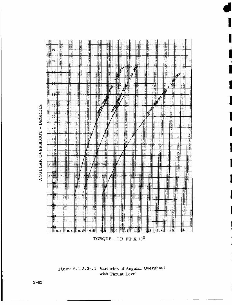
Figure 2.1.5.3-1 shows the maximum overshoot the vehicle experiences after the

inversion maneuver as a function of thrust level. The overshoot is taken as the

amplitude of the first oscillation after the retarding thruster has been turned off

and is the angle the vehicle exceeds (in a + or - direction) 180 degrees. Three

timing sequences have been studied, corresponding to 2.50 hours, 2.30 hours,

and 2.00 hours total maneuver time.

Figure 2.1.5.3-2 shows the allowable variation in the torque level for overshoots

up to approximately 40 degrees (for the three maneuver times considered}. The

tolerance has been made symmetrical (assuming that plus and minus errors in

thrust are equally likely} by adjusting the nominal torque (Figure 2.1.5.3-3). The

allowable tolerance increases as the total maneuver time is reduced. In evaluating

the overshoot, effects from thruster misalignments, center of mass wander due

to thermal bending, rise and decay times, and unequal thrusters (+ and - direction}

must ultimately be considered. All of these factors will serve to reduce the margin

on a successful maneuver, hence the allowable overshoot contributed by thrust

level error has been tentatively selected to be 30 degrees.

The motion of the satellite in pitch during the inversion maneuver is shown in

Figures 2.1.5.3-4 through -6, for the three timing sequences. Note that at the

I

III

I

I

I

I

I

I

I

I

1

2-60

high torque levels, the vehicle has overshot, and is returning towards 180 degrees

before the thrust is terminated. These plots were used to obtain the cross plots

of Figure 2.1.5.3-1 through -3. Using Figure 2.1.5.3-7, the thrust level corres-

ponding to the given torque levels can be determined.

2.1.5.4 Orbital Equations for Eccentricity Maneuvers

Prior to the removal of the requirement for a MAGGE orbit eccentricity change

using pulsed solid rocket thrusters, orbit equations incorporating the effects of

these thrusters were generated for use in the ATS Math Model. Three sets of

orbital equations are required.

The first set is for the initial satellite orbit prior to the application of thrust.

The precession of the line of nodes and the line of apsides is included.

The second set is for the satellite orbit during the application of thrust. It is

assumed that the motion of the satellite is confined to a plane. This plane is the

orbital plane at the instant immediately prior to the application of thrust. At

the end of the thrust period, the satellite is in a new orbit which is described by

the first set of equations, but with new orbital parameters.

The third set is for the earth's orbit. This is needed to determine the direction

of the sun.

2.1.5.4.1 Satellite Orbit Equations with no Applied Thrust

The right ascension of the ascending node is:

n = + a (t- tp,

where ni is the initial value, _ is the average nodal procession rate, t is the

instantaneous time, and t i is the initial time at injection into orbit.

(i)

2-61

!iil'"::* +i,. : _"...." ilittilit!iti!....'IH

.... ,,: l_l:'i*[il tltti!1_t!_l!!];l!i!

';P _',f _i!! !!: I:1: iii! i' 't, , 'it t

fiiii_ :il !i_i_:ii]iiii**i,!!!i iii!_!l!!tlHttitlifliittlI!!!l',i_ iil !',!!1':!]i;i!t_!tliI!_,_ _ i_i,...... ,,,, ;,_!tilllit't'llt:,lt_

_:i_:_ ii!i " i!:i ;,' ii i!L ' , t i_i,il_ql',lt _...

' Y: i *': :t';I ; '[ IT; L[

i:ii:._:.' _,., :itliiritif!!]!1_,,!tt,.l,,,i*'_:l_. i!ii ! i ;!' :li;_ _i'' _i:..::::'!t:It,l,_li',iiii',_t! ]i tI:t,t,l,,l,_t,_

.t!, .... ,.... '+i, :, ill. !{l'.i ii-!'L_i!!it!it!tii]_,!11_I'1i! !111 rtl!,TI

i_',1t!_:,:i,,it!! ,,,_ _ _HitifItI!_II_Ht!_i .....

Z it_7 _! :,ii!{ n,t ilI t7ii _I!FtliI_l'_mllj_:! ..-Iti fi ! t fllttt41 iit 7t:

._,!iiit l i!ii!ii4+_',. _, L !i!_.l!iili/II!tittttlI_ii:i!i_'ii]i',!i!b!!!!:l_i!!!__,IiiI!:!ittt.t'f-tttt!ttllNNii_++'+'"' :*'* Li'fltflttttltfltili,,,+iti,/t*,i :;l_ii,!, li il,__._*!_i_<,',_ii_i!_tiii*ii!i,.,:,:,,!r_liii!:!ii,,!!fttlttttitttl!tlti!tt

;i_i: v: li hl, _:ii ii:ii;; ' i[! '" ,, t!i

iii,!!_.i:,.i:! i!i!:., i:, iiii i!!i t,*_:i!t: it it,,,,,,ilil}t ft iIiiiiL,_ , _ ,, •..... :;: .... ',;; ;i!i iii !ii: !l ii!il H tt itilif ii!:: 7:_l l::ti::"!:! l!I;':_i <,;_: ,+, ........... t .......

ti_;_:l':_l_::,_::_:!i" ',{!ill! _" i:'ll i t_+

ii!itiiiitl!iii!!i'_ iiti_;_:_ _̧ ;_i,:_....... I;1!! Ll;!tl;;l ¸ i' :;;':l;i_'iii i i LI;'' i it,, _ ,,,: i !! l i! i!!

_,* :i_ =ii:i=ii::ili!: _-

:1 1_1It_i i_I i: _:_ +_ 1' :i::: :!i!iiii!i:!iltitlt!it,ldlt!::il:_l ; It! iti_ t ; i 't: " . i_i .!;:4 ;: '.;I' .... '_" "' _II!ii _!i!:....tit::lttt_l ti t,:_ ::,: _!!i

i ILT! t I iI!ll, i II !1I_: I'''

' f 'lfi ; 11, "

'",t: ',',i i!t! !i7!! !;,_!l,t,t,tiil!_;:l,;i'',:;:; _ : ": :..+, i!ii ir ....

li!it!!lit!ilitiiiil!iliii!i_,{!i_!iii!:_!lii_

iiiili!,ii!ilii'_tl;_*_:,:,, i:

'i!li!!t ',_!::_ il !i ii i:i ii']:_i!it '1! !i _ i!:+l!!i! 7411!!7 i] ii _' tr ;

,., i_iilli!i,, !i !i';' t ' !' t[ !iiil _, !li ! ;;

,i, ,_' +l_; i ' " itii! i_t! ' :,_',.

!t_! _i_l:_,ti'i,_ti!,:l'*i_ ii !!i! !i:i il i_;illi;; i Ii _I i I _ It,i'l',,t,,,tl_,!,t_,<t,,_:ill _, 77ii!ill

'_"*'"'iliiii ii!iii!i_ ;;!li,iti,tl!t,_l,l!tll!, ill ....i_'_.,_:,. . :iliit ii., ..;, ., , ill _tiil_!hltimt_tttttttiltl!_i,il" ' *:

ii!!tfillltltltttftiiii_i_i. i; ,, .....!titttt!tBttttlIIttNt iti _ ti"_,i!ii,_,!t!;!"''tittttttlttttltttttttlif!it;7t7t!!!ii!ii!iltilt;ilt!ti!t!tiittl!tt!i!i"i;t)i!!i!I!!!;ii!Iit

i i tit* It i _ t,i ilil

ilti,ii1,tt_,ttt_tlttifiiti!!ii!li ii;iitt!iti!l!tttltfittl!iIit'_ll"iilliiiiil!ft_,t_t._, ,_ , ;,;:'

i!i!t!i!tti!!!ti!!ili!i!!I!ii!i ii ii!Ii!iil!!!+''" _1t!it!_i "ii11!ii! iliii!_i ,,

_"_;t_;;tt!!Iflii,,,,,,,_,;_,<i!1!ttiittiiil iiil _,,!ilitili!t!!!it!!iil!!!i!!_!i!ilii! iJ_iiitlii

TORQUE - LB-FT X 103

2-62

Figure 2. i. 5.3-. 1 Variation of Angular Overshoot

with Thrust Level

'i ;: i ; ' '": ' :_ ' .... : ....... _; _ I ' : '_ • _ :- I-7 _" : ....... •! ! ,! _t+.l.,t:..+1+_+1:_+1_+_,_i,_l_. :: ,t._ :t ++_1_¸ _ ,: :+:1:I I _;,:, . :', ,. " :; , !;,: t ' ;; t ' ; : ........ I ] "i,. i I " '' • : ..... i +, • + .... t ' : i . .+ . '' , .....

i !i 1::7;:1:. i' _1 i ] :! ; !_:..i!':!_,',_21 _, _fl! I ..l.:l_ I' I :: ,1!,' I;;_'l ; I .... I ,' I _':JZ;:l'!l: i,!! ; iKl:: ,[_ t :_.+t', :: ;If' :':.1::: b :1: ' I "

:':,::;1_I:1_::1 I .... _+ : _i+_ ! ' +,!::'_ ! +: _ :1 ':'-Z;l_d -_1'-- ...............

.: ;Ze i ::!i+i :': ' :_ !1:; . l :

_, i_! ,.,.., ...... : , :,. : :+:ill : :..":I::i _ " I i i

' /i: , ......."_: i ,,_:,,,:_ :+::1 i:l+i;:::, :. ,.. .+ -- . -................. i. t i '

,:: ::][i+/ : ::'t I i!+ ,:T_iT:li! ] I/:;, - !_: - .........t........i. I ; ....

iii:: !i:i;ii_ ::_:_:,:_,::!i:1,,l_il, iiliii::iii_l::iil_:::l :i::E_ 7:............... t ,.

ii::iii_{;:_i_! :_li:_r_ii!i,!_,"I .{ I ' I t I: :+:::: ::I-:I'-_TT-'T............._; :" *: " " : : ,t.......... ' "

li;: " -..A ....,=.._i_!ii!it;:,i__I :ii1!:._!t./_ i!ilt t! il i1 il !il I :ti_il::._:i_iliiiit:.!_l_!i::!;!I:::T_!....' +

!,::_{ilti+ii!:,+{!__::iil+:/,!/+:_::t+iiiiiii+li:-i':t:_++'_. I_t_ii::!_!_t+iti_l::t_:., :i:l._i:: il..i_!::;i::i::::i X+,t:iii!!l::!!ti{_ii!!:i::i'! ii{!!::ii:I_:::t::!:::li+il:!_t:::t::_:!:"_::::

!::, _i_ ,:':: ::_": i_:_ti::;_t_;+l_:1'::_,_:1::::::I:.:4i:t::::1:_;:_::1::: : I .....i+.............i

:::--:_:!::i: I_.::-fi:L.....:_-.:...__....._--!-:--:I.........ff_--'+--+-:-"--_:::-"..............i.... i....: ' I " i: .... I ! !

- ---k-----_ ........ +.... _',T._II_-_j__. ;.... _....

Figure 2.1.5.3-2. Allowable Variation in Torque Level

2-63

,: i:i ili

_::!!!!!!

:i!

i::: ill i:!

..: 2:. ;;:

• _!: r!!

_'_ ill

:'i 1i _,[

:, r

::: ) ! i:"" "r ....

::i _ii i!:,2: i)

?i !: ?::

i:} t!

:_ ii! i':• .t,

• ! .,: ::

I;:;_i !i

.... !t7

_.il:!F.

"÷+++-i

:IT:I_!i!_tt '_t t?t

ii: i:; ;il

:" iti i_i

:i! ill _:;

i!! ',_ I!;i:? ili ?i_÷;l *:t t:!

t _, '.li :i!i!: It!1

Figure 2.1.5.3-3. Nominal Torque Level as a Functionof Allowable Overshoot

2-64

I

OZ

160

140

120

I00

80

60

40

2O

00 1 2

Figure 2. I. 5.3-4.

°°°°'%

3 4 5 6

TIME - HOURS

Pitch Performance for Constant Maneuver Time

2-65

al

i

Z

22O

2OO

180

160

140

120

lO0

8O

6O

40

{

I

2O

00 1 2 3 4 5 6

TIME - HOURS

Figure 2.1.5.3-5. Pitch Performance for Constant Maneuver Time

2-66

O

!

Z

_J

220

PITCtl PERFORMANCE FOR CONSTANT FIANEI:VER TIME

160

140

120

100

80

6O

40

20

0 l 2 3 4 5 6

TIME - HOURS

Figure 2. i. 5.3-6. Pitch Performance for Constant Maneuver Time

2-67

::;: :_ 4: : ::: :f:.:!;!.i ii.: :, i: .:;i:,;_!!.i;i:.! ;.::ii.!:':. r:!.: .. :':.':'L:!'!_[[ .' . .... : ::_;' ; . :,_,,4,.,r .... :...::; . ..,::.. .;_ ........ • .... ... , _i ......... . :._, I ... .... _. • ......

....' ....' "_" " i,: .: :,:::::.:!i:.::: ._::,ii:i!iii: ::}i ::: i!:::::: :'::.:1:;.:]i.': : :: _':::.J::i:.ii:i,:i": i: ii :!: :!!i ,!_I _' I:.1 . ::: ;it: . : ,.; ;:': ::;: ;':: ;'" .,.: ;:: :::: "Itl ;::: i:';

i.: _ :","_,_,_ :, ' , , : , t',: , , ' ,:'!!,:1':,': :_"t' ; " ':'! ,jr't" ': ' "'[I ,,

',:,I ;' ; - : " " , ,; ; , " " ",; ";r.; ; g', , r,.. : ....... t ........

';: il!!i ................. !:'t] ..... I ,! ,'. !:t.':'r- *+ • ' .!1}1 r :: :!.::t[.:: :.:":.]:i'_' 7 : :::

,,, : ;. '. :_: ;.;; :,: :,i; :i'Et , : ,

: J,i

., _,_.::,_:;:_:::_!ii:il i! ':!iil !" _ _ :"_' ' ::* :_ i _;I' ,i ii ',i

_,, _liiii!_i:::i:il !i: ii ;i _lii ; !i',:!i!i!i i ii iiii !II !iiii ii i! i!i

t :*_1} tt ![ti , , ,iil ! i}rl: ti * L

:, ...... ,,:= ,, :,,, i_!iifi

iii ....... ;, _1 I ;

;[:[ 'i:: !::i;;!:! !:,ii I!;,! :i!i

:i_::!}i_i_i_ii!t: i::ii,_::! !!i_:i!; ;:,ii :i i!_: ii

Figure 2.1.5.3-7. Thrust Level as a Function of Required Torque

2-68

The argument of perigee is:

Tp = Tpi + Tp (t-tO,

whe: 'e the syn boLs have hc am c _ si nLla] mean

rate of precession of the line of apsides.

I The orbital angle meas_ ,ed f _o_ _ the asc,._nc lug nc_

I ured from perigee is (T-Tp).If the apogee, A, and perigee, ]_, are given the s

, from:

i The eccentricity, of the orbit is:e,

r A-P

If the semimajor axis and the eccentricity are give

I A = a (l+e)

I and the perigee is computed from:P = a (l-e).

N The angular momentum per unit mass is:

, • h = _Ka(1-e2),

I whe _ K is We uni_ .r. al .T_ vitationa] c nstanlThe orbital period, T, is

_ _ 2_a 2

(2)

symbols have the same or similar meanings as the above, and Tp is thewhere the

The orbital angle measured from the ascending node is T. The orbital angle meas-

If the apogee, A, and perigee, P, are given, the semimajor axis, a, is computed

(3)

(4)

If the semimajor axis and the eccentricity are given, the apogee is computed from:

(5)

(6)

(7)

where K is the universal gravitational constant multiplied by the mass of the earth.

e2 (8)

2-69

!If tp is the time of perigee passage, the elapsed time since perigee is (t-tp),

where t has been reduced modulo _. Kepler's equation is: I

2y

E-esinE =-_- (t-tp), (9) I

where K is the eccentric anomaly, in radians. An iterative procedure for solving _1J

this equation is presented. Assume that Eo is the value of E at the previous time |

interval, to. For

t = to +At, (10)

then,

is to be found.

E = E o + AE,

The first trial value of AE is

(11)

AEI =217At

r (1-e cos Eo)(12)

The first trial value of E is

The second trial value of AE is

E1 = E o + AE1. (13)

2?)"AtAE2 = . (14)

T (l-ecos El)

The second trial value of E is,

E2 = Eo + AE2. (15)

This procedure is repeated until the change in two consecutive trial values of E is

less than a prescribed amount.

The orbital angle T', relative to perigee, is

T'= T-Tp (16)

2-70

I This is computed from

, Tan T" 1 +e E

1 'where (T/2) is in the same quadrant as (E/2). $ T an

than 2_, then 2_ should be subtracted from eacl . a_ [ t_ ,_

creased by one. T is computed from,

I T = T'+Tp.

I The geocentric altitude is

RA = a(1-ecos E).

The orbital angular velocity is

The radial velocity is

I eh sinT' eh sin E

I a(l_e2 ) R A

The orbital angular acceleration is

I "_" -2h -T RA3 R A .

The radial acceleration is . .

-- eh (T-T_) _,RA = r cos T.

a (1-e z)

(17)

If T' and E are equal to or greater

than 2_, then 27rshould be subtracted from each, and the orbit count should be in-

(18)

(19)

(20)

(21)

(22)

(23)

2-71

If Tp is zero, the radial acceleration is

• " -K

RAO =- 2R A

(24)

2.1.5.4.2 Satellite Orbit Equations with Applied Thrust

The reference frames used are explained in section 2.1.5 of the ATS First Quar-

terly Report, Document No. 64SD4361, 16 October 1964.

Thrust for changing the eccentricity of the orbit or for station-keeping will be ap-

plied nominally along specified directions with respect to the main body reference

frame, X 1 Y1 ZI" For the sake of generality, and to provide for studies of the ef-

fects of misalignments, the thrust will be assumed to have a component along each

of the three reference axes. These components are FX1, Fy1, and FZl. The

consequent accelerations are:

FXI= (25)

AX1 Mm + Ms '

Fy1= , (26)

Ay1 Mm + Ms

FZl

AZl = Mm+Ms ' (27)

where Mm is the mass of the main body, and Ms is that of the secondary body.

The components in the orbital frame, RI:_, are,

11] pxqAp : [El] t IAyq

L z j.

(28)

It is assumed that AQ and O are so small that their effects can be neglected during

the thrusting period. The problem is then a two-dimensional one in the orbit plane,

2-72

and can be solved as described below. If the assumption that the out-of-plane

components are negligible is not justified, then the three-dimensional problem

must be solved•

The values of the geocentric .altitude, RA, its velocity, I_A, designated u, the

orbit angle, T, and its rate, T, designated v, are known at the beginning of the

thrust period, from the orbital equations •

During application of thrust, the rad cal acceleration is,

j _ __,_. =_ __.E.d

RA

The acceleration along the perpendicular direction in the orbit plane is,

• e • •

RAT +2RAT = Ap.

These equations may be rearranged,

_v_+ _ -_

• Ap - 21_vV _ •

RA

(29)

(30)

(31)

(32)

These may be integrated with respect to time to obtain the instantaneous values

of/_ (or RA) and of v (or T). Then RA and T may be integrated with respect to

time to obtain instantaneous values of RA and T.

The out-of-plane component, AQ, may be integrated with respect to time, to find

the corresponding velocity increment due to thrusting,

| /VQ = AQ dt.

! o(3_)

2-73

At the end of the thrust period, the instantaneous values of the variables are re-

spectively designated RAO, I_AO, T(> and TO. These values are used to find the

new orbit parameters.

The angular momentum per unit mass is,

The semiparameter of the orbit is,

h2

Sp = a (l-e 2) =_: (35)

The eccentricity is computed from

Spw m

e c = ecos (TO- Tp) = RA 1, (36)

RAO Spes = esin(To-Tp) = h ' (37)

2 2 (38)e 2 = e c + e s ,

and e is the positive square root of e 2. The quantity (TO - Tp) is computed from,

es

sin (To - Tp) e ' (39)

ec (40)cos (TO-Tp) = e"

Then the argument of perigee, Tp, is computed by using the known value of TO.

The semimajor axis is,

a = Sp2 "

1-e

(41)

2-74

Ii" The orbital period is,

During the ensuing no-thrust period, the equations of Section I are used. The ini-

I tial conditions for this period are the instantaneous values at the end of the thrust

period.

2.1.5.4.3 Earth Orbit Equations

I These equations are given in Section 2.1.5 of the ATS First Quarterly Report,

I Document No. 64SD4361, 16 October 1964.

Also given are the components SXI, SyI, and SZI, of the solar unit vector S, in

i 7the inertial frame. The components in the orbital frame are:

S : YI (43)

, LsQj LSzIj.

The components in the satellite main body frame are,

= Sp (44)

Lszu Q •

2. i.5.5 Variations in Damping Time Due to Off-Nominal Angles Between the

Plane of the Damping Boom and the Plane of the X-Booms

Tinling and Merrick in their paper "The Exploration of Inertial Coupling in Pas-

sive Gravity Gradient Stabilized Satellites"* discussed the effect on damping of

changing the angle between the secondary boom and the plane of the X-rods. A

I *Item 14 of Section 4.

!I 2-75

plot showingthe effect of this angle was included in their paper. This plot indi-

cated that for a change of i4 degrees about the nominal angle (62.5 degrees), the

damping time increased by ten percent. The increase is not linear for angle

changes less than 4 degrees, but the scale of the plot does not permit accurate

determination of the correct values. The change in damping can be assumed linear

with angle change, however, as a slightly pessimistic approach.

2.1.5.6 Effect of Spring Constant on Damping Performance of MAGGE

An investigation of tolerances on the spring constant of the ATS Gravity Gradient

configuration was prompted by statements of Tinling and Merrick in their AIAA

paper (see item 14 of Section 4) regarding the sensitivity of damping of ATS type

systems to variations in spring constants. Specific mention was made of the poor

performance exhibited by a system which has a spring constant lower than the

recommended nominal value. Figure 7 of Tinling and Merrick's paper shows a

sudden drop-off in system damping capability for a spring constant which is ap-

proximately 18 percent lower than nominal.

The loss of damping capability is more apparent than real, however, and appears

because of the technique Tinling and Merrick used to evaluate the system. In this

technique, the equations of motion are linearized about a specific operating point,

and the minimum damping time constant determined by a computer solution to the

linearized equations. One characteristic of the operating point is that the second-

ary boom must be stable about a null point in the horizontal plane. To achieve this

stability, a minimum spring constant is required. If the spring constant is lower

than this minimum, the analysis will indicate instability with no damping. This

fact was pointed out by Tinling and Merrick in their paper. In actuality, the sys-

tem as a whole is stable and will re-orient itself about a new static position.

Studies performed by GE with "sub-minimum" spring constants (using both root

locus techniques and computer runs) show that the damping about the new position

I

I

I

I

2-76

is of the same order of magnitude as that achieved for the "nominal" operating

point. To demonstrate this, a computer run was made on the GAPS HI computer

program with a spring constant 20% lower than nominal. The results are shown

in Figure 2.1.5.6-1. Note that the damping is approximately the same as with

the nominal spring constant {Figure 2.1.5.6-2) but the secondary boom stabilizes

about a new position approximately ten degrees below the null spring point. This

causes a rotation of the principal moments of inertia of the system which results

in a 0.6 degree pitch bias and a 0.5 degree roll bias {which, because of the scale

of Figure 2.1.5.6-1, are not evident).

Successful operation of the system with a low spring provides a "safety margin"

making the tolerances on the spring constant less critical, but the presence of

the biases on the axes makes it undesirable to have low spring constants. The

tolerance on the spring constant for the ATS damper was, therefore, set at -0,

+20 % specifically to avoid this difficulty. The performance of a system which

has a spring constant 20 % high and a computer run was made for this system

(Figure 2.1.5.6-3). Comparison of Figure 2.1.5.6-3 with Figure 2.1.5.6-2

shows an increase in damping time {particularly in yaw) as expected. However,

the damping time is still good and should cause no difficulty. The steady state

performance of the high spring constant system will be evaluated in the future.

2.1.6 SYSTEM REQUIREMENTS FOR TV

2.1.6.1 Requirements

The following paragraphs describe the basic system requirements for the TV

camera to be flown as an integral part of the ATS gravity gradient experiments.

Current plans cad for two cameras on MAGGE and one camera on each SAGGE

flight. The primary objectives of the TV system are as follows (in order of de-

scending priority):

2-77

IB

I

0r_

.Et

f_

o_..,I

Qo

I¢.D

¢)

I I

2-78

I

i I

I

c_

C/3

C_

, 0

2-79

o

_J

m

I I I T I I I I

I

0

@

r_

I¢.0

2-80

1. Provide sufficient data for the verification of the boom thermal bending

model employed as an integral part of the ATS Mathematical Model. The

equation for thermal bending will employ empirical coefficients; these

coefficients will be adjustable so that the model can be empirically modi-fied to fit observed test data.

2. Provide sufficient data for the verification of mathematical procedures

used to estimate the magnitude and nature of boom dynamic excitationphenomena.

3. Provide the capability for real time gross attitude determination at each

of the ATS ground stations. Real time data is of critical importance in

making real time procedural decisions at the ground stations. Only a

minimum computer capability will be present at the ground stations and

there is a strong probability that the only real time attitude data that can

be made available at the ground stations is a presentation of direct output

from ATS sensors. Calibration charts and curves, used in conjunction

with sensor output raw data, may provide a gross indication of attitude.

The outputs of the earth sensor and the TV camera seem to offer the

most distinct possibilities.

4. Provide backup data for ATS attitude determination. Since the earth will

appear in the field of view of the TV camera (during near steady state

operation) the use of the cameras as a backup source of attitude informa-

tion seems a distinct possibility. Identifiable land masses would provide

yaw information and the location of the earth sphere in the field of view of

the cameras will provide pitch and roll information. Attitude determina-

tion will be a relatively slow process, however, unless automated pro-cedures are utilized.

In addition, to the above, the TV cameras will monitor boom deployment during

the initial capture phase. The objective here is primarily diagnostic in nature --

the cameras will present visual evidence of the success, or the mode of failure,

of the critical boom deployment sequence. In addition, ff sufficient TV picture

resolution can be obtained, it would be highly desirable to determine the time

history of tip mass twist as the booms are deployed. This will be the only op-

portunity to determine absolute twist of the rods; twist measurements after de-

ployment will only be relative in nature. Twist measurements may be the most

critical piece of information required to diagnose reasons for possible disagree-

ment between predicted boom phenomena and observed boom phenomena (Objec-

tives 1 and 2 above).

2-81

All four boom targets on MAGGE should be monitored during the deployment se-

quence. Time-sharing of the two cameras is permissible for power conservation

but each camera should provide pictures at a rate of at least one frame every two

seconds for the duration of deployment. Power to the attitude sensors can await

completion of deployment. The booms will be deployed at a rate of 2 (+1, -1/2)

ft/sec. A flat, circular target (currently six inches in diameter) is attached to

the tip of each boom. Target diameter, by redesign, may be increased slightly;

a 12-inch diameter, however, should be regarded as maximum with the six-inch

diameter a strong preference. For 100-foot booms, the total time for deployment

is nominally 50 seconds, but may be as slow as 67 seconds or as fast as 33 seconds.

The booms will be deployed in the 19-degree half-angle configuration; each TV

camera is required to observe total deployment of two tip masses (targets) so that

all four targets are monitored during initial deployment. The cameras should be-

gin transmission approximately 20 seconds before deployment and continue for

another 30 seconds after completion of deployment; the slower deployment rate

of 67 seconds therefore sets an upper limit of about two minutes transmission

time to cover the deployment sequence. At a transmission rate of one frame/

second Cone frame every two seconds from each of two cameras), 120 frames will

be provided for data analysis and reduction.

The following types of information should be available from the final picture for-

mat provided GE's data processing group:

(a) Relative change in tip mass (target I location as a function of time -- Mag-

nitude and angular direction are required -- one frame each two seconds,

over the total period of observation, is assumed adequate for time history.

Changes in tip mass displacement of two inches should be detectable;

changes in angular direction of displacement of five-degrees should bedetectable.

(b) Absolute location of tip mass, relative to boresi_ht of TV camera r as afunction of time -- Accuracy of absolute measurements need not be as

fine as accuracy of relative measurements. Typically, a magnitude ac-

curacy of four-inches (±2-inches) and an angular accuracy of 10 degrees

(±5-degrees) should be acceptable.

2-82

!

iiI

(c) Relative twist of boom over the period of observation -- This requires a

detectable pattern on the boom-tip target which will reveal orientation of

the target about an axis normal to the target. (Changes of five degrees

should be detectable.)

(d) Absolute twist of boom relative to fixed root of boom -- This, probably,

will depend on an analysis of the boom deployment pictures; nominal twist

after completion of deployment, plus the relative twist of (c), will give an

indication of absolute twist.

(e) Boom curvature -- If the criteria of (a) through (d) are satisfied, there

should be sufficient resolution to observe at least a portion of the boom

itself. Complete boom curvature will then be approximated by extra-

polating the observable curvature out to the observed target location.

The following tables summarize requirements of the TV system. The first table

(Table 2.1.6-1) summarizes parametric requirements; the second table (Table

2.1o 6-2) summarizes tests designed to accomplish the stated objectives, the esti-

mated number of data Lames and the time phasing of TV camera usage. Stated

objective numbers refer to the four enumerated objectives at the beginning of this

memo. To Table 2.1.6-2 should be added a requirement for observing the booms

during scissoring maneuvers.

2° 1° 6.2 Compromises

It is evident from the previous discussion that a TV scan rate of 30 frames per

minute is adequate to meet all of the required objectives. The advantages of re-

ducing scan rate of TV subsystems as presently conceived have been discussed with

representatives of NASA/GSFC many times and are reported in Section 2.4.2.1 of

the Fifth Monthly Progress Report° Further discussion of a slow scan version of

the TV camera subsystem follows in Section 2.4.4 of this report. However, rec-

ognizing that the economic considerations of the ground station equipment may be

a determining factor, General Electric is proceeding with the recent NASA/GSFC

directive to employ the standard-scan system. Taking into account that all of the

parameters of the TV system are still not defined, e.g., overall video bandwidth

and method of data reduction, those areas of the design objectives in which per-

formance is lagging are discussed in the following paragraphs.

2-83

TABLE 2.1.6-1. TV SYSTEM PARAMETRIC REQUIREMENTS

.

.

Target Parameters:

(a) Diameter: 6 in.-12 in. (current design is 6 in.; the 12 in. diameter

should be avoided, if possible, due to instaUation problems).

(b) Target pattern: pattern must be detectable with a resolution satis-

fying the twist measurement requirements; ff possible, the target

should consist of patterns of opaque and transparent materials to

provide proper iUumination during all phases of desired measure-ments.

(c) Assume target to be 100 feet from lens of TV camera; for SAGGE

this distance may increase to 150 feet. (Use 100 feet for design; if

150 feet used, degraded performance will be accepted.)

Frame Rate:

One frame every two seconds (30 frames per minute) seems adequate

for all requirements.

3. Measurement Accuracies:

(a) Relative tip displacement:

(b) Absolute tip displacement:

(c) Relative angular displacement:

(d) Absolute angular displacement:

(e) Relative twist of target:

2 in. detection threshold

_2 in. relative to boresight

5 ° detection threshold

±5 °

5° detection threshold

In reference to the time history of tip mass twist, the TV camera must be able to

see a reference mark on the boom target in order to indicate twist. If we assume

a 2-inch wide stripe on a 6-inch diameter target, it is estimated that the TV cam-

era can provide an indication of twist as the boom is reeled out in deployment from

the vehicle up to a deployed distance of almost 27 feet. Moreover, at this maximum

distance of 27 feet, it appears that the least angle of rotation determinable will be

almost 6 degrees. Beyond 27 feet, the camera cannot resolve the 6-inch long stripe

distinctly enough to indicate twist. This limitation could be overcome by increasing

camera resolution (greater video bandwidth or slower scan rate) or by using a larger

boom target.

2-84

Z

Z

E_

I

E_

,,¢

I

O

z_

0

_ o

O "0

o

o

_o

_ _._ _ _ :o= _

LI

o

_ _ _ • _ _ _, ._ _:_

c_

'0

2_

_0 oo

_°

, ,-_ _,._ _

o

_._-o_ _.o _

m,_ 0_ _-_ _ 0

cO _

_ _

._ I'____ ®._

t-.-

2-85

CD

C9

_9Z

_D

Z

_D

>

I

Ie_o

o

h_

°_

z_

_z

_z

_o

A

2-86

The second area of lagging performance is in indicating the angular direction of

displacement as little as 5 degrees. The TV camera constructs the picture from

horizontal lines, in an x-direction and vertically stacked lines in a y-_lirection.

The angular displacement is therefore determined as the angle whose tangent is

the ratio of y to x. Since we can determine y or x to about 2 1/4 inches at 100

feet, the quadrature direction for a 5-degree angle is readily computed to be al-

most 26 inches. This is the obviously worst case, in which one of the variables

is assumed to have moved only one resolution element in its direction. More

commonly, each variable will change more than one resolution element, in which

case the angle will be greater. Nevertheless, the worst case does represent a

datum of valid interest. Considerable improvement in resolution would be nec-

essary to reduce the 26-inch dimension above to only a few inches.

The other system requirements will be largely satisfied. Much of the performance

of the TV camera depends upon lighting conditions at the boom target. The lighting

condition will be optimum only a short time each orbit. At these times the TV

camera will perform best. The major part of the present design effort is being

directed to maintain performance under as wide a range of illumination conditions

as possible by both camera and target design.

If improvement in the areas of lagging performance is necessary from a systems

standpoint, some greater latitude in TV camera parameters must be granted. This

greater latitude has thus far not been approved. Finally, the accuracy and resolu-

tion described above hold for a 5 mc bandwidth and grow worse as bandwidth is

reduced.

Such a reduced bandwidth would not allow the other system performance values to

be met, since these are consistent with the 5 m bandwidth capabilities.

2-87

2. 1.7 BOOM THERMAL BENDING STUDIES

Thermal bendingof the boom is produced by a temperature gradient across the

boom bending section. Boom curvature can be determined from the temperature

gradient and the physical properties of the boom as:

C = AT a/2r

where

C = curvature (1/in}

AT = temperature gradient (OF)

a = coefficient of thermal expansion (in/in - OF)

r = rod radius (in.).

Under the condition that the boom is considered as a hollow-rod, the temperature

distribution in the rod is symmetrical about the sun-rod centerline plane; the rod

high temperature point will be toward the sun and the low temperature point directly

away from the sun. In Document No. 63SD725 (see item 2, Section 4) the deter-

mination of the temperature gradient for thts condition is given as:

where

2_Sr

AT =kt

= coefficient of absorptivity

S = flux density (BTU/Hr-Ft 2)

r = radius of rod (Ft.)

k = thermal conductivity (BTU/Hr-Ft-°F)

t = material thickness (Ft.).

The deflection of the boom can be obtained from the curvature as:

L L

y = o_ of Cdxdx.

x2-88

I

I

I In the event that the curvature can be considered as constant the deflection atX= Lis:

YL = 2 CL2"

Document No.In reference 63SD725 (Item 2, Section 4) it was shown that this

approach predicted deflections of an overlapped rod which were in essential

agreement, in magnitude, with deflections measured during test.

The tests showed, however, that the rod did not deflect only in the sun-rod plane

but also deflected to the side. In some instances, dependent on sun position relative

to the overlap, the deflections were as much as 45 ° relative to the sun-rod plane.

Analytic temperature distributions, Reference Document No. 64SD4368, (Item 3

of Section 4), revealed the not unexpected fact that the rod circumferential tempera-

ture distributions were unsymmetrical. The distributions generally showing a

strong discontinuity at the overlap. Two analytic approaches were undertaken in

order to better understand the bending of an overlapped rod under a temperature

distribution of this kind. The shell equations for an overlapped rod were written

and prepared for solution by digital computer. A second approach decomposed the

temperature distribution into components which reveal the position and magnitude

of the symmetrical temperature gradient.

These two approaches are presented in Reference Document No. 64SD4368. (Item

3 of Section 4)

I The above reference also presents results of a series of tests in which predicteddeflection magnitudes and measured deflection magnitudes generally disagree by

a factor of about two. Effort spent in attempting to resolve this discrepancy has

been hampered by the lack of reliable measurements of rod temperatures during

test. Current efforts are being directed toward the definition of an additional test

which will produce the required temperature and deflection measurements to an

I 2-89

/accuracy compatible with requirements for correlation with analytical predictions.

Effort is also being devoted to the programming and solution of the shell equations

for comparison with results predicted by beam theory. The determination of a

stiffness matrix for gravity gradient rod elements is discussed in Appendix E.

Section 2. 1. 8 covers a discussion of gravity gradient corrections to thermal

bending tests and indicates the effect is negligible.

2.i.8 GRAVITY CORRECTION FOR THERMAL BENDING TESTS

The rod is fixed at the upper support and held in a vertical orientation. Due toI

the thermal gradient the rod assumes a curvature, C(x) = 1/R. Due to the effect i_

of gravity there is a moment set up which reduces the curvature.

= c(x)-

Referringto figure (1) the deflection x

of the rod is A-u ]

Theslopeis O=/_-dx _ _

and the deflectionis

I

,_--- A ----_

X

For convenience the origin is chosen at the free end of the rod with an X-X axis

selected parallel to the undeflected rod. This choice of coordinates simplifies

the handling of the equation for moments.

2-90

The moment due to gravity is

whe re

mg

U

X

X

m =_o mgudx

-- the weight of the rod per unit length

= the deflection of the rod as defined in the figure

= the distance from the free end.

Then

X

d2u 1 C(x) o_ mgdx 2 R EI u dx

Differentiating this expression gives

3d u mg d C(x)

_-_'3-+-'_ "u -- dx

This expression is general in that to this point no assumption has been made re-

garding variation of mg/EI with length. For the case of the thermal bending test

mg/EI was constant so this will be the case considered here. The solution to this

equation is composed of two parts:

U = Uc+U p

where uc is the solution for the case

d C(x)dx

and Up is the particular solution for

dC(x) _ 0dx

2-91

Although it was not an accomplished fact, the intent in the thermal bending test

was to provide a thermal distributor which did not vary along the length of the rod.

For this case d C(x)/dx = 0.

The behavior of the rod then is described by

d3.....__u+ _3 udX

= 0

whe re

3 mg

The solution to this equation is

x[o /u = C le e 2c°s _ + C 3 sin

Further

-_C1 e-_x +--2"_e_x I/C +3_C3c°s/--2"_22

( 0x/l•0x)

C(x)X 2+

2

@2 Cle-@X +_e C2R = 2 _x -

+ C(x)

,= __3 -_ xdx Cle + e

X

The boundary conditions are when X = 0, u = 0

1--= C(x)R

and whenX=_, 8=0

d

iIL

i

i

2-92

From these boundary conditions the constants of integration are

Cl = c(_)+ 2 cos

C(x)

c,=-[e-O,+ 2 e cos ¢

cs = _ .5- ,_._c,._,

[e-¢£ e¢/2£ (---_._2) ]+ 2 cos ¢ £

Then

u = C(x)14+o[o --¢ £ e¢/2 £+2[e-CX-e ¢x (cos(_x)

For the conditions of the thermal bending test

£ = 96 inches

mg = 1/4 oz per foot = 1/768 lbs/inch

EI _ 2000 lb-in 2

= .008667 in -1

A = uwhenX=£

A = C(x) (4608- 86) = 4522 C(x)

Of this total deflection 4608 C(x) is due to the curvature due to the thermal loading

and 86C(x) is the effect of the weight of the rod under a one g gravity field.

Thus the deflections measured are 98% of the expected deflection in a zero g field

and the correction for the effect of gravity is negligible.

2-93

2.1. 9 BOOM DYNAMICS STUDIES

Progress has been made in the development of a stiffness representation of the

gravity gradient and damper rods for use in dynamic analysis. Since the rod has

an open seam along its length, it is incapable of supporting shear and the stiffness

may be seriously reduced from that expected from beam theory for some loadings.

Development of an analysis of the rod stiffness from shell theory has been under-

taken. This analysis is shown in Appendix E.

Programming for a digital computer to perform a numerical evaluation of the re-

sults is presently under way.

2. 1. 9. 1 Dynamic Response Due to Relief of Thermal Gradients When PassingInto Eclipse

The dynamic effect of relief of thermal bending when the vehicle passes into

eclipse may become significant for both boom design and for vehicle behavior if

the time rate of relief of bending tunes poorly with relation to boom natural

frequencies.

If the thermal gradient at each lengthwise station of the rod can be expressed

as a linear function of time, i.e.,

gradient = C 1 f (t)

the deflections due to temperature can also be expressed as a function of time

uT = C f(x) f(t)

whe re

u T is any deflection parameter such as displacement, or rotation.

<i)

C

f (x)

is a constant relating the temperature gradient to deflection

is the function which relates the deflection to the position of the rod, i.e.,

for a circular arc the deflection is C x2/2 and the rotation is CX.

is the temperature function of time.

1

2-94

Now the force in the system is a product of the stiffness and the difference between

the absolute value of the coordinate and its steady state temperature equilibrium

value at the coordinate. This force is balanced by the inertia and damping of the

system since there are no externally applied forces

K(Ua-UT) + Mu a = 0

or

M_ a + gu a = gu T

where

M

K

f(x)

= K C f(x) f(t) (2)

is the mass matrix

is the stiffness matrix

and u a are the absolute acceleration and displacement vectors

is the vector defining the displacements as in equation (1).

This equation can be solved for the response due to the change in thermal gradient,

passing in or out of eclipse, by methods similar to those used for response to orbit

eccentricity pulse beginning on page 2-84 of the First Quarterly Report. The solu-

tion is straightforward and will be performed when the time function of the tempera-

ture gradient is defined.

2.1. 10 TESTING

General Electric test requirements for the Hugh Aircraft system thermal and vibra-

tion test for the ATS program are given in the following paragraphs.

2. 1.10. 1 Thermal Test Requirements

In the first quarter of 1965 HAC is planning a System Thermal Test in which ap-

proximately 15 0 separate thermocouples will be installed throughout the spacecraft.

The following requirements apply to the components to be used for the HAC system

thermal test.

2-95

All hardware to be supplied for the T-2 thermal tests must simulate the flight

equipment in both external geometry and mode of mechanical/thermal attachment.

In addition, external surface treatment and internal power dissipation must be

simulated where applicable. In general, the simulation of heat capacity is also

required since transient as well as steady state test operation is anticipated.

The individual heat dissipators should be sized for twice the expected power at

30 volts dc. The recommended type of heating element to be used for the simula-

tion of package internal power is: Dale Resistor type RH-Mil-R-18546C available

from Newark Electronics Corporation, Catalog No. 75, 1964.

General Electric will be responsible for the installation of all thermocouples on

the gravity gradient components. These installations must meet the following

requirements:

1. Thermocouples shall be AWG No. 30 Copper-Constantan

2. External lead length shall be approximately five feet.

Thermocouples, installed in the following locations, will be needed for the HAC

System Thermal Test.

Combination Passive Damper

a. Thermocouple on fiat exposed surface of damper.

1 Thermocouple

TV Cameras

Camera 1

1. Thermocouple on lens

2. Thermocouple on vidicon face plate

3.

4.

5 Thermocouples

Thermocouple on external surface of electronics housing

Thermocouple on camera housing

Camera 2

Thermocouple on vidicon face plate

2-96

Solar Aspect Sensor

1. Thermocouple on each detector surface

that is exposed (5).

2. Thermocouple on electronics package

IR Earth Sensor

Sensor 1

1. Thermocouple on filter

2. Thermocouple on lens

3. Thermocouple on cavity wall

Sensor 2

Thermocouple on lens

Power Control Unit

Thermocouple on external surface of

housing.

Damper Boom

1. Thermocouple installed on external

surface of tip mass of the boom

mechanisms (2).

2. Thermocouple installed on erection unit.

Primary Boom

Thermocouple installed on external

surface of each housing (2).

6 Thermocouples

4 Thermocouples

1 Thermocouple

3 Thermocouples

2 Thermocouples

2. 1. 10. 2 Vibration Test Requirements

Mechanical components of the Gravity Gradient subsystem will be delivered to HAC

in the second quarter of 1965. The following requirements apply to these components:

Each component will approximate the flight hardware in mass, c.g., dimensional

envelope, and material.

No functional tests are required for these components.

HAC will be responsible for the installation, calibration, sensitivity checks, and

recording instrumentation of all vibration monitors.

2-97

A total of 75 accelerometers and four strain gages are required for instrumenting

the Gravity Gradient components in the following locations;

Damper/HAC Structure

1. 1 triaxial accelerometer at the bottom of

Damper close to attachment point.

2. 1 trlaxial accelerometer at the upper end of

Damper close to attachment point. (Opposite side

to bottom triaxial accelerometer)

6 Accelerometers

Damper/Damper Boom

1. 1 triaxial accelerometer at GE/DeHavilland

interface.

2. 1 triaxial accelerometer on Damper boom center

structure.

3. 1 triaxial accelerometer on one of the tip masses.

4. 4 strain gages on the bottom cover in the vicinity

of the uncage pins.

9 Accelerometers

4 Strain Gages

Primary Boom Housing/HAC Structure

2 triaxial accelerometers near two opposite

attachment points of boom housing to HAC

structure. 2 Components

12 Accelerometers

One triaxial accelerometer should be installed near attachment of each of the

following components. (Exact location later)

TV Camera/HAC Structure

2 Components

6 Accelerometers

TV Electronics/HAC Structure

2 Components

6 Accelerometers

SAS Detector/HAC Structure

5 Components

15 Accelerometers

2-98

D

SAS Electronics/HAC Structure

1 Component

IR Earth Sensor/HAC Structure

2 Components

Power Control Unit/HAC Structure

1 Component

3 Accelerometers

6 Accelerometers

3 Accelerometers

2.1.10.2.1 Data Requirements

1. All GE data channels should be grouped so efficient data transmissioncan be made at the conclusion of the test.

2. The original tape or a copy is requested of all GE channel information

including a record of the system input occurring at that time.

3. In order that analysis can be performed at GE the data should be on

one-inch tape and be compatible with GE Tape System.

2-99

e

2.2 BOOM SUBSYSTEM

The boom subsystem of the ATS Spacecraft consists of the four primary gravity-

gradient booms, the mechanism required for extending and scissoring the primary

booms, and the two damper booms including the canister for storage and ejection

of the damper booms.

The basic requirements for the boom subsystem are as follows:

1. Provide a set of four erectable booms which can be stowed within the

confines of the ATS Spacecraft during launch and be deployed at sepa-

ration to form an "X" configuration about the spacecraft. Weights

are installed at the boom tips to achieve a prescribed set of inertias

about the three principal axes of the spacecraft.

2. Provide a means of retracting these rods on command to desired lengths.

3. Provide a means of changing the angles included between the booms in a

manner that maintains a symmetrical configuration about the satellite

yaw axis. This action, which is limited to a total of 20 degrees on each

boom, is generally referred to as scissoring.

4. Provide a set of two damper borne booms which will each extend to a

length of 45 feet along the same straight line in opposite directions. These

booms are to carry tip masses to their ends which will provide the proper

interia for the operation of the damper. After initial deployment, no

mechanical connection or wiring is to extend from the damper boom

platform to the spacecraft body. The damper booms are not required to

retract.

5. Accomplish the above within the tolerance/disturbance constraints of the

gravity-gradient stabilization system performance requirements.

The basic extendible boom selected for this mission is the Storable Tubular

Extendible Member (STEM) developed by the deHavilland Aircraft of Canada, Limited.

This technique involves the formation of a tubular section from a flat metal strip

which is formed and heat-tested in the tubular form then flattened under stress

and wound onto a storage drum. Subsequent erection in orbit is accomplished by

paying out the stowed strip through a set of guides which allow the boom to form

into its natural tubular shape. The edges of the metal strip overlap each other to

render stiffness to the operating section.

2-100

Storage/erection units for the STEM tubing are of both motorized and self-erecting

type. The motorized type employs a motor to drive the storage drum and thereby

provide a means of retracting the extended booms. The self-erecting type units

use the strain energy in the stowed metal strip to rotate the storage drum and

erect the boom.

Motorized units were selected for the primary booms due to the requirement to

retract. Self-erecting units were selected for the secondary (damper) booms.

Initial considerations for the scissoring mechanism included several which provided

mechanical coordination of the motion of all four primary booms. Design studies

included versions using bull gears, pulley systems, bellcrank linkages, and

jackscrews. However, the constraints imposed by spacecraft size and other

equipment in the boom mounting area proved the mechanical connection of all

booms to be impractical. An evaluation of the coordination required between booms

for both extension and scissoring showed that a system which depended on electrical

synchronization was not impractical. Accordingly, the following system was

devised:

1.

2.

The four boom units are divided into two pairs.

The two units making-up each pair are mounted as close as possible to

one another and are coupled by a bell-crank linkage to transmit scissoringmotion and a gear train to coordinate extension drum drive.

3. Each pair of units is provided with one motor for extension and one motor

for scissoring. The motors are encased in a hermetically sealed container

to preserve their useful life in space, torque being delivered through aflexible membrain.

4. The two units of each pair, their drive train, motor, and scissoringlinkage are all mounted with a single framework. Extension units are

provoted to this framework.

5. Motion between the two pairs of units is coordinated electrically.

The technical aspects of the Boom Subsystems are fully described in paragraph

2.2 of the '_First Quarterly Report, "Document No. 64SD4361, published by GE

2-101

on October 16, 1964. General Electric Specification SVS 7316 delineates the

requirements for the Boom Subsystem.

2.2.1 150-FOOT ROD CONSIDERATIONS

One of the initial requirements for the primary booms was that the rods for

MAGGE and SAGGE be 100 feet long. The different inertial levels for the medium

and synchronous vehicles were achieved by different weighted tip masses; the

heaver tip mass would be used on the SAGGE. The use of 150-foot rods was

investigated to establish the weight saving that could be effected by the longer rods

for the same inertial levels as the shorter rods. Better than 70 percent saving is

possible in the weight of the tip masses when the longer rods are used. A com-

parison of the tip mass weights is shown in Table 2.2-1 for the 100-foot and 150-

foot rods for MAGGE and SAGGE.

TABLE 2.2-1. TIP MASS WEIGHT PER ROD

Rod Length Tip Mass Weight (Approx. _ounds)

(feet)

100

150

MAGGE

2.5

• 56

SAGGE

10

2.25

The 150-foot rod would weight 0.75 pounds more than the 100-foot rod due to the

additional weight.

The investigation also included a consideration of results when the tip mass weight

was held to the original requirement (2.5 and 10 pounds respectively) while in-

creasing the rod lengths to 150 feet. This ratio of rod length to tip mass weight

would increase the inertia levels by a factor of 2-1/4 relative to the 100-foot rods,

and would have the added advantage of increasing the gravity gradient torques.

Disadvantages include added cost for the maintenance of straightness tolerance and

more sophisticated test equipment required during manufacture of the longer rods.

One-third more silver plating would be required to coat the longer rods, and a

2-102

greater rate of material would be scrapped during manufacture to keep the longer

rods within specified straightness tolerances.

2.2.2 LUBRICATION REQUIREMENTS

Lubrication is required in the boom mechanism to protect the equipment from the

phenomenon of cold welding when exposed to spacial vacuum. Lubrication techniques

was the subject of a joint meeting with NASA, deHavilland and General Electric dur-

ing the reporting period. Three types of lubricants were proposed for consideration;

these include liquid lubrication, the use of self-lubricating materials, and dry film

lubricants.

2.2.2.1 Liquid I.nbrication

The hermetically sealed drive system (a deHavilland bellows drive unit) will be filled

with argon or helium at 5 psia. The drive motor utilizes carbon brushes which re-

quire some absorbed water or organic vapor for effective operation. The absence

of such vapor results in increased contact noise and rapid brush wear. deHavilland

has proposed adding water vapor to the sealing medium. Perhaps some organic vapor

will be provided by the bearing lubricant or motor winding insulation materials.

The erection and scissoring mechanism is, by necessity, open to the space environ-

ment. The aperture size will be such that a labyrinth, molecular type seal is effected.

Preliminary calculations based on F-50 fluid vapor pressure and molecular weight,

the mean free path of the fluid molecules in the vapor phase, and a sticking coefficient

of 1, and piece part geometry have indicated a total leak rate of 2. 235 x 10 -2 gm/year.

Lubricant replenishment would be provided by a lubricant reservoir leaking through

a Veeco molecular seive. Bearings would be of the standard precision type lubricated

by F-50 oil or G-300 grease. All outboard shaft bearings would be shielded to limit

lubricant loss by creepage and evaporation. Teflon or other forms of anti-wetting

agents will not be used since Teflon would reduce the sticking coefficient of the mole-

cules striking the labyrinth seal; therefore the evaporation rate would increase and

may become excessive.

2-103

t2.2.2.2 Self-Lubricating Materials

Self-lubricating materials (Teflon, MoS 2 or Teflon filled plastic material) are prime

material candidates for journal bushings and gears. The main disadvantages of such

materials are lack of dimensional stability, lack of radiation resistance, and low

thermal conductivity for heat rejection. Main emphasis will be placed on a filled

polycarbonate material which consists of polycarbonate, 40% glass and 12% Teflon

filled. The material is injection molded and exhibits good dimensional stability.

Mating gear material will be of the same material (filled polycarbonate) or hard

anodized (dense aluminum oxide coated aluminum).

2.2.2.3 Dry Film Lubricants

deHavilland had proposed the use of tungsten disulphide as the major constituent of

any dry film lubrication system. In this proposed system the coating will be the

Teleflex materiul, a Teflon and tungsten disulphide material using a low fired ce-

ramic binder.

Fischer Bearing Company, manufacturer of precision instrument bearings, has

indicated a willingness to develop a soft metal plating consisting of Teflon and tin

to be applied to standard bearings.

2.2.2.4 Other Approaches

2.2.2.4.1 Soft Metal Plating

Soft metal platings, such as gold and silver, have been used with some degree of

success as lubricants for bearings. The relatively high coefficient of friction of

such materials and the difficulty in obtaining a reliable plated bearing assembly

have virtually eliminated soft metal platings as lubricant materials.

2.2.2.4.2 Cemented Carbides

Cemented carbides display many favorable attributes with respect to bearing appli-

cations. One of the drawbacks on these materials is the relatively high friction

2-104

occurring when sliding is in the boundary friction region. Various researchers

have investigated the possibilities of incorporating a solid film lubricant into the

surface of the cemented carbides. Major emphasis has been placed on high tem-

perature applications.

2.2.2.5 Recommended Lubricants

As a result of meetings with the subcontractor and study, a design philosophy was

established revelant to the use of lubricants with recommendations for the optimum

lubricant for use in the boom subsystem mechanism. The two guidelines used in the

selection are:

1. Lubrication of the open unit by liquid lubricants is prevented by the possi-

bility of forming polymerized films on the booms, thereby drastically

changing its thermal radiative properties.

2. Slow speed and/or intermittent operation bearing applications generally

require some dry film or boundary lubricant to be applied to all surfaces

in relative contact. Therefore, the bearing races and balls should be

coated with MoS2, either as a burnished film or bonded as in the Moly-

kote X-15 coating. Bearing elements should be finished by precision

grinding techniques (4 to 6 microinch surface finish) followed by a

thorough cleaning before the dry film lubricants are applied.

Materials chosen as promising lubricant selection are summarized in Table 2.2-2.

The recommendations made in the GE investigation include lubricants for sealed

units and open units. These are:

1. Sealed Unit

a. Erection Motor Bearings - 440C CRS, lubricated by F-50 orMIL-L-6085 diester fluid.

2. Open Unit

a. Bearings - 440C, Duroid 5813 separator, dry film lubricated by

Alpha Molykote X-15

b. Gears - Teflon and glass filled polycarbonates idler gears.

c. Tape Guide - Teflon coated fiberglass laminate or electroformedmaterial.

2-105

TABLE 2.2-2. PROMISINGLUBRICANT SELECTION

Application

SealedUnit

Bearings

Races

Separator

Balls

OpenUnit

Bearing

Races

Separator

Balls

Gears

Spring

Tape Guide

Basic Material

440 C (CorrosionResistant StainlessSteel-CRS)

Duroid 5813

440C (CRS)

440C (CRS), Cobalt

alloy Star J or

Haynes 6B 1

Duroid 58133

440 (CRS) Cobalt

alloy Star J or

Haynes 6B

Polycarbonates, Epoxy

Teflon, Polymides

1. FiberglassLaminated

2. Electroformal

Material

Lubrication

Liquid

F-50, MIL- L-6085

Depending on De-

sign Requirements

Dry Film

Alpha MolyKote X-152

Idler gears of the

self-lubricating

mtl driver of

2024 aluminum

Burnished film

of MoS 2

Teflon coatings

(fused or epoxy

bonded)

1. Due to the short delivery time of engineering hardware, bearing races made

of Star J or 6B Cobalt alloys may be unobtainable therefore 440C races should

be used. If the cobalt alloys are obtainable they should be heat treated at

800-850°F for 48 hours to stabilize the hexagonal structure necessary to

prevent mass material transfer during boundary friction operation.

2. Alpha Molykote X-15 is a MoS 2 dry film which uses a sodium silicate binder.

3. Duroid 5813 - The material is an extruded composite consisting of Teflon

filled with 15% glass and 10% MoS 2.

2-106

JThese recommendations were presented at the latest design review held at

deHavilland late in November. They will form the basis for the lubrication

techniques for the ATS boom system mechanics.

2.2.3 MOTOR SELECTION

The boom system employs four DC motors per satellite, two for primary boom

extension and retraction and two for primary boom scissoring.

The types of DC motors considered for this application were:

1. Permanent magnet type.

2. Split series wound type.

3. Shunt wound type.

The shunt wound motor was selected for this application because the shunt wound

motor offers a much finer speed control over the range of possible variations in

applied voltage and ambient temperature. Figures 2.2-1 and 2.2-2 show a com-

parison of speed variations between shunt wound and series wound motors of the

size and type suitable for this application. Curves are presented for speed versus

torque over the full ranges of temperature and applied torque anticipated. The

cross-hatched areas delineate the range of required torques. Examination of the

curves in the expected loading areas readily shows that the shunt wound motor

speed will vary much less with variations in loading, temperature, and voltages.

It is necessary to limit the variations in motor speed in order to preclude dele-

terious effects on boom structural integrity and capture performances.

The use of shunt wound motors requires a slightly more complex power switching

system than does the split series motor, but this is offset by the attendant

advantages in speed control.

The use of the permanent magnet type is precluded by the residual magnetic dipole

remaining after power is removed.

2-107

I

0

IQ

0

I I I I I

0

0

r_¢.)

o_--I

o_1

Q)C.)

0

p_

oG0

_JI

o

2-108

o

>

I I I I_ -- 0

113

zl

oI

:D

0

oI--

0

0

2-109

0

Io,1

(D

2.2.4 POTENTIOMETER BOOM LENGTH INDICATOR

The original design concept employed a magnetic reed switch to monitor primary

boom erection. This system, although simple in sensor concept, easy to calibrate,

and not susceptible to boom erection jeopardization, had the disadvantage of

requiring a counter circuit in the telemetry set to measure boom length. In the

event of power interruption, the count would be lost. In order to have up-to-date

boom length information readily available at the ground station at all times, it

would be necessary to design a memory circuit into the telemetry set. The com-

plexity that this requirement introduced into the telemetry set was not considered

offset by the advantages associated with the reed switch. Accordingly, a rotary

potentiometer was included in the extension drive transmission box to monitor

boom length in orbit. Calibration of this potentiometer on the ground will use the

output of the reed switches mounted directly on the erection units, but the reed

switches will not be used for in-orbit telemetry.

2.2.5 100-FOOT STOP

When using a 150-ft primary boom, it becomes necessary to provide a "positive"

extension stop at 100 feet to insure the capability of accurately evaluating the per-

formance of 100-ft booms during Orbit tests. The use of a micro-switch stop (as

is used at the fully extended length) is precluded since this would require slots in

the boom material which might adversely affect strength. Accordingly, it was

decided that a threshold detector would be included in the PCU. The detector

would sense the output of the extension potentiometer and would be preset to trig-

ger at 100 feet during initial boom extension and thereby cutoff motor power. All

other boom length adjustments would be accomplished by proportional command.

2.2.6 MICROSWITCH FUNCTIONS

Table 2.2-3 lists the microswitches used in the boom system and their functions.

2-110

TABLE 2.2-3. MICROSWlTCHFUNCTIONS

Function Type No. Req'd./Sys.

4Full Retraction Power

Limit for Ground Test

Full Extension

Power Limit

Full Extension

Telemetry Monitor

Clutch Solenoid

Power Limit

Clutch Solenoid

Telemetry Monitor

Scissors Power Limit

S.P.S.T.

(Removable)

D.P.3.T.

S.P.D.T.

S.P.S.T.

S.P.D.T.

S.P.S.T.

4

(Note: The 2 switches

for each 1/2 system

will be wired in series. )

4

Independent

4

8

4

2.2.7 BOOM ELECTRICAL ISOLATION

During this reporting period, GE was requested to provide DC electrical isolation

of the primary booms from the spacecraft and to reduce the capacitance between

the boom and the spacecraft to a minimum.

The resistance between each primary boom and the spacecraft structure is to be a

minimum of 108 ohms when measured at laboratory ambient conditions. The

design goal for capacitance between the boom assemblies and the spacecraft is to

be 50 picofarads with a maximum allowable capacitance of 200 picofarads.

The design is proceeding toward accomplishing these electrical isolation require-

ments. It appears that the resistance requirement will be readily realized, but

realization of the capacitance requirement will be marginal.

2.2.8 TIP TARGET CONFIGURATION

A change in the tip target configuration from an articulated 6-inch diameter disc

to a 9-inch diameter disc fixed at a 50 ° angle to each primary boom is currently

2-111

under consideration. This configuration would simplify the tip target design in

that the targets could be stowed tangent to the spacecraft solar array during

launch without the use of an articulated joint. This design is being evaluated

for T/V camera visability.

2.2.9 CLUTCH DESIGN

Prior to the design review meeting held at the subcontractor's facility in late

November, the clutch design embodied two solenoids which drove the clutch to

each of the two required clutch positions. A bistable spring held the clutch in

the desired position when solenoid power was removed. Concern was expressed

over the reliability of the spring and the amount of power required by the solenoids

(current drain was 10 amps for 30 milliseconds).

Accordingly, the following design change is being considered. Both solenoids

and the bistable spring would be replaced by a single rotary solenoid which

would be stable in either position. The new rotary solenoid would draw 2.54

amps at the nominal 28 VDC supplied by the power supply and would draw 3.36

amps at the maximum expected voltage of 37 VDC.

2.2.10 DAMPER BOOM RELEASE MONITOR

In order to provide a telemetry event monitor of damper boom release, a design

improvement is being undertaken to add two microswitches to the upper damper

surface. These microswitches would be triggered by motion of the tip assem-

blies of the damper booms as they move away from the CPD. These switches

would be mounted so that they would not interfere with the motion of the damper

booms after deployment. This design would require no wiring between the

damper booms and the CPD.

2-112

2.3 COMBINATION PASSIVE DAMPER

2.3.1 INTRODUCTION

Two dampers, one a hysteresis damper andthe other an eddy-current damper, are

combined with a clutching mechanism into a single package referred to as the

Combination Passive Damper (CPD). These dampers (coupled to a damping boom)

are alternately operated during the Applications Technology Satellite (ATS) mission

to damp the vibrations of those vehicles that utilize gravity gradient stabilization

techniques. In addition to providing damping torques, the CPD also must meet a

requirement to restore the damper boom to a "null" position with respect to the

satellite. This restoring torque is provided by a magnetic torsional restraint de-

vice incorporated in the eddy current damper system, and by the torsion wire

suspension (tendency to "untwist") in the hysteresis damper system.

2.3.1.1 Basic CPD Functional Description

Basic functions currently incorporated in the CPD design and the associated hardware

to perform these functions are listed below:

Function

Damping

Torsional Restraint

Suspension

Clutching Mechanism

Boom Angle Indicator

Mode Indicator

Caging for Launch

Associated Component(s)

Hysteresis disc and magnets

Eddy Current Disc and Magnets

Torsion Wire (Hysteresis Damper)

Magnetic T.R. (EC Damper)

Torsion Wire (Hysteresis Damper)

Diamagnetic Cones and Magnets

(EC Damper)

Solenoid actuator and DiaphragmClutch

Optical Device

Microswitehes

Pyrotechnic Devices

2-113

Function

Stops at + 45 ° rotation extremes

Minimum Dipole

Associated Component(s}

Spring stop

"Bucking" magnets properly

oriented

2.3.1.2 Chronological Summary of Major Events During Reporting Period

A chronological summary of events is presented below to review the perturbations

that occurred in the CPD effort during the reporting period. Several of these

events resulted in a major re-direction of the CPD design effort.

15 Oct. 1964 -- Presentation of CPD design concept (2 lever} to NASA representa-

tive at GE. As a result of this meeting an all-out effort was made to simplify

the design by deleting the boom/damper alignment feature and working on

the assumption that clutching could occur only at the boom null position.

15-30 Oct. 1964 -- Intensive redesign activity investigating various methods of

clutching at null only, plus overall simplification of the entire concept.

Reviewed resulting designs with NASA on 30 October at GE but no single

concept was satisfactory.

6 Nov. 1964 -- Presented working model of 2-1ever concept of the CPD at a meeting

at NASA Goddard. Model demonstrated smooth operation and stability of

2-1ever concept; however, it still was considered too complex.

13 Nov. 1964 -- Presented the "Diaphragm Clutch" concept at NASA meeting. This

concept contained only one moving part plus the actuator, and agreement

to proceed with this design concept was reached.

17 Nov. 1964 -- The CPD to Spacecraft mounting arrangement concept was agreed

upon during the NASA/Hughes/GE Interface Meeting at GE.

2 Dec. 1964 -- GE was requested by NASA to obtain a proposal from Space Tech-

nology Labs (STL) for the development and delivery of the Hysteresis

Damper portion of the CPD. GE would continue to be responsible for the

entire CPD package including the eddy-current damper.

9 Dec. 1964 -- STL personnel visited GE to receive the RFQ (including GE Specifi-

cation SVS 7331 and associated Work Statement} on which to base their

proposal for the Hysteresis Damper.

2-114

30 Dec. 1964 -- GE Specification SVS 7315 for the CPD Boom Angle Indicator was

issued.

30 Dec. 1964 -- STL completed their Hysteresis Damper Proposal and forwarded

it to GE on this date.

2.3.2 DESIGN EFFORT

2.3.2.1 General

During this report period, there has been a continuing design effort in the form of

conceptual layouts and development engineering activities (discussed below) to meet

the general requirements specified for the CPD.

At the end of the last quarterly report period, the volume in the spacecraft

available for the CPD package had been reduced and in that report, a pre-

liminary layout was presented and discussed that would fit in the designated

envelope and which provided all of the required functions. A "rough" working

model of the essential elements of the design was built which demonstrated

that the concept of switchover and damper centering, as shown in SK56130-808-

12 (included in the last quarterly progress report), was feasible. A picture of

this model is shown in Figure 2.3-1. On 6 Nov. 1964, the model and layout

were shown to and discussed with NASA representatives. The relatively large

number of parts, including several friction type rotating joints, raised a ques-

tion as to the reliability of the design. The requirement to include a device

which aligned the damper index or null point with boom null position at the

time of clutching or switchover was the dominant cause of the relatively large

number of parts.

2-115

2-116

4

Figure 2 . 3 - 1 . "Rough" Working Model

Because of the complexity of the design, it was agreed that a design which would not

include the aforementioned alignment feature would be used. GE then conceived and

laid-out a CPD design, utilizinga so-called "Diaphragm Clutch" switchover mechan-

ism, which had no aligning capability. This design was less complex than previous de-

signs, not only because of the single moving part (plus the actuator member), but also

because with this concept, itwas possible to use a two-way solenoid in place of a rotary

motor as the actuation device. The reliability of the rotary motor actuation had

been questioned because it utilized several rotating bearings and a sliding member.

The problems engendered by direct current electrical motors were also a major

concern with the motor actuator. While in concept the diaphragm clutch, similar to

a pleated Belleville washer, is virtually the ultimate in simplicity, in practice it

has proved to be very difficult to analyze and predict its performance with any

accuracy. Therefore, considerable time was spent in contacting various vendors

to determine what experience they might have had in similar diaphragm applications.

However, it was learned that none of the vendors had any assistance to offer nor

could they recommend any method for analyzing the performance of this type of

diaphragm.

While efforts were under way to obtain either test data or vendor information on these

diaphragms, GE was verbally requested by NASA (on 2 Dec. 1964) to investigate the

practicality of incorporating a separable passive hysteresis damper (PHD), such as

might be developed by Space Technology Laboratories (STL), into the CPD package

in place of the hysteresis damper developed by GE. In response to this request by

the customer, a specification was prepared, preliminary engineering discussions

were held and STL has completed a proposal to GE to supply such a self-contained

damper package. Inclusion of a separable damper package caused a marked change in

the design philosophy of the CPD package. With an integrated, GE designed damper,

the components of the hysteresis damper were incorporated into the CPD package

structure. With the separable concept, more space was required within the CPD

package to accept a vendor-furnished PHD. Distinct, and space consuming mounting

2-117

and output interfaces were also required both on the damper and in the CPD package,

resulting in less efficient weight and space utilization.

The conceptual layout shown in Figure 2.3-2 shows the CPD configuration with the

GE-designed hysteresis damper. Also shown on this drawing are the required modi-

fications to the package to accept the proposed STL hysteresis damper. This layout

includes the diaphragm clutch and a solenoid-actuation adapter.

While the foregoing general design effort discussions have been chiefly concerned

with the activity associated with the overall package design, a considerable amount

of engineering development effort has been applied to the hysteresis damper, the

magnetic suspension, magentic torsional restraint and eddy current damping. These

activities are discussed in some detail in the following sections.

2.3.2.2 Damper Configuration Currently Proposed :'_

The current concept of the damper package (as shown in Figure 2.3-2), is a cylinder

approximately 9 inches in diameter by 12 inches long with the two corners on the end

adjoining the spacecraft being tapered for clearance.

2-118

II

A

P

I

®SECTIOND-I:}

_TL DAMPER

®

,SECTION It-II

//

-- -- ---'-I-'-- .... -1 ....

ALTERNATE -_F'GTION ji_-Al,_

R::::)I_ STL DAMPER

SECTION I_'A

i

SECTION (:'(:

Figure 2.3-2o Damper Configuration

2-119/120

D

The damper is supported at two points at the spacecraft end and at four points

at the outer or boom end. Struts from the spacecraft support the outer end

with the mounting configuration to be determined in subsequent interface meetings.

The Detiavilland damper boom assembly attaches to a suitable interface (_)* located

at the outer end and in operation rotates plus and minus 45 ° from a null position and

about the axis of the CPD package.

During launch, the loads from the booms and the connected part in the damper package

are carried through four caging pins into the end plate of the damper and to the strut

connections. The pins are held in engagement by a cable as discussed in Section 2.3.3.5.

Provisions will also be provided for individual manual caging of the eddy-current rotor

during handling and during testing of the hysteresis damper. This feature is required

since the diamagnetic suspension will not support the eddy-current damper in earth's

gravitational field.

The eddy current damper structure (_) will be supported by 12 magnets (3_ located at

each end of the package. Each set of suspension magnets will be mounted, poles facing

out, in a fiat cone of total included angle of about 140 ° apex. The magnets supportfT_

the rotor by the diamagnetic repulsion of the pyrolytic graphite 4_ mounted on the rotor.

The angular arrangement of the magnets is such that the largest force is supplied in

the radial direction, which is the direction of greatest loads, while there is axial

component resulting from the angle of the cone which produces sufficient axial force

to support the imposed loads in that direction. There is a nominal clearance of

0. 050 inch between the graphite and the magnet face. Stops will be provided to pre-

vent the magnets and the pyrolytic graphite rings from contacting in the event that

transient forces experienced are greater than the design operating loads. No physical

damage will occur when such stops are engaged.

*The circled numbers throughout this section refer to the numbered callouts on

Figure 2.3-2.

2-121

The structure (_ of the eddy

with the damping ring (_.

current rotor connects the two pyrolytic graphite rings (_)

The eddy-current damping is created by the magnetic flux of the two sets of two

magnets _') each causing electrical currents to flow in the aluminum ring. The

interaction of the flux resulting from the current flow in the aluminum and the flux

of the magnets produces the damping force and consequently the torque. The faces

of the magnets are spaced approximately 0. 050 inch away from the aluminum surface.

Torsional restraint for the eddy-current damper is provided by an arrangement of

magnets _'_) and a thin crescent of magnetic material 8_) mounted on an extension of

the eddy-current damper disc. The wider portion of the thin crescent is attracted by

the magnets creating a torque. The principle utilized in this torsional restraint

device was discussed in the report on the result of the first six weeks effort (Docu-

ment No. 64SD4326). There are two sets of torsional restraint magnets arranged

symmetrically about the centerline of the damper to produce balanced loads on the

diamagnetic suspension.

The solenoid (_ is used to shift the damper boom between the eddy current and

hysteresis dampers. It is fitted with a spool shaped part _ at the end of its plunger.

The plunger has a half-inch stroke and is provided with a magnetic or other detent

to hold in either extreme of stroke with about 1 lb force, a capability of about 2 lb

to overcome the detent, and 10 lb force at the point where the switchover is initiated.

The solenoid is double acting to allow shifting in either direction. It is actuated by

a timed pulse of current, but is equipped with limit switches _ used to indicate

which damper (eddy-current or hysteresis) is connected to the damper boom.

The spool of the solenoid engages the inside diameter of a coned diaphragm _ which

has two stable positions and is used as an over-center toggle joint. The outside

diameter of the diaphragm is mounted in the structure _ attached to the damper

booms. In one operating position, the diaphragm is coned such that it forces a

2-122

circular vee clutch groove _ , connected to one damper, into a matching surface

in the boom structure. When the solenoid is operated it pushes the diaphragm fiat

and then overcenter so that it assumes a conical shape in the opposite direction. It

then forces the opposite vee clutch plate _ , into the corresponding groove _ on the

boom structure. In the operating position the solenoid spool has a nominal clearance

to the diaphragm of about 0.1 inch in any direction, and the inoperative clutch vee

and groove has a nominal clearance of about 0.1 inch. Because of this clearance, the

axial position of the damper booms is displaced a nominal 0.1 inch (relative to the

spacecraft) in the eddy-current mode as compared to its position in the hysteresis

mode. The vee shape of the engaging surfaces of the clutch plates insures that the

mating parts will be properly aligned (axially and radially) after switchover occurs.

The diaphragm is sized to give much larger engaging forces than are required during

operation to facilitate alignment and testing in a gravity field.

The disk of the angle indicator _ , which is attached to the boom structure, is of

glass of varying opaqueness, and is symmetrical about a diametral line such that two

opposite sensors of the indicator _ will yield a net electrical signal indicating the

angle of rotation of the booms from the null position. One purpose for using two

sensors is to minimize the effect of motion in the plane of the disk on the angle

indication. The indicator sensor _ , in essence, consists of a light source which

directs a beam through the glass disc _to a light-sensitive indicator. The elec-

tronic package needed for the sensors will be mounted in or on the damper package

as determined by the size of the package.

In Figure 2.3-2, details relative to the incorporation of the STL damper into the CDP

package are shown. The STL and GE damper would occupy the same general location

at the inboard end of the package. In the GE hysteresis damper design the magnet _

is stationary and connected to the stationary part of the structure. The bar magnet _

is used with pole pieces _ that fork over the damper disk _ and are so arranged

to allow clearance of about 0.050 inch. The disk _ in which the hysteresis energy

loss takes place, is mounted on the rotor _ which rotates through an angle of+ 45 °

2-123

during operation. There are also axial andlateral stops_ to prevent contact

betweenmagnetpoles and the disc, or other excessively large motion. The rotor

is mountedon torsion wires _ which in turn are supported at their outboard ends

by leaf springs _ which are anchoredto the structure. The spring is used to

tension the torsion wire thereby producing axial andlateral support without any

other contact with the rotor. The spring is sufficiently flexibte to permit move-

ment of the rotor within its stop limits without overstressing the torsion wire.The outboardend of the rotor has an extension_ that connectsto the vee ring

clutch plate _ , used to connectthe hysteresis damper to the booms. Adjustment

will be built into the torsion wire attachmentswhich will allow alignment between

the damper, the clutch andthe boom attachment structure. This adjustment will

be carefully madeto insure friction free operation under all specified loads in

gravity free space.

If the hysteresis damper developedby STL is used, it will be positioned as shown

in the layout designatedas "Alternate Section A-A for STL Damper" on Figure2.3-2.

The STL packagewill be mountedin sucha manner as to permit all adjustments

necessary to align the rotor and stator of the damper to the CPDpackage.

Angular stops will be provided for both dampers andthe boom structure allowing a

range of rotation of+ 45° from the null position. Simple cantilever springs will be

used in conjunction with the boom structure to give torsional restraint in addition

to the specified 21 dyne cm per degree for MAGGEand 5 dyne cm per degree for

SAGGE. The addedtorsional restraint will be 1000dyne cm per degree for MAGGE

and 250dyne cm per degree for SAGGEin the range of 40° to 45° for both directions

of rotation. No contact will exist betweenthe cantilever springs and the rotatable

member of the damper in the range of + 40 ° rotation.

The main structure of the damper package will consist of the outer end plate _ , two

diametrically opposite structural members _ attached to the end plate running paral-

lel to the damper axis, and a member _ perpendicular to the axis running across the

2-124

ends of longitudinal members at the inner end of the package. They will carry

all launch and operating loads and give the necessary stiffness without the help

of the outer cover _ o The arrangement of these load carrying members will

permit easy assembly of components and adjustment and testing after assembly.

The outer cover will be primarily a dirt, light and handling damage shield.

Two limit switches (not shown) will be mounted on the end plate of the damper

package contacting the end masses of the damper booms. When the booms ex-

tend, the switches will indicate this action.

The interface with the deHavilland Boom Package is at two flanges (_in a com-

mon plane perpendicular to the damper axis with bolts in each flange to carry

the loads.

2.3.2.3 Diaphragm Analysis

2.3 o 2.3.1 Background

As a result of studies which yielded a large number of concepts for the bi-stable

clutch, it was decided to use an axial shift arrangement which utilizes an over-

center toggle mechanism in the form of an annular Belleville washer or diaphragm

(Figure 2.3-3). The toggle mechanism allows either of the two sets of clutch plates

to be held in engagement without contact between the solenoid actuator and the

diaphragm (which would interfere with proper damper performance) after the

diaphragm is pushed over center. The diaphragm appears simpler than a more

conventional spring and linkage toggle arrangement.

A number of spring manufacturers were contacted in an unsuccessful attempt to

find an already developed diaphragm to meet the requirements. The desired size-

deflection-force requirements are 2.4 inches O.D., 0.5 inch I.D., with a 0.3 inch

working height and a force of approximately 8 lb at the working height.

2-125

A design analysis and experimental program was initiated to develop a diaphragm

to meet these requirements. An approximate analysis for a number of different

diaphragm concepts was made to determine their potential. Four designs were

deemed worthy of experimental evaluation and/or further analysis. These designs

are discussed in the following sections.

2.3.2.3.2 Corrugated Diaphragm (Figure 2.3-3)

This diaphragm is shown on the drawing, in blank and after forming. Its holding

fixture is shown in the upper right-hand corner of the drawing. In the totally free

condition this diaphragm or corrugated disk lies flat. When it is constricted

circumferentially in the holding fixture itwill cone-up in the center. The force

required at the calculated point where toggling action occurs is about 9 lbs which

will result in a maximum stress of about 100 _000 psi. A sample diaphragm is being

fabricated and will be tested for its force-deflection characteristics.

2.3.2.3.3 "Flip-Through" Diaphragm (Fluted)

General equations expressing the load deflection characteristics and maximum

stresses were developed for the type washer shown in Figure 2.3-4. The results

are shown graphically in Figures 2.3-5 and 2.3-6 for four different diaphragm

geometries.

A diaphragm of this type 0.012 inch thick and to fit in the holding fixture shown

in drawing Figure 2. _-3 is also to be fabricated and tested.

2.3.2.3.4 Back-to-Back Fluted Diaphragm

The Flip-Through Diaphragm (Fluted) discussed in the preceding paragraph

showed some tendency toward tangential motion (scuffing) along its outer periphery.

With the hope of eliminating this action the more symmetrical shape shown in

Figure 2.3-7 was conceived. Preliminary analytical work is underway to

2-126

lrIIi/

rTifJ,

-" os¢1¢ U C_AT _O_ -_1-_ PP--AT I. 4-(,,4- _:::)t,_.

; .i'Z=J

i= _i[ _r_T , OZ_K_.._ --

AT 1|.2G1E. /')_h

I./ / I=_.G

.250

AT "_. 4-G_ 3_1A.

Figure 2.3-3. Corrugated Belleville Washer

2-127/128

Figure 2.3-4. Clutch Washer

4D

U_O

z::)

!

'_?-.00.J

tO

/

- II

00 JO .20 .30 .4O

HEIGHT - INCHES

12 VOLUTES

fmax = 130,000 PSI

\

t _ = 146,000 PSI/ fmox

/L

._"( FREE ) _,

t =.012

I I.50 .60

Figure 2.3-5o Load Deflection Characteristics and Maximum Stresses

(Cases 1, 2)

2-129

8r

Figure 2.3-6.

5

(DC_Z

o"3

7--

6--

.36"(FREE) l L

2.4 ,_

I'= .014"

I

d.10

AA

fmox = 158,000 PSI

fmox =172,000 PSI

o I I I0 20 30 .40 .50 .60

HEIGHT- INCHES

Load Deflection Characteristics and Maximum Stresses

(Cases 3, 4)

determine a configuration to suit the requirements. A sample will then be built

and its force-deflection characteristics measured. This diaphragm configuration

consists of two rings placed back-to-back with radial corrugations about 1/8 inch

high. Slotted "fingers" are arranged so as to clamp the rings together and also

to form membersby which the solenoid force is transmitted to the diaphragm.

The number of corrugations and fingers, the width, thickness, diameter and

material can be varied to best meet the design requirements. The fingers could

be made of a plastic material with good anti-galling characteristics when working

against the metallic boom structure, clutch plates and solenoid spool.

Two conditions that are difficult to determine analytically, but can be evaluated

during developmental testing, are buckling and the torque required to twist the

diaphragm about its circumferential axis. This latter torque subtracts from the

torque producing the snap-through action.

2-130

SECTION B-B

SECTION A-A 1

- ¢p_..___ F INGERS

_: e A)

J ....

m

) :

)-

Figure 2.3-7. Back-to-Back Fluted Diaphragm

BELLEVILLE WASHER\

/BOOM STRUCTURE SPRI_ -

/ A- RIVETS i

SECTION A-A

m

(

T2.20O.D.

Figure 2.3-8. Belleville Washer with Fingers

2-131

2.3.2.3.5 Belleville Washer with Fingers

This concept is illustrated in Figure 2.3-8 and consists of a Belleville washer

with fingers clamped to it by riveting. The number of fingers used would be

determined by the buckling characteristics of the washer. A washer of the

diameters shown and a free height of 0.069 inch made from 0. 010 inch thick

beryllium copper, is calculated to provide 7.2 lbs force at 0.3 inch working

height at the solenoid spool. The stress when the washer is flat is calculated

to be 234,000 psi. A washer has been obtained of 0.010 inch beryllium copper

which is: 1.5 inch O.D., 1.07 inch I.D., .060 inch free height of cone. This

washer will not satisfy the design requirements, but it will be tested with vary-

ing numbers of fingers to obtain an evaluation of the force-deflection character-

istics with buckling and the location of the over-center toggling point. Any

washer of the simple Belleville type will always yield less force for a given

displacement off center in one direction than in the other. This is not true

of the three other configurations described, and thereby gives them an

advantage.

2.3.3 DEVELOPMENT ENGINEERING ACTIVITIES

2.3.3.1 Diamagnetic Torsional Restraint

An unsuccessful attempt was made to prove the feasibility of a diamagnetic torsional re-

straint device for the eddy-current damper. The primary justification for such a de-

vice, in lieu of a magnetic torsional restraint, would be the elimination of the

magnetic torsional restraint's lateral attraction force, which exerts a large load

on the diamagnetic suspension. The effect (as determined by a preliminary

analysis) on the diamagnetic suspension of using diamagnetic torsional restraint

would be the possible reduction of suspension magnets from 24 to 10 or 12 mag-

nets. This would reduce the CPD weight by about 2.5 pounds.

Two different approaches were tried. The first would make use of the anisotropic

character of the negative magnetic susceptibility of pyrolytic graphite; i. e., this

2-]32

D

A

CPD with Diamagnetic

Torsional Restraint (GE

Dwg SK56130-808-38)

2-133/134

D

material would experience a much stronger repulsion force in the direction per-

pendicular to its laminations than in a direction parallel to its laminations. The

second concept utilizes a varying volume of diamagnetic material placed in a mag-

netic field to generate the necessary forces.

I

The magnetic susceptibility of pyrolytic graphite has been reported to be about

10 times greater in one direction than the other (i. e., the susceptibility in the

direction of "growth" of graphite is 10 times that in a direction perpendicular to

the growth).

A torsional restraint element using this property (as in the first approach) would

contain two or more ring segments of pyrolytic graphite mounted on the rotor,

and an equal number of magnets, mounted on the stator, located as shown in Figure

2.3-8A. In the null position the repulsion force would be directed through the axis,

and produce no torque. When the rotor is rotated away from null, the direction of

the repulsion force would also rotate and produce a torque tending to restore the

null position. By design control over the magnitude of this force a linear restoring

torque versus angle would be achieved.

Pyrolytic graphite elements shaped as shown in Figure 2.3-8A were obtained and

initial tests were conducted using a test fixture as shown in Figure 2.3-9. In

this photograph, the segments for this first concept are shown in the background

while the crescents used in the second approach are mounted on the disc under

the magnet poles. The test results were very disappointing, the system being

unstable at the null position. The repulsion force in the direction in which the

graphite was grown (i. eo, perpendicular to the laminations in the graphite) was

less than twice as great as the force parallel to the laminations, instead of being

ten times as great, as reported in the literature.

Although the pyrolytic graphite used in the rings were suspect, and although a

different arrangement of the magnets would tend to produce slightly better re-

sults, it was decided for schedule reasons not to conduct any further tests and to

discontinue the investigation.

2-135

Figure 2.3-9. Test Fixture

2-136

The elements used for the second concept are shown mounted on the disk in

Figure 2.3-9. The elements are crescent shaped with the laminations of the

graphite being perpendicular to a chord drawn between the two "horns" of

crescent. In this concept, the crescents are placed end-to-end as shown and

the null point is located where the "horns" touch. This is because the least

volume of diamagnetic material is located in the magnetic field at this point.

As the magnets are rotated so that a larger volume of diamagnetic material is

present in the air gap of the magnets, there is a force generated which attempts

to rotate the disc in a direction back towards the null point.

The test was conducted using the largest magnet which could be feasibly included

in the CPD and with a near optimum thickness of graphite. The forces obtained

in the test did not meet those which would be required for the MAGGE torsional

restraint element although they did exceed by a more than adequate margin the

requirements for a SAGGE mission. The success of this concept had been

predicated on tests run some time ago with a similar configuration which utilizes

Bismuth as the diamagnetic element. So again, there is reason to suspect the

pyrolytic graphite. However, to be assured of success, it was felt that it would

be necessary to embark on a development program requiring more time than

ATS schedule would permit.

Thus, the disparity between obtained and desired results dictated that the effort

to produce a workable diamagnetic torsional restraint for a MAGGE version of

ATS be discontinued. Because of the decision that there be only minor differences

between MAGGE and SAGGE versions for the ATS CPD package, it will not be con-

sidered for use on the SAGGE version. It is felt that a suitable diamagnetic tor-

sional restraint element with its attendant advantages could be readily developed

for CPD to be used only for a synchronous application.

2.3.3.2 Diamagnetic Suspension

Many aspects of diamagnetic suspensions were investigated experimentally in

order to obtain information needed for the design of the CPD. A series of 65

2-137

tests were conducted during this reporting period, in which measurement was

made of the repulsion force versus air gap for various permanent magnets in

combination with flat samples of pyrolytic graphite of various thicknesses. The

results of these investigations are summarized below.

2.3.3.2.1 Selection of Permanent Magnet

The force characteristics were determined for five different type permanent

magnets (all Alnico V). The GE Catalog No. 5U41B magnet was found to be

superior to all others tested, in force per unit weight of magnet. All subsequent

tests were conducted using this type magnet.

2.3.3.2.2 Selection of Pyrolytic Graphite Thickness

Force characteristics were obtained using 5U41B magnets with pyrolytic graphite

samples of 1/8 inch, 1/4 inch, and 3/8 inch thicknesses. A large improvement

in suspension capability (about 40 percent} is obtained by increasing thickness

from 1/8 inch to 1/4 inch, but the improvement in going from 1/4 inch to 3/8

inch is less than 5 percent. Therefore, the thickness of the pyrolytic graphite

cones for the CPD was specified as 1/4 inch.

2.3.3.2.3 Effect of Pyrolytic Graphite Layers

The manufacturing process for the pyrolytic graphite cones requires the use of

more than one cone, nested together to give the required 1/4 inch thickness.

Tests were run with two 1/8 inch fiat samples, and the results did not differ

significantly from tests using one 1/4 inch fiat sample. No harmful result is

expected from use of nested cones in the CPD.

2.3.3.2.4 Consistency of Pyrolytic Graphite Samples

A significant difference was noted between pyrolytic graphite samples of the

same thickness. Two 1/8 inch samples produced forces about 15 percent

2-138

different, and two 1/4 inch samples produced forces about 10 percent different.

This variation must be considered in the design.

2.3.3.2.5 Consistency of 5U41B Magnets

Various 5U41B magnets produced the same forces when used in combination with

a given pyrolytic graphite sample, and when charged to the same magnetic strength.

To obtain the desired suspension characteristics, all magnets used in the suspension

will be charged to the same strength and checked prior to assembly.

2.3.3.2.6 Effect of Magnet Grouping

A series of tests were conducted with magnets in groups of two and three magnets,

spaced about 0.4 inch apart, as in the CPD preliminary design. Force levels in

these tests were found to be just two and three times the force measured for a

single magnet. The tests were repeated for smaller spacings. Only when the

spacing was reduced to 0.1 inch did a significant effect appear; at 0.1 inch the

decrease in force was about 10 percent.

2.3.3.2.7 Effect of Magnet Polarity

The tests described immediately above were repeated with the relative polarities

of the magnets reversed. The test results were approximately the same. The

magnet polarity is immaterial for magnet spacings greater than 0.1 inch.

2.3.3.2.8 Effect of Mounting Surfaces

It is planned to grind two flats on the curved parts of the horseshoe magnets to

facilitate mounting. This was done to three of the magnets used in the series of

tests. The depths of cut were 0.030 inch, 0.050 inch, and 0.070 inch, respectively.

The magnets were recharged. Force characteristics were then measured and

found to be identical with those measured prior to machining.

2-139

2.3.3.2.9 Useful Region of Pyrolytic Graphite

A series of tests were conducted to determine which portion of the pyrolytic

graphite was useful in producing force. In these tests the magnet was located

at various positions relative to the edge of the pyrolytic graphite. From these

tests it was determined that the pyrolytic graphite surface should overlap the

projected pole face by 0.1 inch on each "side", where "side" of the magnet is

defined as shown in Figure 2.3-10. No "overlap" is necessary on each end,

again as shown in Figure 2.3-10. That is, the magnet side leakage flux con-

tributes force, but the end leakage flux does not.

2.3.3.2.10 Selection of Magnet Gap Setting

It was pointed out in the first Quarterly Progress Report (p 2-135) that the radial

force gradient is as follows:

K 1 -m go 2r =2-Fome n cos

where F = a + F e -mg represents the force between a single magnet and ao

diamagnetic specimen as a function of air gap, g. Values for the parameters

F ° and, m, may be determined experimentally. The suspension capability, Pr'

is found by multiplying K r by the maximum radial displacement, r,

where r = go/COS

Therefore

Pr =!2 Fo n cos_I m go e -m go

The function in the brackets has been normalized and plotted as Figure 2.3-11.

This curve shows that the maximum load capacity is obtained when the initial air

gap is set at 1/m where m is the decay rate of the single magnet force character--1

istic. This decay rate has,been found experimentally to be m _ 15 inches for the

5U41B magnet. The optimum air gap setting then would be 0. 067 inches. A

value 25 percent above or below this figure would result in a decrease in capacity

2-140

[NO _ _ StO[

Figure 2.3-10. Definition of Magnet Side

1.0 --

0.8 m

o I 0.6

o1i.Iof I I I t

0 O, 2 0.4 0.6 0.8

SO

llm

_So=-_ I I J,.o ,.2 ,., ,.6

Figure 2.3-11. Suspension Load Capacity vs. Initial Air Gap Setting

2-141

of only about 3 percent, so the initial gap setting for the CPD is specified to be

in the range from 0. 050 to 0. 083 inch in order to satisfy the suspension capacity

requirements. Other factors must determine the actual setting. The actual setting

should be kept as small as possible within the specified range, in order to maxi-

mize the radial force gradient, or stiffness, K . Mechanical tolerances and launchr

environmental stresses also must be considered in finalizing the initial gap setting.

2.3.3.3 Eddy-Current Damper

An eddy-current damper disc for the CPD was designed and fabricated, based on

the test data reported in the First Quarterly Report (p 2-144). The aluminum damper

disc has an outside diameter of 8.60 inches and a thickness of 0. 100 inch. This

damper is presently undergoing hmctional testing in the test set-up shown in Figure

2.3-12. Initial test results for this damper indicate a damping coefficient of

1,200,000 dyne-cm/radian/second, which is 20 percent below the specified value.

The present series of tests will evaluate the effect of increasing disc thickness,

and indicate what disc thickness is required to produce a damping coefficient of

1,500,000 dyne-cm/radian/second. Other techniques, involving increases in the

magnetic flux developed, will be evaluated if necessary. As a backup, a copper

damper disc has also been prepared for test. Because of its greater electrical

conductivity, the copper disc is expected to produce up to 130 percent of the re-

quired damping, but will weigh about 1.0 pound, as compared to 0.3 pound for

aluminum.

2.3.3.4 Hysteresis Damper

2.3.3.4.1 Introduction

,In order to verify the reported performance of BTL Hysteresis Damper, the mag-

netic portion of the damper was fabricated to BTL drawings and tested. The ap-

plicable parts of the damper were made exactly as specified in the BTL drawings

plus some supplementary information received from BT L in a meeting with them

on 24 September 1964.

* Bell Telephone Laboratories

2-142

Figure 2.3-12. Test Setup for Eddy-Current Damper

Basically, the BTL Hysteresis Damper consists of a disc of low carbon steel

having the dimensions of approximately 1.75 inch 0. D. , 1.12 inch I. D. , and

thickness varying from 0.003 to 0.010 inch. An Alnico V bar magnet with pole

pieces on the ends is placed inteinal to the disc. The flux from the magnets

travels circumferentially around the disc, varying from a region of zero flux,

adjacent to the ends of magnets to a maximum value 90° away. Actually, the

disc is saturated much before the 90° position. A s the magnet rotates, every

elemental volume of disc between the zero flux and the saturated level undergoes

a change in flux density which results in a hysteresis loss. The magnitude of

the hysteresis loss is independent of rate.

2.3.3.4.2 Damper Test Techniques

Two basic tests were run: hysteresis damping and minor loop characteristics.

These tests give the basic performance characteristics of tne damper. The test

2-143

procedure for measuring the hysteresis damping was as follows: the disc was

hung from a calibrated torsion wire and the magnet was mounted on the sidereal

rate table. The magnet was rotated at a constant rate and the deflection of the disc

measured optically in a calibrated scale. The standard rate for these tests was

750O/hr.

The minor loop characteristics were run in a similar manner except that instead

of running the magnet continuously in one direction, it was reversed in an oscillating

mode for various amplitudes of travel. In order to determine dynamic effects dur-

ing the oscillating mode, the inertia of the disc was changed and its effects on the

minor loop characteristics studied. From the minor loop characteristics, the so-

called A {}angle can be determined. This angle represents the angle required for

the damping torque to build up to steady state after reversal.

The characteristics of a number of different materials and heat treatments were

tested. Generally, only one sample of each material was tested. Although this

was not an ideal situation, it was done to limit the scope of investigation. The

following materials were tested:

0.003 inch 1010 CRS (Shim Stock) -- Annealed and Unannealed

0. 010 inch 1010 CRS (Shim Stock) -- Annealed and Unannealed

0.010 inch 1010 CRS (Bar Stock) -- Unannealed

0. 0014 inch Pure Iron -- Unannealed.

It should be noted that the damper was not tested in an identical manner to the

method used by BTL. BTL used a double torsion wire holding the damping disc,

one from the top and the other from the bottom. This prevented axial or radial

movement of the disc relative to the magnet.

The tests at GE were based on a single torsion wire suspension because:

1. It was desired to test through 360 ° .

2. Test equipment available (rate table} was not adaptable to attaching

a bottom torsion wire without an elaborate test jig.l

2-144

There was no apparent evidence that this single wire suspension method con-

tributed in any way to the "ripple" problem discussed below.

2.3.3.4.3 Damper Test Results

These tests have demonstrated several interesting and important performance

parameters, which may be critical from the systems aspect. These performance

problems are listed and discussed below:

2.3.3.4. 3.1 Variation of Damping Torque (See Table 2.3-1 for Referenced Tests)I

As the magnet rotates relative to the damping disc, the hysteresis damping torque

was found to vary with magnet position. This variation (ripple) is reproducible

and was found to exist for all samples tested and is independent of rate. This can

be attributed to the magnetic anisotropy. BTL reported less than 10 percent ripple

for cold rolled steel (CRS) whereas our values were much higher, only two tests

giving less than 10 percent with '_ypical" values between 20 percent and 40 percent.

Considerable investigations were made into the nature of this discrepancy with no

positive answers. Among the possible causes are:

1. Test equipment. BTL used double torsion wire and GE used a single wire.

2. Test method. GE rotated magnets continuously. BTL may have used a

static method.

3. Data. GE took data over 3600 of disc; BT L only over +20 ° to _+300 range.

GE can read disc deflection to. 1° giving torques to 10 dyne cm.

4. Materials. GE used standard shim stock at BTL's suggestion. BTL did

not provide information on the source of their materials.

Composite discs made of two or more discs stacked up so that their anisotropic

torques subtract from each other were tested. The magnitude of ripple was reduced

substantially (rests 46, 47 and 48). The limiting condition for using composite

discs is the magnitude of damping torque and the thinnest disc which can be rolled.

2-145

0

Io_

F_

0

0

o

2

0

co

co

0

0 •

0

oooooo

o

b...

0

oooo._._._

00

v,,-.40000

00,,,,4

0

C_"_ 0o 0

O

0 0 ,-_

"_ '_ r/l r/1

.o :n _ _N _

0 00 r_ r_ _ "_

oo

o

0

o

_,-t b- b-

ooooo

_1

00000

000000000000

000000

000000000000

eooooo

00000000

0000

00000000

OOoo

0000000000

00000

00000

NNNNN

ooe_

00000000

0000

0000

0000_oeo

2-146

A

0

O

I

n

oa,-I

k

ooo _oo

_._

ooo

2-147

Magnetic anisotropy is a function of the metallurgical processing of a material.

The material composition, amount of cold work, intermediate anneals, etc.,

greatly affects the magnetic characteristics.

The magnitude of the ripple is independent of rotational rate. It was also present

when the damping disc was tilted, being approximately the same magnitude as un-

tilted. The substitution of a "good" magnet for one which was thought to be "poor"

had no effect on ripple. Typical test data is given by tests 37, 30, 31, 33 and 46.

2.3.3.4.3.2 302 Stainless Steel Holders

BTL specified 302 SS Holders to position the damping disc. It was found that the

hysteresis damping torque in 0. 010 inch holders was approximately 238 dyne cm.

(See test 28). BTL drawings specified 0.004 inch holders which, if used, would

produce approximately 94 dyne cm. BTL reported that they experienced no loss

in these holders, but did not know if they had been annealed during fabrication.

The hysteresis loss appears excessive, especially for SAGGE which requires 41

dyne cm damping torque. Annealing may solve this problem, provided that the

effects of the radiation environment is not significant.

2.3.3.4.3.3 Eddy-Current Damping

The magnitude of the eddy-current damping torque in the hysteresis damper was

measured and is less than 10 percent -- probably in the magnitude of 10 dyne cm

for 0. 003 inch annealed CES at a rotational rate of 750 to 3000O/hour.

2.3.3.4.3.4 Minor Loops

Two rules can be established regarding the formation of minor hysteresis loops:

(1) If steady state conditions prevail and the direction of rotation of the mag-

net is reversed, a certain angle, AO, is required for the damping to reach

steady state value. This angle is a function of the magnitude of hysteresis

damping, inertia, and the magnetic angle due to material characteristicsand flux distribution.

2-148

(2) If the A0 angle is greater than the angle of oscillation, steady state damp-

ing will be reached when the position of reversal is reached. Typical

tests are 11 and 16. (See Table 2.3-2.)

TABLE 2.3-2. "AO" TEST SUMMARY

Material

.003 Annealed

.010 inch

Annealed

Inertia

Minimum

Medium

Medium

Maximum

Test

Oscillation No.

"A0"

Direction

CWtoCCW CCWtoCW

+90 ° 38 35 ° 35 °

+45 ° 39 35 ° 35 °

+50 ° 16 100 ° >100 °

+90 ° 43

+90 ° 44

20 ° 30 °

20 ° 25 °

Holders

Plastic

Plastic

SS

Plastic

Plastic

2.3.3.4.3.5 "Hang-Off" Angle

With hysteresis damping there is an inherent hang-off angle which is defined by

the ratio of damping torque to wire spring constant. This angle represents the

limits of a dead band.

2.3.3.4.4 Analysis of Related BT L Test Data

The above discussion summarizes the test results on a BTL damper which was

fabricated and tested at GE. One of the unexplained characteristics was the large

magnitude of ripple which was measured at GE but which BTL did not observe.

BTL forwarded to GE test data and the discs, which were used for the tests, for

GE to run comparative tests. An analysis of the BTL test data that was sent was

made to determine the magnitude of ripple. Since the BTL data was taken over

+20 ° rather than 360 °, a simple statistical analysis of the GE data for +20 ° was

made to obtain a common basis for comparison and to determine if any substantial

difference in ripple exists.

2-149

2.3.3.4• 4.1 Results of Analysis

1. BTL Data

Material

o

a•

0.004 inch 1010 CRS Unannealed

Annealed


Annealed


0.0204 inch Vanadium Permandur

(Field Aligned)

G. E• Data

Material -0. 003" 1010 CRS (Shim Stock)Test #37

T D = 162 dyne cm.

Maximum T R over 360 °

Over 40 ° Band

Mean of 18 readings

Mode of 18 readings

Median of 18 readings

Minimum of 18 readings

Over Selected 90 ° Band (+45 °) Minimum T R

b. Material - .010" 1010 CRS (Shim Stock)Test #30

T D = 342 dyne cm.

Maximum T R over 360 °

Over 40 ° Band

Mean of 36 readings

Mode of 36 readings

Median of 36 readings

Minimum of 36 readings

Over Selected 90 ° Band (+45 °) Minimum T R

Damping Torque

T D - dyne cm

593

339

1242

480

1385

9O5

T R

53

22

22

26

4.4

13.2

182

66

66

77

22

44

T R

T D

.327

• 136

• 136

• 161

.027

•082

.532

• 193

• 193

•225

•0642

•128

TRipple

TD

.11

.20

.06

.14

.06

.07

%TR

T D

100%

41.6

41.6

49.2

8.3

100%

36.3

36.3

42.2

12.1

2-150

4.2 Discussion of Results

BTL Data

On the basis of six tests on four different materials and heat treatments

run over only + 20 ° (40 ° total), BTL reported three as having more than

10 percent ripple. This gives further credance to the concept that mag-

netic anisotropy does exist in the dampers and there is a significant

amount of ripple.

2. GE Data

By a random selection of the operating point of the disc and for a + 20 °

travel, the magnitude of ripple can be substantially reduced. On the two

tests selected, the magnitude of ripple can be reduced from 32.7 percent

to about 15 percent for 0.003 inch annealed and 53.2 percent to about 20

percent for 0.010 inch annealed. However, by operating over a selected

area, the ripple can be reduced to approximately 3 percent and 6.4 per-

cent, respectively, for + 20 ° of travel. For the ATS application which

has _:45 ° of travel a selection of operating area would give ripples of 8.2

percent and 12.8 percent, respectively.

A 0. 010 inch CRS annealed (at 840 ° C) disc was sent to the GE Research

Laboratory for a metallurgical analysis. They reported that the grain

size was somewhat larger than optimum but not large enough to be serious.

No other "peculiarities" of the disc were observed by them. They recom-

mended a lower temperature anneal, 600°C, for smaller grain size and

reduced magnetic anisotropy.

3. Additional Work

It is planned to test several of the samples of material that BTL sent to

GE in order to provide additional correlation in the hysteresis investiga-tion. Further tests will substantiate the results that have been thus far

attained as well as to check GE's test technique against BTL 'S.

2.3.3.4.5 Torsion Wire Suspension Investigation

A test fixture (Figure 2 ° 3-13) was designed and manufactured for the purpose of in-

vestigating the wire suspension system for the hysteresis damper. The fixture

was designed to nearly simulate the suspension which will be used on the hysteresis

damper system of the final CPD Configuration. Tests are planned to check various

materials and configurations for both functional and environmental performance.

Included in the test plans are the measurement of wire suspension spring

2-151

Figure 2.3-13. Torsion W i r e Suspension Test Fixture

characteristics, wire torsional restraint characteristic, wi re to spring attachment

methods, spring and wire fatigue limits and/or characteristics, vibration tests,

life tests, and repeatability tests.

The fixture has been assembled and preliminary adjustments made on the suspen-

sion springs.

2 . 3 . 3 . 5 Caging.

b k z A s c i - h u m caging device is included on Fig. 2.3 .2 .

loaded pins @ that are extendable from the base of the CPD case @ into the

damper boom shaft. The pins are released by the cutting of a cable @I by pyro-

technic cable cutters @. At present, design effort i s being directed to incorporate

the caging device for the eddy-current damper with the damper boom caging device.

If this combination of caging devices i s practical it offers a weight saving, a com-

mand channel saving and should be more reliable. Caging of the hysteresis damper

will probably be F separate device.

It utilizes four spring-

2-152

2.3.3.6 Instrumentation

Instrumentation in the CPD has been reduced to the angle detector discussed in

Section 2.3.4.2 and the mode indicators used to verify that the shift from one

damper to the other damper has taken place. The mode indicators are SPDT

hermetically sealed switches which are available from commercial sources as

qualified components.

2.3.3.7 Magnetic Dipole

It is specified that the magnetic dipole of the CPD not exceed 100 pole-centimeters;

i° e., the torque on the CPD due to interaction with an ambient magnetic field

should not exceed 100 dyne-centimeters per oersted of ambient field.

In order to evaluate the magnetic dipole characteristics of the CPD, a magnetic

mock-up was constructed in accordance with the CPD preliminary design as is

pictured in Figure 2.3-14. This mock-up contained all 24 suspension magnets,

the dampIng magnets and the torsional restraint magnets. A magnetic shield was

not used in this test. This mock-up was suspended from a torsion wire in a known

magnetic field and its magnetic dipole was measured for all three axes° The net

magnetic dipole vector for the entire unshielded CPD was determined from these

data to be 1170 pole-cm, nearly twelve times the specified value of 100 pole-

centimeters.

An auxiliary magnet weighing less than 10 grams was added to the assembly in an

effort to cancel the magnetic dipole vector of the CPD. This approach was suc-

cessful in reducing the dipole from approximately 1015 pole-centimeters in the axis

measured to approximately 180 pole-centimeters ° As this was a simplified initial

attempt at cancelling the dipole, it was felt that even better results could be at-

tained. It was decided to continue these investigations after the magnetic configura-

tion of the CPD had become more firm. At that time other techniques for reducing

magnetic dipole will be investigated; for example, the reversal of polarity of some

selected magnets, and, if necessary, the addition of magnetic shielding to the

assembly.

2-153

Figure 2.3- 14. Magnetic Mock-up

2-154

2.3.4 SUB-CONTRACT ACTIVITIES

2.3.4.1 Hysteresis Damper (STL)

As stated previously, a proposal was requested from Space Technology Laboratory

(STL) for a completely self-contained hysteresis damper which would have a mount-

ing and an output interface to mount within the CPD package. STL visited General

Electric on 9 December 1964 to review Specification SVS 7331 and associated Work

Statement, 4176-WS-008. GE was informed by STL that their proposal had been

completed and was being mailed on 30 December 1964.

2.3.4.2 Boom Angle Detector (DRC)

The angle detector specification (SV 7315) and work statement (4176-WS-005) have

been issued and contract negotiations are in process. The final contract is ex-

pected to be signed in mid-January, with delivery of the first unit planned for the

end of March, 1965.

The angle detector will be accurate to within +1 ° through an angular displacement

of the boom of +10 degrees about null and L10 percent for the angular range of +10

to +45 and -10 to -45 degrees about null. Electrical and mechanical interfaces

will be finalized when final design of the CPD is nearer completion. Since the

CPD thermal environment has not been defined, the operating temperature limits

for the angle indicator have been established based on previous designs by the

vendor. The radiation environment is still unresolved. The power consumption

is estimated to be between 3 to 3.5 watts.

2.3.4.3 Solenoid

Eleven solenoid manufacturers were contacted to obtain design and manufacturing

information on a "two-way" solenoid for changing the damping mode of the CPD.

2-155

Results of the search indicated that a solenoid, to perform this function would be

approximately 3.5 inches long by 1.5 inches in diameter. The weight would be

approximately 1.3 pounds.

The required performance of the solenoid would be as follows:

Stroke Length: 0.5 inches

Force vs Travel: Force (lbs) Travel (inches)

2 0.50

10 0.35

20 0.10

Minimum Holding Force at End of Travel: 1.0 lb.

The specification (SVS 7333), specification control drawing (47-207087) and work

statement (4176-WS-003) have been completed.

2.3.5 TEST EQUIPMENT PROGRESS

2.3.5.1 Low Order Force Fixture No. 1 (LOFF)

LOFF No. 1 has been in continuous use since the conception of the ATS program.

It is being used to evaluate the eddy current damper suspension concepts.

2-156

The air bearing was repaired and made operative with in-house efforts and no oF"

erational difficulties have been encountered. The new vertical motion adjuster and

the leveling device have been designed and manufactured and are ready to be incor-

porated into the setup when the need arises. Modifications will be made to the

erossarm as soon as some downtime is acquired.

The fixtures to adapt the CPD to the LOFF, for suspension force and over-turning

torque tests have not been designed. The detailed design of the adapting fixtures

will begin when the CPD interface is firmly established.

2.3.5.2 DOFFNo. 2

The design of DOFF No. 2 is complete with the exception of the CPD Adapting

Fixtures. The LOFF is presently being assembled in the CPD test area. The

air bearing for the I.OFF will be delivered and installed at the end of January.

The assembly of the bearing air control panel is in process and will be completed

upon arrival of the air bearing.

All other components for DOFF No. 2 have been completed. It is anticipated that

the I_OFF will be checked out and ready for use by the middle of February.

2.3.5.3 Advanced Damping Test Fixture (ADTF)

All hardware for the ADTF has been designed with the exception of the CPD adapt-

ers pending final configuration drawings for the CPD. The vertical height adjuster

and horizontal adjuster are in manufacturing and will be completed by mid-January.

The air bearing will be delivered in mid-January. Upon delivery of the air bearing,

the torquer -pickoff will be installed and tests run to verify operation and to check

calibration. All recording and cor_rol instrumentation has been checked for proper

operation and no serious difficulties or problems have been encountered.

2-157

The room modifications have been completed and air currents are now at a mini-

mum and will have little effect upon the performance of both damping and I_OFF

tests.

Portions of the damping test fixture have been utilized for the past 3 months for oh-

mining design information on both the eddy current and hysteresis damper.

2.3.5.4 Dipole Test Equipment

The Helmholtz Coil has been designed, built and preliminary tests run to verify

field strength versus coil current and field consistency. The coil is presently

being used for engineering dipole tests. The CPD adapting fixtures are to be de-

signed again awaiting completion of final CPD envelope. The remaining hardware

has been obtained and is presently in use. No difficulties have been encountered

in operation of this equipment.

2-158

2.4 ATTITUDE SENSOR SUBSYSTEM

2.4.1 SUBSYSTEM DESCRIPTION

The original concept of the Attitude Sensor Subsystem of the Gravity Gradient Stabili-

zation System for the Applications Technology Satellite is described in the Program

Plan (Item 4 of Section 4), and is accompanied by a discussion of the operating

characteristics of each sensor and electronics package. A further description of the

subsystem and detailed discussion of each component is given in the First Quarterly

Report (Item 1 of Section 4). Since a number of events have occurred which have

changed the original concept, another brief description is presented here.

As shown in Figure 2.4-1, the Attitude Sensor Subsystem presently consists of two

sensors that are procured by the General Electric Company, a three-axis Magnetic

Torquing Coil, and the power control and telemetry circuits associated with the other

components of the Gravity Gradient Stabilization System. One of the TV Camera

systems and the 3-axis Torquing Coil may not be required on the synchronous flights.

Although the present status of the two Infrared Earth Sensors, which were to be sup-

plied by NASA/GSFC to the General Electric Company for incorporation into the

GGSS Attitude Sensor Subsystem, is not clear, the power control circuits for these

two components are included in the Power Control Unit (PCU).

In accordance with NASA/GSFC direction, all squibs will be redundant, as indicated

by "A" and "B" in Figure 2.4-1, to perform the three primary squib functions. To

further increase the reliability, each squib has its own firing circuit in the PCU,

which in turn can be activated by a command from either of the redundant command

decoders provided in the spacecraft. Therefore, each of the three Combination

Passive Damper (CPD) mechanisms, Boom, Damper No. 1, and Damper No. 2,

may be released by any one of four commands from the ground. In addition, consid-

eration is being given to the automatic detonation of the Damper Boom Release squibs,

depending on the separation sequence to be established. The initial deployment of the

primary booms will be started automatically by the separation timer, although the

exact time delay has not yet been finalized.

2-159

I

IEO_

(/_1,

,,in.a.O

II_l-

_r-7

.°; L_J

g__ L-J

_r--I

oE

L_J

m

a.wl ,_ I--Zj,_w L__Ian,,

,,, r-7>._1 m I.-----mo L_J

ol _ I-_mL_J

UI

;Zl;01;0:1i i1 i

_-_1_11

ul I

_d

','9, ._.

_EO(_t-Z

g,el.

I'T;

I-

I i (911:

I_='° _ -_,,__1

1I

r r- _--_- I

i_ ' _-_-II_I I_._I_ _1 I _" IL_J I_ ___l

1II

I.L__

r-- 1I I

Ii=_._ozI,,,_ I

L l

0

o

2-160

2.4.2 POWER CONTROL UNIT

2.4.2.1 Summary

During the report period, preliminary circuit and packaging design was performed

and updated to meet new requirements, on the command interface, power switching,

and diagnostic measurement circuits in the Power Control Unit. Detailed design was

performed in areas where the requirements were considered to be firm. Individual

circuits have been constructed on breadboards and tested, and the assembly and test-

ing of the composite breadboard should be completed during the next report period.

Manufacturing of some of the modular assemblies for the Engineering Units has

begun.

2.4.2.2 General Description

The Power Control Unit accepts power and command input lines from the ATS system

and processes them so that individual control of power to the various attitude sensing

equipment and control devices within the Gravity Gradient Stabilization System is

obtained. The unit houses the electronic circuits necessary for making tempera-

ture, event, and other diagnostic measurements within the system and provides

outputs to the spacecraft telemetry encoders for these measurements. The Power

Control Unit also contains the Separation Timer circuits which accept and process

inputs from the vehicle clock to provide the signals required for initial deployment

of stabilization and damper booms. The design of the PCU centralizes the inter-

face between the spacecraft and the Gravity Gradient Stabilization system, except

where it is clearly more practical and more reliable to run telemetry leads

directly from a monitor to the two vehicle telemetry encoders.

2.4.2.3 Electrical Design

Quite conservative design margins were used in the circuits of the main control

functions of the units. For example, most transistors can experience degradations

in common emitter current gain of 75% and still perform the desired switching

functions. Since, in most cases, the output loads are not completely defined as yet,

formalized detailed design to show the specific margin has not been made.

2-161

2.4.2.3.1 Cornmand Interface Circuits

The design of these circuits was taken directly from the ATS Interface Document,

Appendix A supplied by HAC. Only the resistor types have been changed to another

qualified type so that General Electric's manufacturing operation can use their

normal welded module construction. This change will actually give more design

margin in the circuit.

These circuits are used as buffers for all interfaces with the spacecraft command

decoders and the vehicle clock. They are used to drive latching type relays directly,

or, with further amplification, to drive motor or solenoid type loads. In use, their

drive capability is never required to supply more than 2/3 the load specified in the

HAC design notes for this circuit and a preliminary calculation shows an adequate

design margin.

2.4.2.3.2 Squib Driver

Initially, the preliminary design of the Power Control Unit used the command buffer

circuits with some added stages of amplification that would drive a transistor switch

to fire pyrotechnique devices. Subsequent investigation revealed that HAC uses a

circuit for firing such devices which will not respond to false command pulses of less

than 500 milliseconds duration. In order to protect the Gravity Gradient Stabilization

System from such failure modes (though the probability of this occurrence is not known

to General Electric), it was decided to use a similar circuit for this function, as

shown in figure 2.4.2-1.

An oscilloscope photograph of one of the preliminary tests is shown in Figure 2.4.2-2,

where the sweep rate was 200 milliseconds per centim_eter. The top trace is the

applied command execute pulse of approximately 1.9 seconds and the lower trace

represents the squib firing pulse, about 50 milliseconds wide, and delayed by almost

800 milliseconds. The rise of the simulated execute pulse is not seen in the photo-

graph since the oscilloscope was triggered from this signal.

2-162

I

II'

oq-I

I

2-163

Figure 2.4.2-2. Oscilloscope of Preliminary Squib Driver Tests

(Sweep Rate = 200 msec/cm)

2.4.2.3.3 Solenoid and Motor Armature Drivers

As can be seen from the schematics shown in Figures 2.4.2-3 and -4; these circuits

are an extension of the command interface circuits with added stages of amplification.

The output drive capability of the motor driver is about 1.5 amperes. Resistors R4

and R8 are used for current limiting and may be reduced to give some added design

margin, if required, at a slight expense of pulsed power when the units are on. The

output drive capability of the Solenoid Driver is about 10 amperes. Both circuits

depend on the resistance of the load windings to limit the output currents. In both

of these circuits, diodes are used at the outputs to quench the inductive stored

energy of the load. The diodes were sized to take currents on the order of the peak

load currents.

2.4.2.3.4 Motor (Field) Driver

Figure 2.4.2-5 shows the schematic of a bipolar transistor driver that will be used

to drive 100ma through the field windings of a shunt motor with a reversible polarity,

so that both directions of rotation can be obtained. There is a loss of 2 to 3 volts of

the available 25 to 36 volt power supply in this type of driver circuit and the results

of this loss with regard to motor performance must be established before the design

can be finalized. The alternative to this transistorized driver, a DPDT latching

relay, does not experience the additional voltage drop.

2-164

F-_ o q

I'

v

_ o_

0

_6

I

c4

ZN

Z Q.

O

! I

II'

2-165

W

IIL

--Z

i

Z

N

"I-

v

I aN >

If,

O

o_-4

2-166

vO_

w_

; AAAvv_

O_

v

f-_ -

Z aZwI-x

0 w

gD

Z

O_

0If)I

0

I

vo_

3E

0 _"c_ tue-

0

0

Ic_

2-167

2.4.2.3.5 ReferencePower Supplies

The Power Control Unit generates a -5 volt reference power supply for certain

telemetry functions and a -6 volt reference supply for thermistor temperature

measurements. Both of these supplies make use of the -10 volt reference signals

of the telemetry encoders to establish the diagnostic measurements relative to this

source rather than to a separate, absolute voltage reference, e.g., a zener diode.

Both supplies are identical except for the resistance divider networks establishing

the reference voltage.

Refering to the schematic shown in Figure 2.4.2-6, it can be seen that two refer-

ence voltages inputs appear. The power supply output is designed to follow the most

negative input, since either or both these input voltages may appear at the same time.

Enough open loop gain is provided to reduce the closed loop output impedance to

approximately one ohm. C1 was chosen to be a large enough value for open loop roll-

off so as to prohibit closed loop oscillations. R18 in the output network is provided in

the event analysis shows need for this resistor in designing against oscillations.

The inaccuracies inherent in the circuit are the temperature and lifetime tracking of

the resistance divider networks, and the base-emitter junction drops of the differen-

tial transistor stages. Initial testing has shown performance accuracies of • 10 milli-

volts over the operating ranges of temperature and load conditions.

2.4.2.3.6 Video Switch

The Power Control Unit provides the mechanism to switch the output of the desired

TV camera to the wide-band VCO in the satellite transponder. In order to accom-

plish this switching, a latching relay of the type used for power switching was tested

for this application and determined to be completely satisfactory. Isolation between

the inputs is 60 db or greater from d-c to 8 megacycles and insertion loss is less

than 1 db from d-c to 8 megacycles. Tests were conducted at a signal level of

approximately 0.25 volts rms across 75 ohms. As shown in Figure 2.4.2-1, this

2-168

-24V __A

- IOV"B'_ E F

I,= i.,5,:.,,

L I ,,'_"_ _,_,,

""*[['°*1

'RI3)

' 180K

RI62.21K

: RI4 , RI5' 46.4K : IOK

Q52N2907

:_RI7

T ''SK

Figure 2.4.2-6. -5 Volt Power Supply

2-169

relay will be housed in a separate RF compartment of the PCU and have its power

and control signal enter via feedthru type capacitors with the video signals coming

in through miniature coaxial connectors.

2.4.2.3.7 D-C Current Sensors (See Figure 2.4.2-7)

These sensors are used for the diagnostic measurements of the motor currents. The

sensor is a modification of a standard magnetic amplifier saturating core type sensor

which has been used on other space programs at General Electric.

The average current in the secondary of T2 is theoretically equal to the current in

the primary winding multiplied by the turns ratio. Errors from theory arise in the

design due to:

1. Finite magnetizing current of core materials

2. Deviation from squareness of the cores

3. A-C input voltage and frequency variations.

DC MOTORRETURN

AC INPUT(_ I'_ T! 4

,,c,

I 2

_ T2"_'-

OUTPUTC3

,o2v I

IOUF T

2_ -

Figure 2.4.2-7. Current Sensor Schematic

2-170

Transformer T1 is used to couple the required a-c drive signal from an isolated

source to T2. Empirical results with the breadboard show that the measurement in-

accuracies should be less than + 1% after initial calibration of the offset and linearity.

2.4.2.3.8 A-C Power Supply (See Figure 2.4.2-8)

The a-c power supply is required as a source to drive the d-c current sensor modules.

In order to conserve power, it is gated to the on state only when one of the motors is

being operated and the measurement is desired.

A positive signal (GND) will appear at the anode end of one of diodes CR1 thru CR10

when a motor drive command or timer input goes through one of the Motor Drive

Modules. This signal turns on Q4 which supplies power to the free running multi-

vibrator. Trickle current from -24 volts through R4 to keep Q1 turned on in standby

assures starting of the multivibrator. Q3 is a buffer output which along with bypass

CR15 present a low driving impedance for the two current sensor circuits.

2.4.2.3.9 Ladder Switch

The Ladder Switch shown in Figure 2.4.2-9 is a transistorized single-pole, double

throw switch whose output is either -5 volts or ground. It is used for event monitor-

ing where only a single-pole, single throw switch is available, to convert this type

output to that which is necessary for driving a digital to analog combining network.

The input will accept either a signal which goes directly to ground in its closed posi-

tion or through a limiting resistor to the -24 volt regulated or -30 volt unregulated

bus. In the former case R6 is connected to the input point while in the latter it is left

unused.

2.4.2.4 Mechanical Design

Conceptual layouts have been completed, based upon preliminary schematic informa-

tion. The design approach utilizes standard GE-MSD cordwood modules, plugged

into printed circuit boards. The boards will be foam encapsulated and compression

packed.

2-171

_ 0-.--4od!

tj

r

rr_O

fc,j_

11_1o

"1s

N

--Z

; IF'-_ I

, II,

I

T

L)!

¢dI

c_

2-172

- 24V

INPUTO _'_

R630.1K

RI200K

R3121K

R2147.5K

2N2946

IR4< 47.3K

1I !

-SV

Q22N2946

OUTPUT

Figure 2.4.2-9. Ladder Switch

2-173

Twoenvelopeswere developed, one conforming to an outline drawing received

from Hughes.

Five module types have been detailed and released for production of engineering

models. Six others have been designed to the layout stage. These eleven module

types represent all of the circuits presently defined in the PCU.

2.4.2.4.1 Module Design

This method of packaging parts for spacecraft launch and orbit environment has

been standard in General Electric -- MSD for more than three years. Over one

million failure free module hours of testing have been logged, providing a high

level of confidence in the material and processes used. The module is designed

to be a rugged, reliable, replaceable unit.

2.4.2.4.2 Intereonnection

Due to the extremely high density of connections in the PCU as well as for light-

weight and ruggedness, printed circuit boards are used to mount the modules, and

to provide the intermodule connections. Six printed circuit boards are used. Parts

which are too large to be conveniently located in modules, such as power transistors,

and transformers, are wired and attached directly to the circuit board. Each of

the circuit boards terminates in a connector, carrying 70 to 80 pins. The mating

connectors are mounted in a harness raceway assembly which carries the outgoing

wires to the eight 50-pin interface connectors on the box.

2.4.2.4.3 Mechanical Assembly

The harness is secured in the raceway by lightweight foam encapsulant, applied as

a final assembly step. The printed circuit boards are riveted in ,'picture frame"

2-174

D

hangers which are secured to the box by floating anchor nuts. A visco-elastic

damping foam is placed between the circuit boards to reduce the amplitude response

of the assemblies during vibration.

The box itself is conceived as a brazed assembly of aluminum plates, accessible

from two sides by means of removable covers. An R-F proof enclosure to pro-

vided for the video relay. Mounting flanges and connectors are located as shown

in the Hughes outline drawing No. X-297593.

2.4.2.4.4 Potential Problem s

Nearly 400 wires will be required to run in the harness raceway. The mass of

wire which must be handled may create severe problems in assembly. Considera-

tion will be given to the use of preformed flat cabling.

2.4.2.4.5 Breadboard Construction

The latest breadboard model is shown partially completed in Figure 2.4.2-10.

The top shelf contains the power transistors for the motor, solenoid, and squib

driver circuits, and the enclosed relay for switching the video outputs of the TV

Cameras. Other shelves contain, in descending order, the current sensors and

reference power supply; temperature detector resistors, event ladders and ladder

switch circuits; motor and solenoid command circuits; relay driver command cir-

cuits; squib, torquing coil driver circuits and frame sync buffer amplifiers. Inputs

to the separation timer are wired to the left side of the second shelf, but no logic

circuits have been built up, since the requirements are not yet firm.

The Power Control Unit Component Test Rack for the breadboard and engineering

models is shown in Figure 2.4.2-11.

2-175

d

2- 17 6

Figure 2.4.2-11. PCU Test Rack

2 . 4 . 3 SOLAR ASPECT SENSOR

During finalization of the Solar Aspect Sensor GE Component, Specification, SVS-

7306, several questions arose regarding the performance of the sensor. The three

most important questions were:

1. Degree and source of cross-coupling of the geometrically orthogonal detector eyes,

Maximum er ror to be expected in the sun direction measurement, and

Possible false triggering caused by sunlight reflected from the earth.

2.

3.

The first of these problems was investigated by analytical means and found to be

quite strong for measurements of angles not in the plane of the detector eye slit and

the normal to the eye. It w a s then calculated that the e r ror in the measurements

of the angles actually telemetered ranges from a minimum of 0.48 degree to a

maximum of 1 . 3 degrees. The complete analysis of the first two questions i s given

in Appendix C of this report.

2-177

The influence of the earth-shine on the performance of the Solar Aspect Sensor

has also beeninvestigated analytically.

2.4.3.1 General Description of the Problem

A solar aspect system with full spherical coverage will have both the sun and

the earth in its field of view at the same time. The system must, therefore,

be able to distinguish between the two.

The proposed solar aspect system consists of five detector units with overlapping

fields. One of these detectors is selected by the electronic unit and its readings

are the only information processed. Detector selection is made by comparison

of signals from "AGC" cells which are part of each detector. The detection

sensitivity is at least 1 degree, which corresponds to 3.3% of the signal at 64

degrees.

Interference with sun sensor operation in this case would mean that the flux re-

ceived from the earth is so nearly equal the flux received from the sun, in a

worst case arrangement that the detector facing the earth would be selected.

Erroneous information would then be presented to the telemetry.

Analysis of the problem,therefore, consists of establishing the magnitude of both

the earth-shine flux and the solar flux at the AGC cells. The worst case exists

in the lower (6000 nm) orbit and when one detector is oriented parallel to the

earth terminator while the other detector is inclined 64 degrees to the sun.

The analysis shows that the solar flux received at the AGC cell is eight times

the flux received due to earth shine. False detector selection can, therefore,

be ruled out.

2-178

2.4.3.2 Analysis

A. Dennison (Item 5 of Section 4) formulates the problems as follows:

where

i 0itB E costx Ecos c

dF = dA E dAC t2 Cp

(1)

F c = the luminous flux at the cell due to the brightness BE of an in-

finitesimal earth area dA E

dA = the infinitesimal cell area being illuminatedC

p ' = the distance from dA E

COS rye = "4E 17E" _'

COS _t --* -'*t= 17CC " p

to dAC

The geometry is shown in Figure 2.4.3-1. For a small, planar cellp ' = ¢),

(x E' = txE, tZ'c = tXc, where the unprimed quantities refer to the center of the cell.

Equation (1), therefore becomes

B E cos tz E cos rv

dF = c dA E dAC 2 CP

(2)

B E A cos tzE cos 0tC C

dF = dA Ec 2o

(The integral over the cell can be performed since txE, tXc

the coordinates of dA .)C

and l) are independent of

2-179

i

SUN

;ELL

Figure 2.4.3-1. SAS Geometry

Rewriting (2) in terms of E , the illumination of the cell,C

B E cos _Ecos_c

dec 2 dAEP

(3)

The brightness, B E, cf dA E due to the sun is defined in terms of E E, the illumina-

tion, as

_ a E E (a = earth's albedo) (4)BE

From Figure 2.4.3-2 and the definition of EE,

_BS

E E =--R ,2

(5)

2-180

J_J

where.

Figure 2.4.3-2. Brightness Definition

B = brightness of the sun (assumed uniform over the surface of the sun)s

R t = distance to the sun

'cos ff E

Equation (5) holds only when dA E is illuminated by the entire sun. This condition

is satisfied for {_E < {TEl (see Figure 2.4.3-3). However, E E = 0 for _E > erE 2'

such that the area of concern is {YE1 < {_E < aE 2" _E 2 - fiE 1 < 0.6 ° because of the

dimensions involved, so that it can be assumed with little error that a E < aE1.

From Figure 2.4.3-2 is is evident that cr_ = crE + Act E. But A_E is at most the

half-angle the earth subtends as seen from the sun, Act E < 8". If the sun is not

considered a point sounce, Act E _ 1/4 o. In either case we, therefore, assumeg

erE _ _E"

2-181

//

/

JII

//

/ // / v

/

JI)

/

Figure 2.4.3-3. Infinitesimal Earth Area (dAc) Illuminated

by Entire Sun

Finally, (R-rE) < R' < R, but r E < 10 -4 R, and we can safely say that

R' _ (R-rE)

Then

E E = S cos a E

S = illumination due.to the sun at the earth's surface (zero air mass}

a'S

B E = --_--cos (YE

Equation (3) becomes then

where

aSdE =_

e

cos_E cos_ cosffEc

2P

--4

cos _E = nE " m

dA E

dA E = rE2 sin ¢ dO de

(6)

(7)

2-182

or •

E = CzSFo

2//r E sin_ coscr E cos_E cOSec

2Pe

d_ d8

The functions under the integral in F can be expressed as follows:

r cos @ - rE

cosc_E =_ r2 + rE 2 _ 2rr E cos

+ rE Isin_ sinr cos. Bc L ecos c_ =

cos(8-rc)-COS

c

2 2 rr E cosr 2 + r E -

cos Scl

cosc_ E = cos_ cos_ + sin_ cose sincrc c

Reference 5 proceeds with the numerical integration of Equation (8) for various

cases. However, the interest is in the maximum value of F only.

rEFor thiscase Bc = 0, rc = 0, ac = 0, _ < cos _ < 1, 0 < e < 2 _ and substituting

these into equations (9).

FMAX

( )( )rE2 /21r c/s rE/r sin_ cos_ r-r E cos_ rcos_ - r E d_

0 0 (r2 + rE2-2rrEc°s_) 2

(8)

(9)

dO (10)

Reference 6 gives the value of the integral (10) as

FMA X = 2 rE2 ( ) ]cos0r/r cos _ r2 - rE 2 2

( 2 2rrE c°s_ )4rr E 8r2rE 2 r 2 + rE _

cos _ = 1

FMAX

2

rE

2r

- .13 For r-r E = 6000 n.m. (11)

2-183

Using a = . 40 and substituting into equation (8).

E = .05 Sc

The illumination due to the sun inclined at 64 ° ,

E _ S v cos 64 °S

= added reflection losses at the surface due to the inclination.

T cos 64° _ .40

E = .40 SS

The flux incident on the two cells is then,

F =E As S S

F E = Ec AE

where AS

the earth oriented cell.

(12)

(13)

(14)

is the effective area of the sun oriented cell and A E the effective area of

It is apparent from the physical situation that

A s = A E = WL,

for W = slit width,

L = width of the cell,

since the earth subtends only an angle of 42 ° as seen from 6000 n.m.

The flux on the sun oriented cell is then

F s _ .40 S A s

E A Ec40

.O5

_8F E

2-184

2.4.4 TV CAMERA SUBSYSTEM

2.4.4.1 Summary

Investigation of the TV Camera Subsystem and boom target characteristics con-

tinued throughout the reporting period. Extensive consideration and analysis was

devoted to trade offs associated with slow scan. Despite the distinct advantages

of better resolution and signal-to-noise ratio of a slow-scan system, the modifica-

tions required to existing ground station receiving and recording equipment have

dictated that the TVCS design remain with the standard television scan rates and

format.

The selected vendor, Lear Siegler, revised his cost quotation based on the use of

Hughes Aircraft Company high reliability approved parts. However, a recent

decision to use commercially available parts with selection after a shortened

burn-in period is presently being incorporated into the TVCS component specifica-

tion and work statement, prior to obtaining a new quotation.

Tests were made in the laboratory of several sample target materials to determine

the reflection properties of scaled targets against various backgrounds. Other

tests included the insertion of wideband noise into the video information to deter-

mine the effects of a reduced signal-to-noise ratio caused by the communications

link.

A more detailed discussion of these and other studies is contained in the following

sections.

2.4.4.2 Standby Filament Power

In response to a customer inquiry, consideration has been given to the advantages

of keeping on the filament heater power in the vidicon tube of the TV camera.

Three advantages can be ascribed to this procedure:

2-185

1. The TVCS is available immediately on demand without an approximate

30 second delay for vidicon tube warm-up.

2. Heat dissipated in the vidicon would tend to keep its temperature closer

to optimum during cold ambient environment.

3. Less power is switched when TV camera is activated.

On the other hand, four disadvantages accrue:

1. Continuous sensor power is increased.

2. Heat dissipated in the vidicon would tend to cause the vidicon to exceed

its optimum temperature during hot ambient environment.

3. Life of the heater is expended without actual use of the TV camera.

4. The extra power consumed provides no increase in performance.

Considering the advantages in order: (1) there is no known need to provide for TV

camera operation quicker than the 30-second warm-up specified in SVS-7310, pro-

vided that the heater power can be turned on at least 30 seconds prior to separation,

(2) the heater is remote from the critical temperature area of the faceplate and its

power is not very effective in warming the faceplate over the whole cold temperature

range, (3) the extra power switched is a minor percentage of the total power.

On the other hand, the power wasted in keeping the filaments energized compares

to the total power inversely as the duty cycle (16%). At times when one TVCS is

facing the sun and cannot be used, a greater risk of overheating the vidicon ensues

if the filament power is maintained on. While there is ample life in the heaters to

perform during the required mission life, there are still, according to reliability

theory, only a finite number of hours of operation obtainable. Lastly, according

to the TVCS vendor the performance of the TV camera is neither enhanced nor

degraded by maintaining continuous filament power on the vidicon.

It is concluded that unless operation of the TVCS is required immediately on de-

mand, the application of continuous filament power on the vidicon is unnecessary

and not recommended.

2-186

2.4.4.3 A Slow Scan Version of the TV Camera Subsystem

Optimization of the TVCS requires some reduction in overall video bandwidth with-

out a corresponding reduction in realizable resolution after data reduction. The

several variables that are affected by the equipments in the communications link

from the TV camera to final ground-based data reduction have been given much

consideration and the range of slow scan parameters can now be defined. This

range of parameters is based upon the following objectives:

I. Readout of boom _I _ pos_+_._._..,n__w4thi,........+ 2 inches at I00 feet after

final data reduction.

2. Utilization of a video bandwidth of not less than 2.5 mc to modulate the

HAC transponder.

3. A received down link signal-to-noise ratio at the receiver output of atleast 38 db.

4. Not more than 10% degradation of resolution in recording a permanent

copy of a TV frame.

In order to meet these objectives, characteristics of the system must be specified.

At present, the following characteristics are either calculated or estimated to be

necessary, based upon discussions with vendors and experts in data reduction.

The required number of vertical lines is based upon the relation

V ____

Rv (1 + 1/Kv)

'/ = Recording resolution efficiency - 90%

Kv = vertical flyback velocity ratio - 12

V = total scan lines

Rv = required vertical resolution - 450

With Rv, _ and Kv as listed, total lines must be 542 to obtain 450 line resolution in

the vertical direction. This value is higher than that mentioned in Section 2.4.5.2

of the First Quarterly Report due to _ and assumes that the boom position point can

be identified with one vertical line, as was done previously.

2-187

To obtain 450 line resolution in the horizontal direction, the video bandwidth can

be specified. It is noted that the 450 line horizontal resolution which is being

specified is equal to the vertical resolution. The bandwidth is,

where:

fmax

Wmk f n2 1+ 1h kh

-- X

2K 1+ 1__kv

flTlaX =

w/h =

nl =

video bandwidth

ratio of raster width to height - 4/3

ratio of horizontal to vertical resolution - 1.0

k = utilization ratio - 0.9

f = frame rate (fps)

n = total number of lines - 542

kh = horizontal velocity factor - 7

kv = vertical velocity factor - 13

K = data reduction efficiency - 0.9

Leaving frame rate (f) unspecified, it is seen that

fmax = 0.2065 f (mc).

Required bandwidth is plotted in Figure 2.4.4-1 as a function of frame rate. T_is

graph shows that a 30 frame per second rate means a required video bandwidth of

6.1 inc. Furthermore, since present NASA ground equipment is limited to 4mc,

a frame rate below 20 fps is needed.

Before selecting a frame rate and video bandwidth, the received signal-to-noise

ratio as a function of video bandwidth must be examined to be sure it is adequate.

Figure 2.4.4-2 is a graph of signal-to-noise ratio at the output of the ground sta-

tion receiver versus video bandwidth based on the parameters and calculations

given in Appendix F. Signal-to-noise is defined there as peak signal-to-rms

noise. The graph of Figure 2.4.4-2 is based on a 40-foot dish, 90°K noise tem-

perature, 5° elevation angle and clear weather. It is noted that 5° elevation is not

usable in bad weather and the loss at 5° compared to zenith is 3.1 db.

2-188

IO--

.OI I

OI K)O

!

I

a

woo.1o

BASED ON 542 TOTAL SCAN LINES

I I I

,I I I0

FRAME RATE - fr - fp$

Figure 2.4.4-1. TVCS Video Bandwidth (mc) versus

Frame Rate (fps)

tO

i

i

Z --

m --

0"1 I

0

REFERENCE: _6 db FOR

40-ft DISH, 90"K NOI_E

TEMP IN CLEAR WEATHER

NOTE: REQUIRED SNR P. 38db

\I J I I I I I

I0 20 30 40 5O 6O 70

SNR-db

Figure 2.4.4-2. TVCS Received Signal/Noise

2-189

The required signal-to-noise ratio is now stated as 38 db or greater. This is con-

sidered a minimum needed so as not to allow a further degradation in resolution

due to a noisy signal. It would also be a reasonable engineering approach to allow

a degradation due to noise and then require a correspondingly wider bandwidth to

recover the anticipated loss. One further comment is that the CCIR recommenda-

tion here would be for a minimum of 45 db (unweighted) signal-to-noise ratio. In

summary, the required minimum SNR is approximately 4 db below CCIR recom-

mendations at zenith and 7 db below them at 5 ° elevation.

From Figure 2.4.4-2 the maximum bandwidth allowed to obtain 38 db signal-to-

noise is 2.2 mc. Referring to Figure 2.4.4-2, a bandwidth of 2.2 mc is available

with the proposed slow scan raster of 542 lines if the frame rate is slightly less

than 11 frames per second.

The exact number of lines and the exact frame rate cannot be as arbitrarily imple-

mented as could be inferred from the analysis above without considerable complica-

tion to the circuits. However, with these as a basis, the exact values can be de-

termined. The standard scan of the camera presently considered for use has a

31.5 kc master oscillator. This frequency is divided down by frequency dividers

in the ratios 7, 5_ 5 and 3 to generate 525 lines interlaced at 60 fields per second

and 30 frames per second. In selecting the slow scan parameters it can be shown

that by using a 5.4 kc master oscillator and by dividing in the ratios 6, 6, 5, 3

there will be 540 lines, non-interlaced generated and the frame rate of 10 frames

per second is also realized. The changes in the sync generators of the camera

are then simply a change of counting ratio from 7 t_ 6 and from 5 to 6 in the first

two frequency dividers. In addition, the slight resolution improvement of non-

interlace is provided.

The possible choices of the number of scan lines that are applicable to give the

required resolution and which at the same time do not require extensive redesign

by the TVCS vendor are examined according to the following reasoning. Frequency

dividers for standard 525 scan lines are in the ratios 3, 5, 5, 7. Other possibilities

for an odd number of scan lines are:

2-190

Ratios Scan Lines

3, 3, 5, 5 225

3, 5, 5, 5 375

5, 5, 5, 5 625

3, 5, 7, 7 735

and for an even number of scan lines are:

3, 5, 5, 6 450

3, 4, 6, 7 504

3, 5, 6, 6 540

4, 4, 5, 7 560

4, 4, 6, 6 576

3, 4, 7, 7 588

3, 5, 6, 7 630

It is noted that for interlace, an odd number of lines is a practical requirement.

For non-interlaced scan any number of lines can be used. It has been established

that a greater number of lines than 525 is desirable to allow for degradation due

to data reduction. Since the current design divides the frequency between 3 and 7

times per divider stage, and since it uses only four stages, these become the con-

ditions for minimal circuitry changes. As the table shows, the choice of 540 lines

requires a change in two dividers: i.e., one of the x5 dividers must increase its

count to x6, and the x7 divider must decrease its count to x6. Changing two

dividers by one count each represents a least change to the frequency divider

system and may require only circuit adjustment. The only other changes antici-

pated are a reduction of master oscillator frequency from 31.5 kc to 5.4 kc, and

correction of coupling time constants throughout, both of which are inevitable

when frame time is reduced.

The use of a slower scan has been discussed with representatives of the proposed

vendor of the TV Camera Subsystem, and it was determined that a frame rate of

10 fps does not require use of the shuttering technique and is not a major change

to the component as quoted.

2-191

In conclusion, the parameters affecting the ultimate performance of the TVCS have

been analyzed and it has been determined that the optimum raster should contain

540 lines and have a frame rate of 10 frames per second. The General Electric

Company therefore recommends to NASA/GSFC that the TV Camera Subsystem

operate at a frame rate of 10 frames per second, to take advantage of the increased

resolution and reduced video bandwidth without a concomitant increase in size,

weight or power.

2.4.4.4 Available Readout Accuracy of TV Camera Subsystem

The readout accuracy of boom position after data recording at the ground station

has been estimated based upon the concept of equivalent video bandwidth. The

principal effect is upon the horizontal readout accuracy since the vertical readout

accuracy is largely determined by the number of active scan lines.

The vertical readout accuracy at the camera was previously determined to be 2.1

inches at 100 feet. Allowing a 10% deterioration during data recordAng the vertical

readout accuracy becomes 2.3 inches.

The horizontal readout accuracy is a function of the overall effective video band-

width. An adequate (30 db) signal-to-noise ratio is tacitly assumed. For a 5-mc

overall bandwidth, the horizontal readout accuracy would be 3.75 inches. How-

ever, the overall bandwidth is a function of the bandwidth of the separate band-

limiting stages through the system. These are approximately identified as

follows:

TV Camera 5.6 to 8 mc

HAC Transponder 2.5 to 5 mc

Ground Tape Recorder 4 to 4.3 mc

In addition, an estimated 10% deterioration in recorded data reproduction should be

provided for. Certain comments are pertinent about these video bandwidths. The

TVCS component specification calls for 8 mc bandwidth. However, if HAC parts

2-192

must be used it is likely that a good trade in performance will require a reduction

in video bandwidth at the camera. The vendor has already indicated 5.6 mc as a

minimum consistent with other requirements. There remains no written input as

to the bandwidth of the HAC transponder. 2.5 and 5 mc are the extremes re-

portedly suggested by Hughes. Ground tape recorders are rated between 4.0 and

4.3 mc according to NASA/GSFC.

The two extreme cases will be considered. For the optimistic case the video band-

widths are 8, 5 and 4.3 mc respectively. Assuming the individual _sponses are

down 3 db at these frequencies, the overall response is 3.85 mc, and 3.46 mc with

a 10% deterioration for reproduced data.

Considering the pessimistic case, the video bandwidths are 5.6, 2.5 and 4 mc

respectively and the corresponding overall response is 2.5 mc, and 2.25 mc with

the 10% deterioration.

These overall responses were determined graphically based upon a realizable ratio

of 1.8 of frequency at 3 db point with compensated complifiers to that without

compensation. A rigorous analysis of the overall response of the 6 to 9 individual

video amplifier stages is extemely complex and unwarranted. The graphical

method used is described below.

It can be seen from the graph of Figure 2.4.4-3 that the obtainable horizontal read-

out accuracy will be between 4.8 and 6.7 inches at 100 feet.

2.4.4.4.1 Graphical Method

The usual video amplifier consists of one or more stages of amplification in which

the amplitude response is compensated so as to obtain a moderate gain over a wide

bandwidth. The approximate voltage transfer characteristic of a simple video

stage has the following LaPlace transform --

eo S3 + as + b_= K x

e. 1 $4+ C82+ b

2-193

7

Z

}-_2

gw_r

B

TVCS PERFORMANCE INCLUDING EFFECTS OF DATA REDUCTION ON GROUND,

o I 1 I I I2 3 4 5 6 7

Figure 2.4.4-3. Horizontal Readout Accuracy versus Overall

Equivalent Video Bandwidth

where

a = (n- 1)/n 2

b = 1/n 2

c = (2n-1)/n 2

K = voltage gain

n = modified damping ratio

This is seen to reduce to a simple lag for a value of n equal to zero. A mod-

erate extension of high frequency response occurs ff n is given a value of 1/2

in that the 3-db point occurs at 1.8 fo where fo is the frequency for 3-db loss of

amplitude when n is zero, As a rough approximation it is assumed that each

contributing component of the system has this type of amplitude response with its

own particular value of the -3db frequency. By letting all K's be unity and plotting

2-194

each response around the normalized frequency of 1.8f o the graphs of Figure 2.4.4-4

and 2.4.4-5 were obtained. These figures contain three curves of amplitude versus

frequency corresponding to the three elements of the system plus a fourth curve

which is constructed by summing algebraically the ordinates of the other three at

each frequency. The overall system bandwidth is then described by the frequency

of the resultant curve at which 3db loss occurs. This frequency is 3.85 mc/s for

Figure 2.4.4-4 and 2.5 for Figure 2.4.4-5.

2.4.4.5 Testing, TV Camera

Figures 2.4.4-6, 2.4.4-7, and 2.4.4-8 summarize the results to date of the sample

targetmaterials that have been used to determine the reflection properties of scaled

targets against bright (to simulate cloud cover) and dark (to simulate the sky) bac_-

grounds. The optimum reflection surface was found to consist of a specular

aluminum coating on the back of Lucite disc with a very thin coating of a "frosting"

material on the front. This represents the best of eleven samples tested to date.

Z--

",-2

IA

i,i>

JW

W

.J0.

-8

0 -- v

-I0 --

-12

\\\

I ] i i \ I I I i2 3 4 5 6 7 8 9 I0

f- MC/S

A i =

Figure 2.4.4-4. Composite Response of 3 Video Responses

Having -3db Points at 8, 5, & 4.3 mc/s

2-195

2 m

i

p-

Jw¢r

LIJ¢-_

JfL

-2

-4

-6

-B

-10

-12

Figure 2.4.4-5.

\

L I i I i I I

2 3 4 5 6 7

f-mc/s

Composite Response of 3 Video Responses

Having -3 db Points at 5.6, 4 & 25 mc/s

9 I0

OFF-SCALE

100 -

b-z

_o¢rm

nr

<_ _oi

0

I-

.J

z

¢/)

0 3

Figure 2.4.4-6.

,k 1____

4 7 8

TARGET NUMBER

CAMERA, TARGET & SUN

ON A SINGLE LINE

•k AODED DULLING

h9 10 II

Signal Ratio vs Target Type

2-196

60

50

70 8O 90

TARGET AT 30 °

TO CAMERA

40

30

5O

60 70 80 90

=

il

4O

50

60

70

80

90

Figure 2.4.4-7.

:50 20 I0

\

N

NZ

,pl,i!!!

Relative Signal vs Sun Angle

o

Figure 2.4.4-8. Signal Ratio vs Sun Angle

2-197

The most recent approach is an attempt to obtain a relatively improved contrast

against the backgrounds, from black sky to very white clouds, by a color dis-

crimination. Sample targets for this approach have been prepared but not yet

tested.

Other tests have been made to determine the effects of the communications link by

inserting wideband white noise into the video information. While noise that represents

the actually expected noise has not yet been used in these tests, results using a

somewhat wider noise bandwidth indicate that the threshold of target discernibility is

about 22 db and that minimum acceptable results can be expected only if the signal-

to-noise ratio is 27 db or greater.

Tests have also been made of the least observable signal. This condition was

obtained by changing the angle of "sun" illumination against a white (cloud) background.

It was observed that even though the target "pip" could be detected on the single scan

line displayed on an oscilloscope, extremely careful adjustment of the monitor

controls was required to observe the target on the TV monitor after a change in

apparent target brightness due to a change of sun angle.

2.4.5 INFRARED EARTH SENSOR

Since the status of the IR Earth Sensor has not been clearly defined, no significant

effort has been expended on this component during this reporting period. However, the

electrical interface of temperature monitoring circuits was defined and is documented

here for future reference.

The Power Control Unit will develop a -6 volt i-0.5% reference voltage for use by

other temperature detectors in the Attitude Sensor Subsystem, covering the range

of -10°C to +50°C. h_ series with the return path of these sensors are 4990 ohm

+ 1% resistors across which the telemetry voltage is developed, as shown in

Figure 2.4.5-1.

2-198

INFRAREDEARTH SENSOR

L ..... __(

r "

I -6VDC '_4990 T_ ,,/ - FNCODER AI +.,, ._o_ <_ OHMS

I -v._ 'o i+ I °/o _D" TO TELEMETRY--'=" _,, ,,/ ENCODER B

POWER CONTROL

L _°"'__" ....NOTE:CONNECTOR PiN DESIGNATIONS

ARE REPRESENTATIVE ONLY.

Figure 2.4.5-1. Temperature Measuring Circuit for Infrared Earth Sensor

2.4.6 RF ATTITUDE SENSOR

2.4.6.1 Introduction

This report describes the work performed toward the development of a Radio

Frequency Attitude Sensor for the Applications Technological Satellite. Had the

work been pursued to completion, the program would have resulted in an RF

Attitude Sensor designed and produced to meet the environmental conditions of a

satellite, in orbits out to synchronous.

The sensor would have received a signal at 6212. 094 mc and measured its angle of

arrival to within one degree. This attitude data would have been presented to an

on-board telemetry system in digital form with eight bits of data for each of the

measured (pitch and roll) channels.

2-199

The design goal for the equipment reliability over a three-year operating life was

to be 80 percent, with a 50 percent operating duty cycle. This goal was to be met

through the use of high reliability components and extensive component derating.

The RF Attitude Sensor was to have consumed five watts maximum from the

spacecraft power supply and weighed no more than eight pounds. The physical

size of the equipment (Figure 2.4.6-1} was to be six inches by six inches by six

inches excluding connectors and mounting feet. The antenna face of the unit

included a boresight mirror for alignment with the spacecraft structure.

2.4.6.2 Electrical Design

The RF Attitude Sensor is based upon three receiver channels and a data processor

as shown in Figure 2.4.6-2. The central receiver is used to feed phase detectors,

referenced by a locally generated 10-kc signal. The output of the quadrature phase

detector is used, via a dc amplifier and stabilizing filter, to control a voltage tuned

crystal oscillator. The 18.94 mc output of the crystal oscillator is multiplied

by 324 and 328 to generate two signals at 6136.4 Mc and 6212.1 mc. The 6136.4 mc

signal serves as a LO signal to mix with the received signal to produce a 75.76 mc

IF signal. When the loop is locked the 6212.1 mc signal (pilot tone} will be 10-kc

away from the received signal and mix with it in the detector to produce a 10 kc

video output from the receiver. This output 10 kc carries the phase angle in-

formation of the received signal. Both the received signal and the pilot tone

signal are processed through many common stages; as a result the phase delays of

these stages affect both signals. Due to the common effect of these phase delays

they are removed as errors from the system.

The in-phase phase detector output is used as a "lock on" signal for telemetry

purposes and as a sweep inhibit to assure lock on of the pilot tone on the proper

side of the received signal. A video signal proportional to received amplitude

(minimum expected signal} is taken from the limiter and used as a sweep stop signal.

2-200

Figure 2.4.6-1. R F Attitude Sensor Mockup

2-201

>-

ZZwI-

S

0w

Z

> h

2

¢Y

.J

z

I _'.JW

' ?

_ oo >

--WW

0

Om2

JOW-

Om

L_._I'-

0

n."

_ :31-

J

o

cd

c_

oo

0Oq

(D

_d<

I

°_,-I

2-202

Thus advantage is taken of the good received signal-to-noise-ratio to allow a

relatively fast acquisition search rate. This same video is sent, from each of the

three receivers, to a summer where they are combined to telemeter receiver

video level to the ground.

Upon receipt of a read pulse from the vehicle telemetry subsystem (TMSS) a data

collection process in the attitude sensor is started. Power is applied to the digital

circuits and the next positive going zero crossing of the pitch video starts an eight

bit counter counting the 2.56 mc signal from which the i0 kc ref_reace signal is

derived. The first positive going zero crossing of the central video stops the

counting process. The resultant count accumulated is a digital representation of

the spacecraft pitch axis attitude with respect to the received phase front. This

signal is then read to buffer storage where it is presented to the telemetry sub-

system.

This process is then repeated for the roll channel after which power is removed

from all digital processing circuits (except the buffer storage) until the next

read pulse. In the data collection area there are two approaches under consideration.

If the noise generated by the ground and sensor oscillator-multipliers proves to be

such as to degrade the data seriously the data sample will be taken over 128 cycles

(of the 10 kc) in each channel. This will reduce the noise errors by more than ten.

This area is discussed in more detail in Appendix G.

2.4.6.2.1 75.76 MC IF Amplifier

In an effort to reduce design time to a minimum, and use proven circuitry, the

75 mc IF was obtained by redesigning an existing 68 mc low noise preamplifier.

Since the 68 mc pre-amplffier had sufficient gain and bandwidth it was only necessary

to retune the tank circuits to 75.76 mc, and adjust the emitter biasing resistors to

accommodate the change in emitter voltage from -12 volts to -5.2 volts.

2-203

Figure 2.4.6-3 is a complete schematic of the 75mc IF amplifier. The IF consists

of two stages of amplification, which for stability are loaded with 2K ohm resistors

in the collector circuits. Neutralization is also used in the output stage.

The 75 mc IF was also constructed in its final configuration using Modular Weldment.

Table 2.4.6-1 is a comparison of the breadboard IF with the final package in several

stages of completion.

TABLE 2.4.6-1. 75 MC IF MEASUREMENTS

Breadboard

Gain

Bandwidth

inputSaturation

Level

30 db

10 mc

-37 dbm

Final Configuration

Pre Potting

29 db

11 mc

-35 dbm

Post PottingCover

28 db 30 db

10.3 mc 10.3 mc

-35 dbm -35 dbm

2N917 I

t 5.1 i

2K

8

• TI 2NI97

.001

ALL CAPS EXPRESSED IN WHOLE NO. ARE IN PF

ALL OTHERS IN /J. F

LI 7T # 32 WIRE SPACEWOUND WITH I WIRE DIA BETWEEN EACH TURN

TI,T2 PRI 71/2T SEC I I/2T#34 WIRE COREO. 16"OD

I;T2

, • I

f

.001

! _ ,-v-v-v-,

,,_ .001

CORE 0.21" OO

.TL_ o -5.2V

.O01

- o+ 12V

,._ .001

Figure 2.4.6-3. 75.76 Mc IF Schematic

2-204

As can be seen from Table 2.4.6-1 there is very little difference between the

breadboard, and the final module with cover. However, comparing the bread-

board with the pre and post potting stage, there are slight differences in both gain

and bandwidth.

No temperature testing was done on either the breadboard or the final module before

the project was halted. No difficulty is expected in temperature since the 68 mc

pre-amplifier was designed and tested to operate over the temperature range of

-35°C to +125°C.

2.4.6.2.2 IF Filter

The signal T.o noise ratio for the minimum expected signal must be positive prior

to the detector to avoid signal suppression by the noise. With the expected overall

noise figure of 10 db and a minimum expected signal of -84 dbm the signal-to-noise

ratio in a 10 mc bandwidth should be +10 db. Thus, to provide a safe design that

guards against signal suppression, it appears that an IF bandwidth of 10 mc is a

convenient upper bound.

To achieve a better signal-to-noise ratio a filter for the IF was designed. This

filter (Figure 2.4.6-4) was a direct adaptation of one used on another program.

The bandwidth (3 db) of the filter was 1.5 megacycles and the filter had an insertion

loss of approximately six db.

r-- _ _ ] aT l aTI IT 3T

NPO

a - I i

t___ _ 1

I pfI(

I3T IT

3pf I

..,_L.,±l !

Figure 2.4.6-4. Receiver IF Filter

2-205

The breadboard filters were built in final module configuration. The resultant

size was 1/2 by 1/2 by 2-1/2 inches. The construction of filters in a form factor

such as this, has shown to have large effects upon operation. It was for this reason

that the first breadboard module was made in the final module form factor.

2.4.6.2.3 IF Amplifier - Detector

The last IF amplifier and detector circuit is shown in Figure 2.4.6-5. The amplifier

is a simple tuned stage incorporating a 2N917. The transistor is biased to allow the

amplifier to remain linear up to and including the largest signal level encountered.

With this system of signal processing this maximum "signal" is the pilot tone which

remains constant. The amplifier is coupled to a simple diode detector which is h_

turn ac coupled to an emitter follower. The 10 kc tone being the signal of interest

in the system, the dc level oi the detector is unimportant. Over the entire range

of circuit and signal dynamics the output level of this detector ranges between 10

and 300 millivolts peak to peak. Considerable care must be taken with stray

signals - especially the 10 kc - to prevent spurious modulation in the system. The

chokes and capacitors shown on the +12 volt supply line are to assure good filtering

over the frequency range of 10 kc to 76 me.

2N917 4T : 4T IN5750 luf

4.Tuh

._OK

"_/N871

+',(- 0

_ O+I2V

+±± ±'T T °°'

2-206

Figure 2.4.6-5. Last IF Amplifier-Detector

2.4.6.2.4 Video Filter

The video filter following the detector in the receiver should meet an interesting

set of conditions. In order to preserve the phase angle of the signal received by the

antennas, the filters in all three channels should be nearly identical. A reasonable

tolerance to allow for phase differential between the three filters is one degree.

The easiest way to assure meeting such a specification would be to keep the band-

width wide. If a wide-band filter is used, however, the signal-to-noise ratio at the

input of the limiter-phase measuring system may not be high enongh to get accurate

data. Another drawback to a wide filter is the harmonic distortion arising from

the detection process on the single sideband type of signal from the IF amplifier.

To hold harmonic distortion errors down in the system it is desirable to have all

harmonics 50 db or more below the carrier.

From the phase-angle viewpoint it would be simple and desirable to use a low

pass filter to get rid of thermal noise. Indeed if thermal noise of the receiver

front end were the predominant noise in the system, from a noise viewpoint this

would be sufficient. For the breadboard evaluation of the IF and the data processing

concept this is the type of filter that was used. For the final system however, the

second harmonic distortion begins to dominate the filter picture. To achieve 20 db

filtering of the second harmonic relative to the 10 kc fundamental it is necessary

to utilize a bandpass type of filter. Thus, phase tracking and control of this

filter must be handled with care.

If a 10 kc filter with a bandpass of two kc were used it would be expected to exhibit

a phase slope on the order of 0.15 degree per cycle per second change in frequency.

With a one percent drift in filter frequency due to temperature, a phase error hi the

order of 0.75 degree would be expected per channel, or worst case 1.5 degrees error

per measurement. With ten percent tracking t filter-to-filter, the error should be

held to 0.15 degree per measurement. Thus while care is required, the requirements

are within the state of the art.

2-207

A type of filter that appeared attractive for this application was the twin tee feed-

back amplifier. Figure 2.4.6-6 shows a schematic diagram of the circuit tried.

The feedback resistor (Rf) controls the bandwidth of this amplifier and for the values

shown the bandwidth was 2 kc at the three db points. Two units were built utilizing

one percent resistors and five percent capacitors. The center frequency of the two

units differed by five percent. A group of capacitors were then matched to one

percent or less on a bridge and all circuit capacitors were replaced. The frequency

difference, filter-to-filter, was now less than one percent.

An unfortunate characteristic of this type of filter was discovered, however. The

output terminal of the micrologic amplifier looks at a point that is essentially wide-

band. As a result there is no filtering of internally generated noise by the overall

circuit. For weak signal case then, the noise generated in the filter amplifier

becomes limiting. Enough work was not done to determine if this could be cured

by a following low pass filter. If this type of filter should prove to be unusable

lOOK 1 i42"2K

INPUTO--_ _ - 0 OUTPUT

715/1 86.6K 86.6K 715D.

_L 2oo200pf _ pf

i

200 pf 42.2 K

,,499K 200 pf

,I2V

42.2K

13.3K 0.01

Figure 2.4.6-6. 10 Kc Filter

2-208

an L-C tuned circuit could be used with some increase in size. Vendor data

indicates frequency drifts with temperature of 0.1 percent can be achieved over

the entire temperature range of interest.

2.4.6.2.5 Limiters

Since the received signal amplitude varies over a dynamic range of 30 db, some

form of amplitude control is necessary. With a good signal-to-noise ratio existing

prior to detection the simplest form of control is one of video limiti_ng. The circuit

of Figure 2.4.6-7 is currently used in the breadboard. This circuit is designed to

carefully control clipping levels throughout the dynamic range so as to minimize

zero crossing phase shifts. The gain of the amplifiers up to the point where the

telemetry video output is taken, is controlled so as to remain linear up to minimum

expected signal. At the minimum expected signal level the limiting action is just

beginning. Therefore this point is a valid signal for the telemetry verification of

received signal and for acquisition sweep-stop purposes.

By selecting diodes as matched pairs it is found that the symmetry of clipping can

be achieved by the circuit at the output end of the limiter as well as the circuit at

the input end. To simplify the design (as well as to eliminate the same noise problem

discussed in the video filter section) the final equipment would not incorporate the

micrologic amplifier approach to the limiter.

2.4.6.2.6 Acquisition Control

The acquisition control circuit (Figure 2.4.6-8) for the attitude sensor has two inputs.

A 10 kc signal from the limiter is fed to an emitter follower detector, This detector

is designed to give a single pulse to a Schmitt trigger circuit as the received signal is

swept into the bandpass of the loop. The Schmitt trigger (utilizing a Fairchild _ L

702 amplifier) is used to stop the sweep circuit. The 10 kc signal input will only

stop the sweep momentarily as the signal approaches. If the VXO frequency is

2-209

0

/

!

I

>

Q

w vOmZZ

_<

W ..1 ..1._lJJ

o,_,-I

r_

r/l

I

_4

o_,,I

2-210

+12V

46.4_K 3.01K

FROM I I

Figure 2.4.6-8. Acquisition Control

such that the pilot tone is on the proper side of the received signal the input

from the"r' phase detector rises as lock occurs. This then permanently triggers

the Schmitt trigger to keep the sweep stopped.

2.4.6.2.7 Sweep Circuit

To meet the specification for acquisition time for the attitude sensor a sawtooth

type of sweep circuit was designed. This waveform will "waste" the least time

in searching at an acquirable rate. A requirement of the sweep is to stop-and-

hold when the received signal is in the bandpass of the phase-locked loop. A

perfect stop-and-hold is not possible so the sweep rate under the "stopped" condition

must be low enough to allow the phase locked loop to respond and acquire the signal.

Due to the maximum acquirable rate of the loop, the search rate must be in the

order of one search every two seconds. A rate as low as this dictates dc coupling

as the only practical approach. With the sweep directly coupled to the VXO it was

2-211

decided to have the sweep circuit provide the bias for the varicap in the oscillator

circuit. In addition, provision was made for a temperature compensation (T/C)

network in the VXO to be coupled to the sweep, to control the varicap bias level.

Temperature compensation of the entire circuitry involved in frequency control is

therefore accomplished through a bias voltage. The circuit for this bias control can

be seen at the lower left of the sweep circuit schematic Figure 2.4.6-9.

The acquisition control circuit gives out a positive level whenever the received

signal is in the bandpass of the phase locked loop. This signal is applied to two

cascaded inverter circuits to provide the proper control levels to "stop" the sweep

circuit, control the rate after "stop" and prevent flyback under lock conditions.

The sweep voltage proper is generated by an integrating amplifier utilizing a p L

702 micrologic operational amplifier. A second DL 702 is used as a Schmitt trigger

to sense when the sweep has reached a preset value and generate a flyback pulse.

This pulse is coupled through a diode and R a to reset the integrating capacitor (6 pf

non polar). Selecting the value of R a controls the amplitude of the sweep by deter-

mining reset or flyback excursion. The diode between pins one and two on the

integrating pL 702 prevents overdrive and "hang-up" from the reset pulse. Adjust-

ment of the values of R 1 and R 2 controls the sweep rate of the circuit. The circuit

will operate over a range of rates from 0.07 to 10 cps. The amplitude can be adjusted

from four to eight volts peak-to-peak. Operation is satisfactory over a temperature

range of -35°C to +85°C.

2.4.6.2.8 Frequency Multiplier

The frequency multiplier is required to provide sufficient power at eight and 12 times

the oscillator's frequency to drive the harmonic generator and varactor chain, with

a minimum of side band interaction.

Table 2.4.6-2 shows the specification to which the multiplier was designed.

2-212

0X

0I-

v0

v

0d

0

op._

o

h(0

00

I_o

0

_On"O01--n-_[Zb. 0

0

>

o4-I-

0_0_Oxp-n->

>

!

2-213

TABLE 2.4.6-2. FREQUENCY MULTIPLIER SPECIFICATION

_O

Input level

Output frequencies

Output levels

Side Band Suppression

Input, Output Impedance

Temperature Range

Line Voltage Variation

18.94 mc

-10 dbm

8 f and 12 f0 0

8 fo at + 13 ± 1-1/2 dbm

12 fo at + 16+ 1-1/2 dbm

-70 db rain. below output

50 ohms

-35oc to + 85°C

V c ± 3%

Other conditions imposed on the design of the frequency multiplier were: 1) the use

of approved types of components, 2) component derating to 25% of maximum rating

value, and 3) designing the circuit such that it could be split into modules whose

length would not exceed 5 inches.

Figure 2.4.6-10 is a block diagram of the multiplier showing each block as a module

and the function of each block.

Figure 2.4.6-11 is a schematic of the X2 module. It consists of a transistor doubler

followed by a double tuned bandpass filter and finally a 37.88 mc amplifier. The

output of the X2 circuit is split and fed to the X4 and X6 modules.

X4

\/

I 12fo

XS \/

8f o

TO HARMONIC

/ GENERATOR

t ;>,2,0TOVARACTO AMP CHAIN

fo : 18.94 MC

Figure 2.4.6-10. Multiplier Block Diagram

2-214

If

IL

0

X

0

Z

G_L

f

I

W

I -6w_

_z

IT I(

I

_w

,._o_

i ___oI_.U _-

I .j.jjZJ,-I

!

d

2-215

Table 2.4.6.3 lists the measured parameters of the X2 module.

TABLE 2.4.6-3. SPECIFICATION OF X2 MODULE

Gain

Bandwidth

Side Band Suppression fO

3f'. 0

4fO

16 db

1.12 Mc

84 db below output

84 db below output

24 db below output

The X4 schematic is shown in Figure 2.4.6-12. In this circuit the first stage is a

quadrupler and the following stages are used to provide filtering and amplification.

L-type coupling is used at the higher frequencies in preference to transformer

coupling due to better control in matching and higher Q's in the L-type. Due to the

limitation that no variable capacitors were available, matching is limited by the

range of inductance tuning, which is limited due to the number of turns used. To

obtain the required sideband suppression, a sacrifice was made in gain.

Table 2.4.6-4 lists the measured parameters of the X4 circuit.

TABLE 2.4.6-4. X4 CIRCUIT SPECIFICATION

Gain

Bandwidth

Sideband Suppression

13 db

3.2 Mc

All sideband 80 db or more below output.

Figure 2.4.6-13 shows the schematic of the X6 circuit. The multiplying is done in

the first stage with the remaining stages providing gain and filtering. In Figure 2.4.6-14

the circuit of the 227.28 mc amplifier is shown. It was necessary to match the input

of the amplifier to the 500 ohm coaxial cable used, since the mismatch produced

too much loss of gain. Variable capacitors would have been particularily helpful in

this circuit to obtain better matching conditions at the output.

2-216

)

.i,-4

r_

itD

_4

2-217

4

2-218

°_,,I

r_

_4I

_4

oP,,4

Difficulty is anticipated when the transition from breadboard to final package of

the X6 and X6 amplifier circuit is made, since at 227 mc lead lengths and grounding

can become significant problem areas. Trouble was encounted in the breadboard in

both these areas.

Table 2.4.6-5 shows the measured parameters of the breadboard X6 and X6

amplifier.

TABLE 2.4.6-5. X6 and X6 AMPLIFIER SPECIFICATIONS

Gain

Bandwidth

Sideband Suppression

13 db

7.8 mc

All side bands down 75 db below output

With all modules interconnected with coaxial cable not exceeding 4 inches, and all

outputs measured into 50 ohms the parameters of interest of the complete multiplier

were measured and the results are shown in Table 2.4.6-6.

TABLE 2.4.6-6. MULTIPLIER SPECIFICATION

Input (at 18.94 mc)

Output

at 151.52 mc

at 227.28 mc

Bandwidth

-10 dbm

22 mw (+13.4 dbm)

42 mw (+16.2 dbm)

at 151.52 mc

at 227.28 mc

DC Dissipation

Sideband Rejection

at 151.52 mc output

at 227.28 mc output

3.2 mc

7.8 mc

624 mw

All sidebands are 77 db or more

below output

All sidebands are 72 db or more

below output

2-219

I

2-220

m m .

I

il-l

v

N..J

0

_(o

N N

tM w

.5,.d

\

0

--II

II

KII

__I

IIII

I

II

_I

0

o_zzz

N _J N

d d o

0 0 0

W hJ W

,q. ,q. ,_.Z

-d d o_ Z Z Zn

eli I.- _-- I--U --I¢_ --1¢_ --

J

,_ J J .J

r_

<

I

_4

A comparison of Table 2.4.6-2 with Table 2.4.6-6 shows that with the exception

of line variation and temperature the multiplier meets the initial requirements.

With a constant input of -10 dbm at 18.94 mc the output power variation for +3%

line variation was from 22 to 27.5 mw for the X8 output and from 37 to 44 mw for

the X12 output, which is within the specification. If the input is also allowed to vary

+ 3 db along with the line voltage then the extremes in output power variation be-

comes 20 to 29 mw for the X8 output, while the X12 output remained unchanged at

37 to 44 mw.

Over the temperature range of 25°C to 85°C the output power of the X8 output de-

creased over 3 db, from 24 mw to 10.5 row, while with line voltage variation the

X8 output drops further to 8.5 mw at 85°C. The X12 output power remained a

constant 40 mw to 85°C and decreased 5 mw with the line voltage variation.

The main reason for the X8 output dropping with temperature is that the X8 portion

of the multiplier is operated as a linear device for minimum noise output, and no

temperature compensation is included. In the X12 circuitry a portion is operated

in satura_on Lhus providing some temperature compensation. No further work was

done on improving the temperature responses of the multiplier since the program

was halted.

To finish the design of the frequency multiplier there are two major areas which

require further work. One is to temperature compensate the X8 circuitry while

still maintaining a low noise output. The other area is in going from breadboard

to final package configuration of the X6 and X6 amplifier.

2.4.6.2.9 2.56 Mc Oscillator

The 2.56 mc signal for the 10 kc reference divider is generated by a crystal

oscillator as shown in Figure 2.4.6-15. The series resonant mode for the crystal

is used in the feedback loop of the oscillator to assure crystal-controlled

2-221

i

0

0

0

v0

0

0if')

II

r_

II

- I _zo0 W Z

_- _-w"z_

NZI ff)_,_

-,_

_ (._ n,,

w J --I,_,1 -,1

J

0

©0

t_

_4

_dI

q_

_4

2-222

oscillation. The output of the oscillator is capacitively coupled to a video buffer

which amplifies the signal and shapes it into a series of pulses for use in the eight

bit divider.

2.4.6.2.10 Digital Processing

The following describes pertinent characteristics and design considerations of the

digital circuitry contained in RF Attitude Sensor. About 75% of the circuits

discussed in this report were bread_ho_arded and tested at room temperature;

therefore, the details contained in the enclosed schematic diagrams can be con-

sidered quite firm. While size restrictions dictated the use of integrated circuits

to perform all logic functions, due to input power limitations, conventional circuits

had to be used in some cases.

The digital portion in this unit can be divided in two major sub-groups:

1. The pitch/roll counter and associated storage

2. The divider (by 256) and phase detector.

Tbe pitch/roll counter subassembly, the block diagram of which is shown in

Figure 2.4.6-16, is by far the larger of the two and it consists of:

1. One 8-bit counter time-shared by the roll and pitch channels

2. Sixteen buffer storage stages, eight for each channel

3. Miscellaneous switching and steering circuits.

In order to keep the power consumption to a bare minimum, the DC voltage

necessary to energize this subassembly, except the storage stages, is turned

on for two milliseconds out of every three seconds by a pulse generated by

the leading edge of the "READ" command. These two milliseconds are used

as shown in Figure 2.4.6-17.

2-223

PITCH

ROLL

I

PITCHSTORAGE

I C

I

1

8-BIT COUNTER

lROLL

STORAGE

Figure 2.4.6-16. Digital Data Collection

I I MSECII A It "B" "C"

'_ O.Z MSEC

0.4

MSEC

"D .... E"

I

Where:

"A" and "E"

lilly

Figure 2.4.6-17. Data Timing Diagram

- time allowed for the rise and fall respectively of the

power supply

- time utilized to count and store the quantized phase of the

pitch channel

2-224

- inoperative time between pitch and roll counts

- time utilized to count and store the quantized phase ofthe roll channel.

Figures 2.4.6-18 and 2.4.6-19 show the complete logic diagrams for the data

collection circuits of the attitude sensor. During time "B" the pitch and the central

signals are allowed to set and reset respectively, the flip-flop A-5, thus opening the

gate A-6 and letting through a burst of 2.56 mc pulses for a period equal to the time

difference between Lhe two _ignals. This burst of pulses is counted and then stored

in binary form in the "pitch v' buffer storage stages. Flip-flop A-11 ensures that

one and only one burst of pulses is allowed through, while the one shot A-14 allows

for the counterWs trickle time before generating the "STORE PITCH" pulse. A

reset pulse of very small duration (. 25 I_sec or less) is generated at the beginning

of time "]3" and "]Y' to empty out the counter just prior to the arrival of the burst

of pulses to be counted.

Nothing happens during time "C", and at time "D" the Roll information goes through

the same sequence as the pitch information did at time "B". The information stored

'm be+_ +_he pitch and roll registers is available for almost three full seconds before

being erased by the clear pulse which occurs when the next "READ _ cul,,n_and in

received.

2.4.6.2-11 256 Divider and Phase Detector

This subassembly (Figure 2.4.6-20) consists of an eight stage straight divider and

a quadrature phase detector using half adders.

The 2.56 mc signal is divided by 256 and then it is compared with the signal coming

from the central channel. The 90 degrees phase shift is obtained by paralleling the

eighth stage of the divider with an additional flip-flop which is triggered by the

"FUNCTION _' output of the seventh stage rather than the "FUNCTION".

2-225

Differential amplifier level translators are used in all cases for the transition from

integrated to conventional circuitry in order to minimize temperature effects.

2.4.6.2.12 Video Telemetry Circuit

The purpose of the video telemetry circuit was two fold. It was desired to have

a summer circuit which would have three discrete output levels as a function

of three discrete inputs, and it was necessary to convert these to outputs having

a separate ground from the Attitude Sensor circuits.

The pitch, roll, and central signals are fed to emitter followers of the 3-channel

summer (See Figure 2.4.6-21) Q1, Q3, and Q5. The signals are then coupled

to amplifiers Q2' Q4' and Q6" The signals are half wave rectified and summed

across the 2.05K resistor. The summer output is fed to D 1 of the chopper

amplifier. The input, feeding the base of Q1 of the chopper amplifier, (see

Figure 2.4.6-22) is a square wave proportional to the summer output signal.

The output of Q1 is then fed to the Q2' Q2 combination which is a Darlington

circuit phase-splitter.

The square wave outputs on the emitter and collector of Q3 are coupled to the

full wave bridge network. The full wave bridge converts its inputs to D-C voltages

and the output is applied to the 2 pf 10K filter combination which is terminated to

the second ground plane.

The output levels of the video telemetry circuit remained distinct as a function

of the temperature as indicated in Table 2.4.6-7. As the temperature was varied

between the extremes (-35°C to +85°C) the output voltage varied linearly.

2-226

PITCK

ROLL

CII000

-5.2

-I.15 MC309/

R2 / "/C3' I0 K _. 200

_ 71'_,_6 , I

R5 IK

20 ..----- _ -I..5

/ %

,-_)5

c4 iR6 200 MC302

PULSE "'"

::T- \ i

\ -i.s\

\\MC30S\

\\

\-5.2 MC309 __.

L _ _/I

_; RI8 • CI4 % Q x_'

_ ___' IOK / 200 _.. _5

_ _L ) $R20 :_R21

_ _ -,.5MC509

-5 2, / %

" _R24 //_15 _%_IOK .._..,j._ O0 L

CENTRAL'_41_' _ J $R26 _R27

I'"_..@._.@._ -,.5

A A

.¢

jf

I_O MC502

RI4 MC302 i CIII000

J --L5

RII3.9K

Cl6tO00 MC502 R23

6_ CI71000

-I.5 7_ MC3CI..^_.. 6 6 t-..,,---

I ' 1" 1"%/_1"

-_; "l _ 5_.

MC304

_-1.15

_"-- I. 15

MC304

IMSEC

PULSE

R361.2K

MC309

\

8 Mc306 ! MC30S RESET

6 7_A4 .)---'-_b_ IA 51-_1 6 MC306

81_-_ I _t--r--t

• ' ' _ c "c-P-2,_25_

' -,.'5' --'1

-I.5 :

7

STORE8 6 PITCH

9 _, MC309

"_ STORE

IO_ R OLL

- -I.5

CR3

,._CR4

TRANSISTORS 2N2907

PIN NO. I OF ALL MC 303,306 AND MC309 -I.15V

PIN NO. 2 OF ALL INTEGRATED CIRCUITS -5.2V

PIN NO. 3 OF ALL INTEGRATED CIRCUITS GRD

CLEARSTORAGE

CLOCK

F igure 2.4.6-18. 8-Bid Counter

2-227/228

CLOCK 7_1 45

RESET _

+I2V_

R37

977

R3831(

-5.2V,-_,

STORE

R5622K

CR5'22K

CR7

R.54,1.5K

- 5.2V

+ 12V

510R66

r.5K

STORE _ _

ROLL

-5.2

ALL DIODES IN3730

-IZ

, " J' ,_JoJ' ,_c_o

L c.,:_p._l T_

-C3 C4

-200 200 T

S R

STORAGE FLIP FLOP

-l.15V

R46_

3K_

'R60:22K

CRI3

_"1>1_ --

CRI4

6

!

: R73

2 2K

CR29

CR30 I

&

R48_

3K,>

:R61

' 22(_RI 5

cm6 I I

_R74

.22K

CR32 I

7 5

f/.,3L...j"._ I

_ _VRsog I

:R6Z l'22_RI7

"l,_1...._1

' 22K

CR33

CR34 I

P'I I"-t-------I

-l---.J

R52 <_

3K_> CLEAR

STO R AG/E

'R76

:2ZK

CR55

CR36 I

:R77

'510

Figure 2.4.6-19. 8-Bit Counter

2-229/230

0

+®__

la_- I _' ®_ >

®. S, I ^_" _j c!

I=-I- I_N I=:

:

IN

p-

2-231

O

O

_D

e.ou_

I_D

o_

Om

+

m÷

D N.i

•4- u. I

"t-o

÷

o_

cq

÷ u.

.J

..JO

O

v

÷ i

.J

t--ZbJ0

I

0_,-_

2-232

tO

!

re)

+

0I

I

+

0b-0t_z

vre)

a4

(..9

z_

L)

o5

+

04

0

v tO

04

2-233

o_..I

-&

0

L)

d!

e_

4d

g

TABLE 2.4.6-7. OUTPUT VOLTAGE VS NUMBER OF CHANNELS ON AS

A FUNCTION OF TEMPERATURE

Channels On Temperature

-35°C 25°C +85°C

1 -0.75V -0.9V -1.3V

1&2 -2.9V -3.2V -3.8V

l&2&3 -4.5V -4.8V -5.1V

2.4.6.2.13 Power Supply

The requirements for low power consumption and very efficient voltage conversion

are recognized as a strong requirement for satellites. Just as important are the

requirements for small size and weight. With these in mind it was decided that

a square wave DC to DC converter was the most acceptable. An attempt was

made to do without a regulator, since the spacecraft power source nominal

voltage is reasonably constant except for occasional voltage transients. These

transients are to be filtered with input and output filters to within tolerable limits.

It was estimated that the following voltage and power levels would be required:

Voltage Current Power(milliamperes} (watts}

+25.0 20 .500

+ 12.0 150 1. 800

-5.2 1,170 6.100

-12.0 50 .600

In order to obtain a small and efficient power supply it was necessary to employ

a conversion frequency in the neighborhood of 20 kc. This frequency allows the

use of small filters as well as the use of Permalloy tape-wound cores for the

transformer instead of Orthonol which is normally used at lower frequencies.

In addition, Permalloy power loss is an order of magnitude less than the

Orthonol material.

2-234

The design is a basic square wave converter which employs a saturating, current

limited drive transformer to provide base drive for power transistors which

switch a nonsaturating power transformer. The drive transformer is a tape

wound bobin core which is current limited by a resistor when the core goes

into saturation. The power transistor has a very low saturation resistance,

high current gain, high voltage breakdown, and a reasonably fast switching speed.

The wire size for the power transformer was chosen as large as possible to

minimize the IR drops. Since no regula_ng scheme was anticipated, it was

extremely important to minimize voltage drops in the transistor switches, trans-

former and lead wire. Thus with temperature and load fluctuations the output

voltage change can be minhnized. The greatest anticipated effect on output

voltage is due to the output rectifiers which have a temperature coefficient

of about 1.8 millivolts per degree and thus a maximum change over temperature

environment of about 216 millivolts. This effect can partially be compensated by

the change due to the copper conductor IR drop.

A scheme for reduction of power consumption in the logic circuitry has been

devised. This scheme switches power to the logic circuitry for two milliseconds

and then the logic circuit is turned off for three seconds. Thus the instantaneous

logic power of about 5 watts, averages out to about 10 to 20 milliwatts. However,

the switching transistors, diodes, etc., must still be capable of the peak current

demand. Switching the logic load was tried on the breadboarded power supply.

This produced transients of several tenths of volts on the other output voltages

as was expected. Additionally this limits the input source impedance to a very

low value. This then limits the amount of input filtering which can take place.

Since the duty cycle of this load is very low, the final design would incorporate

a separate converter for the logic circuitry. This will eliminate the transient

problems, and if necessary a voltage regulator can be used because of the low

duty cycle involved, Time did not permit the design of this circuitry.

2-235

A schematic of the power supply which supplies all but the logic circuitry is

shownin Figure 2.4.6-23. The efficiency obtained for a power input of 5.0

watts was 78%. Thus the power loss was about 1.1 watts. Approximately

400 mw is attributed to rectification. The transformer magnetizing current

of 20 ma accountsfor another 560 mw. The remaining 160mw is attributed

to transistor, copper, drive, and stray losses.

The input filter will be a combination RLC filter. This will account for an

additional 3 to 5 percent loss in efficiency. The power supply for the logic

circuitry can be as inefficient as 50percent and still not affect the overall

efficiency becauseof the low duty cycle. Thus an overall efficiency of 72 percent

is expected, requiring about 5.25 watts of input power.

2.4.6.3 Mechanical Desi_m

Specifications for the RF Attitude Sensor package included dimensions of 6 by 6

by 6 inches and a design-goal weight of 8 pounds. The mechanical design approach

to accomplish the packaging of the equipment shown in Figure 2.4.6-24 is described

in detail in the sections that follow. Basically, all items utilized in the package

are necessary to the design, and where possible are required to share functions.

No primary structure is provided. The circuit modules are mounted to equipment

plates, and these in turn serve as the structural link between the RF assembly and

the package base (or mounting) plate.

The RF assembly, equipment plates, and base plate are tied together with thin

rigid covers. The covers are forced to take stress loading and are in reality

a strong link in the package structure.

The equipment plates provide mounting for the circuit modules, house the DC and

signal inter-module cabling (thus eliminating haywire) provide functional circuit

2-236

,T/'J

0

I

2-237

w

,.i0- _

ObJt_

5Z0bJ

b_

b_

0

0

r_

4!

4d

oF,,_

2-238

grouping to reduce interconnection, provide structural integrity for both package

and modules, and provide heat transfer paths for both modules and other package

elements.

The package was divided into the following functional areas:

1. RF assembly

2. RF support

3. Equipment Plates

a. No. 1-Power Supply e. No. 5-Multiplier

• Filters • Modules for

• Power Transformer Multiplier Chain

b. No. 2-Receiver • Varactor ChainAssembly

• Modules for IF loopsf. No. 6-Power Supply

c. No. 3-Receiver• Filters

• Modules for IF loops• Power Transformer

d. No. 4-Multiplierg. No. 7-Digital

• Modules for MultiplierChain • Modules for Data

Processing andReadout

4. Base Plate

5. Covers

For purposes of this report the work will be itemized under the following headings:

1. RF Assembly

2. RF Support

3. Varactor Chain

4. Base Plate

5. Covers

6. Modules

7. Equipment Plates

2-239

2.4.6.3.1 RF Assembly

The RF assembly was to be purchased as a tested unit with co-axial IF outputs,

LO output, varactor chain input, and test points for each antenna.

The unit was designed to bolt directly into the RF support element.

RFI shielding was provided at the interface between the RF unit and package mating

parts.

2.4.6.3.2 RFSupport

The RF support was designed as a welded and machined part. The upper section

mated directly with the RF unit, while the lower section mated with the equipment

plate sub-assemblies.

Vibration and thermal loading was distributed by the section design. Two sides of

the support accepted removable covers, the other two sides accepted the cover

plates for power supply equipment plates (No. 1 and No. 6). All four cover

surfaces were grooved to accept rectangular RFI mesh. Stress load was

directed through the equipment plate subassemblies (No. 1 through No. 6) to the

base plate. Thermal paths from the RF unit were provided by the RF support into

the equipment plate subassemblies, and then into the base plate.

2.4.6.3.3 Varactor Chain

The varactor chain was to be purchased as a tested unit with co-axial output and

input connectors.

The unit was to be mounted to equipment plate No. 5, which also contained the

multipliers required to drive the unit.

Equipment plate No. 5 provided a solid heat sink into which the varactor chain

unit was mounted. Thermal paths were provided through the equipment plate

frame and into the base plate.

2-240

I

I

I

|

I

i

2.4.6.3.4 Base Plate

The base plate was designed as a welded, machined part to accept the equipment

plate subassemblies, package covers, and house equipment plate No. 7.

The base plate section contained four package mounting lugs. Grooves for RFI

shielding at the cover junctions and equipment plate No. 7 periphery were also

provided in the section.

2.4.6.3.5 Covers

Two removable package covers were provided to allow for connection of the IF

outputs of the RF assembly to equipment plates No. 2 and No. 3. The covers

also facilitated connections from the various equipment plates to the power

supply equipment plates and telemetry connectors.

Both power supply equipment plates were designed such that the outer plates of

each assembly acted as package covers. Thus it was possible to remove four

covers, making the receiver and multiplier equipment plates more accessible.

Equipment plate No. 6 contained the access port for connection of RF co-axial

cables for external RF test.

2.4.6.3.6 Modules

Module design for RF Attitude Sensor utilized plug-in functional modules. The

system is called MODULAR WELDMENT and has been described fully in

TECHNICAL PROPOSAL for the SENSOR, ATTITUDE, RADIO FREQUENCY.

During the initial stages of design effort the modules were defined functionally

as follows:

2-241

1. IF

2. Detector

3. Filter- Limiter

4. Digital #1

2-242

5. Digital #2

6. Digital #3

7. Digital #4

8. Digital #5

9. Digital #6

10. Digital #7

11. Digital #8

12. Digital #9

13. Digital #10

14. Digital #11

15. Telemetry Amplifier

16. DC amplifier

17. Sweep

18. Power amplifier #1

19, Power amplifier #2

20. X6 multiplier #1

21. X6 multiplier #2

22. X4 multiplier

23. X2 multiplier

24. VCO

25. VXO

26. Input/RFI filter

27. Chopper

28. +24 filter

29. +12 filter

30. -12 filter #1

31. -12 filter #2

32. -5.2 filter

Preliminary layouts for modules Nos. 1, 2, 22_ and 23 were essentially com-

pleted. Preliminary layouts for modules Nos. 4 through 14 were in process

but involved considerable interconnection to complete.

Enough general information about module function and complexity was available

to allow for preliminary equipment plate assignment.

All module tooling was in place and ready for implementation in the building

phase.

2.4.6.3.7 Equipment Plates

Module assignments are as indicated in the introduction.

is as follows:

1.

Equipment plate design

Provision is made on the top cover plate for mounting DC plugs, passage

of co-axial and DC cabling, and connectors where applicable.

2. DC wiring is accomplished from an edge-connector to the various DCplugs.

3. Co-axial cables are run to interconnect modules and provide intra-equipment plate connections.

4. An edge frame is provided to space the top and bottom cover plates

and rigidize the assembly. As described previously, the frame alsodistributes stress and thermal loads.

5. After mechanical and electrical tests the unit is assembled, placed

in a retaining fixture, and the space between the cover plates filled

with hard foam potting compound.

6. Modules are assembled to the DC plugs and the RF cables are attached.

7. The equipment plate can now be checked electrically for proper opera-tion within limits of its modules' functions.

2.4.6.3.8 Equipment Plate Subassemblies

Modules are mounted to the power supply equipment plates with screws. These

modules are one inch by one inch cross section and are quite heavy. The

individual screw mounting is required for electrical and mechanical integrity.

2-243

Digital modulesare one half inch by one half inch cross section and are plugged

directly into areceptacle to distribute their many interconnecting wires. The

modules are mountedthrough the receptacle with mounting screws.

Receiver and multiplier modules are onehalf inch by onehalf inch cross

section and are installed on DC plugs mounted in the equipment plate. Both

receiver equipmentplates are bolted together as an assembly and both multi-

plier equipment plates are bolted together as an assembly. Both assemblies

require co-axial connection to the RF assembly and must be connectedto power

supply equipment Plate No. 1 and digital Plate No. 7. Signal interconnection

must also be provided betweenthese assemblies but most co-axial runs remain

within the equipmentplates.

2-244

2.5 RELIABILITY

2.5.1 PARTS, MATERIALS AND STANDARDS

The emphasis during this quarter in the reliability program for ATS was in the

parts, materials and standards area. Selection and qualification of parts for all

GE equipment were mutually discussed at three presentation meetings between

representatives of NASA/GSFC and GE on October 23 and November 6 and 19, 1964.

At the meeting on October 23rd held at NASA/GSFC, the following parts and stand-

ards topics were discussed:

1. Part Status in respect to HAC Specifications

2. Part Qualification Program

3. Compatibility of the ATS Schedule with the Parts Program

4. Standards activity on ATS

5. Effect of radiation on spacecraft electronics.

The second meeting at NASA on November 6th consisted of a review of the require-

ments contained in NPC-250-1 and its relation to the ATS Program. On November

19th, a presentation was given to NASA representatives at VFSTC concerning

General Electric's compliance to NPC-250-1 on the ATS Program. Manpower

estimates, tasks and exceptions were included as part of the presentation.

2.5.1.1 Documentation

Major documentation prepared and distributed during this quarter was:

490L106 - Approved Parts List (ATS)

490L107 - Approved Materials List (ATS)

SVS7325 - Use of Standard Parts, Materials and Processes

(Rev. A, B & C)

All component specifications and work statements were reviewed for inclusion of

reliability requirements and tasks. An analysis of the radiation spectrum for

2-245

MAGGE and SAGGE flights, especially, the solar flare activity was made for its ef-

fect on the semiconductors and other susceptible parts in the ATS equipment. As a

result of this analysis, the expected degradation in various part parameters was in-

corporated into SVS7325 Revision B. By NASA direction on December 30, 1964,

these analyses were held in abeyance pending further study of this area. GE was

instructed to restrict the allowance of radiation effects on semiconductors to the

much lower figure described in Revision C of Specification SVS-7325.

Part Tasks

Cover drawings for all HAC Specifications were prepared for issue and

designated R45XX.

2. 490L106 was revised and updated twice to include the revisions to 53 HAC

drawings received November 18th as well as to change the format.

3. Advanced order lists were prepared for all subcontractors and designated

as 490L108 through -113. These were prepared to provide documentation

and control of advance ordering consolidation requested by NASA for

overall program cost improvement. A study of the cost reductions attain-

able by this consolidation was presented in detail to NASA on November

18th and subsequent revisions of this indicated that these savings were

not sufficient to cover the extra costs of integrating and rescheduling the

subcontractors t orders. Integration, including Hughes and GE, was alsoevaluated with the same conclusion.

4. Material Substantiation Forms were prepared for qualification tests of

the non-qualified parts. (This is applicable only to parts not already

qualified under HAC specifications).

5. Technical support was provided to Receiving Inspection, Production Control,

Manufacturing, Purchasing, Engineering and subcontractors in the reli-

ability, part and standards areas.

6. Reviewed subcontractors' requests for 103 exceptions to the approved

Parts List.

7. Provided specific recommendation to Lear-Seigler to use five semicon-

ductors appearing on the approved Parts List in lieu of their selection,

as well as nine selected connectors in preference to those requested.

8. Reviewed four Lear-Seigler transformer drawings for conformance to

ATS program requirements.

2-246

m

o

10.

11.

12.

Prepared a semiconductor drawing for Adcole, which is in the revision

process to incorporate data submittal requirements.

Four semiconductor specifications are in process for Adcole to incorporate

additional electrical requirements to cover the anticipated degradation dueto the radiation environment.

Similar tasks have also been undertaken for the Power Control Unit and

Albedo Sensor.

The question of what component testing should be undertaken to supplement

the high reliability parts program and provide an assurance of a 3-year

performance capability under space environments and operational mission

profiles was studied. This question is of particular importance in those

instances in which program costs or schedules preclude the use of high

reliability parts (e.g., the decision to use thesame design with the same

part types as the subcontractor has previously used in the television camera).

Test requirements for this latter type of situation was issued as section

3.10 of SVS-7325, Revision B and called for a minimum of 1000 hours of

testing under launch and space environments with a terminal period of 70__00

hours of failure-free operation as a requirement prior to shipment. Thistype of test would not only supplement the high reliability parts program

but would provide reasonable assurance at practicable costs that not only

were the parts themselves suitable for the ATS application, but also that

their design application and their manufacture and test at component (black

box) level was thoroughly developed, de-bugged and failure free.

Since such tests had not been included in the program cost structure, the

specific requirements of section 3.10 were deleted from SVS-7325,

Revision C. These can be added at such time as such programs are resolved.

2.5.2 PARTS PROGRAM

The GE parts program is built around the Approved Parts List 490L106, the Appli-

cation Standards SVS-7325.

This Parts List is at present chiefly comprised of Hughes Aircraft Company

988,000 series parts.

The GE plan as agreed upon with NASA on October 23, 1964 to utilize parts which

have the highest probability of failure-f_ee operation during the mission life of the

satellite. The program will be implemented as follows:

2-247

1. Select the most reliable part types

2. Select the best suppliers as determined by past performance and vendor

survey per NASA 200-3

3. Perform sound electrical and environmental screening tests

4. Power age the devices

5. Select the parts which exhibit the most stability during power aging.

Data cards will be submitted by parts vendors by part serial number,

machine compiled; and this data evaluated by parts specialists.

Parts Procurement Documents will detail the test particulars including the appli-

cability of:

1. Pre-screening environmental tests (100% basis)

2. Group A Electrical (functional) tests (100% basis)

3. Type B Environmental Tests (sampling basis)

4. X-Ray Fxamination (100% basis)

5. Burn-in Tests (-_240 hrs, 100%basis)

6. Power-Aging Tests (_1250 hrs, 100%basis)

7. Qualification requirements (sampling or one-shot basis)

Additions and changes to the Approved Parts List is to be processed as follows:

1. Sub-contractors shall submit requests for approval for use of all parts

(semi-conductors, valves, connectors, etc.) in ATS hardware that do not

appear on Approved List 490L106 and de-rated per Application Standard

SVS-7325. This request shall contain, as a minimum, the following infor-

mation:

a. Part Type (e.g., IN914, RN65, etc.)

b. Manufacturing name and code

c° Maximum application ranges which part is subjected to in the design

(environmental and electrical derating factors)

d. Procurement Specification if available.

e. Data or documentation that satisfies at least one of the following:

(1) Test results to demonstrate the part meets the important tests

(vibration, shock, temperature, life) of the nearest applicable

MIL specification.

2-248

o

.

e

o

(2) For common usage parts (those parts used by several ATS

contractors and subcontractors), the following shall be included:

(a) A statement that qualification of the part was (or is being)

conducted on the ATS Program and by whom.

(b) The applicable part specification or the Quality Assurance

section of the parts specification.

(c) Qualification test data available.

(3) Evidence that the part is covered by an acceptable vendor high

reliability program and specification.

(4) Details of previous successful application in spacecraft similarto ATSo

(5) Data in accordance with (1) through (4) for an existing similar

part. Acceptance will be considered if the part is of the same

construction, material, processing and quality level and possessessimilar environmental tolerance and failure modes.

The subcontractor is obligated to apply similar disciplines to his sub-tier

vendor. The subcontractor shall submit sub-tier vendor requests to GE

for review in accordance with Para. 1 above.

The subcontractor shall submit a parts specification (unless a specific

Federal specification is used). This specification shall, as a minimum,

include the following:

a. Performance and environmental requirements for the application

including tolerances and parameter changes with life and environments.

b. Complete acceptance criteria including specific ACCEPT/REJECT

definitions and parameter limits. The acceptance test section may be

patterned after the nearest applicable MIL Specification.

c. Reliability Assurance provisions such as screening, burn-in, etc.

d. Identification and data provisions

e. Complete qualification requirements

The subcontractor is obligated to review and approve their sub-tier Vendors'

Part Procurement Specifications. The subcontractor will submit their

sub-tier vendor documents and their evaluation and action to GE for review.

GE will prepare the Missile and Space Quality Purchase Part Specification

(MSQ) and spell out the necessary additional screening, power aging and

special environmental tests required on subcontractors Parts Procurement

Specification. See Figure 2.5-1.

2-249

Subcontractors Part

Procurement Specification No. 12345

GE MSQ

Purchase Part Specification R46ab

1. SCOPE

2. REFERENCE DOCUMENTS

3. REQUIREMENTS

3.1 Make from: S/C No. 12345

3.2 Added MSQ requirements, e.g.,

1250 hr. power aging

etc.Hard vacuum test requirements

Special life tests

Special Data Cards

Qualification test additions

This shall

include MIL

Specification

requirements,

fundamental

screening tests,

Qualification

Particulars,

etc.

Figure 2.5-1. GE Missile and Space Quality Purchase Part

Specification (Typical MSQ)

2-250

GE will reconcile data and respond formally. In general, the part(s)

will be entered on the Approved Parts List 490L106.

Parts Qualification Testing will be conducted by GE (or GE authorized agency) in

accordance with the parts qualification test section of the Approved Parts Procure-

ment Specification.

1. Prior to conducting full-scale parts qualification consideration shall be

given to the following elements:

a. Conduct the qual test on parts and parts application as a portion of

higher levels of assembly testing, e.g., module tests, subsystems

tests, etc.

b. Review other sources of qualification information, e.g., IDEP,

ECRC, PRINCE, other ATS subcontractors, etc. The results of

this review will be documented and entered into the QualificationMatrix Record.

c. Part criticality in its application shall be given priority in the

decisions for qualification testing.

Failure modes shall be utilized as a prime tool in determining criti-

cal environments that are used in the Test Plan for parts qualffica-

o

do

tion testing.

GE will submit full qualification test reports.

Record will be maintained in addition.

A Qualification Matrix

Power Aging Test Data and Degradation Analysis data cards for GE procured parts

and for subcontractor procured parts will be analyzed at GE; parts will be selected

by individual serial number for use in flight hardware. It is estimated 1/2 of the

total procured parts will be selected for use in delivered hardware.

Several elements of the parts business and current assumptions in the GE parts

program are outlined as follows:

1. Disposition of rejected parts as a result of degradation analysis. Nearly

half of all purchased parts will be affected.

2. Parts prices (including power aging, data cards, data reduction and

degradation analysis and resultant decisions) will be an order of mag-

nitude more costly than a MIL + 250 hour Screened Part.

2-251

Historical data on parts included on Approved List 490L106 is to be maintained in

the parts portion of the ATS Project Data Book.

I. Parts test results

This handbook will include:

2. Source of information

3. Established failure rate for specific part (or for the generic part)

4. Stress and de-rating curves

5. Application notes and recommended areas of use

6. Precautions.

Some of this information, developed on the Advent Program will be directly appli-

cable to ATS Program due to certain similarities in mission requirements.

A flow chart which is typical of part qualification procedures is shown in Figure

2.5-2. The procedure by which parts are screened is shown in Figure 2. 5-3, and

the process by which additional parts are added to the Approved Parts list is given

in Figure 2. 5-4.

2-252

A

Z

0

W

n

0U

U0

U)

n."<_,,-.,Z

I-u)

(5ZbJ

t50n-n

U

_r

_C UJoi--

n_

_OoJ

0

_z_

Z0

m

Ol-tJILl 0

lT

_ _ et" F1

I--O_ 0U O W

nr

I- I--

WW

_'"o _.

I-- -J .J

U_ 0 _

_n_p,U.

_- 0U

-J

_ Z

_3g

0

..1

0

I

r_

0

I

_40

.,-,4

2-253

VENDOR

PERFORMS250-HR TEST.

REMOVESREJECTS

FROM LOT

LSURVIVORS

OF 250-HR TEST

SHIPPED FOR USE

IN PROTOTYPE

OR

PERFORM1250-HR TESTS

RECORD DATA

DELIVER PARTSAND DATA

I]II

OC

INCOMING INSPIDENTIFY AS

PROTOTYPE PARTS,RELEASE LOT TO

PROTOTYPE STOCK

INCOMING INSPOF PARTS AND

DATA. SAMPLESMEASURED FOR

CORRELATION WITHVENDOR DATA

FLIGHT SYSTEMPARTS

IDENTIFIED

OTHERSDISPOSED

OF

III

I

IE

III

COMPUTER

TABULATION

OF VENDOR DATA

DATA ANALYSIS

DATA ANALYSISPARTS RELEASED TO

._ F LIGHT SYSTEMBY PART SERIAL

NUMBER

IIIIIII

Figure 2.5-3. Flow for Screening Parts

2-254

J

,II

o_

,,=,

o

Y,

n

LI4

_0hlO

rl m::3

0-I/)

0 h '(-)(.O

)"=4

,<

1.31_

I--I1- _0 _0

,.$

.... _,'_'i__"-_> !

_¢_ Wll I

o-tij-0 o

I:< I_1 }if)

2-255

2.6 QUALITY CONTROL

Testing procedures were defined and facilities implemented in support of design

engineering evaluation for the components and subsystems that comprise the ATS

Gravity Gradient Stabilization System. Quality Control activities for this effort are

described in the following paragraphs.

2.6.1 PRIMARY AND SECONDARY BOOM SUBSYSTEMS

Contact was made with deHavilland to discuss test methods and test equipment.

Tentative agreement was reached on the testing of several critical items such as

rod thickness, rod straightness, and the requirements of a test track. A test

track was designed to accept the deploying rods. Particular concern is the determi-

nation of deployment rate. Processes were incorporated into the design to measure

boom length. A facility was located in the Spacecraft Department Complex to house

the test equipment.

2.6.2 COMBINATION PASSIVE DAMPER

Quality Control requirements were determined and incorporated into the following

Specifications and Work Statements:

Component

Angle Detector

Passive Hysteresis Damper

Two-Way Solenoid

SVS Work Statement

7315 9744-WS-005

7331 4176-WS-008

7333 4176-WS-003

A vendor facility survey to determine the capability of Dynamics Research Co. to

produce an Angle Detector of highest quality was accomplished. It is felt that this

vendor can meet the quality requirements of this component.

Initial quality requirements for the Passive Hysteresis Damper were discussed with

Space Technology Laboratories.

2-256

Quality requirements pertaining to the manufacture of Air Bearings, which form

part of the Low Order Force Fixture (LOFF) and Advanced Damping Test Fixture

(ADTF), were incorporated into Work Statement 9744-WS-004. These Air Bearings

are being manufactured by GE Ordnance Dept. and are subject to Surveillance In-

spection by our QC representative at that Plant.

QC inspection is being accomplished on both the LOFF and ADTF test fixtures.

Each of these units is under construction.

2.6.3 RF ATTITUDE SENSOR

A survey of RGO's facility and quality system for conformance with NASA NPC

200-3 was conducted by Spacecraft Department's Vendor Quality Assurance group.

The survey indicated that RGO conformed to 200-3.

Quality Control Engineering participated in the determination of the component

specification and the RGO work scope. In addition, the component spec (SVS 7506)

and the Work Statement (WS-9744-003) were reviewed and signed off by the respons-

ible QC Engineer.

Based on the Component Spec and the Work Statement, a Quality Control Plan was

developed by QC Engineering and issued which, in detail, spells out the specific

responsibilities of each Quality Control Functional Group and informs ATS Program

Management at Spacecraft Department of the detailed QC activity that will be required

to achieve the high reliability objectives of the Program.

The test requirements associated with the Spacecraft Department's Development,

Qualification, and Acceptance tests were determined after numerous discussions

with representatives of Design and Test Equipment Engineering.

All QC effort was stopped during F/W 49 when the RF Attitude Sensor was dropped

from the ATS Program.

2-257

2.6.4 SOLAR ASPECT SENSOR

Effort during the past quarter on the Solar Aspect Sensor test program has been

principally directed toward the following areas:

1. Defining the basic tests to be performed at General Electric and specifyingthe neededtest equipment

2. Designing the 6-inch xenonsolar simulator and securing vendor quotationfor its fabrication

3. ReviewingAdcole test plans and test equipment

4. Providing support to the program office and componentengineer in thepreparation of the componentspecification and in the estimation of costs.

The basic test in the Solar Aspect Sensor test program will be the ambient tempera-

ture functional test where a complete evaluation of the component's accuracy, field

of view, output impedance, power consumption, and other important electrical and

mechanical characteristics will be made. The componentwill be mountedon a 2-

axis calibrated table and stimulated with the 6-inch solar simulator during these tests.

The operation of the sensor over the full temperature range predicted for the orbit

environment will be checkedby placing the sensor in a temperature chamber with an

optical window to allow stimulation with the 6-inch solar simulator. It will be possible

to introduce small variations in the angle of incidence of the simulated solar beam of

about 20° to fully evaluate bit transition accuracy, eye selection capability, and other-

wise check the proper functioning of the componentunder extreme temperature conditions.

The operating requirements for the thermal vacuum, and humidity tests will be met by

applying power to the SASand stimulating one of the five detectors with a non-collimated

tungsten light source in sucha manner as to produce an all "ones" gray codedoutput.

It will be the purpose of these tests to demonstrate simply that all of the electronic

bit channels are operative and will not demonstrate the accuracy of the SASunder

these conditions.

The schedule limiting item in the test equipment program is the 6-inch solar simula-

tor and it is thus the only equipment item which has received extensive attention to

2-258

date. The solar simulator will be designed to produce a 6-inch diameter beam of

light whose collimation duplicates the 1/2 ° collimation of the sun and whose inten-

sity is equal to that of the sun in the vicinity of the earth. Measurements have been

made at GE as a part of the program which indicate that the 5 KW xenon bulb pro-

duces an average effective brightness of about 3.7 times that of the sun in a 1/2 mm

square region near the cathode of the lamp. These measurements, plus calculations

made with the aid of published GE lamp data, have shown that an optical system

designed to collect energy from the brightest 1.5 mm square region of the 5 KW

xenon arc with a collection half angle of about 27 °, will make it possible to produce

a full solar constant of illumination with 1/2 ° collimation if the transmission ef-

ficiency of the optics is above 45%.

An optical system was tentatively laid out which utilizes a pair of condensing lenses

to image the arc on a field stop which is sized to select only the brightest 1.5 mm

square region of the arc to serve as the object image for a parabolic reflecting

objective mirror. Detailed calculations have been made to predict the character-

istics of this and other similar systems with regard to transmission efficiency,

chrommatic aberation, commatic aberation, and image quality. A Work Statement

was written and vendor quotations secured for the detailed design and fabrication

of the simulator.

2-259

2.7 MANUFACTURING

During the reporting period close liaison has been maintained between Design En-

gineering and Manufacturing Engineering. All design drawings have been reviewed

and signed off by Manufacturing prior to release, which to date includes primarily

engineering test equipment for the combination passive damper.

In addition a working model of a previously proposed clutch mechanism for the

damper was produced, and work is in process to produce component parts for

the latest solenoid actuated clutch mechanism design concept. This part is a

corrugated Belleville washer made of beryllium copper.

2.7.1 POWER CONTROL UNITS

Five module drawings have been received for fabrication.

Coordinated tooling is being built to control the location of outgoing leads to match

the potting molds and the printed circuit boards.

2.7.2 PROCESS DEVELOPMENT

The cleaning procedure for control against magnetic particle contamination of

critical component parts in the combination passive damper during the manufactur-

ing cycle is not yet finalized. The present plan, however, is to utilize as much as

possible the cleaning procedures used on other in-house passive damper programs

requiring similar cleaning requirements, and which have been proven effective based

upon test results.

2-260

2.7.3 MAKE OR BUY STRUCTURE

In accordance with recent program changes the following is the up-to-date make or

buy structure.

Item


TV Camera System

Power Conditioning Unit

Sun Sensor

Angle Detector

Magnetic Torquing Coil

Damper Rods/Mechanisms

Gravity Gradient Rods/Mechanisms

Make BuyX

X

X

X

X

X

X

X

2-261

2.8 MATERIALS RESEARCH AND DEVELOPMENT

Materials effort centered on the Combination Passive Damper and the boom erec-

tion mechanism. In addition a thermal control coating development has started

to encompass the entire system requirement. Specific design information is

included in the respective component sections of this report.

Internal reports issued covering materials support of the system are listed below.

PLR Title

PIR9381-0326

PIR9381-0328

PIR9381-0346

PIR9381-0356

PIR9382-0089

PIR4371-0001

PIR4371-0002

PIR 4371-0009

PIR4371-0023

PIR490LI07

PIR4371-0003

PIR 4371-0032

Short Abstracts Concerning the Properties of Teflon,

July 21, 1964

Gradient Rad Micrometeorite Damage Study,

July 22, 1964

Lubricants and Mechanical Components of

Lubrication Systems for the GGEP System,

September 3, 1964

Preliminary Thermal Control Data on Metallic

Films and Surfaces, October 23, 1964

Adhesive Bonding of Mirrors Aligned to Component

Surfaces, October 16, 1964

Torsional Damper Spring, October 26, 1964

Joint GE-NASA-deHavilland Meeting Concerning

Lubricants for the Boom Erection and Scissoring

Mechanism, October 27, 1964

ATS Lubrication Discussions Held at Goddard

Space Flight Center, November 9, 1964

Non-Magnetic Mating Material for the BcCu

Belleville Spring, December 21, 1964

Approved Materials and Processes for ATS

Proposed SMR&D Program to Support the Thermal

Control Development Effort, October 28, 1964

Mechanical Strengths of Plastics and Coefficients

of Frictions of Metals for Application in the Bi-

Stable Clutch, December 29, 1964

2-262

PIRm

PIR 9381-0337

PIR 9381-0347

Title

Torsion Wire Spring Candidate Materials,

August 19, 1964

Thermal Control Coatings for the GGEP System,

September 8, 1964

2-263

3. NEW TECHNOLOGIES

There are no new technologies to be reported this quarter. Efforts to monitor

the analytical and developmental areas will continue and new technologies will be

reported as they are developed.

3-1/2

4. BIBLIOGRAPHY

1. 'VATS Gravity Gradient Stabilization Systems, First Quarterly Report,

GE Document No. 64SD4361, dated 16 October 1964

2. "Gravity Gradient Thermal Bending Test Report,

dated July 10, 1963

3. "Gravity Gradient Thermal Bending Test Report,

dated October 23, 1964

4. ATS Program Plan

" GE Document No. 63SD725,

" GE Document No. 64SD368,

5. Dennison, A.J., '_rhe Illumination of a Cell Surface in Space Due to the Sun-

light Reflected from Earth, v, GE TIS No. 61SD101

6. yon Shelling, H., et al, "Preliminary Report, Infrared Horizon Sensor Study,

Phase I, "GE General Engineering Laboratory, March 1960

7. Documents of the 10th Plenary Assembly, CCIR, Vol IV, Report 205

8. Giger, A.J., etal, v_rhe Ground Transmitter and Receiver, "pp 1099-1100,

"The Telstar Experiment Part 1, BSTJ, July 1963

9. Documents of the 9th Plenary Assembly, CCIR, Vol I, Rec. 277 (Replaced by

REC. 405 of 10th Plenary Assembly)

10. Report of the Television Allocations Study Organization, Special Issue,

Proc. IRE, June 1960

11. Reference No. 1 Rec. 354

12. Document of the 10th Plenary Assembly, Vol V, Rec 421

13. Inversion Maneuvers of the MAGGE Configuration, GE PIR 9750-035,

dated September 18, 1964

14. Tinling, B., and Merrick, V., W_FheApplication of Inertial Coupling in

Passive Gravity Gradient Stabilized Satellites, "AIAA Paper No. 63-342,

August 12, 1963

4-1/2

5. GLOSSARY

The following is a list of abbreviations and definitions for terms used throughout

this report.

CPD

Crab A_le

GE-MSD

G2S/ATS

HAC

Local Vertical

LOFF

MAGGE

MTBF

MTTF

PIR

RGO

SAGGE

SAS

Scissoring

STEM

SVA Fixture

Thermal Twang

TR

TVCS

PCU


Out-of-orbit angle flight caused by changes in X-rod angle

General Electric Company Missile and Space Division

Gravity Gradient System/ATS

Hughes Aircraft Company

Imaginary line extending from the satellite center of mass

to the center of mass of the earth

Low Order Force Fixture

Medium Altitude Gravity Gradient Experiment (6000-nautical

mile orbit flight)

Mean Time Before Failure

Mean Time To Failure

Program Information Request/Release, GE documentation

Radio Guidance Operation of the General Electric Companyat Utica, New York

Synchronous Altitude Gravity Gradient Experiment (24-hour

orbit flight)

Solar Aspect Sensor

Changing the angle included between the primary booms in a

manner that maintains a symmetrical configuration about thesatellite yaw axis

Storable Tubular Extendable Member

Shock and Vibration Attachment Fixture

Sudden thermal bending which the booms will experience in

passing from a region of total eclipse into a region of con-

tinuous sunlight or vice versa

Torsional Restraint

TV Camera Subsystem

Power Control Unit5-1/2

APPENDICIES

APPENDIX A

I*

SATELLITE ATTITUDE DETERMINATION VIA ON-BOARD EARTH

DETECTOR & RADIO SENSOR INFORMATION

Introduction & ..S_ary

This memorandum i_ the first of a series of analytical studies ofpossible attitude determination systems (or s_s) utillziag received

_'ad.%o signals fran Earth-based _-a_ stations in conjunction with vehicleoa.,board sensor infommaticm. The systems studied thus far are:

1) Lin_-of_-si_£ from. one _.-adlostation, and Earth sensorin formati_a

2) Line,_of-s_ht from one radio station, and Sun sensorinformation

3) , _ine-of-sight from two station_, and Sun sensor infor-matlon

4) Lines-of-slght fr_n t_o stations, received slmultaneo_ly

EquaZions for attitude determination and for th._ evaluation of zhe accuracFof this determinations, for _he first system, are developed in this initial

memorandum. The CreaCn_nt is expansive, but material is included _hich isbasic to the study of all £he aforementioned systems° In particular, thevarious coordinate t_ansformatlon matrices, and the equations for radio line,-

of-sight directio_ costne_ presented in detail here, will no_ be repeated in

the subsequent memoranda° The fundamental difference in she studies of thevarious systems lles in the attitude determination equations and in the con-c_nit_nt error equati_s,

Two kinds of orbits a_e considered herein. The pitch and roll errors

are essentlally the sa_:e as that of the Earth censor, 3 _r (_) = 3 °. C_aphsof yaw error are presenbed_ enc_q_me_i_ all possible relative geometries ofradio s_atlon site _md saCe111te position, %_ithln the purview of line-of-slghthorizon and sensor field-of-vle_ constraints. For the specified F_rCh senso_

accuracy_ and radio sensor accuracy, 30" (_/) = I°, the _O'yaw error canvary from 16 ° to 32 ° for the synchronous orbit, and from 3 ° to 4A ° for the inclinedorbit, within the consCra/m.t of tl, e expected atti_..de angle excursion_. _heexcessive ya_ e_r.or _ould militate agaius_ use of the Earth sensor-rsd_o s_nsorsystem; or the system could find limited use in conjunction with a_othez w_stem0

I_o Line-o__-sight_Orien_t_. in Body S_tem

_a Fig. !, let _he vehicle body reference system (osuallys pri_cipalaxes) be denoted-7-_, _y_ _ . The _c recur from body cente_ of _ to

E_rth _ter _s d_s_emCed _&. Its ori_n_tim is _ive_ by the di_ect/_m single

of by 0"_'" 180_.. Alt_tively, the arlentati_ _ can be gi_n by _h_ palz_f ,

, where _ __ _ £ _ 36_o In si.dl_ fashien_ the orim_aZl_n of • l_-ofo

sight to a radio _sm_Ct_ statism is Eivem by O_, _$_ _ _i " 1_ms

£

(l)

A-1

Note _hac

(2)

_he _adio sensor: mes_es direction angle_ directly_ as folle_mo From Fig,

2, in tho£S-£ _ plane_ a radio plane wave transmitted from _l is received at the_tennas aC different t/meSo The phase difference is

_4h_re_ is _ve length of the radio slgn_lo c_,5 4_ greater o_ lee8 than 90 ° _ord-ink to _ae_h_ the c_ut_ autenn8 receives its S_4_al sooner or later than the X_t8 _ntennao It should be noted that _J_ £1eld-of_vie3_ of the rsdio seus_ islimited to 25 °, _ha_ is

0 _5 °

It _£II be sh_.m _u the sequel _Imt_£ = _ can be computed from ceEts_3_

ma_Cs made by _ Earth (d_) _mSoro _he _e Of_ is deduced from the orrJaonormalicycoodit_n; unamb_gu0usly, because of field-of-vie_.7 _eeC_intiOaSo

It is demonstrated in _he Appendix_ that n_asu_n_mts of the o_ten_ation _ngl_ ofat least C_._ (and preforably t_ree) _m-¢oll_ lines-of-s_ht must be made_ in o_der

to establish completely, the attitude of the v_hiele. _ _he combination of 8mo_s

under co_stdara_io= here. n_ly_ an Earth s_sor and a _adio mot, • _ethmi _tstsfor asserting the s£sns ofc_,o£_and_ _C_me, simultaneous meazuremem.t of the

o_£entatious of _e ud _ , is 8u£ficient to establish _he vehicle attitude unambls-rarely,

mo Co_rdiuate Sys tem_

The etttCude o£ the vehicle body _xls system ts described by the orien_aott_a of this system _r£_ respect to a local ver_:al system, centered st _he body,and r_at_ with reelect Co taerti_l space: at the vehicle orbital rate. O_eof six possible descriptions exists, dep_ndtng upon the e_der of ro_at£oms as-cribed Co the body system in obtaining £ts crlentetlo_. TWo such de_crIptloms_re given herewith° l_e first description is more efficient for ettitude ¢omIm-tmttons; the second desec£ption is the one= hoover, mutually a_sed upon farevaluation of the effioscy of the AoToS. _cabilizstion _n_tem. _ ro_ationsbet3_en the t_o descriptions will be presented.

dlrectiee of (d_d) vertical, _ V is directed o_po_tte to orbital rate vee=,and _¢ forms a rlshc-hsaded _t&n (se_ Fig. 3). Cameldmr _ the body _-_obtains its orieatat/_ v_th respect to the ver_tc81 _78tm by momD of a mze_e_-

£=a of three ro_tLoas -_am, p_tcb_ lad fiallly, roll. _ attitude, or ruler.a_lea, are demoted _8 l_e tnmsfermat_ from vertical to body

A-2

0

:;E -7o

(Iolil .i, st ,'_._ - _lie_+ t _ ; the _ltl'tl lltllii is uir_ if _reh

will be Ibo_, lm_or, ¢o bo c_tile frml the _ll_l s_ :mcllo /o_ milul_"_isi knm_led_l of i orimlJam of flto z_llo ltna-of-si_hl in t_o ,,_ieal (lbi¢)

A-4

(15)

• (_6)

e_ntral _le o_ sate11£¢_ poelti_,

A-5

_-_.__,-._-_pj_--_._pJ ¢ J

I

J

i }\ ]_v

/_\

(ID

l_e tlmt _ V can also be _£tte_

- E,4 - j (18)

Certain t_isonometTtc rela_i_ aze u_ef_l_ and e_e iudieated in the _uso_ of FL8o 50

He_o tl_t £c_ g£vea _p tl_ em_ll_,_pe_Iti.¢_o£ _ $_elll_e can be sps_i£ied by

_To IAm_ofosi_ o_m_tt_ in Wrti_lo sys_

In rig. 6_ a _lio e_atio, q/ is l_e_ a_ _ geocent:rie l_titu_e_! _.l •lou_4tud_ (maem_red east frma G__ lksrid_) L/ . At a give_ tSmo, _ rJ@lhtMe_mi_m (o_ sL&sr_sl f_._le)o£ the sJ.te, measured C-rein_m_l _mm_ i_ /'-i •

The _th rsdiu_ at St m_l ha_tL _e-- At _ time, the satellite . at a d_m, c_ _/,, _ --

Tbo

A-6

- = _ =- F_"-?'.] =_-_. +T"/'S

l --'KTI L" _,l -J _Iuhere, from 1_i_o 7,

t01-£ _, ...... i

mid, from Fig, 8,

(21)

_Jzo _th 8_ locally 8_e_tc81 at _be site, we hive the eautiCis_ of vigibilir7of _ _ltelltee _ _ st_tzm:

Lot

(23)

Hot:e that:

_hen uttltziIK eq_8o 20, 25 8_ n_'_: I from Eqo 17, _ ob_s_Ln

L..

' /7,J •

/

A-7

or

oi'

/

"I -_Y'J "_' ;s, /_l -A_-

I

(27)

(28)

_r_m F_o 7, i_ Is ee_n lhet the ellvation _gle of ihl radio line-o£ostshe Is

¢_-,,- ty,<.,)(29)

a_d me, al_i'i,e to candt_ima _ £o_ visibility iso

is, posttive elevai2ma _le0

(It ehauld be obHaw_d that range _ radio site to satellite may be dirtily:seam_r_ or it say be ce_ed, via eq'eo 21 emd 22, if orbit _i_i tl

# I n_ "1 m_ : will be dua to e_-r_s is I_rbi_ deactivation, _s _ell till _orll ini_tioia eoordlnllie lli_. i ktt_ ere _rlily due Io elliall is mmlatit_d_ determin_tiem eml lmpreci_enes_ l_ knomledgo o£ _he gi4P_e o£ _he I_r_h)o

_4.-8

For the 8poeSal ease o_ a c_rculu _ orbit, _ bare

.Lf = o j .n.,f : (} , _f =O_) v : ._ f

Ibm eq'So 26, 27, mad 28 reduce to

i j

= v H_r _ Lr

(32)

(3.3)

(Lf-L/) o4)

_, _ p,,...,,,. ,_ = w (L,-L,)o,n attimt,, (Cp-L/ ) _ _,j¢4,_o _,k,,

I£ the ss_ollite Io 8t wjndm_-

(35)

IdJm_@

£ = no m/lu3/me 262747

dum_ _f = 22, 766 a. s/les.

Tbs rarth rsd/us, 8t site 8eocentrlc laeitude_/ , /J 8£ven by

f .f i/ 'pm

dmre

ms

IizI:b'meeq_mtor:l,el rmdS_., 3,1WiOi.Iiles

oqum_ o_ eeeenerLelty o_ _rth ebape, takem as_lete srh_oLd

_006723

A-9

34:36no _leSo

Vo _.l_e_stlon o_ _ttch and loll _Ie8 fre_ _.._h Sensor (D/_.__c) ____.

F_rch _ors _e to I_ emplaced. ,me each_ at the lu_ersmctlon of t,hsvehicle yaw axis _r_th the cylindr_csl surface of the vehicle (see F/@o 9)o

_ _a th_ vertical p2r_ _hrough_ z , thac is_ tha_,_ -- _ 7 plane, theunit ve_or along 11_ o£-aiSht fv_n the _r optica_ center to E_rth eentar _

is de st4gna_:ed _._, (s_s F_o I0)o The rad_ of F_cth (considered spherlc_l)is _ ; the dlst_uce £gc_ l_r_ cancer _o vehlcle center of me_s i_-_ ; th@dtsCence from vekiele cent_ to optical c_sr is _- ; ehe sensor focal lengthis _C o The p_oJ_ti_._ of the Earth disc, aC t_m_det_ g_Id c_ s_i in

_che plane _m_l ii::u_ _ is a c_cle who_e _@dius /_, _here

(38)

I

_ae inte_cep_ of this circle by _h_ d_e_e_o_ gc£d_ is_ h_:,_v_r, _ _Llil_m _ho

center o_ _:he elllpss i_ displaced laterally fro_ the circle center by an a_unt

-- I' - % -.o. o,)and _he _nJ.-major _s of cl_ ellipse is

(4O)

(41)

(4a)

(43)

A-15

l.m_/nK tim se_ 48 /_to the ellil_e equ_lea_ and e_ttlug X equal to zero

/

(so)

_n use i_m been msdo o_ the rola_i_J

(51)

A-11

In llke £ashlom. setting y equal to zero in the elllpse equation yields thefollowing results:

J

X, ÷X_ c4,_ _ _" _,c

+ m

./- o ° _ _, _ _0"

The _everse s£ttm£ion holds for he.rive ¢_ _l,o

Errors in _e_remen_ of the _rtd intercepts erase £r_ quantlza_ sadresolugi_m effects, optical e_zor_ assump_ion of Earth sphericity, and ws_lablecloud cover or m_nta_o

For a synchronous o ei_euLar_ equa_ori_l o:bit0 us_ a mean _s_th radius: 3_36 no _les, eq. 38 gives _v. 80680. For an inclined circular o_btt

_l_itude 6000 nomt._ _v : 21.3oo For a field of view limited detector, we ms,-"_'". from Fig° 111.

,t'_4 e,.,,,,,,.

e_ .._<_o°- ,_

A-12

L or

o_< e.._ _/.3 °

0__ ea _8.G8 °fo_ synch, orb£t

for 6000 u°at. orbit

_ppeGe the expected limlt8 of pitch end roll m_Im are

-l_ _; e.< + 10o

Then, from eq'8o 7_ 8, and 9, the expected limits correopomlinK onmre

800 _/'t/_ I0oo

800_ ,_,_<.1_o

o'_ _ <_.14.so.

Evidently, the Kmeth will be "seln" by the detector, at the extreme pitch _mdroll 8ttitude_ on the synehroRous orbit, but not on the 6000 noaile orbit, ifthe half field of vie_, i_ li_tted to 30o; fo_ vL_lbilitycf the Kart:h from _ae latter

orb._.t, _,rWOUld need to be abc_ 360o

Vl._ ,Detecm/xm.. I_ion of Yaw An_le £rom _ Sensor and Rmito Ses_o_ lt_m_emmtl

lrkemtheaa_rtzrelatlmt3s

(S5)

Buts _rom eq'ao 2 end 24,

(_9)

(6o)

A-13

_ote that _l# Gj are emmimted, eq's. 10 at_d 11, from the deduced mtasurmmnte !Ca _/_a" of the k_.h _-r; -_. #md,m_ ire tatetred diroct:ly by gbe radio |

sensor (see Section lZ) and ,,-4, is 8£va by

Solving s_t 58 gives

the. q_drant of d_B_L_t_rd by sig_m of m_sragor _ denmgtnater

_t was pr_viotusly st_ed that Karth detec_o_ and radio mmso_ signalswill not be s_mnl_ly received unless _he ££eld o£ viev _oquireme_$ ofbo_h ewm_o_s are s_l_aneously me_ v£z. :

o e,, <_ °

or 0 _< 0.: _ _°_" 60o0 ,_._txe orbit

It: beb4o_s us _ _o investigate _he conditions under _tch the =adto mta_Lem_11 not *'_ee" _ sat_ll£te: _o that: a r_d£o si_n_leennot: be t_anmitted to_we on-bo_d rad£o ee_u_ro

Co=slde_in S £i=st _ba e_ua_o_ial o_blt_ th_ 1£ue_o£-sigh_ _o _he _atelli_e_r111 lle in the hori_ plane if (see Iq8_ 16)

-,'Tp

_or synchronous 81ti_ud_

_] - 81032o

FO_ _ = 35033 °, ehe_ _ satellite iu _een only if

-,,.,'_<

A-14

Co_ -,,_.('p --

ell. 22 y*elde Xhult.tns

(o.,. _,*-)(63)

[ "" _ _,_ _,-_,_

Xa 1_ftlcul_, far the 6000 ao_la altltude /ncllned orbit_ _ = 28o, and £e_s_a£ion Latlt_le of 35.33o. the lhnlt _t_w, FIg. 15_ is obr_/_edo

_xx. _ _la

A r_rs in n/zect,.tgn an.l,e,s .of _ L/_-ef-si_h_

_LI1 ee_wzn ourselwe only wJLth e_To_s in the de__i_ ofms a result: of detector grEd intercept n_a_urem_nt arrors. At the o_tset_ since

th_

-__e, _.e. .-,.;. e._e. 4_"(64)

,Y.

simltaneo.sly to obta_

A, = ._.__

A-15

II

IAssun,_ V.h_t _ e_rox_ _,_ _5_ _y_are iudepend_ut random ex_ors j

rich z.e_o m_n8_ but _ _he sa_e varisu_ _: (A Y )o Takl_ expectations,

i_" (....). _j (c,) + _'(c,)

(_)

(67)

D=

A-16

In general qd_n,_a m_d _/_ are not un_o_re32U:od, the_ vs_'Lm_es are equaland non-star/rotary (Joe., not cans_snt)o Bmmver_ for soro l_t_h end roll, eq.'s

7, 80 sad _ sho_ thac O_r= O_ _'l =/'_r = 90" " _ tlw-e c_lt/m,,,

A, = B, =-I _ _, -- A, = 0;

For the A°ToS. m,-perime_t, it ts ¢zPected _ pir_b and soil will _ razzed+ 100, HeBce, with good -,,'aliditT£oc£, A_ajclm be t-located Ill __, Wit_equal mad emult,snc vm_i,mece_°

Differentiation of eq. 8 yield8

y_he_

• _-..--. ,,I,. (69)

entf.atious of eq. 61 leads t:o the £o1_:

_e

(n)

A-17

5j

@_) _,.,_,

.+_./(+,) -+,

and ",,_bereA and _ az'a glven respectlvely by eq's. 59 _! 60.

l #

/¢

]_r th_ _/u_to_£al orb£_,

In S_uI_al, (See ]_'8. 7),

_.._. :,,,-.- _,, .-_,., "_;

(72)

(73)

A-18

D

L

l_ea these cou_Itlcem, for sym_roaous altitude oeb£t,_._ 8,68 o.. _..$.7_0.

kbstltutim ©_ eq. 22 luto eq. 73 and subsequmt dlfferentlatkn llthrespect _o_ , £o_ glven (_z-_'Lp), yield8 ¢ondit_ for /L_tmm stud mmxi-mum _ . I_ _ oexmrm if the _telli_ Ls sIKht_ _t the horlzo_; for

the 6000 n._le altitude, 28o inclined orbit, _- 21.3 o. _he minimm _ ,o_ws at such _p matia_y_ _he gollo_ equation.

(74)

The value o_# for miaimm _ (_le be_een radio line-of-sight and 8_t-ell£te local _rtimal) is aho_ in FIK. 16. The physical pLc_ure for thestt_ti_a i_ _hmm in F_g. 17. _--_ _ (and n/n_ _ ) ottawa _en theK_rCh-sr2a_io_oa_ellice pL0me £a noraml to _he c_b£e pla_e. This value of18 Siwm by

"-'_.r"z"_,_= _ (_"-"°-,,__ _,. c,._ .,_,p

(75)

_e _, is the v_-lu_ r.ati_f_.,_ eq. 7_ _ _ is then _ve_ by eq. 73.

It £8 _ evident _ha¢ the error in _ £ucreues as _ deereuu, i.e., as_llir_-]h_'_.h line end radio l£ne-o£-sl_t ap_ ¢lome_e to m coll_w_r

•i_.,_. _ _._.,_,.,_,,_. o"(,, 't'8") ,_..o=_ _o,.,0.=_,.o.,,.As a final obmrA_n, the errors in _he attitude _n_le8 defined by

(see Section IX) are most expedL_Iously found by m_er/x mmhod_.be rJ_e m_mmt sutt'lx of the measurement errors:

-o.*&.¢,) 0

0

A-19

L a_,,,

(77)

08)

m

/ o o o

The required _rclals ubi_ia_e Llnted he_evic_:

(79)

a_',.

_ea _ e=

ae_ ,,.._._. e,..,_e_c) e= _ e.

e_

A-20

XX._ C_mti_Cl_e _al_ of _r.m,

st_.e the _ _ ot _ ¢valuav.ion ia I:o e_ble •_ pl_lible Izl_is:mlkl del:_'ldt_L,_ IqV_mm, co_hles:_i_ viii be 8£wn

_llZton _ ( and paldbly radar _ error) _ _ site _ sd.UIm elJlld ¢o be ea_ fee 811 ¢ba epiC.el, md _, to be m_ll c_m-

pered to the _ erro_ ef£eet8. Once a systma has bern _lu_ed, theansX3_I8 an be es_d to evaluate effect_ o£ Ba_elllte mid etat_ coordinateune_-ea_tiea. The _tlea Ida simply s. fw the Ika_h end radb

cambin_Lcm, that r_e direol_Loes ooslne8 of _be radio Uaeoof-slSb_. -_,_vrv' '_r,'in the lml ve_al (erbSO sTet_m, are rJlum'e_rorl_.

Within the expected lla£us, three poeslble orientatlcm8 of body ase8 _eeaasJ_lered:

= e.- ---O

. zo' e,,.

--- ZO'9 e. = q). =-IO"

eo_rwpomdi_ c_im_-_lm _le_ of /,Irl:h wrtic_l (-_z) _ respect tohod7 am _/st_ m _ follow:

0 0

10 10

-10 -10

0.0

14. 5 135.

14.5 314.5

90.0

100.0

80.0

90.0

81.6

_98.4

nctally at the 8.me L_Lr_le; furrJ_e, ram, lie _e ezpreeeed _ i_meehmo of

latitude dLfferen_e ( _ _ -- t j ) e_ o_ site rSSh_ a_ensLee _t, •

kror ee_fficimr.e runs _ze made _er the synekreno_ equa_rial _b_.

•_d £olrthe ei_.uli_, £ueUaed ocbit

0

"_.e = Z8 : ,,a. e, = 9440

n. md.lml

A-21

b lsstepemdnt ,_e:'l_ble for e)mcl_onm_e oL-btt _ ( Lv- L0); _ tadepehd_nt_lablu for lncll:ed orbit: 8reJ-_ra:d C_,-_)- In order to perf_ the _uatS_:,it _ necesarry to 8_sJlat_ the {nsaeured) direct/on cosinee of the radio Z_ o islKbt under nmoz_ro co_ttttm_s of body aVtLtu4e _msles. Xqua_m for" Chase are lJ.ste4 l

the Appeodiz. Iguns w_e u_a as pre_:rtbed by the sr_t£_ v_lbllity 1L_tts ta4icate4 In Sectl_

VD[_ (also, see F_. 15). _L'na E_:_ _ £teld o£ vtev limtt (30°half eoue snsle)is al_st mot for the pitch and roll lfjd_s, kqwther the radJ_ mm_ field of1/mLt _s u_ ws ssc_ta/n_l by ccsputiu_

-/

and r._m_f_W_ w£r.h 250; if _.he comp_:_ ax_le Tars Kte_t_r than the llnit, e_mr _m_-.tstio_ _e _c cs_rlml tlt_c_h. _+_. r_e a_le be_.-,_en body _ru a:L_ _ radio lime-of-siKht, f._ s_ _or _ synchronous orbit, FJ_. 18. The elevs_=_a m_le 8bo_ Eaz_bho_£=o_ _/, is al_o sh_. _t £s seen that _he field of vi_ requirement LS met fro"U_e s_nch_ e_btt_ for _:be a_ttmte 1/m_ts cmide:ed.

7e: _he incited orbit, _L_h zero a_Ltude 8t_les, _s, i8 at less than 25 °

the _t_lve attitude enK1elt_its, It f_ seen, _:_ag Figs. 15 aud 19, thst the O_1/_n_t _8 reached befe_e the upp_ ho=_ 1/_tt. For the ne88tive atti_ qle l_dts,

_ _)S,l_t _ ob_atned at a_pv_lue b_ then the lo_r h_ lta_t, see 1_8. 20.re_Jlt is a further o._ta_l_nt o_ 8_stbIe _lue8 of _p ,em ms Fig. 21.

The vslu_ r.h_ for _e_n_e_t e_ror8 were

The30_v_iue_ of pitch m_i _olI determi_ti_ e_re_a are then as follmm, /_depeudentof orb£t parameters:

0

20

-20

C'

10

-10

10

-Z0

30

30

3.06 °

3.060

l_e 3_ l_t_e of y_ dete_a_tl_ error are ahe_, 1_8o 22, for ¢be w,mehx'mm__rblto . Fig. 23 sh,o_J .the yaw exact for _he inclined o_blt, f_ zero attitude anslemonly; tn_ curves zor _ne non-=et_ attitude cases _ w/llz_11_ co_did_m_ with t_megh_mo _6e_tly, the _,slle_t _ error occurs ut_m tae gecelltte is at t_O hmr/Jmm,but even this qmlue can b_-s_e_bl_. F_K. 24 8h_m pes_ 3_m error. The laxl_st error

Zq. 71 _m be re-_'ltten,

(8o)

A-22

m

14t

T

7hm. if /_ =3

'I

(81)

is assantf.sUy I.

Tk/s uould _um ef£_'_ about a 55_ decrease 4,- rite t.o_sl ez'ro_ sham /n FISs. 22 mid 2Ao& ampmrhmu of • spr_d of pe_ values, for _a two _bits ceuoidsred and for zero_t_/4xJde 181es, Is siren in the table b_le_.

__---_10"_''_'_H _ t ""t "' t _,,z.-I" I *'' H "' I '"' II "' i o.o

lhrld_17, the di£f/_It'y /m _r.a/n/_ su/eabls y_ der.emi_t:laa ssmrscj, If_ /a t_of _ us_tfi_mt'i_ f_Cer t_y A which cam vm7 frm 8beut 6 r.o 10 _ _ sTu.-

slta'mtmm orb4_t, m_d frees about 3 t:olA f_ _d_ _J_Unod ecbi_. • _-$¢_ f_ •

• nsSnL(Sea£/ea fac_.ew, 8t mso_, uo 8zests_ _hsn 1.

A-23

It; _r£1X be shown h_re chmt u_am.Teznsnt of _he dtxeet£on cos/_m of a liae-of-eight in thm vehicle body eoerd£aace syst_, and a priori ksmuledge of the directioncmines of this line in the vehicle local vertical (_-blt) system, does uoe sloueprovide suf._cient ln£o_aat_on £o_ complete atttL_de detamainattoa. 1_om eqes. 2and 24, a_d _Lz eq° 3,

.2,

I (A-I)

=f.7 _ (A-2)

f_ undef£ned. _q. A-3 _ ac, molutic_.- th_-_' _.s an tn_u£f.4.eteat numbe_ of coem_tnequ_t_, Alte_Cf.vely, _:ki_ _ke _a_po_e of both side_ of Eq, A-2,

A-24

lqrema dtfferemt point ef vim, end _e e_lLicittlr, 1e¢

_., 0-I. 0- 5

b, A;

lh_ Eq. Aol ce_ be _tten as • eoelem_on of three etmltJ_eus equatie_:

(A-6)

Tlnm, _t. A-7 t8 not an Lu_qxnuJ_t equmtion, ge imam uiue unimouem (Urn elummt8 of_'_ )end euly e_ht tndepe_de_ equtims. An _JdLt_1 pf_oe of iafarusttem is ue_d.

r_ t,eia¢ of _ ef the _,_tcal situatSen, if _he dire_tie8 8qlm of • ,i,MXeliae_f-siSht _Lth respect _o be_t_ Wstm are mmmm_, the bed_ _e_ mm beabout UIm ltae-ofo!d_t , £e_dm_ tb_m am_mi:rJI_ _. Xf the dtbr_tiom am_lmm ofm add,ttJmmnl lin_-of-stKbt are _ (e_ in the preset: study, if tim d_'eet:iom_1_ of _11tr.e _ v_-l:le_lare mmm_x_l) _I_ zms_mct to body _ the set

(8e, tq_. 26), it is evident tkt a pmmiblo _b/4pd_ _,:t_, due t:o _¢_08 int_m element8. 55_L8 mint be :r_olved by rea_m ef £f_ld of vteg _emotrsiato or other mm_.

A-25

In _ eXstem m_lyHd in rJ_L8 stmdys the ueme L5 prodded by the offset: o_ thew_rth detoeto_ _rou the utell",.te ceater. 8o that: proper signs can be _bed eo

_ e _ _ f_ _ ; the o_n of _ el 18 eb_lnod from knouledse of uhieh

KurJt detecter t8 activated. _twn. e 8 ,_ (_s _e uniquely det_; vLthradio liae-_o£-sl_,t i_tJ_n provided, _dS iS tmiq_ely deteru_.

Hote;

Fi.g. 26

A-26

D

I

i

1

L

I

°

I:,6,1i

I

A-27

f •

r,

• Ft_ 3

I

f

D

A-28

• _ ° _1_11_ _ .

Fl_.f

5_:pt-o.¢ " r, ,,..,_f_ ._I'l

1'.!

A-29

I

t

,,TL_

I

J

:J_,8

III

'1

A-30

'{P,

O" 0 i

A-3I

#

I

I

I

i

!

/ lj _'"'_ .

/ ,f--->/i \'\ v.

I ,_, -L,_i '_f Z._]__,_i :

Fic,,I_

, 1

i , p#dw_

Jl-ax_

_ I (_,fT..

A-32

:,I ¸, ,

_ttHt,tt

LLt |'i-;: t

_:: ::i

figiaii

mlV_i

.:-flh!i_-_i_-,t,tti,'.

'_!ht

[i!ili:ili

A-33

, !

A-34

"1

=6(ju

F-n

x_o_

?:t

i,

"_' iii

!i!i i_i

_'

::_ i!i

tit :.,

i_! "'"

::f ii:d ;::-!! _°*

N

N_;r. L_2:S !i!ttl

iSi i_ii

:tl

Hi ili

m_

A-35

"1

I

-i

I

!

IN'

t_e_

&

A-37

A-38

O

J¢

0

W

m

i 0

I

ZUZ

I-.

o0

0

+._

.°.

J

::4

:2;..

:'.2

t_*

'ti

..°

-H _

111

! i-I

':"r

°.°

,°o

A-39

I

ill

I

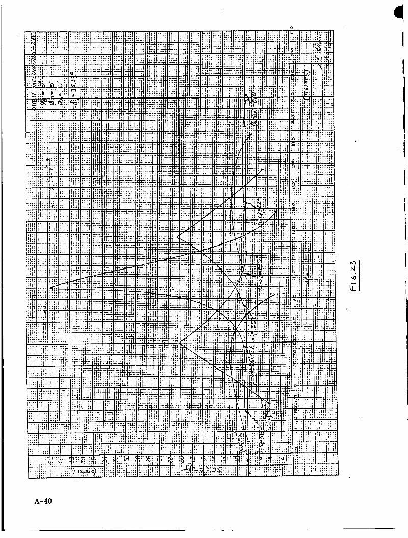
I-l-l, I

H_

H_

lrl..

._,

m

_t-.

2J....

+ H

t_.

_._

i_;"'!l!Ii

;!i N

:._,X

?:N

N :i-}

i!_ _1.,%'"

{{ _'b7!r !:_i

4,r?_iF

O

:4!1 ,11

i_ "_

I,

!I

';' ii

if: I_'>:

7_._.

i

!1', i]i

ill lIt_+: i'I-

i4.117_:+

It

I,

_r t_U

_' i:!÷+

ii

V

t

t.

il:

'i11

#

A-40

:II

,o

T_St-t+.

t!

T_

-tT

r_-I?

-It

:I.1

li

4_

:Izl-

?t-

b.I

It:

1!:

i-II:II

r;liIf'

li--

.ab

tl"

2'..1

"i

r.*'

;J.

11!

.:4,:ttl

m

_+

:tl!!

:l

it

LI,

I _,

M-

I|

t_

H

!i:

:I ¸

i,

_tM_

,i

_°.

'ii

'if

i:_:

• !_

L.2

i ;

'k

ii1]

ii

r;

A-41

iiilliii

,°*,***.

tii'!ii!

::_ i!ii

!:il !ltl

ilii !!!i:I!': i!ti

ii:/:i!_tiiii !Hi

ii:ii_i

[!il Itii

:II:

::': :'z:

.... !!:i

: _I iI;l

i::i ,

: : ::2

MO

B.-I

i=.

|m

!

i

I

i

I

A-42

UU

o_

I'_. _.

.H;

ili.:.I:

h'!

:t

H

H_

iii

111

mt,!

gt

ii!Nf

iiJ,

mi

!t

_tf

!t'_!'t:1h:!

_J

A-43

i

Ri

; _,-_c°s" r., >o.,_,;,8o"

"1

1

A-44

l

-i

, 1

A-45/46

APPENDIX B

SATELLITE ATTITUDE DETERMINATION VIA ON-BOARD RADIO

SENSOR MEASUREMENTS, TWO GROUND TRANSMITTER STATIONS

I o INT_INCTION & S_RY

This memorandum presents the equations required for the com-

putation of vehicle attitude utilizins the radio signals received,essentially simultaneously, from two separated earth-bound radiostations. The accuracy of this computation based on sensor measurementinaccuracy, is evaluated. It is found that the conditions for worst

error are different for this system than for the previously studiedsystem of earth-sensor, radio sensor combination. By properly selectingthat system which yields the better accuracy, excessively hish errors

are avoided, although the yaw accuracy may still be considered inadequate.

TWo types of orbits are considered: the equatorial synchronous

orbit, and an inclined (Ip " 28 °) orbit with 6,000 nora. altitude. Bychoosing the synchronous sate11Ite lonsitude to lle midway between thelongitude of the radio station sites, minimum errors are obtained (forzero attitude angles):

pitch error (3a') _ 1.9:roll error (3o _) .7 0yaw error (3o-") 17.2

By exercisin E system selectivity, the maximum and minimum errors, forthe t_clined orbit are:

max. min opitch error (3o--) 3° 1uroll error (30-) 3° .6 °yaw error (3_-) 16.8 ° 2.2 °

Errors may be further reduced by the Judicious application ofweighting techniques. An extensive numerical evaluation of the effect

of these techniques on system errors has not been made; fundamentally,it would be necessary to investigate the degree of correlation between

the two types of systems considered. Reference Memo, Flight DynamicsData Memo 4143-PD_M-007, "Satellite Attitude Determination Via On-BoardEarth Detector & Radio Sensor Xnformation"o

IX. _ION OF LOCAL VERTICAL O_.E_TATI{_

In Figure 1, consider the satellite at point , which is sin_ltaneouslyin view of two radio stations on the surface of the earth, designatedas S 1 and S 2o Further, the stations are within the field of view of aradio sensor on board the vehicle. Let the local vertical, directed from

vehicle to earth center be denoted 2£ . The angles _ and _ are readilydetermined from knowledge of the coordinates of sites and vehicle in thegeocentric equatorial system. If the satellite orbit has been deter-

mined, the angular coordinates _e' rg" and distance _p are known asfunctions of time. Thus:

B-1

The station vector is given by:

A like expression holds for ('_e o Note that _,

changes at earth rate:/

"_,= GHA T (,_)+L,(a)

is constant, but _.!

(3)

where L., is longitude, measured positive eastward from Greenwich°

The central ansle _ is given by:

_e

o!Y,_< <and the line-of-sight distance is

,where CI - earth radius at S 1. Angle _t is then obtained from

I

_,-_ _, Y,= _r_- C,_-- _I:t,

<6)

o_70<__ _e___< 90°_Z is found in similar fashion. It is to be noted that stations

may determine _ by direct measurement of range and elevation, but

less accurately than from knowledge of orbit parameters and time, using

the followlng relatlon (see Figure 2):

now the otlentation oft., and_j., the unit vectorsConsider

along lines,_of-sight from vehicle to _radio stations,:_ in a body coordinate

system. If the stations transmit signals to the radio attitude sensor_

the direction angles _1, _1 ' °el, _ will be measured (see Figure3). Thus

= .4, "rx + .,,_,Z_ _'._, 7.._.

B-2

where

(9)

(n 1 and n 2 must be positive because the radio sensor coverage is

less than hemispherical), But _£ can be written

= +"°+_"_ ++÷+ +e-+_•* _'+- _m

The angles _, -_-Eare i--diately given lfo_, _ are determined°

-_------------------- (n)

O_:_S 90"(The positive root for _N is taken since the radio sensor is along

the positive _ axis _defined to be coincident with _E when _ 0;see reference memorandum for.bodyocoordinate system definition)° Pitch

and roll angles of the i x _ iy - £z system with respect to localvvertical system are given by (see reference memo for derivation):

"_"8 _- ._-]C-._@E)_ 0<'_.-- _0 °

o_< _<+o"

)

(13)

(14)

The problem resolves into flndlng/_,2_.

(The body system and attitude set defined by the order of rotation

yaw-pltch-roll is redrawn, from the reference memo_ In Figure 4. An

alternative set defined by the order pltch-roll-yaw £d described in thereference memo; the functional relation between the two sets _f anglesis given therein and will not be repeated here° Note that determination

ofj_E,/;_,_.£: that is_ the crien=ation _i local vertical with respect to

B-3

/

f,Ibody axes, does not alone suffice to p_..ovid_information on yaw angle _Bconstraints afforded by knowledge of_-_,X._orientations in the local-vertical (orbit) system are required, bu_ more" this in the nextsection)°

Now, from knowledge of _ p and_£ , it is possible to determine

andre , albeit with ambiguities, which can, however, be resolvedb_yEmeans ok other sensor information° Taking the dot products of

equations 8 and 9 with equati_}n 10p we obtain:

But, the orthonormality condition must be met:

_; /7_' _ 2 (17)

Equations 15p 16p 17 constitute a set in the unknowns-_ _t/Cf_o

Elimination of _e and/_ yields a quartic equation in/nZ_.ofthe followingform:

o..x+ x% cxZ+..,4x =O(18)

The coefficients are functions of the measured angles O< Ip _I ,oC& p _Z

and the orbit-site specified orientations of lines-of-sight with respect

to vertical, _ , _ o The functional relations are set forth in the

appendix° After equation 18 is solved_Is given by:

= A-BX _+ PX -f-E' (19)

The coefficient functions are tabulated in the appendix._is thengiven, of courser by equation 12.

The physical reason for ambisiutles is seen in Figere 5. At a

given instant of tlmep correspondin E to when measurements are made, the

b_5.1axls tread can_e conceived to be capable of being rotated about the, vector, with_,Nat the half-cone an_le'4_l,_and.o¢ ! '_I' remaining

unchanged. Likewise_ there can be a conical rotation aboutA._. Tireposition of-_is found at one of two possible intersections of-the cones;

_hasp there_oret.one of two possible values. After ambiguities dueto'quaking processes are eliminated by verification of solutions in theoriginal set_ e_uations 15, 16 17p further ambiguity can be resolved by

comparing__with _he values directly measured by an eartn sensor_

B-4

which values are measured with fair precision, as indicated in thereference memo o Note tha_ some false values can also be eliminated byconsideration of intersection constraints:

It_.is _to be noted that a unique solution co _-Eis obtained ifrE, _,,_-sare Co-planar or if _e base circle (figure 5) are tangent;that is,'if "

However, the co-plsnarity situation results in indeterminacy of yawangle

llI DETERMINATION OF YAW ANGLE

Equations 8, 9 and 10 may be solved for _'X"

(20)

In the above, the direction cosines of_4_,andM-$Z (in the body system)are measured, and the direction cosines o_are_presumed computed as

indicated in the previous section° Now from the'_" matrix relating bodyaxes to local vertical system (see reference memo_ equation 3)_

quadrant from signs of numerator & denominator!

I

If the orbit has been determined, the direction cosines of_, and__

are known in the local vertical (orbit) system; that is,

x,, = Z t',, r,,(23)

(24)

B-5

IV

(B_presstons for these direction cosines are given in the reference

memo, section IV). Znsertin S equations 23 and 24 into equation 20and thence into equation 22, an equation is obtained for yaw angle interms of measured and orbit determined quantities:

/ s / /

/ /

This equation is valid only i£ the determinant D is non-zero_ X£equation 25 is represented as

P

then the quadrant of_i£ obtained £ran the signs o£_and_ _

ERROR ANALYSTS

g££ects on attitude determination accuracy due to errors in orbitdete_nination and in site corrdinates will be neglected because:

2)

These e££ects will presumably be small compared to attitudesensor measurement error e££ects and

The primary purpose o£ the present analysis is to providea comparison o£ the relative accuracy o£ various techniqueso£ utilizing vehicle on-board measurements with ground-basedcomputation to obtain attitude Lu£ormation; orbit determinatiouerror ef£ects should be o£ similar magnitude £or all o£ thetechniques studied.

Assume that the measurment errors are independent random variableswith zero means and equal, variances (noise power), that is

Then the attitude error variances are given by

- (26)

(27)

(28)

In the above

_'l "_ °_z

B-6

Expressions for the elements of these matrices are tabulated in the

a_e,_,..oret_,t4' .,f,_',-S,'4' '"_°"_;,"S_"recon-siderederrorless.

Conversion from the errors in attitude angles with respect tothe X - Y - Z system to errors in attitude angles with respect to theX1-YI-Z 1 system are readily found as follmas:

(29)

(30)

(31)

. _ _

Fozmalae for the partials _.--_ _ etc. are listed in the reference mamo.

The foregoing indicates the_eat a_mant of cc_p_tion required forevaluation of the accuracy of field data.

B-?

For present purposes in view of the small excursion expected

in attitude an81es ( _1_" +_ 20° , _'_+ 10°, _)_" +_ 10v) andbecause of results obtained for the error analysis of the systemdiscussed in the reference memo, it suffices to simulate and evaluateaccuracy for the condition of zero attitude ansles.

For this special case, the following is obtained:

(32)

,or -erosttitud, angleS.a.'_m'O,_." 1, Then from

equation 21,

large, It behooves us to determine under what situation tbe/_.- 0condition will be met. The sites to be considered are:

Rosman: 36.133°N latitude, 82.833°I_ longitude

MoJave: 35.333°N latitude, 116.90°_ longitude

Takin 8 the more westardly site as _1 (satellite in direct orbit comesinto view of this station first)_ we have

= ° /-/=-/I °0

6_= _6.13_ - L__ =- fl2.8._ °

_z-/, _- _.o_ °

B-8

i

I

I

Consider the synchronous equatorial orbit first (see Figure 6). Wecannot have ml= m2 - 0 since the sites _re not on the equator. __We

cannot have_. =£,= O si_e this implies coincidence of_s, and_,.

¢ . _We cannot hav_a_In_= 0 or -/_q 0 since these would_ imply4_, o_4D-,

equal_. --t° zero which ca_otbe. -.FinallY' in order for_-_o_ lie in the

; plane,

Solving for Lp-L1, weobtain ( L _L ) = -70oh-. It will be shown inthe next section that this value is outside the limit for simultaneousvisibility from both stations. For the synchronous orbit, therefore,there are no discontinuities in the error evaluations. It is clear

however, that errors increase _s the two lines of sight approach

collinearity, that is, as approaches zero, where

As will be showns _'/decreases at the horizon visibility limits_

so that errors would be expected to be large near these limits.

Now for an inclined orbit, eit_er_ oral.can be zero, but they

cannot be zero simultaneously. (_! is zero when _ --_ goes through aminimmn; _ and 4_'a_cannot be mininm_ at the same t_me). Neither m1 orm2 can be zero if the inclination of the orbit is leas than site.._.L_=_-'*_'°_-..-_T_ equation 27 of _h_.... reference memo_ m I can be zero only_

For _'I_'.,C:t_" the :ondittou caunot be met. Finally, examining thecondltion_, m2 ml_.x, using equations 26 and 27 of the referencememo, we ob_aln the va_lue of the an_lar position of the satelllte '

measured from ascending uode, for which the condition is met:

+ °The critical value off.(note double value) as function of_-_nd

, shown;" Figure 7. As shown in the next section,for _= 28 ishowever, this value falls outside of the limits of simultaneous visl _

billty from the radio stations, for most values of_--._p. Where._?does fall within visibility bounds, attitude computation cannot be • c.f,J_

performed.

Vo VISIBILITY LIMITS

For visibility of the satellite from the radio stations_ the

B-9

elevation of both lines-of-siEht must be positive simultaneously;

i.e., lines_of-sight must both be above the horizons at the stations°

This is equivalent to the conditions

o_<_< _" (_ < so°simultaneously met. In addition9 the stations must both be within

the field of view of the on-board radio sensor9 whence the simultaneouscondltlons

o_-e; & 25 °

o_<_..4 _s °must be met. For zero attitude angles, _ = _ _2 ffi _° The maximum

possible value of _/ (or of _ ) is

For the synchronous equatorlal orbit_ _, = 8.68 ° . For the 28 °

Incllned orblt, 62000 nom. altitude, _ := 21.3°. Hence our con-cern need be only with the station (si_taneous) visibility limits.

The situation may b.c,.represented as in Figure 8. Simultaneous

visibility starts when_-_aJust comes in; it ends when .,_%! Just goesout. For the equatorial orbit_

Setting In_] L.._-: 81032 ° for the synchronous orbit9 with g =

35.33 , gives the limits on (/-p-L l ) for one sight llne only:

- I s.3 ° ._<Lp -L, -I_.T _.._.°But the satellite will not be in view of the more easterly station

unle s s

(_,-L,)_- -_. _, C_,-=,):-,'_. _ °Simultaneous visibility then extends only for

_ _s. z ° <_(,_,.-,,') <_-cs. 3 °

-zs._°_.< O-_,-L_)_<÷s.z °The corresponding permissible values of _p are giver by

_<'p ffi (L-_.-L,)_->,.,Figure 9 gives a graphical representarlon of the concepts.

B-IO

For the inclined orbit, repeat_ equation 22 of the reference

muo,

SettinS _',]_.,- 68.7°_ upper and lower limits for-_q_D as function of

( _- .X_.p)-_an be obtained. Since _1 _e _ che"_._ limits as

function of ( __-- are simply Siven by the values_ from equation37, at

Superposition of the two sets o£ curves, yields the region of simul-

taneous visibility, Figure 10o Note the constricted range of _occurring at _..I-..CLp = 270 °. of only 37 °.

_JANTZTATIVE ACCURACY ASSESSI_RT

Figure ii shows the elevation angles _'1' _ as well as the anglebet_een li_s of s_m_-t I/ f"_ _-he ,_-h_,_-._ _q,_,_or!.l orbit.

Evidnetly, maximum V occurs for the satellite_position about midwaybetween the station meridians, or for J-p"Le_la°o 3 _" e_'rors were

computed for _(_=-_', with results shown in Figure 12. It is seen

that errors are minlmun when _/ is maximum; that is, for /--_o = 99 °

west. _ote that thls is in contrast to the earth sensor-radio sensor

system accuracy, where errors are mlnlm_l at the limit of visibility;

that is, near the horizon). The yaw error is still excessive, even at

minimum.

Figures 13, I_ 15oShO_ attitude determination accuracy for theinclined orbit,_p 28 , 6,000n.m. altitude, and for zero attitude

angles. Evidently very large errors can prevail, some tim in orbit,for the inclined orbit case.

Let the system described be denoted system D; let the earth sensor

radio sensor system be denoted as system Ao If attitude in£ormation

is available from both system, the results from one or the other of

the systems can be selected on the basis o£ system accuracy. The

choice of system, for the synchronous orbit, depends on the satellite

longitude L_ ; this choice is shown graphically, Figure 16. On this

basis, given the choise of either system, pitch and roll errors will not

exceed 3 degrees for any£_ (wlthlnvlew of either one or both radio

stations): hoeever, the yaw error does not go below 17 degrees. Figures

17 through 23 show accuracy, for the inclined orbit, when that system is

chosen whleh provides the smaller error; dashed lines indicate imposedvlewlng l_nitatlons. Peak and minimum yaw errors are shown, Figure 24,

B-11

for the inclined orbit, when system selectivity is exercised.

The spread is from 2 to 16_ de_ees. Note that _.! is the instantaneous

right ascension of NoJave when transmitting for the satellite; or if

only Rosman is in view of the satellite, then RosmanWs instantaneous

right ascension is _ +34.07 degrees.

Given that both systems A and D are available for attitude deter-

mination, then this determination may be made over a considerable pot _

tion of the inclined orbit. For J_p = 9440 n.m. we have as orbitalrate

030 = =. ol G4- aAD,^NS/MIN.

VIIo

and the orbital period is

- t41Nu'r

Earth's rate is W E - o00437 radlans/mlnute. Thus

B

Starting at any point on the lowest curve in Figure 10 (where .,_/comes in), a straight llne inclined 75 degrees to the abscissa may be

drawn; intersection oftthls llne with the various curves yield values

of _I at which the successive events occur. Dividing the change in _,

by W_ gives the time transpired between events. The result is shown "Figure 25, On the average, attitude determination can be obtained over

60_ of the orbit, from the time when MoJave first sights the satellite.

_i_rrma z_c_S

When both systems A and D produce attitude determination results,

it may appear desirable to average these results, in an effort to reduce

the noise error. It will be assumed that all measurement error sources

produce purely random errors only. Let the weighting coefficients be

denoted fA and fD and let the restriction be imposed that

In particular, we wish to reduce the yaw error. Let the computed yaw

angle from the systems be denoted _A and _ respectively. Theaverage_ or estimate of true value, is

(38)

B-12

/

and the variance in this estimate ts

(39)

where E is expectation operator, Note that the covariance is not

zero since system D uses a radio line-of-sight.

Three weighting techniques willbe considered, in order of in-

c,easingco_lexity _t s-6_,,,-as_,_ DO,f _,_A >_(Ag_then_. A choice exists whethe_to accept _balone, or whether t_

average with _vA . The latter choice £8 only worthwhile if _r_ is

significantly less tha _A___ Suppose straight arithmetic averaging_that iS, :)_t :_ = °m equation 39, then,

= ,

where the correlation coefficient e is defined by

(40)

PAl%_*+ a.j

Mote, in particular_ that equation 40 yields the familiar result

if _Oand_=l , that is, a 307. redu_tlou in error. Figure 26 gives

a plot of equation 40, It is evident that only for_|Is the straight

averaging technique acceptable ove_ all possible_o (Note that for

<1. a choiceexistsbe_een"'t'" andT'AOnly,si_=ey"C_},')Aisthenlessthan _'(A _gD)"

To obtain an optimum weighting function we must minimize equation

39, subject to the normality constraint on the weighting coefficients°

Suppose _ were zero. We would then wish to minimize

where _ is an undetermined parameter. Differentiating this function

with respect to fA and fD respectively and setting equal to zezo_ and

using the constraint condition the follo_ing results are obtained:

: +/ , -

B-13

Evldently_ use of this technique requires that ndevaluated in order to obtain k. If _ = 09 Dbe

which is the minimum error for all k. If however, e is not zero,then

,r, D : , ,

Equation 42 is shown plotted_ Figure 27. Only ifuC is zero ornegative_ is this technique suitable over all val of k.

Finaliy_ considering that _ will not likely be zero_ we minimize

Zhlsyields /_p._

_' C,_</")b V_-2¢._,,-, '_ "

(43)

Equation 43 is shown plotted_ Figure 28° Note that the error ratio is

less than I for all Icand for all e ; in particular, full correlationproduces zero error°

The computation of _ is generally q_zite complex. As a simplified

case,ifY_a_a= q%=Oandif_(_,l-(_,)=_), thecovarlan_e(for system A connoting station and Eart_ sensor viewing) can be

shown to be given by the following:

Z,<, -.,.,.z)(44)

B-14

VIII _ORS DUE TO.NOW-$IMUI_, ANEITY OF RADIO S_

In Figure 29, for illustrative purposes, consider a circular,

equatorial orbit. At time t I, when station 2 is at S 2 , the directioncosines of_-_ , in the body system, are measured. At a time t2= t 1

+_t, when th_ satellite has moved from _ to P2, and station 2 hasI •

moved from S 2 to S z , the direction cosines of _ are measured. Thelater measurements are used in computing the atc%tude of the satellite

Evidently errors are committed due to earth's to'ration, sa _ellite

vertical rotation, and body system rotation, durln K 4 t.

Let unprimed quantities represent conditions at: time t _ primedquantities refer to eondltione at time t_ . Subscript I or 2 refers

to measurements, with respect to body system, of 4! or ._'5_ respectively;subscript _ refers to measurements with respect to satellite local

vertical system. Thus,1

(45)

l _I . ---I

(46,T

Let

I

The errors committed are due to using 2£ instead of the (unmeasured

and unkm)_l) --'_ > ,_ instead of _nstead of We wish to find4b

Now

I I --- I

where

S V

B-15

in equation 48,

(49)B

It can be shown that (subscript B on attitude angles, indicating orderof rotation of Euler angles adhered to throughout this memo, is implied):

o

(51)

Substitution of e_.uations 51 and 45 into equation 48_ using trans-formation matrix-_" (see reference memo)_ and assuming small attitudeangles and rates_ _e coe£ficients in equation 49 are obtained:

From these,

(55)

rotation and s_elllte angular orbit rate by _ubtracting (_J_)_' from

the measured._ . This can be done because_tt,_2_,_d their rates

B-16

are colputable as functions of time. These rates may be obtained by

computer differentiation, or from the explicity equations listed iu

the appendix. If __ is sufficiently small, we may useZ

Otherw£se, it is necessary rouse

-where _ and _ are the approximately com_uted values before com-

pe.satio.° S,-,lsr rsrk, pertsin to (A_)_, (_)V • Note _tsuch compensation is required for the synchronous orbit, since 5_ _L

does not rotate then with respect to local (satellite) vertical systems.

/7

In_, after co_ensatlon, is

/

The residual error

whence

Likewise,

,or_"-e- _--O,thefollo_i.g_re_si_shold:

(59 i_

(60)

(62)

B-17

(65)

Since we are evaluating errors anywhere in orbits the attitude rateswill be taken as random varlables9 havlngthe same distributions and

oqualvarlan_es9that is,Stf.)--f('9""<_Then.tili=in_equations58 thmugh 659 we obtain (for zero attitude angles only):

L {"<'<:-_.-_J+........

o,,o<. +,.__ _.,_

where the dividend Is given by equation 66_ the divisor by equation

32. Like definltions hold for "_/i _@(see appendix for explicitformulation)° The r_dio of atd. _v,tof error9 due to time difference_to the std. dev. of error_ due to measurement errors_ is

The std, dev. of total error is then

: [" =whence the fractional arEmentatlon due to time difference in measure _

_ents_ is

B-18

Similar definitions apply for _ _) _

Zt _r_ll be assumed that, over any orbit, it is equally probablefor each of the attitude rates to have any value between _imumexpected limits; that i8, uniform (rectaugulaz) dtstzibu_.ious ereassumed. Taking _he maximum value as .03 degrees/sec.p _t-9 secs_

and dr' =lf we have

Figure 30 sh_s percent error augmenta_Lon, fo_ the synchronous orbit

only_ and for zero attitude angles. Evidentlyp for _ t--9 secsthe effect of measurement time difference is less than 87. of the std.deviation under condition of measurement simultaneity. Figure 31 showsthe effect o£ increasing _ t ou maximum percentag_ augmentation. Ifthe maximum 3_(_is 3 degrees_ based on system selection, for any

(Lp-_- I ) (see gur'eFil 16), and the inaccuracy of this estimate is noteo exceed ½ degree° then ,:_ cannot be permitted to exceed 14 secs.

B-19

"T..:

w_

B-20

z

0

o

x

o

\\

\

B-21

eo_

_6U '-}

0 71

_o

4_

zO

36o

3zo

_o

22o

6o

,Po

0

-IIii

_ii.:!: _!i!!! ,:_z :i,_!i. i.I

....... : !.:'d :!i!R:: :::i':L_

:ii:: ill :m::, !il

il iii!iii :i_I:_,,'

:!_$ili iiitli-_ ...... :

iii:li.:"

i!ii:ili::.i:_.,,. _._,_:.:,:, :_.,_:;.;:::.::!!::/_mr:

lhlr, : .......iii

..........__._::_.... i71!.: -.

/

;1:7T_! :

T',!-_T:"'7:7

!_i:.!iL_:I_i:,_,.i!12:i:......i rT; _'.

,__:

il b.i'f .....

.... t' :I :iili;i_2_! !,h:

;tlt_., .::lit;

!fiiil

:;:tuff ' "

:tT411_,

Li'.t;: ;;: I

i!i_ti ....

:i!itl

?i:J:

:I ;[. ;1 .... '

i/

I

t!a,,

B-22

0_+

I

z__<++

04

I-.,iO_

P_

V:

:.:,,

if,

t!_i"! i-

t-i !

!i +*'

.+ r,q

;_,+.:

+2_

L.I_L

: :-l-_r

+i,',-:i:

:2:-

_+_.

::

2_T

-r'

L:::

+,++

r.,+

+::i+t_2_

Hr;

__

t2;_

ttl2

+US

+_ !i+.... :+!;:_T:_! .i]-2_:[![

iii:,

÷-+-+_.

. +_ +++++_ +e++-.... _+4-+

++Vt:

++.

,++++-+; 4-

_!i:;+g!!

++_..:-_,-,

÷ +++_ .+ +-_i

_: ,.+.....:jr

i:': gtT..+..

++.i;+::: ,++++_i] ++: : _ .':

%:: t_N :;

::_ ::_. i!_+++ ::t I :::-'- :::-; i::;

'+:i:_.:t,.T2:_ :i: +'_.

+.i: T::; ::!

-- ' k.:

!L,L + : :;;

-t .r. 4,_

• :_i :n:?:! . . :

_tt :i +":

..+ .. +,

.... + .,_

I! ......

: .+

++:: !+iT

++{_ :_H-:+ +;++t+

+j:+........,+ ++++_+ + ++ ++

:: L_+ . ......

+'++_:+ ,, t:T+ :::=

:f .+-+.......• . ',_" -M4 ::4

-:iJ _ ++++

:r_:i_-i+ +i-_-tU: 4u:

• +:7-_ :_+:, t

_+ ::-:+:t"+_ _ :i:

++ ++....:i:il+ .... :;:; ;i-:+::+,: :I I+. .:i! _.+

..... :i:]++++.... H::",i+::+, "'";_U.;..... ',+:::++-:kT _'_:+:_ IT::1::in-:_

" ""L_.;-_! 2=i :; :, +_,::+:: ?If: : _"?u+ ii

::t +. : +++ .... + ::!

-- !-:-:_" : r: ....

l;'.I . +++ _:

==_:i..+.._ +,_: ++;+a4

1:++: :;::I!: .... :::: .,+{:44M_t:=.+-

_:I+ ; .....+++;i:: '+-i.++.+: ;+._. :.+

:++_14;;:::+] :::_+"':_ +++++_+__.+_+

4+hlt'+:,_. :+'++ :n i'__,tttt+ +f;1 t r , .

+ :g: ++: _:,

,.., .......... ++.

: t+t+:-++" :'+::_s+:l::

_:+iI_:++_:!:-]:_:::FYT:::",!t+-: r"t :!: :_:'',tT

.... :':}fii_-'.+_ :i+: 4:? ........

B-23

"7._'

o•

_u

O_

oJ_L

C)

B-24

U

_u

o°o_

b_

O_

B-25

O

o-L_

x_O_

B-26

•T _.

TU

_zd_u

Ww_"r_

OQ

Olu

O_

4--

tT

!:

.il

LI-;

:tb

%1I. ; L

B-27

&

;ruz

j,

:r

0

o

o

!:ii_ii_!:t.'....... i l,,,,i11- +,t;: .!

',t :: ',;,-: ]![{_t* I' "

_i !Tt!T' ._+,,;,_;: W

::.i':u::!?

!i::_l!i,

:!i:a:.::

l-i...... i_

........iJ

•;t"t_.t_.......!;F

i;;tlt'

!ii:iH:il:T!

-,t • :-: :

_ z'l': : I ;I

I1:?m>_l. '.-_l

::",r,irl

,,,!2

ii4.; .

:y._tlil;._1.i; l:r;Iq

i: ;ix: ':]

i:i::f_i:i_

:i:t:,:;!

1;IHfilil!i;:_

41ilWiWui;l:,t

lHt:,!rTi!t_,fi!i_Htit!4+: ,-ll, i II i;

l!.il IiF _:,_

_ICliill :-:_,,11l'bll_':t,,.+I_, ,_,,+ "'_,i'l;_.:ll::_ 14,

IIII::.:I._7:( [;

,!-_ i F.tt l't'il t, _.

i N!t-....': li!' ii

, TF

' +; :i

i::t:7ilt::+,,i If!i!iltJ*'|:;:'l ii: ',;, ._ , , j-

t;!iit::'!i

:tiI:!!t....:':::

ltr|::;ti

:-_V.+:ti::it:iF+:Tl;:,:

mJ!t_:i:Fi::'::fl:liil:'ilt-t.,, :':'lil,f4:t,: ri-,:il i;-t :it....,,.

!?_I "1

:illii::l....:i

ij;llt:ii:: : :

t',4_iI:l[ii. ::i

+.r: :! r:;:

ll'll ;ill

!tl liliII'_ ,,+i

;iil 1"_'!

F!F :":i

.... ;LH

i;t',

!it ;I:

_i!i flii:i;!

7t_ .;7'.

.÷_.....

t_'" ;I11

I+.I! ....

_"i i t-l-i

!:!: _:I:

11111 I'?I _

.... t2 i.i

_!i s,:Irl _: :

, -, t,o.I;+.; !i:'

_': ,i_:

_i!! ::.;

ip-f ":_i

:!!::::

T::t-.-::

,;:i :It,

:il

!it! •:2"

._ :'....+..:: : f'.il.

tfi !:4:

-l-ill I II ....

"; :1:4

,: i_:rt

::2-'i ::;'

• ' 1111 ; .+T11.

_, ...._!: iT:_-

li!,' _r':

• t!:; '_°"

! .: t:;! ....

ili" :i : tlfi::;!:.::::;4!

fi::':,r. +1

• ' , t . ; : ;'!d '

_A..-L T._,-:

;::: itl::..! it!i

:: ::77 .,i,

:i: I .:..

;: _'-r , ;.:I _r_

i:i_.... :,:i

_:_i !i_i "_'._r !;:-.._;

.... '', '-,

ST:::!:,:_iii:i!!::i!

!::_ ',:,:';t .;,

•:::li!f fii+_

::Tr "'TT ::_

1!'

!;:!,

ri!:i

:t!il-

:It _T

., ;!

r!i!f

" iit'It; I .il, i]-:i4:i,

:_t r:fii, :_ Pl-

It:'

'l

FI .

_:: f!!:;i, ;4

"I,:i_lll,,.q

F!

t;_:!ill:!_It ! :|•: '

:::Fi:itt:.-I [t t: + "

_ i i i : '•:, ,-!'."1-.!-

ti; ;;,%. ....

• t 121' ''

ii : I tT ll+: :':+;t¥;.;71:;

:_::ii:IP}

ii'-il'll

"", [:_4t_i}

ii:il::i

::>

_ i:::jii:

,.o,,,,.,

:'.: k!!t]:!!F ..':_; :liTt::-

:li :i!:lli

::" ::

'_ _:!.!!2:

!ii :ii::

i: :!:i

. ., ';ill::::

i!tH::lli !l::k!

_¢I !I!:'::::'-+---"_,I'I':7 " : :li]_ I

i !:tTT'_ ,i::::li l::,:I :!: ::!

;:I:_:+,:I::L:I! _ *;'.tl

:l; t: II

;![iTi+,i -14-1 ;441

'_:!iii: It_iit

': i'.::,: .:,._., ,,*%,

" i :li ii

i;i::ii! "::":2"i

: :::' ;h:l::!i::,ii iti_:!

-i]ii-!!LL._....... _ :i:

::::...:-::::.'

!!':: . ,L"::

:': . •

!!:!:;

1!I': 'l.1;

! 1!'!

,o . _:I

,i;+::ti :;.t+,

TITT -_,,-

m::'.i:

!,

'># .: ."'_'_'4 ;:...,![: :: '

ilili : !;;;

,;:.. :.

!r:: !_

_t:t ;2-.:

]!'.. ::t:

.... '-r__

::':IPllht'l

i_i " "

:,4t: !t,,!,_,_l

i_ i)i;

't' ": .

_d ':ii_ :"?i

ii: ,::

:}r

.+ .....

:7:

l_..22-. l-' .;

:' i::

7!: ::!:1

L .... _'• -,4

',11 . , o

,_. : Iii : i

.... I

::;: :i I:!'

• , , ,|

:i:.

: ;.

-_-

::!:

fii{ _]

I

!t:ia:&

,I ' '

,r

':i

I :

"t.=

" I: i

:!i r :

B-28

I"_j

z_d

x_O_

V4

B-2_

zu

_zo_uW_

O.i,_--j

_L

x;Ok,

X_

B-30

"7._

-rU

_zo,_u

t

04

B-31

U

z 0__u

04

O_-L

x;

_2

B-32

o_:

z o

04I-jO_

x_

B-33

-rU

ir

o

X _

_t _H

4_

ii if:

li !_!

tl I;:

ii '

. ,t

l,

rl, ::,

IL !i

L._ T::

_ ..t,

'' *rl

i[ '

r

_. ;:i,

• t , .I

li it:It}

I! i;iH

t._r

4 _ 4

_t!

-!_

:t!!-Itt

iN

_1_

i!f,r

ttt

_'

1;

tH* *÷

4,,4-

LX

il.4..

!7:

t_

:;t

l-ii!

B-34

"7;_Z

Z o_u_ulll_.-r_

04I-jOu

x_O_

Y

t '_Ir

t_

]1:

2_.r

1-1L

*'4

rM

_44.

-t-i-t"

• +.

_

tM

!fii

].

i

r.f.

ItI

iT! •+i

J=l

-_44-

t_

4-.--

:t }!

L

4:

!t: =

' i

Z ::

;I Lt:

;X- ,

i r:

,i

f ,

_ti1 4:

'" 11

i: :i]

:f.

:, r

I

!! !:

iL

l-_. I L,++ iI-

ii, ,5

" K

t_ t5

fiitF

....9fff

ttt 1!

11! rt:

_'- t*

ii!; , !

*44

H; E

ii"t'_:;_ t+-

::l t!:4_-H:

q-i5

B-35

;_; .- .... i;: t ,I:: i:' :! ;:t : t 1"

......... t ......... il ,_it t=t;;:I

:i :: il _ i!: i'.i ill iql::_t ;::t

i:!::i! i_:1::! i:I!"_ Li:fq!l:_,il::_ ii_:_ _ :,: i;,I ,,i!i;itl NI

..-_.:--_-- 7 _. i-:,ti_. ' ,.

• ..... I "' i ....

t:! ,:-_ !!! ::i! _:I!!:_:::'!:t_i_1_i!t

if: :t_ ili ;',i_ ii::i:_: ::it::;4 ::1::: 4._ 1 t: i:,_ '":: :: i_l:_i_] ;:q

.... :,¢ _' ,d_ ......... , ,

"._.! ::i_l :i_!]_ :::l._i: :'12;( ;:::i:i: i:i_i ]_.r.:_ Fill!':' ii&!:T:. :ii.]

!:! ii_I :i :_ i!:]l"i 'q liT::: !:i,I::i i:_l i t: i: ," -£ _. :_',1

..... I .... ':_i ....... I ........

:: ! [2:i: 1 :"t:!,!__:7 ,::i

':2-2_t::--t:-:-!::L ' ' __--_t -.7,-

i.:!] !l:i:_:iit:::i:_;:, .cii:_,:i!: si:ij_:;!l;s:,::2i:tli :_, !if!

_2 2i2;:: .!it,::.t::t:ii::L2/:' :I:2: :2:: :.'TT' :;; t:.! :t:T!! tiT: :::

_.i:!_ ::', ::i! ::: ti::i];i,i ii:i i::r-"--_ .,. .'-Tt 2%1 t--':-I:.,.t :;. ;;4-;.. •

': "::; t::t :_;: ;: ;',2't'.I:; 1;:, :;;!

ii :l : !i:: ii: 1.1111[:1,;i ii:i ;:2

:2 ii: i!: !i!i::2'.t:1; ]7.2 ;2;1 ::; 1.., I :: ...... i::

2_ -M _ :-247:i:li+u. _ _-:-

..: " .. .; ;4 . . ::. I : {i ......... i t'''.F:::. ,2::L.= 2: ::a ::a.t:2 v:2_,= L_i:::t::: i. :i :i?l.!isli< ::i: ii:i: ili:,i:i;ill iiii;iii; i.,;i?:'.ii1;:: :i: :2 :: ,: : : ::ii:i '.i'.

, .';-I;,l: L'

'I:I::.

• _._t " "

• ;Sa

t/i'l,,,;,

d:::q

411I:1

•._:_

2! ._._i: ;:.4",' !!:;i' -_-4!F _:';",,.:: ::,4 , ,,:,:: :: : • l::r .':.......; i:- "-:-:-i

:::" :: ': ::: ,.:: : 1:t _, . :;.:t ,_:':,: ,. : ......-,.t,,, l ......... '. .. ,' ............... ='.[.:.,! .... :._::.

:; ::1 .... ] ..... q:;':;I _;...... ' ": ............. _............... :t ..... _. I ........ I.4_ __" _ ... .... _ ._Ll _ _. _ .........

.-T ...... _ ::/q .;_.. ._::;: ; ':i_; _ ...-: _:-:r'--- _r-_ i

.7-T-T--::]:::'-)_.T::::i_:::_.2:i7 :I_::tf::::;:::I:",:.i.: .:_;

ii----:I:::_ ::::i!:i:::'-_]::ii_.A::_:_:#--I-_'-t:

" ' _ .: : ' :_ .... 11-i......... _:' ' :-,--.:.,-':,."......... t.... f....... 4-- _-. _ _... . . ;, _ , :,1: , . .::_:i, .,_.:,.A .,:,_:_/__,...: .....I;,i,....,_-- _-77: --_ .--_'--' . 1:_' ..... "TT";I , , -?,'-",+--"'7._,,d ;

:',:.t:::: :: : ::': .:t: ::1 " :, :]::i : ' _ ..... t .... . '..... : i" " 1" ': .... _ _ ;_.... : : _: "' i ]

:": " ........ :'" ': :: : " : ": " i: :: ::: ' :'' : ' :::_'' ;::!:; ' "! '_:. i

: ;:,!.: l.:. : :: :. 1 '.:1::\;.:':1 : :!:'I"':_]::: .L_ :

:-Fi]:::: ::' :::: : ::' :'. ::', ': :t :1: : .:

::.:.7::::::-:::-:l::-:I;:IT:'::7 i :....:. I : :I

...... _.2 : l'i_: : ,I " _..:_''_ .....' .- :-..:1.-_ '. !

.:7.:_ ::;:7:7:;_,':7_':TI77T!:_:l::::;,'::_: •/ " '• i, , .:t ';:' ; "1 ::',: ,! ' ----~

.;" ;.__. " :2:_; .... 2z- "_' ' :._: -- ......... [- .*..... :

I

l

B-36

J

"7."

x_

B-37

t_

B-38

FI_. Z"/

lrl

B-39

TU

_u

O_

_L

x;01=

#.

B-40

_zo_u

x_Ou.

'F -_1 "+" ?tl IP

_: , 7t!! 11t I!

it :_41 I:-;:_ ;x It

, t I_'. ¢1 "tt!'

;%*i_ t,l _"..... :l:,: I_: ih

;;¢: ht: ,_ .+,,

' '1 qP _:

i _iHli!Hl::_iiiJ

i t'_ !"* "_

[i _-!_ ,_,.

..... :.[

i!F,:-:;:*.:,:r!I!:;,:;:;;: m' I:: iJ

:I_ ._::t :4_ "" }}:.* .... _* CK fi _!

.... [zi: t! ! fr! '" ;, ;H !.hi !_J";ii ._i

.... f:! !*tli *t_ +'+ 4-1

;tl_; 1Vt: ,,t H

_i -;i*_'.; _4 i'_ _! It ti!

-_ 444-4t!4

't i_ 4"t

_t . _,_d

..+_.

,H "*;;.....

:; -.t:!-l!F!

" :'i!T !!', , . _:_"i "_ i -F_ ._

11 lit1! " . 1 ''' 4;i-r

_.K _. _.fl !_i!;,_ :_!

......."]iiil .........I-T t4tZ;I; p .... .;;; .;1_t:

I !_ _; :lh!_M_ ::_

I"1-!-P

_" lt: ;,:r "-tl_tl! 11Tt!lt! t!_

._ :'..t .it ..... _ ,.,, ;tl _;t'

i. .,. I:z:: _ L1:. _ii i:?$,

• -.* _-.. _ I.,

,, ;,_ '_" .... . :, _i_ "'."., .,.

_ ;;q t_' , :.. !HiI-_I_-_,;i ;_ ni,]

iJthIi_ i_JI:"1::._i;;_:::: !il

t il ',i :;'" .l_ii: ' _; .... • : _:. !,r ,;+;

t:! ,:: i;!i ih:,;l:_: _, I!:i'!_!fi: : !: li!!i

.... ;, I1tt _

i,.;_ }j tit[ _";_::_

i! .... ;t ;:;:_ TI! IV, i;I _ H. H!H lit ":: ....

B-41

/

"_E I ._; #'V'¢ks

& : V -,x,.bX_E

_r

t_ ,QWA,,..

--" C_S /e'_E",I "

.

I -i "7 "

" " - (L.__..'j

f

,'._I "I,.c-z(_..,-_)_ _(A-,_') e-_'-_',,c'_ '7

-4 (e'- e) :,_ ,_') f _c'-,-_ .:'j:-'._ _ [_c '-- .',.:')']"

v - _: .I _,L ,

i i _i_

';_4J-

.7---/.ZI ?/. : x .., _¢.j

;i,'_, _ ,_-)c _.b -"-",4 2.A "

,"Z;7._c _C

,.:_*. _-_P

B-43

f ,_iI.

E,_I

B

iii

, ) z,..t..--.------

' i'I¢

/I%.

, / '_)

E-/,'.,.,...,'/_, _,¢ -_<.

L'_, _' '_'_'-;- ) _-_)

!._,_, "_" "TT, ,

B...44

I "_"'/_I" ,# ./ ? :

L _

. • . -'ll .

o

EI<.,_ ,,_<_ .'

":t, @,+/, _ _,<, _'+j_)

f-

B-45

v_

• f"

.p (_ .)

_I°,• r

I -- -

_P_.

_£,, _';'_,3c,;_;_co_C',_-._,._I

.i=%

B...46

. . _ . .. ::" . " . . .' ..- _ .

:"- 4d_

B..47

J

._ ' t_;v. ,,,,, ) .t _<t,, ,"I' +t,"""<. .t

"i'

Jr- . _ .... _..1 _ ' ),

"\_, j : ! '\ , !

] _, ] jz'_: ,£ A.$, ""

/.

,4_ 7-

i ." r f /; 0 : y" . /",/

,. ,,,.: , .'i _o

' i i, "

" C,'-

:;,,,,,, t,.,,1,

,i

i )¢ i/h . ) ( ,'lt_ ,' ; _.97. i/, tel) I_ :." .,. 7>

I 1

,I, -

B-48

/!

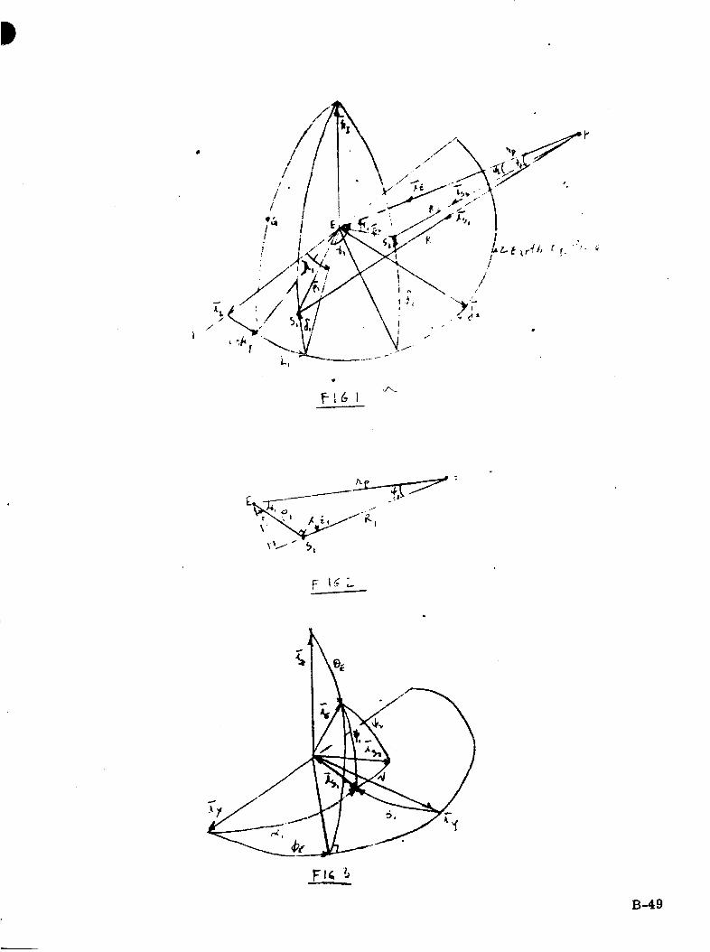
oi

_ f

"_--._&2_, 3a_ !

B-49

,f

F.

1:t6 't

\.#

i, j'l¢

m

p

B-50

r

/

... t

'\

II_ 4e_ o_,_

/ .... e_.c°._.,_J-

/.f

.r

i

I

. t_,',z_, a#

4

// ..._2 C_.3"_;tA • .'I° .

\

I

#

I

B-51/52

APPENDIX C

ANALYS_ OF THE PROPOSED SOLAR ASPECT SYSTEM

Io Sums* 7

The performance of the proposed Solar Aspect System was analysed and an

exact transfer function was established.

By me, ms of this tramsfer function quantit_tive answers were obtained in two

areas of major interest as to the performance of the instrument:

1o The degree and source of cross-coupling of the two geowetricallyorthogonal detector eyes, and

2o The maximum error to be expected in the _asurement of the :undirection°

The cross-eoupllng was found to be quite strong for measurement of a_gies not

in the plane of z'-_ eye s!It _-,_4t_he__-ozmal to the eye° That is. the ouY.put of the

instrument would be f:ay code "128" for an am_le of 64 degrees to the '_)" direction

and 1.vlng in the abo_e p!aLe, but the output would be Stay code "98" if :he single

is 64 deEzees %rith respect to the "O" direction and 64_degz_es wlth respe.ct to the

plane def:tned by the eye s!it and- the nozmll tO _ eye.

The error in the measurement of anEles _ A & B, in the two planes def:i._ed by

the slits of the _o eyes and the normal to the. eyes is a function of _-- __n_E!eS

themselves o The nmxlmum error ranges from 0o4S degrees at f = 50 desrees, B = 90

deErees to 1.3 de:;rees at A = 50 deErees, B = 26 degrees or B = 50 degrees_.

A = 26 degrees o

2o Derivation of the Transfer Function

The confiEuratlon of the _Icole sun sensor _etector -_nl£ is shown in Figure Io

The coordinate system attached to the seDsor will be used throughout thi:_ paper°

Figure 2 shows the construction of each eye of the detector_ From this, it is

evident that the angle which the incident light makes with the detector :;_ deter-

mined once the li*_ht strikes particular solar cells behind the retLcleo The instru-

ment output, E, in 8ray code, is the number of diglt8 the light beem is ::emoved from

the line directly b_.ow the sllt when it strikes the bottom of the retlc _o In

Eeneral, for eye #I,

(1)

(2)

for eve #2,

O)

"! i

Ez = _Z £r

(4)

I, ,Il,_,l -- I0) I) Z.) _)_ ..... ) I?-._

[mzl = O}l)Z,Z ) ...... )lZ

C-I

The quantities in equation (1) throush (4) are shown in Ft_e 3. AnSlls A _d Bare the augles the projection of the incident vectom£nto the X-Z-pl_e and Y-Z-plane,respec_ively_ make _th the X-Y-plane. U(A,B) and V(&,B) are the distances from theoris£n to the intercept of the light beam with • line parallel to the X-axisY-axis, respeccfvely, on the bottom of che retfcle. K ta the widch of the leut aiS-nificaut b£ts shown £n Figure 2.

Th, e p_obbem of find£ng the transfer function £8, therefore, to find U(A,B),V(A,B) and K.

From the geometry shown in Ffsure 3 the £ollow£ng relat£ona _re evtden£:

(5)

(6)

(7)

(8)

(9)

cot ¢ -- cot/_ t_ lbcot: A -- t_ e cos _b

't t_. _'

Also= using N = (index of refraction of quartz) "I

C_nbiui_ (9), (5), and (6), _ find

I + t4_z¢

(11) Uz = <z ta. zO'I + t_ _ A cot"5

Then #__w%_'_)! can be found from (7), (10) and (6):

6ota_ = cot/% t_ 5

C°SZ _ = I tcot_t_5

(:_,,z0 -_. cot_A C I* _tZA t_J5)cot_A t_ z 5

C_ _0 = cot_5 _ cotzl%

s_'_z19 : co_ A + cot_I + cot_A + cot _ 5

SfJO' = NZ(,cd_fit c°t_5),It cot'A t cot z5

C-2

I + (t-__)(cot__ +_ot_l_L_- cot_k _ cot 7"I_

(1_.3

(12) into (11),

t_ _ cot z A

In a more recognizeble form,

U _ .- t _ IVZ-cosaAcorse s;_zA_)

tz/Vz cos zAU zI-N_c.o_ z& * (,I-_') cO_" I_ s"_z&

I_2e minus s£g:_ ts clear from the geometry o

(I_) V = --tN cos6l-Iq_cosZb$ (I-N z) cotzA sd_Zf,

The d£g£t _.d_-h_ K, can uow be found from (13) or (I_), The pattern is linear,each digit corre_9onds to 1/2 degree in the X-_--pleno (for eye _1), and the field-of-vte_ of the £_,.ctrument is 64 de_reeSo Therefore,

Substituting (9) into (II),

IX : --tN cos2& °Izg _[ I- N_'cosZ2G °

C-3

In summary, the transfer function for eye #1 la9

(t6) IPhil-- O_l}Z) ..... _I2E

- L cosAV'I'_N',c_'A ._CI-N_)c_t_l_s_'_A '

The trans£er funct£on for eye #2 is,

(17)"

_(A_5 - L_ cos 15 I

m

_/I- HZcos 260'cos 260

When the instrument i8 in use/not equations (16) and (17) but their inverlea

/"_ E 2) an(] B (El, E2) are needed,A _1 _

A (El, E 2) and B (El, E2) are more eas£1y fotmd from equat£oas (5) .through (10)than by simultaneous solution of (16) and (!7)_ From (7} and (5) we hive then,

c,0t' 4 _.t_-ze - lU/v)I+ (ylv) z

(18) cot _A- t_(9 UzU z + \/_-

From equation (9) alxl (10).

_ VZtZ,z e, (u _- )Sc_ =I+ _ [u'+v')

SC'_z0 = UZ + Vz

N'(t_, u_,V _)

C-4

(19)N,t • - (_-m) (u" +v')

Sub=tituting (1), (2) and (19) into (18),

cot z A = _N'{'- - (I-_'_ (u, +v')

e ?.t_

El z

- (,-.'i e-/)

(_) Cot A -- E,_._.. VL_- U-_') (¢,_* _) '

(21) cot l_ --_ E_

3 o _a1_tion of -_-,--_-:.-r_,,.!_.o_____.___r- .... _ Be_-tween.the Detector Eves

E_:alinatlon of the transfer function, equate_on (16)., sh_,_s that tlm. £uartzzetic]_ is the sotzce of the czoss-¢oupltng. "Cross-coL_plins" is to be t_ierstoodas the depemdence of El_ the output of eye #1, on angle B which !£es in _n ortho-gonal plane to angle A.

Subetltution of N - I, i.e._ the quartz block remove_. £-_u equ&tlon _...,y le lds:

Ei --- rrL,

(2z) t_(A'6): - L cot AL : 12-_ t_._. Z6 °

i_,1_-1_(,%6)IL I_,-,-,1

Equation (22) i_ clearly a function o£ A o_ly, _o cross-coupling exlsts.

T_ere is, _er, also a real s_tuat£on "__1_,.r_ f(A, B) ts m f_mct_on of A onlyoTh£s occurs when I_ = 900:; then

(23)-. L co£ A

C-5

Equation (16) is plotted in Figure 4 _,_[th angle B as _ _rametero From this ehestrong eross-coupllng effect is evident; for insean=_, El. = 128 for I - 26 °, B _ .q_3°_

while E 1 = 98 for A = 26 °, B = 26o_

The pol,nt8 in the field-of-vlew where maximum cro_s-coupllng o_cur_ can be fo_

by differemtiating the term depending on the angle B in the denc_i_tor of (16)

setting the r_sult eq,_l to zero and solving for A a1_d B slmultaneously_

(24)

Portlor_ of the left side and the right side of equation (24) are plc.t_ed in

Figure 5o It is seen that the maximum cros_-coupllng occurs _en A is between _6 a

and 26o6 ° and B is between 38°7 ° and 51,,3° (only in these ranges h&ve the curves

the same values)o

In summary, e_m_£rmtion of the transfer function 9h_ _hat:

_v Cross-coupling between the two geometrically orthogonal axes ocetrre

beca_,se there are two different _aterlal_ _n the optical, pata of the

light: ray that i._ being measured,: a.ir an.i q_r_tr=z._

cident light lies in the X-Z-(Y-.Z)-plane (se_ FI_u.,_ 3)°

3_ The cross-coupllng L_ a maximum ,_her_ one. ang.,!n_ e ,go A, is ,_t the

edge of the fleld-of-view (26 ° t_ 2(o6 '_})while the other an_l_, e.g,,,

B. Is between 38.7 ° a_d 51.3°o

Two kinds of errors occur in the Adeole ,'s_m se.sor, qum_t_z._tion errors and

•__rrors due to a s_if:_ of the edges of each digit (transltion-edge errors)°

quantizetl,)n error. _ is due to _he finite size of each quamtumo lt_

maximum value is :'£I/2 digit t_c_ the center of the d£slt, its distribution isuniform°

the transitlon-edge error_, E_, is due to manufacturlng toleranceo in the

reticle, m_salign_nt and drift i_ the electronics which ee_abllshes the edge by

rmlling the output cf a "bit" cell _r_th a con£rol c_ll of 1/2 full outpu¢o The

maximum transition-edge error is also -_ 1/2 digit, its distribution can be a_stmedas _Otq_tl_

\

C-6

_Ne naxismm erroz of the system measuz£nS angles A and g is then, neglectinS

higher powers of D E_

DE = DE1 = DE.-,. since the eyes are identical.

From the phys.4__.al sftuat£on it is evident that the m_ximum error, DE _ equalsone dlglt_ 1/2 d_it due to quantlzatlon and I.,,v2 digJ.c due to the shift c;f thetransition edge in the worst case,

DE = I dlg£to

To find the derlvative..8)_ )the following pr.ocedure _ use_.

E, : I_-(A,_,)

,__.,.: _,_A+

a,--, _,_

r' F-

%, %,.

• etco

C-7

d_,

dEz.l

qo_-

b

b

Tlmz_foro, eq_t£_ ©oeff£©tnta5

(27) <

D i) _"z D

-+

--L cos A

_co_,_A+ (I-Iv_)r.ot_B -_t".ZA'

-C cos(A_e,.l- _,__co_ (_-_')¢o_,,,s_+,_B+

C-8

L.s_'. A E I_ CI- _') cot'.12,3D- tv_cos'A ._ Cl-_z) cotZ8 s_,_'tt]'/_

- L CI-tV_) cos._ s&¢A cot6 _cscZ6_

,C-Nzcosz6 t (I -NT) cotZA __83 _z

"L'he il_r_vatlve_ ,..xs then, from (27) and (28),

t_- I

- _ • , :,,_)j

C-9

Evahu_tlon of equations (29) and substitution into equation (26) then gives the

maxh_n e_ror co be expected at p_rtlcular values of angks A and Bo

Equations (29) and (26) were programmed for the LBM 7094 computer and tlm com-

puter output is sho_n in Table Io The column headings have the following correspon-dence:

A = Angle A in degrees

B

DA(I_I)

nA(2_ l>

DA(I,2)

DA(2_2),

m4A

= AngT.e B " "

= _A[ _)E t in radtans I_r digit

.-.- ,, ,, ,, ,,

o " " " "

= F_ximum error in Angle A, in degrees

= _xlan_ error In Av_le B, in deles

The maximum error _nAngle A is 1o30 degrees when A = 50° and B = 26° which is

consistent _rlth the ares of mRximum cross-couplin_ of FiEare 5o

The minlnmme1_or In Angle A occurs for A = 50°, B = 90° and is o48d_sreeo

The error In A when it is measured in the X-Z-plane (see Fig° 3), however_ is

sllghtly large_ th_n 1/2 degree, This occurs because, although E2 = 89 there is

posaLble error o_ one dlgit in the readlng _f B,.

T_. error c&ic,:.lations ass_r_e that the bi_s error which is present du_. to the

entls_,metric piano,merit of the pattern around _._ro is removed° That is, ":he patternis placed such th_: t_ edge of the '_)" digit i._ direetly under the sllt rather than

its center° ..T_refore_ .I/.2must be added to ea,:h reading El or E2 from the sensor

before it is put J._to the inverse functions (20) or (21).

For example,, out_utsE 1 = O, E 2 = 0 correspond t0 the £ollow_ng sng.le_,

cotA = cotB = 0,_ _ _r._/o XIO-_

,_ltZ _- - O,S_,t X 0 ._'i

C-IO

Zn summary, maxim_ errors for _masurement of the angles A m_l B u m _unct/xm

of the. 41e8 th_lelves wene obtalnmio The _:rors range from approxlaaC_ly 0.5degrees to lo3 d_.grees ° 1_ore exlmts a bias e_or in the Instrument due t0_ the

gemmtry of the pateerno This bias error must be removed before the remdlngs areconverted into anglmeo

C-II

C

/Ele

II!!I!

7_

1II

_.____1

FI_ 1

CO_FIC_I_ATIONOF THE ADCOL! _ S_OR

C-12

SerlsOr

Electronics

Entrance Slit

Reticle

Gray-coded Pattern

To Telemetry

>

C-13

/

// I

//

/ //

//

o

_et_cLe

FI_ 3

C-14

_J

C-15

C-16

C)

0 _r_

o

A

TABLE I

D_[I,I) DA[2,1) DA(I,2) DAKZ,2) EMA EMB

90.

90.

90.

90.

90.

90.

90.

90.

90.

90.90.

90.

90.90.

85.

85.

85.

85.

85.

85.

85.

85.85.

85.

85.

85.

85.

85.

90.

85.

80.75.

70.

65.

60.55.

50.

45.

40.

35.

30.

l 26.

0.00891 0.00000 0.000300.00893 O. O.

0.00898 O. O.0.C0908 O. O.

0.00922 O. O.

0.00941 O. O.0.00967 O. O.

0.01000 O. O.

0.01044 O. O.

0.01102 O- O.0.01180 O. O.

0.01286 O. O.

0.01435 O. O.0.01602 O. O.

0.038910.008900.008860.008790.038710.038620.008530.038460.038420.008440.008550.008810.039330.03995

0.510440.511480.51464

0.520080.528390.539110.553790.57306

0_598320;631610.676090.736750.822320.91776

0.51044d.5o966O.5O736

0 50375_o[ 991310.49397'

0.488870.48456

0.482410.483540.490_70.504960.53295

0.57014

J

90. 0.00890 0.00000 0.00000 0.03893 0.50966 0.511481

85. 0.00891 0.00004 0.00034 0.03891 0.512_6 0.5127680. 0.00897 0.00007 0.00037 0.03887 0.51872 0.5124775. 0.00906 u.vu_=___,, 0.0_In0..I o=n_R_l_._ 0.52568 0.51079

70. 0.00920 0.00014 0.00015 0.00873 0.53609 0.50798!

65, 0,00939 0,00017 0.00020 0.00864 0.54978 0.504481

60. 0.00965 0.00019 0.00026 P,03855 0.56754 0.50088 I

55. 0.00998 0.00022 0.00032 0.038_7 0.59048 0.4979850. 0,01042 0.00024 0.000%0 0.038%3 0.62026 0,49683

45= 0.0!I00 0.00026 0.00051 0.00845 0.65937 0.49888

40. 0.01177 0.00027 0._0065 0.03856 3.7ii66 0.5!0612

35. 0.01283 0.00028 0.00085 0.03882 0.78341 0.521551

30. 0.01431 0.00029 0.00115 0.00931 0. 8854_ 0.54992 I26. 0.01597 0.00029 0.00152 0.03996 1.0019_ 0.58731

80.

80.

80.80.

80.

80.

80.

80.

80.

80.

80.

80.

80.

80.

0.00886 0.00000 0.00030 0.00898 0.50736 0.51464

0.00887 0.00007 0.00037 0.0_897 0.51247 0.51832

0.00893 0.00015 0,00015 0o008_3 0. 5197_ 0.51978

0.00902 0.00021 0.00022 0,00886 0.5295_ 0.520010.00916 0.00028 0,00031 0.00878 0.54222 0.51898

0.00934 0.00034 0.00040 0.00868 0.55841 0.51709

0.00960 0.00039 0,00051 0.03859 0.57932 0.51490 I

0,00992 0.00044 0.00064 0.00851 0.60533 0.51321 I0.01036 0.00048 0.00050 0.03847 0.63927 0.51306

0.01093 0.00052 0.00131 0.038%8 0,68371 0._1588

0.01169 0.00055 0.00128 0.00859 0.74319 0._23590.01273 0.00057 0.00157' 0.00885 0.82516 0.53950

0.01419 0.00058 0.00226 0.00933 0.94270 0.56808 I

0.01583 0.00059 0.00299 0.03998 1.07844 3.60555 I!

C-17

7_.

76.

"5.

7 _.

76.

-5.

75.

7 !;.

75.

75.

90.

85.

80.

75.

70.

65.

60.

55.

50.

45.

40.

35.

30.

26.

0.00879

0.00636

O. A0895

3.00909

O. 00927

0.009.51

0.00983

9.0[025

0.01081

0.01155

C.01257

0.01400

0.01561

TABLE I

0.00000

0.00011

0.00022

0.00033

0.00043

0.00052

0.00061

0.00068

0.00074

0.00079

0.00084

0.00087

0.00089

0.00090

(toni'd.)

0.00000

0.00011

0.00021

0.00033

0.00045

0.00050

0.00075

0.00094

0.00118

0.00148

0.00139

0.00246

0.00332

0.00439

0.00908

0.09905

0.09902

0.00895

0.09887

0.09877

0.00857

0.00859

0.09854

0.03_5_

0.03855

0.00@89

0.039.37

0.01031

0.50375

0.51079

0.52001

0.53176

0.54651

0.56498

0.58815

0.61748

0.65510

0.70425

0.77008

0.86110

0.9-9247

1.14549

0.52008

0.52558

0.52955

0.53176

0.53252

.0.53222

0.53140

0.53084

0.53156

0.53503

0.54325

0.55927

0.58788

0.62526

70.

70.

73.

7C.

76.

70.

7C .

7?.

7C.

?0.

70.

70.

90.

_5.

80.

75.

70.

65.

60.

55.

50.

45.

40.

35.

30.

26.

0.00871

0.00_75

0.00_78

0.008R7

0. 00899

0.00917

0. 00940

3.03971

0.01012

0.,31066

0.01137

0.01236

9.01374

0.01530

0.00000

0.00015

0.00031

0.00045

0.00059

0.00072

0.00083

0.00093

0.00102

0.00109

0.00115

0.00119

0.00122

0.00123

0.00030

0.000!&

0.00028

0.00043

0.00059

0.00077

0.000_8

0.00123

0.0015_

0.00192

0.00245

0.00319

0.00430

0.00557

0.09922

0.03920

0.03916

0.03939

0.03899

0.038890.038?8

0.03859

0.03863

0.03853

0.038720.03895

0.00943

0.01005

0.49913

9.50798

0.51898

0.53252

0.54915

0.56951

0.59502

0.62693

0.66767

3.72080

_.79197

0.89062

1.03371

1.20150

0.52809

0.536990.54222

0.54651

0.54915

0.55046

0.55099

0.55149

0.55300

0.55696

0.56543

0.581_5

0.60987

0.64697

65.

65.

65.

(3.(,tJ.

65,

•; 5.

65.

55.

65.

65.

L5.

90.

_5.

60.

75.

70.

05.

60.

55.

50.

45.

40.

35.

30.

26.

0.00862

0.00864

0.00868

0.00877

D. ,-,6889

O. 00906

3. 3C9280.C0957

0. 0099(_

0.01047

0.01116

0.01210

0.01345

0.01494

0.00000

0.00020

0.00040

0.00059

0.00077

0.00094

0.00109

0.00122

0.00133

0.00142

0.00149

0.00154

0.00157

0.00159

0.00000

0.00017

0.00034

0.00052

0.00972

0.00094

0.00119

0.00149

0.00136

0.00233

0.00295

0.00384

0.00517

0.00680

0.009410.03939

0.03934

0.039270.09917

0.03935

0.03894

0.09884

0.09877

0.00875

0.03883

0.03935

0.0395.l0.01013

0.49397

0.50448

0.51709

0.53222

0.550%6

9.57263

0.59988

3.63389

0.67713

0.73340

0.80876

0.913%2

1.06579

1.24538

0.53911

0.54978

0.55841

0.56498

0.569610.57253

0.57453

0.576060.57825

0.58256

0.59106

0.60684

0.63479

0.67138

C-18

60.60.60.60.60.60.60.60.60.60.60.60.60.60.

90. 0.00853 0.0000085. 0.008_5 0.00026

80. 0.00859 0.0005175. 0.00867 0.00075

70. 0.00878 0.00098

65. 0.00894 0,00119

60. 0.00915 0.00138

55, 0.00943 0,00154

50. 3.00979 0.00168

45. 0.01028 0.0017940. 0.01093 0.00187

35. 0.01182 0.00193

30. 0.01309 0,00197

26. 0.01452 0.00199

TABLE I (Cont'd.)

0.00000 0.03967

0,00019 0.03955

0.00039 0.03950

0.00061 0.039510.00083 0.03940

0.00109 0.039?8

0.00138 0.03915

0.00172 0.00993

0.00214 0.00895

0.00268 0.09891

0.00339 0.038970.00440 0.039180,0059L 0.03961

0.00776 0.01022

3.488870.50088

0.514900.531400.550990.574533.603223.63880

0.68386

0.742360.82066

0.92F531.08_461.27653

O. 553"_9 !

0.56754:

0.57932

0.588150.59532

0 5998_

0i6032210 60576

0.60854

0.61332

0.62131

0.636540.663550.69943

55,55.

55.

55.

55.

55.

55.55.

55.

55.

55.

55.

55.

55.

50.

50.

50.

50.

50,

50.50.

50.

50.50.

50.

50.

50.

50.

90. 0.00846 0.00000

85. 0.00847 0.00032

80. 0.00851 0.00064

75. 0.00859 0.00094

70. 0.00869 0.0012365, 0,00884 0,00149

60. 0.00903 0.00172

55. 0.00929 0.00192

50. 0.00963 0.00209

45. 0.01009 0.00222

40, 0.01069 0.0023235. 0.01153 0.00238

30. ^ ^_ n nn2A_26. O.Ol&O8 0.00244

90. 0.008_2 0.00000

85. 0.00843 0.00060

80. 3.00847 0.00080

75. 0.00854 0.00118

70. 0.00863 0.00153

65. 0.00877 0.00186

60. 0.00895 0.0021455. 0.00918 0.00238

50. 0.00950 0.00258

45. 0.00991 0.00274

40. 0.01048 0.00285

35. 0.01126 0.00292

30. 0.01237 0.00296

26. 0,01366 0.00297

0.00000 0.01000

0.00022 0.03998

0.00044 0.00992

0.00058 0.03983

0.00093 0.039710.00122 0.039570.00154 O. _°_=

0.0019.2 0.33929

0.00238 0.00918

0.00298 0.03913

0.00376 0.03917

0.00486 0.339350.00651 0.039750.00852 0.01034

0.00009 0:0!044

0.00024 0.01042

0.000_8 0.010.36

0.00074 0.01025

0.00132 0.01012

0.00133 0.03996

0.00158 0.93979

0.00209 0.039630.00258 0.03950

0.00322 0.039610.00435 0.339420.00522 0.039570.00695 0.039950.00937 0.01051

3,48466

I 3.49798011513210.530B4

o 5 1493257636

3=60576

0.642380.688543.748320.828250.93940

1.102301.29497

1

3.48241

D.49683

0.51336

0.53156

3.55300

3.57825

0.608540.64564

3.692213.75231

0.83251

0.94490

1.10725

1.30140I

0.57306

0 59048 I0_60533 1

0.61748

0.62693

0.63359

0.6389!

0-64238 10 645560_650D9

0.657860.672130.69793

0.75245

0.598320.62026

l 0.639270.65510

0.66767

0.67713

0 683860]68855

0.69221

0.69637 10.70320

0.71596

0.739770.77244

C-19

45.45.

45.

45.

45.

45.

45.

45.

45.

45.

45.45.

45,45.

TABLE I (Cont'd.)

90. 0.00944 0.00000 0.00090 0.01192 0.48354

85. 3.00S45 0.00051 0.00026 0.01139 0.49888

80. 0.00848 0.00101 0.00052 0.01093 3.5158875. 0.00854 0.00148 0.00079 0.01081 0.53593

70. 0.00863 0.00192 0.00139 0.01056 9.55696

65. 0.00875 0.00233 0.00142 0.01047 0.58256

60. 0.00891 0.00268 0.00179 0.01028 9.6139255. 0.00913 0.00298 0.00222 0.01009 9.65099

50. 0.00941 0.00322 0.00274 0.09991 9.6963645. 0.00979 0.00340 0.00340 0.09979 0.75584

40. 0.01031 0.00352 0.00426 0.03976 9.83499

35. 0.01103 0.00359 0.00546 0.03987 0.94488

30. 0,0L206 0.00362 0,00724 0,0_02_ 1,1057726. 0.01323 0.00362 0.00941 0,01074 1.29733

0.63152

0.659370.683710.70%25

0.720800.733400.742370.74833

0.75231

0.75584

0._61170.771640.792500.82244

40.

40.

40.40.

40.

40.

40.

40.

40.

40.

40.

40.

40.

40.

90. 0.00855 0.00000 O.O00DO 0.01180

85. 0.00856 0.00065 0.00027 0.0117780. 0.00859 0.00128 0.00055 0.01159

75. 0.00865 0.00189 0.00084 0.01155

70. 0.00872 0.00245 0.00115 0.01137

65. 0.00893 0.00295 0.00149 0.01115

60. 0.00897 0.00339 0.00187 0.01093

55. 0.00917 0.00376 0.00232 0.01059

50. 0.00942 0.00405 0.00295 0.01048

45. 0.00976 0.00426 0.00352 0.0103140. 0.01023 0.00440 0.00440 0.01023

35, 0.01088 0,00446 0.00551 0.01029

30. 0.01182 0.00447 0.00738 0.01057

26. 0.01289 0.00444 0,00954 0.01195

0.490379.5 6123.52369

0.54325

0.565439.59196

3.62131

0.65786

0.703190.761170.83802

0.944431

1.13034

1.28532

0.67609

0.71156

0.743190.77038

0.79197

0.80876

0.82057

0.82825

0.832510.83500

0.83802

0.845350.861500.88737

35.

35.35.35.35.35.35.35.35.35.35.35.35.35.

90. 0.00881 0.00000 0.00000 0.01286 0.50496

85. 0.00882 0.00085 0.00028 0.01283 3.52155

80. 0.00885 0.00167 0.00057 0.01273 0.5395075. 0.00889 0.00246 0.00087 0.01257 0.55927

70. 0.00896 0.00319 0.00119 0.01236 0,581%5165. 0.00905 0.00384 0.00154 0.01219 0.60684 !

60. 0.00918 0.00440 0.00193 0.01182 0.63654

55. 0.00935 0.00486 0.00238 0.01153 9.6721350. 0.00957 0.00522 0.00292 0.01126 0.71596

45. 0.00987 0.00546 0.00359 0.01193 0.7715440. 0.01029 0.00561 0.00446 0.01088 0.84505

35. 0.01087 0.00565 0.00555 0.01087 0.94627

0.00561 0.00738 O.OIIOS 1.09387 I30. 0.0117126. 0.01269 0°00553 0.00947 0.01159 1.26939

!

0.73676

0.78342

0.82516

0.86110

0.89063

0.913420.92953

0.93941

0.944300.94488

0.94443

0.94628

0.956350.97571

C-20

,

30.

30.

30.

30.30.

30.

30.

30.

30.

30.30.

30.

30.30.

90. 0.00930 0.0000085. 0.00931 0.00115

BO. 0.00933 0.00226

75. 0_00937 0.0033270. 0.00943 0.0043065. 0.00951 0.00517

60. 0.00961 0.00591

55. 0.00976 0.00651

50. 0.00995 0.00695

45. 0.01021 0.0072440. 0.CI057 0.0073835. 0.01108 0.00738

30. 0.01182 0.0072626. 0.01269 0.00709

TABLE I (Co.t 'd. )

0.000300.000290.000580.000990.001220.001570.001970.002420.00296

0.00362

0.004470.0O551

0.007260.00923

0.01435

0.31431

0.01419

0.014300.01374

0.01341

0.01309

0.012730.012370.012360.01182

0.01171

0.011820.31216

3.532953.549920.568393.587883.609870.634790.66366

3.697933.73977

0.792493.86150

3.95605

1.093211.25579

0.822323.885440.94270

0.992471.033721.96579

1.08847

I.ID2DI

1.107251.10577

1.10034

1.0930_

1.093221.10308

26.26.

26.

26.

26.

26.

26.

26.

26.

26.

26.

26.

26.

90. 0.I00995 0.00000

85. 0.00996 0.00152l

80. 0.00998 0.00299

75. 0.01001 0.00439

70. 0.01006 0.00567

65. 0.01-013 0.00680

60. 0.01022 0.00776

55. 0.01034 0.00852

50. 0.01051 0.00907

45. 0.01074 0.0094140. 0.01105 0.00954

35. 0.01150 0.00947

30. 0.01216 0.00923

26. 0.01294 0.00894

0.000300.00029

0.00059

0.00090

0.00123

0.00159

0.00199

0.00244

0.00297

0.00352

0.004440.00553

0.007090._08 _7_

0.016320.01597

0.01583

0.01551

0.01530

0.01494

0.01452

0.01438

0.01354

0.013230.012B9

0.012590.012690.01294

0.570150.587323.605550.625260.646980.671380.69943

3.77244

0.822443.887370.975711.10337

!.25334

0.91777

1.00191

1.07845

1.14550

1.20151

1.24539

1.27654

1.29499

1.30141

1.29734

1.28534

1.26940

1.255801.25335

I

C-21/22

APPENDIX D

ATS SOLAR TORQUE

The solar torques on the main vehicle are derived for numerical integration

where all shadowing and up to N-multiple specular reflections are considered on

the main body with the effects due to the scallops, the rocket nozzle and recessed

ends all considered. The diffuse reflections may be included for all convex ex-

ternal surfaces since no multiple reflections occur for this condition; however this

analysis does not include the multiple diffuse reflections that occur in the ends.

The system numerical integration was chosen due to the advantages: 1) Multiple

reflections and shadowing produce quite complicated integrals; which, if all are

integrable would yield some long computational equations, 2) A far more complex

system may be analyzed than possible with the many assumptions needed to ex-

plicitly find the torque expressions, 3) The variation of the specular reflection

with angle of incidence may also be considered without approximation. Although

this is a numerical integration, it is doubtful that the computer time is greater

than that needed for a comparable program of expiicit torque expression.

D°I

NOMENCLATURE

DI, D2 :

D3 :

h I :

h 2 :

h3 :

h 4 :

hN :

H :

The lengths of the main vehicle on each side of the x s, Ys

plane projected on the smlgrld plane nornml to s.

Distance from the vehicle zs axis to the midpoint of a scallop.

Distance from the YsZs plane to the _z s plane edge of the vehicle

Length along zs of scallops

Distance along zs from the XsY s plane to the plane dividing the

smaller and larger radii of the main vehicle.

Distance from x y plane to -z s end of the smaller cylinder ofSS

the malnvehlcle.

Distance the big end of the rocket nozzle is from the XsY s plane

measured along -z s.

Distance the +z s cover end plane is from the XsY s plane.

iS, Jg: The number of squares along the +Xss and +Yss _X_s respectivelyfrom the -Xss, -Yss corner of the sun grid. This is the area

of integration

J: The number of the scallop in consideration

k: The number of the scallop closest to the sun physically.

ks: The number of reflections (multiple)

kz: The general qtmnti_y to tell the z s coordinate of a disk (plane)parallel to the xsY s plane to be reflected from.

ml, m2: The number of squares along the x_ s and Yss sides of the sungrid which defines the grid divis_on.

Mc: The slope of the rocket nozzle cone where Mc< 0. (If Mc - 0 thecone frustum would then be a cylinder).

!

no, n : The index of refraction of outer space and of the surfacerespectively.

rl: Radius of the larger cylinder of the main vehicle on the +z s half.

D-2

r 2 :

r 3 :

%:

rms:

The maximum of r m and r 1 thus defining the size of the sun grid.

Radius of the smaller cylinder of the main vehicle

Radius of the cylinder that contains all scallops as defined byEquation (18).

Distance from a general point on a scallop to the main vehicleaxis.

Radius of the open end of the rocket nozzle.

rNd: Radius of the rocket nozzle where it intersects the plane of theshielding disk.

rNdz: Radius of the cross-section circle of the nozzle cone at anarbitrary point.

rs: Radius of the scallop surfaces.

Sl, s 2, s3: Light vector in XsYsZ s components in general intersectionequations.

Sxl, Sy 1, Szl: Unit vector away from the sun in Xl, Yl, z 1 components

U1,U2,U3: Coordinates in Xs,Y_,Z of the intersection of a reflectedbeam of light with _heSnext surface it strikes.

Main body coordlr_tes

Coordinate system wlth the sun s in the XsY s plane

xl,Yl,Zl:

xslYsJZs:

- C_"_d4-"_ used to find the sun gridA_SmYss=Zss: ..... _y_tem

XcB,YcB,ZcB: Coordinates of the center of mass in xl,YlZ 1 components

Absorption coefficient subscripted to indicate the surface. The

number of primes indicates the properties if the SlJ_has been

previously reflected this number of times. See _

Ratio of diffuse to specular reflection

The angle of incidence of light on an incremental surface

Greek

o< :

D-3

#

q_ : The angle the cone nozzle incremental normal is from the XsY s plane.

_' : The ingle of refraction of an incremental area.

%t : Angle measured at the vehicle axis including one full scallop

and half the gap between on each side.

: The angle between the XsZ s plane to the center of the k th scallop.

: The diffuse reflection coefficient subscripted and primed as

_o : Solar flux pressure constant

_J: _s for each surface indicated by i subscript after k previousreflectlons.

: Specular reflection coefficient (See _j_ )

_- :

c_0_ :

General angle measured positively around +z s axis from +x s axis.

The angles the sun s makes with -z 1 axis and around +z 1 axismeasuring from x 1 respectively.

Parameter used to find the light Sks intersection vector Iwith a given surface of revolution.

Vectors

C : Vector from the coordinate origin _o the center of mass.

Incremental force vector due to photons striking an incremental

area.

_,L :

The vector from the coordinate origin to the intersection of

a reflected beam with its intercepting surface.

Incremental torque vector of solar torque due to a small area

used in the numerical integration.

Instanteous torque vector in XlYlZ 1 components in the processof numerical integration. At the end of the integration fora given attitude, "_ becomes the desired solar torque of theoverall vehicle (less rods).

Surface normal unit vector drawn such that Sks "_ >o if the

surface is illuminated by _-k5 •

D-4

Cl : Pertaining to the circular cylindrical surface of radius r Ifor light striking the outside surface only.

C1P : Same as C1 except for light sCriktn S the inside surface (atthe end) only.

C3 : Pertaining to the circular cylindrical surface of radius r 3

d : Pertaining to the plane disk around the rocket nozzte coverin Sthat end (around the nozzle)o

e : Pertaining to the disk recessed in the C1 cylinder

: Pertaining to a general jth scallop when U_ht strikes itsconcave surface.

Jp : Same as J except for light striking the convex scallop surface.

k s : Indicating the number of previous reflections.

N ." Pertaining to an _gina_ a.WOL-_-----L'--_O_--6 --..--A_°_._.._.__ the onen. endof the nozzle.

Nd : Pertaining to the outer surface of the cone frustum of therocket nozzle.

Si : A general subscript to denote any of the surface subscriptsof the vehlcle.

D-5

Figure I places the vehicle in its coordinate system. The sun

is likewise defined in this coordinate system, by a unit vector away

from the sun. The torques are drawn about a three axis off-set vector

. In X_Yl,Z 1 coordinates these vectors are written*

c

III

/

/ [ °',-I el)

We assume the vehicle is composed of fourteen mathematically dif-

ferent surfaces but of these t there are nine (eight scallops and a

cylinder extremedy) illuminated on the back. The unit normal vectors

into the areas are respectively:

_ for the thermal shield at the circular end, _a for the ring

disk around the conical nozzle, _c_ for the larger cylindrical sur-

face, _,_ for the normal into the conical surface and _, for an

imaginary absorbing disk over the open end of the nozzle, and _, to

_ for the individual scalloped surfaces starting numbering with the

* The sub 1 on the right side indicates the components are with respect

to xI, Yl, Zl coordinates.

D-6

one on the positive x 1 axis and numbering counterclockwise as seenfrom +z 1 axis. The normals for the curved surfaces represent normalsfor arbitrary incremental areas. Note, the xlY 1 plane lies in theplane o£ the extreme edge of all scallops and the other extreme of the

_-c_ smaller cylinder is _ from the xlY 1 plane leaving the physicalgap.

The force on an incremental area is

where _so" 1 for direct illumination (t = O), and _ are the indirect

illumination reflection coefficients determining the light of this force.

The lever arm for each incremental force on its area, denoted by

-_ , with an appropriate subscript, is drawn from the vehicle centerwhich the torques are about, to the incremental area.of mass, C ,

The torque is then

where integration is over each respective surface and the summationtotals the components for all different surfaces. The approach to the

integration is numerical due to the complicity of the geometry.

The two cylindrical outside surfaces are assumed to have no shadow-.... __-_^ --_l_nn: T_n_tegrations are sire-in 8 and of course have no mu._.v.= .. .........

plified by converting to a coordinate system with the sun in a principalplane. We therefore write _" ,

(4)

D-7

The new coordinate system is formed by rotating x l and YI about

z I by _ so the new coordinate system, Xs,Ys,Z s has _ in the YsZspIane. Then

_j "_, \ o o _,.Figure 2-b shows the vehicle in Xs,Y°,Zo with its torque_ center ¢and the sun, _- . From (1), (4) _nd'(5), _ , and -_- in sun

coordinates are . . ,

_ . 8 , _ "_"_l o _ (6)

All the light from the sun illuminating the entire cyllndrical

body passes through a rectangular segment of a plane normal to _ as

shown in Figure 2-b choose r2 the maximum of rI and rm,

T'_ = ,,_o,,:_ (C I jf_,,)(7)

D-8

where r I is the radius of the cylinder at the _s end and r is theradius _f a cyllnder circumscribing the scallops whose radi_s isdetermined by the intersection of adjacent scallop surfaces circularly

extended, (See Equation (18)). For the numerical integration, this

plane normal to _- is the surface to _be _ntegrated over. We sectionby dividing the one side by ml, thus _ is an increwental lenEthand dividing the other side _--_ where now an increwental area on thisplane is _

_ (s)lr_,wL

Figure 2-a indicates the D1 and D2 functions are defined as

(9)

The coordinates at the center of each _ _ are ound by writing

in a coordinate system such that _ is along an axis, as in Figure 3.

Figure 3

Y's$,

This transformation is

/cos _-=, 0X.¢(I0)

D-9

Let the grid plane be labeled starting at the most negative Xss and

Yss corner then the coordinates at the center of the ig,Jgth surfaceare

- m,\_ zj (If)

thus we define a sun Erid in coordinates xss , Yss, Zss defined by

rotating Xs,Ys,Zs about Ys by (+_) thus putting the unit vectoraway from the sun, along -Zss axis, defined by Equation (lO). Thecoordinates in (Ii) transformed by (10) are

(12)

Consider the scallops in the x ,ys,ZFigure 4-a with the k th surface clo|est tg

tlon ..T from the XsZ s plane where

_V

o < 5 <_' ="/I

coordinates as shown in

the sun, with its mid sec-

(13)

where _ is determined frc_ _ by

(14)

Therefore the k integer is defined from (13) and (14) as

(15)

If _ is the angle around the zs axis (from the xs axis) tothe intersection with the sun vector _" then the jth surface that

this boom would most likely hit is

<_f o

(15a)

D-10

On the other hand, if J is known, then we may find Q- the angle aroundz s axis from x s to the center of the jth scallop from Figure .A-a or (15a)

As shown in Figure 4-b, _ in the scallop included angle measured

from its midpoint counterclockwise. The range of _ over its scallopis

(16)

Since the scallops are separated sllghtly a looser geometry is needed.Considering the scallops to be circularly extended until adjacentones intersect, we define a circumscribed circular cyllnder of radiusrm, as mentioned before.

i

l

I

l Figure _'-_

D-II

Figure 4-b

/

\

//

/

X!

Assuming we know D3,the distance from the vehicles central axls

to the midpoint of each scallop and _ , the maxlmumhalf angle sub-

tended by the scallop, _ may be found by the low of sines

The inequality limits us to a unique solution. If the height of

the trlangle is imagined to be drawn normal to rm we see

(18)

Also from the law of cosinesI

(18a)

The inside surfaces on either end of this vehicle and the

outside surfaces of the scallops are more involved since these repre-

sent concave surfaces which give rise to shadowing and multiple reflec-

tlons, both specular and diffuse.

D-12

In general multiple specular reflections with shadowing are the

result of at least three (not necessarily different) surfaces and thelaw of reflection. First the light from the sun, E partlally illum-

inates a surface,_(x£ , y_ , z_ ) = 0 where a three dimensional

curved (or straight) _ine _ _,,,(x_ , Yz, zL ) acts as a shadow line,on one side of which no light re_hes t-he _ Surface. Line _ iseither formed by the physical edges and/or the sun tangent curve on

a shadowing surface. The light may then be specularly reflected, Slwhere Sl depends on the _ surface normal vector. Figure 5 illustrates _

l \ ., ll/-----4 ;o ",tt:77: a

!

t Figure 5

I these surfaces with their arbitrary points. If (x½ , Yt , zd ) isan arbitrary point on the _ surface, its normal vector, _f is

• l.-S:'_l

I subscripted _ 's represent the partial derivative of _ withwhere the

respect to the subscriptingvariable, and N/ normaltzes_so _'_1 - 1

and is away from the sun. To find the reflected _1 vector we writein components parallel to the surface normal and to the surface itself:

The reflection _1 has the same surface component but the negativenormal component, thus

_,- - (_'_h _ +[_- l;_D _3

D-13

or

If • _ 40 no reflection takes place from this side of the surface.

Now the beam of light leaving some point on _ travels along W1 toits intersection on g surface, thus an analytic description of thisline is

Slxl = 5, i (21)

80

=1 (22)

then Xg is found from

Thus, a beam of light is reflected from a point (to be integrated)

on surface _ at (x t, y_ z ) to a point on surface g determinedby equations (23) _d (22) respectively. Now, since the surface, g

is known, its normal,

may be determined as in equation (19).

equation (20) to be

(24)

Now "s2 is found from rew_itlng

Equations (22) and (23) are then written for the new surface (if thereis one). If a reflected beam fails to strike another surface, its

torque computation halts and a new beam on _ is chosen. This is the

integration over the illuminated portion of _ . The shadow llne on

from _ is determined by rewriting (23) and (.22) as

D-14

The force vector ducts light reflected from

specular reflection coefficient for surfaceis multiplied by theand in general, the

solar properties of the reflected beam on surface g are considered

different from those if _ illuminates g directly. Often a surface,illuminated by a light vector, may be such that the vector mathemat-ically intersects the surface more than once. This is the case for a

circular cylinder if a vector intersects it and is not tangent to it.

For surfaces such that there are more than two intersections, a more

elegant procedure is needed to determine which intersection is actuallysought. However, here we deal with planes which have unique intersec-tions and simple surfaces of revolution with at most two intersections.

There are two simple means to determine which intersection.

Let the intersection point to be tested as a physical possibility be

represented by the vector-_. Also let the light vector be @is wherek s may be zero for direct illumination or k s represents the n_ber ofprevious reflections. And let the surface normal vector at_ be

where we now assume we know whether the light is inside or outside ofthe closed surface. This determines n to be out of or into the sur-

face respectively to make the desired choice give

5-D >o (25a)

Another method is needed if the light vector originates inside a closed

_urf_ce. M_-the_-__t_eally it will determine two intersections, one inthe direction of the light and the other in the opposite direc_lo_.To rule out the second possibility we impose the condition

where _ represents the position vector of the light source inside

the closed surface. We may note if the light is originated on a cir-cular =yllndrlcal surface to reflect on the same surface that the

best test is (25a).

D-15

To compare the relative magnitudes of the incremental areas on each

surface, consider light of area _ directly from the sun. Then thearea this light illuminates on surface _ of Figure 5 is a_._ .Its reflection then again has the cross-sectional area _ . Then

the area illuminated on the g surface is _,.w_ where sl is the reflec-

tion of _ from _ givenby Equation (20). Also if th_ intensity Is

1 for s then the intensity for _1 is _ where ?_A is the specular

reflection coefficient of._, surface for direct illumination. Alsothe intensity of _ is _s_ _s_ where _ is the Coefficient ofspecular reflectio_ of the surface _ for _he first indirectly ilium-

inated ray (as indicated by one prim3), and so on. This more fully

explains Equation (2) and how it is to be used.

Next is the consideration of logic as to which surface is illuminated,and which shadows another. This is simple to understand in theory.

As in Figure 5 we consider _ passing throughaa given point (on the grid

in Figure 2-b) and intersecting a surface. We then, as efficientlyas possible, determine which surface this reflection crosses first.

To find the intersections given a surface, a vector and a point through

which it passes we resort to analytic geometry. In Figure 2-b, we

may generalize the vehicle as consisting entirely of planes parallel

to XsYs, a frustum of circular cone whose axis is parallel to z andtranslated cylinders with all axes parallel to zs (note the cyl_nders

maybe considered as cones however their solution is less efficient.

Let, in general a light unit vector passing through (_,_a_)(inthe direction of advancing light) be ( S, _ _ S3 ) and let (r_ _-> _ )

be the cylindrical (or polar) coordinate of the surface-vector inter-

section of the planes and cylinders and cone except for the scallops.

Also let ( _j _ _ _ ) be the intersection on the scallop cylinderswith _- now reserved for determining which scallop.

In particular we find the intersection of _ on a plane (or dlsk)

described by

(26)

Then the equation of the line Joining (u,)_zj_j ) and ( _> 6-> _ ) is

D-16

_erefore we have

(28)

c r- I

where

(29)

and

(29a)

Next consider the intersection of _3/ passing through (w,_,_3)_r_th the cylinders of the scallops and main vehicle. If the cylinderradius is r, and it may be translated as indicated in Figure 4, it

may have a parametric representation given by

3 -- (r+ s.,r- c

The e__,atiou of the line joining the intersection and (_, >_z_ _ )

The first two members are independent of z can be written

We now define the temporary quantity, _ by

(32)

D-17

Equations (32) and (31) give the solution

if I l ' 2._._.{(l"-I-l_l- (_r',-.*_/) -t- (i4,_l.,.#-I;I C°_)] l'_< I (33a)

and (30) now gives z to be

If we are working with one of the scallops,

_,_I _(35)

If (35) is not satisfied or, in the case of the other cylinders, we

may have chose the wrong solution of _ in (33). The other soluation

of (33),

.' ,'r r ,,, , (36)

This new value of _ is then used. This happens since a light ray

intersects a cylinder in two places but physically the light is stopped

at the first intersection_ and the second beocmes extraneous. The

conditions that must be met to determine the correct solution are

either (25a) or (25b).

The same type of thing happens for the frustum of a cone whose

equation is*

where

(37)

(37a)

and where Mc ts the slope of the cone edge,

_-r__= _4+6 _

(38)

D-18

where T.J is the small radius of the cone nozzle and _ is the

larger as shown in FtEare 2-b. The height of the cone is impliedin Figure 1 where h_ is the distance to the f_ cylinder from the

xlY 1 plane and _ is the distance (negative) from xlY I planeto the clrcle end of the nozzle. Again the equation of-lntersectlonis

This time for simplicity we choose to find z first.last members give

.while the second and last members give

ss " ._.__L.I

The first and

(39)

The sum of the squares of these equations gives a quadratic in zS

only, if T_&_

then

(39a)

is taken from (37a). Let

-- _ _a_ S,_ / (40a)

J

(41)

or

(41a)

D-19

The surface normals are not listed in terms of their respective coord-

inates. Note a surface may have a normal each direction when lightmay illuminate it on each side. Figure i shows all surfaces andtheir respective area unit normal vectors. However we are interested

in writing them in the s-coordlnates (as in Figure 2-b). The normal

for the cylinder of radius r 3 is into the cylinder since the lightstrikes the convex surface,

The end of the cylinder of radius r I may be £11umlnated outside andin so we write normal vectors for these cases respectively

__o Js

(43)

The scallops likewise may be illuminated on their concave or convex

surfaces. The surface normals for these cases are respectively forthe j th surface

[-- co_ (',_ ¢')\

-- _, (,_+_) (44)

The plane surfaces or disks over the end of the nozzle cone base, over

the vehicle end (with the protruding nozzle cone), and over the +z s

end have normal unit vectors respectively

Also the frustum of the cone has a unit normal of

(45a)

D -20

where _c is the half angle at the vertex of the cone frustum if it

were extended into the vehicle. This angle 18 found by the frustum'sdimensions to be

and is considered always positive acute.

(45b)

In all eases we choose the normal such that the dot product with the

illumination light vector in the direction of propagation is positive.The primes represent illumination of the inside of the surface•

The general torque for the summation in Equation (3) is found from

Equations (2), (6) and (8), the psragraph following Equation (25), andthe general intersection vector-r for each surface

In this equation, the subscript _ks designates the k_ reflectionstrikes. Also there are i primes [g] since physlca_ly each reflec-

tlon may be different wave length distributions and consequently

different reflection ratios. Mathematically we must define _g$o- 1

for all surfaces which _uld mean physically that all light strikes

the flrst_urface. Note the sequence of subscripts _ and conse-quently _3i depends upon the path the multlply-reflected light

takes and is determined by the Intersection procedure that describes

Equations (19) to (25).

From the_pro_cedure of finding the vectors involved in Equation (46),

we know T, _k_ and _ksare in the s-coordinates while _ is givenin 1-coordinates by Equation (1). However (5) implies

D-21

In general let

f

(48)

G

Then we have

__ -I_"_ 173 Jl

(49)

Performing the indicated cross product in (45) with(1) and (48) give the 1-coordinate components of antorque about C as follows:

the vectors inincremental solar

D-22

This torque represents the additional torque on the vehicle due toan incremental area of a surface illuminated by the ks th reflected

ray. This is then added to the torques previously summed, thus

-LF_r = L -r -+"aL (51)

Reflection Coefficient Versus An_le of Incidence

The surface boundary conditions of the electromagnetic wave enteringa piece of dielectric (glass) has the property that the_and

vectors are refracted and reflected differently for different polar-

izatious. Chapter 7 of Optics by F. W. Sears indicates that for

natural (unpolarized) light, the relfection coefficient is

• _ (4-_0. (52)

where _ is the angle of incidence andwhere

qoS_'.¢ = r_: s,_,_

is the refraction angle,

(53)

Shell's law determines this angle from the angle of incidence andthe Indlcles of refraction for both media. This function gives

about .05 from normal to almost 60°. Then this value climbs up to

I at 900 (tangent to the surface). Equation (52) assumes all light

incident on a surface is either specularly reflected or absorbed

and refracted. However, our work as___m_es another possibility is

present. Tha_ is, the light is diffusely reflected according to

Lamber_'s law. If we consider a surface moael composed of tiny

specular reflecting hemispheres, we find most of the wanted properties.

The reflections at shallow angles are statistically cancelled by

shadowing while the overall plane between the hemispheres will givea statistical specular reflection. We assume therefore that the

absorption is

D-23

and that the diffuse reflection is a certain percentage of the

specular reflection

= (55)

where _ is approximated by laboratory imperical measurements.

Therefore from (52) and (55),

_5 -- "i'__ (56)

The values of 4, _A and _5 are then placed in Equations (50) for

the solar torque determination, where _ is determined for each sur-face by

and _lis found from Equation (53)

(58)

D-24

APPENDIX E

STIFFNESS MATRIX FOR AN ELEMENT OF THE GRAVITY

GRADIENT ROD, PRELIMINARY

1 - INTRODUCTION

OBJECTIVE - To obtain a stiffness matrix for the gravity gradient rod which

would reflect the behaviour of the rod more accurately than theassumption that the rod behaves like a beam.

METHOD

Procedures and formulae as given by Reference (1) shall be fully utilized

where applicable. A rod of length "L" shall be considered. One end of

the rod shall be considered to be clamped so that the boundary conditions

as given by Equation 36 of Reference 1 apply for this end. The other end

of the rod shall be _ven unit deflections and rotations "A" through '_I"and the resulting edge loads shall be calculated. The resultants of these

edge loads shall be calculated to obtain the stiffness coefficients.

Reference Used in this appendix:

(1) "Gravity Gradient Thermal Bending Test Report," GE Document No.

64SD368, dated October 23, 1964

(2) "Gravity Gradient Thermal Bending Test Report," GE Document No.

63SD725, dated July 10, 1963

E-1

SI_IV F._l.,l VEAl T'IoN

\\

\\

\

\

\

\

/ trZ=o

oO

["-0

IAL _ O

"_ = 0eDy

- UN/T D _--c_. C T/o/.4

\,f'%'

f

E-2

"-_ -- UIV IT 'ZoT_'7"./otV t_t3olgT -._ AXI

- VN/T 7_o'T.A750N _e_ouT -cc_ AX,5

/, _1

(,-"_ ,,,.,__--_ _._.,_ _=_____.___x - 0

L

4

_ I

.

F- LINI-i" "-_OT'A -I-ION' i.._,_ocl7

I'lL@

/E-3

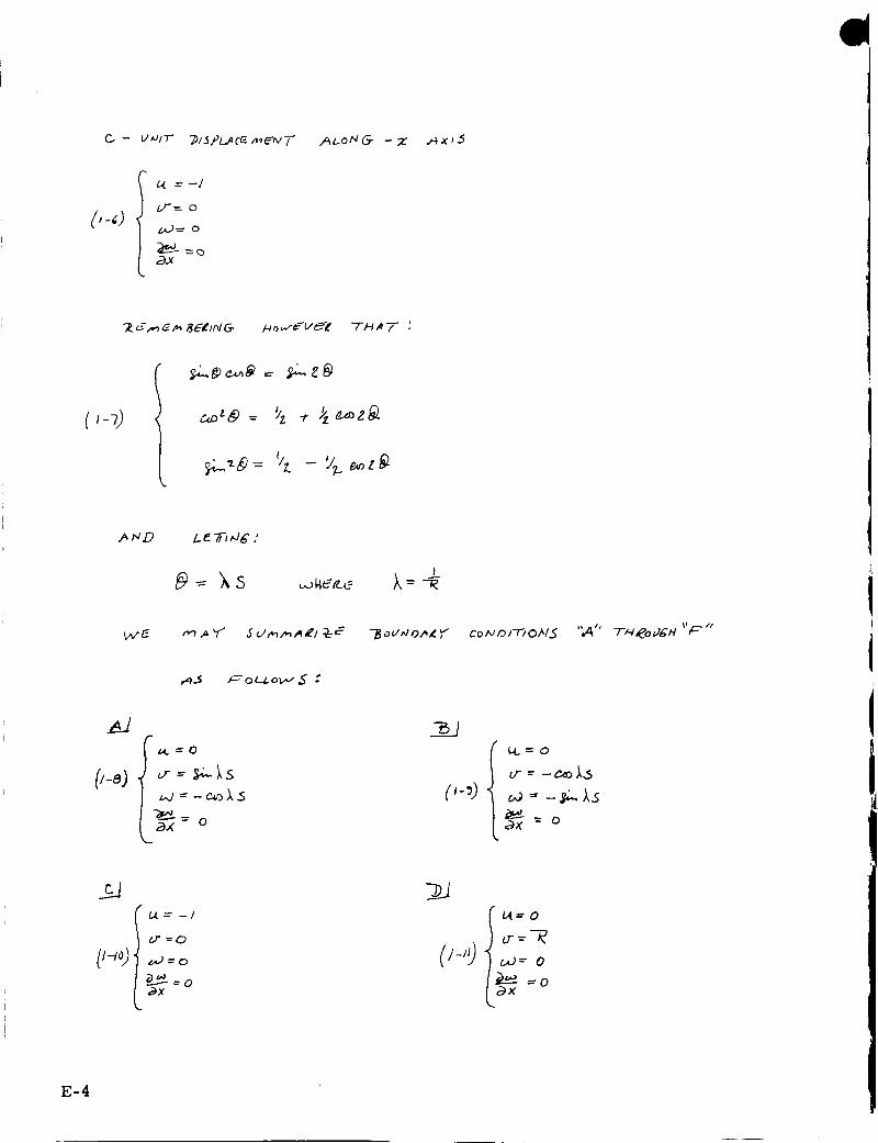
f c4 =--/

c,_O_ o

_.x

ALONG- -_ ._x_5

.A_D

I

,___ /-_o _. o_, ._ :

_t=O

_,_ = - c_ _

t4.=O

cr -- - c_,t_

M'=O

t._=o

_xf pl=O

cr = -'_

i-_- =o&x

E-4

I

I

k a_x-

0

0

o

4- 0

+ 0

4-- 0

FCJ

I u,_= D -I- CLt__.r-= 0 -t- o

[_-'- o ,-o

_, /v Z) :

f

_s

l --_r.,

c,_e= -k_'_ ¢.. u,z,,0.)= -_ _,_e

+o

+ bze £..,.LZA_S

÷0

+<3

-* b_F ._ a,15

E-5

-s._ k

N,r.

;Z:=L

"-_ E ,'_ ,'_ L 0 A-0.5 p,.-(_,_ "-P_Sl¢N_-Te"t) A $ F °LL°_'C:

3

S

END

t. o _DS

t4 ,h

It

F_ - Ta_iOtq _QT _.

_,_ - F o _ __ ,,_SSo _/ A"_e-_ w ,"-r _ U/

g-6

Ii

,

Se

(e-,) E = .._N_ &--5 e

-&

50

So

--5o

(_-_,) ,_ - .

-TI.-/ E _ D 6 E

T _ ,Z" -7-_A 5/5

LOA_5 _F /_E

0 F _/5 PL A C E,,_EmTD

C,4L C U L A "7"e'.O 0/V

A ._ F O U._O L,V5 "

£:-7

cA $_ - A

:_=0; _ Z=L :

(O o,.= o iC, _ _.---o

Oz.) 0-= o

_H_SE COHOIT_oNS WILL. ,'_E S,_"rI.fF/ED

(z-Jr) _--- i/(z} ._ A.s= Wlz) e_ ,%

WHICH _°#-_ _.¢ DQtVO To _I .SOL V T-/o /V _-o_

THE _ oge Lo,_o5 ,_Y _E r_oO_D

_ _ THE F I.J'_JC7"I o _/ J "

4La A ._ -n" oF /2 E F I.

FoV_.j _ _ v-,_e_

A ._ Fou.o_vs :

I

i

I

lz-n)

-'_ E @ W ,,_ E ; "-/_,_ .,_"-i-/,_ z_ D E _ I ¢',ATI vE J oF

61 _ ZE

e_ -- !/v/(z) e.,o_5

"_¢-_ _ _I Ia--_ - _As

a×----, = L_/ e,_,_s

"_. /-"J _.j III

_3

as t

_z d" I

_¢.,a i

v.-8

,

I

I

0 _ 7"._/t,,I "

+(_)r_,,.._,.,,,':I'-_(z;_',-_v'_-_[,.-_- ._,j,.7

.,_ o "7",, 01_

,¢

--p'_ce" - ?_-t

c.

A

E

F

!

?

4--

b-

1.5

I._

7

B

9

1o

//

/5"

/6

I_.-9

i_ U E H T_ ,_ 7" _. { j

o F T,_E Z ¢!_.

-T _

5 T,_E i:o_cE (o,e mo,,.,e,,.,-r ) J_ T_E "2:)/,eeCT'?ON

--D VE T-o _ d_IT _EFLEET/oN ( 0 8 {_O-7"A moW_

lid TM_ /vE._T_v'E --'D/leEC-T"/old OF T-_ j J/_ CO0£DtM,4TEj 7-/4eW

5 E,_ ^; "T'H_ T t

?Z_ 3

F_(L)-- &.,

f

,= {oi= Iz__g./._

E-IO

CA3E -

14 =_0

ij- _O

-c_oL S

S_'L c e" (_ V,47"/o _5 _,_,D -r',,J E'Se ,_Jo u _.AR,P"

BE S_'7"?s"f/E_ _'Y" 7-,4,E Fu_,,'c 7?0 ,uS '

( .--- UCx) _:..._,<

l _--- V_x) c._A_<

Co_l OlT-/OfV S

iI 4

_v#_cH co f-RES/) o/v/35 7"0 ,._dL uT'/ OA/ Fa_ L.o,_O .Z" .oF-

P.EF. I.

_I/ HICAI h/l+_l v _b_$TITI/7"ED JM ( _-I) TI-'tI_OgC/-t ( Z-V_) G It_

___) ., (,_)_<(,_u_,v')- {(_'- ' v'

E-11

/S_L_ cdM_ t,JT'5

/z- z_

,4t_ord_

A DDFT]OI'ZA_

F_8(L)--b,_

c OE F/_I(LENT"5 _WE To

/_5 FOLLOWS :

f

F

F_ s (o) -- /z',,,2.

C_SE - C

"--_o_'mo_/Zv'f c_H,_,7"Jo_v5 .'

X_-O "

0---0

.'7" ice= °

5_-C

S _ = U(_') _ J,os \

-#-Hi5 Eo_-uT/o/f COI_ESPo/VO5 To 50L OTIO I',/ Fo_ 7..OAD -_7 '/ W #_E#"

E-12

_ _ s e - D °_ ,V-FJD

F o/--Lo_'$ ;

A Z)_TJ o N_c S 7"/_F_ve_5 CoEFI ClEA/-iS A5

_r=,D(L)=_,,

-"-7_C<4: D,,<,-

/---7,_(_7: _,:,4

e ASE-E

AS FoM-.o_,"S :

L =o

M. =" &tE

or-=- 0

L.J_ o

_As

w xT H ,3 -I_ART3

Up I_v ._ -P_T3.

E-15

CAS_-- _ CANT/_)

.-- U t,o_Ls:-- VTj_.ko__ _,o=0

w/ TT÷

FoP. 2r-El LET

E-16

CA 56- _ Co,fT'.Z)

wu,=,,,ce ,,,,,,.y',,,,c.-. (z-_s) r,,e,,,.,,,_(r-,,.)

F,,,,,= _ (u' , _;,V,,-_- w _..k

F_,,_ F,_, = F,e,= o

_,,.o (_-,J r.,,e,,,,_. (z-_.).

NoTE TH,_T _t.THoQG/4 (_-#o) ,_ppE,_Of 7-_ -a,--,-r.HE °e"_,'_E ,_5 (Z': / I

".7"HEY .p_-_E QUITE I)IFFE_[..':_uT"" _I#CC" C.') V _/" 1,0 _-4oj .'_,_.f,'T" ,_U EQc/._C

,"--0 a_e, o, o R_sPec'r.,v'_c,y" @ X=Z.. T,,..,,E @ V 1,,/" ,.., ('z-/-/_ .,',__T E,E

EQL.'_/.. 7"0 (9} I_) --I ,,_ESPE CF'_YE?...7" L_ 1Z = L .

l_ o _ 7_-_ _ LeT '

,., = U(,,) e_t. ,t5

¢-_UL_ 7"-/ oPI EHt _ :

(z-_O _=_ = /%° +,%, +_ (e. ,, ...._)

E-17

I

_ $E - E eolv TID

TH C

" _,,EeL)= A5

A sS,o c,'A TED 3 T/'rF AI_ _;-_ C OEFF/clEHT.._ _E GIV'EM

_ (o ;-- k,_,_-

N o TE T_4 A T -T'#E

A _ 6_vE/v ;_y (!-/3)

_ u c H T _ ,a -z- ZZZ-F_ , HD

IA/ R / T _ "-_ J _ E C "T'L, _"" I

_oUIV DA_Z_" /' offD[T_o.d.S

S_/_ _v ,.K -To _--

L

III I

C_ ;L= L Fa ,_

oF A 3Ef_E3

IAI _-@ fZ_4 "7-O

So TH't_ T _v'E

&AjE E

-z_ _ _F v ;ZG1'

:J_Eo la_/D Z-E z

E-t8

i,

I

I

F,F,= ( u'

"-I"/-_ 7-oT,4 C. _ _'-,_,_ LOD,-OS A,£_ &l vE_I _ y ;

F_- = _ + _'_ _ F]_, (_= __.__ )

_ A) ---.k,o,,

E-19

5-_ODiPlC/_T_oN S TO -REF-J

c_5_-A

I L_ ---'0 .

64-=0

Z _J=o

_x

O-.O Ixl r0 ITI O N,._ ;

SS ut_ _ O FoRm OF- SOL- UTlO N

.--- Vix) _s

_b :_=L

_'-A

CA=O

o--= 3k.Xs

"To E Q W_TIo)I 5 O},{t)j (31 oF REF-I "

T'H j_

(_ -I ) U"

(_-_) -- C, U'

(_-31

-P/_0P0 S_O $oL uTlo Kl _v,J1LL -]'_ E vALiD

c,(J + czV' _v/I-- q,- C3 :O

+c.V" cs\l +c,, -c 7W=o

co U' _/" _d" W_+ C,oV- c_ +-c,z_-c,, ÷ =o

--PROVI DE Ib TI4AT '

,-qS INDIC AT_ID ON

T_m5 oF R -F--_L.

\4;<)--e_" ( c, _ ?,+ f, _.)+ e-P,

--J_.l(_ OP £EF-i W_ 5ol..,OTIo/q TO _,-12 B-_'_ 3-3

C0 Iq _'T/--_ N-F ,_ 15 _ I v'+ i,.+ B_(''

IN

E -20

(3 -7)

(3-s 3)

(E5 o.) oF ,_P-/

_eF- I

Cii e C4. =0

+ C. "_c"bo=°

_, +_,_+ __,- _ C'-_ I ='0

E-21

I

I-4,_VE THE

/o? t //; a_) "

5 -iS)

(_- J-l)

(_-,o)

/ ,_ )_B- c.O

(3-_,)

C,= C,z-m -c e_8

c\ :-%_ + c,%

C_= C,_ _ C, zc

r --uS = U, _c 4-C, _-c

_57-_/2,,m zeoC0

"x'c., _dc., :Z'c., _c m._f r_gF,'_op,1 eQo,_-_o_,,15 (70) A_u.D (7/) OF _EF-

,' (_ 5 / /,_ QLT,_ ."_E C c.' 5

C,a c%. _, _ . C----_ -_o _,, /_ _.... ., - - _ _- ) j _ , "_3

Z../ /v E ,,_[_ E q_U,a-.F/ O;'<.f W/ 7-H /G U/VK'/qo_;AZ_/

w _4_C _4 c ,,_,v 7-5e.--

E -22

CASE p- CONTI_

m

o(, C

C'IC4 C i=I _,,

-a3,

ANO "

Am D

('s-z,) _,-

ON TA FJLE C- I ( "PC o31) OF -R F- F - I ,

(e p('C eL ,_ _L )

0

0

0

73Y':

o o o

o o 0

o 0 0

._ H O tM I,.I

E-23

r_S_

L'S- 17)

c_4

0

0

0

O

o

'1

o o o I

O 0 o

o o 0

0 0 0

o o o

o

J

o 0 o

L- L_ L_'

cL cL_ _L_

c 2cL ._cLz

E -24

c A 5F__- ,'73

"T3OUNa_¢Y coN JIT/oH5

@(_ Z'=o" (_-=,o

X _--oZ'=L :I I..X=O

_-B _= - _,L,_s

_ SS,J_E_ F=o_'m OF _OL I.)T(O N ;

_-_- V(x) -at, ks

WF- A.,_e LED TO _ SeT ,OF O ROIN_@-Y ""D I F FP-_e PT{,_ C EC'_ VA Tli_r'l 5

w'J "FH A CH,,_,_ _ CT_',e (.,c?') C. E _ U,_Tt,aN WITH !De CTtCP,(.- r-O 6F F/C_E_JT-_

A S j'=O12 c._SiE-/'_ S_, T HdP*T "['/.t_" F::'Oil_(vl OF:: U I _! _ I_ I1D_.NTtCAL

_VI_TM L__4) J ("5-q.i {'_-G). A S "_,EF,JIEe" "THe CONSTAN"T'S ..A,ee -"J)E"T'E-.g-m,_E _

-#o_ [._-_-$'} E _,,cEPT T,#'T" FOe CaSE -'_ :

w'j..la r..._ W'_L.L. LEAD "TO A -'J)IFF6 _EN"T SET 0F CON 5T',_NT._.

E -25

C_5_- -C

-B ou_ D _ K'-F' C.'oN bFT{o N S

Ur=O

/,,,.)-=o

=r..)

U"= O

/>--e _= o

=0

A SSU_,,ED ForLM OF- 5oLUTIOIq,"

_o=o

k, S "B E F-o_.E THF-

C__-_3) e x_eP-r

C.,oNST,_N-r"S /_A'.(' "B,_ -TjE."Fe#.,_NE{) _rZoM

"-TH A-T FO_' c,4se- C "

7"

(--I) O)0_0) -r- =_O=c,_T'_: S _ T_ANS'OOSEI

c.,_3c- -b

-_3 g U_rD i_,£_ CON DITIOJq ,._ "

Or-=o

)x

tr=-_

---0

I_ 5_umeD _=o£_ OF = 5o_uT'/O_

i w_

_: VF) _°s

AS _Fo_G Tm_"

IJ-L3/) E 2(c_PT

=

E -26

CAS_-

"D o ul_O A_y" CoN O I'T;oNS '

Z'= o

7" :o I:: -..°oo,_, sSu_ D FoJe,,_ oF $OLOTIOt_I ('_o= o) ',

u: VOW,:):¢.._oS _- \/,_.J _,A_ 4

/v_ o D/,_(C..,_T-Io /,/5 :

-I-

..I-

.l-

Jr

-I-_,_E3 TO o 8,-TA;FJ

o

bz_ _ z),s

o

E-27

I

CASE- F"

"-_ o u _,JD _ f? y" Co_'_oITIoN,S :

_-F_

IT= 0 LF'= 0

I _0= o _0--- CoF

I-F,

•'_ 0

4- 0

4- 0

+ 0

+ 0

ASsuI_eD _-o_ OF S OL_TION :

4. V,iz_J,:.,_sW_I_) _ eAs

/_ aaL r" [3- z3)

_ o ,_ / /"_/," .4 T/ o/'/J" :

Tl_e_ "Tic, e5 To o6T_lta Tl_e _pEof_14r_

0

f°lo

O

E-28

IN "-r/Jt,.S

_C_-,s)--..O._ S_

00,J_ C_.-'/"1l...,_ _S 7"0

I

- S_ 0 So

FI_-A'I

S.

=-- 3_0_

Io'°(_-_) A_: -_o -i_s_'_

- So

o

E-29

5 UI_STI TUTi_)e,- A-_ AND A-¢ INTo A-I AND l_l_iTI_G 00('

_XPAN SIoN TO 5 -re/2 mS WE 08TA _O :

_=L.

r,_---0

_HD 0._,L _S GIv_H 3Y TASL_

i1"

°1 'l'l'

16 Re.S_ ,_ gC_- T/-; e: _a i'-o

61-1

AS_ U_E

E -30

-'8 o t)ND_,eY _Qd/_e'me,,gTS

I.=L "

7){ "---° 2,a- U"= O

oa- (-_)La. o..,,c_),.._a_.._. 0ag

@

L_=O

O,-=O

t._=O

So

I_-B)

"7"/.4 ,_"7- '

(A-_.)

/ F -FH _- _ 0 TSN T/A L E_Gy oF

8'f" "

2tlF;,. (_) = /,,,,,_- _.,z'

'TH_ & Y'57"_--/_ 1,5 _2, v_.a/

5T_.CF_ES_, C._EF'ClENT"

l=L

Fo,_cE ^ "-Dt,,'E 7-0

_ /.40 _,dl,,,I _lq F J(_- A - l .

W JA + _e-fi, al dc

"_UT

-_ =lee

-fel_

5r#_,N E_¢ #'8. Y

Tf_/_C"fto/v,., c 0 N

-_spc_cema _W5

"7"/48- "PF-_/,_ET_-_' "C " BovAIDING

ON TNe p_el _g TE_

t,4 _,a = z _ _xi dc

g -31

H6 NC_ :

(/_ -I 0 )

Fo/£

+

dc <_ as _ :(-=L

SO

"_xbs

14 _I',lC__. :

C_-,_ V_

p-,,)_(-=-(.

C-_l__ Iv.'"-¢_-_;_i - -_Lv'-]_._TI#AT '

E -32

_lq D '

of_'

,_ob_rt ToT_._ IoTo (A-14) :

J

/_----.

{A -Z_.)

2

z (,k~-),.)

E-33

3o THAT :

T_-tF_. 3-1"IFFNES5 Co6FFICIEN'I- IS _lVElg "_y '

/,4 0 7"6 T|4 AT (A- ZS) -72_oVlI0_3 THE EXPI_6.,cSIoI'4

sr, ?,-:,_,=_5c.._F,;,_,_.," F,,,6-(L): _,,,,_.

Fo_ T_E

7 1-1,_ T '

TO F _I_ D THE -_ F_M A I_JI _ G -]_ _ tt lh

u/E ASSU_F__ T/-I_- -T5 o O_ Dm_ _"

-8Y l_-?3 except

.D_=-I ) T_ uS"

LOAD3 F]/6- _, Fs'-5_

_£QUII_E mE_)T3 A.S 4"IV6z.]

T_,_ T _('L TAKES OtV THe.- I/AI.. UE

E -34

L,L=O

0"=0It11_O

_z'-- 0

Z

,,T=O '

I-

/.A----O

0"--0

(_='.0

/So_z

L

&Y

F" M_vc77o_J6;

( A - 31_

(A -3_

(_-t) "

Ii"

E-35

F_o_I (.'z-_)"5o

J-_o

A n/D '

_L

._)_ _.=o _._._(-,)_

14ENCF_ ',

,..£

I FI)_+'

I

So

i _i_____

E -36

-Z)_)_

_Ef_,o

_p_o _I

To

3Ugs-'r'I'I_TII_IG- A-3"7/ _-3_ INTO A-3_ IqOTt-- TH,aT

T_ _ou_o_ _omo_ _ _ _ U V,W_ A_

_= oj t _o THAT :

S OKI 7-/T_G

= _ .,7 r_'_ -/_)__ l _j. _._ _-_ as

A-3_ _ A-._8 IHTo A-_ <:) l#_ oS"T,_N'

'_-SG

_G

,.,r(._)-"+(-,__ ]

F", i,I_+!

V'l _-_* E.,,L _,_I

5o

, ,)-3<,

-_,

I

E-37

<)u_'

f _,,' x_v:)tJ:_ Z=L

_,,,-_.O-)=&,,,._:: _s_(oJ:&:,._j ,c,.,_(o)=k/¢/._

036 FFICI6t, IKF ;

E -38

CASE- /4

THE _Ie.AL/IT Y G" R ,q DIEI,./T r(oD -RE S u L"T, tOf_.-- F_o t_, A

0 F 5-7"/FF,,,/C_;5 COEF'_'/C/EHz'.S _ %Soc/,K7L=,D _/I-/-_ -T'H/,S 3HELL

-['HE -_;)/S PL ,4 CE /I,1E_T,U.

u.(L,5)

I

1.1

I

-- $r

LET:

E-39

5o --F/ 4 A "7- '

,=_So

-- 9"r ,_L

-/-H/5 _e"ra./o;,/ ,v o_/2_/_ 70 G/v/;- ,_

oF 7"/--/_ ,_z.wcT?o,..,.,L_'.5 _'_ -+-So.

,GE 7:":/_ _':p_ :_c-,v7-:7)/o/v

C. _N.C /,e_£ 5oc :T/o /u5 /_J 7"/--/E ,coK,,yl :

":" 9" _7. _,,I_::_ ,L,s

--;e I-_l_ ,L,s

E -40

So

0 _'_ O

cJ_O

THAT :

U_(4= I-O_+' V.OJ=W,,,O.)--

(_1] M÷I

L.,,_ = 0

"PoT_ _o T/A L. E N6f_g V

L

E-41

"r5 u T ',

_l',lD SlOUCh" /-,'_ (L,S) =0/

9-X /7-

.-/r

AND

U-il4_H £_ '

a,rl,a.

o_ :

_//4 _,_ '

S

So

-£

,,_),,,,s_/,s

_5

E -42

s_- 50

_L.,s_s =

E-43

/

/

Z

3

D

4-

4

z_

!l I

3

Z

3

4-

2-

4-

3

,t

_,L

-/

- 31"z

- _/7_

-1

2-

s-/_.

3

Z

o

_ z/_

y_

0 0

Z

6o Fo# _ =,_

0

5o

0

0

0

7-a _ _-/

E -44

57-1FFNEI$ C OE F;'_C_EN?" IS #IVEI_ BY'

E-45

OFF -:DJ_C_oJ_ c T'_,'_ 5

"T"t-1_-12E

_I'P GE"

IN ,aCC O_P_NCE ,_J/-TH T-H_ _odN#_,°_" _12)ITlOlqS

)

F_. -_ fs.

- _.

4 _,_ _ _qr-- ,_ C O_ } I _ _ _ ]. c]3-- 0

_o

u-5,_

E-46

¢.1,,s :/.. _s ds= ¢. (_,,-_)so _(,L, _)s.)

&

0 z_j oo

4 u#5 $"7"/TuT"t_

E-48

toe F,_zClE NT"5 :

L

_. C_J-=-/e_o,,+

{&-zo).

; 5 7"0 .6_.- Fo u,#D .Su4S_ d2U6 ^# TZ. _.

E- 49/50

D

APPENDIX F

SIGNAL-TO-NOISE CALCULATIONS FOR THE TV CAMERA SUBSYSTEM

1. Summary

SNR calculations for the TV Sensor are given in Tables F-1 and F-2, based on link

parameters obtained from NASA/GSFC. The results show that when a 40-foot

ground antenna is employed, TV pictures of good quality can be expected only when

a medium-altitude satellite is near zenith. For other cases involving either medium

or synchronous-altitude satellites, performance ranges from marginal to poor,

depending on weather conditions.

The use of an 85-foot antenna results in TV pictures that range in quality from good

to excellent under all conditions.

2. Technical Discussion

The down-link calculations of IF signal-to-noise ratio are shown in Table F-l,

assuming a synchronous-altitude satellite at maximum range and a 40-foot ground

antenna. The IF signal-to-noise ratio of 6.8 db requires the use of the phase-lock

demodulator in the ground receiver, since this SNR is below the threshold of a con-

ventional FM demodulator. Even assuming a phase-lock demodulator, the result-

ing margin of 0.8 db does not provide an adequate safety factor to account for

further reduction in signal strength due to variation in satellite attitude, or for in-

creased attenuation and receiver noise resulting from bad weather conditions. The

atmospheric attenuation at 4Gc will probably not exceed 1 db, except for a very

small fraction of the time, at a minimum elevation angle of 5 deg. (See Item 7 of

Section 4). This attenuation would also produce an increase in the apparent

F-1

TABLE F-1. SNRCALCULATIONS (DOWN-LINK}

(i)Transmitter power

(2)Satellite antenna gain

System losses (3)

Range attenuation (4}

(5)Receiving antenna gain

Received power

Receiver noise (6)

SNR (7)

(8)Margin

Loss

(db)

4

197

Gain

(db)

14.7

52

Power Level

(dbm)

36

Notes:

(1) Transmitter power output = 4 watts preceding diplexer.

(2) Includes gain reduction at low elevation angles, but no allowance for

variation in satellite attitude.

(3) 1 db loss for ground receiver and 3 db loss for satellite (Includes trans-

mission line losses, diplexer loss, polarization loss, etc.)

(4) Slant range = 22,000 nm for rain. elevation angle of 5 deg. at synchronous

altitude. Clear weather conditions.

(5) 40 ft. parabolic antenna, efficiency = 60 percent, frequency = 4 gc.

(6) N = 77B= kT = 1.38 x 10-23x90OK = 1.24 x 10 -21 watt/cps.

= -179 dbm/cps

For B = 25 mc, -14N = 3.1x10 w.

N = -105.1 dbm

(7) With an 85-foot dish having a 50°K noise temperature, the SNR, will be about

9 db higher (6.5 db increase in antenna gain and 2.5 db reduction in noise

temperature).

(8) Assuming 6 db threshold for a phase-lock demodulator.

F-2

TABLE F-2. OUTPUTSNR(1'2) FOR TV SENSOR

Synchronous altitude

Clear weather (typical)

summer conditions)

Bad weather (heavy

rain and clouds)

Medium altitude

Clear weather

Bad weather

85-foot dish,

50°K noise temp.

in clear weather

5 °

Elev.

37.6 (3) db

33.6 (5)

38.7 (7)

34.7 (5)

Zenith

40.7 (4) db

_40.7 (6)

44.7 (8)

_-44.7 (6)

40-foot dish,

90°K noise temp.

in clear weather

5 °

Elev.

28.6 (3) db

below

threshold

29.7 (7)

below

threshold

Zenith

31.7 (4)db

_31.7 (6)

35.7 (8)

_35.7 (6)

Notes:

(i) All results include 2.7 db preemphasis improvement.

(2) No allowance for satelliteantenna gain reduction due to attitudevariation.

(3) Range = 22,000 nm, satelliteantenna gain = 14.7 db

(4) Range = 19,300 nm, satelliteantenna gain = 16.7 db

(5) Atmospheric loss = I db, noise temp. increased to 100°K.

(6) Effects of bad weather should be almost negligible at zenith.

(7) Range = 8500 nm, satelliteantenna gain = 7.5 db.

(8) Range = 6000 nm, satelliteantenna gain = 10.5 db.

receiver noise temperature of as much as 50°K, however. According to Figure 6

of Ref. 7", the sky temperature {To) in clear weather at 4 Gc is about 25°K, for a

5 deg. elevation angle. For heavy rain or clouds having a physical temperature

(T 1) of 290°K and a loss of 1 db (_ = 0.8), the sky temperature is

T = (i - (_) T 1 + _ TS O

= 78OK

*See Item 7 of Section 4.

F-3

or an increase of 53°K. This order of increase in the noise temperature of a low-

noise receiver is substantiated by measurements made on the Bell System Antenna

at Andover (See Item 8 of Section 4).

The overall result of bad weather effects, in the present case, would therefore be

to increase the range attenuation by 1 db and to increase the receiver noise from

90°K to about 143°K (2 db). The margin of 0.8 db shown in Table F-l, therefore,

disappears completely in bad weather, and the received signal is below the thres-

hold even of the phase-lock demodulator.

To compute the output SNR of the TV signal, clear weather will be assumed, with

the demodulator operating above threshold as shown in Table F-1. Since frequency

modulation is to be employed at the transmitter, the receiver is assumed to be

suitably filtered to recover the FM signal. The noise voltage spectrum will there-

fore be triangular. The average signa 1-to-noise ratio at the output of an FM

receiver is given by:

where

So _ 3_.Af_ 2 C

kTmJ_f = peak frequency deviation

fm = baseband cutoff frequency

C = received carrier power

= IF noise spectral density

For TV, the SNR is usually specified in terms of the ratio of peak-to-peak signal

power to rms noise power. The peak-to-peak signal power (Sp) is proportional to

(2Af) 2, while S is proportional to (_f)2. Hence S = 8 So, and the above equationo _ p

can be rewritten as

s C= 12N r/fm

O

F-4

D

for

Af

N O

= 5 me peak (10 me peak-to-peak) and fm= 4.5 mc,

= 11.7 -98.3 dbm + 179 dbm/cps -66.5

= 25.9 db

According to NASA/GSFC, the use of the preemphasis and deemphasis circuits re-

commended by CCIR (see Item 9 of Section 4) will result in an SNR improvement of

about 2.7 db. The resulting SNR is therefore

Sp = 25.9+ 2.7= 28.6dbN O

It is recognized here that the SNR requirements for detecting the location of the boom

tip target against varying earth and sky backgrounds have not yet been established.

Tests in the laboratory have indicated that detection of the target is sometimes possible

with a 20 db SNR and at other times is not possible at a 35 db SNR, depending on the

background and illumination characteristics. However, since it was stated by

representatives of NASA/GSFC at the interface meeting of 30 July 1964 that the

TV transmission system would meet the recommendations of the CCIR for active

communication satellites, these standards are used here as a basis of comparison.

The Report of the Television Allocations Study Organization(Ref. 10)states that a

SNR of 29 db* results in a picture quality that is regarded as "passable" or better

by 70% of the observers, where the qualitative rating implies that noise is per-

ceptible but not objectionable. For a picture to be rated as "fine" or better (noise

virtually imperceptible) by 90% or more of the viewers, an SNR of 38 to 40 db would

be required. This is just the improvement in SNR that is afforded by the use of an

85-foot dish having a receiver noise temperature of 50°K in clear weather. The

achievement of a 40 db SNR is probably satisfactory for the present application,

although this still does not quite meet the CCIR recommendation for active

*The SNR specified in Item 10 of Section 4 is the ratio of rms carrier power at

sync peak to rms noise power. This is about 1 db higher than the ratio of black-

to-white video signal power to rms noise power, which is the ratio employed here.

F-5

9

communication satellite systems (see Item 11 of Section 4). This recommendation

states that the peak-to-peak signal to weighted rms noise ratio should be at least

55 db for 99% of the time. Since weighting attenuates noise by about 10 db (Item 12

of Section 4} for "triangular" noise, the recommended peak-to-peak signal to

unweighted noise ratio would be 45 db.

These results for synchronous altitude have been extended to cover the medium

altitude case, and the SNR to be expected in the various cases of interest is

summarized in Table F-2.

High-quality performance can be expected using the 85-foot antenna except in very

bad weather at low elevation angles, and even here the performance is such that most

viewers would regard typical scenes to be "fine" quality.

This quality is only achieved for a 40-foot antenna when the medium-altitude

satellite is near zenith. At low elevation angles, the performance is marginal

even in clear weather, and in bad weather the signal falls below the threshold

of the ground receiver.

F-6

APPENDIX G

RF ATTITUDE SENSOR

SYSTEM ERROR. ANALYSIS

System Performance Without Modification

To evaluate the measurement performance of the RF Attitude Sensor system as

presently conceived it becomes necessary to locate and evaluate all sources of

error in the system.

Receiver Noise

":;_. _ received signal (minimum) level of -84 dbm and assuming a 3 db power loss

in the microwave coupler the signal to noise ratio can be calculated as:

KT = -174

B

F

+40 (10 kc)

+i0

= -174 + 50 = -124 dbm receiver noise power

Signal level = -84 dbm -3 db = -87 dbm

S/N ratio = 19.4- 87 = 37 db

Assuming the noise is completely uncorrelated the rms phase error can be calcu-

lated in the following manner.

Let

S(t) = A cos _o t (Signal)

The phase error due to quadrature noise is #c (t) as shown:

.(t)

s(t) G-1

for small angles

n(t) _ n(t)¢¢ (t)= tan -1 _ =-_--

2

A 2

2For gaussian noise of n(t), [n(t)] is proportional to the noise power.

The signal power is proportional to A2/2

• The ratio [n(t)]2/A 2 = N/2S

Where N is the noise power and S the signal power

S/N = 1/2¢¢2

For 37 db:

S/N = 5 x 103

2(¢_) 2 = 0.2 x 10-3; (¢¢)2 = 10-4

¢c = 10-2 rad = 0.58 degrees

Quantizing Error

This error (since the phase-locked loop keeps the central channel phase-coherent

with the counted 2.56 mc signal) occurs only on one end of the counting period and

can have a peak to peak value of + one count. Since one count equals 0.705 elec-

trical degrees the peak to peak error equals 1.41 degrees or an rms value of 0.4

degrees.

Signal Leakage

Leakage of signals in the microwave assembly could cause system errors provided

the phase of the undesired signal changes as a function of time. Since the design

of the microwave assembly has been specified to minimize these effects, the ex-

pected leakage of any importance is due to reflection of the received and pilot tone

signals off the mixers, out the antenna to another antenna and to the "wrong" chan-

nel. Assuming a 20 db (VSWR 1. 225:1) loss in reflection from the mixer and utiliz-

ing the directivity and spurious coupling factors specified by the microwave

G-2

subcontractor the signal leakage becomes -49 db and -52 db for the received and

pilot tone signals respectively. The leakage error then would be:

Pilot tone 0.1 ° rms

Received Signal 0.14 ° rms

Video Signal Processing

The time delay incorporated from the envelope detector to the signal count gate

can contribute to system error if the time delay of one channel with respect to

another changes as a function of time. By the use of wideband components except

for a well controlled video filter in each channel, this effect should be controll-

able to less than 0.2 degree. For purposes of calculation one degree is assumed.

The system errors exclusive of pilot tone and received signal stability and other

unknowns add to:

Receiver Noise

Quantizing error

Leakage (Signal)

Leakage (Pilot Tone)

Video Processing

RMS sum

0.6 °

0.4 °

0.14 °

0.1 o

1.0 o

1.25 degrees

Thus it appears that an rms error of _ 6.5 degrees (_) due to stability and

other unknowns would be allowable before the system error specification (6.7 °)

would be exceeded.

A quantity that will probably contribute some system error will be differential

phase changes due to the incident polarization angle upon the antennas. This

quantity will probably contribute a phase error on the order of one degree. Since

the antennas will be close wound archimedean spirals precisely placed and oriented

by a photographic process, it is expected that this contribution will be well con-

trolled. Since at this time there is no way to measure and evaluate a completed

microwave assembly, assume a contribution of 3 degrees.

G-3

The abovemeasured and assumedvalues of system phase error leave a contribu-

tion of _ _ = 5.8 degrees error allowable for oscillator and multiplier noise

before the specification value of 6.72 degrees (electrical) is exceeded.

Oscillator Noise

In consideration of oscillator noise it is becoming clear that there are a number

of different phenomena affecting the instantaneous phase (and thus frequency) of

the oscillator. According to the currently published data these phenomena affect

the oscillator performance over different time spans to various degrees. Depend-

ing upon the oscillator design and measuring apparatus these effects may or may

not be separable. Over the time of interest in this system, however, the effects

of importance can be reduced to two.

There is an FM type of effect which can be explained intuitively as the occurrence

of a step function in oscillator phase within the feedback loop of the oscillator.

This disturbance will cause the oscillator to proceed oscillating on its new phase

point independent of its past history. This type of noise will, if uncorrected,

result in a random walk of phase to a new phase arbitrarily far from the original

phase as time elapses.

The second type of noise of interest is that of additive phase noise of zero mean.

This noise will be relatively broad band, limited only by the noise bandwidth of

the oscillator and/or the following multiplier stages. Since this noise is of zero

mean, if removed the oscillator will revert to its unperturbed state. This noise

will affect the system in exactly the same manner as noise originating in the mul-

tiplier or receiver front end and in the complete system will be inseparable from

these other noise sources.

For the FM type of noise, since it is introduced in all three channels the correla-

tion of the noise over the time of measurement interest is important and the error

can be evaluated as follows.

G-4

Since the phase-locked loop proposed for the RF Altitude Sensor system has negli-

gible effect upon the stability of the oscillator over the time of interest, the os-

cillator noise will be considered on a free-running basis.

To limit the rms error to 2 degrees over the measurement time of 10 -4 seconds

the necessary coherence time can be calculated as

_¢ rms =_

where _e rms is the desired maximum error; t the maximum data sample time and

T c the coherence time for the oscillator.

Thus

Tc = t/¢ 2 = 10-4/(0. 035) 2 = 0.08 sec.

The required stability (minimum) for the oscillator would then be:

$2 = t'/Tc = , 1

2 tv2 2a_ 00 Tc t'

Where S is the stability factor of the oscillator over the time t'

$2= 1

(2_ x 6.2 x 109) 2 (0.08)

=. 83 x 10 -20

and

S = . 93 x 10 "10 (1 second)

if the allowable ¢c were 4 ° then

S = 1.8 x 10 -10 (1 second)

The oscillator additive phase noise and the noise introduced in the system by multi-

plication of the VCO to obtain the pilot tone are both additive noises whose mean

remains zero.

G-5

As a result the performance of the system due to these effects can be related to

the signal-to-noise ratio at the output of the multiplier. (To separate this from

the random walk of phase due to oscillator noise, an ideal oscillator is assumed. )

Further the noise is assumed completely uncorrelated over 10 -4 second.

To limit the oscillator and multiplier phase noise contribution to two degrees rms,

the noise is assumed to be all quadrature to the signal and considering both turn

on and turn off of the counter:

o2 0.035 rad.

force - r-_. =

S 1

N2 (0.035)2

2

= 8.12x 102=29 db

This then is the minimum signal-to-noise ratio (out of the multiplier) allowable for

a 2 degrees rms error contribution.

Expected RF Attitude Sensor System Performance

Oscillator Noise:

A number of examples of short term stabilities for various oscillators, both fixed

and variable, are given in TIS # R63RG027, pages 2-10 and 2-11. This data in-

dicates that short term stability of 1 x 10 -10 is reasonable for a controlled (vari-

able) crystal oscillator.

A more pertinent oscillator is that used for the last 3-1/2 years on production

MISTRAM-A transponders. This oscillator is constructed as a single potted as-

sembly in a total metal enclosure making an extremely rigid structure. A pro-

duction module was tested in a phase-locked loop to determine the capability of

the oscillator. The basic frequency of the oscillator was 4 mc; the loop oper-

ating frequency was 8216 mc (multiplication factor of 2054) and the closed loop

noise bandwidth was tested down to 1 kc. (This bandwidth was as low as current

interest justified at the time.)

G-6

L

Under these conditions there was no discernable phase jitteron the loop due to

oscillator noise. Allowing for measurement inaccuracies the rms phase error

was certainly less than three degrees.

Calculating the stability factor of the oscillator from equation (2-9) (pg 2-13

R63RG027)

(A¢) 2 2 _ (ST1/2)2f92= Bo (A_b = 3°)

2 2_7 S2 (8x109) 2(.052) = (T = 1 sec)

103

S2 = (27.1) x 10 -4 x 103 = 67.5 x 10 -22

1.28 ?r x1020

= _-2 x 10 -11 (1 second)

The equivalent coherence time (referred to a frequency of 6.2 Gc) would be

1T =

c 2 S2_o T

(27tx6.2x109x8.2x 10-11)2 x 1 sec

= 0.I second.

The corresponding phase error due to FM noise, in a data sample time of 10 -4

seconds, is

¢_ =_TTc

O=1.8

The above calculation assumes that the measured/estimated phase jitter seen in the

phase-locked loop was due entirely to FM type noise and its random walk result. In

G-7

actuality it is nearly certain that there was considerable additive phase noise

present also. It will now be assumed that all of the phase jitter in the phase-

locked loop is due to phase (additive) noise, rather than to FM noise, and the

phase error caused by this noise in the RF Attitude Sensor receiver will be com-

puted. To be conservative, contributions from both noise sources will then be

included in the overall evaluation of phase errors in the system.

Recognizing the fact that the oscillator-multiplier must have had significant phase

noise, its upper bound can be estimated in the following manner. If it is assumed

that the additive phase noise constituted all the error, and further assuming the

bandwidth prior to the phase detector was wide with respect to the sampling in-

terval of interest in RF Attitude Sensor, then it can be said that the phase jitter

seen was all the phase jitter that will affect the system. In this case the minimum

possible bandwidth prior to the phase detector was 100 kc. This satisfies the sec-

ond condition. Since the frequency of interest in the measurement was 8.2 Gc and

the RF Attitude Sensor frequency of interest is 6.2 Gc the phase jitter seen can be

related to the RF Attitude Sensor case by the ratio of frequencies:

¢¢ _< 3x8.26.2 =2.27 °

Thus, making the assumption that the FM noise is insignificant, a worst case sig-

nal-to-noise ratio can be calculated.

S 1 1 2.... 3.12 x i0

N 2 (¢E)2 2 (0.04) 2

In db the worst case S/N ratio is:

S/N>110 log (3.12x102 ) =24.4db

In this case with the previous mentioned assumptions this is the minimum signal

to noise ratio for an rms combination of the contributions of two oscillators and

two multiplier chains.

G-8

There is insufficient data to apportion this error to the individual contributors so

if a worst case is assumed, namely that all this noise was due only to the one

oscillator under test, then the following prediction of RF Attitude Sensor system

error can be made.

F or both turn on and turn off

1/2

¢ CT = _2.272_ + 2.27)_J'1 = 3.6 degrees rms.

It is felt that these calculations represent a reasonable and conservative value of

stability for a rigidly potted, crystal variable oscillator. In fact it is seriously

doubted that when this oscillator was designed (4-1/2 years ago) that it was op-

timized in any way for short term stability since its intended use was in a loop

whose noise bandwidth was 40 kc. As a result even better stability may well be

obtainable.

To evaluate the phase noise contribution of the multiplier for RF Attitude Sensor

the following was done. The multiplier for the pilot tone can be shown as-

VCO __.J X2 _J X4 [_._ DiodeMult

18.9 _--_[_-_ _I X41mc

6212 mc

The active section of the multiplier which multiplies the signal from 18.9 mc to

151 mc and generates the power to drive the step recovery diode was disconnected

from the oscillator and its input properly terminated. The output noise power

was then measured. The oscillator signal was reapplied and the signal output

power measured. At this point, the signal to noise ratio was found to be 82 db.

G-9

Since the S/N ratio due to phase noise will degrade as the square of the multipli-

cation factor the signal-to-noise ratio at C band can be expected to be 82 - 32.3

= 49.7 db.

Since all active stages (which can amplify thermal noise} of the multiplier for RF

Attitude Sensor were included in this measurement, and since the noise induced

after the first "times 8" multiplication must be 18 db higher to yield the same

contribution it is felt that all significant sources of multiplier phase noise have been

included. As a result the rms phase error expected from the pilot tone multi-

plier is:

For 49.7db: S/N=.93x105

2 (¢_)2=1.075x10 -5

(¢¢)2 __ 5 x 10 -6

¢c = 2.2 x 10 -3 rad -_ 0.13 degrees rms

Adding up all the important sources of phase error for the system an rms sum is

obtained.

Receiver Noise 0.6 °

Quantizing Error 0.4 °

Leakage (signal) 0.14 °

Leakage (pilot tone) 0.1 °

Video Processing 1.0 °

Antenna effects 3.0 °

FM noise (Oscillator) 1.8 °

Phase Noise

(O sclllator) 3.6 °

Multiplier Noise 0.13 °

RMS Sum 5.17 degrees

Due to the very pessimistic nature of some of the above assumptions it appears that

the specification of 6.7 degrees rms for the entire system can be met with ample

safety margin. This leaves a total of 4 ° rms of unknowns to be allotted to the ground

station and to other factors of lesser importance.

G-10

D

System Modification

Should additional performance in the presence of noise be needed or desired a data

processing scheme that takes an average can be rather easily incorporated. The

present concept is to take one data point every three seconds or when ever re-

quested by the telemetry subsystem. With this arrangement total data gathering

time is less than two msec per read pulse. With averaging circuits a total of

128 data points per read pulse would be accumulated and upon read to buffer stor-

age the seven least significant bits would be discarded, thus reading the data av-

erage to storage. This would increase the data gathering time to about 22 msec

per read pulse and increase average power input on the order of 100 milliwatts.

This approach would decrease the effect of rapidly varying errors by an order of

magnitude.

0-11/12

D

MC309C20

I000 _ 200

I lOK

-I.15

--5.2

)J' R95 MC309IOK - -

022 I " _ zoo

START_ A'2 _i-'_ A6Z _ 5

P,rc,p_ l ,__..c_l,__..R96 $ i g R97 • R98

20K_ ._L.IO K _,.5_ i K

MC 309

_MC309

III

,%_o .,,0.4

1 3KI" | _ I r._R III I I

-I .5 II

CZ3510

- 7 CLEAR

MC302 _ _..*= MC302 _.^_I _ RIW _¢.u _ flit/c:

/ 61 IAIs tOK tO00 61 IAIs3.9K

-I.5

-5.2

I _ MC309,_ MC309

R,O_ _ 200 _r_-__" s__e

'ROLL I \k. ) '_R,O'r _._OeR,O.._ _ '[,OK ?,K

" ; __ -I.5

i

_OK$ _ 2oo

s,o,.___ ) _,,,,,,;;---c_o_,,,,,___...R.O $ ^.;'2:'Y I =OK T IK

_ -h5

-6V - -

IOK .r ISK _ _ 5.1K 30 MS PULSE/ f=_"% TO POWER SUPPLY

R.3 025_ I J, Ir

-6V "

i e .9 Ri20

I I I / _ _ I MS PULSE

c_' _ _,S.,K.047 _ .,J-

MC304

.ISV

'_- 1.15V

MC304

MC306

6

MC308 MC308 MC308 MC308 MC308 MC308 MC308

4

7

6 STORE[ROLL

MC309

9 5

STORE PITCH

PIN NO. I OF ALL MC303,306 ANO 309 = -I,15V

PIN NO. 2 OF ALL INTEGRATED CIRCUITS = -5.ZV

PIN NO, 3 OF ALL INTEGRATED CIRCUITS = GRD

.IZ2L2K

C33

I_f

- I.SV NOT E: This circuit would replace the

8-Bit Counter (Figure 2.4.6-18)

if averaging were employed.

Figure G-1. Averaging Logic

C,-13/14

D

APPENDIX H

RF ATTITUDE SENSOR

EFFECTS OF SHORT TERM STABILITY

ON DIGITAL PHASE MEASUREMENT

THE SYSTEM

The portions of the RF Attitude Sensor system that are significant to this analysis

are illustrated in Figure H-1. Only two channels are shown, and the other chan-

nel would be treated in the same way and would produce similar results. The

mixer is not shown in detail because its action does not affect the analysis. Also

the fact that the local oscillator signal is derived from the VCO is of no conse-

quence to this analysis and is not shown.

The received signals are indicated in Figure H-1. The frequency tog is the ground

transmitter frequency and ¢g(t) represents phase perturbations caused by oscillator

short term stability. The phases Ca and ¢b represent the information, and the

quantity to be measured, from which the attitude can be obtained, is the difference

Ca-¢ b.

The voltage controlled oscillator is controlled by the phase detecter which com-

pares el(t), the output of Channel 1, with the local reference signal (this reference

is at 10 kc). The phase detector output is filtered before being applied to the VCO,

and the frequency ¢o(t ) of the output is proportional to this filtered voltage. The

phase Cs(t ) represents the phase perturbations caused by the short term stability

of the VCO, and this phase is added to the output phase.

The output of the detector on channel 1 is given by

el(t) = Cg(t) - m ¢s(t) + ¢ a - ¢ o(t) (i)

H-I

I

CHANNEL I

_ugt+ Sg(t) + _b

YI o,,_.. I_COUPLER r

AMP

r

DETECTOR I

(¢Ug-Wo)t + @2(t_)

ILO

CHANNEL 2

=or + _g(t) + _a

YII DIRECT.COUPLER

AMP

t

tfc

GATE

COUNTER" I

MULT IXm

T

I PHASE _4__ REFDETECTOR _r t + Sr

Figure H-1

H-2

The action of the control loop causesthe relation amongthe frequencies to be

g o r (2)

Now, solving the control loop equations, the outputs of the two channels may be

computed for the closed loop situation. The results, in operator notation, are

Cg(S) - m C s(S ) _a KH (s)

_1 (s) - 1 +KH (s) + + CrI+KH (s) I+KH (s)

_giS) - m _s(S) _a KH (s)

_2 (s) = I+KH (s) + + _r +_b-_a1+ KHis) I+KH is)

(3)

(4 )

K is the open loop gain and H (s) is the response of the filter.

THE MEASUREMENT

From Equations (3) and (4) it is evident that the measurement required is _1-_2

which gives the desired phase difference _a-_b. If this were done instantaneously,

as in an analog phase detector, the effect of oscillator stability _g and _s would

cancel out and would not cause error in the result. However in the proposed sys-

tem the measurement is extended over a time up to the period of the reference

(0.1 msec), and the oscillator errors can be significant.

The phase measurement is made by measuring the time between the instants that

_1 and _2 have the same value. Since multiples of _ are easy to sense ithese are

zero crossings), this is the value of those used. Said in another way, the

phase difference is measured by measuring the time between a zero crossing ot

_1 and a zero crossing of ¢2"

This is expressed analytically as follows:

has the value

_1 (t) + a_rt = _r t + _r (t) + _i

At some time t the output of channel 1

(5)

where _n(t) represents the net phase error caused by the ground and spacecraft

oscillators. The angle _i is some initial value which is almost equal to ¢5r. In any

case, this initial value is fixed.

H-3

At a time T later, the output of Channel2 has the samevalue as is given by

Equation (5). This value is

¢2(t + T) + a_r(t + T) = _r(t + T) + Cn(t + T) + ¢i + Cb - Ca (6)

Equating (5) and (6) gives the result

Ca - ¢b = ¢_r T + Cn (t + T) - Cn(t) (7)

The average result of this measurement is

Ca - ¢ b = a_rt(8)

where the bar represents ensemble average.

by short term stability is a¢ given by

2L0n 0n, 2a¢ (t _- T) - (t

The rms value of the error caused

(9)

Thus ff is the rms phase error accumulated in the time T, where T can be as¢

large as 0.1 msec.

This may be expressed in terms of the short term stability for the oscillator that

causes the phase error ¢ . The stability is generally defined asn

{y¢ (10)

S(T) =

where _¢ is the phase error accumulated in the time T (exactly as defined in Eq. 9)

and _ is the radian frequency at which this phase is accumulated. Thus the phase

error is given by

_¢ = _}T S (T) radians (11)

Stability is generally not known for intervals as short as 0.1 msec.

stability generally behaves according to 1/wZT':.

phase is

However, the

Using this relation the accumulated

(12)

H-4

The correlation time T c is the time for the accumulated phase to equal 1 radian.

Thus, the constant k is

k = 1/_l-T c (13)

and Eq. 12 becomes

_¢ = radians(14)

Results using Equations (11) and (14) are as follows. Suppose a¢ is 2 degrees, the

radio frequency is C-band (6 Gc), and the time interval is 0. 1 msec. Then, ac-

cording to Equation (11) the stability required is about one part in 10 8 for 0.1 msec.

Since the stability behaves as 1/_f_, the requ_ed stability based on one second is

about one part in 1010. From Equation (14) the required correlation time is ap-

proximately 0.1 second.

In arriving at Equation (9) the effect of the phase locked loop on the short term

stability has been neglected. To take this into account we may consider the phase

error _' (t) which is the result of modifying Cn(t) by the term (1 + KH) -1 in Eq. 3n

and 4. Then

2

= [¢n (t+ T)-¢n (t)] 2

= 2 fie ( )12 _oT) df0

(15)

R¢{I(T ) is the autocorrelation of the phase error as modified by the loop. G¢(_

is the spectrum of the unmodified phase error and I E(a})[ is the appropriate loop

response.

H-5

U sing typical values for the loop filter and integrating Equation (15) gives the result

2 2 2 I

_¢ = B:Tc -e co BoT =_r_sin B °(16)

where B ° is the loop noise bandwidth in cycles per second. Since the product BoT

is small (B o = 1 kc and T = 0.1 msec), Equation (16) may be approximated by

2 T(17)

which is the same as Equation (14). This shows that the loop has negligible effect.

ACCURACY IMPROVEMENT BY SMOOTHING

One way to improve the accuracy is to average a large number of measurements.

To determine the accuracy improvement, rewrite Equation (7) in the form

C_r Ti = (Ca_ Cb)i_ [ ¢n(ti + Ti)- ¢n(ti) 1 (18)

Summing up N of these measurements yields:

S = a_r 1"=1_ Ti = 1_'=1 (Ca - cb)i -i=l_ Cn(ti + Ti) - cn (ti)(19)

The average value is

N

- N T.= a_r _ Ti = a_r i

I=i

N

i=l(Ca- Cb )i = N (Ca- Cb )

(20)

Thus, the desired output is

S

Ca - Cb = N

and it is assumed that ¢ a - Cb does not change over the time interval.

(21)

H-6

The rms error in S is cys as given by

211_s = _n (ti + Ti) - _n(ti"----1

To be conservative, assume that the measurement intervals are adjacent to one

another and that the time intervals T i are equal (T i = T). Then the phase error

sum becomes

(22)

N

i _= 1 I @n (ti + Ti) - _n(ti) 1 = _n(ti +NT) - _n(ti )(23)

The RMS error is given by

2 I_n(ti i)1crs = +NT) --_n(t

2(24)

The RMS error in _a - _b is _ which is

_=--=NC

(25)

According to Equation (25), average has the effect of increasing the correlation time.

Without average the required correlation time was given as 0.1 second. If an av-

erage is taken over one hundred measurements, the required correlation time is

only 1 msec. Only 10 msec would be required to make the one hundred measure-

ments.

FREQUENCY MULTIPLIER NOISE

For good oscillators, and for very short measuring intervals, the phase error caused

by frequency multiplier noise often swamps out the phase error caused by short term

stability. This is illustrated in Figure H-2. The oscillator stability goes as 1/_f-T-as

indicated. The effect of multiplier noise goes as l/T, and this predominates at small

T. The crossover point depends on the relative quality of the oscillator and of the

multiplier.

H-7

The accumulatedphasefor small values of T, whenthe multiplier dominates, is

given by

ff¢ = _ T S IT)(25)

= 0_K

where we have written

S (T) =--K (26)T

which corresponds to the behavior of the multiplier. Thus the rms phase error is

constant for very small T. A typical range of values for K is 10 -12 to 10 -11. The

corresponding phase error is between 2.1 and 21 degrees. Of course this error

will be improved by averaging in the same way as the oscillator induced error.

OSCILLATOR (I

\\

MULTIPLIER (I/T)

TIME

Figure H-2. Typical Stability

H-8

APPENDIX I

RF ATTITUDE SENSORAPPLICATION OF ATS PROJECT

APPROVED PARTS

The initial Radio Guidance Operation (RGO) proposal and design of the Radio Fre-

quency Attitude Sensor was based largely upon the use of component parts which

had been qualified for use in other equipments. Failure rates used in prediction

of equipment MTBF were based upon actual field experience with the parts.

Parts which had not previously been in use were to have been .qualified based upon

the RF Attitude Sensor application. Design of the circuitry, subassemblies, as-

semblies and the sensor was, of course, dictated to a large extent by the com-

ponent parts selected.

Direction to apply, as completely as possible, parts from the ATS Approved Parts

List, 490L106, was interpreted as utilization only to the extent that the mechanical

configuration and module construction (Modular Weldment) would not have to be

altered. In the preliminary review of the Hughes Aircraft Company part specifi-

cations, several parts were determined to be not usable for the following reasons:

1. Several capacitors, in particular parts 988503, 988529 and 988541,

were found to be too large for module use. Their use would necessi-

tate either increased module cross-section area or a significant

increase in module length with the components mounted longitudinal,

contrary to the normal transverse mounting. A substantial penalty

would be paid in size and weight as well as assembly cost.

2. Some of the parts (such as diodes 988701 and 988723, in the specific

applications) would not permit a derating of 4.

. The crystals defined by Specification 988660 were not considered to

be satisfactory for the intended application. It was considered that

another satisfactory vendor, with whom the RGO has had extensive

experience in the servo loop application of voltage tuned crystals,

would be capable of supplying the required crystals.

I-1

. The 988826 transistor would not provide the necessary power output

at frequencies up to 227 megacycles without a considerable increase

in the required number of stages.

In addition to the above specific factor, there were other general reasons for not

desiring to use HAC approved parts. These were as follows:

1. Many newer and improved parts are available. It was suspected thata substantial amount of time and effort had gone into attempting to

qualify the parts and establish vendor approvals; and, as a result,

other improved parts were continually becoming available.

2. No specific consideration appeared to be given to radiation environ-

ment in spite of the satellite application.

3. Modular connections were intended to be welded. The part specifi-

cations do not consider weldable lead materials.

4. Many of the approved vendors initially contacted appeared to be, to

some extent, unfamiliar with the specifications and reluctant to quote

on providing the parts.

Following some preliminary redesign effort and selection of the approved parts

which were considered to be usable without significantly affecting the general

electrical and mechanical design approach, quotations were requested for the

appropriate quantities from approved vendors. There was experienced imme-

diate reluctance on the part of many vendors to quote to the specifications and

receipt of even verbal quotations was exceedingly slow.

As verbal and written quotations were received, the impact upon the program

schedule and cost became very evident. Specific and general effects are given

below.

1.

.

The majority of the vendors provided a list of exceptions to the

specifications. This would necessitate an extensive coordination

effort.

Delivery promises on items normally considered to be "off-the-shelf" were on the order of sixteen weeks for flight items and ten

weeks for prototype items. In the case of long lead items with

normal delivery of ten to twelve weeks, deliveries on flight items

were as long as six months with four months for prototype items.

I-2

. A great deal of variation in costs on the same items from different

vendors has been evidenced. The basic prices received were

generally four to five times the commercial price; and, particularly

with items required in small quantities, the lot charge results in an

overall unit price of ten times or more greater than the commercial

price.

The application of approved parts necessitated modifications to the design; and,

as a result, it is not possible to present a full comparison of commercial versus

approved parts costs. However, some typical costs of like items are presented

below in order to indicate the impact on cost. In most cases, the commercial

price is the actual cost of the approved part without aging and is greater than a

true commercial cost. The prices used are based upon the quantities which were

required for the attitude sensor.

Item Commercial Unit Approved Prototype Flight Lot

Type Equivalent Cost Part Unit Cost Unit Cost Charge

Transistor 2N2977 $33.00 988851-1 $ 33.00 $ 37.70 $1149.00

Transistor 2N2907 $17.00 988853-1 $ 20°45 $ 23.05 $1927.30

Diode - $ 3.13 988704 $ 53.91 $ 80.53

Resistor - $ 1.00 988611 $ 2.50 $ 3.50

Varactor - $50.00 988903-2 $100. 00 $100.00 $3000.00

Capacitor - $15.01 988500-144 $ 16.07 $ 18.88

Choke - $ .69 988670 $ 6.88 $ 6.88 $ 51.00

A conservative estimate of the increase in direct material cost for the attitude

sensor due to the use of approved parts is that it would be greater by a factor of

five. This does not take into account the associated costs which could be incurred

in the process of resolving specification difficulties and working out delivery

problems.

A modification of the approach to achieve high reliability should be given consider-

ation. A reduced component part activity coupled with aging of sub-assemblies,

assemblies and units could provide greater assurance in other areas which contribute

to failures. This type of program would verify not only that satisfactory component

parts have been received but that the parts are properly applied and that potential

I-3

failures have not been introduced through the assembly and test process. A pro-

gram of this nature, with a modified component part approach, could be less costly

to implement than use of the ATS approved parts.

I-4

AVITY STAB_ZATION SYSTEM APPLICATIONS SATELLITE ...

Documents

Transcript of AVITY STAB_ZATION SYSTEM APPLICATIONS SATELLITE ...