Direction des bibliothèques AVIS Ce document a été numérisé par la Division de la gestion des documents et des archives de l’Université de Montréal. L’auteur a autorisé l’Université de Montréal à reproduire et diffuser, en totalité ou en partie, par quelque moyen que ce soit et sur quelque support que ce soit, et exclusivement à des fins non lucratives d’enseignement et de recherche, des copies de ce mémoire ou de cette thèse. L’auteur et les coauteurs le cas échéant conservent la propriété du droit d’auteur et des droits moraux qui protègent ce document. Ni la thèse ou le mémoire, ni des extraits substantiels de ce document, ne doivent être imprimés ou autrement reproduits sans l’autorisation de l’auteur. Afin de se conformer à la Loi canadienne sur la protection des renseignements personnels, quelques formulaires secondaires, coordonnées ou signatures intégrées au texte ont pu être enlevés de ce document. Bien que cela ait pu affecter la pagination, il n’y a aucun contenu manquant. NOTICE This document was digitized by the Records Management & Archives Division of Université de Montréal. The author of this thesis or dissertation has granted a nonexclusive license allowing Université de Montréal to reproduce and publish the document, in part or in whole, and in any format, solely for noncommercial educational and research purposes. The author and co-authors if applicable retain copyright ownership and moral rights in this document. Neither the whole thesis or dissertation, nor substantial extracts from it, may be printed or otherwise reproduced without the author’s permission. In compliance with the Canadian Privacy Act some supporting forms, contact information or signatures may have been removed from the document. While this may affect the document page count, it does not represent any loss of content from the document.

Université de Montréal

Modéliser la polarisation électronique par un continuunl

diélectrique intramoléculaire

Vers un chanlp de force polarisable pour la chinlie

bioorganiq ue

par

Jean-François Truchon

Département de chimie

Faculté des Arts et des Sciences

Thèse présentée à la Faculté des études supérieures

en vue de l'obtention du grade de Philosophiœ Doctor (Ph.D.)

en chimie

décembre, 2008

© Jean-François Truchon, 2008

Université de Montréal

Faculté des études supérieures

Cette thèse intitulée:

Modéliser la polarisation électronique par un continuum diélectrique intramoléculaire

Vers un champ de force polarisable pour la chimie bioorganique

présentée par:

Jean-François Truchon

a été évaluée par un jury composé des personnes suivantes :

Matthias Ernzerhof, président-rapporteur

Radu 1. Iftimie, directeur de recherche

Christopher 1. Bayly, codirecteur

Benoît Roux, codirecteur

Michel Lafleur, membre du jury

Enrico Puri sima, examinateur externe

Normand Mousseau, représentant du doyen de la FES

III

Résumé

Cette thèse présente l'étude d'une nouvelle méthodologie appelée EPIC (Electronic

Polarizationfrom the Internai Continuum) pour inclure la polarisation électronique dans un

champ de force de mécanique moléculaire. Un continuum diélectrique intramoléculaire

permet de modéliser l'induction électronique avec précision. L'outil mathématique employé

repose sur l'équation de Poisson, issue de l'électrostatique classique, et sur une fonction de

diélectrique qui définit un volume moléculaire polarisable. La fonction de diélectrique

moléculaire, élément principal du modèle, est construite à l'aide de rayons atomiques et

d'un diélectrique intérieur, des paramètres empiriques ajustables.

Une nouvelle formule pour calculer le tenseur de polarisabilité d'un volume

diélectrique de forme quelconque permet d'optimiser les paramètres empiriques choisis.

L'accord entre les polarisabilités moléculaires du modèle EPIC avec l'expérience ou la

mécanique quantique dépasse les précédents de la littérature, en particulier au niveau du

nombre inférieur de paramètres ajustables requis. L'anisotropie de la polarisabilité est

obtenue sans la complexité des modèles polarisables déjà utilisés en mécanique

moléculaire. La validation est effectuée sur un ensemble de 707 tenseurs de polarisabilité

calculés avec B3L YP aux fins de la présente étude. Le modèle obtenu couvre ainsi une

grande partie des fonctionnalités chimiques propres aux biomolécules et à la chimie

bioorganique.

Des calculs du potentiel électrostatique induit par une perturbation électrique locale

indiquent que le modèle EPIC et la mécanique quantique sont en excellent accord. De plus,

un protocole général pour l'optimisation des charges atomiques partielles, baignant dans un

volume diélectrique moléculaire, est dérivé. Ces avancements sont mis à l'épreuve par le

calcul de la courbe d'énergie potentielle d'interaction d'un complexe cation-n et du pont-H

formé par un dimère de 4-pyridone - applications où la polarisabilité est essentielle.

IV

Le modèle EPIC est ajusté sur des molécules isolées. Alors, la réutilisation de ces

paramètres pour la phase condensée est vérifiée en comparant des indices de réfraction

expérimentaux avec la constante diélectrique optique calculée en appliquant EPIC sur les . molécules de gouttes liquides obtenues par dynamique moléculaire. La corrélation montre

une pente unitaire et un coefficient de corrélation de 0.95.

Des calculs d'énergies libres d'hydratation avec 485 solutés montrent que le

potentiel électrostatique permanent, l'induction électronique et la polarisation d'un solvant

implicite peuvent être obtenus avec le même ensemble de paramètres empiriques. Cela

démontre la justesse des fondements physiques du modèle présenté. Nos travaux sur les

solvants implicites nous ont amenés à revoir certaines idées préconçues sur la signification

des paramètres traditionnellement utilisés et à proposer une fonction de diélectrique à trois

zones qui reflète mieux les différents phénomènes physiques en présence. Le découplage de

chacune des étapes de paramétrisation est un avantage considérable pour généraliser le

modèle EPIC.

Un champ de force polarisable général et fiable a le pouvoir d'améliorer la

prédictibilité des simulations moléculaires. Le modèle électrostatique EPIC est précis et

requiert peu de paramètres ajustables, ce qui pourra en faire la pierre angulaire pour la mise

au point d'un champ de force polarisable général et précis. Cela pourrait avoir des

retombées importantes pour le design de médicaments, l'étude des processus biologiques,

etc.

Mots-clés: Champ de force, mécanique moléculaire, polarisabilité, polarisation

électronique, potentiel électrostatique, diélectrique, Poisson-Boltzmann, paramétrisation,

DRESP, EPIC.

v

Abstract

This thesis presents the study of a new approach, called EPIC (Electronic

polarization from the Internai Continuum), to include electronic polarization in molecular

mechanical force fields. An intramolecular dielectric continuum is shown to accurately

model the electronic induction. EPIC is based on Poisson's equation, from classical

electrostatics, and makes use of a dielectric function that varies in space, defining a

polarizable molecular volume. The obtàined partial differential equation issolved with a

finite difference algorithm. The molecular dielectric function, central to EPIC, is built with

atomic radii and an internai dielectric constant: empirical and adjustable parameters.

The chosen empirical parameters are optimized with a new numerical procedure for

the calculation of the polarizability tensor resulting from a dielectric volume. The

agreement between the EPIC molecular polarizabilities and those obtained with quantum

mechanics or experiment exceeds literature precedents, especially because of the much

smaller number of fitted parameters required. The polarizability anisotropy is accurately

modeled without the extra complexity necessary in previous polarizable models. EPIC is

validated on a datas et containing 707 polarizability tensors calculated with B3L YP for this

study. Thereby, the presented optimized parameters can account for the polarizability of a

wide variety of functional chemical groups found in biomolecules and bioorganic

chemistry.

The assessment of the electrostatic potential induced by a local electric perturbation

shows excellent agreement between EPIC and quantum mechanics. Furthermore, a new

general approach for the calculation of atomic partial charges placed in a dielectric volume

is derived. These progress are tested with the calculation of the potential energy

dissociation curve for a cation- 7t system and a H-bonded 4-pyridone dimer, both shown to

be strongly dependent on polarizability.

VI

The EPIC model is fitted uniquely on isolated molecules. Rence, the transferability

of the obtained parameters to the condensed phase is verified by comparing experimental

refractive indices with the optical dielectric constants that are calculated by applying EPIC

at a molecular level on liquid drop lets obtained from molecular dynamic simulations. The

correlation shows a unitary slope and a coefficient of 0.95.

Free energy of hydration calculations on 485 solutes show that the permanent

electrostatic potential, the electronic induction and the electrical response from an implicit

solvent model are simultaneously obtained with the same set of parameters. This

demonstrates the physical soundness of the EPIC model. The research on implicit solvent

models forces us to challenge certain dogmas on the signification of traditionaly used

parameters and to propose a 3-zone dilectric function that better reflects the underlying

physical princip les. The decoupling of each of the fitting steps is a considerable advantage

for the generalisation of the EPIC model.

A general polarizable force field has the potential to greatly improve the predictive

power of molecular simulations. The accurate electrostatic EPIC model needs few

adjustable parameters and, hence, could form the comerstone for the development of a

general and more accurate polarizable force field, which could have important impacts in

many areas such as drug design, biological processes understanding, etc.

Keywords : Force field, molecular mechanics, polarisability,electronic polarisation,

electrostatic potential, dielectric, Poisson-Boltzmann, parameterization, DRESP,EPIC.

VIl

Table des matières

1 INTRODUCTION ...................................................................................... 1

1.1 La mécanique quantique .............................................................................. 4

1.2 La polarisabilité moléculaire ...................................................................... 12

1.3 La mécanique moléculaire ......................................................................... 17

1.4 Champs de force polarisables: précédents de la littérature ....................... 22

1.5 Un solvant implicite à partir du continuum diélectrique ............................ 28

l.6 Le modèle polarisable proposé .................................................................. 36

1.7 Problèmes étudiés dans cette thèse ............................................................ 40

1.8 Bibliographie .............................................................................................. 42

2 ÉLABORATION D'UN MODÈLE PRÉCIS ET RAPIDE FONDÉ

SUR L'ÉLECTROSTATIQUE CONTINUE POUR LA PRÉDICTION

2.1

2.2

2.2.1

2.2.2

2.2.3

2.2.4

2.3

2.3.1

2.3.2

2.4

2.4.1

2.4.2

2.4.3

DE LA POLARISABILITÉ MOLÉCULAIRE .................................... 49

Introduction ................................................................................................ 53

Existing empirical polarizable models ....................................................... 55

Point inducible dipole ................................................................................ 55

Drude oscillator .......................................................................................... 55

Fluctuating charges .................................................................................... 56

Limitations with the PID related methods ................................................. 56

Dielectric polarizability model.. ................................................................. 57

The model .................................................................................................. 57

Spherical dielectric ..................................................................................... 59

Methods ...................................................................................................... 61

Calculations ................................................................................................ 61

Fitting procedure ........................................................................................ 62

Definitions .................................................................................................. 63

3

2.4.4

2.5

2.5.1

2.5.2

2.5.3

2.5.4

2.5.5

2.6

2.6.1

2.6.2

2.6.3

2.7

2.8

3.l

3.2

3.2.1

3.2.2

3.2.3

3.2.4

3.3

3.3.1

3.3.2

3.3.3

3.3.4

viii

Molecule datasets ....................................................................................... 64

Results ........................................................................................................ 66

Diatomics: the Ch polarizability hypersurface .......................................... 66

Diatomics: polarizability ............................................................................ 69

Organic datasets: typical PB parameters .................................................... 71

Alkanes and aromatics ............................................................................... 72

Conformational dependency ofpolarizability ............................................ 78

Discussion .................................................................................................. 79

Transferability ............................................................................................ 79

Inner dielectrics .......................................................................................... 80

Link to the optical dielectric constants ....................................................... 81

Conclusion ................................................................................................. 83

Bibliography ............................................................................................... 85

UTILISER LA POLARISATION PROVENANT DU CONTINUUM

INTERNE POUR LES INTERACTIONS INTERMOLÉCULAIRES

.................................................................................................................... 94

Introduction ................................................................................................ 98

Methods ...................................................................................................... 99

A Least-Squares Method .......................................................................... 100

Computational details ............................................................................... 103

Induced polarization ................................................................................. 104

Molecule datas et. ...................................................................................... 105

Results and discussion ............................................................................. 105

DRESP vs RESP ...................................................................................... 107

Use of an existing charge model: the AMI-BCC/DRESP example ........ 108

Induced electrostatic potential.................................................................. 110

Induction by a symmetric field ................................................................ 112

4

3.3.5

3.3.6

3.4

3.5

3.6

4.1

4.2

4.2.1

4.2.2

4.2.3

4.2.4

4.2.5

4.3

4.3.1

4.3.2

4.3.3

4.3.4

4.3.5

4.4

4.4,1

4.4.2

4.4.3

4.5

IX

Cation-1t interactions ................................................................................ 115

H-bond of the pyridine-4(1H)-one dimer.. ............................................... 118

Conclusion ............................................................................................... 124

Supporting Information ............................................................................ 127

Bibliography ............................................................................................. 130

APPROCHES INTEGREES FONDEES SUR UN CONTINUUM

DIELECTRIQUE POUR TRAITER LA POLARISABILITE

MOLECULAIRE ET LA PHASE CONDENSEE: INDICE DE

REFRACTION ET LA SOLV A TA TION IMPLICITE. .................... 137

Introduction .............................................................................................. 141

Theory and Methods ................................................................................ 143

3-Zone die1ectric in implicit solvents ....................................................... 143

Mo1ecular polarizability tensor ................................................................ 148

Refractive index ca1culations ................................................................... 153

Free energy of hydration .......................................................................... 156

Quantum calculations ............................................................................... 160

Datasets .................................................................................................... 160

Po1arizability training dataset (PTD) ....................................................... 160

Polarizability validation dataset ............................................................... 161

Polarizability dataset ................................................................................ 161

Hydration free Energy Dataset.. ............................................................... 161

Refractive indices dataset. ........................................................................ 162

Results and discussion ............................................................................. 162

Polarizability tensor ................................................................................. 162

Refractive indices ..................................................................................... 172

Hydration free energies ............................................................................ 175

Conclusion ............................................................................................... 181

x

4.6 Acknowledgment ..................................................................................... 184

4.7 Supporting Information ............................................................................ 184

4.8 Bibliography ............................................................................................. 185

5 CONCLUSION ....................................................................................... 195

ANNEXE 1 DÉCLARATIONS DES COAUTEURS ..••.•••••..•.••............•..•••..... 1

ANNEXE II DÉRIVATION DE L'ÉQUATION DE POISSON ......••••...•••.....•.. IV

ANNEXE III OÙ LA DENSITÉ DE CHARGE INDUITE APPARAÎT-ELLE? .... IX

ANNEXE IV UNITÉS DES CALCULS PAR DIFFÉRENCES FINIES .............. XI

ANNEXE V POLARISABILITÉS MOLÉCULAIRES B3L YP ...................... XV

Xl

Liste des tableaux

1.1. Permittivité relative (Ssolv) expérimentale de quelques liquides (20°C et 1 atm) .......... 33

2.1. Compared polarizabilities (a.u.) of diatomic molecules when the radii and tin are fit to

B3L YP/aug-cc-pVTZ polarizabilities - two fitting methods are involved: 1 radius and

1 dielectric per element, 1 radius per element and a single dielectric for aU five ........ 70

2.2. Unsigned average errors for all molecules in Figure 2.2, relative to B3L YP/aug-cc-

p VTZ, of average polarizability and anisotropy obtained with various parameters

typically used in PB applications ................................................................................. 72

2.3. Optimized radii (À) and inner dielectrics with sensitivity accounting for aU molecule

sets (Figure 2.2) - parameter sets P2E and PIE ........................................................... 73

2.4. Average errors and stdev against experimentO for aU molecules in Figure 2.2 ............. 78

4.1. Reported optimal polarization radii ((Jin) and atom typing for the four G 1 sets defining

the internaI dielectric (c.f. eq.(4J)) ............................................................................ 166

4.2. Error obtained with the optimized polarization radii of the Gl sets when EPIC

molecular polarizability tensors are compared to B3L YP for different molecule

datasets ....................................................................................................................... 170

4.3. Solvent cavity atomic radii (crcavity) and y for the 3-zone dielectric model optimized on

485 experimental free energy of hydration with different G l-ein solute models and

tJ.Gnp sources ............................................................................................................... 177

4.4. Effects of using different solvent cavity radii set (Table 4.3) with the G 1-12 solute

model (Table 4.1) on tJ.Ghyd ........................................................................................ 179

XlI

Liste des figures

1.1. Le potentiel électrostatique pennanent rpo (a) d'une molécule d'eau dans le plan des

atomes est perturbée par un monopole localisé à différents endroits. Le potentiel total

rp est donné à gauche (b et d) et le potentiel induit rpind à droite (c et e). Un potentiel

très positif est rouge et très négatif est bleu négatif. Le monopole induit un dipôle, en

polarisant les électrons de la molécule d'eau, qui diffère selon sa position et défonne le

potentiel électrostatique de façon qualitativement et quantitativement appréciable.

Obtenu avec EPIe ........................................................................................................ Il

1.2 Polarisabilité selon les axes principaux en unités atomiques (calculs B3L YP) pour

quatre molécules. Le cercle indique l'axe qui sort du plan de la feuille ...................... 14

1.3. Potentiel électrostatique de la molécule 4-pyridone obtenu (a) avec des charges

atomiques partielles selon l'éq. (1.31) et (b) par la mécanique quantique où l'éq. (1.14)

est calcué avec HF/6-3l G*. L'approximation des charges atomiques permet de

reproduire précisément le potentiel électrostatique produit par la densité électronique

et les noyaux (rcP)) à une distance où les interactions intermoléculaires prennent

place ............................................................................................................................. 22

1.4. Illustration du modèle des dipôles atomiques induits pour une molécule de benzéne

avec des atomes de carbone polarisables qui subissent l'influencent d'un champ

électrique externe complexe (flèches bleueus). Les charges atomiques ne sont pas

montrées, mais contribuent à induire les dipôles atomiques en produisant un champ

électrique interne qui s'ajoute à celui créé par les dipôles induits et au champ

électrique externe ......................................................................................................... 25

1.5 Le modèle de solvatation implicite suggère que le champ électrique produit par un

soluté polaire organisera les configurations des molécules d'eau (a) de telle sorte que

l'effet moyen peut être décrit par un champ de polarisation du solvant (b).

L'accumulation des charges partielles positives des H et négatives des 0 de l'eau sont

illustrées par du rouge et du bleu respectivement. ....................................................... 29

X III

1.6 Une cavité dans un diélectrique est fonnée pour une molécule de benzène. Des sphères

sont positionnées sur les atomes de la molécule avec différents rayons. L'enveloppe

extérieure défini la cavité. Il s'agit d'une surface dite de van der Waals (vdW) .......... 34

l.7. Cette figure illustre le concept d'un continuum polarisable. Un champ électrique

externe est appliqué (flèches bleues) à la molécule de benzène (a). L'intérieur du

volume polarisable qui enveloppe la molécule est polarisé selon les lignes du champ

électrique externe. À chaque point de l'espace, un dipôle infinitésimal est induit. Si le

champ externe n'est plus unifonne (b), les dipôles induits s'alignent toujours selon le

champ externe .............................................................................................................. 37

1.8 Les lignes du champ électrique total sont représentées pour un diélectrique sphérique

dans le vide qui subit un champ électrique externe uniforme orienté selon x (a) À

l'intérieur de la sphère le champ électrique est inférieur au champ externe dû à la

polarisation. Le potentiel électrostatique induit en (b), produit par la polarisation de la

sphère, est celui d'un dipôle ponctuel placé au centre de la sphère et résulte de charges

liées (bound charges) accumulées à la surface de la sphère ........................................ 38

2.1. The dielectric contribution to the sphere dielectric continuum polarizability goes

asymptotically to one and most of the contributions are below Ein = 10 ..................... 60

2.2 The molecules used are divided in 12 datasets and six chemical classes: the

heteroaromatics training set 'aromatics-t' (a), the heteroaromatics validation set

'aromatics-v' (b), the pyridones training set 'pyridones-t' (c), the pyridones validation

set 'pyridones-v' (d), the furans training set 'furans-t', the pyrroles training set

'pyrroles-t', the thiophenes training set 'thiophenes-t' (e), the furans validation set

'furans-v', the pyrroles validation set 'pyrroles-v', the thiophenes validation set

'thiophenes-v' (f), the alkanes training set 'alkanes-t' (g) and the alkanes validation set

'alkanes-v' (h). In the case of n-butane, n-hexane and n-octane, two confonners are

considered: all trans (t) and gauche (g). The X atoms in a molecule are either aH 0, aB

S, or aB NH .................................................................................................................. 65

XIV

2.3. The EPIC model behavior is explored for Ch. The average polarizability (a) and the

anisotropy (b) isolines (in a.u.) are plotted as a function of the Cl atomic radius, used

to define the vdW surface, and the value of the inner dielectric. The target Ch B3L YP

values are 31.43 (average) and 18.24 (anisotropy) (c.r.Table 2.1). The polarizability

tensor error function isolines in (c) identify the regions where the EPIC model matches

the B3LYP polarizability tensor. The external dielectric is set to one and the inter­

nuc1ear distance of Ch is fixed at 2.05Â. These figures show that a high dielectric

value is required to match the QM anisotropy, and that a number of minima can be

found on the error hypersurface ................................................................................... 68

2.4 Comparison between B3LYP/aug-cc-pVTZ polarizabilities and EPIC models P2E and

Pl E for aIl molecules from Figure 2.2. The averaged relative error on average

polarizability (eqn (2.10», anisotropy (eqn (2.9» and the deviation angle of the

eigenvectors (eqn (2.11» are shown together with the corresponding STDEV reported

as error bars. The results for the 2-dielectric fit (P2E) training sets (a) and validation

sets (b) show small errors in the average polarizability and relatively small errors in

the anisotropy. The results for the I-dielectric fit (P 1 E) training sets (c) and the

validation sets (d) show larger errors in the alkanes anisotropy and generally larger

errors than the P2E parameters (shown under combined P2E). Combined errors of the

training and validation sets are similar. ........................................................................ 75

2.5. Correlation between B3LYP/aug-cc-pVTZ polarizability components and the EPIC

model P2E. In (a), the polarizability components for aIl sets of Figure 2.2 are

correlated and the ± 1 0% error lines are illustrated. The linear regression shows

excellent agreement, especially for polarizabilities smaller than 150 a.u. In (b), 13

stable conformérs of n-octane are examined. The all trans conformation

polarizabilities are identified with circ1es. The average polarizability error on the 13

conformers is 1.9% and the anisotropy error is 5.8%. A linear regression gives a R2 of

0.997, a slope of 1.21 and an ordinate at the origin of -19.5. This means that the EPIC

xv

model P2E overestimates the polarizability of n-octane consistently through all

conformers ................................................................................................................... 76

3.1. Molecule datas et which contains aryls and alkanes chemical classes. These 15 aromatic

and 21 alkane molecules are extracted from reference J. We use the notation 't' to

indicate the all-trans conformation and 'g' when one or more gauche dihedrals are

present; these are separate entries .............................................................................. 106

3.2. Benzene, pyridine and cyclopropane optimal charges fitting equally the same

electrostatic potential with a dielectric of one (RESP, non-polarizable) and the P2E

model (DRESP). The significantly higher charges with the P2E model cornes from the

internaI dielectric screening of the point charges ....................................................... 108

3.3. Correlation plot of the RRMSD obtained with AMI-BCC and AMI-BCC/DRESP

charging schemes. The RRMSD are calculated against the B3L YP permanent

electrostatic potential on the FCC grid ....................................................................... 109

3.4. Average RRMSD on the induced ESP maps as calculated with EPIC using three

parameter sets (P2E, PIE and Bondi, see the text). The ESP maps are generated by a

+O.5e located at non-redundant positions and the reference induced ESP is calculated

from B3L YP 6-311 ++G(3df,3dp) .............................................................................. III

3.5. The induced electrostatic potential of an argon atom sandwiched in between two +0.5e

charges positioned at 3.0 A of the nucleus. The solid iso-surface corresponds to the

B3L YP/6-311 ++G(3df,3pd) and the mesh iso-surface to the result from EPIC

(radius=1.3 A, dielectric=7.4). The induced moment is an induced quadrupole with the

d/ orbital symmetry. The traditional atomic polarizable approaches have a zero

induced electrostatic potential. ................................................................................... 114

3.6. The induced electrostatic potential for benzene is shown by iso-contour lines spaced by

5kcal/mol/e on one of the six symmetry plan perpendicular to the ring. The external

perturbing potential is produced by two + 1 e charges positioned 2A above and below

the benzene ring. The induced potential obtained at the B3L YP/6-311 ++G(3df,3pd)

XVI

level (a) is compared to the EPIC/P2E (b) and AMOEBA, a good quality QM derived

point-inducible model (c) ........................................................................................... 117

3.7. The electrostatic interaction energy between a benzene molecule and H+ displaced

along the C6 symmetry axis corresponds to the electrostatic component of a cation-1t

system formed with an atomic cation. The non-polarizable model using ESP derived

charges is far from the B3L YP calculated energy, the EPIC/P2E model c10sely follows

the B3L YP curve and AMOEBA captures most of the electronic polarization of

B3L YP. The EPIC electrostatics fitted on B3L YP monomer reproduces the correct

cation-1t electrostatic energy without adjustment.. ..................................................... 119

3.8. The reported electrostatic interaction energies of the H-bonded 4-pyridone dimer (a)

show that the EPIC/P2E model produces the appropriate polarization as opposed to the

non-polarizable permanent charge model (Coulomb) when compared to B3LYP

(3.15). The EPIC/Bondi calculations produce the correct electronic response at long

ranges of H-bond distances but saturates as the vdW dielectric surfaces of the

monomers start overlapping. The observed deviations are a result of the numerical

instability that occur when the dielectric spheres come into contact at 2.6 A. (b) The

BSSE/corrected B3L YP interaction energies of the dimer unveils a very strong H­

bond of -10.8 kcal/mol at the minimum located at l.78 A. The reported c1assical

approaches combined the electrostatic energies (shown in a) and a fitted repulsive

vdW term. EPIC/P2E matches the B3L YP energies over the examined range whereas

the Coulomb non-polarizable model deviates at longer distances as a result of the

difficulty for such a model to match both regions ..................................................... 123

4.1. This figure shows the smooth dielectric function used in this work for a single atom

with (J = 0.95Â, ëin = 12, ëexl = 1 and A = 10.0 (Cl of the GI-12 set). Starting from the

center of the atom (r = 0), the dielectric (blue curve) stays constant until the 'density',

expressed with a sum of Gaussians (pink curve) , reaches a certain sm aIl value that

causes the dielectric to smoothly transition to the external dielectric value. The

steepness and the position of the switching region depends on the value of the A

XVll

parameter. The sum-of-Gaussians density expression is explained in equation 4.2 (see

text) ............................................................................................................................ 145

4.2. The 3-zone dielectric function allows an accurate description of both the solute

polarization and the solvent polarization within the EPIC approach. (a) The radial

component of the dielectric for a single atom (G 1-12 aromatic carbon) is shown

together with the polarization ((Jin) and the solvent cavity ((Jcavity) atomic radii. Each

plateau of the dielectric function de fines a zone. The intennediate zone corresponds to

the solute/solvent contact distance. (b) The resulting dielectric function is also shown

inthe ring plane of 4-pyridone (b) when applying the G2-l2 parameters ................. 147

4.3. The iso-contour plot of the RRMS error between B3LYP/aug-cc-pVTZ and EPIC

polarizability tensors are shown as a function of the Sin and A parameters of eq. (4.1).

This RRMS surface was generated from a simultaneous fit of the H, alkyl C, aromatic

C and aromatic N atomic polarization radii on training set of Il aromatic and 14

alkane molecules against their B3L YP polarizabilities. It shows that in order for a

single dielectric model to fitthe polarizabilities ofthese two chemical classes to within

10% error, the Sin needs to be sufficiently large (>6). Deviations in the anisotropy of

the polarizability are the main source of error for lower values of Sin . ...................... 164

4.4. Correlation graph between the B3LYP/aug-cc-pVTZ directional polarizabilities (al

black circles, a2 red triangles and a3 green squares in a. u.) for three G 1 dielectric

parameter sets (c.f. Table 4.1). Each figure shows the data for 707 molecules for a

total of 2121 points. From these figures, it is clear that a small number of parameters

(optimized on 265 molecules) can generalize weIl. A large Sin= 24 (a) produces the

best fit, a medium range Sin= 12 produces slightly larger discrepancies and a small Sin=

4 produces significantly larger deviations, in keeping with the results of the range-

finding study on the small datas et.. ............................................................................ 171

4.5. The calculated refractive indices (n) of 23 organic molecules are compared to

experiment. Three dielectric parameter sets are used a) G 1-24 b) G 1-12 and c) G 1-4

(Table 4.1). For each set, the pre-optimized radii can be found in Table 4.1. The

XVlll

reported refractive indices (n) were obtained by polarizing a liquid droplet fonned by

carving spheres from periodic MD liquid simulation snapshots. The Clausius·Mossoti

equation leads to n2= ê oo close to experiment, in spite of the large êin' The predicted

values are systematically higher than experiment, which can be explained by potential

artifacts or a polarizability shift when passing from vacuum to condensed phase (see

text). As with the polarizabilities, the predictions deteriorate with decreasing êin, in

keeping with the results of the range-finding study on the smaU dataset. ................. 173

4.6. One of the 50 CC14 drop lets is cut in its center and three dielectric functions (eq. (4.1))

are plotted: a) GI-24 b) GI·I2 and c) GIA. The red color is associated with c(r)=cin

and b1ue to c(r)=I ....................................................................................................... 174

Liste des sigles

AE

AUE

B3LYP

D

DFT

DRESP

EPIC

ESP

PB

PE

RESP

RMS

RRMS

S.I.

TFD

u.aja.u.

Average error

A veraged unsigned error

Fonctionnelle d'échange .. corrélation Becke-Lee/Y anglParr

Debye (dipole moment uni~s)

Density functional theory

Dielectric RESP

Electronic Polarization from InternaI Continuum

Electrostatic potential

Poisson-Boltzmann

Poissons's Equation

Restrained ESP

Root-mean-square deviation

Relative root-mean-square deviation

Système international d'unités

Théorie de la fonctionnelle de la densité

Systèm~ des unités atomiques / atomic units

xix

Notation

v

M " o (0)

Ex

V ·Ë(r)

Vf(r)

V 2 f(r)

Boo

U

E

ffJ

p

t5(r)

a

h

Vecteur tridimensionnel

MatriceM

Opérateur différentiel 0

Valeur moyenne de l'observable 0

La composante x du vecteur Ë .

La divergence du champ vectoriel Ë au point r

Le gradient de la fonction! au point r

Le laplacien de la fonction! au point r

Permittivité du vide

Permittivité relative au vide / diélectrique

Constante diélectrique optique

Énergie

Champ électrique

Potentiel électrostatique

Densité de charge

Fonction delta de Dirac

Polarisabilité

Constante de Planck

xx

XXI

Ji Moment dipolaire

q Charge

n Indice de réfraction

% Susceptibilité électrique

p Polarisation électrique

XXII

À Sheila, Julianne et Catherine

XX1ll

Remerciements

Je voudrais d'abord remercier mes trois directeurs et codirecteurs de thèse. Merci à

Christopher Bayly pour sa disponibilité, sa grande générosité, sa patience et son support si

important tout au long de mes travaux. Son mentorat laissera une empreinte majeure sur ma

façon de faire de la science. Je voudrais également remercier Radu Iftimie qui m'a accueilli

dans son laboratoire à bras ouverts. Sa disponibilité, sa facilité à transmettre les

connaissances, sa gentillesse et la confiance dont il m'a fait preuve furent très appréciées.

Merci à Benoît Roux pour son temps, sa contribution scientifique et son enseignement.

Je ne pourrais passer sous silence l'aide qu'Anthony Nicholls m'a apportée tout au

long de mes travaux. Son aide, ses conseils et sa connaissance profonde du sujet ont été

d'une importance capitale pour l'avancement des travaux de recherche et ma formation. Il a

fait preuve d'une rare générosité à mon égard.

J'aimerais remercier mon employeur, Merck Frosst, de m'avoir permis de me

concentrer exclusivement sur les travaux de recherche qui font l'objet de cette thèse dans le

cadre du Merck Research Laboratories Doctoral Pro gram 1. Je me dois de remercier le

Conseil de Recherches en Sciences Naturelles et Génie pour une bourse d'études

supérieures du Canada. Il faut souligner également les ressources informatiques mises à ma

disposition par le Réseau Québécois de Calcul Haute Performance et Merck & Co. Merci à

la compagnie OpenEye Inc. pour des licences gratuites pour une panoplie de bibliothèques

informatiques qui ont constitué le cœur de beaucoup d'outils calculatoires que j'ai écrits.

Je tiens à remercier mes collègues de l'Université de Montréal: Patrick Maurer,

Vibin Thomas et Titus Sandu pour les nombreuses discussions scientifiques. Un merci

particulier à François 'Ti Pou' Goyer et Étienne Lanthier pour leur camaraderie et les dîners

xxiv

parfois colorés. Merci à mes collègues de Merck Frosst: Daniel McKay et Sathesh Bhat

pour leur expertise et leur amitié.

l'aimerais remercier mes parents, Lise Truchon et Luc Dubé, pour leur amour,

l'énergie qu'ils ont mise à me faire grandir et les outils qu'ils m'ont donnés. Merci à mes

grands-parents Sabin Truchon, Andrée Saint-Louis et Gabrielle Jean pour leur affection et

leur support spécial pendant mes études.

Merci à mon épouse Sheila Perriard d'avoir révisé ce document. l'aimerais souligner

son amour, son dévouement exceptionnel, son aide et ses encouragements dans les

moments plus difficiles. Merci pour ces deux belles filles, Julianne et Catherine, qui

embellissent ma vie et font vibrer mon âme.

1 Introduction

La chimie est la science qui se penche sur la composition de la matière, de sa

transformation par des réactions chimiques et de son comportement. L'élément d'étude est

l'atome, une entité d'une dimension si petite qu'elle dépasse l'entendement humain. À

travers les siècles, l'existence de l'atome a été le sujet de vifs débats entre philosophes ou

scientifiques respectés. Fort étrangement, ce sont les physiciens qui ont mis en évidence le

monde atomique de façon définitive. En particulier, la théorie cinétique des gaz, élaborée

par James Clerk Maxwell (1831-1879) et Ludwig Boltzmann (1844-1906), a permis de

calculer théoriquement la masse des particules gazeuses, d'expliquer l'origine de la

température et de la pression par des hypothèses atomistiques et d'obtenir la loi des gaz

parfaits, une loi jusque-là uniquement empirique. Ce fut la naissance de la mécanique

statistique qui appliquait les lois de la probabilité aux atomes qui devaient être animés par

les lois macroscopiques de Newton. Poussant plus loin cette théorie, Einstein publie en

1905 un article dans lequel un modèle basé sur la mécanique statistique permet d'expliquer

le mouvement brownien (mouvement perpétuel et aléatoire de particules micrométriques

flottant sur un liquide). Plus important encore, l'année suivante, il utilise son modèle

théorique pour prédire le comportement de rotation de ces particules micrométriques,

prédictions vérifiées trois ans plus tard par Jean Perrin, un physicien français. Cette

réussite, impressionnante pour l'époque, fut considérée comme une preuve irréfutable de la

nature atomique de la matière l. Pour la chimie, ce fut le début de l'ère des modèles

physiques théoriques.

Les équations mathématiques fondamentales nécessaires à la compréhension de la

chimie moderne ont presque toutes été découvertes pendant la première moitié du XXe

siècle; la mécanique quantique et l'équation de Schrodinger étant les piliers théoriques de la

chimie moderne. Depuis, le défi majeur de la chimie théorique a été de concevoir des

modèles permettant de prédire et de comprendre les phénomènes expérimentaux qui

surviennent à une échelle incommensurablement petite, comme l'avait fait Einstein.

L'avènement de l'ordinateur et sa démocratisation ont permis des possibilités d'application

de ces modèles théoriques jusque-là inimaginables. En effet, la nature statistique de la

2

chimie exige souvent de considérer un grand nombre de molécules et de résoudre des

équations mathématiques de plus en plus difficiles. Donc, aujourd'hui, la machine à calculer

qu'est l'ordinateur occupe une place importante dans la découverte scientifique et

technologique. Bien que l'ordinateur ait révolutionné la science, sa puissance de calcul n'est

pas infinie et nécessite presque toujours de procéder par approximations par rapport aux

équations fondamentales, ce qui limite le domaine de validité d'un modèle. Dans cette

perspective, la présente thèse a pour objet de développer un nouveau modèle mathématique

basé sur des approximations raisonnables.

Souvent, ces approximations comportent des paramètres empiriques et un niveau de

complexité variable. Le principe du rasoir d'Occam veut qu'un phénomène soit expliqué et

prédit avec le nombre minimum d'hypothèses·. Or, il s'avère souvent en science que les

théories les plus générales et prédictives contiennent un nombre minimum d'hypothèses ou

de postulats, par exemple la mécanique quantique. Les représentations les plus simples ont

aussi souvent l'avantage de présenter un pouvoir d'interprétation plus grand. Du point de

vue théorique, il serait souhaitable d'utiliser la mécanique quantique le plus souvent

possible pour nos études in silico. Il s'agit de la théorie la plus fondamentale et la plus

exacte pour décrire et prédire le comportement des électrons et des noyaux, éléments

constitutifs des atomes et des molécules. D'un point de vue pragmatique, cependant, la

complexité des équations mathématiques qui doivent être résolues en mécanique quantique

représente une limite technique importante. Par exemple, le calcul de la constante

d'équilibre pour la liaison d'une molécule-médicament à sa cible enzymatique est vraiment

hors d'atteinte si l'on utilise seulement les principes fondamentaux de la physique. Or, de

façon générale, prédire des propriétés thermodynamiques de nouvelles molécules pas

• Bien que le rasoir d'Occam repose sur la notion arbitraire de simplicité, ce principe assure que la théorie soit

générale et prédictive. Il faut cependant ajouter qu'une bonne théorie, comme la mécanique quantique, établit

un lien logique avec les théories qui la précèdent. Ceci n'est pas considéré par le principe du rasoir d'Occam,

mais a été une source de succès en science.

3

encore synthétisées est d'une grande importance scientifique et technologique. Depuis

longtemps, donc, des modèles plus rapides à calculer et plus exacts sont développés dans ce

but.

Il est apparu très tôt qu'il était possible de prendre des fonctions d'énergie potentielle

simples, issues de la mécanique classique, et d'en ajuster les paramètres pour en faire des

modèles fiables. Dans certains cas, ces modèles empiriques sont plus exacts que les

méthodes fondées sur la mécanique quantique qui, elles aussi, sont presque toujours

entachées d'approximations par rapport à aux équations fondamentales. La fonction

d'énergie potentielle est d'une importance capitale puisqu'elle constitue l'élément clé de la

plupart des théories physiques qui font le lien avec l'expérience, entre autres la mécanique

statistique.

Cependant, les méthodologies plus rapides commencent à montrer leurs limites. En

effet, Mobley et aP ont établi que la précision théorique pour le calcul d'énergie libre de

liaison d'un inhibiteur à une enzyme est d'environ 2 kcallmol pour une enzyme plutôt

simple. Cette erreur est énorme et constitue un obstacle majeur pour le succès des méthodes

théoriques dans le monde du développement de médicaments. Pour le comprendre,

définissons une constante d'inhibition Ki et l'énergie libre de complexation I1Gj • La

thermodynamique nous apprend que f:1Gi =-RTln(KJ. On peut facilement montrer que

Kica!c / Kicxp = exp ( - E / RT) où E est l'erreur du calcul. Donc, une surestimation de 2 kcallmol

de I1Gj rend la constante d'équilibre 30 fois trop petite! Le calcul d'énergie libre

d'hydratation de molécules bioorganiques est un autre exemple pour lequel les mêmes

auteurs3 ont montré une erreur moyenne. de plus de 1 kcallmol. Comme la fonction

d'énergie potentielle est une source connue d'erreurs importantes et qu'elle constitue le

pilier des méthodes utilisées pour ces calculs d'énergie libre, elle est une cible de choix

pour l'amélioration des modèles et de leur prédictibilité. Nous voudrons donc, dans cette

thèse, améliorer la fonction d'énergie qui est le fondement pour de nombreuses applications

de la théorie.

4

Plus précisément, nous étudierons une voie, encore inexplorée, pour introduire la

polarisation électronique dans la fonction d'énergie potentielle fondée sur la mécanique

classique. Au cours des chapitres suivants, nous caractériserons cette nouvelle

méthodologie. Bien que l'idée d'introduire la polarisation électronique ne soit pas nouvelle,

la généralisation de ces approches à l'ensemble de la chimie bioorganique n'a pas été faite,

malgré les 30 ans de travaux dans ce domaine. L'utilisation efficace d'une méthode qui tient

compte de la réponse des électrons dans le contexte de développement de médicaments

exige une grande polyvalence et une grande précision. Pour s'en rendre compte, il suffit

d'examiner la complexité et le degré de fonctionalisation chimique des médicaments. Ceci

nous amène à formuler un autre objectif des travaux présentés qui est de vérifier les

avantages de généralisation, de polyvalence et d'exactitude amenés par l'approche que nous

proposons.

Pour comprendre davantage la nature des améliorations qui seront apportées et être

en mesure de formuler des objectifs clairs, il est approprié de mettre en place le cadre

théorique et la méthodologie qui sous-tendent la recherche présentée.

1.1 La mécanique quantique

La mécanique quantique est une théorie physique qui permet, entre autres,

d'expliquer le comportement des électrons et des noyaux dans une molécule. Elle prévoit

que les électrons et les noyaux d'une molécule, au lieu de suivre une trajectoire comme le

prédirait la mécanique classique, sont distribués dans l'espace avec une fonction de densité

de probabilité donnée par le carré de la fonction d'onde 1<I>(RI1'~ ,oJ12 où Rn est un vecteur

contenant la position cartésienne des M noyaux et r: la position des N électrons dont les N

états de spin correspondants sont alignés dans le vecteur {je' La fonction d'onde est

complètement définie comme étant une solution à l'équation de Schrôdinger (indépendante

du temps)

5

(1.1 )

où il est un opérateur hermitique et V l'énergie totale du système, une valeur propre

quantifiée. Une simplification importante s'opère lorsque l'on tire avantage de la grande

légèreté des électrons comparativement aux noyaux. Les électrons peuvent ainsi être

considérés dans leur état d'énergie minimum pour toute position des noyaux dans une

fonction d'onde électronique fondamentale. Cette approximation donne lieu à une surface

d'énergie potentielle électronique de Born-Oppenheimer sur laquelle les noyaux se

déplacent. Ainsi, la fonction d'onde totale se simplifie en un produit de fonction d'onde

nucléaire ('P n) et électronique ('P) qui dépend paramétriquement de la position des

noyaux:

(1.2)

Pour simplifier la notation, nous omettrons la dépendance paramétrique de la fonction

d'onde électronique sur la position de noyaux. La dynamique des noyaux peut alors être

étudjée en résolvant l'équation de Schrodinger qui dépend seulement de la position des

noyaux soumis à un potentiel électronique effectif qui est donné par l'énergie de l'état

fondamental de la fonction d'onde du problème électronique. L'équation de Schrodinger

pour les noyaux devient alors

[ h2 ~ 1 2 - 1 - -

--8 2 L..,.-V'n+Ve'ec(Rn) 'Pn(Rn)=Vnoyaux'Pn(Rn) J[ n mn

(1.3)

avec mn la masse du noyau n et Velee la surface de Born-Oppenheimer. Dans cette thèse,

l'approximation de Born-Oppenheimer est sous-entendue.

Se concentrant désormais sur la fonction d'onde électronique, la théorie prévoit

qu'en moyenne une quantité observable A prend une valeur donnée par

(l.4)

6

où Â est l'opérateur associé à A. Par exemple, la densité électronique p(P) qui correspond

au nombre d'électrons par unité de volume à chaque point de l'espace est calculée en

utilisant

p(P) = L···L J~,2'" J~,N'P(;;, ,â'e)'P·(;;' ,â'J 0'1 eTN

(1.5)

La densité électronique ne dépend que des coordonnées spatiales et peut être observée

expérimentalement par des méthodes basées sur la diffraction des rayons X, par exemple.

,En mécanique quantique électronique, tout le travail mathématique consiste à

trouver la fonction d'onde qui obéit à une équation différentielle aux valeurs propres, Pour

un système électronique, l'équation de Schrôdinger se décline comme suit·

(1.6)

Dans l'éq. (1.6), le membre de gauche comporte un terme d'énergie cinétique des électrons,

un potentiel de Coulomb pour l'interaction électron-noyau et un autre terme de Coulomb

pour l'interaction électron-électron. En fait, l'éq. (1.6) peut se réécrire sous forme d'une

équation aux valeurs propres

{Pl' = U'I' (1.7)

avec un opérateur hamiltonien H. L'équation de Schrôdinger établit la théorie cible pour la

chimie, Ce sera, en quelque sorte, un point de repère théorique pour les travaux de cette

thèse. L'équation de Schrôdinger n'a pas de solution analytique pour les systèmes à plus

d'un électron (H, H/, He +, etc,) de telle sorte que des méthodes numériques sont

nécessaires. Pire encore, même une solution numérique est très difficile à obtenir et il faut

recourir à des approximations .

• Les unités atomiques sont utilisées à partir d'ici dans cette section,

7

Pour nous aider, le principe variationnel stipule que la fonction d'onde optimale a la

propriété suivante

U = min U['I'] = min ('1' 1 fI l 'l') '1' '1' ('1' 1'1')

(l.8)

c'est-à-dire que la fonction propre de l'Hamiltonien minimise l'énergie U. Ceci constitue un

guide mathématique pour le développement de méthodes approximatives comme la

méthode de Hartree-Fock qui est le point de départ des méthodes dites ab initio4,5. La

méthode de Hartree-Fock fait uniquement une approximation sur la forme de la fonction

d'onde en posant qu'elle est le déterminant d'un produit de fonctions mono-électroniques.

L'avantage de prendre le déterminant est que la fonction ainsi obtenue obéit à la propriété

d'antisymétrie des électrons. Ce déterminant est à l'origine de ce que l'on nomme l'échange

Hartree-Fock et a pour effet de créer une répulsion entre les électrons de spins parallèles.

C'est le seul terme d'interaction électron-électron non classique de la méthode Hartree­

Fock, le terme classique étant l'énergie coulombienne répulsive entre électrons. Mis à part

sa calculabilité, la méthode Hartree-Fock offre une façon systématique d'inclure le terme

d'énergie manquant appelé l'énergie de corrélation.

Une autre théorie quantique est utilisée en chimie: la théorie de la fonctionnelle de

la densité (TFD)6,7. La TFD repose sur un formalisme parallèle à celui de la fonction

d'onde. L'énergie électronique peut aussi être exactement décrite par une équation

complexe de la densité électronique (c.f. éq. (l.5)), une fonction beaucoup plus simple que

la fonction d'onde puisqu'elle ne dépend que des trois variables spatiales. En TFD, on écrit

l'énergie d'un système électrons-noyaux comme

(l.9)

où le premier terme du membre de droite est une énergie cinétique d'un système d'électrons

non interagissant, le deuxième terme correspond à l'énergie coulombienne d'interaction

entre noyaux et électrons, le troisième terme est l'énergie d'interaction coulombienne entre

électrons et le dernier terme est l'énergie d'échange-corrélation. Tous les termes de l'éq.

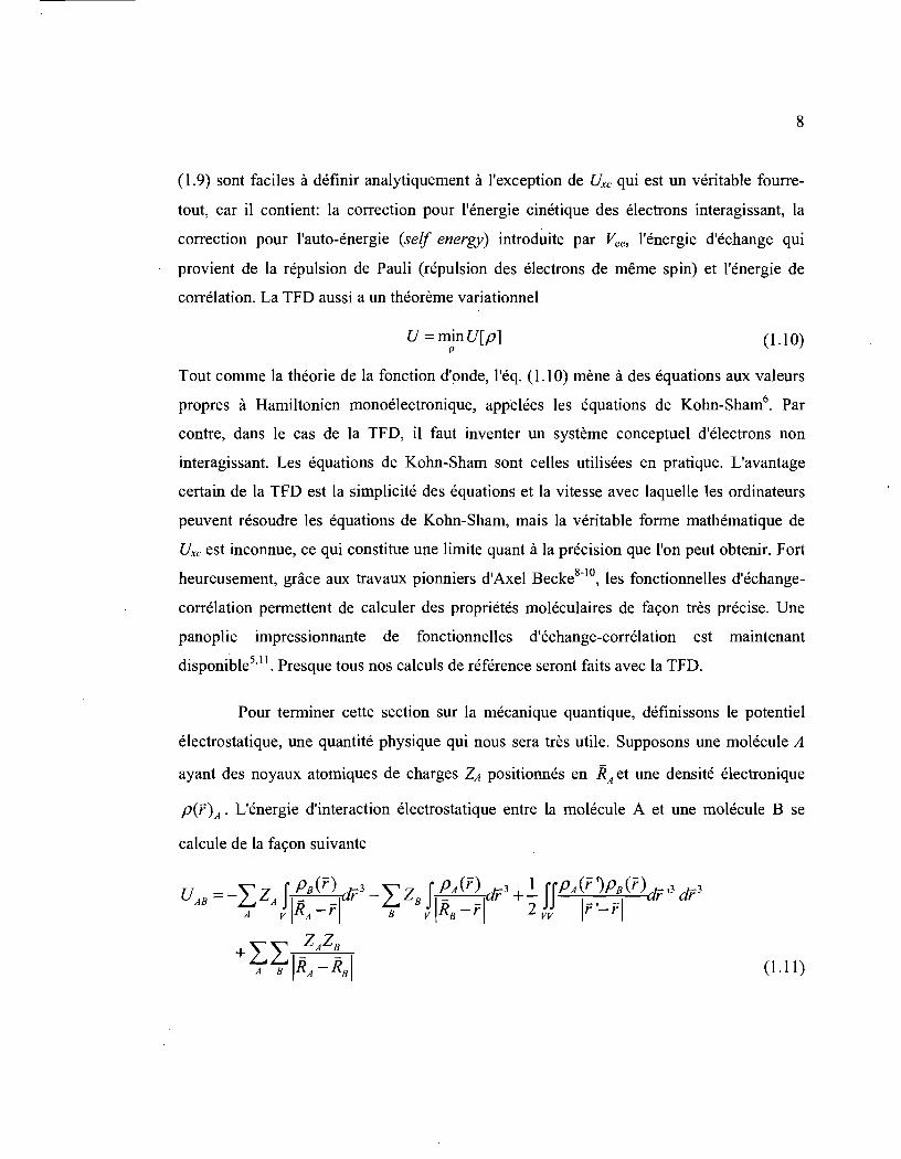
8

(1.9) sont faciles à définir analytiquement à l'exception de Uxc qui est un véritable fourre­

tout, car il contient: la correction pour l'énergie cinétique des électrons interagissant, la

correction pour l'auto-énergie (self energy) introduite par Vee, l'énergie d'échange qui

provient de la répulsion de Pauli (répulsion des électrons de même spin) et l'énergie de

corrélation. La TFD aussi a un théorème variationnel

U =minU[p] p

(1.10)

Tout comme la théorie de la fonction d'onde, l'éq. (1.10) mène à des équations aux valeurs

propres à Hamiltonien monoélectronique, appelées les équations de Kohn-Sham6. Par

contre, dans le cas de la TFD, il faut inventer un système conceptuel d'électrons non

interagissant. Les équations de Kohn-Sham sont celles utilisées en pratique. L'avantage

certain de la TFD est la simplicité des équations et la vitesse avec laquelle les ordinateurs

peuvent résoudre les équations de Kohn-Sham, mais la véritable forme mathématique de

Uxc est inconnue, ce qui constitue une limite quant à la précision que l'on peut obtenir. Fort

heureusement, grâce aux travaux pionniers d'Axel Becke8-

IO, les fonctionnelles d'échange­

corrélation permettent de calculer des propriétés moléculaires de façon très précise. Une

panoplie impressionnante de fonctionnelles d'échange-corrélation est maintenant

disponibleS, II. Presque tous nos calculs de référence seront faits avec la TFD.

Pour terminer cette section sur la mécanique quantique, définissons le potentiel

électrostatique, une quantité physique qui nous sera très utile. Supposons une molécule A

ayant des noyaux atomiques de charges ZA positionnés en RA et une densité électronique

pep) A' L'énergie d'interaction électrostatique entre la molécule A et une molécule B se

calcule de la façon suivante

(1.11 )

9

u = _.!. JJ 17A (P ')PB(f) df ,3 dr 3 _.!. JJ 17B(P ')PA(f) dr!3 dr 3

AB 2VV Ip'-pi 2VV Ip'-pi + 1 fJPA(~?P!(f) dft3 dr3 +! fJ17A(~?17~(r) dr ,3 dr 3

2vv Ir -ri 2vv Ir -ri (1.12)

avec 17A(P) = I.ZAo(P-RA )

A

(1.13)

Pour passer de l'éq. (1.11) à l'éq. (1.12), nous formulons une densité de charge des noyaux

17 A (P) à l'aide de la fonction delta de Dirac, ce qui nous permet de réécrire chacun des

termes comme une intégrale. Ce faisant, nous introduisons un double comptage des

interactions, c'est-à-dire qu'une même distance r entre deux points de l'espace se produit de

deux façons dans l'intégrale double, alors que chacune des distances entre les deux mêmes

points ne devraient être comptées qu'une seule fois. Cela explique les facteurs d'une demie.

Nous pouvons réécrire ces équations en unissant la densité de charge des noyaux et des

électrons d'une molécule dans une fonction de densité de charge totale r, ce qui mène à

l'éq. (1.13). Nous pouvons maintenant définir une fonction fort utile, le potentiel

électrostatique d'une molécule

(1.14)

qui permet de calculer l'énergie d'interaction électrostatique entre A et B par une intégrale

sur l'espace en 3 dimensions

(1.15)

Le potentiel électrostatique peut être compris comme l'énergie électrique qu'il faut fournir

pour amener un proton d'une distance infinie, d'énergie totale nulle par définition, à une

10

distance à laquelle l'interaction prend place (ce qui est évident si rA (r) est remplacé par

une fonction delta dans l' éq. (1.15)).

Il est nécessaire de mentionner que les densités électroniques utilisées pour écrire

l'éq. (1.11) devraient se modifier quand les molécules A et B se rapprochent ou changent

simplement leurs orientations. Nous pouvons alors mettre en évidence le phénomène de

polarisation de façon explicite

m (f) = fIlO(f) + mind (f) = Jr~(f') cff ,3+ J-t5Pif ') cff ,3 't'A 't'A 't'A 1_ -'1 1- -'1 . v r - r v r-r (1.16)

où cpo est le potentiel électrostatique permanent de la molécule (molécule isolée) et, cpind, le

résultat d'un déplacement de la densité électronique r5p causé par la présence de la molécule

B (ou d'une perturbation quelconque). La Figure l.la illustre cpo pour la molécule d'eau à

l'aide d'isolignes tracées dans le plan des atomes qui est perturbé par un monopole placé à

trois endroits différents. Le potentiel total cp est montré à gauche (b et d) et le potentiel

induit cpÎnd correspondant à droite (c et g). La perturbation du potentiel électrostatique

amène des changements substantiels qui ont un impact quantitatif sur l'énergie. L'énergie

d'interaction entre deux molécules A et B qui se perturbent coopérativement s'écrit

(1.17)

L'énergie de polarisation, aussi appelée énergie inductive, est toujours attractive. 11 s'agit en

fait de degrés de liberté supplémentaires donnés au système pour réduire son énergie totale.

Le concept de potentiel électrostatique induit sera abondamment utilisé dans les chapitres

suivants, puisqu'ils traiteront principalement de la polarisation électronique. Une des

manifestations de la polarisation électronique qui est quantifiable est la polarisabilité

moléculaire, traitée dans la prochaine section.

11

·2 ., 0

a X (angslrom)

1 >-

b ·3 ·2 ., 0

X (anga1rom)

2 3 c X (angslrom)

·2

·2·1 ,

d X (ang.trom) e X (ang6,rom)

Figure 1.1. Le potentiel électrostatique pennanent qJ0 (a) d'une molécule d'eau dans le plan des atomes est perturbé par un monopole localisé à différents endroits. Le potentiel total qJ

est donné à gauche (b et d) et le potentiel induit qJind à droite (c et e). Un potentiel très positif est rouge et très négatif est bleu. Le monopole induit un dipôle, en polarisant les électrons de la molécule d'eau, qui diffère selon sa position et défonne le potentiel électrostatique de façon qualitativement et quantitativement appréciable. Obtenu avec EPIC.

12

1.2 La polarisabilité moléculaire

La polarisabilité moléculaire jouera un rôle central dans cette thèse, il est donc

opportun de la définir et de brièvement expliquer comment elle se calcule en mécanique

quantique. Nous pouvons dire que la polarisabilité est le résultat de la déformation de la

densité électronique lorsqu'un champ électrique externe perturbe celle-ci. De façon

générale, le champ électrique perturbant peut prendre n'importe quelle forme et son origine

peut être diverse: onde électromagnétique, autre molécule, dispositif électronique, etc.

Aussi, le champ électrique peut varier dans le temps, comme dans le cas d'une onde

lumineuse. Ici, et dans le reste de cette thèse, nous traiterons principalement du cas où le

champ électrique externe (ou perturbateur) est uniforme et varie suffisamment lentement

pour que les électrons soient toujours à l'état fondamental. Un champ électrique uniforme ,a

la même valeur et la même direction partout dans l'espace sauf, peut-être, à proximité de la

molécule. De façon mathématique, la polarisabilité dipolaire (appelée polarisabilité dans ce

travail) est définie par un développement en série de Taylor du moment dipolaire en

fonction des trois composantes du champ électrique uniforme externe d'une molécule qui

s'écrit

(L 18)

Notons que l'éq. (1.18) utilise la notation tensorielle d'Einstein·, Par définition, donc, le

dipôle total est une somme du dipôle permanent et des dérivées du dipôle par rapport au

champ électrique quand ce dernier est nul. Il est clair que si le champ électrique est petit,

• Un indice en lettre grecque peut être remplacé par x, y ou z et quand deux quantités qui portent le même

indice se multiplient, il s'agit d'une sommation sur l'indice, Si les deux mêmes indices se retrouvent sur les

variables multipliées, il s'agit d'une double sommation.

13

les premières dérivées seront suffisantes pour expliquer la déviation du dipôle. Les six

premières dérivées indépendantes définissent le tenseur de polarisabilité qui peut être écrit

comme une matrice 3x3 symétrique. Quand le champ augmente, la variation n'est plus

linéaire et le tenseur d'hyperpolarisabilité (Papy) devient nécessaire. L'ordre de grandeur du

champ électrique qui nous intéresse dans cette thèse justifie l'emploi du seul terme linéaire.

Dans certaines situations, par exemple avec un cation divalent (Ca2j, le champ électrique

local s'est montré suffisamment fort pour produire une déviation à la linéarité dans certains

modèles polarisables 12, mais dans le cas de la polarisabilité produite par un champ

électrique uniforme, ce cas d'exception n'est pas examiné. Par conséquent, l'approximation

linéaire prédit que le dipôle induit est proportionnel au champ électrique

-ind = Ë P = a3x3 • (1.19)

avec lX la matrice des dérivées, par exemple: lXo,1 ::: ax.y ::: (dpx 1 dEy) E:O • Le rôle du tenseur

de polarisabilité est de moduler la grandeur de l'induction selon l'orientation de la molécule

par rapport au champ. Malheureusement, lX varie quand une molécule tourne, mais la trace

est invariante, ce qui permet de définir la polarisabilité moyenne

(1.20)

où amoy est une valeur scalaire qui ne dépend pas de l'orientation de la molécule. Lorsque la

symétrie de la molécule la rend isotrope, l'éq. (1.19) s'écrit

n ind =a Ë r moy (1.21 )

Cependant, pour plusieurs molécules, cette approximation est erronée. Pour mieux

saisir la signification des éléments de lX, il est utile de trouver l'orientation de la molécule

qui rend ce tenseur diagonal. Dans ce cas, les axes x, y et z indiquent les directions

principales de polarisation et le moment dipolaire induit pour un champ électrique de

grandeur E orienté en x se calcule avec Px = axxE (même chose pour les autres axes). La

14

Figure 1.2 montre quatre exemples de molécules orientées dans le système d'axe illustré au­

dessus de chacune. La molécule adamantane est complètement isotrope, comme indiqué par

la valeur numérique sur les axes, et l'éq. (1.21) s'applique. La molécule de benzène a deux

axes principaux de polarisabilité dégénérés dans le plan de la molécule avec une

polarisabilité environ deux fois moindre dans l'axe qui sort du plan. Les molécules de

quinoxaline et d'isothiazole ont trois polarisabilités différentes pour chacun des axes et

l'orientation des moments principaux de la polarisabilité pour l'isothiazole n'est pas aussi

évidente que pour les autres cas. L'importance du dipôle induit pour un même champ

externe dépend fortement de l'orientation de la molécule.

L09

109 109 • ~

3

83 45 •

o L

11

164 59 • ~

4

64 40 •

Figure 1.2 Polarisabilité selon les axes principaux en unités atomiques§ (calculs B3L yp13)

pour quatre molécules. Le cercle indique l'axe qui sort du plan de la feuille.

Terminons cette section en faisant un survol des méthodes de calcul de la

polarisabilité. Prenons d'abord la formule pour calculer l'énergie d'interaction entre un

dipôle total et le champ électrique appliqué

§ Les unités atomiques (u.a.) de la polarisabilité peuvent être obtenues des unités en S.I. (Cm21V) en divisant

par 41tEo et en convertissant le m3 en bohr3• Pour convertir des A3 en u.a., il faut diviser par 0.148184.

15

(1.22)

En comparant les éq. (1.18) et (1.22), on retrouve les relations

af.1a a2U(Ë) --=- =a tf aEp aEpaEa a

(1.23)

qui donnent lieu à deux méthodes de calcul de la polarisabilité. Premièrement, la méthode

des différences finies fait un calcul numérique approximatif de la dérivée selon le champ

électrique

(1.24)

où Ea le champ électrique appliqué est généralement petit. Avec les différences finies, le

dipôle est calculé avec différentes valeurs du champ électrique séparées par 2LlEa. Cette

méthode est facile à programmer et donne des résultats raisonnables avec des calculs de

mécanique quantique14• Une deuxième approche utilisée en mécanique quantique fait appel

à la théorie des perturbations (formalisme de Rayleigh-Schrodingert,15 qui nécessite de

définir un Hamiltonien perturbateur donné, dans le cas du champ électrique uniforme, par

Mf ::: r . Ë. Au deuxième ordre, l'énergie d'interaction entre le dipôle induit par la

déformation de la densité électronique et le champ électrique est

(1.25)

16

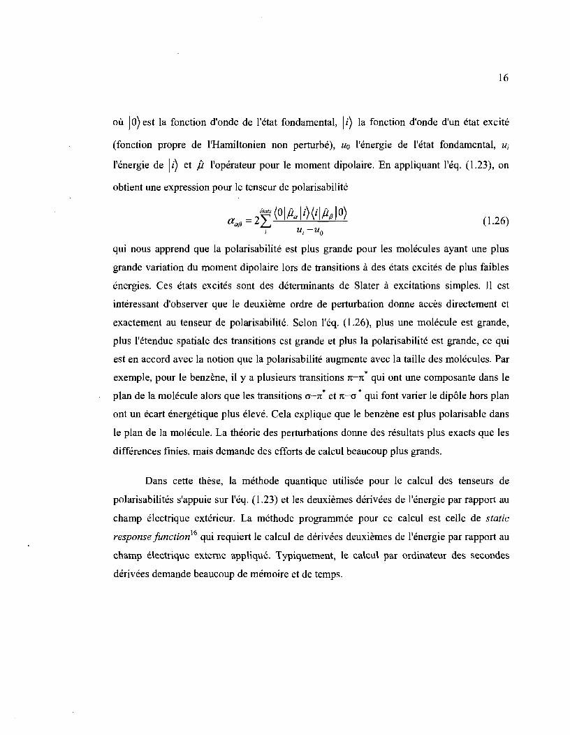
où 10) est la fonction d'onde de l'état fondamental, 1 i) la fonction d'onde d'un état excité

(fonction propre de l'Hamiltonien non perturbé), Uo l'énergie de l'état fondamental, Uj

rénergie de 1 i) et fi l'opérateur pour le moment dipolaire. En appliquant l'éq. (1.23), on

obtient une expression pour le tenseur de polarisabilité

(1.26)

qui nous apprend que la polarisabilité est plus grande pour les molécules ayant une plus

grande variation du moment dipolaire lors de transitions à des états excités de plus faibles

énergies. Ces états excités sont des déterminants de Slater à excitations simples. Il est

intéressant d'observer que le deuxième ordre de perturbation donne accès directement et

exactement au tenseur de polarisabilité. Selon l'éq. (1.26), plus une molécule est grande,

plus l'étendue spatiale des transitions est grande et plus la polarisabilité est grande, ce qui

est en accord avec la notion que la polarisabilité augmente avec la taille des molécules. Par

exemple, pour le benzène, il y a plusieurs transitions n-n 0

qui ont une composante dans le

plan de la molécule alors que les transitions cr-n° et n-cr ° qui font varier le dipôle hors plan

ont un écart énergétique plus élevé. Cela explique que le benzène est plus polarisable dans

le plan de la molécule. La théorie des perturbations donne des résultats plus exacts que les

différences finies, mais demande des efforts de calcul beaucoup plus grands.

Dans cette thèse, la méthode quantique utilisée pour le calcul des tenseurs de

polarisabilités s'appuie sur l'éq. (1.23) et les deuxièmes dérivées de l'énergie par rapport au

champ électrique extérieur. La méthode programmée pour ce calcul est celle de static

response function 16 qui requiert le calcul de dérivées deuxièmes de l'énergie par rapport au

champ électrique externe appliqué. Typiquement, le calcul par ordinateur des secondes

dérivées demande beaucoup de mémoire et de temps.

17

1.3 La mécanique nloléculaire

La mécanique quantique est inefficace pour simuler de très gros systèmes comme

des protéines ou des phénomènes qui surviennent à l'état liquide sur de longues échelles de

temps. Or, par des approximations judicieuses, on arrive à simplifier grandement l'équation

aux valeurs propres de Schrôdinger pour le déplacement des noyaux donnée par l'éq. (1.3).

Premièrement, pour un grand éventail de cas, incluant la plupart des systèmes

biomoléculaires simulés sans bris ou formation de liens chimiques, il est acceptable

d'ignorer la nature quantique des noyaux et supposer qu'ils se comportent comme des

particules classiques mues par la loi de Newton (ft = ma). Cela se traduit par l'utilisation

de l'énergie cinétique classique et l'éq. (1.3) peut s'écrire

(1.27)

avec Pn la quantité de mouvement du noyau n. Les noyaux se déplacent dans un potentiel

effectif électronique donné par la surface de Born-Oppenheimer Uélec. Comme il est

beaucoup plus facile de résoudre un système d'équations différentielles ordinaires à

conditions initiales qu'une équation aux valeurs propres, .le problème est grandement

simplifié. Il reste toutefois à résoudre l'équation de Schrôdinger électronique qui n'est

quand même pas une mince tâche.

Une seconde approximation doit intervenir. Nous remplaçons l'équation de

Schrôdinger électronique par une fonction d'énergie potentielle qui conserve le

comportement de Uélec , mais qui s'écrit par une fonction directe empirique et paramétrique.

Le terme mécanique moléculaire signifie que les deux approximations mentionnées ci­

dessus sont appliquées.

18

Dans le jargon' de la mécanique moléculaire, nous appelons champ de force la

fonction d'énergie potentielle empirique des noyaux atomiques. Par exemple, le champ de

force utilisé par le logiciel AMBER17,18 et développé dans le groupe de Peter Kollman

(1944-2001) a la forme suivante

V(R) = vL (R)+V NL (R) (1.28)

où l'énergie potentielle du système moléculaire, V, est divisée en une énergie

intramoléculaire, VL , qui dépend des coordonnées internes (longueur des liens, angles, etc.)

et en un deuxième terme, VNL , qui traite des interactions entre atomes non liés. Plus

spécifiquement l'énergie potentielle interne est donnée par

;=1 ;=1 ;=1 (1.29) 1 Nd

+-L L Vn [1 + cos(nrp; - Y;)] 2 ;=1 n

Dans l'éq. (1.29), l'énergie d'étirement et de compression de chacun des Nb liens chimiques

hors de leur longueur d'équilibre (re) est traité un comme un oscillateur harmonique dont la

constante de force, un paramètre ajustable, est kb. Une constante de force peut être

spécifique à un lien ou bien être utilisée pour plusieurs, en fonction du typage choisi. De la

même façon, l'énergie de déformation des Na angles formés par trois atomes chaînés,

comme l'angle H-Q-H de la molécule d'eau, est dictée par le paramètre ajustable ka. Un

angle de déformation hors plan (souvent appelé angle impropre), <1>, permet de maintenir

un centre trigonal dans le plan. Finalement, un terme d'énergie pour chacun des angles

dièdres sert de véritable fourre-tout. Il s'agit d'une expansion en série de cosinus de Fourier

(le terme en sinus est inutile étant donné que la parité peut être garantie par un angle de

phase y) qui permet d'exprimer de façon exacte, à la limite d'un grand nombre de termes n,

n'importe quel potentiel périodique sur la période [0, 2n]. Il sert normalement à inclure des

effets électroniques reliés à la conjugaison électronique, par exemple, et à corriger les

19

défauts de tous les autres termes. La fonction UL définit en grande partie la structure

tridimensionnelle des molécules qui peuvent se déformer au gré des forces appliquées.

Le deuxième terme de la fonction d'énergie potentielle totale du champ de force

AMBER, comme bien d'autres, se définit comme

(1.30)

où les sommations sont faites sur toutes les paires distinctes d'atomes non liés. Règle

générale, les atomes séparés par moins de trois liens chimiques ne sont pas considérés alors

que ceux séparés par quatre liens ou plus peuvent partiellement être considérés. La

première sommation est faite sur un terme Lennard-Jones 12-6 qui décrit à la fois les forces

répulsives entre les électrons dues à la répulsion de Fermi (ou de l'échange électronique) et

les forces attractives de van der Waals. La répulsion de Fermi résulte de l'interpénétration

des nuages électroniques qui forcent les électrons de même spin à occuper un espace

commun. C'est une force très intense, mais active seulement à courte distance qu'on appelle

parfois la distance de contact de Fermi. Des calculs de haut niveau ont montré un

comportement exponentiel pour la répulsion de Fermi ~exp(_axr)15, mais l'avantage

calculatoire et la précision de la forme en r- 12 en ont justifié l'utilisation. Quant aux forces

de van der Waals, leurs comportements théoriques suivent une loi en 1/r6• Elles sont petites

et agissent à courte distance.

Le dernier terme, mais non le moindre, de l'éq. (1.30) est une approximation de

l'énergie d'interaction électrostatique avec des charges atomiques partielles et ajustables qi

qui sont positionnées, d'habitude, sur les noyaux. Ces charges n'ont pas de signification

physique sinon qu'elles reproduisent le potentiel électrostatique de la molécule qui les

porte. Les charges atomiques partielles sont presque toujours ajustées pour reproduire la

fonction du potentiel électrostatique q;(r) de l'éq. (1.14) qui est calculée à l'aide de la

mécanique quantique. Le potentiel électrostatique reproduit se trouve à l'extérieur de la

zone de Fermi, c'est-à-dire là où la densité électronique est pratiquement nulle. Cela est

20

nécessaire puisqu'un modèle qui compte sur des charges atomiques ponctuelles ne peut

habituellement pas décrire le potentiel électrostatique complexe près des noyaux qui est

d'ailleurs de peu d'intérêt pour traiter les interactions intermoléculaires. Le potentiel

électrostatique classique utilisé s'écrit alors

Na q, rp(f) = L 4 I~ -1

i 1Œo r-li (1.31 )

La Figure 1.3 compare le potentiel électrostatique de la molécule 4-pyridone calculé avec la

mécanique quantique (éq. (1.14)) en (a) à l'approximation de l'éq. (1.31) en (b). De tous les

termes de l'éq. (l.28), l'énergie électrostatique a la plus longue portée et est en grande partie

responsable du caractère unique d'une molécule. L'énergie électrostatique peut être

répulsive ou attractive mais, en dehors de la zone de Fermi, est presque toujours le terme

intermoléculaire dominant.

Une ombre se dresse cependant au tableau. La mécanique moléculaire est surtout

utilisée pour étudier des systèmes en milieu condensé comme l'eau liquide. Or, il est connu

que la polarité des molécules augmente considérablement dans un solvant polaire. Par

exemple, la molécule d'eau voit son moment dipolaire passer de 1.8 D à l'état gazeux à 2.8

D à l'état liquide19,2o. Cette augmentation du moment dipolaire est expliquée par la

polarisation électronique qui peut constituer une composante importante de l'énergie

d'interaction entre des espèces polaires: La polarisation due au solvant ne peut être

négligée. De plus, la polarisation électronique constitue une part importante des interactions

dans certains systèmes. Par exemple, l'énergie d'induction dans un système cation-1t est

aussi importante que l'interaction électrostatique monopole-benzène. Pourtant, les calculs

du potentiel électrostatique nécessaires à l'ajustement des charges atomiques, se font dans le

vide (état gazeux).

L'inclusion du potentiel électrostatique moléculaire induit qJind (éq. (1.16)) devient alors une

condition sine qua non au succès des champs de force. La rédemption vient de deux

stratégies plutôt brutales: augmenter par un facteur empirique toutes les charges partielles

21

atomiques ajustées sur (jJ0 21, utiliser une méthode quantique·· qui commet l'erreur de

produire systématiquement un moment dipolaire trop élevé pour la phase gazeuse22• Dans

chacun des cas, toutefois, les charges atomiques partielles demeurent constantes dans les

simulations qui utilisent l'éq. (1.30) et l'effet de polarisation obtenu ne s'ajuste pas à

l'environnement. Par exemple, un inhibiteur qui se lie au site actif d'une enzyme voit son

environnement changer radicalement de polarité. Un soluté qui se trouve à l'interface de

deux phases peut être dans une situation analogue. De plus, certaines interactions

intermoléculaires ne peuvent être expliquées quantitativement que par la prise en compte de

la polarisabilité moléculaire: interactions cation_1t23-27

, ponts-H de molécules très

polaires27,28, hydràtation d'ions29

-32

, affinité enzyme-inhibiteur33• Il s'agit d'un problème de

longue date qui persiste encore et qui est une source d'erreurs importantes et difficiles à

corriger avec les champs de force non polarisables.

Bref, la mécanique moléculaire est un outil de choix qui a été méticuleusement

élaboré au cours des 30 dernières années et constitue un fer de lance pour l'étude de

biomolécules, entre autres choses. L'omission de la polarisabilité moléculaire pour

simplifier la paramétrisation limite encore ce domaine d'étude. Dans cette thèse, nous

amènerons une nouvelle méthode qui modélise la polarisation électronique .

•• La méthode de Hartree-Fock avec une petite base orbital aire comme 6-31 G*.

22

~ 0 ~ 0 >- >-

-2 -2

-6

-B

-8 -6 -4 -2 -8 -6 .. -2

x (Al x (Al

a b

Figure 1.3. Potentiel électrostatique de la molécule 4-pyridone obtenu (a) avec des charges

atomiques partielles selon l'éq. (1.31) et (b) par la mécanjque quantique où l'éq. (1.14) est

calculée avec HF/6-31 G*. L'approximation des charges atomiques permet de reproduire

précisément le potentiel électrostatique produit par la densité électronique et les noyaux

(r(P) ) à une distance où les interactions intermoléculaires prennent place.

1.4 Champs de force polarisables: précédents de la littérature

Une des premières simulations qui permettaient à un champ de force d'adapter le

potentiel électrostatique des molécules à l'environnement a été réalisée par Warshel et

Levitt il y a plus de 30 ans34. Depuis ce temps, ce sujet a toujours été d'actualité tt sans être

tt ISI Web of Knowledge répertoriait 4154 articles, en date du 20 décembre 2008, dont le sujet est po/ariz* en

cooccurrence avecforcefield* ou molecular mechanic* ou AMBER ou CHARMM.

23

résolu de façon satisfaisante. Deux classes de méthodes, que nous examinerons ici, ont été

développées jusqu'à maintenant.

Tout d'abord, le modèle des dipôles atomiques induits35-39 aSSOCIe un point

polarisable aux atomes d'une molécule et, d'une façon analogue à l'éq. (1.21), un dipôle

ponctuel proportionnel au champ électrique total est induit sur chaque noyau polarisable:

(1.32)

Ce modèle est illustré pour le cas d'une molécule de benzène assujettie à un champ

électrique complexe à la Figure 1.4. Dans l'éq. (1.32), le champ électrique total t(r) est

créé par les charges atomiques partielles responsables du potentiel électrostatique

permanent et par les dipôles induits. Si l'on veut utiliser ce modèle dans le cadre d'un

champ de force, il faut calculer les dipôles atomiques induits qui produiront un potentiel

électrostatique induit en utilisant l'équationI5,35,39

(1.33)

avec rij ="f; - f; , le vecteur qui sépare la charge/dipôle source de la position du dipôle induit

j; la longueur de cette distance est notée rij. La matrice ~ est le tenseur du champ dipolaire

donné par

rij,xry,ij

r:,y - X' rij2

rij,zrij,y

r. r. 1 Ij,X, Ij,Z

r. r. I),y I),Z

rij\ - X'rij2

(1.34)

avec la composante y du vecteur de distance rij noté rij,y' Il est évident que l'éq. (1.33)

nécessite une solution autocohérente. Le terme d'énergie résultant est assez compliqué15 et

nécessite, pour chaque configuration, de résoudre l'éq. (1.33).

24

Un cas particulier de (1.33) peut être utilisé pour calculer le tenseur de polarisabilité

d'une molécule portant des dipôles polarisables. Dans le cas où un champ électrique

uniforme externe est appliqué sans les charges partielles atomiques, on trouve

(1.35)

En réarrangeant (1.35), le tenseur de polarisabilité moléculaire peut être obtenu. Fait à

remarquer, la polarisabilité moléculaire est modulée par une interaction intramoléculaire

des dipôles induits. À partir de (1.35), on se rend compte que plus les dipôles induits i qui

entourent l'atome j seront grands, moins le champ effectif senti par l'atome j sera grand.

C'est cet effet intramoléculaire qui est la plus imp?rtante source de l'anisotropie du tenseur

de polarisabilité.

Le modèle des dipôles ponctuels induits a toutefois une complication importante car, quand

deux dipôles sont à proximité, la solution autocohérente de l'éq. (1.33) ou de l'éq. (1.35)

peut diverger. Dans le cas de deux points polarisables (ex. molécule diatomique), les

composantes de la polarisabilité suivant l'axe de la séparation (l1I) et perpendiculaire à

l'axe (a.J obtenues sont

_ a A +aA +4aAaA 1 r3

l11 - 1 4a a 1 r6 A A

_aA+aA 2aAa A lr3

aJ. - 6 l-aAaA Ir

(1.36)

où r est la distance qui sépare les deux atomes polarisables35• Si le dénominateur est zéro, la

solution diverge. Cette divergence est un problème intrinsèque à ce modèle et a été appelée

la catastrophe de la polarisabilité (polarizability catastrophéo). On peut pallier ce problème

en modifiant le tenseur du champ dipolaire fy de façon à écranter l'interaction entre dipôles

en fonction de la distance qui les sépare. La façon la plus fréquente est le terme exponentiel

de Thole38,39 qui utilise une fonction exponentielle de la distance intemuc1éaire. La

25

méthode des dipôles induits ponctuels s'est avérée très efficace pour modéliser la

polarisabilité moyenne des molécules35,41, mais connait des problèmes considérables à

reproduire l'anisotropie du tenseur de polarisabilité, c'est-à-dire la dépendance

directionnelle de la grandeur du dipôle induit.

••• ,

Figure 1.4. Illustration du modèle des dipôles atomiques induits pour une molécule de

benzène avec des atomes de carbone polarisables qui subissent l'influence d'un champ

électrique externe complexe (flèches bleues). Les charges atomiques ne sont pas montrées,

mais contribuent à induire les dipôles atomiques en produisant un champ électrique interne

qui s'ajoute à celui créé par les dipôles induits et au champ électrique externe.

Une correction essentielle37.42 pour le modèle consiste à associer non pas une polarisabilité

moyenne à un atome, mais plutôt un tenseur de polarisabilité atomique, ce qui ajoute une

grande complexité pour la création de modèles généraux et l'ajustement des paramètres.

A vec la méthode qui sera présentée dans cette thèse, nous voudrons à la fois produire un

tenseur de polarisabilité adéquat et réduire le nombre de paramètres ajustables ainsi que la

complexité.

26

Pour finir, la méthode des dipôles induits a également des variantes. Les

oscillateurs de Drude12•43 offrent une alternative calculatoire en représentant un dipôle par

une charge partielle attachée au noyau par un ressort. La constante de force du ressort est

directement reliée à la polarisabilité atomique et les équations ressemblent énormément à

celles présentées ici. Cependant, l'utilisation d'un ressort permet d'appliquer des stratégies

dans les calculs de dynamique moléculaire qui les rendent plus rapides43•44

. Un autre

modèle analogue utilise une distribution de charges par des fonctions gaussiennes et

l'énergie d'interaction interne, responsable pour l'anisotropie, provient de l'intégrale

coulombienne du recouvrement des densités de charges. Ce modèle a un comportement

équivalent aux dipôles induits ponctuels40 avec l'avantage que la méthode peut être

généralisée aux autres moments atomiques multipolaires induits, avantage qui n'a pas

encore trouvé sa niche. Ces méthodes analogues aux dipôles atomiques induits partagent le

même problème de la càtastrophe de la polarisabilité et de l'anisotropie12,40.43.4

4.

La deuxième classe de méthodes utilisées pour introduire la polarisabilité permet

aux charges partielles atomiques d'être transférées d'un atome à l'autre dans une molécule45-

50. Elle est dite méthode des charges fluctuantes (ou fluctuating charge). Ce modèle se

fonde sur le principe de l'égalisation de l'électronégativité qui peut être comparé au

mouvement de chaleur entre bains thermiques qui équilibreront leur température. Ici, la

chaleur s'apparente aux charges et la température à l'électronégativité. La justification pour

cette théorie relève du champ d'étude de la théorie de la fonctionnelle de la densitë. À

chaque atome est associée une électronégativité intrinsèque qui dépend de son

environnement chimique et cette électronégativité peut être perturbée par le champ

électrique qu'il subit. En utilisant le principe de l'égalisation de l'électronégativité, l'énergie

de créer une charge partielle sur un atome isolé se développe en série de Taylor

(1.37)

27

avec U~ l'énergie de l'atome A à l'état fondamental, %~ l'électronégativité intrinsèque de

l'atome et J~A est deux fois la dureté de l'électronégativité de l'atome. Ces quantités peuvent

se calculer à partir de la mécanique quantique, mais sont toujours, en pratique, considérées

comme des paramètres ajustables. La fonction d'énergie électrostatique pour un ensemble

moléculaire s'écrit alors

atomes

U = L UA (QA) + LJABQAQB (1.38) A A<B

où JAB prend la forme de l'interaction de Coulomb pour des atomes A et B appartenant à des

molécules différentes et devient une intégrale de recouvrement de Coulomb entre orbitales

de Slater centrée sur les atomes d'une même molécule. Comme pour les dipôles ponctuels

induits, il faut résoudre un système d'équations linéaires. Celles-ci sont obtenues en

minimisant la déviation à une électronégativité atomique unique pour tout le système

(1.39)

qui doit être maintenue pour chaque atome. Aucune charge n'est transférée entre molécules.

Un problème pour ce modèle est que la polarisabilité ne peut se produire que dans la

direction des liens chimiques. Par exemple, la molécule de benzène, selon les principes de

ce modèle, a une polarisabilité nulle en dehors du plan; pour une molécule diatomique on a

al. = O. Une des approches utilisées pour remédier à ce problème est l'ajout des sites

auxiliaires qui, dans le cas de la molécule de benzène, se traduit par des charges au-dessus

et en dessous du plan pour la molécule de benzène. Toutefois, cette complication n'est pas

générale et constitue une barrière à la généralisation du modèle et à la détermination des

autres paramètres du champ de force.

Bref, avec les dipôles induits ponctuels et les charges fluctuantes, l'atteinte d'une

bonne précision nécessite l'ajout de paramètres et d'atteindre un niveau de complexité qui

en réduit la généralité. Une autre problématique qui limite la création de champ de forces

28

polarisables, généraux et fiables est le couplage des charges atomiques, responsables en

partie de la polarisation intramoléculaire, et des paramètres propres à la polarisation. Ce

couplage rend difficile l'optimisation des paramètres puisque des charges produisant un

dipôle statique plus élevé peuvent compenser pour une polarisabilité moindre et vice-versa.

C'est une forme d'indétermination.

1.5 Un solvant implicite à partir du continuum diélectrique

Le sujet présenté ici fait contraste avec ceux abordés dans les sections précédentes.

Il est néanmoins nécessaire, pour bien comprendre l'origine des concepts utilisés dans cette

thèse, de survoler comment les effets de solvant peuvent être modélisés par un continuum

diélectrique. Il s'agit ici de la polarisation moyenne des molécules de solvant par

l'interaction avec un soluté. Ce type de modèle n'est pas seulement utilisé pour calculer des

énergies libres d'hydratation, mais aussi pour modéliser les effets électrostatiques du

solvant sur des biomolécules comme des protéines complexées à des petites molécules ou

de l'ADN. Ces approches servent principalement à réduire l'échantillonnage des

configurations du solvant. Elles sont donc très rapides avec une précision souvent

satisfaisante. On les utilise dans le contexte de la mécanique moléculaire et de la

d . l' l' 51 52 ynamlque mo ecu aire . .

Un soluté polaire comme l'acétonitrile, placé dans un solvant polaire comme l'eau,

formera des interactions polaires par l'intermédiaire des moments électriques et des ponts­

H. La Figure I.Sa donne un exemple de configuration des molécules d'eau autour de

l'acétonitrile dans l'eau. En fait, cette configuration statique n'est qu'un instantané

(snapshot) des configurations que la première couche de molécules de solvant peut adopter.

Contrairement aux modèles de solvants explicites, où les coordonnées des

molécules d'eau seraient échantillonnées selon une distribution de Boltzmann, un modèle

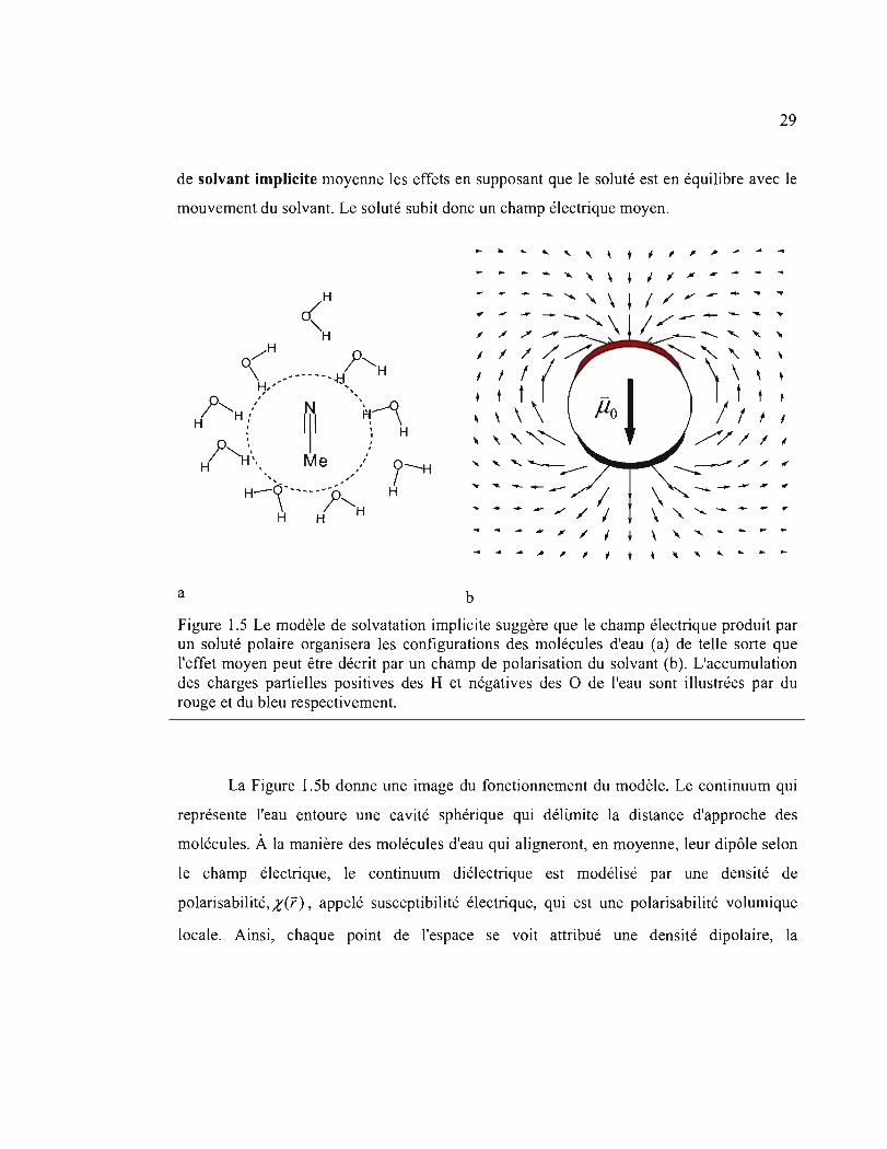
29

de solvant implicite moyenne les effets en supposant que le soluté est en équilibre avec le

mouvement du solvant. Le soluté subit donc un champ électrique moyen.

~ ~ ... .... "' , \ t ~ " , .- .A .A ...

- ~ .. - ..... "' , ~ 1 JI ~ .... -- - ........ '1.. \ ~ 1 /' ;' ~ ~ - -- "" \ //-- ... ~

; / .,., ....... -. ----- "' '- '" H 0/ 1""-

\ .-.------l:l H H .- '.

l""-H :/ t:J. "'f>j--o\ H { III 'H

1"H'-. Me / H, , , , H'-:t -----}~ H H H

j----H H

1 1 ;(~ ~~~ \ , 1 1 , + t ~\ I~ t , \ ; 1 , \ " "'''-... /// 1 1

\ " ..... .... ... - ~

.... .. ..... ,JJo JI ,

a b

Figure 1.5 Le modèle de solvatation implicite suggère que le champ électrique produit par un soluté polaire organisera les configurations des molécules d'eau (a) de telle sorte que l'effet moyen peut être décrit par un champ de polarisation du solvant (b). L'accumulation des charges partielles positives des H et négatives des 0 de l'eau sont illustrées par du rouge et du bleu respectivement.

La Figure 1.5b donne une image du fonctionnement du modèle. Le continuum qui

représente l'eau entoure une cavité sphérique qui délimite la distance d'approche des

molécules. À la manière des molécules d'eau qui aligneront, en moyenne, leur dipôle selon

le champ électrique, le continuum diélectrique est modélisé par une densité de

polarisabilité, X(r), appelé susceptibilité électrique, qui est une polarisabilité volumique

locale. Ainsi, chaque point de l'espace se voit attribué une densité dipolaire, la

30

polarisationP(f), qui est un champ vectoriel volumique. Utilisant une réponse linéaire,

nous obtenons

P(r) == x(r)Ë(r) (1.40)

qui est semblable à l'éq. (1.32), à l'exception ici que chaque point de l'espace possède un

dipôle induit. Donc, pour calculer P(r), il faut connaître le champ électrique Ë(f) qui peut

être calculé en résolvant l'équation de Poisson

V' . (e(f)Ë(f) = pl (f) eo

(1.41)

où

e(f) = X(f) + 1 (1.42)

est appelé fonction de diélectrique et pl (r) la densité de charge libre ifree charge density)

qui provient de charges statiques, par exemple les charges atomiques partielles qui

reproduisent le potentiel électrostatique. Une dérivation de l'équation de Poisson est donnée

en Appendice II. Dans l'éq. (1.41), 60 est la permittivité du vide et e(r)eo la permittivité

locale. Ainsi, la constante diélectrique est sans unité et représente la permittivité relative au

vide. Quand e=l, la polarisabilité est nulle et quand e > 1 le milieu est polarisé est s'oppose

au champ électrique. La Figure 1.5b illustre le champ vectoriel de P(f) pour le problème

d'un dipôle à l'intérieur d'une cavité sphérique. Une conséquence de la formation du champ

de polarisation est l'apparition d'une densité de charge induite, aussi appelée densité des

charges liées (bound charge density), qui se calcule

pb(r) -V'.(x(r)Ë(r»

-V' ·P(r) (1.43)

L'appendice II démontre mathématiquement l'origine de cette équation. Ici cependant, nous

pouvons comprendre intuitivement que les dipôles du solvant implicite qui s'arrêtent à la

frontière de la cavité auront une extrémité soit chargée négativement (près du méthyle de

l'acétonitrile) soit chargée positivement. Cela est représenté par les zones rouges et bleues à

31

la Figure 1.5b. Par contre, les dipôles qui se suivent à la queue dans le solvant verront leurs

charges se neutraliser. Finalement, il ne faut pas croire que le modèle sous-entend que les

molécules d'eau s'alignent parfaitement selon le champ vectoriel tracé à la Figure 1.5b. Le

modèle prévoit plutôt un alignement moyen du solvant de telle sorte que chacun des dipôles

tracés ne représente pas une molécule d'eau, mais plutôt l'effet moyen à cet endroit.

En plus d'avoir une valeur conceptuelle intéressante, la solvatation implicite a

surtout été utilisée pour faire des calculs quantitatifs. Historiquement, les méthodes

électrostatiques continues ont été parmi les premières approches à considérer les effets de

solvant53-55 et sont encore aujourd'hui très populaires pour estimer l'énergie libre de

solvatation51,56,57. On peut écrire l'énergie libre pour solvater (ou hydrater dans l'eau) un

soluté I1Gsa'v en une somme de deux processus

(1.44)

où I1Gnp est l'énergie libre non polaire nécessaire pour former une cavité dans le solvant et

englobe la variation d'énergie et d'entropie du solvant causé par l'insertion du soluté.

I1Gelec est l'énergie libre électrostatique qui provient du processus qui consiste à rendre

polaire la cavité formée. Ce dernier terme englobe l'entropie et l'énergie reliées à la

réorganisation du solvant causé par la polarité du soluté. Dans le cas où la polarisation du

soluté est prise en compte, I1Ge,ec contient également l'énergie libérée par le solvant due à

la réorganisation de la distribution de charge à l'intérieur du soluté. Théoriquement, l'éq.

(1.44) est exacte puisque I1Gsa1v est une fonction d'état et que tout chemin impliquant des

transformations réversibles donne accès au travail thermodynamique entre deux états. En

pratique, calculer I1Gsa'v exactement est un défi. L'équation de Poisson est uniquement

utilisée pour calculer fl.Gelec ' Comme il en sera question à plusieurs reprises dans cette

thèse, la forme de la cavité est très importante pour le calcul de I1Ge,ec '

32

L'énergie libérée en mettant un dipôle statique Po dans une cavité sphérique a une

solution mathématique donnée par l'équation

AG =- 1 (Eso1v-l JI-12 elec 4 3 2 1 110

Jrt:oa Eso1v + (1.45)

où a est le rayon de la cavité et GSO/V la constante diélectrique du solvant. En fait, GSO/V

apparaît dans les équations à cause des éq. (1.41) et (1.42). Le continuum a une fonction

diélectrique E(r) = Eso1v ' une constante, à l'extérieur de la cavité et change abruptement à

l'intérieur de celle-ci étant donné qu'aucune molécule de solvant ne peut s'y polariser. La

constante diélectrique d'un liquide augmente grossièrement avec la polarité (dont le terme

le plus imporant pour une molécule neutre est le moment dipolaire) de celui-ci, comme le

rapporte la Table 1.1 qui met quand même en évidence que c'est plutôt la densité dipolaire

(la somme des dipôles moléculaires par unité de volume) qui est corrélée avec GSO/V' Cela

signifie que la capacité d'un liquide à se polariser dépend surtout de la densité dipolaire.

L'eau constitue une exception qui est cependant assez peu significative étant donné que la

différence entre deux constantes diélectriques élevées est beaucoup moins importante

qu'entre deux plus petites comme l'on peut le calculer avec l'éq. (1.45).

Onsager, dans un article marquantH publié en 193654, a résolu le problème posé à

l'époque par les solvants polaries en ajoutant un point polarisable au centre de la sphère et

résolu les équations de nouveau.

tt Cet article est le sixième plus cité de la revue Journal of the American Chemical Society de tous les temps.

33

Table 1.1. Pennittivité relative (Esolv) expérimentale58 de quelques liquides (20 oC

et 1 atm)

Substance ~solv Moment dipolaire Volume molaire Densité dipolaireo (Debye) (mL/mol) (Debye x moVmL )

Fonnamide 109.0 3.73 39.7 0.009

Eau 78.4 1.85 18.1 0.010

Acétonitrile 37.5 3.92 52.2 0.075

Métanol 32.7 1.70 40.5 0.042

Pyridine 12.3 2.22 80.6 0.027

Benzène 2.3 0 89.1 0.025

Cyclohexane 2.0 0 108.1 0.019

°Moment dipolaire / Volume molaire.

Le résultat obtenu par Onsager donne:

(1.46)

avec a la polarisabilité moyenne du soluté qu'Onsager a obtenue par la fonnule suivante

( n~ -1 J( 3V J

a== n~+2 4Jr;A (1.47)

qui utilise l'indice de réfraction nd, le volume molaire Vm et la constante d'Avogadro NA.

Nous reviendrons sur l'origine de l'éq. (1.47) à la section suivante. Ici, il suffit de dire que le

34

facteur le plus à droite représente le cube du rayon d'une sphère qui a le volume qu'occupe

en moyenne une seule molécule.

Ces modèles, développés avant l'avènement de super ordinateurs, ont été cruciaux • pour la compréhension de la solvatation et du comportement électrique des molécules en

interactions. Depuis le milieu des années 1980, des méthodes numériques ont permis de

délaisser la cavité sphérique et de résoudre l'équation de Poisson avec des cavités qui

épousent davantage la forme des molécules. La Figure 1.6 montre la surface de van der

Waals du benzène qui se forme en prenant l'enveloppe extérieure du volume formé par des

sphères positionnées sur les atomes. Généralement, les rayons des sphères atomiques

proviennent de distances de contact tirées de données cristallographiques59. La constante

diélectrique à l'extérieur de la cavité provient des valeurs expérimentales alors que le

diélectrique interne est souvent 1.

H H

H H

H

Figure 1.6. Une cavité dans un diélectrique est formée pour une molécule de benzène. Des sphères sont positionnées sur les atomes de la molécule avec différents rayons. L'enveloppe extérieure définit la cavité. Il s'agit d'une surface dite de van der Waals (vdW).

35

Finalement, il est opportun de faire mention d'une méthode appelée Poisson­

Boltzmann (PB) qui ajoute l'effet des sels sur les énergies de solvatation. Ici, on reprend

l'équation de Poisson donnée par l'éq. (lAI) et on ajoute au terme de droite une distribution

de charges supplémentaires

V (êoê(r)V' ({J('f» = _pl (r)- :~.>iziA(P)exp --,'..;....;....;;.. - ions [ z.({J('f) J

i kBT (1.48)

avec ((J(r) le potentiel électrostatique§§, Ci la concentration de l'ion i de charge Zi, A(P) une

surface qui délimite la distance d'approche des ions de la molécule, kB la constante de

Boltzmann et T la température. Ce que l'éq. (1.48) ajoute, c'est une distribution uniforme de

charges selon une distribution de Boltzmann dont l'énergie est simplement donnée par

l'interaction des ions avec le potentiel électrostatique combiné du solvant et du soluté. Des

zones avec potentiel négatif seront davantage peuplées par des cations Na+, ce qui se traduit

par une densité de charge positive dans cette région. L'éq. (1.48) peut aussi être rendue

linéaire quand la concentration des sels est faible, comme suggéré par la théorie Debye­

Hückel. Un terme linéaire remplace alors l'exponentielle par le premier terme dans un

développement en série de Taylor et accélère grandement les solutions numériques.

L'équation de Poisson utilisée dans le restant de cette thèse est un cas particulier de

l'équation de Poisson Boltzmann pour laquelle la concentration des ions est zéro.

Les modèles de solvants implicites ont fait leurs preuves pour le calcul d'énergies

libres d'hydratation et se sont montrés utiles pour la simulation de biomolécules. Ils

présentent cependant des limites dont il faut être conscient. Premièrement, ils permettent

d'étudier des phénomènes en équilibre thermodynamique pour lesquels les degrés de liberté

configurationels du solvant peuvent être échantillonnés pour un processus donné. Cela

suppose que la relaxation dipolaire est adiabatique au processus étudié. Deuxièment, les

molécules de solvant sont considérées isotropes dans le sens où les détails de leur potentiel

§§ La relation entre le potentiel électrostatique et le champ électrique est -V qJ(f) = Ë(i') .

36

électrostatique sont réduits à un simple dipôle60. Troisièmement, l'absence de molécules

explicites enlève complètement l'effet de viscosité du solvant.

1.6 Le modèle polarisable proposé

L'idée principale de cette thèse est d'utiliser le principe de diélectrique continu non

pas pour décrire la solvatation, mais plutôt pour modéliser la polarisation électronique.

L'approche mathématique considérée, comme pour la solvatation, est l'équation de Poisson

donnée par l'éq. (1.41).

Reprenant l'idée d'un continuum polarisable, l'intérieur de la molécule est dit

continument polarisable. Comme schématisé à la Figure 1.7a, l'intérieur de la molécule a

une constante diélectrique plus élevée alors que le diélectrique externe est celui du vide. En

d'autres mots, nous venons de créer une molécule de benzène dans le vide où / de l'éq.

(1.43) joue le rôle du ôp de l'éq. (1.16). Le principe de la polarisation interne est schématisé

à la Figure 1.7b où un champ électrique complexe externe (comme des molécules polaires

voisines) induit des dipôles sur l'ensemble du volume de la molécule. Cela fait contraste

avec le modèle des dipôles ponctuels induits et des charges fluctuantes étant donné que

l'effet est distribué et ne tient pas seulement compte du champ électrique évalué aux

positions atomiques, mais plutôt sur l'ensemble du volume moléculaire. Un tel modèle

pourrait être utilisé pour tenir compte de la polarisation électronique dans un champ de

force polarisable, car l'équation de Poisson nous donnera accès au potentiel électrostatique

et donc aux énergies d'interaction intermoléculaires.

37

Resoulignons l'idée que l'équation de Poisson sous-entend que la polarisation est

obtenue de façon adiabatique, c'est-à-dire, que la réponse du milieu polarisé est considérée

comme étant instantannée. De ce point de vue, les électrons ont une réponse énormément

plus rapide que les noyaux, et l'équation de Poisson embrasse complètement l'idée de la

1

E· > 1 ln

a

Figure 1.7. Cette figure illustre le concept d'un continuum polarisable. Un champ électrique externe est appliqué (flèches bleues) à la molécule de benzène (a). L'intérieur du volume polarisable qui enveloppe la molécule est polarisé selon les lignes du champ électrique externe. À chaque point de l'espace, un dipôle infinitésimal est induit. Si le champ externe n'est plus uniforme (b), les dipôles induits s'alignent toujours selon le champ externe.

surface de Born-Oppenheimer. Même qu'en ce sens, l'équation de Poisson est plus

appropriée pour modéliser la polarisation électronique que la polarisation du solvant.

Il est utile à ce point d'étudier un problème pour lequel une solution analytique

existe. Prenons une sphère avec une constante diélectrique fin à l'intérieur et fext= 1 à

l'extérieur. En appliquant un champ électrique uniforme Ëo, nous pouvons calculer que le

potentiel électrostatique induit est celui d'un dipôle ponctuel situé au centre de la sphère61 et

prend la valeur

38

(c -IJ -n =a3 _ln_ xE

l''''md 2 0 cin + (1.49)

où a est le rayon de la sphère. Les lignes du champ électrique'" ainsi que le dipôle induit

pour ce problème sont illustrés à la Figure 1.8. En comparant les éq. (1.49) et (1.21), on

observe que la polarisabilité de la sphère prend la valeur

3 (c. -1 J . =a _tn_ asphere . + 2 .

Cm ( 1.50)

Il est intéressant de souligner que pour une sphère, à tout le moins, le modèle des dipôles

induits ponctuels et le diélectrique continu sont équivalents. Par contre, il deviendra évident

dans les chapitres suivants que cela n'est pas le cas de façon générale.

---- -----a b

Figure 1.8 Les lignes du champ électrique total sont représentées pour un diélectrique sphérique dans le vide qui subit un champ électrique externe uniforme orienté selon x (a) À l'intérieur de la sphère le champ électrique est inférieur au champ externe dû à la polarisation. Le potentiel électrostatique induit en (b), produit par la polarisation de la sphère, est celui d'un dipôle ponctuel placé au centre de la sphère et résulte de charges liées (bound charges) accumulées à la surface de la sphère .

••• Une ligne de champ électrique est la trajectoire que prendrait une particule chargée soumise au champ

électrique en question. Plus les lignes sont denses, plus le champ augmente. La direction va du potentiel élevé

vers le potentiel plus petit.

39

Nous avons discuté de la notion de continuum diélectrique dans les contextes très

différents de la polarisation du solvant et d'électrons. Pour faire le lien entre les différentes

valeurs expérimentales de diélectrique que peut prendre une seule substance avec les

processus moléculaires sous-jacents, il faut parler du phénomène de relaxation diélectrique.

Une onde électromagnétique est une source fréquemment utilisée de champ électrique qui

varie en fonction du temps. La réponse d'une substance au champ électrique dépend de sa

capacité à relaxer durant une période d'oscillation. Si l'oscillation est trop rapide, le champ

moyen senti sera nul et le processus de relaxation n'aura pas le temps de prendre place62. La

polarisation électronique survient dans le domaine du visible avec un temps de relaxation

sous la femtoseconde. La polarisation atomique, qui résulte d'une réponse vibrationnelle, se

produit dans le domaine de l'infrarouge avec un temps de relaxation de quelques de

femtosecondes. Finalement, la relaxation dipolaire, qui résulte de la réorientation des

dipôles suite à la rotation moléculaire, survient dans le domaine des micro-ondes, et prend

place à l'intérieur d'une nanoseconde. Il est à noter que, pour un champ électrique donné,

tous les phénomènes plus rapides jouent un rôle. La constante diélectrique du solvant est

principalement due à la relaxation dipolaire, mais aussi contient les contributions de toutes

les autres relaxations. La constante diélectrique qui correspond à la relaxation électronique

a un lien étroit avec l'indice de réfraction. En effet, la relation entre l'indice de réfraction et

le diélectrique de polarisation électronique est donnée par61

(l.51)

avec n l'indice de réfraction et 800 la constante diélectrique dans la limite d'une fréquence

infinie, c'est-à-dire quand seulement les électrons répondent au champ ttt. En pratique, la

bande jaune du sodium à 589 nm (période de 2 fs) est souvent utilisée pour mesurer 800 •

ttt L'éq. (1.51) est donnée par un tenseur si le matériau est anisotrope, c'est-à-dire que l'arrangement des

molécules est différent, en moyenne, selon les axes. Un matériau biréfringent a cette propriété. Les liquides,

cependant, en l'absence d'un champ électrique externe macroscopique, sont isotropes.

40

Comme l'indice de réfraction de substances bioorganiques est compris entre l.3 et l. 7, Goo

adopte des valeurs qui s'étendent entre l.7 et 2.9.

L'idée que la composante électronique de la polarisation macroscopIque peut être

représentée par un diélectrique n'est donc pas nouvelle dans cette thèse63-65

. Par contre, ce

concept n'a été appliqué que dans les calculs avec solvant implicite sans même vouloir

décrire les détails moléculaires de la polarisation. Dans les calculs avec solvant implicite, il

est ainsi parfois reconnu que ces effets électroniques peuvent être bénéfiques et, quand ils

sont inclus, la valeur approximative utilisée pour Gin est 2.54,57,64,66-70 Ce raisonnement se

fonde sur les concepts énoncés au paragraphe précédent et donc, par analogie, on admet

l'égalité Gin= Goo. Le lien entre Gin et Goo date de l'article d'Onsager de 193654 dans lequel il

utilise le résultat de l'éq. (1.50) avec Gin = Goo pour obtenir l'éq. (l.47). Nous verrons aux

chapitres 2 et 4 que ce choix n'est pas approprié pour l'obtention de polarisabilité

moléculaire et nous proposerons une explication.

1. 7 Problèmes étudiés dans cette thèse

Tout d'abord, l'objectif de l'utilisation des travaux présentés dans cette thèse est

d'inclure la polarisation électronique dans un champ de force polarisable dont le but ultime

est de pouvoir étudier, avec plus d'exactitude, une panoplie de problèmes qui vont de

l'énergie libre de liaison d'un inhibiteur à une enzyme, à l'étude des propriétés de l'état

liquide.

La nouvelle approche méthodologique fondée sur l'électrostatique continue est le

point central des travaux présentés dans cette thèse. Sa validation occupera une place

prépondérante. Au chapitre 2, nous ferons la démonstration que le concept proposé

fonctionne pour modéliser la polarisabilité moléculaire de molécules isolées à caractère

différent. Au chapitre 3, nous poserons les bases méthodologiques pour adapter le nouveau

modèle polarisable aux calculs d'énergie intermoléculaires, quantités nécessaires dans un

41

champ de force. Au chapitre 4, nous ferons la démonstration que le modèle développé est

généralisable à un très grand nombre de fonctionnalités chimiques. Nous développerons

une nouvelle fonction de diélectrique qui permet d'inclure de façon précise la polarisabilité

moléculaire dans les calculs d'énergie libre d'hydratation avec un modèle de solvent continu

implicite. Ce chapitre démontre également que des propriétés propres à la phase condensée

peuvent être obtenues de façon précise. Nous clôturerons cette thèse avec une conclusion.

42

1.8 Bibliographie

1. Gingras, Y. Parlons sciences; Les Éditions du Boréal: Montréal, 2008.

2. Mobley, D. L.; Graves, A. P.; Chodera, J. D.; McReynolds, A. C.; Shoichet, B. K.; DiU, K. A. Predicting absolute ligand binding free energies to a simple model site. J. Mol. Biol., 2007, 371, 1118-1134.

3. Mobley, D. L.; Dumont, E.; Chodera, J. D.; DiU, K. A. Comparison of charge models for fixed-charge force fields: Small-molecule hydration free energies in explicit solvent. J. Phys. Chem. B, 2007, J J J, 2242-2254.

4. Szabo, A. Modern Quantum Chemistry, McGraw-Hil1: New York, 1989

5. Cramer, C. J. Essentials ofComputational Chemistry Theories and Models; 2 ed.; John Wiley & Sons: San Francisco, 2004.

6. Parr, R. G.; Yang, W. Density-Functional Theory of Atoms and Molecules; Oxford Science Publications: New York, 2009.

7. Koch, W.; Haulthausen, M. C. A Chemist's Guide to Density Functional Theory; 2 ed.; Wiley-VCH: Weinheim, 2001.

8. Becke, A. D. Density-Functional Exchange-Energy Approximation with Correct Asymptotic-Behavior. Phys. Rev. A, 1988, 38, 3098-3100.

9. Becke, A. D. Density-Functional Thermochemistry .3. the Role of Exact Exchange. J. Chem. Phys., 1993,98,5648-5652.

10. Becke, A. D. A New Mixing of Hartree-Fock and Local Density-Functional Theories. J. Chem. Phys., 1993,98, 1372-1377.

11. Perdew,1. P.; Burke, K.; Ernzerhof, M. Generalized gradient approximation made simple. Phys. Rev. Lett., 1996, 77,3865-3868.

43

12. Harder, E.; Anisimov, V. M.; Vorobyov, 1. V.; Lopes, P. E. M.; Noskov, S. Y.; MacKerell, A. D.; Roux, B. Atomic level anisotropy in the electrostatic modeling of lone pairs for a polarizable force field based on the classical Drude oscillator. J Chem. Theory Comput., 2006, 2, 1587-1597.

13. Truchon, 1.-F.; Nicholls, A.; Iftimie, R. 1.; Roux, B.; Bayly, C. 1. Accurate Molecular Polarizability based on Continuum Electrostatics. J Chem. Theory Comput., 2008, 4, 1480-1493.

14. Calaminici, P.; Jug, K.; Koster, A. M. Density functional calculations ofmolecular polarizabilities and hyperpolarizabilities. The Journal ofChemical Physics, 1998, 109, 7756-7763.

15. Stone, A. J. The Theory oflntermolecular Forces; Oxford University Press: Oxford, 2002; Vol. 32.

16. Dykstra, C. E.; Jasien, P. G. Derivative Hartree-Fock Theory to All Orders. Chem. Phys. Lett., 1984, 109,388-393.

17. Comell, W. D.; Cieplak, P.; Bayly, C. 1.; Gould, I. R.; Merz, K. M.; Ferguson, D. M.; Spellmeyer, D. c.; Fox, T.; Caldwell, 1. W.; Kollman, P. A. A 2Nd Generation Force-Field for the Simulation ofProteins, Nucleic-Acids, and Organic-Molecules. J Am. Chem. Soc., 1995, 117,5179-5197.

18. Bayly, C. 1.; Cieplak, P.; Comell, W. D.; Kollman, P. A. A Well-Behaved Electrostatic Potential Based Method Using Charge Restraints for Deriving Atomic Charges - the Resp Model. J Phys. Chem., 1993,97, 10269-10280.

19. Lamoureux, G.; MacKerell, A. D.; Roux, B. A simple polarizable model ofwater based on classical Drude oscillators. J Chem. Phys., 2003, 119, 5185-5197.

20. Silvestrelli, P. L.; Parrinello, M. Water molecule dipole in the gas and in the liquid phase. Phys. Rev. Lett., 1999,82,3308-3311.

21. Cox, S. R.; Williams, D. E. Representation of the Molecular Electrostatic Potential by A Net Atomic Charge Model. J Comput. Chem., 1981,2,304-323.

44

22. Singh, U. c.; Kollman, P. A. An Approach to Computing Electrostatic Charges for Molecules. J. Comput. Chem., 1984,5, 129-145.

23. Dougherty, D. A. Cation-pi interactions in chemistry and biology: A new view of benzene, Phe, Tyr, and Trp. Science, 1996,271,163-168.

24. Ma, 1. C.; Dougherty, D. A The cation-pi interaction. Chem. Rev., 1997,97, 1303-1324.

25. Gallivan,1. P.; Dougherty, D. A Cation-pi interactions in structural biology. P. Natl. Acad Sei. U. S. A., 1999,96,9459-9464.

26. Caldwell, J. W.; Kollman, P. A Cation-Pi Interactions - Nonadditive Effects Are Critical in Their Accurate Representation. J. Am. Chem. Soc., 1995,117,4177-4178.

27. Truchon, J.-F.; Nicholls, A; Grant, J. A.; Iftimie, R. 1.; Roux, B.; Bayly, C. 1. Extending the Polarizable Continuum Dielectric Model to Account for Electronic Polarization in Intermolecular Interactions. Submitted, 2008.

28. Chen, Y. F.; Dannenberg, 1. 1. Cooperative 4-pyridone H-bonds with extraordinary stability. A DFT molecular orbital study. J. Am. Chem. Soc., 2006, 128, 8100-8101.

29. Wick, c.; Dang, L. X. Molecularmechanism oftransporting a polarizable iodide anion across the water-CC14 liquid/liquid interface. J. Chem. Phys., 2007, 126, 134702.

30. Jungwirth, P.; Tobias, D. J. Chloride anion on aqueous c1usters, at the air-water interface, and in liquid water: Solvent effects on CI- polarizability. J. Phys. Chem. A, 2002, 106,379-383.

31. Lamoureux, G.; Roux, B. Absolute hydration free energy scale for alkali and halide ions established from simulations with a polarizable force field. J. Phys. Chem. E, 2006, 110, 3308-3322.

32. Dang, L. X.; Rice, lE.; Caldwell, l; Kollman, P. A. Ion Solvation in Polarizable Water - Molecular-Dynamics Simulations. J Am. Chem. Soc., 1991, 113,2481-2486.

45

33. Jiao, D.; Golubkov, P. A.; Darden, T. A.; Ren, P. Calculation of prote in-ligand binding free energy by using a polarizable potential. Proc. Nat!. Acad. Sei. U. S. A., 2008,105,6290-6295.

34. Warshel, A.; Levitt, M. Theoretical studies of enzymic reactions: Dielectric, electrostatic and steric stabilization of the carbonium ion in the reaction of lysozyme. J Mol. Biol., 1976, 103, 227-249.

35. Applequist, l; Carl, 1. R.; Fung, K. K. Atom dipole interaction model for molecular polarizability. Application to polyatomic molecules and determination of atom polarizabilities. J Am. Chem. Soc., 1972,94,2952-2960.

36. Applequist, J. Atom Dipole Interaction-Model for Molecular Optical-Properties. Acc. Chem. Res., 1977,10, 79-85.

37. Birge, R. R. Calculation of Molecular Polarizabilities Using An Anisotropic Atom Point Dipole Interaction-Model Which Includes the Effect of Electron Repulsion. J Chem. Phys., 1980, 72,5312-5319.

38. Thole, B. T. Molecular Polarizabilities Calculated with A Modified Dipole Interaction. Chem. Phys., 1981,59,341-350.

39. van Duijnen, P. T.; Swart, M. Molecular and atomic polarizabilities: Thole's model revisited. J Phys. Chem. A, 1998, 102,2399-2407.

40. Elking, D.; Darden, T.; Woods, R. J. Gaussian induced dipole polarization model. J Comput. Chem., 2007,28, 1261-1274.

41. Miller, K. 1.; Savchik, 1. A. New Empirical-Method to Calculate Average Molecular Polarizabilities. J Am. Chem. Soc., 1979, 101, 7206-7213.

46

42. Harder, E.; Anisimov, V. M.; Whitfield, T.; MacKerell, A. D.; Roux, B. Understanding the Dielectric Properties of Liquid Amides from a Polarizable Force Field. J. Phys. Chem. B, 2008, 112, 3509-3521.

43. Lamoureux, G.; Roux, B. Polarizable force-field based on drude oscillators: Molecular dynamics simulation and parametrization. Biophys. J., 2001, 80, 328A-328A

44. Lamoureux, G.; Roux, B. Modeling induced polarization with c1assical Drude oscillators: Theory and molecular dynamics simulation algorithm. J. Chem. Phys., 2003,119,3025-3039.

45. Gasteiger, 1.; Marsili, M. New Model for Calculating Atomic Charges in Molecules. Tetrahedron Lett., 1978,3181-3184.

46. Rappe, A K.; Goddard, W. A Charge equilibration for molecular dynamics simulations. J. Phys. Chem., 1991,95,3358-3363.

47. Rick, S. W.; Stuart, S. J.; Berne, B. J. Dynamical fluctuating charge force fields: Application to liquid water. J. Chem. Phys., 1994, 101,6141-6156.

48. Stem, H. A; Kaminski, G. A; Banks, 1. L.; Zhou, R. H.; Berne, B. 1.; Friesner, R. A Fluctuating charge, polarizable dipole, and combined models: Parameterization from ab initio quantum chemistry. J. Phys. Chem. B, 1999, 103,4730-4737.

49. Kaminski, G. A; Stem, H. A; Berne, B. J.; Friesner, R. A.; Cao, Y. X. X.; Murphy, R. B.; Zhou, R. H.; Halgren, T. A. Development ofa polarizable force field for proteins via ab initio quantum chemistry: First generation model and gas phase tests. J. Comput. Chem., 2002,23,1515-1531.

50. Kaminski, G. A; Stem, H. A; Berne, B. 1.; Friesner, R. A Development of an accurate and robust polarizable molecular mechanics force field from ab initio quantum chemistry. J. Phys. Chem. A, 2004, 108, 621-627.

51. Prabhu, N. V.; Zhu, P. 1.; Sharp, K. A Implementation and testing of stable, fast implicit solvation in molecular dynamics using the smooth-permittivity fini te difference Poisson-Boltzmann method. J. Comput. Chem., 2004, 25, 2049-2064.

47

52. Luo, R.; David, L.; Gilson, M. K Accelerated Poisson-Boltzmann calculations for statie and dynamic systems. 1. Comput. Chem., 2002, 23, 1244-1253.

53. Born, M. Volumen und Hydratationswarme der Ionen. Z. Phys. A: Hadrons Nue!., 1920, l, 45-48.

54. Onsager, L. Electric Moments of Molecules in Liquids. 1. Am. Chem. Soc., 1936, 58, 1486-1493.

55. MeQuarrie, D. A. Statistical Mechantes; University Science Books: Sausalito, 2000.

56. Massova, I.; Kollman, P. A. Combined molecular meehanical and continuum solvent approaeh (MM-PBSAlGBSA) to prediet ligand binding. Perspectives in Drug Discovery and Design, 2000,18, 113-135.

57. Nicholls, A.; Mobley, D. L.; Guthrie, J. P.; Chodera, J. D.; BayIy, C. 1.; Cooper, M. D.; Pande, V. S. Predicting small-moleeule solvation free energies: An informaI blind test for computational chemistry. J. Med. Chem., 2008, 51, 769-779.

58. CRC Handbook ofChemistry and Physics; 74 ed.; CRC Press, Ine.: Boea Raton, 1993.

59. Bondi, A. van der Waals Volumes and Radii. J. Phys. Chem., 1964, 68, 441-451.

60. Mobley, D. L.; Barber, A. E.; Fennell, C. J.; Dill, K A. Charge asymmetries in hydration of polar solutes. J. Phys. Chem. B, 2008, 112, 2405-2414.

61. Botteher, C. 1. F. Theory ofElectric Polariza/ion; 2 ed.; Elsevier Seientific Publishing Company: New York, 1973; Vol. 1.

62. Broadband Dielectric Spectroscopy; Springer-Verlag: Berlin, 2003.

63. Sharp, K; Jean-Charles, A.; Honig, B. A Local Dielectrie-Constant Madel for Solvation Free-Energies Whieh Accounts for Solute Polarizability. 1. Phys. Chem., 1992,96,3822-3828.

48

64. Tan, Y. H.; Luo, R. Continuum treatment of electronic polarization effect. 1. Chem. Phys., 2007,126,094103.

65. Tan, Y. H.; Tan, C. H.; Wang, J.; Luo, R. Continuum polarizable force field within the Poisson-Boltzmann framework. 1. Phys. Chem. B, 2008, 112, 7675-7688.

66. Warwicker, J.; Watson, H. C. Calculation of the Electric-Potential in the Active-Site Cleft Due to Alpha-Helix Dipoles. J. Mol. Biol., 1982, 157, 671-679.

67. Jayaram, B.; Liu, Y.; Beveridge, D. L. A modification ofthe generalized Born theory for improved estimates of solvation energies and pK shifts. J. Chem. Phys., 1998,109, 1465-1471.

68. Warshel, A.; Sharma, P. K.; Kato, M.; Parson, W. W. Modeling electrostatic effects in proteins. Biochimica et Biophysica Acta-Proteins and Proteomics, 2006, 1764, 1647-1676.

69. Green, D. F.; Tidor, B. Evaluation ofa initio charge determination methods for use in continuum solvation calculations. 1. Phys. Chem. B, 2003, 107, 10261-10273.

70. Sitkoff, D.; Sharp, K. A.; Honig, B. Accurate Calculation of Hydration Free­Energies Using Macroscopic Solvent Models. J. Phys. Chem., 1994,98, 1978-1988.

, 2 Elaboration d'un modèle précis et rapide fondé sur

l'électrostatique continue pour la prédiction de la

polarisabilité moléculaire

Résumé. Une nouvelle approche pour modéliser la polarisation électronique par un

continuum diélectrique est introduite. Il est démontré, à l'aide de solutions à l'équation de

Poisson par différences finies, que le modèle de la polarisation électronique par le

continuum interne produit des tenseurs de polarisabilité moléculaire en phase gazeuse

précis pour un ensemble de 98 molécules reconnues difficiles. Cet ensemble est composé

d'hétéroaromatiques, d'alcanes et de diatomiques. La source de la polarisation électronique

est un diélectrique interne élevé capable de calculer des polarisabilités en accord avec les

valeurs produites par B3L YP/aug-cc-pVTZ et l'expérience. À la différence d'autres

approches qui modélisent la polarisation électronique, ce modèle simple évite la catastrophe

de la polarisabilité et permet de calculer des anisotropies moléculaires précises à l'aide de

très peu de paramètres ajustables, et ce, sans recourir à des sites auxiliaires ou à des centres

atomiques anisotropes. En moyenne, l'erreur positive de la polarisabilité moyenne et l'erreur

produite sur l'anisotropie, relativement à B3L YP, sont de 2 % et de 5 %, respectivement. La

corrélation entre les moments principaux de la polarisabilité de B3L YP et ceux obtenus

avec cette approche donne un R2 de 0.990 et une pente de 0.999. Même l'anisotropie de F2,

une véritable gageure pour les modèles existants, peut être reproduite avec une erreur de 2

%. En plus de rendre disponibles de nouveaux paramètres pour une méthode rapide et

applicable telle quelle au calcul des polarisabilités, ce travail élargit l'usage de l'équation de

Poisson à des domaines qui requièrent des polarisabilités moléculaires précises.

Mise en contexte. Le premier pas à faire dans l'élaboration d'une nouvelle méthodologie

est de la valider. Dans ce chapitre, nous vérifions que l'idée d'utiliser un continuum

diélectrique pour modéliser la polarisabilité moléculaire fonctionne. Nous vérifions

également si elle est facilement généralisable, c'est-à-dire si l'on peut optimiser un petit

50

nombre de paramètres tout en maintenant un bon niveau de précision. Cette caractéristique

est importante si l'on veut être en mesure de développer des paramètres pour un grand

nombre de fonctionnalités chimiques, comme celles que l'on retrouve dans les molécules

biologiquement actives. Un des éléments clés pour le succès de notre méthode est l'idée

d'optimiser les paramètres sur les tenseurs de polarisabilités quantiques (ou expérimentaux).

Or, pour en être capable, il a fallu développer une méthode pour calculer la polarisabilité

d'un diélectrique de volume quelconque dans le vide. Cette technique n'avait pas été

rapportée dans la littérature et constitue une nouveauté qui paraît pratiquement banale dans

l'article, mais qui est au cœur même de travail présenté dans cette thèse.

Dans ce chapitre comme dans les suivants, les calculs des tenseurs de polarisabilités

qui servent de référence proviennent de la théorie de la fonctionelle de la densité et de la

fonctionnelle d'échange et corrélation B3LYP. Ce choix permet d'obtenir des polarisabilités

moyennes avec une erreur de 5 % en moyenne par rapport à l'expérience quand une base

orb~talaire avec suffisamment de fonctions diffuses est utilisée. Des erreurs systématiques

plus élevées ont été rapportées et caractérisées par d'autres chercheurs et nous en avons

tenu compte. Nous avons estimé que la méthode B3L YP est la plus exacte étant donné les

ressources de calcul dont nous disposions. Nous estimons que si nous pouvons reproduire

le niveau de théorie B3LYP, notre méthode empirique sera utile et pourra éventuellement

être améliorée avec des ressources calculatoires supplémentaires. Cependant, il est probable

que B3L YP soit une approche suffisamment exacte pour l'élaboration de modèles

empiriques.

Reproduit avec la permISSIOn de : Jean-François Truchon, Anthony Nicholls, Radu 1.

Iftimie, Benoît Roux et Christopher 1. Bayly, Accurate Molecular Polarizabilities Based

Continuum Electrostatics, Journal of Chemical Theory and Computation 4, 1480 (2008).

Copyright 2008 American Chemical Society.

Accurate molecular polarizabilities based on continuum electrostatics

Jean-François Truchona,b, Anthony NichoUse, Radu 1. Iftimiea, Benoît Rouxd and

Christopher 1. Bayll

51

°Département de chimie, Université de Montréal, CP. 6128 Succursale centre-ville,

Montréal, Québec, Canada H3C 3J7 b Merck Frosst Canada Ltd., 16711 TransCanada

Highway, Kirkland, Québec, Canada H9H 3L1 COpenEye Scientific Software, Inc., Santa

Fe, New Mexico 87508 dlnstitute of Molecular Pediatrie Sciences, Gordon Center for

Integrative Science, Unive.rsity of Chicago, Illinois 929 East 5th Street, Chicago, Illinois

60637

Abstract

A novel approach for representing the intramolecular polarizability as a continuum

dielectric is introduced to account for molecular electronic polarization. It is shown using a

finite-difference solution to the Poisson equation, that the Electronic Polarization from

InternaI Continuum (EPIC) model yields accurate gas-phase molecular polarizability

tensors for a test set of 98 chaUenging molecules composed of heteroaromatics, alkanes and

diatomics. The electronic polarization originates from a high intramolecular dielectric that

pro duces polarizabilities consistent with B3L YP/aug-cc-pVTZ and experimental values

when surrounded by vacuum dielectric. In contrast to other approaches to model electronic

polarization, this simple model avoids the polarizability catastrophe and accurately

calculates molecular anisotropy with the use of very few fitted parameters and without

resorting to auxiliary sites or anisotropic atomic centers. On average, the unsigned error in

the average polarizability and anisotropy compared to B3L YP are 2% and 5%, respectively.

The correlation between the polarizability components from B3L YP and this approach lead

to a R2 of 0.990 and a slope of 0.999. Even the F2 anisotropy, shown to be a difficult case

52

for existing polarizability models, can be reproduced within 2% error. In addition to

providing new parameters for a rapid method directly applicable to the calculation of

polarizabiIities, this work extends the widely used Poisson equation to areas where accurate

molecular polarizabilities matter.

53

2.1 Introduction

The linear response of the electronic charge distribution of a molecule to an external

electric field, the polarizability, is at the origin of many chemical phenomena such as

electron scatteringl, circular dichroism2

, optics3, Raman scattering4

, softness and hardness5,

electronegativity6, etc. In atomistic simulations, polarizability is believed to play an

important and unique role in intermolecular interactions of heterogeneous media such as

ions passing through ion channel in cell membranes7, in the study of interfaces8 and in

protein-ligand binding9•

Polarizability is considered to be a difficult and important problem from a ,

theoretical point of view. Much effort has been invested in the calculation of molecular

polarizability at different levels of approximation. At the most fundamentallevel, electronic

polarization is described by quantum mechanics (QM) electronic structure theory such as

extended basis set density functional theory (DFT) and ab initio molecular orbital theory.

However, the extent of the computational resources required is an impediment to the wide

application of these methods on large molecular sets or on large molecular systems such as

drug-like molecules 10. In order to circumvent these limitations, empirical physical models,

based on classical mechanics, have been parameterized to fit experimental or quantum

mechanical polarizabilities.

In this article, we explore a new empirical physical model to account for electronic

polarizability in molecules. The Electronic Polarization from InternaI Continuum (EPIC)

model uses a dielectric constant and atomic radii to define the electronic volume of a

molecule. The molecular polarizability tensor is calculated by solving the Poisson equation

(PE) with a finite difference algorithm. The concept that a dielectric continuum can account

for solute polarizability has been examined previously. For example, Sharp et al. Il showed

that condensed phase induced molecular dipole moments are accounted for with the

continuum solvent approach and that it leads to accurate electrostatic free energy of

54

solvation. More recently Tan and LU012 have attempted to find an optimal inner dielectric

value that reproduces condensed phase dipole moments in different continuum solvents. In

spite of the se efforts, we found that none of these models can account correctly for

molecular polarizability. Here, the concept is explored with the objective of producing a

high accuracy polarizable electrostatic model. Therefore, we focus on the optimization of

atomic radii and inner dielectrics to reproduce the B3LYP/aug-cc-pVTZ polarizability

tensor.

In this preliminary work, we seek to establish the soundness and accuracy of the

EPIC model in the calculation of the molecular polarizability tensor on three classes of

molecules: homonuclear diatomics, heteroaromatics and alkanes. These molecular classes

required a special attention with previous polarizable models due to their high anisotropy13-

15. Overall, 53 different molecules are used to fit our model and ~5 molecules to validate

the results. Five specific questions are addressed: Can this model accurately calculate the

average polarizability? If so, can it further account for the anisotropy and the orientation of

the polarizability components? How few parameters are needed to account for highly

anisotropic molecules and how does this compare to other polarizable models? How

transferable are the parameters obtained with this model? Is the model able to account for

conformational dependency? In answering these questions, we obtained a fast and validated

method with optimized parameters to accurately calculate the molecular polarizability

tensor for a large variety of heteroaromatics not previously considered.

The remainder of the article is organized as follows. In the next section, we briefly

review the most successful existing polarizable approaches. Then we introduce the

dielectric polarizable method with a polarizable sphere analytical model. A methodology

section in which we outline the computational details follows. The molecular polarizability

results are then reported. This is followed by a discussion and conclusion.

55

2.2 Existing empirical polarizable models

In this section, we briefly review existing models, focusing on aspects relevant to

this study.

2.2.1 Point inducible dipole

The point inducible dipole model (PID) was first outlined by Silberstein in 190i6.

This model has been extensively used to calculate molecular polarizabilityI4,15,17-22 and to

account for many-body effects in condensed phase simulations23-25 . Typically, in the PID,

an atom is a polarizable site where the electric field direction and strength together with the

atomic polarizability define the induced atomic dipole moment. Since the electric field at an

atomic position is in part due to other atoms' induced dipoles, the set of equations must be

solved iteratively (or through a matrix inversion). In 1972, Applequist19 showed that the

PID can accurately reproduce average molecular polarizability of a diverse set of

molecules, but also that the mathematical formulation of the PID can lead to a polarizability

catastrophe. Brietly, when two polarizable atoms are close to each other, the solution to the

mathematical equations involved is either undetermined (with the matrix inversion

technique) or the neighbor dipole moments cooperatively increase to infinity. To

circumvent this problem, Tholel4,22 modified the dipole field tensor with a damping

function, which depends on a lengthscale parameter meant to represent the spatial extent of

the polarized electronic clouds; his proposed exponential modification is still important and

remains in use13 ,14.26.

2.2.2 Drude osciUator

The Drude oscillator (DO) represents electronic polarization by introducing a

massless charged particle attached to each polarizable atom by a harmonie spring27 . When

the Drude charge is large and tightly bound to its atom, the induced dipole essentially

56

behaves like a PID. The DO model is attractive because it preserves the simple charge­

charge radial Coulomb electrostatic term already present and it can be used in molecular

dynamics simulation packages without extensive modifications. The DO model has not yet

been extensively parameterized to reproduce molecular polarizability tensors, but recent

results suggest that it could perform as well as PID methods. Finally, the DO model also

requires a damping function to avoid the polarizability catastrophe26•

2.2.3 Fluctuating charges

A third c1ass of empirical model, called fluctuating charge (FQ), was first published

III a study by Gasteiger and Marsili28 in 1978 to rapidly estimate atomic charges.

Subsequently, FQ was adapted to reproduce molecular polarizability and applied in

molecular dynamic simulations29•3o

• It is based on the concept that partial atomic charges

can flow from one atomic center to another based on the local electrostatic environment

surrounding each atom. The equilibrium point is reached when the defined atomic

electronegativities are equal. The FQ model, like the DO, has mainly been used in

condensed phase siqmlations and not specifically parameterized to reproduce molecular

polarizabilities. A major problem with FQ is the calculation of directional polarizabilities

(eigenvalues of the polarizability tensor). For planar or linear chemical moieties (ketone,

aromatics, alkane chains, etc.) the induced dipole can only have a component in the plane

of the ring or in li ne with the chain. For instance, out-of-plan polarizability of benzene can

only be correctly calculated if out-of-plane auxiliary sites are built. For alkane chains,

though, there is no simple solution3l. For this reason, the ability of the FQ model to

accurately represent complex molecular polarizabilities is c1early limited.

2.2.4 Limitations with the PID related methods

The PID and the related models have been parameterized and show an average error

on the average polarizability around 5%. However, errors in the anisotropy are often

57

around 20% or higher15,20. Oiatomic molecules are not handled correctly by any of these

methods leading to errors of 82% in the anisotropy for F2 for examplel3 ,14.

Heteroaromatics, which are abundant moities in drugs, are often poorly described by PlO

methods. This limitation is due to the source of anisotropy in the PlO model i.e. the

interatomic dipole interaction located at static atom positions. It is nevertheless possible to

improve the se models. For example, using full atomic polarizability tensors instead of

isotropic polarizabilities have reduced the errors in polarizability components from 20% to

7%20,21. In the case of the 00 model, acetamide polarizabilities have been corrected by the

addition of atom-type-dependent damping parameters and anisotropie harmonic springs32.

In these cases, the improvement required a significant amount of additional parameters

which brings an additional level of difficulty in their generalization. As illustrated below,

our model seems to address most of these complications without additional parameters and

complexity.

2.3 Dielectric polarizability Dlodel

The mathematical model that we explore in this article is based on simple concepts

that have proved extremely useful in chemistry33-38. We propose a specific usage that we

clarify and de scribe in this section.

2.3.1 The model

Traditionally in Poisson-Boltzmann (PB) continuum solvent calculations, the solute

is described as a region of low dielectric containing a set of distributed point charges; the

polar continuum solvent (usually water) is described by a region of high dielectric. This

theoretical approach gives the choice to either include average solution salt effects (PB) or

to use the pure solvent (PE). Solving PE for such a system is equivalent to calculating a

charge density around the solute at the boundary (where the dielectric changes)39. This,

among other things, allows the calculation of the free energy of charging of a cavity in a

58

continuum solvent where, at least in the case of water, polarization cornes mostly from

solvent nuclear motion averaging. While the dielectric boundary is de facto representing the

moiecular polarization, the dielectric constants and radii employed traditionally are

parameterized by fitting to energies (such as solvation or binding free energies) without

regard for the molecular polarizabilities themselves. These energies are also dependent on

. details of the molecular electronic charge distribution, the solvent/solute boundary, and

sometimes the nonpolar energy terms, ail of which obfuscate the parameterization with

respect to the key property ofmolecular polarizability.

Our approach is to use an intramolecular effective dielectric constant, together with

associated atomic radii, to accurately represent the detailed molecular polarizability. For

this to be a widely applicable model of polarizability, the generality between related

chemical species of a given set of intramolecular effective dielectric constants and

associated atomic radii would have to be demonstrated. Such a polarizability mode l,

independent per se of the molecule's charge distribution, could then subsequently be

combined with a suitable static charge model to produce a polarizable electrostatic term

applicable to force fields.

To evaluate the model, the simplest starting point is gas-phase polarizabilities, using

a higher dielectric value inside the molecule and vacuum dielectric outside40• This way, the

charge density formed at the exterior/interior boundary cornes from the polarization of the

molecule alone. Comparison of the polarizability tensors from such calculations directly to

those from B3LYP/aug-cc-pVTZ calculations allows proof-of-concept of the model. The

resulting parameters can be used to rapidly calculate molecular polarizabilities on large

molecules.

To calculate the molecular polarizability, we first solve EPIC for a system in which

the interior/exterior boundary is described by a van der Waals (vdW) surface, an inner

dielectric and a uniform electric field. The electric field is simply produced from the

boundary conditions when solving on a grid (electric clamp). From the obtained solution, it

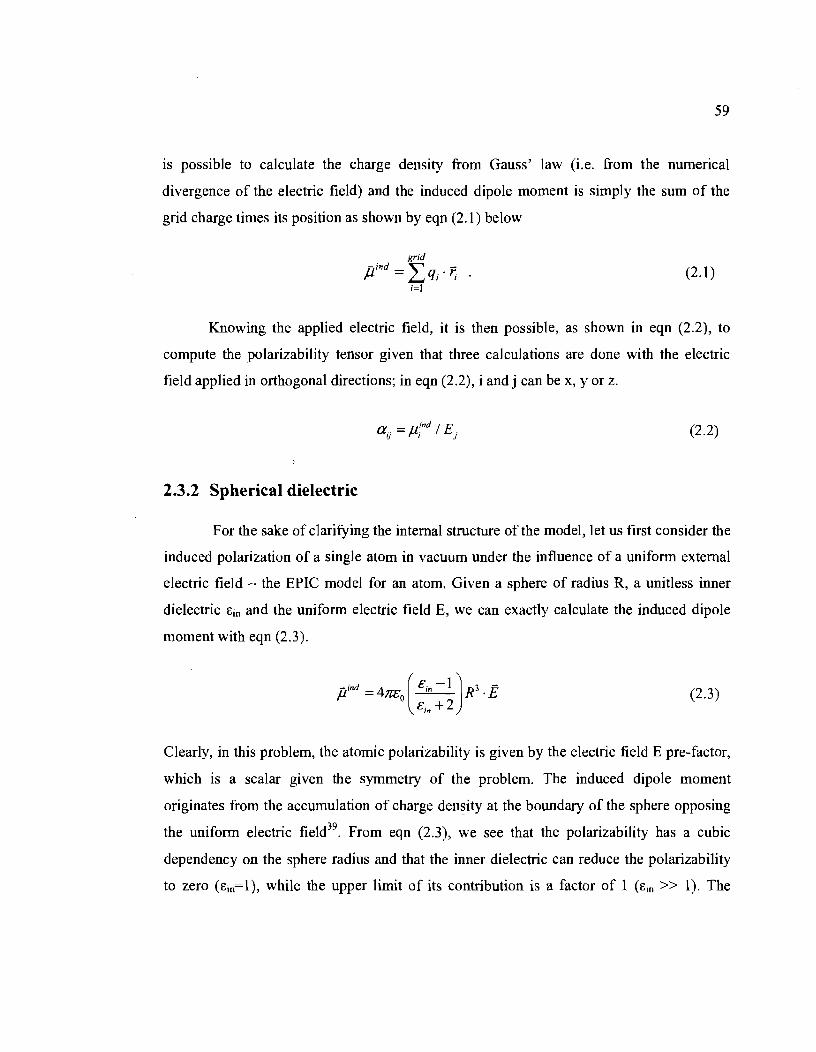
59

is possible to calculate the charge density from Gauss' law (i.e. from the numerical

divergence of the electric field) and the induced dipole moment is simply the sum of the

grid charge times its position as shown by eqn (2.1) below

(2.1)

Knowing the applied electric field, it is then possible, as shown in eqn (2.2), to

compute the polarizability tensor given that three calculations are done with the electric

field applied in orthogonal directions; in eqn (2.2), i andj can be x, y or z.

(2.2)

2.3.2 Spherical dielectric

For the sake of clarifying the internaI structure of the mode1, let us first consider the

induced polarization of a single atom in vacuum under the influence of a uniform external

electric field - the EPIC model for an atom. Given a sphere of radius R, a unitless inner

dielectric Ein and the uniform electric field E, we can exactly ca1culate the induced dipole

moment with eqn (2.3).

(2.3)

Clearly, in this problem, the atomic polarizability is given by the electric field E pre-factor,

which is a scalar given the symmetry of the problem. The induced dipole moment

originates from the accumulation of charge density at the boundary of the sphere opposing

the uniform electric field39. From eqn (2.3), we see that the polarizability has a cubic

dependency on the sphere radius and that the inner dielectric can reduce the polarizability

to zero (Ein=l), while the upper limit of its contribution is a factor of 1 (Ein » 1). The

60

contribution of Ciu to the atomic polarizability asymptotically reaches a plateau as shown in

Figure 2.1.

1.0

N 0.8 + e: .!if 0.6 -..-~

le: 0.4 w-- 0.2

0.0 ~ ___________ ----l

o 10 20 30 40 50 60 70 80 Inner dielectric (Sin)

Figure 2.1. The dielectric contribution to the sphere dielectric continuum polarizability goes asymptotically to one and most of the contributions are below Ciu = 10.

It is interesting to make a parallel between eqn (2.3) and the PID mode l, where the

polarizable point would be located exactly at the nucleus. In this particular case, it is

possible to equate the polarizability from PE, induced by the radius and the dielectric, to

any point polarizabilityll . However, when the electric field is not uniform, the PID induced

atomic dipole originating from the evaluation of the electric field at a single point may not

be representative, leading to inaccuracies41. This is in contrast with the EPIC model that

builds the response based on the electric field lines passing through the entire surface

defined by the sphere, allowing a response more complex than that of a point dipole. In

molecules, the atomic polarizabilities of the PID model do not find their counterparts in the

EPIC model since it is difficult to assign non-overlapping dielectric spheres to atoms and

obtain the correct molecular behavior. The Ch molecule studied in this work is an example.

61

2.4 Methods

2.4.1 Calculations

Prior to the DFT calculation, SMILES42-44 strings of the desired structures were

transformed into hydrogen-capped three-dimensional structures with the program

OMEGA 45. The n-octane conformer set was also obtained from OMEGA. The resulting

geometries were optimized with the Gaussian'0346 pro gram using B3L yp4749 with a 6-

31 ++G(d,p) basis setSO•51 without symmetry. The atomic radii and molecular inner

dielectrics were fit based on molecular polarizability tensors calculated at the B3L YP level

of theory52 with the Gaussian'Q3 program. The extended Dunning's aug-cc-p VTZ basis

set53.54, known to lead to accurate gas phase polarizabilities, was used55• An extended basis

set is required to obtain accurate gas phase polarizabilities that would otherwise be

underestimated.

The solutions to the PE were obtained with the finite difference PB solver Zap56

from OpenEye Inc. modified to allow voltage c1amping of box boundaries to create a

uniform electric field. The electric field is applied perpendicularly to two facing box sides

(along the z axis). The difference between the fixed potential values on the boundaries is set

to meet: ô-<p == Ez x ô-Z, where ô-<p is the difference in potential, Ez is the magnitude of the

uniform electric field and t1Z is the grid length in the z direction. The salt concentration was

set to zero and the dielectric boundary was defined by the vdW surfaces. The grid spacing

was set to 0.3 A and the extent of the grid was set such that at least 5 A separated the box

wall from any point on the vdW surface. As detailed in the Supporting Information, grid

spacing below 0.6 A did not show significant deterioration of the results. Small charges of

±O.OOle were randomly assigned to the atoms to ensure ZAP would run, typically

converging to 0.000001 kT.

62

In tables where optimized parameters are reported, a sensitivity value associated

with each fitted parameter is also reported. The sensitivity of a parameter corresponds to its

smallest variation producing an additional 1 % error in the fitness function considering only

molecules using this parameter. The sensitivity is calculated with a three-point parabolic fit

around the optimal parameter value and the change required obtaining the 1 % extra error is

extrapolated. Therefore, the reported sensitivity indicates the level of precision for a given

parameter and whether or not sorne parameters could be eventually merged.

2.4.2 Fitting procedure

Eqn (2.4) shows the fitness function F utilized in the fitting of the atomic radii, and

the inner dielectrics.

F({R},{E})=_I_f L laffMQ~aij 1+_I_tl-lviM ,v~l. 3N 1=1 j=xx,n',zz aij Na i=1 1 cos 45

(2.4)

In eqn (2.4), N corresponds to the number of molecules used in the fit, aij to the

polarizability component j of the molecule i and Vij to the eigenvector of the polarizability

componentj ofmolecule i. Ne is the number ofnon-degenerate eigenvectors found in all the

molecules. This fitness function is minimal when the three calculated polarizability

components are identical to the QM values and when the corresponding component

directions are aligned with the QM eigenvectors of the polarizability tensor.

As shown in the Cb example (c.f. section 2.5.1), the hypersurface ofeqn (2.4) has a

number of local minima; it is important that our fitting procedure allows these to be

examined. Because the calculations were fast, we decided to proceed in two steps: First, a

systematic search was carried out varying each fitted parameter over a range and testing aU

combinations. The 30 best sets of parameters were then relaxed using a Powell

minimization algorithm and the set of optimized parameters leading to the smallest error

was kept.

63

2.4.3 Definitions

The polarizability tensor is a symmetric 3x3 matrix derived from six unique values.

It can be used to calculate the induced dipole moment ~i (i takes the value x, y and z) given

a field vector E

ind E E E Pi = a ix x + a iy y + a iz z (2.5)

In this work, we use the eigenvalues and eigenvectors of the polarizability tensor. The

eigenvalues are rotationally invariant and their corresponding eigenvectors indicate the

direction of the principal polarizability components. The three molecular eigenvalues are

named axx, ayy, Œzz and by convention axx ::; ayy ::; a,.2' The average polarizability (or

isotropie polarizability) is calculated with eqn (2.6) below. We also define the polarizability

anisotropy in eqn (2.7). This particular definition of anisotropy is an invariant in the Kerr

effect and has been often used in the literature57.

a xx + a}'V + a zz a = ' avg 3

(2.6)

(a -a )2 +(a -a )2 +(a -a )2 ila ::: xx yy xx II y}' zz (2.7) 2

Eqn (2.7) can be rewritten In terms of only two independent differences in the

polarizabilities as shown in eqn (2.8),

(2.8)

where a = a zz a)')! and b == a)}' - a.u ' In the case ~f degenerate molecules as in diatomics,

eqn (2.8) reduces to the unsigned difference between two different polarizability

eigenvectors.

64

We now define errors as used in the rest of this article. Eqn (2.9) gives the average

unsigned error of the approximated anisotropy (Au) where N corresponds to the number of

molecules, ai,avg to the average polarizability (eqn (2.6)) ofmolecule i and QM corresponds

to the DFT values.

(2.9)

Similarly, the average unsigned error of the average polarizability is defined by

(2.10)

Finally we define an average angle error between the eigenvectors v from QM and our

parameterized model as

(2.11 )

We prefer the use of the error in the average polarizabiliy, the anisotropy and the deviation

angle over the error in the polarizability components or the tensor elements. This allows us

to analyze the physical origin of the errors, and in particular how much eomes from

anisotropy, normally a more stringent property to fit

2.4.4 Molecule datasets

Our dataset is made to challenge the EPIe model with anisotropie cases known to

be difficult It is formed from three chemical classes: diatomics, heteroaromaties, and the

alkanes. White not comprehensive, these datasets were deemed sufficient for proof of

concept. Exeept for the diatomics, all the molecules examined are subdivided into 12

65

datasets and 6 chemical classes as in Figure 2.2. For each class there is a training set ('-t'

o o N

(; N

x r S~~ x ~_~N l'x '>.. X ~ l "" 0-l:J N "" X Q X X o x _ _ X X=N.O,S f

CH, ./'-.. /'-/ ~ A I,g I,g

X!-< 6OO O 9

H,C-CH, /'V'V'V ~ ~ I,g

<DO) ~hh x x x x, OOm o LN <l~ ~JN 1 Q # ~ 1 ~

X=NOS Xe

Figure 2.2 The molecules used are divided in 12 datasets and six chemical classes: the heteroaromatics training set 'aromatics-t' (a), the heteroaromatics validation set 'aromatics­v' (b), the pyridones training set 'pyridones-t' (c), the pyridones validation set 'pyridones-v' (d), the furans training set 'furans-t', the pyrroles training set 'pyrroles-t', the thiophenes training set 'thiophenes-t' (e), the furans validation set 'furans-v', the pyrroles validation set 'pyrroles-v', the thiophenes validation set 'thiophenes-v' (f), the alkanes training set 'alkanes-t' (g) and the alkanes validation set 'alkanes-v' (h). In the case of n-butane, n­hexane and n-octane, two conformers are considered: aIl trans (t) and gauche (g). The X atoms in a molecule are' either an 0, an S, or an NH.

postfix), used in the parameterization, and a validation set ('-v' postfix) to verify the

transferability of the obtained parameters.

Trying to cover most of the unsubstituted aromatic molecules, we selected 5 classes

of aromatics: aromatics, pyridones, pyrroles, furans and thiophenes. The aromatics are

limited to C, H and divalent N atoms. The pyridones contain aromatic amides; while these

also exist as their hydroxypyridine tautomers, in water the equilibrium is strongly driven

66

toward the pyridone form, which we exclusively study. The pyrroles, filfans and thiophenes

classes are made from the same scaffolds except differing by one atomic element for each

c1ass. In the training sets, balancing the number of molecules is important to avoid

overfitting. Each non-degenerate molecular polarizability tensor contributes six datapoints

(i.e. from six independent tensor elements). Degenerate molecules contribute either four or

one independent data points, depending on the degree of symmetry. The pyridones-v, the

pyrroles-v, the thiophenes-v and the furans-v sets aIl contain multiple functional groups.

The alkanes-t set contains both small and large isotropic molecules (methane and

neopentane). It also contains anisotropic molecules like trans-hexane. We included two

conformers of butane and hexane because their isotropie polarizability is similar but their

anisotropy differs. Cyclic species are also included due to their special nature. The alkanes­

v set contains fused cyclic alkanes and an octane in two different conformations of which

the trans form is highly anisotropic. We also mixed cyclic alkanes with chain alkanes in the

validation set; aIl this with the desire of having a validation set significantly different from

the training set to really assess the transferability of the fitted parameters. For this reason,

none of the molecules from the validation sets are used in the parameterization.

2.5 Results

2.5.1 Diatomics: the Ch polarizability hypersurface

The Ch homonuc1ear diatomie is the simplest molecule that unveils the dependency

of the polarizabilities on the radius and the inner dielectric. In Figure 2.3, parameter

hypersurfaces are illustrated for Ch made of two spheres of radius R separated by 2.05 A (DFT equilibrium distance) within which the inner dielectric is higher than one and the

outer dielectric set to the vacuum value of one. When the two spheres overlap (R > 1 A), the

molecular volume is described by a vdW surface. Figure 2:3a shows the contour plot of the

average polarizability of the molecule as a function of the Cl radius and inner dielectric. As

67

with the sphere polarizability, the radius has a strong impact on the average polarizability

and the influence of the inner dielectric is significantly redueed beyond a value of la. The

anisotropy, however, is more affected by the dielectric constant and varies less rapidly and

over a larger range of radius and dielectric than the average polarizability. The Ch example

illustrates the need for high dielectric compared to experimental values and this is

especially true when a molecule is highly anisotropic. Figure 2.3b shows that for low

values of the inner dielectric, the dependenee of the anisotropy on the radius diminishes.

Importantly, it is clear that the EPIC model does not have the polarizability

catastrophe problem associated with the PID family of polarizable models. When two

polarized spheres start tooverlap, the interaction between the induced dipoles does not

diverge. One reason for this is that the induced polarization is spread over spaee, rather than

being concentrated at a point. AIso, when two atoms approach each other, their volumes

and hence the total polarizability is decreased. Renee, the atomic radii in the EPIC model

play a role somewhat similar to the Thole shielding factor used in PID and DO models.

The Ch bond-parallel and -perpendicular polarizabilities obtained by DFT are 25.4

and 43.6 a.u. respectively, leading to an average polarizability of 31.4 a.u. and an

anisotropy of 18.2 a.u. Pairs of radius and dielectric that can reproduce the DFT values can

be visually identified by plotting the isolines of the fitness function (2.12) as shown in

Figure 2.3c.

(2.12)

68

1.7 1.7 1.7

E'1.6 1.6 1.6

0 !:; 1.5 1.5 1.5 CI)

Cl r:::: CO 1.4 1.4 1.4 -Cf) ~ 1.3 1.3 1.3

""C CO 0::: 1.2 1.2 1.2

1.1 1.1 1.1

1.0 1.0 1.0

5 10 15 20 25 5 10 15 20 25 5 10 15 20 25

Inner dielectric Inner dielectric Inner dielectric

a b c

Figure 2.3. The EPIC model behavior is explored for Ch. The average polarizability (a) and the anisotropy (b) isolines (in a.u.) are plotted as a function of the CI atomic radius, used to define the vdW surface, and the value of the inner dielectric. The target CI2 B3L YP values are 31.43 (average) and 18.24 (anisotropy) (c.f.Table 2.1). The polarizability tensor error function isolines in (c) identify the regions where the EPIC model matches the B3L YP polarizability tensor. The extemal dielectric is set to one and the inter-nuclear distance of Ch is fixed at 2.05A. These figures show that a high dielectric value is required to match the QM anisotropy, and that a number of minima can be found on the error hypersurface.

Four local minima are identified (three are obvious from the figure) from which two,

located at (R= 1.4,c= 11.5) and (R= 1.3,c=20.0) produce an overall error less than 5%. The

existence of the multiple minima is due to the multi-objective nature of the fitness function.

For instance, at (R=1.5, c=7.0) the average value is matched but not the anisotropy. Similar

hypersurfaces have been found with PE in a different contexe7,58. The error surface has

minima where the isolines of -30 a.u. in Figure 2.3b and the isoline of -20 a.u. in Figure

69

2.3c are close to each other, simultaneously matching the DFT values. Higher minima are

found when only one of the anisotropy or the average polarizability match the DFTvalues.

Finally, it is interesting to note, as alluded to in the previous section, that for Ch it is

not possible to assign a small sphere « 1 A) to each atom, no matter how large is the

dielectric, and reproduce the correct polarizability. This clarifies the difference between the

EPIC and PID models. Although they both serve the same purpose, the two models do not

present ideiltical physical pictures. For instance, shielding must be introduced explicitly in

PID whereas it is an intrinsic feature of the EPIC model.

2.5.2 Diatomics:. polarizability

Homonuclear diatomic molecules constitute a difficult·test for a polarizable model.

For example, the FQ model does not allow for bond-perpendicular polarizability, which is

typically half of the bond-parallel polarizability. van Duijnen et al. 14 have re-parameterized

the PID-Thole model and they obtained 22% error on the average polarizabilities of H2, N2

and Ch. Their error in the anisotropy is significantly larger. More recently, a special

parameterization for homo-halides with the PID-Thole model gave an error of9% and 82%

on the average polarizability and anisotropy of F2 respectively13. In the case of Ch, the

error on the average polarizability and anisotropy are 2% and 20%; finally for Br2 the same

authors found 0.8% and 13%. However, Birge20 assigned anisotropic atomic polarizabilities

and obtained the experimental v~lues for H2 and N2. These large errors of the models

without atomic anisotropy have been attributed to the difficulty of increasing the atomic

induced dipoles interaction. Fitting our model to match B3L YP/aug-cc-pVTZ molecular

polarizabilities lead to significantly smaller errors as shown in Table 2.1. In the best case,

we fit different inner dielectric and radius for each e1ement. This is a good example of

overfitting since two parameters are used to reproduce two polarizabilities. However, it is a

way to verify that the dielectric model is flexible enough to de al with the diatomics without

using atomic anisotropy parameters. Table 2.1 shows the results for five diatomic

70

Table 2.1. Compared polarizabilities (a.u.) of diatomic molecules when the radii and Ein are fit to B3L YP/aug-cc-pVTZ polarizabilities - two fitting methods are involved: 1 radius and 1 dielectric per element, 1 radius per element and a single dielectric for aIl five.

(lJ.. a.1I a.avg fla. Davg Daniso

{%t {%t H2 EPIC (0.88, 7.8)C 4.92 6.83 5.55 1.91 0.1 0.3

(0.83)d 4.47 6.60 5.18 2.12 6.7 4.1 B3LYP 4.92 6.81 5.55 1.89 expa 4.86 6.28 5.33 1.42

N2 EPIC (1.02,19.5r 10.49 15.89 12.29 5.40 1.8 3.7 (l.03)d 10.35 15.58 12.09 5.23 0.2 2.3

B3LYP 10.42 15.38 12.07 4.96 expa 9.8 16.1 11.90 6.3

F2 EPIC (0.86,20.5t 6.26 12.64 8.39 6.37 0.5 1.5 (0.84)d 6.06 11.20 7.77 5.14 6.9 16.3

B3LYP 6.18 12.68 8.35 6.50

Ch EPIC (1.34,19.3t 25.64 43.90 31.73 18.26 0.9 0.1 (l.34)d 25.38 43.03 31.26 17.65 0.7 1.9

B3LYP 25.35 43.59 31.43 18.24 expa 24.5 44.6 31.15 20.1

Br2 EPIC (l.53,17.5t 36.84 62.42 45.37 25.57 1.0 2.2 (1.52)d 36.19 62.73 45.04 26.54 1.7 0.1

B3LYP 36.96 63.53 45.82 26.57 aExperimental values are from ref 19.

bError relative to B3L YP values. cThe number in the parentheses are the optimal (radius A, dielectric) individually fit for each molecule. dThe optimal radius (in A) fit for each individual diatomic is reported in parentheses given a globally fit dielectric of 18.0.

molecules and the reported errors for the average polarizability and anisotropy are: 0.1 %

and 0.3% for H2, 1.8% and 3.7% for N2, 0.5% and 1.5% for F2, 0.9% and 0.1% for Ch,

1.0% and 2.2% for Br2. These results clearly show enough flexibility to account for both

71

average polarizability and anisotropy. The second fitting scenario involved a single

dielectric for aIl five molecules and five atomic radii, fitting 6 parameters to 10 data points.

The optimal parameters give results still in relatively good agreement with DFT with a

maximum of 16% error made in the case ofF2 anisotropy. For both optimal parameter sets,

the radii and dielectrics are reported in Table 2.1 in parenthesis. These encouraging results

on diatomics show that the EPIC model can correctly account for polarizability on a

minimal group of two atoms. Therefore, we expect that the local polarizability may be weIl

represented in larger molecules.

2.5.3 Organic datasets: typical PB parameters

As an initial check on how weIl typical radii and inner dielectric used in PB

applications cou Id reproduce the molecular polarizabilities, we first examined the set of

parameters obtained by Tan and LU012 that lead to reasonable dipole moments in different

continuum external dielectrics. In their work, they not only fit the inner dielectric but also

the atomic charges. They use the PCM radii and obtained a best inner dielectric of 4. This

combination of parameters produces an error of 52% in the average polarizability (eqn

(2.10)) compared to B3L YP (aIl molecules from Figure 2.2 and an error of 18% (eqn (2.9))

in the anisotropy as outlined in Table 2.2. In both cases, the standard deviations (STDEV)

of the errors are large. The other two sets of radii examined are those from CHARM2259

and Bondi60. We applied four representative inner dielectrics: 2, 4, 8 and 16 spanning the

range of dielectrics often reported to be optimal. Table 2.2 shows very high errors for aIl

the combinations, the best being Bondi radii with an Înner dielectric of 4 which lead to an

average polarizability error of 9% with a STDEV of 6% and an anisotropy error of 26%

with a STDEV of 15%. These particular parameters have a bimodal error distribution

producing smaller errors for alkanes than for aromatics, which is consistent with other

findings (vide infra). Clearly, the parameters from previous studies are not appropriate for

the calculation of vacuum molecular polarizabilities and they do not accurately account for

the electronic polarization. When attempting to only optimize the inner dielectric, while

72

keeping the atomic radii to their Bondi values, it was not possible to ob tain small errors on

the anisotropy. In the next sections, we present details about new parameterizations that are

in much better agreements with DFT values. As outlined in Table 2.2, we reduced the error

produced by the best Bondi combination by a factor of 4 for both the average polarizability

and anisotropy. The STDEV is also greatly reduced allowing for more confidence and

robustness in the polarizability predictions.

Table 2.2. Unsigned average errors for all molecules in Figure 2.2, relative to B3L YP/aug-cc-p VTZ, of average polarizability and anisotropy obtained with various parameters typically used in PB applications.

Radii ()avg STDEV ()aniso STDEV(%) Ein (%) (%) (%2 Tan et al.a 4 52 20 18 10

CHARM22b 2 40 13 47 23 4 26 26 28 13 8 84 40 17 26 16 129 50 54 44

Bondi C 2 51 6 47 23 4 9 6 26 15 8 51 15 14 16 16 91 17 52 29

EPIC/P2Ed 4.98 14.55 2 2 5 4 EPIC/PlEd 11.7 2 2 6 6

aReference 12. bReference 59. cBondi radii from reference 60. The Hydrogen radius is following Rowland and Taylor's recommendations61

.

dEPIC used with parameters fit in this work reported in ref. 1.

set to 1.1 A

2.5.4 Alkanes and aromatics

Figure 2.4a and b summarize the results obtained with the best parameter set, fitted

with two inner dielectrics (P2E), for the 12 sets formed by the 6 classes: alkanes, aromatics,

pyridones, pyrroles, furans and thiophenes. The optimal parameters with the atom-typing

73

scheme used to generate the molecular polarizabilities are given in Table 2.3, along with

Bondi radii60. In Figure 2.4, the comparisons are between the DFT polarizabilities and the

EPIe model. The errors are reported with histograms and error bars corresponding to the

average unsigned errors (eqns (2.9), (2.10) and (2.11» and the corresponding STDEV

indicating the range of variation of the errors.

Table 2.3. Optimized radii (À) and inner dielectrics with sensitivity° accounting for all molecule sets (Figure 2.2) - parameter sets P2E and PIE.

Atom type description Optimal Sensitivity Optimal Sensitivity Bondi

(P2E) (P2E) (PIE) (PIE) Radiib

alkanes e alkyl 1.39 0.04 1.13 0.03 1.70 H bond on an alkyl e 0.99 0.02 0.78 0.05 1.20 Dielectric alkanes 4.98 0.27 11.70 1.18

aromatics e aromatic 1.32 0.05 1.30 0.04 1.70 H bonded to aromatic e or N 0.64 0.09 0.78 0.05 1.20 N aromatic 1.06 0.16 1.10 0.14 1.55 o furan-like aromatic 0.74 0.23 0.75 0.27 1.52 o in pyridone carbonyl 0.95 0.25 1.03 0.16 1.52 S thiophene-like 1.50 0.06 1.58 0.05 1.80 Dielectric aromatics 14.56 1.50 11.70 1.18 aSmallest parameter variation required to produce a 1 % additional error in fitting function (see Method section for details). ~eference 60.

In Figure 2.4a, the error on the average polarizabilities is less than 3% for aU classes

of the training sets, less than 1 % for the thiophenes-t set and the combined average error is

less than 2%. The corresponding error on the average polarizabilities for the validation sets

in Figure 2.4b is slightly higher with a maximum of 3.2% for the pyrrole-v set; the

combined error is 2.4%.

While this low level of error obtained in the average polarizability has also been

observed with other polarizable methods, the anisotropy of the polarizability is less

74

tractable. Previous models normally require the use of directional atomic

pOlarizabilitiesI5,20,21 especial1y for aromatics. In our training sets, as shown in Figure 2.4a,

we obtain a combined error for the anisotropy of 4%. The worst set, pyridones-t, has an

average error of only 7.1 %. Although this c1ass is found in biologically active molecules,

we could not find published results from other empirical polarizable models for molecular

polarizability tensors. We believe that this class might be particularly difficult due to

variable aromaticity and accounting for a range of chemical functionalities with the same

parameters (imidazolones, 2-pyridones, 4-pyridones, etc.).

The anisotropy average error on the validation set in Figure 2.4b ranges from 2.5%

for the alkanes-v up to 7.4% for the aromatics-v. lt is not surprising that the error is larger

for the validation sets than for the training sets. Overall, however, when comparing the

anisotropy error made on the combined sets, it is not significantly higher: 5.3% for the

validation sets versus 4% for the training sets. On the other hand, the STDEV is

significantly higher in the validation set.

The aromatics class shows the highest anisotropy shift from the training set to the

validation set. Phenazine and phenanthrene are responsible for two out of three large

discrepancies between B3L YP and EPIC. lt is interesting to note that when comparing

B3L YP average polarizability and anisotropy to experiment, the errors are Il % and 30%

for phenazine, 17% and 20% for anthracene. The same errors, when comparing our model

and experiment, are 5% and 15% for phenazine, 1.7% and 1.4% for anthracene. The EPIC

model is thus more accurate for these molecules, which can be partIy explained by the

known size-consistency defect of DFT for oligocenes (benzene, naphthalene, anthracene,

tetracene, etc.) that are usually too anisotropic55• In general, DFT methods have problems

reproducing the polarizability of long delocalized molecules and this has been attributed to

deficiency of the currently used functionals to account for a self-interaction correction62. lt

75

f: J~ l14 _ .... nea-I ~ 14 _1I_v

~ 12

_ .."."MlCS-I

~ 12

_ .-ornatiCS-Y

.. pynd0ne5-1 pyndona-v

~ 10 _ pyr""es-l

! 60 110 _ pyrroIes-v

_ furana-I _ uans·y ~ , 60

.~ 8 f 50 _ thiophenes-v l'50 _ lhiophenn-I

.~ 8 i f 40 :0

_com_ t 40 :0 _ CClmbined

i 6 J 6 30

~: 1 4

20 ~ 4

2 ........ r ~o ~ 2 10

Q. 0 0 . - 0

a Bvo<age an, __

œv.atM>n Ingle b a_

anlsotropy _angle

_22 90 _22 90 ~2O

___ 1

~20 _ .lkanea-v _ aromatica-I 80 80 ~ 18 ~ 18 _ aromatics-v

~ 16 ...... P)'1cIonos·1 70 ~ 16 pyndones-v 70

~ 14

_ pyrroles-I

! 60 ~ 14 _ pyrrole ... ! 60 _ lurans-I

~ 12 _ lhiopl>enes-I f 50 -a' 12 f 50 _ combined c

:0 10

f 40 :0 10 40

~ 8 _ comblned (P2E)

30 j 8 30

J ~Uüw 20 l 6

20 4

~ u,llh 10 ~ 2 10

1 0 Q. 0 0

C lMfage anlsotropy dO'Jiallon Ingi. d _rage polarizabillty anlsotropy de""tion angle

Figure 2.4 Comparison between B3LYP/aug-cc-pVTZ polarizabilities and EPIC models P2E and PIE for ail molecules from Figure 2.2. The averaged relative error on average polarizability (egn (2.10)), anisotropy (egn (2.9)) and the deviation angle of the eigenvectors (egn (2.11)) are shown together with the corresponding STDEV reported as error bars. The results for the 2-dielectric fit (P2E) training sets (a) and validation sets (b) show small errors in the average polarizability and relatively small errors in the anisotropy. The results for the I-dielectric fit (P 1 E) training sets (c) and the validation sets (d) show larger errors in the alkanes anisotropy and generally larger errors th an the P2E parameters (shown under combined P2E). Combined errors of the training and validation sets are similar.

is therefore possible that our model, fit on smaller molecules, tend to produce better

behavior on these delocalized molecules. Another implication is that large molecules

should not be used for the training of a polarizable model with DFT methods. Figure 2.5a

shows that in fact the correlation between the polarizability components of the entire set of

molecules of Figure 2.2 is excellent up to 150 a.u. Part of the discrepancy might be

attributable to a different behavior of DFT methods in that range of polarizabilities. In this

respect, optimized effective potential (OEP) and time-dependent DFT methods have shown

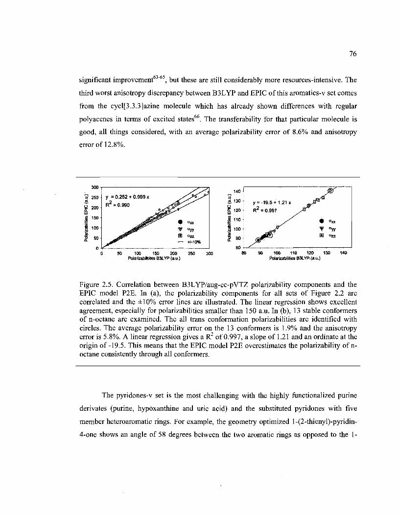
76

significant improvement63-65

, but these are still considerably more resources-intensive. The

third worst anisotropy discrepancy between B3L YP and EPIC ofthis aromatics-v set cornes

from the cyc1[3.3.3]azine molecule which has already shown differences with regular

polyacenes in terms of excited states66. The transferability for that particular moleculeis

good, aU things considered, withan average polarizability error of 8.6% and anisotropy

error ()f 12.8%.

300.,.----------------:,....-."

-; 250 ~ 1f 200 w J 150

~ 100 .~ ~ 50

y = 0.252 + 0.999 x

R2 = 0.990

• a.n

'5' "'II iii "zz

+/-10%

o~--------------------~ o 50 100 150 200 250 300

PoIarizabilitilesB3L'i'P (a.u.)

140

~130 u li: 120 w .1Il110 ~ .~ 100

~ 90

y = -19.5 + 1.21 x

R2 = 0.997

80~~-----------------' 80 90 100 110 120 130 140

Polarizabilities B3L'i'P (a.u.)

Figure 2.5. Correlation between B3LYP/aug-cc-pVTZ polarizability components and the EPIC model P2E. In (a), the polarizability components for all sets of Figure 2.2 are correlated and the ± 1 0% error lines are illustrated. The linear regression shows excellent agreement, especially for polarizabilities smaUer than 150 a.u. In (b), 13 stable conformers of n-octane are examined. The all trans conformation polarizabilities are identified with circ1es. The average polarizability error on the 13 conformers is 1.9% and the anisotropy error is 5.8%. A linear regression gives a R2 of 0.997, a slope of 1.21 and an ordinate at the origin of -19.5. This means that the EPIC model P2E overestimates the polarizability ofn­octane consistently through all conformers.

The pyridones-v set is the most challenging with the highly functionalized purine

derivates (purine, hypoxanthine and uric acid) and the substituted pyridones with five

member heteroaromatic rings. For example, the geometry optimized 1-(2-thienyl)-pyridin-

4-one shows an angle of 58 degrees between the two aromatic rings as opposed to the 1-

77

(oxadiazol)-imidazolone that has the two connected rings co-planar and a fully delocalized

electron 1t system. This datas et is not dissimilar from the chemical functionalization of

drug-like molecules.

The average angles between the eigenvectors of the polarizability components of the

B3LYP and EPIe are less than 5.5 degrees in a11 sets, although in sorne molecules the

angles can be as large as 23 degrees, i.e. for thiazole. For the pyridones-t and pyridones-v

sets, the angular diffences remain surprisingly small.

Fina11y, Table 2.4 shows that compared to experimental values, the parameterized

EPIe method performs comparably to B3L YP against the subset of 25 molecules for which

experimental data is available. Indeed, EPIe produces a ôavg of 3.9% with experiment

compared to 4.1 % for B3L YP. It also gives a Ôaniso of 9.0% with experiment compared to

10.5% in the case ofB3LYP. The STDEV of the errors from B3LYP match EPIe values.

The discrepancy between B3L YP and EPIe calculated for the molecules of Figure 2.2 is

sma11er leading to a ôavg of 1.9% and a Ôaniso of 4.6%. The level of error compared to

experiment obtained with both B3LYP and EPIe is not necessarily beyond experimental

uncertainty .

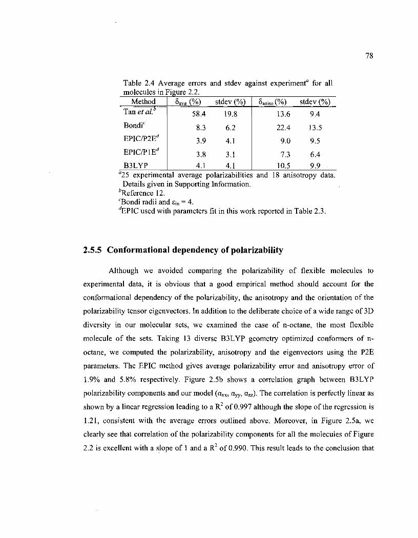
Table 2.4 Average errors and stdev against experimenta for all molecules in Figure 2.2.

Method ôav/( (%) stdev (%) Ôaniso(%) stdev (%) Tanetal. b 8 5 .4 19.8 13.6 9.4

BondiC 8.3 6.2 22.4 13.5

EPICIP2Ed 3.9 4.1 9.0 9.5

EPICIP1Ed 3.8 3.1 7.3 6.4

B3LYP 4.1 4.1 10.5 9.9 a25 experimental average polarizabilities and 18 anisotropy data.

Details given in Supporting Information. bReference 12. CBondi radii and Ein = 4. dEPIC used with parameters fit in this work reported in Table 2.3.

2.5.5 Conformational dependency of polarizability

78

Although we avoided comparing the polarizabi1ity of flexible mo1ecules to

experimental data, it is obvious that a good empirica1 method should account for the

conformational dependency of the polarizability, the anisotropy and the orientation of the

polarizability tensor eigenvectors. In addition to the deliberate choice of a wide range of 3D

diversity in our molecular sets, we examined the case of n-octane, the most flexible

molecule of the sets. Taking 13 diverse B3L YP geometry optimized conformers of n­

octane, we computed the polarizabi1ity, anisotropy and the eigenvectors using the P2E

parameters. The EPIC method gives average polarizability error and anisotropy error of

1.9% and 5.8% respective1y. Figure 2.5b shows a correlation graph between B3LYP

polarizability components and our model (axx, ayy, azz). The correlation is perfectly linear as

shown by a linear regression leading to a R2 of 0.997 although the slope of the regression is

1.21, consistent with the average errors outlined above. Moreover, in Figure 2.5a, we

c1early see that correlation of the polarizability components for all the molecules of Figure

2.2 is excellent with a slope of 1 and a R2 of 0.990. This result leads to the conclusion that

79

our model is at least consistently making the same errors for n-octane conformers compared

to B3L YP. Finally, the orientations of the polarizability components differ by 0.97 degrees

with a maximum value of 3.7 degrees; this is in spite of the broken symmetry in the gauche

octane conformers.

2.6 Discussion

2.6.1 Transferability

Shanker and Applequist15, with a variation of the PID model, studied seven

nitrogen heterocyclic molecules that we also included in our sets: pyridine, pyrimidine,

pyrazine, 9H-purine, quinoxaline, quinoline and phenazine. Using 12 parameters including

directional atomic polarizabilities, they show an average polarizability (eqn (2.10» and

anisotropy errors (eqn (2.9» of 10% and 12% respectively67; the parameterized EPIC

(Table 2.2) produces correspondingly 3% and 5% of error with only 4 parameters; we feel

that the reduced requirement for fitted parameters is due to a better physical model. Similar

comparisons can be made to the work of Miller21 where it is reported that 6 parameters for

benzene, 9 parameters for pyridine, 9 parameters for naphthalene and 12 parameters for

quinoline are needed to obtain both the average polarizability and anisotropy. With the

EPIC method, again the same 4 parameters do for aIl.

Recently, Williams and Stone68 have parameterized a polarizable model on n­

propane, n-butane, n-pentane and n-hexane in both their trans and gauche conformations.

With their simplest Ctg model, they use 10 atomic polarizability parameters to fit the

polarizability tensors to B3L YP values. They obtain a very smaU error on both the average

polarizability and the anisotropy of 1.16% and 2.37% respectively. Making the same

comparison with our mode l, we obtain 1.7% of average polarizability error and 3.99% of

anisotropy erroI. Although the error is slightly larger with our EPIC model, this is obtained

with only three parameters also producing similar levels of errors in our extended set of

80

alkanes. Furthermore, the level of errors reported by Williams et al. and our studies are all

within the accuracy ofB3LYP method.

The small number of parameters (c.f. Table 2.3) needed to fit all the aromatic

compounds of Figure 2.2 is a good indication of the transferability and the generality of the

method for heteroaromatic compounds. For example the same nitrogen radius could

simultaneously fit pyridine, pyridone, pyrrole, and ev en branched nitrogen. In the case of

alkanes, we have examined most characteristic shapes. Moreover, the training and

validation sets produce similar errors, thus the expected performance of our method in the

general case can be approximated by the errors on the validation sets.

Overall, we obtain the same level of error as the best PID methods parameterized

with anisotropic atomic polarizabilities and about threefold more parameters. Although the

number of parameters is not an issue for a small and homogenous set of molecules, it would

become a serious barrier for further development of a model applicable to the immense

functional group complexity of drug-like molecules, one of the main goals of this ongoing

effort.

2.6.2 100er dielectrics

The choice of fitting two inner dielectrics, one for the alkanes and one for the

heteroaromatics, makes the calculation of new mixed molecules such as t-butylbenzene not

possible unless we have a way to switch from a high dielectric (benzene) to a lower

dielectric (t-butyl) intramolecularly. Overall, the value of multiple dielectrics, based on

chemical constituency, seems proven as well as being physically reasonable. This is a

potentially useful strategy in the development of a future general polarizability model.

However, simultaneously fitting the polarizabilities of aU the compounds from Figure 2.2

with a single dielectric still gives reasonable results. Table 2.3 reports the values of the

optimal parameters used to produce the data of Figure 2.4c and d. We fit one radius per

element except for oxygen, which is split into furan~like and pyridone-like, and for carbon

81

which is split into alkane and aromatic. We first had two hydrogen radii, but there was no

significant cost to merge them into one single radius. The results, shown in Figure 2Ac and

d, when compared with those of Figure 2Aa and b, show a significant increase in the errors

on the alkanes-t and alkanes-v sets although the errors on the heteroaromatics classes

remain similarly small. It is nevertheless surprising that the level of error remains low when

describing the electronic dielectric with a single constant when, in princip le, the electronic

local polarization should vary intramolecularly as suggested by Oxtobl9.

Finally, it is reassuring that the best radii for both reported parameterizations follow

the chemical sense of atomic size. The remarkably reduced size of the optimal radii

compared to usuai soivent vdW radii (like Bondi) is worth few comments. First, our

reduced radii explain a different physical reàlity than the vdW radii: the former relates to

the electronic response and the latter to the repulsive vdW forces that keep solvent away,

for exampie. Furthermore, the high dielectric and the small radii were needed to fit the

correct polarizability anisotropy. This modulates the shape of the molecules. A benzene

molecule is flattened when the carbon radii are reduced and thus the out-of-plane

polarizable volume is reduced while the in-the-plane length is more or less conserved. The

polarizability density (also caUed the susceptibility given by Eox[Ein(r)-l]) being constant

inside the molecular vol~me, a higher die1ectric value is then needed to conserve the

molecular polarizability.

2.6.3 Link to the optical dielectric constants

Intramolecular dielectric constants in the context of PE or PB can adopt many

values depending on the system and the phenomeIia involved35,37,58,70 and have been

attributed values from 1 10 20. The optimal inner dielectric of solutes in continuum solvent

free energy and in ligand-prote in binding calculations do not agree37• Here, we attempt to

position our work in this jungle of dielectrics.

82

We are concerned uniquely with the electronic polarization component. None of the

optimal dielectric constants fitted in this work match the experimental optical dielectric

constants calculated as the square of the refractive index, which normally have values

between 1.2 and 4.0. We partly justify the need for larger dielectrics in section 6.2, but

there are other factors that should also be considered. It is important to realize that the link

between the molecular polarizability and the macroscopic optical dielectric constant is

given by the Lorentz-Lorenz relation shown in eqn (2.12) where N is the number of

molecule in the volume V and E is the macroscopic dielectric when the light frequency is

high compare to the dipolar or ionic relaxation time (Eo is the vacuum permittivity

constant).

a = 3e 0 V [ e -1 ] avg N e+2 (2.13)

In the Lorentz-Lorenz equation a molecule is approximated as a spherical dielectric with an

effective molecular volume given by the ratio of the macroscopic space occupied by one

molecule. Rowever, from our atomistic perspective the effective volume of a molecule is

defined by the electronic density and does not inc1ude the empty space between molecules

effectively inc1uded in eqn (2.12). Renee, in the EPIe model that we parameterize, the

average polarizability is the link to refractive index and not the inner dielectric. The main

reason for this is the inconsistency between the atomistic and macroscopic definitions of

the molecular volume. This raises the point that using experimental optical dielectrics

assigned to the solute interior in continuum solvent approaches should be further

questioned.

A misleading impression can also come from the non-linear behavior of the

dielectric on the polarizability. This brings us back to Figure 2.1 where we can appreciate

that if Ein is increased from 4 to 8, the polarizability pre-factor is increased from 0.5 to 0.7

while when Ein=14.6, our optimized aromatic dielectric, the pre-factor reaches 0.82 for an

83

increase of 64% over the Bin=4 case. Similar effects are also observed in non-spherical

shapes and this gives sorne perspective on the high inner dielectric constants that we obtain

in this work.

Finally, we believe that the use of accurate parameters to de scribe solute

polarizability in the context of continuum solvent could improve the quality of these

methods. Unfortunately, the radii and dielectrics obtained in the present work cannot be

used in continuum solvent models directly. Obviously, the solvent charge density should be

found at the regular vdW distances. Therefore, to simultaneously include the solute

electronic response and the correct solvent response, there is a dielectric region between our

optimal radii and the vdW radii that still needs to be elucidated. We believe that this

interesting question needs to be addressed to extend the use of our findings to implicit

solvent models. Once done, one could think of obtaining a polarizable model close to the

'polarizable continuum model' (PCM) of Tomase1 in which the electronic density would be

simply replaced by an 'electronic volume' defined with radii and a dielectric constant.

2.7 Conclusion

ln this work, the simple physical picture afforded by a continuum dielectric

representation has been used to accurately model molecular dipole polarizability tensors.

The molecular inner dielectric in the EPIC model accounts for the electronic polarization.

To tackle gas-phase polarizabilities, we capitalized on existing finite difference Poisson­

Boltzmann code to calculate the induced dipole moment of a molecule in vacuum in the

presence of a uniform electric field. As opposed to the usual use of PE or PB in continuum

models, the molecule is a region of higher dielectric and the external dielectric is set to the

vacuum value. The calculations are fast and resource-sparing, with equivalently good

results up to a grid spacing of 0.5 A, even though a discrete vdW dielectric boundary is

used.

84

This EPIC model of molecular polarizability possesses sorne important differences

with other approximations such as the point inducible dipole and the fluctuating charge

models. It is based on a local differential equation solved on a grid, which brings to the

same level of complexity the polarizability and coulombic electrostatic components. In

particular, EPIC avoids the polarizability catastrophe found in the other PID based models.

Furthermore, it allows, in principle, for a more thorough response to the electric field than

the PID or the FQ models based on the fact that the response emerges from the electric field

lines that cross the molecule surface instead of evaluations only at atomic nuclear positions.

This study involved the parameterization of atomic radii, used in the definition of

the vdW dielectric boundary, and the molecular inner dielectric. Previous values of these

variables found in the literature are unacceptably poor at approximating molecular

polarizability. We attribute this discrepancy to the fact that previous models simultaneously

optimize different kinds of interdependent parameters fitting to a complex energy property

instead of focusing on solute polarization. Indeed, the previous purpose of using dielectric

continuum was in the context of continuum solvent, often completely n~glecting the solute

response per se. To test the newly proposed method, we selected difficult chemical classes:

the homonuclear diatomics, a wide variety of heteroaromatics and a diverse set of alkanes.

A total of 5 diatomics plus 48 molecules are part of the training sets, subdivided into 6

chemical classes to which we add 45 molecules for validation purposes.

In previous models, the polarizabilities of these classes of compounds were

correctly calculated only when anisotropic atomic polarizabilities were employed (or

auxiliary sites in the case of FQ). Already, with about threefold less parameter than other

studies with different models, we have obtained averaged polarizability errors smaller than

5% and averaged anisotropy errors less than 8% considering all sets. The polarizability

components calculated with the EPIC/P2E model correlates very well with B3L YP/aug-cc­

pVTZ with a R2 of 0.990 and a slope of 0.999. The orientations of the polarizability

eigenvectors are also well reproduced. The flexibility of the model ev en allowed the

85

calculation of an accurate anisotropy for F 2 without resorting to auxiliary sites or

anisotropic parameters. We also found that the EPIC model was able to consistently

calculate the molecular polarizabilities on 13 different conformers of n-octane. Because of

the success of parsimonious parameterization of the EPIC model on difficult chemical

classes, we believe that the parameterization can be generalized for aIl organic chemistry

with adequate accuracy. In doing this, we found that intra-molecularly varying dielectric

constant might be needed to account for the molecular anisotropy.

Overall, this study exemplified that a phenomena as complex as electronÏc

polarization can be accurately modeled with a simple dielectric continuum mode!. The

principal implications of these findings are in the areas of Poisson-Boltzmann methods and

in polarizable force field development. However, the level of accuracy obtained might also

have impact beyond our initial consideration, for example in the field of spectroscopy.

2.8 Bibliography

1. Lane, N. F. Theory of Electron-Molecule Collisions. Rev. Mod. Phys., 1980,52,29-

119.

2. Kirkwood, J. G. On the Theory ofOptical Rotatory Power. J. Chem. Phys., 1937,5,

479-491.

3. Wagnière, G. H. Linear and Nonlinear Optical Properties of Molecules; VCH ed.;

VCH; Helvetica Chimica Acta Publishers: Weinheim, 1993.

4. Maroulis, G.; Hohm, U. Electric polarizabilitiesof Ge(CH3)(4) from collision­

induced light-scattering experiments and ab initio calculations. Phys. Rev. A, 2007,

76,032504.

5. Vela, A.; Gazquez, J. L. A Relationship Between the Static Dipole Polarizability,

the Global Softness, and the Fukui Function. J Am. Chem. Soc., 1990,112, 1490-

1492.

86

6. Nag1e, J. K. Atomic Po1arizability and Electronegativity. J Am. Chem. Soc., 1990,

J12,4741-4747.

7. Allen, T. W.; Andersen, O. S.; Roux, B. Energetics of ion con,duction through the

gramicidin channel. Proc. Natl. Acad Sei. Us. A., 2004, 101, 117-122.

8. Wick, C. D.; Kuo, L F. W.; Mundy, C. 1.; Dang, L. X. The Effect ofPolarizability

for Understanding the Molecular Structure of Aqueous Interfaces. J Chem. Theory

Comput., 2007, 3, 2002-2010.

9. Guo, H.; Gresh, N.; Roques, B. P.; Salahub, D. R. Many-body effects in systems of

peptide hydrogen-bonded networks and their contributions to ligand binding: A

comparison of the performances of DFT and polarizable molecular mechanics. J.

Phys. Chem. E, 2000,104,9746-9754.

10. Lipinski, C. A.; Lombardo, F.; Dominy, B. W.; Feeney, P. J. Experimental and i

computational approaches to estimate solubility and permeability in drug discovery

and development settings. Adv. Drug Deliv. Rev., 1997, 23, 3-25.

Il. Sharp, K.; Jean-Charles, A.; Honig, B. A Local Dielectric-Constant Model for

Solvation Free-Energies Which Accounts for Solute Polarizability. J. Phys. Chem.,

1992, 96, 3822-3828.

12. Tan, Y. H.; Luo, R. Continuum treatment of electronic polarization effect. J Chem.

Phys., 2007, 126, 094103.

13. Elking, D.; Darden, T.; Woods, R. 1. Gaussian induced dipole polarization model. J

Comput. Chem., 2007, 28, ]261-1274.

87

14. van Duijnen, P. T.; Swart, M. Molecular and atomic polarizabilities: Thole's model

revisited.1. Phys. Chem. A, 1998, 102, 2399-2407.

15. Shanker, B.; Applequist, J. Polarizabilities ofnitrogen heterocyclic molecules from

atom monopole dipole interaction theory. 1. Phys. Chem., 1996, 100, 3879-3881. .

16. Silberstein, L. Philos. Mag., 1917,33,521-533.

17. Bode, K. A.; Applequist, 1. A new optimization of atom polarizabilities in

halomethanes, aldehydes, ketones, and amides by way of the atom dipole interaction

model. 1. Phys. Chem., 1996, 100, 17820-17824.

18. Applequist, 1. Atom Charge-Transfer in Molecular Polarizabilities - Application of

the Olson-Sundberg Model to Aliphatic and Aromatic-Hydrocarbons. J. Phys.

Chem., 1993,97,6016-6023.

19. Applequist, 1.; Carl, J. R.; Fung, K. K. Atom dipole interaction model for molecular

polarizability. Application to polyatomic molecules and determination of atom

polarizabilities.1. Am. Chem. Soc., 1972,94,2952-2960.

20. Birge, R. R. Calculation of Molecular Polarizabilities Using An Anisotropic Atom

Point Dipole Interaction-Model Which Includes the Effect of Electron Repulsion. 1.

Chem. Phys., 1980, 72,5312-5319.

21. Miller, K. 1. Calculation of the Molecular Polarizability Tensor. 1. Am. Chem. Soc.,

1990,112,8543-8551.

22. Thole, B. T. Molecular Polarizabilities Calculated with A Modified Dipole

Interaction. Chem. Phys., 1981,59,341-350.

23. Warshel, A.; Levitt, M. Theoretical studies of enzymic reactions: Dielectric,

electrostatic and steric stabilization of the carbonium ion in the reaction of

lysozyme. 1. Mol. Biol., 1976, 103, 227-249.

24. Cieplak, P.; Kollman, P. A; Lybrand, T. A new water potential inc1uding

polarization: Appilcation to gas-phase, liquid, and crystal properties of water. J.

Chem. Phys., 1990,92,6755-6760.

25. Kaminski, G. A; Stem, H. A; Berne, B. J.; Friesner, R. A Development of an

accurate and robust polarizable molecular mechanics force field from ab initio

quantum chemistry. J. Phys. Chem. A, 2004, 108, 621-627.

88

26. Noskov, S. Y.; Lamoureux, G.; Roux, B. Molecular dynamics study ofhydration in

ethanol-water mixtures using a polarizable force field. J. Phys. Chem. B, 2005, 109,

6705-6713.

27. Lamoureux, G.; Roux, B. Modeling induced polarization with c1assical Drude

oscillators: Theory and molecular dynamics simulation algorithm. J. Chem. Phys.,

2003,119,3025-3039.

28. Gasteiger, J.; Marsili, M. New Mode1 for Calculating Atomic Charges in Molecules.

Tetrahedron Leu., 1978,3181-3184.

29. Rick, S. W.; Stuart, S. 1.; Berne, B. J. Dynamical fluctuating charge force fields:

Application to liquid water. J. Chem. Phys., 1994,101,6141-6156.

30. Rappe, A K.; Goddard, W. A Charge equilibration for molecular dynamics

simulations. J. Phys. Chem., 1991,95,3358-3363.

31. Chelli, R.; Procacci, P.; Righini, R.; Califano, S. Electrical response in chemical

potential equalization schemes. J. Chem. Phys., 1999,111,8569-8575.

32. Harder, E.; Anisimov, V. M.; Whitfield, T.; MacKerell, A D.; Roux, B.

Understanding the Dielectric Properties of Liquid Amides from a Polarizable Force ,

Field. J. Phys. Chem. B, 2008, 112,3509-3521.

33. Honig, B.; Nicholls, A Classical Electrostatics in Biology and Chemistry. Science,

1995,268,1144-1149.

34. Roux, B.; MacKinnon, R. The cavity and pore helices the KcsA K + channel:

Electrostatic stabilization of monovalent cations. Science, 1999,285, 100-102.

35. Antosiewicz, 1.; McCammon, J. A.; Gilson, M. K. Prediction of Ph-Dependent

Properties ofProteins. J. Mol. Biol., 1994,238,415-436.

89

36. Simonson, T.; Archontis, G.; Karplus, M. A Poisson-Boltzmann study of charge

insertion in an enzyme active site: The effect of dielectric relaxation. J. Phys. Chem.

B, 1999, J03, 6142-6156.

37. Naim, M.; Bhat, S.; Rankin, K. N.; Dennis, S.; Chowdhury, S. F.; Siddiqi, 1.;

Drabik, P.; Sulea, T.; Bayly, C. 1.; Jakalian, A.; Puri sima, E. O. Solvated Interaction

Energy (SIE) for Scoring Protein-Ligand Binding Affinities. 1. Exploring the

Parameter Space. J. Chem. Inf. Madel., 2007, 47, 122-133.

38. Fogolari,F.; Brigo, A.; Molinari, H. The Poisson-Boltzmann equation for

biomolecular electrostatics: a tooIJor structural biology. J. Mol. Recognit., 2002,

15, 377-392.

39. Griffiths, D. 1. Introduction ta Electrodynamics; 3rd ed.; Prentice-Hall Inc.: Upper

Saddle River, NJ, 1999.

40. Nicholls, A. The 233rd ACS National Meeting, Chicago, IL, March 25-29; 2007.

41. Schropp, B.; Tavan, P. The Polarizability ofPoint-Polarizable Water Models:

Density Functional TheorylMolecular Mechanics Results. J. Phys. Chem. B, 2008,

112, 6233-6240.

42. Weininger, D. Smiles .3. Depict - Graphical Depiction ofChemical Structures. J.

Chem. Inf. Madel., 1990,30,237-243.

43. Weininger, D.; Weininger, A.; Weininger, 1. L. Smiles .2. Aigorithm for Generation

of Unique Smiles Notation. J. Chem. Inf. Madel., 1989,29,97-101.

44. Weininger, D. Smiles, A Chemical Language and Infonnation-System .1.

Introduction to Methodology and Encoding Rules. J. Chem. Inf. Model., 1988,28,

31-36.

45. OMEGA, version 2.2.1; Santa Fe, NM, USA, 2007.

46. Gaussian 03, Revision C.02; Wallingford CT, USA, 2004.

90

47. Becke, A. D. Density-Functional Thennochemistry .3. the Role of Exact Exchange. ~

J. Chem. Phys., 1993,98,5648-5652.

48. Becke, A. D. A New Mixing of Hartree-Fock and Local Density-Functional

Theories. J. Chem. Phys., 1993,98,1372-1377.

49. Stephens, P. 1.; Devlin, F. 1.; Chabalowski, C. F.; Frisch, M. 1. Ab-Initio

Calculation ofVibrational Absorption and Circular-Dichroism Spectra Using

Density-Functional Force-Fields. J. Phys. Chem., 1994,98,11623-11627.

50. Frisch, M. J.; Pople, J. A.; Binkley, J. S. Self-consistent molecular orbital methods.

Supplementary functions for Gaussian basis sets. J. Chem. Phys., 1984,80,3265-

3269.

51. Clark, T.; Chandrasekhar, 1.; Spitznagel, G. W.; Schleyer, P. V. Efficient Diffuse

Function-Augmented Basis-Sets for Anion Calculations .3. the 3-21 +G Basis Set

for ISt-Row Elements, Li-F. J. Comput. Chem., 1983,4,294-301.

52. Rice, 1. E.; Handy, N. C. The calculation offrequency-dependent polarizabilities as

pseudo-energy derivatives. J. Chem. Phys., 1991, 94, 4959-4971.

53. Woon, D. E.; Dunning, 1. Gaussian basis sets for use in correlated molecular

calculations. III. The atoms aluminum through argon. J. Chem. Phys., 1993,98,

1358-1371.

91

54. Kendall, R. A.; Dunning, J.; Harrison, R. J. Electron affinities of the first-row atoms

revisited. Systematic basis sets and wave functions. J. Chem. Phys., 1992,96,6796-

6806.

55. Hammond, J. R.; Kowalski, K.; deJong, W. A Dynamic polarizabilities of

polyaromatic hydrocarbons using coupled-cluster linear response theory. J. Chem.

Phys., 2007, 127, 144105.

56. Grant, J. A; Pickup, B. T.; Nicholls, A A smooth permittivity function for Poisson­

Boltzmann solvation methods. J. Comput. Chem., 2001, 22,608-640.

57. Kassimi, N. E. B.; Lin, Z. J. Aza-substituted thiophene derivatives: Structures,

dipole moments, and polarizabilities. J. Phys. Chem. A, 1998, 102,9906-9911.

58. Rankin, K. N.; Sulea, T.; Puri sima, E. O. On the transferability ofhydration­

parametrized continuum electrostatics models to solvated binding calcu1ations. J.

Comput. Chem., 2003,24,954-962.

59. MacKerell, AD.; Bashford, D.; Bellott, M.; Dunbrack, R. L.; Evanseck, J. D.;

Field, M. J.; Fischer, S.; Gao, 1.; Guo, H.; Ha, S.; Joseph-McCarthy, D.; Kuchnir,

L.; Kuczera, K.; Lau, F. T. K.; Mattos, C.; Michnick, S.; Ngo, T.; Nguyen, D. T.;

Prodhom, B.; Reiher, W. E.; Roux, B.; Schlenkrich, M.; Smith, 1. c.; Stote, R.;

Straub, 1.; Watanabe, M.; Wiorkiewicz-Kuczera, 1.; Yin, D.; Karplus, M. AI1-Atom

Empirica1 Potential for Molecular Modeling and Dynamics Studies of Proteins. J.

Phys. Chem. B, 1998,102,3586-3616.

60. Bondi, A van der Waals Volumes and Radii. J. Phys. Chem., 1964, 68, 441-451.

61. Rowland, R. S.; Taylor, R. lntermolecular nonbonded contact distances in organic

crystal structures: Comparison with distances expected from van der Waals radii. J.

Phys. Chem., 1996, 100, 7384-7391.

62. Sekino, H.; Maeda, Y.; Kamiya, M.; Hirao, K. Polarizability and second

hyperpolarizability evaluation of long molecules by the density functional theory

with long-range correction. J. Chem. Phys., 2007, 126, 014107.

92

63. van Faassen, M.; de Boeij, P. L. Excitation energies,for a benchmark set of

molecules obtained within time-dependent current-density functional the ory using

the Vignale-Kohn functionaL J. Chem. Phys., 2004, 120, 8353-8363.

64. van Faassen, M.; Jensen, L.; Berger, 1. A; de Boeij, P. L. Size-scaling of the

polarizability oftubular fullerenes investigated with time-dependent (current)­

density-functional theory. Chem. Phys. Leu., 2004, 395,274-278.

65. van Faassen, M. Time-dependent current-density-functional theory applied to atoms

and molecules. Int. J. Mod Phys. B, 2006,20,3419-3463.

66. Leupin, W.; Berens, S. 1.; Magde, D.; Wirz, 1. Pico second Fluorescence from the

2Nd Excited Singlet-State of Cyc1[3.3.3]Azine, A Bridged 12-Pi-Perimeter

Annulene - Spectra and Kinetics for S2 -] SO and S2 -] SI Transitions. J. Phys.

Chem., 1984,88, 1376-1379.

67. For purine and quinoxaline, the B3LYP/aug-cc-pVTZ components from tbis work

are used for the comparison since they match the experimental average

polarizability reported by Shanker et aL A veraged experimental components

reported by Shanker et al. are used for pyrimidine and pyrazine.

68. Williams, G. 1.; Stone, A 1. Transferable polarizabilities for the alkanes. Mol.

Phys., 2004, 102, 985-991.

69. Oxtoby, D. W. Local Polarization Theory for Field-Induced Molecular Multipoles.

J. Chem. Phys., 1980,72,5171-5176.

70. Elcock, A H.; Sept, D.; McCammon, 1. A Computer simulation ofprotein-protein

interactions. J. Phys. Chem. B, 2001, 105, 1504-1518.

--------~----_ .... ~ .... _~.

93

71. Miertus, S.; Scrocco, E.; Tomasi, J. Electrostatic Interaction of A Solute with A

Continuum ~ A Direct Utilization of Abinitio Molecular Potentials for the Prevision

ofSolventEffects. Chem. Phys., 1981, 55, 117~129.

3 Utiliser la polarisation provenant du continuum

interne pour les interactions intermoléculaires

Résumé. Récemment, le tenseur de polarisabilité moléculaire dans le vide de molécules

variées a été modélisé avec exactitude (Truchon, J.-F. et al, J Chem Theory and Comput

2008, 4, 1480) à l'aide d'un diélectrique intramoléculaire continu. Cette étude préliminaire a

montré que la polarisation électronique peut être bien modélisée lorsque des rayons

atomiques et des diélectriques internes appropriés sont employés. Dans cet article, avec les

paramètres ajustés pour reproduire des polarisabilités moléculaires ab initio quantiques,

nous élargissons l'application de l'approche polarisation électronique provenant d'un

continuum interne (electronic polarisationfrom internai continuum: EPIC) aux interactions

intermoléculaires. Nous dérivons d'abord DRESP (diélectrique RESP) qui est une nouvelle

procédure fondée sur la méthode des moindres carrés pour ajuster les charges atomiques

partielles sur le potentiel électrostatique quantique en présence d'un diélectrique interne> 1.

Nous esquissons également une procédure pour adapter tout modèle de charges atomiques

existant à l'approche EPIC. L'étude de la capacité du modèle EPIC à reproduire une

polarisation locale, par opposition à une polarisation uniforme, résulte en une racine du

carré de la déviation égale à 1 % relativement aux calculs quantiques lorsque moyennée sur

37 molécules dont des hétéroaromatiques et des alcanes. L'avantage du modèle polarisable

continu sur les modèles avec polarisabilité centrée sur les atomes est illustré avec un atome

et une molécule de benzène qui sont symétriquement perturbés. Nous appliquons EPIC à un

système composé d'un cation atomique et d'une molécule de benzène formant une

interaction cation-n:, ce qui montre que rapproche étudiée donne une bonne énergie

d'induction. Finalement, cet article montre que la composante quantique de l'énergie

électrostatique dans un pont-H très polarisé, liant le dimère de 4-pyridone (molécule très

polaire et très polarisable), est bien reproduite sans ajustement de paramètres

supplémentaires.

95

Mise en contexte. Nous avons démontré au chapitre précédent que l'idée d'utiliser un

continuum diélectrique pour reproduire le tenseur de polarîsabilité moléculaire fonctionne

mieux que les approches précédentes. Or, notre objectif ultime n'est pas seulement de

reproduire la polarisabilité moléculaire, mais aussi d'utiliser EPIC dans un champ de force

dans le contexte de simulations de biomolécules en solution.

Un premier pas de plus que nous ferons dans ce chapitre sera d'évaluer comment le

potentiel électrostatique induit par un champ qui n'est pas uniforme, mais plutôt local, se

compare avec les résultats de la mécanique quantique. En effet, en solution, une molécule

subit un champ électrique qui est loin d'être uniforme. Il n'est donc pas évident que

l'ajustement des rayons atomiques et de la constante diélectrique interne du chapitre

précédent puisse être adapté au cas d'intérêt.

Deuxièmement, le couplage entre la polarisation intramoléculaire et les charges atomiques

partielles pose un défi considérable à la communauté scientifique qui voudrait généraliser

les paramètres. Dans ce chapitre, nous dérivons les équations et la méthodologie

nécessaires à l'obtention de charges atomiques partielles qui reproduisent le potentiel

électrostatique permanent prédit par la mécanique quantique dans le contexte où ces

charges baignent dans un milieu diélectrique. Ceci est essentiel à l'obtention du terme

d'interaction électrostatique dans un champ de force. Conservant l'idée d'avoir une méthode

polyvalente et des paramètres complètement généraux, nous montrerons que, contrairement

aux approches prises jusqu'à maintenant, nous sommes en mesure de découpler

l'optimisation de la polarisabilité et des charges atomiques partielles.

Finalement, nous construirons un champ de force pour calculer le terme d'énergie

d'interaction de deux dimères dans le vide pour lesquels la polarisabilité joue un rôle

crucial.

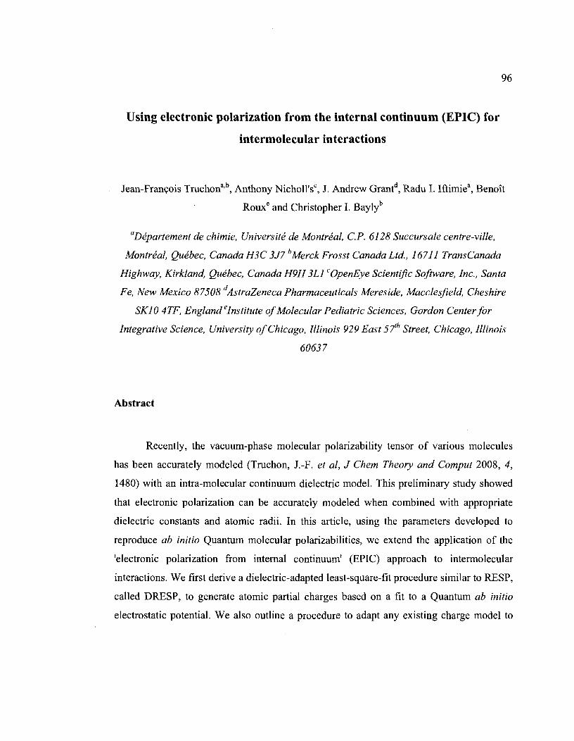
Using electronic polarization from the internai continuum (EPIe) for

intermolecular interactions

96

Jean-François Truchona,b, Anthony Nicholl'sC, J. Andrew Grantd, Radu 1. Iftimiea, Benoît

Rouxe and Christopher I. Bayll

aDépartement de chimie, Université de Montréal, c.P. 6128 Succursale centre-ville,

Montréal, Québec, Canada H3C 3J7 b Merck Frosst Canada Ltd., 16711 TransCanada

Highway, Kirkland, Québec, Canada H9H 3Ll COpenEye Scientific Software, Inc., Santa

Fe, New Mexico 87508 dAstraZeneca Pharmaceuticals Mereside, Macclesfield, Cheshire

SK10 4TF, EnglandeInstitute of Molecular Pediatrie Sciences, Gordon Center for

Integrative Science, University of Chicago, Illinois 929 East 5th Street, Chicago, Illinois

60637

Abstract

Recently, the vacuum-phase molecular polarizability tensor of various molecules

has been accurately modeled (Truchon, J.-F. et al, J Chem Theory and Comput 2008, 4,

1480) with an intra-molecular continuum dielectric model. This preliminary study showed

that electronic polarization can be accurate1y mode1ed when combined with appropriate

dielectric constants and atomic radii. In this article, using the parameters developed to

reproduce ab initio Quantum molecular polarizabilities, we extend the application of the

'electronic polarization from internaI continuum' (EPIC) approach to intermolecular

interactions. We first derive a dielectric-adapted least-square-fit procedure similar to RESP,

called DRESP, to generate atomic partial charges based on a fit to a Quantum ab initio

electrostatic potential. We also outline a procedure to adapt any existing charge model to

97

EPIe. The ability of this to reproduce local polarization, as opposed to unifonn

polarization, is also examined leading to an induced electrostatic potential relative root

mean square deviation of 1 %, relative to ab initia, when averaged over 37 molecules

including aromatics and alkanes. The advantage of using a continuum model as opposed to

an atom-centered polarizable potential is illustrated with a symmetrically perturbed atom

and benzene. We apply EPIe to a cation-n binding system fonned by an atomic cation and

benzene and show that the EPIe approach can accurately account for the induction energy.

FinaIly, this article shows that the ab initia electrostatic component in the difficult case of

the H-bonded 4-pyridone dimer, a highly polar and polarized interaction, is weIl reproduced

without parameter adjustment.

98

3.1 Introduction

An intramolecular continuum dielectric model has been recently applied to the

calculation of molecular polarizabilities and shown to accurately reproduce those computed

using high-level ab intio Quantum Mechanical (QM) calculations1. The electronic

polarization from internaI continuum (EPIC) approach showed that, relative to other

methods, significantly less parameters were required to describe the anisotropy in

molecular polarizability which was illustrated by calculations on a set of aromatic, diatomic

and alkane molecules. This workfocuses on the ability of the parameterized EPIC model to

reproduce electrostatic potentials and in particular the response of this potential to external

electric fields typical of those responsible for electronic polarization in intermolecular

interactions. This is considered an essential feature for force-field based methodologies.

Many researchers have published work on combining a polarizable force-field with

Poisson-Boltzmann (PB) formalism mainly to take advantage of the implicit solvent

averaging modeled by a solvent dielectric constant. For example, the 'Polarizable Force

Field' (PFFi combines a point induced dipole (PID) model with a continuum solvent.

Similarly the 'Atomic Multipole Optimized Energetics for Biomolecular Applications'

(AMOEBA) force field couples a static multipolar expansion with atomic polarizabilities3

in the context of a PB description of solvent. However, such models are computationally

complex requiring atomic tensors to model response effects. In contrast, this work

demonstrates that solute polarizability can be modeled using simple dielectric response

theory, and requires only a small number of fitled atomic radii and isotropic relative

permittivities (dielectrics). Here, however, we focus on explicit interactions, not on solvent

reaction fields. Complex electron distributions and response are modeled using atom­

centered point charges and a continuum dielectric. A crucial feature of the model is that

screening effects produced by intramolecular polarization of the dielectric are explicitly

99

accounted for in calculating atomic charges by least-squares fitting to the electrostatic

potential (ESP) computed using ab initio Quantum techniques.

This article describes such a modified RESP4 approach to calculating atomic

charges from the ESP. To indicate that dielectric screening is accounted for in the model,

the approach is referred to as DRESP. In the rest of this article, we derive the equations

relative to DRESP and show the resulting charges on few examples. Additionally, we

propose a general way of adapting an existing charge model to behave properly when used

with EPIC and we show its performances in reproducing the AMI-BCC5,6 permanent ESP

on selected molecules. The ability of the proposed polarization model to reproduce the

response to non-uniform perturbations is also examined. In doing this, we have found that it

is not necessary to refit radii and dielectric values optimized based on the vacuum-phase

molecular polarizabilities only, thus our previously published parameter sets! are directly

applied. These findings suggest that a general smaU molecule polarizable model based on

continuum electrostatics could be developed. Finally, we apply the EPIC polarizable model

to two problems of fundamental importance in biological applications (namely cation-n

binding and H-bonding) to demonstrate its performance.

3.2 Methods

Below, a least-squares method, hereafter named DRESP, is derived for fitting

atomic point charges to a QM electrostatic potential in the presence of an internaI dielectric.

The computational details for both the finite difference Poisson's equation (PE) solver and

B3L YP calculations are then presented. Details on the calculation of the induced ESP are

also given. Finally, the mole cule dataset used to validate the current approaches is

described.

100

3.2.1 A Least-Squares Method

The derivation presented in this section is a generalization of the least-squares

method already in use to fit atomic charges to an ESP computed on a grid. Finding the

optimal set of atomic charges in the presence of a locally changing dielectric requires a

special treatment. For example, Tan and Lu07 designed an iterative optimization scheme.

The objective here is to obtain a set of equations linear in the atomic charges that can .be

easily and quickly solved computationally. The following derivation uses the Poisson's

equation linearity in both the charge density and the potential such that the solution for each

individual charge can be superimposed to produce the correct solution for the entire system.

The ESP at a point r of space, q;(r), can be written in an integral formulation with a

kemel function G(r,r~ (a Green's function) that defines the contribution of the local charge

density p(r~ at a point r of space as shown in (3.1). The discrete nature of point charges

allows us to write the charge density as a sum of N Dirac delta functions t5 centered at each

of the N charge positions ri in (3.2) leading to (3.3):

rp(r) = J G(r,r ')p(f ')df' (3.1)

n

= JG(f,r')(~>5(r'-?;)QJdf' (3.2) i=1

N

= LG(f,?;)Q (3.3) i=l

Now, we define a basis of N atom-source potential <I>i (f) functions which describe the

potential produced by a unit charge placed at atom i, setting aIl the other atomic charges to

zero. Thus from (3.3):

<I>i (f) = G(r,?;) (3.4)

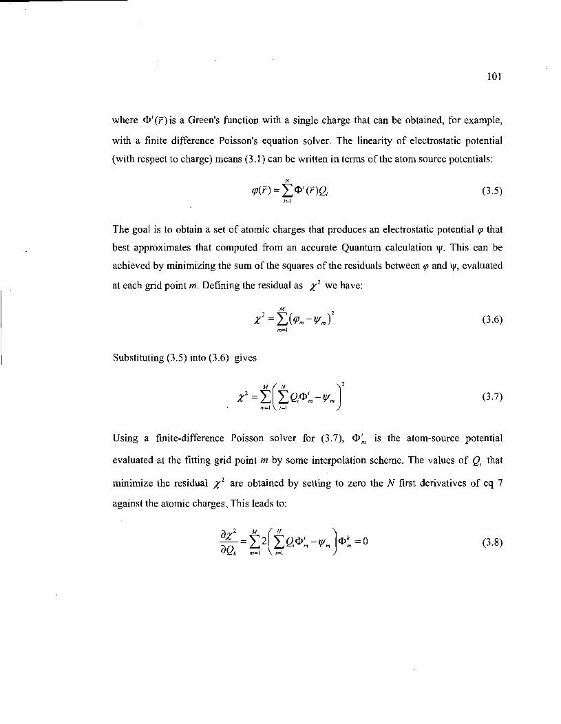
101

where «1>; (f) is a Green's function with a single charge that can be obtained, for example,

with a finite difference Poisson's equation solver. The linearity of electrostatic potential

(with respect to charge) means (3.1) can be written in terms of the atom source potentials:

N

qJ(f) = L «1>; (f)Q (3.5) ;=1

The goal is to obtain a set of atomic charges that produces an electrostatic potential cp that

best approximates that computed from an accurate Quantum calculation \jf. This can be

achieved by minimizing the sum of the squares of the residuals between cp and \jf, evaluated

at each grid point m. Defining the residual as X2 we have:

M

X2 = L( qJm -lf/m)2 (3.6) m=1

Substituting (3.5) into (3.6) gives

(3.7)

Using a finite-difference Poisson solver for (3.7), «I>~ is the atom-source potential

evaluated at the fitting grid point m by sorne interpolation scheme. The values of Q; that

minimize the residual X2 are obtained by setting to zero the N first derivatives of eq 7

against the atomic charges. This leads to:

(3.8)

To simplify the notation, we define a matrix A and a vector b:

M

" i k Ait = L.... <p m <p m

m=1

M

b. = "liE <pi 1 ~Y'm m

m=1

The linear system of equations to solve becomes

N

bi = LAikQk k=1

102

(3.9)

(3.10)

(3.11)

(3.12)

If the internaI dielectric is set to 1 (vacuum and no polarization) in the computation of

atom-source potentials, then the linear equations in (3.12) are those used by RESP4•

However by introducing an arbitrary dielectric to model solute polarizability in the

calculation of the atom-source potentials, it is possible to account for the contribution of

polarization effects in obtaining charges that fit to the Quantum electrostatic potential. In

practice, one can solve Poisson's equation and interpolate the electrostatic potential on the

fitting grid for each Green's function related systems. In general, this procedure requires a

solution per point charge. It is also possible to incorporate Lagrangian constraints and

regularizing restraints as with RESP4• The introduction of the dielectric effects into the

overall procedure is indicated by calling the modified procedure Dielectric RESP (DRESP).

In this work, while we choose to not use restraints, we constrained topologically equivalent

atoms to have identical charges and applied a constraint to the molecular formaI charge. For

example, the high symmetry of benzene leads to only one charge degree of freedom

whereas in 4-pyridone there are 7 such degrees of freedom. In the remainder of this work,

103

we set the hyperbolic restraints to zero for the aIl the fit using a dielectric of one (RESP) or

higher (DRESP). Normally the RESP hyperbolic restraints reduce the charges to make

them more transferable at the expense of reducing the fit quality; for this work restraints

were not used. FinaIly, the general formulation presented here allows to use any kind of

dielectric boundary functions (smoothed or not) and multiple dielectric values.

3.2.2 Computational details

Ab initio Quantum electronic calculations were aIl based on density functional

theory (DFT) using the B3L yp8-JO functional as implemented in the Gaussian 03 11

software. The molecular geometries were optimized as reported in a previous studyl with a

6-31++G(d,p) basisl2. Subsequent ESP and energy calculations were performed using these

optimal geometries but with an extended 6-311 ++G(3df,3pd) basis set. Molecular

symmetry was not used as part of the calculations and an accurate convergence criteria was

specified for the iterative calculation of the eLectron density matrix (by using the keyword

Scf=Tight, which sets the average density change to be smaller than 10-8 a.u.). Interaction

energies reported in this work were aIl corrected for basis set superposition error (BSSE)

using the Boys and Bemardi counterpoise method13•14

•

Finite difference Poisson calculations were done using the program Zap l5. A grid

spacing of 0.5 A was used to calculate potentials for both the DRESP charge fitting

procedure and in the analysis of induced polarization. A smaller grid spacing of 0.3 A was

needed when solving PE to obtain smooth intermolecular energy curves. The grid boundary

was positioned 10 A away from the closest point on the vdW surface. The convergence grid

energy was set to 0.00006 kcal/mol and a Richards vdW surface16 was used to define the

moLecular dielectric boundary. The molecule inner dielectric and atomic radii were based

on the parameterization that reproduced vacuum QM polarizabilities 1. The three parameter

sets reported previouslyl are examined in this work, namely: "P2E" a parameter set which

adopts different dielectric values for alkane and aromatic molecules, "PIE" parameter set in

104

which a single dielectric is used to describe the solute response of aU molecules, and finally

"Bondi" which combines a dielectric of 4 with Bondi radii 17 (H radius set to 1.1 A). The

P2E and Pl E parameter sets use optimal radii which are systematically smaller than Bondi

radii, necessary to accurately reproduce the anisotropy of the molecular polarizability.

In addition to the grid specific to the Zap calculations, a grid was needed to compute

the vacuum and the induced ESP . For this purpose, a face-centered cubic (FCC) grid

ranging from 1.4 to 2.0 times the atomic Bondi vdW radii was employed5,6. These distances

were determined to lead to an adequate sampling18 of the ESP for atomic charge

determination. The FCC grid spacing was set to 0.5 A.

3.2.3 Induced polarization

To examine the accuracy of the die1ectric polarization mode 1, molecules were

probed with a +0.5e point charge positioned exterior to the vdW surface ofmolecules. This

probe charge has been used by others19,2o and was recently shown to be well-adapted to

examine the polarizability of aromatics20. In this work, the probe charge positions were

determined using a single Conolly surface21 with a vdW distance scaling factor of 2.0 and a

density of 0.4 point per A2. Redundant probe charge positions, by symmetry, were partially

eliminated. For example, this resulted in benzene having 6 positions for the perturbing

charge, whereas 1,2,4-triazine had 47.

The induced potential is obtained by difference relative to the vacuum potential.

Care must be taken to eliminate the contribution of the perturbing point charge to the

calculation of the induction potential. This is handled automatically in the Quantum case as

a consequence of the coding of Gaussian03. However, when using Zap an extra calculation

is required to de termine the explicit Coulombic potential arising from the perturbing

charge. In total, the induced potential required three PE solutions per molecule on a

constant grid. The numerical accuracy was ensured with the low energy convergence

criterion.

105

The difference between QM induction potential (lf/) and that from EPIe model

( rp) is characterized as a relative root mean square deviation (RRMSD) as follows:

(3.13)

3.2.4 Molecule dataset

The molecule dataset used in this work contains 15 polar and non-polar aromatics

and 22 alkanes as shown in Figure 3.1. In addition, 4-pyridone is used in the study of a H­

bond potential. The aromatic molecules exhibit quite a large spectrum of values for the ESP

at the surface studied and possess a wide range of polarity. Due to their anisotropy, they

constitute a good challenge to polarizable methods. Because of their non-planarity,

biphenyl and its analogs have a different shape of the potential and a different conjugation

of the 1t electron system compared to the other aryl molecules. Finally, the alkanes are quite

polarizable in spite of their low polarity and the mole cules used exercise many kind of

shapes. Ail the molecule structures in this dataset are from the previous studyl.

3.3 Results and discussion

In this section, the ability of the proposed least-squares fitting method, DRESP, to

produce an accurate permanent electrostatic potential is first exàmined and compared to the

usualleast-squares fitting RESP approach. We then continue by proposing a general way of

coupling an existing charge model to EPIe, illustrated w1th the AMI-BeC charge model,

which 1S general and shows many advantages in condensed phase simulations5,6,22.23. The

ability of the EPIe approach to produce an accurate induced ESP in the presence of a

locally varying electric field is also examined. Finally, the polarizable and permanent

106

features of EPIe are used to study the electrostatic energy profiles in two challenging cases:

cation-TC and 4-pyridone H-bonded dimers.

o o . N benzene pyrimidine pyridine 1,2,4-triazine pyrazine triazine quinazoline

~ ~ naphthalene

CC)'-'::::'-':::: 8 N~

quinoline

00 biphenyl

N N lX) N N

phthalazine pyridazino[4.5-d]pyridazine pyrazino[2.3]pyrazine

O-C) 0 ~=) 5-phenylpyrimidine 3-phenylpyridazine

x methane ethane propane g,t-butane g,t-hexane g,t-octane isobutane neopentane

o 0 0 CO

decalin bicyclo[2.2.2]octane adamantane isopropylcyclopropane tert-butylcyclobutane

Figure 3. L Molecule dataset which contains aryls and alkanes chemical classes. These 15 aromatic and 21 alkane molecules are extracted from reference 1. We use the notation 't' to indicate the all-trans conformation and 'g' when one or more gauche dihedrals are present; these are separate entries.

107

3.3.1 DRESP vs RESP

Given the way EPIC incorporates electronic polarization, the usual strategy to fit

atomic partial charges to reproduce the QM ab initio ESP must be modified. This is due to

the presence of a dielectric continuum inside the molecular electronic volume that screens

the effects of a charge even at long distances. The DRESP approach, outlined in the

Method section, solves this issue and provides a set of linear equations that give the optimal

set of charges, in the least-squares sense, that reproduce the QM ab initio ESP. We first

apply DRESP with the P2E parameters and compare the RRMSD made on the permanent

ESP ofB3LYP for the molecules of Figure 3.1. The atomic partial charges are also fitted to

the same vacuum QM ESP using RESP. The DRESP charges are significantly larger than

those obtained with RESP. This is illustrated in Figure 3.2 for benzene, pyridine and

cyclopropane: the C/H charges ofbenzene are found to be ±O.12e as calculated with RESP

and ±O.61 with the dielectric P2E model calculated with DRESP, the charges on pyrimidine

are also significantly smaller. with RESP than with DRESP and similarly for the

cyclopropane. Although large and chemically counter-intuitive charges are needed when

Poisson's equation is used, they produce the same ESP as the regular coulombic approach.

Figure 3.2 also reports comparable RRMSD deviations between DRESP and RESP for

benzene, pyridine and cyclopropane. The RRMSD reported on cyclopropane is high, but it

is known that for simple alkanes the atomic partial charge approximation is poor24,25.

However, since the actual ESP for the alkanes is very small, this defect might be negligible

in intermolecular interactions although the alkane polarizability is not. Finally, it is

important to keep in inind that whenever a radius or an inner dielectric value change, the

DRESP charges cannot be transferred but must be re-optimized against the same QM ab

initio ESP grid.

108

H1 1

HX;( HXN192H3 H2, ~H l '

HAH H A H H ~C4HS H H7 H H

QRESP QORESP QRESP QORESP QRESP QORESP

H1 0.12 0.61 N1 -0.72 -2.56 C1 -0.28 -0.72 C2 -0.12 -0.61 C2 0.57 1.49 H2 0.14 0.36

H3 0.01 0.24 C4 -0.64 -1.26 Hs 0.21 0.60 C6 0.39 -0.20 H7 0.05 0.62

RRMS 14% 11% RRMS 13% 13% RRMS 66% 54%

Figure 3.2. Benzene, pyridine and cyc1opropane optimal charges fitting equally the same electrostatic potential with a dielectric of one (RESP, non-polarizable) and the P2E model (DRESP). The significantly higher charges with the P2E model cornes from the internaI dielectric screening of the point charges.

3.3.2 Use of an existing charge model: the AMI-BCC/DRESP example

AM 1-BeC from Jakalian et al. 5.6 is an accurate charge model applicable to aIl small

organic molecules and based on the over-polarized HF/6-3l * ESP known to pro duce good

charges adapted to polar media such as water. AMI-BeC was shown to be better or equal

to much more computationally expensive methods in matching experimental free energies

of solvation of small molecules22•26

• A significant advantage of AMI-BeC is that the

atomic point charges are obtained by adjusting with pre-fitted bond-charge corrections the

AM 1 electronic population analysis charges. Because the bond-charge corrections

published by Jakalian et al. are adapted to produce polar media charges, a gas-phase AMl­

BeC model is needed for use with a polarizable electrostatic model. In this work, we

demonstrate proof-of-concept for the coupling of a general AMI-Bee/vacuum model,

fitted to vacuum B3LYP/cc-pVTZ ESP27, to the dielectric polarizable model. The approach

109

taken here uses the AMI-BCC/vacuum charges to calculate the ESP on a fitting FCC grid,

detailed in the Methods section, to which dielectric adapted charges are fitted using the

DRESP method. We call this fitting strategy AMI-BCC/DRESP. Although we apply this

strategy to the AM 1-BCC/vacuum charging scheme, it is general in the sense that any other

charge model could be adapted the same way.

In Figure 3.3, we compare the B3LYP/6-311++G(3df,3pd) ESP to both the AMl­

BCC/vacuum and the AMI-BCCIDRESP ESP. The correlation between the two RRMSD is

excellent for aromatics and the AMI-BCC/DRESP charges produce slightly smaller

RRMSD for the alkanes, which we think is not significant given the low level of accuracy

for this chemical class. This demonstrates that extending an existing charge model,

developed in a non-polarizable context, is easy and accurate. More importantly, the·

parameterization of the poiarizable parameters and of the permanent charges can be fully

120 -~ 0 ~ 0

@ 100 Dl

::2 c::: c::: 0-en 80 UJ c::: Cl Ü 60 0 aromatics Ü

alkanes (0 0 1 ~

::2 40 «

20 20 40 60 80 100 120

AM1-BCC RRMSD (%)

Figure 3.3. Correlation plot of the RRMSD obtained with AMI-BCC and AMl­BCC/DRESP charging schemes. The RRMSD are calculated against the B3L YP permanent electrostatic potential on the FCC grid.

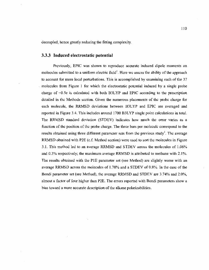
110

decoupled, hence greatly reducing the fitting complexity.

3.3.3 Induced electrostatic potential

Previously, EPIe was shown to reproduce accurate induced dipole moments on

molecules submitted to a uniform electric field 1• Here we assess the ability of the approach

to account for more local perturbations. This is accomplished by examining each of the 37

molecules from Figure 1 for which the electrostatic potential induced by a single probe

charge of +0.5e is calculated with both B3L YP and EPIe according to the prescription

detailed in the Methods section. Given the numerous placements of the probe charge for

each molecule, the RRMSD deviations between B3L YP and EPIe are averaged and

reported in Figure 3.4. This includes around 1700 B3LYP single point calculations in total.

The RRMSD standard deviation (STDEV) indicates how much the error varies as a

function of the position of the probe charge. The three bars per molecule correspond to the

results obtained using three different parameter sets from the previous studyl. The average

RRMSD obtained with P2E (c.f. Method section) were used to sort the molecules in Figure

3.1. This method led to an average RRMSD and STDEV across the molecules of 1.06%

and 0.3% respectively; the maximum average RRMSD is attributed to methane with 2.1 %.

The results obtained with the PIE parameter set (see Method) are slightly worse with an

average RRMSD across the molecules of 1.70% and a STDEV of 0.8%. In the case of the

Bondi parameter set (see Method), the average RRMSD and STDEV are 3.74% and 2.0%,

almost a factor of four higher than P2E. The errors reported with Bondi parameters show a

bias toward a more accurate description of the alkane polarizabilities.

c.. Cf) w "0 al u ::>

"0 .!; c.. >-...J C") ((l

If)

::> If) '-al > Cl Cf)

::2 0:: 0::

12%

11%

10% 9% 8% 7%

6%

5% 4%

3% 2% 1%

0%

_ P2E _ P1E _ Bondi

111

Figure 3.4. Average RRMSD on the induced ESP maps as calculated with EPIC using three parameter sets (P2E, PIE and Bondi, see the text). The ESP maps are generated by a +O.5e located at non-redundant positions and the reference induced ESP is calculated from B3L YP 6-311 ++G(3df,3dp) .

To examine the effect of induction by the +O.5e charge on the alkanes, non-polar

aromatics, and polar aromatics, it is of interest to compare the grid unsigned average of the

induced and vacuum ESPs for each c1ass. In the case of the alkanes, the unsigned average

of the induced ESP is about 3 times higher than the vacuum ESP evaluated on the fitting

grid. Benzene and non-polar aromatics have comparable induced and static ESP positive

magnitudes and, in the case of polar aromatics such as pyrimidine, the induced ESP is

between twofold and threefold smaller than the vacuum ESP. This indicates that the level

112

of electronic polarization is significant and appropriately challenging to the polarizable

model. The RRMSD obtained with the induced ESP is much lower than the RRMSD of the

static ESP fit by atomic charges. This shows that the model can accurately account for

locally induced polarization although the induced ESP is certainly simpler than the ESP

originating from the unperturbed molecule.

Here, we use the induced ESP to test the ability of the EPIC model, parameterized

solely on the QM gas phase polarizability tensor, in reproducing a molecule's induced QM

electronic response to a polarizing charge. The very smaU RRMSD obtained with the P2E

and the PIE parameter sets indicate that the local polarization with a non-uniform electric

field is as accurately modeled as the induced dipole moment due to a uniform electric field1

(molecular polarizability), the basis of the P2E and PIE parameterization. In contrast, most

previous polarizable models28-3o obtain their polarizability parameters (and often

simultaneously the charges) by fitting to the induced ESP on polarized molecules.

3.3.4 Induction by a symmetric field

The parameterization of polarizable models usually involves simple fields such as

uniform external electric fields or fields produced by a probe point charge or a probe

dipole. These external fields induce mainly a molecular dipole moment, which should be

reasonably weIl accommodated given a simple functional form for a polarizable model.

However, in condensed media, the electric field is rarely simple and is often transiently

symmetric around a molecule. In this section we compare the induced electrostatic potential

in a non-trivial electric field applied on an argon atom and benzene; three methods are

examined: point inducible dipoles, EPIC and B3L YP.

In the first system, the argon atom is sandwiched between tWQ positive point

charges positioned at 3.0 A above and below the atom. The EPIC argon radius used is set to

\ 113

1.31 A and the dielectric=7.36 as fit to reproduce the (gas-phase) B3L YP atomic

polarizability of argon (11.1 a.u.). Given the symmetry of this system, the net electric field

at the argon nucleus is zero. Since the point inducible dipole1 and the fluctuating charges31

polarizable models respond only to the net electric field at the nucleus, neither of these

models would show induction in this case. As illustrated on Figure 3.5, the B3LYP induced

electrostatic potential is a quadrupole with the dz2 hydrogenoid-like orbital symmetry.

Remarkably, the EPIe induced electrostatic potential has the same symmetry and is of

similar magnitude.

The second system examined consists of benzene sandwiched by two +1 e point

charges located at 2A above and below the ring. This is a fairly large perturbation where

the point charges are positioned approximately at the Lt Ibenzene equilibrium distance.

Although in nature it is unlikely that two Li+ atoms would be stable in such a sandwich

system, the perturbing electric field varies quickly from zero at the center of the benzene

ring to 2/r at infmity. So within the volume of the benzene, the field varies enough to

significantly test the model. The symmetry of this arrangement is such that the external

electric field has only a component in the plane of the ring at the atomic positions, although

the out-of-plane polarization should be predominant. A similar system was used to show

the failure of the fluctuating point charges model by Stem et al. 31• In princip le the point

inducible and related polarizability models should also have difficulty since the magnitude

of the induced 'potential would then be fully dictated by the in-plane polarizability

component For our comparison, we used the AMOEBA polarizability model for benzene

which includes a Thole exponential damping parame ter of 0.39 coupled with carbon and

hydrogen isotropic polarlzabilities of 1.334 A3 and 0.8 A3 respectively (as provided in

TINKER 4.2 distribution parameter file). The Thole parameter has the role of adjusting the

molecular polarizability anisotropy by reducing the atomic induced-dipole/induced-dipole

interactions thereby avoiding the polarizability catastrophe, inherent to the PID models.

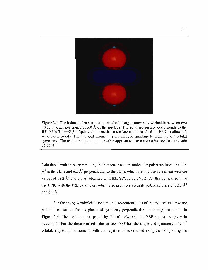
114

Figure 3.5. The induced electrostatic potential of an argon atom sandwiched in between two +0.5e charges positioned at 3.0 A of the nucleus. The solid iso-surface corresponds to the B3LYP/6-311 ++G(3df,3pd) and the mesh iso-surface to the result from EPIC (radius=1.3 A, dielectric=7.4). The induced moment is an induced quadrupole with the dz

2 orbital symmetry. The traditional atomic polarizable approaches have a zero induced electrostatic potential.

Calculated with these parameters, the benzene vacuum molecular polarizabilities are Il.4

A3 in the plane and 6.2 A3 perpendicular to the plane, which are in close agreement with the

values of 12.2 A3 and 6.7 A3 obtained with B3LYP/aug-cc-pYTZ. For this comparison, we

use EPIC with the P2E parameters which also produces accurate polarizabilities of 12.2 A3

and 6.6 A3.

For the charge-sandwiched system, the iso-contour lines of the induced electrostatic

potential on one of the six planes of symmetry perpendicular to the ring are plotted in

Figure 3.6. The iso-lines are spaced by 5 kcal/mol/e and the ESP values are given in

kcal/mol/e. For the three methods, the induced ESP has the shape and symmetry of a dz2

orbital, a quadrupole moment, with the negative lobes oriented along the axis joining the

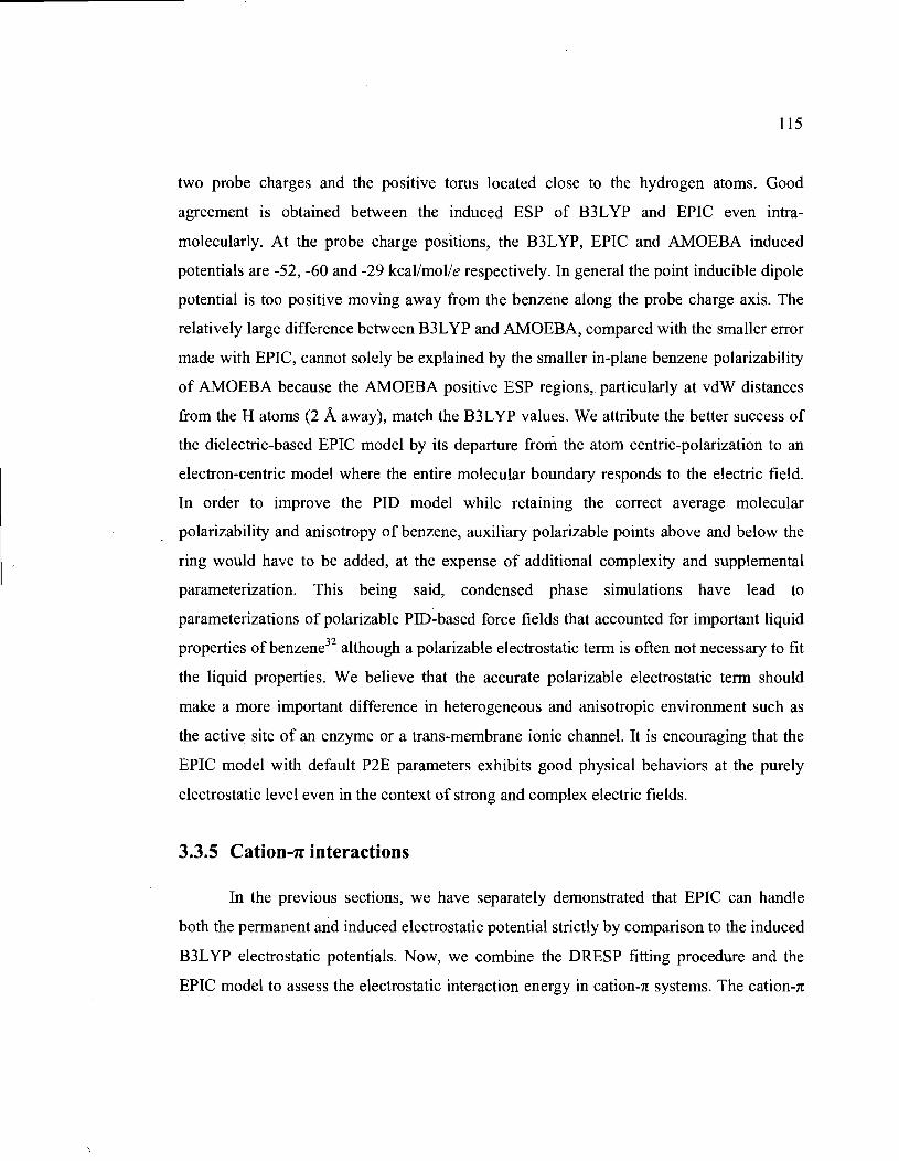
115

two probe charges and the positive toms located close to the hydrogen atoms. Good

agreement is obtained between the induced ESP of B3L YP and EPIe even intra­

molecularly. At the probe charge positions, the B3L YP, EPIe and AMOEBA induced

potentials are -52, -60 and -29 kcallmolle respectively. In general the point inducible dipole

potential is too positive moving away from the benzene along the probe charge axis. The

relatively large difference between B3L YP and AMOEBA, compared with the smaller error

made with EPIe, cannot solely be explained by the sm aller in-plane benzene polarizability

of AMOEBA because the AMOEBA positive ESP regions, particularly at vdW distances

from the H atoms (2 A away), match the B3LYP values. We attribute the better success of

the dielectric-based EPIe model by its departure from the atom centric-polarization to an

electron-centric model where the entire molecular boundary responds to the electric field.

In order to improve the PID model while retaining the correct average molecular

polarizability and anisotropy of benzene, auxiliary polarizable points above and below the

ring would have to be added, at the expense of additional complexity and supplemental

parameterization. This being said, condensed phase simulations have lead to

parameterizations of polarizable PID-based force fields that accounted for important liquid

properties of benzene32 although a polarizable electrostatic term is often not necessary to fit

the liquid properties. We believe that the accurate polarizable electrostatic term should

make a more important difference in heterogeneous and anisotropic environment such as

the active site of an enzyme or a trans-membrane ionic channel. It is encouraging that the

EPIe model with default P2E parameters exhibits good physical behaviors at the purely

electrostatic level even in the context of strong and complex electric fields.

3.3.5 Cation-7t interactions

In the previous sections, we have separately demonstrated that EPIe can handle

both the permanent and induced electrostatic potential strictly by comparison to the induced

B3LYP electrostatic potentials. Now, we combine the DRESP fitting procedure and the

EPIe model to assess the electrostatic interaction energy in cation-n systems. The cation-n

116

attractive interaction energy between benzene and Li+, Na+ or K +, displaced along the

benzene six-fold symmetry axis, was shown to be impossible to describe with nonadditive

models33. However, the contribution of the induction energy (from electrostatic

polarization) is crucial for an accurate description of cation-1t binding33,34. Furthermore, the

presence of cation-1t interactions in many biological systems35-37 makes this application a

critical validation for a new polarizable electrostatic term. Therefore, in this section we

decompose the total interaction energies and check if the induction found with the P2E

parameter set is quantitatively correct.

At the QM level, the total interaction energy between an atomÎC cation and benzene can be

conceptually split into electrostatic, vdW repulsive, and vdW attractive components. Each

term is normally represented separately in a force field, although one term often

compensates for another containing deficiencies. We are now only interested in examining

the electrostatic component and we focus on the proton since its vdW interaction with the

benzene can be neglected. Other cations have similar electrostatic profiles outside their

vdW range (data not shown). At the force field level, if the protonlbenzene interaction

energy is described correctly, aIl that remains to be added is the repulsive vdW term in

order to model other, more physiologically relevant, atomic cation-1t interactions. This will

be shown in the next section in a different application.

The energy of interaction between a benzene molecule and H+ is calculated at the

B3L YP/6-311 ++G(3df,3pd) level with no basis function positioned on the proton to avoid

unphysical stabilization. Figure 3.7 reports the energies as a function of the distance from

the center of the benzene ring using B3LYP, a non-polarizable Coulomb potential

calculated with RESP-fitted atomic charges, the electrostatic component of the polarizable

AMOEBA force field, and our polarizable EPICIP2E model. For the non-polarizable and

AMOEBA models, the parameters mentioned in section 3.4 are used. Figure 3.7 shows that

EPIC matches quantitatively the B3L YP energy profile. As found previously33, the non-

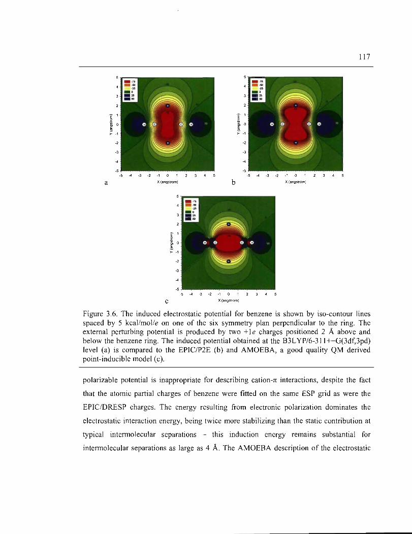
a

Ê 1 e ~ 0 R >- -1

-2

-3

-4

-4 ~ ~ ~ 0 1 234 5

X (angstrom)

Ê1 e ln 0

~ >- -1

-2

-3

-4

-5

b

Ê 1 g ~ 0

~ >- -1

-2

-3

-4

-5 ~ -4 ~ ~ ~ 0 1 234 5

X (angstrom)

c -5 -4 -3 -2 -1 0 1 2 3 4 5

X (angslrom)

117

Figure 3.6. The induced electrostatic potential for benzene is shown by iso-contour lines spaced by 5 kcal/mol/e on one of the six symmetry plan perpendicular to the ring. The extemal perturbing potential is produced by two + 1 e charges positioned 2 À above and below the benzene ring. The induced potential obtained at the B3L YP/6-31l ++G(3df,3pd) level (a) is compared to the EPIC/P2E (b) and AMOEBA, a good quality QM derived point-inducible model (c).

polarizable potential is inappropriate for describing cation-rr interactions, despite the fact

that the atomic partial charges of benzene were fitted on the same ESP grid as were the

EPIC/DRESP charges. The energy resulting from electronic polarization dominates the

electrostatic interaction energy, being twice more stabilizing than the static contribution at

typical intermolecular separations - this induction energy remains substantial for

intermolecular separations as large as 4 À. The AMOEBA description of the electrostatic

118

energy captures most of the induction energy. This model, like EPIC, is derived from ab

initio calculations, but includes atom-based multipole expansion terms up to the quadrupole

for the permanent potential. In addition, AMOEBA adds an atomic polarizability on the

hydrogen atoms. The difference between B3L YP and AMOEBA energies can be explained,

in part, by AMOEBA's slightly smaller out-of-the-plane polarizability (c.f. section 3.4).

Tsuzuki et al. 34 have shown that it is possible to get the cation-n system correctly modeled

with a PID model if it is parameterized in a specialized manner. In their work they not only

use atomic multipoles, but also anisotropic atomic polarizability located on the carbon

atoms. Once more, we see that the EPIC model with P2E parameters is robust and general,

needing only a small number of default parameters to account for the different aspects of

electronic polarization. The accuracy of this model implies that the vdW term will not need

to compensate for errors in the close-range electrostatics thus easing its pararneterization.

3.3.6 H-bond of the pyridine-4(1H)-one dimer

The induction energy in H-bonds is implicitly included in existing additive force

fields. The single-minimum interaction energy profile representing an H-bond becomes a

trade-off between the attractive electrostatic term and the short-range repulsive vdW term

ofa force field. For example, in the original AMBER force field a special 12-10 Lennard­

Jones potential was initially needed to de scribe short range H-bonding potentials38. In more

recently developed non-polarizable force fields39, both the condensed phase overpolarized

HF /6-31 G( d) charges and the addition of hydrogen atom types using small Lennard-Jones

radius (cr) parameters corrected for the lack of induction energy. Including explicitly

induction energies should, in princip le, simplify the parameterization of vdW potential and

incorporate non-additive condensed phase effects such as H-bond cooperativity40,41. In this

section, we examine the challenging case of pyridin-4( 1.H)-one, hereafter 4-pyridone,

which was shown to form strong intermolecular H-bonds42 when monomers are co-planar

and aligned along the two-fold axis passing through the NH and the CO bonds. This is in

part due to the large dipole moment of 7 Debye and the high polarizability component of 97

119

a.u. both oriented along the H-bond axis that should polarize the monomers and thereby

constitute an interesting second application for the validation of polarization using EPIe.

This is a case where polarizability needs to be taken into account even at the dimer level. In

what follows, we conduct two different studies which objectives are a) to assess if the EPIC

model with DRESP charges gives the correct electrostatic interaction energy profile

compared to B3L YP and b) to reproduce the dimer H-bond dissociation energy curve

obtained by B3LYP.

0 -0 E -10 --ro u C. >. -20 Cl .... <l) c <l) -30 c 0 ,.Q 13 1

1 ca -40 CS) .... <l)

ë u -50 ~ 1ii 0 ....

-60 13 ---A-- RESP/non-polarizable <l) -""1- B3LYP/H+

LiJ --0-- EPie (Bondi)

-70 2.0 2.5 3.0 3.5 4.0 4.5

Cation / benzene distance (A)

Figure 3.7. The electrostatic interaction energy between a benzene molecule and H+ displaced along the C6 symmetry axis corresponds to the electrostatic component of a cation-1t system formed with an atomic cation. The non-polarizable model using ESP derived charges is far from the B3LYP calculated energy, the EPICIP2E model closely follows the B3L YP curve and AMOEBA captures most of the electronic polarization of B3L YP. The EPIC electrostatics fitted on B3LYP monomer reproduces the correct cation-1t electrostatic energy without adjustment.

120

3.3.6.1 4-pyridone dimer electrostatic interaction energy

Unlike the previouscation-1t application, evaluating the perfonnance of our

electrostatic approach here involves partitioning the total electronic structure energy into its

components because the vdW tenn cannot be neglected. We will divide the total energy

into an electrostatic (~Eelec) tenn and an exchange-repulsion (hereafter called the vdW

repulsion and noted ~Evdw) tenn. The short range attractive dispersion energy is omitted

because B3L YP does not capture it and it remains very small compared to the range of

energies involved.

Given this partitioning, we calculate ~Eelec by subtracting ~Evdw from the total

interaction energy (~Etot). The delta symbol in front of the energy signifies that this is an

interaction energy, meaning the difference in energy between the interacting system and the

energies of the monomers. To approximate the ~EvdwDFT tenn, we used benzo-l,4-quinone

(quinone) and benzene which both have a relatively small ESP. The benzene hydrogen

replaces the 4-pyridone H donar and the quinone oxygen the acceptor, fonning a quasi H­

bond. The assumption here is that the vdW repulsive tenn is similar between the two

systems. The monomer geometries are he Id fixed and the carbonyl oxygen to benzene H

distances are the same as the 4-pyridone H-bonded dimer distances. The ESP of both

molecules is relatively small and can be approximated using RESP-derived atomic point

charges (~EelecREsP); thus ~Eelec is calculated using equations (3.l4) and (3.15):

~EvdwDFT ~ ~EtotDFT (benzene, quinone) - ~EelecREsP (benzene,

quinone)

~EelecDFT ~ ~EtotDFT (4-pyridone,4-pyridone) - ~EvdwDFT

(3.14)

(3.15)

Figure 3.8a shows ~EelecDFT, ~EelecREsP and ~EelecDREsP associated with the 4-

pyridone dimer for distances going from 1.6 A to 4 A. The equilibrium distance is found at

1.78 A 42; details of the energies are reported in the Supplemental Material. As reported in

121

Figure 3.8a, the induction energy stabilization obtained withEPICIP2E matches B3L YP

over most of the distances. The deviations at close contact «2 A) may be attributable to

defects in the approximation given by eq. (3.14). Comparing the Coulomb and B3LYP

curves at the equilibrium distance, the induction energy is almost -5 kcal/mol, a significant

increase over the Coulomb value of -11.6 kcallmol. The quantitative match between the

approximated B3L YP electrostatic H-bond energy shows that the induction interaction is

appropriately described by our polarizable EPIC/P2E. It is important to emphasize that the

radii and dielectric parameters (P2E) used were not fitted to any energy but to the QM gas­

phase molecular polarizability tensors for many molecules simultaneouslyl. In Figure 3.8a,

we can also see the EPIClBondi interaction curve that uses DRESP derived charges and the

Bondi parameter set (c.f. Method). The long range interaction energies are appropriate but

when the electronic volumes, defined by the Bondi radii (1.52 A for oxygen and 1.1 A for

the hydrogen), start to interpenetrate, the induction energy becomes insufficient and

undergoes numerical instability that we attribute to the vdW surface used in the finite

difference PB solver, known to form cusps.

3.3.6.2 4~pyridone di mer dissociation energy

To get an idea of how weil EPIC polarization could be incorporated into an atomic

force field, a vdW term was fitted to see how weil the QM energy profile could be

reprdduced; the details of the fitted vdW terms are given in the Supplemental Material. The

resulting complete interaction energy profiles for the H-bond formation of the 4-pyridone

di mer, ~Etot(4-pyridone,4-pyridone), are presented in Figure 3.8b. For the DFT profile

(~EtotDFT), the approximation of (3.15) is not needed because only the total energy is

examined. The B3L YP/6-311 ++G(3df,3pd) BSSE corrected energies show a very stable H­

bond with a dissociation energy of -10.8 kcal/mol..

A few comments on the vdW fitting process are in order. In keeping with high-Ievel

QM calculation of exchange-repulsion energies,43 we have used a two-parameter

122

exponential vdW energy function ~EvdwEPIC(r) fitted to the residuals ~EtotDFT (r) -

~EelecEPJc(r) calculated along the intermolecular H-bond axis. Fortunately, the vdW

dispersion energy, an attractive force, is absent in DFT methods and should not be needed

here. The fit of the EPIC/P2E residuals resulted in a dissociation energy curve

quantitatively reproducing the B3L YP energies in aU ranges examined, giving a correlation

coefficient (R2) of 0.999.

Note that the atomic partial charges derive from a DRESP fit to the monomer only. In

contrast, the Coulomb model residuals (using atomic partial charges from the gas-phase

monomer without polarizability) could not be fit to an exponential as successfully,

exhibiting an attractive potential well of about -1 kcallmollocated at 2.3 Â. This example

shows that, at the level of the dimer, the lack of polarizability introduces a requirement for

a more complex functional form for the vdW term in order to compensate. Finally, the

EPIClBondi potential has difficulty capturing the energy minimum and exhibits numerical

instability. At very short H-bond distances «1.5 Â), EPIC/P2E also exhibits similar

instability behavior, but fortunately this is less relevant given that the high repulsive vdW

energy is dominant. This is due to the smaller dielectric radii assigned to the oxygen and

hydrogen atoms in the fit. The use of a smooth dielectric boundary could significantly

reduce these effects 15.

While these applications demonstrate the use of EPIC to incorporate electronic

polarization into short-range intermolecul~r interactions, the generalization of this model

for use in the condensed phase will require special attention in the parameterization.

Indeed, it has been proposed based on vanous evidences that the condensed phase

molecular polarizability per monomer is smaller than its gas phase polarizability. In

practice, the correction to a PID model was made by fitting the polarizabilities on ab initio

values obtained with a relatively small basis set, which systematically produces smaller

molecular polarizabilities43. Hence for the PID model, the parameterized polarizability

cannot accurately account for both the gas- and condensed-phase polarization, one of the

123

main objectives for a polarizable force field. We are currently examining this problem with

EPIC and this will be addressed in a subsequent publication.

0 -2 ~

(5 -3 .€ -4 co -4 0 ~

~

-8 (5 >. E -5 e> :::::, Q) co ffi -12 0 0 -6 ~

D= 'D= H-N _ O------H-N _ 0

o·

c: >. 0 e> -7 ~ -16

Q) c: ... Q) -8 .sl "0 c: c:

ë::; -20 0 -9 B3LYP .0 ~ • 1

1iî --9--- EPIC/P2E I

g -24 EPie/Bondi -10

--b,-

• B3LYP - - 9- - - EPIC/P2E - -b, - EPIC/Bondi

0 Coulomb Q) ······0····· -11 iii

······0····· Coulomb

-28 -12

1.5 2.0 2.5 3.0 3.5 4.0 1.5 2.0 .2.5 3.0 3.5 4~

H-bond distance (A) H-bond distance (A)

a b

Figure 3.8. The reported electrostatic interaction energies of the H-bonded 4-pyridone dimer (a) show that the EPIC/P2E model produces the appropriate polarization as opposed to the non-polarizable permanent charge model (Coulomb) when compared to B3L YP (3.l5). The EPIe/Bondi calculations produce the correct electronic response at long ranges of H-bond distances but saturates as the vdW dielectric surfaces of the monomers start overlapping. The observed deviations are a result of the numerical instability that occur when the dielectric spheres corne into contact at 2.6 A. (b) The BSSE/corrected B3LYP interaction energies of the dimer unveils a very strong H-bond of -10.8 kcal/mol at the minimum located at 1.78 A. The reported classical approaches combined the electrostatic energies (shown in a) and a fitted repulsive vdW term. EPIC/P2E matches the B3LYP energies over the examined range whereas the Coulomb non-polarizable model deviates at longer distances as a result of the difficulty for such a model to match both regions.

124

3.4 Conclusion

This work extends the proof-of-concept of the EPIC (electronic polarization from

intramolecular continuum) approach to intermolecular interactions l. We show that in

general the presence of an intramolecular continuum dielectric, for example in PB or PE

formalisms, requires a modification of the conventional method for obtaining accurate

atomic partial charges. We derive a least-squares approach called DRESP, by analogy to

RESP, which not only reproducesthe ab initio electrostatic potential but also offers a way

to transfer the atomic partial charges from an existing vacuum charge model. We

demonstrate this by successfully transferring the charges from an AMI-BCC/vacuum

charging scheme of a set of 37 molecules including polar and non-polar aromatics and

alkanes. In general, the charges obtained are significantly larger whenever the dielectric

inside the molecule is larger than one. Even more importantly, our results show that the

polarizable parameters of EPIC can be derived independently from the permanent

electrostatic terms. In fact, the atomic radii and dielectrics fitted to vacuum ab initio

molecular polarizabilities were derived in the absence of atomic partial charges. We believe

that this parame ter decoupling will be an important asset to broaden the approach to

encompass bio-organic chemistry.

Although EPIC was successfully fitted previously to reproduce ab initio dipole

moments induced by a uniform electric field l, it was important to demonstrate that the full

electrostatic potential induced by a more local or complex perturbation would be as

accurate. To this end, we tested the validity of our parameters with a perturbing +0.5e

probe charge moved on a Connolly surface. This is frequently employed to fit the

polarizable parameters in force fields. The results were very encouraging leading to an

average of 1% RRMSD deviation, relative to B3L YP, obtained from about 1700

calculations done on our set of 37 molecules. This shows that we cao fit the EPIC radii and

125

dielectrics on gas-phase molecular polarizabilities and expect an accurate local electronic

polarization response as weIl.

A potential advantage of EPIC over other polarizable models is its use of 'electronic

polarizability density' through the intramolecular continuum dielectric. As opposed to PID

models, the electric field induction is effective through the entire molecular volume. A

recent study by Schropp and Tavan44 suggests that the usual approximation that the

polarizability is centered on atomic nuclei artificially invalidates the use of gas-phase

derived atomic polarizabilities into condensed phase simulations unless non-obvious and

non-general corrections are applied. To further examine the ability of EPIC to deal with

inhomogeneous environments, an argon atom and a benzene molecule were sandwiched by

positive point charges. In both cases EPIC led to an accurate induced electrostatic potential

relative to B3LYP. The ab initio derived AMOEBA polarizable force field parameters were

used for comparison and show a significant quantitative discrepancy of the out-of-plane

potential. In agreement with Schropp and Tavan, we attribute this deficiency to the

difficulty of atom centered polarizabilities to account for locally varying electric field.

We also applied our independently generated charges, radii and dielectrics to

calculate the cation-1t electrostatic interaction energy between a benzene molecule and a

proton. This energy corresponds, more generally, to the electrostatic component for the

binding of Li+, Na-;- or K+ to benzene where the induction energy is predominant. The

results show that EPIC with parameters derived uniquely on the monomer le ad to B3L YP

quality binding energies. In addition, the H-bonding electrostatîc energy of the 4-pyrîdone

dîmer has been examîned and we found that EPICIP2E quantîtatively matches the

approximated B3LYP electrostatics and total interaction energies whereas the non­

polarizable term obtained with fixed charges derived from the ESP were not sufficient.

Although' we have not covered an exhaustive intermolecular list, these two applications are

challenging cases that clearly show that the approach can work. Our fitting strategy of the

electrostatÎc on the monomers can be easily generalized. In the 4-pyridone dimer example,

126

we also show that the vdW tenn, needed to obtain the full energy, would not have to

compensate for the poor electrostatic at short distances. This is one important and expected

advantage from an accurate polarizable electrostatic model.

This work shows a new and potentially advantageous electrostatic term which could

be applied to molecular dynamics or Monte Carlo simulations. Recently, molecular

dynamics simulations using a PB sol ver to include implicitly the effects of solvent

polarization were successfully carried out 2,3,15,45-48. In order to fully use the concepts

discussed herein as the electrostatic foundation of a force field, there are remaining

scientific points to be addressed. The dielectric boundary will require a special attention if

stable forces are to be calculated. AIso, transferability of the parameters obtained from ab

initia gas-phase calculations to the condensed phase need to be addressed. The extension of

the parameteriz'ation will command a major effort not only for the electrostatic term, but

also for aIl the other force field terms which need to balance the electrostatics.

Acknowledgment. The authors thank Dr. Chen from Lamar University for

providing to us the coordinates of the optimized 4-pyridone dimer. We thank Daniel J.

McKay from Merck Frosst and Georgia McGaughey from Merck & Co. for useful

comments on the manuscript. This work was made possible by the computational resources

of Réseau Québécois de Calcul Haute Performance (RQCHP). The authors are grateful to

OpenEye Ine. for free academic licenses. l-F.T. thanks the Natural Sciences and

Engineering Research Council of Canada (NSERC) for a Canada graduate scholarship

(CGS D) and Merck & Co. for support through the MRL Doctoral Program. R. 1. 1.

acknowledges financial support from the NSERC. B. R. is supported by NIH grant

GM072558

127

3.5 Supporting Information

Data related to Figure 3.7 for the interaction energy of a positive point charge (H+)

move along the benzene C6 symetry axis forming a cation-pi interaction.

RESpb B3L YP/H+b EPIC/Bondib

1,87 -65,76 -47,60 -25,37 -102,60 2,00 -56,43 -42,30 -22,98 -52,37 -82,75 2,20 -44,79 -35,26 -19,66 -43,74 -61,00 2,40 -36,02 -29,59 -16,87 -36,36 -46,48 2,60 -29,33 -25,00 -14,52 -30,18 -36,30 2,80 -24,14 -21,25 -12,54 -25,09 -28,90 3,00 -20,08 -18,18 -10,87 -20,95 -23,40 3,20 -16,86 -15,64 -9,47 -17,60 -19,30 3,40 -14,29 -13,53 -8,27 -14,89 -16,00 3,60 -12,22 -11,76 -7,26 -12,69 -13,50 3,80 -10,53 -10,28 -6,40 -10,90 -11,40 4,00 -9,15 -9,02 -5,66 -9,42 -9,78 4,20 -8,02 -7,95 -5,03 -8,43 4,40 -7,09 -7,04 -4,48 -7,32

aDistance between the point charge and the center of the benzene ring in Angstrom.

bElectrostatic interaction energies in kcal/mol.

128

Data related to Figure 3.8 for the interaction energies between two H-bonded 4-

pyridone molecules. The data is spread over few tables. The notation for the column labels

follows the tables.

Distance 1,600 1,800 2,000 2,200 2,400 2,600 2,800 3,000 3,200 3,400 3,600 3,800 4,000

Distance 1,600 1,800 2,000 2,200 2,400 2,600 2,800 3,000 3,200 3,400 3,600 3,800 4,000

Eq. (3.14) rhs Eq. (3.14) rhs term 1 term 2

~E(B,Q)tot DFT ~E(B,Q)elec RESP 10,648 -2,018 4,200 -1,527 1,219 -1,181

-0,039 -0,930 -0,484 -0,744 -0,575 -0,603 -0,538 -0,495 -0,465 -0,411 -0,394 -0,344 -0,332 -0,291 -0,282 -0,247 -0,240 -0,212 -0,205 -0,183

Figure 8a Figure8a (EPIC/P2E} (EPIC/Bondi} ~E(P ,P)elec ~E(P,P)elec EPIC/P2E EPIC/BONDI

-28,47 -16,382 -18,31 -14,592 -13,02 -12,799 -10,41 -11,798

-8,74 -9,705 -7,31 -8,661 -6,25 -6,889 -5,44 -5,884 -4,79 -4,976 -4,23 -4,376 -3,75 -3,901

-3,4 -3,441 -3,06 -3,119

Eq. (3.15) rhs Eq. (3.14) Ihs term 1 Figure 8b

(B3LYP)

~Evdw DFT 12,666 5,727 2,400 0,891 0,260 0,028

-0,043 -0,054 -0,050 -0,041 -0,035 -0,028 -0,022

Figure 8a (Coulomb} ~E(P,P)elec

Coulomb -14,064 -11,629

-9,792 -8,368 -7,238 -6,326 -5,577 -4,953 -4,428 -3,982 -3,598 -3,267 -2,978

~E(P,P)tot DFT -9,340

-10,800 -10,440

-9,440 -8,310 -7,250 -6,330 -5,560 -4,920 -4,380 -3,930 -3,550 -3,210

vdW residuals Evdw

EPIC/P2E 19,130 7,510 2,584 0,970 0,430 0,060

-0,080 -0,120 -0,130 -0,150 -0,180 -0,150 -0,150

Eq. (3.15) Ihs

~Eelec DFT -22,006 -16,527 -12,840 -10,331 -8,570 -7,278 -6,287 -5,506 -4,870 -4,339 -3,895 -3,522 -3,188

vdW residuals Evdw

EPIC/Bondi 7,042 3,792 2,359 2,358 1,395 1,411 0,559 0,324 0,056

-0,004 -0,029 -0,109 -0,091

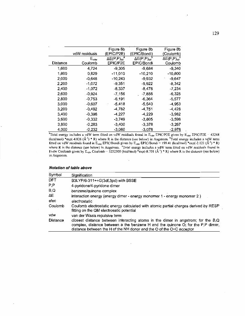
129

Figure 8b Figure 8b Figure 8b vdW residuals {EPIC/P2E} {EPIC/Bondi~ {Coulomb}

Evdw D.E(P,P)tota D.E(P ,P)tot D.E(P,P)totC

Distance Coulomb EPIC/P2E EPIC/Bondi Coulomb 1,600 4,724 -9,305 -9,684 -9,340 1,800 0,829 -11,010 -10,210 -10,800 2,000 -0,648 -10,243 -9,932 -9,647 2,200 -1,072 -9,351 -9,922 -8,342 2,400 -1,072 -8;337 -8,478 -7,234 2,600 -0,924 -7,156 -7,858 -6,325 2,800 -0,753 -6,191 -6,364 -5,577 3,000 -0,607 -5,418 -5,540 -4,953 3,200 -0,492 -4,782 -4,751 -4,428 3,400 -0,398 -4,227 -4,229 -3,982 3,600 -0,332 -3,749 -3,805 -3,598 3,800 -0,283 -3,400 -3,378 -3,267 4,000 -0,232 -3,060 -3,078 -2,978

"Total energy includes a vdW tenn fitted on vdW residuals round in Evdw EPIC/P2E given by Evdw EPIC/P2E = 43248 (kcal/mol) *exp(-4.826 (Â"') * R) where R is the distance (see below) in Angstrom. bTotal energy includes a vdW tenn fitted on vdW residuals round in Evdw EPIC/Bondi given by Evdw EPIClBondi = 199.41 (kcal/mol) *exp(-2.l21 (Â"') * R) where R is the distance (see below) in Angstrom. cTotal energy incIudes a vdW term fitted on vdW residuals round in Evdw Coulomb given by Evdw Coulomb = 5252300 (kcal/mol) *exp(-8.701 (Â"') * R) where R is the distance (see below) in Angstrom.

Notation of table above

Symbol DFT P,P B,O D.E elec Coulomb

vdw Distance

Signification B3LYP/6-311++G(3df,3pd) with BSSE 4-pyridone/4-pyridone dimer benzene/quinone complex interaction energy (energy dimer - energy monomer 1 - energy monomer 2 ) electrostatic Coulomb electrostatic energy calculated with atomic partial charges derived by RESP fitting on the aM electrosatic potential van der Waals repulsive term closest distance between interacting atoms in the dimer in angstrom; for the B,O complex, distance between a the benzene H and the quinone 0; for the P,P dimer, distance between the H of the NH donor and the 0 of the O=C acceptor

3.6 Bibliography

1. Truchon, 1.-F.; Nicholls, A.; Iftimie, R. 1.; Roux, B.; Bayly, C. 1. Accurate

Molecular Polarizability based on Continuum Electrostatics. 1. Chem. Theory

Comput., 2008, 4, 1480-1493.

2. Maple, J. R.; Cao, Y. X.; Damm, W. G.; Halgren, T. A.; Kaminski, G. A.; Zhang, L.

Y.; Friesner, R. A. A polarizable force field and continuum solvation methodology

for modeling of prote in-ligand interactions. J. Chem. Theory Comput., 2005, 1, 694-

715.

3. Schnieders, M. J.; Baker, N. A.; Ren, P.; Ponder, 1. W. Polarizable atomic multipole

solutes in a Poisson-Boltzmann continuum. 1. Chem. Phys., 2007, 126, 124114.

4. Bayly, C. 1.; Cieplak, P.; Corne lI, W. D.; Kollman, P. A. A Well-Behaved

Electrostatic Potential Based Method Using Charge Restraints for Deriving Atomic

Charges - the Resp Model. J. Phys. Chem., 1993,97,10269-10280.

5. Jakalian, A.; Bush, B. L.; Jack, D. B.; Bayly, C. 1. Fast, efficient generation ofhigh­

quality atomic Charges. AMI-BCC model: 1. Method. 1. Comput. Chem., 2000, 21,

132-146.

6. Jakalian, A.; Jack, D. B.; Bayly, C. 1. Fast, efficient generation ofhigh-quality

atomic charges. AMI-BCC model: II. Parameterization and validation. 1. Comput.

Chem., 2002,23, 1623-1641.

7. Tan, Y. H.; Luo, R. Continuum treatment of electronic polarization effect. 1. Chem.

Phys., 2007, 126, 094103.

8. Becke, A. D. Density-Functional Thermochemistry .3. the Role of Exact Exchange.

J. Chem. Phys., 1993,98,5648-5652.

9. Becke, A D. A New Mixing of Hartree-Fock and Local Density-Functional

Theories. J. Chem. Phys., 1993, 98,1372-1377.

10. Stephens, P. 1.; Devlin, F. 1.; Chabalowski, C. F.; Frisch, M. J. Ab-Initio

Calculation ofVibrational Absorption and Circular-Dichroism Spectra Using

Density-Functional Force-Fields. J. Phys. Chem., 1994, 98, 11623-11627.

Il. Gaussian 03. Revision C.02; Wallingford CT, USA, 2004

131

12. Frisch, M. 1.; Pople, 1. A.; Binkley, J. S. Self-consistent molecular orbital methods

25. Supplementary functions for Gaussian basis sets. J Chem. Phys., 1984,80,

3265-3269.

13. Simon, S.; Duran, M.; Dannenberg, J. J. How does basis set superposition error

change the potential surfaces for hydrogen bonded dimers? J Chem. Phys., 1996,

105, 11024-11031.

14. Boys, S. F.; Bernardi, F. The calculation of small molecular interactions by the

differences of separate total energies. Sorne procedures with reduced errors

(Reprinted from Molecular Physics, vol 19, pg 553-566, 1970). Mol. Phys., 2002,

100,65-73.

15. Grant, J. A; Pickup, B. T.; Nicholls, A. A smooth permittivity function for Poisson­

Boltzmann solvation methods. J Comput. Chem., 2001,22,608-640.

16. Richards, F. M. Areas, Volumes, Packing, and Protein-Structure. Annu. Rev.

Biophys. Bioeng., 1977, 6,151-176.

17. Bondi, A. van der Waals Volumes and Radii. J Phys. Chem., 1964, 68,441-451.

132

18. Singh, U. C.; Kollman, P. A. An Approach to Computing Electrostatic Charges for

Molecules. J. Comput. Chem., 1984,5, 129-145.

19. Anisimov, V. M.; Lamoureux, G.; Vorobyov, 1. V.; Huang, N.; Roux, B.;

MacKerell, A. D. Determination of electrostatic parameters for a polarizable force

field based on the c1assical Drude oscillator. J. Chem. Theory Comput., 2005, 1,

153-168.

20. Elking, D.; Darden, T.; Woods, R. J. Gaussian induced dipole polarization model. J.

Comput. Chem., 2007, 28, 1261-1274.

21. Connolly, M. L. Solvent-Accessible Surfaces ofProteins and Nucleic-Acids.

Science, 1983,221,709-713.

22. Mobley, D. L.; Dumont, E.; Chodera, J. D.; Dili, K. A. Comparison of charge

models for fixed-charge force fields: Small-molecule hydration free energies in

explicit solvent. J. Phys. Chem. B, 2007,111,2242-2254.

23. Mobley, D. L.; Graves, A. P.; Chodera, J. D.; Shoichet, B. K.; DilI, K. A. Predictive

absolute binding free energy calculations for an engineered binding site in T4

Lysozyme. Biophys. J., 2007, 368A-368A.

24. Williams, D. . Abraha, A. Site charge models for molecular.electrostatic

potentials of cyc10alkanes and tetrahedrane. J. Comput. Chem., 1999,20, 579-585.

25. Williams, D. Failure of Net Atomic Charge Models to Represent the Van-Der­

Waals Envelope Electric-Potential ofN-Alkanes. J. Comput. Chem., 1994,15, 719-

732.

133

26. Nicholls, A; Mobley, D. L.; Guthrie, 1. P.; Chodera, 1. D.; Bayly, C. 1.; Cooper, M.

D.; Pande, V. S. Predicting small-molecule solvation free energies: An informaI

blind test for computational chemistry. J Med. Chem., 2008, 51, 769-779.

27. The B3LYP/cc-pVTZ ESP based bond charge corrections were obtained through

private communications with Cooper, M. D. and Bayly, C. 1.

28. Lopes, P. E. M.; Lamoureux, G.; Roux, B.; MacKerell, A. D. Polarizable empirical

force field for aromatic compounds based on the c1assical drude oscillator. J. Phys.

Chem. B, 2007, 111,2873-2885.

29. Kaminski, G. A.; Stern, H. A; Berne, B. 1.; Friesner, R. A; Cao, Y. X. X.; Murphy,

R. B.; Zhou, R. H.; Halgren, T. A Development of a polarizable force field for

proteins via ab initio quantum chemistry: First generation model and gas phase

tests.J. Comput. Chem., 2002,23,1515-1531.

30. Anisimov, V. M.; Vorobyov, I. V.; Lamoureux, G.; Noskov, S.; Roux, B.;

MacKerell, A. D. CHARMM aU-atom polarizable force field parameter

development for nucleic acids. Biophys. J, 2004, 86, 415A-415A.

31. Stern, H. A; Kaminski, G. A.; Banks, 1. L.; Zhou, R. H.; Berne, B. 1.; Friesner, R.

A Fluctuating charge, polarizable dipole, and combined models: Parameterization

from ab initio quantum chemistry. J Phys. Chem. B, 1999,103,4730-4737.

32. Jorgensen, W. L.; Severance, D. L. Aromatic-aromatic interactions: free energy

profiles for the benzene dimer in water, chloroform, and liquid benzene. J Am.

Chem. Soc., 1990, 112,4768-4774.

33. Caldwell,1. W.; Kollman, P. A. Cation-Pi Interactions - Nonadditive Effects Are

Critical in Their Accurate Representation. J. Am. Chem. Soc., 1995,117,4177-

4178.

134

34. Tsuzuki, S.; Yoshida, M.; Uchimaru, T.; Mikami, M. The Origin of the Cation/pi;

Interaction: The Significant Importance of the Induction in Li+ and Na+

Complexes. J. Phys. Chem. A, 2001, 105, 769-773.

35. Gallivan,1. P.; Dougherty, D. A. Cation-pi interactions in structural biology. P.

Natl. Acad. Sei. Us. A., 1999,96,9459-9464.

36. Roux, B. Nonadditivity in Cation Peptide Interactions - A Molecular-Dynamics and

Ab-Initio Study ofNa+ in the Gramicidin Channel. Chem. Phys. Lett., 1993,212,

231-240.

37. Ma, 1. c.; Dougherty, D. A. The cation-pi interaction. Chem. Rev., 1997,97, 1303-

1324.

38. Weiner, S. J.; Kollman, P. A.; Case, D. A.; Singh, U. C.; Ghio, C.; Alagona, G.;

Profeta, S.; Weiner, P. A New Force-Field for Molecular Mechanical Simulation of

Nuçleic-Acids and Proteins. J. Am. Chem. Soc., 1984, 106, 765-784.

39. Comell, W. D.; Cieplak, P.; Bayly, C. 1.; Gould, 1. R.; Merz, K. M.; Ferguson, D.

M.; Spellmeyer, D. c.; Fox, T.; Caldwell, 1. W.; Kollman, P. A. A 2Nd Generation

Force-Field for the Simulation ofProteins, Nucleic-Acids, and Organic-Molecules.

J. Am. Chem. Soc., 1995, 117, 5179-5197.

40. Guo, H.; Gresh, N.; Roques, B. P.; Salahub, D. R. Many-body effects in systems of

peptide hydrogen-bonded networks and their contributions to ligand binding: A

comparison of the performances ofDFT and polarizable molecular mechanics. J.

Phys. Chem. B, 2000, 104, 9746-9754.

41. Guo, H.; Salahub, D. R. Cooperative hydrogen bonding and enzyme catalysis.

Angew. Chem. Int. Edit., 1998, 37, 2985-2990.

135

42. Chen, Y. F.; Dannenberg, J. J. Cooperative 4-pyridone H-bonds with extraordinary

stability. A DFT molecular orbital study. J. Am. Chem. Soc., 2006, 128, 8100-8101.

43. Harder, E.; Kim, B. C.; Friesner, R. A.; Berne, B. J. Efficient simulation method for

polarizable protein force fields: Application to the simulation of BPTI in liquid. J.

Chem. Theory Comput., 2005, l, 169-180.

44. Schropp, B.; Tavan, P. The Polarizability ofPoint-Polarizable WaterModels:

Density Functional TheorylMolecular Mechanics Results. J. Phys. Chem. B, 2008,

112,6233-6240.

45. Luo, R.; David, L.; Gilson, M. K. Accelerated Poisson-Boltzmann calculations for

static and dynamic systems. J. Comput. Chem., 2002, 23, 1244-1253.

46. Prabhu, N. V.; Zhu, P. 1.; Sharp, K. A. Implementation and testing of stable, fast

implicit solvation in molecular dynamics using the smooth-permittivity finite

difference Poisson-Boltzmann method. J. Comput. Chem., 2004,25,2049-2064.

47. lm, W.; Beglov, D.; Roux, B. Continuum Solvation Model: computation of

electrostatic forces from numerical solutions to the Poisson-Boltzmann equation.

Comput. Phys. Commun., 1998, 111, 59-75.

-------------- -_ .... ~ .. -_.

48. Lu, Q.; Luo, R. A Poisson~-Boltzmann dynamics method with nonperiodic

boundary condition. J. Chem. Phys., 2003, 119, 11035-11047.

136

137

4 Approches intégrées fondées sur un continuum

diélectrique pour traiter la polarisabilité moléculaire

et la phase condensée: indice de réfraction et la

solvatation implicite

Résumé. L'idée d'utiliser un continuum diélectrique à l'intérieur d'une molécule pour

modéliser précisément la polarisabilité moléculaire est prolongée pour inclure un plus

grand nombre de molécules bioorganiques et la phase condensée. Les rayons atomiques de

polarisation et le diélectrique interne (Ein) ont été optimisés pour reproduire des tenseurs de

polarisabilité quantique B3LYP/aug-cc-pVTZ provenant d'un ensemble de 707 molécules.

Les erreurs moyennes sur la polarisabilité isotropique et sur l'anisotropie sont de 2.6 % et

5.2 % respectivement. Il est montré que les rayons de contact habituels des applications

Poisson-Boltzmann et un diélectrique interne faible ne sont pas appropriés et requièrent une

révision substantielle. Pour reproduire l'anisotropie de la polarisabilité, la constante

diélectrique interne doit être supérieure à 6. En réinterprétant le lien théorique entre. Ein et

l'indice de réfraction expérimental (n), cette étude montre, avec 23 molécules organiques

couvrant toutes les valeurs de n, que même avec Ein=24, les indices de réfraction obtenus

démontrent une bonne corrélation avec l'expérience (pente de 1.00, ordonnée à l'origine de

0.05 et R 0.95). La nouvelle méthodologie utilisée ici pour calculer un indice de

réfraction quasi macroscopique montre que l'application d'EPIC à la phase condensée

conduit à un comportement souhaitable. Bien que le but premier en développant EPIC était

d'inclure la polarisabilité pour des calculs avec solvant explicite, nous élargissons

également le modèle pour inclure la polarisabilité pour les calculs avec solvant implicite.

Cela demande d'utiliser une fonction diélectrique douce à 3 régions qui permet de passer de

la polarisation diélectrique à l'intérieur de la molécule au diélectrique continu du solvant.

L'ajustement et la validation de ce modèle sont faits avec 485 énergies libres d'hydratation.

Avec 8 rayons atomiques pour décrire la cavité du solvant et une seule tension de surface,

138

l'erreur positive moyenne est de 1.1 kcallmol et produit un coefficient de corrélation de 0.9,

ce qui valide l'utilisation d'EPIC dans la phase condensée.

Mise en contexte. Les résultats encourageants obtenus aux chapitres 2 et 3 laissent une

avenue complètement inexplorée: la phase condensée. Puisque la niche que nous voulons

donner à EPIC est précisément pour les simulations en phase condensée, il nous faut

aborder la question. Dans ce chapitre, nous examin·erons la polarisabilité d'agrégats

composés de milliers de molécules et vérifierons qu'ils concordent avec l'indice de

réfraction expérimental, une mesure de la polarisation électronique macroscopique. Parce

que les méthodes Poisson-Boltzmann dans les applications biomoléculaires prennent de

l'ampleur, nous intégrerons notre modèle et nos concepts aux calculs avec solvants

implicites qui représentent plusieurs facettes de la phase condensée. Ceci mettra à l'épreuve

les chargés atomiques, déterminées avec la méthode du chapitre 3, et le modèle polarisable

du chapitre 2 puisque la polarisation coopérative du soluté et du solvant nécessite une

bonne balance des différentes composantes électrostatiques. Cette intégration demandera

l'élaboration d'un nouveau type de fonctions diélectriques.

Pour être en mesure de faire une validation adéquate sur les points mentionnés ci-haut, nous

devrons poursuivre un de nos objectifs principaux, c'est-à-dire la généralisation de nos

paramètres pour la polarisabilité à une grande partie de la chimie bioorganique. Nous

porterons une attention particulière dans ce chapitre à la généralisation des paramètres.

Avec la reproduction de l'indice de réfraction expérimental, nous répondons à la question

du sens physiqu~ soulevée par une grande constante diélectrique interne. De plus, nous

montrons que le potentiel électrostatique permanent (charges atomiques partielles) n'est pas

seulement approprié pour le calcul d'interactions électrostatiques entre dimères, mais aussi

pour la réponse moyenne du solvant. Nous démontrons également que les rayons atomiques

reliés à la polarisabilité et ceux utilisés habituellement pour les calculs en solvants

implicites ont des rôles très distincts à jouer.

139

Integrated Continuum Dielectric Approaches to treat Molecular

Polarizability and the Condensed Phase: Refractive Index and Implicit

Solvation

Jean-François Truchona,b, Anthony Nichollsc , Benoît Rouxd

, Radu 1. Iftimiea and

Christopher I. Bayll*

aDépartement de chimie, Université de Montréal, c.P. 6128 Succursale centre-ville,

Montréal, Québec, Canada H3C 3J7 b Merck Frosst Canada Ltd., 16711 TransCanada

Highway, Kirkland, Québec, Canada H9H 3L1 COpenEye Scientific Software, Inc., Santa

Fe, New Mexico 87508 dlnstitute of Molecular Pediatrie Sciences, Gordon Center for

Integrative Science, University of Chicago, Illinois 929 East 5th Street, Chicago, Illinois

60637

Abstract

The idea of using a dielectric continuum inside a molecule to accurately model

molecular polarizability is extended to include a larger spectrum of bioorganic molecules

and the condensed phase. Atomic polarization radii and an internaI dielectric (Ein) were

fitted to reproduce ab initio B3LYP/aug-cc-pVTZ polarizability tensors taken from a

dataset of 707 molecules. The average unsigned error on the isotropic polarizability and

anisotropy are 2.6% and 5.2% respectively. It is shown that usual Poisson-Boltzmann

contact radii and a low internaI dielectric are not appropriate and require major revision. To

account for the anisotropy of polarizability, the internaI dielectric (Ein) constant needs to be

larger than 6.0. Re-interpreting the theoretical link between Ein and the experimental

refractive index (n), this study shows, with a set of 23 organic molecules spanning the

entire range of n, that ev en with Ein=24 the obtained refractive indices can correlate well

with experiment (slope of 1.00, intercept of 0.05 and R = 0.95). The novel methodology

140

used here to calculate a macroscopic-like refractive index shows that the application of the

EPIC parameterization to condensed phase leads to suitable behavior. Although the primary

goal in developing EPIC was to include polarizability in explicit solvent calculations, we

also extend the model to work with implicit solvent. This requires the use of a 3-zone

smooth dielectric function to transition from the polarization dielectric inside the molecules

to the dielectric continuum of the solvent. The parameterization and validation of this

model are performed against 485 experimental free energies of hydration. Using 8 solvent

cavity atomic radii and a single surface tension an average unsigned error of 1.1 kcal/mol

and a correlation coefficient of 0.9 are obtained, validating the use of the EPIC model in the

condensed phase.

141

4.1 Introduction

The newly introduced treatment of electronic polarization by an internaI continuum

(EPIC) was shown to be accurate in reproducing experimental and density functional (DFT)

molecular polarizability tensors with a remarkably small number of adjustable parameters l.

Moreover, the high accuracy found when computing intermolecular interaction energies, in

which the appropriate treatment of electronic polarization is crucial, opens up the

possibility of using EPIe to include polarizability in force fields2. This led us to propose

the use of EPIe to embed polarizability in all-atom-explicit-solvent calculations. EPIe uses

continuum dielectric electrostatic theory to account for the way electronic density polarizes

under the presence of an external electric field that can come from either other molecules in

explicit condensed phase ca1culations, or the reaction field in an implicit solvent

ca1culation. In contrast with the point inducible dipoles3-5 or the Drude's oscillator models6

,7

that use the atomic nuclear positions as polarizable centers, EPIe employs a polarizability

density that induces a dipole density, normally referred to as polarization, throughout the

molecule volume as a response to the local electric field. In a recent study, Schropp and

Tavan8 proposed that the use of single centers in point inducible dipole polarizable

calculations was responsible for the large difference between the best condensed phase

atomic p01arizability and the best vacuum phase atomic polarizabilities previously

noticed9,1O. Other studies, based on Quantum Mechanical (QM) assessment, suggest that the

polarizability in condensed phase should only be slightly reducedll. The idea of using a

continuum dielectric to account for electronic polarization was first formulated by Sharp et

al. 12, but was not further pursued until Tan and LUOl3 optimized the internaI dielectric of

solutes to produce the electrostatic potential in the context of Poisson-Boltzmann

calculations with different implicit solvents. In their two studies13,14, they do not attempt to

give a detailed molecular polarizability description, but rather focus on the shi ft in dipole

moments when a solute is put in different solvent. It is difficult to decouple the solvent

polarization from the solute polarization and the cooperative polarization when calculations

142

in implicit solvent are done. The CUITent study uses previously developed techniques 1,2 to

separate the charge fitting from the polarizability fitting by optimizing separately an

electronic volume on quantum mechanics (QM) polarizability tensors for molecules in

vacuum, as was done originally with other polarizable models3,5,15. Curiously, we found

that in order to accurately reproduce the polarizability tensors of even challenging

molecules, the atomic radii needed to be much smaller than the van der Waals (vdW)

contact radii usually used in implicit solvent calculations (e.g. Bondi radii 16). At the same

time, the internai dielectric needed to be surprisingly high in order to reproduce the

anisotropy of the polarizabilities. While that work allowed for a systematic way of

adjusting a dielectric function to account for electronic polarization, it raised two issues: the

abnormally high internai dielectric of 14 seems questionable and the small radii made

implicit solvent calculations impractical. Regarding the first issue, the dielectric inside the

molecule is closely related to the refractive index squared (f.ro=n2) of the pure liquid, which

adopts values between 1.7 and 2.9 for organic liquids, far below our large values.

Regarding the second issue, if such small atomic radii were used to define the molecular

cavity in solvent, the free energy of charging wou Id become umealistically negative e.g. in

Poisson-Boltzmann (PB) calculations. In this work, we specifically address both issues and

demonstrate the physical soundness of the approach. An important change from our

previous work is the use of a smooth dielectric boundary to represent both the solute and

the solvent polarization. We present a newly designed dielectric function with 3 zones (3-

zone dielectric) that permits the use ofEPIC for implicit solvent calculations. We show that

describing the dielectric function this way better reflects the underlying physical princip les

involved in solvation than the usual 2-zone dielectric (i.e. inside and outside the cavity).

Another question that we examine is the ability to optimize the EPIC parameters in

a general and robust way with few parameters on a larger variety of chemical functionality

than in earlier work. For this purpose, we have formed a large database of QM molecular

polarizability tensors for 707 diverse bioorganic molecules (or a total of 4242

polarizabilities) along with their optimized molecular geometries (c.f. Annexe V). As will

143

be outlined below, this datas et contains a large variety of chemical functional groups

representing a significant component of bioorganic chemistry. This substantially enlarged

parameterization of the polarizable EPIe model is then used for the calculation of refractive

indices and hydration free energies. The validity of both the internaI dielectric function and

the 3-zone dielectric function is assessed with the independent fit of the solvent cavity

atomic radii (which define the third zone of the function) on 485 experimental free energies

ofhydration.

In the remainder of this article, section 2 presents the theoretical basis and methods

employed, where we present the 3-zone dielectric function for implicit solvent calculations

and we review the polarizability tensor calculation. This is followed by the theoretical

background for the calculation of the refractive index. A theoretical layout for free energy

of hydration caleulations and computational details related to quantum calculations close

this section. Section 3 describes the chemical datasets used in section 4 where the results

and their analysis are presented. Section 4 closes with a 3rd zone dielectric optimization on

experimental hydration freeenergies, leading into the conclusons.

4.2 Theory and Methods

4.2.1 3-Zone dielectric in implicit solvents

The dielectric function in continuum approaches is fundamental as it is modulating

aIl sources· of polarization. In this work, we move away from our previous use of vdW

envelope surfaces 17 toward a smooth functional form based on a sum of atomic Gaussians

which has previously proven successful18,19 in PB applications. Although useful, the hard

dielectric boundary often leads to numerical problems: iterative convergence failure, slower

convergence, strong dependency on orientation and translation, and unstable force

evaluationsI8,20. The use of smooth solute/solvent dielectric boundary was shown to

144

Improve over the hard boundary on all these aspects. More specifically, the molecular

dielectric function used in the present work is given by

(4.1)

where êin is the dielectric constant inside the molecular volume and êeXI the dielectric value

outside. The dielectric here is expressed as a permittivity relative to the vacuum

permittivity. The exponential behaves as a switching function that is tumed on or off

depending on the value of a molecular 'density' function ln (r). The A parameter modulates

the steepness of the switching function. The details of the dielectric are then incorporated

into the 'density' function

" (1- _12 J na/oms r-r

In(r) = ~ p . exp -k '0/ (4.2)

The summation runs over all atoms and a 3-dimensional Gaussian defines the radial

extent of the atomic volume; (1i are atomic radii and ri their positions. The (1i will be the

subject of an extensive parameterization in the next sections. The constant k is set to 2.3442

and p to 2.7 following the Grant et al. recommendation l8• Eq. (4.1) can be conceptually

understood in terms of electronic density that would have a constant susceptibility

(polarizability density) inside and drops rapidly as the density vanishes as shown in Figure

4.1.

The main methodological novelty proposed in this work is the 3-zone dielectric for

the coupling of EPIC with implicit solvation. When atomic radii are optimized on QM­

based mcilecular polarizability tensors, their resulting small size prevents their use to define

the cavity formed by the solute in implicit solvent calculations. Indeed, it presents a

dilemma: on the one hand, accurate solute polarization requires atomic radii far smaller

than accepted contact radii. On the other hand, the solvent boundary for implicit solvation

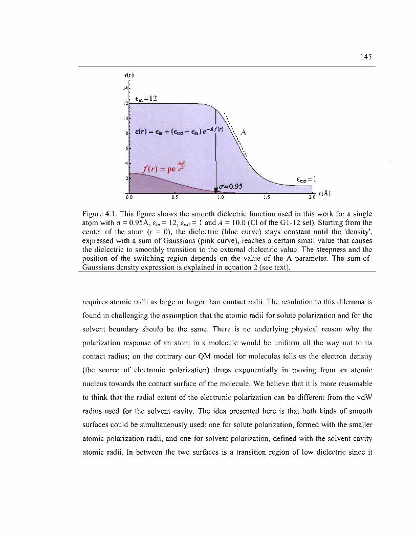
,,(rI

14

é lll =12 �2f---------_____

10

8 €(r) = €in + (€nt - Eu,,) e-A!(r)

. . .A .

6

4

2

(1"=0.95 é ext = 1

...JO.LO------'O-S ----=:::::=~I:::I:.0==-----I-'-.S-----2~.0 dA)

145

Figure 4.1. This figure shows the smooth dielectric function used in this work for a single atom with 0" = 0.95Â, E:in = 12, E:exI = 1 and A = 10.0 (CI of the G 1-12 set). Starting from the center of the atom (r = 0), the dielectric (blue curve) stays constant until the 'density', expressed with a sum of Gaussians (pink curve), reaches a certain small value that causes the dielectric to smoothly transition to the extemal dielectric value. The steepness and the position of the switching region depends on the value of the A parameter. The sum-of­Gaussians density expression is explained in equation 2 (see text).

requires atomic radii as large or larger than contact radii. The resolution to this dilemma is

found in challenging the assumption that the atomic radii for solute polarization and for the

solvent boundary should be the same. There is no underlying physical reason why the

polarization response of an atom in a molecule wou Id be uniform ail the way out to its

contact radius; on the contrary our QM model for molecules tells us the electron density

(the source of electronic polarization) drops exponentially in moving from an atomic

nucleus towards the contact surface of the molecule. We believe that it is more reasonable

to think that the radial extent of the electronic polarization can be different from the vdW

radius used for the solvent cavity. The idea presented here is that both kinds of smooth

surfaces could be simultaneously used: one for solute polarization, formed with the smaller

atomic polarization radii, and one for solvent polarization, defined with the solvent cavity

atomic radii. In between the two surfaces is a transition region of low dielectric since it

146

describes where the solvent and the solute electrons are both at a minimum. This leads to a

3-zone dielectric function to which we give the form

(4.3)

where 8in is the dielectric constant inside the molecular cavity, 8solv the bulk solvent

dielectric constant (80 for water), and 8/rans the dielectric constant in the zone of transition

between the solute and the solvent. For the smooth inner dielectric boundary, A has the

same meaning as in eq. (4.1) and J;Jf} is given by eq. (4.2). The additional exponential

term, for the outer dielectric boundary (with solvent), is a switching function that turns on

when a second Gaussian sum (fso,v (f)) becomes sufficiently smalL The fsa'v (r) term is

also given by eq. (4.2) with the difference that the atomic radii are larger as they define the

solvent cavity. The B parameter is responsible for the steepness of the cavity boundary, but

with a sufficiently large value it hàs the effect of moving the position of the boundary as if

the radii were scaled. The radial behaviour of the 3-zone dielectric is illustrated in Figure

4.2 for a single atom (a) and for the 4-pyridone molecule (b), both with typical parameters.

In eq.(4.3}, it is important to set 81rans = 1 when the frrst zone of the dielectric function is

fitted on molecular polarizability since the shape of the dielectric function needs to drops to

one in order to present the same ability to polarize. AIso, if the atomic partial charges are

fitted with DRESP, a change in the frrst zone boundary would also change the ability of the

dielectric to form the full internai polarization taken into account during the charge fitting

process.

147

("Ir)

"

'"

40

20 <'in

tsolv

:/ / -,j

B,,'/

Cf"Ç I Vlty 1

l ,l 'I

f---- --I._, ••••• A ,~

~/ +----~--=='--:----......""F_---___:_, fiA)

a

2

~ >- -,

-2

-3

-4

-5

-6

-5 -4 -3 -2 -, 2

b x (A)

Figure 4.2. The 3-zone dielectric function allows an accurate description of both the solute polarization and the solvent polarization within the EPIC approach. (a) The radial component of the dielectric for a single atom (G 1-12 aromatic carbon) is shown together with the polarization «(Jin) and the solvent cavity «(Jcavily) atomic radii. Each plateau of the dielectric function defines a zone. The intermediate zone corresponds to the solute/solvent contact distance. (b) The resulting dielectric function is also shown in the ring plane of 4-pyridone (b) when applying the G2-12 parameters.

148

4.2.2 Molecular polarizability tensor

In this section, we review the methodology previously developed to calculate

molecular polarizability tensor with a finite difference Poisson solver1 and we summarize

how the parameters inv01ved are optimized in this work.

4.2.2.1 Method

Our fonnulation of electronic polarization based on continuum electrostatics allows

the calculation of induced multipolar moments by considering the bound charge density,

which results from the polarizability density of the media (from the bound electrons in our

case). A fonnula to calculate the bound charge density iS21

pb(n =-V([E(F)-l]Ë(n) Eo (4.4)

=-V ·PCf)

where / is the bound charge density and Ë(f) the total electric field. Physically, / is a

consequence of the fonnation of dipoles at each point in space due to the electric field (the

polarization pen or dipole density). The bound charge' density can be thought of as an

induced charge density from the dielectric polarization that appears where the dielectric

varies, as an excess of charge builds due to the he ad or tail of the dipole density. Although

the polarization occurs everywhere the dielectric is greater than one, the bound charge

density appears in regions of spaces where E(f) varies, such as the dielectric boundary of a

molecule. Eq (4.4) is useful since it transfonns the locally induced dipoles into a scalar

value, the bound charge density, which can be used more easily as done below. In eq.(4.4),

E(f) -1 plays the role of a local polarizability density, also called the electric susceptibility,

and p(n = (E(r) -l)Ë(n corresponds to the induced dipole density (polarization). The

anal ogy with the point inducible dipole model, a different polarizable model, is obvious

since, in that case, the atomic induced dipole is given by {l(P;) = ajË(p;) where P(P;) , ai and

149

Ë(~) are the dipole induced at the atomic position ~, the atomic polarizability and the

electric field at ~. Here, the polarization is more smoothly distributed over the molecular

volume. Eq. (4.4) is intrinsic to the definition ofPoisson's equation.

A c1assical example, for which an analytical solution exists, is the dielectric sphere

in vacuum experiencing an external electric field .. In this case the mathematics show that

bound charges appear on the surface of the sphere with opposite charge sign on both

hemispheres, resulting in an induced potential equivalent to an ideal induced dipole

moment aligned with the external field located at the center of the sphere. The induced

dipole moment is proportional to the external electric field and the sphere polarizability

(J.,sphere is given by the Clausius-Mossoti equation

[

csphere -1 J 3

asphere = + 2 RsPhere Csphere

(4.5)

where Rsphere is the sphere radius. For a molecular system, the analytical solution is

unknown and we use a fmite difference algorithm to solve Poisson's equation numerically

with a uniform electric field in the form of a voltage clamp applied by means of the

boundary conditions. More precisely, a uniform electric field in the z direction can be

produced with a null potential on one side of the grid boundary and the value -EextxLz on

the opposite side, where Lz is the box size in the z direction and Eext the magnitude of the

applied field. On the four other sides, paraUel to the field, the grid boundary potential is

simply calculated as a linear interpolation along the z direction: <p(z-zO) = -(z-zO)xEexr. As

with the dielectric sphere in vacuum, a molecular dielectric volume responds linearly to the

applied field (given an isotropic dielectric function) and the proportionality constant is the

molecular polarizability tensor. The field is applied in three orthogonal directions to build

the polarizability tensor, which depends on the orientation of the molecule:

150

/lx,x /lx,y + /ly,x /lx,z + /lz,x

Eext 2Eexi 2Eext

a= /ly,y /ly,z + /lz,y (4.6)

Eext 2Eext

Eex,

where Px,y is the x component of the induced dipole moment when an external electric field

of magnitude Eex, is applied in the y direction. Sorne experimental values are available for

the eigenvalues of this tensor in vacuum (cexF 1); also, the polarizability tensor can be

calculated using approaches based on quantum mechanics (QM) methods such as density

functional theory.

The induced dipole moment is calculated analogously to the sphere dielectric

system, integrating the bound charge density over space. From eq. (4.4) (or simply from

Gauss's law), one can show that

(4.7)

In the present context, there is no free charge density pi (r) (from atomic partial charges,

for instance) and as such the bound charge density, induced only by the external uniform

electric field, is given by the divergence of the field. With a finite difference solver, the

total charge (bound and free charges) can be calculated by integrating over each differential

volume element (grid cube) which leads to bound charges on grid points. This can be done

simply by calculating

(4.8) _ (hyhz)( ) [hxhz)( ) (hxhy )( ) - - ---,;: tpi+ljk + tpi-Ijk - 2tpijk - T tpij+lk + tpij-Ik - 2tpijk - T ~jk+1 + tpijk-l - 2tpijk

where qijk, qbijk and q;jkare the total charge, the bound charge and the freecharge inside the

volume element associated with the ijk grid point, ({Jijk and ({Jijk-l the electrostatic potential at

151

the (x,y,z) and (x,y,z-dz) grid points respectively. The grid spacing in x, y and z are given by

hx, hx and hz. The grid free charge qijk are zero for this calculation and, in general, it is given

by the atomic partial charges as distributed on the grid. Finally, the total dipole moment is

given by

Grid

p= Lrijk qijk (4.9) i,j,k

With the free charges equal to zero (no atomic partial charge), the dipole calculated is then

the induced dipole and the only contributor is the bound charge density. More generally,

any molecular electric moment can be calculated with analogs to eq. (4.9). The overall

procedure to calculate the polarizability tensor requires three solutions from the numerical

solver. The calculation does not involve atomic partial charges (free charges) which allows

them to be fit independently (although this must still be done in the context of the

molecular dielectric).

4.2.2.2 Computational details

The finite difference Poisson calculations were performed with a modified version

of the OpenEye Inc. ZapTK22• The distance between two grid points was set to 0.35 A and

the grid boundary was at least 5 A away from the surface defined by the polarization radii.

Atomic charges of ±O.OOle were assigned randomly on the atoms as the grid energy was

used to determine the convergence of the algorithm set to 0.000001 kB T. The results were

not sensitive to these small charges. Atom typing was assigned via SMARTS23-25 with the

OpenEye Inc. OEchem toolkit26.

4.2.2.3 Optimization of the polarizabilities

The atomic radii were optimized in order to minimize a chi-square function using a

Levenberg-Marquardt algorithm as implemented in scipy27, a scientific Python library. The

error was defined as the difference between the 6 components of the polarizability tensor

obtained with B3L yP and EPIC

mo/ecu/es

%2= l k=x.x,."Y,xz

,Y.Y.J'Z,zz

152

(4.10)

where o.xyJ is one of the six-independent polarizability tensor elements of molecule i either

under optimization (EPIC) or from the QM target values. By using the six independent

tensor elements, we inc1uded both the magnitude and the direction of the polarizability in a

natural way28. We optimized the cube of the polarization radii because their contribution to

the polarizability grows with the atomic volume (c.f. eq. (4.5». For analysis purposes, we

also defined the average polarizability (eq. (4.11» and the anisotropy of the polarizability

tensor (eq. (4.12» below

~a= (a) -a2 )2 + (a) a 3 )2 +(a2 a 3 )2

2

(4.11)

(4.12)

where 0.1 :S 0.2 :S 0.3 are the eigenvalues of the polarizability tensor. The polarizability

anisotropy is significantly harder to fit than the average polarizability. We defined the error

in the average polarizability (eq. (4.13)) and anisotropy (eq. (4.14)) for a set of molecules

as

N laQM -a 1 tS = J.-~ i,avg i,avg

avg NL.. a~M 1 I,avg

(4.13)

1 N l~aiQM - ~ai 1

tSaniso = N L QM 1 ai,avg

(4.14)

where N is the total number of molecules considered and QM corresponds to the target

value. FinaIly, the relative root-mean-square deviation (RRMS) of the tensor was defined as

mo/ecu/es

L i k=xx ,.x:,v ,xz,

RRMS = ----:~~-----L (af,~r

k=xx ,xy ,Xl,

yy,yz,zz

(4.15)

153

and constituted a single me tric for the overall fitness of the optimized polarizability tensors.

If the RRMS was calculated for a single molecule, the summations on the molecules in the

numerator and the denominator were simply omitted.

4.2.3 Refractive index calculations

4.2.3.1 Theory

The dielectric constant of an isotropic material at the high frequency limit (too) is

related to the material refractive index29 n by

(4.16)

where n is usually measured with the D line of the sodium spectrum at 589 nm (nD)' The Eoo

corresponds to the material's dielectric constant solely due to the electronic polarization

since the frequency of the visible light is too high for nuclear relaxation to contribute.

Typically, a pure liquidof an organic compound will have a refractive i.ndex between 1.3

and 1.7 leading to a €oo between 1.7 and 2.9. Since the work of Debye and OnsagerI2,13,30,31,

it has become a dogma that the interior dielectric (ein) of a solute cavity in implicit solvent

models should be close to the experimental too in order to capture the dipole moment

change due to the cooperative solute-solvent polarization. It is when we seek for accuracy

in solute polarization that we found the generally accepted relation eoo = Ein to badly fail]. A

way to reconcile this puzzling finding is by computing the macroscopic refractive index

that corresponds to what is measured instead of assuming it is the same as the internai

refractive index (quoting Onsager30). The Clausius-Mossoti equation relates the

polarizability of a sphere to its interior dielectric. Since Eoo and n are macroscopic intensive

quantities, their measurement should not depend on the size of the studied sample, given

that it is large enough to exhibit a macroscopic behavior, the worst case being the use of a

single molecule. It is not to say that Onsager's use of the Clausius-Mossoti equation with

154

the radius of a single molecule was not justified. In fact, he was primarily interested in the

molecular polarizability (amol) and used the formula

(4.17)

where v is the volume of the liquid sphere considered and n the number of molecules it

contains. In eq. (4.17), the rightmost factor corresponds to the cube of an effective single

spherical molecule radius. It is however understood that the same molecular polarizability

is obtained as long as the vin factor is preserved and is therefore size independent with the

key assumption that Eoo is filling the space uniformly, i.e. that it is a spatially averaged

value. In order to calculate the refractive indices for the general case where the internaI

dielectric is not uniformly distributed in the liquid, we generated pure liquid configurations

from molecular dynamics (MD) simulations at room temperature and cut out spherical

clusters (or droplets) from individual snapshots. We maintained the vin ratio by fixing the

density to experiment and calculating the drop let effective Ein with the formula

2 R~roP/el + 2adrop/el n = -::-'-------''--R 3

drop/el - a drop/el

(4.18)

here Rdroplet and adroplet are the droplet radius and polarizability. We assigned the dielectric

function on aIl molecules and applied the procedure outlined above to calculate the drop let

polarizability and thereby access the droplet refractive index. Averaging the droplet

refractive index over many droplets yields an approximation of the bulk refractive index.

4.2.3.2 Computational details

To obtain the liquid phase droplets, molecular dynamic simulations, usmg the

AMBER 8.0 package, were performed on 3375 molecules (15x15x15) in a cubic box. The

NVT ensemble and periodic boundary conditions allowed the density to be fixed to the

experimental value. The temperature was set to 20°C to match the experimental conditions

used to report refractive indices and maintained constant with the Berendsen's weak

155

coupling algorithm32 with the kinetic energy adjusted every 1 ps. The short-range non­

bonded interaction cutoff was set to 8.0 Â and long range interactions computed with

particle mesh Ewaldl4.33 using the default Amber 8.0 setup. The molecules were charged

with AMI_BCC34,35 and the Generalized Amber Force Field (GAFFi6 was used. The

SHAKE procedure37 was used to fix ail bond lengths to hydrogen.

The initialliquid box was generated by positioning the molecules on a cubic lattice,

randomly oriented with the Marsaglia38 quaternions method. The system was first

minimized until the root-mean-square (RMS) of the gradient is less than 0.1 kcallmol/ Â.

This was followed by a 8 ps annealing phase integrated by steps of 1 fs, during which the

non-bonding interactions were gradually tumed on and the temperature increased from 0 K

to 40 K and decreased to 0 K. The system was then heated over 20 ps up to 293.15 K with a

2 fs integration time step. Following a 1 ns equilibration, 50 evenly-spaced snapshots were

written over a 2 ns production mn. Each of the liquid boxes for a given molecule was then

wrapped in the primary cell. A sphere with a diameter set to 85% of the box length formed

a liquid drop let when picking aH molecules with an atom lying inside the sphere. The

droplet radius was then determined by considering the position of the outermost non­

hydrogen atoms. The precisedefinition of the radius is not unique and we have verified, for

example, that using the experimental density to calculate the radius of the corresponding

ideal sphere gives refractive indices within ±0.0l of those obtained by the chosen

algorithm. AIso, this model assumes a perfectly spherical object, ignoring the dimples

formed because of the finite size of the spheres. The relatively large size of the droplet and

the averaging over 50 independentconfigurations reduced the effect of this approximation.

The solution to Poisson's equation in the presence of the voltage clamp boundary

conditions was obtained on a rectangular grid sized to encompass the full drop let plus half

its radius on each side of the droplet. The target grid spacing was set to be 0.5A. The

smooth dielectric functions (eq. (4.1)), fitted on the molecular polarizability tensors only,

were assigned together with the matching atomic polarization radii, internaI dielectric Gin

156

and A parameter. Theextemal dielectric was always set to the vacuum value 8ext = 1. The

convergence criteria for the ZapTk solver was based on the grid energy and set to 0.0001

kT. This convergence criterion required the assignement of atomic charges that we choose

to be ±O.OOle were randomly placed on half the atoms, keeping an overall neutral system.

Given the strength of the externat field applied, this was not perceptibly afTecting the

answer.

4.2.4 Free energy of hydration

4.2.4.1 Theory

Implicit solvent models are commonly used to incorporate the effects of solvation in

molecular models as a mean field39-43

. These models considerably reduce the computational

burden. needed to sample the solvent configurationa1 space when each atom of the solvent

are explicitly simulated. An important validation for solvation models cornes from the

experimental free energy of hydration (t1.Ghyd) that consists in the chemical potential

difference for the transfer of a solute from vacuum to bulk solvent. The computational

evaluation of t1.Ghyd is separated into two processes. Firstly, the non-polar free energy of

hydration (t1.Gnp) cornes from the formation of the solute-shaped cavity in the bulk solvent

that causes a reorganization of the solvent molecules, and non-polar interactions between

the solute and the solvent. Secondly, the electrostatic free energy of hydration (t1.Gelec)

results from the electrostatic work necessary to place the solute charge density in the solute

cavity, involving interactions between solute and solvent charge densities and their

response to one another. This results in the equation

(4.19)

The longstanding use of implicit solvent to evaluate t1.Gelec is based on a high continuum

dielectric solvent region that gets polarized by a static solute electric field. White the solute

cavity is traditionally formed with a molecular surface with a discrete transition of the

157

dielectric function at the solute-solvent boundary, we chose a smooth boundary transition

as explained earlier. The solute cavity volume and shape is determined by atomic radii. For

a given set of charges, atomic radii that are too small exaggerate the affinity of the solute

for water, white radii that are too large will have the opposite effect. The calculation of

I1Geiec is normally done with a non-polarizable solute or, if the cavity is assigned a Cin > 1,

the very significant screening of the atomic partial charges requires a special treatment that

was not done until recentl/. For non-polarizable solutes, knowing that water increases the

dipole moment of solvated molecules often by as much as 15%, the atomic charges should

not be fit on a gas phase QM ESP. For this reason, the charges are often generated from

RESp44 or AM1_BCC34,35 that are known to be sufficiently overpolarized compared to the

gas phase.

In the 3-zone dielectric model that we propose in this article (c.r. Figure 4.2a and

eq.(4.3»), the [IfSt zone should accurately account for the solute polarizability, which allows

for the use of vacuum phase atomic charges obtained independently of the internaI

dielectric function. The second zone located between the internai dielectric and the solvent

is set to vaéuum and the transition to the full implicit solvent model of the third zone needs

to be parameterized. Following the suggestion of Grant et al. 18 for their non-polarizable 2-

zone dielectric function, we fixed the B parameter in eq. to 11.8, which leaves the solvent

cavity atomic radii to be fitted on the experimental free energy of hydration. However, in

order to compare the calculated I1Ghyd to experiment, we needed to use existing values or

methods for I1Gnp• Fortunately, converged molecular dynamics free energy45,46 calculations

based on free energy perturbation (FEP) calculations are available for each compound from

our hydration free energy dataset. We feel this is the best achievable theoretical estimation

of I1Gnp , sothis is our preferred estimation in current study. However, since this is not very

useful for prospective evaluations of I1Ghyd, due to the heavy computational demands for

such FEP calculations, we also tested a surface area based model that calculates I1Gnp as

(4.20)

158

where 1 is a surface tension and S the surface area of the molecule as defined by a solvent

accessible surfacel7 created with a lA A rolling probe and the Bondi radii 16• This crude

approximation has been proven useful and it can be improved by atom typing the 147 or by

using sorne treatment of the dispersion energy48-51 instead; in this work a single value of 1

was fitted for each model.

4.2.4.2 Computatiooal details

The atomic partial charges responsible for the permanent electrostatic potential

(ESP) were determined by a least-squares-fit on the QM ESP calculated on a face-centered­

cubic grid of points. Following lakalian et ap4, the grid spacing was set to 0.5 A and the

grid points were positioned around the molecule in a volume formed by two vdW surfaces,

each built with Bondi radii scaled by a factor of lA and 2.0. The dielectric has the effect of

scaling down by a factor of IIEin the charges; this is partly compensated by the bound

charges appearing from the internaI polarization. Hence, the least-squares-fit requîres a

Poisson solver in order to capture the overall effect, which depends on the shape of the

dielectric boundary. It is noteworthy that the charge fitting pro cess is independent of the

EPIe polarizability model and, as such, can be fit after the solute dielectric parameters are

optimized. The details of the procedure, called DRESP, can be found elsewhere2.

A fini te difference Poisson solver was written to allow the implementation of the 3-

zone dielectric model. Here is a brief description of the algorithms implemented. We use

successive over-relaxation (SOR) and a Gauss-Seidel iterative scheme52,53 where the over­

relaxation parameter w is estimated by

(4.21) 1[2

À =1----max 2(n _1)2

159

where n the number of grid points in one of the dimension of the grid52• This crude estimate

of the spectral radius of the A matrix in the finite difference form of the Poisson's equation

used (see Appendix ofref. 18), was sufficient to reduce by a factor of approximately 30 the

number of Gauss-Seidel steps necessary.

The free charges of the system were assigned on the grid with a quadratic inverse

interpolation scheme18 that has the advantage of conserving the dipole moment, has a

continuous first derivative and is more robust to the effects of rotation and translation. The

same interpolation rule is used to calculate the potential in between grid points. In our

calculations, we use a convergence criteria base on grid energy defined as the sum of the

electrostatic potential times the distributed free charges on the grid. This convenient

criterion is directly related to the energy in an absolute way and thus ensures that relative

energies are also converged. The boundary conditions, in energy calculations, were

determined with a Coulomb potential.

The I1.Ge/ec was computed by taking the grid charge energy difference between a

solution obtained in vacuum (Bexi = 1) and another solution in water (Bexi 80) from the

resulting Poisson's equation and calculated with

1 A/oms

I1.Gelec

="2 l qi ( rp(~) wa/er - rp(~) vacuum)

1

(4.22)

where qi is the atomic partial charge qf atom i, 1P(~racuum is the interpolated electrostatic

potential at atom i position f;. The grid spacing for the solver was set to 0.35 A and the

minimum distance between the solute internaI radii and the grid boundary was set to 7 A. In

those cases where the solute was non-polarizable, &in was set to one. Finally, the parameters

(solvent cavity atomic radii and surface tension) were adjusted with the same Levenberg­

Marquardt algorithm used for the fit to the polarizability tensor. AIl parameters were

simultaneously optimized.

160

4.2.5 Quantum calculations

The B3L YP exchange-correlation functiona154,55 was used for aU DFT quantum

calculations ofthis work within the Gaussian 03 software56• AlI molecular structures ofthis

work were initially relaxed with B3L yP and the 6-31 G( d,p) basis set57-59

• Property

calculations required larger basis sets for accuracy. The electrostatic potential values were

obtained with B3 L YP and the 6-311++G(3df,3pd) extended triple zeta basis set57-59

• The

molecular polarizability tensor computations used the aug-cc-pVTZ basis set60, as it was

shown to lead to accurate results61• The implemented method in Gaussian 03 to calculate

the molecular polarizability tensor is the Coupled Perturbed Hartree Fock (CPHF)

method62. The Hartree-Fock calculations' performed to fit water-adapted atomic partial

charges were also performed with the Gaussian 03 software with the 6-31G(d,p) basis set.

4.3 Datasets

In this work, we made extensive use of three kinds of data: B3L YP/aug-cc-p VTZ

polarizability tensors, free energies of hydration and refractive indices. A total of five

datasets were created.

4.3.1 Polarizability training dataset (PTD)

A training dataset was used to optimize the internaI radius in order to match B3L YP

polarizability tensors. To this end, we made use of the previously published training

datasets 1 and added new molecules for a total of 265 polarizability tensors. In this datas et,

many neutral functional groups are represented: alkanes, alkenes, alkynes, halogens

(bromo, fluoro, chloro), alcohols, thiols, amines, ethers, thioether, nitriles, aldehydes,

ketones, esters, thioesthers, amides, acids, ureas, imines, amidines, sulfones, sulfoxides,

sulfonamides, heteroaromatics, hydrazines, hydroxamic acids, N-oxides, pyridones and

peptides. In addition, charged functional groups were also included with the sole purpose of

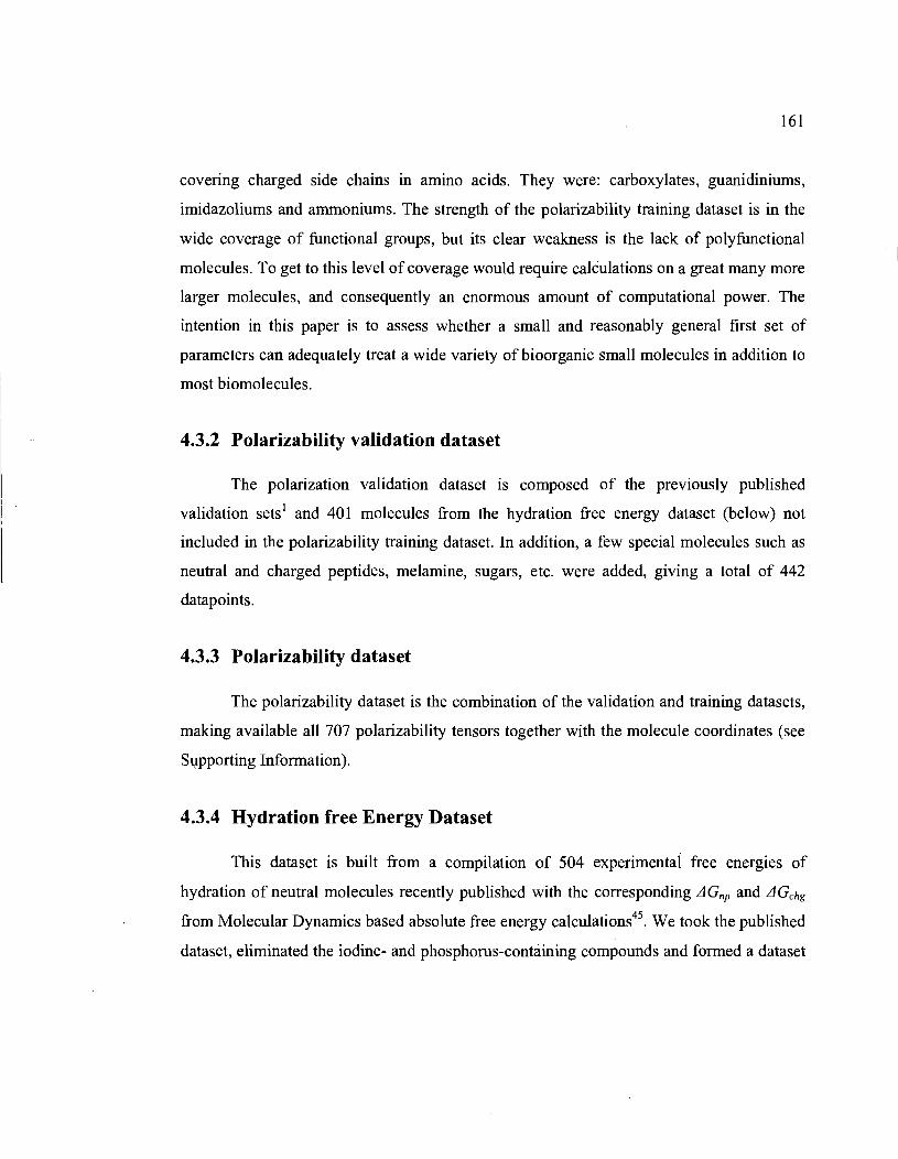
161

covenng charged side chains in ammo acids. They were: carboxy1ates, guanidiniums,

imidaz01iums and ammoniums. The strength of the polarizability training dataset is in the

wide coverage of functional groups, but its clear weakness is the 1ack of polyfunctional

molecules. To get to this level of coverage would require calCulations on a great many more

larger m01ecules, and consequently an enormous amount of computational power. The

intention in this paper is to assess whether a small and reasonably general first set of

parameters can adequately treat a wide variety of bioorganic small molecules in addition to

most biomolecules.

4.3.2 Polarizability validation dataset

The polarization validation datas et is composed of the previously published

validation sets! and 401 molecules from the hydration free energy datas et (below) not

included in the polarizability training datas et. In addition, a few special molecules such as

neutral and charged peptides, melamine, sugars, etc. were added, giving a total of 442

datapoints.

4.3.3 Polarizability dataset

The polarizability dataset is the combination of the validation and training datasets,

making available all 707 polarizability tensors together with the molecule coordinates (see

Sl,lpporting Information).

4.3.4 Hydration free Energy Dataset

This dataset is built from a compilation of 504 experimental free energles of

hydration of neutral molecules recently published with the corresponding LlGnp and LlGchg

from Molecular Dynamics based absolute free energy calculations45. We took the published

dataset, eliminated the iodine- and phosphorus-contéiining compounds and formed a datas et

162

of 485 molecules on which we could fit the solvent part of the dielectric function (eq.( 4.3))

and the surface tension coefficient (r).

4.3.5 Refractive indices datas et

The refractive indices dataset contains 23 small organic molecules (c.f. Figure 4.5)

thatare liquids at 20°C, for which the density and the refractive indices are taken from the

CRC Handbook of Chemistry and Physics63. They span a variety of functional groups and

most of the entire spectrum of refractive indices measured for bioorganic molecules.

4.4 Results and discussion

4.4.1 Polarizability tensor

This work follows the precedent of ref. 1 in fitting atomic polarization radii and a

single inner dielectric constant to QM molecular polarizability tensors to produce an

accurate EPIC model of electronic polarization. In this section, we generalize the

parameterization to account for most of the biomolecules and a significantly wider

spectrum of bioorganic functional groups. In contrast to our previous work, we use a

smooth dielectric function as described earlier and a single internaI dielectric (Gin) value.

4.4.1.1 Choice of Gin and A parameters

It was previously shown that a more accurate polarizable model was obtained when

different Gin were fitted for alkanes and aromatics. However, the single-Gin model performed

as well as the multi-Gin model and DFT against experimental directional polarizabilities.

Furthermore, in another studl that examined the local electronic polarization, the same

single-Gin model was only slightly worse than the multi-Gin mode!. In this work we pursue

the single-Gin model because it greatly simplified the Poisson solver implementation and the

robust parameterization for a wide spectrum ofbioorganic chemistry.

163

Before the global parameterization of polarizability atomic radii, a range-finding

study was performed with a smaller training set examining which combination of tin and A

(c.f. eq. (4.1))' is best to use for extending the EPIe parameterization previously initiatedJ•

We used a set of 13 alkanes (set g in ref. 1) inc1uding methane, propane, cyc1opropane,

butane (ci s, trans) , hexane (cis, trans) , and neopentane,. together with a set of 10

heteroaromatic molecules (set a in ref. 1). We forriled the two-dimensional grid of tin and A

pairs and optimized four radii (hydrogen, alkane carbon, aromatic carbon and aromatic

nitrogen) for each point of the grid. The polarizability tensor RRMS deviation from QM for

this datas et at each (tin, A) pair is shown as an iso-contour plot in Figure 4.3. It is c1ear that

in order to fit a general dielectric function, a sufficiently large tin is needed. AIso, the

flatness of the error surface allows for multiple equivalent choices, a potential advantage if

other criteria become more stringent in the development of the polarizable model. As

shown by red circ1es in Figure 4.3, four starting points were selected for further

examination: Gl-24 (tin=24, A=4.188), Gl-12 (tin=12, A=lO), Gl-9 (tin=9, A=5) and Gl-4

(tin=4, A=lO). In the case of Gl-24 only, the A parameter was relaxed to a value of 4.18.

The Gl-12 seems slightly superior to the Gl-9. Finally, while the Gl-4 parameter set

showed the worst RRMS, it was still a good case for having a small value of tin, picked by

Tan and LU013 as being optimal. Each of the G 1 tin and A choices was fixed in the global

parameterization of atomic polarization radii described below. Finally, Figure 4.3 shows

that making a poor selection of (tin, A), in particular having tin< 6, cannot be redeemed by

adjusting either the radii or the A parameter.

164

24

22

20

18

16

14

Gin

12

10

8

6

4

2

2 4 6 8 10 12 14 16 18

A parameter

Figure 4.3. The iso-contour plot of the RRMS error between B3LYP/aug-cc-pVTZ and EPIC polarizability tensors are shown as a function of the Gin and A parameters ofeg. (4.1). This RRMS surface was generated from a simultaneous fit of the H, alkyl C, aromatic C and aromatic N atomic polarization radii on training set of Il aromatic and 14 alkane molecules against their B3L YP polarizabilities. It shows that in order for a single dielectric model to fit the polarizabilities of these two chemical classes to within 10% error, the Gin

needs to be sufficiently large (>6). Deviations in the anisotropy of the polarizability are the main source of error for lower values of Gin.

4.4.1.2 The optimized polarization radii

The parameterization of tbe four G 1 sets on the 265 molecules of the polarizability

training dataset proceeded as described in the Method section. The Gin and A values were

fixed and the atomic polarization radii ai were adjusted to optimize the fit to the B3L YP

polarizability tensors. The atom typing of the radii was a primary concem and we aimed at

165

minimizing the number of radii fitted to reduce the fitting complexity, ensuring a better

generalization of the chemistry. Each non-symmetric molecule produced 6 data points from

their polarizability tensor; structuraHy symmetric molecules produced fewer data points.

The number of fitted parameters was kept small compared to the number of associated data

points to prevent over-fitting. The determination of the atom typing was do ne iteratively by

hand: [Ifst, the polarizability training dataset was designed in terms of chemical functional­

group classes. Adjustable parameters were added gradually with new molecules having

unmet che mi cal functionalities. Often, the addition of a new chemical functionality class

led to one or two additional parameters. We also merged atom types wh en the radii values

were similar and the fitness metrics (X2, Javg and janiso) were not significantly affected. For

example, the alkane H and C radii were the first to be fitted. This was followed by aromatic

C, H and N. It was determined early that a single aromatic and alkyl atom type for C and H

could be utilized. Then the alcohol oxygen radius, halogen radii, alkene carbon and alkyne

.carbon radii were individually fitted. The final stage was a global simultaneous fit of aH

radii with ail the molecules of the polarizability training dataset. Because of its special

importance as a solvent, water was treated separately with its own special 0 and H radii.

The resulting polarization radii are given in Table 4.1 for the fourG 1 parameter

sets. It is important to note that the ordering of atom types in Table 4.1 matters since the

atom typing was done in the given order (from top to bottom) to deal with the issue of a

particular atom falling in more than one category (H for instance). The first observation is

that ail polarization radii are significantly smaller than vdW contact radii such as Bondi l6,

Pauling64 or Parse40 often used in Poisson-Boltzmann approaches. Instead of being a

contradiction, this finding unveils the two different natures of the physical phenomena

described. On the one hand, the polarization radii aim at calibrating how the electrons

polarize in reaction to an external field created, for example, by an interacting molecule. On

the other hand the vdW radii determine the position of the repulsive molecular wall towards

solvent. It is also expected that the larger the t:in, the smaller the radii: to maintain the over­

ail polarization the dielectric must increase as the radii decrease. This is illustrating a

166

Table 4.1. Reported optimal polarization radii ((Jin) and atom typing for the four G 1 sets defining the internaI dielectric (c.f. eq.( 4.1 )).

SMARTS23.25 Typical functional

Radius (À) grou2s

Model name: GI-4 GI-9 GI-12 GI-24

Fixed parameters

ein 4 9 12 24 A 10 5 10 4.19

H

[H] all H 0.83 0.65 0.55 0.52 C

[CX4] alkanes 0.78 0.79 0.67 0.62 [c,CX2,CX3] aromatic, sp, Sp2 1.25 1.02 0.87 0.78

N

[n,NXI,NX3,$(Nc),$(NN)] aromatic, nitriles, Sp3, aniline,

1.09 0.89 0.76 0.69

hydrazine, 0.74a

[$(N[C,S]=*)] amides, amidines, 0.89 0.77 0.64 0.58 sulfonamides

[$(N=C)] imine, amidine 1.07 0.93 0.81 0.76 [$([#7]-[OX 1])] N-oxides, nitro 0.00 0.79 0.68 0.59

0

[$([OX2]([H])[#6,#7]),o,$([0D2]([C alcohols, furan, hydroxamic X4,c])[CX4]), acids, ethers, ketones, 0.88 0.73 0.63 0.60 $(0=[ c,C,S])] aldehydes, amides, sulfones

[$(OC=[O,N])] Esters, carboxylic acids 0.68 0.55 0.46 0.46 [$([OXIH#7])] N-oxide, nitro 1.08 0.89 0.77 0.74

Others

[S,s] All sulfur atoms 1.44 1.22 1.06 1.01 [F] 0.77 0.62 0.53 0.51 [Cl] 1.30 1.09 0.95 0.91 [Br] 1.47 1.24 1.0.7 1.03

Water Special fit

[$([OX2]([H])[H]] 0.93 0.86 0.76 0.75 [$([H][OX2][H])] 0.64 0.45 0.36 0.31

Charged atoms

[$([H] [#7+ ]),$([H] [#7][#6]=[#7+] [H] proton in guanidiniums, ), amidiniums, ammoniums,

$([H][ #7][#6]=[ #7+ ]),$([H][ n+ ]-c-n) pyridiniums 0.44 0.43 0.37 0.01

$([H]n-c-[ n+ Dl [$([O-]C=O),$(O=C[O-])] o in carboxylates 1.20 1.02 0.88 0.85 [$([NX4+ ]),$([#7+ ]=C-N),$(N- N in ammoniums,

0.00 0.34 0.39 0.52 C=[N+]))] guanidiniums, amidiniums,

[$([n+ ]-c-n),$([n]-c-[n+])] N in imidazoliums 0.00 0.00 0.00 0.42

167

general feature of the model that produces larger polarizabilities when either the 'electronic

volume', decided by the radii, or the internaI dielectric increase. The sort of relationship

involved is given in eq. (4.5) above for a hard sphere and elsewhere for a diatomic l.

It is aiso interesting to compare polarization radii between elements and between the

different chemical environments. First, it is remarkable that the carbon atom can be split

into only two atom types: Sp3 and others. The smaller Sp3 carbon radius implies that carbon

makes a much smaller contribution to the overall polarizability when Sp3 hybridized than

when pi electrons are present, i.e. in the sp or Sp2 hybridization states. This can be

rationalized by the presence of 1t. molecular orbitaIs, the different number of connected H

atoms, and the difference in the moiecule shape and the related anisotropy.

The nitrogen atoms were subdivided into four atom types amongst which two

encompass almost aIl instances in the datasets. The first of these is a general nitrogen type

assigned to amines, nitriles, hydrazines or anilines for example. The smaller second major

nitrogen radius makes amide, amidine or sulfonamide nitrogen less polarizable.

SurprisingIy, the more specific nitro and N -oxide nitrogen radius, in the G 1-4 set, has a

radius of zero. The dielectric on this nitrogen atom is only slightly smaller than Gin because

of the large bound oxygen radii and the short N-O bond, typically 1.2 A, which allows

dielectric from the oxygen to spread over onto the nitrogen. It is also interesting to note that

in the G 1-24 set, there was a gain in accuracy when the nitrile nitrogen had its own radius.

The oxygen atom behavior can mainly be accounted for by two adjustable radii

types, which was a significant advantage in the fitting process - the N-oxide and nitro

functional groups still being an exception. Another interesting result is the large radius of

the sulfur atom that is comparable to the bromine radius. However, it is not to say that the

polarizability contribution of sulfur is equivalent. In fact, the bromine bonds are longer and

hence offer a larger polarizable volume. This argument is also useful to explain why the

fluorine radius is smaller than the hydrogen radius. For example, the model predicts a

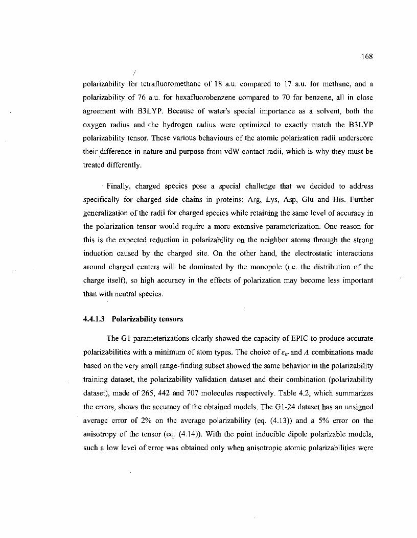
168

1 polarizability for tetrafluoromethane of 18 a.u. compared to 17 a.u. for methane, and a

polarizability of 76 a.u. for hexafluorobenzene compared to 70 for benzene, all in close

agreement with B3LYP. Because of water's special importance as a solvent, both the

oxygen radius and -the hydrogen radius were optimized to exactly match the B3L YP

polarizability tensor. These various behaviours of the atomic polarization radii underscore

their difference in nature and purpose from vdW contact radii, which is why they must be

treated differently .

. Finally, charged species pose a special challenge that we decided to address

specifically for charged side chains in proteins: Arg, Lys, Asp, Glu and His. Further

generalization of the radii for charged species while retaining the same level of accuracy in

the polarization tensor would require a more extensive parameterization. One reason for

this is the expected reduction in polarizability on the neighbor atoms through the strong

induction caused by the charged site. On the other hand, the electrostatic interactions

around charged centers will be dominated by the monopole (i.e. the distribution of the

charge itself), so high accuracy in the effects of polarization may become less important

than with neutral species.

4.4.1.3 Polarizability tensors

The G 1 parameterizations clearly showed the capacity of EPIe to produce accurate

polarizabilities with a minimum of atom types. The choice of êin and A combinations made

based on the very smaU range-finding subset showed the same behavior in the polarizability

training datas et, the polarizability validation datas et and their combination (polarizability

dataset), made of 265, 442 and 707 molecules respectively. Table 4.2, which summarizes

the errors, shows the accuracy of the obtained models. The G 1-24 dataset has an unsigned

average error of 2% on the average polarizability (eq. (4.l3)) and a 5% error on the

anisotropy of the tensor (eq. (4.14)). With the point inducible dipole polarizable models,

such a low level of error was obtained only when anisotropic atomic polarizabilities were

169

fitted5•15

,65.67, making their generalization very challenging. The other 01 models are worse,

and as predicted from the range-finding study results shown in Figure 4.3, the 01-4 set is

inadequate to reproduce the directional difference in the polarizability (the large daniso

values in Table 4.2). That the error obtained on both the training dataset and the validation

dataset was similar indicates that our radii are not overfit. Finally, the three directional

polarizabilities (eigenvalues of the tensor) obtained for the 707 molecules (2121 data

points) are compared to the corresponding B3L yP values in Figure 4.4 for three

representative 01 sets. The excellent correlation is obvious for the 01-24 and 01-12, and

deteriorates in the 01-4 EPIC model (the Pearson correlation coefficients are 0.99, 0.99,

0.96 and the s~opes 0.97, 1.02 and 1.20 respectively). An apparent outlier is the (J,3

(longitudinal polarizability) of (3E)-hexa-l,3,5-triene for which B3LYP gives a value of

176 a.u. compared to the EPIC value of 125 a.u. For this specifie molecule, Sekino et al. 68

showed that B3L YP greatly overestimates the 0.3 value of acetylene chains. Their better

estimate, based on very ace urate CCSD and MP2 QMresults, predicts a value of -135 a.u.,

close to the EPIC value. Another remarkable discrepancy between EPIC and B3LYP is

observed in Figure 4.4 for the 0.3 of l,4-dioxidopyrazine (doubly oxidized nitrogen on

pyrazine) that is predicted to be 103 a.u. by the 01~12 model versus 129 a.u. by B3LYP. A

similar observation can be made for 4-nitroaniline. Although we have not found better

estimates for these molecules, they most certainly constitute a challenge both for classical

and ab initia polarizability calculations.

170

Table 4.2. Error obtained with the optimized polarization radii of the G 1 sets when EPIC molecular polarizability tensors are compared to B3L YP for different molecule datasets.

Modela Ôavgb (%) Ôaniso

b (%) RRMSb (%)

Polarizability training datas et: 265 molecules

Gl-4 5.0 20.9 12.7

Gl-9 3.2 9.1 6.7

Gl-12 2.9 5.3 5.0

Gl-24 2.3 5.2 4.4

Polarizability validation datas et: 442 molecules

Gl-4 4.0 18.2 12.3

Gl-9 2.7 7.6 6.7

Gl-12 2.6 5.1 5.3

Gl-24 2.1 5.4 4.6

Polarizability dataset: 707 molecules

Gl-4 4.4 19.2 12.4

Gl-9 2.9 8.2 6.7

Gl-12 2.7 5.2 5.2

Gl-24 2.2 5.4 4.6

aModel using the parameters given in Table 4.1. bC.f. section 4.2.2.3

300

250

a. >- 200 ..J

'" III

~ 150 :ë <Il N .",

<Il Ci 100 a.

50

0 0

a

Y = mx + b m = 0.97 b = 1.32 R= 0.994

50 100 150 200 250 300

Polarizability G1-24

300

250

a. ~ 200

'" III

~ 150 :ë <Il N

.",

<Il Ci 100 a.

50

0 0 50

c

171

300

250

a. >- 200 ..J

'" III

~ 150 :ë <Il N .",

Y = mx + b <Il Ci 100 m= 1.02 a.

b = -3.34 R= 0.992

50

o~--,---~--~---.--~--~

b

100 150

o

y= mx + b m = 1.20 b =-17.5 R = 0.957

200

Polarizability G 1-4

50 100 150 200 250 300

Polarizability G1-12

250

Figure 4.4_ Correlation graph hetween the B3L YP/aug-cc-pVTZ directional polarizabilities (al black circ1es, a2 red triangles and a3 green squares in a.u.) for three G 1 dielectric parameter sets (c.f. Table 4.1). Each figure shows the data for 707 molecules for a total of 2121 points. From these figures, it is c1ear that a small number of parameters (optimized on 265 molecules) can generalize weIl. A large Gin = 24 (a) produces the best fit, a medium range Gin =12 (b) produces slightly larger discrepancies and a small Gin = 4 (c) produces significantly larger deviations, in keeping with the results of the range-finding study on the small dataset.

172

4.4.2 Refractive indices

In the previous subsection, we have developed dielectric functions that predict

remarkably weIl, relative to QM, the polarizabilities of a single molecule in the gas phase.

In this section we present the macros copie refractive index calculations and the

corresponding effective high frequency limit dielectric (cao). ln a previous publicationl, we

proposed that the vacuum of the intermolecular spacing may be sufficient to reduce the

effective macroscopic Cao resulting from the high intramolecular cin obtained in the

optimization to polarizability tensors. Here we use a theoretical approach to verity this

hypothesis. Another important point addressed by the refractive index calculation is the

transferability of the dielectric function from the gas phase to the condensed phase.

AB explained in further detail in the Theory and Method sections, we form liquid

drop lets containing thousands of molecules from snapshots obtained by MD simulations

and calculate the effective Cao by the use of the Clausius-Mossoti equation. The smaU range

spanned by experimental refractive indices makes this test somewhat stringent. Figure 4.5

shows the correlation between the results obtained with three representative EPIC

parameterizations and experiment; 01-9 is omitted here and for the remainder of the article

because the results are so similar to those of 01-12. The first observation is the close

agreement between the magnitudes of the Cao values. This clearly demonstrates that the

effective Cao of the liquid drop1ets have the appropriate value in spite of the high Sin,

confirming our hypothesis. Figure 4.6 provides a visual explanation for the apparent

mismatch between the small effective Cao compared to the productives Sin. This figure shows

the molecular dielectric inside a CC4 droplet wh en it is sliced through its center. The 01-

24, 01-12 and 01-4 models have a quite variable low-dielectric intermolecular space. The

coloring scheme of the dielectric function (eq. (4.1)) assigns red when s(r) ;;::::: Sin and dark

blue when s(r) = 1. The low dielectric intermolecular space increases with Sin as the atomic

radii decrease. It is striking that these three parameterizations produce the same refractive

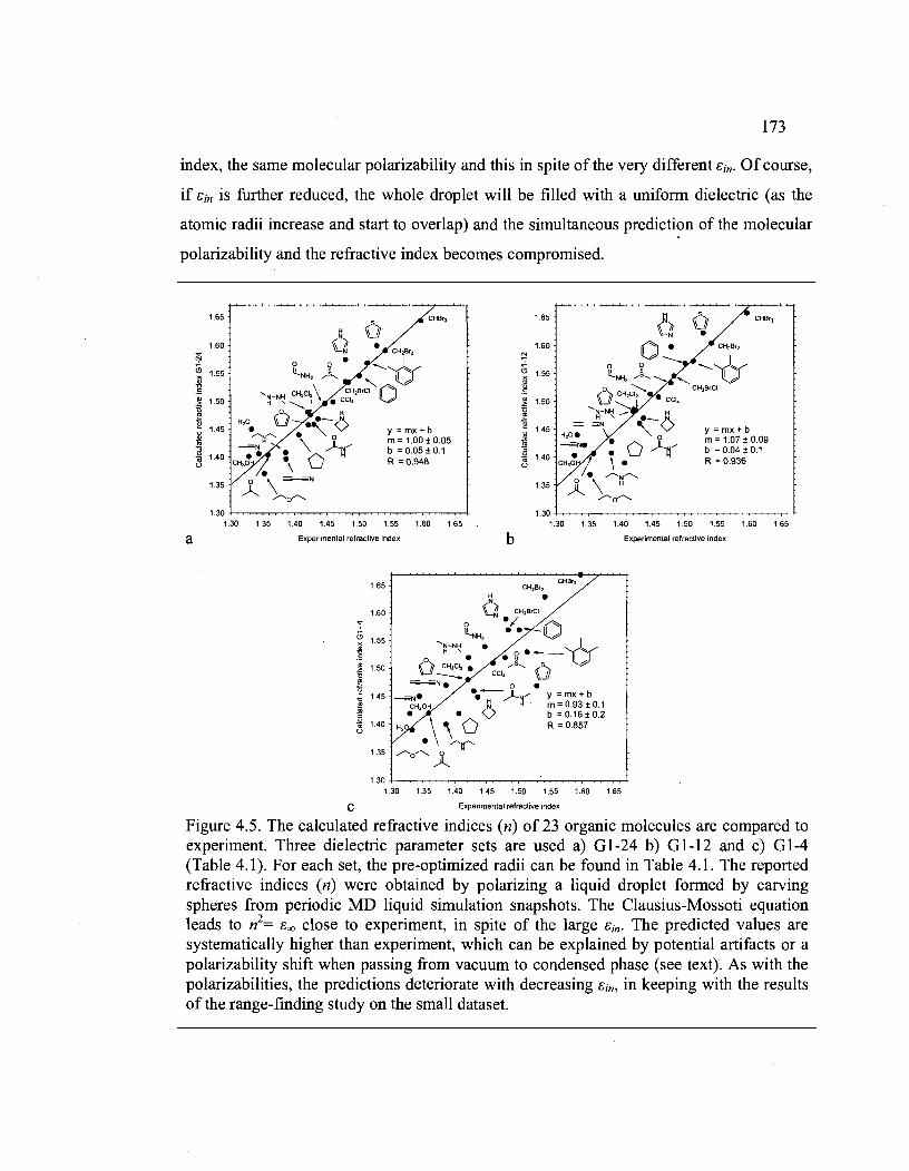
173

index, the same molecular polarizability and this in spite of the very different Gin. Of course,

if Gin is further reduced, the whole droplet will be filled with a uniform dielectric (as the

atomic radii increase and start to overlap) and the simultaneous prediction of the molecular

polarizability and the refractive index becomes compromised.

a

1.65

1.60

~ i 1.55

.~ 1.50

l al 1.45

m "';

~ 1.40 ü

1.35

5 o

y = mx ~ b m = 1.00 ± 0.05 b = 0.05 ± 0.1 R =0.94B

1.65

1.60

~ ~ 1.55

" ~ ~ 1.50

~ !! al 1.45

m ~ 1.40 ü

1.35

5 o •

y = mx ~ b m = 1.07 ± 0.09 b = 0.04 ± 0.1 R =0.936

1~ 1~ 1M 1~ 1~ 1S 1~ 1~ 1~ 1~ 1M 1~ 1~ 1S 1~ 1~

Experimental refractive index

1.65

1.60 ... (!i 1.55 ~ ~ .~ 1.50 tl

i ;; 1.45 S J)l

~ 1.40 ü

b

1.30 1.35 1.40 1.45 1.50 1.55 1.60 1.65

C Experimental refractive index

Experimental refradive index

Figure 4.5. The calculated refractive indices (n) of 23 organic molecules are compared to experiment. Three dielectric parameter sets are used a) G1-24 b) G1-12 and c) G1-4 (Table 4.1). For each set, the pre-optimized radii can be found in Table 4.1. The reported refractive indices (n) were obtained by polarizing a liquid droplet formed by carving spheres from periodic MD liquid simulation snapshots. The Clausius-Mossoti equation leads to n2= Goo close to experiment, in spite of the large Gin. The predicted values are systematically higher than experiment, which can be eXplained by potential artifacts or a polarizability shift when passing from vacuum to condensed phase (see text). As with the polarizabilities, the predictions deteriorate with decreasing Gin, in keeping with the results of the range-finding study on the small datas et.

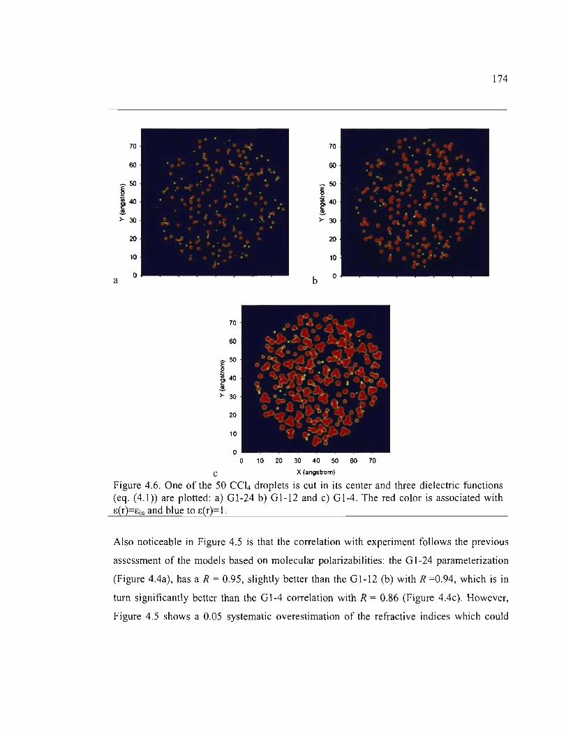
70

60

~50

~ 01 40 ~ ~ >-30

20

10

0 a

70

60

I50

~ 40 c: ~ >- 30

20

10

70

60

~50

~ ô'l4O ~ ~ >-30

20

10

b 0

10 20 30 40 50 60 70

C X (angstrom)

174

Figure 4.6. One of the 50 CCI4 droplets is cut in its center and three dielectric functions (eg. (4.1)) are plotted: a) GI-24 b) Gl-12 and c) Gl-4. The red color is associated with E(r)=Ein and blue to E(r)= 1.

Aiso noticeable in Figure 4.5 is that the correlation with experiment follows the previous

assessment of the models based on molecular polarizabilities: the G 1-24 parameterization

(Figure 4.4a), has a R = 0.95, slightly better than the G 1-12 (b) with R =0.94, which is in

turn significantly better than the Gl-4 correlation with R = 0.86 (Figure 4.4c). However,

Figure 4.5 shows a 0.05 systematic overestimation of the refractive indices which cou Id

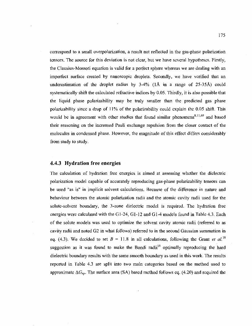
175

correspond to a small overpolarization, a result not reflected in the gas-phase polarization

tensors. The source for this deviation is not dear, but we have several hypotheses. Firstly,

the Clausius-Mossoti equation is valid for a perfect sphere whereas we are dealing with an

imperfect surface created by nanoscopic drop lets. Secondly, we have verified that an

underestimation of the drop let radius by 3-4% (lA in a range of 25-35A) could

systematically shift the calculated refractive indices by 0.05. Thirdly, it is also possible that

the liquid phase polarizability may be truly smaller than the predicted gas phase

polarizability since a drop of Il % of the polarizability could explain the 0.05 shift. This

would be in agreement with other studies that found sit~ilar phenomena8.11.69 and based

their reasoning on the increased Pauli exchange repulsion from the doser contact of the

molecules in condensed phase. However, the magnitude of this effect differs considerably

from study to study.

4.4.3 Hydration free energies

The calculation of hydration free energies is aimed at assessing whether the dielectric

polarization model capable of accurately reproducing gas-phase polarizability tensors can

be used "as is" in implicit solvent calculations. Because of the difference in nature and

behaviour between the atomic polarization radii and the atomic cavity radii used for the

solute-solvent boundary, the 3-zone dielectric model is required. The hydration free

energies were calculated with the Gl-24, Gl-12 and Gl-4 models found in Table 4.3. Each

of the solute models was used to optimize the solvent cavity atomic radii (referred to as

cavity radii and noted G2 in what follows) referred to in the second Gaussian summation in

eq. (4.3). We decided to set B = 11.8 in all calculations, following the Grant et alY

suggestion as it was found to make the Bondi radii16 optimally reproducing the hard

dielectric boundary results with the same smooth boundary as used in this work. The results

reported in Table 4.3 are split into two main categories based on the method used to

approximate !1Gnp. The surface area (SA) based method follows eq. (4.20) and required the

176

optimization of the surface tension parameter (y). The mam effort here is however

concentrated with the use of fj,.Gnp by converged free energy perturbation (FEP)

calculations45,46. This is the first category ofresults that we examine below.

4.4.3.1 Results with FEP-based non-polar term

Two main classes of solute are studied as reported in Table 4.3. Firstly, we set E:in =

E:lrans = 1 in eq. (4.3), effectively tuming eq. (4.3) into a 2-zone dielectric function with a

non-polarizable solute as defined previously by Grant et al. 18• For the non-polarizable

solute model, we used water-polarized static atomic charges as given by ESP-fitting to HF-

6-31G(d,p) wavefunction (G2-HF). These charge sets are positive controls, following the

traditional approaches for non-polarizable force fields and which have been shown to

produce the right degree of static polarization of the solute in water70• The G2-E:in, with E:in =

4, 12 and 24 (c.f. Table 4.1), has polarizable solutes assigned charges fitted to the

B3L YP/6-311 ++G(3df,3pd) ESP known to reproduce the gas phase dipole moment of the

molecules, being usually between 10% and 20% smaller than what is normally expected in

water. Polarizability should rightly compensate for the use of gas phase charges.

It is quite interesting to observe in Table 4.3 that by allowing the cavity radii to optimize in

each model, the same level of error over the 485 experimental free energies of hydration is

obtained for the G2-HF, G2-4, G2-12 and G2-24 solute models. The average unsigned error

(AUE) compared to experiment is 1 kcal/mol with a standard deviation of 1 kcal/mol. The

Pearson correlation coefficient (R) is around 0.89 in all these G2 models. The relative root­

mean-square deviation (RRMS) obtained is 0.35 and the average signed error (AE) is found

to be between -0.15 kcal/mol and -0.18 kcal/mol. These errors can be compared to the

Rizzo et al.47 results, on almost the same dataset (460 neutral molecules included in the 485

that we use), that produce an AUE of 1.47 kcal/mol with RESP charges and R = 0.88. The

reported numbers of Rizzo et al. were obtained with a SA evaluation of fj,.Gnp that allow

them to subsequently optimize 14 atom typed surface tensions (y), which improved the

AUE to 1 kcal/mol while R = 0.89. For comparison, in the current study, we fit 8 atomic

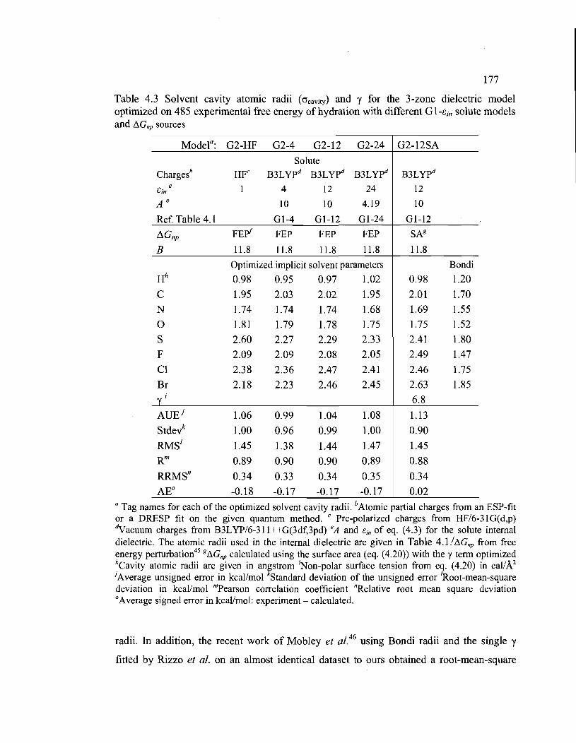
177

Table 4.3 Solvent cavity atomic radii (O"cavity) and y for the 3-zone dielectric model optimized on 485 experimental free energy of hydration with different G 1-cin solute models and !1Gnp sources

Modela: G2-HF G2-4 G2-12 G2-24 G2-12SA

Solute

Chargesb HFc B3Lypd B3Lypd B3Lypd B3Lypd

Cin e 4 12 24 12

A e 10 10 4.19 10

Ref Table 4.1 GI-4 GI-12 GI-24 Gl-12

!1Gnp FEpf FEP FEP FEP SAg

B 11.8 11.8 11.8 11.8 11.8

Optimized implicit solvent parameters Bondi

H h 0.98 0.95 0.97 1.02 0.98 1.20

C 1.95 2.03 2.02 1.95 2.01 1.70

N 1.74 1.74 1.74 1.68 1.69 1.55

0 1.81 1.79 1.78 1.75 1.75 1.52

S 2.60 2.27 2.29 2.33 2.41 1.80

F 2.09 2.09 2.08 2.05 2.49 1.47

Cl 2.38 2.36 2.47 2.41 2.46 1.75

Br 2.18 2.23 2.46 2.45 2.63 1.85 yi 6.8 AUEj 1.06 0.99 1.04 1.08 1.13

Stdevk 1.00 0.96 0.99 1.00 0.90

RMS' 1.45 1.38 1.44 1.47 1.45

Rm 0.89 0.90 0.90 0.89 0.88

RRMSn 0.34 0.33 0.34 0.35 0.34 AEo -0.18 -0.17 -0.17 -0.17 0.02

a Tag names for each of the optimized solvent cavity radii. b Atomic partial charges from an ESP-fit or a DRESP fit on the given quantum method. C Pre-polarized charges from HF/6-3lG(d,p) dVacuum charges from B3LYP/6-311++G(3df,3pd) eA and ëin of eq. (4.3) for the solute internaI dielectric. The atomic radii used in the internaI dielectric are given in Table 4.1! !1Gnp from free energy perturbation45 g!1Gnp calculated using the surface area (eq. (4.20)) with the y term optimized hCavity atomic radii are given in angstrom Non-polar surface tension from eq. (4.20) in cal/A2

j Average unsigned error in kcal/mol kStandard deviation of the unsigned error 'Root-mean-square deviation in kcal/mol mpearson correlation coefficient nRelative root mean square deviation o Average signed error in kcal/mol: experiment - calculated.

radii. In addition, the recent work of Mob1ey et al. 46 using Bondi radii and the single y

fitted by Rizzo et al. on an almost identica1 dataset to ours obtained a root-mean-square

178

deviation of2.05 kcal/mol. Finally, in a different article, Mobley et al. 45 obtained a RMS of

1.26 kcallmol and R = 0.89 with explicit-solvent converged FEP calculations. The FEP

based llGnp used in this work cornes from this latter study. Our results are comparable to or

better than most other studies. We attribute the small errors to the optimization of the radii,

not necessarily to the quality of the solute model. We can however examine the fitted

cavity radii with the different solute models to understand the effects of the electrostatic

model on the solute cavity size.

The level of solute polarization brought by the polarizable solute models (G2-4 to

02-24) seems similar to what is obtained with the G2-HF solute model. This can be

assessed by comparing the atomic radii and the cross-validation error showed in Table 4.4

where the G 1-12 solute model is used with the different G2 radii sets. The level of error

produced when Gin 12 and 24 or with the G2-HF cavity radii is similar, the G2-4 being

the worst. The cross-validation results of Table 4.4 also show the transferability of the third

zone dielectric parameters given that the solute has the 'physically appropriate electrostatic

behavior. A possible advantage of the polarizable solute model is when the solvation free

energies are computed relative to a solvent much less polar than water (e.g. a non-polar

solvent or a non-polar binding site in a protein). In this case, the HF based charges may not

be appropriate71. The fitted radii of Table 4.3 are significantly different from the contact

Bondi radii reported in the last column. Firstly, the H radius is a little smaller than the usual

1.1 A contact radius in aIl cases (the Bondi radius of 1.2 A for H was recognized to be a

little too large and was revised to be 1.1 An). The carbon radius obtained here is much

larger than the Bondi radius and makes the C-H bonds behave like a united atom model. In

this perspective the carbon radius size obtained here is similar to the Nina et al. 73 carbon

radius they calculated by looking at MD water charge density in explicit solvent

simulations. For the other elements, we also find larger radii than Bondi, in agreement with

a recent study by Nicholls et al. 31

179

Table 4.4. Effects of using different solvent cavity radii set (Table 4.3) with the G 1-12

solute model (Table 4.1) on I1Ghyd

G2-12 G2-24 G2-4

AVEa 1.04 1.08 1.17

Stdevb 0.99 1.03 1.19

Re 0.90 0.90 0.86

RRMSd 0.34 0.35 0.39

AEe -0.17 0.16 -0.23

a Average unsigned error in kcallmol bStandard deviation on the AUE in kcallmol CPearson correlation coefficient dRelative root-mean-square deviation

G2-HF

1.10

1.01

0.89

0.35

0.15

eAverage signed error in kcallmol: experiment - calculated

The larger cavity radii can be rationalized by considering the difference between

contact radii (Bondi) and the cavity radii needed in implicit solvent calculations. The

former is defined by crystal contacts between neighboring molecules and the latter defines

where the mean solvent charge density appears. In terms of the 3-zone dielectric model, the

contact radii would be located in the middle of the second zone where the electronic density

should be minimal given that the dielectric goes to one (no electrons to be polarized on the

solute side). This is supported by the fact that Fermi repulsion between the solvent

molecule electrons and the solute electrons reduces the total electronic density exactly in

the contact zone to its minimum. In Figure 4.2a, the contact radius of an aromatic carbon

atom would become 1.7 A, exactly the Bondi radius value. Similarly the middle of the blue

area in Figure 4.2b de fines the contact line between solvent molecules and the solute.

Although we claim here that having cavity radii larger than Bondi radii may be

physically motivated, it is not possible at this stage to know if this effect should be as large

as we find. In particular, the fluorine radii in Table 4.3 are surprisingly large. This was also

180

found by Nicholls et al. 31 where their optimal fluorine radius was 2.4 À. Knowing that

fluorine is particularly hydrophobic, this may be just another peculiar behavior ofthis atom.

The Cl and Br radii difference in the G2-4, G2-l2 and G2-24 sets uncover a drawback of

using a small êin. Because the polarization radius of Cl and Br are larger in the G 1-4 than in

the other EPIC parameterizations, the transition zone shown in Figure 4.2 cannot reach E(r)

= 1 (in the case of Br, it only decreases to E(r) = 3) and as a result the full polarizability

coming from the halogen atom is not reached as the solvent cuts into the first zone

die1ectric function. This prevents enough solute bound charge density from building up.

A last point to mention in regard to the 3-zone dielectric function is its potential

advantage in reducing the occurrence of the reentrant surface problem that often brings a lot

of fluctuation in energy or force computations in proteins, for instance. The problem is the

artificial formation of a cavity with high dielectric inside a protein due to the irregularity of

molecl.llar surfaces. The large size of the atomic cavity radii in the G2 sets and the use of a

smooth dielectric function should contribute to create a sufficiently deep buffer of low

dielectric and make implicit solvent models more stable. Indeed, the smoothness of the

surface around 4-pyridone observed in Figure 4.2b looks like a solvent accessible surface 17.

This entire question is however left for future research.

4.4.3.2 ResuUs with surface area-based non-polar term

Although the use of the very computationally intense FEP-based I1Gnp may be more

physically grounded, the obtained models cannot practically be used in a prospective

manner due to the heavy computational demands for such FEP calculations. For this reason,

we also optimized the cavity radii and the surface tension with the G 1-12 solute models. In

these calculations the solvent accessible surface area was calculated with the Bondi radii

and kept constant. The results are reported in Table 4.3. The error levels reported are

comparable to those obtained with I1Gnp from FEP calculation. The G2-12/SA model gives

error levels a little larger than the G2-l2: AUE = 1.13 kcallmol with a standard deviation of

181

0.90 kcaVmol, R = 0.88, RRMS = 0.34, RMS = 1.45 kcaVmol and AE = 0.02 kcallmol. It is

comforting that the optimal surface tensions of the two optimizations are close to each

other. The radii obtained for the 02-12/SA fit are similar to the 02-12 fit except for S, F, Cl

and Br. It is possible that the hydrophobicity of these atoms isoverestimated by the single

surface tension term used with the Bondi radii to determined I1Gnp .

4.5 Conclusion

The EPIC approach to molecular polarizability has been parameterized to include

many more chemical functional groups than a previous effort l. This required generating a

dataset of 707 B3L YP/aug-cc-pVTZ molecular polarizability tensors. The ability of EPIC

to account for both the average polarizability and the anisotropy of the tensor was

remarkable given that the optimization of only 14 parameters (excluding water and charged

species) led to a relative unsigned error in the average polarizability and anistropy of 2.6%

and 5.2% respectively (01-12). An example of the parsimony of the atom typing is that a

single radius parameter was sufficient for aromatic, nitrile, amine, aniline or hydrazine

types of nitrogen. Obtaining the same level of error with both the validation and training

datasets suggests that overfitting is not an issue. With previous polarizable models, such as

point-inducible dipoles, this level of accuracy could only be attained with added complexity

such as anisotropic polarizable centers or molecule-specific Thole screemng

parameters5,15,28,65-67.

We found that the anisotropy could only be reproduced accurately if the interior

dielectric constant was higher than 9.0. Above this value, almost any interior dielectric can

also work well as long as the atomic polarization radii are appropriately adjusted. The need

for a high interior dielectric raised the question of the physical soundness of the model as

Gin=Goo=n2 has become a dogma in the implicit solvent literature13,30,3l,39,4o,74-76 whenever the

182

dielectric constant is used to replace electronic response. The conceptual flaw of this

equality cornes from the fact that the interior dielectric (Cin) is not uniformly distributed

whereas the refractive index (n) cornes from a macroscopic measurement assuming a

uniform S::.o in space. To verify that the optimized models agree with experimental refractive

indices, we devised a new protocol to calculate a liquid refractive index from microscopic

simulations. To this end, 23 organic molecules spanning the entire range of bioorganic­

molecule-like refractive indices state were simulated by molecular dynamics in the liquid

state and coo was calculated with the Clausius-Mossoti relation. The obtained refractive

indices now come from the effective polarization of liquid configurations having

intramolecular high dielectric with low-dielectric interstices. The results show a good

correlation for aIl three Ol-cin parameter sets. The highest interior dielectric (ein = 24) gave

the best correlation with a slope of 1.00, an intercept of 0.05 and a correlation coefficient of

0.95. It is interesting to note that the polarizability anisotropy may play a role since the 01-

4 parameters (ein=4) gave the poorest correlation and was also the worst model for

polarizability anisotropy. Nevertheless, these results indicate that, when coupled with the

appropriate radii, many choices of ein can give results in good agreement with the

experimental refractive indices.

To use the EPIC polarizable electrostatic model with implicit solvent, we have

developed a smoothed-boundary 3-zone dielectric function that works with the internaI

dielectric continuum model. The threè zones are the internaI dielectric constant ein, a

transition zone that goes to the vacuum dielectric (Clrons=l), and a third zone defined by the

molecular cavityboundary, i.e. where the dielectric function reaches the bulk liquid

dielectric. With this function, keeping the [IfSt zone fixed at the atomic polarization radii

and Cin determined for the gas phase polarizabilities, only the molecular cavity boundary

needs to be parameterized. A dataset of 485 experimental free energy of hydration was used

to optimize the solvent cavity radii, one per element, with different charge models. The

resulting level of error was smaller than found in previous implicit solvent studies with a

typical average unsigned error of 1 kcal/mol with a standard deviation of about 1 kcal/mol

183

and a Pearson correlation coefficient of 0.9. Atomic charge sets fitted from the unpolarized

gas phase B3L YP density coupled with EPIe polarization led to cavity radii comparable to

those obtained with the polar-condensed-phase-like HF/6-31G(d,p) charges. The low

sensitivity of the optimal cavity radii resulting from the fit with different polarizable solutes

(the different G 1-Gin) further supports the generality of the approach. These results clearly

show that EPIe can lead to accurate description of solute polarization in implicit solvent.

The anisotropy of the molecular polarizability does not seem to play an important role in

fitting experimental hydration free energies. However, when considering intermolecular

interactions, such as in an enzyme active site, the heterogeneity of the environment and of

the interactions may require an accurate directional polarizability. An important example of

this is in cation-1t interactions2,77

The proposed global optimization scheme involves several independent layers. The

polarizability part is fitted on uncharged QM mo1ecular polarizability tensors. The charges

are added with the DRESP fit on ab initio electrostatic potentials calculated on a grid, as

usuaI, except that here the QM method can be systematically improved since gas phase

charges are needed. For implicit solvation, solvent-related radii are obtained from a fit to

experimentai hydration free energies. Flexibility and transferability has been demonstrated

for each stage. The ease with which we could fit the polarizability of so many functionai

groups makes us believe that the further extension of the parameterization and atom typing

should be straightforward given more data. Moreover, the decoupling of the fitted

polarization from the fitted charges, as well as the physical soundness of each step, makes

the above parameterization scheme even more robust and general than is possible for two­

body additive force fields.

This work partly addresses the question of applicability of EPIe in polar condensed

phase. The ca1culations of the refractive indices were weIl behaved and show the high

values for Gin are not unphysical. It is not clear if the slightly larger calculated

polarizabilities of the drop lets were due to a change in polarizability when going from gas

184

phase to condensed phase. Also, the level of electronic induction seen in the 3-zone implicit

solvent calculations suggests that both solute and solvent polarization in polar media is well

modeled. To confirm those findings, it would be interesting to perform explicit atoms

simulations with the EPIC model and Poisson's equation.

The EPIC approach to polarizability has shown unprecedented accuracy and

flexibility on many accounts for su ch a simple model. Although the optimized parameters

are unconventional compared to traditional Poisson-Boltzmann applications, it is for sound

physical reasons that even clarify aspects of the implicit solvent approaches. In this paper

and the two previous ones1.2

, EPIC was shown to be a powerful tool to include the effects .

of electronic polarization in molecular mechanics type calculations, especially appropriate

to biomolecular force fields.

4.6 Acknowledgment

This work was made possible by the computational resources of the réseau

québécois de calcul haute performance (RQCHP). The authors are grateful to OpenEye Inc.

for free academic licenses. R. 1. 1. acknowledges financial support from the Natural

Sciences and Engineering Research Council of Canada (NSERC). l-F. T. is supported by

NSERC through a Canada graduate scholarship (COS D) and by Merck & Co. through the

MRL Doctoral Program. 1. B. R. is supported by NIH grant OM072558.

4.7 Supporting Information

DFT and EPIC polarizabilities are available for all 707 molecules examined

together with the optimized coordinates of the molecules used to calculate the polarizability

tensor. Calculated and experimental refractive indices are provided. The detaited free

energies of hydration can also be found. This information is available free of charge via the

Internet at http://pubs.acs.org.

4.8 Bibliography

1. Truchon, J.-F.; Nicholls, A.; Iftimie, R. 1.; Roux, B.; Bayly, c. 1. Accurate

Molecular Polarizability based on Continuum Electrostatics. J. Chem. Theory

Comput., 2008, 4, 1480-1493.

2. Truchon, J.-F.; Nicholls, A.; Grant, J. A.; Iftimie, R. 1.; Roux, B.; Bayly, C. 1.

185

Extending the Polarizable Continuum Dielectric Model to Account for Electronic

Polarization in Intermolecular Interactions. Submitted, 2008,

3. Applequist, J.; Carl, J. R.; Fung, K. K. Atom dipole interaction model for molecular

polarizability. Application to polyatomic molecules and determination of atom

polarizabilities. J. Am. Chem. Soc., 1972,94,2952-2960.

4. Warshel, A.; Levitt, M. Theoretical studies of enzymic reactions: Dielectric,

electrostatic and steric stabilization of the carbonium ion in the reaction of

lysozyme. J. Mol. Biol., 1976, 103, 227-249.

5 .. Miller, K. J. Calculation ofthe Molecular Polarizability Tensor. J. Am. Chem. Soc.,

1990,112,8543-8551.

6. Lamoureux, G.; Allouche, D.; Souaille, M.; Roux, B. Incorporating electronic

polarizability in molecular dynamics: A model based on drude oscillators. Biophys.

J., 2000, 78, 330A-330A.

7. Lamoureux, G.; Roux, B. Polarizable force-field based on drude oscillators:

Molecular dynamics simulation and parametrization. Biophys. J., 2001, 80, 328A-

328A.

----- ---------------------

186

8. Sehropp, B.; Tavan, P. The Polarizability ofPoint-Polarizable Water Models:

Density Funetional TheorylMoleeular Meehanies Results. J. Ph ys. Chem. E, 2008,

J J 2, 6233-6240.

9. Lamoureux, G.; MacKerell, A. D.; Roux, B. A simple polarizable model ofwater

based on classical Drude oseillators. J. Chem. Phys., 2003, J J 9, 5185-5197.

10. Anisimov, V. M.; Lamoureux, G.; Vorobyov, 1. V.; Huang, N.; Roux, B.;

MacKerell, A. D. Determination of eleetrostatic parameters for a polarizable force

field based on the classieal Drude oseillator. J. Chem. Theory Comput., 2005, J,

153-168.

11. Morita, A. Water polarizability in condensed phase: Ab initio evaluation by cluster

approach. J. Comput. Chem., 2002, 23, 1466-1471.

12. Sharp, K.; Jean-Charles, A.; Honig, B. A Local Dielectric-Constant Model for

Solvation Free-Energies Which Accounts for Solute Polarizability. J. Phys. Chem.,

1992,96,3822-3828.

13. Tan, Y. H.; Luo, R. Continuum treatment of eleetronic polarization effeet. J. Chem.

Phys., 2007, J 26,094103.

14. Tan, Y. H.; Tan, C. H.; Wang, J.; Luo, R. Continuum polarizable force field within

the Poisson-Boltzmann framework. J. Phys. Chem. E, 2008, 112, 7675-7688.

15. Birge, R. R. Calculation of Moleeular Polarizabilities Using An Anisotropie Atom

Point Dipole Interaction-Model Which Includes the Effect of Electron Repulsion. J.

Chem. Phys., 1980,72,5312-5319.

187

16. Bondi, A. van der Waals Volumes and Radii. J. Phys. Chem., 1964,68,441-451.

17. Richards, F. M. Areas, Volumes, Packing, and Protein-Structure. Annu. Rev.

Biophys. Bioeng., 1977,6,151-176.

18. Grant, J. A.; Pickup, B. T.; Nicholls, A. A smooth permittivity function for Poisson­

Boltzmann solvation methods. J. Comput. Chem., 2001, 22, 608-640.

19. Prabhu, N. V.; Zhu, P. J.; Sharp, K. A. Implementation and testing of stable, fast

implicit solvation in molecular dynamics using the smooth-permittivity finite

difference Poisson-Boltzmann method. J. Comput. Chem., 2004,25,2049-2064.

20. lm, W.; Beglov, D.; Roux, B. Continuum Solvation Model: computation of

electrostatic forces from numerical solutions to the Poisson-Boltzmann equation.

Comput. Phys. Commun., 1998, 11 J, 59-75.

21. Griffiths, D. J. Introduction to Electrodynamics; 3rd ed.; Prentice-Hall Inc.: Upper

Saddle River, NJ, 1999.

22. Zap Toolkit, version 2.2.1; Santa Fe, NM, USA, 2007

23. Weininger, D. Smiles .3. Depict - Graphical Depiction ofChemical Structures. J.

Chem. In! Model., 1990, 30, 237-243.

24. Weininger, D.; Weininger, A.; Weininger, J. L. Smiles .2. Aigorithm for Generation

of Unique Smiles Notation. J. Chem. In! Model., 1989,29,97-101.

25. Weininger, D. Smiles, A Chemical Language and Information-System.1.

Introduction to Methodology and Encoding Rules. J. Chem. In! Model., 1988,28,

31-36.

26. OEChem Too/kit, version 2.2.1; Santa Fe, NM, USA, 2007

188

27. SciPy: Open Source Scientific Toolsfor Python, 2001

28. Elking, D.; Darden, T.; Woods, R. J. Gaussian induced dipole polarization model. 1.

Comput. Chem., 2007, 28, 1261-1274.

29. Bottcher, C. J. F. Theory of Electric Polarization; 2 ed.; Elsevier Scientific

Publishing Company: New York, 1973; Vol. l.

30. Onsager, L. Electric Moments of Molecules in Liquids. 1. Am. Chem. Soc., 1936,

58, 1486-1493.

31. Nicholls, A.; Mobley, D. L.; Guthrie, J. P.; Chodera, J. D.; Bayly, C. 1.; Cooper, M.

D.; Pande, V. S. Predicting small-molecule solvation ftee energies: An informaI

blind test for computational chemistry. 1. Med Chem., 2008, 51, 769-779.

32. Berendsen, H. J. C.; Postma, J. P. M.; Vangunsteren, W. F.; Dinola, A.; Haak, J. R.

Molecular-Dynamics wîth Coupling to An External Bath. 1. Chem. Phys., 1984,81,

3684-3690.

33. Darden, T.; York, D.; Pedersen, L. Particle Mesh Ewald - An N.Log(N) Method for

Ewald Sums in Large Systems 1. Chem. Phys., 1993, 98, 10089-10092.

34. Jakalian, A.; Jack, D. B.; Bayly, C. L Fast, efficient generation ofhigh-quality

atomic charges. AMI-BCC model: IL Parameterization and validation. 1. Comput.

Chem., 2002,23, 1623-1641.

35. Jakalian, A.; Bush, B. L.; Jack, D. B.; Bayly, C. I. Fast, efficient generation ofhigh­

quality atomic Charges. AMI-BCC model: I. Method. J. Comput. Chem., 2000,21,

132-146.

189

36. Wang, 1. M.; Wolf, R. M.; Caldwell, J. W.; Kollman, P. A.; Case, D. A.

Development and testing of a general amber force field. 1. Comput. Chem., 2004,

25, 1157-1174.

37. Ryckaert, J. P.; Ciccotti, G.; Berendsen, H. J. C. Numerical-Integration ofCartesian

Equations of Motion of A System with Constraints - Molecular-Dynamics ofN­

Alkanes.1. Comput. Phys., 1977,23,327-341.

38. Marsag1ia, G. Choosing a Point from the Surface of a Sphere. The Ann. of Math.

Stat., 1972,43,645-646.

39. Warwicker, 1.; Watson, H. C. Calcu1ation of the Electric-Potential in the Active-Site

Cleft Due to Alpha-Helix Dipoles. 1. Mol. Biol., 1982, 157, 671-679 ~

40. Sitkoff, D.; Sharp, K. A.; Honig, B. Accurate Calculation ofHydration Free­

Energies Using Macroscopic Solvent Models. 1. Phys. Chem., 1994, 98, 1978-1988.

41. MacKerell, A. D.; Bashford, D.; Bellott, M.; Dunbrack, R. L.; Evanseck, 1. D.;

Field, M. J.; Fischer, S.; Gao, 1.; Guo, H.; Ha, S.; Joseph-McCarthy, D.; Kuchnir,

L.; Kuczera, K.; Lau, F. T. K.; Mattos, c.; Michnick, S.; Ngo, T.; Nguyen, D. T.;

Prodhom, B.; Reiher, W. E.; Roux, B.; Schlenkrich, M.; Smith, J. c.; Stote, R.;

Straub, J.; Watanabe, M.; Wiorkiewicz-Kuczera, 1.; Yin, D.; Karplus, M. All-Atom

Empirical Potential for Molecular Modeling and Dynamics Studies ofProteins. 1.

Phys. Chem. B, 1998, 102, 3586-3616.

42. Roux, B.; Simonson, T. Implicit solvent models Biophysical Chemistry, 1999, 78,

1-20.

190

43. Mobley, D. L.; DilI, K. A; Chodera, J. D. Treating entropy and conformational

changes in implicit solvent Simulations of small molecules. J. Phys. Chem. B, 2008,

112,938-946.

44. Bayly, C. 1.; Cieplak, P.; Cornell, W. D.; Kollman, P. A. A Well-Behaved

Electrostatic Potential Based Method Using Charge Restraints for Deriving Atomic

Charges - the Resp Model. J. Phys. Chem., 1993, 97, 10269-10280.

45. Mobley, D. L.; Bayly, C. 1.; Cooper, M. D.; Shirts, M. R.; Dili, K. A. Small

Molecule Hydration Free Energies in Explicit Solvent: An Extensive Test of Fixed­

Charge Atomistic Simulations. J. Chem. Theory Comput., 2009, 5,350-358.

46. Mobley, D. L.; Dumont, E.; Chodera, J. D.; Dili, K. A Comparison of charge

models for fixed-charge force fields: Small-molecule hydration free energies in

explicit solvent. J. Phys. Chem. B, 2007,111, 2242-2254.

47. Rizzo, R. c.; Aynechi, T.; Case, D. A; Kuntz, 1. D. Estimation ofabsolute free

energies ofhydration using continuum methods: Accuracy of partial, charge models

and optimization of nonpolar contributions. J. Chem. Theory Comput., 2006, 2, 128-

139.

48. Gallicchio, E.; Levy, R. M. AGBNP: An analytic implicit solvent model suitable for

molecular dynamics simulations and high-resolution modeling. J. Comput. Chem.,

2004,25,479-499.

49. Pitera, J. W.; van Gunsteren, W. F. The importance of solute-solvent van der Waals

interactions with interior atoms ofbiopolymers. J. Am. Chem. Soc., 2001,123,

3163-3164.

191

50. Choudhury, N.; Pettitt, B. M. Local density profiles are coupled to solute size and

attractive potential for nanoscopic hydrophobie solutes. Molecular Simulation,

2005,31,457-463.

51. Wagoner, J. A.; Baker, N. A. Assessing implicit models for nonpolar mean

solvation forces: The importance of dispersion and volume terms. Proc. Natl. Acad.

Sci. U. S. A., 2006,103,8331-8336.

52. Nicholls, A.; Honig, B. A Rapid Finite-Difference Algorithm, Utilizing Successive

Over-Relaxation to Solve the Poisson-Boltzmann Equation. J Comput. Chem.,

1991, 12, 435-445.

53. Varga, R. S. Matrix Iterative Analysis; 2 ed.; Springer: New York, 2000.

54. Becke, A. D. Density-Funetional Thermochemistry .3. the Role of Exact Exchange.

J Chem. Phys., 1993,98,5648-5652.

55. Becke, A. D. A New Mixing of Hartree-Fock and Local Density-Functional

Theories. J. Chem. Phys., 1993,98, 1372-1377.

56. Gaussian 03, Revision C.02; Wallingford CT, USA, 2004

57. Kendall, R. A.; Dunning, 1.; Harrison, R. 1. Electron affinities ofthe frrst-row atoms

revisited. Systematie basis sets and wave funetions. J Chem. Phys., 1992,96,6796-

6806.

58. Frisch, M. 1.; Pople, 1. A.; Binkley, J. S. Self-consistent molecular orbital methods

25. Supplementary functions for Gaussian basis sets. J Chem. Phys., 1984,80,

3265-3269.

59. Clark, T.; Chandrasekhar, J.; Spitznagel, G. W.; Schleyer, P. V. Efficient Diffuse

Function-Augmented Basis-Sets for Anion Calculations .3. the 3-21 +G Basis Set

for ISt-Row Elements, Li-F. J. Comput. Chem., 1983,4,294-301.

60. Woon, D. E.; Dunning, J. Gaussian basis sets for use in correlated molecular

calculations. III. The atoms aluminum through argon. J. Chem. Phys., 1993,98,

1358-1371.

192

61. Hammond, J. R.; Kowalski, K.; deJong, W. A. Dynamic polarizabilities of

polyaromatic hydrocarbons using coupled-cluster linear response theory. J. Chem.

Phys., 2007, 127, 144105.

62. Dykstra, C. E.; Jasien, P. G. Derivative Hartree-Fock Theory to Ali Orders. Chem.

Phys. Leu., 1984,109,388-393.

63. Handbook ofChemistry and Physics; 83 ed.; CRC Press: New York, 2002.

64. Pauling, L. The Nature of the Chemical Bond; Cornell University Press: Ithaca:

New York, 1960.

65. Shanker, R; Applequist, J. Polarizabilities of nitrogen heterocyclic molecules from

atom monopole dipole interaction. theory. J. Phys. Chem., 1996, 100, 3879-3881.

66. Bode, K. A; Applequist, J. A new optimization of atom polarizabilities in

halomethanes, aldehydes, ketones, and amides by way of the atom dipole interaction

model. J. Phys. Chem., 1996, 100, 17820-17824.

67. Harder, E.; Anisimov, V. M.; Whitrield, T.; MacKerell, A D.; Roux, R

Understanding the dielectric properties of liquid amides from a polarizable force

field. J. Phys. Chem. B, 2008, 112, 3509-3521.

68. Sekino, H.; Maeda, Y.; Kamiya, M.; Hirao, K. Polarizability and second

hyperpolarizability evaluation of long molecules by the density functional theory

with long-range correction. J. Chem. Phys., 2007, 126, 014107.

69. Kaminski, G. A.; Stern, H. A.; Berne, B. J.; Friesner, R. A. Development of an

accurate and robust polarizable molecular mechanics force field from ab initio

quantum chemistry. J. Phys. Chem. A, 2004, 108, 621-627.

193

70. Singh, U. c.; Kollman, P. A. An Approach to Computing Electrostatic Charges for

Molecules. J. Comput. Chem., 1984,5, 129-145.

71. Eksterowicz, J. E.; Miller, 1. L.; Kollman, P. A. Calculationofchloroform/water

partition coefficients for the N-methylated nucleic acid bases. J. Phys. Chem. B,

1997,101,10971-10975.

72. Rowland, R. S.; Taylor, R. lntermolecular nonbonded contact distances in organic

crystal structures: Comparison with distances expected from van der Waals radii. J.

Phys. Chem., 1996,100, 7384-7391.

73. Nina, M.; Beglov, D.; Roux, B. Atomic radii for continuum electrostatics

calculations based on molecular dynamics free energy simulations. J. Phys. Chem.

B,1997,101,5239-5248.

74. Jayaram, B.; Liu, Y.; Beveridge, D. L. A modification of the generalized Born

theory for improved estimates of solvation energies and pK shifts. J. Chem. Phys.,

1998,109, 1465-1471.

75. Warshel, A.; Sharma, P. K.; Kato, M.; Parson, W. W. Modeling electrostatic effects

in proteins. Biochimica et Biophysica Acta-Proteins and Proteomics, 2006, 1764,

1647-1676.

194

76. Green, D. F.; Tidor, B. Evaluation of a initio charge detennination methods for use

in continuum solvation calculations. J. Phys. Chem. B, 2003, 107, 10261-10273.

77. Jiao, D.; Golubkov, P. A.; Darden, T. A.; Ren, P. Calculation ofprotein-ligand

binding free energy by using a polarizable potential. Proceedings of the National

Academy of Sciences, 2008, 105, 6290-6295.

195

5 Conclusion

L'objectif principal de cette thèse était de valider un nouveau cadre méthodologique

pour inclure une composante électrostatique polarisable générale et précise dans un champ

de force biomoléculaire. La méthode EPIC, qui modélise la polarisation électronique par un

continuum diélectrique intramoléculaire, s'est avérée meilleure que les méthodes existantes,

c'est-à-dire les dipôles atomiques induits et les charges fluctuantes. En ce qui a trait au

modèle des charges fluctuantes, leur complète incapacité à modéliser la composante de la

polarisabilité perpendiculaire aux plans ou aux liens chimiques, en fait une méthode très

peu générale. Par contre, notre méthode se compare plus justement avec celle des dipôles

atomiques induits sur plusieurs comptes.

Premièrement, la polarisabilité moléculaire a pu être obtenue avec un nombre

considérablement inférieur de paramètres et une .complexité réduite. En particulier,

l'anisotropie de la polarisabilité est naturellement modélisée sur une panoplie de molécules

reconnues difficiles pour ces modèles: aromatiques, diatomiques, alcanes. Avec seulement

14 rayons atomiques optimisés sur un ensemble de 265 tenseurs de polarisabilité, nous

avons pu démontrer que la précision de la méthode EPIC est comparable à celle des calculs

de structure électronique avancés. Les fonctionnalités chimiques couvertes par notre

paramétrisation globale sont: alcanes, alcènes, alcynes, halogènes (bromo, fluoro, chi oro ),

alcools, thiols, amines, éthers, thioéthers, nitriles, aldéhydes, cétones, esters, thioesters,

amides, acides carboxyliques, urées, imines, amidines, sulfones, sulfoxides, sulfonamides,

hétéroaromatiques, hydrazines, acides hydroxamiques, N-oxides, nitro, pyridones, etc. Ces

groupements fonctionnels incluent les acides aminés, les acides nucléiques, les sucres, les

lipides, les acides gras, etc. L'anisotropie de la polarisabilité est certainement une quantité à

bien reproduire étant donné le type de groupements fonctionnels qui composent les

196

molécules biologiquement actives que l'on souhaiterait étudier. Même pour des molécules

aussi simples que des amides moléculaires, il a été récemment démontré que l'anisotropie

est essentielle pour reproduire la constante diélectrique des liquides.

Deuxièmement, puisque la réponse au champ électrique ne provient pas seulement

de la position des atomes, mais est distribuée sur le volume électronique, les cas où la

perturbation électrique a une certaine symétrie sont bien mieux traités qu'avec les méthodes

polarisables traditionnelles. Cela a été démontré clairement avec deux exemples. Il suffit de

penser à un anion (Cr) dans l'eau, à un soluté qui subit un champ électrique complexe de la

première couche de solvant ou à deux ponts-H formés par la partie amide d'un substrat lié à

un site actif enzymatique, pour comprendre que cet avantage pourrait être considérable

pour les applications typiques d'un champ de force.

Troisièmement, l'approche EPIC ne souffre pas de la catastrophe de la polarisabilité

qUi est inhérente aux modèles polarisables avec dipôles induits sur les atomes. Ce

problème, qui demande une correction ad hoc par une fonction d'atténuation dite de Thole,

est causé par le fait que la polarisabilité ne change pas quand deux points polarisables se

rapprochent. Or, avec EPIC, quand deux atomes liés se rapprochent, le volume polarisable

diminue par le recouvrement des fonctions de diélectriques, et donc la polarisabilité totale

diminue. La correction de Thole appliquée aux dipôles induits sur les atomes est en partie

responsable de la difficulté à généraliser cette approche puisqu'elle devient spécifique à une

molécule lorsque l'on a besoin d'obtenir une bonne anisotropie.

Il n'était toutefois pas suffisant de bien calculer des tenseurs de polarisabilité. En

effet, le potentiel électrostatique induit est l'élément nécessaire dans un champ de force

polarisable. Pour s'assurer que la méthode, optimisée sur des polarisabitlitées moléculaires,

fonctionne aussi quand la perturbation n'est pas uniforme, le potentiel électrostatique induit

par une perturbation locale non uniforme a été calculé au Chapitre 3. Bien que la

polarisabilité moléculaire soit précisément calculée avec certains rayons atomiques ajustés

pour la méthode EPIC, l'introduction de la polarisabilité dans un champ de force nécessite

197

surtout que le potentiel électrostatique induit par une perturbation locale soit précis. Cela a

été vérifié au chapitre 3 et les résultats sont concluants.

La question d'établir une méthodologie générale, flexible et fiable pour l'ensemble

de la chimie bioorganique a beaucoup influencé notre travail. Tout d'abord, comme

mentionné plus haut, EPIC nous a permis de modéliser précisément la polarisabilité de

beaucoup de molécules composées de groupements fonctionnels variés avec peu de

paramètres. En ce qui concerne la génération des charges partielles atomiques nécessaires

pour fixer le potentiel électrostatique permanent, nous avons établi une méthode qui

découple complètement l'optimisation des paramètres de polarisabilité de l'ajustement des

charges atomiques. Ceci est différent de tout ce que l'on a pu relever dans la littérature. Le

découplage est habituellement rendu difficile par la polarisation intramoléculaire qui

modifie le potentiel électrostatique produit par la molécule. Notre formalisme, qui repose

sur des fonctions de Green faciles à calculer numériquement, permet ce découplage. Plus

encore, nous avons démontré que l'on peut transférer les charges atomiques obtenues d'une

façon traditionnelle en calculant des fonctions de Green appropriées. Ces processus

d'obtention des charges atomiques ou du transfert de charges existantes ne montraient pas

de perte au niveau de la précision. Pour résumer, nous avons simplifié le problème de la

paramétrisation charges/polarisabilité et pouvons revaloriser les modèles de charges

atomiques déjà existants dans le contexte d'un champ de force polarisable qui reposerait sur

l'approche EPIC. Il faudra toutefois que les charges utilisées avec EPIC n'aient pas été

prépolarisées.

Avec un modèle polarisable précis et paramétrisé sur un large éventail de

groupements chimiques et une façon générale pour introduire les charges partielles

atomiques, nous avons tous les ingrédients du terme électrostatique pour construire un

nouveau champ de force polarisable. Cela a été démontré par deux exemples qui nécessitent

un bon traitement de la polarisation électronique: une interaction cation-n et un pont-H

formé dans le dimère de 4-pyridone. Il restait à démontrer que le modèle polarisable obtenu

198

puisse aussi être transféré du cas avec une molécule isolée en phase gazeuse au cas de la

phase condensée. Le fait que nous ayons été en mesure de reproduire des indices de

réfraction macroscopiques à l'aide d'agrégats sphériques contenant quelques milliers de

molécules montre un bon degré de transférabilité. Toutefois, une légère surestimation des

indices de réfraction peut être l'indication que certains petits ajustements sont nécessaires.

Nous avons donc accompli les objectifs principaux que nous nous étions fixés. Nos

travaux nous ont également permis de faire avancer les connaissances et les méthodes sur

plusieurs points qui dépassent nos objectifs premiers.

Premièrement, nous avons mis au point trois techniques qm se sont avérées

importantes pour l'avancement de nos travaux. Nous rapportons pour la première fois une

approche pour le calcul de la polarisabilité moléculaire en phase gazeuse avec un

algorithme aux différences finies. Cela nous a conduits à développer également une

méthode théorique pour calculer l'indice de réfraction d'une substance liquide. Une autre

nouveauté méthodologique est l'approche DRESP qui a permis d'établir un protocole

rigoureux pour déterminer les charges atomiques optimales en présence d'un diélectrique

interne supérieur à un.

Deuxièmement, les travaux de cette thèse ont changé considérablement certains

dogmes reliés à la signification des paramètres utilisés dans les approches largement

utilisées de Poisson-Boltzmann (PB). Nous avons montré que l'égalité Ein = Eoo était

arbitraire et avons proposé une façon cohérente pour déterminer Ein qui se fonde sur la

réalité physique représentée par le diélectrique interne, c'est-à-dire la polarisation

électronique. En effet, pour obtenir des valeurs raisonnables pour le tenseur de

polarisabilité moléculaire, il a fallu que Ein » Eoo. Bien que ce résultat en surprenne plus

d'un, nos calculs des indices de réfraction macroscopiques à partir de notre fonction de

diélectrique microscopique démontrent que les bons ingrédients physiques sont présents.

199

Troisièmement, nos travaux ont permis de clarifier le rôle joué par les rayons

atomiques qui définissent différentes surfaces. Nous avons obtenu des rayons atomiques

optimaux différents de ce que la littérature nous offrait. La taille des rayons atomiques

optimaux qui définissent le volume de polarisation électronique est plus petite dans nos

travaux que celle traditionnellement utilisée dans les calculs PB. D'autre part, nos rayons

atomiques, qui décrivent la cavité formée par le soluté dans le solvant, sont plus grands que

ceux utilisés dans les calculs PB. Cela peut sembler surprenant étant donné le pouvoir

prédictif des énergies libres d'hydratation de ces approches, tel que rapporté dans la

littérature. En réalité, nous avons montré que les paramètres utilisés dans les calculs avec

solvant implicite, peuvent compenser l'un pour l'autre et donc, que ce pouvoir prédictif n'est

pas gage d'un bon fondement physique. Nous avons résolu cette apparente contradiction en

élaborant une fonction de diélectrique à trois zones qui distingue le phénomène de

polarisation électronique (première zone) et de polarisation du solvant (troisième zone). La

zone de transition a une polarisabilité nulle, ce qui peut être compris comme un endroit où

la densité électronique du soluté et du solvant est très faible. Le lien avec le concept de

répulsion de Fermi est évident, ce qui nous permet de dire que cette zone transitoire peut

être définie comme la zone de contact soluté/solvant. Le centre de cette deuxième zone

correspond assez fidèlement aux rayons dits de contact (comme les rayons de Bondi)

utilisés dans les calculs de PB. L'aspect rassurant du modèle élaboré est que chacune des

composantes peut être optimisée pour reproduire uniquement le phénomène physique

associé: les rayons de polarisation vs polarisabilité, charges atomiques vs potentiel

électrostatique en phase gazeuse, rayons de cavité vs énergie libre d'hydratation. L'aspect

d'autant plus encourageant est, qu'avec cette approche, nous avons été capables de

reproduire les énergies libres d'hydratation expérimentales de 485 molécules avec une

erreur RMS entre 1.2 et 1.4 kcaVmol, ce qui constitue même une amélioration par rapport

aux précédents de la littérature avec calculs PB qui était de 2 kcaVmol. La méthodologie

utilisée nous permet de croire que cette exactitude accrue est en partie due à un meilleur

modèle physique pour la polarisation électronique, le potentiel électrostatique permanent et

200

le bon niveau de polarisation du solvant - composantes importantes pour un champ de force

polarisable.

Quatrièmement, nous avons proposé initialement au chapitre 2 que l'intérieur d'une

molécule devrait avoir des régions avec des constantes diélectriques internes différentes

pour rendre des polarisabilités moléculaires précises. Nous avons montré que l'utilisation

d'une frontière diélectrique lisse (smooth) permet d'utiliser une seule constante diélectrique

pour l'intérieur de molécules sans perdre trop de précision.

Les résultats obtenus dans cette thèse ouvrent la voie à beaucoup d'avenues pour les

travaux futurs. D'abord, il yale développement d'un champ de force à partir du terme

électrostatique polarisable élaboré aux chapitres précédents. En effet, les termes

intramoléculaires et intermoléculaires de Lennard-Jones devront être revus. En particulier,

les potentiels des angles de torsion devraient nécessiter un effort considérable. Il est

possible de croire que l'inclusion de la polarisabilité réduira la complexité des potentiels de

torsion. Fort heureusement, il y a déjà une mécanique connue pour optimiser tous ces

termes.

L'idée d'utiliser EPIC pour décrire complètement l'électrostatique dans une

simulation Monte Carlo ou de dynamique moléculaire n'a pas été validée, malgré que des

résultats partiels qui n'ont pas été présentés dans cette thèse, laissent croire que cela serait

possible.

Puisque la méthode EPIC requiert une solution numérique, il sera important

d'améliorer la vitesse des calculs numériques. L'implémentation de la méthode par

différences finies faites pour les travaux de cette thèse est environ 1000 fois plus lente que

le simple calcul des interactions électrostatiques par la loi de Coulomb. Avec une approche

multigrid, nous avons pu vérifier que ce facteur n'est plus que de 10 fois, ce qui rivalise

avec les approches polarisables rapides comme les oscillateurs de Drude. Il est de plus

possible de tirer avantage de la parallélisation efficace des approches multigrid. Il faudra

201

s'assurer de mettre au point des méthodes numériques rapides et fiables pour le calcul des

forces électrostatiques.

Le but ultime de l'élaboration d'un champ de force plus précis et général demeure

éloigné et nécessite encore un effort considérable. Comme la première étape dans un

processus de développement de champ de force est la partie électrostatique, nous avons

franchi un bon pas. En effet, les étapes restantes sont moins incertaines puisque la

méthodologie est connue. L'implémentation de la solution à l'équation Poisson

numériquement rapide qui calcule les forces, l'ajout des termes de vdW et des énergies

internes dans un champ de force nous permettra d'utiliser les concepts développés dans

cette thèse pour les appliqués à toutes sortes de problèmes importants tant au niveau

industriel que fondamental.

Annexe 1

Déclaration des coauteurs

Nom de l'étudiant: Jean-François Truchon Nom du programme: Philosophire Doctor (Ph.D.) en chimie

Auteurs:

Titre: Journal: Volume: Page: Année:

Jean-François Truchon, Anthony Nicholls, Radu 1. Iftimie, Benoît Roux et Christopher 1. Bayly Accurate molecular polarizabilities based on continuum electrostatics Journal of Chemical Theory and Computing 4 1480 2008

À titre de coauteur de l'article identifié ci-dessus, je suis d'accord pour que Jean-François

Truchon inclue cet article dans sa thèse de doctorat qui a pour titre Modéliser la

polarisation électronique par un continuum diélectrique intramoléculaire : Vers un champ

de force polarisable pour la chimie bioorganique.

Anthony Nicholls Coauteur Signature Date

Radu 1. lftimie Coauteur Signature Date

Benoît Roux Coauteur Signature Date

Christopher Bayly Coauteur Signature Date

ii

Nom de l'étudiant: Jean-François Truchon Nom du programme: Philosophire Doctor (Ph.D.) en chimie

Auteurs:

Titre:

Journal:

Jean-François Truchon, Anthony Nicholls, 1. Andrew Grant, Radu 1. Iftimie, Benoît Roux et Christopher 1. Bayly Extending the polarizable continuum dielectric model to account for electronic polarization in intennolecular interactions soumis à Journal of Computational Chemistry

À titre de coauteur de l'article identifié ci-dessus, je suis d'accord pour que Jean-François

Truchon inclue cet article dans sa thèse de doctorat qui a pour titre Modéliser la

polarisation électronique par un continuum diélectrique intramoléculaire : Vers un champ

de force polarisable pour la chimie bioorganique.

Nicholls Coauteur Signature Date

J. Andrew Grant Coauteur Signature Date

Radu 1. Iftimie Coauteur Signature Date

Benoît Roux Coauteur Signature Date

Signature Date

11l

Nom de l'étudiant: Jean-François Truchon Nom du programme: Philosophire Doctor (Ph.D.) en chimie

Auteurs:

Titre:

Journal:

Jean-François Truchon, Anthony Nicholls, Benoît Roux, Radu I. Iftimie et Christopher 1. Bayly

soumis à Journal of Chemical Theory and Computation

À titre de coauteur de l'article identifié ci-dessus, je suis d'accord pour que Jean-François

Truchon inclue cet article dans sa thèse de doctorat qui a pour titre Modéliser la

polarisation électronique par un continuum diélectrique intramoléculaire : Vers un champ

de force polarisable pour la chimie bioorganique.

Anthony Nicholls Coauteur Signature Date

Benoît Roux Coauteur Signature Date

Radu 1. Iftimie Coauteur Signature Date

Christopher Bayly Coauteur Signature Date

iv

Annexe II

Dérivation de l'équation de Poisson

Dans cette annexe, nous obtiendrons l'équation de Poisson en partant du concept de densité

de polarisabilité.

Définissons le champ vectoriel P(r) , que nous appellerons polarisation, qui correspond au

dipôle volumique local, la densité dipolaire induite pour chaque élément de volume dV, et

calculons le moment dipolaire associé à chaque point de l'espace avec

dpind (f) =P(r)dV (Il. 1)

ce qui nous permet de calculer le moment dipolaire total pour la molécule ou le système

étudié

pind = fP(r)dV (Il. 2)

Maintenant, reprenons l'idée de la réponse linéaire au champ électrique et définissons une

densité de polarisabilité X, aussi appelée la susceptibilité électrique, qui donne lieu à la

polarisation

P(f) = Z(f)· Ë(r) (II. 3)

Ici Ë(f) est le champ électrique total à chaque point de l'espace. De façon plus générale, la

susceptibilité pourrait être un tenseur. Nous aurions également pu inclure d'autres termes

dans le développement en série de Taylor comme la densité de moment quadrupolaire

induit par le champ électrique. Par contre, ces complications mathématiques ne semblent

pas nécessaires, et nous les évitons.

L1y

--+-----~~~----_r----~e=~----_;--.x (x-L1x, y) (x, y)

(x, y-L1y)

, dx

(x+L1x, y) '\\

Px,droit

Figure 11.1. Discrétisation de la polarisation d'un milieu diélectrique.

v

Le concept de la susceptibilité électrique n'est pas nouveau dans cette thèse. Ce qui

est différent est le contexte de son utilisation. En fait, nous utilisons la susceptibilité

électrique pour décrire la réponse électronique intramoléculaire, c'est-à-dire l'effet du

déplacement des électrons qui subissent un champ électrique externe. Cela fait contraste

avec l'usage plutôt macroscopique de la susceptibilité électrique en électrostatique. En

mécanique quantique, ceci se traduit par une différence de densité électronique Jp(r) causée

par l'application d'un champ électrique qui perturbe la densité électronique déjà présente

p(r). Relions à présent les éq. (II. 1), (II. 2) et (II. 3) à Jp(r). Ce faisant, nous obtiendrons le

potentiel électrostatique induit, ce qui donne accès, à tout le moins par la loi de Coulomb, à

la nouvelle énergie du système. Pour développer une stratégie mathématique, jetons un

coup d'œil à la Figure ILL Au centre, un carré centré à (x,y) possède une surface f."S ==

VI

Ax~y·. Commençons par rappeler qu'un dipôle peut se représenter avec un vecteur portant

des charges de signe opposé à ses extrémités. Le dipôle d'un tel arrangement est alors

fl=qxï (II. 4)

où ï est un vecteur parallèle au dipôle qui porte une charge négative à son extrémité

d'origine et une charge positive à son point final. Cette formule est valide pour un dipôle

ponctuel également, mais dans la mesure où lïl est petit. À la Figure II. 1 , nous pouvons

imaginer que le champ de polarisation qui traverse les parois de l'élément de surface ~S,

posera une extrémité dipolaire positive d'un côté et une extrémité négative de l'autre. Ainsi,

la densité surfacique de charge produite à l'intérieur de ~S par le champ de polarisation

P(x, y) permettra d'évaluer bp(x,y). Il faut réaliser que seulement la polarisation située sur

la ligne contour du carré contribuera puisque les points à l'intérieur du carré voient leurs

charges dipolaires s'annuler. Premièrement, trouvons le moment dipolaire produit par la

surface du rectangle centré sur le côté droit de ~s et de largeur dx

[

Y+ÔY/2 1 {ldroil = J P(x+Ax/2,y)dy dx

y-ôy/2

= [P(x+Ax/ 2,y)~y Jdx (II. 5)

où {ldroil est le dipôle produit par le rectangle d'intégration, de dimension dx~y. Ici, nous

supposons que les dimensions choisies sont suffisamment petites pour que le vecteur de

polarisation soit constant sur la surface d'intégration. Si nous décomposons {ldroil en flx,droil

et fly,droil' il apparaît que la composante en y n'apportera aucune charge à l'intérieur de ~s.

Ainsi, nous pouvons nous concentrer uniquement sur flx,droil qui a une composante nulle en

y. De plus, reprenant l'éq. (II. 4), nous pouvons calculer la charge que porterait un vecteur

• L'utilisation de deux dimensions permet de simplifier les équations tout en demeurant général et valide pour

3 coordonnées spatiales.

VIl

dirigé en x de longueur dx de telle sorte que J.1x ,droit = qdroitdx, ce qui nous conduit à l'éq. (II.

6):

J.1x ,droit = P ( + !!.x / 2 )~ dx x x ,y !Y

=> qdd~dx =-~(x+!!.x/2,y)dy => qdroit = -~(x+!!.x / 2,y)~y (II. 6)

Si ~ est positif et sort du carré, il contribue à la charge totale à l'intérieur de la surface ~S

avec charge négative et, par convention, cela fait apparaître une charge négative dans éq.

(II. 6). De la même façon, on obtient la charge amenée dans le carré par le côté gauche:

qgauche = ~(x-!!.x / 2,y)~y (II. 7)

Nous pouvons alors calculer la contribution horizontale à la densité surfacique de charge

~ _ qgauche+qdroit _ ~(x+!!.x/2,y)-~(x-!!.x/2,y) ~- M - !!.x (II. 8)

La même démarche se fait pour le haut et le bas du carré permettant le calcul de la charge

surfacique amenée par le champ de polarisation. L'étape suivante est de prendre la limite

quand III et ~y tendent vers zéro. Le résultat d'un tel processus est connu en calcul

différentiel: c'est la divergence du champ de polarisation. Cela nous conduit à

op=-v·pcn = -V . (EoX(P)Ë(P)) (II. 9)

où éq. (II. 3) a été utilisée. L'équation (II. 9) est une équation différentielle locale qui

permet de calculer la densité de charge induite à chaque point (x,y) de l'espace, une fois que

le champ électrique total est connu (qui lui-même a une composante induite). Or, comme le

champ électrique total dépend également de la densité de charge permanente, définissons la

densité de charge totale p(P)

p(P) = pl (P) + op(P)

= pl (P) + pb(p)

(II. 10)

Vlll

avec l'exposant f signifiant free et b bound, ce qui suit une nomenclature déjà établie.

L'étape finale de notre développement est d'utiliser la loi de Gauss qui s'applique à la

densité de charge totale à chaque point de l'espace. Voici un rappel de l'équation de Gauss

v . Ë(P) = pep) (II. Il)

Co

avec eo qui est la permittivité du vide. Nous pouvons réécrire l'équation de Gauss dans le

contexte des éq. (II. 9) et (II. 10)

Co V . Ë(P) = pl (P) - V . (coX(P)Ë(P) )

V . [co (X(P) + l)Ë(r) ] = pl (P)

Si l'on définit une fonction e(r) comme

x(P) = c(P) -1

cela nous amène à l'équation de Poisson, la pierre angulaire de cette thèse

(II. 12)

(II. 13)

(II. 14)

En réécrivant pour le potentiel électrostatique -V rp(P) = Ë(P), une formulation équivalente

de l'équation de Poisson est

(II. 15)

IX

Annexe III

Où la densité de charge induite apparaît-elle?

Les charges liées (bound) ou induites n'apparaissent qu'aux régions de l'espace où la

fonction de diélectrique varie. Par exemple, au chapitre l, le calcul du potentiel

électrostatique pour le problème de la sphère diélectrique sous l'influence d'un champ

électrique unifonne prédit qu'une densité de charge apparaît à la surface de la sphère,

l'unique endroit où la fonction de diélectrique varie. Ceci est général et en voici la

démonstration. Utilisons d'abord les éq. (II. 9) et (II. 13), pour écrire les égalités suivantes:

pb (F) = -V . P(F)

== -V· [Eo (E(F)-1)Ë(F) ]

== -EoË(F)· Vi(F)-EoE(F)V. Ë(F) +EoV, Ë(F)

==-EoË(F),VE(F)+Eo(1 E(F))V.Ë(F) (III. 1)

Supposons maintenant que la fonction diélectrique E(F) ne varie pas en F, c'est-à-dire que

V E(F) ::::: 0, et éq. (III. 1) s'écrit

pb (F) == Eo (l-E(F)) V· Ë(F)

::::: (l-E(F))(pb(F) + pl (F))

= E(F)pb(F)+ pb(F)-E(F)pl (F) (III. 2)

où l'on a fait usage de la loi de Gauss Eo V . Ë = p == pb + pl. Véq. (III. 2) se simplifie pour

donner éq. (III. 3).

pb (F) ::::: ( 1 - E!F) J pl (F) E(r)

(III. 3)

L'éq. (III. 3) signifie que la densité de charge induite sera nulle localement si a) la fonction

de diélectrique a un gradient nul (ne varie pas localement) et la densité de charge libre est

nulle b) le diélectrique local est 1. Dans le cas où la fonction de diélectrique ne varie pas

x

localement, mais que la densité de charge libre n'est pas nulle, la densité de charge totale

est donnée par

p(f) = pi (r) + pb (f)

pi(r)

e(f) (III. 4)

où l'on a combiné éq. (III. 3) et éq. (II. 10). Donc, l'effet d'écrantage dont il est fait mention

au Chapitre 3 provient de deux phénomènes. Premièrement, les charges atomiques

partielles qui sont des charges libres sont situées dans des régions où la fonction

diélectrique est une constante. Ainsi, leur effet est divisé par ëin ce qui devrait nécessiter des

charges 12 fois plus grandes pour produire le même potentiel électrostatique. La cause en

est la création d'une densité locale induite locale qui écrante la charge de beaucoup selon

éq. (III.3) Deuxièmement, la variation de la fonction de diélectrique à la surface de

polarisation induit une densité de charge de signe opposée à celle donnée par éq. (111.3)

puisque le gradient du diélectrique est négatif. Ceci compense pour l'effet Il ëin de telle

sorte que pour le cas d'une charge centrée dans un diélectrique sphérique (modèle de Born),

le potentiel électrostatique à l'extérieur de la sphère demeure le même que si Gin = 1 comme

le montrent les équations analytiques. Cela est indépendant de la taille de la sphère. Par

ailleurs, dans le cas où la charge dans la sphère est décentrée vers la droite, les équations

analytiques de Tanford-Kirkwood" prévoient que le potentiel du côté gauche, à l'extérieur

de la sphère, sera moindre que si ëin 1. Par contre, le facteur n'est pas aussi grand que 1/

ëin. Ceci montre que dans le cas d'une cavité de forme générale, cet effet se fera sentir de

façon non évidente .

• Tanford, C. et Kirkwood, J.G. Theory of protein titration curves. 1. General equations for impenetrable

spheres. Journal of the American Chemical Society, 79, (1957) 5333-5347

Xl

Annexe IV

Unités des calculs par différences finies

La conversion des unités en électrostatique pose souvent des difficultés. Dans les

calculs numériques, il faut utiliser des grandeurs raisonnables pour les variables qui ne sont

pas en S.I. Dans cette annexe, les unités utilisées dans le programme écrit pour cette thèse

qui résout l'équation de Poisson par la méthode des différences finies sont présentées.

Posons d'abord que l'unité de charge est celle du proton, l'unité de distance le A, le

diélectrique est relatif à la permittivité du vide et l'unité d'énergie est le RT (énergie

associée à la température).

Le potentiel électrostatique. L'unité d'énergie est le RT (T est la température et R

la constante des gaz parfaits). Définissons d'abord le RT et sa conversion en d'autres unités:

1RT= 8.314472 JK1mor l x 298.15K x 0.001 kJ/J = 2.478960 kJ/mol

= 2.478960 kJ/mol / (4.184 kJ/kcal)

= 0.5924856 kcallmol

Le système d'équations linéaires résolues en différences finies est le suivant

avec rpijk le potentiel électrostatique au point de grille ijk, hx le pas de grille suivant l'axe des

X, êi+l/2jk la fonction de diélectrique évaluée à mi-chemin entre les points de grille ijk et

Xll

i+ Ijk, et qijk la charge libre totale dans le volume couvert par le point de grille ijk (il ne

s'agit pas de la densité de charge, mais de son intégrale sur le volume V;jk). Supposons que

nous voulions le potentiel en SI (JIC) alors que les unités utilisées sont celles mentionnées

plus haut. Il faudrait alors multiplier le potentiel obtenu numériquement" par 180.95126:

[Q]E C(C 1 e) [tp]51 = [L]E[ë]E x lO-JO(m / Angstrom)E(C2 J-J)

[Q]E xI80.95126(J/C) [L]dë]E

avec C = 1.602176E-19 la constante de Coulomb et E = 8.8541878E-12 la permittivité du

vide. Si l'on voulait que le programme exprime naturellement le potentiel obtenu en llC,

nous pourrions multiplier les charges qijk par 180.95126 lors de l'initialisation tout en

conservant le système unitaire choisi pour les autres quantités. Toutefois, nous préférons

que le potentiel obtenu soit plutôt en RT / e où e est la charge d'un proton. La constante

multiplicatrice des charges devrait plutôt être 7042.9316:

[qJhT/e = [qJ]S1 (J 1 C)x2478.960-1(RTmol / J)xC(C / e)xNa(morJ)

= [qJ]S1 x38.921705(RT 1 e)

.[qJhT/e = [Q]E x7042.9316(RT 1 e) [L]E[éh

Cette multiplication des charges nous amène à être prudents lorsque l'on doit utiliser des

charges obtenues par calcul.

Conversion des charges induites. Plus particulièrement, le calcul numérique des charges

induites (liées) est fait à partir du potentiel obtenu aux points de grille qui est en RTle. Pour

convertir les charges obtenues en unités de e, regardons l'équation aux différences finies

utilisée pour calculer la charge induite au point de grille ijk:

• La notation avec crochets pour [AlB signifie la valeur numérique de la propriété A exprimée dans les unités

B. Quand les unités sont celles utilisées dans le programme (comme la charge du proton ou la distance en A),

on appelle ce système d'unités E. Les lettres en caractère gras sont des constantes universelles en SI. Les

unités sont données entre parenthèses.

qui se simplifie dans le cas où h = hx = hy = hz :

b _ _ f 6h (n. _ <Pi+ljk + <Pi-Ijk + <Pij+lk + <Pij-Ik + <Pijk+1 + <Pijk-I J qijk - qijk + Co 'l'ijk 6 .

La charge en SI se calcule comme suit

[Q]s/ = [L]s/[cp]s/ x (m)(J / C)xEx(C2 / N / m2

)

et l'on peut changer les unités de distance et de potentiel avec

[QJs/ = [LJE[tpJRT1eE / 38.921705(J / Cri (RT / e)xlO-lo(m / Angstrom)

= [LJdtpJRTle X 2.274871519xlO-23 (C)

[Q]E = [L]E[tp]RTle X 2.274871519xlO-23 (C) xc-1 (e IC)

= [L JE [tp JRTle X 1.41986325 x 1 0--4 (e)

[QJE = [LJdtpJRTle /7042.9316(e)

Xlll

Il faut donc diviser le résultat obtenu par 7042.9316, ce qui est complètement cohérent avec

la transformation des charges libres qui est faite initialement.

Calcul de la polarisabilité. Si le potentiel est calculé en unités de RT/e et les distances en

Â, le champ électrique sera en RT/elA. Si on veut que le champ électrique soit uniforme, on

peut fixer le potentiel à une borne à zéro et il faut trouver le potentiel à l'autre borne:

!::.<P =E~<p(L)=E.M M

Ici l1L est la longueur totale de la grille dans la direction où le champ électrique est

appliqué. Donc, les valeurs numériques assignées au potentiel sur les frontières de la grille

sont en RT/e et ne nécessitent aucune conversion puisque n'importe quelle valeur est

acceptable étant donné que la réponse donnée par l'équation de Poisson est linéaire. Il est

donc maintenant plus important de convertir la polarisabilité obtenue en un système

d'unités connues. Prenons la formule pour le dipôle

XIV

M

Ji = Lqmrm = aË m=O

qui calcule le dipôle produit par les charges qm positionnées en Pm. Nous pouvons alors

calculer la polarisabilité en SI à partir des unités utilisées dans le programme

[a] = [Q]SI [L ]SI SI [E]SI

[a]SI = [Q[~~~]E (e)(A)(RTr l (e)(A)xC2(C2e-2)

xIQ-20 (m2 A-2)x2478.960-I(RT)(J-1mol) * Na(moZ- l)

[a] = [Q]E[L]E 6.23594365xlO-38 (C2m2 / J) SI [E]E

où Na est la constante d'Avogadro. La conversion vers un système d'unités plus approprié

aux calculs moléculaires, c'est-à-dire les A3, peut alors être faite comme suit

l [a] 3 =--[a]SI

m 41rEo

[a] = [Q]AL]E 6.23594365 x 1Q-38 (C2m2 J-I) /4/1r /E(C-2 lm) m

3

[Eh

= [Q]E[Lh x5.604586652xIO-28(m3) [Eh

[a] = [Q]E[L]E x5.604586652xlQ-28(m3)x1Q30(A3m-3) A

3

[Eh

= [Q]AL]E x560.4586652(A3) [E]E

Donc, si le moment dipolaire calculé est donné en el et que le potentiel imposé est en

RT/elA, 0l! multiplie le quotient dipôle sur champ par 560.45866 pour obtenir des A3. Le

système d'unité utilisé dans cette thèse est plutôt le bohr3 (bo3

) (unités atomiques). Comme

1 bohr mesure 0.52917725 A, la conversion est: [alb~ = [al)3 /0.148185.

xv

Annexe V

Polarisabilités moléculaires B3L YP

Ici, les polarisabilités moléculaires pour les 707 molécules dont il a été question au

Chapitre 4 sont données. Le nom IUP AC est suivi des valeurs propres du tenseur de

polarisabilité, de la polarisabilité moyenne et de l'anisotropie. Les unités de polarisabilité

sont le bohr3. Dans le tableau ci-bas, si une molécule se retrouve sur plusieurs lignes, c'est

qu'elle y est représentée dans plus d'une conformation.

Nom FORMULE 01 02 03 Oavg 110

acetic acid C2H402 26.9 37.7 40.0 34.9 6.9

cyclopropanecarboxylic acid C4H602 47.2 53.1 67.0 55.8 10.2

3-oxopropanoic acid C3H403 43.8 47.1 55.3 48.7 10.1

benzoic acid C7H602 53.2 98.1 123.1 91.5 29.7

pyrazine-2-carboxylic acid C5H402N2 46.3 84.3 111.8 80.8 26.3

methanol C1H401 20.4 20.9 24.1 21.8 2.7

propan-2-ol C3H801 43.5 47.2 49.2 46.6 3.3

2-methylpropan-2-ol C4H1001 56.8 59.4 60.1 58.8 2.7

glycerol C3H803 49.1 54.7 62.9 55.6 11.3

glycerol C3H803 52.4 54.6 58.0 55.0 4.4

propane-1,3-diol C3H802 44.9 49.3 59.8 51.3 10.9

propane-1,3-diol C3H802 48.6 49.3 54.9 50.9 6.3

cyclohexane-1,3,5-triol C6H1203 74.7 92.1 96.0 87.6 15.0

phenol C6H601 47.2 85.5 95.1 75.9 22.0

pyridine-2,4-diol C5H502N1 45.6 86.7 96.9 76.4 22.7

formaldehyde C1H201 13.2 18.4 22.9 18.2 2.3

acetaldehyde C2H401 24.4 31.5 37.5 31.1 5.0

propanedial C3H402 34.7 44.3 56.7 45.2 9.1

benzaldehyde C7H601 50.6 93.8 119.5 88.0 26.7

XVI

furan-2-carbaldehyde C5H402 40.6 66.3 99.9 68.9 19.6

butane C4H10 49.7 52.6 59.0 53.8 7.1

hexane C6H14 72.1 74.3 88.8 78.4 13.7

cyclobutane C4H8 44.8 51.5 51.5 49.3 2.0

cyclohexane C6H12 65.7 76.0 76.0 72.5 7.3

cyclopentane C5H10 54.6 63.6 63.7 60.6 4.5

cyclopropane C3H6 33.9 38.8 38.8 37.2· 0.8

2,3-dimethylbutane C6H14 68.8 81.3 84.8 78.3 12.5

isobutane C4H10 49.5 56.6 56.6 54.2 5.3

methane C1H4 17.2 17.2 17.2 17.2 0.1

neopentane C5H12 66.5 66.5 66.5 66.5 0.2

propane C3H8 38.5 40.8 46.1 41.8 4.7

butane C4H10 48.7 51.6 62.7 54.3 9.5

hexane C6H14 68.8 73.8 96.7 79.8 20.1

ethylene C2H4 23.0 25.7 36.3 28.3 5.3

2,3-dimethylbut-2-ene C6H12 60.7 78.6 101.4 80.3 18.3

2-methylprop-1-ene C4H8 42.5 54.3 65.3 54.0 10.3

(E}-pent-2-ene C5H10 55.1 59.5 88.9 67.8 18.1

(E}-but-2-ene C4H8 42.4 49.2 72.3 54.6 14.7

cyclopenta-1,3-diene C5H6 42.8 65.4 68.5 58.9 12.6

1,2-divinylbenzene C10H10 75.1 149.6 168.3 131.0 39.7

formamide C1H301N1 20.4 28.5 36.7 28.5 5.9

N-methylacetamide C3H701N1 40.5 53.6 63.8 52.6 13.0

pyrrolidin-2-one C4H701N1 46.4 60.3 70.2 59.0 9.1

1-pyrrolidin-1-ylethanone C6H1101N1 65.8 86.9 100.4 84.4 17.9

N-( 4-pyridyl)acetam ide C7H801N2 62.6 108.6 147.6 106.3 37.9

1 H-pyrrole-3-carboxamide C5H601N2 50.5 87.4 104.9 80.9 26.6

N-methylpyrimidine-2-carboxamide C6H701N3 59.6 101.3 135.9 98.9 35.1

2-formamidoacetamide C3H602N2 43.3 67.4 80.6 63.8 21.5

propan-2-imine C3H7N1 38.1 51.2 56.7 48.7 8.9

N-methylpropan-2-imine C4H9N1 48.0 61.4 79.1 62.8 13.4

N-methylacetamidine C3H8N2 44.8 63.3 67.0 58.4 13.9

acetamidine C2H6N2 34.9 48.9 55.1 46.3 10.1

N ,N, N'-trimethylacetamidine C5H12N2 67.1 85.7, 101.2 84.7 15.3

XVll

2-methyl-1,4,5,6-tetrahydropyrimidine C5H10N2 60.9 81.2 90.7 71.6 16.3

1-methoxyethanimine C3H701N1 41.3 56.2 61.1 52.9 11.9

1-methylsulfanylethanimine C3H7N1S1 51.7 74.9 85.3 70.6 17.2

1-phenylethanimine C8H9N1 63.6 112.0 142.9 106.2 35.1

N-phenylpropan-2-imine C9H11N1 85.8 111.4 166.0 121.1 33.8

ammonia H3N1 14.0 14.0 15.9 14.7 1.5

N-methylmethanamine C2H7N1 35.5 38.9 43.8 39.4 6.7

N,N-dimethylmethanamine C3H9N1 49.6 54.4 54.4 52.8 7.6

1-methylpiperazine C5H12N2 74.6 82.5 88.8 82.0 15.4

propane-1,2,3-triamine C3H11N3 62.0 72.1 75.9 70.0 12.7

aniline C6H7N1 51.4 89.0 107.6 82.6 24.5

pyrimidin-2-amine C4H5N3 44.0 74.9 97.3 72.1 21.1

N-ethylaniline C8H11N1 71.4 109.6 150.7 110.6 37.4

benzene-1,3,5-triamine C6H9N3 63.7 129.2 129.2 107.4 33.9

N,N-dimethylaniline C8H11N1 71.6 114.5 145.9 110.7 34.6

methylammonium C1H6N1 19.4 19.4 22.6 20.5 1.1

ethylammonium C2H8N1 29.7 31.5 36.7 32.6 2.7

propylam":J0nium C3H10N1 39.8 42.1 53.6 45.2 4.0

dimethylammonium C2H8N1 29.1 30.5 36.1 31.9 3.8

trimethylammonium C3H10N1 38.6 45.4 45.4 43.1 5.6

tetramethylammonium C4H12N1 54.2 54.2 54.2 54.2 0.2

1,2,3,4,5,6-hexamethylbenzene C12H18 97.2 176.0 176.2 149.8 45.9

tetralin C10H12 79.6 124.4 145.4 116.5 32.5

7 -oxabicyclo[3. 3. 01octa-5, 8-diene C7H801 59.9 88.8 98.4 82.4 18.4

2,4,6-triethyl-1,3,5-triazine C9H15N3 103.7 147.1 148.0 132.9 23.3

4-[( 1 R,2R)-2-(2-furyl )cyclopropyl]-3H-

imidazole C10H1001N2 95.7 126.3 185.3 135.8 43.7

4,5-dipropylpyridazine C10H16N2 102.6 152.8 157.4 137.6 30.6

1,3-dioxolan-2-one C3H403 35.8 43.8 58.3 46.0 7.8

dimethyl carbonate C3H603 39.9 48.4 66.4 51.6 15.7

methyl N-methylcarbamate C3H702N1 43.1 53.8 73.5 56.8 16.8

oxazolidin-2-one C3H502N1 39.3 50.0 62.7 50.7 8.8

formate C1H102 24.3 39.8 42.3 35.5 6.4

acetate C2H302 35.8 52.2 58.4 48.8 7.5

xviii

propanoate C3H502 46.0 63.9 70.9 60.3 12.1

cyclopropanecarboxylate C4H502 56.5 66.0 80.4 67.6 11.3

3-oxopropanoate C3H303 55.7 57.0 69.9 60.9 9.6

benzoate C7H502 62.2 111.6 132.2 102.0 33.1

pyrazine-2-carboxylate C5H302N2 53.9 96.7 122.6 91.1 29.3

methyl formate C2H402 26.9 35.8 41.8 34.8 7.3

methyl acetate C3H602 37.3 47.6 56.6 47.2 11.0 W'

tetrahydropyran-2-one C5H802 53.9 66.5 78.5 66.3 9.7

2-pyridyl acetate C7H702N1 70.0 93.3 127.6 96.9 30.8

methyl furan-3-carboxylate C6H603 53.4 84.6 110.0 82.7 25.7

methyl benzoate C8H802 63.3 108.1 143.8 105.1 35.1

methoxymethane C2H601 31.8 32.5 39.7 34.7 6.2

2-methoxyethoxyethane C5H1202 68.1 74.8 93.0 78.6 16.3

2-methoxyethoxyethane C5H1202 67.8 69.4 96.1 17.8 21.4

1,4-dioxane C4H802 52.9 55.9 65.5 58.1 8.2

1,3,5-trioxane C3H603 44.9 51.9 51.9 49.6 6.3

dimethoxymethoxymethane C4H1003 59.2 71.0 74.4 68.2 10.9

ethoxyethane C4H1001 52.7 56.8 71.5 60.3 12.5

anisole C7H801 57.6 94.2 117.7 89.9 27.8

7,9-dioxa-3,5-diazabicyclo[4.3.0]nona-

2,4, 10-triene C5H402N2 47.8 78.9 106.3 17.6 21.9

acetylene C2H2 19.7 19.7 32.1 23.9 6.0

but-2-yne C4H6 39.6 39.6 75.8 51.7 15.6

prop-1-ynylbenzene C9H8 65.6 102.2 179.6 115.8 38.7

hepta-1,5-diyne C7H8 63.9 88.3 104.7 85.7 18.8

1-methoxybut-2-yne C5H801 53.8 56.6 103.5 71.3 24.3

(E)-hex-2-en-4-yne C6H8 53.7 62.3 135.6 83.9 29.5

pent-3-ynenitrile C5H5N1 46.8 57.2 92.2 65.4 20.6

2-ethynylpyrimidine-5-carbonitrile C7H3N3 55.6 83.8 190.0 109.8 42.0

but-2-ynamide C4H501N1 42.4 57.8 94.3 64.9 20.7

carbon tetrabromide C1Br4 102.0 102.0 102.0 102.0 0.2

bromoform C1H1Br3 61.4 91.0 91.0 81.1 14.4

1,1,1-tribromopropane C3H5Br3 96.5 107.4 112.2 105.4 7.0

2,2,3,3-tetrabromobutane C4H6Br4 115.6 144.0 153.2 137.6 15.3

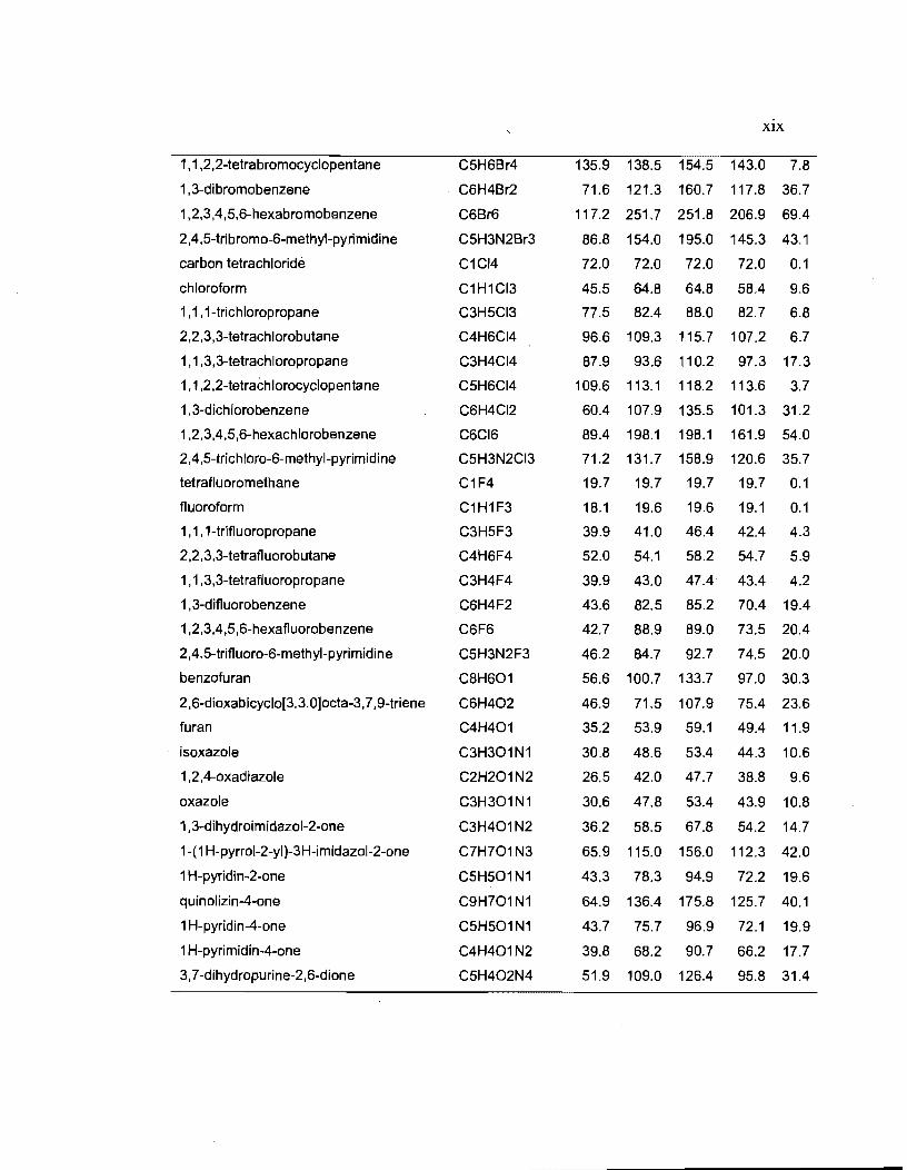
XIX

1,1,2,2-tetrabromocyclopentane C5H6Br4 135.9 138.5 154.5 143.0 7.8

1,3-dibromobenzene C6H4Br2 71.6 121.3 160.7 117.8 36.7

1,2,3,4,5,6-hexabromobenzene C6Br6 117.2 251.7 251.8 206.9 69.4

2,4,5-tribromo-6-methyl-pyrimidine C5H3N2Br3 86.8 154.0 195.0 145.3 43.1

carbon tetrachloridé C1CI4 72.0 72.0 72.0 72.0 0.1

chloroform C1H1CI3 45.5 64.8 64.8 58.4 9.6

1,1,1-trichloropropane C3H5CI3 77.5 82.4 88.0 82.7 6.8

2,2,3,3-tetrachlorobutane C4H6CI4 96.6 109.3 115.7 107.2 6.7

1,1,3,3-tetrachloropropane C3H4CI4 87.9 93.6 110.2 97.3 17.3

1.1,2.2-tetrachlorocyclopentane C5H6CI4 109.6 113.1 118.2 113.6 3.7

1.3-dichlorobenzene C6H4CI2 60.4 107.9 135.5 101.3 31.2

1.2.3,4,5,6-hexachlorobenzene C6CI6 89.4 198.1 198.1 161.9 54.0

2,4,5-trichloro-6-methyl-pyrimidine C5H3N2CI3 71.2 131.7 158.9 120.6 35.7

tetrafluoromethane C1F4 19.7 19.7 19.7 19.7 0.1

fluoroform C1H1F3 18.1 19.6 19.6 19.1 0.1

1,1,1-trifluoropropane C3H5F3 39.9 41.0 46.4 42.4 4.3

2,2,3,3-tetrafluorobutane C4H6F4 52.0 54.1 58.2 54.7 5.9

1,1,3,3-tetrafluoropropane C3H4F4 39.9 43.0 47.4- 43.4 4.2

1,3-difluorobenzene C6H4F2 43.6 82.5 85.2 70.4 19.4

1,2,3,4,5,6-hexafluorobenzene C6F6 42.7 88.9 89.0 73.5 20.4

2,4,5-trifluoro-6-methyl-pyrimidine C5H3N2F3 46.2 84.7 92.7 74.5 20.0

benzofuran C8H601 56.6 100.7 133.7 97.0 30.3

2 .6-dioxabicyclo[3.3. 0]octa-3. 7 ,9-triene C6H402 46.9 71.5 107.9 75.4 23.6

furan C4H401 35.2 53.9 59.1 49.4 11.9

isoxazole C3H301N1 30.8 48.6 53.4 44.3 10.6

1,2,4-oxadiazole C2H201N2 26.5 42.0 47.7 38.8 9.6

oxazole C3H301N1 30.6 47.8 53.4 43.9 10.8

1,3-dihydroimidazol-2-one C3H401N2 36.2 58.5 67.8 54.2 14.7

1-( 1 H-pyrrol-2 -yi )-3H-imidazol-2-one C7H701N3 65.9 115.0 156.0 112.3 42.0

1 H-pyridin-2-one C5H501N1 43.3 78.3 94.9 72.2 19.6

quinolizin-4-one C9H701N1 64.9 136.4 175.8 125.7 40.1

1 H-pyridin-4-one C5H501N1 43.7 75.7 96.9 72.1 19.9

1 H-pyrimidin-4-one C4H401N2 39.8 68.2 90.7 66.2 17.7

3,7 -dihydropurine-2,6-dione C5H402N4 51.9 109.0 126.4 95.8 31.4

xx

4H-1,2,4-triazole C2H3N3 29.8 49.4 52.6 44.0 11.0

2,6-diazabicyclo[3.3.0]octa-3, 7, 9-triene C6H6N2 54.6 87.4 121.0 87.7 26.3

1 H-imidazole C3H4N2 34.3 56.0 58.8 49.7 12.1

1H-indole C8H7N1 60.1 108.2 143.1 103.8 33.1

1 H-pyrazole C3H4N2 34.5 55.8 58.1 49.5 12.1

1 H-pyrrole C4H5N1 39.4 62.1 64.8 55.4 13.7

benzothiophene C8H6S1 65.8 119.8 157.4 114.4 34.3

2 ,6-dithiabicyclo[3.3.0]octa-3, 7 ,9-triene C6H4S2 65.4 113.0 145.9 108.1 29.8

isothiazole C3H3N1S1 40.5 64.5 74.1 59.7 13.3

1,2,4-thiadiazole C2H2N2S1 36.5 59.1 67.0 54.2 11.9

thiazole C3H3N1S1 40.8 66.9 71.9 59.8 13.2

thiophene C4H4S1 45.0 72.0 78.4 65.1 15.3

benzene C6H6 45.1 82.6 82.6 70.1 18.3

naphthalene C10H8 66.3 126.0 173.2 121.8 38.7

phenylbenzene C12H10 88.2 139.6 212.2 146.7 51.7

phthalazine C8H6N2 59.1 116.6 150.5 108.7 33.4

2,5,7,10-tetrazabicyclo[4.4.0]deca-

2,4,6,8,10-pentaene C6H4N4 52.6 95.1 155.0 100.9 32.6

3,4,8,9-tetrazabicyclo[4.4.0]deca-

2,4,7,9,11-pentaene C6H4N4 107.1 130.0 96.5 68.9 0.2

pyridine C5H5N1 41.1 74.0 78.7 64.6 16.7

pyrimidine C4H4N2 37.3 67.9 71.1 58.8 15.0

quinoline C9H7N1 62.7 118.5 167.3 116.2 36.9

1,2,4-triazine C3H3N3 34.5 60.9 67.8 54.4 13.8

N-hydroxyformamide C1H302N1 23.0 36.4 40.5 33.3 7.5

N-hydroxy-N-methyl-acetamide C3H702N1 44.0 62.7 66.7 57.8 12.9

3-hydroxy-1,3-oxazinan-4-one C4H703N1 53.3 76.1 78.6 69.3 14.2

1-hydroxy-3, 4-dihydroqui nol in-2 -one C9H902N1 75.1 129.7 170.2 125.0 38.4

pyridine-3-carbohydroxamic acid C6H602N2 57.1 98.6 137.1 97.6 33.6

1,3-dihydroimidazoJe C3H5N2 27.5 48.4 51.3 42.4 10.5

5-ethyl-1,3-dihydroimidazole C5H9N2 49.5 69.3 86.5 68.4 16.0

3,5-dimethyl-1 H-imidazole C5H9N2 46.6 70.5 89.7 68.9 20.6

4-methyl-1 ,3-dihydroimidazole C4H7N2 37.1 59.2 71.1 55.8 14.5

2,4,5-trimethyl-1,3-dihydroimidazole C6H11N2 55.9 88.7 103.9 82.8 21.1

XXI

acetone C3H601 34.6 47.2 47.6 43.1 7.3

pentane-2,4-dione C5H802 57.3 72.8 77.9 69.3 14.1

cyclopentanone C5H801 51.2 64.6 69.6 61.8 7.9

cyclohexane-1,4-dione C6H802 59.3 76.6 90.0 75.3 13.1

1-pyrazin-2-ylethanone C6H601N2 53.4 92.9 120.2 88.8 27.9

hydrogen cyanide C1H1N1 14.4 14.4 23.1 17.3 3.7

acetonitrile C2H3N1 24.7 24.7 41.0 30.2 7.4

pentanedinitrile C5H6N2 52.4 62.6 94.2 69.7 23.6

pentanedinitrile C5H6N2 59.4 64.6 79.2 67.8 12.1

cyclopentanecarbonitrile C6H9N1 68.1 69.6 82.7 73.5 8.4

benzonitrile C7H5N1 51.1 87.8 125.6 88.2 27.7

terephthalonitrile C8H4N2 57.5 93.5 177.6 109.5 39.3

pyrimidine-2-carbonitrile C5H3N3 44.5 73.7 112.5 76.9 24.9

1-nitrobutane C4H902N1 59.7 68.5 82.9 70.4 15.3

1-nitropropane C3H702N1 47.2 58.6 66.9 57.6 10.6

2-nitrophenol C6H503N1 54.8 108.8 122.6 95.4 30.6

nitrobenzene C6H502N1 50.1 98.3 119.0 89.1 29.9

3-nitroaniline C6H602N2 56.0 114.6 136.0 102.2 34.9

1-oxidopyridine C5H501N1 43.2 79.4 103.0 75.2 21.0

1,4-dioxidopyrazine C4H402N2 41.6 76.2 129.1 82.3 23.5

trimethyl-oxido-ammonium C3H901N1 57.5 57.6 58.2 57.7 1.3

methylsulfonylmethane C2H602S1 53.2 54.7 59.1 55.7 5.4

methylsulfinylmethane C2H601S1 47.1 58.7 60.4 55.4 6.3

1-ethylsulfonylpropane C5H1202S1 80.8 83.9 116.6 93.8 26.2

1-[(R)-ethylsulfinyl]propane C5H1201S1 76.9 86.9 118.4 94.1 26.0

methylsulfonylbenzene C7H802S1 80.4 111.2 140.7 110.8 28.0

[(S)-methylsulfinyl]benzene C7H801S1 78.2 111.1 143.0 110.8 28.4

thiolane 1, 1-dioxide C4H802S1 68.3 72.9 81.1 74.1 7.3

thiolane 1-oxide C4H801S1 64.2 74.1 82.2 73.5 7.8

N-methylmethanesulfonamide C2H702N1S1 58.6 61.9 70.6 63.7 8.5

N-methylmethanesulfinamide C2H701N1S1 53.5 64.0 77.4 65.0 12.8

N-(methylsulfamoyl)methanamine C2H802N2S1 66.0 69.6 78.8 71.5 8.8

N-methylsulfinamoylmethanamine C2H801N2S1 62.7 68.7 85.8 72.4 12.9

thiazolidine 1, 1-dioxide C3H702N1S1 64.9 67.9 77.6 70.1 7.6

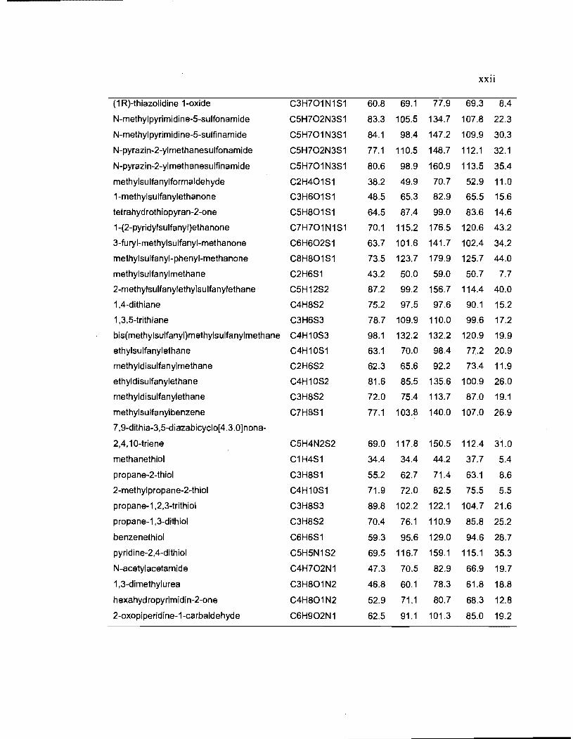
XXll

(1 R)-thiazolidine 1-oxide C3H701N1S1 60.8 69.1 77.9 69.3 8.4

N-methylpyrimidine-5-sulfonamide C5H702N3S1 83.3 105.5 134.7 107.8 22.3

N-methylpyrimidine-5-sulfinamide C5H701N3S1 84.1 98.4 147.2 109.9 30.3

N-pyrazin-2-ylmethanesulfonamide C5H702N3S1 77.1 110.5 148.7 112.1 32.1

N-pyrazin-2-ylmethanesulfinamide C5H701N3S1 80.6 98.9 160.9 113.5 35.4

methylsulfanylformaldehyde C2H401S1 38.2 49.9 70.7 52.9 11.0

1-methylsulfanylethanone C3H601S1 48.5 65.3 82.9 65.5 15.6

tetrahydrothiopyran-2-one C5H801S1 64.5 87.4 99.0 83.6 14.6

1-(2-pyridylsulfanyl)ethanone C7H701N1S1 70.1 115.2 176.5 120.6 43.2

3-furyl-methylsulfanyl-methanone C6H602S1 63.7 101.6 141.7 102.4 34.2

methylsulfanyl-phenyl-methanone C8H801S1 73.5 123.7 179.9 125.7 44.0

methylsulfanylmethane C2H6S1 43.2 50.0 59.0 50.7 7.7

2-methylsulfanylethylsulfanylethane C5H12S2 87.2 99.2 156.7 114.4 40.0

1,4-dithiane C4H8S2 75.2 97.5 97.6 90.1 15.2

1,3,5-trithiane C3H6S3 78.7 109.9 110.0 99.6 17.2

bis(methylsulfanyl)methylsulfanylmethane C4H10S3 98.1 132.2 132.2 120.9 19.9

ethylsulfanylethane C4H10S1 63.1 70.0 98.4 77.2 20.9

methyldisulfanylmethane C2H6S2 62.3 65.6 92.2 73.4 11.9

ethyldisulfanylethane C4H10S2 81.6 85.5 135.6 100.9 26.0

methyldisulfanylethane C3H8S2 72.0 75.4 113.7 87.0 19.1

methylsulfanylbenzene C7H8S1 77.1 103.8 140.0 107.0 26.9

7,9-dithia-3,5-diazabicyclo[4.3.o]nona-

2,4,10-triene C5H4N2S2 69.0 117.8 150.5 112.4 31.0

methanethiol C1H4S1 34.4 34.4 44.2 37.7 5.4

propane-2-thiol C3H8S1 55.2 62.7 71.4 63.1 8.6

2-methylpropane-2-thiol C4H1OS1 71.9 72.0 82.5 75.5 5.5

propane-1,2,3-trithiol C3H8S3 89.8 102.2 122.1 104.7 21.6

propane-1,3-dithiol C3H8S2 70.4 76.1 110.9 85.8 25.2

benzenethiol C6H6S1 59.3 95.6 129.0 94.6 28.7

pyridine-2,4-dithiol C5H5N1S2 69.5 116.7 159.1 115.1 35.3

N-acetylacetamide C4H702N1 47.3 70.5 82.9 66.9 19.7

1,3-dimethylurea C3H801N2 46.8 60.1 78.3 61.8 18.8

hexahydropyrimidin-2-one C4H801N2 52.9 71.1 80.7 68.3 12.8

2-oxopiperidine-1-carbaldehyde C6H902N1 62.5 91.1 101.3 85.0 19.2

xxiii

(E)-but-2-enal C4H601 38.6 50.9 87.1. 58.9 17.1

N-[(E)-prop-1-enyl]acetamide C5H901N1 54.7 72.5 122.9 83.4 29.3

1.3-dihydropyrrol-2-one C4H501N1 40.3 64.1 69.5 58.0 13.5

[(Z)-1-methylprop-1-enyl] acetate C6H1002 69.1 84.3 100.5 84.6 17.9

1,2-dimethylprop-1-

enylsulfanylformaldehyde C6H1001S1 83.1 98.9 130.0 104.0 18.7

(E)-pent-3-en-2-one C5H801 48.8 65.6 96.3 70.2 21.8

hydrazine H4N2 22.0 22.2 26.9 23.7 3.9

1,1,2-trimethylhydrazine C3H10N2 57.0 60.9 70.0 62.6 11.0

phenylhydrazine C6H8N2 58.7 96.7 124.2 93.2 29.0

1 H-pyrrol-3-ylhydrazine C4H7N3 54.5 79.4 97.5 77.1 22.7

piperazin-1-amine C4H11N3 71.2 79.8 86.4 79.1 14.5

N-methylaminoformamide C2H601N2 40.2 51.5 61.2 50.9 10.8

diaziridine C1H4N2 27.7 31.7 32.2 30.5 2.4

adamantane C10H16 108.8 108.8 108.9 108.8 0.4

bicyclo[2.2.2]octane C8H14 89.7 89.8 91.4 90.3 0.4

octane C8H18 92.0 96.5 119.6 102.7 23.3

decalin C10H18 99.9 118.2 132.8 116.9 20.7

ethane C2H6 27.9 27.9 32.1 29.3 2.3

isopropylcyclopropane C6H12 65.1 75.8 82.8 74.6 8.1

1.2,3,3a,4,5,6,6a-octahydropentalene C8H14 82.0 92.7 100.4 91.7 10.1

tert-butylcyclobutane C8H16 90.1 95.9 108.0 98.0 10.1

octane C8H18 88.7 95.8 132.3 105.6 31.9

(3E)-hexa-1,3,5-triene C6H8 51.7 66.5 176.3 98.2 34.0

ammonium H4N1 9.3 9.3 9.3 9.3 0.1

oxatriazole C1H101N3 23.8 38.4 43.0 35.1 8.4

1-(2-furyl)pyrrole C8H701N1 64.3 104.7 157.8 108.9 39.0

2-(2-furyl)furan C8H602 60.8 98.1 167.5 108.8 36.9

difuro[3,2-b:2',3'-d]furan C8H403 57.7 89.1 167.5 104.8 37.4

benzo[1,2-b:3,4-b':5,6-b"]trifuran C12H603 78.5 185.8 185.8 150.0 49.9

1,7 -dihydropurin-6-one C5H40'IN4 50.1 102.4 120.7 91.1 28.6

2,4-dihydro-1,2,4-triazol-3-one C2H301N3 31.7 52.8 62.4 48.9 13.0

1-( 1 ,3,4-oxadiazol-2-yl)-3H-imidazol-2-

one C5H402N4 54.4 97.9 132.5 94.9 35.0

XXIV

7H-purine C5H4N4 48.1 88.8 118.4 85.1 27.7

1-(2-furyl )pyridin-2-one C9H702N1 87.3 114.2 160.8 120.8 37.1

2 H-pyridazin-3-one C4H401N2 39.5 70.7 89.2 66.5 18.6

3H-pyrimidin-4-one C4H401N2 39.3 72.5 85.5 65.8 17.4

1 H-pyrazin-2-one C4H401N2 39.6 72.0 91.1 67.6 18.0

1-(2-thienyl)pyridin-4-one C9H701N1S1 92.8 122.8 214.6 143.4 44.5

7,9-dihydro-3H-purine-2,6,8-trione C5H403N4 53.7 114.2 139.1 102.4 34.8

1-(1 H-pyrrol-2-yl)pyrrole C8H8N2 79.3 103.1 151.7 111.4 35.7

2-(1 H-pyrrol-2-yl)-1 H-pyrrole C8H8N2 68.3 112.2 179.7 120.1 43.6

4,7 -dihydro-1 H-dipyrrolo[3,2-b:2',3'-

d]pyrrole C8H7N3 69.0 114.6 188.1 123.9 42.2

1 H-tetrazole C1H2N4 26.8 45.6 46.7 39.7 9.4

4,7-dihydro-1 H-benzo[1 ,2-b:3,4-b':5,6-

b"]tri pyrrol e C12H9N3 89.8 214.1 214.1 172.7 58.8

anthracene C14H10 87.2 170.0 298.4 185.2 64.6

phenanthrene C14H10 86.8 179.7 261.8 176.1 61.2

phenazine C12H8N2 81.3 156.6 287.2 175.0 60.2

3-phenylpyridazine C10H8N2 75.8 131.5 204.8 137.4 50.4

5-phenylpyrimidine C10H8N2 79.9 126.9 196.3 134.4 49.1

pyrazine C4H4N2 37.4 66.0 75.9 59.7 15.4

pyrido[2, 1 ,6-de]quinolizine C12H9N1 80.5 212.8 212.8 168.7 50.0

quinazoline C8H6N2 59.0 113.9 154.5 109.1 34.1

quinoxaline C8H6N2 59.4 111.1 163.7 111.4 36.2

1,3,5-triazine C3H3N3 33.8 62.4 . 62.4 52.9 13.2

hydroxylamine H301N1 17.2 17.7 22.9 19.3 3.6

2-azaniumylacetate C2H502N1 33.8 44.8 52.7 43.8 6.5

(2R)-2,3,4,5-tetrahydropyrrole~2-

carboxylic acid C5H1002N1 56.3 69.6 79.8 68.6 12.1

(2S )-2 -aza ni umyl-3-h ydroxy-propanoate C3H703N1 48.5 63.2 68.9 60.2 12.2

(2S)-2-azaniumylpropanoate C3H702N1 45.0 59.4 62.1 55.5 10.1

(2R)-2-azaniumyl-4-methylsulfanyl-

butanoate C5H1102N1S1 92.2 95.1 120.6 102.6 23.5

(2R)-2-azaniumyl-3-(4-

hydroxyphenyl)propanoate C9H1103N1 87.8 131.5 171.2 130.2 43.9

xxv

(3 R )-3-( azaniumyla mi no )-4-hydroxy-4-

oxo-butanoate C4H804N2 66.2 80.3 99.8 82.1 16.1

(2R)-2-azaniumyl-3-carbamoyl-

propanoate C4H803N2 68.8 74.9 87.3 77.0 9.3

[( 1 S,2S )-1-carboxy-2-hydroxy-

propyl]ammonium C4H1003N1 59.3 66.9 73.0 66.4 10.7

(2R)-2-amino-3-methyl-butanoate C5H1002N1 81.3 94.8 102.2 92.8 14.3

(2R)-2-azaniumyl-3-phenyl-propanoate C9H1102N1 85.6 128.7 157.5 123.9 40.1

(2S)-2-amino-3-( 1 ,3-dihydroimidazol-5-

yl)propanoic acid C6H1002N3 65.5 98.6 127.5 97.2 27.7

2-aminoacetic acid C2H502N1 34.3 46.1 51.7 44.0 9.7

(2S)-pyrrolidine-2-carboxylic acid C5H902N1 63.1 76.0 87.1 75.4 15.0

(2S)-2-amino-3-hydroxy-propanoic acid C3H703N1 53.8 62.0 67.1 61.0 8.0

(2S)-2-aminopropanoic acid C3H702N1 49.1 58.6 62.1 56.6 10.2

(2R)-2-amino-4-methylsulfanyl-butanoic

acid C5H1102N1S1 86.6 100.5 120.2 102.5 22.0

(2S )-2-amino-3-(4-

hydroxyphenyl)propanoÎc acid C9H1103N1 96.9 127.1 166.2 130.1 34.8

(2R )-2-aminobutanedioic acid C4H704N1 63.9 71.5 85.9 73.8 17.6

(2S)-2-amino-3-carbamoyl-propanoic acid C4H803N2 70.4 77.4 90.3 79.4 15.6

(2R.3R)-2-amino-3-hydroxy-butanoic acid C4H903N1 60.8 76.4 83.2 73.5 15.8

(2S)-2-amino-3-phenyl-propanoic acid C9H1102N1 94.6 124.2 153.2 124.0 30.5

(2S)-2-amino-3-(1 H-imidazol-4-

yl)propanoic acid C6H902N3 79.8 105.0 124.9 103.2 26.9

1,1,1-trichloroethane C2H3CI3 64.1 73.9 73.9 70.6 2.6

1,1,1-trifluoro-2,2,2-trimethoxy-ethane C5H903F3 75.4 81.5 85.3 80.7 5.8

(2S )-1 ,1 ,1-trifluoropropan-2-ol C3H50'IF3 43.6 47.6 50.4 47.2 4.9

1.1.1-trimethoxyethane C5H1203 73.2 80.7 84.1 79.3 6.9

1,1,2-trichloroethane C2H3CI3 62.3 72.2 74.2 69.6 7.5

1-acetoxyethyl acetate C6H1004 78.2 88.8 103.0 90.0 17.2

1,1-dichloroethane C2H4CI2 46.8 57.5 66.8 57.0 8.5

1.1-dichloroethylene C2H2CI2 38.9 63.0 65.5 55.8 12.4

1-ethoxyethoxyethane C6H1402 78.0 89.6 102.3 90.0 16.2

1 ,1-difluoroethane C2H4F2 28.7 30.3 31.7 30.2 1.6

----------------_ .................... -

XXVI

1 ,2,3-trimethylbenzene C9H12 71.9 127.1 131.4 110.1 32.2

1,2,4-trimethylbenzene C9H12 72.3 117.9 143.7 111.3 34.0

2-acetoxyethyl acetate C6H1004 76.0 87.7 109.7 91.1 18.8

1,2-dibromoethane C2H4Br2 58.0 60.9 106.4 75.1 22.0

1,2-dichlorobenzene C6H4CI2 60.2 111.3 128.3 99.9 30.1

1,2-dichloroethane C2H4CI2 47.5 56.6 64.6 56.2 9.6

(28)-1,2-dichloropropane C3H6CI2 61.8 68.6 74.7 68.4 7.7

2-ethoxyethoxyethane C6H1402 79.7 88.1 106.5 91.4 18.8

1,2-dimethoxyethane C4H1002 57.3 61.2 78.8 65.8 15.2

ethylene glycol C2H602 36.5 39.5 40.5 38.8 3.0

mesitylene C9H12 72.7 131.2 131.3 111.7 31.9

1,3-dichloropropane C3H6CI2 61.6 65.0 78.5 68.4 11.0

1,3-dimethylnaphthalene C12H12 84.3 159.9 208.2 150.8 48.7

1,4-dichlorobenzene C6H4CI2 60.4 96.3 148.4 101.7 34.5

1 ,4-dichlorobutane C4H8C12 71.6 79.1 92.9 81.2 15.6

1 ,4-dimethylpiperazine C6H14N2 85.3 92.4 110.6 96.1 22.8

1,4-dimethylnaphthalene C12H12 84.0 172.9 190.0 148.9 46.6

1-bromo-2-chloro-ethane C2H4CI1Br1 52.1 55.0 91.5 66.2 18.6

1-bromo-2-methyl-propane C4H9Br1 68.3 70.2 85.5 74.7 10.4

1-bromobutane C4H9Br1 63.4 68.3 99.0 76.9 20.4

1-bromoheptane C7H15Br1 93.3 100.8 154.5 116.2 39.2

1-bromohexane C6H13Br1 83.4 90.5 135.4 103.1 32.0

1-bromooctane C8H17Br1 103.3 112.5 172.1 129.3 44.7

1-bromopentane C5H11Br1 73.4 78.7 118.1 90.1 26.0

1-bromopropane C3H7Br1 53.4 56.3 82.0 63.9 15.2

2-chloro-1 ,1, 1-trifluoro-ethane C2H2F3CI1 39.1 40.4 52.3 43.9 6.8

1-chlorobutane C4H9C11 57.4 62.4 86.2 68.7 17.2

1-chlorohexane C6H13CI1 80.0 88.1 112.0 93.4 23.3

1-chloropentane C5H11CI1 69.6 78.0 93.8 80.5 17.0

1-chloropropane C3H7CI1 48.5 53.4 63.4 55.1 8.6

1-ethylnaphthalene C12H12 88.0 164.2 191.2 147.8 42.5

1-methylimidazole C4H6N2 44.1 67.7 76.6 62.8 16.5

1-methylpyrrole C5H7N1 49.3 73.9 84.0 69.1 18.2

1-methylcyclohexene C7H12 68.1 87.0 100.8 85.3 17.5

xxvii

1-methylnaphthalene C11 H10 75.2 148.3 182.1 135.2 42.3

naphthalen-1-ol C10H801 68.2 137.6 175.9 127.2 40.7

naphthalen-1-amine C10H9N1 72.4 149.8 180.4 134.2 42.8

1-nitropentane C5H1102N1 70.0 78.5 101.5 83.3 20.8

2,2,2-trifluoroethanol C2H301F3 33.6 34.4 37.7 35.3 2.8

2,2,4-trimethylpentane C8H18 94.5 100.4 114.1 103.0 15.4

2,2.5-trimethylhexane C9H20 105.8 110.8 128.6 115.0 19.4

2,2-dimethylbutane C6H14 75.4 75.8 83.3 78.2 7.2

2.3.4-trimethylpentane C8H18 92.8 100.4 112.9 102.0 15.8

2.3-dimethylbuta-1,3-diene C6H10 55.8 79.7 106.0 80.5 21.6

2,3-dimethylnaphthalene C12H12 84.0 149.5 222.6 152.0 51.0

2,3-dimethylphenol C8H1001 65.3 119.1 123.2 102.5 30.5

2,3-dimethylpyridine C7H9N1 59.7 100.3 115.8 91.9 26.2

2,4-dimethylphenol C8H1001 65.5 112.7 132.0 103.4 31.3

2,4-dimethylpyridine C7H9N1 60.2 100.3 117.1 92.6 26.7

2,5-dimethylphenol C8H1001 65.5 107.9 136.6 103.4 33.4

2,5-dimethylpyridine C7H9N1 60.1 93.2 125.3 92.9 29.5

(2S,5S}-2,5-dimethyltetrahydrofuran C6H1201 69.4 75.8 91.3 78.8 11.1

2,6-dimethylaniline C8H11N1 69.7 128.4 129.4 109.2 32.8

2,6-dimethylnaphthalene C12H12 84.6 145.9 229.7 153.4 54.4

2,6-dimethylphenol C8H1001 65.6 117.2 125.5 102.7 30.7

2,6-dimethylpyridine C7H9N1 60.5 101.9 115.9 92.8 26.7

2-bromo-2-methyl-propane C4H9Br1 70.5 70.5 87.4 76.1 6.6

2-bromopropane C3H7Br1 53.9 61.2 75.9 63.7 9.9

2-butoxyethanol C6H1402 77.4 83.6 109.2 90.1 23.5

2-chloro-1.1 .1-trimethoxy-ethane C5H1103CI1 77.3 96.6 103.0 92.3 17.5

2-chloro-2-methyl-propane C4H9CI1 64.8 64.8 74.5 68.0 3.0

2-chloroaniline C6H6N1CI1 58.8 107.8 124.9 97.2 29.6

(2S)-2-chlorobutane C4H9CI1 58.2 72.0 73.3 67.8 10.4

2-chlorophenol C6H501CI1 54.8 98.1 118.8 90.6 27.7

2-chloropropane C3H7CI1 48.1 55.2 63.9 55.7 7.4

2-chloropyridine C5H4N1CI1 49.3 82.2 109.8 80.4 24.6

1-chloro-2-methyl-benzene C7H7CI1 61.7 108.2 125.4 98.4 29.0

2-ethoxyethanol C4H1002 58.6 61.5 75.3 65.1 11.8

xxviii

2-ethylpyrazine C6H8N2 60.3 86.9 112.6 86.6 22.9

2-ethylpyridine C7H9N1 63.9 93.7 117.0 91.5 25.1

1-ethyl-2-methyl-benzene C9H12 76.2 118.7 133.9 109.6 28.4

2-f1uorophenol C6H501F1 46.5 85.7 95.1 75.8 22.2

2-isobutylpyrazine C8H12N2 84.2 111.0 136.5 110.6 24.5

1,1,1,2-tetramethoxyethane C6H1404 92.1 95.8 104.8 97.6 9.1

2-methoxyaniline C7H901N1 63.8 116.7 125.2 101.9 30.7

2-methoxyethanamine C3H901N1 49.8 53.1 68.1 57.0 15.1

2-methoxyethanol C3H802 47.5 49.8 59.7 52.3 8.9

2-methoxyphenol C7H802 59.5 104.6 120.6 94.9 29.4

2-methylbut-2-ene C5H10 51.7 64.7 85.3 67.2 15.3

isoprene C5H8 46.9 63.2 98.1 69.4 17.9

(2R)-2-methylbutan-1-ol C5H1201 63.7 71.9 76.5 70.7 9.6

2-methylbutan-2-ol C5H1201 66.1 69.2 76.6 70.6 8.2

isopentane C5H12 61.5 65.8 69.8 65.7 7.1

2-methylhexane C7H16 83.8 85.3 104.3 91.1 16.9

2-methylpent-1-ene C6H12 64.9 77.9 94.5 79.1 17.4

2-methylpentan-2-ol C6H1401 76.0 79.8 94.5 83.4 14.0

(3R)-2-methylpentan-3-ol C6H1401 73.6 81.7 93.6 83.0 14.6

isohexane C6H14 69.8 76.9 90.6 79.1 14.9

2-methylpropan-1-ol C4H1001 52.7 59.8 63.8 58.8 8.6

2-methylpyrazine C5H6N2 47.2 77.2 97.1 73.8 20.7

2-methylpyridine C6H7N1 50.9 84.4 100.8 78.7 22.7

(2S)-2-methyltetrahydrofuran C5H1001 58.8 64.0 75.1 66.0 9.0

2-methylthiophene C5H6S1 54.1 87.0 95.6 78.9 20.3

naphthalen-2-ol C10H801 68.3 129.3 189.3 129.0 43.1

naphthalen-2-amine C10H9N1 72.3 134.3 204.9 137.1 46.0

2-nitroaniline C6H602N2 55.8 122.4 134.8 104.3 34.0

2-nitropropane C3H702N1 51.8 56.1 62.3 56.7 5.1

1-methyl-2-nitro-benzene C7H702N1 59.0 118.5 130.9 . 102.8 33.3

2-phenylethanol C8H1001 70.8 103.4 132.0 102.0 29.9

2-propoxyethanol C5H1202 67.7 72.3 93.2 77.7 18.3

3,3,3-trimethoxypropanenitrile C6H1103N1 86.6 88.2 105.0 93.2 9.3

3,3-dimethylbutan-2-one C6H1201 71.7 81.1 83.9 78.9 8.8

XXIX

3.3-dimethylpentane C7H16 84.7 91.9 92.7 89.7 7.1

3,4-dimethylphenol C8H1001 65.1 111.2 132.6 102.9 31.5

3.4-dimethylpyridine C7H9N1 59.3 102.5 111.9 91.2 26.2

3,5-dimethylphenol C8H1001 65.6 118.8 126.3 103.6 30.6

3,5-dimethylpyridine C7H9N1 59.7 98.1 118.7 92.1 27.9

1-(3-pyridyl)ethanone C7H701N1 56.5 98.8 126.0 93.8 31.7

3-chloroaniline C6H6N1CI1 58.8 105.8 129.9 98.2 30.4

3-chlorophenol C6H501CI1 54.8 99.9 119.2 91.3 27.6

3-chloroprop-1-ene C3H5CI1 46.4 47.2 75.2 56.2 13.4

3-chloropyridine C5H4N1CI1 48.9 82.0 109.4 80.1 25.0

3-hydroxybenzonitrile C7H501N1 53.3 96.5 133.6 94.4 31.1

pyridine-3-carbonitrile C6H4N2 47.4 80.3 120.3 82.7 27.2

3-ethylphenol C8H1001 69.9 107.5 130.7 102.7 28.7

3-ethylpyridine C7H9N1 63.8 92.8 116.9 91.2 24.9

pyridine-3-carbaldehyde C6H501N1 46.9 85.9 113.2 82.0 25.9

3-hydroxybenzaldehyde C7H602 52.7 100.6 128.6 94.0 30.3

3-methoxyaniline C7H901N1 63.7 105.2 138.5 102.5 33.7

3-methoxyphenol C7H802 59.6 101.3 125.8 95.6 30.3

3-methyl-1 H-indole C9H9N1 69.0 126.4 156.5 117.3 37.8

3-methylbut-1-ene C5H10 58.3 61.3 80.8 66.8 11.9

3-methylbutan-1-ol C5H1201 64.4 69.0 78.1 70.5 10.4

3-methylbutan-2-one C5H1001 59.6 67.8 73.9 67.1 10.7

3-methylbutanoic acid C5H1002 65.3 67.7 82.3 71.7 12.9

(3S)-3-methylheptane C8H18 90.2 96.9 125.8 104.3 27.1

(3R)-3-methylhexane C7H16 81.8 88.9 100.8 90.5 14.0

3-methylpentane C6H14 69.9 75.7 90.0 78.5 15.2

3-methylpyridine C6H7N1 50.4 83.8 100.7 78.3 22.9

3-nitrophenol C6H503N1 52.2 106.5 127.1 95.3 33.0

1-methyl-3-nitro-benzene C7H702N1 59.3 114.2 136.1 103.2 34.3

3-phenylpropan-1-ol C9H1201 84.6 112.9 147.8 115.1 32.1

1-(4-pyridyl)ethanone C7H701N1 56.7 103.1 120.2 93.3 30.4

4-bromophenol C6H501Br1 60.4 97.4 140.7 99.5 32.7

1-bromo-4-methyl-benzene C7H7Br1 67.7 103.1 153.6 108.1 36.5

4-chloroaniline C6H6N1CI1 58.7 95.7 140.8 98.4 32.8

xxx

4-chlorophenol C6H501CI1 54.7 92.4 126.8 91.3 29.4

4-hydroxybenzonitrile C7H501N1 53.2 90.4 142.5 95.4 31.9

pyridine-4-carbonitrile C6H4N2 47.5 84.6 114.9 82.3 26.0

4-ethylphenol C8H1001 69.8 103.1 135.7 102.9 30.1

4-ethylpyridine C7H9N1 63.9 96.3 112.8 91.0 23.4

1-ethyl-4-methyl-benzene C9H12 77.1 108.9 147.8 111.3 33.6

4-fluorophenol C6H501F1 46.2 85.1 95.6 75.6 22.1

pyridine-4-carbaldehyde C6H501N1 47.0 90.4 107.3 81.6 24.9

4-hydroxybenzaldehyde C7H602 52.7 96.2 138.6 95.8 30.9

1-isopropyl-4-methyl-benzene C10H14 90.7 117.9 162.4 123.7 35.1

4-methoxyaniline C7H901N1 63.6 101.6 141.7 102.3 35.3

4-methyl-1 H-imidazole C4H6N2 43.9 67.5 78.0 63.1 16.7

1-(p-tolyl)ethanone C9H1001 69.5 114.8 161.5 115.3 40.1

4-methylbenzaldehyde C8H801 59.9 102.7 147.5 103.4 33.9

(2R)-4-methylpentan-2-ol C6H1401 76.4 80.7 92.6 83.2 12.7

4-methylpenta.n-2-one C6H1201 69.5 78.6 91.4 79.8 17.1

4-methylpyridine C6H7N1 50.5 87.5 96.7 78.3 22.0

4-propylphenol C9H1201 80.0 112.7 156.2 116.3 36.4

4-nitroaniline C6H602N2 55.8 103.6 163.1 107.5 37.0

4-nitrophenol C6H503N1 52.1 100.7 140.3 97.7 33.7

4-tert-butylphenol C10H1401 92.5 125.8 163.1 127.2 35.7

(E)-1,2-dichloroethylene C2H2CI2 39.0 46.7 86.0 57.2 18.6

(E)-hept-2-ene C7H14 77.3 80.6 123.6 93.8 29.2

(E)-hex-2-enal C6H1001 61.6 71.7 124.0 85.8 27.4

(E)-oct-2-enal C8H1401 84.0 92.7 160.4 112.4 38.7

4-methoxy-N,N-dimethyl-benzamide C10H1302N1 97.2 133.1 202.9 144.4 49.6

I\J,N,4-trimethylbenzamide C10H130'IN1 94.9 130.0 187.1 137.3 44.2

N, N-dimethylformamide C3H701N1 40.1 54.7 64.9 53.2 10.2

l\J-methyl-N-(2 ,2 ,2-trifluoroethyl )an i 1 ine C9H10N1F3 83.0 126.5 160.9 123.4 37.3

N-methylaniline C7H9N1 61.3 99.6 129.4 96.8 30.5

4-methylmorpholine C5H11011\J1 69.3 79.0 82.3 76.9 12.3

1-methylpiperidine C6H13N1 74.9 83.4 87.0 81.8 9.3

(Z)-1,2-dichloroethylene C2H2CI2 39.1 54.4 73.4 55.6 13.3

(Z)-pent-2-ene C5H10 54.9 60.6 86.0 67.2 15.2

XXXI

acenaphthene C12H10 80.2 161.8 185.7 142.6 42.8

1-phenylethanone C8H801 60.3 106.2 132.9 99.8 32.7

isopropenylbenzene C9H10 70.9 115.1 149.9 112.0 35.3

azetidine C3H7N1 42.2 47.2 49.3 46.2 3.5

benzamide C7H701N1 58.2 104.0 126.4 96.2 31.4

trifl uoromethylbenzene C7H5F3 56.1 91.8 104.7 84.2 23.6

phenylmethanol C7H801 60.6 94.4 111.7 88.9 23.0

bromomethylbenzene C7H7Br1 77.9 104.3 145.8 109.4 28.5

chloromethylbenzene C7H7CI1 70.9 98.9 129.9 99.9 25.8

1-chloro-2-(2-chloroethoxy)ethane C4H801CI2 72.1 94.3 95.0 87.1 15.9

bromobenzene C6H5Br1 58.4 94.4 127.6 93.5 28.6

bromoethane C2H5Br1 43.4 46.1 63.3 50.9 9.5

bromomethane C1 H3Br1 33.1 33.1 46.7 37.6 6.1

bromo-trifluoro-methane C1F3Br1 35.3 35.3 47.4 39.3 5.9

but-1-ene C4H8 45.6 48.5 68.6 54.3 12.1

but-1-yne C4H6 40.3 43.6 67.3 50.4 12.2

buta-1,3-diene C4H6 37.6 46.5 90.2 58.1 17.4

butan-1-ol C4H1001 52.1 56.5 68.6 59.1 11.2

(2S)-butan-2-ol C4H1001 53.2 57.6 66.2 59.0 9.6

butanenitrile C4H7N1 45.4 48.6 72.4 55.5 14.9

butyric acid C4H802 47.4 59.7 71.5 59.5 15.8

butanal C4H801 45.0 56.8 64.5 55.4 12.6

chlorobenzene C6H5CI1 52.8 89.4 114.0 85.4 25.6

chloro-difluoro-methane C1H1 F2CI1 27.9 29.5 38.3 31.9 4.6

chloroethane C2H5CI1 37.2 39.9 52.2 43.1 7.3

chloroethylene C2H3CI1 31.0 37.6 57.6 42.1 10.4

chloro-fluoro-methane C1H2F1CI1 26.8 28.4 38.0 31.1 4.7

chloromethane C1H3CI1 26.6 26.7 37.2 30.2 4.9

(1 R.2S)-1.2-dimethylcyclohexane C8H16 87.0 98.2 104.5 96.6 11.1

cyclohepta-1,3,5-triene C7H8 60.7 96.4 99.8 85.7 18.8

cycloheptanol C7H1401 79.4 90.6 97.4 89.1 11.4

cyclohexanol C6H1201 68.7 79.1 85.1 77.6 10.3

cyclohexanone C6H1001 62.7 76.4 82.9 74.0 10.0

cyclohexene C6H10 59.0 73.2 83.2 71.8 12.0

xxxii

cyclohexanamine C6H13N1 75.9 82.6 86.0 81.5 7.9

cyclopentanol C5H1001 60.9 66.4 68.0 65.1 3.9

cyclopentene C5H8 48.5 61.3 69.3 59.7 9.0

decan-1-ol C10H2201 111.5 121.5 177.0 136.7 48.0

decan-2-one C10H2001 104.8 122.5 169.9 132.4 46.9

2-isopropylsulfanylpropane C6H14S1 89.5 93.6 123,2 102.1 20.2

1-butoxybutane C8H1801 92.6 '100.6 141.1 111.4 35.4

N-butylbutan-1-amine C8H19N1 96.2 105.4 147.2 116.2 39.5

1-propoxypropane C6H1401 72.6 77.9 106.0 85.5 23.9

1-propylsulfanylpropane C6H14S1 82.8 92.3 135.8 103.7 32.6

N-propylpropan-1-amine C6H15N1 76.2 83.2 111.5 90.3 27.6

dibromomethane C1H2Br2 47.5 52.1 79.0 59.5 13.6

dichloromethane C1H2CI2 35.8 40.0 56.9 44.2 9.0

diethyl propanedioate C7H1204 87.5 95.0 129.0 103.8 27.6

diethyl butanedioate C8H1404 87.0 108.6 154.4 116.7 43.2

N-ethylethanamine C4H11N1 56.3 62.1 76.9 65.1 16.0

2-isopropoxypropane C6H1401 75.8 81.9 94.7 84.1 12.4

N-isopropylpropan-2-amine C6H15N1 82.2 84.4 100.0 88.9 15.5

methoxymethoxymethane C3H802 45.7 49.7 58.4 51.3 8.8

acetamide C2H501N1 30.8 43.7 46.6 40.4 8.5

ethanethiol C2H6S1 44.6 46.8 60.0 50.5 9.5

ethanol C2H601 31.7 34.1 37.1 34.3 3.0

ethyl acetate C4H802 47.7 59.7 72.5 60.0 13.7

ethyl butanoate C6H1202 67.8 80.7 107.0 85.2 25.0

eth yi formate C3H602 37.5 46.6 58.7 47.6 10.3

ethyl pentanoate C7H1402 77.8 91.2 125.3 98.1 32.2

ethoxybenzene C8H1001 67.9 104.8 138.2 103.6 33.9

ethyl propanoate C5H1002 57.6 69.2 90.0 72.3 20.3

ethanamine C2H7N1 35.7 38.5 43.9 39.4 4.4

ethylbenzene C8H10 67.8 100.2 122.5 96.8 25.6

fluorobenzene C6H5F1 44.3 82.0 84.3 70.2 19.2

fluoromethane C1H3F1 16.9 16.9 18.5 17.4 0.3

(2R)-2-bromo-2-chloro-1 ,1, 1-trifluoro-

ethane C2H1 F3CI1 Br1 53.4 63.6 77.7 64.9 10.3

xxxiii

hept-1-ene C7H14 77.8 81.0 120.1 93.0 29.1

hept-1-yne C7H12 70.7 77.2 120.0 89.3 29.2

heptan-1-ol C7H1601 82.1 89.2 121.2 97.5 28.7

heptan-2-one C7H1401 75.0 90.1 115.3 93.4 29.2

heptan-4-one C7H1401 74.9 88.5 114.8 92.8 30.1

heptanal C7H1401 75.1 90.6 115.7 93.8 30.2

hex-1-ene C6H12 67.7 70.0 102.2 80.0 22.7

hex-1-yne C6H10 60.6 67.0 101.1 76.3 22.8

hexa-1,5-diene C6H10 67.0 79.7 88.0 78.2 11.8

1,1,2,3,3,3-hexafluoroprop-1-ene C3F6 34.3 43.1 54.8 44.1 8.8

hexan-1-ol C6H1401 72.1 78.5 103.1 84.6 22.0

hexan-2-one C6H1201 64.9 78.9 97.8 80.5 23.4

(3S )-hexan-3-ol C6H1401 73.3 80.2 97.9 83.8 18.3

hexanal C6H1201 65.1 79.3 98.4 80.9 23.4

hexanoic acid C6H1202 67.5 81.6 106.1 85.1 26:7

hydrogen sulfide H2S1 24.8 24.9 25.6 25.1 1.2

indane C9H10 70.0 111.8 131.5 104.4 27.9

isopentyl acetate C7H1402 84.5 90.2 116.3 97.0 23.1

isopentyl formate C6H1202 74.6 79.5 99.2 84.4 17.4

isobutyl acetate C6H1202 70.1 83.4 101.1 84.9 19.2

isobutyl formate C5H1002 60.0 71.5 85.8 72.4 14.7

isobutylbenzene C10H14 91.2 124.3 146.3 120.6 27.8

2-methylpropanal C4H801 46.8 57.2 61.4 55.1 8.0

(2R)-2-chloro-2-(difluoromethoxy)-1,1,1-

trifluoro-ethane C3H20'I F5CI1 54.5 64.1 70.5 63.0 9.1

isopropyl acetate C5H1002 62.0 69.9 84.2 72.0 13.0

isopropyl formate C4H802 51.7 58.0 69.2 59.6 9.5

cumene C9H12 81.6 108.9 136.7 109.1 26.4

m-cresol C7H801 56.5 98.0 114.7 89.7 27.1

m-xylene C8H10 63.6 106.9 122.8 97.8 28.3

methanesulfonyl chloride C1H302S1CI1 52.4 54.8 69.2 58.8 7.0

2,2-dichloro-1 ,1-difluoro-1-methoxy-

ethane C3H401 F2CI2 60.4 76.5 86.0 74.3 14.5

methyl 2 -chloroacetate C3H502CI1 46.4 57.2 78.8 60.8 18.6

XXXIV

methyl 2-cyanoacetate C4H502N1 44.7 56.2 82.3 61.1 20.8

methyl cyclohexanecarboxylate C8H1402 90.8 99.2 115.4 101.8 17.0

1-cyclohexylethanone C8H1401 86.8 95.6 113.9 98.8 19.7

methyl cyclopropanecarboxylate C5H802 57.3 61.9 86.6 68.6 15.6

1-cyclopropylethanone C5H801 54.6 61.4 76.1 64.0 11.2

methoxyethane C3H801 42.4 44.2 55.9 47.5 9.6

methylsulfanylethane C3H8S1 53.2 59.9 78.4 63.8 13.9

methyl hexanoate C7H1402 77.6 90.4 125.9 98.0 34.7

2-methoxypropane C4H1001 53.2 58.3 66.3 59.3 9.2

methyl octanoate C9H1802 97.5 112.2 162.2 124.0 46.3

methyl 4-methoxybenzoate C9H1003 75.5 119.3 188.7 127.9 48.5

methyl 4-nitrobenzoate C8H704N1 68.6 124.6 185.2 126.1 49.4

methyl pentanoate C6H1202 67.6 79.6 107.9 85.0 27.4

methyl propanoate C4H802 47.3 57.8 73.0 59.4 16.3

1-methoxypropane C4H1001 52.4 55.5 71.8 59.9 13.9

2-methoxy-2-methyl-propane C5H1201 67.3 68.5 76.2 70.7 6.5

methyl 2,2,2-trifluoroacetate C3H302F3 40.1 49.4 57.5 49.0 10.8

methyl 2,2-dimethylpropanoate C6H1202 74.6 82.2 93.6 83.5 12.2

methanamine C1H5N1 24.8 25.5 29.4 26.6 3.6

methylcyclohexane C7H14 75.4 85.9 95.0 85.4 11.9

methylcyclopentane C6H12 64.6 73.5 81.7 73.3 8.9

morpholine C4H901N1 58.4 61.7 69.0 63.0 9.0

butane-1-thiol C4H10S1 66.0 70.6 89.5 75.4 16.3

but yi acetate C6H1202 67.9 81.5 107.3 85.6 23.9

hexanamide C6H1301N1 73.7 86.2 112.7 90.9 27.8

butan-1-amine C4H11N1 56.3 60.7 75.4 64.1 15.3

butylbenzene C10H14 91.7 119.4 158.8 123.3 36.1

decane C10H22 108.6 117.6 168.7 131.6 45.0

heptane C7H16 78.8 85.1 114.1 92.6 25.0

heptan-1-amine C7H17N1 86.0 93.5 128.8 102.8 31.1

hexan-1-amine C6H15N1 76.0 82.7 110.7 89.8 25.3

nonane C9H20 98.7 106.8 150.2 118.6 37.2

octan-1-amine C8H19N1 96.2 104.4 146.4 115.6 39.5

pentane C5H12 58.8 63.1 79.0 67.0 14.2

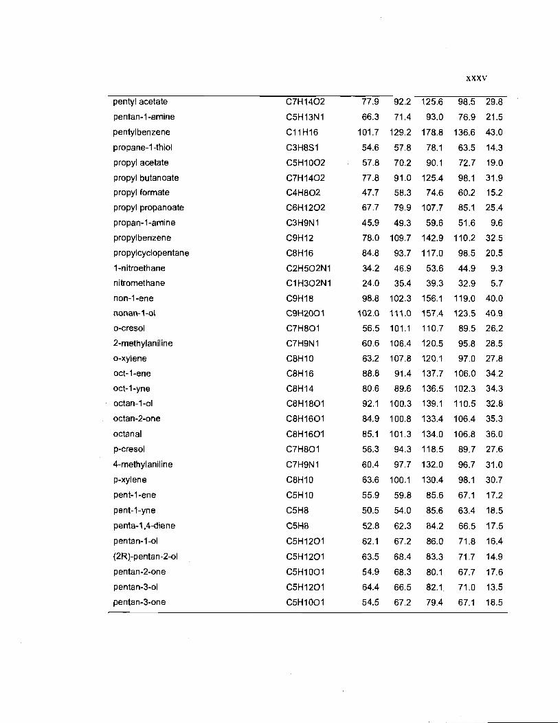
xxxv

pentyl acetate C7H1402 77.9 92.2 125.6 98.5 29.8

pentan-1-amine C5H13N1 66.3 71.4 93.0 76.9 21.5

pentylbenzene C11H16 101.7 129.2 178.8 136.6 43.0

propane-1-thiol C3H8S1 54.6 57.8 78.1 63.5 14.3

propyl acetate C5H1002 57.8 70.2 90.1 72.7 19.0

propyl butanoate C7H1402 77.8 91.0 125.4 98.1 31.9

propyl formate C4H802 47.7 58.3 74.6 60.2 15.2

propyl propanoate C6H1202 67.7 79.9 107.7 85.1 25.4

propan-1-amine C3H9N1 45.9 49.3 59.6 51.6 9.6

propylbenzene C9H12 78.0 109.7 142.9 110.2 32.5

propylcyclopentane C8H16 84.8 93.7 117.0 98.5 20.5

1-nitroethane C2H502N1 34.2 46.9 53.6 44.9 9.3

nitromethane C1H302N1 24.0 35.4 39.3 32.9 5.7

non-1-ene C9H18 98.8 102.3 156.1 119.0 40.0

oooao-1-01 C9H2001 102.0 111.0 157.4 123.5 40.9

o-cresol C7H801 56.5 101.1 110.7 89.5 26.2

2-methylaniline C7H9N1 60.6 106.4 120.5 95.8 28.5

o-xylene C8H10 63.2 107.8 120.1 97.0 27.8

oct-1-ene C8H16 88.8 91.4 137.7 106.0 34.2

oct-1-yne C8H14 80.6 89.6 136.5 102.3 34.3

octan-1-01 C8H1801 92.1 100.3 139.1 110.5 32.8

octan-2-one C8H1601 84.9 100.8 133.4 106.4 35.3

octanal C8H1601 85.1 101.3 134.0 106.8 36.0

p-cresol C7H801 56.3 94.3 118.5 89.7 27.6

4-methylaniline C7H9N1 60.4 97.7 132.0 96.7 31.0

p-xylene C8H10 63.6 100.1 130.4 98.1 30.7

pent-1-ene C5H10 55.9 59.8 85.6 67.1 17.2

pent-1-yne C5H8 50.5 54.0 85.6 63.4 18.5

penta-1 A-diene C5H8 52.8 62.3 84.2 66.5 17.5

pentan-1-01 C5H1201 62.1 67.2 86.0 71.8 16.4

(2R)-pentan-2-01 C5H1201 63.5 68.4 83.3 71.7 14.9

pentan-2-one C5H1001 54.9 68.3 80.1 67.7 17.6

pentan-3-01 C5H1201 64.4 66.5 82.1 71.0 13.5

pentan-3-one C5H1001 54.5 67.2 79.4 67.1 18.5

xxxvi

pentanal C5H1001 55.1 68.7 80.5 68.1 17.3

pentanenitrile C5H9N1 55.5 61.4 88.0 68.3 19.6

pentanoic acid C5H1002 57.5 70.8 88.4 72.3 21.5

phenyl formate C7H602 59.7 93.1 116.3 89.7 27.5

[(1 R)-1.2.2-trifluoroethoxy]benzene C8H701F3 70.0 105.6 135.7 103.8 31.8

piperazine C4H10N2 63.6 68.2 72.6 68.1 10.8

piperidine C5H11N1 65.0 72.1 74.4 70.5 8.9

prop-2-en-1-ol C3H601 39.3 41.4 58.6 46.4 8.9

propan-1-ol C3H801 41.9 44.7 52.9 46.5 6.9

propanenitrile C3H5N1 35.1 38.2 54.6 42.6 9.6

propionic acid C3H602 37.2 48.9 54.6 46.9 10.4

prop-1-ene C3H6 32.9 38.1 52.9 41.3 9.1

propanal C3H601 34.7 46.6 47.5 42.9 7.4

prop-1-yne C3H4 29.9 29.9 52.8 37.5 10.1

pyrrolidine C4H9N1 53.5 59.4 61.9 58.3 6.2

sec-butylbenzene C10H14 97.6 118.1 147.1 120.9 22.7

styrene C8H8 58.7 100.1 147.0 101.9 34.3

(2R)-2-bromo-1.1.1.2-tetrafluoro-ethane C2H1F4Br1 45.6 47.7 62.9 52.1 8.8

tert-butylbenzene C10H14 90.7 122.7 149.6 121.0 30.8

tetrahydrofuran C4H801 47.7 52.7 58.5 53.0 4.5

tetrahydropyran C5H1001 59.5 65.6 70.8 65.3 7.2

toluene C7H8 54.5 91.4 105.8 83.9 24.1

1,4-dimethylcyclohexane C8H16 84.9 95.8 114.8 98.5 17.7

1.1.2-trichloroethylene C2H1CI3 46.9 71.1 93.9 70.7 18.4

N.N-diethylethanamine C6H15N1 83.3 94.4 94.4 90.7 13.4

trimethoxymethylbenzene C10H1403 112.8 127.0 160.8 133.5 24.5

undecan-2-one C11H2201 114.7 133.5 188.3 145.5 55.2

{2R.3R,4S.5R.6R)-6-

{hydroxymethyl)tetrahydropyran-2 ,3. 4.5-

tetrol C6H1206 85.1 107.0 111.8 101.3 21.0

{2S,3S,4R.5R)-5-

(hyd roxymethyl )tetrahydrofuran-2.3,4-tri 01 C5H1005 78.8 81.0 88.9 82.9 5.7

(2R,4R,5R)-5-

(hydroxymethyl)tetrahydrofuran-2,4-diol C5H1004 72.5 78.2 87.2 79.3 8.8