eScholarship provides open access, scholarly publishingservices to the University of California and delivers a dynamicresearch platform to scholars worldwide.

Lawrence Berkeley National LaboratoryLawrence Berkeley National Laboratory

Peer Reviewed

Title:Automatic segmentation of histological structures in mammary gland tissue sections

Author:Fernandez-Gonzalez, RodrigoDeschamps, ThomasIdica, Adam K.Malladi, RavikanthOrtiz de Solorzano, Carlos

Publication Date:02-17-2004

Publication Info:Lawrence Berkeley National Laboratory

Permalink:http://escholarship.org/uc/item/99r8w60x

Keywords:Breast Cancer Molecular Analysis Automatic Segmentation 3D Reconstruction Fast MarchingLevel Set

1

Automatic segmentation of histological structures inmammary gland tissue sections∗

R. Fernandez-Gonzalez1,4,∗∗

, T. Deschamps2,3, A. Idica1, R. Malladi3 and C. Ortiz de Solorzano1

1Life Sciences Division, Lawrence Berkeley National Laboratory, Berkeley2Mathematics Department, University of California, Berkeley

3Mathematics Department, Lawrence Berkeley National Laboratory, Berkeley4UC Berkeley & San Francisco Joint Graduate Group in Bioengineering, Berkeley

{rfgonzalez,tdeschamps,akidica,r malladi,codesolorzano}@lbl.gov

∗A preliminary version of this work was presented at the Photonics West 2003 Conference: Automatic segmentation of structures innormal and neoplastic mammary gland tissue sections. R. Fernandez-Gonzalez, T. Deschamps, A. Idica, R. Malladi, C. Ortiz de Solorzano.Proceedings of Photonics West 2003, vol. 4964(26).∗∗Corresponding author: R. Fernandez-Gonzalez, Life Sciences Division, Lawrence Berkeley Lab, 1 Cyclotron Road, Building 84, MS

84-171, Berkeley, CA 94720, USA, Phone: (510) 486 5359, Fax: (510) 486 5730, e-mail: RFGonzalez@lbl.gov

2

Abstract

Real-time three-dimensional (3D) reconstruction of epithelial structures in human mammary gland tissue blocks mapped with selected

markers would be an extremely helpful tool for breast cancer diagnosis and treatment planning. Besides its clear clinical application, this

tool could also shed a great deal of light on the molecular basis of breast cancer initiation and progression.

In this paper we present a framework for real-time segmentation of epithelial structures in two-dimensional (2D) images of sections of

normal and neoplastic mammary gland tissue blocks. Complete 3D rendering of the tissue can then be done by surface rendering of the

structures detected in consecutive sections of the blocks.

Paraffin embedded or frozen tissue blocks are first sliced, and sections are stained with Hematoxylin and Eosin. The sections are then

imaged using conventional bright field microscopy and their background is corrected using a phantom image.

We then use the Fast-Marching algorithm to roughly extract the contours of the different morphological structures in the images. The

result is then refined with the Level-Set method which converges to an accurate (sub-pixel) solution for the segmentation problem. Finally,

our system stacks together the 2D results obtained in order to reconstruct a 3D representation of the entire tissue block under study. Our

method is illustrated with results from the segmentation of human and mouse mammary gland tissue samples.

Keywords: Breast Cancer, Molecular Analysis, Automatic Segmentation, 3D Reconstruction, Fast-Marching, Level-Set

3

I. Introduction

The mature mammary gland is a tree-like organ made of three different levels of branching ducts converging at the

nipple [1]. The ducts are lined by epithelial cells and end in secretory lobulo-alveolar structures, which are the sites of

milk production during lactation. In cancer, this hierarchical organization is disrupted by uncontrolled growth of the

epithelium, and sometimes by the subsequent invasion of the surrounding tissue [2]. These morphological or structural

changes are accompanied by other genetic and epigenetic changes at the cellular level (see figure 1). An example of

this is seen in ductal carcinoma in situ (DCIS) which is a preinvasive form of cancer. In DCIS the molecular changes

common in breast cancer can be observed together with well-defined morphological patterns, like comedo or cribiform

ones, with or without central necrosis [3], [4].

An interesting problem is the quantification of these genetic or molecular changes in the context of the tissue envi-

ronment where they occur. This way, by looking at cancer as an organ, which is inherently heterogeneous and dynamic,

we believe that we will obtain a better understanding of the events that drive the progression of the disease. Therefore,

since the normal mammary gland and its neoplastic variants are neither flat nor homogeneous, the approach to this

problem should be three-dimensional as well, and take into account the heterogeneity of the gland. However, most

classical methods in biology focus on only a single type of abnormalities (molecular or morphological) and/or neglect

three-dimensionality and heterogeneity.

Although imaging of both tissue structure and function in vivo would be extremely desirable, the existing in vivo

imaging methods (X-ray, MRI, optical tomography, etc.) do not provide the necessary resolution for cell-level molecular

analysis. In addition, these methods provide morphological information that can only be indirectly related to the function

of the tissue. Consequently, ex-vivo microscopic analysis of the tissue from flat fixed sections is the routine method in

histopathology. However, the limited capacity for the human eye to extrapolate and visualize 3D structures from

sequences of 2D scenes renders this method unsuitable for quantitative 3D tissue characterization. To overcome these

issues we have developed a system for simultaneous morphological and molecular analysis of thick tissue samples [5]. The

system consists of a computer-assisted microscope and a JAVA-based image display, analysis and visualization program

(R3D2). R3D2 allows semi-automatic acquisition, annotation, storage, 3D reconstruction and analysis of histological

structures (intraductal tumors, normal ducts, blood vessels, etc.) from thick tissue specimens. For this purpose the tissue

needs to be embedded in a permanent or semi-rigid medium after collection. The tissue is then fully sectioned, and the

resulting sections are stained in a way that visually highlights the desired structures. In histopathology, Hematoxylin and

Eosin (H&E) is the most common combination of dyes used to observe the morphology of the tissue. In order to image

not only structure, but also molecular events, we alternate H&E staining with fluorescent staining (immunofluorescence,

fluorescence in situ hybridization,...) of proteins and selected genes in consecutive sections.

This paper will focus on the annotation of the structures of interest on the H&E stained sections. Manual segmentation

has been used before to delineate histological structures [6], [7], [8]. In order to build the 3D reconstruction of the block,

we initially annotated each of the interesting features of the tissue on each section by using manually drawn contours.

4

This step constituted the bottleneck in the study of samples. Semi-automatic approaches to segmentation of features

of interest in histological sections have also been used [9], but they still involve too much user interaction to be used

to reconstruct large tissue samples. Automatic annotation (segmentation) of the structures of interest is the answer to

this problem. In this paper, we propose an automatic method followed by interactive correction that greatly reduces

the amount of interaction required, thus allowing us to use our system for imaging and reconstruction of large, complex

tissue structures.

Automatic extraction of contours in 2D images is usually done with Active contour models, originally presented by

Kass, Witkins and Terzopoulos [10]. These methods are based on deforming an initial contour (polygon) toward the

boundary of the desired object to extract in an image. The deformation is achieved by minimizing a certain energy

function, which is computed by integrating along the contour, terms related to its continuity, and terms related to the

pixel values of the area of the image where the contour is defined. That energy function approaches a minimum near

the object boundary, and thus, the minimization process drives the curve toward the desired shape.

As an alternative, implicit surface evolution models have been introduced by Malladi et. al [11], [12] and Caselles et.

al [13]. In these models, the curve and surface models evolve under an implicit speed law containing two terms, one that

attracts it to the object boundary and the other that is closely related to the regularity of the shape. Specifically, the

proposal is to use the Level-Set approach of Osher and Sethian [14]. This is an interface propagation technique used for

a variety of applications, including segmentation. The initial curve is represented here as the zero Level-Set of a higher

dimensional function, and the motion of the curve is embedded within the motion of that higher dimensional function.

An energy formulation similar to the Active Contours leads to a minimization process with several advantages. First,

the zero Level-Set of the higher dimensional function is allowed to change topology and form sharp corners. Second,

geometric quantities such as normal and curvature are easy to extract from the hypersurface. Finally, the method expands

straightforwardly to 3D [15], but adding a dimension to the problem increases the computational cost associated with the

method. The narrow-band approach of Adalsteinsson and Sethian [16] accelerates the Level-Set flow by considering for

computations only a narrow band of pixels around the zero level-set. But in our experience, the narrow band technique

does not reduce the computational cost to a reasonable limit, due to the large size of the images of the sections.

Thus, we propose to use the Fast-Marching method [17]. This method considers monotonically advancing fronts (speed

always positive or negative), providing a result very quickly, albeit one that is not as accurate as the one obtained by

using the Level-Set algorithm. Malladi and Sethian [18] showed that the Fast-Marching method can be used as the initial

condition for the slower but more accurate Level-Set segmentation, obtaining real-time delineation of the structures of

interest. The combination of all these tools is the framework we are using in order to reconstruct normal and cancerous

ducts in mammary gland tissue sections of DCIS samples.

This paper is organized as follows: section II describes the general tissue handling and image acquisition protocols

that we use, as well as the theoretical basis of the segmentation scheme; section III shows the results of applying our

method to histological tissue sections; and section IV discusses the results and suggests some future developments and

improvements to our approach.

5

II. Methodology

A. Tissue processing and imaging

The tissue processing and staining protocol used is illustrated in figure 2.

Tissue blocks of 4 to 5 mm thickness were sliced into 5µm (thin) sections (Step 1). The odd sections were stained

with Hematoxylin and Eosin (H&E),a standard staining combination in histopathology used to obtain morphological

information both at the cytological (single cell) and architectural (organ) levels. The even sections were stained using

some fluorescence technique (immunocytochemistry, fluorescence in situ hybridization, ...) depending on the molecular

phenomena that we wanted to study. Describing the acquisition and analysis of the fluorescent images is out of the scope

of this paper, which focuses on the segmentation of epithelial structures in the H&E stained sections. Therefore, the

rest of this section describes only the protocol used for the H&E stained sections. Low magnification (2.5×), panoramic

images of all the sections were automatically acquired using a motorized Zeiss Axioplan I microscope coupled with a

monochrome XilliX Microimager CCD camera (Step 2). To create these large panoramic images, the system scanned

the entire sections, taking single-field-of-view snapshots and tiled them together into single, whole-view images of the

sections. The required sequence of microscope movements and camera operations is produced by an application running

on the Sun Ultra 10 workstation that controls the camera and all moving parts of the microscope.

Next we annotated the structures of interest (ducts, lymph nodes, tumors, ...) in the images of the H&E stained

sections (Step 3). These annotated structures were used to render a three-dimensional model of each tissue block (Step

4).

These four initial steps are the focus of this paper. However, to better understand the rational for it, we continue

describing the final three steps, which are out of the intended scope for this paper. The user can select to revisit areas in

the three-dimensional rendition of the organ, based on their morphology. This can be done on the H&E sections or on

the intermediate fluorescent sections. To do so, the system requires the user to acquire high magnification (40− 100×)

images of corresponding section(s) (Steps 5 & 6). If the high magnification images are taken from the intermediate

immunofluorescent sections, quantification routines can be run on these new images (Step 7).

Manually annotating all the relevant morphological structures in all the sections of fully-sectioned tissue blocks is

feasible but, for all purposes, impractical due to the tremendous human effort. Although it might be the most accurate

and reliable approach, manual annotation is not possible except when reconstructing small, very simple tissue volumes.

As a result, we have developed automatic methods that eliminate or greatly reduce human interaction, thus making the

reconstruction of complex systems possible. What follows describes our approach.

B. Segmentation

B.1 Background removal

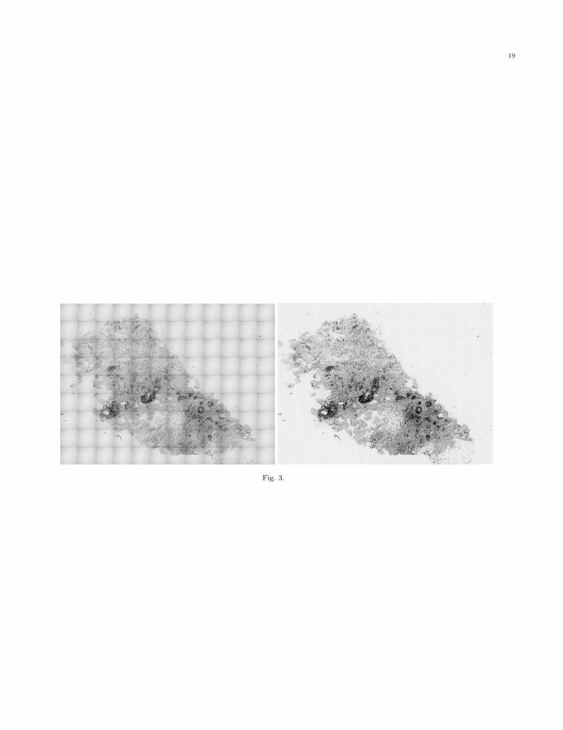
The algorithm that we use to acquire an image of an entire section creates a mosaic from a set of snapshots (one per

field of view). This approach gives rise to a background pattern across the image (figure 3-left) involving relatively large

6

gradients in between elements of the mosaic.

Objects of interest often span through several fields of view, and since our segmentation approach depends largely on

the gradients of the image, we need to eliminate the background pattern in order to obtain good segmentation results.

This can be done by performing a set of arithmetic operations on the “mosaic” image, known as background compen-

sation. First we need a phantom, that is, an image of an empty field of view taken under the same illumination conditions

and microscope configuration that we used to acquire the initial image. Since most of the images that we acquire have

an empty frame in the upper left corner, it is simple to choose that frame as our phantom for the corresponding section.

After normalizing the pixel values in the phantom, and for each frame in the entire image, we divide the value at each

pixel by the value at the corresponding pixel in the phantom frame. The resulting image is background-corrected as

shown in figure 3-right, and it is a better input for our segmentation algorithms.

B.2 Preliminary segmentation: Fast-Marching method

Consider a monotonically advancing 2D front C with speed F always positive in the normal direction, starting from

an initial point p0,

∂C

∂t= F−→n . (1)

This equation drives the evolution of a front starting from an infinitesimal circular shape around p0 until each point p

inside the image domain is visited and assigned a crossing time U(p), which is the time t at which the front reaches the

point p.

The gradient of the arrival time is inversely proportional to the speed function, and thus we have a form of the Eikonal

equation

|∇U |F = 1 and U(p0) = 0 (2)

One way to solve Equation (2) is to use upwind finite difference schemes and iterate the solution in time [15]. In other

words, the scheme relies on one-sided differences that looks in the upwind direction of the moving front,thereby picking

the correct viscosity solution, namely

(max (u− Ui−1,j , u− Ui+1,j , 0))2+ (max (u− Ui,j−1, u− Ui,j+1, 0))

2=

1

F 2i,j

(3)

The key to solving this equation rapidly is to observe that the information propagates from smaller values of U to

larger values in the upwind difference structure in Equation (3). The idea is to construct the time surface, one piece at

a time, by only considering the ‘frontier’ points; we detail the Fast Marching method in Table I.

Notice that in solving Equation (3), only Alive points are considered. This means that for each point the calculation is

made using the current values of U at the neighbors, and not estimates at other trial points. Considering the neighbors of

the grid point (i, j) in 4-connectedness, we designate {A1, A2} and {B1, B2} as the two couples of opposite neighbors such

that we get the ordering U(A1) ≤ U(A2), U(B1) ≤ U(B2), and U(A1) ≤ U(B1). Since we have u ≥ U(B1) ≥ U(A1),

we can derive

(u− U(A1))2 + (u− U(B1))

2 =1

F 2i,j

(4)

7

Computing the discriminant (∆) of Equation (4) we complete the steps described in Table II. Thus the algorithm needs

only one pass over the image to find a solution. To execute all the operations that we just described in the minimum

amount time, the Trial points are stored in a min-heap data structure [17]. Since the complexity of changing the value of

one element of the heap is bounded by a worst-case processing time of (O(log2 N)), the total algorithm has a complexity

of O(N log2 N) on a grid with N nodes.

Finally, we define the speed of propagation in the normal direction as a decreasing function of the gradient |∇I(x)|,

that is, a function that is very small near large image gradients (i.e. possible edges) and large when the brightness level

is constant:

F (x) = exp−α|∇I(x)| , α > 0 (5)

where α is the edge strength, or the weight that we give to the presence of a gradient in order to slow down the

front. Depending on this value the speed function falls to zero more or less rapidly, and thus, it could stop a few grid

points away from the real edge. Also, variations in the gradient along the boundary can cause inaccurate results. False

gradients due to noise can be avoided using an edge preserving smoothing scheme on the image as a preprocessing step;

see [19].

The user can run the Fast-Marching method from a given set of initial points (mouse clicks on the background of the

images). Alternatively, the user can decide to segment only the structures within a manually defined rectangular region

of interest. If the region is too big, sub-sampling can be used so that the segmentation process is not too slow. However,

this option must be used carefully, since sub-sampling smooths the boundaries of the objects present in the image and

can completely obliterate smaller structures. The resulting contour (or contours if we are segmenting several objects at

the same time) will provide an excellent initial condition for the Level-Set method.

Putting all of these elements together we are able to get a good approximation of the shape of the object that we are

trying to segment (figure 5).

In order to improve the final result, we propose to run a few iterations of the Level-Set method using the result of the

Fast-Marching method as the initial condition.

B.3 Final segmentation: Level-Set method

Once we have obtained a good approximation of the shape of the object using the Fast-Marching algorithm, we can

afford to use the more computationally expensive Level-Set method to improve the result of the segmentation. The

essential idea here is to embed our marching front as the zero Level-Set of a higher dimensional function. In our case, we

take that function to be φ(x) = ±d, where d is the signed distance from x to the front (see figure 4), assigning negative

distances for pixels inside the evolving curve, and positive distances for pixels outside it.

Following the arguments in [14], we obtain the following evolution equation:

φt + F (x, y)|∇φ| = 0, (6)

where F is again the speed in the normal direction. This is an initial value partial differential equation, since it

8

describes the evolution of the solution on the basis of an initial condition defined as φ(x, t = 0) = φ0. As pointed out

before, the Level-Set approach offers several advantages:

• the zero Level-Set of the function can change topology and form sharp corners;

• a discrete grid can be used together with finite differences to approximate the solution;

• intrinsic geometric quantities like normal and curvature can be easily extracted from the higher dimensional function,

and

• everything extends directly to 3D.

To mold the initial condition (in our case the result of the Fast-Marching method) into the desired shape we use two

force terms. By substituting these two terms in the motion equation [18], [20] we get:

φt − g(1− εκ)|∇φ| − β∇g · ∇φ = 0 , ε > 0 , β > 0 (7)

where g is an edge indicator function defined by the speed of the front (5) in the Eikonal Equation (2); κ is the

curvature of the expanding front, and φt is the unknown that we are trying to compute. As before, the image I(x) can

be preprocessed using an edge-preserving smoothing scheme.

The second term of the equation has two components. The first one slows the surface in the neighborhood of high

gradients (edges), while the second one (motion by curvature) provides regularity to the curve. The parameter ε is the

weight of the motion by curvature term, and determines the strength of its regulatory effect: the bigger we make ε, the

more we constrain the possibility to obtain sharp corners and irregular contours. In practice, an intermediate value of ε

provides a good trade-off between contour smoothing and accuracy.

Finally, the last term of the equation attracts the front to the object boundaries. It aligns all the Level-Sets with the

ideal gradient, which would be a step function centered at the point of maximum gradient in the original image. β is

the weight of the advection of the front by the edge vector field ∇g. It determines the strength of the attraction of the

front to the edges.

At times, for very small objects, it is possible to use the Level-Set method from the initial point. However, for any

type of morphological structure, we can use the result of the Eikonal equation (2), U(x, y), as the initial condition for

the Level-Set algorithm: φ(x, y; t = 0) = U(x, y). Then by solving Equation (7) for a few time steps using the narrow

band approach, we obtain an accurate, real-time segmentation of the desired object (see figure 5).

III. Results

In this section we consider the problem of reconstructing DCIS areas in a tissue biopsy of a cancerous human breast

as well as a group of normal ducts through an entire mouse mammary gland. The tissue samples were sliced for a

total of 55 sections in the human tissue and 206 sections in the mouse one. We used all of the sections (55) for the

reconstruction of the human case and 40 sections for reconstruction of the mouse case. Manually delineating all the

structures in every section is an extremely time-consuming process. To automatically segment those structures using the

framework described in section II, we begin by defining a Region-Of-Interest (ROI) where we will run the segmentation

9

algorithm. This ROI can be extended to cover the entire section, but considering the size of the images it is wise

to use sub-sampling in order to run the algorithm in real time. The level of sub-sampling can be determined by the

user: greater sub-sampling can be used on large ROIs, without compromising the resolution and accuracy of the final

segmentation.

After defining the ROI, we have to tune the different parameters of the segmentation process, particularly α (Equa-

tion (5)) and ε (Equation (7)). This is done by the user based on the default values provided by the algorithm and

the type of object that he/she is trying to segment. However, we have observed that a particular set of parameters

is frequently good enough to segment similar structures (i.e., all the tumors, all the ducts, all the lymph nodes, ...)

throughout all the sections of a particular tissue block. Thus, the user only needs to modify the parameters the first

time that he/she tries to segment a new type of morphological element in the tissue.

After selecting the parameters of the flow, initial points are defined inside (to find the internal contour) or outside (to

find the external contour) of the structures of interest. In most cases one mouse-click is enough, though large images

may require several, evenly distributed clicks. The value of U(x) at these points is set to zero as in equation 2, and

the Fast-Marching algorithm of table I is executed. When this method finishes, the final U(x) function is passed as the

initial condition to the Level-Set motion equation (7). We then iterate this equation for a few steps. This segmentation

scheme provides a result in less than one second for images whose size (after sub-sampling, if any) is around 2 kilobytes

(e.g., 512× 512 pixels) running on a Sun Ultra 10 workstation with 1 GB of RAM.

A. Human case segmentation

Figure 6 displays an example of the result obtained with the combination of the Fast-Marching and the Level-Set

methods in a tissue biopsy from a patient with intraductal carcinoma (DCIS).

Figure 6-middle shows the segmentation of a tumor mass in a human tissue block. The results of the segmentation can

be edited and removed with the interactive tools provided by our system (see figure 6-right). For this segmentation, an

area was selected around the structures of interest and no sub-sampling was used. The initial contours are represented

by blue points in figure 6-left.

B. Mouse case segmentation

In figure 7 we can see the segmentation of the external contours of several ducts in a particular area of a mouse

mammary gland. In this case we also run the algorithm on a ROI on one of the sections with no sub-sampling factor.

Figure 7-left displays the points where we initialized the contours. Figures 7-middle and right show the results of the

segmentation before and after interactive correction of the results respectively.

C. 3D Reconstruction

Finally the segmented shapes are connected (manually) between sections, and 3D reconstructions of the samples are

built. Figure 8 shows a reconstruction of the tumors contained in the human tissue block, including the tumor shown in

figure 6. Increasing the “motion by curvature” term, as described in section II, can reduce surface noise. In figure 9 we

10

can see the reconstruction of the normal ducts segmented in the images of the mouse mammary gland (see one of the

corresponding 2D segmentations in figure 7).

D. Further examples

Figures 10 and 11 show two more examples of the results that can be obtained with our segmentation approach. In

both cases the initial ROI was sub-sampled by a factor of two in both the X and Y directions. Interestingly, the same

segmentation parameters (α and ε) were used for both examples.

Figure 10-left shows an DCIS lesion together with a normal duct in a human tissue section. Both structures were

segmented at the same time using a single initial point, as can be seen in figure 10-middle. Figure 10-right shows the

results incorporated to the full resolution image.

In figure 11-left, a terminal ductal lobular unit (TDLU) can be observed. These are lobuloalveolar structures where

milk is produced during lactation in the human breast. The multiple alveoli that form the TDLU, together with

the presence of a ductal part, make automatic segmentation of this type of structure a difficult task. However, after

subsampling the image, our algorithm is able to find a contour that surrounds the entire structure (figures 11-middle

and 11-right), thus allowing its 3D reconstruction.

IV. discussion

We have developed a microscopy system that semi-automatically reconstructs histological structures from fully sec-

tioned tissue samples. However, the interaction required to operate the system is quite intensive, limiting the scope

of its application to small tissue volumes or to studies not requiring high throughput analysis of the samples. In this

paper we have presented a method that reduces the time and interaction needed to build the 3D reconstruction of a

tissue block, thus increasing the potential throughput of the system and therefore allowing us to use this approach for

the reconstruction of large, complex specimens. To achieve this goal we have combined image processing techniques and

two well-established schemes for interface propagation: the Fast-Marching method and the Level-Set method.

Our approach starts by correcting the background of the images. This is an important step, since the background

pattern generated during image acquisition modifies the gradient of the image, and the speed function that we use for

interface propagation depend on that gradient. Once the background has been corrected, we run the Fast-Marching

method. This technique provides a good approximation of the boundaries of the objects that we are trying to segment

in a very short time, since it assumes monotonic speed functions (always positive or always negative). We then use

the approximation provided by the Fast-Marching method as the initial condition for the Level-Set method. This more

computationally expensive algorithm is run for just a few steps, enough to fit the front to the contours of the structures

of interest, but not as many as to make the segmentation too time consuming.

Though this approach is very useful, it can still be improved. The most accurate segmentations (and reconstructions)

are obtained on full resolution images. However, for some large structures like lymph nodes, or when trying to delineate

multiple elements at the same time (for example a group of ducts), segmentation on a full resolution image is not

11

real-time, and can take up to one minute. Using sub-sampling takes the segmentation execution time back to real time

at the expense of some accuracy loss. Also, in areas with a lot of texture in the tissue around the ducts (stroma) tuning

the parameters of the algorithm (α and ε) becomes more difficult. At times this process can take a few trials, since the

expanding front tends to get trapped in high gradients that do not correspond to the boundaries of the feature that we

are trying to segment, but to the texture of the stroma. Finally, once all the structures of interest have been segmented,

the user still needs to manually connect them between sections. This constitutes a new bottleneck in the tissue analysis

process.

For these reasons, we are currently working on a time-step independent scheme that is expected to be faster than the

current one. To improve the accuracy of the results, we have developed an edge-preserving smoothing algorithm based

on the Beltrami flow [19], which can replace the Gaussian smoothing currently used before executing the segmentation

methods. This algorithm eliminates false gradients due to noise, while enhancing gradients due to object boundaries,

thus allowing the front to fit the boundaries of the object more accurately. Finally, the Level-Set approach is readily

extensible to 3D. The ability to segment 3D structures of interest versus 2D ones would save the process of connecting

the segmented 2D contours from section to section, thus improving the analysis time. Also, since geometric properties

can be easily extracted from the higher dimensional function used in the Level-Set algorithm, we could readily obtain

some information about the extracted volume from the segmentation algorithm itself. We are also working on a fully

interactive segmentation method on the model of the Intelligent Scissors [21], because the selection of the seed points for

segmentation is something that cannot be automated, due to the high variability in the shapes of the object to segment.

In conclusion, we have presented a real-time method for automatic segmentation of morphological structures in

mammary gland tissue sections. It is precisely the delineation of those structures that required heaviest user interaction

in our sample-analysis protocol. Therefore, the automatic approach to segmentation that we describe here represents a

first step toward real-time reconstruction and analysis of mammary gland samples. Achieving that goal would allow us to

accelerate our studies on the biological basis of human breast cancer. Moreover, obtaining real-time reconstruction and

analysis of samples from our system would be useful for pathological diagnosis in a clinical environment: 3D renderings

of all the morphological structures in a mammary gland biopsy could be mapped with the distribution of particular

markers of breast cancer within few hours of extracting the tissue from the patient. From an intra-surgically point of

view, the renderings would prove - tissue processing and stain permitting - as an important tool in the evaluation of

breast tumors and their margins.

12

Acknowledgments

The U.S. Army Medical Research Materiel Command under grants DAMD17-00-1-0306 and DAMD17-00-1-0227,

the Lawrence Berkeley National Laboratory Directed Research and Development program and the California Breast

Cancer Research Program, through project #8WB-0150 supported this work. This work was also supported by the

Director, Office of Science, Office of Advanced Scientific Research, Mathematical, Information, and Computational

Sciences Division, U.S. Department of Energy under Contract No. DE-AC03-76SF00098.

13

References

[1] L. Hennighausen and G.W. Robinson, “Think globally, act locally: the making of a mouse mammary gland,” Genes Development, vol.

12, no. 4, pp. 449–455, february 1998.

[2] L.M. Franks and N.M. Teich, Introduction to the cellular and molecular biology of cancer, Oxford University Press, Oxford, 1997.

[3] T. Tot, L. Tabar, and P.B. Dean, Practical Breast Pathology, Thieme, Falun Central Hospital, 1st edition, 2002.

[4] R.D. Cardiff and S.R. Wellings, “The comparative pathology of human and mouse mammary glands,” Journal of Mammary Gland

Biology and Neoplasia, vol. 4, no. 1, pp. 105–122, 1999.

[5] R. Fernandez-Gonzalez, A. Jones, E. Garcia-Rodriguez, P.Y. Chen, A. Idica, M.H. Barcellos-Hoff, and C. Ortiz de Solorzano, “A system

for combined three-dimensional morphological and molecular analysis of thick tissue samples,” Microscopy Research and Technique, vol.

59, no. 6, pp. 522–530, december 2002.

[6] T. Ohtake, R. Abe, I. Kimijima, T. Kukushima, A. Tsuchiya, K. Hoshi, and H. Wakasa, “Computer graphic three-dimensional recon-

struction of the mammary duct-lobular systems,” Cancer, vol. 76, no. 1, pp. 32–45, 1995.

[7] D.F. Moffat and J.J. Going, “Three-dimensional anatomy of complete duct systems in human breast: pathological and developmental

implications,” Journal of Clinical Pathology, vol. 49, pp. 48–52, 1996.

[8] T. Ohtake, I. Kimijima, T. Fukushima, M. Yasuda, K. Sekikawa, S. Takenoshita, and R. Abe, “Computer-assisted complete three-

dimensional reconstruction of the mammary gland ductal/lobular systems,” Cancer, vol. 91, no. 12, june 2001.

[9] F. Manconi, R. Markham, G. Cox, E. Kable, and I.S. Fraser, “Computer-generated, three-dimensional reconstruction of histological

parallel serial sections displaying microvascular and glandular structures in human endometrium,” Micron, vol. 32, pp. 449–453, 2001.

[10] M. Kass, A. Witkin, and D. Terzopoulos, “Snakes: Active contour models,” International Journal of Computer Vision, vol. 1, no. 4,

pp. 321–331, 1988.

[11] R. Malladi, J.A. Sethian, and B.C Vemuri, “A topology-independent shape modeling scheme,” in Proceedings of SPIE Conference on

Geometric Methods in C omputer Vision II, San Diego, CA, july 1993, vol. 2031, pp. 246–258.

[12] R. Malladi, J.A. Sethian, and B.C. Vemuri, “Shape modelling with front propagation: A level set approach,” IEEE Transactions On

Pattern Analysis And Machine Intelligence, vol. 17, no. 2, pp. 158–175, Feb. 1995.

[13] V. Caselles, F. Catte, T. Coll, and F. Dibos, “A geometric model for active contours,” Numerische Mathematik, vol. 66, pp. 1–31, 1993.

[14] S. Osher and J.A. Sethian, “Fronts propagating with curvature dependent speed: algorithms based on the hamilton-jacobi formulation,”

Journal of Computational Physics, vol. 79, pp. 12–49, 1988.

[15] J.A. Sethian, Level set methods: Evolving Interfaces in Geometry, Fluid Mechanics, Computer Vision and Materials Sciences, Cam-

bridge University Press, University of California, Berkeley, 2nd edition, 1999.

[16] D. Adalsteinsson and J.A. Sethian, “A fast level set method for propagating interfaces,” Journal of Computational Physics, vol. 118,

pp. 269–277, 1995.

[17] J.A. Sethian, “A fast marching level set method for monotonically advancing fronts,” Proceedings of the National Academy of Sciences

of the United States of America, vol. 93, no. 4, pp. 1591–1595, Feb. 1996.

[18] R. Malladi and J.A. Sethian, “A real-time algorithm for medical shape recovery,” in Proceedings of the IEEE International Conference

14

on Computer Vision (ICCV’98), Jan. 1998, pp. 304–310.

[19] N. Sochen, R. Kimmel, and R. Malladi, “A general framework for low level vision,” IEEE Transactions on Image Processing, vol. 7,

no. 3, pp. 310–318, march 1998.

[20] C. Ortiz de Solorzano, R. Malladi, S.A. Lelievre, and S.J. Lockett, “Segmentation of nuclei and cells using membrane related protein

markers,” journal of Microscopy, vol. 201, no. 3, pp. 404, 2001.

[21] W. Barrett and E. Mortensen, “Interactive live-wire boundary extraction,” Medical Image Analysis, vol. 1, no. 4, pp. 331–341, 1997.

15

• Fig. 1: Morphological and genetic alterations in breast cancer. The images show two optical sections of human

mammary gland tissue acquired using a confocal laser scanning microscope; nuclei are displayed in red, a probe for

a certain DNA sequence in chromosome 17 is shown in green. Left image: normal tissue; as expected, each nucleus

contains up to two green signals (up to two copies of chromosome 17 per nucleus in a single optical section). Right

image: neoplastic lesion; not only do some nuclei contain more than 2 copies of the probe, but also they have distinct

morphological changes that can be observed in this section.

• Fig. 2 Protocol followed on tissue blocks. The different steps (sectioning, annotation, reconstruction, high magnification

acquisition and molecular analysis) are illustrated. Samples are fully sectioned at 5µm (Step 1). The odd sections

are stained with H&E, the even ones with some kind of fluorescence technique (application-dependent). Images are

acquired of all the sections (Step 2), and structures of interest are delineated in the H&E-stained ones (Step3). A

3D reconstruction of the specimen is created from these markings (Step 4). From the 3D reconstruction of the tissue

different areas can be selected for molecular analysis (Step 5). The system will take high magnification images of those

areas on the corresponding fluorescent sections (Step 6). Image analysis tools can then be used to quantify the presence

and distribution of molecular markers in the high magnification images (Step 7).

• Fig. 3: Background correction. a) Image of a section belonging to a human case. The background pattern created by

the acquisition method is readily noticeable. b) Same image after background correction.

• Fig. 4: Basic concept behind the Level-Set method. The marching front is embedded as the zero Level-Set of a higher

dimensional function.

• Fig. 5: The segmentation of a lymph node in a mouse mammary gland section is shown in black. Left image: result

of the Fast-Marching method; it provides a good approximation to the boundaries of the lymph node; the blue point in

the middle of the lymph node is the initial contour from which the algorithm was run. Right image: result of using the

Level-Set method after the Fast-Marching method; the final contour is more accurate and smoother. In both cases the

images were subsampled in the x and y directions to be able to run the segmentation in real time.

• Fig. 6: Segmentation of a DCIS tumor in human mammary gland tissue. Left image: Initial contour (blue dot).

Middle image: Results of the segmentation with red lines delineating tumor masses. Right image: results after edition

using the interactive tools provided by the system.

• Fig. 7: Segmentation of normal ducts in a mouse mammary gland tissue sample. Left image: initial data; middle

image: results of the segmentation (red/black lines delineate normal ducts); right image: results after editing using the

interactive tools provided by the system.

• Fig. 8: 3D reconstruction of tumors in a human mammary gland tissue block. Tumor masses are rendered as gray

volumes. The scene was stretched 10 times in the Z direction to obtain a better view.

• Fig. 9: 3D reconstruction of normal ducts in a mouse mammary gland. Ducts are rendered as gray volumes. A single

duct and its branches can be traced throughout the gland. The Z direction was not stretched in this case.

• Fig. 10: Segmentation of a different DCIS tumor in human mammary gland tissue. Left image: the duct on the left

contains a DCIS lesion with a necrotic center; the one on the right is normal. Middle image: the ROI was subsampled

16

by a factor of 2 in both the X and Y directions; the blue dot represents the initial seed. Right image: results of the

segmentation on the full resolution image.

• Fig. 11: Segmentation of a terminal ductal lobular unit in a human mammary gland. Left image: the duct on the

left contains a section of a TDLU, one of the sites of milk production in the human breast. Middle image: the ROI

was subsampled by a factor of 2 in both the X and Y directions; the blue dot represents the initial seed. Right image:

results of the segmentation on the full resolution image.

17

Fig. 1.

18

Fig. 2.

19

Fig. 3.

20

Algorithm for 2D Fast Marching– Definitions:∗ Alive set: all grid points where the action value U has been reached and will not be changed;∗ Trial set: next grid points (4-connectedness neighbors) to be examined. An estimate U of U has been computed using

Equation (3) from Alive points only (i.e. from U);∗ Far set: all other grid points, where there is no estimate for U yet;

– Initialization:∗ Alive set: reduced to the starting point p0, with U(p0) = U(p0) = 0;∗ Trial set: reduced to the four neighbors p of p0 with initial value U(p) = 1

F(p) (U(p) =∞);

∗ Far set: all other grid points, with U =∞;– Loop:∗ Let p = (imin, jmin) be the Trial point with the smallest action U ;∗ Move it from the Trial to the Alive set (i.e. U(p) = Uimin,jmin

is frozen);∗ For each neighbor (i, j) (4-connectedness in 2D) of (imin, jmin):· If (i, j) is Far, add it to the Trial set and compute Ui,j using Eqn. 3;· If (i, j) is Trial , update the action Ui,j using Eqn. 3.

TABLE I

Fast Marching algorithm

21

1. – If ∆ ≥ 0, u should be the largest solution of Equation (4);∗ If the hypothesis u > U(B1) is wrong, go to 2;∗ If this value is larger than U(B1), this is the solution;– If ∆ < 0, B1 has an action too large to influence the solution. It means that u > U(B1) is false. Go to 2;

Simple calculus can replace case 1 by the test:

If 1Fi,j

> U(B1)− U(A1), u =

U(B1)+U(A1)+

√

2 1

F2

i,j

−(U(B1)−U(A1))2

2is the largest solution of Equation (4)

else go to 2;2. Considering that we have u < U(B1) and u ≥ U(A1), we finally have u = U(A1) +

1Fi,j

.

TABLE II

Solving locally the upwind scheme

22

Fig. 4.

23

Fig. 5.

24

Fig. 6.

25

Fig. 7.

26

Fig. 8.

27

Fig. 9.

28

Fig. 10.

29

Fig. 11.