www.elsevier.com/locate/nima

Author’s Accepted Manuscript

Automatic procedure for mass and chargeidentification of light isotopes detected in CsI(Tl) ofthe GARFIELD apparatus

L. Morelli, M. Bruno, G. Baiocco, L. Bardelli, S.Barlini, M. Bini, G. Casini, M. D’Agostino, M.Degerlier, F. Gramegna, V.L. Kravchuk, T. Marchi,G. Pasquali, G. Poggi, NUCL-EX Collaboration

PII: S0168-9002(10)00663-7DOI: doi:10.1016/j.nima.2010.03.099Reference: NIMA51443

To appear in: Nuclear Instruments and Methodsin Physics Research A

Received date: 18 January 2010Revised date: 1 March 2010Accepted date: 5 March 2010

Cite this article as: L. Morelli, M. Bruno, G. Baiocco, L. Bardelli, S. Barlini, M. Bini, G.Casini, M. D’Agostino, M. Degerlier, F. Gramegna, V.L. Kravchuk, T. Marchi, G. Pasquali,G. Poggi and , Automatic procedure for mass and charge identification of light isotopesdetected in CsI(Tl) of the GARFIELD apparatus, Nuclear Instruments and Methods inPhysics Research A, doi:10.1016/j.nima.2010.03.099

This is a PDF file of an unedited manuscript that has been accepted for publication. Asa service to our customers we are providing this early version of the manuscript. Themanuscript will undergo copyediting, typesetting, and review of the resulting galley proofbefore it is published in its final citable form. Please note that during the production processerrors may be discovered which could affect the content, and all legal disclaimers that applyto the journal pertain.

Accep

ted m

anusc

ript

Automatic procedure for mass and charge1

identification of light isotopes detected in2

CsI(Tl) of the GARFIELD apparatus3

L. Morelli a, M. Bruno a, G. Baiocco a, L. Bardelli b, S. Barlini b,4

M. Bini b, G. Casini b, M. D’Agostino a,∗, M. Degerlier c,5

F. Gramegna c, V. L. Kravchuk a,c, T. Marchi d,c, G. Pasquali b,6

G. Poggi b7

aDipartimento di Fisica dell’Universita and INFN, Bologna, Italy8bDipartimento di Fisica dell’Universita and INFN, Firenze, Italy9

cINFN, Laboratori Nazionali di Legnaro, Italy10dDipartimento di Fisica dell’Universita, Padova, Italy11

NUCL-EX Collaboration12

Abstract13

Mass and charge identification of light charged particles detected with the 18014CsI(Tl) detectors of the GARFIELD apparatus is presented. A “tracking” method15to automatically sample the Z and A ridges of “Fast-Slow” histograms is developed.16An empirical analytic identification function is used to fit correlations between Fast17and Slow, in order to determine, event by event, the atomic and mass numbers of the18detected charged reaction products. A summary of the advantages of the proposed19method with respect to “hand-based” procedures is reported.20

Key words: Inorganic scintillators; Light ions; Response function; Pulse-shape21identification; Calibration.22

23PACS: 29.40.Mc, 29.40.Wk24

Preprint submitted to Elsevier 10 March 2010

Accep

ted m

anusc

ript

1 Introduction25

The availability of 4π multi-detectors [1–3] provides the opportunity for studying26very complex nuclear phenomena and events associated to small cross sections. The27price to be paid, however, comes in form of a vast amount of multi-dimensional data,28which need to be calibrated before obtaining physical correlations.29

The calibration of the measured signals can be quite man-power and time consuming,30for several reasons:31

• the large number of detecting elements covering the laboratory solid angle,32• different detectors (ionization chambers, drift chambers, semiconductors, scintil-33

lators) can be used in experiments, each requiring an “ad hoc” procedure,34• the rich variety of nuclear species produced in the reaction in a wide energy range.35

New semi-automatic methods are therefore required to perform a comprehensive36data calibration and analysis in a reasonable amount of time.37

We recall hereafter the scheme of the usually employed procedures to identify (A,Z)38isotopes, which do not rely on the “brute force”, even more time-consuming, ap-39proach like graphical cuts.40

Two steps are normally necessary for each detector used in the experiment (for41instance when the (A,Z) identification is performed through Fast-Slow [4]) or via42ΔE −Eresidual[5]):43

(1) In a bidimensional scatter plot several points are “by hand” sampled on the44ridges of well defined isotopes. Some isotopes can be easily identified by sim-45ple inspection, either due to their abundance (4He) or their separation from46other masses (1,2,3H). Charge, mass and coordinates of the sampled points are47organized in a table.48

(2) The parameters characterizing the detector response to the charge (Z) and49mass (A) are determined by fitting the coordinates of the previously sampled50points. If an analytical[5], even empirical [6] function, describing one of the51two variables as a function of the other does not exist, the set of points for a52

∗ Corresponding author: E-mail address: dagostino@bo.infn.it (M. D’Agostino)

2

Accep

ted m

anusc

ript

given isotope (A,Z) are fitted one by one via polynomial functions[4,7]. The fit53parameters are stored in a table.54

Once the identification function is determined, by studying the ridges, therefore the55most probable correlations, the event by event identification can be performed. For56all the measured events, isotopes are identified in mass and charge, by minimizing57the distance of the measured signals with respect to the values provided by the58identification function, calculated with the parameters of the hit detector.59

Clearly, in the case of a large number of detectors/telescopes, the most time con-60suming step of the identification procedure is the first one, because of the accurate61sampling of a huge number of points on each isotope branch needed to obtain in62the second step a reliable set of parameters. However [6], even the efforts to ana-63lytically link the employed variables are of great importance, to make it possible to64identify isotopes which cannot be sampled, because of their low statistics (e.g. in65backward-angle detectors).66

Our aim is to improve both the previous steps, in order to greatly reduce, for a67large number of detectors, the time dedicated to offline calibration with respect to68methods based on graphical cuts or “by hand” sampling procedures.69

In this paper we present a new procedure, developed in the ROOT framework [11],70aimed at extracting from Fast-Slow components coming from CsI(Tl) scintillators71mass and charge of the detected Light Charged Particles (LCP, Z ≤ 2) and Frag-72ments. The ROOT powerful set of software tools uses object oriented programming73and provides the user with several methods of displaying and analyzing data.74

We will show that our procedure, compared with other methods, considerably saves75time without loss of precision.76

We present here the application of our identification procedure to data collected in77experiments performed by the Nucl-ex collaboration [12] at the Tandem-Alpi com-78plex of LNL (Laboratori Nazionali di Legnaro) with the GARFIELD apparatus [2].79These experiments have been performed after the completion of the upgrading to80digital electronics; in this way, without the need of adding complicated and costly81analog channels, we could obtain the Fast-Slow components from the CsI(Tl) by82means of ADC-Digital Signal Processor (DSP) boards [8,9] which processed the83electric signals directly fed by the charge preamplifiers.84

3

Accep

ted m

anusc

ript

2 The experiment85

In this paper we show the results of the identification procedure firstly applied to86the data coming from the reaction 32S+58Ni at 16.5 AMeV incident energy. At the87end, we show the application of the same procedure to data of other measured reac-88tions. For all the reactions the energy range of the measured particles and fragments89extends from very low values up to 150 MeV.90

The main detector of the GARFIELD apparatus consists on two gas chambers with91microstrip readout, followed by CsI(Tl) scintillators[2], for a total of 180 telescopes92made of ΔE gaseous detectors (filled by CF4 gas at 50 mbar pressure) and CsI(Tl)93stopping detectors. The GARFIELD chambers cover the angular range 30o ≤ θlab ≤94150o.95

The characteristics of the CsI(Tl) scintillators of the GARFIELD array used in these96tests have been described in detail elsewhere[13,14]. We only recall here that the scin-97tillators have been carefully tested in order to select those with light-output resolu-98tion of about 3% for α−particles of about 5 MeV (standard three peaks radioactive99source[13,14]). Moreover using around 8 AMeV Li and C elastically scattered beams100on Au target the light-output resolution resulted in the range 2-3%.101

Fragments (Z ≥ 3) are identified in charge by analyzing ΔE − E matrices, where102ΔE is the energy lost in the gas and E the residual energy, measured by the CsI(Tl)103light output.104

A new designed electronics [8,9] has been used for the signal coming from CsI(Tl)105detectors for identifying the light isotopes by means of pulse-shape analysis. The Fast106and Long components of the CsI luminescence have been obtained via ADC-DSP107channel, one for each crystal as described hereafter.108

The charge signal integrated in a preamplifier is sampled by an ADC (125 MS/s109sampling frequency, nominal 12 bits precision) and the information is processed by110a DSP which, among other variables, produces Short and Long components. These111are obtained applying to the ADC sampled points two shaping filters with different112time constants. In our case a semigaussian filter (tf = 700 ns) produces the Short113component, while a triangular shaping with a peaking time of about 6 μs [9] gives114the Long contribution. The Long component is basically proportional to the total115

4

Accep

ted m

anusc

ript

light output, for any particle species.116

Fig. 1. (Color online) Fast-Slow bidimensional plots of a GARFIELD sector for the re-action 32S+58Ni 16.5 AMeV incident energy. For a better presentation in some of thepanels Fast and Slow have been scaled by the reported factor.

117

Of course, Short and Long contributions are largely linearly associated, since part118of the signal produced by the long-time fluorescence components of the CsI(Tl) is119

5

Accep

ted m

anusc

ript

integrated within the Short quantity. For a good isotope visualization and a better120presentation of the data in the identification scatter-plots, one tries a partial decor-121relation and fill the histos with new quantities obtained from a linear mixing of122Short and Long. In our case we choose the quantities Fast=Short and Slow=Long-1234*Short as done in Ref. [9], capable of separating the isotopic lines, leaving the Slow124observable larger than 0 (see Fig.1).125

We show in Fig.1 the Fast-Slow bidimensional plots for one of the 24 azimuthal126sectors of GARFIELD, as shown on-line by the Garfield data monitor recently im-127plemented [10]. An offset of 500 channels has been added to the signals, for a better128presentation of all figures.129

3 Identification procedure130

The procedure we are proposing is based on an automatic tracking of the ridge of the131LCP branches, with the aim of confining the action of the researcher only to check132the final isotope mass spectra and to evaluate the quality of the isotopic designation,133through a Figure-of-Merit[20] (FoM).134

We show in Fig.2 the 2-dimensional Fast-Slow histogram, for the GARFIELD CsI(Tl)135crystal placed at θ = 35o, which has been used for tuning the identification proce-136dure, which will be shown to properly work for all the other crystals employed in137the experiment (see Fig.8 of Sect.3.2).138

Lines visible in the histogram correspond to particles with different A and Z values139(isotope lines). The ridge sequence of γ, p, d,3 H,3 He and α-particles can be easily140distinguished, while other, more dispersed, ridges need to be more carefully studied.141

The left-most, significantly wide correlations at small Slow values are due to the142superpositions of heavy fragments, induced by the decrease of the decay time of the143Fast signal [15].144

With dedicated measurements of Li and C elastically scattered beams on Au target145(superimposed as contours in the zoomed region of the right panel of Fig.2) and by146inspecting the left panel of Fig.2 we have established that, in our energy regime,147Li fragments, not isotopically resolved, are still distinguishable from the “cloud”.148

6

Accep

ted m

anusc

ript

Fig. 2. (Color online) Fast-Slow 2d-histogram of a GARFIELD crystal placed at θ = 35o.In the right panel an expanded view is shown, corresponding to the rectangle of left panel.Calibration beams of Li and C (57 and 95 MeV incident energy, respectively) are super-imposed as contour plots.

Another thin line with very low statistics just before the wide heavy-fragment cor-149relation, could correspond to Be fragments, while B, C and (presumably) heavier150fragments cannot be resolved. We will show in Sect.3.2 a more detailed investigation151on this region.152

The ridge of Fig.2 between α-particles and Li fragments can be attributed to 2153α-particles impinging on the same detector. The position of this ridge has been154simulated [16] by artificially mixing pairs of measured α−particles and by summing155up both the Fast and Slow components. By varying the difference of the simulated156signals of each pair and by looking at the width of their correlation, it resulted that157the experimentally observed correlation corresponds more likely to 2 α-particles with158nearly the same energy, emitted by the decay of unstable 8Be fragments at small159relative angles and therefore hitting the same crystal.160

As said, we suggest (see Section 3.1) an automatic tracking of the (A,Z) ridges based161on ROOT functions. However any other program able to treat bidimensional spectra162

7

Accep

ted m

anusc

ript

can be implemented by functions recognizing (A,Z) ridges.163

We will show (see Section 3.2) how an empirical, analytical function can be built164and used both in the step of fitting sampled points and in the step of event by event165(A,Z) identification.166

We will finally demonstrate (see Section 3.3) the advantage of fitting the sampled167ridges with only one identification function. We will also show the application of our168procedure to other experiments.169

3.1 Sampling of isotope ridges with ROOT functions170

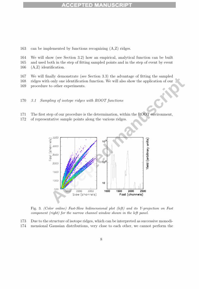
The first step of our procedure is the determination, within the ROOT environment,171of representative sample points along the various ridges.172

Fig. 3. (Color online) Fast-Slow bidimensional plot (left) and its Y-projection on Fastcomponent (right) for the narrow channel window shown in the left panel.

Due to the structure of isotope ridges, which can be interpreted as successive monodi-173mensional Gaussian distributions, very close to each other, we cannot perform the174

8

Accep

ted m

anusc

ript

peak search by using the ROOT function TSpectrum2. Indeed this function is able175to find a 2-dimensional Gaussian peak out of the background, provided that this176peak is at sufficient distance from other 2-dimensional peaks.177

Therefore we used the ROOT method Projection and the TSpectrum Class, to per-178form the peak search firstly along the X (Fig.3) axis, then along the Y axis.179

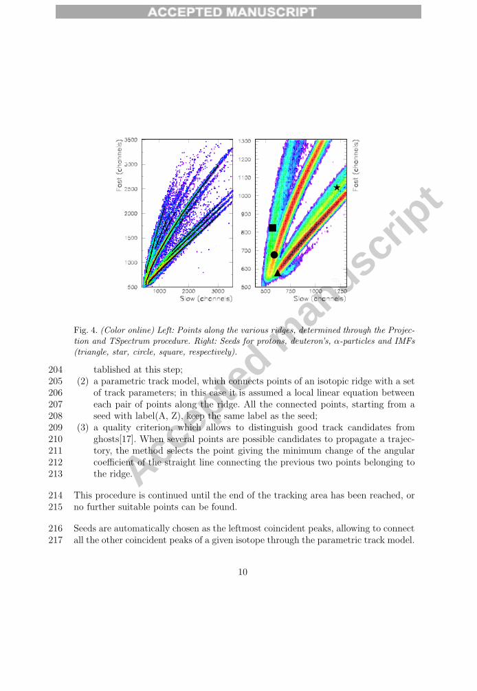
Finally a peak observed on the Y projection is validated only if a peak in the X180projection falls in the same cell of the bidimensional plot. This gives a series of181coincident peaks, lying on the isotope ridges, see left panel of Fig.4.182

The requirement of a validation, obviously leads to obtain coincident peaks in Fast183and Slow regions where isotope ridges are seen as well separated distributions. For184instance, coincident peaks on the deuteron ridge start at Slow≈1000 channels, since185at smaller values the proton, deuteron and Triton ridges merge in only one region186of the bidimensional plot.187

The dimension of the cell has to be chosen in order to have a sufficient statistics to188avoid spurious peaks and to be able to continue the peak search up to the highest189values of the Slow component.190

The error in the determination of the peak position depends on the dimension of the191cell. For the GARFIELD CsI(Tl) crystal, used for tuning the identification procedure192(Fig.2), a minimal statistics of 35 counts has been required and the error has been193estimated to be of the order of 5 channels.194

At this stage coincident peaks falling on the isotope ridges need to be connected195and a (A,Z) label has also to be assigned to each collection of connected peaks, from196now on called a “cluster”.197

To do this, a “tracking” method has been used which automatically connects the198peaks along each (A, Z) ridge.199

“Tracking“ is essentially a local method of pattern recognition[17], here split in three200components:201

(1) a method to generate track seeds (Fig.4 right panel), which are the starting202points for the propagation procedure. The nature (A,Z) of these points is es-203

9

Accep

ted m

anusc

ript

Fig. 4. (Color online) Left: Points along the various ridges, determined through the Projec-tion and TSpectrum procedure. Right: Seeds for protons, deuteron’s, α-particles and IMFs(triangle, star, circle, square, respectively).

tablished at this step;204(2) a parametric track model, which connects points of an isotopic ridge with a set205

of track parameters; in this case it is assumed a local linear equation between206each pair of points along the ridge. All the connected points, starting from a207seed with label(A, Z), keep the same label as the seed;208

(3) a quality criterion, which allows to distinguish good track candidates from209ghosts[17]. When several points are possible candidates to propagate a trajec-210tory, the method selects the point giving the minimum change of the angular211coefficient of the straight line connecting the previous two points belonging to212the ridge.213

This procedure is continued until the end of the tracking area has been reached, or214no further suitable points can be found.215

Seeds are automatically chosen as the leftmost coincident peaks, allowing to connect216all the other coincident peaks of a given isotope through the parametric track model.217

10

Accep

ted m

anusc

ript

More in details, a link from each seed is searched, with the criterion that the second218coincident peak has to be on the right of the seed and with larger Fast component.219These two connected peaks form a segment, which is then extended recursively by220adding coincident peaks linked to the last one. The label (A, Z) of the seeds is221given by the user. In our case Fast and Slow, coming from DSPs, do not contain222offsets and seeds are close to the origin, therefore not sensitive to the variation of223the amplification factors of the considered chain. As a consequence, seeds needed to224be labelled only once, then they resulted valid for all the 180 crystals employed in225our measurements.226

At the end about 2500 coincident peaks were found and labelled in the case of227Fig.4, much more than the number of peaks which can be sampled by “hand-based”228procedures.229

In the next Section we show how to find the parameters characterizing each crystal,230through a fitting procedure and how to perform a (A, Z) event calibration.231

3.2 Empirical analytic function and isotope identification232

We have already stressed in Sect.3 the importance of fitting the points sampled233or tracked on a bidimensional plot with only one analytical function, in order to234generate curves for any isotope (A,Z), even not sampled.235

To build an empirical, but analytical, function, we started from the consideration236that a power law relation can been employed [18] for the total light output (our237Long component) of a crystal as a function of the energy. A power-law was used in238Ref.[18] to calibrate in MeV the light output of the crystal. In this case ions were239already identified in (A, Z) via a ΔE − Eresidual analysis.240

In our case, due to the almost linear correlation between Fast and Long, we expect241a power-law behaviour for both the Fast and the Slow variables as a function of the242energy. This also implies a power-law relationship between the Fast and the Slow.243More details are given in the Appendix.244

A plot of the Fast-Slow correlation in a double logarithmic representation is shown245in Fig.5, for the coincident peaks shown in Fig.4.246

11

Accep

ted m

anusc

ript

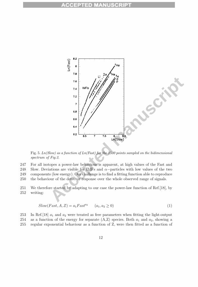
Fig. 5. Ln(Slow) as a function of Ln(Fast) for the 2500 points sampled on the bidimensionalspectrum of Fig.2.

For all isotopes a power-law behaviour is apparent, at high values of the Fast and247Slow. Deviations are visible for IMFs and α−particles with low values of the two248components (low energy). Our challenge is to find a fitting function able to reproduce249the behaviour of the detector response over the whole observed range of signals.250

We therefore started by adapting to our case the power-law function of Ref.[18], by251writing:252

Slow(Fast, A, Z) = a1Fasta2 (a1, a2 ≥ 0) (1)

In Ref.[18] a1 and a2 were treated as free parameters when fitting the light-output253as a function of the energy for separate (A,Z) species. Both a1 and a2, showing a254regular exponential behaviour as a function of Z, were then fitted as a function of255

12

Accep

ted m

anusc

ript

the charge and used for subsequent analyses (see Fig. 8 of Ref.[18]).256

To reach the goal of obtaining only one analytical function for all our observed257isotopic species, we incorporated in Eq. 1 the exponential behaviors of a1 and a2.258We needed also to modify a1 with another term dependent on (A, Z). Therefore our259function will contain 7 fit parameters, instead of the 6 of Ref.[18]:260

a1 = [d1 + d2exp(−d3Zeff)] exp(−d4Zeff)

a2 = [d5 − d6exp(−d7Zeff)] (di ≥ 0, i = 1, 7) (2)

with Zeff = (AZ2)1/3, which represents the most effective way, within our approach,261to take into account the charge and the mass of the analyzed isotope ridges.262

The points belonging to the tracked clusters are fitted by Eq.s 1 and 2 with Mi-263nuit [19] package.264

The fit is performed in two steps:265

(1) The fit is made only on the clusters starting from the seeds shown in Fig.4, i.e.266on protons, deuterons, α-particles and IMFs clusters. At the end of this step,267other clusters are automatically labelled by the program, which estimates the268distance of each coincident point, not yet labelled, from the curve of Eq. 1 for269all the possible (A,Z) values. The shortest distance between the measured co-270incident point and each curve determines the appropriate assignment of (A,Z).271

(2) The fit is now performed on all the labelled clusters, to find the fit parameters272characterizing the crystal under study.273

The resulting total274

χ2 =1

d.o.f.

∑ (Slow − SlowEq1)2

errors2

for the crystal shown in this paper is 1.6 (d.o.f. stands here for the degrees of freedom,275number of the sampled points minus the number of free parameters).276

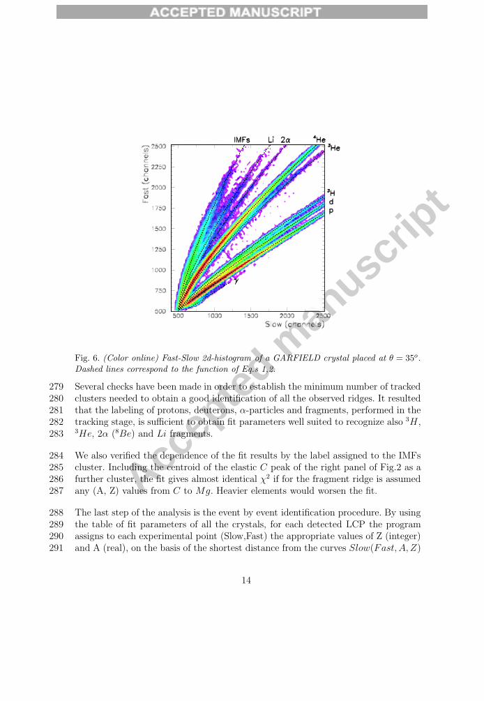
In Fig.6 we show the analytical function (Eq.s 1,2) superimposed to the bidimen-277sional plot of Fig.2.278

13

Accep

ted m

anusc

ript

Fig. 6. (Color online) Fast-Slow 2d-histogram of a GARFIELD crystal placed at θ = 35o.Dashed lines correspond to the function of Eq.s 1,2.

Several checks have been made in order to establish the minimum number of tracked279clusters needed to obtain a good identification of all the observed ridges. It resulted280that the labeling of protons, deuterons, α-particles and fragments, performed in the281tracking stage, is sufficient to obtain fit parameters well suited to recognize also 3H ,2823He, 2α (8Be) and Li fragments.283

We also verified the dependence of the fit results by the label assigned to the IMFs284cluster. Including the centroid of the elastic C peak of the right panel of Fig.2 as a285further cluster, the fit gives almost identical χ2 if for the fragment ridge is assumed286any (A, Z) values from C to Mg. Heavier elements would worsen the fit.287

The last step of the analysis is the event by event identification procedure. By using288the table of fit parameters of all the crystals, for each detected LCP the program289assigns to each experimental point (Slow,Fast) the appropriate values of Z (integer)290and A (real), on the basis of the shortest distance from the curves Slow(Fast, A, Z)291

14

Accep

ted m

anusc

ript

of Eq. 1 calculated for all the possible (A,Z) values. In the event by event identifi-292cation γ and IMFs are only counted and neglected for further analysis.293

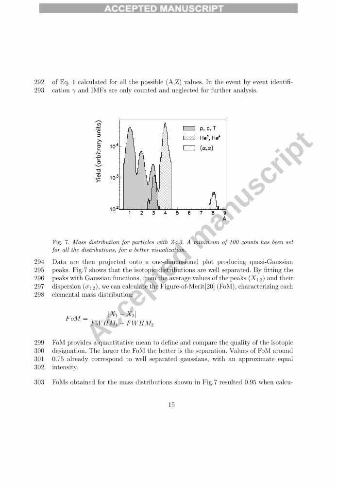
Fig. 7. Mass distribution for particles with Z<3. A minimum of 100 counts has been setfor all the distributions, for a better visualization.

Data are then projected onto a one-dimensional plot producing quasi-Gaussian294peaks. Fig.7 shows that the isotopic distributions are well separated. By fitting the295peaks with Gaussian functions, from the average values of the peaks (X1,2) and their296dispersion (σ1,2), we can calculate the Figure-of-Merit[20] (FoM), characterizing each297elemental mass distribution:298

FoM =|X1 −X2|

FWHM1 + FWHM2

FoM provides a quantitative mean to define and compare the quality of the isotopic299designation. The larger the FoM the better is the separation. Values of FoM around3000.75 already correspond to well separated gaussians, with an approximate equal301intensity.302

FoMs obtained for the mass distributions shown in Fig.7 resulted 0.95 when calcu-303

15

Accep

ted m

anusc

ript

lated for proton-deuteron distributions, 0.97 for deuteron-Triton and 1.0 for Z=2304isotopes. These values imply a contamination for adjacent masses smaller than few305percent.306

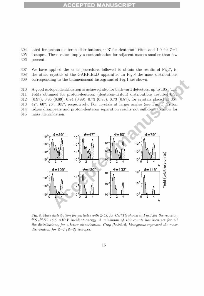
We have applied the same procedure, followed to obtain the results of Fig.7, to307the other crystals of the GARFIELD apparatus. In Fig.8 the mass distributions308corresponding to the bidimensional histograms of Fig.1 are shown.309

A good isotope identification is achieved also for backward detectors, up to 105o. The310FoMs obtained for proton-deuteron (deuteron-Triton) distributions resulted 0.95311(0.97), 0.95 (0.89), 0.84 (0.89), 0.73 (0.83), 0.73 (0.87), for crystals placed at 35o,31247o, 60o, 75o, 105o, respectively. For crystals at larger angles (see Fig. 1) Triton313ridges disappears and proton-deuteron separation results not sufficient to allow for314mass identification.315

Fig. 8. Mass distribution for particles with Z<3, for CsI(Tl) shown in Fig.1,for the reaction32S+58Ni 16.5 AMeV incident energy. A minimum of 100 counts has been set for allthe distributions, for a better visualization. Gray (hatched) histograms represent the massdistribution for Z=1 (Z=2) isotopes.

16

Accep

ted m

anusc

ript

3.3 Stability of calibration throughout several experiments316

The use of an analytical function (Eq.s 1,2) to fit the clusterized ridges gives the pos-317sibility to extend the identification even to low statistics regions, where a sampling318through “hand-based” procedures cannot be performed.319

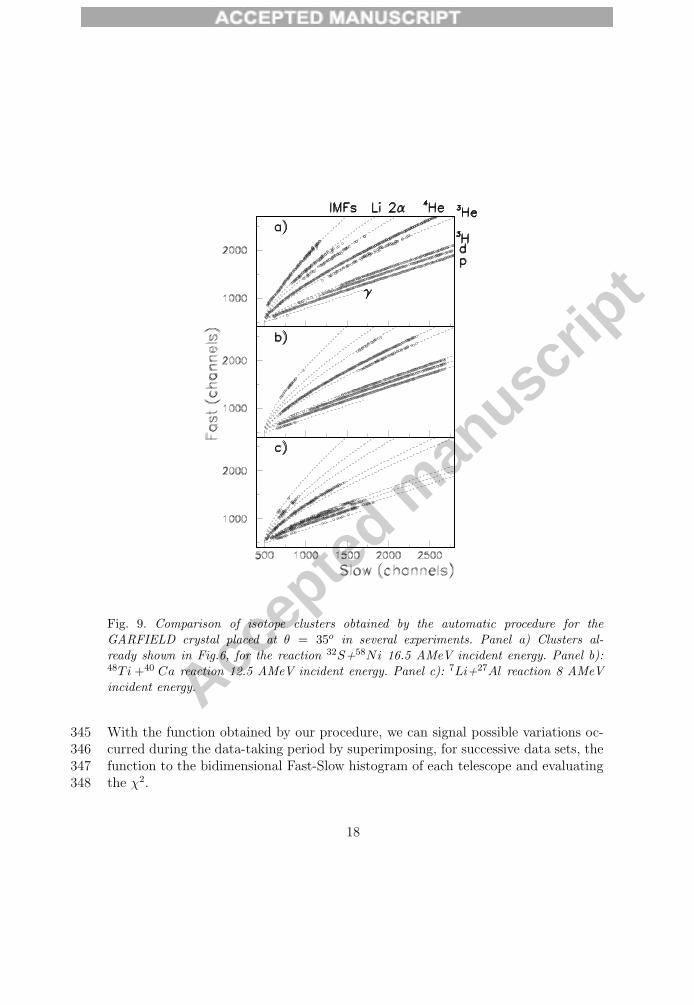
We show in Fig.9 isotope clusters obtained by our automatic procedure, for the320GARFIELD crystal placed at θ = 35o in different experiments.321

Three reactions are considered:322

• 32S+58Ni 16.5 AMeV incident energy (panel a)),323• 48T i +40 Ca 12.5 AMeV incident energy (panel b)),324• 7Li+27Al 8 AMeV incident energy (panel c)).325

Fast and Slow in these experiments have been normalized through pulser runs. Lines326correspond to the function of Eq.s 1,2 calculated in all cases with the parameters327obtained by fitting the 32S+58Ni clusters (see Fig. 6).328

From Fig.9 and from the fact that we have checked our procedure by taking the same329statistics for the three reactions, it appears that the production of some isotopes330depends on the measured reactions. For instance the isotope clusters labelled as 2α,331originated by 8Be decay, is present in higher energy reaction, but not for the Li332induced reaction. The same holds for 3He clusters, present in the panels a) and b)333of Fig. 9 and absent in the panel c).334

This demonstrates that if (A, Z) identification would have been performed with335graphical cuts or other “hand-based” procedures, for a reaction not producing some336isotopes (3He, for instance), further samplings would have been needed for experi-337ments at higher incident energy, or with larger neutron contents of the two partners338of the reaction.339

Another useful consequence of using an analytic function (like Eq.s 1,2) and a table340of fit parameters for all the crystals is the possibility to check the data for drifts of341the response of each detector. The use of a precision pulser, of course, is the main342tool to reveal and correct for the electronics instabilities but it does not detect other343effects connected to the behavior of the detectors (like aging or temperature effects).344

17

Accep

ted m

anusc

ript

Fig. 9. Comparison of isotope clusters obtained by the automatic procedure for theGARFIELD crystal placed at θ = 35o in several experiments. Panel a) Clusters al-ready shown in Fig.6, for the reaction 32S+58Ni 16.5 AMeV incident energy. Panel b):48T i +40 Ca reaction 12.5 AMeV incident energy. Panel c): 7Li+27Al reaction 8 AMeVincident energy.

With the function obtained by our procedure, we can signal possible variations oc-345curred during the data-taking period by superimposing, for successive data sets, the346function to the bidimensional Fast-Slow histogram of each telescope and evaluating347the χ2.348

18

Accep

ted m

anusc

ript

4 Conclusions349

The advantages obtained with the automatic calibration procedure presented in this350paper may be summarized in the following points.351

• The time dedicated to offline calibration is greatly reduced. Indeed the time needed352with our procedure to automatically sample, label, fit more than 2500 points and353to identify in (A,Z) some hundred thousands of events is about 2 minutes. On354the contrary, by using “hand-based” procedures, at least 10 minutes are needed355to only sample some tens of points on the isotope ridges. Saving a lot of time is356particularly important, especially in experiments involving many telescopes.357

• The use of an analytical form of the Fast-Slow correlation Eq. 1 makes it possible358the extrapolation to A-regions where graphical cuts are not easy to make, due to359low statistics.360

• Possible drifts of the crystal response can be diagnosed by controlling the con-361stancy of the parameters, characterizing the individual response of each telescope,362during the sequence of runs throughout a whole experiment.363

• The method ensures fast, standardized and reliable mass and charge identification364for multi-telescope systems.365

The procedure described in this paper can be extended to higher incident energies,366where the number of isotopes to be identified increases.367

In particular the method has been tested with Fast-Slow plots obtained in a recent368FAZIA experiment at LNS (July-November ’09,[3]), where particle identification up369to Z∼5 was available, providing good performances [23].370

5 Acknowledgments371

The authors wish to thank R. Cavaletti, A. Paolucci, G. Tobia for the technical372support during the experiment and S. Sambi for the help in the data analysis.373

The authors also wish to thank the accelerator staff of the Tandem-Alpi complex of374LNL (Laboratori Nazionali di Legnaro) for having provided high quality beams.375

19

Accep

ted m

anusc

ript

This work was supported in part by grants of Alma Mater Studiorum (Bologna376University).377

6 Appendix378

To justify the assumption that Fast and Slow are linked by a power-law relationship,379as assumed in Sect. 3.2, we have firstly to perform an energy calibration of the Long380component and then show that both our Fast and Slow keep the memory of a power-381law behaviour as a function of the energy. It has indeed been observed that light382output signals, collected through photomultipliers [21] or photodiodes [18], even383if partially integrated, follow a light-energy power-law relation in a wide range of384particle energies, Z and A.385

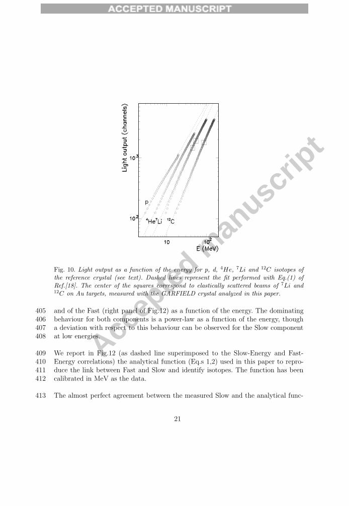
In Fig.10 we show the light-output response of a crystal (under beam in previous386experiments and used here as reference crystal) calibrated in (A, Z, E) through a387ΔE − E technique. ΔE is the energy lost by isotopes in a 300μm Silicon detec-388tor [22] and E is the residual energy in the CsI(Tl). By using energy-loss tables, the389calibrated ΔE scale allows to calculate the energy deposited in the crystal for each390particle. Thereby the light (channels)-energy (MeV) correlation is established. The391dashed lines of Fig.10 represent the fit performed with Eq. (1) of Ref.[18].392

We show in Fig. 10 only few isotopes, representative of those observed with Fast-393Slow technique in this paper. For a more complete discussion of the light-output394calibration from protons to 58Ni see Ref [14].395

The center of the squares in Fig.10 correspond to elastically scattered beams of 7Li396and 12C on Au targets, used to normalize the Long component of the GARFIELD397crystal analyzed in this paper to the light-output of the reference crystal.398

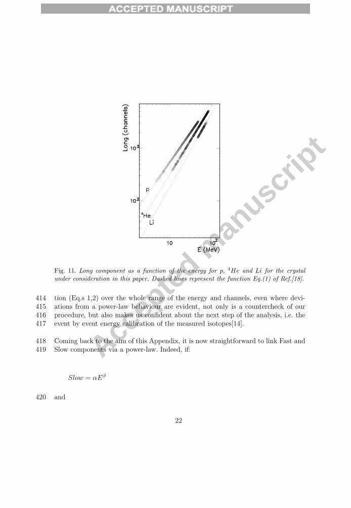
As a check of the normalization procedure over the whole range of energy for the399selected isotopes, we show in Fig. 11 the correlation Long-Energy for p, 4He and Li400clusters of Fig.5, for the crystal under consideration in this paper. The dashed line401is the function used to fit isotopes of the reference crystal, simply superimposed to402the clusters.403

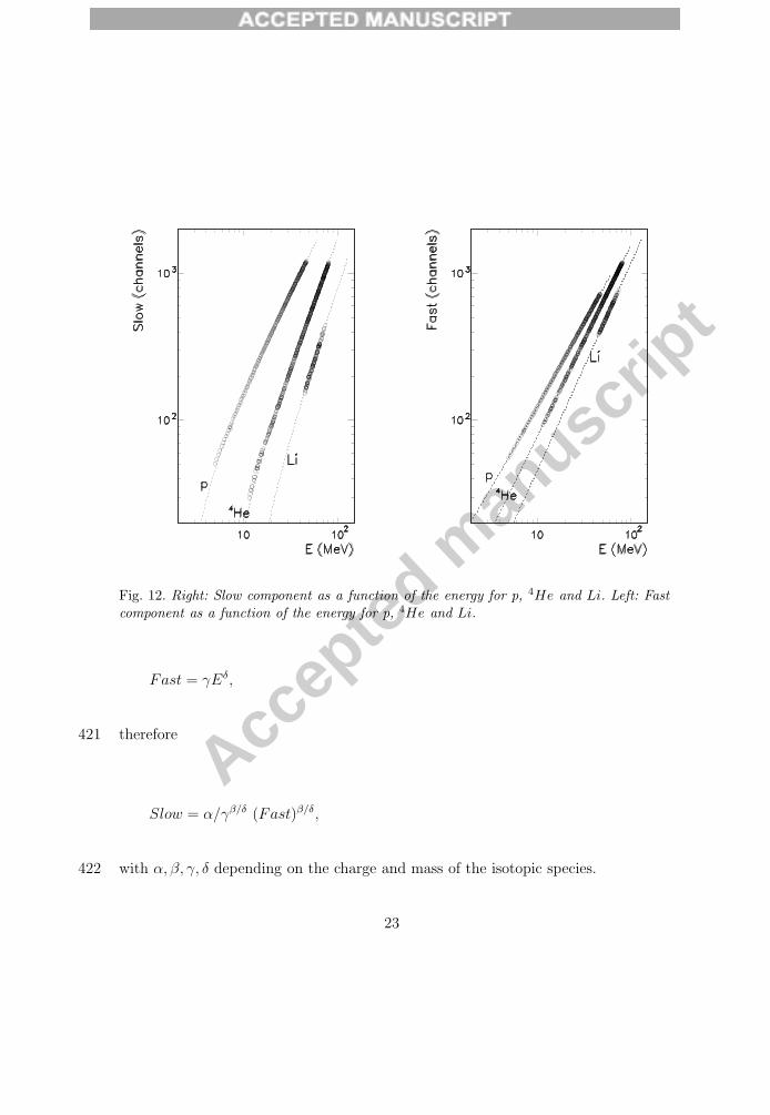
For the same clusters we can now test the behaviour of the Slow (left panel of Fig.12)404

20

Accep

ted m

anusc

ript

Fig. 10. Light output as a function of the energy for p, d, 4He, 7Li and 12C isotopes ofthe reference crystal (see text). Dashed lines represent the fit performed with Eq.(1) ofRef.[18]. The center of the squares correspond to elastically scattered beams of 7Li and12C on Au targets, measured with the GARFIELD crystal analyzed in this paper.

and of the Fast (right panel of Fig.12) as a function of the energy. The dominating405behaviour for both components is a power-law as a function of the energy, though406a deviation with respect to this behaviour can be observed for the Slow component407at low energies.408

We report in Fig.12 (as dashed line superimposed to the Slow-Energy and Fast-409Energy correlations) the analytical function (Eq.s 1,2) used in this paper to repro-410duce the link between Fast and Slow and identify isotopes. The function has been411calibrated in MeV as the data.412

The almost perfect agreement between the measured Slow and the analytical func-413

21

Accep

ted m

anusc

ript

Fig. 11. Long component as a function of the energy for p, 4He and Li for the crystalunder consideration in this paper. Dashed lines represent the function Eq.(1) of Ref.[18].

tion (Eq.s 1,2) over the whole range of the energy and channels, even where devi-414ations from a power-law behaviour are evident, not only is a countercheck of our415procedure, but also makes us confident about the next step of the analysis, i.e. the416event by event energy calibration of the measured isotopes[14].417

Coming back to the aim of this Appendix, it is now straightforward to link Fast and418Slow components via a power-law. Indeed, if:419

Slow = αEβ

and420

22

Accep

ted m

anusc

ript

Fig. 12. Right: Slow component as a function of the energy for p, 4He and Li. Left: Fastcomponent as a function of the energy for p, 4He and Li.

Fast = γEδ,

therefore421

Slow = α/γβ/δ (Fast)β/δ,

with α, β, γ, δ depending on the charge and mass of the isotopic species.422

23

Accep

ted m

anusc

ript

References423

[1] see for instance:424U. Lynen et al. Gesellschaft fur Schwerionenforschung Report n. GSI-02-89;425R. T. de Souza et al. Nucl. Instr. and Meth. A295 (1990) 109;426I. Iori et al. Nucl. Instr. and Meth. A325 (1993) 458;427J. Pouthas et al. Nucl. Instr. and Meth. A357 (1995) 418;428S. Aiello et al. Nucl. Phys. A583 (1995) 461;429B. Davin et al. Nucl. Instr. and Meth. A473 (2001) 302;430M. S. Wallace et al. Nucl. Instr. and Meth. A583 (2007) 302;431S. Wuenschel et al. Nucl. Instr. and Meth. A604 (2009) 578.432

[2] F. Gramegna et al., Nucl. Instr. And Meth. A389 (1997) 474; F. Gramegna et al.,4332004 IEEE Nucl. Science Symposium, Rome, 16-22 October 2004.434

[3] FAZIA collaboration, web site http://fazia.in2p3.fr/435

[4] http://indra.in2p3.fr/KaliVedaDoc/436

[5] L. Tassan-Got Nucl. Instr. and Meth. B194(2002) 503;437N. Le Neindre et al. Nucl. Instr. and Meth. A490 (2002) 251.438

[6] P. F. Mastinu, P. M. Milazzo, M. Bruno, M. D’Agostino, L. Manduci, Nucl. Instr.439and Meth. A338 (1994) 419 and Erratum: Nucl. Instr. and Meth. A343 (1994) 663.440

[7] N. Colonna et al. Nucl. Instr. and Meth. A321 (1992) 529.441

[8] L. Bardelli et al., Nucl. Instr. and Meth. A491 (2002) 244; Nucl. Phys. A746 (2004)442272; Nucl. Instr. And Meth. A560 (2006) 517.443

[9] G. Pasquali et al. Nucl. Instr. And Meth. A570 (2007) 126.444

[10] L. Bardelli “A ROOT-based data-monitor software for the GARFIELD experiment”,445LNL 2007 Annual Report, LNL-INFN(REP)-207/2007446

[11] http://root.cern.ch/447

[12] http://www.bo.infn.it/nucl-ex/448

[13] F. Tonetto et al. Nucl. Instr. and Meth. A420 (1999) 181;449U. Abbondanno, et al., Nucl. Instr. and Meth. A488 (2002) 604.450

[14] G. Casini, et al., LNL 2004 Annual Report, LNL-INFN(REP)-204/2005 ISBN 88-4517337-008-X, pp. 212-214; Nucl. Instr. and Meth., to be submitted.452

24

Accep

ted m

anusc

ript

[15] F. Benrachi et al. Nucl. Instr. and Meth. A281 (1989) 137.453

[16] R. Wada et al. Phys.Rev.C69 (2004) 044610.454

[17] R. Mankel Pattern recognition and Event Reconstruction in Particle Physics455Experiments, arXiv:physics/0402039v1 (2004).456

[18] V. Avdeichikov et al., Nucl. Instr. and Meth. A466 (2001) 427.457

[19] MINUIT D506 routine from the CERN Program Library.458

[20] R. A. Winyard et al., Nucl. Instr. and Meth. 95 (1971) 141.459

[21] V. Avdeichikov et al., Nucl. Instr. and Meth. A501 (2003) 505-513.460

[22] A. Moroni et al., Nucl. Instr. and Meth. A556 (2006) 516.461

[23] FAZIA collaboration, private communication and to be published.462

25