Pattern Recognition 42 (2009) 1041 -- 1051

Contents lists available at ScienceDirect

Pattern Recognition

journal homepage: www.e lsev ier .com/ locate /pr

Automatic analysis of 3D lowdose CT images for early diagnosis of lung cancer

A. El-Baza,∗, G. Gimel'farbb, R. Falkc, M. Abo El-GhardaBioengineering Department, University of Louisville, Louisville, KY, USAbComputer Science Department, University of Auckland, New ZealandcDirector Medical Imaging Division, Jewish Hospital, Louisville, Kentucky, USAdUrology and Nephrology Department, University of Mansoura, Mansoura, Egypt

A R T I C L E I N F O A B S T R A C T

Article history:Received 5 December 2007Received in revised form 12 June 2008Accepted 4 August 2008

Keywords:Computed tomographyGrowth rate estimationGlobal registrationLocal registrationSegmentationPulmonary nodulesEarly diagnosisLung cancer

Our long term research goal is to develop a fully automated, image-based diagnostic system for earlydiagnosis of pulmonary nodules that may lead to lung cancer. This paper focuses on monitoring the de-velopment of lung nodules detected in successive chest low dose (LD) CT scans of a patient. We proposea new methodology for 3D LDCT data registration which is non-rigid and involves two steps: (i) globaltarget-to-prototype alignment of one scan to another using the learned prior appearance model followedby (ii) local alignment in order to correct for intricate relative deformations. After equalizing signals fortwo subsequent chest scans, visual appearance of these chest images is described using a Markov–Gibbsrandom field (MGRF) model with multiple pairwise interaction. An affine transformation that globallyregisters a target to a prototype is estimated by the gradient ascent-based maximization of a specialGibbs energy function. To get an accurate visual appearance model, we developed a new approach toautomatic selection of most characteristic second-order cliques that describe pairwise interactions inthe LDCT data. To handle local deformations, we displace each voxel of the target over evolving closedequi-spaced surfaces (iso-surfaces) to closely match the prototype. The evolution of the iso-surfaces isguided by a speed function in the directions that minimize distances between the corresponding voxelpairs on the iso-surfaces in both the data sets. Preliminary results on the 135 LDCT data sets from 27patients show that the proposed accurate registration could lead to precise diagnosis and identificationof the development of the detected pulmonary nodules.

© 2008 Elsevier Ltd. All rights reserved.

1. Introduction

Because lung cancer is the most common cause of cancer deaths,fast and accurate analysis of pulmonary nodules is of major im-portance for medical computer-aided diagnostic (CAD) systems.We have already introduced the following three fully automaticsuccessive pre-processing stages of such a system for monitoringpulmonary nodules: (i) a segmentation algorithm to separate lungregions from low dose (LD) CT images [1,2]; (ii) a nodule detectionalgorithm showing the accuracy up to 93.3% on the experimentaldatabase containing 200 real LDCT chest data sets with 36,000 2Dslices [3], and (iii) an accurate segmentation algorithm to separatethe detected pulmonary nodules from the lung regions in the LDCTimages [4,5]. This paper details the fourth stage, namely, an accu-rate registration of the detected nodules for subsequent volumetricmeasurements in order to monitor how the nodules are developingover the time.

∗ Corresponding author. Tel.: +15028525092; fax: +15028521577.E-mail address: aselba01@louisville.edu (A. El-Baz).

0031-3203/$ - see front matter © 2008 Elsevier Ltd. All rights reserved.doi:10.1016/j.patcog.2008.08.015

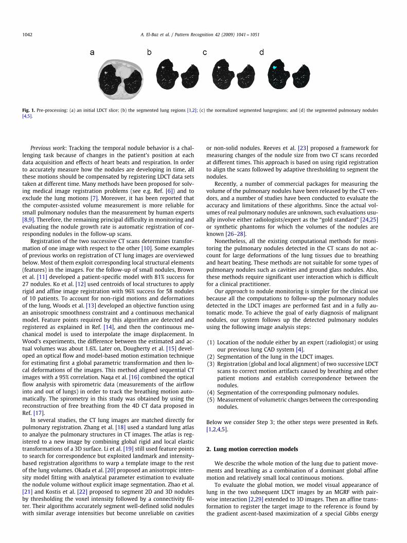
Fig. 1 illustrates the above three pre-processing stages ofthe proposed CAD system that are not discussed in this paper. Aninitial LDCT slice in Fig. 1(a) is segmented with the algorithms inRefs. [1,2] in order to isolate lung tissues from the surroundingstructures in the chest cavity as shown in Fig. 1(b). Then the isolatedregions are normalized (see Section 2.1.1 for more detail) as shownin Fig. 1(c), and the nodules in the normalized regions are segmented[4,5] by evolving deformable boundaries under forces that dependon the learned current and prior appearance models as shown inFig. 1(d).1 This paper describes global and local registration modelsbeing the core of the proposed approach to monitoring the noduledevelopment.

1 At Step (i) each LDCT slice is modelled as a bi-modal sample from a simpleMarkov–Gibbs random field (MGRF) of interdependent region labels and condition-ally independent voxel intensities (gray levels). This step is necessary for moreaccurate separation of nodules from the lung tissues at Step (iii) because voxels ofboth the nodules and other chest structures around the lungs have quite similarintensities.

1042 A. El-Baz et al. / Pattern Recognition 42 (2009) 1041 -- 1051

Fig. 1. Pre-processing: (a) an initial LDCT slice; (b) the segmented lung regions [1,2]; (c) the normalized segmented lungregions; and (d) the segmented pulmonary nodules[4,5].

Previous work: Tracking the temporal nodule behavior is a chal-lenging task because of changes in the patient's position at eachdata acquisition and effects of heart beats and respiration. In orderto accurately measure how the nodules are developing in time, allthese motions should be compensated by registering LDCT data setstaken at different time. Many methods have been proposed for solv-ing medical image registration problems (see e.g. Ref. [6]) and toexclude the lung motions [7]. Moreover, it has been reported thatthe computer-assisted volume measurement is more reliable forsmall pulmonary nodules than the measurement by human experts[8,9]. Therefore, the remaining principal difficulty in monitoring andevaluating the nodule growth rate is automatic registration of cor-responding nodules in the follow-up scans.

Registration of the two successive CT scans determines transfor-mation of one image with respect to the other [10]. Some examplesof previous works on registration of CT lung images are overviewedbelow. Most of them exploit corresponding local structural elements(features) in the images. For the follow-up of small nodules, Brownet al. [11] developed a patient-specific model with 81% success for27 nodules. Ko et al. [12] used centroids of local structures to applyrigid and affine image registration with 96% success for 58 nodulesof 10 patients. To account for non-rigid motions and deformationsof the lung, Woods et al. [13] developed an objective function usingan anisotropic smoothness constraint and a continuous mechanicalmodel. Feature points required by this algorithm are detected andregistered as explained in Ref. [14], and then the continuous me-chanical model is used to interpolate the image displacement. InWood's experiments, the difference between the estimated and ac-tual volumes was about 1.6%. Later on, Dougherty et al. [15] devel-oped an optical flow and model-based motion estimation techniquefor estimating first a global parametric transformation and then lo-cal deformations of the images. This method aligned sequential CTimages with a 95% correlation. Naqa et al. [16] combined the opticalflow analysis with spirometric data (measurements of the airflowinto and out of lungs) in order to track the breathing motion auto-matically. The spirometry in this study was obtained by using thereconstruction of free breathing from the 4D CT data proposed inRef. [17].

In several studies, the CT lung images are matched directly forpulmonary registration. Zhang et al. [18] used a standard lung atlasto analyze the pulmonary structures in CT images. The atlas is reg-istered to a new image by combining global rigid and local elastictransformations of a 3D surface. Li et al. [19] still used feature pointsto search for correspondence but exploited landmark and intensity-based registration algorithms to warp a template image to the restof the lung volumes. Okada et al. [20] proposed an anisotropic inten-sity model fitting with analytical parameter estimation to evaluatethe nodule volume without explicit image segmentation. Zhao et al.[21] and Kostis et al. [22] proposed to segment 2D and 3D nodulesby thresholding the voxel intensity followed by a connectivity fil-ter. Their algorithms accurately segment well-defined solid noduleswith similar average intensities but become unreliable on cavities

or non-solid nodules. Reeves et al. [23] proposed a framework formeasuring changes of the nodule size from two CT scans recordedat different times. This approach is based on using rigid registrationto align the scans followed by adaptive thresholding to segment thenodules.

Recently, a number of commercial packages for measuring thevolume of the pulmonary nodules have been released by the CT ven-dors, and a number of studies have been conducted to evaluate theaccuracy and limitations of these algorithms. Since the actual vol-umes of real pulmonary nodules are unknown, such evaluations usu-ally involve either radiologists/expert as the “gold standard” [24,25]or synthetic phantoms for which the volumes of the nodules areknown [26–28].

Nonetheless, all the existing computational methods for moni-toring the pulmonary nodules detected in the CT scans do not ac-count for large deformations of the lung tissues due to breathingand heart beating. These methods are not suitable for some types ofpulmonary nodules such as cavities and ground glass nodules. Also,these methods require significant user interaction which is difficultfor a clinical practitioner.

Our approach to nodule monitoring is simpler for the clinical usebecause all the computations to follow-up the pulmonary nodulesdetected in the LDCT images are performed fast and in a fully au-tomatic mode. To achieve the goal of early diagnosis of malignantnodules, our system follows up the detected pulmonary nodulesusing the following image analysis steps:

(1) Location of the nodule either by an expert (radiologist) or usingour previous lung CAD system [4].

(2) Segmentation of the lung in the LDCT images.(3) Registration (global and local alignment) of two successive LDCT

scans to correct motion artifacts caused by breathing and otherpatient motions and establish correspondence between thenodules.

(4) Segmentation of the corresponding pulmonary nodules.(5) Measurement of volumetric changes between the corresponding

nodules.

Below we consider Step 3; the other steps were presented in Refs.[1,2,4,5].

2. Lung motion correction models

We describe the whole motion of the lung due to patient move-ments and breathing as a combination of a dominant global affinemotion and relatively small local continuous motions.

To evaluate the global motion, we model visual appearance oflung in the two subsequent LDCT images by an MGRF with pair-wise interaction [2,29] extended to 3D images. Then an affine trans-formation to register the target image to the reference is found bythe gradient ascent-based maximization of a special Gibbs energy

A. El-Baz et al. / Pattern Recognition 42 (2009) 1041 -- 1051 1043

function. To model accurately visual appearance of the LDCT imagesof lungs, we developed a more effective than in Ref. [29] method foran automatic selection of most characteristic pairwise interactions.

Local deformations are handled with a new approach based ondeforming each voxel over evolving closed iso-surfaces (equi-spaced

Fig. 2. Pairwise voxel interactions system.

Fig. 3. (a) Two cross-sections in the 3D relative interaction Gibbs energies and (b) the 2D cross-section of the relative interaction Gibbs energies at the plane � = 0.

surfaces) in such a way as to closely match a prototype (i.e. a refer-ence lung object). A speed function guides the evolution of the iso-surfaces to minimize distances between the corresponding voxelspairs on the iso-surfaces on both the images.

2.1. Global alignment

Basic notation:

• Q = {0, . . . ,Q − 1}—a finite set of scalar image signals (e.g. graylevels).

• R = [(x, y, z) : x = 0, . . . ,X − 1; y = 0, . . . ,Y − 1; z = 0, . . . , Z − 1]—a 3Darithmetic lattice supporting digital LDCT image data g : R → Q.

• Rp ⊂ R—an arbitrary-shaped part of the lattice occupied by aprototype.

• N = {(�1,�1, �1), . . . , (�n,�n, �n)}—a finite set of (x, y, z)-coordinateoffsets defining neighboring voxels, or neighbors {((x + �, y + �,z+ �), (x−�, y−�, z− �)) : (�,�, �) ∈ N} ∧Rp interacting with eachvoxel (x, y, z) ∈ Rp.

• T—an indicator of vector or matrix transposition.

1044 A. El-Baz et al. / Pattern Recognition 42 (2009) 1041 -- 1051

0

0.05

0.1

0.15

0.2

0.25femp(E)

P2(E)

0

−0.05

0.05DeviationAbsolute Deviation

0 10 20 30 40 50Energy

0 10 20 30 40 50Energy

0 10 20 30 40 50Energy

0 10 20 30 40 50Energy

0

0.05

0.1

0.15

0.2

0.25

0

0.05

0.1

0.15

0.2

0.25

t = 28

0 10 20 30 40 50Energy

0 10 20 30 40 50Energy

0

0.05

0.1

0.15

0.2

0.25

0

−0.2

−0.1

0.1

0.2

0.3

Fig. 4. Empirical energy distribution femp(E) and the estimated mixture of two dominant Gaussians P2(E) representing the low- and high-energy distributions (a); thesign-alternate and absolute deviations between the femp(E) and P2(E) (b); the mixture model estimated the absolute deviations (c); the resulting positive and negativecomponents of the LCDG (d); the final LCDG (e) that approximates the empirical distribution, and the two estimated weighed energy distributions �Plo(E) and (1−�)Phi(E) (f).

The set N yields a 3D neighborhood graph on Rp describing trans-lation invariant pairwise interactions between the voxels with |N|families C�,�,� of the second-order cliques c�,�,�(x, y, z)= ((x, y, z), (x+�, y+�, z+ �)) shown in Fig. 2. Quantitative interaction strengths forthe clique families are given by a vector VT=[VT

�,�,� : (�,�, �) ∈ N] of

potentials VT�,�,� = [V�,�,�(q, q′) : (q, q′) ∈ Q2] being functions of signal

co-occurrences in the cliques.

2.1.1. Data normalizationTo account for possible monotone (order-preserving) changes of

signals, e.g. due to different sensor characteristics, every LDCT dataset is equalized using the cumulative empirical probability distribu-tion of its signals [35].

2.1.2. MGRF-based appearance modelThe main idea of learning the appearance model using an MGRF

is to find the neighborhood system (i.e. the subsets of voxels which

have strong relations with each current voxel) and to estimate theinteraction between each two voxels in this neighborhood system(see Fig. 2).

In a generic MGRF with multiple pairwise interaction in Fig. 2[2,29], the Gibbs probability P(g) ∝ exp(E(g)) of an object g alignedwith the prototype g0 on Rp is specified with the Gibbs energy E(g)=|Rp|VTF(g). Here,

• FT(g) is the vector of scaled empirical probability distri-butions of signal co-occurrences over each clique family:FT(g) = [��,�,�F

T�,�,�(g) : (�,�, �) ∈ N];

• ��,�,� = |C�,�,�|/|Rp| is the relative size of the family C�,�,�, and• F�,�,�(g) is the vector of empirical probabilities for this family:

F�,�,�(g) = [f�,�,�(q, q′|g) : (q, q′) ∈ Q2]T where

◦ f�,�,�(q, q′|g) = |C�,�,�;q,q′ (g)|/|C�,�,�| are empirical signal co-occurrence probabilities and

A. El-Baz et al. / Pattern Recognition 42 (2009) 1041 -- 1051 1045

Fig. 5. The 3D neighborhood system (a) estimated for the lung tissues; its 2Dcross-section in the plane � = 0 (b; in white) and its superposition onto the lungsreconstructed from the LDCT images (c).

Fig. 6. 3D voxelwise Gibbs energies projected onto the 2D axial, coronal, and saggital planes for visualization: 2D slices of the original LDCT images (a), the voxelwise Gibbsenergies for |N| = 275 (b) and |N| = 3927 (c).

◦ C�,�,�;q,q′ (g) ⊆ C�,�,� is a subfamily of the cliques c�,�,�(x, y, z)supporting the co-occurrence (gx,y,z = q, gx+�,y+�,z+� = q′) in g.

The co-occurrence distributions and the Gibbs energy for the objectare determined over Rp, i.e. within the prototype boundary after anobject is affinely aligned with the prototype. To account for the affinetransformation, the initial image is resampled to the back-projectedRp by interpolation.

The appearance model consists of the neighborhood N and thepotential V to be learned from the prototype. Below we will showhow to estimateN and V for the lung tissues from the LDCT images.

Learning the potentials: In the first approximation, the maximumlikelihood estimate (MLE) of V is proportional to the scaled andcentered empirical co-occurrence distributions for the prototype[2,29]:

V�,�,� = ���,�,�

(F�,�,�(g

0) − 1Q2U

), (�,�, �) ∈ N

where U is the vector with unit components. The common scalingfactor � is also computed analytically; it is approximately equal toQ2 if Q?1 and ��,�,� ≈ 1 for all (�,�, �) ∈ N. In our case it can be setto � = 1 because the registration uses only relative potential valuesand energies.

Learning the characteristic neighbors: To find the character-istic neighborhood set N, the relative energies E�,�,�(g0) =��,�,�V

T�,�,�F�,�,�(g0), i.e. the scaled variances of the corresponding

empirical co-occurrence distributions for the clique families, arecompared for a large number of possible candidates. For illustration,

1046 A. El-Baz et al. / Pattern Recognition 42 (2009) 1041 -- 1051

Fig. 7. Marginal distributions Plo and Phi estimated using the mixture of two positive Gaussians (the resulting threshold � = 16 produces the neighborhood of the size of|N| = 3927).

Fig. 8. Initialization of the proposed global registration algorithm projected ontothe 2D axial, coronal, and saggital planes for visualization.

Fig. 3(a) shows 2D axial and saggital cross-sections of the estimatedrelative 3D Gibbs energies E�,�,�(g0), and Fig. 3(b) shows the 2D axialcross-section of these energies for 5100 clique families with theinter-voxel offsets |�|�50; 0���50 and � = 0.

To automatically select the characteristic neighbors, we con-sider an empirical probability distribution of the energies as amixture of a large “non-characteristic” low-energy componentand a considerably smaller characteristic high-energy component:P(E) = �Plo(E) + (1 − �)Phi(E). The components Plo(E) and Phi(E) areof arbitrary shape and thus are approximated with linear combi-nations of positive and negative discrete Gaussians (LCDG) usingefficient expectation–maximization-based algorithms introduced inRefs. [1,2] (the latter estimate both the components and the prior �).Fig. 4 shows the approximation steps for these algorithms. Theintersection of the estimated mixture components gives an energythreshold � for selecting the characteristic neighbors: N = {(�,�) :E�,�(g0)��} where Phi(�)�Plo(�)�/(1 − �). The above example re-sults in the threshold � = 28 producing 275 characteristic neighborsshown in Fig. 5. Fig. 6 presents the relative 3D voxelwise Gibbsenergies ex,y,z(g0) for this system:

ex,y,z(g0) =∑

(�,�,�)∈NV�,�,�(g

0x,y,z, g

0x+�,y+�,z+�)

The advantages of using the LCDG model to estimate the neighbor-hood system are highlighted by approximating the same empiricaldistribution with a conventional mixture of two positive Gaussians(see Fig. 7). In this case the resulting neighborhood system is toolarge (3927 voxels) to capture only the features of the lung tissuesand thus relates also to some parts of the background. As a result,the voxels-wise Gibbs energies for |N| = 3927 in Fig. 6(c) are notsmooth that significantly affects the quality of global registration.

2.1.3. Appearance-based registrationThe desired affine transformation of an object g corresponds to

a local maximum of its relative energy E(ga) = VTF(ga) under thelearned appearance model [N,V]. Here, ga is the part of the object

image reduced to Rp by a 3D affine transformation a= [a11, . . . , a34]:x′=a11x+a12y+a13z+a14; y′=a21x+a22y+a23z+a24; z′=a31x+a32y+a33z + a34. Its initial step is a pure translation (a11 = a22 = a33 = 1;a12 = a13 = a21 = a23 = a31 = a32 = 0) ensuring the most “energetic”overlap between the object and prototype. In otherwords, the choseninitial position (a∗

14, a∗24, a

∗34) in Fig. 8 maximizes the energy. Then the

gradient ascent-based search for the local energy maximum closestto the initialization selects all the 12 parameters a.

We compared our global alignment to three popular conven-tional techniques, namely, to the area-based registration by mu-tual information (MI) [30] or normalized MI (NMI) [31] and to thefeature-based registration that establishes correspondences betweenthe images with 3D scale-invariant feature transform (SIFT) [32].Results of the global alignment of two segmented lungs are shown inFigs. 9 and 10. It is clear from Figs. 9(a) and 10(c and d) that theglobal alignment is not perfect due to local deformation.

To clarify why the MI- or NMI-based alignment is less accurate,Fig. 11 compares the MI/NMI and Gibbs energy values for a se-quence of affine parameters that appear at successive steps of thegradient ascent-based search for the maximum similarity in termsof MI or energy. Both the MI and NMI have many outstanding localmaxima that potentially hinder the search, whereas the energy ismuch smoother and practically unimodal in these experiments. The3D SIFT-based alignment fails because it cannot establish accuratecorrespondences between the similar lung areas.

2.2. Local motion model

To handle local deformations, we deform a target object overevolving closed equi-spaced surfaces (or distance iso-surfaces) sothat it closely matches the prototype. The evolution is guided by aspeed function and intends to minimize distances between corre-sponding voxel pairs on the iso-surfaces in both the images. The con-ventional normalized cross-correlation (NCC) of the voxelwise Gibbsenergies is used to find correspondences between the iso-surfaces.

Our approach involves the following steps. First, a distance mapinside the object is generated using fast marching level sets [33].Second, the distance map is used to generate iso-surfaces (Fig. 12).Note that the number of iso-surfaces is not necessarily the samefor both the images and depends on the accuracy and the speed re-quired by the user. The third step consists in finding correspondencesbetween the iso-surfaces using the NCC:

NCC =∑m

x=1

∑my=1

∑mz=1 (e(g

0xyz) − g0 )(e(gxyz) − g)√∑m

x=1

∑my=1

∑mz=1 (e(g0

xyz) − g0 )2√∑m

x=1

∑my=1

∑mz=1 (e(gxyz) − g)2

where g0 = (1/m3)∑m

x=1∑m

y=1∑m

z=1 e(g0xyz) and g = (1/m3)

∑mx=1∑m

y=1∑m

z=1 e(gxyz). Here, e(gxyz) is the Gibbs energy at site (x, y, z); g0

A. El-Baz et al. / Pattern Recognition 42 (2009) 1041 -- 1051 1047

Fig. 9. Global registration results projected onto the 2D axial (A), coronal (C), and saggital (S) planes for visualization: our (a), MI-based (b), NMI-based (c), and SIFT-based(d) algorithms of 3D global registration.

Fig. 10. 3D global and local registration: (a) the reference data, (b) the target data, (c) the target data after a 3D affine transformation, (d) the checkerboard visualization toshow the motion of lung tissues, (e) our non-rigid registration, and (f) the checkerboard visualization to show the quality of the proposed local deformation model.

is the prototype (reference) image; g is the target image, and m isthe size of the 3D cubic window. Note that all the experiments aredone for m = 3.

Finally, the evolution process deforms the iso-surfaces in the firstdata set (the target image) to match the iso-surfaces in the seconddata set (the prototype).

The following notation is used below for defining the evolutionequation:

• bhg1 = [ph

k : k = 1, . . . ,K]—K control points on a surface h on thereference data such that pk=(xk, yk, zk) form a circularly connectedchain of line segments (p1,p2), . . . , (pK−1,pK ), (pK ,p1);

• bg2 = [p

n : n = 1, . . . ,N]—N control points on a surface on thetarget data such that pn = (xn, yn, zn) form a circularly connectedchain of line segments (p1,p2), . . . , (pN−1,pN), (pN ,p1);

• S(phk ,p

n)—the Euclidean distance between a point on the surface

h in the image g1 and the corresponding point on the surface inthe image g2;

• S(pn,p

−1n )—the Euclidean distance between a point on the surface

in the image g1 and the nearest point on the surface − 1 in g1,and

• �(.)—the propagation speed function.

The evolution b� → b�+1 of a deformable boundary b in discrete time,� = 0, 1, . . . , is specified by the system p

n,�+1 = pn,� + �(p

n,�)un,�; n =1, . . . ,N of difference where �(p

n,�) is a propagation speed function forthe control point p

n,� and un,� is the unit vector along the ray betweenthe two corresponding points. The propagation speed function

�(pn,�) = min{S(ph

k ,pn,�), S(p

n,�,p

−1n,� ), S(p

n,�,p+1n,� )}

satisfies the condition �(pn,�) = 0 if S(ph

k ,pn,�) = 0 and prevents the

current point from cross-passing the closest neighbor surfaces asshown in Fig. 13. The latter restriction is known as the smoothnessconstraint.

1048 A. El-Baz et al. / Pattern Recognition 42 (2009) 1041 -- 1051

Fig. 11. Values of the Gibbs energy, MI, and NMI at the successive steps of thegradient ascent-based search.

Fig. 12. Equi-spaced surfaces: a 2D axial cross-section (a) and 3D illustration (b).

The checkerboard visualization (Fig. 10(d)) of the data set inFig. 10(a) and the aligned data set in Fig. 10(c) highlights the effectof the motion of lung tissues. It can be seen that the connectionsat the lung edges between the two volumes are not smooth whenusing only the global registration model. This is due to the localdeformation which comes from breathing and heart beats. Theconnections of the lung edges between the two volumes becomeconsiderably smoother after using the proposed local deformation(see Fig. 10).

Validation: To validate the proposed local registration, we simu-lated local deformations on the real LDCT data set using the free formdeformation (FFD) approach [34] that simulates local displacementswith 3D cubic splines. To measure the registration accuracy, threedifferent types of the deformation fields, namely, with small, mod-erate, and large deformations indicated in Table 1, were generatedwith the FFD. Our registration model has been applied to each typeof deformation, and the accuracy has been quantitatively assessed bycomparing the simulated and recovered voxel displacements. Fig. 14shows typical results of such comparisons for a set of 162 randomlyselected voxel positions.

Fig. 13. Evolution scenario.

Table 1Registration accuracy for simulated displacements

Simulated displacements

Small Moderate Large

Max/mean/st.d. 1.7/0.6/0.4 10.8/2.3/0.7 19.9/9.1/1.1

Alignment error

Max/mean/st.d. 0.6/0.4/0.3 1.4/1.0/0.4 2.1/1.2/1.6

All units in mm; st.d. denotes the standard deviation.

3. Experimental results

The proposed registration models have been tested on the clini-cal data sets collected from 27 patients. Each patient has five LDCTscans, with the 3-month period between each two successive scans.This preliminary clinical database was collected by the LDCT scanprotocol using a multidetector GE Light Speed Plus scanner (GeneralElectric, Milwuakee, USA) with the following scanning parameters:the slice thickness of 2.5mm reconstructed every 1.5mm; scanningpitch 1.5mm; 140KV; 100MA; and the field-of-view 36cm.

After the two volumes at different time instants are registered,the task is to find out if the nodules are growing or not. For thispurpose, the lung nodules were segmented after registration usingour previous approach [4,5]. Once the nodules are segmented in theoriginal and the registered image sequences, the volumes of the nod-ules are calculated using the voxel resolution value from the scan-ner (in our case, 0.7, 0.7, and 2.5mm, respectively). Fig. 15 showsthe estimated growth rate for the two detected pulmonary nod-ules (for two different patients over one year) before and after dataalignment.

It is clear that our alignment algorithm facilitates accurate eval-uations of temporal changes in the nodule size. Moreover, theproposed alignment might help doctors and radiologists to track thenodule growth direction which is crucial for surgical or radiationtreatment. Also, it is apparent that the malignant nodule doublesin size for 360 or less days, while the volumetric changes in thebenign nodule are very small (maximum 6% over one year, seeFig. 16).

Statistical analysis using the unpaired t-test shows that the dif-ferences in the average growth rate between the malignant and be-nign nodules found with the proposed registration algorithm arestatistically significant at the 95% and higher levels (the p-values in

A. El-Baz et al. / Pattern Recognition 42 (2009) 1041 -- 1051 1049

Fig. 14. Comparing the 162 randomly selected voxel positions for the small (a),moderate (b), and large (c) deformation fields: The ground truth is in blue, and thecorresponding positions found with our method are in red.

Table 2 are considerably below 0.05). At the same time Table 2 showsthat no significant difference is found if the growth rate is measuredwithout the data alignment step (all the p-values are above 0.05).Fig. 16 shows volumetric changes for 14 malignant and 13 benignnodules. It is obvious that the growth rate of the malignant nodulesis considerably higher than the growth rate of the benign nodules,and this encourages to use the estimated growth rate as a discrimi-natory feature.

A traditional Bayesian classifier based on the analysis of thegrowth rate of both benign and malignant nodules for 27 patientsdiagnosed 14 and 13 patients as malignant and benign, respec-tively. For simplicity, this classifier used a multivariate Gaussianmodel of the growth rate with the rates at 3, 6, 9, and 12 monthsas four discriminant features. The same patients were diagnosed by

Fig. 15. Results of our registration for two patients over one year.

Fig. 16. Estimated volumetric changes for 14 malignant and 13 benign nodules.

Table 2Growth rate statistics for 14 patients with malignant nodules and 13 patients withbenign nodules

Scanning period With the proposed registration Without the registration

Malignant Benign p Malignant Benign p

M �M B �B M �M B �B

3 months 22 16 0.9 0.7 �10−4 5.6 4.8 2.8 1.9 0.126 months 49 20 2.9 2.3 �10−4 11 6.6 8.4 5.1 0.319 months 91 29 4.5 3.8 �10−4 24 9.3 17 11 0.0812 months 140 32 5.4 4.3 �10−4 30 11 20 16 0.07

is the mean rate, %; � the standard deviation, %; p the p-value, i.e. the probabilitythat the observed differences between the two types of nodules are purely due tochance.

biopsy (the ground truth) showing that the classification was 100%correct. Therefore, the proposed image analysis techniques could bea promising supplement to the current technologies for diagnosinglung cancer.

1050 A. El-Baz et al. / Pattern Recognition 42 (2009) 1041 -- 1051

4. Conclusions

A new approach for the accurate registration of 3D spiral LDCTimages is introduced. It combines an initial global affine alignmentof one scan (a target) to another scan (a prototype) using the learnedprior appearance model and a subsequent local alignment thataccounts for more intricate continuous deformations. Preliminaryresults on 27 patients showed that the proposed registration couldlead to accurate diagnosis and identification of temporal develop-ment of detected pulmonary nodules. The present C + + imple-mentation on the Intel quad processor (3.2GHz each) with 16GBmemory and 1.5 TB hard drive with the RAID technology takes about330 s for processing 182 LDCT slices of the size of 512 × 512 pixelseach, i.e. about 1.8 s per slice.

Our future work will focus on testing the proposed approachon more diverse data sets. We have already started to collect thedata from additional 200 patients with different types of pulmonarynodules (e.g. ground glass, cavity, etc.), in order to better measurethe accuracy and limitations of the proposed framework. Also, wewill investigate the possibility of adding other geometrical featuresdescribing the shape of malignant and benign nodules in additionto the growth rate to determine whether this will lead to moreaccurate diagnosis than with the current methodology. The proposedframework is suitable not only for 3D LDCT chest images but also forother organs and scanning modalities. In particular, it can be usedto compensate kidney motions in an image-based CAD system forautomatic detection of kidney renal rejection on dynamic-contrast-enhanced MRI images (DCE-MRI) [36].

Acknowledgments

This research work has been supported by Wallace H. CoulterFoundation and the Kentucky Science and Engineering Foundationas per Grant Agreement #KSEF-148-502-08-229 with the KentuckyScience and Technology Corporation.

References

[1] A. Farag, A. El-Baz, G. Gimel'farb, Precise segmentation of multi-modal images,IEEE Trans. Image Process. 15 (4) (2006) 952–968.

[2] A. El-Baz, Novel stochastic models for medical image analysis, Ph.D. Dissertation,University of Louisville, Louisville, KY, USA, 2006, pp. 115–150 (Chapter 5).

[3] A. Farag, A. El-Baz, G. Gimel'farb, Quantitative nodule detection in low dose chestCT scans: new template modeling and evaluation for CAD system design, in:Proceedings of the International Conference on Medical Image Computing andComputer-Assisted Intervention (MICCAI'05), Palm Springs, CA, USA, October26–29, 2005, pp. 720–728.

[4] A. Farag, A. El-Baz, G. Gimel'farb, R. Falk, M. Abou El-Ghar, T. Eldiasty,S. Elshazly, Appearance models for robust segmentation of pulmonary nodulesin 3D LDCT chest images, in: Proceedings of the International Conference onMedical Image Computing and Computer-Assisted Intervention (MICCAI'06),vol. 1, Copenhagen, Denmark, October 1–6, 2006, pp. 662–670.

[5] A. El-Baz, A. Farag, G. Gimel'farb, R. Falk, M. Abou El-Ghar, T. Eldiasty, Aframework for automatic segmentation of lung nodules from low dose chestCT scans, in: Proceedings of the IAPR International Conference on PatternRecognition (ICPR'06), Hong Kong, vol. 3, August 20–24, 2006, pp. 611–614.

[6] J. Maintz, M. Viergever, A survey of medical image registration, J. Med. ImageAnal. 2 (1998) 1–36.

[7] J. Ko, D. Naidich, Computer-aided diagnosis and the evaluation of lung disease,J. Thora. Imaging 19 (3) (2004) 136–155.

[8] W. Kostis, D. Yankelevitz, A. Reeves, S. Fluture, C. Henschke, Small pulmonarynodules: reproducibility of three-dimensional volumetric measurement andestimation of time to follow-up CT, Radiology 231 (2) (2004) 446–452.

[9] R. Maurer, R. Maciunas, J. Fitzpatrick, Registration of head CT images to physicalspace using a weighted combination of points and surfaces, IEEE Trans. Med.Imaging 17 (5) (1998) 753–761.

[10] B. Horn, Closed-form solution of absolute orientation using unit quaternions,J. Opt. Soc. Am. B 4 (4) (1987) 629–642.

[11] M. Brown, M. McNitt-Gray, N. Mankovich, J. Goldin, J. Hiller, L. Wilson,D. Aberle, Method for segmenting chest CT image data using an anatomicalmodel: preliminary results, IEEE Trans. Med. Imaging 16 (6) (1997) 828–839.

[12] J. Ko, M. Betke, Chest CT: automated nodule detection and assessment of changeover time-preliminary experience, Radiology 218 (2001) 267–273.

[13] K. Woods, L. Fan, C. Chen, Y. Wang, Model supported image registration andwarping for change detection in computer-aided diagnosis, Applied ImageryPattern Recognition (AIPR) Annual Workshops, Washington DC, USA, October16–18, 2000, pp. 180–186.

[14] L. Fan, C. Chen, An integrated approach to 3D warping and registration fromlung images, in: Proceedings of the SPIE Conference on Developments in X-RayTomography II, Denver, CO, July 1999, pp. 24–35.

[15] L. Dougherty, J. Asmuth, W. Gefter, Alignment of CT lung volumes with anoptical flow method, Acad. Radiol. 10 (3) (2003) 249–254.

[16] I. Naqa, D. Low, J. Deasy, A. Amini, P. Parikh, M. Nystrom, Automated breathingmotion tracking for 4D computed tomography, Nuclear Science Symposium onConference Record, vol. 5, 2003, pp. 3219–3222.

[17] D. Low, M. Nystrom, E. Kalinin, P. Parikh, J. Dempsey, J. Bradley, S. Mutic,S. Wahab, T. Islam, G. Christensen, D. Politte, B. Whiting, A method for thereconstruction of four-dimensional synchronized CT scans acquired during freebreathing, Med. Phys. 30 (6) (2003) 1254–1263.

[18] L. Zhang, J. Reinhardt, 3D pulmonary CT image registration with a standardlung atlas, in: Proceedings of the SPIE Conference on Medical Imaging, vol.4322, 2000, pp. 67–77.

[19] B. Li, G. Christensen, J. Dill, E. Hoffman, J. Reinhardt, 3-D inter-subject warpingand registration of pulmonary CT images for a human lung model, in:Proceedings of the SPIE Conference on Medical Imaging, San Diego, CA, vol.4683, 2002, pp. 324–335.

[20] K. Okada, D. Comaniciu, A. Krishnan, Robust anisotropic gaussian fitting forvolumetric characterization of pulmonary nodules in multislice CT, IEEE Trans.Med. Imaging 24 (3) (2005) 409–423.

[21] B. Zhao, A. Reeves, D. Yankelevitz, C. Henschke, Two-dimensional multicriterionsegmentation of pulmonary nodules on helical CT images, Med. Phys. 26 (1999)889–895.

[22] W. Kostis, A. Reeves, D. Yankelevitz, C. Henschke, Three-dimensionalsegmentation and growth-rate estimation of small pulmonary nodules in helicalCT images, IEEE Trans. Med. Imaging 22 (2003) 1259–1274.

[23] A. Reeves, A. Chan, D. Yankelevitz, C. Henschke, B. Kressler, W. Kostis, Onmeasuring the change in size of pulmonary nodules, IEEE Trans. Medical Imaging25 (4) (2006) 435–450.

[24] D. Wormanns, G. Kohl, E. Klotz, A. Marheine, F. Beyer, W. Heindel, S. Diederich,Volumetric measurements of pulmonary nodules at multi-row detector CT: invivo reproducibility, Eur. Radiol. 14 (2004) 86–92.

[25] M. Revel, C. Lefort, A. Bissery, M. Bienvenu, L. Aycard, G. Chatellier, G. Frija,Pulmonary nodules: preliminary experience with three-dimensional evaluation,Radiology 231 (2004) 459–466.

[26] J. Goo, T. Tongdee, R. Tongdee, K. Yeo, C. Hildebolt, K. Bae, Volumetricmeasurement of synthetic lung nodules with multi-detector row CT: effectof various image reconstruction parameters and segmentation thresholds onmeasurement accuracy, Radiology 235 (3) (2005) 850–856.

[27] J. Ko, H. Rusinek, E. Jacobs, J. Babb, M. Betke, G. McGuinness, D. Naidich,Small pulmonary nodules: volume measurement at chest CT-phantom study,Radiology 228 (3) (2003) 864–870.

[28] H. Jiang, K. Kelly, Theoretical prediction of lung nodule measurement accuracyunder different acquisition and reconstruction conditions, in: Proceedings of theSPIE (Medical Imaging 2004: Physiology, Function and Structure From MedicalImages), vol. 5369, 2004, pp. 406–412.

[29] G. Gimel'farb, Image Textures and Gibbs Random Fields, Kluwer AcademicPublishers, Dordrecht, 1999.

[30] P. Viola, Alignment by maximization of mutual information, Ph.D. Dissertation,MIT, Cambridge, MA, 1995.

[31] C. Studholme, D. Hill, D. Hawkes, An overlap invariant entropy measure of 3Dmedical image alignment, Pattern Recognition 32 (1999) 71–86.

[32] A. Aly, Local features invariance beyond 2D gray spaces, Ph. D. Dissertation,University of Louisville, Louisville, KY, USA, May 2007.

[33] J. Sethian, Fast marching level set method for monotonically advancing fronts,Proc. Natl. Acad Sci. USA 93 (1996) 1591–1595.

[34] D. Rueckert, L. Sonoda, C. Hayes, D. Hill, M. Leach, D. Hawkes, Nonrigidregistration using freeform deformations: application to breast MR images, IEEETrans. Med. Imaging 18 (8) (1999) 712–721.

[35] R. Gonzalez, R. Woods, Digital Image Processing, Addison-Wesley PublishingCompany, New York, 1992.

[36] A. El-Baz, G. Gimel'farb, M. Abou El-Ghar, New motion correction models forautomatic identification of renal transplant rejection, in: Proceedings of theInternational Conference on Medical Image Computing and Computer-AssistedIntervention (MICCAI'07), Brisbane, Australia, October 29–November 2, 2007,pp. 235–243.

About the Author—AYMAN S. EL-BAZ received the B.Sc. and M.S. degrees in electrical engineering from Mansoura University, Egypt, in 1997 and 2000, respectively. Hereceived the Ph.D. degree in electrical engineering from University of Louisville, Louisville, KY, USA, in July 2006. He joined the Bioengineering Department, Universityof Louisville, Louisville, KY, in August 2006, where he is currently an Assistant Professor of Bioengineering, and where he is the Founder and Director of the BioimagingLaboratory. Dr. El-Baz has a extensive experience in the fields of bioimaging modeling and computer-assisted diagnosis systems. He has developed new techniques foraccurate identification of probability mixtures for segmenting multi-modal images, new probability models and model-based algorithms for recognizing lung nodules and

A. El-Baz et al. / Pattern Recognition 42 (2009) 1041 -- 1051 1051

blood vessels in magnetic resonance and computer tomography imaging systems, and new registration techniques based on multiple second-order signal statistics, all ofwhich have been reported at several international conferences. Dr. El-Baz has extensive experience in automated detection, segmentation, and diagnosis of lung nodulesin LDCT images. His work related to novel image analysis techniques for lung cancer detection and diagnosis have earned him multiple awards including first place atthe annual Research Louisville 2002, 2005, 2006, and 2007 meetings and the “Best Paper Award in Medical Image Processing” from the prestigious ICGST InternationalConference on Graphics, Vision and Image Processing (GVIP-2005). He has authored or coauthored more than 70 technical articles. Dr. El-Baz is a member of Eta Kappa Nu.He is a regular reviewer for a number of technical journals and national agencies.