Earth-Science Reviews 136 (2014) 155–174

Contents lists available at ScienceDirect

Earth-Science Reviews

j ourna l homepage: www.e lsev ie r .com/ locate /earsc i rev

Australian sea levels—Trends, regional variability and influencing factors

Neil J. White a,⁎, Ivan D. Haigh b,c,d, John A. Church a, Terry Koen e, Christopher S. Watson f, Tim R. Pritchard e,Phil J. Watson e, Reed J. Burgette f,g, Kathleen L. McInnes a, Zai-Jin You h, Xuebin Zhang a, Paul Tregoning i

a Centre for Australian Weather and Climate Research and Wealth from Oceans Flagship, CSIRO Marine and Atmospheric Research, Hobart, Tasmania, Australiab Ocean and Earth Science, National Oceanography Centre, University of Southampton, European Way Southampton, UKc School of Civil, Environmental and Mining Engineering, The University of Western Australia, M470, 35 Stirling Highway, Crawley, WA 6009, Australiad Oceans Institute, University of Western Australia, Australiae Office of Environment and Heritage, P.O. Box A290, Sydney South, NSW 1232, Australiaf School of Land and Food, University of Tasmania, Private Bag 76, Hobart, Tasmania 7001, Australiag Department of Geological Sciences, New Mexico State University, Las Cruces, NM 88003, USAh School of Civil Engineering, Ludong University, Yantai, Chinai Research School of Earth Sciences, Australian National University, Canberra, ACT, Australia

⁎ Corresponding author.E-mail addresses: Neil.White@csiro.au (N.J. White), I.D

Christopher.Watson@utas.edu.au (C.S. Watson), Tim.Pritc(R.J. Burgette), Kathleen.Mcinnes@csiro.au (K.L. McInnes)

http://dx.doi.org/10.1016/j.earscirev.2014.05.0110012-8252/Crown Copyright © 2014 Published by Elsevie

a b s t r a c t

a r t i c l e i n f o

Article history:Received 7 October 2013Accepted 17 May 2014Available online 27 May 2014

Keywords:Mean sea levelLand movementsTide gaugesAltimetry dataAustralia

There has been significant progress in describing and understanding global-mean sea-level rise, but the regionaldepartures from this global-mean rise are more poorly described and understood. Here, we present a com-prehensive analysis of Australian sea-level data from the 1880s to the present, including an assessment ofsatellite-altimeter data since 1993. Sea levels around the Australian coast are well sampled from 1966 to thepresent. The first Empirical Orthogonal Function (EOF) of data from 16 sites around the coast explains 69% ofthe variance, and is closely related to the El Niño Southern Oscillation (ENSO), with the strongest influence onthe northern and western coasts. Removing the variability in this EOF correlated with the Southern OscillationIndex reduces the differences in the trends between locations. After the influence of ENSO is removed andallowing for the impact of Glacial Isostatic Adjustment (GIA) and atmospheric pressure effects, Australianmean sea-level trends are close to global-mean trends from 1966 to 2010, including an increase in the rate ofrise in the early 1990s. Since 1993, there is good agreement between trends calculated from tide-gauge recordsand altimetry data, with some notable exceptions, some of which are related to localised vertical-land motions.For the periods 1966 to 2009 and 1993 to 2009, the average trends of relative sea level around the coastlineare 1.4 ± 0.3 mm yr−1 and 4.5 ± 1.3 mm yr−1, which become 1.6 ± 0.2 mm yr−1 and 2.7 ± 0.6 mm yr−1

after removal of the signal correlated with ENSO. After further correcting for GIA and changes in atmosphericpressure, the corresponding trends are 2.1 ± 0.2 mm yr−1 and 3.1 ± 0.6 mm yr−1, comparable with theglobal-average rise over the same periods of 2.0 ± 0.3 mm yr−1 (from tide gauges) and 3.4 ± 0.4 mm yr−1

(from satellite altimeters). Given that past changes in Australian sea level are similar to global-mean changesover the last 45 years, it is likely that future changes over the 21st centurywill be consistent with global changes.A generalised additive model of Australia's two longest records (Fremantle and Sydney) reveals the presence ofboth linear and non-linear long-term sea-level trends, with both records showing larger rates of rise between1920 and 1950, relatively stable mean sea levels between 1960 and 1990 and an increased rate of rise fromthe early 1990s.

Crown Copyright © 2014 Published by Elsevier B.V. This is an open access article under the CC BY license(http://creativecommons.org/licenses/by/3.0/).

Contents

1. Introduction . . . . . . . . . . . . . . . . . . . . . . . . . . . . . . . . . . . . . . . . . . . . . . . . . . . . . . . . . . . . . . 1561.1. Overview . . . . . . . . . . . . . . . . . . . . . . . . . . . . . . . . . . . . . . . . . . . . . . . . . . . . . . . . . . . . 1561.2. Previous analyses . . . . . . . . . . . . . . . . . . . . . . . . . . . . . . . . . . . . . . . . . . . . . . . . . . . . . . . . 156

.Haigh@soton.ac.uk (I.D. Haigh), John.Church@csiro.au (J.A. Church), Terry.Koen@environment.nsw.gov.au (T. Koen),hard@environment.nsw.gov.au (T.R. Pritchard), Phil.Watson@environment.nsw.gov.au (P.J. Watson), burgette@nmsu.edu, b.you@ldu.edu.cn (Z.-J. You), Xuebin.Zhang@csiro.au (X. Zhang), paul.tregoning@anu.edu.au (P. Tregoning).

r B.V. This is an open access article under the CC BY license (http://creativecommons.org/licenses/by/3.0/).

156 N.J. White et al. / Earth-Science Reviews 136 (2014) 155–174

1.3. Aims and structure . . . . . . . . . . . . . . . . . . . . . . . . . . . . . . . . . . . . . . . . . . . . . . . . . . . . . . . 1572. Data sets . . . . . . . . . . . . . . . . . . . . . . . . . . . . . . . . . . . . . . . . . . . . . . . . . . . . . . . . . . . . . . . 157

2.1. Tide-gauge records . . . . . . . . . . . . . . . . . . . . . . . . . . . . . . . . . . . . . . . . . . . . . . . . . . . . . . . 1572.2. Altimeter data . . . . . . . . . . . . . . . . . . . . . . . . . . . . . . . . . . . . . . . . . . . . . . . . . . . . . . . . . . 1582.3. Reference frames and vertical land movements . . . . . . . . . . . . . . . . . . . . . . . . . . . . . . . . . . . . . . . . . . . 1582.4. Climate indices . . . . . . . . . . . . . . . . . . . . . . . . . . . . . . . . . . . . . . . . . . . . . . . . . . . . . . . . . 162

3. Australia-wide sea-level variability and trends . . . . . . . . . . . . . . . . . . . . . . . . . . . . . . . . . . . . . . . . . . . . . . 1623.1. Variability . . . . . . . . . . . . . . . . . . . . . . . . . . . . . . . . . . . . . . . . . . . . . . . . . . . . . . . . . . . . 1633.2. Trends . . . . . . . . . . . . . . . . . . . . . . . . . . . . . . . . . . . . . . . . . . . . . . . . . . . . . . . . . . . . . 164

4. Trends over other periods . . . . . . . . . . . . . . . . . . . . . . . . . . . . . . . . . . . . . . . . . . . . . . . . . . . . . . . . 1664.1. The long records . . . . . . . . . . . . . . . . . . . . . . . . . . . . . . . . . . . . . . . . . . . . . . . . . . . . . . . . . 1664.2. 1993 to 2010—Comparison of satellite altimeter and tide-gauge data . . . . . . . . . . . . . . . . . . . . . . . . . . . . . . . . . 168

5. Discussion . . . . . . . . . . . . . . . . . . . . . . . . . . . . . . . . . . . . . . . . . . . . . . . . . . . . . . . . . . . . . . . 1706. Conclusion . . . . . . . . . . . . . . . . . . . . . . . . . . . . . . . . . . . . . . . . . . . . . . . . . . . . . . . . . . . . . . . 172Acknowledgements . . . . . . . . . . . . . . . . . . . . . . . . . . . . . . . . . . . . . . . . . . . . . . . . . . . . . . . . . . . . . 172Appendix A. Supplementary data . . . . . . . . . . . . . . . . . . . . . . . . . . . . . . . . . . . . . . . . . . . . . . . . . . . . . . 172References . . . . . . . . . . . . . . . . . . . . . . . . . . . . . . . . . . . . . . . . . . . . . . . . . . . . . . . . . . . . . . . . . 172

1. Introduction

1.1. Overview

Sea-level change has becomeamajor global scientific issue involvinga wide range of disciplines (Church et al., 2010) with broad societal im-pacts (Nicholls and Cazenave, 2010). While there has been significantprogress in describing (Douglas, 1991; Church et al., 2004; Church andWhite, 2006, 2011; Jevrejeva et al., 2006; Ray and Douglas, 2011) andunderstanding (Church et al., 2011a, 2013a; Moore et al., 2011;Church et al., 2013b; Gregory et al., 2013) global-mean sea-level(GMSL) rise, the regional departures from this global-mean rise aremore poorly described and understood. The mean rate of GMSL riseover the 20th century was around 1.7 mm yr−1, with an increase toaround 3mmyr−1 over the last 20 years (Church andWhite, 2011). Re-cent descriptions of local sea-level changes have been completed for anumber of regions, some examples being studies of the North Sea(Wahl et al., 2013), British Isles (Woodworth et al., 2009), the EnglishChannel (Haigh et al., 2009), the German Bight (Wahl et al., 2011), Nor-wegian and Russian coasts (Henry et al., 2012), the Mediterranean(Calafat and Jordà, 2011; Tsimplis et al., 2011, 2012), USA (Snay et al.,2007; Sallenger et al., 2012), and New Zealand (Hannah and Bell,2012), the Indian Ocean (Han et al., 2010), Pacific Ocean (Merrifieldet al., 2012) and Australia (Church et al., 2006). In this paper, we focuson describing and improving understanding of sea-level rise and vari-ability around Australia, and its connection to variability in the sur-rounding oceans.

1.2. Previous analyses

Gehrels et al. (2012) used sea levels recorded in saltmarsh sedimentsto infer sea levelwas stable in the Tasmanian andNewZealand region, atabout 0.3m lower than at present, through themiddle and lateHoloceneup to the late 19th century. The rate of sea-level rise then increased inthe late 19th century, resulting in a 20th century average rate of relativesea-level rise in eastern Tasmania of 1.5 ± 0.4 mm yr−1. This, andother analyses (e.g. Lambeck, 2002; Gehrels and Woodworth, 2013)suggest an increase in the rate of global and regional sea-level rise inthe late 19th and/or the early 20th Centuries. The earliest known directmeasurements of sea level in Australia are from a two-year record(1841–1842) at Port Arthur, Tasmania relative to an 1841 benchmark(Hunter et al., 2003). Hunter et al. (2003) estimated a sea-level riseover the 159 years to 1999–2002 of 0.135 m (at an average rate of0.8 mm yr−1). If, following Gehrels et al. (2012), most of this rise oc-curred after 1890, the 20th century rate would be 1.3 mm yr−1, or1.5 mm yr−1 after correction for land uplift (Hunter et al., 2003 andHunter pers comm).

Recent analyses extend to studies involving the two long near-continuous tide-gauge records; on the East coast at Sydney (FortDenison, 1886–), and on the west coast Fremantle (1897–). Youet al. (2009) estimated rates of relative sea level rise at Fort Denisonof 0.63 ± 0.14 mm yr−1 for 1886–2007, 0.93 ± 0.20 mm yr−1 for1914–2007 and 0.58 ± 0.38 mm yr−1 for 1950–2007. Mitchellet al. (2000) estimated a trend of 0.86 mm yr−1 for 1914–1997. ForFremantle, Haigh et al. (2011) found rates of relative sea level riseof 1.46 ± 0.15 mm yr−1 for the period 1897–2008, −0.54 ±2.42 mm yr−1 for 1967–1990, 1.71 ± 0.68 mm yr−1 for 1967–2008, and 5.66 ± 2.90 mm yr−1 for 1992–2008. Other long runningsites (e.g. Williamstown and Port Adelaide Inner Harbour) have notbeen useful for determining long-term trends because of deficiencies,including large gaps and/or datum shifts for Williamstown, and landsubsidence for Port Adelaide. TheNewcastle records also have problemswith subsidence (Watson, 2011). In general, individual Australian tide-gauge records are too short and contain too much variability for detec-tion of statistically significant accelerations or decelerations in sea-levelrise.

In a companion paper to the present study, Burgette et al. (2013)used a network adjustment approach to mitigate inter-annual anddecadal variability, estimating weighted average linear rates of sea-level change relative to the land (trend ± 1 standard error) of 1.4 ±0.6, 1.7 ± 0.6 and 4.6 ± 0.8 mm yr−1, over three temporal windowsincluding the altimeter era: 1900–2011; 1966–2011; and 1993–2011respectively. Similar spatial patterns in rates of sea-level changewere observed, with the highest rates present in Northern Australia.Burgette et al. (2013) also showed that time-series variability (noisewith respect to a linear model) changes spatially, best described by afirst-order Gauss–Markov model in the west, whilst east coast stationswere better described by a power-law process.

Aubrey and Emery (1986) estimated an average relative sea-levelrise of 1.3 mm yr−1 from 25 Australian tide-gauge records with lengthvarying from as little as 11 years to as much as 87 years. They ascribedthe sea-level rise in the south-east and the sea-level fall in the northto differential land motion. Bryant et al. (1988) pointed out thatthis spatial variability was mainly due to climatic, not geological,signals. Mitchell and Lennon (1992) found a median value of rel-ative rise of 1 mm yr−1 and an average of 1.51 ± 0.18 mm yr−1 (95%confidence interval) for 39 Australian Records, the shortest having alength of about 11 years. Amin (1993) estimated an average rate ofrise of 1.7 mm yr−1 using data from just four ports on the west andnorth-west coast of Australia (Fremantle, Geraldton, Wyndham andDarwin) for the 21-year period from 1966 to 1986. Church et al.(2006) estimated a relative sea-level trend averaged around Australiaof 1.2 mm yr−1 from 1920 to 2000. Haigh et al. (2011) analysed datafrom 14 tide gauges around Western Australia. They concluded that

157N.J. White et al. / Earth-Science Reviews 136 (2014) 155–174

the Fremantle record indicated a rate of rise comparable with es-timates of global mean change, and that in southern Western Australiathe rate of MSL rise was less than the global average, but that itwas greater than the global average in northern Western Australia.For the period of high-quality satellite-altimeter data (since 1993),sea levels around Australia have been rising at close to the global aver-age (about 3mmyr−1) in the south and south-east and above the globalaverage in the north and north-west (Deng et al., 2011; Haigh et al.,2011).

Multiple studies (Pariwono et al., 1986; Amin, 1993; Church et al.,2004; Feng et al., 2004; Church et al., 2006; Haigh et al., 2011) allidentified inter-annual and decadal sea-level variability related toENSO on the west, south-west and south coasts of Australia. In particu-lar, Feng et al. (2004), Church et al. (2006) and Haigh et al. (2011)showed that sea level rose rapidly in the 1920s and 1940s and againin the 1990s at Fremantle, but was relatively stable between 1970 and1990. These studies also noted that the multidecadal variations inFremantle sea level were related to climate variability in the tropicalPacific as characterised by the Southern Oscillation Index (SOI). Haighet al. (2011) found the strength of the correlation of Fremantle sealevel and the SOI was not constant in time and that the variabilityin sea level around the Western Australian coast was weakly nega-tively correlated to the Indian Ocean Dipole (IOD) index and weaklypositively correlated to the Southern Annular Mode (SAM) for the peri-od 1967–2008. For the Pacific and Indian Oceans, Zhang and Church(2012) showed that, for the satellite altimeter data since 1993, a multi-ple linear regression of sea level on time, a Multivariate ENSO Indexand the Pacific Decadal Oscillation explained more of the variancethan a linear regression on time only. However, there was low skill inthe Tasman Sea, consistent with a several year lag between the Inter-decadal Pacific Oscillation and low frequency sea level at Sydney(Holbrook et al., 2011).

1.3. Aims and structure

In this paper, we present a comprehensive analysis of Australian sea-level data from the 1880s to the present, with a focus on understandingand quantifying the long-term trends and the influence of inter-annualand decadal variability, and correlations of this variability with climateindices.We also consider the effects of changes in atmospheric pressure(the inverse barometer effect, Wunsch and Stammer, 1997), as well asvertical land motion (VLM).

When discussing trends, the quantity of most interest to coastalmanagers, engineers and planners, is the rate of mean sea-level riserelative to the land, referred to herein as relative mean sea level(RMSL). Our analysis is focussed on changes in RMSL determinedusing monthly means of tide gauge measurements, each of which areobserved relative to the land supporting the tide gauge. Estimates ofRMSL change are not directly comparable to measurements of sealevel made from satellite altimetry, which by definition are made withrespect to an Earth-fixed geocentric reference frame, hereon termedgeocentric MSL. Comparison and interpretation of relative and geocen-tric MSL requires understanding of ongoing vertical land motion(VLM) and its influence on sea level observed over all spatial scalesfrom point locations to across the global oceans. In this context, weintroduce ocean-volume MSL (OVMSL) as a measure of change in thevolume of water in the oceans, corrected for the various effects ofVLM, including changes in the Earth's gravity field (geoid) and shapeof the ocean basins. We define in detail relative, geocentric and ocean-volume MSL in Section 2.3.

We commence with a review of data sets and reference frames(Section 2), before investigating the characteristics of inter-annual anddecadal variability in the sea-level data (Section 3). Sea-level trend esti-mates are presented (Sections 3 & 4) then discussed (Section 5) and fi-nally conclusions are given (Section 6).

2. Data sets

2.1. Tide-gauge records

Tide-gauge measurements of sea level began in the 18th centurywith visual observations of the heights of high and low waters at afew locations (mostly in Europe). By the 1830s automatic float tidegauges had been developed that could record the full tidal curve andby the end of the 19th century these had been installed at most majorports around the world (Woodworth et al., 2011). The observationswere originally designed to support port operations and navigation. InAustralia, they were also used to determine the Australian HeightDatum (AHD) using data from 1966 to 1968 from 30 tide gauges(Featherstone and Filmer, 2012).

Our analysis focuses predominantly on monthly mean data fromthe Permanent Service for Mean Sea Level (PSMSL; Woodworth andPlayer, 2003; PSMSL, 2012). Data are available for more than 2000gauges around the world in the form of both monthly and annual(derived from the monthly values) RMSL. However, there is a paucityof long southern hemisphere tide-gauge records; only two of 123records held by the PSMSL which pre-date 1900 are located in thesouthern hemisphere, the two longest records being Sydney (FortDenison) from 1886 and Fremantle from 1897.

The data available from the PSMSL are designated either ‘MetricData’ or ‘Revised Local Reference’ (RLR) data. Many Metric recordshave large discontinuities from one section of data to the next. ForRLR records, sufficient levelling information is available to unambigu-ously join a number of sections into one continuous record (relative toa common benchmark) suitable for analysis of long-term trends.Thus, the RLR records are preferred for trend analysis. However, someof the RLR records still have problems due to localised VLM (e.g. wharfinstability or local subsidence), and some of the longer Metric recordsare usable for long-term analysis due to their continuous nature.

The Australian National Tidal Centre (NTC), which is now part of theAustralian Bureau of Meteorology, collects data from several state orga-nisations and port authorities who operate tide gauges around the coastof Australia and providemonthlyMSL values to the PSMSL. TheNTC alsomaintains a national network of 16 tide gauges around Australia as partof the Australian Base Line Sea Level Monitoring Network (ABSLMP).This array of SEAFRAME (SEA-level Fine Resolution Acoustic MeasuringEquipment) tide gauges was installed between 1991 and 1993.

The PSMSL's RLR andMetric subsets contain 81 records from 76 sitesand 215 records from 139 sites from around the coast of Australia, re-spectively. We focus on the RLR dataset, but exclude records with lessthan 15 years of data. At Newcastle and Sydney (Fort Denison), differ-ent records were combined to form single longer time series at eachsite (see supplementary material for details). After careful consider-ation, we supplemented this RLR dataset with records from the Metricset. In some cases, we replaced RLR records with the equivalent Metricrecord where these were longer and free from datum issues.

Our final dataset comprises records at 69 sites (Fig. 1, Table 1). Inaddition to the PSMSL quality control procedures, each record wascompared to the time series from neighbouring sites and to a ‘MSLindex’, that represents the coherent part of the MSL variability aroundAustralia (see Section 3). This MSL index was created, following amethod described in Woodworth et al. (2009), Haigh et al. (2009) andWahl et al. (2013), by: de-trending each of the time series usinglinear regression over their whole record length; and then, for eachyear, averaging all of the MSL values available for that year. Usingthis method, we were able to identify values which deviated signifi-cantly from this index. The values (1% of the data set) were then ex-cluded from the analysis. A detailed list of the acceptable recordsas well as the suspect values excluded from the analysis, alongwith fig-ures showing the comparison of each record with time series fromneighbouring sites and the MSL index, is given in the supplementarymaterial. In addition, if, for any calendar year of any record, there are

158 N.J. White et al. / Earth-Science Reviews 136 (2014) 155–174

less than 11 goodmonthly values, all values for that year and record arerejected.

A graphical comparison of yearly averagedRMSL from the Australiantide gauges with globally averaged GMSL from Church and White(2011) may be undertaken by first expressing both datasets as OVMSL(Fig. 2a, see Section 2.3 for detail on corrections required to generateOVMSL—note that the Church and White (2011) GMSL is already inthe sense of OVMSL). For this comparison, the 1971–2000 mean wasfirst removed from the GMSL time series (already expressed in thesense of ocean-volume). Tide-gauge time series were then added fol-lowing conversion from RSL to OVMSL using GIA (but not GPS VLM)data and removal of mean differences with respect to the GMSL seriesover whatever common years they had in the 1971–2000 (inclusive)time span. This time span was chosen because it is the earliest 30-yearperiod for which all tide-gauge records have sufficient data. The recordsflagged because of possible groundmovement and credibility issues arenot used in calculating averages, but are shown on Fig. 2a for compar-ison. It is clear these suspect gauges deviate significantly from the ma-jority of tide-gauge records and the GMSL time series. Since 1920,OVMSL around the Australian coast approximately follows the globalmean over longer (multi-decadal) time periods, but with substantialexcursions from the long-term mean due to inter-annual and decadalvariability (Fig. 2a). For example, Australian MSL rose slightly fasterthan the global average from 1920 to 1950, slower than the globalaverage from about 1960 to 1990, and similar to the global averagesince about 1990. Note the clearly coherent signals (such as the falls insea level during the 1983, 1986 and 1997 El Niño events). Fig. 2b issimilar, except that signals correlated with ENSO (as characterisedby the Southern Oscillation Index—SOI) have been removed from theAustralian tide-gauge data that is displayed, as will be discussed in de-tail in Sections 3 and 4.

45°S

40°

35°

30°

25°

20°

15°

10°

5°

110°E 120° 130°

Darwin

Port Hedland

Geraldton

Fremantle

Bunbury

Albany Port Linco

Long

Lat

itu

de

a

Fig. 1. (a): Tide-gauge locations (black and cyan dots) andGPS sites (crosses) used in this study.go anti-clockwise around the coastline to Karumba with a diversion to Tasmania. The 16 gaugetion 3 are named and shown as cyan dots. The open cyan circles indicate the gauges used for varby the bars, blue for RLR records and red for Metric records. Small unusable fragments have beerecord is at least partly an ABSLMP array.

2.2. Altimeter data

Satellite altimeters have provided high quality, near-global mea-surements of sea-surface height (SSH) since 1993. Altimeter derivedSSH data at 1 Hz (~7 km along-track) has an accuracy of ~2–3 cmwith respect to an Earth-fixed reference frame (Fu and Cazenave,2001). Local, regional or global means of altimeter SSH may beexpressed as geocentric or OVMSL (see Section 2.3). Here, we use datafrom the TOPEX/Poseidon (1993–2002), Jason-1 (2002–2009) andOSTM/Jason-2 (2008–2011) satellite altimeter missions (the years inbrackets indicating the years of data used from eachmission) that mea-sure SSH from 66°S to 66°N every ~10 days. The dataset used in thispaper has been mapped to a 1° × 1° grid and averaged into monthlyvalues (see Church and White, 2011, Chapter 1 of Fu and Cazenave,2001, http://www.cmar.csiro.au/sealevel/sl_meas_sat_alt.html andhttp://www.altimetry.info/ for further detail).

The satellite altimeter data uses orbits referenced to ITRF2008, andhas (as far as possible) consistent corrections for path delays (dry tropo-sphere, wet troposphere, ionosphere), surface wave effects (sea-statebias) and ocean tides. There is no adjustment to agree with tide gaugedata. See Fu and Cazenave (2001), Church and White (2011) for moredetail. Note that the altimeter processing has been upgraded sinceChurch and White (2011) and, apart from the improved corrections,there is now no calibration against tide gauges for any of the missions.

2.3. Reference frames and vertical land movements

In order to place locally observed trends in relative MSL (RMSL, thefocus of this paper), into a regional or global context and comparewith observations from satellite altimetry, we need to consider thedifferent reference frames in use and account for the effects of VLM.

140° 150° 160°

Milner Bay

ln

Port PiriePort Adelaide (Outer)

Victor Harbour

Geelong

Williamstown

SydneyNewcastle

Mackay

Townsville

Karumba

Tasmania

itude

The lengths of the records are indicated in Fig. 1(b). Bars on Fig. 1(b) start atMilner Bay ands used in section 3 and table 4 are shown as cyan dots and named. The gauges used in sec-iability, but not trends in Section 3. (b): Data spans for records used in the study are shownn removed as described in the text. The ‘(A)’ annotations after the names indicate that the

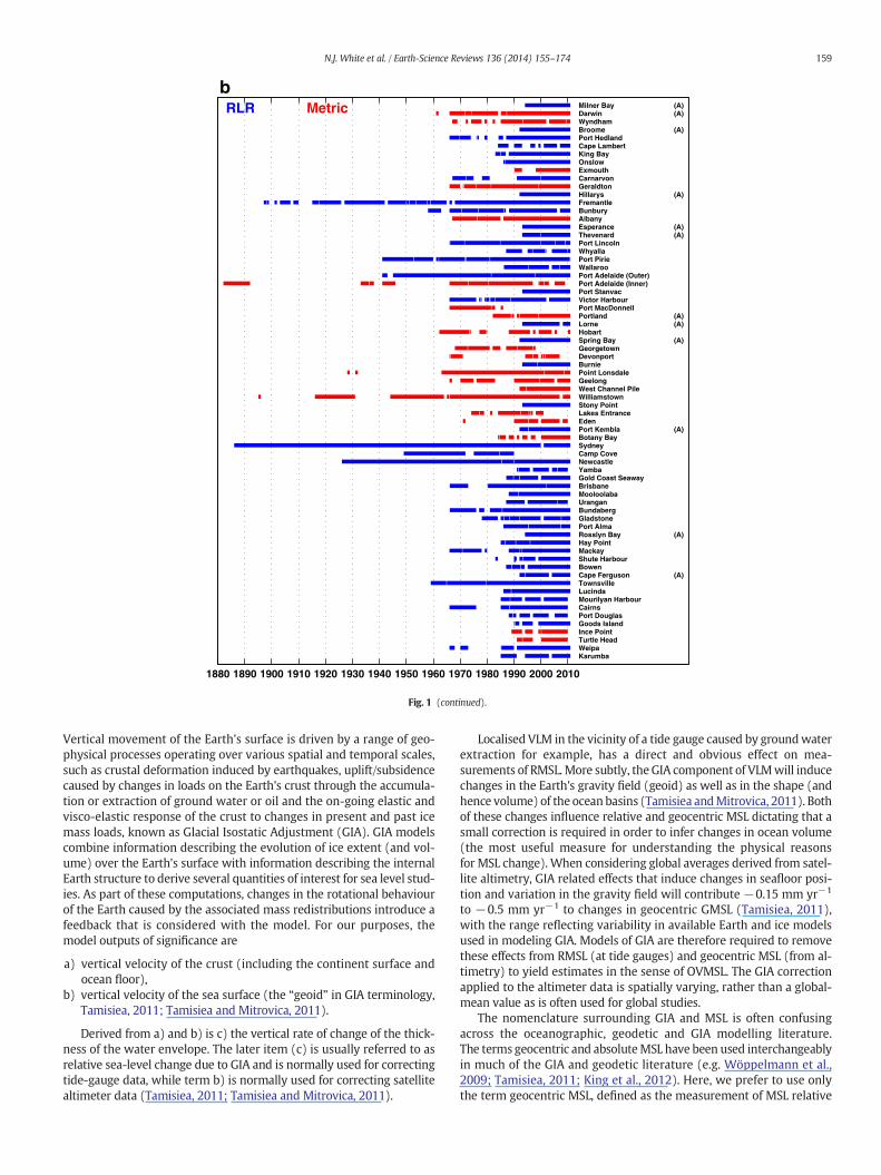
1880 1890 1900 1910 1920 1930 1940 1950 1960 1970 1980 1990 2000 2010

RLRb

Metric Milner Bay (A)Darwin (A)WyndhamBroome (A)Port HedlandCape LambertKing BayOnslowExmouthCarnarvonGeraldtonHillarys (A)FremantleBunburyAlbanyEsperance (A)Thevenard (A)Port LincolnWhyallaPort PirieWallarooPort Adelaide (Outer)Port Adelaide (Inner)Port StanvacVictor HarbourPort MacDonnellPortland (A)Lorne (A)HobartSpring Ba A)GeorgetownDevonportBurniePoint LonsdaleGeelongWest Channel PileWilliamstownStony PointLakes EntranceEdenPort Kembl

y (

a (A)Botany BaySydneyCamp CoveNewcastleYambaGold Coast SeawayBrisbaneMooloolabaUranganBundabergGladstonePort AlmaRosslyn Bay (A)Hay PointMackayShute HarbourBowenCape Ferguson (A)TownsvilleLucindaMourilyan HarbourCairnsPort DouglasGoods IslandInce PointTurtle HeadWeipaKarumba

Fig. 1 (continued).

159N.J. White et al. / Earth-Science Reviews 136 (2014) 155–174

Vertical movement of the Earth's surface is driven by a range of geo-physical processes operating over various spatial and temporal scales,such as crustal deformation induced by earthquakes, uplift/subsidencecaused by changes in loads on the Earth's crust through the accumula-tion or extraction of ground water or oil and the on-going elastic andvisco-elastic response of the crust to changes in present and past icemass loads, known as Glacial Isostatic Adjustment (GIA). GIA modelscombine information describing the evolution of ice extent (and vol-ume) over the Earth's surface with information describing the internalEarth structure to derive several quantities of interest for sea level stud-ies. As part of these computations, changes in the rotational behaviourof the Earth caused by the associated mass redistributions introduce afeedback that is considered with the model. For our purposes, themodel outputs of significance are

a) vertical velocity of the crust (including the continent surface andocean floor),

b) vertical velocity of the sea surface (the “geoid” in GIA terminology,Tamisiea, 2011; Tamisiea and Mitrovica, 2011).

Derived from a) and b) is c) the vertical rate of change of the thick-ness of the water envelope. The later item (c) is usually referred to asrelative sea-level change due to GIA and is normally used for correctingtide-gauge data, while term b) is normally used for correcting satellitealtimeter data (Tamisiea, 2011; Tamisiea and Mitrovica, 2011).

Localised VLM in the vicinity of a tide gauge caused by groundwaterextraction for example, has a direct and obvious effect on mea-surements of RMSL. More subtly, theGIA component of VLMwill inducechanges in the Earth's gravity field (geoid) as well as in the shape (andhence volume) of the ocean basins (Tamisiea andMitrovica, 2011). Bothof these changes influence relative and geocentric MSL dictating that asmall correction is required in order to infer changes in ocean volume(the most useful measure for understanding the physical reasonsfor MSL change).When considering global averages derived from satel-lite altimetry, GIA related effects that induce changes in seafloor posi-tion and variation in the gravity field will contribute −0.15 mm yr−1

to −0.5 mm yr−1 to changes in geocentric GMSL (Tamisiea, 2011),with the range reflecting variability in available Earth and ice modelsused in modeling GIA. Models of GIA are therefore required to removethese effects from RMSL (at tide gauges) and geocentric MSL (from al-timetry) to yield estimates in the sense of OVMSL. The GIA correctionapplied to the altimeter data is spatially varying, rather than a global-mean value as is often used for global studies.

The nomenclature surrounding GIA and MSL is often confusingacross the oceanographic, geodetic and GIA modelling literature.The terms geocentric and absoluteMSL have been used interchangeablyin much of the GIA and geodetic literature (e.g. Wöppelmann et al.,2009; Tamisiea, 2011; King et al., 2012). Here, we prefer to use onlythe term geocentric MSL, defined as the measurement of MSL relative

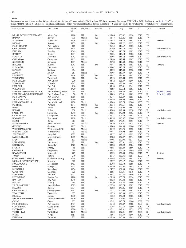
Table 1Summary of useable tide-gauge data. Columns from left to right are (1) name as in the PSMSL archive, (2) shorter version of the name, (3) PSMSL id, (4) RLR orMetric (see Section 2), (5) isthis an ABSLMP station, (6) latitude, (7) longitude, (8) first and (9) last year of useable data as defined in the text, (10) used for Trends (T), Variability (V) or not at all (X), (11) comments.

PSMSL name Short name PSMSLid

RLR/Metric ABSLMP? Lat Long Start End T/V/X? Comment

MILNER BAY (GROOTE EYLANDT) Milner Bay 1160 RLR Yes −13.86 136.42 1994 2010 TVDARWIN Darwin 935 Metric Yes −12.47 130.85 1961 2010 TVWYNDHAM Wyndham 1116 Metric −15.45 128.10 1967 2010 X See textBROOME Broome 1159 RLR Yes −18.00 122.22 1992 2010 TVPORT HEDLAND Port Hedland 189 RLR −20.32 118.57 1966 2010 TVCAPE LAMBERT Cape Lambert 1328 RLR −20.59 117.19 1984 2010 X Insufficient dataKING BAY King Bay 1549 RLR −20.62 116.75 1983 2010 TVONSLOW Onslow 1631 RLR −21.65 115.13 1986 2010 TVEXMOUTH Exmouth 1762 Metric −21.95 114.14 1990 2010 X Insufficient dataCARNARVON Carnarvon 1115 RLR −24.90 113.65 1967 2010 TVGERALDTON Geraldton 1031 Metric −28.78 114.60 1966 2010 TVHILLARYS Hillarys 1761 RLR Yes −31.83 115.74 1992 2010 X See textFREMANTLE Fremantle 111 RLR −32.07 115.75 1897 2010 TVBUNBURY Bunbury 834 RLR −33.32 115.66 1958 2010 TVALBANY Albany 957 Metric −35.03 117.89 1967 2010 TVESPERANCE Esperance 1114 RLR Yes −33.87 121.90 1993 2010 TVTHEVENARD Thevenard 386 RLR Yes −32.15 133.64 1993 2010 TVPORT LINCOLN Port Lincoln 230 RLR −34.72 135.87 1966 2010 TVWHYALLA III Whyalla 1367 RLR −33.01 137.59 1987 2010 TVPORT PIRIE Port Pirie 216 RLR −33.18 138.01 1941 2010 TVWALLAROO II Wallaroo 1420 RLR −33.93 137.62 1983 2010 TVPORT ADELAIDE (OUTER HARBOR) Port Adelaide (Outer) 448 RLR −34.78 138.48 1941 2010 V Belperio (1993)PORT ADELAIDE (INNER HARBOR) Port Adelaide (Inner) 50 Metric −34.83 138.51 1882 2008 X Belperio (1993)PORT STANVAC Port Stanvac 1506 RLR −35.11 138.47 1993 2010 TVVICTOR HARBOUR Victor Harbour 1069 RLR −35.56 138.64 1966 2010 TVPORT MACDONNELL II Port MacDonnell 1178 Metric −38.05 140.70 1966 1985 TVPORTLAND Portland 1547 Metric Yes −38.34 141.61 1982 2010 TVLORNE Lorne 1836 RLR Yes −38.55 143.99 1993 2010 TVHOBART Hobart 838 Metric −42.88 147.33 1958 2010 X Insufficient dataSPRING BAY Spring Bay 1216 RLR Yes −42.55 147.93 1992 2010 TVGEORGETOWN Georgetown 1120 Metric −41.13 146.85 1968 2005 TVDEVONPORT Devonport 1118 Metric −41.18 146.37 1966 2006 X Insufficient dataBURNIE Burnie 683 RLR −41.05 145.91 1993 2010 TVPOINT LONSDALE Point Lonsdale 301 Metric −38.29 144.61 1928 2010 X See textGEELONG Geelong 1117 Metric −38.09 144.39 1966 2010 TVWEST CHANNEL PILE West Channel Pile 1778 Metric −38.19 144.76 1992 2010 TVWILLIAMSTOWN Williamstown 93 Metric −37.87 144.92 1895 2010 TVSTONY POINT Stony Point 1033 RLR −38.37 145.22 1993 2010 TVLAKES ENTRANCE Lakes Entrance 1379 Metric −37.88 147.97 1974 2010 TVEDEN Eden 833 Metric −37.07 149.90 1971 2009 TVPORT KEMBLA Port Kembla 831 RLR Yes −34.47 150.91 1992 2010 TVBOTANY BAY Botany Bay 1525 Metric −33.98 151.22 1984 2010 TVSYDNEY Sydney 65 RLR −33.85 151.23 1886 2010 TVCAMP COVE Camp Cove 549 RLR −33.83 151.28 1949 1989 TVNEWCASTLE III Newcastle 267 RLR −32.92 151.80 1926 2010 V See textYAMBA Yamba 310 RLR −29.43 153.36 1991 2009 TVGOLD COAST SEAWAY 2 Gold Coast Seaway 1704 RLR −27.95 153.42 1987 2010 X See textBRISBANE (WEST INNER BAR) Brisbane 822 RLR −27.37 153.17 1966 2010 TVMOOLOOLABA 2 Mooloolaba 1493 RLR −26.68 153.13 1988 2010 TVURANGAN Urangan 2073 RLR −25.30 152.92 1987 2009 TVBUNDABERG Bundaberg 1154 RLR −24.77 152.38 1966 2010 TVGLADSTONE Gladstone 825 RLR −23.85 151.31 1978 2010 TVPORT ALMA Port Alma 2072 RLR −23.58 150.87 1986 2010 TVROSSLYN BAY Rosslyn Bay 1760 RLR Yes −23.16 150.79 1994 2010 TVHAY POINT Hay Point 1246 RLR −21.28 149.30 1985 2010 TVMACKAY Mackay 564 RLR −21.10 149.23 1966 2010 TVSHUTE HARBOUR 2 Shute Harbour 1569 RLR −20.28 148.78 1983 2010 TVBOWEN II Bowen 2074 RLR −20.02 148.25 1987 2010 TVCAPE FERGUSON Cape Ferguson 1492 RLR Yes −19.28 147.06 1992 2010 TVTOWNSVILLE I Townsville 637 RLR −19.25 146.83 1959 2010 TVLUCINDA Lucinda 1630 RLR −18.52 146.38 1986 2010 TVMOURILYAN HARBOUR Mourilyan Harbour 1629 RLR −17.58 146.08 1985 2009 TVCAIRNS Cairns 953 RLR −16.92 145.78 1966 2009 TVPORT DOUGLAS 2 Port Douglas 1471 RLR −16.48 145.47 1988 2009 X Insufficient dataGOODS ISLAND Goods Island 1368 RLR −10.56 142.15 1990 2010 TVINCE POINT Ince Point 1300 Metric −10.51 142.31 1975 2009 TVTURTLE HEAD Turtle Head 1749 Metric −10.52 142.21 1991 2009 X Insufficient dataWEIPA Weipa 1157 RLR −12.67 141.87 1966 2010 TVKARUMBA Karumba 835 RLR −17.50 140.83 1985 2010 TV

160 N.J. White et al. / Earth-Science Reviews 136 (2014) 155–174

1880 1890 1900 1910 1920 1930 1940 1950 1960 1970 1980 1990 2000 2010−250

−200

−150

−100

−50

0

50

100

150

200

250

300

350

400Individual tide gauges (56)Mean of gauges

Gauges not used (see text)GMSL (tide gauges)

Mean around the Australiancoast from satellites

GMSL (satellites)S

ea le

vel r

elat

ive

to 1

971

to 2

000

mea

n (m

m)

a

1880 1890 1900 1910 1920 1930 1940 1950 1960 1970 1980 1990 2000 2010−250

−200

−150

−100

−50

0

50

100

150

200

250

300

350

400Individual tide gauges (56)Mean of gaugesGauges not used (see text)GMSL (tide gauges)

Mean around the Australiancoast from satellites

GMSL (satellites)

Sea

leve

l rel

ativ

e to

197

1 to

200

0 m

ean

(mm

) b

1880 1890 1900 1910 1920 1930 1940 1950 1960 1970 1980 1990 2000 20100

10

20

30

40

50

60

Num

ber

of g

auge

s

c

Fig. 2. (a) Overview of Australian sea-level data and comparisonwith global sea-level estimates, all expressed as OVMSL (Section 2.3). The gauges flagged “TV” in column 10 of Table 1 areplotted in grey. The records flagged because of possible groundmovement and credibility issues are plotted in cyan, but not used in calculating averages. The arithmetic mean of the tidegauges considered to be of reasonable quality is plotted as a heavy black line. The GMSL estimated from satellite altimeters (see Section 2.2) is plotted as a heavy red line, and the area-weightedmean from satellite altimeters along a line around the Australian coast is plotted in orange. The cyan trace that goes very high at the end isWyndham, and the one that goes verylow in the 2000s is Point Lonsdale. (b) As in (a) but after the signal correlated with the Southern Oscillation Index is removed (see Section 3). (c) The changing number of gauge stationsavailable for use over time.

161N.J. White et al. / Earth-Science Reviews 136 (2014) 155–174

to an Earth-fixed reference frame with its coordinate origin at the time-averaged centre of mass of the Earth (the geocentre). Observations ofboth relative and geocentric MSL inevitably include some componentof GIA, hencewe choose to use the termOVMSL to denote anymeasure-ment (relative or geocentric) that has been corrected to remove the ef-fects of GIA, and thus imply sea-level change in the sense of changingocean volume. We do not consider sources of VLM other than GIA forthis analysis because of the lack of information available.

While traditional surveying techniques are used tomonitor the localstability of a tide gauge relative to the local benchmark, observationsfrom continuously operating Global Positioning System (GPS) sites arethe preferred data for computing VLM in the same reference frame assatellite altimetry known as the International Terrestrial ReferenceFrame (e.g. ITRF08, Altamimi et al., 2011). These geocentric estimatesof VLM derived from GPS receivers located at or near to tide gauges en-able the transformation from relative to geocentric MSL, and thus allowdirect comparison with altimetry (e.g. Wöppelmann et al., 2009; King

et al., 2012). Here we use the analysis of sparsely located GPS datafrom Burgette et al. (2013) that provides VLM at 12 Australian GPS sta-tions (each with at least five years of near continuous GPS data) locatedwithin 100 km of tide-gauge locations (Fig. 1; Table 2). These data areprocessed using the preferred strategy of Tregoning and Watson(2009), including the latest developments in algorithms, particularlyrelating to the treatment of the atmospheric delay and crustal loadinginduced by the atmosphere. We estimate VLM from the GPS coordinatetime series using a maximum likelihood approach as implemented inthe CATS (Create and Analyse Time Series) software (Williams, 2008).Further detail on the approach and noise models (consistent withother studies that investigate noise properties across the global trackingnetwork, e.g. Santamaría-Gómez et al., 2011) can be found in Burgetteet al. (2013).

TheGPS-derivedVLMestimates (Table 2) suggest subtle subsidence atmany sites, however velocities at 7 of the 12 sites are not significantly dif-ferent from zero at the one standard error (typically 0.3 to 0.8 mm yr−1)

Table 2Vertical landmotion (VLM) at the 12 GPS sites located within 100 km of tide gauges and having at least 5 years of continuous GPS data. VLM estimates provided include linear rates de-rived fromGPS (GPS VLM,mmyr−1 ± 1 standard error), the predicted GIA crustal velocities (GIA VLM,mm yr−1) and theGIA induced contribution to relativemean sea level (GIA RMSL,mmyr−1). GPS VLM estimates (from the CATS analysis), significantly different from zero at the one standard error level are shown in italics. GPS and GIA VLM velocities are in the sense ofpositive being up. For the GIA RMSL trends, a negative number means that the land is rising with respect to the sea surface.

Site no. Latitude Longitude Data start Data end n GPSVLM

GIAVLM

GIARMSL

HOB2 −42.8047 147.4387 2000.1 2011.0 24,178 0.0 ± 0.5 −0.2 −0.2BUR1 −41.0501 145.9149 2002.2 2007.0 10,766 −0.2 ± 0.8 −0.1 −0.2TOW2 −19.2693 147.0557 2000.1 2011.0 24,164 −0.2 ± 0.4 −0.0 −0.2DARW −12.8437 131.1327 2000.1 2011.0 22,414 −1.6 ± 1.4 0.0 −0.3KARR −20.9814 117.0972 2000.1 2011.0 24,262 0.2 ± 0.8 −0.1 −0.2HIL1 −31.8255 115.7386 2003.0 2011.0 17,654 −3.1 ± 0.7 −0.1 −0.2PERT −31.8019 115.8852 2000.1 2011.0 22,939 −2.1 ± 0.7 −0.1 −0.2YAR2 −29.0466 115.3470 2000.1 2011.0 24,626 0.9 ± 0.4 −0.1 −0.2MOBS −37.8294 144.9753 2002.8 2011.0 18,865 −0.3 ± 0.5 0.0 −0.3CEDU −31.8667 133.8098 2000.1 2011.0 24,213 −0.3 ± 0.4 −0.1 −0.3SYDN −33.7809 151.1504 2005.4 2011.0 12,803 −0.4 ± 0.7 −0.1 −0.2ADE1 −34.7290 138.6473 2000.1 2010.7 23,415 −0.4 ± 0.3 −0.0 −0.3

162 N.J. White et al. / Earth-Science Reviews 136 (2014) 155–174

level. Hillarys (HIL1) and Perth (PERT) show land subsidence that islikely associated with fluid extraction (Deng et al., 2011; Featherstoneet al., 2012) with, possibly, an extra contribution from land settlementat Hillarys, highlighting that localised effects are important in some re-gions. The Adelaide GPS (ADE1) site also shows subsidence, but at aslower rate than for Hillarys, consistent with earlier analysis (Belperio,1993). The Darwin site (DARW) shows subsidence, but at a ratethat is only just significant at the one standard error level. We notethat the Darwin site has the largest formal uncertainty, highlightingthat the linear plus periodic components model used to describe thetime series are a poor descriptor of the complex quasi-seasonal energy,largely of hydrological origin, that is evident in the time series forDarwin (e.g. Tregoning et al., 2009). The Yarragadee GPS site (YAR2,which is ~45 km inland) has a significant positive (upward) verticalmotion, and, with the exception of a possible effect from an uncalibrat-ed antenna radome and a time variable GPS constellation, we have noexplanation for the trend observed at this site.

The predicted contribution of GIA to VLM may be compared withthe GPS based estimates of VLM (Table 2). Using the model describedin Tamisiea (2011), we extract both the contributions of GIA to VLM(hereon GIA VLM), as well as its contribution to relative MSL (hereonGIA RMSL), at sites around Australia where VLM is directly measuredusing GPS data. The GIA-induced crustal motions throughout the 20thcentury are small, but mostly negative ranging from −0.2 mm yr−1 to0.0 mm yr−1 at these locations. The corresponding contributions toRMSL change at these sites are all negative (Table 2), but again small.At the 69 tide gauge sites used in this study, GIA alone would cause aRMSL fall by −0.1 to −0.4 mm yr−1 (Tamisiea, 2011; Fleming et al.,2012). That is, for the 20th and 21st centuries, these GIA motionscause RMSL rise around Australia to be lower than they would other-wise be.

In summary, predictions of GIA and measurements from GPS showthat vertical land movements around most of the Australian coastline

Table 3Definitions and sources of climate indices.

ClimateIndex

Period Description

SOI 1880–2011 Defined as the normalised air pressure differenceMEI 1950–2011 Based on six observed variables over the tropical P

wind, sea surface temperature, surface air tempermei.html#data

PDO 1900–2011 Defined as the leading principal component of NoIPO 1880–2008 Defined as the leading principal component of NoDMI 1880–1997 The intensity of the IOD is represented by the SST

gradient is named the Dipole Mode Index (DMI).SAM 1948–2011 Defined as the normalised air pressure difference

are small, with more pronounced localised subsidence at a few specificsites.

2.4. Climate indices

In order to investigate the inter-annual variability of MSL and how itmight be affected by regional climate variability, we make use of sixclimate indices. The Southern Oscillation Index (SOI) is a descriptor ofthe El Niño-Southern Oscillation (ENSO) (Walker, 1923; Montgomery,1940). Sustained negative values of the SOI indicate El Niño episodesand positive values are associated with La Niña events. TheMultivariateENSO Index (MEI) is a more complete and flexible descriptor of ENSO(Wolter, 1987; note that its definition has the opposite sign to theSOI). The Pacific Decadal Oscillation (PDO) is a pattern of climate vari-ability with a similar expression to El Niño, but acting on a longer timescale, and with a pattern most clearly expressed in the North Pacific/North American sector (Trenberth and Hurrell, 1994). The Inter-decadal Pacific Oscillation (IPO) (Power et al., 1999; Parker et al.,2007) is a manifestation of the PDO covering more of the PacificOcean (down to 55°S). The Indian Ocean Dipole (IOD), represented bytheDipoleMode Index (DMI), is a coupled ocean–atmosphere phenom-enon in the Indian Ocean and has a strong relationship to ENSO (Sajiet al., 1999). The Southern Annular Mode (SAM) effectively indicatesthe strength of the westerly winds in the Southern Oceans (Gong andWang, 1999). The source of the different climate indices uses in thispaper, periods covered and a brief description of how they are calculat-ed are listed in Table 3.

3. Australia-wide sea-level variability and trends

We focus here on the 45 year period from 1966 to 2010 (inclusive)as this is the longest period for which data is available around thewhole country. There are 16 near-continuous tide-gauge records

between Tahiti and Darwin. http://www.bom.gov.au/climate/current/soihtm1.shtmlacific, namely: sea-level pressure, zonal and meridional components of the surfaceature, and total cloudiness fraction of the sky. http://www.esrl.noaa.gov/psd/enso/mei/

rth Pacific SST variability. http://jisao.washington.edu/pdo/rth and South Pacific SST variability. http://www.iges.org/c20c/anomaly difference between the eastern and the western tropical Indian Ocean. Thishttp://www.jamstec.go.jp/frsgc/research/d1/iod/e/index.htmlbetween 40°S and 70°S. http://web.lasg.ac.cn/staff/ljp/data-nam-sam-nao/sam-aao.htm

163N.J. White et al. / Earth-Science Reviews 136 (2014) 155–174

providing coverage of all areas of the Australian coastline with the ex-ception of the Gulf of Carpentaria (Figs. 1, 3). Coverage is significantlylower before 1966 (Fig. 2c). After 1993, there are more than twice thenumber of records available but the spatial coverage is similar, withthe exception of an additional gauge in the Gulf of Carpentaria.

3.1. Variability

Seasonal (annual and semi-annual) signalswere removed from eachrecord by estimating simultaneously annual and semi-annual sinusoidsusing least squares. After filling 1-month gaps by spline interpola-tion we filled the remaining small gaps (max length 58 months) in re-cords at 10 stations with data from the neighbouring stations. In all,298 months were filled (3.4% of the total). This procedure is justifiedby the clear along-shore coherence between nearby gauges and thefact that leaving out the record with the largest gapmakes minimal dif-ference to the results. The variances of themonthlyMSL are amaximumat Darwin in the north and decrease going anti-clockwise aroundAustralia (with a second maximum in the South Australian gulfs) to

1000

−100

Darwin

1000

−100

Port Hedland

1000

−100

Geraldton

1000

−100

Fremantle

1000

−100

Bunbury

1000

−100

Albany

1000

−100

Port Lincoln

1000

−100

Port Pirie

1000

−100

Port Adelaide (Outer)

1000

−100

Victor Harbour

1000

−100

Geelong

1000

−100

Williamstown

1000

−100

Sydney

1000

−100

Newcastle

1000

−100

Mackay

1000

−100

Townsville

150

−15SO

IM

on

thly

MS

L (

mm

)

1970 1975 1980 1985 1

Fig. 3.Monthly RMSL time series for the 16near continuous records available for January toDeceis also shown. Cross-correlations between adjacent time series are shown on the right. The cro

Townsville, for which the variance is less than half that at Darwin(Table 4, col. 3). Note that we use records from Port Adelaide (Outer)and Newcastle here to focus on variability rather than trends but trendsfrom these records are not used, due to datum and subsidence issues asdiscussed previously. We calculated a low-frequency component usinga one-year low-pass filter, using a Finite Impulse Response (FIR) filter(−6 dB at one year)—see Fig. 4, solid lines. Empirical Orthogonal Func-tions (EOFs; Preisendorfer, 1988) were calculated from the low-passed,de-trended (using least squares) data to identify the variability that iscommon tomany records and the Principal Component (PC) time serieswere correlated against each of the six regional climate indices.

For the high frequency component (the difference between the orig-inal monthly time series and the low-passed time series), the variancesare largest on the south coast where the strong westerly winds and thewide shelf generate large amplitude coastal-trapped waves (Provis andRadok, 1979; Church and Freeland, 1987). The first EOF mode of thehigh frequency component (not shown), accounting for almost 50% ofthe variance, has maximum amplitude on the south coast, decreasingnorthwards along the east coast, and little signal on the west coast.

0.86

0.83

0.93

0.93

0.89

0.59

0.82

0.90

0.85

0.80

0.86

0.63

0.84

0.17

0.70

0.49

0.68

990 1995 2000 2005 2010

mber 2010, fromDarwin in thenorth, anticlockwise to Townsville in thenortheast. The SOIss-correlation between Townville and Darwin is shown below Townsville.

Table 4RMSL andOVMSL linear trends (mm yr−1) and variances (mm2) of sea-level records for the period 1966 to 2010. A low-pass filter (see text) is used to obtain the low- and high-frequencycomponents. The variances of the unfiltered andfilteredmonthly data (columns 3 and 5) are calculated after removal of a linear trend (columns 2 and 4). The variances after removing thecomponent of the first EOF linearly correlated to ENSO and the linear trend are given in columns 7 and 6. The linear trend after removal of the SOI-correlated signal and includingthe adjustment for atmospheric pressure and GIA is given in column 8. The means and standard deviations in the last row only use data from 14 of the 16 stations—i.e. not includingPort Adelaide and Newcastle—see Table 1 and the associated discussion.

1 2 3 4 5 6 7 8

Site Monthly + low-pass filter + ENSO removal + → OcVol

RMSLtrend(mm yr−1)

resvar(mm2)

RMSLtrend(mm yr−1)

resvar(mm2)

RMSLtrend(mm yr−1)

resvar(mm2)

OVMSLtrend(mm yr−1)

Darwin 2.6 5429 2.4 4129 2.7 999 3.1Port Hedland 1.8 5351 1.5 3920 1.9 1126 2.1Geraldton 1.2 4787 1.0 3064 1.3 1040 1.5Fremantle 1.8 4615 1.7 2920 2.0 965 2.3Bunbury 0.9 4524 0.8 2637 1.1 1140 1.4Albany 0.9 3547 0.8 2039 1.1 757 1.4Port Lincoln 1.9 4130 1.9 1632 2.0 944 2.3Port Pirie 2.0 5102 2.0 2349 2.2 1321 2.6Port Adelaide (Outer) 1.7 5518 1.6 2161 1.9 1304 2.2Victor Harbour 0.8 5306 0.7 2193 0.9 1335 1.2Geelong 1.2 3269 1.1 1271 1.3 907 1.7Williamstown 2.1 3689 2.0 1420 2.2 1132 2.7Sydney 0.8 2497 0.8 819 0.9 620 1.3Newcastle 1.2 3149 1.2 1180 1.3 823 1.8Mackay 1.5 3099 1.3 1184 1.4 1077 1.8Townsville 1.3 2474 1.2 980 1.3 751 1.8Mean (s.d.) 1.5 (0.6) 1.4 (0.5) 1.6 (0.6) 1.9 (0.6)

164 N.J. White et al. / Earth-Science Reviews 136 (2014) 155–174

EOF 2, accounting for almost 20% of the variance has amaximum on thewest coast and EOF 3 has amaximumamplitude on the east coast. Theseresults are consistent with wind forced coastal-trapped waves propa-gating south along the west coast (Hamon, 1966), east across theGreat Australian Bight (Provis and Radok, 1979; Church and Freeland,1987) and northwards along the east coast (Hamon, 1966; Churchet al., 1986a,b; Freeland et al., 1986).

Low frequency variability (i.e. inter-annual or longer) dominatestheMSL time series at Darwin (over 4000mm2, 75% of the total varianceat Darwin) and the monthly anomalies appear to propagate rapidlysouthward along the west coast of Australia, eastward along the southcoast (the direction of coastal-trapped wave propagation), but withthe magnitude of perturbations decreasing with distance (Fig. 4,Table 4, col. 5). The perturbations are almost in phase along the eastcoast and have a smaller variance (of order 1000 mm2; about 30% ofthe total at each location) than on the west and south coasts. The firstEOF mode of the low-passed signals (Fig. 5a), accounting for 69% ofthe variance, has a simple spatial structure of decreasing amplitudearound Australia. Correlations and lags between Principal Component1 (PC 1), i.e. the time series associated with the first EOF, Fig. 5b aremost highly correlated with the SOI (+0.87 at 0 lag). Maximum corre-lations and their associated lags for the six climate indices are shown inTable 5. EOF 2 only explains about 11% of the variance, has maximumamplitude along the south coast and the maximum correlation with cli-mate indices is with the SAM (−0.43 at 0 lag).

The large percentage variance explained by one EOF, its simple spa-tial structure, and its high correlationwith the SOI (and other Pacific cli-mate indices) suggests that it should be possible to robustly removesignificant inter-annual and decadal variability from individual records.To do this, for each location iwe produce an ENSO-removed time series(her,i) as follows:

her;i ¼ hor;i − ei � λ1 � b� SOI

where: hor,i is the original (low-passed) RMSL time series, as on Fig. 4 atlocation i, ei is the value of EOF 1 at location i (as on Fig. 5a), λ1 is the ei-genvalue associated with EOF 1, b is the regression coefficient of PC 1against the SOI (SOI being the independent variable) and SOI is thelow-pass filtered SOI time series.

For Darwin, this simple procedure reduces the variance about thelinear best fit by about 75% (Fig. 4, dotted lines; Table 4 col. 7) withthe resultant time series having reduced inter-annual to decadal vari-ability. For other locations, variance of the order of 60% was removedon the west coast, 30–50% on the south coast, and 15–30% on the eastcoast. This process very effectively reduces the differences betweenthe time series (Fig. 6a and b), allowing more accurate estimation ofthe long-term trends in RMSL, which in turn leads to a clearer pictureof the spatial variation in trends.

We also tested more complicated schemes where there was a directcorrelation between the SOI and each individual record, includingallowing for a time lag, and following Zhang and Church (2012), simul-taneously regressing each RMSL record against a high passed version ofthe SOI and a low passed version of the PDO. Although these modelshave a greater number of parameters, the results were very similar. Asa result, for further analysis, we used the simple scheme that exploitedthe highly correlated nature of the variability; i.e. using the EOF signalcorrelated with SOI. This simple model is adequate for this analysis.We also note that, although the low-passed sea level and SOI mainlycontain variations at inter-annual time scales, there is still some vari-ability at longer time scales. There is debate on whether the PDO andENSO are totally independent of each other, since the PDO and ENSOare highly correlated at decadal and longer time scales (Newmanet al., 2003; Power and Colman, 2006). The low-passed sea level andSOI contain not only inter-annual variability but also decadal (and lon-ger) variability, which could be associated with ENSO and PDO. SeeZhang and Church (2012) for amore detailed discussion of the relation-ship between ENSO and the PDO.

3.2. Trends

Fourteen of the sixteen gauges are useful for calculating trends(Section 3.1). The 1966–2010 average of the RMSL trends fromthe monthly data, from these 14 tide gauges is about 1.5 mm yr−1,with a range from 0.8 mm yr−1 at Sydney and Victor Harbour to2.6 mm yr−1 at Darwin. The 14 rates have a standard deviation of0.6 mm yr−1 (Table 4). Trends are derived using linear least squares,and serial correlation is accounted for using an autoregressive errorstructure of order 1 AR(1) model (Chandler and Scott, 2011). Filtering

1000

−100 0.911000

−100 0.911000

−100 0.951000

−100 0.951000

−100 0.941000

−100 0.691000

−100 0.771000

−100 0.891000

−100 0.731000

−100 0.751000

−100 0.771000

−100 0.661000

−100 0.841000

−100 0.371000

−100 0.651000

−100 0.62

150

−15S

OI

0.75M

on

thly

MS

L (

mm

)

1970 1975 1980 1985 1990 1995 2000 2005 2010

0.070.00

−0.07PC

1

0.87

Darwin

Port Hedland

Geraldton

Fremantle

Bunbury

Albany

Port Lincoln

Port Pirie

Port Adelaide (Outer)

Victor Harbour

Geelong

Williamstown

Sydney

Newcastle

Mackay

Townsville

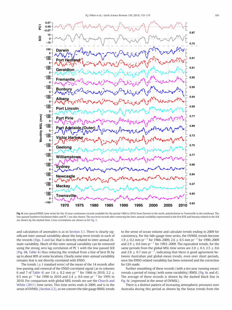
Fig. 4. Low-passed RMSL time series for the 16 near continuous records available for the period 1966 to 2010, from Darwin in the north, anticlockwise to Townsville in the northeast. Thelow-passed SouthernOscillation Index and PC 1 are also shown. The sea-level records after removing the inter-annual variability represented in the first EOF and linearly related to the SOIare shown by the dashed lines. Cross-correlations are shown as for Fig. 3.

165N.J. White et al. / Earth-Science Reviews 136 (2014) 155–174

and calculation of anomalies is as in Section 3.1. There is clearly sig-nificant inter-annual variability about the long-term trends in each ofthe records (Figs. 3 and 6a) that is directly related to inter-annual cli-mate variability. Much of this inter-annual variability can be removedusing the strong zero lag correlation of PC 1 with the low passed SOI(Fig. 6b, Table 4) thus reducing the residual from a line of best fit byup to about 80% at some locations. Clearly some inter-annual variabilityremains that is not directly correlated with ENSO.

The trends (±1 standard error) of the mean of the 14 records afterlow-passing and removal of the ENSO-correlated signal (as in columns6 and 7 of Table 4) are 1.6 ± 0.2 mm yr−1 for 1966 to 2010, 2.2 ±0.5 mm yr−1 for 1990 to 2010 and 2.4 ± 0.6 mm yr−1 for 1993 to2010. For comparison with global MSL trends we use the Church andWhite (2011) time series. This time series ends in 2009, and is in thesense of OVMSL (Section 2.3), sowe convert the tide gauge RMSL trends

to the sense of ocean volume and calculate trends ending in 2009 forconsistency. For the tide-gauge time series, the OVMSL trends become1.9 ± 0.2 mm yr−1 for 1966–2009, 2.6 ± 0.5 mm yr−1 for 1990–2009and 2.9 ± 0.6 mm yr−1 for 1993–2009. The equivalent trends, for thesame periods from the global MSL time series are 2.0 ± 0.3, 2.5 ± 0.6and 2.8 ± 0.7 mm yr−1, indicating that there is good agreement be-tween Australian and global-mean trends, even over short periods,once the ENSO-related variability has been removed and the correctionfor GIA made.

Further smoothing of these records (with a ten year running mean)reveals a period of rising (with some variability) RMSL (Fig. 6c and d).The average of these records is shown by the dashed black line inFig. 6c (expressed in the sense of OVMSL).

There is a distinct pattern of increasing atmospheric pressures overAustralia during this period as shown by the linear trends from the

0

0.1

0.2

0.3

0.4

0.5

Dar

win

Po

rt H

edla

nd

Ger

ald

ton

Fre

man

tle

Bu

nb

ury

Alb

any

Po

rt L

inco

ln

Po

rt P

irie

Po

rt A

del

aid

e (O

ute

r)

Vic

tor

Har

bo

ur

Gee

lon

g

Will

iam

sto

wn

Syd

ney

New

cast

le

Mac

kay

To

wn

svill

e

EO

F 1

a

b

1970 1975 1980 1985 1990 1995 2000 2005 2010−30

−20

−10

0

10

20

30

SO

I

−0.15

−0.10

−0.05

0.00

0.05

0.10

0.15

PC

1

Fig. 5. (a) The first EOF of the low passed sea-level time series plotted against the tide-gauge sites; and (b) the corresponding PC and low-passed SOI plotted against time.

166 N.J. White et al. / Earth-Science Reviews 136 (2014) 155–174

HadSLP2 data set (Allan and Ansell, 2006), slightly depressing observedsea level trends, particularly in the east and north-east of Australia(Fig. 7). This depression of sea level is about 0.2mmyr−1 for themajor-ity of the east Australian coast and over 0.25mmyr−1 from28°S to 36°S.If we then also apply the inverse barometer correction the meanAustralian tide gauge trends become 2.1 ± 0.2, 2.9 ± 0.5 and 3.1 ±0.6 mm yr−1 for 1966 to 2009, 1990 to 2009 and for 1993 to 2009, re-spectively, still close to the global-mean rates (Table 6).

4. Trends over other periods

We now examine the trends of RMSL (for records that are at least80% complete as indicated in Table 1) as measured directly by the tidegauges (i.e. without any corrections for VLM or the inverse barometereffect). We focus here on two periods: the first being that spanned bythe two longest tide gauge records (Sydney from 1886 to 2010 andFremantle from 1897 to 2010); and the second being the period fromJanuary 1993 to December 2010 when many more tide gauge records(57), and also satellite altimeter data, are available. Different but related

Table 5Maximum correlations and their associated lags between PC 1 and the climate indices. Apositive lag indicates that the index is later than PC 1.

Index Correlation Lag (months)

SOI +0.87 +0MEI −0.84 +1PDO −0.63 +3IPO −0.82 +1SAM +0.26 −9DMI −0.43 +0

statistical approaches have been used to analyse data from these threeperiods; the chosen methodology depends upon whether the focus ison specific or multiple gauge sites, the length of series, and how bestto quantify and remove inter-annual variation. Uncertainties in trendsare expressed as one standard error (i.e. 68% confidence level).

4.1. The long records

Monthly RMSL data from Australia's two longest recording sites(Fremantle and Sydney) were independently used to search for thepresence of both linear and non-linear long-term trends (Fig. 8a and brespectively). An extended multiple regression method knownas generalised additive models (GAMs; Wood, 2006) was used as thebasis for developing a flexible statistical model to quantify non-linearsmooth time trends in RMSL. GAMs have an advantage over the moreglobally-fittingmodels such as polynomials in that nonlinearity is fittedlocally and hence trends can be of an arbitrary shape. The process imple-mented closely followed that of Morton and Henderson (2008).

A general statistical model was proposed, the components of whichaccounted for: (i) seasonality (annual and semi-annual variability);(ii) a climate ‘noise’ covariate (inter-annual variability as measured bySOI since the EOF technique cannot be applied to a single RMSL series);(iii) nonlinear trend (modelled as a spline, see further details below);and (iv) serial correlation (autocorrelation) of the residual terms. Themodel took the form:

RMSLi ¼ α1 cos 2πti–φ1ð Þ þα2 cos 4πti–φ2ð Þ seasonalityþ β SOI climateþ γ1 þ γ2ti þ s ti; dfð Þ time trendþ εi noise

ð1Þ

1970 1975 1980 1985 1990 1995 2000 2005 2010

−100

0

100

MS

L an

omal

y (m

m)

a

1970 1975 1980 1985 1990 1995 2000 2005 2010

−100

0

100

MS

L an

omal

y (m

m)

b

1970 1975 1980 1985 1990 1995 2000 2005 2010−100

−50

0

50

100Individual tide gauges (in ocean volume sense)Mean of tide gauges

GMSL from tide gauges (yearly values, no smoothing)MS

L an

omal

y (m

m)

c

1970 1975 1980 1985 1990 1995 2000 2005 2010−100

−50

0

50

100

Darw Hedl Gera Freo Bunb Alba Linc Piri Vict Geel Will Sydn Mack Town

Mean of tide gauges

MS

L an

omal

y (m

m) d

Fig. 6. (a) Low-passed RMSL sea levels for the 14 records available for 1966 to 2010, and (b) after the component of EOF 1 related to ENSO have been removed. Note: Newcastle and PortAdelaide (Outer) are not displayed. In (c), the data smoothedwith a ten year running average are comparedwith the average of the records and the globalmean sea level from Church andWhite (2011). (d) As in (c), but with the 14 tide-gauge records plotted in different colours to more easily distinguish them. Data displayed on panels (c) and (d) is in the sense of OVSML.

167N.J. White et al. / Earth-Science Reviews 136 (2014) 155–174

where i refers to successive monthly observations and ti = time inyears. The amplitude and phase of the annual and semi-annual seasonalperiodic terms (α1, φ1 and α2, φ2, respectively) were estimated fromthe linear coefficients of orthogonal sine and cosine basis functions ineach case. Inter-annual variability wasmodelled as a linear relationshipbetween SOI and RMSL (regression coefficient β), with SOI being fil-tered using a 3 month runningmean tomimic its short term cumulativeeffect upon RMSL. The time trend was composed of two parts: the firstbeing the linear component {γ1 + γ2 ti} where γ1 is the model's inter-cept term and γ2 is the estimated linear rate of change spanning thefull time series; and the seconddenoted by s(ti ; df), is a cubic smoothingspline with formal degrees of freedom df chosen as 6 for this analysis.This spline term accounts for deviations from linearity over time, witha flexibility approximately equivalent to a polynomial of a similar de-gree (df) (Morton andHenderson, 2008). An autoregressive error struc-ture of order 1 (AR(1))was included in themodel whereby the error forith observation is formed as εi = ρεi−1 + ξi, with ρ being the estimatedfirst order autocorrelation and ξi is an independent random error term.All parameters were estimated using the method of maximum likeli-hood. The model was implemented using the statistical software pack-age R (The Comprehensive R Network: http://cran.r-project.org/).

Having checked model assumptions via residual diagnostic plots,the model fitted the Fremantle data somewhat better (approximate

adjusted R2 = 0.67) than the Sydney data (R2 = 0.42), with all modelterms highly significant at both sites. Results from the model fit showsignificant annual (36.0 and 102.7 mm) and semi-annual (21.2 and30.4 mm) amplitudes for Sydney and Fremantle respectively (Table 7).Annual maxima in RMSL occur in late May at Sydney, and early June inFremantle, consistent with other studies (e.g. Fig. 4 in Burgette et al.,2013). Further investigation of the seasonal amplitudes using an alter-nate technique (not shown here) that treats the model terms as timevariable quantities with defined process noise within a Kalman filter(Davis et al., 2012), suggests a possible trend in the annual amplitudeat Fremantle (~99 mm in ~1920 to ~104 mm in ~2011). These valueslie within the formal error of the GAMs time-constant estimate of102.7 ± 3.3 mm. About a 10% increase in annual amplitude is evidentat Fort Denison (~33mm in ~1925 to ~37mm in ~2011), again broadlyconsistent with GAMs time-constant estimate and standard error of36.0 ± 2.2 mm.

The results for the linear SOI model term are consistent with theanalysis of Section 3 and show a significant correlation of SOI withinter-annual variability in RMSL, with correlation stronger at Fremantle(r = 0.47, SOI term β = 3.15 ± 0.28) than at Sydney (r = 0.17, β =0.92 ± 0.18). Using the alternate Kalman filter strategy, we note smallincreases in the SOI coefficient over time (~3 in 1920 to ~4 in 2011 atFremantle, and ~0.2 in 1910 to ~1 in 2011 at Fort Denison), consistent

45°S

40°

35°

30°

25°

20°

15°

10°

5°

110°E

110°E

120° 130° 140° 150° 160°Longitude

Lat

itu

de

Longitude

Lat

itu

de

45°S

40°

35°

30°

25°

20°

15°

10°

5°

120° 130° 140° 150° 160°

hPa yr−1

a

−0.04 −0.03 −0.02 −0.01 0 0.01 0.02 0.03 0.04

mm yr−1

b

−0.4 −0.3 −0.2 −0.1 0 0.1 0.2 0.3 0.4

Fig. 7. (a) Trends in local atmospheric pressure from the HadSLP2 data set from 1966 to2010; (b) equivalent trends in sea level from applying the inverse barometer effectusing the atmospheric pressure changes shown on the top panel relative to the time-varying over-ocean global-mean atmospheric pressure.

168 N.J. White et al. / Earth-Science Reviews 136 (2014) 155–174

with the changes observed by Haigh et al. (2011). As per the seasonalterms, this average of the time variable estimates is consistent withthe GAMS time invariant model parameters.

The non-linear component of the time trend (i.e. (s(ti; df), Eq. (1)) issignificant at both sites (Table 7). This suggests that the linear component

Table 6Rates of Australian averaged MSL rise for different periods compared with rates of GMSL. Notewithout removal of SOI-correlated signals (corresponding to the solid lines on Fig. 4—tagged ‘(signals, plus other corrections as noted—tagged ‘(ER)’. Note also that mean tide-gauge trends shgauge data. As a result these numbers can be slightly different from the ‘meanof trends’ numbertable (1.8) is slightly (but insignificantly) different from it's near-equivalent (1.9) in the last en

1966–2010 1990–2010

Tide gauge relative (Unc) 1.4 ± 0.3 4.0 ± 0.9Tide gauge relative (ER) 1.6 ± 0.2 2.2 ± 0.5Tide gauge + OV (ER) 1.8 ± 0.2 2.4 ± 0.5GMSL + OVTide gauge + OV + AP (ER) 2.1 ± 0.2 2.6 ± 0.5Altimeter GMSL (OV)

(γ1 + γ2 ti, Eq. (1)) inadequately describes the underlying trendwithinthese data. At Fremantle, the rate of rise (Fig. 8c) is positive overlong periods (1897–2010) with an average long-term linear trend of1.58 ± 0.09 mm yr−1 (Table 7). However, between 1920 and 1960the trend averages to about 2.2 mm yr−1, is near zero from 1960 to1990, and then increases rapidly to approximately 4.0 mm yr−1 overthe last two decades. For Sydney (Fig. 8d), RMSL dips curiously between1910 and 1940, a period which coincides with the digitising of archivedcharts (Hamon, 1987). RMSL reaches a maximum rate of rise of about3 mm yr−1 around 1950, falls again to a minimum of close to zero inabout 1980 and is then rising at 1.5 mm yr−1 over the final decadesand about 2 mm yr−1 at the end of the record. Sydney's rate of riseover all available data (1886 to 2010) is 0.65 ± 0.05 mm yr−1

(Table 7) and the 1914–2010 trend is 0.98 ± 0.07 mm yr−1.In summary, it is clear that RMSL is increasing on average at both

sites, and that variability is strongly correlated with ENSO (most sig-nificantly at Fremantle). Having accounted for correlation with theSOI and modelling noise using an AR(1) process, the rates of RMSLrise at both sites were found to be non-linear, most significantly forthe Fort Denison record. Variation in rates away from the linear trend(Fig. 8c, and d) shows little coherence in time between Fremantle andFort Denison, suggesting contributions from local effects (e.g. VLM andregional oceanographic and atmospheric variability).

4.2. 1993 to 2010—Comparison of satellite altimeter and tide-gauge data

Results in Sections 3.2, 4.1 and 4.2 suggest that there has been an in-crease in the rate of MSL rise around Australian since early in the 1990s.The high-quality satellite-altimeter record commences in 1993 follow-ing the launch of the TOPEX/Poseidon satellite. Tide-gauge coverageand quality from this time is also significantly improved, with the na-tional ABSLMP array (Bureau of Meteorology, 2011) of high-qualityacoustic gauges commencing operation in the early 1990s. Prior to pre-senting an analysis using all 57 available tide-gauge records coveringthis period and the off-shore altimeter data, we graphically comparemonthly sea-level time series from a subset of representative tidegauges with the altimeter data in Fig. 9. The locations have been chosento illustrate the range of variability around the coast. In this comparison,we use the unfiltered, monthly tide-gauge data, convert it to the senseof ocean volume, then match the means of the two time series and re-move the common mean (the satellite-altimeter data set used here isin the sense of ocean volume). There is no adjustment of the altimeterdata tomake it agreewith tide gauge (or other in situ) data. It is also im-portant to note that this comparison is of sea level observed at the coast(at the tide gauge) with that observed at the nearest offshore altimeterpoint (~40–200 kmaway). The altimeter therefore is sampling differentoceanic processes that can affect the coherence of two time series(Fig. 9).

The tide-gauge and altimeter time series show a high level ofcoherence at many sites. At some locations (e.g. Darwin and MilnerBay), the monthly time series are very highly correlated across alltime scales, with matching high frequency variability and annual

OV is ocean volume and AP is atmospheric pressure correction. The first row shows trendsUnc)’). The second, third and fourth rows show trends after removal of the SOI-correlatedown here are a trend of means, and account is taken of the time varying spread of the tides shown on the bottom rowof Table 4. For example thefirst number in the third rowof thistry in the bottom row of Table 4.

1993–2010 1966–2009 1990–2009 1993–2009

4.1 ± 1.2 1.4 ± 0.3 4.2 ± 0.9 4.5 ± 1.32.4 ± 0.6 1.6 ± 0.2 2.4 ± 0.5 2.7 ± 0.62.6 ± 0.6 1.9 ± 0.2 2.6 ± 0.5 2.9 ± 0.6

2.0 ± 0.3 2.5 ± 0.6 2.8 ± 0.72.8 ± 0.6 2.1 ± 0.2 2.9 ± 0.5 3.1 ± 0.63.3 ± 0.4 3.4 ± 0.4

Fig. 8. Upper panels show the fitted generalised additive models (GAMs) and approximate pointwise 95% confidence intervals fitted to RMSL (adjusted for SOI and seasonality) atFremantle and Sydney. Note the use of different RMSL scales. Lower panels show the non-constant trends as instantaneous rates of change (first differences) and approximate pointwise95% confidence intervals; dashed lines are the estimated long-term linear trend of 1.58 mm yr−1 for Fremantle and 0.65 mm yr−1 for Sydney.

169N.J. White et al. / Earth-Science Reviews 136 (2014) 155–174

signal. At other locations (e.g. Cape Ferguson and Fremantle), theannual signal has a larger variability at the coast than offshore,likely a result of local winds, ocean currents and seasonal temper-ature and salinity variations on the wide continental shelf. For loca-tions on the southern east coast of Australia, there are significantdifferences at high frequencies, most likely related to the effect ofEast Australian Current and its associated mesoscale variabilitydominating the offshore altimeter record.

A careful comparison for Gold Coast Seaway indicates the section ofthe tide-gauge record from about 1993 to 1999 is most likely anoma-lous, probably as a result of a previously undetected datum shift inabout 1999/2000. Burgette et al. (2013) verified this finding using dif-ferences in adjacent tide gauge time series. More detailed analysis ofthe altimeter and tide-gauge records at the Burnie site (Fig. 9) confirmsthe high quality of both records. The Burnie gauge serves as one of fewinternational in situ validation sites for the Jason-class altimeter mis-sions (Watson et al., 2011). When sea levels are estimated off shorefrom Burnie with in situ instrumentation (such that the altimeter andthe in situ observations are both measuring geocentric sea level at thesame time), the RMS (RootMean Square) difference from the twomea-surements is approximately 30 mm, indicating the quality of the bothobserving systems and confirming the altimeter systems are observingwithin their specifications.

Table 7Estimates of linear parameters (and standard errors) from fitting the long term trend GAM to m

Fremantle

Source Parameters Model term Estimate

Intercept γ1 Intercept 3595.88Seasonality α1 Amplitude 102.68

φ1 Phase 2.65α2 Amplitude 30.38φ2 Phase −0.70

Climate β SOI 3.15Linear trend γ2 t 1.58Non-linear trend s(ti; df) F5,1246 = 3.00,Autocorrelation ρ AR(1) 0.45

Fig. 10a shows linear trends from January 1993 to December 2010for the Australian region from the satellite-altimeter data (contours),overlaid with estimates from the tide-gauges (coloured dots). Bothdata sets show the largest trends of up to 12mmyr−1 ormore occurringin the north and north west. The lowest trends occur along the eastcoast of Australia between 20°S and 35°S, with magnitudes generallyranging from about 2 mm yr−1 (at about 27°S) to over 5 mm yr−1 inthe altimeter and tide-gauge data, and off southern Australia wherethe rates are more than 4 mm yr−1.

In general, the offshore and coastal rates of sea-level change are sim-ilar (Fig. 10a), with a few exceptions. As discussed above:

• the Gold Coast seaway contains a datum shift and as a resulthas anomalously large rates compared to the neighbouring stationsand the offshore rates (the red dot on Fig. 10a at about 28°S). Thelocations where there is significant subsidence, as discussed inSection 2.3 (Hillarys and Port Adelaide), have larger rates in thetide-gauge records than the altimeter series.

• There is a secondarymaximum off shore from south-eastern Australia(about 35°S) with peak off shore rates of over 5 mm yr−1 but coastalrates of 3–4mmyr−1. The difference is related to the strengthening ofthe East Australian Current (Hill et al., 2008; Deng et al., 2011).

onthly RMSL data from Fremantle and Sydney. See text for a description of model terms.

Sydney

S.E. Estimate S.E.

171.24 5697.95 89.543.32 35.96 2.200.03 2.16 0.062.51 21.19 1.910.08 −1.09 0.090.28 0.92 0.180.09 0.65 0.05

P = 0.011 F5,1487 = 17.64, P b 0.0010.06 0.27 0.05

1990 1995 2000 2005 2010−500

−250

0

250

500

Satellite −12.0,131.0

Darwin −12.5,130.8Corr = 0.97

MS

L an

omal

y (m

m) a

1990 1995 2000 2005 2010−500

−250

0

250

500

Satellite −29.0,114.0

Geraldton −28.8,114.6Corr = 0.88

MS

L an

omal

y (m

m)

1990 1995 2000 2005 2010−500

−250

0

250

500

Satellite −32.0,115.0

Hillarys −31.8,115.7Corr = 0.91

MS

L an

omal

y (m

m)

1990 1995 2000 2005 2010−500

−250

0

250

500

Satellite −32.0,115.0

Fremantle −32.1,115.8Corr = 0.90

MS

L an

omal

y (m

m)

1990 1995 2000 2005 2010−500

−250

0

250

500

Satellite −40.0,146.0

Burnie −41.0,145.9Corr = 0.88

MS

L an

omal

y (m

m) e

1990 1995 2000 2005 2010−500

−250

0

250

500

Satellite −35.0,151.0

Port Kembla −34.5,150.9Corr = 0.40

MS

L an

omal

y (m

m) f

b g

c h

d i

1990 1995 2000 2005 2010−500

−250

0

250

500

Satellite −34.0,152.0

Sydney −33.9,151.2Corr = 0.32

MS

L an

omal

y (m

m)

1990 1995 2000 2005 2010−500

−250

0

250

500

Satellite −28.0,154.0

Gold Coast Seaway −27.9,153.4Corr = 0.21

MS

L an

omal

y (m

m)

1990 1995 2000 2005 2010−500

−250

0

250

500

Satellite −19.0,147.0

Cape Ferguson −19.3,147.1Corr = 0.61

MS

L an

omal

y (m

m)

1990 1995 2000 2005 2010−500

−250

0

250

500

Satellite −14.0,136.0

Milner Bay −13.9,136.4Corr = 0.98

MS

L an

omal

y (m

m) j

Fig. 9. Comparisons of monthly tide-gauge and satellite-altimeter data, expressed as OVMSL for a selection of locations. Tide-gauge data is plotted in blue, satellite altimeter data in red.Tide gauge names and positions are in blue, and satellite altimeter grid points in red. Correlations between the pairs of time series are shown in black.

170 N.J. White et al. / Earth-Science Reviews 136 (2014) 155–174

• The records at Wyndham and Port Pirie show larger rates of rise butwe have no GPS observations to confirm whether this is a result ofmotion of the tide gauge or more local MSL trends associated withtheir locations at the head of gulfs and distant from the open ocean.

• Gauges at Eden (south east), Bunbury (south west) and King Bay(north west) all have trends that are anomalous comparedwith near-by locations to both the north and south. There may be unresolveddatum or VLM issues with these records.

As discussed in Section 3 (especially Figs. 3, 4 and 6), there is signif-icant inter-annual variability that is highly correlated with a number ofclimate indices. Because the 1993 to 2010 period is short, this variabilityis responsible for a significant fraction of the regional pattern of trendsand a linear trend is a poor representation of the longer-term rates ofchange in MSL, particularly in the north and west of the continent(Zhang and Church, 2012). Fig. 10b shows trends after removal of theENSO-correlated signal. Note that this is done in a slightly differentway to how it is done for 1966–2010, as we don't have EOF values atall locations. A simple regression of the MSL time series against theSOI is used here.

Uncertainties (1 standard error) on the trends shown on Fig. 10 aretypically around 1–2 mm yr−1, so there is a clear change in the patternfrom this process. Note also that on Fig. 10b most trends around the

coast are around 2–4 mm yr−1, consistent with the global mean rateover this period.

5. Discussion

Most assessments of regional RMSL have been in well-instrumentedregions of the Northern Hemisphere. The Australian region is perhapsthe best instrumented southern hemisphere location for a comparableassessment, as performed here. Australia has the two longest sea-levelrecords in the southern hemisphere, Sydney Fort Denison from 1886and Fremantle from 1897. The number of tide gauges around theAustralian coast increased slowly until the mid 1960s when there wasa significant increase to nearly 30. For 1966 to 2010 (45 years, approx-imately a full PDO cycle and many ENSO cycles) there is almost com-plete coverage of the Australian coastline. The number of gaugesincreased further during the late 1980s–early 1990s and we used 57for this study.

Our analysis indicates considerable inter-annual and decadal vari-ability in RMSL at Australian gauges; largest in the north and west(about 10–15 cm) and smallest in the south and east. A large part ofthe variability is coherent around thewhole of the coastline and is close-ly related to Pacific Ocean climate variability as represented by (e.g.) theSOI and PDO indices. The RMSL signal is transmitted from the Western

−1mm yr−2 −1 0 1 2 3 4 5 6 7 8 9 10 11 12 13

mm yr−1−2 −1 0 10 1 2 3 4 5 6 7 8 9 1 1 12 13

45°S

40°

35°

30°

25°

20°

15°

10°

5°

110°E

110°E

120° 130° 140° 150° 160°Longitude

Lat

itu

de

a

45°S

40°

35°

30°

25°

20°

15°

10°

5°

120° 130° 140° 150° 160°Longitude

Lat

itu

de

b

Fig. 10. Sea-level trends from January 1993 to December 2010 from satellite altimeters(colour contours) and tide gauges (coloured dots), both expressed as OVMSL—(a) trendsprior to removal of the ENSO signal and b) trends following the removal of the ENSOsignal. The red dot on the east coast at 28°S is Gold Coast Seaway—see text. Mean trenddifferences between altimeter/tide gauge pairs are less than 0.4 and 1.0 mm yr−1 (tidegauge mean lower) on panels (a) and (b) respectively. Standard deviations are 2.0 and2.1 mm yr−1 respectively.

171N.J. White et al. / Earth-Science Reviews 136 (2014) 155–174

Pacific Ocean through the Indonesian Archipelago to Australia's north-west coast (where the variability is highest), from where it propagatesanti-clockwise around Australia (Wijffels and Meyers, 2004) with mag-nitude decreasing with distance. Sea-level variability from the westernequatorial Pacific Ocean is weaker along the Australian east coastwhere westward propagating Rossby wave signals from the subtropicalPacific Ocean directly impact on coastal RMSL (Holbrook et al., 2011).The Indian and Southern Oceans have a much weaker influence onAustralian RMSL than the Pacific Ocean.

For 1966 to 2010, a single pattern of inter-annual variability is able toexplain 69% of the low-passed variance around the Australian coastline.A simple model based on an EOF analysis of Australian monthly RMSLs

and correlation with the SOI removes much of the combined impact ofthe inter-annual and decadal variability on the observations, reducingthe differences in the trends. Our results show that, over decadal andlonger periods, geographical differences in the rate of RMSL changearound the Australian coastline are related to ocean variability andchange rather than to differential land motion (as argued by Aubreyand Emery, 1986).

In comparison to many regions on Earth, much of the Australiancoastline is stable in terms of vertical land motion. The GIA componentof VLM introduces only small contributions to RMSL (up to about−0.4 mm yr−1, in the sense of the land rising relative to the sea sur-face). However, localised subsidence at specific tide gauges is importantfor some sites (e.g. Hillarys, Port Adelaide and, potentially, Darwin),leading to a higher rate of RMSL rise at these locations compared to ad-jacent tide gauges. These results also highlight the importance of under-taking regional assessments of RMSL, consideringdata fromanumber oftide-gauge records, rather than drawing conclusions based on analysisof a single tide-gauge record, even if that record is long. For shorter pe-riods (since 1993) the satellite-altimeter data is a powerful tool.

Changes in atmospheric pressure also influence Australian RMSL byrates up to a few tenths of a millimetre per year over 1966 to 2010.The spatial scale of these changes is again of the order of hundreds tothousands of kilometres with the largest changes being an increase inatmospheric pressure over much of eastern Australia over this period,resulting in a decreased rate of RMSL rise as measured by the tidegauges. This effect can be larger for shorter periods.

The above results indicate that the spatial scale of the variability inRMSL observed in the region is in the order of thousands of kilometresand point to the importance of assessing regional changes. For compar-ison theNewSouthWales coastline is approximately 1100 km from endto end. Note, however, that local VLM issues can still be important.

After correcting for the impact of changes in atmospheric pressure(the inverse barometer effect), removing the SOI-correlated signaland expressing estimates in the sense of ocean-volume (i.e. correctingfor the effects of GIA), the average Australian trend over 1966 to 2009was 2.1 ± 0.2 mm yr−1 (trend ± 1 standard error), comparable withthe global-average rise over the similar period (1966–2009) of 2.0 ±0.3 mm yr−1. The GIA contribution is small (~10% of the signal) andwill continue essentially unchanged for centuries. The inverted barom-eter correction is of similar magnitude over recent decades, but canchange sign and we would expect the net effect to be small over longer(centennial) time periods. However, these effects are important in un-derstanding Australian sea-level rise and its relationship to global sealevel.

Since 1993, Pacific climate variations caused OVMSL on theAustralian coastline, particularly in the north and west, to rise muchmore rapidly than the globalmean (asmuch as four times the global av-eraged trend) but OVMSL rates of risewere similar to the global averagein the southeast of the continent. However, much of this regional pat-tern is associated with climate variability and, after removal of theSOI-correlated signals, the maximum in the altimeter regional patternoff the northern coasts of Australia is significantly reduced. This patternis very similar to the results (for 1993 to 2009) of Zhang and Church(2012) who analysed satellite altimeter data and its relationship tothe SOI and the PDO.

The two periods (1966 to 2010 and 1993 to 2010) are suggestive ofan increase in the rate of rise of Australian (SOI-corrected) OVMSL from1.8 ± 0.2 mm yr−1 to 2.6 ± 0.6 mm yr−1, and 2.1 ± 0.2 mm yr−1 to2.8 ± 0.6 mm yr−1 when also corrected for atmospheric pressure ef-fects. The two long records (Sydney and Fremantle) indicate a largerthan average rate of rise prior to 1960 (Section 4 and Haigh et al.,2011; Watson, 2011), as does the ocean-volume GMSL time series(Church and White, 2011).

The trends over the various time periods are summarised in Table 6.The most complete comparisons are available for periods 1966 to 2009,1990 to 2009 and 1993 to 2009 as the tide gauge-based GMSL data

172 N.J. White et al. / Earth-Science Reviews 136 (2014) 155–174

finishes in 2009. For these periods the average trends of relative sealevel around the coastline are 1.4 ± 0.3, 4.2 ± 0.9 and 4.5 ±1.3 mm yr−1, which become 1.6 ± 0.2, 2.4 ± 0.5 and 2.7 ± 0.6 mm yr−1 after removal of the signal correlated with ENSO. After furthercorrecting for GIA and changes in atmospheric pressure, the corre-sponding trends are 2.1 ± 0.2, 2.9 ± 0.5 and 3.1 ± 0.6 mm yr−1, com-parable with the global-average rise over the same periods of 2.0 ±0.3 and 2.5 ± 0.6 mm yr−1 (from tide gauges) and 3.4 ± 0.4 mm yr−1

(from satellite altimeters).There is good agreement between our results (after removing the

ENSO signal) and Burgette et al. (2013) who differenced adjacent timeseries to minimise the effects of common-mode signals on the trendestimates. This suggests that both techniques are removing a commonsignal that would otherwise influence the determination of underlyingrates of RMSL rise. For the ten common tide gauges in the two studiesanalyzed over the period beginning in 1966, the mean difference inrate is 0.2 ± 0.3 mm yr−1. The correspondence between the resultsfrom these very different strategies shows both methods can robustlyresolve precise rates of RMSL change, and, therefore, more clearly iden-tify the climatic origin of the dominant large-scale signal in the tide-gauge records.

The considerable variability, unless removed, significantly biasesestimates of the underlying RMSL trends, particularly in shorter tide-gauge records. This leads to the question: What is the minimum recordlength required to determine ‘long term’ RMSL trends around Australia.Douglas (1991), Tsimplis and Spencer (1997),Woodworth et al. (1992),Woodworth et al. (1999), and Haigh et al. (2009) analysed datasetsfrom different parts of the world and demonstrated that 30 and50 years of records are required to obtain standard errors in the orderof 0.5 and 0.3mmyr−1, respectively. However, the effect of serial corre-lation was not taken into account in these earlier studies. When includ-ing the effect of serial correlation we find that, to obtain standard errorsof 0.5 mm yr−1 (0.3 mm yr−1) record lengths of about 45 (65) and 30(45) years are required for Fremantle and Sydney, before the coherentpart of the variability is removed and about 30 (40) and 25 (35) years,after the coherent variability is removed.

Given that past changes in Australian OVMSL are similar to global-mean changes over the last 45 years, it is likely that future changesover the 21st century will be consistent with global changes. OngoingGIA would result in RMSL changes around Australian being slightlyless (between 0.2 and 0.3mmyr−1; equivalent to 1.8 to 2.7 cmbetween2010 and 2100, neglecting any error in GIA models) than the global-mean changes. Another effect related to GIA is the visco-elastic andgravitational response of the Earth to modern-day ice melt (Tamisieaand Mitrovica, 2011). This is expected to increase sea levels in theAustralian region by a few (perhaps 3–5) centimetres this century(Church et al., 2011b, Slangen et al., 2012). It is possible that other, asyet poorly determined, spatial patterns of sea-level rise associatedwith changes in ocean circulation may have regional impacts as large,or larger, than those of GIA. Analysis of long tide gauge records revealedboth linear and non-linear long-term sea-level trends, so simple extrap-olation is inappropriate, especially under climate change scenarios.

The detailed description of the Sydney Fort Denison tide gauge andits data (Hamon, 1987) highlights a number of uncertainties and poten-tial problems in the earlier parts of this record. Some of thesemay be re-lated to chart digitising problems and some to registration errors, bothphysical and in the data recording. Great care should be taken ininterpreting a single long record, no matter how much care was takenwith it at the time of digitisation and in post-processing. The scales ofthe phenomena discussed here are of the order of several hundred tothousands of kilometres (Figs. 3, 4, 5, 6 and 10), so we should not relyon single records for predicting long-term and large-spatial-scale phe-nomena. There is more data for a number of sites around Australiathat could be digitised and made available, and doing this would im-prove our knowledge of the recent past and the present. Maintenanceand upgrading of existing equipment and the associated infrastructure

such as GPS receivers is also important. New GPS receivers are beingadded to the network, including installations at Fort Denison andNewcastle in 2012.

6. Conclusion

A large part of the inter-annual and decadal variability in sea levelaround the whole coast of Australia is coherent and highly correlatedwith the Southern Oscillation Index and can be represented by a singleEOF. Removing this coherent variability fromboth tide-gauge and altim-etry records around Australia significantly reduces uncertainties of sea-level trends with more uniformity in regional trends than previouslyreported. An assessment of the two longest tide-gauges records(Sydney, 1886–2010; Fremantle, 1897–2010) shows that the rate ofrise has been non-linear in nature with both records showing largerates of rise around the 1940s, relatively stable RMSLs between 1960and 1990 and an increased rate of rise from the early 1990s. From1966 to 2010, when there is good coverage of most of the Australiancoastline, the average Australian relative rate of rise is slower than theglobal mean prior to about 1985, but the mean Australian OVMSL ratefrom tide gauges is close to the global mean. Since 1993, MSL trendsare considerably higher than the global mean around NorthernAustralian and similar to the global mean around southern Australia.Higher sea-level trends in northern Australia are largely associatedwith natural climate variability. Even after attempts to remove the ef-fects of this natural variability, trends around most of Australia, showan increased rate of rise from the early 1990s, consistent with globalmean trends.

Acknowledgements

Altimeter data was provided by NASA, CNES, NOAA and EUMETSAT.The altimeter data used was validated with support by the AustralianIntegrated Marine Observing System (IMOS), established by theAustralian Government through theNational Collaborative Research In-frastructure Strategy (NCRIS) and the Super Science Initiative. Wewould like to thank Simon Williams (National Oceanography CentreLiverpool, UK) for the CATS software. We would also like to thankProfessor Ian Gordon and Dr Sue Finch (Statistical Consulting Centre,University of Melbourne), and other reviewers for their review com-ments and advice. A workshop, hosted to bring together the team towrite this paper, was funded by Office of Environment and Heritage,New South Wales.

Appendix A. Supplementary data - descripton of tide-gauge data

Supplementary data to this article can be found online at http://dx.doi.org/10.1016/j.earscirev.2014.05.011.

References

Allan, R., Ansell, T., 2006. A new globally complete monthly historical gridded mean sealevel pressure dataset (HadSLP2): 1850–2004. J. Clim. 19, 5816–5842. http://dx.doi.org/10.1175/JCLI13937.1.

Altamimi, Z., Collilieux, X., Métivier, L., 2011. ITRF2008: an improved solution of the inter-national terrestrial reference frame. J. Geod. 85, 457–473.

Amin, M., 1993. Changing mean sea level and tidal constants on the west coast ofAustralia. Mar. Freshw. Res. 44 (6), 911–925.

Aubrey, D.G., Emery, K.O., 1986. Australia: an unstable platform for tide-gauge measure-ments of changing sea levels. J. Geol. 94 (5), 699–712.

Belperio, A.P., 1993. Land subsidence and sea level rise in the Port Adelaide estuary: im-plications for monitoring the greenhouse effect. Aust. J. Earth Sci. 40 (4), 359–368.

Bryant, E.A., Roy, P.S., Thom, B.G., 1988. Australia—an unstable platform for tide-gaugemeasurements of changing sea levels: a discussion. J. Geol. 96, 635–640.

Bureau ofMeteorology, 2011. The Australian Baseline Sea LevelMonitoring Project, Annu-al Sea Level Data Summary Report, July 2010 - June 2011. , published online at http://www.bom.gov.au/oceanography/projects/abslmp/rports_yearly.shtml.

Burgette, R.J.,Watson, C.S., Church, J.A., White, N.T., Tregoning, P., Coleman, R., 2013. Char-acterizing and minimizing the effects of noise in tide gauge time series: relative andgeocentric sea level rise around Australia. Geophys. J. Int. 194 (2), 719–736. http://dx.doi.org/10.1093/gji/ggt131.

173N.J. White et al. / Earth-Science Reviews 136 (2014) 155–174

Calafat, F.M., Jordà, G., 2011. A Mediterranean sea level reconstruction (1950–2008) witherror budget estimates. Glob. Planet. Chang. 79 (1–2), 118–133.

Chandler, R.E., Scott, E.M., 2011. Statistical methods for Trend Detection and Analysis inthe Environmental Sciences. Statistics in Practice seriesJohn Wiley and Sons Ltd.978-0-470-01543-8,.

Church, J.A., Freeland, H.J., 1987. The energy source for the coastal-trapped waves in theAustralian Coastal Experiment region. J. Phys. Oceanogr. 17 (3), 289–300.

Church, J.A., White, N.J., 2006. A 20th century acceleration in global sea-level rise.Geophys. Res. Lett. 33 (1). http://dx.doi.org/10.1029/2005GL024826.

Church, J.A., White, N.J., 2011. Sea-level rise from the late 19th to the early 21st century.Surv. Geophys. 32 (4), 585–602.

Church, J.A., Freeland, H.J., Smith, R.L., 1986a. Coastal-trappedwaves on the east Australiancontinental shelf. Part I: Propagation of modes. J. Phys. Oceanogr. 16 (11), 1929–1943.

Church, J.A., White, N.J., Clarke, A.J., Freeland, H.J., Smith, R.L., 1986b. Coastal trappedwaves on the east Australian continental shelf. Part II: Model verification. J. Phys.Oceanogr. 16 (11), 1945–1957.

Church, J.A., White, N.J., Coleman, R., Lambeck, K., Mitrovica, J.X., 2004. Estimates of the re-gional distribution of sea level rise over the 1950–2000 period. J. Clim. 17 (13),2609–2625.

Church, J.A., Hunter, J.R., McInnes, K.L., White, N.J., 2006. Sea-level rise around theAustralian coastline and the changing frequency of extreme sea-level events. Aust.Meteorol. Mag. 55, 253–260.

Church, J.A., Woodworth, P.L., Aarup, T., Wilson, W.S. (Eds.), 2010. Understanding Sea-Level Rise and Variability. Wiley-Blackwell Publishing, Chichester, UK. ISBN: 978-1-4443-3451-7.

Church, J.A., White, N.J., Konikow, L.F., Domingues, C.M., Cogley, C.M., Rignot, E., Gregory, J.M., 2011a. Revisiting the Earth's sea-level and energy budgets for 1961 to 2008.Geophys. Res. Lett. 38, L18601. http://dx.doi.org/10.1029/2011GL048794 http://www.agu.org/journals/gl/gl1118/2011GL048794/.

Church, J.A., Gregory, J.M., White, N.J., Platten, S.M., Mitrovica, J.X., 2011b. Understandingand projecting sea level change. Oceanography, vol. 24(2). Oceanography Society,pp. 130–143.

Church, J.A., White, N.J., Konikow, L.F., Domingues, C.M., Cogley, J.G., Rignot, E., Gregory, J.M., 2013a. Correction to Revisiting the Earth's sea-level and energy budgets for 1961to 2008. Geophys. Res. Lett. 40, 4066.

Church, J.A., Monselesan, D., Gregory, J.M., Marzeion, B., 2013b. Evaluating the ability ofprocess based models to project sea-level change. Environ. Res. Lett. 8 (1). http://dx.doi.org/10.1088/1748-9326/8/1/014051.

Davis, J.L., Wernicke, B.P., Tamisiea, M.E., 2012. On seasonal signals in geodetic time series.J. Geophys. Res. 117 (B1). http://dx.doi.org/10.1029/2011JB008690.

Deng, X., Griffin, D.A., Ridgway, K., Church, J.A., Featherstone, W.E., White, N.J., Cahill, M.,2011. Satellite altimetry for geodetic, oceanographic, and climate studies in theAustralian region. Coastal Altimetry. Springer, Germany. ISBN: 978-3-642-12795-3,pp. 473–508.

Douglas, B.C., 1991. Global sea level rise. J. Geophys. Res. 96, 6981–6992.Featherstone,W.E., Filmer, M.S., 2012. The north-south tilt in the AustralianHeight Datum

is explained by the ocean's mean dynamic topography. J. Geophys. Res. 117 (C8).Featherstone,W.E., Filmer, M.S., Penna, N.T.,Morgan, L.M., Schenk, A., 2012. Anthropogen-

ic land subsidence in the Perth Basin: challenges for its retrospective geodetic detec-tion. J. R. Soc. West. Aust. 95, 53–62.

Feng, M., Li, Y., Meyers, G., 2004. Multidecadal variations of Fremantle sea level: footprintof climate variability in the tropical Pacific. Geophys. Res. Lett. 31 (16).

Fleming, K., Tregoning, P., Kuhn, M., Purcell, A., McQueen, H., 2012. The effect of meltingland-based ice masses on sea-level around the Australian coastline. Aust. J. EarthSci. 59 (4). http://dx.doi.org/10.1080/08120099.2012.664828.

Freeland, H.J., Boland, F.M., Church, J.A., Clarke, A.J., Forbes, A.M.G., Huyer, A., Smith, R.L.,Thompson, R.O.R.Y., White, N.J., 1986. The Australian Coastal Experiment: a searchfor coastal-trapped waves. J. Phys. Oceanogr. 16 (7), 1230–1249.

Fu, L.L., Cazenave, A. (Eds.), 2001. Satellite Altimetry and Earth Sciences: A Handbook ofTechniques and Applications. Academic Press, International Geophysics Series.

Gehrels, W.R., Woodworth, P.L., 2013. When did modern rates of sea-level rise start?Glob. Planet. Chang. 100, 263–277.

Gehrels, W.R., Callard, S.L., Moss, P.T., Marshall, W.A., Blaauw, M., Hunter, J.J., Milton, A.,Garnett, M.H., 2012. Nineteenth and twentieth century sea-level changes in Tasmaniaand New Zealand. Earth Planet. Sci. Lett. 315–316, 94–102.

Gong, D., Wang, S., 1999. Definition of Antarctic Oscillation Index. Geophys. Res. Lett. 26,459–462.

Gregory, J.M., White, N.J., Church, J.A., Bierkens, M.F.P., Box, J.E., van den Broeke, R., Cogley,J.G., Fettweis, X.E., Hanna, E.P., Leclercq, P.W., Marzeion, B., Oerlemans, J., Wada, Y.,Wake, L.M., van de Wal, R.S.W., 2013. Twentieth-century global-mean sea-levelrise: is the whole greater than the sum of the parts? J. Clim. 26, 4476–4499. http://dx.doi.org/10.1175/JCLI-D-12-00319.1.

Haigh, I.D., Nicholls, R.J., Wells, N.C., 2009. Mean sea-level trends around the EnglishChannel over the 20th century and their wider context. Cont. Shelf Res. 29 (17),2083–2098.

Haigh, I.D., Eliot,M., Pattiaratchi, C.,Wahl, T., 2011. Regional changes inmean sea level aroundWestern Australia between 1897 and 2008. Proceedings of the 20th Australasian Coastaland Ocean Engineering Conference, Perth, 28–30 September.

Hamon, B.V., 1966. Continental shelf waves and the effects of atmospheric pressure andwind stress on sea level. J. Geophys. Res. 71, 2883–2893.

Hamon, B.V., 1987. A Century of Tide Records: Sydney (Fort Denison) 1886–1986. Tech-nical Report No.7. 0158-9776Flinders Institute for Atmospheric and Marine Sciences.

Han, W., Meehl, G.A., Rajagopalan, B., Fasullo, J.T., Hu, A., Lin, J., Large,W.G.,Wang, J., Quan,X.-W., Trenar, L.L., Wallcraft, A., Shinoda, T., Yeage, S., 2010. Patterns of Indian Oceansea-level change in a warming climate. Nat. Geosci. 3, 546–550. http://dx.doi.org/10.1038/ngeo901.

Hannah, J., Bell, R.G., 2012. Regional sea level trends in New Zealand. J. Geophys. Res. 117(C1). http://dx.doi.org/10.1029/2011JC007591.

Henry, O., Prandi, P., Llovel, W., Cazenave, A., Jevrejeva, S., Stammer, D., Meyssignac, B.,Koldunov, N.V., 2012. Tide gauge-based sea level variations since 1950 along the Nor-wegian and Russian coasts of the Arctic Ocean; contribution of the steric components.J. Geophys. Res. Oceans 117 (C6) (1978–2012).

Hill, K.L., Rintoul, S.R., Coleman, R., Ridgway, K.R., 2008. Wind forced low frequency vari-ability of the East Australia Current. Geophys. Res. Lett. 35 (8).

Holbrook, N.J., Goodwin, I.D., McGregor, S., Molina, E., Power, S.B., 2011. ENSO to multi-decadal time scale changes in East Australian Current transports and Fort Denisonsea level: oceanic Rossby waves as the connecting mechanism. Deep-Sea Res. IITop. Stud. Oceanogr. 58 (5), 547–558.

Hunter, J., Coleman, R., Pugh, D., 2003. The sea level at Port Arthur, Tasmania, from 1841to the present. Geophys. Res. Lett. 30 (7). http://dx.doi.org/10.1029/2002GL016813.

Jevrejeva, S., Grinsted, A., Moore, J.C., Holgate, S., 2006. Nonlinear trends andmultiyear cy-cles in sea level records. J. Geophys. Res. Oceans 111 (C9) (1978–2012).

King, M.A., Keshin, M., Whitehouse, P.L., Thomas, I.D., Milne, G., Riva, R.E., 2012. Regionalbiases in absolute sea‐level estimates from tide gauge data due to residual un-modeled vertical land movement. Geophys. Res. Lett. 39 (14). http://dx.doi.org/10.1029/2012GL052348.

Lambeck, K., 2002. Sea level change from mid Holocene to recent time: an Australian ex-ample with global implications. Geodyn. Ser. 29, 33–50.

Merrifield, M.A., Thompson, P.R., Lander, M., 2012. Multidecadal sea level anomalies andtrends in the western tropical Pacific. Geophys. Res. Lett. 39. http://dx.doi.org/10.1029/2012GL052032 (L13602).

Mitchell, W.M., Lennon, G.W., 1992. Sea Level Monitoring in the Australasian Region. Re-port of the International Seminar and Follow-up Study onMean Sea Level Monitoringin Asian and Oceania Region. Japan Hydrographic Association, Tokyo (February).

Mitchell,W.M., Chittleborough, J., Ronai, B., Lennon, G.W., 2000. ‘Sea Level Rise in Australiaand the Pacific’, in The South Pacific Sea Level and Climate Change Newsletter. Q.Newsl. 5, 10–19.

Montgomery, R.B., 1940. Report on the work of G.T. Walker. Mon. Weather Rev. 68, 1–26.Moore, J.C., Jevrejeva, S., Grinsted, A., 2011. The historical global sea-level budget. Ann.

Glaciol. 52 (59), 8–14.Morton, R., Henderson, B.L., 2008. Estimation of nonlinear trends in water quality: an im-

proved approach using generalized additive models. Water Resour. Res. 44 (7).http://dx.doi.org/10.1029/2007WR006191.

Newman, M., Compo, G.P., Alexander, M.A., 2003. ENSO-forced variability of the PacificDecadal Oscillation. J. Clim. 16, 3853–3857.

Nicholls, R.J., Cazenave, A., 2010. Sea-level rise and its impact on coastal zones. Science328 (5985), 1517–1520.

Pariwono, J.I., Bye, J.A.T., Lennon, G.W., 1986. Long‐period variations of sea‐level inAustralasia. Geophys. J. R. Astron. Soc. 87 (1), 43–54.

Parker, D.E., Folland, C.K., Scaife, A.A., Colman, A., Knight, J., Fereday, D., Baines, P., Smith,D., 2007. Decadal to interdecadal climate variability and predictability and the back-ground of climate change. J. Geophys. Res. Atmos. 112 (D18). http://dx.doi.org/10.1029/2007JD008411.

Permanent Service for Mean Sea Level (PSMSL), 2012. Tide Gauge Data. Retrieved 22August 2012 from http://www.psmsl.org/data/obtaining/.

Power, S., Colman, R., 2006. Multi-year predictability in a coupled general circulationmodel. Clim. Dyn. 26, 247–272.

Power, S., Casey, T., Folland, C.K., Colman, A., Mehta, V., 1999. Inter-decadal modulation ofthe impact of ENSO on Australia. Clim. Dyn. 15, 319–323.

Preisendorfer, R.W., 1988. Principal Component Analysis in Meteorology and Oceanogra-phy. Elsevier, Amsterdam, (436 pp.).

Provis, D.G., Radok, R., 1979. Sea-level oscillations along the Australian coast. Mar. Freshw.Res. 30 (3), 295–301.

Ray, R.D., Douglas, B.C., 2011. Experiments in reconstructing twentieth-century sea levels.Prog. Oceanogr. 91, 496–515. http://dx.doi.org/10.1016/j.pocean.2011.07.021.

Saji, N.H., Goswami, B.N., Vinayachandran, P.N., Yamagata, T., 1999. A dipole mode in thetropical Indian Ocean. Nature 401, 360–363.

Sallenger Jr., A.H., Doran, K.S., Howd, P.A., 2012. Hotspot of accelerated sea-level rise onthe Atlantic coast of North America. Nat. Clim. Chang. 2, 884–888. http://dx.doi.org/10.1038/nclimate1597.

Santamaría-Gómez, A., Bouin, M.N., Collilieux, X., Wöppelmann, G., 2011. Correlated er-rors in GPS position time series: implications for velocity estimates. J. Geophys. Res.Solid Earth 116 (B1). http://dx.doi.org/10.1029/2010jb007701 (1978–2012).

Slangen, A.B.A., Katsman, C.A., van de Wal, R.S.W., Vermeersen, L.L.A., Riva, R.E.M., 2012.Towards regional projections of twenty-first century sea-level change based onIPCC SRES scenarios. Clim. Dyn. 38 (5–6), 1191–1209. http://dx.doi.org/10.1007/s00382-011-1057-6.

Snay, R., Cline, M., Dillinger, W., Foote, R., Hilla, S., Kass, W., Soler, T., 2007. Using globalpositioning system‐derived crustal velocities to estimate rates of absolute sea levelchange from North American tide gauge records. J. Geophys. Res. Solid Earth 112(B4). http://dx.doi.org/10.1029/2006JB004606 (1978–2012).

Tamisiea, M.E., 2011. Ongoing glacial isostatic contributions to observations of sea levelchange. Geophys. J. Int. 186 (3), 1036–1044. http://dx.doi.org/10.1111/j.1365-246X.2011.05116.x.

Tamisiea, M.E., Mitrovica, J.X., 2011. The moving boundaries of sea level change: under-standing the origins of geographic variability. Oceanography 24 (2), 24–39.

Tregoning, P., Watson, C., 2009. Atmospheric effects and spurious signals in GPS analyses.J. Geophys. Res. Solid Earth 114 (B9). http://dx.doi.org/10.1029/2009jb006344(1978–2012).

Tregoning, P., Watson, C.S., Ramillien, G., McQueen, H., Zhang, J., 2009. Detecting hydro-logic deformation using GRACE and GPS. Geophys. Res. Lett. 36 (15). http://dx.doi.org/10.1029/2009GL038718.

174 N.J. White et al. / Earth-Science Reviews 136 (2014) 155–174

Trenberth, K.E., Hurrell, J.W., 1994. Decadal atmosphere–ocean variations in the Pacific.Clim. Dyn. 9 (6), 303–319.

Tsimplis, M.N., Spencer, N.E., 1997. Collection and analysis of monthly mean sea level datain the Mediterranean and the Black Sea. J. Coast. Res. 13, 534–544.

Tsimplis, M., Spada, G., Marcos, M., Flemming, N., 2011. Multi-decadal sea level trends andland movements in the Mediterranean Sea with estimates of factors perturbing tidegauge data and cumulative uncertainties. Glob. Planet. Chang. 76 (1–2), 63–76.

Tsimplis, M.N., Raicich, F., Fenoglio-Marc, L., Shaw, A.G.P., Marcos, M., Somot, S.,Bergamasco, A., 2012. Recent developments in understanding sea level rise at theAdriatic coasts. Phys. Chem. Earth A/B/C 40, 59–71.

Wahl, T., Jensen, J., Frank, T., Haigh, I.D., 2011. Improved estimates of mean sea levelchanges in the German Bight over the last 166 years. Ocean Dyn. 61 (5), 701–705.

Wahl, T., Haigh, I.D., Woodworth, P.L., Albrecht, F., Dillingh, D., Jensen, J., Nicholls, R.,Weisse, R., Wöppelmann, G., 2013. Observed mean sea level changes around theNorth Sea coastline from the beginning of the 19th century to the present. EarthSci. Rev. 124. http://dx.doi.org/10.1016/j.earscirev.2013.05.003.

Walker, G.T., 1923. Correlation in seasonal variations of weather. VIII. A preliminary studyof world-weather. Mem. Indian Meteorol. Dep. 24 (4), 75–131.

Watson, P.J., 2011. Is there evidence yet of acceleration in mean sea level rise aroundmainland Australia? J. Coast. Res. 27 (2), 368–377.

Watson, C., White, N., Church, J., Burgette, R., Tregoning, P., Coleman, R., 2011. Absolutecalibration in Bass Strait, Australia: TOPEX, Jason-1 and OSTM/Jason-2. Mar. Geod.34 (3–4), 242–260. http://dx.doi.org/10.1080/01490419.2011.584834.

Wijffels, S., Meyers, G., 2004. An intersection of oceanic waveguides: variability in theIndonesian throughflow region. J. Phys. Oceanogr. 34 (5), 1232–1253.

Williams, S.D.P., 2008. CATS: GPS coordinate time series analysis software. GPS Solutions12 (2), 147–153.

Wolter, K., 1987. The Southern Oscillation in surface circulation and climate over the trop-ical Atlantic, Eastern Pacific, and Indian Oceans as captured by cluster analysis. J. Clim.Appl. Meteorol. 26 (4), 540–558.

Wood, S.N., 2006. Generalized Additive Models: An Introduction with R. Chapman & Hall/CRC 978-1-58488-474-3,.

Woodworth, P.L., Player, R., 2003. The permanent service for mean sea level: an update tothe 21st century. J. Coast. Res. 19, 287–295.

Woodworth, P.L., Pugh, D.T., DeRonde, J.G., Warrick, R.G., Hannah, J. (Eds.), 1992. Sea LevelChanges: Determination and Effects, vol. 69. American Geophysical Union, Washing-ton, DC, pp. 1–196.

Woodworth, P.L., Tsimplis, M.N., Flather, R.A., Shennan, I., 1999. A review of the trends ob-served in British Isles mean sea level data measured by tide gauges. Geophys. J. Int.136 (3), 651–670.

Woodworth, P.L., Teferle, R.M., Bingley, R.M., Shennan, I., Williams, S.D.P., 2009. Trends inUK mean sea level revisited. Geophys. J. Int. 176 (1), 19–30.

Woodworth, P.L., Gehrels, W.R., Nerem, R.S., 2011. Nineteenth and twentieth centurychanges in sea level. Oceanography 24 (2), 80–93.

Wöppelmann, G., Letetrel, C., Santamaria, A., Bouin, M.-N., Collilieux, X., Altamimi, Z.,Williams, S.D.P., Martin Miguez, B., 2009. Rates of sea‐level change over the past cen-tury in a geocentric reference frame. Geophys. Res. Lett. 36 (12). http://dx.doi.org/10.1029/2009GL038720.

Wunsch, C., Stammer, D., 1997. Atmospheric loading and the oceanic “inverted barome-ter” effect. Rev. Geophys. 35, 79–107.

You, J.-Z., Lord, D.B., Watson, P.J., 2009. Estimation of Relative Mean Sea Level Rise fromFort Denison Tide Gauge Data. Proceedings of the 19th Australasian Coastal andOcean Engineering Conference, Wellington, New Zealand.

Zhang, X., Church, J.A., 2012. Sea level trends, interannual and decadal variability in thePacific Ocean. Geophys. Res. Lett. 39 (21).