Australasian Language TechnologyAssociation Workshop 2018

Proceedings of the Workshop

Editors:Sunghwan Mac Kim

Xiuzhen (Jenny) Zhang

10–12 December 2018The University of OtagoDunedin, New Zealand

Australasian Language Technology Association Workshop 2018

(ALTA 2018)

http://alta2018.alta.asn.au

Online Proceedings:

http://alta2018.alta.asn.au/proceedings

Gold Sponsors:

Silver Sponsor:

Bronze Sponsors:

Volume 16, 2018 ISSN: 1834-7037

II

ALTA 2018 Workshop Committees

Workshop Co-Chairs

• Xiuzhen (Jenny) Zhang (RMIT University)• Sunghwan Mac Kim (CSIRO Data61)

Publication Co-chairs

• Sunghwan Mac Kim (CSIRO Data61)• Xiuzhen (Jenny) Zhang (RMIT University)

Programme Committee

• Abeed Sarker, University of Pennsylvania• Alistair Knott, University of Otago• Andrea Schalley, Karlstads Universitet• Ben Hachey, The University of Sydney and Digital Health CRC• Benjamin Borschinger, Google• Bo Han, Accenture• Daniel Angus, University of Queensland• Diego Mollá, Macquarie University• Dominique Estival, Western Sydney University• Gabriela Ferraro, CSIRO Data61• Gholamreza Haffari, Monash University• Hamed Hassanzadeh, Australian e-Health Research Centre CSIRO• Hanna Suominen, Australian National University and Data61/CSIRO• Jennifer Biggs, Defence Science Technology• Jey-Han Lau, IBM Research• Jojo Wong, Monash University• Karin Verspoor, The University of Melbourne• Kristin Stock, Massey University• Laurianne Sitbon, Queensland University of Technology• Lawrence Cavedon, RMIT University• Lizhen Qu, CSIRO Data61• Long Duong, Voicebox Technology Australia• Maria Kim, Defence Science Technology• Massimo Piccardi, University of Technology Sydney• Ming Zhou, Microsoft Research Asia• Nitin Indurkhya, University of New South Wales• Rolf Schwitter, Macquarie University• Sarvnaz Karimi, CSIRO Data61• Scott Nowson, Accenture• Shervin Malmasi, Macquarie University and Harvard Medical School• Shunichi Ishihara, Australian National University

III

• Stephen Wan, CSIRO Data61• Teresa Lynn, Dublin City University• Timothy Baldwin, The University of Melbourne• Wei Gao, Victoria University of Wellington• Wei Liu, University of Western Australia• Will Radford, Canva• Wray Buntine, Monash University

IV

Preface

This volume contains the papers accepted for presentation at the Australasian Language TechnologyAssociation Workshop (ALTA) 2018, held at The University of Otago in Dunedin, New Zealand on10-12 December 2018.

The goals of the workshop are to:• bring together the Language Technology (LT) community in theAustralasian region and encourageinteractions and collaboration;

• foster interaction between academic and industrial researchers, to encourage dissemination ofresearch results;

• provide a forum for students and young researchers to present their research;• facilitate the discussion of new and ongoing research and projects;• increase visibility of LT research in Australasia and overseas and encourage interactions with thewider international LT community.

This year’s ALTA Workshop presents 10 peer-reviewed papers, including 6 long papers and 4 shortpapers. We received a total of 17 submissions for long and short papers. Each paper was reviewed bythree members of the program committee, using a double-blind protocol. Great care was taken to avoidall conflicts of interest.

ALTA 2018 includes a presentations track, following the workshops since 2015 when it was firstintroduced. This aims to encourage broader participation and facilitate local socialisation of internationalresults, including work in progress and work submitted or published elsewhere. Presentations werelightly reviewed by the ALTA chairs to gauge overall quality of work and whether it would be of interestto the ALTA community. Offering both archival and presentation tracks allows us to grow the standardof work at ALTA, to better showcase the excellent research being done locally.

ALTA2018 continues the tradition of including a shared task, this year on classifying patent applications.Participation is summarised in an overview paper by organisers Diego Mollá and Dilesha Seneviratne.Participants were invited to submit a system description paper, which are included in this volumewithoutreview.

We would like to thank, in no particular order: all of the authors who submitted papers; the programmecommittee for the time and effort they put into maintaining the high standards of our reviewing process;the shared task organisers DiegoMollá and Dilesha Seneviratne; our keynote speakers Alistair Knott andKristin Stock for agreeing to share their perspectives on the state of the field; and the tutorial presenterPhil Cohen for his efforts towards the tutorial of collaborative dialogue. We would like to acknowledgethe constant support and advice of the ALTA Executive Committee such as budgets, sponsorship andmore.

Finally, we gratefully recognise our sponsors: CSIRO/Data61, Soul Machines, Google, IBM, Seek andARC Centre of Excellence for the Dynamics of Language. Importantly, their generous support enabledus to offer travel subsidies to all students presenting at ALTA, and helped to subsidise conferencecatering costs and student paper awards.

Xiuzhen (Jenny) ZhangSunghwan Mac KimALTA Programme Chairs

V

ALTA 2018 Programme

Monday, 10 December 2018Tutorial Session (Room 1.19)14:00–17:00 Tutorial: Phil Cohen

Towards Collaborative Dialogue17:00 End of Tutorial

VI

Tuesday, 11 December 2018Opening & Keynote (Room 1.17)9:00–9:15 Opening9:15–10:15 Keynote 1 (from ADCS): Jon Degenhardt (Room 1.17)

An Industry Perspective on Search and Search Applications10:15–10:45 Morning teaSession A: Text Mining & Applications (Room 1.19)10:45–11:05 Paper: Rolando Coto Solano, Sally Akevai Nicholas and Samantha Wray

Development of Natural Language Processing Tools for Cook Islands Maori11:05–11:25 Paper: Bayzid Ashik Hossain and Rolf Schwitter

Specifying Conceptual Models Using Restricted Natural Language11:25–11:45 Presentation: Jenny McDonald and Adon Moskal

Quantext: a text analysis tool for teachers11:45–11:55 Paper: Xuanli He, Quan Tran, William Havard, Laurent Besacier, Ingrid Zukerman and Gho-

lamreza HaffariExploring Textual and Speech information in Dialogue Act Classification with Speaker DomainAdaptation

11:55–13:00 Lunch13:00–14:00 Keynote 2: Alistair Knott (Room 1.17)

Learning to talk like a baby

14:00–14:15 Break14:15–15:15 Poster Session 1 (ALTA & ADCS)15:15–15:45 Afternoon tea15:45–16:50 Poster Session 2 (ALTA & ADCS)16:50 End of Day 1

VII

Wednesday, 12 December 20189:00–10:15 Keynote 3 (from ADCS): David Bainbridge (Room 1.17)

Can You Really Do That? Exploring new ways to interact with Web content and the desktop10:15–10:45 Morning teaSession B: Machine Translation & Speech (Room 1.19)10:45–11:05 Paper: Cong Duy Vu Hoang, Gholamreza Haffari and Trevor Cohn

Improved Neural Machine Translation using Side Information11:05–11:25 Presentation: Qiongkai Xu, Lizhen Qu and Jiawei Wang

Decoupling Stylistic Language Generation11:25–11:45 Paper: Satoru Tsuge and Shunichi Ishihara

Text-dependent Forensic Voice Comparison: Likelihood Ratio Estimation with the HiddenMarkov Model (HMM) and Gaussian Mixture Model – Universal Background Model (GMM-UBM) Approaches

11:45–11:55 Paper: Nitika Mathur, Timothy Baldwin and Trevor CohnTowards Efficient Machine Translation Evaluation by Modelling Annotators

11:55–12:55 Lunch12:55–13:55 Keynote 4: Kristin Stock (Room 1.17)

"Where am I, and what am I doing here?" Extracting geographic information from naturallanguage text

13:55–14:05 BreakSession C: Shared session with ADCS (Room 1.17)14:05–14:30 Paper: Alfan Farizki Wicaksono and Alistair Moffat (ADCS long paper)

Exploring Interaction Patterns in Job Search14:30–14:50 Paper: Xavier Holt and Andrew Chisholm

Extracting structured data from invoices14:50–15:05 Paper: Bevan Koopman, Anthony Nguyen, Danica Cossio, Mary-Jane Courage and Gary Fran-

cois (ADCS short paper)Extracting Cancer Mortality Statistics from Free-text Death Certificates: A View from theTrenches

15:05–15:15 Paper: Hanieh Poostchi and Massimo PiccardiCluster Labeling by Word Embeddings and WordNet’s Hypernymy

15:15–15:35 Afternoon teaSession D: Word Semantics (Room 1.19)15:35–15:55 Paper: Lance De Vine, Shlomo Geva and Peter Bruza

Unsupervised Mining of Analogical Frames by Constraint Satisfaction15:55–16:05 Paper: Navnita Nandakumar, Bahar Salehi and Timothy Baldwin

A Comparative Study of Embedding Models in Predicting the Compositionality of MultiwordExpressions

Shared Task Session (Room 1.19)16:05–16:15 Paper: Diego Mollá-Aliod and Dilesha Seneviratne

Overview of the 2018 ALTA Shared Task: Classifying Patent Applications16:15–16:25 Paper: Fernando Benites, Shervin Malmasi, Marcos Zampieri

Classifying Patent Applications with Ensemble Methods16:25–16:35 Paper: Jason Hepburn

Universal Language Model Fine-tuning for Patent Classification

16:35–16:45 Break16:45–16:55 Best Paper Awards16:55–17:20 Business Meeting & ALTA Closing17:20 End of Day 2

VIII

Contents

Invited talks 1

Tutorials 3

Long papers 5

Improved Neural Machine Translation using Side InformationCong Duy Vu Hoang, Gholamreza Haffari and Trevor Cohn 6

Text-dependent Forensic Voice Comparison: Likelihood Ratio Estimation with the Hidden MarkovModel (HMM) and Gaussian Mixture ModelSatoru Tsuge and Shunichi Ishihara 17

Development of Natural Language Processing Tools for Cook Islands MaoriRolando Coto Solano, Sally Akevai Nicholas and Samantha Wray 26

Unsupervised Mining of Analogical Frames by Constraint SatisfactionLance De Vine, Shlomo Geva and Peter Bruza 34

Specifying Conceptual Models Using Restricted Natural LanguageBayzid Ashik Hossain and Rolf Schwitter 44

Extracting structured data from invoicesXavier Holt and Andrew Chisholm 53

Short papers 60

Exploring Textual and Speech information in Dialogue Act Classification with Speaker DomainAdaptationXuanli He, Quan Tran, William Havard, Laurent Besacier, Ingrid Zukerman and Gho-lamreza Haffari 61

Cluster Labeling by Word Embeddings and WordNet’s HypernymyHanieh Poostchi and Massimo Piccardi 66

A Comparative Study of Embedding Models in Predicting the Compositionality of Multiword Ex-pressionsNavnita Nandakumar, Bahar Salehi and Timothy Baldwin 71

Towards Efficient Machine Translation Evaluation by Modelling AnnotatorsNitika Mathur, Timothy Baldwin and Trevor Cohn 77

IX

ALTA Shared Task papers 83

Overview of the 2018 ALTA Shared Task: Classifying Patent ApplicationsDiego Mollá and Dilesha Seneviratne 84

Classifying Patent Applications with Ensemble MethodsFernando Benites, Shervin Malmasi, Marcos Zampieri 89

Universal Language Model Fine-tuning for Patent ClassificationJason Hepburn 93

X

Invited keynotes

1

Alistair Knott (University of Otago & Soul Machines)

Learning to talk like a baby

In recent years, computational linguists have embraced neural network models, and the vector-basedrepresentations of words and meanings they use. But while computational linguists have readily adoptedthe machinery of neural network models, they have been slower to embrace the original aim of neuralnetwork research, which was to understand how brains work. A large community of neural networkresearchers continues to pursue this “cognitive modelling” aim, with very interesting results. But thework of these more cognitively minded modellers has not yet percolated deeply into computationallinguistics. In my talk, I will argue the cognitive modelling tradition of neural networks has much tooffer computational linguistics. I will outline a research programme that situates language modellingin a broader cognitive context. The programme is distinctive in two ways. Firstly, the initial objectof study is a baby, rather than an adult. Computational linguistics models typically aim to reproduceadult linguistic competence in a single training process, that presents an “empty” network with a corpusof mature language. I will argue that this training process doesn’t correspond to anything in humanexperience, and that we should instead aim to model a more gradual developmental process, that firstachieves babylike language, then childlike language, and so on. Secondly, the new programme studiesthe baby’s language system as it interfaces with her other cognitive systems, rather than by itself. It paysparticular attention to the sensory and motor systems through which a baby engages with the physicalworld, which are the primary means by which it activates semantic representations. I will argue thatthe structure of these sensorimotor systems, as expressed in neural network models, offer interestinginsights about certain aspects of linguistic structure. I will conclude by demoing a model of the interfacebetween language and the sensorimotor system, as it operates in a baby at an early stage of languagelearning.

Kristin Stock (Massey University)

“Where am I, and what am I doing here?” Extracting geographic information from natural languagetext

The extraction of place names (toponyms) from natural language text has received a lot of attention inrecent years, but location is frequently described in more complex ways, often using other objects asreference points. Examples include: ‘The accident occurred opposite the Orewa Post Office, near thepedestrian crossing’ or ‘the sample was collected on the west bank of the Waikato River, about 3kmupstream from Huntly’. These expressions can be vague, imprecise, underspecified, rely on access toinformation about other objects in the environment, and the semantics of spatial relations like ‘opposite’and ‘on’ are still far from clear. Furthermore, many of these kinds of expressions are context sensitive,and aspects such as scale, geometry and type of geographic feature may influence the way the expressionis understood. Both machine learning and rule-based approaches have been developed to try to firstlyparse expressions of this kind, and secondly to determine the geographic location that the expressionrefers to. Several relevant projects will be discussed, including the development of a semantic rather thansyntactic approach to parsing geographic location descriptions; the creation of a manually annotatedtraining set of geographic language; the challenges highlighted from human descriptions of locationin the emergency services context; the interpretation and geocoding of descriptions of flora and faunaspecimen collections; the development of models of spatial relations using social media data and theuse of instance-based learning to interpret complex location descriptions.

2

Tutorials

3

Towards Collaborative Dialogue

Phil Cohen (Monash University)

This tutorial will discuss a program of research for building collaborative dialogue systems, whichare a core part of virtual assistants. I will briefly discuss the strengths and limitations of currentapproaches to dialogue, including neural network-based and slot-filling approaches, but then concentrateon approaches that treat conversation as planned collaborative behaviour. Collaborative interactioninvolves recognizing someone’s goals, intentions, and plans, and then performing actions to facilitatethem. People have learned this basic capability at a very young age and are expected to be helpful aspart of ordinary social interaction. In general, people’s plans involve both speech acts (such as requests,questions, confirmations, etc.) and physical acts. When collaborative behavior is applied to speech acts,people infer the reasons behind their interlocutor’s utterances and attempt to ensure their success. Suchreasoning is apparent when an information agent answers the question “Do you know where the Sydneyflight leaves?” with “Yes, Gate 8, and it’s running 20 minutes late.” It is also apparent when one asks“where is the nearest petrol station?” and the interlocutor answers “2 kilometers to your right” eventhough it is not the closest, but rather the closest one that is open. In this latter case, the respondenthas inferred that you want to buy petrol, not just to know the location of the station. In both cases, theliteral and truthful answer is not cooperative. In order to build systems that collaborate with humansor other artificial agents, a system needs components for planning, plan recognition, and for reasoningabout agents’ mental states (beliefs, desires, goals, intentions, obligations, etc.).

In this tutorial, I will discuss current theory and practice of such collaborative belief-desire-intentionarchitectures, and demonstrate how they can form the basis for an advanced collaborative dialoguemanager. In such an approach, systems reason about what they plan to say, and why the user saidwhat s/he did. Because there is a plan standing behind the system’s utterances, it is able to explain itsreasoning. Finally, we will discuss potential methods for incorporating such a plan-based approach withmachine-learned approaches.

4

Long papers

5

Improved Neural Machine Translation using Side Information

Cong Duy Vu Hoang† and Gholamreza Haffari‡ and Trevor Cohn†† University of Melbourne, Melbourne, VIC, Australia‡Monash University, Clayton, VIC, Australia

vhoang2@student.unimelb.edu.au, gholamreza.haffari@monash.edu,t.cohn@unimelb.edu.au

Abstract

In this work, we investigate whether sideinformation is helpful in the context ofneural machine translation (NMT). Westudy various kinds of side information,including topical information and personaltraits, and then propose different waysof incorporating these information sourcesinto existing NMT models. Our experi-mental results show the benefits of side in-formation in improving the NMT models.

1 Introduction

Neural machine translation is the task of gener-ating a target language sequence given a sourcelanguage sequence, framed as a neural network(Sutskever et al., 2014; Bahdanau et al., 2015, in-ter alia). Most research efforts focus on inducingmore prior knowledge (Cohn et al., 2016; Zhanget al., 2017; Mi et al., 2016, inter alia), incor-porating linguistics factors (Hoang et al., 2016b;Sennrich and Haddow, 2016; Garcıa-Martınezet al., 2017) or changing the network architecture(Gehring et al., 2017b,a; Vaswani et al., 2017; El-bayad et al., 2018) in order to better exploit thesource representation. Consider a different direc-tion, situations in which there exists other modal-ity other than the text of the source sentence. Forinstance, the WMT 2017 campaign1 proposed touse additional information obtained from imagesto enrich the neural MT models, as in (Calixtoet al., 2017; Matusov et al., 2017; Calixto andLiu, 2017). This task, also known as multi-modaltranslation, seeks to leverage images which cancontain cues representing the perception of theimage in source text, and potentially can con-tribute to resolve ambiguity (e.g., lexical, gender),

1http://www.statmt.org/wmt17/multimodal-task.html

vagueness, out-of-vocabulary terms, and topic rel-evancy.

Inspired from the idea of multi-modal transla-tion, in our work, we propose the use of anothermodality, namely metadata or side information.Previously, Hoang et al. (2016a) have shown theusefulness of side information for neural languagemodels. This work will investigate the potentialusefulness of side information for NMT models.In our work, we target towards unstructured andheterogeneous side information which potentiallycan be found in practical applications. Specifi-cally, we investigate different kinds of side infor-mation, including topic keywords, personality in-formation and topic classification. Then we studydifferent methods with minimal efforts for incor-porating such side information into existing NMTmodels.

2 Machine Translation Data with SideInformation

First, let’s explore some realistic scenarios inwhich the side information is potentially useful forNMT.

TED Talks The TED Talks website2 hosts tech-nical videos from influential speakers around theworld on various topics or domains, such as: ed-ucation, business, science, technology, creativity,etc. Thanks to users’ contributions, most of suchvideos are subtitled in multiple languages. Basedon this website, Cettolo et al. (2012) created aparallel corpus for the MT research community.Inspired by this, Chen et al. (2016) further cus-tomised this dataset and included an additionalsentence-level topic information.3 We considersuch topic information as side information. Fig-

2https://www.ted.com/talks3https://github.com/wenhuchen/

iwslt-2015-de-en-topics

Cong Duy Vu Hoang, Gholamreza Haffari and Trevor Cohn. 2018. Improved Neural Machine Translation using SideInformation. In Proceedings of Australasian Language Technology Association Workshop, pages 6−16.

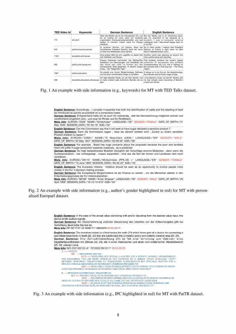
ure 1 illustrates some examples of this dataset. Ascan be seen, the keywords (second column, treatedas side information) contain additional contextualinformation that can provide complementary cuesso as to better guide the translation process. Let’stake an example in Figure 1 (TED Video Id 172),the keyword “art” provides cues for words andphrases in target sequence such as: “place, de-sign”; whereas the keyword “tech” refers to “Me-dia Lab, computer science”.

Personalised Europarl For the second dataset,we evaluate our proposed idea in the context ofpersonality-aware MT. Mirkin et al. (2015) ex-plored whether translation preserves personalityinformation (e.g., demographic and psychometrictraits) in statistical MT (SMT); and further Rabi-novich et al. (2017) found that personality infor-mation like author’s gender is an obvious signal insource text, but it is less clear in human and ma-chine translated texts. As a result, they created anew dataset for personalised MT4 partially basedon the original Europarl. The personality such asauthor’s gender will be regarded as side informa-tion in our setup. An excerpt of this dataset isshown in Figure 2. As can be seen from the figure,there exist many kinds of side information pertain-ing to authors’ traits, including identification (ID,name), native language, gender, date of birth/age,and plenary session date. Here, we will focus onthe “gender” trait and evaluate whether it can haveany benefits in the context of NMT complement-ing the work of Rabinovich et al. (2017) attempteda similar idea as part of a SMT, rather than NMT,system.

Patent MT Collection Another interesting datais patent translation which includes rich side in-formation. PatTR5 is a sentence-parallel corpuswhich is a subset of the MAREC Patent Cor-pus (Waschle and Riezler, 2012a). In general,PatTR contains millions of parallel sentences col-lected from all patent text sections (e.g., title, ab-stract, claims, description) in multiple languages(English, French, German) (Waschle and Riezler,2012b; Simianer and Riezler, 2013). An appeal-ing feature of this corpus is that it provides a la-belling at a sentence level, in the form of IPC (In-ternational Patent Classification) codes. The IPC

4http://cl.haifa.ac.il/projects/pmt/index.shtml

5http://www.cl.uni-heidelberg.de/statnlpgroup/pattr/

codes explicitly provide a hierarchical classifica-tion of patents according to various different ar-eas of technology to which they pertain. This kindof side information can provide a useful signal forMT task – which has not yet been fully exploited.Figure 3 gives us an illustrating excerpt of this cor-pus. We can see that each of sentence pair in thiscorpus is associated with any number of IPC la-bel(s) as well as other metadata, e.g., patent ID,patent family ID, publication date. In this work,we consider only the IPC labels. The full mean-ing of all IPC labels can be found on the officialIPC website,6 however we provide in Figure 3 theglossess for each referenced label. Note that thoseIPC labels form a WordNet style hierarchy (Fell-baum, 1998), and accordingly may be useful inmany other deep models of NLP.

3 NMT with Side Information

We investigate different ways of incorporatingside information into the NMT model(s).

3.1 Encoding of Side Information

In this work, we propose the use of unstructuredheterogeneous side information, which is oftenavailable in practical datasets. Due the hetero-geneity of side information, our techniques arebased on a bag-of-words (BOW) representationof the side information, an approach which wasshown to be effective in our prior work (Hoanget al., 2016a). Each element of the side informa-tion (a label, or word) is embedded using a matrixW s

e ∈ RHs×|Vs|, where |Vs| is the vocabulary ofside information and Hs the dimensionality of thehidden space. These embedding vectors are usedfor the input to several different neural architec-tures, which we now outline.

3.2 NMT Model Formulation

Recall the general formulation of NMT (Sutskeveret al., 2014; Bahdanau et al., 2015, inter alia) asa conditional language model in which the gen-eration of target sequence is conditioned on thesource sequence (Sutskever et al., 2014; Bahdanauet al., 2015, inter alia), formulated as:

yt+1 ∼ pΘ (yt+1|y<t,x)

= softmax (fΘ (y<t,x)) ; (1)

6http://www.wipo.int/classifications/ipc/en/

7

TED Video Id Keywords German Sentence English Sentence

172 arts,tech

Aber das Media Lab ist ein interessanter Ort, und es ist wichtig für mich, denn ich studierte ursprünglich Computerwissenschaften und erst später in meinem Leben habe ich Design entdeckt.

But the Media Lab is an interesting place, and it's important to me because as a student, I was a computer science undergrad, and I discovered design later on in my life.

645 politics,issues,businessIn anderen Worten, ich glaube, dass der französische Präsident Sarkozy recht hat, wenn er über eine Mittelmeer Union spricht.

So in other words, I believe that President Sarkozy of France is right when he talks about a Mediterranean union.

1193 recreation,arts,issues Eine andere Welt tat sich ungefähr zu dieser Zeit auf: Auftreten und Tanzen.

Another world was opening up around this time: performance and dancing.

692 politics,arts,issues,env

Dieses Gebäude beinhaltet die Weltgrößte Kollektion von Sammlungen und Artefakten die der Ro l le der USA im Kampf au f der Chinesischen Seite gedenken. In diesem langen Krieg -- die "fliegenden Tiger".

This building contains the world's largest collection of documents and artifacts commemorating the U.S. role in fighting on the Chinese side in that long war -- the Flying Tigers.

1087 politics,education Es erlaubt uns, Kunst, Biotechnologie, Software und all solch wunderbaren Dinge zu schaffen.

It allows us to do the art, the biotechnology, the software and all those magic things.

208 recreation,education,arts,issuesIch liebe Bartóks Musik, so wie Herr Teszler, und er hatte wirklich jede Aufnahme Bartóks die es gab.

I love Bartok's music, as did Mr. Teszler, and he had virtually every recording of Bartok's music ever issued.

Fig. 1 An example with side information (e.g., keywords) for MT with TED Talks dataset.

English Sentence: Accordingly , I consider it essential that both the identification of cattle and the labelling of beef be introduced as quickly as possible on a compulsory basis . German Sentence: Entsprechend halte ich es auch für notwendig , daß die Kennzeichnung möglichst schnell und verpflichtend eingeführt wird , und zwar für Rinder und für Rindfleisch .Meta Info: EUROID="2209" NAME="Schierhuber" LANGUAGE="DE" GENDER="FEMALE" DATE_OF_BIRTH="31 May 1946" SESSION_DATE="97-02-19" AGE="50"English Sentence: Can the Commission say that it will seek to have sugar declared a sensitive product ?German Sentence: Kann die Kommission sagen , dass sie danach streben wird , Zucker zu einem sensiblen Produkt erklären zu lassen ?Meta Info: EUROID="22861" NAME="Ó Neachtain (UEN)." LANGUAGE="EN" GENDER="MALE" DATE_OF_BIRTH="22 May 1947" SESSION_DATE="03-09-02" AGE="56"English Sentence: For example , Brazil has huge concerns about the proposals because the poor and landless there will suffer if sugar production expands massively , as is predicted .German Sentence: So hegt beispielsweise Brasilien bezüglich der Vorschläge enorme Bedenken , denn wenn die Zuckerproduktion , wie vorhergesagt , massiv expandiert , wird das die Not der Armen und Landlosen dort noch verstärken .Meta Info: EUROID="28115" NAME="McGuinness (PPE-DE )." LANGUAGE="EN" GENDER="FEMALE" DATE_OF_BIRTH="13 June 1959" SESSION_DATE="05-02-22" AGE="45"English Sentence: The European citizens ' initiative should be seen as an opportunity to involve people more closely in the EU 's decision-making process .German Sentence: Die Europäische Bürgerinitiative ist als Chance zu werten , um die Menschen stärker in den Entscheidungsprozess der EU miteinzubeziehen .Meta Info: EUROID="96766" NAME="Ernst Strasser" LANGUAGE="DE" GENDER="MALE" DATE_OF_BIRTH="29 April 1956" SESSION_DATE="10-12-15-010" AGE=“54"

Fig. 2 An example with side information (e.g., author’s gender highlighted in red) for MT with person-alised Europarl dataset.

Fig. 3 An example with side information (e.g., IPC highlighted in red) for MT with PatTR dataset.

8

where the probability pΘ (.) of generating the nexttarget word yt+1 is conditioned on the previouslygenerated target words y<t and the source se-quence x; f is a neural network which can beframed as an encoder-decoder model (Sutskeveret al., 2014) and can use an attention mechanism(Bahdanau et al., 2015; Luong et al., 2015). Inthis model, the encoder encodes the informationof the source sequence; whereas, the decoder de-codes the target sequence sequentially from left-to-right. The attention mechanism controls whichparts of the source sequence where the decodershould attend to in generating each symbol of tar-get sequence. Later, advanced models have beenproposed with modifications of the encoder anddecoder architectures, e.g., using the 1D (Gehringet al., 2017b,a) and 2D (Elbayad et al., 2018)convolutions; or a transformer network (Vaswaniet al., 2017). These advanced models have ledto significantly better results in terms of both per-formance and efficiency via different benchmarks(Gehring et al., 2017b,a; Vaswani et al., 2017; El-bayad et al., 2018).

Regardless of the NMT architecture, we aim toexplore in which case side information can be use-ful, as well as the effective and efficient way of in-corporating them with minimal modification of theNMT architecture. Mathematically, we formulatethe NMT problem given the availability of side in-formation e as follows:

yt+1 ∼ pΘ (yt+1|y<t,x, e)

= softmax (fΘ (y<t,x, e)) ; (2)

where e is the representation of additional side in-formation we would like to incorporate into NMTmodel.

3.3 Conditioning on Side Information

Keeping in mind that we would like a generic in-corporation method so that only minimal modifi-cation of NMT model is required, we propose andevaluate different approaches.

Side Information as Source Prefix/Suffix Themost simple way to include side information is toadd the side information as a string prefix or suf-fix to the source sequence, and letting the NMTmodel learn from this modified data. This methodrequires no modification of the NMT model. Thismethod was firstly proposed by Sennrich et al.(2016a) who added the side constraints (e.g., hon-

orifics) as suffix of the source sequence for con-trolling the politeness in translated outputs.

Side Information as Target Prefix Alterna-tively, we can add the bag of words as a targetprefix, inspired from Johnson et al. (2017) whointroduces an artificial token as a prefix for spec-ifying the required target language in a multilin-gual NMT system. Note that this method leads toadditional benefits in the following situations: a)when the side information exists, the model takesthem as inputs and then does its translation taskas normal; b) when the side information is miss-ing, so the model first generates the side informa-tion itself and subsequently uses it to proceed withtranslation.

Output Layer Similar to Hoang et al. (2016a) –who considers side information in the model fo-cusing on the output side which worked well inLM, this method involves in two phases. First,it transforms the representation of the side infor-mation into a summed vector representation, e =∑

m∈[1,M ] ewsm

. We also tried the average oper-ator in our preliminary experiments but observedno difference in end performance.

Next, the side representation vector, e, is addedto the output layer before the softmax transforma-tion of the NMT model, e.g.,

yt+1 ∼ softmax(W o · fdect (. . .) + be + bo

)be = W e · e;

(3)where W e ∈ R|VT |×Hs is an additional weightmatrix (learnable model parameters) for linearprojection of side information representation ontothe target output space (Hs is a predefined dimen-sion for embedding side information). The ratio-nale behind this method is to let the model learn tocontrol the importance of the existing side infor-mation contributed to the generation. The functionfdect (. . .) is specific to our chosen network repa-rameterisation, based on RNN (Sutskever et al.,2014; Bahdanau et al., 2015; Luong et al., 2015),or convolution (Gehring et al., 2017b,a; Elbayadet al., 2018), or transformer (Vaswani et al., 2017).Although we make an effort for modification ofthe NMT model, we believe that it is minimallysimple, and generic to suit many different stylesof NMT model.

Multi-task Learning Consider the case wherewe would like to use existing side information to

9

improve the main NMT task. We can define a gen-erative model p (y, e|x), formulated as:

p (y, e|x) := p (y|x, e)︸ ︷︷ ︸translation model

· p (e|x)︸ ︷︷ ︸classification model

;

(4)where p (y|x, e) is a translation model condi-tioned on the side information as explained earlier;p (e|x) can be regarded as a classification model– which predicts the side information given thesource sentence. Note that side information canoften be represented as individual words – whichcan be treated as labels, making the classificationmodel feasible.

Importantly, the above formulation of a gener-ative model would require summing over “e” attest/decode time, which might be done by decod-ing for all possible label combinations, then re-porting the sentence with the highest model score.This may be computationally infeasible in prac-tice. We resort this by approximating the NMTmodel as p (y|x, e) ≈ p (y|x), resulting in

p (y, e|x) ≈ p (y|x) · p (e|x) ; (5)

and thus force the model to encode the shared in-formation in the encoder states.

Our formulation in Equation 5 gives rise tomulti-task learning (MTL). Here, we propose thejoint learning of two different but related tasks:NMT and multi-label classification (MLC). Here,the MLC task refers to predicting the labels thatpossibly represent words of the given side infor-mation. This is interesting in the sense that themodel is capable of not only generating the trans-lated outputs, but also explicitly predicting whatthe side information is. Here, we adopt a simpleinstance of MTL for our case, called soft param-eter sharing similar to (Duong et al., 2015; Yangand Hospedales, 2016). In our MTL version, theNMT and MLC tasks share the parameters of theencoders. The difference between the two is at thedecoder part. In the NMT task, the decoder is keptunchanged. For the MLC task, we define its ob-jective function (or loss), formulated as:

LMLC := −M∑

m=1

1Tws

mlog ps; (6)

where ps is the probability of predicting the pres-ence or absence of each element in the side infor-

mation, formulated as:

ps = sigmoid

(W s

[1

|x|∑i

g′ (xi)

]+ bs

);

(7)where x is the source sequence, comprising ofx1, . . . , xi, . . . , x|x| words. Here, we denote ageneric function term g′ (.) which refers to a vec-torised representation of a specific word depend-ing on designing the network architecture, e.g.,stacked bidirectional (forward and backward) net-works over the source sequence (Bahdanau et al.,2015; Luong et al., 2015); or a convolutional en-coder (Gehring et al., 2017b,a) or a transformerencoder (Vaswani et al., 2017).7 Further, W s ∈R|Vs|×Hx and bs ∈ R|Vs| are two additional modelparameters for linear transformation of the sourcesequence representation (whereHx is a dimensionof the output of the g′ (.) function, it will differfrom network architectures as discussed earlier).

Now, we have two objective functions at thetraining stage, including the NMT loss LNMT andthe MLC loss LMLC . The total objective functionof our joint learning will be:

L := LNMT + λLMLC ; (8)

where: λ is the coefficient balancing the two taskobjectives, whose value is fine-tuned based on thedevelopment data to optimise for NMT accuracymeasured using BLEU (Papineni et al., 2002).

The idea of MTL applied for NLP was firstlyexplored by (Collobert and Weston, 2008), laterattracts increasing attentions from the NLP com-munity (Ruder, 2017). Specifically, the idea be-hind MTL is to leverage related tasks which canbe learned jointly — potentially introducing an in-ductive bias (Feinman and Lake, 2018). An alter-native explanation of the benefits of MTL is thatjoint training with multiple tasks acts as an addi-tional regulariser to the model, reducing the riskof overfitting (Collobert and Weston, 2008; Ruder,2017, inter alia).

4 Experiments

4.1 Datasets

As discussed earlier, we conducted our experi-ments using three different datasets including TEDTalks (Chen et al., 2016), Personalised Europarl

7Here, to avoid repeating the materials, we will not elab-orate their formulations.

10

No. of labels ExamplesTED Talks 11 tech business arts issues education health env recre-

ation politics othersPersonalised Europarl 2 male female

PatTR-1 (deep) 651 G01G G01L G01N A47F F25D C01B . . .PatTR-2 (shallow) 8 G A F C H B E D

Table 1 Side information statistics for the three datasets, showing the number of types of the side infor-mation label, and the set of tokens (display truncated for PatTR-1 (deep)).

(Rabinovich et al., 2017), and PatTR (Waschleand Riezler, 2012b; Simianer and Riezler, 2013),translating from German (de) to English (en). Thestatistics of the training and evaluation sets can beshown in Table 2. For the TED Talks and Per-sonalised Europarl datasets, we followed the samesizes of data splits since they are made availableon the authors’ github repository and website. Forthe PatTR dataset, we use the Abstract sectionsfor patents from 2008 or later, and the develop-ment and test sets are constructed to have 2000sentences each, similar to (Waschle and Riezler,2012b; Simianer and Riezler, 2013).

It is important to note the labeling informationfor side information. We extracted all kinds of sideinformation from three aforementioned datasets inthe form of individual words or labels. This makesthe label embeddings much easier. Their relevantstatistics and examples can be found in Table 1.

We preprocessed all the data using Moses’straining scripts8 with standard steps: punctuationnormalisation, tokenisation, truecasing. For train-ing sets, we set word-based length thresholds forfiltering long sentences since they will not be use-ful when training the seq2seq models as suggestedin the NMT literature (Sutskever et al., 2014; Bah-danau et al., 2015; Luong et al., 2015, inter alia).We chose 80, 80, 150 length thresholds for TEDTalks, Personalized Europarl, and PatTR datasets,respectively. Note that the 150 threshold indi-cates that the sentences in the PatTR dataset isin average much longer than in the others. Forbetter handling the OOV problem, we segmentedall the preprocessed data with subword units us-ing byte-pair-encoding (BPE) method proposed bySennrich et al. (2016b). We already know thatlanguages such English and German share an al-phabet (Sennrich et al., 2016b), hence learningBPE on the concatenation of source and target

8https://github.com/moses-smt/mosesdecoder/tree/master/scripts

languages (hence called shared BPE) increasesthe consistency of the segmentation. We applied32000 operations for learning the shared BPE byusing the open-source toolkit.9 Also, we used devsets for tuning model parameters and early stop-ping of the NMT models based on the perplexity.Table 2 shows the resulting vocabulary sizes aftersubword segmentation for all datasets.

4.2 Baselines and Setups

Recall that our method for incorporating the ad-ditional side information into the NMT models isgeneric; hence, it is applicable to any NMT ar-chitecture. We chose the transformer architecture(Vaswani et al., 2017) for all our experiments sinceit arguably is currently the most robust NMT mod-els compared to RNN and convolution based ar-chitectures. We re-implemented the transformer -based NMT system using the C++ Neural NetworkLibrary - DyNet10 as our deep learning backendtoolkit. Our re-implementation results in the opensource toolkit.11

In our experiments, we use the same configura-tions for all transformer models and datasets, in-cluding: 2 encoder and decoder layers; 512 inputembedding and hidden layer dimensions; sinusoidpositional encoding; dropout with 0.1 probabilityfor source and target embeddings, sub-layers (at-tention + feedforward), attentive dropout; and la-bel smoothing with weight 0.1. For training ourneural models, we used early stopping based ondevelopment perplexity, which usually occurs af-ter 20-30 epochs.12

We conducted our experiments with various in-corporation methods as discussed in Section 3. We

9https://github.com/rsennrich/subword-nmt

10https://github.com/clab/dynet/11https://github.com/duyvuleo/Transformer-DyNet/12The training process of transformer models is much

faster than the RNN and convolution - based ones, but re-quires more epochs for convergence.

11

dataset # tokens (M) # types (K) # sents # length limitTED Talks de→en

train 3.73 3.75 19.78 14.23 163653 80dev 0.02 0.02 4.03 3.15 567 n.a.test 0.03 0.03 6.07 4.68 1100 n.a.

Personalised Europarl de→entrain 8.46 8.39 21.15 14.04 278629 80dev 0.16 0.16 14.67 9.83 5000 n.a.test 0.16 0.16 14.76 9.88 5000 n.a.

PatTR de→entrain 33.07 32.52 24.97 13.28 656352 150dev 0.13 0.13 13.50 6.88 2000 n.a.test 0.13 0.12 13.35 6.89 2000 n.a.

Table 2 Statistics of the training & evaluation sets from datasets including TED Talks, PersonalisedEuroparl, and PatTR; showing in each cell the count for the source language (left) and target language(right); “#types” refers to subword-segmented vocabulary sizes; “n.a.” is not applicable, for developmentand test sets. Note that all the “#tokens”’ and “#types”’ are approximated.

Method TED Talks Personalised Europarl PatTR-1 PatTR-2base 29.48 31.12 45.86

si−src−prefix 29.28 30.87 45.99 45.97si−src−suffix 29.36 31.03 46.01 45.83

si−trg−prefix−p 29.06 30.89 45.97 45.85si−trg−prefix−h 29.28 30.93 46.03 45.92

output−layer 29.99† 31.22 46.32† 46.09w/o side info 29.62 31.10 46.14 45.99

mtl 29.86† 31.12 46.14 46.01

Table 3 Evaluation results with BLEU scores of various incorporation variants against the baseline; bold:better than the baseline, †: statistically significantly better than the baseline.

denote the system variants as follows:

base refers to the baseline NMT system using thetransformer without using any side informa-tion.

si-src-prefix and si-src-suffix refer to the NMTsystem using the side information as respec-tive prefix or suffix of the source sequence(Jehl and Riezler, 2018), applied to bothtraining and decoder/inference.

si-trg-prefix refers to the NMT system using theside information as prefix of the target se-quence. There are two variants, including“si-trg-prefix-p” means the side informationis generated by the model itself and is thenused for decoding/inference; “si-trg-prefix-h”means the side information is given at decod-ing/inference runtime.

output-layer refers to the method of incorporat-ing side information in the final output layer.

mtl refers to the multi-task learning method.

It’s worth noting that the dimensional valuefor the output-layer method was fine-tuned over

the development set, using the value range of{64, 128, 256, 512}. Similarly, the balancingweight in the mtl method is fine-tuned using thevalue range of {0.001, 0.01, 0.1, 1.0}. For evalua-tion, we measured the end translation quality withcase-sensitive BLEU (Papineni et al., 2002). Weaveraged 2 runs for each of the method variants.

4.3 Results and Analysis

The experimental results can be seen in Ta-ble 3. Overall, we obtained limited success forthe method of adding side information as prefixor suffix for TED Talks and Personalised Europarldatasets. On the PatTR dataset, small improve-ments (0.1-0.2 BLEU) are observed. We experi-mented two sets of side information in the PatTRdataset, including PatTR-1 (651 deep labels) andPatTR (8 shallow labels).13 The possible reasonfor this phenomenon is that the multi-head atten-tion mechanism in the transformer may have someconfusion given the existing side information, ei-

13The shallow setting takes the first character of each labelcode, which denotes the highest level concept in the type hi-erarchy, e.g., G01P (measuring speed) → G (physics), withdefinitions as shown in Fig 3.

12

ther in source or target sequences. In some am-biguous cases, the multi-head attention may notknow where it should pay more attention. Anotherpossible reason is that the implicit ambiguity ofside information that may exist in the data.

Contrary to these variants, the output-layer vari-ant was more consistently successful, obtainingthe best results across datasets. In the TED Talksand PatTR datasets, this method also providesthe statistically significant results compared to thebaselines. Additionally, we conducted another ex-periment by splitting the TED Talks and coarsePatTR-2 datasets by the meta categories, then ob-served the individual effects when incorporatingthe side information with output-layer variant, asshown in Figure 4a and 4b. In the TED Talksdataset, we observed improvements for most cat-egories, except for “business, education”. In thecoarse PatTR-2 dataset, the improvements are ob-tained across all categories. The key behind thissuccess of the output-layer variant is that the rep-resentation of existing side information is addedin the final output layer and controlled by addi-tional learnable model parameters. In that sense,it results in a more direct effect on lexical choiceof the NMT model. This resembles the success inthe context of language modelling as presented inHoang et al. (2016a). Further, we also obtainedthe promising results for the mtl variant althoughwe did implement a very simple instance of MTLwith a sharing mechanism and no side informationgiven at a test time. For a fair comparison with theoutput-layer method, we added an additional ex-periment in which the output-layer method doesnot have the access of side information. As ex-pected, its performance has been dropped, as canbe seen in the second last row in Table 3. In thiscase, the mtl method without the side informationat a test time performs better. We believe thatmore careful design of the mtl variant can lead toeven better results. We also think that the hybridmethod combining the output-layer and mtl vari-ants is also an interesting direction for future re-search, e.g., relaxing the approximation as shownin Equation 5.

Given the above results, we can find that thecharacteristics of side information plays an impor-tant role in improving the NMT models. Our em-pirical experiments show that topical information(as in the TED Talks and PatTR datasets) is moreuseful than the personal traits (as in the Person-

BLEU

25.0

27.5

30.0

32.5

35.0

Category

arts business education environment health issues politics recreation technology others

29.228.6

30.230.430.5

31.3

27.5

33.5

27.9

30.5

29.1

27.928.3

29.629.7

31.4

27.1

34.7

28.0

29.6

baseline output-layer

(a) The TEDTalks dataset.

BLEU

30.0

34.2

38.4

42.6

46.8

51.0

Category

A B C D E F G H

50.148.648.9

35.8

42.1

47.5

45.4

43.0

49.4

47.447.8

35.2

39.6

47.145.4

42.4

baseline output-layer

(b) The coarse PatTR-2 dataset.

Fig. 4 Effects on individual BLEU scores for eachof categories in the TEDTalks and coarse PatTR-2datasets, with the NMT model enhanced with theoutput-layer variant.

alised Europarl dataset). However, sometimes it isstill good to reserve the personal traits in the tar-get translations (Rabinovich et al., 2017) althoughtheir BLEU scores are not necessarily better.

5 Related Work

Our work is mainly inspired from Hoang et al.(2016a) who proposed the use of side informa-tion for boosting the performance of recurrent neu-ral network language models. We further applythis idea for a downstream task in neural machinetranslation.

We’ve adapted different methods in the litera-ture for this specific problem and evaluated usingdifferent datasets with different kinds of side in-formation.

Our methods for incorporating side informa-tion as suffix, prefix for either source or target se-quences have been adapted from (Sennrich et al.,2016a; Johnson et al., 2017). Also working onthe same patent dataset, Jehl and Riezler (2018)proposed to incorporate document meta informa-tion as special tokens, similar to our source pre-fix/suffix method, or by concatenating the tag witheach source word. They report an improvements,consistent with our findings, although the changes

13

they observe are larger, of about 1 BLEU point,albeit from a lower baseline.

Also, Michel and Neubig (2018) proposed topersonalise neural MT systems by taking the vari-ance that each speaker speaks/writes on his owninto consideration. They proposed the adaptationprocess which takes place in the “output” layer,similar to our output layer incorporation method.

The benefit of the proposed MTL approach isnot surprising, resembling from existing works,e.g., jointly training translation models from/tomultiple languages (Dong et al., 2015); jointlytraining the encoders (Zoph and Knight, 2016) orboth encoders and decoders (Johnson et al., 2017).

6 Conclusion

In this work, we have presented various situationsto which extent the side information can boost theperformance of the NMT models. We have stud-ied different kinds of side information (e.g. topicinformation, personal trait) as well as present dif-ferent ways of incorporating them into the existingNMT models. Though being simple, the idea ofutilising the side information for NMT is indeedfeasible and we have proved it via our empiricalexperiments. Our findings will encourage practi-tioners to pay more attention to the side informa-tion if exists. Such side information can providevaluable external knowledge that compensates forthe learning models. Further, we believe that thisidea is not limited to the context of neural LM orNMT, but it may be applicable to other NLP taskssuch as summarisation, parsing, reading compre-hension, and so on.

Acknowledgments

We thank the reviewers for valuable feedbacks anddiscussions. Cong Duy Vu Hoang is supportedby Australian Government Research Training Pro-gram Scholarships at the University of Melbourne,Australia.

ReferencesDzmitry Bahdanau, Kyunghyun Cho, and Yoshua Ben-

gio. 2015. Neural Machine Translation by JointlyLearning to Align and Translate. In Proc. of 3rdInternational Conference on Learning Representa-tions (ICLR2015).

Iacer Calixto and Qun Liu. 2017. Incorporatingglobal visual features into attention-based neu-ral machine translation. In Proceedings of the

2017 Conference on Empirical Methods in Natu-ral Language Processing, EMNLP 2017, Copen-hagen, Denmark, September 9-11, 2017. pages992–1003. https://aclanthology.info/papers/D17-1105/d17-1105.

Iacer Calixto, Qun Liu, and Nick Campbell. 2017.Doubly-attentive decoder for multi-modal neuralmachine translation. In Proceedings of the 55th An-nual Meeting of the Association for ComputationalLinguistics, ACL 2017, Vancouver, Canada, July 30- August 4, Volume 1: Long Papers. pages 1913–1924. https://doi.org/10.18653/v1/P17-1175.

Mauro Cettolo, Christian Girardi, and Marcello Fed-erico. 2012. WIT3: Web Inventory of Transcribedand Translated Talks. In Proceedings of the 16thConference of the European Association for Ma-chine Translation (EAMT). Trento, Italy, pages 261–268.

Wenhu Chen, Evgeny Matusov, Shahram Khadivi,and Jan-Thorsten Peter. 2016. Guided align-ment training for topic-aware neural ma-chine translation. CoRR abs/1607.01628.http://arxiv.org/abs/1607.01628.

Trevor Cohn, Cong Duy Vu Hoang, Ekaterina Vy-molova, Kaisheng Yao, Chris Dyer, and Gholam-reza Haffari. 2016. Incorporating Structural Align-ment Biases into an Attentional Neural Transla-tion Model. In Proceedings of the 2016 Confer-ence of the North American Chapter of the Associ-ation for Computational Linguistics: Human Lan-guage Technologies. Association for ComputationalLinguistics, San Diego, California, pages 876–885.http://www.aclweb.org/anthology/N16-1102.

Ronan Collobert and Jason Weston. 2008. A uni-fied architecture for natural language process-ing: Deep neural networks with multitask learn-ing. In Proceedings of the 25th InternationalConference on Machine Learning. ACM, NewYork, NY, USA, ICML ’08, pages 160–167.https://doi.org/10.1145/1390156.1390177.

Daxiang Dong, Hua Wu, Wei He, Dianhai Yu, andHaifeng Wang. 2015. Multi-task learning for mul-tiple language translation. In ACL (1). The Associa-tion for Computer Linguistics, pages 1723–1732.

Long Duong, Trevor Cohn, Steven Bird, and PaulCook. 2015. Low resource dependency parsing:Cross-lingual parameter sharing in a neural networkparser. In Proceedings of the 53rd Annual Meet-ing of the Association for Computational Linguisticsand the 7th International Joint Conference on Natu-ral Language Processing (Volume 2: Short Papers).Association for Computational Linguistics, pages845–850. https://doi.org/10.3115/v1/P15-2139.

Maha Elbayad, Laurent Besacier, and Jakob Ver-beek. 2018. Pervasive attention: 2d con-volutional neural networks for sequence-to-sequence prediction. CoRR abs/1808.03867.http://arxiv.org/abs/1808.03867.

14

Reuben Feinman and Brenden M. Lake.2018. Learning inductive biases with sim-ple neural networks. CoRR abs/1802.02745.http://arxiv.org/abs/1802.02745.

Christiane Fellbaum, editor. 1998. WordNet: An Elec-tronic Lexical Database. Language, Speech, andCommunication. MIT Press, Cambridge, MA.

Mercedes Garcıa-Martınez, Loıc Barrault, and FethiBougares. 2017. Neural machine translation bygenerating multiple linguistic factors. CoRRabs/1712.01821. http://arxiv.org/abs/1712.01821.

Jonas Gehring, Michael Auli, David Grangier, andYann Dauphin. 2017a. A convolutional en-coder model for neural machine translation. InProceedings of the 55th Annual Meeting of theAssociation for Computational Linguistics, ACL2017, Vancouver, Canada, July 30 - August4, Volume 1: Long Papers. pages 123–135.https://doi.org/10.18653/v1/P17-1012.

Jonas Gehring, Michael Auli, David Grangier, De-nis Yarats, and Yann N. Dauphin. 2017b. Con-volutional sequence to sequence learning. InProceedings of the 34th International Conferenceon Machine Learning, ICML 2017, Sydney, NSW,Australia, 6-11 August 2017. pages 1243–1252.http://proceedings.mlr.press/v70/gehring17a.html.

Cong Duy Vu Hoang, Trevor Cohn, and Gholam-reza Haffari. 2016a. Incorporating Side Informa-tion into Recurrent Neural Network Language Mod-els. In Proceedings of the 2016 Conference ofthe North American Chapter of the Associationfor Computational Linguistics: Human LanguageTechnologies. Association for Computational Lin-guistics, San Diego, California, pages 1250–1255.http://www.aclweb.org/anthology/N16-1149.

Cong Duy Vu Hoang, Reza Haffari, and TrevorCohn. 2016b. Improving Neural Translation Mod-els with Linguistic Factors. In Proceedings ofthe Australasian Language Technology AssociationWorkshop 2016. Melbourne, Australia, pages 7–14.http://www.aclweb.org/anthology/U16-1001.

Laura Jehl and Stefan Riezler. 2018. Document-levelinformation as side constraints for improved neuralpatent translation. In Proceedings of the 13th Con-ference of the Association for Machine Translationin the Americas, AMTA 2018, Boston, MA, USA,March 17-21, 2018 - Volume 1: Research Papers.pages 1–12. https://aclanthology.info/papers/W18-1802/w18-1802.

Melvin Johnson, Mike Schuster, Quoc Le, MaximKrikun, Yonghui Wu, Zhifeng Chen, Nikhil Thorat,Fernand a Vigas, Martin Wattenberg, Greg Corrado,Macduff Hughes, and Jeffrey Dean. 2017. Google’smultilingual neural machine translation system: En-abling zero-shot translation. Transactions of the As-sociation for Computational Linguistics 5:339–351.https://transacl.org/ojs/index.php/tacl/article/view/1081.

Thang Luong, Hieu Pham, and Christopher D. Man-ning. 2015. Effective Approaches to Attention-based Neural Machine Translation. In Proceed-ings of the 2015 Conference on Empirical Methodsin Natural Language Processing. Association forComputational Linguistics, Lisbon, Portugal, pages1412–1421. http://aclweb.org/anthology/D15-1166.

Evgeny Matusov, Andy Way, Iacer Calixto, DanielStein, Pintu Lohar, and Sheila Castilho. 2017.Using images to improve machine-translating e-commerce product listings. In Proceedings ofthe 15th Conference of the European Chap-ter of the Association for Computational Lin-guistics, EACL 2017, Valencia, Spain, April3-7, 2017, Volume 2: Short Papers. pages637–643. https://aclanthology.info/papers/E17-2101/e17-2101.

Haitao Mi, Baskaran Sankaran, Zhiguo Wang, and AbeIttycheriah. 2016. Coverage Embedding Models forNeural Machine Translation. In Proceedings of the2016 Conference on Empirical Methods in Natu-ral Language Processing. Association for Compu-tational Linguistics, Austin, Texas, pages 955–960.

Paul Michel and Graham Neubig. 2018. Extremeadaptation for personalized neural machine trans-lation. In Proceedings of the 56th Annual Meet-ing of the Association for Computational Lin-guistics (Volume 2: Short Papers). Associationfor Computational Linguistics, pages 312–318.http://aclweb.org/anthology/P18-2050.

Shachar Mirkin, Scott Nowson, Caroline Brun, andJulien Perez. 2015. Motivating personality-aware machine translation. In Proceedingsof the 2015 Conference on Empirical Meth-ods in Natural Language Processing. Associationfor Computational Linguistics, pages 1102–1108.https://doi.org/10.18653/v1/D15-1130.

Kishore Papineni, Salim Roukos, Todd Ward, andWei-Jing Zhu. 2002. BLEU: A Method for Au-tomatic Evaluation of Machine Translation. InProceedings of the 40th Annual Meeting on As-sociation for Computational Linguistics. Asso-ciation for Computational Linguistics, Strouds-burg, PA, USA, ACL ’02, pages 311–318.https://doi.org/10.3115/1073083.1073135.

Ella Rabinovich, Raj Nath Patel, Shachar Mirkin, Lu-cia Specia, and Shuly Wintner. 2017. Personal-ized machine translation: Preserving original authortraits. In Proceedings of the 15th Conference of theEuropean Chapter of the Association for Computa-tional Linguistics: Volume 1, Long Papers. Asso-ciation for Computational Linguistics, pages 1074–1084. http://aclweb.org/anthology/E17-1101.

Sebastian Ruder. 2017. An overview of multi-task learning in deep neural networks. CoRRabs/1706.05098. http://arxiv.org/abs/1706.05098.

Rico Sennrich and Barry Haddow. 2016. Linguisticinput features improve neural machine translation.

15

In Proceedings of the First Conference on MachineTranslation: Volume 1, Research Papers. Associ-ation for Computational Linguistics, pages 83–91.https://doi.org/10.18653/v1/W16-2209.

Rico Sennrich, Barry Haddow, and Alexandra Birch.2016a. Controlling politeness in neural machinetranslation via side constraints. In Proceedingsof the 2016 Conference of the North AmericanChapter of the Association for Computational Lin-guistics: Human Language Technologies. Associ-ation for Computational Linguistics, pages 35–40.https://doi.org/10.18653/v1/N16-1005.

Rico Sennrich, Barry Haddow, and AlexandraBirch. 2016b. Neural machine translation ofrare words with subword units. In Proceed-ings of the 54th Annual Meeting of the As-sociation for Computational Linguistics (Volume1: Long Papers). Association for ComputationalLinguistics, Berlin, Germany, pages 1715–1725.http://www.aclweb.org/anthology/P16-1162.

Patrick Simianer and Stefan Riezler. 2013. Multi-task learning for improved discriminative trainingin SMT. In Proceedings of the Eighth Workshopon Statistical Machine Translation. Association forComputational Linguistics, Sofia, Bulgaria, pages292–300. http://www.aclweb.org/anthology/W13-2236.

Ilya Sutskever, Oriol Vinyals, and Quoc V. Le. 2014.Sequence to Sequence Learning with Neural Net-works. In Proceedings of the 27th InternationalConference on Neural Information Processing Sys-tems. MIT Press, Cambridge, MA, USA, NIPS’14,pages 3104–3112.

Ashish Vaswani, Noam Shazeer, Niki Parmar, JakobUszkoreit, Llion Jones, Aidan N Gomez, Ł ukaszKaiser, and Illia Polosukhin. 2017. Attention is allyou need. In I. Guyon, U. V. Luxburg, S. Ben-gio, H. Wallach, R. Fergus, S. Vishwanathan, andR. Garnett, editors, Advances in Neural Informa-tion Processing Systems 30, Curran Associates, Inc.,pages 5998–6008. http://papers.nips.cc/paper/7181-attention-is-all-you-need.pdf.

Katharina Waschle and Stefan Riezler. 2012a.Analyzing Parallelism and Domain Similar-ities in the MAREC Patent Corpus. Mul-tidisciplinary Information Retrieval pages12–27. http://www.cl.uni-heidelberg.de/ rie-zler/publications/papers/IRF2012.pdf.

Katharina Waschle and Stefan Riezler. 2012b. Struc-tural and Topical Dimensions in Multi-Task PatentTranslation. In Proceedings of the 13th Confer-ence of the European Chapter of the Associationfor Computational Linguistics (EACL 2012), Avi-gnon, France. http://www.aclweb.org/anthology-new/E/E12/E12-1083.pdf.

Yongxin Yang and Timothy M. Hospedales.2016. Trace norm regularised deep multi-

task learning. CoRR abs/1606.04038.http://arxiv.org/abs/1606.04038.

Jiacheng Zhang, Yang Liu, Huanbo Luan, Jingfang Xu,and Maosong Sun. 2017. Prior knowledge inte-gration for neural machine translation using poste-rior regularization. In Proceedings of the 55th An-nual Meeting of the Association for ComputationalLinguistics (Volume 1: Long Papers). Associationfor Computational Linguistics, pages 1514–1523.https://doi.org/10.18653/v1/P17-1139.

B. Zoph and K. Knight. 2016. Multi-sourceneural translation. In Proc. NAACL.http://www.isi.edu/natural-language/mt/multi-source-neural.pdf.

16

Text-dependent Forensic Voice Comparison: Likelihood Ratio Estima-

tion with the Hidden Markov Model (HMM) and Gaussian Mixture

Model – Universal Background Model (GMM-UBM) Approaches

Satoru Tsuge

Daido University, Japan

tsuge@daido-it.ac.jp

Shunichi Ishihara

Australian National University

shunichi.ishihara@anu.edu.au

Abstract

Among the more typical forensic voice

comparison (FVC) approaches, the acous-

tic-phonetic statistical approach is suitable

for text-dependent FVC, but it does not

fully exploit available time-varying infor-

mation of speech in its modelling. The au-

tomatic approach, on the other hand, es-

sentially deals with text-independent cas-

es, which means temporal information is

not explicitly incorporated in the model-

ling. Text-dependent likelihood ratio (LR)-

based FVC studies, in particular those that

adopt the automatic approach, are few.

This preliminary LR-based FVC study

compares two statistical models, the Hid-

den Markov Model (HMM) and the

Gaussian Mixture Model (GMM), for the

calculation of forensic LRs using the same

speech data. FVC experiments were car-

ried out using different lengths of Japanese

short words under a forensically realistic,

but challenging condition: only two speech

tokens for model training and LR estima-

tion. Log-likelihood-ratio cost (Cllr) was

used as the assessment metric. The study

demonstrates that the HMM system con-

stantly outperforms the GMM system in

terms of average Cllr values. However,

words longer than three mora are needed if

the advantage of the HMM is to become

evident. With a seven-mora word, for ex-

ample, the HMM outperformed the GMM

by a Cllr value of 0.073.

1 Introduction

After the DNA success story, the likelihood ratio

(LR)-based approach became the new paradigm

for evaluating and presenting forensic evidence in

court. The LR approach has also been applied to

speech evidence(Rose, 2006), and it is increasing-

ly accepted in forensic voice comparison (FVC)

as well (Morrison, 2009).

There are two different approaches in FVC.

They are the ‘acoustic-phonetic statistical ap-

proach’ and the ‘automatic approach’ (Morrison et

al., 2018). The former usually works on compara-

ble phonetic units that can be found in both the of-

fender and suspect samples. In the latter, acoustic

measurements are usually carried out over all por-

tions of the available recordings, resulting in more

detailed acoustic characteristics of the speakers.

The common statistical models used in the auto-

matic approach are the Gaussian mixture model –

universal background model (GMM-UBM)

(Reynolds et al., 2000) and i-vectors with proba-

bilistic linear discrimination analysis (PLDA)

(Burget et al., 2011). Due to its nature, the auto-

matic approach is mainly used for text-

‘independent’ FVC, and there is a good amount of

research on this (Enzinger & Morrison, 2017;

Enzinger et al., 2016). The acoustic-phonetic sta-

tistical approach is a type of text-‘dependent’ FVC

because it tends to focus on particular linguistic

units, such as phonemes, words, phrases, etc. Hav-

ing said that, even if one is targeting a particular

word or phrase, for example ‘hello’, all obtainable

features are not exploited in the acoustic-phonetic

statistical approach because it still tends to focus

on particular segments or phonemes of the word

or phrase, e.g. the formant trajectories of the diph-

thong and the static spectral information of the

fricative (Rose, 2017).

One of the advantages of text-dependent FVC

is the availability of the time-varying characteris-

tics of a speaker, which is information that can be

explicitly included in the modelling.

There are a good number of LR-based text-

independent FVC studies in the automatic ap-

proach (Enzinger & Morrison, 2017; Enzinger et

al., 2016). However, although there are some stud-

Satoru Tsuge and Shunichi Ishihara. 2018. Text-dependent Forensic Voice Comparison: Likelihood Ratio Estimation withthe Hidden Markov Model (HMM) and Gaussian Mixture Model. In Proceedings of Australasian Language TechnologyAssociation Workshop, pages 17−25.

ies in which text-independent models (e.g. GMM)

were applied to text-dependent FVC scenarios

(Morrison, 2011), to the best of our knowledge,

studies on LR-based text-dependent FVC in the

automatic approach are scarce.

In this study, a text-dependent LR-based FVC

system with the GMM-UBM based system

(GMM system) and that with the hidden Markov

model (HMM system) are compared in their per-

formance using the same data. The transitional

characteristic of individual speech can be explicit-

ly modelled in the latter system.

Words of various length are used for testing

purposes to see how word duration influences the

performance of the systems. Having the forensi-

cally realistic condition of data sparsity in mind,

we used only two tokens of each word for model-

ling and testing.

It is naturally expected that, given a sufficient

amount of data, the HMM system outperforms the

GMM system. However, it is not so clear whether

the above expectation is realistic when the amount

of data is limited. Even if the HMM system works

better, it is important to establish how the HMM

and GMM systems compare with respect to the

calculation of strength of LR, and also how and

under what conditions the former is more advan-

tageous than the latter.

2 Likelihood Ratios

The LR framework has been advocated by many

as the logically and legally correct framework for

assessing forensic evidence and reporting the out-

come in court (Aitken, 1995; Aitken & Stoney,

1991; Aitken & Taroni, 2004; Balding & Steele,

2015; Evett, 1998; Robertson & Vignaux, 1995).

A substantial amount of fundamental research on

FVC has been carried out since the late 1990s

(Gonzalez-Rodriguez et al., 2007; Morrison,

2009; Rose, 2006), and it is now accepted in an

increasing number of countries (Morrison et al.,

2016).

In the LR framework, the task of the forensic

expert is to estimate strength of evidence and re-

port it to the court. LR is a measure of the quanti-

tative strength of evidence, and is calculated using

the formula in 1).

In 1), E is the evidence, i.e. the measured prop-

erties of the voice evidence; p(E|Hp) is the proba-

bility of E, given Hp, in other words the prosecu-

tion or same-speaker hypothesis; p(E|Hd) is the

probability of E, given Hd, in other words the de-

fence or different-speaker hypothesis (Robertson

& Vignaux, 1995). The LR can be considered in

terms of the ratio between similarity and typicali-

ty. Similarity here means the similarity of evi-

dence attributable to the offender and the suspect,

respectively. Typicality means the typicality of

that evidence against the relevant population.

The relative strength of the given evidence with

respect to the competing hypotheses (Hp vs. Hd) is

reflected in the magnitude of the LR. If the evi-

dence is more likely to occur under the prosecu-

tion hypothesis than under the defence hypothesis,

the LR will be higher than 1. If the evidence is

more likely to occur under the defence hypothesis

than under the persecution hypothesis, the LR will

be lower than 1. For example, LR = 30 means that

the evidence is 30 times more likely to occur on

the assumption that the evidence is from the same

person than on the assumption that it is not.

The important point is that the LR is concerned

with the probability of the evidence, given the hy-

pothesis (either Hp or Hd). The probability of the

evidence can be estimated by forensic scientists.

They legally must not and logically cannot esti-

mate the probability of the hypothesis, given the

evidence. This is because the forensic scientist is

not legally in a position to refer to the ultimate

‘guilty vs. non-guilty’ question, i.e. the probability

of the hypothesis, given the evidence. That is the

task of the trier-of-fact. Furthermore, the forensic

scientist would need to refer to the Bayesian theo-

rem to estimate the probability of the hypothesis,

given the evidence, using prior information that is

only accessible to the trier-of-fact; thus the foren-

sic scientist cannot logically estimate the probabil-

ity of the hypothesis.

3 Experimental Design

In this section, the nature of the database used for

the experiments is explained first. This is followed

by an illustration as to how the speaker compari-

sons were set up for the experiments. The acoustic

features used in this study will be explained to-

wards the end.

3.1 Database

Our data were extracted from the National Re-

search Institute of Police Science (NRIPS) data-

LR=p(E|Hp)

p(E|Hd) 1)

18

base (Makinae et al., 2007). The database consists

of recordings collected from 316 male and 323

female speakers. All utterances were read-out

speech, consisting of single syllables, words, se-

lected sentences and so on. The word-based re-

cordings stored in the database provided the data

used in this study.

Participants ranged in age from 18 to 76 years.

The metadata provide information on the areas of

Japan (or overseas in some cases) where they have

resided, as well as their height, weight, and their

health conditions on the day of recording. Only

male speakers who completed the recordings in

two different sessions separated by 2-3 months,

without any mis-recordings for the target 66

words, were selected for the current study (result-

ing in 310 speakers). Each word was recorded on-

ly twice in each session.

The rhythmic unit of Japanese is the mora.

Based on mora, the 66 words, all listed in Table 1,

consist of 25 two-, 16 three-, 22 four-, 2 five- and

1 seven-mora words.

The 310 speakers were separated into six dif-

ferent, mutually exclusive groups: Gr1 (59 speak-

ers), Gr2 (60), Gr3 (60), Gr4 (60), Gr5 (60) and

Gr6 (13). Five different experiments were con-

ducted using the six groups, as shown in Table 2.

The test database was used for simulating two

types of offender-suspect comparisons: same-

speaker (SS) and different-speaker (DS). An LR

was estimated for each of the comparisons. The

development database was also called upon for

simulating offender-suspect comparisons, but the

derived scores (pre-calibration LRs) were specifi-

cally used to obtain the weights for calibration (re-

fer to §4.4 for details on calibration). The back-

ground database was used to build the statistical

model for typicality.

As mentioned earlier, there are two recordings

per speaker for each word in each session. The

suspect model was built using two recordings tak-

en from one session, and an LR was estimated for

each of the two recordings of the other session

(offender evidence). The same process was re-

peated by swapping the recordings of the sessions.

In this way, 4 LRs were obtained for each SS

comparison, and 8 LRs for each DS comparison.

Thus, the number of comparisons is 4*n (n =

number of speakers) for the SS comparisons, and

8*nC2 (C=combination) for the DS comparisons.

Using the five different groups (Gr1~5) separately

ze.ro

‘zero’

ku.ru.ma

‘car’

ko.o.so.ku

‘highway’

hya.ku

‘hundred’

ka.ne

‘money’;=

go.ze.n

‘AM’

re.e

‘zero’

de.n.wa

‘telephone’

ya.ku.so.ku

‘promise’

sa.n.bya.ku

‘three hundred’

da.i.jyo.o.bu

‘fine’

wa.ta.shi

‘I’

i.chi

‘one’

ke.e.sa.tsu

‘police’

o.n.na

‘woman’

ro.p.pya.ku

‘six hundred’

ki.no.o

‘yesterday’

ko.do.mo

‘child’

sa.n

‘three’

do.ku

‘poison’

o.ku.sa.n

‘wife’

ha.p.pya.ku

‘eight hundred’

kyo.o

‘today’

ke.e.ta.i

‘mobile phone’

yo.n

‘four’

re.n.ra.ku

‘contact’

re.su.to.ra.n

‘restaurant’

se.n

‘thousand’

a.shi.ta

‘tomorrow’

ka.ji

‘fire’

ro.ku

‘six’

ba.ku.da.n

‘bomb’

po.su.to

‘post’

i.s.se.n

‘one thousand’

ge.n.ki.n

‘cash’

ko.n.bi.ni

‘store’

na.na

‘seven’

gi.n.ko.o

‘bank’

sa.a.bi.su.e.ri.a

‘road house’

go.go

‘afternoon’

a.no.o

‘well (filler)’

ta.ku.shi.i

‘taxi’

shi.chi

‘seven’

ji.ka.n

‘time’

sa.n.ze.n

‘three thousand’

e.ki

‘station’

ne.e

‘well (filler)’

i.n.ta.a

‘interchange’

ha.chi

‘eight’

mo.shi.mo.shi

‘hello (phone)’

ha.s.se.n

‘eight thousand’

o.ma.e

‘you’

a.no.ne.e

‘well (filler)’’

me.e.ru

‘mail’

kyu.u

‘nine’

ha.i

‘yes’

ma.n

‘ten thousand’

o.i

‘hay’

na.ka.ma

‘mate’

ba.n.go.o

‘number’

jyu.u

‘ten’

o.re.

‘I’

o.ku

‘million’

ba.ku.ha.tsu

‘explosion’

ka.i.sha

‘company’

ko.o.za

‘account’

Table 1: 66 target words with their glosses. Each mora is separated by a period.

Experiments Test Dev Back

Exp1 Gr1 Gr2 Gr3,4,5,6

Exp2 Gr2 Gr3 Gr1,4,5,6

Exp3 Gr3 Gr4 Gr1,2,5,6

Exp4 Gr4 Gr5 Gr1,2,3,6

Exp5 Gr5 Gr1 Gr2,3,4,6

Table 2: Usage of Gr1~6 for experiments (Exp). Test,

Dev and Back refer to test, development and back-

ground databases.

19

as a test database, it was possible, altogether, to

carry out 1188 SS comparisons and 69392 DS

comparisons. The breakdowns of the SS and DS

comparisons are given in Table 3 for the five ex-

periments (Exp1~5).

The NRIPS database also contains the record-

ings of 50 sentences that are based on ATR pho-

netically balanced Japanese sentences (Kurematsu

et al., 1990). These sentences were used to build

the initial statistical models (refer to §4.1 and §4.2

for details).

3.2 Acoustic Features

Twelve mel-frequency cepstral coefficients

(MFCCs), 12 Δ MFCCs and Δ log power (a fea-

ture vector of 25th-order) were extracted with a 20

msec wide hamming window shirting every 10

msec.

4 Estimation of Likelihood Ratios

In this section, the two different modelling tech-

niques used in the current study are explained.

This is followed by an exposition of the method

for calculating scores with these models. The

method used for converting the scores to the LRs,

namely calibration, will be explained last.

For this study, the suspect model, rather than

being based solely on the data of the suspect

speaker, was generated by adapting a speaker-

unspecific model (background model) by means

of a maximum a posteriori (MAP) procedure.

Three different numbers of Gaussians (4, 8 and

16) were tried in the models.

4.1 GMM Models

The following is the process of building a speak-

er-specific word-dependent GMM for each speak-

er.

1) To build a speaker-unspecific word-

independent GMM using the recordings of the

phonetically balanced utterances;

2) To build a speaker-unspecific word-dependent

GMM for each word by training the speaker-

unspecific word-independent GMM, which

was generated in 1), with the relevant word

recordings of the background database;

3) To build the speaker-specific word-dependent

GMM (suspect model = λsus) for each word by

training the speaker-unspecific word-

independent GMM, which was built in 2),

with the speaker specific data in the test data-

base, while applying a MAP adaptation.

The speaker-unspecific word-dependent GMM,

which was built in 2) for each word, was used as

the background model (λbkg).

4.2 HMM Models

The following is the process of building a speak-

er-specific word-dependent HMM for each speak-

er.

1) To build speaker-unspecific phoneme-

dependent HMMs using the recordings of the

phonetically balanced utterances;

2) To build an initial speaker-unspecific word-

dependent HMM for each word by concate-

nating speaker-unspecific phoneme-

dependent HMMs, which were built in 1).

3) To build speaker-specific word-dependent

HMM (suspect model = λsus) by training the

initial speaker-unspecific word-dependent

HMM, which was built in 2), with the speaker

specific data in the test database, while apply-

ing a MAP adaptation.

The initial speaker-unspecific word-dependent

HMM, which was built in 2), was trained with the

relevant word recordings of the background data-

base, and the resultant model was used as the

speaker-unspecific word-dependent background

model (λbkg).

4.3 Score Calculations

The score of each comparison can be estimated

using the equation given in 2), in which s = score,

xt = an observation sequence of vectors of acous-

tic features constituting the offender data of which

there are a total of T, λsus = suspect model and λbkg = background model.

𝑠 =1

𝑇∑log(𝑝(𝑥𝑡|𝜆𝑠𝑢𝑠))

𝑇

𝑡=1

− log (𝑝(𝑥𝑡|𝜆𝑏𝑘𝑔))

2)

Experiments SS DS

Exp1: Gr1 (59) 236 13688

Exp2: Gr2 (60) 240 14160

Exp3: Gr3 (60) 240 14160

Exp4: Gr4 (58) 232 13224

Exp5: Gr5 (60) 240 14160

Total 1188 69392

Table 3: Numbers of SS and DS comparisons for each

word.

20

A score is estimated as the mean of the relative

values of the two probability density functions for

the feature vectors extracted from the offender da-

ta, and was calculated for each of the SS and DS

comparisons.

4.4 Scores to Likelihood Ratios

The outcomes of the GMM and HMM systems

are not LRs, but are known as scores. The value of

a score provides information about the degree of

the similarity between the two speech samples, i.e.

the offender and suspect samples, having taken in-

to account their typicality with respect to the rele-

vant population; it is not directly interpretable as

an LR (Morrison, 2013, p. 2). Thus, the scores

need to be converted to LRs by means of a cali-

bration process. As we will see in §6, calibration

is an essential part of LR-based FVC.

Logistic-regression calibration (Brümmer & du

Preez, 2006) is a commonly used method that

converts scores to interpretable LRs by applying

linear shifting and scaling in the log odds space. A

logistic-regression line (e.g. y = ax + b; x = score;

y = log10LR) whose weights (i.e. a and b in y = ax

+ b) are estimated from the SS and DS scores of

the development database is used to monotonical-

ly shift (by the amount of b) and scale (by the

amount of a) the scores of the testing database to

the log10LRs.

5 Assessment Metrics

A common way of assessing the performance of

a classification system is with reference to its

correct- or incorrect-classification rate: for in-

stance, how many of the SS comparisons were

correctly assessed as coming from the same

speakers, and how many of the DS comparisons

were correctly assessed as coming from different

speakers. In the context of LR-based FVC, an LR

can be used as a classification function with LR

= 1 as unity. However, correct- or incorrect-

classification rate is a binary decision (same

speaker or different speakers), which refers to the

ultimate issue of ‘guilty vs. non-guilty’. As ex-

plained in §2, it is not the task of the forensic ex-

pert, but of the trier-of-fact, to make such a deci-

sion. Thus, any metrics based on binary decision

are not coherent with the LR framework.

As emphasised in §2, the task of the forensic

expert is to estimate the strength of evidence as

accurately as possible, and the strength of evi-

dence, which can be quantified by means of a LR,

is not binary in nature, but continuous. For exam-

ple, both LR = 10 and LR = 20 support the correct

hypothesis for the SS comparisons, but the latter

supports the hypothesis more strongly than the

former. The relative strength of the LR needs to be

taken into account in the assessment.

Hence, in this study, the log-likelihood-ratio

cost (Cllr), which is a gradient metric based on

LR, was used as the metric for assessing the per-

formance of the LR-based FVC system. The cal-

culation of Cllr is given in 3) (Brümmer & du

Preez, 2006).

Cllr=1

2

(

1

NHp∑ log2 (1+

1

LRi)

NHp

i forHp=true+

1

NHd∑ log2(1+LRj)

NHd

j forHd=true )

3)

In 3), NHp and NHd are the number of SS and

DS comparisons, and LRi and LRj are the linear

LRs derived from the SS and DS comparisons, re-

spectively. Under a perfect system, all SS compar-

isons should produce LRs greater than 1, since or-

igins are identical; as, in the case of DS compari-

sons, origins are different, DS comparisons should

produce LRs less than 1. Cllr takes into account

the magnitude of derived LR values, and assigns

them appropriate penalties. In Cllr, LRs that sup-

port the counter-factual hypotheses or, in other

words, contrary-to-fact LRs (LR < 1 for SS com-

parisons and LR > 1 for DS comparisons) are

heavily penalised and the magnitude of the penal-

ty is proportional to how much the LRs deviate

from unity. Optimum performance is achieved

when Cllr = 0 and decreases as Cllr approaches and

exceeds 1. Thus, the lower the Cllr value, the better

the performance.

The Cllr measures the overall performance of a

system in terms of validity based on a cost func-

tion in which there are two main components of

loss: discrimination loss (Cllrmin) and calibration

loss (Cllrcal) (Brümmer & du Preez, 2006). The

former is obtained after the application of the so-

called pooled-adjacent-violators (PAV) transfor-

mation – an optimal non-parametric calibration

procedure. The latter is obtained by subtracting

the former from the Cllr. In this study, besides Cllr,

Cllrmin and Cllr

cal are also referred to.

The magnitude of the derived LRs is visually

presented using Tippett plots. Details on how to

read a Tippett plot are explained in §6, when the

plots are presented.

21

6 Experimental Results and Discussions

The average Cllr, Cllrmin and Cllr

cal values were cal-

culated according to the mora numbers; they are

plotted in Figure 1 as a function of word duration,

separately for the HMM and GMM systems. The

numerical values of Figure 1 are given in Table 4.

Although this was expected, it can be seen from

Figure 1a and Table 4 that the overall perfor-

mance (Cllr) of both systems improves as the

words become longer in terms of mora, and also

that the HMM system constantly outperforms the

GMM system as far as average Cllr values are

concerned. The performance gap between the two

systems becomes wider as the number of mora in-

creases, with the performance of the two systems

being similar with words of two and three moras.

For 12 out of the 25 two-mora words and 6 out of

the 16 three-mora words, the GMM system per-

formed better than the HMM system in terms of

Cllr. In other words, the evidence suggests that the

HMM may not be clearly advantageous for short

words, e.g. two- or three-mora words. For the sake

of reference, for only 6 out of the 22 four-mora

words, the GMM system outperformed the HMM

system. For the five- and seven-mora words, the

HMM system constantly outperformed the GMM

system.

The discriminability of the systems (Cllrmin)

(Figure 1b) also exhibits the same trend as the

overall performance in that discriminability im-

proves with more moras, the HMM system con-

stantly performed better than the GMM system,

and the performance of the former improves at a

faster rate than that of the latter. As a result, there

is a larger gap in discriminability between the two

systems with the seven-mora word (0.052 =

0.099-0.047) than there is with the two-mora

words (0.009 = 0.270-0.261).

The calibration loss of both systems (Cllrcal)

(Figure 1c) is very similar for two-, three-, four-

and five-mora words, which are essentially the

same for the two systems (2: 0.038 and 0.040; 3:

0.032 and 0.037; 4: 0.029 and 0.030; 5: 0.028 and

0.028). The calibration loss improves (albeit at a

very small rate) as a function of word duration,

except in the case of the GMM system with the

seven-mora word.

As has been described by means of Figure 1

and Table 4, it is clearly advantageous to include

temporal information in modelling in Japanese,

even under the challenging condition of data spar-

sity. However, the difference in performance may

not be evident with short, e.g. two- and three-

mora, words. Put differently, if a forensic speech

expert is working on a comparable word or phrase

of relatively good length, the decision to either in-

clude transitional information in the modelling or

not is likely to substantially impact on the out-

come. For example, the HMM system outper-

formed the GMM system by the Cllr values of

0.073 (= 0.136 - 0.063) with the seven-mora

word.

Three different numbers of Gaussians – 4, 8

and 16 – were used in the study. Table 5 shows

which mixture number of Gaussians performed

best for words of different mora duration accord-

ing to the different systems. For example, out of

the 25 two-mora words, the GMM system with a

mixture number of 8 (M = 8) returned the best re-

sult for 11 words, and the HMM system with a

mixture number of 4 (M = 4) yielded the lowest

Cllr value for 13 words.

According to Table 5, there is a clear difference

between the two systems with respect to the best

performing mixture number of Gaussians, in that

the GMM tends to require a higher mixture num-

ber for optimal performance (overall, 76% of

words worked best with a mixture number of 16),

while the HMM generally does not require a

2 3 4 5 7

Cllr G 0.309 0.239 0.182 0.146 0.136

H 0.302 0.230 0.156 0.114 0.063

Cllrmin G 0.270 0.206 0.152 0.118 0.099

H 0.261 0.192 0.126 0.085 0.047

Cllrcal G 0.038 0.032 0.029 0.028 0.037

H 0.040 0.037 0.030 0.028 0.016

Table 4: Numerical information of Figure 1.

G = GMM and H = HMM.

Mora System M = 4 M = 8 M = 16

2 (25) G 0 11 14

H 13 5 7

3 (16) G 0 2 14

H 13 3 0

4 (22) G 0 1 21

H 14 4 3

5 (2) G 0 2 0

H 1 1 1

7 (1) G 0 0 1

H 0 0 1

Total G 0 (0%) 16 (24%) 50 (76%)

H 41 (62%) 13 (20%) 12 (18%)

Table 5: Best-performing Gaussian numbers (M) for

words with different mora numbers.

G = GMM and H = HMM.

22

higher mixture number (overall, 62% of words

performed best with a mixture number of 4).

To investigate whether there are any differences

in the nature and magnitude of the derived LRs, a

Tippett plot was generated for each word in each

experiment, and this was done separately for the

GMM and HMM systems. Figure 2 has Tippett

plots of the five-mora word ‘daijyoobu’ with 16

Gaussians: Panel a) = GMM and Panel b) =

HMM. The plots are fairly typical and illustrate

the differences between the two systems. Tippet plots show the cumulative proportion of

the LRs of the DS comparisons (DSLRs), which

are plotted rising from the right, as well as of the

LRs of the SS comparisons (SSLRs), plotted ris-

ing from the left. The solid curves are for LRs and

the dotted curves are for scores (pre-calibration

LRs). For all Tippett plots, the cumulative propor-

tion of trails is plotted on the y-axis against the

log10 LRs on the x-axis.

As can be seen in Figure 2, the derived scores

(pre-calibration LRs), which are given in dotted

curves, are uncalibrated in different ways for the

GMM and HMM systems: the former (Figure 2a)

is uncalibrated to the left and the latter (Figure 2b)

is uncalibrated to the right. This indicates that cal-

ibration is essential in both systems. In fact, cali-

brating system output is recommended as standard

practice (Morrison, 2018).

The dotted curves are more widely apart in

Figure 2a (GMM) than in Figure 2b (HMM). This

means that the magnitude of the derived scores is

Figure 1: Cllr (Panel a), Cllrmin (b) and Cllr

cal (c) values are plotted as a function of mora duration, separately for

GMM (empty circle) and HMM (filled circle) systems. Note that the Y-axis scale in Panel c is different from

that in Panels a and b.

a) Cllr b) Cllrmin

c) Cllrcal

23

greater with the GMM system than with the

HMM system. However, after calibration (solid

curves), it can be seen that the magnitude of the

DSLRs is very similar between the two systems

while the SSLRs are far stronger for the HMM

system than for the GMM system. That is, the cal-

ibration causes different effects in the two sys-

tems; it brings about more conservative LRs for

the GMM system, but enhanced LRs for the

HMM system.

Although calibration usually results in a better

performance, its impact on the magnitude of LRs

seems to be different depending on various fac-

tors, including the types of features and modelling

techniques. Many FVC studies, in particular those

based on the acoustic-phonetic statistical ap-

proach, report that calibration results in more con-

servative LRs than scores (Rose, 2013), while it

contributes to stronger LRs for the automatic ap-

proach (Morrison, 2018). However, it is not clear

at this stage what the observed differences be-

tween the two systems with respect to the rela-

tionship between the scores and LRs entail. This

warrants further investigation.

Apart from the similar degree of magnitude of

the DSLRs (including both consistent-with-fact

and contrary-to-fact LRs) that were obtained for

the GMM and HMM systems, Figure 2 shows

that the magnitude of the consistent-with-fact

SSLRs is far greater for the HMM system (Figure

2b), and also that all of the SS comparisons were

accurately classified as being from the same

speakers for the HMM system. As a result, the

HMM system is assessed to be better in Cllr than

the GMM system (GMM: Cllr = 0.182 and HMM:

Cllr = 0.156).

7 Conclusions

This is a preliminary study investigating the use-

fulness of speaker-individuating information man-

ifested in the time-varying aspect of speech in a

text-dependent FVC system, in particular in the

automatic FVC approach. In this study, perfor-

mance of the GMM and HMM systems was com-

pared using the same data under a forensically re-

alistic, but challenging condition, which is sparsi-

ty of data. Even with short durations of two-,

three-, four-, five- and seven-mora words, the

HMM system constantly outperformed the GMM

system in terms of average Cllr values. However,

the benefits of the transitional information become

evident when the HMM system is built with

words longer than two- or three mora. With a sev-

en-mora word, for example, the HMM system

performed better than the GMM system by a Cllr

value of 0.073.

This study also demonstrates that the outcomes

(scores) of the GMM and HMM systems are not

well-calibrated; thus calibration is an essential

part of the FVC if they are to be used as models in

the system.

Acknowledgments

The authors thank the reviewers for their valuable

comments.

Figure 2: Tippett plots of the five-mora word

‘daijyoobu’ (Exp5) with 16 Gaussians: Panel a) =

GMM and Panel b) = HMM

a) GMM

b) HMM

24

References

Aitken, C. G. G. (1995). Statistics and the Evaluation

of Evidence for Forensic Scientists. Chichester:

John Wiley.

Aitken, C. G. G., & Stoney, D. A. (1991). The Use of

Statistics in Forensic Science. New York; London:

Ellis Horwood.

Aitken, C. G. G., & Taroni, F. (2004). Statistics and

the Evaluation of Evidence for Forensic Scientists.

Chichester: John Wiley & Sons.

Balding, D. J., & Steele, C. D. (2015). Weight-of-

evidence for Forensic DNA Profiles. Chichester:

John Wiley & Sons.

Brümmer, N., & du Preez, J. (2006). Application-

independent evaluation of speaker detection.

Computer Speech and Language, 20(2-3), 230-275.

Burget, L., Plchot, O., Cumani, S., Glembek, O.,

Matějka, P., & Brümmer, N. (2011).

Discriminatively trained probabilistic linear

discriminant analysis for speaker verification.

Proceedings of the Acoustics, Speech and Signal

Processing (ICASSP), 2011 IEEE International

Conference on, 4832-4835.

Enzinger, E., & Morrison, G. S. (2017). Empirical test

of the performance of an acoustic-phonetic

approach to forensic voice comparison under

conditions similar to those of a real case. Forensic

Science International, 277, 30-40.

Enzinger, E., Morrison, G. S., & Ochoa, F. (2016). A

demonstration of the application of the new

paradigm for the evaluation of forensic evidence

under conditions reflecting those of a real forensic-

voice-comparison case. Science & Justice, 56(1),

42-57.

Evett, I. W. (1998). Towards a uniform framework for

reporting opinions in forensic science casework.

Science & Justice, 38(3), 198-202.

Gonzalez-Rodriguez, J., Rose, P., Ramos-Castro, D.,

Toledano, D. T., & Ortega-Garcia, J. (2007).

Emulating DNA: Rigorous quantification of

evidential weight in transparent and testable

forensic speaker recognition. Ieee Transactions on

Audio Speech and Language Processing, 15(7),

2104-2115.

Kurematsu, A., Takeda, K., Sagisaka, Y., Katagiri, S.,

Kuwabara, H., & Shikano, K. (1990). Atr Japanese

Speech Database as a Tool of Speech Recognition

and Synthesis. Speech Communication, 9(4), 357-

363.

Makinae, H., Osanai, T., Kamada, T., & Tanimoto, M.

(2007). Construction and preliminary analysis of a

large-scale bone-conducted speech database.

Proceedings of the Institute of Electronics,

information and Communication Engineers, 97-

102.

Morrison, G. S. (2009). Forensic voice comparison

and the paradigm shift. Science & Justice, 49(4),

298-308.

Morrison, G. S. (2011). A comparison of procedures

for the calculation of forensic likelihood ratios

from acoustic-phonetic data: Multivariate kernel

density (MVKD) versus Gaussian mixture model-

universal background model (GMM-UBM).

Speech Communication, 53(2), 242-256.

Morrison, G. S. (2013). Tutorial on logistic-regression

calibration and fusion: Converting a score to a

likelihood ratio. Australian Journal of Forensic

Sciences, 45(2), 173-197.

Morrison, G. S. (2018). The impact in forensic voice

comparison of lack of calibration and of

mismatched conditions between the known-speaker

recording and the relevant-population sample

recordings. Forensic Science International, 283,

E1-E7.

Morrison, G. S., Enzinger, E., & Zhang, C. (2018).

Forensic Speech Science. In I. Freckelton & H.

Selby (Eds.), Expert Evidence. Sydney, Australia:

Thomson Reuters.

Morrison, G. S., Sahito, F. H., Jardine, G., Djokic, D.,

Clavet, S., Berghs, S., & Dorny, C. G. (2016).

INTERPOL survey of the use of speaker

identification by law enforcement agencies.

Forensic Science International, 263, 92-100.

Reynolds, D. A., Quatieri, T. F., & Dunn, R. B.

(2000). Speaker verification using adapted

Gaussian mixture models. Digital Signal

Processing, 10(1-3), 19-41.

Robertson, B., & Vignaux, G. A. (1995). Interpreting

Evidence: Evaluating Forensic Science in the

Courtroom. Chichester: John Wiley.

Rose, P. (2006). Technical forensic speaker

recognition: Evaluation, types and testing of

evidence. Computer Speech and Language, 20(2-

3), 159-191.

Rose, P. (2013). More is better: Likelihood ratio-

based forensic voice comparison with vocalic

segmental cepstra frontends. International Journal

of Speech, Language and the Law, 20(1), 77-116.

Rose, P. (2017). Likelihood ratio-based forensic voice

comparison with higher level features: research and

reality. Computer Speech and Language, 45, 475-

502.

25

Development of Natural LanguageProcessing Tools for Cook Islands Maori

Rolando Coto-Solano1, Sally Akevai Nicholas2, and Samantha Wray3

1School of Linguistics and Applied Language StudiesVictoria University of Wellington

Te Whare Wananga o te Upoko o te Ika a Mauirolando.coto@vuw.ac.nz2School of Language and Culture

Auckland University of Technologysally.nicholas@aut.ac.nz

3Neuroscience of Language LabNew York University Abu Dhabi, United Arab Emirates

samantha.wray@nyu.edu

Abstract

This paper presents three ongoing projectsfor NLP in Cook Islands Maori: Un-trained Forced Alignment (approx. 9% er-ror when detecting the center of words),automatic speech recognition (37% WERin the best trained models) and automaticpart-of-speech tagging (92% accuracy forthe best performing model). These new re-sources fill existing gaps in NLP for thelanguage, including gold standard POS-tagged written corpora, transcribed speechcorpora, and time-aligned corpora downto the phoneme level. These are part ofefforts to accelerate the documentation ofCook Islands Maori and to increase its vi-tality amongst its users.

1 Introduction

Cook Islands Maori has been moderately welldocumented with two dictionaries (Buse et al.,1996; Savage, 1962), a comprehensive description(Nicholas, 2017), and a corpus of audiovisual ma-terials (Nicholas, 2012). However these materialsare not yet sufficiently organized or annotated soas to be machine readable and thus maximally use-ful for both scholarship and revitalization projects.The human resources needed to achieve the de-sired level of annotation are not available, whichhas encouraged us to take advantage of NLP meth-ods to accelerate documentation and research.

1.1 Minority Languages and NLP

Lack of resources makes it difficult to train data-driven NLP tools for smaller languages. This iscompounded by the difficulty in generating inputfor Indigenous and endangered languages, wheredwindling numbers of speakers, non-standardizedwriting systems and lack of resources to train spe-cialist transcribers and analysts create a viciouscycle that makes it even more difficult to take ad-vantage of NLP solutions. Amongst the hundredsof languages of the Americas, for example, veryfew have large spoken and written corpora (e.g.Zapotec from Mexico, Guaranı from Paraguay andQuechua from Bolivia and Peru), some have spo-ken and written corpora, and only a handful pos-sess more sophisticated tools like spell-checkersand machine translation (Mager et al., 2018).

Overcoming these limitations is an importantpart of accelerating language documentation. Cre-ating NLP resources also enhances the profile ofendangered languages, creating a symbolic impactto generate positive associations towards the lan-guage and attract new learners, particularly youngmembers of the community who might not other-wise see their language in a digital environment(Aguilar Gil, 2014; Kornai, 2013).

As for Polynesian languages, te reo Maori,the Indigenous language spoken in Aotearoa NewZealand, is the one that has received the most at-tention from the NLP community. It has multiplecorpora and Google provides machine-translationsfor it as part of Google Translate, and tools suchas speech-to-text, text-to-speech and parsing are

Rolando Coto Solano, Sally Akevai Nicholas and Samantha Wray. 2018. Development of Natural Language ProcessingTools for Cook Islands Maori. In Proceedings of Australasian Language Technology Association Workshop, pages 26−33.

under development (Bagnall et al., 2017). Otherlanguages in the family have also received someattention. For example, Johnson et al., (2018) haveworked on forced alignment for Tongan.

1.2 Cook Islands MaoriSouthern Cook Islands Maori1 (ISO 639-3 rar,or glottology raro1241) is an endangered EastPolynesian language indigenous to the realm ofNew Zealand. It originates from the southernCook Islands (see figure 1). Today however,most of its speakers reside in diaspora popu-lations in Aotearoa New Zealand and Australia(Nicholas, 2018). The languages most closelyrelated to Cook Islands Maori are the languagesof Rakahanga/Manihiki (rkh, raka1237) andPenrhyn (pnh, penr1237) which originate fromthe northern Cook Islands. Te reo Maori (mri,maor1246) and Tahitian (tah, tahi1242),both East Polynesian languages, are also closelyrelated. There is some degree of mutual intelligi-bility between these languages but they are gen-erally considered to be separate languages by lin-guists and community members alike.

Figure 1: Cook Islands (CartoGIS Services et al.,2017)

Cook Islands Maori is severely endangered1Southern Cook Islands Maori (henceforth Cook Islands

Maori) has historically been called Rarotongan by non-Indigenous scholars. However, this name is disliked by thespeech community and should not be used to refer to South-ern Cook Islands Maori but rather to the specific variety orig-inating from the island of Rarotonga (Nicholas, 2018:36).

(Nicholas, 2018, 46). Overall its vitality is be-tween a 7 (shifting) and an 8a (moribund) onthe Expanded Graded Intergenerational Disrup-tion Scale (Lewis and Simons, 2010, 2). Amongthe diaspora population and that on the islandof Rarotonga there has been a shift to Englishand there is very little intergenerational transmis-sion of Cook Islands Maori. The only contextswhere the vitality is strong is within the smallpopulations of the remaining islands of the south-ern Cook Islands, where Cook Islands Maori stillserves as the lingua franca (see Nicholas (2018)for a full discussion).

1.3 Grammatical Structure

The following is a selection of grammatical fea-tures of Cook Islands Maori as described inNicholas (2017). Cook Islands Maori is of theisolating type with very few productive morpho-logical processes. There is widespread polysemy,particularly within the grammatical particles. Forexample, in the following sentence, glossed usingthe Leipzig Glossing Rules (Bickel et al., 2008),there are four homophones of the particle i: thepast tense marker, the cause preposition, the loca-tive preposition and the temporal locative preposi-tion.

(1) IPST

matebe-dead

aDET

MereMere

iCAUSE

tethe

mangoshark

iLOC

rotoinside

iLOC

tethe

moanaocean

iLOC.TIME

tethe

Tapati.Sunday

‘Mere was killed by the shark in the oceanon Sunday.’

Furthermore, nearly every lexical item that canoccur in a verb phrase can also occur in a nounphrase without any overt derivation, making taskslike POS tagging more difficult (see section 2.3).The unmarked constituent order is predicate ini-tial. There are verbal and non-verbal predicatetypes. In sentences with verbal predicates the un-marked order is VSO. The phoneme paradigm issmall, as is typical for Polynesian languages, with9 consonants and 5 vowels which have a phonemiclength distinction.

27

2 CIM NLP Projects Under Development

There is a need to accelerate the documentationof the endangered Cook Islands Maori language,so that it can be revitalized in Rarotonga andAotearoa New Zealand and its usage domainscan be expanded in the islands where it is stillthe lingua franca. We have begun working onthis through three projects: (i) We have used un-trained forced speech alignment to generate corre-spondences between transcriptions and their audiofiles, with the purpose of improving phonetic andphonological documentation. (ii) We are trainingspeech-to-text models to automatize the transcrip-tion of both legacy material and recordings madeduring linguistic fieldwork. (iii) We are develop-ing an interface-accompanied part-of-speech tag-ger as a first step towards full automatic parsing ofthe language. The following subsections providedetails about the current state of each project.

2.1 Untrained Forced Alignment

Forced alignment is a technique that matches thesound wave with its transcription, down to theword and phoneme levels (Wightman and Talkin,1997). This makes the work of generating align-ment grids up to 30 times faster than manual pro-cessing (Labov et al., 2013). In theory, forcedalignment needs a specific language model tofunction (e.g. an English language model aligningEnglish text). However, untrained forced align-ment, where for example Cook Islands Maori au-dio recordings and transcriptions are processed us-ing an English language model, has been provento be useful for the alignment of text and audioin Indigenous and under-resourced languages (Di-Canio et al., 2013).

In order to use this technique, a dictionary ofCook Islands Maori to English Arpabet was built,so that the Cook Islands Maori words could be in-troduced as new English words into the the align-ment tool. Some examples are shown in table 1.The phones of Cook Islands Maori words werematched with the closest English phone in theArpabet system (e.g. the T in kite ‘to know’).Some Cook Islands Maori phones were not avail-able in English; long Cook Islands Maori vowelswere replaced by the equivalent accented vowel inEnglish, and the glottal stop was replaced by theArpabet phone T, as in nga‘i ‘place’.

The English language acoustic model fromFAVE-align (Rosenfelder et al., 2014) was used

CIM Arpabetkite K IY1 T EH1nga‘i NG AE1 T IY1

Table 1: Arpabet conversion of CIM data

to align previously transcribed recordings of CookIslands Maori speech. Figure 2 shows the outputof this process, a time-aligned transcription of theaudio in the Praat (Boersma et al., 2002) TextGridformat.

Figure 2: Praat TextGrid for CIM forced alignedtext

After the automatic TextGrids were generated,1045 phonemic tokens (628 vowels, 298 conso-nants, 119 glottal stops) and the words containingthem were hand-corrected to verify the accuracyof the automatic system. Table 2 shows a summaryof the results. The alignment showed error rates of9% for the center of words and 20% for the centerof vowels2. This error is higher than that observedfor other instances of untrained forced alignment(2%, 7% and 3% than that observed for the CentralAmerican languages Bribri, Cabecar and Malecurespectively (Coto-Solano and Solorzano, 2016;Coto-Solano and Solorzano, 2017)), but it pro-vides significant improvements in speed over handalignment.

Type of interval Error (relative to theduration of the interval)

Words 9% ± 12%Vowels 20% ± 25%

Table 2: Errors for Untrained Forced Alignment

Utilization of forced alignment as a method fordocumentation and phonetic research has already

2We are currently documenting phonetic variation in vow-els using data that was first force aligned and then manu-ally corrected. Because of this, we don’t know at this pointwhether the 20% error is due to phonetic differences betweenEnglish and CIM vowels, or if it’s due to the data itself.

28

been demonstrated for Austronesian languages.In Nicholas and Coto-Solano (2018), Cook Is-lands Maori phonemic tokens including vowels,consonants and glottal stops were forced-alignedand manually corrected to study the glottal stopphoneme. This work was able to show that in is-lands such as ‘Atiu, whose dialect is reported ashaving lost the glottal stop, the phoneme survivesas shorter stop or as creaky voice. The correctedPraat TextGrids are publicly available at Paradisec(Thieberger and Barwick, 2012), in the collectionof Nicholas (2012).

2.2 Automatic Speech Recognition

We have begun the training of an AutomaticSpeech Recognition (ASR) system using the Kaldisystem (Povey et al., 2011), both independentlyand through the ELPIS pipeline developed by Co-EDL (Foley et al., 2018). While this work is still inprogress, our preliminary results point to the needof custom models for each speaker. As can be seenin table 3, our recordings produced models withvery different per-speaker word-error rates. (The“all speakers” model has cross-speaker test set).This, in addition to the paucity of data (approx. 80minutes of speech for all speakers) makes the taskextremely difficult.

Speaker WERFemale, middle-aged,

controlled environment37%

Female, middle-aged,open environment

55%

Female, elderly,open environment

62%

Male, elderly,open environment

68%

All speakers 64%

Table 3: Errors for Untrained Forced Alignment(per-speaker)

The recording with the best performance wasrecorded in a very controlled environment (a silentroom with a TASCAM DR-1 recorder). The worstrecordings were those of elderly speakers whowere speaking in their living rooms with open win-dows. The main issue here is that it is preciselythese kinds of recordings (open environments withelderly practitioners of traditional knowledge ortellers of traditional stories) that are of most in-terest to linguists and practitioners of language re-

vitalization, and it is in those environments wherewe can see our worst performance. More work onthis area is needed (e.g. crowdsourcing the record-ing of fixed phrases from numerous speakers formore reliable training).

2.3 Part-of-Speech TaggingWe have begun developing automatic part-of-speech (POS) tagging to aid in linguistic researchof the syntax of Cook Islands Maori, and to buildtowards a full parser of the language. To beginour work we hand-tagged 418 sentences (2916words) using the part of speech tags from Nicholas(2017). This is the only POS annotated corpus ofCook Islands Maori existing to date. The corpusis currently being prepared for public release.

The corpus is currently annotated using two lev-els of tagging: a more shallow/broad level with 23tags, and a second, narrower level with 70 tags.For example, the shallow level contains tags likev for verbs, n for nouns and tam for tense-aspect-mood particles. The narrower level provides fur-ther detail for each tag. For example, it separatesthe verbs into v:vt for transitive verbs, v:vifor intransitives, v:vstat for stative verbs, andv:vpass for passives.

Classification experiments were carried out inthe WEKA environment for machine learning(Hall et al., 2009). We tested algorithms that webelieved would cope with the sparseness of thedata given the size of the corpus. These algo-rithms were: D. Tree (J48): an open-source Java-based extension of the C4.5 decision tree algo-rithm (Quinlan, 2014) and R. Forest: merger ofrandom decision trees (with 100 iterations). In-cluded as a reference baseline is a zeroR classifi-cation algorithm predicting the majority POS classfor all words. All algorithms were evaluated bysplitting the entire corpus of 2916 words into a90% set of sentences for training and 10% set fortesting.

The model used position-dependent word con-text features for classification of each word’s POS.These included:

• the word (w)

• the previous word (w-1)

• the word before the previous word (w-2)

• the word two before the previous word (w-3)

• the following word (w+1)

29

Model AccuracyShallow/broad POS tags

D Tree (j48) 87.59%R Forest (I = 100) 92.41%zeroR (baseline) 21.03%

Narrow POS tagsD Tree (j48) 80.00%R Forest (I = 100) 82.41%zeroR (baseline) 15.52%

Table 4: Accuracy of POS tagging models. Per-formance is reported in accuracy (per-token)

A comparison of the classification algorithmsusing the features above is shown in Table 4. Asseen here, the current top performing classifier thatwe have identified is a Random Forest classifier.This algorithm performs best when the POS tagsare less informative; that is, it performs best on theshallow/broad tags with an accuracy of 92.41%.Despite the fact that the narrow tags do not col-lapse across types and therefore are more diffi-cult to classify, the best performer for the narrowtags is also the Random Forest classifier. Thisperformance is comparable to other POS taggingtasks for under-resourced languages for which anew minimal dataset was manually tagged as thesole input for training, such as 71-78% for Kin-yarwanda and Malagasy using a Hidden MarkovModel (Garrette and Baldridge, 2013). It is alsocomparable to POS tagging for related languageswith relatively larger corpora, such as Indonesian(94% accuracy, with 355,000 annotated tokens)(Fu et al., 2018).

To obtain an assessment of directions for futurework aimed at improving the model, we also deter-mined the most commonly confused tags by con-sulting a confusion matrix. The most common er-rors for the top performer (Shallow/broad tags asclassified by the Random Forest) are seen in table5. Recall from section 1.3 that grammatically, lex-ical items which occur in a noun phrase can alsooccur in a verb phrase with no overt derivationalmarking. This explains the fact that the majorityof errors occurred as the result of confusion be-tween v and n.

After training the model, we built a JavaServerPages (JSP) interface to demo the model and ob-tain POS tagged versions of new, raw untaggedsentences. This is illustrated in figure 3 below.The interface is in the process of being prepared

Error type % ofassigned tag⇒ correct tag errorsn (NOUN)⇒ v (VERB) 23%tam (tense aspect mood)⇒ prep 9%prep⇒ tam (tense aspect mood) 5%v (VERB)⇒ n (NOUN) 5%

Table 5: Most common POS tagger errorsfor shallow/broad tags for top-performing tagger(Random Forest)

for public launch.

Figure 3: Interface for the POS tagger

The assignation of parts of speech is a very dif-ficult task in Cook Islands Maori not only becauseof its data-driven nature, but because the orthog-raphy of Cook Islands Maori has not been fixeduntil recently. As detailed in Nicholas (2013), his-torically and even today there are numerous vari-ations in spelling. The glottal stop is frequentlyomitted in spelling, as are the macrons for vo-calic length. As a result, words like ‘e ‘nominalpredicate marker’ can be written as ‘e or e, in-creasing the homography of the language. Fig-ure 4 shows the JSP interface attempting to tagtwo variants of the greeting ‘Aere mai ‘Welcome’.The first is spelled according to the current ortho-graphic guidelines, with a glottal stop character atthe beginning, and the first word gets tagged cor-rectly as an intransitive verb. The second word,however, is spelled without the glottal stop, whichleads the model to misidentify it as a noun. Futurework includes experiments on how to best tacklethis problem by utilizing naturally occurring va-riety written as spontaneous orthographies, look-ing at solutions already found for languages withnon-standardized writing systems such as collo-quial Arabic (Wray et al., 2015).

30

Figure 4: Error when tagging words without aglottal stop

2.4 Language Revitalization Applications

In addition to the scholarly advances these projectswill support, they also have utility for the revital-ization of Cook Islands Maori. The forced align-ment work will support the teaching of the phonet-ics, phonology, and ‘pronunciation’, as well as im-prove community understanding of variation. Theconsumption of audio visual material with closedcaptions in the target language is known to be ben-eficial for language learning (Vanderplank, 2016),and automatic speech recognition will greatly in-crease the quantity of such material available tolearners. The increased size of the searchable cor-pus of Cook Islands Maori will facilitate the pro-duction of corpus-based and multimedia pedagog-ical materials. Similarly, the POS tagged data willprovide further benefits for the accurate design ofpedagogical materials and the linguistic trainingof teachers who speak Cook Islands Maori. Ad-ditional tools that can be developed using this wellannotated corpus include text-to-speech technol-ogy and chatbot applications.

3 Future work

There is much work to be done to move forwardin these three projects. The next step for the POStagging is to add resilience to cope with the non-stardardized writing it will most commonly find.As for the speech recognition, crowdsourcing sim-ilar to that carried out by Bagnall et al (2017)might help increase the amount of controlled, pre-transcribed audio available for speech recognitiontraining. Furthermore, we are investigating the in-corporation of algorithms for treatment of audiodata with low signal-to-noise ratio to improve au-dio quality which theoretically should lower thehigh word error rate for recordings conducted inan open, noisy environment.

4 Conclusions

This paper summarizes ongoing work in the ap-plication of NLP techniques to Cook IslandsMaori, including untrained forced alignment forproducing time-aligned transcriptions down to thephoneme, automatic speech recognition for theproduction of transcriptions from recordings ofspeech, and part-of-speech tagging for producingtagged text. We have given an overview of thestate of these projects, and presented ideas for fu-ture work in this area. We believe that this inter-disciplinary work can accelerate and enhance notonly the documentation of the language, but canultimately bring more of the Cook Islands com-munity in contact with its language and help in itsrevitalization.

Acknowledgments

We wish to thank Dr. Ben Foley and Dr. MiriamMeyerhoff of CoEDL for their support in numer-ous aspects of this project, as well as three anony-mous reviewers for their helpful comments. Wealso wish to thank Jean Mason, Director of theRarotonga Library, Teata Ateriano, principal ofthe School of Ma’uke, and Dr. Tyler Peterson fromArizona State University for their continued sup-port in the documentation of Cook Islands Maori.

ReferencesYasnaya Elena Aguilar Gil. 2014. para qu pub-

licar libros en lenguas indgenas si nadie los lee?e’px. http://archivo.estepais.com/site/2014/para-quepublicar-libros-en-lenguas-indigenas-si-nadie-los-lee/.

Douglas Bagnall, Keoni Mahelona, and Peter-LucasJones. 2017. Korero Maori: a serious attempt atspeech recognition for te reo Maori. Paper presentedat the Conference 2017 NZ LingSoc, Auckland.

Balthasar Bickel, Bernard Comrie, and Martin Haspel-math. 2008. The leipzig glossing rules. conventionsfor interlinear morpheme by morpheme glosses. Re-vised version of February .

Paul Boersma et al. 2002. Praat, a system for doingphonetics by computer. Glot international 5.

Jasper E Buse, Raututi Taringa, Bruce Biggs, andRangi Moeka‘a. 1996. Cook Islands Maori dic-tionary with English-Cook Island Maori finderlist.Pacific Linguistics, Research School of Pacific andAsian Studies, Australian National University, Can-berra, ACT.

31

CartoGIS Services, College of Asia andthe Pacific, and The Australian Na-tional University. 2017. Cook islands.http://asiapacific.anu.edu.au/mapsonline/base-maps/cook-islands [Accessed 2017-10-06].

Rolando Coto-Solano and Sofıa Flores Solorzano.2017. Comparison of two forced alignment sys-tems for aligning bribri speech. CLEI Electron. J.20(1):2–1.

Rolando Coto-Solano and Sofia Flores Solorzano.2016. Alineacion forzada sin entrenamiento para laanotacion automatica de corpus orales de las lenguasindıgenas de costa rica. Kanina 40(4):175–199.

Christian DiCanio, Hosung Nam, Douglas H Whalen,H Timothy Bunnell, Jonathan D Amith, andRey Castillo Garcıa. 2013. Using automatic align-ment to analyze endangered language data: Testingthe viability of untrained alignment. The Journalof the Acoustical Society of America 134(3):2235–2246.

Ben Foley, Josh Arnold, Rolando Coto-Solano, Gau-tier Durantin, T. Mark Ellison, Daan van Esch, ScottHeath, Frantisek Kratochvil, Zara Maxwell-Smith,David Nash, Ola Olsson, Mark Richards, Nay San,Hywel Stoakes, Nick Thieberger, and Janet Wiles.2018. Building speech recognition systems for lan-guage documentation: The coedl endangered lan-guage pipeline and inference system (elpis). In 6thIntl. Workshop on Spoken Language Technologiesfor Under-Resourced Languages.

Sihui Fu, Nankai Lin, Gangqin Zhu, and Shengyi Jiang.2018. Towards indonesian part-of-speech tagging:Corpus and models. In LREC.

Dan Garrette and Jason Baldridge. 2013. Learninga part-of-speech tagger from two hours of annota-tion. In Proceedings of NAACL 2013. Atlanta, USA,pages 138–147.

Mark Hall, Eibe Frank, Geoffrey Holmes, BernhardPfahringer, Peter Reutemann, and Ian H Witten.2009. The weka data mining software: an update.ACM SIGKDD explorations newsletter 11(1):10–18.

Lisa M Johnson, Marianna Di Paolo, and Adrian Bell.2018. Forced alignment for understudied languagevarieties: Testing prosodylab-aligner with tongandata. Language Documentation & Conservation .

Andras Kornai. 2013. Digital language death. PloSone 8(10):e77056.

William Labov, Ingrid Rosenfelder, and Josef Frue-hwald. 2013. One hundred years of sound changein philadelphia: Linear incrementation, reversal, andreanalysis. Language 89(1):30–65.

M. Paul Lewis and Gary F. Simons. 2010. Mak-ing EGIDS assessment for the ethnologue.www.icc.org.kh/download/Making EGIDS-Assessments English.pdf [Accessed 2017-07-20].

Manuel Mager, Ximena Gutierrez-Vasques, GerardoSierra, and Ivan Meza. 2018. Challenges of lan-guage technologies for the indigenous languages ofthe americas. Proceedings of the 27th InternationalConference on Computational Linguistics (COLING2018) .

Sally Nicholas. 2017. Ko te Karama o te Reo Maori ote Pae Tonga o Te Kuki Airani: A Grammar of South-ern Cook Islands Maori. Ph.D. thesis, University ofAuckland.

Sally Akevai Nicholas. 2012. Te Vairanga Tuatuao te Te Reo Maori o te Pae Tonga: Cook Is-lands Maori (Southern dialects) (sn1). Digitalcollection managed by PARADISEC. [OpenAccess] DOI: 10.4225/72/56E9793466307http://catalog.paradisec.org.au/collections/SN1.

Sally Akevai Nicholas. 2018. Language contexts: TeReo Maori o te Pae Tonga o te Kuki Airani alsoknown as Southern Cook Islands Maori. LanguageDocumentation and Description 15:36–64.

Sally Akevai Nicholas and Rolando Coto-Solano.2018. Using untrained forced alignment to studyvariation of glottalization in cook islands mori. InNWAV-AP5. University of Brisbane.

Sally Akevai Te Namu Nicholas. 2013. Orthographicreform in cook islands maori: Human considera-tions and language revitalisation implications. 3rdInternational Conference on Language Documenta-tion and Conservation (ICLDC) .

Daniel Povey, Arnab Ghoshal, Gilles Boulianne, LukasBurget, Ondrej Glembek, Nagendra Goel, MirkoHannemann, Petr Motlicek, Yanmin Qian, PetrSchwarz, et al. 2011. The kaldi speech recogni-tion toolkit. In IEEE 2011 workshop on automaticspeech recognition and understanding. IEEE SignalProcessing Society, EPFL-CONF-192584.

J Ross Quinlan. 2014. C4. 5: programs for machinelearning. Elsevier.

Ingrid Rosenfelder, Josef Fruehwald, Keelan Evanini,Scott Seyfarth, Kyle Gorman, Hilary Prichard, andJiahong Yuan. 2014. FAVE (Forced Alignment andVowel Extraction) Program Suite.

Stephen Savage. 1962. A dictionary of the Maori lan-guage of Rarotonga / manuscript by Stephen Sav-age. New Zealand Department of Island Territories,Wellington.

Nicholas Thieberger and Linda Barwick. 2012. Keep-ing records of language diversity in melanesia, thepacific and regional archive for digital sources inendangered cultures (paradisec). Melanesian lan-guages on the edge of Asia: Challenges for the 21stCentury pages 239–53.

32

Robert Vanderplank. 2016. Effects of and effects withcaptions: How exactly does watching a tv pro-gramme with same-language subtitles make a dif-ference to language learners?. Language Teaching49(2):235.

Colin W Wightman and David T Talkin. 1997. Thealigner: Text-to-speech alignment using markovmodels. In Progress in speech synthesis, Springer,pages 313–323.

Samantha Wray, Hamdy Mubarak, and Ahmed Ali.2015. Best Practices for Crowdsourcing Dialec-tal Arabic Speech Transcription. In Proceedings ofWorkshop on Arabic Natural Language Processing.

33

Unsupervised Mining of Analogical Frames by Constraint Satisfaction

Lance De Vine Shlomo Geva Peter BruzaQueensland University of Technology

Brisbane, Australia{l.devine, s.geva, p.bruza}@qut.edu.au

Abstract

It has been demonstrated that vector-basedrepresentations of words trained on large textcorpora encode linguistic regularities that maybe exploited via the use of vector space arith-metic. This capability has been extensivelyexplored and is generally measured via taskswhich involve the automated completion oflinguistic proportional analogies. The ques-tion remains, however, as to what extent it ispossible to induce relations from word embed-dings in a principled and systematic way, with-out the provision of exemplars or seed terms.In this paper we propose an extensible and effi-cient framework for inducing relations via theuse of constraint satisfaction. The method isefficient, unsupervised and can be customizedin various ways. We provide both quantitativeand qualitative analysis of the results.

1 Introduction

The use and study of analogical inference andstructure has a long history in linguistics, logic,cognitive psychology, scientific reasoning and ed-ucation (Bartha, 2016), amongst others. The useof analogy has played an especially importantrole in the study of language, language change,and language acquisition and learning (Kiparsky,1992). It has been a part of the study of phonology,morphology, orthography and syntactic grammar(Skousen, 1989), as well as the development ofapplications such as machine translation and para-phasing (Lepage and Denoual, 2005).

Recent progress with the construction of vec-tor space representations of words based on theirdistributional profiles has revealed that analogi-cal structure can be discovered and operationalisedvia the use of vector space algebra (Mikolov et al.,2013b). There remain many questions regardingthe extent to which word vectors encode analog-ical structure and also the extent to which this

structure can be uncovered. For example, we arenot aware of any proposal or system that is fo-cussed on the unsupervised and systematic discov-ery of analogies from word vectors that does notmake use of exemplar relations, existing linguisticresources or seed terms. The automatic identifica-tion of linguistic analogies, however, offers manypotential benefits for a diverse range of researchand applications, including language learning andcomputational creativity.

Computational models of analogy have beenstudied since at least the 1960’s (Hall, 1989;French, 2002) and have addressed tasks relatingto both proportional and structural analogy. Manycomputational systems are built as part of inves-tigations into how humans might perform analog-ical inference (Gentner and Forbus, 2011). Mostmake use of Structure Mapping Theory (SMT)(Gentner, 1983) or a variation thereof which mapsone relational system to another, generally using asymbolic representation. Other systems use vectorspace representations constructed from corpora ofnatural language text (Turney, 2013). The analo-gies that are computed using word embeddingshave primarily been proportional analogies and areclosely associated with the prediction of relationsbetween words. For example, a valid semanticproportional analogy is “cat is to feline as dog isto canine” which can be written as “cat : feline ::dog : canine.”

In linguistics proportional analogies have beenextensively studied in the context of both in-flectional and derivational morphology (Blevins,2016). Proportional analogies are used as partof an inference process to fill the cells/slots in aword paradigm. A paradigm is an array of mor-phological variations of a lexeme. For example,{cat, cats} is a simple singular-noun, plural-nounparadigm in English. Word paradigms exhibitinter-dependencies that facilitate the inference of

Lance De Vine, Shlomo Geva and Peter Bruza. 2018. Unsupervised Mining of Analogical Frames by ConstraintSatisfaction. In Proceedings of Australasian Language Technology Association Workshop, pages 34−43.

new forms and for this reason have been studiedwithin the context of language change. The in-formativeness of a form correlates with the degreeto which knowledge of the form reduces uncer-tainty about other forms within the same paradigm(Blevins et al., 2017).

In this paper we propose a construction whichwe call an analogical frame. It is intended to elicitassociations with the terms semantic frame andproportional analogy. It is an extension of a lin-guistic analogy in which the elements satisfy cer-tain constraints that allow them to be induced in anunsupervised manner from natural language text.We expect that analogical frames will be usefulfor a variety of purposes relating to the automatedinduction of syntactic and semantic relations andcategories .

The primary contributions of this paper are two-fold:

1. We introduce a generalization of proportionalanalogies with word embeddings which wecall analogical frames.

2. We introduce an efficient constraint satisfac-tion based approach to inducing analogicalframes from natural language embeddings inan unsupervised fashion.

In section 2 we present background and relatedresearch. In section 3 we present and explain theproposal of Analogical Frames. In section 4 wepresent methods implemented for ensuring searchefficiency of Analogical Frames. In section 5 wepresent some analysis of empirical results. In sec-tion 6 we present discussion of the proposal and insection 7 we conclude.

2 Background and Related Work

2.1 Proportional Analogies

A proportional analogy is a 4-tuple which we writeas x1 : x2 :: x3 : x4 and read as “x1 is to x2 asx3 is to x4”, with the elements of the analogy be-longing to some domain X (we use this notationas it is helpful later). From here-on we will usethe term “analogy” to refer to proportional analo-gies unless indicated otherwise. Analogies can bedefined over different types of domains, for ex-ample, strings, geometric figures, numbers, vec-tor spaces, images etc. (Stroppa and Yvon, 2005)propose a definition of proportional analogy overany domain which is equipped with an internal

composition law⊕making it a semi-group (X ,⊕).This definition also applies to any richer algebraicstructure such as groups or vector spaces. In Rn,given x1, x2 and x3 there is always only one pointthat can be assigned to x4 such that proportionalityholds. (Miclet et al., 2008) define a relaxed formof analogy which reads as “x1 is to x2 almost asx3 is to x4”. To accompany this they introduce ameasure of analogical dissimilarity (AD) which isa positive real value and takes the value 0 whenthe analogy holds perfectly. A set of four pointsRn can therefore be scored for analogical dissimi-larity and ranked.

2.2 Word Vectors and ProportionalAnalogies

The background just mentioned provides a use-ful context within which to place the work on lin-guistic regularities in word vectors (Mikolov et al.,2013b; Levy et al., 2014). (Mikolov et al., 2013b)showed that analogies can be completed using vec-tor addition of word embeddings. This means thatgiven x1, x2 and x3 it is possible to infer the valueof x4. This is accomplished with the vector offsetformula, or 3COSADD (Levy et al., 2014).

argmaxx4

s(x4, x2 + x3 − x1) 3CosAdd

The s in 3COSADD is a similarity measure. Inpractice unit vectors are generally used with co-sine similarity. (Levy et al., 2014) introduced anexpression 3COSMUL which tends to give a smallimprovement when evaluated on analogy comple-tion tasks.

argmaxx4

s(x4, x3) · s(x4, x2)s(x4, x1) + ε

3COSMUL

3COSADD and 3COSMUL are effectively scor-ing functions that are used to judge the correctnessof a value for x4 given values for x1, x2 and x3.

2.3 Finding Analogies

Given that it is possible to complete analogies withword vectors it is natural to ask whether analogiescan be identified without being given x1, x2 andx3. (Stroppa and Yvon, 2005) considers an anal-ogy to be valid when analogical proportions holdbetween all terms in the analogy. They describe afinite-state solver which searches for formal analo-gies in the domain of strings and trees. As notedby several authors (Lavallee and Langlais, 2009;

35

Langlais, 2016; Beltran et al., 2015) a brute forcesearch to discovering proportional analogies iscomputationally difficult, with the complexity ofa naive approach being at least O(n3) and perhapsO(n4). A computational procedure must at leasttraverse the space of all 3-tuples if assuming thatthe 4th term of an analogy can be efficiently in-ferred.

For example, if we use a brute force approachto discovering linguistic analogies using a vocab-ulary of 100 000 words, we would need to ex-amine all combinations of 4-tuples, or 1000004,or 1020 combinations. Various strategies may be

x1 x2

x3 x4

Figure 1: A Proportional Analogy template, with 4variables to be assigned appropriate values

considered for making this problem tractable. Thefirst observation is that symmetries of an analogyshould not be recomputed (Lepage, 2014). Thiscan reduce the compute time by 8 for a single anal-ogy as there are 8 symmetric configurations.

Another proposed strategy is the construction ofa feature tree for the rapid computation and anal-ysis of tuple differences over vectors with binaryattributes (Lepage, 2014). This method was usedto discover analogies between images of Chinesecharacters. This has complexity O(n2). It com-putes the n(n+1)

2 vectors between pairs of tuplesand collects them together into clusters contain-ing the same difference vector. A variation of thismethod was reported in (Fam and Lepage, 2016)and (Fam and Lepage, 2017) for automatically dis-covering analogical grids of word paradigms us-ing edit distances between word strings. It is notimmediately obvious, however, how to extend thisto the case of word embeddings where differencesbetween word representations are real valued vec-tors.

A related method is used in (Beltran et al., 2015)for identifying analogies in relational databases.It is less constrained as it uses analogical dis-similarity as a metric when determining validanalogies.

(Langlais, 2016) extend methods from (Lepage,

2014) to scale to larger datasets for the purposeof machine translation, but also limit themselvesto the formal or graphemic level instead of moregeneral semantic relations between words.

2.4 Other Related Work

The present work is related to a number of re-search themes in language learning, relationallearning and natural language processing. We pro-vide a small sample of these.

(Holyoak and Thagard, 1989) introduce the useof constraint satisfaction as a key requirement formodels of analogical mapping. Their computerprogram ACME (Analogical Constraint MappingEngine) uses a connectionist network to balancestructural, semantic and pragmatic constraints formapping relations. (Hummel and Holyoak, 1997)propose a computational model of analogical in-ference and schema induction using distributedpatterns for representing objects and predicates.(Doumas et al., 2008) propose a computationalmodel which provides an account of how struc-tured relation representations can be learned fromunstructured data. More specifically to languageacquisition, (Bod, 2009) uses analogies over treesto derive and analyse new sentences by combin-ing fragments of previously seen sentences. Theproposed framework is able to replicate a range ofphenomena in language acquisition.

From a more cognitive perspective (Kurtz et al.,2001) investigates how mutual alignment of twosituations can create better understanding of both.Related to this (Gentner, 2010), and many others,argue that analogical ability is the key factor in hu-man cognitive development.

(Turney, 2006, 2013) makes extensive investi-gations of the use of corpus based methods fordetermining relational similarities and predictinganalogies.

(Miclet and Nicolas, 2015) propose the conceptof an analogical complex which is a blend of ana-logical proportions and formal concept analysis.

More specifically in relation to word embed-dings, (Zhang et al., 2016) presents an unsu-pervised approach for explaining the meaning ofterms via word vector comparison.

In the next section we describe an approachwhich addresses the task of inducing analogies inan unsupervised fashion from word vectors andbuilds on existing work relating to word embed-dings and linguistic regularities.

36

3 Analogical Frames

The primary task that we address in this paper isthe discovery of linguistic proportional analogiesin an unsupervised fashion given only the distri-butional profile of words. The approach that wetake is to consider the problem as a constraint sat-isfaction problem (CSP) (Rossi et al., 2006). Weincrease the strength of constraints until we canaccurately decide when a given set of words andtheir embeddings forms a valid proportional anal-ogy. At this point we introduce some terminology:

Constraint satisfaction problems are generallydefined as a triple P = 〈X,D,C〉 whereX = {x1, ..., xn} is a set of variables.D = {d1, ..., dn} is the set of domains associatedwith the variables.C = {c1, ..., cm} is the set of constraints to be sat-isfied.

A solution to a constraint satisfaction prob-lem must assign a single value to each variablex1, ..., xn in the problem. There may be multiplesolutions. In our problem formulation there is onlyone domain which is the set of word types whichcomprise the vocabulary. Each variable must beassigned a word identifier and each word is as-sociated with one or more vector space represen-tations. Constraints on the words and associatedvector space representation limit the values thatthe variables can take. From here-on we will weuse the bolded symbol xi to indicate the vectorspace value of the word assigned to the variablexi.

In our proposal we use the following fiveconstraints.

C1. AllDiff constraint. The Alldiff constraintconstrains all terms of the analogy to be distinct(The Alldiff constraint is a common constraint inCSPs), such that xi 6= xj for all 1 < i < j < n.

C2. Asymmetry constraint. The asymmetry con-straint (Meseguer and Torras, 2001) is used toeliminate unnecessary searches in the search tree.It is defined as a partial ordering on the values ofa subset of the variables. In the case of a 2x3 ana-logical frame (figure 2), for example, we define theordering as:

x1 ≺ x2 ≺ x3, and x1 ≺ x4.where the ordering is defined on the integer

identifiers of the words in the vocabulary.C3. Neighbourhood Constraint. The neigh-

bourhood constraint is used to constrain the value

of variables to the words which are within thenearest neighbourhood of the words to which theyare connected. We define this as:

xi ∈ Neight(xj) and xj ∈ Neight(xi)

whereNeight(xi) is the nearest neighbourhoodof t words of the the word assigned to xi, asmeasured in the vector space representation of thewords.

C4. Parallel Constraint. The Parallel Con-straint forces opposing difference vectors to havea minimal degree of parallelism.

x2 − x1 · x5 − x4 < pThreshold

where pThreshold is a parameter. For the paral-lel constraint we ensure that the difference vectorx2 − x1 has a minimal cosine similarity to thedifference vector x5 − x1. This constraint over-laps to some extent with the proportionality con-straint (below), however it serves a different pur-pose, which is to eliminate low probability candi-date analogies.

C5. Proportionality Constraint. The Propor-tionality Constraint constrains the vector spacerepresentation of words to form approximate ge-ometric proportional analogies. It is a quarternaryconstraint. For any given 4-tuple, we use the con-cept of “inter-predictability” (Blevins et al., 2017)to decide whether the 4-tuple is acceptable. Weenforce inter-predictability by requiring that eachterm in a 4-tuple is predicted by the other threeterms. This implies four analogy completion taskswhich must be satisfied for the variable assign-ment to be accepted.

x1 : x2 :: x3 : x⇒ x = x4

x2 : x1 :: x4 : x⇒ x = x3

x3 : x4 :: x1 : x⇒ x = x2

x4 : x3 :: x2 : x⇒ x = x1

(Stroppa and Yvon, 2005) use a similar ap-proach with exact formal analogies. With ourapproach, however, we complete analogies usingword vectors and analogy completion formulas(eg. using 3COSADD or 3COSMUL, or a deriva-tive).

The proportionality constraint is a relatively ex-pensive constraint to enforce as it requires manyvector-vector operations and comparison againstall word vectors in the vocabulary. This constraintmay be checked approximately which we discussin the next section.

37

3.1 The Insufficiency of 2x2 AnalogiesWhen we experiment with discovering 2x2 analo-gies using the constraints just described we findthat we can’t easily set the parameters of the con-straints such that only valid analogies are pro-duced, without severely limiting the types ofanalogies which we accept. For example, the fol-lowing analogy is produced “oldest : old :: earliest: earlier”. We find that these types of mistakes arecommon. We therefore take the step of expandingthe number of variables so that the state space isnow larger (figure 2).

x11

4

x2

4

2x3

4

3

x41

x52

x63

Figure 2: A 2x3 Analogical Frame

The idea is to increase the inductive support foreach discovered analogy by requiring that analo-gies be part of a larger system of analogies. Werefer to the larger system of analogies as an Ana-logical Frame. It is important to note that in figure2, x1 and x3 are connected. The numbers asso-ciated with the edges indicate aligned vector dif-ferences. It is intended that the analogical pro-portions hold according to the connectivity shown.For example, proportionality should hold such thatx1 : x2 :: x4 : x5 and x1 : x3 :: x4 : x6 andx2 : x3 :: x5 : x6. It is also important to notethat while we have added only two new variables,we have increased the number of constraints by al-most 3 times. It is not exactly 3 because there issome redundancy in the proportions.

3.2 New FormulasWe now define a modified formula for complet-ing analogies that are part of a larger systems ofanalogies such as the analogical frame in figure 2.It can be observed that 3COSADD and 3COSMUL

effectively assigns a score to vocabulary items andthen selects the item with the largest score. Wedo the same but with a modified scoring functionwhich is a hybrid of 3COSADD and 3COSMUL.3COSADD or 3COSMUL could both be used aspart of our approach, but the formula which wepropose, better captures the intuition of larger sys-tems of analogies where the importance is placedon 1) symmetry, and 2) average offset vectors.

When we are not given any prior knowledge, orexemplar, there is no privileged direction withinan analogical frame. For example, in figure 2, thepair (x2, x5) has the same importance as (x4, x5).

We first construct difference vectors and thenaverage those that are aligned.

dif2,1 = x2 − x1 dif4,1 = x4 − x1

dif5,4 = x5 − x4 dif5,2 = x5 − x2

dif6,3 = x6 − x3

difsum1 = dif2,1 + dif5,4

difsum2 = dif4,1 + dif5,2 + dif6,3

dif1 =difsum1

|difsum1|

dif2 =difsum2

|difsum2|The vector dif1 is the normalized average off-

set vector indicated with a 1 in figure 2. The vectordif2 is the normalized average offset vector indi-cated with a 4 in figure 2.

Using these normalized average difference vec-tors we define the scoring function for selecting x5given x1, x2 and x4 as:

argmaxx5

s(x5,x4) · s(x5,dif1) (1)

+ s(x5,x2) · s(x5,dif2)

The formulation makes use of all informationavailable in the analogical frame. Previous workhas provided much evidence for the linear com-positionality of word vectors as embodied by3COSADD (Vylomova et al., 2015; Hakami et al.,2017). It has also been known since (Mikolovet al., 2013a) that averaging the difference vectorsof pairs exhibiting the same relation results in adifference vector with better predictive power forthat relation (Drozd et al., 2016).

Extrapolating from figure 2 larger analogicalframes can be constructed, such as 2 x 4, 3 x 3,or 2 x 2 x 3. Each appropriately connected 4-tuplecontained within the frame should satisfy the pro-portionality constraint.

4 Frame Discovery and Search Efficiency

The primary challenge in this proposal is to effi-ciently search the space of variable assignments.We use a depth first approach to cover the searchspace as well several other strategies to make thissearch efficient.

38

4.1 Word Embedding Neighbourhoods

The most important strategy is the concentrationof compute resources on the nearest neighbour-hoods of word embeddings. Most analogies in-volve terms that are within the nearest neighbor-hood of each other when ranked according to sim-ilarity (Linzen, 2016). We therefore compute thenearest neighbour graph of every term in the vo-cabulary as a pre-processing step and store the re-sult as an adjacency list for each vocabulary item.We do this efficiently by using binary represen-tations of the word embeddings (Jurgovsky et al.,2016) and re-ranking using the full precision wordvectors. The nearest neighbour list of each vocab-ulary entry is used in two different ways, 1) for ex-ploring the search space of variable assignments,and 2) efficiently eliminating variable assignments(next section) that do not satisfy the proportionalanalogy constraints.

When traversing the search tree we use the ad-jacency list of an already assigned variable to as-sign a value to a nearby variable in the frame. Thebreadth of the search tree at each node is thereforeparameterized by a global parameter t assigned bythe user. The parameter t is one of the primary pa-rameters of the algorithm and will determine thelength of the search and the size of the set of dis-covered frames.

4.2 Elimination of Candidates by Sampling

A general principle used in most CSP solvingis the quick elimination of improbable solutions.When we assign values to variables in a frame weneed to make sure that the proportional analogyconstraint is satisfied. For four given variable as-signmentsw1, w2, w3 andw4 this involves makingsure that w4 is the best candidate for completingthe proportional analogy involving w1, w2 and w3.This is equivalent to knowing if there are any bet-ter vocabulary entries than w4 for completing theanalogy. Instead of checking all vocabulary en-tries we can limit the list of entries to the m near-est neighbours of w2, w3 and w4

1 to check if anyscore higher than w4. If any of them score higherthe proportional analogy constraint is violated andthe variable assignment is discarded. The advan-tage of this is that we only need to check 3 x mentries to approximately test the correctness ofw4.

1assuming w1 is farthest away from w4 and that the near-est neighbours of w1 are not likely to help check the correct-ness of w4

We find that if we set m to 10 then most incorrectanalogies are eliminated. An exhaustive check forcorrectness can be made as a post processing step.

4.3 Other Methods

Another important method for increasing effi-ciency is testing the degree to which opposing dif-ference vectors in a candidate proportional anal-ogy are parallel to each other. This is encapsulatedin constraint C4. While using parallelism as a pa-rameter for solving word analogy problems hasnot been successful (Levy et al., 2014), we havefound that the degree of parallelism is a good in-dicator of the confidence that we can have in theanalogy once other constraints have been satisfied.Other methods employed to improve efficiency in-clude the use of Bloom filters to test neighbour-hood membership and the indexing of discoveredproportions so as not to repeat searching.

4.4 Extending Frames

Frames can be extended by extending the initialbase frame in one or more directions and search-ing for additional variable assignments that satisfyall constraints. For example, a 2x3 frame can beextended to a 2x4 frame by assigning values to twonew variables x7 and x8 (figure 3).

x1 x2 x3 x7//

x4 x5 x6 x8//

Figure 3: Extending a 2x3 frame

As frames are extended the average offset vec-tors (equation 1) are recomputed so that the off-set vectors become better predictors for computingproportional analogies.

5 Experimental Setup and Results

The two criteria we use to measure our proposalinclude a) accuracy of analogy discovery, b) com-pute scalability. Other criteria are also possiblesuch as relation diversity and interestingness of re-lations.

The primary algorithm parameters are 1) Thenumber of terms in the vocabulary to search, 2)the size of the nearest neighbourhood of each termto search, 3) the degree of parallelism required foropposing vector differences and 4) whether to ex-tend base frames.

39

5.1 Retrieving Analogical Completions fromFrames

When frames are discovered they are stored in aFrame Store, a data structure used to efficientlystore and retrieve frames. Frames are indexed us-ing posting lists similar to a document index. Tocomplete an incomplete analogy, all frames whichcontain all terms in the incomplete analogy are re-trieved. For each retrieved frame the candidateterm for completing the analogy is determined bycross-referencing the indices of the terms withinthe frame (figure 4). If diverse candidate termsare selected from multiple frames, voting is usedto select the final analogy completion, or randomselection in the case of tied counts.

a1,1 : a1,3 :: a3,1 :?

a1,1 a1,2 a1,3a2,1 a2,2 a2,3a3,1 a3,2 a3,3

Figure 4: Determining an analogy completion froma larger frame

We conducted experiments with embeddingsconstructed by ourselves as well as with publiclyaccessible embeddings from the fastText web site2

trained on 600B tokens of the Common Crawl(Mikolov et al., 2018) .

We evaluated the accuracy of the frames by at-tempting to complete the analogies from the wellknown Google analogy test set.3 The greatestchallenge in this type of evaluation is adequatelycovering the evaluation items. At least three of theterms in an analogy completion item need to be si-multaneously present in a single frame for the itemto be attempted. We report the results of a typicalexecution of the system using a nearest neighbour-hood size of 25, a maximum vocabulary size of 50000, and a minimal cosine similarity between op-posing vector differences of 0.3. For this set ofparameters, 8589 evaluation items were answeredby retrieval from the frame store, covering approx-imately 44% of the evaluation items (table 1). Ap-proximately 30% of these were from the semanticcategory, and 70% from the syntactic. We com-pared the accuracy of completing analogies usingthe frame store, to the accuracy of both 3CosAdd

2https://fasttext.cc/docs/en/english-vectors.html3http://download.tensorflow.org/data/questions-words.txt

Table 1: Analogy Completion on Google Subset

3CosAdd 3CosMul FramesSem. (2681) 2666 2660 2673Syn. (5908) 5565 5602 5655Tot. (8589) 8231 8262 8328

and 3CosMul using the same embeddings as usedto build the frames.

Results show that the frames are slightly moreaccurate than 3CosAdd and 3CosMul, achieving96.9% on the 8589 evaluation items. It needs tobe stressed, however, that the objective is not tooutperform vector arithmetic based methods, butrather to verify that the frames have a high degreeof accuracy.

To better determine the accuracy of the discov-ered frames we also randomly sampled 1000 of the21571 frames generated for the results shown intable 2, and manually checked them. The raw out-puts are included in the online repository4. Theseframes cover many relations not included in theGoogle analogy test set. We found 9 frames witherrors giving an accuracy of 99.1%.

It should be noted that the accuracy of frames isinfluenced by the quality of the embeddings. How-ever, even with embeddings trained on small cor-pora it is possible to discover analogies providedthat sufficient word embedding training epochshave been completed.

The online repository contains further empiricalevaluations and explanations regarding parameterchoices, including raw outputs and errors made bythe system.

5.2 Scaling: Effect of Neighbourhood Sizeand pThreshold

Tables 2 and 3 show the number of frames discov-ered on typical executions of the software. The re-ported numbers are intended to give an indicationof the relationship between neighbourhood size,number of frames produced and execution time.The reported times are for 8 software threads.

5.3 Qualitative Analysis

From inspection of the frames we see that a largepart of the relations discovered are grammatical ormorpho-syntactic, or are related to high frequency

4https://github.com/ldevine/AFM

40

Table 2: Par Thres = 0.3 (Less Constrained)

Near. Sz. 15 20 25 30Frames 13282 16785 19603 21571Time (sec) 20.1 29.3 38.3 45.9

Table 3: Par Thres = 0.5 (More Constrained)

Near. Sz. 15 20 25 30Frames 6344 7995 9286 10188Time (sec) 10.4 15.7 21.1 26.0

entities. However we also observe a large num-ber of other types of relations such as synonyms,antonyms, domain alignments and various syntac-tic mappings. We provide but a small sample be-low.

eyes eye blindnessears ear deafness

Father Son HimselfMother Daughter Herself

geschichte gesellschaft musikhistoire societe musique

aircraft flew skies airships sailed seas naval

always constantly constantoften frequently frequent

sometimes occasionally occasional

faint weak

fainter weaker

bright strong

brighter stronger

(2 x 2 x 2 Frame)

We have also observed reliable mappings withembeddings trained on non-English corpora.

The geometry of analogical frames can also beexplored via visualizations of projections onto 2Dsub-spaces derived from the offset vectors. 5

6 Discussion

We believe that the constraint satisfaction ap-proach introduced in this paper is advantageousbecause it is a systematic but flexible and can makeuse of methods from the constraint satisfactiondomain. We have only mentioned a few of theprimary CSP concepts in this paper. Other con-straints can be included in the formulation such

5Examples provided in the online repository

as set membership constraints where sets may beclusters, or documents.

One improvement that could be made to the pro-posed system is to facilitate the discovery of re-lations that are not one-to-one. While we foundmany isolated examples of one-to-many relationsexpressed in the frames, a strictly symmetricalproportional analogy does not seem ideal for cap-turing one-to-many relations.

As outlined by (Turney, 2006) there are manyapplications of automating the construction and/ordiscovery of analogical relations. Some of theseinclude relation classification, metaphor detection,word sense disambiguation, information extrac-tion, question answering and thesaurus generation.

Analogical frames should also provide insightinto the geometry of word embeddings and mayprovide an interesting way to measure their qual-ity.

The most interesting application of the system isin the area of computational creativity with a hu-man in the loop. For example, analogical framescould be chosen for their interestingness and thenexpanded.

6.1 Software and Online RepositoryThe software implementing the proposed systemas a set of command line applications can be foundin the online repository6. The software is imple-mented in portable C++11 and compiles on bothWindows and Unix based systems without com-piled dependencies. Example outputs of the sys-tem as well as parameter settings are provided inthe online repository including the outputs createdfrom embeddings trained on a range of corpora.

7 Future Work and Conclusions

Further empirical evaluation is required. Theestablishment of more suitable empirical bench-marks for assessing the effectiveness of openanalogy discovery is important. The most inter-esting potential application of this work is in thecombination of automated discovery of analogiesand human judgment. There is also the possibilityof establishing a more open-ended computearchitecture that could search continuously foranalogical frames in an online fashion.

6 https://github.com/ldevine/AFM

41

ReferencesPaul Bartha. 2016. Analogy and analogical reasoning.

The Stanford Encyclopedia of Philosophy.

William Correa Beltran, Helene Jaudoin, and OlivierPivert. 2015. A clustering-based approach to themining of analogical proportions. In Tools with Ar-tificial Intelligence (ICTAI), 2015 IEEE 27th Inter-national Conference on, pages 125–131. IEEE.

James P Blevins. 2016. Word and paradigm morphol-ogy. Oxford University Press.

James P Blevins, Farrell Ackerman, Robert Malouf,J Audring, and F Masini. 2017. Word and paradigmmorphology.

Rens Bod. 2009. From exemplar to grammar: A prob-abilistic analogy-based model of language learning.Cognitive Science, 33(5):752–793.

Leonidas AA Doumas, John E Hummel, and Cather-ine M Sandhofer. 2008. A theory of the discoveryand predication of relational concepts. Psychologi-cal review, 115(1):1.

Aleksandr Drozd, Anna Gladkova, and Satoshi Mat-suoka. 2016. Word embeddings, analogies, and ma-chine learning: Beyond king-man+ woman= queen.In Proceedings of COLING 2016, the 26th Inter-national Conference on Computational Linguistics:Technical Papers, pages 3519–3530.

Rashel Fam and Yves Lepage. 2016. Morphologicalpredictability of unseen words using computationalanalogy.

Rashel Fam and Yves Lepage. 2017. A study of thesaturation of analogical grids agnostically extractedfrom texts.

Robert M French. 2002. The computational modelingof analogy-making. Trends in cognitive Sciences,6(5):200–205.

Dedre Gentner. 1983. Structure-mapping: A theo-retical framework for analogy. Cognitive science,7(2):155–170.

Dedre Gentner. 2010. Bootstrapping the mind: Ana-logical processes and symbol systems. CognitiveScience, 34(5):752–775.

Dedre Gentner and Kenneth D Forbus. 2011. Compu-tational models of analogy. Wiley interdisciplinaryreviews: cognitive science, 2(3):266–276.

Huda Hakami, Kohei Hayashi, and Danushka Bolle-gala. 2017. An optimality proof for the pairdiff oper-ator for representing relations between words. arXivpreprint arXiv:1709.06673.

Rogers P Hall. 1989. Computational approaches toanalogical reasoning: A comparative analysis. Ar-tificial intelligence, 39(1):39–120.

Keith J Holyoak and Paul Thagard. 1989. Analogicalmapping by constraint satisfaction. Cognitive sci-ence, 13(3):295–355.

John E Hummel and Keith J Holyoak. 1997. Dis-tributed representations of structure: A theory ofanalogical access and mapping. Psychological re-view, 104(3):427.

Johannes Jurgovsky, Michael Granitzer, and ChristinSeifert. 2016. Evaluating memory efficiency and ro-bustness of word embeddings. In European Con-ference on Information Retrieval, pages 200–211.Springer.

Paul Kiparsky. 1992. Analogy. International Encyclo-pedia of Linguistics.

Kenneth J Kurtz, Chun-Hui Miao, and Dedre Gentner.2001. Learning by analogical bootstrapping. TheJournal of the Learning Sciences, 10(4):417–446.

Philippe Langlais. 2016. Efficient identification of for-mal analogies.

Jean-Francois Lavallee and Philippe Langlais. 2009.Unsupervised morphological analysis by formalanalogy. In Workshop of the Cross-Language Eval-uation Forum for European Languages, pages 617–624. Springer.

Yves Lepage. 2014. Analogies between binary im-ages: Application to chinese characters. In Compu-tational Approaches to Analogical Reasoning: Cur-rent Trends, pages 25–57. Springer.

Yves Lepage and Etienne Denoual. 2005. Purest everexample-based machine translation: Detailed pre-sentation and assessment. Machine Translation,19(3-4):251–282.

Omer Levy, Yoav Goldberg, and Israel Ramat-Gan.2014. Linguistic regularities in sparse and explicitword representations. In CoNLL, pages 171–180.

Tal Linzen. 2016. Issues in evaluating seman-tic spaces using word analogies. arXiv preprintarXiv:1606.07736.

Pedro Meseguer and Carme Torras. 2001. Exploit-ing symmetries within constraint satisfaction search.Artificial intelligence, 129(1-2):133–163.

Laurent Miclet, Sabri Bayoudh, and Arnaud Delhay.2008. Analogical dissimilarity: definition, algo-rithms and two experiments in machine learning.Journal of Artificial Intelligence Research, 32:793–824.

Laurent Miclet and Jacques Nicolas. 2015. From for-mal concepts to analogical complexes. In CLA 2015,page 12.

Tomas Mikolov, Kai Chen, Greg Corrado, and Jef-frey Dean. 2013a. Efficient estimation of wordrepresentations in vector space. arXiv preprintarXiv:1301.3781.

42

Tomas Mikolov, Edouard Grave, Piotr Bojanowski,Christian Puhrsch, and Armand Joulin. 2018. Ad-vances in pre-training distributed word representa-tions. In Proceedings of the International Confer-ence on Language Resources and Evaluation (LREC2018).

Tomas Mikolov, Wen-tau Yih, and Geoffrey Zweig.2013b. Linguistic regularities in continuous spaceword representations. In HLT-NAACL, volume 13,pages 746–751.

Francesca Rossi, Peter Van Beek, and Toby Walsh.2006. Handbook of constraint programming. El-sevier.

Royal Skousen. 1989. Analogical modeling of lan-guage. Springer Science & Business Media.

Nicolas Stroppa and Franccois Yvon. 2005. An ana-logical learner for morphological analysis. In Pro-ceedings of the Ninth Conference on ComputationalNatural Language Learning, pages 120–127. Asso-ciation for Computational Linguistics.

Peter D Turney. 2006. Similarity of semantic relations.Computational Linguistics, 32(3):379–416.

Peter D Turney. 2013. Distributional semantics beyondwords: Supervised learning of analogy and para-phrase. arXiv preprint arXiv:1310.5042.

Ekaterina Vylomova, Laura Rimell, Trevor Cohn, andTimothy Baldwin. 2015. Take and took, gaggle andgoose, book and read: Evaluating the utility of vec-tor differences for lexical relation learning. arXivpreprint arXiv:1509.01692.

Yating Zhang, Adam Jatowt, and Katsumi Tanaka.2016. Towards understanding word embeddings:Automatically explaining similarity of terms. In BigData (Big Data), 2016 IEEE International Confer-ence on, pages 823–832. IEEE.

43

Specifying Conceptual Models Using Restricted Natural Language

Bayzid Ashik HossainDepartment of Computing

Sydney, NSWAustralia

bayzid-ashik.hossain@mq.edu.au

Rolf SchwitterDepartment of Computing

Sydney, NSWAustralia

rolf.schwitter@mq.edu.au

Abstract

The key activity to design an infor-mation system is conceptual modellingwhich brings out and describes the generalknowledge that is required to build a sys-tem. In this paper we propose a novel ap-proach to conceptual modelling where thedomain experts will be able to specify andconstruct a model using a restricted formof natural language. A restricted naturallanguage is a subset of a natural languagethat has well-defined computational prop-erties and therefore can be translated un-ambiguously into a formal notation. Wewill argue that a restricted natural lan-guage is suitable for writing precise andconsistent specifications that lead to exe-cutable conceptual models. Using a re-stricted natural language will allow thedomain experts to describe a scenario inthe terminology of the application domainwithout the need to formally encode thisscenario. The resulting textual specifica-tion can then be automatically translatedinto the language of the desired conceptualmodelling framework.

1 Introduction

It is well-known that the quality of an informationsystem application depends on its design. To guar-antee accurateness, adaptability, productivity andclarity, information systems are best specified atthe conceptual level using a language with namesfor individuals, concepts and relations that areeasily understandable by domain experts (Bernuset al., 2013). Conceptual modelling is the mostimportant part of requirements engineering and isthe first phase towards designing an informationsystem (Olive, 2007). The conceptual design pro-cedure generally includes data, process and be-

havioral perceptions, and the actual database man-agement system (DBMS) that is used to imple-ment the design of the information system (Bernuset al., 2013). The DBMS could be based on any ofthe available data models. Designing a databasemeans constructing a formal model of the desiredapplication domain which is often called the uni-verse of discourse (UOD). Conceptual modellinginvolves different parties who sit together and de-fine the UOD. The process of conceptual mod-elling starts with the collection of necessary infor-mation from the domain experts by the knowledgeengineers. The knowledge engineers then use tra-ditional modelling techniques to design the systembased on the collected information.

To design the database, a clear understandingof the application domain and an unambiguous in-formation representation scheme is necessary. Ob-ject role modelling (ORM) (Halpin, 2009) makesthe database design process simple by using nat-ural language for verbalization, as well as dia-grams which can be populated with suitable ex-amples and by adding the information in terms ofsimple facts. On the other hand, entity relation-ship modelling (ERM) (Richard, 1990; Frantiska,2018) does this by considering the UOD in termsof entities, attributes and relationships. Object-oriented modelling techniques such as the unifiedmodelling language (UML) (O´ Regan, 2017) pro-vide a wide variety of functionality for specifyinga data model at an implementation level which issuitable for the detailed design of an object ori-ented system. UML can be used for database de-sign in general because its class diagrams providea comprehensive entity-relationship notation thatcan be annotated with database constructs.

Alternatively, a Restricted Natural Language(RNL) (Kuhn, 2014) can be used by the domainexperts to specify system requirements for con-ceptual modelling. A RNL can be defined as asubset of a natural language that is acquired by

Bayzid Ashik Hossain and Rolf Schwitter. 2018. Specifying Conceptual Models Using Restricted Natural Language. InProceedings of Australasian Language Technology Association Workshop, pages 44−52.

constraining the grammar and vocabulary in orderto reduce or remove its ambiguity and complexity.These RNLs are also known as controlled naturallanguage (CNL) (Schwitter, 2010). RNLs fall intotwo categories: 1. those that improve the read-ability for human beings especially for non-nativespeakers, and 2. those that facilitate the automatedtranslation into a formal target language. The mainbenefits of an RNL are: they are easy to under-stand by humans and easy to process by machines.In this paper, we show how an RNL can be usedto write a specification for an information sys-tem and how this specification can be processedto generate a conceptual diagram. The grammarof our RNL specifies and restricts the form of theinput sentences. The language processor trans-lates RNL sentences into a version of descriptionlogic. Note that the conceptual modelling processusually starts from scratch and therefore cannotrely on existing data that would make this processimmediately suitable for machine learning tech-niques.

2 Related Work

There has been a number of works on formalizingconceptual models for verification purposes (Be-rardi et al., 2005; Calvanese, 2013; Lutz, 2002).This verification process includes consistency andredundancy checking. These approaches first rep-resent the domain of interest as a conceptualmodel and then formalize the conceptual modelusing a formal language. The formal representa-tion can be used to reason about the domain of in-terest during the design phase and can also be usedto extract information at run time through queryanswering.

Traditional conceptual modelling diagramssuch as entity relationship diagrams and unifiedmodelling language diagrams are easy to gener-ate and easily understandable for the knowledgeengineers. These modelling techniques are wellestablished. The problems with these conven-tional modelling approaches are: they have no pre-cise semantics and no verification support; theyare not machine comprehensible and as a conse-quence automated reasoning on the conceptual di-agrams is not possible. Previous approaches usedlogic to formally represent the diagrams and toovercome these problems. The description logic(DL) ALCQI is well suited to do reasoning withentity relationship diagrams (Lutz, 2002), UML

class diagrams (Berardi et al., 2005) and ORM di-agrams (Franconi et al., 2012). The DL ALCQIis an extension of the basic propositionally closeddescription logic AL and includes complex con-cept negation, qualified number restriction, and in-verse role.

Table 1 shows the constructs of the ALCQIdescription logic with suitable examples. It isreported that finite model reasoning with AL-CQI is decidable and ExpTime-complete1. Us-ing logic to formally represent the conceptual dia-grams introduces some problems too. For exam-ple, it is difficult to generate logical representa-tions, in particular for domain experts; it is alsodifficult for them to understand these representa-tions and no well established methodologies areavailable to represent the conceptual models for-mally. A solution to these problems is to usea RNL for the specification of conceptual mod-els. There exist several ontology editing andauthoring tools such as AceWiki (Kuhn, 2008),CLOnE (Funk et al., 2007), RoundTrip Ontol-ogy Authoring (Davis et al., 2008), Rabbit (De-naux et al., 2009), Owl Simplified English (Power,2012) that already use RNL for the specification ofontologies; they translate a specification into a for-mal notation. There are also works on mappingformal notation into conceptual models (Brock-mans et al., 2004; Bagui, 2009).

3 Proposed Approach

Several approaches have been proposed to uselogic with conventional modelling techniques toverify the models and to get the semantics of thedomains. These approaches allow machines to un-derstand the models and thus support automatedreasoning. To overcome the disadvantages asso-ciated with these approaches, we propose to usean RNL as a language for specifying conceptualmodels. The benefits of an RNL are: 1. the lan-guage is easy to write and understand for domainexperts as it is a subset of a natural language, 2.the language gets its semantics via translation intoa formal notation, and 3. the resulting formal no-tation can be used further to generate conceptualmodels.

Unlike previous approaches, we propose towrite a specification of the conceptual model inRNL first and then translate this specification intodescription logic. Existing description logic rea-

1http://www.cs.man.ac.uk/∼ezolin/dl/

45

Construct Syntax Exampleatomic concept C Studentatomic role P hasChildatomic negation ¬C ¬ Studentconjunction C uD Student u Teacher(unqual.) exist. restriction ∃R ∃ hasChilduniversal value restriction ∀R.C ∀ hasChild.Malefull negation ¬(C uD) ¬ (Student u Teacher)qual. cardinality restrictions ≥ nR.C ≥ 2 hasChild.Femaleinverse role p− ∃hasChild−.Teacher

Table 1: The DL ALCQI.

soners2,3 can be used to check the consistencyof the formal notation and after that desired con-ceptual models can be generated from this nota-tion. Our approach is to derive the conceptualmodel from the specification whereas in conven-tional approaches knowledge engineers first drawthe model and then use programs to translate themodel into a formal notation (Fillottrani et al.,2012). Figure 1 shows the proposed system ar-chitecture for conceptual modelling.

3.1 Scenario

Let’s consider an example scenario of a learningmanagement system for a university stated below:

A Learning Management System (LMS) keepstrack of the units the students do during theirundergraduate or graduate studies at a particularuniversity. The university offers a number ofprograms and each program consists of a numberof units. Each program has a program name anda program id. Each unit has a unit code anda unit name. A student can take a number ofunits whereas a unit has a number of students. Astudent must study at least one unit and at mostfour units. Every student can enrol into exactlyone program. The system stores a student id anda student name for each student.

We reconstruct this scenario in RNL and af-ter that the language processor translates the RNLspecification into description logic using a feature-based phrase structure grammar (Bird et al., 2009).Our RNL consists of function words and contentwords. Function words (e.g., determiners, quanti-fiers and operators) describe the structure of the

2https://franz.com/agraph/racer/3http://www.hermit-reasoner.com/

RNL and their number is fixed. Content words(e.g, nouns and verbs) are domain specific and canbe added to the lexicon during the writing process.The reconstruction process of this scenario in RNLis supported by a look-ahead text editor (Guy andSchwitter, 2017). The reconstructed scenario inRNL looks as follows:

(a) No student is a unit.

(b) No student is a program.

(c) Every student is enrolled in exactly one pro-gram.

(d) Every student studies at least one unit and atmost four units.

(e) Every student has a student id and has a stu-dent name.

(f) No program is a unit and is a student.

(g) Every program is composed of a unit.

(h) Every program is enrolled by a student.

(i) Every program has a program id and has aprogram name.

(j) No unit is a student and is a program.

(k) Every unit is studied by a student.

(l) Every unit belongs to a program.

(m) Every unit has a unit code and has a unitname.

Additionally, we use the following terminologi-cal statements expressed in RNL:

(n) The verb studies is the inverse of the verbstudied by.

46

Figure 1: Proposed system architecture for conceptual modelling using restricted natural language.

(o) The verb composed of is the inverse of theverb belongs to.

3.2 Grammar

A feature-based phrase structure grammar hasbeen built using the NLTK (Loper and Bird, 2002)toolkit to parse the above-mentioned specification.The resulting parse trees for these sentences arethen translated by the language processor into theirequivalent description logic statements. Below weshow a scaffolding of the grammar rules with fea-ture structures that we used for our case study:

S ->NP[NUM=?n, FNC=subj]VP[NUM=?n]FS

VP[NUM=?n] ->V[NUM=?n] NP[FNC=obj] |V[NUM=?n] Neg NP[NUM=?n, FNC=obj] |VP[NUM=?n] CC VP[NUM=?n]

NP[NUM=?n, FNC=subj] ->UQ[NUM=?n] N[NUM=?n] |NQ[NUM=?n] N[NUM=?n] |Det[NUM=?n] N[NUM=?n] |KP[NUM=?n] VB[NUM=?n] |KP[NUM=?n] VBN[NUM=?n]

NP[NUM=?n, FNC=obj] ->Det[NUM=?n] N[NUM=?n] |RB[NUM=?n] CD[NUM=?n] N[NUM=?n] |KP[NUM=?n] VB[NUM=?n] |KP[NUM=?n] VBN[NUM=?n]

V[NUM=?n] ->Copula[NUM=?n] |VB[NUM=?n] |Copula[NUM=?n] VBN[NUM=?n] |

Copula[NUM=?n] JJ[NUM=?n]

VB[NUM=pl] -> "study" | ...VB[NUM=sg] -> "studies" | ...VBN -> "studied" "by" | ...Copula[NUM=sg] -> "is"Copula[NUM=pl] -> "are"

JJ -> "inverse" "of"CC -> "and" | "or"

Det[NUM=sg] -> "A" | "a" | ...Det -> "The" | "the"

UQ[NUM=sg] -> "Every"NQ -> "No"

Neg -> "not"

N[NUM=sg] -> "student" | ...N[NUM=pl] -> "students" | ...

RB -> "exactly" | ...

CD[NUM=sg] -> "one"CD[NUM=pl] -> "two" | ... | "four"

KP -> "The" "verb" | ...

FS -> "."

In order to translate the resulting syntax treesinto the description logic representation, we haveused the owl/xml syntax4 of Web Ontology Lan-guage (OWL) as the formal target notation.

3.3 Case Study

The translation process starts by reconstructing thespecification in RNL that follows the rules of the

4https://www.w3.org/TR/owl-xmlsyntax/

47

feature based grammar. While writing the specifi-cation in RNL, we tried to use the same vocabularyas in the natural language description.

The first two sentences of our specification usea negative quantifier in subject position and an in-definite determiner in object position:

(a) No student is a unit.

(b) No student is a program.

The translation of the sentence (a) into owl/xmlnotation results in the declaration of two atomicclasses student and unit which are disjointfrom each other.

<Declaration><Class IRI="\#student"/>

</Declaration><Declaration>

<Class IRI="\#unit"/></Declaration><DisjointClasses>

<Class IRI="\#student"/><Class IRI="\#unit"/>

</DisjointClasses>

Similarly, the translation of the sentence (b)results in the declaration of two disjoint atomicclasses student and program. Both sentences(a) and (b) are related to expressing atomic nega-tion in the DL ALCQI (see table 1).

<Declaration><Class IRI="\#student"/>

</Declaration><Declaration>

<Class IRI="\#program"/></Declaration><DisjointClasses>

<Class IRI="\#student"/><Class IRI="\#program"/>

</DisjointClasses>

The RNL that we have designed for this casestudy allows for verb phrase coordination; for ex-ample, the two above-mentioned sentences (a+b)can be combined in the following way:

(a+b) No student is a unit and is a program.

The translation of this sentence (a+b) results inthe declaration of three atomic classes student,unit and program where student is disjointfrom both unit and program.

<Declaration><Class IRI="\#student"/>

</Declaration><Declaration>

<Class IRI="\#unit"/></Declaration><Declaration>

<Class IRI="\#program"/>

</Declaration><DisjointClasses>

<Class IRI="\#student"/><Class IRI="\#unit"/>

</DisjointClasses><DisjointClasses>

<Class IRI="\#student"/><Class IRI="\#program"/>

</DisjointClasses>

Now let us consider the following RNL sen-tences that use a universal quantifier in subject po-sition and a quantifying expression in object posi-tion:

(c) Every student is enrolled in exactly one pro-gram.

(d) Every student studies at least one unit and atmost four units.

The universally quantified sentence (c) whichcontains a cardinality quantifier in the objectposition is translated into an object propertyenrolled in that has the class student asdomain and the class program as range with anexact cardinality of 1. This corresponds to a qual-ified cardinality restriction in the DL ALCQI.

<Declaration><ObjectProperty IRI="#enrolled_in"/>

</Declaration><ObjectPropertyDomain>

<ObjectProperty IRI="#enrolled_in"/><Class IRI="#student"/>

</ObjectPropertyDomain><ObjectPropertyRange>

<ObjectProperty IRI="#enrolled_in"/><ObjectExactCardinality cardinality="1">

<ObjectProperty IRI="#enrolled_in"/><Class IRI="#program"/>

</ObjectExactCardinality></ObjectPropertyRange>

The universally quantified sentence (d) whichhas a compound cardinality quantifier in object po-sition is translated into the object property studythat has the class student as domain and theclass unit as range with a minimum cardinalityof 1 and maximum cardinality of 4. The trans-lation of this sentence corresponds to a qualifiedcardinality restriction in the DL ALCQI.

<Declaration><ObjectProperty IRI="#study"/>

</Declaration><ObjectPropertyDomain><ObjectProperty IRI="#study"/><Class IRI="#student"/>

</ObjectPropertyDomain><ObjectPropertyRange><ObjectProperty IRI="#study"/><ObjectMinCardinality cardinality="1"><ObjectProperty IRI="#study"/>

48

<Class IRI="#unit"/></ObjectMinCardinality>

</ObjectPropertyRange><ObjectPropertyRange>

<ObjectProperty IRI="#study"/><ObjectMaxCardinality cardinality="4"><ObjectProperty IRI="#study"/><Class IRI="#unit"/></ObjectMaxCardinality>

</ObjectPropertyRange>

The following RNL sentence has a universalquantifier in subject position and a coordinatedverb phrase with indefinite noun phrases in objectposition:

(e) Every student has a student id and has a stu-dent name.

The translation of this sentence (e) results intwo data properties for the class student. Thefirst data property is has student id with adata type integer and the second data prop-erty is has student name with the data typestring:

<Declaration><DataProperty IRI="\#has_student_id"/>

</Declaration><DataPropertyDomain>

<DataProperty IRI="\#has_student_id"/><Class IRI="#student"/>

</DataPropertyDomain><DataPropertyRange>

<DataProperty IRI="\#has_student_id"/><Datatype abbreviatedIRI="xsd:integer"/>

</DataPropertyRange><Declaration>

<DataProperty IRI="\#has_student_name"/></Declaration><DataPropertyDomain>

<DataProperty IRI="\#has_student_name"/><Class IRI="#student"/>

</DataPropertyDomain><DataPropertyRange>

<DataProperty IRI="\#has_student_name"/><Datatype abbreviatedIRI="xsd:string"/>

</DataPropertyRange>

(f) Every program is composed of a unit.

The universally quantified sentence (f) whichcontains an indefinite determiner in the objectposition is translated into the object propertycomposed of with the class program as do-main and the class unit as range. This is corre-sponds to an unqualified existential restriction inthe DL ALCQI.

<Declaration><ObjectProperty IRI="#composed_of"/>

</Declaration><ObjectPropertyDomain>

<ObjectProperty IRI="#composed_of"/>

<Class IRI="#program"/></ObjectPropertyDomain><ObjectPropertyRange>

<ObjectProperty IRI="#composed_of"/><ObjectSomeValuesFrom>

<ObjectProperty IRI="#composed_of"/><Class IRI="#unit"/>

</ObjectSomeValuesFrom></ObjectPropertyRange>

The following two RNL sentences have a defi-nite determiner both in subject position and objectposition and specify lexical knowledge for the lan-guage processor:

(g) The verb studies is the inverse of the verbstudied by.

(h) The verb composed of is the inverse of theverb belongs to.

The translation of these two sentences resultsin the specification of inverse object properties.The translation of sentence (g) leads to the objectproperties study and studied by which areinverse object properties. Similarly, the transla-tion of sentence (h) states that the object propertiescomposed of and belong to are also inverseobject properties. These statements correspond tothe inverse role construct in the DL ALCQI.

<InverseObjectProperties><ObjectProperty IRI="#study"/><ObjectProperty IRI="#studied_by"/>

</InverseObjectProperties><InverseObjectProperties>

<ObjectProperty IRI="#composed_of"/><ObjectProperty IRI="#belong_to"/>

</InverseObjectProperties>

The rest of the specification is similar to the ex-amples that we have discussed above.

4 Reasoning

After generating the owl/xml notation for the RNLspecification, we use Owlready (Lamy, 2017)that includes the description logic reasoner Her-miT (Glimm et al., 2014) for consistency check-ing. Owlready is a Python library for ontology-oriented programming that allows to load OWL2.0 ontologies and performs various reasoningtasks. For example, consistency checking of thespecification can be performed on the class level.If a domain expert writes for example ”No studentis a unit” and later specifies that ”Every unit is astudent”, then the reasoner can detect this incon-sistency and informs the domain expert about thisconflict. The owl/xml notation below shows how

49

this inconsistency (”owl:Nothing”) is reported af-ter running the reasoner.<rdf:Description

rdf:about="http://www.w3.org/2002/07/owl#Nothing"><owl:equivalentClassrdf:resource=

"http://www.w3.org/2002/07/owl#Nothing"/><owl:equivalentClass rdf:resource="#student"/><owl:equivalentClass rdf:resource="#unit"/>

</rdf:Description>

This inconsistency can be highlighted directlyin the RNL specification; that means the domainexpert can fix the textual specification and doesnot have to worry about the underlying formal no-tation.

5 Conceptual Model Generation

In the next step, we extract necessary informa-tion such as a list of entities (classes), attributes(data properties) and relationships (object proper-ties) from the owl/xml file to generate the con-ceptual model. This information is extracted byexecuting XPath (Berglund et al., 2003)5 queriesover the owl/xml notation and then it is used tobuild a database schema containing a number oftables representing the entities with associated at-tributes. Relationships among the entities are rep-resented by using foreign keys in the tables. AnSQL script is generated containing SQLite com-mands6 for this database schema.

This SQL script is executed by using SQLite togenerate the corresponding database for the spec-ification. After that, we use SchemaCrawler7 togenerate the entity relationship diagram (see fig.2) from the SQL script. SchemaCrawler is afree database schema discovery and comprehen-sion tool that allows to generate diagrams fromSQL code.

For mapping a description logic representationto an entity relationship diagram, we have usedthe approach described by Algorithm 1. All theclasses in the OWL file become entities in the ER-diagram. Object properties are mapped into rela-tions between the entities and data properties aremapped into attributes for these entities. The qual-ified cardinality restrictions of the object prop-erties define relationship cardinalities in the dia-gram.

We understand conceptual modelling as a roundtripping process. That means a domain expert can

5https://www.w3schools.com/xml/xml xpath.asp6https://www.sqlite.org/index.html7https://www.schemacrawler.com/

Algorithm 1: Mapping description logic rep-resentation to SQLite commands for generat-ing entity relationship diagrams.

Input: Logical notation in description logicOutput: SQLite scriptentity list= extract class(owl/xml file);data property list=extract data property(owl/xml file);object property list=extract object property(owl/xml file);

for enity in entity list docreate table(entity)for data property indata property list do

add data property(entity,data property)

for object property inobject property list do

if cardinality == 1 thenadd data property(entity,data property)

endend

endfor object property inobject property list do

create relationship(entity,object property)

endend

write the RNL specification first, then generate theconceptual model from the specification, and thena knowledge engineer might want to modify theconceptual model. These modifications will thenbe reflected on the level of the RNL by verbalis-ing the formal notation. During this modificationprocess the reasoner can be used to identify in-consistencies found in a given specification and togive appropriate feedback to the knowledge engi-neer on the graphical level or to the domain experton the textual level.

6 Discussion

The outcome of our experiment justifies the pro-posed approach for conceptual modelling. Wehave used a phase structure grammar to convert aRNL specification into description logic. This ex-periment shows that it is possible to generate for-mal representations from RNL specifications and

50

Figure 2: Entity relationship diagram generated from the formal representation using SchemaCrawler.

these formal representations can be mapped to dif-ferent conceptual models. The proposed approachfor conceptual modelling addresses two researchchallenges8: 1. providing the right set of mod-elling constructs at the right level of abstractionto enable successful communication among thestakeholders (i.e. domain experts, knowledge en-gineers, and application programmers); 2. pre-serving the ease of communication and enablingthe generation of a database schema which is a partof the application software.

7 Future Work

We are planning to develop a fully-fledged re-stricted natural language for conceptual modellingof information systems. We want to use this lan-guage as a specification language that will helpthe domain experts to write the system require-ments precisely. We are also planning to developa conceptual modelling framework that will allowusers to write specifications in RNL and will gen-erate conceptual models from the specification.This tool will also facilitate the verbalization ofthe conceptual models and allow users to manipu-late the models in a round tripping fashion (fromspecification to conceptual models and conceptualmodels to specifications). This approach has sev-eral advantages for the conceptual modelling pro-cess: Firstly, it will use a common formal repre-sentation to generate different conceptual models.Secondly, it will make the conceptual modellingprocess easy to understand by providing a frame-work to write specifications, generate visualiza-tions, and verbalizations. Thirdly, it is machine-processable like other logical approaches and sup-port verification; furthermore, verbalization will

8http://www.conceptualmodeling.org/ConceptualModeling.html

facilitate better understanding of the modellingprocess which is only available in limited formsin the current conceptual modelling frameworks.

8 Conclusion

In this paper we demonstrated that an RNL canserve as a high-level specification language forconceptual modelling, in particular for specifyingentity-relationship models. We described an ex-periment that shows how we can support the pro-posed modelling approach. We translated a spec-ification of a conceptual model written in RNLinto an executable description logic program thatis used to generate the entity-relationship model.Our RNL is supported by automatic consistencychecking, and is therefore very suitable for for-malizing and verifying conceptual models. Thepresented approach is not limited to a particularmodeling framework and can be used apart fromentity-relationship models also for object-orientedmodels and object role models. Our approach hasthe potential to bridge the gap between a seem-ingly informal specification and a formal represen-tation in the domain of conceptual modelling.

ReferencesSikha Bagui. 2009. Mapping OWL to the entity re-

lationship and extended entity relationship models.International Journal of Knowledge and Web Intel-ligence 1(1-2):125–149.

Daniela Berardi, Diego Calvanese, and Giuseppe DeGiacomo. 2005. Reasoning on uml class diagrams.Artificial Intelligence 168(1):70–118.

Anders Berglund, Scott Boag, Don Chamberlin,Mary F Fernandez, Michael Kay, Jonathan Ro-bie, and Jerome Simeon. 2003. XML Path Lan-guage (XPath). World Wide Web Consortium (W3C)https://www.w3.org/TR/xpath20/.

51

Peter Bernus, Kai Mertins, and Gunter Schmidt. 2013.Handbook on architectures of information systems.Springer Science & Business Media.

Steven Bird, Ewan Klein, and Edward Loper. 2009.Publications received. Computational Linguistics36:283–284.

Sara Brockmans, Raphael Volz, Andreas Eberhart, andPeter Loffler. 2004. Visual modeling of owl dl on-tologies using uml. In International Semantic WebConference. Springer, pages 198–213.

Diego Calvanese. 2013. Description Logics for Con-ceptual Modeling Forms of reasoning on UML ClassDiagrams. EPCL Basic Training Camp 2012-2013.

Brian Davis, Ahmad Ali Iqbal, Adam Funk, ValentinTablan, Kalina Bontcheva, Hamish Cunningham,and Siegfried Handschuh. 2008. Roundtrip ontol-ogy authoring. In International Semantic Web Con-ference. Springer, pages 50–65.

Ronald Denaux, Vania Dimitrova, Anthony G Cohn,Catherine Dolbear, and Glen Hart. 2009. Rabbit toowl: ontology authoring with a cnl-based tool. InInternational Workshop on Controlled Natural Lan-guage. Springer, pages 246–264.

Pablo R Fillottrani, Enrico Franconi, and Sergio Tes-saris. 2012. The icom 3.0 intelligent conceptualmodelling tool and methodology. Semantic Web3(3):293–306.

Enrico Franconi, Alessandro Mosca, and Dmitry Solo-makhin. 2012. Orm2: formalisation and encodingin owl2. In OTM Confederated International Con-ferences” On the Move to Meaningful Internet Sys-tems”. Springer, pages 368–378.

Joseph Frantiska. 2018. Entity-relationship diagrams.In Visualization Tools for Learning Environment De-velopment, Springer, pages 21–30.

Adam Funk, Valentin Tablan, Kalina Bontcheva,Hamish Cunningham, Brian Davis, and SiegfriedHandschuh. 2007. Clone: Controlled language forontology editing. In The Semantic Web, Springer,pages 142–155.

Birte Glimm, Ian Horrocks, Boris Motik, Giorgos Stoi-los, and Zhe Wang. 2014. HermiT: An OWL 2 Rea-soner. Journal of Automated Reasoning 53(3):245–269.

Stephen C Guy and Rolf Schwitter. 2017. The peng aspsystem: architecture, language and authoring tool.Language Resources and Evaluation 51(1):67–92.

Terry Halpin. 2009. Object-role modeling. In Encyclo-pedia of Database Systems, Springer, pages 1941–1946.

Tobias Kuhn. 2008. Acewiki: A natural and expressivesemantic wiki. arXiv preprint arXiv:0807.4618.

Tobias Kuhn. 2014. A survey and classification of con-trolled natural languages. Computational Linguis-tics 40(1):121–170.

Jean-Baptiste Lamy. 2017. Owlready: Ontology-oriented programming in python with automaticclassification and high level constructs for biomed-ical ontologies. Artificial intelligence in medicine80:11–28.

Edward Loper and Steven Bird. 2002. Nltk: The natu-ral language toolkit. In Proceedings of the ACL-02Workshop on Effective tools and methodologies forteaching natural language processing and computa-tional linguistics-Volume 1. Association for Compu-tational Linguistics, pages 63–70.

Carsten Lutz. 2002. Reasoning about entity relation-ship diagrams with complex attribute dependencies.In Proceedings of the International Workshop inDescription Logics 2002 (DL2002), number 53 inCEUR-WS (http://ceur-ws.org). pages 185–194.

Gerard O´ Regan. 2017. Unified modelling language.In Concise Guide to Software Engineering, Springer,pages 225–238.

Antoni Olive. 2007. Conceptual Modeling of Informa-tion Systems. Springer-Verlag, Berlin, Heidelberg.

Richard Power. 2012. Owl simplified english: a finite-state language for ontology editing. In Interna-tional Workshop on Controlled Natural Language.Springer, pages 44–60.

Barker Richard. 1990. CASE Method: Entity Relation-ship Modelling. Addition-Wesley Publishing Com-pany, ORACLE Corporation UK Limited.

Rolf Schwitter. 2010. Controlled natural languages forknowledge representation. In Proceedings of the23rd International Conference on ComputationalLinguistics: Posters. Association for ComputationalLinguistics, pages 1113–1121.

52

Extracting structured data from invoices

Xavier Holt *Sypht

xavier@sypht.com

Andrew Chisholm *Sypht

andy@sypht.com

Abstract

Business documents encode a wealth ofinformation in a format tailored to humanconsumption – i.e. aesthetically disbursednatural language text, graphics and tables.

We address the task of extracting key fields(e.g. the amount due on an invoice)from a wide-variety of potentially unseendocument formats. In contrast to tradi-tional template driven extraction systems,we introduce a content-driven machine-learning approach which is both robustto noise and generalises to unseen docu-ment formats. In a comparison of our ap-proach with alternative invoice extractionsystems, we observe an absolute accuracygain of 20% across compared fields, and a25%–94% reduction in extraction latency.

1 Introduction

To unlock the potential of data in documents wemust first interpret, extract and structure their con-tent. For bills and invoices, data extraction enablesa wide variety of downstream applications. Ex-traction of fields such as the amount due andbiller information enable the automation of in-voice payment for businesses. Moreover, extrac-tion of information such as the daily usage orsupply charge as found on an electricity bill(e.g. Figure 1) enables the aggregation of usagestatistics over time and automated supplier switch-ing advice. Manual annotation of document con-tent is a time-consuming, costly and error-proneprocess (Klein et al., 2004). For many organi-sations, processing accounts payable or expenseclaims requires ongoing manual transcription for

* Authors contributed equally to this work

Figure 1: Energy bill with extracted fields.

verification of payment, supplier and pricing in-formation. Template and RegEx driven extrac-tion systems address this problem in part by shift-ing the burden of annotation from individual doc-uments into the curation of extraction templateswhich cover a known document format. These ap-proaches still necessitate ongoing human effort toproduce reliable extraction templates as new sup-plier formats are observed and old formats changeover time. This presents a significant challenge– Australia bill payments provider BPAY covers26,000 different registered billers alone1.

We introduce SYPHT – a scaleable machine-learning solution to document field extraction.SYPHT combines OCR, heuristic filtering and a su-pervised ranking model conditioned on the con-tent of document to make field-level predictionsthat are robust to variations in image quality, skew,orientation and content layout. We evaluate sys-tem performance on unseen document formats andcompare 3 alternative invoice extraction systemson a common subset of key fields. Our systemachieves the best results with an average accuracyof 92% across field types on unseen documentsand the fastest median prediction latency of 3.8seconds. We make our system available as an API2

– enabling low latency key-field extraction scal-able to hundreds of document per second.

1www.bpay.com.au2www.sypht.com

Xavier Holt and Andrew Chisholm. 2018. Extracting structured data from invoices. In Proceedings of AustralasianLanguage Technology Association Workshop, pages 53−59.

2 Background

Information Extraction (IE) deals broadly with theproblem of extracting structured information fromunstructured text. In the domain of invoice andbill field extraction, document input is often bet-ter represented as a sparse arrangement of multipletext blocks rather than a single contiguous body oftext. As financial documents are often themselvesmachine-generated, there is broad redundancy inthis spatial layout of key fields across instances ina corpus. Early approaches exploit this structureby extracting known fields based on their relativeposition to extracted lines (Tang et al., 1995) anddetected forms (Cesarini et al., 1998). Subsequentwork aims to better generalise extractions patternsby constructing formal descriptions of documentstructure (Couasnon, 2006) and developing sys-tems which allow non-expert end-users to dynam-ically build extraction templates ad-hoc (Schusteret al., 2013). Similarly, the ITESOFT system (Ru-siol et al., 2013) fits a term-position based extrac-tion model from a small sample of human labeledsamples which may be updated iteratively overtime. More recently, D’Andecy et al. (2018) buildupon this approach by incorporating an a-priorimodel of term-positions to their iterative layout-specific extraction model, significantly boostingperformance on difficult fields.

While these approaches deliver high-precisionextraction on observed document formats theycannot reliably or automatically generalise to un-seen field layouts. Palm et al. (2017) present theclosest work to our own with their CloudScan sys-tem for zero-shot field extraction from unseen in-voice document forms. They train a recurrent neu-ral network (RNN) model on a corpus of over 300K

invoices to recognize 8 key fields, observing an ag-gregate F-score of 0.84 for fields extracted fromheld-out invoice layouts on their dataset. We con-sider a similar supervised approach but addressthe learning problem as one of value ranking in-place of sequence tagging. As they note, systemcomparison is complicated by a lack of a pub-licly available data for invoice extraction. Giventhe sensitive nature of invoices and prevalence ofpersonally identifiable information, well-foundedprivacy concerns constrain open publishing in thisdomain. We address this limitation in part by rig-orously anonymising a diverse set of invoices andsubmit them for evaluation to publicly availablesystems — without making public the data itself.

3 Task

We define the extraction task as follows: given adocument and set of fields to query, provide thevalue of each field as it appears in the document.If there is no value for a given field present re-turn null. This formulation is purely extractive– we do not consider implicit or inferred field val-ues in our experiments or annotation. For exam-ple, while it may be possible to infer the valueof tax paid with high confidence given the net

and gross amount totals on an invoice, withoutthis value being made explicit in text the correctsystem output is null. We do however considerinference over field names. Regardless of how avalue is presented or labeled on a document, if itmeets our query field definition systems must ex-tract it. For example, valid invoice number val-ues may be labeled as “Reference”, “DocumentID” or even have no explicit label present. Thiscanonicalization of field expression across docu-ment types is the core challenge addressed by ex-traction systems.

To compare system extractions we first nor-malise the surface form of extracted values bytype. For example, dates expressed under a varietyof formats are transformed to yyyy-mm-dd andnumeric strings or reference number types (e.g.ABN, invoice number) have spaces and extrane-ous punctuation is removed. We adopt the eval-uation scheme common to IE tasks such as SlotFilling (McNamee et al., 2009) and relation ex-traction (Mintz et al., 2009). For a given fieldpredictions are judged true-positive if the pre-dicted value matches the label; false-positive ifthe predicted value does not match the label; true-negative if both system and label are null; andfalse-negative if the predicted value is null andlabel is not null. In each instance we considerthe type-specific normalised form for both valueand label in comparisons. Standard metrics suchas F-score or accuracy may then be applied to as-sess system performance.

Notably we do not consider the position of out-put values emitted by a system. In practise it iscommon to find multiple valid expressions of thesame field at different points on a document – inthis instance, labeling each value explicitly is bothlaborious for annotators and generally redundant.This may however incorrectly assign credit to sys-tems for a missed predictions in rare cases, e.g.if both the net and gross totals normalise to the

54

same value (i.e. no applicable tax) a system maybe marked correct for predicting either token foreach field.

3.1 FieldsSYPHT provides extraction on a range of fields.For the scope of this paper and the sake of compar-ison, we restrict ourselves to the following fieldsrelevant to invoices and bill payments:

Supplier ABN represents the Australian Busi-ness Number (ABN) of the invoice or bill supplier.For example, 16 627 246 039.

Document Date the date at which the documentwas released or printed. Generally distinct fromthe due date for bills and may be presented in a va-riety of formats, e.g. 11st December, 2018or 11-12-2018.

Invoice number a reference generated by thesupplier which uniquely identifies a document,e.g. INV-1447. Customer account numbers arenot considered invoice references.

Net amount the total amount of new charges forgoods and services, before taxes, discounts andother bill adjustments, e.g. $50.00.

GST the amount of GST charged as it relates tothe net amount of goods and services, e.g. $5.00.

Gross amount the total gross cost of newcharges for goods and services, including GST orany adjustments, e.g. $55.00.

4 SYPHT

In this section we describe our end-to-end systemfor key-field extraction from business documents.We introduce a pipeline for field extraction at ahigh level and describe the prediction model andfield annotation components in detail.

Although our system facilitates human-in-the-loop prediction validation, we do not utilisehuman-assisted predictions in our evaluation ofsystem performance in Section 5.

Preprocessing documents are uploaded in a va-riety of formats (e.g. PDF or image files) and nor-malised to a common form of one-JPEG image perpage. In development experiments we observefaster performance without degrading predictionaccuracy by capping the rendered page resolution(∼8MP) and limiting document colour channels toblack and white.

OCR each page is independently parsed by anOptical Character Recognition (OCR) system inparallel which extracts textual tokens and theircorresponding in-document positions.

Filtering for each query field we filter a subsetof tokens as candidates in prediction based on thetarget field type. For example, we do not considercurrency denominated values as candidate fills fora date field.

Prediction OCRed tokens and page imagesmake up the input to our prediction model. Foreach field we rank the most likely value from thedocument for that field. If the most likely predic-tion falls below a tuned likelihood threshold, weemit null to indicate no field value is predicted.We describe our model implementation and train-ing in Section 4.1.

Validation (optional) — consumers of theSYPHT API may specify a confidence threshold atwhich uncertain predictions are human validatedbefore finalisation. We briefly describe our predic-tion assisted annotation and verification work-flowsystem in Section 4.2.

Output a JSON formatted object containing theextracted field-value pairs, model confidence andbounding-box information for each prediction isreturned via an API call.

4.1 Model and training

Given an image and OCRed content as input, ourmodel predicts the most likely value for a givenquery field. We use Spacy3 to tokenise the OCR

output. Each token is then represented through awide range of features which describe the token’ssyntactic, semantic, positional and visual contentand context. We utilise part-of-speech tags, word-shape and other lexical features in conjuction witha sparse representation of the textual neighbour-hood around a token to capture local textual con-text. In addition we capture a broad set of posi-tional features including the x and y coordinates,in-document page offset and relative position of atoken in relation to other predictions in the doc-ument. Our model additionally includes a rangeof proprietary engineered features tailored to fieldand document types of interest.

Field type information is incorporated into themodel through token-level filtering. Examples of

3spacy.io/models/en#en_core_web_sm

55

Figure 2: Our annotation and prediction verification tool — SYPHT VALIDATE. Tasks are presentedwith fields to annotate on the left and the source document for extraction on the right. We display thetop predictions for each target field as suggestions for the user. In this example the most likely Amount

due has been selected and the position of this prediction in the source document has been highlighted forconfirmation.

field types which benefit from filtering are date,currency and integer fields; and fields with check-sum rules. To handle multi-token field outputs,we utilise a combination of heuristic token merg-ing (e.g. pattern based string combination forSupplier ABNs) and greedy token aggregationunder a minimum sequence likelihood thresholdfrom token level predictions (e.g. name and ad-dress fields).

We train our model by sampling instances at thetoken level. Matcher functions perform normali-sation and comparison to annotated document la-bels for both for single and multi-token fields. Alltokens which match the normalised form of thehuman-agreed value for a field are used to gen-erate positive instances in a process analogous todistant supervision (Mintz et al., 2009). Other to-kens in a document which match the field-type fil-ter are randomly sampled as negative training in-stances. Instances of labels and sparse featuresare then used to train a gradient boosting decisiontree model (LightGBM)4. To handle null predic-tions, we fit a threshold on token-level confidencewhich optimises a given performance metric; i.e.F-score for the models considered in this work.If the maximum likelihood value for a predictedtoken-sequence falls below the threshold for thatfield, a null prediction is returned instead.

4github.com/Microsoft/LightGBM

4.2 Validation

An ongoing human annotation effort is often cen-tral to the training and evaluation of real-worldmachine learning systems. Well designed user-experiences for a given annotation task can sig-nificant reduce the rate of manual-entry errors andspeed up data collection (e.g. Prodigy5). We de-signed a predication-assisted annotation and val-idation tool for field extraction – SYPHT VALI-DATE. Figure 2 shows a task during annotation.

Our tool is used to both supplement the train-ing set and optionally – where field-level confi-dence does not meet a configurable threshold; pro-vide human-in-the-loop prediction verification inreal time. Suggestions are pre-populated throughSYPHT predictions, transforming an otherwise te-dious manual entry task into a relatively simpledecision confirmation problem. Usability featuressuch as token-highlighting and keyboard naviga-tion greatly decrease the time it takes to annotatea given document.

We utilise continuous active learning by priori-tising the annotation of new documents from ourunlabeled corpus where the model is least confi-dent. Conversely we observe high-confidence pre-dictions which disagree with past human annota-tions are good candidates for re-annotation; oftenindicating the presence of annotation errors.

5https://prodi.gy/

56

4.3 Service architectureSYPHT has been developed with performance atscale as a primary requirement. We use a micro-service architecture to ensure our system is bothrobust to stochastic outages and that we can scaleup individual pipeline components to meet de-mand. Services interact via a dedicated messagequeue which increases fault-tolerance and ensureconsistent throughput. Our system is capable ofscaling to service a throughput of hundreds of re-quests per second at low latency to support mobileand other near real-time prediction use-cases. Weconsider latency a core metric for real-world sys-tem performance and include it in our evaluationof comparable systems in Section 5.

5 Evaluation

In this section we describe our methodology forcreating the experimental dataset and system eval-uation. We aim to understand how a variety ofalternative extraction systems deals with variousinvoice formats. As a coarse representation of vi-sual document structure, we compute a perceptualhash (Niu and Jiao, 2008) from the first-page ofeach document in a sample of Australian invoices.Personally identifiable information (PII) was thenmanually removed from each invoice by a humanreviewer. SYPHT VALIDATE was used to generatethe labels for the task, with between two and fourannotators per field dependent on inter-annotatoragreement. Annotators worked closely to ensureconsistency between their labels and the data defi-nitions listed in Section 3.1, with all fields havinga sampled Cohen’s kappa greater that 0.8, and allfields except net amount having a kappa greaterthan 0.9. During the annotation procedure fourdocuments were flagged as low quality and ex-cluded from the evaluation set, resulting in a finalcount of 129. In each of these cases annotatorscould not reliably determine field values due topoor image quality. We evaluated against our de-ployed system after ensuring that all documents inthe evaluation set were excluded from the model’straining set.

5.1 Compared systemsABBYY6 We ran ABBYY FlexiCapture 12 inbatch mode on a modern quad-core desktop com-puter. While ABBYY software provides tools forcreating extraction templates by hand, we utilised

6www.abbyy.com/en-au/flexicapture/

the generic invoice extraction model for paritywith other comparison systems. By contrast withother systems which provided seamless API ac-cess, we operated the user interface manually andwere unable to reliably record the distribution ofprediction time per document. As such we onlynote the average extraction time aggregated overall test documents in Table 2

EzzyBills 7 automate data entry of invoice andaccount-payable in buisness accounting systems.We utilised the EzzyBills REST API.

Rossum8 advertise a deep-learning driven dataextraction API platform. We utilised their PythonAPI9 in our experiments.

6 Results

Table 1 presents accuracy results by field for eachcomparison system. SYPHT delivers the highestperformance across measures fields with a macroaveraged accuracy exceeding our comparable re-sults by 23.7%, 22.8% and 20.2% (for Ezzy, AB-BYY, Rossum respectively). Interestingly we ob-serve low scores across the board on the net

amount field with every systems performing sig-nificantly worse than the closely related gross

amount. This field also obtained the lowest levelof annotator agreement and was notoriously diffi-cult to reliably assess – for example, the inclusionor exclusion of discounts, delivery costs and otheradjustments to various sub totals on an invoice of-ten complicates extraction.

The next best system Rossum performed sur-prising well considering their coverage of thethe European market; excluding support forAustralian-specific invoice fields such as ABN.Still, even after excluding ABN, net amount andGST which may align to different field definitions,SYPHT maintains an 8 point accuracy advantageand more than 14 times lower median predictionlatency.

Table 2 summarises the average prediction la-tency in seconds for each system alongside thetimes for documents at the 25th, 50th and 75thpercentile of the response time distribution. Un-der the constraint of batch processing within thedesktop ABBYY extraction environment we wereunable to reliable record per-document prediction

7www.ezzybills.com/api/8www.rossum.ai9pypi.org/project/rossum

57

Field Ezzy ABBYY Rossum OursSupplier ABN 76.7 80.6 - 99.2Invoice Number 72.1 82.2 86.8 94.6Document Date 67.4 45.0 90.7 96.1Net Amount 53.5 51.2 55.8 80.6GST Amount 69.8 72.1 45.0 90.7Gross Amount 75.2 89.1 84.5 95.3Avg. 69.1 70.0 72.6 92.8

Table 1: Prediction accuracy by field.

Avg. 25th 50th 75thRossum 67.06 47.7 54.4 91.0

Ezzy 27.9 20.6 26.9 34.5ABBYY 5.6 - - -

Ours 4.2 3.3 3.8 4.8

Table 2: Prediction latency in seconds.

times and thus do not indicate their prediction re-sponse percentiles. SYPHT was faster than allcomparison systems, and significantly faster rel-ative to the other SaaS based API services. Evenwith the lack of network overhead inherent to AB-BYY’s local extraction software, SYPHT maintainsa 25% lower average prediction latency. In a di-rect comparison with other API based products wedemonstrate stronger results still, with EzzyBillsand Rossum being slower than SYPHT by a fac-tor of 6.6 and 15.9 respectively in terms of meanprediction time per document.

7 Discussion and future work

While it is not a primary component of our cur-rent system, we have developed and continue todevelop a number of solutions based on neuralnetwork models. Models for sequence labelling,such as LSTM (Gers et al., 1999) or Transformer(Vaswani et al., 2017) networks can be directly en-sembled into the current system. We are also ex-ploring the use of object classification and detec-tion models to make use of the visual componentof document data. Highly performant models suchas YOLO (Redmon and Farhadi, 2018), are partic-ularly interesting due to their ability to be used inreal-time. We expect sub-5 second response timesto constitute a rough threshold for realistic deploy-ment of extraction systems in real time applica-tions, making SYPHT the best system in contrastto either of the other two API-based services.

We also see an exciting opportunity to provideself-service model development – the ability for acustomer to use their own documents to generatea model tailored to their set of fields. This wouldallow us to offer SYPHT for use cases where ei-ther we cannot or would not collect the prerequi-site data. SYPHT VALIDATE provides a straight-forward method for bootstrapping extraction mod-els by providing rapid data annotation and efficientuse of annotator time through active learning.

8 Conclusion

We present SYPHT, a SaaS API for key-field ex-traction from business documents. Our compar-ison with alternative extraction systems demon-strate both high accuracy and lower latency acrossextracted fields – enabling applications in real timefor invoices and bill payment.

Acknowledgements

We would like to thank members of the SYPHT

team for their contributions to the system, annota-tion and evaluation effort: Duane Allam, FarzanMaghami, Paarth Arora, Raya Saeed, SaskiaParker, Simon Mittag and Warren Billington.

References

Francesca Cesarini, Marco Gori, Simone Marinai, andGiovanni Soda. 1998. Informys: A flexible invoice-like form-reader system. IEEE Trans. Pattern Anal.Mach. Intell. 20(7):730–745.

Bertrand Couasnon. 2006. Dmos, a generic doc-ument recognition method: application to tablestructure analysis in a general and in a spe-cific way. International Journal of DocumentAnalysis and Recognition (IJDAR) 8(2):111–122.https://doi.org/10.1007/s10032-005-0148-5.

58

Vincent Poulain D’Andecy, Emmanuel Hartmann,and Marcal Rusinol. 2018. Field extraction byhybrid incremental and a-priori structural tem-plates. In 13th IAPR International Workshopon Document Analysis Systems, DAS 2018, Vi-enna, Austria, April 24-27, 2018. pages 251–256.https://doi.org/10.1109/DAS.2018.29.

Felix A Gers, Jurgen Schmidhuber, and Fred Cummins.1999. Learning to forget: Continual prediction withlstm .

Bertin Klein, Stevan Agne, and Andreas Dengel. 2004.Results of a study on invoice-reading systems in ger-many. In Simone Marinai and Andreas R. Dengel,editors, Document Analysis Systems VI. SpringerBerlin Heidelberg, Berlin, Heidelberg, pages 451–462.

Paul McNamee, Heather Simpson, and Hoa TrangDang. 2009. Overview of the TAC 2009 KnowledgeBase Population Track. In Proceedings of the 2009Text Analysis Conference.

Mike Mintz, Steven Bills, Rion Snow, and DanJurafsky. 2009. Distant supervision for relationextraction without labeled data. In Proceed-ings of the Joint Conference of the 47th AnnualMeeting of the Association for ComputationalLinguistics and the 4th International Joint Con-ference on Natural Language Processing of theAsian Federation of Natural Language Process-ing. Association for Computational Linguistics,Stroudsburg, PA, USA, volume 2, pages 1003–1011.http://dl.acm.org/citation.cfm?id=1690219.1690287.

Xia-mu Niu and Yu-hua Jiao. 2008. An overviewof perceptual hashing. Acta Electronica Sinica36(7):1405–1411.

Rasmus Berg Palm, Ole Winther, and Florian Laws.2017. Cloudscan - A configuration-free invoiceanalysis system using recurrent neural networks.In 14th IAPR International Conference on Docu-ment Analysis and Recognition, ICDAR 2017, Ky-oto, Japan, November 9-15, 2017. pages 406–413.https://doi.org/10.1109/ICDAR.2017.74.

Joseph Redmon and Ali Farhadi. 2018. Yolov3:An incremental improvement. arXiv preprintarXiv:1804.02767 .

Maral Rusiol, Tayeb Benkhelfallah, and Vin-cent Poulain D’Andecy. 2013. Field extractionfrom administrative documents by incrementalstructural templates. In Proceedings of the 12thInternational Conference on Document Analysisand Recognition. IEEE Computer Society, pages1100–1104.

Daniel Schuster, Klemens Muthmann, Daniel Esser,Alexander Schill, Michael Berger, Christoph Wei-dling, Kamil Aliyev, and Andreas Hofmeier. 2013.Intellix – end-user trained information extractionfor document archiving. In Proceedings of the

2013 12th International Conference on DocumentAnalysis and Recognition. IEEE Computer Society,Washington, DC, USA, ICDAR ’13, pages 101–105.https://doi.org/10.1109/ICDAR.2013.28.

Y. Y. Tang, C. Y. Suen, Chang De Yan, and M. Cheriet.1995. Financial document processing based on staffline and description language. IEEE Transactionson Systems, Man, and Cybernetics 25(5):738–754.https://doi.org/10.1109/21.376488.

Ashish Vaswani, Noam Shazeer, Niki Parmar, JakobUszkoreit, Llion Jones, Aidan N Gomez, ŁukaszKaiser, and Illia Polosukhin. 2017. Attention is allyou need. In Advances in Neural Information Pro-cessing Systems. pages 5998–6008.

59

Short papers

60

Exploring Textual and Speech information in Dialogue Act Classificationwith Speaker Domain Adaptation

Xuanli He∗ Quan Hung Tran∗ William HavardMonash University Monash University Univ. Grenoble Alpes

xuanli.he1@monash.edu hung.tran@monash.edu william.havard@gmail.com

Laurent Besacier Ingrid Zukerman Gholamreza HaffariUniv. Grenoble Alpes Monash University Monash University

laurent.besacier@imag.fr ingrid.zukerman@monash.edu gholamreza.haffari@monash.edu

Abstract

In spite of the recent success of Dia-logue Act (DA) classification, the major-ity of prior works focus on text-based clas-sification with oracle transcriptions, i.e.human transcriptions, instead of Auto-matic Speech Recognition (ASR)’s tran-scriptions. Moreover, the performance ofthis classification task, because of speakerdomain shift, may deteriorate. In this pa-per, we explore the effectiveness of usingboth acoustic and textual signals, either or-acle or ASR transcriptions, and investigatespeaker domain adaptation for DA classi-fication. Our multimodal model proves tobe superior to the unimodal models, par-ticularly when the oracle transcriptions arenot available. We also propose an effec-tive method for speaker domain adapta-tion, which achieves competitive results.

1 Introduction

Dialogue Act (DA) classification is a sequence-labelling task, mapping a sequence of utterances totheir corresponding DAs. Since DA classificationplays an important role in understanding sponta-neous dialogue (Stolcke et al., 2000), numeroustechniques have been proposed to capture the se-mantic correlation between utterances and DAs.

Earlier on, statistical techniques such as Hid-den Markov Models (HMMs) were widely usedto recognise DAs (Stolcke et al., 2000; Julia et al.,2010). Recently, due to the enormous success ofneural networks in sequence labeling/transductiontasks (Sutskever et al., 2014; Bahdanau et al.,2014; Popov, 2016), several recurrent neural net-work (RNN) based architectures have been pro-posed to conduct DA classification, resulting in

∗Equal contribution

promising outcomes (Ji et al., 2016; Shen and Lee,2016; Tran et al., 2017a).

Despite the success of previous work in DAclassification, there are still several fundamentalissues. Firstly, most of the previous works relyon transcriptions (Ji et al., 2016; Shen and Lee,2016; Tran et al., 2017a). Fewer of these focus oncombining speech and textual signals (Julia et al.,2010), and even then, the textual signals in theseworks utilise the oracle transcriptions. We arguethat in the context of a spoken dialog system, or-acle transcriptions of utterances are usually notavailable, i.e. the agent does not have access tothe human transcriptions. Speech and textual datacomplement each other, especially when textualdata is from ASR systems rather than oracle tran-scripts. Furthermore, domain adaptation in text orspeech-based DA classification is relatively under-investigated. As shown in our experiments, DAclassification models perform much worse whenthey are applied to new speakers.

In this paper, we explore the effectiveness of us-ing both acoustic and textual signals, and investi-gate speaker domain adaptation for DA classifica-tion. We present a multimodal model to combinetext and speech signals, which proves to be supe-rior to the unimodal models, particularly when theoracle transcriptions are not available. Moreover,we propose an effective unsupervised method forspeaker domain adaptation, which learns a suitableencoder for the new domain giving rise to repre-sentations similar to those in the source domain.

2 Model Description

In this section, we describe the basic structure ofour model, which combines the textual and speechmodalities. We also introduce a representationlearning approach using adversarial ideas to tacklethe domain adaptation problem.

Xuanli He, Quan Tran, William Havard, Laurent Besacier, Ingrid Zukerman and Gholamreza Haffari. 2018. ExploringTextual and Speech information in Dialogue Act Classification with Speaker Domain Adaptation. In Proceedings ofAustralasian Language Technology Association Workshop, pages 61−65.

Figure 1: The multimodal model. For the utterance t, the left and right sides are encoded speech andtext, respectively.

2.1 Our Multimodal ModelA conversation is comprised of a sequence of ut-terances u1, ...,uT , and each utterance ut is la-beled with a DA at. An utterance could in-clude text, speech or both. We focus on onlineDA classification, and our classification model at-tempts to directly model the conditional probabil-ity p(a1:T |u1:T ) decomposed as follows:

p(a1:T |u1:T ) =T∏t=1

p(at|at−1,ut). (1)

According to Eqn. 1, during the training time theprevious label is from the ground-truth data, whilethis information comes from the model during theinference stage. This discrepancy, referred as labelbias, can result in error accumulation. To incorpo-rate the previous DA information and mitigate thelabel-bias problem, we adopt the uncertainty prop-agation architecture (Tran et al., 2017b). The con-ditional probability term in Eqn. 1 is computed asfollows:

at|at−1,ut ∼ qt

qt = softmax(W · c(ut) + b)

W =∑a

qt−1(a)Wa , b =

∑a

qt−1(a)ba

where W a and ba are DA-specific parametersgated on the DA a, c(ut) is the encoding of theutterance ut, and qt−1 represents the uncertaintydistribution over the DAs at the time step t− 1.Text Utterance. An utterance ut includes a list ofwords w1

t , ..., wnt . The word wit is embedded by

xit = e(wit) where e is an embedding table.Speech Utterance. We apply a frequency-basedtransformation on raw speech signals to acquire

Mel-frequency cepstral coefficients (MFCCs),which have been very effective in speech recogni-tion (Mohamed et al., 2012). To learn the context-specific features of the speech signal, a convo-lutional neural network (CNN) is employed overMFCCs:

x′1t , ...,x

′mt = CNN(s1t , ..., s

kt )

where sit is a MFCC feature vector at the positioni for the t-th utterance.Encoding of Text+Speech. As illustrated in Fig-ure 1, we employ two RNNs with LSTM units toencode the text and speech sequences of an utter-ance ut:

c(ut)tx = RNNθθθ(x

1t , ...,x

nt )

c(ut)sp = RNNθθθ′(x

′1t , ...,x

′mt ).

where the encoding of the text c(ut)tx and speechc(ut)

sp are the last hidden states of the corre-sponding RNNs whose parameters are denoted byθθθ and θθθ′. The distributed representation c(ut)of the utterance ut is then the concatenation ofc(ut)

tx and c(ut)sp.

2.2 Speaker Domain AdaptationDifferent people tend to speak differently. Thiscreates a problem for DA classification systems,as unfamiliar speech signals might not be recog-nised properly. In our preliminary experiments,the performance of DA classification on speakersthat are unseen in the training set suffers from dra-matic performance degradation over test set. Thismotivates us to explore the problem of speaker do-main adaptation in DA classification.

We assume we have a large amount of labelledsource data pair {Xsrc, Ysrc}, and a small amount

62

Figure 2: Overview of discriminative model. Dashed lines indicate frozen parts

of unlabelled target data Xtrg, where an utteranceu ∈ X includes both speech and text parts. In-spired by Tzeng et al. (2017), our goal is to learna target domain encoder which can fool a domainclassifier Cφ in distinguishing whether the utter-ance belongs to the source or target domain. Oncethe target encoder is trained to produce represen-tations which look like those coming from thesource domain, the target encoder can be used to-gether with other components of the source DAprediction model to predict DAs for the target do-main (see Figure 2).

We use a 1-layer feed-forward network as thedomain classifier:

Cφφφ(r) = σ(WC · r + bC)

where the classifier produces the probability ofthe input representation r belonging to the sourcedomain, and φφφ denotes the classifier parameters{WC , bC}. Let the target and source domain en-coders are denoted by ctrg(utrg) and csrc(utrg),respectively. The training objective of the domainclassifier is:

minφφφ

L1(Xsrc, Xtrg, Cφφφ) =

− Eu∼Xsrc [logCφφφ(csrc(u))]

− Eu∼Xtrg [1− logCφφφ(ctrg(u))].

As mentioned before, we keep the source encoderfixed and train the parameters of the target domainencoder. The training objective of the target do-main encoder is

minθθθ′trg

L2(Xtrg, Cφφφ) =

− Eu∼Xtrg [logCφφφ(ctrg(u))]

where the optimisation is performed over thespeech RNN parameters θθθ′trg of the target encoder.We also tried to optimise other parameters (i.e.CNN parameters, word embeddings and text RNNparameters), but the performance is similar to the

speech RNN only. This is possibly because themajor difference between source and target do-main data is due to the speech signals. We al-ternate between optimising L1 and L2 by usingAdam (Kingma and Ba, 2014) until a training con-dition is met.

3 Experiments

3.1 Datasets

We test our models on two datasets: the MapTaskDialog Act data (Anderson et al., 1991) and theSwitchboard Dialogue Act data (Jurafsky et al.,1997).

MapTask dataset This dataset consist of 128 con-versations labelled with 13 DAs. We randomlypartition this data into 80% training, 10% devel-opment and 10% test sets, having 103, 12 and 13conversations respectively.

Switchboard dataset There are 1155 transcrip-tions of telephone conversations in this dataset,and each utterance falls into one of 42 DAs. Wefollow the setup proposed by Stolcke et al. (2000):1115 conversations for training, 21 for develop-ment and 19 for testing. Since we do not haveaccess to the original recordings of Switchboarddataset, we use synthetic speeches generated by atext-to-speech (TTS) system from the oracle tran-scriptions.

3.2 Results

In-Domain Evaluation. Unlike most prior work(Ji et al., 2016; Shen and Lee, 2016; Tran et al.,2017a), we use ASR transcripts, produced by theCMUSphinx ASR system, rather than the oracletext. We argue that most dialogues in the realworld are in the speech format, thus our setup iscloser to the real-life scenario.

As shown in Tables 1 and 2, our multimodalmodel outperforms strong baselines on Switch-board and MapTask datasets, when using the ASRtranscriptions. When using the oracle text, the in-

63

formation from the speech signal does not lead tofurther improvement though, possibly due to theexistence of acoustic features (such as tones, ques-tion markers etc) in the high quality transcriptions.On MapTask, there is a large gap between oracle-based and ASR-based models. This degradation ismainly caused by the poor quality acoustic signalsin MapTask, making ASR ineffective compared todirectly predicting DAs from the speech signal.

Models Accuracy

Oracle textStolcke et al. (2000) 71.00%Shen and Lee (2016) 72.60%Tran et al. (2017a) 74.50%Text only (ours) 74.97%Text+Speech (ours) 74.98%

Speech and ASRSpeech only 59.71%Text only (ASR) 66.39%Text+Speech (ASR) 68.25%

Table 1: Results of different models on Switch-board data.

Models Accuracy

Oracle textJulia et al. (2010) 55.40%Tran et al. (2017a) 61.60%Text only (ours) 61.73%Text+Speech (ours) 61.67%

Speech and ASRSpeech only 39.32%Text only (ASR) 38.10%Text+Speech (ASR) 39.39%

Table 2: Results of different models on MapTaskdata.

Out-of-Domain Evaluation. We evaluate ourdomain adaptation model on the out of domaindata on Switchboard. Our training data comprisesof five known speakers, whereas development andtest sets include data from three new speakers. Thespeeches for these 8 speakers are generated by aTTS system.

As described in Section 2.2, we pre-train ourspeech models on the labeled training data fromthe 5 known speakers, then train speech encoders

for the new speakers using speeches from bothknown and new speakers. During domain adap-tation, the five known speakers are marked as thesource domain, while the three new speakers aretreated as the target domains. For domain adap-tation with unlabelled data, the DA tags of boththe source and target domains are removed. Wetest the source-only model and the domain adap-tation models merely on the three new speakersin test data. As shown in Table 3, comparedwith the source-only model, the domain adapta-tion strategy improves the performance of speech-only and text+speech models, consistently andsubstantially.

Methods Speech Text+SpeechUnadapted 48.73% 63.57%

Domain Adapted 54.37% 67.21%Supervised Learning 56.19 % 68.04%

Table 3: Experimental results of the unadapted(i.e. source-only) and domain adapted models us-ing unlabeled data on Switchboard, as well as thesupervised learning upperbound.

To assess the effectiveness of our domain adap-tation architecture, we compare it with the super-vised learning scenario where the model has ac-cess to labeled data from all speakers during train-ing. To do this, we randomly add two thirds oflabelled development data of new speakers to thetraining set, and apply the trained model to the testset. The supervised learning scenario is an upper-bound to our domain adaptation approach, as itmakes use of labeled data; see the results in thelast row of Table 3. However, the gap betweensupervised learning and domain adaptation is notbig compared to that between the adapted and un-adapted models, showing that our domain adap-tion technique has been effective.

4 Conclusion

In this paper, we have proposed a multimodalmodel to combine textual and acoustic signals forDA prediction. We have demonstrated that theour model exceeds unimodal models, especiallywhen oracle transcriptions do not exist. In addi-tion, we have proposed an effective domain adap-tation technique in order to adapt our multimodalDA prediction model to new speakers.

64

ReferencesAnne H Anderson, Miles Bader, Ellen Gurman Bard,

Elizabeth Boyle, Gwyneth Doherty, Simon Garrod,Stephen Isard, Jacqueline Kowtko, Jan McAllister,Jim Miller, et al. 1991. The hcrc map task corpus.Language and speech 34(4):351–366.

Dzmitry Bahdanau, Kyunghyun Cho, and YoshuaBengio. 2014. Neural machine translation byjointly learning to align and translate. CoRRabs/1409.0473.

John J Godfrey, Edward C Holliman, and Jane Mc-Daniel. 1992. Switchboard: Telephone speech cor-pus for research and development. In Acoustics,Speech, and Signal Processing, 1992. ICASSP-92.,1992 IEEE International Conference on. IEEE, vol-ume 1, pages 517–520.

Yangfeng Ji, Gholamreza Haffari, and Jacob Eisen-stein. 2016. A latent variable recurrent neural net-work for discourse relation language models. CoRRabs/1603.01913.

Fatema N. Julia, Khan M. Iftekharuddin, and Atiq U.Islam. 2010. Dialog act classification using acousticand discourse information of maptask data. Inter-national Journal of Computational Intelligence andApplications 09(04):289–311.

D. Jurafsky, E. Shriberg, and D. Biasca. 1997. Switch-board SWBD-DAMSL shallow-discourse-functionannotation coders manual. Technical Report Draft13, University of Colorado, Institute of CognitiveScience.

Diederik P. Kingma and Jimmy Ba. 2014. Adam:A method for stochastic optimization. CoRRabs/1412.6980. http://arxiv.org/abs/1412.6980.

Abdel-rahman Mohamed, Geoffrey Hinton, and Ger-ald Penn. 2012. Understanding how deep belief net-works perform acoustic modelling. In Acoustics,Speech and Signal Processing (ICASSP), 2012 IEEEInternational Conference on. IEEE, pages 4273–4276.

Ramesh Nallapati, Bing Xiang, and Bowen Zhou.2016. Sequence-to-sequence rnns for text summa-rization. CoRR abs/1602.06023.

Alexander Popov. 2016. Deep Learning Architec-ture for Part-of-Speech Tagging with Word and Suf-fix Embeddings, Springer International Publishing,Cham, pages 68–77.

Sheng-syun Shen and Hung-yi Lee. 2016. Neural at-tention models for sequence classification: Analysisand application to key term extraction and dialogueact detection. CoRR abs/1604.00077.

Andreas Stolcke, Klaus Ries, Noah Coccaro, ElizabethShriberg, Rebecca A. Bates, Daniel Jurafsky, PaulTaylor, Rachel Martin, Carol Van Ess-Dykema, and

Marie Meteer. 2000. Dialogue act modeling for au-tomatic tagging and recognition of conversationalspeech. CoRR cs.CL/0006023.

Ilya Sutskever, Oriol Vinyals, and Quoc V. Le. 2014.Sequence to sequence learning with neural net-works. CoRR abs/1409.3215.

Quan Hung Tran, Ingrid Zukerman, and GholamrezaHaffari. 2017a. A hierarchical neural model forlearning sequences of dialogue acts. In Proceedingsof the 15th Conference of the European Chapter ofthe Association for Computational Linguistics: Vol-ume 1, Long Papers. volume 1, pages 428–437.

Quan Hung Tran, Ingrid Zukerman, and GholamrezaHaffari. 2017b. Preserving distributional informa-tion in dialogue act classification. In Proceedings ofthe 2017 Conference on Empirical Methods in Nat-ural Language Processing. pages 2141–2146.

Eric Tzeng, Judy Hoffman, Kate Saenko, and TrevorDarrell. 2017. Adversarial discriminative domainadaptation. CoRR abs/1702.05464.

65

Cluster Labeling by Word Embeddingsand WordNet’s Hypernymy

Hanieh PoostchiUniversity of Technology Sydney

Capital Markets CRChpoostchi@cmcrc.com

Massimo PiccardiUniversity of Technology Sydney

massimo.piccardi@uts.edu.au

Abstract

Cluster labeling is the assignment of rep-resentative labels to clusters of documentsor words. Once assigned, the labels canplay an important role in applications suchas navigation, search and document clas-sification. However, finding appropriatelydescriptive labels is still a challengingtask. In this paper, we propose variousapproaches for assigning labels to wordclusters by leveraging word embeddingsand the synonymy and hypernymy rela-tions in the WordNet lexical ontology. Ex-periments carried out using the WebAPdocument dataset have shown that one ofthe approaches stand out in the compari-son and is capable of selecting labels thatare reasonably aligned with those chosenby a pool of four human annotators.

1 Introduction and Related Work

Document collections are often organized intoclusters of either documents or words to facilitateapplications such as navigation, search and classi-fication. The organization can prove more usefulif its clusters are characterized by sets of represen-tative labels. The task of assigning a set of labelsto each individual cluster in a document organi-zation is known as cluster labeling (Wang et al.,2014) and it can provide a useful description ofthe collection in addition to fundamental supportfor navigation and search.

In Manning et al. (2008), cluster labeling ap-proaches have been subdivided into i) differen-tial cluster labeling and ii) cluster-internal label-ing. The former selects cluster labels by compar-ing the distribution of terms in one cluster withthose of the other clusters while the latter selectslabels that are solely based on each cluster indi-

vidually. Cluster-internal labeling approaches in-clude computing the clusters’ centroids and usingthem as labels, or using lists of terms with high-est frequencies in the clusters. However, all theseapproaches can only select cluster labels from theterms and phrases that explicitly appear in the doc-uments, possibly failing to provide an appropri-ate level of abstraction or description (Lau et al.,2011). As an example, a word cluster containingwords dog and wolf should not be labeled with ei-ther word, but as canids. For this reason, in thispaper we explore several approaches for labelingword clusters obtained from a document collec-tion by leveraging the synonymy and hypernymyrelations in the WordNet taxonomy (Miller, 1995),together with word embeddings (Mikolov et al.,2013; Pennington et al., 2014).

A hypernymy relation represents an asymmetricrelation between a class and each of its instances.A hypernym (e.g., vertebrate) has a broader con-text than its hyponyms (bird, fishes, reptiles etc).Conversely, the contextual properties of the hy-ponyms are usually a subset of those of their hy-pernym(s). Hypernymy has been used extensivelyin natural language processing, including in re-cent works such as Yu et al. (2015) and HyperVec(Nguyen et al., 2017) that have proposed learningword embeddings that reflect the hypernymy rela-tion. Based on this, we have decided to make useof available hypernym-hyponym data to proposean approach for labeling clusters of keywords by arepresentative selection of their hypernyms.

In the proposed approach, we first extract a setof keywords from the original document collec-tion. We then apply a step of hierarchical cluster-ing on the keywords to partition them into a hier-archy of clusters. To this aim, we represent eachkeyword as a real-valued vector using pre-trainedword embeddings (Pennington et al., 2014) andrepeatedly apply a standard clustering algorithm.

Hanieh Poostchi and Massimo Piccardi. 2018. Cluster Labeling by Word Embeddings and WordNet’s Hypernymy. InProceedings of Australasian Language Technology Association Workshop, pages 66−70.

Figure 1: The proposed cluster labeling pipeline.

For labeling the clusters, we first look up all thesynonyms of the keywords and, in turn, their hy-pernyms in the WordNet hierarchy. We then en-code the hypernyms as word embeddings and usevarious approaches to select them based on theirdistance from the clusters’ centers. The experi-mental results over a benchmark document collec-tion have shown that such a distance-based selec-tion is reasonably aligned with the hypernyms se-lected by four, independent human annotators. Asa side result, we show that the employed word em-beddings spontaneously contain the hypernymyrelation, offering a plausible justification for theeffectiveness of the proposed method.

2 The Proposed Pipeline

The proposed pipeline of processing steps isshown in Figure 1. First, keywords are extractedfrom each document in turn and accumulated inan overall set of unique keywords. After mappingsuch keywords to pre-trained word embeddings,hierarchical clustering is applied in a top-downmanner. The leaves of the constructed tree areconsidered as the clusters to be labeled. Finally,each cluster is labeled automatically by leverag-ing a combination of WordNet’s hypernyms andsynsets and word embeddings. The following sub-sections present each step in greater detail.

2.1 Keyword Extraction

For the keyword extraction, we have used the rapidautomatic keyword extraction (RAKE) of Rose etal. (2010). This method extracts keywords (i.e.,single words or very short word sequences) from agiven document collection and its main steps canbe summarized as:

1. Split a document into sentences using a pre-defined set of sentence delimiters.

2. Split sentences into sequences of contiguouswords at phrase delimiters to build the candi-date set.

3. Collect the set of unique words (W ) that ap-pear in the candidate set.

4. Compute the word co-occurrence matrixX|W |×|W | for W .

5. Calculate word score score(w) =deg(w)/freq(w), where deg(w) =∑

i∈{1,...,|W |}X[w, i] and freq(w) =∑i∈{1,...,|W |}(X[w, i] 6= 0).

6. Score each candidate keyword as the sum ofits member word scores.

7. Select the top T scoring candidates as key-words for the document.

Alternatively, RAKE can use other combina-tions of deg(w) and freq(w) as the word scor-ing function. The keywords extracted from all thedocuments are accumulated into a set, C, ensuringuniqueness.

2.2 Hierarchical Clustering of Keywords

A top-down approach is used to hierarchicallycluster the keywords in C. First, each componentword of each keyword is mapped onto a numeri-cal vector using pre-trained GloVe50d1 word em-beddings (Pennington et al., 2014); missing wordsare mapped to zero vectors. Then, each keywordk is represented with the average vector

−→k of its

component words. Then, we start from set C asthe root of the tree and follow a branch-and-boundapproach, where each tree node is clustered intoc clusters using the k-means algorithm (Hartiganand Wong, 1979). A node is marked as a leaf ifit contains less than n keywords or it belongs tolevel d, the tree’s depth limit. The leaf nodes arethe clusters to be named with a set of verbal terms.

2.3 Cluster Labeling

As discussed in Section 1, we aim to label eachcluster with descriptive terms. The labels shouldbe more general than the cluster’s members to ab-stract the nature of the cluster. To this end, weleverage the hypernym-hyponym correspondencesin the lexical ontology. First, for each cluster, wecreate a large set, L, of candidate labels by includ-ing the hypernyms2 of the component words, ex-panded by their synonyms, of all the keywords.The synonyms are retrieved from the WordNet’ssets of synonyms, called synsets. Then, we ap-ply the four following approaches to select l labelsfrom set L:

1http://nlp.stanford.edu/data/wordvecs/glove.6B.zip

2Nouns only (not verbs).

67

• FreqKey: Choose the l most frequent hyper-nyms of the l most frequent keywords.

• CentKey: Choose the l most central hyper-nyms of the l most central keywords.

• FreqHyp: Choose the l most frequent hyper-nyms.

• CentHyp: Choose the l most central hyper-nyms.

Approaches FreqKey and FreqHyp are based onfrequencies in the collection. For performanceevaluation, we sort their selected labels in de-scending frequency order. In CentKey and Cen-tHyp, the centrality is computed with respect tothe cluster’s center in the embedding space asthe average vector of all its keywords −→K =1|K|

∑k∈K−→k . The distance between hypernym h

and the cluster’s center is d(−→h ,−→K) = ||−→h −−→K ||,

where−→h is the average vector of the hypernym’s

component words. The labels selected by thesetwo approaches are sorted in ascending distanceorder.

3 Experiments and Results

For the experiments, we have used the WebAPdataset3 (Keikha et al., 2014) as the document col-lection. This dataset contains 6, 399 documents ofdiverse nature with a total of 1, 959, 777 sentences.For the RAKE software4, the hyper-parameters arethe minimum number of characters of each key-word, the maximum number of words of each key-word, and the minimum number of times eachkeyword appears in the text, and they have beenleft to their default values of 5, 3, and 4, respec-tively. Likewise, parameter T has been set to itsdefault value of one third of the words in the co-occurrence matrix. For the hierarchical clustering,we have used c = 8, n = 100 and d = 4 based onour own subjective assessment.

3.1 Human Annotation and EvaluationFor the evaluation, eight clusters (one from eachsub-tree) were chosen to be labeled manually byfour, independent human annotators. For this pur-pose, for each cluster, we provided the list of itskeywords, K, and the candidate labels, L, to theannotators, and asked them to select the best l =10 terms from L to describe the cluster. Initially,

3https://ciir.cs.umass.edu/downloads/WebAP/

4https://github.com/aneesha/RAKE

Figure 2: Precision at k (P@k) for k = 1, . . . , 10averaged over the eight chosen clusters for thecompared approaches.

we had considered asking the annotators to alsoselect representative labels from K, but a prelimi-nary analysis showed that they were unsuitable todescribe the cluster as a whole (Table 1 shows anexample). Although the annotators were asked toprovide their selection as a ranked list, we did notmake use of their ranking order in the evaluation.

To evaluate the prediction accuracy, for eachcluster we have considered the union of the listsprovided by the human annotators as the groundtruth (since |L| was typically in the order of 150−200, the intersection of the lists was often emptyor minimal). As performance figure, we havedecided to report the well-known precision at k(P@k) for values of k between one and ten. Wehave not used the recall since the ground truth hadsize 40 in most cases while the prediction’s sizewas kept to l = 10 in all cases, resulting in a high-est possible recall of 0.25. Figure 2 compares theaverage P@k for k = 1, . . . , 10 for the four pro-posed approaches. The two approaches based onminimum distance to the cluster center (CentKeyand CentHyp) have outperformed the other two ap-proaches based on frequencies (FreqKey and Fre-qHyp) for all values of k. This shows that the wordembedding space is in good correspondence withthe human judgement. Moreover, approach Cen-tHyp has outperformed all other approaches for allvalues of k, showing that the hypernyms’ central-ity in the cluster is the key property for their effec-tive selection.

3.2 Visualization of Keywords andHypernyms

Hypernyms are more general terms than the cor-responding keywords, thus we expect them to bein larger mutual distance in the word embedding

68

Keywords

website www, clearinghouse, nih website, bulletin, websites, hotline, kbr publications, pfm file, syst publication, gov web site, dhhs publication, beta site,lexis nexis document, private http, national register bulletin, daily routines, data custodian, information, serc newsletter, certified mail, informational guide,dot complaint database, coverage edit followup, local update, mass mailing, ahrq web site, homepage, journal messenger, npl site, pdf private, htm centers,org website, web site address, telephone directory, service records, page layout program, service invocation, newsletter, card reader, advisory workgroup,library boards, full text online, usg publication, webpage, bulletin boards, fbis online, teleconference info, journal url, insert libraries, headquarters files,volunteer website http, bibliographic records, vch publishers, ptd web site, tsbp newsletter, electronic bulletin boards, email addresses, ecommerce, traveler,api service, intranet, website http, newsletter nps files, mail advertisement transmitted, subscribe, nna program, npci website, bulletin board, fais information,archiving, page attachment, nondriver id, mail etiquette, ip address, national directory, web page, pdq editorial boards, aml sites, dhs site, ptd website, directoryers web site, forums, digest, beta site management, directories, ccir papers, ieee press, fips publication, org web site, clearinghouse database, monterey database,hotlines, dslip description info, danish desk files, sos web site, bna program, newsletters, inspections portal page, letterhead, app ropri, image file directory,website, electronic mail notes, web site http, customized template page, mail addresses, health http, internet questionnaire assistance, electronic bulletin board,eos directly addresses, templates directory, beta site testers, informational, dataplot auxiliary directory, coverage edit, quarterly newsletter, distributed, reader,records service, web pages.

Annotator 1 electronic communication, computer network, web page, web site, mail, text file, computer file, protocol, software, electronic equipmentAnnotator 2 computer network, telecommunication, computer, mail, web page, information, news, press, code, softwareAnnotator 3 news, informing, medium, web page, computer file, written record, document, press, article, essayAnnotator 4 communication, electronic communication, informing, press, medium, document, electronic equipment, computer network, transmission, record

CentHyp electronic communication, information measure, text file, web page, informing, print media, web site, computer file, commercial enterprise, reference book

Table 1: An example cluster. The hypernyms selected by CentHyp and by at least one annotator areshown in boldface.

Figure 3: Two-dimensional visualization of anexample cluster (this figure should be viewed incolor). The black and blue dots are the cluster’skeywords and the keywords’ hypernyms, respec-tively. The green dots are the hypernyms selectedby the human annotators, the red dots are the hy-pernyms selected by CentHyp, and their intersec-tion is recolored in magenta. The cluster’s centeris the turquoise star.

space. To explore their distribution, we have usedtwo-dimensional multidimensional scaling (MDS)visualizations (Borg and Groenen, 2005) of se-lected clusters. For each cluster, the keywords setK, the hypernyms set L, and the cluster’s centerhave all been aggregated as a single set before ap-plying MDS. An examples is shown in Figure 3.As can be seen, the hypernyms (blue dots) nicelydistribute as a circular crown, external and con-centric to the keywords (black dots), showing thatthe hypernymy relation corresponds empirically toa radial expansion away from the cluster’s center.This likely stems from the embedding space’s re-quirement to simultaneously enforce meaningfuldistances between the different keywords, the key-words and the corresponding hypernyms, and be-tween the hypernyms themselves. The hypernymsselected by the annotators (green and magenta

dots) are among the closest to the cluster’s cen-ter, and thus those selected by CentHyp (red andmagenta dots) have the best correspondence (ma-genta dots alone) among the explored approaches.

3.3 A Detailed ExampleAs a detailed example, Table 1 lists all the key-words of a sample cluster and the hypernyms se-lected by the four human annotators and CentHyp.Some of the hypernyms selected by more thanone annotator (e.g., “electronic communication”,“web page” and “computer file”) have also beensuccessfully identified by CentHyp. On the otherhand, CentHyp has selected at least two terms(“commercial enterprise” and “reference book’)that are unrelated to the cluster. Qualitatively, wedeem the automated annotation as noticeably infe-rior to the human annotations, yet usable wherevermanual annotation is infeasible or impractical.

4 Conclusion

This paper has explored various approaches for la-beling keyword clusters based on the hypernymsfrom the WordNet lexical ontology. The proposedapproaches map both the keywords and their hy-pernyms to a word embedding space and leveragethe notion of centrality in the cluster. Experimentscarried out using the WebAP dataset have shownthat one of the approaches (CentHyp) has outper-formed all the others in terms of precision at k forall values of k, and it has provided labels which arereasonably aligned with those of a pool of annota-tors. We plan to test the usefulness of the labelsfor tasks of search expansion in the near future.

Acknowledgments

This research has been funded by the Capital Mar-kets Cooperative Research Centre in Australia andsupported by Semantic Sciences Pty Ltd.

69

ReferencesI. Borg and P. J. F. Groenen. 2005. Modern Mul-

tidimensional Scaling: Theory and Applications.Springer Series in Statistics. Springer New York.

J A. Hartigan and M. A. Wong. 1979. A K-MeansClustering Algorithm. JSTOR: Applied Statistics28(1):100–108.

M. Keikha, J. H. Park, W. B. Croft, and M. Sanderson.2014. Retrieving Passages and Finding Answers.In Proceedings of the 2014 Australasian DocumentComputing Symposium (ADCS). pages 81–84.

J. H. Lau, K. Grieser, D. Newman, and T. Baldwin.2011. Automatic Labelling of Topic Models. InProceedings of the 49th Annual Meeting of the Asso-ciation for Computational Linguistics: Human Lan-guage Technologies (ACL). volume 1, pages 1536–1545.

C. D. Manning, P. Raghavan, and H. Schutze. 2008.Introduction to Information Retrieval. CambridgeUniversity Press, New York, NY, USA.

T. Mikolov, I. Sutskever, K. Chen, G. Corrado, andJ. Dean. 2013. Distributed Representations ofWords and Phrases and their Compositionality. InProceedings of the 26th International Conference onNeural Information Processing Systems (NIPS), vol-ume 2, pages 3111–3119.

G. A. Miller. 1995. WordNet: A Lexical Database forEnglish. Communications of the ACM 38(11):39–41.

K. A. Nguyen, M. Koeper, S. Schulte im Walde, andN. T. Vu. 2017. Hierarchical Embeddings for Hy-pernymy Detection and Directionality. In Proceed-ings of the 2017 Empirical Methods in Natural Lan-guage Processing (EMNLP). pages 233–243.

J. Pennington, R. Socher, and C. D. Manning. 2014.GloVe: Global Vectors for Word Representation. InProceedings of the 2014 Empirical Methods in Nat-ural Language Processing (EMNLP). volume 14,pages 1532–1543.

S. Rose, D. Engel, N. Cramer, and W. Cowley.2010. Automatic Keyword Extraction from Individ-ual Documents. In Text Mining. Applications andTheory, Wiley-Blackwell, chapter 1, pages 1–20.

J. Wang, C. Kang, Y. Chang, and J. Han. 2014. A Hi-erarchical Dirichlet Model for Taxonomy Expansionfor Search Engines. In Proceedings of the 23rd In-ternational Conference on World Wide Web (WWW).pages 961–970.

Z. Yu, H. Wang, X. Lin, and M. Wang. 2015. LearningTerm Embeddings for Hypernymy Identification. InProceedings of the 24th International Joint Confer-ence on Artificial Intelligence (IJCAI). pages 1390–1397.

70

A Comparative Study of Embedding Models in Predicting theCompositionality of Multiword Expressions

Navnita Nandakumar Bahar Salehi Timothy BaldwinSchool of Computing and Information Systems

The University of MelbourneVictoria 3010, Australia

nnandakumar@student.unimelb.edu.au {salehi.b,tbaldwin}@unimelb.edu.au

Abstract

In this paper, we perform a compara-tive evaluation of off-the-shelf embeddingmodels over the task of compositional-ity prediction of multiword expressions(“MWEs”). Our experimental results sug-gest that character- and document-levelmodels do capture some aspects of MWEcompositionality and are effective at mod-elling varying levels of compositionality,but ultimately are not as effective as a sim-ple word2vec baseline. However they havethe advantage over word-level models thatthey do not require token-level identifica-tion of MWEs in the training corpus.

1 Introduction

In recent years, the study of the semantic id-iomaticity of multiword expressions (“MWEs”:Baldwin and Kim (2010)) has focused on com-positionality prediction, a regression task involv-ing the mapping of an MWE onto a continuousscale, representing its compositionality either as awhole or for each of its component words (Reddyet al., 2011; Ramisch et al., 2016; Cordeiro et al.,to appear). In the case of couch potato “an idlerwho spends much time on a couch (usually watch-ing television)”, e.g., on a scale of [0, 1] the over-all compositionality may be judged to be 0.3, andthe compositionality of couch and potato as 0.8and 0.1, respectively. The main motivation for thestudy of compositionality is to better understandthe semantic of the compound and the semanticrelationships between the component words of theMWEs, which has applications in various infor-mation retrieval and natural language processingtasks (Venkatapathy and Joshi, 2006; Acosta et al.,2011; Salehi et al., 2015b).

Separately, there has been burgeoning interest

in learning distributed representations of wordsand their meanings, starting out with word em-beddings (Mikolov et al., 2013; Pennington et al.,2014) and now also involving the study ofcharacter- and document-level models (Baroniet al., 2014; Le and Mikolov, 2014; Bojanowskiet al., 2017; Conneau et al., 2017). This work hasbeen applied in part to predicting the composition-ality of MWEs (Salehi et al., 2015a; Hakimi Pariziand Cook, 2018), work that this paper builds ondirectly, in performing a comparative study of theperformance of a range of off-the-shelf representa-tion learning methods over the task of MWE com-positionality prediction.

Our contributions are as follows: (1) we showthat, despite their effectiveness over a range ofother tasks, recent off-the-shelf character- anddocument-level embedding learning methods areinferior to simple word2vec at modelling MWEcompositionality; and (2) we demonstrate the util-ity of using paraphrase data in addition to simplelemmas in predicting MWE compositionality.

2 Related work

The current state-of-the-art in compositionalityprediction involves the use of word embeddings(Salehi et al., 2015a). The vector representa-tions of each component word (e.g. couch andpotato) and the overall MWE (e.g. couch potato)are taken as a proxy for their respective meanings,and compositionality of the MWE is then assumedto be proportional to the relative similarity be-tween each of the components and overall MWEembedding. However, word-level embeddings re-quire token-level identification of each MWE inthe training corpus, meaning that if the set ofMWEs changes, the model needs to be retrained.This limitation led to research on character-levelmodels, since character-level models can implic-

Navnita Nandakumar, Bahar Salehi and Timothy Baldwin. 2018. A Comparative Study of Embedding Models in Predictingthe Compositionality of Multiword Expressions. In Proceedings of Australasian Language Technology AssociationWorkshop, pages 71−76.

itly handle an unbounded vocabulary of compo-nent words and MWEs (Hakimi Parizi and Cook,2018). There has also been work in the extensionof word embeddings to document embeddings thatmap entire sentences or documents to vectors (Leand Mikolov, 2014; Conneau et al., 2017).

3 Embedding Methods

We use two character-level embedding models(fastText and ELMo) and two document-levelmodels (doc2vec and infersent) to compare withword-level word2vec, as used in the state-of-the-art method of Salehi et al. (2015a). In each case,we use canonical pre-trained models, with the ex-ception of word2vec, which must be trained overdata with appropriate tokenisation to be able togenerate MWE embeddings, as it treats wordsatomically and cannot generate OOV words.

3.1 Word-level Embeddings

Word embeddings are mappings of words to vec-tors of real numbers. This helps create a morecompact (by means of dimensionality reduction)and expressive (by means of contextual similarity)word representation.

word2vec We trained word2vec (Mikolovet al., 2013) over the latest English Wikipediadump.1 We first pre-processed the corpus, re-moving XML formatting, stop words and punc-tuation, to generate clean, plain text. We theniterated through 1% of the corpus (followingHakimi Parizi and Cook (2018)) to find every oc-currence of each MWE in our datasets and con-catenate them, assuming every occurrence of thecomponent words in sequence to be the compoundnoun (e.g. every couch potato in the corpus be-comes couchpotato). We do this because insteadof a single embedding for the MWE, word2vecgenerates separate embeddings for each of thecomponent words, owing to the space betweenthem. If the model still fails to generate embed-dings for either the MWE or its components (dueto data sparseness), we assign the MWE a defaultcompositionality score of 0.5 (neutral). In the caseof paraphrases, we compute the element-wise av-erage of the embeddings of each of the componentwords to generate the embedding of the phrase.

1Dated 02-Oct-2018, 07:23

3.2 Character-level Embeddings

In a character embedding model, the vector for aword is constructed from the character n-gramsthat compose it. Since character n-grams areshared across words, assuming a closed-world al-phabet,2 these models can generate embeddingsfor OOV words, as well as words that occur infre-quently. The two character-level embedding mod-els we experiment with are fastText (Bojanowskiet al., 2017) and ELMo (Peters et al., 2018), asdetailed below.

fastText We used the 300-dimensional modelpre-trained on Common Crawl and Wikipedia us-ing CBOW. fastText assumes that all words arewhitespace delimited, so in order to generate a rep-resentation for the combined MWE, we removeany spaces and treat it as a fused compound (e.g.couch potato becomes couchpotato). In the caseof paraphrases, we use the same word averagingtechnique as we did in word2vec.

ELMo We used the ElmoEmbedder class inPython’s allennlp library.3 The model was pre-trained over SNLI and SQuAD, with a dimension-ality of 1024.

Note that the primary use case of ELMo is togenerate embeddings in context, but we are notproviding any context in the input, for consis-tency with the other models. As such, we areknowingly not harnessing the full potential of themodel. However, this naive use of ELMo is notinappropriate as the relative compositionality ofa compound is often predictable from its compo-nent words only, even for novel compounds suchas giraffe potato (which has a plausible composi-tional interpretation, as a potato shaped like a gi-raffe) vs. couch intelligence (where there is no nat-ural interpretation, suggesting that it may be non-compositional).

3.3 Document-level Embeddings

Document-level embeddings aim to learn vec-tor representations of documents (sentences oreven paragraphs), to generate a representation

2Which is a safe assumption for languages with small-scale alphabetic writing systems such as English, but po-tentially problematic for languages with large orthographiessuch as Chinese (with over 10k ideograms in common use,and many more rarer characters) or Korean (assuming wetreat each Hangul syllable as atomic).

3options file = https://bit.ly/2CInZPV,weight file = https://bit.ly/2PvNqHh

72

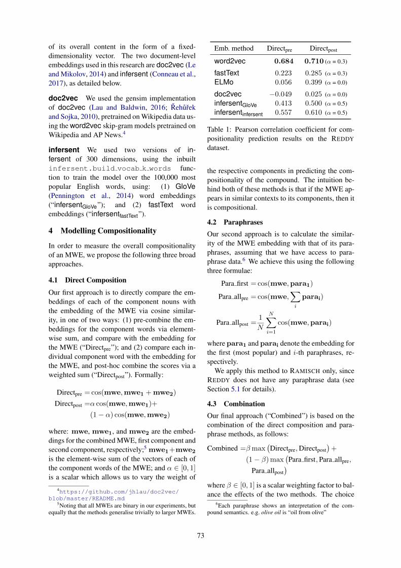
of its overall content in the form of a fixed-dimensionality vector. The two document-levelembeddings used in this research are doc2vec (Leand Mikolov, 2014) and infersent (Conneau et al.,2017), as detailed below.

doc2vec We used the gensim implementationof doc2vec (Lau and Baldwin, 2016; Rehurekand Sojka, 2010), pretrained on Wikipedia data us-ing the word2vec skip-gram models pretrained onWikipedia and AP News.4

infersent We used two versions of in-fersent of 300 dimensions, using the inbuiltinfersent.build vocab k words func-tion to train the model over the 100,000 mostpopular English words, using: (1) GloVe(Pennington et al., 2014) word embeddings(“infersentGloVe”); and (2) fastText wordembeddings (“infersentfastText”).

4 Modelling Compositionality

In order to measure the overall compositionalityof an MWE, we propose the following three broadapproaches.

4.1 Direct Composition

Our first approach is to directly compare the em-beddings of each of the component nouns withthe embedding of the MWE via cosine similar-ity, in one of two ways: (1) pre-combine the em-beddings for the component words via element-wise sum, and compare with the embedding forthe MWE (“Directpre”); and (2) compare each in-dividual component word with the embedding forthe MWE, and post-hoc combine the scores via aweighted sum (“Directpost”). Formally:

Directpre =cos(mwe,mwe1 +mwe2)

Directpost =α cos(mwe,mwe1)+

(1− α) cos(mwe,mwe2)

where: mwe, mwe1, and mwe2 are the embed-dings for the combined MWE, first component andsecond component, respectively;5 mwe1+mwe2is the element-wise sum of the vectors of each ofthe component words of the MWE; and α ∈ [0, 1]is a scalar which allows us to vary the weight of

4https://github.com/jhlau/doc2vec/blob/master/README.md

5Noting that all MWEs are binary in our experiments, butequally that the methods generalise trivially to larger MWEs.

Emb. method Directpre Directpost

word2vec 0.684 0.710 (α = 0.3)

fastText 0.223 0.285 (α = 0.3)ELMo 0.056 0.399 (α = 0.0)

doc2vec −0.049 0.025 (α = 0.0)infersentGloVe 0.413 0.500 (α = 0.5)infersentinfersent 0.557 0.610 (α = 0.5)

Table 1: Pearson correlation coefficient for com-positionality prediction results on the REDDY

dataset.

the respective components in predicting the com-positionality of the compound. The intuition be-hind both of these methods is that if the MWE ap-pears in similar contexts to its components, then itis compositional.

4.2 ParaphrasesOur second approach is to calculate the similar-ity of the MWE embedding with that of its para-phrases, assuming that we have access to para-phrase data.6 We achieve this using the followingthree formulae:

Para first =cos(mwe,para1)

Para allpre =cos(mwe,∑i

parai)

Para allpost =1

N

N∑i=1

cos(mwe,parai)

where para1 and parai denote the embedding forthe first (most popular) and i-th paraphrases, re-spectively.

We apply this method to RAMISCH only, sinceREDDY does not have any paraphrase data (seeSection 5.1 for details).

4.3 CombinationOur final approach (“Combined”) is based on thecombination of the direct composition and para-phrase methods, as follows:

Combined =βmax(Directpre,Directpost

)+

(1− β)max(Para first,Para allpre,

Para allpost)

where β ∈ [0, 1] is a scalar weighting factor to bal-ance the effects of the two methods. The choice

6Each paraphrase shows an interpretation of the com-pound semantics. e.g. olive oil is “oil from olive”

73

Emb. method Directpre Directpost Para first Para allpre Para allpost Combined

word2vec 0.667 0.731 (α = 0.7) 0.714 0.822 0.880 0.880 (β = 0.0)

fastText 0.395 0.446 (α = 0.7) 0.569 0.662 0.704 0.704 (β = 0.0)ELMo 0.139 0.295 (α = 0.0) 0.367 0.642 0.664 0.669 (β = 0.2)

doc2vec −0.146 0.048 (α = 1.0) 0.405 0.372 0.401 0.419 (β = 0.3)infersentGloVe 0.321 0.427 (α = 0.7) 0.639 0.704 0.741 0.774 (β = 0.5)infersentfastText 0.274 0.380 (α = 0.8) 0.615 0.781 0.783 0.783 (β = 0.0)

Table 2: Pearson correlation coefficient for compositionality prediction results on the RAMISCH dataset.

of the max operator here to combine the sub-methods for each of the direct composition andparaphrase methods is that all methods tend to un-derestimate the compositionality (and empirically,it was superior to taking the mean).

5 Experiments

5.1 Datasets

We evaluate the models on the following twodatasets, which are comprised of 90 English bi-nary noun compounds each, rated for composi-tionality on a scale of 0 (non-compositional) to 5(compositional). In each case, we evaluate modelperformance via the Pearson’s correlation coeffi-cient (r).

REDDY This dataset contains scores for thecompositionality of the overall MWE, as well asthat of each component word (Reddy et al., 2011);in this research, we use the overall compositional-ity score of the MWE only, and ignore the compo-nent scores.

RAMISCH Similarly to REDDY, this datasetcontains scores for the overall compositionalityof the MWE as well as the relative composition-ality of each of its component words, in addi-tion to paraphrases suggested by the annotators,in decreasing order of popularity (Ramisch et al.,2016); in this research, we use the overall compo-sitionality score and paraphrase data only.

5.2 Results and Discussion

The results of the experiments on REDDY andRAMISCH are presented in Tables 1 and 2, re-spectively. In this work, we simplistically presentthe results for the best α and β values for eachmethod over a given dataset, meaning we are ef-fectively peaking at our test data. Sensitivity ofthe α hyper-parameter is shown in Figures 1 and

0 0.25 0.5 0.75 1−0.25

0

0.25

0.5

0.75

1

α

r

ELMofastTextdoc2vec

infersentGloVeinfersentfastText

word2vec

Figure 1: Sensitivity analysis of α (REDDY)

0 0.25 0.5 0.75 1−0.25

0

0.25

0.5

0.75

1

α

r

ELMofastTextdoc2vec

infersentGloVeinfersentfastText

word2vec

Figure 2: Sensitivity analysis of α (RAMISCH)

2, for the REDDY and RAMISCH datasets, respec-tively.

The first observation to be made is that noneof the pretrained models match the state-of-the-artmethod based on word2vec, despite the simplic-ity of the method. ELMo and doc2vec in partic-ular perform worse than expected, suggesting thattheir ability to model non-compositional languageis limited. Recall, however, our comment about

74

using ELMo naively, in not including any con-text when generating the embeddings for the com-ponent words and, more importantly, the overallMWE. The results show that doc2vec performsbetter when representing paraphrases, and strug-gles with compounds without sentential context.

In Table 1, we find Directpost to produce a highercorrelation in all cases, with α ranging from 0.0 to0.5, suggesting that the second element (= head)contributes more to the overall compositionality ofthe MWE than the first element (= modifier); thisis borne out in Figure 1.

In Table 2, on the other hand, we find that, withthe exception of ELMo, the α values favour themodifier of the MWE over the head (i.e. α > 0.5;also seen in Figure 2), implying that the formeris more significant in predicting the composition-ality of the MWE. The reason for the mismatchbetween the two datasets is not immediately clear,other than the obvious data sparsity.

We also see that the paraphrases achieve ahigher correlation across all models, suggestingthis is a promising direction for future study.The low β values for Combined also confirmthat the paraphrase methods have greater predic-tive power than the direct composition methods.Among the paraphrase experiments, we find thatPara allpost— the average of the similarities of theMWE with each of its paraphrases — consistentlyachieves the best results. We hypothesize thatthe paraphrases provide additional information re-garding the compounds that further help determinetheir compositionality.

6 Conclusions and Future Work

This paper has investigated the application of arange of embedding generation methods to thetask of predicting the compositionality of anMWE, either directly based on the MWE and itscomponent words, or indirectly based on para-phrase data for the MWE. Our results show thatmodern character- and document-level embeddingmodels are inferior to the simple word2vec ap-proach at the task. We also show that paraphrasedata captures valuable data regarding the compo-sitionality of the MWE.

Since we have achieved such promising resultswith the paraphrase data, it might be interestingto consider other possible settings in future tests.While none of the other approaches could outper-form word2vec, it is useful to note that they were

pretrained and, as such, did not require any manip-ulation of the training corpus in order to generatevector embeddings of the MWEs. This means theycan be applied to new datasets without the need forretraining and are, therefore, more robust.

In future work, we intend to train the modelsused in our study on a fixed corpus, to comparetheir performance in a more controlled setting. Wewill also do proper tuning of the hyperparametersover held-out data, and plan to experiment withother languages.

ReferencesOtavio Acosta, Aline Villavicencio, and Viviane Mor-

eira. 2011. Identification and treatment of multi-word expressions applied to information retrieval.In Proceedings of the Workshop on Multiword Ex-pressions: from Parsing and Generation to the RealWorld. Portland, USA, pages 101–109.

Timothy Baldwin and Su Nam Kim. 2010. Multiwordexpressions. In Nitin Indurkhya and Fred J. Dam-erau, editors, Handbook of Natural Language Pro-cessing, CRC Press, Boca Raton, USA. 2nd edition.

Marco Baroni, Georgiana Dinu, and GermanKruszewski. 2014. Don’t count, predict! asystematic comparison of context-counting vs.context-predicting semantic vectors. In Proceedingsof the 52nd Annual Meeting of the Association forComputational Linguistics (ACL 2014). Baltimore,USA, pages 238–247.

Piotr Bojanowski, Edouard Grave, Armand Joulin, andTomas Mikolov. 2017. Enriching word vectors withsubword information. Transactions of the Associa-tion for Computational Linguistics 5:135–146.

Alexis Conneau, Douwe Kiela, Holger Schwenk, LoıcBarrault, and Antoine Bordes. 2017. Supervisedlearning of universal sentence representations fromnatural language inference data. In Proceedings ofthe 2017 Conference on Empirical Methods in Nat-ural Language Processing. pages 670–680.

Silvio Cordeiro, Aline Villavicencio, Marco Idiart, andCarlos Ramisch. to appear. Unsupervised composi-tionality prediction of nominal compounds. Compu-tational Linguistics .

Ali Hakimi Parizi and Paul Cook. 2018. Do character-level neural network language models captureknowledge of multiword expression compositional-ity? In Proceedings of the Joint Workshop on Lin-guistic Annotation, Multiword Expressions and Con-structions (LAW-MWE-CxG-2018). pages 185–192.

Jey Han Lau and Timothy Baldwin. 2016. An empiri-cal evaluation of doc2vec with practical insights intodocument embedding generation. In Proceedingsof the 1st Workshop on Representation Learning forNLP. pages 78–86.

75

Quoc Le and Tomas Mikolov. 2014. Distributed repre-sentations of sentences and documents. In Proceed-ings of the 31st International Conference on Ma-chine Learning (ICML 2014). Beijing, China, pages1188–1196.

Tomas Mikolov, Kai Chen, Greg Corrado, and JeffreyDean. 2013. Efficient estimation of word represen-tations in vector space. In Proceedings of Workshopat the International Conference on Learning Repre-sentations.

Jeffrey Pennington, Richard Socher, and Christo-pher D. Manning. 2014. GloVe: Global vectors forword representation. In Empirical Methods in Nat-ural Language Processing (EMNLP). pages 1532–1543.

Matthew Peters, Mark Neumann, Mohit Iyyer, MattGardner, Christopher Clark, Kenton Lee, and LukeZettlemoyer. 2018. Deep contextualized word rep-resentations. In Proceedings of the 2018 Confer-ence of the North American Chapter of the Associ-ation for Computational Linguistics: Human Lan-guage Technologies, Volume 1 (Long Papers). pages2227–2237.

Carlos Ramisch, Silvio Cordeiro, Leonardo Zilio,Marco Idiart, and Aline Villavicencio. 2016. Hownaked is the naked truth? a multilingual lexicon ofnominal compound compositionality. In Proceed-ings of the 54th Annual Meeting of the Associationfor Computational Linguistics (Volume 2: Short Pa-pers). pages 156–161.

Siva Reddy, Diana McCarthy, and Suresh Manandhar.2011. An empirical study on compositionality incompound nouns. In Proceedings of 5th Interna-tional Joint Conference on Natural Language Pro-cessing. pages 210–218.

Radim Rehurek and Petr Sojka. 2010. Software frame-work for topic modelling with large corpora. In Pro-ceedings of the LREC 2010 Workshop on New Chal-lenges for NLP Frameworks. pages 45–50.

Bahar Salehi, Paul Cook, and Timothy Baldwin. 2015a.A word embedding approach to predicting the com-positionality of multiword expressions. In Proceed-ings of the 2015 Conference of the North Ameri-can Chapter of the Association for ComputationalLinguistics: Human Language Technologies. pages977–983.

Bahar Salehi, Nitika Mathur, Paul Cook, and TimothyBaldwin. 2015b. The impact of multiword expres-sion compositionality on machine translation eval-uation. In Proceedings of the NAACL HLT 2015Workshop on Multiword Expressions. Denver, USA,pages 54–59.

Sriram Venkatapathy and Aravind K Joshi. 2006. Us-ing information about multi-word expressions forthe word-alignment task. In Proceedings of theWorkshop on Multiword Expressions: Identifyingand Exploiting Underlying Properties. pages 20–27.

76

Towards Efficient Machine Translation Evaluation by ModellingAnnotators

Nitika Mathur Timothy Baldwin Trevor CohnSchool of Computing and Information Systems

The University of MelbourneVictoria 3010, Australia

nmathur@student.unimelb.edu.au {tbaldwin,tcohn}@unimelb.edu.au

Abstract

Current machine translation evaluationsuse Direct Assessment, based on crowd-sourced judgements from a large poolof workers, along with quality controlchecks, and a robust method for combin-ing redundant judgements. In this paperwe show that the quality control mecha-nism is overly conservative, increasing thetime and expense of the evaluation. Wepropose a model that does not filter work-ers, and takes into account varying anno-tator reliabilities. Our model effectivelyweights each worker’s scores based on theinferred precision of the worker, and ismuch more reliable than the mean of ei-ther the raw or standardised scores.

1 Introduction

Accurate evaluation is critical for measuringprogress in machine translation (MT). Despiteprogress over the years, automatic metrics arestill biased, and human evaluation is still a fun-damental requirement for reliable evaluation. Theprocess of collecting human annotations is time-consuming and expensive, and the data is alwaysnoisy. The question of how to efficiently collectthis data has evolved over the years, but there isstill scope for improvement. Furthermore, oncethe data has been collected, there is no consensuson the best way to reason about translation quality.

Direct Assessment (“DA”: Graham et al.(2017)) is currently accepted as the best practicefor human evaluation, and is the official methodat the Conference for Machine Translation (Bo-jar et al., 2017a). Every annotator scores a setof translation-pairs, which includes quality controlitems designed to filter out unreliable workers.

However, the quality control process has lowrecall for good workers: as demonstrated in Sec-tion 3, about one third of good data is discarded,increasing expense. Once good workers are identi-fied, their outputs are simply averaged to producethe final ‘true’ score, despite their varying accu-racy.

In this paper, we provide a detailed analysis ofthese shortcomings of DA and propose a Bayesianmodel to address these issues. Instead of stan-dardising individual worker scores, our model canautomatically infer worker offsets using the rawscores of all workers as input. In addition, bylearning a worker-specific precision, each workereffectively has a differing magnitude of vote inthe ensemble. When evaluated on the WMT 2016Tr-En dataset which has a high proportion of un-skilled annotators, these models are more efficientthan the mean of the standardised scores.

2 Background

The Conference on Machine Translation (WMT)annually collects human judgements to evaluatethe MT systems and metrics submitted to theshared tasks. The evaluation methodology hasevolved over the years, from 5 point adequacy andfluency rating, to relative rankings (“RR”), to DA.With RR, annotators are asked to rank translationsof 5 different MT systems. In earlier years, thefinal score of a system was the expected numberof times its translations score better than transla-tions by other systems (expected wins). Bayesianmodels like Hopkins and May (Hopkins and May,2013) and Trueskill (Sakaguchi et al., 2014) werethen proposed to learn the relative ability of theMT systems. Trueskill was adopted by WMT in2015 as it is more stable and efficient than the ex-pected wins heuristic.

DA was trialled at WMT 2016 (Bojar et al.,

Nitika Mathur, Timothy Baldwin and Trevor Cohn. 2018. Towards Efficient Machine Translation Evaluation by ModellingAnnotators. In Proceedings of Australasian Language Technology Association Workshop, pages 77−82.

2016a), and has replaced RR since 2017 (Bojaret al., 2017a). It is more scalable than RR as thenumber of systems increases (we need to obtainone annotation per system, instead of one anno-tation per system pair). Each translation is ratedindependently, minimising the risk of being influ-enced by the relative quality of other translations.Ideally, it is possible that evaluations can be com-pared across multiple datasets. For example, wecan track the progress of MT systems for a givenlanguage pair over the years.

Another probabilistic model, EASL (Sakaguchiand Van Durme, 2018), has been proposed thatcombines some advantages of DA with Trueskill.Annotators score translations from 5 systems atthe same time on a sliding scale, allowing usersto explicitly specify the magnitude of differencebetween system translations. Active learning toselect the systems in each comparison to increaseefficiency. But it does not model worker reliabil-ity, and is, very likely, not compatible with longi-tudinal evaluation, as the systems are effectivelyscored relative to each other.

In NLP, most other research on learning annota-tor bias and reliability has been on categorical data(Snow et al., 2008; Carpenter, 2008; Hovy et al.,2013; Passonneau and Carpenter, 2014).

3 Direct Assessment

To measure adequacy, in DA, annotators are askedto rate how adequately an MT output expresses themeaning of a reference translation using a contin-uous slider, which maps to an underlying scale of0–100. These annotations are crowdsourced us-ing Amazon Mechanical Turk, where “workers”complete “Human Intelligence Tasks” (HITs) inthe form of one or more micro-tasks.

Each HIT consists of 70 MT system transla-tions, along with an additional 30 control items:

1. degraded versions of 10 of these translations;2. 10 reference translations by a human expert,

corresponding to 10 system translations; and3. repeats of another 10 translations.

The scores on the quality control items are usedto filter out workers who either click randomlyor on the same score continuously. A conscien-tious worker would give a near perfect score toreference translations, give a lower score to de-graded translations when compared to the corre-sponding MT system translation, and be consistentwith scores for repeat translations.

The paired Wilcoxon rank-sum test is used totest whether the worker scored degraded transla-tions worse than the corresponding system trans-lation. The (arbitrary but customary) cutoff ofp < 0.05 is used to determine good workers. Thepaired Wilcoxon rank-sum test (p < 0.05) is usedto test whether the worker scored degraded trans-lations worse than the corresponding system trans-lation. The remaining workers are further testedto check that there is no significant difference be-tween their scores for repeat-pairs.

Worker scores are manually examined to filterout workers who obviously gave the same score toall translations, or scored translations at random.Only these workers are rejected payment. Thus,other workers who do not pass the quality controlcheck are paid for their efforts, but their scores areunused, increasing the overall cost.

Some workers might have high standards andgive consistently low scores for all translations,while others are more lenient. And some workersmay only use the central part of the scale. Stan-dardising individual workers’ scores makes themmore comparable, and reduces noise before calcu-lating the mean.

The final score of an MT system is the meanstandardised score of its translations after discard-ing scores that do not meet quality control criteria.The noise in worker scores is cancelled out whena large number of translations are averaged.

To obtain accurate scores of individual transla-tions, multiple judgments are collected and aver-aged. As we increase the number of annotatorsper translation, there is greater consistency and re-liability in the mean score. This was empiricallytested by showing that there is high correlation be-tween the mean of two independent sets of judg-ments, when the sample size is greater than 15(Graham et al., 2015).

However, both these tests are based on asample-size of 10 items, and, as such, the firsttest has low power; we show that it filters out alarge proportion of the total workers. One solu-tion would be to increase the sample size of thedegraded-reference-pairs, but this would be at theexpense of the number of useful worker annota-tions. It is better to come up with a model thatwould use the scores of all workers, and is morerobust to low quality scores.

Automatic metrics such as BLEU (Papineniet al., 2002) are generally evaluated using the Pear-

78

(a) all language pairs

(b) Tr-En language pair

Figure 1: Accuracy of “good” vs “bad” workers inthe WMT 2016 dataset.

son correlation with the mean standardised scoreof the good workers. We similarly evaluate aworker’s accuracy using the Pearson correlation ofthe worker’s scores with this ground truth. Over allthe data collected for WMT16, the group of goodworkers are, on average, more accurate than thegroup of workers who failed the significance test.However, as seen in Figure 1a, there is substantialoverlap in the accuracies of the two groups. Wecan see that very few inaccurate workers were in-cluded. However, about a third of the total workerswhose scores have a correlation greater than 0.6were not approved. In particular, over the Tr-EnDataset, the significance test was not very effec-tive, as seen in Figure 1b.

Workers whose scores pass the quality controlcheck are given equal weight, despite the variationin their reliability. Given that quality control is notalways reliable (as with the Tr-En dataset, e.g.),this could include worker with scores as low asr = 0.2 correlation with the ground truth.

While worker standardisation succeeds in in-creasing inter-annotator consistency, this processdiscards information about the absolute quality ofthe translations in the evaluation set. When us-ing the mean of standardised scores, we cannotcompare MT systems across independent evalua-

tions. In the evaluation of the WMT 17 NeuralMT Training Task, the baseline system trained on4GB GPU memory was evaluated separately fromthe baseline trained on 8 GB GPU memory and theother submissions. In this setup of manual eval-uation, Baseline-4GB scores slightly higher thanBaseline-8GB when using raw scores, which ispossibly due to chance. However, it scores sig-nificantly higher when using standardised scores,which goes against our expectations (Bojar et al.,2017b).

4 Models

We use a simple model, assuming that a workerscore is normally distributed around the true qual-ity of the translation. Each worker has a precisionparameter τ that models their accuracy: workerswith high τ are more accurate. In addition, weinclude a worker-specific offset β, which modelstheir deviation from the true score.

For each translation i ∈ T , we draw the truequality µ from the standard normal distribution.1

Then for each worker j ∈ W , we draw their ac-curacy τj from a gamma distribution with shapeparameter k and rate parameter θ.2 The offset βjis again drawn from the standard normal distribu-tion. The worker’s score rij is drawn from a nor-mal distribution, with mean µi +βj , and precisionτj .

rij = N(µi + βj , τ

−1j

)(1)

To help the model, we add constraints on thequality control items: the true quality of the de-graded translation is lower than the quality of thecorresponding system translation. In addition, thetrue quality of the repeat items should be approxi-mately equal.

We expect that the model will learn a high τ forgood quality workers, and give their scores higherweight when estimating the mean. We believe thatthe additional constraints will help the model toinfer the worker precision.

DA can be viewed as the Maximum LikelihoodEstimate of this model, with the following sub-stitutions in Equation (1): sij is the standardisedscore of worker j, βj is 0 for all workers, and τ is

1We first standardise scores (across all workers together)in the dataset

2We use k = 2 and θ = 1 based on manual inspectionof the distribution of worker precisions on a developmentdataset (WMT18 Cs-En)

79

µi rij

βj τj

T

W

Figure 2: The proposed model, where worker j ∈W has offset βj and precision τj , translation i ∈ Thas quality µi, and worker j scores translation iwith rij

.

constant for all workers.

sij = N(µi, τ

−1)

(2)

The choice of a Gaussian distribution to modelworker scores is technically deficient as a Gaus-sian is unbounded, but it is still a reasonable ap-proximation. This could be remedied, for exam-ple, by using a truncated Gaussian distribution,which we leave to future work.

We want to maximise the likelihood of the ob-served judgments:

P (r) =

W∫∫j=1

P (βj)P (τj)

T∫i=1

P (µi)

P (ri,j |µi, β, τ) dβ dτ dµ

=

W∫∫j=1

N (βj |0, 1) Γ (τj |k, θ)T∫

i=1

N (µi|0, 1)

N(rij |µi, τ−1

)dβ dτ dµ (3)

We use the Expectation Propagation algorithm(Minka, 2001) to infer posteriors over µ andworker parameters β and τ .3 Expectation Prop-agation is a technique for approximating distribu-tions which can be written as a product of factors.It iteratively refines each factor by minimising theKL divergence from the approximate to the truedistribution.

5 Experiments

We evaluate our models on data from the segment-level WMT 16 dataset (Bojar et al., 2016b). Wechoose the Turkish to English (Tr-En) dataset,which consists of 256 workers, of which about

3We use the Infer.NET (Minka et al., 2018) framework toimplement our models.

Figure 3: Pearson’s r of the estimated true scorewith the “ground truth” as we increase the numberof workers per translation.

two thirds (67.58%) fail the quality control mea-sures. It consists of 560 translations, with at least15 “good” annotations for each of these transla-tions (see Figure 1b).

We use the mean of 15 good standardised anno-tations as a proxy for the gold standard when eval-uating efficiency, and starting from one worker,increase the number of workers to the maximumavailable. Figure 3 shows that our models are con-sistently more accurate than the mean of the stan-dardised scores.

Figure 4 shows the learned precision and offsetfor 5 annotators per translation, against the preci-sion and offset of worker scores calculated withrespect to the “ground truth”. This shows that themodel is learning worker parameters even whenthe number of workers is very small, and is us-ing this information to get a better estimate of themean (the model obtains r = 0.72, compared tor = 0.65 for the mean z-score).

On further examination of the outlier in Fig-ure 4a, we find that this worker is pathologicallybad. They give a 0 score for all the translations inone HIT, and mostly 100s to the other half. Thisbehaviour is not captured by our model.

6 Discussion and Future Work

We showed that significance tests over a small setof quality control items are ineffective at identify-ing good and bad workers, and propose a modelthat does not depend on this step. Instead, it usesconstraints on the quality control items to learnworker precision, and returns a more reliable es-timate of the mean using fewer worker scores pertranslation. This model does not tell us when tostop collecting judgments. It would be useful toknow to have a method to determine when to stop

80

(a) Worker Precision

(b) Worker Offset

Figure 4: Scatter plot of worker precision/offsetinferred by the model with only 5 workers pertranslation, against the precision/offset of thedeltas of the worker score and the “ground truth”.

collecting annotations based on scores received,instead of relying on a number obtained from one-time experiments.

More importantly, we need to have ways to cal-ibrate worker scores to ensure consistent evalua-tions across years, so we can measure progress inMT over time. Even if a better model is foundto calibrate workers, this does not ensure consis-tency in judgments, and we believe the HIT struc-ture needs to be changed. We propose to replacethe 30 quality control items with items of reliablyknown quality from the previous year. The corre-lation between the worker scores and the knownscores can be used to assess the reliability of theworker. Moreover, we can scale the worker scoresbased on these known items, to ensure consistentscores over years.

Acknowledgements

We thank the anonymous reviewers for their valu-able feedback and suggestions. This work wassupported in part by the Australian ResearchCouncil.

ReferencesOndrej Bojar, Rajen Chatterjee, Christian Federmann,

Yvette Graham, Barry Haddow, Shujian Huang,Matthias Huck, Philipp Koehn, Qun Liu, Var-vara Logacheva, Christof Monz, Matteo Negri,Matt Post, Raphael Rubino, Lucia Specia, andMarco Turchi. 2017a. Findings of the 2017Conference on Machine Translation (WMT17).In Proceedings of the Second Conference onMachine Translation, Volume 2: Shared TaskPapers. Copenhagen, Denmark, pages 169–214.http://www.aclweb.org/anthology/W17-4717.

Ondrej Bojar, Rajen Chatterjee, Christian Federmann,Yvette Graham, Barry Haddow, Matthias Huck,Antonio Jimeno Yepes, Philipp Koehn, VarvaraLogacheva, Christof Monz, Matteo Negri, Aure-lie Neveol, Mariana Neves, Martin Popel, MattPost, Raphael Rubino, Carolina Scarton, Lucia Spe-cia, Marco Turchi, Karin Verspoor, and MarcosZampieri. 2016a. Findings of the 2016 Conferenceon Machine Translation. In Proceedings of the FirstConference on Machine Translation. Berlin, Ger-many, pages 131–198.

Ondrej Bojar, Yvette Graham, Amir Kamran, andMilos Stanojevic. 2016b. Results of the WMT16Metrics Shared Task. In Proceedings of the FirstConference on Machine Translation. Berlin, Ger-many, pages 199–231.

Ondrej Bojar, Jindrich Helcl, Tom Kocmi, JindrichLibovicky, and Tomas Musil. 2017b. Resultsof the WMT17 Neural MT Training task. InProceedings of the Second Conference on Ma-chine Translation, Volume 2: Shared Task Pa-pers. Copenhagen, Denmark, pages 525–533.http://www.aclweb.org/anthology/W17-4757.

Bob Carpenter. 2008. Multilevel Bayesian models ofcategorical data annotation. Technical report, Alias-i.

Yvette Graham, Timothy Baldwin, Alistair Moffat, andJustin Zobel. 2017. Can machine translation sys-tems be evaluated by the crowd alone. Natural Lan-guage Engineering 23(1):330.

Yvette Graham, Nitika Mathur, and Timothy Baldwin.2015. Accurate evaluation of segment-level ma-chine translation metrics. In Proceedings of the2015 Conference of the North American Chapter ofthe Association for Computational Linguistics Hu-man Language Technologies. Denver, USA, pages1183–1191.

Mark Hopkins and Jonathan May. 2013. Models oftranslation competitions. In Proceedings of the51st Annual Meeting of the Association for Com-putational Linguistics (ACL 2013). Sofia, Bulgaria,pages 1416–1424.

Dirk Hovy, Taylor Berg-Kirkpatrick, Ashish Vaswani,and Eduard H Hovy. 2013. Learning whom to trust

81

with MACE. In Proceedings of the 2013 Confer-ence of the North American Chapter of the Associ-ation for Computational Linguistics: Human Lan-guage Technologies (NAACL HLT 2013). Atlanta,USA, pages 1120–1130.

T. Minka, J.M. Winn, J.P. Guiver, Y. Zaykov, D. Fabian,and J. Bronskill. 2018. Infer.NET 0.3. Mi-crosoft Research Cambridge. http://dotnet.github.io/infer.

Thomas P. Minka. 2001. Expectation propagation forapproximate Bayesian inference. In Proceedings ofthe Seventeenth Conference on Uncertainty in Arti-ficial Intelligence. Seattle, USA, pages 362–369.

Kishore Papineni, Salim Roukos, Todd Ward, and Wei-Jing Zhu. 2002. Bleu: A method for automatic eval-uation of machine translation. In Proceedings of the40th Annual Meeting of the Association for Compu-tational Linguistics (ACL 2002). Philadelphia, USA,pages 311–318.

J. Rebecca Passonneau and Bob Carpenter. 2014. Thebenefits of a model of annotation. Transactionsof the Association of Computational Linguistics2(1):311–326.

Keisuke Sakaguchi, Matt Post, and BenjaminVan Durme. 2014. Efficient elicitation of annota-tions for human evaluation of machine translation.In Proceedings of the Ninth Workshop on StatisticalMachine Translation. Baltimore, USA, pages 1–11.

Keisuke Sakaguchi and Benjamin Van Durme. 2018.Efficient online scalar annotation with bounded sup-port. In Proceedings of the 56th Annual Meet-ing of the Association for Computational Linguis-tics (Volume 1: Long Papers). pages 208–218.http://aclweb.org/anthology/P18-1020.

Rion Snow, Brendan O’Connor, Daniel Jurafsky, andAndrew Y. Ng. 2008. Cheap and fast — but is itgood? evaluating non-expert annotations for naturallanguage tasks. In Proceedings of the Conference onEmpirical Methods in Natural Language Process-ing. Honolulu, USA, pages 254–263.

82

ALTA Shared Task papers

83

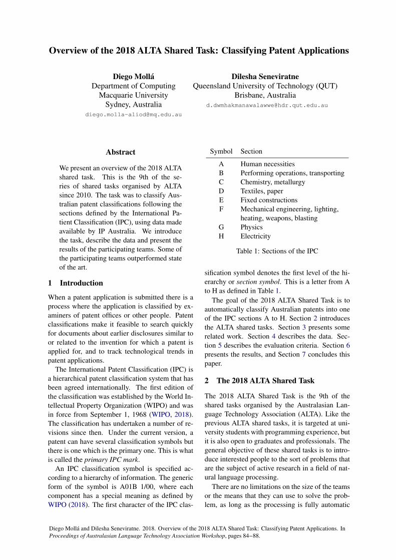
Overview of the 2018 ALTA Shared Task: Classifying Patent Applications

Diego MollaDepartment of Computing

Macquarie UniversitySydney, Australia

diego.molla-aliod@mq.edu.au

Dilesha SeneviratneQueensland University of Technology (QUT)

Brisbane, Australiad.dwmhakmanawalawwe@hdr.qut.edu.au

Abstract

We present an overview of the 2018 ALTAshared task. This is the 9th of the se-ries of shared tasks organised by ALTAsince 2010. The task was to classify Aus-tralian patent classifications following thesections defined by the International Pa-tient Classification (IPC), using data madeavailable by IP Australia. We introducethe task, describe the data and present theresults of the participating teams. Some ofthe participating teams outperformed stateof the art.

1 Introduction

When a patent application is submitted there is aprocess where the application is classified by ex-aminers of patent offices or other people. Patentclassifications make it feasible to search quicklyfor documents about earlier disclosures similar toor related to the invention for which a patent isapplied for, and to track technological trends inpatent applications.

The International Patent Classification (IPC) isa hierarchical patent classification system that hasbeen agreed internationally. The first edition ofthe classification was established by the World In-tellectual Property Organization (WIPO) and wasin force from September 1, 1968 (WIPO, 2018).The classification has undertaken a number of re-visions since then. Under the current version, apatent can have several classification symbols butthere is one which is the primary one. This is whatis called the primary IPC mark.

An IPC classification symbol is specified ac-cording to a hierarchy of information. The genericform of the symbol is A01B 1/00, where eachcomponent has a special meaning as defined byWIPO (2018). The first character of the IPC clas-

Symbol Section

A Human necessitiesB Performing operations, transportingC Chemistry, metallurgyD Textiles, paperE Fixed constructionsF Mechanical engineering, lighting,

heating, weapons, blastingG PhysicsH Electricity

Table 1: Sections of the IPC

sification symbol denotes the first level of the hi-erarchy or section symbol. This is a letter from Ato H as defined in Table 1.

The goal of the 2018 ALTA Shared Task is toautomatically classify Australian patents into oneof the IPC sections A to H. Section 2 introducesthe ALTA shared tasks. Section 3 presents somerelated work. Section 4 describes the data. Sec-tion 5 describes the evaluation criteria. Section 6presents the results, and Section 7 concludes thispaper.

2 The 2018 ALTA Shared Task

The 2018 ALTA Shared Task is the 9th of theshared tasks organised by the Australasian Lan-guage Technology Association (ALTA). Like theprevious ALTA shared tasks, it is targeted at uni-versity students with programming experience, butit is also open to graduates and professionals. Thegeneral objective of these shared tasks is to intro-duce interested people to the sort of problems thatare the subject of active research in a field of nat-ural language processing.

There are no limitations on the size of the teamsor the means that they can use to solve the prob-lem, as long as the processing is fully automatic

Diego Mollá and Dilesha Seneviratne. 2018. Overview of the 2018 ALTA Shared Task: Classifying Patent Applications. InProceedings of Australasian Language Technology Association Workshop, pages 84−88.

— there should be no human intervention.As in past ALTA shared tasks, there are two cat-

egories: a student category and an open category.

• All the members of teams from the studentcategory must be university students. Theteams cannot have members that are full-timeemployed or that have completed a PhD.

• Any other teams fall into the open category.

The prize is awarded to the team that performsbest on the private test set — a subset of the eval-uation data for which participant scores are onlyrevealed at the end of the evaluation period (seeSection 5).

3 Related Work

Extensive research has been conducted on au-tomating patent classification in the IPC hierarchyand a wide variety of approaches have been pro-posed. These approaches use features that are gen-erated/extracted from patent content (claim, de-scription, etc), patent metadata (title, applicantname, filing date, inventor name, etc) and cita-tions to represent patent documents in classifica-tion (Liu and Shih, 2011). Patent content-basedfeatures are the most popular choice among thedifferent types of features to address patent classi-fication (Liu and Shih, 2011). In addition, featuresbased on patent metadata which are considered tohave strong classification power have been usedto boost the classification performance (Richterand MacFarlane, 2005). Further, patents are notisolated but they are connected through citationswhich provide rich information about the patentnetwork. Thus, researchers have utilised patent ci-tation information to generate features for patentclassification (Liu and Shih, 2011; Li et al., 2007).While all these types of features have served tobuild classifiers, which features can represent thepatents well is still an open question (Gomez andMoens, 2014b).

Some of the widely used classification algo-rithms in the literature for building patent clas-sification systems are Naive Bayes (NB), Artifi-cial Neural Network (ANN), Support Vector Ma-chines (SVM), K-Nearest Neighbour (KNN), De-cision Trees (DT) and Logistic Regression (LR).The greater part of these systems has focused onachieving classification effectiveness. SVM hasshown superior performance in terms of effective-ness with some datasets (Fall et al., 2003), yet

it has not been able to scale with large datasets.Seneviratne et al. (2015) have proposed a doc-ument signature-based patent classification ap-proach employing KNN which can address thescalability and efficiency with a competitive effec-tiveness.

Given that there are different evaluation mea-sures and different datasets, it is difficult to com-pare the performance between many patent classi-fication approaches. Apart from the shared eval-uation tasks of patent classification like CLEF-IP2010 (Piroi et al., 2010) and CLEF-IP 2011 (Piroiet al., 2011), where the performance of systemswere evaluated using benchmark datasets, a lim-ited number of approaches — e.g. by Fall et al.(2003), Tikk et al. (2005) and Seneviratne et al.(2015) — have evaluated their methods usingpublicly available complete data sets like WIPO-alpha1 and WIPO-de.2 The majority of other sys-tems have been evaluated using ad-hoc datasets,making it difficult to extrapolate their perfor-mance (Gomez and Moens, 2014b).

The CLEF-IP 2010 and 2011 classificationtasks required to classify patents at the IPC sub-class level (Piroi et al., 2010, 2011), which is finergrained than the section level used in the ALTAshared task. Both of these classification tasks usedevaluation measures such as Precision@1, Preci-sion@5, Recall@5, Map and F1 at 5, 25 and 50.While the best results of these experiments varied,the best results were from Verberne and D’hondt(2011), who achieved 0.74, 0.86, and 0.71 for pre-cision, recall, and F1 score respectively.

Most of the researchers who have conductedexperiments with complete WIPO-alpha andWIPO-de datasets have reported their results atIPC section and subclass levels. For example, thehierarchical classification method by Tikk et al.(2005) has achieved an accuracy of 0.66 at the sec-tion level with the WIPO-alpha dataset and 0.65with the WIPO-de dataset. Gomez and Moens(2014a) have reported their classification resultsfor WIPO-alpha at the section level and the re-ported values for accuracy and macro-averaged F1score are 0.74 and 0.71 respectively.

1 http://www.wipo.int/classifications/ipc/en/ITsupport/Categorization/dataset/wipo-alpha-readme.html

2http://www.wipo.int/classifications/ipc/en/ITsupport/Categorization/dataset/index.html

85

ID Label

0 A1 G2 A3 A4 D5 A

Table 2: First 5 rows of the training data

4 Data

The data used in the 2018 ALTA Shared Task con-sists of a collection of Australian patents parti-tioned into 3,972 documents for training and 1,000documents for test. The documents are plain textfiles which are the result of applying a text ex-tracting tool on the original PDF files. As aresult, there are errors in the documents, someof which are documented by the participants ofthe shared task (Benites et al., 2018; Hepburn,2018). In particular, 61 documents contain thestring “NA[newline]parse failure”. In addition,meta-data information such as titles, authors, etc.are not marked up in the documents.

The data have been anonymised by replacingthe original file names with unique IDs startingfrom number 1. Prior to assigning the IDs, thefiles have been shuffled and split into the trainingand test sets. Two CSV files are used to specifythe training and test data, so that the training datacontains the annotated sections, and the test dataonly contain the IDs of the test documents. Table 2shows the first lines of the CSV file specifying thetraining data.

Figure 1 shows the label distributions of thetraining and test data. There was no attempt to ob-tain stratified splits and consequently there wereslight differences in the distributions of labels. Wecan also observe a large imbalance in the distribu-tion of labels, where the most frequent label (“A”)occurs in more than 30% of the data, and the leastfrequent label (“D”) occurs in only 0.2% to 0.3%of the data.

5 Evaluation

As in previous ALTA shared tasks, the 2018shared task was managed and evaluated usingKaggle in Class, with the name “ALTA 2018 Chal-

D

F

E

H

B

C

G

A

0.3

4.5

7.2

8.3

11.1

16

19.7

32.8

0.2

3.8

6.3

10.2

13

14.6

20

31.9

Train Test

Figure 1: Distribution of labels in percentages

lenge”.3 This enabled the participants to submitruns prior to the submission deadline for immedi-ate feedback and compare submissions in a leader-board.

The framework provided by Kaggle in Class al-lowed the partition of the test data into a publicand a private section. Whenever a participatingteam submitted a run, the evaluation results of thepublic partition were immediately available to theteam, and the best results of each team appearedin the public leaderboard. The evaluation resultsof the private partition were available to the com-petition organisers only, and were used for the fi-nal ranking after the submission deadline. To splitthe test data into the public and private partitions,we used the defaults provided by Kaggle in Class.These defaults performed a random partition with50% of the data falling into the public partition,and the remaining 50% falling into the private par-tition. The participants were able to see the entireunlabelled evaluation data, but they did knot knowwhat part of the evaluation data belonged to whichpartition.

Each participating team was allowed to submitup to two (2) runs per day. By limiting the numberof runs per day, and by not disclosing the resultsof the private partition, the risks of overfitting tothe private test results were controlled.

The chosen evaluation metric was the micro-averaged F1 score. This metric is common in

3https://www.kaggle.com/c/alta-2018-challenge

86

multi-label classification tasks, and measures theharmonic mean of recall and precision accordingto the formula:

F1 = 2p · rp+ r

Where p is the precision computed as the ratio oftrue positives to all predicted positives, and r is therecall computed as the ratio of true positives to allactual positives. In particular:

p =

∑k∈C tpk∑

k∈C tpk +∑

k∈C fpk

r =

∑k∈C tpk∑

k∈C tpk +∑

k∈C fnk

Where tpk, fpk and fnk are the number of truepositives, false positives, and false negatives, re-spectively, in class k ∈ {A,B,C,D,E, F,G,H}.

6 Results

A total of 14 teams registered in the student cate-gory, and 3 teams registered in the open category.Due to the nature of the Kaggle in Class frame-work, Kaggle users could register to the Kag-gle system and submit runs without notifying theALTA organisers, and therefore a number of runswere from unregistered teams. In total, 14 teamssubmitted runs, of which 6 were registered in thestudent category and 3 were registered in the opencategory. The remaining teams were disqualifiedfor the final prize. Table 3 shows the results ofthe public and private submissions of all teams, in-cluding the runs of disqualified teams.

Table 3 also includes two baselines. The NaiveBayes baseline was made available to the partic-ipants as a Kaggle kernel.4 The baseline imple-mented a simple pipeline using the sklearn envi-ronment5 that implemented a Naive Bayes classi-fier using tf.idf features. Both the Naive Bayesclassifier and the tf.idf vectoriser used the defaultsprovided by sklearn and were not fine-tuned. Allof the participant’s best runs outperformed thebaseline.

The SIG CLS baseline is the system reportedby Seneviratne et al. (2015). The system wasretrained with the shared task data with small

4https://www.kaggle.com/dmollaaliod/naive-bayes-baseline

5https://scikit-learn.org/stable/

Team Category Private Public

BMZ Open 0.778 0.776Jason Hepburn Student 0.764 0.784Forefront Analytics Open 0.732 0.722(disqualified) — 0.722 0.704NLPGirls Student 0.702 0.748Western Journalists Student 0.702 0.742ANUCompGrads Student 0.698 0.720NLP-CIC Student 0.696 0.712Hemu Student 0.694 0.726SIG CLS baseline 0.650 0.638HAL9000 Open 0.630 0.646(disqualified) — 0.626 0.656(disqualified) — 0.604 0.638Naive Bayes baseline 0.408 0.448

Table 3: Micro-averaged F1 of the best public andprivate runs

changes on the system settings.6 Virtually all par-ticipants obtained better results than this secondbaseline.

In past competitions of the ALTA shared taskthere were some differences between the rankingsgiven in the public and the private submissions.This is the first time, however, that the best teamsin the public and the private runs differ. Fol-lowing the rules of the shared task, the winningteam was BMZ, and the best team in the studentcategory was Jason Hepburn. These two teamsdescribe their system in separate papers (Beniteset al., 2018; Hepburn, 2018).

7 Conclusions

The 2018 ALTA Shared Task was the 9th of theseries of shared tasks organised by ALTA. Thisyear’s task focused on document classification ofAustralian patent applications following the sec-tions defined by the International Patent Classifi-cation (IPC). There was very active participation,with some teams submitting up to 30 runs. Par-ticipation was increasingly active near the finalsubmission date, and the top rows of the publicleaderboard changed constantly. To the best ofour knowledge, prior to this shared task the best-performing system using the WIPO-alpha set re-ported an accuracy of 0.74 and a macro-averagedF1 score of 0.71 (Gomez and Moens, 2014a). Ta-

6The specific system settings were: signature width of8,192 bits, and 10-nearest neighbours. The complete patenttext was used to build the patent signatures.

87

Team Test Data Micro-F1 Macro-F1 Accuracy

BMZ ALTA 0.78 0.75 0.78Jason Hepburn ALTA 0.77 0.75 0.77

Gomez and Moens (2014a) WIPO-alpha 0.71 0.74Tikk et al. (2005) WIPO-alpha 0.66

Table 4: Micro-F1, Macro-F1 and Accuracy of best-performing systems and comparison with literature.

ble 4 shows the accuracy and micro- and macro-averaged F1 score of the two top-performing sys-tems in the test set of the ALTA shared task.7 Bothsystems achieved better results in all comparablemetrics, which indicates that they appear to haveoutperformed the state of the art.

Acknowledgments

This shared task was made possible thanks tothe data provided by the Digital TransformationAgency and IP Australia.

ReferencesFernando Benites, Shervin Malmasi, and Marcos

Zampieri. 2018. Classifying patent applicationswith ensemble methods. In Proceedings ALTA2018.

Caspar J Fall, Atilla Torcsvari, Karim Benzineb, andGabor Karetka. 2003. Automated categorization inthe international patent classification. In Acm SigirForum. ACM, volume 37, pages 10–25.

Juan Carlos Gomez and Marie-Francine Moens. 2014a.Minimizer of the reconstruction error for multi-classdocument categorization. Expert Systems with Ap-plications 41(3):861–868.

Juan Carlos Gomez and Marie-Francine Moens. 2014b.A survey of automated hierarchical classificationof patents. In Professional Search in the ModernWorld, Springer, pages 215–249.

Jason Hepburn. 2018. Universal language model fine-tuning for patent classification. In ProceedingsALTA 2018.

Xin Li, Hsinchun Chen, Zhu Zhang, and Jiexun Li.2007. Automatic patent classification using citationnetwork information: an experimental study in nan-otechnology. In Proceedings of the 7th ACM/IEEE-CS joint conference on Digital libraries. ACM,pages 419–427.

7Due to a glitch with the Kaggle framework we were un-able to determine the public and private partitions of the testset. Consequently, the systems were tested on the combinedpublic and private partitions.

Duen-Ren Liu and Meng-Jung Shih. 2011. Hybrid-patent classification based on patent-network analy-sis. Journal of the American Society for InformationScience and Technology 62(2):246–256.

Florina Piroi, Mihai Lupu, Allan Hanbury, Alan PSexton, Walid Magdy, and Igor V Filippov. 2010.Clef-ip 2010: Retrieval experiments in the intel-lectual property domain. In CLEF (notebook pa-pers/labs/workshops).

Florina Piroi, Mihai Lupu, Allan Hanbury, andVeronika Zenz. 2011. Clef-ip 2011: Retrieval in theintellectual property domain. In CLEF (notebookpapers/labs/workshop).

Georg Richter and Andrew MacFarlane. 2005. Theimpact of metadata on the accuracy of automatedpatent classification. World Patent Information27(1):13–26.

Dilesha Seneviratne, Shlomo Geva, Guido Zuccon,Gabriela Ferraro, Timothy Chappell, and MagaliMeireles. 2015. A signature approach to patent clas-sification. In Asia Information Retrieval Sympo-sium. Springer, pages 413–419.

Domonkos Tikk, Gyorgy Biro, and Jae Dong Yang.2005. Experiment with a hierarchical text catego-rization method on wipo patent collections. In Ap-plied Research in Uncertainty Modeling and Analy-sis, Springer, pages 283–302.

Suzan Verberne and Eva D’hondt. 2011. Patent classi-fication experiments with the linguistic classificationsystem lcs in clef-ip 2011. In CLEF (Notebook Pa-pers/Labs/Workshop).

WIPO. 2018. Guide to the international patent classifi-cation, version 2018. Technical report, World Intel-lectual Property Organization.

88

Classifying Patent Applications with Ensemble Methods

Fernando Benites1, Shervin Malmasi2,3, Marcos Zampieri4

1Zurich University of Applied Sciences, Switzerland2Harvard Medical School, United States

3Macquarie University, Australia4University of Wolverhampton, United Kingdom

benf@zhaw.ch, shervin.malmasi@mq.edu.au, m.zampieri@wlv.ac.uk

AbstractWe present methods for the automaticclassification of patent applications usingan annotated dataset provided by the or-ganizers of the ALTA 2018 shared task -Classifying Patent Applications. The goalof the task is to use computational methodsto categorize patent applications accord-ing to a coarse-grained taxonomy of eightclasses based on the International PatentClassification (IPC). We tested a varietyof approaches for this task and the bestresults, 0.778 micro-averaged F1-Score,were achieved by SVM ensembles usinga combination of words and characters asfeatures. Our team, BMZ, was ranked firstamong 14 teams in the competition.

1 Introduction

According to statistics of the World IntellectualProperty Organization (WIPO),1 the number ofpatent applications filled across the world keepsgrowing every year. To cope with the large volumeof applications, companies and organizations havebeen investing in the development of software toprocess, store, and categorize patent applicationswith minimum human intervention.

An important part of patent application formsis, of course, composed of text. This has led to thewidespread use of NLP methods in patent applica-tion processing systems as evidenced in Section 2.One such example is the use of text classificationmethods to categorize patent applications accord-ing to standardized taxonomies such as the Inter-national Patent Classification (IPC)2 as discussedin the studies by Benzineb and Guyot (2011); Fallet al. (2003).

1http://www.wipo.int/ipstats/en/2http://www.wipo.int/classifications/

ipc/en/

In this paper, we present a system to automati-cally categorize patent applications from Australiaaccording to the top sections of the IPC taxonomyusing a dataset provided by the organizers of theALTA 2018 shared task on Classifying Patent Ap-plications (Molla and Seneviratne, 2018).3 Thedataset and the taxonomy are presented in moredetail in Section 3. Building on our previous work(Malmasi et al., 2016a; Malmasi and Zampieri,2017), our system is based on SVM ensembles andit achieved the highest performance of the compe-tition.

2 Related Work

There have been a number of studies applyingNLP and Information Retrieval (IR) methods topatent applications specifically, and to legal textsin general, published in the last few years.

Applications of NLP and IR to legal textsinclude the use of text summarization methods(Farzindar and Lapalme, 2004) to summarize le-gal documents and most recently, court ruling pre-diction. A few papers have been published onthis topic, such as the one by Katz et al. (2014)which reported 70% accuracy in predicting de-cisions of the US Supreme Court, Aletras et al.(2016); Medvedeva et al. (2018) which exploredcomputational methods to predict decisions of theEuropean Court of Human Rights (ECRH), and(Sulea et al., 2017a,b) on predicting the decisionsof the French Supreme Court. In addition to theaforementioned studies, one recent shared task hasbeen organized on court rule prediction (Zhonget al., 2018).

Regarding the classification of patent applica-tions, the task described in this paper, a relateddataset WIPO-alpha was used in the experiments

3http://www.alta.asn.au/events/sharedtask2018/

Fernando Benites, Shervin Malmasi, Marcos Zampieri. 2018. Classifying Patent Applications with Ensemble Methods. InProceedings of Australasian Language Technology Association Workshop, pages 89−92.

and it is often used in such studies. The WIPO-alpha consists of a different number of patents(in the thousands, but it grows every year) andis usually used in its hierarchical call form (Tikkand Biro, 2003). Recently, word embeddings andLSTMs were applied to the task (Grawe et al.,2017). There, the experiments were hierarchicallyconducted but in a superficial manner.

Hoffmann et al. investigated in depth the hierar-chical problem of WIPO-alpha with SVMs (Hof-mann et al., 2003; Tsochantaridis et al., 2004; Caiand Hofmann, 2007). They showed that using a hi-erarchical approach produced better results. Manystudies showed that evaluating a hierarchical clas-sification task is not trivial and many measures canintegrate the class ontology. Still, using multiplehierarchical measures can introduce bias (Bruckeret al., 2011). Yet, there was much improvementin the last 3-4 years in the text classification field.This is one reason, why, when reengaging againin the WIPO-alpha dataset, investigating only thetop nodes of WIPO class ontology might be a goodstart for future successive tasks.

Finally, at the intersection between patent appli-cations and legal texts in general, Wongchaisuwatet al. (2016) presented experiments on predictingpatent litigation and time to litigation.

3 Data

The dataset released by the organizers of theALTA 2018 shared task consists of a collection ofAustralian patent applications. The dataset con-tains 5,000 documents released for training and1,000 documents for testing. The classes rele-vant for the task consisted of eight different mainbranches of the WIPO class ontology as follows:

• A: Human necessities;

• B: Performing operations, transporting;

• C: Chemistry, metallurgy;

• D: Textiles, paper;

• E: Fixed constructions;

• F: Mechanical engineering, lighting, heating,weapons, blasting;

• G: Physics;

• H: Electricity.

The documents were created using automatedOCR and therefore, not thoroughly cleaned be-fore release. For example, there were documents

with expressions such as “NA\\nparse failure”and page numbers in the middle of paragraphswhich made processing more challenging. Weenhanced the dataset with data from the WIPO-alpha repository gathered in October 2018 consist-ing of 46,319 training documents and 28,924 testdocuments. We also took a random sub-sampleof 100,000 documents from the WIPO-en gammaEnglish dataset, which contains 1.1 million patentdocuments in total.

We utilized all of the available text fields in thetexts and concatenated them into a single docu-ment.

4 Methodology

4.1 Preprocessing

The documents come from different sources andauthors, therefore no standard representation ex-ists and there is high variation in formatting acrossthe documents. Since we do not utilize documentstructure in our approach, we decided to eliminateit by collapsing the documents into a single blockof text. This was done be replacing all consecutivenon-alphanumeric characters with a single space.Next, we converted the text to lowercase and re-moved any tokens representing numbers.

4.2 Features

For feature extraction we used and extendedthe methods reported in Malmasi and Zampieri(2017). Term Frequency (TF) of n-grams withn ranging from 3 to 6 for characters and 1-2for words have been used. Along with term fre-quency we calculated the inverse document fre-quency (TF-IDF) (Gebre et al., 2013) which re-sulted in the best single feature set for prediction.

4.3 Classifier

We used an ensemble-based classifier for this task.Our base classifiers are linear Support Vector Ma-chines (SVM). SVMs have proven to deliver verygood performance in a number of text classifica-tion problems. It was previously used for complexword identification (Malmasi et al., 2016a), triageof forum posts (Malmasi et al., 2016b), dialectidentification (Malmasi and Zampieri, 2017), hatespeech detection (Malmasi and Zampieri, 2018),and court ruling prediction (Sulea et al., 2017a).

90

Training Public (Validation) Private (Test)(1) Baseline 20k feats. 0.709 0.710 0.692(2) Baseline 40k feats. 0.715 - -(3) Baseline w/ WIPO-alpha 0.775 0.758 0.744(4) Semi-supervised 0.734 0.728 0.704(5) Ensemble w/ WIPO-alpha + gamma 0.787 0.776 0.778

Table 1: F1-micro performance of the systems in training (10-fold CV), in the validation and in the testsets (train, public and private leaderboard).

4.4 Systems

We developed a number of different systems. Asbaselines we employed single SVM models withTF-IDF, using the top 20k and 40k more frequentwords as features, resulting in two models. Wecreated a third baseline which included the WIPO-alpha data for training.

For system 4, we augmented system 3 with asemi-supervised learning approach similar to thesubmission by Jauhiainen et al. (2018) to the di-alect identification tasks at the VarDial workshop(Zampieri et al., 2018). This approach consistsof classifying the unlabelled test set with a modelbased on the training data, then selecting the pre-dictions with the highest confidence and usingthem as new additional training samples. This ap-proach can be very useful if there are few trainingsamples and out-of-domain data is expected.

Finally, for system 5, we extended system 4to be an ensemble of both word- and character-based models, and to include additional trainingdata from the WIPO-alpha and WIPO-en gammadatasets, as described in 3.

5 Results

In this section, we investigate the impact of the dif-ferent systems and data. We give special attentionto the competition results showing these in differ-ent settings. This is particularly interesting sincethe amount of data with WIPO-alpha and the vo-cabulary of the ALTA data without pre-processingwas relatively large.

5.1 Official Results

We present the results obtained in the trainingstage, the public leaderboard, and the privateleaderboard in Table 4.1. The shared task was or-ganized using Kaggle4, a data science platform, inwhich the terms Public Leaderboard and Private

4https://www.kaggle.com/

Leaderboard are used referring to what is com-monly understood as development or validationphase and test phase. This is important in the sys-tem development stage as it helps preventing sys-tems from overfitting. We used 10-fold cross vali-dation in the training setup.

As can be seen in Table 4.1, the ensemble sys-tem with additional data achieved the best per-formance. This can be attributed to the use oflarge amounts of additional training data, a semi-supervised approach, and an ensemble model withmany features.

6 Conclusion and Future Work

This paper presented an approach to categoriz-ing patent applications in eight classes of theWIPO class taxonomy. Our system competed inthe ALTA 2018 - Classifying Patent Applicationsshared task under the team name BMZ. Our bestsystem is based on an ensemble of SVM classifierstrained on words and characters. It achieved 0.778micro-averaged F1-Score and ranked first place inthe competition among 14 teams.

We observed that expanding the training datausing the WIPO datasets brought substantial per-formance improvement. This dataset is similarto that provided by the shared task organizers interms of genre and topics and it contains 15 timesmore samples. The use of an ensemble-based ap-proach prevented the system from overfitting andproviding more robust predictions.

In future work we would like to use hierarchicalapproaches to classify patent applications using amore fine-grained taxonomy. Finally, we wouldalso like to investigate the performance of deeplearning methods for this task.

Acknowledgments

We would like to thank the ALTA 2018 shared taskorganizers for organizing this interesting sharedtask and for replying promptly to our inquiries.

91

ReferencesNikolaos Aletras, Dimitrios Tsarapatsanis, Daniel

Preotiuc-Pietro, and Vasileios Lampos. 2016. Pre-dicting Judicial Decisions of the European Court ofHuman Rights: A Natural Language Processing Per-spective. PeerJ Computer Science 2:e93.

Karim Benzineb and Jacques Guyot. 2011. Auto-mated Patent Classification. In Current challengesin patent information retrieval, Springer, pages 239–261.

Florian Brucker, Fernando Benites, and Elena P.Sapozhnikova. 2011. An Empirical Comparisonof Flat and Hierarchical Performance Measures forMulti-Label Classification with Hierarchy Extrac-tion. In Procedings of KES Part I.

Lijuan Cai and Thomas Hofmann. 2007. Exploitingknown taxonomies in learning overlapping concepts.In IJCAI. volume 7, pages 708–713.

Caspar J Fall, Atilla Torcsvari, Karim Benzineb, andGabor Karetka. 2003. Automated Categorization inthe International Patent Classification. In Acm SigirForum. ACM, volume 37, pages 10–25.

Atefeh Farzindar and Guy Lapalme. 2004. LegalText Summarization by Exploration of the ThematicStructures and Argumentative Roles. Proceedingsof the Text Summarization Branches Out Workshop .

Binyam Gebrekidan Gebre, Marcos Zampieri, PeterWittenburg, and Tom Heskes. 2013. Improving Na-tive Language Identification with TF-IDF Weight-ing. In Proceedings of the BEA Workshop.

M. F. Grawe, C. A. Martins, and A. G. Bonfante.2017. Automated Patent Classification Using WordEmbedding. In 2017 16th IEEE InternationalConference on Machine Learning and Applications(ICMLA). pages 408–411.

Thomas Hofmann, Lijuan Cai, and Massimiliano Cia-ramita. 2003. Learning with taxonomies: Classify-ing documents and words. In NIPS workshop onsyntax, semantics, and statistics.

Tommi Jauhiainen, Heidi Jauhiainen, and KristerLinden. 2018. Heli-based experiments in swiss ger-man dialect identification. In Proceedings of theVarDial Workshop.

Daniel Martin Katz, Michael J. Bommarito II, and JoshBlackman. 2014. Predicting the behavior of thesupreme court of the united states: A general ap-proach. CoRR abs/1407.6333.

Shervin Malmasi, Mark Dras, and Marcos Zampieri.2016a. LTG at SemEval-2016 task 11: ComplexWord Identification with Classifier Ensembles. InProceedings of SemEval.

Shervin Malmasi and Marcos Zampieri. 2017. Germandialect identification in interview transcriptions. InProceedings of the VarDial Workshop.

Shervin Malmasi and Marcos Zampieri. 2018. Chal-lenges in Discriminating Profanity from HateSpeech. Journal of Experimental & Theoretical Ar-tificial Intelligence 30(2):187–202.

Shervin Malmasi, Marcos Zampieri, and Mark Dras.2016b. Predicting Post Severity in Mental HealthForums. In Proceedings of CLPsych Workshop.

Masha Medvedeva, Michel Vols, and Martijn Wieling.2018. Judicial Decisions of the European Court ofHuman Rights: Looking into the Crystal Ball. Pro-ceedings of the Conference on Empirical Legal Stud-ies .

Diego Molla and Dilesha Seneviratne. 2018. Overviewof the 2018 ALTA Shared Task: Classifying PatentApplications. In Proceedings of ALTA.

Octavia-Maria Sulea, Marcos Zampieri, Shervin Mal-masi, Mihaela Vela, Liviu P Dinu, and Josef vanGenabith. 2017a. Exploring the use of text clas-sification in the legal domain. arXiv preprintarXiv:1710.09306 .

Octavia-Maria Sulea, Marcos Zampieri, Mihaela Vela,and Josef van Genabith. 2017b. Predicting the LawArea and Decisions of French Supreme Court Cases.In Proceedings of RANLP.

Domonkos Tikk and Gyorgy Biro. 2003. Experimentwith a hierarchical text categorization method onthe wipo-alpha patent collection. In Proceedings ofISUMA 2003.

Ioannis Tsochantaridis, Thomas Hofmann, ThorstenJoachims, and Yasemin Altun. 2004. Support vectormachine learning for interdependent and structuredoutput spaces. In Proceedings of the ICML.

Papis Wongchaisuwat, Diego Klabjan, and John OMcGinnis. 2016. Predicting Litigation Likelihoodand Time to Litigation for Patents. arXiv preprintarXiv:1603.07394 .

Marcos Zampieri, Shervin Malmasi, Preslav Nakov,Ahmed Ali, Suwon Shon, James Glass, Yves Scher-rer, Tanja Samardzic, Nikola Ljubesic, Jorg Tiede-mann, et al. 2018. Language Identification and Mor-phosyntactic Tagging: The Second VarDial Evalua-tion Campaign. In Proceedings of VarDial Work-shop.

Haoxi Zhong, Chaojun Xiao, Zhipeng Guo, CunchaoTu, Zhiyuan Liu, Maosong Sun, Yansong Feng,Xianpei Han, Zhen Hu, Heng Wang, et al. 2018.Overview of CAIL2018: Legal Judgment PredictionCompetition. arXiv preprint arXiv:1810.05851 .

92

Universal Language Model Fine-tuning for Patent Classification

Jason HepburnMacquarie University

Sydney, Australiajason.hepburn@students.mq.edu.au

Abstract

This paper describes the methods usedfor the 2018 ALTA Shared Task. Thetask this year was to automatically classifyAustralian patents into their main Interna-tional Patent Classification section. Ourfinal submission used a Support VectorMachine (SVM) and Universal LanguageModel with Fine-tuning (ULMFiT). Oursystem achieved the best results in the stu-dent category.

1 Introduction

For the last nine years the Australasian LanguageTechnology Association (ALTA) has run a sharedtask competition for students. This year the sharedtask is to classify patent applications into their pri-mary section code (Molla and Seneviratne, 2018).

Patent applications are classified and comparedto previous inventions in the field. Accurate classi-fication of patents is crucial to patent officers, po-tential inventors, and industry. The patent classifi-cation process is dependant on human labour andwith the rate of submissions increasing there is anever greater need for an Automated Patent Classi-fication (APC) system (Fall et al., 2003).

The International Patent Classification (IPC)has a tree structured class hierarchy (Silla and Fre-itas, 2011). At the highest level of this hierarchyis the IPC Section designated by the capital let-ters A to H (Table 1). Following the tree struc-ture from Sections are Classes, Sub-classes, andGroups. There are approximately 69,000 differ-ent categories at the group level. The classificationtaxonomy is revised annually and previous patentscan be reclassified (D’hondt et al., 2013).

Most patents have a main code in addition toa set of secondary codes. These secondary codescan be very distant to each other. For some codes

A Human necessitiesB Performing operations, transportingC Chemistry, metallurgyD Textiles, paperE Fixed constructionsF Mechanical engineering, lighting,

heating, weapons, blastingG PhysicsH Electricity

Table 1: IPC Sections

it is obligatory to also assign other codes (eg. AllC12N are also classed A61P). Codes can haveplacement rules defining a preference for one codewhen two may apply.

At the semantic level all patents are different asthey must describe a new idea or invention. Someterms, phrases, or acronyms can have very differ-ent meaning in different fields. Applicants try toavoid narrowing the scope of the invention and assuch can use vague or general terms. As an ex-ample, pharmaceutical companies tend to describeevery possible therapeutic use for an application.This can make it difficult to classify these patents.

We structure this paper as follows: Section 2introduces related research for APC; Section 3 de-scribes the data set provided for the competition;Section 4 describes the methods used; Section 5presents and discusses the results; Section 6 con-cludes this paper.

2 Related works

With the need for reliable and efficient APC sys-tems considerable research has been conducted inthis area.

Fall et al. (2003) introduce the publicly avail-able WIPO-alpha data set for patent classification(See section 3.2). They give a comprehensive de-scription of the problem and much of its complex-

Jason Hepburn. 2018. Universal Language Model Fine-tuning for Patent Classification. In Proceedings of AustralasianLanguage Technology Association Workshop, pages 93−96.

ities. One such complexity is the similarities ofsection G and H which are ”Physics” and ”Elec-tricity” respectively. The authors give a detailedanalysis of the classification errors between thesetwo sections.

Various classification models are tested andcompared including Naıve Bayes, K-NearestNeighbours, and SVM. Fall et al. (2003) show thatthe best performing model is a SVM with a linearkernel using only the first 300 words of the docu-ment.

Benzineb and Guyot (2011) describe in greatdetail the task and challenges of APC. APC can beused to classify new applications as well as helpwith searches for similar prior art. Interestinglythey noted that SVMs are more accurate than Neu-ral Network approaches.

D’hondt et al. (2013) assess the use of statisti-cal and linguistic phrases for patent applications.Adding phrases, particularly bigrams, to unigramssignificantly improves classification.

Seneviratne et al. (2015) build on Falls workwith a focus on improving the efficiency of clas-sification. Dimensionality reduction is used in theform of a signature approach to reduce computa-tion and enable a larger vocabulary. For top pre-dictions a marginal improvement is made.

3 Data sets

In this section we describe the two data sets usedby our system. The first data set is provided forthe ALTA Shared task 1. The second is the WIPO-alpha data set introduced by Fall et al. (2003).

3.1 ALTA

The data provided contains 4972 Australian patentapplications. 3972 of them are part of the trainingset labelled with the main IPC section. The other1000 applications in the test set are unlabelled.

The section counts are significantly unbalancedwith the largest, section A, having 1303 comparedto section D having 14 (see Figure 1).

3.2 WIPO-alpha

WIPO-alpha is a collection of patent applicationsform the World Intellectual Property Organization.The documents are all in English and publishedbetween 1998 and 2002. Each patent is a struc-tured XML document. This allows for analysis ofseparate parts of the documents such as the title

1www.alta.asn.au/events/sharedtask2018

D

F

E

H

B

C

G

A

14

178

287

330

442

637

781

1,303

Figure 1: ALTA training set counts by IPC Sec-tion

or abstract. Documents include the full IPC mainclassification as well as secondary classifications.

There are 75,250 documents in the data set splitinto approximately 60% train and 40% test. Thesplitting of the train and test sets has tried to main-tain an equal distribution IPC main group level.

4 Methodology

We used several statistical classifiers to completethis task. In this section we describe in detail themethods used and the steps they involved. Sec-tion 4.1 describes the pre-processing of the ALTAand WIPO-alpha data sets. Section 4.2 describesthe SVM classifier motivated by Fall et al. (2003).Section 4.3 describes ULMFiT from Howard andRuder (2018) and how it is adapted to this task.Section 4.5 describes the system used to deal withthe classification errors between Section G and H.

4.1 Pre-processing

During the exploration of the data it wasfound that there is a large variation of doc-ument length. There are 48 documents inthe ALTA training data set which containedonly ”NA parse failure”. These documentswere excluded from the training set and whenfound in the test set automatically classified asSection A which is the majority class. Lookingcloser at the large documents some contain longstrings of DNA and amino acid sequences. Thelargest document appears to contain a large num-ber of incorrectly encoded characters. Motivatedby Fall et al. (2003), this and other noisy data isavoided by only using a small portion of the be-gining of the document.

94

Patent documents from the WIPO data set arein XML format. These documents were convertedinto plain text to best replicate the format of thetarget ALTA documents. This was achieved byconcatenating the document Title, Abstracts, andClaim.

4.2 SVMFor the SVM classifier we use the Python Scikit-learn (Pedregosa et al., 2011) library. Documentsare indexed using term frequency-inverse docu-ment frequency (tf-idf) and only using the first35002 characters. Motivated by D’hondt et al.(2013) we use unigrams and bigrams. As withthe work of Fall et al. (2003) linear kernels for theSVM were found to perform best.

4.3 ULMFiTUniversal Language Model Fine-tuning (ULM-FiT) is a transfer learning technique introduced byHoward and Ruder (2018). This technique usesthe following three steps: a) General-domain lan-guage model pretrainig (4.3.1); b) Target task lan-guage model fine-tuning(4.3.2); and c) Target taskclassifier fine-tuning (4.3.3).

4.3.1 General-domain language modelpretraining

The first step is to carry out unsupervised train-ing of a language model on a large corpus to cre-ate a general-domain language model. As thisstep is not domain specific here we have usedthe pretrained model3 from Howard and Ruder(2018). This model uses the state of the art lan-guage model AWD LSTM trained on Wikitext-103 (Merity et al., 2017)

4.3.2 Target task language model fine-tuningThe general-domain language model is then fine-tuned on data from the target task. The pretrainingallows this stage to converge faster and results in arobust language model even for small datasets. Akey advantage here is that words that are uncom-mon in the target training set retain robust repre-sentations from the pretraining. As this fine-tuningis also unsupervised here we use both the ALTAtraining and test sets as well as the WIPO-alphatraining set 4.

2Testing of different lengths found that 3500 charactersperformed best.

3http://files.fast.ai/models/wt103/4Fine-tuining on only the ALTA data set performed poorly

compared to SVM

Data Model Private Public MeanALTA SVM 0.714 0.722 0.718

ULMFiT 0.662 0.712 0.687WIPO SVM 0.684 0.728 0.706

ULMFiT 0.738 0.730 0.734Both SVM 0.748 0.754 0.751

ULMFiT 0.770 0.760 0.765Ensemble 0.764 0.772 0.768Ensemble + G/H 0.752 0.784 0.768

Table 2: F1 scores

4.3.3 Target task classifier fine-tuningThe final step adds two additional linear blocksto the pretrained language model. The first lin-ear layer takes as the input the pooled last hiddenlayers of the language model and applies a ReLUactivation. The last layer is fully connected witha softmax activation to output the probability overthe target classes.

4.4 Ensemble

The ensemble stage is combined using hard vot-ing. The four systems that had the highest re-sults on the public set were used. Specificallythis includes SVM and ULMFiT trained only withWIPO-alpha and the same models trained with thecombined ALTA and WIPO-alpha data. Ties werebroken by defaulting to the best performing sys-tem which was ULMFiT trained on the combinedALTA and WIPO-alpha data.

4.5 G/H decider

To reduce many of the errors that occur betweensection G and H we use two more SVM classi-fiers trained only on the ALTA training set. Thefirst is a binary classifier to separate the G/H fromNot G/H. The second classifier is trained to sep-arate section G from H. These classifiers were ap-plied at the ensemble stage such that if the firstmodel classified the document as G/H then the en-semble label was overridden by the G or H label ofthe second model.

5 Results

Results for this task were evaluated by micro-averaged F1-Score and shown in Table 2.

When only using the smaller ALTA data setSVM outperformed ULMFiT. Training with thelarger WIPO-alpha data significantly improved theperformance of ULMFiT. This validated the use of

95

the WIPO-alpha data set as it performed better onthe ALTA test set despite not using the ALTA datafor training.

Training with both data sets together improvedboth models further.

The performance of some models turned out tobe quite different on the private and public splitsof the test set. The model that performed best onthe public set was third on the private set and thebest performance on the private set was third onthe public set. The final results on the Kaggle 5

leaderboard also showed similar changes in resultsfor other teams.

Kaggle’s default is to take the two best perform-ing submissions from the public scores as the finalsubmission to the competition. From these two thebest private score is used as the final result. Thismean that our best performing private score wasnot available for the final result.

When viewing only the public results it ap-peared that the Ensemble with G/H decider (sec-tion 4.5) performed best. The mean of the publicand private scores show that both ensembles per-formed the same with a score of 0.768. The bestprivate score was achieved with ULMFiT trainedon both the ALTA and WIPO-apha data.

6 Conclusion

Patent classification for the 2018 ALTA SharedTask has proven to be a good representation of thechallenges of Language Technology. In this pa-per we describe some of the challenges of patentclassification. We show that ULMFiT outperformsSVM for patent classification.

Acknowledgments

We would like to thank Dr. Diego Molla Aliod forhis time and support with this task and paper.

ReferencesKarim Benzineb and Jacques Guyot. 2011. Au-

tomated Patent Classification, Springer BerlinHeidelberg, Berlin, Heidelberg, pages 239–261.https://doi.org/10.1007/978-3-642-19231-912.

Eva D’hondt, Suzan Verberne, Cornelis Koster,and Lou Boves. 2013. Text represen-tations for patent classification. Com-putational Linguistics 39(3):755–775.https://doi.org/10.1162/COLI a 00149.

5www.kaggle.com/c/alta-2018-challenge

C. J. Fall, A. Torcsvari, K. Benzineb, and G. Karetka.2003. Automated categorization in the internationalpatent classification. SIGIR Forum 37(1):10–25.https://doi.org/10.1145/945546.945547.

Jeremy Howard and Sebastian Ruder. 2018. Uni-versal language model fine-tuning for text clas-sification. In Proceedings of the 56th AnnualMeeting of the Association for Computational Lin-guistics (Volume 1: Long Papers). Associationfor Computational Linguistics, pages 328–339.http://aclweb.org/anthology/P18-1031.

Stephen Merity, Nitish Shirish Keskar, and RichardSocher. 2017. Regularizing and Optimiz-ing LSTM Language Models. arXiv preprintarXiv:1708.02182 .

Diego Molla and Dilesha Seneviratne. 2018. Overviewof the 2018 alta shared task: Classifying patent ap-plications. In Proceedings 2018 Australasian Lan-guage Technology Workshop ALTA 2018.

F. Pedregosa, G. Varoquaux, A. Gramfort, V. Michel,B. Thirion, O. Grisel, M. Blondel, P. Pretten-hofer, R. Weiss, V. Dubourg, J. Vanderplas, A. Pas-sos, D. Cournapeau, M. Brucher, M. Perrot, andE. Duchesnay. 2011. Scikit-learn: Machine learningin Python. Journal of Machine Learning Research12:2825–2830.

Dilesha Seneviratne, Shlomo Geva, Guido Zuccon,Gabriela Ferraro, Timothy Chappell, and MagaliMeireles. 2015. A signature approach to patent clas-sification. In Guido Zuccon, Shlomo Geva, HideoJoho, Falk Scholer, Aixin Sun, and Peng Zhang, edi-tors, Information Retrieval Technology. Springer In-ternational Publishing, Cham, pages 413–419.

Carlos N. Silla and Alex A. Freitas. 2011. A survey ofhierarchical classification across different applica-tion domains. Data Mining and Knowledge Discov-ery 22(1):31–72. https://doi.org/10.1007/s10618-010-0175-9.

96